Modified Gravity and Cosmology

Timothy Cliftona, Pedro G. Ferreiraa, Antonio Padillab, Constantinos Skordisb

aDepartment of Astrophysics, University of Oxford, UK.bSchool of Physics and Astronomy, University of Nottingham, UK.

Abstract

In this review we present a thoroughly comprehensive survey of recent work on modi-fied theories of gravity and their cosmological consequences. Amongst other things, wecover General Relativity, Scalar-Tensor, Einstein-Aether, and Bimetric theories, as wellas TeVeS, f(R), general higher-order theories, Horava-Lifschitz gravity, Galileons, GhostCondensates, and models of extra dimensions including Kaluza-Klein, Randall-Sundrum,DGP, and higher co-dimension braneworlds. We also review attempts to construct a Pa-rameterised Post-Friedmannian formalism, that can be used to constrain deviations fromGeneral Relativity in cosmology, and that is suitable for comparison with data on thelargest scales. These subjects have been intensively studied over the past decade, largelymotivated by rapid progress in the field of observational cosmology that now allows,for the first time, precision tests of fundamental physics on the scale of the observableUniverse. The purpose of this review is to provide a reference tool for researchers and stu-dents in cosmology and gravitational physics, as well as a self-contained, comprehensiveand up-to-date introduction to the subject as a whole.

Keywords: General Relativity, Gravitational Physics, Cosmology, Modified Gravity

Preprint submitted to Physics Reports March 13, 2012

arX

iv:1

106.

2476

v3 [

astr

o-ph

.CO

] 1

2 M

ar 2

012

Contents

1 Introduction 5

2 General Relativity, and its Foundations 112.1 Requirements for Validity . . . . . . . . . . . . . . . . . . . . . . . . . . . 11

2.1.1 The foundations of relativistic theories . . . . . . . . . . . . . . . . 112.1.2 Observational tests of metric theories of gravity . . . . . . . . . . . 142.1.3 Theoretical considerations . . . . . . . . . . . . . . . . . . . . . . . 20

2.2 Einstein’s Theory . . . . . . . . . . . . . . . . . . . . . . . . . . . . . . . . 222.2.1 The field equations . . . . . . . . . . . . . . . . . . . . . . . . . . . 232.2.2 The action . . . . . . . . . . . . . . . . . . . . . . . . . . . . . . . 24

2.3 Alternative Formulations . . . . . . . . . . . . . . . . . . . . . . . . . . . . 252.3.1 The Palatini procedure . . . . . . . . . . . . . . . . . . . . . . . . 252.3.2 Metric-affine gravity and matter . . . . . . . . . . . . . . . . . . . 272.3.3 Other approaches . . . . . . . . . . . . . . . . . . . . . . . . . . . . 27

2.4 Theorems . . . . . . . . . . . . . . . . . . . . . . . . . . . . . . . . . . . . 292.4.1 Lovelock’s theorem . . . . . . . . . . . . . . . . . . . . . . . . . . . 292.4.2 Birkhoff’s theorem . . . . . . . . . . . . . . . . . . . . . . . . . . . 302.4.3 The no-hair theorems . . . . . . . . . . . . . . . . . . . . . . . . . 31

2.5 The Parameterised Post-Newtonian Approach . . . . . . . . . . . . . . . . 322.5.1 Parameterised post-Newtonian formalism . . . . . . . . . . . . . . 322.5.2 Parameterised post-Newtonian constraints . . . . . . . . . . . . . . 34

2.6 Cosmology . . . . . . . . . . . . . . . . . . . . . . . . . . . . . . . . . . . 372.6.1 The Friedmann-Lemaıtre-Robertson-Walker solutions . . . . . . . 372.6.2 Cosmological distances . . . . . . . . . . . . . . . . . . . . . . . . . 382.6.3 Perturbation theory . . . . . . . . . . . . . . . . . . . . . . . . . . 402.6.4 Gravitational potentials and observations . . . . . . . . . . . . . . 422.6.5 The evidence for the ΛCDM model . . . . . . . . . . . . . . . . . . 442.6.6 Shortcomings of the ΛCDM model . . . . . . . . . . . . . . . . . . 46

3 Alternative Theories of Gravity with Extra Fields 493.1 Scalar-Tensor Theories . . . . . . . . . . . . . . . . . . . . . . . . . . . . . 49

3.1.1 Action, field equations, and conformal transformations . . . . . . . 493.1.2 Brans-Dicke theory . . . . . . . . . . . . . . . . . . . . . . . . . . . 523.1.3 General scalar-tensor theories . . . . . . . . . . . . . . . . . . . . . 593.1.4 The chameleon mechanism . . . . . . . . . . . . . . . . . . . . . . 66

3.2 Einstein-Æther Theories . . . . . . . . . . . . . . . . . . . . . . . . . . . . 683.2.1 Modified Newtonian dynamics . . . . . . . . . . . . . . . . . . . . 683.2.2 Action and field equations . . . . . . . . . . . . . . . . . . . . . . . 693.2.3 FLRW solutions . . . . . . . . . . . . . . . . . . . . . . . . . . . . 703.2.4 Cosmological perturbations . . . . . . . . . . . . . . . . . . . . . . 713.2.5 Observations and constraints . . . . . . . . . . . . . . . . . . . . . 73

3.3 Bimetric Theories . . . . . . . . . . . . . . . . . . . . . . . . . . . . . . . . 753.3.1 Rosen’s theory, and non-dynamical metrics . . . . . . . . . . . . . 763.3.2 Drummond’s theory . . . . . . . . . . . . . . . . . . . . . . . . . . 773.3.3 Massive gravity . . . . . . . . . . . . . . . . . . . . . . . . . . . . . 77

2

3.3.4 Bigravity . . . . . . . . . . . . . . . . . . . . . . . . . . . . . . . . 793.3.5 Bimetric MOND . . . . . . . . . . . . . . . . . . . . . . . . . . . . 80

3.4 Tensor-Vector-Scalar Theories . . . . . . . . . . . . . . . . . . . . . . . . . 813.4.1 Actions and field equations . . . . . . . . . . . . . . . . . . . . . . 823.4.2 Newtonian and MOND limits . . . . . . . . . . . . . . . . . . . . . 843.4.3 Homogeneous and isotropic cosmology . . . . . . . . . . . . . . . . 863.4.4 Cosmological perturbation theory . . . . . . . . . . . . . . . . . . . 913.4.5 Cosmological observations and constraints . . . . . . . . . . . . . . 93

3.5 Other Theories . . . . . . . . . . . . . . . . . . . . . . . . . . . . . . . . . 963.5.1 The Einstein-Cartan-Sciama-Kibble Theory . . . . . . . . . . . . . 963.5.2 Scalar-Tensor-Vector Theory . . . . . . . . . . . . . . . . . . . . . 99

4 Higher Derivative and Non-Local Theories of Gravity 1014.1 f(R) Theories . . . . . . . . . . . . . . . . . . . . . . . . . . . . . . . . . . 101

4.1.1 Action, field equations and transformations . . . . . . . . . . . . . 1024.1.2 Weak-field limit . . . . . . . . . . . . . . . . . . . . . . . . . . . . . 1064.1.3 Exact solutions, and general behaviour . . . . . . . . . . . . . . . . 1114.1.4 Cosmology . . . . . . . . . . . . . . . . . . . . . . . . . . . . . . . 1144.1.5 Stability issues . . . . . . . . . . . . . . . . . . . . . . . . . . . . . 120

4.2 General combinations of Ricci and Riemann curvature. . . . . . . . . . . . 1234.2.1 Action and field equations . . . . . . . . . . . . . . . . . . . . . . . 1234.2.2 Weak-field limit . . . . . . . . . . . . . . . . . . . . . . . . . . . . . 1254.2.3 Exact solutions, and general behaviour . . . . . . . . . . . . . . . . 1264.2.4 Physical cosmology and dark energy . . . . . . . . . . . . . . . . . 1284.2.5 Other topics . . . . . . . . . . . . . . . . . . . . . . . . . . . . . . 131

4.3 Horava-Lifschitz Gravity . . . . . . . . . . . . . . . . . . . . . . . . . . . . 1374.3.1 The projectable theory . . . . . . . . . . . . . . . . . . . . . . . . . 1414.3.2 The non-projectable theory . . . . . . . . . . . . . . . . . . . . . . 1444.3.3 Aspects of Horava-Lifschitz cosmology . . . . . . . . . . . . . . . . 1464.3.4 The ΘCDM model . . . . . . . . . . . . . . . . . . . . . . . . . . . 1484.3.5 HMT-da Silva theory . . . . . . . . . . . . . . . . . . . . . . . . . 148

4.4 Galileons . . . . . . . . . . . . . . . . . . . . . . . . . . . . . . . . . . . . 1504.4.1 Galileon modification of gravity . . . . . . . . . . . . . . . . . . . . 1514.4.2 Covariant galileon . . . . . . . . . . . . . . . . . . . . . . . . . . . 1574.4.3 DBI galileon . . . . . . . . . . . . . . . . . . . . . . . . . . . . . . 1584.4.4 Galileon cosmology . . . . . . . . . . . . . . . . . . . . . . . . . . . 1604.4.5 Multi-galileons . . . . . . . . . . . . . . . . . . . . . . . . . . . . . 161

4.5 Other Theories . . . . . . . . . . . . . . . . . . . . . . . . . . . . . . . . . 1644.5.1 Ghost condensates . . . . . . . . . . . . . . . . . . . . . . . . . . . 1644.5.2 Non-metric gravity . . . . . . . . . . . . . . . . . . . . . . . . . . . 1664.5.3 Dark energy from curvature corrections . . . . . . . . . . . . . . . 169

5 Higher Dimensional Theories of Gravity 1725.1 Kaluza-Klein Theories of Gravity . . . . . . . . . . . . . . . . . . . . . . . 172

5.1.1 Kaluza-Klein compactifications . . . . . . . . . . . . . . . . . . . . 1735.1.2 Kaluza-Klein cosmology . . . . . . . . . . . . . . . . . . . . . . . . 174

5.2 The Braneworld Paradigm . . . . . . . . . . . . . . . . . . . . . . . . . . . 179

3

5.2.1 The ADD model . . . . . . . . . . . . . . . . . . . . . . . . . . . . 1805.3 Randall-Sundrum Gravity . . . . . . . . . . . . . . . . . . . . . . . . . . . 181

5.3.1 The RS1 model . . . . . . . . . . . . . . . . . . . . . . . . . . . . . 1825.3.2 The RS2 model . . . . . . . . . . . . . . . . . . . . . . . . . . . . . 1845.3.3 Other RS-like models . . . . . . . . . . . . . . . . . . . . . . . . . 1855.3.4 Action and equations of motion . . . . . . . . . . . . . . . . . . . . 1885.3.5 Linear perturbations in RS1 and RS2 . . . . . . . . . . . . . . . . 189

5.4 Brane Cosmology . . . . . . . . . . . . . . . . . . . . . . . . . . . . . . . . 1955.4.1 Brane based formalism – covariant formulation . . . . . . . . . . . 1975.4.2 Bulk based formalism – moving branes in a static bulk . . . . . . . 1995.4.3 Cosmological perturbations . . . . . . . . . . . . . . . . . . . . . . 200

5.5 Dvali-Gabadadze-Porrati Gravity . . . . . . . . . . . . . . . . . . . . . . . 2075.5.1 Action, equations of motion, and vacua . . . . . . . . . . . . . . . 2075.5.2 Linear perturbations on the normal branch . . . . . . . . . . . . . 2095.5.3 Linear perturbations (and ghosts) on the self-accelerating branch . 2115.5.4 From strong coupling to the Vainshtein mechanism . . . . . . . . . 2145.5.5 DGP cosmology . . . . . . . . . . . . . . . . . . . . . . . . . . . . 221

5.6 Higher Co-Dimension Braneworlds . . . . . . . . . . . . . . . . . . . . . . 2285.6.1 Cascading gravity . . . . . . . . . . . . . . . . . . . . . . . . . . . 2305.6.2 Degravitation . . . . . . . . . . . . . . . . . . . . . . . . . . . . . . 235

5.7 Einstein Gauss-Bonnet Gravity . . . . . . . . . . . . . . . . . . . . . . . . 2365.7.1 Action, equations of motion, and vacua . . . . . . . . . . . . . . . 2375.7.2 Kaluza-Klein reduction of EGB gravity . . . . . . . . . . . . . . . 2405.7.3 Co-dimension one branes in EGB gravity . . . . . . . . . . . . . . 2405.7.4 Co-dimension two branes in EGB gravity . . . . . . . . . . . . . . 244

6 Parameterised Post-Friedmannian Approaches and Observational Con-straints 2466.1 The Formalism . . . . . . . . . . . . . . . . . . . . . . . . . . . . . . . . . 247

6.1.1 Evolution of perturbations on super-horizon scales . . . . . . . . . 2486.1.2 The simplified PPF approach, and its extensions . . . . . . . . . . 2496.1.3 The Hu-Sawicki frame-work . . . . . . . . . . . . . . . . . . . . . . 253

6.2 Models for µ and ζ on Sub-Horizon Scales . . . . . . . . . . . . . . . . . . 2546.2.1 The importance of shear . . . . . . . . . . . . . . . . . . . . . . . . 2546.2.2 The growth function . . . . . . . . . . . . . . . . . . . . . . . . . . 2556.2.3 Current constraints on the PPF parameters . . . . . . . . . . . . . 2576.2.4 Constraining the growth rate . . . . . . . . . . . . . . . . . . . . . 2586.2.5 The EG diagnostic . . . . . . . . . . . . . . . . . . . . . . . . . . . 259

6.3 Forecasting Constraints from Future Surveys . . . . . . . . . . . . . . . . 260

7 Discussion 262

4

1. Introduction

The General Theory of Relativity is an astounding accomplishment: Together withquantum field theory, it is now widely considered to be one of the two pillars of modernphysics. The theory itself is couched in the language of differential geometry, and wasa pioneer for the use of modern mathematics in physical theories, leading the way forthe gauge theories and string theories that have followed. It is no exaggeration to saythat General Relativity set a new tone for what a physical theory can be, and has trulyrevolutionised our understanding of the Universe.

One of the most striking facts about General Relativity is that, after almost an entirecentury, it remains completely unchanged: The field equations that Einstein communica-tion to the Prussian Academy of Sciences in November 1915 are still our best descriptionof how space-time behaves on macroscopic scales. These are

Gµν =8πG

c4Tµν (1)

where Gµν is the Einstein tensor, Tµν is the energy momentum tensor, G is Newton’sconstant, and c is the speed of light. It is these equations that are thought to govern theexpansion of the Universe, the behaviour of black holes, the propagation of gravitationalwaves, and the formation of all structures in the Universe from planets and stars all theway up to the clusters and super-clusters of galaxies that we are discovering today. Itis only in the microscopic world of particles and high energies that General Relativity isthought to be inadequate. On all other scales it remains the gold standard.

The great success of General Relativity, however, has not stopped alternatives beingproposed. Even during the very early days after Einstein’s publication of his theory therewere proposals being made on how to extend it, and incorporate it in a larger, moreunified theory. Notable examples of this are Eddington’s theory of connections, Weyl’sscale independent theory, and the higher dimensional theories of Kaluza and Klein. Tosome extent, these early papers were known to have been influential on Einstein himself.They certainly influenced the physicists who came after him.

The ideas developed by Eddington during this period were later picked up by Dirac,who pointed out the apparent coincidence between the magnitude of Newton’s constantand the ratio of the mass and scale of the Universe. This relationship between a funda-mental constant and the dynamical state of a particular solution led Dirac to conjecturethat Newton’s constant may, in fact, be varying with time. The possibility of a varyingNewton’s constant was picked up again in the 1960s by Brans and Dicke who developedthe prototypical version of what are now known as scalar-tensor theories of gravity. Thesetheories are still the subject of research today, and make up Section 3.1 of our report.

Building on the work of Hermann Weyl, the Soviet physicist Andrei Sakharov pro-posed in 1967 what would prove to be one of the most enduring theories of modifiedgravity. In Sakharov’s approach, the Einstein-Hilbert action, from which the Einsteinfield equations can be derived, is simply a first approximation to a much more complicatedaction: Fluctuations in space-time itself lead to higher powers corrections to Einstein’stheory. In 1977 Kellogg Stelle showed formally that these theories are renormalizable inthe presence of matter fields at the one loop level. This discovery was followed by a surgeof interest, that was boosted again later on by the discovery of the potential cosmologi-cal consequences of these theories, as found by Starobinsky and others. In Section 4 wereview this work.

5

The idea of constructing a quantum field theory of gravity started to take a front seatin physics research during the 1970s and 80s, with the rise of super-gravity and super-string theories. Both of these proposals rely on the introduction of super-symmetry, andsignalled a resurgence in the ideas of Kaluza and Klein involving higher dimensionalspaces. Boosted further by the discovery of D-branes as fundamental objects in stringtheories, this avenue of research led to a vastly richer set of structures that one couldconsider, and a plethora of proposals were made for how to modify the effective fieldequations in four dimensions. In Section 5 we review the literature on this subject.

By the early 1970s, and following the ‘golden age’ of general relativity that took placein the 1960s, there was a wide array of candidate theories of gravity in existence thatcould rival Einstein’s. A formalism was needed to deal with this great abundance of pos-sibilities, and this was provided in the form of the Parameterised Post-Newtonian (PPN)formalism by Kenneth Nordtvedt, Kip Thorne and Clifford Will. The PPN formalismwas built on the earlier work of Eddington and Dicke, and allowed for the numeroustheories available at the time to be compared to cutting edge astrophysical observationssuch as lunar laser ranging, radio echo, and, in 1974, the Hulse-Taylor binary pulsar.The PPN formalism provided a clear structure within which one could compare and as-sess various theories, and has been the benchmark for how theories of gravity should beevaluated ever since. We will give an outline of the PPN formalism, and the constraintsavailable within it today, in Section 2.

The limits of General Relativity have again come into focus with the emergence ofthe ‘dark universe’ scenario. For almost thirty years there has existed evidence that, ifgravity is governed by Einstein’s field equations, there should be a substantial amount of‘dark matter’ in galaxies and clusters. More recently, ‘dark energy’ has also been foundto be required in order to explain the apparent accelerating expansion of the Universe.Indeed, if General Relativity is correct, it now seems that around 96% of the Universeshould be in the form of energy densities that do not interact electromagnetically. Suchan odd composition, favoured at such high confidence, has led some to speculate on thepossibility that General Relativity may not, in fact, be the correct theory of gravity todescribe the Universe on the largest scales. The dark universe may be just another signalthat we need to go beyond Einstein’s theory.

The idea of modifying gravity on cosmological scales has really taken off over the pastdecade. This has been triggered, in part, by theoretical developments involving higherdimensional theories, as well as new developments in constructing renormalizable theoriesof gravity. More phenomenologically, Bekenstein’s relativistic formulation of Milgrom’sModified Newtonian Dynamics (MoND) has provided a fresh impetus for new study:What was previously a rule of thumb for how weak gravitational fields might behave inregions of low acceleration, was suddenly elevated to a theory that could be used to studycosmology. Insights such as Bertschinger’s realisation that large-scale perturbations inthe Universe can be directly related to the overall expansion rate have also made itpossible to characterise large classes of theories simply in terms of how they make theUniverse evolve. Finally, and just as importantly, there has been tremendous progressobservationally. A key step here has been the measurement of the growth of structureat redshifts of z ' 0.8, by Guzzo and his collaborators. With these measurementsone can test, and reject, a large number of proposals for modified gravity. This workis complemented by many others that carefully consider the impact of modificationsto gravity on the cosmic microwave background, weak lensing and a variety of other

6

cosmological probes. As a result, testing gravity has become one of the core tasks ofmany current, and future, cosmological missions and surveys.

In this report we aim to provide a comprehensive exposition of the many developmentsthat have occurred in the field of modified gravity over the past few decades. We will focuson how these theories differ from General Relativity, and how they can be distinguishedfrom it, as well as from each other. A vast range of modified theories now exist in theliterature. Some of these have extra scalar, vector or tensor fields in their gravitationalsector; some take Sakharov’s idea in an altogether new direction, modifying gravity inregions of low, rather than high, curvature; others expand on the ideas first put forwardby Kaluza and Klein, and take them into new realms by invoking new structures. Indeed,as the reader will see from our table of contents, there are now a great many possibleways of modifying gravity that can, in principle, be tested against the real Universe. Wewill attempt to be as comprehensive in this report as we consider it reasonably possibleto be. That is, we will attempt to cover as many aspects of as many different theories aswe can.

To be able to efficiently assess the different candidate theories of gravity we have optedto first lay down the foundations of modern gravitational physics and General Relativityin Section 2. We have aimed to make this a self-contained section that focuses, to someextent, on why general relativity should be considered ‘special’ among the larger class ofpossibilities that we might consider. In this section we also survey the current evidencefor the ‘dark universe’, and explain why it has become the standard paradigm. From herewe move on to discuss and compare alternative theories of gravity and their observationalconsequences. While the primary focus of this report is to elucidate particular theories,we will also briefly delve into the recent attempts that have been made to construct aformalism, analogous to the PPN formalism, for the cosmological arena. We dub theseapproaches ‘Parameterised Post Friedmannian’.

Let us now spell out the conventions and definitions that we will use throughoutthis review. We will employ the ‘space-like convention’ for the metric, such that whenit is diagonalised it has the signature (− + ++). We will choose to write space-timeindices using the Greek alphabet, and space indices using the Latin alphabet. Whereconvenient, we will also choose to use units such that speed of light is equal to 1. Underthese conventions the line-element for Minkowski space, for example, can then be written

ds2 = ηµνdxµdxν = −dt2 + dx2 + dy2 + dz2. (2)

For the Riemann and Einstein curvature tensors we will adopt the conventions of Misner,Thorne and Wheeler [902]:

Rµναβ = ∂αΓµνβ − ∂βΓµνα + ΓµσαΓσνβ − ΓµσβΓσνα (3)

Gµν = Rµν −1

2gµνR, (4)

where Rµν = Rαµαν and R = Rαα. The energy-momentum tensor will be defined withrespect to the Lagrangian density for the matter fields as

Tµν =2√−g

δLmδgµν

, (5)

7

where the derivative here is a functional one. Throughout this review we will refer tothe energy density of a fluid as ρ, and its isotropic pressure as P . The equation of state,w, is then defined by

P = wρ. (6)

When writing the Friedmann-Lemaıtre-Robertson-Walker (FLRW) line-element we willuse t to denote the ‘physical time’ (proper time of observers comoving with the fluid),and τ =

∫dt/a(t) to denote the ‘conformal time’ coordinate. Unless otherwise stated,

when working with linear perturbations about an FLRW background we will work in theconformal Newtonian gauge in which

ds2 = a2(τ)[−(1 + 2Ψ)dτ2 + (1− 2Φ)qijdx

idxj], (7)

where qij is the metric of a maximally symmetric 3-space with Gaussian curvature κ:

ds2(3) = qijdx

idxj =dr2

1− κr2+ r2dθ2 + r2 sin2 θdφ2. (8)

When dealing with time derivatives in cosmology we will use the dot and prime operatorsto refer to derivatives with respect to physical and conformal time, respectively, such that

˙ ≡ d

dt(9)

′ ≡ d

dτ. (10)

In four dimensional space-time we will denote covariant derivatives with either a semi-colon or a ∇µ. The four dimensional d’Alembertian will then be defined as

≡ gµν∇µ∇ν . (11)

On the conformally static three-dimensional space-like hyper-surfaces the grad operatorwill be denoted with an arrow, as ~∇i, while the Laplacian will be given by

∆ ≡ qij ~∇i~∇j . (12)

As is usual, we will often make use of the definition of the Hubble parameter definedwith respect to both physical and conformal time as

H ≡ a

a(13)

H ≡ a′

a. (14)

The definitions we have made here will be restated at various points in the review, sothat each section remains self-contained to a reasonable degree. The exception to thiswill be Section 5, on higher dimensional theories, which will require the introduction ofnew notation in order to describe quantities in the bulk.

Let us now move onto the definitions of particular terms. We choose to define theequivalence principles in the following way:

8

• Weak Equivalence Principle (WEP): All uncharged, freely falling test particles fol-low the same trajectories, once an initial position and velocity have been prescribed.

• Einstein Equivalence Principle (EEP): The WEP is valid, and furthermore in allfreely falling frames one recovers (locally, and up to tidal gravitational forces) thesame laws of special relativistic physics, independent of position or velocity.

• Strong Equivalence Principle (SEP): The WEP is valid for massive gravitating ob-jects as well as test particles, and in all freely falling frames one recovers (locally,and up to tidal gravitational forces) the same special relativistic physics, indepen-dent of position or velocity.

Of these, the EEP in particular is known to have been very influential in the conceptionof General Relativity. One may note that some authors refer to what we have called theEEP as the ‘strong equivalence principle’.

Let us now define what we mean by ‘General Relativity’. This term is often usedby cosmologists to refer simply to Einstein’s equations. Particle physicists, on the otherhand, refer to any dynamical theory of spin-2 fields that incorporates general covarianceas ‘general relativity’, even if it has field equations that are different from Einstein’s1. Inthis report when we write about ‘General Relativity’ we refer to a theory that simulta-neously exhibits general covariance, and universal couplings to all matter fields, as wellas satisfying Einstein’s field equations. When we then discuss ‘modified gravity’ thiswill refer to any modification of any of these properties. However, it will be clear fromreading through this report that almost all the proposals we report on preserve generalcovariance, and the universality of free fall. Let us now clarify further what exactly wemean by ‘modified’ theories of gravity.

As we will discuss in the next section, the effect of gravity on matter is tightlyconstrained to be mediated by interactions of the matter fields with a single rank-2 tensorfield. This does not mean that this field is the only degree of freedom in the theory, butthat whatever other interactions may occur, the effect of gravity on the matter fields canonly be through interactions with the rank-2 tensor (up to additional weak interactionsthat are consistent with the available constraints). The term ‘gravitational theory’ canthen be functionally defined by the set of field equations obeyed by the rank-2 tensor,and any other non-matter fields it interacts with. If these equations are anything otherthan Einstein’s equations, then we consider it to be a ‘modified theory of gravity’. Wewill not appeal to the action or Lagrangian of the theory itself here; our definition is anentirely functional one, in terms of the field equations alone.

While we have constructed the definition above to be as simple as possible, there areof course a number of ambiguities involved. Firstly, exactly what one should consider asa ‘matter field’ can be somewhat subjective. This is especially true in terms of the exoticfields that are sometimes introduced into cosmology in order to try and understandthe apparent late-time accelerating expansion of the Universe. Secondly, we have notdefined exactly what we mean by ‘Einstein’s equations’. In four dimensions it is usuallyclear what this term refers to, but if we allow for the possibility of extra dimensions

1Note that under this definition the Einstein-Hilbert and Brans-Dicke Lagrangians, for example,represent different models of the same theory, which is called General Relativity.

9

then we may choose for it to refer either to the equations derived from an Einstein-Hilbert action in the higher dimensional space-time, or to the effective set of equationsin four dimensional space-time. Clearly these two possible definitions are not necessarilyconsistent with each other. Even in four dimensions it is not always clear if ‘Einstein’sequations’ include the existence of a non-zero cosmological constant, or not.

To a large extent, the ambiguities just mentioned are a matter of taste, and have nobaring on the physics of the situation. For example, whether one chooses to refer to thecosmological constant as a modification of gravity, as an additional matter field, or aspart of Einstein’s equations themselves makes no difference to its effect on the expansionof the Universe. In this case it is only convention that states that the Einstein equationswith Λ is not a modified theory of gravity. Although less established than the caseof the cosmological constant, similar conventions have started to develop around othermodifications to the standard theory. For example, quintessence fields that are minimallycoupled to the metric are usually thought of as additional matter fields, whereas scalarfields that non-minimally couple to the Einstein-Hilbert term in the action are usuallythought of as being ‘gravitational’ fields (this distinction existing despite what numerousstudies call non-minimally coupled quintessence fields). Although not always clear, wetry to follow what we perceive to be the conventions that exist in the literature in thisregard. We therefore include in this review a section on non-minimally coupled scalar-tensor theories, but not a section on minimally coupled quintessence fields.

10

2. General Relativity, and its Foundations

General Relativity is the standard theory of gravity. Here we will briefly recap some ofits essential features, and foundations. We will outline the observational tests of gravitythat have been performed on Earth, in the solar system, and in other astrophysicalsystems, and we will then explain how and why it is that General Relativity satisfiesthem. We will outline why General Relativity should be considered a special theory inthe more general class of theories that one could consider, and will present some of thetheorems it obeys as well as the apparatus that is most frequently used to parameterisedeviations away from it. This will be followed by a discussion of the cosmological solutionsand predictions of the concordance general relativistic ΛCDM model of the Universe.

2.1. Requirements for Validity

In order to construct a relativistic theory of gravity it is of primary importance toestablish the properties it must satisfy in order for it to be considered viable. Theseinclude foundational requirements, such as the universality of free fall and the isotropyof space, as well as compatibility with a variety of different observations involving thepropagation of light and the orbits of massive bodies. Today, radio and laser signalscan be sent back and forth from the Earth to spacecraft, planets and the moon, anddetailed observations of the orbits of a variety of different astrophysical bodies allowus to look for ever smaller deviations from Newtonian gravity, as well as entirely newgravitational effects. It is in this section that we will discuss the gravitational experimentsand observations that have so far been performed in these environments. We will discusswhat they can tell us about relativity theory, and the principles that a theory must obeyin order for it to stand a chance of being considered observationally viable.

2.1.1. The foundations of relativistic theories

First of all let us consider the equivalence principles. We will not insist immediatelythat any or all of these principles are valid, but will rather reflect on what can be saidabout them experimentally. This will allow us to separate out observations that testequivalence principles, from observations that test the different gravitational theoriesthat obey these principles – an approach pioneered by Dicke [423].

The least stringent of the equivalence principles is the WEP. The best evidence insupport of the WEP still comes from Eotvos type experiments that use a torsion balanceto determine the relative acceleration of two different materials towards distant astro-physical bodies. In reality these materials are self-gravitating, but their mass is usuallysmall enough that they can effectively be considered to be non-gravitating test particlesin the gravitational field of the astrophysical body. Using beryllium and titanium thetightest constraint on the relative difference in accelerations of the two bodies, a1 anda2, is currently [1110]

η = 2|a1 − a2||a1 + a2|

= (0.3± 1.8)× 10−13. (15)

This is an improvement of around 4 orders of magnitude on the original results of Eotvosfrom 1922 [472]. It is expected that this can be improved upon by up to a further 5orders of magnitude when space based tests of the equivalence principle are performed

11

[1282]. These null results are generally considered to be a very tight constraint on thefoundations of any relativistic gravitational theory if it is to be thought of as viable: TheWEP must be satisfied, at least up to the accuracy specified in Eq. (15).

Let us now briefly consider the gravitational redshifting of light. This is one of thethree “classic tests” of General Relativity, suggested by Einstein himself in 1916 [465].It is not, however, a particularly stringent test of relativity theory. If we accept energy-momentum conservation in a closed system then it is only really a test of the WEP,and is superseded in its accuracy by the Eotvos experiment we have just discussed. Theargument for this is the following [423, 594]: Consider an atom that initially has aninertial mass Mi, and a gravitational mass Mg. The atom starts near the ceiling of alab of height h, in a static gravitational field of strength g, and with an energy reservoiron the lab floor beneath it. The atom emits a photon of energy E that then travelsdown to the lab floor, such that its energy has been blue-shifted by the gravitationalfield to E′ when it is collected in the reservoir. This process changes the inertial andgravitational masses of the atom to M ′i and M ′g, respectively. The atom is then loweredto the floor, a process which lowers its total energy by M ′ggh. At this point, the atomre-absorbs a photon from the reservoir with energy E′ = (M ′′i − M ′i)c

2 and is thenraised to its initial position at the ceiling. This last process raises its energy by M ′′g gh,where here M ′′i and M ′′g are the inertial and gravitational masses of the atom after re-absorbing the photon. The work done in lowering and raising the atom in this way isthen w = (M ′′g −M ′g)gh. Recalling that the energy gained by the photon in travellingfrom the lab ceiling to the lab floor is E′ − E, the principle of energy conservation thentells us that (E′ −E) = w = (M ′′g −M ′g)gh. Now, if the WEP is obeyed then Mi = Mg,and this equation simply becomes (E′ − E) = E′gh. This, however, is just the usualexpression for gravitational redshift. Crucial here is the assumption that local positioninvariance is valid, so that both Mi and Mg are independent of where they are in the lab.If the laws of physics are position independent, and energy is conserved, gravitationalredshift then simply tests the equivalence of gravitational and inertial masses, whichis what the Eotvos experiment does to higher accuracy. Alternatively, if we take theWEP to be tightly constrained by the Eotvos experiment, then gravitational redshiftexperiments can be used to gain high precision constraints on the position dependenceof the laws of physics [118]. The gravitational redshift effect by itself, however, does notappear to be able to distinguish between different theories that obey the WEP and localposition invariance. In Dicke’s approach it should therefore be considered as a test ofthe foundations of relativistic gravitational theories, rather than a test of the theoriesthemselves.

The next most stringent equivalence principle is the EEP. Testing this is a consid-erably more demanding task than was the case for the WEP, as one now not only hasto show that different test particles follow the same trajectories, but also that a wholeset of special relativistic laws are valid in the rest frames of these particles. Despitethe difficulties involved with this, there is still very compelling evidence that the EEPshould also be considered valid to high accuracy. The most accurate and direct of thisevidence is due to the Hughes-Drever experiments [633, 433], which test for local spatialanisotropies by carefully observing the shape and spacing of atomic spectral lines. Thebasic idea here is to determine if any gravitational fields beyond a single rank-2 tensorare allowed to couple directly to matter fields. To see why this is of importance, let usfirst consider a number of point-like particles coupled to a single rank-2 tensor, gµν . The

12

Lagrangian density for such a set of particles is given by

L =∑

I

∫mI

√−gµνuµuνdλ, (16)

where mI are the masses of the particles, and uµ = dxµ/dλ is their 4-velocity measuredwith respect to some parameter λ. The Euler-Lagrange equations derived from δL =0 then tell us that the particles in Eq. (16) follow geodesics of the metric gµν , andRiemannian geometry tells us that at any point we can choose coordinates such thatgµν = ηµν locally. We therefore recover special relativity at every point, and the EEPis valid. Now, if the matter fields couple to two rank-2 tensors then the argument usedabove falls apart. In this case the Lagrangian density of our particles reads

L =∑

I

∫ [mI

√−gµνuµuν + nI

√−hµνuµuν

]dλ, (17)

where hµν is the new tensor, and nI is the coupling of each particle to that field. Theparticles above can now no longer be thought of as following the geodesics of any onemetric, as the Euler-Lagrange Equations (17) are not in the form of geodesic equations.We therefore have no Riemannian geometry with which we can locally transform toMinkowski space, and the EEP is violated. The relevance of this discussion for theHughes-Drever experiments is that EEP violating couplings, such as those in Eq. (17),cause just the type of spatial anisotropies that these experiments constrain. In this casethe 4-momentum of the test particle in these experiments becomes

pµ =mgµνu

ν

√−gαβuαuβ

+nhµνu

ν

√−hαβuαuβ

, (18)

and as gµν and hµν cannot in general be made to be simultaneously spatially isotropic,we then have that pµ is spatially anisotropic, and should cause the type of shifts andbroadening of spectral lines that Hughes-Drever-type experiments are designed to de-tect. The current tightest constraints are around 5 orders of magnitude tighter than theoriginal experiments of Hughes and Drever [765, 301], and yield constraints of the order

n . 10−27m, (19)

so that couplings to the second metric must be very weak in order to be observationallyviable. This result strongly supports the conclusion that matter fields must be coupled toa single rank-2 tensor only. It then follows that particles follow geodesics of this metric,that we can recover special relativity at any point, and hence that the EEP is valid.It should be noted that these constraints do not apply to gravitational theories withmultiple rank-2 tensor fields that couple to matter in a linear combination, so that they

can be written as in Eq. (16) with gµν =∑I cIh

(I)µν , where cI are a set of I constants.

Local spatially isotropy, and the EEP, is always recovered in this case.Beyond direct experimental tests, such as Hughes-Drever-type experiments, there are

also theoretical reasons to think that the EEP is valid to high accuracy. This is a con-jecture attributed to Schiff, that states ‘any complete and self-consistent gravitationaltheory that obeys the WEP must also satisfy the EEP’. It has been shown using conser-vation of energy that preferred frame and preferred location effects can cause violations

13

of the WEP [594]. This goes some way towards demonstrating Schiff’s conjecture, butthere is as yet still no incontrovertible proof of its veracity. We will not consider the issuefurther here.

The experiments we have just described provide very tight constraints on the WEP,the EEP, and local position invariance. It is, of course, possible to test various otheraspects of relativistic gravitational theory that one may consider as ‘foundational’ (forexample, the constancy of a constant of nature [1240]). For our present purposes, how-ever, we are mostly interested in the EEP. Theories that obey the EEP are often describedas being ‘metric’ theories of gravity, as any theory of gravity based on a differentiablemanifold and a metric tensor that couples to matter, as in Eq. (16), can be shown tohave test particles that follow geodesics of the resulting metric space. The basics ofRiemannian geometry then tells us that at every point in the manifold there exists atangent plane, which in cases with Lorentzian signature is taken to be Minkowski space.This allows us to recover special relativity at every point, up to the effects of secondderivatives in the metric (i.e. tidal forces), so that the EEP is satisfied. Validity of theEEP can then be thought of as implying that the underlying gravitational theory shouldbe a metric one [1273].

2.1.2. Observational tests of metric theories of gravity

In what follows we will consider gravitational experiments and observations that canpotentially be used to distinguish between different metric theories of gravity.

Solar system tests

As well as the gravitational redshifting of light that we have already mentioned, theother two ‘classic tests’ of General Relativity are the bending of light rays by the Sun,and the anomalous perihelion precession of Mercury. These can both be considered testsof gravitational theories beyond the foundational issues discussed in the previous section.That is, each of these tests is (potentially) able to distinguish between different metrictheories of gravity. As well as these two tests, there are also a variety of other gravitationalobservations that can be performed in the solar system in order to investigate relativisticgravitational phenomena. A viable theory of gravity must be compatible with all ofthem. For convenience we will split these into tests involving null trajectories (such aslight bending) and tests involving time-like trajectories (such as the perihelion precessionof planets).

First of all let us consider tests involving null geodesics. As already mentioned,the most famous of these is the spatial deflection of star light by the Sun. In GeneralRelativity the deflection angle, θ, of a photon’s trajectory due to a mass, M , with impactparameter d, is given by

θ =2M

d(1 + cosϕ) ' 1.75′′, (20)

where ϕ is the angle made at the observer between the direction of the incoming photonand the direction of the mass. The 1.75′′ is for a null trajectory that grazes the limb of theSun. This result is famously twice the size of the effect that one might naively estimateusing the equivalence principle alone [464]. The tightest observational constraint to dateon θ is due to Shapiro, David, Lebach and Gregory who use around 2500 days worth ofobservations taken over a period of 20 years. The data in this study was taken using 87

14

VLBI sites and 541 radio sources, yielding more than 1.7 × 106 measurements that usestandard correction and delay rate estimation procedures. The result of this is [1131]

θ = (0.99992± 0.00023)× 1.75′′, (21)

which is around 3 orders of magnitude better than the observations of Eddington in 1919.A further, and currently more constraining, test of metric theories of gravity using

null trajectories involves the Shapiro time-delay effect [1130]. Here the deflection in timeis taken into account when a photon passes through the gravitational field of a massiveobject, as well as the deflection in space that is familiar from the lensing effects discussedabove. The effect of this in General Relativity is to cause a time delay, ∆t, for a light-likesignal reflected off a distant test object given by

∆t = 4M ln

[4r1r2

d2

]' 20

(12− ln

[(d

R

)2(au

r2

)])µs, (22)

where r1 and r2 (both assumed d) are the distances of the observer and test objectfrom an object of mass M , respectively. The second equality here is the approximatemagnitude of this effect when the photons pass close by the Sun, and the observer is onEarth. Here we have written R as the radius of the Sun, and au as the astronomicalunit. The best constraint on gravity using this effect is currently due to Bertotti, Iessand Tortora using radio links with the Cassini spacecraft between the 6th of June andthe 7th of July 2002 [147]. These observations result in the constraint

∆t = (1.00001± 0.00001)∆tGR, (23)

where ∆tGR is the expected time-delay due to general relativity. The Shapiro time-delayeffect in fact constrains the same aspect of relativistic gravity as the spatial deflectionof light (this will become clear when we introduce the parameterised post-Newtonianformalism later on). This aspect is sometimes called the ‘unit curvature’ of space.

Let us now consider tests involving time-like trajectories. The ‘classical’ test of Gen-eral Relativity that falls into this category is the anomalous perihelion precession ofMercury (this is called a test, despite the fact that it was discovered long before GeneralRelativity [777]). In Newtonian physics the perihelion of a test particle orbiting an iso-lated point-like mass stays in a fixed position, relative to the fixed stars. Adding othermassive objects into the system perturbs this orbit, as does allowing the central mass tohave a non-zero quadrupole moment, so that the perihelion of the test particle’s orbitslowly starts to precess. In the solar system the precession of the equinoxes of the co-ordinate system contribute about 5025′′ per century to Mercury’s perihelion precession,while the other planets contribute about 531′′ per century. The Sun also has a non-zeroquadrupole moment, which contributes a further 0.025′′ per century. Taking all of theseeffects into account, it still appears that the orbit of Mercury in the solar system has ananomalous perihelion precession that cannot be explained by the available visible matter,and Newtonian gravity alone. Calculating this anomalous shift exactly is a complicatedmatter, and depends on the exact values of the quantities described above. In Table 1we display the observed anomalous perihelion precession of Mercury, ∆ω, as calculatedby various different groups. For a more detailed overview of the issues involved, and anumber of other results, the reader is referred to [1039]. In relativistic theories of gravity

15

Source ∆ω /( ′′ per century)Anderson et al. [48] 42.94± 0.20Anderson et al. [49] 43.13± 0.14Krasinsky et al. [746]: EPM1988 42.984± 0.061

DE200 42.977± 0.061Pitjeva [1040]: EPM1988 42.963± 0.052

DE200 42.969± 0.052

Table 1: The value of the perihelion precession of Mercury obtained from observations by various authors.The acronyms EPM1988 and DE200 refer to different numerical ephemerides, which are reviewed in[1041].

the additional post-Newtonian gravitational potentials mean that the perihelion of a testparticle orbiting an isolated mass is no longer fixed, as these potentials do not drop offas ∼ 1/r2. There is therefore an additional contribution to the perihelion precession,which is sensitive to the relative magnitude and form of the gravitational potentials, andhence the underlying relativistic theory. For General Relativity, the predicted anomalousprecession of a two body system is given by

∆ω =6πM

p' 42.98′′, (24)

where m is the total mass of the two bodies, and p is the semi-latus rectum of the orbit.The last equality is for the Sun-Mercury system, and is compatible with the observationsshown in Table 1. Each relativistic theory predicts its own value of ∆ω, and by comparingto observations such as those in Table 1 we can therefore constrain them. This test is anadditional one beyond those based on null geodesics alone as it tests not only the ‘unitcurvature’ of space, but also the non-linear terms in the space-time geometry, as well aspreferred frame effects.

Another very useful test involving time-like geodesics involves looking for the ‘Nordtvedteffect’ [986]. This effect is the name given to violations of the SEP. In the previous sectionwe only considered tests of the WEP and EEP, which provide strong evidence that viablegravitational theories should be ‘metric’ ones. Now, it is entirely possible to satisfy theWEP and EEP, with a metric theory of gravity, while violating the SEP. Such violationsdo not occur in General Relativity, but do in most other theories. Every test of theNordtvedt effect is therefore a potential killing test of general relativity, if it delivers anon-null result. To date, the most successful approach in searching for SEP violationsis to use the Earth-Moon system in the gravitational field of the Sun as a giant Eotvosexperiment. The difference between this and the laboratory experiments described inthe previous section is that while the gravitational fields of the masses in WEP Eotvosexperiments are entirely negligible, this is no longer the case with the Earth and Moon.By tracking the separation of the Earth and Moon to high precision, using lasers reflectedoff reflectors left on the Moon by the Apollo 11 mission in 1969, it is then possible togain the constraint [1277]

η = (−1.0± 1.4)× 10−13, (25)

where η is defined as in Eq. (15). This is indeed a null result, consistent with GeneralRelativity, and is tighter even than the current best laboratory constraint on the WEP. It

16

can therefore be used to constrain possible deviations from General Relativity, and in factconstrains a similar (but not identical) set of gravitational potentials to the perihelionprecession described previously.

A third solar system test involving time-like geodesics is the observation of spinningobjects in orbit. While currently less constraining than the other tests discussed sofar, these observations allow insight into an entirely relativistic type of gravitational be-haviour: gravitomagnetism. This is the generation of gravitational fields by the rotationof massive objects, and was discovered in the very early days of General Relativity byLense and Thirring [1204, 785]. The basic idea here is that massive objects should ‘drag’space around with them as they rotate, a concept that is in good keeping with Mach’sprinciple. Although one can convincingly argue that the same aspects of the gravita-tional field that cause frame-dragging are also being tested by perihelion precession andthe Nordtvedt effect, it is not true that in these cases the gravitational fields in questionare being communicated through the rotation of matter. Now, in the case of GeneralRelativity it can be shown that the precession of a spin vector S along the trajectoryof a freely-falling gyroscope in orbit around an isolated rotating massive body at rest isgiven by

dS

dτ= Ω× S, (26)

where

Ω =3

2v ×∇U − 1

2∇× g. (27)

Here we have written the vector g = g0i, and have taken v and U to be the velocity ofthe gyroscope and the Newtonian potential at the gyroscope, respectively. The first termin (27) is called ‘geodetic precession’, and is caused by the ‘unit curvature’ of the space.This effect exists independent of the massive bodies rotation. The second term in (27)is the Lense-Thirring term, and causes the frame-dragging discussed above. The mostaccurate measurement of this effect claimed so far is at the level of 5 − 10% accuracy,and has been made using the LAser GEOdynamics Satellites (LAGEOS) [302] (therehas, however, been some dispute of this result [641, 642]). The Gravity Probe B missionis a more tailor made experiment which was put in orbit around the Earth between April2004 and September 2005. The current accuracy of results from this mission are at thelevel of ∼ 15% [476], although this could improve further after additional analysis isperformed.

All of the tests discussed so far in this section have been for long-ranged modificationsto Newtonian gravity. As well as these, however, there are a host of alternatives to Gen-eral Relativity that also predict short-ranged deviations from 1/r2 gravity. These rangefrom extra-dimensional theories [673, 702], to fourth-order theories [307] and bimetrictheories [308], all of which predict ‘Yukawa’ potentials of the form

U = α

∫ρ(x′)e−|x−x

′|/λ

|x− x′| d3x′3, (28)

where α parameterises the ‘strength’ of the interaction, and λ parameterises its range.The genericity of these potentials, often referred to as ‘fifth-forces’, provides strong mo-tivation for experimental attempts to detect them. Unfortunately, due to the their scaledependence, one can no longer simply look for the extra force on one particular scale, and

17

then extrapolate the result to all scales. Instead, observations must be made on a wholerange of different scales, so that we end up with constraints on α at various different val-ues of λ. These observations are taken from a variety of different sources, with the scale ofthe phenomenon being observed typically constraining λ of similar size. So, for example,on the larger end of the observationally probed scale we have planetary orbits [1197] andlunar laser ranging [1277] constraining α . 10−8 between 108m . λ . 1012m. On inter-mediate scales the LAGEOS satellite, and observations of gravitational accelerations atthe top of towers and under the oceans provide constraints of α that range from α . 10−8

at λ ∼ 107m [1053] to α . 10−3 at 10−1m . λ . 104m [459, 1312]. At smaller scaleslaboratory searches must be performed, and current constraints in this regime rangefrom α . 10−2 at λ ∼ 10−2m, to α . 106 at λ ∼ 10−5m [624, 819, 291]. Weaker con-straints at still smaller scales are available using the Casimir effect. For a fuller discussionof these searches, and the experiments and observations involved, the reader is referredto the reviews by Fischbach and Talmadge [507], and Adelberger, Heckel and Nelson [11].

Gravitational waves, and binary pulsars

A generic prediction of all known relativistic theories of gravity is the existence ofgravitational waves: Propagating gravitational disturbances in the metric itself. How-ever, while all known relativistic gravitational theories predict gravitational radiation,they do not all predict the same type of radiation as the quadrupolar, null radiationthat we are familiar with from General Relativity. It is therefore the case that whilethe mere existence of gravitational radiation is not itself enough to effectively discrimi-nate between different gravitational theories, the type of gravitational radiation that isobserved is. The potential differences between different types of gravitational radiationcan take a number of different forms, which we will now discuss.

Firstly, one could attempt to determine the propagation speed of gravitational waves.In General Relativity it is the case that gravitational waves have a velocity that is strictlyequal to that of the speed of light in vacuum. Generically, however, this is not true: Sometheories predict null gravitational radiation, and others do not. So, for example, if onewere able to detect gravitational waves from nearby supernovae, then comparing thearrival time of this radiation with the arrival time of the electromagnetic radiation wouldprovide a potentially killing test of General Relativity. There are, however, a numberof different theories that predict null gravitational radiation. Tests of the velocity ofgravitational waves therefore have the potential to rule out a number of theories, but bythemselves are not sufficient to distinguish any one in particular.

A second, more discriminating test, is of the polarity of gravitational radiation. Gen-eral Relativity predicts radiation with helicity modes ±2 only, and so far is the onlyproposed theory of gravity that does so. In general, there are six different polarisationstates – one for each of the six ‘electric’ components of the Riemann tensor, R0i0j . Thesecorrespond to the two modes familiar from General Relativity, as well as two modeswith helicity ±1, and two further modes with helicity 0. One of these helicity-0 modescorresponds to an additional oscillation in the plane orthogonal to the wave vector kµ,while the remaining 3 modes all correspond to oscillations in a plane containing kµ. Theextent to which observations of these modes can constrain gravitational theory dependson whether or not the source of the radiation can be reliably identified. If the sourcecan be identified, then the vector kµ is known, and one should then be able to uniquely

18

identify the individual polarisation modes discussed above. We then have 6 differenttests of relativistic gravitational theory – one for each of the modes. In the absence ofany knowledge of kµ, however, one cannot necessarily uniquely identify all of the modesthat are present in a gravitational wave, although it may still be possible to constrainthe modes being observed to a limited number of possibilities.

Direct observations of gravitational waves, of the kind discussed above, provide anexcellent opportunity to further constrain gravity. Indeed, some theories can be shownto be indistinguishable from General Relativity using post-Newtonian gravitational phe-nomena in the solar system alone, while being easily distinguishable when one also con-siders gravitational radiation. This is the case with Rosen’s bimetric theory of gravity[1068, 779, 1275]. To date, however, the direct detection of gravitational radiation hasyet to be performed. At present the highest accuracy null-observations of gravitationalradiation are those of the Laser Interferometer Gravitational-wave Observatory (LIGO).This experiment consists of two sites in the USA (one in Livingston, Louisiana and one inRichland, Washington). Each site is an independent interferometer constructed from two4 km arms, along which laser beams are shone. The experiment has an accuracy capableof detecting oscillations in space at the level of ∼ 1 part in 1021, but has yet to make apositive detection. Further experiments are planned for the future, including AdvancedLIGO, which is scheduled to start in 2014, and the Laser Interferometer Space Antenna(LISA). Both Advanced LIGO and LISA are expected to make positive detections ofgravitational waves.

Another way to search for gravitational waves is to look for their influence on thesystems that emitted them. In this regard binary pulsar systems are of particular interest.Pulsars are rapidly rotating neutron stars that emit a beam of electromagnetic radiation,and were first observed in 1967 [604]. When these beams pass over the Earth, as thestar rotates, we observe regular pulses of radiation. The first pulsar observed in a binarysystem was PSR B1913+16 in 1974, by Russell Hulse and Joseph Taylor [634]. Thisis a particularly ‘clean’ binary system of a pulsar with rotational period ∼ 59ms inorbit around another neutron star. Binary pulsars are of particular significance forgravitational physics for a number of reasons. Firstly, they can be highly relativistic.The Hulse-Taylor binary system, for example, exhibits a relativistic periastron advancethat is more than 30 000 times that of the Mercury-Sun system. In this regard theyprovide an important compliment to the observations of post-Newtonian gravity that weobserve in the solar system. Secondly, they are a source of gravitational waves. Giventhe high degree of accuracy to which the orbits of these systems are known, the changein angular momentum due to gravitational radiation can be determined and observed.In the Hulse-Taylor system the observed decrease in orbital period over the past 30 yearsis 0.997± 0.002 of the rate predicted by General Relativity [1267]. Finally, neutron starsare composed of a type of compact matter that is of particular interest for the study ofself-gravitational effects. For a review of pulsars in this context the reader is referred to[1177].

There are large number of relativistic parameters that can be probed by observationsof binary pulsar systems [359]. To date, however, the most constrained are the 5 ‘post-Keplerian’ effects, which are the rate of periastron advance, the rate of change of orbitalperiod, the gravitational redshift, and two Shapiro time-delay effects. These effects arefamiliar from the solar system tests discussed above, apart from the change in orbitalperiod that is negligible in the solar system. One further effect that has been measured

19

only relatively recently is the ‘geodetic’ precession of the pulsar spin vector about itsangular momentum vector [744]. This is a purely relativistic effect that is observed viachanges in the observed pulse profile over a period of time that can be attributed toour line of sight to the pulsar crossing the emitting region at varying positions due tothe precession. The determination of the precession rate using these observations is,however, complicated somewhat by a degeneracy between the a priori unknown shape ofthe emitting region and the geometry of the system as a whole [1268, 314].

Not all of the post-Keplerian effects are always apparent in any given binary system,and not all provide independent tests of gravity. For example, in the Hulse-Taylor binaryonly three of these effects can be observed (the inclination angle of the system on thesky is too large to observe any significant Shapiro delay), and there are two unknownquantities in the system (the masses of the pulsar, and that of its companion). The Hulse-Taylor binary therefore provides only 3− 2 = 1 test of relativistic gravity. The recentlydiscovered ‘Double Pulsar’ PSR J0737-3039A/B [840], however, does significantly better[745]. All five post-Keplerian effects are visible in this system, and because both neutronstars are observable as pulsars the ratio of their masses can be directly inferred from theirorbits. This leaves only one unknown quantity, and hence gives 5 − 1 = 4 independenttests of relativistic gravity. So far, all binary pulsar tests of gravity, including those ofthe double pulsar, are consistent with General Relativity.

Finally, let us return to constraining gravitational theory through the emission ofgravitational waves. The effect of emitting gravitational radiation from a binary systemis to change its orbital period. In General Relativity we know that only quadrupoleradiation with positive energy should be emitted from a system. For most relativistictheories, however, dipole gravitational radiation is also expected, and sometimes this cancarry away negative energy. The existence of dipole radiation is sometimes attributedto violations of the SEP, whereby the centre of the mass responsible for gravitationalradiation is no longer the same as the centre of inertial mass. If the centre of inertial massis what stays fixed, then the centre of mass responsible for the gravitational radiation canmove and generate dipole radiation. Dipole radiation is expected to be most dominant inbinary systems with high eccentricity, and where the companion mass is a white dwarf.No evidence for dipolar radiation yet exists [154, 776]. Null observations that attestto this result therefore allow for experimental limits to be set on theories that predictpositive energy dipolar radiation. The lack of any observation of dipolar radiation canalso be used to rule out with high confidence theories that allow negative energy dipolarradiation, such as Rosen’s theory [1275].

2.1.3. Theoretical considerations

As he developed the Special Theory of Relativity, it is often assumed that Einstein’sinspiration came from experiments pointing towards the constancy of the speed of light.It is true that he was certainly aware of these experiments, but he was also inspired bytheory, specifically his faith in the principle of relativity and the validity of Maxwell’sequations in any inertial frame. So too, in developing models of modified gravity, weshould not only take our lead from observation but also from theory. Indeed, theoreticalconsiderations are a very powerful tool in testing new models. Typically these involvethe study of classical and quantum fluctuations about classical solutions. Do the clas-sical fluctuations propagate super-luminally? Can we excite a ghost? Do the quantumfluctuations become strongly coupled at some unacceptably low energy scale?

20

Ghosts

Ghosts are a common feature of many modified gravity models that hope to explaindark energy. Intuitively it is easy to see why this might be the case. To get cosmicacceleration we need an additional repulsive force to act between massive objects atlarge distances. If this force is to be mediated by a particle of even spin, such as a scalar(spin 0) or a tensor (spin 2), then the kinetic term describing this must have the “wrong”sign2, that is, it must be a ghost.

We should be clear about the distinction between the kind of ghost that arises incertain modified gravity models and the Faddeev-Popov ghost used in the quantisationof non-abelian gauge theories. The latter is introduced in the path integral to absorbunphysical gauge degrees of freedom. It does not describe a physical particle and canonly appear as an internal line in Feynman diagrams. In contrast, the ghosts that hauntmodified gravity describe physical excitations and can appear as external lines in Feynmandiagrams.

When a physical ghost is present one has a choice: Accept the existence of negativenorm states and abandon unitarity, or else accept that the energy eigenvalues of the ghostare negative [317]. Since the former renders the entire quantum description completelynon-sensical, one usually accepts the latter. However, it now follows that the ghostwill generate instabilities if it couples to other, more conventional, fields. When thesefields are already excited, the ghost can and will continually dump its energy into the“conventional” sector through classical processes, since its energy is unbounded frombelow. Even in vacuum, one will get the spontaneous (quantum) production of ghost-non-ghost pairs, and in a Lorentz invariant theory, the production rate is divergent [317].

There are a few ways to try to exorcise the ghost. One is to isolate it somehow,such that it completely decouples from other fields. Another option is to make it heavy,so much so that its mass exceeds the cut-off for the effective theory describing the rel-evant fluctuations, and one can happily integrate it out. A third option is to breakLorentz invariance, perhaps spontaneously, so that one can introduce an explicit Lorentznon-invariant cut-off to regulate the production rate of ghost-non-ghost pairs (see, forexample, [653]). However, perhaps the safest way to deal with a ghost is to dismiss asunphysical those solutions of a theory upon which the ghost can fluctuate. This schoolof thought is exploited to good effect in the ghost condensate model [590].

Strong coupling

Some modified gravity models are said to suffer from “strong coupling” problems.Given a classical solution to the field equations, this refers to quantum fluctuations onthat solution becoming strongly coupled at an unacceptably low scale. For example, inDGP gravity, quantum fluctuations on the Minkowski vacuum becomes strongly coupledat around Λ ∼ 10−13 eV ∼ 1/(1000km). In other words, for scattering processes aboveΛ, perturbative quantum field theory on the vacuum is no longer well defined, and one

2In our conventions, the Lagrangian for a canonical scalar is L = − 12

(∂ψ)2, whereas a ghost has

L = + 12

(∂ψ)2.

21

must sum up the contribution from all the multi-loop diagrams. One then has completeloss of predictivity. Furthermore, the classical solution itself is meaningless at distancesbelow Λ−1 since it would require a scattering process involving energies above the cut-offto probe its structure.

The strong coupling scale is, of course, dependent on the background classical solution,and may even depend on position in space-time. Whether the inferred strong couplingscale is acceptable, or not, again depends on the background. For example, strongcoupling at 1000 km on the Minkowski vacuum of DGP gravity is not really an issue asMinkowski space does not represent a good approximation to the classical solution in thevicinity of the Earth. Indeed, for the classical solutions sourced by the Earth to leadingorder, quantum fluctuations will become strongly coupled at some scale that depends onthe radial distance from the Earth’s centre. Computed at the Earth’s surface one shouldrequire that this lies below an meV since quantum gravity effects have yet to show up inany lab based experiments up to this scale.

It has actually been argued that strong coupling on the vacuum can be a virtuein modified gravity models [447]. This is because it can be linked to a breakdown ofclassical perturbation theory, which is necessary for the successful implementation of theVainshtein mechanism [1241, 399]. We discuss the Vainshtein mechanism and strongcoupling in some detail in the context of DGP gravity in Section 5.5.4. Here we willmake some generic statements. Consider a model of gravity that deviates from GR atlarge distances. To be significant in terms of understanding dark energy, this deviationmust be at least O(1) on cosmological scales, but be suppressed down to . O(10−5) onSolar System scales. Therefore, the field or fields that are responsible for the modificationmust be screened within the Solar System. How can this screening occur? One way is forthe fields to interact so strongly that they are frozen together, so much so that they areunable to propagate freely. This is the idea behind the Vainshtein mechanism – higherorder derivative interactions help to suppress the extra modes near the source (the Sun).

Alternative ways to screen the extra fields have been suggested in the form of thechameleon [689, 688], and the symmetron [608] mechanisms. Both methods exploit thedependence of the effective potential on the environment. For the chameleon, the mass ofthe field is environmentally dependent, getting heavy in the Solar System. For the sym-metron, the strength of the matter coupling is (indirectly) environmentally dependent,tending to zero near a heavy source.

2.2. Einstein’s Theory

Having considered the requirements that must be satisfied by a viable relativistictheory of gravity, let us now consider Einstein’s theory of General Relativity in particular.General Relativity satisfies all of the requirements described in the previous section, eitherby construction (for the foundational requirements) or by trial (in the case of tests ofmetric theories of gravity).

General Relativity is a gravitational theory that treats space-time as a 4-dimensionalmanifold. The connection associated with covariant differentiation, Γµαβ , should beviewed as an additional structure on this manifold, which, in general, can be decomposedinto parts that are symmetric or antisymmetric in its last two indices:

Γµαβ = Γµ(αβ) + Γµ[αβ]. (29)

22

In General Relativity we take Γµ[αβ] = 0, or, in the language of differential geometry,

we assume that torsion vanishes. We are then left with only the symmetric part of theconnection, which describes the curvature of the manifold.

Now, to define distances on the manifold one also requires a metric tensor, gµν . Alongthe curve γ this gives the measure of distance

s =

∫

γ

dλ√gµν xµxν , (30)

where λ is a parameter along the curve, xµ = xµ(λ), and over-dots here mean dif-ferentiation with respect to λ. The metric should also be considered as an additionalstructure on the manifold, which is in general independent from the connection. Therelationship between the connection and the metric is defined via the non-metricity ten-sor, Qµαβ ≡ ∇µgαβ . In General Relativity it is assumed that the non-metricity tensorvanishes. We can now use the metric to define the Levi-Civita connection, which hascomponents given by the Christoffel symbols:

Γµαβ =

µ

αβ

≡ 1

2gµν (gαν,β + gβν,α − gαβ,ν) . (31)

To summarise, as a consequence of the two assumptions Qµαβ = 0 and Γµ[αβ] = 0 ,

the components of the connection are uniquely given by the Christoffel symbols via (31),and so the connection, and all geometric quantities derived from it, are defined entirelyin terms of the metric. In General Relativity, therefore, the metric tells us everythingthere is to know about both distances and parallel transport in the space-time manifold.

The resulting set of structures is known as a Riemannian manifold (or, more accu-rately, pseudo-Riemannian in the case where the metric is not positive definite, as isrequired to recover special relativity in the tangent space to a point in space-time). Rie-mannian manifolds have a number of useful properties including tangent vectors beingparallel to themselves along geodesics, the geodesic completeness of space-time implyingthe metric completeness of space-time, and a particularly simple form for the contractedBianchi identities:

∇µ(Rµν − 1

2gµνR

)= 0, (32)

where Rµν and R = gµνRµν are the Ricci tensor and scalar curvature, respectively . Thislast equation is of great significance for Einstein’s equations.

2.2.1. The field equations

Having briefly discussed the geometric assumptions implicit in General Relativity, letus now display the field equations of this theory:

Rµν −1

2gµνR = 8πGTµν − gµνΛ. (33)

Here Tµν is the energy-momentum tensor of matter fields in the space-time, and Λ is thecosmological constant. These equations are formulated such that energy-momentum isa conserved quantity (due to the contracted Bianchi identity and metric-compatibilityof the connection), so that special relativity can be recovered in the neighbourhood of

23

every point in space-time (up to tidal forces), and so that the usual Newtonian Poissonequation for weak gravitational fields is recovered in non-inertial frames kept at a fixedspace-like distances from massive objects (up to small corrections).

The Field Equations (33) are a set of 10 generally covariant, quasi-linear second-orderPDEs in 4 variables, for the 10 independent components of the metric tensor. Theyconstitute 4 constraint equations and 6 evolution equations, with the contracted Bianchiidentities ensuring that the constraint equations are always satisfied. Furthermore, theconserved nature of Tµν and the Riemannian nature of the manifold ensure that theWEP and EEP are always satisfied: Massless test particles follow geodesics, and in anyfreely falling frame one can always choose ‘normal coordinates’ so that local space-timeis well described as Minkowski space.

2.2.2. The action

As with most field theories, the Field Equations (33) can be derived from the variationof an action. In the case of General Relativity this is the Einstein-Hilbert action:

S =1

16πG

∫ √−g(R− 2Λ)d4x+

∫Lm(gµν , ψ)d4x, (34)

where Lm is the Lagrangian density of the matter fields, ψ, and the gravitational La-grangian density has been taken to be Lg =

√−g(R − 2Λ)/16πG. Let us now assumethe Ricci scalar to be a function of the metric only, so that R = R(g). Variation of Eq.(34) with respect to the metric tensor then gives the Field Equations (33), where

Tµν ≡ 2√−gδLmδgµν

. (35)

The factors of√−g are included in Eq. (34) to ensure that the Ls transform as scalar

densities under coordinate transformations, i.e. as

L = det

(∂xµ

∂xν

)L, (36)

under coordinate transformations xµ = xµ(xν). This property ensures S is invariantunder general coordinate transformation, and that the resulting tensor field equations aredivergence free (i.e. the contracted Bianchi identities and energy-momentum conservationequations are automatically satisfied).

We have outlined here how Einstein’s equations can be obtained from the variation ofan invariant action with respect to the metric, once it has been assumed that the space-time manifold is Riemannian. The vanishing of torsion and non-metricity then tell us thatthe metric is the only independent structure on the manifold, and the invariant actionprinciple ensures that we end up with a set of tensor field equations in which energy-momentum is conserved. Because of this formulation the WEP and EEP are satisfiedidentically. Now, when considering alternative theories of gravity one often wants tomodify the field equations while conserving these basic properties. Modified theories ofgravity are therefore often formulated in a similar way; from the metric variation of aninvariant action principle under the assumption of Riemannian geometry, with a universalcoupling of all matter fields to the same metric.

24

2.3. Alternative Formulations

The discussion in the previous section involved deriving Einstein’s equations underthe a priori assumption of Riemannian geometry (i.e. assuming to begin with that thetorsion vanishes and that the connection is metric compatible). In this case the metric isthe only remaining geometric structure, and a simple metric variation of the action is theonly option. We can, however, be less restrictive in specifying the type of geometry wewish to consider. For the case of the Einstein-Hilbert action, Eq. (34), this usually stillleads to the Einstein Equations (33). For alternative theories of gravity, however, this isoften not the case: Different variational procedures, and different assumptions about thegeometric structures on the manifold, can lead to different field equations. It is for thisreason that we now outline some alternative formulations of General Relativity. A largecollection of many such formulations can be found in [1032].

2.3.1. The Palatini procedure

The most well known deviation from the metric variation approach is the ‘Palatiniprocedure’ [1020]. Here the connection is no longer immediately assumed to be metriccompatible, but is still assumed to be symmetric and thus torsionless. In addition, allmatter fields are still taken to couple universally to the metric only3. The action to bevaried is then

S =1

16πG

∫ √−g[gµν ΓRµν − 2Λ

]d4x+

∫Lm(gµν , ψ)d4x, (37)

where ΓRµν indicates that the Ricci tensor here is defined with respect to the connec-tion and not the metric (at this stage the metric and connection are still independentvariables), and is given by

ΓRµν = ∂αΓαµν − ∂µΓααν + ΓββαΓαµν − ΓαµβΓβαν . (38)

The Ricci tensor defined above, as well as the Einstein tensor derived from it, are in gen-eral asymmetric. However, they become symmetric as soon as we assume the connectionis symmetric. Variation of Eq. (37) with respect to the connection gives the conditionthat the connection is in fact the Levi-Civita connection. Variation with respect to themetric then recovers the Einstein equations.

If the torsionless condition on the connection is dropped then complications arise, ashas been shown by Hehl and Kerlick [600]. The general form of the connection can beshown to be given by

Γµαβ =

µ

αβ

+ Jµαβ =

µ

αβ

+Kµ

αβ + Lµαβ . (39)

The tensor field Kµαβ is the contorsion tensor, that can be defined in terms of the

antisymmetric components of the connection, known as the torsion, as

Kµαβ ≡ S

µαβ − S

µαβ − S

µβα , (40)

3This assumption has limited validity, however, as it cannot be applied to tensor fields without usinga covariant derivative.

25

where Sµαβ = Γµ[αβ] is the torsion tensor. The tensor field Lµαβ is defined in terms of

the non-metricity tensor as

Lµαβ ≡1

2

(Qµαβ −Q

µαβ −Q

µβα

). (41)

To avoid confusion, we continue to denote the covariant derivative associated with theLevi-Civita connection as ∇µ, while we use Γ∇µ to denote the covariant derivativeassociated with Γµαβ .

Varying the action with respect to the metric gµν we find the analogue of the Einsteinequations:

G(µν) + Λgµν = 8πGTµν . (42)

One should note that only the symmetric part of the Einstein tensor appears here, andthat we have used Tµν rather than Tµν to emphasise the fact that Tµν is defined at

constant Γµαβ in the variation, i.e. Tµν = − 2√−g

δLmδgµν

∣∣Γ. On the other hand Tµν =

− 2√−g

δLmδgµν

∣∣J

. This is not an important distinction at this stage, as we have assumed

that matter field do not couple to the connection, and hence Tµν = Tµν . It will, however,be important in the following subsection and in Section 3.5.1.

Varying with respect to the connection defines the Palatini tensor as P αβµ = 8πG√

−gδ(√−gR)

δΓµαβ,

that can be written as

Pαµβ = Sµαβ + 2gµ[αSβ] + gµ[αQβ] − gµ[αQν

ν]β , (43)

where Sµ = Sαµα, and where we have split the non-metricity tensor into trace and

traceless parts as Qµαβ = Qµgαβ + Qµαβ , with gαβQµαβ = 0. The Palatini tensor hasonly 60 independent components because it is identically traceless: P µα

α = 0. Now, thesecond field equation is the vanishing of the Palatini tensor,

P αβµ = 0, (44)

but this provides only 60 constraints among the 64 independent components of the con-nection. In fact it may be shown that the equation P αβ

µ = 0 is equivalent to theconnection taking the following form [600]:

Γµαβ =

µ

αβ

− 1

2Qαδ

µβ =

µ

αβ

+

2

3Sαδ

µβ . (45)

Clearly then, there are 4 degrees of freedom left undetermined by the field equations.Thus the Palatini approach in its most general form does not lead to a unique set of fieldequations4.

The constraint Qµ = 0 is sufficient to produce a consistent theory. This, however, hasto be imposed as a Lagrange multiplier in the action via a term

∫d4x√−gλαQα. Once

this is done, one recovers General Relativity uniquely. For theories of gravity other thanGeneral Relativity the difference between the metric variation and the Palatini procedureis even more significant: The resulting field equations are, in general, different. This willbe spelt out explicitly for some specific theories in the sections that follow.

4It is often said that the Palatini procedure uniquely recovers GR. As we have seen, however, thisis a myth. It does so only after further assumptions, for instance that the torsion vanishes, or that theconnection is metric compatible, or that Qα = 0. To make the Palatini variation well defined one hasto impose such conditions in the action by means of Lagrange multipliers.

26

2.3.2. Metric-affine gravity and matter

A further generalisation of the metric variation approach is to keep the metric andconnection completely independent, as discussed above, and further allow matter tocouple not only to the metric, but also the connection [600]. In this case the action takesthe form

S =1

16πG

∫ √−g(gµν ΓRµν − 2Λ)d4x+

∫Lm(gµν ,Γ

µαβ , ψ)d4x, (46)

where Γµαβ and gµν are once again independent. Performing the variations we recoverEq. (42) as before, and

P αβµ = 8πG∆ αβ

µ , (47)

where ∆ αβµ = − 1√

−gδLmδΓµαβ

is called the hypermomentum tensor [600, 601].

In this case Tµν 6= Tµν , but it is straightforward to find that

Tµν = Tµν +∇ρ[∆ρ

(µν) −∆ρ

(µ ν) −∆ρ

(µν)

], (48)

where ∇µ is the covariant derivative associated with the Levi-Civita connection.Equation (47) can be shown to be self-inconsistent for reasonable forms of matter,

as the Palatini tensor is invariant under projective transformations of the form Γµαβ →Γµαβ + λαδ

µβ , while there is no reason to suspect this invariance is exhibited by the

matter fields and hence the hypermomentum. Equivalently, the Palatini tensor obeysthe identity P α

αµ = 0, while there is no reason that this should identically hold for thehypermomentum5. One way to impose self-consistency is to demand that both torsionand non-metricity must vanish (by using Lagrange multipliers in the action), leadingagain to General Relativity. This type of self-consistency is, however, very strong, andweaker constraints have been found in [600]. One such weaker constraint leads to theEinstein-Cartan-Sciama-Kibble theory [601], that we shall briefly describe in Section3.5.1.

2.3.3. Other approaches

There are a variety of other formalisms that one can use to derive Einstein’s equations.We will not go into the full details of all of these here, but merely mention some of theapproaches that exist in the literature. For brevity we will only consider vacuum generalrelativity here.

In the ‘vierbein’ formalism the Einstein-Hilbert action can be written

S =

∫d4x e eµαe

νβR αβµν , (49)

5Consider for example a simple Einstein-Æther model for which the matter action is SM =∫d4x√−g [α∇µAν∇νAµ + λ(AµAµ + 1)]. The hypermomentum is ∆ αβ

µ = −2Aβ∇µAα which clearlydoes not obey ∆ α

αµ = 0. The variation done this way is inconsistent. On the other hand using the

Lagrange constraint∫d4x√−gβ αβ

µ Jµαβ in the action imposes Jµαβ = 0, and hence the vanishing of

the Palatini tensor. This leads to a modified Eq. (47), as P αβµ = 0 = 8πG(∆ αβ

µ − β αβµ ), and to a

modified Eq. (42), which now includes derivatives of β αβµ . After using Eq. (48), however, the resulting

equations are completely equivalent to the metric variation.

27

where indices with hats correspond to a basis in the tangent space defined by the setof contravariant vectors, e µ

µ , with determinant e = det[e µµ ]. The inverse of e µ

µ is e µµ ,

such that e µρ e ρ

ν = δµν , and e µρ e ρ

ν = δµν . The metric tensor is constructed as gµν =

ηµνeµµ e ν

ν . The spin connection ω αβµ then defines a space-time and Lorentz covariant

derivative, Dµ, as Dµvρν = ∇µvρν +ω ρ

µ λvλν , where ∇µ is the Levi-Civita connection6. The

curvature tensor R αβµν is defined in terms of the spin connection as

R µνµν ≡ ∂µω µν

ν − ∂νω µνµ + ω µρ

µ ων

νρ − ω µρν ω

νµρ . (50)

Variation now proceeds as in the Palatini formalism by assuming that the spin connectionand vierbein are independent fields, from which one obtains the two field equations

D[µeαν] = 0, (51)

and

Gαρ ≡ eααeµρeνβRαβ

µν − 1

2(eµαe

νβR αβµν )eαρ = 0, (52)

where Gµν is the Einstein tensor. Equation (51) can be used to obtain the spin connectionin terms of the partial derivatives of the vierbein, and the resulting relation implies that

ω αβµ is torsion-less, i.e. one recovers Cartan’s first structure equation, deµ+ωµν∧eν = 0.

The second equation says that the vacuum Einstein equations are recovered.Another interesting alternative formulation of General Relativity is given by the Ple-

banski formalism [1042]. It is derived from the action

S =

∫ΣAB ∧RAB −

1

2ΨABCDΣAB ∧ ΣCD, (53)

where upper case indices denote two component spinor indices to be raised and loweredwith εAB and its inverse, and where the exterior product ∧ acts on space-time indices,which have been suppressed. The curvature 2-form RAB ≡ dωAB +ω C

A ∧ωCB is definedwith respect to a spin connection 1-form ω B

A . Variation of this action with respect toΨABCD and ωAB then tells us that the 2-form ΣAB is the exterior product of some setof 1-forms that we can identify with the tetrad θAA

′, and that the connection ωAB is

torsion-free with respect to ΣAB . Using this together with the variation of the actionwith respect to ΣAB then gives the vacuum Einstein equations, where the metric is givenby g = θAA

′ ⊗ θAA′ .One further alternative formulation of General Relativity is the purely affine ‘Edding-

ton formalism’ [460]. In previous subsections we outlined how one can either treat themetric as the only independent structure on the manifold, or treat the metric and con-nection as being two independent structures. Another approach is to take the connectionas the only structure on the manifold. In this case, the simplest way of constructing aLagrangian density with the correct weight (and without a metric) is to simply take thesquare root of the determinant of the Ricci tensor itself:

S =

∫ √−det[Rµν(Γ)]d4x. (54)

6Given a metric, gµν , the Levi-Civita connection can always be defined. The question is whetherthat is the connection that is used to define parallel transport.

28

Varying this action with respect to the connection then gives the field equations

∇ρ(√−det[Rαβ(Γ)]Rµν

)= 0, (55)

which can be shown to be equivalent to Einstein’s equations in vacuum with a cosmolog-ical constant, if we take the connection to be the Levi-Civita connection. Due to the lackof a metric in the action for this theory, however, it is not a trivial matter to introducematter fields into the theory [69].

Finally, let us mention that approaches exist that treat gravity as simply a spin-2field on flat space [114, 115]. It has been conjectured that one could reconstruct theEinstein-Hilbert action in such an approach by considering consistency conditions orderby order in perturbation theory. This will, of course, be an invalid treatment whengravity is strong, and in cosmology.

2.4. Theorems

There a number of theorems in General Relativity that are of great importance forthe structure of the theory itself, as well as for the solutions to the field equations. Thesetheorems underpin a lot of the acquired intuition on how gravity should function indifferent environments, and what the resulting phenomenology should be. In alternativetheories of gravity, however, the theorems of General Relativity often fail, allowing newbehaviours that would otherwise be impossible.

Here we briefly recap what we consider to be some of the most important theoremsof General Relativity. In later sections we will show how these theorems are violated inalternative theories, and discuss the consequences of this.

2.4.1. Lovelock’s theorem

Lovelock’s theorem [831, 832] limits the theories that one can construct from themetric tensor alone. To enunciate this theorem, let us begin by assuming that the metrictensor is the only field involved in the gravitational action. If the action can be writtenin terms of the metric tensor gµν alone, then we can write

S =

∫d4xL(gµν). (56)

If this action contains up to second derivatives of gµν , then extremising it with respectto the metric gives the Euler-Lagrange expression

Eµν [L] =d

dxρ

[∂L

∂gµν,ρ− d

dxλ

(∂L

∂gµν,ρλ

)]− ∂L∂gµν

, (57)

and the Euler-Lagrange equation is Eµν(L) = 0. Lovelock’s theorem can then be statedas the following:

Theorem 2.1. (Lovelock’s Theorem)The only possible second-order Euler-Lagrange expression obtainable in a four dimen-sional space from a scalar density of the form L = L(gµν) is

Eµν = α√−g

[Rµν − 1

2gµνR

]+ λ√−ggµν , (58)

29

where α and λ are constants, and Rµν and R are the Ricci tensor and scalar curvature,respectively.

This powerful theorem means that if we try to create any gravitational theory in afour-dimensional Riemannian space from an action principle involving the metric tensorand its derivatives only, then the only field equations that are second order or less areEinstein’s equations and/or a cosmological constant. This does not, however, imply thatthe Einstein-Hilbert action is the only action constructed from gµν that results in theEinstein equations. In fact, in four dimensions or less one finds that the most generalsuch action is

L = α√−gR− 2λ

√−g + βεµνρλRαβµνRαβρλ + γ√−g

(R2 − 4RµνR

νµ +RµνρλR

ρλµν

),

where β and γ are also constants. The third and fourth terms in this expression do not,however, contribute to the Euler-Lagrange equations as

Eµν[εαβρλRγδαβRγδρλ

]= 0 (59)

Eµν[√−g

(R2 − 4RαβR

βα +RαβρλR

ρλαβ

)]= 0, (60)

where the action of Eµν on any function X is defined as in Eq. (57). The first of theseequations is valid in any number of dimensions, and the second is valid in four dimensionsonly.

Lovelock’s theorem means that to construct metric theories of gravity with field equa-tions that differ from those of General Relativity we must do one (or more) of the fol-lowing:

• Consider other fields, beyond (or rather than) the metric tensor.

• Accept higher than second derivatives of the metric in the field equations.

• Work in a space with dimensionality different from four.

• Give up on either rank (2,0) tensor field equations, symmetry of the field equationsunder exchange of indices, or divergence-free field equations.

• Give up locality.

The first three of these will be the subject of the next three sections of this report. Thefourth option requires giving up on deriving field equations from the metric variation ofan action principle, and will not be considered further here.

2.4.2. Birkhoff’s theorem

Birkhoff’s theorem7 is of great significance for the weak-field limit of General Rela-tivity. The theorem states [160]

7This theorem is commonly attributed to Birkhoff, although it was already published two years earlierby Jebsen [659]. It is not to be confused with Birkhoff’s pointwise ergodic theorem.

30

Theorem 2.2. (Birkhoff’s Theorem)All spherically symmetric solutions of Einstein’s equations in vacuum must be static andasymptotically flat (in the absence of Λ).

Strictly speaking, there are very few situations in the real Universe in which Birkhoff’stheorem is of direct applicability: Exact spherical symmetry and true vacuums are rarely,if ever, observed. Nevertheless, Birkhoff’s theorem is very influential in how we under-stand the gravitational field around (approximately) isolated masses. It provides strongsupport for the relativistic extension of our Newtonian intuition that far from such ob-jects their gravitational influence should become negligible, or, equivalently, space-timeshould be asymptotically flat8. We can therefore proceed with some confidence in treat-ing the weak-field limit of General Relativity as a perturbation about Minkowski space.Birkhoff’s theorem also tells us that certain types of gravitational radiation (from a starthat pulsates in a spherically symmetric fashion, for example) are not possible.

As we will show below, Birkhoff’s theorem does not hold in many alternative theoriesof gravity. We therefore have less justification, aside from our own intuition, in treatingthe weak field limit of these theories as perturbations about Minkowski space. We mustinstead be more careful, as the space-time we perform our expansion around can haveasymptotic curvature, leading to either time or space-dependence of the background (orsome combination of the two). What is more, the perturbations themselves may be time-dependent, and their form can be sensitive to the type of asymptotic curvature that thebackground exhibits. Behaviours such as these are not expected in General Relativity[837].

2.4.3. The no-hair theorems

These theorems are named after the phrase coined by Wheeler that “black holes haveno hair”. The first of these theorems was given by Israel and showed that the onlystatic uncharged asymptotically flat black hole solution to Einstein’s equations is theSchwarzschild solution [650]. He later extended this theorem to include charged objects[651], and Carter extended it to black holes with angular momentum [262]. The theoremis therefore often stated today as “the generic final state of gravitational collapse is aKerr-Newman black hole, fully specified by its mass, angular momentum, and charge ”[1254].

Complementary to the black hole no-hair theorems is the no-hair ‘theorem’ of de Sitterspace. The claim here is that in the context of General Relativity with a cosmologicalconstant all expanding universe solutions should evolve towards de Sitter space. Thishas been shown explicitly by Wald for all Bianchi type models9 [1255].

These theorems play an important role in General Relativity and cosmology. Someprogress has been made in extending them to alternative theories of gravity, but therehave also been explicit examples of them being violated in particular theories. This willbe discussed further in subsequent sections.

8Of course, in a cosmological setting asymptotic regions are never realised as we will eventually comeacross the other masses in the Universe.

9Except type-IX universes with large amounts of spatial curvature.

31

2.5. The Parameterised Post-Newtonian Approach

This section is a recap of the Parameterised Post-Newtonian (PPN) formalism thatis widely used by both theoretical and observational gravitational physicists. The ideahere is to create a construction that encompasses a wide array of different gravitationaltheories, and that contains parameters that can be constrained by observations in a rea-sonably straightforward fashion. In this way labour can be saved on both the theoreticaland observational ends of the spectrum: Observers can apply their results to constraina wide array of theories without having to trawl through the details of the individualtheories themselves, and theorists can straightforwardly constrain their new theories bycomparing to the already established bounds on the PPN parameters without having tore-calculate individual gravitational phenomena. To date, this approach has been highlysuccessful, and in the following sections of this report we will often refer to it. We willtherefore outline here how the PPN formalism proceeds. For a more detailed explanationof the principles and consequences of this formalism the reader is referred to [1274].

2.5.1. Parameterised post-Newtonian formalism

The PPN formalism is a perturbative treatment of weak-field gravity, and thereforerequires a small parameter to expand in. For this purpose an “order of smallness” isdefined by

U ∼ v2 ∼ P

ρ∼ Π ∼ O(2),

where U is the Newtonian potential, v is the 3-velocity of a fluid element, P is the pressureof the fluid, ρ is its rest-mass density and Π is the ratio of energy density to rest-massdensity. Time derivatives are also taken to have an order of smallness associated withthem, relative to spatial derivatives:

|∂/∂t||∂/∂x| ∼ O(1).

Here we have chosen to set c = 1. The PPN formalism now proceeds as an expansion inthis order of smallness.

For time-like particles coupled to the metric only the equations of motion show thatthe level of approximation required to recover the Newtonian limit is g00 to O(2), withno other knowledge of other metric components beyond the background level being nec-essary. The post-Newtonian limit for time-like particles, however, requires a knowledgeof

g00 to O(4)

g0i to O(3)

gij to O(2).

Latin letters here are used to denote spatial indices. To obtain the Newtonian limit of nullparticles we only need to know the metric to background order: Light follows straightlines, to Newtonian accuracy. The post-Newtonian limit of null particles requires aknowledge of g00 and gij both to O(2).

The way in which the PPN formalism then proceeds is as follows. First one identifiesthe different fields in the theory. All dynamical fields should then be perturbed from

32

their expected background values, and the perturbations assigned an appropriate orderof smallness each. For theories containing a metric the appropriate expansion is usually

g00 = −1 + h(2)00 + h

(4)00 +O(6) (61)

g0i = h(3)0i +O(5) (62)

gij = δij + h(2)ij +O(4), (63)

where superscripts in brackets denote the order of smallness of the term. If, for example,the theory contains an additional scalar field, then the usual expansion for this quantityis

φ = φ0 + ϕ(2) + ϕ(4) +O(6), (64)

where φ0 is the constant background value of φ. Additional vector and tensor gravita-tional fields can be specified in a corresponding way.

The energy-momentum tensor in the PPN formalism is then taken to be that of aperfect fluid. To the relevant order, the components of this tensor are given by

T00 = ρ(1 + Π + v2 − h00) +O(6) (65)

T0i = −ρvi +O(5) (66)

Tij = ρvivj + Pδij +O(6). (67)

Taking these expressions, the field equations for the theory in question, and substitutingin the perturbed expressions for the dynamical fields in the theory, as prescribed above,the field equations can then be solved for order by order in the smallness parameter.

The first step in such calculations is usually to solve for h(2)00 . With this solution in

hand, one then proceeds to solve for h(2)ij and h

(3)0i simultaneously, and finally h

(4)00 can be

solved for. If additional fields exist, beyond the metric, then these quantities must also

be solved for to increasing order of smallness as the calculation proceeds. In finding h(2)ij ,

h(3)0i and h

(4)00 one needs to specify a gauge. After such a specification one still, of course,

has the freedom to make additional gauge transformations of the form xµ → xµ + ξµ,where ξµ is O(2) or smaller. This freedom should be used at the end of the process totransform the metric that has been obtained into the “standard post-Newtonian gauge”.This is a gauge in which the spatial part of the metric is diagonal, and terms containingtime derivatives are removed. Once this has been done then one is in possession of thePPN limit of the theory in question.

We have so far outlined the procedure that one needs to follow in order to gain theappropriate form of the metric that couples to matter fields in the weak-field limit. Oncedone, the result can then be compared to the ‘PPN test metric’ below:

g00 = −1 + 2GU − 2βG2U2 − 2ξG2ΦW + (2γ + 2 + α3 + β1 − 2ξ)GΦ1

+2(1 + 3γ − 2β + β2 + ξ)G2Φ2 + 2(1 + β3)GΦ3 − (β1 − 2ξ)GA+2(3γ + 3β4 − 2ξ)GΦ4

g0i = −1

2(3 + 4γ + α1 − α2 + β1 − 2ξ)GVi −

1

2(1 + α2 − β1 + 2ξ)GWi

gij = (1 + 2γGU)δij .

33

Here β, γ, ξ, β1, β2, β3, β4, α1, α2 and α3 are the ‘post-Newtonian parameters’, U isthe Newtonian gravitational potential that solves the Newtonian Poisson equation, andΦW , Φ1, Φ2, Φ3, Φ4, A, Vi and Wi are the ‘post-Newtonian gravitational potentials’(the precise form of these potentials is given in [1274]). The particular combination ofparameters before each of these potentials is chosen here so that they have particularphysical significance, once gravitational phenomena have been computed.

2.5.2. Parameterised post-Newtonian constraints

Comparison of the weak field metric of a particular theory with the PPN test metricabove allows one to read off values for the PPN parameters β, γ, ξ, β1, β2, β3, β4, α1, α2

and α3 for the theory in question. The test metric has been constructed to include thetype of potentials that often appear when one modifies gravity10. The great utility ofthe PPN formalism is that observers can take the PPN test metric above and constrainthe parameters without having a particular theory in mind. These constraints can thenbe applied directly to a large number of gravitational theories, without having to workout how complicated gravitational phenomena work in each theory individually.

In General Relativity we have that β = γ = 1 and ξ = β1 = β2 = β3 = β4 = α1 =α2 = α3 = 0. Other theories will predict other values for these parameters, and we willdiscuss these on a case by case basis in the sections that follow. Observationally, one canuse the gravitational phenomena discussed in Section 1 to impose the constraints thatfollow.

As already discussed, observations that involve only null geodesics are sensitive to

the Newtonian part of the metric, g(2)00 , and the term g

(2)ij only. These two terms involve

the PPN parameter γ only. We can now use constraints on the bending of light by theSun to get a constraint on γ. Using the PPN test metric the predicted bending of lightthat one should observe is [1274]

θ = 2(1 + γ)m

r=

(1 + γ)

2θGR, (68)

where m is the mass of the Sun, r is its radius, and θGR is the general relativisticprediction. Using the observed value of θ given in Section 1 then gives [1131]

γ − 1 = (−1.7± 4.5)× 10−4, (69)

which is consistent with the general relativistic value of γ = 1. Similarly, we can use thePPN test metric to find that the Shapiro time delay effect is given by [1274]

∆t =(1 + γ)

2∆tGR, (70)

where subscript GR again means the value of this quantity as predicted by GeneralRelativity. Taking the observed value of ∆t given in Section 1 then gives the even tighterconstraint [147]

γ − 1 = (2.1± 2.3)× 10−5, (71)

10It is not, however, an exhaustive collection of all possible potentials, and in some theories it isoccasionally necessary to include additional terms.

34

again consistent with γ = 1. It can now be clearly seen that the bending of light by theSun, and the Shapiro time delay effect do, in fact, constrain the same aspect of space-timegeometry. They can therefore be considered as complimentary to each other.

If we now consider observations of gravitational phenomena that involve time-likegeodesics then we are able to observe, potentially, all of the post-Newtonian potentials inthe PPN test metric. This becomes clear from the expression for perihelion precession,which now becomes

∆ω =6πM

p

[1

3(2 + 2γ − β) +

1

6(2α1 − α2 + α3 + 2β2)

µ

M+ J2

(r2

2Mp

)],

where M is the total mass of the two bodies involved, µ is their reduced mass, and pis the semi-latus rectum of the orbit. The affect of modifying the geometry can be seenhere to be degenerate with the effect due to the solar quadrupole moment, J2. Oncethe value of this quantity is known, however, then one is able to gain constraints onthe above combination of β, γ, α1, α2, α3 and β2. This can be done for any or all ofthe observations of the perihelion precession of Mercury given in Section 1, and if wetake the value of γ to be that given by Eq. (71), as well as11 α1 ∼ α2 ∼ α3 ∼ β2 ∼ 0and a reasonable value of J2 ∼ 10−7, then this gives constraints on β of the orderβ−1 ∼ O(10−3) or O(10−4). However, as already noted, these constraints are somewhatsensitive to a number of assumptions about the orbits of the other planets, as well as thesolar quadrupole moment.

The Nordtvedt effect is similarly an observation of time-like geodesics. In this case itis convenient to define the ‘Nordtvedt parameter’

ηN ≡ 4β − γ − 3− 10

3ξ − α1 +

2

3α2 −

2

3β1 −

1

3β2, (72)

which is not to be confused with the equivalence principle violation parameter η definedin Equation (15). The observations of Williams, Turyshev and Boggs [1277] then give theconstraint ηN = (4.4± 4.5)× 10−4, which, if we again take γ to be given by observationsof the Shapiro time delay effect with all other PPN parameters being zero, gives us

β − 1 = (1.2± 1.1)× 10−4, (73)

which is a much cleaner constraint on β than those which can be derived from observationsof the perihelion precession of Mercury.

In ‘conservative’ theories of gravity it is usually only the PPN parameters β andγ (and sometimes ξ) that vary from their general relativistic values. These quantitiesare often interpreted as the degree of non-linearity in the gravitational theory, and theamount of spatial curvature per unit mass that is produced, respectively. The otherparameters ξ, αi and βi are usually interpreted as corresponding to preferred locationeffects, preferred frame effect and the violation of conserved quantities. When consideringtheories in which such effects are expected to be absent it is therefore usual to assumethat these parameters are all zero, and to search instead for constraints on β and γ.

Of course, one can subject the ξ, αi and βi parameters to observational scrutiny in anumber of ways. The table below gives a selection of the tightest constraints currentlyavailable:

11These values will be given some justification shortly.

35

Parameter Limit Sourceξ 10−3 Ocean tides [1274]α1 10−3 Lunar laser ranging [928]α2 4× 10−7 Alignment of Sun’s spin axis with ecliptic [987]α3 4× 10−20 Pulsar acceleration [1176]

Further constraints and discussion on the βi parameters can be found in [1274]. For moredetails of the observations leading to these constraints on ξ and αi the reader is referredto the source material cited above and [1274].

The constraints on the PPN parameters that we have discussed above are all, todate, in reasonably good agreement with General Relativity, and it is likely that futureobservations of, for example, the ‘double pulsar’ [840, 745] will tighten these constraintseven further in coming years. This excellent concordance of numerous different physicalphenomena means that one must reconcile any alterations to General Relativity withobservations in weak field systems that appear to be narrowing down on a general rel-ativistic description. As we will describe in the sections that follow, this places tightconstraints on a variety of different modified theories of gravity: It must be the casethat any alternative theories that we consider should reproduce General Relativity inthe appropriate weak field limit, or at least something very close to it.

There are a number of mechanisms that have been considered in the literature thatallow for a general relativistic weak field limit even in theories that are, in general, verydifferent from General Relativity. These include the Vainshtein mechanism [1241] whichoccurs when large derivative interactions are present, the Chameleon mechanism of theo-ries with non-minimal coupling to scalar fields [689], as well as the attractor mechanism ofDamour and Nordtvedt [356]. These different approaches allow, potentially, for theoriesthat deviate considerably from General Relativity to exist without disturbing gravita-tional physics in the solar system to a large extent. They are thought to be successful ina number of different environments, and have sometimes been applied to situations thatare quite different to the ones in which they were originally conceived.

As well as successful reproductions of general relativistic behaviour, however, therehave also been a number cases found in the literature of theories that produce weak fieldgravity that is surprisingly inconsistent with the predictions of General Relativity. Per-haps the most famous of these is the van Dam-Veltman-Zakharov (vDVZ) discontinuitythat was originally found in the context of Pauli-Fierz gravity [1243, 1296] (a theory withone dynamical metric, and one non-dynamical a priori specified metric). Here the gravi-ton acquires a mass through the introduction of terms into the gravitational Lagrangianthat, in the weak field limit, look like mass terms for the perturbations hµν aroundMinkowski space, i.e. like m2hµνhµν . Naively one might then expect in the limit m→ 0,when the graviton becomes massless, that the zero mass theory of General Relativityshould be recovered. This is, however, not the case. Instead one finds from the study oflinear perturbations around Minkowski space that γ → 1/2, which can be seen from theconstraints above to be in strong disagreement with a number of different observations,including light bending and time delay effects. The general relativistic limit in this caseis therefore a singular one, and any finite but non-zero graviton mass, no matter howsmall, appears to give results that are incompatible with observations. Similar results

36

have also been found in some theories of gravity constructed from more general functionsof the Ricci curvature than the Einstein-Hilbert action [294], and are expected in othertheories as well. In these cases one must either abandon the theory as being incompatiblewith observations, or show that the treatment being applied is unsatisfactory because,for example, one of the mechanisms discussed previously should be applied.

Issues such as those just discussed can make the study of weak field gravity in modifiedtheories a more complicated subject than it is in General Relativity. One must be carefulto make sure that the treatments being applied are justifiable, that the limits of the theorytake the expected form (rather than being singular), and that non-linear mechanisms andnon-perturbative effects are being fully taken into account. How this should be done forspecific modified theories of gravity will be the subject of subsequent sections. In somecases it is still an active area of research.

2.6. Cosmology

We now turn to cosmology, which forms a major part of this review. In this sec-tion we first describe cosmology from the point of view of General Relativity, includingFriedmann-Lemaıtre-Robertson-Walker (FLRW) solutions, cosmic distance measures andcosmological perturbation theory. We then consider the observational evidence that hasled to the rise of the “Dark Sector”, thus arriving at the so-called ΛCDM ‘concordancemodel’. We end this section with a short discussion of the successes of ΛCDM, its pre-dictions and potential shortcomings.

2.6.1. The Friedmann-Lemaıtre-Robertson-Walker solutions

The Robertson-Walker metric in the synchronous coordinate system is

ds2 = −dt2 + a2(t)qijdxidxj , (74)

where qij is a maximally symmetric 3-metric of Gaussian curvature κ. In a sphericallysymmetric coordinate system this can be written

ds2 = −dt2 + a2

[dr2

1− κr2+ r2dΩ

]

where κ is a real constant. If κ = 0, the hyper-surfaces of constant t are flat, if κ > 0they are positively curved, and if κ < 0 they are negatively curved. The function a(t) iscalled the scale factor, and we assume it to be normalised to unity today.

The Hubble parameter is defined as

H =1

a

da

dt, (75)

with H0 = H(a = 1) being the Hubble constant, i.e. the value of the Hubble parameterat the present time.

The dynamics of the scale factor is given by the Friedmann equation

3H2 = 8πG∑

i

ρi (76)

37

where ρi are the energy densities of all possible fluids, including photons ργ , neutrinosρν (possibly with mass mν), pressureless matter ρm, and spatial curvature ρκ. We mayalso define the relative densities

Ωi =ρiρT, (77)

where ρT is the total energy density ρT = 3H2

8πG =∑i ρi. The Friedmann equation then

becomes the constraint∑i Ωi = 1.

If each fluid is uncoupled then energy-momentum conservation gives

ρi + 3H(1 + wi)ρi = 0, (78)

where w is the equation of state, defined by P = wρ. For the known forms of matterwγ = 1

3 , wm = 0, wκ = − 13 , and wν is in the range [0, 1

3 ]. We may solve Eq. (78) for a fewcases of interest, and then determine the dynamics of the scale factor. For radiation weobtain ρr = ρ0ra

−4, for pressureless matter ρm = ρ0ma−3, for curvature ρκ = − 3κ

8πGa−2,

and for a cosmological constant ρΛ = 18πGΛ.

A general analytic solution in the case where all the above fluids are present is im-possible. However, analytic solutions can be found in certain special cases. If a single

fluid is present and w is constant then a3(1+w)/2 = 3(1+w)2 H0t, provided w 6= −1. For

the case of radiation we get a =√

2H0t, and for pressureless matter a =(

3H0t2

)2/3. The

case of a cosmological constant is special: One obtains a = eH0t, the de Sitter solution,in which space (in this coordinate system) is exponentially expanding.

In many cases of interest it is convenient to use a different time coordinate, theconformal time, τ , defined by dt = adτ . In a radiation dominated universe we then havea(τ) = H0τ , in a matter dominated universe a = 1

4 (H0τ)2, and for the de Sitter universea = 1

H0(τ∞−τ) , where τ∞ is the value of the conformal time at a → ∞. In a universe

filled with both radiation and matter we get a =√

Ω0rH0τ + Ω0m

4 (H0τ)2. A summaryof these solutions is shown in Table 2.

Matter type a(t) a(τ)

radiation a = (2H0t)1/2 a = H0τ

dust a = ( 32H0t)

2/3 a = 14 (H0τ)2

radiation & dust complicated a =√

Ω0rH0τ + Ω0m

4 (H0τ)2

Λ a = eH0t a = 1H0(τ∞−τ)

Table 2: A summary of particular solutions to the Friedmann equation.

2.6.2. Cosmological distances

Given a Friedmann universe obeying Einstein’s field equations, it is useful to defineobservables that characterise the background evolution. Distances play an important roleif we are to map out its behaviour (see [612] for a more detailed explanation). Hubble’slaw v = H0d allows us to define a Hubble time, tH = 1

H0= 9.78 × 109 h−1 yr and the

Hubble distance, DH = cH0

= 3000 h−1 Mpc. We can also integrate along a light ray to

38

get the comoving distance:

DC = c

∫ t0

t

cdt′

a(t′).

From −κ = Ωκ/D2H , and performing the radial integral (assuming the observer is at

r = 0), we have

DC =

∫ DM

0

dr√1− κr2

=

DH√Ωκ

sinh−1[√

ΩκDM/DH ] for Ωκ > 0

DM for Ωκ = 0DH√|Ωκ|

sin−1[√|Ωκ|DM/DH ] for Ωκ < 0,

where the proper motion distance (also known as the transverse comoving distance) isDM . This can be rewritten as

DM =

DH√Ωκ

sinh[√

ΩκDC/DH ] for Ωκ > 0

DC for Ωκ = 0DH√|Ωκ|

sin[√|Ωκ|DC/DH ] for Ωκ < 0.

It is then possible to find an expression for the angular diameter distance:

DA =DM

1 + z.

Hence, if we know the proper size of an object and its redshift we can work out, fora given universe, the angular diameter distance, DA. If we measure the brightness orluminosity of an object, we know that the flux of that object at a distance DL is given byF = L

4πD2L

, where DL is aptly known as the luminosity distance and is related to other

distances through:DL = (1 + z)DM = (1 + z)2DA.

This relation is a consequence of Etherington’s theorem [474], and holds in any metrictheory of gravity, irrespective of the field equations. It is however violated if the photonnumber is not conserved (e.g. due to photon-axion mixing), or if photons are extinguisheddue to the presence of dust. It turns out that in astronomy one often works with alogarithmic scale, i.e. with magnitudes. One can then define the distance modulus:

DM ≡ 5 log

(DL

10 pc

),

which can be measured from the apparent magnitude, m, (related to the flux at theobserver), and the absolute magnitude, M , (what the magnitude would be if the observerwas at 10 pc from the source) through m = M +DM .

Finally, let us consider Hubble’s law. Take two objects that are a distance d apart,and Taylor expand the scale factor today to find

a(t) = a(t0) + a(t0)[t− t0] +1

2a(t0)[t− t0]2 + · · · .

39

On small scales the distance to the emitter is roughly related to the time of emission, t,by d ' c(t0 − t). We can then rewrite the above expression as

(1 + z)−1 = 1−H0d

c− q0H

20

2

(d

c

)2

+ · · · ,

where q0 = −aa/a2|t=t0 is the deceleration parameter. On small scales and at smallredshifts we then have Hubble’s law, cz = H0d.

To constrain the background evolution it is necessary to have good distance mea-surements. So, for example, with measurement of supernovae light curves at differentredshifts it is, in principle, possible to measure DL(z). Alternatively one might try tomeasure DA(z) by observing known length scales in the universe. This has been donespectacularly well with the sound horizon of the cosmic microwave background at redshiftz ' 1100. More tentatively, there is a constraint on a combination of DA(z) and H(z)using the imprint of acoustic oscillations of baryons on galaxy clustering at moderate tolow redshifts, z ' 0.1− 0.3.

2.6.3. Perturbation theory

We now turn to perturbation theory, which is an indispensable tool for making predic-tions for a variety of cosmological observations. For extensive treatments of cosmologicalperturbation theory the reader is referred to [90, 717, 469, 917]. Here we shall onlyconsider scalar fluctuations, for which the perturbed FLRW metric can be written

ds2 = a2

−(1− 2Ξ)dτ2 − 2(~∇iβ)dτdxi +

[(1 +

1

3χ

)qij +Dijν

]dxidxj

, (79)

where Dij ≡ ~∇i~∇j− 13qij∆ is a trace-less spatial derivative operator. We note that ~∇i is

the covariant derivative compatible with the 3-metric qij . Perfect fluids with shear haveenergy-momentum tensors that can be written as

Tµν = (ρ+ P )uµuν + Pgµν + Σµν , (80)

where ρ is the energy density, P is the pressure, uµ the 4-velocity of the fluid (normalisedto uµuµ = −1), and Σµν is the anisotropic stress tensor which obeys uµΣµν = Σµµ = 0.In a homogeneous and isotropic space Σµν = 0, and uµ is aligned with the time direction

such that in the coordinate system used above it has components uµ = (a,~0). For firstorder scalar perturbations we can parameterise Tµν as

T 00 = −ρδ (81)

T 0i = −(ρ+ P )~∇iθ (82)

T i0 = (ρ+ P )~∇i(θ − β) (83)

T ij = δPδij + (ρ+ P )DijΣ, (84)

while the fluid velocity is uµ = a(1−Ξ, ~∇iθ). Here δP is the pressure perturbation, andΣ the scalar anisotropic stress.

For any variable X, its perturbation δX is not necessarily an observable quantity,and may depend on a gauge. In particular, one can always define a new perturbation

40

δX′ = δX+LξX through the Lie derivative acting on the background tensor X through avector field ξµ. The perturbations δX are thus in general gauge-dependent12. For scalarperturbations we can write ξµ = a(−ξ, ~∇iψ), and then find how our variables transformunder gauge transformations using the Lie derivative. All of them, apart from Σ, aregauge-dependent, with transformations given by

Ξ→ Ξ− ξ′

a β → β + 1a [ξ +Hψ − ψ′]

χ→ χ+ 1a [6Hξ + 2∆ψ] ν → ν + 2

aψδ → δ − 3

a (1 + w)Hξ θ → θ + 1aξ

δPρ → δP

ρ + 1a [w′ − 3w(1 + w)H] ξ Σ→ Σ.

where H = a′

a .Given our set of perturbation variables, two linear combinations of them can be

removed13 (set to zero). Popular gauges are

• Newtonian gauge: ν = β = 0. The remaining metric perturbations give rise to theNewtonian potentials Φ = − 1

6χ and Ψ = −Ξ.

• Synchronous gauge: Ξ = β = 0 (this does not completely fix the gauge). Theremaining metric perturbations are related to the Ma-Bertschinger [841] variablesas χ = h and −k2ν = h+ 6η.

• Comoving gauge: θ = ν = 0. Strictly speaking there is a multitude of comovinggauges depending on which velocity θ is set to zero. Thus we may speak of a”baryon comoving gauge” if θb = 0, a ”photon comoving gauge” if θγ = 0, the total

matter comoving gauge if θT =∑X(ρX+PX)θX∑X(ρX+PX) = 0, etc.

• Uniform density gauge: δ = ν = 0. Once again there is a multitude of uniformdensity gauges depending on which density fluctuation is set to zero, as in thecomoving gauges above.

• Spatially flat gauge: χ = ν = 0.

It is possible to find combinations of perturbation variables that are gauge invariant,but note that there are an infinite number of them as any linear combination of gauge-invariant variables is also gauge-invariant. Two popular gauge-invariant metric variablesare the Bardeen potentials Φ and Ψ:

Φ ≡ −1

6(χ−∆ν) +

1

2H(ν′ + 2β), (85)

and

Ψ ≡ −Ξ− 1

2(ν′′ + 2β′)− 1

2H(ν′ + 2β). (86)

12The Stewart-Walker lemma [1188] states that the only gauge-invariant perturbed tensors are thosethat have background values that are either zero or a constant multiple of the identity matrix.

13One has to be careful and not over constrain the gauge by removing two combinations that transformwith the same gauge variable, e.g. δ and θ both transform with ξ and therefore cannot be set to zerosimultaneously.

41

The Newtonian gauge is special in this case as Φ = Φ and Ψ = Ψ. From now on wewill refer to Φ and Ψ without a “hat” as the Newtonian gauge potentials. The Einsteinequations in the Newtonian gauge give

2(∆ + 3κ)Φ− 6H(Φ′ +HΨ) = 8πGa2∑

i

ρiδi (87)

2(Φ′ +HΨ) = 8πGa2∑

i

(ρi + Pi)θi (88)

Φ′′ +HΨ′ + 2HΦ′ +

(2H′ +H2 +

1

3∆

)Ψ− (

1

3∆ + κ)Φ = 4πGa2

∑

i

δPi (89)

and

Φ−Ψ = 8πGa2∑

i

(ρi + Pi)Σi (90)

Combining Eqs. (87) and (88) we can find Φ in terms of the matter variables as

2(∆ + 3κ)Φ = 3H2∑

i

Ωi [δi + 3H(1 + wi)θi] (91)

while Ψ is then obtained using Eq. (90).Finally, all scalar modes can be decomposed in terms of a complete set of eigen-modes

of the Laplace-Beltrami operator. For example, a variable A can be decomposed as

A(xi, t) =

∫d3k Y (xj , kk) A(ki, t),

where the eigen-modes, Y (xj , kk), obey(∆ + k2

)Y = 0 . In the special case of topolog-

ically trivial and spatially flat hyper-surfaces of constant t, we simply have Y = eikjxj

.The integral transform above is then a Fourier transform. The value of k depends on thegeometry and topology of the spatial hyper-surfaces: In the case of trivial topology ktakes values k =

√k2∗ − κ, where k∗ is continuous and obeys k∗ ≥ 0 for zero or negative

spatial curvature, while k∗ = N√κ for positive spatial curvature, where N ≥ 3 is an

integer.

2.6.4. Gravitational potentials and observations

One of the main sources of information in cosmology is through the observation ofperturbations about a Friedmann background. Such perturbations can be probed throughtheir effects on the dynamics of particles and light, which we will now describe (see [1028]for further details):

• Density fluctuations: Fluctuations in the matter density field, δ(x), will reflectvarious properties of the cosmological model. The simplest approach is to assumethat δ(x) is a multivariate Gaussian random field that is entirely described by thepower spectrum, P (k), defined by

〈|δk|2〉 ≡ P (k), (92)42

where δk is the Fourier transform of δ(x). The shape of the power spectrumcontains a wealth of information: The amplitude of clustering as a function of scale,its redshift dependence, how its shape on small scales is distorted by small scalevelocities (known as redshift space distortions), and acoustic features imprinted bythe baryons from pre-recombination (known as baryon acoustic oscillations) canall be used as distance indicators. The power spectrum can be estimated fromsurveys of galaxies or clusters of galaxies, the clustering properties of which can bedirectly related to the amplitude of fluctuations in the density field (under certainassumptions of how galaxies (or clusters) trace the density field (known as bias)).

• Peculiar velocities: The motion of galaxies relative to the Hubble flow, vi, is de-scribed by the non-relativistic geodesic equation given above. In the linear regime,the peculiar velocity can be related directly to the density field via the gravitationalpotential:

vik = −iafH0kiδkk2

,

where f ≡ d ln δ/d ln a and we have assumed the general relativistic result Φ =Ψ. Peculiar velocities will be observable through their effects on the redshift ofobjects, either in redshift galaxy surveys (through their distortion of P (k)), orwhen supplemented with independent distance measurements of each object (usingthe Tully-Fisher relation or supernova light curves) in peculiar velocity surveys.

• Anisotropies in the Cosmic Microwave Background (CMB): The CMB will be sen-sitive to density fluctuations, peculiar velocities, and the gravitational potentials.

It is usual to characterise anisotropies in the CMB in terms of δT (n)T , the dimen-

sionless deviations of the black-body temperature of the Universe in a directiongiven by the unit vector, n. We can expand

δT (n)

T=∑

`m

a`mY`m(n),

where we have spherical harmonics, Y`m(n), and define the angular power spectrumC` = 1

2`+1

∑m〈|a`m|2〉. Like P (k), the C`s contain a wealth of information about

the cosmological model. It is now instructive to delve slightly further into the form

of δT (n)T . We can schematically split CMB anisotropies into three cosmological

contributions,

δT (n)

T=δT (n)

T

∣∣LS

+δT (n)

T

∣∣ISW

+δT (n)

T

∣∣SEC

,

where the first term encompasses all effects from the surface of last scattering, thesecond term (the Integrated Sachs Wolfe effect) is due to integrated effects alongthe line of sight, and the last term encompasses secondary effects such as weaklensing of the CMB, the Sunyaev-Zel’dovich effect and other such contributions.Let us focus on the effect of the gravitational potentials, the consequence of whichwe can see through the geodesic equation for light rays given above [150]. The

43

accumulated redshift of a beam of light along the line of sight is given by

(1 + z) =Eobs

Eem= 1 + Ψem −Ψobs −

∫ z

0

(Φ + Ψ)(dτ/dz) dz + higher order terms.

where factors such as the integrated visibility function have been ignored for sim-plicity. The first term is the Sachs-Wolfe effect and, in the case of the CMB, willgive a redshift to the photons as they climb out of potential wells at the surfaceof last scattering. The second term is the ISW effect, and depends on the timedependence of the gravitational potentials along the line of sight, as advertisedabove.

• Weak lensing: Lensing arise when photon light rays are deflected due to thegravitational potentials along the line of sight. The deflection angle is given byδ~θ = −~∇⊥(Φ + Ψ)dτ , and allows us to relate the true position, ~θtrue, to the de-

flected position, ~θdef , via ~θtrue = ~θdef − rLSrLδ~θ, where rL (rLS) is the distance to

the lens (between the lens and the source). In practise we probe the gradient ofthe deflection through the inverse magnification matrix:

M−1 =∂~θtrue

∂~θdef

= I +

∫ zS

0

rLrLSrS

~∇⊥~∇⊥(Φ + Ψ)dτ.

This two by two matrix is parameterised by the convergence, K, and shear param-eters γ1 and γ2. In the case of small deflections this gives

(93)

M =

(1 +K + γ1 γ2

γ2 1 +K − γ1

). (94)

This information can be extracted from imaging surveys of distant galaxies. Thegalaxy shapes (or ellipticities) will be distorted by the intervening gravitationalpotentials. These distortions will induce correlations between the galaxy shapesthat will reflect the underlying cosmology. Lensing will, of course, also affect theCMB photons as they pass through potential wells.

2.6.5. The evidence for the ΛCDM model

There is currently a consensus that in an FLRW Universe that is governed by Ein-stein’s field equations, roughly 95% of the overall energy density must be ‘dark’ in orderto be compatible with observations. The current best fit model claims that about 25%of this dark material is in the form of a non-relativistic, non-interacting form of mattercalled dark matter, and that the remaining 70% is in the form of a non-clustering formof energy density with a negative equation of state known as dark energy.

The broad case for Cold Dark Matter (CDM) is as follows [1028]:

• The rotation curves of galaxies tend to flatten out at large radii. This flatteningcan be explained if the baryonic part of the galaxy resides in a halo of dark matterwith a density profile that falls of as 1/r2.

44

• Clusters of galaxies appear to have deeper potential wells than would be inferredfrom baryonic matter. This is manifest in the motions of galaxies, as well asthe X-ray temperature of gas, and weak lensing measurements of the integratedgravitational potentials. Dark matter halos surrounding clusters explain all theseobservations.

• Diffusion damping during recombination is expected to wipe out all small-scalestructure in baryons, preventing the formation of galaxies at late times. Darkmatter, however, can sustain structure during the damping regime, and will seedthe formation of galaxies.

The case for dark energy has been around since the early 1980s. After the proposal ofthe original models of inflation, the idea that the Universe should have Euclidean spatialgeometry became ever more entrenched in the standard lore. Given that baryons madeup a small fraction of the total energy budget, and that dark matter makes up about25%, there was clearly a shortfall of pressureless matter at late times. Furthermore,estimates of the ages of globular clusters of around 12-14 billion years were incompatiblewith a flat, matter dominated universe [1228].

There was also tentative evidence from large-scale clustering that a flat, cold darkmatter dominated Universe could not explain some of the observations. Most notably,an analysis of the APM galaxy catalogue in [463] seemed to show that a Universe witha cosmological constant might explain the amount of galaxy clustering on a wide rangeof scales. Now, with the advent of what has been dubbed “precision cosmology” in thelate 1990s, the evidence for dark energy has become even more compelling. In particular,the following results make a strong case for presence of an energy density with negativeequation of state:

• Measurements of the luminosity distance of type Ia supernovae are consistent witha universe with a cosmological constant, and inconsistent with a flat, matter domi-nated universe or an open universe [1034, 1063]. The latest results seem to constrainthe equation of state, w = P/ρ ' −1.068+0.080

−0.082 [330, 1190].

• Measurements of the CMB anisotropies from large to small scales [732, 442], com-bined with measurements of galaxy clustering from the Sloan Digital Sky Sur-vey (SDSS) [1058], greatly favour a model with ΩΛ = 0.725 ± 0.016 and w =−1.10± 0.14.

• The cross correlation between the ISW effect from the CMB and a variety of surveysof large-scale structure favour w = −1.01+0.30

−0.40, at around 4σ [534, 611].

• The number density of clusters of galaxies as a function of redshift disfavour a flat,matter dominated universe. The presence of massive clusters at high redshift pointaccelerating expansion out to redshift z ' 2 [32].

Although each individual observation may be subject to a variety of interpretations, anddifferent systematic effects, the overall concordance is remarkable. Indeed, the modelthat best fits these observations is now known as the concordance model, or ΛCDM.

45

2.6.6. Shortcomings of the ΛCDM model

Perhaps the most serious problem with ΛCDM is the cosmological constant problem:That the observed value of Λ is around 120 orders of magnitude smaller than the naiveexpectation that it should be of the Planck Mass, M4

Pl. Super-Symmetric (SUSY) theoriescan lower this expectation to that of the SUSY breaking scale, but this still required abare Λ0 to cancel the vacuum energy coming from the SUSY symmetry breaking scaleto about 60 decimal places. One could consider arguing that some unknown physics athigh energies may provide a mechanism for achieving this level of fine-tuning, but thisseems unlikely as the problem already manifests itself at low energies.

Now, suppose that we want to describe all physics up to scales just above the electronmass. Then the contribution to the vacuum energy Λ will include a bare term Λ1, a termcoming from the electron and a term coming from the neutrino. This is schematicallygiven by

Λ = Λ1 + cem4e + cνm

4ν . . . ,

where ce and cν are coefficients. If we now lower the energy below the electron mass,and integrate out the electron, we instead have

Λ = Λ0 + cνm4ν . . . ,

for a new bare term Λ0. To get the same observable vacuum energy, Λ, we must nowhave that Λ1 and Λ0 cancel to 32 decimal places.

It may be thought that there could exist some mechanism that relaxes the effectivecosmological constant14 to zero dynamically, but Weinberg [1265] has shown that this isimpossible. Suppose that there is a set of N scalars, φA, that are responsible for drivingthe effective Λ to zero. These scalars will contribute an effective potential, V (φA), tothe cosmological constant. If we are to approach a global Minkowski metric at theseenergy levels, then V (φA) must cancel the other contributions to Λ to high accuracy asthe fields settle to the minimum. However, this is hardly a readjustment mechanism:If the cosmological constant changes slightly, then the mechanism fails. This proof as-sumes Poincare invariance in the scalar sector, which could, however, be considered anunnecessary assumption (see Horndeski’s theory in Section 3.1.3).

The present value of Λ, as implied by cosmological observations, has another potentialproblem associated with it: It has an energy density of the same order of magnitude asthe average matter density in the Universe today,

ρΛ|a=1 ∼ ρm|a=1.

These two quantities scale with the size of the Universe in very different ways, and sotheir similarity at the present time appears naively to be somewhat of a coincidence.Hence, this problem is sometimes referred to as the coincidence problem.

Aside from the problems of the cosmological constant, there are some problems thatplague dark matter as well. The first is another coincidence problem: Why is the darkmatter energy density so close to the baryon energy density? This is actually worsethan it might seem. Baryons are produced non-thermally, out of equilibrium. CDM is

14By effective cosmological constant we mean the Ricci curvature of the vacuum.

46

usually thought to be produced thermally, as weak interaction cross-sections naturallygive rise to the right dark matter abundance via thermal production. But how can twocomponents that have very different production mechanisms have very similar energydensities15? Solutions to this puzzle have been proposed [91, 679, 1205, 699, 680, 365,210, 587, 586, 876, 27] but they typically require additional particles to those that formthe dark matter, and there is as yet no well accepted mechanism.

Other problems with dark matter are observational, and we will discuss them onlybriefly. The density profile of CDM, as determined from N-body simulations, is inferredto be cuspy. For example the Navarro-Frenk-White (NFW) profile [946] gives ρCDM ∝ 1

rclose to the centre of a halo. Other simulations give similar results: ρCDM ∝ r−α withα ∼ 0.7 − 1.5. Galaxies, however, are observed to have cores such that ρ flattens outat the centre. This is the cusp problem [366] and proposed solutions within the CDMparadigm include self-interacting dark matter [1174], fuzzy dark matter [628], or variousfeedback processes that expel dark matter. Note that simulations do not have enoughresolution to probe the small scales where the problem manifests itself, but rely insteadon extrapolations. However, simulations with increasingly smaller resolutions (althoughstill above the probed scales) have not indicated any kind of alleviation to the cuspproblem.

Another problem is that of missing satellites [867, 211]. The CDM paradigm predictsa rich sub-structure within the main galactic halo that should lead to numerous dwarfgalaxies orbiting the main galaxy. Indeed, simulations indicate that about 500 satellitegalaxies should be orbiting the Milky way [909]. On the contrary, however, only about30 such dwarfs have been observed. A possible resolution within the CDM paradigm isthat most of these galaxies are dark galaxies, i.e. have very little or no stars in them,and are instead completely dominated by dark matter [1146].

A third problem is the tight correlation between dark matter and baryons in galaxiesthat manifests itself in a universal acceleration scale, a0 ∼ 1.2× 10−10m s−2 [895, 1094],the Tully-Fisher relation [879, 878], and the Faber-Jackson relation [1092]. Within theCDM paradigm, such correlations are not expected to be present, as baryons should notknow how the dark matter behaves. For further apparent discrepancies between ΛCDMand small scale observations the reader is referred to [756].

On cluster scales and larger, the ΛCDM model can boast of success coming from ahost of observations: Strong and weak lensing of clusters, X-ray observations of clusters,the CMB angular power spectrum, the matter power spectrum, P (k), and supernovadata. Yet there are a few cases of interesting discrepancies. The collision velocity ofthe bullet cluster [318] may be so large that the probability of it occurring in a ΛCDMscenario is at best ∼ 10−9 [780]. In [510], however, the opposite conclusion is reached, sothis appears far from settled. Cosmological voids seem to be more empty of galaxies thanexpected, as has been championed by Peebles [1030]. The CMB angular power spectrumhas a lack of large-scale power above 60o [1172] (although the statistical significance ofthis is debatable, due to cosmic variance). Certain violations of statistical isotropy orother anomalies on large scales in the CMB have also been reported [591, 337, 1294]. Itremains to be seen whether these are really problems with ΛCDM, if they are due to

15There are also non-thermal candidates for dark matter, e.g. axions, but this does not change theargument.

47

systematic effects, or if they are statistical flukes. These difficulties do, however, providesome motivation for looking at alternatives to ΛCDM.

48

3. Alternative Theories of Gravity with Extra Fields

In General Relativity the gravitational force is mediated by a single rank-2 tensorfield, or a massless spin-2 particle in the quantum field theory picture. While thereis good reason to couple matter fields to gravity in this way, there is less reason tothink that the field equations of gravity should not contain other fields, and one is ingeneral free to speculate on the existence of such additional fields in the gravitationalsector. The simplest scenario that one could consider in this context is the addition ofan extra scalar field, but one might also choose to consider extra vectors, tensors, oreven higher rank fields [511, 1247]. Of course, the effect of such additional fields needsto be suppressed at scales where General Relativity has been well tested, such as inthe lab or solar system. This is usually achieved making couplings very weak, althoughnovel screening mechanisms such as the chameleon mechanism [689, 688] and Vainshteinmechanism [1241] have also been explored.

This section represents an overview of four-dimensional gravity theories with extrafields, focusing on additional scalars, vectors and tensors. We note that some theoriesin other sections of this review can also be considered as theories with extra fields (e.g.f(R) gravity, galileons, and ghost condensates). The reader is referred to later sectionsfor details of this.

3.1. Scalar-Tensor Theories

The scalar-tensor theories of gravity are some of the most established and well studiedalternative theories of gravity that exist in the literature. They are often used as theprototypical way in which deviations from General Relativity are modelled, and are ofparticular interest as the relatively simple structure of their field equations allow exactanalytic solutions to be found in a number of physically interesting situations. Scalar-tensor theories arise naturally as the dimensionally reduced effective theories of higherdimensional theories, such as Kaluza-Klein and string models. They are also often usedas simple ways to self-consistently model possible variations in Newton’s constant, G.

3.1.1. Action, field equations, and conformal transformations

A general form of the scalar-tensor theory can be derived from the Lagrangian density[142, 988, 1253]

L =1

16π

√−g [f(φ)R− g(φ)∇µφ∇µφ− 2Λ(φ)] + Lm(Ψ, h(φ)gµν), (95)

where f, g, h and Λ are arbitrary functions of the scalar field φ and Lm is the Lagrangiandensity of the matter fields Ψ. The function h(φ) can be absorbed into the metric by aconformal transformation of the form [422]

h(φ)gµν → gµν . (96)

The conformal frame picked out by this choice is one in which there is no direct interactionbetween the scalar field and matter fields, and is usually referred to as the Jordan frame.As discussed in previous sections, test-particles in this conformal frame follow geodesicsof the metric to which they are coupled, and the weak equivalence principle is satisfiedfor massless test particles. The effect of this transformation on the remainder of the

49

Lagrangian can then be absorbed into redefinitions of the as yet unspecified functions f ,g and Λ.

By a redefinition of the scalar field φ we can now set f(φ) → φ, without loss ofgenerality. The Lagrangian density (95) can then be written as

L =1

16π

√−g[φR− ω(φ)

φ∇µφ∇µφ− 2Λ(φ)

]+ Lm(Ψ, gµν), (97)

where ω(φ) is an arbitrary function, often referred to as the ‘coupling parameter’, andΛ is a φ-dependent generalisation of the cosmological constant. This theory reducesto the well known Brans-Dicke theory [184] in the limit ω → constant and Λ → 0,and approaches General Relativity with a cosmological constant in the limit ω → ∞,ω′/ω2 → 0 and Λ→ constant.

The variation of the action derived from integrating (97) over all space, with respectto gµν , gives the field equations

φGµν +

[φ+

1

2

ω

φ(∇φ)2 + Λ

]gµν −∇µ∇νφ−

ω

φ∇µφ∇νφ = 8πTµν . (98)

Now, as well as the metric tensor gµν , these theories also contain the dynamical scalarfield φ, and so we must vary the action derived from Eq. (97) with respect to thisadditional degree of freedom. After eliminating R with the trace of (98), this yields

(2ω + 3)φ+ ω′(∇φ)2 + 4Λ− 2φΛ′ = 8πT. (99)

where primes here denote differentiation with respect to φ. These are the field equationsof the scalar-tensor theories of gravity.

It is well known that these theories admit the very useful property of being ‘confor-mally equivalent’ to General Relativity. By this we mean that under a transformationof the metric that alters scales, but not angles, one can find a new metric that obeysthe Einstein equation, with the scalar contributing as an ordinary matter field. Thisdoes not, however, mean that scalar-tensor theories are the same as General Relativity,as the metric that couples to matter fields must also transform. The theory that is re-covered after conformally transforming is one in which the metric obeys a set of fieldsequations similar to Einstein’s, but with an unusual matter content that does not followgeodesics of the new metric (with the exception of radiation fields, or null geodesics,which are themselves conformally invariant). This property of scalar-tensor theories cansometimes allow their field equations to be manipulated into more familiar forms, thatallow solutions to be found more readily.

To be explicit, a conformal transformation of the metric gµν into gµν can be written

gµν = e2Γ(x)gµν , (100)

where Γ(x) is an arbitrary function of the space-time coordinates xµ. The line-elementis then correspondingly transformed as ds2 = e2Γ(x)ds2, and the square root of thedeterminant of the metric as

√−g = e4Γ√−g (in four dimensions). After performingsuch a transformation we can use the term ‘conformal frame’ to distinguish the new,rescaled metric from the original.

50

Among the infinite possible conformal frames we can then identify two which haveparticular significance: The Jordan frame and the Einstein frame. The Jordan frame isthe one in which the energy-momentum tensor is covariantly conserved and in which test-particles follow geodesics of the metric. This is the frame picked out by the transformation(96), and is the one in which scalar-tensor theories are most usually formulated. TheEinstein frame is the conformal frame in which the field equations of the theory take theform of the Einstein equations with the scalar contributing as an ordinary scalar field,as discussed above.

Under the transformation (100) it can be shown that the Ricci tensor and Ricci scalartransform as

Rµν = Rµν − 2∇µ∇νΓ + 2∇µΓ∇νΓ−(2∇αΓ∇αΓ + Γ

)gµν (101)

e2ΓR = R− 6∇µΓ∇µΓ− 6Γ, (102)

while the d’Alembertian transforms as e2Γφ = φ+ 2∇µΓ∇µφ. Here, over-bars on op-erators or indices denote that they are defined using the metric gµν . Under these trans-formations we will now show how the scalar-tensor theories defined by the Lagrangian(97), in the Jordan frame, can all be transformed into the Einstein frame.

First, consider the term in Eq. (97) containing the Ricci scalar, which under theconformal transformation (100) becomes

L1 =1

16π

√−gφe2Γ(R− 6gµνΓ,µΓ,ν − 6Γ). (103)

The non-minimal coupling to the Ricci scalar can now be removed by making the choiceof conformal factor e2Γ = φ−1 such that gµν = gµν/φ. This defines the conformal trans-formation between Jordan and Einstein frames in the scalar-tensor theories. Applyingthe transformation (100) to the rest of Eq. (97) then gives

L =1

16π

√−g(R− 2(3 + 2ω)∇µΓ∇µΓ− 2e4ΓΛ

)+ Lm(Ψ, e2Γgµν). (104)

Now, by making the definitions√

4π/(3 + 2ω) ≡ ∂Γ/∂ψ and 8πV (ψ) ≡ e4ΓΛ, for thescalar ψ and the function V (ψ), we can write the transformed Lagrangian (104) as

L =1

16π

√−gR−√−g(

1

2∇µψ∇µψ + V (ψ)

)+ Lm(Ψ, e2Γgµν). (105)

In the absence of any matter fields the scalar-tensor theories can now be clearly seen tobe conformally related to Einstein’s theory in the presence of a scalar field in a potential.This potential disappears when Λ = 0

In the Brans-Dicke theory [184] the coupling parameter ω is constant, and the scalarfields φ and ψ are therefore related by

lnφ =

√16π

(3 + 2ω)ψ.

For more general theories with ω = ω(φ) the definition of ψ must be integrated to obtaina relation between φ and ψ. By extremising the action (105) with respect to gµν and ψ

51

we get the Einstein frame field equations

Gµν = 8π

[Tµν + ∇µψ∇νψ −

(1

2∇αψ∇αψ + V

)gµν

](106)

and

ψ − dV

dψ= −√

4παT (107)

where α−2 = 3 + 2ω and where we have defined the energy-momentum tensor Tµν withrespect to gµν so that Tµν = e6ΓTµν . It can now be explicitly seen that while the Jordanframe energy-momentum tensor is covariantly conserved, ∇µTµν = 0, its counterpart inthe Einstein frame is not, ∇µTµν =

√4παT ∇νψ.

3.1.2. Brans-Dicke theory

The Brans-Dicke theory is given by the Lagrangian density (97) with ω =constant,and Λ = 0 [184]. The behaviour of this theory in the vicinity of isolated masses is wellunderstood, and in the case of static and spherical symmetry can be solved exactly bythe line-element [185]

ds2 = −e2αdt2 + e2β(dr2 + r2dΩ2)

where α = α(r) and β = β(r) are given by one of the following four solutions:

I eα = eα0

[1− B

r

1 + Br

] 1λ

eβ = eβ0

(1 +

B

r

)2[

1− Br

1 + Br

] (λ−C−1)λ

φ = φ0

[1− B

r

1 + Br

]Cλ

II α = α0 +2

Λtan−1

( rB

)

β = β0 −2(C + 1)

Λtan−1

( rB

)− ln

[r2

(r2 +B2)

]

φ = φ0e2CΛ tan−1( rB )

III α = α0 −r

B

β = β0 − 2 ln( rB

)+

(C + 1)r

B

φ = φ0e−CrB

IV α = α0 −1

Br

β = β0 +(C + 1)

Br

φ = φ0e− CBr .

52

Here we have defined λ2 ≡ (C + 1)2 − C (1− ωC/2) > 0 in solution I, and Λ2 ≡C (1− ωC/2) − (C + 1)2 > 0 in solution II. The constant C is arbitrary in I and II,and given by C = (−1±

√−2ω − 3)/(ω+ 2) in III and IV. The constants B, α0, β0 and

φ0 are arbitrary throughout.Now, while solution I is valid for all values of ω, solutions II, III and IV are only

valid for ω < −3/2. Solution I is also known to be conformally related to the minimallycoupled massless scalar field solution of Buchdahl [207]. It can be seen that these solutionsare not all independent of each other. By a transformation of the form r → 1/r andsome redefinition of constants, solution II can be transformed into the ω < −3/2 rangeof solution I [152] and solution III can be transformed into solution IV [153]. It wasalso shown in [152] that the independent solutions I and IV are both conformally relatedto the general solution of the static, spherically symmetric case in the Einstein frame, asfound by Wyman [1289].

These solutions are very useful for understanding the gravitational fields around anisolated body in Brans-Dicke theory, but are not the only spherically symmetric vacuumsolutions of the Brans-Dicke field equations. A non-static spherically symmetric vacuumexact solution is also known [313]:

ds2 = −A(r)α(1− 1√

3β)dt2

+A(r)−α(1+ 1√

3β)t

2(β−√

3)

3β−√

3[dr2 +A(r)r2(dθ2 + sin2 θdφ2)

], (108)

with

φ(r, t) =

(1− 2C

r

)± 12β

t2/(√

3β−1), (109)

where we have A(r) = 1 − 2Cr , α = ±

√3

2 , β =√

2ω + 3, and C =constant. Thissolution reduces to a flat vacuum FLRW metric in the limit C → 0 (an inhomogeneoussolution requires C 6= 0). The metric (108) is spatially homogeneous at large r and hassingularities at t = 0 and r = 2C; the coordinates r and t therefore cover the ranges0 ≤ t <∞ and 2C ≤ r <∞. This solution is known to be conformally related to [635],and shows explicitly the lack of validity of Birkhoff’s theorem in Brans-Dicke theory.It also reduces to the Schwarzschild solution when ω → ∞. Black hole solutions inBrans-Dicke theory with a power-law potential have been investigated in [850].

Let us now consider the weak field limit of this theory. Following the PPN prescriptionoutlined in previous sections one can straightforwardly find that the relevant values forthe PPN parameters are:

βPPN = 1 and γPPN =1 + ω

2 + ω, (110)

with all other parameters equalling zero. The value of Newton’s constant can also beshown to be given by

G =

(4 + 2ω

3 + 2ω

)1

φ0, (111)

where φ0 is the background (unperturbed) value of the scalar field. It can be seenthat in the general relativistic limit ω → ∞ we then recover the usual values of the

53

PPN parameters, and that for finite ω the only parameter that deviates from its generalrelativistic value is γ.

This value of γ is valid for both the static and non-static exact solutions shown above.It is interesting to note, however, that it is not the value of γ that one should expectto measure outside of a black hole that has formed from gravitational collapse in thistheory. Such an object can be shown to have an external gravitational field with γ = 1[1107], as predicted by Hawking [595]. This does not, however, mean that gravitationalcollapse to a black hole proceeds in the same way in Brans-Dicke theory as it does inGeneral Relativity. In the Brans-Dicke case apparent horizons are allowed to pass outsideof the event horizon, scalar gravitational waves are emitted during the collapse, and thesurface area of the event horizon can decrease with time. Such behaviour does not occurin General Relativity, and is allowed here because Brans-Dicke theory can violate thecondition Rµνk

akν ≥ 0, where kaka = 0. The problem of understanding black holethermodynamics in Brans-Dicke theory has been addressed in [674]. Here it was foundthat the expression for the entropy of a black hole with an horizon Σ of area A is givenby

SBH =1

4

∫

Σ

d2x√g(2)φ =

φA

4, (112)

such that SBH is always non-decreasing, even if the area decreases. This shows thatthe second law of black hole thermodynamics can indeed be extended to Brans-Dicketheories, with the effective gravitational constant being replaced by 1/φ. For an intuitiveinterpretation of this result in the Einstein frame, and for further discussion on this topic,the reader is referred to [489].

Having discussed the gravitational fields of point-like objects in Brans-Dicke theory,let us now proceed to use observations of weak field phenomena to constrain the theory.This can be done most effectively using the constraint on γ given in Equation (71),derived from observations of the time delay of radio signals from the Cassini spacecraftas it passed behind the Sun. Together with the expression (110), shown above, this givesthe 2σ constraint on the coupling parameter

ω & 40 000. (113)

This is a very restricting constraint on the theory, and shows that deviations of thiskind from General Relativity must be very small indeed (see the following subsection,however, for a discussion of scalar-tensor theories that can evade this bound while stillexhibiting significantly different behaviour to General Relativity in the early universe).

Let us now proceed to discuss the cosmology of Brans-Dicke theory. Using the usualFLRW line-element, and assuming a perfect fluid matter content, the field equationsreduce to:

H2 =8πρ

3φ− κ

a2−H φ

φ+ω

6

φ2

φ2(114)

φ

φ=

8π

φ

(ρ− 3P )

(2ω + 3)− 3H

φ

φ, (115)

where over-dots denote differentiation with respect to the proper time of a comovingobserver, H = a/a, and ρ+3H(ρ+P ) = 0. The general solutions to Eq. (114) and (115)

54

are now fully understood [576, 95]. At early times the vacuum solutions of O’Hanlon andTupper [993] are recovered, while at late-times one approaches the power-law solutionsof Nariai [938] (when κ = 0):

a(t) = t2[1+ω(1−W )]/[4+3ω(1−W 2)] (116)

φ(t) = φ0t[2(1−3W )]/[4+3ω(1−W 2)], (117)

where16 p = Wρ. These solutions can be considered “Machian” in the sense that thematter fields are driving the expansion of the Universe, rather than φ.

Let us now consider the general FLRW solutions in terms of a transformed timecoordinate η = η(t). Such solutions can be found any equations of state W [576], buthere let us consider only the radiation dominated solutions with W = 1/3. In this casethe new time coordinate η is simply the conformal time τ given by adτ ≡ dt, and thegeneral solution for ω > −3/2 is

a(τ) = a1(τ + τ+)

12 + 1

2√

1+ 23ω (τ + τ−)

12−

1

2√

1+ 23ω (118)

φ(τ) = φ1(τ + τ+)− 1

2√

1+ 23ω (τ + τ−)

+ 1

2√

1+ 23ω (119)

where τ±, a1 and φ1 are integration constants, and where 8πρr0/3φ1a21 = 1. For ω <

−3/2, however, we instead find

a(τ) = a1

√(τ + τ−)2 + τ2

+ exp

−1√

23 |ω| − 1

tan−1 τ + τ−τ+

, (120)

φ(τ) = φ1

2√

23 |ω| − 1

tan−1 τ + τ−τ+

. (121)

For ω > −3/2 (ω < −3/2) we see that the scale factor here undergoes an initial periodof rapid (slow) expansion and at late times is attracted towards the solution a(τ) ∝ τ ,

or, equivalently, a(t) ∝ t12 . Similarly, φ can be seen to be changing rapidly at early

times and slowly at late times. These two different behaviours, at early and late times,can be attributed to periods of free scalar–field domination and radiation domination,respectively. If ρr0 = 0 is chosen then these solutions become vacuum ones that aredriven by the φ field alone, and for ω < −3/2 the initial singularity can be seen to beavoided. Corresponding behaviour can also be shown to exist for other equations of state,W . For a more detailed discussion of this phenomenon we refer the reader to [105].

Unlike in General Relativity, in the Brans-Dicke theory it is also possible to havespatially flat and positively curved exact vacuum solutions. Spatially flat solutions can

16Note that in this section we use an upper case W to denote the equation of state of the fluid, ratherthan the usual lower case w used in the rest of the review. This is to avoid confusion with the couplingparameter ω.

55

be found by assuming φ ∝ tx and a ∝ ty, and by setting a(0) = 0. When κ = 0 thevacuum Brans-Dicke equations are then solved by [993]

a(t) ∝ t13 (1+2(1−

√3(3+2ω))−1), (122)

φ(t) ∝(t

t0

)−2(1−√

3(3+2ω))−1

. (123)

For spatially closed solutions one can follow the method prescribed in [95]. Here onedefines a new quantity y ≡ φa2, and uses the conformal time coordinate τ , to write thefield equations as

(lnφ),τ =√

3Ay−1(2ω + 3)−1/2 and y,2τ = −4κy2 +A2,

where A is a constant. For κ > 0 these equations can be integrated to find y =(A/2

√κ) sin(2

√κ(τ − τ0)), which then gives the solutions

φ(τ) ∝ tan

√3

(2ω+3) (√κ(τ − τ0)), (124)

a(τ) ∝ sin1/2(2√κ(τ − τ0))

tan

√3

4(2ω+3) (√κ(τ − τ0))

. (125)

Spatially flat and closed vacuum FLRW solutions such as those shown here do not existin General Relativity, and show the potential for interesting new behaviour at early timesin scalar-tensor theories of gravity. Phase plane analyses of perfect fluid FLRW solutionsto the Brans-Dicke field equations have been performed in [731, 1096, 613].

A number of anisotropic cosmological solutions of the Brans-Dicke field equations arealso known. Bianchi type-I solutions have been found in [1075, 133], type-II in [822,580, 825], type-III solutions in [826], type-V solutions in [821, 823, 827, 828, 581], type-V I0 and V Ih solutions in [829, 830, 131], type-V IIh solutions in [824, 579], type-V IIIsolutions in [825, 820], type-IX solutions in [825, 820], and Kantowski-Sachs solutions in[826]. Inhomogeneous cosmological solutions have also been found [313], and braneworldcosmologies have been considered in [75, 1054]. We will not reproduce any of thesesolutions here, but rather refer the reader to the citations above, and references therein.For a discussion of the cosmic no-hair theorems in Brans-Dicke theory the reader isreferred to [582], where it is shown that these theorems are valid without imposing anystrong constraints on the coupling constant, ω, so that initially anisotropic universes canevolve towards an isotropic final state.

Now let us consider perturbed FLRW space-times, within which cosmological obser-vations are usually interpreted. For the Brans-Dicke theory these equations have beenstudied many times before, starting with [939]. Here we will present these equations inthe synchronous gauge and with κ = 0, as found in [290]. In this case the equations takeon a simpler form. For the more general case the reader is referred to [934], or to theω =constant limit of Eqs. (145)-(149) in Section 3.1.3 for the corresponding equationsin the conformal Newtonian gauge. Now, the perturbed metric can be written as

gµν = gµν + a2(τ)hµν , (126)

where a(τ) is the FLRW scale factor, gµν is the unperturbed FLRW metric with κ = 0,and hµν is the perturbation that satisfies h00 = h0ν = 0 in the synchronous gauge. We

56

can then proceed as normal, and decompose the remaining non-zero hij perturbationsinto harmonic modes, and decouple the scalar, vector and tensor components. The scalarpart of the perturbations can be written as in Section 2

hij =1

3hqij +Dijν, (127)

where the synchronous gauge has been adopted, while δφ is the perturbation to the Brans-Dicke scalar. The Dij operator, as in Section 2, is defined by Dij = ~∇i~∇j − 1

3qij∆. Asusual we define η = −(h+ k2ν)/6 (see section 2). The perturbed equations are17:

− 2k2η +

(H+

1

2

φ′

φ

)h′ =

8πa2

φ

∑

f

ρfδf +

(ωφ′

φ− 3H

)δφ′

φ

−[k2 + 3H2 +

ω

2

φ′2

φ2

]δφ

φ(128)

2η′ =8πa2

φ

∑

f

(ρf + Pf )θf +1

φδφ′ − 1

φ

(H− ωφ

′

φ

)δφ(129)

1

2ν′′ +

(H+

φ′

2φ

)ν′ + η =

8πa2

φ(ρ+ P )Σf +

δφ

φ(130)

and

δφ′′ + 2Hδφ′ + k2δφ+1

2φ′h′ =

8πa2

2ω + 3

∑

f

(δρf − 3δPf ). (131)

Here the perturbations to the energy density and pressure of the non-interacting fluidsf are written as δρf and δPf , with the peculiar velocity potentials and anisotropicstress written as θf and Σf , respectively. Primes denote differentiation with respect toconformal time, τ .

For the tensor modes we can write the metric perturbations as hij = hTQij , whereQij is a harmonic function, and with no tensor component involved in δφ. The evolution

equation for hT is then given by

h′′T + 2Hh′T + k2hT =8πa2

φ

∑

f

(ρf + Pf )Σf , (132)

where Σf is the tensor contribution to the anisotropic stress of the fluid f . We will notwrite the vector perturbation equations here, which are not expected to be significantfor most cosmological applications. For perturbation equations written in terms of gaugeinvariant variables the reader is referred to [1285] for the covariant approach, or [934] forthe Bardeen variable approach (for the Brans-Dicke theory one should take ω =constantin this last reference).

The background cosmological evolution and perturbations can be used to place con-straints on Brans-Dicke theory from a number of different sources. The CMB is one

17Various typos in the corresponding equations in [290] have been corrected.

57

such source, and can be used to place constraints on the coupling parameter, ω. Thishas been done a number of times in the literature [935, 7, 1284], with the latest resultsbased on constraints given by the WMAP 5 year data, the ACBAR 2007 data, the CBIpolarisation data, and the BOOMERanG 2003 flight, together with large-scale structuredata from the SDSS data release 4, giving ω > 97.8 or ω < −120.0 to 2σ [1284]. Thisis in keeping with the results of [7], but significantly weaker than those claimed by [935]of ω > 1000 to 2σ based on the WMAP first year data. Among the detailed processesthat lead to these constraints one can see that the change in the horizon size at matter-radiation equality is altered in Brans-Dicke theory due to the different expansion rates[799]. This length scale is imprinted on the spectrum of perturbations as during theradiation era perturbations inside the horizon are effectively frozen, while during matterdomination perturbations grow on all length scales. Different expansion rates also affectthe horizon size at recombination, which affects the level of ‘Silk damping’ that occurs onsmall scales due to viscosity and heat conduction. What is more, the thickness of the lastscattering surface is also changed, which affects anisotropy on small scales through theexponential damping which has its cutoff determined by this quantity. The upcomingdata from the Planck satellite is, of course, expected to tighten the constraints givenabove still further.

Another cosmological probe that has been extensively applied to Brans-Dicke theoryis that of the primordial nucleosynthesis of light elements [1292, 59, 354, 265, 266, 1126,312]. In the Brans-Dicke theory the scalar field φ is approximately constant during theepoch of radiation domination. Nucleosynthesis therefore proceeds largely as in a generalrelativistic cosmology (up to the effect of ‘kicks’ on the scalar field due to the annihilationof electron-positron pairs [358]), but with a different value of G during this process, andhence a different expansion rate. Of course, the time at which weak interactions freezeout in the early universe is determined by equality between the rate of the relevantweak interactions and the Hubble rate. When the weak interaction rate is the greaterthen the ratio of neutrons to protons it tracks its equilibrium value, while if the Hubblerate is greater than the weak–interaction rate then the ratio of neutrons to protons iseffectively ‘frozen–in’, and β–decay is the only weak process that still operates with anyefficiency. This is the case until the onset of deuterium formation, at which time theneutrons become bound and β–decay ceases. Now, the onset of deuterium formation isprimarily determined by the photon to baryon ratio, ηγ , which inhibits the formationof deuterium nuclei until the critical temperature for photodissociation is past. As thevast majority of neutrons finally end up in 4He the primordial abundance of this elementis influenced most significantly by the number of neutrons at the onset of deuteriumformation, which is sensitive to the temperature of weak–interaction freeze–out, andhence the Hubble rate, and so G, at this time. Conversely, the primordial abundances ofthe other light elements are mostly sensitive to the temperature at deuterium formation,and hence ηγ , when nuclear reactions occur and the light elements form. The reader isreferred to [83] for further discussion of these points. The typical bounds that can beachieved on the coupling parameter from observations of element abundances are thengiven by ω & 300 or ω . −30, assuming the power-law solutions (116) and (117). Byusing the general solutions (118)-(121), however, these bounds can be somewhat relaxedor tightened, depending on the behaviour of φ in the early universe [312].

While the cosmological bounds discussed above are weaker than those derived in thesolar system, and in binary pulsars, they probe a very different physical environment and

58

scale. They are therefore usually considered complimentary to the constraints imposedfrom observations of weak field gravity, and a useful consistency check. After all, one maywish to consider theories in which the coupling parameter ω varies throughout cosmichistory. Theories in which such behaviour can occur explicitly are the subject of Section3.1.3.

3.1.3. General scalar-tensor theories

The Brans-Dicke theory that has so far been considered is a very special scalar-tensortheory, with only a single constant parameter. The more general class of scalar-tensortheories contains two free functions, given by ω(φ) and Λ(φ) in Eq. (97). Let us nowconsider these more general theories.

First of all let us consider the case in which Λ(φ) = 0. Such theories have beenwell studied in the literature, and are often used to model the possibility of havinga coupling parameter ω in the early universe that is small enough to have interestingeffects, while being large enough in the late universe to be compatible with the stringentbounds imposed upon such couplings by observations of gravitational phenomena in thesolar system, and other nearby astrophysical systems. This interest is bolstered by thepresence of an attractor mechanism that ensures General Relativity is recovered as astable asymptote at late times in FLRW cosmology [356]. We will explain this attractorin more detail below.

Of course, in generalising the Brans-Dicke theory we want to know what the con-sequences are for constraints imposed in the weak field limit. The extra complicationcaused by allowing ω to be a function of φ means that exact solutions are hard to find.Perturbative analyses can still be readily performed, however, leading to the PPN pa-rameters

βPPN = 1 +dω/dφ

(4 + 2ω)(3 + 2ω)2and γPPN =

1 + ω

2 + ω, (133)

with all other parameters equalling zero. The value of γ here can be seen to be the same asin the Brans-Dicke theory, while the value of β reduces to the Brans-Dicke (and GeneralRelativity) value of unity when ω =constant. Observations from the Cassini satellitetherefore place upon ω the same tight constraint as in Brans-Dicke theory (ω & 40 000to 2σ). This constraint, however, now only applies to the local value of ω (i.e. withthe present day value of φ in the solar system). The variation of ω with φ can then beconstrained by observations of post-Newtonian phenomena that constrain β, such as thelunar laser ranging experiments described in previous sections. To constrain ω for othervalues of φ, however, requires making observations in other physical environments, suchas in the early universe, or near black holes.

Let us now consider the cosmological solutions of these theories. It has been shownby Clarkson, Coley and O’Neill in [303] that the Ehlers-Geren-Sachs theorem can beextended to cover scalar-tensor theories of gravity. Taking the FLRW line-element, andassuming a perfect fluid matter content, the field equations in this case reduce to

H2 =8πρ

3φ− κ

a2−H φ

φ+ω

6

φ2

φ2(134)

φ

φ=

8π

φ

(ρ− 3P )

(2ω + 3)− 3H

φ

φ− (dω/dφ)φ2

(2ω + 3)φ, (135)

59

where over-dots again denote differentiation with respect to the proper time of comovingobservers. These equations are similar to those of the Brans-Dicke theory, Eqs. (114)and (115), except for the extra term on the RHS of Eq. (135). Exact solutions withκ = 0 have been found to Eqs. (134) and (135) in [94, 1004, 108, 942], and vacuumand radiation dominated solutions for arbitrary spatial curvature have been found in[95, 899, 111]. Some of the methods used in these papers are extended to anisotropiccosmologies in [898], and the asymptotics of FLRW cosmologies in scalar-tensor theorieshave been studied in [112, 1125]. Exact homogeneous and anisotropic solutions arefound in [327, 156] that act as past and future attractors for the general solution. Exacthomogeneous self-similar solutions are found in [132], and inhomogeneous self-similarsolutions are found in [157]. We will not reproduce these solutions here, some of whichcan be quite complicated, but will instead return to the attractor mechanism expoundedin [356].

This mechanism is most easily seen in the Einstein conformal frame, given by theLagrangian (105), such that for a spatially flat FLRW geometry the evolution equationfor the scalar field can be written as

8π

(3− 4πψ′2)ψ′′ + 4π(1− w)ψ′ +

√4π(1− 3w)α = 0, (136)

where here primes denote differentiation with respect to the natural log of the Einsteinframe scale factor, a, and w is the equation of state P = wρ. The reader will recall thatψ =

√(3 + 2ω)/16π lnφ is the scalar field in the Einstein frame, and α−2 = 3+2ω denotes

the strength of coupling between the scalar and tensor degrees of freedom. Equation(136) is clearly the equation for a simple harmonic oscillator with a dynamical mass,a damping force given by −4π(1 − w), and a driving force given by the gradient of apotential (1− 3w)Γ, where the reader will recall Γ =

√4π∫αdψ. This interpretation of

Γ as an effective potential is often used to justify an expansion of the form

Γ = α0(ψ − ψ0) +β0

2(ψ − ψ0)2 +O((ψ − ψ0)3), (137)

where ψ0 is an assumed local minimum of Γ(ψ), and α0 and β0 are constants. In termsof this parameterisation the PPN parameters βPPN and γPPN then become

1− βPPN = − α20β0

2(1 + α20)2

(138)

1− γPPN =2α2

0

1 + α20

. (139)

The requirement of positive mass in (136) can also be seen to be equivalent to therequirement of positive energy density, ρ, in the Einstein frame.

The cosmological dynamics that result from Eq. (136) are that ψ, and hence φ,approach a constant value during the radiation dominated epoch. This is due to thevanishing of the ‘potential’ in (136) when w = 1/3, and the negativity of the effective‘damping force’. Once radiation domination ends, however, and matter domination be-gins, then the scalar field rolls down to the minimum, ψ0, of the now non-zero potentialΓ(ψ) (assuming such a minimum exists). Once this minimum is reached, after somepossible oscillations in the case of an under-damped system, then we are left with α = 0,

60

which is the general relativistic limit of these theories. This is a very useful general prop-erty of any scalar-tensor theory which has a local minimum in its parameter Γ(ψ), andmeans that interesting new behaviour is possible at early times, while still being (poten-tially) compatible with observations that appear to point towards General Relativity atlate-time.

Using order-of-magnitude approximations, the authors of [356] claim that this attrac-tor mechanism is powerful enough to drive the value of the PPN parameter 1−γ down tovalues of as low as ∼ 10−7. This is a couple of order of magnitudes below the level thatis probed by even the observations of the Cassini spacecraft, but is not inconceivablysmall. In particular, it may be that upcoming observations of binary pulsar systemscould achieve such levels. Further predictions of this scenario are a possible oscillationin the effective value of Newton’s constant near the beginning of the matter dominatedepoch of the Universe’s history, as well as a prediction for the locally measured value ofβPPN given by

βPPN − 1 =β0

32π(1− γ2), (140)

where β0 is defined in Eq. (137). The validity and limitations of these results areextended, and are further studied in [357, 1095].

Let us now consider perturbations around a general FLRW background, in thesegeneralised theories. We will work in the conformal Newtonian gauge, which has theusual correspondence with Bardeen’s gauge invariant variables. Tensor perturbationson cosmological backgrounds have been studied in [109], while the scalar part of theperturbed line-element takes the form

ds2 = a2[−(1 + 2Ψ)dτ2 + (1− 2Φ)qijdx

idxj], (141)

where we have used conformal time, τ , and qij is now the metric of a static 3-space withconstant curvature. Perturbations to the scalar field and energy momentum tensor aregiven by δφ and

δT 00 = −δρ (142)

δT 0i = −(ρ+ P )~∇iθ (143)

δT ij = δPδij + (ρ+ P )DijΣ, (144)

where ρ, P and θ are the total energy density, pressure and peculiar velocity of the matterfields. The first-order perturbation equations are then given by [934]

2

a2

[3

(a′

a

)2

Ψ + 3a′

aΦ′ + (k2 − 3κ)Φ

]+

3δφ

a2φ

[(a′

a

)2

+ κ

](145)

= −8π

φδρ− 1

a2φ

[[6

(a′

a

)Ψ + 3Φ′

]φ′ − 3

(a′

a

)δφ′ − k2δφ

]

− δφ

2a2

(φ′

φ

)2dω

dφ+

ω

a2φ

[δφ

2

(φ′

φ

)2

−(φ′

φ

)δφ′ +

φ′2

φΨ

],

61

2

a2

[a′

aΨ′ +

[2

(a′

a

)′+

(a′

a

)2

− k2

3

]Ψ + Φ′′ + 2

a′

aΦ′ +

k2

3Φ− κΦ

](146)

=8πδP

φ+

δφ

a2φ

[2

(a′

a

)′+

(a′

a

)2

+ κ

]

− 1

a2φ

[2φ′′Ψ + φ′

[Ψ′ + 2

a′

aΨ + 2Φ

]− δφ′′ − a′

aδφ′ − 2k2δφ

3

]

+δφ

2a2

(φ′

φ

)2dω

dφ− ω

a2φ

[δφ

2

(φ′

φ

)2

−(φ′

φ

)δφ′ +

φ′2

φΨ

],

and

2

a2

[a′

aΨ + Φ′

]=

8π

φ(ρ+ P )θ − 1

a2φ

[(a′

a

)δφ+ φ′Ψ− δφ′

]+ωφ′δφ

a2φ2. (147)

We also have the perturbed scalar field equation

δφ′′ + 2a′

aδφ′ + k2δφ− 2φ′′Ψ− φ′

(Ψ′ + 4

a′

aΨ + 3Φ′

)− 8πa2 (δρ− 3δP )

(2ω + 3)(148)

= − a2

(2ω + 3)

[d2ω

dφ2

φ′2δφ

a2+

2

a2

dω

dφ

(φ′δφ′ − φ′2Ψ

)+

2

a2

dω

dφ

(φ′′ + 2

a′

aφ′)δφ

],

as well as the condition

Φ−Ψ =8πa2

φ(ρ+ P )Σ +

δφ

φ. (149)

This last equation shows that, unlike in General Relativity, Φ 6= Ψ when anisotropicstresses vanishes (unless the perturbations to the scalar field also vanish). Primes heredenote differentiation with respect to the conformal time, τ , and k is the wave-numberof the perturbation.

Using the equations given above with κ = 0, an analysis of the first year WMAP datahas been performed and used to constrain the parameters α0 and β0 of the attractormodel in [935]. The authors of this study find that the following constraint can beimposed on these parameters at the 2σ level of significance:

α0 < 5× 10−4−7β0 . (150)

One should bear in mind here that as β0 → 0 Brans-Dicke theory is recovered, andas α0 → 0 General Relativity is recovered. As a corollary of this result these authorsalso constrain the value of Newton’s constant at recombination to be no more than 5%different from the value measured in the solar system today, at the 2σ confidence level.The effect of allowing a non-zero spatial curvature should be expected to weaken thesebounds.

Big bang nucleosynthesis has also been explored in the context of general scalar-tensortheories [1210, 358, 319, 773]. In [358] it is found that the inferred upper bound on thebaryon density in the Universe is relatively insensitive to the presence of a gravitationalscalar field, and that the parameters of the attractor model must satisfy the constraint

α20 . 10−6.5β−1

0

(Ωmh

2

0.15

)−1.5

, (151)

62

when β0 & 0.5. For β0 . 0.5 these bounds are weakened by a few orders of magni-tude. These results are extended and refined in [319], who also allow for a non-zeroself-interaction potential for the scalar field. The apparent tension between observed andtheoretically predicted abundances of Lithium-7 is addressed in the context of scalar-tensor theories in [773]. Here the authors point out that a period of expansion slowerthan in General Relativity before primordial nucleosynthesis, together with a period ofmore rapid expansion during nucleosynthesis, can resolve this conflict. They find such be-haviour in numerous scalar-tensor gravity theories, both with and without self-interactionpotentials.

Inflation in scalar-tensor theories of gravity has been extensively studied, often underthe name ‘extended inflation’, as coined by La and Steinhardt for the case of Brans-Dicketheory [762]. The motivation behind this is the possibility of producing a successfulinflationary phase transition from a false vacuum state, thus avoiding the fine tuningproblems associated with ‘new inflation’. Unfortunately, it was soon found that bubblecollisions at the end of inflation produce unacceptable fluctuations in the CMB [1264, 761,804]. Suggestions to improve this situation were to include a self-interaction potentialfor the scalar field [763], generalise the couplings of the Brans-Dicke scalar to otherfields [617] (see also [614, 1260]), include quantum effects [616], add additional couplingsbetween the inflaton and the space-time curvature [775], or to consider more generalscalar-tensor theories of gravity [1185, 526]. The latter of these approaches was dubbed‘hyper-extended inflation’. The inflationary solutions of general scalar-tensor theorieshave been studied in detail in [106, 212, 86], and specific models that could be compatiblewith observations were proposed in [554]. Density perturbations in inflationary scalar-tensor scenarios have been investigated extensively in [861, 578, 1127, 937, 908, 798, 410,412, 345, 411, 760, 1181, 1193, 863, 1262]. Studies of topological defects [333, 1089], blackholes [625], gravitational waves [1229, 145], baryogenesis [99, 100], baryon asymmetry[1295], dark matter [874, 875], the formation of voids [802, 803], bubble nucleation ratesand dynamics [1283, 1088], reheating [328], stochastic inflation [523, 525, 524, 1191, 1192],slow roll inflation [96, 527, 1212], non-Gaussianity [1047], isotropisation of the Universe[583, 584], and quantum cosmology [533] have all also been performed in the contextof inflation in scalar-tensor theories. The initial conditions for inflation in scalar-tensortheories have been considered in [407, 441, 406]. For further details the reader is referredto 1993 review of extended inflation by Steinhardt [1184].

Theories of gravity with non-minimally coupled scalar fields and non-zero self-interactionpotentials have been studied by a number of authors under the name ‘extended quintessence’[1035, 74, 35, 1061, 1109]. Such theories can act as dark energy as well as model possibledeviations from General Relativity at early times. These papers include studies of smallangle CMB temperature and polarisation power spectra, the integrated Sachs-Wolfe ef-fect, the matter power spectrum, supernovae observations and the affects that should beexpected on weak lensing observations. The FLRW solutions of theories with power-lawself-interaction potentials have been studied in further detail in [252], where the attractormechanism to general relativity is investigated, as well the presence of periods of accel-erating expansion at late and early times. Late-time acceleration in models without apotential for the scalar field is studied in [483].

Another interesting possibility in scalar-tensor theories of gravity is the idea of ‘grav-itational memory’, proposed by Barrow in [93]. The idea here is that when a blackhole forms one of two things can happen (or some combination of them). Firstly, the

63

Schwarzschild radius of a black hole, which is given by rS = 2G(t)m, could vary as thevalue of the scalar field controlling the value of G varies in the background universe. Inthis case there is no such thing as a static black hole solution to the gravitational fieldequations, unless the black hole exists in a static universe. Secondly, the Schwarzschildradius of a black hole could be frozen in at its value when the black hole formed, sothat rS = 2G(tf )m, where tf is the time when the black hole formed. In this caseblack holes that formed early on in the Universe’s history would remember, in somesense, the conditions of the early universe, this being reflected in the value of G(tf ). AsBarrow points out, these two possibilities have consequences for the evaporation, andexplosion, of black holes in the late universe. This idea has motivated a number ofstudies on the gravitational field of collapsed objects in scalar-tensor theories of gravity[97, 1211, 1213, 654, 593, 860, 948, 947]. One particularly interesting approach is thatof matched asymptotic expansions, which suggests that the first option is followed, andblack holes do not have any gravitational memory [1135, 1136, 1134].

Horndeski’s theory

The most general four dimensional scalar-tensor theory with second-order field equa-tions was worked out by Horndeski in [623]. It has the following Lagrangian

LH = δαβγµνσ

[κ1∇µ∇αφR νσ

βγ − 4

3κ1,X∇µ∇αφ∇ν∇βφ∇σ∇γφ

+κ3∇αφ∇µφR νσβγ − 4κ3,X∇αφ∇µφ∇ν∇βφ∇σ∇γφ

]

+δαβµν

[(F + 2W )R µν

αβ − 4F,X∇µ∇αφ∇ν∇βφ+ 2κ8∇αφ∇µφ∇ν∇βφ]

−3[2(F + 2W ),φ +Xκ8]∇µ∇µφ+ κ9(φ,X), (152)

where X = ∇µφ∇µφ, and δν1ν2...νnµ1µ2...µn = n!δ

[ν1µ1 δ

ν2µ2...δ

νn]µn . The theory depends on four arbi-

trary functions of φ and X, κi = κi(φ,X) as well as F = F (φ,X), which is constrainedso that F,X = κ1,φ − κ3 − 2Xκ3,X . Note that W = W (φ), which means that it canbe absorbed into a redefinition of F (φ,X). This paper is not very well known, and asa result Horndeski’s theory has not been well explored. It has, however, been recentlyresurrected in [276], where aspects of the theory on FLRW backgrounds were studied.The effective Lagrangian describing the cosmology in the minisuperspace approximationis given by

LeffH (a, a, φ, φ) = a3

3∑

n=0

(An −Bn

κ

a2

)Hn, (153)

where H = a/a is the Hubble parameter, and where we have

A0 = −Q7,φφ+ κ9 (154)

B0 = Q1,φφ+ 12κ3φ2 − 12F (155)

A1 = −12F,φφ+ 3(Q7φ− Q7) + 6κ8φ3 (156)

B1 = −Q1φ+ Q1 (157)

A2 = −12F − 12F,Aφ2 (158)

A3 = 8κ1,Aφ3, (159)

64

where

Q1 =∂Q1

∂φ= −12κ1, and Q7 =

∂Q7

∂φ= 6F,φ − 3φ2κ8. (160)

It is assumed that matter is minimally coupled to the metric gµν , and not to the scalar.Indeed, it is argued that if the equivalence principle is to hold then this can be as-sumed without further loss of generality. The cosmological field equations are presentedimplicitly as a generalised Friedmann equation:

1

a3

[a∂Leff

H

∂a+ φ

∂LeffH

∂φ− Leff

H

]= −ρ, (161)

and the scalar equation of motion

∂LeffH

∂φ− d

dt

[∂Leff

H

∂φ

]= 0, (162)

where ρ is the energy density of the cosmological fluid.In [276] the authors look for those corners of Horndeski’s theory that admit a self-

tuning mechanism. They demand that the vacuum space-time is Minkowski, irrespectiveof the value of the cosmological constant, and that this should remain true even aftera phase transition in which the cosmological constant changes by some amount. Thisis not in violation of Weinberg’s theorem since Poincare invariance is explicitly brokenby the scalar. These considerations reduce Horndeski’s theory to four base Lagrangiansknown as the Fab Four:

Ljohn =√−gVjohn(φ)Gµν∇µφ∇νφ (163)

Lpaul =√−gVpaul(φ)Pµναβ∇µφ∇αφ∇ν∇βφ (164)

Lgeorge =√−gVgeorge(φ)R (165)

Lringo =√−gVringo(φ)G, (166)

where G = RµναβRµναβ − 4RµνR

µν +R2 is the Gauss-Bonnet combination, and

Pµναβ = −Rµναβ + 2Rµ[αδνβ] − 2Rν[αδ

µβ] −Rδ

µ[αδ

νβ]

is the double dual of the Riemann tensor. These terms give rise to self-tuning cosmologiesfor κ < 0. The relevant cosmological field equations are given by

Hjohn +Hpaul +Hgeorge +Hringo = − [ρΛ + ρmatter] , (167)

where we have separated the net cosmological constant contribution, ρΛ, and the mattercontribution, ρmatter, and where

Hjohn = 3Vjohn(φ)φ2(

3H2 +κ

a2

)

Hpaul = −3Vpaul(φ)φ3H(

5H2 + 3κ

a2

)

Hgeorge = −6Vgeorge(φ)

[(H2 +

κ

a2

)+Hφ

V ′george

Vgeorge

]

Hringo = −24V ′ringo(φ)φH(H2 +

κ

a2

).

65

The scalar equations of motion are Ejohn + Epaul + Egeorge + Eringo = 0 where

Ejohn = 6d

dt

[a3Vjohn(φ)φ∆2

]− 3a3V ′john(φ)φ2∆2

Epaul = −9d

dt

[a3Vpaul(φ)φ2H∆2

]+ 3a3V ′paul(φ)φ3H∆2

Egeorge = −6d

dt

[a3V ′george(φ)∆1

]+ 6a3V ′′george(φ)φ∆1

+6a3V ′george(φ)∆21

Eringo = −24V ′ringo(φ)d

dt

[a3

(κ

a2∆1 +

2

3∆3

)],

and we define ∆n = Hn −(√−κa

)n. We see that the self-tuning is achieved at the level

of the scalar equation of motion, since on a Minkowski solution one has H2 = − κa2 =⇒

∆n = 0 for n ≥ 1. In vacuum, the cosmological constant controls the value of the scalarvia the generalised Friedmann equation. A detailed study of the phenomenology of thefab four has yet to be carried out, but the authors of [276] argue that the ‘john’ and‘paul’ terms are expected to play a crucial role, as their derivative interactions could giverise to Vainshtein effects that could help pass solar system constraints. The Vainshteinmechanism is discussed in detail in Section 5.5.4.

Note that it has been shown that Horndeski’s general theory is equivalent to [402] infour dimensions [710]. Aspects of cosmological perturbations are studied in [710] thatmay be applied to the Fab Four in the appropriate special case.

3.1.4. The chameleon mechanism

The ‘chameleon mechanism’ was introduced as a concept in gravitational physics byKhoury and Weltman in [689, 688]. The basic concept here is that if we consider theorieswith a non-minimally coupled scalar field, then in the presence of other matter fieldsthese scalars can acquire an effective mass parameter that is environmentally dependent.One can then potentially satisfy the tight constraints on non-minimally coupled scalardegrees of freedom that are imposed in relatively dense environments, such as exist inthe solar system, while still having interesting new behaviour in less dense environments,such as those that can exist in cosmology.

This mechanism is usually formulated in the Einstein conformal frame, where thecoupling between the scalar curvature and scalar field is minimal, but where the scalarfield couples non-minimally to matter fields. The relevant action is then

L =√−g

1

16πR− 1

2gµνψ,µψ,ν − V (ψ)

+ Lm(Ψi, e

2√

8πβiψ gµν), (168)

where, in the notation used in Eq. (105), we have taken Γ =√

8πβiψ, and where the βiare a set of constants denoting the coupling of ψ to each of the i matter fields Ψi. Inthe scalar-tensor theories so far discussed the scalar field should be considered coupledto each of the matter fields with the same universal coupling, which in the Brans-Dicketheory is given by β−2 = 2(3 + 2ω). Assuming such a coupling, the non-relativistic limitof the scalar field equation can then be written as

∇2ψ =dVeff

dψ, (169)

66

where Veff(ψ) ≡ V (ψ) + ρe√

8πβψ. This new ‘effective potential’ can be seen to be depen-dent on the ambient energy density, and if ψ and β are both positive then any runawaypotential with dV/dψ < 0 will result in an effective potential with a local minimum whoseposition depends on ρ. What is more, for couplings of the type specified in Eq. (168)the local effective mass of the scalar field ψ, given by mψ = d2Veff/dψ

2, can be seen togenerically increase with increasing ρ. Hence, the name ‘chameleon’.

The behaviour of scalar fields outside of massive objects, when the chameleon mech-anism is present, can be shown to be crucially dependent on the ratio of ∆ψ to Φc.Here ∆ψ denotes the difference in the value of the scalar field inside the object, ψc, andasymptotically, ψ∞, while Φc is the value of the Newtonian potential at the surface ofthe object, where r = Rc. More precisely, when one satisfies the condition

√8π(ψ∞ − φc)

6βΦc 1 (170)

then the resulting configuration of gravitational fields is found to be one in which ψoccupies the minimal of the effective potential inside the bulk of the massive object,except for a thin region of depth ∆Rc just below its surface where the value of ψ rises.Outside of the object ψ increases further, and approaches its asymptotic value ψ∞ as

ψ ' ψ∞ −2β√8π

(3∆RcRc

)Mce

−m∞(r−Rc)

r, (171)

where m∞ is the effective mass of the field at asymptotically large distances from theobject of mass Mc. Now, the ratio of the thickness of the shell just below the object’ssurface to the object’s overall radius, ∆Rc/Rc, can be shown to be well approximated bythe LHS of Eq. (170). The condition given in (170) is then equivalent to the conditionthat a ‘thin shell’ should be present, with ∆Rc/Rc 1.

If the ‘thin shell’ condition is not met then one instead has ψ ∼ ψ∞ everywhere, andthe exterior solution is given by

ψ ' ψ∞ −2β√8π

Mce−m∞(r−Rc)

r. (172)

A comparison of Eq. (172) with Eq. (171) immediately shows that without a thin shellvariations in ψ are no longer suppressed by the small factor of 3∆Rc/Rc, and that weshould therefore expect in this case more obvious consequences to the existence of ψwithin the vicinity of massive objects. Khoury and Weltman proceed to argue that inorder to avoid violations of the weak equivalence principle, and unacceptable deviationsfrom the predictions of General Relativity in the solar system, we should require thatthe Earth, and other astrophysical bodies, should satisfy the thin shell condition [688].

This idea of a scalar field with an environmentally dependent mass has sparkedwidespread interest since it was proposed. In particular, it allows for the possibility ofmeasuring fifth forces, or violations of the weak equivalence principle, that are different inspace than they are on Earth, [689, 688, 499, 912, 1236, 190, 913, 1199, 1091, 1225, 198].It can act as dark energy [191, 197], and has been studied in the context of structureformation [196, 188], as well as a number of other cosmological scenarios [912, 190, 913,191, 484, 239, 362]. The effect of ‘chameleon particles’ on searches for axion-like particles

67

and experiments involving magnetic fields have been studied in [192, 14, 537], and theireffect on the propagation of light in astrophysics in [219, 220]. Experimental searches forchameleons have now been performed by GammeV [298, 1182, 1238, 1183], and ADMX[1079], which have started to constrain the viable parameter space of these theories.Other tests of this scenario are also proposed in [187, 789, 788, 1108, 199, 186].

3.2. Einstein-Æther Theories

Vector-tensor theories, in the form of Einstein-æther theories, have had a revival overthe past decade, and are now often used as a counterfoil to test General Relativity. Theyhave the particular property that they single out a preferred reference frame and havebecome somewhat of a theoretical workhorse for studying violations of Lorentz symmetryin gravitation. In the Einstein-æther theory [655] violations of Lorentz invariance arisewithin the framework of a diffeomorphism-invariant theory, and their modern incarna-tions are a refinement of the gravitationally coupled vector field theories first proposedby Will and Nordtvedt in the 1970s [1276, 989]. The presence of a Lorentz-violatingvector field, henceforth called the æther, can dramatically affect cosmology: It can leadto a renormalisation of the Newton constant [257], leave an imprint on perturbations inthe early universe [809, 677], and in more elaborate actions it can even affect the growthrate of structure in the Universe [1311, 1314, 589].

3.2.1. Modified Newtonian dynamics

Some of the theories that we will discuss in this subsection and the next have beenconstructed to give modifications to Newtonian gravity on galactic scales. To be morespecific, they should lead to Milgrom’s Modified Newtonian Dynamics [895], also knownas MOND, in regimes of low acceleration. Given its relevance for Einstein-æther theories,we will now briefly describe the motivation for MOND, and how it works. We also brieflymention some of its successes and failures.

MOND was first proposed as a possible explanation of the need for dark matter ingalaxies, based on observations of their rotational velocities. With Newtonian gravityand the visible baryonic matter in galaxies only one expects that the rotational velocity,vr, should depend on the distance from the centre of the galaxy, r, as vr ∝ r−1/2. Whatis in fact found in observations of spiral galaxies is that vr is approximately constantat large radii. The conventional answer to this problem is to posit that galaxies sitin halos of dark matter, with energy density profiles that vary as ρ ∼ r−2 for large r.Milgrom’s proposal was that, alternatively, Newton’s inverse square law of gravity couldbe modified in the low-acceleration regime of galactic dynamics. Such a modification, itwas ventured, may be able to account for the anomalously high rotational velocities inspiral galaxies without invoking any new matter fields.

In MOND the spherically symmetric gravitational potential has two regimes: Highacceleration and low acceleration. In regions of high acceleration (where |~a| a0, forconstant a0), it simply satisfies Newton’s second law: ~a = −∇Φ where Φ is the gravi-tational potential. On the other hand, in the low acceleration regime (where |~a| a0),Newton’s second law is modified to (|~a/a0)~a = −∇Φ. Albeit a simple rule of thumb,Milgrom’s proposal is remarkably successful at fitting a large range of spiral galaxy ob-servations. Furthermore, it can be used to explain the Tully-Fisher relation that relatesthe velocity of rotation of a spiral galaxy with its intrinsic luminosity. Unfortunately

68

MOND is unable to explain the dynamics of clusters of galaxies without recourse toadditional dark matter (possibly in the form of neutrinos), and the behaviour of dwarfspheroidals in different environments is also problematic. Nevertheless, it is an interestingproposal that has had a renewed surge of interest in the past decade.

The non-relativistic Poisson equation in MOND can be written as

~∇ ·[µ

(|~∇Φ|a0

)~∇Φ

]= 4πGρ, (173)

where ρ is the energy density in baryons, and the function µ(x) → 1 as x → ∞ andµ(x) → x as x → 0. There are a variety of proposals for the precise form of µ(x) thatfit observations of galaxies to a greater or lesser degree. As a theory of modified gravity,however, MOND’s greatest limitation is that it is restricted to non-relativistic regimes.It therefore cannot be used to make prediction on cosmological scales, nor can it be usedto calculate fundamentally relativistic observables, such as lensing. Many of the theoriesthat follow in this section have been constructed to address this deficiency: They arerelativistic gravitational theories that have MOND as a non-relativistic limit.

3.2.2. Action and field equations

As the name suggests, vector-tensor theories involve the introduction of a space-time4-vector field, Aµ. A general action for such theories is given by

S =

∫d4x√−g

[1

16πGR+ L(gµν , Aν)

]+ SM (gµν ,Ψ), (174)

where Sm is the matter action. Note that the matter fields Ψ in SM couple only to themetric gµν , and not to Aν .

Let us now focus on Einstein-æther theories, and hence forth consider Aµ to have atime-like direction. The simplest (and most thoroughly studied) version of the Einstein-æther theory is quadratic in derivatives of Aν , and has the form

LEA(gµν , Aν) ≡ 1

16πG[Kµν

αβ∇µAα∇νAβ + λ(AνAν + 1)], (175)

where Kµναβ ≡ c1g

µνgαβ + c2δµαδνβ + c3δ

µβδνα − c4A

µAνgαβ and λ is a Lagrangemultiplier. In what follows we will use the notation c12... ≡ c1 + c2 + . . . . We call thetheory derived from Eqs. (174) and (175) the linear Einstein-æther theory.

A more general, non-linear Lagrangian for the æther field can be written in the form

LGEA(gµν , Aµ) =M2

16πGF (K) +

1

16πGλ(AµAµ + 1), (176)

where K = Kµναβ∇µAα∇νAβ , and M has the dimension of mass. We shall call this a

generalised Einstein-æther theory.Such actions arise from Lorentz violating physics in quantum gravity. Indeed, the

linear Einstein-æther theory can be constructed using the rules of effective field theory,and has been shown to be stable with regard to quantum effects [1279]. Such theories,however, can suffer from instabilities at the classical level, with the onset of caustics in afinite time [331]. This raises the question of whether the vector field in such theories are

69

merely an effective (possibly composite) degrees of freedom, or whether they are genuinefundamental fields.

The gravitational field equations for this theory, obtained by varying the action forthe Generalised Einstein-æther theory with respect to gµν are given by

Gµν = Tµν + 8πGTmatterµν , (177)

Tµν =1

2∇α(FK(J α

(µ Aν) − Jα(µAν) − J(µν)Aα))

−FKY(µν) +1

2gµνM

2F + λAµAν , (178)

where FK ≡ dFdK and Jµα ≡ (Kµν

αβ+Kνµβα)∇νAβ . Brackets around indices denote sym-

metrisation, and Yµν is defined by the functional derivative Yµν = ∇αAρ∇βAσ∂(Kαβ

ρσ)

∂gµν .The equations of motion for the vector field, obtained by varying with respect to Aν , are

∇µ(FKJµν) + FKyν = 2λAν , (179)

where we have defined yν = ∇αAρ∇βAσ∂(Kαβ

ρσ)

∂Aν . Finally, variations of the action withrespect to λ fix AνAν = −1.

3.2.3. FLRW solutions

In a homogeneous and isotropic universe with perfect fluid matter content, the vectorfield will only have a non-vanishing ‘t’ component, so that Aµ = (1, 0, 0, 0). The equations

of motion then simplify dramatically, so that ∇µAµ = 3H and K = 3αH2

M2 , where α ≡c1 + 3c2 + c3. Note that the α we have defined here has the same sign as K. The fieldequations then reduce to

[1− αK1/2 d

dK

(F

K1/2

)]H2 =

8πG

3ρ, (180)

d

dt(−2H + FKαH) = 8πG(ρ+ P ). (181)

If we now take F (x) = γxn, the modified Friedmann equations become[

1 + ε

(H

M

)2(n−1)]H2 =

8πG

3ρ, (182)

where ε ≡ (1− 2n)γ(−3α)n/6. We also get the relationship

γ =6(Ωm − 1)

(1− 2n)(−3α)n

(M

H0

)2(n−1)

, (183)

where Ωm ≡ 8πGρ0/3H20 , and H0 is the Hubble constant today. Let us now consider a

few special cases: If n = 1/2, the Friedmann equations are unchanged (ε = 0) and there isno effect on the background cosmology; with n = 1 we have that ε = γα/2 and Newton’sconstant is rescaled by a factor of 1/(1 + ε) [257]; if n = 0 we recover a cosmologicalconstant, Λ ' sign(−γ)M2. More generally, we will obtain different regimes dependingon the relative size of each term in the modified Friedmann equation. We can summarisethese behaviours in Figure 3.2.3.

70

Figure 1: A schematic representation of the late-time evolution of FLRW solutions as a function of nand γ, for n < 1.

3.2.4. Cosmological perturbations

The four-vector Aµ can be perturbed as Aµ = (1 − Ψ, 1a~∇iV ), where V is a small

quantity. Perturbing K to linear order then gives K = K0 +K1, where K0 = 3αH2

M2 and

K1 = −2αHM2 (k2 Va + 3HΨ + 3Φ). The gravitational potentials Ψ and Φ come from the

perturbed metric:

ds2 = a2(τ)[−(1 + 2Ψ)dτ2 + (1− 2Φ)qijdx

idxj], (184)

were qij is the unperturbed conformal metric of the hyper-surfaces of constant τ .The evolution equation for the perturbations in the vector field are

0 = c1[V ′′ + k2V + 2HV ′ + 2H2V + Ψ′ + Φ′ + 2HΨ] (185)

+c2[k2V + 6H2V − 3a′′

aV + 3Φ′ + 3HΨ]

+c3[k2V + 2H2V − a′′

aV + Φ′ +HΨ]

+FKKFK

[−K1αH−K ′0(−c1(V ′ + Ψ) + 3c2HV + c3HV )].

The perturbation in the vector field is sourced by the two gravitational potentials Φ and

71

Ψ. The first-order perturbations to the vector field’s stress-energy tensor are

a2δT 00 = FKc1[−Hk2V − k2V ′ − k2Ψ] (186)

+FKα[Hk2V + 3HΦ′ + 3H2Ψ]− 3FKKαH2K1

= FKc1[−Hk2V − k2V ′ − k2Ψ] + FKα(2n− 1)[Hk2V + 3HΦ′ + 3H2Ψ],

a2δT 0i = ikiFKc1

[V ′′ + 2HV ′ + a′′

aV + Ψ′ +HΨ

](187)

+ikiFKα

[2H2V − a′′

aV

]+ ikiFKKK

′0[c1(HV + V ′ + Ψ)− αHV ],

a2δT ij = FKc2k2[2HV + V ′]δij + FK(c1 + c3)[2HV + V ′]kikj (188)

+FKα

[2HΦ′ + Φ′′ + 2

a′′

aΨ−H2Ψ +HΨ′

]δij + FKK(c1 + c3)K ′0V k

ikj

−FKK [αK1a′′

a+ (c1 + c2 + c3)K1H2 + αHK ′1−αK ′0Φ′ − 2αK ′0HΨ + α ln(FKK)′K1H− c2K ′0k2V ]δij ,

where the second expression for a2δT 00 assumes the monomial form for F (K). In the

absence of anisotropic stresses in the matter fields, we may obtain an algebraic relationbetween the metric potentials Φ and Ψ by computing the transverse, traceless part ofthe perturbed Einstein equations. This gives

k2(Ψ− Φ) =3

2a2(kikj −

1

3δij)(δT

ij ) (189)

= (c1 + c3)k2[FK(2HV + V ′) + FKKK′0V ].

We then find the following expression for the perturbed field equations:

k2Φ = −1

2FKc1k

2[V ′ + Ψ + (3 + 2c3)HV ] (190)

−4πGa2∑

a

(ρaδa + 3(ρa + Pa)Hθa

).

Before we look at the cosmological consequences of these theories, and constraints thatcan be imposed on them, it is instructive to study the effect of the vector field duringmatter domination. This should allow us some insight into how the growth of structureproceeds in the generalised Einstein-æther case. First let us consider the simplest casein which the dominant contribution to the energy density is baryonic, so that we cantreat it as a pressureless perfect fluid. Let us also introduce the new variable V ′ ≡ E.For illustrative ease we will initially consider only the case where V is described by

a growing monomial, such that V = V0

(ττ0

)p, During the matter dominated era we

then have a2δT 00 ' −lEξ(k)k2τ5+p−6n and k2(Ψ − Φ) ' −lSξ(k)k2τ5+p−6n, where

lE ≡ −(c1(2 + p)n+ 2α(1− 2n)n), lS ≡ −(c1 + c3)n(6n− p− 10), and

ξ(k) ∼ γV0(k)

(1

τ0

)pk6−6nhub

(3αΩm

(H0

M

)2)n−1

, (191)

72

where khub ≡ 1/τtoday. Hence, the vector field affects the evolution equations for thematter and metric perturbations only through its contribution to the energy densityand anisotropic stress. On large scales, kτ 1, and assuming adiabatic initial con-

ditions for the fields δ,Φ, θ, this leads to δ = C1(k) + 6lSξ(k)(10+p−6n)τ

5+p−6n, where C1 is

a constant of integration and we have omitted the decaying mode. Therefore, evenbefore horizon crossing, the anisotropic stress term due to the vector field can influ-ence time evolution of the baryon density contrast. On small scales, kτ 1, we find

δ(k, τ) = C2(k)τ2 +( 1

2 lE+lS)

(5+p−6n)(10+p−6n)ξ(k)(kτ)2τ5+p−6n, where C2(k) is another constant

of integration. Hence, for sub-horizon modes, the influence of the vector field on the evo-lution of δ is a combination of its affect on the energy density and anisotropic stresscontributions, though both, in this limit, result in the same contributions to the scaledependence and time evolution of the density contrast.

3.2.5. Observations and constraints

Let us now consider the constraints that can be imposed on these theories. Firstof all we will consider the linear Einstein-æther theory, and then we will consider thegeneralised Einstein-æther models.

In the case of the linear Einstein-æther theory, a number of non-cosmological con-straints on the ci have been derived: Most notably, a Parameterised Post-Newtonian(PPN) analysis of the theory leads to a reduction in the dimensionality of parameterspace. This is occurs due to the requirement that c2 and c4 must be expressed in termsof the other two parameters in the theory as c2 = (−2c21−c1c3 +c23)/3c1 and c4 = −c23/c1.Additionally, the squared speeds of the gravitational and æther waves with respect tothe preferred frame must be greater than unity, so as to prevent the generation of vac-uum Cerenkov radiation by cosmic rays. A final constraint arises from considering theeffects of the æther on the damping rate of binary pulsars. The rate of energy loss insuch systems by gravitational radiation agrees with the prediction of General Relativityto one part in 103. In the case of the Einstein-æther theory it has been shown that toagree with General Relativity in these systems we must require that c+ ≡ c1 + c3 andc− ≡ c1 − c3 are related by an algebraic constraint. A more exotic, but viable, subsetof the parameter space can be considered if we set c1 = c3 = 0. The PPN and pulsarconstraints are then no longer applicable, and a cosmological analysis is potentially theonly way of constraining the values of the coupling constants.

Using a combination of CMB and large-scale structure data [1315] it is possible toimpose constraints on the coefficients of the theory, ci, as well as the overall energydensity in the æther field. The main effect on the evolution of perturbations is throughthe change in the background evolution, and not necessarily through the presence ofperturbations in the vector field. Indeed, artificially switching off the perturbations inthe æther field has essentially no effect on the power spectrum of large-scale structure,and a small effect (of approximately 10%) on the angular power spectrum of the CMB.In Figure 2 we plot the join constraints on c+ and c− that can be imposed from theseobservables.

If we consider the generalised Einstein-æther theory, we find that the effect on theCMB is much more pronounced. Let us first consider a Universe with no dark matter,and in which the perturbations in the æther field simultaneously mimic a perturbed pres-sureless fluid in the formation of large scale structure, whilst behaving entirely differently

73

0.0 0.2 0.4 0.6 0.8 1.0c+0.0

0.2

0.4

0.6

0.8

1.0

c

Figure 2: Likelihood plot in the parameter space of −c+ and −c− from observations of the CMB andlarge-scale structure. The black lines are the 1 and 2σ contours, for which we have marginalised over thevalues of the other parameters. The hatched region is excluded by Cerenkov constraints. The dashedline indicates the constraints available from binary pulsars.

in the cosmological background [1314]. The first requirement for successful perturbationevolution is that structure can form at all. One necessary condition for this is that thesound speed of the structure seed is not too large, since this would wash out structure.It is therefore required that the sound horizon in the models we are considering shouldbe less than the smallest scales where linear structure can form: CSkmaxτ . 1, wherekmax ∼ 0.2h/Mpc. For matter power observations at τ ∼ 3 × 104, which is the presentepoch, this yields CS . 10−4.

There are two underlying physical processes that can constrain these models. Thefirst is a change in the rate of growth of the amplitude of perturbations. This can causediscrepancies between the amplitudes we expect in the matter power spectrum and theCMB, since the evolution between the two is different. It can also lead to an integratedSachs-Wolfe effect during the matter era, as Φ becomes time dependent. The secondprocess is due to the increased magnitude Φ − Ψ. This also leads directly to a non-negligible integrated Sachs-Wolfe effect in the matter dominated era. The details of eachof these processes depends on the functional form of F , the time-dependence of the ξgrowing mode, and the choice of the parameters ci. It is extremely challenging to findcombinations of the parameters that allows for a realistic growth of structure, whilesimultaneously ensuring the integrated Sachs-Wolfe effect is acceptably small.

A consequence of these two effects is that it is impossible to find models where theæther field replaces the dark matter that fit the available cosmological data. This is notdue to the matter power spectra, which can be reasonably fitted to the SDSS data, butfrom the CMB. In the low-` regime a large ISW effect is clearly present, destroying any

74

chance of fitting the CMB data at large scales. The positions of the peaks are also poorlyfit by the model. Finally, to fit the matter power spectrum to the data requires rescaledby a factor 0.02, which corresponds to a galaxy bias of 0.14. Such a scaling is consideredto be improbably small, on physical grounds. All these effects cause severe problemswhen attempting to simultaneously fit the CMB and large-scale structure.

Finally, let us consider the possibility of late-time accelerating expansion. A detailedcomparison with the data seems to allow a range of values for the index n, and the threecoupling terms of the theory, which can produce this behaviour. In the limit nae → 0,however, the æther field behaves exactly as a cosmological constant term.

3.3. Bimetric Theories

In this section we will consider theories that involve two rank-2 tensors. These areoften referred to as “bimetric”, or “tensor-tensor”, theories of gravity. The first formu-lation of a bimetric theory appears to be due to Rosen [1067, 1068], and involves theaddition of an extra non-dynamical rank-2 tensor into the theory. Rosen’s theory, how-ever, is now known to lead to the existence of states that are unbounded from below intheir energy. As a result Rosen’s theory predicts the spin up of pulsars, as gravitationalwaves with negative energy are emitted. This severely violates the constraints on thesesystems that have been imposed by observations of millisecond pulsars [779].

Following in Rosen’s footsteps, there were a number of proposals over the years ofhow one could formulate a viable bimetric theory of gravity. Here we highlight what weconsider to be some of the most interesting cases. These include Drummond’s bimetric(or “bi-vierbein”) theory, which is claimed to mimic the dark matter in spiral galaxies[434], as well as arguments by Magueijo that bimetric theories could exhibit a variablespeed of light, thus providing a way to model time-varying fundamental constants. Morerecently, Banados and collaborators have shown that a general form of bigravity, whichincludes specific forms previously proposed in[647, 355] might allow one to account forsome aspects of the dark sector [85, 70]. Finally, Milgrom has recently proposed abimetric theory that reduces to MOND in the appropriate limits. In what we follows,we will briefly outline each of these theories.

The basic idea behind bimetric, or tensor-tensor, theories is the introduction of asecond ‘metric’ tensor into the theory18: a dynamical metric, gµν , and a second metric,gαβ . The first of these is usually universally coupled to the matter fields, and is used toconstruct the energy-momentum tensor of the non-gravitational fields. It is this field isused to define the geodesic equations of test particles. The equations that govern gµν ,however, are not the Einstein field equations: They invariably involve gαβ as well.

If the gαβ is not dynamical, then it is usually taken to be highly symmetric (i.e.exhibiting the maximal 10 Killing vectors X, such that LX gαβ = 0). An obvious choicefor gαβ is the Minkowski metric, ηµν , so that all components of the Riemann tensorconstructed from gαβ vanish. Rosen’s bimetric theory is a particular example of sucha construction, as are some attempts to construct a massive theory of gravity. If gαβis to be dynamical, then a kinetic term of the Einstein-Hilbert form is required in the

18A second rank-2 tensor would probably be a more accurate description of what is actually beingadded here, as the term ‘metric’ implies a particular geometric function. Nevertheless, the term ‘metric’for this additional field is commonly used, and so we follow this convention here.

75

gravitational action. Coupling terms are then also required between gαβ and gµν , withthe matter fields usually coupling to either one, or a combination of both, metrics.

3.3.1. Rosen’s theory, and non-dynamical metrics

As advertised, Rosen’s bimetric theory is constructed with an extra flat metric, gαβ =ηαβ , such that19

Rµνρσ(gαβ) = 0. (192)

We can now define a covariant derivative in terms of gαβ , which we will call ∇µ, suchthat the field equations for the dynamical metric can be written

1

2gαβ∇α∇βgµν −

1

2gαβgδε∇αgδµ∇βgεν = −8πG

√−g√−g (Tµν −1

2gµνg

αβTαβ) (193)

The energy-momentum tensor satisfies the conventional conservation equation ∇µTµν =0.

Rosen’s theory has been the subject of a number studies over the years. It has beenfound to be extremely successful when subjected to a PPN analysis, and compared toSolar System observations [779]. In fact, almost all the PPN parameters in Rosen’stheory are indistinguishable from those of General Relativity. The only exception isα2 = v2

g/c2− 1, where vg is the speed of gravitational waves in Rosen’s theorem, and c is

the speed of light. One should note here, however, that vg is not uniquely determined bythe theory, but rather by the cosmological solutions to the theory. One can then adjustthe initial conditions of the Universe in order to tune α2. If this is done then the theory isobservationally indistinguishable from General Relativity in the weak field, low velocityregime of post-Newtonian gravitational physics.

Rosen’s theory fails, however, when its predictions for the emission of gravitationalwaves are compared to observations of binary pulsars. Will and Eardley found that unlessthe binary system under consideration obeys very specific properties, in terms of massesand mass differences, then Rosen’s theory leads to the emission of a large amount of dipolegravitational radiation [1275]. This in turn results in a sizeable increase in the orbitalperiod of the system, which is not observed. Binary pulsar observations are thereforeincompatible with this theory. Rosen later proposed replacing flat space metric by ana priori specified, but time-varying, cosmological background [1069]. Unfortunately thisdoes not circumvent the pulsar problem.

Other bimetric theories that also have been proposed with an additional a priorispecified, non-dynamical metric field. These include Rastall’s theory [1055, 1056] andLightman and Lee’s theory [808], for which the PPN limits of both theories are known. Ithas been conjectured by Will, however, that all such theories that incorporate prior spec-ified geometry could suffer the same deficiency as Rosen’s, when it comes to calculatingthe emission of gravitational radiation from binary systems [1274].

19Note that this equation can be derived from an action principle by including a space-time dependentrank-2 tensor as a Lagrange multiplier. We will not go into the details of how to do this here.

76

3.3.2. Drummond’s theory

Let us now turn to a more recent formulation of the bimetric theory. In [434] itwas proposed to work in the vierbein formulation with gαβ = ηABe

Aαe

Bβ and gαβ =

ηAB eAα e

Bβ . In this case both sets of vierbein are dynamical. While eAα is used to construct

the Einstein-Hilbert action, eBβ is used to construct the action from which the energy-momentum tensor is derived. The missing pieces of the theory are then a transformation

tensor, M AB , and a scalar, φ, which relate eAµ and eBµ by

eAµ = eφM ABeBµ . (194)

Finally, we then need to define a “linking action”. This is given by Drummond as

SL =1

16πG1

∫d4x√−ggµνTr(jµjν)

+1

16πG2

∫d4x√−ggµν(∂µφ∂νφ)

+1

16πG1

∫d4x√−gm

2

4

(M AAM

AA

+MAAM AA − γ

)

− 1

16πG2

∫d4x√−gm2φ2, (195)

where the current jµ is defined as

jABµ ≡ gBC [∇µM AB

]MBC, (196)

and where G1 and G2 are new gravitational constants, m is a mass parameter, and γ isa free parameter which corresponds to the cosmological constant. Note that the actionfor M is similar to that of the non-linear sigma model found in meson physics.

Drummond has shown that his bimetric theory has a well defined Newtonian limitand so, in principle, can satisfy the time delay measurements from radio signals. He alsoclaims that the higher order correction is exactly what is needed to satisfy Solar Systemconstraints from the precession of the orbit of Mercury, and that in the weak field limitthe dynamical metric gαβ ' ηαβ + hαβ gives rise to a potential of the form

h00 = −GMr

(1 +

G1

Ge−mr

). (197)

Hence, for mr 1 the effective Newton’s constant is GN = G+G1, while for large scalesGN ' G. Such a correction can alleviate the problem of flat galactic rotation curves thatarises in standard Newtonian gravity with no dark matter, but does not completelyresolve it. Albeit an intriguing proposal for a theory of modified gravity, there has beenlittle progress in studying the various astrophysical and cosmological consequences ofDrummond’s theory.

3.3.3. Massive gravity

The theory of a single massive spin-2 field can also be considered as a bimetric theory,with a non-dynamical background metric gαβ and a dynamical fluctuation given by gαβ =

77

gαβ + hαβ . Taking the background to be Minkowski space, for simplicity, we can thengenerate a mass for the spin-2 field hαβ by adding the Pauli-Fierz (PF) term to theEinstein-Hilbert action [504], resulting in

SPF =1

16πG

∫d4x√−gR+

m2

4

√−g[gµνgαβ − gµαgµβ

]hµνhαβ , (198)

where m is a constant mass parameter. It is well known that, in four dimensions, amassive spin-2 field ought to have five propagating degrees of freedom: Two of helicity2, two of helicity 1, and one of helicity 0. However, a generic mass term with arbitrarycoefficients will result in higher derivative terms for the helicity-0 mode, giving rise toan additional ghost-like degree of freedom. The form of the PF mass term is specifi-cally chosen so that this is not the case to linear order. Massive gravity exhibits someinteresting phenomenology, not least the so-called vDVZ discontinuity, and its possibleresolution via the Vainshtein mechanism. These will be discussed in more detail in thecontext of DGP gravity in Section 5.5.

Unfortunately, the PF Lagrangian by itself cannot describe a consistent theory be-cause the ghost-like mode reappears at non-linear order [175]. This mode is often referredto as the Boulware-Deser ghost, and it was believed that one could not find generalisa-tions of the theory that succeeded in eliminating it to all orders [342]. There has, however,been some recent progress on this issue by de Rham and Gabadadze and collaborators[517, 380, 383, 382, 385] who have proposed the following action [382, 385]:

SGPF =1

16πG

∫d4x√−gR+m2√−gU(g, h), (199)

where U(g, h) =∑4n=2 amδ

µ1

[ν1. . . δµmνm]K

µ1ν1· · ·Kµm

νm and where the am are constants, and

Kµν =

√δµν + gµαhαν − δµν =

1

2gµαhαν −

1

8gµαhαβg

βγhγν + . . . . (200)

It is now clear that the leading order part of the potential gives the PF mass term uponchoosing a2 = 2. To study the behaviour of the theory beyond linear order it is convenientto restore general coordinate invariance by means of the Stuckelberg trick. To this endone can perform the following field redefinition [382, 64],

hµν =hµνMpl

+ ηµν − ηαβ∂φα

∂xµ∂φβ

∂xν(201)

=hµνMpl

+ 2∂µ∂νπ

Λ33

− ηαβ∂α∂µπ∂β∂νπ

Λ63

, (202)

where in going from Eq. (201) to Eq. (202) we have set φα = xα − ηαβ∂βπ/Λ3, inorder to focus on the dynamics of the helicity zero mode. Note that Λ3 = (Mplm

2)1/3

and Mpl = 1/√

8πG. For the original PF action, Eq. (198), the Boulware-Deser ghost

reveals itself by expanding the action in terms of hµν . At zeroth order one finds higherderivative terms for π that contribute to the equations of motion, indicating the presenceof the ghostly extra mode. In contrast, the generalised PF action is chosen so that theresulting higher derivative terms contribute a total derivative at zeroth order in hµν .

78

This is a crucial first step in avoiding the extra mode. One can go further and studythe theory in the so-called decoupling limit, m→ 0,Mpl →∞, and Λ3 =constant. Aftersome suitable field redefinitions one finds that the theory contains the quintic galileonLagrangian [382]. Note that it does not reproduce the galileon theory discussed in Section

4.4 exactly, since generically there is mixing with a graviton of the form hµνX3µν , where

X3µν is cubic in π. This mixing cannot be eliminated by a local field redefinition and may

have important phenomenological consequences. In particular, when this coupling comesin with a particular sign it can prevent the recovery of GR inside the Vainshtein radiusaround a heavy source [738, 739, 297]. In any event, one can confidently say that theBoulware-Deser ghost does not appear in the decoupling limit. Of course, it is possiblethat this limit corresponds to taking its mass to infinity, and that it will reemerge in thefull theory. Whether or not this is the case has yet to be established.

Self-accelerating and self-tuning cosmologies were studied de Rham and Gabadadze’stheory in [384], whilst spherically symmetric solutions have also been considered recently[738, 739, 297].

3.3.4. Bigravity

A class of theories that were first proposed in the 1970s by Isham, Salam, Stradthee[647], and revisited a few years ago by Kogan [355] and collaborators, have recently beenresurrected by Banados and collaborators [84, 85, 70] (see for [1150] a short overview).Further studies of bi-gravity include weak-field solutions and gravitational waves [140],exact spherically symmetric solutions [141] and the energy of black holes [329]. Thestarting point [84] is an extension of Eddington’s affine theory (see section 2) so that thedynamical fields are a metric gµν (with curvature scalar R) and a connection Cαµν withRicci tensor Kµν [C]. The action is

S[g, C] =1

16πG

∫d4x√−g(R− 2Λ) +

2

α`2

√−det[gµν − `2Kµν ] (203)

where Λ is a cosmological constant, α is a dimensionless parameter and ` is a length scale.It may be shown [85] by introducing a 2nd metric gµν corresponding to the connectionCαµν that the above theory is a special case of bigravity with action given by

S =1

16πG

∫d4x

[√−g(R− 2Λ) +√−g(R− 2Λ)−

√−g 1

`2(g−1)αβgαβ

], (204)

where Λ = α`2 is a cosmological constant term. In these theories, both metrics are used

to build Einstein-Hilbert actions even though only one of them couples to the mattercontent.

Such bigravity theories lead to interesting behaviour on cosmological scales [85, 70].The homogeneous and isotropic FLRW metrics can be written as gαβ = diag(−1, a2, a2, a2)and gαβ = diag(−X2, Y 2, Y 2, Y 2), where X and Y are functions of t alone. The corre-sponding Friedmann equations are then of the form

H2 =8πG

3(ρ+ ρ), (205)

where ρ = Y 3/(8πG`2Xa3). This fluid satisfies a conventional conservation equation ofthe form

dρ

dt= −3(1 + w)ρ, (206)

79

where w, satisfies a somewhat intricate evolution equation, given by

dw

dt= 2w

[1 + 3w +

√4(−w)3/2Ωα− 2

(1 + 3w)ρ`ρc

], (207)

where ρc = ρ + ρ, ρ` = (8πG`2)−1 and Ω = ρ/ρc. The extra metric here can lead to arange of interesting behaviours and, in particular, can drive the expansion to a de Sitterphase, or mimic the effects of dark matter. Anisotropic universes in these models werestudied in [1066].

The cosmological evolution of perturbations in these theories has been worked outin some detail, and it turns out that the perturbations in the auxiliary field can berewritten in the form of a generalised dark matter fluid [626] with density, momentum,pressure and shear that obey evolution equations. As a result, it is possible to work outcosmological observables such as CMB anisotropies and large-scale structure. In [70] itwas found that distinctive signatures emerge during periods of accelerated expansion. Ifthe ρ field dominates, and is responsible for cosmic acceleration, there is a clear instabilityin the gravitational potentials; they not only grow but diverge leading very rapidly to anoverwhelming integrated Sachs-Wolfe effect on large scales. It is difficult to reconcile theangular power spectrum of fluctuations and the power spectrum of the galaxy distributionpredicted by a bimetric theory that unifies the dark sector with current data. If we restrictourselves to a regime in which ρ simply behaves as dark matter, however, then the best-fitbimetric model is entirely indistinguishable from the standard CDM scenario.

Bigravity theory can also be extended to consider more complicated actions, such as

SL = − 1

16πG

∫d4x√−g[κ0(g−1)αβgαβ + κ1((g−1)αβgαβ)2 + κ2(g−1)αβ(g−1)αβ

],(208)

and, although a full analysis of its PPN parameters has been undertaken [308], its cosmol-ogy remains to be explored. Black holes, and their thermodynamics, have been studiedin bimetric gravity in [71].

3.3.5. Bimetric MOND

A bimetric theory of MOND, somewhat akin to bigravity, has recently been proposedby Milgrom [896]. The action for bimetric MOND, or BIMOND, is of the form

S =1

16πG

∫d4x

[β√−gR+ α

√−gR− 2(gg)1/4a2

0M]

−SM (gµν , ψ)− SM (gµν , ψ) (209)

where M is the interaction term that connects the two metrics, and ψ and ψ are thematter fields that couple to gµν and gµν , respectively. The factor M is a non-linearfunction of the tensor Υµν , given by

Υµν = CαµβCβνα − CαµνCααα, (210)

where

Cαµν = Γαµν − Γαµν , (211)80

and Γαµν and Γαµν are the Christoffel symbols constructed from gµν and gµν , respectively.Note that the even though the Γs are not tensors, C, constructed in this way, is a tensor.The constants α and β can be kept unrelated, leading to different gravitational couplingsin the two sectors. If we set α = β, however, but leave β arbitrary, then we get the fieldequations

βGµν + Sµν = −8πGTµν (212)

andβGµν + Sµν = −8πGTµν , (213)

which look like the conventional Einstein equations, except for the contributions fromSµν and Sµν which contain the interaction terms between the two metrics. These tensorsare quadratic in Cαµν , and are non-linear functions of g, g and gµν gµν .

This theory has been constructed to reproduce MOND phenomenology on smallscales, in the weak field and low acceleration regime. Its cosmological implications havebeen studied in [315, 897], where it was shown that in the high acceleration regime BI-MOND reproduces conventional FLRW behaviour. In low acceleration regime, however,we have that the scale factor a(τ) (where τ is conformal time) can take the form theform a ' τp, where [315]

p =1− 3w

(1 + 2w + 8nw − 3w − 8nw − 6ww). (214)

and where w and w are the equations of state for the matter coupled to gµν and gµν , andn is one of the parameters in M. This leads to an interesting range of behaviours. Forexample, it is possible to have a dust filled universe that is static, if the matter coupledto the second metric is radiation. It is shown in [897] that to calculate fluctuations aboutan FLRW background in either metric requires a knowledge of the matter coupled toboth metrics. It is also shown that the growth of fluctuations does not proceed in apurely Newtonian way, but has a MOND contribution as well.

3.4. Tensor-Vector-Scalar TheoriesIn General Relativity, the space-time metric gµν is the sole dynamical agent of gravity.

We have seen above that scalar-tensor theories extend this by adding a scalar field thatmediates a spin-0 gravitational interaction, while in Einstein-æther theories one makesuse of a vector field. TeVeS has both of these types of fields as extra degrees of freedom: Ascalar field, φ, and a (dual) vector field, Aµ, both of which participate in the gravitationalsector. Like GR, it obeys the Einstein equivalence principle, but unlike GR it violatesthe strong equivalence principle.

TeVeS is a product of past antecedent theories, namely the Aquadratic Lagrangiantheory of gravity (AQUAL) and its relativistic version [125], the phase-coupling gravita-tion [126], the disformal relativistic scalar field theory [130], and the Sanders’ stratifiedvector field theory [1093]. Since its inception [128] TeVeS has been intensively researched,including studies of cosmology [128, 592, 1153, 419, 427, 1147, 177, 1305, 1148, 502],spherically symmetric solutions [128, 535, 660, 1082, 774, 1154], gravitational collapseand stability [1124, 331], solar system tests [128, 535, 124, 1198, 1081], gravitationallensing [128, 295, 288, 1307, 1306, 287, 498, 1291, 1128, 296, 870], issues of superlumi-nality [205], and the travel time of gravitational waves [664, 663, 414]. A thorough andup-to-date review of TeVeS can be found in [1152]. Here we will concentrate mostly oncosmological features of the theory.

81

3.4.1. Actions and field equations

The original and most common way to specify TeVeS is to write the action in a mixedframe. That is, we write the action in the “Bekenstein frame” for the gravitational fields,and in the ‘physical frame’, for the matter fields. In this way we ensure that the Einsteinequivalence principle is obeyed. The three gravitational fields are the metric, gµν (with

connection ∇a), that we refer to as the Bekenstein metric, the Sanders vector field, Aµ,and the scalar field, φ. To ensure that the Einstein equivalence principle is obeyed, wewrite the action for all matter fields using a single ‘physical metric’, gµν (with connection∇µ), that we call the ‘universally coupled metric’ 20. The universally coupled metric isalgebraically defined via a disformal relation [127] as

gµν = e−2φgµν − 2 sinh(2φ)AµAν . (215)

The vector field is further enforced to be unit-time-like with respect to the Bekensteinmetric, i.e.

gµνAµAν = −1. (216)

The unit-time-like constraint is a phenomenological requirement for the theory to givean acceptable amount of light bending. Using the unit-time-like constraint, Eq. (216),it can be shown that the disformal transformation for the inverse metric is

gµν = e2φgµν + 2 sinh(2φ)AµAν , (217)

where Aµ = gµνAν . The existence of a scalar and a vector field may seem odd at first,but they are both the product of a series of extensions from older theories, based ontheoretical and phenomenological constraints.

Actions

TeVeS is based on an action, S, which is split as

S = Sg + SA + Sφ + Sm, (218)

where Sg, SA, Sφ and Sm are the actions for gµν , the vector field, Aµ, the scalar field,φ, and matter fields, respectively.

As already discussed, the action for gµν , Aµ, and φ is written using only the Bekensteinmetric, gµν , and not gµν , and is such that Sg is of Einstein-Hilbert form

Sg =1

16πG

∫d4x

√−g R, (219)

where g and R are the determinant and scalar curvature of gµν , respectively, while Gis the bare gravitational constant. The relation between G and the measured value ofNewton’s constant, GN , will be elaborated on below, in Section 3.4.2.

20Some work on TeVeS, including the original articles by Sanders [1093] and Bekenstein [128], referto the Bekenstein frame metric as the “geometric metric”, and denote it as gµν , while the universallycoupled metric is referred to as the “physical metric”, and is denoted by gµν . Since it is more commonto denote the metric which universally couples to matter as gµν , in this review we interchange the tilde.

82

The action for the vector field, Aµ, is given by

SA = − 1

32πG

∫d4x

√−g [KFµνFµν − 2λ(AµA

µ + 1)] , (220)

where Fµν = ∇µAν−∇νAµ leads to a Maxwellian kinetic term, λ is a Lagrange multiplierthat ensures the unit-timelike constraint on Aµ, and K is a dimensionless constant.Indices on Fµν are moved using the Bekenstein metric, i.e. Fµν = gµαFαν . This formof a vector field action has been considered by Dirac as a way of incorporating electronsinto the electromagnetic potential [424, 425, 426]. More recently it has been consideredas a natural generalisation of GR, in the Einstein-æther theories discussed in Section 3.2[656, 655].

The action for the scalar field, φ, is given by

Sφ = − 1

16πG

∫d4x√−g[µ gµν∇µφ∇νφ+ V (µ)

], (221)

where µ is a non-dynamical dimensionless scalar field, gµν is a new metric defined by

gµν = gµν −AµAν , (222)

and V (µ) is an arbitrary function which typically depends on a scale, `B . Not all choicesof V (µ) give the correct Newtonian or MONDian limits in a quasi-static situation. Theallowed choices are presented in Section 3.4.2. The metric gµν is used in the scalar fieldaction, rather than gµν , to avoid the superluminal propagation of perturbations. Notethat it is possible to write the TeVeS action using gµν , with the consequence of havingmore general vector field kinetic terms (see the appendix of [1152]).

It is also easier in some cases to work with an alternative form for the scalar fieldaction that does not have the non-dynamical field, µ, but rather has the action writtendirectly in terms of a non-canonical kinetic term for φ given by a free function f(X),with X defined by

X = `2B gµν∇µφ∇νφ. (223)

The field µ is then given in terms of f(X) by µ = dfdX , while f(X) can be related to V

by f = µX + `2BV .The matter fields in the action are coupled only to the ‘universally coupled metric’,

gµν , and thus their action is of the form

Sm[g, χA,∇χA] =

∫d4x√−g L[g, χA,∇χA], (224)

for some generic collection of matter fields, χA. The matter stress-energy tensor is thendefined with respect to δSm in the usual way.

It should be stressed that the action for the scalar field has been constructed suchthat the theory has a MONDian non-relativistic limit, under the right conditions, forspecific choices of functions V (µ) (or equivalently F (X)). The action for the vector fieldhas no particular significance other than the fact that it is simple. More general actionscan be considered without destroying the MOND limit, but that in addition provide newfeatures or improved phenomenology.

83

The field equations

The field equations of TeVeS are found using a variational principle. This gives twoconstraint equations, namely the unit-timelike constraint, given in Eq. (216), and theµ-constraint:

gµν∇µφ∇νφ = −dVdµ

, (225)

that is used to find µ as a function of ∇µφ. The field equations for gµν are given by

Gµν = 8πG[Tµν + 2(1− e−4φ)AαTα(µAν)

]

+µ[∇µφ∇νφ− 2Aα∇αφ A(µ∇ν)φ

]+

1

2(µV ′ − V ) gµν

+K

[FαµFαν −

1

4FαβFαβ gµν

]− λAµAν , (226)

where Gµν is the Einstein tensor constructed from gµν . The field equations for the vectorfield, Aµ, are

K∇αFαµ = −λAµ − µAν∇νφ∇µφ+ 8πG(1− e−4φ)AνTνµ, (227)

and the field equation for the scalar field, φ, is

∇µ[µgµν∇νφ

]= 8πGe−2φ

[gµν + 2e−2φAµAν

]Tµν . (228)

The Lagrange multiplier can be solved for by contracting Eq. (227) with Aµ.

3.4.2. Newtonian and MOND limits

We now describe the quasi-static limit, as relevant for establishing the existence of theNewtonian and MONDian limits. The details of the derivation we consider here can befound in [128], while an alternative shorter derivation in the spirit of the PPN formalismis given in [1152].

It can be shown that the PPN parameter γ is unity in TeVeS, hence the universallycoupled metric can be written as

ds2 = −(1 + 2Φ)dt2 + (1− 2Φ)δijdxidxj , (229)

where Φ is related to the acceleration of particles, ~a, by ~a = −~∇Φ. The scalar field isperturbed as φ = φc+ϕ, where φc is the cosmological value of φ. The Bekenstein metrictakes a similar form to gµν :

ds2 = −e−2φc(1 + 2Φ)dt2 + e2φc(1− 2Φ)δijdxidxj . (230)

The vector field does not play a role at this order of perturbations, and is simply givenby

Aµ = e−φc(−1− Φ, 0, 0, 0). (231)

84

The field equations to O(v2) are then

∆Φ =8πG

2−Kρ, (232)

and

~∇ ·[µ~∇ϕ

]= 8πGρ, (233)

while the potential Φ is given via the disformal transformation Φ = Φ+ϕ. Eqs. (232) and(233) can be solved for any quasi-static situation, regardless of the boundary conditions

or the symmetry of the system in question, provided a function µ(|~∇ϕ|) is supplied.To find the Newtonian and MONDian limits we can consider, for simplicity, spher-

ically symmetric situations. In this case we can combine Eqs. (232) and (233) into asingle equation for Φ, called the AQUAL equation:

~∇ ·[µm~∇Φ

]= 4πGNρ, (234)

where

µm =GN2G

µ(1 + µ

2−K

) . (235)

The ratio GN/G is not free, but is found by taking the limit µm → 1, i.e. the Newtonianlimit. Consistency requires that µ → µ0 which is then a constant21 contained in thefunction f (or V ). This gives the relation

GNG

=2

µ0+

2

(2−K). (236)

The MOND limit is now clearly recovered as µm → |~∇ΦN |a0

, and we get

µ→ 2G

GN

|~∇ϕ|a0

=2G

GN

1

`Ba0eφc√X, (237)

where X is given in Eq. (223). Since µ = dfdX , we may integrate the above equation to

find the function f(X), which in the MOND limit should be given by

f → 2

3`Ba0

1(1µ0

+ 12−K

)eφcX3/2, (238)

where the integration constant has been absorbed into the cosmological constant associ-ated with the metric gµν . Since both X and f are dimensionless we may define a newconstant β0, such that a0 is a derived quantity given by

a0 =2

3β0`B

1(1µ0

+ 12−K

)eφc , (239)

21The constant µ0 is related to the constant k introduced by Bekenstein as µ0 = 8πk

.

85

and the function f has the MONDian limit f → β0X3/2. Since in the Newtonian limit

we have f → µ0X, there are at least three constants that can appear in f(X), namelyµ0, β0 and `B .

In terms of the function dVdµ the MONDian limiting case implies that dV

dµ → − 49β2

0`2Bµ2

as µ → 0, while it diverging as µ → µ0 in the Newtonian limit. This second limit isimposed if dVdµ → (µ0−µ)−m, for some constant m. Bekenstein chooses this to be m = 1,although other choices are equally valid, even functions that have essential singularities.

It is clear from Eq. (239) that a0 depends on the cosmological boundary condition,φc, which can differ for each system, depending on when it was formed. It could thus beconsidered as a slowly varying function of time. This possibility has been investigatedby Bekenstein and Sagi [129], and by Limbach et al. [810].

The two limiting cases for f(X) are somewhat strange. In particular we require thatf(X) → X for X 1 to recover the Newtonian limit, and that f(X) → X3/2 forX 1 (i.e. a higher power) to recover the MONDian limit. This signifies that in thiskind of formulation of relativistic MOND (i.e. in terms of a scalar field) the functionf(X) should be non-analytic. It further signifies that f(X) can be expanded in positivepowers of

√X for small X, and in positive powers of 1

X for large X, but that thesetwo expansions cannot be connected. In other words, it is impossible to perturbativelyconnect the Newtonian regime with the MONDian regime via a perturbation series in|~∇ϕ|.

The Bekenstein free function in [128] is given in the notation used in this review by

dV

dµ= − 3

32π`2Bµ20

µ2(µ− 2µ0)2

(µ0 − µ), (240)

which means that β0 = 43

√2πµ0

3 , and thus

a0 =

√3

2√

2πµ0`B

1(1µ0

+ 12−K

)eφc . (241)

This is in agreement with [129] (the authors of [177] erroneously inverted a fraction intheir definition of a0).

3.4.3. Homogeneous and isotropic cosmology

Homogeneous and isotropic Friedmann-Lemaitre-Robertson-Walker (FLRW) solu-tions to the field equations of TeVeS have been extensively studied [128, 592, 1153,419, 427, 1147, 177, 1305, 1148, 502]. In this case the universally coupled metric can bewritten in the conventional synchronous form as

ds2 = −dt2 + a2(t)qijdxidxj , (242)

where a(t) is the ‘physical scale factor’. Here we assume for simplicity that the hyper-surfaces of constant t are spatially flat (see [1147] for the curved case). The Bekensteinmetric then has a similar form, and can be written as

ds2 = −dt2 + b2(t)qijdxidxj , (243)

86

for a second scale factor b(t). The disformal transformation relates the two scale factorsby a = be−φ, while the two time coordinates t and t are related by dt = eφdt. Thephysical Hubble parameter is defined as usual as by H = a

a , while the Bekenstein frame

Hubble parameter is H = d ln bdt

eφH + dφdt

. Cosmological evolution is governed by theanalogue of the Friedmann equation:

3H2 = 8πGe−2φ (ρφ + ρ) , (244)

where ρ is the energy density of physical matter, which obeys the energy conservationequation with respect to the universally coupled metric, and where the scalar field energydensity, ρφ, is given by

ρφ =e2φ

16πG

(µdV

dµ+ V

). (245)

Similarly, one can define a scalar field pressure by

Pφ =e2φ

16πG

(µdV

dµ− V

)(246)

The scalar field evolves according to the two differential equations:

dφ

dt= − 1

2µΓ, (247)

anddΓ

dt+ 3HΓ = 8πGe−2φ(ρ+ 3P ), (248)

where µ is found by inverting φ′2

= 12dVdµ .

It is important to note that the vector field must point to the time direction, so thatit can be written as Aµ = (

√g00,~0). In this case it does not contain any independent

dynamical information, and it does not explicitly contribute to the energy density. Itsonly effect is on the disformal transformation which relates the Bekenstein-frame Fried-mann equation, Eq. (244), with the physical Friedmann equation. This is also true incases where the vector field action is generalised, and where the only effect is a constantrescaling of the left-hand-side of the Bekenstein-frame Friedmann equation, as discussedin [1148].

FLRW solutions with the Bekenstein function

In the original TeVeS paper [128] Bekenstein studied the cosmological evolution ofan FLRW universe by assuming that the free function is given by Eq. (240). He showedthat the scalar field contribution to the Friedmann equation is very small, and that φevolves very little from the early universe until today. He noted that with this choice offunction, a cosmological constant term has to be added in order to have an acceleratingexpansion today, as appears to be required by cosmological observations.

Many other studies on cosmology in TeVeS have also used the Bekenstein function,see for example [592, 1153, 427, 1148]. In particular, Hao and Akhoury noted that theintegration constant obtained by integrating Eq. (240) can be used to get a period

87

of accelerating expansion, and that TeVeS therefore has the potential to act as darkenergy [592]. However, such an integration constant cannot be distinguished from a barecosmological constant term in the Bekenstein frame, and so it is somewhat dubious as towhether this can really be interpreted as dark energy arising from TeVeS. Nevertheless, itwould not be a surprising result if some other TeVeS functions could, in fact account fordark energy, as the scalar field action in TeVeS close resemblances that of k-essence [65,66]. Zhao has investigated this issue further [1305](see below).

Exact analytical and numerical solutions with the Bekenstein free function, Eq. (240),have been found by Skordis et al.in [1153], and by Dodelson and Liguori in [427]. It turnsout that not only, is the scalar field is subdominant, as Bekenstein noted, but its energydensity also tracks the matter fluid energy density. The ratio of the energy density inthe scalar field to that of ordinary matter then remains approximately constant, so thatthe scalar field tracks the matter dynamics. One then gets that

Ωφ =(1 + 3w)2

6(1− w)2µ0, (249)

where w is the equation of state of the matter fields22. Since µ0 is required to be verylarge, the energy density in the scalar field is always small, with values typically less thanΩφ ∼ 10−3 in a realistic situation. Tracker solutions are also present for this choice offunction in versions of TeVeS with more general vector field actions [1148].

In realistic situations, tracking in the radiation era is almost never realised, as hasbeen noted by Dodelson and Liguori [427]. Rather, during the radiation era, the scalarfield energy density is subdominant but slowly growing, such that φ ∝ a4/5. However,upon entering the matter era φ settles into the tracker solution. This transient solutionin the radiation era has been generalised by Skordis to arbitrary initial conditions forφ, more general free functions (see below), and a general vector field action [1148]. Itshould be stressed that the solution in the radiation era is important for setting up initialconditions for the perturbations about FLRW solutions that are relevant for studyingthe CMB radiation and Large-Scale Structure (LSS).

From Eq. (239) we see that a0 for a quasi-static system depends on the cosmologicalvalue of the scalar field at the time the system broke off from the expansion, and collapsedto form a bound structure. It is then possible that different systems could exhibit differentvalues of a0 depending on when they formed. The impact of evolving a0 on observationshas been investigated in [129, 810].

Finally, note that the sign of φ changes between the matter and cosmological constanteras. In doing so, the energy density of the scalar field goes momentarily through zero,since it is purely kinetic and vanishes for zero φ [1153].

FLRW solutions by generalising the Bekenstein function

Bourliot et al. [177] studied more general free functions, that have the Bekensteinfunction as a special case. In particular they introduced two new parameters, a constant,

22Note that this excludes the case of a stiff fluid with w = 1.

88

µa, and a power index, n, such that the free function is generalised to

dV (n)

dµ= − 3

32π`2Bµ20

µ2(µ− µaµ0)n

µ0 − µ. (250)

This function23 reduces to the Bekenstein function when n = 2 and µa = 2. It retainsthe property of having a Newtonian limit as µ→ µ0 and a MOND limit as µ→ 0. Thecosmological evolution depends on the power index, n. More general functions can alsobe constructed by considering the sum of the above prototypical function with arbitrary

coefficients, i.e. by taking dVdµ =

∑n cn

dV (n)

dµ [177].

Clearly dVdµ (µaµ0) = 0, and at this point φ → 0. Now suppose that the integration

constant is chosen such that V (µaµ0) = 0 as well. Then, just like the case of theBekenstein function, one finds tracker solutions: The function µ is driven to µ = µaµ0,at which point φ = 0. There are no oscillations around that point, but it is approachedslowly so that it is exactly reached only in the infinite future. The scalar field relativedensity is now given by

Ωφ =(1 + 3w)2

3µa(1− w)2µ0, (251)

independent of the value of n. It should also be pointed out that the evolution of thephysical Hubble parameter, H, can be different than the case of GR even in the trackingphase [177]. For example in the case w = 0 we have H ∝ a−nh , where nh = 1+3µaµ0

2(µaµ0−1) .

Furthermore, just like the Bekenstein case, the radiation era tracker is untenablefor realistic cosmological evolutions, for which µ0 must be large so that Ωφ is small(. 10−3). In this case we once again get a transient solution where the scalar fieldevolves as φ ∝ a4/(3+n) [1148]. In the case that the integration constant is chosensuch that V (µaµ0) 6= 0 one has an effective cosmological constant present. Thus, onceagain, we get tracker solutions until the energy density of the Universe drops to valuescomparable with this cosmological constant, at which time tracking comes to an end,and the Universe enters a de Sitter phase.

The cases −2 < n < 0 turn out to be pathological as they lead to singularities in thecosmological evolution [177]. The case n = −3 is well behaved when the matter fluid is acosmological constant, but is also pathological when w = −1 [177]. The cases for whichn ≤ −4 are well behaved in the sense that no singularities occur in the cosmologicalevolution. Contrary to the n ≥ 1 cases, the cosmological evolution drives the functionµ to infinity. Moreover, these cases do not display the tracker solutions of n ≥ 1, butrather the evolution of ρφ is such that it evolves more rapidly than the matter density,ρ, and so quickly becomes subdominant. The general relativistic Friedmann equation isthus recovered, such that 3H2 = 8πGρ. This also results in H = H, which means thatthe scalar field is slowly rolling.

The evolution of the scalar field variables Γ, φ and µ then depends on the equationof state of the matter fields. If the background fluid is a cosmological constant, then weget de Sitter solutions for both metrics, and it can be shown that Γ = 2H(e−3Ht − 1).

23Note that [177] uses a different normalisation for V , and their results can be recovered by rescaling

the `B used in this report by `B → `B

√32µn−3

0 .

89

For the case of a stiff fluid, with w = 1, we get that Γ has power-law solutions that areinverse powers of t, so that Γ = 6

t + Γ0

t3 . A similar situation arises when −1 < w < 1, for

which we get Γ = 2(1+3w)1−w H, and the Hubble parameter evolves as H = 2

3(1+w)1t . Notice

that the limit w → 1, for the −1 < w < 1 case, does not smoothly approach the w = 1case.

Mixing different powers of n ≥ 1 leads once again to tracker solutions. One mayhave to add an integration constant in order to keep V (µaµ0) = 0, although for certaincombinations of powers n and coefficients ci this is not necessary. Mixing n = 0 with someother n ≥ 1 cannot remove the pathological situation associated with the n = 0 case.Mixing n = 0 with both positive and negative powers could however lead to acceptablecosmological evolution since the effect of the negative power is to drive µ away from theµ = µaµ0 point. In general, if we mix an arbitrary number of positive and negativepowers we get tracker solutions provided we can expand the new function in positivedefinite powers of (µ− µ′aµ0), where µ′a is some number different from the old µa.

The observational consequences for the CMB and LSS have not been investigated forthis class of function, unlike the case of the Bekenstein function.

Inflationary/accelerating expansion for general functions

Diaz-Rivera, Samushia and Ratra [419] have studied cases where TeVeS leads toinflationary, or self-accelerating, solutions. They first consider the vacuum case, in which

they find that de Sitter solutions exist with b ∼ eH0 t, where the Bekenstein frame Hubble

constant H0 is given by the free function as H0 =

õ2

0V6 , and where dV

dµ = 0 (i.e. the

scalar field is constant, φ = φi). Such a solution will always exist in vacuum providedthat the free function satisfies dV

dµ (µv) = 0 and V (µv) 6= 0, for some constant µv. In thatcase, the general solution is not de Sitter since both φ and µ will be time-varying, butwill tend to de Sitter as µ→ µv. Indeed, the n ≥ 1 case of Bourliot et al. [177] with anintegration constant is precisely this kind of situation.

In the non-vacuum case, for a fluid with equation of state P = wρ, they makethe ansatz b3(1+w) = e(1+3w)φ. This brings the Friedmann equation into the form3H2 = 8πGρ0 + 1

2 (µdVdµ + V ), where ρ0 is the matter density today. Once again, theyassume that the free-function-dependent general solution drives µ to a constant µv, butφ is evolving. Thus, we must have that φ = φ1t+ φ2, such that φ = φ1 is a constant. Inorder for φ1 to be non-zero we must have dV

dµ (µv) 6= 0. However, there is a drawback tothis approach. As they point out, consistency with the scalar field equation requires thatw < −1. Furthermore, although this solution is a de Sitter solution in the Bekenstein-frame, it corresponds to a power-law solution for the universally coupled metric. In orderfor this power-law solution to lead to acceleration, they find that −5/3 < w < −1. Thisrange of w corresponds to a phantom fluid.

Accelerated expansion in TeVeS

The simplest case of accelerated expansion in TeVeS is provided by a cosmologicalconstant term. This is equivalent to adding an integration constant to V (µ) [592, 177],and it corresponds to the accelerated expansion considered by Diaz-Rivera, Samushiaand Ratra [419] in both the vacuum and non-vacuum cases (see above). These solutions

90

therefore suffer from the usual fine-tuning and coincidence problems, and so it is ofinterest to look for accelerating solutions without such a constant, simply by employingthe scalar field (these need not be de Sitter solutions).

Zhao used a function dVdµ ∝ µ2 to obtain solutions which provide acceleration, and

compared his solution with the SN1a data [1305], finding good agreement. However, itis not clear whether other observables, such as the CMB angular power spectrum, orobservations of LSS are compatible with this function. Furthermore, this function is notrealistic, as it does not have a Newtonian limit (it is always MONDian). Although nofurther studies of accelerated expansion in TeVeS have been performed, it is plausibleto think that certain choices of function could lead to acceleration. This is because thescalar field action has the same form as a k-essence/k-inflation action [65, 66], whichhas been considered as a candidate theory for acceleration. More precisely, the systemof cosmological equations corresponds to k-essence coupled to matter. It is not knownin general whether this type of model has similar features as the uncoupled k-essencemodels, although Zhao’s study indicates that this a possibility.

Realistic FLRW cosmology

In TeVeS, cold dark matter is absent. Therefore in order to get acceptable valuesfor the physical Hubble constant today (i.e. around H0 ∼ 70 km s−1 Mpc−1) , we haveto supplement the absence of CDM with something else. The reason for this is simplythat if all the energy density in the Universe today was in the form of baryons, then theHubble constant would be lower than what is observed by a factor of ∼5. Possibilitiesof what this supplementary material could be include the scalar field itself, massiveneutrinos [1153, 502], and a cosmological constant. At the same time, one has to getthe right angular diameter distance to recombination [502]. These two requirements canplace severe constraints on the allowed form of the free functions.

3.4.4. Cosmological perturbation theory

Cosmological perturbation theory in TeVeS has been formulated to linear order in[1147], and in variants of TeVeS with more general vector field actions in [1148]. Thescalar modes of the linearly perturbed universally coupled metric are given in the con-formal Newtonian gauge, as usual, by

ds2 = −a2(1 + 2Ψ)dτ2 + a2(1− 2Φ)qijdxidxj , (252)

where τ is conformal time, defined by dt = adτ . Here, we will assume, for simplicity,that the spatial curvature is zero. The reader is referred to [1147, 1148] for the curvedcases, as well as for an enunciation of vector and tensor perturbations. The scalar fieldis perturbed as φ = φ + ϕ, where φ is the FLRW background scalar field, and ϕ is theperturbation. The vector field is perturbed as Aµ = ae−φ(1 + Ψ − ϕ, ~∇iα), such thatthe unit-timelike constraint is satisfied. This removes the time component of Aµ as anindependent dynamical degree of freedom. Thus, there are two additional dynamicaldegrees of freedom, when comparing to cosmological perturbation theory in GR: Thescalar field perturbation, ϕ, and the vector field scalar mode, α.

The perturbed field equations for the scalar modes can be found in the conformalNewtonian gauge in [1153], and in more form (including in the synchronous gauge)

91

in [1147]. Perturbation equations for more general TeVeS actions are given in [1148].Here we only present the Newtonian gauge equations of the original TeVeS formulation.We define the following variables: Φ = Φ−ϕ, Ψ = Ψ−ϕ, ζ = −(1− e−4φ)α and H = b′

b .The scalar field obeys the two first order equations

γ′ = −3Hγ +µ

ae−3φk2

(ϕ+ φ′α

)− eφ

aµφ′

[6Φ′ + 2k2ζ

]

+8πGae−3φ

∑

f

δρf + 3δPf +∑

f

(ρf + 3Pf )(

Ψ− 2ϕ) (253)

and

ϕ′ = − 1

2Uae−φγ + φ′Ψ. (254)

The vector field equations are given by

K(E′ + HE

)= −µφ′(ϕ− φ′α) + 8πGa2(1− e−4φ)

∑

f

(ρf + Pf )(θf − α) (255)

andα′ = E + Ψ +

(φ′ −H

)α (256)

and finally the Einstein equations are given by the Hamiltonian constraint

−2(k2 − 3κ

)Φ− 2e4φH

[3Φ′ + k2ζ + 3HΨ

]+ ae3φφ′γ

−Kk2E = 8πGa2∑

f

ρf [δf − 2ϕ] (257)

the momentum constraint equation

Φ′ + κζ + HΨ− µφ′ϕ = 4πGa2e−4φ∑

f

(ρf + Pf )θf (258)

and the two propagation equations

6Φ′′ + 2k2(ζ ′ − e−4φΨ

)+ 2e−4φ

(k2 − 3κ

)Φ + 2H

[6Φ′ + 3Ψ′ + 2k2ζ

]

+4φ′[3Φ′ + k2ζ

]+ 3

µ

Uae−φφ′γ + 6

[2H′ + H2 + 4φ′H

]Ψ

= 24πGa2e−4φ(δP − 2Pϕ) (259)

andΦ− Ψ + e4φ

[ζ ′ + 2

(H+ φ′

)ζ]

= 8πGa2∑

f

(ρf + Pf )Σf (260)

Let us now turn to the problem of specifying initial conditions for the scalar modes,which in general should depend on the chosen form of the free function. The exactadiabatic growing mode in TeVeS, and generalised variants, have been found by Skordisin [1148], but only for the case of the generalised Bekenstein function. If the free function

92

is such so that the scalar field contribution to the background expansion during theradiation era is very small, however, then the adiabatic modes for other free functionsshould be only marginally different from the ones found in [1148]. In particular, the onlyeffect should be a difference in the initial conditions of ϕ, which is not expected to makeany difference to observations.

The only study that has been performed of the observational signatures of TeVeS inthe CMB radiation and in LSS is due to Skordis, Mota, Ferreira and Bœhm [1153]. Herethe initial conditions were chosen such that both ϕ and α, as well as their derivatives,are initially zero. While this is not a purely adiabatic initial condition, it turns out thatit is close enough to ensure that no observable difference can be seen from isocurvaturecontamination. Detailed studies of isocurvature modes in TeVeS have not yet beenconducted. In the light of the problems that TeVeS has with observations of the CMBradiation [1153], however, it may be important to investigate what effects isocurvaturemodes are likely to have. Preliminary studies by Mota, Ferreira and Skordis have shownthat setting the vector field perturbations to be large initially can have a significantimpact [910].

In addition to the four regular isocurvature modes that exist in GR, there could inprinciple exist four further isocurvature modes in TeVeS: Two associated with the scalarfield, and two associated with the vector field. Preliminary studies by Skordis have shownthat none of the scalar field isocurvature modes are regular in either the synchronousor conformal Newtonian gauges. Conversely, under certain conditions of the vector fieldparameters one of the vector field isocurvature modes can be regular, while the other oneis never regular. Thus, it may be possible to have one regular isocurvature mode in theTeVeS sector. The observational consequences of this mode are still unknown, as is itsgeneration method from early universe inflation. Studies of the observable spectra basedon vector or tensor modes are also yet to be conducted although the necessary equationscan be found in [1147, 1148].

3.4.5. Cosmological observations and constraints

Let us now consider the observational signatures of the perturbation theory discussedabove, and how they can be used to constrain TeVeS.

Large-scale structure observations

A traditional criticism of MOND-type theories was their lack of a dark matter com-ponent, and therefore their presumed inability to form large-scale structure compatiblewith current observational data. This criticism was based on intuition formed from ageneral relativistic universe filled with baryons only. In that case it is well known that,since baryons are coupled to photons before recombination, they do not have enoughtime to grow into structures on their own. Furthermore, their oscillatory behaviour atrecombination is preserved, and is visible as large oscillation in the observed galaxy powerspectrum Pgg(k). Finally, on scales smaller than the diffusion damping scale they areexponentially suppressed due to Silk damping. Cold dark matter solves all of these prob-lems because it does not couple to photons, and therefore can start creating potentialwells early on in the Universe’s history, into which the baryons can fall. This is enoughto generate the right amount of structure, erase most of the oscillations, and overcomethe Silk damping.

93

TeVeS contains two additional fields, not present in GR, that change the structure ofthe equations significantly. The first study of large-scale structure observations in TeVeSwas conducted by Skordis, Mota, Ferreira and Bœhm in [1153]. Here the perturbedTeVeS equations were solved numerically for the case of the Bekenstein function, andthe effects on the matter power spectrum, P (k), were determined. It was found thatTeVeS can indeed form large-scale structure compatible with observations, dependingon the choice of TeVeS parameters in the free function. In fact, the form of the matterpower spectrum, P (k), in TeVeS looks quite similar to the corresponding spectrum inΛCDM. Thus, one has to turn to other observables to distinguish the TeVeS from GeneralRelativity.

Dodelson and Liguori [427] provided an analytical explanation of the growth of struc-ture that was found numerically in [1153]. They concluded the growth in TeVeS cannotbe due to the scalar field, as the scalar field perturbations are Bessel functions that decay-ing in an oscillatory fashion. Instead, they reasoned, the growth of large-scale structurein TeVeS is due to the vector field perturbation.

Let us see how the vector field leads to growth. Using the tracker solutions in thematter era, from Bourliot et al. [177], we can find the behaviour of the backgroundfunctions a, b and φ. Using these in the perturbed field equations, after setting thescalar field perturbations to zero, it can be shown that in the matter era the vector fieldperturbation α obeys the equation

α′′ +b1τα′ +

b2τ2α = S(Ψ,Ψ′, θ) (261)

in the conformal Newtonian gauge, where

b1 =4(µ0µa − 1)

µ0µa + 3, (262)

b2 =2

(µ0µa + 3)2

[µ2

0µ2a −

(5 +

4

K

)µ0µa + 6

], (263)

and where S is a source term which does not explicitly depend on α. If we simultaneouslytake the limits µ0 → ∞ and K → 0, for which Ωφ → 0, meaning that the TeVeScontribution is absent, then we get b1 → 4 and b2 → 2. In this case the two homogeneoussolutions to Eq. (261) are τ−2 and τ−1, which are decaying.

Dodelson and Liguori show that the source term S(Ψ, Ψ, θ) is not sufficient to createa growing mode in the general solution to Eq. (261), and that in the general relativisticlimit TeVeS does not, therefore, provide enough growth for structure formation. Now letus consider the general case. Assuming that the homogeneous solutions to (261) can bewritten as τn, it can be shown that for the generalised Bekenstein function of Bourliotet al. [177] we can get

n ≈ −3

2+

1

2

√1 +

32

Kµ0µa. (264)

Thus, we can have n > 0, provided that for fixed µ0µa we also have24

K . 0.01. (265)

24Smaller values of µ0µa can also raise this threshold.

94

Figure 3: LEFT: The evolution in redshift of baryon density fluctuations in TeVeS (solid line), and inΛCDM (dashed line) for a wavenumber k = 10−3Mpc−1. In both cases, the baryon density fluctuatesbefore recombination, and grows afterwards. In the case of ΛCDM, the baryon density eventually followsthe CDM density fluctuation (dotted line), which starts growing before recombination. In the case ofTeVeS, the baryons grow due to the potential wells formed by the growing mode in the vector field, α(dot-dashed line). RIGHT: The difference of the two gravitational potentials, Φ−Ψ, for a wavenumberk = 10−3Mpc−1 as a function of redshift for both TeVeS (solid line), and ΛCDM (dotted line).

If this condition is met then there can exist a growing mode in α, which in turn feedsback into the perturbed Einstein equation and sources a non-decaying mode in Φ thatcan drive structure formation. This is displayed graphically in the left panel of Figure 3.It is a striking result that even if the contribution of the TeVeS fields to the backgroundFLRW equations is negligible (∼ 10−3 or less), one can still get a growing mode thatdrives structure formation.

CMB observations

A general relativistic universe dominated by baryons cannot fit the most up to dateobservations of anisotropies in the CMB [984]. This is true even if a cosmological constantand/or three massive neutrinos are incorporated into the matter budget, so that the firstpeak of the CMB angular power spectrum is at the right position25. This, however, is notproof that only a theory with CDM can fit CMB observations (as claimed in [1155, 1173]).A prime example to the contrary is the Eddington-Born-Infeld theory [70]. However, thelinear Boltzmann equation, and the resulting CMB angular power spectrum, have beencalculated in TeVeS, using initial conditions that are close to adiabatic [1153]. The re-sulting fits to the data were poor, at least for the Bekenstein free function, showing thatCMB observations are, nevertheless, problematic for TeVeS. It may be that the newisocurvature modes discussed above can provide a richer phenomenology but it remainsto be seen whether this can save this theory.

25In this case the third peak is unacceptably lower than the second.

95

The difference in the gravitational potentials: Φ−Ψ

The result of Dodelson and Liguori [427] have a further direct consequence: Theperturbation equations in TeVeS that relate the difference of the two gravitational po-tentials, Φ − Ψ, to the shear of matter, have additional contributions coming from theperturbed vector field, α. This is not due to the existence of the vector field per se, butcomes from the disformal transformation in which the vector field plays an importantpart. Indeed, in a single metric theory where the vector field action is Maxwellian, as inTeVeS, there is no contribution from the vector field to Φ−Ψ. Now, as the vector fieldis required to grow in order to drive structure formation, it will also inevitably lead togrowth in Φ−Ψ. This is precisely what we see numerically in the right panel of Figure 3.If Φ−Ψ can be measured observationally, then it will provide an excellent test of TeVeS.This possibility is discussed in more detail in section 6.

3.5. Other Theories

3.5.1. The Einstein-Cartan-Sciama-Kibble Theory

In this subsection we will briefly describe the Einstein-Cartan-Sciama-Kibble (ECSK)theory [259, 260, 261, 1104, 1105, 691]. The ECSK theory is in many cases equivalent toGeneral Relativity and departs from GR only when at least one matter field has intrinsicspin. The ECSK theory has been reviewed by Hehl et al. [601], and more recently byTrautman [1215].

The ECSK theory as a theory with torsion

The ECSK theory is basically General Relativity with the addition of torsion. Theconnection is assumed to be metric compatible, but has non-zero torsion, and is thusgiven by

Γµαβ =

µ

αβ

+Kµ

αβ , (266)

where Kµαβ is the contorsion tensor given in terms of the torsion Sµαβ by Eq. (40). The

Riemann tensor is antisymmetric in both the first and the last two indices, and hencethe Ricci tensor is its only unique non-vanishing contraction. It is, however, asymmetric,and is given by Eq. (38).

The addition of torsion to the connection has a direct consequence on the geometryof curves. In this case, autoparallels (straightest lines) are not necessarily extremals(shortest or longest lines) as they are in GR. The former are given by

d2xµ

ds2+ Γµαβ

dxα

ds

dxβ

ds= 0, (267)

while the latter are found by minimising the proper length∫γ

√−gµνdxµdxν , and are

given byd2xµ

ds2+

µ

αβ

dxα

ds

dxβ

ds= 0. (268)

Spin-less test particles and gauge-fields (e.g. photons) do not feel the torsion and followthe extremals. However, spinning test particles do feel the torsion and obey analogues

96

of the Mathisson-Papapetrou equations [868, 1024]. The notions of autoparallel and ex-tremal curves coincide if and only if the torsion is totally antisymmetric. The reader isreferred to [599, 1214, 8] for further discussion.

The action and field equations

The action for the ECSK theory is the same as the one for the metric-affine gravitydescribed in Eq. (46), with the additional assumption that the connection is metriccompatible. To make sure that no inconsistency arises one has to impose Qµαβ = 0 witha Lagrange multiplier. Variation with respect to Γµαβ then proceeds in the usual way.

We can follow a different approach, however, and assume from the start that Qµαβ =0, and that the connection is given by Eq. (266). We can then vary the action, Eq. (46),without the Lagrange constraint, but instead take as independent variables the metricand the contorsion. Variation with respect to the inverse metric at constant contorsionthen gives

ΓG(µν) +∇α[P

α(µν) − Pα(µν)

]= 8πGTµν , (269)

where the matter stress-energy tensor is given by Tµν = − 12√−g

δLmδgµν

∣∣K

. Variation with

respect to the contorsion gives

P αβµ = 8πGτ αβ

µ , (270)

where τ αβµ = − 1√

−gδLmδKµ

αβis the spin angular momentum tensor of matter. Due to

the anti-symmetry of the contorsion in the first and third indices we also have thatταµβ = −τβµα. Note, however, that the metricity assumption also means that the Palatinitensor simplifies to

Pαµβ = Sµαβ + 2gµ[αSβ], (271)

which is also antisymmetric in the first and third indices. Hence no inconsistency arisesfrom Eq. (270), as it does in the general metric-affine case. Now, Eq. (269) onlydetermines the symmetric part of the Einstein tensor, but we also need the anti-symmetricpart. Using Eqs. (271) and (38) gives the anti-symmetric part of the Einstein tensor as

G[µν] = R[µν] =∗∇αP α

µ ν , (272)

where∗∇µ = Γ∇µ + 2Sµ. Equations (269), (270) and (272) form a consistent set of field

equations for the ECSK theory.We can proceed one further step, however, and consider the torsion rather than the

contorsion as the 2nd independent variable. This leads to the definition of the spin-energypotential, µ αβ

ν ≡ − 1√−g

δLmδSµαβ

. Due to the antisymmetry of the torsion in the last two

indices, the spin-energy potential also obeys µναβ = −µνβα. It is straightforward toshow that the spin-energy potential and the spin angular momentum tensors are relatedto each other by

ταµβ = −µ[αβ]µ (273)

andµµαβ = τµαβ − τβµα + ταβµ. (274)

97

Carrying out the variation this way defines a new stress-energy tensor, σµν , at constantSµαβ by σµν ≡ − 1

2√−g

δLmδgµν

∣∣S

. This is related to Tµν by

σµν = Tµν − 2[Sβα(ντ

αβµ) + Sαβ(ντ

αβµ) − τβα(µSν)αβ − τα β

(µ Sν)βα

]. (275)

The field equations obtained from varying the action with respect to the metric are

ΓG(µν) +∇α[P αµν + P α

νµ

]

+2[P βα(µSν)αβ + Pα β

(µ Sν)βα − Sβα(νPαβ

µ) − Sαβ(νPαβ

µ)

]= 8πGσµν . (276)

After some algebra, and using Eq. (272) to form the full asymmetric Einstein tensor, wefind that the Einstein equations simplify to

ΓGµν = 8πGΣµν , (277)

where

Σµν = σµν +∗∇αµ α

µ ν (278)

is a new stress-energy tensor. This new stress-energy tensor has a very important inter-pretation [601]: It is none other than the canonical stress-energy tensor. Thus, in theECSK theory the usual symmetrisation procedure of the canonical stress-energy tensorto obtain the stress-energy tensor that enters the Einstein equations is not necessary.

Equations (277) and (270) form a consistent set of field equations that determine thegeometry of the space-time from the matter stress-energy and spin distribution. Theyare supplemented by the conservation laws

∗∇νΣ ν

µ = 2Σ βα Sαµβ − τ βλ

α Rαµβλ (279)

and∗∇ατ α

µ ν = Σ[µν]. (280)

Let us now discuss a further property of the ECSK theory. By inspecting of the fieldequations (277) and (270) we notice that there are no derivatives of the torsion appearinganywhere. Thus, the torsion in the ECSK theory is non-dynamical. Its presence isdirectly given in terms of the spin-angular momentum of matter by Eq. (270). Thismeans that it completely vanishes in vacuum, or in cases where matter does not coupleto contorsion (e.g. scalar and gauge fields). Since Sαµν is algebraically determined onecan eliminate it from all of the field equations. The final form of the field equations aftereliminating torsion is then found to be

Gµν = 8πGTµν + (8πG)2

2τβα(µτ

α βν) − 2τατ

α(µν) − ταµβτα β

ν

+1

2

[2τµαβταµβ + ταµβταµβ − 2τατ

α]gµν

, (281)

where Gµν is the Einstein tensor of gµν , obtained in the usual way from the Levi-Civita

connection, and τµ = τββµ.

98

Consequences of the ECSK theory

We introduced the ECSK theory as a minimal modification of GR through the in-troduction of torsion and the application of the Palatini procedure. As was shown byKibble [691], and then later by Hehl et al. [601], the ECSK theory emerges as the mini-mal description of space-time when one constructs a local gauge theory of the Poincaregroup. There are, however, a number of unsatisfactory features of this interpretation.Quantisation of the theory fares no better than in GR. It is still non-renormalizable (thespin contact interactions are reminiscent of 4-fermion interaction terms in quantum fieldtheory), and the torsion has vanishing canonical momentum, which makes it hard toconstruct a quantum description. The reader is referred to [601] for more details.

One may then ask when is the ECSK theory different from GR? By inspection, Eq.(281) tells us that the spin-potential modifications enter with an additional power of thePlanck mass. Thus, we only expect the ECSK theory to deviate from GR at very highspin-densities of matter. For electrons the critical mass density such that spin effects areimportant is ∼ 1038kg m−3 while for neutrons it is ∼ 1045kg m−3 [602]. Conditions forsuch high densities can exist in the early universe.

Cosmology with spin and torsion has been studied in the hope that the cosmo-logical singularity may be avoided. However, it appears that only under very unre-alistic circumstances can one avoid the cosmological singularity in the ECSK theory(see [601, 686, 1195, 757]).

3.5.2. Scalar-Tensor-Vector Theory

As a matter of completeness, we will briefly present the Scalar-Tensor-Vector theoryof gravity (STVG) proposed in [905]. STVG is a theory that contains a vector field, φµ,three scalar fields, G, ω and µ, and a metric, gαβ . A key characteristic of this theory isthat the modified acceleration law for weak gravitational fields has a repulsive Yukawaforce, as well as the normal Newtonian force. The action for STVG takes the form

S = SGrav + Sφ + SS + SM , (282)

where

SGrav =1

16π

∫d4x√−g

[1

G(R+ 2Λ)

], (283)

Sφ =

∫d4x√−g[ω(

1

4BµνBµν + V (φ))], (284)

SS = =

∫d4x√−g

[1

G3

(1

2gµν ~∇µG~∇νG− V (G)

)]

∫d4x√−g

[1

G

(1

2gµν ~∇µω~∇νω − V (ω)

)]

∫d4x√−g

[1

µ2G

(1

2gµν ~∇µµ~∇νµ− V (µ)

)], (285)

and where Bµν = ∂µφν − ∂νφµ.

99

This action has been studied in [905] where the full field equations, the weak field limit,and cosmological solutions are presented. As would be expected from the complexity ofthe action, it is difficult to completely solve this system in the detail required to makeaccurate predictions. Hence, the author of [905] has posited a certain number of scalingrelations that translate into spatial dependences for G, ω and µ. It is argued in [905]that the classical action for this theory could be considered as an effective field theory fora renormalisation-group-flow-quantum-gravity scenario. The reader is referred to [905]for further details.

100

4. Higher Derivative and Non-Local Theories of Gravity

Recall from Section 2.4.1 that General Relativity represents the most general the-ory describing a single metric that in four dimensions has field equations with at mostsecond-order derivatives [831, 832]. One way to extend GR is therefore to permit thefield equations to be higher than second order. Indeed, such a generalisation might beconsidered desirable as it will cause the graviton propagator to fall off more quickly in theUV, thereby improving the renormalisability properties. Modifying gravity in this way,however, also has a number of drawbacks. In particular, it can introduce instabilitiesinto the theory, such as ghost-like degrees of freedom (see Sections 2.1.3, 4.1.5, and 4.2.5,and [1281] for an overview).

In this section we consider those gravity theories that are higher than second-order inderivatives. Such theories can have interesting phenomenology, and in many cases can beshown (or, at least, argued to be) less susceptible to instabilities than one may have ini-tially suspected. For example, if the higher derivatives act only on what would otherwisebe non-dynamical modes, then they may simply render them dynamical, rather than au-tomatically generating a ghost. This is what happens in f(R) gravity, where the higherorder derivatives act on the conformal mode that does not propagate in GR. In Horava-Lifschitz gravity, as another example, one allows for higher-order spatial derivatives, asopposed to higher time derivatives, in order to guard against ghost-like instabilities. Inboth of these examples the theory can deviate considerably from GR, while still main-taining some basic stability properties.

This section also includes galileon and ghost condensate theories. Strictly speakingthese are not higher-derivative theories since their field equations are at most secondorder in derivatives. In fact, the galileon theory in particular is constructed with thisin mind. Nevertheless we include them in this section as both theories contain non-trivial derivative interaction terms. We will not discuss theories with infinite derivatives,as occur in string field theory, or p-adic string theory (see [904] for discussion of suchtheories).

4.1. f(R) Theories

Fourth-order theories of gravity have a long history, dating back to as early as 1918[1269], only a few years after the first papers on General Relativity by Einstein. Thesetheories generalise the Einstein-Hilbert action by adding additional scalar curvature in-variants to the action, or by making the action a more general function of the Ricci scalarthen the simple linear one that leads to Einstein’s equations. Here we consider the latterof these options, a choice that leads by Lovelock’s theorem to fourth-order field equa-tions for anything except the addition of a constant term to the gravitational Lagrangian.Such theories, generically referred to as f(R) theories of gravity, have been intensivelystudied, and have a number of reviews dedicated to them [969, 1118, 1167, 374, 978].This interest was stimulated in the 1960s, 70s and 80s by the revelations that the quan-tisation of matter fields in an unquantised space-time can lead to such theories [1239],that f(R) theories of gravity can have improved renormalisation properties [1186], andthat they can lead to a period of accelerating expansion early in the Universe’s history[1179]. More recently they have been of considerable interest as a possible explanationfor the observed late-time accelerating expansion of the Universe.

101

4.1.1. Action, field equations and transformations

The f(R) generalisations of Einstein’s equations are derived from a Lagrangian den-sity of the form

L =√−gf(R), (286)

where the factor of√−g is included, as usual, in order to have the proper weight. This

is clearly about as simple a generalisation of the Einstein-Hilbert density as one couldpossibly conceive of. The field equations derived from such an action are automaticallygenerally covariant and Lorentz invariant for exactly the same reasons that Einstein’sequations are. Unlike the Einstein-Hilbert term, however, the field equations that oneobtains from the least action principle associated with Eq. (286) depend on the varia-tional principle that one adopts. Different possibilities are the ‘metric variation’ wherethe connection is assumed to be the Levi-Civita one, the ‘Palatini approach’ in whichEq. (286) is varied with respect to the metric and connection independently, and the‘metric-affine’ approach in which the same process occurs but the matter action is nowtaken to be a functional of the connection as well as the metric. In this section we willmostly be concerned with the metric variational approach, although we will also outlinehow the other procedures work below.

Metric variational approach

Let us now derive the field equations in the metric variational approach. IntegratingEq. (286) over a 4-volume, including a matter term and varying with respect to gµνyields

δS =

∫dΩ√−g

[1

2fgµνδgµν + fRδR+

χ

2Tµνδgµν

], (287)

where fR means the functional derivative of f with respect to R, χ is a constant, and Tµνis the energy-momentum tensor defined by a variation of the matter action with respectto gµν in the usual way. Assuming the connection is the Levi-Civita one we can thenwrite

fRδR ' −[fRRµν + fR;ρσ(gµνgρσ − gµρgνσ)]δgµν , (288)

where ' is used here to mean equal up to surface terms [568]. Looking for a stationarypoint of the action, by setting the first variation to zero, then gives

fRRµν −1

2fgµν − fR;µν + gµνfR =

χ

2Tµν . (289)

These are the f(R) field equations with which we will be primarily concerned in thissection. It can be seen that for the special case f = R the LHS of Eq. (289) reduces tothe Einstein tensor, and the field equations are second-order in derivatives of the metric.For all other cases, except an additional constant, the equations in (289) are fourth-orderin derivatives.

Conformal transformation in the metric variational approach

As with scalar-tensor theories, the f(R) theories of gravity derived from the metricvariational approach can be conformally transformed into a frame in which the field

102

equations become those of General Relativity, with a minimally coupled scalar field. Thisis sometimes referred to as ‘Bicknell’s theorem’ in the case of f(R) theories, particularlywhen the minimally coupled scalar field is in a quadratic potential [155]. In the generalcase we consider conformal transformations of the form [101, 853]

gµν = fRgµν , (290)

together with the definition

φ ≡√

3

χln fR, (291)

which allows the field equations from the metric variational principle, Eqs. (289), to betransformed into

Rµν −1

2gµνR =

χ

2

(φ,µφ,ν −

1

2gµν g

ρσφ,ρφ,σ − gµνV)

+χ

2Tµν . (292)

Here Tµν is a non-conserved energy-momentum tensor, and we have defined

V = V (φ) ≡ (RfR − f)

χf2R

. (293)

Theories derived from an action of the form (286) can therefore always be conformallytransformed into General Relativity with a massless scalar field (as long as fR 6= 0), anda non-metric coupling to the matter fields.

Legendre transformation in the metric variational approach

As well as conformal transformations, one can also perform Legendre transformationson f(R) theories in the metric variational approach. Such transformations allow the fieldequations of f(R) to take the form of a scalar-tensor theory (albeit it a slightly strangeone). These transformed theories maintain the universal metric coupling of the matterfields, unlike the case of conformal transformations.

The first step here is to notice that the Eq. (286) can be written in the equivalentform

L =√−g [f(χ) + f ′(χ)(R− χ)] , (294)

where χ is a new field, and the prime denotes differentiation. Variation with respect toχ then gives

f ′′(χ)(R− χ) = 0, (295)

so that χ = R for all f ′′(χ) 6= 0. Substitution of this result back into Eq. (294) thenimmediately recovers Eq. (286), showing that the two Lagrangian densities are indeedequivalent. What is more, the special case f ′′(χ) = 0 can be seen to correspond to theEinstein-Hilbert action.

Now, if we make the definitionφ ≡ f ′(χ), (296)

and assume that φ(χ) is an invertible function, then we can define a potential

Λ(φ) ≡ 1

2[χ(φ)φ− f(χ(φ))] . (297)

103

In terms of this new scalar field we can then write the density (294) as

L =√−g [φR− 2Λ(φ)] , (298)

which is clearly just a scalar-tensor theory, as specified in Eq. (97), with vanishing cou-pling constant, ω = 0. As we have not transformed the metric, the coupling of this fieldto any matter fields that are present remains unchanged.

The Palatini procedure

Starting again from the density (286) we can also proceed in a entirely different wayto the metric variational approach just described. Instead of assuming the connectionfrom which the Ricci scalar is constructed is the Levi-Civita one, we could instead treatthe metric and connection as independent fields. For the case of General Relativity avariation with respect to the connection then simply results in the connection beingshown to be the Levi-Civita one, so that the difference between the metric variationalapproach and the Palatini approach is a semantic one. For the case of f(R) theories,however, the Palatini approach leads to an entirely different set of field equations.

Starting with an integral of Eq. (286) over some 4-volume, and extremising withrespect to gµν now gives

fRRµν −1

2gµνf =

χ

2Tµν , (299)

where Tµν is once again the usual energy-momentum tensor. In this expression Rµνis now defined independently from the metric, and R should be taken to be given bygµνRµν . The next step is the variation of Eq. (286) with respect to Γµνσ, which resultsin (√−ggµνfR

);σ

= 0, (300)

where the covariant derivative here should be understood to be taken with respect toΓµνσ, which is not the Levi-Civita connection unless fR =constant (as is the case inGR). It is remarkable that the field equations (299) do not involve any derivatives ofthe metric, and only first derivatives of the connection. These are a different set of fieldequations to Eq. (289), and should be considered a different set of theories to the f(R)in which R is a priori taken to be constructed from the Levi-Civita connection.

It can be noted from Eq. (300) that even if the connection is not compatible with themetric gµν , we can still define a new metric, gµν = fRgµν , with which it is compatible.Rewriting the full field equations under this conformal transformation we see that werecover General Relativity with a minimally coupled scalar field in a potential, but nokinetic term:

L =√−g

[R− 2V (φ)

], (301)

where φ ≡ fR and V (φ) = (R(φ)φ − f(φ))/2φ2. Here R(φ) and f(φ) are given byinverting the definition of φ, and R should be understood to be constructed from themetric connection compatible with gµν . Transforming back to the original conformalframe this theory then can be shown to be equivalent to a scalar-tensor theory withω = −3/2 and Λ = (RfR − f)/2 [999].

While being an interesting variant on the metric variational incarnation of the f(R)theories, there are a number of very severe problems in proceeding with the Palatini

104

procedure in this way. Not least of these is the apparent ill-posed nature of the Cauchyproblem in the presence of most matter fields, which is discussed in [766]. Without awell-posed initial value problem f(R) gravity in the Palatini formalism lacks predictivepower, and hence is not a good candidate for a viable theory of gravity. Furthermore, thePalatini approach to f(R) gravity also appears to introduce problematic strong couplingsbetween gravity and matter fields at low energies [509, 640], and singularities in systemsthat are usually well described by weak fields [87, 88, 89]. For these reasons we will focuson f(R) theories in the metric variational approach in the sections that follow.

For further details of the Palatini approach to f(R) gravity, and the results thatfollow from it, the reader is referred to [1167]. For studies of weak field gravity in thePalatini formalism the reader is referred to [92, 429, 881, 999, 30, 1000, 1163, 1001, 1078,224, 665, 31, 1077], and for cosmology to [1251, 509, 883, 28, 882, 884, 29, 1162, 1164,724, 34, 727, 258, 793, 1232, 725, 781, 782, 497]. An interesting class of theories thatinterpolate between the Palatini approach to f(R) theories and the metric variationalapproach to f(R) theories is investigated in [39, 726].

The metric-affine approach

One further approach to the f(R) theories of gravity is the ‘metric-affine’ formula-tion. Here one again considers the metric and connection to be independent, as in thePalatini procedure, but now allows the matter action to be a function of both metric andconnection (rather than metric alone, as is the case in Palatini and metric variationalformalisms). The relevant action for the theory then becomes [1168]

S =

∫dΩ√−gf(R) + Sm(gµν ,Γ

µνσ,Ψ), (302)

where R = gµνRµν , and Rµν is taken to be a function of the connection only, as in thePalatini procedure. One can therefore think of the action (302) as a generalisation ofthe Palatini action, which is recovered when the dependence of the matter action, Sm,on Γµνσ vanishes.

As is the case in General Relativity, the invariance of the Ricci scalar under theprojective transformation Γµνσ → Γµνσ + λνδ

µσ can lead to inconsistency of the field

equations, as matter fields do not generically exhibit an invariance of this type. Thisinvariance can be cured by adding to the action an additional Lagrange multiplier termof the form S =

∫dΩ√−gBµΛν [νσ], and results in the field equations

fRRµν −1

2gµνf =

χ

2Tµν , (303)

together with Γµ[µν] = 0, and

1√−g[(√−gfRgµσ

);σδνρ −

(√−gfRgµν)

;ρ

]+ 2fRg

µσΓν[σρ]

=χ

2

[∆ µνρ − 2

3∆ σ[νσ δ

µ]ρ

], (304)

where ∆ νρµ ≡ −(2/

√−g)δSm/δΓµνρ. It can then be shown that ∆

[νρ]µ = 0 corresponds

to a vanishing of the torsion, and ∆(νρ)µ 6= 0 introduces non-zero non-metricity [1168].

105

The metric-affine approach has not been studied as intensively as the other approaches tof(R) gravity that we have already discussed, and will not feature heavily in the sectionsthat follow.

4.1.2. Weak-field limit

The weak field limit of f(R) theories of gravity has been extensively studied in theliterature. Here we will first consider perturbations about Minkowski space, and thenperturbations around de Sitter space, time dependent backgrounds, and inhomogeneousbackgrounds.

Perturbations about Minkowski space

The first attempt at finding the Newtonian limit of an f(R) theory appears to havebeen performed by Pechlaner and Sexl for the case of f = R+αR2 [1029]. The first stephere is to write down the perturbed line-element as

ds2 = −(1 + 2ψ)dt2 + (1− 2φ)(dx2 + dy2 + dz2), (305)

neglecting time derivatives and second order terms in φ and ψ one then finds that theRicci scalar, R = −2∆ψ + 4∆φ, obeys

6αδR−R = −χ2ρ, (306)

and that the potential ψ obeys

(1 + 6α∆)∆ψ =χ

4(1 + 8α∆)ρ, (307)

where ∆ is the Laplacian on Euclidean 3-space. The derivatives of ρ in this last equationoccur due to replacing terms containing φ with those obtained from taking derivativesof Eq. (306), and do not occur in the actual field equations themselves.

Inserting a delta function source, ρ = mδ, and integrating Eq. (307), using thesolution to Eq. (306) to find φ, one then gets the solutions [1029]

16πψ = −χmr

(1 +

e−m0r

3

), (308)

16πφ = −χmr

(1− e−m0r

3

), (309)

where boundary conditions at infinity have been imposed to eliminate exponentiallyincreasing modes, and where we have defined the mass

m20 ≡

1

6α. (310)

Mass terms similar to this continue to exist for more general theories, and more generalsituations, as we will outline shortly. One can see straight away that for large masses, withm0 r−1, the Yukawa potentials in Eqs. (308) and (309) are exponentially suppressed,and we recover ψ = φ ∝ −m/r. In the limit of small masses, however, when m0 r−1,

106

we instead find that ψ = 2φ ∝ −m/r. For the case of f = R+ αR2 gravity we thereforealready expect the PPN parameter γ to be 1 when the mass of the scalar degree offreedom is large, and 1/2 when it is small.

One is, of course, also interested in other functions of f(R), and can consider the caseof analytic f(R) theories that can be expanded as

f(R) =

∞∑

i=1

ciRi, (311)

where the ci are constants. To full post-Newtonian order the weak field solution in thepresence of a perfect fluid is then given in full generality as [307]

g00 =− 1 +2

c1(U + c2R)− 2

c21U2 + 2

c22c21R2 − 16c2

3c21UR− 7

18πc1V(UR)

+3c2

4πc1V(R2) +

64

9c21V(ρU)− 44c2

3c21V(ρR)− 40c2

3c31V(~∇ρ · ~∇U)

+40c22c31V(~∇ρ · ~∇R) +

2

c1V(ρΠ) +

4

c1V(ρv2) +

6

c1V(P ) +

1

6πc1X(UR)

− 1

4π

(c2c1− c3

2c2

)X(R2)− 4

3c21X(ρU) +

8c23c21

X(ρR)

+8c23c31

X(~∇ρ · ~∇U)− 8c22c31X(~∇ρ · ~∇R)− 2

c1X(P ) +

2

3c1X(ρΠ) (312)

g0i =− 7Vi2c1− Wi

2c1+X(ρvi)

6c1− Yi

6c1− Zi

6√

6c1c2(313)

gij =

(1 +

2

c1(U − c2R)

)δij (314)

where U is the usual Newtonian potential, and the other potentials are defined as

Vi ≡∫ ρ(x′)vi(x

′)|x−x′| d3x′ Wi ≡

∫ ρ(x′)(v(x′)·(x−x′))(x−x′)i|x−x′|3 d3x′

X(Q) ≡∫Q′e−√ c1

6c2|x−x′|

|x−x′| d3x′ Yi ≡∫ ρ′v′·(x−x′)(x−x′)i

|x−x′|3 e−√

c16c2|x−x′|

d3x′

V(Q) ≡∫

Q′

|x−x′|dx′3 Zi ≡

∫ ρ′v′·(x−x′)(x−x′)i|x−x′|2 e

−√

c16c2|x−x′|

d3x′

χ ≡∫ρ′e−√

c16c2|x−x′|

d3x′ R = 13c2

∫ ρ(x′)|x−x′|e

−√

c16c2|x−x′|

d3x′,

where R is the Ricci scalar, P is pressure, ρ is the rest-mass energy density, and Π isthe specific energy density (as defined in [1274]). The terms in Eqs. (313)-(314) that arefunctionals of derivatives of ρ, U and R can be recast into a form where such derivativesdo not appear by further manipulations [307].

From the above it can be seen that the results of General Relativity are recovered,to the appropriate order, when c2 → c3 → 0. For non-vanishing values of the theseconstants a large number of extra Yukawa potentials are present, and for large enoughvalues of c2 we can again see that γ → 1/2, as the scalar degree of freedom becomesmassless.

107

The study of gravitational waves about a Minkowski space background in f(R) theo-ries has been undertaken by Berry and Gair in [146]. Here the authors consider analyticfunctions of the type prescribed by Eq. (311), and find that an extra mode of oscil-lation is possible. The gravitational waves emitted by extreme-mass-ratio inspirals arethen calculated, and the authors conclude that current laboratory bounds (that result in|c2/c1| < 10−9m2) mean that the extra oscillatory mode they find cannot be excited byastrophysical sources.

Perturbations about de Sitter backgrounds

As well as the usual expansions about Minkowski space, in order to determine thepost-Newtonian behaviour of a theory, one is also interested in perturbations about otherbackgrounds. Here we will consider de Sitter space as a background. This is not meant tobe an elucidation of cosmological perturbation theory, but rather a consideration of weakfield expansions as applicable to systems such as the solar system and binary pulsars.Minkowski space is not always a stable solution of f(R) theories of gravity that attemptto produce self-accelerating cosmologies at late-times, and in these cases time-dependentbackgrounds, and de Sitter space in particular, become of increasing interest for weakfield studies.

Much work has been performed on establishing the weak field limit of f(R) theoriesabout a de Sitter background, as relevant for theories that try and account for late-time accelerating expansion without dark energy, see e.g. [1050, 421, 1171, 943, 998,1129, 1300, 930]. The majority of these studies conclude that, in the absence of extramechanisms to mask such behaviour, one should expect to find γ = 1/2. This was shownin an early paper on the subject in [292], and is the familiar limit of theories in whicha scalar degree of freedom has low mass. Here we will briefly sketch out the method bywhich such a result is found for more general f(R), following the approach of [294].

The first step here is to identify a de Sitter solution with constant Ricci curvatureR = R0 = 12H2

0 . The line-element is then perturbed as

ds2 = −(1 + 2ψ −H20r

2)dt2 + (1− 2φ+H20r

2)dr2 + r2dΩ2, (315)

where we have chosen to present the de Sitter background using a static coordinate patch.We then proceed by perturbing the Ricci scalar as

R = R0 +R1, (316)

where R1 R0. The perturbative expansion then linearises all field equations withrespect to φ, ψ, R1 and H2

0r2, and their derivatives, while neglecting all time derivatives.

The case of spherical symmetry is considered for simplicity.To lowest order the trace of the field equations is now

∆R1 −(fR − fRRR0

3fRR

)R1 = − χρ

6fRR, (317)

where fR and fRR should be understood to be the value of these quantities at R = R0

(implicit here is an assumption that these quantities are all of the same order of magnitudeas R0, and that R0 in the weak-field systems under consideration takes the same value as

108

in the cosmological background solution). From cosmological considerations the secondterm on the left-hand side of Eq. (317) is then neglected, as the factor in bracketscorresponds to the mass squared of the scalar degree of freedom, which must be smallcompared to r−1 in order to have late-time accelerating expansion. The resulting formof R1 is therefore found to be

R1 'χm

24πfRRr, (318)

where m is the mass of the object at the centre of symmetry. Applying the same approx-imations to the (t, t) component of the field equations results in

∆ψ =χρ

2fR− R1

2+fRRfR∇2R1, (319)

which on substitution of the expression for R1 gives to lowest order

ψ ' − χm

12πfRr. (320)

The remaining field equations then give φ, to the same order of approximation, as

φ ' − χm

24πfRr' ψ

2. (321)

This calculation has not been performed in the PPN gauge, which uses an isotropicspatial coordinate system, but nevertheless one can verify that when interpreted withinthe standard PPN framework it does indeed give [1001]

γ =1

2. (322)

In this section we have discussed de Sitter space as a background to perturb around.However, establishing whether de Sitter space is, in fact, a stable asymptotic solution off(R) theories, and establishing the genericity of initial conditions that lead to de Sitterspace at late times, has not yet been discussed. We will consider this subject in followingsections.

Perturbations about other backgrounds

Having considered the maximally symmetric Minkowski space and de Sitter spacebackgrounds, we can now also consider less symmetric spaces to perturb around. Thisenterprise is hindered by our ability to find less symmetric solutions to the field equations(289). We can, however, make progress with some simple cases.

If we consider f(R) theories in which f = R1+δ then one can find exact non-static,homogeneous and isotropic vacuum solutions [241]. Such solutions can be shown to be,under certain conditions, stable asymptotic attractors for the general class of spatiallyflat, vacuum FLRW solutions [248]. They will be discussed further in the cosmology sec-tion that follows. For this same class of f(R) theories exact static, spherically symmetricvacuum solutions are also known [310], which can also be seen to be generic asymp-totes of the general solution, with the specified symmetries applied [310]. We are now in

109

possession of two exact solutions, for the same theories, which have less than maximalsymmetry, and which can be used as backgrounds to perturb around.

Spherically symmetric, time independent perturbations around the homogeneous,time-dependent background found in [241] are given to linear order by [304]

ds2 = −(1 + 2ψ)dt2 + a2(t)(1− 2φ)(dr2 + r2dΩ2),

where a(t) = tδ(1+2δ)(1−δ) . The perturbations φ(r) and ψ(r) are then found to be

ψ = −c1r

+2c2(1− 6δ + 4δ2 + 4δ3)

(5− 14δ − 12δ2)r2

φ = − (1− 2δ)c1r

− δc2r2.

The corresponding perturbative analysis about the static, spherically symmetric back-ground found in [310] gives

ds2 = −r2δ(1+2δ)(1−δ) (1 + V (r))dt2

+(1− 2δ + 4δ2)(1− 2δ − 2δ2)

(1− δ)2(1 +W (r))dr2 + r2dΩ2,

where V (r) and W (r) are given in full generality by V (r) = c3V1(r) + c4V2(r) + c5V3(r)and W (r) = −c3V1(r) + c4W2(r) + c5W3(r), where

V1 = −r−(1−2δ+4δ2)

(1−δ) (323)

and where V2, V3, W2 and W3 are oscillatory modes [310]. It can immediately be seenthat the form of the linearised perturbations around these two backgrounds are quitedifferent to each other, even though the field equations they obey are identical. One canverify that an observer in the homogeneous, time-dependent background should measure

β = 1 and γ = 1− 2δ,

which gives δ = −1.1 ± 1.2 × 10−5 when the constraint derived from the Cassini spaceprobe on γ is applied [147]. On the other hand an observer in the static backgroundshould measure an anomalous extra gravitational force that goes like [310]

F ∼ −δr.

When subjected to constraints from observations of the perihelion precession of Mercury,the presence of this extra force gives δ = 2.7±4.5×10−19 [310]. The different forms of thegravitational potentials and forces in these examples show that the choice of symmetriesof the background space-time can have important consequences for its weak field limit,and the constraints on the underlying theory that are derived from it.

Chameleon mechanism

110

As with a variety of other modified theories of gravity, the ‘Chameleon Mechanism’has been applied to f(R) theories. This mechanism was outlined in Section 3.1.4, wherea summary of some of the accumulated literature on it was outlined. Here we will simplyreiterate the basic point that this mechanism potentially allows a means by which theorieswith a light effective scalar degree of freedom can evade solar system and binary pulsartests of the PPN parameter γ by allowing the scalar to acquire a higher mass in thelocale of high mass concentrations, such as the Sun and Earth.

The chameleon mechanism has been applied to specific f(R) theories, and its be-haviour in this application considered further, in e.g. [267, 945, 1180, 495, 193, 1199,244, 629]. As with other applications of the Chameleon mechanism, if a ‘thin shell’ ispresent then the mass of the scalar degree of freedom in these theories is thought to beable to be supressed enough to satisfy solar system tests of gravity.

4.1.3. Exact solutions, and general behaviour

Having discussed the weak field solutions which are of interest for inferring constraintson f(R) theories from observations of gravitational phenomena in the solar system andbinary pulsar systems, let us now consider the behaviour of solutions to the full non-linear field equations. Here we will be concerned with exact solutions, which can beobtained in some simple cases, as well as what can be inferred about the general be-haviour of non-linear solutions by other methods, and what theorems can tell us aboutthe behaviours that are possible. The relatively simple structure of f(R) theories makesuch considerations a feasible proposition. The geodesic deviation equation in generalf(R) theories has been studied in [569].

Isolated masses, and black holes

Progress was made into understanding the static spherically symmetric vacuum so-lutions of f(R) theories of gravity by Mignemi and Wiltshire in [891]. These authorsconsider theories with higher powers of the Ricci scalar added to the Einstein-HilbertLagrangian, and use a dynamical systems analysis to determine the behaviour of the gen-eral solutions with the specified symmetries. They find the asymptotes of these solutions,for a variety of different cases, and show that the only static spherically symmetric solu-tions of the theories they consider that have regular horizons are the Schwarzschild solu-tions. They further find that by dropping the requirement of regularity the Schwarzschildsolution is also the only solution to these theories that is asymptotically flat.

The black hole ‘no-hair’ theorems have been considered in the context of f(R) =R + αR2 theories by Whitt [1270]. Collapse to a black hole, however, has not been asextensively studied in f(R) theories of gravity as it has in Brans-Dicke theory, wheredirect numerical calculations have been performed [1107]. Nevertheless, the same logicthat tells us that the vacuum black hole solutions of general relativity are the only vacuumblack hole solution of Brans-Dicke theory that can result from gravitational collapse, alsosuggest that this should be true for f(R) gravity. In particular, most of the results ofHawking on this subject only rely on inequalities of the form

Rµν lµlν ≥ 0, (324)

where lµ is a null vector, and not on the details of the field equations themselves [595].This null energy condition is true of the conformally transformed scalar fields equations

111

in Brans-Dicke theory, and is also true in f(R) gravity. It therefore seems reasonableto expect that the vacuum black hole solutions of f(R) gravity should also be the sameas the vacuum black hole solutions of General Relativity. The subject of black holeradiation in the context of f(R) gravity has been studied in [200, 322, 16, 543, 378] and[489] where it was shown that black holes in f(R) gravity have a entropy given by

S =fRA

4. (325)

The subject of the de Sitter no-hair theorems and isotropisation in f(R) gravity has beenconsidered by Barrow and Ottewill [110] and Goheer, Leach and Dunsby [540], whereit was shown that flat FLRW isotropic points can exist in the phase plane of Bianchisolutions, and that de Sitter space can be a stable asymptote of f(R) theories of gravity.One should, however, be aware that such behaviour depends on the theory in question,and the initial conditions. For example, for theories with negative powers of R in aseries expansion of their Lagrangian one may generically expect such terms to becomeimportant asymptotically. In this case accelerating power-law expansion is an attractorsolution [306]. This will be discussed further in the cosmology section below.

As well as the black hole solutions of General Relativity, it is known that othervacuum solutions to f(R) theories of gravity that can describe isolated masses also exist.Due to the complicated nature of the field equations in these theories, however, onlya few exact solutions that describe these situations have been found. For the case off(R) = R1+δ solutions are known that correspond to an isolated mass in a homogeneousand time dependent background, and an isolated mass in a static, spherically symmetricbackground. The former of these solutions is given by the line-element [304]

ds2 = −A1(r)dt2 + a2(t)B1(r)(dr2 + r2dΩ2), (326)

where a(t) = tδ(1+2δ)(1−δ) , and where A1(r) and B1(r) are given by

A1(r) =

(1− C1

r

1 + C1

r

) 2q

, and B1(r) =

(1 +

C1

r

)4

A(r)q+2δ−1,

where q2 = 1− 2δ + 4δ2. The latter solution is given by [310]

ds2 = −A2(r)dt2 +dr2

B2(r)+ r2dΩ2 (327)

where

A2(r) = r2δ(1+2δ)(1−δ) +

C2

r(1−4δ)(1−δ)

,

B2(r) =(1− δ)2

(1− 2δ + 4δ2)(1− 2δ(1 + δ))

(1 +

C2

r(1−2δ+4δ2)

(1−δ)

).

The constants C1 and C2 appear in these solutions as mass parameters, and it can beseen that both Eq. (326) and Eq. (327) reduce to the Schwarzschild solution when

112

δ → 0. The problem of static, spherically symmetric solutions in general f(R) has beenconsidered in [992], where a covariant formalism was developed for studying the problem,and the non-uniqueness of the Schwarzschild solution was demonstrated. The δ = 1/4case of Eq. (327) was rediscovered in [243]. Black holes coupled to Yang-Mills fields havebeen studied in [872], where an exact solution was found for the case f =

√R.

These solutions are interesting for a number of reasons. Firstly, they show that thegeneralisation of the solutions of General Relativity to other theories of gravity is notalways unique; i.e. there can be multiple solutions in modified theories of gravity thatreduce to the same solution in the limit of general relativity. It may therefore be thecase that one needs to understand the symmetries of the background space-time to agreater extent than is necessary in General Relativity, in order to fully understand whichsolution should be used to model a given situation. Secondly, Eq. (326) shows explicitlythat Birkhoff’s theorem is not valid in general, when one considers generalisations of Ein-stein’s theory. Spherically symmetric vacuum solutions of modified theories of gravity cantherefore be time-dependent, which can lead to new phenomenology. Birkhoff’s theorem,in the context of f(R) gravity, has been considered in [490]. Thirdly, Eq. (327) displaysnon-trivial asymptotic behaviour as r → ∞. Such behaviour is unexpected in generalrelativity, and again opens the window to new phenomenology. The results of Mignemiand Wiltshire [891] even suggest that such behaviour is generic. A fourth point is thatthe solution given in Eq. (326) has been shown in [488] to exhibit a naked singularity.This has clear implications for the applicability of the cosmic censorship hypothesis tomodified theories of gravity. The Misner-Sharp energy in spherically symmetric space-times is considered in [225].

Cosmological solutions

A variety of cosmological solutions in f(R) theories of gravity are known, and havehad their stability analysed. Here we will briefly review and provide references to studiesof these solutions.

The conditions for existence and stability of de Sitter solutions in f(R) gravity appearsto have been first studied in [110]. One can show that for any theory for which there isa value of R which satisfies

fR(RdS)RdS = 2f(RdS) (328)

there exists a de Sitter solution with RdS = 4Λ. The stability of de Sitter solutions inf(R) gravity was studied in [110, 1049, 486]. These solutions are of obvious importancefor cosmology at both early and late times. One can note that with f(R) ∝ R2 Eq. (328)is satisfied with any value of R. Theories with R2 terms in their Lagrangian’s have beenstudied extensively, due to the naturalness of adding an R2 term to the Einstein-Hilbertaction, and due to their improved renormalisation properties [1186]. They were alsointroduced and studied by Starobinsky for cosmological purposes, and in particular theirability to give rise to an early non-singular period of accelerating expansion in a naturalway [1179].

Less symmetric cosmological solutions than de Sitter space can also be found for somef(R) theories. In particular, theories of the type f(R) = R1+δ are again of interest here,as they admit simple exact solutions. As mentioned in the preceding section, a power-law

113

exact solution for a spatially flat vacuum FLRW solution is known to be given by [241]

a(t) = tδ1+2δ1−δ , (329)

and a spatially flat solution in the presence of a perfect barotropic fluid with equation ofstate P = wρ is also known [248]

a(t) = t2(1+δ)3(1+w) . (330)

The stability of these solutions, and their properties as asymptotes of the general solution,have been investigated in [248] and [310]. In fact, it has been shown that these are theonly power-law perfect fluid FLRW solutions that exist for any f(R) gravity theory[539]. Explicit non-power-law general solutions with FLRW symmetries were found in[305], both with spatial curvature, and in the presence of a perfect fluid. These solutionsshow explicitly that in the early universe both non-singular and inflationary behaviourare possible. The energy conditions in FLRW solutions have been considered in [1033],and braneworld cosmology in these theories have been considered in [68].

Beyond exact solutions, FLRW cosmological solutions have also been studied in f(R)theories of gravity using dynamical systems analysis. This has been done for the case of anumber of particular f(R) theories in [248, 310, 790, 5, 538] and also in the general case in[390, 306, 40, 253]. The dynamical systems approach has even been applied to perturbedFLRW solutions in [247]. We will discuss perturbed FLRW further in the Cosmologysection that follows. These studies find a variety of interesting cosmological behavioursat both early and late-times. In particular non-singular and accelerating behaviour inthe early universe is again identified, as well as late-time accelerating expansion, and thenon-sequential domination of higher powers in the Ricci curvature, for analytic f(R), asthe initial singularity is approached. The conditions required for a non-singular ‘bounce’are given in [249], and oscillating solutions were considered in [208]. There have alsobeen some concerns expressed as to whether a matter dominated epoch is genericallyexpected to exist after radiation domination [242, 972, 40, 43, 479]. The inverse problemof finding particular forms of f(R) that result in pre-specified cosmological evolutionshas been considered in [240, 929, 242, 376, 973, 496, 251, 980]. Such inversions donot always specify f(R) uniquely [929], and it has been shown that to reproduce exactΛCDM evolution with dust only one is forced towards the Einstein-Hilbert action witha cosmological constant [443].

Exact Bianchi cosmological solutions were discovered for f(R) = Rn theories in [98],and been studied further in [778, 540], where shear dynamics and isotropisation arediscussed. The special case of n = 2 was studied in [209]. Bianchi type I and Vsolutions have been considered in [1132] and [1133], and Bianchi V IIA solutions in [367].Kantowski-Sachs solutions have been studied in [786]. Other know exact solutions arethe Einstein static universe [309, 790, 549, 1122], and the Godel universe [309, 1057].These studies explore the stability of the Einstein static universe, and the existence ofclosed time-like curves in the Godel solution.

4.1.4. Cosmology

Much of the recent motivation for studying f(R) gravity has come from the need toexplain the apparent late-time accelerating expansion of the Universe. Previous motiva-tion for studying f(R) gravity has also come from cosmological considerations, including

114

the presence of an initial singularity, and early universe inflationary expansion. We willtherefore now present an overview of what we consider to be some of the most relevantaspects of f(R) gravity for physical cosmology. In terms of the viability of FLRW ge-ometry in f(R) gravity, the Ehlers-Geren-Sachs theorem of General Relativity has beenextended to cover these theories by Rippl, van Elst, Tavakol, and Taylor in [1065], andmore recently by Faraoni in [487].

Field Equations

To describe the cosmology, up to scalar perturbations, we first define line-element

ds2 = −(1 + 2Ψ)dt2 + a2(t)(1− 2Φ)qijdxidxj , (331)

and the energy-momentum tensor,

T 00 = −ρ− δρ (332)

T 0i = −(ρ+ P )~∇iθ (333)

T ij = Pδij + δPδij + (ρ+ P )DijΣ, (334)

where θ is the peculiar velocity, δP is the pressure perturbation, and Σ is the anisotropicstress. At zeroth order the Friedmann equations are

H2 =1

3F

[8πρ− 1

2(f −RF )− 3HF

]− κ

a2(335)

H = − 1

2F(8πρ+ 8πP + F −HF ) +

κ

a2(336)

where the Ricci scalar is given by R = 6(2H2 + H + κ/a2), and energy-momentumconservation gives, as usual,

ρ+ 3H(ρ+ P ) = 0, (337)

where F = fR, over-dots denote derivatives with respect to t, and κ is spatial curvature.Now let us consider the first-order scalar perturbation equations, which are given in

[637]. Here it is convenient to define a new quantity

χ ≡ 3HΨ + 3Φ. (338)

The perturbation equations are then [637]

χ+

(2H +

F

2F

)χ+

3

2

F

FΨ +

[3H +

3

2F(2F +HF )− k

a2

]Ψ

=1

2F

[8πδρ+ 24πδP + 3δF + 3HδF +

(k2 − 6κ

a2− 6H2

)δF

](339)

and

δF + 3HδF +

(k2

a2− R

3

)δF

=8π

3(δρ− 3δP ) + F (χ+ Ψ) +

(2F + 3HF

)Ψ− F

3δR (340)

115

with fluid evolution equations

δρ+ 3H(δρ+ δP ) = (ρ+ P )

(χ− 3HΨ− k2θ

a

)(341)

and(a4(ρ+ P )kθ)˙

a4(ρ+ P )=k

a

[Ψ +

1

(ρ+ P )

(δP − 2

3(k2 − 3κ)(ρ+ P )Σ

)]. (342)

Here the perturbation to the Ricci scalar, δR, is given by

δR = −2

[χ+ 4Hχ−

(k2

a2− 3H

)Ψ + 2

(k2 − 3κ)

a2Φ

], (343)

and we have the constraint equations

χ+3

2

F

FΨ =

3

2F

[8πa(ρ+ P )θ + δF −HδF

](344)

and(H +

F

2F

)χ+

(k2 − 3κ)

a2Φ +

3HF

2FΨ

= − 1

2F

[8πδρ− 3HδF +

(3H + 3H2 − k2

a2

)δF

]. (345)

Furthermore, we again have that Ψ 6= Φ, in general. Instead it is the case that

Ψ− Φ = −8πa2(ρ+ P )Σ

F− δF

F. (346)

The equivalent equations to those given above can also be derived in the covariant ap-proach to cosmological perturbation theory [250]. In the rest of this section we willconsider the consequences of these equations for various cosmological phenomena.

Inflation

The existence of inflation has provided considerable motivation for the study of f(R)theories of gravity. The pioneering work on this subject was that of Starobinsky in 1980,who found that theories with R2 corrections to their gravitational Lagrangian can have anearly period of de Sitter expansion [1179]. The spectrum of scalar and tensor fluctuationgenerated during this type of inflation have been studied in [916, 1178, 719, 636] wherethey were found to compatible with observations of the CMB. Quantum initial conditions(“tunnelling from nothing”), as well as the process of reheating, were also considered in[1249].

Inflation in f(R) gravity is particularly transparent in the Einstein conformal frame.Here, for the Starobinsky model with [1179]

f(R) = R+R2

6M2, (347)

116

the conformally transformed theory in vacuum is one in which the minimally coupledscalar field exists in a potential

V (φ) =3M2

2χ

(1− e−

√χ3 φ). (348)

This potential is displayed in Figure 4, where it can be seen that slow-roll inflation islikely to occur in the region φ & mpl, and reheating is feasible during oscillations aroundthe minimum at φ = 0. This is, of course, exactly the type of behaviour that one wantsfor a viable inflaton field.

0 0.5 1 1.5 2Φmpl

0

0.5

1

1.5

VHΦL

VH¥L

Figure 4: The potential given in Eq. (348), normalised by its asymptotic value as φ→∞.

In fact, for the theory specified in Eq. (347) one can show that inflation is thetransient attractor of the general solution [852], and that in the region φ mpl slow-rollinflation occurs with

ε = − H

H2' M2

6H2, (349)

and proceeds for N ' (2ε)−1 e-foldings. We will not proceed with showing the detailsof reheating in this model, but only note that around φ ' 0 the potential given in Eq.(348) is well approximated by V ' 1

2M2φ2. For details of how reheating occurs in this

potential the reader is referred to [1249, 892]. Pre-heating in f(R) inflationary modelshas been considered in [1222]. Quantum cosmology, instantons, and their implicationsfor inflation have been studied in [1246, 1027].

Dark Energy

As well as accelerating expansion in the early universe, f(R) theories of gravity arealso capable of producing late-time accelerating expansion. There have been a large num-ber of papers on this subject. There have also been attempts to construct quintessence-like f(R) models which produce both early and late acceleration [974, 976, 977, 975, 82].

An easy way to see the potential for late-time accelerating expansion is to consider theFriedmann equations (335) and (336) in vacuo. One can then identify effective density

117

and pressure parameters by analogy to the Friedmann equations of general relativity.These are

8πρeff =RF − f − 6HF

2F(350)

8πPeff =2F + 4HF + f −RF

2F. (351)

The equation of state of this effective fluid is then given by

w =2F + 4HF + f −RFRF − f − 6HF

, (352)

and one can then determine what is required to achieve w < −1/3, and hence acceleratingexpansion.

One example of this is the now much considered theory of Carroll, Duvuri, Troddenand Turner [255]

f(R) = R− µ2(n+1)

Rn, (353)

where µ is a constant. For power-law evolution the effective equation of state, (352), isthen given at late-times by [255]

w = −1 +2(n+ 2)

3(2n+ 1)(n+ 1), (354)

so that if n = 1, and the extra term in the gravitational Lagrangian is inversely propor-tional to R, then one achieves an equation of state with w = −2/3, and hence acceleratingexpansion. In fact, this just corresponds to the power-law solution given in Eq. (329),for a theory with f(R) ∝ R−n.

The theory specified in Eq. (353) is now known to have a number of deficiencies thatmake it non-viable [999, 43, 479, 428, 485, 258, 473, 1102, 122, 1157]. Some of thesehave to do with the weak-field limit, which we have already discussed, others come fromcosmology, and yet more are due to stability issues, which we will address in Section4.1.5. Many of these problems can be traced back to the value of the effective mass inthe scalar degree of freedom of this theory, which is thought to be either too small forvalidity of gravitational physics in the solar system, or imaginary, leading to some of theinstabilities just alluded to. Models which have been constructed to try and over-comethese problems, while still leading to accelerating expansion at late-times, are those ofStarobinsky [1180]:

f(R) = R− µRc[

1−(

1 +R2

R2c

)−n], (355)

Hu and Sawicki [629]:

f(R) = R− µRc1 + (R/Rc)−2n

, (356)

and Battye and Appleby [56]:

f(R) = R+Rc log[e−µ + (1− e−µ)e−R/Rc

](357)

118

where µ, n and Rc are all positive constants. Attempts to construct viable models thatinclude an early stage of inflationary expansion, as well as late-time accelerating expan-sion, have been made in [321, 468]. All of these theories rely on the chameleon mechanismto satisfy solar system constraints on gravity.

Observational Probes

As with many modifications to gravity, cosmological observables can be used to con-strain f(R) theories of gravity. Here we will briefly survey the literature on this subject.

Primordial nucleosynthesis has been studied in f(R) gravity in [310, 204, 764, 475].Due to the conformal equivalence between these theories and general relativity, the be-haviour of cosmological solutions during the radiation dominated epoch are considerablysimplified: They evolve in a similar way to the radiation dominated solutions of GR, butwith a different value of the effective gravitational constant. This situation is familiarfrom studies of primordial nucleosynthesis in the scalar-tensor theories of gravity out-lined in Section 3.1. In the present case the relevant effective gravitational ‘constant’ isinversely proportional to fR. The value of fR evolves throughout the matter dominatedand accelerating epochs, but is constant during radiation domination. Observations ofthe abundances of light elements then provide constraints on the allowed values of fRduring the radiation dominated epoch, and hence constrain the rate of evolution of thisquantity that is allowed during the rest of the Universe’s history.

Other probes of the background expansion of an FLRW universe are the peak posi-tions of the CMB spectrum of temperature fluctuations, and baryon acoustic oscillations.Observations of these quantities allow the form of a(t) to be constrained, but due to thefreedom in the choice of f(R) are not able to falsify the most general form of these the-ories directly [240, 929, 242, 376, 973, 496, 251, 980]. To go further using cosmologicalobservations we must therefore consider the solutions to the perturbation equations givenabove.

The first thing that one may wish to consider is the growth of density perturbations,δ = δρ/ρ. In a spatially flat universe, manipulation of Eqs. (339)-(346) allows one towrite [1299, 1219, 1226]

δ + 2Hδ − 4πδρ

3fR

(4 + 3(a/k)2M2)

(1 + (a/k)2M2)= 0, (358)

where the mass parameter M is given, just as in the weak field limit discussed in Section4.1.2, as

M2 =fR −RfRR

3fRR. (359)

From the third term on the LHS of Eq. (358) it can be seen that the evolution ofδ depends on the magnitude of M , and, in particular, is different in the two regimesM2 k2/a2 and M2 k2/a2. When the former is true, the density perturbationsevolve as they do in General Relativity, with an effective Newton’s constant given byG = 1/fR. For a matter dominated universe this means

δ ∝ t 23 . (360)

119

In the latter regime, in which M2 k2/a2, this is no longer true. Here, the third termin Eq. (358) is modified from its form in GR by a multiplicative factor of 4/3, and theevolution of δ during the matter dominated era is consequently modified to

δ ∝ t(√

33−1)/6. (361)

The transition between these two limits is theory dependent. For studies on this subjectthe reader is referred to [1180, 629, 122, 377, 1219, 1226, 1043, 1220, 519, 1221, 914, 940].Interesting results are that the change in evolution between the two regimes discussedabove is scale dependent. That is, modes with different wave-numbers can evolve indifferent ways depending on whether they are larger or smaller than a2M2. This lengthscale is therefore imprinted on the density perturbations. Furthermore, oscillating modescan also become present when M2 k2/a2, which can lead to undesirable singularities[515]. The inclusion of an R2 in the gravitational Lagrangian was found to remove thesesingularities in [57]. One can also see that fRR > 0 is need for the stability of scalarmodes.

The modified growth of structure just discussed has consequences for large-scale struc-ture, and the cosmic microwave background, which we will now discuss. The matterpower spectrum in f(R) theories of gravity has been considered in [495, 258, 1102, 122,724, 1157, 790, 46, 45, 814, 1026], and cluster abundances have been used to constrainthese theories in [1115, 818, 500]. The formation of non-linear structure has also beenconsidered in [630, 1006, 1007, 1114, 1303]. Cosmic microwave observations are consid-ered in [790, 1158, 1157, 818] where it is shown that power on large-scales is sensitiveto the modified growth of structure through the integrated Sachs-Wolfe (ISW) effect.This can lead to damped power for small deviations from GR, or amplified power if thedeviations are large enough. Correlating ISW effects in the CMB with observations ofgalaxy number density also leads to tight constraints [1158, 818], due to the sign of theCMB temperature fluctuation changing if the modification to gravity is large enough.

4.1.5. Stability issues

There are a variety of stability issues that are of concern for f(R) theories of gravity.These include ghost degrees of freedom, as evidenced in the Ostrogradski instability, aswell as the instabilities found by Frolov, and Dolgov and Kawasaki. Some of these issueshave been mentioned already. In this section we will discuss them further.

Ghosts, and the Ostrogradski instability

In Section 2.1.3, we discussed the problems associated with ghosts – pathologicalfields that admit physical states of negative energy, or negative norm when quantised. Itis known that ghosts can occur in general higher derivative theories of gravity, see e.g.[1187, 236, 606, 607, 293, 944, 392, 113, 990]. They are not, however, as problematic inf(R) theories as they are for general fourth-order theories, as we will now outline. Letus first consider the existence of negative energy states in the context of Ostrogradski’stheorem [1003].

The Ostrogradski instability states that Lagrangians that contain second derivatives,and are non-linear in those second derivatives, are generically unstable. At first sightsuch a result appears to be problematic for f(R) theories of gravity, which are only linear

120

in second-order derivatives of the metric in the case of General Relativity with a possiblecosmological constant. One can show, however, that these instabilities do not occur forf(R) theories [1281]. This works in the following way: Let us consider a Lagrangian

L = L(g, g, g), (362)

where dots denote derivatives of g with respect to some parameter λ. Now define a setof four canonical variables by Q1 ≡ g, Q2 ≡ g, and

P1 ≡∂L

∂g− d

dλ

∂L

∂g, and P2 ≡

∂L

∂g. (363)

If it is now possible to write g = f(Q1, Q2, P2) then the Hamiltonian of the system canbe written as

H = P1Q1 + P2f − L(Q1, Q2, f). (364)

This Hamiltonian, however, is only linear in the momentum P1, and cannot thereforebe stable. This is Ostrogradski’s instability. Now, f(R) gravity avoids this instabilitybecause one cannot write down the equivalent of g = f(Q1, Q2, P2) for each componentof the metric. Instead, only a single scalar degree of freedom contains the higher-orderderivatives, and by an appropriate field redefinition one can remove this extra field sothat the redefined metric appears in the Lagrangian only linearly in its second-orderderivatives. This is just the conformal transformation discussed in Section 4.1.1. TheOstrogradski instability does not, therefore, apply to f(R) theories of gravity [1281].

Let us now consider ghost-like instabilities from the point of view of linear fluctua-tions. In generic fourth-order theories massive spin-2 degrees of freedom appear alongwith a scalar degree of freedom, and the familiar massless spin-2 degree of freedom fromGeneral Relativity. It is the massive spin-2 fields in this situations that present thegeneric problem with ghosts. Such fields are absent from f(R) theories, however, whichcontain only the massless spin-2 fields of GR, and a single scalar field. Again, this is clearfrom the existence of the conformal transformations outlined in Section 4.1.1. The f(R)theories of gravity therefore do not always suffer from the same problems with ghostsas more general higher-order theories, which will be discussed in more detail in Section4.2.5.

Frolov instability

A potential problem with f(R) theories that modify the infra-red limit of GeneralRelativity has been identified by Frolov in [515]. This instability is caused by the factthat for the scalar degree of freedom in f(R) theories curvature singularities can occurat finite field value and energy level, a phenomenon previously investigated in [4, 203].

To illustrate this problem consider the f(R) proposed by Starobinsky, Eq. (355).The potential for the effective scalar field in this theory is shown in Fig. 5. Duringcosmological expansion, the scalar fields associated with FLRW cosmologies roll downthe slope from φ = 0 to the local minimum at φ ' −0.1. The short section of curvebetween this minimum and the singularity at φ = 0 is the only part of the potentialthe scalar field need experience in the entire history of a perfect FLRW solution. Frolov

121

-1 -0.5 0 0.5 1Φ

0

0.25

0.5

0.75

1

1.25

VHΦL

Figure 5: The potential for the scalar field in Starobinsky’s theory, Eq. (355), with Rc = 1, n = 1 andµ = 2.

argues, however, that relatively small perturbation in curvature, caused by collapse ofdust, are enough to push φ back up the potential to the singularity. The existence ofsuch instability is, of course, undesirable for a physically plausible theory, although itmay be mitigated by the addition of higher power of R to the gravitational Lagrangian[203, 81, 57].

Dolgov-Kawasaki instability

Finally, let us consider another instability that was initially found by Dolgov andKawasaki for the theory given by Eq. (353) with n = 1 [428]. This was later extendedto more general functions of f(R) that modify gravity in the infra-red limit [485] andformalised better in [1124].

The basic point here is that the trace of the field equations, (289), acts as the prop-agation equation for scalar degree of freedom. For Eq. (353) with n = 1 this equationis

R− 3µ4

R−

(3µ4

R2

)= 8πρ, (365)

where we have taken the matter content to be that of dust. Now, de Sitter space is asolution of this equation, with

RdS =1

2(8πρ+

√(8πρ)2 + 12µ4) ' 8πρ, (366)

for cosmologically relevant µ. If we now consider perturbations around this solution with122

R = RdS + δR then we get to lowest order that

6µ4

R3dS

δR+

(1 +

3µ4

R2dS

)δR = 0. (367)

Comparing this with the propagation equation of a massive scalar field gives

m2 = −RdS2− R3

dS

6µ4' − (8πρ)3

6µ4' −106GeV, (368)

where in the last equality the density has been taken to be that of water, ρ ' 103kg/m3,and µ has been taken to be ∼ 10−33eV , as required to account for the observed late-time accelerating expansion of the Universe. This large negative mass corresponds toa catastrophic instability that should make itself apparent on time scales of ∼ 10−26

seconds.For more general theories it can be shown that the effective mass squared in the

relevant scalar field equation takes the same sign as fRR [485]. It is therefore the negativevalue of this quantity in the theory of Eq. (353) that is responsible for its exhibitionof this instability. Further, one can show that the addition of higher powers of R tothe gravitational Lagrangian again helps defend it from instability [968, 421, 970]. TheDolgov-Kawasaki instability has been shown not to occur in the Palatini approach [1165].The existence of this type of instability was rediscovered in [706], for relativistic stars.The problem in this context has been further studied in [417, 72, 1237, 1206, 707, 901],where it was shown that the instability can be avoided by changing the equation of stateof the star, adding a divergence to the scalar field potential, or including chameleoneffects. Neutron stars in f(R) gravity have been studied in [332, 1099], and instabilitiesin systems with time-dependent mass have been studied in [60].

4.2. General combinations of Ricci and Riemann curvature.

In the previous section we considered theories that generalise the Einstein-Hilbertaction by replacing the Ricci scalar, R, with some non-linear function, f(R). Here wego further, and allow the action to be a function of not only R, but of any of the threelinear and quadratic contractions of the Riemann curvature tensor26: R, RµνR

µν andRµνρσR

µνρσ. A systematic approach to studying theories of this type, based on minimalsets of curvature invariants, is proposed and studied in [646, 906].

4.2.1. Action and field equations

The most general weight-zero scalar density that one can construct from g, R, RµνRµν

and RµνρσRµνρσ alone is given by

L = χ−1√−gf(R,RµνRµν , RµνρσR

µνρσ) (369)

where f is an arbitrary function of its arguments, and χ is a constant which can bedetermined from the Newtonian limit. The action is obtained, as usual, by integrating

26There is also a fourth possibility, namely εµνρσRετµνRετ ρσ [418]. This contraction, however, is oflimited physical interest as it does not affect the field equations, due to its parity.

123

this density, together with that of the matter fields, over all space-time. The addition ofsupplementary terms to the density (369), in order to cancel total divergences, and whichcan be transformed to integrals on the boundary, can be problematic (see e.g. [849]) andso, for simplicity, they are usually assumed to vanish.

As with f(R) theories one can proceed by using the metric variation approach (inwhich the connection is a priori taken to be given by the Christoffel symbols), usingthe Palatini formalism (in which the metric and connection are taken to be independentfields in the gravitational action), or the metric-affine formalism (in which the metricand connection are taken to be independent fields throughout the entire action). Herewe will spell out the metric variational approach explicitly, as this is the most commonlyconsidered form of the theory found in the literature. For studies involving the Palatiniprocedure, as applied to the these theories, the reader is referred to [792, 477, 794, 173,795, 1002, 1070].

Varying the action, derived from integrating Eq. (369) over all space, with respect tothe metric, then gives

δI = χ−1

∫dΩ√−g

[1

2fgµνδgµν + fXδX + fY δY + fZδZ

]

= χ−1

∫dΩ√−g

[1

2fgµνδgµν − fX(Rµνδgµν − gµνδRµν) (370)

−2fY (Rρ(µRν)ρδgµν −RµνδRµν)

−2fZ(Rρσε(νRµ)εσρδgµν −RµνρσδRµνρσ)

],

where we have defined X ≡ R, Y ≡ RµνRµν and Z ≡ RµνρσR

µνρσ. Using δRmuνρσ =12gµε(δgεσ;νρ + δgεν;σρ − δgσν;ερ − δgερ;νσ − δgεν;ρσ + δgρν;εσ) we can then write the grav-

itational part of the action as

δI = −χ−1

∫dΩ√−gPµνδgµν , (371)

where

Pµν ≡ −1

2fgµν + fXR

µν + 2fYRρ(µRν)

ρ + 2fZRεσρ(µRν)

ρσε

+fX;ρσ(gµνgρσ − gµρgνσ) +(fYRµν) + gµν(fYR

ρσ);ρσ

−2(fYRρ(µ) ν)

; ρ − 4(fZRσ(µν)ρ);ρσ. (372)

The notation fN here denotes the functional derivative of f with respect to N . Lookingfor a stationary point of this action, by setting the first variation to zero, then gives thefield equations

Pµν =χ

2Tµν − gµνΛ (373)

where matter fields and a cosmological constant have been included. Here, Λ is the cos-mological constant (defined independent of f(X,Y, Z)) and Tµν is the energy-momentumtensor of the matter fields. These field equations are generically of fourth-order, with theexception of cases in which the function f is linear in second derivatives of the metric[418], as occurs in GR.

124

Unlike the case of f(R) theories of gravity, the theories described by the density givenin Eq. (370) are not, in general, conformally related to General Relativity with a scalarfield.

4.2.2. Weak-field limit

Let us consider the weak field limit of theories with additional terms in their actionthat are quadratic in curvature invariants:

L =

√−gχ

(R+ αR2 + βRµνR

µν + γRµνρσRµνρσ

), (374)

where α, β and γ are constants. In this case one can use the well known result that theGauss-Bonnet combination of curvature invariants is a total divergence, i.e.

4RµνRµν −R2 −RµνρσRµνρσ = total divergence, (375)

which in the action integrates to a boundary term that is usually ignored. By redefiningα and β we can therefore write Eq. (374) in the equivalent form

L =

√−gχ

(R+ αR2 + βRµνR

µν), (376)

without any loss of generality in the solutions to the resulting field equations.If we now substitute Eq. (376) into Eq. (373), to get the field equations, we find that

for the perturbed metric

ds2 = −(1 + 2ψ)dt2 + (1− 2φ)(dx2 + dy2 + dz2), (377)

the lowest order equations in the weak-field and slow-motion limit are

2(3α+ β)∆R−R = −χ2ρ (378)

(4α+ β) ∆R−R− 2∆(ψ + β∆ψ) = −χρ, (379)

where the Ricci scalar is given as usual by R = −2∆ψ + 4∆φ. For a delta functionsource, ρ = mδ, Eqs. (378) and (379) can then be seen to have the solutions

16πψ = −χmr

(1 +

e−m1r

3− 4e−m2r

3

)(380)

16πφ = −χmr

(1− e−m1r

3− 2e−m2r

3

), (381)

where

m21 =

1

2(3α+ β)and m2

2 = − 1

β. (382)

These are the solutions found by Stelle in 1978 [1187]. These solutions can be seen toreduce to Eqs. (308) and (309) in the limit β → 0−. More generally, however, thesetheories can be seen to exhibit massive modes with two different mass parameters. Inorder to have non-oscillatory behaviour in the present case we must therefore requirethat both 3α+ β ≥ 0 and β ≤ 0 be simultaneously satisfied.

125

If the solutions given in Eqs. (380) and (381) are the correct ones for describing thespace-time geometry around approximately isolated masses, such as the Sun, then onecan immediately see that if m1 and m2 are both large compared to 1/r then one recoversthe general relativistic prediction of γ = 1, just as with f(R) theories. For small masses,however, the situation is somewhat different from the f(R) case. If both m1 and m2 aresmall compared to 1/r then one has that the leading order term in Eqs. (380) and (381)is a constant (which can be absorbed into coordinate redefinitions), followed by a termproportional to r. This is a considerable deviation from the behaviour γ → 1/2 thatoccurs when m1r is small and m2r is large, which is the limit of f(R) gravity with alow mass parameter. It can also be seen that for m1 ≤ 2m2 gravity is always attractive,while for m1 > 2m2 it is attractive over large distances, while being repellent over smalldistances.

4.2.3. Exact solutions, and general behaviour

Let us now discuss what is known about the solutions to these general fourth-ordertheories of gravity in the context of both isolated masses, and cosmological solutions.

Isolated Masses

Motivation for a number of studies in this area has come from Einstein’s particle pro-gramme, in which one looks for asymptotically flat and singularity free vacuum solutionswhich could be used to model particles [466]. While it is known that no such solutionsexist in General Relativity (Lichnerowicz’s theorem [797]), it has been conjectured thatthey could exist in fourth-order theories [1252].

By studying the solutions of quadratic theories of the type given in Eq. (376) withβ = −3α it has been shown that the solutions to the linearised vacuum field equationscan be both asymptotically flat as r → ∞, and smooth as r → 0 [503]. These theoriesare equivalent to the sum of an Einstein-Hilbert term and a Weyl term. Such resultswould initially appear to be encouraging for Einstein’s programme, but it was latershown that there are, in fact, no solutions with the specified properties that exist withina neighbourhood of Minkowski space [1116]. This means that if any non-trivial staticspherically symmetric vacuum solutions to these theories exist, that are simultaneouslyasymptotically flat and geodesically complete, then they must correspond to very largeenergy densities (exceeding the energy density of neutron stars by at least 40 orders ofmagnitude [1116]).

The theorems of Lichnerowicz [797] and Israel [650] have more recently been consid-ered in the context of fourth-order theories of the form given in Eq. (376) by Nelson[950]. Here it is found that for static space-times with spatial curvature satisfying

m21 − (3)R ≥ 0 (383)

RµνRνµm

21 + RµνR

νρR

ρµ ≥ 0, (384)

the vacuum field equations imply that all asymptotically constant solutions (or asymp-totically flat, if the inequalities are saturated) obey Rµν = 0. The expression for m1 isgiven in Eq. (382). Over-bars here denote quantities projected into space-like hyper-surfaces. The spherically symmetric solution to Rµν = 0 is, of course, the Schwarzschild

126

solution, which is geodesically complete only for the case of Minkowski space. Lichnerow-icz’s theorem can therefore be extended to all theories that obey the inequalities (383)and (384). It is then shown in [950] that if the spatial curvature satisfies

(3)R ≤ m2 (385)

RµνRνρR

ρµ

RµνRνµ≥ −m2, (386)

where m2 is given by Eq. (382), and the space-time is asymptotically constant (orasymptotically flat, if the inequalities are saturated), then the only solutions with m2

1 ≥ 0that exist in the region exterior to a closed spherical null surface also obey Rµν = 0. Theonly asymptotically constant vacuum solutions with a horizon, that satisfy the bounds(385) and (386), are therefore the Schwarzschild solutions. This extends the Israel’s no-hair theorem for black holes to quadratic fourth-order theories of gravity. It is argued in[950] that the inequalities (383)-(386) should be satisfied everywhere where the spatialcurvature is smaller than the scale of the corrections to the Einstein-Hilbert action. Ifthese corrections are motivated by quantum considerations, then we should thereforeexpect all of the inequalities (383)-(386) to be satisfied for astrophysically interestingsystems. The stability of Schwarzschild black holes in the quadratic theories (376) hasbeen studied in [1271, 1186].

The initial value problem for quadratic theories, of the type given in Eq. (376), hasalso been studied in [967], where it was found to be well-posed.

Cosmological Solutions

There are a number of exact cosmological solutions known to exist for fourth-ordertheories containing RµνR

µν and RµνρσRµνρσ. This simplest of these is, of course, de

Sitter space, which exists for theories with general f(X,Y, Z) in Eq. (369), and a cos-mological constant, if [309]

1

2f − Λ = ΛfX + 2Λ2fY +

4

3Λ2fz, (387)

where fN denotes differentiation of f with respect to N . The stability of de Sitter spacein quadratic theories, of the type given in Eq. (376), has been studied in [102], and in themore general case in [325]. Other known exact homogeneous and isotropic cosmologicalsolutions are the Einstein static universe and the Godel universe, the existence of whichhas been discussed in [309] for arbitrary f(X,Y, Z) (together with the conditions forthe existence of closed time-like curves in the case of latter). The existence of power-law FLRW solutions, both in vacuum and in the presence of a perfect fluid, has beendiscussed by Middleton in [887]. Power-law scaling FLRW solutions for theories withL = R+ α

√R2 − 4RµνRµν +RµνρσRµνρσ have been investigated in [1233]. The extent

to which the FLRW solutions of General Relativity can be reproduced in these theoriesis discussed in [848, 949].

As well as isotropic cosmological solutions, a number of studies have also been per-formed of anisotropic cosmological solutions in these theories. The simplest of theseare probably the Bianchi I Kasner-like exact solutions found in [311], which were usedto show that the infinite sequence of anisotropic oscillations that occurs on approach

127

to the initial singularity in General Relativity does not occur in higher-order gravitytheories, except in unphysical situations. This type of solution was further studied in[887]. Exact Bianchi type II and V Ih solutions were found by Barrow and Hervik in[102], for quadratic theories of the type (376), and were used to show the lack of valid-ity of the cosmic no-hair theorems in these theories: Anisotropic inflation with positiveΛ is possible, without de Sitter space as the late-time asymptote. These authors alsoconsidered the general behaviour of Bianchi type I and II solutions in quadratic theo-ries, where the possibility of a stable isotropic singularity was discovered [103]. Bianchitype I, IV , V Ih and V IIh universes have been studied in [104], where it was shownthat periods of anisotropic expansion can occur after a near isotropic expansion, andbefore re-isotropisation at late-times. Bianchi type V IIA solutions have been studied forquadratic theories in [367], and Bianchi type IX universes have been studied by Cotsakiset al. in [340], where the Kasner solution of General Relativity was shown not to be astable early asymptote of the quadratic theories given in Eq. (376).

Stability of past isotropic attractors has been the subject of study by Barrow andMiddleton [107, 888]. In the first of these papers the authors demonstrated the stabilityof past isotropic solutions to the quadratic theories (376) under scalar, vector and tensorinhomogeneous perturbations [107]. This supports the hypothesis that small pertur-bations to the past isotropic attractor form part of the general cosmological solution toquadratic theories of fourth-order gravity. This study is extended to theories with power-law curvature terms, (RµνR

µν)n, in their Lagrangian in [888], where conditions are givenfor the stability of early isotropic states. This study also shows the instability of theexact solution found in [311], as the initial singularity is approached. The asymptoticbehaviour of theories with quadratic corrections to the Einstein-Hilbert were studied,in the context of string cosmology, in [1090, 236, 1218]. Exponential and power-lawFLRW solutions in higher-dimensional string inspired models are found in [855, 856, 17].The evolution of FLRW solutions in generalised theories has also been studied using adynamical systems analysis in [326].

4.2.4. Physical cosmology and dark energy

Having discussed various cosmological solutions in these general fourth-order theo-ries, let us now consider their relevance for observational cosmology and dark energy.We will proceed with this by first discussing studies of more general theories, followedby theories constructed from the Gauss-Bonnet curvature invariant. The Gauss-Bonnetinvariant has special properties, which we will discuss in the Section 4.2.5.

General Theories

In order to construct cosmological models that can produce late-time acceleratingexpansion the authors of [254] considered theories of the type

L = R+µ4n+2

(aR2 + bRµνRµν + cRµνρσRµνρσ)n, (388)

where µ, n, a, b and c are constants. It is found that for these theories there exist

128

power-law attractors for the general spatially flat FLRW solutions, which are given by

a(t) = a0

(t

t0

) 8n2+10n+2−3α±√

Γ4(n+1)

, (389)

where

α ≡ 12a+ 4b+ 4c

12a+ 3b+ 2c(390)

Γ ≡ 9n2α2 − (80n3 + 116n2 + 40n+ 4)α

+64n4 + 160n3 + 132n2 + 40n+ 4. (391)

The smaller of the exponents in Eq. (389) can be seen to → 0 as n → ∞, while thelarger tends to 4n. For large n it is therefore the case that accelerating expansion canoccur at late times. This is a generalisation of the type of model considered in [255], forf(R) gravity. In [880] it is shown that while the theory given in Eq. (388) is capableof explaining the supernova results, to do so and still have an acceptable age for theUniverse it requires the matter content of the Universe to have an equation of state0.07 ≤ w ≤ 0.21, to 2σ. The FLRW solutions of theories with powers of R, RµνR

µν andRµνρσR

µνρσ added to the Einstein-Hilbert action were also studied in [455], where thepossibility of late-time accelerating expansion was considered.

Primordial nucleosynthesis in theories with powers of RµνRµν added to the Einstein-

Hilbert action have been considered in [957], where constraints from observed elementabundances are imposed. As with scalar-tensor theories, the constraints imposed from bigbang nucleosynthesis are largely due to the different expansion rate during the radiationdominated period due to a different value of the effective Newton’s constant.

The addition of a conformally invariant term to the Einstein-Hilbert action has beenconsidered in [953, 954, 951, 952]. In this case the gravitational Lagrangian takes theform given in Eq. (376) with 3α + β = 0, and the resulting field equations are some-times known as the ‘Bach-Einstein equations’. The solutions to these equations havebeen studied in the context of inflation [953], the evolution of background cosmologicalmodels [954], the observational constraints available from pulsars [951], and weak fieldsand gravitational waves [952]. Theories of this type are motivated, in part, from non-commutative geometry [268]. For a review on short scale modifications of gravity in thecontext of non-commutative geometry, see [961].

Theories with L = f(R,R2 − 4RµνRµν +RµνρσR

µνρσ)

Theories that are functions of the Ricci scalar, R, and the Gauss-Bonnet combination,

G = R2 − 4RµνRµν +RµνρσR

µνρσ, (392)

have been particularly well studied, as they are motivated by string theory [886, 530, 529,981], and have improved stability properties (as will be discussed in Section 4.2.5). Thelinear case of f = R+G is known to be equivalent to the Einstein-Hilbert Lagrangian in 4dimensions, up to surface terms, but more general functions, of the type f(R, G), producefield equations that differ from those of General Relativity. The mathematical properties

129

of the Gauss-Bonnet tensor, that occurs from varying the action of these theories, as wellas the more general Lovelock tensor, have been studied in [493, 491, 492, 494].

The general behaviour of spatially flat FLRW solution in theories with L = R+f(G)has been studied by Zhou, Copeland and Saffin in [1309] using a phase plane analysis.In this case the Friedmann equations become

3H2 = GfG − f − 24H3fG +χ

2ρ (393)

2H = 8H3fG − 16HHfG − 8H2fG +χ

2(ρ+ P ), (394)

where R = 6(H + 2H2) and G = 24H2(H +H2). The existence of both stable de Sitterspace, and phantom-like accelerating solutions to the above equations can be demon-strated, as well as trajectories in the phase space that mimic the evolution of the standardΛCDM universe through radiation and matter dominated periods [1309]. The stability ofde Sitter space, as well as radiation and matter dominated epochs has also been studiedby de Felice and Tsujikawa in [371], where the conditions fGG > 0 and fGG → 0+ as

|G| → ∞ were found to be required for models to be viable. These authors suggest thefollowing functional forms for f(G) as examples that satisfy these conditions, and couldproduce acceptable expansion histories for the Universe:

f(G) = λG√G∗

tan−1

(G

G∗

)− λ

2

√G∗ ln

(1 +

G2

G2∗

)− αλ

√G∗ (395)

f(G) = λG√G∗

tan−1

(G

G∗

)− αλ

√G∗, (396)

where α, λ and G∗ are constants. It is further claimed that these forms of f(G) are com-patible with solar system observations [372], producing corrections to the Schwarzschildmetric that are of the form ∼ H2r2

s(r/rs)p, where rs is the Schwarzschild radius of the

Sun, H is the Hubble rate and p is a model dependent quantity. Much larger correctionto General Relativistic predictions are claimed in [364] for theories with polynomial addi-tions of the Gauss-Bonnet term, Gn, to the Einstein-Hilbert action. The cosmologies ofthese theories, and theories with inverse powers of αG+βR added to the Einstein-Hilbertaction (where α and β are constants), have been considered in [391, 979], while the FLRWsolutions of other R+f(G) theories have been considered in [971, 323]. The ‘inverse prob-lem’, of finding FLRW solutions that behave like ΛCDM has been considered for R+f(G)theories in [324]. The phase space of FLRW solutions to L = f(R, G) theories, and thetransition from deceleration to acceleration, has also been studied in [25, 26, 24]. Super-nova, BAO and CMB observations have been used to constrain L = R + f(G) theoriesin [907].

Linear perturbations around spatially flat FLRW universes have been studied in L =f(R, G) theories by de Felice, Gerard and Suyama in [368], and in L = R+f(G) theoriesin particular by Li, Barrow and Mota [791]. The former of these studies uses the velocitypotentials and variational principle approach of Schutz [1119], while the latter uses thecovariant formulation of Ellis and Bruni [469]. In the case of general f(R, G) it is foundthat scalar perturbations in these theories have, in general, six degrees of freedom, two

130

of which propagate on small scales with group velocity [368]

v2g ' −

256

3

H2(fRRfGG − f2RG

)

(8fRGH2 + 16H4fGG + fRR)(fR + 4HfG)

k2

a2. (397)

There can be seen to be a k-dependence in Eq. (397), which does not occur in GeneralRelativity. Such a relation had previously been found for the vacuum case in [393],where it was argued that the space-time is unstable if v2

g < 0, or has super-luminalmodes in short wavelength modes if v2

g > 0. These features are problematic, but can beavoided in theories that satisfy fRRfGG−f2

RG= 0. Such theories have scale independent

propagation speeds only, and include the cases of L = f(R), f(G), G+f(R) and R+f(G).The latter case, being the subject of study in [791], has also been shown to suffer frommatter instabilities. This is due to the evolution equation for perturbations to fG, whichwe write as ε, and which obeys [791]

ε+

(θ +

4θ

θ

)ε+

[(1 +

4θ

θ2

)k2

a2− 2

(θ +

θ2

θ2+

2θ2

9

)−

27(3− 4 ˙fGθ)

48θ4fGG

]ε = S, (398)

where θ = 3H is the expansion scalar, and the reader is referred to [791] for the form ofthe source term S. For stability it is required that the third term in the square bracketsbe positive, and remain dominant over the first, which is expected to be negative duringmatter domination. This requires fGG ≥ 0, and for fGGH

6 to remain suitably small, in

order to avoid instabilities [791, 370]. These are strong constraints on the forms of f(G).It was further shown in [368] that vector modes in the general case of f(R, G) decay, andthat the propagation of tensor modes in these theories is model dependent.

4.2.5. Other topics

Let us now consider some remaining topics in fourth-order gravity, that have yet tobe discussed.

Theories with L = f(R,φ,R2 − 4RµνRµν +RµνρσR

µνρσ)

There has been some study of fourth-order theories that include a scalar field, aswell as the Ricci scalar and the Gauss-Bonnet scalar, in the gravitational action. Thisis motivated by the dilaton that arises in string theory compactifications [886], and hasbeen studied in terms of ‘pre-big bang’ cosmology in [530, 529, 264]. In this scenariothere is an early period of very rapid expansion due to the kinetic term of the scalarfield. Black holes in these theories, and their extensions, have been studied in [890,889, 678, 22, 1209, 700, 229, 231, 573, 574, 994, 995, 857, 285, 228, 996, 858]. Furtherstring motivated study of FLRW cosmology in the context of these theories has also beenperformed in [53, 1217, 1223, 324, 575].

Late-time acceleration has also been studied in theories where a scalar field has beenincluded, along with R and G, in the gravitational action [982, 960, 959, 36, 728, 729,1223, 1097, 324, 37, 983, 80]. These papers have considered the evolution of FLRWspace-times, as well as inflation, structure formation, and the constraints that can beimposed upon them from supernovae, CMB, BAO, solar system observations, and pri-mordial nucleosynthesis. These observations place strong constraints on the theories.

131

Greater-than-fourth-order Theories

Another option that has been considered in the literature is that the action itselfcould contain derivatives of curvature invariants, so that [206]

L = f(R,R,2R, . . . ,nR), (399)

where is the D’Alembertian. Extremising the action associated with this Lagrangian,by varying the metric, gives the field equations [1117]

YRµν −1

2fgµν − Y;µν + gµνY + Xµν =

χ

2Tµν , (400)

where

Xµν ≡n∑

i=1

[1

2gµν(Zi(i−1R);σ);σ −Zi;(µ

(i−1R

);ν)

],

Y ≡n∑

i=0

i∂f

∂(iR),

Zi ≡n∑

j=i

j−i∂f

∂(jR).

The field equations (400) can be seen to generically contain derivatives of the metric oforder 2n + 4, so that the familiar fourth-order theories discussed above are recoveredwhen n = 0. Theories with infinite n have also been considered in the literature, andhave been claimed to be ghost-free [164, 163].

Greater-than-fourth-order theories can be shown to be equivalent, under a conformaltransformation, to General Relativity with two scalar fields [550], and their Newtonianlimit has been considered in [657], where it was found that the familiar form of Newto-nian potentials and Yukawa potentials can be present. Their consequences for inflationhave been studied in [143, 551, 144, 42, 871, 977, 163], and the attractor nature of deSitter space established. Bouncing cosmologies in these theories have been consideredin [164, 162, 163], and the form of the CMB has been investigated in [162]. Primordialnucleosynthesis has been considered in [957], and the consequences of this type of theoryfor dark energy have been considered in [977]. For a more detailed overview of theorieswith greater than four derivatives of the metric in their field equations the reader isreferred to [1118].

Conformal Gravity

One more possibility is to completely abandon the Einstein-Hilbert action, even asa limiting case of the fundamental action. Such a proposal has been advocated byMannheim [866] in the case of conformal Gravity. Here the Einstein-Hilbert action isreplaced by

SC = −αG∫d4x√−gCλµνκCλµνκ, (401)

132

where Cλµνκ is the Weyl tensor, given by

Cλµνκ = Rλµνκ +1

6Rαα[gλνgµκ − gλκgµν ]

−1

2[gλνRµκ − gλκRµν − gµνRλκ + gµκRλν ],

and αG is a dimensionless gravitational self-coupling constant. It has been shown thatsuch an action can be obtained from the path integral of fermionic degrees of freedomfor the conformal and gauge invariant action of a fermionic field.

The case has been made that such a theory has a number of desirable propertieseluding other higher derivative theories of gravity. Even though the equations are fourthorder, signalling the presence of negative energy states, it has been shown that such statesare completely decoupled from what the authors dub the physical sector [865]. Conformalgravity can then be held up as a viable theory of quantum gravity. Furthermore, thepeculiar ultraviolet properties of conformal gravity have been argued to lead to a solutionto the cosmological constant problem.

At a classical level, conformal gravity has been shown to have intriguing properties.For a start, the non-relativistic limit of the field equations leads to a fourth order differen-tial equation for the gravitational potential, Φ, in which the usual Newtonian potentialsthat drop off as 1/r are but one possibility. The general weak gravity potential is of theform

Φ(r) = −Ar

+Br.

Such a form, it has been argued, can be tuned to fit a range of galaxy rotation curves. Asin some other theories of modified gravity, this is achieved by fixing universal parameters.This may be contrasted with the usual dark matter prescription in which, for each galaxy,one can choose the properties of the dark matter halo.

The situation becomes more complicated once one adds couplings to matter fields[864]. Conformal symmetry is spontaneously broken through a new scalar degree offreedom, S, such that the general (conformal) matter action is

IM = −~∫d4x√−g[

1

2SµSµ −

1

12S2Rµµ + λS4 + iψγµ∇µψ − gSψψ],

where ψ is a fermionic field. One can extend this to more general actions containingscalar and fermionic fields. The vacuum expectation value of the scalar field is whatthen sets the Gravitational constant and the coupling to matter. It can also be used torenormalise the cosmological constant.

Although some of the quantum properties of conformal gravity have been worked out,a fully consistent and complete analysis of their cosmology is still lacking. In particular,and in its current incarnation, in which no dark matter is invoked, it is unclear how thecorrect angular diameter distance for the CMB can be obtained.

Theories with L = f(T )

An interesting variant on generalisations of the Einstein-Hilbert action are the L =f(T ) theories, where T is a contraction of the torsion tensor (defined below). These

133

theories generalise the ‘teleparallel’ approach to General Relativity, which correspondsto a Lagrangian L = T , from which Einstein’s equations can be derived [1235]. Here Tis defined by

T =1

4TµνρTµνρ +

1

2TµνρTρνµ − T µ

µν T νρρ, (402)

where Tµνρ is the torsion tensor, defined in terms of the vierbein from gµν = ηαβhαµh

βν ,

asTµνρ = hµα

(∂νh

αρ − ∂ρhαν

). (403)

This definition is equivalent to setting Tµνρ equal to the antisymmetric part of theWeitzenbock connection. Now, varying the action

S =

∫ √−g16πG

f(T )dΩ (404)

with respect to the vierbein fields gives the field equations

fT

(Rµν −

1

2gµνR

)+

1

2gµν (f − ftT ) (405)

+

(1

2(Tµνρ + Tρνµ + Tνµρ)− gµρTσνσ + gµνT

σρσ

)fTT∇σT = 8πGΘµν ,

where we have called the energy-momentum tensor Θµν , to distinguish it from the torsiontensor. It can be seen that in the case f(T ) = T the field equations (405) reduce toEinstein’s equations, so that the theory L = T is equivalent to the Einstein-Hilbertaction, as stated above. For f 6= T , however, the teleparallel approach outlined heregives different field equations to the fourth-order theories we have so far considered.

It was within the framework of these generalised equations that Bengochea and Fer-raro suggested that the late-time accelerating expansion of the Universe could be ac-counted for without dark energy [135]. These authors considered the particular case

f = T − α

(−T )n, (406)

where α and n are constants, and constrained the resulting FLRW cosmology they foundwith supernovae, BAOs and the CMB. They found the best fitting model has n = −0.10,Ωm = 0.27, and has the required radiation, matter and accelerating epochs. A largenumber of papers have followed [135] in a short space of time, exploring the transitionfrom deceleration to acceleration, observational constraints, conformal transformations,and structure formation [815, 1287, 932, 1288, 1227, 289, 134, 1286, 78, 933, 681, 1293,1308, 79].

It has been shown, however, that these theories do not respect local Lorentz invari-ance, and have a number of extra degrees of freedom that are not present in GeneralRelativity as a result [796]. This can seen by noticing that one can write the Ricci scalarin terms of Tµνσ as

R = −T − 2∇µ(T νµν

). (407)

Now, while R is of course a Lorentz scalar, one can show that ∇µ(T νµν

)is not. It there-

fore follows that T is not a Lorentz scalar either, and so the f(T ) theories do not exhibit134

local Lorentz symmetry. The exceptional case is f = T , in which case the non-Lorentzinvariant part of the action can be seen from Eq. (407) to be a total divergence, whichdoes not affect the field equations.

Stability Issues

There are serious concerns with the stability of general theories of the type L =f(R,RµνR

µν , RµνρσRµνρσ). Not least of these is the presence of ‘ghosts’, or perturbative

modes with negative norm, as well as tachyonic instabilities in massive modes [1187, 236,606, 607, 293, 944, 392, 113, 990].

Let us now outline how ghost terms arise in these theories, following the discussionof [606, 607, 293]. This starts by considering the quadratic theory

L =√−g

[R+

1

6m20

R2 − 1

2m22

C2

], (408)

where m0 and m2 are constants, and C2 = CµνρσCµνρσ = RµνρσR

µνρσ − 2RµνRµν +R2

is the square of the Weyl tensor. Any quadratic theory can be written in this form, upto boundary terms, because of the Gauss-Bonnet identity. We now want to identify thescalar and spin-two degrees of freedom in Eq. (408), for which it is convenient to introduceauxiliary fields that play these roles, and to transform so that they have canonical form.We will do this now, following [606]. By introducing an auxiliary scalar field, ϕ, andperforming a conformal transformation gµν = eϕgµν , Eq. (408) can be rewritten as [606]

L =√−g[R− 3

2

(∇ϕ)2

− 3m20

2

(1− e−ϕ

)2 − C2

2m22

]. (409)

By extremising this equation with respect to ϕ, and substituting the resulting value of φback into the Lagrangian density, one recovers Eq. (408). It can be seen from Eq. (409)that ϕ now has the kinetic term of a canonical scalar field. By introducing a secondauxiliary field, πµν , and transforming the metric so that gµν = gµρA ν

ρ /√|A|, where

A νρ = (1 + 1

2φ)δ νρ − φ ν

ρ , we can then rewrite Eq. (409) as [606]

L =√−g

[R− 3

2

(A−1

) ν

µ∇µϕ∇νϕ−

3m20

2√|A|

(1− e−ϕ

)2(410)

−gµν[CρµσC

σνρ − CρµνCσσρ

]+

m22

4√|A|

(φµνφ

µν − φ2)]

' √−g[R− 3

2∇µϕ∇µϕ−

3m20

2ϕ2 +

m22

4

(φµνφ

µν − φ2)

(411)

−1

4

(∇µφ∇µφ− ∇µφνρ∇µφνρ + 2∇µφµν∇νφ− 2∇µφνρ∇ρφνµ

)],

where in the second equality we have expanded out to quadratic order in ϕ and φ νµ

around zero, so that we are considering theories that are close to GR. The field φ νµ = π ν

µ

135

has been introduced here to make clear with respect to which metric the indices are beingraised or lowered: those of π ν

µ are raised and lowered with gµν , while those of φ νµ are

raised and lowered with gµν . The quantities Cµνρ are defined as

Cµνρ =1

2

(g−1

)µσ (∇ν gρσ + ∇ρgνσ − ∇σ gνρ). (412)

The Lagrangian given in Eq. (411) now has scalar, ϕ, and spin-2 modes, φ νµ , both in

canonical form. It can be seen from Eq. (411) that for real φ νµ the spin-2 field does

indeed have the wrong sign before its kinetic term, and is therefore generically a ghost,while for real ϕ the scalar mode is not [1270]. What is more, if m2

0 < 0 or m22 < 0 then

the scalar or spin-2 modes exhibit tachyonic instabilities, respectively.Having outlined the proof for the generic existence of spin-2 ghosts in quadratic

fourth-order theories of gravity, (408), let us now extend this to more general theories ofthe form

L =√−gf(X,Y, Z), (413)

where X ≡ R, Y ≡ RµνRµν and Z ≡ RµνρσR

µνρσ. This demonstration proceeds byshowing that the particle content of theories of the type (413) are the same as thequadratic theories (408) (at least, when considering fluctuations around de Sitter space),and then using the result derived above, that these theories generically contain spin-2ghosts. The first step here is to introduce auxiliary fields φ1, φ2 and φ3 so that theLagrangian density (413) becomes [607, 293]

L =√−g [f + f1(X − φ1) + f2(Y − φ2) + f3(Z − φ3)] , (414)

where fi ≡ ∂f/∂φi, and i = 1, 2, 3. As long as fi is non-degenerate, extremising withrespect to the these three new fields then gives φ1 = X, φ2 = Y and φ3 = Z, so thatEq. (413) is recovered. Using the Gauss-Bonnet combination, and discarding boundaryterms, this equation can then be written as [293]

L =√−g

[(f − φ1f1 − φ2f2 − φ3f3) + f1R+

1

3(f1 + f3)R2 (415)

+1

2(f2 + 4f3)CµνρσC

µνρσ

−1

2(f2 + 2f3)

(CµνρσC

µνρσ − 2RµνRµν +

2

3R2

)],

where Cµνρσ is the Weyl tensor, and the last quantity in brackets is the Gauss-Bonnetcombination. At this point the theory has been shown to be equal to a scalar-scalar-scalar-tensor theory, with the three scalars non-minimally coupled to quadratic curvatureinvariants. Finally, we can choose to expand the density above up to second order influctuations around a de Sitter background with constant Ricci curvature, R0, so that[944]

L =√−g

[−Λ + αR+

1

2m20

R2 − 1

2m22

C2

], (416)

136

where boundary terms have been ignored, and we have defined

Λ ≡ 〈f −XfX +X2(1

2fXX −

1

4fY −

1

6fZ)

+X3(1

2fXY +

1

3fXZ) +X4(

1

8fY Y +

1

18fZZ +

1

6fY Z)〉0

α ≡ 〈fX −XfXX −X2(fXY +2

3fXZ)

−X3(1

4fY Y +

1

9fZZ +

1

3fY Z)〉0

m−20 ≡ 〈(3fXX + 2fY + 2fZ) +X(3fXY + 2fXZ)

+X2(3

4fY Y +

1

3fZZ + fY Z)〉0

m−22 ≡ −〈fY + 4fZ〉0,

where 〈. . . 〉0 denotes the value of the quantity inside the brackets on the de Sitter back-ground. It should be clear that Eq. (416) is identical to Eq. (408), up to the valuesof α and Λ. The particle content of general theories of the type (413), on a de Sitterbackground, therefore also has a scalar mode with mass m0, and a ghost-like spin-2 modewith mass m2.

As mentioned in Section 4.2.4, it has been suggested that theories that are onlyfunctions of the Ricci scalar, R, and the Gauss-Bonnet combination, G = R2−4RµνR

µν+RµνρσR

µνρσ, can evade the ghost problem outlined above [944]. The reason given for thisis that the mass term m−2

2 → 0 as fY → 4fZ , a condition that is satisfied for theories ofthe type L = f(X,Z − 4Y ), or, equivalently, L = f(R,G). When m−2

2 vanishes it canbe seen from Eq. (416) that the term responsible for the ghost spin-2 fluctuations willalso disappear. Further requirements for the non-existence of ghosts in f(R,G) theoriesare discussed in [392], with particular reference to the model of [254]. Such theoriesmay still be subjected to constraints on their parameters by the possible existence oftachyonic instabilities, if m2

0 < 0. For theories with L = f(R,G) it can be seen thatm−2

0 = 13R

2fGG, so that the condition m20 > 0 is equivalent to the stability condition

fGG > 0 found in [371, 370] and [791] in the context of cosmology.

4.3. Horava-Lifschitz Gravity

Horava-Lifschitz (HL) gravity was proposed as a toy model of quantum gravity [618,619, 620]. The model is non-relativistic and relies on anisotropic scaling between spaceand time in the UV to help render the theory asymptotically safe. Furthermore, itwas claimed that General Relativity could be recovered in the infra-red by includingadditional relevant operators. HL gravity in its various guises has been reviewed in anumber of articles [1016, 1166, 1266, 926, 170].

To understand the idea behind HL gravity we must first understand why perturbativeGeneral Relativity is not UV complete. The non-renormalisability arises because thecoupling constant has negative mass dimension, [G] = −2, and the graviton propagatorscales as 1/p2. Consider the following scalar field theory,

S =

∫d4x

[−1

2(∂ϕ)2 + λϕ6

]. (417)

137

Again, the propagator scales like 1/p2, and the coupling constant has mass dimension[λ] = −2, so schematically at least, one might expect this theory to be non-renormalisabletoo. To render the theory asymptotically safe, we need to improve the UV behaviour ofthe propagator. One might do this by adding relativistic higher derivative terms to theaction, but this is known to introduce an additional ghost-like degree of freedom. Thereason for the existence of this ghost can be traced back to higher order time deriva-tives as opposed to space derivatives. This observation suggests an alternative approach.Let us abandon Lorentz invariance and introduce higher order spatial derivatives with-out introducing any higher order time derivatives. The former should improve the UVbehaviour of the propagator, whereas the latter guarantees the absence of ghosts. Wetherefore modify the kinetic term

− 1

2(∂ϕ)2 → 1

2ϕ2 − 1

2ϕ(−∆)zϕ, (418)

where ∆ is the spatial Laplacian. We now have a non-relativistic dispersion relationw2 ∝ k2z, which means that time and space scale differently,

x→ lx, and t→ lzt, (419)

For large enough z, it follows that the coupling constant has a non-negative scalingdimension, [λ] = 4z − 6 so we expect the theory to be power counting renormalisable,and ghost-free. On the flip side, we have broken Lorentz invariance, which is well testedat low energies. However, we can cope with this by adding a relevant operator of theform Lrel = 1

2c2ϕ∆ϕ. This leaves the good UV physics unaffected, but allows Lorentz

invariance to be restored as an emergent symmetry in the IR, with an emergent speed oflight c.

In HL gravity, one applies similar logic to the relevant perturbative degrees of freedom,schematically replacing φ with the graviton, hij . Since we will require time and spaceto scale differently in this model, we must first choose a preferred time, t, which in thelanguage of General Relativity means making an ADM split [902]

ds2 = −N2c2dt2 + qij(dxi +N idt)(dxj +N jdt), (420)

where qij(x, t) is the spatial metric and N i(x, t) is the shift vector. For the lapse functionwe consider two separate scenarios: (i) the projectable case where the lapse N = N(t) ishomogeneous and (ii) the non-projectable case where the lapse N = N(x, t) can dependon space. Having chosen a preferred time, we no longer have the full diffeomorphismgroup, Diff(M), but a subset known as foliation preserving diffeomorphisms, Diff(M,F),generated by

δt = f(t), and δxi = ξi(x, t). (421)

Diff(M,F) is defined by the following set of infinitesimal transformations

δN = ∂t(Nf) + ξi∂jN (422)

δN i = ∂t(Nif + ξi) + LξN i (423)

δqij = f∂tqij + Lξqij . (424)

Note that this hard breaking of diffeomorphism invariance is at the root of many ofthe problems facing HL gravity as it allows additional degrees of freedom to propagate

138

[230, 278]. To see the extra degree of freedom emerge it is convenient to perform aStuckelberg trick [1076], and artificially restore full diffeomorphism invariance at theexpense of introducing a new field – the Stuckelberg field. This field becomes stronglycoupled as the parameters of the low energy theory run towards their diff-invariant values[278] (see also [167, 735, 1025]).

We can think of the lapse and shift as playing the role of gauge fields in Diff(M,F).It follows that the projectable case is the more natural since then the gauge fields havethe same space-time dependence as the corresponding generators. Having said that onemight expect it to be easier to match the non-projectable case to General Relativity inthe infra-red.

In any event, the action from these theories is built from objects that are covariantwith respect to Diff(M,F). These are the spatial metric, qij , and the extrinsic curvature,

Kij = 12N

[qij − 2~∇(iNj)

], where ~∇i is the spatial covariant derivative. In the non-

projectable case one should also consider terms built from ai = ~∇i logN [167]. To buildthe gravitational analogue of the action (417), we replace the kinetic term such that

1

2ϕ2 → 1

κG

√qN(KijK

ij − λK2), (425)

where κG is the gravitational coupling with scaling dimension [κG] = z − 3, and λ isa dimensionless parameter that also runs with scale. Clearly, for the z = 3 theorythe gravitational coupling constant is dimensionless, which may lead one to suspect thetheory to be power counting renormalisable. For z = 3 the leading order term in the UVpart of the action becomes

− 1

2ϕ(−∆)3ϕ→ −κG

√qNV6, (426)

where the dimension six contribution to the potential is

V6 = β~∇kRij ~∇kRij + . . . . (427)

Here β is a dimensionless parameter, Rij is the spatial Ricci tensor and “. . .” denotesany of the other possible dimension 6 operators that one might wish to include, e.g.R3, R∆R, (aiai)

3 etc.Now let us consider the type of relevant operators one might add. If we demand our

action to be invariant under spatial parity xi → −xi and time reversal t→ −t, then weonly need consider even dimensional operators,

Lrel = − 1

κG

√qN(V2 + κGV4). (428)

At dimension four these are [692]

V4 = A1R2 +A2RijR

ij + +B1Raiai +B2Rija

iaj +B3Raii

+ C1(aiai)2 + C2(aiai)a

jj + C3(aii)

2 + C4aijaij , (429)

whereas at dimension two,V2 = −α(aiai)− c2R. (430)

139

Here we have introduced the notation ai1...in = ~∇i1 · · · ~∇in logN . Of course, terms ofthis form are only relevant in the non-projectable case.

The full z = 3 gravitational theory is now given by

S =

∫dtd3x

1

κG

√qN[KijK

ij − λK2 + c2R+ α(aiai)2 − κGV4 − κ2

GV6

]+Sm, (431)

where Sm[N,Ni, qij ; Ψ] is the matter part of the action, and V6 is the relevant dimension6 operator. Note that in the absence of full diffeomorphism invariance we do not requirematter to satisfy energy-momentum conservation [278]. Indeed, in general we expectto see violation of energy conservation since Diff(M) breaking operators in the gravityLagrangian will induce Diff(M) breaking quantum corrections to the matter Lagrangian[692].

Let us compare this to the Einstein-Hilbert action, written in terms of the ADMvariables as

SGR =c4

16πG

∫dtd3x

√qN

[KijK

ij −K2

c2+R

]. (432)

The claim is that λ = 1 and α = 0 are the infra-red fixed points of the renormalisationgroup flow. Of course, the parameter α plays no role in the projectable theory, sinceany terms containing ai = ~∇i logN will vanish for N = N(t). For both the projectableand non-projectable theories, the free parameters run to their infra-red fixed points atlow energies, so that the HL action (431) tends towards the Einstein-Hilbert action (432)with an emergent speed of light, c, and an emergent Newton’s constant, G = κGc

2/16π.Before delving further into the different manifestations of HL gravity, let us pause

to make a few general comments. The first of these is with regard to the large numberof terms appearing in the potential. We have not bothered to present the contributionsfrom dimension six operators since they are two numerous27. To reduce the number ofterms, Horava originally borrowed the notion of detailed balance from condensed mattertheory [619], but this has since been shown to lead to phenomenological problems [278,1169, 1170]. Of course, the large number of terms appearing in the potential is reallyonly an aesthetic concern.

A second, more serious, concern, involves the fine tuning of light cones for each field.Since Lorentz invariance is not exact there is no symmetry guaranteeing that all fields seethe same emergent light cone. We would like there to be some mechanism suppressingLorentz violating operators at low energies but preliminary investigations suggest thatfine tuning is required [1045]. It is possible that supersymmetry may be able help withthis to some extent [565].

Another issue that has yet to be fully explored concerns possible equivalence principleviolations in HL gravity [692]. To see how these might arise it is convenient to go to theStuckelberg picture. The Stuckelberg trick was developed in the context of massive gaugetheories [1076], but it has proven very useful in elucidating some of the key physics ofHL gravity as well (see, for example, [278, 167, 692]). Recall that the anisotropic scalingof space and time requires a hard breaking of Diff(M) down to Diff(M,F). We can

27Note that the full set of inequivalent terms up to dimension six has been presented for the projectablecase in [1169, 1170].

140

artificially restore full diffeomorphism invariance by redefining the ADM slicing in termsof the Stuckelberg field φ(x, t). That is, the slicing goes from

t = constant → φ(x, t) = constant. (433)

The unit normal to the spatial surfaces is covariant under Diff(M) and given by the space-time gradient nµ = ∇µφ/

√−(∇φ)2. We can now express HL gravity as a relativistic

theory involving the space-time metric, gµν , and the Stuckelberg field [167, 692, 532].We do this by defining the space-time analogue of the spatial metric and the extrinsiccurvature in terms of the projection tensor qµν = gµν+nµnν and its Lie derivative 1

2Lnqµν[532]. Violations of the EP can occur because the Stuckelberg field can mediate a forcebetween matter fields carrying Stuckelberg “charge”. As shown in [692], Stuckelberg“charge” is a measure of violation of energy-momentum conservation, schematically givenby

Γ ∼√∣∣∣∣∇µTµν∇αTανTµνTµν

∣∣∣∣ 6= 0. (434)

This is allowed by foliation preserving diffeomorphisms which simply require [692]

qαν∇µTµν = 0, and1√−g

δSmδφ

= − nν∇µTµν

√−(∇φ)2

. (435)

Even if the Stuckelberg charges, Γ1,Γ2, . . . are always small, violation of the EP canstill be large since the relevant Eotvos parameter η ∼ Γ1−Γ2

Γ1+Γ2really only cares about the

charge ratios.

4.3.1. The projectable theory

We now focus on the projectable version of HL gravity, for which the lapse functionis homogeneous, N = N(t). The action is then given by

S =

∫dtd3x

1

κG

√qN[KijK

ij − λK2 − V]

+ Sm, (436)

where the potential V = −c2R+ higher derivative operators. Since the condition ofprojectability is imposed at the level of the theory itself, it follows that the Hamiltonianconstraint is non-local:

∫d3x√q[KijK

ij − λK2 + V]

=δSmδN

. (437)

In comparison with GR where the Hamiltonian constraint is local, this admits a muchlarger class of solutions. Indeed, it has been suggested that the resulting integrationconstant can account for dark matter [924], although this may lead to the formation ofcaustics and the break down of the theory [167].

Dark matter as an integration constant

141

To see how this might emerge, we rewrite the action (436) in the following form

S=c4

16πG

∫dtd3x

√qN

[KijK

ij −K2

c2+R

]+ Sm

+ (1− λ)c2

16πG

∫dtd3x

√qNK2 + UV corrections. (438)

Focusing on the low energy theory, the resulting field equations are [924]

∫d3x√−g

(G(4)µν −

8πG

c2Tµν

)nµnν = O(1− λ) (439)

(G

(4)iµ −

8πG

c4Tiµ

)nµ = O(1− λ) (440)

G(4)ij −

8πG

c4Tij = O(1− λ), (441)

where gµν is the full space-time metric, G(4)µν is the corresponding Einstein tensor, and

nµ = 1N (1,−N i) is the unit normal to hyper-surfaces of constant t. The stress energy

tensor, Tµν , is not necessarily conserved, as previously stated. Note that the non-localHamiltonian constraint, (439), and the local momentum constraint, (440), are preservedby the dynamical equations (441).

Now, these equations can be rewritten as follows [924]:

G(4)µν =

8πG

c4(Tµν + THLµν ) +O(1− λ), (442)

where THLµν = ρHLnµnν and∫d3x√qρHL = 0. Note that this latter condition does not

require ρHL to vanish at all points in space, and one might wish to identify THLµν with a

pressureless fluid moving with 4-velocity nµ. Taking ρHL > 0 in our Hubble patch, wemay associate this integration constant with dark matter [924].

This scenario has been criticised in [167], where it is argued that the cosmologicalfluid THLµν will inevitably lead to the formation of caustics and the break down of the the-ory. To see why this might be the case it is convenient to go to the Stuckelberg picture,where we identify the unit normal with the space-time gradient nµ = ∇µφ/

√−(∇φ)2.

Now THLµν behaves like a pressureless fluid, and in General Relativity it is well knownthat this will lead to the formation of caustics, due to the attractive nature of grav-ity. This is not a problem for real dust, as virialisation can occur. However, in thescenario of [924], the fluid is characterised by the gradient ∇µφ which is problematic asthe Stuckelberg field is not differentiable at the caustic. These conclusions have beendisputed in [923] where it is argued that as the putative caustic begins to form we entera UV regime and the parameter λ runs away from its IR fixed point at λ = 1. At λ 6= 1it is claimed that an extra repulsive force could ultimately prevent caustics from forming.

Perturbation theory – ghosts, tachyons, and strong coupling

Let us now consider linearised perturbations about a Minkowski background. In whatfollows we will work in units where the emergent speed of light is given by c = 1. Given

142

the residual diffeomorphism, in Eqs. (422) to (424), we can choose a gauge defined by

N = 1, Ni = ∂iB + ni, and qij = (1 + 2ζ)δij + hij , (443)

where ni is a divergence-free vector, and hij is a transverse-tracefree tensor. To studythe propagating degrees of freedom we neglect the matter contribution, and integrate outthe constraints. As it is non-local, the Hamiltonian constraint does not affect the localpropagating degrees of freedom. Meanwhile, the momentum constraint yields

B = − 1

c2s∆ζ, and ni = 0, (444)

where

c2s =1− λ3λ− 1

. (445)

This will shortly be identified with the scalar speed of sound at low energies. Pluggingthis into the action and expanding to quadratic order one finds [1170, 926]

S =1

8πG

∫dtd3x

[− 1

c2s

(ζ2 + ζOsζ

)+

1

8

(h2ij + hijOthij

)]+ Sint, (446)

where Sint denotes the interactions and

Os = c2s

(∆ +

∆2

k2UV

+∆3

k4UV

), Ot = ∆ + µ

∆2

k2UV

+ ν∆3

k4UV

, (447)

where µ and ν are dimensionless parameters of order one. Here we assume that allLorentz symmetry breaking terms in V4 and V6 depend on roughly the same scale, kUV .1/√

8πG. The dispersion relation for the scalar is given by

w2 = c2s

(k2 +

k4

k2UV

+k6

k4UV

). (448)

Now we see a problem: At low energies, k kUV , we require c2s > 0 to avoid a tachy-onic instability, where we identify cs with the speed of propagation of the scalar waves.However, as we see from the action (446), c2s > 0 yields a ghost, which is far more trou-bling. We therefore take c2s < 0, but with |cs| being small so as to render the tachyonicinstability mild. But how small does |cs| need to be? The timescale of this instabilityis ts ∼ 1/|cs|k > 1/|cs|kUV , and as this would need to exceed the age of the universe,we infer |cs| < H0/kUV , where H0 is the current Hubble scale [167]. Furthermore, sincemodifications to Newton’s law have been tested down to the meV scale, we may im-pose kUV > meV. This gives |cs| < 10−30, or equivalently |1 − λ| < 10−60, on scalesH0 k kUV .

What about the interaction terms? At low energies, k kUV , and working up tocubic order we find that [735, 1166]

Sint =1

8πG

∫dtd3x

ζ(∂iζ)2 − 2

c4s∂tζ∂iζ

∂i

∆∂tζ

+3

2

[1

c4sζ

(∂i∂j∆

∂tζ

)2

−(

2

c2s+

1

c4s

)ζ(∂tζ)2

]+ . . . . (449)

143

To estimate the strength of these interactions we canonically normalise the quadraticterm (446) in the infra-red by redefining

t =t

|cs|, and ζ =

√8πG|cS |ζ, (450)

so that

Sint =

√8πG

|cs|3∫dtd3x

c2s ζ(∂iζ)2 − 2∂tζ∂iζ

∂i

∆∂tζ

+3

2

[ζ

(∂i∂j∆

∂tζ

)2

−(2c2s + 1

)ζ(∂tζ)2

]+ . . . . (451)

For small |cs|, we see that the largest cubic interactions become strongly coupled at a scaleΛsc ∼

√|cs|3/8πG. Imposing the constraint, |cs| < 10−30 and taking 1/

√8πG ∼ 1018

GeV, we find Λsc . 10−18eV. This lies well below scale of the UV corrections givenby kUV > meV so we can certainly trust the effective low energy description we haveused to derive this scale. The implications for the theory are profound. The scaleΛsc represents the scale at which perturbative quantum field theory breaks down inMinkowski space. For scattering processes above Λsc . 10−18eV we must sum up thecontribution from all multi-loop diagrams. Since the claims of renormalisability are basedon the validity of the perturbative description at all energies, we see that much of themotivation for studying this theory is lost. We also note that any notion of Minkowskispace is meaningless below distances 1/Λsc & 108km since one would require a scatteringprocess at energies above Λsc to probe its structure. In analogy with DGP gravity(see section 5.5) one might hope to raise the scale of strong coupling by consideringfluctuations on curved backgrounds, for example, on the background gravitational fieldgenerated by the Sun [926]. However, this seems optimistic since Minkowski space isan excellent approximation28 to the background geometry at distances of order 1/Λsc &108km, so the derived scale, Λsc ∼

√|cs|3/8πG should still be reliable.

4.3.2. The non-projectable theory

We now consider the non-projectable theory for which the lapse function can dependon space, N = N(x, t), just as in General Relativity. This means the Hamiltonian con-

straint is now local and that terms depending on ai = ~∇i logN could play an interestingrole in the dynamics [169, 168]. Just as in the projectable case, the absence of full dif-feomorphism invariance allows an extra scalar mode to propagate [278]. The action isgiven by

S=c4

16πG

∫dtd3x

√qN

[KijK

ij −K2

c2+R

]+ α

c2

16πG

∫dtd3x

√qNaia

i

+ (1− λ)c2

16πG

∫dtd3x

√qNK2 + Sm + UV corrections. (452)

28At distances r & 108km from the Sun, the Newtonian potential V (r) . 10−8.

144

Again we consider small vacuum perturbations on a Minkowski background, working inunits where c = 1. Given the reduced set of diffeomorphisms, Eqs. (422) to (424), wecannot gauge away the fluctuations in the lapse function that depend on space. Instead,we choose a gauge

N = 1 + χ, Ni = ∂iB + ni, and qij = (1 + 2ζ)δij + hij , (453)

where, as before, ni is a divergence free vector, and hij is a transverse-tracefree tensor.Now integrating out the momentum constraint, one finds

B = − 1

c2s∆ζ, ni = 0,

where c2s is given by equation (445), but, as we will see, we do not identify it with thespeed of sound. The Hamiltonian constraint yields [169, 1025]

χ = − 2

αζ.

Expanding to quadratic order gives [169, 1025]

S =1

8πG

∫dtd3x

[− 1

c2s

(ζ2 + ζOsζ

)+

1

8

(h2ij + hijOthij

)]+ Sint, (454)

where Sint denotes the interactions and

Os = c2s

(α− 2

α∆ +

∆2

k2UV

+∆3

k4UV

), and Ot = ∆ + µ

∆2

k2UV

+ ν∆3

k4UV

, (455)

where µ and ν are dimensionless parameters of order one. Again we assume that allLorentz symmetry breaking terms in V4 and V6 depend on roughly the same scale, kUV .1/√

8πG. We now write down the dispersion relation for the scalar

w2 = c2s

(α− 2

αk2 +

k4

k2UV

+k6

k4UV

). (456)

It follows that the speed of propagation of the scalar waves in the non-projectable theoryare given by

c2s = c2s

(α− 2

α

). (457)

The ghost and the tachyon problems can now be avoided by simultaneously taking [169,1025]

c2s < 0, and 0 < α < 2. (458)

Recall that this was not possible in the projectable case, where we had to accept thetachyonic instability and use the fact that this should be slow relative to a Hubble timeto place strong bounds on |1 − λ|. Since in the non-projectable case we no longer havesuch concerns regarding tachyonic instabilities, the strongest bounds on |1 − λ| and |α|come from preferred frame effects in the Solar System, requiring [1272]

|1− λ|, |α| . 10−7. (459)145

For λ and α satisfying this bound, the speed of propagation of the scalar is

c2s ≈λ− 1

α,

which should not be too slow. If the scalar graviton fluctuations propagated significantlyslower than other fields to which they couple, then those fields would decay into scalargravitons via the Cerenkov process. This would be particularly worrying for light sinceit would result in photon decay and the absence of cosmic rays. To avoid this problemwe take c2s ∼ 1, and so |1 − λ| ∼ |α|. Solar system constraints on these theories areconsidered further in [643, 644, 645], based on the solutions presented in [684], and blackholes are studied in [226, 227, 232].

What about the interactions? Again, focusing on the low energy theory we findthat the quantum fluctuations on Minkowski space become strongly coupled at the scaleΛsc ∼

√|λ− 1|/8πG ∼

√|α|/8πG [1025, 692]. Note that this result can be derived using

a direct method similar to the one presented for the projectable case in the previoussection [1025], or using the Stuckelberg method in the decoupling limit [692]. Now giventhe bounds in Eq. (459), it follows that the strong coupling scale is Λsc . 1015 GeV.If kUV > Λsc we can trust our low energy description, and the derivation of this scale.As explained in the projectable case, strong coupling casts serious doubts on the claimsof renormalisability as these rely on the validity of perturbative quantum field theory.However, if kUV < Λsc, we cannot trust our derivation of the strong coupling scale, sincethe low energy description would not be valid there [168]. In this scenario, new physicsthat softens the interactions kicks in at k ∼ kUV . This situation is reminiscent of thecase in string theory where we introduce the string scale just below the Planck scale,where strong coupling would otherwise occur.

Whilst this seems promising there are some issues facing the non-projectable the-ory. One of these relates to the formal structure of the theory, and in particular theconstraint algebra, which is dynamically inconsistent. This manifests itself through thelapse function vanishing asymptotically for generic solutions to the constraint equations[603]. The asymptotically flat solutions we have just discussed represent a non-genericsubset of measure zero in the space of all solutions.

In the quantum version of the theory, its has been claimed that one must take λ < 1/3in order to have a stable vacuum [1144]. This is incompatible with phenomenologicalrequirements for the following reason: We expect there to be 3 fixed points in the renor-malisation group flow for λ. These are λ = 1 (diff invariance), λ = 1/3 (conformalinvariance) and λ = ∞ [619]. Now, at low energies we require |λ − 1| < 10−7 andc2s = 1−λ

3λ−1 < 0. This suggests that λ flows from infinity in the UV to λ = 1 in the IR.

4.3.3. Aspects of Horava-Lifschitz cosmology

HL gravity was first applied to cosmology in [698, 235]. As we have seen, in the UV,the relevant degrees of freedom have an anisotropic dispersion relation w2 ≈ k6/k4

UV .This is often at the root of much of the interesting cosmology that has subsequentlyarisen, including (i) a scale invariant spectrum of cosmological perturbations, withoutearly time acceleration [925, 284], (ii) cosmological bounces [179, 234, 522, 854, 351],(iii) dark matter as an integration constant [924], (iv) chirality of primordial gravitywaves [1196] and (v) enhancement of baryon asymmetry, abundance of gravity waves,dark matter, and so on [927]. These latter effects occur because the modified dispersion

146

relation results in radiation scaling like 1/a6 as opposed to 1/a4 in the UV regime. Werefer the reader to the following review articles on this subject [926, 1098].

For an FLRW universe, the background cosmology in both the projectable and non-projectable theories is qualitatively very similar. Choosing units where the emergentspeed of light is c = 1, the Friedmann equation takes the following form:

3λ− 1

2H2 =

8πG

3

(ρ+

C(t)

a3

)+ V (a), (460)

where

V (a) =κ

a2

[1 +m

(κ

k2UV a

2

)+ n

(κ

k2UV a

2

)2], (461)

and where m and n are dimensionless parameters of order one. Here κ = 0,±1 is thespatial curvature. We assume that the matter component with energy density, ρ, andpressure, P , satisfies the usual energy-conservation law, ρ + 3H(ρ + P ) = 0, althoughthis is not necessarily required in HL gravity, as we have already discussed.

The contribution from C(t)/a3 depends on the theory in question. For the projectabletheory it corresponds to the “dark matter integration constant” [924], with C(t) →constant at low energies. For the non-projectable theory there is no such contributionand C(t) ≡ 0.

We immediately notice that the effective Newton’s constant seen by cosmology differsfrom the one derived by comparing the low energy effective action to the Einstein-Hilbertaction:

Gcosmo =2

3λ− 1G. (462)

Although as λ→ 1, at low energies, we see that Gcosmo → G.To see how HL cosmology can admit a bounce, consider the limiting behaviour of the

right hand side of Eq. (460). Neglecting C(t)/a3 and assuming ρ scales like 1/a3 or 1/a4

we see that this goes like ∼ nk−4UV

(κ/a2

)3, which is negative if nκ < 0. By continuity,

this suggests that there exists a∗ for which the right-hand side of Eq. (460) is zero ata = a∗. This corresponds to the position of the bounce, since at this point H = 0.

Observational constraints on |λ−1| coming from the background cosmology have beenstudied in [445, 446] using BAO+CMB+SN1a, but they are not particularly strong.At 1σ confidence level they find that |λ − 1| . 0.02, which is far weaker than thebounds presented in previous sections. Recall that in the projectable theory, stabilityconsiderations require |λ − 1| . 10−60, whereas in the non-projectable theory preferredframe effects require |λ− 1| . 10−7.

Cosmological perturbations in HL gravity have also been considered (see, for example,[925, 284, 521, 1257, 712, 1258, 713, 1256, 632, 652]). Indeed, for the projectable theory, ithas been claimed that scalar fluctuations on cosmological backgrounds are stable. This isin contrast to the corresponding fluctuations on Minkowski space [632] which are knownto suffer from either a ghost or tachyonic instability, as we saw in section 4.3.1. Whilstthis may be relevant to long wavelength modes, it is of no consequence on sub-horizonscales where we can trust the perturbative analysis about Minkowski space, to a goodapproximation. Also, gravity waves produced during inflation have been found to bechiral in HL gravity, thereby representing a robust prediction of the theory [1196].

147

4.3.4. The ΘCDM model

HL gravity represents the UV completion of an interesting cosmological model, dubbedΘCDM [171]. In this model, it is assumed that the old cosmological constant problemis solved in some way, such that the net contribution to the cosmological constant isvanishing. The model then seeks to explain the tiny, but non-zero, amount of cosmicacceleration that is currently observed, without any fine tuning. Indeed, it is shownthat the model allows for a technically natural small contribution to cosmic acceleration,without any corrections from other scales in the theory.

A key assumption corresponds to the fact that Lorentz invariance is broken in thegravitational sector. Thus the theory contains a unit time-like vector field which may begeneric (as in Einstein-Aether theory) or expressed in terms of the gradient of a scalarfield defining a global time (sometimes called the khronon29). The proposed accelerationmechanism appears generically when we assume the existence of another field, Θ, whichis taken to be invariant under shift transformations. The model is a valid effective fieldtheory up to a high cut-off just a few orders of magnitude below the Planck scale, witha UV completion offered by HL gravity in the khronon case.

In the absence of any matter sources (including the cosmological constant) the modelpossesses two solutions corresponding to Minkowski and de Sitter space-times. Theformer solution is unstable and the presence of an arbitrarily small amount of matterdestroys it. The cosmological evolution of a matter-filled universe is driven to the deSitter attractor, with effective equation of state w = −1. The value of the effectivecosmological constant on the de Sitter branch is determined by the lowest dimensioncoupling between the Goldstone field and the khronon. Remarkably, it is technicallynatural to assume this coupling to be small as it is protected from radiative correctionsby a discrete symmetry. Thus, in the absence of a contribution from the cosmologicalconstant, the current value of cosmic acceleration would not present any fine-tuningproblem.

Interestingly, the evolution of cosmological perturbations is different in the ΘCDMand ΛCDM models. In particular, the growth of linear perturbations is enhanced inΘCDM as compared to the standard ΛCDM case. The enhancement is most promi-nent at very large scales of order a few gigaparsecs, but extends also to shorter scales.Another difference is the appearance of an effective anisotropic stress, resulting in a non-trivial gravitational slip at very large scales. In principle, these effects may allow one todiscriminate between ΘCDM and ΛCDM in the near future.

4.3.5. HMT-da Silva theory

We have discussed in Sections 4.3.1 and 4.3.2 how the original versions of HL gravityare plagued with problems at the level of both theory and phenomenology. The rootof this is the breaking of diffeomorphism invariance and the additional scalar degree offreedom that propagates as a result. With this in mind, Horava and Melby-Thompson(HMT) proposed a modified version of the projectable theory possessing an additionalU(1) symmetry [621]. It is claimed that this extra symmetry removes the troublesomescalar degree of freedom, so that one is left with a spin-2 graviton as the only propagating

29The khronon field is naturally identified with the Stuckelberg mode in HL gravity at low energies.

148

mode. The HMT action is given by

SHMT =1

κG

∫dtd3x

√qN[KijK

ij −K2 − V (qij , Rij , ~∇kRij)

+νΘij(2Kij + ~∇i~∇jν)]−A(R− 2Ω)

, (463)

where Θij = Rij − 12Rq

ij + Ωqij , and Ω is a dimensionful coupling constant that canrun with scale. This constant controls the scalar curvature of spatial slices, and can bethought of as a second cosmological constant. As with the original projectable theory,we assume N = N(t), with a potential V = −c2R+ . . . containing the usual terms up todimension six in order to guarantee the z = 3 scaling in the UV. In addition, however,HMT theory contains two new fields given by A = A(x, t) and ν = ν(x, t). These areimportant in extending the symmetry group to U(1)×Diff(M,F).

The action is invariant under Diff(M,F), with

δN = ∂t(Nf) (464)

δN i = ∂t(Nif + ξi) + LξN i (465)

δqij = f∂tqij + Lξqij (466)

δA = ∂t(Af) + ξi∂jA (467)

δν = f∂tν + ξi∂jν. (468)

Note that ν transforms as a scalar, whereas A transforms like a spatial scalar and atemporal vector. Indeed, A transforms exactly as the lapse function would in a non-projectable theory. This is not a coincidence. One can think of A as being the next toleading order term in the non-relativistic expansion of the lapse. Of course, one oughtto ask why we have not included the parameter λ in front of the K2 term in the action,as in previous versions of HL gravity. According to [621], the parameter λ is fixed to beequal to one by requiring the action to be invariant under a local U(1) symmetry:

δA = ψ −N i~∇iψ (469)

δν = −ψ (470)

δN i = N ~∇iψ. (471)

It is this symmetry that removes the scalar graviton. Furthermore, fixing λ = 1 ensuresno conflict with observational tests of Lorentz violation at low energies. The HMT modelhas been applied to cosmology in [1259].

Recently, da Silva has argued that in contrast to the claims of [621], one can ac-commodate λ 6= 1 and still retain the U(1) × Diff(M,F) invariance [353]. Indeed, heproposed the following action:

SdaSilva =1

κG

∫dtd3x

√qN[KijK

ij − λK2 − V (qij , Rij , ~∇kRij)

+νΘij(2Kij + ~∇i~∇jν) + (1− λ)[(∆ν)2 + 2K∆ν]]−A(R− 2Ω)

, (472)

which is invariant under the same symmetries as (463). Now we must subject λ to thesame constraints as before, in particular those coming from preferred frame effects. There

149

are claims that the extra symmetry will eliminate the scalar graviton even when λ 6= 1[353], although more detailed study is required to be sure. Preliminary investigations onthis subject have been carried out in [631]. In any event, strong coupling problems haverecently been shown to infect the matter sector of this theory [811], unless one introducesa low scale of Lorentz violation, in a way that is reminiscent of [169, 168].

4.4. Galileons

Galileon theory [963] was originally developed by Nicolis et al. to facilitate a modelindependent analysis of a large class of modified gravity models. In each case, GeneralRelativity on perturbed Minkowski space is modified by an additional single scalar field,the galileon, with derivative self-interactions. Although the galileon and the gravitonboth couple to matter, any direct coupling between them is neglected to leading order.The resulting vacuum Lagrangian is invariant under the following shift in the galileonfield

π → π + bµxµ + c. (473)

This symmetry corresponds to a generalisation of Galilean invariance, hence the name.The inspiration for the model comes from DGP gravity [454]. In Section 5.5, we will seehow the boundary effective theory on the DGP brane is well described by the followingaction,

SDGPeff =

∫d4x

[LGR + LDGP

π

], (474)

where

LGR =1

16πG

1

4hµν

[∂2

(hµν −

1

2hηµν

)+ . . .

]+

1

2hµνT

µν , (475)

LDGPπ =

1

16πG

1

2

[3π∂2π − r2

c (∂π)2∂2π]

+1

2πT. (476)

The Lagrangian (474) has two components: a linearised GR piece, LGR, and a modifica-tion due to the brane bending mode, LDGP

π . It is valid in the so-called decoupling limitin which all interactions go to zero except the scalar self-interactions. Focusing on theπ-Lagrangian, LDGP

π , Nicolis et al. observed that the vacuum field equations are builtexclusively out of second derivatives, ∂µ∂νπ. In particular, this means that there areno terms higher than second order, ensuring a well defined Cauchy problem and avoid-ing any of the potential problems arising from ghosts in higher derivative theories. Inaddition there are no first or zero derivative terms which means that the π Lagrangianpossesses the Galilean symmetry. This is inherited from Poincare invariance in the bulk[1017].

One might expect that almost any co-dimension one braneworld model with largedistance deviations from GR will be described, in part, and in some appropriate limit,by a generalised π Lagrangian possessing the Galilean symmetry. This essentially followsfrom the fact that the extrinsic curvature of the brane is Kµν ≈ ∂µ∂νπ, on scales wherewe can neglect background curvature.

We should also note that even if there is no direct coupling to matter and thereforeno modification of gravity, galileons are of interest in their own right as a source ofenergy-momentum. In particular, one can potentially obtain violations of the null energy

150

condition without introducing any instability [964, 343]. Generically, however, a singlegalileon will result in superluminality, although the situation may be improved by goingto multi-galileon theory (see section 4.4.5).

4.4.1. Galileon modification of gravity

To see how to generalise the decoupling limit of DGP to a larger class of modifiedgravity theories, let us consider the amplitude, A, for the exchange of one gravitonbetween two conserved sources, Tµν and T ′µν . In General Relativity, this amplitude isgiven by

AGR =16πG

p2

[TµνT

′µν − 1

2TT ′

], (477)

where T = Tµµ . We are interested in the case where gravity is modified by an additionalscalar, so that locally we have

δA = A−AGR = − 1

αp2TT ′. (478)

Such a theory can be described by the following action

S =

∫d4x

1

16πG

√−gR(g)− α

2π∂2π +

1

2hµνT

µν + πT + interactions, (479)

where gµν = ηµν + hµν . The fluctuation hµν is identified with the GR graviton, andas such, for a given source and boundary conditions, it coincides with the linearisedsolutions of GR. This statement is true to all orders in the “decoupling” limit

Mpl, α, Tµν →∞, α

M2pl

= const, andTµν

Mpl= const, (480)

where Mpl =√

1/8πG. Note that matter is minimally coupled to the metric gµν =

ηµν + hµν , where the physical graviton is hµν = hµν + 2πηµν .

Galileon Action and Equations of Motion

Now suppose we consider the decoupling limit (480) with the additional assumptionthat the strength of some of the scalar self-interactions can be held fixed. This amountsto neglecting the back-reaction of the scalar onto the geometry so that we can considerit as a field on Minkowski space. We retain some of the scalar self-interactions for thefollowing reason: we are interested in an O(1) modification of GR on cosmological scales,but we would like this to be screened down to . O(10−5) on solar system scales. As wewill see, the derivative self-interactions can help shut down the scalar at short distancesthrough Vainshtein screening30. In the decoupling limit, the action is given by

S[hµν , π

]=

∫d4xLGR + Lπ, (481)

30See section 5.5.4 for a detailed discussion of the Vainshtein mechanism in DGP gravity.

151

where Lπ = Lgal(π, ∂π, ∂∂π) + πT represents the generalisation of the π-Lagrangian inDGP gravity.

The vacuum part of the generalised π-Lagrangian, Lgal(π, ∂π, ∂∂π) gives second orderfield equations, and is assumed to be Galilean invariant in the sense that Lgal → Lgal+total derivative, when π → π+ bµx

µ + c. What is the most general Lagrangian with thisproperty? The answer is remarkably simple, and in four dimensions is given by [963, 400]

Lgal(π, ∂π, ∂∂π) =

5∑

i=1

ciLi(π, ∂π, ∂∂π), (482)

where the ci are constants, and31

L1 = π (483)

L2 = −1

2(∂π)2 (484)

L3 = −1

2∂2π(∂π)2 (485)

L4 = −1

2

[(∂2π)2 − (∂∂π)2

](∂π)2 (486)

L5 = −1

2

[(∂2π)3 − 3(∂2π)(∂∂π)2 + 2(∂∂π)3

](∂π)2. (487)

By construction, the variation of each component is built exclusively out of second deriva-tives,

δ

δπ

∫d4xLi(π, ∂π, ∂∂π) = Ei(∂∂π),

whereEi(∂∂π) = (i− 1)!δµ1

[ν1. . . δ

µi−1

νi−1](∂µ1∂ν1π) . . . (∂µi−1∂

νi−1π).

Specifically,

E1 = 1 (488)

E2 = ∂2π (489)

E3 = (∂2π)2 − (∂∂π)2 (490)

E4 = (∂2π)3 − 3∂2π(∂∂π)2 + 2(∂∂π)3 (491)

E5 = (∂2π)4 − 6(∂2π)2(∂∂π)2 + 8∂2π(∂∂π)3 + 3[(∂∂π)2]2 − 6(∂∂π)4. (492)

It follows that the field equations for the galileon model are therefore given by the fol-lowing:

− 1

2∂2

(hµν −

1

2hηµν

)+ . . . = 8πGTµν , (493)

5∑

i=1

ciEi(π, ∂π, ∂∂π) = −T. (494)

31We define (∂∂π)n = (∂α1∂α2π)(∂α2∂

α3π) . . . (∂αn∂α1π). Note that we have presented the simpler

expressions as suggested by [400].

152

Equation (493) corresponds to the linearised Einstein equations , and so their solution,hµν , corresponds to the standard GR solution for a given source and boundary condi-tions. The modification of GR is encoded entirely in the solution of the scalar equationof motion, (494).

Galileon cosmology as a weak field

The galileon theory has been constructed in terms of a tensor and a scalar propa-gating on a Minkowski background. Whilst it is straightforward to understand the weakgravitational field in the solar system using this description, it is not clear how one shoulddescribe cosmology. Fortunately, at distances below the curvature scale any metric is wellapproximated by a local perturbation about Minkowski space. In what follows, local willmean local in both space and time, which for cosmological solutions will correspond tosub-Hubble distances and sub-Hubble times.

Let us consider a spatially flat FLRW space-time. If we take our position to be givenby ~x = ~y = 0 and t = τ = 0, then for |~x| H−1 and |t| H we have [963]

ds2 = −dτ2 + a(τ)2d~y2 ≈[1− 1

2H2|~x|2 +

1

2(2H +H2)t2

](−dt2 + d~x2), (495)

where the Hubble scale H and its time derivative H are evaluated now. We recognisethis as a perturbation on Minkowski space in Newtonian gauge,

ds2 ≈ −(1 + 2Ψ)dt2 + (1− 2Φ)d~x2 , (496)

where the Newtonian potentials are 32

Ψ = −1

4H2|~x|2 +

1

4(2H +H2)t2 , and Φ = −Ψ . (497)

For a given cosmological fluid, the corresponding GR solutions have Hubble parameterHGR. Since hµν agrees with the linearised GR solution, we have htt = −2ΨGR, and

hij = 2ΨGRδij , where

ΨGR = −1

4H2GR|~x|2 +

1

4(2HGR +H2

GR)t2 . (498)

Now in our modified theory the physical Hubble parameter (associated with hµν) differs

from the corresponding GR value, H 6= HGR. Since hµν = hµν + 2πηµν , we have anon-trivial scalar

π = Ψ−ΨGR . (499)

Note that a Galilean transformation π → π+bµxµ+c merely corresponds to a coordinate

transformation xµ → xµ − cxµ + 12 (xνx

νbµ − 2bνxνxµ) in the physical metric.

32It may look like that since Φ − Ψ = 2Φ 6= 0 that this construction introduces anisotropic stress.This is not the case, however, as strictly speaking the condition for the absence of anisotropic stress isDi j(Φ−Ψ) = 0. It is easy to show that Di j |~x|2 = 0, hence, no anisotropic stress is present.

153

Self-accelerating solutions

Of particular interest are self-accelerating solutions. A self-accelerating vacuum isone that accelerates even in the absence of any sources for the fields hµν and π. Theseare familiar to us from DGP gravity (see Section 5.5), where the self-accelerating solutionis haunted by ghosts. Is the same true in a general galileon scenario? Or can we identifya scenario that admits a consistent self-accelerating solution?

There is some ambiguity as to what is actually meant by ‘self-acceleration’ if thetadpole term

∫d4xc1π is present in the galileon Lagrangian. The point is that at the

level of the graviton equations of motion, the source corresponds to the vacuum energy, λ.However, at the level of the scalar equations of motion the tadpole term,

∫d4x c1π, has

the effect of renormalising the vacuum energy seen by the π field, λ → λ + c1. Indeed,in a braneworld context, one might associate the tadpole with the vacuum energy inthe bulk. To avoid considering a simple cosmological constant, we set the bare vacuumenergy λ = 0, and require the π-tadpole term to vanish, c1 = 0. This guarantees thatMinkowski space is a solution for the physical metric since the field equations are solvedby hµν = 0, and π = 0. Note that this Minkowski solution need not be stable, asin the ghost condensate scenario. On the contrary, our interest is in stable de Sittersolutions. Given the constraints λ = 0, and c1 = 0, any de Sitter solution is necessarilyself-accelerating.

We now consider maximally symmetric vacua in the absence of vacuum energy, λ = 0,and the tadpole, c1 = 0. The corresponding GR solution is always Minkowski space,with hµν = 0. Non-trivial solutions for the scalar π = π(x), however, could give riseto self-acceleration. A self-accelerating vacuum with de Sitter curvature H2 would haveπ = − 1

4H2xµx

µ. Plugging this into the field equations (494), with c1 = 0, and T = 0,gives [963]

− 2c2H2 + 3c3H

4 − 3c4H6 +

3

2c5H

8 = 0. (500)

Clearly non-trivial solutions exist for suitable choices of the parameters ci, so self-accelerating solutions also exist.

Are these vacua consistent? To investigate this we need to consider fluctuations hµν ,and δπ = π − π about the self-accelerating vacuum. Because of the Galilean symmetry,the galileon structure is preserved in the effective theory describing fluctuations,

S[hµν , δπ

]=

∫d4xLGR + Lδπ,

where Lδπ =∑5i=1 diLi(δπ, ∂δπ, ∂∂δπ)+δπT . The coefficients can be obtained from the

coefficients in the underlying theory via a linear map di =∑iMijcj , where the matrix

Mij depends on the background curvature, H2 [963].There are two immediate things to consider: (i) does the spectrum of fluctuations

contain a ghost, and (ii) does the scalar get screened on solar system scales? For ageneral galileon theory, to avoid the ghost we must choose parameters such that d2 > 0.In DGP gravity, where the ghost is known to be present on the self-accelerating branch,one would find dDGP

2 < 0 (see Section 5.5.3 for further details).In order to screen the scalar at solar system scales one must appeal to the Vainshtein

mechanism. Again, we discuss the Vainshtein mechanism in detail in the context of DGP

154

gravity in Section 5.5.4. The mechanism works in exactly the same way in a generalgalileon theory. For simplicity we assume spherical symmetry for fluctuations on theself-accelerating background and consider the profile outside of a heavy non-relativisticsource, Tµν = diag(ρ(r), 0, 0, 0). Now, it is well known that the GR solution is given bythe standard Newtonian potential

|hµν(r)| ∼ GM

r, (501)

where the mass of the source M =∫ρ(r)dV . The galileon solution δπ(r) is given by

[963, 223]

d2

(δπ′

r

)+ 2d3

(δπ′

r

)2

+ 2d4

(δπ′

r

)3

=M

4πr3. (502)

Note that E5 is identically zero when evaluated on a spherically symmetric field. At largedistances one can neglect the higher order terms in Eq. (502) and derive the linearisedsolution

δπlin(r) = − M

4πd2r. (503)

Now |hµν(r)| ∼ |δπlin(r)| so we have an O(1) modification of GR. At shorter distances,the non-linear terms in Equation (502) become important and start to dominate. Thishappens at the so-called ‘Vainshtein radius’, given by [223]

rV ∼ max

(d3M

d22

)1/3

,

(d4M

2

d32

)1/6.

Depending on which of the non-linear terms dominates, the profile of the galileon fieldchanges to

δπnonlin(r) ∼

(Md3

)1/2√r if the term with d3 dominates

(Md4

)1/3

r if the term with d4 dominates

For a suitable choice of parameters one can have |hµν(r)| |δπnonlin(r)| on solar systemscales, and might claim that the modification of gravity does indeed get screened. How-ever, it is important to note that the Vainshtein mechanism itself has yet to be properlyunderstood in a well defined and fully covariant theory. We discuss some aspects of thisat the end of Section 5.5.4.

Nonetheless, our galileon analysis indicates that self-accelerating solutions that areghost-free and exhibit some form of Vainshtein screening on solar system scales couldexist. However, there are also other concerns. Firstly, we should consider the questionof back-reaction. Our galileon description holds provided we can neglect the effect of thescalar field back onto the geometry. This turns out not to be problematic provided wetake |di| .M2

pl/H2i−4 [963].

More serious concerns appear when we study fluctuations about the spherically sym-metric solutions we have just described. These can cause problems at both the classicaland the quantum levels. At the quantum level, one must identify the scale at which

155

the quantum fluctuations become strongly coupled, and the radius at which one can nolonger trust the classical background. As the background solution changes with scale, sodoes the strong coupling scale. This means that there exists a critical radius at whichthe quantum effects start to dominate and one can no longer trust the classical solution.Aspects of strong coupling in DGP gravity are discussed in Section 5.5.4. Here we notethat for a general galileon model the critical radius at which the theory enters a quantumfog can sometimes be unacceptably large33. At the classical level, we find that fluctu-ations at short distances can sometimes propagate extremely slowly, so much so that ahuge amount of Cerenkov radiation would be emitted as the earth moves through thesolar galileon field. Indeed, to simultaneously avoid problems with Cerenkov emissionand a low scale of strong coupling in a ghost-free theory with self-accelerating solutions,one must introduce a tadpole. As we have already explained, this could be consideredundesirable as a tadpole will renormalise the vacuum energy seen by the galileon.

Yet another problem concerns radial fluctuations at large distances. These can prop-agate at superluminal speeds, indicating problems for causality34. This is known to bea problem in DGP gravity [9, 609] and can only be avoided in the general case by elimi-nating all of the interaction terms. This is unacceptable since the interaction terms arecrucial to the successful implementation of the Vainshtein mechanism.

In summary then, while it is possible to obtain self-acceleration in a general galileonmodel that avoids some of the problems facing DGP gravity, one cannot find a com-pletely consistent scenario. However, the situation can be improved by the introductionof a second galileon [1018], as we will discuss in Section 4.4.5.

Conformal galileon

The conformal galileon is constructed in much the same way as the pure galileonwe have just described, except now we demand that the relevant vacuum Lagrangian,Lconformalgal (π, ∂π, ∂∂π), is invariant under the conformal group:

dilations : π(xµ)→ π(bxµ) + log b (504)

translations : π(xµ)→ π(xµ + aµ) (505)

boosts : π(xµ)→ π(Λµνxν) (506)

special conformaltransformations

: π(xµ)→ π(xµ + cµ|x|2 − 2(c · x)xµ)− 2c · x. (507)

33Larger than the Schwarzschild radius of the Sun34Note, however, that it has been suggested that causal paradoxes associated with superluminality do

not always manifest themselves in theories with non-linear scalar interactions [73].

156

It turns out that Lconformalgal =

∑i ciLconformal

i , where [963, 389]35

Lconformal1 = e4π (508)

Lconformal2 = −1

2e2π(∂π)2 (509)

Lconformal3 = −1

2

[∂2π +

1

2(∂π)2

](∂π)2 (510)

Lconformal4 = e−2πL4 −

1

20e−2π(∂π)2 4(∂π) · (∂∂π) · (∂π)

−4(∂π)2∂2π + 3[(∂π)2]2

(511)

Lconformal5 = e−4πL5 + 3e−4π(∂π)2

L4 +

1

56[(∂π)2]3

+5

7(∂π)2[(∂π)2∂2π − (∂π) · (∂∂π) · (∂π)]

. (512)

Aspects of the conformal galileon model are studied in [343, 964]. Violations of the nullenergy condition here can drive inflationary expansion without introducing instabilities.There are, however, some issues with superluminality.

A supersymmetric version of the conformal galileon has been obtained in [687] as aconsistent completion of the supersymmetric ghost condensate.

4.4.2. Covariant galileon

The galileon action (481) describes fields propagating on a Minkowski background,and does not represent a fully covariant theory. Although galileon theory was originallymotivated by co-dimension one braneworld models, it is interesting to consider the fourdimensional covariant completion of the theory in its own right. This has been workedout in [400, 396], and is given by

S[gµν , π] =

∫d4x√−g

[1

16πGR+ Lcovgal

]+ Smatter[gµν , ψi]. (513)

Naturally we recognise the first term in brackets as the standard Einstein-Hilbert action,1

16πG

∫d4x√−gR. The last term corresponds to the matter action. Note that the matter

fields are minimally coupled to the metric gµν = f(π)gµν , where the conformal factordepends on π. An obvious example would be gµν = e2πgµν although this is by no meansa unique choice. Neglecting the tadpole, the covariant completion of Lgal =

∑i ciLi is

35Our sign conventions agree with [963], rather than [389].

157

given by Lcovgal =∑i ciLcovi , where36

Lcov2 = −1

2(∇π)2 (514)

Lcov3 = −1

2π(∇π)2 (515)

Lcov4 = −1

2

[(π)2 − (∇∇π)2 − 1

4R(∇π)2

](∇π)2 (516)

Lcov5 = −1

2

[(π)3 − 3(π)(∇∇π)2 + 2(∇∇π)3

−6Gµν(∇µπ)(∇ν∇απ)∇απ)

](∇π)2. (517)

Note that for the 4th and 5th order terms one must introduce some non-minimal gravi-tational coupling to π. This is necessary since the naive covariant completion of L4 andL5, with minimal couplings, results in equations of motion containing higher derivatives.The non-minimal coupling helps to eliminate those higher derivatives. Now althoughthe field equations in our covariant theory remain at most second order in derivatives,Galilean invariance is broken. We will not present the field equations here since they arelong and complicated, especially for the higher-order terms. The interested reader canfind them in [400], but should be mindful of the fact that the formulae for Lcov4 and Lcov5

presented here differ from those in [400] by an overall factor of 4 and 5, respectively.In a very recent paper, covariant galileon terms are seen to arise in Kaluza-Klein com-

pactifications of Lovelock actions [1242]. This might have been expected since the under-lying theory has at most second-order fields, and this is inherited by the dimensionallyreduced theory. We discuss aspects of Lovelock gravity, and in particular, Gauss-Bonnetgravity, in Section 5.7.

4.4.3. DBI galileon

The galileon Lagrangian Lgal can also be obtained from the non-relativistic limitof a probe brane in five dimensional Minkowski space [389]. The probe brane actioncorresponds to a generalisation of the DBI action, as we will now explain. We take ourbulk coordinates to be (xµ, y), and place the probe brane at y = π(x). The inducedmetric on the brane is then given by gµν = ηµν + ∂µπ∂νπ, from which we deduce thatthe DBI action is

SDBI = −λ∫d4x√−g =

∫d4x− λ

√1 + (∂π)2. (518)

For a slowly moving brane (∂π)2 1, the leading order dynamical piece goes like−λ2 (∂π)2. To generalise this, we first consider objects that transform covariant on thebrane, and then build a Lagrangian from them that gives rises to field equations that areat most second-order. The relevant covariant objects are the extrinsic curvature, Kµν ,

36We define (∇∇π)n = (∇α1∇α2π)(∇α2∇α3π) . . . (∇aαn∇α1π), π = gµν∇µ∇νπ, and (∇π)2 =gµν∇µπ∇νπ.

158

the induced curvature, Rµναβ , and the covariant derivatives of these quantities. Thegeneralised DBI action required to guarantee second-order field equations is

Sgen-DBI =∑

i

ciSi, (519)

where37

S2 = −∫d4x√−g (520)

→ −∫d4x√

1 + (∂π)2 (521)

S3 =

∫d4x√−gK (522)

→ −∫d4xγ

[∂2π − γ2(∂π) · (∂∂π) · (∂π)

](523)

and

S4 = −∫d4x√−gR (524)

→ −∫d4xγ

[(∂2π)2 − (∂∂π)2

+2γ2((∂π) · (∂∂π)2 · (∂π)− ∂2π(∂π) · (∂∂π) · (∂π)

) ](525)

S5 =3

2

∫d4x√−g(J − 2GµνKµν) (526)

→ −∫d4xγ2

[(∂2π)3 + 2(∂∂π)3 − 3(∂2π)(∂∂π)2

+6γ2((∂2π)(∂π) · (∂∂π)2 · (∂π)− (∂π) · (∂∂π)3 · (∂π))

−3γ2((∂2π)2 − (∂∂π)2)(∂π) · (∂∂π) · (∂π)], (527)

with the Lorentz factor γ = 1/√

1 + (∂π)2. The expressions for S3 and S5 can beidentified with the boundary terms in General Relativity and in Gauss-Bonnet gravity,respectively. Of course, the former is the Gibbons-Hawking term, and the latter is theMyers boundary term [931], discussed in more detail in Section 5.7.3. Now, for a slowlymoving probe in Minkowski space, it can be shown that Si ≈

∫d4xLi, which means that,

neglecting the tadpole, Sgen-DBI ≈∫d4xLgal [389]. One can then recover the conformal

galileon by considering a probe brane in AdS, and the covariant galileon by consideringa general bulk geometry [389].

This procedure has recently been extended to probe branes that are curved, givingrise to a more general class of effective theories on curved space [545, 544] (see, also[221]). These represent the analogues of galileons and DBI theories living on dS4 andAdS4, retaining the same number of symmetries as their flat space counterparts. There isa rich structure and in some cases the symmetries can even admit non-trivial potentialsbeyond the usual tadpoles.

37We write (∂µ1π)(∂µ1∂µ2π) . . . (∂µn∂

µn+1π)(∂µn+1π) = (∂π) · (∂∂π)n · (∂π).

159

4.4.4. Galileon cosmology

Galileon cosmology encompasses much more than the original model and its covariantcompletion. The cosmological behaviour of a number of models that are inspired by thegalileon have also been investigated (see, for example, [1145, 711, 704, 375, 714, 404]).These include the braiding model [714, 404, 1046], which is described by the followingaction

S =

∫d4x√−g

[1

16πGR+K(φ,X) +G(φ,X)φ

], (528)

where X = −(∇φ)2. Note that for K = c22 X and G = c2

2 X we recover the covariantgalileon action up to cubic order. This model still gives rise to second-order field equationsand admits some rich phenomenology. It is claimed that the scalar equation of state cancross the phantom divide without introducing any instabilities, and results in a bluetilt for the spectrum tensor perturbations. Constraints on the model coming from largescale structure and non-Gaussianity have been obtained in [693, 903], respectively. Non-Gaussianity in DBI galileon inflation has been studied in [1059]. An even more generalclass of scalar tensor theories yielding second order field equations has recently beenpresented in [402], and is now known to be equivalent to Horndeski’s general theory [623]in four dimensions [710].

It has been argued that some of these generalised models are perhaps too general[222]. The point is that there is no symmetry protecting the theory from large radiativecorrections. This can spoil the functional form of the Lagrangian so much so that werequire more input parameters than we can measure, and we lose all predictivity. Incontrast, the pure galileon, conformal galileon and DBI galileon theories are safe againstradiative corrections since they possess additional symmetries that control the form of thederivative interactions. For this reason, in the remainder of this section we will restrictattention to those models for which the Galilean invariance is only weakly broken, sothat any radiative corrections that break the galileon symmetry are suppressed.

Let us begin with early universe cosmology and the covariant galileon. This can giverise to inflation even in the absence of a potential [222]. The theory is radiatively safebecause the terms that break Galilean symmetry are suppressed by powers of Λ/Mpl,where Λ is the naive cut-off38. As with DBI inflation, fluctuations about the quasi deSitter background will result in large non-Gaussianities at low sound speeds [903, 222].It has been argued that what sets this model apart is the fact that the non-Gaussianity isnot constrained to obey fNL ∼ 1/c2s, making it distinguishable from DBI inflation [222],although this claim has been disputed in [341]. Indeed, it is interesting to note that theauthors of [341] adopt the effective field theory approach to inflation, imposing Galileansymmetry on the small perturbations around the inflationary background. This permitsadditional interactions compared with [222], but maintains stability against radiativecorrections. They find that one can have large (observable) four point functions evenwhen the three point function is small.

We now turn to the cosmology of the late universe. The late time cosmology of thecovariant galileon has been studied for up to cubic [299, 911], quartic [520, 23], andquintic scalar interactions [373, 956, 369]. In the latter model, we focus on the role of thegalileon as a dark energy field – it deviates slightly from the original galileon scenario

38This corresponds to the scale of the galileon self-interactions.

160

[963] because the galileon coupling to matter disappears as Mpl →∞. In any event, themodel is described by the following action

S =

∫d4x√−g

[1

16πGR+ Lφ + Lm(gµν , ψ)

], (529)

where

Lφ =c22

(∇φ)2 +c3

2Λ3(∇φ)2φ+

c42Λ6

(∇φ)2

[2(φ)2 − 2(∇∇φ)2 − 1

2R(∇φ)2

]

+c5

2Λ9(∇φ)2

[(φ)3 − 3(φ)(∇∇φ)2 + 2(∇∇φ)3 − 6Gµν(∇µφ)(∇ν∇αφ)∇αφ

]. (530)

As there is no potential, late time acceleration must be driven by the kinetic terms.There is a late time de Sitter solution characterised by H = HdS =constant and φ =φdS =constant. The existence of this fixes a relationship between c2, c3, c4 and c5 suchthat there are only two free parameters, given by

α = c4x4dS , and β = c5x

5dS ,

where xdS =√

8πG(φdS/HdS

). In [373] conditions are derived that guarantee the

absence of ghosts and imaginary sounds speeds in both the tensor and the scalar sector.The viable region of parameter space, (α, β), where these conditions are met is presented.As regards the cosmological evolution, we see that there exists a tracker solution thatapproaches the late time de Sitter attractor. In Figure 6, we plot the evolution of thegalileon equation of state for the tracker solution, and for generic initial conditions.Note that the tracker has a phantom equation of state. Indeed, even for generic initialconditions, the galileon field is drawn into a phantom phase by the tracker. It turnsout that the tracker solution is disfavoured by a combined data analysis (SNe, BAO,CMB). The generic case fares rather better, especially if we have non-zero curvature, Ωk,although it is still disfavoured with respect to ΛCDM [956].

Matter density perturbations have been studied in detail within the context of thismodel in [369], where it is shown that the growth rate of matter perturbations is largerthan in ΛCDM. In the generic case, for suitable choices of α and β, we typically find thatthe growth index today is γ0 < 0.4, with large variations at earlier times. This makes themodel easily distinguishable from ΛCDM. Another distinguishing feature is the effectivegravitational potential changing with time, even during matter domination.

4.4.5. Multi-galileons

The extension of the galileon scenario to include multiple scalar fields [1017, 1018,1019, 396] and even arbitrary p-forms [397] has recently been developed (see [481, 480]for earlier work). A general multi-galileon theory, in four dimensions, with N real scalardegrees of freedom is given by the Lagrangian [1019, 1310]

LN-gal =

5∑

m=1

αi1...im δµ2...µm

[ν2...νm] πi1∂µ2∂ν2πi2 ...∂µm∂

νmπim , (531)

where αi1...im are free parameters of the theory and δµ1...µm

[ν1...νm] = m!δµ1

[ν1...δµmνm]. As

usual, summation over repeated Lorentz (Greek) and galileon indices (Latin) should be161

(A) Late!time tracking

(B) Tracker

0.1 1 10!2.0

!1.5

!1.0

!0.5

0.0

1"z

wD

E

Figure 6: Taken from Figure 1 in [369]. The equation of state of the galileon field, wDE , versus redshift,z, for α = 1.37 and β = 0.44. The evolution is given for generic initial conditions (A) and for the tracker(B).

understood to be implicit. Note further that we define the m = 1 term of expression(531) to be αi1πi1 . The Lagrangian (531) is constructed so that it is invariant under

πi → πi + (bi)µxµ + ci, i = 1, . . . , N. (532)

One might expect this to appear in the decoupling limit of some co-dimensionN braneworldscenarios, with π1, . . . , πN corresponding to the position of the brane in the N transversedirections [1017]. Indeed, one can generalise the formalism discussed in Section 4.4.3to probe a brane of co-dimension N and recover the multi-galileon theory in the non-relativistic limit [610].

How many free parameters are there in this theory? We can always choose αi1...im tobe symmetric so the total number free parameters is given by

5∑

m=1

(N +m− 1

m

)=

5∑

m=1

(N +m− 1)!

m!(N − 1)!. (533)

Even for N = 3, this corresponds to 55 free parameters. To reduce the number of pa-rameters one can consider imposing internal symmetries on the galileon fields [1019],although this will break the galileon symmetry (532). The phenomenology of sphericallysymmetric solutions with an internal SO(N) has been studied and found to suffer fromproblems with instabilities and superluminality, at least for standard non-derivative mat-ter coupling [50]. One can also prove a generalised form a Goldstone’s theorem wheninternal symmetries are present [1310].

162

Of course, the large number of free parameters is less of an issue in the simple caseof N = 2, dubbed bigalileon theory. The phenomenology of this theory was developedin detail in [1018]. Let us summarise the main results. In direct analogy with thesingle galileon case, the bigalileon theory is formulated on sub-horizon scales as fieldspropagating on Minkowski space. This time we have our GR graviton, hµν , and twoscalar galileons, π and ξ. Only one of the scalars, π, say, couples directly to the traceof the energy-momentum tensor. The other scalar, ξ, couples indirectly through itsmixing with π, so it still has an important role to play. The governing action is given by[1017, 1018]

S[hµν , π, ξ

]=

∫d4xLGR + Lπ,ξ, (534)

where LGR is given by Eq. (475), and

Lπ,ξ =∑

06m+n64

(αm,nπ + βm,nξ)Em,n(∂∂π, ∂∂ξ) + πT, (535)

with

Em,n = (m+ n)!δµ1

[ν1. . . δµmνm δρ1

σ1. . . δρnσn](∂µ1

∂ν1π) . . .

. . . (∂µm∂νmπ) (∂ρ1

∂σ1ξ) . . . (∂ρn∂σnξ) . (536)

The physical metric is given by gµν = ηµν + hµν , where hµν = hµν + 2πηµν . Given a

source Tµν , hµν gives the usual perturbative GR solution, and so 2πηµν gives the modifiedgravity correction. The field equations for the scalars are

T +∑

06m+n64

am,nEm,n = 0, and∑

06m+n64

bm,nEm,n = 0, (537)

where39 am,n = (m+ 1)(αm,n + βm+1,n−1) and bm,n = (n+ 1)(βm,n + αm−1,n+1).In contrast to the single galileon case, self-accelerating solutions can be consistent in

some bigalileon theories. Indeed, one can choose parameters such that we simultaneouslysatisfy each of the following: (i) there is no tadpole, (ii) there is a self-accelerating vac-uum, (iii) fluctuations about the self-accelerating vacuum do not contain a ghost, (iv)spherically symmetric excitations about the self-accelerating vacuum undergo Vainshteinscreening in the solar system, (v) fluctuations about the spherically symmetric solutionsare never superluminal, (vi) fluctuations about the spherically symmetric solutions neverlead to trouble with excessive emission of Cerenkov radiation, (vii) there is not an unac-ceptably low momentum scale for strong coupling on the spherically symmetric solution,and (viii) there are no problems with back-reaction on the spherically symmetric solution(or the vacuum). This supports the case for considering bigalileon theories as a viablealternative to dark energy.

One can also develop models of self-tuning in bigalileon theory, where the vacuum en-ergy does not affect the four dimensional curvature. These models get around Weinberg’sno-go theorem by breaking Poincare invariance. Unfortunately, in order for them to re-main compatible with solar system tests one must limit the amount of vacuum energyto be . meV.

39We define α−1,n = βm,−1 = 0.

163

4.5. Other Theories

Let us now consider some further theories that have yet to be discussed. Theseare ghost condensate theories, non-metric theories, and the dark energy from curvaturecorrections approach of Piazza.

4.5.1. Ghost condensates

Ghost condensate theories involve introducing into the gravitational sector an extrascalar field, φ, with shift symmetry

φ→ φ+ constant. (538)

The only terms in the action that can obey this symmetry are derivative ones, and sothe building block for this theory is taken to be

X = ∂µφ∂µφ. (539)

In [590] it was shown that if the leading order term in the action has the wrong sign,so that φ is a ghost field, it is still possible to construct a theory that is stable to smallfluctuations by including terms that push X to a fixed value, so that

〈X〉 = C. (540)

Theories of this type have a number of interesting properties. For a start, the non-zerovacuum expectation value of the ghost field signals a spontaneous breaking of Lorentzinvariance. What is more, fluctuations in the ghost field about the vacuum expectationvalue appear linearly in the energy-momentum tensor, meaning that anti-gravity is pos-sible. A further interesting point is that in the weak field limit large ghost condensateclumps move more slowly than small clumps, with potentially interesting phenomenolog-ical consequences.

It has been argued in [590] that ghost condensate fields act like the gravitationalcounterpart to the Higgs field of the standard model of particle physics. This is becausegravitational fields propagating through the condensate acquire a massive mode, muchlike particles acquire mass while propagating through the Higgs field. Ghost condensatesalso introduce oscillatory correction to the gravitational potential, with a Jeans instabilitythat grows with time. For mass parameters of the order 10−3eV, these corrections occuron spatial and temporal scales greater than H−1

0 . If the massive modes are of order10MeV, however, then corrections can occur on length scales as small as 1000km, but,again, only on time scales greater than H−1

0 .The action for ghost condensate theories can be written

S =

∫d4x√−g

(R

16πG+M4P (X)

), (541)

where M is a mass scale (confined to be 1meV ≤M ≤ 10MeV), and P (X) is a functionthat must have a non-zero minimum at X = C in order to be a ghost. For stability wethen require

P ′(C) ≥ 0 (542)

P ′(C) + 2CP ′′(C) ≥ 0. (543)164

Extremisation of the action (541), with respect to the metric, yields field equations ofthe form

Gµν = 8πGTφ,µν , (544)

where

Tφ,µν = M4 (P (X)gµν + 2P ′(X)∂µφ∂νφ) , (545)

and for simplicity we have not included a term in the action for normal matter fields.To see why this theory is considered a modified theory of gravity we look at the

perturbed field equations. Writing the metric as gµν = ηµν + hµν , and the ghost field as

φ =√Ct+ π, the Lagrangian density of the theory becomes

L =√−γ

[F0(X) + F1(X)K2 + F2(X)KijKij + · · ·

], (546)

where we have chosen a unitary gauge, and where π has been set to zero. The Fn hereare functions of X that are derived from P (X), and K is the extrinsic curvature of the3 dimensional hyper-surfaces of constant φ. Diffeomorphism invariance in Eq. (546) canbe seen to have been explicitly broken.

Let us now consider cosmology. For a homogeneous and isotropic Universe, the equa-tion of motion for φ is

d

dt

(a3φP ′(X)

)= 0. (547)

If we assume that X → 0 and P ′(C) → 0, as t → ∞, then Eq. (547) tells us thatφ→ ±

√Ct. The Friedmann equation for this theory is

H2 =m2

3(2XP ′(X)− P (X)) , (548)

where the new mass parameter is m ≡√

8πGM2 = M2/MPl. The Raychaudhuri equa-tion is

a

a= −m

2

3(XP ′(X) + P (X)) . (549)

Now, it can be shown that the effect of the ghost field on the expansion of the Universeis such it can mimic radiation domination, matter domination and vacuum domination.Indeed, the simple choice of P (X) = 1

2 (X −C)2 leads to a(t) ∝ (Cmt)1/2 at early times,

and a(t) ∝ (Cmt)2/3 at late times. Adding a constant, such that P (X) = 12 (X − C)2 +

Λ/m2, leads to a period of vacuum domination.A general class of solutions, with matter sources included, has been studied in [755].

Some of these solutions combine dark matter and dark energy-like behaviour, at thebackground level. The behaviour of scalar perturbations in the ghost condensate theorywas worked out in detail in [922]. Modified Newtonian potentials were discovered with

Φ = ΦGR + Φmod (550)

Ψ = ΨGR + Ψmod, (551)165

where ΦGR and ΨGR take their standard form from General Relativity, while Φmod andΨmod are corrections due to the ghost condensate that occur in the limit where thewavelength of the fluctuation is larger than the symmetry breaking scale. If we considerthe case of de Sitter space, where Φmod = Ψmod, then the evolution equations are

∂2t Φmod + 3H0∂tΦmod +

(α

M2

k4

a4− αM2

2M2Pl

k2

a2+ 2H2

0

)Φmod =

αM2

2M2Pl

k2

a2ΦGR, (552)

where α is a combination of dimensionless coefficients of O(1) from the action. Theseequations shows that the Newtonian part of the potential seeds the modified part.

4.5.2. Non-metric gravity

We will now describe the non-metric gravity theory that deforms GR while keepingonly two dynamical degrees of freedom [136, 137, 138, 747, 748]. In this theory thefundamental gravitational object is no longer the metric but a triple of 2-forms Bi =

Biµνdxµ ∧ dxν , where lower-case Latin indices denote internal SU(2) indices and take

values from 1 to 3. The space-time metric is an emergent variable and is given in termsof Biµν as √−ggµν ∝ εαβγδBiµαBjνβBkγδεijk (553)

where εαβγδ is the completely antisymmetric tensor density having components ±1 inany coordinate system. The proportionality symbol is used above, rather than equality,because the metric is defined only up to conformal rescalings. The reason for this is thatBiµν is self-dual, i.e. 1

2ερσ

µν Biρσ = iBiµν is a conformally invariant relation.The class of theories we will now describe contains only two propagating degrees of

freedom [139, 513], just like GR. Spherically symmetric solutions, as well as black holes,have been studied [751, 752, 648], and extensions of these ideas to bimetric theories havealso been considered [1175]. Let us now describe the kinematical setup of the theorybefore proceeding to discuss its dynamics.

Kinematics

Consider the set of 1-forms e0, eI, the tetrad, where the capital Latin indices denoteinternal SO(3) indices (note that this is a different space than SU(2) considered above)such that

ds2 = gµνdxµdxν = −e0e0 + δIJe

IeJ . (554)

From the tetrad we can also define the self-dual 2-forms ΣI(+)

, and similarly the anti

self-dual 2-forms ΣI(−)

), by

ΣI± = ie0 ∧ eI ∓ 1

2εIJKe

J ∧ eK . (555)

Any other self-dual 2-form can then be decomposed in terms of ΣI(+)

. In particular, we

may writeBi = BiIΣ

I

(+). (556)

166

From Bi we can then define the connection one-forms Ai as40

dBi + εijkAj ∧Bk = 0. (557)

The above equation can be solved to get

Aiµ =1

2 detBBiαβδjkB

jµα∇νBkνβ , (558)

where detB = − 124ε

ijkBi νµ Bj ρν Bk µρ . Now, since Bi is conformally invariant, we know

that Ai is too. We can now proceed and define the curvature two-forms F i of Ai as

F i = dAi +1

2εijkA

j ∧Ak. (559)

Dynamics

The action for this theory takes on the form of the well known BF-theory:

S[B,A] =i

8πG

∫ [δijB

i ∧ F j [A]− 1

2V (Bi ∧Bj)

]+ Sm, (560)

where V (M) is a holomorphic function of a complex symmetric 3 × 3 matrix, M, thatis required to be homogeneous of degree one (i.e. V (λM) = λV (M)) so that when itis applied to a four-form such as Bi ∧ Bj the result is also a four-form. We introduce

the internal metric hij = BiIBjJδIJ and further decompose it into trace and traceless

parts as hij = 13h(δij +Hij

), where h = δijh

ij and δijHij = 0. We can then write V as

V (hij) = 13hU(Hij), and expand U as

U(H) = Λ0 −1

8`2trH2 +O(H3), (561)

where the constant Λ0 plays the role of the cosmological constant, while the constant ` isa new scale that describes deviations from GR. The minus sign in the 2nd term above isrequired to avoid instabilities. In particular, as `→ 0 the theory reduces to the Plebanskiformulation of GR with a cosmological constant (see Section 2.3.3).

As discussed above, the metric here is defined only up to conformal transformations.In order to couple the theory to matter fields we have to fix this ambiguity, which canbe achieved by the introduction of a new function R(hij) that is also homogeneous ofdegree one. The conformal freedom is then fixed by requiring41 R(h) = 1. In a similarfashion to V , we can then decompose R as R = 1

3hUm(H), and expand Um as

Um = 1− g

2trH2 +O(H3), (562)

40Strictly speaking this defines a three-form which is then dualised to a one-form.41This method of fixing the conformal ambiguity can be shown to arise naturally by considering the

motion of a test body [749].

167

where g is a dimensionless constant that can be of any sign. This new parameter measuresthe departure from the Urbantke metric, given by an equality in Eq. (553). Rather thanthe two new parameters, g and `, it is sometimes convenient to use the two dimensionlessparameters β and γ, defined by

β = g − 1

3, and γ =

1

`2Λ0− 4

3. (563)

Cosmological consideration then tell us that 0 < g < 1, and hence − 13 < β < 2

3 andγ > 0 [753]. General Relativity is recovered in the limit γ →∞.

Variation of Eq. (560) with respect to A gives Eq. (557), while variation with respectto B gives

δijBiIF

j = BiI

[∂U

∂Hij+

1

3Λδij − 2πGT

(∂Um∂Hij

+1

3Λmδ

ij

)]BjJΣJ

(+)− 8πGTIJΣJ

(−),

(564)where Λ and Λm are the Legendre transforms of U and Um respectively, i.e.

Λ = U − ∂U

∂HijHij and Λm = Um −

∂Um∂Hij

Hij , (565)

and where T IJ = TµνΣIµλΣJνλ, where Tµν is the traceless part of the energy-momentumtensor, Tµν [750].

Cosmology

The cosmology of this theory has been analysed by Krasnov and Shtanov at the levelof perturbed FLRW solutions [753]. Let us first consider the FLRW solutions of thistheory. For homogeneous and isotropic spaces we have BiI = δiI . Hence, we can dropthe distinction between i and I and let Bi = Σi. We also have Hij = 0, so U = Λ0 and

Um = 1, resulting in R = 13h and V = 1

3hΛ0. The fixing condition R = 1 then givesh = 3 and V = Λ0. Under these conditions the field equations can be written

F i =1

3Λ0Σi − 2πG(P − ρ

3)Σi − 2πG(ρ+ P )Σ

i. (566)

For the homogeneous and isotropic space-time we also have e0 = adτ and ei = adxi.After some algebra this gives Aj = iHdxj and F i = iH′dτ ∧ dxj − 1

2εijkH2dxj ∧ dxk.

The field equations can then be written

3H2 = 8πGa2(ρ+ ρΛ), (567)

where PΛ = −ρΛ with Λ0 = 8πGρΛ, and

− 2H′ −H2 = 8πGa2(P + PΛ), (568)

where ρ and P do not include the cosmological constant. Thus, for metric backgroundsthe FLRW solutions of this theory are the same as those of General Relativity. Thesituation changes, however, when we consider linear fluctuations. In this case one getsdepartures from ΛCDM that depend on g and `.

168

We now consider the perturbed space-time metric in the conformal Newtonian gauge.The perturbation for Bij is then given (after some convenient gauge-fixing) in terms ofa new scalar mode χ as

Bij = δij +1

2a2Di

jχ. (569)

The perturbed field equations are then given by [753]

−k2Φ = 4πGa2ρ [δ + 3H(1 + w)θ] +1

3a2k2[k2χ− 3Hχ′

], (570)

Φ′ +HΨ = 4πGa2(ρ+ P )θ − 1

3a2k2χ′, (571)

Φ′′ + 2HΦ′ +HΨ′ +(2H′ +H2

)Ψ +

k2

3(Φ−Ψ) = 4πGa2δP +

k2

9a2χ, (572)

Φ−Ψ = 8πGa2(ρ+ P )Σ +1

a2

(χ′′ +

k2

3χ

), (573)

and one can show that the Bianchi identities are satisfied independently of the χ terms.In this sense the χ field is non-dynamical. The remaining equations determine χ in termsof Φ and Ψ as

χ′′ − 2Hχ′ −[∆ + 4H2 + Λ0γ + 8πGβ(ρ− 3P )

]χ+ a2(Φ + Ψ) = 0, (574)

where ρ and P does not include the cosmological constant. This equation can be solvedto get χ in terms of Φ + Ψ, hence the χ terms in the field equations can be thought of asnon-local modifications of the Einstein equations.

Krasnov and Shtanov also find the vector and tensor mode equations [753]. Further-more, they study the evolution of perturbations during inflation, a well as radiation,matter and Λ dominated epochs, and estimate the effects of the modifications on thematter power spectrum.

4.5.3. Dark energy from curvature corrections

A proposal for IR modifications of gravity has been put forward by Piazza [1036, 1037].The starting point for this is the usual semi-classical gravity, where matter fields arequantised on a curved background manifold. The operators of the matter field theory arethen modified in the IR in a way we will now describe. Schematically, in a cosmologicalsetup, operators corresponding to Fourier modes of physical momentum k are correctedby terms of order H2/k2, where H is the Hubble parameter. These modifications leadto the apparent existence of Dark Energy, but without introducing a new scale in theproblem.

To illustrate this idea consider the vacuum expectation value of the local energydensity of a massless field42:

〈T 00(t, ~x)〉bare =

∫d3k

[k +

fquad(t)

k+flog(t)

k3+ . . .

](575)

= local terms + non-local terms,

42see e.g.[1298, 516] for the explicit expression of a massive scalar on flat FLRW background.

169

where spatial homogeneity has been assumed for simplicity. The local terms can be re-moved by local gravitational counter-terms, while the non-local pieces represent the gen-uine particle/energy content of the chosen “vacuum” state. The first term contributes tothe cosmological constant, and in flat space-time can be removed by the usual procedureof normal-ordering (the f ’s vanish in flat space-time). In curved space-time, however, thepresence of the time-dependent f ’s makes the normal-ordering procedure meaningless.The conjecture of [1036, 1037] is that there exists a theory that resembles semi-classicalGR on small scales, but that has an IR-completion that prohibits the time dependentpieces in (575). If that is the case then one can still deal with the cosmological constantterm by the usual procedure of normal-ordering, as in flat space-time.

To try to construct such a theory [1036, 1037] propose what they call the UltraStrong Equivalence Principle: For each matter field or sector sufficiently decoupled fromall other matter fields, there exists a state (the “vacuum”) for which the expectationvalue of the (bare) energy-momentum tensor is the same as in flat space, regardless ofthe configuration of the gravitational field.

What this principle aims to achieve is to remove the time-dependent terms in Eq.(575) by appropriate modifications of semi-classical gravity that manifest themselveswhen the Fourier modes have wavelengths comparable to the inverse extrinsic curvature(i.e. the inverse Hubble radius H−1). At the present, a complete theory that imple-ments this idea is lacking, but a toy-model with massive scalar fields has been consideredin [1036, 1037]. Letting ~n be the comoving momentum that labels operators in Fourierspace (related to physical momentum as ~n/a), the modification to O(H2a2/n2) is givenby the modified commutation relation

[A

(1)~n , A

(1)†~n′

]= δ(3)(~n− ~n′)

(1− H2a2

2n2+ . . .

), (576)

where A(1)~n is the annihilation operator. This prescription is equivalent to using the

standard commutation relation[A

(0)~n , A

(0)†~n′

]= δ(3)(~n − ~n′) for the standard operator

A(0)~n , but with a modified comoving momentum given by ~k = ~n

(1− H2a2

2n2

)that locally

defines the infinitesimal translations. In a local neighbourhood (smaller than a Hubblepatch) the above prescription can be shown to cancel the quadratically divergent piece

fquad(t) in Eq. (575). Note that the momentum ~k is not conserved, but ~n is.

To extend the above to the global picture one can use the translation operator

e−iλP(1)

, where ~P (1) =∫d3n ~n A

(1)†~n A

(1)~n = ~P (1) =

∫d3n ~k A

(0)†~n A

(0)~n is the momentum

operator constructed with the modified Fourier modes, and λ is the comoving properdistance to a point far away from the origin. In GR the comoving distance λ = d(t)/a(t)is a constant given by the ratio of the physical distance, d(t), to the scale factor, a(t).However, in the present theory one finds instead that

λ =1

4λ3 d

dt(a2H2) + higher orders. (577)

Comoving distances obeying Eq. (577) are, in fact, already strongly disfavoured by ob-servations [958]. One may, however, try to explore further whether the dynamical Hubblescale H(t) itself could provide the scale required by cosmic acceleration by considering

170

the more general expansion

λ = A1λH +A2(λH)2 + . . .

+B1λ2 d

dt(aH) +B2λ

3 d

dt(a2H2) + . . . , (578)

where Ai and Bi are a set of constants. The authors find that certain regions of theresulting parameter space can fit the data as well as ΛCDM.

171

5. Higher Dimensional Theories of Gravity

The first systematic studies of higher dimensional geometry date back to the likesof Riemann, Cayley and Grassmann in the mid nineteenth century. It lies at the heartof General Relativity, where space and time form part of a curved 3 + 1 dimensionalmanifold, as described in Section 2. Of course, Riemannian geometry is not restricted to3+1 dimensions, so we have the tools to study gravitational theories in higher dimensions.Indeed, this is more than just a theoretical curiosity. Superstring theory, arguably ourbest candidate for a quantum theory of gravity, can only be formulated consistently in10 dimensions.

The problem now is a phenomenological one: Gravity does not behave like a 10dimensional force in our experiments and observations. Perhaps the simplest observationalong these lines is the stability of earth’s orbit. In D dimensions of space-time, theNewtonian potential due to a point source will typically go like 1/rD−3. For D 6= 4, itfollows that we cannot have stable planetary orbits, and so it is clear that gravity shouldnot appear 10 dimensional on solar system scales. We use the word appear, because thereexist gravitational models where the extra dimensions are hidden from experiment, butwhich open up at shorter and/or larger distances.

In this section we will review various models of higher dimensional gravity that havebeen proposed. We will only discuss the case of extra spatial dimensions, although extratemporal dimensions have been studied (see eg [1141]). One might worry that extratemporal dimensions lead to problems with causality, as they permit closed time-likecurves in the form of circles in the plane of the two temporal directions.

5.1. Kaluza-Klein Theories of Gravity

Kaluza-Klein (KK) theory grew out of an attempt to unify gravity and electrody-namics [985, 673, 701, 702]. The basic idea was to consider General Relativity on a 4 + 1dimensional manifold where one of the spatial dimensions was taken to be small andcompact. One can perform a harmonic expansion of all fields along the extra dimension,and compute an effective 3 + 1 dimensional theory by integrating out the heavy modes.This idea has been embraced by string theorists who compactify 10 dimensional stringtheories and 11 dimensional supergravity/M-theory on compact manifolds of 6 or 7 di-mensions respectively, often switching on fluxes and wrapping branes on the compactspace (see [552] for a review). Each different compactification gives a different effective4-dimensional theory, so much so that we now talk about an entire landscape of effectivetheories [1194].

Assuming that the extra dimensions have been stabilised, the late-time dynamics ofKK theories is most easily understood at the level of the 4D effective theory. As we willshow, this will generically correspond to a 4D gravity theory with extra fields, examplesof which are studied in detail in Section 3. At early times, when the 3 dimensional spaceis comparable in size to the extra dimensions, the effective description clearly breaksdown. This forms the basis of KK cosmology where one can ask the deeply profoundquestion of why and how the 3 extended dimensions of space were able to grow large,while the extra dimensions remained microscopically small. It seems fair to say that afully satisfactory answer to this question has yet to emerge.

172

We will now discuss some aspects of KK theory, starting with an overview of dimen-sional reduction and effective theory before moving on to a discussion of KK cosmologyat early times. For a more detailed review of KK theory see [76, 1005].

5.1.1. Kaluza-Klein compactifications

To understand the generic features of KK compactifications, it is sufficient to describethe dimensional reduction of General Relativity on a circle, S1. We first define GeneralRelativity in D = d+ 1 dimensions, via the generalised Einstein-Hilbert action

S[γ] =1

16πGD

∫dDX

√−γR, (579)

where GD is Newton’s constant in D dimensions, γAB is the D dimensional metricwith corresponding Ricci tensor, RAB , and Ricci scalar, R = γABRAB . Note that weare neglecting the matter Lagrangian for brevity. We are assuming that one of thespatial dimensions is compactified on a circle of radius L/2π. To this end we can definecoordinates XA = (xµ, z), where the coordinate z lies along the compact direction, suchthat 0 ≤ z < L.

We can expand the metric as a Fourier series of the form

γAB(x, z) =∑

n

γ(n)AB(x)einz/L. (580)

We find that this gives an infinite number of extra fields in d dimensions. Modes withn 6= 0 correspond to massive fields with mass |n|/L, whereas the zero mode correspondsto a massless field. As we take L to be smaller and smaller we see that the mass ofthe first massive field becomes very large. This means that if we compactify on a smallenough circle we can truncate to massless modes in the 4-dimensional theory. Massivemodes will only get excited by scattering processes whose energy lies at or above thecompactification scale 1/L. This also applies to matter fields arising in particle physics.Indeed, particle physics imposes by far the strongest constraints on the size of the extradimension. Standard Model processes have been well tested with great precision downto distances of the order ∼(TeV)−1, with no evidence of extra dimensions yet emerging[941]. Assuming that the extra dimensions are universal, that is the Standard Modelfields can extend all the way into them, we infer that L . 10−19 m. The natural scale ofthe compact dimensions is usually taken be Planckian, L ∼ lpl.

Let us now focus on the zero modes, γ(0)AB(x). We could define γ

(0)µν , γ

(0)µz and γ

(0)zz to

be the d-dimensional fields gµν(x), Aµ(x) and φ(x). In effective field theory language,these will correspond to the metric, gauge field, and dilaton, respectively. In order thatour results are more transparent we will actually define the components of the metric inthe following way:

γ(0)µν = e2αφgµν + e2βφAµAν , γ(0)

µz = e2βφAµ, γ(0)zz = e2βφ, (581)

where α = 1/√

2(d− 1)(d− 2), and β = −(d − 2)α. Since we have truncated to themassless fields, we can integrate out the z part of the action given in Eq. (580). We findthat the d-dimensional effective action is then given by

Seff[g,A, φ] =L

16πGD

∫ddx√−g

(R− 1

2(∇φ)2 − 1

4e−2(d−1)αφF 2

), (582)

173

where F 2 = FµνFµν and Fµν = ∇µAν−∇νAµ is the electromagnetic field strength. The

curvature associated with the d dimensional metric, gµν , is described by the Ricci tensor,Rµν , and Ricci scalar, R = gµνRµν . What we now have is an Einstein-Maxwell-Dilatonsystem in d dimensions. Of course, Kaluza and Klein were particularly interested in thecase of d = 4. They were frustrated by the presence of the dilaton, φ, in the resulting4-dimensional effective theory. The point is that one cannot simply set the dilaton tozero and retain a non-trivial Maxwell field, since this would be in conflict with the fieldequations arising from Eq. (580),

Gµν =1

2

[∇µφ∇νφ−

1

2(∇φ)2gµν + e−2(d−1)αφ

(FµαFν

α − 1

4F 2gµν

)], (583)

∇µ(e−2(d−1)αφFµν

)= 0, (584)

φ = −1

2(d− 1)αe−2(d−1)αφF 2, (585)

where Gµν = Rµν − 12Rgµν is the Einstein tensor in d dimensions. In the usual jargon,

switching off the dilaton does not represent a consistent truncation of the higher dimen-sional theory [440]. We should also note that the physical size of the compact dimensionis not necessarily given by L, but by Leβφ(x). If L is to represent an accurate measureof the compactification scale, we are therefore implicitly assuming that φ is stabilisedclose to zero. For this to happen we need to generate a potential for φ that admits astable solution– this is known as the problem of moduli stabilisation. In more generalcompactifications, moduli potentials can be generated by Casimir effects of fields in thecompact space [54, 55, 238, 335, 336], but the moduli remain unstable [336]. In fact, theproblem of moduli stabilisation has only recently been solved by switching on fluxes tostabilise the volume of the compact space [662, 661].

There are, of course, many different compactifications that have been studied in theliterature, a detailed analysis of which is clearly beyond the scope of this review (see[552]). However, aside from details such as the inclusion of fluxes and branes on thecompact space, the general scheme of each compactification is the same as the one wehave just described. Typically, a compactification of, say, 11 dimensional super-gravitydown to four dimensions will give rise to a gravity theory with a plethora of extra fields.These extra fields include scalars, pseudo-scalars, vectors, pseudo-vectors, and arbitraryp-forms. Modifications of gravity due to extra fields are studied in detail in Section 3.

5.1.2. Kaluza-Klein cosmology

As we have just discussed, for a phenomenologically viable theory with compact (andstabilised) extra dimensions, the characteristic size, L, of the compact manifold shouldnot exceed the scale probed by modern collider experiments, which is currently around10−19 m [941]. It is amusing to compare this to the characteristic size of the 3 large spatialdimensions, which is at least a Hubble length c/H0 ∼ 1026m, or in other words at least45 orders of magnitude greater. Of course, it was not always like that. In the very earlyuniverse, at times t . L/c, one might expect that all spatial dimensions were of the samescale, each playing an equally important role in the dynamical evolution. This begs thequestion: Why did the Universe evolve into a state where just 3 spatial dimensions grew tomacroscopic scales? Put another way, how does one achieve a dynamical compactification

174

mechanism in the early Universe such that 3 spatial dimensions expand exponentiallyto an extremely large size, in contrast to the remaining spatial dimensions? Were thoseextra dimensions somehow prevented from growing beyond a certain size, or did theygrow initially and later contract towards their current state?

These questions have led many authors (see, e.g. [514, 33, 730, 1084, 1083, 1085, 1, 3,2, 997, 555]) to consider the dynamics of anisotropic cosmologies in D = d+1 dimensions,where d = n+ n. Indeed, consider the Bianchi-type metric

ds2 = γabdXadXb = −dt2 + a2(t)qij(x)dxidxj + a2(t)qmn(x)dxmdxn, (586)

where the coordinates xi run over the n spatial dimensions and the coordinates xm

run over the n spatial dimensions. The n-dimensional metric, qij(x), is taken to haveconstant curvature κ, whereas the n-dimensional metric, qmn(x), is taken to have constantcurvature κ. The growth of these two spaces is controlled by the relevant scale factorsa(t) and a(t). Naturally, we will be interested in the case of n = 3, but for the momentlet us keep things general.

We now apply Einstein’s equations in D = d+ 1 dimensions,

Gab ≡ Rab −1

2Rγab = 8πGDTab, (587)

where the energy-momentum tensor is given by an anisotropic fluid,

T ab = diag

−ρ,

n︷ ︸︸ ︷P, . . . , P ,

n︷ ︸︸ ︷P , . . . , P

.

As usual, ρ(t) is the energy density, whereas p(t) is the pressure along the n dimensionsand P (t) is the pressure along the n dimensions. Einstein’s Equations (587) then yieldthe following [514]

n2 (n− 1)

(H2 + κ

a2

)+ n

2 (n− 1)(H2 + κ

a2

)+ nnHH = 8πGDρ, (588)

aa + (n− 1)

(H2 + κ

a2

)+ nHH = 8πGD

d−1

[ρ+ (n− 1)P − nP

], (589)

¨aa + (n− 1)

(H2 + κ

a2

)+ nHH = 8πGD

d−1

[ρ− nP + (n− 1)P

], (590)

whereH = a/a and H = ˙a/a are the Hubble parameters of the two expanding/contractingspaces. Of course, we also have energy conservation, which gives

ρ+ nH(ρ+ P ) + nH(ρ+ P ) = 0. (591)

Note that we do not necessarily have to assume that the cosmological dynamics is gov-erned by D-dimensional General Relativity. We can also consider modifications of GRwhere additional fields are present. For example, in string gas cosmology [183, 1216], weconsider the action

S =1

16πGD

∫dDx√−γe−2φ

(R− 4(∇φ)2 − c

)+ Sm[γ,Ψn], (592)

175

where Sm is the matter part of the action, containing the string gas, and the constantc vanishes in the critical case43, but not otherwise. The resulting field equations can bewritten in the form Gab = 8πGDTab, where

Tab =1

8πGD

[− c

2γab + 8∇aφ∇bφ− 6γab(∇φ)2 − 2(∇a∇b − γab)φ

]+ e2φT

(m)ab , (593)

and T(m)ab = − 2√

−γδSmδγab

. The scalar equation of motion just follows from energy conser-

vation, ∇aTab = 0.Let us return to Equations (588)-(590) with a view toward dynamical compactifi-

cation. Many of the earlier works [33, 730, 1084, 1083, 1085, 1, 3] focus on isotropicperfect fluids, for which P = P = wρ. For simplicity and definiteness, let us follow theanalysis of Abbott, Barr and Ellis [1]. We consider an epoch in which we have radiationdomination, w = 1/(n+ n), so that the evolution equations read

n2 (n− 1)

(H2 + κ

a2

)+ n

2 (n− 1)(H2 + κ

a2

)+ nnHH = 8πGDρ, (594)

aa + (n− 1)

(H2 + κ

a2

)+ nHH = 8πGD

d ρ, (595)

¨aa + (n− 1)

(H2 + κ

a2

)+ nHH = 8πGD

d ρ. (596)

Now, if the n dimensions are taken to be an n-sphere (κ > 0), it is clear from Equation(596) that they will reach a maximum size when H = 0, and will subsequently start torecollapse. In contrast, we can take the n dimensions to be flat or hyperbolic (κ ≤ 0), sothat these dimensions will never turn around. In fact, one can show that as we start toapproach the singularity of the collapsing sub-space (a(t) → 0), the n dimensions entera phase of accelerated expansion. To see this note that H starts to become large andnegative, and so it is clear from Equation (595) that we will enter a phase with a > 0.The typical evolution of the two scale factors is shown in Figure 7. Note that we caneven allow for a sufficiently small κ > 0 and still retain this qualitative behaviour. Theupper bound on κ follows from demanding that the turnaround in a(t) occurs after theturnaround in a(t). The bound is not strong enough to be interesting: It merely impliesthat today’s Universe is larger than the horizon [1].

Of course, it is clear that the classical equations will start to break down in theneighbourhood of the singular point. The physical radius of the n-sphere is a/

√κ, so

we certainly would not expect to trust our field equations when a(t) .√κLD, where

LD ∝ G1/(D−2)D is the fundamental Planck length in D dimensions. In [1], it is assumed

that quantum gravity effects will ultimately stabilise the size of the internal space, endingthe inflationary phase at some time tc, where a(tc) =

√κL, for some compactification

scale L & LD . Albeit without much justification, let us accept this assumption for themoment, and consider the physically interesting case of n = 3. One might hope thatthe inflationary phase is sufficiently long to offer a solution to the flatness, entropy andhorizon problems of the standard cosmology. Consider the entropy problem in particular.Entropy is indeed released from the extra dimensions into the usual 3 dimensions of

43 For the bosonic string the critical dimension is D = 26, whereas for the superstring the criticaldimension is D = 10.

176

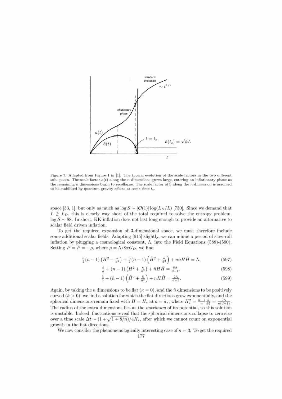
a(t)

a(t)t = tc

a(tc) =!

kL

! t1/2

t

inflationaryphase

standardevolution

a(tc) =!!L

Figure 7: Adapted from Figure 1 in [1]. The typical evolution of the scale factors in the two differentsub-spaces. The scale factor a(t) along the n dimensions grows large, entering an inflationary phase asthe remaining n dimensions begin to recollapse. The scale factor a(t) along the n dimension is assumedto be stabilised by quantum gravity effects at some time tc.

space [33, 1], but only as much as logS ∼ |O(1)| log(LD/L) [730]. Since we demand thatL & LD, this is clearly way short of the total required to solve the entropy problem,logS ∼ 88. In short, KK inflation does not last long enough to provide an alternative toscalar field driven inflation.

To get the required expansion of 3-dimensional space, we must therefore includesome additional scalar fields. Adapting [615] slightly, we can mimic a period of slow-rollinflation by plugging a cosmological constant, Λ, into the Field Equations (588)-(590).Setting P = P = −ρ, where ρ = Λ/8πGD, we find

n2 (n− 1)

(H2 + κ

a2

)+ n

2 (n− 1)(H2 + κ

a2

)+ nnHH = Λ, (597)

aa + (n− 1)

(H2 + κ

a2

)+ nHH = 8Λ

d−1 , (598)

¨aa + (n− 1)

(H2 + κ

a2

)+ nHH = 2Λ

d−1 . (599)

Again, by taking the n dimensions to be flat (κ = 0), and the n dimensions to be positivelycurved (κ > 0), we find a solution for which the flat directions grow exponentially, and thespherical dimensions remain fixed with H = H∗ at a = a∗, where H2

∗ = n−1n

κa2∗

= 2Λn(d−1) .

The radius of the extra dimensions lies at the maximum of its potential, so this solutionis unstable. Indeed, fluctuations reveal that the spherical dimensions collapse to zero sizeover a time scale ∆t ∼ (1+

√1 + 8/n)/4H∗, after which we cannot count on exponential

growth in the flat directions.We now consider the phenomenologically interesting case of n = 3. To get the required

177

number of ∼ 65 e-folds of inflation along the 3 flat directions we need H∗∆t ∼ 65. Forn = 3, H∗∆t ∼ 0.729, so once again inflation is cut short far too early. We could imaginegetting around this problem if we could alter the potential for the radius a, such that itdevelops a minimum as well as a maximum, by switching on fluxes [662, 661]. Generically,it is still very difficult to get enough exponential growth along the familiar 3 dimensionswithout causing the extra dimensions to grow alongside them [615]. For further details onthe latest attempts to embed inflation in higher dimensional theories, we refer the readerto [807, 1048, 812, 666, 218, 873, 166]. Bounds on the variation of fundamental constantsfor dynamical compactifications have been studied in [571, 572], while PPN parametersfor KK models in the solar system were computed in [461]. Note that Kaluza-Kleincosmologies have also recently been applied to the dark energy problem [119, 120].

We end our discussion of Kaluza-Klein cosmology by asking the question: Why arethere 3 large spatial dimensions? We have already alluded to an anthropic explanationdemanding the existence of stable planetary orbits44. To this we could add the existenceof stable atoms and chemistry, both key to the development of intelligent life, and bothrequiring no more than 3 (large) spatial dimensions.

Modern attempts at a dynamical understanding of the dimensionality of space includeString Gas Cosmology [183, 1216] (for reviews see, e.g., [180, 116, 181]). Here the spatialdimensions are taken to be compact and precisely 3 dimensions are allowed to growlarge due to the annihilation of strings wrapping around those dimensions. The point isthat strings winding around compact dimensions oppose their expansion since the energyof the string winding modes increases with radius. To allow the compact dimensions togrow large the winding modes must therefore collide and annihilate with the anti-windingmodes. Generically, we would only expect collisions of 1 + 1 dimensional strings in atmost 3+1 dimensions. Thus, the dimensionality of the string controls the dimensionalityof space by allowing at most 3 spatial dimensions to grow to macroscopic scales. Notethat this result is not spoilt by the inclusion of branes wrapping compact directions, asthese happen to fall out of equilibrium before the strings [21].

Whilst this idea has some appeal at first glance, it has not stood up to intensescrutiny. More detailed quantitative analyses suggest that the desired outcome is notat all generic, and requires highly fine tuned initial conditions [456, 457, 458]. Whilstone can engineer an anisotropic set-up allowing 3 dimensions to grow large as desired,typically the internal dimensions also grow to large sizes, just at a slower rate [456, 457].In fact, it turns out that either all dimensions grow large since the string gas eventuallyannihilates completely, or all dimensions stay small since the string gas gets frozen out[458]. There are also problems at the level of cosmology. For example, when properlycalculated, the scalar perturbations have a blue power spectrum with n = 5, which isstrongly ruled out by observations [670]. It has been argued that a near scale invariantspectrum can be obtained if the dilaton gets frozen during the strong coupled Hagedornphase in the very early Universe [182]. However, such claims still rely on a semi-classicaltreatment of cosmological perturbations that cannot be trusted during the Hagedornphase, as the strings are strongly interacting.

In the context of 10 dimensional string theory, other attempts to explain the dimen-

44On the subject of planetary orbits, it is amusing to note that Kepler himself reasoned that the 3-foldnature of the Holy Trinity was responsible for the perceived dimensionality of space. Ptolemy is reputedto have offered some alternative ideas in his work On Dimensionality, but they have since been lost.

178

sionality of our Universe consider that for integer values of n, the inequality 2n < 10 =⇒n ≤ 4 [444, 683]. This is interesting because it means that the world volume of 3 + 1dimensional branes (known as 3-branes) are less likely to intersect than those of largerbranes. In particular, Karch and Randall [683] have shown that an FLRW universeinitially filled with equal numbers of branes and anti-branes will ultimately come to bedominated by 3-branes and 7-branes. This analysis accounts for the fact that largerbranes dilute more slowly, as well as the likelihood of intersections and annihilations(hence the importance of 7-branes). In a braneworld scenario, this could explain why wemight be more likely to find ourselves living on a 3-brane, as opposed to a larger brane.The consequences of living on a 3-brane are discussed in detail in the Section 5.2.

Finally, we note that for toroidal compactifications, 3 large spatial dimensions can belinked to the stability of the small extra dimensions, at least in the presence of solitonicstrings/branes that correspond to point masses in the large dimensions [462].

5.2. The Braneworld Paradigm

The braneworld paradigm [15, 1074, 62, 52, 63] represents a radical alternative tothe standard Kaluza-Klein scenario, discussed in the previous section. In the KK sce-nario, the extra dimensions must be small and compact, the size of the internal spaceconstrained by collider experiments to be below the inverse TeV scale. In the braneworldscenario the extra dimensions can be much larger, perhaps even infinite in extent. Thisis made possible by relaxing the assumption of universal extra dimensions.

In the braneworld picture the Standard Model fields are not universal, rather theyare confined to lie on a 3 + 1 dimensional hyper-surface, known as the brane, embeddedin some higher dimensional space-time, known as the bulk. Tests of Standard Modelprocesses can only constrain how far the brane may extend into the bulk, or, in otherwords, the brane thickness. They do not constrain the size of the bulk itself. Suchconstraints can only come from gravitational experiments, as gravity is the only forcethat extends into the bulk space-time. As is well known, on small scales gravity ismuch weaker than the other three fundamental forces, making it difficult to test at shortdistances. In fact, the gravitational interaction has only been probed down to ∼ 0.1 mm,with torsion-balance tests of the inverse square law [10]. It is too simplistic, however, tosuggest that this translates into an upper bound on the radius of the bulk. Gravity isintimately related to geometry, and, as we shall see, one can warp the bulk geometry suchthat an infinitely large extra dimension is still allowed by experiment. For an excellentintroduction to large extra dimensions see [1072].

Before delving into a detailed discussion of the various models, we note in passingthat the braneworld paradigm is well motivated by string theory [622, 838, 52]. As wellas fundamental strings, string theory contains fundamental objects known as D-branes[1044]. These are extended objects upon which open strings can end. The braneworldset-up therefore has a natural interpretation in terms of a stack of D-branes embedded ina higher dimensional target space (see Figure 8). Open strings, with their ends attachedto the D-branes, can be identified with the Standard Model fields bound to the brane.Only closed strings can propagate through the bulk, and these are identified with thegravitational interactions.

179

Figure 8: Taken from [51]. Here the brane has 3 macroscopic dimensions, and d‖ compact dimensions.The open strings end on the D branes, whereas the closed strings propagate through the bulk.

5.2.1. The ADD model

The braneworld paradigm really began to gather momentum with the seminal workof Arkani-Hamed, Dimopoulos and Dvali [62], in which the large extra dimension isexploited in order to explain the vast hierarchy between the electro-weak scale, MEW ∼TeV, and the Planck scale, Mpl ∼ 1016 TeV. In this scenario the hierarchy does not goaway completely, rather it is reformulated as a hierarchy between the scale of the extradimensions, µ ∼ 1/L, and the electro-weak scale. The set-up is as follows: StandardModel fermions and gauge bosons are localised on a 3 + 1 dimensional domain wall, inan (effective) D = 4 + n dimensional space-time. We should clarify that D counts thenumber of macroscopic dimensions in this scenario. Any microscopic dimensions, withcharacteristic size given by the fundamental Planck length, behave as in the standardKK scenario described previously.

Now, the width of the wall cannot exceed the inverse TeV scale, as explained above.The bulk space transverse to the wall is compact but much larger than the width ofthe wall (L TeV−1), so much so that we can treat the wall as an infinitely thin 3-brane. In the simplest construction, the bulk action is then described by the generalisedEinstein-Hilbert action

Sbulk =MD−2D

2

∫dDX

√−γR, (600)

where MD is the fundamental Planck scale in D dimensions, γAB is the D dimen-sional metric with corresponding Ricci tensor, RAB , and Ricci scalar, R = γABRAB .The Planck mass is related to the fundamental Newton’s constant in D dimensions by

180

8πGD = M2−DD . At large distances, gravitational interactions along the brane are medi-

ated by the graviton zero mode, which has a homogeneous profile over the extra dimen-sions. Truncating to the zero mode, we can compute the four-dimensional effective actiondescribing long distance gravity along the brane by integrating out the macroscopic extradimensions. This result in

Seff =MD−2D Vn

2

∫d4x√−gR, (601)

where gµν is the four-dimensional metric on the brane, with Ricci tensor Rµν , and Ricciscalar R = gµνRµν , and where the volume of the extra dimensions is given by Vn ∝ Ln.The effective four-dimensional Planck scale, as seen by an observer on the brane, is thengiven by

M2pl ∼M2+n

D Ln. (602)

By taking the macroscopic extra dimensions to be sufficiently large, we can eliminatethe standard hierarchy in D dimensions, MD ∼ MEW ∼ 1 TeV, and replace it with anew hierarchy involving the scale of the extra dimensions, µ ∼ 1/LMEW . This is notin violation of short distance gravity tests, at least in D ≥ 6 dimensions. Indeed, in sixdimensions one can eliminate the hierarchy even for millimetre size extra dimensions.

In actual fact, the strongest constraints on the ADD model do not come from shortdistance gravity tests, but from astrophysics and cosmology [63]. The problem arisesbecause the Kaluza-Klein modes can be extremely light, mKK & 1/L & 10−4 eV, andextremely numerous, NKK ∼M2

pl/M2D . 1032. This means that even though each mode

is only very weakly coupled, with strength 1/Mpl, scattering processes along the brane,at energies E & mKK , can produce a copious number of KK gravitons.

The strongest astrophysical constraint comes from the possible emission of KK modesduring the collapse of SN1987a. Requiring this to not be the dominant cooling processesimposes a lower bound on the fundamental Planck scale. For example, with n = 2 wehave MD ≥ 50 TeV, whereas for n = 3 we have MD ≥ 3 TeV [350].

In cosmology, one has to worry about over-production of KK modes at high temper-atures, since this may destroy the standard Big Bang picture. In order to be consistentwith Big Bang Nucleosynthesis, and the current composition of the Universe, one mustidentify a maximum temperature for the early Universe for a given fundamental scale.Taking the fundamental scale to be MD ∼ 1 TeV imposes a temperature bound T ≤ 10MeV for n = 2, rising to T ≤ 10 GeV for n = 6 [588]. A higher fundamental scale willraise the maximum temperature, but then one loses much of the appeal of the originalmodel. While a low maximum temperature is not in contradiction with cosmologicaldata, it does present a challenge to models of baryogenesis and inflation. The tem-perature bounds can be weakened considerably if one does not require the bulk to beflat. For example, when the bulk manifold is a compact hyperbolic space, the maximumtemperature can be pushed beyond the GeV scale even for n = 2 [671].

5.3. Randall-Sundrum Gravity

As we have already suggested, in a generic braneworld set-up there is no obviousreason why one should demand that the bulk space should be flat, as in the ADD model.In perhaps the most celebrated braneworld model, developed soon after ADD by Randalland Sundrum [1051, 1052], the bulk is an anti-de Sitter space. There are two versions

181

of the Randall-Sundrum model, generally referred to as Randall-Sundrum I (RS1) [1051]and Randall-Sundrum II (RS2) [1052]. Somewhat confusingly, the RS1 model containstwo branes, whereas the RS2 model only contains a single brane.

The RS1 model [1051] was also proposed as a resolution to the hierarchy problem. Itimproves on the ADD model as the compact extra dimension need not be so large as tointroduce a new hierarchy. This is achieved by exploiting the exponential warp factor togenerate a large bulk volume from a small compactification radius. In contrast, the RS2model [1052] contains a single brane and a non-compact extra dimension – it is infinitein extent. This time the bulk warp factor ensures that gravity is localised close to thebrane, so that a brane observer only sees the gravitational effects of the extra dimensionabove scales set by the bulk curvature.

Although the phrase Randall-Sundrum gravity really refers to these two original mod-els, here we extend the definition to include any model with similar features. In thissection we are particularly interested in five-dimensional models containing 3-branes,with some non-trivial geometry , or “warping”, present in the bulk. We begin with anoverview of some of the models. For further details see, for example, [1008, 845].

5.3.1. The RS1 model

In RS1, we have two 3-branes separated by a region of five-dimensional anti-de Sitterspace [1051]. The branes are located at z = 0, and z = zc, and we impose Z2 symme-try across each brane. Neglecting Gibbons-Hawking boundary terms [536], the actiondescribing this model is given by

S =M3

5

2

∫d4x

∫ zc

−zcdz√−γ (R− 2Λ)

− σ+

∫

z=0

d4x√−g(+) − σ−

∫

z=zc

d4x√−g(−) , (603)

where γab is the bulk metric, and g(+)µν and g

(−)µν are the metrics on the branes at z = 0

and z = zc, respectively. M5 is the five-dimensional Planck scale and is related to thefive-dimensional Newton’s constant via the standard relation G5 = 1/8πM3

5 . We alsoinclude a negative bulk cosmological constant, Λ = −6/l2. If we fine-tune the branetensions against Λ, such that

σ+ = −σ− =6M3

5

l=

3

4πG5l,

then we admit a background solution in which the branes exhibit four-dimensionalPoincare invariance:

ds2 = e−2|z|/lηµνdxµdxν + dz2, (604)

for −zc ≤ z ≤ zc. The Z2 symmetry about z = 0 is explicit, whereas the other boundarycondition should be understood to be implicit. The line-element given in Eq. (604)contains an exponential warp factor that is displayed graphically in Figure 9. In betweenthe branes we recognise the geometry to be anti-de Sitter space, written in Poincarecoordinates. Notice the peak in the warp factor at the positive tension brane, and thetrough at the negative tension brane. Although only a toy model, the RS1 set-up is wellmotivated by a number of string theory/super-gravity constructions [622, 838, 439].

182

z

cz = 0 z = z

Figure 9: The behaviour of the warp factor in the RS1 model.

By integrating out the 4D zero-mode we are able to derive the 4D effective Planckscale on a given brane [1051, 1008]:

M2± = ±M3

5 l(

1− e∓2zc/l), (605)

where ± labels the sign of the corresponding brane tension. In terms of the effectiveNewton’s constants we have

G± =G5

l

( ±1

1− e∓2zc/l

). (606)

Now suppose we live on the negative tension brane. If we take the fundamental Planckscale M5 ∼ TeV, the bulk curvature scale to be just below 1/l ∼ 0.01M5, and thedistance between the branes to be such that zc/l ∼ 35, we recover the desired effectivePlanck scale, M− ∼ mpl ∼ 1016 TeV. Thus, the hierarchy problem has been eliminatedaltogether, and not just shifted around, as in the ADD model. In contrast, the hierarchyis not eliminated if we live on the positive tension brane since then the effective Planckmass is given by M+ ∼ e−zc/lM− [1051, 1008].

As it stands, the RS1 model is incomplete. The problem is that on either brane thelow energy 4D effective theory is not GR, but Brans-Dicke gravity. The extra scalarcomes from fluctuations in the brane separation, and is sometimes referred to as theradion [541, 528, 275]. The value of the Brans-Dicke parameter depends on the brane,and is given by [528]

w(±)BD =

3

2

(e±2zc/l − 1

). (607)

Observations require this parameter to be large (wBD > 40000, see Section 3.1.2). Note

that for the positive tension brane w(+)BD can be made arbitrarily large with increasing

brane separation. The same cannot be said for w(−)BD on the negative tension brane. If

we want to live on the negative tension brane we must generate a mass for the radion to183

brane

z

Figure 10: The behaviour of the warp factor in the RS2 model.

suppress its fluctuations. The Goldberger-Wise mechanism does exactly that, and thusstabilises the distance between the branes [542].

5.3.2. The RS2 model

The RS2 model is obtained from RS1 by taking the negative tension brane off toinfinity [1052]. The geometry is then described by the metric in Eq. (604) with zc →∞.The corresponding warp factor is shown in Figure 10, the single peak at z = 0 indicatingthat we have a single brane with positive tension. In this limit M+ →M3

5 l, so we cannoteliminate the hierarchy problem as in the RS1 model. Rather, the situation is more akinto the five-dimensional ADD model, with the curvature scale, 1/l, playing the role of thecompactification scale, µ ∼ 1/L.

What makes the RS2 model interesting is the way in which 4D GR is recovered on thebrane. As we have just seen, in RS1 the observer on the positive tension brane sees a low

energy gravity theory corresponding to Brans-Dicke gravity, with a BD parameter w(+)BD =

32

(e2zc/l − 1

). In the RS2 limit of infinite brane separation the BD scalar decouples

and one is left with 4D GR. As we will see in detail in Section 5.3.5, even though thebulk is infinite in extent, gravity is localised on the brane at energies below the bulkcurvature scale, 1/l. As a method to screen the extra dimensions from the low energyobserver, this represents a radical alternative to the standard method of Kaluza-Kleincompactifications.

The key to gravity localisation is that the bulk volume is finite even though it hasinfinite extent. This ensures that there is a normalisable graviton zero mode, which, inthe absence of any other massless modes, guarantees 4D GR at low enough energies.The finite bulk volume arises because the warp factor falls off exponentially as we moveaway from the brane. Intuitively, gravity localisation occurs because the warping makesit difficult for the graviton to propagate too far away from the brane, so much so thatthe region of the bulk with z & l has no influence on low energy brane interactions.

Since 1/l sets the scale at which the brane observer starts to become sensitive to the

184

bulk, table top experiments of the inverse square law impose the limit 1/l & 10−4 eV. Thistranslates into a lower bound on the fundamental Planck scale, M5 & 105 TeV, whichis well above the electro-weak scale. Since TeV scale gravity is not phenomenologicallyviable in this case, we abandon any discussion of the hierarchy problem for the singlebrane scenario.

Up until now our discussion has centred around weak gravity on the brane. Whatabout strong gravity in the presence of localised sources? Whilst there have been someinteresting numerical studies (see, e.g., [1278, 758]) exact strong gravity solutions arerare in RS2. One exception are the solutions for a domain wall localised on the brane[561, 560]. In contrast, an exact solution describing a braneworld black hole remainselusive45. The difficulty arises because the brane is an accelerated surface, so any blackhole residing on the brane must follow an accelerated trajectory. Such an acceleratedblack hole requires knowledge of the AdS C-metric, but this solution is unknown in fivedimensions. For a nice review of the search for braneworld black hole solutions see [558],and more recently [1200].

RS2 and AdS/CFT

Emparan, Fabbri and Kaloper (EFK) have suggested that a static braneworld blackhole does not exist [470]. To understand their argument we must first recall the AdS/CFTcorrespondence in which type IIB string theory on AdS5×S5 is conjectured to be dual toN = 4 SU(N) super-Yang-Mills, in the large N limit [862]. This suggests an alternativedescription of RS2 gravity [570]: ‘Gravity on an RS2 brane is dual to a strongly coupledconformal field theory (CFT) cut off in the UV, minimally coupled to 4D gravity’. Thereis plenty of evidence for this holographic description of RS2 (see, for example, [570,1100, 438, 1009, 556, 1014, 596, 1138, 695], and for a review [1008]). Another way ofdescribing the correspondence is to say [470]: ‘A classical source on the brane is dualto a quantum corrected source in four dimensions, with the quantum corrections comingfrom the strongly coupled CFT’. The quantum corrections are large because of the largenumber of degrees of freedom in the large-N limit. When applied to the problem offinding a black hole on the brane, this suggests that the solution should not be staticsince it should include the back-reaction of the Hawking radiation [470] (see also [1201]).Fitzpatrick, Randall and Wiseman have disputed this interpretation, pointing out thatthe CFT is strongly coupled and may therefore carry fewer degrees of freedom [508].At this point it is fair to say that as yet there has been no consensus, and the subjectremains an active area of debate (see also [564, 562, 966, 505, 506]).

Note that if we accept the EFK conjecture, we can improve the bound on the bulkcurvature by an order of magnitude, 1/l & 10−3 eV. This is based on the existence oflong-lived black hole X-ray binaries [471]. For smaller values of 1/l these binaries wouldhave already decayed.

5.3.3. Other RS-like models

One of the characteristic features of the Randall-Sundrum models is the structure ofthe bulk geometry, described by a non-factorisable, or warped, metric. One can embrace

45There have been many attempts to find such a solution, most of which remain unpublished.

185

this structure and consider a whole slew of interesting generalisations. Here we considera class of models described by warped geometries of the form

ds2 = a2(z)gµν(x)dxµdxν + dz2. (608)

Many of the most interesting RS-like models exhibit quasi-localisation and give rise tolarge-distance modifications of gravity. Perhaps the most celebrated of these is the DGPmodel [454], which will be discussed in detail in Section 5.5. Other interesting examplesinclude the GRS model [563], the asymmetric brane model [1012, 1013] and the CGPmodel [274]. We begin with the simplest generalisation, however, proposed by Karch andRandall [682] (see also [667]).

The Karch-Randall model

Here we take the RS2 model and de-tune the brane tension, σ+ 6= 6M35 /l, so that one

no longer has Poincare invariance along the brane. For an excess tension, σ+ > 6M35 /l,

the metric gµν is de Sitter, whereas for a tension deficit, σ+ < 6M35 /l, gµν is anti-de

Sitter. The effective cosmological constant on the brane is given by

Λ4 = 3

[(σ+

6M35

)2

− 1

l2

]. (609)

The behaviour of the warp factor also changes. We find that

a(z) = A cosh(c− |z|/l), c = cosh−1(1/A), for anti-de Sitter, (610)

a(z) = A sinh(c− |z|/l), c = sinh−1(1/A), for de Sitter, (611)

where A = l√|Λ4/3|. The decay of the warp factor away from the brane is greatest

for the dS brane, cutting off the space-time at z = lc. This means that gravity ismore strongly localised than in the standard RS2 scenario. In contrast, for the AdSbrane the warp factor turns around at some finite value of z. This means the bulkvolume is infinite, and gravity is not localised at all on the AdS brane as there is nonormalisable zero mode. Actually, when |Λ4| is small (compared with M5), the AdSbrane exhibits quasi-localisation. This is because there is a normalisable mode that isultra-light, with mass m2

ultra−light ∼ Λ24/M5 |Λ4| [1120]. At intermediate energies,

k E multra−light, the light mode behaves as if it were effectively massless and onerecovers 4D gravity. Note that there is no issue with the vDVZ discontinuity in AdSwhen m2

ultra−light/||Λ4| . 0.1[721]. We say that gravity is only quasi-localised becausethe extra-dimension opens up in the far infra-red, at energies E . multra−light.

Now consider what happens when we introduce a second AdS brane, along the linesof an AdS generalisation of the RS1 model [720]. The first thing to note is that bothbranes can have positive tension since the warp factor turns around. The second thingto note is that the bulk volume is rendered finite, and so we have a zero mode as wellas the ultra-light mode. At energies above the mass of both modes gravity is mediatedby the exchange of two spin-2 fields, one massless and one massive. This correspondsto a braneworld realisation of the bigravity scenarios discussed in Section 3.3 (see also[723, 722, 1011]).

186

The GRS model

The GRS model [563] was developed by Gregory, Rubakov and Sibiryakov. The set-up contains three Minkowski branes, one with positive tension and two with negativetension. The positive tension brane is Z2 symmetric and is flanked on either side by asection of anti-de Sitter space as far as a negative tension brane. Beyond the negativetension brane lies an infinite region of Minkowski space. The warp factor goes like [563]

a(z) =

e−|z|/l |z| < zc

e−zc/l |z| > zc.(612)

As the bulk volume is infinite, gravity is not localised, although the decaying warp fac-tor around the positive tension brane gives some degree of quasi-localisation. Again,although there is no zero mode, there is an ultra-light mode, and the extra dimensionopens up at very large distances. Unfortunately, the GRS model is known to be unstabledue to the presence of a ghost in the spectrum of linearised fluctuations [1038].

The asymmetric brane model

The asymmetric brane model [1012, 1013] (see also [1189]) is a single brane mode,llike RS2, only without Z2 symmetry imposed across the brane. Indeed, the fundamentalparameters in the bulk are allowed to differ on either side of the brane, including thebulk cosmological constant and the bulk Planck scales. Allowing the bulk Planck scalesto differ might seem strange, but not if we imagine a string compactification down tofive dimensions in which the dilaton is stabilised at different values on either side of adomain wall (the brane). If the bulk cosmological constant and Planck scales are givenby

Λ =

−6/l21 z > 0

−6/l22 z < 0, M =

M1 z > 0

M2 z < 0.(613)

The asymmetric model then admits Minkowski branes for a suitably tuned brane tension,σ = 3(ε1M

31 /l1 + ε2M

32 /l2), where ε1 = ±1 and ε2 = ±1. The corresponding solutions

have a warp factor of the form [1013]

a(z) =

e−ε1z/l1 z > 0

eε2z/l2 z < 0.(614)

The parameters ε1 and ε2 control whether the warp factor grows (ε = −1) or decays(ε = −1) away from the brane in a given direction. The model includes RS2 as a specialcase.

It is, however, more interesting to consider the case where one of the warp factorsgrows away from the brane while the other decays (e.g. ε2 = −ε1 = 1). The bulk volumeis then infinite so that there is no zero mode, but by choosing the scales appropriatelyone can engineer a degree of quasi-localisation. The point is that on the growing side thegraviton localises at the AdS boundary, where its sees an effective 4D Planck scale M3

1 l1.By taking this scale to be very large, the effect of localisation close to the AdS boundary

187

is almost decoupled from the gravitational dynamics near the brane. We should note thatthe asymmetric model also admits self-accelerating solutions, just as in the DGP model.In fact, the model shares a number of features with the DGP model. This is no coinci-dence, since the DGP model can be obtained as a limiting case of the asymmetric model[736]. It is known that the self-accelerating solutions of DGP contain ghost-like insta-bilities [273, 1015, 559, 546], so the same is expected to be true for the asymmetric model.

The CGP model

The CGP model [274], developed by Charmousis, Gregory and Padilla, also exhibitsquasi-localisation. It combines the main features of both the asymmetric model andthe DGP model in that there is an induced gravity term, and asymmetry across thebrane. Interestingly, the model contains a new type of cosmological solution that tendsto Minkowski space at very late times, but undergoes an intermediate period of cosmicacceleration in the presence of ordinary matter. In fact, it corresponds to a braneworldrealisation of the Cardassian cosmology, with H2 ≈ 8πG

3 (ρ + c√ρ) [512]. Although a

ghost is present when we introduce a small positive vacuum energy, this decouples in theMinkowski limit [740].

5.3.4. Action and equations of motion

In each of the models described in our overview, we have a five dimensional bulkspace split into a series of domains separated from each another by 3-branes. Here weconsider the action and field equations for generic models of this type. The 3-branes maybe thought of as the boundaries of the various domains so that the action is given by

S =

∫

bulk

d5x√−γ

(M3

5

2R+ Lbulk

)+∑

branes

∫

brane

d4x√−g

[−∆

(M3

5K)

+ Lbrane

],

(615)where γab is the bulk metric with corresponding Ricci scalar, R, M5 is the bulk Planckscale, and Lbulk is the Lagrangian density describing the bulk field content. In principleboth M5 and Lbulk can vary from domain to domain. For each brane gµν is the inducedmetric and Lbrane is the Lagrangian density describing the field content on that particularbrane. K = gµνKµν is the trace of extrinsic curvature, Kµν . This should be evaluatedon either side of the brane as it can differ from side to side. Labelling the two sides of agiven brane, using L and R, we define Kµν |L,R = 1

2Ln|L,Rgµν , i.e. extrinsic curvature isgiven by the Lie derivative of the induced metric, with respect to the unit normal na|L,R.The unit normal on both sides points from L to R. Note that what appears in the actionis the jump46

∆(M3

5K)

= M35K|R −M3

5K|L.This corresponds to the Gibbons-Hawking boundary term [536] for the bulk domainson each side of the brane. The ∆ here is not to be confused with the 3-dimensionalLaplacian.

Now there are two (completely equivalent) ways to treat the brane contributions atthe level of the field equations. One approach is to treat them as delta-function sources in

46Henceforth we define the jump of any quantity Q across a brane as ∆Q = Q|R −Q|L.

188

the Einstein equations. However, our preferred approach is to explicitly separate the fieldequations in the bulk from the boundary conditions at the brane. The bulk equations ofmotion are then given by the bulk Einstein equations

Gab = Rab −1

2Rγab =

1

M35

T bulkab , (616)

where T bulkab = − 2√

−γδ

δγab

∫bulk

d5x√−γLbulk is the bulk energy-momentum tensor. The

boundary conditions at Σi are given by the Israel junction conditions [649]

∆[M2

5 (Kµν −Kgµν)]

= −T braneµν , (617)

where T(i)µν = − 2√

−gδ

δgµν

∫brane

d4x√−gLbrane is the brane energy-momentum tensor.

Note that in each of these examples, the bulk geometry is only sourced by a cosmologicalconstant, T bulk

ab = −M35 Λγab.

5.3.5. Linear perturbations in RS1 and RS2

We now consider the theory of linear perturbations. For brevity, we will restrict at-tention to RS1 and RS2, although the methods we use are fairly standard, and shouldapply to all RS-like models (for further details, see [528, 275, 1038, 1011]).

Weak gravity on a RS1 brane

It is enough to consider RS1, as RS2 can be readily obtained by taking the negativetension brane to infinity. Recall that the background metric, γab, is given by Equation(604), with the positive tension brane (the “+” brane) fixed at z = 0 and the negativetension brane (the “−” brane) fixed at z = zc. We see that the induced metric on the

“+” brane is given by g(+)µν = ηµν , and on the “−” brane by g

(−)µν = e−2zc/lηµν . Note

that we have Z2 symmetry across the branes, so we can restrict attention to 0 ≤ z ≤ zc.We now consider small perturbations about the background, so that the metric is

given by γab = γab + δγab. It is convenient to choose Gaussian Normal (GN) gauge,defined by

δγµz = δγzz = 0. (618)

Actually, this is only a partial gauge fixing. Since we have no additional bulk matter,we can also take the metric to be transverse and trace-free in the bulk. In other words,δγµν = χµν(x, z), where

∂νχνµ = χµµ = 0. (619)

This is known as Randall-Sundrum (RS) gauge [1052]. In RS gauge, the linearised bulkequations of motion, δGab = 6

l2 δγab, yield

[e2z/l∂2 +

∂2

∂z2− 4

l2

]χµν = 0, (620)

where ∂2 = ∂µ∂µ.

Unfortunately, we can no longer assume that the branes are fixed at z = 0 and z = zc.The presence of matter on the branes will cause them to bend [528] so that they will now

189

be positioned at z = f+(x) and z = zc + f−(x), for some functions f± that depend onlyon the coordinates xµ. This makes it difficult to apply the Israel junction conditionsat the branes. To get round this we can apply a gauge transformation that fixes theposition of the “+” brane, and another that fixes the position of the “−” brane [275],without spoiling the Gaussian Normal condition (618). This gives rise to two coordinatepatches that are related by a gauge transformation in the region of overlap. We will callthem the “+” patch and the “−” patch accordingly.

We first consider the “+” brane. To fix its position we make the following coordinatetransformation

z → z − f+(x), xµ → xµ +l

2(1− e−2z/l)∂µf+. (621)

The “+” brane is now fixed at z = 0, although the other brane is now at z = zc+f−−f+.It follows that the metric perturbation in the “+” patch is given by

δγµν = χ(+)µν (x, z) = χµν(x, z)− l(1− e−2z/l)∂µ∂νf+ −

2

lf+γµν . (622)

Similarly, to fix the position of the “−” brane we let

z → z − f−(x), xµ → xµ +l

2

(1− e−2(z−zc)/l

)∂µf−. (623)

Now we have the “−” brane at z = zc, but with the “+” brane at z = f+ − f−. Themetric perturbation in the “−” patch is given by

δγµν = χ(−)µν (x, z) = χµν(x, z)− l

(1− e−2(z−zc)/l

)∂µ∂νf− −

2

lf−γµν . (624)

Now the induced metric on the “+” brane is given by g(+)µν = g

(+)µν + δg

(+)µν , where

δg(+)µν = χ(+)

µν (x, 0) = χµν(x, 0)− 2

lf+g

(+)µν , (625)

whereas on the “−” brane it is given by g(−)µν = g

(−)µν + δg

(−)µν , where

δg(−)µν = χ(−)

µν (x, zc) = χµν(x, zc)−2

lf−g

(−)µν . (626)

We are now ready to make use of the linearised Israel junction conditions given by Eq.(617) at each brane to find

∆[M2

5 δ(Kµν −Kgµν)](±)

= σ±δg(±)µν − T (±)

µν , (627)

where σ± = ±6M35 /l is the tension on the “±’ brane, and T (±)

µν is the energy-momentumtensor for matter excitations. Now, owing to the Z2 symmetry, the extrinsic curvaturesimply changes by a sign when evaluated on either side of a given brane. It follows thatthe linearised boundary conditions at each brane are given by

(∂

∂z+

2

l

)χµν

∣∣∣z=0

= −S(+)µν , (628)

(∂

∂z+

2

l

)χµν

∣∣∣z=zc

= −S(−)µν , (629)

190

where

S±µν(x) = ± 1

M35

[T (±)µν −

1

3T (±)g(±)

µν

]− 2∂µ∂νf±, (630)

and where T (±) = gµν(±)T(±)µν is the trace of the appropriate energy-momentum tensor.

Indeed, taking the trace of these equations, and using the fact that χµν is traceless, weclearly see that matter on a brane causes it to be bend, such that

∂2f±a2±

= ∓T(±)

6M35

, (631)

where a± gives the warp factor at the “±” brane (i.e. a+ = 1 and a− = e−zc/l). Equations(620), (628) and (629) give the governing differential equations, and a complete set ofboundary conditions for the graviton mode χµν . We now take Fourier transforms along

the brane directions, Q(x, . . .)→ Q(p, . . .) = 1(2π)2

∫d4x e−ipµx

µ

Q(x, . . .), to find that

χµν(x, z) =1

(2π)2

∫d4p eipµx

µ

χµν(p, z), (632)

where [−p2e2z/l +

∂2

∂z2− 4

l2

]χµν = 0, (633)

and(∂

∂z+

2

l

)χµν

∣∣∣z=0

= −S(+)µν (p),

(∂

∂z+

2

l

)χµν

∣∣∣z=zc

= −S(−)µν (p). (634)

This system is easily solved to give

χµν(p, z) = C(+)(p, z)S(+)µν − C(−)(p, z)S(−)

µν , (635)

where

C(+)(p, z) = − 1

p detA(p)

[I1

(plezc/l

)K2

(plez/l

)+K1

(plezc/l

)I2

(plez/l

)], (636)

and

C(−)(p, z) = − 1

p detA(p)e−zc/l

[I1 (pl)K2

(plez/l

)+K1 (pl) I2

(plez/l

)]. (637)

Note that In, and Kn are modified Bessel’s functions of integer order n [6], and

detA(p) = I1 (pl)K1

(plezc/l

)−K1 (pl) I1

(plezc/l

). (638)

From Eq. (631) we also have

f±(x) = ± 1

(2π)2

a2±

M35

∫d4p eipµx

µ T (±)

6p2. (639)

191

To compute the metric perturbation on each of the branes we simply use Eqs.(622) and(624), given our knowledge of χµν(x, z) and f±(x). At the positive tension brane we thenhave

χ(+)µν =

1

(2π)2

1

M35

∫d4p eipµx

µC(+)(p, 0)

[T (+)µν −

α+

2T (+)g(+)

µν

]

− e−zc/l

lp2 detA(p)

[T (−)µν −

1

3T (−)g(−)

µν

]+ pure gauge terms, (640)

whereas at the negative tension brane we have

χ(−)µν =

1

(2π)2

1

M35

∫d4p eipµx

µC(−)(p, zc)

[T (−)µν −

α−2T (−)g(−)

µν

]

− e−zc/l

lp2 detA(p)

[T (+)µν −

1

3T (+)g(+)

µν

]+ pure gauge terms. (641)

The parameters α± are crucial as they control the tensor structure of the propagator onthe “±” branes. They are given by

α+ =2

3

(1 +

1

lp2C(+)(p, 0)

), α− =

2

3

(1− e−2zc/l

lp2C(−)(p, zc)

). (642)

Using the properties of modified Bessel functions [6], we can show that at low energies,p ke−zc/l, we have [528]

χ(+)µν ≈

1

(2π)2

∫d4p eipµx

µ

2

M2+p

2

[T (+)µν −

(w+BD + 1

2w+BD + 3

)T (+)g(+)

µν

]

+2

M2−p

2

[T (−)µν −

1

3T (−)g(−)

µν

]+ pure gauge terms, (643)

and

χ(−)µν ≈

e−2zc/l

(2π)2

∫d4p eipµx

µ

2

M2−p

2

[T (−)µν −

(w−BD + 1

2w−BD + 3

)T (−)g(−)

µν

]

+2

M2+p

2

[T (+)µν −

1

3T (+)g(+)

µν

]+ pure gauge terms, (644)

where M± and w±BD are the 4D effective Planck scale and Brans-Dicke parameter on the“±” brane, respectively. They are given by Equations (605) and (607). We can now seeexplicitly how BD gravity emerges as the low energy effective theory in RS1, on bothbranes, as claimed in Section 5.3.1.

Graviton spectrum

Let us now pause to comment on the mass spectrum for the graviton. The spectrumcan be obtained by identifying the poles in the propagator. These are given by the

192

solutions to p2 = −m2, where detA(p) = 0. This gives

I1 (iml)K1

(imlezc/l

)−K1 (iml) I1

(imlezc/l

)= 0

=⇒ J1 (ml)Y1

(mlezc/l

)− Y1 (ml) J1

(mlezc/l

)= 0, (645)

where J1 and Y1 are Bessel’s functions of order one. By solving this equation we seethat there is a zero mode, and a tower of heavy Kaluza-Klein modes with mass splitting∆m ∼ 1/l(ezc/l − 1).

Radion effective action

The finite Brans-Dicke parameter indicates the presence of a massless scalar in ad-dition to the massless graviton. This is due to the radion, or brane bending mode,δf = f+ − f−. In some RS-like models (e.g. GRS), the radion can exhibit pathologicalbehaviour that can only be revealed by computing the effective action [1038]. We willnow briefly outline the procedure for doing this.

Let us consider vacuum fluctuations (T (±)µν = 0) in the scalar sector. The first thing

to note is that the Field Equations (620), (628) and (629) admit a solution of the form[275]

χ(rad)µν = − l

2

4e2z/l∂µ∂νψ, (646)

where ∂2ψ = 0 and the vacuum boundary conditions require

fvac± = − l

2a2±ψ, (647)

where fvac± is the vacuum fluctuation in f±. Note that Equation (631) implies ∂2fvac

± = 0,and so Equation (647) is consistent with ∂2ψ = 0. Equation (647) also imposes a relationbetween fvac

+ and fvac− , resulting in a single free scalar degree of freedom, which we take

to be the physical radion mode, ψ. Note that the radion profile in the bulk is localisedclose to the “−” brane, in contrast to the graviton zero mode which is localised closeto the “+” brane. We now work in the “+” patch, which has the branes positioned atz = 0 and z = zc − δfvac. Focusing solely on the scalar sector, the metric perturbationis given by

δγµν = − l2

4e2z/l∂µ∂νψ− l(1− e−2z/l)∂µ∂νf

vac+ − 2

lfvac

+ γµν , δγµz = δγzz = 0. (648)

In order to integrate out the extra dimension, it is convenient to have both branes fixed.We can do this with the following coordinate transformation

z → z +B(z)δfvac, xµ → xµ − e−2z/l∂µ(δfvac)

∫ z

0

e2y/lB(y)dy, (649)

where B(z) is some differentiable function for 0 ≤ z ≤ zc, satisfying B(0) = 0 andB(zc) = 1. While this transformation ensures that δγµz is still zero, the price we pay for

193

fixed branes is that we now have non-vanishing δγzz. More precisely,

δγµν = hµν = − l2

4e2z/l∂µ∂νψ − l(1− e−2z/l)∂µ∂νf

vac+ − 2

l

[fvac

+ − (δfvac)B(z)]γµν

+2e−2z/l∂µ∂ν(δfvac)

∫ z

0

e2y/lB(y)dy, (650)

δγzz = hµz = −2δfvacB′(z). (651)

To quadratic order, the effective action is given by

Seff = −M35

2

∫ zc

0

dz

∫d4x√−γ habδ

[Gab −

6

l2γab

]

+1

2

∫

z=0

d4x√−g(+) hµν

[∆(M2

5 δ(Kµν −Kgµν))(+) − σ+hµν

]

+1

2

∫

z=zc

d4x√−g(−) hµν

[∆(M2

5 δ(Kµν −Kgµν))(−) − σ−hµν

]. (652)

It turns out that δ[Gµν − 6

l2 γµν]

and ∆(M2

5 δ(Kµν −Kgµν))(±)− σ±hµν are identically

zero [1038]. After integrating out a total derivative in z, we arrive at the followingeffective action for the radion:

Sradion = −3

2M2−

∫d4x (∂µψ)2, (653)

where M− is given by Equation (605). Thus, as expected, the radion, ψ, behaves asa massless scalar, and, being localised close to the “−” brane, its coupling strength iscontrolled by the scale M−. As we move the branes further and further away from oneanother, M− increases and the radion starts to decouple (decoupling completely in theRS2 limit). Note that in some models, such as GRS [563], the radion effective actioncomes in with the wrong overall sign, signalling the presence of a physical ghost [1038].There is no such pathology in RS1 or RS2.

Weak gravity on a RS2 brane

Let us now focus on RS2 by taking the negative tension brane to infinity. As zc →∞,the metric on the remaining positive tension brane is given by

χ(+)µν =

1

(2π)2

∫d4p eipµx

µ K2 (pl)

M35 pK1 (pl)

T (+)

µν −1 + K1(pl)

plK2(pl)

3T (+)g(+)

µν

+ pure gauge terms. (654)

At low energies, p k, we again use the properties of modified Bessel functions [6] toshow that

χ(+)µν ≈

1

(2π)2

∫d4p eipµx

µ 2

M24 p

2

[T (+)µν −

1

2T (+)g(+)

µν

]+ pure gauge terms. (655)

194

It follows that gravity is indeed localised on the brane at low energies, with a 4D effectivePlanck scale M2

4 = M35 l, or, equivalently, with an effective Newton’s constant G4 = G5/l.

Note that the tensor structure of the propagator matches that of General Relativity, witha factor of − 1

2 in front of the trace term. This is where the brane bending mode f+(x)plays a crucial role. It cancels part of the graviton zero mode in just the right wayto guarantee good agreement with solar system gravity tests. It is worth noting thatthis neat cancellation of terms does not always happen, even in single brane scenarios.We will see this in DGP gravity, for example, where one has to argue for some sort ofVainshtein effect to pass observational tests.

Let us finally consider massive modes. In RS2 there is actually a continuum ofmassive modes, consistent with the fact that the extra dimension is no longer compact.However, as we have seen, we still recover 4D GR to leading order. The next to leadingorder corrections are obtained by integrating over the continuum, or, equivalently, byconsidering the next to leading order expansion in pl above. The result is that theNewtonian potential reads47

V (r) ∝ 1

r

(1 +

2l2

3r2+O(l3/r3)

).

We refer the reader to [528, 1008, 438] for details of the derivation. Note that the 1/r3

correction can be obtained in a dual picture as the one loop CFT correction to thegraviton propagator [438].

5.4. Brane Cosmology

There are two obvious reasons why cosmology offers an interesting arena in whichto develop the braneworld paradigm. The first is that cosmological branes possess ahigh degree of symmetry, and this makes it possible to solve the field equations. Thesecond is that cosmological physics can be tested by a number of observations, rangingfrom supernova data to the abundance of light elements. In this section we will studythe cosmology of co-dimension one branes, focusing on the RS2 scenario with a single Z2

symmetric brane. We will review the background dynamics [159, 178] before moving on tocosmological perturbation theory [716, 1244]. Further details, including generalisations tomulti-brane scenarios with bulk scalar fields, can be found in the following review articles[1048, 845, 639, 770, 189, 195] (see also [1008, 346, 347, 1139]). Other generalisationsinclude: the cosmology of branes without Z2 symmetry [1012, 1189, 1143]; anisotropicbraneworlds [843, 966]; and branes for which energy is explicitly transferred betweenbulk and brane [694, 695, 1234]. Note that any anisotropy is seen to dissipate on thebrane in RS gravity, a feature that can be identified with CFT particle production in theholographic picture [966]. Bulk-brane energy transfer has been used to account for darkenergy [694, 695, 1234].

Braneworld cosmology can be studied using two different formalisms: The brane basedformalism, and the bulk based formalism. These two approaches are completely equivalentand yield a background cosmology governed by the following Friedmann equations [159,

47Note that this result differs slightly from the original one quoted in [1052].

195

158, 178]

H2 +κ

a2=

Λ4

3+

8πG4

3ρ(

1 +ρ

2σ

)+

µ

a4, (656)

H − κ

a2= −4πG4(ρ+ P )

(1 +

ρ

σ

)− 2µ

a4, (657)

where H = a/a is the Hubble parameter along the brane, a(t) is the scale factor, andκ = 0,±1 describes the spatial curvature. The brane is sourced by a tension, σ, anda cosmological fluid with energy density, ρ(t), and pressure, P (t). The parameters Λ4

and G4 denote the effective cosmological constant and Newton’s constant on the brane,respectively. As in the standard scenario, the Raychaudhuri Equation (657) follows fromthe Friedmann Equation (656) and energy conservation,

ρ+ 3H(ρ+ P ) = 0. (658)

We will now review the derivation of this cosmology using the two equivalent for-malisms. For the moment, however, let us comment on a few of its important features.From Equations (656) and (657) we see that the corrections to the standard cosmologymanifest themselves in a term ∝ ρ2, and a dark radiation term µ

a4 = 8πG4

3 ρweyl. Thelatter corresponds to a non-local “Weyl” contribution and can only be fixed by specifyingthe bulk geometry. In the holographic description of RS2, the ρ2 corrections contributeto the conformal anomaly [1138], while the dark radiation is identified with thermalexcitations of the CFT [570, 1100, 1009, 556, 1014, 596].

Both corrections will strongly affect Big Bang nucleosynthesis (BBN), so their mag-nitude can be constrained by the abundance of light elements. These require that thedark radiation can be at most 10% of the photon energy density, ρweyl/ργ . 0.01, in theperiod following BBN [638]. In addition, the ρ2 corrections to the cosmological evolutionshould be negligible after BBN, which imposes a constraint48 on the tension σ & (MeV)4

[159].The ρ2 corrections play the dominant role in the very early universe and will have a

big impact on the inflationary dynamics. Assuming the inflaton is confined to the branealong with all the Standard Model fields, one finds that the slow roll parameters aregiven by [847]

ε = − H

H2=

1

16πG4

(V ′

V

)2[

1 + Vσ(

1 + V2σ

)2

], (659)

η = − φ

Hφ=

1

8πG4

(V ′′

V

)[1

1 + V2σ

], (660)

where V (φ) is the inflaton potential. At low energies, V σ, these match the standardformulae of 4D General Relativity,

ε ∼ εGR =1

16πG4

(V ′

V

)2

, η ∼ ηGR =1

8πG4

(V ′′

V

).

48Assuming a RS2 scenario with fine tuned tension, σ = 12M35 /l, the BBN constraint is significantly

weaker than the constraint arising from table top experiments quoted in Section 5.3.2, i.e. 1/l & 10−4

eV, giving σ & (100GeV)4[189]. Here we have used the fact that M24 = M3

5 l ∼ 1016 TeV.

196

However, at high energies we have

ε ∼ εGR4σ

V εGR, η ∼ ηGR

2σ

V ηGR. (661)

This means we can get away with steeper potentials in the braneworld case [847]. Thisis essentially because Hubble friction gets enhanced by the ρ2 terms. However, suchpotentials are incompatible with observational constraints as they lead to a large tensor-to-scalar ratio [800].

5.4.1. Brane based formalism – covariant formulation

We shall now derive the background cosmology, Eqs. (656) and (657), using thebrane based formalism. This makes use of the Gauss-Codazzi equations [531, 320], andthe Israel junction conditions to derive the Einstein tensor on the brane [1140]. Wewill assume Z2 symmetry, although we refer the reader to [117] for a non-Z2 symmetricgeneralisation.

The Gauss-Codazzi equations are the fundamental equations of embedded hyper-surfaces. The brane can be thought of as an embedding,

xa = Xa(ξµ), (662)

in the bulk geometry, γab(x). By Z2 symmetry this is the same on both sides of thebrane. We can now define tangent vectors V aµ = ∂Xa/∂ξµ, and the outward pointingunit normal, na, satisfying

γabnanb = 1, γabn

aV bµ = 0.

It follows that the induced metric on the brane is given by

gµν = γab(X)V aµ Vbν . (663)

For such an embedding, the Gauss-Codazzi equations [531, 320] give

Rµναβ = RabcdV aµ V bν V cαV dβ +KµαKνβ −KµβKνα, (664)

∇µ(Kµν −Kgµν) = RabnaV bν , (665)

R−K2 +KµνKµν = −2Gabnanb, (666)

where Rabcd is the Riemann tensor in the bulk, Rµναβ is the Riemann tensor on thebrane, and we recall that the extrinsic curvature of the brane is given by Kµν = 1

2Lngµν ,the Lie derivative of the induced metric, with respect to the normal.

Now, in the RS2 scenario the dynamics of the brane are governed by the bulk equa-tions of motion and the Z2 symmetric junction conditions

Gab =6

l2γab, Kµν −Kγµν = 3σ∗gµν − 4πG5Tµν , (667)

with σ∗ = 4πG5σ3 , where σ is the brane tension and Tµν is the energy-momentum tensor

of additional matter excitations. Of course, in the RS2 scenario we have a fine-tunedtension such that σ∗ = 1/l, but we will keep things general for the moment.

197

Consider the Codazzi Equation (665). Because the bulk is only sourced by a cosmo-logical constant, the right hand side of this equation is identically zero. This is important,because the junction conditions in Eq. (667) now imply the usual conservation law alongthe brane, ∇µTµν = 0. To extract information about the Einstein tensor on the brane,we contract the Gauss Equation (664), and plug in Eq. (667), to give [1140]

Gµν = −Λ4gµν + 8πG4Tµν + (4πG5)2Πµν − Eµν , (668)

where Λ4 = 3(σ2∗ − 1

l2

)is the effective cosmological cosmological constant on the brane,

and the effective Newton’s constant is given by

G4 = G5σ∗. (669)

The corrections to standard 4D gravity are encoded in a local contribution, Πµν , and anon-local “Weyl” contribution, Eµν . The local piece is a quadratic combination of theenergy-momentum tensor

Πµν = −T αµ Tνα +1

3T Tµν +

1

2T αβTαβgµν −

1

6T 2gµν , (670)

whereas the non-local “Weyl” piece is

Eµν = CabcdnaV bµn

cV dν , (671)

where Cabcd is the Weyl tensor of the bulk. It is often referred to as the electric partof the Weyl tensor, and in general one must solve the bulk equations of motion first inorder to evaluate it in full. We should also note that Eµν has vanishing trace, and itsdivergence is sourced by the local quadratic contribution

gµνEµν = 0, ∇µEµν = (4πG5)2∇µΠµν . (672)

The latter equation follows from the divergence of Equation (668), making use of theBianchi identity and the local conservation of energy-momentum, ∇µTµν = 0.

Our interest here lies in the cosmology, so let us now assume spatial homogeneity andisotropy on the brane. The induced metric is given by the usual Friedmann-Lemaıtre-Robertson-Walker (FLRW) metric

ds2 = gµνdξµdξν = −dt2 + a(t)2qijdx

idxj , (673)

where qij(x) is the metric of a hyper-surface of constant curvature, κ = 0,±1. The matterexcitations contribute a cosmological fluid with energy density, ρ(t), and pressure, P (t),such that its energy-momentum tensor is given by

T µν = diag(−ρ(t), P (t), P (t), P (t)). (674)

In the absence of non-trivial sources in the bulk Tµν is conserved, which means we havethe standard relation given by Equation (658).

It remains to compute the non-local piece, Eµν . Although in general we must solve thebulk equations of motion to evaluate this, we can exploit the large amount of symmetry

198

to avoid doing so in the current instance. Making use of the Constraints Equations (672),we can show that

Eµν =µ

a4diag

(−1,

1

3,

1

3,

1

3

),

where µ is an integration constant that should be fixed by the bulk geometry (we willsee in the next section that it can be identified with the mass of a bulk black hole). Notethat Eµν is conserved on a cosmological background, by virtue of the fact that ∇µΠµ

ν = 0.The modified Friedmann Equations (656) and (657) now follow automatically from

Equation (668).

5.4.2. Bulk based formalism – moving branes in a static bulk

The principle limitation of the brane based formalism we have just described is thatit suppresses physics deep inside the bulk. This can be dangerous since it is not at allobvious if a particular choice of the non-local “Weyl” term, Eµν , at the brane will evolveinto a pathological bulk geometry. Such problems can be avoided by solving for the bulkgeometry first. For example, in the brane based formalism, the parameter µ giving riseto dark radiation, is just an integration constant and can take any sign. Using the bulkbased formalism, we are able to identify µ with the mass of a bulk black hole, and usethis to constrain it to be positive.

We will now develop the bulk based formalism for cosmological branes. Again, wewill assume Z2 symmetry across the branes, for brevity. The reader can refer to [1008]for the non-Z2 symmetric generalisation. The bulk based formalism requires us to solvefor the bulk geometry. Since we are interested in cosmological branes (with constantcurvature Euclidean 3-spaces), we study the Einstein equations, Gab = 6

l2 γab, with thefollowing metric ansatz [178]

ds2 = γabdxadxb = e2νA−2/3(−dt2 + dz2) +A2/3qijdx

idxj , (675)

where A and ν are undetermined functions of t and z, and as before qij(x) is the metricof a hyper-surface of constant curvature, κ = 0,±1. Now, in an extremely elegantcalculation, Bowcock et al. [178] were able to prove a generalised form of Birkhoff’stheorem, showing that the bulk geometry is necessarily given by

ds2 = −V (r)dτ2 +dr2

V (r)+ r2qijdx

idxj , (676)

where

V (r) =r2

l2+ κ− µ

r2. (677)

For µ > 0, the metric in Eq. (676) takes the form of a (topological) Schwarzschild blackhole in anti-de Sitter space. Here we have written the solution in an explicitly timeindependent coordinate system, meaning that we can no longer say that we have a staticbrane sitting at a fixed coordinate position. On the contrary, we now have a dynamicbrane, whose trajectory in the these coordinates is more complicated. Braneworld cos-mology from this perspective was first studied by Ida [639], although moving branes ina static anti-de Sitter bulk were considered earlier by Kraus [754].

199

To construct the brane solution, we treat it as an embedding,

τ = τ(t), r = a(t), (678)

of the bulk geometry given in Eq. (676). The induced metric on the brane is then

ds2 = gµνdξµdξν =

(−V (a)τ2 +

a2

V (a)

)dt2 + a2(t)qijdx

idxj (679)

where over-dots denote ∂/∂t. We are free to choose t to correspond to the proper timewith respect to an observer comoving with the brane. This imposes the condition

− V (a)τ2 +a2

V (a)= −1, (680)

ensuring that the brane takes the standard FLRW form, as in Eq. (673). The functiona(t) is then immediately identified with the scale factor along the brane.

The boundary condition at the brane are given in Eq. (667). We must compute theextrinsic curvature, Kµν = 1

2Lngµν , defined as the Lie derivative of the normal pointinginto the bulk. Assuming we cut away the AdS boundary and retain the region r < a(t),we find that the inward pointing unit normal is given by

na = (−a, τ , 0, 0, 0), (681)

where we are free to specify that τ > 0. The components of extrinsic curvature are thengiven by

Kij =

V τ

aδij , Kt

t = −(a+ V ′/2

V τ

). (682)

In the presence of a cosmological fluid, as given by Equation (674), the junction conditionsin Eq. (667) yield the following:

V τ

a= σ∗(1 +

ρ

σ), (683)

a+ 12V′

V τ= σ∗

[1− 2

ρ

σ− 3

P

σ

]. (684)

Making use of Equation (680) we then arrive at the modified Friedmann Equations (656)and (657).

5.4.3. Cosmological perturbations

While the theory describing cosmological perturbations in braneworld gravity hasbeen well developed in recent years (see, for example, [842, 771, 847, 334, 1087, 991, 801,202, 201, 548, 772, 547, 918, 919, 921, 920, 596, 716, 768, 1244, 742, 1245, 703, 705, 715,769, 597, 408, 194, 430, 955, 286, 300, 395, 1062, 787, 245]), even approximate solutionsto the resulting field equations have been notoriously hard to come by. The problemstems from the fact that one has to solve the fully coupled system of brane and bulk,which is, in general, a far from trivial task. Indeed, this will generically render the branebased formalism somewhat incomplete without making ad hoc assumptions about the

200

perturbations of the non-local “Weyl” contribution, Eµν . The bulk based formalism isbetter in this respect, but the resulting system is virtually intractable, and only in somespecial cases, where the bulk and brane equations become separable, has progress beenmade [528, 596, 202, 201, 772]. Note that, unlike in other sections, we will on occasioninclude vector and tensor perturbations, as well as scalars. This is because the bulk cansource vector and tensor modes on the brane, giving qualitatively different behaviour tothat seen in standard 4D cosmology.

Cosmological perturbations in the brane based formalism

We shall now review some aspects of cosmological perturbation theory using the branebased formalism introduced in Section 5.4.1. Further details can be found in [845, 842].The dynamics on the brane are governed by Equation (668), and so perturbations aboutthe background cosmology on the brane satisfy

δGµν = 8πG4δT µν + (4πG5)2δΠµν − δEµν . (685)

To study this we use the standard four-dimensional formalism [90, 717, 469, 917], decom-posing the system into scalar, vector and tensor perturbations with respect to the spatialdiffeomorphism group in the background cosmology. Working with conformal time asopposed to proper time, the perturbed metric is given by

ds2 = a2[−(1 + 2Ψ)dτ2 − 2(βi + ~∇iβ)dxidτ

+[(1− 2Φ)qij +Dijν + 2~∇(iAj) + hij

]dxidxj

], (686)

where Ai and βi are transverse vectors on qij , and hij is a transverse and trace-free tensor.

Recall that the operator Dij = ~∇i~∇j− 13qij∆. The fluctuations energy-momentum on the

brane are written in terms of the fluctuations in density, δ, pressure, δP , fluid 3-velocity,vi, and anisotropic stress, Σij , in the usual way,

δT 00 = −ρδ, δT 0

i = −(ρ+ P )vi, δT ij = δPδij + (ρ+ P )Σij . (687)

The fluid 3-velocity and anisotropic stress can then be decomposed with respect to theirscalar, vector and tensor components,

vi = θ(vector)i + ~∇iθ, (688)

Σij = Σ(tensor)ij + ~∇(iΣ

(vector)j) +DijΣ. (689)

The fluctuation in the quadratic piece is also given in terms of ρδ, δP . . . etc., accordingto

δΠ00 =

2

3ρδT 0

0 , δΠ0i =

2

3ρδT 0

i ,

δΠij = −1

3(ρ+ 3P )δT ij −

2

3(ρ+ P )δij

(δT 0

0 −1

2δT kk

), (690)

where δTµν are given by Equations (687).201

Now we consider the contribution from the non-local “Weyl” perturbation, and iden-tify it with the fluctuation in some dark energy energy-momentum tensor

δEµν = −8πG4δT weylµν .

In direct analogy with Equations (687), we can read off corresponding fluctuations in

Weyl energy density, δweyl, Weyl pressure, δPweyl, Weyl fluid 3-velocity, vweyli , and Weyl

anisotropic stress, Σweylij . We might hope to determine each of these in terms of the local

matter fluctuations, δ, δP . . . etc., by making use of the Constraints Eqs. (672) to linearorder. We find that for scalar perturbations δEµµ = 0 gives49

δPweyl =1

3ρweylδweyl, (691)

and ∇µ[δEµν − (4πG5)2Πµ

ν

]= 0 gives

(δweyl)′ + 4Ψ′ +4

3∆

[β +

1

2ν′ − θweyl

]= 0, (692)

−4

3ρweyl

[(θweyl)′ + Φ− 2

3(∆ + 3κ)Σweyl − δweyl

4

]=

ρ+ P

σρδ + (ρ+ P )[3Hθ − (∆ + 3κ)Σ] , (693)

where ′ denotes differentiation with respect to conformal time, and H = a′/a = aH.Clearly we have too many Weyl unknowns and not enough equations. The bottom line isthat we need to know the Weyl anisotropic stress δπweyl

ij explicitly, and for that we needto abandon the brane based formalism and solve the bulk equations of motion [842].

Some progress can be made at super-horizon scales, since then we can neglect thespatial gradients in Eqs. (692) and (693), and solve for the Weyl energy density andWeyl momentum in terms of ρδ, δP . . . etc., thereby closing the system [842, 548, 771].This simplification has been applied to the study of both density perturbations andvector perturbations at large scales, revealing qualitatively different behaviour to thatin General Relativity [548, 844]. Regarding density perturbations, it can be shown thatthe quantity ρa4∆δ will grow during slow-roll inflation on super-horizon scales (it staysconstant in GR) [548]. It can be shown that vector perturbations can be non-vanishing,even in the absence of vorticity [844].

We can also solve for the (total) curvature perturbation on large scales [771]. Unfor-tunately, this does not mean we can compute large-scale CMB anisotropies. The problemis that to evaluate the (non-integrated) Sachs-Wolfe equation we need knowledge of themetric perturbations. These are sourced by the dark anisotropic stress, according to

Φ− Ψ = 8πG4a2

(4

3ρweyl

)Σweyl, (694)

49The remaining formulae in this section are taken from [771], where one should identify δρ = ρδ, δq =−(ρ+ P )θ, δπ = (ρ+ P )Σ, R = Ψ, A = −Φ, E = 1

2ν, B = −β.

202

where Ψ and Φ are the Bardeen gauge invariants for the metric perturbations, and wehave neglected the local anisotropic stress. The braneworld corrections to the Sachs-Wolfe effect are given by [771]

δT

T=δT

T

∣∣∣GR− 8

3

(ργρcdm

)Sweyl

− 8πG4a2

(4

3ρweyl

)Σweyl +

16πG4

a5/2

∫da a7/2

(4

3ρweyl

)Σweyl, (695)

where Sweyl is the Weyl entropy perturbation, determined by ρδweyl.

Cosmological perturbations in the bulk based formalism

As we saw in the previous section, a proper treatment of cosmological perturbationtheory in brane cosmology requires us to solve the coupled system of brane and bulk.We will now present the details of this in the bulk based formalism, essentially following[716] (see also [1244, 918, 919, 921, 920]). Note that in this section we deviate from ourusual convention of treating cosmological perturbations with respect to conformal timeon the brane, preferring instead to use proper time of comoving observers, in keepingwith the majority of the relevant literature. For consistency, however, we do define thebrane quantities as in the previous section.

We begin with some notation on the background. The bulk metric is given by

ds2 = γabdxadxb = λαβdx

αdxβ + r2qijdxidxj , (696)

where λαβ is some two-dimensional metric, and λαβ and r depend only on the first twocoordinates, xα. This corresponds to a section of (topological) AdS-Schwarzschild, andone can choose a gauge such that

λαβdxαdxβ = −V (r)dτ2 +

dr2

V (r), V (r) =

r2

l2+ κ− µ

r2. (697)

However, here we will leave the choice of gauge unspecified so that our analysis canbe applied in other gauges (e.g. Gaussian-Normal gauge). The background embeddingequation is now given by xa = Xa(ξµ), where ξµ = (t, ξi) are the coordinates along thebrane. We take

Xα = Xα(t), Xi = ξi,

and λαβ(X) ˙Xα ˙Xβ = −1 to ensure that the induced metric on the brane has the standardFLRW form, as in Eq. (673), with scale factor a(t) = r(X). Over-dots here denotedifferentiation with respect to proper time on the brane, t.

We shall now specify the perturbations in the bulk. Decomposing the bulk metric interms of scalar, vectors and tensor components (with respect to qij), we write δγab =hscalarab + hvector

ab + htensorab , where,

hscalarαβ = χαβ , hscalar

αi = r~∇iχα, hscalarij = 2r2 [Aqij +DijE] , (698)

hvectorαβ = 0, hvector

αi = rBαi, hvectorij = 2r2~∇(iHj), (699)

htensorαβ = 0, htensor

αi = 0, htensorij = r2Hij , (700)

203

where Dij = ~∇i~∇j − 13qij∆. Here Bαi and Hi are transverse, and Hij is transverse and

trace-free. One can identify the following gauge invariants in the bulk [716]:

scalars: Yαβ = χαβ − 2D(αQβ), Z = A− 1

3∆E −Qα∂α ln r, (701)

vectors: Fαi = Bαi − rDαHi, (702)

tensors: Hij , (703)

where Dα is the covariant derivative on λαβ , and Qα = r(χα − r∂αE). For simplicitywe will assume that there are no exceptional modes [716] in any sector. Now, the bulkequations of motion, δGab = 0, are extremely complex in general (see [716]). From apractical perspective, the only way to proceed is to assume that the background bulk ismaximally symmetric anti de Sitter space, so there is no bulk black hole (i.e. µ = 0)[918]. The vector and scalar perturbations in the bulk can then be expressed in terms ofa corresponding ‘master variable’. For example, the scalar gauge invariants Yαβ and Zcan be written as

Yαβ =1

r

[DαDβ −

2

3λαβ

(D2 − 1

2l2

)]Ω, Z = −1

2Y =

1

6r

(D2 − 2

l2

)Ω, (704)

where the scalar master variable Ω satisfies[D2 − 3∂α ln rDα +

∆ + 3κ

r2+

1

l2

]Ω = 0. (705)

For the vectors, we introduce the vector master variable, writing the gauge invariant as

Fαi =1

r2εαβD

βΩi, (706)

where εαβ is the total antisymmetric Levi-Civita tensor on λαβ , and Ωi satisfies

Dα

[r5Dβ

(DβΩir3

)+ (∆ + 2κ)Ωi

]= 0. (707)

The tensor gauge invariant, Hij , is essentially its own master variable, and satisfies[D2 + 3Dα ln rDα +

1

r2(∆− 2κ)

]Hij = 0. (708)

To solve for these master variables we need to specify boundary conditions at the brane,as well as the asymptotic boundary conditions. The latter correspond to the conditionof normalisability. Let us now consider the boundary conditions at the brane. The firstthing to note here is that the brane position can fluctuate, so that it now correspondsto an embedding xa = Xa + fa(ξµ). We decompose this fluctuation in terms of scalars

fα, ε, and a transverse vector εi, such that fa = (fα, εi+ ~∇iε). Secondly, in applying theboundary conditions, it is important to express all fields in terms of covariant objectsalong the (background) brane. This suggests that all fields of the form Wα and Wαβ

should be decomposed in terms of their components parallel to the tangent vector ˙Xα

and along the normal nα, as follows:

Wα = −W‖ ˙Xα +W⊥nα, (709)

Wαβ = W‖‖˙Xα ˙Xβ −W‖⊥ ˙Xαnβ −W⊥‖ ˙Xβnα +W⊥⊥n

αnβ . (710)204

The induced metric on the brane then takes the form

ds2 = −(1 + 2Ψ)dt2 − 2a(βi + ~∇iβ)dxidt

+ a2[(1− 2Φ)qij +Dijν + 2~∇(iAj) + hij

]dxidxj , (711)

with

Ψ = −1

2Y‖‖ − U‖ + Kt

tU⊥, β = −U‖a− aν

2, (712)

Φ = −Z − 1

3∆ν +HU‖ − (D⊥ ln r)U⊥, ν = 2(E + ε), (713)

βi = −F‖i − aAi, Ai = Hi + εi, (714)

hij = Hij , (715)

where Uα = Qα+fα. Note that Uα, ν and Ai are invariant under gauge transformationsin the bulk, so these expressions have been written entirely in terms of bulk gaugeinvariants.

The gauge invariants on the brane are the ones familiar to us from standard cos-mological perturbation theory in four dimensions. Given the fluctuation in the braneenergy-momentum tensor

δT tt = −ρδ, δT ti = −a(ρ+ P )vi, δT ij = δPδij + (ρ+ P )Σij , (716)

and Equations (688) and (689), we note that the components of the anisotropic stress

Σ,Σ(vector) and Σ(tensor)ij are all gauge invariant on the brane, along with the following

scalars,

Φ = Φ +1

6∆ν + aσg = −Z − (D⊥ ln r)U⊥, (717)

Ψ = Ψ− (aσg ) = −1

2Y‖‖ + Kt

tU⊥, (718)

θ = θ − σg, (719)

δ = δ + 3Ha

(1 +

P

ρ

)θ, (720)

Γ = ρδ − c2sδP, (721)

the vectors θi and βi = βi + aAi = −F‖i, and the tensor, hij . Note that

σg =aν

2+ β = −U‖

a.

The goal is now to solve for the master variables, subject to boundary conditions setby normalisability and the values of the non-dynamical gauge invariants on the brane,

namely, Γ,Σ,Σ(vector)i and Σ

(tensor)ij . We can then use this knowledge to derive the dy-

namical gauge invariants, Φ, Ψ, βi, hij , θ, δ, and θi. We are already able to express the

205

metric invariants in terms of the master variables (and U⊥) as follows:

Φ =1

2a

[HΩ− (D⊥ ln r)D⊥Ω +

(1

l2+

(∆ + 3κ)

3a2

)Ω

](722)

−(D⊥ ln r)U⊥,

Ψ = − 1

2a

[Ω− 2HΩ +

(2D⊥ ln r − Kt

t

)D⊥Ω−

(1

l2+

2(∆ + 3κ)

3a2

)Ω

](723)

+KttU⊥,

βi = − 1

a2D⊥Ωi. (724)

To fix U⊥, and the remaining dynamical gauge invariants, we need to impose boundaryconditions at the brane, given by the linearised Israel junction conditions δ(Kµ

ν −Kδµν ) =−4πG5δT µν . For the scalars this gives

(∆ + 3κ)D⊥

(Ω

r

)= 8πG5a

2[ρδ − (∆ + 3κ)[(ρ+ P )Σ]

], (725)

(D⊥Ω)− Ktt Ω = 8πGa2

[(ρ+ P )θ − ∂t[a(ρ+ P )Σ]

], (726)

U⊥ = 4πG5a2(ρ+ P )Σ, (727)

−Γ = c2sρδ + (ρ+ P )

(Ψ− ∂t

(aθ)

+2

3(∆ + 3κ)Σ

). (728)

We should now view these equations as follows [716]: Equations (725) and (726) fix δ

and θ given knowledge of the anisotropic stress, Σ and the master variable, Ω, whileEquation (727) fixes U⊥. One can then substitute the expression for Ψ, δ and θ (interms of Ω and Σ) into Equation (728) to derive a Neumann type boundary conditionon Ω. In principle, one should now be able to solve the Master Equation (705), with asuitable boundary condition derived from Eq. (728), and feed the solution back into the

expressions for Φ, Ψ, θ and δ.For vectors, the Israel junction conditions yield

(∆ + 2κ)Ωi = 8πG5a4(ρ+ P )θi, (729)

Ωi = 4πG5a3(ρ+ P )Σ

(vector)i . (730)

This time we view Equation (730) as a Dirichlet type boundary condition on the master

variable. We then solve for Ωi using Equation (707), and subsequently fix βi and θi usingEquations (724) and (729).

Finally, we consider the tensor. Here we solve Equation (708), subject to the followingjunction condition at the brane:

D⊥Hij = −4πG5(ρ+ P )Σ(tensor)ij . (731)

We have now presented the formalism in full, but the task of solving the systemexplicitly is another matter altogether. To do so one must choose coordinates for thebackground bulk. Whilst the static coordinate system might seem the simplest from

206

the bulk perspective, it is rarely used owing to the fact that a Gaussian Normal (GN)coordinate system makes it much easier to specify the boundary conditions. For example,when µ = 0 and κ = 0, the metric in GN coordinates is given by [158]

λαβdxαdxβ = dz2 −N2(t, z)dt2, (732)

r(t, z) = a(t)

[cosh (|z|/l)−

(1 +

ρ(t)

σ

)sinh (|z|/l)

], (733)

where N = r(t,z)a(t) . Even in this case analytic solutions can only be obtained in the case

of a background de Sitter brane, when the Master Equation (705) becomes separable[202, 772]. Numerical solutions, however, have been obtained for scalar perturbations ona radiation dominated brane [245]. It was found that short wavelength density pertur-bations are amplified relative to their value GR during horizon reentry, but not so muchthat they cause an observable effect in the CMB or in large-scale structure.

5.5. Dvali-Gabadadze-Porrati Gravity

The most celebrated braneworld model exhibiting quasi-localisation and an infra-redmodification of gravity is without doubt the DGP model, developed by Dvali, Gabadadzeand Porrati [454]. The model admits two distinct sectors: The normal branch and theself-accelerating branch. The latter has generated plenty of interest since it gives riseto cosmic acceleration without the need for dark energy [394, 398]. However, as we willsee, fluctuations about the self-accelerating vacuum suffer from ghost-like instabilities[273, 1015, 559, 546]. Although the normal branch is less interesting phenomenologically,it is fundamentally more healthy and is the closest thing we have to a consistent non-linearcompletion of massive gravity. Here the graviton is a resonance of finite width, 1/rc, asopposed to a massive field. At short distances, r rc, the brane dynamics do not feelthe width of the resonance, and the theory resembles 4D GR. At large distances, r rc,however, the theory becomes five dimensional as the resonance effectively decays intocontinuum Kaluza-Klein modes. It is claimed that the Vainshtein mechanism works wellon the normal branch of DGP, screening the longitudinal graviton without introducingany new pathological modes, in contrast to massive gravity [405, 399]. The breakdownof classical perturbation theory at the Vainshtein scale can be linked to quantum fluctu-ations on the vacuum becoming strongly coupled at around 1000 km [839, 1073, 447].

5.5.1. Action, equations of motion, and vacua

The DGP model contains a single 3-brane embedded in an otherwise empty fivedimensional bulk space-time. Generalisations that include a bulk cosmological constantand/or bulk branes have been studied [697, 1011]. However, the original DGP action isgiven by

S = M35

∫

Md5x√−γR+

∫

∂Md4x√−g

[−2M3

5K +M2

4

2R− σ + Lmatter

], (734)

where, by Z2 symmetry across the brane, we identify the entire bulk space-time with twoidentical copies ofM, and the brane with the common boundary, ∂M. The bulk metricis given by γab, with corresponding Ricci scalar, R, and M5 is the Planck scale in the

207

bulk. The induced metric on the brane is given by gµν , and K = gµνKµν is the trace ofextrinsic curvature, Kµν = 1

2Lngµν . Here we define the unit normal to point into M.The brane has a bare vacuum energy, or tension, σ, and additional matter contri-

butions contained in Lmatter. However, the key feature in the brane Lagrangian is theinduced curvature term, given by M2

4R. Such a term can be generated by matter loopcorrections [161], or finite width effects [263]. The mass scale, M4, is taken to be Planck-ian, ∼ 1018 GeV. There is a hierarchy between this scale and the bulk Planck scale,M4 M5, which has proven difficult to derive from fundamental theory. Nevertheless,the hierarchy enables us to identify a crossover scale, rc ∼ M2

4 /2M35 , below which the

theory looks four dimensional, and above which it looks five dimensional.The bulk equations of motion are given by the vacuum Einstein equations,

Gab = Rab −1

2Rγab = 0, (735)

and the boundary conditions at the brane are given by the Israel junction conditions,

2M25 (Kµν −Kgµν) = M2

4Gµν + σgµν − Tµν , (736)

where Tµν = − 2√−g

δδgµν

∫∂M d4x

√−gLmatter is the energy-momentum tensor for the

additional matter.Let us now consider the vacua of this theory, corresponding to maximally symmetric

brane solutions with Tµν = 0. For a given tension, there exist two distinct vacua [394,398]. Assuming σ > 0 for definiteness, one finds that these correspond to de Sitter braneswith intrinsic curvature,

H =M3

5

M24

[ε+

√1 +

M24σ

6M35

], (737)

where ε = ±1. In conformal coordinates, the full solution can be written as

ds2 = γabdxadxb = e2εHy(dy2 + gµνdx

µdxν), (738)

where gµνdxµdxν = −dt2 + e2Htdx2 is the 4D de Sitter line-element written in Poincare

coordinates. The domain M corresponds to 0 < y < ∞, while the brane is located onthe boundary at y = 0.

The two branches of this solution are often referred to as the normal branch (ε = −1),and the self-accelerating branch (ε = 1). The latter is so-called because as we take thelimit of vanishing vacuum energy, σ → 0, the metric on the brane is still asymptotically deSitter. The limiting de Sitter curvature is given by the cross-over scale, H = 2M3

5 /M24 ∼

1/rc. If this were to account for dark energy today, the crossover from four to fivedimensions would have to occur at the horizon scale, placing the fundamental Planckscale at M5 ∼ 10 MeV or so. However, as we will discuss in Section 5.5.3, this branchof solution is unstable as it contains physical ghost excitations. The normal branchis asymptotically Minkowski in the limit σ → 0, and does not suffer from a ghostlypathology. On this branch it is phenomenologically more interesting to have the cross-over scale at distances below the horizon scale.

The distinction between branches is best understood by considering their embeddingin the 5D Minkowski bulk. In each case, the brane can be viewed as a 4D hyperboloid

208

Figure 11: Embedding of a de Sitter brane in a flat 5D bulk, taken from [273, 559]. The braneworldvolume is the hyperboloid in the Minkowski bulk. The normal branch corresponds to keeping the interiorof the hyperboloid, while the self-accelerating branch corresponds to the exterior.

of radius 1/H (see Figure 11). The choice of sign, ε = ±1, corresponds to the choicein whether one retains the interior (ε = −1) or the exterior (ε = 1) of the hyperboloid.Note that retaining the exterior ensures that the brane behaves like a domain wall withnegative effective tension, even when σ ≥ 0 [559]. This is an early warning sign that theself-accelerating branch could be pathological.

5.5.2. Linear perturbations on the normal branch

We now consider linear perturbations on the normal branch. For simplicity andbrevity, let us consider the limiting case of vanishing vacuum energy, σ = 0, correspondingto fluctuations about a Minkowski brane in a 5D Minkowski bulk, γab = ηab + hab. It isconvenient to choose harmonic gauge,

∂ahab =

1

2∂bh

aa, (739)

so that the linearised bulk equations of motion take the simple form

[∂2y + ∂2]hab = 0, (740)

where ∂2 = ∂µ∂µ. Taking Fourier transforms with respect to the brane coordinates, so

that

Q(x, y)→ Q(p, y) =1

(2π)2

∫d4xeipµx

µ

Q(x, y),

it can be seen that the normalisable solution is given by

hab(p, y) = e−pyhab(p, 0). (741)

209

We have not yet fully fixed the gauge as there is still a residual symmetry corresponding togauge transformations of the form xa → xa+ ξa, where (∂2

y +∂2)ξa = 0, or, equivalently,

ξa(p, y) = e−py ξa(p, 0). We now use ξy to fix the brane position to lie at y = 0, and ξµ

to set hµy = 0. It follows from the y component of Equation (739) that hyy = h, whereh = ηµνhµν . The ν component of Eq. (739) then gives ∂µhµν = ∂νh.

The junction conditions at the brane,

2M35 δ(Kµν −Kgµν) = M2

4 δGµν − Tµν ,

now yield the following solution for the metric on the brane:

hµν(p, 0) =2

M24 p

2 + 2M35 p

[Tµν −

1

3T ηµν

]+ pure gauge pieces. (742)

At low energies, p 1/rc = 2M35 /M

24 , this becomes

hµν(p, 0) ∼ 1

M35 p

[Tµν −

1

3T ηµν

], (743)

which suggests that the potential for a point mass will scale like V (r) ∝ 1/r2 at largedistances, r rc. This is consistent with 5D gravity, and is to be expected for aninfinitely large 5th dimension. In contrast, at high energies, p 1/rc, we have

hµν(p, 0) ∼ 2

M24 p

2

[Tµν −

1

3T ηµν

]. (744)

This can be compared with the propagator in four-dimensional General Relativity, hGRµν =2

M2plp

2

[Tµν − 1

2 T ηµν]. Thus we almost have agreement. Indeed, since the scaling with

momenta is the same, so the potential for a point mass will go like V (r) ∝ 1/r for r rc.We can understand this as follows: The graviton mediating the interaction between twopoint particles along the brane is bound close to the brane by the induced curvaturethere. It is only at very large distances, when the induced curvature is insignificant, thatthe graviton is able to probe the extra dimension.

However, at this stage it would be premature to say that we have localisation ofgravity at short distances. The problem lies with the tensor structure of the propagator.As we can see, the GR result differs from DGP in that it has a factor of 1

2 as opposedto 1

3 . This is due to the longitudinal mode of the graviton propagating in DGP but notin GR, and will inevitably lead to disagreement with observation. To see this, considerthe amplitude for the interaction between two sources, Tµν and T ′µν , which is given byA = hµνT ′µν . In GR, we have

AGR =2

M2plp

2

[Tµν(p)T ′µν(−p)− 1

2T (p)T ′(−p)

], (745)

whereas in DGP, at high energies, we have

ADGP ∼2

M24 p

2

[Tµν(p)T ′µν(−p)− 1

3T (p)T ′(−p)

]. (746)

210

To get the same potential for the interaction of two non-relativistic sources, we requirethat50 M2

4 = 43M

2pl. Now consider what happens when one of the sources is relativistic,

say T ′µν . We then have T ′ = 0, and so the amplitudes differ by a factor of 34 . So, although

we can recover the standard Newtonian potential, the prediction for light bending aroundthe Sun differs from GR by a factor of 3

4 .This is reminiscent of the vDVZ discontinuity in massive gravity [1243, 1296]. In

fact, it is sometimes said that DGP gravity (on the normal branch) is the closest thingwe have to a non-linear completion of massive gravity. Strictly speaking, the behaviouris more like a massive resonance of width 1/rc, with decay into a continuum of massivemodes occurring at r > rc. However, the similarities with massive gravity do suggest apossible resolution to this issue of tensor structure, and the resulting phenomenologicalproblems. In massive gravity, it has been argued that the linearised analysis around aheavy source breaks down at the so-called Vainshtein radius, which can be much largerthan the Schwarzschild radius [1241]. Below the Vainshtein radius, it is claimed thatnon-linear effects help to screen the longitudinal scalar and match the theory to GRwithout a vDVZ discontinuity. Similar claims have been made in DGP gravity [399], aswe will discuss in Section 5.5.4.

5.5.3. Linear perturbations (and ghosts) on the self-accelerating branch

Let us consider linearised perturbations and ghosts about the self-accelerating vacuumdescribed in Section 5.5.1 (see also [273, 559, 1015, 546, 734]). To reveal the ghost inthe cleanest way possible, it is convenient to retain non-zero tension on the background.It is also enough to consider vacuum fluctuations, so we will set Tµν = 0 for brevity (amore complete discussion including matter fluctuations can be found in [273]).

Recall that the self-accelerating background solution is given by the geometry in Eq.(738), with ε = +1 and the brane positioned at y = 0. A generic perturbation can bedescribed by γab = γab+ δγab, with the brane position shifted to y = F (x). We will workin Gaussian Normal (GN) coordinates, so that

δγyy = δγµy = 0, and δγµν = eHy/2hµν(x, y). (747)

The tensor hµν can be decomposed in terms of the irreducible representations of the 4Dde Sitter diffeomorphism group as

hµν = hTTµν +∇µAν +∇νAµ +∇µ∇νφ−1

4gµνφ+

h

4gµν , (748)

where ∇ is the covariant derivative associated with the 4D de Sitter metric, gµν . Thetensor hTTµν is transverse and trace-free, ∇µhTT µν = gµνhTTµν = 0, and Aµ is transverse,∇µAµ = 0. In addition, we have two scalars, φ and h = gµνhµν .

Following a similar approach to the one outlined for Randall-Sundrum gravity inSection 5.3.5, we can now fix the position of the brane to be at y = 0 while remaining inGN gauge by making the following gauge transformation:

y → y − Fe−Hy, and xµ → xµ − e−Hy

H∇µF. (749)

50To verify this result, simply insert the appropriate energy-momentum tensors for non-relativisticsources, Tµν = diag(ρ, 0, 0, 0), and T ′µν = diag(ρ′, 0, 0, 0), in each expression for the amplitude, andmatch the two results.

211

Although the brane position is now fixed at y = 0, the original brane position F (x)

still enters the dynamics through a book-keeping term, h(F )µν , that modifies the metric

perturbation as

hµν → hTTµν +∇µAν +∇νAµ +∇µ∇νφ−1

4gµνφ+

h

4gµν + h(F )

µν . (750)

The book-keeping term is pure gauge in the bulk, and is given by

h(F )µν =

2

HeHy/2

(∇µ∇ν +H2gµν

)F. (751)

We can now substitute our modified expression for hµν into the linearised fields equationsin the bulk, δGab = 0, and on the brane, 2M3

5 δ(Kµν −Kgµν) = M24 δGµν . It turns out

that the transverse vector, Aµ, is a free field in the linearised theory and can be set tozero. In addition, the yy and yµ equations in the bulk imply that one can consistentlychoose a gauge for which

h = 0, and (+ 4H2)φ = 0. (752)

Note that we now have hµν = hTTµν +h(φ)µν +h

(F )µν , where the contribution from φ(x, y) has

been rewritten ash(φ)µν =

(∇µ∇ν +H2gµν

)φ(x, y). (753)

This mode is now entirely transverse and trace-free in its own right. In the absence ofany additional matter on the brane, Tµν = 0, the same is true of the book-keeping mode,

h(F )µν . This is because the trace of the Israel equation now implies that

(+ 4H2)F = 0. (754)

The entire perturbation hµν(x, y) is therefore now completely transverse and trace-free.This greatly simplifies the bulk and brane equations of motion, giving

[− 2H2 + ∂2

y −9H2

4

]hµν(x, y) = 0 for y > 0, (755)

[M2

4 (− 2H2) + 2M35

(∂y −

3H

2

)]hµν = 0 at y = 0+. (756)

Variables in the tensor and scalar fields can now be separated as follows:

hTTµν (x, y) =∑

m

um(y)χ(m)µν (x), φ(x, y) = W (y)φ(x), (757)

where χ(m)µν is 4D tensor field of mass m satisfying (− 2H2)χ

(m)µν = m2χ

(m)µν . Note that

φ is a 4D tachyonic field satisfying (+ 4H2)φ = 0. This is a mild instability, related tothe repulsive nature of inflating domain walls.

Assuming that the tensor and scalar equations of motion can be treated indepen-dently, we find that there is a continuum of normalisable tensor modes with massm2 ≥ 9H2/4. In addition, there is also a discrete tensor mode with mass

m2d =

1

rc

(3H − 1

rc

), (758)

212

and normalisable wave-function umd(y) = αmde−y√

9H2

4 −m2d . Now, for positive brane

tension, σ > 0, one can easily check that 0 < m2d < 2H2. For massive gravitons

propagating in 4D de Sitter, it is well known that masses lying in this range resultin the graviton containing a helicity-0 ghost [605]. The lightest tensor mode in this caseis therefore perturbatively unstable. For negative brane tension we find m2

d > 2H2, andthere is no helicity-0 ghost in the lightest tensor.

Now consider the scalar equations of motion. The first thing to note is that h(φ)µν

behaves like a transverse trace-free mode with mass m2φ = 2H2, because (−2H2)h

(φ)µν =

2H2h(φ)µν . Since none of the tensor modes have this mass, they are all orthogonal to h

(φ)µν .

This means it was consistent to assume that the scalar and tensor equations of motioncould indeed be treated independently. It turns out that the scalar has a normalisablewave-function W (y) = e−Hy/2, and the 4D scalar φ is sourced by F by the relation

φ(x) = αF (x), α = −

2H − 1

rc

H(H − 1

rc

)

. (759)

This is well defined for σ 6= 0, as in this case H 6= 1/rc. h(φ)µν (x, y) may now be thought

of as a genuine radion mode, measuring the physical motion of the brane with respect toinfinity. It does not decouple even though we only have a single brane. This property isrelated to the fact that the background warp factor, e2Hy, grows as we move deeper intothe bulk.

We have now identified the helicity-0 mode of the lightest tensor as a ghost whenσ > 0. When σ < 0, a calculation of the 4D effective action reveals the ghost to bethe radion (see [273, 1015]). Given that there is always a ghost for non-zero tension, bycontinuity one may expect this to remain the case when σ = 0.

The limit of vanishing tension

To study this limit more closely, let us first ask whether we can trust the abovesolutions in the limit where σ → 0. In this limit H → 1/rc, and the quantity α becomesill-defined. To understand what has gone wrong, note that the mass of the lightest tensor

has the limit m2d → 2H2. This means that it is no longer orthogonal to the radion, h

(φ)µν ,

and so we cannot treat the tensor and scalar equations of motion independently. Thisbehaviour can be traced back to an additional symmetry that appears in the linearisedtheory in the limit of vanishing brane tension. It is analogous to the “partially masslesslimit” in the theory of a massive graviton propagating in de Sitter space [605]. In thattheory, the equations of motion are invariant under the following redefinition of thegraviton field:

χ(√

2H)µν (x)→ χ(

√2H)

µν (x) + (∇µ∇ν +H2gµν)ψ(x). (760)

This field redefinition has the effect of extracting out part of the helicity-0 mode from

χ(√

2H)µν , and as a result of the symmetry this mode disappears from the spectrum. In

DGP gravity this shift must be accompanied by a shift in the scalar field, φ,

φ(x, y)→ φ(x, y)− α√2He−Hy/2ψ(x) = φ(x, y)− lim

σ→0αmde

−y√

9H2

4 −m2dψ(x), (761)

213

in order to render the overall perturbation, hµν(x, y), invariant. These ψ shifts can be

understood as extracting part of the helicity-0 mode from χ(√

2H)µν , and absorbing it into a

renormalisation of φ. The symmetry will have the effect of combining the helicity-0 modeand the radion into a single degree of freedom. It is only after fixing this ψ symmetry thatwe can treat the scalar and tensor equations of motion independently of each another.We could also consider extracting the entire helicity-0 mode and absorbing it into φ, orvice versa.

Actually, there exists a clever choice of gauge that enables us to take a smooth limitas σ → 0 [546]. One can then readily calculate the 4D effective action [273], and derivethe corresponding Hamiltonian [546]. It turns out that the Hamiltonian is unboundedfrom below, signalling a ghost-like instability [546]. This ghost is a combination of theradion and helicity-0 mode, and represents the residual scalar degree of freedom left overafter fixing the aforementioned ψ symmetry.

Ghosts

We have shown that for any value of the brane tension, perturbations about the self-accelerating branch of DGP contain a ghost. As explained in Section 2.1.3, the ghost willgenerate catastrophic instabilities as it couples universally with gravitational strength tothe Standard Model fields and the remaining gravity modes. The existence of the ghostcan be trusted as long as we can trust our effective description. It had been arguedthat this breaks down at the Hubble energy scale, casting doubt on the ghost’s existenceat sub-horizon distances [401]. However the analysis of [741] suggests that the cut-offfor the effective theory is actually at a much higher energy, being the same as that onthe normal branch. As we will see in the next section, for fluctuations on the vacuumthis corresponds to Λcut-off ∼ 10−13 eV. As this is well above the characteristic scale ofthe self-accelerating vacuum, H0 ∼ 10−33 eV, the ghost will cause this vacuum to beinfinitesimally short-lived due to a divergent rate of particle creation51.

It is also worth pointing out that the ghost can manifest itself beyond perturbationtheory. In the presence of a self-accelerating brane one can accommodate a Schwarzschildbulk with negative mass, without introducing any naked singularities. This demonstratesthat the five-dimensional energy is unbounded from below, as suggested by the perturba-tive analysis. Furthermore, standard Euclidean techniques indicate that the spontaneousnucleation of self-accelerating branes is unsuppressed. This is problematic even on thenormal branch, and suggests that self-accelerating branes should be projected out thefrom the theory altogether [559].

5.5.4. From strong coupling to the Vainshtein mechanism

We now return to the normal branch of DGP gravity. In Section 5.5.2, we saw somesimilarities between this theory and massive gravity. Indeed, it happens that the braneto brane graviton propagator is given by

DDGPµναβ(p) = Dmassive

µναβ (p, p/rc), (762)

51Note that it has been argued that this choice of vacuum state explicitly breaks de Sitter invariance[653], and so one is free to impose a Lorentz non-invariant cut-off in the 3-momentum such that thecreation rate is no longer divergent.

214

where Dmassiveµναβ (p,m2) is the propagator for 4D massive gravity. Thus, just as massive

gravity suffers from the vDVZ discontinuity [1243, 1296] as m→ 0, so does DGP gravity(normal branch) in the limit p 1/rc. This means the linearised theory is not reduced toGR at short distances, but to a four-dimensional scalar-tensor theory. If this descriptioncan be trusted at solar system scales, then it leads to wildly inaccurate predictions forthe bending of light around the Sun.

In massive gravity, it turns out that the linearised theory cannot necessarily betrusted at solar system scales. This is because it breaks down at the Vainshtein ra-dius, rmassive

V ∼ (rs/m4)1/5, where rs ∼ 3 km is the Schwarzschild radius of the Sun. For

quantum fluctuations in vacuo, the breakdown of classical perturbation theory at rmassiveV

translates into a strong coupling scale Λcut-off ∼ (Mplm4)1/5 [64]. Note that the equiv-

alent scales in four-dimensional General Relativity are simply the Schwarzschild radiusand the Planck scale.

Strong coupling in DGP gravity

The situation in DGP gravity (normal branch) is similar to the case of massive gravity,as we will now show. While aspects of the strong coupling problem were first identifiedin [696, 1073], the derivation of the strong coupling scale for quantum fluctuations onthe Minkowski brane is most elegantly presented in [839]. Here we review the resultsof this study52 (see also [1017]). Their analysis involves a computation of the boundaryeffective action53, which is found to be

Γ[hµν , Nµ, hyy] =

∫d4x

M24

4

[1

2hµν

(∂2 −

√−∂2

rc

)hµν −

1

4h

(∂2 −

√−∂2

rc

)h

− 1

rcNµ

(√−∂2 +

1

rc

)Nµ +

1

2rch√−∂2hyy −

1

rcNµ∂µhyy −

1

4rchyy√−∂2hyy

]

+1

2

∫d4x hµνT µν + Γint[hµν , Nµ, hyy], (764)

where Nµ = hµy and ∂2 = ∂µ∂µ. The function Γint contains all the higher-order inter-

action terms to be discussed shortly. For now let us focus on the quadratic term. Thiscan be diagonalised by means of the following field redefinition

hµν = hµν + πηµν , Nµ = Nµ + rc∂µπ, hyy = −2rc

(√−∂2 +

1

rc

)π. (765)

52Correcting a few typos along the way.53The boundary effective action, Γ[φ], is obtained by integrating the full action, SM[Φ] + S∂M[φ],

over bulk fields, Φ, satisfying the boundary condition Φ|∂M = φ, i.e.

eiΓ[φ] =

∫Φ|∂M=φ

d[Φ]ei(SM[Φ]+S∂M[φ]). (763)

215

The effective action can then be written as

Γ[hµν , Nµ, π] =

∫d4x

M24

4

[1

2hµν

(∂2 −

√−∂2

rc

)hµν −

1

4h

(∂2 −

√−∂2

rc

)h

− 1

rcNµ

(√−∂2 +

1

rc

)Nµ + 3π

(∂2 −

√−∂2

rc

)π

]

+1

2

∫d4x (hµνT µν + πT ) + Γint[hµν , Nµ, π]. (766)

The next step is to write everything in terms of the canonically normalised fields

hµν =M4

2hµν , Nµ =

M4√2rc

Nµ, π =

√3

2M4π. (767)

This gives

Γ[hµν , Nµ, π] =

∫d4x

1

2hµν

(∂2 −

√−∂2

rc

)hµν −

1

4h

(∂2 −

√−∂2

rc

)h

− 1

2Nµ

(√−∂2 +

1

rc

)Nµ +

1

2π

(∂2 −

√−∂2

rc

)π

+

∫d4x

(1

M4hµνT µν +

1√6M4

πT)

+ Γint[hµν , Nµ, π]. (768)

Turning our attention to the interaction piece, we note that it contains terms thatschematically take the form

∫d4xM3

5

√−∂2(hµν)a(Nµ)b(hyy)c,

∫d4xM2

4

√−∂2

2(hµν)d, (769)

where a+ b+ c ≥ 3, and d ≥ 3. By writing these in terms of the canonically normalisedfields one can easily check that the largest interaction comes from the term with a = 0and b+ c = 3. Indeed, for

√−∂2 1/rc, the interaction term goes like [839, 1017]

Γint = − 1

3√

6Λ3

∫d4x(∂π)2∂2π + sub-leading interactions, (770)

whereΛ = (M4/r

2c )

1/3. (771)

This corresponds to the scale at which quantum fluctuations in vacuum become stronglycoupled. For M4 ∼ Mpl, and rc ∼ 1/H0, we have Λ ∼ 10−13 eV ∼ 1/(1000 km). Inother words, for scattering processes above 10−13 eV perturbative quantum field theoryin a vacuum is no longer well defined. Of course, it is important to realise that we donot actually live in a vacuum, and it has been demonstrated that the strong couplingscale can be raised on curved backgrounds [962]. At the surface of the earth, the newscale corresponds to about 10−5 eV, indicating the presence of large quantum correc-tions to the π field at distances below a centimetre. This will not impact much on table

216

top experiments, however, as the π field is expected to be overwhelmed by the classicalgraviton at this scale, due to Vainshtein screening.

The π-Lagrangian

To see the emergence of the new strong coupling scale most succinctly, it is convenientto take the limit in which the troublesome π field decouples from the graviton. This willalso help us in our discussion of the breakdown of classical perturbation theory aroundheavy sources and the Vainshtein effect. In any event, we take the so-called decouplinglimit [962]

M4, rc, Tµν →∞, and Λ,TµνM4

= fixed, (772)

so that all the sub-leading interactions in Eq. (770) go to zero. The limiting theoryshould be valid at intermediate scales,

max (L4, rs) r rc,

where L4 ∼ 1/M4 is the Planck length, and rs is the Schwarzschild radius of the source(if present). The action goes like

Γ ∼∫d4x [LGR + Lπ] ,

where

LGR =M2

4

4

[1

2hµν∂2hµν −

1

4h∂2h

]+

1

2hµνT µν , (773)

Lπ =M2

4

4

[3π∂2π − r2

c (∂π)2∂2π]

+1

2πT , (774)

and we have set the free field Nµ = 0. Note that LGR is just the standard Einstein-HilbertLagrangian, expanded to quadratic order about Minkowski space. The modification toGR is encoded in Lπ. This is often referred to as the π-Lagrangian and much of theinteresting phenomenology of DGP gravity, from strong coupling and Vainshtein effectson the normal branch to ghosts on the self-accelerating branch, can be studied using thisLagrangian.

In vacuum (Tµν = 0) the π-Lagrangian possesses a symmetry π → π+aµxµ+b, where

aµ and b are constants. This is sometimes referred to as Galilean invariance and is theinspiration for galileon models [963]. The most general Galilean invariant Lagrangiansand will be studied in detail in Section 4.4.

We now return to the question of the strong coupling scale in the theory describedby Eq. (774) in the presence of a classical source. The first thing to note is that ourclassical background is no longer the vacuum, but the solution π = πcl(x) of the classicalfield equations

3∂2π − r2c

[(∂µ∂νπ)(∂µ∂νπ)− (∂2π)2

]= − T

M24

. (775)

Our interest now lies in the quantum fluctuations, π = πcl(x)+ϕ(x), about this solution.Plugging this into the Lagrangian given in Eq. (774) we find

Lπ =M2

4

4

[−Zµν(x)∂µϕ∂νϕ− r2

c (∂ϕ)2∂2ϕ]

+1

2ϕδT , (776)

217

whereZµν(x) = 3ηµν − 2r2

c

(∂µ∂ν − ηµν∂2

)πcl. (777)

For non-trivial solutions πcl(x) is not constant, and so neither is Zµν(x). However,assuming the background varies slowly (relative to the fluctuations) we can treat Zµν asapproximately constant in a neighbourhood of a point in space-time. Further assumingthat the eigen-values of Zµν (x) are all of similar magnitude, ∼ Z(x), we can identify alocalised strong coupling scale,

Λ∗(x) ∼ Λ√Z(x) Λ. (778)

As we will see shortly, for spherically symmetric solutions inside the Vainshtein radius,rV ∼ (rsr

2c )

1/3, we have πcl ∼√rsr/rc, and so Z(r) ∼ (rV /r)

3/2. On the sphere ofradius r the local strong-coupling scale is

Λ∗(r) ∼ Λ(rVr

)3/4

.

It follows that the classical background, πcl, ceases to make sense below a critical length,rmin, where rminΛ∗(rmin) ∼ 1. This is because scattering processes would need to exceedthe local strong coupling scale to probe the structure of the background at r < rmin.This short distance cut-off will typically lie well within the Schwarzschild radius of thesource, and therefore outside of the regime of validity of the π-Lagrangian.

We should also consider the implication of the local strong coupling scale for energeticprocesses taking place on the surface of the Earth. Here the Earth’s gravitational field hasthe dominant effect, so we have Λ∗ ∼ (

√rc/rH)10−5 eV, where rH ∼ 1/H0 ∼ 1026 m is

the current Hubble radius. For rc ∼ rH this means the fluctuations in the π field becomesstrongly coupled at around 1 cm. However it is important to realise that it is only theϕ self-interactions that grow large at this scale. The direct coupling to the graviton andthe coupling to matter are negligible, with the latter going like G4/Z(r) ∼ 10−15G4.Although the scalar fluctuations enter a quantum fog at the centimetre scale they do notspoil our classical description as this is dominated by the graviton, which is fifteen ordersof magnitude larger [962].

Finally, let us note another important feature of the scalar dynamics: As Poincareinvariance is broken by the classical background, πcl, the fluctuations no longer have topropagate on the light cone. Indeed, one can explicitly show that angular fluctuationsabout spherically solutions will be super-luminal, causing problems for causality [9, 609].

The Vainshtein effect in DGP gravity

Let us now consider the Vainshtein effect directly. As we will see, this is a mechanismin which an additional scalar mode is screened at short distances by non-linear interac-tions, thereby eliminating the troublesome vDVZ discontinuity. To see how the scalar isscreened in DGP gravity, we consider the classical solution to the field equations arounda heavy non-relativistic source, Tµν = diag(ρ(r), 0, 0, 0), assuming spherical symmetryfor simplicity. If we are to screen the scalar and recover GR at a given scale, the classical

graviton solution, h(cl)µν , should dominate over the corresponding scalar solution, πcl. In

other words, we should schematically have

|h(cl)µν | |πcl|.

218

Since h(cl)µν is derived from Eq. (773), it is just the standard linearised GR solution given

by the Newtonian potential,

|h(cl)µν | ∼

rsr, (779)

where rs = 2G4M is the Schwarzschild radius of the source, M =∫ρ(r)dV is its mass,

and G4 = 1/8πM24 is the four dimensional Newton’s constant.

In general, the dynamics of the scalar are governed by the Field Equations (775). Itfollows that the spherically symmetric solution, πcl(r), around our heavy source satisfies

π′cl +2r2c

3rπ′2cl =

rs3r2

, (780)

where we have integrated once over a sphere centred at the origin and enclosing the entiresource. Now at large distances we expect the linear term to dominate, giving a solution

π(lin)cl (r) = − rs

3r. (781)

This scales in the same way as the corresponding graviton solution in Eq. (779), and sowe have an O(1) modification of General Relativity. However, the linearised descriptionbreaks down once the non-linear piece becomes comparable, or, equivalently, when

∣∣∣(π(lin)cl )′

∣∣∣ ∼∣∣∣∣r2c

r(π

(lin)cl )′2

∣∣∣∣ . (782)

Substituting our solution from Eq. (781), we see that the linearised theory breaks downat the Vainshtein radius,

rV ∼ (rsr2c )

1/3. (783)

For the Sun we have rs ∼ 3 km, and so

rV ∼(rcrH

)2/3

1018m. (784)

As long as the cross-over scale is not too far inside the cosmological horizon, the Vain-shtein effect extends beyond the edges of the solar system, given by the Oort cloud atan average of 1016 m or so. For the earth we have r⊕s ∼ 9 mm, and so

r⊕V ∼(rcrH

)2/3

1017m. (785)

In each case, the breakdown of classical perturbation theory has the same origin as thestrong coupling of quantum fluctuations in vacuum, namely the self-interaction of thescalar, π, with scale-dependent coupling. Note that the Vainshtein scale can always be ob-tained from the strong coupling scale by trading the Planck length for the Schwarzschildradius of the source.

Now let us ask whether or not the scalar gets screened below the Vainshtein radius.For r rV , the linearised solution in Eq. (781) is no longer a good approximation.

219

On the contrary, the non-linear part of Equation (780) will dominate, so that at shortdistances we have the solution

π(nonlin)cl (r) =

√2rsr

rc. (786)

This implies that at short distances the scalar correction to the Schwarzschild solutiongoes like [567]

δV

V∼ |π

(nonlin)cl ||h(cl)µν |

∼(r

rV

)3/2

. (787)

Given that rV → ∞ as rc → ∞, we see that the scalar does appear to get screened inthis limit, and that one is able to recover GR without any vDVZ discontinuity.

We can now use the correction to the Newtonian force to place bounds on the cross-over scale. At r ∼ 5 AU fractional corrections to the Sun’s gravitational field shouldbe . 10−8 [1197], which implies rc & 10−4rH . Similarly, the corrections to the Earth’sgravitational field may have an observable effect on the precession of the moon, wherecorrections to the potential go like δV/V |moon ∼ 10−13rH/rc [451].

While we have demonstrated aspects of the Vainshtein mechanism at the level ofthe π-Lagrangian, for simplicity, it is worth noting that it was originally discussed usingthe full theory [399, 567]. In [399] it was emphasised how one must choose the correctexpansion parameter at a given scale. Standard perturbation theory corresponds toperforming an expansion in rs/r, but this is not a good expansion parameter in the limitrc → ∞, as then the next-to-leading order terms become singular. At short distances,the claim is that one should expand in powers of r/rV around the Schwarzschild solution[567], so the result can be smoothly patched onto the standard perturbative solution insome neighbourhood of the Vainshtein radius [399].

It is fair to say that the Vainshtein mechanism has not yet been fully explored as aviable concept. While it is clear that there is a breakdown of linear perturbation theoryat the Vainshtein radius in both massive gravity and DGP, the arguments for a smoothtransition to GR are at best promising, but hardly conclusive. N-body simulationsof large-scale structure in DGP gravity, however, support the case for its successfulimplementation [1121, 269]. We will discuss this further in the next section.

One should also worry about the elephant problem54: An elephant is an extendedobject made up of many point particles each with their own Vainshtein radius. Is theVainshtein radius of the elephant the same as the Vainshtein radius of a point particlewith the same mass located at the centre of mass of the elephant? While this may notbe a problem when the size of the source particle distribution is much smaller than theVainshtein radius, it clearly becomes an issue when the particles are well distributed overthe whole Vainshtein sphere. How does one account for such many particle systems? Theanswer is not known and given the role of non-linearities in the Vainshtein mechanismthe problem may well be very complicated, especially in the full covariant theory. See[672] for a recent discussion.

54We thank Nemanja Kaloper for this colourful observation.

220

5.5.5. DGP cosmology

In this section we describe DGP cosmology, from the FLRW background, to linearperturbations and non-linear studies. A thorough review of DGP cosmology up to 2006can be found in [834].

As discussed in Section 5.4.1, Shiromizu, Maeda and Sasaki [1140] found the 4D Ein-stein equations of a 3-brane world embedded in a 5D bulk with Z2 symmetry. Applyingthis formalism to DGP we get

Gµν = (16πGrc)2Πµν − Eµν , (788)

where

Πµν = −1

4TµλT

λν +

1

12T Tµν +

1

24

[3TαβTαβ − T 2

]gµν , (789)

and

Tµν = Tµν −1

8πGGµν . (790)

The Bianchi identities give

∇νEνµ = (16πGrc)2∇νΠν

µ, (791)

while the matter stress-energy tensor satisfies local energy-momentum conservation:∇νT νµ = 0.

The cosmological solutions for an FLRW space-time were found by Deffayet [394] byconsidering the embedding of the DGP brane into a Minkowski bulk. This correspondsto setting Eµν = 0 and plugging an FLRW metric into our field equations (788). Notethat the global structure of the cosmological solutions has been investigated by Lue [833],while some exact solutions in special cases have been found by Dick [420]. If one wereto generalise the bulk to include 5D Schwarzschild, one can run into an unusual class ofsingularity on account of the branch cut in Friedmann equation [1142, 559]. Cosmologicalbranes in generalised DGP gravity can also mimic a phantom equation of state [1086, 835].

Staying with the simplest case of a Minkowski bulk and a tensionless brane, the 00component of the 4D field equations (with Eµν = 0) gives the Friedmann equation as

H2 +κ

a2− ε

rc

√H2 +

κ

a2=

8πG

3ρ, (792)

where ε = −1 for the normal branch, and ε = 1 for the self-accelerating branch. Clearly, ifρ = 0 then the normal branch implies Minkowski space, while the self-accelerating branchgives de Sitter space with Hubble constant H∞ = 1

rc. This self-accelerating model has

been proposed as an alternative to dark energy [398], but as we have already seen, thetheory contains a ghost in its perturbative spectrum. A phenomenological extension ofEq. (792) has been considered by Dvali and Turner [453], where for κ = 0 and ε = 1 the

term H2α

r2−αc

is added to Eq. (792).

After using Eq. (792) the ij component can be re-worked into a modified Raychaud-huri equation, as

2dH

dt+ 3H2 +

κ

a2= −3H2 + 3κ

a2 − 2εrc√H2 + κ

a2 8πGP

1− 2εrc√H2 + κ

a2

. (793)

221

It is instructive to cast the background equations into a form resembling an effectivedark-energy fluid with density ρE and pressure PE . This gives

X = 8πGρE =3ε

rc

√H2 +

κ

a2, (794)

and

Y = 8πGPE = −εdHdt + 3H2 + 2κ

a2

rc√H2 + κ

a2

, (795)

so that we can define the equation of state, wE , as

wE =PEρE

= −dHdt + 3H2 + 2κ

a2

3H2 + 3κa2

. (796)

The Bianchi identities, and energy-momentum conservation, ensure that

dρEdt

+ 3H(ρE + PE) ≡ 0.

As a consequence, during radiation domination we get wE ≈ − 13 , during matter domina-

tion we get wE ≈ − 12 , during a possible spatial curvature dominated era we get wE ≈ − 2

3 ,and eventually during the self-accelerating era we get wE → −1.

Let us now look at the perturbed FLRW universe in DGP. Perturbation theory forDGP was originally worked out in detail by Deffayet [395], and has since been devel-oped by a number of authors. Although braneworld cosmological perturbation theory isdiscussed in detail in Section 5.4.3, we will now present the formalism for DGP gravityexplicitly, in the interests of self-containment.

Let us consider scalar perturbations in the conformal Newtonian gauge. The compo-nents of Eµν are then55

E00 = −µE , (797)

E0i = −~∇iΘE , (798)

Ei j =1

3µEδ

ij +Di

jΣE . (799)

We find the perturbed Einstein equations are then given by

2 (∆ + 3κ)− 6H (Φ′ +HΨ) = AD8πGa2ρδ +BDa2µE , (800)

(Φ′ +HΨ) = AD8πGa2 (ρ+ P ) θ +BDa2ΘE , (801)

Φ′′ +HΨ′ + 2HΦ′ +

(2H′ +H2 +

1

3∆

)Ψ−

(1

3∆ + κ

)Φ

= AD4πGa2δP − BD2

[(1 + wE)AD

(8πGa2ρδ + a2µE

)− a2

2µE

], (802)

55Note that this is consistent with our general analysis for brane world cosmological pertur-bations, provided one identifies µE = −8πG4ρweylδweyl, ΘE = −8πG4

(43ρweyl

)θweyl,ΣE =

−8πG4

(43ρweyl

)Σweyl.

222

Φ−Ψ = a2 r2c (X + 3Y )8πG(ρ+ P )Σ− 3ΣE

3 + r2c (X + 3Y )

, (803)

where we recall that primes denote differentiation with respect to conformal time, and

H = a′

a = aH. Note that we have set AD =2Xr2

c

2Xr2c−3 and BD = 3

2Xr2c−3 = AD − 1,

for simplicity. In the limit rc → ∞ one recovers the familiar perturbation equations ofGeneral Relativity from the above.

We can now use the Bianchi identities to find the field equations for µE and ΘE .They are

µ′E + 4HµE −∆ΘE = 0, (804)

and

Θ′E + 4HΘE −1

3µE + (1 + wE)

(µE + 3

Ha

ΘE

)

+∆ + 3κ

1 + 3wE

4

3ΣE + 2

1 + wEa2

[(2 + 3wE) Φ−Ψ]

= 0. (805)

It is clear that the above equations are not closed due to the presence of the bulkanisotropic stress, ΣE . Several authors have applied a variety of approximations tosolve the linear perturbations in the DGP model. Sawicki and Carroll [1101] assumedthat the Weyl perturbations are zero. It is clear, however, from Eq. (805) that this isnot a consistent approximation.

To fully determine the DGP perturbations one must use the five-dimensional equa-tions. For maximally symmetric 5D space-times, the bulk scalar mode perturbations canbe deduced using a single master variable, Ω, as we discussed in Section 5.4. Assumingthat the bulk cosmological constant is zero, the bulk metric is given by Equation (696),with

λαβ = dz2 − n2(t, z)dt2, n(t, z) = 1 +ε(H2+ dH

dt )√H2+ κ

a2

|z|, (806)

r(t, z) = a(1 + ε

√H2 + κ

a2 |z|). (807)

Using the Master Equation (705), we find

∂

∂t

[1

nb3∂Ω

∂t

]− ∂

∂z

[n

b3∂Ω

∂z

]− ∆ + 3κ

b2n

b3Ω = 0. (808)

The energy-momentum tensor of the Weyl fluid on the brane can then be related to Ω.For the case of a spatially flat universe (κ = 0) one finds

µE = −1

3

k4

a5Ω

∣∣∣∣z=0

, (809)

ΘE =1

3

k2

a4

(∂Ω

∂t−HΩ

) ∣∣∣∣z=0

, (810)

ΣE = − 1

6a3

(3∂2Ω

∂t2− 3H

∂Ω

∂t+k2

a2Ω− 3

H

dH

dt

∂Ω

∂z

) ∣∣∣∣z=0

, (811)

223

where k is the 3-momentum on the homogeneous background. Thus, in general one hasto solve Eq. (808) with appropriate initial and boundary conditions, and then use Eq.(811) in the perturbed Einstein equations. In practise, one can however apply variousapproximations.

Koyama and Maartens [737] assume the small-scale approximation k/a rc,H.Under this assumption Eq. (804) implies that ΘE = 0. In quasi-static situations we alsohave ∂tΩ ≈ 0 and 1

HdHdt 1

H , so that the master equation becomes ∂2zΩ − 2εH

n ∂zΩ −k2

a2n2 Ω = 0. Assuming that the solution of this last equation is regular as z →∞, it can

then be shown that Ω = Ωbr(1 + εHz)−kaH when aH/k 1. Therefore, using Eq. (811)

one finds that µE = 2k2ΣE on the brane, in the quasi-static limit. Inserting this intoEq. (805) gives ΣE , and therefore µE , in terms of the potentials. This in turn allows usto eliminate all the Weyl perturbations, to get

− k2Φ = 4πG

(1− 1

3β

)ρa2δM , (812)

and

− k2Ψ = 4πG

(1 +

1

3β

)ρa2δM , (813)

where β = 1 + 2εHrcwE .Sawicki, Song and Hu [1103] propose a scaling ansatz to close the Bianchi identities,

and solve the master equation on the self-accelerating branch near the cosmological hori-zon. This allows them to move away from the quasi-static regime. The ansatz they useis Ω = A(p)asG(z/zhor), where zhor = aH

∫ a0

daa2H(a)2 , and s is an exponent that is ap-

proximately constant during times when a particular fluid dominates the expansion. Themaster equation then becomes an ordinary differential equation with independent vari-able z/zhor, and can be solved iteratively by assuming the boundary conditions G(0) = 1and G(1) = 0. They find that for super-horizon modes s = 6 during radiation domi-nation, decreasing to s = 4 during matter domination, and finally approaching s = 1during Λ domination. For all sub-horizon modes s = 3, which reproduces the quasi-static approximation of Koyama and Maartens [737]. By iteration, one can correct forthe time-dependence of s, as is necessary during transitions between cosmological eras.Song has performed a similar analysis on the normal branch [1160].

Cardoso et al. [246] solve the master equation numerically by employing null coordi-nates in the t, z plane, thus obtaining the linearised DGP solutions without resorting toany approximations. They find that the quasi-static approximation is valid to within 5%for k ≥ 0.01hMpc−1. Seahra and Hu [1123] develop analytic solutions for both branchesof DGP based on the scaling ansatz, and compare these with numerical solutions in [246].They find that the analytic/scaling solutions are accurate to within a few percent all theway to the horizon, and therefore that the use of the scaling ansatz in the observationalconstraints imposed in [482, 817] is justifiable.

The FLRW background evolution on the self-accelerating branch has been exten-sively tested, using a variety of different cosmological observations. Alcaniz [20] usedmeasurements of the angular size of high redshift compact radio sources [577] to placeconstraints on rc. He finds that 1

4r2cH

20≥ 0.29 at 1σ, with a best-fit value of rc ∼ 0.94H−1

0 .

Jain, Dev and Alcaniz [658] find that gravitationally lensed QSOs require rc ≥ 1.14H−10

224

at 1σ. Deffayet et al. [403] use SN-Ia from [1034], and the angular diameter distanceto recombination of pre-WMAP CMB data, while assuming a flat universe. Their SNanalysis gives 1

4r2cH

20

= 0.17+0.03−0.02 at 1σ, which translates to rc = 1.21+0.09

−0.09H−10 . In-

cluding CMB data increases the preferred value of ΩM , and leads to a best fit modelwith r ∼ 1.4H−1

0 . Fairbairn and Goobar [478] use the SNLS SN-Ia data [67] and BAOdata [467] to show that the self-accelerating model is not compatible with a flat universeat the 99% level. For the generalised model of [453] they find that −0.8 < α < 0.3 at 1σ(the self-accelerating model corresponds to α = 1). Maartens and Majerotto [846] usedSN-Ia [1064, 67], a CMB shift parameter [1261]), and BAO data [467] to place constraintson the self-accelerating FLRW background. They find that the self-accelerating modelis consistent with these data sets to within 2σ, but is worse fit than ΛCDM. This putstension on the self-accelerating model, but as they point out, it is not necessarily reliableto use the BAO data for models other than ΛCDM, as ΛCDM is used throughout theanalysis in [467]. Rydbeck, Fairnbairm and Goobar [1080] repeated the analysis of [467]by including SN-Ia data from ESSENCE [893, 1280], and constraints on the CMB shiftparameter from WMAP-3 [1173] to disfavour the self-accelerating model at the 1 − 2σlevel, depending on whether a peculiar velocity error on the SN-Ia data is included ornot. The inclusion of BAO data from [467] further supports this result.

Moving away from using distance measurements alone, a number of studies have beenperformed on the growth of linear structure using the small-scale quasi-static approxi-mation of Koyama and Maartens [737]. Song, Sawicki and Hu [1161] used the angulardiameter distance to recombination from WMAP-3 [1173], SN-Ia data from [1064, 67],and constraints on the Hubble constant to exclude the spatially flat self-acceleratingmodel at 3σ. By allowing non-zero spatial curvature, however, they show that consis-tency with the data can be improved, but is still marginally worse than spatially flatΛCDM. They then use data coming from BAOs, the linear growth of structure, andISW and galaxy-ISW correlations to show that any self-accelerating models that sharesthe same expansion history as a quintessence-CDM models are strongly disfavoured. Asthese authors argue, one must properly take into account the perturbations on the self-accelerating branch in order to make firm conclusion. Xia considered the generalisedmodel of Dvali and Turner [453] in conjunction with Union SN-Ia data set [733], CMBdistance measurements, GRB data [1106], and a collection of data on the growth of linearstructure [598, 1248, 1203, 1071, 585, 352, 877]. Using the quasi-static approximationof Koyama- Maartens [737] to calculate the growth function, Xia finds α < 0.686 at 2σ.This excludes the self-accelerating value of α = 1.

Fang et al.. [482] perform a thorough test of the self-accelerating model using thePPF approach of [627, 630]. Using CMB and large-scale structure data these authorsfind that the spatially flat model is a 5.3σ poorer fit than ΛCDM, while that open modelis 4.8σ worse. In the latter case non-zero spatial curvature improves the fits for distancemeasurements, but worsens those involving the growth of linear structure. One mayspeculate that changes to the initial power spectrum may be able to improve the thissituation, but the required reduction in large-scale power also produces unacceptablereductions in power in the large-scale CMB polarisation spectrum. Changes of this typecannot therefore save the model. In a follow-up study Lombriser et al. [817] constrainedboth branches of the DGP model by employing the PPF description of the CMB andlarge-scale structure. These authors find that either brane tension or Λ is required for

225

these models to fit the data well, but that both cases the best fitting models are practicallyindistinguishable from ΛCDM. They further find that the cross-over scale is H0rc > 3 ifspatial curvature is included, and H0rc > 3.5 in the spatially flat case.

The growth index on small scales, γ, has been calculated by Wei using a Taylor seriesexpansion in the fractional density parameters ΩDGP and Ωκ [1263]. Ferreira and Skordishave also calculated this quantity, within a more general frame-work of modified gravitymodels, to find γ = 11

16 − 75632ΩDGP + 93

4096Ω2DGP +O(Ω3

DGP ) [501]. This analytic resultis in excellent agreement with numerical studies56.

Although the DGP model is strongly constrained by the observations we have alreadydiscussed, it is still instructive to consider the substantial work that has been performedon constructing and studying non-linear structure formation scenarios in these models[836, 743, 1121, 269, 1112, 1111, 690, 1290, 1113, 1123]. Lue, Scoccimarro and Starkman[836] have considered spherical perturbations on sub-horizon scales, and derived the grav-itational force law in a collapsing top-hat model embedded in an expanding background.They find that the non-linear CDM density contrast evolves as

d2δMdt2

+

[2H − 4

3

1

1 + δM

dδMdt

]dδMdt

= 4πGeffρMδM (1 + δM ), (814)

where

Geff = G

[1 +

2

3β

1

εD

(√1 + εD − 1

)], (815)

and εD = 89β2

ΩMΩ2DGP

δM = 89

(1+ΩM )2

(1+Ω2M )2 ΩMδM . Their model uncovers a transition point

at εD ∼ 1, below which gravity behaves as in GR (in accordance with the Vainshtein

mechanism). This gives a Vainshtein radius of r? =(

16GMr2c

9β2

)1/3

, where M is the mass

of the spherically symmetric object. This result was subsequently re-derived by Koyamaand Silva [741] without the restrictive assumptions of [836]. It can be shown that thesolutions to Eq. (814) are a factor of two larger than the corresponding solutions intheories that obey Birkhoff’s law, and that have similar expansion histories.

The form of Geff in Eq. (815) is due to an additional degree of freedom in DGP: Thebrane-bending mode, as uncovered in [839, 963]. To expand upon this we may rewritethe RHS of Eq. (814) using 4πGeffδρM = ∆Ψ. The potential Ψ can then be written interms of a Poisson potential, ΨP , and a brane-bending mode, ϕ, as Ψ = ΨP + 1

2ϕ. Thesetwo new potentials, ΨP and ϕ, satisfy ∆ΨP = 8πGδρM , and ∆ϕ = 8π(Geff − G)δρM .Ignoring non-local contributions, the brane-bending mode can then be shown to obeythe following equation in the decoupling limit, and in the sub-horizon and quasi-staticregime:

∆ϕ+r2c

3β

[(∆ϕ)

2 −(~∇i~∇jϕ

)(~∇i~∇jϕ

)]=

8πG

3βδρM . (816)

This equation is closely related to the Field Equation (775), following from the π-Lagrangian discussed in Section 5.5.4.

56The terms 316

ΩDGP and 116

Ω2DGP in the Wei [1263] result are incorrect, and appear to have come

from erroneously dropping terms proportional to ΩDGP when going from Eq. (21) to Eq. (22) of thatpaper.

226

Schmidt, Hu and Lima [1113] used the spherical collapse model in DGP to studythe halo mass function, bias and the non-linear matter power spectrum. They find thattop-hat spherical collapse in DGP requires a new, more general method for defining thevirial radius that does not rely on energy conservation. To obtain the comoving numberdensity of halos per logarithmic interval in the virial mass, and the linear bias, they usethe Sheth-Tormen method [1137], while they use the Navarro-Frenk-White [946] form forhalo profiles. In this way they find that the spherical collapse model agrees well with thehalo mass function and bias obtained from N-body simulations, for both the normal andthe self-accelerating branch. For the non-linear power spectrum, the spherical collapsemodel in the self-accelerating branch also matches the simulation results very well. Thisis not true, however, for the normal branch, although even in this case the sphericalcollapse model predictions are better than those obtained from HALOFIT [1156].

N-body simulations of DGP have been conducted by three independent groups:Schmidt [1112, 1111], Chan and Scoccimarro [269], and Khoury and Wyman [690]. Thegeneral result, common to all of these studies, is that the brane-bending mode on theself-accelerating branch provides a repulsive force that greatly suppresses the growth ofstructure, while the opposite effect occurs on the normal branch. All three simulationsalso display the Vainshtein effect.

The N-body simulations conducted by Schmidt were on both the self-accelerating [1112],and the normal branch [1111]. Rather than assuming Eq. (815), Schmidt use a relaxationsolver on Eq. (816) to show that the Vainshtein effect is recovered without making anyassumptions about symmetry. Specifically, he finds that the Vainshtein effect is weak-ened for non-spherically symmetric situations, and in general sets in at smaller scalesthan is found in [690]. Like [690], however, he also finds that the HALOFIT modeldoes not correctly describe the non-linear DGP matter power spectrum. Schmidt thenproceeds to calculate the halo mass function, and shows that the abundance of massivehalos in self-accelerating DGP is much smaller than in CDM models. This last resultputs strong constraints on the self-accelerating model from cluster abundance measure-ments, independent from of the CMB and large-scale structure constraints discussedabove [482, 817]). For the normal branch, structure is enhanced, and the abundance ofmassive halos is larger than a CDM model [1111]. In this case, the halo profiles werealso obtained, and departures from the predictions of GR were seen outside of the halovirial radius. Finally, Schmidt calculates the bispectrum in both the normal and self-accelerating branches. The self-accelerating (normal) branch bispectrum is found to beenhanced (suppressed) for equilateral configurations, but not for squeezed configurations.This is in agreement with [269], and illustrates the diminishing strength of the Vainshteineffect for squashed matter configurations.

Scoccimarro [1121] derives the linear and non-linear equations for the growth of struc-ture in DGP without using the Mukohyama formalism. This results in a set of equationsthat includes non-local terms. For example, in the quasi-static limit it is found that

[∆− a

rc

√−∆

](Φ + Ψ) = 8πGa2ρδ, (817)

rather than ∆(Φ + Ψ) = 8πGa2ρδ, as implied by adding the quasi-static expressionsgiven in Eqs. (812) and (813). Scoccimarro finds that in the linearised quasi-staticlimit the bulk behaviour decouples from the brane behaviour, and thus that the non-local operators can be safely ignored. This ensures the validity of the Koyama-Maartens

227

result [737] on small scales. On larger scales, however, the non-local terms become moreimportant. On very scales the linear approximation for the brane-bending mode breaksdown, and Scoccimarro finds a non-local and non-linear equation for the potential, Ψ, andthe density perturbation, δ. Chan and Scoccimarro [269] perform N-body simulations byaccounting for the non-local operators

√−∆ and 1/

√−∆. These operators contribute to

the equation for the brane bending mode, ϕ, and the potential, Ψ [1121]. They uncoverthe Vainshtein mechanism through a broad transition around k ∼ 2hMpc−1 for z = 1,and k ∼ 1hMpc−1 for z = 0. They also compute the non-linear matter power spectrumand bi-spectrum, the CDM mass function, and the halo bias. The results of all this arein broad agreement with those of Schmidt [1112, 1111].

The simulations of Khoury and Wyman [690] were improved upon in [1290], whereEq. (816) was solved. It was found that in DGP, and higher dimensional cascadinggravity models, peculiar velocities are enhanced by 24 − 34% compared to CDM [780].This corresponds to an enhancement by four orders of magnitude in the probability ofthe occurrence of high velocity merging system such as the “bullet cluster”.

Scoccimarro [1121] and Koyama, Taruya and Hiramatsu [743] have also developedtwo independent techniques based on higher-order perturbation theory in order to findthe non-linear power spectrum. Scoccimarro [1121] shows that the non-linearities comingfrom the brane-bending mode can be described by a time and space dependent gravi-tational constant. He then goes on to develop a re-summation scheme to calculate thenon-linear power spectrum and the bi-spectrum. Koyama, Taruya and Hiramatsu [743]develop a general perturbation theory method that can be applied in the quasi non-linearregime of any theory that has an additional scalar degree of freedom (such as Brans-Dicke,f(R) and DGP). For the case of DGP, they find that their perturbative method recoversthe extreme non-linearity of the Vainshtein mechanism. Their technique has comparedwith the HALOFIT mapping [1156], and the non-linear PPF fit of Hu and Sawicki [630].It is found that HALOFIT over-predicts power on small-scales, in agreement with thefindings of [690, 1112, 1111], while the non-linear PPF fit works well within the regimeof validity of the perturbation theory.

5.6. Higher Co-Dimension Braneworlds

An important characteristic of any braneworld model is the brane’s co-dimension.This is given by the difference between the dimension of the bulk and the dimension ofthe brane. Up to this point we have been concentrating on co-dimension one models.These are by far the most well developed, mainly because they are much more tractable.In this section we will discuss braneworld models with co-dimension n ≥ 2. In this casethe gravitational description typically becomes much more complicated.

We have already seen higher co-dimension branes in Section 5.2.1, when discussingthe ADD model [62] in six or more dimensions. This is a particularly simple exampleof a higher co-dimension braneworld set-up, corresponding to a tension-less brane in aMinkowski bulk. In general, of course, one must consider more complicated scenarios,including the full gravitational back-reaction of brane sources, both in the bulk and onthe brane. Indeed, attempts to solve for a higher co-dimension delta function sourcein Einstein gravity will generically result in a singular bulk geometry unless the energy-momentum of the source is given by pure tension [316]. This is problematic if we insist onusing that infinitely thin defect as a model of our 4-dimensional Universe. However, in arealistic set-up the defect will not really be a delta function source (it will have some finite

228

thickness, and the would-be singularity will be automatically resolved). Alternatively,one could consider a genuine delta function source and avoid issues with the singularityby including higher-order operators in the bulk gravity theory [449, 174, 283, 282].

Despite being extremely difficult to study, higher co-dimension braneworld modelshave been discussed in the literature (see, for example, [256, 316, 1250, 965, 13, 448, 449,450, 518, 436, 669, 668, 381, 386, 388, 379, 387, 900, 12, 338, 339, 174, 280, 281, 277, 1023,1022, 348, 349]). Much of the interest in this field lies in the fact that these models offernew ways to think about the cosmological constant problem [256, 316, 1250, 13, 450, 518].For example, in Section 5.6.2 we will briefly review the importance of higher co-dimensionbranes in the degravitation scenario [61].

Co-dimension two branes are particularly interesting as there is reason to believethat within them one may be able to realise self-tuning of the vacuum energy. Thisis because a maximally symmetric co-dimension two brane generically behaves like acosmic string in the bulk by forming a conical singularity57. Changes in tension thenalter the deficit angle, as opposed to the geometry, of the defect [316]. Braneworldmodels with two extra dimensions shaped like a rugby ball have been developed withthis in mind [256]. The curvature of the brane is now completely determined by the bulkcosmological constant and the magnetic flux, independent of the brane tension. Onemight then infer that phase transitions on the brane that alter the brane tension do notalter the curvature. This is not the case, however, as such a transition can affect thebrane curvature via the backdoor, by altering magnetic flux, so there is no self-tuning[1250, 965]. The situation can sometimes (but not always [214, 215]) be improved byincluding super-symmetry and dilaton dynamics in the bulk to protect the relationshipbetween the bulk cosmological constant and the flux [13, 216, 217, 214, 215]. A low scaleof bulk super-symmetry breaking, set by the size of the rugby ball, can then account fora small amount of dark energy [216]. Other notable contributions to the literature onrugby ball compactifications with fluxes and/or scalars include the following: A detaileddiscussion of the brane-bulk matching conditions[213, 121], an analysis of the low energyeffective theory [708], and a study of cosmological evolution on the brane [1021].

The rugby ball described above represents a compact extra dimension, with poten-tially troublesome/interesting light moduli fields [18, 19]. In any event, it is worth pursu-ing alternative braneworld models with non-compact extra dimensions if they are able toreproduce 4D gravity at some scale. Co-dimension two branes in Gauss-Bonnet gravitywill be discussed in this context in Section 5.7.4. On the other hand, one might expectthat an infinite bulk should be compatible with some form of quasi-localisation of grav-ity by considering generalisations of DGP gravity [454] in any number of dimensions.Such generalisations are sometimes referred to as Brane Induced Gravity (BIG) models[448, 449, 450, 518, 436, 381, 386, 379, 338, 339, 669, 668]. In the simplest scenario we canconsider BIG models on a single 3-brane of co-dimension n, described by the followingaction [448]:

S =M2+n∗2

∫

bulk

d4+nx√−γR+

M2pl

2

∫

bulk

d4x√−gR. (818)

Using higher derivative operators to resolve the singularity in the bulk propagator58, we

57There are exceptions that give rise to curvature singularities as opposed to conical, even for maximalsymmetry on the brane [1208].

58Note that this theory becomes higher-dimensional at large distances, so the finer details of how the

229

find that for n = 2, 3 the Green’s function in momentum space along the brane takes theform [449]

G(p, 0) =2

M2plp

2 + M2+n∗

D(p,0)

, (819)

where

D(p, 0) =

∫dnq

(2π)n1

p2 + q2 + (p2 + q2)2/M2uv

, (820)

and where Muv . M∗ represents the regularisation scale. Taking Muv ∼ 10−3 eV,this theory reproduces normal 4D gravity at intermediate scales M−1

uv r rc, butis modified at sub-millimetre scales and at very large distances. It has therefore beendubbed seesaw gravity in [449]. The large distance cross-over scale can be computedfrom Equation (819),

rc ∼

Mpl

M2∗

√ln(Muvrc) for n = 2

Mpl

M2∗

√Muv

M∗for n = 3.

(821)

Unfortunately, these constructions suffer from the presence of ghosts in the spectrum offluctuations [436].

5.6.1. Cascading gravity

More sophisticated BIG proposals make the transition from 4+n dimensional gravityto 4 dimensional gravity via a series of intermediate steps, (4 + n)D → (4 + n− 1)D →. . .→ 5D → 4D [381, 386, 379, 338, 339, 669, 668]. This could potentially help with theghost problem. These are sometimes referred to as cascading gravity models as the ef-fective description tumbles down a cascade of extra dimensions as we come in from largedistances, and increase the resolution of our description. Let us now turn our attentionto this class of gravity models.

The Kaloper-Kiley model

The first braneworld model to explore a cascade from 6D → 5D → 4D gravitywas developed by Kaloper and Kiley [669, 668]. They considered a landscape of modelsdescribing BIG on a 3-brane in six dimensions. The singularities are resolved by modellingthe 3-brane as a cylindrical 4-brane with compact radius r0. The brane has tension σ5,and some induced curvature weighted by a 5D Planck scale, M5. The effective 4Dtension and Planck scale at distances r r0 are then given by σeff

4 = 2πr0σ5 andM eff

4 = 2πr0M35 , respectively. Note that an axion flux is used to cancel the vacuum

pressure in the compact direction q2 = 2σ5r20.

The resulting vacua resemble a cone in the bulk, with the conical singularity cut away(see Figure 12). The metric is given by

ds26 = ηµνdx

µdxν + dρ2 + f(ρ)2dφ2, (822)

theory behaves there will be sensitive to how we resolve the singularity in the bulk [448].

230

Figure 12: Taken from [669]. An illustration of the 2D bulk geometry formed around the resolved branein vacuum.

where

f(ρ) =

ρ 0 ≤ ρ < r0

(1− b)(ρ+ b

1−br0

)ρ > r0.

The brane tension does not affect the geometry along the brane’s non-compact di-rections. Instead, it controls the deficit angle measured at infinity, according to b =2σ5r0/M

26 , where M6 is the fundamental scale of gravity in the bulk. When the tension

lies below a critical value, σcrit = M26 /2r0, the deficit angle is less than 2π, and the bulk

space is infinite. For sub-critical branes, σ5 < σcrit, the theory generically resemblesthe seesaw gravity theory. We have 4D (Brans-Dicke) gravity at intermediate scales

r0 < r < rc, and a crossover to 6D gravity at a scale rc ∼ Meff4

(1−b)M26

√ln(2(1− b)rc/r0).

Note that the scalar fluctuations naively indicate the possible presence of a ghost, but thisconclusion cannot be trusted since the perturbative theory breaks down due to strongcoupling [669]. This is consistent with the conclusions drawn in [435] for thick braneregularisations of seesaw gravity.

Things are much more interesting in the near critical limit, for which b = 1− ε, where0 < ε 1. In this case the brane lies inside a very deep throat, such that the angulardimension is effectively compactified up to distances of the order r0/ε (see Figure 13).It turns out that perturbation theory is under much better control in this limit, andthat there are no ghosts. The improved behaviour is due to the fact that we make aseries of transitions from 4D → 5D → 6D gravity. Indeed, the theory looks like fourdimensional Brans-Dicke gravity at scales r0 < r < rc, becoming five dimensional beyondrc ∼ M eff

4 /M46 r0. The transition to six dimensions only occurs at very large distances,

r > r0/ε, at which point the cylinder decompactifies.Note that this model does not represent a solution to the cosmological constant prob-

lem. Instead it recasts it in terms of a fine-tuning of the hierarchy between cross-overscales at each transition.

231

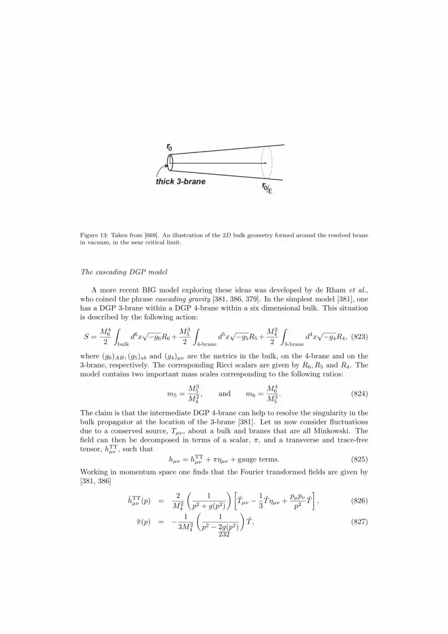
Figure 13: Taken from [669]. An illustration of the 2D bulk geometry formed around the resolved branein vacuum, in the near critical limit.

The cascading DGP model

A more recent BIG model exploring these ideas was developed by de Rham et al.,who coined the phrase cascading gravity [381, 386, 379]. In the simplest model [381], onehas a DGP 3-brane within a DGP 4-brane within a six dimensional bulk. This situationis described by the following action:

S =M4

6

2

∫

bulk

d6x√−g6R6 +

M35

2

∫

4-brane

d5x√−g5R5 +

M24

2

∫

3-brane

d4x√−g4R4, (823)

where (g6)AB , (g5)ab and (g4)µν are the metrics in the bulk, on the 4-brane and on the3-brane, respectively. The corresponding Ricci scalars are given by R6, R5 and R4. Themodel contains two important mass scales corresponding to the following ratios:

m5 =M3

5

M24

, and m6 =M4

6

M35

. (824)

The claim is that the intermediate DGP 4-brane can help to resolve the singularity in thebulk propagator at the location of the 3-brane [381]. Let us now consider fluctuationsdue to a conserved source, Tµν , about a bulk and branes that are all Minkowski. Thefield can then be decomposed in terms of a scalar, π, and a transverse and trace-freetensor, hTT

µν , such that

hµν = hTTµν + πηµν + gauge terms. (825)

Working in momentum space one finds that the Fourier transformed fields are given by[381, 386]

hTTµν (p) =

2

M24

(1

p2 + g(p2)

)[Tµν −

1

3T ηµν +

pµpνp2

T

], (826)

π(p) = − 1

3M24

(1

p2 − 2g(p2)

)T , (827)

232

where59

g(p2) =

πm5

2

√|p2−4m2

6|

tanh−1

(√|p−2m6|p+2m6

) p < 2m6

πm5

2

√|p2−4m2

6|

tan−1

(√|p−2m6|p+2m6

) p > 2m6.(828)

The amplitude between two conserved sources on the brane, Tµν and T ′µν , now takes thesurprisingly simple form

A =2

M24

(1

p2 + g(p2)

)[Tµν T

′µν − 1

3T T ′ − 1

6

p2 + g(p2)

p2 − 2g(p2)T T ′

]. (829)

The last term represents the contribution from the scalar amplitude, whereas the remain-der is the contribution from the massive spin-2 field. The coefficient of scalar amplitudechanges sign as we flow from the IR to the UV,

p2 + g(p2)

p2 − 2g(p2)→− 1

2 as p→ 0

1 as p→∞,(830)

indicating the presence of a ghost in the UV theory, consistent with the results of [436].To eliminate this ghost we must add additional operators to the 3-brane action thatmodify the scalar propagator in the UV60. It turns out that this can be achieved simplyby adding tension, λ, to the 3-brane [381, 388]. As the 3-brane is co-dimension 2, itsvacuum solution is unaffected by the change in tension (it is still Minkowski). In contrast,the 3-brane tension does alter the profile of the fields in the bulk by creating a deficitangle. This means that kinetic terms describing fluctuations on the new vacuum nowreceive corrections from the non-linear bulk interactions. The result is that the scalarpropagator on the 3-brane is modified. One might expect that such effects will necessarilybe suppressed by the five and six dimensional Planck scales, but this is not necessarily sobecause of strong coupling of the scalar in the five dimensional boundary effective fieldtheory [381, 388].

In any event, at higher energies, p m6, the modified amplitude goes like

Aλ ∼2

M24

(1

p2 + 2m5p

)Tµν T ′µν −

1

3T T ′ − 1

6

p2 + 2m5p

p2(

1− 3λ2m2

6M24

)− 4m5p

T T ′

. (831)

For large enough tension, λ >2m2

6M24

3 , the scalar amplitude always has the correct sign,so there is no ghost. However, the tension cannot be arbitrarily large since we require

59Note that the various formulae for propagators and amplitudes in [381, 386] differ. One must takem5,6 → 1

2m5,6 in going from [381] to [386]. The difference is because only one half of the 6D bulk, and

one half of the 4-brane are considered in [386]. This is a perfectly legitimate truncation by Z2 symmetryacross each of the branes. Here, however, we will adopt the conventions of [381] when expressing ourformulae.

60It has also been argued that thickening of the brane can help to eliminate the ghost in this model[386]

233

that the bulk deficit angle is less than 2π. This places an upper bound λ < 2πM46 =

2πm5m6M24 . Provided m6 < m5 we therefore have a window,

2m26M

24

3< λ < 2πm5m6M

24 , (832)

for which the theory is ghost-free in the UV [381, 388]. The condition m6 < m5 hasadded significance in that it permits a transition from 4D to 5D at energies p ∼ m5. Inparticular, we have 4D scalar-tensor gravity in the far UV, for p > m5 > m6,

A(4D)λ ∼ 2

M24 p

2

[Tµν T

′µν − 1

2

(1− λ

m26M

24

1− 3λ2m2

6M24

)T T ′

], (833)

and 5D scalar-tensor gravity for m5 > p > m6,

A(5D)λ ∼ 1

M35 p

[Tµν T

′µν − 1

4T T ′

]. (834)

In the far infra-red, p < m6, we recover 6D gravity,

A(6D) ∼ ln(m6/p)

πM46

[Tµν T

′µν − 1

4T T ′

]. (835)

Thus we have a cascade from 6D → 5D → 4D gravity as we move from large to shortdistances. It is interesting to note that the existence of this cascade seems to be closelyrelated to the absence of ghosts. By taking M4 ∼ Mpl, M5 ∼ 10 MeV and M6 ∼ meV,the cascade occurs at the current horizon scale, as m6 ∼ m5 ∼ H0. Note that a cascadefrom seven dimensions has also been studied in some detail in [387].

For tensions in the range allowed by Eq. (832) the 4D theory at short distances is aBrans-Dicke theory that is incompatible with solar system constraints. The authors of[381] suggest that some sort of Vainshtein mechanism could account for the recovery ofGR at short scales. Indeed, the role of non-linearities in cascading DGP has not yet beenproperly investigated, and one may be concerned that there are issues surrounding thevalidity of the linearised results (as was found in the sub-critical regime of the Kaloper-Kiley model [669]).

Another aspect of cascading DGP that requires further study is cosmology (see[900, 12] for some preliminary work). In [12] a five dimensional proxy theory is usedthat is expected to capture many of the salient features of the original model. Thisproxy model corresponds to a 5D scalar-tensor theory that, in the limit where the scalarand tensor degrees of freedom decouple, agrees with the decoupling limit of the 5Dboundary effective field theory of cascading DGP presented in [381]. Of course, it is byno means unique in this respect.

Induced gravity on intersecting braneworlds

A third BIG model that is very closely related to cascading DGP was developed byCorradini, Koyama and Tasinato [338, 339]. Here a six dimensional bulk contains twointersecting DGP 4-branes, each with induced curvature. At the intersection we place a

234

DGP 3-brane, also with some induced curvature. The cosmological evolution is derivedusing a formalism based on mirage cosmology [685]. The resulting Friedmann equationon the 3-brane is then given by [339]

ρ = 2M24H

2 + 6M35 k2

√1 +

H2

k22

+ 4M46 tan−1

[tanα

√1 +

H2

k22

], (836)

where α is the angle between the two 4-branes, and k2 is a constant that encodes in-formation about the warped geometry in the bulk (and can be derived in a non-trivialway from the parameters of the theory). The model claims to admit self-acceleratingand self-tuning vacua. For fluctuations on a Minkowski 3-brane one may also expect acascade from 6D → 5D → 4D gravity as we move from large to short distances, for suit-ably chosen scales. A thorough perturbative analysis has yet to be done that confirmsthis expectation, or the possible existence of ghosts and strong coupling.

5.6.2. Degravitation

Higher co-dimension braneworld models and cascading gravity are expected to playan important role in realising the degravitation scenario [61]. The idea of degravitationis best understood by rephrasing the cosmological constant problem. Instead of asking“why is the vacuum energy so small?”, we ask “why does the vacuum energy hardlygravitate at all?”. In other words, we accept what our particle physics models are sayingand take the vacuum energy to be up at the (TeV)4 scale or beyond. We then try todevelop a gravity theory that prevents this large vacuum energy from generating a largeamount of curvature.

A phenomenological description of degravitation is given by [61]

G−1(L2)Gµν = 8πTµν , (837)

where Newton’s constant, G, has been promoted to a differential operator, G(L2),depending on a length scale, L, and the covariant d’Alembertian operator, . The idea isthat this operator behaves like a high pass filter characterised by the scale L. Sources withshort characteristic wavelengths, l L, pass through the filter and gravitate normally.Sources with long characteristic wavelengths, l L, such as the cosmological constant,are filtered out and hardly gravitate at all. These considerations amount to imposingthe following limits: G → G for L2(−)→∞ and G → 0 for L2(−)→ 0.

Since the covariant derivative does not commute with the d’Alembertian, Equation(837) suggests that the energy-momentum tensor is not conserved. However, it is impor-tant to realise that this equation is only expected to describe the linearised dynamics ofthe helicity-2 mode of the graviton, given by gµν = ηµν + hµν . The source is conservedwith respect to the full metric, gµν = ηµν + hµν + . . ., where the ellipsis denotes theadditional (Stuckelberg) modes that necessarily appear in a fully covariant theory [452].It is clear that the extra modes must play an important role in the filtering process atlong wavelengths. The transition to normal gravity for short wavelength modes occursprecisely because these modes get screened by the Vainshtein mechanism [1241] (see ourdiscussion of the Vainshtein mechanism in the context of DGP gravity in Section 5.5.4).

The filter operator is often parametrised as follows:

G−1(L2) =

(1− m2()

)G−1, (838)

235

where m2() ∝ L2(α−1)α, and 0 ≤ α < 1. The upper limit is a necessary, but notsufficient, condition for degravitation, whereas the lower limit is required by unitarity[452]. Massive gravity (see Section 3.3.3) corresponds to α = 0, whereas DGP gravity61

(see Section 5.5) corresponds to α = 1/2. It turns out that models with co-dimensionn > 2 are expected to correspond to α = 0 [386].

Using Equation (837) as its starting point, degravitation can be demonstrated in acosmological context by the ratio of scalar curvature to Λ scaling as t−1/2 for a broadclass of filters, where t is the proper time of comoving observers [452]. However, thecorresponding cosmological solution arising from a higher co-dimension brane scenariohas yet to be found explicitly.

Working at the level of the phenomenological equations, N-body simulations for de-gravitation scenarios have been studied by Khoury and Wyman [690]. Their simulationis based on a modified Poisson equation, given by

−[k2

a2+

1

L2

(kL

a

)2α]

Ψ = 4πGρ. (839)

Thus, the emergence of the Vainshtein mechanism is encoded in the simulations via Eq.(815), rather than being recovered from the simulation itself. They find that the matterpower spectrum determined from the simulation agrees well with the HALOFIT [1156]formula for k <∼ 0.2hMpc−1. However, for smaller scales the HALOFIT formula over-predicts power because HALOFIT does not capture the Vainshtein effect. Nevertheless,they find a way to recalibrate the HALOFIT parameters such that it agrees with theirsimulation on all scales.

5.7. Einstein Gauss-Bonnet Gravity

In Section 2.4.1 we outlined how Lovelock’s theorem [831, 832] constrains the classof theories that can be constructed from the metric tensor alone: In four dimensions,the most general rank-2 tensor that can be derived from a variational principle and is(i) symmetric, (ii) divergence free, and (iii) built out of the metric and its first twoderivatives only is given by a linear combination of the metric and the Einstein tensor,i.e.

E(4D)µν = −1

2α0gµν + α1Gµν . (840)

Such a term arises from the variation of the Einstein-Hilbert action in the presence of acosmological constant,

E(4D)µν =

1√−gδ

δgµν

∫d4x√−g (α0 + α1R) . (841)

In four dimensions the Einstein-Hilbert action therefore gives the most general fieldequations with the desired properties. In more than four dimensions, however, this result

61The full DGP theory does not exhibit degravitation, but this is not necessarily the unique theorywith α = 1/2.

236

no longer holds. For D = 5 or 6 dimensions the most general rank-2 tensor satisfyingthe same three conditions is given by [831] (see also [767, 1313])

E(5D/6D)ab = −1

2α0γab + α1Gab + α2Hab, (842)

where (in D dimensions) γab is the metric, Gab = Rab − 12Rγab is the Einstein tensor,

and we have introduced the Lovelock tensor [831]

Hab = 2RRab − 4RaαRcb − 4RacbdRcd + 2RacdeRbcde −1

2Gγab, (843)

where G = RabcdRabcd − 4RabRab +R2, and Rabcd is the Riemann tensor constructedfrom γab. The Lovelock tensor is obtained by variation of the Gauss-Bonnet action,

Hab =1√−γ

δ

δγab

∫dDx√−gG. (844)

These results can generalised still further as the dimensionality of space-time is increased.To see how, note that dDx

√−γR and dDx√−γG correspond to the Euler classes of order

one and order two [936], and are topological in D ≤ 2 and D ≤ 4 respectively62. Togeneralise Lovelock’s theorem to even higher dimensions we must then add the higherorder Euler classes to the corresponding action, and compute the metric variation. TheEuler class at order k depends on kth powers of curvature. In D dimensions we musttherefore include Euler classes up to order [(D− 1)/2], where the square brackets denotethe integer part. The reader is referred to [270], and references therein, for further details.

5.7.1. Action, equations of motion, and vacua

In five or six dimensions General Relativity is just a special case of a broader class oftheories commonly referred to as Einstein-Gauss-Bonnet (EGB) gravity. These theoriesare described by the action

S =1

16πGD

∫dDx√−γ

(R− 2Λ + αG

)+

∫dDxLm(γab, ψ), (845)

where Lm is the Lagrangian density of the higher dimensional matter fields that areminimally coupled to the metric. The corresponding field equations are given by

Gab + Λγab + αHab = 8πGDTab, (846)

where Tab = − 2√−γ

δδγab

∫dDxLm(γab, ψ) is the energy-momentum tensor of the matter

fields. As we will see shortly, although Λ acts like a bare cosmological constant, it differsfrom the effective cosmological constant, Λeff, seen by the geometry.

The Gauss-Bonnet corrections are weighted by the parameter α. This has dimensionsof [length]2 and is often associated with the slope parameter, α′, in heterotic string the-ory. To see why, consider the effective theory describing the dynamics of the heterotic

62One can check explicitly that the Einstein tensor is identically zero in two dimensions, and that theLovelock tensor is identically zero in four dimensions.

237

string on the 10 dimensional target space. Working at tree level in the string couplingand performing a perturbative expansion in the inverse string tension, µ−1

F ∼ 2πα′,we see that the leading order term gives the standard Einstein-Hilbert action, and thenext to leading order term, after some field redefinitions, gives the Gauss-Bonnet ac-tion [566, 886]. In fact, one may have expected such a result based on the fact thatstring theory is known to be ghost free. As noted by Zwiebach [1316], second-ordercorrections to the Einstein-Hilbert action will necessarily give rise to ghosts unless theyappear in the Gauss-Bonnet combination. Note that if we do identify EGB with a stringygeneralisation of General Relativity, we should restrict attention to α ≥ 0 for consistency.

Maximally symmetric vacua

We now consider the maximally symmetric vacuum solutions, γab, satisfying Rabcd =2Λeff

(D−1)(D−2) (γacγbd− γadγbc), where Λeff is the effective cosmological constant seen by the

curvature. There are two possible values for Λeff, given by [279]

Λ±eff = ΛCS

(1±

√1− 2Λ

ΛCS

), (847)

where

ΛCS = − 1

4α

(D − 1)(D − 2)

(D − 3)(D − 4). (848)

For these vacua to be well defined the bare cosmological constant must satisfy the boundΛ/ΛCS ≤ 1/2. It is easy to check that Λ+

eff/ΛCS ≥ 1 ≥ Λ−eff/ΛCS , with equality whenΛ = ΛCS/2. This is known as the Chern-Simons limit (at least in odd dimensions)[1297, 344], and corresponds to the case where the two roots coincide. Note that onlythe lower root has a smooth limit, Λ−eff → Λ, as α → 0, and as such is often referredto as the “Einstein” branch. In contrast, the upper root, Λ+

eff, is not smooth as α → 0,and represents a distinct new feature of EGB gravity that is completely absent in higherdimensional General Relativity. For this reason, this branch is often referred to as the“stringy”, or “Gauss-Bonnet”, branch.

We now consider metric perturbations about these vacua, γab = γab + δγab. Thelinearised field equations then take the remarkably simply form

δGab + Λeffδγab = 8πGeffTab, (849)

where δGab is the linearised Einstein tensor. Thus, we have perturbative Einstein gravitywith an effective Newton’s constant given by

Geff =GD

1− Λeff

ΛCS

. (850)

Assuming that the bare Newton’s constant is positive, GD > 0, it follows that pertur-bative gravity on the Einstein branch (Λeff/ΛCS < 1) is essentially well behaved, asGeff > 0. In contrast, on the Gauss-Bonnet branch (Λeff/ΛCS > 1), we have Geff < 0indicating the presence of a perturbative ghost [279]. We refer the reader to the closingparagraphs of Section 5.5.3 for a discussion of the pathologies associated with ghosts.

238

The above conclusions regarding stability are robust provided we can trust our ef-fective perturbative description. Here we expect this description to be valid at energiesup to a cut-off, Ecut-off ∼ 1/(Geff)1/(D−2. As we approach the Chern-Simons limit(Λ → ΛCS/2), where the two branches coincide, it follows that the cut-off for the effec-tive description should have the limit Ecut-off → 0. This indicates strong coupling, and abreakdown of perturbation theory. To analyse the stability of either branch close to thislimit one must study non-perturbative phenomena such as instanton transitions. Thisreveals that transitions between branches are unsuppressed in the near Chern-Simonsregime, and that there is very strong mixing between the two (almost degenerate) vacua.We conclude that neither of them can accurately describe the true quantum vacuum statein this regime, as both will quickly become littered with bubbles of the other vacuum[279].

Spherically symmetric solutions

Static spherically symmetric solutions to the vacuum field equations were first dis-covered by Boulware and Deser [176],

ds2 = −V (r)dt2 +dr2

V (r)+ r2dΩD−2, (851)

where dΩD−2 is the metric on a unit (D − 2)-sphere. We have two branches for thepotential, V (r), given by [176, 279]

V±(r) = 1 +2ΛCSr

2

(D − 1)(D − 2)

(1±

√1− 2Λ

ΛCS− M(D − 1)

ΛCSΩD−2rD−1

), (852)

where ΩD−2 is the volume of the unit (D − 2)-sphere. M is an integration constantthat one can identify with the mass of a spherically symmetric source (possibly point-like). As above, the lower root corresponds to the Einstein branch, and has a smoothlimit as α→ 0. The upper root corresponds to the Gauss-Bonnet branch, and does nothave a smooth limit. Of course, the two roots are degenerate in the Chern-Simons case(Λ = ΛCS/2).

We shall stay away from the Chern-Simons limit in the remainder of this section. Notethat a generalised form of Birkhoff’s theorem now holds that guarantees that Equation(851) represents the most general spherically symmetric solution, even without the as-sumption of staticity [272]. Let us consider the properties of this solution for a sourceof positive mass, M > 0. On the Einstein branch the singularity at r = 0 is shieldedby an event horizon, and there are no obvious pathologies. This is not the case on theGauss-Bonnet branch, where we have a naked time-like singularity.

At asymptotically large radii the metric functions take the form

V± ≈ −2Λ±effr

2

(D − 1)(D − 2)+ 1± M

ΛCSΩD−2rD−3. (853)

The asymptotic solution here can be seen to resemble the generalised Schwarzschild-Tangherlini solution in D dimensional GR [1202], with cosmological constant Λ±eff, andmass ±M . In particular, on the Gauss-Bonnet branch, it appears as if our solution has

239

negative gravitational energy even for a positive energy source. This conclusion, however,is incorrect. A proper computation of the gravitational energy taking into account allof the Gauss-Bonnet corrections reveals the mass of the solution in Eq. (851) is +M onboth branches [415, 416, 1010]. For an in-depth discussion of this, and related stabilityissues, the reader is referred to [279]. For an excellent review of Lovelock gravities, andtheir black hole solutions, see [270].

5.7.2. Kaluza-Klein reduction of EGB gravity

In Section 5.1.1 we discussed compactification of higher dimensional GR on a circle.The same operation can now be performed with the EGB action, given in Eq. (845). Westart in five dimensions with coordinates (xµ, z), where the z direction is compact. Wecan then dimensionally reduce down to four dimensions using the following ansatz

γµν = gµν + e2φAµAν , γµz = e2φAµ, and γzz = e2φ, (854)

where the metric, gµν , gauge field, Aµ and the dilaton, φ, are all independent of z.Integrating out the compact dimension we arrive at the following effective theory [915]:

Seff =1

16πG5

∫d4x√−gLeff, (855)

where

Leff = eφ[R− 1

4e2φF 2 − 2Λ + α(RµναβR

µναβ − 4RµνRµν +R2)

]

+ αe3φ

[−3

8e2φ

(FµνF

ναF

αβF

βµ −

1

2(F 2)2

)

− (FµαFνβ + FµνFαβ)

(Rαβµν − 4Rα[µδ

βν] +Rδα[µδ

βν]

)

− 2(∇µFαβ)(∇αF βµ)− 2(∇µFαµ)(∇νFαν)− 12(Fµα∇αφ)(Fµβ∇βφ) + 6F 2(∇φ)2

+4(Fαβ∇µφ)∇µFαβ − 4(Fαβ∇µφ)∇αF βµ − 12(Fαβ∇βφ)∇µFαµ]

+ αeφ[8e−φ∇µ∇νeφ − 2e2φFµαFν

α]Gµν + 3αe2φ

[2FαβFβ

µ∇µ∇αeφ + F 2eφ],

(856)

and F 2 = FµνFµν , with Fµν = ∇µAν − ∇νAµ. Note that for Λ = 0 and α = 0 we

recover the results of Section 5.1.1, provided we perform a conformal transformation tothe Einstein frame and canonically normalise the dilaton.

One property of the Lagrangian in Eq. (856) is that it gives rise to field equations thatare at most second order in derivatives. This is, of course, inherited from the underlyingtheory, and enables us to consider an interesting class of scalar-tensor theories by freezingthe gauge field such that Aµ = 0. We refer the reader to Section 3.1, and [38], for furtherdiscussions on four-dimensional theories of this type.

5.7.3. Co-dimension one branes in EGB gravity

Interest in EGB gravity has really taken off in recent years, largely due to its appli-cation to braneworlds. We discussed the braneworld paradigm in some detail in Section

240

5.2. Schematically, the physics of 3-branes in five dimensional EGB gravity is more orless the same as in General Relativity, as we will now discuss.

Generic action and equations of motion

As in the GR case discussed in Section 5.3.4, we split our five dimensional bulk intoa series of domains separated by a series of 3-branes, so that the action is given by

S =

∫

bulk

d5x√−γ

[M3

5

2(R+ αG) + Lbulk

]

+∑

branes

∫

brane

d4x√−g

−∆

[M3

5 (K + 2α(J − 2GµνKµν))]

+ Lbrane

, (857)

where M5 = (1/8πG5)1/3 is the bulk Planck scale. In comparison with Equation (615) wehave a Gauss-Bonnet correction in the bulk and the corresponding Myers boundary term[931] on each brane. The latter depends on the extrinsic curvature, Kµν , the inducedEinstein tensor Gµν = Rµν − 1

2Rgµν , and the trace J = gµνJµν , where [363]

Jµν =1

3

(2KKµαK

αν +KαβK

αβKµν − 2KµαKαβKβν −K2Kµν

). (858)

The bulk field equations are then given by

Rab −1

2Rγab + αHab =

1

M35

T bulkab , (859)

with the boundary conditions at the brane given by the “DGW” junction conditions[363, 553] (see also [409]),

∆M2

5

[Kµν −Kgµν + 2α(3Jµν − Jgµν − 2PµανβK

αβ)]

= −T braneµν . (860)

Here we introduce the double dual of the Riemann tensor, defined as [902]

Pµναβ = −Rµναβ + 2Rµ[αδνβ] − 2Rν[αδ

µβ] −Rδ

µ[αδ

νβ]. (861)

In what follows we will assume that the bulk geometry is only63 sourced by a cosmologicalconstant T bulk

ab = M35 Λγab, which we take to be negative, as in the Randall-Sundrum

model, Λ = −6k2. We will consider a single brane with tension σ, and some inducedcurvature, M2

indR. Its energy momentum tensor is then given by

T braneµν = −σgµν −M2

indGµν + Tµν , (862)

where Tµν denotes the contribution from any additional matter excitations on the brane.For simplicity we will impose Z2 symmetry across the brane (see [1012, 1013] for a dis-cussion of asymmetric configurations).

63For generalisations with bulk scalar fields and bulk Maxwell fields see [271] and [805], respectively.

241

Weak gravity on a Minkowski brane

Let us seek Randall-Sundrum-like vacua, corresponding to a Minkowski brane in anAdS bulk,

ds2 = γabdxadxb = dz2 + e−2|z|/leffηµνdx

µdxν . (863)

The effective AdS curvature in the bulk is then determined by the bulk equations ofmotion (859). We find

1

l2eff

=1

4α

(1±

√1− 8α

l2

), (864)

where the lower root corresponds to the Einstein branch and the upper root to the GBbranch. Meanwhile, the vacuum DGW junction conditions at z = 0 impose the followingconstraint on the brane tension

σ = 6M3

5

leff

(1− 4α

3l2eff

). (865)

Since we are interested in weak gravity on the brane, we consider small fluctuations inthe metric and the brane position. As we saw previously, the linearised equations ofmotion are identical to those found in perturbative General Relativity,

δGab −6

l2eff

δγab = 0. (866)

The linearised junction conditions also take a remarkably simple form,

2(M eff5 )3δ(Kµ

ν −Kδµν ) = M2renδG

µν − T µν , (867)

where we identify the effective five dimensional Planck scale,

(M eff5 )3 = M3

5

(1− 4α

l2eff

)(868)

and the renormalised induced curvature scale,

M2ren = M2

ind +8αM3

5

leff. (869)

The effective Planck scale is consistent with the effective Newton’s constant introducedin Equation (850), (M eff

5 ) = (1/8πGeff)1/3. It follows that our weak gravity descriptionis identical to the corresponding description in General Relativity, provided we make useof the effective cosmological constant and Planck scale in the bulk, and renormalise theinduced curvature on the brane. For further details the reader is referred to [270], andreferences therein (see also [413]).

The characteristic behaviour of weak gravity on the brane is as follows [270]: Atlarge distances we recover four dimensional General Relativity, with an effective fourdimensional Planck scale

M IRpl =

√M2

ind +M35 leff(1 + 4α/l2eff) =

√M2

ren + (M eff5 )3leff. (870)

242

This holds provided 1/leff 6= 0. For 1/leff = 0 the large distance behaviour is five dimen-sional owing to the absence of a normalisable zero mode in the Minkowski bulk.

At short distances we recover four dimensional Brans-Dicke gravity, with a differ-ent effective Planck scale64, MUV

pl =√M2

ind + 8αM35 /leff = Mren, and a Brans-Dicke

parameter given by

2w + 3 =3

4

(M2

ind/leff +M35 (1 + 4α/l2eff)

M35 (1− 4α/l2eff)

)=

3

4

((M IR

pl )2

(M eff5 )3leff

). (871)

This holds provided Mren 6= 0. If Mren = 0 then the short distance behaviour is fivedimensional since there is no effective induced curvature giving rise to quasi-localisationnear the brane.

These results are consistent with the behaviour that would be expected in linearisedtheory on a brane in five dimensional General Relativity, with bulk cosmological con-stant, Λeff = 6/l2eff, bulk Planck scale, M eff

5 , and brane induced curvature scale, Mren.It is interesting to note that the Brans-Dicke parameter gets large close to the Chern-Simons limit as M eff

5 → 0. However, as we saw earlier, quantum fluctuations in the bulkbecome strongly coupled at ∼M eff

5 , so this prediction may be unreliable.

Brane cosmology in EGB gravity

The methods used in Section 5.4 to derive the cosmological evolution of co-dimensionone branes apply equally well to branes in EGB gravity, provided we use the DGWjunction conditions give in Eq. (860). Recall that brane cosmology can be studied usingeither the brane-based formalism or the bulk-based formalism. The brane-based formalismrelies on the covariant formulation of the effective Einstein equation on the brane. Thishas been worked out for EGB gravity and applied to cosmological branes [859] (see also[709]). In the bulk based formalism, the generalised form of Birkhoff’s theorem [272]ensures that the bulk geometry around a FLRW brane is given by

ds2 = −V (r)dτ2 +dr2

V (r)+ r2qijdx

idxj , (872)

where V (r) takes the form

V±(r) = κ+r2

4α

(1±

√1− 8α

l2− 8αµ

r4

), (873)

and qij(x) is the metric of a 3-space of constant curvature, κ = 0,±1. Note that thisgeneralises the black hole solution given in Eq. (852) to different “horizon” topologies[233]. Let us once again assume Z2 symmetry across the brane for simplicity. As inSection 5.4.2, we treat the brane as an embedding τ = τ(t), and r = a(t) in the bulkgeometry, identifying t with the proper time of comoving observers on the brane, anda(t) with the scale factor. After imposing the DGW boundary conditions given in Eq.

64There is a typo in the corresponding expression for MUVpl in [270].

243

(860), we find that the Hubble parameter, H = a/a, obeys [270] (see also [363, 272, 557,851, 718])

[1 +

4α

3

(2(H2 +

κ

a2

)+κ− V (a)

a2

)]√H2 +

V (a)

a2=

ρbrane

6M35

=σ + ρ− 3M2

ind

(H2 + κ

a2

)

6M35

.(874)

This can be recast as a cubic equation in H2 + κa2 , and solved analytically to give a

modified Friedmann equation. The most commonly studied scenario has Mind = 0, withthe bulk taken to lie on the Einstein branch. We then find [363]

H2 +κ

a2=c+ + c− − 2

8α, (875)

where

c± =

√(

1− 8α

l2+

8αµ

a4

)3/2

+α(σ + ρ)2

2M65

± (σ + ρ)

M35

√α

2

2/3

. (876)

This cosmology can give rise to rapid inflation, just as in Randall-Sundrum cosmology[806]. However, the Gauss-Bonnet corrections do introduce some new features at thelevel of cosmological perturbations. For example, in Randall-Sundrum cosmology theconsistency relation between the tensor-to-scalar ratio, r, and the tensor spectral index,nT , agrees with the standard GR result, r = −8nT . This relationship is broken by theGB corrections as the amplitude for the tensor perturbations are no longer monotonicallyincreasing with scale [437]. We also find that observational constraints of GB braneinflation are typically softened relative to Randall-Sundrum cosmology, such that certain“steep” potentials are no longer ruled out [1224].

5.7.4. Co-dimension two branes in EGB gravity

In Section 5.6 we mentioned that higher-order operators could be added to thebulk gravity to regularise the singularities that appear when we have an infinitely thinbraneworld of co-dimension ≥ 2. One of the ways to do this is to add Gauss-Bonnetcorrections in the bulk [174, 283, 282]. The simplest and most well studied scenario is toconsider co-dimension-2 branes in six dimensional EGB gravity without any additionalsources in the bulk (see, for example, [174, 277, 676, 675, 281, 280, 348, 349]). This gives

S =

∫

bulk

d6x√−γ

[1

16πG6(R+ αG)

]+

∫

brane

d4xLbrane. (877)

If we assume axial symmetry in the bulk we get

ds2 = γABdxAdxB = dr2 + L2(x, r)dθ2 + gµν(x, r)dxµdxν , (878)

and it turns out that the Einstein tensor on the brane is given by [174, 277]

Gµν = − 1

4αgµν +

G6

α(1− β)T braneµν + f(β)Wµν , (879)

244

where

Wµν = KλµKνλ −KKµν +

1

2gµν(K2 −KλσK

λσ), (880)

and Kµν = 12∂rgµν . The parameter β is the deficit angle on the brane, and is often

assumed to be constant, although this need not be case [277]. A field dependent deficitangle, β = β(x), will lead to two important effects: Transfer of energy between bulk andbrane, and an effective four dimensional Newton’s “constant” that can vary as Geff =

G6

8πα(1−β(x)) [277]. These can clearly be constrained by observation, but it would be very

interesting to study the role varying β could play in attempts to self-tune the vacuumcurvature in co-dimension 2 models.

The function f(β) depends on the mathematical technique used to derive the bound-ary conditions at the distributional source [277, 676, 675]. The boundary conditionsderived in [174] lead to the condition Wµν |brane = 0, suggesting that Einstein gravityshould be recovered on the brane at all scales, even for an infinitely large bulk. However,it is now understood that these conclusions rely on the assumption ∂rKµν = 0 at thebrane, which is too constraining. For constant β the Friedmann equation on the braneis given by [277]

H2 +κ

a2=

8πGeff

3ρbrane −

1

12α+

c2

ρ2branea

8, (881)

where c2 is an integration constant. However, as we already emphasised, in general β canvary, and in this case one cannot find a closed system of equations on the brane [277].

245

6. Parameterised Post-Friedmannian Approaches and Observational Constraints

As expounded in this review, there now exists a vast range of candidate theories ofgravity that modify Einstein’s theory of General Relativity in one way or another. It isalso seems clear that many more such theories are likely to be proposed in the future.If these theories are to be of any value in understanding and resolving the problemsassociated with the Dark Universe then they must be confronted with cosmological data.This is, in principle, straightforward but time-consuming. It involves working out theperturbation equations for each and every theory, incorporating them into the Einstein-Boltzmann solvers and N-body codes, and calculating a list of observables.

This situation is analogous to the experimental study of General Relativity in theearly 1970s, during what has become known as the ‘Golden Age’ of General Relativity.There, one had a plethora of alternative theories of gravity that needed to be confrontedwith constraints from Solar System measurements. The Parameterised Post-Newtonian(PPN) method was invented in this case as an intermediate step between theory andexperiment. It involves a set of generic parameters that can be easily constrained byexperiments [1207]. Using the PPN method one can then take any given theory, calculatethe PPN parameters it predicts, and compare them with observational constraints. Thisprocess is outlined in Section 2.5.

Over the last few years, the idea of creating such an intermediate step when con-sidering cosmological constraints has starting taking hold. It has been dubbed by somethe ‘Parameterised Post-Friedmannian approach’, and it attempts to encompass, at thelinear level, the behaviour of a wide array of alternative theories of gravity. We will nowoutline the basic idea behind this approach.

The bulk of the cosmological data that can be used to constrain modifications of grav-ity can be interpreted in terms of perturbations about a Friedmann-Lemaıtre-Robertson-Walker universe. Throughout this review we have presented how the evolution of cosmo-logical perturbations is modified in these theories, relative to their behaviour in GeneralRelativity. One can now ask oneself if there is a general way of modifying the equa-tions of cosmological perturbations such that it will encompass all the theories we havepreviously discussed.

The simplest approach, that has been in vogue for the past few years, is to modifytwo of the four Einstein field equations as follows:

− 2k2Φ = 8πµGa2∑

X

ρX [δX + 3(1 + wX)HθX ] (882)

Φ−Ψ = ζΦ, (883)

where two new functions have been introduced: The effective Newton constant, Geff =µG, and the gravitational slip, ζ. One can interpret Geff as the inclusion of a form of grav-itational screening, reducing (or enhancing) the local gravitational force on cosmologicalscales. The gravitational slip phenomenologically parametrises the shear that seems toarise frequently in scenarios of modified gravity. This parametrisation is incredibly usefulfor quantifying deviations from General Relativity, and a number of authors have usedit in their analyses of cosmological data [148, 237, 630, 627, 41, 360, 361, 123, 1302].

It is instructive to see in what circumstances such a parametrisation might arise, andto do this we will develop a consistent formalism in what follows.

246

6.1. The Formalism

In order to generalise the perturbed Einstein equations we follow the approach andnotation used in [1149, 1151, 501, 77]. Here we split the field equations of the theoryin question into a set of evolution equations for the metric, evolution equations for theadditional gravitational fields (if any are present), and a set of constraint equations. Theevolution equations for the metric, and the constraint equations, can then be writtenschematically as

δGmodµν ≡ δGµν − δUµν = 8πG[δTµν + δTEµν

], (884)

where δGµν is the perturbed Einstein tensor, δUµν is the contribution of any other termsthat involve perturbations of the metric, δTµν is the perturbed energy-momentum tensorof matter fields in the space-time, and δTEµν is the contribution of any terms that involveperturbations to the additional gravitational fields.

Let us now be more specific. We can define the following new variables: U∆ ≡−a2δU0

0, ~∇iUΘ ≡ −a2δU0i, UP ≡ δU ii and Di

jUΣ ≡ a2(δU ij − 13δU

kkδij), as well as the

new gauge invariant

Γ ≡ 1

k

(Φ′ +HΨ

), (885)

where the Bardeen potentials Φ and Ψ are defined in Eqs. (85) and (86) of Section 2.6.Dropping the hats (i.e. working in the conformal Newtonian gauge), we can write thetwo constraint equations coming from G00 and G0i as

− 2k2(Φ + 3HkΓ) = 8πGa2∑

X

ρXδX + U∆ (886)

2kΓ = 8πGa2∑

X

(ρX + PX)θX + UΘ, (887)

and the two evolution equations coming from the trace and traceless parts of Gij as

kΓ′ + 2kHΓ +

(H′ −H2 − k2

3

)Ψ +

k2

3Φ = 4πGa2

∑

X

δPX +1

6UP (888)

Φ−Ψ = 8πGa2∑

X

(ρX + PX)ΣX + UΣ.(889)

We can then combine Eqs. (886) and (887) to find a modified Poisson equation:

− 2k2Φ = 8πGa2∑

X

ρX [δX + 3H(1 + wX)θX ] + U∆ + 3HUΘ. (890)

Assuming that the theory in question has at most N -time derivatives in its fieldequations, and bearing in mind from Eqs. (85), (86) and (885) that Φ and Γ have onetime derivative when expressed in an arbitrary gauge, the components of the tensor Uαβ

247

can be written as

U∆ =

N−2∑

n=0

k2−n[AnΦ(n) + EnΓ(n)

], (891)

UΘ =

N−2∑

n=0

k1−n[BnΦ(n) + FnΓ(n)

], (892)

UP =

N−1∑

n=0

k2−n[CnΦ(n) + InΓ(n)

], (893)

UΣ =

N−1∑

n=0

k−n[DnΦ(n) + JnΓ(n)

], (894)

where Φ(n) ≡ dn

dτn Φ, and similarly for Γ. The coefficients An-Jn depend on time andscale through the scale factor, a, and wavenumber, k. For the sake of brevity we willrefrain from explicitly stating these dependences.

Now, although we have defined U above in the Newtonian gauge, the individual termsappearing in the expressions above are all gauge invariant. This fact, however, imposesfurther constraints because the gauge-invariant variable Γ contains second derivatives ofthe scale factor, when expressed in an arbitrary gauge. Hence, to avoid higher derivativesof the background appearing in the field equations, we have to set

EN−2 = FN−2 = IN−1 = JN−1 = 0. (895)

We assume that the evolution equations for the matter fields remain unchanged, and thatthese equations are supplemented by additional evolution equations for the extra gravi-tational fields. Finally, the field equations are closed by imposing the Bianchi identities.This imposes one of two possible options: (i) ∇αTEαβ = ∇αUαβ = 0, which imposes a

series of constraints such that the theory remains consistent, or (ii) ∇α(TEαβ + Uαβ) =0, which is the more general situation. For a detailed discussion of these issues see[1149, 1151, 77].

6.1.1. Evolution of perturbations on super-horizon scales

In principle it may seem that one should explore the long wavelength behaviour ofcosmological perturbations on a case by case basis. It turns out, however, that theinfinite wavelength mode can be studied simply by considering the evolution of the back-ground equations. This observation is due to Bertschinger [148], and proceeds as follows.Consider a background with scale factor a(τ, κ) where κ is the spatial curvature of ahyper-surface of constant τ :

ds2 = a2

[−dτ2 + dχ2 +

1

κsinh2

κ(√κχ)dΩ

](896)

where sinhκ(x) equals sin(x) for κ > 0, equals x for κ = 0, or equals sinh(x) for κ < 0.We can now perturb this space-time as κ→ κ(1 + δκ) , and compensate by a change thecoordinates τ → τ +α and χ→ χ(1− 1

2δκ). Here δκ is a constant, while α = α(τ). Notethat in this case the scale factor a(τ, κ) is perturbed as a(τ +α, κ(1 + δκ)). In words, the

248

scale factor will come out as the solution of some generalised set of Friedmann equations,and will depend on the spatial curvature, κ.

We can now write this new geometry in the form of a perturbed FLRW metric, withbackground curvature κ:

ds2 = a2

−(1 + 2Ψ)dτ2 + (1− 2Φ)

[dχ2 +

1

κsinh2

κ(√κχ)dΩ

], (897)

where

Ψ(τ) =∂ ln a

∂ lnκδκ + α′ +Hα, (898)

Φ(τ) =

(1

2− ∂ ln a

∂ lnκ

)δκ −Hα. (899)

One can now eliminate α to find a generic evolution equation that relates δκ with Φ andΨ without specifying any particular theory of gravity:

1

a2

d

dτ

(a2Φ

H

)= Φ−Ψ +

[1

2a

d

dτ

( aH)− ∂ lnH∂ lnκ

]δκ, (900)

where entropy perturbations have been neglected65. The constant δκ that remains in theequation above has a direct physical interpretation: It is twice the comoving curvatureperturbation. Note that we have also assumed that shear perturbations are negligible onlarge scales, that local energy-momentum us conserved, and that spatial gradients canbe discarded. By choosing H(a, κ), and a relation between Φ and Ψ, one now has theevolution equation completely defined. This is a powerful statement, as it means it ispossible to determine the evolution of large-scale perturbations without delving into thedetails of the theory.

However, in order to complete the system here one still needs to specify a relationbetween Φ and Ψ. As we will describe below, it has become standard practise to assumethe simplest form of the PPF parametrisation, that we described above, on super-horizonscales. Within this approach comparisons have been made between choices of µ and ζ,and the outcomes of numerical solutions for specific theories. These comparisons showreasonable agreement, but, as yet, there is no compelling argument for applying thesimplest PPF parametrisation on large scales. In other words, there is no guarantee thata simple relation of the form Ψ = ζΦ can encompass all possible theories of gravity. Infact, it would appear that Eq. (900) does not allow such an interpretation.

6.1.2. The simplified PPF approach, and its extensions

Let us now revisit the simplest, and by far the most popular, version of the Param-eterised Post Friedmannian approach [148, 237, 630, 627, 41]. Here one considers onlyEqs. (889) and (890). The further assumption that perturbations have no anisotropicstress (i.e. ΣX = 0) then allows one to reorganise them in the form of Eqs. (882) and(883). These equations can then be rewritten in terms of the Uαβ tensor by choosing

U∆ + 3HUθ = 2k2

[1− µµ

]Φ,

UΣ = ζΦ.

65Including entropy perturbations is straightforward, and for this the reader is referred to [148].

249

The coefficients Ai, Bi, Ci and Di must now be chosen to satisfy this condition.It is understandable why this approach is popular, as it has a number of benefits.

Firstly, it is applicable in the quasi-static regime the arises when k → ∞ (i.e. on smallscales relative to the cosmological horizon). Furthermore, the perturbation equationsnow form a closed system. This means that if, for example, we restrict ourselves to adust-filled universe then Eqs. (882) and (883), together with

δ′M = −k2θM + 3Φ′ (901)

θ′M = −HθM + Ψ, (902)

form a complete system of differential equations that can be straightforwardly solved.It is instructive at this point to specify the various versions of the simplified PPF

formalism that are currently in use:

• Caldwell, Cooray and Melchiorri [237, 360] introduced the system66

µ = 1

ζ ≡ $ = $0a3, (903)

which was later extended to [361]

µ = 1 + µ0a3. (904)

• Bertschinger and Zukin [148, 151] proposed a reduced parametrisation that takesinto account the conservation of long wavelength curvature perturbations. Onlyone parameter is considered67:

γBZ = 1− ζ, (905)

that is further refined as γBZ = 1 + βas, where β and s are constants. Theseauthors make the additional assumptions that γBZ depends only on time, evenon sub-horizon scales, and that the Bertschinger long-wavelength construction (seeSection 6.1.1) can also be extended to sub-horizon scales. The latter of these as-sumptions allows them to solve for Φ, from which Ψ and δ are then determined. Theassumption of scale-independence is later relaxed further, such that the followingparameterisation can be made

γBZ =1 + β1k

2as

1 + β2k2as

GΦ = µ(1− ζ) = G1 + α1k

2as

1 + α2k2as,

where αi and βi are constants 68.

66The initial convention was that $ = $0Ω0DEΩ0M

a3, but the authors changed their convention in

subsequent publications.67The symbol used was actually γ, to which we have added a subscript ”BZ” to distinguish it from

other parameters with the same name. A similar approach will be used with the other frame-workspresented here.

68We kept the original symbol GΦ here, although under our conventions it would be more accuratelywritten as GΨ, as it plays the role of an effective gravitational constant for a modified Poisson equationfor Ψ.

250

• Amendola, Kunz and Sapone [41] modify the Poisson equation and the slip byconsidering the two functions QA and ηA:

QA = µ,

ηA = −ζ, (906)

while a third variable, ΣA = QA(1 + ηA/2), is also introduced in order to simplifythe relevant expression for gravitational lensing: Φ + Ψ = 2ΣAΦ. A comparison ofthis approach is made with DGP and scalar-tensor theories, both on sub-horizonscales.

• Zhang et al. [1301] make the parameterisation

ηZL =1

1− ζ ,

Geff = µ(1− ζ/2). (907)

These authors also introduce the EG statistic, which we describe further below.

• Zhao et al. [1302] modify the Poisson equation using Ψ. They introduce the twoparameters

ηZG =1

1− ζ ,

µZG = µ(1− ζ), (908)

as well as a third derived parameter ΣZG = µZG(1 + ηZG)/2 = ΣA. Furtherrefinements are made by considering two specific models: A case where µZG =µZG(τ) and ηZG = ηZG(τ) transit from their GR values in the early universe tomodified constant values today, and a case where the two functions are pixelisedin the τ, k plane by 2× 2 pixels per function.

• A parametrisation specifically designed for small scales was proposed by Amin,Blandford and Wagoner [44], where

BA(Hk, a) = (1− ζ)µ = β0(a) + β1(a)Hk + β2(a)H2k + . . .

ΓA(Hk, a) = µ = γ0(a) + γ1(a)Hk + γ2(a)H2k + . . . , (909)

while the matter density fluctuation is likewise parametrised by

δm(a, k) = δ(k)i[δ0(a) + δ1(a)Hk + δ2(a)H2

k

], (910)

where δ(k)i is specified by initial conditions. In this approach different theoriescorrespond to different sets of the functions βi, γi, δi. The authors find the ap-propriate functions for ΛCDM, scalar-tensor theories, quintessence models, f(R)theories, and DGP. They also note, however, that not every theory can be ade-quately matched to this expansion (e.g. k-essence).

251

The simplified PPF approach, though useful as a phenomenological tool that canbe used to constrain µ and ζ, is not without its problems. For a start, it is not clearwhat theories a specific choice of parameters actually encompasses. In [1149, 501, 77]this problem has been addressed in detail, and it is shown that if one wishes to considertheories with second order field equations only then the PPF equations become:

− 2k2Φ = 8πµGa2∑

X

ρX [δX + 3(1 + wX)HθX ] (911)

Φ−Ψ = ζΦ +g

kΦ′, (912)

with the constraint µ = 1− gkH. In other words, if the field equations of the theory are

second order then the simplified PPF approach is not applicable.Let us now consider what the simplified PPF approach does correspond to in the

field equations. Taking the expansion for Uαβ , and considering terms up to the lowestacceptable order, we have:

U∆ = A0k2Φ +A1kΦ′ + E0k

2Γ,

UΘ = B0kΦ +B1Φ′ + F0kΓ,

UP = C0k2Φ + C1kΦ′ + C2Φ′′ + I0k

2Γ + I1kΓ′,

UΣ = D0Φ.

Applying the Bianchi identities one can then determine the above functions in terms ofζ = D0 and g = 1

µ − 1. This gives F0 = E0 = I0 = I1 = 0 (i.e. no Γ terms appearing),and

kB0 = 2k2 g′ +H(g + ζ)

3H′ − 3H2 − k2, A0 = 2g − 3HkB0 , C0 = 2ζ + 3

(1

kB′0 + 2HkB0

),

B1 = 2k2 g

3H′ − 3H2 − k2, A1 = −3HkB1 , kC1 = 3 (B′1 + 2HB1 + kB0) .

Since A1 + 3HkB1 = E0 = F0 = 0, the form of the Poisson Equation (890) is retained.However, since A1, B1 and C2 do not vanish, the field equations contain third timederivatives in arbitrary gauge. This is due to the presence of Φ′′, and corresponds toa higher-order gravitational theory69. In other words, one to simplify the equations forthe gravitational slip, but only at the cost of introducing higher-order terms in the otherevolution equations (to enforce consistency).

The above way of reconstructing the U ’s from the simplified approach is not unique.One can also relax the condition ∇αTEαβ = ∇αUαβ = 0, but this moves us further awayfrom the simplified approach.

A further problem of the simplified approach is that it is impossible to determineµ and ζ for a specific theory without solving the field equations for a specific choice ofinitial conditions. What we would like to have is a one-to-one correspondence betweenthe functions that appear in the parametrised frame-work and those that appear in thetheories themselves, without having to solve the field equations every time (just as in thePPN formalism, discussed in Section 2). This can be achieved by constructing the fieldequations as in Section 6.1.

69Since the form of the Poisson equation is retained, however, both Φ and Ψ remain non-dynamical.Hence, the higher derivatives do not introduce additional propagating degrees of freedom.

252

6.1.3. The Hu-Sawicki frame-work

Hu and Sawicki introduced a frame-work [630], later generalised by Hu [627], thatdepends on a function of time and space, gHS(τ, k), two functions of time, fζ(τ) andfG(τ), and a constant, cΓ. Their frame-work goes beyond the simplified PPF frame-works described above, and tends to them in either the super-horizon or sub-horizonlimits of the late Universe70. The field equations in this case are written as

Φ + Ψ = −8πGa2

cκk2

∑

X

ρX [δX + 3H(1 + wX)θX ]− 8πGa2∑

X

(ρX + PX)ΣX + 2ΓHS ,

Φ−Ψ = 8πGa2∑

X

(ρX + PX)ΣX + gHS (Φ + Ψ) , (913)

where cκ = 1− 3κk2 . The variable ΓHS is obtained by solving the differential equation

2(1 + gHS)

(1 +

cΓH2k

)[Γ′HS +HΓHS +

cΓk

Hk

(ΓHS +

1

2fG(Φ + Ψ)

)]

= (2HgHS − g′HS)(Φ + Ψ) + 8πGa2gHS∑

X

[((ρX + PX)ΣX)

′+H(ρX + PX)ΣX

]

−8πGa2

k2[gHS(1 + fζ) + fG]

∑

X

(ρX + PX)θX +8πGa2

k2(ρE + PE)θT , (914)

where θT =∑X(ρX+PX)θX∑X ρX+PX

is calculated in conformal Newtonian gauge71. In both Eq.

(913) and Eq. (914) ρX and PX do not include contributions from the dark energy.Taking the sub-horizon limit, for which Hk → 0, we get that ΓHS → − 1

2fG(Φ + Ψ), andthe system then reduces to the simplified frame-work with

µ =1 + gHS1 + fG

,

ζ =2gHS

1 + gHS. (915)

In the super-horizon limit the system obeys the Bertschinger construction (see Section6.1.1), with gHS = gHS(τ) while fζ(τ) provides the next order correction (beyond theBertschinger construction). We see that the sub-horizon limit depends only on gHS andfG, while the super-horizon limit depends only on gHS and fζ . The constant cΓ controlsthe transition scale between these two limits.

As in the simplified approaches, it is not clear from the outset what kind of theo-ries this frame-work encompasses. One can find fitting functions gHS , fG and fζ thatreproduce the solutions for specific theories, but only after some experimentation.

70At late times the matter content of the Universe is effectively described by dust and dark energy,for which the dust has no anisotropic stress.

71In the original formulation the comoving gauge was used, but we translated the equations here tomake it more consistent with the other approaches we described.

253

6.2. Models for µ and ζ on Sub-Horizon Scales

On sub-horizon scales the situation is greatly simplified. In this case one can make aquasi-static approximation, and discard all time variations in the perturbed fields. Letus now consider this regime in a few different models.

To start with we can consider f(R) theories. Following [1043] we then have

− k2(Φ + Ψ) = 4πGa2ρMfR

δM ,

Ψ− Φ = − 2fRRk2

3fRRk2 + a2fRfR(Φ + Ψ),

which can be rewritten in the µ-ζ form given above. Note that there is a scale in theseequations, the “Compton wavelength” given by

Q ≡ 3k2

a2

fRRfR

.

For large wavelengths Q → 0, and Ψ − Φ → 0. For small wavelengths Q 1, andΨ− Φ ' −(2/3)fR(Φ + Ψ).

Let us now consider DGP models. In this case the expression for gravitational slipcan be found to be [737]

µ = 1− 1

3β,

ζ =3β − 2

3β − 1, (916)

where β = 1 + 2εHrcwE (for more details see Section 5.5, and in particular Eqs. (812)and (813)).

Finally, let us consider scalar-tensor theories. For a generalised coupling parameter,F (φ), it can be shown that [41]

µ =G∗

FGcav

2(F + F′2)

2F + 3F ′2

ζ =F′2

F + F ′2

The expression above can be very useful in studying the evolution of structure onobservable scales. They can, for example, be used to correctly reproduce the growth rateof structure, and the effects of lensing, on scales of up to hundreds of Mpc.

6.2.1. The importance of shear

An important issue arises if one wishes to distinguish between the effects of darkenergy and the effects of modified gravity. In [759] the authors constructed an explicitexample of how anisotropic stress could mimic the effect of gravitational slip. To seethis let us consider Eq. (889) with UΣ = D0Φ. There is clearly a degeneracy betweenthe two terms on the left hand side. In particular, if we focus on DGP then we have

254

that Σ = 0, but UΣ = 3β−23β−1Φ72. However, we can of course consider an alternative

model where gravity is unmodified, but the dark energy has anisotropic stress given by(1 + wE)ΣE = − 1

2k23β−23β−1δM . This would be an odd form of dark energy, but it could

also explain observations that may otherwise have been attributed to gravitational slip.Distinguishing between such models is, of course, made easier when considering a widevariety of different scales.

6.2.2. The growth function

The primary effect of modified gravity will be on the growth of structure. The timeevolution of the density field can be a sensitive probe of not only the expansion rateof the Universe but also its matter content. In a flat, matter dominated universe wehave that δM , the density contrast of matter, evolves as δM ∝ a. We can parametrisedeviations from this behaviour in terms of the growth function, f , given by

f ≡ δ′MHδM

, (917)

or by the introduction of a parameter γ through [1031, 813, 783, 784]

f = ΩγM . (918)

Note that γ and f are not parameters in the usual sense, but are derived quantities (indi-rect observables, to some extent). It is, however, sometimes convenient to parameterisesome results or processes in terms of these quantities.

For standard growth in the presence of a cosmological constant one has γ ≈ 6/11 toa very good approximation, although this can change with ΩM . For the case of GeneralRelativity with a dark energy component with equation of state P = wρ (where w isconstant) we have

γ = γ0 + γ1ΩE +O(Ω2E) (919)

where ΩE = 1− ΩM , and where γ0 and γ1 are given by

γ0 =3(1− w)

5− 6w,

γ1 =γ0

2w

[6w2 − 7w + 2

5− 12w− 2− 3w

3γ0

]. (920)

In the case of a cosmological constant (i.e. with w = −1) these expressions reduce to

γ =6

11+

15

2057ΩE + . . . ,

which gives the first order correction to the expression γ ≈ 6/11, given above.

72Actually, as discussed in Section 5.5, DGP has shear but the quasi-static limit imposes the conditionµE = 2k2ΣE between energy density associated with the perturbation of the Weyl tensor and the shear.This in turn generates the term UΣ above.

255

A natural question to ask is how the growth parameter, γ, depends on modificationsof gravity. There have been a number of attempts at finding analytic expressions thatrelate γ to parameters in the underlying theory. This has focused on specific theories, aswell as the extended PPF approach. We now discuss some of the results.

An expression for the growth parameter in the quasi-static limit of f(R) theories wasfound in [58]. Here one can define a time dependent mass scale:

M2(a) =1

3fRR,

where fRR is the second functional derivative of f with respect to the Ricci scalar, R,evaluated at the General Relativistic value of R. A non-local expression for γ can thenbe found of the form

γ =6

11− ΩΛk

2

2ΩMa−11/2

∫ a

0

a3/2da

k2 + a2M2(a).

One can see that for k aM(a) this expression for γ remains the same as in GeneralRelativity, but that once k crosses the mass threshold modifications start to kick-in.

In DGP models the correct expression for γ is given by73 [501]

γ =11

16+

7

5632ΩE −

93

4096Ω2E +O(Ω3

E). (921)

This result is in excellent agreement with numerical studies (to within 2% or better forΩE < 0.8, and to 5% for ΩE < 0.9).

An attempt at finding approximate analytic expressions for γ was presented in [501].In this report we will restrict ourselves to limiting cases where ζ ' ζ1ΩE . If we thenassume that we can Taylor expand γ as in Eq. (919) then we find the coefficients

γ0 =3(1− w + ζ1)

5− 6w, (922)

γ1 =3w

2

[−3Y1 − (2− 3w)Y 2

1 + 4Y2

], (923)

where we have defined

Y1 ≡ 1− w + ζ1w(5− 6w)

,

Y2 ≡ (1− w)(15w2 − 4w − 1) + ζ1(9w2 + 2w − 2)

2w2(12w − 5)(5− 6w)− ζ2

1

2w2(12w − 5)(5− 6w).

A comparison between the approximation described above and the exact numerical valueof γ is shown in Figure 14. More general expression for γ that include the impact of µ,varying w, higher-order terms in ΩE , as well as scale dependent correction in Hk arepresented in [501].

73Incorrect values for γ in DGP models have been presented in [816, 41, 1263].

256

Figure 14: The growth parameter, γ, for a selection of gravitational slip parameters of the form ζ = ζ1ΩE ,as a function of ΩM . The dashed curves are the numerical results for ζ1 = 0, 0.2, 0.4 and 0.6 in ascendingorder, and the corresponding analytic approximations are plotted as solid lines.

6.2.3. Current constraints on the PPF parameters

At the time of writing this report, there have only been a few attempts at constrainingthe PPF parameters using existing cosmological data sets [123, 361, 1302]. Let us nowconsider each of these in turn.

In [123] the authors find constraints on Q = µ and R = 1 − ζ using the Unionset of Supernovae from the Supernovae Cosmology Project (with an additional sample),the joint 2dF and DR7 SDSS survey estimate of the Baryon Acoustic Oscillations, theWMAP 7-year CMB Temperature and Polarisation data, the matter power spectrumfrom the SDSS DR7 release, auto and cross-correlation functions from 2MASS and theSDSS LRG catalogue with ISW and the COSMOS weak lensing survey.

A scale and time dependent form of the PPF parameters is proposed:

Q(k, a) = 1 + [Q0ek/kc +Q∞(1− ek/kc)− 1]as,

R(k, a) = 1 + [R0ek/kc +R∞(1− ek/kc)− 1]as.

Setting kc → ∞ and s = 0 the authors then find time independent constraints on theparameters: 0.97 < Q < 1.01 and 0.99 < R < 1.02 (both at the 95% confidence level).Their analysis shows that primary constraints come from the WMAP7 data, and thatcurrent weak lensing and cross correlations between galaxies and ISW have a minimaleffect. Allowing time dependence greatly relaxes the constraints on the parameters:1.04 < Q < 2.66 and −0.22 < R < 1.44 (both at the 95% confidence level). If atransition scale of kc = 0.01 Mpc−1 is considered, parameters are then constrained to be0.47 < Q0 < 3.49, −0.80 < R0 < 2.52, 0.97 < Q∞ < 2.65, and −0.43 < R∞ < 1.76.

The analysis of Daniel et al [361] extends the above analysis to include an incarnationof the CFHTLS lensing survey, which has substantially larger coverage than that of theCOSMOS survey. An earlier release of WMAP data is used, and cross correlations

257

between large scale structure and ISW are not included. The authors focus on scale-independent parameters, ζ = ω = ω0a

3 and µ = µ0a3, and find −1.4 < ω0 < 2.8 and

−0.67 < µ0 < 2.0. The authors also consider a more elaborate time evolution of both ωand µ by dividing it up into bins in the following redshift ranges: (a) [0, 1] , (b) [1, 2] and(c) [2, 9]. Setting ω = 0 they then find that µ is constrained to be: −0.074 < µ0a < 0.08,−0.058 < µ0b < 0.14, −0.023 < µ0c < 0.22. Setting µ = 1 they find that ω is constrainedto be: −0.074 < ω0a < 0.08, −0.058 < ω0b < 0.14, −0.023 < ω0c < 0.22.

In [1302] the authors consider two different parameterisations. In the first they con-sider a scale independent but time evolving parametrisation for ηZG and µZG, given byEq. (908) as

µZG(z) =1− µ0

2

(1 + tanh

z − zs∆z

)+ µ0,

ηZG(z) =1− η0

2

(1 + tanh

z − zs∆z

)+ η0.

These authors use essentially the same data sets as in [123], albeit with an earlier releaseof the WMAP data (5 year) and without BAO constraints. They find that if zs = 1then the constraints are 0.65 < µ0 < 1.9 and −0.41 < η0 < 2.18, while if zs = 1 theconstraints are 0.68 < µ0 < 1.11 and 0.7 < η0 < 1.9.

In a second parametrisation the authors bin the parameters in both time and scale.

They choose not to bin in η, but rather in ΣZG = µZG(1+ηZG)2 . This is the combination

that enters into the calculation of both the ISW effect and weak lensing through theirdependence on Φ + Ψ. They consider the following bins: (a) k ∈ [0, 0.1], z ∈ [1, 2], (b)k ∈ [0, 0.1], z ∈ [0, 1], (c) k ∈ [0.1, 0.2], z ∈ [1, 1], and (d) k ∈ [0.1, 0.2], z ∈ [1, 2]. Theresulting constraints are then as follows: In bin (a) 0.96 < Σ1 < 1.04, 0.64 < µ1 < 1.42,in bin (b) 0.93 < Σ2 < 1.07, 0.65 < µ2 < 1.34, in bin (c) 0.58 < Σ3 < 1.02, 0.24 < µ3 <2.24, in bin (d) 0 < Σ4 < 2.23, 0.05 < µ4 < 2.46.

6.2.4. Constraining the growth rate

Over the past few years there have been attempts to target the growth rate directlyusing redshift space distortions. This method involves measuring either the redshiftspace correlation function, ξs(r||, r⊥) (where the r|| and r⊥ correspond to parallel orperpendicular directions to the line of sight), or the redshift space power spectrum,P sg (k). The power spectrum can be related to the real space power spectrum through anextension of what is known as the ‘Kaiser formula’:

P s(k) = P (k)[1 + 2µ2β2 + µ4β2]G

[k2µ2σ2

v

H2(z)

], (924)

where β = fb , b is the bias factor, G(x) encodes the non-linear effect due to velocity

dispersion, and µ is the cosine of the k vector with the line of sight. Note that P s(k)becomes anisotropic (as does the correlation function) and it is through this anisotropythat one can measure β and hence f .

Until recently, measurements of β were seen as constraints on ΩM . The reason for

this is that in ΛCDM we have β ' Ω6/11M (z)/b, and hence measurements of β at different

redshifts can be used to reconstruct the history of ΩM . In [585] it is found that the wide

258

part of the VIMOS-VLT Deep Survey (VVDS) can be used to obtain β = 0.70 ± 0.26at z ' 0.8. This result is then combined with the constraint from the 2dFGRS, β =0.49±0.09 at z ' 0.15, and the 2dF-SDSS LRG and QSO (2SLAQ) constraint (shown inFigure 15). The emphasis in [585] was on finding deviations from growth rate in ΛCDM ,and although not done systematically, their analysis showed that a number of specificmodels could be ruled out.

Figure 15: The growth rate, f , as a function of redshift, z, for a number of different models. The symbolsand error bars correspond to constraints from VVDS, 2dFGRS and WiggleZ. Taken from [165].

The analysis of [585] have led to a number of upcoming redshift surveys focusing,in part, on redshift space distortions. In particular, WiggleZ, FMOS, VIPERS, GAMAand BOSS, many of whom were primarily targeting large scale structure and the BaryonAcoustic Oscillations, will now all deliver constraints on β in the near to medium future.

In [1159] it was argued that measurements of the growth of structure through con-straints on the large scale peculiar velocity dispersion, σ2

v (the large-scale redshift spacedistortion), can be combined with weak lensing measurements to break the degeneracies,and target µ more accurately. With measurements at different redshifts it should bepossible to reconstruct the time evolution of µ.

6.2.5. The EG diagnostic

The effect of modified gravity on the gravitational potentials, Φ and Ψ, can in principlebe teased out with a careful combination of measurements. In [1301] it was argued thatthis should be possible using a cross-correlation between an estimate of the local velocityfield from redshift space distortions, and the gravitational potentials inferred from alensing map from background galaxies. More specifically, from a more general form of

259

Eq. (924),

P s(k) = P s(k)[Pg(k) + 2µ2Pgθ(k) + µ4Pθ(k)]G

[k2µ2σ2

v

H2(z)

], (925)

it is possible to estimate the galaxy-velocity power spectrum, Pgθ, in bandpowers Pα,and the galaxy-galaxy power spectrum, Pg, in bandpowers Pi. From a weak lensingmeasurement of the convergence

κ =1

2

∫ χs

0

∇2(Ψ− Φ)W (χ, χs)dχ,

where W is the lensing kernel, it is possible to construct a cross power spectrum with

galaxies, Cκg(`) '∑α fα(`)P

(2)α , where P

(2)α is the band power estimate of P∇2(Ψ−Φ)g.

These band powers can all be collected into one estimator,

EG ≡Cκg(`,∆`)

3H20a−1∑α fα(`,∆`)Pα

,

where a band averaging over bins of width ∆` has been assumed. It can be shown that

〈EG〉 =

[∇2(Ψ− Φ)

3H20a−1βδ

]

k=`/χ

. (926)

The diagnostic EG will take different values depending on the theory of gravity:EG = Ω0/β in ΛCDM and DGP (with different Ω0 in either case), and EG = Ω0/(1+fR)βin F (R). In TeVeS EG is significantly different from the ΛCDM value, and is scaledependent. Hence, EG is in principle a good diagnostic of the underlying gravitationaltheory.

In [1060], the authors attempted to extract an estimate of EG from a sample of 70,205luminous red galaxies (LRGs) from the SDSS. Their estimate was concentrated at a meanredshift of z ' 0.32 and they found 8 estimates of EG across a range of between 2h−1 to50h−1 Mpc, with a mean of EG = 0.40±0.07. This should be compared with the ΛCDMprediction of EG = 0.408 ± 0.029, the F (R) prediction of EG = 0.328 − 0.365, and anapproximate TeVeS prediction of EG ' 0.22. The authors of [1060] have argued that thisis evidence for the validity of General Relativity on cosmological scales. The results from[1060] are somewhat tentative and preliminary, but nonetheless promising. A judiciouschoice of cosmological parameters may indeed be able to tease out the particularities ofhow Φ and Ψ evolve in different theories of gravity. With planned mega surveys suchLAMOST, LSST and SKA it is likely that very tight constraints on EG will be achievablein the future.

6.3. Forecasting Constraints from Future Surveys

There is still quite a way to go in terms of constraining deviations from GeneralRelativity. As mentioned in the previous section, with the planned mega surveys itshould be possible to reconstruct the time evolution of µ and ζ with ever increasingprecision [431, 432]. With the projected quality of the data, it also makes sense toconsider model independent parameterisations of µ and ζ using some form of Principal

260

Component Analysis (PCA). The authors in [1304] have done just this, and attempted toquantify how many eigen-modes in an expansion of µ and ζ can be accurately constrainedwith surveys such as Planck, DES, LSST, SNAP and JDEM. They find that while withDES it should be possible to constrain up to 20 independent eigen-modes, LSST willimprove this by a factor of 5, allowing detailed reconstruction of the time evolution inmodified gravity. They find that in the best case scenario LSST will accurately constrainthe time and scale dependence of µ and ζ in the range 0.5 < z < 2 and 0.04 < k0.16 h−1

Mpc.

261

7. Discussion

In this review we have discussed recent advances in gravitational physics, many ofwhich have been driven by the discovery of the dark side of the Universe in the late 1990s.In this final section let us now briefly consider the outlook for future gravity research,and, in particular, what we consider to be some of the upcoming highlights.

From a theoretical perspective, model building is an important part of understandingand explaining existing data, as well as making predictions for the future. Tight con-straints already available on solar system and astrophysical scales, however, mean thatmodel builders are presented with a choice: They can either study minimal deviationsaway from General Relativity, or must otherwise look for mechanisms that hide modifi-cations to gravity on the scales probed by experiment. The former of these has value forunderstanding the special nature of General Relativity, and the consequences of movingaway from it, while the latter provides an exciting opportunity to try and solve some ofthe cosmological puzzles that have arisen with the discovery of dark matter and energy.

Modified gravity necessarily involves additional fields, extra dimensions, or brokensymmetries, since we know that GR is the unique diffeomorphism invariant theory of asingle rank-2 tensor that can be constructed from the metric variation of an action infour dimensions. An important consideration is then whether or not these deviationsmanifest themselves at the level of the background cosmology, or merely at the level ofperturbations. Of course, if we wish to account for dark energy, or solve the cosmo-logical constant problem using modified gravity, these deviations must be manifest inthe solutions of the Friedmann equations. We must also require, however, that they donot spoil the successful predictions of the standard cosmology, such as the abundanceof light elements, the peak positions of the CMB acoustic spectrum, or the predictionsfor baryon acoustic oscillations. This requires the background FLRW cosmology of themodified theories to closely mimic the standard evolution of ΛCDM from nucleosynthesisthrough to matter domination.

Let us now consider the assumptions that go into the standard cosmology. Theseinclude [149]

• Einstein’s field equations.

• The universality of free fall.

• Local Lorentz invariance.

• Three spatial dimensions (below the electro-weak scale, at least).

• Conservation of energy-momentum.

• Homogeneity and isotropy of space on large scales.

• Matter fields being well modelled by fluids of dust and radiation.

These assumptions, when confronted with observations, require the presence of darkmatter and dark energy. From a particle physics perspective this is very discomforting, aswe have discussed in Section 2.6.6, as it requires the vacuum energy to be at least 60 ordersof magnitude smaller than expected from particle theory. This problem is exacerbatedby the fact that contributions from the zero-point energy of massive particles changes as

262

the universe cools and goes through phase transitions. To circumvent the difficulties thatthis entails, many model builders therefore assume some unknown symmetry that setsthe vacuum energy, plus any contribution from a bare cosmological constant, to zero.To account for cosmic acceleration they then require modifications to gravity on largescales74.

In some respects addressing the puzzles in cosmology is the easy part of the modelbuilders job. More difficult is to do this in a way that is consistent with the well estab-lished observations of relativistic gravitational phenomena. This often involves identify-ing a screening mechanism that can work on solar system scales. The point here is thatin order to modify the cosmological evolution we have to deviate considerably from GRin the IR, but IR modifications of gravity are known to cause strong deviations from thepredictions of General Relativity for experiments that involve, for example, the bendingor time delay of light. Deviations on the scales that these observations are made musttherefore be suppressed. Currently the most popular examples of this type of mechanismare the Vainshtein mechanism and the chameleon mechanism, both of which we havediscussed in this review, and neither of these is without its problems. It is thereforeimportant for theorists to identify new ways to screen the deviations from GR at shortdistances, and we expect this to be an important avenue of future research.

It is also crucial to ensure that our models obey some basic requirements of stability.There is little motivation for carrying out complicated simulations, and devising expen-sive experiments, to probe theories that are fundamentally sick. For example, we maychoose to ask if the theory contains ghosts, which can lead to catastrophic instabilitiesunless the mass of the ghost lies above the effective theory cut-off, as described in Section2.1.3. Ghosts are rife in modified theories of gravity, and dealing with them is one ofthe principle challenges faced by model builders. Another important thing to establishis the cut-off for our effective classical theory. Modified theories of gravity can becomestrongly coupled at lower than expected energies, and enter a quantum fog. If we wantan effective theory description of gravitational fields at the surface of the earth to beclassical, we need to impose that the cut-off is at least of the order of a few meV , sinceclassical gravity has been tested in the lab at this scale. Conservatively, one may alsowish to impose that the classical description of gravitational fields around the Sun shouldbe trustworthy, at least down to its Schwarzschild radius.

Let us now consider the prospect of future input into this field from experiments andobservations. Tests of Lorentz invariance and the weak equivalence principle, that arealready well established on Earth, are now being proposed and planned as space mis-sions. Space offers a number of benefits over Earth-based experiments, including a lackof seismic noise, and the fact that cooled atoms stay in interferometers longer. There arealso theoretical reasons for wanting to test these foundational issues of gravity in space,such as the proposal by Khoury and Weltman that extra gravitational degrees of free-dom could have an environmental dependence. Space based tests of Lorentz invarianceoffer the possibility of improving constraints on violations of this symmetry by orders ofmagnitudes (see, e.g. [172, 869]). Space based tests of the equivalence are being plannedby the French space agency CNES, under the name MICROSCOPE (MICRO-Satellitea trainee Compensee pour l’Observation du Principe d’Equivalence), and by ESA and

74Some approaches, such as degravitation, (see Section 5.6.2) even use modifications to gravity in orderto screen the effects of the large vacuum energy, thereby removing the need for the unknown symmetry.

263

NASA, under the name STEP (Satellite Test of the Equivalence Principle). These twomissions promise to increase bounds on violations of the weak equivalence principle tothe level of 1 part in 1015, and 1 part in 1018, respectively.

With regards to space based tests of metric theories of gravity, there is also hopefor further improvement on current bounds. The Bepi-Columbo Mercury orbiter beingplanned by ESA will, after a two year mission, be capable of placing constraints on PPNparameters of the order γ − 1 ∼ 3× 10−5, β − 1 ∼ 3× 10−4, and α1 ∼ 10−5 [894]. Thebounds on γ could be improved further by Gaia, a high precision space telescope thatcould constrain γ − 1 to around 1 part in 106. Still greater constraints may be possiblewith LATOR (Laser Astronomic Test of Relativity) [1230]. This mission consists oftwo satellites that orbit the Sun at 1AU, and will have the potential of being able toconstrain γ − 1 to around 1 part in 108, and solar frame-dragging to the level of ∼ 1%.Such constraints are orders of magnitude greater than those that are currently available.

Lunar laser ranging has played an important part in testing gravity over the past4 decades, since retroreflectors were placed on the moon by Apollo astronauts, andthe Soviet Lunokhod rovers [885]. Improvements in ground based technology duringthis time have improved the bounds on PPN parameters that reflected lasers have beenable to impose, but we are now reaching the stage where further gains will be limitedby the retroreflectors themselves. Tightening the current bounds using this technologywill therefore require new space missions, and, in particular, the possibility of plantingretroreflectors on other planets has great potential. Laser ranging of Mars over a 10year period would allow γ − 1 to be constrained to around 1 part in 106 [1231], and theNordtvedt parameter η = 4β − γ − 3 to the level of ∼ 6-2× 10−6 [47]. Again, these areorder of magnitude improvements on current bounds.

Moving beyond the solar system, binary pulsars are an excellent test of relativisticgravity, and offer the possibility of becoming more constraining than solar system test inthe near future [1177]. Pulsars also offer the opportunity to test gravity through the emis-sion of gravitational waves. In particular, pulsar-white dwarf systems have great potentialto constrain the emission of dipolar gravitational, which is a generic prediction of a largenumber of modified theories of gravity. Binary systems PSR J1141-6545, J0751+1807and J1757-5322 are all recently discovered pulsar-white dwarf systems. What is more,continued observation of existing pulsars also offer the possibility of new tests of gravity,as, for example, the perihelion of PSR B1913+16 precesses it may soon allow for testsof the Shapiro time-delay effect. Future prospects for testing gravitational physics usingpulsars are also bright due to the large numbers of these objects that are expected to befound by the Parkes, Arecibo, and Green Bank telescopes, as well, of course, as the SKA(Square Kilometre Array). The chance of detecting a pulsar-black hole systems increasesdramatically with large-scale observations of this kind. Such a system would be poten-tially of great importance for testing strong field gravity. Finally, the double pulsar PSRJ0737-3039A,B also offers a unique test of gravitational physics, with excellent prospectsfor improving constraints on gravity in the future as observations of it continue.

In all of these areas it is likely that the bounds on deviations from General Relativitywill continue to be tightened, with lab tests too promising continued improvement. TheEot-Wash group at the University of Washington, and others, continue to increase boundsat ever smaller scales, and even particle experiments using the LHC at CERN are lookingfor the signs of the extra-dimensions that are crucial for so many modern theories ofgravity. The future prospects for constraining all of these aspects of gravity means that

264

the extra degrees of freedom in modified theories of gravity will have ever smaller regionsof parameter space in which to hide. This also, of course, means that the possibilityof making a detection of a deviation from General Relativity is improved, if any suchdeviations really do exist in nature.

It is, of course, the case that there have been tremendous developments in observa-tional cosmology over the past couple of decades, and these observations have put gravityin the spotlight once again. With measurements of the CMB, weak lensing, and galaxysurveys, as well as probes of the expansion rate with distant supernovae IAs, a strangeUniverse has been uncovered in which more than 95% of the energy budget is in someexotic dark form. The quality of these observations are such that it is difficult to avoidsuch a conclusion if the gravitational force arises from Einstein’s theory of gravity. Analternative point of view is that these observations are pointing at a flaw in our un-derstanding of the behaviour of the Universe on the largest scales, and of behaviour ofgravity at these distances in particular. Indeed, these observations may be a sign thatwe must think beyond Einstein’s General Theory of Relativity, and his field equations.

In the same way that cosmological observations may be hinting at new physics in thegravitational sector, they can also be used to constrain and even rule out alternatives.With a vast range of experiments being planned and constructed throughout the world,it seems that we are a critical juncture in the path to understanding gravity. At ESA, thesatellite mission Euclid is under assessment. This mission could map out vast regionsof space, probing the growth rate and morphology of large-scale structure, both keyobservables for constraining theories of gravity through their effects on gravitationalcollapse. The SKA is in a planning phase with path finders being constructed on twocontinents. SKA will be a vast radio telescope that will generate a survey of up to abillion radio galaxies, mapping out the evolution of structure back to extremely highredshifts. These observatories will also be competing against the Large Synoptic SurveyTelescope (LSST) that will image the sky over a period of ten years, building up a surveyof galaxies that will primarily be used for weak lensing.

These larger experiments will be complemented by smaller, more rapid surveys suchFastSound, Weave, Boss, Viper, KIDS, DES and a host of other collaborations that willproduce galaxy and weak lensing surveys on smaller scales, targeting different redshifts.Interestingly enough, while the original scientific driver for many of these surveys wasto constrain dark energy, they have all taken on board the need to test gravity. Indeedmeasuring the growth rate of gravitational collapse, as a test of modified gravity, hasbecome the core business in all of these surveys.

Einstein developed his General Theory of Relativity almost a century ago, and, al-though it remains a cornerstone of modern physics, one could argue that of all thefundamental forces of nature it is gravity that remains the least well understood. Thisis almost certainly due to the weakness of the gravitational interaction, which makesit incredibly difficult to test in the lab experimentally. Inevitably, experiments on thescale of planets, stars, galaxies, and beyond cannot be performed with the same level ofprecision and control as those conducted for the other forces on Earth. Never the less,technology is now starting to catch up with gravity. The latter half of the twentiethcentury may have belonged to the Standard Model of particle physics, but there is everyreason to suspect that the twenty first century will belong to gravity.

265

Acknowledgements

TC and PGF acknowledge the support of the STFC, CERN, the BIPAC, the OxfordMartin School and Jesus College, Oxford. AP and CS are supported by Royal SocietyUniversity Research Fellowships. For comments, discussion and support we wish to thankTessa Baker, John Barrow, Cliff Burgess, Christos Charmousis, Ed Copeland, KennyDalglish, Gregory Gabadadze, Nemanja Kaloper, Ian Kimpton, Kazuya Koyama, EdMacaulay, Joao Magueijo, Gustavo Niz, Claudia de Rham, Paul Saffin, Thomas Sotiriou,Glenn Starkman, Reza Tavakol, Anzhong Wang, Shuang Yong Zhou, Tom Zlosnik, JoeZuntz, and Jessica Padilla and her Mum.

266

References

References

[1] R. B. Abbott, S. M. Barr, and S. D. Ellis. Kaluza-Klein Cosmologies and Inflation. Phys. Rev.,D30:720, 1984.

[2] R. B. Abbott, B. Bednarz, and S. D. Ellis. Cosmological perturbations in Kaluza-Klein models.Phys. Rev., D33:2147, 1986.

[3] R. B. Abbott, S. D. Ellis, and S. M. Barr. Kaluza-Klein Cosmologies and Inflation. 2. Phys.Rev., D31:673, 1985.

[4] M. C. B. Abdalla, S. Nojiri, and S. D. Odintsov. Consistent modified gravity: dark energy,acceleration and the absence of cosmic doomsday. Classical and Quantum Gravity, 22:L35–42,Mar. 2005, arXiv:hep-th/0409177.

[5] M. Abdelwahab, S. Carloni, and P. K. S. Dunsby. Cosmological dynamics of ‘exponential gravity’.Classical and Quantum Gravity, 25(13):135002, July 2008, 0706.1375.

[6] M. Abramowitz and I. A. Stegun. Handbook of Mathematical Functions with Formulas, Graphs,and Mathematical Tables. Dover, New York, 1964.

[7] V. Acquaviva, C. Baccigalupi, S. M. Leach, A. R. Liddle, and F. Perrotta. Structure forma-tion constraints on the Jordan-Brans-Dicke theory. Phys. Rev. D, 71(10):104025, May 2005,arXiv:astro-ph/0412052.

[8] W. Adamowicz and A. Trautman. The equivalence principle for spin. Bull. Acad. Pol. Sci., Ser.Sci. Math. Astron. Phys., 23: 339, 1975.

[9] A. Adams, N. Arkani-Hamed, S. Dubovsky, A. Nicolis, and R. Rattazzi. Causality, analyticityand an IR obstruction to UV completion. JHEP, 0610:014, 2006, hep-th/0602178.

[10] E. G. Adelberger, J. H. Gundlach, B. R. Heckel, S. Hoedl, and S. Schlamminger. Torsion balanceexperiments: A low-energy frontier of particle physics. Prog. Part. Nucl. Phys., 62:102–134, 2009.

[11] E. G. Adelberger, B. R. Heckel, and A. E. Nelson. Tests of the Gravitational Inverse-Square Law.Annual Review of Nuclear and Particle Science, 53:77–121, Dec. 2003, arXiv:hep-ph/0307284.

[12] N. Agarwal, R. Bean, J. Khoury, and M. Trodden. Cascading Cosmology. Phys. Rev., D81:084020,2010, 0912.3798.

[13] Y. Aghababaie, C. P. Burgess, S. L. Parameswaran, and F. Quevedo. Towards a naturally smallcosmological constant from branes in 6D supergravity. Nucl. Phys., B680:389–414, 2004, hep-th/0304256.

[14] M. Ahlers, A. Lindner, A. Ringwald, L. Schrempp, and C. Weniger. Alpenglow: A signaturefor chameleons in axionlike particle search experiments. Phys. Rev. D, 77(1):015018, Jan. 2008,0710.1555.

[15] K. Akama. An early proposal of ’brane world’. Lect. Notes Phys., 176:267–271, 1982, hep-th/0001113.

[16] M. Akbar and R. Cai. Friedmann equations of FRW universe in scalar tensor gravity, f(R) gravityand first law of thermodynamics. Physics Letters B, 635:7–10, Mar. 2006, arXiv:hep-th/0602156.

[17] K. Akune, K.-i. Maeda, and N. Ohta. Inflation from superstring and M-theory compactificationwith higher order corrections. - II. - Case of quartic Weyl terms. Phys. Rev. D, 73(10):103506,May 2006, hep-th/0602242.

[18] A. Albrecht, C. Burgess, F. Ravndal, and C. Skordis. Exponentially large extra dimensions.Phys.Rev., D65:123506, 2002, hep-th/0105261.

[19] A. Albrecht, C. Burgess, F. Ravndal, and C. Skordis. Natural quintessence and large extradimensions. Phys.Rev., D65:123507, 2002, astro-ph/0107573.

[20] J. Alcaniz. Some observational consequences of brane world cosmologies. Phys.Rev., D65:123514,2002, astro-ph/0202492.

[21] S. Alexander, R. H. Brandenberger, and D. A. Easson. Brane gases in the early universe. Phys.Rev., D62:103509, 2000, hep-th/0005212.

[22] S. O. Alexeyev and M. V. Pomazanov. Black hole solutions with dilatonic hair in higher curvaturegravity. Phys. Rev. D, 55:2110–2118, Feb. 1997, arXiv:hep-th/9605106.

[23] A. Ali, R. Gannouji, and M. Sami. Modified gravity a la Galileon: Late time cosmic accelerationand observational constraints. Phys.Rev., D82:103015, 2010, 1008.1588.

[24] M. Alimohammadi and N. Agharafiei. Quantum attractors of generalized Gauss-Bonnet darkenergy. ArXiv e-prints, Dec. 2009, 0912.0589.

267

[25] M. Alimohammadi and A. Ghalee. Phase space of generalized Gauss-Bonnet dark energy.Phys. Rev. D, 80(4):043006, Aug. 2009, 0908.1150.

[26] M. Alimohammadi and A. Ghalee. Remarks on generalized Gauss-Bonnet dark energy.Phys. Rev. D, 79(6):063006, Mar. 2009, 0811.1286.

[27] R. Allahverdi, B. Dutta, and K. Sinha. Cladogenesis: Baryon-dark matter coincidence frombranchings in moduli decay. Phys. Rev. D, 83(8):083502, Apr 2011.

[28] G. Allemandi, A. Borowiec, and M. Francaviglia. Accelerated cosmological models in first-ordernonlinear gravity. Phys. Rev. D, 70(4):043524, Aug. 2004, arXiv:hep-th/0403264.

[29] G. Allemandi, A. Borowiec, M. Francaviglia, and S. D. Odintsov. Dark energy dominance andcosmic acceleration in first-order formalism. Phys. Rev. D, 72(6):063505, Sept. 2005, arXiv:gr-qc/0504057.

[30] G. Allemandi, M. Francaviglia, M. L. Ruggiero, and A. Tartaglia. Post-newtonian parametersfrom alternative theories of gravity. General Relativity and Gravitation, 37:1891–1904, Nov. 2005,arXiv:gr-qc/0506123.

[31] G. Allemandi and M. L. Ruggiero. Constraining extended theories of gravity using Solar Systemtests. General Relativity and Gravitation, 39:1381–1388, Sept. 2007, arXiv:astro-ph/0610661.

[32] S. W. Allen, A. E. Evrard, and A. B. Mantz. Cosmological Parameters from Observations ofGalaxy Clusters. ArXiv e-prints, Mar. 2011, 1103.4829.

[33] E. Alvarez and M. Belen Gavela. Entropy from Extra Dimensions. Phys. Rev. Lett., 51:931, 1983.[34] M. Amarzguioui, Ø. Elgarøy, D. F. Mota, and T. Multamaki. Cosmological constraints on

f(R) gravity theories within the Palatini approach. A&A, 454:707–714, Aug. 2006, arXiv:astro-ph/0510519.

[35] L. Amendola. Dark energy and the boomerang data. Phys. Rev. Lett., 86(2):196–199, Jan 2001.[36] L. Amendola, C. Charmousis, and S. C. Davis. Constraints on Gauss Bonnet gravity in dark

energy cosmologies. J. Cosmology Astropart. Phys., 12:20, Dec. 2006, arXiv:hep-th/0506137.[37] L. Amendola, C. Charmousis, and S. C. Davis. Solar system constraints on Gauss Bonnet medi-

ated dark energy. J. Cosmology Astropart. Phys., 10:4, Oct. 2007, 0704.0175.[38] L. Amendola, C. Charmousis, and S. C. Davis. Solar System Constraints on Gauss-Bonnet

Mediated Dark Energy. JCAP, 0710:004, 2007, 0704.0175.[39] L. Amendola, K. Enqvist, and T. Koivisto. Unifying Einstein and Palatini gravities. Phys. Rev. D,

83(4):044016, 2011, 1010.4776.[40] L. Amendola, R. Gannouji, D. Polarski, and S. Tsujikawa. Conditions for the cosmological

viability of f(R) dark energy models. Phys. Rev. D, 75(8):083504, Apr 2007.[41] L. Amendola, M. Kunz, and D. Sapone. Measuring the dark side (with weak lensing). J. Cos-

mology Astropart. Phys., 4:13, Apr. 2008, 0704.2421.[42] L. Amendola, A. B. Mayer, S. Capozziello, S. Gottlober, V. Muller, F. Occhionero, and

H. Schmidt. Generalized sixth-order gravity and inflation. Classical and Quantum Gravity,10:L43–L47, May 1993.

[43] L. Amendola, D. Polarski, and S. Tsujikawa. Are f(R) Dark Energy Models CosmologicallyViable? Physical Review Letters, 98(13):131302, Mar. 2007, arXiv:astro-ph/0603703.

[44] M. A. Amin, R. V. Wagoner, and R. D. Blandford. A subhorizon framework for probing therelationship between the cosmological matter distribution and metric perturbations. MNRAS,390:131–142, Oct. 2008, 0708.1793.

[45] K. N. Ananda, S. Carloni, and P. K. S. Dunsby. A characteristic signature of fourth order gravity.ArXiv e-prints, Dec. 2008, 0812.2028.

[46] K. N. Ananda, S. Carloni, and P. K. S. Dunsby. Structure growth in f(R) theories of gravity witha dust equation of state. Classical and Quantum Gravity, 26(23):235018, Dec. 2009, 0809.3673.

[47] J. D. Anderson, M. Gross, K. L. Nordtvedt, and S. G. Turyshev. The Solar Test of the EquivalencePrinciple. ApJ, 459:365, Mar. 1996, arXiv:gr-qc/9510029.

[48] J. D. Anderson, M. A. Slade, R. F. Jurgens, E. L. Lau, X. X. Newhall, and E. Myles. Radar andspacecraft ranging to Mercury between 1966 and 1988. Proceedings of the Astronomical Societyof Australia, 9:324, 1991.

[49] J. D. Anderson et al. in The Sixth Marcel Grossmann Meeting on general relativity, Kyoto,Japan. 1992.

[50] M. Andrews, K. Hinterbichler, J. Khoury, and M. Trodden. Instabilities of Spherical Solutionswith Multiple Galileons and SO(N) Symmetry. 2010, 1008.4128.

[51] I. Antoniadis. Gravity modifications from extra dimensions. J. Phys., A40:6657–6667, 2007.[52] I. Antoniadis, N. Arkani-Hamed, S. Dimopoulos, and G. R. Dvali. New dimensions at a millimeter

to a Fermi and superstrings at a TeV. Phys. Lett., B436:257–263, 1998, hep-ph/9804398.

268

[53] I. Antoniadis, J. Rizos, and K. Tamvakis. Singularity-free cosmological solutions of the superstringeffective action. Nuclear Physics B, 415:497–514, Mar. 1994, arXiv:hep-th/9305025.

[54] T. Appelquist and A. Chodos. Quantum Effects in Kaluza-Klein Theories. Phys. Rev. Lett.,50:141, 1983.

[55] T. Appelquist and A. Chodos. The Quantum Dynamics of Kaluza-Klein Theories. Phys. Rev.,D28:772, 1983.

[56] S. A. Appleby and R. A. Battye. Do consistent f(R) models mimic General Relativity plusLambda? Phys.Lett., B654:7–12, 2007, 0705.3199.

[57] S. A. Appleby, R. A. Battye, and A. A. Starobinsky. Curing singularities in cosmological evolutionof f(R) gravity. J. Cosmology Astropart. Phys., 6:5, June 2010, 0909.1737.

[58] S. A. Appleby and J. Weller. Parameterizing scalar-tensor theories for cosmological probes. ArXive-prints, Aug. 2010, 1008.2693.

[59] K. Arai, M. Hashimoto, and T. Fukui. Primordial nucleosynthesis in the Brans-Dicke theory witha variable cosmological term. A&A, 179:17–22, June 1987.

[60] E. V. Arbuzova, and A. D. Dolgov. Explosive phenomena in modified gravity. Phys. Lett.,B700:289–293, 2011, 1012.1963.

[61] N. Arkani-Hamed, S. Dimopoulos, G. Dvali, and G. Gabadadze. Nonlocal modification of gravityand the cosmological constant problem. 2002, hep-th/0209227.

[62] N. Arkani-Hamed, S. Dimopoulos, and G. R. Dvali. The hierarchy problem and new dimensionsat a millimeter. Phys. Lett., B429:263–272, 1998, hep-ph/9803315.

[63] N. Arkani-Hamed, S. Dimopoulos, and G. R. Dvali. Phenomenology, astrophysics and cosmol-ogy of theories with sub-millimeter dimensions and TeV scale quantum gravity. Phys. Rev.,D59:086004, 1999, hep-ph/9807344.

[64] N. Arkani-Hamed, H. Georgi, and M. D. Schwartz. Effective field theory for massive gravitonsand gravity in theory space. Annals Phys., 305:96–118, 2003, hep-th/0210184.

[65] C. Armendariz-Picon, T. Damour, and V. F. Mukhanov. k-Inflation. Phys. Lett., B458:209–218,1999, hep-th/9904075.

[66] C. Armendariz-Picon, V. F. Mukhanov, and P. J. Steinhardt. A dynamical solution to theproblem of a small cosmological constant and late-time cosmic acceleration. Phys. Rev. Lett.,85:4438–4441, 2000, astro-ph/0004134.

[67] P. Astier et al. The Supernova legacy survey: Measurement of Ωm, ΩΛ and w from the first yeardata set. Astron.Astrophys., 447:31–48, 2006, astro-ph/0510447.

[68] K. Atazadeh, M. Farhoudi, and H. R. Sepangi. Accelerating universe in f(R) brane gravity. Phys.Lett., B660:275–281, 2008, 0801.1398.

[69] M. Banados and P. G. Ferreira. Eddington’s Theory of Gravity and Its Progeny. Physical ReviewLetters, 105(1):011101, July 2010, 1006.1769.

[70] M. Banados, P. G. Ferreira, and C. Skordis. Eddington-Born-Infeld gravity and the large scalestructure of the Universe. Phys. Rev. D, 79(6):063511, Mar. 2009, 0811.1272.

[71] M. Banados, A. Gomberoff, and M. Pino. The bigravity black hole and its thermodynamics.ArXiv e-prints, May 2011, 1105.1172.

[72] E. Babichev and D. Langlois. Relativistic stars in f(R) gravity. Phys. Rev. D, 80(12):121501,Dec. 2009, 0904.1382.

[73] E. Babichev, V. Mukhanov, and A. Vikman. k-Essence, superluminal propagation, causality andemergent geometry. JHEP, 0802:101, 2008, 0708.0561.

[74] C. Baccigalupi, S. Matarrese, and F. Perrotta. Tracking extended quintessence. Phys. Rev. D,62(12):123510, Nov 2000.

[75] A. F. Bahrehbakhsh, M. Farhoudi, and H. Shojaie. FRW cosmology from five dimensional vacuumBrans-Dicke theory. Gen. Rel. Grav. 43:847–869, 2011, 1005.2501.

[76] D. Bailin and A. Love. Kaluza-Klein theories. Rept. Prog. Phys., 50:1087–1170, 1987.[77] T. Baker, P. G. Ferreira, C. Skordis, and J. Zuntz. A fully consistent parameterization of modified

gravity. Phys. Rev. D, 84(12):124018, 2011, 1107.0491.[78] K. Bamba, C. Geng, and C. Lee. Comment on “Einstein’s Other Gravity and the Acceleration

of the Universe”. ArXiv e-prints, Aug. 2010, 1008.4036.[79] K. Bamba, C. Geng, C. Lee, and L. Luo. Equation of state for dark energy in f(T) gravity. ArXiv

e-prints, Nov. 2010, 1011.0508.[80] K. Bamba, Z.-K. Guo, and N. Ohta. Accelerating Cosmologies in the Einstein-Gauss-Bonnet

Theory with Dilaton. Prog. Theo. Phys., 118:879-892, 2007, 0707.4334.[81] K. Bamba, S. Nojiri, and S. D. Odintsov. The future of the universe in modified gravitational

theories: approaching a finite-time future singularity. J. Cosmology Astropart. Phys., 10:45, Oct.

269

2008, 0807.2575.[82] K. Bamba and S. D. Odintsov. Inflation and late-time cosmic acceleration in non-minimal

Maxwell-f(R) gravity and the generation of large-scale magnetic fields. J. Cosmology Astropart.Phys., 4:24, Apr. 2008, 0801.0954.

[83] C. Bambi, M. Giannotti, and F. L. Villante. Response of primordial abundances to a generalmodification of gN and/or of the early universe expansion rate. Phys. Rev. D, 71(12):123524,Jun 2005.

[84] M. Banados. Eddington-Born-Infeld action for dark matter and dark energy. Phys.Rev.,D77:123534, 2008, 0801.4103.

[85] M. Banados, A. Gomberoff, D. C. Rodrigues, and C. Skordis. A note on bigravity and darkmatter. Phys. Rev., D79:063515, 2009, 0811.1270.

[86] A. Banerjee, S. B. Dutta Choudhury, N. Banerjee, and A. Sil. Inflationary solutions in generalscalar tensor theory of gravitation. Pramana, 40:31–34, 1993.

[87] E. Barausse, T. P. Sotiriou, and J. C. Miller. A no-go theorem for polytropic spheres in Palatinif(R) gravity. Class. Quant. Grav., 25:062001, 2008, gr-qc/0703132.

[88] E. Barausse, T. P. Sotiriou, and J. C. Miller. Curvature singularities, tidal forces and the viabilityof Palatini f(R) gravity. Class. Quant. Grav., 25:105008, 2008, 0712.1141.

[89] E. Barausse, T. P. Sotiriou, and J. C. Miller. Polytropic spheres in Palatini f(R) gravity. EASPubl. Ser., 30:189–192, 2008, 0801.4852.

[90] J. M. Bardeen. Gauge Invariant Cosmological Perturbations. Phys.Rev., D22:1882–1905, 1980.[91] S. M. Barr, R. S. Chivukula, and E. Farhi. Electroweak fermion number violation and the

production of stable particles in the early universe. Physics Letters B, 241(3):387 – 391, 1990.[92] D. E. Barraco and V. H. Hamity. Spherically symmetric solutions in f(R) theories of gravity

obtained using the first order formalism. Phys. Rev. D, 62(4):044027, Aug. 2000.[93] J. D. Barrow. Gravitational memory? Phys. Rev. D, 46(8):R3227–R3230, Oct 1992.[94] J. D. Barrow. Nonsingular scalar-tensor cosmologies. Phys. Rev. D, 48:3592–3595, Oct. 1993.[95] J. D. Barrow. Scalar-tensor cosmologies. Phys. Rev. D, 47(12):5329–5335, Jun 1993.[96] J. D. Barrow. Slow-roll inflation in scalar-tensor theories. Phys. Rev. D, 51:2729–2732, Mar.

1995.[97] J. D. Barrow and B. J. Carr. Formation and evaporation of primordial black holes in scalar-tensor

gravity theories. Phys. Rev. D, 54(6):3920–3931, Sep 1996.[98] J. D. Barrow and T. Clifton. Exact cosmological solutions of scale-invariant gravity theories.

Classical and Quantum Gravity, 23:L1–L6, Jan. 2006, arXiv:gr-qc/0509085.[99] J. D. Barrow, E. J. Copeland, E. W. Kolb, and A. R. Liddle. Baryogenesis in extended inflation.

I. Baryogenesis via production and decay of supermassive bosons. Phys. Rev. D, 43:977–983, Feb.1991.

[100] J. D. Barrow, E. J. Copeland, E. W. Kolb, and A. R. Liddle. Baryogenesis in extended inflation.II. Baryogenesis via primordial black holes. Phys. Rev. D, 43:984–994, Feb. 1991.

[101] J. D. Barrow and S. Cotsakis. Inflation and the conformal structure of higher-order gravitytheories. Physics Letters B, 214:515–518, Dec. 1988.

[102] J. D. Barrow and S. Hervik. Anisotropically inflating universes. Phys. Rev., D73:023007, 2006,gr-qc/0511127.

[103] J. D. Barrow and S. Hervik. Evolution of universes in quadratic theories of gravity. Phys. Rev. D,74(12):124017, Dec. 2006, arXiv:gr-qc/0610013.

[104] J. D. Barrow and S. Hervik. Simple types of anisotropic inflation. Phys. Rev. D, 81(2):023513,Jan. 2010, 0911.3805.

[105] J. D. Barrow, D. Kimberly, and J. Magueijo. Bouncing universes with varying constants. Classicaland Quantum Gravity, 21:4289–4296, Sept. 2004, arXiv:astro-ph/0406369.

[106] J. D. Barrow and K. Maeda. Extended inflationary universes. Nuclear Physics B, 341:294–308,Sept. 1990.

[107] J. D. Barrow and J. Middleton. Stable isotropic cosmological singularities in quadratic gravity.Phys. Rev. D, 75(12):123515, June 2007, arXiv:gr-qc/0702098.

[108] J. D. Barrow and J. P. Mimoso. Perfect fluid scalar-tensor cosmologies. Phys. Rev. D, 50(6):3746–3754, Sep 1994.

[109] J. D. Barrow, J. P. Mimoso, and M. R. de Garcia Maia. Amplification of gravitational waves inscalar-tensor theories of gravity. Phys. Rev. D, 48:3630–3640, Oct. 1993.

[110] J. D. Barrow and A. C. Ottewill. The stability of general relativistic cosmological theory. Journalof Physics A: Mathematical and General, 16(12):2757, 1983.

[111] J. D. Barrow and P. Parsons. Behavior of cosmological models with varying g. Phys. Rev. D,

270

55(4):1906–1936, Feb 1997.[112] J. D. Barrow and D. J. Shaw. Some late-time asymptotics of general scalar-tensor cosmologies.

Classical and Quantum Gravity, 25(8):085012, 2008.[113] N. H. Barth and S. M. Christensen. Quantizing fourth-order gravity theories: The functional

integral. Phys. Rev. D, 28:1876–1893, Oct. 1983.[114] Y. V. Baryshev, I. N. Taganov and P. Teerikorpi. Energy-momentum of the gravitational field:

crucial point for gravitation physics and cosmology. Problems of Practical Cosmology, Volume1, p.276-286, 2008, gr-qc/0809.2323.

[115] Y. V. Baryshev, I. N. Taganov and P. Teerikorpi. New possibilities for observational distinctionbetween geometrical and field gravity theories. Problems of Practical Cosmology, Volume 1,p.347-359, 2008, gr-qc/0809.2328.

[116] T. Battefeld and S. Watson. String gas cosmology. Rev. Mod. Phys., 78:435–454, 2006, hep-th/0510022.

[117] R. A. Battye, B. Carter, A. Mennim, and J.-P. Uzan. Einstein equations for an asymmetricbrane-world. Phys. Rev., D64:124007, 2001, hep-th/0105091.

[118] A. Bauch and S. Weyers. New experimental limit on the validity of local position invariance.Phys. Rev. D, 65(8):081101, Apr. 2002.

[119] V. Baukh, A. Zhuk, Sp-brane accelerating cosmologies Phys. Rev. D73 (2006) 104016. [hep-th/0601205].

[120] V. Baukh, A. Zhuk, Dynamical dark energy from extra dimensions Kinematics Phys. Celest.Bodies 25 (2009) 57-63. [arXiv:0809.1385 [astro-ph]].

[121] A. Bayntun, C. Burgess, and L. van Nierop. Codimension-2 Brane-Bulk Matching: Examplesfrom Six and Ten Dimensions. New J.Phys., 12:075015, 2010, 0912.3039.

[122] R. Bean, D. Bernat, L. Pogosian, A. Silvestri, and M. Trodden. Dynamics of linear perturbationsin f(R) gravity. Phys. Rev. D, 75(6):064020, Mar. 2007, arXiv:astro-ph/0611321.

[123] R. Bean and M. Tangmatitham. Current constraints on the cosmic growth history. Phys. Rev. D,81(8):083534, Apr. 2010, 1002.4197.

[124] J. Bekenstein and J. Magueijo. MOND habitats within the solar system. Phys. Rev., D73:103513,2006, astro-ph/0602266.

[125] J. Bekenstein and M. Milgrom. Does the missing mass problem signal the breakdown of Newtoniangravity? Astrophys. J., 286:7–14, 1984.

[126] J. D. Bekenstein. Phase coupling gravitation: symmetries and gauge fields. Phys. Lett., B202:497–500, 1988.

[127] J. D. Bekenstein. The Relation between physical and gravitational geometry. Phys. Rev.,D48:3641–3647, 1993, gr-qc/9211017.

[128] J. D. Bekenstein. Relativistic gravitation theory for the MOND paradigm. Phys. Rev.,D70:083509, 2004.

[129] J. D. Bekenstein and E. Sagi. Do Newton’s G and Milgrom’s a0 vary with cosmological epoch?Phys. Rev., D77:103512, 2008, 0802.1526.

[130] J. D. Bekenstein and R. H. Sanders. Gravitational lenses and unconventional gravity theories.Astrophys. J., 429:480, 1994, astro-ph/9311062.

[131] J. A. Belinchon. Bianchi V I0 in Scalar and Scalar-Tensor cosmologies. ArXiv e-prints, Sep. 2011,1109.2880.

[132] J. A. Belinchon. Generalized Self-similar Scalar-Tensor Theories. ArXiv e-prints, Sep. 2011,1109.2877.

[133] V. A. Belinskij and I. M. Khalatnikov. On the effect of scalar and vector fields on the nature ofthe cosmological singularity. Zhurnal Eksperimental noi i Teoreticheskoi Fiziki, 63:1121–1134,1972.

[134] G. R. Bengochea. Observational information for f(T) theories and Dark Torsion. ArXiv e-prints,Aug. 2010, 1008.3188.

[135] G. R. Bengochea and R. Ferraro. Dark torsion as the cosmic speed-up. Phys. Rev. D,79(12):124019, June 2009, 0812.1205.

[136] I. Bengtsson. The Cosmological constants. Phys.Lett., B254:55–60, 1991.[137] I. Bengtsson. Form connections. 1993, gr-qc/9305004.[138] I. Bengtsson. Form geometry and the ’t Hooft-Plebanski action. 1995, gr-qc/9502010.[139] I. Bengtsson. Note on non-metric gravity. Mod.Phys.Lett., A22:1643–1649, 2007, gr-qc/0703114.[140] Z. Berezhiani, D. Comelli, F. Nesti, and L. Pilo. Spontaneous Lorentz Breaking and Massive

Gravity. Phys. Rev. Lett, 99:131101, 2007, hep-th/0703264.[141] Z. Berezhiani, D. Comelli, F. Nesti, and L. Pilo. Exact Spherically Symmetric Solutions in

271

Massive Gravity. JHEP, 0807:130, 2008, 0803.1687.[142] P. G. Bergmann. Comments on the scalar tensor theory. Int. J. Theor. Phys., 1:25–36, 1968.[143] A. L. Berkin and K. Maeda. Effects of R3 and RR terms on R2 inflation. Physics Letters B,

245:348–354, Aug. 1990.[144] A. L. Berkin and K. Maeda. Inflation in generalized Einstein theories. Phys. Rev. D, 44:1691–

1704, Sept. 1991.[145] M. S. Berman and L. A. Trevisan. Amplification of Gravitational Waves During Inflation in

Brans-Dicke Theory. ArXiv General Relativity and Quantum Cosmology e-prints, Nov. 2001,arXiv:gr-qc/0111100.

[146] C. P. L. Berry and J. R. Gair. Linearized f(R) Gravity: Gravitational Radiation and Solar SystemTests. ArXiv e-prints, Apr. 2011, 1104.0819.

[147] B. Bertotti, L. Iess, and P. Tortora. A test of general relativity using radio links with the Cassinispacecraft. Nature, 425:374–376, Sept. 2003.

[148] E. Bertschinger. On the Growth of Perturbations as a Test of Dark Energy and Gravity. ApJ,648:797–806, Sept. 2006, arXiv:astro-ph/0604485.

[149] E. Bertschinger. Testing General Relativity with Cosmology. The Royal Society, February 2011.[150] E. Bertschinger. One Gravitational Potential or Two? Forecasts and Tests. Phil. Trans. R. Soc.

A, 369:4947, 2011, 1111.4659.[151] E. Bertschinger and P. Zukin. Distinguishing modified gravity from dark energy. Phys. Rev. D,

78(2):024015, July 2008, 0801.2431.[152] A. Bhadra and K. K. Nandi. On the equivalence of the Buchdahl and the Janis-Newman- Win-

nicour solutions. Int. J. Mod. Phys., A16:4543–4545, 2001.[153] A. Bhadra and K. Sarkar. On static spherically symmetric solutions of the vacuum Brans-Dicke

theory. Gen. Rel. Grav., 37:2189–2199, 2005, gr-qc/0505141.[154] N. D. R. Bhat, M. Bailes, and J. P. W. Verbiest. Gravitational-radiation losses from the pulsar

white-dwarf binary PSR J1141 6545. Phys. Rev. D, 77(12):124017, June 2008, 0804.0956.[155] G. V. Bicknell. A geometrical Lagrangian for the neutral scalar meson field. Journal of Physics

A Mathematical General, 7:341–345, Feb. 1974.[156] A. Billyard, A. Coley, and J. Ibanez. Asymptotic behavior of cosmological models in scalar-tensor

theories of gravity. Phys. Rev. D, 59(2):023507, Jan. 1999, arXiv:gr-qc/9807055.[157] A. Billyard, A. Coley, J. Ibanez, and I. Olasagasti. Inhomogeneous cosmological models in scalar-

tensor theories. Europhysics Letters, 46:832–837, June 1999.[158] P. Binetruy, C. Deffayet, U. Ellwanger, and D. Langlois. Brane cosmological evolution in a bulk

with cosmological constant. Phys. Lett., B477:285–291, 2000, hep-th/9910219.[159] P. Binetruy, C. Deffayet, and D. Langlois. Non-conventional cosmology from a brane-universe.

Nucl. Phys., B565:269–287, 2000, hep-th/9905012.[160] G. D. Birkhoff. Relativity and Modern Physics: Harvard University Press. 1923.[161] N. Birrell and P. Davies. Quantum fields in curved space. Cambridge Univ Pr, 1984.[162] T. Biswas, R. Brandenberger, A. Mazumdar, and W. Siegel. Non-perturbative gravity, the Hage-

dorn bounce and the cosmic microwave background. J. Cosmology Astropart. Phys., 12:11, Dec.2007, arXiv:hep-th/0610274.

[163] T. Biswas, T. Koivisto, and A. Mazumdar. Towards a resolution of the cosmological singularityin non-local higher derivative theories of gravity. J. Cosmology Astropart. Phys., 11:8, Nov. 2010,1005.0590.

[164] T. Biswas, A. Mazumdar, and W. Siegel. Bouncing universes in string-inspired gravity. J.Cosmology Astropart. Phys., 3:9, Mar. 2006, arXiv:hep-th/0508194.

[165] C. Blake et al. The WiggleZ Dark Energy Survey: the growth rate of cosmic structure sinceredshift z=0.9. 2011, 1104.2948.

[166] J. J. Blanco-Pillado, D. Buck, E. J. Copeland, M. Gomez-Reino, and N. J. Nunes. Kahler ModuliInflation Revisited. JHEP, 01:081, 2010, 0906.3711.

[167] D. Blas, O. Pujolas, and S. Sibiryakov. On the Extra Mode and Inconsistency of Horava Gravity.JHEP, 0910:029, 2009, 0906.3046.

[168] D. Blas, O. Pujolas, and S. Sibiryakov. Comment on ‘Strong coupling in extended Horava-Lifshitzgravity’. Phys.Lett., B688:350–355, 2010, 0912.0550.

[169] D. Blas, O. Pujolas, and S. Sibiryakov. Consistent Extension of Horava Gravity. Phys.Rev.Lett.,104:181302, 2010, 0909.3525.

[170] D. Blas, O. Pujolas, and S. Sibiryakov. Models of non-relativistic quantum gravity: The Good,the bad and the healthy. 2010, 1007.3503.

[171] D. Blas, S. Sibiryakov, Technically natural dark energy from Lorentz breaking JCAP 1107

272

(2011) 026. [arXiv:1104.3579 [hep-th]].[172] R. Bluhm, V. A. Kostelecky, C. D. Lane, and N. Russell. Probing Lorentz and CPT violation

with space-based experiments. Phys. Rev. D, 68(12):125008, Dec. 2003, arXiv:hep-ph/0306190.[173] M. Borunda, B. Janssen, and M. Bastero-Gil. Palatini versus metric formulation in higher-

curvature gravity. J. Cosmology Astropart. Phys., 11:8, Nov. 2008, 0804.4440.[174] P. Bostock, R. Gregory, I. Navarro, and J. Santiago. Einstein gravity on the codimension 2-brane?

Phys.Rev.Lett., 92:221601, 2004, hep-th/0311074.[175] D. Boulware and S. Deser. Can gravitation have a finite range? Phys.Rev., D6:3368–3382, 1972.[176] D. G. Boulware and S. Deser. String Generated Gravity Models. Phys. Rev. Lett., 55:2656, 1985.[177] F. Bourliot, P. G. Ferreira, D. F. Mota, and C. Skordis. The cosmological behavior of Bekenstein’s

modified theory of gravity. Phys. Rev., D75:063508, 2007, astro-ph/0611255.[178] P. Bowcock, C. Charmousis, and R. Gregory. General brane cosmologies and their global space-

time structure. Class. Quant. Grav., 17:4745–4764, 2000, hep-th/0007177.[179] R. Brandenberger. Matter Bounce in Horava-Lifshitz Cosmology. Phys. Rev., D80:043516, 2009,

0904.2835.[180] R. H. Brandenberger. Challenges for string gas cosmology. 2005, hep-th/0509099.[181] R. H. Brandenberger. String Gas Cosmology. 2008, 0808.0746.[182] R. H. Brandenberger et al. More on the Spectrum of Perturbations in String Gas Cosmology.

JCAP, 0611:009, 2006, hep-th/0608186.[183] R. H. Brandenberger and C. Vafa. Superstrings in the Early Universe. Nucl. Phys., B316:391,

1989.[184] C. Brans and R. H. Dicke. Mach’s principle and a relativistic theory of gravitation. Phys. Rev.,

124:925–935, 1961.[185] C. H. Brans. Mach’s principle and a relativistic theory of gravitation. ii. Phys. Rev., 125(6):2194–

2201, Mar 1962.[186] P. Brax and C. Burrage. Chameleon Induced Atomic Afterglow. ArXiv e-prints, Sept. 2010,

1009.1065.[187] P. Brax, C. Burrage, A. Davis, D. Seery, and A. Weltman. Higgs production as a probe of

chameleon dark energy. Phys. Rev. D, 81(10):103524, May 2010, 0911.1267.[188] P. Brax, R. Rosenfeld, and D. A. Steer. Spherical collapse in chameleon models. J. Cosmology

Astropart. Phys., 8:33, Aug. 2010, 1005.2051.[189] P. Brax and C. van de Bruck. Cosmology and brane worlds: A review. Class. Quant. Grav.,

20:R201–R232, 2003, hep-th/0303095.[190] P. Brax, C. van de Bruck, and A. Davis. Compatibility of the Chameleon-Field Model with

Fifth-Force Experiments, Cosmology, and PVLAS and CAST Results. Physical Review Letters,99(12):121103, Sept. 2007, arXiv:hep-ph/0703243.

[191] P. Brax, C. van de Bruck, A. Davis, J. Khoury, and A. Weltman. Detecting dark energy in orbit:The cosmological chameleon. Phys. Rev. D, 70(12):123518, Dec. 2004, arXiv:astro-ph/0408415.

[192] P. Brax, C. van de Bruck, A. Davis, D. F. Mota, and D. Shaw. Testing chameleon theories withlight propagating through a magnetic field. Phys. Rev. D, 76(8):085010, Oct. 2007, 0707.2801.

[193] P. Brax, C. van de Bruck, A. Davis, and D. J. Shaw. f(R) gravity and chameleon theories.Phys. Rev. D, 78(10):104021, Nov. 2008, 0806.3415.

[194] P. Brax, C. van de Bruck, and A. C. Davis. Brane-world cosmology, bulk scalars and perturba-tions. JHEP, 10:026, 2001, hep-th/0108215.

[195] P. Brax, C. van de Bruck, and A.-C. Davis. Brane world cosmology. Rept. Prog. Phys., 67:2183–2232, 2004, hep-th/0404011.

[196] P. Brax, C. van de Bruck, A. C. Davis, and A. M. Green. Small scale structure formation inchameleon cosmology. Physics Letters B, 633:441–446, Feb. 2006, arXiv:astro-ph/0509878.

[197] P. Brax, C. van de Bruck, A. C. Davis, J. Khoury, and A. Weltman. Chameleon Dark Energy.In C. J. A. P. Martins, P. P. Avelino, M. S. Costa, K. Mack, M. F. Mota, & M. Parry, editor,Phi in the Sky: The Quest for Cosmological Scalar Fields, volume 736 of American Institute ofPhysics Conference Series, pages 105–110, Nov. 2004, arXiv:astro-ph/0410103.

[198] P. Brax, C. van de Bruck, D. F. Mota, N. J. Nunes, and H. A. Winther. Chameleons with FieldDependent Couplings. ArXiv e-prints, June 2010, 1006.2796.

[199] P. Brax and K. Zioutas. Solar chameleons. Phys. Rev. D, 82(4):043007, Aug. 2010, 1004.1846.[200] I. Brevik, S. Nojiri, S. D. Odintsov, and L. Vanzo. Entropy and universality of the Cardy-Verlinde

formula in a dark energy universe. Phys. Rev. D, 70(4):043520, Aug. 2004, arXiv:hep-th/0401073.[201] H. A. Bridgman, K. A. Malik, and D. Wands. Cosmic vorticity on the brane. Phys. Rev.,

D63:084012, 2001, hep-th/0010133.

273

[202] H. A. Bridgman, K. A. Malik, and D. Wands. Cosmological perturbations in the bulk and on thebrane. Phys. Rev., D65:043502, 2002, astro-ph/0107245.

[203] F. Briscese, E. Elizalde, S. Nojiri and S. D. Odintsov. Phantom scalar dark energy as modifiedgravity: Understanding the origin of the Big Rip singularity. Phys. Lett. B, 646:105–111, Mar.2007, arXiv:hep-th/0612220.

[204] A. W. Brookfield, C. van de Bruck, and L. M. H. Hall. Viability of f(R) theories with additionalpowers of curvature. Phys. Rev. D, 74(6):064028, Sept. 2006, arXiv:hep-th/0608015.

[205] J.-P. Bruneton. On causality and superluminal behavior in classical field theories. Applicationsto k-essence theories and MOND-like theories of gravity. Phys. Rev., D75:085013, 2007, gr-qc/0607055.

[206] H. Buchdahl. ber die variationsableitung von fundamental-invarianten beliebig hoher ordnung.Acta Mathematica, 85:63–72, 1964. 10.1007/BF02395741.

[207] H. A. Buchdahl. Reciprocal Static Metrics and Scalar Fields in the General Theory of Relativity.Phys. Rev., 115:1325–1328, 1959.

[208] H. A. Buchdahl. Non-linear Lagrangians and cosmological theory. MNRAS, 150:1, 1970.[209] H. A. Buchdahl. The field equations generated by the square of the scalar curvature: solutions

of Kasner type. Journal of Physics A Mathematical General, 11:871–876, May 1978.[210] M. R. Buckley and L. Randall. Xogenesis. 2010, 1009.0270.[211] J. S. Bullock. Notes on the Missing Satellites Problem. 2010, 1009.4505.[212] A. Burd and A. Coley. Extended inflation and generalised scalar-tensor theories. Physics Letters

B, 267:330–336, Sept. 1991.[213] C. Burgess, D. Hoover, C. de Rham, and G. Tasinato. Effective Field Theories and Matching for

Codimension-2 Branes. JHEP, 0903:124, 2009, 0812.3820.[214] C. Burgess and L. van Nierop. Bulk Axions, Brane Back-reaction and Fluxes. 2010, 1012.2638.[215] C. Burgess and L. van Nierop. Large Dimensions and Small Curvatures from Supersymmetric

Brane Back-reaction. 2011, 1101.0152.[216] C. P. Burgess. Supersymmetric large extra dimensions and the cosmological constant: An update.

Ann. Phys., 313:283–401, 2004, hep-th/0402200.[217] C. P. Burgess. Towards a natural theory of dark energy: Supersymmetric large extra dimensions.

AIP Conf. Proc., 743:417–449, 2005, hep-th/0411140.[218] C. P. Burgess. Lectures on Cosmic Inflation and its Potential Stringy Realizations. PoS,

P2GC:008, 2006, 0708.2865.[219] C. Burrage. Supernova brightening from chameleon-photon mixing. Phys. Rev. D, 77(4):043009,

Feb. 2008, 0711.2966.[220] C. Burrage, A. Davis, and D. J. Shaw. Detecting chameleons: The astronomical polarization

produced by chameleonlike scalar fields. Phys. Rev. D, 79(4):044028, Feb. 2009, 0809.1763.[221] C. Burrage, C. de Rham, and L. Heisenberg. de Sitter Galileon. 2011, 1104.0155.[222] C. Burrage, C. de Rham, D. Seery, and A. J. Tolley. Galileon inflation. JCAP, 1101:014, 2011,

1009.2497.[223] C. Burrage and D. Seery. Revisiting fifth forces in the Galileon model. JCAP, 1008:011, 2010,

1005.1927.[224] A. J. Bustelo and D. E. Barraco. Hydrostatic equilibrium equation and Newtonian limit of

the singular f(R) gravity. Classical and Quantum Gravity, 24:2333–2342, May 2007, arXiv:gr-qc/0611149.

[225] R.-G. Cai, L.-M. Cao, Y.-P. Hu, and N. Ohta. Generalized Misner-Sharp energy in f(R) gravity.Phys. Rev. D, 80(10):104016, Nov. 2009, 0910.2387.

[226] R.-G. Cai, L.-M. Cao, and N. Ohta. Topological black holes in Horava-Lifshitz gravity.Phys. Rev. D, 80(2):024003, Jul. 2009, 0904.3670.

[227] R.-G. Cai, L.-M. Cao, and N. Ohta. Thermodynamics of black holes in Horava-Lifshitz gravity.Phys. Lett. B, 679:504-509, Sep. 2009, 0905.0751.

[228] R.-G. Cai, L.-M. Cao, and N. Ohta. Black holes without mass and entropy in Lovelock gravity.Phys. Rev. D, 81(2):024018, Jan. 2010, 0911.0245.

[229] R.-G. Cai, C.-M. Chen, K.-I. Maeda, N. Ohta, and D.-W. Pang. Entropy function and universalityof entropy-area relation for small black holes. Phys. Rev. D, 77(6):064030, Mar. 2008, 0712.4212.

[230] R.-G. Cai, B. Hu, and H.-B. Zhang. Dynamical Scalar Degree of Freedom in Horava-LifshitzGravity. Phys.Rev., D80:041501, 2009, 0905.0255.

[231] R.-G. Cai, and N. Ohta. Quantum aspects of black holes, evaporation, thermodynamics, Gravityin more than four dimensions, Kaluza-Klein theory, unified field theories; alternative theories ofgravity, Classical black holes. Phys. Rev. D, 74(6):064001, Sep. 2006, hep-th/0604088.

274

[232] R.-G. Cai, and N. Ohta. Horizon thermodynamics and gravitational field equations in Horava-Lifshitz gravity. Phys. Rev. D, 81(8):084061, Apr. 2010, 0910.2307.

[233] R.-G. Cai and K.-S. Soh. Topological black holes in the dimensionally continued gravity.Phys.Rev., D59:044013, 1999, gr-qc/9808067.

[234] Y.-F. Cai and E. N. Saridakis. Non-singular cosmology in a model of non-relativistic gravity.JCAP, 0910:020, 2009, 0906.1789.

[235] G. Calcagni. Cosmology of the Lifshitz universe. JHEP, 0909:112, 2009, 0904.0829.[236] G. Calcagni, S. Tsujikawa, and M. Sami. Dark energy and cosmological solutions in second-order

string gravity. Classical and Quantum Gravity, 22:3977–4006, Oct. 2005, arXiv:hep-th/0505193.[237] R. Caldwell, A. Cooray, and A. Melchiorri. Constraints on a new post-general relativity cosmo-

logical parameter. Phys. Rev. D, 76(2):023507, July 2007, arXiv:astro-ph/0703375.[238] P. Candelas and S. Weinberg. Calculation of Gauge Couplings and Compact Circumferences from

Selfconsistent Dimensional Reduction. Nucl. Phys., B237:397, 1984.[239] F. Cannata and A. Y. Kamenshchik. Chameleon Cosmology Model Describing the Phantom

Divide Line Crossing. ArXiv e-prints, May 2010, 1005.1878.[240] S. Capozziello, V. F. Cardone, and A. Troisi. Reconciling dark energy models with f(R) theories.

Phys. Rev. D, 71(4):043503, Feb. 2005, arXiv:astro-ph/0501426.[241] S. Capozziello, S. Carloni, and A. Troisi. Quintessence without scalar fields. ArXiv Astrophysics

e-prints, Mar. 2003, arXiv:astro-ph/0303041.[242] S. Capozziello, S. Nojiri, S. D. Odintsov, and A. Troisi. Cosmological viability of f(R)-gravity as

an ideal fluid and its compatibility with a matter dominated phase. Physics Letters B, 639:135–143, Aug. 2006, arXiv:astro-ph/0604431.

[243] S. Capozziello, A. Stabile, and A. Troisi. Spherically symmetric solutions in f(R) gravity via theNoether symmetry approach. Classical and Quantum Gravity, 24(8):2153, 2007.

[244] S. Capozziello and S. Tsujikawa. Solar system and equivalence principle constraints on f(R)gravity by the chameleon approach. Phys. Rev. D, 77(10):107501, May 2008, 0712.2268.

[245] A. Cardoso, T. Hiramatsu, K. Koyama, and S. S. Seahra. Scalar perturbations in braneworldcosmology. JCAP, 0707:008, 2007, 0705.1685.

[246] A. Cardoso, K. Koyama, S. S. Seahra, and F. P. Silva. Cosmological perturbations in the DGPbraneworld: Numeric solution. Phys.Rev., D77:083512, 2008, 0711.2563.

[247] S. Carloni, K. N. Ananda, P. K. S. Dunsby, and M. E. S. Abdelwahab. Unifying the study ofbackground dynamics and perturbations in f(R) gravity. ArXiv e-prints, Dec. 2008, 0812.2211.

[248] S. Carloni, P. K. S. Dunsby, S. Capozziello, and A. Troisi. Cosmological dynamics of Rn gravity.Classical and Quantum Gravity, 22:4839–4868, Nov. 2005, arXiv:gr-qc/0410046.

[249] S. Carloni, P. K. S. Dunsby, and D. Solomons. Bounce conditions in f(R) cosmologies. Classicaland Quantum Gravity, 23:1913–1922, Mar. 2006, arXiv:gr-qc/0510130.

[250] S. Carloni, P. K. S. Dunsby, and A. Troisi. Evolution of density perturbations in f(R) gravity.Phys. Rev. D, 77(2):024024, Jan. 2008, 0707.0106.

[251] S. Carloni, R. Goswami, and P. K. S. Dunsby. A new approach to reconstruction methods inf(R) gravity. ArXiv e-prints, May 2010, 1005.1840.

[252] S. Carloni, J. A. Leach, S. Capozziello, and P. K. S. Dunsby. Cosmological dynamics of scalartensor gravity. Classical and Quantum Gravity, 25(3):035008, Feb. 2008, arXiv:gr-qc/0701009.

[253] S. Carloni, A. Troisi, and P. K. S. Dunsby. Some remarks on the dynamical systems approach tofourth order gravity. General Relativity and Gravitation, 41:1757–1776, Aug. 2009, 0706.0452.

[254] S. M. Carroll, A. de Felice, V. Duvvuri, D. A. Easson, M. Trodden, and M. S. Turner. Cosmologyof generalized modified gravity models. Phys. Rev. D, 71(6):063513, Mar. 2005, arXiv:astro-ph/0410031.

[255] S. M. Carroll, V. Duvvuri, M. Trodden, and M. S. Turner. Is cosmic speed-up due to newgravitational physics? Phys. Rev. D, 70(4):043528, Aug. 2004, arXiv:astro-ph/0306438.

[256] S. M. Carroll and M. M. Guica. Sidestepping the cosmological constant with football shapedextra dimensions. 2003, hep-th/0302067.

[257] S. M. Carroll and E. A. Lim. Lorentz-violating vector fields slow the universe down. Phys. Rev. D,70(12):123525, Dec. 2004, arXiv:hep-th/0407149.

[258] S. M. Carroll, I. Sawicki, A. Silvestri, and M. Trodden. Modified-source gravity and cosmologicalstructure formation. New Journal of Physics, 8:323, Dec. 2006, arXiv:astro-ph/0607458.

[259] E. Cartan. Sur une generalisation de la notion de courbure de Riemann et les espaces a torsion.C. R. Acad. Sci. , 174, 593, 1922.

[260] E. Cartan. Sur les varietes a connexion affine et la theorie de la relativitee generalisee I. Ann.

275

Ec. Norm. Sup. , 40, 325, 1923.[261] E. Cartan. Sur les varietes a connexion affine et la theorie de la relativitee generalisee II. Ann.

Ec. Norm. Sup. , 42, 17, 1925.[262] B. Carter. Axisymmetric black hole has only two degrees of freedom. Phys. Rev. Lett., 26(6):331–

333, Feb 1971.[263] B. Carter and R. Gregory. Curvature corrections to dynamics of domain walls. Phys. Rev.,

D51:5839–5846, 1995, hep-th/9410095.[264] C. Cartier, E. J. Copeland, and R. Madden. The graceful exit in string cosmology. Journal of

High Energy Physics, 1:35, Jan. 2000, arXiv:hep-th/9910169.[265] J. A. Casas, J. Garcıa-Bellido, and M. Quiros. Nucleosynthesis Bounds on Jordan-Brans Theories

of Gravity. Modern Physics Letters A, 7:447–456, 1992.[266] J. A. Casas, J. Garcıa-Bellido, and M. Quiros. Updating nucleosynthesis bounds on Jordan-

Brans-Dicke theories of gravity. Physics Letters B, 278:94–96, Mar. 1992.[267] J. A. R. Cembranos. The newtonian limit at intermediate energies. Phys. Rev. D, 73(6):064029,

Mar 2006.[268] A. H. Chamseddine, A. Connes, and M. Marcolli. Gravity and the standard model with neutrino

mixing. Adv. Theor. Math. Phys., 11:991–1089, 2007, hep-th/0610241.[269] K. Chan and R. Scoccimarro. Large-Scale Structure in Brane-Induced Gravity II. Numerical

Simulations. Phys.Rev., D80:104005, 2009, 0906.4548.[270] C. Charmousis. Higher order gravity theories and their black hole solutions. Lect.Notes Phys.,

769:299–346, 2009, 0805.0568.[271] C. Charmousis, S. C. Davis, and J.-F. Dufaux. Scalar brane backgrounds in higher order curvature

gravity. JHEP, 0312:029, 2003, hep-th/0309083.[272] C. Charmousis and J.-F. Dufaux. General Gauss-Bonnet brane cosmology. Class.Quant.Grav.,

19:4671–4682, 2002, hep-th/0202107.[273] C. Charmousis, R. Gregory, N. Kaloper, and A. Padilla. DGP specteroscopy. JHEP, 10:066,

2006, hep-th/0604086.[274] C. Charmousis, R. Gregory, and A. Padilla. Stealth Acceleration and Modified Gravity. JCAP,

0710:006, 2007, 0706.0857.[275] C. Charmousis, R. Gregory, and V. A. Rubakov. Wave function of the radion in a brane world.

Phys. Rev., D62:067505, 2000, hep-th/9912160.[276] C. Charmousis, C. E. J., P. Antonia, and P. M. Saffin. General second order scalar-tensor theory,

self tuning, and the fab four. 2011. submitted.[277] C. Charmousis, G. Kofinas, and A. Papazoglou. The consistency of codimension-2 braneworlds

and their cosmology. JCAP, 1001:022, 2010, 0907.1640.[278] C. Charmousis, G. Niz, A. Padilla, and P. M. Saffin. Strong coupling in Horava gravity. JHEP,

0908:070, 2009, 0905.2579.[279] C. Charmousis and A. Padilla. The Instability of Vacua in Gauss-Bonnet Gravity. JHEP,

0812:038, 2008, 0807.2864.[280] C. Charmousis and A. Papazoglou. Self-properties of codimension-2 braneworlds. JHEP, 07:062,

2008, 0804.2121.[281] C. Charmousis and A. Papazoglou. Properties of codimension-2 braneworlds in six-dimensional

Lovelock theory. J. Phys. Conf. Ser., 189:012007, 2009, 0902.2174.[282] C. Charmousis and R. Zegers. Einstein gravity on an even codimension brane. Phys.Rev.,

D72:064005, 2005, hep-th/0502171.[283] C. Charmousis and R. Zegers. Matching conditions for a brane of arbitrary codimension. JHEP,

0508:075, 2005, hep-th/0502170.[284] B. Chen, S. Pi, and J.-Z. Tang. Scale Invariant Power Spectrum in Horava-Lifshitz Cosmology

without Matter. JCAP, 0908:007, 2009, 0905.2300.[285] C.-M. Chen, D. V. Gal’Tsov, N. Ohta, and D. G. Orlov. Global solutions for higher-dimensional

stretched small black holes. Phys. Rev. D, 81(2):024002, Jan. 2010, 0910.3488.[286] C.-M. Chen, T. Harko, W. F. Kao, and M. K. Mak. Rotational perturbations of Friedmann-

Robertson-Walker type brane-world cosmological models. Nucl. Phys., B636:159–178, 2002, hep-th/0201012.

[287] D.-M. Chen. Strong lensing probability in TeVeS theory. JCAP, 0801:006, 2008, 0712.1633.[288] D.-M. Chen and H. Zhao. Strong gravitational lens probability in TeVeS. Astrophys. J., 650:L9–

L12, 2006, astro-ph/0606506.[289] S. Chen, J. B. Dent, S. Dutta, and E. N. Saridakis. Cosmological perturbations in f(T) gravity.

ArXiv e-prints, Aug. 2010, 1008.1250.

276

[290] X. Chen and M. Kamionkowski. Cosmic microwave background temperature and polarizationanisotropy in Brans-Dicke cosmology. Phys. Rev. D, 60(10):104036, Nov. 1999, arXiv:astro-ph/9905368.

[291] J. Chiaverini, S. J. Smullin, A. A. Geraci, D. M. Weld, and A. Kapitulnik. New ExperimentalConstraints on Non-Newtonian Forces below 100 µm. Physical Review Letters, 90(15):151101,Apr. 2003, arXiv:hep-ph/0209325.

[292] T. Chiba. 1/R gravity and scalar-tensor gravity. Physics Letters B, 575:1–3, Nov. 2003,arXiv:astro-ph/0307338.

[293] T. Chiba. Generalized gravity and a ghost. J. Cosmology Astropart. Phys., 3:8, Mar. 2005,arXiv:gr-qc/0502070.

[294] T. Chiba, T. L. Smith, and A. L. Erickcek. Solar system constraints to general f(r) gravity.Phys. Rev. D, 75(12):124014, Jun 2007.

[295] M.-C. Chiu, C.-M. Ko, and Y. Tian. Theoretical aspects of gravitational lensing in TeVeS.Astrophys. J., 636:565–574, 2006, astro-ph/0507332.

[296] M. C. Chiu, Y. Tian, and C. M. Ko. Necessity of Dark Matter in Modified Newtonian Dynamicswithin Galactic Scales? - Testing the Covariant MOND in Elliptical Lenses. 2008, 0812.5011.

[297] G. Chkareuli and D. Pirtskhalava. Vainshtein Mechanism In Λ3 - Theories. 2011, 1105.1783.[298] A. S. Chou, W. Wester, A. Baumbaugh, H. R. Gustafson, Y. Irizarry-Valle, P. O. Mazur, J. H.

Steffen, R. Tomlin, A. Upadhye, A. Weltman, X. Yang, and J. Yoo. Search for ChameleonParticles Using a Photon-Regeneration Technique. Physical Review Letters, 102(3):030402, Jan.2009, 0806.2438.

[299] N. Chow and J. Khoury. Galileon Cosmology. Phys.Rev., D80:024037, 2009, 0905.1325.[300] D. J. H. Chung and K. Freese. Lensed density perturbations in braneworlds: An alternative to

perturbations from inflation. Phys. Rev., D67:103505, 2003, astro-ph/0202066.[301] T. E. Chupp, R. J. Hoare, R. A. Loveman, E. R. Oteiza, J. M. Richardson, M. E. Wagshul, and

A. K. Thompson. Results of a new test of local Lorentz invariance: A search for mass anisotropyin 21Ne. Physical Review Letters, 63:1541–1545, Oct. 1989.

[302] I. Ciufolini and E. C. Pavlis. A confirmation of the general relativistic prediction of the Lense-Thirring effect. Nature, 431:958–960, Oct. 2004.

[303] C. A. Clarkson, A. A. Coley, and E. S. D. O’Neill. Cosmic microwave background and scalar-tensor theories of gravity. Phys. Rev. D, 64(6):063510, Sept. 2001, arXiv:gr-qc/0105026.

[304] T. Clifton. Spherically symmetric solutions to fourth-order theories of gravity. Classical andQuantum Gravity, 23:7445–7453, Dec. 2006, arXiv:gr-qc/0607096.

[305] T. Clifton. Exact Friedmann solutions in higher-order gravity theories. Classical and QuantumGravity, 24:5073–5091, Oct. 2007, arXiv:gr-qc/0703126.

[306] T. Clifton. Higher powers in gravitation. Phys. Rev. D, 78(8):083501, Oct. 2008, 0807.4682.[307] T. Clifton. Parametrized post-Newtonian limit of fourth-order theories of gravity. Phys. Rev. D,

77(2):024041, Jan. 2008, 0801.0983.[308] T. Clifton, M. Banados, and C. Skordis. The Parameterized Post-Newtonian Limit of Bimetric

Theories of Gravity. ArXiv e-prints, June 2010, 1006.5619.[309] T. Clifton and J. D. Barrow. The existence of Godel, Einstein, and de Sitter universes.

Phys. Rev. D, 72(12):123003, Dec. 2005, arXiv:gr-qc/0511076.[310] T. Clifton and J. D. Barrow. The power of general relativity. Phys. Rev. D, 72(10):103005, Nov.

2005, arXiv:gr-qc/0509059.[311] T. Clifton and J. D. Barrow. Further exact cosmological solutions to higher-order gravity theories.

Classical and Quantum Gravity, 23:2951–2962, May 2006, arXiv:gr-qc/0601118.[312] T. Clifton, J. D. Barrow, and R. J. Scherrer. Constraints on the Variation of G from Primordial

Nucleosynthesis. Phys. Rev., D71:123526, 2005, astro-ph/0504418.[313] T. Clifton, D. F. Mota, and J. D. Barrow. Inhomogeneous gravity. Mon. Not. Roy. Astron. Soc.,

358:601, 2005, gr-qc/0406001.[314] T. Clifton and J. M. Weisberg. A Simple Model for Pulse Profiles from Precessing Pulsars,

with Special Application to Relativistic Binary PSR B1913+16. Astrophys. J., 679:687, 2008,0708.0993.

[315] T. Clifton and T. G. Zlosnik. FRW cosmology in Milgrom’s bimetric theory of gravity.Phys. Rev. D, 81(10):103525, May 2010, 1002.1448.

[316] J. M. Cline, J. Descheneau, M. Giovannini, and J. Vinet. Cosmology of codimension-twobraneworlds. JHEP, 06:048, 2003, hep-th/0304147.

[317] J. M. Cline, S. Jeon, and G. D. Moore. The phantom menaced: Constraints on low-energyeffective ghosts. Phys. Rev., D70:043543, 2004, hep-ph/0311312.

277

[318] D. Clowe, M. Bradac, A. H. Gonzalez, M. Markevitch, S. W. Randall, et al. A direct empiricalproof of the existence of dark matter. Astrophys.J., 648:L109–L113, 2006, astro-ph/0608407.

[319] A. Coc, K. A. Olive, J. Uzan, and E. Vangioni. Big bang nucleosynthesis constraints on scalar-tensor theories of gravity. Phys. Rev. D, 73(8):083525, Apr. 2006, arXiv:astro-ph/0601299.

[320] D. Codazzi. Sulle coordinate curvilinee d’una superficie e dello spazio. Annali di MatematicaPura ed Applicata (1867-1897), 1(1):293–316, 1867.

[321] G. Cognola, E. Elizalde, S. Nojiri, S. D. Odintsov, L. Sebastiani, and S. Zerbini. Class of viablemodified f(R) gravities describing inflation and the onset of accelerated expansion. Phys. Rev. D,77(4):046009, Feb. 2008, 0712.4017.

[322] G. Cognola, E. Elizalde, S. Nojiri, S. D. Odintsov, and S. Zerbini. One-loop f(R) gravity in deSitter universe. J. Cosmology Astropart. Phys., 2:10, Feb. 2005, arXiv:hep-th/0501096.

[323] G. Cognola, E. Elizalde, S. Nojiri, S. D. Odintsov, and S. Zerbini. Dark energy in modified Gauss-Bonnet gravity: Late-time acceleration and the hierarchy problem. Phys. Rev. D, 73(8):084007,Apr. 2006, arXiv:hep-th/0601008.

[324] G. Cognola, E. Elizalde, S. Nojiri, S. D. Odintsov, and S. Zerbini. String-inspired Gauss-Bonnetgravity reconstructed from the universe expansion history and yielding the transition from matterdominance to dark energy. Phys. Rev. D, 75(8):086002, Apr. 2007, arXiv:hep-th/0611198.

[325] G. Cognola, M. Gastaldi, and S. Zerbini. On the Stability of a Class of Modified Gravita-tional Models. International Journal of Theoretical Physics, 47:898–910, Apr. 2008, arXiv:gr-qc/0701138.

[326] G. Cognola and S. Zerbini. Homogeneous Cosmologies in Generalized Modified Gravity. Inter-national Journal of Theoretical Physics, 47:3186–3200, Dec. 2008, 0802.3967.

[327] A. A. Coley. Qualitative Properties of Scalar-Tensor Theories of Gravity. General Relativity andGravitation, 31:1295, Sept. 1999, arXiv:astro-ph/9910395.

[328] P. D. B. Collins and R. F. Langbein. Thermodynamic aspects of extended inflation. Phys. Rev. D,47:2302–2312, Mar. 1993.

[329] D. Comelli, M. Crisostomi, F. Nesti, and L. Pilo. Finite energy for a gravitational potentialfalling slower than 1/r. Phys. Rev. D, 84(10):104026, Nov. 2011, 1105.3010.

[330] A. Conley, J. Guy, M. Sullivan, N. Regnault, P. Astier, C. Balland, S. Basa, R. G. Carlberg,D. Fouchez, D. Hardin, I. M. Hook, D. A. Howell, R. Pain, N. Palanque-Delabrouille, K. M. Per-rett, C. J. Pritchet, J. Rich, V. Ruhlmann-Kleider, D. Balam, S. Baumont, R. S. Ellis, S. Fabbro,H. K. Fakhouri, N. Fourmanoit, S. Gonzalez-Gaitan, M. L. Graham, M. J. Hudson, E. Hsiao,T. Kronborg, C. Lidman, A. M. Mourao, J. D. Neill, S. Perlmutter, P. Ripoche, N. Suzuki, andE. S. Walker. Supernova Constraints and Systematic Uncertainties from the First Three Yearsof the Supernova Legacy Survey. ApJS, 192:1, Jan. 2011.

[331] C. R. Contaldi, T. Wiseman, and B. Withers. TeVeS gets caught on caustics. Phys. Rev.,D78:044034, 2008, 0802.1215.

[332] A. Cooney, S. Dedeo, and D. Psaltis. Neutron stars in f(R) gravity with perturbative constraints.Phys. Rev. D, 82(6):064033, Sept. 2010, 0910.5480.

[333] E. J. Copeland, E. W. Kolb, and A. R. Liddle. Topological defects in extended inflation.Phys. Rev. D, 42:2911–2914, Oct. 1990.

[334] E. J. Copeland, A. R. Liddle, and J. E. Lidsey. Steep inflation: Ending braneworld inflation bygravitational particle production. Phys. Rev., D64:023509, 2001, astro-ph/0006421.

[335] E. J. Copeland and D. J. Toms. Quantized Antisymmetric Tensor Fields And SelfconsistentDimensional Reduction In Higher Dimensional Space-Times. Nucl. Phys., B255:201, 1985.

[336] E. J. Copeland and D. J. Toms. Stability Of Selfconsistent Higher Dimensional CosmologicalSolutions. Phys. Rev., D32:1921, 1985.

[337] C. J. Copi, D. Huterer, D. J. Schwarz, and G. D. Starkman. Large angle anomalies in the CMB.Adv.Astron., 2010:847541, 2010, 1004.5602.

[338] O. Corradini, K. Koyama, and G. Tasinato. Induced gravity on intersecting brane-worlds Part I:Maximally symmetric solutions. Phys. Rev., D77:084006, 2008, 0712.0385.

[339] O. Corradini, K. Koyama, and G. Tasinato. Induced gravity on intersecting brane-worlds PartII: Cosmology. Phys. Rev., D78:124002, 2008, 0803.1850.

[340] S. Cotsakis, J. Demaret, Y. De Rop, and L. Querella. Mixmaster universe in fourth-order gravitytheories. Phys. Rev. D, 48(10):4595–4603, Nov 1993.

[341] P. Creminelli, G. D’Amico, M. Musso, J. Norena, and E. Trincherini. Galilean symmetry in theeffective theory of inflation: new shapes of non-Gaussianity. 2010, 1011.3004.

[342] P. Creminelli, A. Nicolis, M. Papucci, and E. Trincherini. Ghosts in massive gravity. JHEP,0509:003, 2005, hep-th/0505147.

278

[343] P. Creminelli, A. Nicolis, and E. Trincherini. Galilean Genesis: An Alternative to inflation.JCAP, 1011:021, 2010, 1007.0027.

[344] J. Crisostomo, R. Troncoso, and J. Zanelli. Black hole scan. Phys.Rev., D62:084013, 2000,hep-th/0003271.

[345] R. Crittenden and P. J. Steinhardt. Graceful exit in extended inflation and implications fordensity perturbations. Physics Letters B, 293:32–36, Oct. 1992, arXiv:astro-ph/9207002.

[346] C. Csaki, M. Graesser, L. Randall, and J. Terning. Cosmology of brane models with radionstabilization. Phys. Rev., D62:045015, 2000, hep-ph/9911406.

[347] C. Csaki, M. L. Graesser, and G. D. Kribs. Radion dynamics and electroweak physics. Phys.Rev., D63:065002, 2001, hep-th/0008151.

[348] B. Cuadros-Melgar, E. Papantonopoulos, M. Tsoukalas, and V. Zamarias. Black Holes on Thin3-branes of Codimension-2 and their Extension into the Bulk. Nucl. Phys., B810:246–265, 2009,0804.4459.

[349] B. Cuadros-Melgar, E. Papantonopoulos, M. Tsoukalas, and V. Zamarias. Perturbations ofGauss-Bonnet Black Strings in Codimension-2 Braneworlds. 2010, 1012.4747.

[350] S. Cullen and M. Perelstein. SN1987A constraints on large compact dimensions. Phys. Rev. Lett.,83:268–271, 1999, hep-ph/9903422.

[351] E. Czuchry. Bounce scenarios in modified Horava-Lifshitz cosmology. 2010, 1008.3410.[352] J. da Angela, T. Shanks, S. Croom, P. Weilbacher, R. Brunner, et al. The 2dF-SDSS LRG and

QSO Survey: QSO clustering and the L-z degeneracy. Mon.Not.Roy.Astron.Soc., 383:565–580,2008, astro-ph/0612401.

[353] A. M. da Silva. An Alternative Approach for General Covariant Horava-Lifshitz Gravity andMatter Coupling. 2010, 1009.4885.

[354] T. Damour and C. Gundlach. Nucleosynthesis constraints on an extended Jordan-Brans-Dicketheory. Phys. Rev. D, 43(12):3873–3877, Jun 1991.

[355] T. Damour, I. I. Kogan, and A. Papazoglou. Nonlinear bigravity and cosmic acceleration.Phys. Rev. D, 66(10):104025, Nov. 2002, arXiv:hep-th/0206044.

[356] T. Damour and K. Nordtvedt. General relativity as a cosmological attractor of tensor-scalartheories. Phys. Rev. Lett., 70(15):2217–2219, Apr 1993.

[357] T. Damour and K. Nordtvedt. Tensor-scalar cosmological models and their relaxation towardgeneral relativity. Phys. Rev. D, 48(8):3436–3450, Oct 1993.

[358] T. Damour and B. Pichon. Big bang nucleosynthesis and tensor-scalar gravity. Phys. Rev. D,59(12):123502, May 1999.

[359] T. Damour and J. Taylor. Strong-field tests of relativistic gravity and binary pulsars. Phys. Rev.D, 45:1840–1868, 1992.

[360] S. F. Daniel, R. R. Caldwell, A. Cooray, and A. Melchiorri. Large scale structure as a probe ofgravitational slip. Phys. Rev. D, 77(10):103513, May 2008, 0802.1068.

[361] S. F. Daniel et al. Testing general relativity with current cosmological data. Phys. Rev.,D81:123508, 2010. arXiv:1002.1962.

[362] A. Davis, C. A. O. Schelpe, and D. J. Shaw. The Chameleonic Contribution to the SZ RadialProfile of the Coma Cluster. ArXiv e-prints, Aug. 2010, 1008.1880.

[363] S. C. Davis. Generalized Israel junction conditions for a Gauss-Bonnet brane world. Phys.Rev.,D67:024030, 2003, hep-th/0208205.

[364] S. C. Davis. Solar System Constraints on f(G) Dark Energy. ArXiv e-prints, Sept. 2007, 0709.4453.[365] H. Davoudiasl, D. E. Morrissey, K. Sigurdson, and S. Tulin. Unified origin for baryonic visible

matter and antibaryonic dark matter. Phys. Rev. Lett., 105(21):211304, Nov 2010.[366] W. de Blok. The Core-Cusp Problem. Advances in Astronomy, page 789293, 2010, 0910.3538.[367] J. A. de Deus and D. Muller. Bianchi VIIA solutions of quadratic gravity. ArXiv e-prints, Mar.

2011, 1103.5450.[368] A. De Felice, J.-M. Gerard, and T. Suyama. Cosmological perturbation in f(R,G) theories with

a perfect fluid. Phys. Rev. D, 82(6):063526, Sep 2010.[369] A. De Felice, R. Kase, and S. Tsujikawa. Matter perturbations in Galileon cosmology. 2010,

1011.6132.[370] A. de Felice, D. F. Mota, and S. Tsujikawa. Matter instabilities in general Gauss-Bonnet gravity.

Phys. Rev. D, 81(2):023532, Jan. 2010, 0911.1811.[371] A. de Felice and S. Tsujikawa. Construction of cosmologically viable f(G) gravity models. Physics

Letters B, 675:1–8, May 2009, 0810.5712.[372] A. de Felice and S. Tsujikawa. Solar system constraints on f(G) gravity models. Phys. Rev. D,

80(6):063516, Sept. 2009, 0907.1830.

279

[373] A. De Felice and S. Tsujikawa. Cosmology of a covariant Galileon field. Phys.Rev.Lett.,105:111301, 2010, 1007.2700.

[374] A. de Felice and S. Tsujikawa. f(R) Theories. Living Reviews in Relativity, 13:3, June 2010,1002.4928.

[375] A. De Felice and S. Tsujikawa. Generalized Galileon cosmology. 2010, 1008.4236.

[376] A. de La Cruz-Dombriz and A. Dobado. f(R) gravity without a cosmological constant.Phys. Rev. D, 74(8):087501, Oct. 2006, arXiv:gr-qc/0607118.

[377] A. de La Cruz-Dombriz, A. Dobado, and A. L. Maroto. Evolution of density perturbations inf(R) theories of gravity. Phys. Rev. D, 77(12):123515, June 2008, 0802.2999.

[378] A. de La Cruz-Dombriz, A. Dobado, and A. L. Maroto. Black holes in f(R) theories. Phys. Rev. D,80(12):124011, Dec. 2009, 0907.3872.

[379] C. de Rham. An Introduction to Cascading Gravity and Degravitation. Can. J. Phys., 87:201–203, 2009, 0810.0269.

[380] C. de Rham. Massive gravity from Dirichlet boundary conditions. Phys.Lett., B688:137–141,2010, 0910.5474.

[381] C. de Rham et al. Cascading gravity: Extending the Dvali-Gabadadze-Porrati model to higherdimension. Phys. Rev. Lett., 100:251603, 2008, 0711.2072.

[382] C. de Rham and G. Gabadadze. Generalization of the Fierz-Pauli Action. Phys.Rev., D82:044020,2010, 1007.0443.

[383] C. de Rham and G. Gabadadze. Selftuned Massive Spin-2. Phys.Lett., B693:334–338, 2010,1006.4367.

[384] C. de Rham, G. Gabadadze, L. Heisenberg, and D. Pirtskhalava. Cosmic Acceleration and theHelicity-0 Graviton. 2010, 1010.1780.

[385] C. de Rham, G. Gabadadze, and A. J. Tolley. Resummation of Massive Gravity. 2010, 1011.1232.[386] C. de Rham, S. Hofmann, J. Khoury, and A. J. Tolley. Cascading Gravity and Degravitation.

JCAP, 0802:011, 2008, 0712.2821.[387] C. de Rham, J. Khoury, and A. J. Tolley. Flat 3-Brane with Tension in Cascading Gravity. Phys.

Rev. Lett., 103:161601, 2009, 0907.0473.[388] C. de Rham, J. Khoury, and A. J. Tolley. Cascading Gravity is Ghost Free. Phys.Rev.,

D81:124027, 2010, 1002.1075.[389] C. de Rham and A. J. Tolley. DBI and the Galileon reunited. JCAP, 1005:015, 2010, 1003.5917.[390] J. C. C. de Souza and V. Faraoni. The phase-space view of f(R) gravity. Classical and Quantum

Gravity, 24:3637–3648, July 2007, 0706.1223.[391] A. DeFelice and M. Hindmarsh. Unsuccessful cosmology with modified gravity models. J. Cos-

mology Astropart. Phys., 6:28, June 2007, 0705.3375.[392] A. DeFelice, M. Hindmarsh, and M. Trodden. Ghosts, instabilities, and superluminal propaga-

tion in modified gravity models. J. Cosmology Astropart. Phys., 8:5, Aug. 2006, arXiv:astro-ph/0604154.

[393] A. DeFelice and T. Suyama. Vacuum structure for scalar cosmological perturbations in modifiedgravity models. J. Cosmology Astropart. Phys., 6:34, June 2009, 0904.2092.

[394] C. Deffayet. Cosmology on a brane in Minkowski bulk. Phys.Lett., B502:199–208, 2001, hep-th/0010186.

[395] C. Deffayet. On brane world cosmological perturbations. Phys.Rev., D66:103504, 2002, hep-th/0205084.

[396] C. Deffayet, S. Deser, and G. Esposito-Farese. Generalized Galileons: All scalar modelswhose curved background extensions maintain second-order field equations and stress-tensors.Phys.Rev., D80:064015, 2009, 0906.1967.

[397] C. Deffayet, S. Deser, and G. Esposito-Farese. Arbitrary p-form Galileons. Phys.Rev.,D82:061501, 2010, 1007.5278.

[398] C. Deffayet, G. R. Dvali, and G. Gabadadze. Accelerated universe from gravity leaking to extradimensions. Phys. Rev., D65:044023, 2002, astro-ph/0105068.

[399] C. Deffayet, G. R. Dvali, G. Gabadadze, and A. I. Vainshtein. Nonperturbative continuity ingraviton mass versus perturbative discontinuity. Phys. Rev., D65:044026, 2002, hep-th/0106001.

[400] C. Deffayet, G. Esposito-Farese, and A. Vikman. Covariant Galileon. Phys.Rev., D79:084003,2009, 0901.1314.

[401] C. Deffayet, G. Gabadadze, and A. Iglesias. Perturbations of Self-Accelerated Universe. JCAP,0608:012, 2006, hep-th/0607099.

[402] C. Deffayet, X. Gao, D. A. Steer, and G. Zahariade. From k-essence to generalised Galileons.

280

2011, 1103.3260.[403] C. Deffayet, S. J. Landau, J. Raux, M. Zaldarriaga, and P. Astier. Supernovae, CMB, and

gravitational leakage into extra dimensions. Phys.Rev., D66:024019, 2002, astro-ph/0201164.[404] C. Deffayet, O. Pujolas, I. Sawicki, and A. Vikman. Imperfect Dark Energy from Kinetic Gravity

Braiding. JCAP, 1010:026, 2010, 1008.0048.[405] C. Deffayet and J.-W. Rombouts. Ghosts, strong coupling and accidental symmetries in massive

gravity. Phys. Rev., D72:044003, 2005, gr-qc/0505134.[406] S. del Campo. Initial conditions for anisotropic extended-type inflationary universes.

Phys. Rev. D, 45:3386–3393, May 1992.[407] S. del Campo and A. Vilenkin. Initial conditions for extended inflation. Phys. Rev. D, 40:688–690,

July 1989.[408] N. Deruelle, T. Dolezel, and J. Katz. Perturbations of brane worlds. Phys. Rev., D63:083513,

2001, hep-th/0010215.[409] N. Deruelle and C. Germani. Smooth branes and junction conditions in Einstein Gauss-Bonnet

gravity. Nuovo Cim., B118:977–988, 2003, gr-qc/0306116.[410] N. Deruelle, C. Gundlach, and D. Langlois. Perturbations of extended inflation. Phys. Rev. D,

45:3301, May 1992.[411] N. Deruelle, C. Gundlach, and D. Langlois. Vacuum density fluctuations in extended chaotic

inflation. Phys. Rev. D, 46:5337–5345, Dec. 1992.[412] N. Deruelle, C. Gundlach, and D. Polarski. The growth of density fluctuations in a simplified

model of extended inflation. Classical and Quantum Gravity, 9:1511–1524, June 1992.[413] N. Deruelle and M. Sasaki. Newton’s law on an Einstein ‘Gauss-Bonnet’ brane. Prog.Theor.Phys.,

110:441–456, 2003, gr-qc/0306032.[414] S. Desai, E. O. Kahya, and R. P. Woodard. Reduced time delay for gravitational waves with

dark matter emulators. Phys. Rev., D77:124041, 2008, 0804.3804.[415] S. Deser and B. Tekin. Gravitational energy in quadratic curvature gravities. Phys.Rev.Lett.,

89:101101, 2002, hep-th/0205318.[416] S. Deser and B. Tekin. Energy in generic higher curvature gravity theories. Phys.Rev.,

D67:084009, 2003, hep-th/0212292.[417] A. Dev, D. Jain, S. Jhingan, S. Nojiri, M. Sami, and I. Thongkool. Delicate f(R) gravity models

with a disappearing cosmological constant and observational constraints on the model parameters.Phys. Rev. D, 78(8):083515, Oct. 2008, 0807.3445.

[418] B. DeWitt. Dynamical theory of groups and fields. Gordon and Breach, 1965.[419] L. M. Diaz-Rivera, L. Samushia, and B. Ratra. Inflation and accelerated expansion TeVeS cos-

mological solutions. Phys. Rev., D73:083503, 2006, astro-ph/0601153.[420] R. Dick. Standard cosmology in the DGP brane model. Acta Phys.Polon., B32:3669–3682, 2001,

hep-th/0110162.[421] R. Dick. Letter: On the Newtonian Limit in Gravity Models with Inverse Powers of R. General

Relativity and Gravitation, 36:217–224, Jan. 2004, arXiv:gr-qc/0307052.[422] R. H. Dicke. Mach’s principle and invariance under transformation of units. Phys. Rev., 125:2163–

2167, 1962.[423] R. H. Dicke. The Theoretical Significance of Experimental Relativity. American Journal of

Physics, 34:369–370, Apr. 1966.[424] P. A. M. Dirac. A new classical theory of electrons I. Proc. Roy. Soc., A209:291, 1951.[425] P. A. M. Dirac. A new classical theory of electrons II. Proc. Roy. Soc., A212:330, 1952.[426] P. A. M. Dirac. A new classical theory of electrons III. Proc. Roy. Soc., A223:438, 1954.[427] S. Dodelson and M. Liguori. Can Cosmic Structure form without Dark Matter? Phys. Rev. Lett.,

97:231301, 2006, astro-ph/0608602.[428] A. D. Dolgov and M. Kawasaki. Can modified gravity explain accelerated cosmic expansion?

Physics Letters B, 573:1–4, Oct. 2003, arXiv:astro-ph/0307285.[429] A. E. Domınguez and D. E. Barraco. Newtonian limit of the singular f(R) gravity in the Palatini

formalism. Phys. Rev. D, 70(4):043505, Aug. 2004, arXiv:gr-qc/0408069.[430] M. Dorca and C. van de Bruck. Cosmological perturbations in brane worlds: Brane bending and

anisotropic stresses. Nucl. Phys., B605:215–233, 2001, hep-th/0012116.[431] J. Dossett, M. Ishak, J. Moldenauer, Y. Gong and A. Wang. Constraints on growth index

parameters from current and future observations. JCAP, 1004:022, 2010, arXiv:1004.3086.[432] J. Dossett, J. Moldenauer and M. Ishak. Figures of merit and constraints from testing general

relativity using the latest cosmological data set including refined COSMOS 3D weak lensing.Phys. Rev. D., 84(2):023012, 2011, arXiv:1103.1195.

281

[433] R. W. P. Drever. A search for anisotropy of inertial mass using a free precession technique.Philosophical Magazine, 6:683–687, May 1961.

[434] I. T. Drummond. Bimetric gravity and “dark matter”. Phys. Rev. D, 63(4):043503, Feb. 2001,arXiv:astro-ph/0008234.

[435] S. Dubovsky and V. Rubakov. On models of gauge field localization on a brane. Int.J.Mod.Phys.,A16:4331–4350, 2001, hep-th/0105243.

[436] S. Dubovsky and V. Rubakov. Brane induced gravity in more than one extra dimensions: Vio-lation of equivalence principle and ghost. Phys.Rev., D67:104014, 2003, hep-th/0212222.

[437] J.-F. Dufaux, J. E. Lidsey, R. Maartens, and M. Sami. Cosmological perturbations from braneinflation with a Gauss-Bonnet term. Phys.Rev., D70:083525, 2004, hep-th/0404161.

[438] M. J. Duff and J. T. Liu. Complementarity of the Maldacena and Randall-Sundrum pictures.Class. Quant. Grav., 18:3207–3214, 2001, hep-th/0003237.

[439] M. J. Duff, J. T. Liu, and K. S. Stelle. A supersymmetric type IIB Randall-Sundrum realization.J. Math. Phys., 42:3027–3047, 2001, hep-th/0007120.

[440] M. J. Duff and C. N. Pope. Consistent truncations in Kaluza-Klein theories. Nucl. Phys.,B255:355–364, 1985.

[441] M. J. Duncan and L. Gerhard Jensen. Extended inflation in closed cosmologies. Physics LettersB, 247:246–250, Sept. 1990.

[442] J. Dunkley, R. Hlozek, J. Sievers, V. Acquaviva, P. A. R. Ade, P. Aguirre, M. Amiri, J. W.Appel, L. F. Barrientos, E. S. Battistelli, J. R. Bond, B. Brown, B. Burger, J. Chervenak,S. Das, M. J. Devlin, S. R. Dicker, W. Bertrand Doriese, R. Dunner, T. Essinger-Hileman, R. P.Fisher, J. W. Fowler, A. Hajian, M. Halpern, M. Hasselfield, C. Hernandez-Monteagudo, G. C.Hilton, M. Hilton, A. D. Hincks, K. M. Huffenberger, D. H. Hughes, J. P. Hughes, L. Infante,K. D. Irwin, J. B. Juin, M. Kaul, J. Klein, A. Kosowsky, J. M. Lau, M. Limon, Y. Lin, R. H.Lupton, T. A. Marriage, D. Marsden, P. Mauskopf, F. Menanteau, K. Moodley, H. Moseley,C. B. Netterfield, M. D. Niemack, M. R. Nolta, L. A. Page, L. Parker, B. Partridge, B. Reid,N. Sehgal, B. Sherwin, D. N. Spergel, S. T. Staggs, D. S. Swetz, E. R. Switzer, R. Thornton,H. Trac, C. Tucker, R. Warne, E. Wollack, and Y. Zhao. The Atacama Cosmology Telescope:Cosmological Parameters from the 2008 Power Spectra. ArXiv e-prints, Sept. 2010, 1009.0866.

[443] P. K. S. Dunsby, E. Elizalde, R. Goswami, S. Odintsov, and D. Saez-Gomez. ΛCDM universe inf(R) gravity. Phys. Rev. D, 82(2):023519, July 2010, 1005.2205.

[444] R. Durrer, M. Kunz, and M. Sakellariadou. Why do we live in 3+1 dimensions? Phys. Lett.,B614:125–130, 2005, hep-th/0501163.

[445] S. Dutta and E. N. Saridakis. Observational constraints on Horava-Lifshitz cosmology. JCAP,1001:013, 2010, 0911.1435.

[446] S. Dutta and E. N. Saridakis. Overall observational constraints on the running parameter λ ofHorava-Lifshitz gravity. JCAP, 1005:013, 2010, 1002.3373.

[447] G. Dvali. Predictive Power of Strong Coupling in Theories with Large Distance Modified Gravity.New J. Phys., 8:326, 2006, hep-th/0610013.

[448] G. Dvali and G. Gabadadze. Gravity on a brane in infinite volume extra space. Phys.Rev.,D63:065007, 2001, hep-th/0008054.

[449] G. Dvali, G. Gabadadze, X.-r. Hou, and E. Sefusatti. See-saw modification of gravity. Phys.Rev., D67:044019, 2003, hep-th/0111266.

[450] G. Dvali, G. Gabadadze, and M. Shifman. Diluting cosmological constant in infinite volume extradimensions. Phys.Rev., D67:044020, 2003, hep-th/0202174.

[451] G. Dvali, A. Gruzinov, and M. Zaldarriaga. The Accelerated universe and the moon. Phys.Rev.,D68:024012, 2003, hep-ph/0212069.

[452] G. Dvali, S. Hofmann, and J. Khoury. Degravitation of the cosmological constant and gravitonwidth. Phys.Rev., D76:084006, 2007, hep-th/0703027.

[453] G. Dvali and M. S. Turner. Dark energy as a modification of the Friedmann equation. 2003,astro-ph/0301510.

[454] G. R. Dvali, G. Gabadadze, and M. Porrati. 4D gravity on a brane in 5D Minkowski space. Phys.Lett., B485:208–214, 2000, hep-th/0005016.

[455] D. A. Easson. Modified Gravitational Theories and Cosmic Acceleration. International Journalof Modern Physics A, 19:5343–5350, 2004, arXiv:astro-ph/0411209.

[456] R. Easther, B. R. Greene, M. G. Jackson, and D. N. Kabat. Brane gas cosmology in M-theory:Late time behavior. Phys. Rev., D67:123501, 2003, hep-th/0211124.

[457] R. Easther, B. R. Greene, M. G. Jackson, and D. N. Kabat. Brane gases in the early universe:Thermodynamics and cosmology. JCAP, 0401:006, 2004, hep-th/0307233.

282

[458] R. Easther, B. R. Greene, M. G. Jackson, and D. N. Kabat. String windings in the early universe.JCAP, 0502:009, 2005, hep-th/0409121.

[459] D. H. Eckhardt, C. Jekeli, A. R. Lazarewicz, A. J. Romaides, and R. W. Sands. Tower gravityexperiment - Evidence for non-Newtonian gravity. Physical Review Letters, 60:2567–2570, June1988.

[460] A. S. Eddington. The Mathematical Theory of Relativity. 1923.[461] M. Eingorn, A. Zhuk, Kaluza-Klein models: can we construct a viable example? Phys. Rev.

D83 (2011) 044005. [arXiv:1010.5740 [gr-qc]].[462] M. Eingorn, O. R. de Medeiros, L. C. B. Crispino, A. Zhuk, Latent solitons, black strings,

black branes, and equations of state in Kaluza-Klein models Phys. Rev. D84 (2011) 024031.[arXiv:1101.3910 [gr-qc]].

[463] G. Efstathiou, W. J. Sutherland, and S. J. Maddox. The cosmological constant and cold darkmatter. Nature, 348:705–707, Dec. 1990.

[464] A. Einstein. On The influence of gravitation on the propagation of light. Annalen Phys., 35:898–908, 1911.

[465] A. Einstein. The foundation of the general theory of relativity. Annalen Phys., 49:769–822, 1916.[466] A. Einstein and W. Pauli. On the non-existence of regular stationary solutions of relativistic field

equations. The Annals of Mathematics, 44(2):pp. 131–137, 1943.[467] D. J. Eisenstein et al. Detection of the baryon acoustic peak in the large-scale correlation function

of SDSS luminous red galaxies. Astrophys.J., 633:560–574, 2005, astro-ph/0501171.[468] E. Elizalde, S. Nojiri, S. D. Odintsov, L. Sebastiani, and S. Zerbini. Nonsingular exponential grav-

ity: A simple theory for early- and late-time accelerated expansion. Phys. Rev. D, 83(8):086006,2011, 1012.2280.

[469] G. F. R. Ellis and M. Bruni. Covariant and gauge-invariant approach to cosmological densityfluctuations. Phys. Rev. D, 40:1804–1818, Sept. 1989.

[470] R. Emparan, A. Fabbri, and N. Kaloper. Quantum black holes as holograms in AdS braneworlds.JHEP, 08:043, 2002, hep-th/0206155.

[471] R. Emparan, J. Garcia-Bellido, and N. Kaloper. Black hole astrophysics in AdS braneworlds.JHEP, 01:079, 2003, hep-th/0212132.

[472] R. V. Eotvos, D. Pekar, and E. Fekete. Contributions to the law of propertionality of inertia andgravity. Annalen Phys., 68:11–66, 1922.

[473] A. L. Erickcek, T. L. Smith, and M. Kamionkowski. Solar system tests do rule out 1/R gravity.Phys. Rev. D, 74(12):121501, Dec. 2006, arXiv:astro-ph/0610483.

[474] J. Etherington. Phil. Mag., 15:761, 1933.[475] J. D. Evans, L. M. H. Hall, and P. Caillol. Standard cosmological evolution in a wide range of

f(R) models. Phys. Rev. D, 77(8):083514, Apr. 2008, 0711.3695.[476] C. W. F. Everitt et al. Gravity Probe B: Final Results of a Space Experiment to Test General

Relativity. Phys. Rev. Lett., 106:221101, 2011, 1105.3456.[477] Q. Exirifard and M. M. Sheikh-Jabbari. Lovelock gravity at the crossroads of Palatini and metric

formulations. Physics Letters B, 661:158–161, Mar. 2008, 0705.1879.[478] M. Fairbairn and A. Goobar. Supernova limits on brane world cosmology. Phys.Lett., B642:432–

435, 2006, astro-ph/0511029.[479] M. Fairbairn and S. Rydbeck. Expansion history and f(R) modified gravity. J. Cosmology

Astropart. Phys., 12:5, Dec. 2007, arXiv:astro-ph/0701900.[480] D. Fairlie and J. Govaerts. Euler hierarchies and universal equations. J.Math.Phys., 33:3543–

3566, 1992, hep-th/9204074. Revised version.[481] D. Fairlie, J. Govaerts, and A. Morozov. Universal field equations with covariant solutions.

Nucl.Phys., B373:214–232, 1992, hep-th/9110022.[482] W. Fang et al. Challenges to the DGP Model from Horizon-Scale Growth and Geometry. Phys.

Rev., D78:103509, 2008, 0808.2208.[483] H. Farajollahi, M. Farhoudi, A. Salehi, and H. Shojaie. Chameleonic Generalized Brans–Dicke

model and late-time acceleration. ArXiv e-prints, Sep. 2010, 1009.5059.[484] H. Farajollahi and A. Salehi. Cosmic Dynamics in Chameleon Cosmology. International Journal

of Modern Physics D, 19:621–633, 2010, 1004.3508.[485] V. Faraoni. Matter instability in modified gravity. Phys. Rev. D, 74(10):104017, Nov. 2006,

arXiv:astro-ph/0610734.[486] V. Faraoni. de Sitter space and the equivalence between f(R) and scalar-tensor gravity.

Phys. Rev. D, 75(6):067302, Mar. 2007, arXiv:gr-qc/0703044.[487] V. Faraoni. Extension of the EGS theorem to metric and Palatini f(R) gravity. ArXiv e-prints,

283

Nov. 2008, 0811.1870.[488] V. Faraoni. Clifton’s spherical solution in f(R) vacuum harbours a naked singularity. Classical

and Quantum Gravity, 26(19):195013, Oct. 2009, 0909.0514.[489] V. Faraoni. Black hole entropy in scalar-tensor and f(R) gravity: an overview. ArXiv e-prints,

May 2010, 1005.2327.[490] V. Faraoni. Jebsen-Birkhoff theorem in alternative gravity. Phys. Rev. D, 81(4):044002, Feb.

2010, 1001.2287.[491] M. Farhoudi. Classical Trace Anomaly. Int. J. Mod. Phys. D, 14:1233–1250, 2005.[492] M. Farhoudi. On higher order gravities, their analogy to GR, and dimensional dependent version

of Duff’s trace anomaly relation. Gen. Rel. Grav., 38:1261–1284, Aug 2006.[493] M. Farhoudi. Lovelock tensor as generalized Einstein tensor. Gen. Rel. Grav., 41:117–129, Jan

2009.[494] M. Farhoudi. On Third Order Lagrangians, Weyl Invariants & Classical Trace Anomaly in Six

Dimensions. ArXiv e-prints, Jul. 2011, 1107.1034.[495] T. Faulkner, M. Tegmark, E. F. Bunn, and Y. Mao. Constraining f(R) gravity as a scalar-tensor

theory. Phys. Rev. D, 76(6):063505, Sep 2007.[496] S. Fay, S. Nesseris, and L. Perivolaropoulos. Can f(R) modified gravity theories mimic a ΛCDM

cosmology? Phys. Rev. D, 76(6):063504, Sept. 2007, arXiv:gr-qc/0703006.[497] S. Fay, R. Tavakol, and S. Tsujikawa. f(R) gravity theories in Palatini formalism: Cosmological

dynamics and observational constraints. Phys. Rev. D, 75(6):063509, Mar. 2007, arXiv:astro-ph/0701479.

[498] M. Feix, C. Fedeli, and M. Bartelmann. Asymmetric Gravitational Lenses in TeVeS and Appli-cation to the Bullet Cluster. Astron. Astrophys., 480:313, 2008, 0707.0790.

[499] B. Feldman and A. E. Nelson. New regions for a chameleon to hide. Journal of High EnergyPhysics, 8:2, Aug. 2006, arXiv:hep-ph/0603057.

[500] S. Ferraro, F. Schmidt, and W. Hu. Cluster Abundance in f(R) Gravity Models. ArXiv e-prints,Nov. 2010, 1011.0992.

[501] P. G. Ferreira and C. Skordis. The linear growth rate of structure in Parametrized Post Fried-mannian Universes. Phys.Rev., D81:104020, 2010, arXiv:1003.4231.

[502] P. G. Ferreira, C. Skordis, and C. Zunckel. Dark Matter, Modified Gravity and the Mass of theNeutrino. Phys. Rev., D78:044043, 2008, 0806.0116.

[503] B. Fiedler and R. Schimming. Singularity-free static centrally symmetric solutions of some fourthorder gravitational field equations. Astronomische Nachrichten, 304:221–229, 1983.

[504] M. Fierz and W. Pauli. On relativistic wave equations for particles of arbitrary spin in anelectromagnetic field. Proc.Roy.Soc.Lond., A173:211–232, 1939.

[505] P. Figueras, J. Lucietti, and T. Wiseman. Ricci solitons, Ricci flow, and strongly coupled CFTin the Schwarzschild Unruh or Boulware vacua. 2011, 1104.4489.

[506] P. Figueras and T. Wiseman. Gravity and large black holes in Randall-Sundrum II braneworlds.2011, 1105.2558.

[507] E. Fischbach and C. Talmadge. Six years of the fifth force. Nature, 356:207–215, Mar. 1992.[508] A. L. Fitzpatrick, L. Randall, and T. Wiseman. On the existence and dynamics of braneworld

black holes. JHEP, 11:033, 2006, hep-th/0608208.[509] E. E. Flanagan. Palatini Form of 1/R Gravity. Phys. Rev. Lett., 92(7):071101, Feb 2004.[510] J. Forero-Romero, S. Gottloeber, and G. Yepes. Bullet Clusters in the MareNostrum Universe.

Astrophys.J., 725:598–604, 2010, 1007.3902.[511] E. Fradkin and M. A. Vasiliev. On the Gravitational Interaction of Massless Higher Spin Fields.

Phys.Lett., B189:89–95, 1987.[512] K. Freese and M. Lewis. Cardassian Expansion: a Model in which the Universe is Flat, Matter

Dominated, and Accelerating. Phys. Lett., B540:1–8, 2002, astro-ph/0201229.[513] L. Freidel. Modified gravity without new degrees of freedom. 2008, 0812.3200.[514] P. G. O. Freund. Kaluza-Klein Cosmologies. Nucl. Phys., B209:146, 1982.[515] A. V. Frolov. Singularity Problem with f(R) Models for Dark Energy. Physical Review Letters,

101(6):061103, Aug. 2008, 0803.2500.[516] S. Fulling and L. Parker. Renormalization in the theory of a quantized scalar field interacting

with a robertson-walker spacetime. Annals Phys., 87:176–204, 1974.[517] G. Gabadadze. General Relativity With An Auxiliary Dimension. Phys.Lett., B681:89–95, 2009,

0908.1112.[518] G. Gabadadze and M. Shifman. Softly massive gravity. Phys.Rev., D69:124032, 2004, hep-

th/0312289.

284

[519] R. Gannouji, B. Moraes, and D. Polarski. The growth of matter perturbations in f(R) models.J. Cosmology Astropart. Phys., 2:34, Feb. 2009, 0809.3374.

[520] R. Gannouji and M. Sami. Galileon gravity and its relevance to late time cosmic acceleration.Phys.Rev., D82:024011, 2010, 1004.2808.

[521] X. Gao, Y. Wang, R. Brandenberger, and A. Riotto. Cosmological Perturbations in Horava-Lifshitz Gravity. Phys. Rev., D81:083508, 2010, 0905.3821.

[522] X. Gao, Y. Wang, W. Xue, and R. Brandenberger. Fluctuations in a Horava-Lifshitz BouncingCosmology. JCAP, 1002:020, 2010, 0911.3196.

[523] J. Garcıa-Bellido. Jordan-Brans-Dicke stochastic inflation. Nuclear Physics B, 423:221–242, July1994, arXiv:astro-ph/9401042.

[524] J. Garcıa-Bellido and A. Linde. Stationary solutions in Brans-Dicke stochastic inflationary cos-mology. Phys. Rev. D, 52:6730–6738, Dec. 1995, arXiv:gr-qc/9504022.

[525] J. Garcıa-Bellido, A. Linde, and D. Linde. Fluctuations of the gravitational constant in the infla-tionary Brans-Dicke cosmology. Phys. Rev. D, 50:730–750, July 1994, arXiv:astro-ph/9312039.

[526] J. Garcıa-Bellido and M. Quiros. Extended inflation in scalar-tensor theories of gravity. PhysicsLetters B, 243:45–51, June 1990.

[527] J. Garcıa-Bellido and D. Wands. Constraints from inflation on scalar-tensor gravity theories.Phys. Rev. D, 52:6739–6749, Dec. 1995, arXiv:gr-qc/9506050.

[528] J. Garriga and T. Tanaka. Gravity in the brane-world. Phys. Rev. Lett., 84:2778–2781, 2000,hep-th/9911055.

[529] M. Gasperini, M. Maggiore, and G. Veneziano. Towards a non-singular pre-big-bang cosmology.Nuclear Physics B, 494:315–328, Feb. 1997, arXiv:hep-th/9611039.

[530] M. Gasperini and G. Veneziano. Pre-big-bang in string cosmology. Astroparticle Physics, 1:317–339, July 1993, arXiv:hep-th/9211021.

[531] C. Gauss. Disquisitiones generales circa superficies curvas. Typis Dieterichianis, 1828.[532] C. Germani, A. Kehagias, and K. Sfetsos. Relativistic Quantum Gravity at a Lifshitz Point.

JHEP, 0909:060, 2009, 0906.1201.[533] B. Geyer, S. D. Odintsov, and S. Zerbini. Inflationary Brans-Dicke quantum universe. Physics

Letters B, 460:58–62, Aug. 1999, arXiv:gr-qc/9905073.[534] T. Giannantonio, R. Scranton, R. G. Crittenden, R. C. Nichol, S. P. Boughn, A. D. Myers,

and G. T. Richards. Combined analysis of the integrated Sachs-Wolfe effect and cosmologicalimplications. Phys. Rev. D, 77(12):123520, June 2008, 0801.4380.

[535] D. Giannios. Spherically symmetric, static spacetimes in TeVeS. Phys. Rev., D71:103511, 2005,gr-qc/0502122.

[536] G. W. Gibbons and S. W. Hawking. Action Integrals and Partition Functions in QuantumGravity. Phys. Rev., D15:2752–2756, 1977.

[537] H. Gies, D. F. Mota, and D. J. Shaw. Hidden in the light: Magnetically induced afterglow fromtrapped chameleon fields. Phys. Rev. D, 77(2):025016, Jan. 2008, 0710.1556.

[538] N. Goheer, R. Goswami, and P. K. S. Dunsby. Dynamics of f(R)-cosmologies containing Einsteinstatic models. Classical and Quantum Gravity, 26(10):105003, May 2009, 0809.5247.

[539] N. Goheer, J. Larena, and P. K. S. Dunsby. Power-law cosmic expansion in f(R) gravity models.Phys. Rev. D, 80(6):061301, Sept. 2009, 0906.3860.

[540] N. Goheer, J. A. Leach, and P. K. S. Dunsby. Dynamical systems analysis of anisotropic cos-mologies in Rn-gravity. Classical and Quantum Gravity, 24:5689–5708, Nov. 2007, 0710.0814.

[541] W. D. Goldberger and M. B. Wise. Bulk fields in the Randall-Sundrum compactification scenario.Phys. Rev., D60:107505, 1999, hep-ph/9907218.

[542] W. D. Goldberger and M. B. Wise. Modulus stabilization with bulk fields. Phys. Rev. Lett.,83:4922–4925, 1999, hep-ph/9907447.

[543] Y. Gong and A. Wang. Friedmann Equations and Thermodynamics of Apparent Horizons. Phys-ical Review Letters, 99(21):211301, Nov. 2007, 0704.0793.

[544] G. Goon, K. Hinterbichler, and M. Trodden. General Embedded Brane Effective Field Theories.2011, 1103.6029.

[545] G. Goon, K. Hinterbichler, and M. Trodden. Symmetries for Galileons and DBI scalars on curvedspace. 2011, 1103.5745.

[546] D. Gorbunov, K. Koyama, and S. Sibiryakov. More on ghosts in DGP model. Phys. Rev.,D73:044016, 2006, hep-th/0512097.

[547] D. S. Gorbunov, V. A. Rubakov, and S. M. Sibiryakov. Gravity waves from inflating brane ormirrors moving in adS(5). JHEP, 10:015, 2001, hep-th/0108017.

[548] C. Gordon and R. Maartens. Density perturbations in the brane world. Phys. Rev., D63:044022,

285

2001, hep-th/0009010.[549] R. Goswami, N. Goheer, and P. K. S. Dunsby. Existence of Einstein static universes and their

stability in fourth-order theories of gravity. Phys. Rev. D, 78(4):044011, Aug. 2008, 0804.3528.[550] S. Gottlober, H. Schmidt, and A. A. Starobinsky. Sixth-order gravity and conformal transforma-

tions. Classical and Quantum Gravity, 7:893–900, May 1990.[551] S. Gottloeber, V. Mueller, and H. Schmidt. Generalized inflation from R-cubed and R square R

terms. Astronomische Nachrichten, 312:291–297, July 1991.[552] M. Grana. Flux compactifications in string theory: A comprehensive review. Phys. Rept., 423:91–

158, 2006, hep-th/0509003.[553] E. Gravanis and S. Willison. Israel conditions for the Gauss-Bonnet theory and the Friedmann

equation on the brane universe. Phys.Lett., B562:118–126, 2003, hep-th/0209076.[554] A. M. Green and A. R. Liddle. Conditions for successful extended inflation. Phys. Rev. D,

54:2557–2563, Aug. 1996, arXiv:astro-ph/9604001.[555] B. R. Greene and J. Levin. Dark Energy and Stabilization of Extra Dimensions. JHEP, 11:096,

2007, 0707.1062.[556] J. P. Gregory and A. Padilla. Exact braneworld cosmology induced from bulk black holes. Class.

Quant. Grav., 19:4071–4083, 2002, hep-th/0204218.[557] J. P. Gregory and A. Padilla. Brane world holography in Gauss-Bonnet gravity.

Class.Quant.Grav., 20:4221–4238, 2003, hep-th/0304250.[558] R. Gregory. Braneworld black holes. Lect. Notes Phys., 769:259–298, 2009, 0804.2595.[559] R. Gregory, N. Kaloper, R. C. Myers, and A. Padilla. A New Perspective on DGP Gravity.

JHEP, 10:069, 2007, 0707.2666.[560] R. Gregory and A. Padilla. Braneworld instantons. Class. Quant. Grav., 19:279–302, 2002,

hep-th/0107108.[561] R. Gregory and A. Padilla. Nested braneworlds and strong brane gravity. Phys. Rev., D65:084013,

2002, hep-th/0104262.[562] R. Gregory, S. F. Ross, and R. Zegers. Classical and quantum gravity of brane black holes. JHEP,

09:029, 2008, 0802.2037.[563] R. Gregory, V. A. Rubakov, and S. M. Sibiryakov. Opening up extra dimensions at ultra-large

scales. Phys. Rev. Lett., 84:5928–5931, 2000, hep-th/0002072.[564] L. Grisa and O. Pujolas. Dressed Domain Walls and Holography. JHEP, 06:059, 2008, 0712.2786.[565] S. Groot Nibbelink and M. Pospelov. Lorentz violation in supersymmetric field theories.

Phys.Rev.Lett., 94:081601, 2005, hep-ph/0404271.[566] D. J. Gross and J. H. Sloan. The Quartic Effective Action for the Heterotic String. Nucl. Phys.,

B291:41, 1987.[567] A. Gruzinov. On the graviton mass. New Astron., 10:311–314, 2005, astro-ph/0112246.[568] A. Guarnizo, L. Castaeda, and J. M. Tejeiro. Boundary term in metric f(R) gravity: field

equations in the metric formalism. Gen. Rel. Grav. 42:2713, 2010, 1002.0617.[569] A. Guarnizo, L. Castaeda, and J. M. Tejeiro. Geodesic deviation equation in f(R) gravity. Gen.

Rel. Grav. 43:2713, 2011, 1010.5279.[570] S. S. Gubser. AdS/CFT and gravity. Phys. Rev., D63:084017, 2001, hep-th/9912001.[571] U. Gunther, and A. Zhuk, A Note on dynamical stabilization of internal spaces in multidimen-

sional cosmology. Class. Quant. Grav., 18:1441-1460, 2001, hep-ph/0006283.[572] U. Gunther, A. Starobinsky, and A. Zhuk. Multidimensional cosmological models: Cosmological

and astrophysical implications. Phys. Rev. D, 69:044003, 2004, hep-ph/0306191.[573] Z.-K. Guo, N. Ohta, and T. Torii. Black Holes in the Dilatonic Einstein-Gauss-Bonnet Theory in

Various Dimensions. I - Asymptotically Flat Black Holes. Prog. Theo. Phys., 120:581-607, Sep.2008, 0806.2481.

[574] Z.-K. Guo, N. Ohta, and T. Torii. Black Holes in the Dilatonic Einstein-Gauss-Bonnet Theoryin Various Dimensions. II - Asymptotically AdS Topological Black Holes. Prog. Theo. Phys.,121:253-273, Feb. 2009, 0811.3068.

[575] Z.-K. Guo, N. Ohta, and S. Tsujikawa. Realizing scale-invariant density perturbations in low-energy effective string theory. Phys. Rev. D, 75(2):023520, Jan. 2007, hep-th/0610336.

[576] L. E. Gurevich, A. M. Finkelstein, and V. A. Ruban. On the Problem of the Initial State in theIsotropic Scalar-Tensor Cosmology of Brans-Dicke. Ap&SS, 22:231–242, June 1973.

[577] L. Gurvits, K. Kellermann, and S. Frey. The “angular size - redshift” relation for compact radiostructures in quasars and radio galaxies. 1998, astro-ph/9812018.

[578] A. H. Guth and B. Jain. Density fluctuations in extended inflation. Phys. Rev. D, 45:426–432,Jan. 1992.

286

[579] E. Guzman. Exact Brans-Dicke-Bianchi type-V II(h) perfect fluid solutions. Ap&SS, 152:171–173,Feb. 1989.

[580] E. Guzman. General Vacuum Solution for Brans-Dicke-Bianchi Type-II. Ap&SS, 179:331–334,May 1991.

[581] E. Guzman. General vacuum solution for Brans-Dicke-Bianchi type V . General Relativity andGravitation, 23:1007–1010, Sept. 1991.

[582] E. Guzman. Cosmic no-hair theorem in Brans-Dicke cosmology. Physics Letters B, 391:267–270,Feb. 1997.

[583] E. Guzman. Homogeneous Universes in Extended Inflation I. Ap&SS, 249:179–188, Apr. 1997.[584] E. Guzman. Homogeneous Universes in Extended Inflation II. Ap&SS, 249:211–221, Apr. 1997.[585] L. Guzzo et al. A test of the nature of cosmic acceleration using galaxy redshift distortions.

Nature, 451:541, 2008.[586] N. Haba and S. Matsumoto. Baryogenesis from Dark Sector. 2010, 1008.2487.[587] L. J. Hall, J. March-Russell, and S. M. West. A Unified Theory of Matter Genesis: Asymmetric

Freeze- In. 2010, 1010.0245.[588] L. J. Hall and D. Tucker-Smith. Cosmological constraints on theories with large extra dimensions.

Phys. Rev., D60:085008, 1999, hep-ph/9904267.[589] A. Halle, H. Zhao, and B. Li. Perturbations In A Non-Uniform Dark Energy Fluid: Equations

Reveal Effects of Modified Gravity and Dark Matter. ArXiv e-prints, Nov. 2007, 0711.0958.[590] N. A. Hamed, H. S. Cheng, M. A. Luty, and S. Mukohyama. Ghost Condensation and a Con-

sistent IR Modification of Gravity. Journal of High Energy Physics, 5:74, May 2004, arXiv:hep-th/0312099.

[591] F. Hansen, A. Banday, K. Gorski, H. Eriksen, and P. Lilje. Power Asymmetry in Cosmic Mi-crowave Background Fluctuations from Full Sky to Sub-degree Scales: Is the Universe Isotropic?Astrophys.J., 704:1448–1458, 2009, 0812.3795.

[592] J. G. Hao and R. Akhoury. Can relativistic MOND theory resolve both the dark matter and darkenergy paradigms? 2005, astro-ph/0504130.

[593] T. Harada, C. Goymer, and B. J. Carr. Tolman-bondi collapse in scalar-tensor theories as a probeof gravitational memory. Phys. Rev. D, 66(10):104023, Nov 2002.

[594] M. Haugan. Energy conservation and the principle of equivalence. Annals Phys., 118:156–186,1979.

[595] S. W. Hawking. Black holes in the Brans-Dicke theory of gravitation. Comm. Math. Phys.,25:167–171, 1972.

[596] S. W. Hawking, T. Hertog, and H. S. Reall. Brane new world. Phys. Rev., D62:043501, 2000,hep-th/0003052.

[597] S. W. Hawking, T. Hertog, and H. S. Reall. Trace anomaly driven inflation. Phys. Rev.,D63:083504, 2001, hep-th/0010232.

[598] E. Hawkins, S. Maddox, S. Cole, D. Madgwick, P. Norberg, et al. The 2dF Galaxy Red-shift Survey: Correlation functions, peculiar velocities and the matter density of the universe.Mon.Not.Roy.Astron.Soc., 346:78, 2003, astro-ph/0212375.

[599] F. W. Hehl. How does one measure torsion of spacetime? Phys. Lett., A36: 225, 1971.[600] F. W. Hehl and G. D. Kerlick. Metric-affine variational principles in general relativity. I - Rie-

mannian space-time. General Relativity and Gravitation, 9:691–710, Aug. 1978.[601] F. W. Hehl, P. Von Der Heyde, G. D. Kerlick and J. M. Nester. General Relativity with Spin

and Torsion: Foundations and Prospects. Rev. Mod. Phys., 48, 393, 1976.[602] F. W. Hehl and P. Von Der Heyde. Spin and the structure of space-time Annales Poincare

Phys.Theor., 19: 179, 1973.[603] M. Henneaux, A. Kleinschmidt, and G. L. Gomez. A dynamical inconsistency of Horava gravity.

Phys.Rev., D81:064002, 2010, 0912.0399.[604] A. Hewish, S. J. Bell, J. D. H. Pilkington, P. F. Scott, and R. A. Collins. Observation of a rapidly

pulsating radio source. Nature, 217:709–713, 1968.[605] A. Higuchi. Forbidden mass range for spin-2 field theory in de Sitter space-time. Nucl. Phys.,

B282:397, 1987.[606] A. Hindawi, B. A. Ovrut, and D. Waldram. Consistent spin-two coupling and quadratic gravita-

tion. Phys. Rev. D, 53:5583–5596, May 1996, arXiv:hep-th/9509142.[607] A. Hindawi, B. A. Ovrut, and D. Waldram. Nontrivial vacua in higher-derivative gravitation.

Phys. Rev. D, 53:5597–5608, May 1996, arXiv:hep-th/9509147.[608] K. Hinterbichler and J. Khoury. Symmetron Fields: Screening Long-Range Forces Through Local

Symmetry Restoration. Phys. Rev. Lett., 104:231301, 2010, 1001.4525.

287

[609] K. Hinterbichler, A. Nicolis, and M. Porrati. Superluminality in DGP. JHEP, 0909:089, 2009,0905.2359.

[610] K. Hinterbichler, M. Trodden, and D. Wesley. Multi-field galileons and higher co-dimensionbranes. Phys.Rev., D82:124018, 2010, 1008.1305.

[611] S. Ho, C. Hirata, N. Padmanabhan, U. Seljak, and N. Bahcall. Correlation of CMB withlarge-scale structure. I. Integrated Sachs-Wolfe tomography and cosmological implications.Phys. Rev. D, 78(4):043519, Aug. 2008, 0801.0642.

[612] D. W. Hogg. Distance measures in cosmology. ArXiv Astrophysics e-prints, May 1999,arXiv:astro-ph/9905116.

[613] D. J. Holden and D. Wands. Phase-plane analysis of friedmann-robertson-walker cosmologies inbrans-dicke gravity. Classical and Quantum Gravity, 15(10):3271, 1998.

[614] R. Holman, E. W. Kolb, S. L. Vadas, and Y. Wang. False-vacuum decay in generalized extendedinflation. Physics Letters B, 250:24–28, Nov. 1990.

[615] R. Holman, E. W. Kolb, S. L. Vadas, and Y. Wang. Extended inflation from higher dimensionaltheories. Phys. Rev., D43:995–1004, 1991.

[616] R. Holman, E. W. Kolb, S. L. Vadas, and Y. Wang. Scale-invariant extended inflation.Phys. Rev. D, 43:3833–3845, June 1991.

[617] R. Holman, Y. Wang, and E. W. Kolb. Gravitational couplings of the inflaton in extendedinflation. Physical Review Letters, 65:17–20, July 1990.

[618] P. Horava. Membranes at Quantum Criticality. JHEP, 0903:020, 2009, 0812.4287.[619] P. Horava. Quantum Gravity at a Lifshitz Point. Phys.Rev., D79:084008, 2009, 0901.3775.[620] P. Horava. Spectral Dimension of the Universe in Quantum Gravity at a Lifshitz Point.

Phys.Rev.Lett., 102:161301, 2009, 0902.3657.[621] P. Horava and C. M. Melby-Thompson. General Covariance in Quantum Gravity at a Lifshitz

Point. Phys.Rev., D82:064027, 2010, 1007.2410.[622] P. Horava and E. Witten. Eleven-Dimensional Supergravity on a Manifold with Boundary. Nucl.

Phys., B475:94–114, 1996, hep-th/9603142.[623] G. Horndeski. Second-order scalar-tensor field equations in a four-dimensional space. Interna-

tional Journal of Theoretical Physics, 10(6):363–384, 1974.[624] C. D. Hoyle, U. Schmidt, B. R. Heckel, E. G. Adelberger, J. H. Gundlach, D. J. Kapner, and

H. E. Swanson. Submillimeter Test of the Gravitational Inverse-Square Law: A Search for “Large”Extra Dimensions. Physical Review Letters, 86:1418–1421, Feb. 2001, arXiv:hep-ph/0011014.

[625] S. D. H. Hsu. Black holes from extended inflation. Physics Letters B, 251:343–348, Nov. 1990.[626] W. Hu. Structure Formation with Generalized Dark Matter. ApJ, 506:485–494, Oct. 1998,

arXiv:astro-ph/9801234.[627] W. Hu. Parametrized Post-Friedmann Signatures of Acceleration in the CMB. Phys. Rev.,

D77:103524, 2008, 0801.2433.[628] W. Hu, R. Barkana, and A. Gruzinov. Cold and fuzzy dark matter. Phys. Rev. Lett., 85:1158–

1161, 2000, astro-ph/0003365.[629] W. Hu and I. Sawicki. Models of f(R) cosmic acceleration that evade solar system tests. Phys.

Rev. D, 76(6):064004, Sep 2007.[630] W. Hu and I. Sawicki. Parametrized post-Friedmann framework for modified gravity.

Phys. Rev. D, 76(10):104043, Nov. 2007, 0708.1190.[631] Y. Huang and A. Wang. Nonrelativistic general covariant theory of gravity with a running

constant λ. 2010, 1011.0739.[632] Y. Huang, A. Wang, and Q. Wu. Stability of the de Sitter spacetime in Horava-Lifshitz theory.

Mod.Phys.Lett., A25:2267–2279, 2010, 1003.2003.[633] V. W. Hughes, H. G. Robinson, and V. Beltran-Lopez. Upper Limit for the Anisotropy of Inertial

Mass from Nuclear Resonance Experiments. Physical Review Letters, 4:342–344, Apr. 1960.[634] R. A. Hulse and J. H. Taylor. Discovery of a pulsar in a binary system. ApJ, 195:L51–L53, Jan.

1975.[635] V. Husain, E. A. Martinez, and D. Nunez. Exact solution for scalar field collapse. Phys. Rev.,

D50:3783–3786, 1994, gr-qc/9402021.[636] J. Hwang and H. Noh. f(R) gravity theory and CMBR constraints. Physics Letters B, 506:13–19,

May 2001, arXiv:astro-ph/0102423.[637] J.-c. Hwang and H. Noh. Gauge-ready formulation of the cosmological kinetic theory in general-

ized gravity theories. Phys. Rev. D, 65(2):023512, Dec 2001.[638] K. Ichiki, M. Yahiro, T. Kajino, M. Orito, and G. J. Mathews. Observational constraints on dark

radiation in brane cosmology. Phys. Rev., D66:043521, 2002, astro-ph/0203272.

288

[639] D. Ida. Brane-world cosmology. JHEP, 09:014, 2000, gr-qc/9912002.[640] A. Iglesias, N. Kaloper, A. Padilla, and M. Park. How (not) to use the palatini formulation of

scalar-tensor gravity. Phys. Rev. D, 76(10):104001, Nov 2007.[641] L. Iorio. On the reliability of the so-far performed tests for measuring the Lense Thirring effect

with the LAGEOS satellites. New Astronomy, 10:603–615, Aug. 2005, arXiv:gr-qc/0411024.[642] L. Iorio, H. I. M. Lichtenegger, M. L. Ruggiero, and C. Corda. Phenomenology of the Lense-

Thirring effect in the solar system. Astrophys. Sp. Sci., 331:351-395, Feb. 2011.[643] L. Iorio, and M. L. Ruggiero. Phenomenological Constraints on the Kehagias-Sfetsos Solution

in the HORAVA-LIFSHITZ Gravity from Solar System Orbital Motions. Int. J. Mod. Phys. A,25:5399-5408, 2010, 0909.2562.

[644] L. Iorio, and M. L. Ruggiero. Constraining the Kehagias-Sfetsos Solution of the Horava-LifshitzModified Gravity with Extrasolar Planets. Open. Ast. J., 3:167-171, Dec. 2010, 0909.5355.

[645] L. Iorio, and M. L. Ruggiero. HORAVA-LIFSHITZ Gravity:. Tighter Constraints for theKehagias-Sfetsos Solution from New Solar System Data. Int J. Mod. Phys. D, 20:1079-1093,2011, 1012.2822.

[646] M. Ishak and J. Moldenhauer. A minimal set of invariants as a systematic approach to higherorder gravity models. JCAP, 1:24, Jan. 2009, 0808.0951.

[647] C. J. Isham, A. Salam, and J. Strathdee. Relativity-f gravity and gravitational collapse. Nature,244:82, Aug. 1973.

[648] A. Ishibashi and S. Speziale. Spherically symmetric black holes in minimally modified self-dualgravity. Class.Quant.Grav., 26:175005, 2009, 0904.3914.

[649] W. Israel. Singular hypersurfaces and thin shells in general relativity. Nuovo Cim., B44S10:1,1966.

[650] W. Israel. Event horizons in static vacuum space-times. Phys. Rev., 164(5):1776–1779, Dec 1967.[651] W. Israel. Event horizons in static electrovac space-times. Communications in Mathematical

Physics, 8:245–260, Sept. 1968.[652] K. Izumi and S. Mukohyama. Nonlinear superhorizon perturbations in Horava-Lifshitz gravity.

2011, 1105.0246.[653] K. Izumi and T. Tanaka. No de Sitter invariant vacuum in massive gravity theory with ghost.

Prog.Theor.Phys., 121:419–426, 2009, 0709.0199.[654] T. Jacobson. Primordial black hole evolution in tensor-scalar cosmology. Phys. Rev. Lett.,

83(14):2699–2702, Oct 1999.[655] T. Jacobson. Einstein-aether gravity: a status report. PoS, QG-PH:020, 2007, 0801.1547.[656] T. Jacobson and D. Mattingly. Gravity with a dynamical preferred frame. Phys. Rev., D64:024028,

2001, gr-qc/0007031.[657] H. Jaichan. Cosmological perturbations in a sixth-order gravity. Classical and Quantum Gravity,

8:L133–L136, June 1991.[658] D. Jain, A. Dev, and J. Alcaniz. Brane world cosmologies and statistical properties of gravitational

lenses. Phys.Rev., D66:083511, 2002, astro-ph/0206224.[659] J. T. Jebsen. Uber die allgemeinen kugelsymmetrischen Losungen der Einsteinschen Gravitation-

sgleichungen im Vakuum. Ark. Mat. Astr. Fys., 15:1, 1921.[660] X.-h. Jin and X.-z. Li. Oppenheimer-Volkoff Equation in Relativistic MOND Theory. 2006,

gr-qc/0605046.[661] S. Kachru, R. Kallosh, A. D. Linde, and S. P. Trivedi. De Sitter vacua in string theory. Phys.

Rev., D68:046005, 2003, hep-th/0301240.[662] S. Kachru, M. B. Schulz, and S. Trivedi. Moduli stabilization from fluxes in a simple IIB orien-

tifold. JHEP, 10:007, 2003, hep-th/0201028.[663] E. O. Kahya. A Decisive test to confirm or rule out existence of dark matter using gravitational

wave observations. Class. Quant. Grav., 25:184008, 2008, 0801.1984.[664] E. O. Kahya and R. P. Woodard. A generic test of modified gravity models which emulate dark

matter. Phys. Lett., B652:213–216, 2007, 0705.0153.[665] K. Kainulainen, V. Reijonen, and D. Sunhede. Interior spacetimes of stars in Palatini f(R) gravity.

Phys. Rev. D, 76(4):043503, Aug. 2007, arXiv:gr-qc/0611132.[666] R. Kallosh. On Inflation in String Theory. Lect. Notes Phys., 738:119–156, 2008, hep-th/0702059.[667] N. Kaloper. Bent domain walls as braneworlds. Phys. Rev., D60:123506, 1999, hep-th/9905210.[668] N. Kaloper. Brane Induced Gravity: Codimension-2. Mod. Phys. Lett., A23:781–796, 2008,

0711.3210.[669] N. Kaloper and D. Kiley. Charting the Landscape of Modified Gravity. JHEP, 05:045, 2007,

hep-th/0703190.

289

[670] N. Kaloper, L. Kofman, A. D. Linde, and V. Mukhanov. On the new string theory inspiredmechanism of generation of cosmological perturbations. JCAP, 0610:006, 2006, hep-th/0608200.

[671] N. Kaloper, J. March-Russell, G. D. Starkman, and M. Trodden. Compact hyperbolic extradimensions: Branes, Kaluza-Klein modes and cosmology. Phys. Rev. Lett., 85:928–931, 2000,hep-ph/0002001.

[672] N. Kaloper, A. Padilla, N. Tanahashi, Galileon Hairs of Dyson Spheres, Vainshtein’s Coiffureand Hirsute Bubbles, [arXiv:1106.4827 [hep-th]].

[673] T. Kaluza. On the Problem of Unity in Physics. Sitzungsber. Preuss. Akad. Wiss. Berlin (Math.Phys. ), 1921:966–972, 1921.

[674] G. Kang. Black hole area in brans-dicke theory. Phys. Rev. D, 54(12):7483–7489, Dec 1996.[675] S. Kanno and J. Soda. On the higher codimension braneworld. 2004, gr-qc/0410067.[676] S. Kanno and J. Soda. Quasi-thick codimension 2 braneworld. JCAP, 0407:002, 2004, hep-

th/0404207.[677] S. Kanno and J. Soda. Lorentz violating inflation. Phys. Rev. D, 74(6):063505, Sept. 2006,

arXiv:hep-th/0604192.[678] P. Kanti, N. E. Mavromatos, J. Rizos, K. Tamvakis, and E. Winstanley. Dilatonic black holes in

higher curvature string gravity. Phys. Rev. D, 54:5049–5058, Oct. 1996, arXiv:hep-th/9511071.[679] D. B. Kaplan. Single explanation for both baryon and dark matter densities. Phys. Rev. Lett.,

68(6):741–743, Feb 1992.[680] D. E. Kaplan, M. A. Luty, and K. M. Zurek. Asymmetric dark matter. Phys. Rev. D,

79(11):115016, Jun 2009.[681] K. Karami and A. Abdolmaleki. Original and entropy-corrected versions of the holographic and

new agegraphic f(T)-gravity models. ArXiv e-prints, Sept. 2010, 1009.2459.[682] A. Karch and L. Randall. Locally localized gravity. JHEP, 05:008, 2001, hep-th/0011156.[683] A. Karch and L. Randall. Relaxing to three dimensions. Phys. Rev. Lett., 95:161601, 2005,

hep-th/0506053.[684] A. Karch and K. Sfetsos. The black hole and FRW geometries of non-relativistic gravity. Phys.

Lett. B, 678:123-126, Jul. 2009, 0905.0477.[685] A. Kehagias and E. Kiritsis. Mirage cosmology. JHEP, 9911:022, 1999, hep-th/9910174.[686] G. D. Kerlick. How does one measure torsion of spacetime? Phys. Lett., A36: 225, 1971.[687] J. Khoury, J.-L. Lehners, and B. A. Ovrut. Supersymmetric Galileons. 2011, 1103.0003.[688] J. Khoury and A. Weltman. Chameleon cosmology. Phys. Rev. D, 69(4):044026, Feb. 2004,

arXiv:astro-ph/0309411.[689] J. Khoury and A. Weltman. Chameleon Fields: Awaiting Surprises for Tests of Gravity in Space.

Physical Review Letters, 93(17):171104, Oct. 2004, arXiv:astro-ph/0309300.[690] J. Khoury and M. Wyman. N-Body Simulations of DGP and Degravitation Theories. Phys.Rev.,

D80:064023, 2009, 0903.1292.[691] T. W. B. Kibble. Lorentz invariance and the gravitational field. J. Math. Phys., 2, 212, 1961.[692] I. Kimpton and A. Padilla. Lessons from the decoupling limit of Horava gravity. JHEP, 1007:014,

2010, 1003.5666.[693] R. Kimura and K. Yamamoto. Large Scale Structures in Kinetic Gravity Braiding Model. 2010,

1011.2006.[694] E. Kiritsis, G. Kofinas, N. Tetradis, T. N. Tomaras, V. Zarikas, Cosmological evolution with

brane bulk energy exchange. JHEP 0302 (2003) 035. [hep-th/0207060].[695] E. Kiritsis, Holography and brane-bulk energy exchange. JCAP 0510 (2005) 014. [hep-

th/0504219].[696] E. Kiritsis, N. Tetradis, T. N. Tomaras, Induced brane gravity: Realizations and limitations.

JHEP 0108 (2001) 012. [hep-th/0106050].[697] E. Kiritsis, N. Tetradis, T. N. Tomaras, Induced gravity on RS branes. JHEP 0203 (2002) 019.

[hep-th/0202037].[698] E. Kiritsis and G. Kofinas. Horava-Lifshitz Cosmology. Nucl.Phys., B821:467–480, 2009,

0904.1334.[699] R. Kitano, H. Murayama, and M. Ratz. Unified origin of baryons and dark matter. Physics

Letters B, 669(2):145 – 149, 2008.[700] B. Kleihaus, J. Kunz, and E. Radu. Rotating Black Holes in Dilatonic Einstein-Gauss-Bonnet

Theory. ArXiv e-prints, Jan. 2011, 1101.2868.[701] O. Klein. Quantentheorie und funfdimensionale Relativitatstheorie. Zeitschrift fur Physik,

37:895–906, Dec. 1926.[702] O. Klein. The Atomicity of Electricity as a Quantum Theory Law. Nature, 118:516, Oct. 1926.

290

[703] S. Kobayashi, K. Koyama, and J. Soda. Quantum fluctuations of bulk inflaton in inflationarybrane world. Phys. Lett., B501:157–164, 2001, hep-th/0009160.

[704] T. Kobayashi. Cosmic expansion and growth histories in Galileon scalar-tensor models of darkenergy. Phys.Rev., D81:103533, 2010, 1003.3281.

[705] T. Kobayashi, H. Kudoh, and T. Tanaka. Primordial gravitational waves in inflationarybraneworld. Phys. Rev., D68:044025, 2003, gr-qc/0305006.

[706] T. Kobayashi and K. Maeda. Relativistic stars in f(R) gravity, and absence thereof. Phys. Rev. D,78(6):064019, Sept. 2008, 0807.2503.

[707] T. Kobayashi and K. Maeda. Can higher curvature corrections cure the singularity problem inf(R) gravity? Phys. Rev. D, 79(2):024009, Jan. 2009, 0810.5664.

[708] T. Kobayashi, T. Shiromizu, and C. de Rham. Curvature corrections to the low energy effectivetheory in 6D regularized braneworlds. Phys.Rev., D77:124012, 2008, 0802.0103.

[709] T. Kobayashi, T. Shiromizu, and N. Deruelle. Low energy effective gravitational equations on aGauss-Bonnet brane. Phys.Rev., D74:104031, 2006, hep-th/0608166.

[710] T. Kobayashi, M. Yamaguchi, J. ’i. Yokoyama, Generalized G-inflation: Inflation with the mostgeneral second-order field equations, [arXiv:1105.5723 [hep-th]].

[711] T. Kobayashi, H. Tashiro, and D. Suzuki. Evolution of linear cosmological perturbations andits observational implications in Galileon-type modified gravity. Phys.Rev., D81:063513, 2010,0912.4641.

[712] T. Kobayashi, Y. Urakawa, and M. Yamaguchi. Large scale evolution of the curvature perturba-tion in Horava-Lifshitz cosmology. JCAP, 0911:015, 2009, 0908.1005.

[713] T. Kobayashi, Y. Urakawa, and M. Yamaguchi. Cosmological perturbations in a healthy extensionof Horava gravity. JCAP, 1004:025, 2010, 1002.3101.

[714] T. Kobayashi, M. Yamaguchi, and J. Yokoyama. G-inflation: Inflation driven by the Galileonfield. Phys.Rev.Lett., 105:231302, 2010, 1008.0603.

[715] H. Kodama. Behavior of cosmological perturbations in the brane-world model. 2000, hep-th/0012132.

[716] H. Kodama, A. Ishibashi, and O. Seto. Brane world cosmology: Gauge-invariant formalism forperturbation. Phys. Rev., D62:064022, 2000, hep-th/0004160.

[717] H. Kodama and M. Sasaki. Cosmological Perturbation Theory. Prog.Theor.Phys.Suppl., 78:1–166, 1984.

[718] G. Kofinas, R. Maartens, and E. Papantonopoulos. Brane cosmology with curvature corrections.JHEP, 0310:066, 2003, hep-th/0307138.

[719] L. A. Kofman, V. F. Mukhanov, and D. I. Pogosian. The evolution of inhomogeneities in infla-tionary models in the theory of gravitation with higher derivatives. Zhurnal Eksperimental noi iTeoreticheskoi Fiziki, 93:769–783, Sept. 1987.

[720] I. I. Kogan, S. Mouslopoulos, and A. Papazoglou. A new bigravity model with exclusively positivebranes. Phys. Lett., B501:140–149, 2001, hep-th/0011141.

[721] I. I. Kogan, S. Mouslopoulos, and A. Papazoglou. The m → 0 limit for massive graviton in dS(4)and AdS(4): How to circumvent the van Dam-Veltman-Zakharov discontinuity. Phys. Lett.,B503:173–180, 2001, hep-th/0011138.

[722] I. I. Kogan, S. Mouslopoulos, A. Papazoglou, and G. G. Ross. Multi-brane worlds and modificationof gravity at large scales. Nucl. Phys., B595:225–249, 2001, hep-th/0006030.

[723] I. I. Kogan, S. Mouslopoulos, A. Papazoglou, G. G. Ross, and J. Santiago. A three three-braneuniverse: New phenomenology for the new millennium? Nucl. Phys., B584:313–328, 2000, hep-ph/9912552.

[724] T. Koivisto. Matter power spectrum in f(R) gravity. Phys. Rev. D, 73(8):083517, Apr. 2006,arXiv:astro-ph/0602031.

[725] T. Koivisto. Viable Palatini-f(R) cosmologies with generalized dark matter. Phys. Rev. D,76(4):043527, Aug. 2007, 0706.0974.

[726] T. Koivisto. New variational principles as alternatives to the Palatini method. Phys. Rev. D,83(10):101501, 2011, 1103.2743.

[727] T. Koivisto and H. Kurki-Suonio. Cosmological perturbations in the Palatini formulation ofmodified gravity. Class. Quant. Grav., 23:2355–2369, 2006, astro-ph/0509422.

[728] T. Koivisto and D. F. Mota. Cosmology and astrophysical constraints of Gauss Bonnet darkenergy. Physics Letters B, 644:104–108, Jan. 2007, arXiv:astro-ph/0606078.

[729] T. Koivisto and D. F. Mota. Gauss-Bonnet quintessence: Background evolution, large scale struc-ture, and cosmological constraints. Phys. Rev. D, 75(2):023518, Jan. 2007, arXiv:hep-th/0609155.

[730] E. W. Kolb, D. Lindley, and D. Seckel. More Dimensions - Less Entropy. Phys. Rev., D30:1205,

291

1984.[731] S. J. Kolitch and D. M. Eardley. Behavior of Friedmann-Robertson-Walker cosmological models

in scalar-tensor gravity. Annals of Physics, 241:128–151, July 1995, arXiv:gr-qc/9405016.[732] E. Komatsu, K. M. Smith, J. Dunkley, C. L. Bennett, B. Gold, G. Hinshaw, N. Jarosik, D. Larson,

M. R. Nolta, L. Page, D. N. Spergel, M. Halpern, R. S. Hill, A. Kogut, M. Limon, S. S. Meyer,N. Odegard, G. S. Tucker, J. L. Weiland, E. Wollack, and E. L. Wright. Seven-year WilkinsonMicrowave Anisotropy Probe (WMAP) Observations: Cosmological Interpretation. ApJS, 192:18,Feb. 2011, 1001.4538.

[733] M. Kowalski et al. Improved Cosmological Constraints from New, Old and Combined SupernovaDatasets. Astrophys.J., 686:749–778, 2008, 0804.4142.

[734] K. Koyama. Ghosts in the self-accelerating universe. Class. Quant. Grav., 24:R231–R253, 2007,0709.2399.

[735] K. Koyama and F. Arroja. Pathological behaviour of the scalar graviton in Horava-Lifshitzgravity. JHEP, 1003:061, 2010, 0910.1998.

[736] K. Koyama and K. Koyama. Brane induced gravity from asymmetric compactification. Phys.Rev., D72:043511, 2005, hep-th/0501232.

[737] K. Koyama and R. Maartens. Structure formation in the Dvali-Gabadadze-Porrati cosmologicalmodel. JCAP, 0601:016, 2006, astro-ph/0511634.

[738] K. Koyama, G. Niz, and G. Tasinato. Analytic solutions in non-linear massive gravity. 2011,1103.4708.

[739] K. Koyama, G. Niz, and G. Tasinato. Strong interactions and exact solutions in non-linearmassive gravity. 2011, 1104.2143.

[740] K. Koyama, A. Padilla, and F. P. Silva. Ghosts in asymmetric brane gravity and the decoupledstealth limit. JHEP, 03:134, 2009, 0901.0713.

[741] K. Koyama and F. P. Silva. Non-linear interactions in a cosmological background in the DGPbraneworld. Phys.Rev., D75:084040, 2007, hep-th/0702169.

[742] K. Koyama and J. Soda. Evolution of cosmological perturbations in the brane world. Phys. Rev.,D62:123502, 2000, hep-th/0005239.

[743] K. Koyama, A. Taruya, and T. Hiramatsu. Non-linear Evolution of Matter Power Spectrum inModified Theory of Gravity. Phys.Rev., D79:123512, 2009, 0902.0618.

[744] M. Kramer. Determination of the geometry of the psr b1913+16 system by geodetic precession.Astrophys. J., 509:856–860, 1998.

[745] M. Kramer, I. H. Stairs, R. N. Manchester, M. A. McLaughlin, A. G. Lyne, R. D. Ferdman,M. Burgay, D. R. Lorimer, A. Possenti, N. D’Amico, J. M. Sarkissian, G. B. Hobbs, J. E.Reynolds, P. C. C. Freire, and F. Camilo. Tests of General Relativity from Timing the DoublePulsar. Science, 314:97–102, Oct. 2006, arXiv:astro-ph/0609417.

[746] G. A. Krasinskii, E. V. Pit’eva, M. L. Sveshnikov, and L. I. Chuniaeva. The motion of majorplanets from observations 1769-1988 and some astronomical constants. Celestial Mechanics andDynamical Astronomy, 55:1–23, Jan. 1993.

[747] K. Krasnov. Non-Metric Gravity. I. Field Equations. Class.Quant.Grav., 25:025001, 2008, gr-qc/0703002.

[748] K. Krasnov. On deformations of Ashtekar’s constraint algebra. Phys.Rev.Lett., 100:081102, 2008,0711.0090.

[749] K. Krasnov. Motion of a ‘small body’ in non-metric gravity. Phys.Rev., D79:044017, 2009,0812.3603.

[750] K. Krasnov. Plebanski Formulation of General Relativity: A Practical Introduction.Gen.Rel.Grav., 43:1–15, 2011, 0904.0423.

[751] K. Krasnov and Y. Shtanov. Non-Metric Gravity. II. Spherically Symmetric Solution, MissingMass and Redshifts of Quasars. Class.Quant.Grav., 25:025002, 2008, 0705.2047.

[752] K. Krasnov and Y. Shtanov. Halos of Modified Gravity. Int.J.Mod.Phys., D17:2555–2562, 2009,0805.2668.

[753] K. Krasnov and Y. Shtanov. Cosmological perturbations in a family of deformations of generalrelativity. JCAP, 1006:006, 2010, 1002.1210.

[754] P. Kraus. Dynamics of anti-de Sitter domain walls. JHEP, 12:011, 1999, hep-th/9910149.[755] A. Krause and S. Ng. Ghost Cosmology:. Exact Solutions, Transitions Between Standard Cos-

mologies and Ghost Evolution. International Journal of Modern Physics A, 21:1091–1122, 2006,arXiv:hep-th/0409241.

[756] P. Kroupa, B. Famaey, K. de Boer, J. Dabringhausen, M. Pawlowski, et al. Local-Group testsof dark-matter Concordance Cosmology: Towards a new paradigm for structure formation? As-

292

tron.Astrophys., 523:A32, 2010, 1006.1647.[757] J. Kuchowicz. The Einstein-Cartan equations in astrophysically interesting situations. I The case

of spherical symmetry.. Act. Phys. Pol., B5: 555, 1975.[758] H. Kudoh, T. Tanaka, and T. Nakamura. Small localized black holes in braneworld: Formulation

and numerical method. Phys. Rev., D68:024035, 2003, gr-qc/0301089.[759] M. Kunz and D. Sapone. Dark energy versus modified gravity. Phys. Rev. Lett., 98:121301, 2007,

astro-ph/0612452.[760] M. Kuwahara, H. Suzuki, and E. Takasugi. Analytic solutions for cosmological fluctuation equa-

tions in extended inflation models. Phys. Rev. D, 50:661–670, July 1994.[761] D. La and P. J. Steinhardt. Bubble percolation in extended inflationary models. Physics Letters

B, 220:375–378, Apr. 1989.[762] D. La and P. J. Steinhardt. Extended inflationary cosmology. Physical Review Letters, 62:376–

378, Jan. 1989.[763] D. La, P. J. Steinhardt, and E. W. Bertschinger. Prescription for successful extended inflation.

Physics Letters B, 231:231–236, Nov. 1989.[764] G. Lambiase and G. Scarpetta. Baryogenesis in f(R) theories of gravity. Phys. Rev. D,

74(8):087504, Oct. 2006, arXiv:astro-ph/0610367.[765] S. K. Lamoreaux, J. P. Jacobs, B. R. Heckel, F. J. Raab, and E. N. Fortson. New limits on

spatial anisotropy from optically-pumped 201Hg and 199Hg. Physical Review Letters, 57:3125–3128, Dec. 1986.

[766] N. Lanahan-Tremblay and V. Faraoni. The Cauchy problem of f(R) gravity. Classical andQuantum Gravity, 24:5667–5679, Nov. 2007, 0709.4414.

[767] C. Lanczos. A remarkable property of the Riemann-Christoffel tensor in four dimensions. Annalsof Mathematics, 39(4):842–850, 1938.

[768] D. Langlois. Brane cosmological perturbations. Phys. Rev., D62:126012, 2000, hep-th/0005025.[769] D. Langlois. Evolution of cosmological perturbations in a brane- universe. Phys. Rev. Lett.,

86:2212–2215, 2001, hep-th/0010063.[770] D. Langlois. Brane cosmology: An introduction. Prog. Theor. Phys. Suppl., 148:181–212, 2003,

hep-th/0209261.[771] D. Langlois, R. Maartens, M. Sasaki, and D. Wands. Large-scale cosmological perturbations on

the brane. Phys. Rev., D63:084009, 2001, hep-th/0012044.[772] D. Langlois, R. Maartens, and D. Wands. Gravitational waves from inflation on the brane. Phys.

Lett., B489:259–267, 2000, hep-th/0006007.[773] J. Larena, J. Alimi, and A. Serna. Big Bang Nucleosynthesis in Scalar Tensor Gravity: The Key

Problem of the Primordial 7Li Abundance. ApJ, 658:1–10, Mar. 2007, arXiv:astro-ph/0511693.[774] P. D. Lasky, H. Sotani, and D. Giannios. Structure of neutron stars in tensor-vector-scalar theory.

Phys. Rev., D78:104019, 2008, 0811.2006.[775] A. M. Laycock and A. R. Liddle. Extended inflation with a curvature-coupled inflaton.

Phys. Rev. D, 49:1827–1839, Feb. 1994, arXiv:astro-ph/9306030.[776] K. Lazaridis, N. Wex, A. Jessner, M. Kramer, B. W. Stappers, G. H. Janssen, G. Desvignes,

M. B. Purver, I. Cognard, G. Theureau, A. G. Lyne, C. A. Jordan, and J. A. Zensus. Generictests of the existence of the gravitational dipole radiation and the variation of the gravitationalconstant. MNRAS, 400:805–814, Dec. 2009, 0908.0285.

[777] U. J. Le Verrier. Theorie DU mouvement de Mercure. Annales de l’Observatoire de Paris, 5:1,1859.

[778] J. A. Leach, S. Carloni, and P. K. S. Dunsby. Shear dynamics in Bianchi I cosmologies withRn-gravity. Classical and Quantum Gravity, 23:4915–4937, Aug. 2006, arXiv:gr-qc/0603012.

[779] D. L. Lee, W. Ni, C. M. Caves, and C. M. Will. Theoretical frameworks for testing relativisticgravity. V - Post-Newtonian limit of Rosen’s theory. ApJ, 206:555–558, June 1976.

[780] J. Lee and E. Komatsu. Bullet Cluster: A Challenge to LCDM Cosmology. Astrophys.J., 718:60–65, 2010, 1003.0939.

[781] S. Lee. Stability of Palatini-f(R) cosmology. ArXiv e-prints, Oct. 2007, 0710.2395.[782] S. Lee. Palatini f(R) Cosmology. Modern Physics Letters A, 23:1388–1396, 2008, 0801.4606.[783] S. Lee and K. Ng. Growth index with the exact analytic solution of sub-horizon scale linear

perturbation for dark energy models with constant equation of state. Physics Letters B, 688:1–3,Apr. 2010, 0906.1643.

[784] S. Lee and K. Ng. Properties of the exact analytic solution of the growth factor and its applica-tions. Phys. Rev. D, 82(4):043004, Aug. 2010, 0907.2108.

[785] J. Lense and H. Thirring. Uber den Einfluß der Eigenrotation der Zentralkorper auf die Bewegung

293

der Planeten und Monde nach der Einsteinschen Gravitationstheorie. Physikalische Zeitschrift,19:156, 1918.

[786] G. Leon and E. N. Saridakis. Dynamics of anisotropic f(R) cosmology. ArXiv e-prints, July 2010,1007.3956.

[787] B. Leong, P. Dunsby, A. Challinor, and A. Lasenby. 1+3 covariant dynamics of scalar perturba-tions in braneworlds. Phys. Rev., D65:104012, 2002, gr-qc/0111033.

[788] S. A. Levshakov, A. V. Lapinov, C. Henkel, P. Molaro, D. Reimers, M. G. Kozlov, and I. I.Agafonova. Searching for chameleon-like scalar fields with the ammonia method. II. Mapping ofcold molecular cores in NH3 and HC3N lines. ArXiv e-prints, Aug. 2010, 1008.1160.

[789] S. A. Levshakov, P. Molaro, A. V. Lapinov, D. Reimers, C. Henkel, and T. Sakai. Searching forchameleon-like scalar fields with the ammonia method. A&A, 512:A44+, Mar. 2010, 0911.3732.

[790] B. Li and J. D. Barrow. Cosmology of f(R) gravity in the metric variational approach.Phys. Rev. D, 75(8):084010, Apr. 2007, arXiv:gr-qc/0701111.

[791] B. Li, J. D. Barrow, and D. F. Mota. Cosmology of modified Gauss-Bonnet gravity. Phys. Rev. D,76(4):044027, Aug. 2007, 0705.3795.

[792] B. Li, J. D. Barrow, and D. F. Mota. Cosmology of Ricci-tensor-squared gravity in the Palatinivariational approach. Phys. Rev. D, 76(10):104047, Nov. 2007, 0707.2664.

[793] B. Li, K. C. Chan, and M. Chu. Constraints on f(R) cosmology in the Palatini formalism.Phys. Rev. D, 76(2):024002, July 2007, arXiv:astro-ph/0610794.

[794] B. Li, D. F. Mota, and D. J. Shaw. Microscopic and macroscopic behaviors of Palatini modifiedgravity theories. Phys. Rev. D, 78(6):064018, Sept. 2008, 0805.3428.

[795] B. Li, D. F. Mota, and D. J. Shaw. Indistinguishable Macroscopic Behaviour of Palatini Gravitiesand General Relativity. Class. Quant. Grav., 26:055018, 2009, 0801.0603.

[796] B. Li, T. P. Sotiriou, and J. D. Barrow. f(T) gravity and local Lorentz invariance. ArXiv e-prints,Oct. 2010, 1010.1041.

[797] A. Lichnerowicz. Theories Relativistes de la Gravitation et de l’Electromagnetisme. Masson,Paris, 1955.

[798] A. R. Liddle, D. H. Lyth, and W. Sutherland. Structure formation from power law (and extended)inflation. Physics Letters B, 279:244–249, Apr. 1992.

[799] A. R. Liddle, A. Mazumdar, and J. D. Barrow. Radiation-matter transition in jordan-brans-dicketheory. Phys. Rev. D, 58(2):027302, Jun 1998.

[800] A. R. Liddle and A. J. Smith. Observational constraints on braneworld chaotic inflation. Phys.Rev., D68:061301, 2003, astro-ph/0307017.

[801] A. R. Liddle and L. A. Urena-Lopez. Curvaton reheating: An application to braneworld inflation.Phys. Rev., D68:043517, 2003, astro-ph/0302054.

[802] A. R. Liddle and D. Wands. Microwave background constraints on extended inflation voids.MNRAS, 253:637–648, Dec. 1991.

[803] A. R. Liddle and D. Wands. Hyperextended inflation: Dynamics and constraints. Phys. Rev. D,45:2665–2673, Apr. 1992.

[804] A. R. Liddle and D. Wands. There is a big-bubble problem in extended inflation. Phys. Rev. D,46:3655–3658, Oct. 1992.

[805] J. E. Lidsey, S. Nojiri, and S. D. Odintsov. Brane world cosmology in (anti)-de Sitter Einstein-Gauss-Bonnet-Maxwell gravity. JHEP, 0206:026, 2002, hep-th/0202198.

[806] J. E. Lidsey and N. J. Nunes. Inflation in Gauss-Bonnet brane cosmology. Phys.Rev., D67:103510,2003, astro-ph/0303168.

[807] J. E. Lidsey, D. Wands, and E. J. Copeland. Superstring cosmology. Phys. Rept., 337:343–492,2000, hep-th/9909061.

[808] A. P. Lightman and D. L. Lee. New Two-Metric Theory of Gravity with Prior Geometry.Phys. Rev. D, 8:3293–3302, Nov. 1973.

[809] E. A. Lim. Can we see Lorentz-violating vector fields in the CMB? Phys. Rev. D, 71(6):063504,Mar. 2005, arXiv:astro-ph/0407437.

[810] C. Limbach, D. Psaltis, and F. Ozel. The Redshift Evolution of the Tully-Fisher Relation as aTest of Modified Gravity. 2008, 0809.2790.

[811] K. Lin, A. Wang, Q. Wu, and T. Zhu. On strong coupling in nonrelativistic general covarianttheory of gravity. 2011, 1106.1486.

[812] A. D. Linde. Inflation and string cosmology. ECONF, C040802:L024, 2004, hep-th/0503195.[813] E. V. Linder. Cosmic growth history and expansion history. Phys. Rev. D, 72(4):043529, Aug.

2005, arXiv:astro-ph/0507263.[814] E. V. Linder. Exponential gravity. Phys. Rev. D, 80(12):123528, Dec. 2009, 0905.2962.

294

[815] E. V. Linder. Einstein’s other gravity and the acceleration of the Universe. Phys. Rev. D,81(12):127301, June 2010, 1005.3039.

[816] E. V. Linder and R. N. Cahn. Parameterized Beyond-Einstein Growth. Astropart.Phys., 28:481–488, 2007, astro-ph/0701317.

[817] L. Lombriser, W. Hu, W. Fang, and U. Seljak. Cosmological Constraints on DGP BraneworldGravity with Brane Tension. Phys.Rev., D80:063536, 2009, 0905.1112.

[818] L. Lombriser, A. Slosar, U. Seljak, and W. Hu. Constraints on f(R) gravity from probing thelarge-scale structure. ArXiv e-prints, Mar. 2010, 1003.3009.

[819] J. C. Long, H. W. Chan, A. B. Churnside, E. A. Gulbis, M. C. M. Varney, and J. C. Price. Upperlimits to submillimetre-range forces from extra space-time dimensions. Nature, 421:922–925, Feb.2003, arXiv:hep-ph/0210004.

[820] D. Lorenz. Exact Bianchi type-V III and type-IX cosmological models with matter and electro-magnetic fields. Phys. Rev. D, 22:1848–1852, Oct. 1980.

[821] D. Lorenz-Petzold. The general vacuum Bianchi type-V solution in the Brans-Dicke theory.Mathematical Proceedings of the Cambridge Philosophical Society, 95:175, 1983.

[822] D. Lorenz-Petzold. Exact Brans-Dicke-Bianchi Type-II Solutions. Progress of TheoreticalPhysics, 71:406–408, Feb. 1984.

[823] D. Lorenz-Petzold. Exact Brans-Dicke-Bianchi type-V solutions. Mathematical Proceedings ofthe Cambridge Philosophical Society, 96:183, 1984.

[824] D. Lorenz-Petzold. Exact Brans-Dicke-Bianchi type-V II(h) solutions. Ap&SS, 106:409–413, Nov.1984.

[825] D. Lorenz-Petzold. Exact Brans-Dicke-Bianchi types-II, V III, and IX stiff matter solutions.Ap&SS, 98:281–286, Jan. 1984.

[826] D. Lorenz-Petzold. Exact Brans-Dicke Friedmann-Robertson-Walker-Bianchi-Kantowski-Sachsvacuum solutions. Ap&SS, 98:101–113, Jan. 1984.

[827] D. Lorenz-Petzold. The general non-LRS-BDT-Bianchi type-V radiation solution. Ap&SS,103:397–399, Aug. 1984.

[828] D. Lorenz-Petzold. Electromagnetic Brans-Dicke-Bianchi type-V solutions. Ap&SS, 114:277–284,Sept. 1985.

[829] D. Lorenz-Petzold. Exact Brans-Dicke-Bianchi type-V Ih solutions. Acta Physica Polonica B,16:171–178, 1985.

[830] D. Lorenz-Petzold. Bianchi type-V I0 and type-V Ih perfect fluid solutions. Ap&SS, 134:415–416,June 1987.

[831] D. Lovelock. The Einstein Tensor and Its Generalizations. Journal of Mathematical Physics,12:498–501, Mar. 1971.

[832] D. Lovelock. The Four-Dimensionality of Space and the Einstein Tensor. Journal of MathematicalPhysics, 13:874–876, June 1972.

[833] A. Lue. Global structure of Deffayet (Dvali-Gabadadze-Porrati) cosmologies. Phys.Rev.,D67:064004, 2003, hep-th/0208169.

[834] A. Lue. The phenomenology of dvali-gabadadze-porrati cosmologies. Phys.Rept., 423:1–48, 2006,astro-ph/0510068.

[835] A. Lue, G. D. Starkman, How a brane cosmological constant can trick us into thinking that W ¡-1 Phys. Rev. D70 (2004) 101501. [arXiv:astro-ph/0408246 [astro-ph]].

[836] A. Lue, R. Scoccimarro, and G. D. Starkman. Probing Newton’s constant on vast scales: DGPgravity, cosmic acceleration and large scale structure. Phys. Rev., D69:124015, 2004, astro-ph/0401515.

[837] A. Lue and G. D. Starkman. Squeezing MOND into a Cosmological Scenario. Physical ReviewLetters, 92(13):131102, Apr. 2004, arXiv:astro-ph/0310005.

[838] A. Lukas, B. A. Ovrut, K. S. Stelle, and D. Waldram. The universe as a domain wall. Phys.Rev., D59:086001, 1999, hep-th/9803235.

[839] M. A. Luty, M. Porrati, and R. Rattazzi. Strong interactions and stability in the DGP model.JHEP, 0309:029, 2003, hep-th/0303116.

[840] A. G. Lyne, M. Burgay, M. Kramer, A. Possenti, R. N. Manchester, F. Camilo, M. A. McLaughlin,D. R. Lorimer, N. D’Amico, B. C. Joshi, J. Reynolds, and P. C. C. Freire. A Double-PulsarSystem: A Rare Laboratory for Relativistic Gravity and Plasma Physics. Science, 303:1153–1157, Feb. 2004, arXiv:astro-ph/0401086.

[841] C.-P. Ma and E. Bertschinger. Cosmological perturbation theory in the synchronous and confor-mal newtonian gauges. Astrophys. J., 455:7, 1995.

[842] R. Maartens. Cosmological dynamics on the brane. Phys. Rev., D62:084023, 2000, hep-

295

th/0004166.[843] R. Maartens, V. Sahni, T. D. Saini, Anisotropy dissipation in brane world inflation Phys. Rev.

D63 (2001) 063509. [gr-qc/0011105].[844] R. Maartens. Geometry and dynamics of the brane-world. 2001, gr-qc/0101059.[845] R. Maartens and K. Koyama. Brane-World Gravity. Living Rev. Rel., 13:5, 2010, 1004.3962.[846] R. Maartens and E. Majerotto. Observational constraints on self-accelerating cosmology.

Phys.Rev., D74:023004, 2006, astro-ph/0603353.[847] R. Maartens, D. Wands, B. A. Bassett, and I. Heard. Chaotic inflation on the brane. Phys. Rev.,

D62:041301, 2000, hep-ph/9912464.[848] K. I. Macrae and R. J. Riegert. Effect of curvature-squared terms on cosmology. Phys. Rev. D,

24:2555–2560, Nov. 1981.[849] M. S. Madsen and J. D. Barrow. De Sitter ground states and boundary terms in generalised

gravity. Nuclear Physics B, 323:242–252, Aug. 1989.[850] H. Maeda and G. Giribet. Lifshitz black holes in Brans-Dicke theory. ArXiv e-prints, May 2011,

1105.1331.[851] H. Maeda, V. Sahni, and Y. Shtanov. Braneworld dynamics in Einstein-Gauss-Bonnet gravity.

Phys.Rev., D76:104028, 2007, 0708.3237.[852] K. Maeda. Inflation as a transient attractor in R2 cosmology. Phys. Rev. D, 37:858–862, Feb.

1988.[853] K. Maeda. Towards the Einstein-Hilbert action via conformal transformation. Phys. Rev. D,

39:3159–3162, May 1989.[854] K.-i. Maeda, Y. Misonoh, and T. Kobayashi. Oscillating Universe in Horava-Lifshitz Gravity.

Phys. Rev., D82:064024, 2010, 1006.2739.[855] K.-i. Maeda, and N. Ohta. Inflation from M-theory with fourth-order corrections and large extra

dimensions. Phys. Lett. B, 597:400-407, Sep. 2004, hep-th/0405205.[856] K.-i. Maeda, and N. Ohta. Inflation from superstring and M-theory compactification with higher

order corrections. Phys. Rev. D, 71(6):063520, Mar. 2005, hep-th/0411093.[857] K.-i. Maeda, N. Ohta, and Y. Sasagawa. Black hole solutions in string theory with Gauss-Bonnet

curvature correction. Phys. Rev. D, 80(10):104032, Nov. 2009, 0908.4151.[858] K.-i. Maeda, N. Ohta, and Y. Sasagawa. AdS black hole solutions in dilatonic Einstein-Gauss-

Bonnet gravity. Phys. Rev. D, 83(4):044051, Feb. 2011, 1012.0568.[859] K.-i. Maeda and T. Torii. Covariant gravitational equations on brane world with Gauss-Bonnet

term. Phys.Rev., D69:024002, 2004, hep-th/0309152.[860] A. S. Majumdar, D. Gangopadhyay, and L. P. Singh. Evolution of primordial black holes in

Jordan-Brans-Dicke cosmology. MNRAS, 385:1467–1470, Apr. 2008, 0709.3193.[861] N. Makino and M. Sasaki. The Density Perturbation in the Chaotic Inflation with Non-Minimal

Coupling. Progress of Theoretical Physics, 86:103–118, July 1991.[862] J. M. Maldacena. The large N limit of superconformal field theories and supergravity. Adv.

Theor. Math. Phys., 2:231–252, 1998, hep-th/9711200.[863] S. Mallik and D. Rai Chaudhuri. Density perturbation in extended inflation. Phys. Rev. D,

56:625–630, July 1997, arXiv:hep-ph/9612427.[864] P. D. Mannheim. Cosmic Acceleration as the Solution to the Cosmological Constant Problem.

ApJ, 561:1–12, Nov. 2001, arXiv:astro-ph/9910093.[865] P. D. Mannheim. Comprehensive solution to the cosmological constant, zero-point energy,

and quantum gravity problems. General Relativity and Gravitation, 43:703–750, Mar. 2011,0909.0212.

[866] P. D. Mannheim. Making the Case for Conformal Gravity. ArXiv e-prints, Jan. 2011, 1101.2186.[867] M. Mateo. Dwarf Galaxies of the Local Group. Ann. Rev. Astron. Astrophys., 36:435–506, 1998,

astro-ph/9810070.[868] M. Mathisson. Neue mechanik materieller systemes. Acta Phys.Polon., 6: 163, 1937.[869] D. Mattingly. Modern Tests of Lorentz Invariance. Living Reviews in Relativity, 8:5, Sept. 2005,

arXiv:gr-qc/0502097.[870] N. E. Mavromatos, M. Sakellariadou, and M. F. Yusaf. Can TeVeS avoid Dark Matter on galactic

scales? 2009, 0901.3932.[871] A. B. Mayer and H. Schmidt. The de Sitter spacetime as attractor solution in eighth-order

gravity. Classical and Quantum Gravity, 10:2441–2446, Nov. 1993.[872] S. H. Mazharimousavi and M. Halilsoy. Black hole solutions in f(R) gravity coupled with non-

linear Yang-Mills field. ArXiv e-prints, May 2011, 1105.3659.[873] L. McAllister and E. Silverstein. String Cosmology: A Review. Gen. Rel. Grav., 40:565–605,

296

2008, 0710.2951.[874] J. McDonald. Dark matter from an oscillating Brans-Dicke scalar in the extended inflation model.

Phys. Rev. D, 44:2325–2334, Oct. 1991.[875] J. McDonald. Can a Brans-Dicke scalar account for dark matter in extended inflation models?

Phys. Rev. D, 48:2462–2476, Sept. 1993.[876] J. McDonald. Baryomorphosis: Relating the Baryon Asymmetry to the ‘WIMP Miracle’. 2010,

1009.3227.[877] P. McDonald et al. The Linear theory power spectrum from the Lyman-alpha forest in the Sloan

Digital Sky Survey. Astrophys.J., 635:761–783, 2005, astro-ph/0407377.[878] S. S. McGaugh. A Novel Test of the Modified Newtonian Dynamics with Gas Rich Galaxies.

Phys.Rev.Lett., 106:121303, 2011, 1102.3913.[879] S. S. McGaugh, J. M. Schombert, G. D. Bothun, and W. de Blok. The Baryonic Tully-Fisher

relation. Astrophys.J., 533:L99–L102, 2000, astro-ph/0003001.[880] O. Mena, J. Santiago, and J. Weller. Constraining Inverse-Curvature Gravity with Supernovae.

Physical Review Letters, 96(4):041103, Feb. 2006, arXiv:astro-ph/0510453.[881] X. Meng and P. Wang. Letter: Gravitational Potential in the Palatini Formulation of Modified

Gravity. General Relativity and Gravitation, 36:1947–1954, Aug. 2004, arXiv:gr-qc/0311019.[882] X. Meng and P. Wang. Palatini Formulation of Modified Gravity with Squared Scalar Curvature.

General Relativity and Gravitation, 36:2673–2680, Dec. 2004, arXiv:astro-ph/0308284.[883] X. Meng and P. Wang. R2 corrections to the cosmological dynamics of inflation in the Palatini

formulation. Classical and Quantum Gravity, 21:2029–2036, Apr. 2004, arXiv:gr-qc/0402011.[884] X. Meng and P. Wang. Palatini formulation of the R−1-modified gravity with an additional

squared scalar curvature term. Classical and Quantum Gravity, 22:23–32, Jan. 2005, arXiv:gr-qc/0411007.

[885] S. M. Merkowitz. Tests of Gravity Using Lunar Laser Ranging. Living Reviews in Relativity,13:7, Nov. 2010.

[886] R. R. Metsaev and A. A. Tseytlin. Order α’ (two-loop) equivalence of the string equations ofmotion and the σ-model Weyl invariance conditions Dependence on the dilaton and the antisym-metric tensor. Nuclear Physics B, 293:385–419, 1987.

[887] J. Middleton. On the existence of anisotropic cosmological models in higher order theories ofgravity. Classical and Quantum Gravity, 27(22):225013, Nov. 2010, 1007.4669.

[888] J. Middleton and J. D. Barrow. Stability of an isotropic cosmological singularity in higher-ordergravity. Phys. Rev. D, 77(10):103523, May 2008, 0801.4090.

[889] S. Mignemi. Dyonic black holes in effective string theory. Phys. Rev. D, 51:934–937, Jan. 1995,arXiv:hep-th/9303102.

[890] S. Mignemi and N. R. Stewart. Charged black holes in effective string theory. Phys. Rev. D,47:5259–5269, June 1993, arXiv:hep-th/9212146.

[891] S. Mignemi and D. L. Wiltshire. Black holes in higher-derivative gravity theories. Phys. Rev. D,46(4):1475–1506, Aug 1992.

[892] M. B. Mijic, M. S. Morris, and W. Suen. The R2 cosmology: Inflation without a phase transition.Phys. Rev. D, 34:2934–2946, Nov. 1986.

[893] G. Miknaitis, G. Pignata, A. Rest, W. Wood-Vasey, S. Blondin, et al. The ESSENCE SupernovaSurvey: Survey Optimization, Observations, and Supernova Photometry. Astrophys.J., 666:674–693, 2007, astro-ph/0701043.

[894] A. Milani, D. Vokrouhlicky, D. Villani, C. Bonanno, and A. Rossi. Testing general relativity withthe BepiColombo radio science experiment. Phys. Rev. D, 66(8):082001, Oct. 2002.

[895] M. Milgrom. A Modification of the Newtonian dynamics as a possible alternative to the hiddenmass hypothesis. Astrophys.J., 270:365–370, 1983.

[896] M. Milgrom. Bimetric MOND gravity. Phys. Rev., D80:123536, 2009, 0912.0790.[897] M. Milgrom. Cosmological fluctuation growth in bimetric MOND. Phys. Rev. D, 82(4):043523,

Aug. 2010, 1006.3809.[898] J. P. Mimoso and D. Wands. Anisotropic scalar-tensor cosmologies. Phys. Rev. D, 52:5612–5627,

Nov. 1995, arXiv:gr-qc/9501039.[899] J. P. Mimoso and D. Wands. Massless fields in scalar-tensor cosmologies. Phys. Rev. D, 51(2):477–

489, Jan 1995.[900] M. Minamitsuji. Self-accelerating solutions in cascading DGP braneworld. Phys. Lett., B684:92–

95, 2010, 0806.2390.[901] V. Miranda, S. E. Joras, I. Waga, and M. Quartin. Viable Singularity-Free f(R) Gravity without

a Cosmological Constant. Physical Review Letters, 102(22):221101, June 2009, 0905.1941.

297

[902] C. Misner, K. Thorne, and J. Wheeler. Gravitation. WH Freeman & co, 1973.[903] S. Mizuno and K. Koyama. Primordial non-Gaussianity from the DBI Galileons. Phys.Rev.,

D82:103518, 2010, 1009.0677.[904] N. Moeller and B. Zwiebach. Dynamics with infinitely many time derivatives and rolling tachyons.

JHEP, 10:034, 2002, hep-th/0207107.[905] J. W. Moffat. Scalar tensor vector gravity theory. J. Cosmology Astropart. Phys., 3:4, Mar. 2006,

arXiv:gr-qc/0506021.[906] J. Moldenhauer and M. Ishak. A minimal set of invariants as a systematic approach to higher

order gravity models: physical and cosmological constraints. J. Cosmology Astropart. Phys.,12:20, Dec. 2009, 0912.5332.

[907] J. Moldenhauer, M. Ishak, J. Thompson and D. A. Easson. Supernova, baryon acoustic oscilla-tions, and CMB surface distance constraints on f(G) higher order gravity models. Phys. Rev. D,81:063514, Mar. 2010, 1004.2459.

[908] S. Mollerach and S. Matarrese. Non-scale-invariant density perturbations from chaotic extendedinflation. Phys. Rev. D, 45:1961–1970, Mar. 1992.

[909] B. Moore, S. Ghigna, F. Governato, G. Lake, T. R. Quinn, et al. Dark matter substructure ingalactic halos. Astrophys.J., 524:L19–L22, 1999, astro-ph/9907411.

[910] D. F. Mota, P. G. Ferreira, and C. Skordis. Cosmic Microwave Background in TeVeS theory.Work presented at the Alternative gravities workshop in Edinburgh, 2006.

[911] D. F. Mota, M. Sandstad, and T. Zlosnik. Cosmology of the selfaccelerating third order Galileon.JHEP, 1012:051, 2010, 1009.6151.

[912] D. F. Mota and D. J. Shaw. Strongly Coupled Chameleon Fields: New Horizons in Scalar FieldTheory. Physical Review Letters, 97(15):151102, Oct. 2006, arXiv:hep-ph/0606204.

[913] D. F. Mota and D. J. Shaw. Evading equivalence principle violations, cosmological, and otherexperimental constraints in scalar field theories with a strong coupling to matter. Phys. Rev. D,75(6):063501, Mar 2007.

[914] H. Motohashi, A. A. Starobinsky, and J. Yokoyama. Analytic Solution for Matter Density Pertur-bations in a Class of Viable Cosmological f(R) Models. International Journal of Modern PhysicsD, 18:1731–1740, 2009, 0905.0730.

[915] F. Mueller-Hoissen. Dimensionally continued Euler forms, Kaluza-Klein cosmology and dimen-sional reduction. Class. Quant. Grav., 3:665, 1986.

[916] V. F. Mukhanov and G. V. Chibisov. Quantum fluctuations and a nonsingular universe. SovietJournal of Experimental and Theoretical Physics Letters, 33:532, May 1981.

[917] V. F. Mukhanov, H. Feldman, and R. H. Brandenberger. Theory of cosmological perturbations.Part 1. Classical perturbations. Part 2. Quantum theory of perturbations. Part 3. Extensions.Phys.Rept., 215:203–333, 1992.

[918] S. Mukohyama. Gauge-invariant gravitational perturbations of maximally symmetric spacetimes.Phys. Rev., D62:084015, 2000, hep-th/0004067.

[919] S. Mukohyama. Perturbation of junction condition and doubly gauge- invariant variables. Class.Quant. Grav., 17:4777–4798, 2000, hep-th/0006146.

[920] S. Mukohyama. Integro-differential equation for brane-world cosmological perturbations. Phys.Rev., D64:064006, 2001, hep-th/0104185.

[921] S. Mukohyama. Doubly-gauge-invariant formalism of brane-world cosmological perturbations.2002, hep-th/0202100.

[922] S. Mukohyama. An accelerating universe and cosmological perturbation in the ghost condensate.J. Cosmology Astropart. Phys., 10:11, Oct. 2006, arXiv:hep-th/0607181.

[923] S. Mukohyama. Caustic avoidance in Horava-Lifshitz gravity. JCAP, 0909:005, 2009, 0906.5069.[924] S. Mukohyama. Dark matter as integration constant in Horava-Lifshitz gravity. Phys.Rev.,

D80:064005, 2009, 0905.3563.[925] S. Mukohyama. Scale-invariant cosmological perturbations from Horava-Lifshitz gravity without

inflation. JCAP, 0906:001, 2009, 0904.2190.[926] S. Mukohyama. Horava-Lifshitz Cosmology: A Review. Class.Quant.Grav., 27:223101, 2010,

1007.5199.[927] S. Mukohyama, K. Nakayama, F. Takahashi, and S. Yokoyama. Phenomenological Aspects of

Horava-Lifshitz Cosmology. Phys.Lett., B679:6–9, 2009, 0905.0055.[928] J. Muller, K. Nordtvedt, and D. Vokrouhlicky. Improved constraint on the α1 ppn parameter

from lunar motion. Phys. Rev. D, 54:R5927–R5930, 1996.[929] T. Multamaki and I. Vilja. Cosmological expansion and the uniqueness of the gravitational action.

Phys. Rev. D, 73(2):024018, Jan. 2006, arXiv:astro-ph/0506692.

298

[930] T. Multamaki and I. Vilja. Constraining Newtonian stellar configurations in f(R) theories ofgravity. Physics Letters B, 659:843–846, Feb. 2008, 0709.3422.

[931] R. C. Myers. Higher derivative gravity, surface terms and string theory. Phys. Rev., D36:392,1987.

[932] R. Myrzakulov. Accelerating universe from F(T) gravities. ArXiv e-prints, June 2010, 1006.1120.[933] R. Myrzakulov. F(T) gravity and k-essence. ArXiv e-prints, Aug. 2010, 1008.4486.[934] R. Nagata, T. Chiba, and N. Sugiyama. Observational consequences of the evolution of primordial

fluctuations in scalar-tensor cosmology. Phys. Rev. D, 66(10):103510, Nov 2002.[935] R. Nagata, T. Chiba, and N. Sugiyama. WMAP constraints on scalar-tensor cosmology and

the variation of the gravitational constant. Phys. Rev. D, 69(8):083512, Apr. 2004, arXiv:astro-ph/0311274.

[936] M. Nakahara. Geometry, topology, and physics. Taylor & Francis, 2003.[937] S. Nakamura and A. Hosoya. Density Fluctuation in Extended Inflationary Universe. Progress

of Theoretical Physics, 87:401–407, Feb. 1992.[938] H. Nariai. On the Green’s Function in an Expanding Universe and Its Role in the Problem of

Mach’s Principle. Progress of Theoretical Physics, 40:49–59, July 1968.[939] H. Nariai. Gravitational Instability in the Brans-Dicke Cosmology. Progress of Theoretical

Physics, 42:544–554, Sept. 1969.[940] T. Narikawa and K. Yamamoto. Characterizing the linear growth rate of cosmological density

perturbations in an f(R) model. Phys. Rev. D, 81(4):043528, Feb. 2010, 0912.1445.[941] P. Nath and M. Yamaguchi. Effects of Extra Space-time Dimensions on the Fermi Constant.

Phys. Rev., D60:116004, 1999, hep-ph/9902323.[942] A. Navarro, A. Serna, and J. M. Alimi. Asymptotic and exact solutions of perfect-fluid scalar-

tensor cosmologies. Phys. Rev. D, 59(12):124015, May 1999.[943] I. Navarro and K. van Acoleyen. On the Newtonian limit of generalized modified gravity models.

Physics Letters B, 622:1–5, Aug. 2005, arXiv:gr-qc/0506096.[944] I. Navarro and K. Van Acoleyen. Consistent long distance modification of gravity from inverse

powers of the curvature. J. Cosmology Astropart. Phys., 3:8, Mar. 2006, arXiv:gr-qc/0511045.[945] I. Navarro and K. Van Acoleyen. f(R) actions, cosmic acceleration and local tests of gravity. J.

Cosmology Astropart. Phys., 2:22, Feb. 2007, arXiv:gr-qc/0611127.[946] J. F. Navarro, C. S. Frenk, and S. D. White. The Structure of cold dark matter halos. Astrophys.J.,

462:563–575, 1996, astro-ph/9508025.[947] B. Nayak, A. Majumdar, and L. Singh. Astrophysical constraints on primordial black holes in

brans-dicke theory. Journal of Cosmology and Astroparticle Physics, 2010(08):039, 2010.[948] B. Nayak, L. P. Singh, and A. S. Majumdar. Effect of accretion on primordial black holes in

brans-dicke theory. Phys. Rev. D, 80(2):023529, Jul 2009.[949] W. Nelson. Restricting fourth-order gravity via cosmology. Phys. Rev. D, 82(12):124044, Dec.

2010, 1012.3353.[950] W. Nelson. Static solutions for fourth order gravity. Phys. Rev. D, 82(10):104026, Nov. 2010,

1010.3986.[951] W. Nelson, J. Ochoa, and M. Sakellariadou. Constraining the Noncommutative Spectral Action

via Astrophysical Observations. Physical Review Letters, 105(10):101602, Sept. 2010, 1005.4279.[952] W. Nelson, J. Ochoa, and M. Sakellariadou. Gravitational waves in the spectral action of non-

commutative geometry. Phys. Rev. D, 82(8):085021, Oct. 2010, 1005.4276.[953] W. Nelson and M. Sakellariadou. Inflation mechanism in asymptotic noncommutative geometry.

Physics Letters B, 680:263–266, Sept. 2009, 0903.1520.[954] W. Nelson and M. Sakellariadou. Cosmology and the noncommutative approach to the standard

model. Phys. Rev. D, 81(8):085038, Apr. 2010, 0812.1657.[955] A. Neronov and I. Sachs. On metric perturbations in brane-world scenarios. Phys. Lett.,

B513:173–178, 2001, hep-th/0011254.[956] S. Nesseris, A. De Felice, and S. Tsujikawa. Observational constraints on Galileon cosmology.

Phys.Rev., D82:124054, 2010, 1010.0407.[957] S. Nesseris and A. Mazumdar. Newton’s constant in f(R,RµνRµν ,R) theories of gravity and

constraints from BBN. Phys. Rev. D, 79(10):104006, May 2009, 0902.1185.[958] S. Nesseris, F. Piazza, and S. Tsujikawa. The universe is accelerating. Do we need a new mass

scale? Phys.Lett., B689:122–128, 2010, 0910.3949.[959] I. P. Neupane and B. M. N. Carter. Dynamical relaxation of dark energy: A solution to early infla-

tion, late-time acceleration and the cosmological constant problem. Physics Letters B, 638:94–99,July 2006, arXiv:hep-th/0510109.

299

[960] I. P. Neupane and B. M. N. Carter. Towards inflation and dark energy cosmologies from modifiedGauss Bonnet theory. J. Cosmology Astropart. Phys., 6:4, June 2006, arXiv:hep-th/0512262.

[961] P. Nicolini, Noncommutative Black Holes, The Final Appeal To Quantum Gravity: A ReviewInt. J. Mod. Phys. A24 (2009) 1229-1308. [arXiv:0807.1939 [hep-th]].

[962] A. Nicolis and R. Rattazzi. Classical and quantum consistency of the DGP model. JHEP,0406:059, 2004, hep-th/0404159.

[963] A. Nicolis, R. Rattazzi, and E. Trincherini. The Galileon as a local modification of gravity.Phys.Rev., D79:064036, 2009, 0811.2197.

[964] A. Nicolis, R. Rattazzi, and E. Trincherini. Energy’s and amplitudes’ positivity. JHEP, 1005:095,2010, 0912.4258.

[965] H.-P. Nilles, A. Papazoglou, and G. Tasinato. Selftuning and its footprints. Nucl.Phys., B677:405–429, 2004, hep-th/0309042.

[966] G. Niz, A. Padilla, and H. K. Kunduri. Braneworld Isotropization and Magnetic Fields. JCAP,0804:012, 2008, 0801.3462.

[967] D. R. Noakes. The initial value formulation of higher derivative gravity. Journal of MathematicalPhysics, 24:1846–1850, July 1983.

[968] S. Nojiri and S. D. Odintsov. Modified gravity with negative and positive powers of curva-ture: Unification of inflation and cosmic acceleration. Phys. Rev. D, 68(12):123512, Dec. 2003,arXiv:hep-th/0307288.

[969] S. Nojiri and S. D. Odintsov. Introduction to Modified Gravity and Gravitational Alternative forDark Energy. Int. J. Geom. Meth. Mod. Phys., 4:115, 2007, arXiv:hep-th/0601213.

[970] S. Nojiri and S. D. Odintsov. Modified Gravity with ln R Terms and Cosmic Acceleration. GeneralRelativity and Gravitation, 36:1765–1780, Aug. 2004, arXiv:hep-th/0308176.

[971] S. Nojiri and S. D. Odintsov. Modified Gauss Bonnet theory as gravitational alternative for darkenergy. Physics Letters B, 631:1–6, Dec. 2005, arXiv:hep-th/0508049.

[972] S. Nojiri and S. D. Odintsov. Modified f(R) gravity consistent with realistic cosmology: Froma matter dominated epoch to a dark energy universe. Phys. Rev. D, 74(8):086005, Oct. 2006,arXiv:hep-th/0608008.

[973] S. Nojiri and S. D. Odintsov. Modified gravity as an alternative for ΛCDM cosmology. Journalof Physics A Mathematical General, 40:6725–6732, June 2007, arXiv:hep-th/0610164.

[974] S. Nojiri and S. D. Odintsov. Unifying inflation with ΛCDM epoch in modified f(R) gravityconsistent with Solar System tests. Physics Letters B, 657:238–245, Dec. 2007, 0707.1941.

[975] S. Nojiri and S. D. Odintsov. Future evolution and finite-time singularities in f(R) gravity unifyinginflation and cosmic acceleration. Phys. Rev. D, 78(4):046006, Aug. 2008, 0804.3519.

[976] S. Nojiri and S. D. Odintsov. Modified f(R) gravity unifying Rm inflation with the ΛCDM epoch.Phys. Rev. D, 77(2):026007, Jan. 2008, 0710.1738.

[977] S. Nojiri and S. D. Odintsov. Modified non-local-f(R) gravity as the key for the inflation anddark energy. Physics Letters B, 659:821–826, Jan. 2008, 0708.0924.

[978] S. Nojiri and S. D. Odintsov. Unified cosmic history in modified gravity: from F(R) theory toLorentz non-invariant models. Phys. Rep., 505:59–144, Aug. 2011, 1011.0544.

[979] S. Nojiri, S. D. Odintsov, and O. G. Gorbunova. Dark energy problem: from phantom theoryto modified Gauss Bonnet gravity. Journal of Physics A Mathematical General, 39:6627–6633,May 2006, arXiv:hep-th/0510183.

[980] S. Nojiri, S. D. Odintsov, and D. Saez-Gomez. Cosmological reconstruction of realistic modifiedf(R) gravities. Physics Letters B, 681:74–80, Oct. 2009, 0908.1269.

[981] S. Nojiri, S. D. Odintsov, and M. Sami. Dark energy cosmology from higher-order, string-inspiredgravity, and its reconstruction. Phys. Rev. D, 74(4):046004, Aug. 2006, arXiv:hep-th/0605039.

[982] S. Nojiri, S. D. Odintsov, and M. Sasaki. Gauss-Bonnet dark energy. Phys. Rev. D, 71(12):123509,June 2005, arXiv:hep-th/0504052.

[983] S. Nojiri, S. D. Odintsov, and P. V. Tretyakov. From Inflation to Dark Energy in the Non-MinimalModified Gravity. Progress of Theoretical Physics Supplement, 172:81–89, 2008, 0710.5232.

[984] M. R. Nolta et al. Five-Year Wilkinson Microwave Anisotropy Probe (WMAP) Observations:Angular Power Spectra. Astrophys. J. Supp., 180:296–305, 2009, 0803.0593.

[985] G. Nordstrom. On the possibility of unifying the electromagnetic and the gravitational fields.Phys. Z., 15:504–506, 1914, physics/0702221.

[986] K. Nordtvedt. Equivalence Principle for Massive Bodies. I. Phenomenology. Physical Review,169:1014–1016, May 1968.

[987] K. Nordtvedt. Probing gravity to the second post-Newtonian order and to one part in 10 to the7th using the spin axis of the sun. ApJ, 320:871–874, Sept. 1987.

300

[988] K. Nordtvedt, Jr. PostNewtonian metric for a general class of scalar tensor gravitational theoriesand observational consequences. Astrophys. J., 161:1059–1067, 1970.

[989] K. Nordtvedt, Jr. and C. M. Will. Conservation Laws and Preferred Frames in RelativisticGravity. II. Experimental Evidence to Rule Out Preferred-Frame Theories of Gravity. ApJ,177:775, Nov. 1972.

[990] A. Nunez and S. Solganik. Ghost constraints on modified gravity. Physics Letters B, 608:189–193,Feb. 2005, arXiv:hep-th/0411102.

[991] N. J. Nunes and E. J. Copeland. Tracking quintessential inflation from brane worlds. Phys. Rev.,D66:043524, 2002, astro-ph/0204115.

[992] A. M. Nzioki, S. Carloni, R. Goswami, and P. K. S. Dunsby. New framework for studyingspherically symmetric static solutions in f(R) gravity. Phys. Rev. D, 81(8):084028, Apr. 2010,0908.3333.

[993] J. O’ Hanlon and B. O. J. Tupper. Vacuum-field solutions in the Brans-Dicke theory. NuovoCim., B7:305–312, 1972.

[994] N. Ohta, and T. Torii. Black Holes in the Dilatonic Einstein-Gauss-Bonnet Theory in VariousDimensions. III - Asymptotically AdS Black Holes with k = +/-1. Prog. Theo. Phys., 121:959-981,May 2009, 0902.4072.

[995] N. Ohta, and T. Torii. Black Holes in the Dilatonic Einstein-Gauss-Bonnet Theory in VariousDimensions. IV - Topological Black Holes with and without Cosmological Term. Prog. Theo.Phys., 122:1477-1500, Dec. 2009, 0908.3918.

[996] N. Ohta, and T. Torii. Global Structure of Black Holes in String Theory with Gauss-BonnetCorrection in Various Dimensions. Prog. Theo. Phys., 124:207-225, Aug. 2010, 1004.2779.

[997] Y. Okada. Inflation in Kaluza-Klein cosmology. Phys. Lett., B150:103, 1985.[998] G. J. Olmo. The gravity lagrangian according to solar system experiments. Phys. Rev. Lett.,

95(26):261102, Dec 2005.[999] G. J. Olmo. Post-Newtonian constraints on f(R) cosmologies in metric and Palatini formalism.

Phys. Rev. D, 72(8):083505, Oct. 2005, arXiv:gr-qc/0505135.[1000] G. J. Olmo. The Gravity Lagrangian According to Solar System Experiments. Physical Review

Letters, 95(26):261102, Dec. 2005, arXiv:gr-qc/0505101.[1001] G. J. Olmo. Limit to general relativity in f(R) theories of gravity. Phys. Rev. D, 75(2):023511,

Jan. 2007, arXiv:gr-qc/0612047.[1002] G. J. Olmo, H. Sanchis-Alepuz, and S. Tripathi. Dynamical aspects of generalized Palatini

theories of gravity. Phys. Rev. D, 80(2):024013, July 2009, 0907.2787.[1003] M. Ostrogradsky. Memoires de l’Academie Imperiale des Science de Saint-Petersbourg, 4:385,

1850.[1004] A. Oukouiss. Exact and asymptotic solutions to tensor-scalar cosmologies. Nuclear Physics B,

486:413–422, Feb. 1997.[1005] J. M. Overduin and P. S. Wesson. Kaluza-Klein gravity. Phys. Rept., 283:303–380, 1997, gr-

qc/9805018.[1006] H. Oyaizu. Nonlinear evolution of f(R) cosmologies. I. Methodology. Phys. Rev. D, 78(12):123523,

Dec. 2008, 0807.2449.[1007] H. Oyaizu, M. Lima, and W. Hu. Nonlinear evolution of f(R) cosmologies. II. Power spectrum.

Phys. Rev. D, 78(12):123524, Dec. 2008, 0807.2462.[1008] A. Padilla. Brane world cosmology and holography. 2002, hep-th/0210217.[1009] A. Padilla. CFTs on non-critical braneworlds. Phys. Lett., B528:274–282, 2002, hep-th/0111247.[1010] A. Padilla. Surface terms and the Gauss-Bonnet Hamiltonian. Class.Quant.Grav., 20:3129–3150,

2003, gr-qc/0303082.[1011] A. Padilla. Ghost-free braneworld bigravity. Class. Quant. Grav., 21:2899–2918, 2004, hep-

th/0402079.[1012] A. Padilla. Cosmic acceleration from asymmetric branes. Class. Quant. Grav., 22:681–694, 2005,

hep-th/0406157.[1013] A. Padilla. Infra-red modification of gravity from asymmetric branes. Class. Quant. Grav.,

22:1087–1104, 2005, hep-th/0410033.[1014] A. Padilla. A covariant approach to braneworld holography. Class. Quant. Grav., 23:3983–3992,

2006, hep-th/0512083.[1015] A. Padilla. A short review of ‘DGP Specteroscopy’. J. Phys., A40:6827–6834, 2007, hep-

th/0610093.[1016] A. Padilla. The good, the bad and the ugly .... of Horava gravity. J.Phys.Conf.Ser., 259:012033,

2010, 1009.4074.

301

[1017] A. Padilla, P. M. Saffin, and S.-Y. Zhou. Bi-galileon theory I: motivation and formulation. 2010,1007.5424.

[1018] A. Padilla, P. M. Saffin, and S.-Y. Zhou. Bi-galileon theory II: Phenomenology. 2010, 1008.3312.[1019] A. Padilla, P. M. Saffin, and S.-Y. Zhou. Multi-galileons, solitons and Derrick’s theorem. 2010,

1008.0745.[1020] A. Palatini. Deduzione invariantiva deUe equazioni gravitazionali dal principio di Hamilton.

Rend. Circ. Mat. Palermo, 43:203, 1919.[1021] E. Papantonopoulos and A. Papazoglou. Cosmological evolution of a purely conical codimension-2

brane world. JHEP, 0509:012, 2005, hep-th/0507278.[1022] E. Papantonopoulos, A. Papazoglou, and V. Zamarias. Regularization of conical singularities in

warped six- dimensional compactifications. JHEP, 03:002, 2007, hep-th/0611311.[1023] E. Papantonopoulos, A. Papazoglou, and V. Zamarias. Induced cosmology on a regularized brane

in six- dimensional flux compactification. Nucl. Phys., B797:520–536, 2008, 0707.1396.[1024] A. Papapetrou. Spinning test particles in general relativity. 1 Proc.Roy.Soc.Lond., A209: 248,

1951.[1025] A. Papazoglou and T. P. Sotiriou. Strong coupling in extended Horava-Lifshitz gravity. Phys.Lett.,

B685:197–200, 2010, 0911.1299.[1026] C. Park, J. Hwang, and H. Noh. Constraints on a f(R) gravity dark energy model with early

scaling evolution. ArXiv e-prints, Dec. 2010, 1012.1662.[1027] B. C. Paul, S. Mukherjee, and R. Tavakol. Singular instantons in higher derivative theories.

Phys. Rev. D, 65(6):064020, Mar. 2002, arXiv:hep-th/0201009.[1028] J. A. Peacock. Cosmological Physics. Jan. 1999.[1029] E. Pechlaner and R. Sexl. On quadratic lagrangians in General Relativity. Communications in

Mathematical Physics, 2:165–175, Dec. 1966.[1030] P. Peebles. The void phenomenon. Astrophys.J., 557:495–504, 2001, astro-ph/0101127.[1031] P. J. E. Peebles. The large-scale structure of the universe. 1980.[1032] P. Peldan. Actions for gravity, with generalizations: A Review. Class. Quant. Grav., 11:1087–

1132, 1994, gr-qc/9305011.[1033] S. E. Perez Bergliaffa Constraining f(R) theories with the energy conditions. Phys. Lett. B,

642:311–314, 2006, gr-qc/0608072.[1034] S. Perlmutter et al. Measurements of Omega and Lambda from 42 high redshift supernovae.

Astrophys.J., 517:565–586, 1999, astro-ph/9812133. The Supernova Cosmology Project.[1035] F. Perrotta, C. Baccigalupi, and S. Matarrese. Extended quintessence. Phys. Rev. D,

61(2):023507, Dec 1999.[1036] F. Piazza. Modifying Gravity in the Infra-Red by imposing an ‘Ultra-Strong’ Equivalence Prin-

ciple. 2009, 0904.4299.[1037] F. Piazza. The IR-Completion of Gravity: What happens at Hubble Scales? New J.Phys.,

11:113050, 2009, 0907.0765.[1038] L. Pilo, R. Rattazzi, and A. Zaffaroni. The fate of the radion in models with metastable graviton.

JHEP, 07:056, 2000, hep-th/0004028.[1039] S. Pireaux and J. Rozelot. Solar quadrupole moment and purely relativistic gravitation contri-

butions to Mercury’s perihelion advance. Ap&SS, 284:1159–1194, 2003, arXiv:astro-ph/0109032.[1040] E. V. Pitjeva. Experimental testing of relativistic effects, variability of the gravitational constant

and topography of Mercury surface from radar observations 1964-1989. Celestial Mechanics andDynamical Astronomy, 55:313–321, Apr. 1993.

[1041] E. V. Pitjeva. Modern Numerical Ephemerides of Planets and the Importance of Ranging Ob-servations for Their Creation. Celestial Mechanics and Dynamical Astronomy, 80:249–271, July2001.

[1042] J. F. Plebanski. On the separation of Einsteinian substructures. Journal of Mathematical Physics,18:2511–2520, Dec. 1977.

[1043] L. Pogosian and A. Silvestri. Pattern of growth in viable f(R) cosmologies. Phys. Rev. D,77(2):023503, Jan. 2008, 0709.0296.

[1044] J. Polchinski. Dirichlet-Branes and Ramond-Ramond Charges. Phys. Rev. Lett., 75:4724–4727,1995, hep-th/9510017.

[1045] M. Pospelov and Y. Shang. On Lorentz violation in Horava-Lifshitz type theories. 2010, 1010.5249.[1046] O. Pujolas, I. Sawicki, A. Vikman, The Imperfect Fluid behind Kinetic Gravity Braiding

[arXiv:1103.5360 [hep-th]].[1047] T. Qiu and K. C. Yang. Non-Gaussianities of single field inflation with nonminimal coupling.

Phys. Rev. D, 83(8):084022, 2011, 1012.1697.

302

[1048] F. Quevedo. Lectures on string/brane cosmology. Class. Quant. Grav., 19:5721–5779, 2002,hep-th/0210292.

[1049] I. Quiros, Y. Leyva, and Y. Napoles. Note on stability of de Sitter solutions of f(R) theories.Phys. Rev. D, 80(2):024022, July 2009, 0906.1190.

[1050] A. Rajaraman. Newtonian Gravity in Theories with Inverse Powers of R. ArXiv Astrophysicse-prints, Nov. 2003, arXiv:astro-ph/0311160.

[1051] L. Randall and R. Sundrum. A large mass hierarchy from a small extra dimension. Phys. Rev.Lett., 83:3370–3373, 1999, hep-ph/9905221.

[1052] L. Randall and R. Sundrum. An alternative to compactification. Phys. Rev. Lett., 83:4690–4693,1999, hep-th/9906064.

[1053] R. H. Rapp. An estimate of equatorial gravity from terrestrial and satellite data. Geo-phys. Res. Lett., 14:730–732, July 1987.

[1054] S. M. M. Rasouli, M. Farhoudi, and H. R. Sepangi. An anisotropic cosmological model in amodified Brans-Dicke theory. Classical and Quantum Gravity, 28(15):155004, 2011, 1105.5086.

[1055] P. Rastall. A theory of gravity. Canadian Journal of Physics, 54:66–75, Jan. 1976.[1056] P. Rastall. A note on a theory of gravity. Canadian Journal of Physics, 55:38–42, Jan. 1977.[1057] M. J. Reboucas and J. Santos. Godel-type universes in f(R) gravity. Phys. Rev. D, 80(6):063009,

Sept. 2009, 0906.5354.[1058] B. A. Reid, W. J. Percival, D. J. Eisenstein, L. Verde, D. N. Spergel, R. A. Skibba, N. A.

Bahcall, T. Budavari, J. A. Frieman, M. Fukugita, J. R. Gott, J. E. Gunn, Z. Ivezic, G. R.Knapp, R. G. Kron, R. H. Lupton, T. A. McKay, A. Meiksin, R. C. Nichol, A. C. Pope, D. J.Schlegel, D. P. Schneider, C. Stoughton, M. A. Strauss, A. S. Szalay, M. Tegmark, M. S. Vogeley,D. H. Weinberg, D. G. York, and I. Zehavi. Cosmological constraints from the clustering of theSloan Digital Sky Survey DR7 luminous red galaxies. MNRAS, 404:60–85, May 2010, 0907.1659.

[1059] S. Renaux-Petel, Orthogonal non-Gaussianities from Dirac-Born-Infeld Galileon inflation Class.Quant. Grav. 28 (2011) 182001. [arXiv:1105.6366 [astro-ph.CO]].

[1060] R. Reyes, R. Mandelbaum, U. Seljak, T. Baldauf, J. E. Gunn, L. Lombriser, and R. E. Smith.Confirmation of general relativity on large scales from weak lensing and galaxy velocities. Nature,464:256–258, Mar. 2010, 1003.2185.

[1061] A. Riazuelo and J.-P. Uzan. Cosmological observations in scalar-tensor quintessence. Phys. Rev.D, 66(2):023525, Jul 2002.

[1062] A. Riazuelo, F. Vernizzi, D. A. Steer, and R. Durrer. Gauge invariant cosmological perturbationtheory for braneworlds. 2002, hep-th/0205220.

[1063] A. G. Riess et al. Observational Evidence from Supernovae for an Accelerating Universe and aCosmological Constant. Astron. J., 116:1009–1038, 1998, astro-ph/9805201.

[1064] A. G. Riess et al. Type Ia supernova discoveries at z &gt; 1 from the Hubble Space Telescope:Evidence for past deceleration and constraints on dark energy evolution. Astrophys.J., 607:665–687, 2004, astro-ph/0402512.

[1065] S. Rippl, H. van Elst, R. Tavakol, and D. Taylor. Kinematics and dynamics of f(R) theories ofgravity. General Relativity and Gravitation, 28:193–205, Feb. 1996, arXiv:gr-qc/9511010.

[1066] D. C. Rodrigues. Evolution of Anisotropies in Eddington-Born-Infeld Cosmology. Phys.Rev.,D78:063013, 2008, 0806.3613.

[1067] N. Rosen. General Relativity and Flat Space. II. Physical Review, 57:150–153, Jan. 1940.[1068] N. Rosen. A bi-metric theory of gravitation. General Relativity and Gravitation, 4:435–447, Dec.

1973.[1069] N. Rosen. Bimetric gravitation theory on a cosmological basis. General Relativity and Gravita-

tion, 9:339–351, Apr. 1978.[1070] E. Rosenthal. Extended Palatini action for general relativity. Phys. Rev. D, 80(8):084029, Oct.

2009, 0809.2053.[1071] N. P. Ross, J. da Angela, T. Shanks, D. A. Wake, R. D. Cannon, et al. The 2dF-SDSS

LRG and QSO Survey: The 2-Point Correlation Function and Redshift-Space Distortions.Mon.Not.Roy.Astron.Soc., 2006, astro-ph/0612400.

[1072] V. A. Rubakov. Large and infinite extra dimensions: An introduction. Phys. Usp., 44:871–893,2001, hep-ph/0104152.

[1073] V. A. Rubakov. Strong coupling in brane-induced gravity in five dimensions. 2003, hep-th/0303125.

[1074] V. A. Rubakov and M. E. Shaposhnikov. Do We Live Inside a Domain Wall? Phys. Lett.,B125:136–138, 1983.

[1075] V. A. Ruban and A. M. Finkel’Shtejn. Generalization of the Taub-Kazner cosmological metric

303

in the scalar-tensor gravitation theory. Nuovo Cimento Lettere, 5:289–293, 1972.[1076] H. Ruegg and M. Ruiz-Altaba. The Stuckelberg field. Int.J.Mod.Phys., A19:3265–3348, 2004,

hep-th/0304245.[1077] M. L. Ruggiero. Gravitational lensing and f(R) theories in the Palatini approach. General

Relativity and Gravitation, 41:1497–1509, July 2009, 0712.3218.[1078] M. L. Ruggiero and L. Iorio. Solar System planetary orbital motions and f(R) theories of gravity.

J. Cosmology Astropart. Phys., 1:10, Jan. 2007, arXiv:gr-qc/0607093.[1079] G. Rybka, M. Hotz, L. J. Rosenberg, S. J. Asztalos, G. Carosi, C. Hagmann, D. Kinion, K. van

Bibber, J. Hoskins, C. Martin, P. Sikivie, D. B. Tanner, R. Bradley, and J. Clarke. A Search forScalar Chameleons with ADMX. ArXiv e-prints, Apr. 2010, 1004.5160.

[1080] S. Rydbeck, M. Fairbairn, and A. Goobar. Testing the DGP model with ESSENCE. JCAP,0705:003, 2007, astro-ph/0701495.

[1081] E. Sagi. Preferred frame parameters in the tensor-vector-scalar theory of gravity and its gener-alization. Phys. Rev., D80:044032, 2009, 0905.4001.

[1082] E. Sagi and J. D. Bekenstein. Black holes in the TeVeS theory of gravity and their thermody-namics. Phys. Rev., D77:024010, 2008, 0708.2639.

[1083] D. Sahdev. Perfect fluid higher dimensional cosmologies. Phys. Rev., D30:2495–2507, 1984.[1084] D. Sahdev. Towards a Realistic Kaluza-Klein Cosmology. Phys. Lett., B137:155–159, 1984.[1085] D. Sahdev. Perfect fluid higher dimensional cosmologies. 2. Phys. Rev., D39:3155, 1989.[1086] V. Sahni, Y. Shtanov, Brane world models of dark energy JCAP 0311 (2003) 014. [astro-

ph/0202346].[1087] V. Sahni, M. Sami, and T. Souradeep. Relic gravity waves from brane world inflation. Phys.

Rev., D65:023518, 2002, gr-qc/0105121.[1088] N. Sakai and K. Maeda. Bubble dynamics and space-time structure in extended inflation.

Phys. Rev. D, 48:5570–5575, Dec. 1993.[1089] N. Sakai, J. Yokoyama, and K. Maeda. Monopole inflation in Brans-Dicke theory. Phys. Rev. D,

59(10):103504, May 1999, arXiv:gr-qc/9811024.[1090] M. Sami, A. Toporensky, P. Tretjakov, and S. Tsujikawa. The fate of (phantom) dark energy

universe with string curvature corrections. Physics Letters B, 619:193–200, July 2005, arXiv:hep-th/0504154.

[1091] H. Sanctuary and R. Sturani. Effective field theory analysis of the self-interacting chameleon.General Relativity and Gravitation, 42:1953–1967, Aug. 2010, 0809.3156.

[1092] R. Sanders. The Universal Faber-Jackson Relation. 2010, 1002.2765.[1093] R. H. Sanders. A stratified framework for scalar-tensor theories of Modified Dynamics. Astrophys.

J., 480:492–502, 1997, astro-ph/9612099.[1094] R. H. Sanders and S. S. McGaugh. Modified Newtonian dynamics as an alternative to dark

matter. Ann.Rev.Astron.Astrophys., 40:263–317, 2002, astro-ph/0204521.[1095] D. I. Santiago, D. Kalligas, and R. V. Wagoner. Scalar-tensor cosmologies and their late time

evolution. Phys. Rev. D, 58(12):124005, Nov 1998.[1096] C. Santos and R. Gregory. Cosmology in Brans-Dicke Theory with a Scalar Potential. Annals of

Physics, 258:111–134, July 1997, arXiv:gr-qc/9611065.[1097] A. K. Sanyal. If Gauss Bonnet interaction plays the role of dark energy. Physics Letters B,

645:1–5, Feb. 2007, arXiv:astro-ph/0608104.[1098] E. N. Saridakis. Aspects of Horava-Lifshitz cosmology. 2011, 1101.0300.[1099] A. Savas Arapoglu, C. Deliduman, and K. Yavuz Eksi. Constraints on Perturbative f(R) Gravity

via Neutron Stars. ArXiv e-prints, Mar. 2010, 1003.3179.[1100] I. Savonije and E. P. Verlinde. CFT and entropy on the brane. Phys. Lett., B507:305–311, 2001,

hep-th/0102042.[1101] I. Sawicki and S. M. Carroll. Cosmological structure evolution and cmb anisotropies in DGP

braneworlds. 2005, astro-ph/0510364.[1102] I. Sawicki and W. Hu. Stability of cosmological solutions in f(R) models of gravity. Phys. Rev. D,

75(12):127502, June 2007, arXiv:astro-ph/0702278.[1103] I. Sawicki, Y.-S. Song, and W. Hu. Near-horizon solution for DGP perturbations. Phys. Rev.,

D75:064002, 2007, astro-ph/0606285.[1104] D. W. Sciama. On the analogy between charge and spin in General Relativity. (in Recent

developments in General Relativity), Pergamon + PWD (Oxford), 415, 1962.[1105] D. W. Sciama. The physical structure of General Relativity. Rev. Mod. Phys., 36, 463, 1962.[1106] B. E. Schaefer. The Hubble Diagram to Redshift greater than 6 from 69 Gamma-Ray Bursts.

Astrophys.J., 660:16–46, 2007, astro-ph/0612285.

304

[1107] M. A. Scheel, S. L. Shapiro, and S. A. Teukolsky. Collapse to black holes in brans-dicke theory.ii. comparison with general relativity. Phys. Rev. D, 51(8):4236–4249, Apr 1995.

[1108] C. A. O. Schelpe. Chameleon-photon mixing in a primordial magnetic field. Phys. Rev. D,82(4):044033, Aug. 2010, 1003.0232.

[1109] C. Schimd, J. Uzan, and A. Riazuelo. Weak lensing in scalar-tensor theories of gravity.Phys. Rev. D, 71(8):083512, Apr. 2005, arXiv:astro-ph/0412120.

[1110] S. Schlamminger, K. Choi, T. A. Wagner, J. H. Gundlach, and E. G. Adelberger. Test of theEquivalence Principle Using a Rotating Torsion Balance. Physical Review Letters, 100(4):041101,Feb. 2008, 0712.0607.

[1111] F. Schmidt. Cosmological Simulations of Normal-Branch Braneworld Gravity. Phys.Rev.,D80:123003, 2009, 0910.0235.

[1112] F. Schmidt. Self-consistent cosmological simulations of dgp braneworld gravity. Phys. Rev.,D80:043001, 2009.

[1113] F. Schmidt, W. Hu, and M. Lima. Spherical Collapse and the Halo Model in Braneworld Gravity.Phys.Rev., D81:063005, 2010, 0911.5178.

[1114] F. Schmidt, M. Lima, H. Oyaizu, and W. Hu. Nonlinear evolution of f(R) cosmologies. III. Halostatistics. Phys. Rev. D, 79(8):083518, Apr. 2009, 0812.0545.

[1115] F. Schmidt, A. Vikhlinin, and W. Hu. Cluster constraints on f(R) gravity. Phys. Rev. D,80(8):083505, Oct. 2009, 0908.2457.

[1116] H. Schmidt. On static spherically symmetric solutions of the Bach-Einstein gravitational fieldequations. Astronomische Nachrichten, 306:67–70, 1985.

[1117] H. Schmidt. Variational derivatives of arbitrarily high order and multi-inflation cosmologicalmodels. Classical and Quantum Gravity, 7:1023–1031, June 1990.

[1118] H. Schmidt. Fourth Order Gravity: Equations, History, and Applications to Cosmology. Inter-national Journal of Geometric Methods in Modern Physics, 4:209, 2007, arXiv:gr-qc/0602017.

[1119] B. F. Schutz. Perfect Fluids in General Relativity: Velocity Potentials and a Variational Principle.Phys. Rev. D, 2:2762–2773, Dec. 1970.

[1120] M. D. Schwartz. The emergence of localized gravity. Phys. Lett., B502:223–228, 2001, hep-th/0011177.

[1121] R. Scoccimarro. Large-Scale Structure in Brane-Induced Gravity I. Perturbation Theory.Phys.Rev., D80:104006, 2009, 0906.4545.

[1122] S. S. Seahra and C. G. Bohmer. Einstein static universes are unstable in generic f(R) models.Phys. Rev. D, 79(6):064009, Mar. 2009, 0901.0892.

[1123] S. S. Seahra and W. Hu. Analytic Description of DGP Perturbations on All Scales. Phys.Rev.,D82:124015, 2010, 1007.4242.

[1124] M. D. Seifert. Stability of spherically symmetric solutions in modified theories of gravity. Phys.Rev., D76:064002, 2007, gr-qc/0703060.

[1125] A. Serna and J. M. Alimi. Scalar-tensor cosmological models. Phys. Rev. D, 53(6):3074–3086,Mar 1996.

[1126] A. Serna, R. Dominguez-Tenreiro, and G. Yepes. Primordial nucleosynthesis bounds on theBrans-Dicke theory. ApJ, 391:433–442, June 1992.

[1127] T. R. Seshadri. Generation of density perturbations by inflation in scalar-tensor gravity theories.Physics Letters B, 277:67–72, Feb. 1992.

[1128] H. Shan, M. Feix, B. Famaey, and H. Zhao. An analytic model for non-spherical lenses in covariantMOdified Newtonian Dynamics. Mon. Not. Roy. Astron. Soc., 387:1303–1312, 2008, 0804.2668.

[1129] C. Shao, R. Cai, B. Wang, and R. Su. An alternative explanation of the conflict between 1/Rgravity and solar system tests. Physics Letters B, 633:164–166, Feb. 2006, arXiv:gr-qc/0511034.

[1130] I. I. Shapiro. Fourth Test of General Relativity. Physical Review Letters, 13:789–791, Dec. 1964.[1131] S. S. Shapiro, J. L. Davis, D. E. Lebach, and J. S. Gregory. Measurement of the Solar Gravita-

tional Deflection of Radio Waves using Geodetic Very-Long-Baseline Interferometry Data, 19791999. Physical Review Letters, 92(12):121101, Mar. 2004.

[1132] M. Sharif and M. Farasat Shamir. Exact solutions of Bianchi-type I and V spacetimes in the f(R)theory of gravity. Classical and Quantum Gravity, 26(23):235020, Dec. 2009, 0910.5787.

[1133] M. Sharif and M. F. Shamir. Non-vacuum Bianchi types I and V in f(R) gravity. GeneralRelativity and Gravitation, 42:2643–2655, Nov. 2010, 1005.2798.

[1134] D. J. Shaw and J. D. Barrow. Local experiments see cosmologically varying constants. Phys.Lett., B639:596–599, 2006, gr-qc/0512117.

[1135] D. J. Shaw and J. D. Barrow. The local effects of cosmological variations in physical ‘con-stants’ and scalar fields. I: Spherically symmetric spacetimes. Phys. Rev., D73:123505, 2006,

305

gr-qc/0512022.[1136] D. J. Shaw and J. D. Barrow. The local effects of cosmological variations in physical ‘constants’

and scalar fields. II: Quasi-spherical spacetimes. Phys. Rev., D73:123506, 2006, gr-qc/0601056.[1137] R. K. Sheth and G. Tormen. Large scale bias and the peak background split.

Mon.Not.Roy.Astron.Soc., 308:119, 1999, astro-ph/9901122.[1138] T. Shiromizu and D. Ida. Anti-de Sitter no hair, AdS/CFT and the brane-world. Phys. Rev.,

D64:044015, 2001, hep-th/0102035.[1139] T. Shiromizu and K. Koyama. Low energy effective theory for two brane systems: Covariant

curvature formulation. Phys. Rev., D67:084022, 2003, hep-th/0210066.[1140] T. Shiromizu, K.-i. Maeda, and M. Sasaki. The Einstein equation on the 3-brane world. Phys.Rev.,

D62:024012, 2000, gr-qc/9910076.[1141] Y. Shtanov, V. Sahni, Bouncing brane worlds. Phys. Lett. B557 (2003) 1-6. [gr-qc/0208047].[1142] Y. Shtanov, V. Sahni, Unusual cosmological singularities in brane world models. Class. Quant.

Grav. 19 (2002) L101-L107. [gr-qc/0204040].[1143] Y. Shtanov, V. Sahni, A. Shafieloo, A. Toporensky, Induced cosmological constant and other

features of asymmetric brane embedding. JCAP 0904 (2009) 023. [arXiv:0901.3074 [gr-qc]].[1144] F.-W. Shu. Extended Horava Gravity with Physical Ground-State Wavefunction. 2010, 1009.3677.[1145] F. P. Silva and K. Koyama. Self-Accelerating Universe in Galileon Cosmology. Phys.Rev.,

D80:121301, 2009, 0909.4538.[1146] J. D. Simon and M. Geha. The Kinematics of the Ultra-Faint Milky Way Satellites: Solving the

Missing Satellite Problem. Astrophys.J., 670:313–331, 2007, 0706.0516.[1147] C. Skordis. TeVeS cosmology: Covariant formalism for the background evolution and linear

perturbation theory. Phys. Rev., D74:103513, 2006, astro-ph/0511591.[1148] C. Skordis. Generalizing TeVeS Cosmology. Phys. Rev., D77:123502, 2008, 0801.1985.[1149] C. Skordis. Consistent cosmological modifications to the Einstein equations. Phys. Rev. D,

79(12):123527, June 2009, 0806.1238.[1150] C. Skordis. Eddington-Born-Infeld theory and the dark sector. Nucl.Phys.Proc.Suppl., 194:338–

343, 2009.[1151] C. Skordis. Modifications of gravity. Nucl.Phys.Proc.Suppl., 194:332–337, 2009.[1152] C. Skordis. The Tensor-Vector-Scalar theory and its cosmology. Class. Quant. Grav., 26:143001,

2009, 0903.3602.[1153] C. Skordis, D. F. Mota, P. G. Ferreira, and C. Boehm. Large scale structure in Bekenstein’s

theory of relativistic MOND. Phys. Rev. Lett., 96:011301, 2006, astro-ph/0505519.[1154] C. Skordis and T. Zlosnik. The Geometry Of Modified Newtonian Dynamics. 2011, 1101.6019.[1155] A. Slosar, A. Melchiorri, and J. Silk. Did Boomerang hit MOND? Phys. Rev., D72:101301, 2005,

astro-ph/0508048.[1156] R. Smith et al. Stable clustering, the halo model and nonlinear cosmological power spectra.

Mon.Not.Roy.Astron.Soc., 341:1311, 2003, astro-ph/0207664.[1157] Y. Song, W. Hu, and I. Sawicki. Large scale structure of f(R) gravity. Phys. Rev. D, 75(4):044004,

Feb. 2007, arXiv:astro-ph/0610532.[1158] Y. Song, H. Peiris, and W. Hu. Cosmological constraints on f(R) acceleration models.

Phys. Rev. D, 76(6):063517, Sept. 2007, 0706.2399.[1159] Y. Song, G. Zhao, D. Bacon, K. Koyama, R. C. Nichol, and L. Pogosian. Complementarity of

Weak Lensing and Peculiar Velocity Measurements in Testing General Relativity. ArXiv e-prints,Nov. 2010, 1011.2106.

[1160] Y.-S. Song. Large Scale Structure Formation of normal branch in DGP brane world model.Phys.Rev., D77:124031, 2008, 0711.2513.

[1161] Y.-S. Song, I. Sawicki, and W. Hu. Large-scale tests of the DGP model. Phys. Rev., D75:064003,2007, astro-ph/0606286.

[1162] T. P. Sotiriou. Constraining f(R) gravity in the Palatini formalism. Classical and QuantumGravity, 23:1253–1267, Feb. 2006, arXiv:gr-qc/0512017.

[1163] T. P. Sotiriou. The nearly Newtonian regime in non-linear theories of gravity. General Relativityand Gravitation, 38:1407–1417, Sept. 2006, arXiv:gr-qc/0507027.

[1164] T. P. Sotiriou. Unification of inflation and cosmic acceleration in the Palatini formalism.Phys. Rev. D, 73(6):063515, Mar. 2006, arXiv:gr-qc/0509029.

[1165] T. P. Sotiriou. Curvature scalar instability in f(R) gravity. Physics Letters B, 645:389–392, Feb.2007, arXiv:gr-qc/0611107.

[1166] T. P. Sotiriou. Horava-Lifshitz gravity: a status report. 2010, 1010.3218.[1167] T. P. Sotiriou and V. Faraoni. f(R) theories of gravity. Reviews of Modern Physics, 82:451–497,

306

Jan. 2010, 0805.1726.[1168] T. P. Sotiriou and S. Liberati. Metric-affine f(R) theories of gravity. Annals of Physics, 322:935–

966, Apr. 2007, arXiv:gr-qc/0604006.[1169] T. P. Sotiriou, M. Visser, and S. Weinfurtner. Phenomenologically viable Lorentz-violating quan-

tum gravity. Phys.Rev.Lett., 102:251601, 2009, 0904.4464.[1170] T. P. Sotiriou, M. Visser, and S. Weinfurtner. Quantum gravity without Lorentz invariance.

JHEP, 0910:033, 2009, 0905.2798.[1171] M. E. Soussa and R. P. Woodard. Letter: The Force of Gravity from a Lagrangian Containing

Inverse Powers of the Ricci Scalar. General Relativity and Gravitation, 36:855–862, Apr. 2004,arXiv:astro-ph/0308114.

[1172] D. Spergel et al. First year Wilkinson Microwave Anisotropy Probe (WMAP) observations: Deter-mination of cosmological parameters. Astrophys.J.Suppl., 148:175–194, 2003, astro-ph/0302209.

[1173] D. N. Spergel et al. Wilkinson Microwave Anisotropy Probe (WMAP) three year results: Impli-cations for cosmology. Astrophys. J. Suppl., 170:377, 2007, astro-ph/0603449.

[1174] D. N. Spergel and P. J. Steinhardt. Observational evidence for selfinteracting cold dark matter.Phys.Rev.Lett., 84:3760–3763, 2000, astro-ph/9909386.

[1175] S. Speziale. Bi-metric theory of gravity from the non-chiral Plebanski action. Phys.Rev.,D82:064003, 2010, 1003.4701.

[1176] I. Stairs, A. Faulkner, A. Lyne, M. Kramer, D. Lorimer, M. McLaughlin, R. Manchester,G. Hobbs, F. Camilo, A. Possenti, M. Burgay, N. D’Amico, P. Freire, and P. Gregory. Discoveryof three wide-orbit binary pulsars: Implications for binary evolution and equivalence principles.Astrophys. J., 632:1060–1068, 2005.

[1177] I. H. Stairs. Testing General Relativity with Pulsar Timing. Living Reviews in Relativity, 6:5,Sept. 2003, arXiv:astro-ph/0307536.

[1178] A. A. Starobinskii. The Perturbation Spectrum Evolving from a Nonsingular Initially De-SitterCosmology and the Microwave Background Anisotropy. Soviet Astronomy Letters, 9:302, June1983.

[1179] A. A. Starobinsky. A new type of isotropic cosmological models without singularity. PhysicsLetters B, 91(1):99 – 102, 1980.

[1180] A. A. Starobinsky. Disappearing cosmological constant in f(R) gravity. JETP Lett., 86:157–163,2007, 0706.2041.

[1181] A. A. Starobinsky and J. Yokoyama. Density fluctuations in Brans-Dicke inflation. Feb. 1995,arXiv:gr-qc/9502002.

[1182] J. H. Steffen and Gammev Collaboration. Constraints on chameleons and axions-like particlesfrom the GammeV experiment. In Identification of Dark Matter 2008, 2008, 0810.5070.

[1183] J. H. Steffen, A. Upadhye, A. Baumbaugh, A. S. Chou, P. O. Mazur, R. Tomlin, A. Weltman,and W. Wester. Laboratory constraints on chameleon dark energy and power-law fields. ArXive-prints, Oct. 2010, 1010.0988.

[1184] P. J. Steinhardt. Recent advances in extended inflationary cosmology. Classical and QuantumGravity, 10:33, Dec. 1993, arXiv:astro-ph/9212004.

[1185] P. J. Steinhardt and F. S. Accetta. Hyperextended inflation. Physical Review Letters, 64:2740–2743, June 1990.

[1186] K. S. Stelle. Renormalization of higher-derivative quantum gravity. Phys. Rev. D, 16(4):953–969,Aug 1977.

[1187] K. S. Stelle. Classical gravity with higher derivatives. General Relativity and Gravitation, 9:353–371, Apr. 1978.

[1188] J. M. Stewart and M. Walker. Perturbations of spacetimes in general relativity. Proc. Roy. Soc.Lond., A341:49–74, 1974.

[1189] H. Stoica, S. H. H. Tye, and I. Wasserman. Cosmology in the Randall-Sundrum brane worldscenario. Phys. Lett., B482:205–212, 2000, hep-th/0004126.

[1190] E. e. a. Sullivan. SNLS3: Constraints on Dark Energy Combining the Supernova Legacy SurveyThird Year Data with Other Probes. Astrophys. J., 737:102, 2011, 1104.1444.

[1191] M. Susperregi. How typical is General Relativity in Brans-Dicke chaotic inflation? Dec. 1997,arXiv:gr-qc/9712031.

[1192] M. Susperregi and A. Mazumdar. Extended inflation with an exponential potential. Phys. Rev. D,58(8):083512, Oct. 1998, arXiv:gr-qc/9804081.

[1193] M. P. K. Susperregi. Spectrum of density fluctuations in Brans-Dicke chaotic inflation.Phys. Rev. D, 55:560–572, Jan. 1997, arXiv:astro-ph/9606018.

[1194] L. Susskind. The anthropic landscape of string theory. 2003, hep-th/0302219.

307

[1195] J. Tafel. A non-singular homogeneous universe with torsion. Phys. Lett., A45: 341, 1975.[1196] T. Takahashi, J. Soda, Chiral Primordial Gravitational Waves from a Lifshitz Point Phys. Rev.

Lett. 102 (2009) 231301. [arXiv:0904.0554 [hep-th]].[1197] C. Talmadge, J. Berthias, R. W. Hellings, and E. M. Standish. Model-independent constraints on

possible modifications of Newtonian gravity. Physical Review Letters, 61:1159–1162, Sept. 1988.[1198] T. Tamaki. Post-Newtonian parameters in the tensor-vector-scalar theory. Phys. Rev.,

D77:124020, 2008, 0803.4309.[1199] T. Tamaki and S. Tsujikawa. Revisiting chameleon gravity: Thin-shell and no-shell fields with

appropriate boundary conditions. Phys. Rev. D, 78(8):084028, Oct. 2008, 0808.2284.[1200] N. Tanahashi and T. Tanaka. Black holes in braneworld models. 2011, 1105.2997.[1201] T. Tanaka. Classical black hole evaporation in Randall-Sundrum infinite braneworld. Prog.

Theor. Phys. Suppl., 148:307–316, 2003, gr-qc/0203082.[1202] F. Tangherlini. Schwarzschild field in n dimensions and the dimensionality of space problem. Il

Nuovo Cimento (1955-1965), 27(3):636–651, 1963.[1203] M. Tegmark et al. Cosmological Constraints from the SDSS Luminous Red Galaxies. Phys.Rev.,

D74:123507, 2006, astro-ph/0608632.[1204] H. Thirring. Uber die Wirkung rotierender ferner Massen in der Einsteinschen Gravitationsthe-

orie. Physikalische Zeitschrift, 19:33, 1918.[1205] S. Thomas. Baryons and dark matter from the late decay of a supersymmetric condensate.

Physics Letters B, 356(2-3):256 – 263, 1995.[1206] I. Thongkool, M. Sami, and S. R. Choudhury. How delicate are the f(R) gravity models with a

disappearing cosmological constant? Phys. Rev. D, 80(12):127501, Dec. 2009, 0908.1693.[1207] K. S. Thorne and C. M. Will. Theoretical Frameworks for Testing Relativistic Gravity. I. Foun-

dations. ApJ, 163:595, Feb. 1971.[1208] A. J. Tolley, C. Burgess, D. Hoover, and Y. Aghababaie. Bulk singularities and the effective

cosmological constant for higher co-dimension branes. JHEP, 0603:091, 2006, hep-th/0512218.[1209] T. Torii, H. Yajima, and K. Maeda. Dilatonic black holes with a Gauss-Bonnet term.

Phys. Rev. D, 55:739–753, Jan. 1997, arXiv:gr-qc/9606034.[1210] D. F. Torres. Nucleosynthesis bounds on scalar-tensor gravity: power-law couplings. Physics

Letters B, 359:249–253, Feb. 1995.[1211] D. F. Torres. Boson stars in general scalar-tensor gravitation: Equilibrium configurations. Phys.

Rev. D, 56(6):3478–3484, Sep 1997.[1212] D. F. Torres. Slow roll inflation in nonminimally coupled theories: hyperextended gravity ap-

proach. Physics Letters A, 225:13–17, Feb. 1997, arXiv:gr-qc/9610021.[1213] D. F. Torres, A. R. Liddle, and F. E. Schunck. Gravitational memory of boson stars. Phys. Rev.

D, 57(8):4821–4825, Apr 1998.[1214] A. Trautman. On the Einstein-Cartan equations III Bull. Acad. Pol. Sci., Ser. Sci. Math. Astron.

Phys., 20: 895, 1972.[1215] A. Trautman. Einstein-Cartan theory. gr-qc/0606062, 2006.[1216] A. A. Tseytlin and C. Vafa. Elements of string cosmology. Nucl. Phys., B372:443–466, 1992,

hep-th/9109048.[1217] S. Tsujikawa. Density perturbations in the ekpyrotic Universe and string-inspired generalizations.

Physics Letters B, 526:179–185, Feb. 2002, arXiv:gr-qc/0110124.[1218] S. Tsujikawa. Cosmologies from higher-order string corrections. Annalen der Physik, 518:302–315,

Apr. 2006, arXiv:hep-th/0606040.[1219] S. Tsujikawa. Matter density perturbations and effective gravitational constant in modified grav-

ity models of dark energy. Phys. Rev. D, 76(2):023514, July 2007, 0705.1032.[1220] S. Tsujikawa. Observational signatures of f(R) dark energy models that satisfy cosmological and

local gravity constraints. Phys. Rev. D, 77(2):023507, Jan. 2008, 0709.1391.[1221] S. Tsujikawa, R. Gannouji, B. Moraes, and D. Polarski. Dispersion of growth of matter pertur-

bations in f(R) gravity. Phys. Rev. D, 80(8):084044, Oct. 2009, 0908.2669.[1222] S. Tsujikawa, K. Maeda, and T. Torii. Preheating with nonminimally coupled scalar fields

in higher-curvature inflation models. Phys. Rev. D, 60(12):123505, Dec. 1999, arXiv:hep-ph/9906501.

[1223] S. Tsujikawa and M. Sami. String-inspired cosmology: a late time transition from a scaling matterera to a dark energy universe caused by a Gauss Bonnet coupling. J. Cosmology Astropart. Phys.,1:6, Jan. 2007, arXiv:hep-th/0608178.

[1224] S. Tsujikawa, M. Sami, and R. Maartens. Observational constraints on braneworld inflation: TheEffect of a Gauss-Bonnet term. Phys.Rev., D70:063525, 2004, astro-ph/0406078.

308

[1225] S. Tsujikawa, T. Tamaki, and R. Tavakol. Chameleon scalar fields in relativistic gravitationalbackgrounds. J. Cosmology Astropart. Phys., 5:20, May 2009, 0901.3226.

[1226] S. Tsujikawa, K. Uddin, and R. Tavakol. Density perturbations in f(R) gravity theories in metricand Palatini formalisms. Phys. Rev. D, 77(4):043007, Feb. 2008, 0712.0082.

[1227] P. Y. Tsyba, I. I. Kulnazarov, K. K. Yerzhanov, and R. Myrzakulov. Pure kinetic k-essence asthe cosmic speed-up and f(T) - gravity. ArXiv e-prints, Aug. 2010, 1008.0779.

[1228] M. S. Turner, G. Steigman, and L. M. Krauss. Flatness of the universe - Reconciling theoreticalprejudices with observational data. Physical Review Letters, 52:2090–2093, June 1984.

[1229] M. S. Turner and F. Wilczek. Relic gravitational waves and extended inflation. Physical ReviewLetters, 65:3080–3083, Dec. 1990.

[1230] S. G. Turyshev, M. Shao, and K. Nordtvedt. The laser astrometric test of relativity mission.Classical and Quantum Gravity, 21:2773–2799, June 2004, arXiv:gr-qc/0311020.

[1231] S. G. Turyshev, J. G. Williams, M. Shao, J. D. Anderson, K. L. Nordtvedt, Jr, and T. W.Murphy, Jr. Laser Ranging to the Moon, Mars and Beyond. ArXiv General Relativity andQuantum Cosmology e-prints, Nov. 2004, arXiv:gr-qc/0411082.

[1232] K. Uddin, J. E. Lidsey, and R. Tavakol. Cosmological perturbations in Palatini modified gravity.Class. Quant. Grav., 24:3951–3962, 2007, 0705.0232.

[1233] K. Uddin, J. E. Lidsey, and R. Tavakol. Cosmological scaling solutions in generalised Gauss-Bonnet gravity theories. General Relativity and Gravitation, 41:2725–2736, Dec. 2009, 0903.0270.

[1234] K. -i. Umezu, K. Ichiki, T. Kajino, G. J. Mathews, R. Nakamura, M. Yahiro, Observationalconstraints on accelerating brane cosmology with exchange between the bulk and brane. Phys.Rev. D73 (2006) 063527. [astro-ph/0507227].

[1235] A. Unzicker and T. Case. Translation of Einstein’s Attempt of a Unified Field Theory withTeleparallelism. ArXiv Physics e-prints, Mar. 2005, arXiv:physics/0503046.

[1236] A. Upadhye, S. S. Gubser, and J. Khoury. Unveiling chameleon fields in tests of the gravitationalinverse-square law. Phys. Rev. D, 74(10):104024, Nov. 2006, arXiv:hep-ph/0608186.

[1237] A. Upadhye and W. Hu. Existence of relativistic stars in f(R) gravity. Phys. Rev. D, 80(6):064002,Sept. 2009, 0905.4055.

[1238] A. Upadhye, J. H. Steffen, and A. Weltman. Constraining chameleon field theories using theGammeV afterglow experiments. Phys. Rev. D, 81(1):015013, Jan. 2010, 0911.3906.

[1239] R. Utiyama and B. S. Dewitt. Renormalization of a Classical Gravitational Field Interactingwith Quantized Matter Fields. Journal of Mathematical Physics, 3:608–618, July 1962.

[1240] J. Uzan. The fundamental constants and their variation: observational and theoretical status.Reviews of Modern Physics, 75:403–455, Apr. 2003, arXiv:hep-ph/0205340.

[1241] A. I. Vainshtein. To the problem of nonvanishing gravitation mass. Phys. Lett., B39:393–394,1972.

[1242] K. Van Acoleyen and J. Van Doorsselaere. Galileons from Lovelock actions. 2011, 1102.0487.[1243] H. van Dam and M. J. G. Veltman. Massive and massless Yang-Mills and gravitational fields.

Nucl. Phys., B22:397–411, 1970.[1244] C. van de Bruck, M. Dorca, R. H. Brandenberger, and A. Lukas. Cosmological perturbations in

brane-world theories: Formalism. Phys. Rev., D62:123515, 2000, hep-th/0005032.[1245] C. van de Bruck, M. Dorca, C. J. A. P. Martins, and M. Parry. Cosmological consequences of

the brane/bulk interaction. Phys. Lett., B495:183–192, 2000, hep-th/0009056.[1246] H. van Elst, J. E. Lidsey, and R. Tavakol. Quantum cosmology and higher-order Lagrangian

theories. Classical and Quantum Gravity, 11:2483–2497, Oct. 1994, arXiv:gr-qc/9404044.[1247] M. A. Vasiliev. Consistent equation for interacting gauge fields of all spins in (3+1)-dimensions.

Phys.Lett., B243:378–382, 1990.[1248] L. Verde, A. F. Heavens, W. J. Percival, S. Matarrese, C. M. Baugh, et al. The 2dF Galaxy

Redshift Survey: The Bias of galaxies and the density of the Universe. Mon.Not.Roy.Astron.Soc.,335:432, 2002, astro-ph/0112161.

[1249] A. Vilenkin. Classical and quantum cosmology of the Starobinsky inflationary model.Phys. Rev. D, 32:2511–2521, Nov. 1985.

[1250] J. Vinet and J. M. Cline. Can codimension-two branes solve the cosmological constant problem?Phys. Rev., D70:083514, 2004, hep-th/0406141.

[1251] D. N. Vollick. 1/R curvature corrections as the source of the cosmological acceleration.Phys. Rev. D, 68(6):063510, Sept. 2003, arXiv:astro-ph/0306630.

[1252] H. von Borzeszkowski. On singularities of general relativity and gravitational equations of fourthorder. Annalen der Physik, 493:239–248, 1981.

[1253] R. V. Wagoner. Scalar tensor theory and gravitational waves. Phys. Rev., D1:3209–3216, 1970.

309

[1254] R. M. Wald. Final states of gravitational collapse. Phys. Rev. Lett., 26(26):1653–1655, Jun 1971.[1255] R. M. Wald. Asymptotic behavior of homogeneous cosmological models in the presence of a

positive cosmological constant. Phys. Rev. D, 28(8):2118–2120, Oct 1983.[1256] A. Wang. Vector and tensor perturbations in Horava-Lifshitz cosmology. Phys.Rev., D82:124063,

2010, 1008.3637.[1257] A. Wang and R. Maartens. Linear perturbations of cosmological models in the Horava- Lifshitz

theory of gravity without detailed balance. Phys. Rev., D81:024009, 2010, 0907.1748.[1258] A. Wang, D. Wands, and R. Maartens. Scalar field perturbations in Horava-Lifshitz cosmology.

JCAP, 1003:013, 2010, 0909.5167.[1259] A. Wang and Y. Wu. Cosmology in nonrelativistic general covariant theory of gravity. 2010,

1009.2089.[1260] Y. Wang. Constraints on generalized extended inflationary models. Phys. Rev. D, 44:991–998,

Aug. 1991.[1261] Y. Wang and P. Mukherjee. Robust dark energy constraints from supernovae, galaxy clustering,

and three-year wilkinson microwave anisotropy probe observations. Astrophys.J., 650:1–6, 2006,astro-ph/0604051.

[1262] J. Weenink and T. Prokopec. Gauge invariant cosmological perturbations for the nonminimallycoupled inflaton field. Phys. Rev. D, 82(12):123510, Dec. 2010, 1007.2133.

[1263] H. Wei. Growth Index of DGP Model and Current Growth Rate Data. Phys.Lett., B664:1–6,2008, 0802.4122.

[1264] E. J. Weinberg. Some problems with extended inflation. Phys. Rev. D, 40:3950–3959, Dec. 1989.[1265] S. Weinberg. The Cosmological Constant Problem. Rev.Mod.Phys., 61:1–23, 1989. Morris Loeb

Lectures in Physics, Harvard University, May 2, 3, 5, and 10, 1988.[1266] S. Weinfurtner, T. P. Sotiriou, and M. Visser. Projectable Horava-Lifshitz gravity in a nutshell.

J.Phys.Conf.Ser., 222:012054, 2010, 1002.0308.[1267] J. Weisberg, D. J. Nice and J. H. Taylor. Timing Measurements of the Relativistic Binary Pulsar

PSR B1913+16. Astrophys. J., 722:1030–1034, 2010.[1268] J. Weisberg and J. H. Taylor. General relativistic geodetic spin precession in binary pulsar

b1913+16: Mapping the emission beam in two dimensions. Astrophys. J., 576:942–949, 2002.[1269] H. Weyl. Gravitation und Elektrizitat. Sitzungsber. Preuss. Akad. d. Wiss. Teil, 1(465), 1918.[1270] B. Whitt. Fourth-order gravity as general relativity plus matter. Physics Letters B, 145:176–178,

Sept. 1984.[1271] B. Whitt. Stability of Schwarzschild black holes in fourth-order gravity. Phys. Rev. D, 32:379–388,

July 1985.[1272] C. Will. The confrontation between general relativity and experiment. Living Rev. Rel., 9:3,

2006.[1273] C. M. Will. in General relativity. An Einstein centenary survey. 1979.[1274] C. M. Will. Theory and Experiment in Gravitational Physics. Mar. 1993.[1275] C. M. Will and D. M. Eardley. Dipole gravitational radiation in Rosen’s theory of gravity -

Observable effects in the binary system PSR 1913+16. ApJ, 212:L91–L94, Mar. 1977.[1276] C. M. Will and K. Nordtvedt, Jr. Conservation Laws and Preferred Frames in Relativistic Gravity.

I. Preferred-Frame Theories and an Extended PPN Formalism. ApJ, 177:757, Nov. 1972.[1277] J. G. Williams, S. G. Turyshev, and D. H. Boggs. Progress in Lunar Laser Ranging Tests of

Relativistic Gravity. Physical Review Letters, 93(26):261101, Dec. 2004, arXiv:gr-qc/0411113.[1278] T. Wiseman. Relativistic stars in Randall-Sundrum gravity. Phys. Rev., D65:124007, 2002,

hep-th/0111057.[1279] B. Withers. Einstein-aether as a quantum effective field theory. Classical and Quantum Gravity,

26(22):225009, Nov. 2009, 0905.2446.[1280] W. Wood-Vasey et al. Observational Constraints on the Nature of the Dark Energy: First

Cosmological Results from the ESSENCE Supernova Survey. Astrophys.J., 666:694–715, 2007,astro-ph/0701041.

[1281] R. Woodard. Avoiding Dark Energy with 1/R Modifications of Gravity. In L. Papantonopoulos,editor, The Invisible Universe: Dark Matter and Dark Energy, volume 720 of Lecture Notes inPhysics, Berlin Springer Verlag, page 403, 2007, arXiv:astro-ph/0601672.

[1282] P. Worden, R. Torii, J. C. Mester, and C. W. F. Everitt. The STEP Payload and Experiment.Advances in Space Research, 25:1205–1208, 2000.

[1283] A. Wu. Constraints on the nucleation rate in extended inflation. Phys. Rev. D, 45:2653–2664,Apr. 1992.

[1284] F. Wu and X. Chen. Cosmic microwave background with Brans-Dicke gravity II: constraints with

310

the WMAP and SDSS data. 2009, 0903.0385.[1285] F. Wu, L.-e. Qiang, X. Wang, and X. Chen. Cosmic microwave background with Brans-Dicke

Gravity: I. Covariant Formulation. 2009, 0903.0384.[1286] P. Wu and H. Yu. f(T) models with phantom divide line crossing. ArXiv e-prints, Aug. 2010,

1008.3669.[1287] P. Wu and H. Yu. Observational constraints on f(T) theory. Physics Letters B, 693:415–420,

Oct. 2010, 1006.0674.[1288] P. Wu and H. Yu. The dynamical behavior of f(T) theory. Physics Letters B, 692:176–179, Aug.

2010, 1007.2348.[1289] M. Wyman. Static spherically symmetric scalar fields in general relativity. Phys. Rev., D24:839–

841, 1981.[1290] M. Wyman and J. Khoury. Enhanced Peculiar Velocities in Brane-Induced Gravity. Phys.Rev.,

D82:044032, 2010, 1004.2046.[1291] D. Xu et al. Is Gravitational Lensing by Intercluster Filaments Always Negligible? Astrophys.

J., 682:711–720, 2008, 0710.4935.[1292] J. Yang, D. N. Schramm, G. Steigman, and R. T. Rood. Constraints on cosmology and neutrino

physics from big bang nucleosynthesis. ApJ, 227:697–704, Jan. 1979.[1293] R. Yang. Conformal transformation in f(T) theories. ArXiv e-prints, Oct. 2010, 1010.1376.[1294] A. Yoho, F. Ferrer, and G. D. Starkman. Degree-scale anomalies in the CMB: localizing the first

peak dip to a small patch of the north ecliptic sky. 2010, 1005.5389.[1295] M. Yoshimura. Extended inflation, Brans-Dicke dilaton, and baryon asymmetry. Physical Review

Letters, 66:1559–1562, Mar. 1991.[1296] V. I. Zakharov. Linearized gravitation theory and the graviton mass. JETP Lett., 12:312, 1970.[1297] J. Zanelli. Lecture notes on Chern-Simons (super-)gravities. Second edition (February 2008).

2005, hep-th/0502193.[1298] Y. Zeldovich and A. A. Starobinsky. Particle production and vacuum polarization in an

anisotropic gravitational field. Sov.Phys.JETP, 34:1159–1166, 1972.[1299] P. Zhang. Testing gravity against the early time integrated Sachs-Wolfe effect. Phys. Rev. D,

73(12):123504, June 2006, arXiv:astro-ph/0511218.[1300] P. Zhang. Behavior of f(R) gravity in the solar system, galaxies, and clusters. Phys. Rev. D,

76(2):024007, July 2007, arXiv:astro-ph/0701662.[1301] P. Zhang, M. Liguori, R. Bean, and S. Dodelson. Probing Gravity at Cosmological Scales by Mea-

surements which Test the Relationship between Gravitational Lensing and Matter Overdensity.Physical Review Letters, 99(14):141302, Oct. 2007, 0704.1932.

[1302] G. Zhao, T. Giannantonio, L. Pogosian, A. Silvestri, D. J. Bacon, K. Koyama, R. C. Nichol,and Y. Song. Probing modifications of general relativity using current cosmological observations.Phys. Rev. D, 81(10):103510, May 2010, 1003.0001.

[1303] G. Zhao, B. Li, and K. Koyama. N-body Simulations for f(R) Gravity using a Self-adaptiveParticle-Mesh Code. ArXiv e-prints, Nov. 2010, 1011.1257.

[1304] G. Zhao, L. Pogosian, A. Silvestri, and J. Zylberberg. Cosmological Tests of General Rela-tivity with Future Tomographic Surveys. Physical Review Letters, 103(24):241301, Dec. 2009,0905.1326.

[1305] H. Zhao. Constraining TeVeS gravity as effective dark matter and dark energy. Int. J. Mod.Phys., D16:2055–2063, 2008, astro-ph/0610056.

[1306] H.-S. Zhao. An introduction to gravitational lensing in TeVeS gravity. 2006, astro-ph/0611777.[1307] H.-S. Zhao, D. J. Bacon, A. N. Taylor, and K. Horne. Testing Bekenstein’s Relativistic MOND

gravity with Gravitational Lensing. Mon. Not. Roy. Astron. Soc., 368:171–186, 2006, astro-ph/0509590.

[1308] R. Zheng and Q. Huang. Growth factor in f(T) gravity. ArXiv e-prints, Oct. 2010, 1010.3512.[1309] S. Zhou, E. J. Copeland, and P. M. Saffin. Cosmological constraints on f(G) dark energy models.

J. Cosmology Astropart. Phys., 7:9, July 2009, 0903.4610.[1310] S.-Y. Zhou. Goldstone’s Theorem and Hamiltonian of Multi-galileon Modified Gravity. 2010,

1011.0863.[1311] T. G. Zlosnik, P. G. Ferreira, and G. D. Starkman. Growth of structure in theories with a

dynamical preferred frame. Phys. Rev. D, 77(8):084010, Apr. 2008, 0711.0520.[1312] M. A. Zumberge, J. A. Hildebrand, J. M. Stevenson, R. L. Parker, F. N. Spiess, A. D. Chave,

and M. E. Ander. Submarine measurement of the Newtonian gravitational constant. PhysicalReview Letters, 67:3051–3054, Nov. 1991.

[1313] B. Zumino. Gravity theories in more than four dimensions 1. Physics Reports, 137(1):109–114,

311

1986.[1314] J. Zuntz, T. G. Zlosnik, F. Bourliot, P. G. Ferreira, and G. D. Starkman. Vector field models of

modified gravity and the dark sector. Phys. Rev. D, 81(10):104015, May 2010, 1002.0849.[1315] J. A. Zuntz, P. G. Ferreira, and T. G. Zlosnik. Constraining Lorentz Violation with Cosmology.

Physical Review Letters, 101(26):261102, Dec. 2008, 0808.1824.[1316] B. Zwiebach. Curvature Squared Terms and String Theories. Phys. Lett., B156:315, 1985.

312