cosmic dynamics in $f(r)$ modified gravity
TRANSCRIPT
arX
iv:1
005.
2026
v3 [
phys
ics.
gen-
ph]
8 J
un 2
011
Cosmic Dynamics in F (R, φ) Gravity
H. Farajollahi,1, ∗ M. Setare,2, † F. Milani,1, ‡ and F. Tayebi1, §
1Department of Physics, University of Guilan, Rasht, Iran
2Department of Science , Payam Noor University , Bijar, Iran
(Dated: June 9, 2011)
Abstract
In this paper we consider FRW cosmology in F (R,φ) gravity. It is shown that in particular
cases the bouncing behavior may appears in the model whereas the equation of state (EoS) pa-
rameter may crosses the phantom divider. For the dynamical universe, quantitatively we also find
parameters in the model which satisfies two independent tests:the model independent Cosmological
Redshift Drift (CRD) test and the type Ia supernova luminosity distances.
PACS numbers: 04.50.Kd; 98.80.-k
Keywords: Scalar-tensor theory; F (R, φ) gravity; bouncing universe; phantom crossing; velocity drift; lumi-
nosity distance
∗Electronic address: [email protected]†Electronic address: [email protected]‡Electronic address: [email protected]§Electronic address: [email protected]
1
1. INTRODUCTION
There are cosmological observations, such as Super-Nova Ia (SNIa), measurements of the
cosmic microwave background (CMB) temperature fluctuations by the Wilkinson Microwave
Anisotropy Probe (WMAP), the large scale red-shift data from the Sloan Digital Sky Survey
(SDSS) and Chandra X-ray Observatory, that disclose some cross-checked information of our
universe. Based on these observations the universe is very nearly spatially flat, and consists
of approximately 75% dark energy (DE), 25% dust matter (cold dark matter plus baryons),
and negligible radiation, in which the DE may drive the cosmic acceleration expansion [1]-[4].
One possible candidate for DE known as the cosmological constant which is given by
the vacuum energy with a constant equation of state may justify the late time acceleration
[5]–[9]. However, its value is so small ( of order 10−33eV ), in comparison with the Planck
scale (1019GeV ) that suffer from fine-tuning and the coincidence problems [10]. Instead,
there are some other DE models are made by some exotic matter like phantom (field with
negative energy) or some other scalar fields [11, 12]. In general, there are many approaches
to explain the origin of DE, which can be broadly classified into two classes [13, 14]. Either,
through introduction of a more or less exotic form of matter such as phantom, quintessence
[15] or k-essence [16], or through modification of gravity such as brane-world models [17],
Gauss-Bonnet dark energy [18], f(R) gravity [19]-[27], scalar-tensor theories [28], generalized
scalar tensor theories [29], etc.
Furthermore, according to the above observational data there exists the possibility that
the EoS parameter has a dynamical behavior, evolving from larger than -1 (non-phantom
phase) to less than -1 (phantom one ), namely, crosses -1 (the phantom divide) currently or
in near future. In the framework of general relativity, a number of attempts to realize the
phantom crossing have been made by many authors [30]–[32]. In the present work, we study
the crossing behavior in the generalized scalar -tensor theory of gravity, F (R, φ).
A bouncing universe which provides a possible alternative to the Big Bang singularity
problem in standard cosmology has recently attracted a lot of interest in the field of string
theory and modified gravity [33, 34]. In bouncing cosmology, within the framework of the
standard FRW cosmology, the null energy condition (NEC) for a period of time around the
bouncing point is violated . Moreover, after the bouncing when the universe enters into
the hot Big Bang era, the EoS parameter in the universe crosses the phantom divide line
2
[35, 36]. There are cosmological models in the framework of modified gravity which address
both bouncing universe and crossing the barrier and again in here we discuss these in the
framework of F (R, φ) gravity.
To understand the true nature of the driving force of the accelerating universe, mapping
of the cosmic expansion is very crucial [37]. Here, we examine two observational tests in
different redshift ranges to explain the expansion history of the universe [38, 39]. The first
probe we investigate is ”Cosmological Redshift Drift” (CRD) test which maps the expansion
of the universe [40, 41] (For a review see [42]–[45]) and measures the dynamics of the universe
directly via the Hubble expansion factor. The second probe is the observations of the
luminosity distance - redshift relation for SNIa that again verifies the late-time accelerated
expansion of the universe.
This work is arranged as follows. In the next section we present the F (R, φ) gravity. We
drive the field equations and investigate analytically the conditions for the EoS parameter
in the model to manifest phantom crossing and numerically analysis both bouncing and
crossing the phantom line. Section three is devoted to the observational tests by including
them in our analysis through driving CRD test and luminosity distance for the model. We
also visit the Chevallier-Polarski-Linder (CPL) parametrization model [46] in a comparison
with our model and observational data. We finally conclude with a summary and remarks
in section four.
2. THE MODEL
We start with the scalar-tensor theory of gravity where the scalar curvature R in the
action is replaced by F (R, φ),
S =
∫
d4x√−gF (R, φ), (1)
with g is the determinant of the metric tensor gµν and φ is a scalar field. It may originally
turns out that F (R, φ) model which may be considered as a generalisation of F (R) gravity,
(with or without matter) can be used to solve some of the problems in cosmology. However,
in general, the construction of F (R, φ) is not explicit and it is necessary to solve the second
order differential and algebraic equations. In here, we consider a polynomial form of F (R, φ)
as∑∞
n=0 Pn(φ)Rn, as an extension of the formulation given in [27][47], where the scalar field
3
φ is without kinetic term.
The action Eq. (1) is then rewritten as
S =
∫
d4x√−g(
∞∑
n=0
Pn(φ)Rn). (2)
and its variation with respect to the metric tensor gµν gives us the field equations as
0 = −1
2gµν
∞∑
n=0
Pn(φ)Rn + (Rµν + (gµν⊔⊓ −∇µ∇ν))
∞∑
n=0
nPn(φ)Rn−1. (3)
Moreover, variation of the action (2) with respect to the scalar field φ gives
∞∑
n=0
P ′n(φ)R
n = 0, (4)
where P ′n(φ) =
dPn(φ)dφ
. The field equations (3) corresponding to standard spatially-flat FRW
universe for the time and spacial components of the metric yields,
0 = −3H2∞∑
n=0
nPn(φ)Rn−1 − 3H
∞∑
n=0
nPn(φ)Rn−1 + 3H
d
dt
∞∑
n=0
nPn(φ)Rn−1
+1
2
∞∑
n=0
Pn(φ)Rn, (5)
0 = −(3H2 + 2H)
∞∑
n=0
nPn(φ)Rn−1 +
(
d2
dt2+ 2H
d
dt+ H
) ∞∑
n=0
nPn(φ)Rn−1
+1
2
∞∑
n=0
Pn(φ)Rn. (6)
In comparison with the standard Friedman equations,ρeffM2
p= 3H2 and
peffM2
p= −3H2−2H one
can consider the model as standard model with the effect of the F (R, φ) gravity modification
is contributed in the energy density and pressure of the Friedman equations. After some
algebraic calculation, one can read the equivalently effective energy density and pressure
from the above equations as,
ρeff =−M2
p∑∞
n=0 nPn(φ)Rn−1
3(H −Hd
dt)
∞∑
n=0
nPn(φ)Rn−1 − 1
2
∞∑
n=0
Pn(φ)Rn
, (7)
peff =−M2
p∑∞
n=0 nPn(φ)Rn−1
(
d2
dt2+ 2H
d
dt+ H
) ∞∑
n=0
nPn(φ)Rn−1 +
1
2
∞∑
n=0
Pn(φ)Rn
.(8)
Using Eqs. (7) and (8), the conservation equation can be read as,
ρeff + 3Hρeff(1 + ωeff) = 0, (9)
4
where ωeff =peffρeff
. From Eq. (5) one also obtain,
H =A2±
(A2)2 − H +
1
6 ddR
B
12
, (10)
where
A = ln
∞∑
n=0
nPn(φ)Rn−1, (11)
B = ln∞∑
n=0
Pn(φ)Rn. (12)
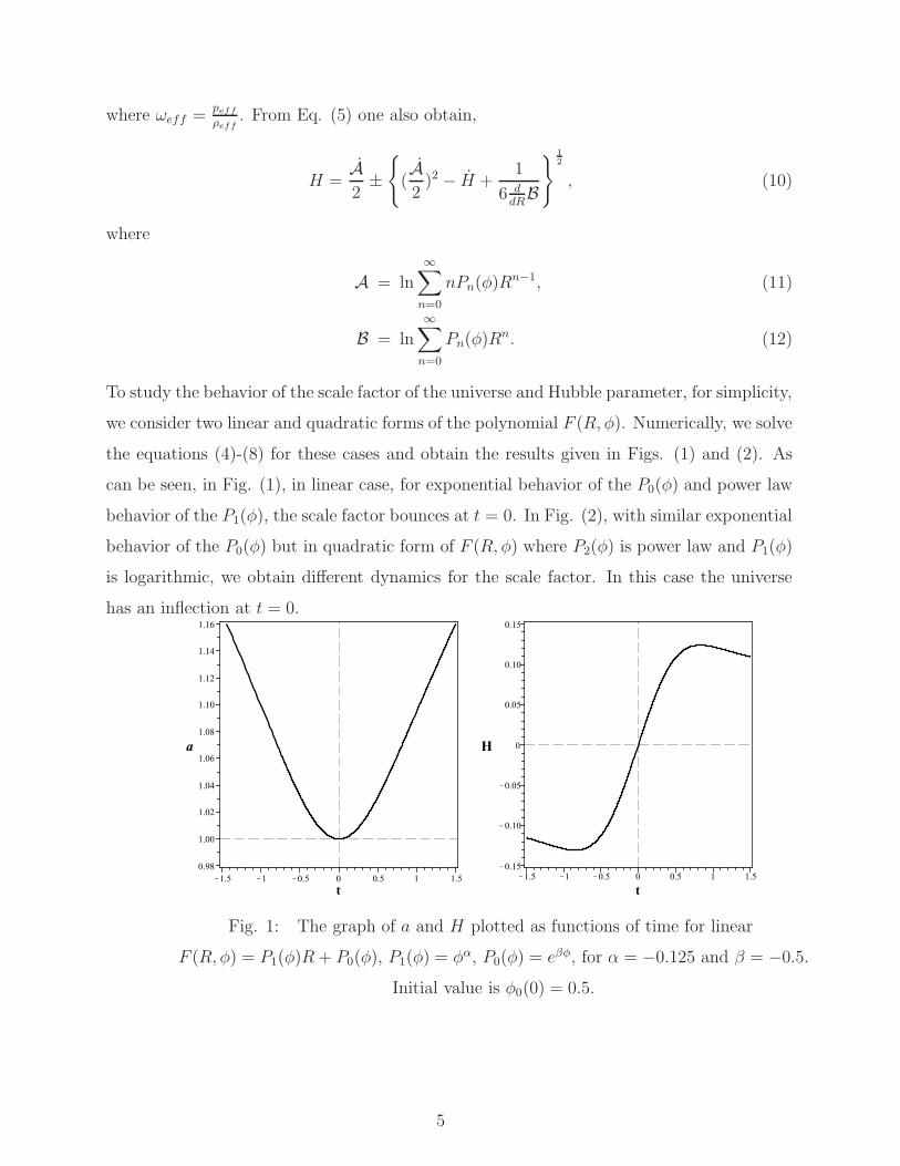
To study the behavior of the scale factor of the universe and Hubble parameter, for simplicity,
we consider two linear and quadratic forms of the polynomial F (R, φ). Numerically, we solve
the equations (4)-(8) for these cases and obtain the results given in Figs. (1) and (2). As
can be seen, in Fig. (1), in linear case, for exponential behavior of the P0(φ) and power law
behavior of the P1(φ), the scale factor bounces at t = 0. In Fig. (2), with similar exponential
behavior of the P0(φ) but in quadratic form of F (R, φ) where P2(φ) is power law and P1(φ)
is logarithmic, we obtain different dynamics for the scale factor. In this case the universe
has an inflection at t = 0.
Fig. 1: The graph of a and H plotted as functions of time for linear
F (R, φ) = P1(φ)R + P0(φ), P1(φ) = φα, P0(φ) = eβφ, for α = −0.125 and β = −0.5.
Initial value is φ0(0) = 0.5.
5
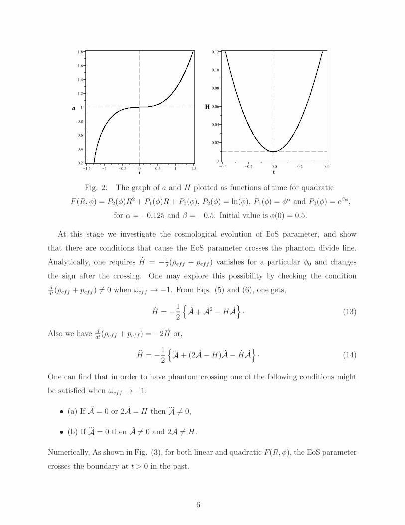
Fig. 2: The graph of a and H plotted as functions of time for quadratic
F (R, φ) = P2(φ)R2 + P1(φ)R+ P0(φ), P2(φ) = ln(φ), P1(φ) = φα and P0(φ) = eβφ,
for α = −0.125 and β = −0.5. Initial value is φ(0) = 0.5.
At this stage we investigate the cosmological evolution of EoS parameter, and show
that there are conditions that cause the EoS parameter crosses the phantom divide line.
Analytically, one requires H = −12(ρeff + peff) vanishes for a particular φ0 and changes
the sign after the crossing. One may explore this possibility by checking the condition
ddt(ρeff + peff ) 6= 0 when ωeff → −1. From Eqs. (5) and (6), one gets,
H = −1
2
A+ A2 −HA
· (13)
Also we have ddt(ρeff + peff) = −2H or,
H = −1
2
...A + (2A −H)A − HA
· (14)
One can find that in order to have phantom crossing one of the following conditions might
be satisfied when ωeff → −1:
• (a) If A = 0 or 2A = H then...A 6= 0,
• (b) If...A = 0 then A 6= 0 and 2A 6= H .
Numerically, As shown in Fig. (3), for both linear and quadratic F (R, φ), the EoS parameter
crosses the boundary at t > 0 in the past.
6
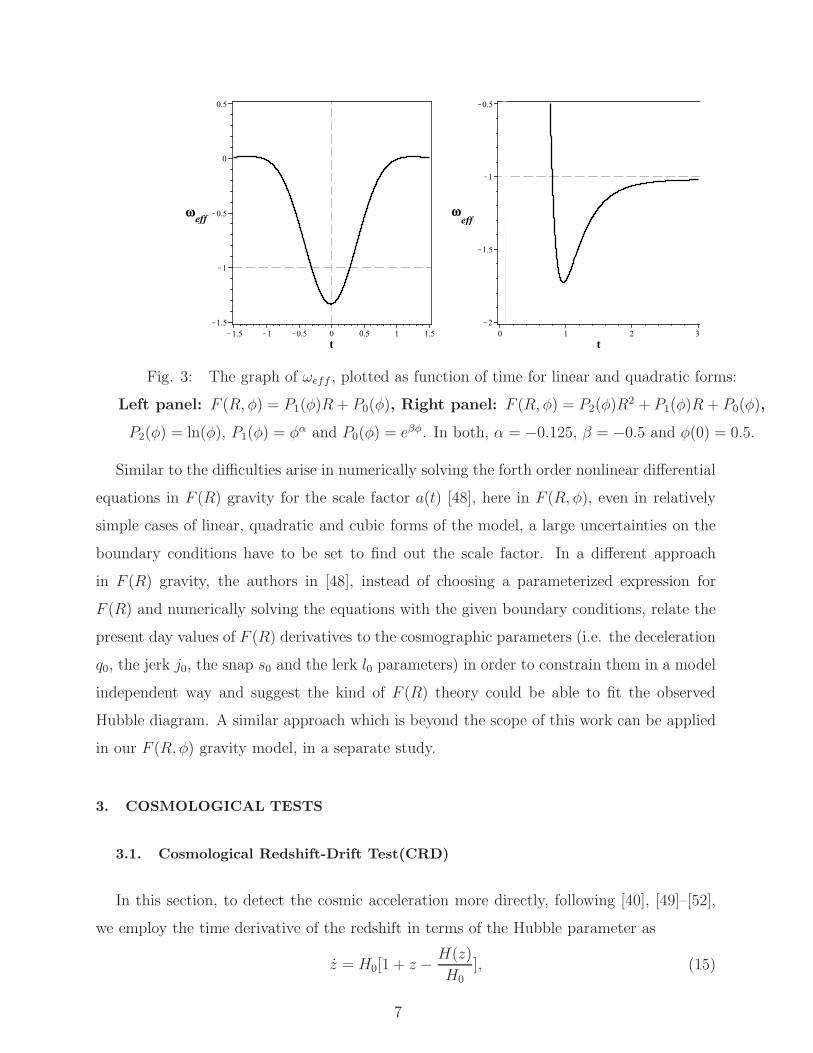
Fig. 3: The graph of ωeff , plotted as function of time for linear and quadratic forms:
Left panel: F (R, φ) = P1(φ)R+ P0(φ), Right panel: F (R, φ) = P2(φ)R2 + P1(φ)R + P0(φ),
P2(φ) = ln(φ), P1(φ) = φα and P0(φ) = eβφ. In both, α = −0.125, β = −0.5 and φ(0) = 0.5.
Similar to the difficulties arise in numerically solving the forth order nonlinear differential
equations in F (R) gravity for the scale factor a(t) [48], here in F (R, φ), even in relatively
simple cases of linear, quadratic and cubic forms of the model, a large uncertainties on the
boundary conditions have to be set to find out the scale factor. In a different approach
in F (R) gravity, the authors in [48], instead of choosing a parameterized expression for
F (R) and numerically solving the equations with the given boundary conditions, relate the
present day values of F (R) derivatives to the cosmographic parameters (i.e. the deceleration
q0, the jerk j0, the snap s0 and the lerk l0 parameters) in order to constrain them in a model
independent way and suggest the kind of F (R) theory could be able to fit the observed
Hubble diagram. A similar approach which is beyond the scope of this work can be applied
in our F (R, φ) gravity model, in a separate study.
3. COSMOLOGICAL TESTS
3.1. Cosmological Redshift-Drift Test(CRD)
In this section, to detect the cosmic acceleration more directly, following [40], [49]–[52],
we employ the time derivative of the redshift in terms of the Hubble parameter as
z = H0[1 + z − H(z)
H0], (15)
7
where z measures the rate of expansion of the universe: z > 0 (< 0) indicates the accelerated
(decelerated) expansion of the universe, respectively. The redshift variation is related to the
apparent velocity drift of the source:
v = cz
1 + z, (16)
where v = ∆v∆tobs
and H0 = 100hKm/sec/Mpc [53]. Since the detection of the signals
correspond to the redshift change and consequently velocity drift is very weak, to measure
the signals, observation of the LY α forest in the QSO spectrum [42]–[45] for a decade
might be needed . In near future this requirement can be provided by a new generation of
Extremely Large Telescope (ELT) which are equipped with aspectrograph to measure such
a small cosmic signal [41][50, 51].
In the following, we use three sets of data (8 points) for redshift drift generated by
performed Monte Carlo. We first revise the CPL parametrization model and compare the
F (R, φ) model with CPL model and observational data [40], [50]–[52].
CPL model
One popular parametrization, which explains evolution of dark energy is the CPL model in
which in a flat universe the time varying EoS parameter in term of redshift z is parameterized
by,
ω(z) = ω0 + ω1(z
1 + z). (17)
In the model, the Hubble parameter also is given by
H(z)2
H20
= Ωm(1 + z)3 + (1− Ωm)e3∫ z
01+ω(z)1+z
dz, (18)
where using Eq. (17) we can obtain the following equation for Hubble parameter
H(z)2
H20
= Ωm(1 + z)3 + (1− Ωm)(1 + z)3(1+ω0+ω1) × exp
[
−3ω1(z
1 + z)
]
· (19)
In CPL model the parametrization is fitted for different values of ω0 and ω1. The velocity
drift with respect to the source redshift is shown in Fig. (5) [40]. A comparison of the model
with the observational data shows that the best fit values are for ω0 = −2.2 and ω1 = 3.5.
F (R, φ) Model
From numerical calculation, in Fig. (4), it can be seen that for three linear, quadratic
and cubic form of F (R, φ), the EoS parameter crosses −1 at different z. In linear case it
crosses twice in the past while in quadratic and cubic cases it crosses only once. It shows
8
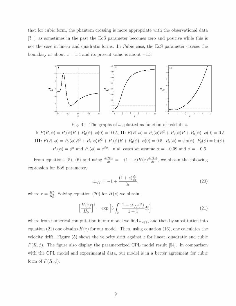
that for cubic form, the phantom crossing is more appropriate with the observational data
[? ] as sometimes in the past the EoS parameter becomes zero and positive while this is
not the case in linear and quadratic forms. In Cubic case, the EoS parameter crosses the
boundary at about z = 1.4 and its present value is about −1.3
Fig. 4: The graphs of ω, plotted as function of redshift z.
I: F (R, φ) = P1(φ)R + P0(φ), φ(0) = 0.05, II: F (R, φ) = P2(φ)R2 + P1(φ)R+ P0(φ), φ(0) = 0.5
III: F (R, φ) = P3(φ)R3 + P2(φ)R
2 + P1(φ)R + P0(φ), φ(0) = 0.5. P3(φ) = sin(φ), P2(φ) = ln(φ),
P1(φ) = φα and P0(φ) = eβφ. In all cases we assume α = −0.09 and β = −0.6.
From equations (5), (6) and using dH(t)dt
= −(1 + z)H(z)dH(z)dz
, we obtain the following
expression for EoS parameter,
ωeff = −1 +(1 + z) dr
dz
3r, (20)
where r = H2
H20. Solving equation (20) for H(z) we obtain,
[H(z)
H0
]2
= exp[
3
∫ z
0
1 + ωeff(z)
1 + zdz
]
· (21)
where from numerical computation in our model we find ωeff , and then by substitution into
equation (21) one obtains H(z) for our model. Then, using equation (16), one calculates the
velocity drift. Figure (5) shows the velocity drift against z for linear, quadratic and cubic
F (R, φ). The figure also display the parameterized CPL model result [54]. In comparison
with the CPL model and experimental data, our model is in a better agreement for cubic
form of F (R, φ).
9
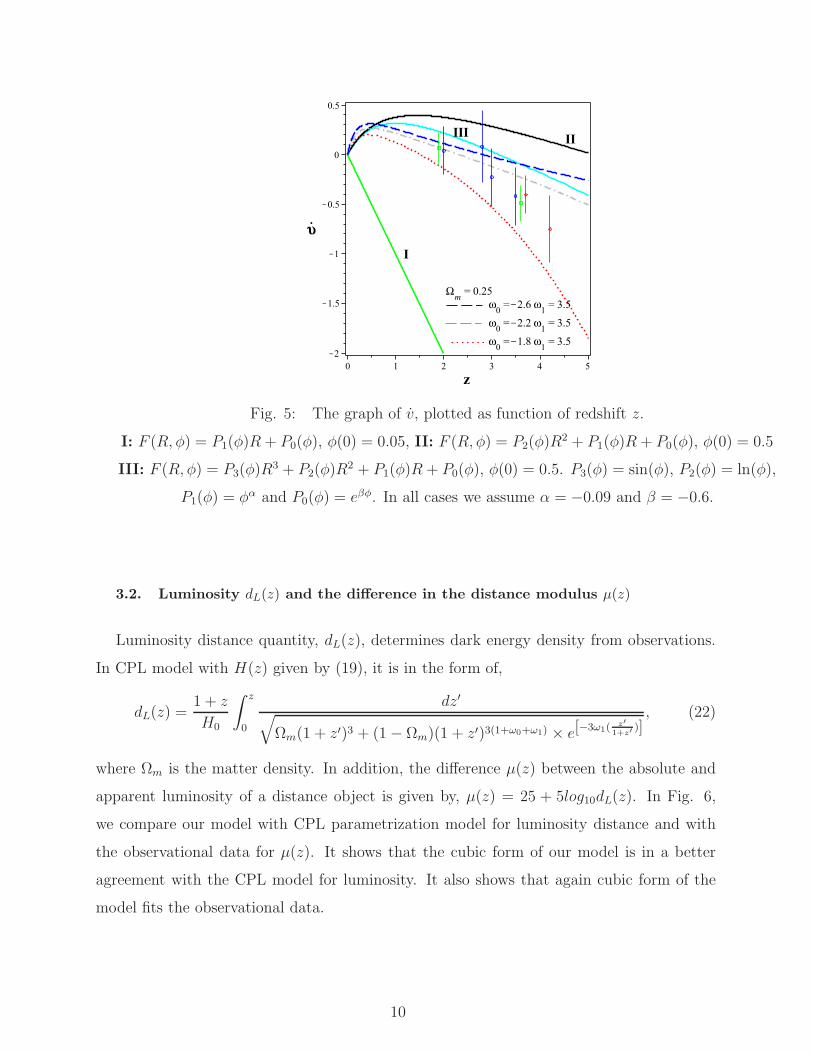
Fig. 5: The graph of v, plotted as function of redshift z.
I: F (R, φ) = P1(φ)R + P0(φ), φ(0) = 0.05, II: F (R, φ) = P2(φ)R2 + P1(φ)R+ P0(φ), φ(0) = 0.5
III: F (R, φ) = P3(φ)R3 + P2(φ)R
2 + P1(φ)R + P0(φ), φ(0) = 0.5. P3(φ) = sin(φ), P2(φ) = ln(φ),
P1(φ) = φα and P0(φ) = eβφ. In all cases we assume α = −0.09 and β = −0.6.
3.2. Luminosity dL(z) and the difference in the distance modulus µ(z)
Luminosity distance quantity, dL(z), determines dark energy density from observations.
In CPL model with H(z) given by (19), it is in the form of,
dL(z) =1 + z
H0
∫ z
0
dz′√
Ωm(1 + z′)3 + (1− Ωm)(1 + z′)3(1+ω0+ω1) × e[−3ω1(z′
1+z′)], (22)
where Ωm is the matter density. In addition, the difference µ(z) between the absolute and
apparent luminosity of a distance object is given by, µ(z) = 25 + 5log10dL(z). In Fig. 6,
we compare our model with CPL parametrization model for luminosity distance and with
the observational data for µ(z). It shows that the cubic form of our model is in a better
agreement with the CPL model for luminosity. It also shows that again cubic form of the
model fits the observational data.
10
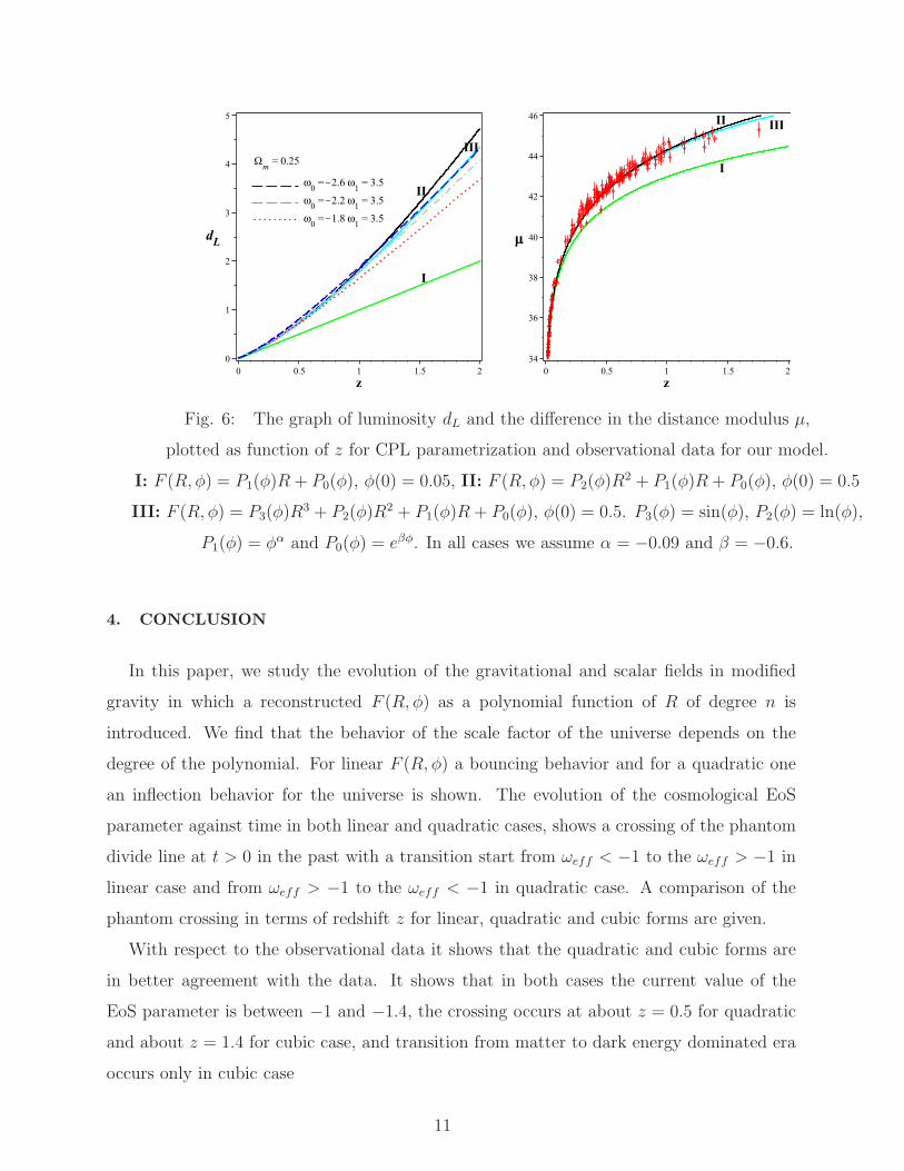
Fig. 6: The graph of luminosity dL and the difference in the distance modulus µ,
plotted as function of z for CPL parametrization and observational data for our model.
I: F (R, φ) = P1(φ)R + P0(φ), φ(0) = 0.05, II: F (R, φ) = P2(φ)R2 + P1(φ)R+ P0(φ), φ(0) = 0.5
III: F (R, φ) = P3(φ)R3 + P2(φ)R
2 + P1(φ)R + P0(φ), φ(0) = 0.5. P3(φ) = sin(φ), P2(φ) = ln(φ),
P1(φ) = φα and P0(φ) = eβφ. In all cases we assume α = −0.09 and β = −0.6.
4. CONCLUSION
In this paper, we study the evolution of the gravitational and scalar fields in modified
gravity in which a reconstructed F (R, φ) as a polynomial function of R of degree n is
introduced. We find that the behavior of the scale factor of the universe depends on the
degree of the polynomial. For linear F (R, φ) a bouncing behavior and for a quadratic one
an inflection behavior for the universe is shown. The evolution of the cosmological EoS
parameter against time in both linear and quadratic cases, shows a crossing of the phantom
divide line at t > 0 in the past with a transition start from ωeff < −1 to the ωeff > −1 in
linear case and from ωeff > −1 to the ωeff < −1 in quadratic case. A comparison of the
phantom crossing in terms of redshift z for linear, quadratic and cubic forms are given.
With respect to the observational data it shows that the quadratic and cubic forms are
in better agreement with the data. It shows that in both cases the current value of the
EoS parameter is between −1 and −1.4, the crossing occurs at about z = 0.5 for quadratic
and about z = 1.4 for cubic case, and transition from matter to dark energy dominated era
occurs only in cubic case
11
We then analyze the model with respect to the CPL model and observational data. The
first cosmological test is the CRD test. The variation of velocity drift for linear, quadratic
and cubic forms of the polynomial with redshift z is shown in Fig. (5). Checking between
our model with CPL parametrization model and observational data shows that cubic form
is in better agreement with the experimental data. The second cosmological test is luminos-
ity distance dL and the difference in the distance modulus µ that the former is calculated
in comparison with the CPL parametrization model and the later with respect to the ob-
servational data. Again, for luminosity distance it shows that the the cubic from of our
model is in better agreement with the CPL model. For µ(z), it show that again the cubic
form of the model very well fit with the observational data. Although, due to numerically
difficult computation we have not considered the higher order polynomial forms of F (R, φ),
but from these three linear, quadratic and cubic forms we may conclude that the presence
of the higher order terms in the model better fits the model with the observational data.
[1] A. G. Riess et al. Astrophys. J. 607 (2004) 665; R. A. Knop et al. Astrophys. J. 598, 102
(2003).
[2] C. L. Bennett et al., Astrophys. J. Suppl. 148, 1 (2003).
[3] K. Abazajian et al. Astron. J. 129 (2005) 1755; Astron. J. 128 (2004) 502; M. Tegmark et al.
Astrophys. J. 606, 702 (2004).
[4] S. W. Allen, R. W. Schmidt, H. Ebeling, A. C. Fabian and L. van Speybroeck, Mon. Not.
Roy. Astron. Soc. 353, 457 (2004).
[5] J. Kratochvil, A. Linde, E. V. Linder, M. Shmakova, JCAP 0407, 001(2004).
[6] S. Nojiri, S. D. Odintsov, Phys. Rev. D 74, (2006) 086005; J. Phys. A 40 (2007) 6725; S.
Capozziello, S. Nojiri, S. D. Odintsov and A. Troisi, Phys. Lett. B 639, 135 (2006); S. Fay, S.
Nesseris and L. Perivolaropoulos, Phys. Rev. D 76, 063504 (2007).
[7] W. Hu and I. Sawicki, Phys. Rev. D 76 (2007) 064004; Y. Song, H. Peiris and W. Hu, Phys.
Rev. D 76, 063517 (2007).
[8] S. Nojiri and S. D. Odintsov, Phys. Lett. B 657 (2007) 238; Phys. Lett. B 652, 343 (2007).
[9] S. A. Appleby and R. A. Battye, Phys. Lett. B 654, 7 (2007).
[10] R. N. Mohapatra, A. Prez-Lorenzana, C. A. de S. Pires, Phys.Rev.D 62, 105030 (2000).
12
[11] M. R. Setare, Phys. Lett. B 654,(2007)1-6; M. R. Setare, Eur. Phys. J. C 52,(2007) 689; R. R.
Caldwell, Phys. Lett. B 545 (2002) 23; J. Hao and X. Li, Astro-Phys. Rev. D 70 (2004) 043529;
E. Elizalde and J. Quiroga, Mod. Phys. Lett. A 19 (2004) 29; Y. Piao and E. Zhou, Phys. Rev.
D 68 (2003) 083515; E. Elizalde, S. Nojiri, Sergei D. Odintsov,Phys.Rev.D70:043539,(2004);
S. Capozziello, S. Nojiri, S.D. Odintsov,Phys.Lett.B632:597-604,(2006); S. Nojiri, Sergei D.
Odintsov,Phys.Lett.B562:147-152,(2003).
[12] M. R. Setare, Phys.Lett. B 642,(2006)1-4; M. R. Setare, Eur. Phys. J. C50, 991-998(2007).
[13] P. J. E. Peebles and B. Ratra, Rev. Mod. Phys. 75, 559 (2003).
[14] E. J. Copeland, M. Sami and S. Tsujikawa, Int. J. Mod. Phys. D 15, 1753 (2006).
[15] Y. Fujii, Phys. Rev. D 26 (1982) 2580; I. Zlatev, L. M. Wang and P. J. Steinhardt, Phys. Rev.
Lett. 82, 896 (1999).
[16] T. Chiba, T. Okabe and M. Yamaguchi, Phys. Rev. D 62 (2000) 023511; C. Armendariz-Picon,
V. Mukhanov, and P. J. Steinhardt, Phys. Rev. Lett. 85, 4438 (2000); S. Sur, S. Das, JCAP,
0901,007 (2009).
[17] M.R. Setare, Phys.Lett.B 642, (2006)421-425; G. R. Dvali, G. Gabadadze and M. Porrati,
Phys. Lett. B 485 (2000) 208; V. Sahni and Y. Shtanov, JCAP 0311, 014 (2003).
[18] M. R. Setare, E. N. Saridakis, Phys.Lett.B670 (2008)1-4; J. Sadeghi, M. R. Setare, A. Banija-
mali and F. Milani, Phys. Rev. D. 79 (2009) 123003; S. Nojiri, Sergei D. Odintsov, M. Sasaki,
Phys.Rev.D71:123509,(2005); S. Nojiri, Sergei D. Odintsov, Phys.Lett.B631:1-6,(2005); G.
Cognola, E. Elizalde, S. Nojiri, Sergei D. Odintsov, S. Zerbini, Phys.Rev.D73:084007,(2006);
S. Nojiri, Sergei D. Odintsov, M. Sami ,Phys.Rev.D74:046004,(2006).
[19] S. Capozziello, V. F. Cardone, S. Carloni and A. Troisi, Int. J. Mod. Phys. D 12 (2003) 1969;
S. M. Carroll, et all, Phys. Rev. D 70 (2004) 043528; S. Nojiri and S. D. Odintsov, Phys. Rev.
D 68, 123512(2003).
[20] S. Tsujikawa, Phys. Rev. D 76, 023514 (2007).
[21] S. Nojiri and S. D. Odintsov, Int. J. Geom. Meth. Mod. Phys. 4 (2007) 115; J. Phys. Conf.
Ser. 66, 012005 (2007).
[22] J. Sadeghi, M. R. Setare, A. Banijamali and F. Milani, Phys. Lett. B 662, 92 (2008).
[23] S. Capozziello, S. Carloni and A. Troisi, RecentRes. Dev. Astron. Astrophys. 1, 625 (2003).
[24] S. Nojiri and S. D. Odintsov, Phys. Lett. B 576, 5 (2003).
[25] F. Faraoni, Phys. Rev. D 75 (2007) 067302; J. C. C. de Souza, V. Faraoni Class. Quant. Grav.
13
24, 3637 (2007); B. Li and J. D. Barrow, Phys. Rev. D 75, 084010 (2007).
[26] S. Nojiri and S. D. Odintsov, Gen. Rel. Grav. 36, 1765 (2004); G. Cognola, E. Elizalde, S.
Nojiri, S. D. Odintsov and S. Zerbini, JCAP 0502 (2005) 010; G. Cognola, E. Elizalde, S.
Nojiri, S. D. Odintsov and S. Zerbini, Phys. Rev. D73 (2006) 084007; J. Santos, J. Alcaniz,
M. Reboucas and F. Carvalho, Phys. Rev. D 76, 083513 (2007).
[27] S. Nojiri and S. D. Odintsov ,Phys. Lett. B 659, 821 (2008).
[28] M. R. Setare, Int.J.Mod.Phys.D 17 (2008)2219; E. Elizalde, S. Nojiri and S. D. Odintsov,
Phys. Rev. D 70 (2004) 043539; L. Perivolaropoulos, JCAP 0510 (2005) 001; S. Nesseris and
L. Perivolaropoulos, Phys. Rev. D 75, 023517 (2007).
[29] M. Alimohammadi, H. Behnamian, Phys.Rev.D80:063008 (2009)
[30] J. Sadeghi, F. Milani and A. R. Amani, Mod. Phys. Lett. A 24, 29 (2009) 2363; M. R. Setare,
Phys. Lett. B 642 (2006)1; Eur. Phys. J. C 50 (2007) 991; Phys. Lett. B 654 (2007) 1; Eur.
Phys. J. C 52 (2007) 689; Phys. Lett. B 642, 421 (2006).
[31] B. Boisseau, G. Esposito-Farese, D. Polarski, A. A. Phys. Rev. Lett. 85 (2000) 2236; V.
Sahni, Yu. V. Shtanov, JCAP 0311 (2003) 014; B. McInnes, Nucl. Phys. B 718 (2005) 55; L.
Perivolaropoulos, Phys. Rev. D 71 (2005) 063503; B. Feng, X. Wang, X. Zhang, Phys. Lett.
B 607, 35 (2005).
[32] Z.-K. Guo, Y.-S. Piao, X. Zhang, Y.-Z. Zhang, Phys. Lett. B 608 (2005) 177; M. Sami, A.
Toporensky, P. V. Tretjakov, Sh. Tsujikawa, Phys. Lett. B 619 (2005) 193; A. Anisimov, E.
Babichev, A. Vikman, JCAP 0506, 006 (2005).
[33] P. Kanti and K. Tamvakis, Phys. Rev. D68, 024014 (2003).
[34] T. Biswas and A. Mazumdar, hep-th/0408026.
[35] Y. F. Cai, T. Qiu, Y. S. Piao, M. Li and X. Zhang, JHEP 0710,071 (2007).
[36] H. Farajollahi, F. Milani, Mod. Phy. lett. A, Vol. 25, No. 27, 2349-2362 (2010).
[37] E. V. Linder, Rep. Prog. Phys, 71, 056901 (2008).
[38] J. Nordin, Goobar, A. Jonsson, JCAP 0802, 008 (2008).
[39] D. Huterer Turner, M.S. Phys.Rev. D 64, 123527 (2001); E. V. Linder, R. N. Cahn, Astropart.
Phys, 28, 481(2007).
[40] J. Liske et al., Mon. Not. Roy. Astr. Soc., 386m 1192 (2008).
[41] S. Cristiani, et al., Nuovo Cim. 122 B, 1159 (2007); Nuovo Cim. 122 B, 1165 (2007).
[42] D. Jain, S. Jhingan, gr-qc/0910.4825v2.
14
[43] A. Sandage, Astrophys. J., 136, 319 (1962).
[44] G. C. McVittie, Astrophys. J., 136, 334 (1962); R. Rudiger, Astrophys. J., 240, 384 (1980);
Lake, K., Astrophys. J., 247, 17 (1981); Rudiger, R., Astrophys. J., 260, 33 (1982); Lake, K.,
Phys. Rev. D 76, 063508 (2007).
[45] A. Loeb, Astrophys. J., 499, L111 (1998).
[46] M. Chevalier, Polarski, D 10 (2001) 213; E. V. Linder,, Phys. Rev. Lett, 90, 091301 (2003).
[47] S. Nojiri, S. D. Odintsov, Phys. Rev. D 68 (2003) 123512; K. Bamba, C. Q. Geng, S. Nojiri
and S. D. Odintsov, Phys. Rev. D 79 (2009) 083014; K. Bamba, C. Q. Geng, S. Nojiri, hep-
th/1003.0769; JCAP 0810 (2008) 045; M. R. Setare, Int. J. Mod. Phys. D 17,2219 (2008).
[48] S. Capozziello, V. F. Cardone, V. Salzano, PRD 78, 063504 (2008).
[49] H. Farajollahi, A. Salehi, Int. J. Mod. Phys. D, Vol. 19, No. 5,1-13 (2010).
[50] L. Pasquini et al., IAU symposium, ed. P. White- lock , M. Dennefeld B. Leibundgut, 232,193
(2006).
[51] L. Pasquini et al., The Messenger, 122,10 (2005).
[52] J. Liske et al., 133,10 (2008). Cristiani, S., Nuovo Cim. 122 B, 1159 (2007).
[53] G. C. McVittie, Astrophys. J., 136,334 (1962).
[54] J. Liske et al., Mon. Not. Roy. Astr. Soc., 000,1 (2007).
15