arX

iv:0

905.

2966

v2 [

astr

o-ph

.CO

] 1

5 O

ct 2

009

Equivalence Principle Implications of Modified Gravity Models

Lam Hui∗ and Alberto Nicolis†

Institute for Strings, Cosmology and Astroparticle Physics (ISCAP),Department of Physics, Columbia University, New York, NY 10027, U.S.A.

Christopher W. Stubbs‡

Department of Physics, Harvard University, Cambridge, MA 02138, U.S.A.(Dated: October 15, 2009)

Theories that attempt to explain the observed cosmic acceleration by modifying general relativityall introduce a new scalar degree of freedom that is active on large scales, but is screened on smallscales to match experiments. We demonstrate that if such screening occurs via the chameleonmechanism, such as in f(R) theory, it is possible to have order unity violation of the equivalenceprinciple, despite the absence of explicit violation in the microscopic action. Namely, extendedobjects such as galaxies or constituents thereof do not all fall at the same rate. The chameleonmechanism can screen the scalar charge for large objects but not for small ones (large/small isdefined by the depth of the gravitational potential, and is controlled by the scalar coupling). Thisleads to order one fluctuations in the ratio of the inertial mass to gravitational mass. We providederivations in both Einstein and Jordan frames. In Jordan frame, it is no longer true that all objectsmove on geodesics; only unscreened ones, such as test particles, do. In contrast, if the scalar screeningoccurs via strong coupling, such as in the DGP braneworld model, equivalence principle violationoccurs at a much reduced level. We propose several observational tests of the chameleon mechanism:1. small galaxies should accelerate faster than large galaxies, even in environments where dynamicalfriction is negligible; 2. voids defined by small galaxies would appear larger compared to standardexpectations; 3. stars and diffuse gas in small galaxies should have different velocities, even if theyare on the same orbits; 4. lensing and dynamical mass estimates should agree for large galaxies butdisagree for small ones. We discuss possible pitfalls in some of these tests. The cleanest is the thirdone where mass estimate from HI rotational velocity could exceed that from stars by 30% or more.To avoid blanket screening of all objects, the most promising place to look is in voids.

PACS numbers: 98.80.-k; 98.80.Es; 98.65.Dx; 98.62.Dm; 95.36.+x; 95.30.Sf; 04.50.Kd; 04.80.Cc

I. INTRODUCTION

The surprising finding of cosmic acceleration about tenyears ago has motivated a number of attempts to mod-ify general relativity (GR) on large scales. They fallroughly into two classes. One involves adding curva-ture invariants to the Einstein-Hilbert action, the mostpopular example of which is f(R) theory [1, 2, 3, 4].The other involves giving the graviton a mass or a res-onance width, the most well known example of which isthe Dvali-Gabadadze-Porrati (DGP) braneworld model[5, 6]. The first class of theories is equivalent to the classicscalar-tensor theories [7, 8]. The second class of theoriesis more subtle but also reduces to scalar-tensor theorieson sub-Hubble scales [9, 10]. In the context of DGP,the extra scalar can be thought of as a brane-bendingmode. In fact, it appears the extra dimension is not evennecessary—four dimensional ghost-free generalizations ofthe DGP model exist where it is the nonlinear interactionof the scalar that causes self-acceleration [11].

All examples to date, therefore, introduce a light scalar

∗Electronic address: lhui@astro.columbia.edu†Electronic address: nicolis@phys.columbia.edu‡Electronic address: stubbs@physics.harvard.edu

(or even multiple light fields) to modify gravity 1. Whilesuch a scalar is welcome phenomenologically on cosmo-logical scales, it must be suppressed or screened on smallscales to satisfy stringent constraints from solar systemand terrestrial experiments. The two classes of theorieshave quite distinctive screening mechanisms. Curvature-invariant theories such as f(R) screen the scalar viathe so-called chameleon mechanism, essentially by giv-ing the scalar a mass that depends on the local density[18, 19, 20, 21, 22, 23, 24]. Theories such as DGP screenthe scalar a la Vainshtein [25], namely strong couplingeffects suppress the scalar on small scales [9, 10].

Our goal in this paper is to study how extended objectsmove in the presence of these two screening mechanisms.We will keep our discussion as general as possible even

1 This is not surprising given a famous theorem due to Weinberg[12] which states that a Lorentz invariant theory of a masslessspin two field must be equivalent to GR in the low energy limit.Low energy modifications of gravity therefore necessarily involveintroducing new degrees of freedom, such as a scalar. Giving thegraviton a small mass or resonance width turns out to introducea scalar a la Stueckelberg [13]. Theories that invoke a Lorentzviolating massive graviton also involve a scalar, namely a ghostcondensate [14, 15]. Recent proposals for degravitation are yetanother example of scalar-tensor theories in the appropriate lim-its [16, 17].

2

as we use f(R) and DGP as illustrative examples. In-deed, neither theory is completely satisfactory: accept-able f(R) models accelerate the universe mostly by acosmological constant rather than by a genuine modi-fied gravity effect [26]; also from an effective field theorystandpoint they are not favored in any sense over moregeneral scalar-tensor theories; DGP and generalizationsthereof [11] probably lack a relativistic ultra-violet com-pletion [27]. However, it is likely the screening mecha-nism, chameleon or strong coupling, will remain relevantin future improvements of these theories.

The problem of motion of extended objects has a vener-able history. Newton famously showed in Principia thatthe Earth’s motion around the Sun can be computed byconsidering the Earth as a point mass. It is worth em-phasizing that such a result is by no means guaranteedeven in Newtonian gravity. This result holds only if thereis a separation of scales, that the dimension of the Earthis small compared with the scale on which the Sun’s grav-itational field varies, in other words that tides from theSun can be ignored. More concretely, the Earth effec-tively sees a linear gradient field from the Sun; secondderivatives of the Sun’s gravitational potential can besafely neglected when computing the Earth’s motion.

We will work within the same zero-tide approximationin this paper. It has long been known that within GR,under the same approximation, extended objects movejust like infinitesimal test particles. In other words, ne-glecting tidal effects all objects move on geodesics, orequivalently, their inertial mass and gravitational massare exactly equal. This has been referred to as the efface-ment principle, that the internal structure of an object,no matter how complicated, has no bearing on its overallmotion [28].

It is also well known that the same is not true in scalar-tensor theories. In such theories, despite the universalcoupling of the scalar to all elementary matter fields, ob-jects with different amounts of gravitational binding en-ergy will move differently. Effectively, they have differentratios of the inertial mass to gravitational mass, knownas the Nordtvedt effect [29].2 This apparent violationof the equivalence principle 3 is generally small becausemost objects have only a small fraction of their total masscoming from their gravitational binding energy. In otherwords, such violation is suppressed by Φ where Φ is the

2 By comparing the free fall of the Earth and the moon towards thesun, lunar laser ranging data already place limits on such strongequivalence principle violation at the level of 10−4 [30], with afactor of ten improvement expected in the near future [31]. Inthis paper, we are interested in theories that respect these solarsystem bounds while exhibiting O(1) deviation from GR in otherenvironments.

3 In this paper, equivalence principle violation means no more andno less than this: that different objects can fall at different rates,or equivalently, they have different ratios of inertial to gravita-tional mass. See [32] for a discussion of different formulations ofthe equivalence principle.

gravitational potential depth of the object. In the par-lance of post-Newtonian expansion, such violation is anorder 1/c2 effect (c is the speed of light). Order one viola-tion of the equivalence principle is however observable inthe most strongly bound objects i.e. black holes, whichdo not couple to the scalar at all—they have no scalarhair. This means black holes and stars fall at appreciablydifferent rates in scalar-tensor theories [33, 34].

In this paper, we wish to point out that there could beorder one violation of the equivalence principle, even forobjects that are not strongly bound, such as galaxies andmost of their constituents (|Φ| ≪ 1). In the parlance ofpost-Newtonian expansion, this is an order 1 effect (i.e.this is not even post-Newtonian!). That this is possibleis thanks to the new twist introduced by recent variantsof scalar-tensor theories, namely their screening mecha-nisms. We will show that the chameleon mechanism leadsto order one violation of the equivalence principle evenfor small |Φ| objects, while the Vainshtein mechanismdoes not. These screening mechanisms were absent intraditional treatments of scalar-tensor theories becausethe latter typically did not have a non-trivial scalar po-tential (needed for chameleon) or higher derivative in-teractions (needed for Vainshtein) i.e. they were of theJordan-Fierz-Brans-Dicke variety [35, 36, 37].

How such equivalence principle violation comes aboutis easiest to see in Einstein frame, where the scalar me-diates an actual fifth force. Under the chameleon mech-anism, screened objects effectively have a much smallerscalar charge compared to unscreened objects of the samemass. Hence, they respond differently to the fifth forcefrom other objects in the same environment; they thenmove differently. That such a gross violation of the equiv-alence principle is possible might come as a surprise inJordan frame. One is accustomed to thinking that all ob-jects move on geodesics in Jordan frame. One of our maingoals is to show that this is in fact not true. Whethertwo different objects fall at the same rate under gravityis of course a frame-independent issue; nonetheless, somereaders might find a Jordan frame derivation illuminat-ing. Here, we follow the elegant methodology developedby Einstein, Infeld & Hoffmann [38] and Damour [28]and apply it to situations where the screening mecha-nisms operate. What we hope to accomplish in part isputting the arguments of Khoury and Weltman [19, 20]on a firmer footing, who first pointed out the existence ofthe chameleon mechanism, and used Einstein frame argu-ments to propose equivalence principle tests using artifi-cial satellites. We also wish to establish that if screeningoccurs via the Vainshtein mechanism, there is no analo-gous order one violation of equivalence principle.

It is worth emphasizing the different physical originsfor equivalence principle violations of the post-NewtonianO(1/c2) type and the Newtonian O(1) type. In anyscalar-tensor theory, the scalar is always sourced bythe trace of the matter energy-momentum tensor. Inother words, at the level of the Einstein frame action,the coupling between the scalar ϕ and matter is of the

3

form ϕTm, where Tm is the trace of the matter energy-momentum. Fundamentally, equivalence principle viola-tions occur whenever different objects couple to ϕ dif-ferently. In a theory like Brans-Dicke, this happens be-cause different objects of the same mass have differentTm. The degree to which their Tm differs is of order 1/c2

(i.e. ∼ Φ the gravitational potential), and so equivalenceprinciple violation of the Brans-Dicke type is typicallysmall, except for relativistic objects whose Tm is highlysuppressed i.e. most of their mass comes from gravita-tional binding energy. An extreme example is the blackhole whose mass is completely gravitational in origin. Intheories where the chameleon mechanism operates, thereis an additional and larger source of equivalence princi-ple violation, and that is through variations in the effec-tive scalar charge that a macroscopic object carries. Thescalar self-interaction in a chameleon theory makes thescalar charge sensitive to the internal structure of theobject; the scalar charge is not simply given by a vol-ume integral of Tm as in Brans-Dicke, but is given by ascreened version of the same. As we will see, chameleonscreening could introduce O(1) fluctuations in the scalarcharge to mass ratio, even for non-relativistic objects.What is perhaps surprising is that this happens despitean explicitly universal scalar coupling at the level of themicroscopic action. One can view this as a classical renor-malization of the scalar charge. We will also see that intheories where the Vainshtein mechanism operates, thereis no such O(1) charge renormalization. Therefore thesetheories only have equivalence principle violation of theBrans-Dicke, or post-Newtonian, type.

Equivalence principle violations of both types dis-cussed above, Newtonian or post-Newtonian, should beclearly distinguished from yet another type of violation,which is most commonly discussed in the cosmology lit-erature — where there is explicit breaking of equivalenceprinciple at the level of the microscopic action, e.g. ele-mentary baryons and dark matter particles are coupled tothe scalar with different strengths [39, 40, 41, 42, 43, 44].In this paper, we are interested in theories where thisbreaking is not put in ’by hand’ i.e. it does not existat the level of the microscopic action; rather, the equiv-alence principle violation comes about for macroscopicobjects by way of differences in response to the screeningmechanism.

Further experimental tests come to mind after ourinvestigation of the problem of motion under the twoscreening mechanisms. We propose several observationaltests using either the bulk motion of galaxies or the in-ternal motion of objects within galaxies. The chameleonmechanism will predict gross violations of the equivalenceprinciple for suitably chosen galaxies while the Vainshteinmechanism will not. Care must be taken in carrying outsome of these tests, however, to avoid possible Yukawasuppression and/or confusion with astrophysical effects.We point out that the most robust test probably comesfrom the measurement of internal stellar and HI velocitiesof small galaxies in voids. Systematic differences between

the two, or lack thereof, will put interesting constraintsor rule out some of the current modified gravity theories.

A guide for the readers. Readers who are interestedprimarily in observational tests can skip directly to §VIwhere relevant results from the more theoretical earliersections are summarized. §II serves as a warm-up exercisewherein we derive the equality of inertial mass and grav-itational mass in GR for extended objects. §III demysti-fies this surprising effacement property of GR by viewingGR through the prism of a field theory of massless spintwo particles. This section is somewhat of a digressionand can be skipped by readers not interested in the fieldtheoretic perspective. §IV is where we deduce the motionof extended objects under the chameleon mechanism inEinstein frame. The Jordan frame derivation is given inthe Appendix. In §V we do the same for the Vainshteinor strong-coupling mechanism. Observational tests arediscussed in §VI, where we also summarize our results.

A number of technical details are relegated to the Ap-pendices. Appendix A discusses how the requisite surfaceintegral in the Einstein-Infeld-Hoffmann approach can bedone very close to the object. Appendix B maps ourparameterization of general scalar-tensor theories to thespecial cases of Brans-Dicke and f(R). Appendix C pro-vides the Jordan frame derivation. Appendix D derivesin detail the equation of motion under the Vainshteinmechanism. Appendix E supplies useful results for anexpanding universe.

A brief word on our notation: the speed of light c isset to unity unless otherwise stated; 8πG and 1/M2

Pl areused interchangeably; the scalar field ϕ (or π) is chosento be dimensionless rather than have the dimension ofmass.

II. THE PROBLEM OF MOTION IN GENERAL

RELATIVITY — A WARM UP EXERCISE

We start with a review of an approach to the prob-lem of motion introduced by Einstein, Infeld & Hoffmann[38] and developed by Damour [28], using GR as a warmup exercise. The idea is to work out the motion of anextended object using energy momentum conservation,rather than to assume geodesic motion from the begin-ning. It helps clarify the notion that the motion of ex-tended objects is something that should be derived ratherthan assumed—depending on one’s theory of gravity, theextended objects might or might not move like infinites-imal test particles.

The Einstein equationGµν = 8πGTm

µν can be rewrit-

ten as:

G(1)µ

ν = 8πG tµν (1)

whereG(1)µ

ν is the part of the Einstein tensorGµν that is

first order in metric perturbations, and tµν is the pseudo

energy-momentum tensor which is related to the energy-

4

momentum tensor Tmµ

ν by

tµν = Tm

µν − 1

8πGG(2)

µν (2)

where G(2)µ

ν is the higher order part of Gµν , including

but not necessarily limited to second order terms. Thesuperscript m on Tm

µν is there to remind us this is the

matter energy-momentum, in anticipation of other kindsof energy-momentum we will encounter later. Note thatthe identity ∂νG

(1)µ

ν = 0 implies tµν is conserved in the

ordinary (as opposed to covariant) sense.Let us draw a sphere of radius r enclosing the extended

object whose motion we are interested in. The linearmomentum in the i-th direction is given by

Pi =

∫

d3x ti0 (3)

where the volume integral is over the interior of thesphere. We assume that ti

0 is dominated by the extendedobject such that Pi is an accurate measure of the linearmomentum of the object itself, even though we are inte-grating over a sphere that is larger than the object.

The gravitational force on the extended object is

Pi =

∫

d3x∂0ti0 = −

∫

d3x∂jtij = −

∮

dSjtij (4)

where in the last equality we have used the Gauss lawto convert a volume integral to a surface integral i.e.dSj = dA xj , where dA is a surface area element andx is the unit outward normal. As expected, the gravi-tational force is given by the integrated momentum fluxthrough the surface. This is the essence of the methodintroduced by Einstein, Infeld & Hoffmann: the problemof motion is reduced to performing a surface integral—i.e. there is no need to worry about internal forces withinthe object of interest.

Assuming that Tmij at the surface of the sphere is

negligible, we need only consider the contribution to tij

from G(2)ij (Eq. (2)). And if the surface is located at

a sufficiently large distance away from the object of in-terest, we can assume the metric perturbations are smalland only second order contributions to G(2)

ij need to be

considered (without assuming metric perturbations aresmall close to the object). In the Newtonian gauge,

ds2 = −(1 + 2Φ)dt2 + (1 − 2Ψ)δijdxidxj , (5)

we have:

G(2)ij = −2Φ(δij∇2Φ − ∂i∂jΦ) − 2Ψ(δij∇2Ψ − ∂i∂jΨ)

+∂iΦ∂jΦ − δij∂kΦ∂kΦ + 3∂iΨ∂jΨ − 2δij∂kΨ∂kΨ

−∂iΦ∂jΨ − ∂iΨ∂jΦ + 2ΨG(1)ij (6)

ignoring time derivatives. On the right hand side, weare being cavalier about the placement of upper/lowerindices—it does not matter as long as we are keeping

only second order terms. The symbol ∇2 denotes ∂k∂k.

The first order Einstein tensor G(1)ij is given by:

G(1)ij = δij∇2(Φ − Ψ) + ∂i∂j(Ψ − Φ) (7)

again, ignoring time derivatives.The next step is to decompose Φ and Ψ around the

surface of the sphere into two parts:

Φ = Φ0 + Φ1(r) , Ψ = Ψ0 + Ψ1(r) (8)

where Φ0 and Ψ0 represent the large scale fields due tothe environment/background while Φ1 and Ψ1 are thefields due to the extended object itself. This decomposi-tion can be formally defined as follows: Φ1 and Ψ1 solvethe Einstein equation with the extended object as theone and only source; Φ0 and Ψ0 are linear gradient fieldsthat can always be added to solutions of such an equation(because the equation consists of second derivatives). Wehave in mind Φ0 and Ψ0 are generated by other sourcesin the environment, and they vary gently on the scale ofthe spherical surface that encloses the object i.e. theirsecond gradients can be ignored:

Φ0(~x) ≃ Φ0(0) + ∂iΦ0(0)xi

Ψ0(~x) ≃ Ψ0(0) + ∂iΨ0(0)xi (9)

where 0 denotes the center of the sphere. In other words,we assume ∂iΦ0 and ∂iΨ0 hardly vary on the scale ofthe sphere. On the other hand Φ1 and Ψ1, the objectgenerated fields, have large variations within the sphere.At a sufficiently large r, we expect both to be

Φ1,Ψ1 ≃ −GM/r (10)

i.e. dominated by the monopole.Note that we have carefully chosen the radius r of the

enclosing sphere to fulfill two different requirements: thatr is smaller than the scale of variation of the backgroundfields, and that r is sufficiently large to have the monopoledominate. The latter condition simplifies our calculationbut is not necessary in fact, as is shown in Appendix A.Also we have in mind a situation where the density withinthe object of interest is much higher than its immediateenvironment—that is the definition of ‘object’ after all—so that the total mass inside our sphere is dominated bythe object’s.

Plugging the decomposition (Eq. (8)) into Eq. (6) andperforming the surface integral as in Eq. (4), we find 4

Pi =1

8πG

∮

dSjG(2)

ij

=r2

2G∂iΦ0

[

−4

3

∂Ψ1

∂r− 2

3

∂Φ1

∂r

]

. (11)

4 We have not assumed equality of Φ0 and Ψ0, nor Φ1 and Ψ1 inEq. (11). Keeping their relationship general will be useful forthe scalar-tensor case. Eq. (11) is derived assuming only thatΦ and Ψ are subject to an object-background split with a linearbackground.

5

This result has several remarkable features. First, onlycross-terms between the background fields (subscript 0)and the object fields (subscript 1) survive the surfaceintegration. A term such as

∮

dSj∂iΦ0∂jΨ0 vanishesbecause by assumption, ∂iΦ0 and ∂jΨ0 are both con-stant (or nearly so on the scale of the sphere). A termsuch as

∮

dSj∂iΦ1∂jΨ1 vanishes because both Φ1 andΨ1 are spherically symmetric. Second, only terms pro-portional to ∂iΦ0 remain. There are no ∂iΨ0 terms. Thisshould come as no surprise—by ignoring time deriva-tives, we are in essence assuming the object is mov-ing with non-relativistic speed and so its motion shouldonly be sensitive to the time-time part of the back-ground/environmental metric.

Finally, plugging the monopole Φ1 and Ψ1 into Eq.(11) gives us:

Pi = −M∂iΦ0 (12)

which is the expected GR prediction in the Newtonianlimit.

To complete this discussion, it is useful to note thatthe mass of the object is given by

M = −∫

d3x t00 . (13)

Its time derivative M =∫

d3x∂it0i can once again be

turned into a surface integral M =∮

dSi t0i. Assuming

the energy flux through the surface is small, we can ap-proximate M as constant. The center of mass coordinateof the object is defined by

X i ≡ −∫

d3xxi t00/M . (14)

Making the constant M approximation, its time deriva-tive is given by

X i =

[∫

d3x∂j(xit0

j) − t0i

]

/M = −∫

d3x t0i/M .

(15)This is precisely Pi/M defined in Eq. (3). Taking anothertime derivative, we can see that Eq. (12) is equivalent to

MX i = −M∂iΦ0 . (16)

As expected, the center of mass of an extended objectmoves on a geodesic. Its mass cancels out of the equa-tion of motion i.e. inertial mass equals gravitational mass.That this holds independent of the internal structure ofthe extended object is sometimes referred to as the ef-facement principle [28].

It is useful to summarize the approximations or as-sumptions we have made to obtain this result, some ofwhich are crucial, some of which not.

1. We have taken the non-relativistic/Newtonian limiti.e. the object has the equation of state of dust and isslowly moving, and time derivatives of the metric are

ignored. These assumptions can be relaxed and the ob-ject would still move on geodesics. For instance, photonssurely move on geodesics in GR, but we will not dwell onthe proof here.

2. We assume the metric perturbations are small atthe surface of the sphere that encloses the object of inter-est. The derivation does not assume however that metricperturbations are small close to the object. For instance,Eq. (16) remains valid for the motion of a black hole.Note also that the assumption of a spherical surface isnot crucial—the surface can take any shape, as discussedin Appendix A.

3. We assume there is a separation of scales, that ex-ternal tides can be ignored on the scale r of the enclosingsurface, and that the monopole contribution dominatesat r. The last assumption can be easily relaxed. Asshown in Appendix A, one could choose an r that is closeto the object, and the higher multipoles would still notcontribute to the relevant surface integral. This is an im-portant point because the enclosing surface is purely amathematical device—it should not matter what shapeor size it takes, as long as it is not so big that too muchof the exterior energy-momentum is enclosed or, equiva-lently, external tides become non-negligible.

Let us end this section with an interesting observa-tion. This derivation makes use of the metric that theextended object sources (Eq. (10)). It is intriguing thatwhat the object sources also determines how the objectresponds to an external background field. In fact this isnot surprising from the Lagrangian viewpoint, and is ina sense the modern generalization of Newton’s third law:the same object-field interaction Lagrangian term yieldsboth the source term in the field equations for gravity andthe gravitational force term in the object’s equation ofmotion. This will be useful in understanding how equiv-alence principle violation comes about in scalar-tensortheories.

III. FIELD-THEORETICAL CONSIDERATIONS

The fact that when tidal effects are negligible, ex-tended objects move along geodesics of the backgroundmetric, looks somewhat magical if derived as above butis in fact forced upon us by Lorentz invariance.5 In par-ticular, it extends beyond the non-relativistic/weak-fieldregime discussed above. For example, a small black-holefalling in a very long-wavelength external gravitationalfield, will follow a geodesic of the latter.

This can be shown by imposing the requirement thatthe theory of massless spin-two particles (gravitons) in-

5 In this section, we digress a bit and wish to throw some lighton the effacement property of GR from a field-theoretical per-spective. Readers interested mainly in the problem of motion inscalar-tensor theories can skip to the next section without lossin the continuity of the logic.

6

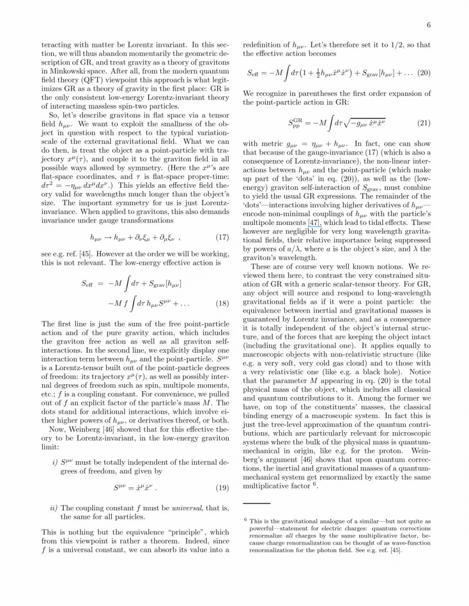
teracting with matter be Lorentz invariant. In this sec-tion, we will thus abandon momentarily the geometric de-scription of GR, and treat gravity as a theory of gravitonsin Minkowski space. After all, from the modern quantumfield theory (QFT) viewpoint this approach is what legit-imizes GR as a theory of gravity in the first place: GR isthe only consistent low-energy Lorentz-invariant theoryof interacting massless spin-two particles.

So, let’s describe gravitons in flat space via a tensorfield hµν . We want to exploit the smallness of the ob-ject in question with respect to the typical variation-scale of the external gravitational field. What we cando then, is treat the object as a point-particle with tra-jectory xµ(τ), and couple it to the graviton field in allpossible ways allowed by symmetry. (Here the xµ’s areflat-space coordinates, and τ is flat-space proper-time:dτ2 = −ηµν dx

µdxν .) This yields an effective field the-ory valid for wavelengths much longer than the object’ssize. The important symmetry for us is just Lorentz-invariance. When applied to gravitons, this also demandsinvariance under gauge transformations

hµν → hµν + ∂νξµ + ∂µξν , (17)

see e.g. ref. [45]. However at the order we will be working,this is not relevant. The low-energy effective action is

Seff = −M∫

dτ + Sgrav[hµν ]

−M f

∫

dτ hµνSµν + . . . (18)

The first line is just the sum of the free point-particleaction and of the pure gravity action, which includesthe graviton free action as well as all graviton self-interactions. In the second line, we explicitly display oneinteraction term between hµν and the point-particle. Sµν

is a Lorentz-tensor built out of the point-particle degreesof freedom: its trajectory xµ(τ), as well as possibly inter-nal degrees of freedom such as spin, multipole moments,etc.; f is a coupling constant. For convenience, we pulledout of f an explicit factor of the particle’s mass M . Thedots stand for additional interactions, which involve ei-ther higher powers of hµν , or derivatives thereof, or both.

Now, Weinberg [46] showed that for this effective the-ory to be Lorentz-invariant, in the low-energy gravitonlimit:

i) Sµν must be totally independent of the internal de-grees of freedom, and given by

Sµν = xµxν . (19)

ii) The coupling constant f must be universal, that is,the same for all particles.

This is nothing but the equivalence “principle”, whichfrom this viewpoint is rather a theorem. Indeed, sincef is a universal constant, we can absorb its value into a

redefinition of hµν . Let’s therefore set it to 1/2, so thatthe effective action becomes

Seff = −M∫

dτ(

1 + 12hµν x

µxν)

+ Sgrav[hµν ] + . . . (20)

We recognize in parentheses the first order expansion ofthe point-particle action in GR:

SGRpp = −M

∫

dτ√

−gµν xµxν (21)

with metric gµν = ηµν + hµν . In fact, one can showthat because of the gauge-invariance (17) (which is also aconsequence of Lorentz-invariance), the non-linear inter-actions between hµν and the point-particle (which makeup part of the ‘dots’ in eq. (20)), as well as the (low-energy) graviton self-interaction of Sgrav, must combineto yield the usual GR expressions. The remainder of the‘dots’—interactions involving higher derivatives of hµν—encode non-minimal couplings of hµν with the particle’smultipole moments [47], which lead to tidal effects. Thesehowever are negligible for very long wavelength gravita-tional fields, their relative importance being suppressedby powers of a/λ, where a is the object’s size, and λ thegraviton’s wavelength.

These are of course very well known notions. We re-viewed them here, to contrast the very constrained situ-ation of GR with a generic scalar-tensor theory. For GR,any object will source and respond to long-wavelengthgravitational fields as if it were a point particle: theequivalence between inertial and gravitational masses isguaranteed by Lorentz invariance, and as a consequenceit is totally independent of the object’s internal struc-ture, and of the forces that are keeping the object intact(including the gravitational one). It applies equally tomacroscopic objects with non-relativistic structure (likee.g. a very soft, very cold gas cloud) and to those witha very relativistic one (like e.g. a black hole). Noticethat the parameter M appearing in eq. (20) is the totalphysical mass of the object, which includes all classicaland quantum contributions to it. Among the former wehave, on top of the constituents’ masses, the classicalbinding energy of a macroscopic system. In fact this isjust the tree-level approximation of the quantum contri-butions, which are particularly relevant for microscopicsystems where the bulk of the physical mass is quantum-mechanical in origin, like e.g. for the proton. Wein-berg’s argument [46] shows that upon quantum correc-tions, the inertial and gravitational masses of a quantum-mechanical system get renormalized by exactly the samemultiplicative factor 6.

6 This is the gravitational analogue of a similar—but not quite aspowerful—statement for electric charges: quantum correctionsrenormalize all charges by the same multiplicative factor, be-cause charge renormalization can be thought of as wave-functionrenormalization for the photon field. See e.g. ref. [45].

7

No analogous statement can be made for scalar cou-plings. Consider indeed a scalar-tensor theory for gravity.Also assume that it is a ‘metric’ theory, which means thatthere is a conformal frame (Jordan’s) where matter-fieldsare all minimally coupled to the same metric. This is theclosest we can get to implementing the equivalence prin-ciple. Now, upon demixing the scalar ϕ from the gravitonhµν (that is, in Einstein frame), this prescription corre-sponds to a direct coupling ϕTm between the scalar andmatter fields, where Tm = Tm

µµ is the trace of the mat-

ter energy-momentum tensor. The problem with such acoupling is that Tm is not associated with any conservedcharges. That is, in the above point-particle approxima-tion, extending GR to a scalar-tensor theory (in Einsteinframe) amounts to adding an interaction term

Sint = Q

∫

dτ ϕ+ . . . , (22)

as well as of course a Lagrangian for ϕ, its self-interactions, and its interactions with hµν . The dots inSint denote interactions involving derivatives of ϕ, whichcan be thought of as multipole interactions—negligiblefor a long-wavelength scalar field. Now, the coupling Qis the spatial integral of Tm over the object’s volume,and is not a conserved charge. So, for instance, if weconsider a collapsing sphere of dust eventually forminga black-hole, its coupling to hµν (the mass M) is con-served throughout the collapse, whereas its coupling toϕ (the scalar charge Q) is not: as the dust particles be-come more and more relativistic, their Tm approacheszero, even as the total mass M remains constant, domi-nated more and more by gravitational binding energy. Infact we already know that for a black-hole, which is theend product of our example, Q must be zero, because ofthe no-hair theorem [48]: a black-hole cannot sustain ascalar profile, which in our language means that in thepoint-particle approximation it cannot couple to a long-wavelength ϕ. So, in comparing how a black-hole and anon-relativistic gas cloud fall in a very long-wavelengthscalar-tensor gravitational field, we expect order one vi-olation of the equivalence principle: the black-hole willnot follow a geodesic of the Jordan-frame metric.

In general, even if we start with a universal couplingϕTm at the microscopic level, the ratio Q/M for ex-tended objects will be object dependent, and sensitiveto how relativistic the object’s internal structure is: itwill be one for very non-relativistic objects (with a suit-able normalization of ϕ), and zero for black holes. Thiskind of variation in Q/M , which is relativistic in nature(O(1/c2) in a post-Newtonian expansion), is available toall scalar-tensor theories. As we will see, theories wherethe chameleon mechanism is at work possess an addi-tional and more dramatic source of Q/M variation—itcan be O(1) even for non-relativistic objects. This screen-ing mechanism arises from a particular kind of scalar self-interaction, and it results in a scalar charge Q not justdetermined by an integral of Tm, but also by the precisenon-linear dynamics of the scalar itself close to the ob-

ject. Essentially, the scalar field profile sourced by theobject at short distances contributes, via non-linearities,to the coupling of the object to a long-wavelength exter-nal scalar. (As we will see, for the Vainshtein mechanismthis scalar charge renormalization does not occur.)

The lesson is this: from the low-energy point-particleaction viewpoint, the charges Q for different objects arefree parameters, and are not forced to be related tothe corresponding total inertial masses M in any way.Therein lies the seed for equivalence principle violation.

IV. THE PROBLEM OF MOTION IN

SCALAR-TENSOR THEORIES — SCREENING

BY THE CHAMELEON MECHANISM

The fact that different objects might fall at differentrates in scalar-tensor theories is easiest to see in Einsteinframe—the scalar ϕ mediates a fifth force and the equiv-alence principle is violated whenever the scalar chargeto mass ratio fluctuates between objects. On the otherhand, that this should be true in Jordan frame mightcome as a bit of a surprise: after all, are not all objectssupposed to move on geodesics in Jordan frame? Wetherefore present two different derivations, one in eachframe. The Einstein frame derivation is presented in§IVA. The Jordan frame derivation is briefly summa-rized in §IVB with details given in Appendix C. In addi-tion, Appendix B describes how to map our descriptionof general scalar-tensor theories to the special cases ofBrans-Dicke and f(R).

The Einstein frame action is

S = M2Pl

∫

d4x√

−g[

12 R− 1

2∇µϕ∇µϕ− V (ϕ)]

+

∫

d4xLm(ψm,Ω−2(ϕ)gµν) . (23)

Here,˜denotes quantities in Einstein frame, R is the Ein-stein frame Ricci scalar, ∇µϕ∇µϕ is supposed to remindus that the contraction is performed with the Einsteinframe metric gµν (there is otherwise no difference be-

tween ∇µϕ and ∇µϕ: ∇µϕ = ∇µϕ = ∂µϕ). The symbolϕ denotes some scalar that would contribute to a fifthforce. Upon a field-redefinition, its kinetic term can al-ways be written as in eq. (23). For notational conve-nience for what follows, we decide to factor an M2

Pl outof the whole scalar-tensor gravitational action. With thisnormalization ϕ is dimensionless. We assume ϕ has apotential V (ϕ), which given our normalization has mass-dimension two. The symbol ψm denotes some matterfield whose precise nature is not so important; the mostimportant point is that it is minimally coupled not to gµν

but to Ω−2(ϕ)gµν , which is precisely the Jordan framemetric:

gµν = Ω−2(ϕ)gµν . (24)

Performing the conformal transformation gives us the

8

Jordan frame action:

S = M2Pl

∫

d4x√−g

[

12Ω2(ϕ)R − 1

2h(ϕ)∇µϕ∇µϕ

−Ω4(ϕ)V]

+

∫

d4xLm(ψm, gµν) (25)

where

h(ϕ) ≡ Ω2

[

1 − 3

2

(

∂ ln Ω2

∂ϕ

)2]

. (26)

The matter energy-momentum in the two frames (definedas the derivative of the action w.r.t. the correspondingmetric) are related by:

Tmµν = Ω2(ϕ)Tm

µν . (27)

In anticipation of the fact that we will be carrying outperturbative computations, let us point out that Ω2(ϕ)must be close to unity for the metric perturbations to besmall in both Einstein and Jordan frames. We can thusapproximate it at linear order in ϕ,

Ω2(ϕ) ≃ 1 − 2αϕ , (28)

where α is a constant, and |αϕ| ≪ 1. We are not assum-ing, however, that the fractional scalar field perturbation(i.e. δϕ/ϕ) is in any way small. In fact, nonlinear effectsin δϕ/ϕ are going to be crucial in enabling the chameleonmechanism. Under the same approximation, a useful re-lation is

∂ ln Ω2

∂ϕ≃ −2α . (29)

The reader might find it helpful to keep in mind a partic-ularly common (if not particularly natural) form of theconformal factor, Ω2 = exp [−2αϕ] with constant α, inwhich case Eq. (29) is exact and Eq. (28) is a Taylorexpansion.

As elaborated in Appendix B, α = 1/√

6 in f(R) mod-els and ωBD = (1 − 6α2)/(4α2) in Brans-Dicke theory.

A. Derivation in Einstein Frame

The Einstein frame metric equation is

Gµν = 8πG

[

Tmµ

ν + Tϕµ

ν]

(30)

where

Tϕµ

ν =1

8πG

∇µϕ∇νϕ− δµ

ν[

12∇αϕ∇

αϕ+ V

]

.(31)

The scalar field equation is

ϕ =∂V

∂ϕ+ 4πG

∂ ln Ω2

∂ϕTm

µµ . (32)

Following the derivation in the GR case (§II), we performan object-background split, derive solutions to the objectfields, and compute an integral of momentum flux overan enclosing sphere to find the net gravitational force onthe extended object.

Object-background Split

We work in the Newtonian gauge:

ds2 = −(1 + 2Φ)dt2 + (1 − 2Ψ)δijdxidxj . (33)

As before (Eq. (8)), we carry out a decomposition of thefields at some radius r away from the object:

Φ = Φ0 + Φ1(r) , Ψ = Ψ0 + Ψ1(r) , ϕ = ϕ0 + ϕ1(r)(34)

where the subscript 0 denotes the back-ground/environmental fields and the subscript 1denotes the object fields. The background fields areassumed to be well approximated by linear gradients:

Φ0(~x) ≃ Φ0(0) + ∂iΦ0(0)xi

Ψ0(~x) ≃ Ψ0(0) + ∂iΨ0(0)xi

ϕ0(~x) ≃ ϕ∗ + ∂iϕ0(0)xi (35)

where 0 denotes the origin centered at the object, andwe use ϕ∗ to denote the background scalar field valuethere. The assumption here is that these backgroundfields sourced by the object’s environment vary on a scalemuch larger than r, where we will draw our enclosingsphere.

It is worth emphasizing that this object-backgroundsplit needs only make sense at the surface of the enclos-ing sphere (over which we will compute the integratedmomentum flux), but not necessarily at the location ofthe object itself.

Solutions for the Object Fields

To work out solutions for the object fields, we firstexamine the Einstein equation linearized in metric per-turbations:

∇2Ψ = 4πG ρ− 14∂0ϕ∂

0ϕ+ 14∂iϕ∂

iϕ+ 12V

∂0∂iΨ = − 12∂

0ϕ∂iϕ

(∂i∂j − 13δij∇

2)(Ψ − Φ) =

∂iϕ∂jϕ− 1

3δij∂kϕ∂

kϕ

∂20Ψ + 1

3∇2(Φ − Ψ) =

16

(

− 32∂0ϕ∂

0ϕ− 12∂kϕ∂

kϕ− 3V)

(36)

where we have assumed the matter is non-relativistic,characterized only by its energy density ρ.

We can ignore all second order scalar field terms onthe right hand side of these equations. This is because

9

as we will see shortly, ϕ is already first order in G. Thusits contribution to Einstein’s equations is on an equalfooting with post-Newtonian corrections, which we areneglecting. In addition, we will ignore V as well. Therationale is that Gρ ≫ V inside the object of interest,whereas outside the object, V or any other sources ofenergy-momentum are just small (in the sense that thetotal mass within the enclosing sphere is dominated bythe object). Essentially, we assume the metric in thevicinity of the object is sourced mainly by matter ratherthan the scalar field:7

∇2Ψ = 4πGρ , ∇2(Φ − Ψ) = 0 . (37)

Under the same assumptions as in §II, we get

Φ1 = Ψ1 = −GM/r (38)

where M is the mass of the object.

As in the case of GR, we in essence assume there is aseparation of scales: that r can be chosen small enoughthat second gradients of the background tidal fields canbe ignored, but large enough for the monopole to dom-inate. The latter condition is helpful but not essential(see Appendix A).

The next task is to compute the scalar field profilesourced by the object. The scalar field equation (Eq.(32)) can be written as

∇2ϕ =∂V

∂ϕ+ α 8πG ρ (39)

where we have ignored time derivatives and correctionsdue to metric perturbations, and we have used the ap-proximation Eq. (29). Here, it is crucial we do not as-sume δϕ/ϕ is small even though ϕ is. The important

V

ρ

Veff

ϕ

ϕ

7 Under this assumption, the anisotropic stress vanishes. This isemphatically an Einstein frame statement. The same will not betrue in Jordan frame.

FIG. 1: A scalar potential for the chameleon mechanism.The effective potential felt by ϕ in the presence of sources isthe sum of the self-interaction potential V (ϕ) and the scalar-matter coupling (α 8πG)ρ ϕ. This can give ϕ a large mass atlocations where the matter density ρ is large.

nonlinearity for the chameleon mechanism is in the po-tential term. For instance, for the potential of fig. 1 thechameleon mechanism could operate, meaning that for anobject of the right size and density, ϕ could be trapped atsome small value inside much of the extended object—avalue where the two terms on the right hand side of Eq.(39) roughly balance. This corresponds to ϕ having alarge mass, or a small Compton wavelength, inside theobject (see Fig. 1). The object will therefore have anexterior scalar profile that is screened i.e. only a frac-tion of the object’s mass (the fraction that happens tolive within a shell approximately a Compton wavelengththick at the object’s boundary) sources the exterior scalarprofile. In other words, we expect the object to producea scalar field that at large r is dominated by a monopoleof the form:

ϕ1(r) = −ǫ α 2GM

r(40)

where ǫ quantifies the degree of screening.If the scalar field remains light inside the object, we

have ∂V/∂ϕ ≪ α8πGρ in which case the exterior scalarprofile is sourced by the full mass of the object, i.e. ǫ = 1in Eq. (40). On the other hand, suppose the scalar fieldis massive and therefore short-ranged inside the object,the exterior scalar profile is sourced only by the massresiding in a shell at the boundary of the object. Sup-pose the object has a radius rc and the shell has thickness∆rc. The scalar field sits at some small equilibrium value(where the potential and density terms on the right handside of Eq. (39) cancel) at all radii interior to the object– that is, except where the shell is. At the shell, thescalar field starts to pull away from this small expecta-tion value because of the force exerted by the densityterm. In other words, at the shell, Eq. (39) can be ap-proximated by δϕ/(rc∆rc) ∼ α 8πGM/(4πr3c/3), whereδϕ = ϕ∗ − ϕc ≃ ϕ∗ (ϕc is the equilibrium value wherethe the potential and density terms balance in the deepinterior of the object, and ϕ∗ is approximately the scalarfield value far away from the object). We therefore have3∆rc/rc ∼ (ϕ∗/2α) · (GM/rc)

−1. This is precisely thefraction by volume of the object that sources the exte-rior scalar field. This means the suppression factor ǫ inEq. (40) should be

ǫ ≃ ϕ∗2α

[

GM

rc

]−1

ifϕ∗2α

[

GM

rc

]−1

< 1 (41)

where GM/rc is the gravitational potential of the object.The inequality is required for consistency: it had betterbe true that 3∆rc/rc < 1 for screening to occur. This isknown as the thin-shell condition. When this condition

10

is violated, there is no screening:

ǫ = 1 ifϕ∗2α

[

GM

rc

]−1

∼> 1 , (42)

essentially meaning that α8πGρ ≫ ∂V/∂ϕ throughoutthe object, in which case the scalar field ϕ cannot evenreach the equilibrium value ϕc inside the object. It isinteresting to note that the thin-shell condition does notdepend explicitly on the potential V . The implicit re-quirement is that the potential is of such a form thatequilibrium (between density and potential) is possible.A more detailed derivation of the thin-shell condition canbe found in [20].

Along the lines of §III, it is useful to introduce the ideaof a scalar charge: by analogy with Ψ1 = −GM/r forthe gravitational potential, let us write the scalar profileas ϕ1 = −2GQ/r (the factor of 2 is motivated by theappearance of 8πρ rather than 4πρ in Eq. (39)). Byinspecting Eq. (40), we can see that the dimensionlessscalar charge Q is

Q ≡ ǫ αM . (43)

Screened objects carry a much reduced scalar charge asviewed from outside.

Just as in the case of the metric fluctuations, one canalways add to ϕ1 a linear gradient of the form Eq. (35)to represent the field generated by sources in the envi-ronment. To summarize, Φ, Ψ and ϕ are given by Eqs.(34), (35), (38) and (40).

Surface Integral of Momentum Flux

We are ready to compute the gravitational force fol-lowing Eq. (4):

Pi = −∮

dSj tij (44)

where the surface integral is again over some sphere en-closing the object of interest. By analogy to Eqs. (1) and(2), the pseudo energy-momentum tensor is:

tµν = Tm

µν + Tϕ

µν − 1

8πGG(2)

µν . (45)

As before, Tmij outside the object is small, and we have

already computed the G(2)ij contribution (just put ˜ on

top of quantities in Eq. (11)). What remains to be done

is to compute the contribution from Tϕij (Eq. (31)).

The same tricks that work for the G(2)ij contribution

work here, and we obtain

−∮

dSj Tϕ

ij = − 1

2Gr2 ∂iϕ0

∂ϕ1

∂r. (46)

Note that there should be a contribution from the poten-tial of the form: 1

G

∮

dSjV ∼ 1G (4πr3/3)∂iϕ0∂V/∂ϕ|ϕ∗

,

but this can be ignored by our assumption that the scalarfield ϕ1 is sourced mainly by the object rather than itsimmediate environment.

Putting together all contributions (Eq. (46) & Einsteinframe analog of Eq. (11)), we therefore have

Pi =r2

2G

[

∂iΦ0

(

−4

3

∂Ψ1

∂r− 2

3

∂Φ1

∂r

)

− ∂iϕ0∂ϕ1

∂r

]

. (47)

Putting our solutions for the various fields into theabove expression, we obtain

MX i = −M∂iΦ0 − ǫαM∂iϕ0

= −M[

∂iΦ0 +Q

M∂iϕ0

]

(48)

where have used Eq. (43), and we have equated Pi and

MX i, where X i is the object center of mass coordinate(Eq. (15)). This is the main result of this section. Thefact that screened and unscreened objects have differentscalar charge to mass ratios Q/M (or equivalently, dif-ferent ǫ) means they fall at different rates. This is theorigin of apparent equivalence principle violation.

This result can be further simplified if we make onemore assumption, which does not necessarily hold in gen-eral. Both Φ0 and ϕ0 are sourced by the environment.Suppose they are sourced in a similar way:

∇2Φ0 = 4πGρ , ∇2ϕ0 = α 8πG ρ (49)

where ρ is the environmental density. The latter equationfollows from Eq. (39) provided that potential terms aresmall compared to density terms on the scales of interest.Eq. (49) then implies

ϕ0 = 2α Φ0 . (50)

Putting this into Eq. (48), we therefore obtain

MX i = −M∂iΦ0

[

1 + 2αQ

M

]

= −M∂iΦ0

[

1 + 2ǫα2]

. (51)

The fact that this result depends on the square ofα makes it clear that the sign of α has no physicalmeaning—chameleon mechanism only requires its sign beopposite to that of ∂V/∂ϕ (see Eq. (39)).

Suppose one has a scalar-tensor theory where 2α2 isorder unity, as is true in f(R) theories, then screened ob-jects (ǫ ∼ 0) and unscreened objects (ǫ = 1) would moveon very different trajectories i.e. order unity apparent vi-olation of the equivalence principle. Note that infinites-imal test particles should go unscreened and thereforehave ǫ = 1.

Let us end with a summary of further approximationswe have made in this section to augment those listed atthe end of §II:

1’. We have taken the non-relativistic or quasi-staticlimit i.e. time derivatives of the scalar field are ignored.

11

2’. We assume the scalar field does not contributemuch to the r.h.s. of Einstein’s equations (36).

3’. We assume there is a separation of scales, that sec-ond derivatives of the background/environmental scalarfield can be ignored on the scale r of the enclosing sur-face, and that the monopole contribution to the object’sscalar profile dominates at r. As discussed in AppendixA, this latter assumption can be relaxed. The formerassumption implicitly requires the Compton wavelengthof the exterior scalar field to be large compared with r.The scalar field would be Yukawa suppressed if this werenot true. This has implications for observational tests aswe will discuss in §VI.

To this list, which mirrors the list in §II, we shouldadd:

4’. We assume the conformal factor Ω2(ϕ) is close tounity, or equivalently |αϕ| ≪ 1 (see Eq. (28)). This as-sumption is not strictly necessary in our Einstein framecalculation. It will become necessary when we try tocompare the Jordan frame calculation with it. One con-sequence of this assumption is that the Einstein frameand Jordan frame masses of the object are roughly equali.e.

M =

∫

d3x ρ ≃∫

d3xρ (52)

since ρ = Ω4ρ, recalling that Tm00 = −ρ and Tm

00 =

−ρ.In summary, the main results of this section are encap-

sulated in Eqs. (47), (48) and (51), which make differ-ent levels of approximations, starting from the minimum.The key observation is that, despite the explicitly uni-versal coupling of the scalar to matter at the microscopiclevel (Eq. (23)), scalar charges of macroscopic objectsget classically renormalized by nonlinear chameleon ef-fects. This produces fluctuations in the scalar charge tomass ratio Q/M for different objects, leading to differentrates of gravitational free fall. Screened objects, whichhave Q/M ∼ 0, accelerate less than unscreened objects.As we will see, no such (non-relativistic) renormalizationoccurs for the Vainshtein mechanism.

B. Derivation in Jordan Frame

In principle, the simplest way to obtain the Jordanframe results is to transform the end results of §IVA,Eqs. (47), (48) and (51), into Jordan frame by a con-formal transformation gµν = Ω−2gµν . After all, whethertwo different objects fall at different rates is a frame-independent issue. This might not, however, satisfy read-ers who are accustomed to the Jordan frame viewpoint:should not everything move on geodesics? In this sec-tion, we therefore briefly sketch a Jordan frame deriva-tion. Details can be found in Appendix C.

The Jordan frame metric in Newtonian gauge is

ds2 = −(1 + 2Φ)dt2 + (1 − 2Ψ)δijdxidxj . (53)

From Eq. (24) and recalling Ω2 ≃ 1 − 2αϕ (Eq. (28)),the Jordan and Einstein frame metric perturbations arerelated by

Φ = Φ + αϕ , Ψ = Ψ − αϕ . (54)

Note how Φ 6= Ψ even if Φ = Ψ.The Jordan frame metric equation is

Gµν = 8πGΩ−2 [Tm

µν + Tϕ

µν ]

+Ω−2[

∇µ∇νΩ2 − δµνΩ2

]

(55)

where

Tϕµ

ν =1

8πG

h∇µϕ∇νϕ

− δµν[

12h∇αϕ∇αϕ+ Ω4V

]

. (56)

The scalar field energy-momentum follows from (the min-imally coupled portion of) the Jordan frame action Eq.(25). Note that ϕ does not have a canonical kinetic term,hence the presence of h(ϕ) (Eq. (26)). In some theories,h might even be zero, such as in f(R).

The Einstein-Infeld-Hoffmann approach to the prob-lem of motion is to compute the gravitational force as asurface integral of the momentum flux (Eq. (4)). Themomentum flux can be obtained from the spatial com-ponents of the pseudo-energy-momentum tensor, whichis defined by Eq. (1):

tµν = Ω−2(Tm

µν + Tϕ

µν) − 1

8πGG(2)

µν

+Ω−2

8πG

[

∇µ∇νΩ2 − δµνΩ2

]

. (57)

Comparing this with Eq. (45), we can see the calcula-tion should be similar to the Einstein frame case, exceptthat we have an overall conformal factor Ω−2 multiplyingthe matter and scalar field energy-momentum, and thatthere are some uniquely Jordan frame contributions totµ

ν (second line). These differences originate from thedifferences in the metric equation (55) from the Einsteinequation: a non-constant effective ‘G’, and extra sourcesforGµ

ν beyond the matter and scalar energy-momentum.Phrased in this way, it is not obvious that the integral

of momentum flux should imply geodesic motion in Jor-dan frame. In fact, it does not in general. Relegating thedetails to Appendix C, it can be shown that the centerof mass of an object moves according to:

MX i = −M ∂iΦ0 + (1 − ǫ)αM ∂iϕ0 (58)

where Φ0 and ϕ0 are respectively the back-ground/environmental (time-time) metric perturbationand scalar field, M is the inertial mass and X i is thecenter of mass coordinate. This is manifestly consistentwith the Einstein frame equation of motion Eq. (48)

once we recognize that Φ0 = Φ0 − αϕ0 according to Eq.(54).

12

The parameter ǫ is controlled by the relative size ofthe object’s gravitational potential and the environmen-tal scalar field; see Eqs. (41) & (42). An unscreenedobject, which has ǫ = 1, would move on a geodesic inJordan frame, just as expected for an infinitesimal testparticle. A screened object, where the chameleon mech-anism operates to make ǫ ∼ 0, would not move on ageodesic even in Jordan frame. In other words, it ap-pears as if for screened objects, the gravitational massand the inertial mass are unequal. This can be mademore explicit if we make a simplifying assumption, thatboth Φ0 − αϕ0 and ϕ0 are sourced mainly by density(Eq. (49)), in which case ϕ0 = 2αΦ0/(1 + 2α2), and theequation of motion simplifies to

MX i = M

[

1 + 2ǫα2

1 + 2α2

]

∂iΦ0 (59)

which is consistent with its Einstein frame counterpartEq. (51). Thus, in Jordan frame,

inertial mass = M

grav. mass = M1 + 2ǫα2

1 + 2α2. (60)

An unscreened object is subject to a gravitational forcethat is 1 + 2α2 larger than a screened object. For theo-ries such as f(R), this is not a small effect: α = 1/

√6

implies 1 + 2α2 = 4/3 (Appendix B). This might comeas a surprise in the Jordan frame, where the metric isminimally coupled to matter (Eq. (25)). Despite con-ventional wisdom, specifying the Jordan frame metricdoes not completely specify the motion of an extendedobject. The motion of an object should be ultimately de-termined by energy-momentum conservation. Since thescalar field contributes energy-momentum, it retains adirect influence on the motion of the object. This directinfluence magically cancels only for unscreened objects,which thus move on geodesics.8 The key physics is the(non-relativistic and classical) renormalization of scalarcharge by the nonlinear chameleon mechanism, as dis-cussed in §IVA. An object’s coupling to the backgroundscalar field is suppressed if it is screened, and unsup-pressed if it is not. 9

8 The cancellation occurs between the effective Newton constantGΩ−2 and the uniquely Jordan frame terms Ω−2∂∂Ω2 in thepseudo-energy-momentum (Eq. (57)).

9 For a screened object (let’s say a galaxy halo) in an unscreenedenvironment, it is worth noting that the scalar field ϕ experiencesa jump at the thin shell of the object (from a large expectationvalue outside to a small one inside), which means that whilethe Einstein frame metric perturbations are smooth across theshell, the Jordan frame metric perturbations jump (Eq. (54)).This resolves what might perhaps be puzzling to some: that thescreened halo as a whole does not move on the Jordan framegeodesic, while infinitesimal particles inside it do. The key ob-servation is that they see rather different overall Jordan framemetrics (even after accounting for the fact that a particle inside

V. THE PROBLEM OF MOTION IN

SCALAR-TENSOR THEORIES — SCREENING

BY STRONG COUPLING A LA VAINSHTEIN

Another class of scalar-tensor theories where the scalaris efficiently screened at short distances is massive grav-ity theories. These are not scalar-tensor theories to theletter, for at scales of order of the graviton’s Comptonwavelength, and larger, there is no propagating scalardegree of freedom. However, at much shorter scales the(helicity-zero) longitudinal polarization of the gravitonbehaves like a scalar universally coupled to matter withgravitational strength, and the dynamics is accuratelydescribed by a scalar-tensor theory [13]. What makesthese theories potentially interesting is that this effec-tive scalar comes equipped with important derivativeself-interactions, which can make it decouple at shortdistances from compact objects, thus recovering agree-ment with solar system tests. This is known as the Vain-shtein effect, and it shows up explicitly in the DGP model[5]—which is a much healthier alternative to the mini-mal Fierz-Pauli theory of massive gravitons. However aswe will see shortly, unlike the chameleon mechanism theVainshtein effect does not lead to O(1) violations of theequivalence principle—in fact it leads to the same vio-lations one would have for a purely linear Brans-Dicketheory, which are O(1/c2).

For simplicity and definiteness, we will analyze the ex-ample of DGP. Everything we say can be straightfor-wardly extended to the ‘galileon’, which was argued inref. [11] to be the broadest generalization of (the scalar-tensor limit of) DGP that robustly implements the Vain-shtein effect without introducing ghost degrees of free-dom. The scalar sector of DGP (in Einstein frame) hasthe Lagrangian [9]

Lπ = −3M2Pl(∂π)2 − 2

M2Pl

m2(∂π)2π + π Tm

µµ , (61)

where m is the DGP critical mass scale—the analogue ofthe graviton’s mass—and is generally set to the currentinverse Hubble scale. We are using a dimensionless nor-malization for the scalar field π, so that the Jordan-framemetric to which matter fields couple minimally is

hµν = hµν + 2π ηµν . (62)

That is, in the non-relativistic limit π is a shift in theNewtonian potential:

Φ = Φ + π . (63)

the object of course sees additional metric perturbations arisingfrom other particles of the object). In Einstein frame, there is nomystery: neither the screened halo nor its constituent particlesexperience any scalar force. We thank Wayne Hu for discussionson this issue.

13

RSV

π0

=

S

π

S

0

RV

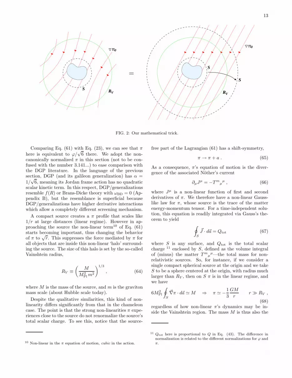
FIG. 2: Our mathematical trick.

Comparing Eq. (61) with Eq. (23), we can see that π

here is equivalent to ϕ/√

6 there. We adopt the non-canonically normalized π in this section (not to be con-fused with the number 3.141...) to ease comparison withthe DGP literature. In the language of the previoussection, DGP (and its galileon generalization) has α =

1/√

6, meaning its Jordan frame action has no quadraticscalar kinetic term. In this respect, DGP/generalizationsresemble f(R) or Brans-Dicke theory with ωBD = 0 (Ap-pendix B), but the resemblance is superficial becauseDGP/generalizations have higher derivative interactionswhich allow a completely different screening mechanism.

A compact source creates a π profile that scales like1/r at large distances (linear regime). However in ap-proaching the source the non-linear term10 of Eq. (61)starts becoming important, thus changing the behaviorof π to

√r. This suppresses the force mediated by π for

all objects that are inside this non-linear ‘halo’ surround-ing the source. The size of this halo is set by the so-calledVainshtein radius,

RV ≡(

M

M2Plm

2

)1/3

, (64)

where M is the mass of the source, and m is the gravitonmass scale (about Hubble scale today).

Despite the qualitative similarities, this kind of non-linearity differs significantly from that in the chameleoncase. The point is that the strong non-linearities π expe-riences close to the source do not renormalize the source’stotal scalar charge. To see this, notice that the source-

10 Non-linear in the π equation of motion, cubic in the action.

free part of the Lagrangian (61) has a shift-symmetry,

π → π + a . (65)

As a consequence, π’s equation of motion is the diver-gence of the associated Nother’s current

∂µJµ = −Tm

µµ , (66)

where Jµ is a non-linear function of first and secondderivatives of π. We therefore have a non-linear Gauss-like law for π, whose source is the trace of the matterenergy-momentum tensor. For a time-independent solu-tion, this equation is readily integrated via Gauss’s the-orem to yield

∮

S

~J · d~a = Qtot (67)

where S is any surface, and Qtot is the total scalarcharge 11 enclosed by S, defined as the volume integralof (minus) the matter Tm

µµ—the total mass for non-

relativistic sources. So, for instance, if we consider asingle compact spherical source at the origin and we takeS to be a sphere centered at the origin, with radius muchlarger than RV , then on S π is in the linear regime, andwe have

6M2Pl

∮

S

~∇π · d~a ≃M ⇒ π ≃ −1

3

GM

rr ≫ RV ,

(68)regardless of how non-linear π’s dynamics may be in-side the Vainshtein region. The mass M is thus also the

11 Qtot here is proportional to Q in Eq. (43). The difference innormalization is related to the different normalizations for ϕ andπ.

14

scalar charge, and according to the analysis of §III, Mthen is the coupling between the object and very long-wavelength external/background π’s. This implies thereis no chameleon-like non-relativistic renormalization ofthe scalar charge, and no O(1) violation of the equiv-alence principle. The only violations of the equivalenceprinciple we may have are associated with how relativisticthe source’s internal structure is, i.e. on how the volumeintegral of Tm

µµ differs from the total ADM mass, which

is a post-Newtonian O(1/c2) effect 12. For the benefit ofthe skeptical reader, in Appendix D we explicitly checkthis statement along the lines of the previous sections.

This would be the end of the story, if our universe weremade up of very isolated compact sources, with typicaldistances between one another much bigger that theirtypical Vainshtein radius. Unfortunately we live preciselyin the opposite limit. For macroscopic sources the Vain-shtein radius is so huge that treating those sources inisolation makes no sense. For instance, for the sun wehave

R⊙V ∼ 1021 cm , (69)

much bigger than the distance to the closest stars. Wecan repeat the same estimate at all scales, and checkthat nowhere in the universe π is in the linear regime.This makes a comprehensive study of the effects of π inour universe a formidable task, because by definition of anon-linear system, we cannot simply superimpose the πfields due to different sources. However here we want tofocus on possible violations of the equivalence principle,and for these we will be able to draw surprisingly generalconclusions.

Consider then the more realistic situation of an objectin the presence of other sources. To be as general as pos-sible, let’s imagine that the object in question has sizablemultiple moments as well. The situation is schematicallydepicted in Fig. 2(left). We would like to compute theforce acting on the object following the approach of theprevious sections. In order to approximate the π fieldcreated by the other sources (π0, in the figure) as a lin-ear pure-gradient field, we have to draw our surface Svery close to the object. In fact since π is deep in thenon-linear regime, we have two problems

1. How do we separate π0 from π1—the π generatedby the object? The total π is not simply the sumof the two contributions.

2. What is the effect of the object’s multipole mo-ments? In a non-linear regime, the multipoles of πare not directly related to the object’s multipoles.Also, their behavior with r w.r.t. to the monopole’sis different than in the linear case.

12 Notice that since in Eq. (68) we are considering a huge volumewith sizable non-linearities for π, we have to make sure that π’scontribution to the total ADM mass be negligible. It is straight-forward to check that this is indeed the case.

As to point 1, we are rescued once again by the sym-metries of the π dynamics, which will also make point 2uninteresting for our purpose.

Besides the aforementioned shift-symmetry on π, thesource-free part of the Lagrangian (61) is invariant undera constant shift in the derivative of π,

∂µπ → ∂µπ + cµ , (70)

dubbed ‘galilean invariance’ in ref. [11, 27]. In factthis is what makes DGP—and suitable generalizationsthereof—capable of the Vainshtein effect in the presenceof generic localized sources, and of sustaining interestingnon-linear cosmological solutions [11]. Galilean invari-ance allows us to add a pure-gradient field to any non-linear solution, to get a new non-linear solution. Considertherefore the π field generated by all other sources in theabsence of our object, and denote this by π0. Now, if ourobject is much smaller than the typical variation scale ofπ0, which is set by the distance to the other sources, thenwe can approximate π0 as a constant-gradient field in aneighborhood of the object. This means that in such aneighborhood, we can freely add π0 to the non-linear so-lution π1 we would have for the object in isolation, i.e. inthe absence of the other sources. The full π field

π = π0 + π1 (71)

is a consistent solution to the non-linear problem in theneighborhood in question. It is in fact the solution, be-cause it has (a) the right source—the object, and (b)the right boundary conditions: in moving away from theobject, the perturbation in ∂µπ induced by the objectdecays away as 1/

√r and we are left with ∂µπ0.

In summary, thanks to Galilean invariance the split-ting of Eq. (71) is well defined whenever the object ismuch smaller than its typical distance to nearby sources,which is a much milder requirement than linearity. Wecan then draw our sphere S very close to the object, asin Fig. 2(left), and compute the force acting on it alongthe lines of the previous sections. We do this explicitlyin Appendix D for a spherical object. However for anirregular object with sizable multipole moments, we donot even know the non-linear solution π1 for the objectin isolation. Nevertheless, here we can use a mathemat-ical trick. We have argued that the full solution on Sis the field the object would have in isolation, π1, plusa constant-gradient field, π0. Nothing prevents us fromconsidering a physically different situation, but with thesame total field on S. This would of course yield thesame result for the total force acting on the object. Avery convenient situation to consider is, the object in iso-lation with the same background constant-gradient π0 asin our case, but extended linearly throughout space, asdepicted in Fig. 2(right). That is, we can forget aboutthe external sources, and declare that in fact π0 has aconstant gradient throughout space. In doing so, we arenot changing the total π and its gradient on S—thus weare not changing the total force we would compute by

15

integrating over S. We can now change the radius ofS and bring it outside the Vainshtein region, where π’sdynamics is linear, its multipoles decay faster than themonopole, and the computation is precisely as for a linearscalar field. By changing the radius of S, we are modify-ing the total mass enclosed by S by π’s contribution to it.As long as this is negligible, as can be explicitly checked,the total force computed this way does not depend onthe radius of S.

We therefore conclude that, as far as the coupling ofan extended object to a background π field is concerned,theories with the Vainshtein effect behave exactly as thelinear Brans-Dicke theory. The Vainshtein mechanismentails equivalence principle violations only of the post-Newtonian O(1/c2) type.

VI. DISCUSSION — OBSERVATIONAL TESTS

Let us briefly summarize the main results so far, es-pecially those relevant for a discussion of observationaltests.

1. In theories where screening of the scalar field occursvia strong coupling effects (Vainshtein), such as DGP,the coupling of objects to the external scalar fields is un-suppressed to good approximation for all objects whosemass is not dominated by the gravitational binding en-ergy. They therefore fall at the same rate under grav-ity. There remains, however, equivalence principle vio-lations at the level of Φ, or O(1/c2) in the language ofpost-Newtonian expansion, just as in Brans-Dicke theory,where Φ is the gravitational potential depth of the ob-ject in question. Order one violation of the equivalenceprinciple is visible only when comparing the motion ofrelativistic objects such as black holes (|Φ| ∼ 1) with themotion of less compact objects such as stars (|Φ| ≪ 1).We will focus on observational tests of the chameleonmechanism instead, where the equivalence principle vio-lations are more dramatic and readily detectable even innon-relativistic/non-compact objects.

2. The chameleon mechanism implies that the cou-pling of screened objects to the external/backgroundscalar field is highly suppressed relative to unscreened ob-jects. They therefore fall at significantly different rates.More precisely, the equation of motion for the center ofmass of an object is, in Jordan frame (Eq. (58)):

MX i = −M∂iΦ0 + (1 − ǫ)αM∂iϕ0 (72)

where X i is the center of mass coordinate, Mis the inertial mass, Φ0 is the time-time part ofthe external/background metric and ϕ0 is the exter-nal/background scalar field (through which the objectmoves). Here we have adopted a convenient parame-terization of the relevant conformal factor Ω2(ϕ) in thescalar-tensor action (Eqs. (25) & (28)):

Ω2(ϕ) = 1 − 2αϕ , |αϕ| ≪ 1 (73)

where α is a constant. Eq. (73) can be thought of asa small field expansion of e.g. exp[−2αϕ]. The quantityǫ represents the degree of screening. Unscreened objectshave ǫ = 1, while screened objects have ǫ < 1. Thescreening parameter ǫ is controlled by (Eqs. (41) & (42)):

ǫ ≃ ϕ∗2α(GM/rc)

ifϕ∗

2α(GM/rc)< 1 (screened)

ǫ ≃ 1 ifϕ∗

2α(GM/rc) ∼> 1 (unscreened)(74)

where rc is the size of the object in question, and ϕ∗ is thevalue of the external scalar field. Screening is thereforecontrolled by the ratio of the exterior scalar field and thegravitational potential of the object. Unless the values ofthe two are finely tuned, one generally expects ǫ ≪ 1 ifscreening occurs at all. Eq. (72) tells us only unscreenedobjects, those with a sufficiently shallow gravitational po-tential, have equal inertial mass and gravitational massin Jordan frame.

3. The precise ratio of inertial mass to gravitationalmass predicted by Eq. (72) depends on how the externalscalar field ϕ0 is sourced. There are two useful limits toconsider. One is when the external scalar field is sourcedprimarily by density (Eq. (C17)) in which case the equa-tion of motion is well-approximated by

MX i = −M[

1 + 2ǫα2

1 + 2α2

]

∂iΦ0 (75)

which implies the unscreened and screened gravitationalmass are related by

unscreened g. mass = (1 + 2α2) × screened g. mass(76)

The other limiting case is when the external scalar fieldprofile is determined primarily by the potential, in whichcase ϕ0 is Yukawa suppressed on sufficiently large scales(scales larger than the Compton wavelength of the scalarfield ∼ 1/mϕ). If ϕ0 is Yukawa suppressed, the sec-ond term on the right of Eq. (72) is small regardlessof whether the object is screened or not. In this regime,one cannot observe equivalence principle violations bycomparing motions of different objects. As we will dis-cuss below, it is therefore important to avoid Yukawasuppression when performing observational tests.

4. Observationally, the single most important parame-ter besides α2 in a chameleon theory is the quantity ϕ∗/α(see Eq. (73)). For a given object, the relevant ϕ∗ is thescalar field value in its immediate surrounding. If thisis sufficiently small, the object will be screened accord-ing to Eq. (74). In other words, if the object is sittingin some high density environment which is itself screened(i.e. small scalar field value), it is likely that the object isalso screened. We will refer to this as blanket screening.In an environment where blanket screening of all objectsapplies, violations of equivalence principle will be hardto detect.

Conversely, if the object is sitting in an environmentwhere the density is at the cosmic mean or even lower

16

(voids), the chances are better that the object is un-screened because the relevant ϕ∗ is larger. In otherwords, to find unscreened objects, it is useful to avoidoverdense regions and to focus on objects with a shallowgravitational potential such that (Eq. (74)):

GM

rc ∼<ϕ∗2α

(77)

where ϕ∗ is taken to be the cosmic mean value. Wealready know ϕ∗/(2α) ∼< 10−6 from requiring that theMilky Way be screened to avoid gross deviations fromGR in solar system experiments [22] (see also [49] fora recent revision of the Milky Way’s mass). Thisleaves us an interesting window for testing theories likef(R). The smallest galaxies of interest have GM/rc ∼10−8(v/30 km/s)2. Therefore, if ϕ∗/α for our modifiedgravity theory satisfies

10−8∼<ϕ∗2α ∼< 10−6 (observationally interesting) (78)

massive galaxies at the high end would be screened whileless massive galaxies at the low end would not, offer-ing many opportunities for observing equivalence princi-ple violations, as we will see. The parameter space forchameleon mechanism is illustrated in Fig. 3.

−610−8 ∗ϕ /2α

61/

10

α

FIG. 3: Schematic experimental bounds in the chameleon pa-rameter space. The shaded region is already excluded, bydemanding that the Milky way be screened. The dashed lineis the improvement we propose. Further improvement is pos-sible using Lyman-alpha clouds. For α ≪ 1 the chameleonis very weakly coupled to matter to begin with, and clearlythis relaxes the bound on the other parameter. Curvatureinvariant theories such as f(R) have α = 1/

√6, though this

value is not protected by symmetry. The generic expectationis α ∼ O(1).

5. To make our discussion more concrete, it is usefulto keep in mind a particular class of examples, the socalled f(R) theories. As shown in Appendix B, f(R)corresponds to a specific value for α:

α = 1/√

6 for f(R) (79)

and so the unscreened gravitational force is 4/3 higherthan the screened one (Eq. (75)). This value for α arisessimply from demanding that ϕ be an auxiliary field inJordan frame (i.e. h(ϕ) = 0 in Eq. (25)). It is worthstressing however that from a theoretical viewpoint f(R)theories are not favored over more generic scalar-theories.For instance the property that ϕ has no kinetic energyin Jordan frame is not protected by any symmetry, thusone generically expects that upon quantum correctionsan f(R) theory will become a scalar-tensor theory not be-longing to the f(R) class. In fact, the resulting α could be

even larger than the 1/√

6. On the other hand, the struc-ture of the π Lagrangian in DGP and in galileon theoriesis protected by a symmetry—Galilean symmetry—whichforbids the quantum generation of Lagrangian terms withfewer than two derivatives per field [9].

The most important parameter in an f(R) theory isfR ≡ df/dR evaluated at the cosmic mean, and it can beshown

fR = −2αϕ∗ . (80)

Appendix B also shows that common parameterizationsof f(R) theories connect ϕ∗ and the Compton wavelength1/mϕ of the scalar field:

m−1ϕ ∼

√

ϕ∗αH−1 (81)

where H−1 is the Hubble scale. The fifth force is Yukawasuppressed between a pair of objects separated by scaleslarger than 1/mϕ. This places an important restrictionon the range of observational tests available for these the-ories. One should keep in mind though that Eq. (81) canbe evaded by considering more general potentials than iscommonly discussed (see Appendix B).

Observational tests. Below we list a series of possi-ble observational tests [50]. They can be viewed in oneof two ways: if they turn up positive, we will have a mea-surement of ϕ∗/α and α within the chameleon frameworkand a refutation of screening by strong coupling; if theyturn up negative, we can interpret the results either as anupper limit on ϕ∗/α and α for the chameleon mechanismor as indirect support for the strong coupling picture (oras yet another confirmation of GR of course). Tests 1 and2 focus on the bulk motion of individual galaxies whiletests 3, 4 and 5 focus on the internal motion of their con-stituents. Fig. 4 illustrates these various possibilities.Further tests are discussed at the end.

Test 1. Eq. (75) tells us that unscreened galax-ies (whose gravitational potential is sufficiently shallowthat Eq. (77) is satisfied) accelerate faster compared toscreened galaxies by a factor of 1 + 2α2, which is 4/3for f(R) theories. We therefore expect small galaxies tomove faster than large ones in general. One must becareful not to confuse this with dynamical friction whichcould cause a similar effect (sometimes referred to as ve-locity bias; see [51, 52]).

A common way to probe the peculiar motion of galax-ies is via redshift space distortions. On large (linear)

17

scales, where dynamical friction is unimportant, onecould use the anisotropy of the redshift space correla-tion function to measure β = b−1d lnD/d ln a where bis the linear galaxy bias, D is the linear growth factorand a is the scale factor [53, 54]. The new twist intro-duced by the chameleon mechanism is that effectivelyd lnD/d ln a, which arises from the ratio between pecu-liar motion and mass overdensity, could be different fordifferent size galaxies. This means if one takes the ratioβ1/β2 between small and large galaxies, and multiplies itby the appropriate ratio of the real space power spectrumP 13 to remove the dependence on galaxy bias, GR wouldreturn unity while the chameleon mechanism would noti.e.

β1

β2

√

P1

P2= 1 for GR

6= 1 for chameleon (82)

where 1 denotes the unscreened (small) galaxies and 2denotes the screened (large) galaxies. The precise pre-diction for chameleon theory is a bit complex and will bepresented elsewhere. This is a worthwhile test to carryout—if anything, it serves as a consistency test for GR—but as a test of f(R) theories, one must take care to avoidYukawa suppression. For those classes of f(R) theoriesthat obey Eq. (81), the Compton wavelength is fairlyshort given current upper limits on ϕ∗/α (Eq. (78)). Inthat case, Yukawa suppression implies the relative mo-tion between pairs of galaxies separated on linear scalesis likely insensitive to the scalar force. We emphasize,however, that the relation between Compton wavelengthand ϕ∗/α in Eq. (81) is not general and can be relaxed.

Alternatively, one could focus on the relative pecu-liar motion between galaxies on small scales, but thenone needs to contend with the possibility of both blan-ket screening and dynamical friction. One way aroundthese problems is to adopt the method of [55] which al-lows one to study the pairwise velocity dispersion as afunction of environment. Voids would be the ideal envi-ronment which bypasses both problems, and allows onein principle to observe the systematically different pecu-liar velocities between screened and unscreened galaxies.However, because the observed peculiar motion is alwaysgalaxy weighted, one must devise a way to disentangleapparent velocity difference due to different (nonlinear)galaxy biases from genuine velocity difference due to thechameleon mechanism.

In summary, the cleanest galaxy bulk motion test isprobably to examine redshift distortions on large (linear)scales where there are no complications from dynamicalfriction or nonlinear galaxy bias. In this case, a neces-sary requirement for order unity observable effects is that

13 This can be obtained from looking at Fourier modes that pointtransverse to the line of sight.

the scalar Compton wavelength (at cosmic mean density)cannot be too small, i.e. it must extend to linear scales.

Test 2. In environments such as voids, where blanketscreening of all galaxies does not occur, the systematicdifference in the motion of small versus large galaxies im-plies their density distributions would differ from stan-dard expectations. For instance, galaxies are expectedto stream away from voids. The fact that small galax-ies stream at a faster velocity means voids defined bythem would appear larger than expectations based on thelarge galaxies. This prediction of the chameleon mecha-nism is intriguing because as emphasized by Peebles [56]the observed voids defined by the small galaxies appeartoo large compared to predictions from ΛCDM model,whereas the observed void sizes defined by larger galax-ies appear consistent with the standard model [57, 58].For the chameleon mechanism to provide a viable solu-tion to the void problem, one must consider models thatevade the Compton wavelength condition of Eq. (81).

More generally, because screened and unscreenedgalaxies move differently, their clustering bias will evolvedifferently, giving potentially observable effects whichwill be explored elsewhere (see e.g.[59]).

Test 3. Perhaps the cleanest way to test thechameleon mechanism is to examine the internal motionsof objects inside an unscreened galaxy i.e. whose poten-tial is sufficiently shallow that GM/rc ∼< ϕ∗/(2α) (Eq.(77)). The sun has

GM

rc∼ 2 × 10−6 (83)

and main sequence stars are expected to have a sim-ilar gravitational potential [60]. Current constraints(ϕ∗/(2α) ∼< 10−6; Eq. (78)) therefore likely imply themajority of stars inside an unscreened galaxy are them-selves screened, because the stars have a fairly deep po-tential. On the other hand, diffuse gas inside the samegalaxy likely remains unscreened because the gravita-tional potential at a gas cloud should be dominated bythe potential of the galaxy rather than that of the gascloud itself. For instance HI gas clouds typically have anatomic number density of ∼ 10 cm−3 and a size of ∼ 10 pc[61] giving a tiny self-potential of GM/rc ∼ 10−11. 14

Therefore, at the same radius from galactic center, theHI gas clouds should move with an acceleration that islarger than that of the stars by a factor of 1+2α2, whichis 4/3 for f(R). Mass estimates constructed from thesetwo tracers will differ by the same factor 15. By focusingon internal motions, this test avoids issues to do with

14 One might also worry that a galactic disk could have a deepergravitational potential than the halo and potentially blanketscreen all objects in it. In practice, the gravitational potential ofa disk is comparable to that of the halo [62].

15 When comparing HI rotational velocity with stellar rotationalvelocity from a disk galaxy, care should be taken to account fora possible asymmetric drift [63]. A proper dynamical modeling

18

|Φ |self

10−4

10−5

10−6

10−610−810−11

10−8

|Φ |env

galaxydwarf

MilkyWay

group

∗ /2α

D

B

C

ϕ

ϕ2α

∗gas

cluster

galaxydwarf

starMilky Way,

A

FIG. 4: A schematic illustration of observational tests. Φself

and Φenv represent the gravitational potentials of an objectand its environment. They can be thought of as ∼ (v/c)2,where v is the internal velocity. The value ϕ∗/(2α) delineatesscreening or lack thereof—objects/environments with a po-tential deeper than ϕ∗/(2α) are screened (shaded), and thosewith a shallower potential are unscreened (unshaded). Cur-rent constraints tell us ϕ∗/(2α) has to be less than ∼ 10−6.There are many comparison tests one can make. For instance,an unscreened diffuse gas cloud residing in a dwarf galaxy(A), versus a screened star residing in the same galaxy (B)—A falls faster than B. This situation can be replicated on alarger scale e.g. a dwarf galaxy in the fields/voids (A) ver-sus a massive galaxy in the same fields/voids (B). Anotherexample: a dwarf galaxy out in the fields/voids (A), versus adwarf galaxy residing in a group or cluster (D)—D is blanketscreened by its environment and would exhibit no equivalenceprinciple violations in its internal motions of gas clouds andstars, while A would have observable violations. On the otherhand, a massive galaxy would have no such (internal) equiva-lence principle violations whether it be in the fields/voids (B)or in a group/cluster (C).

Yukawa suppression that plagues the bulk motion testsof some f(R) models i.e. the scalar Compton wavelengthprobably exceeds the size of a galaxy (Eq. (81)). To max-imize the chance that the galaxy studied is unscreened,one should look for the smallest galaxies, preferably invoids or at least in the fields 16. A small galaxy with

should unveil systematic difference in the mass estimated fromHI and that from stars, should the chameleon mechanism be atwork.

16 Screened galaxies are not interesting for this test because boththe stars and the HI gas would be blanket screened.

internal v ∼ 30 km/s would provide us either a positivedetection of the chameleon mechanism, or an upper limiton ϕ∗/(2α) of about 10−8, for an O(1) α like in f(R).

Test 4. In addition to estimating masses of galax-ies from their internal dynamics, one could also esti-mate their masses using gravitational lensing. Photonsshould behave as unscreened particles and move on nullgeodesics in the Jordan frame. They therefore see the(Φ + Ψ)/2 potential. Unscreened non-relativistic objects(such as HI gas clouds) on the other hand should move ac-cording to the Φ potential, while screened non-relativisticobjects (such as stars) should move according to Eq. (72)with ǫ ∼ 0. Eq. (C6) together with the assumption ofnegligible Yukawa suppression then tells us that the massestimate from photons should equal the mass estimatefrom stars, and both should be smaller than the massestimate from HI by a factor of 1 + 2α2. Carrying outthis test might be a bit challenging as one would ideallylike to measure the lensing mass for the smallest galaxiespossible to avoid screening of the whole galaxy. Stack-ing small galaxies and performing a weak lensing shearmeasurement is likely the way to go.

Incidentally, returning briefly to the subject of bulkmotion: for the same reasons articulated above, weaklensing measurements on large scales should yield con-sistent results when compared against redshift distortionmeasurements of screened (large) galaxies, but inconsis-tent results when compared against redshift distortionsof unscreened (small) galaxies 17. This adds a possiblenew twist to existing tests of this sort proposed in theliterature [64].

Test 5. Kesden and Kamionkowski [65] recently pro-posed an interesting test of the equivalence principle: ifdark matter particles and stars fall at different rates un-der gravity, the tidal streams from infalling galactic satel-lites would be asymmetric. To this the chameleon mech-anism adds a new twist: only unscreened (small) galax-ies will exhibit this asymmetry; screened (large) galaxieswill not, because both dark matter and stars are blanketscreened. The current limit of ϕ∗/(2α) ∼< 10−6 guaran-tees that the Milky Way does not exhibit the Kesden-Kamionkowski effect. To see it, one would have to ex-amine smaller galaxies, preferably out in the fields orvoids. It is also important to emphasize the difference inthe origin of equivalence principle violation in this paperfrom that in most of the cosmology literature, including[65]. In most of the literature, equivalence principle vi-olation is there from the beginning, in the sense that itexists at the level of the microscopic action i.e. elemen-tary baryons and dark matter particles are coupled tothe scalar differently (see discussion in §I). In this pa-per, there is no explicit equivalence principle violation atthe level of the microscopic action—it gets turned on bythe chameleon mechanism and differentiates not so much

17 Modulo Yukawa suppression, as usual.

19

between baryons and dark matter, but between objectswith a deep gravitational potential and those with a shal-low potential.

The tidal stream test brings to mind an interestingquestion: if stars and dark matter inside an unscreenedgalaxy fall at different rates under some external gravi-tational field, shouldn’t the galaxy fall apart in the sensethat the stars and dark matter separate (even in the ab-sence of significant tidal forces)? This should happenat some level, but should not be a large effect as long asinternal gravitational forces dominate over external ones.

Perhaps the ultimate test objects are low column den-sity Lyman-alpha clouds in the intergalactic medium.They have very shallow gravitational potentials and cantherefore be used to probe a much lower ϕ∗/(2α) thanare afforded by dwarf galaxies. Comparing the motions ofclouds [66, 67] and galaxies in similar environments couldunveil the chameleon mechanism at work or put severelimits beyond those depicted in Fig. 3. This is probablya good place to end this discussion. Many of the ideaspresented above need to be worked out in detail, andundoubtedly there are many other possible observationaltests. We hope to pursue these in the future.

Acknowledgments

We thank Kurt Hinterbichler, Justin Khoury, JannaLevin and Jacqueline van Gorkum for discussions, andWayne Hu for useful comments. LH thanks Chris Hiratafor raising the issue of the motion of galaxies in f(R)theories at a CITA workshop in June 2008. Research forthis work is supported by the DOE, grant DE-FG02-92-ER40699, and the Initiatives in Science and EngineeringProgram at Columbia University.

APPENDIX A: THE EFFECT OF HIGHER

MULTIPOLES

We want to show that as long as the external fieldsΦ0,Ψ0 are approximately linear on the spherical sur-face S, higher multipole moments of the object have noeffect—as expected, tidal effects are there only if the ex-ternal field gradients vary appreciably over the object’svolume. We will do this explicitly for GR. The gener-alization to the scalar-tensor case is straightforward inEinstein frame. Our discussion here thus makes clear thesurface S can in fact be chosen quite close to the object;it is not necessary to choose a large radius r so that onlythe monopole survives. As we will see, even the sphericalshape of the surface is unnecessary. So, S can just be theobject’s surface.

Let us not assume that the object’s multipole momentsare negligible. We have to dot Eq. (6) with dSj , and in-tegrate over a surface S surrounding the object. We neednot assume this surface is spherical. The first simplifica-

tion is that (Eq. (37))

Φ = Ψ , (A1)

which means that the term proportional to G(1)ij van-

ishes, and that many terms are equal. Also

∇2Φ = 0 , (A2)

as long as the environmental ρ right at S is negligible(which it must be if we are approximating Φ0 = Ψ0 aslinear). We are left with

G(2)ij = 4Φ ∂i∂jΦ + 2∂iΦ ∂jΦ − 3δij(∂kΦ)2 . (A3)

The second simplification comes from the fact that wehave to integrate this in dSj , over a closed surface. Thismeans that we can add a curl for free. We use this free-dom to eliminate the second-derivative term, thus getting

G(2)ij → −2∂iΦ ∂jΦ + δij(∂kΦ)2 . (A4)

The total force thus is

~P = − 1

8πG

∮

S

[

2 ~E( ~E · n) − nE2]

dS , (A5)

where we defined the ‘electric field’

~E ≡ ~∇Φ , (A6)

and n is the outgoing normal. We now decompose ~E:

~E = ~E0 + ~E1 , (A7)

where the first term is the environmental background,

~E0 ≃ const , (A8)

and the second is due to the object itself. ExpandingEq. (A5) we get

− (8πG) ~P =

∮

S

[

2 ~E0( ~E0 · n) − nE20

]

dS

+ 2

∮

S

[

~E0( ~E1 · n) + ~E1( ~E0 · n) − n ~E0 · ~E1

]

dS

+

∮

S

[

2 ~E1( ~E1 · n) − nE21

]

dS . (A9)

The first line vanishes for constant ~E0 because∮

S

njdS = 0 , (A10)

for any closed surface. To show that the last line alsovanishes in general, we make use of a vector form of the

Kirchoff integral (see e.g. ref. [68]): if ~E is an electrostaticfield with no source on S, and G(~x − ~x ′) is a Green’sfunction,

∇2G(~x − ~x′) = δ3(~x− ~x ′) , (A11)

20

then∮

S

[

2 ~E(~∇G·n)−n ~E·~∇G+n×(

~∇G× ~E)

]

dS = 0 , (A12)

whenever the point ~x ′ is inside the volume bounded by

S. To be totally clear, ~E is a function of ~x, over whichwe are integrating. G instead is a function both of ~x andof ~x ′. The gradients are taken w.r.t. ~x. If we replace~E → ~E1, we multiply by the object’s density ρ1(~x

′), andintegrate in ~x ′ over the object’s volume, the l.h.s. reducesprecisely to the last line of eq. (A9). Physically, its van-ishing means that the object does not exert any net forceon itself—as expected.

We are thus left with the second line of Eq. (A9)—the

mixed terms. Factoring ~E0 out of the integral, we haveto compute the tensor integral

Iij ≡∮

S

Ei1 r

j dS =

∮

S

∂iΦ1 rj dS , (A13)

and then take suitable contractions:

Pk = − 1

4πGIij[

δijEk0 + δikEj

0 − δjkEi0

]

. (A14)

However, although not manifestly, Iij is a symmetric ten-sor:

∮

S

∂iΦ1 rj dS =

∫

V

∂i∂jΦ1 d3x . (A15)

This means that only the first term in brackets inEq. (A14) survives, and we have

~P = − 1

4πG~E0

∮

S

~∇Φ1 · d~S . (A16)

The flux of ~∇Φ1 through S defines the total mass en-closed by S, and we finally get

~P = −M ~∇Φ0 , (A17)

independently of higher multipole moments of the ob-ject’s mass distribution.

APPENDIX B: MAPPING TO BRANS-DICKE

AND f(R)

It is useful to relate the Jordan frame scalar-tensor ac-tion of Eq. (25) to certain classes of scalar-tensor theoriesin the literature.

Brans-Dicke theory, as it is usually written, corre-sponds to choosing the potential V = 0, and defining

φBD ≡ 1

GΩ2(ϕ) =

1

Gexp [−2αϕ] . (B1)

Eq. (25) then becomes

S =

∫

d4x√−g 1

16π

[

φBDR− ωBD

φBD∇µφBD∇µφBD

]

+

∫

d4xLm(ψm, gµν) (B2)

where

ωBD ≡ 1 − 6α2

4α2. (B3)

Phenomenologically allowed Brans-Dicke theory has alarge ωBD which corresponds to a small α. With the ad-dition of a suitable potential, the chameleon mechanismmakes even small ωBD theories observationally viable. In-deed, f(R) theories correspond to ωBD = 0, or α = 1/

√6.

More concretely, consider a scalar-tensor theory with thefollowing action parameters (Eq. (25)):

Ω2 = 1 +df

dφC

Ω4V =1

2

[

φCdf

dφC− f

]

(B4)

where f is some function of a field φC , which is relatedto our familiar ϕ through

Ω2 = exp [−2αϕ] = 1 +df

dφC(B5)

with α set to 1/√

6. Chiba [7] showed that this is exactlyequivalent to an f(R) theory with

S =

∫

d4x√−g 1

16πG[R+ f(R)]

+

∫

d4xLm(ψm, gµν) . (B6)

This can be easily seen by integrating out φC , or equiva-lently ϕ, which is a pure auxiliary field. Eq. (B5) makesclear why in f(R) theory, df/dR, which is simply df/dφC

for φC = R, plays the role of a scalar field—for practicalpurposes, Ω2 ≃ 1 − 2αϕ, and therefore

df

dR≃ −2αϕ (B7)

which we also refer to as −2q in Appendix C (Eq. (C1)).The Compton wavelength m−1

ϕ can be derived from

m2ϕ =

∂2V

∂ϕ2. (B8)

Note our somewhat unusual normalizations for V andϕ in Eq. (23): the actual potential is M2

PlV and thecanonically normalized scalar field is MPlϕ. These extrafactors ofMPl nicely cancel in the definition for the scalarmassmϕ. For certain potentials, such as a power law, onecan approximate

∂2V

∂ϕ2∼ 1

ϕ

∂V

∂ϕ. (B9)

Assuming ϕ is sitting in equilibrium, i.e. the right handside of Eq. (39) vanishes, we obtain

m2ϕ ∼ αH2

ϕ∗(B10)

21

where we have assumed the local density ρ is at the cos-mic mean, and ϕ∗ is the corresponding scalar field value.The Compton wavelength in other environments can becomputed in an analogous fashion.

We should emphasize that Eqs. (B9) and thus (B10)are by no means forced upon us. A common parameteri-zation of the f(R) potential does have this form [22], butit is not necessary. For instance, an exponential potentialof the form V ∝ expβ/ϕ can evade these restrictions, ifa suitable choice of the coefficient β is made.

APPENDIX C: JORDAN FRAME DERIVATION

— SCREENING BY CHAMELEON

Here, we supply details that are skipped in §IVB forour Jordan frame derivation of the equation of motion.It will prove convenient to define a parameter q:

Ω2(ϕ) ≡ 1 − 2q(ϕ) i. e. q = αϕ (C1)

where Ω2(ϕ) is the conformal transformation betweenEinstein and Jordan frames (see Eqs. (24) & (28)). Weassume |q| ≪ 1.

In addition to the Jordan frame metric equation (55),we need the scalar field equation:

hϕ+1

2

∂h

∂ϕ∇αϕ∇αϕ− ∂Ω4V

∂ϕ+

1

2

∂Ω2

∂ϕR = 0 . (C2)

Both the metric equation and the scalar field equationlook considerably more complicated than their Einsteinframe counterparts (Eqs. (30) & (32)). The differenceswill be crucial in reconciling the Einstein frame and theJordan frame viewpoints on the problem of motion.

Linearizing the metric perturbations, but not thescalar field perturbation, we obtain the following metricequations:

∇2Ψ = Ω−2(

4πGρ− 14h∇0ϕ∇0ϕ+ 1

4h∇iϕ∇iϕ

+ 12Ω4V + 1

2∇2Ω2

)

∂0∂iΨ = − 12Ω−2h∇0ϕ∇iϕ− 1

2Ω−2∇i∇0Ω2

(∂i∂j − 13δij∇

2)(Ψ − Φ) =

Ω−2(

h∇i∇jϕ− 13δi

jh∇kϕ∇kϕ)

+Ω−2(

∇i∇jΩ2 − 13δi

j∇2Ω2)

4∇2Ψ − 2∇2Φ − 6∂20Ψ =

Ω−2(

8πGρ+ h∇αϕ∇αϕ+ 4Ω4V)

+3Ω−2Ω2 (C3)

where the last equation comes from the space-time trace.Combining this trace equation with the scalar field equa-tion (Eq. (C2)), we obtain:

Ω−2ϕ+ Ω−4 ∂Ω2

∂ϕ∂µϕ∂

µϕ =∂V

∂ϕ− Ω−4 ∂ ln Ω2

∂ϕ4πGρ .(C4)

This is nothing other than the conformally transformedversion of the scalar field equation in Einstein frame ( Eq.(32)). Ignoring time derivatives, metric perturbationsand using Eqs. (28) & (29), we obtain

∇2ϕ =∂V

∂ϕ+ α 8πGρ . (C5)

This scalar field equation has exactly the same form asits Einstein frame counterpart Eq. (39), and thereforethe chameleon mechanism works in the same way. Letus stress that the important chameleon nonlinearity isretained in Eq. (C5), namely that the potential V is notlinearized. For instance, it could have the form of 1/ϕn

where n is positive (see Fig. 1).The metric equations Eq. (C3) can be simplified by

invoking the same set of assumptions we used in the Ein-stein frame i.e. time derivatives are small, ϕ≪ 1, and Vcan be ignored both inside the object of interest (becauseGρ≫ V ) and outside at the radius of interest r:

∇2(Ψ + Φ)/2 = 4πGΩ−2ρ ≃ 4πGρ

∇2(Ψ − Φ) = Ω−2∇2Ω2 ≃ −2∇2q . (C6)

This is the analog of Eq. (37) in Einstein frame.Employing the same decomposition of fields into con-

tributions from environment (subscript 0) and object(subscript 1) as before,

Φ = Φ0 + Φ1(r) , Ψ = Ψ0 + Ψ1(r) , ϕ = ϕ0 + ϕ1(r)(C7)

we obtain the following solutions to Eqs. (C5) & (C6):

Φ0 = Φ0(0) + ∂iΦ0(0)xi , Φ1 = −GMr

+ q1

Ψ0 = Ψ0(0) + ∂iΨ0(0)xi , Ψ1 = −GMr

− q1

ϕ0 = ϕ∗ + ∂iϕ0(0)xi , ϕ1 = −ǫ α2GM

r(C8)

where q1 is defined below (Eq. (C11)). These solutionsare obtained under the same set of assumptions enumer-ated at the end of §IVA, namely we can find a radius routside the object which is: 1. small enough such thatsecond derivatives of the environmental fields can be ig-nored; 2. large enough such that the monopole contribu-tion from the object itself dominates. The solution for ϕis non-trivial: see discussion in §IVA on the chameleonmechanism. The quantity ǫ signifies whether chameleonscreening occurs: it equals unity if there is no screening,and becomes small if there is screening (see Eqs. (41) &(42)).

Note that we could have easily obtained these expres-sions by applying the small conformal transformation Eq.(54) to the corresponding Einstein frame results.

The next step is to use these solutions to compute thegravitational force by way of a surface integral at radiusr (Eq. (4)). Here, we need to be careful in defining therelevant pseudo energy-momentum tensor. The Jordan

22

frame metric equation (Eq. (55)) can be rewritten in theform of Eq. (1) with

tµν = Ω−2(Tm

µν + Tϕ

µν) − 1

8πGG(2)

µν

+Ω−2

8πG

[

∇µ∇νΩ2 − δµνΩ2

]

. (C9)

As usual, we ignore the exterior matter energy-momentum at radius r. We have already computed therelevant surface integral involving G(2) (Eq. (11)). Weneed to redo the surface integral over the scalar fieldenergy-momentum because unlike in Einstein frame, ourscalar field here is non-canonical. We also need to con-sider a scalar field contribution that is unique to Jordanframe (second line of Eq. (C9)).

Eqs. (56) together with (26) tell us that

Ω−2Tϕij =

1

8πG

∂iϕ∂jϕ− δi

j[

12∂kϕ∂

kϕ+ V]

−6[

∂iq ∂jq − δi

j 12∂kq ∂

kq]

(C10)

where we have ignored time derivatives, and used Ω2 ≡1−2q with |q| ≪ 1. As expressed in Eq. (29), we can ap-proximate ∂q/∂ϕ as constant, which means we can Taylorexpand q(ϕ) to first order:

q = q0 + q1 where

q0 ≡ q(ϕ∗) + α(ϕ0 − ϕ∗) , q1 ≡ αϕ1 (C11)

where ϕ∗ is some typical scalar field value exterior to theobject, and ϕ0 and ϕ1 are as defined in Eq. (C8).

Applying the same arguments that go into obtainingthe Einstein frame result Eq. (46), we find

−∮

dSjΩ−2Tϕ

ij =

r2

2G

[

− ∂iϕ0∂ϕ1

∂r+ 6 ∂iq0

∂q1∂r

]

.

(C12)Lastly, the contribution from the uniquely Jordan

frame terms (last line of Eq. (C9)) works out to be

−∮

dSjΩ−2

8πG

[

∇i∇jΩ2 − δijΩ2

]

=r2

3G×

[

−4∂iq0∂q1∂r

+ 4∂iq0∂Ψ1

∂r− ∂iq0

∂Φ1

∂r− ∂iΦ0

∂q1∂r

]

.(C13)

Combining together all these contributions from Eqs.(11), (C12) & (C13), we find

Pi = −∮

dSjtij

=r2

2G

[

− ∂iΦ0∂

∂r(43Ψ1 + 2

3Φ1 + 23q1) − ∂iϕ0

∂ϕ1

∂r

+∂iq0∂

∂r(10

3 q1 + 83Ψ1 − 2

3Φ1)]

=r2

2G

[

− ∂i(Φ0 − q0)∂(Φ1 + Ψ1)

∂r− ∂iϕ0

∂ϕ1

∂r

]

, (C14)

where for the last equality we have used the fact thatΦ1 − Ψ1 = 2q1 from Eq. (C8).

Substituting the solutions for Φ1, Ψ1 and ϕ1 from Eq.(C8), and equating Pi with MX i where X i is the centerof mass coordinate (Eq. (15)), we obtain

MX i = −M∂i(Φ0 − q0) − ǫαM∂iϕ0 . (C15)

This result is consistent with the Einstein frame equationof motion Eq. (48) once we recognize that Φ0 = Φ0 − q0(see Eq. (54)). In fact, we can simplify this further byusing Eq. (C11):

MX i = −M ∂iΦ0 + (1 − ǫ)αM ∂iϕ0 (C16)

which reproduces Eq. (58).We can simplify this further if we make an additional

assumption about how the environmental fields Φ0 andϕ0 are sourced, which does not necessarily hold in gen-eral. That both Φ0 − q0 and ϕ0 are sourced primarily bythe density:

∇2(Φ0 − q0) = 4πGρ , ∇2ϕ0 = α 8πGρ (C17)

where ρ is the environmental density. These are theanalogs of Eq. (49) in the Einstein frame. With thisassumption, we can see that

∂iϕ0

[

1 + 2α2]

= 2α∂iΦ0 (C18)

which then implies Eqs. (59) and (60).

APPENDIX D: TOTAL FORCE IN THE

VAINSHTEIN CASE

Consider the effective 4D description of DGP. It is ascalar-tensor theory, where the scalar Lagrangian in Ein-stein frame is given by Eq. (61). Assuming that we havea spherical object, we want to compute the total forceacting on it as

Pi = −∮

S

tijdSj , (D1)

where S is a sphere surrounding the object, possibly deepin the non-linear regime for π. The effective stress-tensorti

j receives three kinds of contributions:

1. A gravitational one, bilinear in Φ and Ψ, propor-tional to G(2)

ij ;

2. A free scalar-like one, schematically of the form∂π ∂π, coming from the quadratic part of eq. (61);

3. A cubic one, of the form ∂π ∂π ∂2π, coming fromthe cubic part of eq. (61).

The first two contributions are already dealt with in §II,§IVA, and we need not compute them again here. Wewill focus instead on the third contribution, which is the

23

intrinsically new feature introduced by the Vainshtein ef-fect.

The cubic part of the stress-energy tensor is

T (3)µν =

2M2Pl

m2

[

2 ∂µπ∂νππ −(

∂µπ∂ν(∂π)2 + ∂νπ∂µ(∂π)2)

+ ηµν∂απ∂α(∂π)2

]

. (D2)

This comes from varying the cubic part of the π action(61) w.r.t. to the metric. (The variation of π is straight-forward upon rewriting π = 1√

−g∂µ(

√−ggµν∂νπ).) We

want to compute

∮

S

T (3)ijdSj . (D3)

We split the total π field as the sum of an environmentalone and of that created by the object

π = π0 + π1 . (D4)

As discussed in §V, this splitting is well defined even inthe non-linear regime, as long as the external field π0 canbe approximated as a constant gradient field:

~∇π0 ≃ const. (D5)

Also, assuming spherical symmetry of the source, we re-strict to a radial π1:

π1 = π1(r) . (D6)

Given (D5), second derivatives in (D2) have to act on π1.Also, upon integrating over the sphere the only survivingterms in (D2) are those involving one π0 field and twoπ1’s—all the others integrate to zero because of sphericalsymmetry. We thus have

∮

S

T (3)ijdSj =

2M2Pl

m2

∮

S

[

2 ∂iπ0

(

∂jπ1 ∇2π1 − ∂kπ1 ∂j∂kπ1

)

− 2 ∂kπ0

(

∂iπ1 ∂j∂kπ1 − δij ∂lπ1 ∂k∂lπ1

)

+ (i↔ j)]

dSj . (D7)

Using

∂iπ1 = ri π′1 (D8)

∂i∂jπ1 =(

δij − rirj)π′

1

r+ rirj π

′′1 (D9)

(primes denote derivatives w.r.t. r) we finally get

∮

S

T (3)ijdSj =

2M2Pl

m2

∮

S

dS1

r

[

∂iπ0 2π′12

+ ∂jπ0 6π′12rirj

]

=8πM2

Pl

m24Rπ′

12∂iπ0 , (D10)

where R is the radius of S. To this, we have to addthe GR contribution (12), as well as the scalar contribu-tion coming from the quadratic part of the Lagrangian—eq. (46), corrected by a factor 6 to make up for the non-canonical normalization of π:

~P = −M~∇Φ0 − 8πM2PlR

2[

3π′1 +

4

m2

π′12

R

]

~∇π0 . (D11)

We now have to relate π′1 to the mass of the source

and to R. As discussed in §V, the field equation derivingfrom (61) can be rewritten as a Gauss law,

∮

~J · d~S = M , (D12)

where for a spherically symmetric π1(r) the current ~J is[10]

~J = M2Pl

[

6π′1 +

8

m2

π′12

r

]

r . (D13)

This is precisely the combination appearing in eq. (D11).We thus see that the total force acting on the object issimply

~P = −M~∇Φ0 −M~∇π0 , (D14)

independently of R, that is, independently of whetherthe sphere S is in the linear or non-linear region. Thisequation is in Einstein frame. Transforming to Jordanframe gives simply:

~P = −M~∇Φ0 (D15)

APPENDIX E: RESULTS IN AN FRW UNIVERSE

Here, we wish to provide extensions of our results to anexpanding universe. We will do this in Einstein frame.Jordan frame results can be obtained by making a con-formal transformation (Eqs. (24), (28), (54)).

The metric is

ds2 = a(η)2[

−(1 + 2Φ)dη2 + (1 − 2Ψ)δijdxidxj

]

.

(E1)We will use ′ for derivative with respect to conformaltime η.

The components of the Einstein tensor up to first order

24

in metric perturbations are

G00

= − 3

a2

(

a′

a

)2

− 2

a2∇2Ψ +

6

a2

a′

a

(

a′

aΦ + Ψ′

)

Gi0

= − 2

a2

(

a′

a∂iΦ + ∂iΨ

′)

G0i=

2

a2

(

a′

a∂iΦ + ∂iΨ

′)

Gij

= δij

[

− 1

a2

(

2a′′

a− a′

2

a2

)

+2

a2

(

2a′′

a− a′

2

a2

)

Φ

− 1

a2∇2(Ψ − Φ) +

2

a2

(

Ψ′′ +a′

a

(

2Ψ′ + Φ′)

)

]

+1

a2∂i∂j(Ψ − Φ) . (E2)

The affine connection components are, up to first or-der:

Γ000 =

a′

a+ Φ′ , Γ0

0i = ∂iΦ

Γ0ij = δij

[

a′

a(1 − 2Ψ − 2Φ) − Ψ′

]

Γi00 = ∂iΦ , Γi

0j = δij

[

a′

a− Ψ′

]

Γijk = −δij∂kΨ − δik∂jΨ + δjk∂iΨ . (E3)

Using a ¯ to denote the spatially homogeneous compo-nents, we have the following zeroth-order Einstein equa-tions

3a′

2

a4= 8πG

[

¯ρ+1

2M2

Pl˙ϕ2

+M2PlV (ϕ)

]

−a′′

a3− 1

2

a′2

a4= 4πG

[

1

2M2

Pl˙ϕ2 −M2

PlV (ϕ)

]

.(E4)

The somewhat unusual appearance of factors of M2Pl

arises from our choice of action (Eq. (23)) which makes ϕdimensionless. Working within the same approximationas before, we can ignore the kinetic term for ϕ. The po-tential V consists of a constant piece (cosmological con-stant) plus a ϕ dependent piece. The latter is constrainedby the last expression of Eq. (36), which tells us if ϕ issitting at equilibrium, then δV ∼ α ¯ρϕ/M2

Pl ≪ ¯ρ/M2Pl.

This means the non-constant part of V can actually beignored i.e. as far as the background expansion is con-cerned, a theory with a small scalar field value such asf(R) should be very close to simply having a cosmologi-cal constant [26]. A possible exception is if the potentialviolates ∂V/∂ϕ ∼ δV/ϕ.

In the non-relativistic (no time derivatives, small pe-culiar velocities) plus sub-Hubble limit, the first orderEinstein equations reduce to the analog of Eq. (37):

∇2Ψ = 4πGa2ρ , ∇2(Φ − Ψ) = 0 . (E5)

Writing ϕ = ϕ + δϕ, the perturbed (though not neces-sarily first order) scalar field equation in the quasi-staticlimit is

1

a2∇2δϕ =

∂V

∂δϕ+ α8πGδρ . (E6)

analogous to Eq. (39).To implement the surface integral approach to the

problem of motion, we need some generalized conceptof conservation in comoving space. Let us make the fol-

lowing split: Gµν

= ¯Gµν + δGµ

ν, where ¯Gµ

ν is the FRWbackground piece. The perturbed (not necessarily small)

piece δGµν

can be written as the sum of the first or-

der part δG(1)µ

νplus the rest. It can be shown that in

the quasi-static, sub-Hubble limit, we have the followingidentities:

∂ν(a3δG(1)0ν) = 0

∂ν(a4δG(1)iν) = a4∂iΦ

[

¯G0

0− 1

3¯Gk

k]

, (E7)

where the first expression assumes the quasi-static/non-relativistic, sub-Hubble limit while the second expressionis exact.

The perturbed Einstein equation, keeping all the non-linearities but subtracting out the background FRWpiece, can be written as

δG(1)µ

ν= 8πGδtµ

ν

δtµν ≡ δTµ

ν − 1

8πG(δGµ

ν − δG(1)µ

ν) . (E8)

We therefore have the following modified ‘conservation’laws of the pseudo-energy-momentum:

∂ν(a3δt0ν) = 0

∂ν(a4δtiν) = a4∂iΦ

[

¯T 0

0− 1

3¯T k

k]

. (E9)

Note that indexes on δtµν

are raised and lowered by thebackground FRW metric.

The mass of our object of interest is

M = −∫

d3xa3δt00, (E10)

where we assume the mass is dominated by the overden-sity; the background contributes very little over our vol-ume. Note that x is comoving. The first conservation lawcan be used to show that M is nearly constant—as longas there is negligible flux through the surface boundingour volume. Define then the center of mass coordinate

X i ≡ −∫

d3xa3δt00xi/M , (E11)

and the same conservation law tells us

X i′ = −∫

d3xa3δt0i/M =

∫

d3xa3δti0/M , (E12)

25

where the ′ denotes derivative with respect to conformaltime. Finally, we can employ the second ’conservation’law to show

(aX i′)′ =a4

M

∫

d3x

−∂jδtij+ ∂iΦ

¯T 0

0−

¯T k

k

3

.

(E13)The first term on the right can be rewritten as a surfaceintegral using Gauss law. The second term, upon split-ting Φ = Φ0 +Φ1 as usual, gives us something like a∂iΦ0

times the mass from the background, which is negligiblecompared with the mass of the object.

Carrying out the surface integral, we obtain the analog

of Eq. (51):

M

[

X i′′ +a′

aX i′]

= −M [1 + 2ǫα2]∂iΦ0 , (E14)

which holds in the quasi-static, sub-Hubble limit. Theonly difference from our earlier result is the appearanceof a Hubble drag term, as expected.

Transforming to Jordan frame, the equation is

M

[

X i′′ +a′

aX i′]

= −M∂iΦ0 + (1 − ǫ)αM∂iϕ0 ,(E15)

which is analogous to Eq. (C16).

[1] S. M. Carroll, V. Duvvuri, M. Trodden andM. S. Turner, “Is cosmic speed-up due to new grav-itational physics?,” Phys. Rev. D 70, 043528 (2004)[arXiv:astro-ph/0306438].

[2] S. Nojiri and S. D. Odintsov, “Modified gravity with neg-ative and positive powers of the curvature: Unification ofthe inflation and of the cosmic acceleration,” Phys. Rev.D 68, 123512 (2003) [arXiv:hep-th/0307288].

[3] S. M. Carroll, A. De Felice, V. Duvvuri, D. A. Easson,M. Trodden and M. S. Turner, “The cosmology of gener-alized modified gravity models,” Phys. Rev. D 71, 063513(2005) [arXiv:astro-ph/0410031].

[4] T. P. Sotiriou, V. Faraoni, “f(R) Theories of Gravity,”Rev. Mod. Phys. (in press) [arXiv:0805.1726].

[5] G. R. Dvali, G. Gabadadze and M. Porrati, “4D gravityon a brane in 5D Minkowski space,” Phys. Lett. B 485,208 (2000) [arXiv:hep-th/0005016].

[6] C. Deffayet, “Cosmology on a brane in Minkowski bulk,”Phys. Lett. B 502, 199 (2001) [arXiv:hep-th/0010186].

[7] T. Chiba, “1/R gravity and scalar-tensor gravity,” Phys.Lett. B 575, 1 (2003) [arXiv:astro-ph/0307338].

[8] T. Chiba, “Generalized gravity and ghost,” JCAP 0503,008 (2005) [arXiv:gr-qc/0502070].

[9] M. A. Luty, M. Porrati and R. Rattazzi, “Strong inter-actions and stability in the DGP model,” JHEP 0309,029 (2003) [arXiv:hep-th/0303116].

[10] A. Nicolis and R. Rattazzi, “Classical and quantum con-sistency of the DGP model,” JHEP 0406, 059 (2004)[arXiv:hep-th/0404159].

[11] A. Nicolis, R. Rattazzi and E. Trincherini, “The galileonas a local modification of gravity,” arXiv:0811.2197 [hep-th].

[12] S. Weinberg, “Photons and gravitons in perturbation the-ory: Derivation of Maxwell’s and Einstein’s equations,”Phys. Rev. 138, B988 (1965).

[13] N. Arkani-Hamed, H. Georgi and M. D. Schwartz, “Ef-fective field theory for massive gravitons and grav-ity in theory space,” Annals Phys. 305, 96 (2003)[arXiv:hep-th/0210184].

[14] N. Arkani-Hamed, H. C. Cheng, M. A. Luty andS. Mukohyama, “Ghost condensation and a consistent in-frared modification of gravity,” JHEP 0405, 074 (2004)[arXiv:hep-th/0312099].

[15] S. L. Dubovsky, “Phases of massive gravity,” JHEP

0410, 076 (2004) [arXiv:hep-th/0409124].[16] G. Dvali, S. Hofmann and J. Khoury, “Degravitation of

the cosmological constant and graviton width,” Phys.Rev. D 76, 084006 (2007) [arXiv:hep-th/0703027].

[17] P. Batra, K. Hinterbichler, L. Hui and D. N. Kabat,“Pseudo-redundant vacuum energy,” Phys. Rev. D 78,043507 (2008) [arXiv:0801.4526 [hep-th]].

[18] D. F. Mota and J. D. Barrow, “Varying alpha in amore realistic universe,” Phys. Lett. B 581, 141 (2004)[arXiv:astro-ph/0306047].

[19] J. Khoury and A. Weltman, “Chameleon cos-mology,” Phys. Rev. D 69, 044026 (2004)[arXiv:astro-ph/0309411].

[20] J. Khoury and A. Weltman, “Chameleon fields: Awaitingsurprises for tests of gravity in space,” Phys. Rev. Lett.93, 171104 (2004) [arXiv:astro-ph/0309300].

[21] J. A. R. Cembranos, “The newtonian limit at inter-mediate energies,” Phys. Rev. D 73, 064029 (2006)[arXiv:gr-qc/0507039].

[22] W. Hu and I. Sawicki, “Models of f(R) Cosmic Acceler-ation that Evade Solar-System Tests,” Phys. Rev. D 76,064004 (2007) [arXiv:0705.1158 [astro-ph]].

[23] S. Capozziello and S. Tsujikawa, “Solar system andequivalence principle constraints on f(R) gravity bychameleon approach,” Phys. Rev. D 77, 107501 (2008)[arXiv:0712.2268 [gr-qc]].

[24] G. Cognola, E. Elizalde, S. Nojiri, S. D. Odintsov, L. Se-bastiani and S. Zerbini, “A class of viable modifiedf(R) gravities describing inflation and the onset of ac-celerated expansion,” Phys. Rev. D 77, 046009 (2008)[arXiv:0712.4017 [hep-th]].

[25] A. I. Vainshtein, “To the problem of nonvanishing grav-itation mass,” Phys. Lett. B 39, 393 (1972).

[26] P. Brax, C. van de Bruck, A. C. Davis and D. J. Shaw,“f(R) Gravity and Chameleon Theories,” Phys. Rev. D78, 104021 (2008) [arXiv:0806.3415 [astro-ph]].

[27] A. Adams, N. Arkani-Hamed, S. Dubovsky, A. Nicolisand R. Rattazzi, “Causality, analyticity and an IR ob-struction to UV completion,” JHEP 0610, 014 (2006)[arXiv:hep-th/0602178].

[28] T. Damour, “The Problem of Motion in Newtonian andEinsteinian Gravity” in “Three Hundred Years of Grav-itation,” edited by S. Hawking & W. Israel, Cambridge,UK: Univ. Pr. (1989) p. 128

26

[29] K. Nordtvedt, “Equivalence principle for massive bodies.I. Phenomenology,” Phys. Rev. 169, 1014 (1968).

[30] J.G. Williams, S.G. Turyshev, D.H. Boggs, “Lunar LaserRanging Tests of the Equivalence Principle with theEarth and Moon,” [arXiv:gr-qc/0507083].

[31] Battat, J.B.R. et al, “The Apache Point Observatory Lu-nar Laser-ranging Operation (APOLLO): Two Years ofMillimeter-Precision Measurements of the Earth-MoonRange,” PASP 121, 29 (2009).

[32] T. P. Sotiriou, V. Faraoni and S. Liberati, “Theory ofgravitation theories: a no-progress report,” Int. J. Mod.Phys. D 17, 399 (2008) [arXiv:0707.2748 [gr-qc]].

[33] C. M. Will and H. W. Zaglauer, “Gravitational Radia-tion, Close Binary Systems, and the Brans-Dicke Theoryof Gravity,” Astrophys. J. 346, 366 (1989).

[34] C. M. Will, “The Confrontation between General Rela-tivity and Experiment,” Living Reviews in Relativity 9,3 (2006) [arXiv:gr-qc/0510072].

[35] M. Fierz, Helv. Phys. Acta 29, 128 (1956).[36] P. Jordan, “The present state of Dirac’s cosmological hy-

pothesis,” Z. Phys. 157, 112 (1959).[37] C. Brans and R. H. Dicke, “Mach’s principle and a rel-

ativistic theory of gravitation,” Phys. Rev. 124, 925(1961).

[38] A. Einstein, L. Infeld and B. Hoffmann, “The Gravi-tational equations and the problem of motion,” AnnalsMath. 39, 65 (1938).

[39] J. A. Frieman and B. A. Gradwohl, “Dark matter and theequivalence principle,” Phys. Rev. Lett. 67, 2926 (1991).

[40] C. W. Stubbs, “Experimental limits on any long rangenongravitational interaction bewteen dark matter and or-dinary matter,” Phys. Rev. Lett. 70, 119 (1993).

[41] G. Farrar and P. J. E. Peebles, “Interacting Dark Mat-ter and Dark Energy,” Astrophys. J. 604, 1 (2004)[arXiv:astro-ph/0307316].

[42] S. S. Gubser and P. J. E. Peebles, “Cosmology with a dy-namically screened scalar interaction in the dark sector,”Phys. Rev. D 70, 123511 (2004) [arXiv:hep-th/0407097].

[43] R. Bean, E. E. Flanagan, I. Laszlo and M. Trodden,“Constraining Interactions in Cosmology’s Dark Sector,”Phys. Rev. D 78, 123514 (2008) [arXiv:0808.1105 [astro-ph]].

[44] J. A. Keselman, A. Nusser and P. J. E. Peebles,“Galaxy Satellites and the Weak Equivalence Principle,”arXiv:0902.3452 [astro-ph.GA].

[45] S. Weinberg, “The Quantum theory of fields. Vol. 1:Foundations,” Cambridge, UK: Univ. Pr. (1995) 609 p

[46] S. Weinberg, “Photons And Gravitons In S-Matrix The-ory: Derivation Of Charge Conservation And EqualityOf Gravitational And Inertial Mass,” Phys. Rev. 135,B1049 (1964).

[47] W. D. Goldberger and I. Z. Rothstein, “An effective fieldtheory of gravity for extended objects,” Phys. Rev. D 73,104029 (2006) [arXiv:hep-th/0409156].

[48] J. D. Bekenstein, “Novel ”no-scalar-hair” theorem forblack holes,” Phys. Rev. D 51, 6608 (1995).

[49] M. J. Reid et al., “Galactic Structure, Fundamental Pa-rameters and Non-Circular Motions,” [arXiv:0902.3913].

[50] Theories that exhibit chameleon or Vainshtein screen-ing can also be tested by more standard large scalestructure techniques (that is, techniques that do notexploit the equivalence principle violations discussed inthis paper). See for instance: H. Oyaizu, “Non-linearevolution of f(R) cosmologies I: methodology,” Phys.

Rev. D 78, 123523 (2008) [arXiv:0807.2449 [astro-ph]];H. Oyaizu, M. Lima and W. Hu, “Non-linear evolu-tion of f(R) cosmologies II: power spectrum,” Phys.Rev. D 78, 123524 (2008) [arXiv:0807.2462 [astro-ph]];F. Schmidt, M. V. Lima, H. Oyaizu and W. Hu, “Non-linear Evolution of f(R) Cosmologies III: Halo Statis-tics,” Phys. Rev. D 79, 083518 (2009) [arXiv:0812.0545[astro-ph]]; F. Schmidt, A. Vikhlinin and W. Hu, “Clus-ter Constraints on f(R) Gravity,” arXiv:0908.2457 [astro-ph.CO]; K. Koyama, A. Taruya and T. Hiramatsu, “Non-linear Evolution of Matter Power Spectrum in ModifiedTheory of Gravity,” Phys. Rev. D 79, 123512 (2009)[arXiv:0902.0618 [astro-ph.CO]]; F. Schmidt, Phys. Rev.D 80, 043001 (2009) [arXiv:0905.0858 [astro-ph.CO]];R. Scoccimarro, “Large-Scale Structure in Brane-InducedGravity I. Perturbation Theory,” arXiv:0906.4545 [astro-ph.CO]; K. C. Chan and R. Scoccimarro, “Large-ScaleStructure in Brane-Induced Gravity II. Numerical Sim-ulations,” arXiv:0906.4548 [astro-ph.CO]; F. Schmidt,arXiv:0910.0235 [astro-ph.CO].

[51] R. G. Carlberg, H. M. P. Couchman and P. A. Thomas,“Cosmological Velocity Bias,” Astrophys. J. 352, L29(1990).

[52] P. Colin, A. A. Klypin and A. V. Kravtsov, “VelocityBias in a Cold Dark Matter Model,” Astrophys. J. 539,561 (2000).

[53] N. Kaiser, “Clustering in Real Space and in RedshiftSpace,” Mon. Not. R. Astron. Soc. 227, 1 (1987).

[54] A. J. S. Hamilton, “Linear Redshift Distortions: a Re-view,” in “The Evolving Universe,” Kluwer AcademicPublishers (1998) p. 185 [arXiv:astro-ph/9708102].

[55] M. A. Strauss, J. P. Ostriker and R. Cen, “TheGalaxy Pairwise Velocity Dispersion as a Functionof Local Density,” Astrophys. J. 494, 20 (1998)[arXiv:astro-ph/9707249].

[56] P. J. E. Peebles, “The Void Phenomenon,” Astrophys. J.557, 495 (2001) [arXiv:astro-ph/0101127].

[57] A. Tikhonov and A. Klypin, “The emptiness of voids: yetanother over-abundance problem for the LCDM model,”arXiv:0807.0924 [astro-ph].

[58] J. L. Tinker and C. Conroy, “The Void Phenomenon Ex-plained,” Astrophys. J. 691, 633 (2009) [arXiv:0804.2475[astro-ph]].

[59] L. Hui and K. P. Parfrey, “The Evolution of Bias - Gener-alized,” Phys. Rev. D 77, 043527 (2008) [arXiv:0712.1162[astro-ph]].

[60] R. Kippenhahn and A. Weigert, “Stellar Structure andEvolution,” Springer-Verlag (1990).

[61] C. Heiles and T. H. Troland, “The Millennium Arecibo21 Centimeter Absorption-Line Survey. II. Properties ofthe Warm and Cold Neutral Media,” Astrophys. J. 586,1067 (2003) [arXiv:astro-ph/0207105].

[62] G. Rhee, A. Klypin and O. Valenzuela, “The ro-tation curves of dwarf galaxies: a problem forCold Dark Matter?,” Astrophys. J. 617, 1059 (2004)[arXiv:astro-ph/0311020].

[63] J. Binney and S. Tremaine, “Galactic Dynamics,”Princeton University Press (1987).

[64] P. Zhang, M. Liguori, R. Bean and S. Dodelson, “Prob-ing Gravity at Cosmological Scales by Measurementswhich Test the Phys. Rev. Lett. 99, 141302 (2007)[arXiv:0704.1932 [astro-ph]].

[65] M. Kesden and M. Kamionkowski, “Tidal Tails Test theEquivalence Principle in the Dark Sector,” Phys. Rev. D

27

74, 083007 (2006) [arXiv:astro-ph/0608095].[66] L. Hui, “Recovery of the shape of the mass power spec-

trum from the Lyman alpha forest,” Astrophys. J. 516,519 (1999) [arXiv:astro-ph/9807068].

[67] L. Hui, N. Y. Gnedin and Y. Zhang, “The Statistics ofDensity Peaks and the Column Density Distribution of

the Lyman-Alpha Forest,” Astrophys. J. 486, 599 (1997)[arXiv:astro-ph/9608157].

[68] J. D. Jackson, “Classical Electrodynamics,” John Wiley& Sons, 1998.