1

انمحاضرة

االونى

Basic Principle of Surveying

2

م هندست انسدود وانمىارد انمائيهقس كهيت انهندست -جامعت االنبار

انفصم اندراسي االول انمرحهت انثانيت

3

Dr. Khamis Naba Sayl

Table of contents

Chapter No. Chapter one Basic Principle of Surveying

1-1 DEFINITION OF SURVEYING

1-2 GEOMATICS

1-3 GEODETIC AND PLANE SURVEYS

1-4 UNITS AND SIGNIFICANT FIGURES

1-5 ROUNDING OFF NUMBERS

1-6 THEORY OF ERRORS IN OBSERVATION

1-7 ELIMINATING MISTAKES AND SYSTEMATIC

ERRORS

1-8 MOST PROBABLE VALUE

1-9 MEASURES OF PRECISION

1-10 ERROR PROPAGATION

CHAPTER TWO DISTANCE MEASUREMENTS USING

TAPE

2-1 DIRECT METHOD USING TAPE

2-2 CORRECTION FOR TAPE MEASUREMENTS

1- Correction for Absolute Length

2- Correction for Temperature

3- Correction for Pull or Tension

4- Correction for Sag

5- Correction for Pull or Tension

6- Correction for Alignment

CHAPTER THREE LEVELING—THEORY AND METHODS

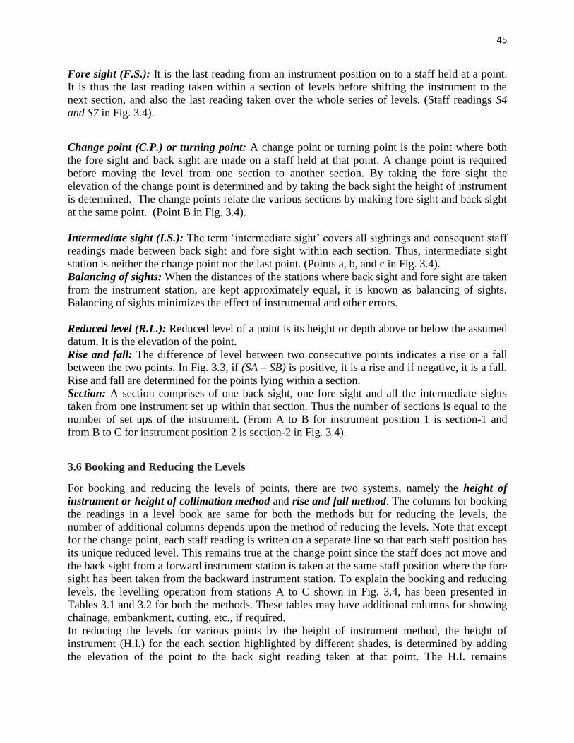
3-1 INTRODUCTION

3-2 LEVELING

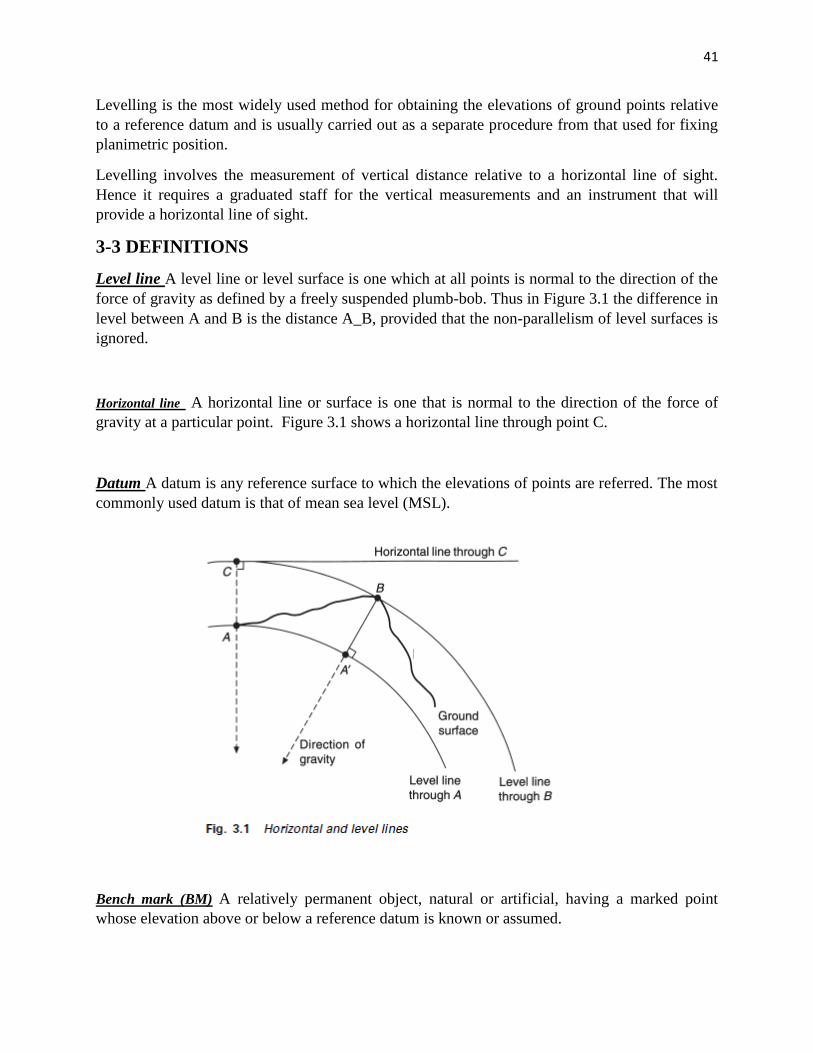
3-3 DEFINITIONS

3-4 CURVATURE AND REFRACTION

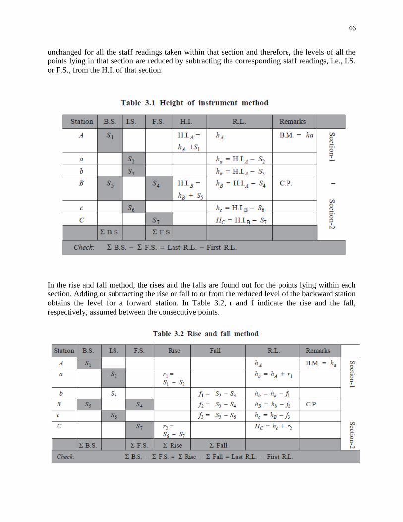
3-5 DIRECT DIFFERENTIAL LEVELLING

3-6 BOOKING AND REDUCING THE LEVELS

3-7 RECIPROCAL LEVELLING

3-8 LOOP CLOSURE AND ITS APPORTIONING

3-9 TWO-PEG TEST

3-10 TRIGONOMETRIC LEVELING

3-11 LEVELLING APPLICATIONS

1- Sectional

4

2- Contouring

3-12 PRECISION IN LEVELING

CHAPTER FOUR DISTANCE MEASUREMENTS USING

TRIGONOMETRIC & EDM

4-1 TACHEOMETRIC OR OPTICAL METHOD 4.2 ELECTRONIC DISTANCE MEASUREMENT

CHAPTER FIVE ANGLES, AZIMUTH, AND BEARING 5-l Introduction

5-2 Kind of horizontal angles

5-3 Direction of line

5-4 Azimuth

5-5 Bearings

5-6 Comparison of azimuth and bearings

5-7 Computing Azimuth

5-8 Computing Bearings

5-9 MAGNETIC DECLINATION

5-10

CHAPTER SIX TRAVERSING 6-1 Introduction

6-2 Balancing angles

6-3 COMPUTATION OF PRELIMINARY

AZIMUTHS OR BEARINGS

6-4 DEPARTURES AND LATITUDES

6-5 DEPARTURES AND LATITUDES CLOSER

CONDITION

6-6 TRAVERSE ADJUSTMENT

6-7 COMPASS (BOWDITCH) RULE

6-8 RECTANGULER COORDINATES

6-9 ALTERNATIVE METHODS FOR MAKING

TRAVERSE COMPUTATIONS

6-10 INVERSING

6-11 COMPUTING FINAL ADJUSTED TRAVERSE

LENGTHS AND DIRECTIONS

5

REFERENCES

1- Elementary Surveying An Introduction to Geomatics by Charles D.

Ghilani & Paul R. Wolf,2016

2- Surveying Dr. A.M.CHANDRA 2005

3- Engineering Surveying six edition W. Schofield and M. Breach2007

هندست انمساحت عباس زيدان خهف )انجامعت انتكنهىجيت( -4

6

Surveying I

Chapter one

Basic Principle of Surveying 1-1 LEARNING OBJECTIVES

At the end of this chapter, students will be able to:

1. Define surveying and other technical terms

2. Describe the importance of surveying

3. Identify and state the different types of surveying

4. Describe different surveying applications

5. State the different types of errors in surveying

1-2 DEFINITION OF SURVEYING

Surveying, which has recently also been interchangeably called geomatics, has traditionally been

defined as the science, art, and technology of determining the relative positions of points

above, on, or beneath the Earth’s surface, or of establishing such points.

In a more general sense, however, surveying (geomatics) can be regarded as that discipline

which covers all methods for measuring and collecting information about the physical earth and

our environment, processing that information, and disseminating a variety of resulting products

to a wide range of clients. Surveying has been important since the beginning of civilization. Its

earliest applications were in measuring and marking boundaries of property ownership.

Throughout the years its importance has steadily increased with the growing demand for a

variety of maps and other spatially related types of information and the expanding need for

establishing accurate line and grade to guide construction operations.

Today the importance of measuring and monitoring our environment is becoming increasingly

critical as our population expands, land values appreciate, our natural resources dwindle, and

human activities continue to stress the quality of our land, water, and air. Using modern ground,

aerial, and satellite technologies, and computers for data processing, contemporary surveyors are

now able to measure and monitor the Earth and its natural resources on literally a global basis.

Never before has so much information been available for assessing current conditions, making

sound planning decisions, and formulating policy in a host of landuse, resource development,

and environmental preservation applications.

A surveyor is a professional person with the academic qualifications and technical expertise to

conduct one, or more, of the following activities;

• To determine, measure and represent the land, three-dimensional objects, point-fields, and

routes;

• To collect and interpret land and geographically related information;

• To use that information for the planning and efficient administration of the land, the sea and

any structures thereon; and

• To conduct research into the above practices and to develop them.

Detailed Functions

7

The surveyor‘s professional tasks may involve one or more of the following activities, which

may occur either on, above, or below the surface of the land or the sea and may be carried out in

association with other professionals.

1. The determination of the size and shape of the earth and the measurements of all data needed

to define the size, position, shape and contour of any part of the earth and monitoring any change

therein.

2. The positioning of objects in space and time as well as the positioning and monitoring of

physical features, structures and engineering works on, above or below the surface of the earth.

3. The development, testing and calibration of sensors, instruments and systems for the above-

mentioned purposes and for other surveying purposes.

4. The acquisition and use of spatial information from close range, aerial and satellite imagery

and the automation of these processes.

5. The determination of the position of the boundaries of public or private land, including

national and international boundaries, and the registration of those lands with the appropriate

authorities.

6. The design, establishment and administration of geographic information systems (GIS) and the

collection, storage, analysis, management, display and dissemination of data.

7. The analysis, interpretation and integration of spatial objects and phenomena in GIS, including

the visualization and communication of such data in maps, models and mobile digital devices.

8. The study of the natural and social environment, the measurement of land and marine

resources and the use of such data in the planning of development in urban, rural and regional

areas.

9. The planning, development and redevelopment of property, whether urban or rural and

whether land or buildings.

10. The assessment of value and the management of property, whether urban or rural and

whether land or buildings.

11. The planning, measurement and management of construction works, including the estimation

of costs.

1-3 GEOMATICS

Geomatics is a relatively new term that is now commonly being applied to encompass the areas

of practice formerly identified as surveying. The name has gained widespread acceptance in the

United States, as well as in other English-speaking countries of the world, especially in Canada,

the United Kingdom, and Australia. Many college and university programs in the United States

that were formerly identified as ―Surveying‖ or ―Surveying Engineering‖ are now called

―Geomatics‖ or ―Geomatics Engineering.‖

The principal reason cited for making the name change is that the manner and scope of practice

in surveying have changed dramatically in recent years. This has occurred in part because of

recent technological developments that have provided surveyors with new tools for measuring

and/or collecting information, for computing, and for displaying and disseminating information.

It has also been driven by increasing concerns about the environment locally, regionally, and

globally, which have greatly exacerbated efforts in monitoring, managing, and regulating the use

of our land, water, air, and other natural resources. These circumstances, and others, have

brought about a vast increase in demands for new spatially related information.

8

1-4 GEODETIC AND PLANE SURVEYS

Two general classifications of surveys are geodetic and plane. They differ principally in the

assumptions on which the computations are based, although field measurements for geodetic

surveys are usually performed to a higher order of accuracy than those for plane surveys.

In geodetic surveying, the curved surface of the Earth is considered by performing the

computations on an ellipsoid (curved surface approximating the size and shape of the Earth). It is

now becoming common to do geodetic computations in a three-dimensional, Earth-centered,

Earth-fixed (ECEF) Cartesian coordinate system. The calculations involve solving equations

derived from solid geometry and calculus. Geodetic methods are employed to determine relative

positions of widely spaced monuments and to compute lengths and directions of the long lines

between them. These monuments serve as the basis for referencing other subordinate surveys of

lesser extents.

Satellite positioning can provide the needed positions with much greater accuracy, speed, and

economy. GNSS receivers enable ground stations to be located precisely by observing distances

to satellites operating in known positions along their orbits. GNSS surveys are being used in all

forms of surveying including geodetic, hydrographic, construction, and boundary surveying.

In plane surveying, except for leveling, the reference base for fieldwork and computations is

assumed to be a flat horizontal surface. The direction of a plumb line (and thus gravity) is

considered parallel throughout the survey region, and all observed angles are presumed to be

plane angles. For areas of limited size, the surface of our vast ellipsoid is actually nearly flat. On

a line 5 mi long, the ellipsoid arc and chord lengths differ by only about 0.02 ft. A plane surface

tangent to the ellipsoid departs only about 0.7 ft at 1 mi from the point of tangency. In a triangle

having an area of 75 square miles, the difference between the sum of the three ellipsoidal angles

and three plane angles is only about 1 sec. Therefore, it is evident that except in surveys covering

extensive areas, the Earth‘s surface can be approximated as a plane, thus simplifying

computations and techniques. In general, algebra, plane and analytical geometry, and plane

trigonometry are used in plane-surveying calculations.

1-4 SPECIALIZED TYPES OF SURVEYS Many types of surveys are so specialized that a person proficient in a particular discipline may

have little contact with the other areas. Persons seeking careers in surveying and mapping,

however, should be knowledgeable in every phase, since all are closely related in modern

practice. Some important classifications are described briefly here.

Control surveys establish a network of horizontal and vertical monuments that serve as a

reference framework for initiating other surveys.

Topographic surveys determine locations of natural and artificial features and elevations used

in map making.

Land, boundary, and cadastral surveys establish property lines and property corner markers.

The term cadastral is now generally applied to surveys of the public lands systems.

Hydrographic surveys define shorelines and depths of lakes, streams, oceans, reservoirs, and

other bodies of water. Sea surveying is associated with port and offshore industries and the

9

marine environment, including measurements and marine investigations made by shipborne

personnel.

Alignment surveys are made to plan, design, and construct highways, railroads, pipelines, and

other linear projects. They normally begin at one control point and progress to another in the

most direct manner permitted by field conditions.

Construction surveys provide line, grade, control elevations, horizontal positions, dimensions,

and configurations for construction operations. They also secure essential data for computing

construction pay quantities.

As-built surveys document the precise final locations and layouts of engineering works and

record any design changes that may have been incorporated into the construction. These are

particularly important when underground facilities are constructed, so their locations are

accurately known for maintenance purposes, and so that unexpected damage to them can be

avoided during later installation of other underground utilities.

Mine surveys are performed above and below ground to guide tunneling and other operations

associated with mining. This classification also includes geophysical surveys for mineral and

energy resource exploration.

Solar surveys map property boundaries, solar easements, obstructions according to sun angles,

and meet other requirements of zoning boards and title insurance companies.

Ground, aerial, and satellite surveys are broad classifications sometimes used. Ground surveys

utilize measurements made with ground-based equipment such as automatic levels and total

station instruments. Aerial surveys are accomplished using either photogrammetry or remote

sensing. Photogrammetry uses cameras that are carried usually in airplanes to obtain images,

whereas remote sensing employs cameras and other types of sensors that can be transported in

either aircraft or satellites.

1-5 UNITS AND SIGNIFICANT FIGURES

1-4-1 Introduction

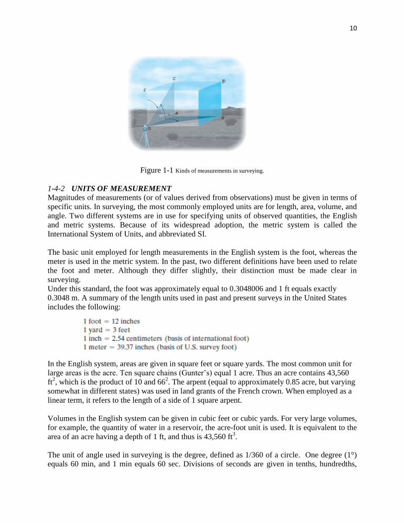
Five types of observations illustrated in Figure 1.1 form the basis of traditional plane surveying:

(1) horizontal angles, (2) horizontal distances, (3) vertical (or zenith) angles, (4) vertical

distances, and (5) slope distances. In the figure, OAB and ECD are horizontal planes, and OACE

and ABDC are vertical planes. Then as illustrated, horizontal angles, such as angle AOB, and

horizontal distances, OA and OB, are measured in horizontal planes; vertical angles, such as

AOC, are measured in vertical planes; zenith angles, such as EOC, are also measured in vertical

planes; vertical lines, such as AC and BD, are measured vertically (in the direction of gravity);

and slope distances, such as OC, are determined along inclined planes. By using combinations of

these basic observations, it is possible to compute relative positions between any points.

10

Figure 1-1 Kinds of measurements in surveying.

1-4-2 UNITS OF MEASUREMENT Magnitudes of measurements (or of values derived from observations) must be given in terms of

specific units. In surveying, the most commonly employed units are for length, area, volume, and

angle. Two different systems are in use for specifying units of observed quantities, the English

and metric systems. Because of its widespread adoption, the metric system is called the

International System of Units, and abbreviated SI.

The basic unit employed for length measurements in the English system is the foot, whereas the

meter is used in the metric system. In the past, two different definitions have been used to relate

the foot and meter. Although they differ slightly, their distinction must be made clear in

surveying.

Under this standard, the foot was approximately equal to 0.3048006 and 1 ft equals exactly

0.3048 m. A summary of the length units used in past and present surveys in the United States

includes the following:

In the English system, areas are given in square feet or square yards. The most common unit for

large areas is the acre. Ten square chains (Gunter‘s) equal 1 acre. Thus an acre contains 43,560

ft2, which is the product of 10 and 66

2. The arpent (equal to approximately 0.85 acre, but varying

somewhat in different states) was used in land grants of the French crown. When employed as a

linear term, it refers to the length of a side of 1 square arpent.

Volumes in the English system can be given in cubic feet or cubic yards. For very large volumes,

for example, the quantity of water in a reservoir, the acre-foot unit is used. It is equivalent to the

area of an acre having a depth of 1 ft, and thus is 43,560 ft3.

The unit of angle used in surveying is the degree, defined as 1/360 of a circle. One degree (1°)

equals 60 min, and 1 min equals 60 sec. Divisions of seconds are given in tenths, hundredths,

11

and thousandths. Other methods are also used to subdivide a circle, for example, 400 grads (with

100 centesimal min/grad and 100 centesimal sec/min. Another term, gons, is now used

interchangeably with grads. The military services use mils to subdivide a circle into 6400 units.

A radian is the angle subtended by an arc of a circle having a length equal to the radius of the

circle. Therefore, 2ח rad = 360° , 1 rad =57°17ʹ 44.8″=57.2958° and 0.01745 rad = 1° .

As noted previously, the meter is the basic unit for length in the metric or SI system.

Subdivisions of the meter (m) are the millimeter (mm), centimeter (cm), and decimeter (dm),

equal to 0.001, 0.01, and 0.1 m, respectively. A kilometer (km) equals 1000 m, which is

approximately five eighths of a mile. Areas in the metric system are specified using the square

meter (m2). Large area s, for example, tracts of land, are given in hectares (ha), where one

hectare is equivalent to a square having sides of 100 m. Thus, there are 10,000 m2, or about

2.471 acres per hectare. The cubic meter (m3) is used for volumes in the SI system. Degrees,

minutes, and seconds, or the radian, are accepted SI units for angles.

1-4-3 SIGNIFICANT FIGURES

In recording observations, an indication of the accuracy attained is the number of digits

(significant figures) recorded. By definition, the number of significant figures in any observed

value includes the positive (certain) digits plus one (only one) digit that is estimated or rounded

off, and therefore questionable. For example, a distance measured with a tape whose smallest

graduation is 0.01 ft, and recorded as 73.52 ft, is said to have four significant figures; in this case

the first three digits are certain, and the last is rounded off and therefore questionable but still

significant.

The number of significant figures is often confused with the number of decimal places. Decimal

places may have to be used to maintain the correct number of significant figures, but in

themselves they do not indicate significant figures. Some examples follow:

Two significant figures: 24, 2.4, 0.24, 0.0024, 0.020

Three significant figures: 364, 36.4, 0.000364, 0.0240

Four significant figures: 7621, 76.21, 0.0007621, 24.00.

Zeros at the end of an integer value may cause difficulty because they may or may not be

significant. In a value expressed as 2400, for example, it is not known how many figures are

significant; there may be two, three, or four, and therefore definite rules must be followed to

eliminate the ambiguity. The preferred method of eliminating this uncertainty is to express the

value in terms of powers of 10.

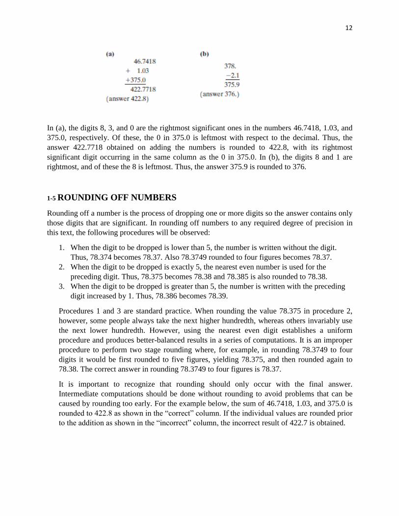
When observed values are used in the mathematical processes of addition, subtraction,

multiplication, and division, it is imperative that the number of significant figures given in

answers be consistent with the number of significant figures in the data used. The following three

steps will achieve this for addition or subtraction: (1) identify the column containing the

rightmost significant digit in each number being added or subtracted, (2) perform the addition or

subtraction, and (3) round the answer so that its rightmost significant digit occurs in the leftmost

column identified in step (1). Two examples illustrate the procedure:

12

In (a), the digits 8, 3, and 0 are the rightmost significant ones in the numbers 46.7418, 1.03, and

375.0, respectively. Of these, the 0 in 375.0 is leftmost with respect to the decimal. Thus, the

answer 422.7718 obtained on adding the numbers is rounded to 422.8, with its rightmost

significant digit occurring in the same column as the 0 in 375.0. In (b), the digits 8 and 1 are

rightmost, and of these the 8 is leftmost. Thus, the answer 375.9 is rounded to 376.

1-5 ROUNDING OFF NUMBERS

Rounding off a number is the process of dropping one or more digits so the answer contains only

those digits that are significant. In rounding off numbers to any required degree of precision in

this text, the following procedures will be observed:

1. When the digit to be dropped is lower than 5, the number is written without the digit.

Thus, 78.374 becomes 78.37. Also 78.3749 rounded to four figures becomes 78.37.

2. When the digit to be dropped is exactly 5, the nearest even number is used for the

preceding digit. Thus, 78.375 becomes 78.38 and 78.385 is also rounded to 78.38.

3. When the digit to be dropped is greater than 5, the number is written with the preceding

digit increased by 1. Thus, 78.386 becomes 78.39.

Procedures 1 and 3 are standard practice. When rounding the value 78.375 in procedure 2,

however, some people always take the next higher hundredth, whereas others invariably use

the next lower hundredth. However, using the nearest even digit establishes a uniform

procedure and produces better-balanced results in a series of computations. It is an improper

procedure to perform two stage rounding where, for example, in rounding 78.3749 to four

digits it would be first rounded to five figures, yielding 78.375, and then rounded again to

78.38. The correct answer in rounding 78.3749 to four figures is 78.37.

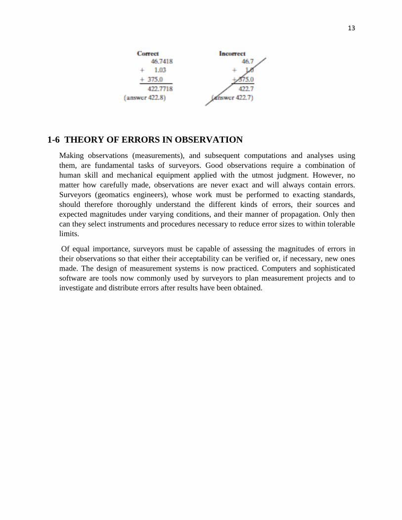
It is important to recognize that rounding should only occur with the final answer.

Intermediate computations should be done without rounding to avoid problems that can be

caused by rounding too early. For the example below, the sum of 46.7418, 1.03, and 375.0 is

rounded to 422.8 as shown in the ―correct‖ column. If the individual values are rounded prior

to the addition as shown in the ―incorrect‖ column, the incorrect result of 422.7 is obtained.

13

1-6 THEORY OF ERRORS IN OBSERVATION

Making observations (measurements), and subsequent computations and analyses using

them, are fundamental tasks of surveyors. Good observations require a combination of

human skill and mechanical equipment applied with the utmost judgment. However, no

matter how carefully made, observations are never exact and will always contain errors.

Surveyors (geomatics engineers), whose work must be performed to exacting standards,

should therefore thoroughly understand the different kinds of errors, their sources and

expected magnitudes under varying conditions, and their manner of propagation. Only then

can they select instruments and procedures necessary to reduce error sizes to within tolerable

limits.

Of equal importance, surveyors must be capable of assessing the magnitudes of errors in

their observations so that either their acceptability can be verified or, if necessary, new ones

made. The design of measurement systems is now practiced. Computers and sophisticated

software are tools now commonly used by surveyors to plan measurement projects and to

investigate and distribute errors after results have been obtained.

14

انمحاضرة

انثانيت

Basic Principle of Surveying

15

1-6 THEORY OF ERRORS IN OBSERVATION

Making observations (measurements), and subsequent computations and analyses using

them, are fundamental tasks of surveyors. Good observations require a combination of

human skill and mechanical equipment applied with the utmost judgment. However, no

matter how carefully made, observations are never exact and will always contain errors.

Surveyors (geomatics engineers), whose work must be performed to exacting standards,

should therefore thoroughly understand the different kinds of errors, their sources and

expected magnitudes under varying conditions, and their manner of propagation. Only then

can they select instruments and procedures necessary to reduce error sizes to within tolerable

limits.

Of equal importance, surveyors must be capable of assessing the magnitudes of errors in

their observations so that either their acceptability can be verified or, if necessary, new ones

made. The design of measurement systems is now practiced. Computers and sophisticated

software are tools now commonly used by surveyors to plan measurement projects and to

investigate and distribute errors after results have been obtained.

1-6- 1 DIRECT AND INDIRECT OBSERVATIONS

Observations may be made directly or indirectly. Examples of direct observations are applying a

tape to a line, fitting a protractor to an angle, or turning an angle with a total station instrument.

An indirect observation is secured when it is not possible to apply a measuring instrument

directly to the quantity to be observed. The answer is therefore determined by its relationship to

some other observed value or values. As an example, we can find the distance across a river by

observing the length of a line on one side of the river and the angle at each end of this line to a

16

point on the other side, and then computing the distance by one of the standard trigonometric

formulas. Many indirect observations are made in surveying, and since all measurements contain

errors, it is inevitable that quantities computed from them will also contain errors. The manner

by which errors in measurements combine to produce erroneous computed answers is called

error propagation.

1-6-2 ERRORS IN MEASUREMENTS

By definition, an error is the difference between an observed value for a quantity and its true

value, or

E = X - X¯

where E is the error in an observation, X the observed value, and X¯ its true value. It can be

unconditionally stated that (1) no observation is exact, (2) every observation contains errors, (3)

the true value of an observation is never known, and, therefore, (4) the exact error present is

always unknown. These facts are demonstrated by the following. When a distance is observed

with a scale divided into tenths of an inch, the distance can be read only to hundredths (by

interpolation). However, if a better scale graduated in hundredths of an inch was available and

read under magnification, the same distance might be estimated to thousandths of an inch. And

with a scale graduated in thousandths of an inch, a reading to ten thousandths might be possible.

Obviously, accuracy of observations depends on the scale‘s division size, reliability of

equipment used, and human limitations in estimating closer than about one tenth of a scale

division. As better equipment is developed, observations more closely approach their true values,

but they can never be exact. Note that observations, not counts (of cars, pennies, marbles, or

other objects), are under consideration here.

1-6-3 MISTAKES

These are observer blunders and are usually caused by misunderstanding the problem,

carelessness, fatigue, missed communication, or poor judgment. Examples include transposition

of numbers, such as recording 73.96 instead of the correct value of 79.36; reading an angle

counterclockwise, but indicating it as a clockwise angle in the field notes; sighting the wrong

target; or recording a measured distance as 682.38 instead of 862.38. Large mistakes such as

these are not considered in the succeeding discussion of errors. They must be detected by careful

and systematic checking of all work, and eliminated by repeating some or all of the

measurements. It is very difficult to detect small mistakes because they merge with errors. When

not exposed, these small mistakes will therefore be incorrectly treated as errors.

1-6-4 SOURCES OF ERRORS IN MAKING OBSERVATIONS

Errors in observations stem from three sources, and are classified accordingly.

Natural errors are caused by variations in wind, temperature, humidity, atmospheric pressure,

atmospheric refraction, gravity, and magnetic declination. An example is a steel tape whose

length varies with changes in temperature.

17

Instrumental errors result from any imperfection in the construction or adjustment of

instruments and from the movement of individual parts. For example, the graduations on a scale

may not be perfectly spaced, or the scale may be warped. The effect of many instrumental errors

can be reduced, or even eliminated, by adopting proper surveying procedures or applying

computed corrections.

Personal errors arise principally from limitations of the human senses of sight and touch. As an

example, a small error occurs in the observed value of a horizontal angle if the vertical crosshair

in a total station instrument is not aligned perfectly on the target, or if the target is the top of a

rod that is being held slightly out of plumb.

1-6-5 TYPES OF ERRORS

Errors in observations are of two types: systematic and random.

Systematic errors, also known as biases, result from factors that comprise the ―measuring

system‖ and include the environment, instrument, and observer. So long as system conditions

remain constant, the systematic errors will likewise remain constant. If conditions change, the

magnitudes of systematic errors also change. Because systematic errors tend to accumulate, they

are sometimes called cumulative errors.

Conditions producing systematic errors conform to physical laws that can be modeled

mathematically. Thus, if the conditions are known to exist and can be observed, a correction can

be computed and applied to observed values. An example of a constant systematic error is the

use of a 100-ft steel tape that has been calibrated and found to be 0.02 ft too long. It introduces a

0.02-ft error each time it is used, but applying a correction readily eliminates the error. An

example of variable systematic error is the change in length of a steel tape resulting from

temperature differentials that occur during the period of the tape‘s use. If the temperature

changes are observed, length corrections can be computed by a simple formula.

Random errors are those that remain in measured values after mistakes and systematic errors

have been eliminated. They are caused by factors beyond the control of the observer, obey the

laws of probability, and are sometimes called accidental errors. They are present in all surveying

observations.

The magnitudes and algebraic signs of random errors are matters of chance. There is no absolute

way to compute or eliminate them, but they can be estimated using adjustment procedures

known as least squares. Random errors are also known as compensating errors, since they tend to

partially cancel themselves in a series of observations. For example, a person interpolating to

hundredths of a foot on a tape graduated only to tenths, or reading a level rod marked in

hundredths, will presumably estimate too high on some values and too low on others. However,

individual personal characteristics may nullify such partial compensation since some people are

inclined to interpolate high, others interpolate low, and many favor certain digits—for example,

7 instead of 6 or 8, 3 instead of 2 or 4, and particularly 0 instead of 9 or 1.

18

1-6-6 PRECISION AND ACCURACY

A discrepancy is the difference between two observed values of the same quantity. A small

discrepancy indicates there are probably no mistakes and random errors are small. However,

small discrepancies do not preclude the presence of systematic errors.

Precision refers to the degree of refinement or consistency of a group of observations and is

evaluated on the basis of discrepancy size. If multiple observations are made of the same

quantity and small discrepancies result, this indicates high precision. The degree of precision

attainable is dependent on equipment sensitivity and observer skill.

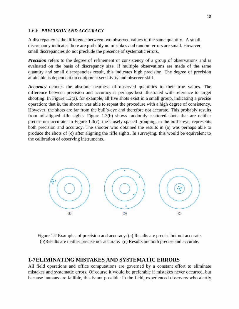
Accuracy denotes the absolute nearness of observed quantities to their true values. The

difference between precision and accuracy is perhaps best illustrated with reference to target

shooting. In Figure 1.2(a), for example, all five shots exist in a small group, indicating a precise

operation; that is, the shooter was able to repeat the procedure with a high degree of consistency.

However, the shots are far from the bull‘s-eye and therefore not accurate. This probably results

from misaligned rifle sights. Figure 1.3(b) shows randomly scattered shots that are neither

precise nor accurate. In Figure 1.3(c), the closely spaced grouping, in the bull‘s-eye, represents

both precision and accuracy. The shooter who obtained the results in (a) was perhaps able to

produce the shots of (c) after aligning the rifle sights. In surveying, this would be equivalent to

the calibration of observing instruments.

Figure 1.2 Examples of precision and accuracy. (a) Results are precise but not accurate.

(b)Results are neither precise nor accurate. (c) Results are both precise and accurate.

1-7 ELIMINATING MISTAKES AND SYSTEMATIC ERRORS

All field operations and office computations are governed by a constant effort to eliminate

mistakes and systematic errors. Of course it would be preferable if mistakes never occurred, but

because humans are fallible, this is not possible. In the field, experienced observers who alertly

19

perform their observations using standardized repetitive procedures can minimize mistakes.

Mistakes that do occur can be corrected only if discovered. Comparing several observations of

the same quantity is one of the best ways to identify mistakes. Making a common sense estimate

and analysis is another. Assume that five observations of a line are recorded as follows: 567.91,

576.95, 567.88, 567.90, and 567.93. The second value disagrees with the others, apparently

because of a transposition of figures in reading or recording. Either casting out the doubtful

value, or preferably repeating the observation can eradicate this mistake. When a mistake is

detected, it is usually best to repeat the observation.

However, if a sufficient number of other observations of the quantity are available and in

agreement, as in the foregoing example, the widely divergent result may be discarded. Serious

consideration must be given to the effect on an average before discarding a value. It is seldom

safe to change a recorded number, even though there appears to be a simple transposition in

figures. Tampering with physical data is always a bad practice and will certainly cause trouble,

even if done infrequently.

1-8 MOST PROBABLE VALUE

It has been stated earlier that in physical observations, the true value of any quantity is never

known. However, its most probable value can be calculated if redundant observations have been

made. Redundant observations are measurements in excess of the minimum needed to determine

a quantity. For a single unknown, such as a line length that has been directly and independently

observed a number of times using the same equipment and procedures, the first observation

establishes a value for the quantity and all additional observations are redundant. The most

probable value in this case is simply the arithmetic mean, or

Where M¯ is the most probable value of the quantity, the sum of the individual measurements M,

and n the total number of observations. The above equation can be derived using the principle of

least squares, which is based on the theory of probability.

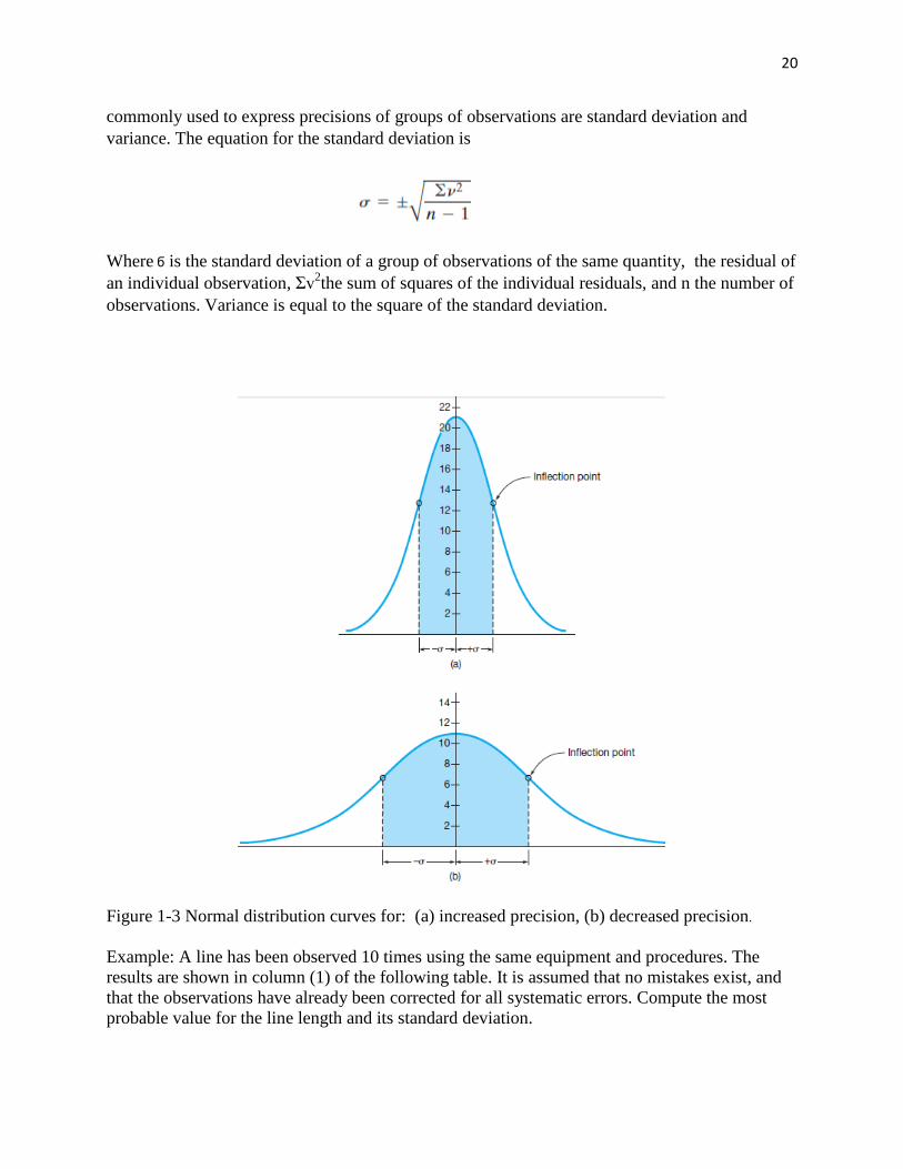
1-9 MEASURES OF PRECISION As shown in Figures 3.3 and 3.4, although the curves have similar shapes, there are significant

differences in their dispersions; that is, their abscissa widths differ. The magnitude of dispersion

is an indication of the relative precisions of the observations. Other statistical terms more

20

commonly used to express precisions of groups of observations are standard deviation and

variance. The equation for the standard deviation is

Where ϭ is the standard deviation of a group of observations of the same quantity, the residual of

an individual observation, Σv2the sum of squares of the individual residuals, and n the number of

observations. Variance is equal to the square of the standard deviation.

Figure 1-3 Normal distribution curves for: (a) increased precision, (b) decreased precision.

Example: A line has been observed 10 times using the same equipment and procedures. The

results are shown in column (1) of the following table. It is assumed that no mistakes exist, and

that the observations have already been corrected for all systematic errors. Compute the most

probable value for the line length and its standard deviation.

21

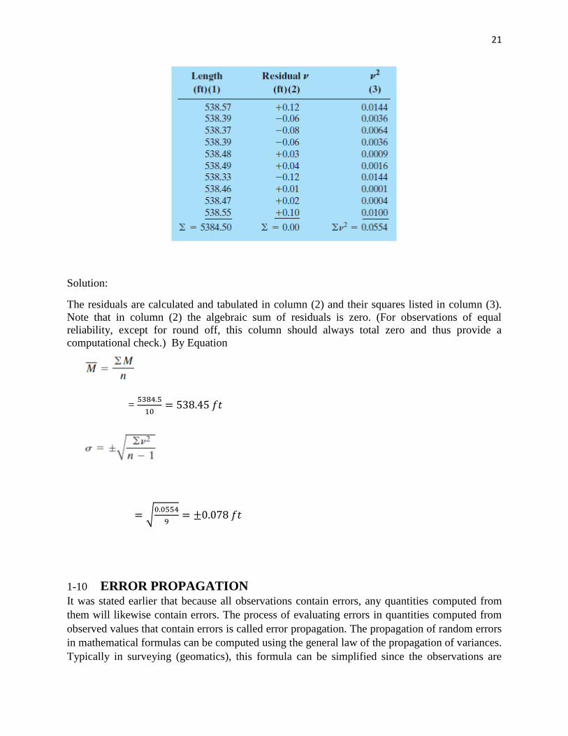
Solution:

The residuals are calculated and tabulated in column (2) and their squares listed in column (3).

Note that in column (2) the algebraic sum of residuals is zero. (For observations of equal

reliability, except for round off, this column should always total zero and thus provide a

computational check.) By Equation

=

√

1-10 ERROR PROPAGATION

It was stated earlier that because all observations contain errors, any quantities computed from

them will likewise contain errors. The process of evaluating errors in quantities computed from

observed values that contain errors is called error propagation. The propagation of random errors

in mathematical formulas can be computed using the general law of the propagation of variances.

Typically in surveying (geomatics), this formula can be simplified since the observations are

22

usually mathematically independent. For example, let a, b, c, --- ,n be observed values containing

errors Ea, Eb, Ec, -- , En respectively. Also let Z be a quantity derived by computation using these

observed quantities in a function f, such that

Then assuming that a, b, c, --- ,n are independent observations, the error in the computed quantity

Z is

where the terms are the partial derivatives of the

function f with respect to the variables a, b, c, --- ,n. In the subsections that follow, specific

cases of error propagation common in surveying are discussed, and examples are presented.

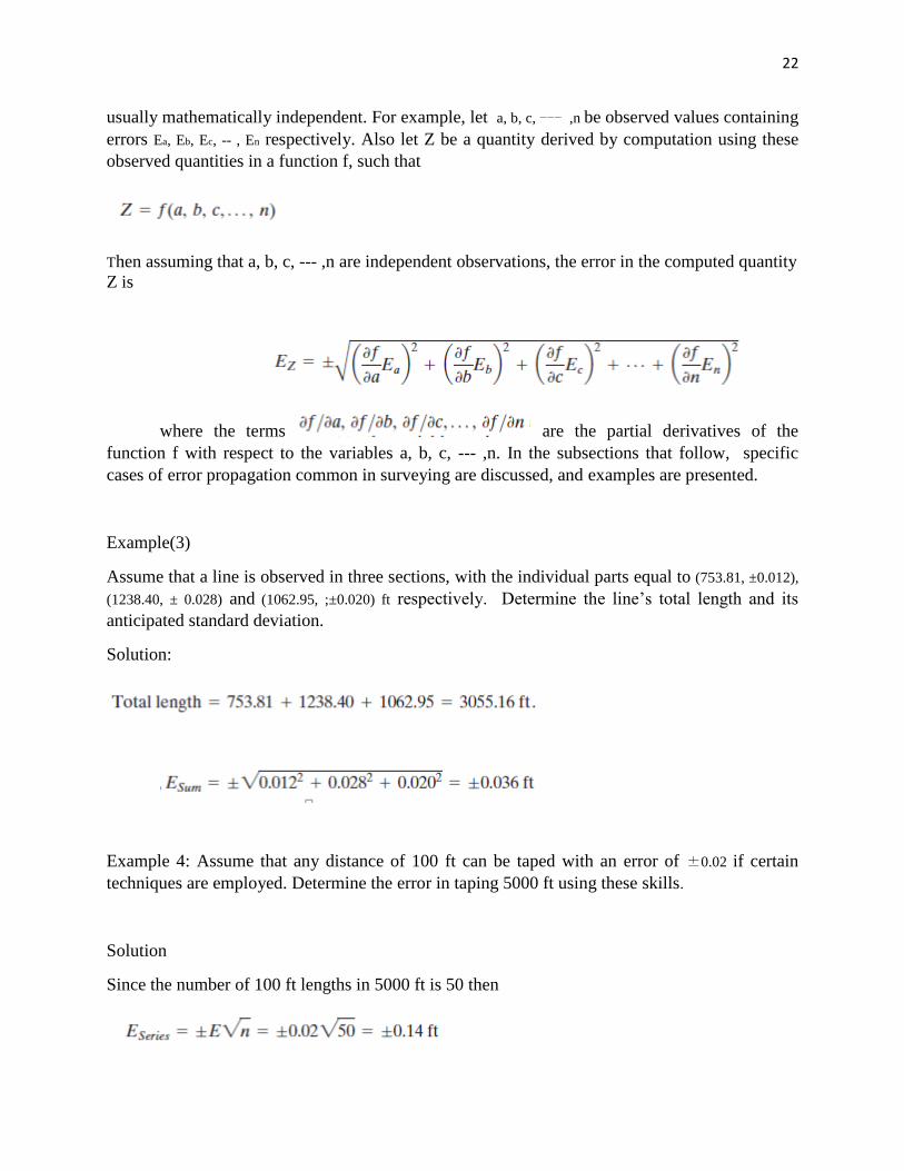
Example(3)

Assume that a line is observed in three sections, with the individual parts equal to (753.81, ±0.012),

(1238.40, ± 0.028) and (1062.95, ;±0.020) ft respectively. Determine the line‘s total length and its

anticipated standard deviation.

Solution:

Example 4: Assume that any distance of 100 ft can be taped with an error of ±0.02 if certain

techniques are employed. Determine the error in taping 5000 ft using these skills.

Solution

Since the number of 100 ft lengths in 5000 ft is 50 then

23

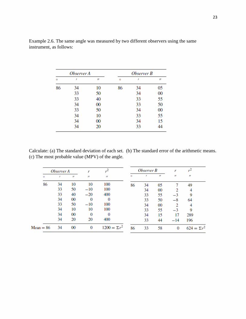
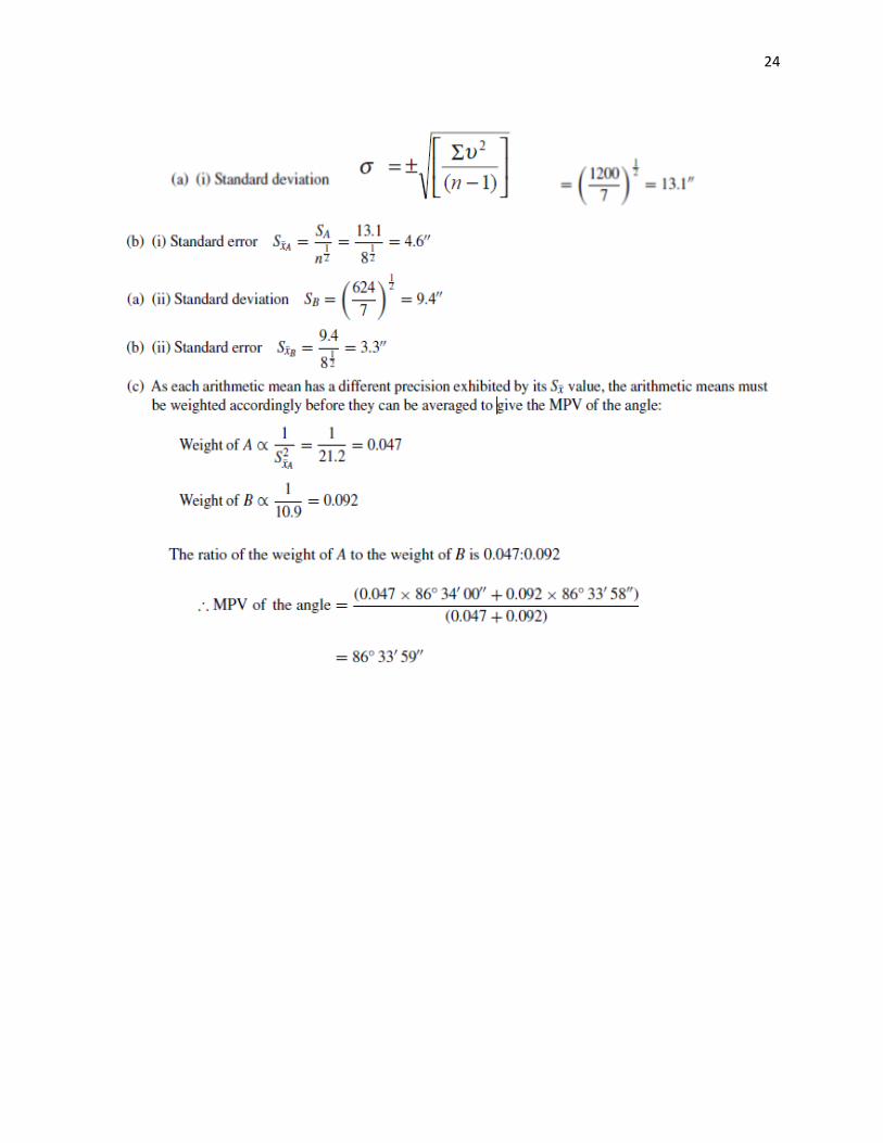
Example 2.6. The same angle was measured by two different observers using the same

instrument, as follows:

Calculate: (a) The standard deviation of each set. (b) The standard error of the arithmetic means.

(c) The most probable value (MPV) of the angle.

24

25

H.W

1- An angle is observed repeatedly using the same equipment and procedures. Calculate (a) the

angle‘s most probable value, (b) the standard deviation, and (c) the standard deviation of the

mean.

23°30ʹ 00″, 23°29 ʹ 40″, 23°30 ʹ 15″ and, 23°29 ʹ 50″.

2- A distance AB is observed repeatedly using the same equipment and procedures, and the

results, in meters, are listed in Problems 3.6 through 3.10. Calculate (a) the line‘s most probable

length, (b) the standard deviation, and (c) the standard deviation of the mean for each set of

results.

65.401, 65.400, 65.402, 65.396, 65.406, 65.401, 65.396, 65.401, 65.405, and 65.404

3- Convert the following distances given in meters to U.S. survey feet: (a) 4129.574 m (b)

738.296 m (c) 6048.083 m.

4- Convert the following distances given in feet to meters: (a) 537.52 ft (b) 9364.87 ft (c)

4806.98 ft

5- Compute the area in acres of triangular lots shown on a plat having the following

recorded right-angle sides: (a) 208.94 ft and 232.65 ft.

26

المحاضرة

الثالثة

DSTANCE MEASUREMENTS

27

Chapter two

DSTANCE MEASUREMENTS

LEARNING OBJECTIVES

At the end of this chapter, the student will be able to:

1. Measure horizontal distance

2. Identify and use different measurements

3. Identify equipment's of horizontal measurement.

4. Identify the sources of errors and corrective actions.

Three methods of distance measurement are:

1-Direct method using a tape or wire

2-Tacheometric method or optical method

3- EDM (Electromagnetic Distance Measuring equipment) method.

2.1 DIRECT METHOD USING TAPE

In this method, steel tapes or wires are used to measure distance very accurately. Nowadays,

EDM is being used exclusively for accurate measurements but the steel tape still is of value for

measuring limited lengths for setting out purposes.

2-2 CORRECTION FOR TAPE MEASUREMENTS

Tape measurements require certain corrections to be applied to the measured distance depending

upon the conditions under which the measurements have been made. These corrections are

discussed below.

2.2.1 Correction for Absolute Length Due to manufacturing defects the absolute length of the tape may be different from its designated

or nominal length. Also with use the tape may stretch causing change in the length and it is

imperative that the tape is regularly checked under standard conditions to determine its absolute

length. The correction for absolute length or standardization is given by

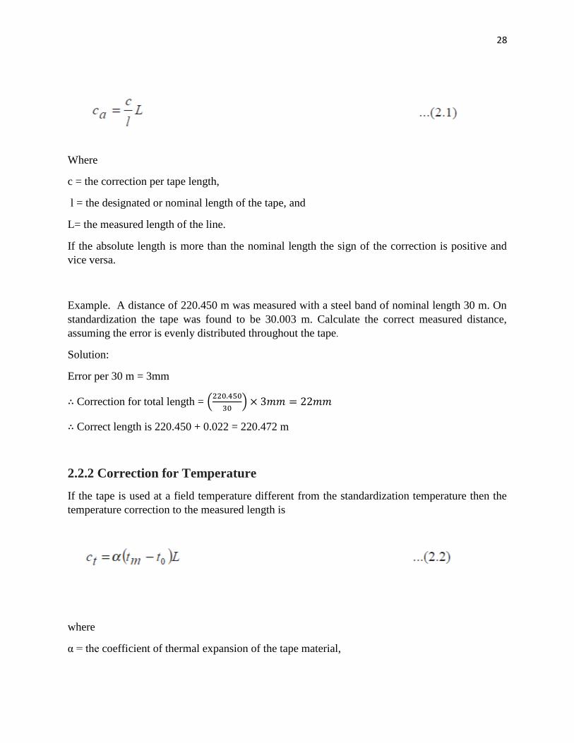
28

Where

c = the correction per tape length,

l = the designated or nominal length of the tape, and

L= the measured length of the line.

If the absolute length is more than the nominal length the sign of the correction is positive and

vice versa.

Example. A distance of 220.450 m was measured with a steel band of nominal length 30 m. On

standardization the tape was found to be 30.003 m. Calculate the correct measured distance,

assuming the error is evenly distributed throughout the tape.

Solution:

Error per 30 m = 3mm

∴ Correction for total length = (

)

∴ Correct length is 220.450 + 0.022 = 220.472 m

2.2.2 Correction for Temperature

If the tape is used at a field temperature different from the standardization temperature then the

temperature correction to the measured length is

where

α = the coefficient of thermal expansion of the tape material,

29

tm = the mean field temperature, and

t0 = the standardization temperature.

The sign of the correction takes the sign of (tm- t0 ).

2.1.3 Correction for Pull or Tension

If the pull applied to the tape in the field is different from the standardization pull, the pull

correction is to be applied to the measured length. This correction is

where

P = the pull applied during the measurement,

P0 = the standardization pull,

A = the area of cross-section of the tape, and

E = the Young‘s modulus for the tape material.

The sign of the correction is same as that of (P – P0).

2.2.4 Correction for Sag

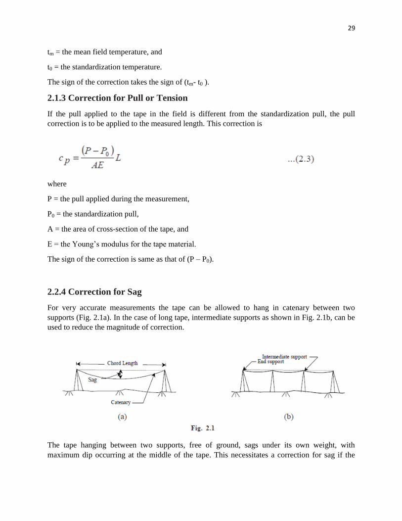
For very accurate measurements the tape can be allowed to hang in catenary between two

supports (Fig. 2.1a). In the case of long tape, intermediate supports as shown in Fig. 2.1b, can be

used to reduce the magnitude of correction.

The tape hanging between two supports, free of ground, sags under its own weight, with

maximum dip occurring at the middle of the tape. This necessitates a correction for sag if the

30

tape has been standardized on the flat, to reduce the curved length to the chord length. The

correction for the sag is

where

W = the weight of the tape per span length.

The sign of this correction is always negative.

If both the ends of the tape are not at the same level, a further correction due to slope is required.

It is given by

where

α = the angle of slope between the end supports.

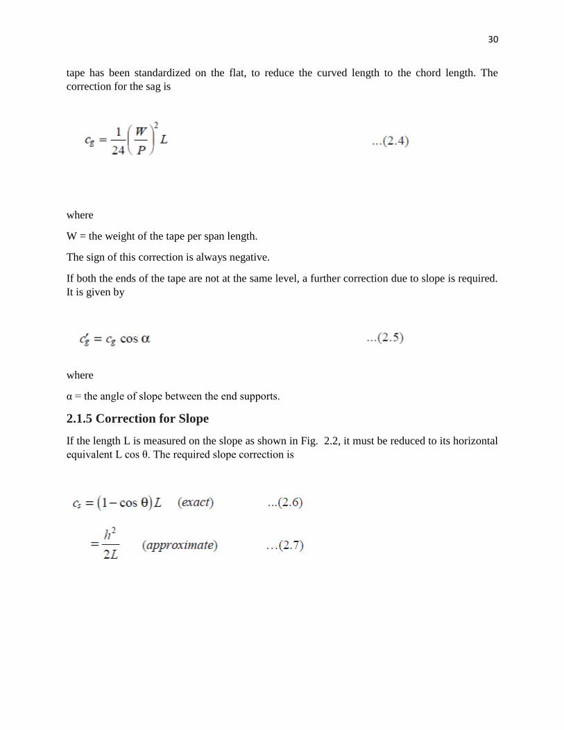
2.1.5 Correction for Slope

If the length L is measured on the slope as shown in Fig. 2.2, it must be reduced to its horizontal

equivalent L cos θ. The required slope correction is

31

where

θ = the angle of the slope, and

h = the difference in elevation of the ends of the tape.

The sign of this correction is always negative.

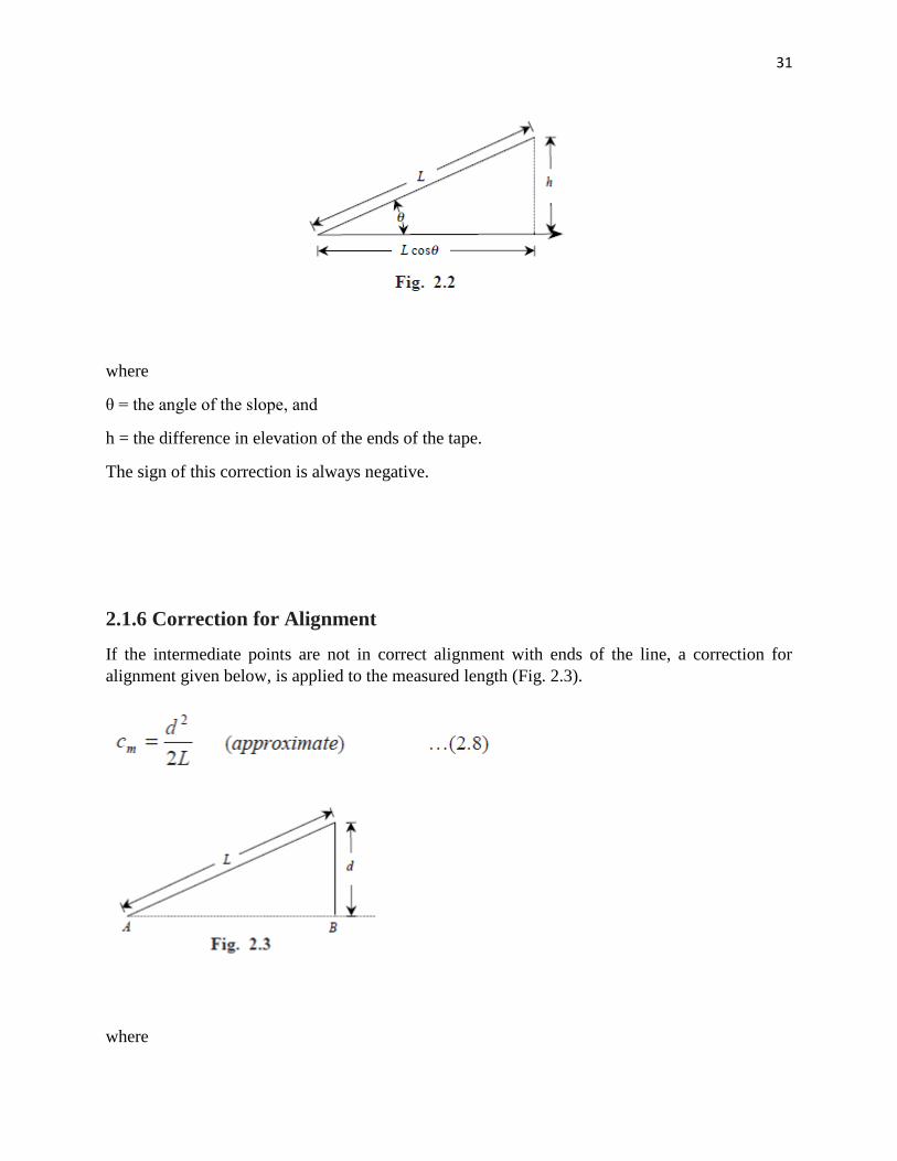
2.1.6 Correction for Alignment

If the intermediate points are not in correct alignment with ends of the line, a correction for

alignment given below, is applied to the measured length (Fig. 2.3).

where

32

d = the distance by which the other end of the tape is out of alignment.

The correction for alignment is always negative.

Example 2.2. A line AB between the stations A and B was measured as 348.28 using a 20 m

tape, too short by 0.05 m. Determine the correct length of AB, the reduced horizontal length of

AB if AB lay on a slope of 1 in 25, and the reading required to produce a horizontal distance of

22.86 m between two pegs, one being 0.56 m above the other.

Solution:

(a) Since the tape is too short by 0.05 m, actual length of AB will be less than the measured

length. The correction required to the measured length is

It is given that

c = 0.05 m; l = 20 m L = 348.28 m

The correct length of the line

= 348.28 – 0.87 = 347.41 m

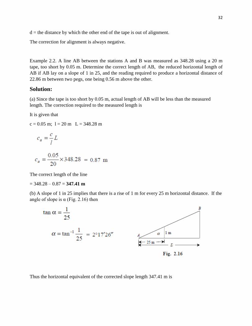
(b) A slope of 1 in 25 implies that there is a rise of 1 m for every 25 m horizontal distance. If the

angle of slope is α (Fig. 2.16) then

Thus the horizontal equivalent of the corrected slope length 347.41 m is

33

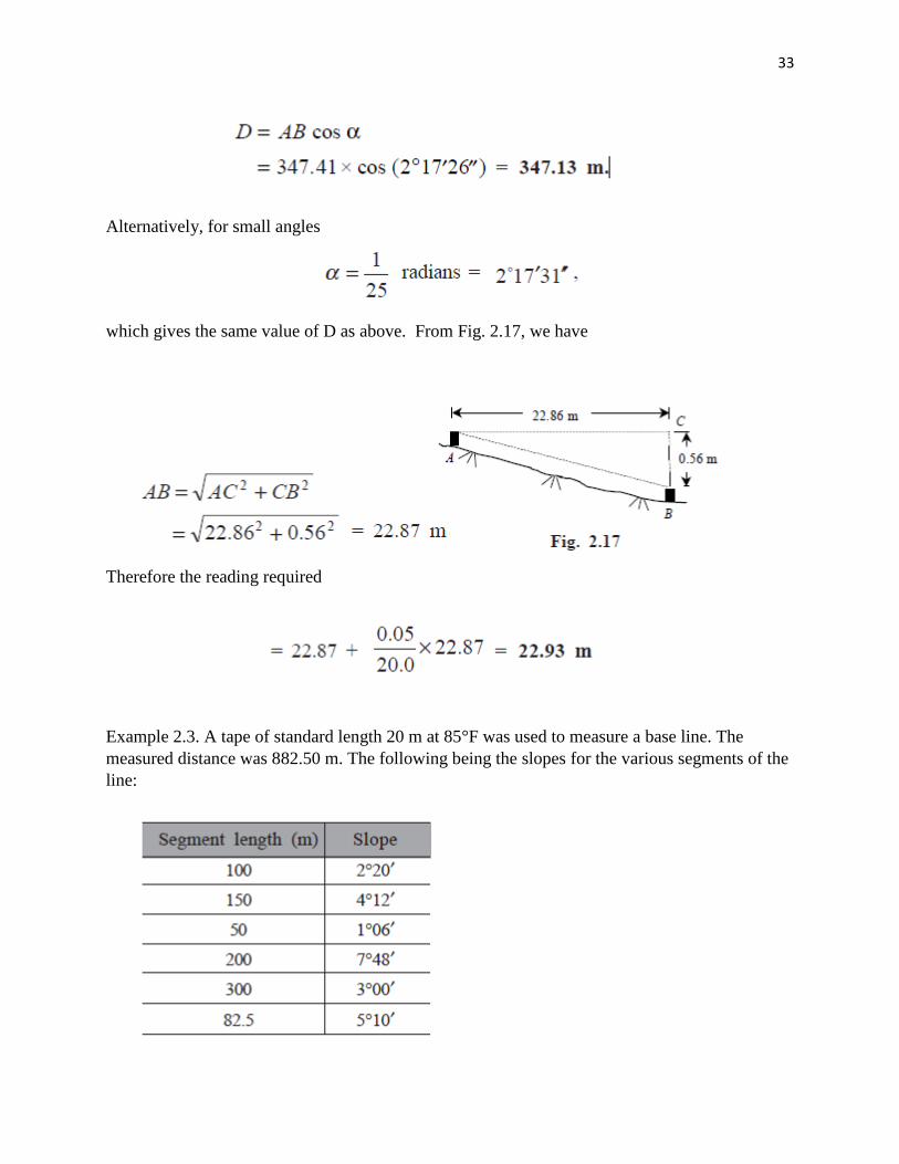
Alternatively, for small angles

which gives the same value of D as above. From Fig. 2.17, we have

Therefore the reading required

Example 2.3. A tape of standard length 20 m at 85°F was used to measure a base line. The

measured distance was 882.50 m. The following being the slopes for the various segments of the

line:

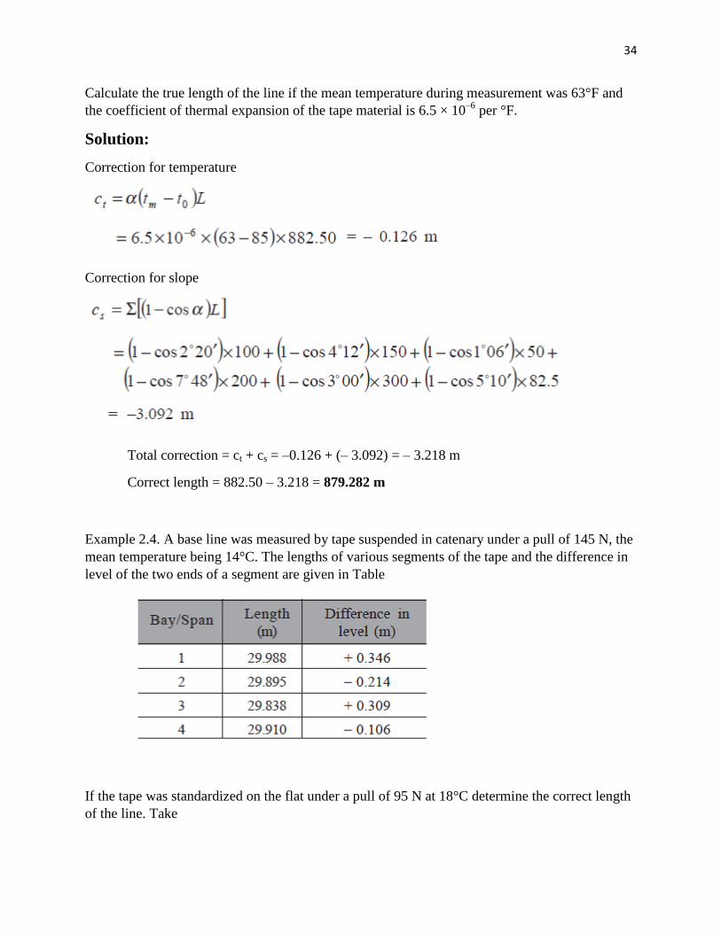
34

Calculate the true length of the line if the mean temperature during measurement was 63°F and

the coefficient of thermal expansion of the tape material is 6.5 × 10–6

per °F.

Solution:

Correction for temperature

Correction for slope

Total correction = ct + cs = –0.126 + (– 3.092) = – 3.218 m

Correct length = 882.50 – 3.218 = 879.282 m

Example 2.4. A base line was measured by tape suspended in catenary under a pull of 145 N, the

mean temperature being 14°C. The lengths of various segments of the tape and the difference in

level of the two ends of a segment are given in Table

If the tape was standardized on the flat under a pull of 95 N at 18°C determine the correct length

of the line. Take

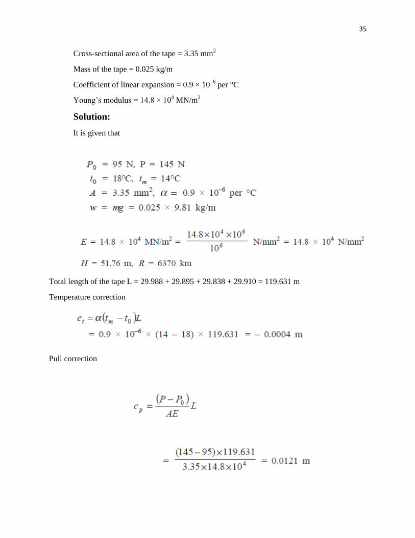
35

Cross-sectional area of the tape = 3.35 mm2

Mass of the tape = 0.025 kg/m

Coefficient of linear expansion = 0.9 × 10–6

per °C

Young‘s modulus = 14.8 × 104 MN/m

2

Solution:

It is given that

Total length of the tape L = 29.988 + 29.895 + 29.838 + 29.910 = 119.631 m

Temperature correction

Pull correction

36

Sag correction

Slope correction

= - 0.0056

Correct length = 119.631 – 0.0056 = 119.6254 m

EXAMPLE 2-5

37

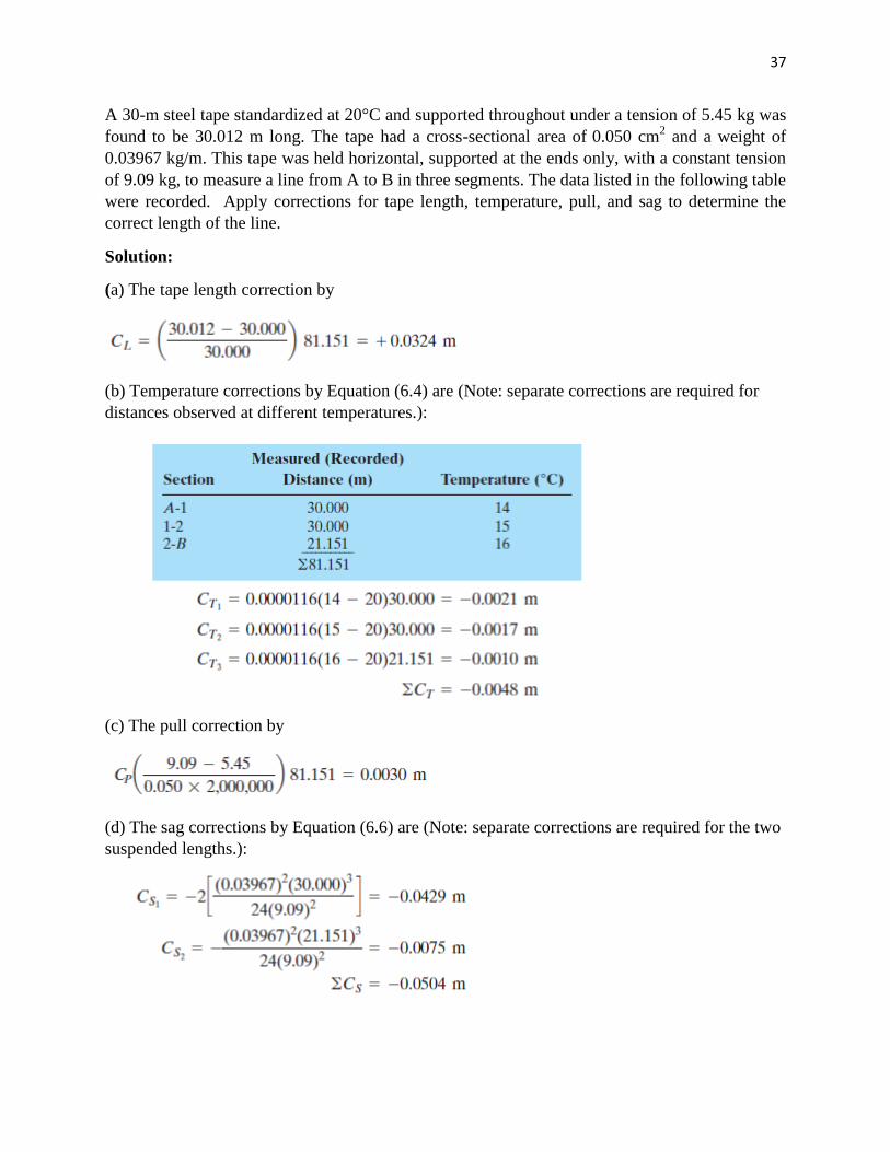
A 30-m steel tape standardized at 20°C and supported throughout under a tension of 5.45 kg was

found to be 30.012 m long. The tape had a cross-sectional area of 0.050 cm2 and a weight of

0.03967 kg/m. This tape was held horizontal, supported at the ends only, with a constant tension

of 9.09 kg, to measure a line from A to B in three segments. The data listed in the following table

were recorded. Apply corrections for tape length, temperature, pull, and sag to determine the

correct length of the line.

Solution:

(a) The tape length correction by

(b) Temperature corrections by Equation (6.4) are (Note: separate corrections are required for

distances observed at different temperatures.):

(c) The pull correction by

(d) The sag corrections by Equation (6.6) are (Note: separate corrections are required for the two

suspended lengths.):

38

(e) Finally, corrected distance AB is obtained by adding all corrections to the measured distance,

or

AB = 81.151 + 0.0324 - 0.0048 + 0.0030 - 0.0504 = 81.131 m

H.w

1) A 100-ft steel tape standardized at 68°F and supported throughout under a tension of 20 lb

was found to be 100.012 ft long. The tape had a cross-sectional area of0.0078 in.2 and a weight

of 0.0266 lb/ft. This tape is used to lay off a horizontal distance CD of exactly 175.00 ft. The

ground is on a smooth 3% grade, thus the tape will be used fully supported. Determine the

correct slope distance to layoff if a pull of 15 lb is used and the temperature is 87°F.

2) A tape of 30 m length suspended in catenary measured the length of a base line. After

applying all corrections the deduced length of the base line was 1462.36 m. Later on it was found

that the actual pull applied was 155 N and not the 165 N as recorded in the field book. Correct

the deduced length for the incorrect pull. The tape was standardized on the flat under a pull of 85

N having a mass of 0.024 kg/m and cross-sectional area of 4.12 mm2. The Young‘s modulus of

the tape material is 152000 MN/ m2 and the acceleration due to gravity is 9.806 m/s

2.

39

المحاضرة

الرابعة

LEVELING—THEORY AND METHODS

40

Chapter Three

LEVELING—THEORY AND METHODS

LEARNING OBJECTIVES

At the end of this chapter, the students will be able to:

1. Define and describe different types of leveling.

2. Understand the principles of leveling and measure vertical distances

3. Apply the skills of leveling

4. Identify measurement errors and take corrective

3.1 .INTRODUCTION This chapter describes the various heighting procedures used to obtain the elevation of points of

interest above or below a reference datum. The most commonly used reference datum is mean

sea level (MSL). There is no such thing as a common global MSL, as it varies from place to

place depending on local conditions. It is important therefore that MSL is clearly defined

wherever it is used.

The engineer is, in the main, more concerned with the relative height of one point above or

below another, in order to ascertain the difference in height of the two points, rather than a direct

relationship to MSL. It is not unusual, therefore, on small local schemes, to adopt a purely

arbitrary reference datum. This could take the form of a permanent, stable position or mark,

allocated such a value that the level of any point on the site would not be negative. For example,

if the reference mark was allocated a value of 0.000 m, then a ground point 10 m lower would

have a negative value, minus 10.000 m. However, if the reference value was 100.000 m, then the

level of the ground point in question would be 90.000 m. As minus signs in front of a number

can be misinterpreted, erased or simply forgotten about, they should, wherever possible, be

avoided.

The vertical height of a point above or below a reference datum is referred to as the reduced level

or simply the level of a point. Reduced levels are used in practically all aspects of construction:

to produce ground contours on a plan; to enable the optimum design of road, railway or canal

gradients; to facilitate ground modelling for accurate volumetric calculations. Indeed, there is

scarcely any aspect of construction that is not dependent on the relative levels of ground points.

3.2 LEVELLING

41

Levelling is the most widely used method for obtaining the elevations of ground points relative

to a reference datum and is usually carried out as a separate procedure from that used for fixing

planimetric position.

Levelling involves the measurement of vertical distance relative to a horizontal line of sight.

Hence it requires a graduated staff for the vertical measurements and an instrument that will

provide a horizontal line of sight.

3-3 DEFINITIONS

Level line A level line or level surface is one which at all points is normal to the direction of the

force of gravity as defined by a freely suspended plumb-bob. Thus in Figure 3.1 the difference in

level between A and B is the distance A_B, provided that the non-parallelism of level surfaces is

ignored.

Horizontal line A horizontal line or surface is one that is normal to the direction of the force of

gravity at a particular point. Figure 3.1 shows a horizontal line through point C.

Datum A datum is any reference surface to which the elevations of points are referred. The most

commonly used datum is that of mean sea level (MSL).

Bench mark (BM) A relatively permanent object, natural or artificial, having a marked point

whose elevation above or below a reference datum is known or assumed.

42

Mean sea level (MSL). The average height for the surface of the seas for all stages of tide over a

19-year period.

Vertical datum Any level surface to which elevations are referenced. This is the surface that is

arbitrarily assigned an elevation of zero. This level surface is also known as a reference datum

since points using this datum have heights relative to this surface.

Elevation. The distance measured along a vertical line from a vertical datum to a point or object.

If the elevation of point A is 802.46 ft, A is 802.46 ft above the reference datum. The elevation

of a point is also called its height above the datum.

Geoid. A particular level surface that serves as a datum for all elevations and astronomical

observations.

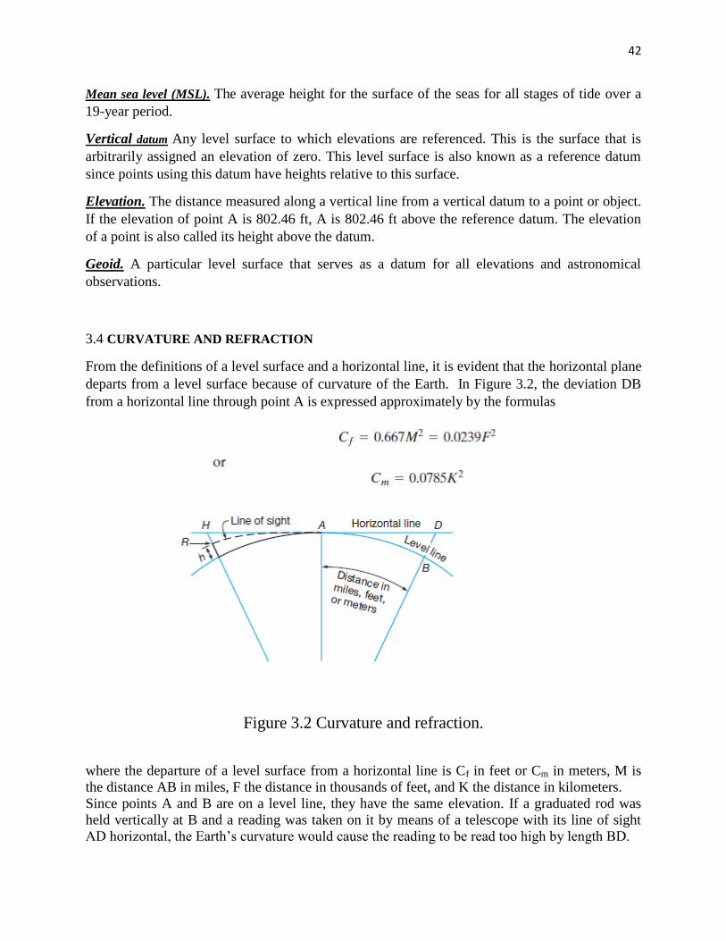
3.4 CURVATURE AND REFRACTION

From the definitions of a level surface and a horizontal line, it is evident that the horizontal plane

departs from a level surface because of curvature of the Earth. In Figure 3.2, the deviation DB

from a horizontal line through point A is expressed approximately by the formulas

Figure 3.2 Curvature and refraction.

where the departure of a level surface from a horizontal line is Cf in feet or Cm in meters, M is

the distance AB in miles, F the distance in thousands of feet, and K the distance in kilometers.

Since points A and B are on a level line, they have the same elevation. If a graduated rod was

held vertically at B and a reading was taken on it by means of a telescope with its line of sight

AD horizontal, the Earth‘s curvature would cause the reading to be read too high by length BD.

43

Light rays passing through the Earth‘s atmosphere are bent or refracted toward the Earth‘s

surface. Thus a theoretically horizontal line of sight, like AH in Figure 3.2, is bent to the curved

form AR. Hence, the reading on a rod held at R is diminished by length RH.

The effects of refraction in making objects appear higher than they really are (and therefore rod

readings too small) can be remembered by noting what happens when the sun is on the horizon.

At the moment when the sun has just passed below the horizon, it is seen just above the horizon.

The sun‘s diameter of approximately 32 min is roughly equal to the average refraction on a

horizontal sight. Since the red wavelength of light bends the greatest, it is not uncommon to see a

red sun in a clear sky at dusk and dawn.

Displacement resulting from refraction is variable. It depends on atmospheric conditions, length

of line, and the angle a sight line makes with the vertical. For a horizontal sight, refraction Rf in

feet or Rm in meters is expressed approximately by the formulas

This is about one seventh the effect of curvature of the Earth, but in the opposite direction.

The combined effect of curvature and refraction, h in Figure 3.2, is approximately

Where hf is in feet and hm is in meters.

For sights of 100, 200, and 300 ft, hf = 0.00021, 0.00082, and 0.0019 ft, respectively, or 0.00068

m for a 100 m length.

3.5 DIRECT DIFFERENTIAL LEVELLING Differential levelling or spirit levelling is the most accurate simple direct method of determining

the difference of level between two points using an instrument known as level with a levelling

staff. A level establishes a horizontal line of sight and the difference in the level of the line of

sight and the point over which the levelling staff is held, is measured through the levelling staff.

Fig. 3.3 shows the principle of determining the difference in level Δh between two points A and

B, and thus the elevation of one of them can be determined if the elevation of the other one is

known. SA and SB are the staff readings at A and B, respectively, and hA and hB are their

respective elevations.

44

From the figure, we find that

(i) if SB < SA, the point B is higher than point A.

(ii) if SB > SA, the point B is lower than point A.

(iii) to determine the difference of level, the elevation of ground point at which the level is set

up, is not required.

Before discussing the booking and methods of reducing levels, the following terms associated

with differential levelling must be understood.

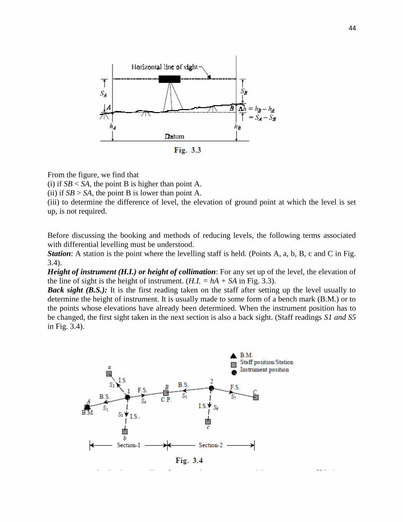
Station: A station is the point where the levelling staff is held. (Points A, a, b, B, c and C in Fig.

3.4).

Height of instrument (H.I.) or height of collimation: For any set up of the level, the elevation of

the line of sight is the height of instrument. (H.I. = hA + SA in Fig. 3.3).

Back sight (B.S.): It is the first reading taken on the staff after setting up the level usually to

determine the height of instrument. It is usually made to some form of a bench mark (B.M.) or to

the points whose elevations have already been determined. When the instrument position has to

be changed, the first sight taken in the next section is also a back sight. (Staff readings S1 and S5

in Fig. 3.4).

45

Fore sight (F.S.): It is the last reading from an instrument position on to a staff held at a point.

It is thus the last reading taken within a section of levels before shifting the instrument to the

next section, and also the last reading taken over the whole series of levels. (Staff readings S4

and S7 in Fig. 3.4).

Change point (C.P.) or turning point: A change point or turning point is the point where both

the fore sight and back sight are made on a staff held at that point. A change point is required

before moving the level from one section to another section. By taking the fore sight the

elevation of the change point is determined and by taking the back sight the height of instrument

is determined. The change points relate the various sections by making fore sight and back sight

at the same point. (Point B in Fig. 3.4).

Intermediate sight (I.S.): The term ‗intermediate sight‘ covers all sightings and consequent staff

readings made between back sight and fore sight within each section. Thus, intermediate sight

station is neither the change point nor the last point. (Points a, b, and c in Fig. 3.4).

Balancing of sights: When the distances of the stations where back sight and fore sight are taken

from the instrument station, are kept approximately equal, it is known as balancing of sights.

Balancing of sights minimizes the effect of instrumental and other errors.

Reduced level (R.L.): Reduced level of a point is its height or depth above or below the assumed

datum. It is the elevation of the point.

Rise and fall: The difference of level between two consecutive points indicates a rise or a fall

between the two points. In Fig. 3.3, if (SA – SB) is positive, it is a rise and if negative, it is a fall.

Rise and fall are determined for the points lying within a section.

Section: A section comprises of one back sight, one fore sight and all the intermediate sights

taken from one instrument set up within that section. Thus the number of sections is equal to the

number of set ups of the instrument. (From A to B for instrument position 1 is section-1 and

from B to C for instrument position 2 is section-2 in Fig. 3.4).

3.6 Booking and Reducing the Levels

For booking and reducing the levels of points, there are two systems, namely the height of

instrument or height of collimation method and rise and fall method. The columns for booking

the readings in a level book are same for both the methods but for reducing the levels, the

number of additional columns depends upon the method of reducing the levels. Note that except

for the change point, each staff reading is written on a separate line so that each staff position has

its unique reduced level. This remains true at the change point since the staff does not move and

the back sight from a forward instrument station is taken at the same staff position where the fore

sight has been taken from the backward instrument station. To explain the booking and reducing

levels, the levelling operation from stations A to C shown in Fig. 3.4, has been presented in

Tables 3.1 and 3.2 for both the methods. These tables may have additional columns for showing

chainage, embankment, cutting, etc., if required.

In reducing the levels for various points by the height of instrument method, the height of

instrument (H.I.) for the each section highlighted by different shades, is determined by adding

the elevation of the point to the back sight reading taken at that point. The H.I. remains

46

unchanged for all the staff readings taken within that section and therefore, the levels of all the

points lying in that section are reduced by subtracting the corresponding staff readings, i.e., I.S.

or F.S., from the H.I. of that section.

In the rise and fall method, the rises and the falls are found out for the points lying within each

section. Adding or subtracting the rise or fall to or from the reduced level of the backward station

obtains the level for a forward station. In Table 3.2, r and f indicate the rise and the fall,

respectively, assumed between the consecutive points.

47

The arithmetic involved in reduction of the levels is used as check on the computations. The

following rules are used in the two methods of reduction of levels.

a) For the height of instrument method

(i) Σ B.S. – Σ F.S. = Last R.L. – First R.L.

(ii) Σ [H.I. . (No. of I.S.‘s + 1)] – Σ I.S. – Σ F.S. = Σ R.L. – First R.L.

(b) For the rise and fall method

Σ B.S. – Σ F.S. = Σ Rise – Σ Fall = Last R.L. – First R.L.

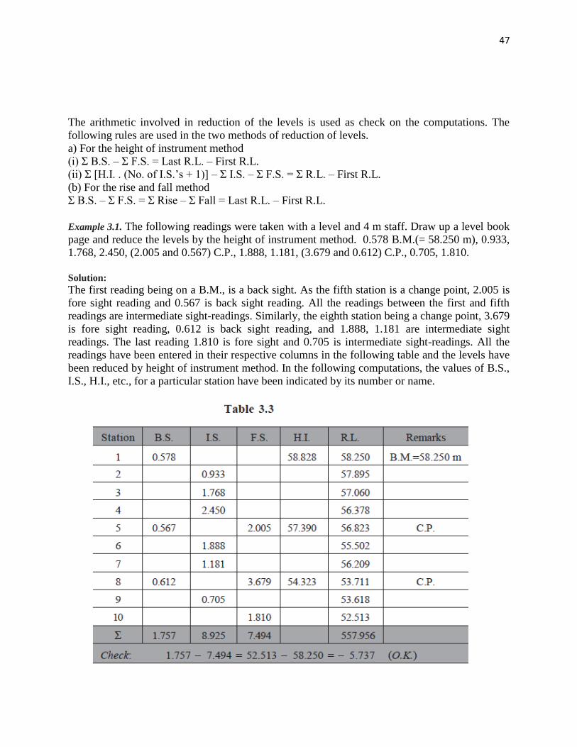
Example 3.1. The following readings were taken with a level and 4 m staff. Draw up a level book

page and reduce the levels by the height of instrument method. 0.578 B.M.(= 58.250 m), 0.933,

1.768, 2.450, (2.005 and 0.567) C.P., 1.888, 1.181, (3.679 and 0.612) C.P., 0.705, 1.810.

Solution:

The first reading being on a B.M., is a back sight. As the fifth station is a change point, 2.005 is

fore sight reading and 0.567 is back sight reading. All the readings between the first and fifth

readings are intermediate sight-readings. Similarly, the eighth station being a change point, 3.679

is fore sight reading, 0.612 is back sight reading, and 1.888, 1.181 are intermediate sight

readings. The last reading 1.810 is fore sight and 0.705 is intermediate sight-readings. All the

readings have been entered in their respective columns in the following table and the levels have

been reduced by height of instrument method. In the following computations, the values of B.S.,

I.S., H.I., etc., for a particular station have been indicated by its number or name.

48

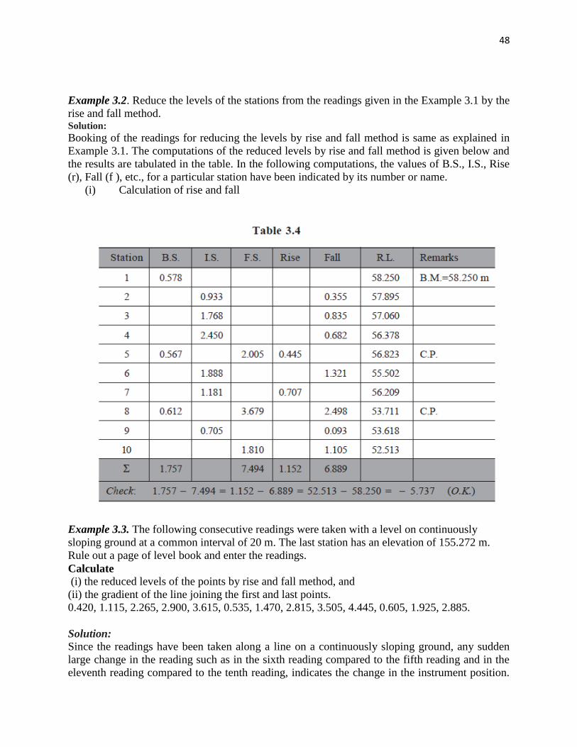
Example 3.2. Reduce the levels of the stations from the readings given in the Example 3.1 by the

rise and fall method. Solution:

Booking of the readings for reducing the levels by rise and fall method is same as explained in

Example 3.1. The computations of the reduced levels by rise and fall method is given below and

the results are tabulated in the table. In the following computations, the values of B.S., I.S., Rise

(r), Fall (f ), etc., for a particular station have been indicated by its number or name.

(i) Calculation of rise and fall

Example 3.3. The following consecutive readings were taken with a level on continuously

sloping ground at a common interval of 20 m. The last station has an elevation of 155.272 m.

Rule out a page of level book and enter the readings.

Calculate

(i) the reduced levels of the points by rise and fall method, and

(ii) the gradient of the line joining the first and last points.

0.420, 1.115, 2.265, 2.900, 3.615, 0.535, 1.470, 2.815, 3.505, 4.445, 0.605, 1.925, 2.885.

Solution:

Since the readings have been taken along a line on a continuously sloping ground, any sudden

large change in the reading such as in the sixth reading compared to the fifth reading and in the

eleventh reading compared to the tenth reading, indicates the change in the instrument position.

49

Therefore, the sixth and eleventh readings are the back sights and fifth and tenth readings are the

fore sights. The first and the last readings are the back sight and fore sight, respectively, and all

remaining readings are intermediate sights.

The last point being of known elevation, the computation of the levels is to be done from last

point to the first point. The falls are added to and the rises are subtracted from the known

elevations. The computation of levels is explained below and the results have been presented in

the following table.

(ii) Calculation of gradient

The gradient of the line 1-11 is

50

Ex3-4 Data from a differential leveling have been found in the order of B.S., F.S..... etc. staring

with the initial reading on B.M. (elevation 150.485 m) are as follows : 1.205, 1.860, 0.125,

1.915, 0.395, 2.615, 0.880, 1.760, 1.960, 0.920, 2.595, 0.915, 2.255, 0.515, 2.305, 1.170. The

final reading closes on B.M.. Put the data in a complete field note form and carry out reduction

of level by Rise and Fall method. All units are in meters.

B.S. (m) F.S. (m) Rise (m) Fall (m) Elevation (m) Remark

1.205 150.485 B.M.

0.125 1.860 0.655 149.830

0.395 1.915 1.7290 148.040

0.880 2.615 2.220 145.820

1.960 1.760 0.880 144.940

2.595 0.920 1.040 145.980

2.255 0.915 1.680 147.660

2.305 0.515 1.740 149.450

1.170 1.135 150.535 B.M.

In case of Rise and Fall method for Reduction of level, following arithmetic checks are applied

to verify calculations.

B.S. - F.S. = Rise - Fall = Last R.L. - First R.L.

With reference to Table

B.S. - F.S. = 4.795 - 7.145 = - 2.350

Rise - Fall. = 1.130 - 3.480 = - 2.350

Last R.L. - First R.L.= 97.650 - 100.000 = -2.350

51

المحاضرة الخامسة

LEVELING—THEORY AND METHODS

Example 3.5. A page of level book is reproduced below in which some readings marked as

(×), are missing. Complete the page with all arithmetic checks.

52

For the computation of reduced levels the given reduced level of point 7 is to be used. For the

points 1 to 6, the computations are done from points 6 to 1, upwards in the table and for points 8

to 10, downwards in the table.

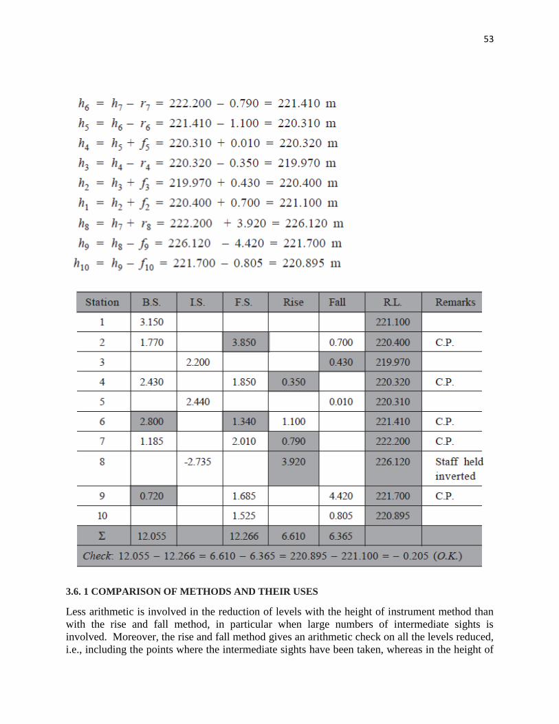
53

3.6. 1 COMPARISON OF METHODS AND THEIR USES

Less arithmetic is involved in the reduction of levels with the height of instrument method than

with the rise and fall method, in particular when large numbers of intermediate sights is

involved. Moreover, the rise and fall method gives an arithmetic check on all the levels reduced,

i.e., including the points where the intermediate sights have been taken, whereas in the height of

54

instrument method, the check is on the levels reduced at the change points only. In the height of

instrument method the check on all the sights is available only using the second formula that is

not as simple as the first one.

The height of instrument method involves less computation in reducing the levels when there are

large numbers of intermediate sights and thus it is faster than the rise and fall method. The rise

and fall method, therefore, should be employed only when a very few or no intermediate sights

are taken in the whole levelling operation. In such case, frequent change of instrument position

requires determination of the height of instrument for the each setting of the instrument and,

therefore, computations involved in the height of instrument method may be more or less equal

to that required in the rise and fall method. On the other hand, it has a disadvantage of not having

check on the intermediate sights, if any, unless the second check is applied.

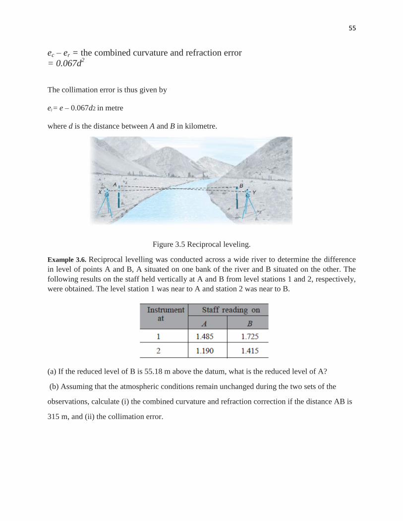
3.7 RECIPROCAL LEVELLING

Reciprocal levelling is employed to determine the correct difference of level between two points

which are quite apart and where it is not possible to set up the instrument between the two points

for balancing the sights. It eliminates the errors due to the curvature of the earth, atmospheric

refraction and collimation.

If the two points between which the difference of level is required to be determined are A and B

then in reciprocal levelling, the first set of staff readings (a1 and b1) is taken by placing the staff

on A and B, and instrument close to A. The second set of readings (a2 and b2) is taken again on A

and B by placing the instrument close to B. The difference of level between A and B is given by

and the combined error is given by

where

e = el + ec – er

el = the collimation error assumed positive for the line of sight inclined upward,

ec = the error due to the earth‘s curvature, and

er = the error due to the atmospheric refraction.

We have

55

ec – er = the combined curvature and refraction error

= 0.067d2

The collimation error is thus given by

el = e – 0.067d2 in metre

where d is the distance between A and B in kilometre.

Figure 3.5 Reciprocal leveling.

Example 3.6. Reciprocal levelling was conducted across a wide river to determine the difference

in level of points A and B, A situated on one bank of the river and B situated on the other. The

following results on the staff held vertically at A and B from level stations 1 and 2, respectively,

were obtained. The level station 1 was near to A and station 2 was near to B.

(a) If the reduced level of B is 55.18 m above the datum, what is the reduced level of A?

(b) Assuming that the atmospheric conditions remain unchanged during the two sets of the

observations, calculate (i) the combined curvature and refraction correction if the distance AB is

315 m, and (ii) the collimation error.

56

Solution:

To eliminate the errors due to collimation, curvature of the earth and atmospheric refraction over

long sights, the reciprocal levelling is performed. From the given data, we have

a1 = 1.485 m, a2 = 1.725 m

b1 = 1.190 m, b2 = 1.415 m

The difference in level between A and B is given by

R.L. of B = R.L. of A + ∆h

R.L. of A = R.L. of B – ∆h

= 55.18 – 0.303 = 54.88 m. The total error e = el + ec – er

and ec – er = 0.067 d2

= 0.067 × 0.3152 = 0.007 m.

Therefore collimation error el = e – (ec – er)

= 0.008 – 0.007 = 0.001 m.

3.8 LOOP CLOSURE AND ITS APPORTIONING

A loop closure or misclosure is the amount by which a level circuit fails to close. It is the

difference of elevation of the measured or computed elevation and known or established

elevation of the same point. Thus loop closure is given by

e = computed value of R.L. – known value of R.L.

57

If the length of the loop or circuit is L and the distance of a station to which the correction

c is computed, is l, then

Alternatively, the correction is applied to the elevations of each change point and the closing

point of known elevation. If there are n1 change points then the total number points at which the

corrections are to be applied is

n = n1 + 1

and the correction at each point is

The corrections at the intermediate points are taken as same as that for the change points to

which they are related.

Another approach could be to apply total of –e/2 correction equally to all the back sights and

total of +e/2 correction equally to all the fore sights. Thus if there are nB back sights and nF fore

sights then

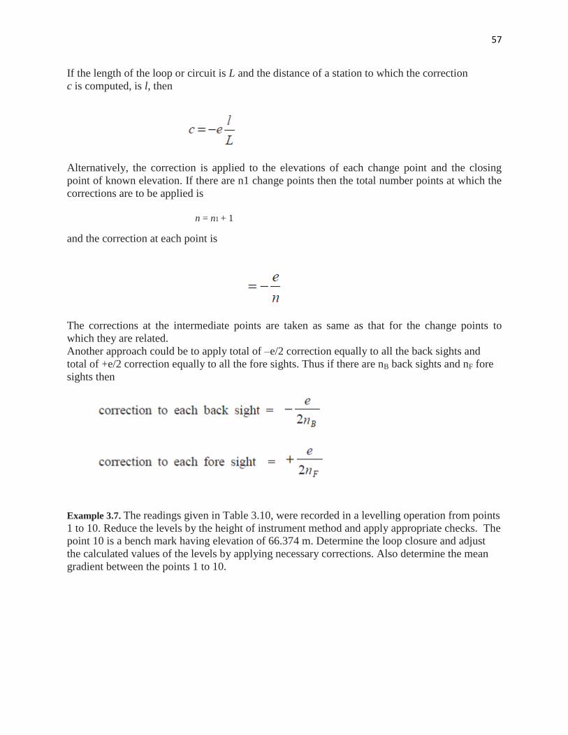
Example 3.7. The readings given in Table 3.10, were recorded in a levelling operation from points

1 to 10. Reduce the levels by the height of instrument method and apply appropriate checks. The

point 10 is a bench mark having elevation of 66.374 m. Determine the loop closure and adjust

the calculated values of the levels by applying necessary corrections. Also determine the mean

gradient between the points 1 to 10.

58

Reduced levels of the points

H.I.1 = h1 + B.S.1 = 68.233 + 0.597 = 68.830 m

h2 = H.I.1 – F.S.2 = 68.233 + 3.132 = 65.698 m

H.I.2 = h2 + B.S.2 = 65.698 + 2.587 = 68.285 m

h3 = H.I.2 – I.S.3 = 68.285 – 1.565 = 66.720 m

h4 = H.I.2 – I.S.4 = 68.285 – 1.911 = 66.374 m

h5 = H.I.2 – I.S.5 = 68.285 – 0.376 = 67.909 m

h6 = H.I.2 – F.S.6 = 68.285 – 1.522 = 66.763 m

H.I.6 = h6 + B.S.6 = 66.763 + 2.244 = 69.007 m

h7 = H.I.6 – I.S.7 = 69.007 – 3.771 = 65.236 m

h8 = H.I.6 – F.S.8 = 69.007 – 1.985 = 67.022 m

H.I.8 = h8 + B.S.8 = 67.022 + 1.334 = 68.356 m

h9 = H.I.8 – I.S.9 = 68.356 – 0.601 = 67.755 m

h10 = H.I.8 – F.S.10 = 68.356 – 2.002 = 66.354 m

Loop closure and loop adjustment

The error at point 10 = computed R.L. – known R.L.

= 66.354 – 66.374 = –0.020 m

Therefore correction = +0.020 m

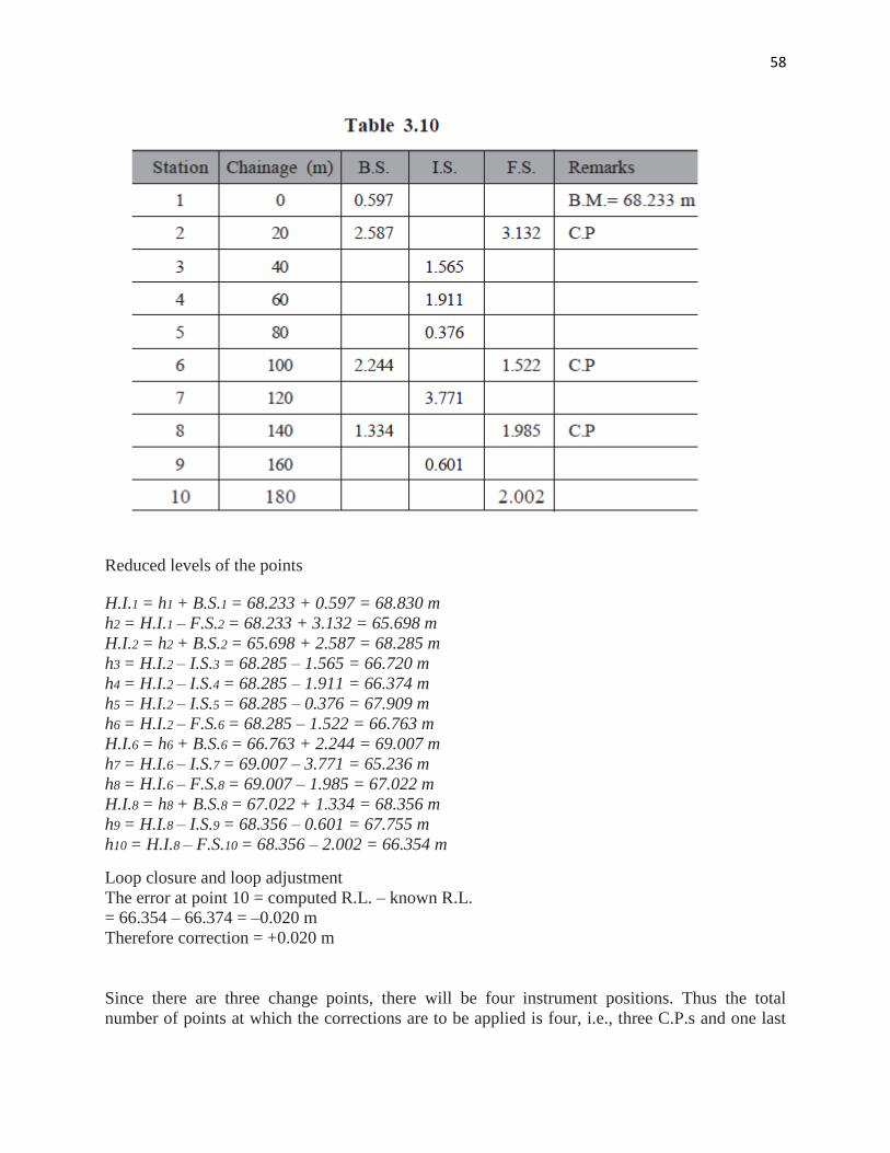
Since there are three change points, there will be four instrument positions. Thus the total

number of points at which the corrections are to be applied is four, i.e., three C.P.s and one last

59

F.S. It is reasonable to assume that similar errors have occurred at each station. Therefore, the

correction for each instrument setting which has to be applied progressively, is

i.e., the correction at station 1 0.0 m

the correction at station 2 + 0.005 m

the correction at station 6 + 0.010 m

the correction at station 8 + 0.015 m

the correction at station 10 + 0.020 m

The corrections for the intermediate sights will be same as the corrections for that instrument

stations to which they are related. Therefore,

correction for I.S.3, I.S.4, and I.S.5 = + 0.010 m

correction for I.S.7 = + 0.015 m

correction for I.S.9 = + 0.020 m

Applying the above corrections to the respective reduced levels, the corrected reduced levels

are obtained. The results have been presented in Table 3.11.

60

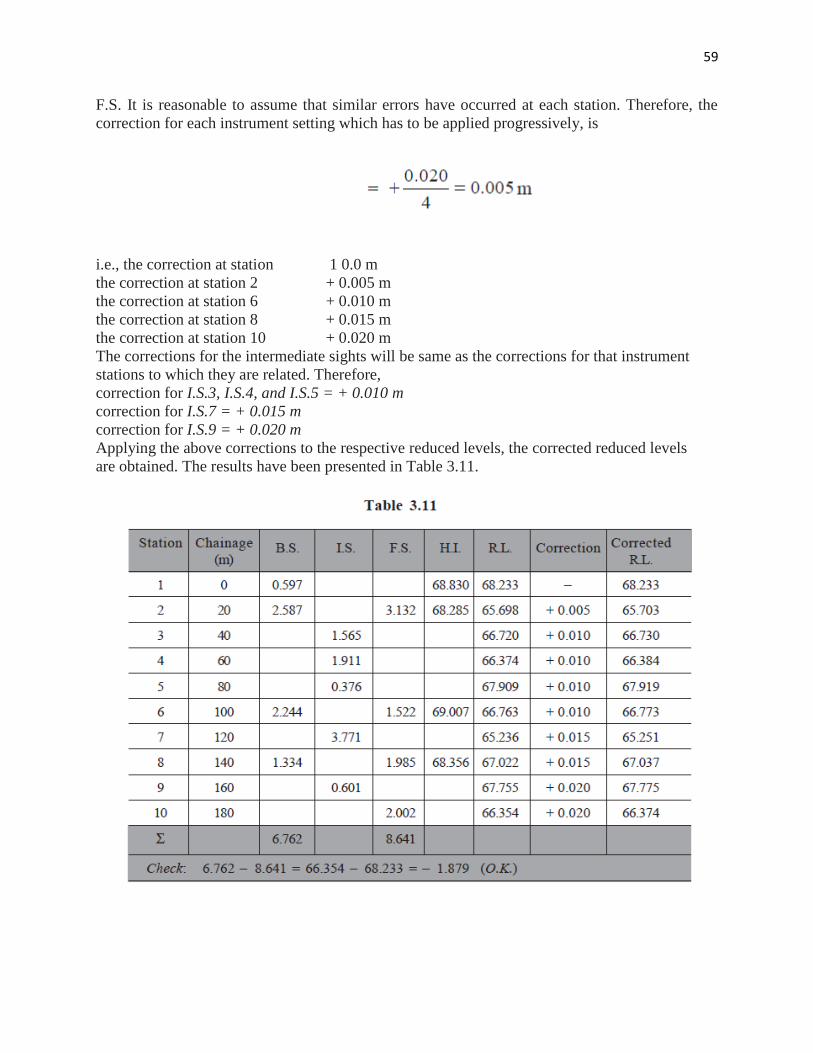
Gradient of the line 1-10

The difference in the level between points 1 and 10, Δh = 66.324 – 68.233 = –1.909 m

The distance between points 1-10, D = 180 m

Gradient = –

= – 0.0106

= 1 in 94.3 (falling)

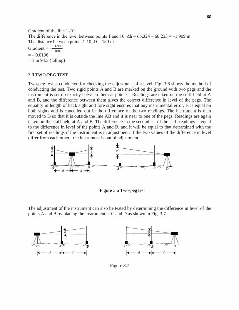
3.9 TWO-PEG TEST

Two-peg test is conducted for checking the adjustment of a level. Fig. 3.6 shows the method of

conducting the test. Two rigid points A and B are marked on the ground with two pegs and the

instrument is set up exactly between them at point C. Readings are taken on the staff held at A

and B, and the difference between them gives the correct difference in level of the pegs. The

equality in length of back sight and fore sight ensures that any instrumental error, e, is equal on

both sights and is cancelled out in the difference of the two readings. The instrument is then

moved to D so that it is outside the line AB and it is near to one of the pegs. Readings are again

taken on the staff held at A and B. The difference in the second set of the staff readings is equal

to the difference in level of the points A and B, and it will be equal to that determined with the

first set of readings if the instrument is in adjustment. If the two values of the difference in level

differ from each other, the instrument is out of adjustment.

Figure 3.6 Two-peg test

The adjustment of the instrument can also be tested by determining the difference in level of the

points A and B by placing the instrument at C and D as shown in Fig. 3.7.

Figure 3.7

61

Example 3.8 the readings obtaining from two-peg test carried out on an automatic level with a

single level staff set up alternately a two pages A and B placed 50 m apart were as followes:

1- With the level midway between A and B

Staff reading at A =1.283

Staff reading at B =0.860

2- With the level positioned 5 m from peg B on the line A B produced

Staff reading at A =1.612

Staff reading at B =1.219

Calculate :

i- The collimation error of the level per 50 m of sight

ii- The reading that should have been observed on the staff A from the level in position

5m from B.

Solution:

1) Collimation error e = (0.860-1.283)-(1.219-1.612)

= -0.030 m per 50 m

2) For the instrument in position 5 m from peg B, the reading that should have been

obtained on the staff when held on at A is

*

+

This is checked by computing the reading that should have been obtained on the staff when held

on at B

*

+5= 1.222

The actual difference 1.222- 1.645= 0.860-1.283 = -0.423

3.10 Trigonometric Leveling

The difference in elevation between two points can be determined by measuring (1) the inclined

or horizontal distance between them and (2) the zenith angle or the altitude angle to one point

from the other. (Zenith and altitude angles, described in more detail in Section 8.13, are

measured in vertical planes. Zenith angles are observed downward from vertical, and altitude

angles are observed up or down from horizontal.) Thus, in Figure 4.9, if slope distance S and

zenith angle z or altitude angle between C and D are observed, then V, the elevation difference

between C and D, is

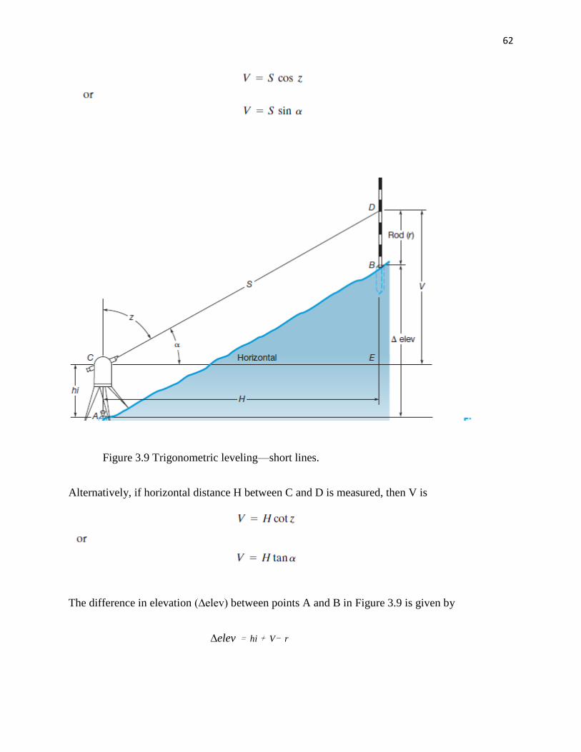
62

Figure 3.9 Trigonometric leveling—short lines.

Alternatively, if horizontal distance H between C and D is measured, then V is

The difference in elevation (∆elev) between points A and B in Figure 3.9 is given by

∆elev = hi + V- r

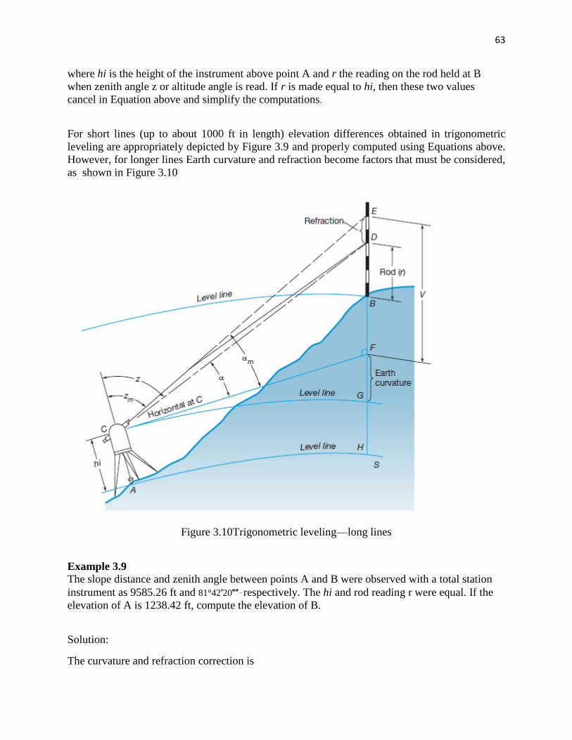
63

where hi is the height of the instrument above point A and r the reading on the rod held at B

when zenith angle z or altitude angle is read. If r is made equal to hi, then these two values

cancel in Equation above and simplify the computations.

For short lines (up to about 1000 ft in length) elevation differences obtained in trigonometric

leveling are appropriately depicted by Figure 3.9 and properly computed using Equations above.

However, for longer lines Earth curvature and refraction become factors that must be considered,

as shown in Figure 3.10

Figure 3.10Trigonometric leveling—long lines

Example 3.9

The slope distance and zenith angle between points A and B were observed with a total station

instrument as 9585.26 ft and 81°42ʹ20″″–respectively. The hi and rod reading r were equal. If the

elevation of A is 1238.42 ft, compute the elevation of B.

Solution:

The curvature and refraction correction is

64

(Theoretically, the horizontal distance should be used in computing curvature and refraction. In

practice, multiplying the slope distance by the sine of the zenith angle approximates it.)

Finally, the elevation of B is

3.11 LEVELLING APPLICATIONS

Of all the surveying operations used in construction, levelling is the most common. Practically

every aspect of a construction project requires some application of the levelling process. The

more general are as follows.

3.11.1 Sectional levelling This type of levelling is used to produce ground profiles for use in the design of roads, railways

and pipelines.

In the case of such projects, the route centre-line is set out using pegs at 10 m, 20 m or 30 m

intervals. Levels are then taken at these peg positions and at critical points such as sudden

changes in ground profiles, road crossings, ditches, bridges, culverts, etc. A plot of these

elevations is called a longitudinal section. When plotting, the vertical scale is exaggerated

compared with the horizontal, usually in the ratio of 10 : 1. The longitudinal section is then used

in the vertical design process to produce formation levels for the proposed route design figure

3.11.

Whilst the above process produces information along a centre-line only, cross-sectional levelling

extends that information at 90◦ to the centre-line for 20–30 m each side. At each centre-line peg

the levels are taken to all points of interest on either side. Where the ground is featureless, levels

at 5 m intervals or less are taken. In this way a ground profile at right angles to the centre-line is

obtained. When the design template showing the road details and side slopes is plotted at

formation level, a cross-sectional area is produced, which can later be used to compute volumes

of earthwork. When plotting cross-sections the vertical and horizontal scales are the same, to

permit easy scaling of the area and side slopes (Figure 3.12).

From the above it can be seen that sectional levelling also requires the measurement of

horizontal distance between the points whose elevations are obtained. As the process involves

the observation of many points, it is important to connect to existing BMs at regular intervals. In

65

most cases of route construction, one of the earliest tasks is to establish BMs at 100 m intervals

throughout the area of interest. Levelling which does not require the measurement of distance,

such as establishing BMs at known positions, is sometimes called ‗fly levelling‘.

Figure 3.11 Longitudinal section of proposed route

66

Figure 3.12 cross section

3.11.2 Contouring

A contour is a horizontal curve connecting points of equal elevation. Contours graphically

represent, in a two-dimensional format on a plan or map, the shape or morphology of the terrain.

The vertical distance between contour lines is called the contour interval. Depending on the

accuracy required, they may be plotted at 0.1 m to 0.5 m intervals in flat terrain and at 1 m to 10

m intervals in undulating terrain. The interval chosen depends on:

(1) The type of project involved; for instance, contouring an airstrip requires an extremely small

contour interval.

(2) The type of terrain, flat or undulating.

(3) The cost, for the smaller the interval the greater the amount of field data required, resulting in

greater expense.

Contours are generally well understood so only a few of their most important properties will be

outlined here.

(1) Contours are perpendicular to the direction of maximum slope.

(2) The horizontal separation between contour lines indicates the steepness of the ground. Close

spacing defines steep slopes, wide spacing gentle slopes.

(3) Highly irregular contours define rugged, often mountainous terrain.

(4) Concentric closed contours represent hills or hollows, depending on the increase or decrease

in

elevation.

(5) The slope between contour lines is assumed to be regular.

(6) Contour lines crossing a stream form V‘s pointing upstream.

(7) The edge of a body of water forms a contour line.

Contours are used by engineers to:

(1) Construct longitudinal sections and cross-sections for initial investigation.

(2) Compute volumes.

(3) Construct route lines of constant gradient.

(4) Delineate the limits of constructed dams, road, railways, tunnels, etc.

(5) Delineate and measure drainage areas.

If the ground is reasonably flat, the optical level can be used for contouring using either the

direct or indirect methods. In steep terrain it is more economical to use other heighting, as

outlined later.

(1) Direct contouring

In this method the actual contour is pegged out on the ground and its planimetric position

located. A backsight is taken to an appropriate BM and the HPC of the instrument is obtained,

say 34.800 m AOD. A staff reading of 0.800 m would then place the foot of the staff at the 34 m

contour level. The staff is then moved throughout the terrain area, with its position pegged at

every 0.800 m reading. In this way the 34 m contour is located. Similarly a staff reading of 1.800

67

m gives the 33 m contour and so on. The planimetric position of the contour needs to be located

using an appropriate survey technique.

This method, although quite accurate, is tedious and uneconomical and could never be used over

a large area. It is ideal, however, in certain construction projects that require excavation to a

specific single contour line.

This method, although quite accurate, is tedious and uneconomical and could never be used over

a large area. It is ideal, however, in certain construction projects that require excavation to a

specific single contour line.

(2) Indirect contouring

This technique requires establishing a grid of intersecting evenly spaced lines over the site. A

theodolite and steel tape may be used to set out the boundary of the grid. The grid spacing will

depend upon the roughness of the ground and the purpose for which the data are required. All the

points of intersection throughout the grid may be pegged or shown by means of paint from a

spray canister. Alternatively ranging rods at the grid intervals around the periphery would permit

the staff holder, with the aid of an optical square, to align himself with appropriate pairs and thus

fix each grid intersection point, for example, alignment with rods B-B and 2-2 fixes point B2

(Figure 3.13). Alternatively assistants at ranging rods B and 2 could help to line up the staff

holder. When the RLs of all the intersection points are obtained, the contours are located by

linear interpolation between the levels, on the assumption of a uniform ground slope between

each pair of points. The interpolation may be done arithmetically using a pocket calculator, or

graphically.

Consider grid points B2 and B3 with reduced levels of 30.20mand 34.60mrespectively and a

horizontal grid interval of 20m (Figure 3.14). The height difference between B2 and B3 is

4.40mand the 31mcontour is 0.80 m above B2. The horizontal distance of the 31 m contour from

B2 = x1

where (20/4.40) = 4.545 m = K

and x1 = K × 0.80 m = 3.64 m

Similarly for the 32 m contour:

x2 = K × 1.80 m = 8.18 m

and so on, where (20/4.40) is a constant K, multiplied each time by the difference in height from

the reduced level of B2 to the required contour value. For the graphical interpolation, a sheet of

transparent paper (Figure 3.15) with equally spaced horizontal lines is used. The paper is placed

over the two points and rotated until B2 obtains a value of 30.20 m and B3 a value of 34.60 m.

Any appropriate scale can be used for the line separation. As shown, the 31, 32, 33 and 34 m

contour positions can now be pricked through onto the plan.

This procedure is carried out on other lines and the equal contour points joined up to form the

contours required.

68

Figure 3.13 Grid layout for contouring

Figure 3.14 Contour calculations

Figure 3.15 Graphical contour plotting

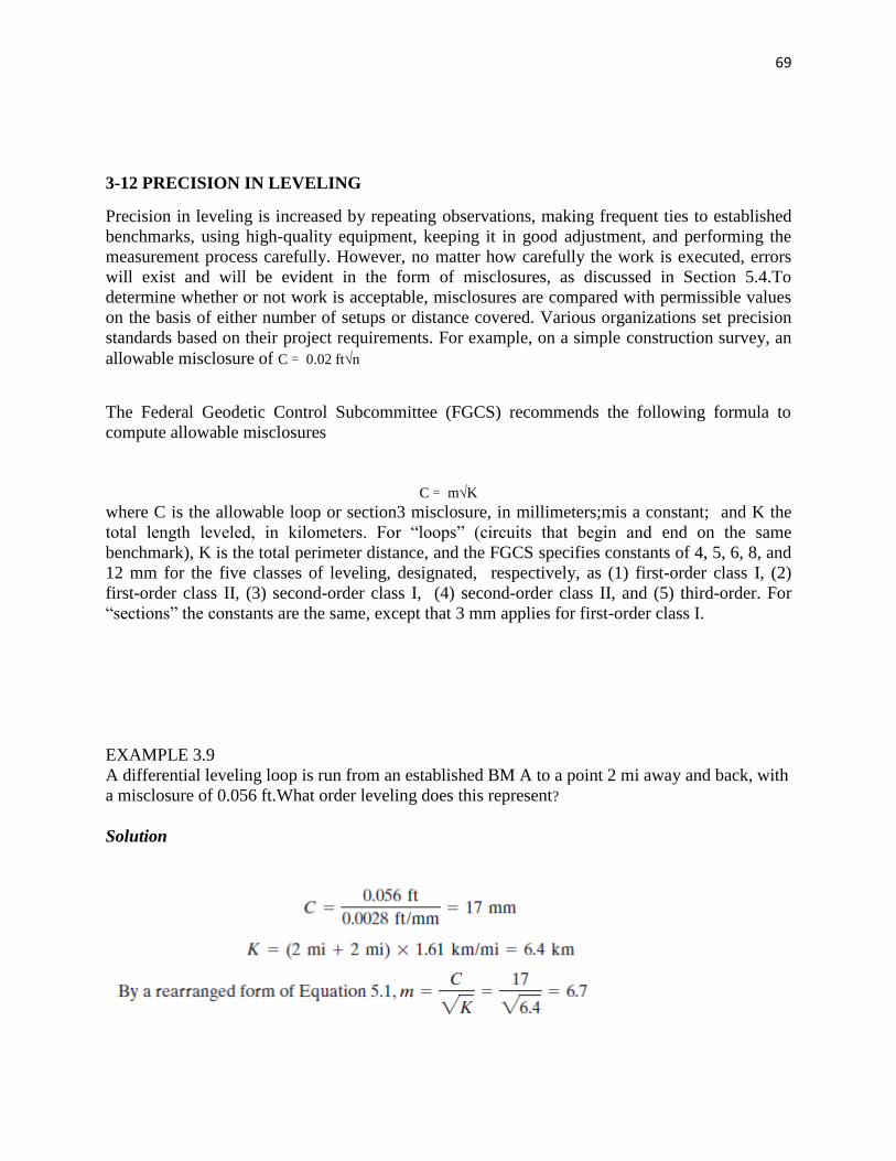
69

3-12 PRECISION IN LEVELING

Precision in leveling is increased by repeating observations, making frequent ties to established

benchmarks, using high-quality equipment, keeping it in good adjustment, and performing the

measurement process carefully. However, no matter how carefully the work is executed, errors

will exist and will be evident in the form of misclosures, as discussed in Section 5.4.To

determine whether or not work is acceptable, misclosures are compared with permissible values

on the basis of either number of setups or distance covered. Various organizations set precision

standards based on their project requirements. For example, on a simple construction survey, an

allowable misclosure of C = 0.02 ft√n

The Federal Geodetic Control Subcommittee (FGCS) recommends the following formula to

compute allowable misclosures

C = m√K

where C is the allowable loop or section3 misclosure, in millimeters;mis a constant; and K the

total length leveled, in kilometers. For ―loops‖ (circuits that begin and end on the same

benchmark), K is the total perimeter distance, and the FGCS specifies constants of 4, 5, 6, 8, and

12 mm for the five classes of leveling, designated, respectively, as (1) first-order class I, (2)

first-order class II, (3) second-order class I, (4) second-order class II, and (5) third-order. For

―sections‖ the constants are the same, except that 3 mm applies for first-order class I.

EXAMPLE 3.9

A differential leveling loop is run from an established BM A to a point 2 mi away and back, with

a misclosure of 0.056 ft.What order leveling does this represent?

Solution

70

انمحاضرة

انسادست

Part 2

Distance measurements

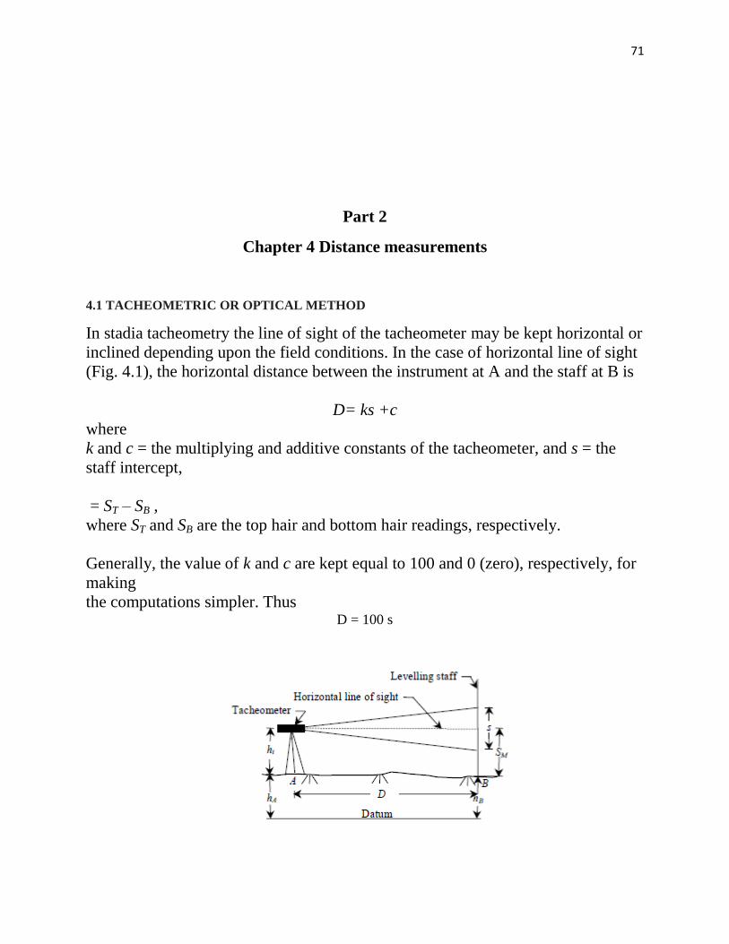
71

Part 2

Chapter 4 Distance measurements

4.1 TACHEOMETRIC OR OPTICAL METHOD

In stadia tacheometry the line of sight of the tacheometer may be kept horizontal or

inclined depending upon the field conditions. In the case of horizontal line of sight

(Fig. 4.1), the horizontal distance between the instrument at A and the staff at B is

D= ks +c

where

k and c = the multiplying and additive constants of the tacheometer, and s = the

staff intercept,

= ST – SB ,

where ST and SB are the top hair and bottom hair readings, respectively.

Generally, the value of k and c are kept equal to 100 and 0 (zero), respectively, for

making

the computations simpler. Thus D = 100 s

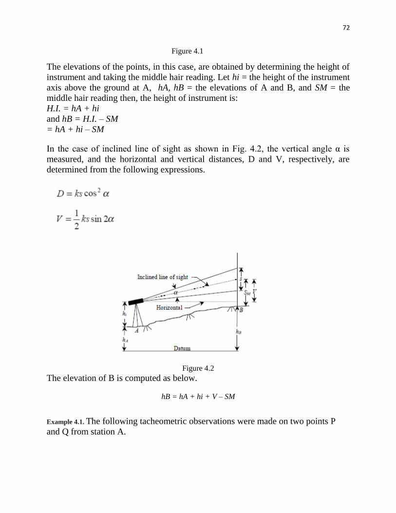
72

Figure 4.1

The elevations of the points, in this case, are obtained by determining the height of

instrument and taking the middle hair reading. Let hi = the height of the instrument

axis above the ground at A, hA, hB = the elevations of A and B, and SM = the

middle hair reading then, the height of instrument is:

H.I. = hA + hi

and hB = H.I. – SM

= hA + hi – SM

In the case of inclined line of sight as shown in Fig. 4.2, the vertical angle α is

measured, and the horizontal and vertical distances, D and V, respectively, are

determined from the following expressions.

Figure 4.2

The elevation of B is computed as below.

hB = hA + hi + V – SM

Example 4.1. The following tacheometric observations were made on two points P

and Q from station A.

73

The height of the tacheometer at A above the ground was 1.55 m. Determine the

elevations of P and Q if the elevation of A is 75.500 m. The stadia constant k and c

are respectively 100 and 0.00 m. Solution:

Since the vertical angles are given, the line of sights are inclined for both the

points. From Eqs.

we have

The given data are

The height of the instrument

74

H.I. = Elevation of A + instrument height

= 75.500 + 1.55 = 77.050 m

Elevation of P

hP = H.I. – VAP – middle hair reading at P

= 77.050 – 7.022 – 0.978

= 69.050 m

Elevation Q HQ = H.I. + VAQ – middle hair reading at Q

= 77.050 + 24.912 – 1.286

= 100.676 m.

4.2 ELECTRONIC DISTANCE MEASUREMENT

4.2.1 Introduction

A major advance in surveying instrumentation occurred approximately 60 years

ago with the development of electronic distance measuring (EDM) instruments.

These devices measure lengths by indirectly determining the number of full and

partial waves of transmitted electromagnetic energy required in traveling between

the two ends of a line. In practice, the energy is transmitted from one end of the

line to the other and returned to the starting point; thus, it travels the double path

distance. Multiplying the total number of cycles by its wavelength and dividing by

2, yields the unknown distance.

Electronic distance measurement is based on the rate and manner that

electromagnetic energy propagates through the atmosphere. The rate of

propagation can be expressed with the following equation

where V is the velocity of electromagnetic energy, in meters per second; f the

modulated frequency of the energy, in hertz;2 and λ the wavelength, in meters.

The velocity of electromagnetic energy in a vacuum is 299,792,458 m/sec. Its

speed is slowed somewhat in the atmosphere according to the following equation

75

where c is the velocity of electromagnetic energy in a vacuum, and n the

atmospheric index of refraction. The value of n varies from about 1.0001 to

1.0005, depending on pressure and temperature, but is approximately equal to

1.0003.Thus, accurate electronic distance measurement requires that atmospheric

pressure and temperature be measured so that the appropriate value of n is known.

76

المحاضرة

السابعة

Angles, Azimuths, and Bearings

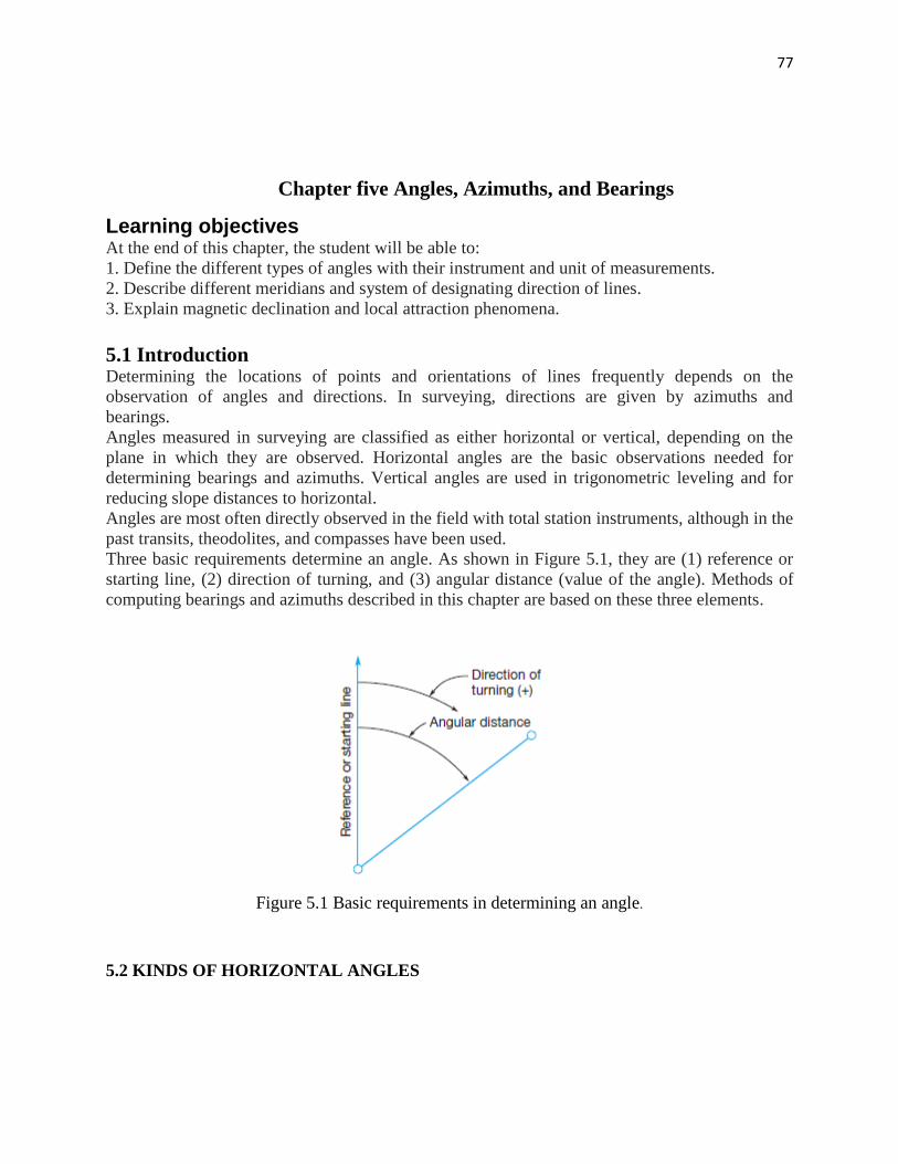
77

Chapter five Angles, Azimuths, and Bearings

Learning objectives At the end of this chapter, the student will be able to:

1. Define the different types of angles with their instrument and unit of measurements.

2. Describe different meridians and system of designating direction of lines.

3. Explain magnetic declination and local attraction phenomena.

5.1 Introduction Determining the locations of points and orientations of lines frequently depends on the

observation of angles and directions. In surveying, directions are given by azimuths and

bearings.

Angles measured in surveying are classified as either horizontal or vertical, depending on the

plane in which they are observed. Horizontal angles are the basic observations needed for

determining bearings and azimuths. Vertical angles are used in trigonometric leveling and for

reducing slope distances to horizontal.

Angles are most often directly observed in the field with total station instruments, although in the

past transits, theodolites, and compasses have been used.

Three basic requirements determine an angle. As shown in Figure 5.1, they are (1) reference or

starting line, (2) direction of turning, and (3) angular distance (value of the angle). Methods of

computing bearings and azimuths described in this chapter are based on these three elements.

Figure 5.1 Basic requirements in determining an angle.

5.2 KINDS OF HORIZONTAL ANGLES

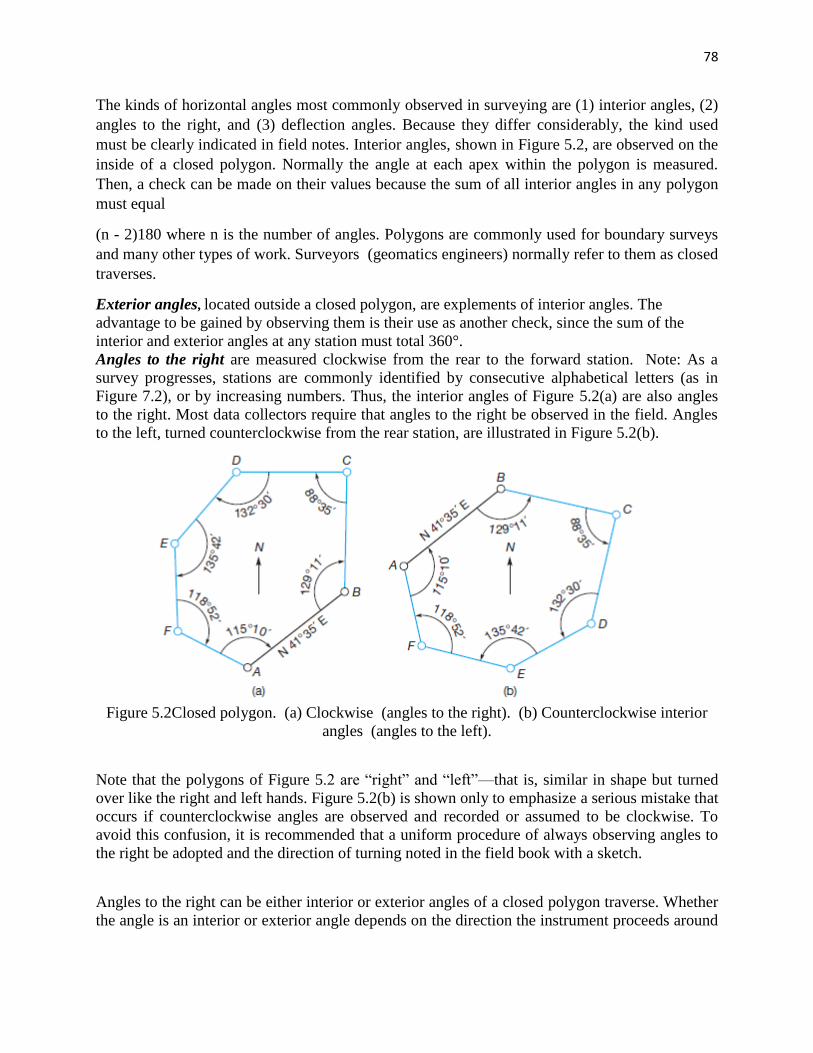
78

The kinds of horizontal angles most commonly observed in surveying are (1) interior angles, (2)

angles to the right, and (3) deflection angles. Because they differ considerably, the kind used

must be clearly indicated in field notes. Interior angles, shown in Figure 5.2, are observed on the

inside of a closed polygon. Normally the angle at each apex within the polygon is measured.

Then, a check can be made on their values because the sum of all interior angles in any polygon

must equal

(n - 2)180 where n is the number of angles. Polygons are commonly used for boundary surveys

and many other types of work. Surveyors (geomatics engineers) normally refer to them as closed

traverses.

Exterior angles, located outside a closed polygon, are explements of interior angles. The

advantage to be gained by observing them is their use as another check, since the sum of the

interior and exterior angles at any station must total 360°.

Angles to the right are measured clockwise from the rear to the forward station. Note: As a

survey progresses, stations are commonly identified by consecutive alphabetical letters (as in

Figure 7.2), or by increasing numbers. Thus, the interior angles of Figure 5.2(a) are also angles

to the right. Most data collectors require that angles to the right be observed in the field. Angles

to the left, turned counterclockwise from the rear station, are illustrated in Figure 5.2(b).

Figure 5.2Closed polygon. (a) Clockwise (angles to the right). (b) Counterclockwise interior

angles (angles to the left).

Note that the polygons of Figure 5.2 are ―right‖ and ―left‖—that is, similar in shape but turned

over like the right and left hands. Figure 5.2(b) is shown only to emphasize a serious mistake that

occurs if counterclockwise angles are observed and recorded or assumed to be clockwise. To

avoid this confusion, it is recommended that a uniform procedure of always observing angles to

the right be adopted and the direction of turning noted in the field book with a sketch.

Angles to the right can be either interior or exterior angles of a closed polygon traverse. Whether

the angle is an interior or exterior angle depends on the direction the instrument proceeds around

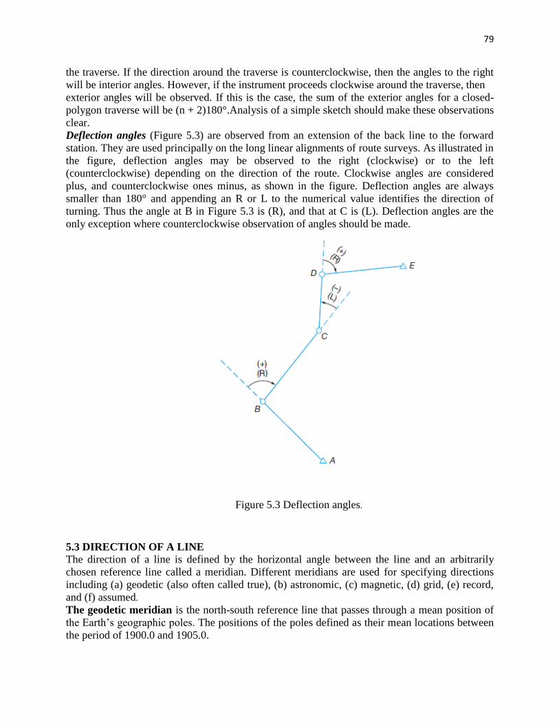
79

the traverse. If the direction around the traverse is counterclockwise, then the angles to the right

will be interior angles. However, if the instrument proceeds clockwise around the traverse, then

exterior angles will be observed. If this is the case, the sum of the exterior angles for a closed-

polygon traverse will be (n + 2)180°.Analysis of a simple sketch should make these observations

clear.

Deflection angles (Figure 5.3) are observed from an extension of the back line to the forward

station. They are used principally on the long linear alignments of route surveys. As illustrated in

the figure, deflection angles may be observed to the right (clockwise) or to the left

(counterclockwise) depending on the direction of the route. Clockwise angles are considered

plus, and counterclockwise ones minus, as shown in the figure. Deflection angles are always

smaller than 180° and appending an R or L to the numerical value identifies the direction of

turning. Thus the angle at B in Figure 5.3 is (R), and that at C is (L). Deflection angles are the

only exception where counterclockwise observation of angles should be made.

Figure 5.3 Deflection angles.

5.3 DIRECTION OF A LINE

The direction of a line is defined by the horizontal angle between the line and an arbitrarily

chosen reference line called a meridian. Different meridians are used for specifying directions

including (a) geodetic (also often called true), (b) astronomic, (c) magnetic, (d) grid, (e) record,

and (f) assumed.

The geodetic meridian is the north-south reference line that passes through a mean position of

the Earth‘s geographic poles. The positions of the poles defined as their mean locations between

the period of 1900.0 and 1905.0.

80

Wobbling of the Earth‘s rotational axis causes the position of the Earth‘s geographic poles to

vary with time. At any point, the astronomic meridian is the north-south reference line that

passes through the instantaneous position of the Earth‘s geographic poles. Astronomic meridians

derive their name from the field operation to obtain them, which consists in making observations

on the celestial objects. Geodetic and astronomic meridians are very nearly the same, and the

former can be computed from the latter by making small corrections.

A magnetic meridian is defined by a freely suspended magnetic needle that is only influenced

by the Earth‘s magnetic field.

Surveys based on a state or other plane coordinate system employ a grid meridian for reference.

Grid north is the direction of geodetic north for a selected central meridian and held parallel to it

over the entire area covered by a plane coordinate system.

In boundary surveys, the term record meridian refers to directional references quoted in the

recorded documents from a previous survey of a particular parcel of land. Another similar term,

deed meridian, is used in the description of a parcel of land as recorded in a property deed.

An assumed meridian can be established by merely assigning any arbitrary direction—for

example, taking a certain street line to be north. The directions of all other lines are then found in

relation to it.

From the above definitions, it should be obvious that the terms north or due north, if used in a

survey, must be defined, since they do not specify a unique line.

5.4 AZIMUTHS

Azimuths are horizontal angles observed clockwise from any reference meridian. In plane

surveying, azimuths are generally observed from north, but astronomers and the military have

used south as the reference direction. Examples of azimuths observed from north are shown in

Figure 5.4. As illustrated, they can range from 0° to 360° in value. Thus the azimuth of OA is

70°; of OB, 145°; of OC, 235°; and of OD, 330°.

Azimuths may be geodetic, astronomic, magnetic, grid, record, or assumed, depending on the

reference meridian used. To avoid any confusion, it is necessary to state in the field notes, at the

beginning of work, what reference meridian applies for azimuths, and whether they are observed

from north or south.

A line‘s forward direction can be given by its forward azimuth, and its reverse direction by its

back azimuth. In plane surveying, forward azimuths are converted to back azimuths, and vice

versa, by adding or subtracting 180°. For example, if the azimuth of OA is 70°, the azimuth of

AO is

70° + 180° = 250°.

If the azimuth of OC is 235°, the azimuth of CO is 235° - 180° = 55°.

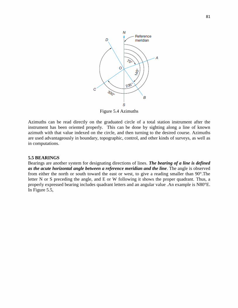
81

Figure 5.4 Azimuths

Azimuths can be read directly on the graduated circle of a total station instrument after the

instrument has been oriented properly. This can be done by sighting along a line of known

azimuth with that value indexed on the circle, and then turning to the desired course. Azimuths

are used advantageously in boundary, topographic, control, and other kinds of surveys, as well as

in computations.

5.5 BEARINGS

Bearings are another system for designating directions of lines. The bearing of a line is defined

as the acute horizontal angle between a reference meridian and the line. The angle is observed

from either the north or south toward the east or west, to give a reading smaller than 90°.The

letter N or S preceding the angle, and E or W following it shows the proper quadrant. Thus, a

properly expressed bearing includes quadrant letters and an angular value .An example is N80°E.

In Figure 5.5,

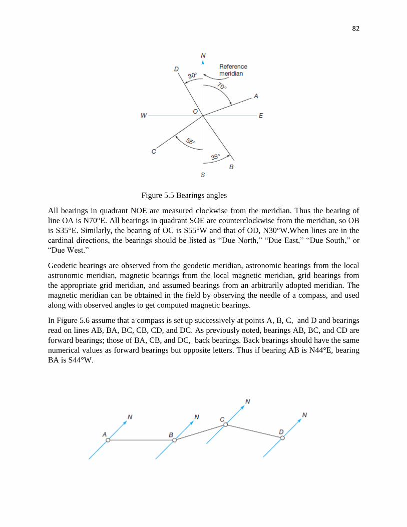
82

Figure 5.5 Bearings angles

All bearings in quadrant NOE are measured clockwise from the meridian. Thus the bearing of

line OA is N70°E. All bearings in quadrant SOE are counterclockwise from the meridian, so OB

is S35°E. Similarly, the bearing of OC is S55°W and that of OD, N30°W.When lines are in the

cardinal directions, the bearings should be listed as ―Due North,‖ ―Due East,‖ ―Due South,‖ or

―Due West.‖

Geodetic bearings are observed from the geodetic meridian, astronomic bearings from the local

astronomic meridian, magnetic bearings from the local magnetic meridian, grid bearings from

the appropriate grid meridian, and assumed bearings from an arbitrarily adopted meridian. The

magnetic meridian can be obtained in the field by observing the needle of a compass, and used

along with observed angles to get computed magnetic bearings.

In Figure 5.6 assume that a compass is set up successively at points A, B, C, and D and bearings

read on lines AB, BA, BC, CB, CD, and DC. As previously noted, bearings AB, BC, and CD are

forward bearings; those of BA, CB, and DC, back bearings. Back bearings should have the same

numerical values as forward bearings but opposite letters. Thus if bearing AB is N44°E, bearing

BA is S44°W.

83

Figure 5.6 Forward and back bearings

84

انمحاضرة

انثامنت

Angles, Azimuths, and Bearings

85

5.6 COMPARISON OF AZIMUTHS AND BEARINGS

Because bearings and azimuths are encountered in so many surveying operations, the

comparative summary of their properties given in Table 5.1 should be helpful. Bearings are

readily computed from azimuths by noting the quadrant in which the azimuth falls, then

converting as shown in the table.

Example 5.1 The azimuth of a boundary line is128°13ʹ 46″ Convert this to a bearing.

Solution

The azimuth places the line in the southeast quadrant. Thus, the bearing angle is

180° - 128°13ʹ 46″ = 51°46ʹ14″

and the equivalent bearing is S51°46ʹ14″E.

Table 5.1 COMPARISON OF AZIMUTHS AND BEARINGS

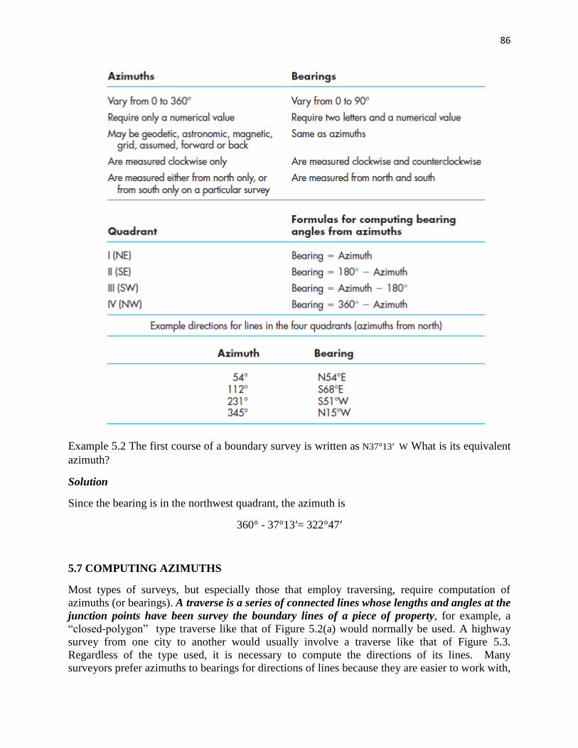
86

Example 5.2 The first course of a boundary survey is written as N37°13ʹ W What is its equivalent

azimuth?

Solution

Since the bearing is in the northwest quadrant, the azimuth is

360° - 37°13ʹ= 322°47ʹ

5.7 COMPUTING AZIMUTHS

Most types of surveys, but especially those that employ traversing, require computation of

azimuths (or bearings). A traverse is a series of connected lines whose lengths and angles at the

junction points have been survey the boundary lines of a piece of property, for example, a

―closed-polygon‖ type traverse like that of Figure 5.2(a) would normally be used. A highway

survey from one city to another would usually involve a traverse like that of Figure 5.3.

Regardless of the type used, it is necessary to compute the directions of its lines. Many

surveyors prefer azimuths to bearings for directions of lines because they are easier to work with,

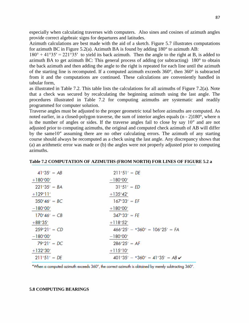
87

especially when calculating traverses with computers. Also sines and cosines of azimuth angles

provide correct algebraic signs for departures and latitudes.

Azimuth calculations are best made with the aid of a sketch. Figure 5.7 illustrates computations

for azimuth BC in Figure 5.2(a). Azimuth BA is found by adding 180° to azimuth AB:

180° + 41°35ʹ = 221°35ʹ to yield its back azimuth. Then the angle to the right at B, is added to

azimuth BA to get azimuth BC: This general process of adding (or subtracting) 180° to obtain

the back azimuth and then adding the angle to the right is repeated for each line until the azimuth

of the starting line is recomputed. If a computed azimuth exceeds 360°, then 360° is subtracted

from it and the computations are continued. These calculations are conveniently handled in

tabular form,

as illustrated in Table 7.2. This table lists the calculations for all azimuths of Figure 7.2(a). Note

that a check was secured by recalculating the beginning azimuth using the last angle. The

procedures illustrated in Table 7.2 for computing azimuths are systematic and readily

programmed for computer solution.

Traverse angles must be adjusted to the proper geometric total before azimuths are computed. As

noted earlier, in a closed-polygon traverse, the sum of interior angles equals (n - 2)180°, where n

is the number of angles or sides. If the traverse angles fail to close by say 10″ and are not

adjusted prior to computing azimuths, the original and computed check azimuth of AB will differ

by the same10″ assuming there are no other calculating errors. The azimuth of any starting

course should always be recomputed as a check using the last angle. Any discrepancy shows that

(a) an arithmetic error was made or (b) the angles were not properly adjusted prior to computing

azimuths.

Table 7.2 COMPUTATION OF AZIMUTHS (FROM NORTH) FOR LINES OF FIGURE 5.2 a

5.8 COMPUTING BEARINGS

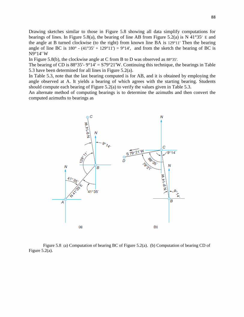
88

Drawing sketches similar to those in Figure 5.8 showing all data simplify computations for

bearings of lines. In Figure 5.8(a), the bearing of line AB from Figure 5.2(a) is N 41°35ʹ E and

the angle at B turned clockwise (to the right) from known line BA is 129°11ʹ Then the bearing

angle of line BC is 180° - (41°35ʹ + 129°11ʹ) = 9°14ʹ, and from the sketch the bearing of BC is

N9°14ʹ W

In Figure 5.8(b), the clockwise angle at C from B to D was observed as 88°35ʹ.

The bearing of CD is 88°35ʹ- 9°14ʹ = S79°21ʹW. Continuing this technique, the bearings in Table

5.3 have been determined for all lines in Figure 5.2(a).

In Table 5.3, note that the last bearing computed is for AB, and it is obtained by employing the

angle observed at A. It yields a bearing of which agrees with the starting bearing. Students

should compute each bearing of Figure 5.2(a) to verify the values given in Table 5.3.

An alternate method of computing bearings is to determine the azimuths and then convert the

computed azimuths to bearings as

Figure 5.8 (a) Computation of bearing BC of Figure 5.2(a). (b) Computation of bearing CD of

Figure 5.2(a).

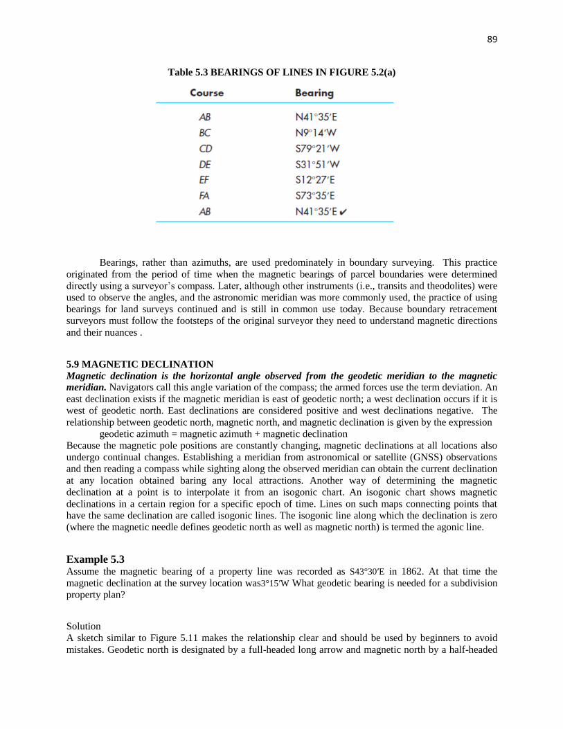
89

Table 5.3 BEARINGS OF LINES IN FIGURE 5.2(a)

Bearings, rather than azimuths, are used predominately in boundary surveying. This practice

originated from the period of time when the magnetic bearings of parcel boundaries were determined

directly using a surveyor‘s compass. Later, although other instruments (i.e., transits and theodolites) were

used to observe the angles, and the astronomic meridian was more commonly used, the practice of using

bearings for land surveys continued and is still in common use today. Because boundary retracement

surveyors must follow the footsteps of the original surveyor they need to understand magnetic directions

and their nuances .

5.9 MAGNETIC DECLINATION

Magnetic declination is the horizontal angle observed from the geodetic meridian to the magnetic

meridian. Navigators call this angle variation of the compass; the armed forces use the term deviation. An

east declination exists if the magnetic meridian is east of geodetic north; a west declination occurs if it is

west of geodetic north. East declinations are considered positive and west declinations negative. The

relationship between geodetic north, magnetic north, and magnetic declination is given by the expression

geodetic azimuth = magnetic azimuth + magnetic declination

Because the magnetic pole positions are constantly changing, magnetic declinations at all locations also

undergo continual changes. Establishing a meridian from astronomical or satellite (GNSS) observations

and then reading a compass while sighting along the observed meridian can obtain the current declination

at any location obtained baring any local attractions. Another way of determining the magnetic

declination at a point is to interpolate it from an isogonic chart. An isogonic chart shows magnetic

declinations in a certain region for a specific epoch of time. Lines on such maps connecting points that

have the same declination are called isogonic lines. The isogonic line along which the declination is zero

(where the magnetic needle defines geodetic north as well as magnetic north) is termed the agonic line.

Example 5.3 Assume the magnetic bearing of a property line was recorded as S43°30ʹE in 1862. At that time the

magnetic declination at the survey location was3°15ʹW What geodetic bearing is needed for a subdivision

property plan?

Solution

A sketch similar to Figure 5.11 makes the relationship clear and should be used by beginners to avoid

mistakes. Geodetic north is designated by a full-headed long arrow and magnetic north by a half-headed

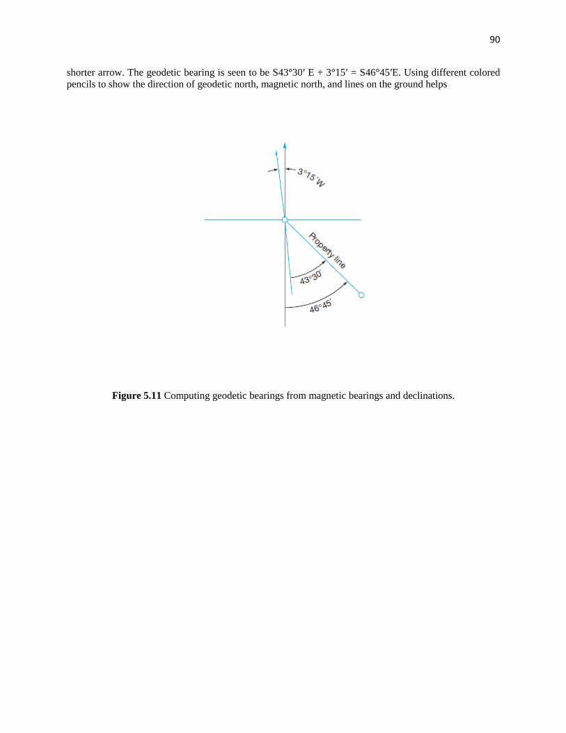
90

shorter arrow. The geodetic bearing is seen to be S43°30ʹ E + 3°15ʹ = S46°45ʹE. Using different colored

pencils to show the direction of geodetic north, magnetic north, and lines on the ground helps

Figure 5.11 Computing geodetic bearings from magnetic bearings and declinations.

91

المحاضرة

التاسعةTraversing

92

Chapter six

Traversing

6.1 Introduction

Measured angles or directions of closed traverses are readily investigated before leaving the

field. Linear measurements, even though repeated, are more likely a source of error, and must

also be checked. Although the calculations are lengthier than angle checks, with today‘s

programmable calculators and portable computers they can also be done in the field to

determine, before leaving, whether a traverse meets the required precision. If specifications have

been satisfied, the traverse is then adjusted to create perfect ―closure‖ or geometric consistency

among angles and lengths; if not, field observations must be repeated until adequate results are

obtained.

Investigation of precision and acceptance or rejection of the field data are extremely important in

surveying. Adjustment for geometric closure is also crucial. For example, in land surveying the

law may require property descriptions to have exact geometric agreement.

Different procedures can be used for computing and adjusting traverses. These vary from

elementary methods to more advanced techniques based on the method of least squares. The

usual steps followed in making elementary traverse computations are (1) adjusting angles or

directions to fixed geometric conditions, (2) determining preliminary azimuths (or bearings) of

the traverse lines, (3) calculating departures and latitudes and adjusting them for misclosure, (4)

computing rectangular coordinates of the traverse stations, and (5) calculating the lengths and

azimuths (or bearings) of the traverse lines after adjustment. These procedures are all discussed

in this chapter and are illustrated with several examples.

6.2 BALANCING ANGLES

In elementary methods of traverse adjustment, the first step is to balance (adjust) the angles to

the proper geometric total. For closed traverses, angle balancing is done readily since the total

error is known, although its exact distribution is not. Angles of a closed traverse can be adjusted

to the correct geometric total by applying one of two methods:

1. Applying an average correction to each angle where observing conditions were approximately

the same at all stations. The correction for each angle is found by dividing the total angular

misclosure by the number of angles.

2. Making larger corrections to angles where poor observing conditions were present.

Of these two methods, the first is almost always applied. Example 6.1

For the traverse of Figure 6.1, the observed interior angles are given in Table 10.1. Compute the

adjusted angles using methods 1 and 2.

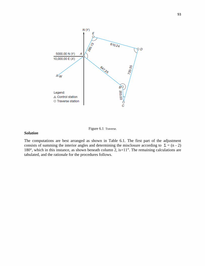
93

Figure 6.1 Traverse.

Solution

The computations are best arranged as shown in Table 6.1. The first part of the adjustment

consists of summing the interior angles and determining the misclosure according to Σ = (n - 2)

180°, which in this instance, as shown beneath column 2, is+11″. The remaining calculations are

tabulated, and the rationale for the procedures follows.

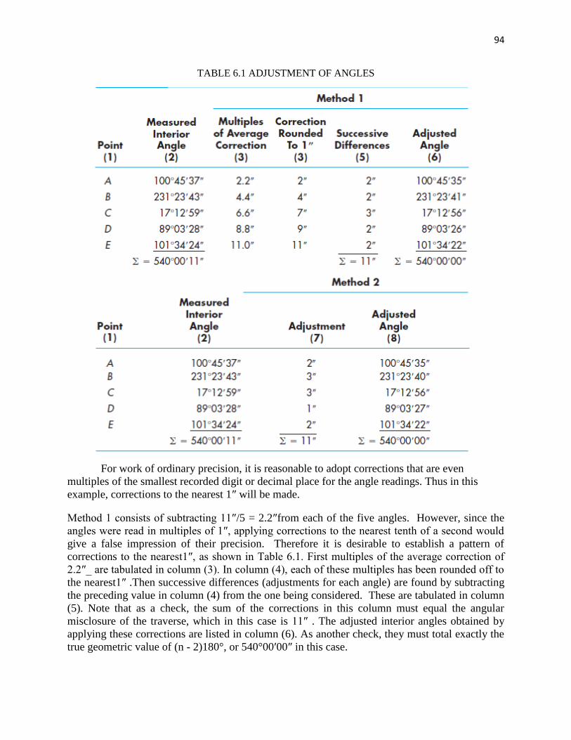
94

TABLE 6.1 ADJUSTMENT OF ANGLES

For work of ordinary precision, it is reasonable to adopt corrections that are even

multiples of the smallest recorded digit or decimal place for the angle readings. Thus in this

example, corrections to the nearest 1″ will be made.

Method 1 consists of subtracting 11″/5 = 2.2″from each of the five angles. However, since the

angles were read in multiples of 1″, applying corrections to the nearest tenth of a second would

give a false impression of their precision. Therefore it is desirable to establish a pattern of

corrections to the nearest1″, as shown in Table 6.1. First multiples of the average correction of

2.2″_ are tabulated in column (3). In column (4), each of these multiples has been rounded off to

the nearest1″ .Then successive differences (adjustments for each angle) are found by subtracting

the preceding value in column (4) from the one being considered. These are tabulated in column

(5). Note that as a check, the sum of the corrections in this column must equal the angular

misclosure of the traverse, which in this case is 11″ . The adjusted interior angles obtained by

applying these corrections are listed in column (6). As another check, they must total exactly the

true geometric value of (n - 2)180°, or 540°00ʹ00″ in this case.

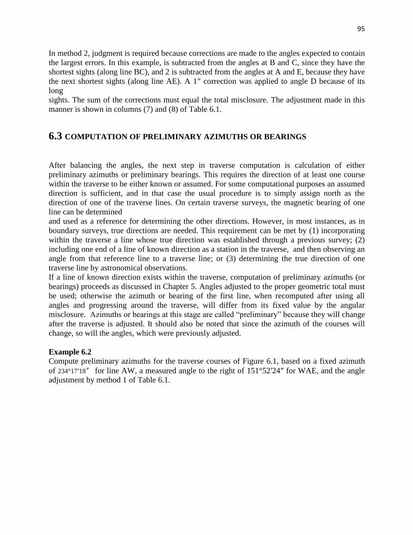
95

In method 2, judgment is required because corrections are made to the angles expected to contain

the largest errors. In this example, is subtracted from the angles at B and C, since they have the

shortest sights (along line BC), and 2 is subtracted from the angles at A and E, because they have

the next shortest sights (along line AE). A 1″ correction was applied to angle D because of its

long

sights. The sum of the corrections must equal the total misclosure. The adjustment made in this

manner is shown in columns (7) and (8) of Table 6.1.

6.3 COMPUTATION OF PRELIMINARY AZIMUTHS OR BEARINGS

After balancing the angles, the next step in traverse computation is calculation of either

preliminary azimuths or preliminary bearings. This requires the direction of at least one course

within the traverse to be either known or assumed. For some computational purposes an assumed

direction is sufficient, and in that case the usual procedure is to simply assign north as the

direction of one of the traverse lines. On certain traverse surveys, the magnetic bearing of one

line can be determined

and used as a reference for determining the other directions. However, in most instances, as in

boundary surveys, true directions are needed. This requirement can be met by (1) incorporating

within the traverse a line whose true direction was established through a previous survey; (2)

including one end of a line of known direction as a station in the traverse, and then observing an

angle from that reference line to a traverse line; or (3) determining the true direction of one

traverse line by astronomical observations.

If a line of known direction exists within the traverse, computation of preliminary azimuths (or

bearings) proceeds as discussed in Chapter 5. Angles adjusted to the proper geometric total must

be used; otherwise the azimuth or bearing of the first line, when recomputed after using all

angles and progressing around the traverse, will differ from its fixed value by the angular

misclosure. Azimuths or bearings at this stage are called ―preliminary‖ because they will change

after the traverse is adjusted. It should also be noted that since the azimuth of the courses will

change, so will the angles, which were previously adjusted.

Example 6.2

Compute preliminary azimuths for the traverse courses of Figure 6.1, based on a fixed azimuth

of 234°17ʹ18″ for line AW, a measured angle to the right of 151°52ʹ24″ for WAE, and the angle

adjustment by method 1 of Table 6.1.

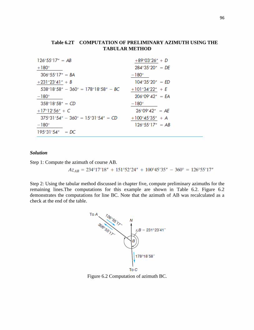
96

Table 6.2T COMPUTATION OF PRELIMINARY AZIMUTH USING THE

TABULAR METHOD

Solution

Step 1: Compute the azimuth of course AB.

Step 2: Using the tabular method discussed in chapter five, compute preliminary azimuths for the

remaining lines.The computations for this example are shown in Table 6.2. Figure 6.2

demonstrates the computations for line BC. Note that the azimuth of AB was recalculated as a

check at the end of the table.

Figure 6.2 Computation of azimuth BC.

97

المحاضرة

العاشرة

Traversing

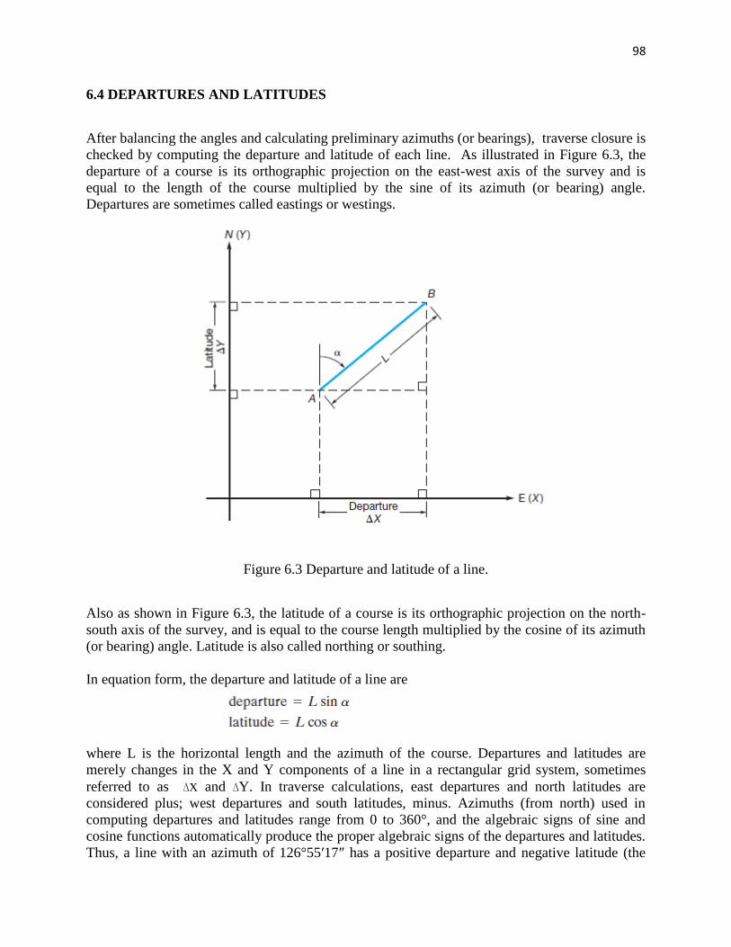
98

6.4 DEPARTURES AND LATITUDES

After balancing the angles and calculating preliminary azimuths (or bearings), traverse closure is

checked by computing the departure and latitude of each line. As illustrated in Figure 6.3, the

departure of a course is its orthographic projection on the east-west axis of the survey and is

equal to the length of the course multiplied by the sine of its azimuth (or bearing) angle.

Departures are sometimes called eastings or westings.

Figure 6.3 Departure and latitude of a line.

Also as shown in Figure 6.3, the latitude of a course is its orthographic projection on the north-

south axis of the survey, and is equal to the course length multiplied by the cosine of its azimuth

(or bearing) angle. Latitude is also called northing or southing.

In equation form, the departure and latitude of a line are

where L is the horizontal length and the azimuth of the course. Departures and latitudes are

merely changes in the X and Y components of a line in a rectangular grid system, sometimes

referred to as ∆X and ∆Y. In traverse calculations, east departures and north latitudes are

considered plus; west departures and south latitudes, minus. Azimuths (from north) used in

computing departures and latitudes range from 0 to 360°, and the algebraic signs of sine and

cosine functions automatically produce the proper algebraic signs of the departures and latitudes.

Thus, a line with an azimuth of 126°55ʹ17″ has a positive departure and negative latitude (the

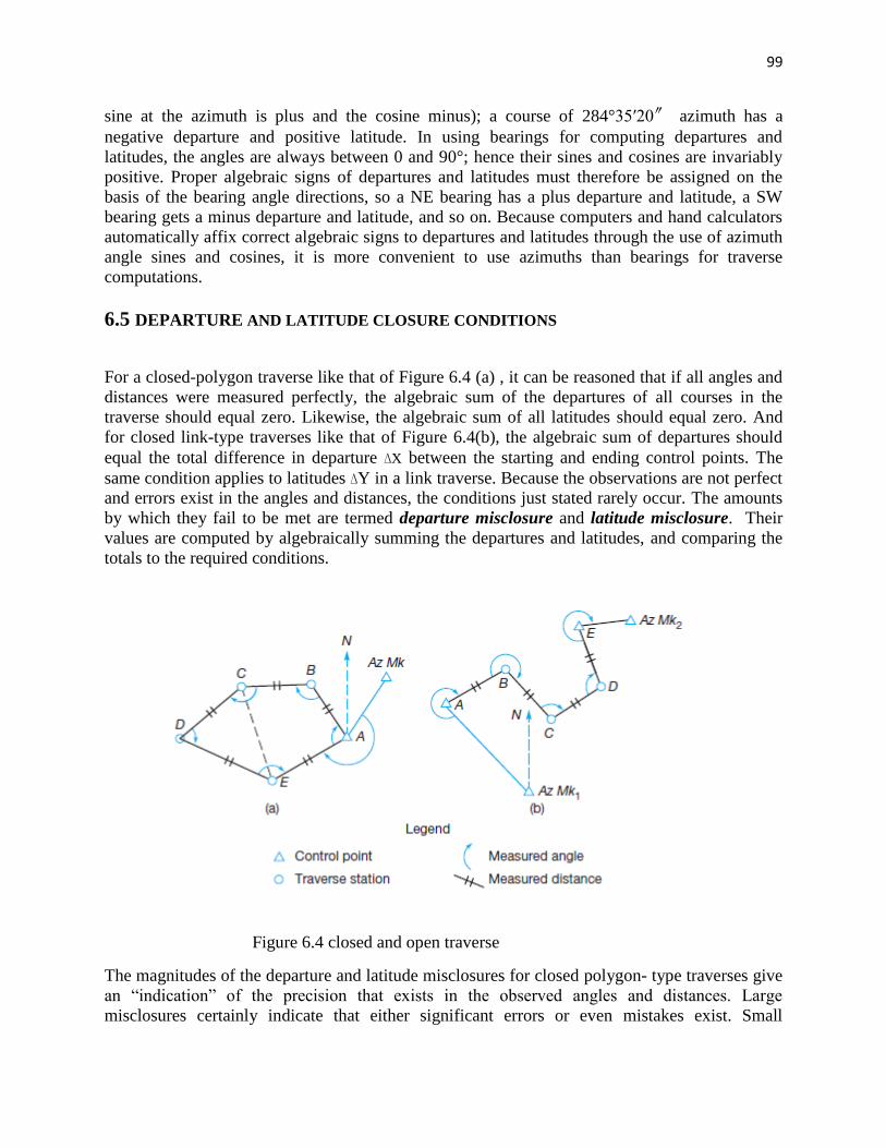
99

sine at the azimuth is plus and the cosine minus); a course of 284°35ʹ20″ azimuth has a

negative departure and positive latitude. In using bearings for computing departures and

latitudes, the angles are always between 0 and 90°; hence their sines and cosines are invariably

positive. Proper algebraic signs of departures and latitudes must therefore be assigned on the

basis of the bearing angle directions, so a NE bearing has a plus departure and latitude, a SW

bearing gets a minus departure and latitude, and so on. Because computers and hand calculators

automatically affix correct algebraic signs to departures and latitudes through the use of azimuth

angle sines and cosines, it is more convenient to use azimuths than bearings for traverse

computations.

6.5 DEPARTURE AND LATITUDE CLOSURE CONDITIONS

For a closed-polygon traverse like that of Figure 6.4 (a) , it can be reasoned that if all angles and

distances were measured perfectly, the algebraic sum of the departures of all courses in the

traverse should equal zero. Likewise, the algebraic sum of all latitudes should equal zero. And

for closed link-type traverses like that of Figure 6.4(b), the algebraic sum of departures should

equal the total difference in departure ∆X between the starting and ending control points. The

same condition applies to latitudes ∆Y in a link traverse. Because the observations are not perfect

and errors exist in the angles and distances, the conditions just stated rarely occur. The amounts

by which they fail to be met are termed departure misclosure and latitude misclosure. Their

values are computed by algebraically summing the departures and latitudes, and comparing the

totals to the required conditions.

Figure 6.4 closed and open traverse

The magnitudes of the departure and latitude misclosures for closed polygon- type traverses give

an ―indication‖ of the precision that exists in the observed angles and distances. Large

misclosures certainly indicate that either significant errors or even mistakes exist. Small

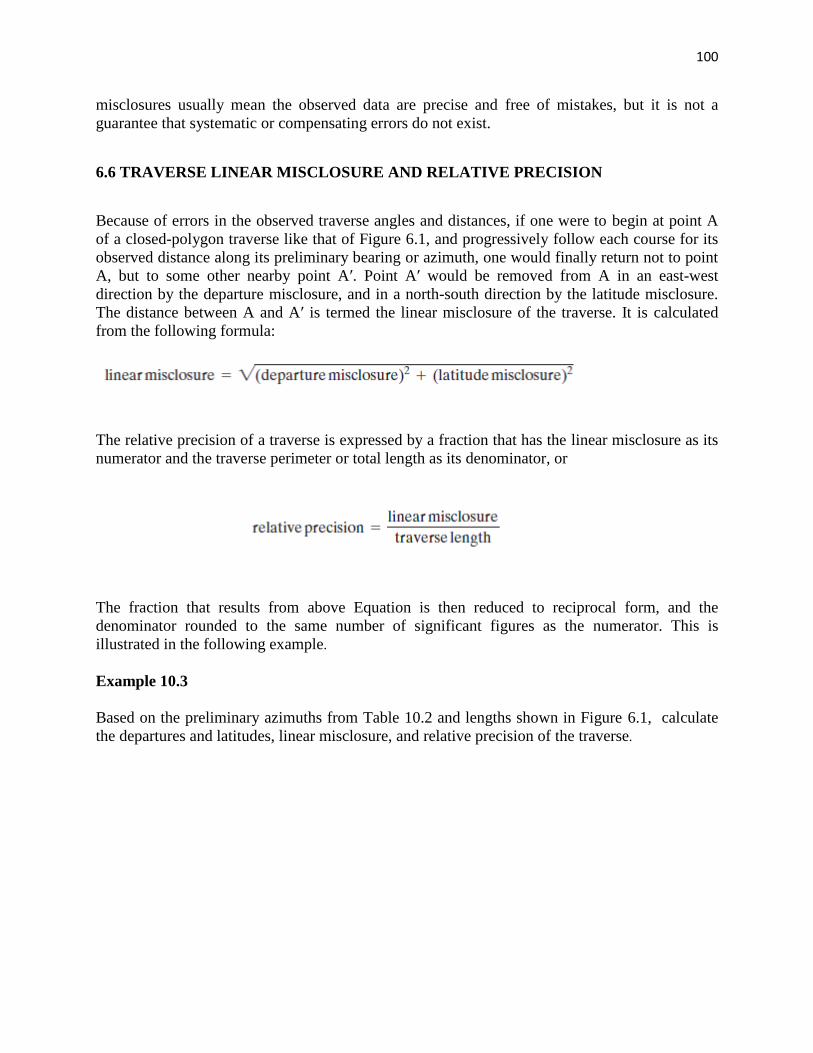
100

misclosures usually mean the observed data are precise and free of mistakes, but it is not a

guarantee that systematic or compensating errors do not exist.

6.6 TRAVERSE LINEAR MISCLOSURE AND RELATIVE PRECISION

Because of errors in the observed traverse angles and distances, if one were to begin at point A

of a closed-polygon traverse like that of Figure 6.1, and progressively follow each course for its

observed distance along its preliminary bearing or azimuth, one would finally return not to point

A, but to some other nearby point Aʹ. Point Aʹ would be removed from A in an east-west

direction by the departure misclosure, and in a north-south direction by the latitude misclosure.

The distance between A and Aʹ is termed the linear misclosure of the traverse. It is calculated

from the following formula:

The relative precision of a traverse is expressed by a fraction that has the linear misclosure as its

numerator and the traverse perimeter or total length as its denominator, or

The fraction that results from above Equation is then reduced to reciprocal form, and the

denominator rounded to the same number of significant figures as the numerator. This is

illustrated in the following example.

Example 10.3

Based on the preliminary azimuths from Table 10.2 and lengths shown in Figure 6.1, calculate

the departures and latitudes, linear misclosure, and relative precision of the traverse.

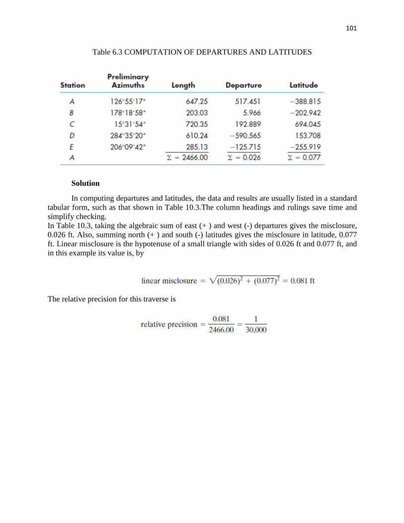
101

Table 6.3 COMPUTATION OF DEPARTURES AND LATITUDES

Solution

In computing departures and latitudes, the data and results are usually listed in a standard

tabular form, such as that shown in Table 10.3.The column headings and rulings save time and

simplify checking.

In Table 10.3, taking the algebraic sum of east (+ ) and west (-) departures gives the misclosure,

0.026 ft. Also, summing north (+ ) and south (-) latitudes gives the misclosure in latitude, 0.077

ft. Linear misclosure is the hypotenuse of a small triangle with sides of 0.026 ft and 0.077 ft, and

in this example its value is, by

The relative precision for this traverse is

102

انمحاضرة

انحاديت عشر

Traversing

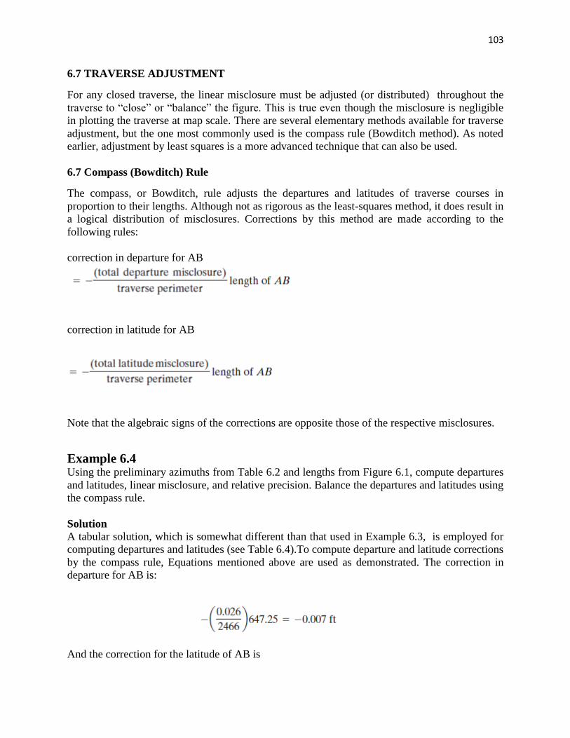
103

6.7 TRAVERSE ADJUSTMENT

For any closed traverse, the linear misclosure must be adjusted (or distributed) throughout the

traverse to ―close‖ or ―balance‖ the figure. This is true even though the misclosure is negligible

in plotting the traverse at map scale. There are several elementary methods available for traverse

adjustment, but the one most commonly used is the compass rule (Bowditch method). As noted

earlier, adjustment by least squares is a more advanced technique that can also be used.

6.7 Compass (Bowditch) Rule

The compass, or Bowditch, rule adjusts the departures and latitudes of traverse courses in

proportion to their lengths. Although not as rigorous as the least-squares method, it does result in

a logical distribution of misclosures. Corrections by this method are made according to the

following rules:

correction in departure for AB

correction in latitude for AB

Note that the algebraic signs of the corrections are opposite those of the respective misclosures.

Example 6.4 Using the preliminary azimuths from Table 6.2 and lengths from Figure 6.1, compute departures

and latitudes, linear misclosure, and relative precision. Balance the departures and latitudes using

the compass rule.

Solution

A tabular solution, which is somewhat different than that used in Example 6.3, is employed for

computing departures and latitudes (see Table 6.4).To compute departure and latitude corrections

by the compass rule, Equations mentioned above are used as demonstrated. The correction in

departure for AB is:

And the correction for the latitude of AB is

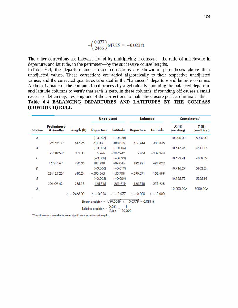
104

The other corrections are likewise found by multiplying a constant—the ratio of misclosure in

departure, and latitude, to the perimeter—by the successive course lengths.

InTable 6.4, the departure and latitude corrections are shown in parentheses above their

unadjusted values. These corrections are added algebraically to their respective unadjusted

values, and the corrected quantities tabulated in the ―balanced‖ departure and latitude columns.

A check is made of the computational process by algebraically summing the balanced departure

and latitude columns to verify that each is zero. In these columns, if rounding off causes a small

excess or deficiency, revising one of the corrections to make the closure perfect eliminates this.

Table 6.4 BALANCING DEPARTURES AND LATITUDES BY THE COMPASS

(BOWDITCH) RULE

105

نمحاضرة ا

انثانيت عشر

Traversing

106

6.8 RECTANGULAR COORDINATES

Rectangular X and Y coordinates of any point give its position with respect to an arbitrarily

selected pair of mutually perpendicular reference axes. The X coordinate is the perpendicular

distance, in feet or meters, from the point to the Y axis; the Y coordinate is the perpendicular

distance to the X axis. Although the reference axes are discretionary in position, in surveying

they are normally oriented so that the Y axis points north-south, with north the positive Y

direction. The X axis runs east-west, with positive X being east. Given the rectangular

coordinates of a number of points, their relative positions are uniquely defined.

Coordinates are useful in a variety of computations, including (1) determining lengths and

directions of lines, and angles; (2) calculating areas of land parcels; (3) making certain curve

calculations; and (4) locating inaccessible points. Coordinates are also advantageous for plotting

maps.

Given the X and Y coordinates of any starting point A, the X coordinate of the next point B is

obtained by adding the adjusted departure of course AB to XA.

Likewise, the Y coordinate of B is the adjusted latitude of AB added to YA. In equation form this

is

For closed polygons, the process is continued around the traverse, successively adding departures

and latitudes until the coordinates of starting point A are recalculated. If these recalculated

coordinates agree exactly with the starting ones, a check on the coordinates of all intermediate

points is obtained (unless compensating mistakes have been made). For link traverses, after

progressively computing coordinates for each station, if the calculated coordinates of the closing

control point equal that point‘s control coordinates, a check is obtained.

Example 6.5

Using the balanced departures and latitudes obtained in Example 6.4 (see Table 6.4) and starting

coordinates XA = 10,000.00 and YA = 5,000.00 calculate coordinates of the other traverse points.

Solution

The process of successively adding balanced departures and latitudes to obtain coordinates is

carried out in the two rightmost columns of Table 6.4. Note that the starting coordinates XA =

10,000.00 and YA = 5,000.00 are recomputed at the end to provide a check. Note also that X and

Y coordinates are frequently referred to as eastings and northings, respectively, as is indicated in

Table 6.4.

6.9 ALTERNATIVE METHODS FOR MAKING TRAVERSE COMPUTATIONS

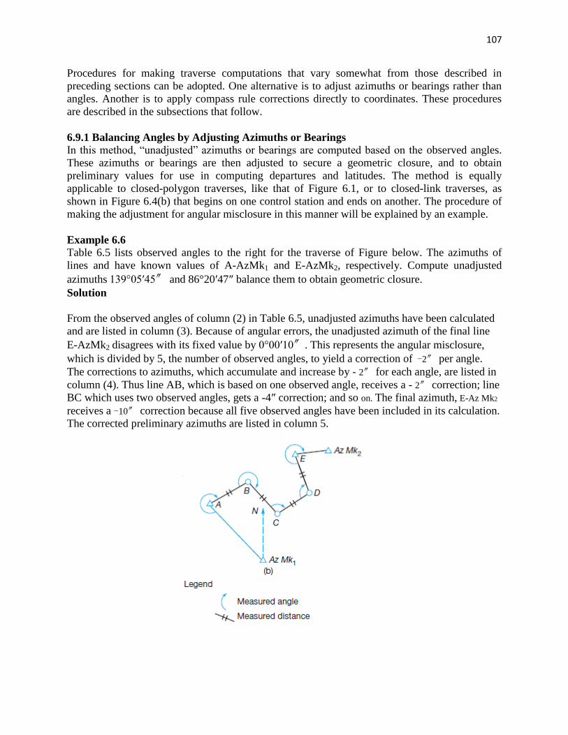
107

Procedures for making traverse computations that vary somewhat from those described in

preceding sections can be adopted. One alternative is to adjust azimuths or bearings rather than

angles. Another is to apply compass rule corrections directly to coordinates. These procedures

are described in the subsections that follow.

6.9.1 Balancing Angles by Adjusting Azimuths or Bearings

In this method, ―unadjusted‖ azimuths or bearings are computed based on the observed angles.

These azimuths or bearings are then adjusted to secure a geometric closure, and to obtain

preliminary values for use in computing departures and latitudes. The method is equally

applicable to closed-polygon traverses, like that of Figure 6.1, or to closed-link traverses, as

shown in Figure 6.4(b) that begins on one control station and ends on another. The procedure of

making the adjustment for angular misclosure in this manner will be explained by an example.

Example 6.6

Table 6.5 lists observed angles to the right for the traverse of Figure below. The azimuths of

lines and have known values of A-AzMk1 and E-AzMk2, respectively. Compute unadjusted

azimuths 139°05ʹ45″ and 86°20ʹ47″ balance them to obtain geometric closure.

Solution

From the observed angles of column (2) in Table 6.5, unadjusted azimuths have been calculated

and are listed in column (3). Because of angular errors, the unadjusted azimuth of the final line

E-AzMk2 disagrees with its fixed value by 0°00ʹ10″. This represents the angular misclosure,

which is divided by 5, the number of observed angles, to yield a correction of -2″ per angle.

The corrections to azimuths, which accumulate and increase by - 2″ for each angle, are listed in

column (4). Thus line AB, which is based on one observed angle, receives a - 2″ correction; line

BC which uses two observed angles, gets a -4″ correction; and so on. The final azimuth, E-Az Mk2

receives a -10″ correction because all five observed angles have been included in its calculation.

The corrected preliminary azimuths are listed in column 5.

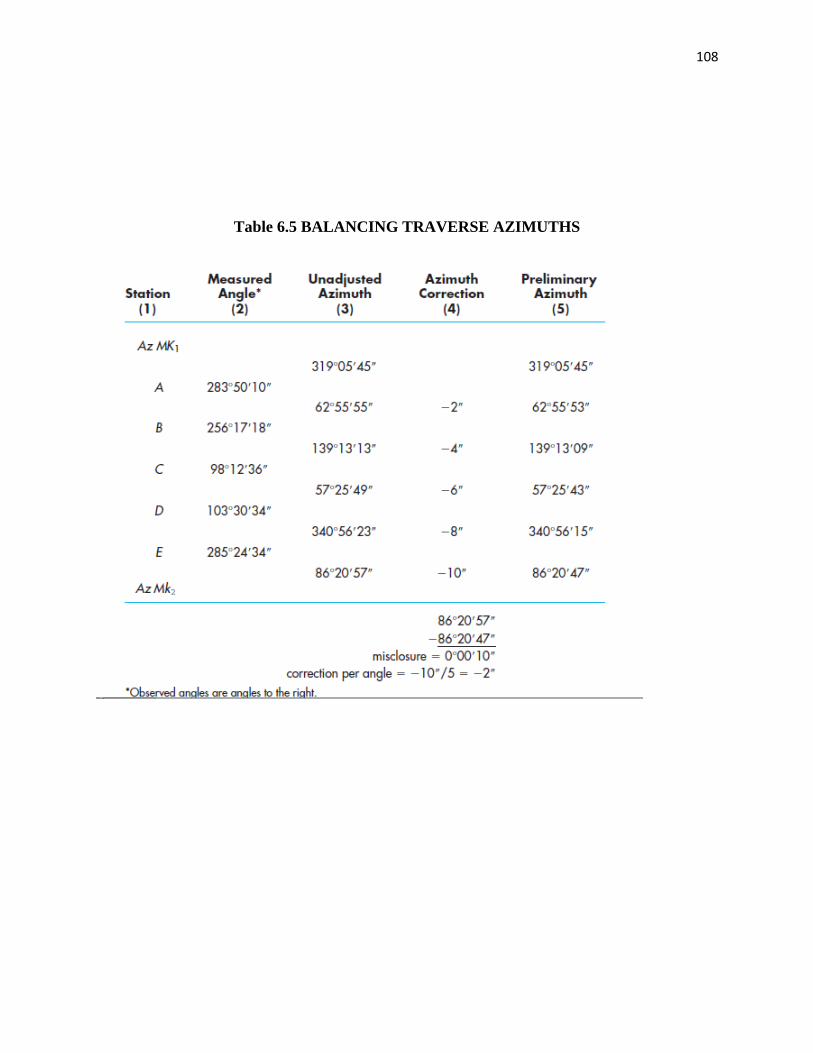
108

Table 6.5 BALANCING TRAVERSE AZIMUTHS

109

انمحاضرة

انثانثت عشر

Traversing

110

6.9.2 Balancing Departures and Latitudes by Adjusting Coordinates In this procedure, commencing with the known coordinates of a beginning station, unadjusted

departures and latitudes for each course are successively added to obtain ―preliminary‖

coordinates for all stations. For closed-polygon traverses, after progressing around the traverse,

preliminary coordinates are recomputed for the beginning station. The difference between the

computed preliminary X coordinate at this station and its known X coordinate is the departure

misclosure. Similarly, the disagreement between the computed preliminary Y coordinate for the

beginning station and its known value is the latitude misclosure. Corrections for these

misclosures can be calculated using compass-rule Equations and applied directly to the

preliminary coordinates to obtain adjusted coordinates. The result is exactly the same as if

departures and latitudes were first adjusted and coordinates computed from them, as was done in

Examples 6.4 and 6.5.

Closed traverses can be similarly adjusted. For this type of traverse, unadjusted departures and

latitudes are also successively added to the beginning station‘s coordinates to obtain preliminary

coordinates for all points, including the final closing station. Differences in preliminary X and Y

coordinates, and the corresponding known values for the closing station, represent the departure

and latitude misclosures, respectively. These misclosures are distributed directly to preliminary

coordinates using the compass rule to obtain final adjusted coordinates. The procedure will be

demonstrated by an example.

Example 6.7

Table 10.6 lists the preliminary azimuths (from Table 6.5) and observed lengths (in feet) for the

traverse of Figure 6.4(b).The known coordinates of stations A and Eare XA = 12,765.48, YA =

43,280.21, XE = 14,797.12 and YE = 44,384.51 ft . Adjust this traverse for departure and latitude

misclosures by making corrections to preliminary coordinates.

Solution

From the lengths and azimuths listed in columns (2) and (3) of Table 6.6, departures and

latitudes are computed and tabulated in columns (4) and (5). These unadjusted values are

progressively added to the known coordinates of station A to obtain preliminary coordinates for

all stations, including E, and are listed in columns (6) and (7). Comparing the preliminary X and

Y coordinates of station E with its known values yields departure and latitude misclosures of

+0.179 and - 0.024 ft, respectively. From these values, the linear misclosure of 0.181 ft and

relative precision of 1/21,000 are computed.

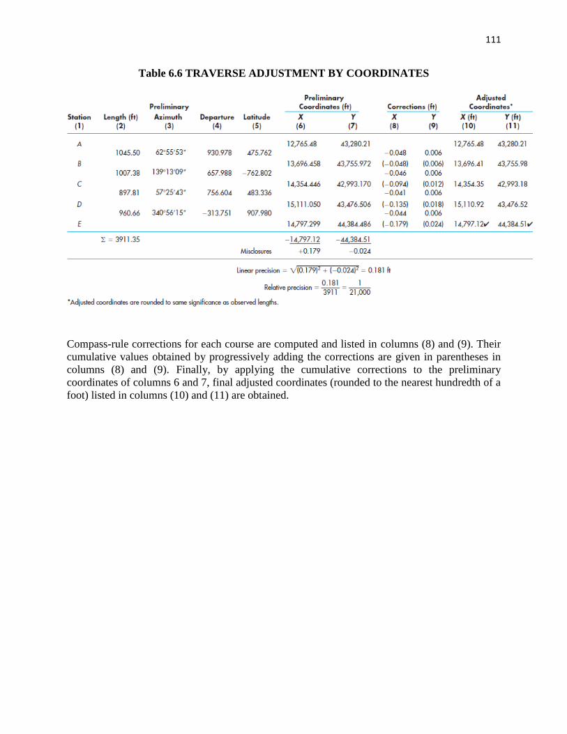
111

Table 6.6 TRAVERSE ADJUSTMENT BY COORDINATES

Compass-rule corrections for each course are computed and listed in columns (8) and (9). Their

cumulative values obtained by progressively adding the corrections are given in parentheses in

columns (8) and (9). Finally, by applying the cumulative corrections to the preliminary

coordinates of columns 6 and 7, final adjusted coordinates (rounded to the nearest hundredth of a

foot) listed in columns (10) and (11) are obtained.

112

انمحاضرة

انرابعت عشر

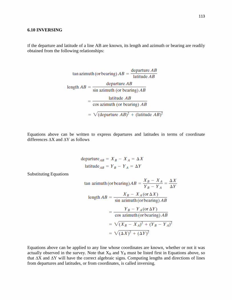
113

6.10 INVERSING

If the departure and latitude of a line AB are known, its length and azimuth or bearing are readily

obtained from the following relationships:

Equations above can be written to express departures and latitudes in terms of coordinate

differences ∆X and ∆Y as follows

Substituting Equations

Equations above can be applied to any line whose coordinates are known, whether or not it was

actually observed in the survey. Note that XB and YB must be listed first in Equations above, so

that ∆X and ∆Y will have the correct algebraic signs. Computing lengths and directions of lines

from departures and latitudes, or from coordinates, is called inversing.

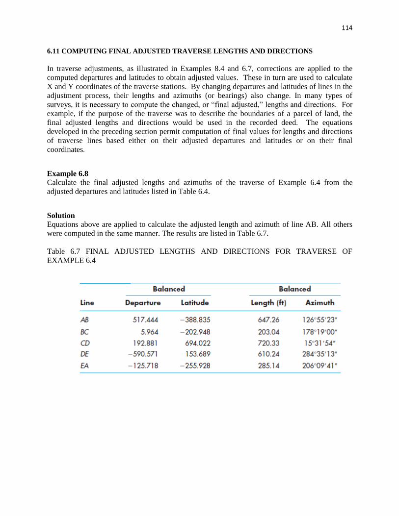
114

6.11 COMPUTING FINAL ADJUSTED TRAVERSE LENGTHS AND DIRECTIONS

In traverse adjustments, as illustrated in Examples 8.4 and 6.7, corrections are applied to the

computed departures and latitudes to obtain adjusted values. These in turn are used to calculate

X and Y coordinates of the traverse stations. By changing departures and latitudes of lines in the

adjustment process, their lengths and azimuths (or bearings) also change. In many types of

surveys, it is necessary to compute the changed, or ―final adjusted,‖ lengths and directions. For

example, if the purpose of the traverse was to describe the boundaries of a parcel of land, the

final adjusted lengths and directions would be used in the recorded deed. The equations

developed in the preceding section permit computation of final values for lengths and directions

of traverse lines based either on their adjusted departures and latitudes or on their final

coordinates.

Example 6.8

Calculate the final adjusted lengths and azimuths of the traverse of Example 6.4 from the

adjusted departures and latitudes listed in Table 6.4.

Solution

Equations above are applied to calculate the adjusted length and azimuth of line AB. All others

were computed in the same manner. The results are listed in Table 6.7.

Table 6.7 FINAL ADJUSTED LENGTHS AND DIRECTIONS FOR TRAVERSE OF

EXAMPLE 6.4

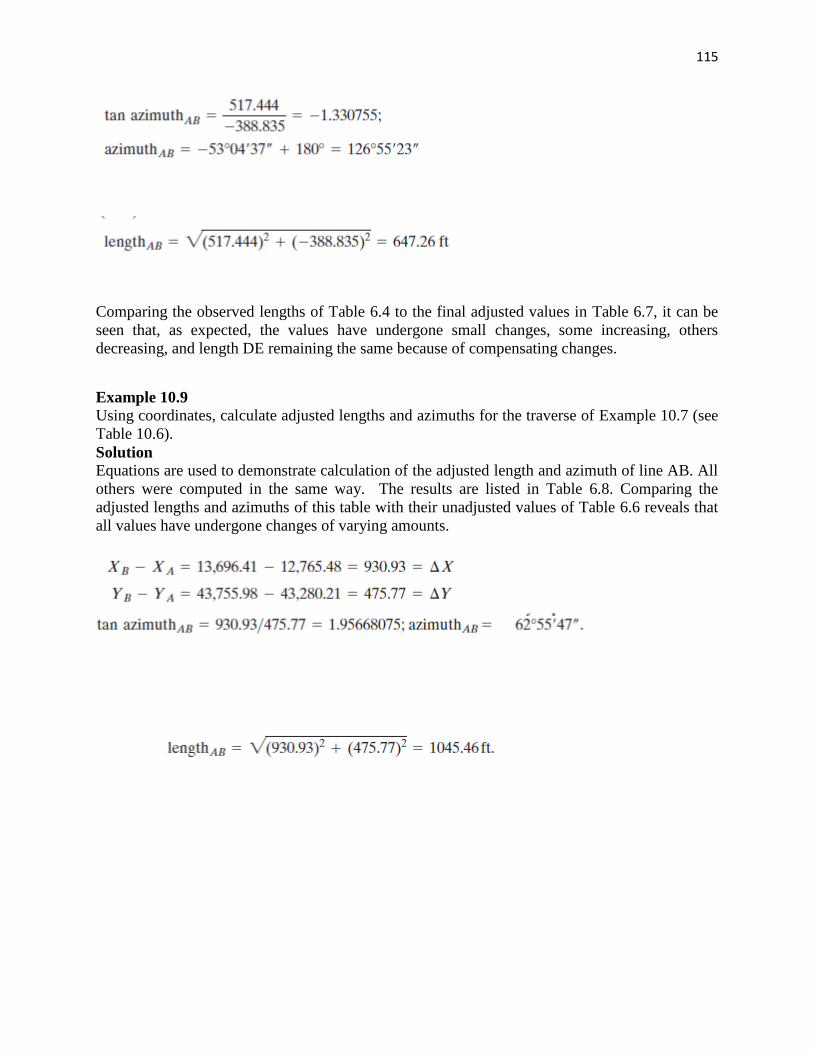
115

Comparing the observed lengths of Table 6.4 to the final adjusted values in Table 6.7, it can be

seen that, as expected, the values have undergone small changes, some increasing, others

decreasing, and length DE remaining the same because of compensating changes.

Example 10.9

Using coordinates, calculate adjusted lengths and azimuths for the traverse of Example 10.7 (see

Table 10.6).

Solution

Equations are used to demonstrate calculation of the adjusted length and azimuth of line AB. All

others were computed in the same way. The results are listed in Table 6.8. Comparing the

adjusted lengths and azimuths of this table with their unadjusted values of Table 6.6 reveals that

all values have undergone changes of varying amounts.

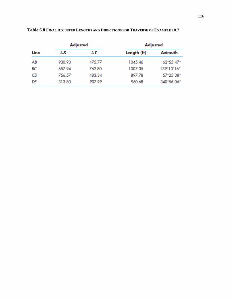
116

Table 6.8 FINAL ADJUSTED LENGTHS AND DIRECTIONS FOR TRAVERSE OF EXAMPLE 10.7