early modified gravity: implications for cosmology
TRANSCRIPT

Early Modified Gravity: Implications for Cosmology
Philippe Brax,1, ∗ Carsten van de Bruck,2, † Sebastien
Clesse,3, 4, ‡ Anne-Christine Davis,5, § and Gregory Sculthorpe2, ¶
1Institut de Physique Theorique, CEA, IPhT, CNRS, URA 2306, F-91191Gif/Yvette Cedex, France2Consortium for Fundamental Physics, School of Mathematics and Statistics,University of Sheffield, Hounsfield Road, Sheffield, S3 7RH, United Kingdom3Namur Center of Complex Systems (naXys), Department of Mathematics,
University of Namur, Rempart de la Vierge 8, 5000 Namur, Belgium4Physik Department T70, Excellence Cluster Universe, James-Franck-Strasse,
Technische Universitat Munchen, 85748 Garching, Germany5DAMTP, Centre for Mathematical Sciences, University of Cambridge, Wilberforce Road, Cambridge CB3 0WA, UK
(Dated: December 13, 2013)
We study the effects of modifications of gravity after Big Bang Nucleosynthesis (BBN) whichwould manifest themselves mainly before recombination. We consider their effects on the CosmicMicrowave Background (CMB) radiation and on the formation of large scale structure. The modelsthat we introduce here represent all screened modifications of General Relativity (GR) which evadethe local tests of gravity such as the violation of the strong equivalence principle as constrainedby the Lunar Ranging experiment. We use the tomographic description of modified gravity whichdefines models with screening mechanisms of the chameleon or Damour-Polyakov types and allowsone to relate the temporal evolution of the mass and the coupling to matter of a scalar field to itsLagrangian and also to cosmological perturbations. The models with early modifications of gravityall involve a coupling to matter which is stronger in the past leading to effects on perturbationsbefore recombination while minimising deviations from ΛCDM structure formation at late times.We find that a new family of early transition models lead to discrepancies in the CMB spectrumwhich could reach a few percent and appear as both enhancements and reductions of power fordifferent scales.
PACS numbers:
I. INTRODUCTION
The observed accelerated expansion of the Universe [1] can be explained within General Relativity (GR) by includingthe cosmological constant Λ, a new parameter whose presence is not forbidden by the basic postulates or symmetriesof GR. Allowing for Λ and some form of cold dark matter (CDM), cosmologists have arrived at a standard model ofcosmology, the ΛCDM model, whose predictions are in remarkable agreement with observations, such as those fromthe cosmic microwave background radiation (CMB) and large scale structures in the Universe. But both CDM andthe cosmological constant require some deeper understanding. Within extensions of the standard model of particlephysics, CDM may find an explanation such as new particles in models with supersymmetry [2]. The cosmologicalconstant term, however, has yet to be embedded within field theories of particle physics.
Instead of a Λ-term in Einstein’s theory, equivalent to a constant energy density which has to be fine-tuned, manycosmologists would prefer a dynamical explanation for the accelerated expansion [3], preferably one which does notdepend on some initial conditions. Therefore, models have been developed in which a dynamical field, usually a scalarfield, drives the accelerated expansion of the universe at late times [4]. If the field couples to matter (baryonic ornot) and the forces are very long-ranged (typically of the order of the horizon scale), the coupling is constrained tobe very small, already at times when the photons decouple from baryonic matter in the early universe. In addition,local experiments [7–13] constrain the coupling of a long-ranged scalar field to normal matter to be smaller than10−5 that of gravity. Given the strong constraints on long-ranged forces, other types of field theories have beenstudied, in particular screened models of modified gravity [5]. In these models, the gravitational sector is modified
∗Email address: [email protected]†Email address: [email protected]‡Email address: [email protected]§Email address: [email protected]¶Email address: [email protected]
arX
iv:1
312.
3361
v1 [
astr
o-ph
.CO
] 1
1 D
ec 2
013

2
to include a scalar degree of freedom, whose interactions with ambient matter make the field either short ranged (asin chameleon/F (R) theories [14–22]) or the effective coupling becomes small in region of high density (as it is thecase of symmetron [23–26] and/or dilaton models [27]). These theories behave effectively as the ΛCDM model forthe background evolution. The evolution of perturbations on scales outside the Compton wavelength of the scalarfield is expected to differ only slightly from ΛCDM. Only on smaller scales, deviations from ΛCDM are expectedin these models. The interaction range usually changes with the cosmological expansion in these models as can thecoupling strength, but usually local constraints today impose that in the present universe the range of interaction isless than 1 Mpc. Therefore to test these models with cosmological observations, predictions for structure formationat small length scales need to be studied in detail using N-body simulations [28–31]. Larger scales affected by linearperturbation theory can show deviations which are smaller but could still be within reach by precision cosmology. Inthe future, besides the large scale structure surveys at low redshifts, the 21-cm signal from the reionisation or the latedark ages will possibly enable us to draw a tomographic view of the matter distribution up to redshifts z ∼ 25 [32–34],higher redshifts being much more difficult to probe with Earth-based radiotelescopes. At those redshifts, short scaleswhich would be non-linear in the very late time Universe appear in the linear regime. 21-cm tomography thereforeshould be promising to constrain deviations from the linear growth of perturbations in General Relativity, and thusto constrain modified gravity [35].
In this paper, we address the following questions: i) How can screened gravity affect the evolution of linear perturba-tions before recombination? And ii) imposing the BBN and local test constraints on screened modified gravity theory,can we find new regimes/models for which those effects leave observable imprints on the CMB as well as the matterpower spectrum? These questions are considered for two classes of screened gravity models: generalised chameleons,to which the f(R), dilaton and chameleon models belong, and a new phenomenological model where the coupling ofthe scalar field to matter undergoes a transition before the time of last scattering. For this purpose, we use the factthat models of screened modified gravity can be described by two functions of the scale-factor a [36, 37]: the effectivemass m(a) of the scalar field and the couplings to matter β(a). This tomographic approach has the advantage thatseveral models are described within one framework via different m(a) and β(a) functions. We shall see that therecan be significant deviations from ΛCDM in the CMB spectrum for the transition models where the modificationsof gravity are significant before recombination. These manifest themselves as both enhancements and reductions ofpower on different scales. It is possible to choose parameters such that these differences are at the percent level whilepreserving structure formation and evading local tests of gravity. In contrast we find that, for generalised chameleonmodels with couplings that are stronger at earlier rather than later times, the constraint on the variation over timeof particle masses is violated before we observe effects on the CMB. For these models it would seem that large scalestructure is the best cosmological test. Therefore we conclude that the signatures of the generalised chameleons andthe early transition models are sufficiently different to envisage the possibility of distinguishing different models ofmodified gravity using CMB data if they were ever to be observed.
The paper is organised as follows: In the next Section, we briefly summarise models of screened modified gravity,using the m(a), β(a) parametrisation. We will also impose local constraints on those theories. In Section 3 we writedown the perturbation equations and derive an analytical solution for the baryon perturbation during tight coupling.In Section 4 we study the evolution of the perturbations numerically. We conclude in Section 5. Details of the numericalimplementation are summarised in the appendix.
II. SCREENED MODIFIED GRAVITY
A. Scalar models
We are interested in the effects of scalars mediating a screened modification of gravity on the CMB and Large ScaleStructure formation. We shall work in the Einstein frame1 where the Einstein equations are preserved and depend onthe energy momentum tensor of the scalar field:
Tφµν = ∂µφ∂νφ− gµν(
1
2(∂φ)2 + V
). (1)
We impose that matter couples to both gravity and the scalar field via the metrics
g(α)µν = A2
(α)(φ)gµν , α = b, c (2)
1 We consider only models where the scalar field has a mass much larger than the Hubble rate, implying that perturbations in the Jordanand Einstein frames are equivalent.

3
for each matter species. Their couplings to matter are defined as
βα(φ) = mPl∂ lnAα(φ)
∂φ(3)
where m−2Pl ≡ 8πGN is the reduced Planck mass, and which may be field dependent in dilatonic models for instance.
It is a universal constant β = 1√6
in f(R) models. We will give specific examples later using generalised chameleonic
models and models where the coupling function has a transition before recombination.In all the models that we will consider, the background cosmology is tantamount to a ΛCDM model since Big
Bang Nucleosynthesis (BBN). Deviations from General Relativity only appear at the perturbative level. Moreover,the effective potential for the scalar field in the matter era is modified by the presence of matter as a consequence ofthe non-trivial matter couplings
Veff(φ) = V (φ) +∑α
(Aα(φ)− 1) ρα (4)
where the sum is taken over the non-relativistic species and ρα is the conserved energy density of the fluid α, relatedto the normal Einstein frame matter density by ρα = ρEα /Aα. The potential acquires a slowly varying minimum φ(ρα)
as long as the mass m2 = d2Veff
d2φ |φ(ρα) is larger than the Hubble rate. We will always assume that this is the case in
the following. Due to the interaction with the scalar field, matter is not conserved and satisfies
DµTµν(α) =
βαmPl
(∂νφ)T (α). (5)
where Tµν(α) is the energy momentum tensor of the species α and T (α) its trace. Notice that radiation is not affected
by the presence of the coupled scalar field. The Einstein equations are not modified and read
Rµν −1
2gµνR = 8πGN
(∑α
T (α)µν + Tφµν
). (6)
The conservation equations and the Einstein equations are enough to characterise the time evolution of the fields.
B. Tomography
It is convenient to introduce the total coupling function A
A =∑α
fαAα (7)
where fα = ρα/ρ is the constant fraction of the species α where ρ =∑α ρα is the total conserved energy density of
non-relativistic matter. The total coupling β is obtained accordingly
βA =∑α
fαβαAα. (8)
Screened modified gravity models satisfy a tomographic description [36, 37] whereby the potential V (φ) and thecoupling constants βα(φ) can be reconstructed solely from the knowledge of the density or scale factor dependence ofthe mass m(a) at the minimum of the effective potential and the total coupling constant β(a). At the minimum
dV
dφ= −βAρ
mPl, (9)
and
m2(a) =d2Veff
d2φ=d2V
d2φ+β2Aρ
m2Pl
+Aρ
mPl
dβ
dφ(10)
Differentiating Eq. 9 with respect to conformal time,
d2V
d2φφ′ = −
(Aρ
dβ
dφ+ βρ
dA
dφ
)φ′
mPl− βAρ′
mPl, (11)
4
and then using Eq. 10 we find
φ′ =3HβAρm2(a)mPl
, (12)
and so, given ρ = ρ0/a3,
φ(a) = φc +3ρ0
mPl
∫ a
ai
β(a)
a4m2(a)da, (13)
where φc is the field value at the minimum corresponding to the density ρ(ai) and we have taken A ≈ 1 (justified bythe constraint on the time variation of fermion masses, see section II D). Eq. 9 also implies that
V (a) = V0 −3ρ2
0
m2Pl
∫ a
ai
β2(a)
a7m2(a)da, (14)
yielding an implicit definition of V (φ).
C. The models
When the field sits in the minimum of the effective potential, the background follows that closely of a ΛCDM model,with the evolution of V (a) ≈ const given in (14). But we will see that quite distinctive features can appear when theevolution of perturbations is studied. To be concrete, we will concentrate on two models in this paper, which we willnow describe.
1. Generalised Chameleons
In our first model the scalar field mass and the couplings to baryons and dark matter evolve effectively like power-laws in the scale factor,
m(a) = m0a−p, βα(a) = β0αa
−b . (15)
Such a model corresponds to generalised chameleons [36, 37]. Setting p ≥ 3, b = 0 and βb0 = βc0 = 1/√
6, one recoversthe large curvature f(R) model [36, 37].
We focus here on the case b > 0, for which the coupling to matter is very large during the tight coupling regimebut smaller at later times. As we shall discuss in section II E, the local tests will impose different constraints on m0
and β0 for different combinations of the exponents p and b. One also requires p ≥ 3/2 during the matter dominatedera, and p ≥ 2 during the radiation era, so that the scalar field mass is always much larger than the Hubble rate,guaranteeing a ΛCDM background expansion.
2. Transition in β
The second model we consider is where the Universe undergoes a smooth but rapid transition from an epoch ofstrong coupling between the scalar field and matter to one when the coupling is small and has negligible effect on thegrowth of perturbations [38, 39]. Using the tomographic maps allowing one to reconstruct V (φ) and β(φ), one findsthat the potential is an inverse power law both before and after a transition point φtrans where the potential decreasesabruptly. The effective potential, both before and after the transition, has a minimum with a large mass where thefield gets trapped. Dynamically, the field undergoing the transition jumps from the minimum before the transition tothe minimum after the transition where it will oscillate a few times before being rapidly (the amplitude decreases likea−3/2) stuck at the minimum again. We will neglect these decaying oscillations in the following and assume that thefield tracks the minimum at all times (for a similar type of phenomenon, see the thorough analysis of the transitionin [26]. In order to satisfy the constraints imposed by local tests we are considering very high masses and this willensure that the field remains close to the minimum through the transition.
We can parameterise this behaviour with the function
βc,b(a) = β0 +βi2
[1 + tanh(C(atrans − a))] , (16)
5
where the parameter C controls the duration of the transition. We choose the effective mass of the scalar field toevolve like a power-law
m(a) = m0a−p. (17)
By setting the transition prior to last scattering, we ensure that all the effects on the CMB angular power spectrumand on the matter power spectrum are mainly caused by the modification of gravity before recombination. Notehowever that the linear perturbations at recombination, which can be used as initial conditions for the growth of thematter perturbations, are modified and thus can lead to a different evolution compared to the ΛCDM model, even ifthere is no direct effect of modified gravity on the growth of structures. For the parameters we have considered, valuesof β0 . 10−4m0/H0 do not lead to any visible modification in the growth of perturbations after last scattering. Sincewe are considering rather high masses this means a strong coupling even up to the present epoch is not ruled out.
D. BBN Constraint
In all the models that we consider the masses of fundamental particles vary as
mψ = A(φ)mbare, (18)
where mbare is the bare mass appearing in the matter Lagrangian. The measurements of primordial light elementabundances place a tight constraint on the time variation of fermion masses since BBN [40–42]
∆mψ
mψ=
∆A
A. 0.1. (19)
Therefore we must require that A ≈ 1 since BBN. Using (3) and (12) we get
dA
da=
3β2ρ
am2m2Pl
, (20)
and so
∆A = 9Ωm,0H20
∫ a0
aBBN
β2(a)
a4m2(a)da . 0.1. (21)
For chameleon models this is
9Ωm,0H20β
20
m20
(a2p−2b−30 − a2p−2b−3
BBN )
2p− 2b− 3. 0.1. (22)
For the case 2p− 2b− 3 > 0 this yields
β0
m0.
(2p− 2b− 3
90Ωm,0H20
)1/2
. O(103) Mpc, (23)
while for 2p− 2b− 3 = 0
β0
m0. (90Ωm,0H
20 ln109)−1/2 . O(102) Mpc. (24)
However if 2p− 2b− 3 < 0 we find
β0
m0.
(|2p− 2b− 3|
9Ωm,0H20
)1/2
109(2p−2b−3)−1
2 . O(106+9(2p−2b−3)
2 ) Mpc, (25)
which results in a much tighter constraint on β0
m0than that coming from the local tests.
For the model with a transition in β the constraint is
9Ωm,0H20
m20(2p− 3)
[β2ini(a
2p−3trans − a
2p−3BBN ) + β2
0(a2p−30 − a2p−3
trans)] . 0.1. (26)

6
We shall only consider cases where 2p− 3 > 0 so that
9Ωm,0H20β
2ini
m20(2p− 3)
a2p−3trans . 0.1, (27)
and if we let atrans = 10−t we find
βini
m0.
(2p− 3
9Ωm,0H20
)−1/2
10t(2p−3)−1
2 . O(103+t(p− 32 )) Mpc. (28)
Typically, we will see that this constraint is superseded by the local constraints.
E. Local tests
We will now examine the constraints on our two models coming from local tests of gravity. We focus on three testswhich can yield strong constraints on screened models. The first comes from the requirement that the Milky Wayshould be screened in order to avoid large, disruptive effects on its dynamics [8, 9]. The second is the laboratory testsof gravity involving spherical bodies which should not feel a large fifth force [6, 7]. The last one follows from the lunarranging experiment [10–13] which looks for violations of the strong equivalence principle, and which turns out to bethe strongest constraint for the models we have chosen.
The screening condition is a simple algebraic relation
|φin − φout| ≤ 2βoutmPlΦN , (29)
where ΦN is Newton’s potential at the surface of a body and φin,out are the values of the field inside and outside thebody. Using the tomography equation (13), we find the relation
|φin − φout|mPl
=3
m2Pl
∫ aout
ain
β(a)
am2(a)ρ(a)da, (30)
where ain,out are defined by ρ(ain,out) = ρin,out This condition expresses the fact that the effective modification ofNewton’s constant felt by an unscreened body in the presence of a screened object due to the scalar field goes from
2β2 to 2β2 |φin−φout|2βmPlΦN
. When two screened bodies such as the moon and the earth fall in the gravitational field of the
sun, the scalar field induces a relative acceleration between them which is measured by the square of their scalarcharges
Q =|φin − φout|mPlΦN
(31)
and the lunar ranging experiment requires that the earth’s charge Q⊕ ≤ 10−7 where φ⊕ ∼ 10−9.For the Milky Way, the density inside the galaxy is typically 106 times the cosmological matter density now, i.e.
aG ∼ 10−2. The value outside the galaxy is the cosmological one (if it is in a dense cluster then aout < 1 and thescreening condition is less stringent) so the screening condition reads
|φG − φ0|mPl
=3
m2Pl
∫ a0
aG
β(a)
am2(a)ρ(a)da ≤ 2βGΦG (32)
where ΦG ∼ 10−6. For the generalised chameleon model, this is
9Ωm0β0H20
(2p− b− 3)m20
(a2p−b−30 − a2p−b−3
G ) ≤ 2βGΦG . (33)
When 2p− b− 3 < 0, the contribution from aG dominates and one gets
m20
H20
&9Ωm0
2|2p+ b− 3|ΦGa2p−3G & O(106−2(2p−3)) . (34)
If on the other hand 2p− b− 3 > 0, the contribution from a0 dominates and, setting a0 ≡ 1 as usual, one has
m20
H20
&9Ωm0
2(2p− b− 3)ΦG& O(106) . (35)

7
For the transition model with atrans < aG, one gets a similar constraint,
m20
H20
&9Ωm0
2(2p− 3)ΦG& O(106) . (36)
which is independent of the value of β0.Tests of gravity in cavities involve spherical bodies of order 10 cm, with a Newtonian potential of order Φc ∼ 10−27
and a density ρc ∼ 10 g [15]. This density is of order of the cosmological density just before BBN when the scalarfield must have settled at the minimum of the effective potential. Outside, in the cavity, the scalar field takes a valuesuch that its mass is of order mcavL ∼ 1 corresponding to a scale factor acav = (Lm0)1/p. The constraint reads
|φc − φcav|mPl
=3
m2Pl
∫ acav
ac
β(a)
am2(a)ρ(a)da ≤ 2βcΦc , (37)
which for the chameleon model with 2p− b− 3 > 0 is
m20
H20
&9Ωm0
2Φc
a2p−b−3cav
2p− b− 3abc & O(102) . (38)
For the transition model we find
m20
H20
&9Ωm0
2Φc
a2p−3cav
2p− 3& O(108) , (39)
which is a tighter constraint than that coming from the screening of the Milky Way.A much more stringent condition follows from the lunar ranging experiment,
3
m2Pl
∫ aG
ac
β(a)
am2(a)ρ(a)da ≤ Q⊕Φ⊕ , (40)
where Q⊕Φ⊕ ∼ 10−16 and ac is associated with the densities inside the earth. For the generalised chameleon modelthe case 2p− b− 3 < 0 leads to
m20
H20
&9Ωm0β0
|2p− b− 3|Q⊕Φ⊕a2p−b−3c . (41)
Since ac 1, considering values for which 2p−b−3 . −1 implies an extremely stringent constraint on the ratio m20/β0
that precludes any visible cosmological signature of the model. We therefore focus on the opposite case 2p− b− 3 > 0for which one gets
m20
H20
&9Ωm0β0
Q⊕Φ⊕
a2p−b−3G
2p− b− 3& β0O(1016−2(2p−b−3)) . (42)
For cases where β0 ∼ O(1), b ' 0 and p & 3, the lunar ranging bound on m0 is weaker than the constraint from theMilky Way. For the transition model, assuming atrans < aG and 2p− 3 > 0, the condition is
m20
H20
&9Ωm0βiQ⊕Φ⊕
a2p−3trans
2p− 3& βia
2p−3transO(1016) . (43)
For the case p = 3, βi = 1013 and ztrans = 1090, this gives the constraint m0 & 1010H0.
III. PERTURBATIONS
In this section, we study the evolution of perturbations with analytical methods, to gain an understanding of thephysics involved. From now on we will work in natural units where 8πGN = 1. We are interested in the first orderperturbations of the Einstein equation and the conservation equations. In the absence of anisotropic stress, the metriccan be described in the conformal Newton gauge
ds2 = a(η)(−(1 + 2Φ)dη2 + (1− 2Φ)dx2), (44)

8
where Φ is Newton’s potential. In this gauge the relevant Einstein equations are (in Fourier space)
k2Φ + 3H(Φ′ +HΦ) = −a2∑α
δρα − a2
(φ′2
a2Φ− φ′
a2δφ′ − V,φδφ
)(45)
and
k2(Φ′ +HΦ) = a2∑α
(1 + wα)θα + k2φ′δφ , (46)
where δρα = ρEα δα is the Einstein frame density perturbation. The Hubble rate is H = a′/a and the equation of stateof each species is wα. We have defined the divergence of the velocity field of each species θ = ∂iv
i. The perturbedKlein-Gordon equation reads
δφ′′ + 2Hδφ′ + (k2 + a2V,φφ)δφ+ 2Φa2Veff,φ − 4Φ′φ′ + a2 (βcδρc + βbδρb) + a2(βc,φρ
Ec + βb,φρ
Eb
)δφ = 0 . (47)
We now consider the perturbation equations in CDM, baryons and radiation. The conservation equation for CDMleads to the coupled equations
δ′c = −(θc − 3Φ′) + βc,φφ′δφ+ βcδφ
′, (48)
and
θ′c = −Hθc + k2Φ + k2βcδφ− βcφ′θc. (49)
For the baryons we get
δ′b = −θb + 3Φ′ + βb,φφ′δφ+ βbδφ
′, (50)
and
θ′b = −Hθb +aneσTR
(θγ − θb) + k2Φ + βbk2δφ− βbφ′θb, (51)
where we have added the interaction term to account for the coupling to photons via Thompson scattering andR = 3ρEb /4ργ .
The Thompson scattering cross section depends on the electron mass me which is field dependent due to theconformal rescaling of the metric, i.e. me is proportional to Ab(φ). However, since the scalar field tracks the minimum
of the effective potential, the time variation of the electron mass in one Hubble time is suppressed by O(H2
m2 ) 1 andcan therefore be neglected.
To describe the photons we shall work in the fluid approximation and since the Boltzmann hierarchy is not alteredby the presence of a scalar field we have
δ′γ = −4
3θγ + 4Φ′ (52)
and
θ′γ =k2
4δγ + k2Φ + aneσT (θb − θγ). (53)
We also need to specify the initial conditions for all the perturbations. We will be interested in modes which willenter the horizon before radiation-matter equality. Adiabatic initial conditions are determined by δic = δib = 3
4δiγ and
δib = − 32Φi.
On subhorizon scales and neglecting the time variation of φ, the equations simplify:
δ′c = −θc, (54)
θ′c = −Hθc + k2Φ + k2βcδφ. (55)
δ′b = −θb, (56)

9
θ′b = −Hθb +aneσTR
(θγ − θb) + k2Φ + βbk2δφ, (57)
δ′γ = −4
3θγ (58)
θ′γ =k2
4δγ + k2Φ + aneσT (θb − θγ). (59)
To leading order in the tight-coupling approximation aneσT →∞ which implies θb ≈ θγ , and therefore the photonand baryon density contrasts are linked by δb ≈ 3
4δγ . This leads to
δ′′b = − R′
(1 +R)δ′b − k2c2sδb − k2Φ− R
(1 +R)βbk
2δφ, (60)
where cs = 1/√
3(1 +R) is the standard sound-speed. The Klein-Gordon equation in the subhorizon limit is
δφ = − βcδρc + βbδρbk2
a2 + V,φφ + βc,φρEc + βb,φρEb. (61)
Using this and approximating the Poisson equation with 2k2Φ = −a2δρc, and then defining δb = (1 +R)−1/2δ yields
δ′′+c2sk2
(1− 9Ωbβ
2bRH2
k2 + a2V,φφ + 3H2(βc,φΩc + βb,φΩb)
)δ = −k2(1+R)1/2
(1 +
2βbβc
1 +a2V,φφ+3H2(βc,φΩc+βb,φΩb)
k2
R
R+ 1
)Φ.
(62)This can be simplified by introducing
δ = δ + (1 +R)1/2
(1 +
2βbβc
1 +a2V,φφ+3H2(βc,φΩc+βb,φΩb)
k2
R
R+ 1
)Φ
c2s, (63)
where the effective speed of sound is
c2s = c2s
(1− 9Ωbβ
2bRH2
k2 + a2V,φφ + 3H2(βc,φΩc + βb,φΩb)
). (64)
This leads to
δ′′ + k2c2s δ = 0, (65)
and using the WKB method the solution is
δ = c−1/2s B cos krs, (66)
where B is set by the initial conditions and rs(η) =∫ η
0csdη is the modified sound horizon. We can relate this to back
to the baryon perturbation,
δb =δ
(1 +R)1/2−
(1 +
2βbβc
1 +a2V,φφ+3H2(βc,φΩc+βb,φΩb)
k2
R
R+ 1
)Φ
c2s. (67)
We should note that the WKB approximation is only valid if the time variation of cs is smooth. This will be violatedfor a short period in the models with a transition in β.
As implied above the evolution of the Newtonian potential before last scattering is dominated by that of the CDMperturbations. Equations (54) and (55) therefore lead to the growth equation for CDM
δ′′c +Hδ′c −3
2H2Ωc
(1 +
2β2c
1 +a2V,φφ+3H2(βc,φΩc+βb,φΩb)
k2
)δc −
3H2Ωbβbβc
1 +a2V,φφ+3H2(βc,φΩc+βb,φΩb)
k2
δb = 0 (68)
As noted in [43] we can identify three possible sources of modification to the CMB angular power spectrum. These arethe modified sound horizon which could cause a shift in the peak positions, the modified evolution of the Newtonianpotential due to anomalous growth of the CDM perturbations, and an extra contribution to the growth of the baryonperturbations proportional to Φ and the couplings to both baryons and CDM.

10
IV. NUMERICAL RESULTS: CMB ANGULAR POWER SPECTRUM AND MATTER POWERSPECTRUM
We have implemented the linear perturbation dynamics for two models of screened gravity within a modified versionof the CAMB code [44]. The details of the modifications that were required are given in the appendix.
A. Transition in β
For the transition model we observe deviations from ΛCDM in both the CMB angular power spectrum and thematter power spectrum which increase with increasing βi/m0. Keeping the ratios βi/m0 and β0/m0 constant (withthe other parameters fixed) results in identical effects. In the CMB the nature of the deviations varies with l andthere are alternating periods of enhancement and reduction of power. We see no shift in the positions of the peaks(see Figs. 1 and 2). This is because the sound horizon is virtually unchanged. Consequently there is also no shift inthe position of the baryon acoustic peaks in the matter power spectrum.
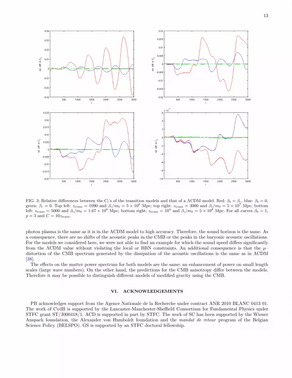
The exact effects of the transition model on the angular power spectrum are different depending on when thetransition occurs. In Fig. 3 we illustrate this with 4 different transition redshifts. For a transition at last scattering(ztrans = 1090) we see clear oscillations in the relative difference of the Cl’s whose amplitude increases with increasingl. This corresponds to enhanced amplitudes of the odd peaks and troughs and reduced amplitudes of the even peaksand troughs as can be seen in Fig. 1. For βi/m0 = 5 × 10⁶ Mpc the deviations exceed the percent level. In thecases ztrans = 3000 and ztrans = 5000 we see apparently periodic alternation of enhancement and reduction of power.Increasing the transition redshift lengthens these periods. This can be seen in Fig. 2 which shows that for ztrans = 3000two consecutive peaks are enhanced. On average the deviations are greater on smaller scales and the enhancementslarger than the reductions. There are also oscillatory features within the intervals of increased and decreased power.Values of βi/m0 = 5× 10⁷ Mpc for ztrans = 3000 and βi/m0 = 1.67× 10⁸ Mpc for ztrans = 5000 produce deviations ofaround 1%. Finally, for ztrans = 10000 there is only a slight oscillating enhancement of the relative difference for l . 400(just before the first trough) and then a more significant reduction in power for l & 400 with irregular oscillations inthe relative difference. At this redshift the deviations approach the percent level for βi/m0 = 5× 10⁸ Mpc.
Fig. 3 also displays the relative importance of the couplings to CDM and baryons for the effects on the CMB. Ifwe set βb = 0 the deviations are smaller (generally no more than half a percent) but visible. The oscillations in therelative difference are out of phase with those of the βb = βc case but there is a greater similarity between the effectsfor different transition redshifts than with βb = βc. On the other hand if we set βc = 0 the deviations are completelynegligible in all cases. These results suggest that the dominant contribution to the modified effects is the term in Eq.(67) which contains both βc and βb and causes the modifications to the growth of the baryon perturbations beforelast scattering.
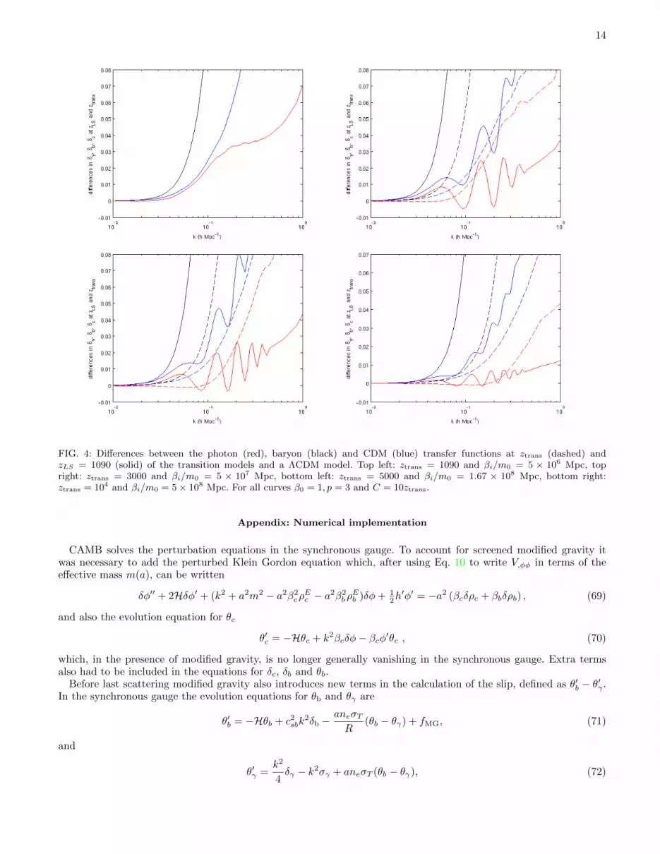
The simplest case to understand is that of the transition at last scattering since the evolution of perturbations isgoverned by the same modified equations right up to the creation of the CMB. In Fig. 4 we show the effect of modifiedgravity on the transfer functions. Superimposed on the oscillations in the photon transfer function that lead to theCMB anisotropies is an enhancement of power which increases with k. The peaks and troughs in the angular powerspectrum correspond to those in δ2
γ (shown in Fig. 5). We see that the odd peaks, corresponding to maxima in δγ ,are enhanced with respect to ΛCDM whilst the even ones, corresponding to minima in δγ , are reduced. So far thisagrees with what we observe in the Cl’s for the ztrans = 1090 case. The troughs in δ2
γ come from the zeros in δγ andso at these points the difference with ΛCDM vanishes. However, as we observed above the troughs in the Cl’s arealternately enhanced and reduced just like the peaks. We can understand this by noting that the Cl troughs, unlikethose in δ2
γ , are not zeros. This is because the anisotropy at a given l is created by many modes with wavenumbersgreater than that of the principal corresponding k-mode. The biggest contribution though will come from modes withonly slightly larger k which explains why the troughs preceding odd peaks are also higher and those preceding evenpeaks are also lower.
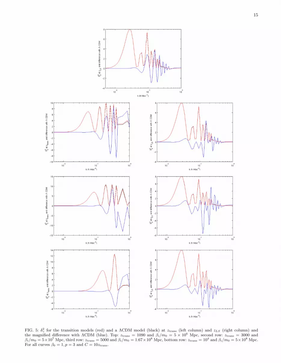
When the transition occurs before last scattering the picture is more complicated. The periods of enhancement andreduction of power in the Cl’s are different. As can be seen in Fig. 4 the effect of modified gravity on the photontransfer function at last scattering is no longer positive on all scales. There are instead oscillations in the differencewith ΛCDM and these are out of phase with those in the transfer function itself. This results in a more complicatedand unpredictable pattern of enhancements and reductions of power on different scales in the δ2
γ spectrum (see Fig. 5,right) and therefore the CMB. If however we look at the photon transfer functions at ztrans (Fig. 5, left) we see thatthey are always enhanced compared to the ΛCDM case and the effects on δ2
γ are the same as those for the transitionat last scattering. The only exception to this is the case with ztrans = 5000 where, because on small scales the maximaas well as the minima in the photon transfer function at ztrans are negative, the heights of the corresponding peaks inδ2γ are reduced. Therefore the different effects on the CMB of the models with earlier transitions are not the result of

11
FIG. 1: CMB angular power spectra of the transition model with ztrans = 1090 and βi/m0 = 5 × 10⁶ Mpc (red) and a ΛCDMmodel (black), zooming in on the 4th and 5th peaks.
modified gravity as such, but rather the period of effectively ΛCDM evolution following the transition during whichthe perturbations in δγ will have undergone oscillations. For example, a mode which has a maximum in δγ at thetransition might have become a minimum by recombination. As the maximum would have been higher compared tothe ΛCDM case so the minimum would be lower and this would generate an enhanced even peak in the Cl’s.
As can be seen in Fig. 6 the effect on the linear matter power spectrum is an increase of power on small scaleswhich is greater for higher values of βi/m0. This is due to the enhanced growth on small scales of the CDM (and toa lesser extent baryon) perturbations before last scattering (see Fig. 4) which occurs despite the fact that, as a resultof the very high effective mass of the field, effectively all scales (k . 1012 Mpc−1) are always outside the Comptonwavelength. This is because before the transition the couplings to matter are so strong that the factors containing β’sin Eq. (68) are still significant. The deviations from ΛCDM become noticeable at lower k values for later transitions.Roughly speaking, for cases with ∼ 1% deviation in the Cl’s, the relative difference in P (k) only becomes much morethan 1% at about k = 0.1h Mpc−1. One should expect non-linear effects to become important on smaller scales earlierthan in the ΛCDM model, therefore non-linear structures on small scales form earlier in the models we consider inthis paper.
It should be noted that for the cases shown, for which β0 = 1, the effect of the coupling after the transition isnegligible and the observed modifications to the matter power spectrum are entirely due to the anomalous growthbefore the transition at ztrans after which the equations governing the evolution of linear perturbations are effectivelythose of a ΛCDM model. We also note that reducing the value of C (while keeping the other parameters fixed), andtherefore extending the duration of the transition, results in smaller deviations from ΛCDM, particularly on smallerscales.
Compared to the constraints coming from the local tests and the variation of particle masses, the CMB probesa different part of the parameter space of the model. For values of the coupling β of order of unity and masses ofthe order of 1 Mpc−1, there is no effect on the CMB whereas the parameters are excluded by lunar ranging tests.However, if the coupling can take very large values prior to recombination (e.g. β ∼ 1014 for ztrans ∼ 104) then theCMB constrains the model more strongly than all the local tests.

12
FIG. 2: CMB angular power spectra of the transition model with ztrans = 3000 and βi/m0 = 5 × 10⁷ Mpc (red) and a ΛCDMmodel (black), zooming in on the 5th and 6th peaks.
B. Generalised chameleons
For the generalised chameleon models we find that for parameters satisfying the constraints given in sections II Dand II E there are no visible effects on the CMB but the matter power spectrum is affected in the usual way. In Figs.6 and 7 we can show results for an example case ruled out by the BBN constraint. The enhanced growth in P (k) onsmall scales is greater than each of the transition examples but the effects on the Cl’s are much smaller. However, wealso see that as the difference in the photon transfer function is always positive the amplitude of the peaks in δ2
γ isalternately enhanced and reduced and the oscillations in the relative difference of the Cl’s are in phase with those ofthe model with a transition at last scattering. This shows that the effects have the same origin.
In contrast to the transition models, we therefore find that the CMB does not provide complementary, additionalconstraints on generalised chameleons.
V. CONCLUSIONS
We have studied models of modified gravity where the screening effects at late time and locally in the solar systemstill allow for observable effects on cosmological perturbations prior to the recombination era.
We have investigated two types of models: the generalised chameleons with an increasing coupling to matter in thepast and a new transition model where the coupling to matter is significantly larger before recombination comparedto late times. We have presented analytical estimates and full numerical results using a modified version of CAMBwhich takes into account the effects of modified gravity. We find that even when the constraints from local tests aresatisfied the transition model can produce percent level deviations from ΛCDM in the CMB angular power spectrumand that these deviations take the characteristic form of alternating enhancements and reductions of power. For thegeneralised chameleons though it appears that models satisfying the BBN and local test constraints cannot leaveobservable signatures in the CMB. We should emphasise that local constraints and the BBN constraints are alreadyquite strong constraints. The examples we have considered here predict only small deviations (at most a few percent)of the CMB anisotropies from the ΛCDM model.
In both the transition and the generalised chameleon models, the effective sound speed of the coupled baryon–
13
FIG. 3: Relative differences between the Cl’s of the transition models and that of a ΛCDM model. Red: βb = βc, blue: βb = 0,green: βc = 0. Top left: ztrans = 1090 and βi/m0 = 5 × 10⁶ Mpc; top right: ztrans = 3000 and βi/m0 = 5 × 10⁷ Mpc; bottomleft: ztrans = 5000 and βi/m0 = 1.67 × 10⁸ Mpc; bottom right: ztrans = 104 and βi/m0 = 5 × 10⁸ Mpc. For all curves β0 = 1,p = 3 and C = 10ztrans.
photon plasma is the same as it is in the ΛCDM model to high accuracy. Therefore, the sound horizon is the same. Asa consequence, there are no shifts of the acoustic peaks in the CMB or the peaks in the baryonic acoustic oscillations.For the models we considered here, we were not able to find an example for which the sound speed differs significantlyfrom the ΛCDM value without violating the local or BBN constraints. An additional consequence is that the µ–distortion of the CMB spectrum generated by the dissipation of the acoustic oscillations is the same as in ΛCDM[38].
The effects on the matter power spectrum for both models are the same: an enhancement of power on small lengthscales (large wave numbers). On the other hand, the predictions for the CMB anisotropy differ between the models.Therefore it may be possible to distinguish different models of modified gravity using the CMB.
VI. ACKNOWLEDGEMENTS
PB acknowledges support from the Agence Nationale de la Recherche under contract ANR 2010 BLANC 0413 01.The work of CvdB is supported by the Lancaster-Manchester-Sheffield Consortium for Fundamental Physics underSTFC grant ST/J000418/1. ACD is supported in part by STFC. The work of SC has been supported by the WienerAnspach foundation, the Alexander von Humboldt foundation and the mandat de retour program of the BelgianScience Policy (BELSPO). GS is supported by an STFC doctoral fellowship.
14
FIG. 4: Differences between the photon (red), baryon (black) and CDM (blue) transfer functions at ztrans (dashed) andzLS = 1090 (solid) of the transition models and a ΛCDM model. Top left: ztrans = 1090 and βi/m0 = 5 × 10⁶ Mpc, topright: ztrans = 3000 and βi/m0 = 5 × 10⁷ Mpc, bottom left: ztrans = 5000 and βi/m0 = 1.67 × 10⁸ Mpc, bottom right:ztrans = 104 and βi/m0 = 5 × 10⁸ Mpc. For all curves β0 = 1, p = 3 and C = 10ztrans.
Appendix: Numerical implementation
CAMB solves the perturbation equations in the synchronous gauge. To account for screened modified gravity itwas necessary to add the perturbed Klein Gordon equation which, after using Eq. 10 to write V,φφ in terms of theeffective mass m(a), can be written
δφ′′ + 2Hδφ′ + (k2 + a2m2 − a2β2cρEc − a2β2
bρEb )δφ+ 1
2h′φ′ = −a2 (βcδρc + βbδρb) , (69)
and also the evolution equation for θc
θ′c = −Hθc + k2βcδφ− βcφ′θc , (70)
which, in the presence of modified gravity, is no longer generally vanishing in the synchronous gauge. Extra termsalso had to be included in the equations for δc, δb and θb.
Before last scattering modified gravity also introduces new terms in the calculation of the slip, defined as θ′b − θ′γ .In the synchronous gauge the evolution equations for θb and θγ are
θ′b = −Hθb + c2sbk2δb −
aneσTR
(θb − θγ) + fMG, (71)
and
θ′γ =k2
4δγ − k2σγ + aneσT (θb − θγ), (72)
15
FIG. 5: δ2γ for the transition models (red) and a ΛCDM model (black) at ztrans (left column) and zLS (right column) andthe magnified difference with ΛCDM (blue). Top: ztrans = 1090 and βi/m0 = 5 × 10⁶ Mpc, second row: ztrans = 3000 andβi/m0 = 5×10⁷ Mpc, third row: ztrans = 5000 and βi/m0 = 1.67×10⁸ Mpc, bottom row: ztrans = 104 and βi/m0 = 5×10⁸ Mpc.For all curves β0 = 1, p = 3 and C = 10ztrans.

16
FIG. 6: Relative differences between the matter power spectra of the modified gravity models and that of a ΛCDM model.Transition models: ztrans = 1090 and βi/m0 = 5× 10⁶ Mpc (red), ztrans = 3000 and βi/m0 = 5× 10⁷ Mpc (blue), ztrans = 5000and βi/m0 = 1.67 × 10⁸ Mpc (green), ztrans = 104 and βi/m0 = 5 × 10⁸ Mpc (red dashed) and a generalised chameleon modelwith m0 = 108, β0 = 9 × 10⁷, p = 3 and b = 2 (blue dash-dotted).
where c2sb is the adiabatic sound speed of the baryons (not to be confused with c2s, the sound speed of the coupledbaryon-photon fluid) and we have introduced the notation
fMG ≡ βbk2δφ− βbφ′θb (73)
corresponding to the additional terms due to screened gravity. During the tight coupling regime the Thomson dragterms in Eqs. 71 and 72 take very large values making these equations difficult to integrate numerically. In CAMBan alternative form of these equations is used which is valid in the regime τc τ and kτc 1. In the following wefollow [45] to derive the equivalent set of equations in the presence of screened modified gravity. The first step is touse Eq. 72 to write
(θb − θγ)/τc = −θ′γ + k2
(1
4δγ − σγ
), (74)
and then substitute the corresponding term into Eq. 71. One gets
θ′b = −a′
aθb + c2sbk
2δb −Rθ′γ +Rk2
(1
4δγ − σγ
)+ fMG . (75)
Then one can rewrite θ′γ = θ′b + (θ′γ − θ′b) in Eq. 74, and replace (θ′γ − θ′b) by using Eq. 75. By defining the functions
f ≡ τc1 +R
(76)
and
g ≡ −a′
aθb + c2sbk
2δb −Rθ′γ +Rk2(1
4δγ − σγ) + fMG , (77)
one obtains
θb − θγ = f [g − (fg)′] +O(τ3c ) , (78)
17
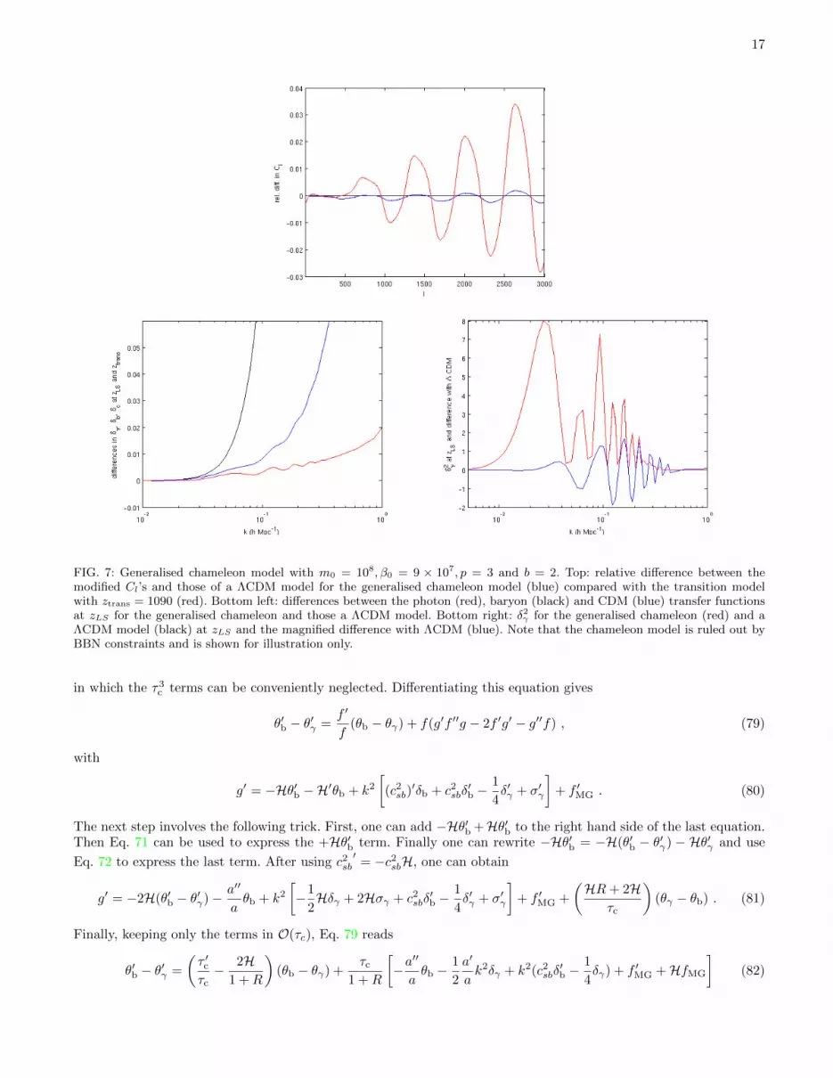
FIG. 7: Generalised chameleon model with m0 = 108, β0 = 9 × 10⁷, p = 3 and b = 2. Top: relative difference between themodified Cl’s and those of a ΛCDM model for the generalised chameleon model (blue) compared with the transition modelwith ztrans = 1090 (red). Bottom left: differences between the photon (red), baryon (black) and CDM (blue) transfer functionsat zLS for the generalised chameleon and those a ΛCDM model. Bottom right: δ2γ for the generalised chameleon (red) and aΛCDM model (black) at zLS and the magnified difference with ΛCDM (blue). Note that the chameleon model is ruled out byBBN constraints and is shown for illustration only.
in which the τ3c terms can be conveniently neglected. Differentiating this equation gives
θ′b − θ′γ =f ′
f(θb − θγ) + f(g′f ′′g − 2f ′g′ − g′′f) , (79)
with
g′ = −Hθ′b −H′θb + k2
[(c2sb)
′δb + c2sbδ′b −
1
4δ′γ + σ′γ
]+ f ′MG . (80)
The next step involves the following trick. First, one can add −Hθ′b +Hθ′b to the right hand side of the last equation.Then Eq. 71 can be used to express the +Hθ′b term. Finally one can rewrite −Hθ′b = −H(θ′b − θ′γ) − Hθ′γ and use
Eq. 72 to express the last term. After using c2sb′
= −c2sbH, one can obtain
g′ = −2H(θ′b − θ′γ)− a′′
aθb + k2
[−1
2Hδγ + 2Hσγ + c2sbδ
′b −
1
4δ′γ + σ′γ
]+ f ′MG +
(HR+ 2H
τc
)(θγ − θb) . (81)
Finally, keeping only the terms in O(τc), Eq. 79 reads
θ′b − θ′γ =
(τ ′cτc− 2H
1 +R
)(θb − θγ) +
τc1 +R
[−a′′
aθb −
1
2
a′
ak2δγ + k2(c2sbδ
′b −
1
4δγ) + f ′MG +HfMG
](82)

18
During the tight coupling regime θb is obtained by integrating
θ′b =1
1 +R
[−a′
aθb + c2sbk
2δb + k2R(1
4δγ − σγ) + fMG
]+
R
1 +R(θ′b − θ′γ) , (83)
which is derived directly from the Eq. 75 and in which the slip is given by Eq 82.Compared to the standard general relativistic case we get two contributions from modified gravity. The first is the
term fMG in Eq. 83 and the second comes from an additional τc(f ′MG +HfMG)/(1 +R) term in the slip.The derivative of fMG is given by
f ′MG = β′bkδφ+ βbkδφ′ − β′bφ′θb − βbφ
′′θb − βbφ′θ′b (84)
= β′bkδφ+ βbkδφ′ − β′bφ′θb − βbφ
′′θb − βbφ′(−a
′
aθb + c2sbk
2δb + fMG) +R
τcβbφ
′(θb − θγ) , (85)
where the last equation is obtained after using Eq. 71.To get an equation for θ′γ we can use Eq. 71 to express the drag term as
(θb − θγ)/τc = −R(θ′b +Hθb − c2sbk2δb − fMG) (86)
and then substitute this in Eq. 72 to obtain
θ′γ =k2
4δγ − k2σγ −R(θ′b +Hθb − c2sbk2δb − fMG). (87)
This last equation is used at all times in CAMB with θ′b determined by Eq. 83 during the tight-coupling regime andby Eq. 71 otherwise.
We have also modified the source terms. These are computed by integrating by parts the line of sight integral givingthe CMB temperature multipoles today. This is required in CAMB for the Bessel functions to be the only l-dependentvariables in the remaining line of sight integral (see Seljak and Zaldarriaga for more details). However, we find thatmodifying the source terms does not have any visible effects on the CMB angular power spectrum for the models andparameters we have considered.
Finally, in order to avoid the time-consuming numerical integration of the field perturbations at early times whenthey oscillate quickly, we have introduced the approximation
δφ = − βcδρc + βbδρbk2
a2 +m2 − β2cρEc − β2
bρEb
(88)
when the condition
(k2 + a2m2 − a2β2cρEc − a2β2
bρEb )δφ |2Hδφ′ + 1
2h′φ′| (89)
is satisfied.
[1] A. G. Riess et al. [Supernova Search Team Collaboration], Astron. J. 116 (1998) 1009 [astro-ph/9805201].[2] J. Ellis and K. A. Olive, In *Bertone, G. (ed.): Particle dark matter* 142-163 [arXiv:1001.3651 [astro-ph.CO]].[3] E. J. Copeland, M. Sami and S. Tsujikawa, Int. J. Mod. Phys. D 15 (2006) 1753 [hep-th/0603057].[4] T. Clifton, P. G. Ferreira, A. Padilla and C. Skordis, Phys. Rept. 513 (2012) 1 [arXiv:1106.2476 [astro-ph.CO]].[5] J. Khoury, B. Jain:2012tn arXiv:1011.5909 [astro-ph.CO].[6] E. G. Adelberger, B. R. Heckel and A. E. Nelson, Ann. Rev. Nucl. Part. Sci. 53 (2003) 77 [hep-ph/0307284].[7] E. G. Adelberger [EOT-WASH Group Collaboration], hep-ex/0202008.[8] R. Pourhasan, N. Afshordi, R. B. Mann and A. C. Davis, JCAP 1112 (2011) 005 [arXiv:1109.0538 [astro-ph.CO]].[9] B. Jain, V. Vikram and J. Sakstein, Astrophys. J. 779 (2013) 39 [arXiv:1204.6044 [astro-ph.CO]].
[10] J. G. Williams, S. G. Turyshev and D. H. Boggs, Phys. Rev. Lett. 93 (2004) 261101 [gr-qc/0411113].[11] J. G. Williams, S. G. Turyshev and D. Boggs, Class. Quant. Grav. 29 (2012) 184004 [arXiv:1203.2150 [gr-qc]].[12] J. G. Williams, S. G. Turyshev and T. W. Murphy, Jr., Int. J. Mod. Phys. D 13 (2004) 567 [gr-qc/0311021].[13] J. G. Williams, S. G. Turyshev and D. H. Boggs, Int. J. Mod. Phys. D 18 (2009) 1129 [gr-qc/0507083].[14] J. Khoury and A. Weltman, Phys. Rev. Lett. 93 (2004) 171104 [arXiv:astro-ph/0309300].[15] J. Khoury and A. Weltman, Phys. Rev. D 69, 044026 (2004) [arXiv:astro-ph/0309411].[16] Ph. Brax, C. van de Bruck, A-C Davis, J. Khoury and A. Weltman, Phys.Rev.D70:123518,2004 [arXiv: astro-ph/0408415]
19
[17] D. F. Mota and D. J. Shaw, Phys. Rev. Lett. 97 (2006) 151102 [arXiv:hep-ph/0606204].[18] A. W. Brookfield, C. van de Bruck and L. M. H. Hall, Phys. Rev. D 74, 064028 (2006) [hep-th/0608015].[19] T. Faulkner, M. Tegmark, E. F. Bunn and Y. Mao, Phys. Rev. D 76, 063505 (2007) [astro-ph/0612569].[20] P. Brax, C. van de Bruck, A. -C. Davis, D. J. Shaw, Phys. Rev. D78 (2008) 104021. [arXiv:0806.3415 [astro-ph]].[21] S. A. Appleby and R. A. Battye, Phys. Lett. B 654, 7 (2007) [arXiv:0705.3199 [astro-ph]].[22] W. Hu, I. Sawicki, Phys. Rev. D76 (2007) 064004. [arXiv:0705.1158 [astro-ph]].[23] K. Hinterbichler, J. Khoury, Phys. Rev. Lett. 104 (2010) 231301. [arXiv:1001.4525 [hep-th]].[24] M. Pietroni, Phys. Rev. D 72 (2005) 043535 [astro-ph/0505615].[25] K. Hinterbichler, J. Khoury, A. Levy and A. Matas, Phys. Rev. D 84 (2011) 103521 [arXiv:1107.2112 [astro-ph.CO]].[26] P. Brax, C. van de Bruck, A. -C. Davis, B. Li, B. Schmauch and D. J. Shaw, Phys. Rev. D 84 (2011) 123524 [arXiv:1108.3082
[astro-ph.CO]].[27] P. Brax, C. van de Bruck, A. -C. Davis, D. Shaw, Phys. Rev. D82 (2010) 063519. [arXiv:1005.3735 [astro-ph.CO]].[28] P. Brax, C. van de Bruck, A. -C. Davis, B. Li and D. J. Shaw, Phys. Rev. D 83 (2011) 104026 [arXiv:1102.3692 [astro-
ph.CO]].[29] P. Brax, A. -C. Davis, B. Li, H. A. Winther and G. -B. Zhao, JCAP 1304 (2013) 029 [arXiv:1303.0007 [astro-ph.CO]].[30] P. Brax, A. -C. Davis, B. Li, H. A. Winther and G. -B. Zhao, JCAP 1210 (2012) 002 [arXiv:1206.3568 [astro-ph.CO]].[31] A. -C. Davis, B. Li, D. F. Mota and H. A. Winther, Astrophys. J. 748 (2012) 61 [arXiv:1108.3081 [astro-ph.CO]].[32] J. R. Pritchard and A. Loeb, Rept. Prog. Phys. 75 (2012) 086901 [arXiv:1109.6012 [astro-ph.CO]].[33] S. Furlanetto, A. Lidz, A. Loeb, M. McQuinn, J. Pritchard, P. Shapiro, J. Aguirre and M. Alvarez et al., arXiv:0902.3259
[astro-ph.CO].[34] S. Clesse, L. Lopez-Honorez, C. Ringeval, H. Tashiro and M. H. G. Tytgat, Phys. Rev. D 86 (2012) 123506 [arXiv:1208.4277
[astro-ph.CO]].[35] P. Brax, S. Clesse and A. -C. Davis, JCAP 1301 (2013) 003 [arXiv:1207.1273 [astro-ph.CO]].[36] P. Brax, A. -C. Davis and B. Li, Phys. Lett. B 715 (2012) 38 [arXiv:1111.6613 [astro-ph.CO]].[37] P. Brax, A. -C. Davis, B. Li and H. A. Winther, Phys. Rev. D 86 (2012) 044015 [arXiv:1203.4812 [astro-ph.CO]].[38] C. van de Bruck and G. Sculthorpe, Phys. Rev. D 87, 044004 (2013) [arXiv:1210.2168 [astro-ph.CO]].[39] P. Brax and P. Valageas, arXiv:1305.5647 [astro-ph.CO].[40] K. A. Olive, M. Pospelov, Phys. Rev. D77 (2008) 043524. [arXiv:0709.3825 [hep-ph]].[41] P. F. Bedaque, T. Luu and L. Platter, Phys. Rev. C 83 (2011) 045803 [arXiv:1012.3840 [nucl-th]].[42] J. C. Berengut, V. V. Flambaum and V. F. Dmitriev, Phys. Lett. B 683 (2010) 114 [arXiv:0907.2288 [nucl-th]].[43] P. Brax, A. -C. Davis, Phys. Rev. D85, 023513 (2012).[44] CAMB Code Home Page, http://camb.info/.[45] C.-P. Ma and E. Bertschinger, Astrophys. J. 455, 7 (1995).