Modelling trimmed fat from commercial primal cuts

Y.C.S.M. Laurenson , B.J. Walmsley, V.H. Oddy, P.L. Greenwood and M.J. McPhee

NSW Department of Primary Industries, Trevenna Rd, Armidale, NSW 2351 Email: malcolm.mcphee@dpi.nsw.gov.au

Abstract: A number of studies over the last five years have been conducted to determine total body fat (kg) in cattle and subsequently retail beef yield. Abattoirs are not consistent in the quantity of fat they trim off commercial bone-out primal cuts (e.g., striploin, cube roll etc.). The trimming of fat on a single primal by different abattoirs can range from 3 to 7 mm. If a relationship between mm of fat trimmed and kg of fat removed from primal cuts was developed then total body fat (kg) from commercial slaughters could then be estimated. The estimate of total body fat would assist in establishing a method for determining denuded yield which would then be used as a national standard for describing retail beef yield independent of abattoir. The estimate of retail beef yield would then be implemented into the BeefSpecs calculator.

The objective of this study was to develop a relationship between trim (mm) and kg of fat removed. Images from X-ray computed tomography (CT) scans of 8 primal cuts from 10 Angus steers were manipulated to generate CT scan images for trims ranging from 0 to 15 mm. These images were analysed to determine the weights of fat and muscle in each primal, which were subsequently converted to ratios. Eleven non-linear growth functions were fitted to the generated data and compared to assess their ability to accurately predict the trimmed muscle ratio. The Schnute growth function was identified as the best fit model with the lowest AICc (corrected Akaike’s Information Criterion) (AICc = -480.879, adjusted R2 = 0.945, RMSE = 0.023). The proposed model (and parameter estimates) can be used to estimate the kg of fat removed and therefore aid in the estimation of retail beef yield.

Keywords: CT scanning, images, retail beef yield, growth functions

20th International Congress on Modelling and Simulation, Adelaide, Australia, 1–6 December 2013 www.mssanz.org.au/modsim2013

600

Laurenson et al., Modelling trimmed fat from commercial primal cuts

1. INTRODUCTION

A number of studies (unpublished) over the last five years have been conducted to determine total body fat (kg) in cattle and subsequently retail beef yield. Abattoirs are not consistent in the quantity of fat they trim off commercial bone-out primal cuts (e.g., Striploin, Cube Roll etc.). The trimming of fat on a single primal by different abattoirs can range from 3 to 7 mm. If a relationship between mm of fat trimmed and kg of fat removed was developed then total body fat (kg) from commercial slaughters could be estimated. The estimate of total body fat would assist in establishing a method for determining denuded yield to be used as a national standard for describing retail beef yield independent of abattoir. The estimate of retail beef yield would then be implemented into the BeefSpecs calculator (Walmsley et al., 2011). Thus, the purpose of this study is to develop a model that will convert mm of fat trimmed off primal cuts to kg of fat removed.

2. MATERIAL AND METHODS

2.1 Animal management & slaughter

This study was carried out using 10 weaned Angus steers. From weaning, five steers were fed pasture and five steers were fed pasture plus high energy pellets (12.3 MJ ME/kg DM, 110g CP/kg DM) at 1% live weight for 168 days. All steers were then backgrounded (management of post-weaning growth to produce feeder steer that meet feedlot entry specifications) until 18 months of age when they were feedlot fed for 250 days until slaughter in August 2010. Live weight did not differ due to nutritional treatment at any stage (Greenwood et al., 2011). The average (± s.e.) age, live weight and empty body weight at slaughter were 788 (± 4.6) days, 805 (± 23.6) kg and 688 (± 20.2) kg, respectively. After slaughter, the left carcass sides were cut into 20 primal cuts. Primal cuts were vacuum packed and transported (at 1-2°C) to the University of New England Meat Sciences CT unit where they were weighed and X-ray computed tomography (CT) scanned.

2.2 CT scanning

Primal cuts were scanned using a Picker Ultra Z Spiral CT scanner (Philips Medical Imaging Australia, Sydney NSW). The X-ray tube operated at 130kV and 100mAs. A pitch of 1.5, field of view of 480 mm and cross-sectional thickness of 15 mm were used. The chuck primal exceeded the field of view and was consequently separated into sub-primal cuts (chuck inter and chuck sub). Further, the flank and chuck sub exceeded the maximum length of the scanner table and consequently two contiguous scans were performed.

2.3 Image analysis

CT scans from 8 primal cuts (Striploin, Rump, Eye Round, Cube Roll, Chuck Tender, Blade, Chuck and Brisket) were analysed using Image J software (National Institutes of Health, USA). The pixel to mm scale was set for each animal using the subcutaneous fat at the P8 (rump) site (measured by ultrasound) and the corresponding image. This led to a constant scale being used (2 pixels = 1 mm).

2.4 Tissue composition

To infer the tissue composition of these primal cuts, histograms of the grey scale cross-sectional images were created and the resultant bimodal distribution was used to determine threshold values for fat and muscle. However, each cross-section does not contain an equal amount of information from which to estimate threshold values, and thus threshold values were weighted according to cross-section area to increase accuracy. The average (± s.e.) upper threshold for fat (threshold 1) and muscle (threshold 2) was 120 (± 0.5) and 214 (± 0.8), respectively. As such, tissue was identified as fat if the grey scale units fell within the range between 0 and threshold 1, or as muscle for the range between threshold 1 and threshold 2.

2.5 Tissue and total primal weight

Tissue weight for each section was calculated as (Navajas et al., 2010):

Tissue weight (mg) = Tissue area (mm2) * cross-sectional thickness (mm) * tissue density (mg/mm3) (1)

where, tissue (fat and muscle) areas were determined according to the thresholds derived above (section 2.4), cross-sectional thickness (15 mm), and assuming fixed values for tissue density (Fat = 0.918mg/mm3, Muscle = 1.062mg/mm3) (Nord & Payne, 1995; Frigerio et al., 1972).

Total tissue weights for each primal were then calculated as the sum of the corresponding tissue weights for each cross-section, and the total primal weight was calculated as the sum of the total tissue (fat and muscle) weights for each primal.

601

Laurenson et al., Modelling trimmed fat from commercial primal cuts

Fat

Muscle

1mm

1mm

1mm

0mm

Initial image

0mm trim

1, 2, 3… mm e.g. 5mm trim

5mm trim

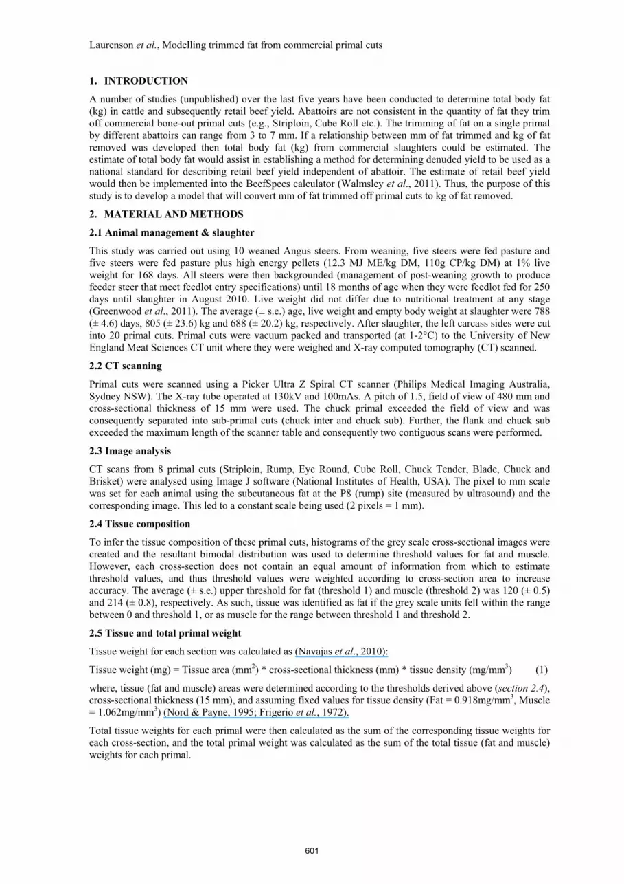
Figure 1. Overview of the procedure carried out within Image J to generate images of trimmed fat and

muscle for trims ranging from 0 to 15mm fat depth. Solid arrows indicate progression of procedure; dashed arrows indicate direction of image translation. Example provided is for section 8 of the Rump

for animal 1.

2.6 Image manipulation

Figure 1 provides an overview of the process used to generate cross-section images with specific depths of fat (trim, mm). In short, each cross-section was analysed to determine its tissue composition (section 2.4), and separate cross-section images created for fat and lean muscle. However, it is improbable that lean muscle can be completely separated from fat within the abattoir. Consequently the 0 mm trim cross-section image was generated using templates of the muscle translated by + or – 1 mm on the x-axis and – 1 mm on the y-axis. These templates were then superimposed upon each other and the resultant template subtracted from the initial cross-section image to generate an image of the trimmed fat for a 0 mm trim. A cross-section image for the trimmed muscle was then created by subtracting the 0 mm fat image from the initial greyscale cross-section image. Images of trimmed fat and muscle for increasing trim were generated using the same procedure with the addition of including templates shifted at +1 mm intervals on the y-axis. Trimmed fat and muscle cross-section images were thereby generated for trims ranging from 0 to 15 mm at 1 mm intervals.

2.7 Trimmed fat and muscle weight/ratio

The cross-section images of trimmed fat from trims ranging from 0 mm to 15 mm were analysed as described above (section 2.5) to obtain their weight (mg).

The cross-section weight (mg) of trimmed muscle was consequently calculated as:

Trimmed muscle (mg) = total cross-section (mg) – trimmed fat (mg) (2)

Primal weights for trimmed fat and muscle are then calculated as the sum of each primal’s cross-section images. Ratios for trimmed fat/total primal, and trimmed muscle/total primal were calculated from the estimated weights for each primal and each animal.

2.8 Modelling the trimmed fat and muscle ratios

Data generated (Equations 1 and 2; sections 2.6 and 2.7) was used to estimate parameters for 11 non-linear growth functions (Table 1). These parameter estimates define the y-intercept, upper asymptote and growth rate. However, the lean muscle ratio varies across primals and animals, leading to variation in parameter estimates (i.e. parameter estimates are not constant). Thus, parameters were described as their linear regression with lean muscle ratio, effectively doubling the number of parameters requiring estimation (gradient and y-intercept of linear regression for each of the parameters given in Table 1). Mircosoft®-Excel

602

Laurenson et al., Modelling trimmed fat from commercial primal cuts

Table 1. Non-linear growth functions (a, b, c and d are parameters to be estimated; x = trim (mm); p = number of parameters). Adapted from Fekedulegn et al. (1999) & Khamis et al. (2005).

Model Equation pNegative exponential

))exp(1()( bxaxf −−= 2

Monomolecular ))exp(1()( cxbaxf −−= 3

Mitscherlich xbcaxf −=)( 3

Gompertz ))exp(exp()( cxbaxf −−= 3

Logistic ))exp(1/()( cxbaxf −+= 3

Schnute dcxbaxf ))exp(()( += 4

Weibull )exp()( dcxbaxf −−= 4

Richards dcxbaxf /1))exp(1/()( −== 4

Chapman-Richards

)1/(1))exp(1()( dcxbaxf −−−= 4

von Bertalanffy )1/(11 ))exp(()( dd cxbaxf −− −−= 4

Morgan-Mercer-Flodin

)/()()( dd xcaxbcxf ++= 4

Table 2. Measured and CT scan estimation of primal weights (kg). Primal weights are provided for each animal as well as their mean average (± s.e.).

Beef Primal Cuts Animal 1 2 3 4 5 6 7 8 9 10 Average (± s.e.)

Measured Hind quarter

Striploin 11.88 10.39 9.00 8.72 11.01 10.07 11.72 10.00 9.96 11.44 10.42 (0.34)

Rump 12.26 11.02 10.66 11.66 11.52 12.80 13.48 12.19 11.55 11.67 11.88 (0.26)

Eye Round 3.14 3.12 2.56 2.95 3.45 3.51 3.77 3.76 2.93 3.23 3.24 (0.12)

Fore quarter

Cube Roll 3.63 3.64 2.98 3.95 4.53 3.62 4.10 4.41 3.60 3.97 3.84 (0.14)

Chuck Tender 1.81 1.66 1.74 1.93 2.29 2.09 2.43 1.64 1.93 2.62 2.01 (0.11)

Blade 10.65 8.47 8.90 11.13 11.23 12.46 12.48 10.97 8.58 10.74 10.56 (0.46)

Chuck 33.34 28.46 27.07 30.91 35.04 32.86 36.30 33.18 29.36 41.11 32.76 (1.31)

Brisket 31.19 24.06 21.50 22.60 26.46 24.35 26.57 27.37 22.05 24.15 25.03 (0.93)

CT scan estimation Hind quarter

Striploin 11.87 10.41 9.07 8.73 11.05 10.02 11.73 9.98 9.96 11.44 10.42 (0.34)

Rump 12.26 11.04 10.69 11.70 11.51 12.90 13.65 12.29 11.53 11.73 11.93 (0.28)

Eye Round 3.12 3.13 2.54 2.94 3.41 3.46 3.72 3.75 2.90 3.20 3.22 (0.12)

Fore quarter

Cube Roll 3.61 3.71 2.99 4.03 4.56 3.66 4.15 4.43 3.63 3.98 3.87 (0.14)

Chuck Tender 1.77 1.64 1.75 1.93 2.29 2.12 2.44 1.62 1.92 2.60 2.01 (0.11)

Blade 10.65 8.50 8.97 11.19 11.31 12.56 12.50 11.02 8.60 10.75 10.60 (0.47)

Chuck 33.66 28.79 27.44 31.24 35.46 33.28 36.80 33.27 29.65 41.51 33.11 (1.32)

Brisket 31.18 24.24 21.72 17.04 26.60 24.69 26.86 27.50 22.11 24.39 24.63 (1.21)

Solver was used to estimate the parameter values which resulted in the algebraically lowest corrected Akaike’s Information Criterion (AICc).

Akaike’s information criterion (AIC) was calculated as (Akaike, 1974):

AIC = n * ln(Re) + 2p (3)

where, n is the sample size [n = 1280 (animals * primals * trims)], p is the number of parameters [4 to 8 (doubling of parameters given in Table 1 due to linear regression with lean muscle ratio)] and Re is the residual sum of squares defined by:

=

−=n

iiie omR

1

2)( (4)

where, oi is the observed trimmed muscle ratio, mi is the modelled trimmed muscle ratio for the ith observation.

AICc is consequently calculated as (Hurvich & Tsai, 1989):

1

)1(2

−−++=

pn

ppAICAICc (5)

The differing growth functions were subsequently compared by assessing their AICc values, adjusted R2 and root mean square error (RMSE) to determine the most appropriate growth function to describe the relationship between trimmed muscle ratio and trim (mm).

Adjusted R2 was calculated as:

22 (1 )( 1)

11

R nAdjustedR

n p

− −= −− −

(6)

where, R2 is the coefficient of determination

603

Laurenson et al., Modelling trimmed fat from commercial primal cuts

Table 3. Average (± s.e.) ratio of trimmed muscle weight to total primal weight for each of the 8 primal cuts. Values (rounded to 3 decimal places) are provided for lean, 0mm, 1mm, 2mm,…, 14mm and 15mm trims.

Trim (mm)

Beef Primal Cuts Hind quarter Fore quarter

Striploin Rump Eye Round

Cube Roll Chuck Tender

Blade Chuck Brisket

lean 0.657 (0.015)

0.604 (0.010)

0.749 (0.006)

0.752 (0.009)

0.825 (0.016)

0.734 (0.007)

0.654 (0.009)

0.485 (0.010)

0 0.698 (0.015)

0.652 (0.010)

0.795 (0.007)

0.835 (0.008)

0.877 (0.015)

0.786 (0.006)

0.718 (0.009)

0.552 (0.011)

1 0.710 (0.015)

0.662 (0.010)

0.807 (0.006)

0.852 (0.007)

0.889 (0.014)

0.798 (0.007)

0.734 (0.008)

0.575 (0.011)

2 0.728 (0.015)

0.678 (0.010)

0.824 (0.006)

0.874 (0.006)

0.904 (0.013)

0.815 (0.007)

0.753 (0.008)

0.601 (0.011)

3 0.746 (0.015)

0.694 (0.010)

0.840 (0.007)

0.893 (0.006)

0.917 (0.012)

0.829 (0.007)

0.770 (0.007)

0.625 (0.011)

4 0.764 (0.015)

0.709 (0.011)

0.854 (0.007)

0.909 (0.005)

0.928 (0.010)

0.842 (0.007)

0.785 (0.007)

0.647 (0.012)

5 0.781 (0.015)

0.724 (0.011)

0.868 (0.008)

0.923 (0.004)

0.938 (0.009)

0.853 (0.007)

0.793 (0.007)

0.666 (0.012)

6 0.798 (0.015)

0.738 (0.011)

0.879 (0.008)

0.934 (0.004)

0.947 (0.008)

0.863 (0.007)

0.809 (0.006)

0.685 (0.011)

7 0.814 (0.015)

0.751 (0.011)

0.889 (0.009)

0.944 (0.003)

0.953 (0.007)

0.871 (0.007)

0.819 (0.006)

0.701 (0.011)

8 0.830 (0.015)

0.764 (0.011)

0.895 (0.009)

0.951 (0.003)

0.958 (0.007)

0.879 (0.006)

0.828 (0.006)

0.716 (0.011)

9 0.845 (0.014)

0.777 (0.011)

0.899 (0.010)

0.956 (0.003)

0.961 (0.007)

0.886 (0.006)

0.836 (0.005)

0.730 (0.011)

10 0.859 (0.014)

0.788 (0.011)

0.902 (0.009)

0.960 (0.003)

0.963 (0.007)

0.892 (0.006)

0.843 (0.005)

0.743 (0.011)

11 0.871 (0.013)

0.799 (0.011)

0.904 (0.009)

0.963 (0.002)

0.963 (0.006)

0.898 (0.006)

0.850 (0.005)

0.754 (0.011)

12 0.882 (0.013)

0.808 (0.011)

0.906 (0.009)

0.965 (0.002)

0.964 (0.006)

0.903 (0.006)

0.855 (0.005)

0.764 (0.011)

13 0.892 (0.012)

0.817 (0.011)

0.907 (0.009)

0.967 (0.002)

0.964 (0.006)

0.907 (0.006)

0.861 (0.005)

0.774 (0.011)

14 0.900 (0.011)

0.825 (0.011)

0.909 (0.009)

0.969 (0.002)

0.965 (0.006)

0.911 (0.006)

0.866 (0.005)

0.782 (0.010)

15 0.908 (0.011)

0.832 (0.011)

0.910 (0.009)

0.971 (0.002)

0.965 (0.006)

0.915 (0.006)

0.870 (0.004)

0.790 (0.010)

0

0.1

0.2

0.3

0.4

0.5

0.6

0.7

0.8

0.9

1

0 5 10 15

Trim (mm)

Tri

mm

ed

mu

scle

:To

tal p

rim

al w

eig

ht

Figure 2. Average lean muscle ratio (solid line) and average trimmed muscle ratio (dashed line) for 0 to

15mm trim on the Rump primal cut.

RMSE was calculated as:

eRRMSE

n= (7)

3. RESULTS

3.1 Validating CT scan estimated weights

Table 2 provides the measured and CT scan estimated weights for each primal, given as individual animal primal weights and as a mean average (± s.e). The estimation of primal weights using CT scanning was very accurate when making a comparison with the measured (observed) weights (R2 = 0.996).

3.2 Trimmed muscle ratio

Figure 2 gives the mean lean muscle ratio and mean trimmed muscle ratio (for 0 to 15 mm trim) for the Rump primal (given as an example of the relationship between trim and trimmed muscle ratio). Results from other primal cuts followed a similar profile differing only in the lean muscle ratio and the rate at which the trimmed muscle ratio approaches the upper asymptote. Table 3 provides the mean (± s.e.) trimmed muscle ratio for each of the 8 primal cuts and for lean, 0 mm, 1 mm, 2 mm,…, 14 mm and 15 mm trims.

604

Laurenson et al., Modelling trimmed fat from commercial primal cuts

Table 4. Parameter estimates (rounded to 3 decimal places) for differing growth functions. a, b, c and d are parameters to be estimated for the growth functions outlined in Table 1. r, s, t, u, v, w, y and z are parameters to be estimated for the linear regression between parameters a, b, c and d, and the lean muscle ratio (q) for individual primal cuts.

Growth Model Parameter No. of estimated

parameters a = rq + s b = tq + u c = vq + w d = yq + z

r s t u v w y z Negative

exponential 0.726 0.356 3.708 -0.562 4

Monomolecular 0.026 0.012 -11.01 -16.64 0.051 -0.048 6

Mitscherlich 0.424 0.655 -0.614 0.626 -0.043 0.933 6

Gompertz 0.014 0.005 -0.358 -3.670 0.012 -0.012 6

Logistic 0.416 0.639 -1.190 1.086 0.163 0.039 6

Schnute -7.550 7.810 -79.39 74.08 -0.021 -0.253 0.342 -0.331 8

Weibull 0.496 0.577 -0.531 0.537 0.029 0.066 0.191 1.069 8

Richard’s 0.407 0.654 -0.530 0.501 0.090 0.069 0.254 0.366 8

Chapman-Richards -0.063 0.065 -0.600 -1.517 0.028 -0.025 0.309 0.483 8

Von Bertalanffy 0.488 0.587 -0.060 0.056 0.071 0.069 0.022 0.938 8

Morgan-Mercer-Flodin

-6971 -2603 1.103 -0.016 6311 3247 0.459 0.385 8

Table 5. AICc, adjusted R2 and RMSE values for growth models fitted to trimmed muscle ratio data.

Model AICc Adjusted R2 RMSE Negative exponential 4931.950 0.295 0.191 Monomolecular -150.368 0.929 0.026

Mitscherlich -418.712 0.942 0.024

Gompertz -135.063 0.928 0.026

Logistic -416.166 0.942 0.024

Schnute -480.879 0.945 0.023

Weibull -421.865 0.943 0.024

Richards -437.315 0.848 0.023

Chapman-Richards -239.112 0.934 0.025

von Bertalanffy -436.777 0.943 0.023

Morgan-Mercer-Flodin -350.451 0.939 0.024

3.3 Parameter estimation and model fit

Table 4 provides the calculated parameter estimations for the growth functions described in Table 1.

Table 5 gives the AICc, adjusted R2 and RMSE for each of the growth functions investigated.

4. DISCUSSION

The Schnute growth function (Table 5) was identified as the best fit model (i.e. lowest AICc value = -480.879, highest adjusted R2 = 0.945, and lowest RMSE = 0.023). For all growth functions the AICc, adjusted R2 and RMSE altered in relation to each other, where reductions in adjusted R2 was evident as an increase in AICc and RMSE. However, there was one notable exception. The Richards function had the second lowest AICc value of -437.315 and RMSE of 0.023 whilst the adjusted R2 was 0.848. The Richards growth function provided a very good fit for the majority of the data. However, it was not flexible enough to accurately estimate trimmed muscle ratio for higher trim values, resulting in several outliers. These outliers had a large impact on the coefficient of determination, but not on calculations based on the residual sum of squares (i.e. residuals for outliers were diluted by the large number of very low residual values). These results highlight the importance of using more than one method to compare models. Further, the comparison between the AICc values for the negative exponential and the monomolecular growth functions (4931.95 and -150.368, respectively) highlights the necessity of including a parameter to determine the y-intercept. A mechanistic model, currently under development, will use the Schnute growth function to model trimmed fat to calculate total body fat and subsequently estimate retail beef yield which will be implemented into the BeefSpecs calculator (Walmsley et al., 2011).

4. CONCLUSION

The Schnute growth function (Schnute, 1981) was identified as the best fit model for estimating the relationship between trimmed muscle ratio and trim. Thus, the final model for estimating the trimmed muscle ratio is given as:

605

Laurenson et al., Modelling trimmed fat from commercial primal cuts

dcxbaxf ))exp(()( += (8)

where, f is the muscle ratio, x is the trim (mm), a = -7.55q + 7.81, b = -79.39q + 74.08, c = -0.02q – 0.25, d = 0.34q - 0.33, and q is the lean muscle ratio. The trimmed fat ratio is calculated as 1 – trimmed muscle ratio. Thus, if the trim (mm) and weight of the trimmed primal is known, then the weight of the trimmed fat can be calculated.

ACKNOWLEDGEMENTS

Funding to conduct this work from Meat and Livestock Australia and the CRC for Beef Genetic Technologies is gratefully acknowledged.

REFERENCES

Akaike, H. (1974). A new look at the statistical model identification. IEEE Transactions on Automatic Control, 19(6): 716-772.

Fekedulegn, D., M.P. Mac Siurtain, and J.J. Colbert (1999). Parameter estimation on nonlinear growth models in forestry. Silva Fennica, 33(4): 327-336.

Frigerio, N.A., R.F. Coley and M.J. Sampson (1972). Depth dose determinations I. Tissue-equivalent liquids for Standard Man and muscle. Physics in Medicine and Biology, 17(6): 792.

Greenwood P.L., J.P. Siddell, M. J. McPhee, B.J. Walmsley, G. Geeskink and D.W. Pethick (2011). Development of fat depots and associations with beef quality. Proceedings of the 8th International Symposium on the Nutrition of Herbivores (ISNH8). Adv Anim Biosci 2:498.

Hurvich, C.M.and C.L. Tsai (1989). Regression and time series model selection in small samples. Biometrica, 76: 297-307.

Khamis, A., Z. Ismail, K. Haron and A.T. Muhammad (2005). Nonlinear Growth Models for Modelling Oil Palm Yield Growth. Journal of Mathematics and Statistics, 1(3): 225-233.

Navajas, E.A., C.A. Glasbey, A.V. Fisher, D.W. Ross, J.J. Hyslop, R.I. Richardson, G. Simm, and R. Roehe (2010). Assessing beef carcass tissue weights using computed tomography spirals of primal cuts. Meat Science, 84: 30-38.

Nord, R.H. and R.K. Payne (1995) Body composition by dual–energy Xray absorptiometry – a review of the technology. Asia Pacific Journal of Clinical Nutrition, 4(1): 173-175.

Schnute, J. (1981). A versatile growth model with statistically stable parameters. Canadian Journal of Fisheries and Aquatic Sciences, 38: 1128-1140.

Walmsley, B.J., V.H. Oddy, M.J. McPhee, D.G. Mayer and W.A. McKiernan (2011). Development of the BeefSpecs fat calculator: A tool designed to assist decision making to increase on-farm and feedlot profitability. In ‘MODSIM 2011 International Congress on Modelling and Simulation.’ (F. Chan, D. Marinova and RS. Anderssen eds.). Modelling and Simulation Society of Australia and New Zealand. Perth Convention and Exhibition Centre, Perth, Australia. p 898–904.

606