A Universal Primal-Dual Convex Optimization Framework

Alp Yurtsever: Quoc Tran-Dinh; Volkan Cevher:

: Laboratory for Information and Inference Systems, EPFL, Switzerland{alp.yurtsever, volkan.cevher}@epfl.ch

; Department of Statistics and Operations Research, UNC, USAquoctd@email.unc.edu

Abstract

We propose a new primal-dual algorithmic framework for a prototypical con-strained convex optimization template. The algorithmic instances of our frame-work are universal since they can automatically adapt to the unknown Holdercontinuity degree and constant within the dual formulation. They are also guaran-teed to have optimal convergence rates in the objective residual and the feasibilitygap for each Holder smoothness degree. In contrast to existing primal-dual algo-rithms, our framework avoids the proximity operator of the objective function. Weinstead leverage computationally cheaper, Fenchel-type operators, which are themain workhorses of the generalized conditional gradient (GCG)-type methods. Incontrast to the GCG-type methods, our framework does not require the objectivefunction to be differentiable, and can also process additional general linear inclu-sion constraints, while guarantees the convergence rate on the primal problem.

1 IntroductionThis paper constructs an algorithmic framework for the following convex optimization template:

f‹ :“ minxPX

tfpxq : Ax´ b P Ku , (1)

where f : Rp Ñ RY t`8u is a convex function, A P Rnˆp, b P Rn, and X and K are nonempty,closed and convex sets in Rp and Rn respectively. The constrained optimization formulation (1) isquite flexible, capturing many important learning problems in a unified fashion, including matrixcompletion, sparse regularization, support vector machines, and submodular optimization [1–3].

Processing the inclusion Ax´ b P K in (1) requires a significant computational effort in the large-scale setting [4]. Hence, the majority of the scalable numerical solution methods for (1) are ofthe primal-dual-type, including decomposition, augmented Lagrangian, and alternating directionmethods: cf., [4–9]. The efficiency guarantees of these methods mainly depend on three propertiesof f : Lipschitz gradient, strong convexity, and the tractability of its proximal operator. For instance,the proximal operator of f , i.e., proxf pxq :“ arg minz

fpzq ` p1{2q}z´ x}2(

, is key in handlingnon-smooth f while obtaining the convergence rates as if it had Lipschitz gradient.

When the set Ax´bPK is absent in (1), other methods can be preferable to primal-dual algorithms.For instance, if f has Lipschitz gradient, then we can use the accelerated proximal gradient methodsby applying the proximal operator for the indicator function of the set X [10, 11]. However, as theproblem dimensions become increasingly larger, the proximal tractability assumption can be restric-tive. This fact increased the popularity of the generalized conditional gradient (GCG) methods (orFrank-Wolfe-type algorithms), which instead leverage the following Fenchel-type oracles [1,12,13]

rxs7X ,g :“ arg maxsPX

txx, sy ´ gpsqu , (2)

where g is a convex function. When g “ 0, we obtain the so-called linear minimization oracle [12].When X ” Rp, then the (sub)gradient of the Fenchel conjugate of g, ∇g˚, is in the set rxs7g .

1

arX

iv:1

502.

0312

3v3

[m

ath.

OC

] 6

Nov

201

5

The sharp-operator in (2) is often much cheaper to process as compared to the prox operator [1,12]. While the GCG-type algorithms require O p1{εq-iterations to guarantee an ε -primal objectiveresidual/duality gap, they cannot converge when their objective is nonsmooth [14].

To this end, we propose a new primal-dual algorithmic framework that can exploit the sharp-operatorof f in lieu of its proximal operator. Our aim is to combine the flexibility of proximal primal-dualmethods in addressing the general template (1) while leveraging the computational advantages ofthe GCG-type methods. As a result, we trade off the computational difficulty per iteration with theoverall rate of convergence. While we obtain optimal rates based on the sharp-operator oracles,we note that the rates reduce to O

`

1{ε2˘

with the sharp operator vs. O p1{εq with the proximaloperator when f is completely non-smooth (cf. Definition 1.1). Intriguingly, the convergence ratesare the same when f is strongly convex. Unlike GCG-type methods, our approach can now handlenonsmooth objectives in addition to complex constraint structures as in (1).

Our primal-dual framework is universal in the sense the convergence of our algorithms can optimallyadapt to the Holder continuity of the dual objective g (cf., (6) in Section 3) without having to knowits parameters. By Holder continuity, we mean the (sub)gradient ∇g of a convex function g satisfies}∇gpλq ´ ∇gpλq} ď Mν}λ ´ λ}ν with parameters Mν ă 8 and ν P r0, 1s for all λ, λ P Rn.The case ν “ 0 models the bounded subgradient, whereas ν “ 1 captures the Lipschitz gradient.The Holder continuity has recently resurfaced in unconstrained optimization by [15] with universalgradient methods that obtain optimal rates without having to know Mν and ν. Unfortunately, thesemethods cannot directly handle the general constrained template (1). After our initial draft appeared,[14] presented new GCG-type methods for composite minimization, i.e., minxPRp fpxq ` ψpxq,relying on Holder smoothness of f (i.e., ν P p0, 1s) and the sharp-operator of ψ. The methodsin [14] do not apply when f is non-smooth. In addition, they cannot process the additional inclusionAx´ b P K in (1), which is a major drawback for machine learning applications.

Our algorithmic framework features a gradient method and its accelerated variant that operates onthe dual formulation of (1). For the accelerated variant, we study an alternative to the universalaccelerated method of [15] based on FISTA [10] since it requires less proximal operators in thedual. While the FISTA scheme is classical, our analysis of it with the Holder continuous assumptionis new. Given the dual iterates, we then use a new averaging scheme to construct the primal-iteratesfor the constrained template (1). In contrast to the non-adaptive weighting schemes of GCG-typealgorithms, our weights explicitly depend on the local estimates of the Holder constants Mν at eachiteration. Finally, we derive the worst-case complexity results. Our results are optimal since theymatch the computational lowerbounds in the sense of first-order black-box methods [16].Paper organization: Section 2 briefly recalls primal-dual formulation of problem (1) with somestandard assumptions. Section 3 defines the universal gradient mapping and its properties. Section 4presents the primal-dual universal gradient methods (both the standard and accelerated variants), andanalyzes their convergence. Section 5 provides numerical illustrations, followed by our conclusions.The supplementary material includes the technical proofs and additional implementation details.Notation and terminology: For notational simplicity, we work on the Rp{Rn spaces with theEuclidean norms. We denote the Euclidean distance of the vector u to a closed convex set X bydist pu,X q. Throughout the paper, } ¨ } represents the Euclidean norm for vectors and the spectralnorm for the matrices. For a convex function f , we use ∇f both for its subgradient and gradient, andf˚ for its Fenchel’s conjugate. Our goal is to approximately solve (1) to obtain xε in the followingsense:Definition 1.1. Given an accuracy level ε ą 0, a point xε P X is said to be an ε-solution of (1) if

|fpxεq ´ f‹| ď ε, and dist pAxε ´ b,Kq ď ε.

Here, we call |fpxεq ´ f‹| the primal objective residual and dist pAxε ´ b,Kq the feasibility gap.

2 Primal-dual preliminaries

In this section, we briefly summarise the primal-dual formulation with some standard assumptions.For the ease of presentation, we reformulate (1) by introducing a slack variable r as follows:

f‹ “ minxPX ,rPK

tfpxq : Ax´ r “ bu , px‹ : fpx‹q “ f‹q. (3)

Let z :“rx, rs and Z :“XˆK. Then, we have D :“tz P Z : Ax´r“bu as the feasible set of (3).

2

The dual problem: The Lagrange function associated with the linear constraint Ax ´ r “ b isdefined as Lpx, r,λq :“ fpxq ` xλ,Ax´ r´by, and the dual function d of (3) can be defined anddecomposed as follows:

dpλq :“ minxPXrPK

tfpxq ` xλ,Ax´ r´ byu “ minxPX

tfpxq ` xλ,Ax´ byuloooooooooooooooomoooooooooooooooon

dxpλq

`minrPK

xλ,´ryloooooomoooooon

drpλq

,

where λ P Rn is the dual variable. Then, we define the dual problem of (3) as follows:

d‹ :“ maxλPRn

dpλq “ maxλPRn

!

dxpλq ` drpλq)

. (4)

Fundamental assumptions: To characterize the primal-dual relation between (1) and (4), we re-quire the following assumptions [17]:Assumption A. 1. The function f is proper, closed, and convex, but not necessarily smooth. Theconstraint sets X and K are nonempty, closed, and convex. The solution set X ‹ of (1) is nonempty.Either Z is polyhedral or the Slater’s condition holds. By the Slater’s condition, we mean ripZq Xtpx, rq : Ax´ r “ bu ‰ H, where ripZq stands for the relative interior of Z .

Strong duality: Under Assumption A.1, the solution set Λ‹ of the dual problem (4) is alsononempty and bounded. Moreover, the strong duality holds, i.e., f‹ “ d‹.

3 Universal gradient mappings

This section defines the universal gradient mapping and its properties.

3.1 Dual reformulation

We first adopt the composite convex minimization formulation [11] of (4) in convex optimizationfor better interpretability as

G‹ :“ minλPRn

tGpλq :“ gpλq ` hpλqu , (5)

where G‹ “ ´d‹, and the correspondence between pg, hq and pdx, drq is as follows:#

gpλq :“ maxxPX

txλ,b´Axy ´ fpxqu “ ´dxpλq,

hpλq :“ maxrPK

xλ, ry “ ´drpλq.(6)

Since g and h are generally non-smooth, FISTA and its proximal-based analysis [10] are not directlyapplicable. Recall the sharp operator defined in (2), then g can be expressed as

gpλq “ maxxPX

x´ATλ,xy ´ fpxq(

` xλ,by,

and we define the optimal solution to the g subproblem above as follows:

x˚pλq P arg maxxPX

x´ATλ,xy ´ fpxq(

” r´ATλs7X ,f . (7)

The second term, h, depends on the structure of K. We consider three special cases:

paq Sparsity/low-rankness: If K :“ tr P Rn : }r} ď κu for a given κ ě 0 and a given norm } ¨ },then hpλq “ κ}λ}˚, the scaled dual norm of } ¨ }. For instance, if K :“ tr P Rn : }r}1 ď κu,then hpλq “ κ}λ}8. While the `1-norm induces the sparsity of x, computing h requires the maxabsolute elements of λ. If K :“ tr P Rq1ˆq2 : }r}˚ ď κu (the nuclear norm), then hpλq “ κ}λ},the spectral norm. The nuclear norm induces the low-rankness of x. Computing h in this case leadsto finding the top-eigenvalue of λ, which is efficient.

pbq Cone constraints: If K is a cone, then h becomes the indicator function δK˚ of its dual coneK˚. Hence, we can handle the inequality constraints and positive semidefinite constraints in (1). Forinstance, if K ” Rn`, then hpλq “ δRn

´pλq, the indicator function of Rn´ :“ tλ P Rn : λ ď 0u. If

K ” Sp`, then hpλq :“ δSp´pλq, the indicator function of the negative semidefinite matrix cone.

pcq Separable structures: If X and f are separable, i.e., X :“śpi“1 Xi and fpxq :“

řpi“1 fipxiq,

then the evaluation of g and its derivatives can be decomposed into p subproblems.

3

3.2 Holder continuity of the dual universal gradient

Let ∇gp¨q be a subgradient of g, which can be computed as ∇gpλq “ b´Ax˚pλq. Next, we define

Mν“Mνpgq :“ supλ,λPRn,λ‰λ

#

}∇gpλq´∇gpλq}}λ´ λ}ν

+

, (8)

where ν ě 0 is the Holder smoothness order. Note that the parameter Mν explicitly depends onν [15]. We are interested in the case ν P r0, 1s, and especially the two extremal cases, wherewe either have the Lipschitz gradient that corresponds to ν “ 1, or the bounded subgradient thatcorresponds to ν “ 0.

We require the following condition in the sequel:Assumption A. 2. Mpgq :“ inf

0ďνď1Mνpgq ă `8.

Assumption A.2 is reasonable. We explain this claim with the following two examples. First, if g issubdifferentiable and X is bounded, then ∇gp¨q is also bounded. Indeed, we have

}∇gpλq} “ }b´Ax˚pλq} ď DAX :“ supt}b´Ax} : x P X u.

Hence, we can choose ν “ 0 and Mνpgq “ 2DAX ă 8.

Second, if f is uniformly convex with the convexity parameter µf ą 0 and the degree q ě 2, i.e.,x∇fpxq ´∇fpxq,x ´ xy ě µf }x ´ x}q for all x, x P Rp, then g defined by (6) satisfies (8) with

ν “ 1q´1 and Mνpgq “

`

µ´1f }A}

2˘

1q´1 ă `8, as shown in [15]. In particular, if q “ 2, i.e., f

is µf -strongly convex, then ν “ 1 and Mνpgq “ µ´1f }A}

2, which is the Lipschitz constant of thegradient ∇g.

3.3 The proximal-gradient step for the dual problem

Given λk P Rn and Mk ą 0, we define

QMkpλ; λkq :“ gpλkq ` x∇gpλkq,λ´ λky `

Mk

2}λ´ λk}

2

as an approximate quadratic surrogate of g. Then, we consider the following update rule:

λk`1 :“ arg minλPRn

QMkpλ; λkq ` hpλq

(

” proxM´1k h

´

λk ´M´1k ∇gpλkq

¯

. (9)

For a given accuracy ε ą 0, we define

ĎMε :“

„

1´ ν

1` ν

1

ε

1´ν1`ν

M2

1`νν . (10)

We need to choose the parameter Mk ą 0 such that QMkis an approximate upper surrogate of g,

i.e., gpλq ď QMkpλ;λkq ` δk for some λ P Rn and δk ě 0. If ν and Mν are known, then we can

set Mk “ ĎMε defined by (10). In this case, QĎMε

is an upper surrogate of g. In general, we do notknow ν and Mν . Hence, Mk can be determined via a backtracking line-search procedure.

4 Universal primal-dual gradient methods

We apply the universal gradient mappings to the dual problem (5), and propose an averaging schemeto construct txku for approximating x‹. Then, we develop an accelerated variant based on the FISTAscheme [10], and construct another primal sequence t¯xku for approximating x‹.

4.1 Universal primal-dual gradient algorithm

Our algorithm is shown in Algorithm 1. The dual steps are simply the universal gradient methodin [15], while the new primal step allows to approximate the solution of (1).

Complexity-per-iteration: First, computing x˚pλkq at Step 1 requires the solution x˚pλkq P

r´ATλks7

X ,f . For many X and f , we can compute x˚pλkq efficiently and often in a closed form.

4

Algorithm 1 (Universal Primal-Dual Gradient Method pUniPDGradq)Initialization: Choose an initial point λ0 P Rn and a desired accuracy level ε ą 0.Estimate a value M´1 such that 0 ăM´1 ď ĎMε. Set S´1 “ 0 and x´1 “ 0p.for k “ 0 to kmax

1. Compute a primal solution x˚pλkq P r´ATλks7

X ,f .2. Form ∇gpλkq “ b´Ax˚pλkq.3. Line-search: Set Mk,0 “ 0.5Mk´1. For i “ 0 to imax, perform the following steps:

3.a. Compute the trial point λk,i “ proxM´1k,ih

´

λk ´M´1k,i∇gpλkq

¯

.3.b. If the following line-search condition holds:

gpλk,iq ď QMk,ipλk,i;λkq ` ε{2,

then set ik “ i and terminate the line-search loop. Otherwise, set Mk,i`1 “ 2Mk,i.End of line-search

4. Set λk`1 “ λk,ik and Mk “Mk,ik . Compute wk“ 1Mk

, Sk“Sk 1`wk, and γk“ wkSk

.5. Compute xk “ p1´ γkqxk´1 ` γkx

˚pλkq.end forOutput: Return the primal approximation xk for x‹.

Second, in the line-search procedure, we require the solution λk,i at Step 3.a, and the evaluation ofgpλk,iq. The total computational cost depends on the proximal operator of h and the evaluations ofg. We prove below that our algorithm requires two oracle queries of g on average.Theorem 4.1. The primal sequence txku generated by the Algorithm 1 satisfies

´}λ‹}dist pAxk ´ b,Kq ď fpxkq ´ f‹ ďĎMε}λ0}

2

k ` 1`ε

2, (11)

dist pAxk ´ b,Kq ď 4ĎMε

k ` 1}λ0 ´ λ‹} `

d

2ĎMεε

k ` 1, (12)

where ĎMε is defined by (10), λ‹ P Λ‹ is an arbitrary dual solution, and ε is the desired accuracy.

The worst-case analytical complexity: We establish the total number of iterations kmax to achievean ε-solution xk of (1). The supplementary material proves that

kmax “

—

—

—

—

–

»

–

4?

2}λ‹}

´1`b

1` 8 }λ‹}}λ‹}r1s

fi

fl

2

inf0ďνď1

ˆ

Mν

ε

˙2

1`ν

ffi

ffi

ffi

ffi

fl

, (13)

where }λ‹}r1s “ max t}λ‹}, 1u. This complexity is optimal for ν “ 0, but not for ν ą 0 [16].

At each iteration k, the linesearch procedure at Step 3 requires the evaluations of g. The supple-mentary material bounds the total number N1pkq of oracle queries, including the function G and itsgradient evaluations, up to the kth iteration as follows:

N1pkq ď 2pk ` 1q ` 1´ log2pM´1q` inf0ďνď1

"

1´ν

1`νlog2

ˆ

p1´νq

p1`νqε

˙

`2

1`νlog2Mν

*

. (14)

Hence, we haveN1pkq « 2pk`1q, i.e., we require approximately two oracle queries at each iterationon the average.

4.2 Accelerated universal primal-dual gradient method

We now develop an accelerated scheme for solving (5). Our scheme is different from [15] in twokey aspects. First, we adopt the FISTA [10] scheme to obtain the dual sequence since it requiresless prox operators compared to the fast scheme in [15]. Second, we perform the line-search aftercomputing ∇gpλkq, which can reduce the number of the sharp-operator computations of f and X .Note that the application of FISTA to the dual function is not novel per se. However, we claim thatour theoretical characterization of this classical scheme based on the Holder continuity assumptionin the composite minimization setting is new.

5

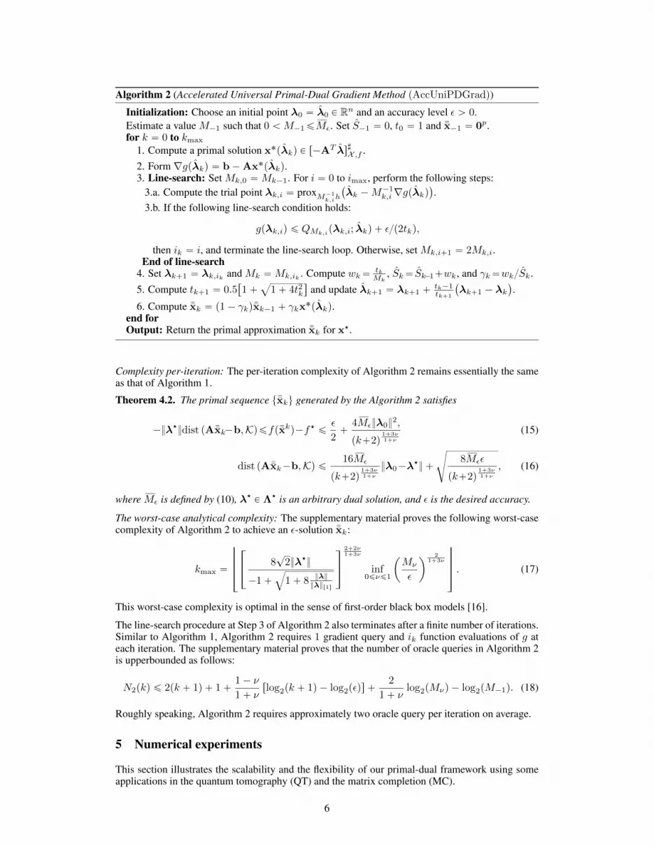
Algorithm 2 (Accelerated Universal Primal-Dual Gradient Method pAccUniPDGradq)

Initialization: Choose an initial point λ0 “ λ0 P Rn and an accuracy level ε ą 0.Estimate a value M´1 such that 0 ăM´1ďĎMε. Set S´1 “ 0, t0 “ 1 and ¯x´1 “ 0p.for k “ 0 to kmax

1. Compute a primal solution x˚pλkq P r´AT λs7X ,f .2. Form ∇gpλkq “ b´Ax˚pλkq.3. Line-search: Set Mk,0 “Mk´1. For i “ 0 to imax, perform the following steps:

3.a. Compute the trial point λk,i “ proxM´1k,ih

`

λk ´M´1k,i∇gpλkq

˘

.3.b. If the following line-search condition holds:

gpλk,iq ď QMk,ipλk,i; λkq ` ε{p2tkq,

then ik “ i, and terminate the line-search loop. Otherwise, set Mk,i`1 “ 2Mk,i.End of line-search

4. Set λk`1 “ λk,ik and Mk “Mk,ik . Compute wk“ tkMk

, Sk“ Sk 1`wk, and γk“wk{Sk.

5. Compute tk`1 “ 0.5“

1`a

1` 4t2k‰

and update λk`1 “ λk`1 `tk´1tk`1

`

λk`1 ´ λk˘

.

6. Compute ¯xk “ p1´ γkq¯xk´1 ` γkx˚pλkq.

end forOutput: Return the primal approximation ¯xk for x‹.

Complexity per-iteration: The per-iteration complexity of Algorithm 2 remains essentially the sameas that of Algorithm 1.

Theorem 4.2. The primal sequence t¯xku generated by the Algorithm 2 satisfies

´}λ‹}dist pA¯xk´b,Kqďfp¯xkq´f‹ ď ε

2`

4ĎMε}λ0}2,

pk`2q1`3ν1`ν

(15)

dist pA¯xk´b,Kq ď 16ĎMε

pk`2q1`3ν1`ν

}λ0´λ‹} `

d

8ĎMεε

pk`2q1`3ν1`ν

, (16)

where ĎMε is defined by (10), λ‹ P Λ‹ is an arbitrary dual solution, and ε is the desired accuracy.

The worst-case analytical complexity: The supplementary material proves the following worst-casecomplexity of Algorithm 2 to achieve an ε-solution ¯xk:

kmax “

—

—

—

—

–

»

–

8?

2}λ‹}

´1`b

1` 8 }λ}}λ}r1s

fi

fl

2`2ν1`3ν

inf0ďνď1

ˆ

Mν

ε

˙2

1`3ν

ffi

ffi

ffi

ffi

fl

. (17)

This worst-case complexity is optimal in the sense of first-order black box models [16].

The line-search procedure at Step 3 of Algorithm 2 also terminates after a finite number of iterations.Similar to Algorithm 1, Algorithm 2 requires 1 gradient query and ik function evaluations of g ateach iteration. The supplementary material proves that the number of oracle queries in Algorithm 2is upperbounded as follows:

N2pkq ď 2pk ` 1q ` 1`1´ ν

1` νrlog2pk ` 1q ´ log2pεqs `

2

1` νlog2pMνq ´ log2pM´1q. (18)

Roughly speaking, Algorithm 2 requires approximately two oracle query per iteration on average.

5 Numerical experiments

This section illustrates the scalability and the flexibility of our primal-dual framework using someapplications in the quantum tomography (QT) and the matrix completion (MC).

6

5.1 Quantum tomography with Pauli operators

We consider the QT problem which aims to extract information from a physical quantum system. Aq-qubit quantum system is mathematically characterized by its density matrix, which is a complexpˆp positive semidefinite Hermitian matrix X6 P Sp`, where p “ 2q . Surprisingly, we can provablydeduce the state from performing compressive linear measurements b “ ApXq P Cn based on Paulioperators A [18]. While the size of the density matrix grows exponentially in q, a significantly fewercompressive measurements (i.e., n “ Opp log pq) suffices to recover a pure state q-qubit densitymatrix as a result of the following convex optimization problem:

ϕ‹“minXPSp

`

"

ϕpXq :“1

2}ApXq´b}22 : trpXq “ 1

*

, pX‹ : ϕpX‹q “ ϕ‹q, (19)

where the constraint ensures that X‹ is a density matrix. The recovery is also robust to noise [18].

Since the objective function has Lipschitz gradient and the constraint (i.e., the Spectrahedron) istuning-free, the QT problem provides an ideal scalability test for both our framework and GCG-typealgorithms. To verify the performance of the algorithms with respect to the optimal solution in large-scale, we remain within the noiseless setting. However, the timing and the convergence behavior ofthe algorithms remain qualitatively the same under polarization and additive Gaussian noise.

# iteration100 101 102

Relativesolution

error:

∥Xk−X

⋆∥ F

∥X⋆∥ F

10-2

10-1

100

# iteration100 101 102

Objectiveresidual:|ϕ(X

k)−

ϕ⋆|

10-4

10-3

10-2

10-1

100

101

102

UniPDGradAccUniPDGradFrankWolfe

computational time (s)102 103 104

Relativesolution

error:

∥Xk−X

⋆∥ F

∥X⋆∥ F

10-2

10-1

100

computational time (s)102 103 104

Objectiveresidual:|ϕ(X

k)−

ϕ⋆|

10-4

10-3

10-2

10-1

100

101

Figure 1: The convergence behavior of algorithms for the q “ 14 qubits QT problem. The solid linescorrespond to the theoretical weighting scheme, and the dashed lines correspond to the line-search(in the weighting step) variants.

To this end, we generate a random pure quantum state (e.g., rank-1 X6), and we take n “ 2p log prandom Pauli measurements. For q “ 14 qubits system, this corresponds to a 26814351456 dimen-sional problem with n “ 1381099 measurements. We recast (19) into (1) by introducing the slackvariable r “ ApXq ´ b.

We compare our algorithms vs. the Frank-Wolfe method, which has optimal convergence rate guar-antees for this problem, and its line-search variant. Computing the sharp-operator rxs7 requires atop-eigenvector e1 of A˚pλq, while evaluating g corresponds to just computing the top-eigenvalueσ1 of A˚pλq via a power method. All methods use the same power method subroutine, which isimplemented in MATLAB’s eigs function. We set ε “ 2 ˆ 10´4 for our methods and have awall-time 2ˆ 104s in order to stop the algorithms. However, our algorithms seems insensitive to thechoice of ε for the QT problem.

Figure 1 illustrates the iteration and the timing complexities of the algorithms. UniPDGrad al-gorithm, with an average of 1.978 line-search steps per iteration, has similar iteration and timingperformance as compared to the standard Frank-Wolfe scheme with step-size γk “ 2{pk ` 2q. Theline-search variant of Frank-Wolfe improves over the standard one; however, our accelerated variant,with an average of 1.057 line-search steps, is the clear winner in terms of both iterations and time.We can empirically improve the performance of our algorithms even further by adapting a similarline-search strategy in the weighting step as Frank-Wolfe, i.e., by choosing the weights wk in agreedy fashion to minimize the objective function. The practical improvements due to line-searchappear quite significant.

5.2 Matrix completion with MovieLens dataset

To demonstrate the flexibility of our framework, we consider the popular matrix completion (MC)application. In MC, we seek to estimate a low-rank matrix X P Rpˆl from its subsampled entriesb P Rn, where Ap¨q is the sampling operator, i.e., ApXq “ b.

7

# iteration100 101 102 103

(ϕ(X

)−ϕ⋆)/ϕ⋆

10-2

10-1

100

101

102

UniPDGradAccUniPDGradFrankWolfe

# iteration100 101 102 103

(RMSE

-RMSE⋆)/RMSE⋆

10-2

10-1

100

101

# iteration0 1000 2000 3000 4000 5000

RMSE

1.05

1.07

1.09

1.11

1.13

computational time (min)0 1 2 3 4 5

RMSE

1.05

1.07

1.09

1.11

1.13

Figure 2: The performance of the algorithms for the MC problems. The dashed lines correspond tothe line-search (in the weighting step) variants, and the empty and the filled markers correspond tothe formulation (20) and (21), respectively.

Convex formulations involving the nuclear norm have been shown to be quite effective in estimatinglow-rank matrices from limited number of measurements [19]. For instance, we can solve

minXPRpˆl

"

ϕpXq“1

n}ApXq ´ b}2 : }X}˚ ď κ

*

, (20)

with Frank-Wolfe-type methods, where κ is a tuning parameter, which may not be available a priori.We can also solve the following parameter-free version

minXPRpˆl

"

ψpXq “1

n}X}2˚ : ApXq “ b

*

. (21)

While the nonsmooth objective of (21) prevents the tuning parameter, it clearly burdens the compu-tational efficiency of the convex optimization algorithms.

We apply our algorithms to (20) and (21) using the MovieLens 100K dataset. Frank-Wolfe algo-rithms cannot handle (21) and only solve (20). For this experiment, we did not pre-process the dataand took the default ub test and training data partition. We start out algorithms form λ0 “ 0n, weset the target accuracy ε “ 10´3, and we choose the tuning parameter κ “ 9975{2 as in [20]. Weuse lansvd function (MATLAB version) from PROPACK [21] to compute the top singular vectors,and a simple implementation of the power method to find the top singular value in the line-search,both with 10´5 relative error tolerance.

The first two plots in Figure 2 show the performance of the algorithms for (20). Our metrics arethe normalized objective residual and the root mean squared error (RMSE) calculated for the testdata. Since we do not have access to the optimal solutions, we approximated the optimal values,ϕ‹ and RMSE‹, by 5000 iterations of AccUniPDGrad. Other two plots in Figure 2 compare theperformance of the formulations (20) and (21) which are represented by the empty and the filledmarkers, respectively. Note that, the dashed line for AccUniPDGrad corresponds to the line-searchvariant, where the weights wk are chosen to minimize the feasibility gap. Additional details aboutthe numerical experiments can be found in the supplementary material.

6 ConclusionsThis paper proposes a new primal-dual algorithmic framework that combines the flexibility of prox-imal primal-dual methods in addressing the general template (1) while leveraging the computationaladvantages of the GCG-type methods. The algorithmic instances of our framework are universalsince they can automatically adapt to the unknown Holder continuity properties implied by the tem-plate. Our analysis technique unifies Nesterov’s universal gradient methods and GCG-type methodsto address the more broadly applicable primal-dual setting. The hallmarks of our approach includesthe optimal worst-case complexity and its flexibility to handle nonsmooth objectives and complexconstraints, compared to existing primal-dual algorithm as well as GCG-type algorithms, while es-sentially preserving their low cost iteration complexity.

Acknowledgments

This work was supported in part by ERC Future Proof, SNF 200021-146750 and SNF CRSII2-147633. We would like to thank Dr. Stephen Becker of University of Colorado at Boulder for hissupport in preparing the numerical experiments.

8

References

[1] M. Jaggi, Revisiting Frank-Wolfe: Projection-free sparse convex optimization. J. Mach. Learn.Res. Workshop & Conf. Proc., vol. 28, pp. 427–435, 2013.

[2] V. Cevher, S. Becker, and M. Schmidt. Convex optimization for big data: Scal-able, randomized, and parallel algorithms for big data analytics. IEEE Signal Process.Mag., vol. 31, pp. 32–43, Sept. 2014.

[3] M. J. Wainwright, Structured regularizers for high-dimensional problems: Statistical andcomputational issues. Annu. Review Stat. and Applicat., vol. 1, pp. 233–253, Jan. 2014.

[4] G. Lan and R. D. C. Monteiro, Iteration-complexity of first-order augmented Lagrangianmethods for convex programming. Math. Program., pp. 1–37, Jan. 2015, doi:10.1007/s10107-015-0861-x.

[5] S. Boyd, N. Parikh, E. Chu, B. Peleato, and J. Eckstein, Distributed optimization and statisticallearning via the alternating direction method of multipliers. Found. and Trends in MachineLearning, vol. 3, pp. 1–122, Jan. 2011.

[6] P. L. Combettes and J.-C. Pesquet, A proximal decomposition method for solving con-vex variational inverse problems. Inverse Problems, vol. 24, Nov. 2008, doi:10.1088/0266-5611/24/6/065014.

[7] T. Goldstein, E. Esser, and R. Baraniuk, Adaptive primal-dual hybrid gradient methods forsaddle point problems. 2013, http://arxiv.org/pdf/1305.0546.

[8] R. Shefi and M. Teboulle, Rate of convergence analysis of decomposition methods based onthe proximal method of multipliers for convex minimization. SIAM J. Optim., vol. 24, pp. 269–297, Feb. 2014.

[9] Q. Tran-Dinh and V. Cevher, Constrained convex minimization via model-based excessive gap.In Advances Neural Inform. Process. Syst. 27 (NIPS2014), Montreal, Canada, 2014.

[10] A. Beck and M. Teboulle, A fast iterative shrinkage-thresholding algorithm for linear inverseproblems. SIAM J. Imaging Sci., vol. 2, pp. 183–202, Mar. 2009.

[11] Y. Nesterov, Smooth minimization of non-smooth functions. Math. Program., vol. 103, pp. 127–152, May 2005.

[12] A. Juditsky and A. Nemirovski, Solving variational inequalities with monotone operatorson domains given by Linear Minimization Oracles. Math. Program., pp. 1–36, Mar. 2015,doi:10.1007/s10107-015-0876-3.

[13] Y. Yu, Fast gradient algorithms for structured sparsity. PhD dissertation, Univ. Alberta,Edmonton, Canada, 2014.

[14] Y. Nesterov, Complexity bounds for primal-dual methods minimizing the model of objectivefunction. CORE, Univ. Catholique Louvain, Belgium, Tech. Rep., 2015.

[15] Y. Nesterov, Universal gradient methods for convex optimization problems. Math. Program.,vol. 152, pp. 381–404, Aug. 2015.

[16] A. Nemirovskii and D. Yudin, Problem complexity and method efficiency in optimization.Hoboken, NJ: Wiley Interscience, 1983.

[17] R. T. Rockafellar, Convex analysis (Princeton Math. Series), Princeton, NJ: Princeton Univ.Press, 1970.

[18] D. Gross, Y.-K. Liu, S. T. Flammia, S. Becker, and J. Eisert, Quantum statetomography via compressed sensing. Phys. Rev. Lett., vol. 105, pp. Oct. 2010,doi:10.1103/PhysRevLett.105.150401.

[19] E. Candes and B. Recht, Exact matrix completion via convex optimization. Commun. ACM,vol. 55, pp. 111–119, June 2012.

[20] M. Jaggi and M. Sulovsky, A simple algorithm for nuclear norm regularized problems. InProc. 27th Int. Conf. Machine Learning (ICML2010), Haifa, Israel, 2010, pp. 471–478.

[21] R. M. Larsen, PROPACK - Software for large and sparse SVD calculations. Available: http://sun.stanford.edu/„rmunk/PROPACK/.

9

Supplementary document:

A Universal Primal-Dual Convex Optimization Framework

In this supplementary document, we provide the technical proofs and additional implementationdetails, and it is organized as follows: Section A defines the key estimates, that forms the basis ofthe universal gradient algorithms. Sections B and C present the proofs of Theorems 4.1 and 4.2respectively. Finally, Section D provides the implementation details of the quantum tomographyand the matrix completion problems considered in Section 5.

A The key estimate of the proximal-gradient step

Lemma 2 in [1], which we present below as Lemma A.1, provides key properties for constructinguniversal gradient algorithms. We refer to [1] for the proof of this lemma.

Lemma A.1. Let function g satisfy the Assumption A.2. Then for any δ ą 0 and

M ě

„

1´ ν

1` ν

1

δ

1´ν1`ν

M2

1`νν ,

the following statement holds for any λ,λ P Rn :

gpλq ď gpλq ` x∇gpλq, λ´ λy `M

2}λ´ λ}2

loooooooooooooooooooooooomoooooooooooooooooooooooon

QM pλ,λq

`δ

2.

This lemma provides an approximate quadratic upper bound for g. However, it depends on thechoice of the inexactness parameter δ and the smoothness parameter ν. If ν “ 1, then M can be setto the Lipschitz constant M1, and it becomes independent of δ.

The algorithms that we develop in this paper are based on the proximal-gradient step (9) on the dualobjective function G. This update rule guarantees the following estimate:

Lemma A.2. Let QM be the quadratic model of g. If λk`1, which is defined by (9), satisfies

gpλk`1q ď QMkpλk`1; λkq `

δk2

(22)

for some δk P R, then the following inequality holds for any λ P Rn :

Gpλk`1q ď gpλkq ` x∇gpλkq,λ´ λky ` hpλq `δk2`Mk

2

”

}λ´ λk}2 ´ }λ´ λk`1}

2ı

.

Proof of Lemma A.2. We note that the optimality condition of (9) is

0 P ∇gpλkq `Mkpλk`1 ´ λkq ` Bhpλk`1q,

which can be written as λk´λk`1 PM´1k p∇gkpλkq` Bhpλk`1qq. Let ∇hpλk`1q P Bhpλk`1q be

a subgradient of h at λk`1. Then, we have

λk ´ λk`1 “1

Mk

”

∇gpλkq `∇hpλk`1q

ı

. (23)

1

Now, using (23), we can derive

∆rkpλq “1

2}λ´ λk`1}

2 ´1

2}λ´ λk}

2

“ xλk ´ λk`1,λ´ λk`1y ´1

2}λk ´ λk`1}

2

(23)“

1

Mkx∇gpλkq `∇hpλk`1q,λ´ λk`1y ´

1

2}λk ´ λk`1}

2

“ ´1

Mk

„

x∇gpλkq,λk`1 ´ λky `Mk

2}λk`1 ´ λk}

2

`1

Mkx∇hpλk`1q,λ´ λk`1y `

1

Mkx∇gpλkq,λ´ λky

(22)ď

1

Mk

„

gpλkq ´ gpλk`1q `δk2

`1

Mkx∇hpλk`1q,λ´ λk`1y `

1

Mkx∇gpλkq,λ´ λky

ď1

Mk

„

gpλkq ´ gpλk`1q `δk2

`1

Mkrhpλq ´ hpλk`1qs `

1

Mkx∇gpλkq,λ´ λky

“1

Mk

„

gpλkq ` x∇gpλkq,λ´ λky ` hpλq `δk2

´1

MkGpλk`1q

where the last inequality directly follows the convexity of h.

Clearly, (22) holds if Mk ě ĎMε, which is defined by (10), due to Lemma A.1, whenever δk“ε ą 0.

If ν and Mν are known, we can set Mk “ ĎMε, then the condition (22) is automatically satisfied.However, we do not know ν and Mν a priori in general. In this case, Mk can be determined via aline-search procedure on the condition (22).

The following lemma guarantees that the line-search procedure in Algorithms 1 and 2 terminatesafter a finite number of line-search iterations.Lemma A.3. The line-search procedure in Algorithm 1 terminates after at most

ik “ tlog2pĎMε{M´1qu` 1

number of iterations.

Similarly, the line-search procedure in Algorithm 2 terminates after at most

ik “

—

—

—

–log2

ˆ

k ` 1

ε

˙

` log2

¨

˝

M2

1`νν

M´1

˛

‚

ffi

ffi

ffi

fl` 1

number of iterations.

Proof. Under Assumption A.2, Mν defined in Lemma A.1 is finite. When δk “ ε ą 0 is fixed as in

Algorithm 1, the upper bound ĎMε “

”

1´νp1`νqε

ı

1´ν1`ν

M2

1`νν defined by (10) is also finite. Moreover,

the condition (22) holds whenever Mk,i ě ĎMε. Since Mk,i “ 2Mk,i´1 “ 2iMk,0 ě 2iM´1, thelinesearch procedure is terminated after at most ik “ tlog2p

ĎMε{M´1qu` 1 iterations.

Now, we show that the line-search procedure in Algorithm 2 is also finite. By the updating rule oftk, we have tk`1 :“ 0.5p1`

a

1` 4t2kq ď 0.5p1` p1` 2tkqq “ tk ` 1. By induction and t0 “ 1,we have tk ď k ` 1. Using the definition (10) of ĎMδk with δk “ ε

tkand tk ď k ` 1, we can show

that

ĎMδk “

„

1´ ν

1` ν

1

δk

1´ν1`ν

M2

1`νν ď

„

tkε

1´ν1`ν

M2

1`νν ď

„

k ` 1

ε

1´ν1`ν

M2

1`νν . (24)

2

Next, we note that the condition (22) holds whenever Mk,i ě ĎMδk . However, since Mk,i “

2iMk,0 ě 2iM´1, by using (24), it is sufficient to show that the following condition holds for afinite i:

2iM´1 ě

„

k ` 1

ε

1´ν1`ν

M2

1`νν .

This condition leads to i ě log2

ˆ

“

k`1ε

‰

1´ν1`ν M

21`νν

˙

´ log2pM´1q. Hence, at the kth iteration, we

require at most ik “Z

log2

`

k`1ε

˘

` log2

ˆ

M2

1`νν

M´1

˙^

` 1 line-search iterations, which is finite.

B Convergence analysis of the universal primal-dual gradient algorithm

In this section, we analyze the convergence of the Algorithm 1 (UniPDGrad). We first provide theconvergence guarantee of the dual function in Theorem B.1. Then, we prove the convergence rateand the worst-case complexity given in Theorem 4.1.

B.1 Convergence rate of the dual objective function

Theorem B.1. Let tλku be the sequence generated by UniPDGrad. Then,

Gpλkq ´Gpλq ď Gk ´Gpλq ďĎMε

k ` 1}λ0 ´ λ}2 `

ε

2, (25)

for any λ P Rn, where ĎMε is defined by (10) and the two averaging sequences

λk(

and tGku aredefined as follows:

λk :“1

Sk

kÿ

i“0

1

Miλi`1 and Gk :“

1

Sk

kÿ

i“0

1

MiGpλi`1q, where Sk :“

kÿ

i“0

1

Mi.

Proof. For ĎMε defined by (10), since the line-search is successful as shown in Lemma A.1, thecondition (22) is satisfied at iteration i with Mi ď 2ĎMε. The following inequality directly followsLemma A.2 considering the convexity of g:

Gpλi`1q ď Gpλq `ε

2`Mi

2

“

}λ´λi}2 ´ }λ´λi 1}

2‰

, @λ P Rn.

Taking the weighted sum of this inequality over i, we get

Gk ď Gpλq `ε

2`

1

2Sk

“

}λ´λ0}2 ´ }λ´λk`1}

2‰

, (26)

for any λ P Rn, and Gpλkq ď Gk since G is a convex function. Finally, since Mi ď 2ĎMε, we haveSk ě

pk`1q

2ĎMε. Substituting this estimate into (26), we obtain (25).

B.2 The proof of Theorem 4.1: Convergence rate of the primal sequence

Proof. We use the following three expressions to relate the convergence in the dual sequence to theconvergence in the primal sequence:

gpλiq “ ´fpx˚pλiqq ` xλi,b´Ax˚pλiqy,

∇gpλiq “ b´Ax˚pλiq,

Gpλi`1q ě G‹ “ ´d‹ “ ´f‹.

(27)

Substituting these expressions into Lemma A.2, we get the following key estimate in the primalspace that holds for any λ P Rn:

fpx˚pλiqq ´ f‹ ď xb´Ax˚pλiq,λy ` hpλq `

ε

2`Mi

2

“

}λ´ λi}2 ´ }λ´ λi`1}

2‰

.

3

Taking the weighted sum of this inequality over i and considering the convexity of f , we get

fpxkq ´ f‹ ď xb´Axk,λy ` hpλq `

ε

2`

1

2Sk

“

}λ´λ0}2 ´ }λ´λk`1}

2‰

. (28)

Setting λ “ 0n, we get the bound on the right hand side of (15),

fpxkq ´ f‹ ď

ε

2`}λ0}

2

2Skďε

2`

ĎMε}λ0}2

k ` 1.

The inequality on the left hand side of (11) follows the following saddle point formulation:f‹ ď Lpx, r,λ‹q “ fpxq ` xλ‹,Ax´ b´ ry ď fpxq ` }λ‹}}Ax´ b´ r}, (29)

@r P K and @x P X , where the last inequality holds due to Cauchy-Schwarz inequality. The proofof the convergence rate in the objective residual (11) follows by setting x “ x in (29).

Next, we prove the convergence rate of the feasibility gap (12). We start from the following saddlepoint formulation:

f‹ ď Lpx, r,λ‹q “ fpxq ` xλ‹,Ax´ b´ ry, @r P K, @x P X .

Substituting this estimate with x “ xk into (28), we get the following inequality:

xAxk ´ b´ r˚pλq,λ´ λ‹y ´1

2Sk

“

}λ´λ0}2 ´ }λ´ λk`1}

2‰

ďε

2

ùñ minrPK

"

xAxk ´ b´ r,λ´ λ‹y ´1

2Sk}λ´λ0}

2

*

ďε

2

ùñ maxλPRn

minrPK

"

xAxk ´ b´ r,λ´ λ‹y ´1

2Sk}λ´λ0}

2

*

ďε

2

ùñ minrPK

maxλPRn

"

xAxk ´ b´ r,λ´ λ‹y ´1

2Sk}λ´λ0}

2

*

ďε

2

ùñ minrPK

"

xAxk ´ b´ r,λ0 ´ λ‹y `Sk2}Axk ´ b´ r}2

*

ďε

2

for any λ P Rn, where r˚pλq :“ arg maxrPK xr,λy, and the third implication holds due to theSion’s minimax theorem. Hence, there exists a vector r P K, that satisfies the following inequality:

xAxk ´ b´ r,λ0 ´ λ‹y `Sk2}Axk ´ b´ r}2 ď

ε

2.

Using Cauchy-Schwarz inequality, this implies

´}Axk ´ b´ r}}λ0 ´ λ‹} `Sk2}Axk ´ b´ r}2 ď

ε

2.

Solving this inequality for }Axk ´ b´ r}, we getdist pAxk ´ b,Kq ď }Axk ´ b´ r}

ď1

Sk

„

}λ0 ´ λ‹} `b

}λ0 ´ λ‹}2 ` Skε

ď1

Sk

”

2}λ0 ´ λ‹} `a

Skεı

.

We note that Sk ě k`12ĎMε

, and this completes the proof.

B.2.1 The worst-case complexity analysis

For simplicity, we choose λ0 “ 0n without loss of generality. Then, in order to guarantee both

dist pAxk´b,Kq ď ε and |fpxkq ´ f‹| ď ε, we require„

4ĎMε

k`1 }λ‹} `

b

2ĎMεεk`1

}λ‹}r1s ď ε due to

Theorem 4.1, where }λ‹}r1s :“ max t}λ‹}, 1u. This leads to (13) as

k`1 ě

»

–

4?

2}λ‹}

´1`b

1`8 }λ‹}}λ‹}r1s

fi

fl

2ĎMε

εñ kmax “

—

—

—

—

–

»

–

4?

2}λ‹}

´1`b

1`8 }λ‹}}λ‹}r1s

fi

fl

2

inf0ďνď1

ˆ

Mν

ε

˙2

1`ν

ffi

ffi

ffi

ffi

fl

.

4

Hence, the worst-case complexity to obtain an ε-solution of (1) in the sense of Definition 1.1 is

O

˜

inf0ďνď1

ˆ

Mν

ε

˙2

1`ν

¸

,

which is optimal if ν “ 0.

Next, we estimate the total number of oracle quires in UniPDGrad, as in [1]. The total number oforacle quires up to the iteration k is given by N1pkq “

řkj“0pij ` 1q. However, since ij ´ 1 “

log2pMj{Mj´1q, we have

N1pkq “kÿ

j“0

pij ` 1q “ 2pk ` 1q ` log2pMkq ´ log2pM´1q.

It remains to use Mk ď 2ĎMε to obtain (14).

C Convergence analysis of the accelerated universal primal-dual algorithm

We now analyze the convergence of AccUniPDGrad (Algorithm 2) in terms of the objective residualand the feasibility gap.

The dual main step of our algorithm is to update λk`1 and λk`1 from λk and λk as follows:$

’

’

&

’

’

%

λk :“ p1´ τkqλk ` τkλk

λk`1 :“ proxM´1k h

´

λk ´M´1k ∇gpλkq

¯

λk`1 :“ λk ´1τk

´

λk ´ λk`1

¯

,

(30)

where λ0 “ λ0, τ0 “ 1 andτ2k “ τ2k´1p1´ τkq. (31)

The parameter Mk is determined based on the following line-search condition:

gpλk`1q ď gpλkq ` x∇gpλkq,λk`1 ´ λky `Mk

2}λk`1 ´ λk}

2 `ε

2tk, (32)

with Mk ěMk´1.

Next, we simplify the scheme (30) in the following lemma:Lemma C.1. The scheme (30) can be restated as follows:

$

’

&

’

%

λk`1 :“ proxM´1k h

`

λk ´M´1k ∇gpλkq

˘

tk`1 :“ 12

“

1`a

1` 4t2k‰

λk`1 :“ λk`1 `tk´1tk`1

pλk`1 ´ λkq ,

(33)

where λ0 “ λ0 and t0 “ 1, and Mk is determined based on the line-search condition (32).

This dual scheme is of the FISTA form [2], except for the line-search step.

Proof. Let tk “ τ´1k , then t0 “ τ´1

0 “ 1. From (30), we have λk ´ λk`1 “1τkpλk ´ λk`1q “

tkpλk´λk`1q. We also have λk “ p1´τkqλk`τkλk, which leads to λk “1τkrλk´p1´τkqλks “

tkrλk ´ p1´ t´1k qλks. Combining these expressions, we get

tkpλk ´ λk`1q “ λk ´ λk`1 “ tkrλk ´ p1´ t´1k qλks ´ tk`1rλk`1 ´ p1´ t

´1k`1qλk`1s,

and this can be simplified as follows:

tk`1λk`1 “ tkλk`1 ` tk`1p1´ t´1k`1qλk`1 ´ tkp1´ t

´1k qλk

“ ptk ` tk`1 ´ 1qλk`1 ´ ptk ´ 1qλk.

Hence λk`1 “ λk`1 `tk´1tk`1

pλk`1 ´ λkq, which is the third step of (33).

Next, from the condition (31), we have t2k`1 ´ tk`1 ´ t2k “ 0. Hence, tk`1 “12

”

1`a

1` 4t2k

ı

,which is exactly the second step of (33).

5

C.1 The proof of Theorem 4.2: Convergence rate of the primal sequence

Proof. From Lemma A.2, we have

Gpλk 1q ď“

gpλkq`x∇gpλkq,λ´λky`hpλq‰

`τkε

2

`Mkxλk´λk 1, λk´λy´Mk

2}λk 1´λk}

2 (34)

ď Gpλq`τkε

2`Mkxλk´λk 1, λk´λy´

Mk

2}λk 1´λk}

2. (35)

Note that these inequalities hold @λ P Rn. Next, we subtract G‹ from (34) to get

Gpλk 1q ´G‹ ď

“

gpλkq`x∇gpλkq,λ´λky`hpλq ´G‹‰

`τkε

2

`Mkxλk´λk 1, λk´λy´Mk

2}λk 1´λk}

2, (36)

and we set λ “ λk in (35), and then subtract G‹ from the both sides, that results in the followinginequality:

Gpλk 1q´G‹ ď Gpλkq´G

‹`τkε

2´Mk

2}λk 1´λk}

2 `Mkxλk ´ λk 1, λk ´ λky. (37)

We obtain the following estimate by summing the two inequalities that we get by multiplying (36)by τk and (37) by p1´ τkq, and then dividing the resulting estimate by Mkτ

2k :

1

Mkτ2k

“

Gpλk 1q´G‹‰

ďp1´τkq

Mkτ2k

“

Gpλkq´G‹‰

`1

2

“

}λk´λ}2 ´ }λk 1´λ}2‰

`ε

2Mkτk

`1

Mkτk

“

gpλkq`x∇gpλkq,λ´λky ` hpλq ´G‹‰

. (38)

Next, we sum this inequality over k as follows:kÿ

i“0

Gpλi 1q ´G‹

Miτ2iď

kÿ

i“0

„

p1´τiq

Miτ2i

“

Gpλiq´G‹‰

`1

2

“

}λi´λ}2 ´ }λi 1´λ}2‰

`ε

2Miτi

`1

Miτi

“

gpλiq`x∇gpλiq,λ´λiy ` hpλq ´G‹‰

ď

kÿ

i“1

Gpλiq´G‹

Mi´1τ2i´1

`1

2

“

}λ0 ´ λ}2 ´ }λk`1 ´ λ}2‰

`ε

2

kÿ

i“0

1

Miτi

`

kÿ

i“0

1

Miτi

“

gpλiq ` x∇gpλiq,λ´ λiy ` hpλq ´G‹‰

,

where the second inequality follows τ0 “ 1 and p1´τkqMkτ2

kď 1

Mk´1τ2k´1

for k “ 1, 2, . . . , which holdssince Mk ěMk´1. This implies the followings:

0 ďGpλk 1q ´G

‹

SkMkτ2kď

1

Sk

kÿ

i“0

1

Miτi

“

gpλiq ` x∇gpλiq,λ´ λiy ` hpλq ´G‹‰

`1

2Sk

“

}λ0 ´ λ}2 ´ }λk`1 ´ λ}2‰

`ε

2

ùñ ´1

Sk

kÿ

i“0

1

Miτi

“

gpλiq`x∇gpλiq,λ´λiy`hpλq´G‹‰

ď1

2Sk

“

}λ0´λ}2´}λk`1´λ}

2‰

`ε

2.

Now, we use the following expressions to map this estimate into the primal sequence:

gpλiq “ ´fpx˚pλiqq ` xλi,b´Ax˚pλiqy,

∇gpλiq “ b´Ax˚pλiq,

G‹ “ ´d‹ “ ´f‹.

6

Then, considering the convexity of f , we get

fp¯xkq ´ f‹ ď xb´A¯xk,λy ` hpλq `

ε

2`

1

2Sk

“

}λ0 ´ λ}2 ´ }λk`1 ´ λ}2‰

ďε

2`}λ0}

2

2Sk, (39)

where we obtain the second inequality by setting λ “ 0n.

We can reformulate (31) as 1τk“ 1

τ2k´ 1

τ2k´1

. Using this relation, M0 ď Mi ď Mk ď 2ĎMετk “

2t1´ν1`ν

kĎMε ď 2pk ` 2q

1´ν1`ν ĎMε and k`2

2 ď tk ă k ` 2 for i “ 0, 1, . . . , k, we can show that

Sk :“kÿ

i“0

1

Miτiě

kÿ

i“0

1

2ĎMετkτi“

1

2ĎMετk

”

1`kÿ

i“1

` 1

τ2i´

1

τ2i´1

˘

ı

ět2k

2pk ` 2q1´ν1`ν ĎMε

ěpk ` 2q

1`3ν1`ν

8ĎMε

. (40)

We get the bound on the right hand side of (15) by substituting (40) into (39). The inequality on theleft hand side of (15) follows the saddle point formulation (29) by setting x “ ¯xk.

Finally, we prove the convergence rate in the feasibility gap (16). By the same arguments as in theproof of Theorem 4.1, we have

dist pA¯xk ´ b,Kq ď 2}λ0 ´ λ‹}

Sk`

c

ε

Sk.

We complete the proof by substituting (40) into this estimate.

C.2 The worst-case complexity analysis

We analyze the worst-case complexity of AccUniPDGrad algorithm to achieve an ε-solution ¯xk. Forsimplicity, we consider the case λ0 “ 0n without loss of generality. Then, we require

«

16ĎMε

pk ` 2q1`3ν1`ν

}λ‹} `

d

8ĎMεε

pk` 2q1`3ν1`ν

ff

}λ‹}r1s ď ε

due to the Theorem 4.2, where }λ‹}r1s :“ max t}λ‹}, 1u. By solving this inequality, we get

k ` 2 ě

»

–

8?

2}λ‹}

´1`b

1` 8 }λ‹}}λ‹}r1s

fi

fl

2`2ν1`3ν

„

ĎMε

ε

1`ν1`3ν

.

Using the definition (10) of ĎMε and considering the fact that”

1´ν1`ν

ı

1´ν1`ν

ď 1 for ν P r0, 1s, we findthe maximum number of iterations that satisfies the above inequality as follows:

kmax “

—

—

—

—

–

»

–

8?

2}λ‹}

´1`b

1` 8 }λ‹}}λ‹}r1s

fi

fl

2`2ν1`3ν

inf0ďνď1

ˆ

Mν

ε

˙2

1`3ν

ffi

ffi

ffi

ffi

fl

,

which is indeed (17).

Hence, the worst-case complexity to obtain an ε-solution of (1) in the sense of Definition 1.1 is

O

˜

inf0ďνď1

ˆ

Mν

ε

˙2

1`3ν

¸

,

which is optimal in the sense of first-order black box models [3].

7

Next, we consider the number of oracle quires in AccUniPDGrad. At iteration k, the algorithmrequires ik`2 function evaluations of g, as we need ik`1 in the line-search and one for gpλkq.Hence, the total number of oracle quires up to the iteration k is N2pkq “

řkj“0pij ` 2q. Since

ij “ log2pMj{Mj´1q, we have

N2pkq “ 2pk ` 1q ` log2pMkq ´ log2pM´1q.

Using the same argument as in the proof of Lemma A.3, we have Mk ď 2ĎMετk ď

2“

k`1ε

‰

1´ν1`ν M

21`νν . Hence, we obtain (18) as

N2pkq ď 2pk ` 1q ` 1`1´ ν

1` νrlog2pk ` 1q ´ log2pεqs `

2

1` νlog2pMνq ´ log2pM´1q.

D The implementation details

In this section, we specify key steps of UniPDGrad and AccUniPDGrad for two important applica-tions that we used in Section 5. We also provide an analytic step-size that guarantees the line-searchcondition without function evaluation.

We performed the experiments in MATLAB, using a computational resource with 4 CPUs of 2.40GHz and 16 GB memory space for the matrix completion, and 16 CPUs of 2.40 GHz and 512 GBmemory space for the quantum tomography problem.

D.1 Constrained convex optimization involving a quadratic cost

In both quantum tomography and the matrix completion problems, we consider some problem for-mulations from the following convex optimization template that involves a quadratic cost:

minxPRp

"

1

2}Apxq ´ b}2 : x P X

*

.

For notational simplicity, we consider the problem in Rp{Rn spaces in this section, but the ideasapply in general.

Evaluation of the sharp-operator corresponding to the objective function 1{2}Apxq´b}2 requires asignificant computational effort. Yet, by introducing the slack variable r “ Apxq ´ b, we can writean equivalent problem as

minpr,xqPRnˆRp

"

1

2}r}2 : Apxq ´ r “ b, x P X

*

.

We can write the Lagrange function associated with the linear constraint as

Lpr,x,λq “ 1

2}r}2 ` xλ, r´Apxq ` by,

from which we can derive the (negation of the) dual function

gpλq “ ´ minrPRn,xPX

Lpr,x,λq “ ´minrPRn

1

2}r}2 ` xλ, ry

(

`maxxPX

xλ,Apxqy ` xλ,by

“1

2}λ}2 ` xλ,b´Apx˚pλqqy, (41)

and its subgradient∇gpλq “ λ´ b`Apx˚pλqq,

where x˚pλq P rAT pλqs7X ” arg maxxPX xAT pλq,xy.

For the special case, X is a norm ball, i.e., X ” tx : }x} ď κu, we can simplify (41) as follows:

gpλq “1

2}λ}2 ` xλ,by ` κ}AT pλq}. (42)

8

Computing an analytical step-size: Now, we consider the line-search procedure in UniPDGradand AccUniPDGrad. Since hpλq term is absent in these problems, the line-search condition (22)can be simplified as

gpλk`1q “ gpλk ´ αk∇gpλkqq ď gpλkq ´αk2}∇gpλkq}2 ` δk{2, (43)

where we use the notational convention λk “ λk and δk “ ε for UniPDGrad, and δk “ ε{tk forAccUniPDGrad. Using the definition (42), we can upper bound gpλk ´ αk∇gpλkqq by

Upαkq :“ gpλkq ` pα2k{2q}∇gpλkq}2 ´ αkxλk ´ b,∇gpλkqy ` αkκ}AT p∇gpλkqq}.

The condition (43) holds if Upαkq “ gpλkq ´αk2 }∇gpλkq}

2 ` δk{2. Solving this second orderequation, we obtain αk explicitly as

αk “´P `

b

P 2 ` 4δk}∇gpλkq}2

2}∇gpλkq}2,

where P :“ }∇gpλkq}2 ` 2κ}AT p∇gpλkqq} ´ 2xλk ´ b,∇gpλkqy. Note that, we can use thismethod to find a good estimate for the initial smoothness constant M´1 in the initialization step.

D.2 Constrained convex optimization involving a norm cost

Now, we consider the second application, which is reformulated as

minXPRpˆl

"

ψpXq “1

n}X}2˚ : ApXq ´ b P K

*

,

where K is an `2-norm ball, i.e., K :“ tr : }r} ď κu. Once again, by introducing the slack variabler “ ApXq ´ b, we get

minXPRpˆl,rPRn

"

1

n}X}2˚ : ApXq ´ r “ b, r P K

*

.

Clearly, the dual components g and h defined in (6) can be expressed as:

gpλq “ maxXPRpˆl

"

xAT pλq,Xy ´1

n}X}2˚

*

` xb,λy “n

4}AT pλq}2 ` xb,λy,

hpλq “ maxrPK

x´λ, ry “ max}r}ďκ

x´λ, ry “ κ}λ},

where } ¨ } represents the Euclidean norm for vectors and the spectral norm for matrices. In (21), weconsider a special case where K ” t0nu, hence hpλq “ 0.

Clearly, X˚pλq “ σ1e1eT1 P rAT pλqs7ψ , where σ1 “ }AT pλq} is the top singular value of AT pλq

and e1 is the associated left singular vector. Hence, we can write the (sub)gradient of g as

∇gpλq “ b´ApX˚pλqq.

We can compute both σ1 and e1 efficiently by using the power method or the Lanczos algorithm.

References

[1] Y. Nesterov, Universal gradient methods for convex optimization problems. Math. Program.,vol. 152, pp. 381–404, Aug. 2015.

[2] A. Beck and M. Teboulle, A fast iterative shrinkage-thresholding algorithm for linear inverseproblems. SIAM J. Imaging Sci., vol. 2, pp. 183–202, Mar. 2009.

[3] A. Nemirovskii and D. Yudin, Problem complexity and method efficiency in optimization.Hoboken, NJ: Wiley Interscience, 1983.

9