Journal of Neuroscience Methods 142 (2005) 17–26

Trimmed estimators for robust averaging of event-related potentials

Zbigniew Leonowicz∗,1, Juha Karvanen, Sergei L. Shishkin2

Laboratory for Advanced Brain Signal Processing, RIKEN Brain Science Institute, Saitama 351-0198, Japan

Received 18 March 2004; received in revised form 15 July 2004; accepted 16 July 2004

Abstract

Averaging (in statistical terms, estimation of the location of data) is one of the most commonly used procedures in neuroscience and the basicprocedure for obtaining event-related potentials (ERP). Only the arithmetic mean is routinely used in the current practice of ERP research,though its sensitivity to outliers is well-known. Weighted averaging is sometimes used as a more robust procedure, however, it can be notsufficiently appropriate when the signal is nonstationary within a trial. Trimmed estimators provide an alternative way to average data. In thispaper, a number of such location estimators (trimmed mean, Winsorized mean and recently introduced trimmed L-mean) are reviewed, aswell as arithmetic mean and median. A new robust location estimator tanh, which allows the data-dependent optimization, is proposed foraveraging of small number of trials. The possibilities to improve signal-to-noise ratio (SNR) of averaged waveforms using trimmed locatione©

K tors

1

ptoroacatwart

(sU

M

vent.ichthe

ch-ing,iquectu-

al orelec-tr antaindoge-pteduseber

strat-mayal.,very

pro-da

0d

stimators are demonstrated for epochs randomly drawn from a set of real auditory evoked potential data.2004 Elsevier B.V. All rights reserved.

eywords:Averaging; Event-related potentials; Evoked potentials; Mean; Median; Trimmed mean; Robust estimators of location; Trimmed estima

. Introduction

Averaging is probably the most common basic statisticalrocedure in experimental science. It is used for estimating

he location of data (or “central tendency”) in the presencef random variations among the observations, which can beemoved by this procedure. Data variations can be the resultf variations in the phenomenon of interest or of some un-voidable measuring errors. In signal processing terms, thisan be considered as contamination of useful “signal”, suchs event-related brain activity, by useless “noise”, such as ar-

ifacts and ongoing activity, both not repeatedly associatedith the event. In the case of linear summation of signalnd noise (“additive model”), the fact that only the event-elated signal is time-locked to the event and noise is notime-locked, allows the cancellation of the noise by averaging

∗ Corresponding author. Tel.: +81-484-679765; fax: +81-484-679694.E-mail addresses:zbigniew.leonowicz@pwr.wroc.pl

Z. Leonowicz), juha.karvanen@hut.fi (J. Karvanen),hishkin@brain.riken.jp (S.L. Shishkin).RL: http://www.bsp.brain.riken.jp.

1 On leave from Wroclaw University of Technology, Wroclaw, Poland.2 Department of Human and Animal Physiology, Faculty of Biology,

.V. Lomonosov Moscow State University, Russia.

the data separately for each time point relative to the eAveraging is typically done using arithmetic mean, whis the most widely known estimator of the location ofdata.

Event-related averaging is important for various teniques from single neuron firing recording to optical imagbut is most essential for the old and still important technof event-related potentials (ERP). ERPs are voltage fluations repeatedly associated in time with some physicmental events, which can be extracted from the ongoingtroencephalogram (EEG) using signal averaging(Picton eal., 2000). The term “evoked potentials” (EPs) is used foimportant subset of ERPs which are “evoked” by a cerevent, usually a sensory one, but not by independent ennous processes. Additive model is most commonly accefor event-related activity and ongoing EEG, allowing theof averaging for the extraction of ERP. Though a numof studies cast doubts on the additive model by demoning that event-related modifications of the ongoing EEGalso contribute to ERP(Makeig et al., 2002; Jansen et2003), averaging has been proved to be practically aefficient procedure and is used, therefore, as the basiccedure in ERP analysis(Picton et al., 1995, 2000; LopesSilva, 1999).

165-0270/$ – see front matter © 2004 Elsevier B.V. All rights reserved.

oi:10.1016/j.jneumeth.2004.07.008

18 Z. Leonowicz et al. / Journal of Neuroscience Methods 142 (2005) 17–26

Temporal resolution in the order of milliseconds makesERPs an important tool for estimating of the timing for infor-mation processing in the human brain(Picton et al., 2000).Thus, the improvement of signal-to-noise ratio by averaging,which is the essence of computing the ERP, should receivea serious attention. In particular, an important task is the de-velopment of efficient methods for averaging of small setsof single-trial ERPs, where data may strongly deviate fromGaussian distribution. Due to deviation from Gaussian dis-tribution, their location may not be estimated correctly byarithmetic mean. The number of data epochs (which corre-spond to experimental trials) used for averaging should be aslow as possible because of various reasons: fatigue, learningand other factors affecting the brain response of the subject;even the way the subjects perform the task may change ifthe task is repeated many times. In some applications such asbrain–computer interface (BCI) only a few trials can usuallybe used each time the averaging is computed(Wolpaw et al.,2002).

In some cases the improvement of ERP averaging can beobtained with various techniques which compensate for thetrial-to-trial variability, mainly the latency jitter. Such ap-proaches, however, require that the ERP could be recogniz-able in single trials, which is often impossible, and involvethe risk that the outcome can be merely the result of liningu

ob-t thism esti-meq de-v ss ra tedt sulto ingc dingt tion-a ,m f on-g igha thero parto d fora

min-i t,1 dK -v witho om-p dingt tivet e tot ed by

the nonstationarity of noise within an epoch. It was shownthat median averaging can improve averaging of endogenousERPs using small number of trials(Yabe et al., 1993). A de-tailed study byOzdamar and Kalayci (1999)demonstratedthe advantages of median averaging over conventional aver-aging for auditory brain stem responses which have low SNRdue to very low amplitude and thus requires high number ofepochs to be averaged.

The disadvantage of median averaging is that it does notonly remove the outliers but also uses the rest of data only inthe sense of the order of the values. It is evident that someuseful information can be lost by this procedure, comparingto conventional averaging, which employs the data valuesthemselves instead of their order. In practice, median aver-aged waveforms include a rather strong high frequency noise(though it seems to be easily removable by filtering(Ozdamarand Kalayci, 1999)), and the results are not always improvedrelative to conventional mean averaging(Fox and Dalebout,2002). One should also consider a possibility of unpredictableeffects arising from the “over-robustness” of median. For ex-ample, the value of median will not change at all if we add avery large value to each of data values above median(Streiner,2000).

Is it possible to combine advantages of mean and medianaveraging? In fact, an estimator of data location which liesb me is“ n int d orm thes

s isq hel mev thers aver-a ng ita od-i tione so ted, tot

y oft andt ch ast ed too

( elymedmed

( ked

(

p the background noise(Picton et al., 1995, 2000).Improving the noise reduction by averaging can be

ained with a technique called weighted averaging. Inethod, each epoch is given a weight depending onated noise in this epoch(Hoke et al., 1984; Lutkenhonert al., 1985; Davila and Mobin, 1992; Łe¸ski, 2002). Thoughuite many variations of weighting averaging have beeneloped (for review see, e.g.,Łeski (2002)), this method itill rarely used for averaging of ERP. As stated inOzdamand Kalayci (1999), there are still unsolved issues rela

o computation of weights and their influence on the ref averaging. An important limitation of weighted averagomes from the noise model which it assumes. Accoro this model, noise varies between epochs, but is stary within each epoch(Lutkenhoner et al., 1985). Howeverany types of noise (not only artifacts but also waves ooing EEG) can strongly vary within an epoch, having hmplitude in some time points and low amplitudes in ones. Thus, the weights can be underestimated for thef epoch where a strong noise occurs and overestimatenother part of epoch where the noise is low.

Median averaging is another approach suggested formizing the influence of noise in ERPs(Borda and Fros968; Yabe et al., 1993; Picton et al., 1995;Ozdamar analayci, 1999; Fox and Dalebout, 2002). It is similar to conentional averaging on the basis of arithmetic mean,nly difference that median is used instead of mean. Cutation of median includes ordering of samples accor

o their amplitudes of all epochs for each time point relao stimulus, independently from other time points. Duhis independence, median averaging cannot be affect

etween those two extremes already exists and its natrimmed mean”. In this method (see the exact definitiohe next section), a part of extreme values is discardeodified, but all other values are used for averaging in

ame way as in conventional mean averaging.It is important to note that rejection of extreme value

uite different from the procedure of artifact rejection. Tatter procedure typically implies removing not only extrealues but all trials including extreme values or some oigns of artifacts and in this sense it is closer to weightedging, which defines the impact of an epoch by estimatis a whole. Surprisingly, though trimmed mean and its m

fied version, Winsorized mean, are efficient robust locastimators(Stuart and Keith Ord, 1994), averaging of ERPn the basis of these estimators has never been repor

he best of our knowledge.The goal of this paper is to demonstrate the efficienc

rimmed estimators of data location for computing ERPso propose some ways to optimize their parameters, surimming parameters and parameters for weights relatrder of averaged amplitudes.

In this paper, we:

1) briefly review a number of locator estimators, nammean, median, and three trimmed estimators: trimmean, Winsorized mean and recently proposed trimL-mean,

2) report results of their testing using real auditory evopotential (AEP) data and their resampling,

3) propose a new adaptable location estimator.

Z. Leonowicz et al. / Journal of Neuroscience Methods 142 (2005) 17–26 19

2. Statistical estimators of location

2.1. Problem of robustness of estimation of the datalocation

The problem of sensitivity of an estimator to the presenceof outliers, i.e. “the data points that deviate from the patternset by the majority of the data set”(Hampel et al., 1986),has lead to the development ofrobustlocation measures. Ro-bustness of an estimator is measured by thebreakdown value,which tells us how many data points need to be replaced byarbitrary values in order to make the estimator explode (tendto infinity) or implode (tend to zero). For instance: arithmeticmean has 0% breakdown whilst median is very robust withbreakdown value of 50%(Hampel et al., 1986).

2.2. Arithmetic mean

The most widely used statistical measure and the bestknown estimator of location is thearithmetic mean(seeFig.1(a)).

µmean=N∑

i=1

1

Nxi (1)

The arithmetic mean is a standard location estimator usedf ever,i oneo Theb

2

waybx

K

µ

w thei ofw rith-m

eas-i inF

2

M f the( size2 f thes q.

(2) the weight one is applied to the (M + 1)th sample in thecase when the number of samples is odd and weights equalto 1/2 to bothMth and (M + 1)th samples when the numberof samples is even(Stuart and Keith Ord, 1994)(seeFig.1(b)).

2.5. Trimmed mean

For theα-trimmed mean (wherep = αN) the weightswi

as in (2) can be defined as:

wi =

1

N − 2p, p + 1 ≤ i ≤ N − p

0, otherwise(3)

Thus, the trimmed mean correspond to the mean valueof data samples wherep highest andp lowest samples areremoved (seeFig. 1(c)).

Application of trimming lowers the influence of extremedata values on the result of averaging. However, unlikein median, substantial part of data can be included intoaverage.

2.6. Winsorized mean

tiono f in-f ze iss thee( hen eeF

w

-s istri-b

vm ined(

2

et ofL edf . Us-i anb

or averaging of ERPs and for many other purposes, howt is not robust. In the case of arithmetic mean, onlyutlier may make the estimate infinitely large or small.reakdown value becomes here lim

N→∞(1/N) = 0.

.3. Robust location measures

Many location estimators can be presented in unifiedy ordering the values of the sample asx(1) ≤ x(2) ≤ · · · ≤(N) and then applying the weight functionwi (Stuart andeith Ord, 1994)

r =N∑

i=1

wix(i), (2)

herewi is a function designed specifically to reducenfluence of certain observations (data points) in formeighting andx(i) represents the ordered data. For the aetic mean it holdswi = 1/N.To make the comparison between different estimators

er, we present all weighting functions (as in (2)) plottedig. 1.

.4. Median

Suppose that the data have the size of (2M + 1), whereis a positive integer, then the median is the value o

M + 1)th ordered observation. In the case of even dataM the median is defined as the value of the mean oamplesM andM + 1. According to the framework of E

In the case of trimmed mean, the tails of the distribuf the data are simply ignored. It can lead to the loss o

ormation and should be avoided when the sample simall. Winsorized mean is similar to trimmed mean withxception that it replaces each observation in eachα fractionp = αN) of the tail of the distribution by the value of tearest unaffected observation. Weightwi becomes here (sig. 1(d))

i =

0, i ≤ p or i ≥ N − (p − 1)p + 1

N, i = p + 1 or i = N − p

1

N, p + 2 ≤ i ≤ N − (p + 1)

(4)

Usually, the values in the range 0≤ p ≤ 0.25N are conidered, depending on the heaviness of the tails of the dution.

An interesting observation is that themedian can beiewed as an extreme case of thetrimmedmeanorWinsorizedeanwhen only one or two central data points are reta

Stuart and Keith Ord, 1994).

.7. Trimmed L-mean (TL-mean)

Recently, Elamir and Seheult (2003)proposed thrimmed L-moments (TL-moments) as a generalization-moments(Hosking, 1990). TheTL-mean can be estimat

rom a sample as a linear combination of order statisticsng the formulation of equation (2) the weight function ce calculated as follows (p = 0 for arithmetic mean)

20 Z. Leonowicz et al. / Journal of Neuroscience Methods 142 (2005) 17–26

Z. Leonowicz et al. / Journal of Neuroscience Methods 142 (2005) 17–26 21

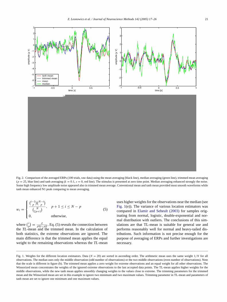
Fig. 2. Comparison of the averaged ERPs (100 trials, raw data) using the mean averaging (black line), median averaging (green line), trimmed mean averaging(p = 25, blue line) and tanh averaging (k = 0.1, s = 0, red line). The stimulus is presented at zero time point. Median averaging enhanced strongly the noise.Some high frequency low amplitude noise appeared also in trimmed mean average. Conventional mean and tanh mean provided most smooth waveforms whiletanh mean enhanced N1 peak comparing to mean averaging.

wi =

(i−1p

)(N−ip

)(

N2p+1

) , p + 1 ≤ i ≤ N − p

0, otherwise,

(5)

where(

ip

) = i!p!(i−p)! . Eq. (5) reveals the connection between

the TL-mean and the trimmed mean. In the calculation ofboth statistics, the extreme observations are ignored. Themain difference is that the trimmed mean applies the equalweight to the remaining observations whereas theTL-mean

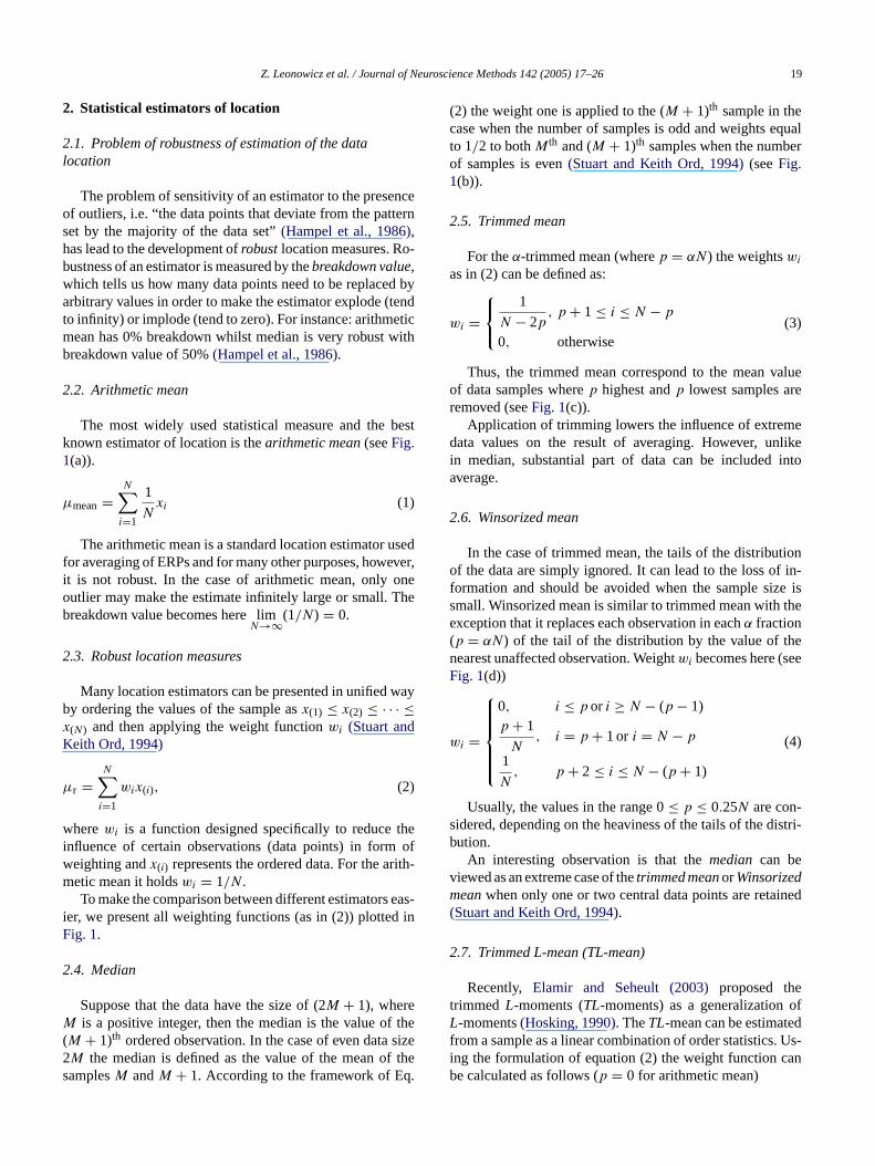
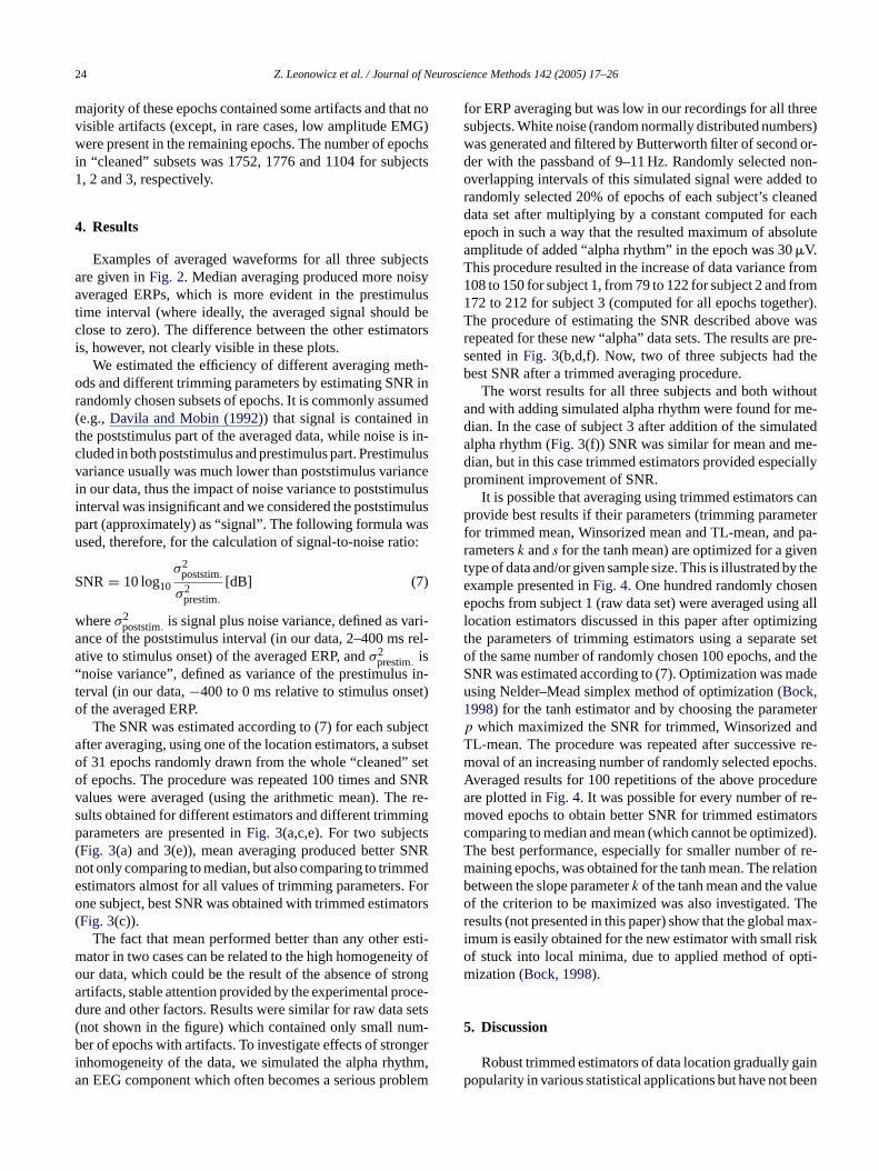
Fig. 1. Weights for the different location estimators. Data (N = 20) are sorted in ascending order. The arithmetic mean uses the same weight 1/N for allobservations. The median uses only the middle observation (odd number of observations) or the two middle observations (even number of observations). Notethat the scale is different in figure (b). The trimmed mean applies a zero weight for extreme observations and an equal weight for all other observations. TheWinsorized mean concentrates the weights of the ignored extreme observations to the last accepted data points. The TL-mean applies higher weights for themiddle observations, while the new tanh mean applies smoothly changing weights to the values close to extreme. The trimming parameters for the trimmedmean and the Winsorized mean are set in this example to ignore two minimum and two maximum values. Trimming parameter in TL-mean and parameters oftanh mean are set to ignore one minimum and one maximum values.

uses higher weights for the observations near the median (seeFig. 1(e)). The variance of various location estimators wascompared inElamir and Seheult (2003)for samples orig-inating from normal, logistic, double-exponential and nor-mal distribution with outliers. The conclusions of this sim-ulations are that TL-mean is suitable for general use andperforms reasonably well for normal and heavy-tailed dis-tributions. Such information is not precise enough for thepurpose of averaging of ERPs and further investigations arenecessary.

22 Z. Leonowicz et al. / Journal of Neuroscience Methods 142 (2005) 17–26

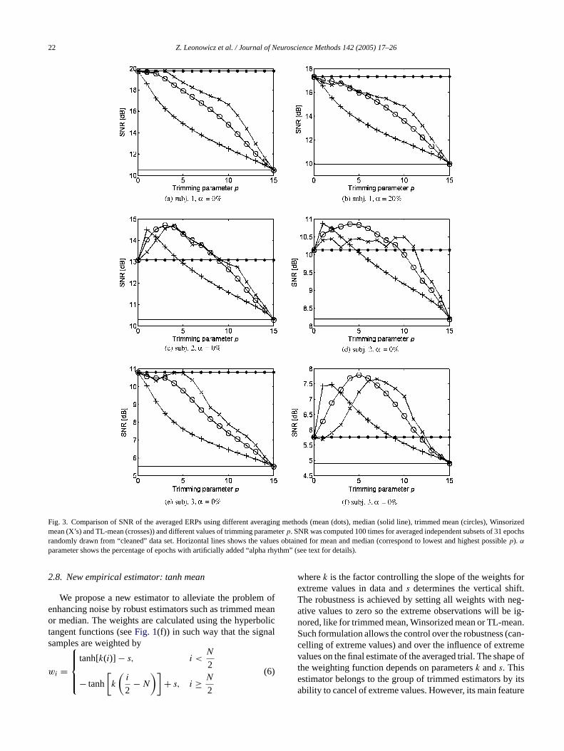
Fig. 3. Comparison of SNR of the averaged ERPs using different averaging methods (mean (dots), median (solid line), trimmed mean (circles), Winsorizedmean (X’s) and TL-mean (crosses)) and different values of trimming parameterp. SNR was computed 100 times for averaged independent subsets of 31 epochsrandomly drawn from “cleaned” data set. Horizontal lines shows the values obtained for mean and median (correspond to lowest and highest possiblep). α

parameter shows the percentage of epochs with artificially added “alpha rhythm” (see text for details).

2.8. New empirical estimator: tanh mean

We propose a new estimator to alleviate the problem ofenhancing noise by robust estimators such as trimmed meanor median. The weights are calculated using the hyperbolictangent functions (seeFig. 1(f)) in such way that the signalsamples are weighted by

wi =

tanh[k(i)] − s, i <N

2

− tanh

[k

(i

2− N

)]+ s, i ≥ N

2

(6)

wherek is the factor controlling the slope of the weights forextreme values in data ands determines the vertical shift.The robustness is achieved by setting all weights with neg-ative values to zero so the extreme observations will be ig-nored, like for trimmed mean, Winsorized mean or TL-mean.Such formulation allows the control over the robustness (can-celling of extreme values) and over the influence of extremevalues on the final estimate of the averaged trial. The shape ofthe weighting function depends on parametersk ands. Thisestimator belongs to the group of trimmed estimators by itsability to cancel of extreme values. However, its main feature

Z. Leonowicz et al. / Journal of Neuroscience Methods 142 (2005) 17–26 23

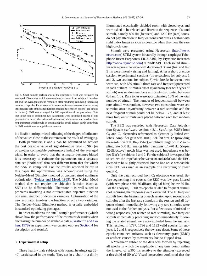
Fig. 4. Small sample performance of the estimators. SNR was estimated foraveraged 100 epochs which were randomly chosen from subject 1 raw dataset and for averaged epochs remained after randomly removing increasingnumber of epochs. Parameters of trimmed estimators were optimized usingindependent sets of the same number of randomly chosen epochs (see detailsin the text). SNR was averaged for 100 repetitions of the procedure. Notethat in the case of tanh mean two parameters were optimized instead of oneparameter in three other trimmed estimators, while mean and median haveno parameters which could be optimized; this could at least partly contributeto SNR variations amongst the estimators.

is a flexible and optimized adjusting of the degree of influenceof the values close to the extremes on the result of averaging.

Both parametersk and s can be optimized to achievethe best possible value of signal-to-noise ratio (SNR) (orof another computable performance index) of the averagedtrials. In order to avoid that the estimator becomes biasedit is necessary to estimate the parameters on a separatedata set (“hold-out” data set) different from that for whichthe SNR is computed. For the results reported below inthis paper the optimization was accomplished using theNelder–Mead (Simplex) method of unconstrained nonlinearoptimization(Nelder and Mead, 1965). The Nelder–Meadmethod does not require the objective function (such asSNR) to be differentiable. Therefore it is well-suited toproblems involving a non-differentiable objective functionof a small number of decision variables. Optimization of thenew estimator involves the function of only two variables.The Nelder–Mead (Simplex) method is usually embeddedin standard optimizing packages.

In order to address the small sample performance (whichshows how the performance of the estimator degrades whendecreasing the number of available data)(Gastwirth and Co-hen, 1979)an experiment was carried out (seeSection 4fordescription and results).

3

28–4 mly

illuminated electrically shielded room with closed eyes andwere asked to be relaxed and listen to the sequence of soundstimuli, namely 800 Hz (frequent) and 1200 Hz (rare) tones,do not pay attention to frequent tones but press a button withright index finger as soon as possible when they hear the rarehigh-pitch tone.

Stimuli were presented using Neuroscan (http://www.neuro.com) STIM system binaurally through earplugs (Tube-phone Insert Earphones ER-3 ABR, by Etymotic Researchhttp://www.etymotic.com) at 70 dB SPL. Each sound stimu-lus was a pure sine wave with duration of 35 ms (first and last5 ms were linearly rising and falling). After a short practicesession, experimental sessions (three sessions for subjects 1and 2, two sessions for subject 3) with breaks between themwere run, with 689 stimuli (both rare and frequent) presentedin each of them. Stimulus onset asynchrony (for both types ofstimuli) was random numbers uniformly distributed between0.4 and 1.6 s. Rare tones were approximately 10% of the totalnumber of stimuli. The number of frequent stimuli betweenrare stimuli was random, however, two constraints were set:stimulus onset asynchrony between a rare stimulus and thenext frequent stimuli could not be below 1.2 s; and at leastthree frequent stimuli were placed between each two randomstimuli.

The EEG was recorded with Neuroscan Data Acquisi-t romC ar-l ingt -p opes1 s be-l iblets sible( owerq

e-f tered( z.F uli( uents suchs l fre-q eren ed orw uents w-i ysis.T sub-j hesee MG)o

tinga hint eda he

. Experimental setup

Three healthy male subjects with normal hearing (age0) participated in the study. They sat in a chair in a di

ion System (software version 4.3.1, SynAmps 5083) f3 and C4 electrodes referenced to electrically linked e

obes. Amplifier gain was 1000, A/D bit size 12 (providhe resolution of 0.084�V/bit), amplitude range 5.5 mV, samling rate 500 Hz, analog filter bandpass 0.1–70 Hz (sl2 dB/octave), notch filter was not used. Impedance wa

ow 5 k� for subjects 1 and 2. For the subject 3 it was posso achieve the impedance between 20 and 40 k� and the EEGeemed to be slightly distorted, but no line noise was vithis EEG was used as an example of a recording of luality).

Only the data recorded from C4 electrode was used. Bore segmenting into epochs, the EEG was low-pass filwith zero phase shift, 96 dB/oct. digital filter) below 30 Hor the analysis,±500 ms epochs related to frequent stimnot requiring the response) were extracted. The 16 freqtimuli from the beginning of each session up to secondtimulus after the first rare stimulus in the session and aluent stimuli immediately following any rare stimulus wot used in the further analysis. For a few cases of missrong responses (not related to rare stimulus), two freqtimuli immediately preceding and two immediately follong the related stimuli were also excluded from the analhis resulted in 1787, 1796 and 1193 valid epochs for

ects 1, 2 and 3, respectively (below: raw data). Some of tpochs contained artifacts, such as electromyogram (Er artifacts caused by movements, but no clipped data.

A “cleaned” subset of the data was formed by rejecll epochs in which the amplitude in any time point (wit

he interval of±500 ms relative to the stimulus) exceedthreshold of 50�V. Visual inspection confirmed that t

24 Z. Leonowicz et al. / Journal of Neuroscience Methods 142 (2005) 17–26

majority of these epochs contained some artifacts and that novisible artifacts (except, in rare cases, low amplitude EMG)were present in the remaining epochs. The number of epochsin “cleaned” subsets was 1752, 1776 and 1104 for subjects1, 2 and 3, respectively.

4. Results

Examples of averaged waveforms for all three subjectsare given inFig. 2. Median averaging produced more noisyaveraged ERPs, which is more evident in the prestimulustime interval (where ideally, the averaged signal should beclose to zero). The difference between the other estimatorsis, however, not clearly visible in these plots.

We estimated the efficiency of different averaging meth-ods and different trimming parameters by estimating SNR inrandomly chosen subsets of epochs. It is commonly assumed(e.g.,Davila and Mobin (1992)) that signal is contained inthe poststimulus part of the averaged data, while noise is in-cluded in both poststimulus and prestimulus part. Prestimulusvariance usually was much lower than poststimulus variancein our data, thus the impact of noise variance to poststimulusinterval was insignificant and we considered the poststimuluspart (approximately) as “signal”. The following formula wasused, therefore, for the calculation of signal-to-noise ratio:

S

w ari-a rel-a“ s in-t et)o

bjecta ubseto seto SNRv e re-s ingp ts( SNRn mede . Foro ators(

esti-m ity ofo tronga oce-d sets( m-b ngeri thm,a blem

for ERP averaging but was low in our recordings for all threesubjects. White noise (random normally distributed numbers)was generated and filtered by Butterworth filter of second or-der with the passband of 9–11 Hz. Randomly selected non-overlapping intervals of this simulated signal were added torandomly selected 20% of epochs of each subject’s cleaneddata set after multiplying by a constant computed for eachepoch in such a way that the resulted maximum of absoluteamplitude of added “alpha rhythm” in the epoch was 30�V.This procedure resulted in the increase of data variance from108 to 150 for subject 1, from 79 to 122 for subject 2 and from172 to 212 for subject 3 (computed for all epochs together).The procedure of estimating the SNR described above wasrepeated for these new “alpha” data sets. The results are pre-sented inFig. 3(b,d,f). Now, two of three subjects had thebest SNR after a trimmed averaging procedure.

The worst results for all three subjects and both withoutand with adding simulated alpha rhythm were found for me-dian. In the case of subject 3 after addition of the simulatedalpha rhythm (Fig. 3(f)) SNR was similar for mean and me-dian, but in this case trimmed estimators provided especiallyprominent improvement of SNR.

It is possible that averaging using trimmed estimators canprovide best results if their parameters (trimming parameterfor trimmed mean, Winsorized mean and TL-mean, and pa-r ent y thee ene ng alll izingt te seto d theS adeu1 eterp ndT ve re-m chs.A durea re-m torsc zed).T f re-m lationb ueo Ther max-i risko pti-m

5

gainp een

NR= 10 log10

σ2poststim.

σ2prestim.

[dB] (7)

hereσ2poststim. is signal plus noise variance, defined as v

nce of the poststimulus interval (in our data, 2–400 mstive to stimulus onset) of the averaged ERP, andσ2

prestim. isnoise variance”, defined as variance of the prestimuluerval (in our data,−400 to 0 ms relative to stimulus onsf the averaged ERP.

The SNR was estimated according to (7) for each sufter averaging, using one of the location estimators, a sf 31 epochs randomly drawn from the whole “cleaned”f epochs. The procedure was repeated 100 times andalues were averaged (using the arithmetic mean). Thults obtained for different estimators and different trimmarameters are presented inFig. 3(a,c,e). For two subjecFig. 3(a) and 3(e)), mean averaging produced betterot only comparing to median, but also comparing to trimstimators almost for all values of trimming parametersne subject, best SNR was obtained with trimmed estimFig. 3(c)).

The fact that mean performed better than any otherator in two cases can be related to the high homogeneur data, which could be the result of the absence of srtifacts, stable attention provided by the experimental prure and other factors. Results were similar for raw datanot shown in the figure) which contained only small nuer of epochs with artifacts. To investigate effects of stro

nhomogeneity of the data, we simulated the alpha rhyn EEG component which often becomes a serious pro

ametersk ands for the tanh mean) are optimized for a givype of data and/or given sample size. This is illustrated bxample presented inFig. 4. One hundred randomly chospochs from subject 1 (raw data set) were averaged usi

ocation estimators discussed in this paper after optimhe parameters of trimming estimators using a separaf the same number of randomly chosen 100 epochs, anNR was estimated according to (7). Optimization was msing Nelder–Mead simplex method of optimization(Bock,998)for the tanh estimator and by choosing the paramwhich maximized the SNR for trimmed, Winsorized a

L-mean. The procedure was repeated after successioval of an increasing number of randomly selected epoveraged results for 100 repetitions of the above procere plotted inFig. 4. It was possible for every number ofoved epochs to obtain better SNR for trimmed estima

omparing to median and mean (which cannot be optimihe best performance, especially for smaller number oaining epochs, was obtained for the tanh mean. The reetween the slope parameterk of the tanh mean and the valf the criterion to be maximized was also investigated.esults (not presented in this paper) show that the globalmum is easily obtained for the new estimator with smallf stuck into local minima, due to applied method of oization(Bock, 1998).

. Discussion

Robust trimmed estimators of data location graduallyopularity in various statistical applications but have not b

Z. Leonowicz et al. / Journal of Neuroscience Methods 142 (2005) 17–26 25

adopted for the ERP research yet. The examples presentedabove demonstrate that trimmed estimators may improve theresults of averaging, the procedure which is crucial for ERPanalysis. The evidence they provide for such improvementis preliminary due to limited number of tests and subjectsin the study. However, we can claim that if improvement ofaveraging of ERP is especially important, trimmed estimatorsshould be considered as a possible alternative to conventionalaveraging.

As alternatives to conventional averaging, weighted av-eraging and median averaging were considered in the ERPliterature so far. In the introduction, we already argued thatweighted averaging assumes quite unrealistic noise model.Median averaging seems to be too robust estimator whichmay discard too large part of information presented in thedata. Trimmed estimators are more robust than conventionalmean but not as “over-robust” as median. Of course, when ar-tifacts are few or can be easily removed and data are very closeto normal, there is no need to use other estimators than mean.But in many cases when strong deviations from Gaussianityoccurs (e.g., when a small number of trials is averaged), av-eraging based on arithmetic mean can be not sufficient andtrimmed estimators become a reasonable choice. Additionalopportunities to improve averaging are given by weightingof the amplitude values from different epochs according tot eanp sidet re inu har-a timep on-s s ofw lues( liedt andm ughp tanhm f ther gingu ERPw casesp eticm ean,W bestc

a-t s canb uires,o n in-c le atl ple,u ingo ion)a thattm s of

non-trimmed samples (see (4), (5), andFig. 1). This fact ex-plains why TL-mean’s dependence on trimming parameter isquite different from such dependence for trimmed and Win-sorized mean (Fig. 3). More precise optimization, which isespecially important in the case of tanh mean, can be donewith Nelder–Mead (Simplex) method of unconstrained non-linear optimization(Nelder and Mead, 1965). The parameterto be optimized should be chosen carefully according to theobjectives of the specific study (note that different approachesto estimation of SNR in ERP exist; see, e.g.,Hoke et al., 1984;Coppola et al., 1978; Davila and Mobin, 1992;Ozdamar andDelgado, 1996). For unbiased optimization, a separate set ofdata with characteristics similar to the analyzed data shouldbe used.

We considered in this paper only symmetrically trimmedestimators, because they are appropriate for amplitude distri-butions without high asymmetry, and amplitude distributionsof non-averaged ERP data typically are not very asymmetri-cal. Asymmetric trimmed mean estimators allowing differentproportion of trimming at lower and higher tails of the dis-tribution (e.g.,(Lee, 2003)) probably can be also applied foraveraging of ERPs, especially for small samples where theasymmetry of the distribution may be high.

Trimmed estimators are a class of robust estimators of datalocations which can help to improve averaging of ERPs whenn narya od asa ry ro-b eanc , dueo ofa eredd pro-p

A

ievf

R

B Or-ome.

B roughr Clin

C ponseoen-

D rans

E An

heir rank, which is provided by TL-mean and by tanh mroposed in this paper. Note that this type of weighting in

he averaging procedure is different from such procedusual weighted averaging, which utilizes epoch (trial) ccteristics rather than the amplitudes only at the givenoint; this is important for efficient processing of highly ntationary data. Trimming can be also understood in termeighted averaging, as giving zero weight to extreme va

Fig. 1 gives an idea of how this viewpoint can be appo all estimators studied in this paper, including medianean). Because the trimming itself is evidently a rather rorocedure, more advanced weighting, as in TL-mean andean, can probably provide additional improvements o

esults of averaging. As our current results show, averasing trimmed estimators may provide much smootheraveforms than median averaging and at least in somerovide better SNR of ERP than both median and arithmean. However, no clear difference between trimmed minsorized and TL-mean was found in the cases of the

hoice of trimmed parameters for each of them.Optimization of the choice of the specific location estim

or and its trimming parameters or any other parametere done for each specific data set. This procedure reqf course, additional efforts and expertise. However, if arease of SNR is strongly desirable, it can be worthwhieast to compare the results of averaging with, for examsual arithmetic mean, trimmed mean (e.g., with trimmf 25% of data samples from each tail of the distributnd TL-mean (with a small trimming parameter). Note

he trimming parameter in TL-mean andk ands for the tanhean influence not only trimming but also the weight

umber of trials is small, the data are highly nonstationd include outliers. Their advantages can be understoreasonable compromise between median which is veust but discard too much information and arithmetic monventionally used for averaging which use all data butf this, is sensitive to outliers. Additional improvementveraging can be gained by introducing weighting of ordata, as in newly introduced TL-mean and tanh meanosed in this paper.

cknoledgements

The authors would like to thank Dr. Pando Gr. Georgor his valuable suggestions about the tanh averaging.

eferences

ock RK. Simplex Method: Nelder–Mead. Geneva: CERN Europeanganization for Nuclear Research; 1998. Online, http://abbaneo.hcern.ch/rkb/AN16pp/node262.html.

orda RP, Frost Jr JD. Error reduction in small sample averaging ththe use of the median rather than the mean. ElectroencephalogNeurophysiol 1968;25(4):391–2.

oppola R, Tabor R, Buchsbaum MS. Signal to noise ratio and resvariability measurements in single trial evoked potentials. Electrcephalogr Clin Neurophysiol 1978;44(2):214–22.

avila CE, Mobin MS. Weighted averaging of evoked potentials. IEEE TBiomed Eng 1992;39(4):338–45.

lamir EAH, Seheult AH. Trimmed L-moments. Comput Stat Data2003;43:299–314.

26 Z. Leonowicz et al. / Journal of Neuroscience Methods 142 (2005) 17–26

Fox LG, Dalebout SD. Use of the median method to enhance detection ofthe mismatch negativity in the responses of individual listeners. J AmAcad Audiol 2002;13(2):83–92.

Gastwirth JL, Cohen ML. Small sample behavior of some robustlinear estimators of location. J Am Stat Assoc 1970;65(30):946–73.

Hampel FR, Ronchetti EM, Rousseeuw PJ, Stahel W. Robust statistics: theapproach based on influence functions. Toronto: Wiley; 1986.

Hoke M, Ross B, Wickesberg R, Lutkenhoner B. Weighted averaging – the-ory and application to electric response audiometry. ElectroencephalogrClin Neurophysiol 1984;57(5):484–89.

Hosking JRM. L-moments: analysis and estimation of distributions using lin-ear combinations of order statistics. J Royal Stat Soc B 1990;52(1):105–24.

Jansen BH, Agarwal G, Hegde A, Boutros NN. Phase synchronizationof the ongoing EEG and auditory EP generation. Clin Neurophysiol2003;114(1):79–85.

Lee JY. Low bias mean estimator for symmetric and asymmetric unimodaldistributions. Comput Methods Programs Biomed 2003;72(2):99–107.

Łeski JM. Robust weighted averaging. IEEE Trans Biomed Eng2002;49(8):796–804.

Lopes da Silva F. Event-related potentials: methodology and quantifica-tion. In: Niedermeyer E, Lopes da Silva F, editors. Electroencephalogra-phy: basic principles, clinical applications, and related felds. Baltimore:Williams and Wilkins; 1999. 947–57.

Lutkenhoner B, Hoke M, Pantev C. Possibilities and limitations of weightedaveraging. Biol Cybern 1985;52(6):409–16.

Makeig S, Westerfield M, Jung TP, Enghoff S, Townsend J, CourchesneE, Sejnowski TJ. Dynamic brain sources of visual evoked responses.Science 2002;295(5555):690–4.

Nelder JA, Mead R. A simplex method for function minimization. ComputJ 1965;7:308–313.

OzdamarO, Delgado RE. Measurement of signal and noise characteristicsin ongoing auditory brainstem response averaging. Ann Biomed Eng1996;24(6):702–5.

OzdamarO, Kalayci T. Median averaging of auditory brain stem responsesEar Hearing 1999;20:253–64.

Picton TW, Lins OG, Scherg M. The recording and analysis of event-relatedpotentials. In: Boller F, Grafman J, editors. Handbook of Neuropsychol-ogy, vol. 10. Amsterdam: Elsevier; 1995. p. 3–73.

Picton TW, Bentin S, Berg P, Donchin E, Hillyard SA, Johnson Jr R, MillerGA, Ritter W, Ruchkin DS, Rugg MD, Taylor MJ. Guidelines for usinghuman event-related potentials to study cognition: recording standardsand publication criteria. Psychophysiology 2000;37(2):127–52.

Streiner DL. Do you see what I mean? Indices of central tendency. Can JPsychiatry 2000;45(9):833–6.

Stuart A, Keith Ord J. Kendall’s advanced theory of statistics. London: Ed-ward Arnold; 1994.

Wolpaw JR, Birbaumer N, McFarland DJ, Pfurtscheller G, Vaughan TM.Brain–computer interfaces for communication and control. Clin Neuro-physiol 2002;113:767–91.

Yabe H, Saito F, Fukushima Y. Median method for detecting endogenousevent-related brain potentials. Electroencephalogr Clin Neurophysiol1993;87(6):403–7.