optimum ratio estimators for the population proportion

For Peer Review O

nly

Optimum ratio estimators for the population proportion-

CMMSE-10

Journal: International Journal of Computer Mathematics

Manuscript ID: GCOM-2010-0717-B.R1

Manuscript Type: Original Article

Date Submitted by the Author:

07-Feb-2011

Complete List of Authors: Muñoz, Juan Francisco; University of Granada Álvarez, Encarnación; University of Granada Arcos, Antonio; University of Granada Rueda, Maria del Mar; University of Granada Gonzalez, Silvia; University of Jaen, Statistics and Operational Research Santiago, Agustín; University of Guerrero

Keywords: Auxiliary information, ratio type estimator, survey sampling, population proportion estimation, simple random sample

URL: http://mc.manuscriptcentral.com/gcom E-mail: [email protected]

International Journal of Computer Mathematicspe

er-0

0722

238,

ver

sion

1 -

1 Au

g 20

12Author manuscript, published in "International Journal of Computer Mathematics (2011) 1"

DOI : 10.1080/00207160.2011.587512

http://dx.doi.org/10.1080/00207160.2011.587512

http://peer.ccsd.cnrs.fr/peer-00722238

http://hal.archives-ouvertes.fr

For Peer Review O

nly

February 7, 2011 8:59 International Journal of Computer Mathematics Paper4

International Journal of Computer MathematicsVol. 00, No. 00, January 2008, 1–10

RESEARCH ARTICLE

Optimum ratio estimators for the population

proportion-CMMSE-10

Juan Francisco Munoza, Encarnacion Alvarezb, Antonio Arcosc, Marıa del Mar Rueda d∗,

Silvia Gonzaleze and A. Santiagof

abDepartment of Quantitative Methods for Economy and Enterprise, University of

Granada, Spain ; cdDepartment of Statistics and Operational Research, University of

Granada, Spain ; eDepartment of Statistics and Operational Research, University of Jaen,

Spain ; eFaculty of Mathematics , University of Guerrero, Mexico

(v3.6 released September 2008)

The problem of the estimation of a population proportion using auxiliary information hasbeen recently studied by Rueda et al. (2011), which proposed several ratio estimators of thepopulation proportion and studied some theoretical properties. In this paper, we define a newratio estimator based on a linear combination of two ratio estimators defined by Rueda et al.(2011). The variance of the new estimator is calculated and it is used to obtain the optimumvalue into the linear combination in the sense of minimal variance. Theoretical and empiricalstudies show that the suggested ratio estimator performs better than alternative estimators.

Keywords: Auxiliary information, ratio type estimator, proportion estimation, finitepopulation, simple random sampling

AMS Subject Classification: 62D05

1. Introduction

In the presence of auxiliary information, there exist many design-based approaches(see [4], [6], [2]) to improve the precision of estimators in comparison to customarymethods, which do not involve auxiliary information. However, techniques involv-ing auxiliary information have been discussed for quantitative variables, and theextension to the estimation of a population proportion requires further investi-gation. For example, one should be aware of the risks when confidence intervalsare constructed for a population proportion, since limits outside [0, 1] could beachieved.

We consider the scenario of a finite population U = {1, . . . ,N} containing Nunits. Let A1, . . . , AN denote the values of an attribute of interest A, where Ai = 1if ith unit possesses the attribute A and Ai = 0 otherwise. Let B denote an auxiliaryattribute associated with A and values given by B1, . . . , BN . We also assume thata sample s, of size n, is selected from U according to the well known simple randomsampling without replacement (SRSWOR).

The aim is to estimate the population proportion of individuals that possesthe attribute A, i.e. PA = N−1

∑Ni=1 Ai. Assuming a finite population, the naive

∗Corresponding author. Email: [email protected]

ISSN: 0020-7160 print/ISSN 1029-0265 onlinec© 2008 Taylor & FrancisDOI: 0020716YYxxxxxxxxhttp://www.informaworld.com

of 12


International Journal of Computer Mathematics

123456789101112131415161718192021222324252627282930313233343536373839404142434445464748495051525354555657585960

peer

-007

2223

8, v

ersi

on 1

- 1

Aug

2012

https://www.researchgate.net/publication/242735032_The_calibration_approach_in_survey_theory_and_practice_Survey_Methodology?el=1_x_8&enrichId=rgreq-02e3a6fd940128502085b44bae7a7bf9&enrichSource=Y292ZXJQYWdlOzIyMDY2MjEwNjtBUzoxMDM5MzM2MzI1ODE2MzRAMTQwMTc5MTExNzI0OA==

For Peer Review O

nly


2 Taylor & Francis and I.T. Consultant

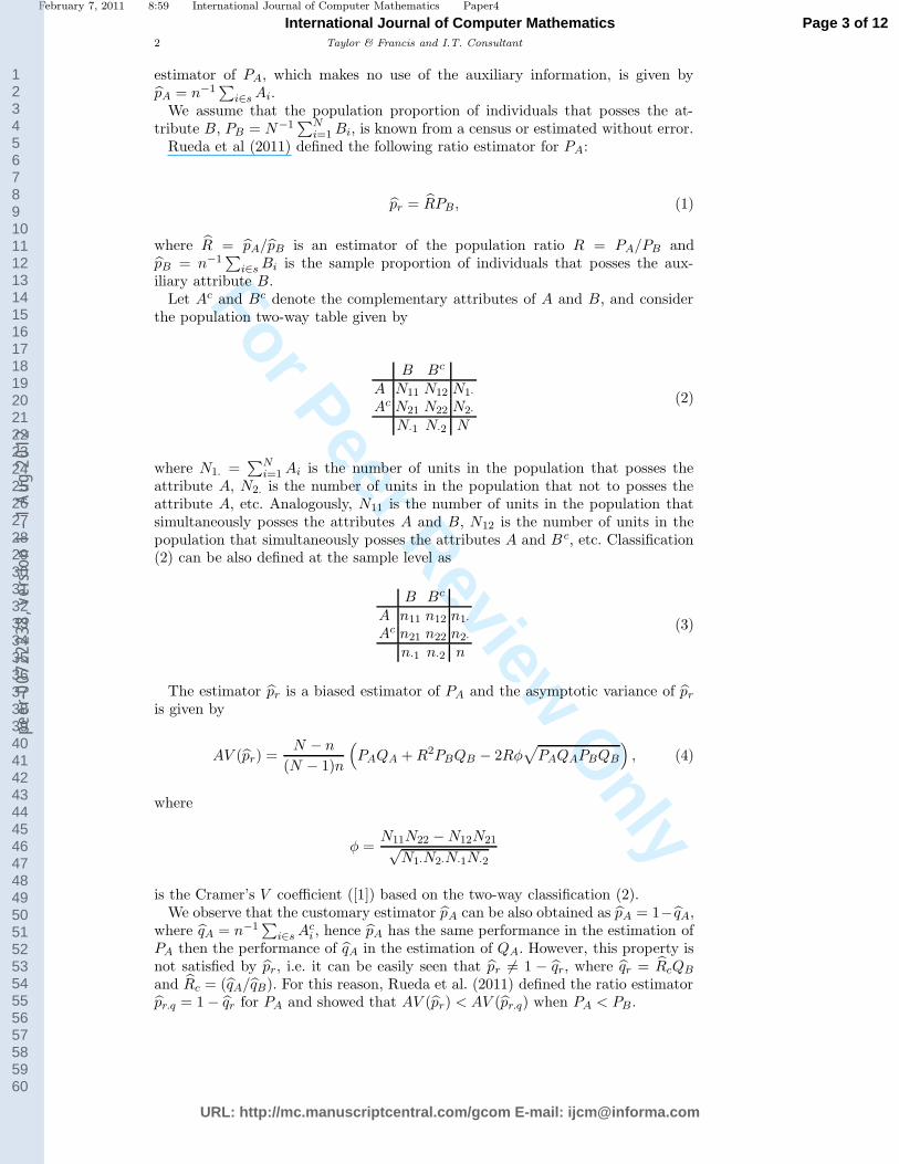
estimator of PA, which makes no use of the auxiliary information, is given bypA = n−1

∑i∈s Ai.

We assume that the population proportion of individuals that posses the at-tribute B, PB = N−1

∑Ni=1 Bi, is known from a census or estimated without error.

Rueda et al (2011) defined the following ratio estimator for PA:

pr = RPB , (1)

where R = pA/pB is an estimator of the population ratio R = PA/PB andpB = n−1

∑i∈s Bi is the sample proportion of individuals that posses the aux-

iliary attribute B.Let Ac and Bc denote the complementary attributes of A and B, and consider

the population two-way table given by

B Bc

A N11 N12 N1·

Ac N21 N22 N2·

N·1 N·2 N

(2)

where N1. =∑N

i=1 Ai is the number of units in the population that posses theattribute A, N2. is the number of units in the population that not to posses theattribute A, etc. Analogously, N11 is the number of units in the population thatsimultaneously posses the attributes A and B, N12 is the number of units in thepopulation that simultaneously posses the attributes A and B c, etc. Classification(2) can be also defined at the sample level as

B Bc

A n11 n12 n1·

Ac n21 n22 n2·

n·1 n·2 n

(3)

The estimator pr is a biased estimator of PA and the asymptotic variance of pr

is given by

AV (pr) =N − n

(N − 1)n

(PAQA + R2PBQB − 2Rφ

√PAQAPBQB

), (4)

where

φ =N11N22 − N12N21√

N1·N2·N·1N·2

is the Cramer’s V coefficient ([1]) based on the two-way classification (2).We observe that the customary estimator pA can be also obtained as pA = 1− qA,

where qA = n−1∑

i∈s Aci , hence pA has the same performance in the estimation of

PA then the performance of qA in the estimation of QA. However, this property isnot satisfied by pr, i.e. it can be easily seen that pr 6= 1 − qr, where qr = RcQB

and Rc = (qA/qB). For this reason, Rueda et al. (2011) defined the ratio estimatorpr.q = 1 − qr for PA and showed that AV (pr) < AV (pr.q) when PA < PB .

of 12



123456789101112131415161718192021222324252627282930313233343536373839404142434445464748495051525354555657585960

peer

-007

2223

8, v

ersi

on 1

- 1

Aug

2012

https://www.researchgate.net/publication/50868943_Estimators_and_Confidence_Intervals_for_the_Proportion_Using_Binary_Auxiliary_Information_with_Applications_to_Pharmaceutical_Studies?el=1_x_8&enrichId=rgreq-02e3a6fd940128502085b44bae7a7bf9&enrichSource=Y292ZXJQYWdlOzIyMDY2MjEwNjtBUzoxMDM5MzM2MzI1ODE2MzRAMTQwMTc5MTExNzI0OA==

For Peer Review O

nly


International Journal of Computer Mathematics 3

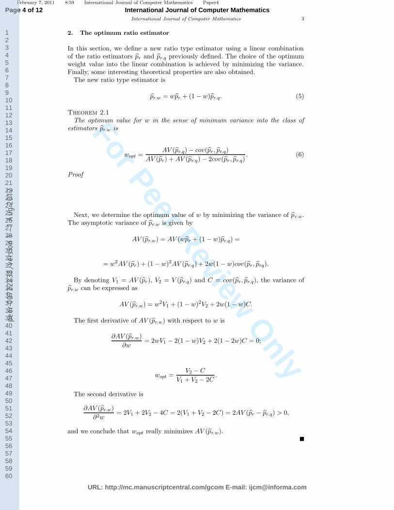
2. The optimum ratio estimator

In this section, we define a new ratio type estimator using a linear combinationof the ratio estimators pr and pr.q previously defined. The choice of the optimumweight value into the linear combination is achieved by minimizing the variance.Finally, some interesting theoretical properties are also obtained.

The new ratio type estimator is

pr.w = wpr + (1 − w)pr.q. (5)

Theorem 2.1

The optimum value for w in the sense of minimum variance into the class ofestimators pr.w is

wopt =AV (pr.q) − cov(pr, pr.q)

AV (pr) + AV (pr.q) − 2cov(pr, pr.q). (6)

Proof

Next, we determine the optimum value of w by minimizing the variance of pr.w.The asymptotic variance of pr.w is given by

AV (pr.w) = AV (wpr + (1 − w)pr.q) =

= w2AV (pr) + (1 − w)2AV (pr.q) + 2w(1 − w)cov(pr , prq).

By denoting V1 = AV (pr), V2 = V (pr.q) and C = cov(pr, pr.q), the variance ofpr.w can be expressed as

AV (pr.w) = w2V1 + (1 − w)2V2 + 2w(1 − w)C.

The first derivative of AV (pr.w) with respect to w is

∂AV (pr.w)

∂w= 2wV1 − 2(1 − w)V2 + 2(1 − 2w)C = 0;

wopt =V2 − C

V1 + V2 − 2C.

The second derivative is

∂AV (pr.w)

∂2w= 2V1 + 2V2 − 4C = 2(V1 + V2 − 2C) = 2AV (pr − pr.q) > 0,

and we conclude that wopt really minimizes AV (pr.w).�

of 12



123456789101112131415161718192021222324252627282930313233343536373839404142434445464748495051525354555657585960

peer

-007

2223

8, v

ersi

on 1

- 1

Aug

2012

For Peer Review O

nly



Therefore, the optimum ratio estimator in the sense of minimum variance intothe class (5) is

pr.OPT = woptpr + (1 − wopt)pr.q.

In practice, pr.OPT could be unknown, since wopt depends on population vari-ances, which are generally unknown. In this situation, we can use the estimator

pr.opt = woptpr + (1 − wopt)pr.q, (7)

where

wopt =V (pr.q) − cov(pr, pr.q)

V (pr) + V (pr.q) − 2cov(pr, pr.q). (8)

Following Sarndal et al. (1992) pg 372, the variance of pr.w can be expressed as

AV (pr.w) = (V1 + V2 − 2C)

(w − V2 − C

V1 + V2 − 2C

)2

+V1V2 − C2

V1 + V2 − 2C,

and we can deduce that the variance of the optimum estimator is

AV (pr.OPT ) =V1V2 − C2

V1 + V2 − 2C.

An estimator of the variance of the optimum estimator can be obtained as

V (pr.opt) =V (pr)V (pr.q) − cov2(pr, pr.q)

V (pr) + V (pr.q) − 2cov(pr, pr.q).

We observe that AV (pr.OPT ) depends on the covariance C = cov(pr, pr.q). The-orem 2 gives an expression for C.

Theorem 2.2 The covariance between the ratio estimators pr and pr.q is

cov(pr, pr.q) =N − n

N − 1

1

n

(PAQA + RRcPBQB − (R + Rc)φ

√PAQAPBQB

),

where Rc = QA/QB is the population ratio of the complementary proportions ofthe attributes A and B.

Proof

Using Taylor series (see Sarndal et al. 1992, pg 178), R can be expressed as

R ∼= R +1

nPB

∑

i∈s

(Ai − RBi) = R +1

PB(pA − RpB),

and similarly

Rc∼= Rc +

1

QB(qA − RcqB).

of 12



123456789101112131415161718192021222324252627282930313233343536373839404142434445464748495051525354555657585960

peer

-007

2223

8, v

ersi

on 1

- 1

Aug

2012

For Peer Review O

nly



Using the previous expressions we obtain

C = cov(pr, 1 − qr) = −cov(RPB , RcQB) =

−PBQBcov

(R +

1

PB(pA − RPB), Rc +

1

QB(qA − RcqB)

)=

= V (pA) + RRcV (pB) − (R + Rc)cov(pA, pB) =

=N − n

N − 1

1

n

(PAQA + RRcPBQB − (R + Rc)φ

√PAQAPBQB

).

�

An estimator of the covariance cov(pr, pr.q) is

cov(pr, pr.q) =1 − f

n − 1

(pAqA + RRcpB qB − (R + Rc)φ

√pAqApB qB

),

where

φ =n11n22 − n12n21√

n1·n2·n·1n·2.

Theorem 2.3

The optimum weight wopt in expression (6) can be expressed as

wopt =Rc − β

Rc − R,

where

β =cov(pA, pB)

V (pB).

Proof

Knowing that

V1 = V (pA) + R2V (pB) − 2Rcov(pA, pB),

V2 = V (qA) + R2cV (qB) − 2Rccov(qA, qB) =

= V (pA) + R2cV (pB) − 2Rccov(pA, pB)

of 12



123456789101112131415161718192021222324252627282930313233343536373839404142434445464748495051525354555657585960

peer

-007

2223

8, v

ersi

on 1

- 1

Aug

2012

For Peer Review O

nly



and

C = V (pA) + RRcV (pB) − (R + Rc)cov(pA, pB),

the numerator and the denominator of wopt in (6) are given by

V2 − C = V (pB)(R2c − RRc) − cov(pA, pB)[2Rc − (R − Rc)] =

= V (pB)Rc(Rc − R) − cov(pA, pB)(Rc − R) =

= (Rc − R)[V (pB)Rc − cov(pA, pB)]

and

V1 + V2 − 2C = V (pB)(R2 + R2c − 2RRc) − cov(pA, pB)[2R + 2Rc − 2(R + Rc)] =

= V (pB)(Rc − R)2

By replacing these expressions in (6) we obtain

wopt =V2 − C

V1 + V2 − 2C=

(Rc − R)[V (pB)Rc − cov(pA, pB)]

V (pB)(Rc − R)2=

=V (pB)Rc − cov(pA, pB)

(Rc − R)V (pB)=

Rc − β

Rc − R.

�

Following theorem 2.3, the estimated optimum weight wopt given by (8) can becalculated as

wopt =Rc − β

Rc − R, (9)

where

β =cov(pA, pB)

V (pB).

From expression (9) we conclude that wopt = 1, that is pr.opt = pr, if β = R,

whereas wopt = 0, that is pr.opt = pr.q, if β = Rc. In other words, the ratio estimator

pr has a larger weight into the optimum estimator pr.opt as β is closer to R. On the

of 12



123456789101112131415161718192021222324252627282930313233343536373839404142434445464748495051525354555657585960

peer

-007

2223

8, v

ersi

on 1

- 1

Aug

2012

For Peer Review O

nly



other hand, the ratio estimator pr.q has a larger weight into the optimum estimator

pr.opt as β is closer to Rc.

Theorem 2.4

The asymptotic variance of the optimum ratio estimator pr.OPT can be calculatedas

AV (pr.OPT ) = V (pA)(1 − φ2).

Proof

The asymptotic variance of pr.OPT is

AV (pr.OPT ) =V1V2 − C

V1 + V2 − 2C,

where the denominator, as seen in proof of theorem 2.3, can be obtained as

V1 + V2 − 2C = V (pB)(R − Rc)2.

Next, we obtain the numerator of AV (pr.OPT ). For the sake of simplicity, wedenote VA = V (pA), VB = V (pB) and CAB = cov(pA, pB). We had that

V1 = VA + R2VB − 2RCAB,

V2 = VA + R2cVB − 2RcCAB

and

C = VA + RRcVB − (R + Rc)CAB .

First,

V1V2 = V 2A + R2

cVAVB − 2RcVACAB + R2VAVB + R2R2cV

2B

−2R2RcVBCAB − 2RVACAB − 2RR2cVBCAB + 4RRcC

2AB.

The square of the covariance can be expressed as

C2 = V 2A + R2R2

cV2B + (R + Rc)

2C2AB + 2VARRcVB

−2(R + Rc)VACAB − 2RRc(R + Rc)VBCAB =

= V 2A + R2R2

cV2B + R2C2

AB + R2cC

2AB + 2RRcC

2AB + 2VARRcVB

of 12



123456789101112131415161718192021222324252627282930313233343536373839404142434445464748495051525354555657585960

peer

-007

2223

8, v

ersi

on 1

- 1

Aug

2012

For Peer Review O

nly



−2RVACAB − 2RcVACAB − 2R2RcVBCAB − 2RR2cVBCAB.

Then, the numerator of AV (pr.OPT ) is

V1V2 − C2 = VAVB(R2c − 2RRc + R2) − C2

AB(R2 + R2c − 2RRc) =

= (VAVB − C2AB)(R − Rc)

2.

The variance of pr.OPT can be also obtained as

AV (pr.OPT ) =VAVB − C2

AB

VB=

V (pA)V (pB) − cov(pA, pB)2

V (pB). (10)

Replacing V (pA), V (pB) and cov(pA, pB) in (10) by their respective expressionsunder SRSWOR we obtain

AV (pr.OPT ) =N − n

N − 1

1

n

[PAQAPBQB − φ2PAQAPBQB

PBQB

]=

=N − n

N − 1

1

nPAQA(1 − φ2) = V (pA)(1 − φ2).

�

Theoretical comparison between the ratio estimator pr.OPT and the simple ex-pansion estimator pA is fairly simple using theorem 2.4. In fact, pr.OPT is moreefficient than pA, since 1− φ2 ≤ 1, and both estimators has the same performancewhen φ2 = 0.

Using theorem 2.4, an estimator of the optimum ratio type estimator variance is

V (pr.opt) = V (pA)(1 − φ2).

3. Simulation study

In this section, the proposed optimum ratio estimator pr.opt is compared numericallywith alternative proportion estimators. Simulation studies are based on severalsimulated populations which cover a wide number of possible scenarios, includingsmall and large proportions, small and large Cramer’s V coefficients between theattribute of interest and the auxiliary attributes, etc. Simulated populations arebriefly described as follows.

A total of 30 populations of N = 1000 units were generated to study the ef-fect of different aspects on the estimators of a population proportion. Populationswere generated as a random sample of 1000 units from a Bernoulli distributionwith parameter p = {0.1, 0.25, 0.5, 0.75.0.9}, and the attributes of interest werethus achieved with the aforementioned population proportions. Auxiliary attributeswere also generated by using the same distribution, but we randomly change a givenproportion of values in order to the Cramer’s V coefficient between the attributeof interest and the auxiliary attribute goes from 0.5 to 0.9. Since PA < PB whenPA = 0.25, we also generated populations with PA = 0.25 and PA > PB , which

of 12



123456789101112131415161718192021222324252627282930313233343536373839404142434445464748495051525354555657585960

peer

-007

2223

8, v

ersi

on 1

- 1

Aug

2012

For Peer Review O

nly



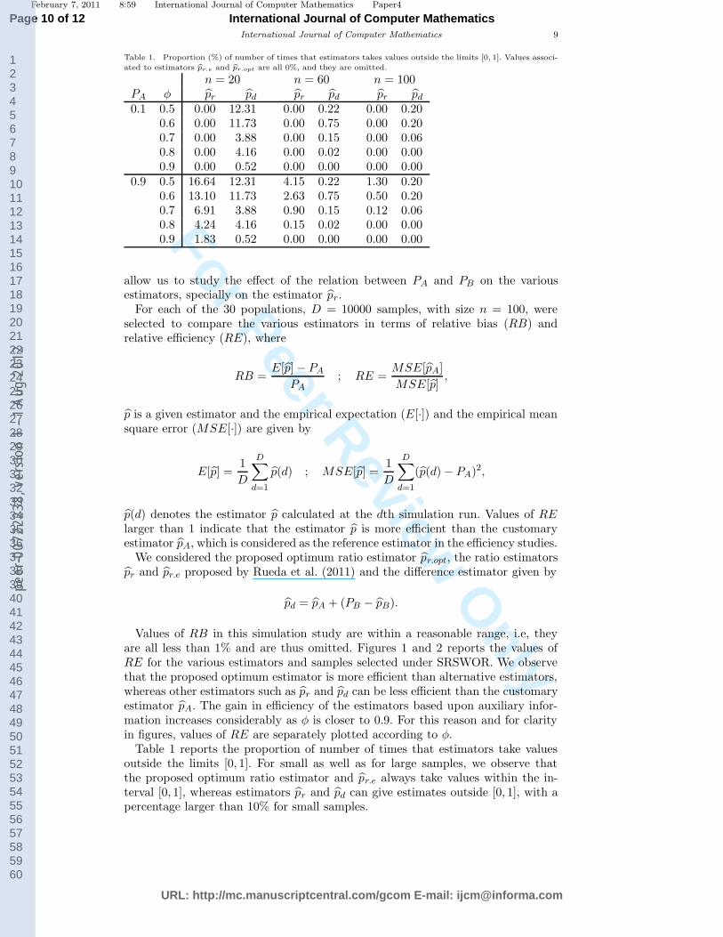
Table 1. Proportion (%) of number of times that estimators takes values outside the limits [0, 1]. Values associ-

ated to estimators bpr.e and bpr.opt are all 0%, and they are omitted.

n = 20 n = 60 n = 100PA φ pr pd pr pd pr pd

0.1 0.5 0.00 12.31 0.00 0.22 0.00 0.200.6 0.00 11.73 0.00 0.75 0.00 0.200.7 0.00 3.88 0.00 0.15 0.00 0.060.8 0.00 4.16 0.00 0.02 0.00 0.000.9 0.00 0.52 0.00 0.00 0.00 0.00

0.9 0.5 16.64 12.31 4.15 0.22 1.30 0.200.6 13.10 11.73 2.63 0.75 0.50 0.200.7 6.91 3.88 0.90 0.15 0.12 0.060.8 4.24 4.16 0.15 0.02 0.00 0.000.9 1.83 0.52 0.00 0.00 0.00 0.00

allow us to study the effect of the relation between PA and PB on the variousestimators, specially on the estimator pr.

For each of the 30 populations, D = 10000 samples, with size n = 100, wereselected to compare the various estimators in terms of relative bias (RB) andrelative efficiency (RE), where

RB =E[p] − PA

PA; RE =

MSE[pA]

MSE[p],

p is a given estimator and the empirical expectation (E[·]) and the empirical meansquare error (MSE[·]) are given by

E[p] =1

D

D∑

d=1

p(d) ; MSE[p] =1

D

D∑

d=1

(p(d) − PA)2,

p(d) denotes the estimator p calculated at the dth simulation run. Values of RElarger than 1 indicate that the estimator p is more efficient than the customaryestimator pA, which is considered as the reference estimator in the efficiency studies.

We considered the proposed optimum ratio estimator pr.opt, the ratio estimatorspr and pr.e proposed by Rueda et al. (2011) and the difference estimator given by

pd = pA + (PB − pB).

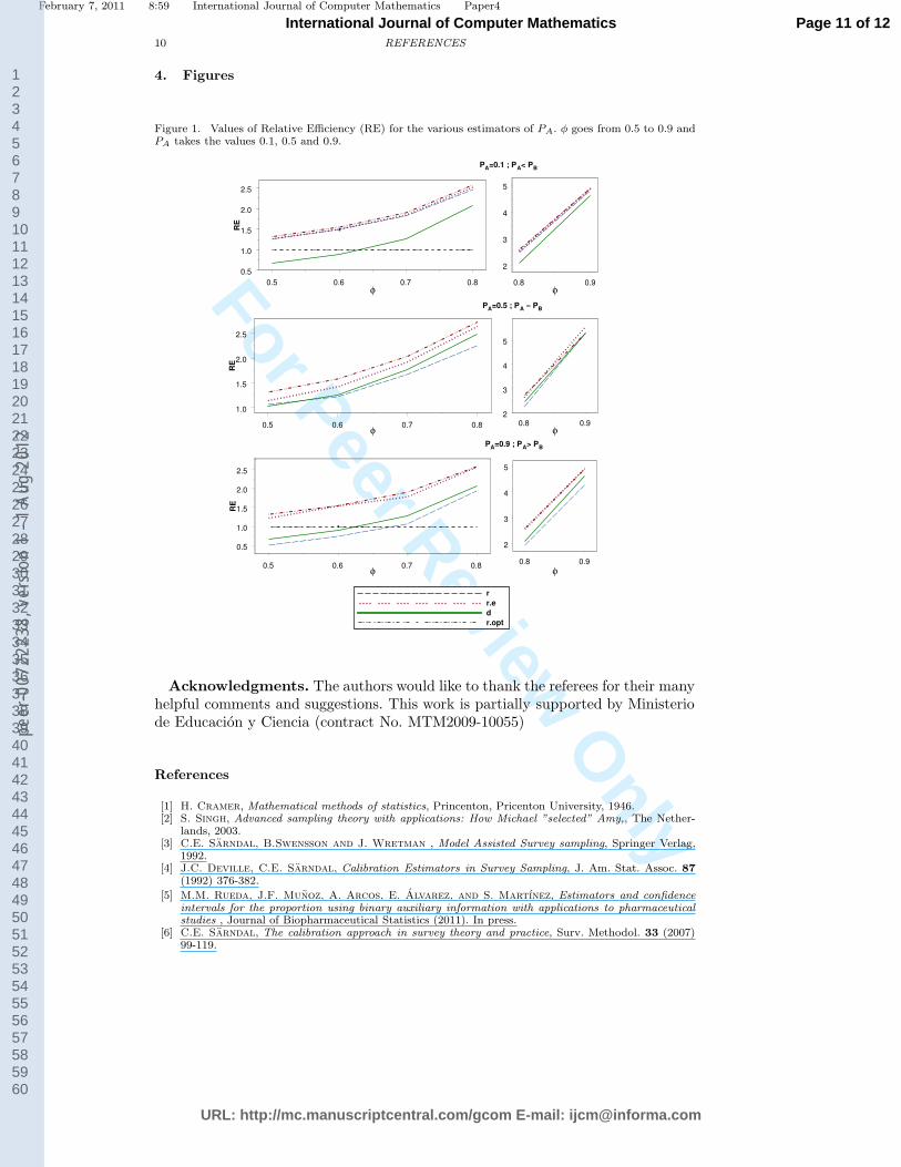
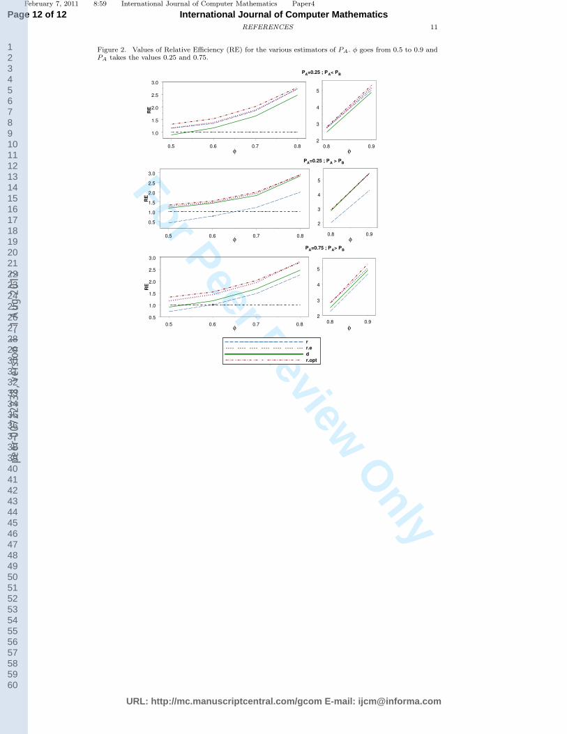
Values of RB in this simulation study are within a reasonable range, i.e, theyare all less than 1% and are thus omitted. Figures 1 and 2 reports the values ofRE for the various estimators and samples selected under SRSWOR. We observethat the proposed optimum estimator is more efficient than alternative estimators,whereas other estimators such as pr and pd can be less efficient than the customaryestimator pA. The gain in efficiency of the estimators based upon auxiliary infor-mation increases considerably as φ is closer to 0.9. For this reason and for clarityin figures, values of RE are separately plotted according to φ.

Table 1 reports the proportion of number of times that estimators take valuesoutside the limits [0, 1]. For small as well as for large samples, we observe thatthe proposed optimum ratio estimator and pr.e always take values within the in-terval [0, 1], whereas estimators pr and pd can give estimates outside [0, 1], with apercentage larger than 10% for small samples.

of 12



123456789101112131415161718192021222324252627282930313233343536373839404142434445464748495051525354555657585960

peer

-007

2223

8, v

ersi

on 1

- 1

Aug

2012


For Peer Review O

nly


10 REFERENCES

4. Figures

Figure 1. Values of Relative Efficiency (RE) for the various estimators of PA. φ goes from 0.5 to 0.9 andPA takes the values 0.1, 0.5 and 0.9.

0.5 0.6 0.7 0.8

φ

0.5

1.0

1.5

2.0

2.5

RE

0.8 0.9

φ

2

3

4

5

PA=0.1 ; PA< PB

0.5 0.6 0.7 0.8φ

1.0

1.5

2.0

2.5

RE

0.8 0.9

φ

2

3

4

5

PA=0.5 ; PA ≈ PB

0.5 0.6 0.7 0.8φ

0.5

1.0

1.5

2.0

2.5

RE

0.8 0.9

φ

2

3

4

5

r

r.e

d

r.opt

PA=0.9 ; PA> PB

Acknowledgments. The authors would like to thank the referees for their manyhelpful comments and suggestions. This work is partially supported by Ministeriode Educacion y Ciencia (contract No. MTM2009-10055)

References

[1] H. Cramer, Mathematical methods of statistics, Princenton, Pricenton University, 1946.[2] S. Singh, Advanced sampling theory with applications: How Michael ”selected” Amy,, The Nether-

lands, 2003.[3] C.E. Sarndal, B.Swensson and J. Wretman , Model Assisted Survey sampling, Springer Verlag,

1992.[4] J.C. Deville, C.E. Sarndal, Calibration Estimators in Survey Sampling, J. Am. Stat. Assoc. 87

(1992) 376-382.

[5] M.M. Rueda, J.F. Munoz, A. Arcos, E. Alvarez, and S. Martınez, Estimators and confidenceintervals for the proportion using binary auxiliary information with applications to pharmaceuticalstudies , Journal of Biopharmaceutical Statistics (2011). In press.

[6] C.E. Sarndal, The calibration approach in survey theory and practice, Surv. Methodol. 33 (2007)99-119.

of 12



123456789101112131415161718192021222324252627282930313233343536373839404142434445464748495051525354555657585960

peer

-007

2223

8, v

ersi

on 1

- 1

Aug

2012

https://www.researchgate.net/publication/243784196_Calibration_Estimators_in_Survey_Sampling?el=1_x_8&enrichId=rgreq-02e3a6fd940128502085b44bae7a7bf9&enrichSource=Y292ZXJQYWdlOzIyMDY2MjEwNjtBUzoxMDM5MzM2MzI1ODE2MzRAMTQwMTc5MTExNzI0OA==

https://www.researchgate.net/publication/243784196_Calibration_Estimators_in_Survey_Sampling?el=1_x_8&enrichId=rgreq-02e3a6fd940128502085b44bae7a7bf9&enrichSource=Y292ZXJQYWdlOzIyMDY2MjEwNjtBUzoxMDM5MzM2MzI1ODE2MzRAMTQwMTc5MTExNzI0OA==







https://www.researchgate.net/publication/44816799_Moel_Assisted_Survey_Sampling?el=1_x_8&enrichId=rgreq-02e3a6fd940128502085b44bae7a7bf9&enrichSource=Y292ZXJQYWdlOzIyMDY2MjEwNjtBUzoxMDM5MzM2MzI1ODE2MzRAMTQwMTc5MTExNzI0OA==

https://www.researchgate.net/publication/44816799_Moel_Assisted_Survey_Sampling?el=1_x_8&enrichId=rgreq-02e3a6fd940128502085b44bae7a7bf9&enrichSource=Y292ZXJQYWdlOzIyMDY2MjEwNjtBUzoxMDM5MzM2MzI1ODE2MzRAMTQwMTc5MTExNzI0OA==

For Peer Review O

nly


REFERENCES 11

Figure 2. Values of Relative Efficiency (RE) for the various estimators of PA. φ goes from 0.5 to 0.9 andPA takes the values 0.25 and 0.75.

0.5 0.6 0.7 0.8

φ

1.0

1.5

2.0

2.5

3.0

RE

0.8 0.9

φ

2

3

4

5

PA=0.25 ; PA< PB

0.5 0.6 0.7 0.8φ

0.5

1.0

1.5

2.0

2.5

3.0

RE

0.8 0.9

φ

2

3

4

5

PA=0.25 ; PA > PB

0.5 0.6 0.7 0.8φ

0.5

1.0

1.5

2.0

2.5

3.0

RE

0.8 0.9

φ

2

3

4

5

r

r.e

d

r.opt

PA=0.75 ; PA> PB

of 12



123456789101112131415161718192021222324252627282930313233343536373839404142434445464748495051525354555657585960

peer

-007

2223

8, v

ersi

on 1

- 1

Aug

2012

optimum ratio estimators for the population proportion

Documents