1

Modelling the Spatial Properties of Group Members in the Internet

UCLA CSD TR # 030011

Jun-Hong Cui, Dario Maggiorini, Michalis Faloutsos, Mario Gerla, Khaled Boussetta

Abstract

This work focuses on measuring and modelling the distribution of members for group communications (especially multicast)

in the Internet. In current literature, the spatial properties of group members has not been studied, although temporal properties

have received some attention. However, the placement of members can have significant impact on the design and evaluation of

multicast schemes and protocols as shown in previous studies. In our work, we identify properties of members that reflect their

spatial clustering and the correlation among them (such as participation probability, and pairwise correlation). Then, we obtain

values for these properties by monitoring the membership of network games, large audio-video broadcasts from IETF and NASA.

Finally, we provide a comprehensive model that can generate realistic groups. We evaluate our model against the measured data

with excellent results. A realistic group membership model can help us improve the effectiveness of simulations and guide the

design of group-communication protocols.

I. I NTRODUCTION

Where should we place group members in a multicast (or more general group communication) simulation? So far,

the common practice was to use uniformly random distributions due to the lack of a more systematic and potentially

more realistic way. Multicast research can greatly benefit from realistic models and a systematic evaluation method-

ology ([11] [36] [14] [29] [32] [12] [34] [33] [37] [41] [19]). Despite the significant breakthroughs in modelling the

traffic and the topology of the Internet, there has been little progress in multicast modelling. As a result, the design

and evaluation of multicast protocols is based on commonly accepted but often unproven assumptions. For example,

the majority of simulation studies assumes that the users are uniformly distributed in the network. In this paper, we

challenge this assumption and study the spatial properties of group members, such as clustering and correlation.

The design and development of multicast protocols can benefit significantly from a realistic modelling of the spatial

properties of the group members. Spatial information can help us address the scalability issues, which has always been

a major concern in multicasting. Similarly, reliable multicast protocols need spatial information in order to fine-tune

their performance or even evaluate their viability. Furthermore, spatial properties of a group with common interest

members transcend the scope of IP multicast. Group communications is an undeniable necessity independently of

the specifics of the technology that is used to support it. For example, web caching, peer-to-peer communication,

application level multicast protocols can and should consider the member locality.

The spatial properties of group membership have not been adequately measured and modelled, although the need

to do so has been advocated by several studies. For example, some research works show the importance of the spatial

2

distribution of members [41] [19] [32]. However, there does not exist a generative model for such a distribution,

which is partly due to unavailability of real data. In more detail, there have been several studies on the temporal group

properties [5] [21]. In addition, several studies examine the scaling properties of multicast trees [14] [32] [12] [13] and

the aggregatability of multicast state [33] [37] [41] [19]. Philips et al. [32] conclude that the affinity and disaffinity of

members can affect the size of the multicast tree significantly. Thaler et al. [37] and Fei et al. [19] observe that the

location of members has significant influence on the performance of their state reduction schemes.

In this work, we model the spatial properties of group members focusing on their topological clustering and corre-

lations. A distinguishing point of our work is that we use extensive measurements to understand the real distributions

and develop a powerful model to generate realistic distributions. Our contributions can be summarized into two main

thrusts.

1. Real data analysis.We measure and analyze the membership of net games and large audio-video broadcasts

from IETF and NASA (over the MBONE). We quantify properties of the membership focusing on: a) the clustering,

b) the distribution of the participation, and c) the distribution of thepairwisecorrelation of members or clusters in a

group. We observe that the MBONE multicast and gaming exhibit differences, as suggests the need for a flexible and

comprehensive model to capture the different characteristics. In our clustering analysis, we use the seminal approach

of network-aware clustering [23]. More specifically, we make the following observations.

• MBONE multicast members:The group members are highly clustered and the clusters show strong pairwise

correlations in their participation.

• Net game members:The clustering is much less significant and there does not seem to be a strong correlation

between users. Interestingly, we observe a daily periodicity in participating players.

2. GEM: A model for realistic group generation. We developGEneralizedMembership model (GEM) that can

generate realistic member distributions. These distributions are given as input parameters to the model, enabling users

to match the desired distribution. The main innovation of the model is the capability to match pairwise participation

probabilities. To achieve this, we employ the Maximum Entropy method [42], which has been successfully used in

other disciplines, such as statistical mechanics, thermodynamics, data analysis, spectral analysis, protein structure

prediction, natural language understanding, computer vision, etc. The Maximum Entropy method chooses the solution

with maximum “randomness” or entropy in an under-defined system. As a result, GEM can simulate the following

membership behavior:

• Uniform distribution, which is the common assumption but not always realistic.

• Skewed participation distribution without pairwise correlations.

• Skewed participation distribution with pairwise correlations.

Through simulations, we validate our model with very positive results: We are able to generate groups whose

statistical behavior matches very well the real distributions.

3

The analysis and the framework presented in this work can be of interest to communities beyond multicast re-

searchers: applications with multiple recipients such as web caching, streaming multimedia and peer-to-peer file shar-

ing are also interested in the location of users ([10] [40] [25]). We provide our data and our model to the community

with the hope that it can be part of a realistic and systematic evaluation methodology for this kind of research ([1]).

The rest of this paper is organized as follows. Section II gives some background on multicast group modelling and

some related work. Section III classifies the spatial properties of group members. Section IV quantifies the spatial

group properties using real data from the MBONE and net games. Section V describes our powerful group membership

model. In Section VI, we validate the capabilities of our model. Finally, we conclude our work in section VII.

II. BACKGROUND AND RELATED WORK

In this section, we give some background on multicast group modelling and some related research efforts.

The properties of multicast group behavior can be classified into two categories: spatial and temporal properties.

Spatial properties consider the distribution of multicast group members in the network. Temporal properties con-

centrate on the distribution of inter-arrival time and life time of group members, in other words, the group member

dynamics. In the following, we give an overview of the related work on the modelling of multicast group behavior.

The majority of multicast research assumes simplified assumptions on the distribution of members in the network.

Protocol developers almost always assume that users are uniformly distributed in the network (such as [38], [39], [9],

[26], [18], and [14], etc.). This is partly due to the unavailability of real data. On the other hand, it is interesting

to observe that skewed distributions have been observed in multiple aspects of communication networks from traffic

behavior [27] [31] to preferences for content [15] and peer-to-peer networks [22].

There have been some studies on the temporal group properties, such as [5] and [21]. [5] measured and studied

the member arrival interval and membership duration for MBONE. It showed that, for multicast sessions on MBONE,

an exponential function works well for the member inter-arrival time of all type of sessions, while for membership

duration time, an exponential function works well for short sessions, but a Zipf [43] distribution works well for longer

sessions. [21] conducted a follow-on study for net games. The authors found that player duration time fits an expo-

nential distribution, while inter-arrival time fits a heavy-tailed distribution for net game sessions.

Several seminal research works which examine the scaling properties of multicast trees ([14] [32] [12] [13] [34])

and the aggregatability of multicast state ([33] [37] [41] [19]) show that the spatial properties do matter in multicast

research. In [14], Chuang and Sirbu discovered that the scaling of the tree cost follows power law with respect to the

group size. Philips et al. gave a theoretical analysis of the Chuang and Sirbu scaling law in [32]. They also considered

member affinity1, and concluded that, for a fixed number of members, affinity can significantly affect the size of the

delivery tree. These two works mainly focus on multicast efficiency (the gain of multicast vs unicast). Besides defining

1Member affinity means the members are likely to cluster together, while disaffinity means that they tend to spread out.

4

a metric to measure multicast efficiency, Chalmers and Almeroth ([12] [13]) also examined the shape of the multicast

trees through measurements from MBONE, basically concentrating on the the distribution and frequency of the degree

of in-tree nodes, the depth of receivers, and the node class distribution. In this work, Chalmers and Almeroth also

indicate that the member clustering has strong impact on the multicast efficiency.

Our ability to aggregate the multicast state is also significantly affected by the spatial properties of the group mem-

bers. State aggregation has been the goal of several research efforts ([33], [37], and [19]). These papers proposed

different state reduction schemes, and showed that group spatial properties, such as clustering of members and cor-

relation between members, affects the performance of their approaches. In [41], Wong et al. did a comprehensive

analysis of multicast state scalability considering network topology, group density, clustering/affinity of members and

inter-group correlation. They conclude that application-driven membership has significant impact on multicast state

distribution and concentration.

Recently, there is another seminal work [29] which is dedicated to affinity research of group members. In this work,

Lucas et al. proposed several new metrics to better characterize the affinity property between group members. They

also conducted three case studies (multicast, replica placement, and sensor networks) and demonstrated that the better

characterization of affinity can significantly help to predict the network performance. This work, however, did not

provide real group membership measurement and a comprehensive model to generate group members.

In multicast modelling, besides the above group modelling work, there is yet another important research topic:

multicast group size estimation [20] [28] [7] [17] [6] [30]. In [20] and [28], different estimators of group size were

developed based on probabilistic polling mainly for static groups, while the research studies of [7], [17] and [30] aim at

proposing audience size estimators and protocols for dynamic groups. In [6], Dolev et al. discovered the rank-degree

power law of multicast trees, based on which they obtained an estimation on the number of group members (i.e., group

size). Clearly, there is a close relationship between group size and the distribution of members, however, the group

size estimation is beyond the scope of this paper. The focus of this paper is the measurement and modelling of group

member distribution.

III. SPATIAL PROPERTIES OFGROUPMEMBERS

In this section, we identify and define several spatial properties of group membership, which we quantify through

measurements in the next section. For simplicity, we refer to the hosts or routers in the Internet as “nodes” or “network

nodes”.

1. Member Clustering: Clustering captures the proximity of the group members. We are interested in the proxim-

ity from a networking point of view, and we use the network-aware clustering method [23] in our measurement. Some

nodes in a cluster might become members of a multicast group. We call the number of group members in a cluster as

“member cluster size”. This metric will be used in Section IV-B.

5

Though some earlier studies proposed models to capture the clustering of group members ([37], [41]) (based on

common intuitions), they do not provide measurements of the clustering in the Internet.

Note that the metrics we present below can refer to a node or a cluster. We will use the term “cluster”, since a node

is a cluster of size1. When one or more nodes in a cluster join a group, we say this cluster participates in the group.

In our analysis we focus on clusters for large groups. On the one hand, we achieve good analysis granularity [24]. On

the other hand, this approach facilitates the design of group generation model (as illustrated in Section V.

2. Group Participation Probability: Different clusters have different probabilities in participating in multicast

groups: some clusters are more likely to be part of a group. The uniform distribution of participation is a special case

where all clusters have the same probability.

Multiple Group Participation: If we have many groups, we define the participation probability of a cluster as the

ratio of groups that the cluster joins.

Time-based Participation: For a single but long-lived group, the participation probability can be defined as the

percentage of time that a cluster is part of the group. We find this definition particularly attractive, since our data is

often limited in the number of groups. It should be noted that, in our analysis, we use this definition.

Recently, [19], Fei et al. proposed a node-weighted model to incorporate the difference among network nodes, where

each node is assigned a weight representing the probability for that node to be in a group.

3. Pairwise Correlation in Group Participation: This metric captures the joint probability that two clusters are

members of a group. The intuition is that common-interest or related users (e.g. friends) will probably share more

than one groups. More specifically, we quantify the pairwise correlation between two clusters as follows. Given two

clustersCi andCj , we denote the participation probabilities of clusterCi andCj aspi andpj respectively, and the

joint participation probability ofCi andCj is aspi,j . The correlation coefficient betweenCi andCj , coef(i, j), is the

normalized covariance betweenCi andCj ([35]):

coef(i, j) =(pi,j − pi × pj)√

pi × (1− pi)×√

pj × (1− pj). (1)

Multiple Group Pairwise Correlation: In the presence of many groups, we can use the multiple group participation

probability to compute pairwise correlation.

Time-based Pairwise Correlation: In this work, we measured and analyzed single but long lived sessions (from

MBONE and net games). Thus we can use the time-based participation probability that we defined above to compute

time-based pairwise correlation.

In the literature, there has been some effort to model the pairwise correlation. In [37], a two-dimensional array

of randomly allocated correlation probabilities is used. In [41], the authors simulated the correlation implicitly by

encouraging the members of sets of nodes to join the same group, once one of the nodes of the set has joined.

6

Note that in this paper, we focus on pairwise correlation. Although measuring and modelling higher-dimensional

correlations is possible, these metrics are usually not used in the community.

To our best knowledge, this is the first study which use real data to verify and quantify the spatial properties of group

members. In addition, no previous effort has provided a comprehensive model for all of the above properties of group

membership, as we do in this work.

IV. M EMBERSHIPPROPERTIESMEASURED FROMMBONE AND NET GAMES

In this section, we present the measurement and analysis results of the spatial properties of multicast group mem-

bership in real applications. We use data from two major applications: audio-video broadcasts on MBONE and net

games. The first is single-source large-scale application, while the second is multiple-source interactive application.

The MBONE is an overlay network on the Internet, and it has served as a testbed for multicast researchers since

1992. Net games is one of the most popular multiple-source applications. Though most of net games are implemented

using multiple unicasts, we are interested in the spatial group properties, which are independent of the underlying

implementation.

A. Measurement Methodology

MBONE. We use data sets provided by Chalmers and Almeroth from University of Santa Barbara ([12] [13]). The

data sets are divided into two groups: real data sets and cumulative data sets, which are summarized in Table 1 and

Table 2 separately.

The real data sets include IETF43-A, IETF43-V and NASA, and the cumulative data sets include UCSB-2000,

UCSB-2001, Gatech-2001 and UOregon-2001. For the details of measurement on MBONE, please see references

[12] and [13]. One thing deserving more description is the generation of cumulative data sets: multicast paths are

traced using a number of sources (UCSB, Georgia Tech, and Univ. of Oregon) for a series of 22,000 IP addresses

that were known to have participated in multicast groups over a two years period, June’97-June’99. In these data sets,

although most of the traces were collected recently and reflect the latest multicast infrastructure, the group members

represent a relatively random sample taken from the older MBONE. Due to the limited number of real data sets, we

use cumulative data sets to get an intuition of how the size of groups affects the property of member clustering.

Net Games. For net games, we use the QStat tool [3] to collect data. QStat is a program designed to poll and

display the status of game servers. Some game servers offer a querying mechanism, which can retrieve some specific

information, such as the number of players, players’ nicknames, IP addresses, scores, and connection time etc. To

analyze clustering of members, we need members’ IP addresses (the reason will be clarified in Section IV-B). Not

all games, however, provide players’ IP addresses. Quake I is one of the few games that allow this. Thus, we choose

Quake I though it is a little bit old game. Using QStat, we measured70 Quake game servers (obtained from a master

7

TABLE I

MBONE REAL GROUPDATA SETS

Receivers

Name Description Trace Period Total Maximum Average

IETF43-A 43rd IETF Meeting Audio Dec. 7-11, 1998 107 93 58.72

IETF43-V 43rd IETF Meeting Video Dec. 7-11, 1998 129 90 48.59

NASA NASA Shuttle Launch Feb. 14-21, 1999 62 62 40.33

TABLE II

MBONE CUMULATIVE GROUPDATA SETS

Receivers

Name Description Trace Period Total Maximum Average

SYNTH-1 UC Santa Barbara Jan. 6-10, 2000 1,871 1653 805.94

SYNTH-2 Georgia Tech Jul. 12-25, 2001 1,497 1497 958.17

SYNTH-3 University of Oregon Dec. 18-19, 2001 1,019 1019 492.45

SYNTH-4 UC Santa Barbara Dec. 19-22, 2001 1,018 1018 474.35

server) for five days (across a weekend), and the servers are polled every one minute. We select the10 most popular

servers (5 of them providing IP addresses of players) for our analysis, and the selected game servers are illustrated in

Table 3.

From each data set of MBONE and net games (note that, one data set corresponds to one multicast session or group),

we sample the group membership at regular intervals (1 minute). Each sample of group membership is composed of

members with IP address or player ID for some net games data sets (in which IP address of players are not provided).

To give some intuition of the data sets, we plot some examples chosen from real MBONE data and net game data in

Fig. 1, Fig. 2, Fig. 3, and Fig. 4. In all these figures, the X-axis is the time, and the Y-axis represents the number of

members (receivers for MBONE or players for net games). We can see clearly how the number of members changes

with the time.

MBONE multicast: decelerating increase and “black-out” phases.In Fig. 1 and Fig. 2, we see that the IETF

broadcast increases close to monotonically but with decreasing rate of increase. We also notice some short periods

(there is also a big period for IETF Video) in which the number of members drop suddenly and then rise again. One

possible explanation is the network instability: either the tree was torn down and rebuilt or the measurements got lost.

Another possible reason is that these might correspond to breaks of the IETF meeting, such as lunch time. Fig. 3 shows

8

TABLE III

NETGAMES GROUPDATA SETS

Players

Name Game Server Meassurement Period Total Maximum Average

QS-1 quake.dircon.co.uk May 14-18, 2002 352 8 1.71

QS-2 sense-sea.oz.net May 14-18, 2002 265 11 1.89

QS-3 195.147.246.71 May 14-18, 2002 234 11 1.72

QS-4 ut2003.kos.net May 14-18, 2002 158 10 2.22

QS-5 zoologi38.zoologi.su.se May 14-18, 2002 391 11 2.34

QS-6 200.230.198.53: 26004 May 14-18, 2002 1198 10 3.31

QS-7 frodo.trinicom.com May 14-18, 2002 437 16 4.04

QS-8 bridge.widomaker.com May 14-18, 2002 417 13 3.67

QS-9 200.230.198.53: 26001 May 14-18, 2002 1298 8 3.50

QS-10 209.48.106.170 May 14-18, 2002 604 15 8.12

the sampled data sets for NASA broadcast. We see that NASA broadcast has smaller number of drop periods than IETF

broadcast. One reason to explain this is that, unlike IETF meeting, NASA shuttle launch is a more continuous event.

The big drop period can be explained by some break of network connection or some unexpected and uninteresting

event.

Net games: membership is strongly periodic.Fig. 4 shows very interesting behavior of net game (Quake) players:

in each day, there is a big spike in user participation. Moreover, there are more players during the weekend (May 17th

and May 18th). This periodicity is natural given the nature of the activity: For a game server, due to the delay

constraints of gaming, most of the players come from areas within some range (say, in several hops). Thus the players

are more likely to be active in some relatively fixed periods of time in a day. For example, in Fig. 4, we see that late

night is a very active period for game players in this server.

In the rest of this section, we examine the three membership properties of the above data sets: member clustering,

group participation probability, and pair-wise correlation in group participation.

B. Member Clustering

To model member clustering, we employ network-aware clustering. Intuitively, two members tend to be in the same

cluster if they are close in terms of network routing. In the Internet, this kind of grouping can be done based on IP

addresses. We adopt the method in [23] to identify member clusters using network prefixes, based on information

9

0

10

20

30

40

50

60

70

80

90

100

Dec 07 Dec 08 Dec 09 Dec 10 Dec 11 Dec 12

Num

ber

of R

ecei

vers

Days

Fig. 1. The data set sampled from IETF Meeting Audio (IETF43-A).

0

10

20

30

40

50

60

70

80

90

100

Dec 07 Dec 08 Dec 09 Dec 10 Dec 11 Dec 12

Num

ber

of R

ecei

vers

Days

Fig. 2. The data set sampled from IETF Meeting Video (IETF43-V).

available from BGP routing snapshots (we use the BGP dump tables obtained from [2]). This way, clustered nodes are

likely to to be under common administrative control.

In the following, we briefly outline network-aware clustering for completeness (For details, please refer to [23]).

For each of the data sets, we first extract the network prefixes/netmasks from BGP dump tables and the IP addresses

of members from group membership samples, then we classify all the member IP addresses which have the same

longest-match prefix into one cluster, which is identified by the shared prefix. For instance, suppose we want to

cluster the IP addresses216.123.0.1, 216.123.1.5, 216.123.16.59, and216.123.51.87. In the routing table, we find

the longest-match prefixes are216.123.0.0/19, 216.123.0.0/19, 216.123.0.0/19, and216.123.48.0/21 respectively.

Then we can classify the first three IP addresses into a cluster identified by the prefix/netmask216.123.0.0/19 and the

10

0

10

20

30

40

50

60

70

Feb 14 Feb 15 Feb 16 Feb 17 Feb 18 Feb 19 Feb 20 Feb 21 Feb 22

Num

ber

of R

ecei

vers

Days

Fig. 3. The data set sampled from NASA Shuttle Launch (NASA).

0

1

2

3

4

5

6

7

8

9

10

11

12

13

14

15

16

17

May 14 May 15 May 16 May 17 May 18 May 19

Num

ber

of P

laye

rs

Days

Fig. 4. The data set sampled from net game server 1 (QS-7).

last one into another cluster identified by216.123.48.0/21. It should be noted that other clustering methods, such as

network topology based approach, are possible. But network-aware clustering is an easy and effective way for us to

do clustering considering the data we have achieved. In later sections, we will show that our analysis and model are

not constrained by the clustering method.

For each data set, we want to see the number of group members per cluster. As recalled, we refer to the number

of group members in a cluster as themember cluster size(or cluster size for short). For all the group membership

samples, we examine the Cumulative Distribution Function (CDF) of the cluster size. The results for data sets from

MBONE and net games are shown in Fig. 5. Therefore, for a given cluster size in the X-axis, we see how many clusters

have at most that size.

11

0

0.1

0.2

0.3

0.4

0.5

0.6

0.7

0.8

0.9

1

1 2 3 10 20 30 100

CD

F

Cluster size

IETF videoIETF audio

NASA

Gatech 2001UCSB 2000UCSB 2001

Univ. OregonNetgames

Fig. 5. CDF of cluster size for data sets from MBONE and net games. The upper set of curves are for net game data sets

(with 5 game servers providing IP addresses of players), the middle set of curves are for MBONE real data sets (IETF43-A,

IETF43-A, and NASA), and the lower set of curves are for MBONE cumulative data sets.

Group members form clusters with skewed size distribution. Group members are significantly clustered in

MBONE data sets. In Fig. 5, we can see three different groups of curves: the upper group for net game data sets

(with 5 game servers providing IP addresses of players), the middle group for MBONE real data sets (IETF43-A,

IETF43-A, and NASA), and the lower group for MBONE cumulative data sets. In each group, the data sets have

similar member clustering property: for example, for MBONE real data sets, more than20% clusters have2 or more

group members; for MBONE cumulative data sets (UCSB-2000, UCSB-2001, Gatech-2001 and UOregon-2001), they

have more significant clustering features: more than60% clusters have2 or more group members; while for net games,

the corresponding group of CDF curves do not show strong member clustering: about90% “clusters” have size1.

Group size has significant effect on the cluster size distribution.We observe that it is primarily the size of

the group that affects the range of the distribution. When comparing the groups of curves, we can conclude that the

MBONE cumulative data sets have more significant clustering feature than MBONE real data sets. We attribute this to

the larger size of the group. The average number of members for each cumulative data set (from500 to 1000) is much

higher than that for real data sets (around50). The bigger the group is, the more members tend to be in one cluster and

the more significant of the member clustering feature is. As for net games, the feature of member clustering is even

less significant: most “clusters” have only one member, which means that Quake players are more likely scattered over

the network. This observation suggests that probably the gain from some multicast or intelligent caching schemes may

not provide significant benefits in this case.

The absence of clustering in the net games can be attributed to many factors. One observation is that the maximum

number of players (16 in Quake) is controlled by the game servers because of management issues. Thus, the possibility

12

for the members to fall in one cluster becomes smaller. Another possible explanation may be that the game players are

not necessarily from a similar area of the network potentially. This suggests that gaming community is scattered, or

alternatively, that net games bring together people from significantly different places.

The practical implications of member clustering. Understanding the clustering properties can help us develop

efficient protocols to improve the scalability and the performance of applications. The member clustering captures

the proximity of the members in the network especially with the use of network-aware clustering. For example, in a

well clustered group, we can potentially develop hierarchical protocols that can exploit the spatial distribution of the

members like hierarchical multicasting [8] and peer-to-peer routing [25].

C. Group Participation Probability

By examining the group participation probability of different data sets, we find thatuniform participation proba-

bility across clusters or nodes does not hold for some applications.This strongly suggests that the uniform model

used so far for most research is not realistic. In the analysis below, we study the distribution across clusters or nodes

that participate at least once in a multicast group. Clearly, there are clusters or nodes in the network that do not appear

in any group. In fact, we expect that these clusters (or nodes) are probably large in number, which reinforces the

observation that not all clusters (or nodes) are created equal regarding multicast participation. Note that, given the

limited number of groups, we measured the time-based participation probability as defined in the previous section.

We give the CDF of the participation probability of clusters or nodes for MBONE and net games in Fig. 6 and Fig. 7

respectively. Given a probability in the X-axis, we can see how many clusters or nodes have at most that probability

to participate in the multicast group.

0

0.1

0.2

0.3

0.4

0.5

0.6

0.7

0.8

0.9

1

0 0.1 0.2 0.3 0.4 0.5 0.6 0.7 0.8 0.9 1

CD

F

Participation probability

IETF audio IETF video NASA

Fig. 6. CDF of the participation probability of clusters for data sets from MBONE (real data).

MBONE: the cluster participation probability is non-uniform. In Fig. 6, we see that the MBONE clusters are

13

0

0.1

0.2

0.3

0.4

0.5

0.6

0.7

0.8

0.9

1

0 0.1 0.2 0.3 0.4 0.5 0.6 0.7 0.8 0.9 1

CD

F

Participation probability

Fig. 7. CDF of the participation probability of nodes for data sets from net games (including 10 data sets).

not equal in participating in a group. If the clusters had the same probabilityp of participating in a group, the CDF

of the participation probability would appear as a vertical line at the exactp on the X-axis. The current plot of the

CDF shows a roughly linear increase with close to 45 degrees slope. This suggests that we have a wide range of

participation probabilities: for any value on the X-axis, we can find a cluster with such a participation probability. To

determine what kind of distribution the participation probability follows deserves more measurement data and further

investigation, which is beyond the scope of this paper though.

Net Games: the node participation probability roughly follows uniform distribution. For net games, since

the member clustering feature is not significant at all (about90% “clusters” have size1), we simply analyze the node

participation probability which is approximated by the frequency of nodes joining the net game session. Fig. 7 plots the

CDF of the participation probability for net games. We observe that the plot is qualitatively different from the MBONE

distribution. For all the Quake servers we examined, more than95% of nodes only have participation probability less

than0.1%. We can say the uniformly random group membership model is sufficiently realistic for net games (Quake).

Interestingly, this suggests that user participation is approximately equally distributed, and we do not find players that

would always join a game server. This is consistent with our intuition: a player joins and leaves the game at will

and the player’s behavior is not heavily affected by other factors as in applications on MBONE, such as IETF43 and

NASA, where the delivery content does influence the behavior of members significantly.

D. Pairwise Correlation in Group Participation

We study the time-based pairwise correlation of clusters or nodes. For each group, we sample it and compute the

participation probability for all clusters or nodes and the pairwise participation probability between any two clusters

or nodes. Then, using Equation 1, we calculate the matrix of correlation coefficients. For net games, we analyze the

14

correlation between nodes directly, since most clusters are trivially nodes.

We examine the pairwise correlation of the clusters, which can be formulated as a matrix. We visualize this matrix

by plotting the CDF of the correlation coefficient of clusters in Fig. 8 and Fig. 9 for both groups of data sets (MBONE

and net games). In these figures, given a correlation coefficient in the X-axis, we know how many pairs of clusters or

nodes have at most that correlation coefficient in multicast participation.

0

0.1

0.2

0.3

0.4

0.5

0.6

0.7

0.8

0.9

1

-1 -0.8 -0.6 -0.4 -0.2 0 0.2 0.4 0.6 0.8 1

CD

F

Correlation Coefficient

IETF audio IETF video NASA

Fig. 8. CDF of the correlation coefficient of clusters for data sets from MBONE (real data).

0

0.1

0.2

0.3

0.4

0.5

0.6

0.7

0.8

0.9

1

-1 -0.8 -0.6 -0.4 -0.2 0 0.2 0.4 0.6 0.8 1

CD

F

Correlation Coefficient

QS-1QS-2

QS-3QS-4

QS-5QS-6

QS-7QS-8

QS-9QS-10

Fig. 9. CDF of the correlation coefficient of nodes for data sets from net games (including 10 data sets).

The results for pairwise correlation are consistent with those for participation probability: significant correlation

feature for MBONE applications, while very weak correlation phenomena for net games.

MBONE: clusters exhibit strong pairwise correlation. This further argues that the selection of users with fixed

15

equal probability is not realistic for this kind of groups. Fig. 8 shows that most of the correlation coefficients between

clusters are not0 (in fact, for both IETF video and audio data sets, only1.5% of cluster pairs have0 correlation

coefficient; and for NASA data set, the percentage of0 correlation coefficient is8%). This means that most of the

clusters are not independent2. Moreover, about90% (for IETF data sets) or70% (for the NASA data set) of correlation

coefficients are greater than0 (positive correlation). This can be explained by the fact that, in an IETF meeting or

a NASA shuttle launch multicasting, many members have very similar interests in specific sessions and thus many

clusters tend to be coupled together.

Net games: pairwise user participation shows weak correlation.In Fig. 9, we observe that some game servers

have more significant correlation features than others. However, for all the servers, more than55% (up to 80% for

some servers) of node-pairs have correlation coefficient as0. In other words, most pairs of nodes are independent.

The explanation for the difference between MBONE applications and net games regarding pairwise correlation is very

similar to the arguments for the participation probability distribution. Players participate in the game servers randomly

and repeated players do not seem to want to join the same server as some other particular player joins. Again, we can

say that the simple uniformly random membership model can describe the membership of net games and the absence

of pairwise correlation.

Note that we did not analyze the correlation and participation for the cumulative data sets, since by their nature, they

do not provide sufficient details to generate the required distributions.

E. Does Member Clustering Affect Skewed Distribution and Pairwise Correlation?

In the above, we measured and analyzed the participation probability and correlation of clusters in stead of nodes for

MBONE application, and we observed skewed distribution and strong pairwise correlation. An interesting question

would be: does member clustering affect the observed properties? Or in other words, are the new properties caused

by our additional processing, i.e., member clustering, or they come by the nature of the applications? In this section,

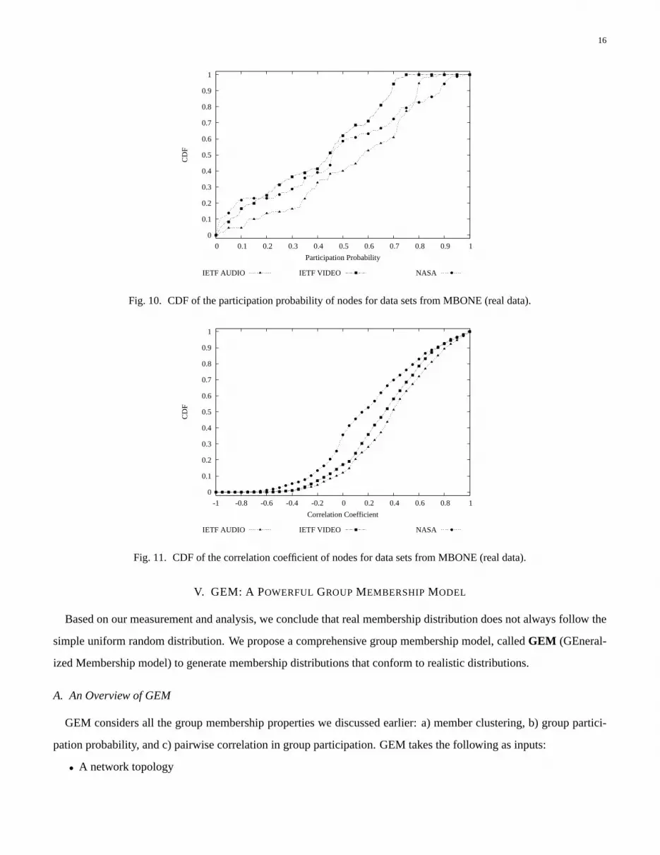
we show the analysis results of MBONE applications without member clustering. That is, we plot the CDF curves of

participation probability and pairwise correlation of nodes (without clustering). And the results are showed in Fig. 10

and Fig. 11.

We can see that Fig. 10 and Fig. 11 have very similar curves to Fig. 6 and Fig. 8, though the values are slightly

different due to the absence of member clustering. This confirms that the the properties of skewed distribution and

strong pairwise correlation come with the MBONE applications instead of the processing of clustering (which does

affect the values though). In our analysis, we focus on clusters for MBONE sessions mainly because we want to

achieve good analysis granularity for large groups and facilitate the design of group generation model (as we will see

in next section).

2It is easy to verify that, for any two variables which follow 0-1 distribution, if their coefficient is 0 then they are independent, and vise versa.

16

0

0.1

0.2

0.3

0.4

0.5

0.6

0.7

0.8

0.9

1

0 0.1 0.2 0.3 0.4 0.5 0.6 0.7 0.8 0.9 1

CD

F

Participation Probability

IETF AUDIO IETF VIDEO NASA

Fig. 10. CDF of the participation probability of nodes for data sets from MBONE (real data).

0

0.1

0.2

0.3

0.4

0.5

0.6

0.7

0.8

0.9

1

-1 -0.8 -0.6 -0.4 -0.2 0 0.2 0.4 0.6 0.8 1

CD

F

Correlation Coefficient

IETF AUDIO IETF VIDEO NASA

Fig. 11. CDF of the correlation coefficient of nodes for data sets from MBONE (real data).

V. GEM: A POWERFUL GROUPMEMBERSHIPMODEL

Based on our measurement and analysis, we conclude that real membership distribution does not always follow the

simple uniform random distribution. We propose a comprehensive group membership model, calledGEM (GEneral-

ized Membership model) to generate membership distributions that conform to realistic distributions.

A. An Overview of GEM

GEM considers all the group membership properties we discussed earlier: a) member clustering, b) group partici-

pation probability, and c) pairwise correlation in group participation. GEM takes the following as inputs:

• A network topology

17

• Clustering method (which determines how to form clusters in the given topology)

• Target group behavior: the distribution of group participation probability, the pairwise correlation in group par-

ticipation of clusters, and the distribution of member cluster size (i.e., the number of member nodes in a cluster)

GEM generates multicast groups whose members follow the given distributions and constraints. Fig. 12 is a block

diagram of GEM, illustrating how GEM works at a high level.

1. Create clusters in given topology

2. Select clusters as member clusters

Acoording to input distributions

3. Choose nodes for each member cluster

Network topology

Group behaviorClustering method

Dist. of member cluster size

Dist. of pairwise correlation

Dist. of participation prob.

Outputs

GEM

Inputs

Desired number of multicast groups

that follow the given distributions

Fig. 12. An illustration of GEM.

To summarize, GEM works in the following steps:

1. Cluster Creation:Based on the input network topology, GEM first classify nodes into many disjoint clusters

using the specified clustering algorithm. To give GEM flexibility, we leave this as an input parameter, as will be

discussed below.

2. Member Cluster Generation:GEM creates groups and chooses their cluster members among the clusters in a

randomized fashion. The selection of clusters follows the given distributions for clusters participation and pairwise

correlation. Note that, in this paper, we also refer the clusters which are chosen for a group as “member clusters” of

the group.

3. Node selection:In each chosen cluster (i.e. member cluster), GEM random selects nodes based on member

cluster size.

18

GEM is a generalized and very powerful model. First, it is not tied to a particular membership distribution. This

makes the usefulness of the model extend beyond the accuracy of a set of measurements. At the same time, our

measurements provide guidelines for the choice of realistic distributions. In the tool we develop based on GEM, the

measured distributions will be provided as choices to the users ([1]). Second, clustering method is an input of GEM.

Note that, GEM operates first at the cluster level and then node level. It generates groups treating a cluster as one

entity. The reason for doing this is to simulate the network-level clustering that we have observed. After we identify

the member clusters, then we assume that inside a cluster we have a number of active participants according to the

measured distributions (that is member cluster size distribution). There are many possible clustering methods, such as

network-aware clustering for real network topologies (with IP addresses) [23], topology based approaches using graph

k-clustering algorithms [16] [4]. In this paper, we will not extend the discussions on clustering methods, which simply

fall in another hot forum.

B. Member Cluster Generation

The core of GEM is to select the member clusters. The problem can be stated as follows: given a set of clusters,

the group participation probability of each cluster, and the pairwise correlation between any two clusters, we want to

generate sets of member clusters, which follow the given distributions. In other words, if we generate many multicast

groups which contain member clusters, the measured distributions should match the targets.

B.1 Problem Formulation

Let us start with the following definitions. We assumeK clusters:C1, C2, ..., Ci, ..., CK . Let us denote aspi the

participation probability of clusterCi, that is, how oftenCi participates in a multicast group. For any two clustersCi

andCj , there is a correlation coefficientcoef(i, j), where1 ≤ i, j ≤ K. Based onpi, pj , andcoef(i, j), we can

easily compute the joint probabilitypi,j as shown in Equation (2) (derived from Equation (1)).

pi,j = coef(i, j)×√

pi × (1− pi)× pj × (1− pj) + pi × pj . (2)

As a result, we obtain a symmetric joint probability matrixPm wherePm(i, j) = pi,j wheni 6= j andPm(i, i) = pi.

Considered at the granularity of clusters, a multicast group can be represented by aK-dimensional vector of binary

valuesx = (x1, x2, ..., xi, ..., xK), wherexi = 1 if and only if clusterCi is a member cluster of the group (else

xi = 0).

Now, we can formalize the problem as follows. If we assume many groups3, we can model theparticipation distri-

bution of the clustersby K random binary variables,(X1, X2, ..., Xi, ..., XK), whereXi represents the group partic-

3The presentation is easier when we talk about multiple groups, in other words, the multiple group participation. If we have one group we can

talk about the time-based participation.

19

ipation of clusterCi. Then, the generation of multicast groups becomes generating vectorsx = (x1, x2, ..., xi, ..., xK),

which follow the following constraints:

• P (Xi = 1) = pi,∀i, meaning thatXi follows the given participation probabilitypi

• P (Xi = 1, Xj = 1) = pi,j , meaning that for any two variablesXi andXj , the joint probability ispi,j .

Note that the problem is in some sense under-defined. Complete knowledge of the distribution of(X1, X2, ..., Xi, ..., XK)

would require us to know the probability of appearance for every of theO(2K) binary vectors. In other words, we

would needO(2K) values to be able to generate the desired distribution. We only have partial information: our total

input isO(K + K2) (K participation probability values andC2K = (K2 −K)/2 joint probability values). Intuitively,

we need to make some assumptions to “fill” the missing information.

Maximum Entropy Method. For the missing constraints, we will assume that they have maximum entropy. En-

tropy is a measure of randomness of a system, and it is the “opposite” of order. In addition, nature tends to increase

its entropy. A table with nicely stacked papers in alphabetical order has high order (low entropy). A wind from the

window can shuffle the papers, which leads to high entropy. It is unlikely that a subsequent wind will restack and

alphabetize the papers.

In our approach, we use entropy to replace the missing information. Given an unconstrained choice, we will choose

according to the Maximum Entropy (ME) [42]. This is a non-trivial but solved problem in statistical analysis [42]. In

fact, Maximum Entropy method has been widely used in many disciplines, such as statistical mechanics, thermody-

namics, data analysis, spectral analysis, protein structure prediction, natural language understanding, computer vision,

etc. In GEM, we apply this method in member cluster generation. Let us denotep∗(x) the Maximum Entropy dis-

tribution. Intuitively, we can see this as a multidimensional problem with only a few constrained dimensions. The

ME distributionp∗(x) satisfies the constraints along the specified dimensions, and it is as unstructured as possible in

the unconstrained dimensions. If we see entropy as lack of information, the Maximum Entropy distribution represents

all the “known information” and nothing more than that. Our member cluster generation algorithm combines two

“conflicting” forces: it maximizes the entropy (randomness), while it tries to match given distributions. Note that

it is possible to use a distribution with “any” entropy. However, to compute any-entropy distribution is demanding.

Moreover, using maximum entropy is more meaningful: if we do not know, we assume the distribution as random as

possible.

B.2 Algorithms for Member Cluster Generation

Based on the properties ofpi andpi,j , we classify the the desired distributions into three cases as follows (with the

order of increasing constraints):

1. Uniform distribution without correlation: all clusters have equal probability to join. This is the widely-used

multicast membership model.

20

2. Non-uniform distribution without correlation: participation probability is higher for some clusters.

3. Non-uniform distribution with pairwise correlation: as above plus some pairs of nodes appear more often to-

gether.

Note that for the first two cases, it is not necessary to use a maximum entropy distribution, since there are no correla-

tions among clusters. Straightforward algorithms can be used to generate member clusters as shown below.

Uniform distribution without correlation. In this case,pi = p, andpi,j = pi × pj = p2 (or coef(i, j) = 0) for

any i andj, where1 ≤ i, j ≤ K. Among the three cases mentioned above, this is the case with maximum entropy,

because there are almost no constraints: member clusters are chosen uniformly among all clusters, and clusters are

independent of each other. The member cluster generation algorithm is straightforward in this case, and it is described

in Algorithm 1.

Algorithm 1 Member Cluster Generation (Case 1)

Require: For K variables,X1, X2, ..., Xi, ..., XK , P (Xi = 1) = p, andP (Xi = 1, Xj = 1) = p2 (or coef(i, j) =

0), where1 ≤ i, j ≤ K. Notes:Xi represents the group participation of clusterCi with values of0 (not join) or1

(join)

Ensure: A set ofK-dimension vectors,(x1, x2, ..., xi, ..., xK), which follows given distribution.

1: while more groups to generatedo

2: for i = 1 to K do

3: generate a random number between0 and1, let it beu

4: if u < p then

5: xi = 1 (clusterCi joins multicast group)

6: else

7: xi = 0 (clusterCi will not join multicast group)

8: end if

9: end for

10: end while

Non-uniform distribution without correlation. In this case,pi,j = pi × pj (or coef(i, j) = 0) for anyi, j, where

1 ≤ i, j ≤ K, whilepi is usually unequal between different clusters. Compared with case 1, this case needs to consider

non-uniform distribution, that is,pi for different clusters. However, all the clusters are still independent of each other.

Thus, the member cluster generation algorithm is still straightforward. It is described in Algorithm 2.

Non-uniform distribution with pairwise correlation. In this case, we need to consider pairwise correlation

between any two clusters, which means thatpi,j = pi × pj , for 1 ≤ i, j ≤ K does not hold necessarily (i.e.

coef(i, j) 6= 0). For this case, we have to calculate the maximum entropy distributionp∗(x) subject to the given

21

Algorithm 2 Member Cluster Generation (Case 2)Require: For K variables,X1, X2, ..., Xi, ..., XK , P (Xi = 1) = pi, andP (Xi = 1, Xj = 1) = pi × pj (or

coef(i, j) = 0), where1 ≤ i, j ≤ K. Notes:Xi represents the group participation of clusterCi with values of0

(not join) or1 (join)

Ensure: A set ofK-dimension vectors,(x1, x2, ..., xi, ..., xK), which follows given distribution.

1: while More groups to generatedo

2: for i = 1 to K do

3: generate a random number between 0 and 1, let it be u

4: if u < pi then

5: xi = 1 (clusterCi joins multicast group)

6: else

7: xi = 0 (clusterCi will not join multicast group)

8: end if

9: end for

10: end while

constraints. Then, we use Gibbs Sampler ([35]) approach to sample it, i.e., to obtain instances of membership values,

(x1, x2, ..., xi, ..., xK).

Calculating the Maximum Entropy distribution. Given the constraintsP (Xi = 1) = pi, andP (Xi = 1, Xj =

1) = pi,j , where1 ≤ i, j ≤ K, or in other words, given a probability matrixPm = [pi,j ], the maximum entropyp∗(x)

is the solution to the following problem:

p∗(x) = arg max{−∫

p(x)logp(x)dx}, (3)

subject to ∫xixjp(x)dx = pi,j , when i 6= j, (4)

and ∫xip(x)dx = pi, (5)

and ∫p(x)dx = 1. (6)

22

We solve this constrained optimization problem by Lagrange multipliers. Then the problem becomes to findp(x)

that maximizes the following function,

E[p] = −∫

p(x)logp(x)dx−K∑

i=1

λi,i(∫

xip(x)dx− pi)

−i=K,j=K∑

i=1,j=1,i6=j

λi,j(∫

xixjp(x)dx− pi,j)

− λ0(∫

p(x)dx− 1).

(7)

By calculus of variation, we setδE[p]δp = 0, and we have

−logp(x)− 1−K∑

i=1

λi,ixi −i=K,j=K∑

i=1,j=1,i6=j

λi,jxixj − λ0 = 0 (8)

Therefore, the solution forp∗(x) is:

p∗(x; Λ) = p∗(x1, x2, ..., xK ; Λ)

=1

Z(Λ)exp[−

K∑i=1

λi,ixi −i=K,j=K∑

i=1,j=1,i6=j

λi,jxixj ],(9)

whereΛ = [λi,j ] is the Lagrange parameter, and

Z(Λ) =∑

x

exp[−K∑

i=1

λi,ixi −i=K,j=K∑

i=1,j=1,i6=j

λi,jxixj ], (10)

is the normalization function that depends onΛ, and it has the following properties:

1Z

∂Z

∂λi,j= −pi,j . (11)

Unfortunately, a closed form solution forΛ is not available in general. Thus, we seek a numerical solution by

solving the following equations iteratively.dλi,j

dt= pt

i,j − pi,j , (12)

wherepti,j is the intermediate probability computed at stept, based on the intermediate distributionpt(x; Λ). It can

be proved that there is a unique solution forΛ = [λi,j ] (Interested readers can refer to [42] for detailed proof). In

Algorithm 3, we briefly describe the iterative procedure to construct the maximum entropy distributionp∗(x), and

then use Gibbs Sampler ([35]) to obtain instances of member clusters.

B.3 Discussions

Maximum Entropy Value Deceasing from Case 1 to Case 3. In the above three cases, we find that the maximum

entropy value decreases from case 1 to case 3. As is consistent with our intuition: for case 1, we do not know anything

23

Algorithm 3 Member Cluster Generation (Case 3)Require: For K variables,X1, X2, ..., Xi, ..., XK , P (Xi = 1) = pi, andP (Xi = 1, Xj = 1) = pi,j , where

1 ≤ i, j ≤ K. Notes:Xi represents the group participation of clusterCi with values of0 (not join) or1 (join)

Ensure: A set ofK-dimension vectors,(x1, x2, ..., xi, ..., xK), which follows given distribution.

1: initialize Λ asΛ0

2: E0 = 0 //initialize judgement term as 0

3: t = 0 //initialize step counter

4: repeat

5: t = t + 1

6: computeZt based on Equation (10), then we knowpt(x; Λ).

7: use Gibbs Sampler ([35]) to samplept(x; Λ) and computepti,j .

8: λti,j = λ

(t−1)i,j + (pt

i,j − pi,j) //updateΛ

9: computeEt = exp(−(∑

i,j(pti,j − pi,j)2))

10: until |Et − Et−1| < ε //the iteration reaches steady state

11: computeZt based on Equation (10), then we knowpt(x; Λ).

12: use Gibbs Sampler ([35]) to samplept(x; Λ), and output the series of generated vectorsx.

except the portion of clusters to join the multicast group; for case 2, we know a little bit more: different cluster has

different group participation probability; while for case 3, besides the knowledge in case 2, we even know the pairwise

correlation, which adds more constraints to the ME distribution, as leads to a smaller ME value compared to case 2.

Input Distribution Validation . It can be shown that the technique we use in case 3 will lead provably to the

correct distribution, if such a solution exists. Note that in some cases, the given distribution may be self-contradicting

(especially when the parameters are simply input from the GEM users). For example, cluster A and cluster B have

high positive correlation, and so do cluster B and C. However, the correlation of C and A is negative. It may not be

possible to satisfy such a constraint. Thus, GEM needs to check whether the input distributions are valid or not. In

fact, givenpi, pj , andpi,j , the only constraint we need to consider is thatpi + pj ≤ 1 + pi,j should hold (as can be

easily deducted from the basic definitions of probability and joint probability).

Generating Bounded Size Groups. Sometimes, we want to control the size of the groups in our simulations. We

can impose constraints in our approaches to stop the creation of a group once a size is reached. However, this may

affect the correlations and probabilities in case 3. A suggested method is to recompute the probabilities and correlations

under the given condition, i.e., bounded group size.pi is recomputed aspi [(∑K

i=1 pi)/constraied group size], where∑Ki=1 pi is the expected group size without group size constraint. Andpi,j is changed correspondingly. This approach

will slightly introduce more computation. Thus, a future work direction is to investigate the possibility of an efficient

24

heuristic algorithm design for bounded size group generation.

VI. EXPERIMENTAL VALIDATION

In this section, through experiments, we validate that GEM can generate realistic groups with great success and the

generated groups match very well the real data.

A. Experiment Design

Based on our measurement results and analysis, we observe that GEM can model both MBONE applications and

net games: to model net games, Algorithm 1 can be used, since uniform distribution without correlation approximately

characterizes net games’s spatial properties; while to model MBONE applications, such as IETF and NASA, GEM

needs to employ Algorithm 3, because in these applications, the features of non-uniform distribution and correlation

are very significant. Since Algorithm 1 is pretty straightforward, to validate GEM, in this section, we only consider

MBONE applications (IETF and NASA), which will be modelled by GEM Algorithm 3.

Based on our measurement results of MBONE applications, we give inputs, such as the distributions of group

participation probability and pairwise correlation of clusters, and the distribution of member cluster size, to GEM,

and GEM generates multicast groups using Algorithm 3. Note that, in our validation experiments, we only consider

possible member clusters, which has participation probability greater than0, as is the same as the methodology in

our measurement. Then, we analyze the generated multicast groups similarly, and compute the distributions of group

participation probability and pairwise correlation of clusters, and the distribution of member cluster size. And finally,

we compare the results from real measurement data and simulation data generated by GEM.

B. Results and Analysis

We give the comparison results for data set IETF43-Video as an example. The curves for CDF of member cluster

size, participation probability, and correlation coefficient are shown in Fig. 13, Fig. 14, and Fig. 15 respectively. To

show the limitation of the uniform random model, we also plot the curves for its corresponding simulation data in

Fig. 14 and Fig. 15.

From Fig. 13 and Fig. 14, we can see that, for member cluster size and participation probability, the two CDF curves

for measurement and GEM simulation data are “perfectly” matched. For the correlation coefficient (shown in Fig. 15),

the CDF curves for measurement and GEM simulation data are “nearly” matched. The difference is because CDF is an

accumulative function, and the CDF of correlation coefficient involves much more variables (the number of variables

is O(K2) in total) than the CDF of participation probability (the number of variables isK). And simulation errors are

propagated accumulatively. In addition, to facilitate the computation in ME method, we approximate some very small

(in terms of the absolute value) correlation coefficients as zero (which means the corresponding constraints could be

25

0

0.1

0.2

0.3

0.4

0.5

0.6

0.7

0.8

0.9

1

1 2 3 10 20 30 100

CD

F

Cluster size

From simulation From real measurements

Fig. 13. The comparison of member cluster size distribution for IETF43-Video between measurement and modelling data.

0

0.1

0.2

0.3

0.4

0.5

0.6

0.7

0.8

0.9

1

0 0.1 0.2 0.3 0.4 0.556 0.7 0.8 0.9 1

CD

F

Participation probability

From GEM simulationFrom real measurements

Uniform model simulation

Fig. 14. The comparison of group participation probability distribution of clusters for IETF43-Video between measurement and

modelling data (GEM and Uniform model).

ignored). But this will add experiment errors to the simulation. Another observation in Fig. 14 and Fig. 15 is that the

uniform random model could not generate realistic multicast groups, as shows the limitation of its capabilities.

For other sessions,such as IETF Audio and NASA, we get similar results. Thus, based on our experimental results,

we can conclude that our model can produce group members which follow given distribution successfully.

VII. C ONCLUSIONS ANDFUTURE WORK

In this work, we measured and modelled the spatial properties of group communications. Our contributions can be

summarized as follows:

26

0

0.1

0.2

0.3

0.4

0.5

0.6

0.7

0.8

0.9

1

-1 -0.8 -0.6 -0.4 -0.2 0 0.2 0.4 0.6 0.8 1

CD

F

Correlation Coefficient

From GEM simulationFrom real measurements

Uniform model simulation

Fig. 15. The comparison of correlation coefficient distribution of clusters for IETF43-Video between measurement and modelling

data (GEM and Uniform model).

• We identify and quantify the spatial properties of members: member clustering, group participation probability,

and pairwise correlation, in net games and large audio-video broadcasts from IETF and NASA on MBONE.

• We observe that MBONE multicast members are highly clustered and the clusters exhibit skewed distribution

and strong pairwise correlations in their participation.

• We find that net game members are not as clustered and there does not seem to be a strong correlation between

users. The uniform random membership can roughly model net games (Quake).

• We develop GEM, a powerful group membership model, that can generate realistic member distribution. GEM

combines two conflicting forces: it maximizes the entropy of the distribution, at the same time it tries to match given

constraints.

• We validate our model with great success: the generated groups match very well the real data.

We provide our data and our model as a contribution to the community with the hope that it can be part of a realistic

and systematic multicast evaluation methodology ([1]).

Future Work. We would like to continue this work in two main directions. First, we want to study more appli-

cations with multiple recipients, such as large scale net games, large scale media streaming, peer-to-peer file sharing

and web caching, and explore their spatial properties. We believe that different applications have different spatial

properties, and GEM can be extended to well characterize and model these applications, as will assist research and de-

velopment of multicast and other group communication technologies. Second, we would like to integrate in our model

temporal properties of group members and develop a comprehensive tool kit to improve the efficiency of modelling

and simulations in the related field.

27

VIII. A CKNOWLEDGEMENT

The authors would express special thanks to Robert Chalmers and Kevin Almeroth from University of California,

Santa Barbara. Without their data, the authors would not be able to analyze multicast groups from MBONE.

REFERENCES

[1] Group Membership Measurement and Modelling Project Page at UCLA.http://www.cs.ucla.edu/NRL/hpi/MCModel/index.html.

[2] NLANR Global ISP interconnectivity by AS number.http://moat.nlanr.net/AS/.

[3] QStat.http://www.qstat.org.

[4] N. Abbas and L. Stewart. Clustering bipartite and chordal graphs: complexity, sequential and parallel algorithm.Discrete Appl. Math.,

91(1-3):1–23, 1999.

[5] K. Almeroth and M. Ammar. Collection and modeling of the join/leave behavior of multicast group members in the MBone.Proceedings

of High Performance Distributed Computing Focus Workshop (HPDC ’96), Aug. 1996.

[6] S. Alouf, E. Altman, C. Barakat, and P. Nain. Estimating membership in a multicast session. InProceedings of the ACM SIGMETRICS’03,

June 2003.

[7] S. Alouf, E. Altman, and P. Nain. Optimal on-line estimation of the size of a dynamic multicast group. InProceedings of the IEEE

INFOCOM ’02, June 2002.

[8] S. Banerjee, C. Kommareddy, and B. Bhattacharjee. Scalable application layer multicast. InProceedings of ACM SIGCOMM, Aug. 2002.

[9] T. Billhartz and et al. Performance and resource cost comparisons for the CBT and PIM multicast routing protocols.IEEE Journal on

Selected Areas in Communications, 1997.

[10] L. Breslau, P. Cao, L. Fan, G. Phillips, and S. Shenker. Web caching and zipf-like distributions: Evidence and implications. InINFOCOM

(1), pages 126–134, 1999.

[11] R. Caceres, N. Duffield, J. Horowitz, D. Towsley, and T. Bu. Multicast-based inference of network-internal characteristics: Accuracy of

packet loss estimation.IEEE INFOCOM, 1999.

[12] R. Chalmers and K. Almeroth. Modeling the branching characteristics and efficiency gains of global multicast trees.Proceedings of the

IEEE INFOCOM’ 2001, Apr. 2001.

[13] R. Chalmers and K. Almeroth. On the topology of multicast trees.IEEE/ACM Transactions on Networking, 11(1):153–165, Feb. 2003.

[14] J. Chuang and M. Sibru. Pricing multicast communications: A cost-based approach.Proceedings of the Internet Society INET’98

Conference, July 1998.

[15] M. Crovella and A. Bestavros. Self-similarity in World Wide Web traffic, evidence and possible causes.SIGMETRICS, pages 160–169,

1996.

[16] J. S. Deogun, D. Kratsch, and G. Steiner. An approximation algorithm for clustering graphs with dominating diametral path.Inf. Process.

Lett., 61(3):121–127, 1997.

[17] D. Dolev, O. Mokryn, and Y. Shavitt. On multicast trees: Structure and size estimation. InProceedings of the IEEE INFOCOM’03, Mar.

2003.

[18] M. Faloutsos, A. Banerjea, and R. Pankaj. QoSMIC: Quality of Service sensitive Multicast Internet protoCol.ACM SIGCOMM’98,

Vancouver, British Columbia, Sept. 1998.

[19] A. Fei, J.-H. Cui, M. Gerla, and M. Faloutsos. Aggregated Multicast with inter-group tree sharing.Proceedings of NGC2001, Nov. 2001.

[20] T. Friedman and D. F. Towsley. Multicast session membership size estimation. InProceedings of the IEEE INFOCOM’99 (2), pages

965–972, 1999.

28

[21] T. Henderson and S. Bhatti. Modelling user behaviour in networked games.Proceedings of ACM Multimedia’01, Sept. 2001.

[22] M. Jovanovic. Modeling large-scale peer-to-peer networks and a case study of gnutella.Master thesis,University of Cincinnati, 2001.

[23] B. Krishnamurthy and J. Wang. On network-aware clustering of web clients.Proceddings of SIGCOMM’00, 2000.

[24] B. Krishnamurthy and J. Wang. Topology modeling via cluster graphs. InProceedings of the First ACM SIGCOMM Workshop on Internet

Measuremen, Aug. 2001.

[25] B. Krishnamurthy, J. Wang, and Y. Xie. Early measurements of a cluster-based architecture for p2p systems. InProceedings of the First

ACM SIGCOMM Workshop on Internet Measuremen, Aug. 2001.

[26] S. Kumar, P. Radoslavov, D. Thaler, C. Alaettinoglu, D. Estrin, and M. Handley. The MASC/BGMP architecture for inter-domain multicast

routing. InProceedings of ACM SIGCOMM’98, pages 93–104, Sept. 1998.

[27] W. Leland, M. Taqqu, W. Willinger, and D. Wilson. On the self-similar nature of ethernet traffic.IEEE Transactions on Networking,

2(1):1–15, Feb. 1994. (earlier version in SIGCOMM ’93, pp 183-193).

[28] C. Liu and J. Nonnenmacher. Broadcast audience estimation. InProceedings of the IEEE INFOCOM’00 (2), pages 952–960, 2000.

[29] G. Lucas, A. Ghose, and J. Chuang. On characterizing affinity and its impact on network performance. InProcessdings of ACM SIGCOMM

Workshop on Models, Methods and Tools for Reproducible Network Research, Aug. 2003.

[30] M. Nekovee, A. Soppera, and T. Burbridge. An adaptive method for dynamic audience size estimation in multicast. InProceedings of the

ACM SIGCOMM/COST 264 NGC’03, Sept. 2003.

[31] V. Paxson and S. Floyd. Wide-area traffic: The failure of poisson modeling.IEEE/ACM Transactions on Networking, 3(3):226–244, June

1995. (earlier version in SIGCOMM’94, pp. 257-268).

[32] G. Philips and S. Shenker. Scaling of multicast trees: comments on the Chuang-Sirbu scaling law. InProceedings of ACM SIGCOMM’99,

pages 41–51, Sept. 1999.

[33] P. I. Radoslavov, D. Estrin, and R. Govindan. Exploiting the bandwidth-memory tradeoff in multicast state aggregation. Technical report,

USC Dept. of CS Technical Report 99-697 (Second Revision), July 1999.

[34] P. Rajvaidya and K. Almeroth. Analysis of routing characteristics in the multicast infrastructure.IEEE INFOCOM, 2003.

[35] S. M. Ross.Introduction to Probability Models (Seventh Edition). Academic Press, 2000.

[36] J. K. Shapiro, J. Kurose, D. Towsley, and S. Zabel. Topology discovery service for router-assisted multicast transport.Proceedings of

OpenArch 2002, 2002.

[37] D. Thaler and M. Handley. On the aggregatability of multicast forwarding state.Proceedings of IEEE INFOCOM, Mar. 2000.

[38] B. M. Waxman. Routing of multipoint connections.IEEE Journal on Selected Areas in Communications, 6(9):1617–1622, Dec. 1988.

[39] L. Wei and D. Estrin. The trade-offs of multicast trees and algorithms.Proceedings of the International Conference on Computer

Communications and Networks (ICCCN), 1994.

[40] A. Wolman, G. M. Voelker, N. Sharma, N. Cardwell, A. R. Karlin, and H. M. Levy. On the scale and performance of cooperative web

proxy caching. InSymposium on Operating Systems Principles, pages 16–31, 1999.

[41] T. Wong and R. Katz. An analysis of multicast forwarding state scalability. InProceedings of the 8th International Conference on Network

Protocols (ICNP), Japan, Nov. 2000.

[42] S. C. Zhu, Y. N. Wu, and D. Mumford. FRAME: Filters, Random field And Maximum Entropy: — Towards a Unified Theory for Texture

Modeling. — International Journal of Computer Vision, 27(2) pp.1-20, March/April, 1998.

[43] G. K. Zipf. Human behavior and the principle of least effort.Reading, MA: Addison-Wesley, 1949.