an equivalent stiffness approach for modelling the behaviour of compression members according to...

Journal of Constructional Steel Research 63 (2007) 55–70www.elsevier.com/locate/jcsr

An equivalent stiffness approach for modelling the behaviour ofcompression members according to Eurocode 3

A.M. Barszcz, M.A. Gizejowski∗

Department of Metal Structures, Warsaw University of Technology, 00-637 Warsaw, Poland

Received 7 October 2005; accepted 17 March 2006

Abstract

The development of design procedures based on inelastic advanced analysis is a key consideration for future steel design codes. In advancedanalysis the effect of imperfections has to be modelled in such a way that the incremental analysis fully captures this effect in the process of momentredistribution. In modelling the influence of imperfections on the behaviour of individual members of real structures, different approaches havebeen used to globally represent this effect in the overall analysis of structural systems. They are referred to as the initial bow imperfection approachor as the equivalent transverse load approach. When using the abovementioned approaches in analysis of multiple member structural systems, thedesigner is required to arrange the directions of bow imperfections or equivalent transverse loads in such a way that the imperfection arrangementleads to the least constrained solution, i.e. the lowest ultimate load predicted from all possible sets of member initial imperfection arrangements.Since there is still ongoing research on the development of simple application rules ensuring that the designer obtains a unique solution whenchoosing a certain set of member initial imperfections, there is at the same time interest in the development of alternative approaches to modellingthe influence of member imperfections on the behaviour of structural systems. This paper provides the necessary background information as well asdescribes the formulation and modelling techniques used in the development of a new approach to modelling the influence of imperfections on thestability behaviour of structural components and systems. This new approach, called hereafter an equivalent stiffness approach, has an advantageover the previously described approaches since an imperfect member is treated as a hypothetically straight element, flexural and axial stiffnesses ofwhich at each load level are predicted in a continuous fashion dependent upon the actual force and deformation states. This type of modelling doesnot require any explicit modelling of equivalent geometric imperfections or equivalent forces and their directions in advanced analysis; thereforealso it does not require any buckling mode assessment. Moreover, the effects of strain hardening and section class may conveniently be includedin modelling. Finally, European buckling curves are used to estimate the values of parameters of the developed model that can be immediatelyused in advanced analysis conducted according to Eurocode 3.c© 2006 Elsevier Ltd. All rights reserved.

Keywords: Steel frameworks; Compression elements; Imperfections; Merchant–Rankine–Murzewski approach; European buckling curves; Equivalent flexuralstiffness; Equivalent axial stiffness

1. Introduction

The member elastic behaviour and more importantly itsbehaviour in the inelastic region are affected by structuralimperfections. Key imperfections influencing the performanceof individual elements, especially those under compression, canbe grouped into two categories: (1) geometric, (2) material.

Geometric imperfections result mainly from: (1) mechanicalfabrication of structural members, (2) their manufacturing into

∗ Corresponding author. Tel.: +48 660 028 154; fax: +48 22 825 65 32.E-mail addresses: [email protected], [email protected]

(M.A. Gizejowski).

0143-974X/$ - see front matter c© 2006 Elsevier Ltd. All rights reserved.doi:10.1016/j.jcsr.2006.03.003

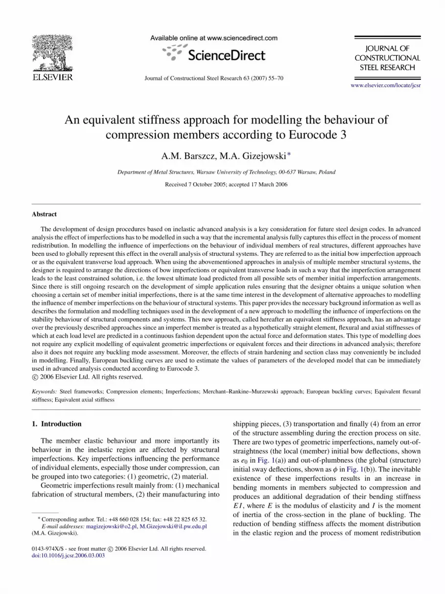
shipping pieces, (3) transportation and finally (4) from an errorof the structure assembling during the erection process on site.There are two types of geometric imperfections, namely out-of-straightness (the local (member) initial bow deflections, shownas e0 in Fig. 1(a)) and out-of-plumbness (the global (structure)initial sway deflections, shown as φ in Fig. 1(b)). The inevitableexistence of these imperfections results in an increase inbending moments in members subjected to compression andproduces an additional degradation of their bending stiffnessE I , where E is the modulus of elasticity and I is the momentof inertia of the cross-section in the plane of buckling. Thereduction of bending stiffness affects the moment distributionin the elastic region and the process of moment redistribution

http://www.elsevier.com/locate/jcsr

mailto:[email protected]

mailto:[email protected]

http://dx.doi.org/10.1016/j.jcsr.2006.03.003

56 A.M. Barszcz, M.A. Gizejowski / Journal of Constructional Steel Research 63 (2007) 55–70

Fig. 1. Geometric imperfections; (a) out-of-straightness, (b) out-of-plumbness.

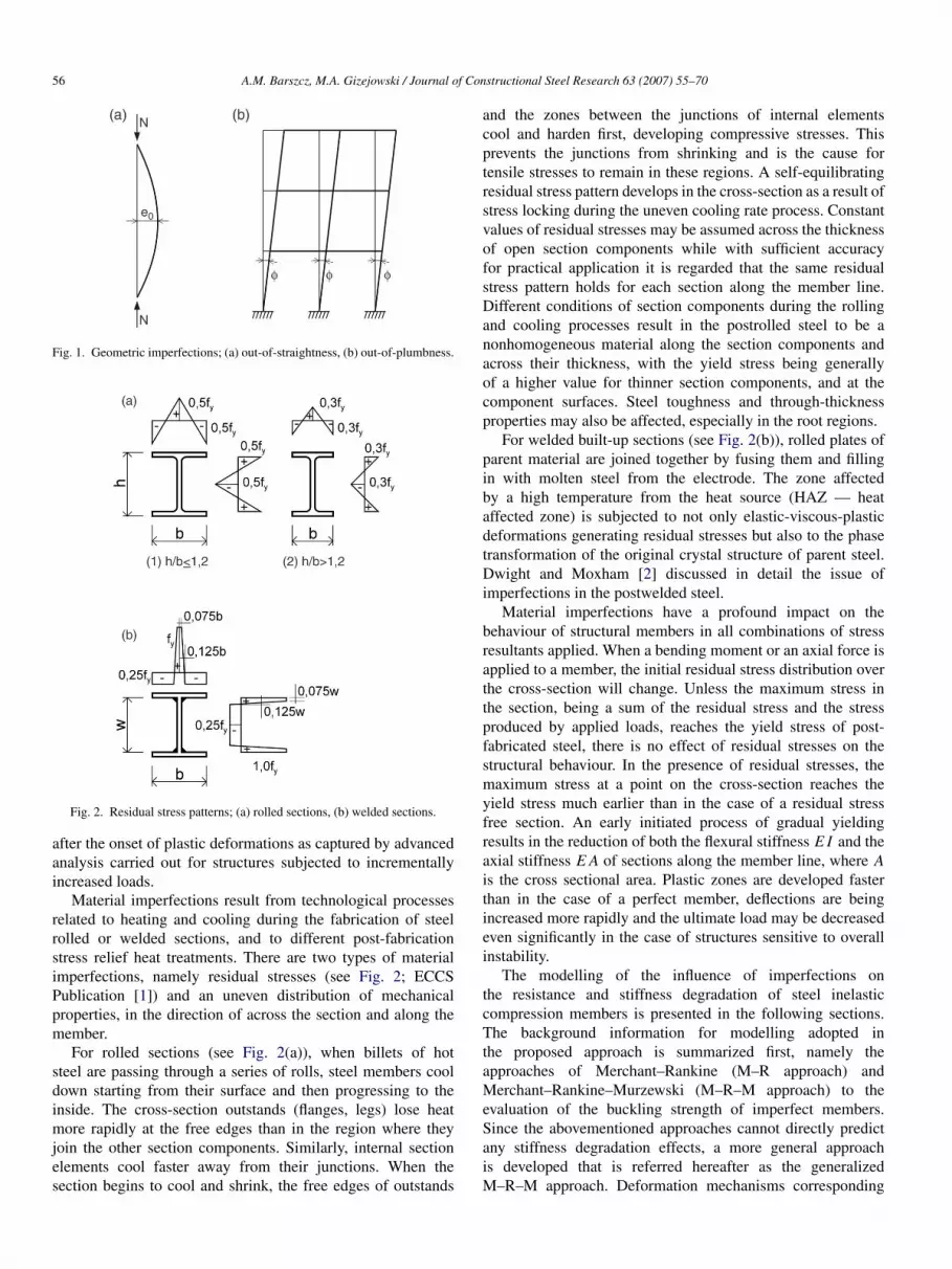
Fig. 2. Residual stress patterns; (a) rolled sections, (b) welded sections.

after the onset of plastic deformations as captured by advancedanalysis carried out for structures subjected to incrementallyincreased loads.

Material imperfections result from technological processesrelated to heating and cooling during the fabrication of steelrolled or welded sections, and to different post-fabricationstress relief heat treatments. There are two types of materialimperfections, namely residual stresses (see Fig. 2; ECCSPublication [1]) and an uneven distribution of mechanicalproperties, in the direction of across the section and along themember.

For rolled sections (see Fig. 2(a)), when billets of hotsteel are passing through a series of rolls, steel members cooldown starting from their surface and then progressing to theinside. The cross-section outstands (flanges, legs) lose heatmore rapidly at the free edges than in the region where theyjoin the other section components. Similarly, internal sectionelements cool faster away from their junctions. When thesection begins to cool and shrink, the free edges of outstands

and the zones between the junctions of internal elementscool and harden first, developing compressive stresses. Thisprevents the junctions from shrinking and is the cause fortensile stresses to remain in these regions. A self-equilibratingresidual stress pattern develops in the cross-section as a result ofstress locking during the uneven cooling rate process. Constantvalues of residual stresses may be assumed across the thicknessof open section components while with sufficient accuracyfor practical application it is regarded that the same residualstress pattern holds for each section along the member line.Different conditions of section components during the rollingand cooling processes result in the postrolled steel to be anonhomogeneous material along the section components andacross their thickness, with the yield stress being generallyof a higher value for thinner section components, and at thecomponent surfaces. Steel toughness and through-thicknessproperties may also be affected, especially in the root regions.

For welded built-up sections (see Fig. 2(b)), rolled plates ofparent material are joined together by fusing them and fillingin with molten steel from the electrode. The zone affectedby a high temperature from the heat source (HAZ — heataffected zone) is subjected to not only elastic-viscous-plasticdeformations generating residual stresses but also to the phasetransformation of the original crystal structure of parent steel.Dwight and Moxham [2] discussed in detail the issue ofimperfections in the postwelded steel.

Material imperfections have a profound impact on thebehaviour of structural members in all combinations of stressresultants applied. When a bending moment or an axial force isapplied to a member, the initial residual stress distribution overthe cross-section will change. Unless the maximum stress inthe section, being a sum of the residual stress and the stressproduced by applied loads, reaches the yield stress of post-fabricated steel, there is no effect of residual stresses on thestructural behaviour. In the presence of residual stresses, themaximum stress at a point on the cross-section reaches theyield stress much earlier than in the case of a residual stressfree section. An early initiated process of gradual yieldingresults in the reduction of both the flexural stiffness E I and theaxial stiffness E A of sections along the member line, where Ais the cross sectional area. Plastic zones are developed fasterthan in the case of a perfect member, deflections are beingincreased more rapidly and the ultimate load may be decreasedeven significantly in the case of structures sensitive to overallinstability.

The modelling of the influence of imperfections onthe resistance and stiffness degradation of steel inelasticcompression members is presented in the following sections.The background information for modelling adopted inthe proposed approach is summarized first, namely theapproaches of Merchant–Rankine (M–R approach) andMerchant–Rankine–Murzewski (M–R–M approach) to theevaluation of the buckling strength of imperfect members.Since the abovementioned approaches cannot directly predictany stiffness degradation effects, a more general approachis developed that is referred hereafter as the generalizedM–R–M approach. Deformation mechanisms corresponding

A.M. Barszcz, M.A. Gizejowski / Journal of Constructional Steel Research 63 (2007) 55–70 57

to the elementary behaviour of perfect compression membersare used for the development of two instability strength andstiffness degradation models: (1) the B-model allowing forthe evaluation of strength and flexural stiffness degradation,and (2) the D-model — for strength and axial stiffnessdegradation. The former is based on the Shanley bifurcationinstability criterion of inelastic members and the latter onthe divergence instability criterion at the limit point on themember load–deformation characteristic. Both models operateon generalized stress–strain characteristics of a hypotheticallyperfect member that reproduces the effect of imperfections onthe strength and stiffness of imperfect members. The modellingtechnique and its physical explanation are presented. Finally thecalibration exercise of model parameters is carried out againstthe European buckling curves.

2. Resistance and stiffness of imperfect compressionmembers

Approaches used for the development of standard bucklingcurves use simple deterministic behavioural models, which canbe classified into two groups:

(1) Approach using the geometric imperfections, or theirforce equivalents, resulting from the maximum tolerance valuesadopted in fabrication and erection specifications, and thetangent stiffness to represent the effects of residual stresses onthe member strength and on the structure ultimate load (Chenand Kim [3]).

(2) Approach using either the equivalent geometricimperfections, or their force equivalents (see Eurocode 3: Part1-1 [4], BS 5950: Part 1 [5]) that are greater than the tolerancevalues adopted in fabrication and erection specifications, orusing the further reduced tangent modulus approach (see Chenand Kim [3]), and treating them as substitute safety factorsto represent globally the combined effect of all the memberimperfections on the structural component strength and also onthe strength of the whole structure.

Recently, Goncalves and Camotim [6] proposed a deter-ministic based model for the inclusion of the equivalent geo-metric imperfections. The method presented required a sepa-rate second-order analysis of the frame for the ultimate statechecking of each compression member (column). The equiv-alent geometric imperfection of the checked column was ob-tained through the multiplication of the frame critical bucklingmode shape by the corresponding scaling factor. The scalingfactor was to be calculated for each checked column in a waythat corresponded to the magnitude given in Eurocode 3: Part1-1 [4] for the so-called equivalent column (hinged at both endsand held in position).

Simple probabilistic based models have also been developedwhich can be classified in the second group listed above (seeMurzewski [7]). The focus is made in this section to summarisethe probabilistic strength based models since their furtherdevelopment is the primary objective of this paper, and thento develop the new model that allows for the evaluation of boththe strength and stiffness of imperfect elements.

2.1. Merchant–Rankine approach

The global effect of imperfections on the resistance of framestructures has been evaluated in practical design by using theoriginal equation resulting from the M–R approach (for themodified approach see BS 5950: Part 1 [5]):

1Λult

=1

Λpl+

1Λcr

(1)

where:Λult = ultimate load factor of imperfect structure,Λpl = limit load factor from the plastic first order analysis ofthe perfect structure,Λcr = critical load factor from the elastic second order(stability) analysis of the perfect structure.

All the factors in Eq. (1) are evaluated with respect tothe considered combination of design loads. Eq. (1) resultsfrom Merchant’s generalization [8] of the formula proposedby Rankine for the estimation of the buckling strength ofindividual compression members, Allen [9]. Adopting thenotation used in Eurocode 3: Part 1-1 [4], Eq. (1) canbe converted for a single buckling curve described by thefollowing standard equation:

Nb,R =

[1 +

(γd

γmλ

2)]−1

Nc,R (2)

where:Nb,R = characteristic buckling resistance of the imperfectmember,Nc,R = characteristic value of the squash load or the cross-section resistance in compression,γd = partial safety factor for the design value of the critical loadof slender imperfect members,γm = partial safety factor for the design value of the squashload,

λ =

√Nc,RNcr

; the dimensionless slenderness ratio,Ncr = characteristic value of the critical load of slendermembers.

The design buckling resistance of the imperfect member canbe expressed as:

Nb,Rd =Nb,R

γm. (3)

The partial safety factor γd in Eq. (2) can be notionallyregarded as the factor applied to the modulus of elasticity in theelastic critical load equation. When the member is subjected toflexural buckling, the design value of the critical load can bewritten down as follows, Gizejowski et al. [10]:

Ncr,d =Ncr

γd=

(π

λ

)2 E A

γd=

(π

λ

)2Eb,d A (4)

where:E = modulus of elasticity for steel (E = 210 GPa),Eb,d = design value of the elastic buckling modulus Eb definedas

Eb =

(λ

π

)2

Nb, (5)


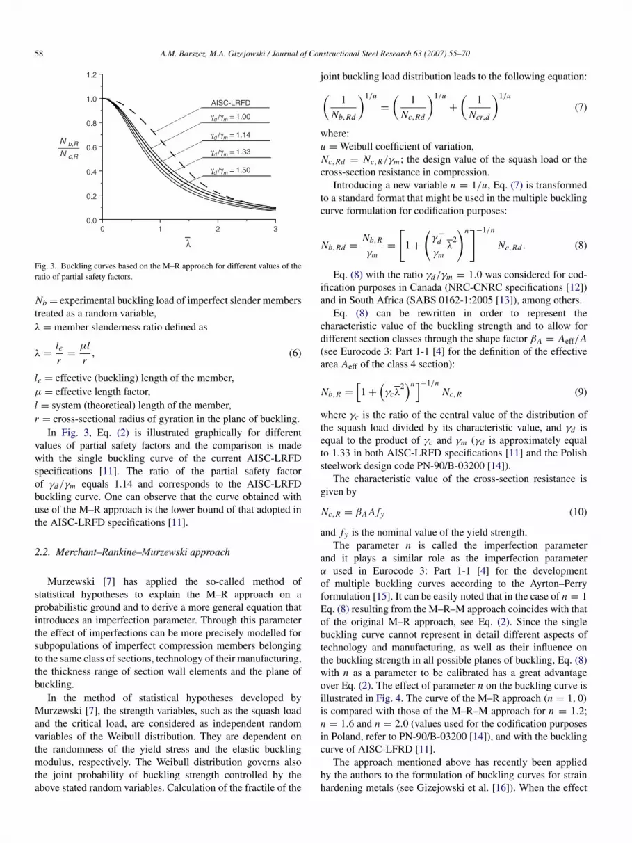
Fig. 3. Buckling curves based on the M–R approach for different values of theratio of partial safety factors.

Nb = experimental buckling load of imperfect slender memberstreated as a random variable,λ = member slenderness ratio defined as

λ =ler

=µl

r, (6)

le = effective (buckling) length of the member,µ = effective length factor,l = system (theoretical) length of the member,r = cross-sectional radius of gyration in the plane of buckling.

In Fig. 3, Eq. (2) is illustrated graphically for differentvalues of partial safety factors and the comparison is madewith the single buckling curve of the current AISC-LRFDspecifications [11]. The ratio of the partial safety factorof γd/γm equals 1.14 and corresponds to the AISC-LRFDbuckling curve. One can observe that the curve obtained withuse of the M–R approach is the lower bound of that adopted inthe AISC-LRFD specifications [11].

2.2. Merchant–Rankine–Murzewski approach

Murzewski [7] has applied the so-called method ofstatistical hypotheses to explain the M–R approach on aprobabilistic ground and to derive a more general equation thatintroduces an imperfection parameter. Through this parameterthe effect of imperfections can be more precisely modelled forsubpopulations of imperfect compression members belongingto the same class of sections, technology of their manufacturing,the thickness range of section wall elements and the plane ofbuckling.

In the method of statistical hypotheses developed byMurzewski [7], the strength variables, such as the squash loadand the critical load, are considered as independent randomvariables of the Weibull distribution. They are dependent onthe randomness of the yield stress and the elastic bucklingmodulus, respectively. The Weibull distribution governs alsothe joint probability of buckling strength controlled by theabove stated random variables. Calculation of the fractile of the

joint buckling load distribution leads to the following equation:(1

Nb,Rd

)1/u

=

(1

Nc,Rd

)1/u

+

(1

Ncr,d

)1/u

(7)

where:u = Weibull coefficient of variation,Nc,Rd = Nc,R/γm ; the design value of the squash load or thecross-section resistance in compression.

Introducing a new variable n = 1/u, Eq. (7) is transformedto a standard format that might be used in the multiple bucklingcurve formulation for codification purposes:

Nb,Rd =Nb,R

γm=

[1 +

(γ −

d

γmλ

2

)n]−1/n

Nc,Rd . (8)

Eq. (8) with the ratio γd/γm = 1.0 was considered for cod-ification purposes in Canada (NRC-CNRC specifications [12])and in South Africa (SABS 0162-1:2005 [13]), among others.

Eq. (8) can be rewritten in order to represent thecharacteristic value of the buckling strength and to allow fordifferent section classes through the shape factor βA = Aeff/A(see Eurocode 3: Part 1-1 [4] for the definition of the effectivearea Aeff of the class 4 section):

Nb,R =

[1 +

(γcλ

2)n]−1/n

Nc,R (9)

where γc is the ratio of the central value of the distribution ofthe squash load divided by its characteristic value, and γd isequal to the product of γc and γm (γd is approximately equalto 1.33 in both AISC-LRFD specifications [11] and the Polishsteelwork design code PN-90/B-03200 [14]).

The characteristic value of the cross-section resistance isgiven by

Nc,R = βA A fy (10)

and fy is the nominal value of the yield strength.The parameter n is called the imperfection parameter

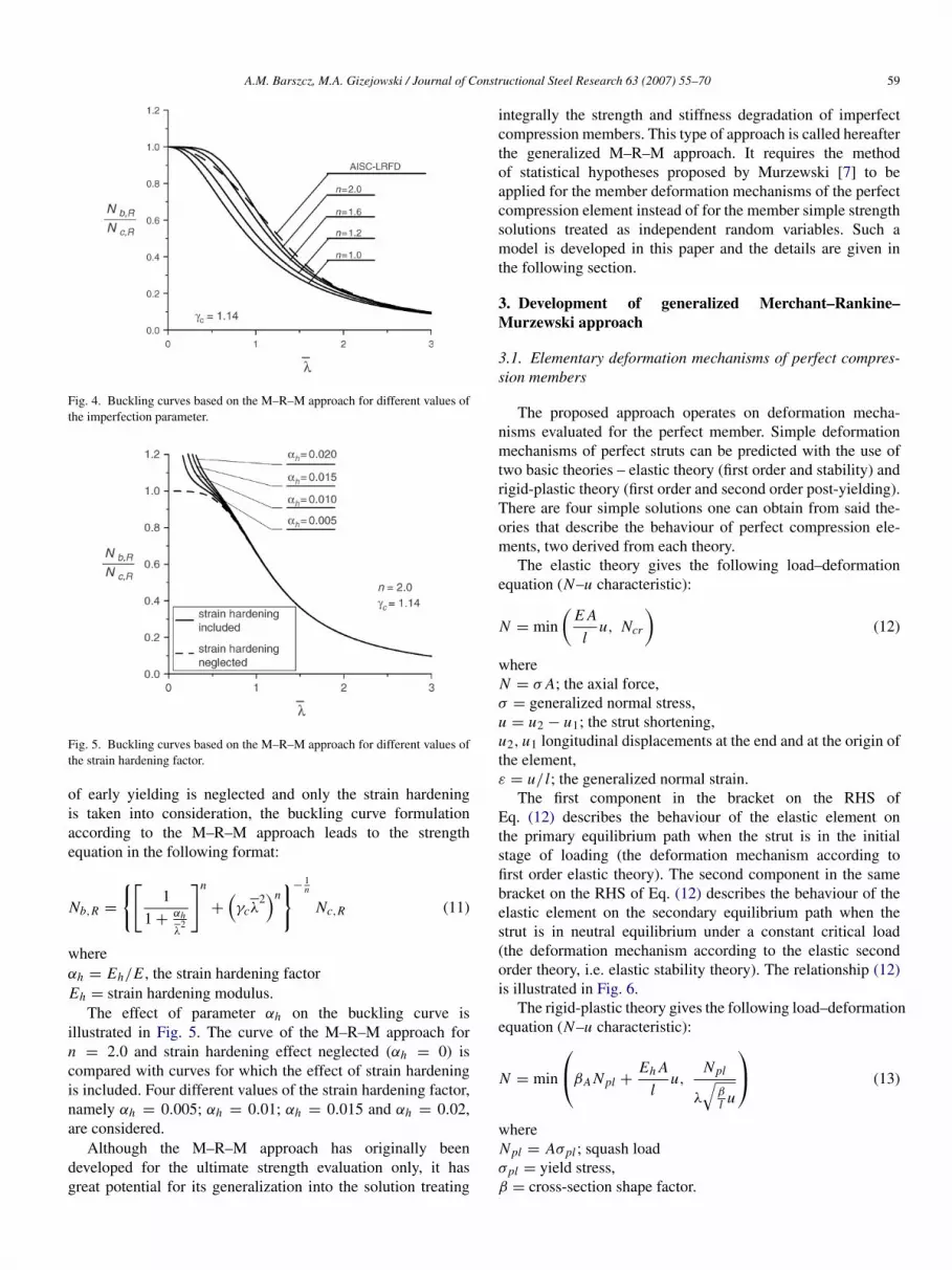
and it plays a similar role as the imperfection parameterα used in Eurocode 3: Part 1-1 [4] for the developmentof multiple buckling curves according to the Ayrton–Perryformulation [15]. It can be easily noted that in the case of n = 1Eq. (8) resulting from the M–R–M approach coincides with thatof the original M–R approach, see Eq. (2). Since the singlebuckling curve cannot represent in detail different aspects oftechnology and manufacturing, as well as their influence onthe buckling strength in all possible planes of buckling, Eq. (8)with n as a parameter to be calibrated has a great advantageover Eq. (2). The effect of parameter n on the buckling curve isillustrated in Fig. 4. The curve of the M–R approach (n = 1, 0)

is compared with those of the M–R–M approach for n = 1.2;n = 1.6 and n = 2.0 (values used for the codification purposesin Poland, refer to PN-90/B-03200 [14]), and with the bucklingcurve of AISC-LFRD [11].

The approach mentioned above has recently been appliedby the authors to the formulation of buckling curves for strainhardening metals (see Gizejowski et al. [16]). When the effect


Fig. 4. Buckling curves based on the M–R–M approach for different values ofthe imperfection parameter.

Fig. 5. Buckling curves based on the M–R–M approach for different values ofthe strain hardening factor.

of early yielding is neglected and only the strain hardeningis taken into consideration, the buckling curve formulationaccording to the M–R–M approach leads to the strengthequation in the following format:

Nb,R =

{[1

1 +αh

λ2

]n

+

(γcλ

2)n}−

1n

Nc,R (11)

whereαh = Eh/E , the strain hardening factorEh = strain hardening modulus.

The effect of parameter αh on the buckling curve isillustrated in Fig. 5. The curve of the M–R–M approach forn = 2.0 and strain hardening effect neglected (αh = 0) iscompared with curves for which the effect of strain hardeningis included. Four different values of the strain hardening factor,namely αh = 0.005; αh = 0.01; αh = 0.015 and αh = 0.02,are considered.

Although the M–R–M approach has originally beendeveloped for the ultimate strength evaluation only, it hasgreat potential for its generalization into the solution treating

integrally the strength and stiffness degradation of imperfectcompression members. This type of approach is called hereafterthe generalized M–R–M approach. It requires the methodof statistical hypotheses proposed by Murzewski [7] to beapplied for the member deformation mechanisms of the perfectcompression element instead of for the member simple strengthsolutions treated as independent random variables. Such amodel is developed in this paper and the details are given inthe following section.

3. Development of generalized Merchant–Rankine–Murzewski approach

3.1. Elementary deformation mechanisms of perfect compres-sion members

The proposed approach operates on deformation mecha-nisms evaluated for the perfect member. Simple deformationmechanisms of perfect struts can be predicted with the use oftwo basic theories – elastic theory (first order and stability) andrigid-plastic theory (first order and second order post-yielding).There are four simple solutions one can obtain from said the-ories that describe the behaviour of perfect compression ele-ments, two derived from each theory.

The elastic theory gives the following load–deformationequation (N–u characteristic):

N = min(

E A

lu, Ncr

)(12)

whereN = σ A; the axial force,σ = generalized normal stress,u = u2 − u1; the strut shortening,u2, u1 longitudinal displacements at the end and at the origin ofthe element,ε = u/ l; the generalized normal strain.

The first component in the bracket on the RHS ofEq. (12) describes the behaviour of the elastic element onthe primary equilibrium path when the strut is in the initialstage of loading (the deformation mechanism according tofirst order elastic theory). The second component in the samebracket on the RHS of Eq. (12) describes the behaviour of theelastic element on the secondary equilibrium path when thestrut is in neutral equilibrium under a constant critical load(the deformation mechanism according to the elastic secondorder theory, i.e. elastic stability theory). The relationship (12)is illustrated in Fig. 6.

The rigid-plastic theory gives the following load–deformationequation (N–u characteristic):

N = min

βA Npl +Eh A

lu,

Npl

λ

√βl u

(13)

whereNpl = Aσpl ; squash loadσpl = yield stress,β = cross-section shape factor.


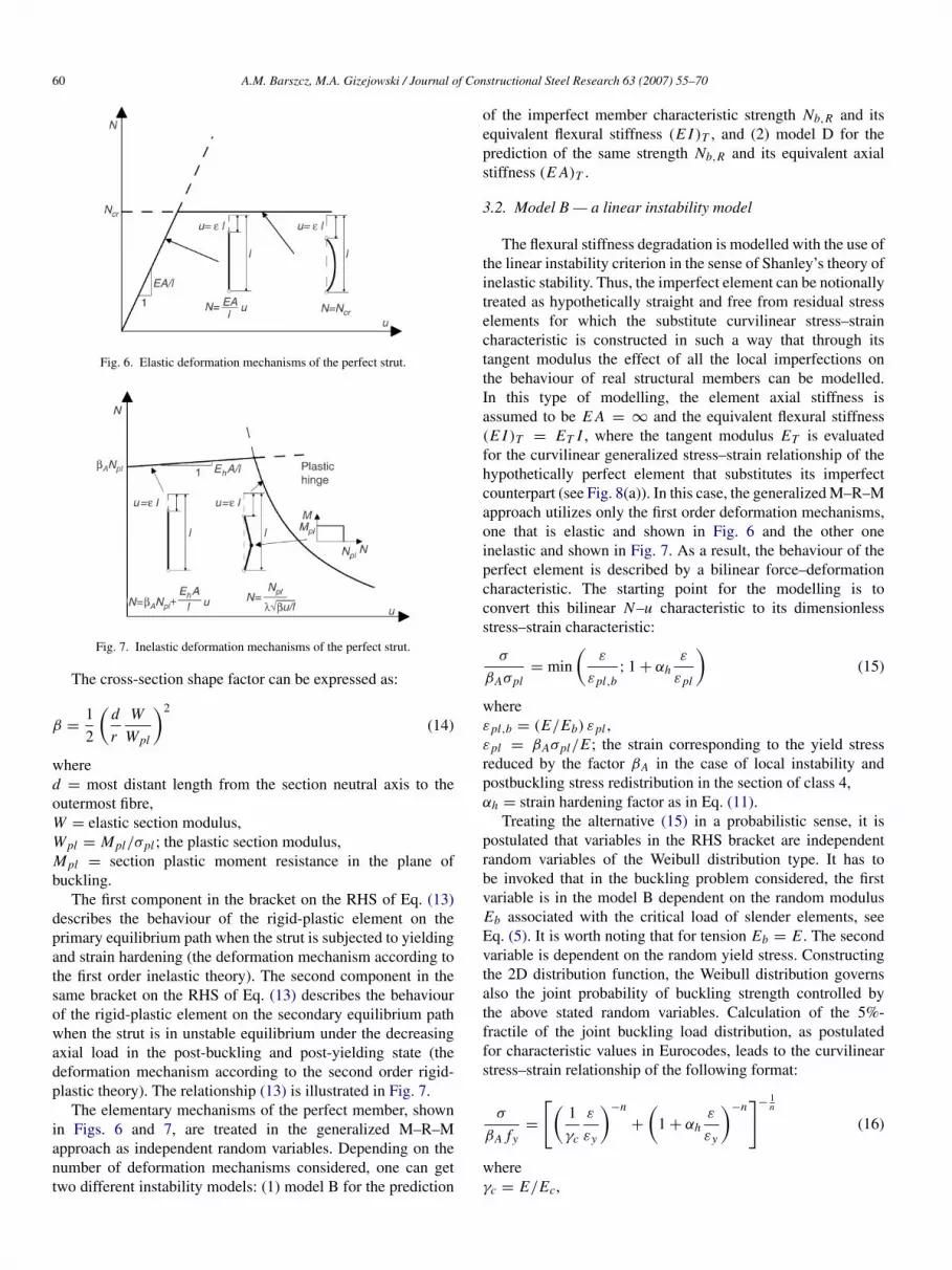
Fig. 6. Elastic deformation mechanisms of the perfect strut.

Fig. 7. Inelastic deformation mechanisms of the perfect strut.

The cross-section shape factor can be expressed as:

β =12

(d

r

W

Wpl

)2

(14)

whered = most distant length from the section neutral axis to theoutermost fibre,W = elastic section modulus,Wpl = Mpl/σpl ; the plastic section modulus,Mpl = section plastic moment resistance in the plane ofbuckling.

The first component in the bracket on the RHS of Eq. (13)describes the behaviour of the rigid-plastic element on theprimary equilibrium path when the strut is subjected to yieldingand strain hardening (the deformation mechanism according tothe first order inelastic theory). The second component in thesame bracket on the RHS of Eq. (13) describes the behaviourof the rigid-plastic element on the secondary equilibrium pathwhen the strut is in unstable equilibrium under the decreasingaxial load in the post-buckling and post-yielding state (thedeformation mechanism according to the second order rigid-plastic theory). The relationship (13) is illustrated in Fig. 7.

The elementary mechanisms of the perfect member, shownin Figs. 6 and 7, are treated in the generalized M–R–Mapproach as independent random variables. Depending on thenumber of deformation mechanisms considered, one can gettwo different instability models: (1) model B for the prediction

of the imperfect member characteristic strength Nb,R and itsequivalent flexural stiffness (E I )T , and (2) model D for theprediction of the same strength Nb,R and its equivalent axialstiffness (E A)T .

3.2. Model B — a linear instability model

The flexural stiffness degradation is modelled with the use ofthe linear instability criterion in the sense of Shanley’s theory ofinelastic stability. Thus, the imperfect element can be notionallytreated as hypothetically straight and free from residual stresselements for which the substitute curvilinear stress–straincharacteristic is constructed in such a way that through itstangent modulus the effect of all the local imperfections onthe behaviour of real structural members can be modelled.In this type of modelling, the element axial stiffness isassumed to be E A = ∞ and the equivalent flexural stiffness(E I )T = ET I , where the tangent modulus ET is evaluatedfor the curvilinear generalized stress–strain relationship of thehypothetically perfect element that substitutes its imperfectcounterpart (see Fig. 8(a)). In this case, the generalized M–R–Mapproach utilizes only the first order deformation mechanisms,one that is elastic and shown in Fig. 6 and the other oneinelastic and shown in Fig. 7. As a result, the behaviour of theperfect element is described by a bilinear force–deformationcharacteristic. The starting point for the modelling is toconvert this bilinear N–u characteristic to its dimensionlessstress–strain characteristic:

σ

βAσpl= min

(ε

εpl,b; 1 + αh

ε

εpl

)(15)

whereεpl,b = (E/Eb) εpl ,εpl = βAσpl/E ; the strain corresponding to the yield stressreduced by the factor βA in the case of local instability andpostbuckling stress redistribution in the section of class 4,αh = strain hardening factor as in Eq. (11).

Treating the alternative (15) in a probabilistic sense, it ispostulated that variables in the RHS bracket are independentrandom variables of the Weibull distribution type. It has tobe invoked that in the buckling problem considered, the firstvariable is in the model B dependent on the random modulusEb associated with the critical load of slender elements, seeEq. (5). It is worth noting that for tension Eb = E . The secondvariable is dependent on the random yield stress. Constructingthe 2D distribution function, the Weibull distribution governsalso the joint probability of buckling strength controlled bythe above stated random variables. Calculation of the 5%-fractile of the joint buckling load distribution, as postulatedfor characteristic values in Eurocodes, leads to the curvilinearstress–strain relationship of the following format:

σ

βA fy=

[(1γc

ε

εy

)−n

+

(1 + αh

ε

εy

)−n]−

1n

(16)

whereγc = E/Ec,


Fig. 8. Instability model B; (a) hypothetical member, (b) generalized stress–strain characteristic, (c) buckling curves original and calibrated.

Ec = characteristic value of the modulus Eb,εy = βA fy/E ; the nominal value of the strain corresponding tothe characteristic value of the yield stress reduced by the factorβA that accounts for local instability and postbuckling stressredistribution in the section of class 4,n = curvature parameter of the substitute stress–straincharacteristic accounting for the effect of residual stresses onthe member behaviour in model B.

Eq. (16) can be used for both tension and compressionof imperfect members, as illustrated in Fig. 8(b). The lowerbound solution (for γc = γ ) is valid for compressionof slender members. The partial safety factor γc can benotionally regarded as a slenderness dependent factor thatglobally reproduces the effect of geometric imperfectionson the behaviour of compression members. The followingempirical formula is suggested for the evaluation of γc:

γc = γ +1 − γ

1 + λ2 (17)

where γ = asymptotic value of γc.The upper bound solution in Fig. 8(b) is valid for compres-

sion of stocky members and for tension members. Contrary toslender compression members, geometric imperfections do notdegrade the member behaviour of stocky members in compres-sion and members in tension, therefore γc = 1 in this case.Hence, the characteristic described by Eq. (17) in the case ofstocky compression members, for which λ → 0 and γc → 1,becomes the same as for tension members. The area betweenthe stress–strain curves corresponding to compression of mem-bers with different values of the slenderness ratio (cases definedby γc = γ and γc = 1) is shaded in Fig. 8(b).

The tangent modulus factor (tangent flexural stiffness factor)can be derived from Eq. (16):

τ =ET

Ec=

1Ec

dσ

dε=

d(

σβA fy

)d(

1γc

εεy

)

=

αhγc

(1γc

εεy

)n+1+

(1 + αh

εεy

)n+1

[(1γc

εεy

)n+

(1 + αh

εεy

)n] (n+1)n

. (18)

The characteristic value of the buckling resistance ofimperfect elements can now be calculated as a loadcorresponding to Shanley’s theory of inelastic buckling:

Nb,R =π2 ET A

λ2 =π2τ Ec A

λ2 . (19)

Introducing the reduction factor for the flexural bucklingmode χ as used in Eurocode 3: Part 1-1 [4] lets Eq. (19) bewritten in a dimensionless format:

χ =Nb,R

βA A fy=

π2τ Ec

λ2βA fy=

π2τ E

γcλ2βA fy(20)

or in terms of the relative stress and member dimensionlessslenderness ratio as:

σ

βA fy=

τ

γcλ2 =

τ(γ +

1−γ

1+λ2

)λ

2. (21)

From Eq. (21) one can express the member slenderness ratioin terms of the relative stress (being equal to the bucklingreduction factor), the tangent modulus factor and the γ -factoras follows:

λ2

=12

−1γ

(1 −

τσ

βA fy

)

+

√√√√[ 1γ

(1 −

τσ

βA fy

)]2

+ 41γ

τσ

βA fy

. (22)

Round brackets in Eq. (22) comprise expressions thatcontribute to the slenderness dependent partial safety factorγc, see Eq. (17). Taking the bracket values as zeros impliesthat the slenderness independent value of γc = γ is adopted.This assumption was used in the so-called further reducedtangent modulus method of advanced analysis developed byChen and Kim [3], and then was also adopted by Gizejowskiand Barszcz [17]. The empirical formula used in this paper – seeEq. (17) – allows for a more rational treatment of theinfluence of geometrical imperfections on the equivalentflexural stiffness.


Fi
g. 9. Instability model D; (a) hypothetical member, (b) generalized stress–strain characteristic, (c) buckling curves original and calibrated.
By combining Eqs. (16), (18) and (22) one can calibratethe model B parameters αh, γ and n in such a way that foroptimally chosen values of these parameters the least errornorm e is obtained. This norm is calculated as a mean fromthe values ei , a discrete number m of squared differencesbetween the values of the strength of the calibrated bucklingcurve and the relative stress obtained from the tangent modulusformulation developed herein:

e = min

m∑

i=1ei

m

= min

m∑

i=1

[(σmaxβA fy

)i− χi

]2

m

(23)

whereχi = buckling reduction factor calculated from the calibratedbuckling curve for the slenderness ratio λi corresponding toEq. (22) in which

[σmax/

(βA fy

)]i and τi are calculated

according to Eqs. (16) and (18) for the same relative strain(ε/εy

)i ,

σmax = stress corresponding to the buckling resistance (seeFig. 8(b)),m = total number of discrete values

(ε/εy

)i considered.

Fig. 8(c) shows graphically the interpretation of thequantities used in Eq. (21) where the buckling curve drawn bythe dotted line represents the standard curve from the designcode, and the solid line is the curve seeking the best fit to thestandard one.

3.3. Model D — a nonlinear instability model

The axial stiffness degradation is modelled with use ofthe nonlinear instability criterion in the sense of divergenceof equilibrium at the limit point on the load–deformationcharacteristic. Thus, the imperfect element is to be notionallytreated as a hypothetically straight and residual stress freeelement for which the substitute curvilinear stress–straincharacteristic is constructed in such a way that it reproducesthe effect of all the local imperfections on the behaviour ofthe real structural member. In this modelling, the elementflexural stiffness is assumed to be E I = ∞ and the equivalentaxial stiffness (E A)T = ET A = κ E A, where the tangentmodulus ET is a different function than that evaluated for the

substitute stress–strain relationship in model B and κ is thetangent modulus factor for the evaluation of the equivalentaxial stiffness of the imperfect compression member. Thegeneralized stress–strain relationship of a hypothetically perfectelement reproducing the behaviour of the imperfect elementconsists of: the ascending branch, the limit point and thedescending branch (see Fig. 9(a)). In this case, the generalizedM–R–M approach utilizes all the deformation mechanisms,namely two elastic shown in Fig. 6 and also two inelasticas shown in Fig. 7. As a result, the behaviour of the perfectelement is described by a multi-curve force–deformationcharacteristic. The starting point for the modelling is toconvert the multi-curve N–u characteristic to its generalizedstress–strain characteristic. In the dimensionless format it isgiven by:

σ

βAσpl= min

ε

εpl; 1 + αh

ε

εpl;

(λpl

λ

)2

;1

π(

λλpl

)√β ε

εpl

.

(24)

whereλpl = the point of intersection of the Euler hyperbola andthe yield stress reduced by the factor βA in the case of localinstability and postbuckling stress redistribution in the sectionof class 4.

The slenderness λpl is given by:

λpl = π

√E

βAσpl. (25)

Treating the alternative (24) in a probabilistic sense, asin the case of model B, then assuming that variables in theRHS bracket are independent random variables of the Weibulldistribution type, constructing the joint distribution functionand finally calculating the 5%-fractile of the joint bucklingload distribution, as postulated for characteristic values inEurocodes, leads to the curvilinear stress–strain relationship ofthe following format:

σ

βA fy=

( ε

εy

)−n

+

(1 + αh

ε

εy

)−n


+

(1

γ λ2

)−n

+

1

πλ√

γβ εεy

−n−1n

(26)

whereγ = asymptotic value of the partial safety factor for the criticalload,εy = strain defined by Eq. (16),β = cross-section shape factor defined by Eq. (14),n = curvature parameter of the stress–strain characteristic formodel D.

By comparison of Eq. (16) and (26) one can conclude thatomitting the last two terms in the RHS square brackets of Eq.(26), and replacing the modulus E by Eb, leads to Eq. (16). Thedifference results only in the first term, namely in Eq. (16) thereis a partial safety factor γc. The reason for the partial safetyfactor in model B was explained earlier on statistical grounds.In Eq. (26) the value E in the first term plays a role of thematerial constant, since the whole load–deformation curve ofimperfect elements tends to be described by this equation. Thesafety factor in this case is not a slenderness dependent variable.The constant γc = γ is not therefore applied to the elasticitymodulus but to those components of the RHS square bracket inEq. (26) that are associated with the buckling load as well aswith the postbuckling and postyielding behaviour (slendernessratio dependent terms).

The tangent modulus factor (tangent axial stiffness factor)κ corresponding to the strength Eq. (26) can be calculated asfollows:

κ =1E

d(

σβA fy

)d(

εεy

) =

( ε

εy

)−n

+

(1 + αh

ε

εy

)−n

+

(1

γ λ2

)−n

+

1

πλ√

γβ εεy

−n−1+n

n

×

(

ε

εy

)−(1+n)

+ αh

(1 + αh

ε

εy

)−(1+n)

−1

2πλ√

γβ

(√εεy

)3

1

πλ√

γβ εεy

−(1+n)

. (27)

The shape factor β is dependent on the cross-section type,see Eq. (14). When used in Eqs. (26) and (27), it has to betreated as a substitute buckling curve dependent parametersubjected to calibration in order to reproduce the buckling curveof the code of practice under consideration.

The pick point on the characteristic described by Eq. (26) isassociated with the buckling reduction factor χ :

χ =

(σmax

βA fy

)(28)

whereσmax = stress corresponding to the buckling resistance (seeFig. 9 (b)) for which the tangent axial stiffness factor κ

according to Eq. (27) becomes zero.The buckling curve can be reconstructed from maxima

of the slenderness ratio dependent dimensionless stress–straindiagram given by Eq. (26). Thus the characteristic value ofbuckling resistance is calculated from the following equation:

Nb,R =

(σmax

βA fy

)βA A fy . (29)

By combining Eqs. (26)–(28) one can calibrate the modelD parameters αh, γ, β and n in such a way that for optimallychosen values of these parameters the least value of the errornorm e is obtained as has been explained for model B.

Fig. 9(c) shows graphically the interpretation of thequantities used in Eq. (26) where the buckling curve drawn bythe dotted line represents a standard curve from the design code,and the solid line is the curve seeking the best fit to the standardone. The authors show in the next section that buckling curvesconstructed from the maxima of the function given by Eq. (26)agree, for parameters αh, γ, n that are the same as in model Band for an optimally calibrated value β in model D, with thebuckling curves adopted in the calibration exercise of modelsB and D. The calibration exercise is performed to conformto European buckling curves through the equivalent stiffnessesfrom models B and D that are developed in this section.

4. Calibration of model parameters conforming to Euro-pean imperfections

The generalized M–R–M approach presented in the previoussection for the development of two instability models Band D is used herein for modelling of the family of fiveEuropean buckling curves, see Eurocode 3: Part 1-1 [4]. Thebuckling reduction factor for the whole buckling curve familyof Eurocode 3 has the following format:

χ =1

φ +

√φ2 − λ

2≤ 1 (30)

whereφ = 0, 5

(1 + η + λ

2)

η = Ayrton–Perry slenderness initial lack of straightness factor.According to Ayrton–Perry [15], the η-factor can be written

as follows:

η =e0

d

(d

r

)2

(31)

wheree0 = initial lack of straightness (the maximum coordinate, seeFig. 1(a)),r , d = variables as identified in Eqs. (6) and (14), respectively.

Since the buckling curve is constructed as slendernessdependent, it does not involve explicitly the section properties.


Table 1Imperfection factors α for European buckling curves

Buckling curve a0 a b c d

α 0.13 0.21 0.34 0.49 0.76

Eurocode 3: Part 1-1 [4] adopts the following empirical formulafor the η-factor:

η = α(λ − 0, 2

)(32)

where α = imperfection factor specified by a different value foreach European buckling curve.

The imperfection factors corresponding to appropriateEuropean buckling curves a0, a, b, c and d are given in Table 1.The selection criteria of buckling curves in Eurocode 3: Part1-1 [4] are according to the section type, thickness of theflange element, steel strength, manufacturing process and theplane of buckling, see Table 2. The parameters involved in thedeveloped models B and D based on the generalized M–R–Mapproach are calibrated in order to reproduce these bucklingcurves. The calibration procedure is applied for each bucklingcurve separately in two stages:

1. Parameters n, α and γ are first calibrated through Eqs.(16)–(18) in order to reproduce European buckling curveswith help of model B.

2. The parameters calibrated in the first stage are then used inmodel D with the same values, and only the value of theparameter β is calibrated in order to obtain the best fit toEuropean buckling curves through Eqs. (26)–(28).

4.1. Model B — a linear instability model

Three model parameters γ, αh and n are calibrated in orderto reproduce five European buckling curves through modelB. Each point i on the calibrated buckling curve correspondsto a certain member slenderness ratio λi (see Fig. 8(c)). Itrepresents, on the curvilinear stress–strain characteristic, atangent stiffness that reproduces the effect of all the localimperfections on the bifurcation instability of the imperfectmember through the buckling criterion of the Shanley theoryof inelastic buckling (see Fig. 8(b)). Since the effect of γc-factor on the shape of the calibrated buckling curve is morepronounced for slender members, and it becomes negligible

Table 3Parameters calibrated for the linear instability model B

Parameters Values of calibrated curve dependent parameters forthe buckling curvea0 a b c d

γ 1.10 1.15 1.20 1.30 1.40αh 0.002 0.005 0.009 0.013 0.017n 5.8 4.2 3.0 2.4 1.9

for stocky members, the calibration may be done using itsasymptotic value γc = γ . The summary of the modelparameters calibrated under this assumption is given in Table 3.

The comparison of the buckling curves a0, a, b, c and d,reproduced through the developed linear instability model Band model parameters from Table 3, is given in Fig. 10. Eachcalibrated curve is compared with the original European curveand the limiting curves constructed from the values being 0, 95and 1, 05 of that of Eurocode 3: Part 1-1 [4]. It can be seen thatfor all the calibrated buckling curves they are within the limitingcurves and they are very close to the original European curves.

The advantage of this new formulation of European bucklingcurves is that calibrated curves can be directly used in theprediction of the equivalent flexural stiffness and the flexuralstiffness degradation functions corresponding to real structuralelements, imperfections of which conform with those adoptedin Eurocode 3: Part 1-1 [4].

Landesmann and Batista [18] formulated recently the tan-gent stiffness degradation functions corresponding to Europeanbuckling curves. They can be written in the following format:

τ = 1 forN

Nc,R≤ e1 (33a)

τ =2e2 f 2

1

f 22

[f3 +

√(f3 −

f1f2

) (f3 +

f1f2

)]for e1 <

N

Nc,R≤ 1, (33b)

where functions fi (i = 1, 2, 3) were dependent on the axialforce ratio N/Nc,R :

f1 = e3 −e4√

N/Nc,R

√e5 − e6

(N/Nc,R

)+(N/Nc,R

)2 (34a)

Table 2Selection of European buckling curves for buckling about the major axis of I-sections

Cross-section fabrication Depth-to-width ratio Flange thickness t f (mm) Buckling curve for steelstrength (MPa)<450 ≥450

Rolledh/b > 1, 2

≤40 a a040 < tt ≤ 100 b a

h/b > 1, 2≤100 b a>100 d c

Welded any≤40 b40 < tt ≤ 100 c>100 d


Fig. 10. Comparison of buckling curve calibration in model B; (a) buckling curve a0, (b) buckling curve a, (c) buckling curve b, (d) buckling curve c, (e) bucklingcurve d.

Table 4Constants ei for the tangent modulus evaluated for the reproduction ofBrazilian/European buckling curves

Constant ei for i equal to Buckling curvea b c d

1 0.110 0.060 0.010 0.0102 0.268 0.279 0.267 0.2773 105.0 85.0 245.0 95.014 978.8 482.7 979.7 230.225 1.044 1.073 1.109 1.1796 2.032 2.042 2.042 2.0097 500.0 250.0 500.0 125.1

f2 = e7(N/Nc,R − 1

)(34b)

f3 = 1 +

(f1

2 f2

)2

+ α

(f1

2 f2− 0.2

)(34c)

whereα = imperfection factor as specified in Table 1,ei = coefficients listed in Table 4.

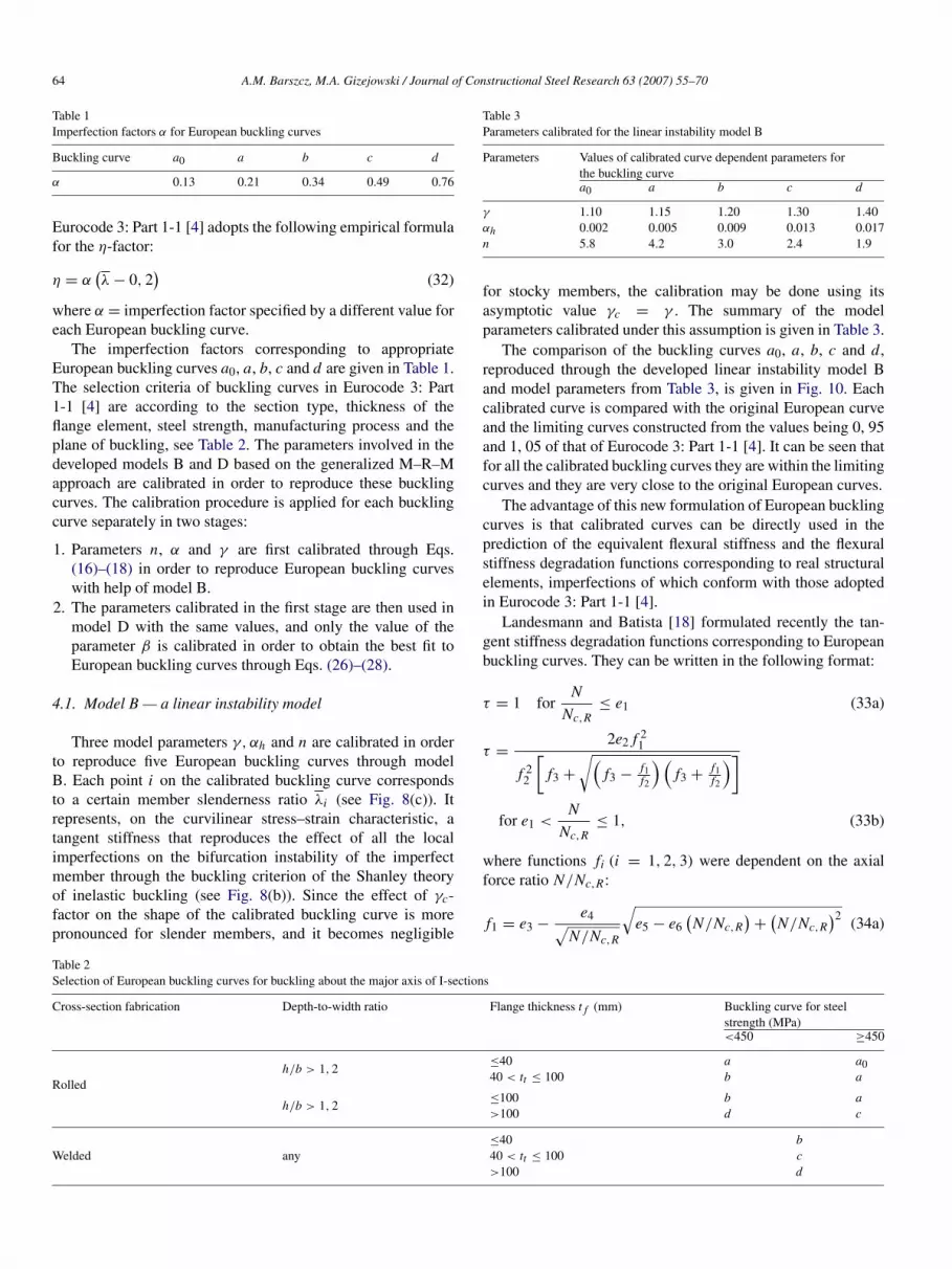
The stiffness degradation functions corresponding to thedeveloped model B and the model parameters calibrated inthis section are compared with the functions proposed byLandesmann and Batista [18], and described by Eqs. (33) and(34). The comparison is given in Fig. 11 for curves a, b, cand d . The functions of the present study are presented fortwo values of the γc-factor, namely γc = 1, 0 (for stockymembers) and γc = γ (for slender members), where the valuesof γ -factor for each European curve are taken from Table 3.

The area occupied by the degradation functions for membersof intermediate values of the slenderness ratio is shaded. Thefunction proposed previously by Chen and Kim [3] for thefurther reduced tangent modulus method of the North Americanapproach to advanced analysis is also drawn for comparison.The results are indicative of the following:

(a) The degradation function of the further reduced tangentmodulus method is not accurate enough to represent thestability behaviour of imperfect member subpopulations ofdifferent cross-section types and planes of buckling, as hasbeen adopted in Eurocode 3: Part 1 [4].

(b) The stiffness degradation characteristic adopted in thefurther reduced tangent modulus method starts from thevalue of 0.85 of the original axial stiffness. In contrast tothe previously compared curve, the other curves start fromthe value equal to unity in the Landesmann and Batistaproposal while in the authors’ proposal they start fromdifferent values 1/γ dependent upon the buckling curve andthe element slenderness ratio.

(c) The stiffness degradation characteristic adopted in thefurther reduced tangent modulus method is an upper boundsolution for characteristics corresponding to the multiplebuckling curves formulation adopted in Eurocode 3: Part1.1 [4].

(d) “Exact” degradation functions of Landesmann and Batista[18], given by Eqs. (33) and (34), cannot be used for theaxial force close to unity since the values of these functionsincrease indefinitely in this region.


Fig. 11. Comparison of stiffness degradation functions for buckling curve calibration in model B; (a) buckling curve a, (b) buckling curve b, (c) buckling curve c,(d) buckling curve d.

(e) If compared with the functions proposed by Landesmannand Batista [18], stiffness degradation functions of modelB developed by the authors on the basis of the M–R–Mapproach create: (1) a lower bound estimation for slendermembers, and (2) an upper bound estimation for the stockymembers.

4.2. Model D — a nonlinear instability model

Four model parameters γ, αh, β and n are calibrated inorder to reproduce five European buckling curves throughmodel D. As in model B, each point i on the calibratedbuckling curve corresponds to a certain member slendernessratio λi (see Fig. 9(c)). It however indicates a differentdegradation function for the member axial stiffness than thatof the member flexural stiffness for the same slenderness.The limit point i shown in Fig. 9(b) on the curvilinearstress–strain characteristic that reproduces the effect of allthe local imperfections on the divergence instability of theimperfect member, represents a point of the zero tangentstiffness. The buckling curve constructed from the maximaof the curvilinear stress–strain characteristic of members ofdifferent slenderness ratio represents the buckling reductionfactor of the characteristic strength of imperfect elements.The parameters γ, αh and n are taken for model D ofthe same value as optimally calibrated for model B (seeTable 3). In order to reproduce the buckling curves through thenonlinear instability model, the parameter β is to additionally

Table 5Parameter β calibrated for the nonlinear instability model D

Parameters Values of calibrated curve dependent parameter β

for the buckling curvea0 a b c d

β 0.15 0.13 0.11 0.08 0.06

be calibrated. The calibration procedure is applied for eachbuckling curve separately for calibrated European bucklingcurves. The summary of the calibrated model D parameter β

is given in Table 5. The comparison of the buckling curvesreproduced through the developed nonlinear instability modelD and model parameters from Table 5 is given in Fig. 12 forcurves a0, a, b, c and d. The calibrated curve is compared withthe original European curve and the limiting curves constructedas 0.95 and 1.05 of that of Eurocode 3: Part 1-1 [4]. It canbe seen that for all the calibrated buckling curves they arewithin the limiting curves and they are very close to theoriginal European curves; therefore they are also close to thosepredicted by model B of the present study. This is a veryimportant feature of the developed modelling that facilitatesits future application in the Continuous Stiffness Degradationmethod (CSD method, see Gizejowski et al. [10]) of advancedanalysis that shall comply with the reliability level adopted inEurocode 3: Part 1-1 [4].

The advantage of the presented new formulation ofEuropean buckling curves is that it can be directly used in


Fig. 12. Comparison of buckling curve calibration in model D; (a) buckling curve a0, (b) buckling curve a, (c) buckling curve b, (d) buckling curve c, (e) bucklingcurve d.

the prediction of the equivalent axial stiffness and the axialstiffness degradation function corresponding to real structuralelements, imperfections of which conform with those adoptedin Eurocode 3: Part 1-1 [4]. In advanced analyses proposed sofar, the assumption of the same stiffness degradation functionwas used for the prediction of member tangent flexural andaxial stiffnesses, see Chen and Kim [3] in the North Americanapproach and Landesmann and Batista [18] in the Brazilianapproach. The approach of the present study allows for thedistinction to be made between both degradation effects, andalso for the evaluation of the axial stiffness degradation functionin a more accurate way.

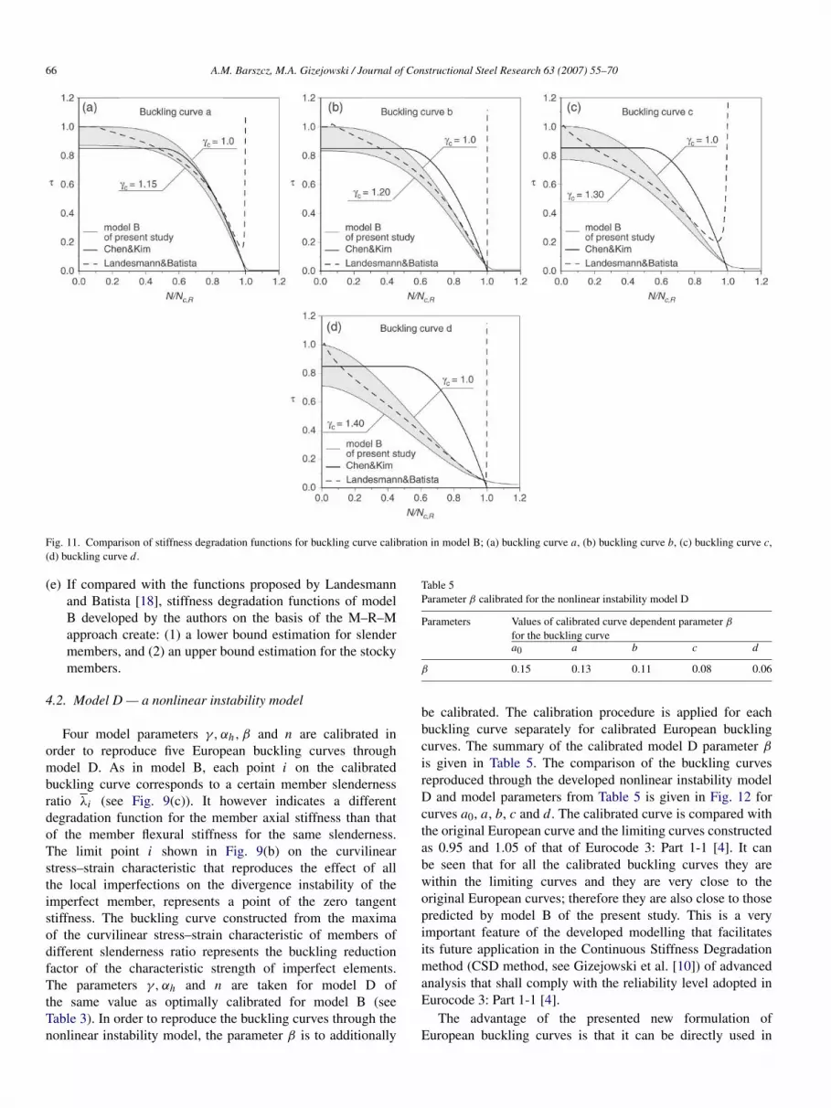
The equivalent axial stiffness degradation functions corre-sponding to the developed model D and the model param-eters calibrated in this section are compared with the func-tions proposed by Chen and Kim [3] for their further reducedtangent modulus method, and functions of Landesmann andBatista [18] used in the comparison made for model B in theprevious subsection. The comparison is given in Fig. 13 forcurves a, b, c and d . The results are indicative of the follow-ing:

(a) The degradation functions of the further reduced tangentmodulus method developed by Chen and Kim [3], and alsothe functions conforming with Eurocode 3 provisions anddeveloped by Landesmann and Batista [18], are not accurateenough to represent the stability behaviour of imperfectmembers as far as their axial response is considered. They

cannot reflect the behaviour of imperfect bracing members(members hinged at both ends) so that it is somewhatquestionable to use them in advanced analysis of trusses orframes with bracing systems.

(b) The stiffness degradation characteristic adopted in thefurther reduced tangent modulus method starts from thevalue of 0.85 of the original axial stiffness in contrastto the other compared curves; they start from the valueequal to unity in the Landesmann and Batista proposaland in the authors’ proposal. Therefore the further reducedtangent modulus curve unnecessarily underpredicts thetangent axial stiffness in the range of the small axial forcewhile for the high values of the axial force it considerablyoverpredicts the tangent axial stiffness, especially whenmodel D predicts small positive or negative values.

(c) The axial stiffness degradation functions of model Ddeveloped by the authors on the basis of the M–R–Mapproach are slenderness dependent and for a highermember slenderness ratio they prove to be the lower boundestimation for the stiffness degradation functions developedby Landesmann and Batista [18].

4.3. Effects of buckling length and effective cross-section areaon buckling curves

The buckling resistance of imperfect members reported sofar was considered in a general format without an explicittreatment of the member effective length factor µ = le/ l and


Fig. 13. Comparison of stiffness degradation functions for buckling curve calibration in model D; (a) buckling curve a, (b) buckling curve b, (c) buckling curve c,(d) buckling curve d.

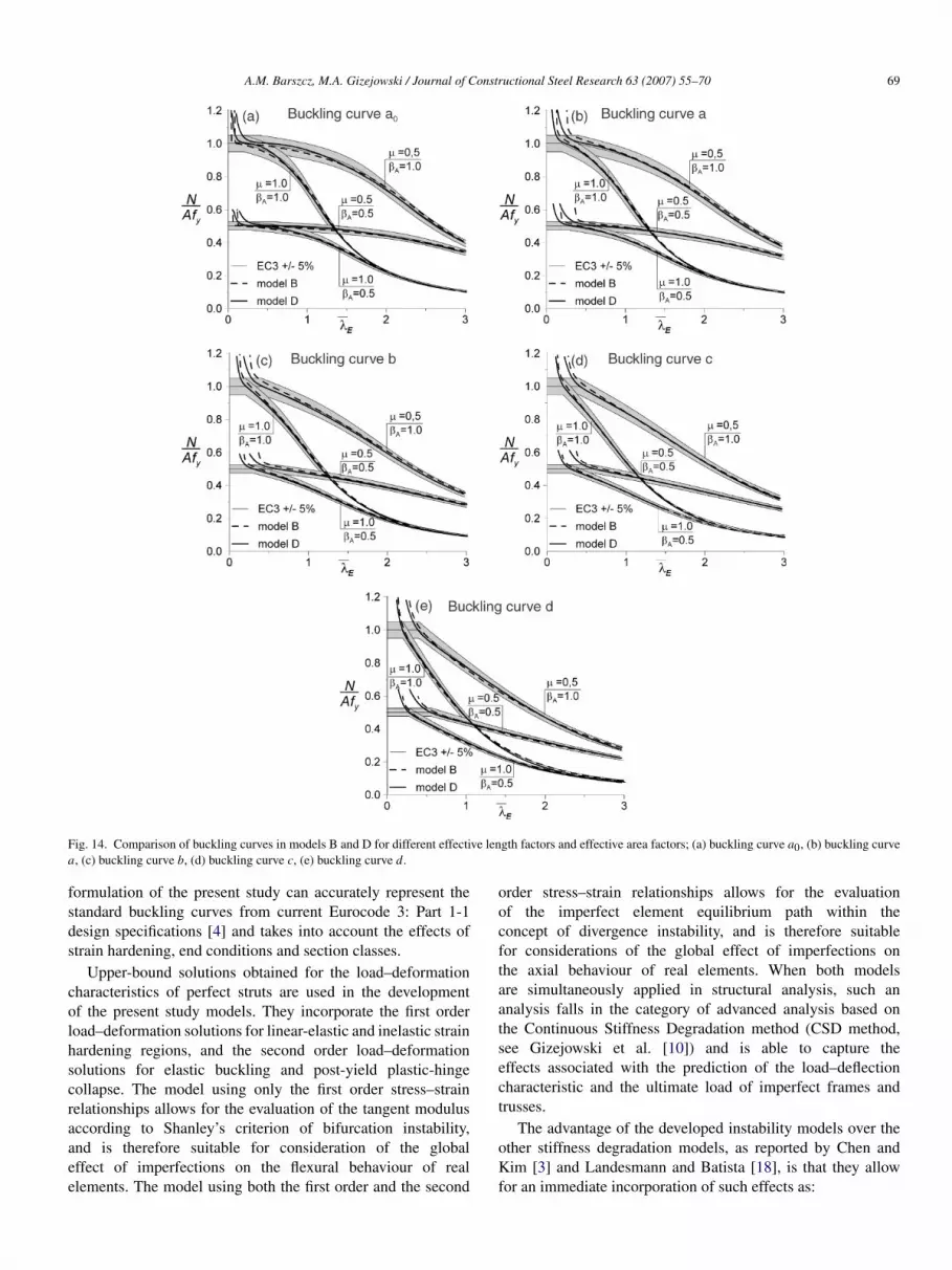
the effective area factor βA = Aeff/A. The effective lengthis implicitly considered in the definition of the slendernessratio according to Eq. (6). Let us show that both developedinstability models for strength and stiffness evaluation ofimperfect members lead to a reasonable accuracy if comparedwith the original Eurocode 3 formulation in the case of differenteffective length factors µ of the element held in position at bothends and subjected to different rotational end conditions as wellas for different effective area factors βA.

The comparison of buckling curves for different effectivelength factors is made with the use of the so-called relativeEuler strut slenderness ratio defined as:

λE =λ

√βAµ

(35)

whereλE = λE/λc; Euler strut relative slenderness ratio,λE = Euler strut slenderness ratio of the member hinged at bothends and held there in the position that is equal to λ when thelatter is evaluated for µ = 1, see Eq. (6),

λc = π√

Efy

; member slenderness calculated for the

intersection point where the Euler hyperbola reaches thecharacteristic value of steel strength.

The comparison of buckling curves a0, a, b, c and d,according to the two developed instability models B and Dreproducing the original European buckling curves, is givenin Fig. 14. Two extreme values of the effective length factor,

namely µ = 0.5 and µ = 1, and two extreme values ofthe effective area factor, namely βA = 0.5 and βA = 1 areconsidered. The Eurocode 3 curves are drawn together withtheir upper and lower limits of (+/−5%). It may be observedthat for both extreme values of µ and βA factors a similaraccuracy of the reproduction of European buckling curves isobtained. It is therefore easy to prove that the above statementis valid for all other values of the effective length factor andthe effective area factor. This is an important feature desirablefor the implementation of developed models in design usingadvanced analysis when different member end conditions anddifferent section classes are accounted for in analysis.

5. Conclusions

The paper describes the application of a generalizedM–R–M approach to the modelling of the behaviour ofimperfect compression members. Two instability modelsdenoted as B and D are suggested, the former based on thebifurcation instability criterion (linear instability or tangentmodulus theory) and the latter based on the divergenceinstability criterion (nonlinear instability or limit equilibriumtheory).

The authors report on a new approach to the formulationof multiple buckling curves and the construction of substitutestress–strain characteristics that can be used for the evaluationof the strength and stiffness degradation effects of imperfectmembers in advanced analysis of real structural systems. The


Fig. 14. Comparison of buckling curves in models B and D for different effective length factors and effective area factors; (a) buckling curve a0, (b) buckling curvea, (c) buckling curve b, (d) buckling curve c, (e) buckling curve d.

formulation of the present study can accurately represent thestandard buckling curves from current Eurocode 3: Part 1-1design specifications [4] and takes into account the effects ofstrain hardening, end conditions and section classes.

Upper-bound solutions obtained for the load–deformationcharacteristics of perfect struts are used in the developmentof the present study models. They incorporate the first orderload–deformation solutions for linear-elastic and inelastic strainhardening regions, and the second order load–deformationsolutions for elastic buckling and post-yield plastic-hingecollapse. The model using only the first order stress–strainrelationships allows for the evaluation of the tangent modulusaccording to Shanley’s criterion of bifurcation instability,and is therefore suitable for consideration of the globaleffect of imperfections on the flexural behaviour of realelements. The model using both the first order and the second

order stress–strain relationships allows for the evaluationof the imperfect element equilibrium path within theconcept of divergence instability, and is therefore suitablefor considerations of the global effect of imperfections onthe axial behaviour of real elements. When both modelsare simultaneously applied in structural analysis, such ananalysis falls in the category of advanced analysis based onthe Continuous Stiffness Degradation method (CSD method,see Gizejowski et al. [10]) and is able to capture theeffects associated with the prediction of the load–deflectioncharacteristic and the ultimate load of imperfect frames andtrusses.

The advantage of the developed instability models over theother stiffness degradation models, as reported by Chen andKim [3] and Landesmann and Batista [18], is that they allowfor an immediate incorporation of such effects as:


(1) Strain hardening of steel.(2) Member end conditions that may even change with respect

to semi-rigid joint action or joint and member progressiveyielding under increasing loads.

(3) Member section class in compression that may affectthe member strength and stiffness degradation process,therefore the moment redistribution process in the entirestructural system in the course of its loading.

The above mentioned features create the basis for thedevelopment of advanced analysis that can predict both thestructure strength and load–deflection characteristic in a morereliable way, closer to the reliability level of strength criteriaof individual elements adopted in current design codes, andyet released from the restrictions of no local buckling andpostbuckling redistribution of stresses in members of class4 in compression. The model parameters calibrated in thispaper allow for the implementation of the equivalent memberstiffnesses in computer advanced analysis software in order toconform with the reliability level adopted in Eurocode 3: Part 1-1 [4]. Research in this regard is now underway in the EuropeanEureka/SEFIE project E!3034 and the results are expected to bepublished soon, Barszcz and Gizejowski [19].

Acknowledgements

This paper is part of research carried out under the EuropeanEureka/SEFIE project E!3034 “Steelbiz as an E-forum for theDevelopment of Eurocodes for Steel Construction” coordinatedby the Steel Construction Institute, UK; task B3 “ContinuouslyIntegrated Approach – Analysis and Design of Steel StructuresAccounted for Nonlinear Behaviour of Members and Joints”financed by the State Committee for Scientific Research andcoordinated by the Building Research Institute in Warsaw,Poland.

Certain aspects of this paper were originally publishedin the proceedings of Eurosteel 2005, the Fourth EuropeanConference on Steel and Composite Structures [17].

References

[1] ECCS Publication No. 33. Ultimate limit state calculation of swayframes with rigid joints. Brussels: European Convention of ConstructionalSteelwork; 1984.

[2] Dwight JB, Moxham KE. Compressive strength of welded plates. In:International colloquium on stability of structures under static anddynamic loads; 1977. p. 463–80.

[3] Chen WF, Kim SE. LRFD steel design using advanced analysis. BocaRaton: CRC Press; 1997.

[4] EN 1993-1-1, Eurocode 3. Design of steel structures — Part 1-1: Generalrules and rules for buildings. Brussels: CEN; 2005.

[5] BS 5950: Structural use of steelwork in buildings: Part 1: Code of practicefor design in simple and continuous construction: Hot rolled section.London: BSI; 2001.

[6] Goncalves R, Camotim D. On the incorporation of equivalent memberimperfections in the in-plane design of steel frames. Journal ofConstructional Steel Research 2005;61:1226–40.

[7] Murzewski J. Theory of random load carrying capacity of rod structures.Studies in Engineering, No. 15. Warsaw: PWN; 1976 [in Polish].

[8] Merchant W. The failure load of rigid jointed framework as influenced bystability. The Structural Engineer 1954;32:185–90.

[9] Allen D. Merchant–Rankine approach to member stability. Journal of theStructural Division 1978;104:1909–14.

[10] Gizejowski MA, Barszcz AM, Branicki JC, Uzoegbo HC. Review ofanalysis methods for inelastic design of steel semi-continuous frames.Journal of Constructional Steel Research 2006;62:81–92.

[11] AISC-LRFD. Load and resistance factor design specifications. 2nd ed.Chicago: American Institute of Steel Construction; 1994.

[12] NRC-CNRC: National building code of Canada. Ottawa: NationalResearch Council of Canada; 1995.

[13] SABS 0160. Code of practice for the standard use of steel: Part 1: Limitstates design of hot rolled steelwork. Pretoria: South African Bureau ofStandards; 2005.

[14] PN-90/B-03200. Steel structures: Static calculations and design. Warsaw:PKNMiJ; 1990.

[15] Ayrton WE, Perry J. On struts. The Engineer 1886;62:464.[16] Gizejowski MA, Barszcz AM, Nikonowicz KM. A new buckling curves

formulation for aluminium alloy elements. In: Hancock GJ, Bradford MA,Wilkinson TJ, Uy B, Rasmussen KJR, editors. Advances in structures —steel, concrete, composite and aluminium. Rotterdam: Balkema; 2003.p. 413–9.

[17] Gizejowski MA, Barszcz AM. A new formulation of European bucklingcurves: A generalized M–R–M approach. In: Hoffmeister B, Hechler O,editors. Steel and composite structures: Research-Eurocodes-Practice —Proceedings of the 4th european conference on steel and compositestructures: Eurosteel 2005, vol. A. Aachen: Druck und Veragshaus MainzGmbH Aachen; 2005. p. 1.5-1–1.5-8.

[18] Landesmann A, Batista E, De Miranda. Advanced analysis of steelframed buildings using Brazilian standards and Eurocode 3. Journal ofConstructional Steel Research 2005;61:1051–74.

[19] Barszcz AM, Gizejowski MA. Advanced analysis for design of steelstructures to Eurocode 3. Journal of Constructional Steel Research (inpreparation).

an equivalent stiffness approach for modelling the behaviour of compression members according to...

Documents