modelling precipitation hardening in an a356+0.5cu cast
TRANSCRIPT

Préparée à MINES ParisTech
Modélisation du durcissement par précipitation dans unalliage d’aluminium de fonderie A356+0.5Cu
rModelling precipitation hardening in an A356+0.5Cu cast
aluminum alloy
Anass ASSADIKI19 Juin 2020
École doctorale no621
ISMME: Ingénierie desSystèmes, Matériaux, Mé-canique, Énergétique
Spécialité
Sciences et génie desmatériaux
Composition du jury :
Michel PerezProfesseur, Université de Lyon Rapporteur
David BalloyProfesseur, Université de Lille Rapporteur
Ivan GuillotProfesseur, ICMPE Président
Shahrzad EsmaeiliProfesseur, Université de Waterloo Examinateur
Georges CailletaudProfesseur, MINES ParisTech Examinateur
Warren J. PooleProfesseur, Université de la Colombie-Britannique
Examinateur
Vladimir A. EsinChargé de recherche, MINES ParisTech Examinateur
Rémi MartinezIngénieur de recherche PhD, Linamar Examinateur


Contents
Acknowledgements 3
Introduction 5
1 Industrial and scientific context 91.1 Cylinder heads . . . . . . . . . . . . . . . . . . . . . . . . . . . . 101.2 Overview on aluminum and its alloys . . . . . . . . . . . . . . . . 121.3 Cast aluminum alloys of the 3xx series . . . . . . . . . . . . . . . 15
1.3.1 Solidification . . . . . . . . . . . . . . . . . . . . . . . . . 151.3.2 Alloying elements . . . . . . . . . . . . . . . . . . . . . . 161.3.3 As-cast microstructure . . . . . . . . . . . . . . . . . . . . 18
1.4 Precipitation hardening and heat treatments . . . . . . . . . . . . 191.4.1 Heat treatments . . . . . . . . . . . . . . . . . . . . . . . 221.4.2 Peak hardness and nomenclature . . . . . . . . . . . . . . 24
1.5 Precipitation sequences . . . . . . . . . . . . . . . . . . . . . . . 271.5.1 Al-Si-Cu alloys . . . . . . . . . . . . . . . . . . . . . . . . 271.5.2 Al-Si-Mg alloys . . . . . . . . . . . . . . . . . . . . . . . . 271.5.3 Al-Si-Mg-Cu alloys . . . . . . . . . . . . . . . . . . . . . . 28
1.6 Conclusion . . . . . . . . . . . . . . . . . . . . . . . . . . . . . . 31
2 Experimental study of the A356+0.5Cu alloy 332.1 Studied alloy: A356+0.5Cu . . . . . . . . . . . . . . . . . . . . . 342.2 Specimen preparation . . . . . . . . . . . . . . . . . . . . . . . . 352.3 Precipitates characterization . . . . . . . . . . . . . . . . . . . . . 36
2.3.1 Experimental procedure for TEM study . . . . . . . . . . . 362.3.2 Nature and morphology of precipitates . . . . . . . . . . . 372.3.3 Size distributions of precipitates . . . . . . . . . . . . . . . 42
2.4 Tensile tests . . . . . . . . . . . . . . . . . . . . . . . . . . . . . 462.4.1 Experimental procedure . . . . . . . . . . . . . . . . . . . 462.4.2 Test results . . . . . . . . . . . . . . . . . . . . . . . . . . 49
2.5 Conclusion . . . . . . . . . . . . . . . . . . . . . . . . . . . . . . 53
3 Precipitation kinetics model 553.1 Nucleation . . . . . . . . . . . . . . . . . . . . . . . . . . . . . . 563.2 Growth . . . . . . . . . . . . . . . . . . . . . . . . . . . . . . . . 60
1

2 CONTENTS
3.2.1 The growth rate . . . . . . . . . . . . . . . . . . . . . . . 603.2.2 Interfacial compositions . . . . . . . . . . . . . . . . . . . 633.2.3 Mean matrix composition . . . . . . . . . . . . . . . . . . 663.2.4 Effect of precipitate morphology . . . . . . . . . . . . . . . 67
3.3 The KWN method . . . . . . . . . . . . . . . . . . . . . . . . . . 723.3.1 Model parameters . . . . . . . . . . . . . . . . . . . . . . 77
3.4 Simulation results . . . . . . . . . . . . . . . . . . . . . . . . . . 793.5 Conclusion . . . . . . . . . . . . . . . . . . . . . . . . . . . . . . 84
4 Yield stress model and FE computations 854.1 Origin of yield stress . . . . . . . . . . . . . . . . . . . . . . . . . 864.2 Contributions to yield stress . . . . . . . . . . . . . . . . . . . . . 88
4.2.1 Peierls-Nabarro stress . . . . . . . . . . . . . . . . . . . . 884.2.2 Solid solution strengthening . . . . . . . . . . . . . . . . . 884.2.3 Precipitation hardening . . . . . . . . . . . . . . . . . . . 894.2.4 Work hardening . . . . . . . . . . . . . . . . . . . . . . . 904.2.5 Grain size effect . . . . . . . . . . . . . . . . . . . . . . . 91
4.3 The yield stress model . . . . . . . . . . . . . . . . . . . . . . . . 914.4 Simulation results . . . . . . . . . . . . . . . . . . . . . . . . . . 964.5 Coupling to the finite element method . . . . . . . . . . . . . . . 99
4.5.1 Coupling of the precipitation and yield stress models to FEM 994.5.2 2D calculation setup . . . . . . . . . . . . . . . . . . . . . 1044.5.3 Analysis of the precipAlu post-processing results . . . . . 1054.5.4 Analysis of the mechanical calculation results . . . . . . . . 107
4.6 Conclusion . . . . . . . . . . . . . . . . . . . . . . . . . . . . . . 109
Conclusion and perspectives 117
References 137
Appendices 139A Frost & Ashby properties of FCC metals . . . . . . . . . . . . . . 139B Thermo-Calc macro example . . . . . . . . . . . . . . . . . . . . 141C Source code for the precipitation and yield stress model . . . . . . 143D Source code for the precipAlu postprocessing . . . . . . . . . . . 153E Thermal calculation input file . . . . . . . . . . . . . . . . . . . . 157F Material file for FEM mechanical calculations . . . . . . . . . . . . 158G precipAlu post-processing input file . . . . . . . . . . . . . . . . 159H Mechanical calculation input file . . . . . . . . . . . . . . . . . . . 160

Acknowledgements
First of all, I would like to thank all the members of the jury for being incrediblyaccommodating and flexible. My defense took place in a very peculiar context.The world was impacted by a sweeping pandemic and the initial date set for mydefense coincided with the beginning of lockdown measures in many countries.The circumstances of the defense were being changed entirely and it was madeconsiderably easier by the wonderful involvement of the members of jury.
My thanks go to Ivan Guillot for presiding over the jury and going over thecomplicated administrative work relative to the remote defense. Thanks to MichelPerez and David Balloy for accepting to examine my work. I greatly appreciatedthe precise and generous comments in your reports. Your presence in my jury isa true honor and I greatly enjoyed our discussion during the defense. My thanksgo to Shahrzad Esmaeili for her great involvement in the examination of my workand the detailed feedback which was instrumental in the preparation of my defenseand subsequent corrections of the manuscript.
Five years ago, I was accepted in the first class of the newly created specializedmasters entitled design of materials and structures (DMS) at Centre des Materi-aux MINES ParisTech. The mastermind behind the creation of this program wasGeorges Cailletaud. Through this program I was able to develop enough skills inmetallurgy, mechanics and numerical computation to qualify for a PhD position. Iam eternally grateful for all the late evening hours you stayed with me at the lab,Georges, directly teaching me important basics. Thank you for helping me throughthe most difficult times with your ruthless solution oriented mind and constantlypositive attitude. Thank you for setting up the defense and going through thelabyrinth of administrative procedures in the uncertain context it took place in.You will forever be my reference in terms of rigor, humility and positivity. Theparticular circumstances of my defense made it so that I was your very last PhDstudent. I wish you a happy retirement and I think every single one of your studentswould join me to thank you for your great service to research and teaching.
I was very lucky to have had the opportunity to spend a full year at the Univer-sity of British Columbia in wonderful Vancouver - Canada. I was warmly welcomedand integrated in the aluminum research group lead by Warren J. Poole at theMaterials Engineering Department. Thank you Warren for your hospitality andfor making available critical human and material resources that were pivotal forthe completion of this work. Warren, thanks to you I was reminded of the en-gineering part of materials science and engineering. Thank you for helping me
3

4 CONTENTS
make the most of my stay in UBC and for coordinating the experimental workwith McMaster University. I would like to also specifically thank Xiang Wang fromMcMaster University for all the meticulous and extensive TEM work featured inthis manuscript. I am thankful for your generosity and hospitality during my visitto the CCEM.
I would like to thank Vladimir Esin for teaching me pretty much everything Iknow about metallurgy and thermodynamics. Vladimir, your humanity is withoutpair and every PhD student that worked with you, myself included, attributes alarge part of their success to your support both technically and psychologically.Thank you for supporting me during the toughest times and for always taking intoaccount personal circumstances in setting objectives for me.
Thank you Rémi Martinez, my industrial supervisor, for your continuous supportdespite major changes in your career path. You helped me keep the industrialelement of this work in front of my eyes while still providing the freedom to divedeep into the science. Thank you for your mentoring and your involvement insetting up the PhD project.
I would also like to thank Denis Massinon for starting the research collaborationendeavor between Montupet (now Linamar) and Centre des Matériaux more thanfifteen years ago. I am honored to have been a part of this large and continuedresearch effort. I wish you all the best in your new career move.
I would like to thank Djamel Missoum, Nikolay Osipov and Kais Ammar for theirhelp with Z-Set and coding issues generally speaking. You helped get me out onmany tricky situations, your contribution has been pivotal for the accomplishmentof this work.
Throughout my stay at Centre des Matériaux and UBC I have met some trulyamazing people. Many of whom remain my best friends to this day. Alexiane,Nicolas, Laurane, William, Thomas, Aurélien and many others, thank you all foryour friendship, your support and your priceless humor. I keep precious memorieswith each one of you, thank you for making this journey pleasurable !
Thank you mom and dad for all the sacrifices you have made so that I couldpursue my studies and aspirations abroad. You have given me a wonderful up-bringing and I am forever thankful for the values you instilled in me. Without yoursupport and encouragement, none of this would have been possible. I love you andwish you health and serenity.
Thank you brother and sister for always taking care of me, your little brother.Thank you for always being encouraging and supportive.
Finally, to my wife and love of my life, I say thank you. You are my backboneand my muse. When I started my thesis I was a single international. By the endof it you had given me a family. Not in my wildest dreams did I picture my wifeand my own daughter watching my PhD defense. I am eternally grateful to you.I love you both.

Introduction
The global ecological circumstances have had multiple organizing bodies optingfor different ways to ensure the sustainability of the environment. The EuropeanUnion (EU) has been particularly responsive to the global ecological challenges.Regarding transport vehicle emissions, the EU has been setting, during the pastthree decades, increasingly stringent toxic emission standards on new vehicles (Fig-ure 1). Carbon monoxide (CO), nitrous oxydes (NOx) and particulate matter (PM)are the main combustion engine emissions concerned with these regulations. Theseemissions fall under the local category while carbon dioxide (CO2) for example isconsidered a more globally acting pollutant. A limit of 130 g/km of CO2 emissionwas set between 2012 and 2015, and a target of 95 g/km will apply by 2020 [1].
All these requirements translate into design constraints and directives for auto-motive manufacturers. Two main development directions ensue: weight reductionand the amelioration of the efficiency of internal combustion engines. Lighterweight allows the reduction of fuel consumption which results in fewer toxic emis-sions. More efficient engines have higher specific power1 as they make better useof fuel. This allows engine downsizing without any loss in performance.
These development directions have been driving the substitution of steel andcast iron with lighter alloys such as aluminum alloys and, less predominantly, mag-nesium alloys [2]. Extensive use of aluminum alloys in the structure and bodypanels of vehicles is entering the market nowadays. One impressive example isthe 2015 Ford F-150 pick-up truck losing around 300 kg in comparison to itspredecessor [3].
Regarding engines, there has been an ever-growing shift in the last two decadesfrom iron to aluminum alloys. It is worth noting that this substitution concernsmainly cylinder heads (Figure 2), although aluminum engine blocks are becomingincreasingly prevalent. Aside from the obvious and significant weight reduction (atleast 50%), use of aluminum alloy is also motivated by its high thermal conduc-tivity which allows more efficient heat extraction. The cylinder head contains gas,coolant and lubrication oil circuits which are independent from one another. Theinternal geometry of the cylinder head is therefore highly intricate. Thus theseparts are manufactured using various casting processes. Cast aluminum alloys of-fer an advantage in that area as well as they possess good castability and arecompatible with subsequent finishing manufacturing processes. Their significantlylower melting temperatures compared to iron presents an additional cost related
1Power per unit volume of engine displacement.
5

6 CONTENTS
PMNOx
CO
Date of approval
Em
issi
onlim
its(g
/km
)
Euro62014
Euro5b2011
Euro5a2009
Euro42005
Euro32000
Euro21996
Euro11992
10
1
0.1
0.01
0.001
Figure 1 – The Euro emission standards for diesel engines (lines) and petrol engines(points) [1].
advantage.Obtaining higher engine efficiency requires the alteration of the thermodynamic
conditions under which the combustion reaction takes place. Higher levels of tem-perature and pressure have to be achieved in the combustion chambers to ensure amore complete combustion of the air and fuel mixture. Consequently, the search forhigher efficiency leads to more severe service conditions for the constituent alloysleading to their premature aging. In order to satisfy these requirements, the poten-tial of aluminum alloys for cylinder heads has to be exploited in its entirety. Thiscan only be achieved by acquiring better control over the process-microstructure-properties triptych.
Cast aluminum alloys draw their properties from precipitation microstructures,the formation and evolution of which are diffusion controlled. It is then paramountto understand and model the effect of thermal exposure on the precipitation kineticsand their subsequent effect on mechanical properties.
First, one can distinguish the phenomenological approach to model the agingbehavior of aluminum alloys. It consists in the introduction of internal variablesinto the constitutive equations of the material accounting for the progression ofthe aging process [5, 6]. It is an easy to implement and straightforward approachwhich also presents the advantage of relatively low calculation costs. However, theabsence of any physical underpinning to the internal variables is a major drawback.Also, the additional constitutive law parameters have to be identified throughextensive mechanical tests for each alloy composition and heat treatment state.Such approaches are very useful for in-service behavior simulations without beingsuitable for sharp thermal transients. For example, simulation of the effect ofsolutionizing heat treatments fall outside of the domain of applicability of such

CONTENTS 7
Figure 2 – Exploded view of an internal combustion engine showing the positionof the cylinder head [4].
methods.It is the second type of “microstructure-informed” approaches that allow the
simulation of such thermal histories [7, 8, 9, 10, 11]. These approaches are moreclosely related to the emerging integrated computational materials engineering(I.C.M.E.) discipline [12]. Physics-based models are relied upon to describe thetemperature dependent precipitation kinetics on the one hand, and precipitationstate dependent mechanical properties on the other hand. The impact of the mi-crostructural evolution in the alloy is therefore directly integrated in the calculationchain. Obviously, this means that these type of models hold more predictive ca-pabilities. It is also possible to extend them to different chemical compositionswhich can be used for designing new alloys. However, calculation costs increasesignificantly in comparison to phenomonological approaches.
The aim of this work was to develop a multiscale calculation chain enablingsimulations of heat treatments of cylinder heads manufactured using cast aluminumalloys of type A356+0.5Cu. The modelling effort starts at the microscale with aprecipitation kinetics model following on work done by Martinez et al. for A319type alloys [13]. A transition to the macroscale is represented by a hardeningmodel allowing the description of the evolution of yield strength in full dependenceof the precipitation state. The validity of both levels of the model is verified usingthe results of an experimental microstructural study and tensile test campaignperformed on an A356+0.5Cu at different aging states. Finally, coupling to thefinite element method (FEM) ensures the transition to the structural scale. Theend result will be to calculate the mechanical property gradient within the cylinderhead due to the heterogenous thermal exposure during heat treatments.
This manuscript is organized in five chapters with a conclusion and perspectivesat the end. This work has been conducted over a period of three years. The first

8 CONTENTS
and third year took place in Centre des Matériaux Mines ParisTech in Evry, France,and the second year was spent in the Advanced Materials and Process EngineeringLaboratory of the University of British Columbia in Vancouver, Canada. Whileit is written in the english language, a chapter summary in french can be foundpreceding each chapter. The first chapter provides the reader with elements of sci-entific and industrial context as well as certain fundamentals from literature. Thesecond chapter presents the results from the microstructural and mechanical char-acterization campaign conducted on the A356+0.5Cu alloy. Chapter three outlinesthe components of the precipitation kinetics model and its governing equations.Simulations are then compared to the results of the microstructural characteriza-tion. Finally, chapter four, describes the yield stress model and its coupling to theprecipitation model and the integration of the model to the FEM method. Theyield stress model is confronted to the mechanical characterization results and a2D examples of FEM calculations is presented.

Chapter 1
Industrial and scientific context
RésuméLa culasse est une pièce critique du moteur à combustion interne. Il s’agit d’une
pièce géométriquement complexe qui subit des contraintes thermomécaniquessévères en service. En réponse aux exigences écologiques, les culasses sont doré-navant fabriquées principalement avec des alliages d’aluminium.
Dans ce chapitre, le fonctionnement du moteur à combustion interne est rap-pelé en soulignant le rôle de la culasse dans chaque étape. Ensuite, les étapesdu procédé de fonderie utilisé pour la fabrication des culasses sont détaillées. Desgénéralités sur l’aluminium et ses alliages sont présentées, en portant un intérêtparticulier aux alliages de fonderie de la série 3xx qui font l’objet de ce travail.
Les étapes de solidification dendritique sont expliquées et les microstructuresrésultantes sont décrites. Finalement, l’importance des traitements thermiquesdans l’activation du durcissement par précipitation et, in fine, l’amélioration de ladureté est illustrée. Les étapes des traitements thermiques, leur classification, ainsique les séquences de précipitation ayant lieu sont présentées. Un inventaire desphases participant aux séquences de précipitation de chaque famille d’alliages estétabli.
9

10 CHAPTER 1. INDUSTRIAL AND SCIENTIFIC CONTEXT
Figure 1.1 – Schematic of the 4 strokes that make up a thermodynamic cycle of apetrol internal combustion engine [14].
1.1 Cylinder heads
Internal combustion engines convert the energy produced by the combustionreaction of the air and fuel mixture into kinetic energy. The combustion occurs ina combustion chamber in which wall temperature and pressure are controlled. Ina 4-stroke piston engine, this chamber consists of the enclosed space between theengine block cylinders, the cylinder head and the pistons. The air and fuel mixtureis introduced into the chamber through the cylinder head during the intake stroke(a.k.a. the induction stroke). The pistons then compress the mixture against thefire deck of the cylinder head during the compression stroke. The combustionthen either occurs spontaneously (diesel engines) or forcibly thanks to a sparkplug (petrol engines) during the power stroke (a.k.a. the ignition stroke). Thecombustion gases then expand pushing down the pistons that transfer their motionto the crankshaft all the way to the wheels through the remaining elements of thepowertrain. Finally, the cycle ends in the exhaust gases being pushed out by thepistons through the exhaust circuit of the cylinder head during the exhaust stroke(Figure 1.1).
The cylinder head plays major roles all throughout the thermodynamic cycleof an internal combustion engine. It hosts the intake and exhaust valves as wellas independent circuits for exhaust gases, coolant and lubricant oils. It evidentlyis one of the most geometrically complex parts of the internal combustion engine.This part is subject to large amounts of thermomechanical stresses during service.Temperatures as high as 280C can be reached in the hottest areas of the firedeckof the cylinder head, usually the intervalve brigdes (Figure 1.2). Add to that,

1.1. CYLINDER HEADS 11
Figure 1.2 – Firedeck side of the cylinder head for the Ford 1.0L 3 cylinder enginewith the integrated exhaust manifold (the red square shows the sensitive intervalvearea).
pressures approximating 180 bars are reached inside the combustion chambers. Itis also worth mentioning that important stresses ensue from bolts and/or screwsassembling the cylinder head to the engine block.
The intricacy of the internal geometry of cylinder heads reduces the compatiblemanufacturing processes to gravity and die casting. While additive manufacturingprocesses are capable of producing such geometries, they are far from being suitablefor this application for obvious cost and technology readiness considerations.
The manufacturing process of cylinder heads is detailed in 7 major steps in thefollowing paragraphs.
1) Alloy preparation: In a melting furnace, aluminum master alloys in the formof ingots are introduced in appropriate proportions to produce the desiredcompositions. Chemical spectroscopy allows for control over this process andfor potential deviations from the specifications to be systematically corrected.The resulting melt is poured in a transfer ladle where it gets degassed using anitrogen jet. This ensures that excess hydrogen is extracted which drasticallyreduces subsequent porosity of the castings. Finally, the molten slag isremoved and the melt is poured in a suspension furnace awaiting casting.
2) Coring: The internal cavities of the cylinder head are produced with sand coresthat are prepared in coring boxes using sand and resin mixtures. Usually,multiple separate cores have to be produced and then glued together toproduce the entirety of the internal geometry of the part.

12 CHAPTER 1. INDUSTRIAL AND SCIENTIFIC CONTEXT
3) Casting: The sand cores are placed inside the mold (or the die in the case ofinjection casting). The metallic parts of the mold are usually sprayed witha demolding agent to prevent gripping once solidification occurs. This alsominimises contamination of the liquid melt with iron from the tooling. Themelt is then poured (or injected) into the mold and is left to solidify.
4) Decoring: The cast solidifies around the sand cores which have to be subse-quenty removed. This can be achieved by subjecting the cylinder head tovarious hammerings and vibrations. Although a thermosetting resin is usedin the manufacturing process, the recuperated sand can still be recycled andreused.
5) Cutting: Excess metal, which consists of feeders, fillers and sprues is removedto obtain the near-finished shape of the cylinder head. This scrap metalis carefully sorted according to chemical composition in order to be fullyrecycled and reused.
6) Heat treatment: Certain cylinder heads are delivered as-cast, in what is calledthe F state. However, in the F state, the mechanical properties of the alu-minum alloys are significantly low in comparison to the heat treated states(labelled T5, T6, T64, T7, etc..). Such cylinder heads are usually mountedin low performance small engines. In most cases, cylinder heads are requiredto undergo specific heat treatments to improve their mechanical properties.Heat treatment sequences include solutionizing, quenching or controlled aircooling and subsequent aging heat treatments. The mechanical propertiesare improved thanks to the precipitation microstructures that are obtainedas a consequence of the heat treatment. A detailed description of the differ-ent types of heat treatments as well as the phenomena responsible for theprecipitation microstructures can be found in the following sections.
7) Machining: The cylinder heads are machined to obtain the final shape accord-ing to client specifications.
1.2 Overview on aluminum and its alloysAluminum is the third most abundant element in the crust of planet Earth. The
main aluminum ore in the world is a mineral called bauxite containing 30 to 60 %aluminum oxides and it is strip-mined in many areas in the world [15]. Bauxite isrefined into alumina (Al2O3) thanks to the Bayer process [16]. In the early 19th
century, producing aluminum from alumina was extremely complicated and costlymaking aluminum more expensive than gold and silver. At this point, applicationsof aluminum were limited to jewelry and luxury cutlery [17].
In 1886, chemists Charles Hall from the USA and Paul Héroult from France,independently and almost simultaneously developed an electrolysis process whichdrastically reduced the cost of aluminum smelting. This discovery coincided with

1.2. OVERVIEW ON ALUMINUM AND ITS ALLOYS 13
the emergence of large industries to which aluminum and its alloys would be aperfect fit: transportation of electricity, internal combustion engine driven vehiclesand aeronautics [15]. Thus, aluminum and its alloys made their entry into thesemarkets thanks to their properties of high thermal and electrical conductivity, goodmechanical properties, intrinsic corrosion resistance, low density and low meltingtemperature.
Pure aluminum has the following elementary physical properties:- Crystal structure : Face-centered cubic (FCC);
- Lattice parameter at 25C : a = 0.404 nm;
- Melting temperature : Tm = 660C ;
- Density near room temperature : d = 2700 kg.m−3;
- Thermal conductivity at 25C : k = 217.6 W.m−1 .K−1;
- Electrical resistivity at 25C : ρ = 2.63x10⁻⁸ Ω.m;
- Proof stress : 30 to 40 MPa.
Pure aluminum has mediocre mechanical properties and is usually alloyed toother chemical elements to increase its strength.
Aluminum master alloys are available in two different categories:
Primary alloys: originating from aluminum smelters, characterized by high levelsof purity. These alloys are destined for top tier industries such as aeronauticsin which the high added value products justify the high cost of raw materials.
Secondary alloys: originating from recycling, characterized by the presence ofnotable amounts of impurities. Iron is chief among these impurities in termsof the negative impact on mechanical fatigue properties. These alloys arebetter suited for the automotive industry due to their significantly low cost(95 % less than primary alloys).
Another categorization of aluminum alloys can be established on the basisof the metalworking process type to which they are destined. Two categoriescan be distinguished: wrought alloys and cast alloys. The former are destinedfor processes involving plastic deformation such as extrusion, rolling, stampingand deep drawing. The latter are destined for casting processes which involvetransformation to the liquid state. Tables 1.1 and 1.2 present a summary ofthe main aluminum alloy series with their respective main alloying elements andapplications for each category.
The designation system used is that of the north american Aluminum Associ-ation Incorporated which is the most widely used [18, 19]. Note that Tables 1.1and 1.2 also show whether each series is heat treatable or not, which is yet anothercategorization of aluminum alloys. The strength of a heat treatable alloy can be

14 CHAPTER 1. INDUSTRIAL AND SCIENTIFIC CONTEXT
increased by subjecting it to a heat treatment as opposed to a non-heat treatableone. However, aluminum alloys can also be strain hardened to have their strengthincreased but this applies only to wrought alloys since castings are generally neverdeformed.
While most alloying elements are used to control mechanical properties, someof them are added to modify process related behavior as well as resistance tocertain types of corrosion (stress, pitting and crevice corrosion). It is worth notingthat, for casting applications that involve complex geometries, series 3xx and 4xxare the most widely used as alloying with silicon improves castability.
Table 1.1 – Summary of the main wrought aluminum alloy series with their mainalloying elements and their applications [19, 15].
Series Alloying elements Heat treatable Application1xxx min. 99 %wt. Pure Al No Electric wires, foil, packaging2xxx Cu Yes Aerospace, automotive, pres-
sure vessels3xxx Mn No Beverage cans, heat exchang-
ers4xxx Si Yes1 Wires5xxx Mg No Marine, automotive6xxx Mg + Si Yes Extrusions for aerospace, au-
tomotive, marine and con-struction
7xxx Zn Yes Aerospace and automotive(high strength)
1: with some exceptions
Table 1.2 – Summary of the main cast aluminum alloy series with their mainalloying elements and their applications [19, 15].
Series Alloying elements Heat treatable Application1xx minimum 99 % Pure Al No N.A.2xx Cu Yes Aircraft construction and
high pressure casings3xx Si + Mg and/or Cu Yes Cylinder heads, engine
blocks, pistons, casings,wheels
4xx Si Yes Thin walled intricate casings5xx Mg No Fittings, utensils7xx Zn Yes Farming and mining tools,
furniture8xx Sn No Bearings, bushings

1.3. CAST ALUMINUM ALLOYS OF THE 3XX SERIES 15
Figure 1.3 – Al-Si binary phase diagram at atmospheric pressure, calculated usingThermo-Calc (TCAL4 database).
1.3 Cast aluminum alloys of the 3xx seriesThe 3xx series of aluminum alloys designates alloys containing large quantities
of silicon (6 to 13 %wt.) along with either copper, magnesium or both. Siliconimproves castability (flow properties of the liquid phase) and it expands duringsolidification compensating the relatively high shrinkage of aluminum (about 5.6%). This allows a more economical design of the feeders and gives further designfreedom in terms of small-dimension details. Furthermore, it reduces the risk ofhot-tear cracking and the appearance of shrinkage cavities in the castings. Finally,as can be seen in the Al-Si binary phase diagram (Figure 1.3), adding silicon toaluminum decreases the melting temperature which has obvious impacts on energyconsumption during processing.
1.3.1 SolidificationSolidification can occur when a metal reaches temperatures below its melting
(liquidus) temperature Tm. However, this transformation can take place sponta-neously and homogeneously only when high levels of undercooling are reached (i.e.high values for ∆T = Tm − T ). Therefore, solid nuclei usually start forming onthe mold walls rather than the much hotter core. These nuclei then grow competi-tively to form the grain structure. In order to control the grain size, heterogeneousnucleation can be induced by providing preexisting sites that reduce the interfacialterm of the free energy associated with solidification. This process is referred to as“inoculation”, and for cast aluminum alloys of the 3xx series it is usually achievedby adding TiB2 particles to the melt [20].

16 CHAPTER 1. INDUSTRIAL AND SCIENTIFIC CONTEXT
When Al-Si alloys are cast, solidification starts from the mould walls and poten-tially in sufficiently undercooled regions around inoculant particles. In the exampleof a hypoeutectic alloy (<13%wt. Si), the solidification path is as follows (α-Alrefers to the FCC aluminum solid solution):
Liquid → Liquid + Primary α-Al → Primary α-Al + Eutectic constituant (α-Al+ Si phase).
The equilibrium concentration of Si in the α-Al phase decreases as temperatureis decreased. Therefore the formation and growth of α-Al is accompanied by therejection of excess Si back into the liquid. This increases the Si concentration ofthe liquid near the solid/liquid interface which decreases its solidus temperature. Itis what is referred to as constitutional undercooling. It can be assumed that duringthe first stages of solidification the solidification front remains planar. However,a local increase of the growth velocity of the interface can create a protrusion inthe solid/liquid interface (Figure 1.4a). Seeing as the protrusion can expell ex-cess solute more efficiently (larger contact surface with the liquid), its surroundingarea witnesses a stronger constitutional undercooling. This makes it more likelyfor another protrusion to form in the neighboring area, and then process repeatsitself. These protrusions then develop into long arms the surface of which can alsobecome unstable and break up into secondary or even tertiary arms. The continu-ous enrichment in solute of the liquid between these arms moves its compositiontowards the eutectic composition. Once reached, the liquid isothermally solidifiesinto the eutectic constituent, i.e. there is a simultaneous formation of α-Al andthe Si-phase. This solidification structure is referred to as “dendrite” from thegreek “déndron” for tree (Figure 1.4b) [21].
(a) (b)
Figure 1.4 – Schematic of dendrite formation and morphology : (a) stages ofbreakdown of a planar solid/liquid interface which forms the dendritic structure[22] and (b) a dendrite with its primary, secondary and tertiary arms [23].
1.3.2 Alloying elementsAlongside silicon, other chemical elements are found in the composition of 3xx
series cast aluminum alloys. There are three families of alloys in this series that

1.3. CAST ALUMINUM ALLOYS OF THE 3XX SERIES 17
are the most widely used in automotive applications. They are summarized inTable 1.3 along with their composition ranges and the hardening phase systemsthey rely upon. The alloying elements present in these alloys alter its microstructureand, in fine, its properties in ways that will be described hereafter.Silicon: In addition to its previously described effect on casting related properties,
silicon contributes to the formation of a hardening phase with magnesium(the β-Mg2Si system). Silicon also forms the pure silicon phase which isvery hard compared to α-Al which raises the hardness of the alloy and de-creases its ductility. The hardness difference between the aforementionedphases explains the decohesive ductile failure behavior of such alloys wherevoids nucleate, grow and coalesce at the interface between these two phases[24]. The Si-phase in an as-cast alloy generally has a fibrous or lamellarmorphology with sharp edges depending on the solidification velocity andthe presence of interfering agents such as strontium (Figure 1.5a and 1.5b).If left unmodified, these sharp edges of the Si-phase act as stress concentra-tors and can promote crack initiation [25]. The high hardness of the Si-phaseincreases wear resistance of the alloy which decreases its machinability.
Copper: It contributes to the formation of a hardening phase (the θ-Al2Cu system)therefore improving yield strength and hardness. Combining it with siliconand magnesium leads to the formation of another hardening phase (the Q-phase system). However, it has detrimental effects on corrosion resistanceand lowers the thermal conductivity of the alloy when added in large amounts.It can also decrease the resistance of the alloy to hot-tear cracking [26].
Magnesium: As mentioned before, it participates in the formation of hardeningphases together with silicon (β-Mg2Si) or silicon and copper (Q-phase). Itreinforces corrosion resistance of the alloy but reduces its castability andmachinability [6].
Strontium: This element is added in small amounts (100 to 200 ppm) to mod-ify the structure of the eutectic constituent. It disturbs the competitivegrowth of the Si-phase into lamellae thanks to its high atomic radius. Thispromotes the fibrous morphology over the lamellar morphology and allowsthe subsequent globularization of the Si-phase with solutionizing heat treat-ments (Figure 1.5c). The globularization of the eutectic Si-phase occurs dueto the existence of a driving force for ripening at the solutionizing tempera-ture. Assuming an isotropic interface energy, this driving force is due to thefact that a spherical shape has the smallest surface area per volume thanany other shape, thus a globular morphology reduces the total free energy.The Si-phase in its globular morphology is far less deleterious to dynamicmechanical properties than its alternatives. It is worth noting that otherelements such as sodium, calcium or antimony have similar effects.
Iron: While iron is not to be considered an alloying element per se, it is worthmentioning its significant effects on the properties of cast aluminum alloys.

18 CHAPTER 1. INDUSTRIAL AND SCIENTIFIC CONTEXT
As mentioned previously, it is prevalent mostly in secondary alloys. Frequentcontact with iron in tooling and assembly increases its amounts in recycledalloys. Therefore, it is present in the composition as an ineradicable impurity(0.25 to 0.8 %wt. versus 0.03 to 0.15 %wt in primary alloys). Due to itsvery low solubility in α-Al, iron forms iron-rich intermetallic phases duringsolidification. In the presence of silicon alone, the observed phases are eitherthe α-Al8Fe2Si phase or the β-Al5FeSi. When magnesium is also presentthe π-Al8FeMg3Si6 phase can form and in the presence of manganese, theα-Al15(Fe,Mn)3Si2 phase can be observed [27]. These phases have differentmorphologies as is shown in Figure 1.6 and while they all have a negative im-pact on ductility and fracture behavior, the platelet-shaped β-Al5FeSi phaseis reported to be the most deleterious (Figure 1.6b) [28].
Table 1.3 – Cast aluminum alloy families of the 3xx series for automotive applica-tions.
Family Alloying elements (%wt.) Hardeningphases
Example alloy
Al-Si-Cu Cu - 3 to 5 % θ-Al2Cu A319 (Al-7%Si-3%Cu)
Al-Si-Mg Mg - 0.25 to 1% β-Mg2Si A356 (Al-7%Si-0.4%Mg)
Al-Si-Cu-Mg Cu - 0.5 to 1% θ-Al2Cu A356+0.5CuMg - 0.3% Mg β-Mg2Si move
Q-phase(Al-7%Si-0.4%Mg-0.5%Cu)
1.3.3 As-cast microstructureIn light of what was presented up to here, it can be summarized that the as-
cast microstructure of a 3xx series aluminum alloy contains the following features:α-Al dendrites, the eutectic constituent, iron-rich intermetallics and intermetallicsinvolving alloying elements with hardening potential (θ-Al2Cu, β-Mg2Si and Q).
In addition to these phases, the presence of cast defects and gas pores is alsocharacteristic of these alloys (Figure 1.7). Although they both appear as voidsin the microstructure, pores containing gas can be distinguished thanks to theirroundness. Casting defects are due to shrinkage and can occur as a consequenceof an inappropriate design of feeders. Pores in cast aluminum alloys are due tothe high solubility of hydrogen in liquid aluminum. Hydrogen diffuses very easilyin solid aluminum which allows it to form gas bubbles of molecular hydrogen (H2).Although the melt is degassed using a nitrogen jet, some hydrogen can still remainin the melt and it can also be picked up during the casting operations.

1.4. PRECIPITATION HARDENING AND HEAT TREATMENTS 19
(a) (b)
(c)
Figure 1.5 – Deep-etched micrographs of a 319 alloy : (a) SEM secondary elec-tron micrograph of non-modified as-cast alloy showing a lamellar eutectic Si-phasemorphology, (b) SEM secondary electron of a Strontium-modified as-cast alloyshowing a fibrous eutectic Si-phase morphology [29] and (c) optical micrograph ofa T7 heat treated 319 strontium-modified alloy showing the globular morphologyof the eutectic Si-phase [7].
As shown in figure 1.8, the phases that have hardening potential have largeand bulky shapes in the as-cast state. Their effect on the yield strength of thealloy is very limited in this state. It is only after proper heat treatments that theirhardening potential is unlocked and mechanical properties are improved.
1.4 Precipitation hardening and heat treatmentsHardening occurs when free movement of dislocations is impeded therefore al-
lowing the material to accommodate more deformation energy. Among the possibleobstacles to the movement of dislocations are grain boundaries, other dislocations,solute atoms and precipitates. For cast aluminum alloys precipitation hardeningconstitutes the biggest contribution to the yield strength. However, the primaryprecipitates obtained after solidification are not effective in impeding dislocationmovement due to their large dimensions and their heterogeneous distribution. In

20 CHAPTER 1. INDUSTRIAL AND SCIENTIFIC CONTEXT
(a) (b)
(c)
Figure 1.6 – Optical micrographs showing the different iron-rich intermetallicphases and their different morphologies in an A356 alloy (Al-7%Si-0.4%Mg) : (a)Chinese-script shape of the α–Al15(Fe,Mn)3Si2, (b) platelet shape of the β–Al5FeSiand (c) blocky shape of the π-phase [28].

1.4. PRECIPITATION HARDENING AND HEAT TREATMENTS 21
(a) (b)
Figure 1.7 – Micrographs of an Al-7%Si0.3%Mg alloy showing void defects : (a)shrinkage void and (b) gas porosity [30].
(a) (b)
Figure 1.8 – Hardening phases in the as-cast state : (a) micrograph showing theθ-Al2Cu in an as-cast 319 alloy [31] and (b) micrograph showing a bulky β-Mg2Siparticle in an as-cast A356 alloy [32].

22 CHAPTER 1. INDUSTRIAL AND SCIENTIFIC CONTEXT
(a) (b)
Figure 1.9 – Hardening phases in heat-treated 3xx series aluminum alloys : (a)dark field TEM micrograph of θ′-Al2Cu precipitates in a heat treated 319 alloy [33]and (b) Bright field TEM micrograph of β′′-Mg2Si precipitates in a heat treatedA356+0.5Cu alloy (this study).
order to optimize the contribution of the precipitates to the yield strength, theirsize, distribution and their structure have to be controlled.
1.4.1 Heat treatmentsEffective precipitation microstructures such as those presented in Figure 1.9
are obtained as a consequence of subjecting the alloy to heat treatments. For castaluminum alloys, these heat treatments generally follow the steps hereafter:
Solutionizing: The alloy is exposed for a number of hours to high temperaturesat which phases such as θ-Al2Cu, β-Mg2Si and Q are thermodynamicallyunstable (generally above 500C ).This leads to their partial or full dissolution and the enrichment of the α-Alsolid solution in solute atoms (Mg, Cu and Si). Since dissolution is diffusioncontrolled, the higher the solutionizing temperature the lower the duration atwhich the alloy has to be maintained under it. However, the as-cast conditionbeing chemically heterogeneous, it is probable that certain areas in the alloyare at near-eutectic compositions which lowers their melting temperature.Therefore, solutionizing temperatures must be low enough to avoid incipientmelting, i.e. localized melting of the alloy which has catastrophic effects onthe mechanical properties.In order to gain in high temperature exposure time (and therefore in energycost), it is possible to perform step-solutionizing. A first step at low tempera-ture begins the dissolution process while also homogenizing the compositiontherefore eliminating the risk of incipient melting. Then follows a secondstep at higher temperature which accelerates dissolution.

1.4. PRECIPITATION HARDENING AND HEAT TREATMENTS 23
It is important to recall that exposure to such high temperatures is whatallows the eutectic Si-phase to take its globular shape in a strontium-modifiedalloy.
Quenching: After solutionizing, the alloy is cooled rapidly, usually by immersionin a water bath. Rapid cooling prohibits the formation of phases due tothe insufficient time for diffusion. Therefore, a thermodynamically unstablesupersaturated α-Al solid solution is obtained.It is worth noting that during quenching, residual stresses appear in thecasting as a consequence of the thermal shock. The water baths are usuallymaintained at temperatures of 65 to 90C to attenuate this shock.
Natural aging: The alloy is maintained at room temperature where the supersat-urated solid solution can already start to decompose and nanometric clus-ters of solute atoms can form. These clusters are usually identified as theGuinier-Preston (GP) zones which can appear as disks of solute atoms in thealuminum matrix (Figure 1.10). Signs of precipitation hardening can alreadybe observed at this stage.
Artificial aging: The alloy is exposed to temperatures ranging from 150 to280C . At these temperatures diffusion of solute elements is activatedand the supersaturated solid solution starts transforming into the two-phaseequilibrium given by the phase diagram. However, this transformation fol-lows a specific path in cast aluminum alloys as it transits through multiplemetastable states before arriving at the final equilibrium. If we consider analloy in which an equilibrium phase P is to precipitate from a supersatu-rated α-Al solid solution (α(1)), the precipitation sequence usually takes thefollowing form:
α(1) → α(2) + Clusters/GP zones → α(3) + P ′′ → α(4) + P ′ → αeq + P
where α(i) represent different composition sets of the α-Al solid solutionleading up to αeq, the equilibrium composition at the aging temperature. P ′′and P ′ are metastable precursors to the stable P phase. These precursors aregenerally coherent or semi-coherent with the aluminum matrix contrary tothe stable phase which is incoherent. Although from a thermodynamic pointof view the equilibrium involving the P phase has a lower total free energythan its metastable precursors, the energy barrier for nucleation is lowerfor the coherent and semi-coherent metastable precursors. This makes thetransition through these metastable phases kinetically advantageous, thusexplaining the precipitation sequence.The duration of the artificial aging is chosen so as to obtain the desiredphases with the required volume fraction. This categorizes aging heat treat-ments into three types: under-aging, peak-aging and over-aging. The notionof peak hardness will be explained in the following section.

24 CHAPTER 1. INDUSTRIAL AND SCIENTIFIC CONTEXT
Figure 1.10 – High resolution transmission electron microscopy (HRTEM) micro-graph showing Guinier-Preston zones in an Al-1.84%at. Cu [34].
Note that as a result of quenching, residual stresses are created in the mate-rial. The higher the cooling rate during quenching the higher these residualstresses. Artificial aging allows the relaxation of these residual stresses thusallowing for a better dimensional stability of the parts for the subsequentmachining operations.
It is worth noting that these are the classical steps of the most widely usedheat treatments in cast aluminum alloys for automotive applications. There aresome heat treatments that replace quenching and subsequent aging with controlledair-cooling after solutionizing. It is also possible to perform two stage aging heattreatments at different temperatures triggering a second precipitation sequencesand thus an additional hardening effect. Other heat treatments may also be limitedto natural aging rather than artificial aging.
1.4.2 Peak hardness and nomenclatureDuring the aging treatment, a sequence of phase transformations takes place in
the α-Al matrix. Right after quenching, the matrix is free of precipitates and onlyclusters/GP zones and solid solution strengthening contribute to the overall hard-ness. As shown in Figure 1.11, the hardness starts at a relatively low level becauseof the limited hardening capabilities of the GP zones which are easily sheared bydislocations (Figure 1.12). Figure 1.13a is a high resolution transmission electronmicroscopy (HRTEM) micrograph showing a sheared GP zone which appears likea step.
As the transformation continues, the coherent θ′′ phase (a metastable precur-sor to the stable θ-Al2Cu in Al-Cu alloys) starts to form and its volume fractionincreases. The dimensions of this phase are larger than those of the GP zonesand it precipitates in large numbers which renders shearing by dislocations moredifficult thus raising hardness.

1.4. PRECIPITATION HARDENING AND HEAT TREATMENTS 25
Then, the transition to the θ′ phase takes place and the new precipitatingphases start to lose coherence with the matrix and shearing becomes increasinglyunlikely. Therefore, dislocations move across the precipitates according to a differ-ent mode known as the Orowan bypassing mechanism (Figure 1.12). Figure 1.13bis a HRTEM micrograph showing the cross section of a couple of metastable β′precipitates in an Al-Si-Mg alloy in the process of being bypassed by a dislocationaccording to the Orowan mechanism. These precipitates continue their growth andget increasingly further appart which decreases the stress necessary for a dislocationto glide through them as depicted by the size dependence in Figure 1.12.
The continued growth of precipitates at fixed volume fraction is known asOstwald ripening and it consists of growth of large precipitates at the expense ofthe small ones. This phenomenon is driven by the reduction of the total free energyof the system by decreasing the total area of the precipitates/matrix interface. Asripening progresses, precipitates become larger and further apart which decreasestheir contribution to the hardness of the material. This process is accompaniedby the final stage of the transformation, that of the formation of θ phase. At thispoint, coherence is lost entirely and hardness continues to decrease as a result ofcontinued ripening.
A hardness peak is observable in Figure 1.11 which, for this 319 alloy, corre-sponds to the presence of the θ′ phase. However, it is also possible for peak hard-ness to correspond to a mixture of two coexisting precursors to the stable phase[22]. A distinction between three types of aging heat treatments can therefore bemade: under-aging (before peak hardness), peak aging (up to peak hardness) andover-aging (beyond peak hardness).
Figure 1.11 – Evolution of hardness in a 319 aluminum alloy as a function of agingduration at 210Cwith the corresponding precipitation sequence [35].
The precipitation sequences taking place during different heat treatments aretherefore fundamental for the evolution of mechanical properties. Heat treatmentsare designated with the letter “T” followed by differentiating digits. The mostwidely used heat treatments for cast aluminum alloys are described in the following:

26 CHAPTER 1. INDUSTRIAL AND SCIENTIFIC CONTEXT
- T4: solutionizing, quenching and natural aging,
- T5: controlled cooling after casting and artificial aging,
- T6: solutionizing, quenching and peak-aging,
- T64: solutionizing, quenching and under-aging,
- T7: solutionizing, quenching and over-aging.
Figure 1.12 – Schematic representation of dislocation/precipitate interaction : (a)shearing, (b) bypassing and (c) the qualitative relationship between particle sizeand the stress necessary to activate each mechanism [36, 37].
(a) (b)
Figure 1.13 – HRTEM micrographs showing precipitate crossing mechanisms : (a)sheared GP zone in an Al-1.84 at.% Cu alloy [38] and (b) dislocation bypassingtwo β′-Mg2Si precipitates in an Al-Si-Mg alloy, the dislocation line is pointed toby the dotted arrow, the areas pointed to by solid arrows are the dislocation loopsaround the precipitates [39].

1.5. PRECIPITATION SEQUENCES 27
1.5 Precipitation sequencesIn the previous section, a generic precipitation sequence was used for illustra-
tion. In this section the specific sequences for each cast aluminum alloy family willbe specified according to various studies in literature.
1.5.1 Al-Si-Cu alloysThe pioneering studies revolving around precipitation hardening in aluminum
alloys concerned the Al-Cu system [40]. In this alloy system the precipitationsequence is reported by Kelly et al. [41] as follows:
α(1) → α(2) + Clusters/GP zones → α(3) + θ′′-Al3Cu → α(4) + θ′-Al2Cu → αeq
+ θ-Al2Cu.
Three types of Al-Cu precipitates are distinguished, each with its unit cellpresented in Figure 1.14. In this system the key strengthening phases are θ′′ andθ′. The crystallographic characteristics of the phases taking part in this sequenceare summarized in Table 1.4. In these alloys, peak hardness is associated witheither θ′ or a mixture of θ′ and θ′′.
1.5.2 Al-Si-Mg alloysFor Al-Si-Mg alloys, the hardening phase system is β-Mg2Si and it precipitates
according to the following sequence reported by Shivkumar et al. [44] and Duttaet al. [45]:
Table 1.4 – Summary of the crystallographic characteristics of the phases belongingto the θ-Al2Cu hardening system [42, 43].
Phase Crystal structure Coherency and orientation Morphologyrelationship with α-Al
θ′′-Al3Cu Bulk-centered tetragonalaθ′′ = 0.404 nm ; cθ′′ =0.768 nm
Coherent(001)θ′′//(001)α[100]θ′′//[100]α
Disks
θ′-Al2Cu Bulk-centered tetragonalaθ′ = 0.404 nm ; cθ′ = 0.580nm
Coherent (broad faces)(001)θ′//(001)α[100]θ′//[100]αSemi-coherent (edges)
Plates
θ-Al2Cu Bulk-centered tetragonalaθ = 0.607 nm ; cθ = 0.487nm
Incoherent Plates

28 CHAPTER 1. INDUSTRIAL AND SCIENTIFIC CONTEXT
α(1) → α(2) + Clusters/GP zones → α(3) + β′′ → α(4) + β′-Mg1.8Si → αeq +β-Mg2Si + Si-phase.
The sequence begins with magnesium-rich GP zones that quickly transforminto the coherent β′′ phase. This phase is reported by Mortsell et al. [46, 47] tohave a chemical composition of Mg6−xAl1+xSi4 with 0 6 x 6 2. This phase isresponsible for peak hardness of alloys of the A356 type.
Further aging leads to the formation of the semi-coherent β′. At this stage,other phases have been reported by other authours to either replace the β′ phase orcoexist it. The B′ phase was observed by Edwards et al. [48] in an Al-0.80%Mg-0.79%Si-0.18%Cu and Miao et al. [49] observed the same phase in a 6022 wroughtaluminum alloy. Furthermore, Andersen et al. [50, 51] reported the U1 and U2phases in a 6082 wrought alloy. The exact precipitation sequence depends on thecomposition and heat treatment parameters (temperature, heating rate, duration).Finally, the incoherent stable phase β appears and replaces its metastable precur-sors. The crystallographic characteristics of the phases taking part in this sequenceare summarized in Table 1.5. Figure 1.15 shows schematics of the unit cells ofeach one of the phases of the β system.
1.5.3 Al-Si-Mg-Cu alloysThe addition of copper to Al-Si-Mg alloys is known to have an accelerating
effect on the precipitation kinetics of the β′′ phase as well as increasing its volumefraction. Copper can also participate in the formation of a variety of quaternaryphases. The precipitation sequence is therefore significantly more complex andmany transition phases are still not completely distinguished and identified. Saitoet al. [47] summarized the precipitation sequence for quaternary alloys as follows:
α(1) → α(2) + GP zones → α(3) + β′′ + L/C/QP/QC → α(4) + β′ + Q′ → αeq
+ Q.
Perovic et al. [59] studied the precipitation sequence in Al-Mg-Si alloys wheresilicon is in excess in comparison to the copper additions. They proposed a simpler
Figure 1.14 – Unit cells of FCC α-Al and the precipitates from the θ system [42].

1.5. PRECIPITATION SEQUENCES 29
Table 1.5 – Summary of the crystallographic characteristics of the phases belongingto the β-Mg2Si hardening system [48, 49, 52, 53, 54, 55].
Phase Crystal structure Coherency and orienta-tionrelationship with α-Al
Morphology
β′′-Mg6−xAl1+xSi40 6 x 6 2
Monoclinica = 1.516 nm ; b =0.405 nmc = 0.674 nm ; β =105.3
Coherent(010)β′′//(001)α
Needles/rods
β′-Mg1.8Si Hexagonala = b = 0.715 nmc = 0.405 nm
Semi-coherent(001)β′//(001)α
Rods
β-Mg2Si Cubica = 0.635 nm
Incoherent Plates
B′-Mg9Al3Si7 Hexagonala = b = 1.04 nmc = 0.405 nm
Semi-coherentclose to(001)B′//(001)α
Lathes
U1-MgAl2Si2 Trigonala = b = 0.405 nmc = 0.674 nm, γ = 120
Semi-coherent(100)U1//(001)α
Needles
U2-MgAlSi Orthorhombica = 0.675 nm ; b =0.405 nmc = 0.794
Semi-coherent(010)U2//(001)α
Needles
precipitation sequence for such alloys which is as follows:
α(1) → α(2) + Clusters/GP zones → α(3) + β′′ → α(4) + Q′′(λ, L) + β′ + Q′→ αeq + Q.
The crystallographic and morphological characteristics of the phases takingpart in this sequence are summarized in Table 1.6.
Adding Cu to ternary Al-Si-Mg alloys reportedly improves them in a twofoldmanner. On the one hand, Cu increases the number density of β′′ precipitateswhich allows the alloy to reach a higher hardness peak. On the other hand, Cuadditions delays softening of the alloy during service at high temperatures. It does

30 CHAPTER 1. INDUSTRIAL AND SCIENTIFIC CONTEXT
(a) (b)
(c)
Figure 1.15 – Unit cells of the precipitates from the β system : (a) β′′ [56], (b) β′[57, 50] and (c) β [58].
so by altering the precipitation sequence which provides more thermally stableCu-containing hardening phases (Q′, Q, etc..) [46]. When an alloy is over-aged,the hardening phase dominance transitions from the β system to the Q system.This delays the softening effect of ripening and the transition to the stable andincoherent phases stage of the precipitation sequence.
The unit cells of Q and Q′ are identical and differ only slightly in parametervalues. A representation of this unit cell is shown in Figure 1.16.
Figure 1.16 – Unit cell of Q and Q′ [62].

1.6. CONCLUSION 31
Table 1.6 – Summary of the crystallographic characteristics of the phases belongingto the Q-phase hardening system [60, 54, 55, 61].
Phase Crystal structure Coherency and orienta-tionrelationship with α-Al
Morphology
Q′-Al3Cu2Mg9Si7 Hexagonala = 1.032 nm , c =0.405 nm ; γ = 120
Semi-coherent(001)Q′//(001)α
Lathes
Q-Al3Cu2Mg9Si7 Hexagonala = 1.039 nmc = 0.4017 nm ; γ =120
Incoherent Lathes
L Disordered - Lathes
QP and QC Hexagonal Semi-coherent Lathes
C-Mg4AlSi3.3Cu0.7 Monoclinica = 1.032 nm ; b =0.405 nmc = 0.810 nm ; β =100.9
Semi-coherent Plates
1.6 ConclusionCylinder heads are very complex parts of the internal combustion engine and
are therefore manufactured using casting processes. These parts are also the mostheavily stressed both mechanically and thermally. Aluminum alloys of series 3xxhave multiple properties that make them suitable for cylinder head applications.In relationship to the manufacturing process, alloys of this series have good alow melting temperature, good castability and machinability, low shrinkage andadequate hot-tear resistance. Regarding behavior, aluminum alloys have a highthermal conductivity thus improving the efficiency of cooling and they possessgood mechanical properties.
The necessary in-service mechanical properties for the cylinder head applica-tion are obtained as a result of appropriate heat treatments. These heat treat-ments trigger precipitation sequences which produce microstructures rich in fineand finely dispersed metastable precipitates. Each family of alloys is characterizedby a specific precipitation sequence. For an alloy of type A356+0.5Cu, harden-ing is ensured mainly by the β-Mg2Si hardening system and, for long aging heattreatment durations, by the Q-phase system.
In the next chapter, the studied alloy of type A356+0.5Cu will be presented.

32 CHAPTER 1. INDUSTRIAL AND SCIENTIFIC CONTEXT
The results of the transmission electron microscopy study conducted on it at differ-ent aging conditions will be presented. This microstructural characterization willbe complemented by a tensile test campaign which will associate microstructureto mechanical behavior.

Chapter 2
Experimental study of theA356+0.5Cu alloy
RésuméL’alliage de cette étude est du type A356+0.5Cu. Dans ce chapitre, cet al-
liage ainsi que les résultats de la campagne expérimentale de son comportementen vieillissement sont présentés. Des échantillons ont été coulés et ils ont été as-sujettis à un traitement thermique de mise en solution, trempe à l’eau et revenu à200Cpour des durées différentes (0.1, 1, 10 et 100 heures).
Ces échantillons ont été examinés par MET afin d’étudier la séquence de pré-cipitation ayant lieu et d’obtenir des distributions de tailles expérimentales. Cesdernières ont été utilisées par la suite dans la validation et la calibration du modèlede précipitation.
Finalement, des essais de traction ont été effectués pour ces conditions de vieil-lissement afin d’obtenir l’évolution de la limite d’élasticité de l’alliage en fonctionde la durée du revenu à 200C . Ces résultats ont été utilisés par la suite pour lavalidation et la calibration du modèle d’estimation de la limite d’élasticité.
33

34 CHAPTER 2. EXPERIMENTAL STUDY OF THE A356+0.5CU ALLOY
2.1 Studied alloy: A356+0.5Cu
The studied alloy is a primary Al-Si-Cu-Mg alloy of type A356+0.5Cu, thechemical composition of which is presented in Table 2.1. The real compositionwas measured using spark ionization mass spectrometry and was averaged overmultiple areas in a sample. This is a comparatively low-alloyed cast aluminumalloy with less than 1%wt. total additions (Si excepted). This prevents the lossin thermal conductivity which can be observed in other alloys such as the 319alloy containing more than 3%wt. Cu [63]. As mentioned in the previous chapter,this quaternary alloy has a higher hardness peak and an improved resistance tosoftening thanks to Cu additions.
The phase diagram of the alloy was computed by Thermo-Calc using the TCAL5database. Figure 2.1 shows a plot of the volume fraction of the different phasesas a function of temperature. The solidus temperature is 562Cand the liquidustemperature is 607C . The solvus temperature of the β-Mg2Si is 446C , thusdefining the solutionizing heat treatment temperature window between 446 and562C . Solvus temperatures of the phases in the diagram as given by the Thermo-Calc are compared to values from literature in Table 2.2. This serves as validationof the representativeness of the TCAL5 database regarding the studied alloy sys-tem.
Figure 2.1 shows that up to temperatures as high as 407C , the Q-phase isthe stable phase, which is commensurate with the precipitation sequence reportedin literature. It can also be observed that the θ-Al2Cu phase can coexist with theQ-phase at low temperatures (<266C ).
Table 2.1 – Chemical composition of the studied A356+0.5Cu alloy in %wt.
Si Cu Mg Sr Fe Ti OtherNominal 7 0.5 0.3 0.01 < 0.15 < 0.15 < 0.1Measured 6.63 0.52 0.36 0.0067 0.114 0.136 0.054
Table 2.2 – Comparison between calculated solvus temperatures of phases usingthe TCAL5 database and experimental values from literature.
Phases Solvus temperature of phase (C ) ReferencesTCAL5 Literatureβ-Al9Fe2Si2 566 567.2 [6, 64]Si 568 577.9 [65]Q-phase 407 421.5 [35]β-Mg2Si 446 441.3 [66]

2.2. SPECIMEN PREPARATION 35
FCC α-Al
Si phase
Q-AlCuMgSi
β-Mg2Si
Liquid
Al9Fe2Si2
θ-Al2Cu
Al15SiM4
Temperature (C )
Volu
me
frac
tion
ofph
ase
7006005004003002001000
1
0.1
0.01
0.001
0.0001
1e-05
Figure 2.1 – Volume fraction of phases as a function of temperature for anA356+0.5Cu alloy calculated with Thermo-Calc using the TCAL5 database.
2.2 Specimen preparationThe studied alloy was characterized using TEM and tensile tests. The objectives
of this experimental work are in summary:
1. Investigating the precipitation sequence occuring in the alloy when it under-goes an aging heat treatment.
2. Produce statistically viable experimental size distributions of precipitates tobe compared to the simulations in order to calibrate and validate the precip-itation model.
3. Measure yield strength at different aging conditions to be compared to thesimulations in order to calibrate and validate the yield stress model.
The samples were extracted from AFNOR1 normalized cast aluminum alloyspecimens (Figure 2.2). They were then solutionized for 5 hours at 540C , waterquenched and artificially aged at 200C for durations of 0.1, 1, 10 and 100 hours.The solutionizing heat treatments were conducted in a salt bath (60%wt. KNO3+ 40%wt. NaNO2), while the artificial aging treatments were conducted in anoil bath. The use of baths for the heat treatments allows a more efficient andhomogeneous heat transfer.
1AFNOR: Association Française de NORmalisation (French Normalization Association)

36 CHAPTER 2. EXPERIMENTAL STUDY OF THE A356+0.5CU ALLOY
Figure 2.2 – AFNOR cast aluminum alloy specimen in the experimental study.
2.3 Precipitates characterization
2.3.1 Experimental procedure for TEM studyFor each one of the studied aging conditions, small sheets were extracted
from the bulk samples. The TEM foils were then cut from these thin sheetsand mechanically polished to a thickness of 80-100 µm. Finally, the samples weretwin-jet polished.
Jet polishing was performed in a 30% nitric acid + 70% methanol solution, at15 V in a temperature ranging from -30 to -40C . The thin foils were examined in aPhilips CM-12 transmission electron microscope operated at 120 kV. These obser-vations were performed at the Canadian Centre for Electron Microscopy (CCEM)of McMaster University in Hamilton Ontario. The contributions of Xiang Wang inthe observations and detailed reports are greatly appreciated.
Contrary to the stable phases, the metastable phases are known to be eithercoherent or semi-coherent with the aluminum FCC matrix. These phases formon the 100 planes of FCC aluminum solid solution (Tables 1.4, 1.5 and 1.6).Therefore, in order to observe them using TEM, the aluminum matrix was orientedalong a 〈001〉α zone axis. Figure 2.3 presents a drawing of an elementary cube ofthe aluminum matrix containing rod-shaped precipitates, oriented along the 〈001〉directions. In the viewing direction, the precipitates can either be seen as roundcross sections or elongated edge sections.
It is worth noting that this has been particularly challenging in this Si-richalloy. This is due to the scarcity of sufficiently thin areas the orientation of whichis close enough to 〈001〉α. The high volume fraction of the eutectic constituent inthe alloy is responsible for the substandard quality of the electrolytic jet polishingresults. Figure 2.4 shows a comparison between the resulting jet polished areas forthe studied A356+0.5Cu alloy and a typical 6xxx series wrought alloy containingsignificantly less Si.

2.3. PRECIPITATES CHARACTERIZATION 37
Figure 2.3 – Schematic of the expected morphology and orientation of the precip-itates as observed with TEM along a 〈001〉α zone axis.
2.3.2 Nature and morphology of precipitatesFigure 2.5 presents bright field and dark field micrographs as well as the cor-
responding selected area diffraction (SAD) patterns for samples aged 0.1 hr at200Cwith a 〈001〉α zone axis. A large number of very fine homogeneously dis-tributed precipitates are observed thanks to their roughly circular cross sections.The corresponding SAD patterns exhibit streaks of diffuse spots parallel to the〈100〉α and 〈010〉α directions. The fine precipitates and the SAD pattern are com-mensurate with coherent rod-shaped short β′′ precipitates oriented along [100]αdirections.
Although the SAD patterns point to the presence of short elongated precipi-tates, their edge sections are not observable on the micrographs. It is worth notingthat the chemical composition of the β′′ phase has an average atomic number closeto that of aluminum. Thus, chemical contrast is almost inexistant. The edge sec-tions of precipitates are visible mostly thanks to the coherence strain field aroundthe precipitates which is due to the misfit between them and the aluminum matrix.Since the artificial aging for these samples lasted only 6 minutes, the precipitatesare still in the early formation stage and their length is small. This results in a lowstrain field around them which makes the contrast too low to be observable. It isto be acknowledged that the possibility of the presence of spherical GP zones atsuch an early stage of precipitation cannot be entirely overruled.
In the samples aged for 1 hr, a large number of fine homogeneously distributedprecipitates is observed (Figure 2.6). The corresponding SAD patterns exhibitstreaks of sharp spots parallel to the 〈100〉α directions. The precipitates are rod-shaped β′′ precipitates oriented along [100]α directions.
In these images, precipitates are presented as roughly circular cross sections and

38 CHAPTER 2. EXPERIMENTAL STUDY OF THE A356+0.5CU ALLOY
(a) (b)
Figure 2.4 – Micrographs showing the result of electrolytic jet polishing : (a) in thestudied A356+0.5Cu alloy and (b) in a typical 6xxx series wrought alloy containingless Si.
elongated edge sections. The longer duration of the artificial aging in this conditionallows further growth of the precipitates. Thus, the length of these precipitatesis sufficient for there to be a strong enough strain field contrast allowing theirobservation.
After aging for 10 hours at 200C , a large number of relatively coarser andhomogeneously distributed precipitates are observed (Figure 2.7). The precipitatesare rod-shaped β′′ precipitates oriented along [100]α directions.
A different type of precipitates can be observed in significantly smaller number.These lath-shaped precipitates are recognized by their rectangular cross sections(BF images) and their comparatively bigger lengths (DF images). These precipi-tates are believed to be the Q′/Q′′ phases.
A more complex microstructure is observed after aging for 100 hrs. Observa-tions were performed along a near 〈001〉α zone axis and they show a majority offine lath-shaped precipitates with a roughly rectangular cross sections (Figure 2.8).Two alignment families can be observed: a majority of precipitates oriented at10 to 12 away from 〈001〉α directions, and a minority of precipitates orientedalong the habit 〈001〉α directions (pointed to in Fig. 2.8a). The SAD patterns(Figures 2.8g and 2.8h) are in accordance with the simulated SAD pattern forthe Q′ phase (Fig. 2.8i). Phases similar to the minor phase were observed in anAA6111 [67] and an Al-Si-Mg alloy with high Cu content [68] and were identifiedas Q′′ and L respectively. Due to their small size, quantitative EDS measurementson these precipitates is not attainable since signal from the surrounding matrix isalso picked up. Qualitatively however, as displayed in Figure 2.9, it can be seen incomparison to the matrix that these phases are rich in Al, Si, Mg and Cu. Thus,based on all these elements of observation, these lath precipitates are identified asmajoritarily the Q′ phase coexisting, in smaller numbers, with the Q′′ phase.
Rod-shaped small precipitates are still observable but in significantly fewer

2.3. PRECIPITATES CHARACTERIZATION 39
(a) (b) (c)
(d) (e) (f)
(g) (h) (i)
Figure 2.5 – TEM observations along the 〈001〉α zone axis for samples aged 0.1 hr at 200C (a) through (c):bright field images (d) through (f): dark field images (g) through (i): SAD patterns and the simulated patternfor β′′.

40 CHAPTER 2. EXPERIMENTAL STUDY OF THE A356+0.5CU ALLOY
(a) (b) (c)
(d) (e) (f)
(g) (h) (i)
Figure 2.6 – TEM observations along the 〈001〉α zone axis for samples aged 1 hr at 200C (a) through (c): brightfield images (d) through (f): dark field images (g) through (i): SAD patterns and the simulated pattern for β′′.

2.3. PRECIPITATES CHARACTERIZATION 41
(a) (b) (c)
(d) (e) (f)
(g) (h) (i)
Figure 2.7 – TEM observations along the 〈001〉α zone axis for samples aged 10 hrs at 200C (a) through (c):bright field images (d) through (f): dark field images (g) through (i): SAD patterns and the simulated patternfor β′′.

42 CHAPTER 2. EXPERIMENTAL STUDY OF THE A356+0.5CU ALLOY
Table 2.3 – Summary of precipitate predominance for each aging condition in thestudied A356+0.5Cu alloy.
Duration of aging at 200C (hr) β′′ Q′/Q′′0.1 ++++ Not observed1 ++++ Not observed10 ++++ +100 + ++++
numbers. Their scarcity is also reflected by the absence of their trace in the SADpattern.
In general, the aforementioned precipitates appear to be homogeneously dis-tributed. Nevertheless, evidence of heterogeneous precipitation can be seen onmultiple instances presented in Figure 2.10. Precipitates appear aligned in “string”which suggests preferential nucleation on dislocation lines.
In addition to the fine precipitates, coarse precipitates of different morphologiesare observed (Fig. 2.11). Elongated, cuboidal, globular and irregular shapes arepresent. EDS spectra of such coarse precipitates shows high Si content (Fig. 2.12).Further SAD analysis and indexation allowed the identification of the Si diamondstructure. It was concluded that these coarse precipitates are the Si phase.
2.3.3 Size distributions of precipitatesIn addition to the identification of the nature of precipitates, quantitative mea-
surements were carried out in order to obtain experimental size distributions fordifferent aging conditions. These size distributions were used to calibrate and val-idate the precipitation kinetics model that was developed in this study. Table 2.3presents a summary of precipitate predominance for each aging condition.
Length and diameter distributions for rod-shaped β′′ precipitates were madefor samples aged at 200C for 0.1, 1 and 10 hrs. Length, width and thicknessdistributions for lath-shaped Q′ precipitates were made for samples aged for 100hrs. It is important to note that it was not possible to measure the dimensionsin more than one direction for the same precipitate due to their morphology andorientation. Thus, an average aspect ratio for precipitates cannot be extracted fromthis data. It is then the mean aspect ratio of the average measured precipitate ineach distribution that was used in the model.
The TEM images were imported into commercial ImageJ software. After cali-bration, precipitate dimensions were measured manually and saved to produce sizedistributions. The distributions are expressed as number fractions with respect tosize bins of equal amplitude. Table 2.4 presents the type of TEM images used forthe measurement of each dimension, and the number of measured precipitates toproduce valid statistics for each one of them. For each size distribution, a totalnumber ranging from 285 to 520 precipitates were measured.
Table 2.5 references the experimental size distribution of rod-shaped β′′ for

2.3. PRECIPITATES CHARACTERIZATION 43
(a) (b) (c)
(d) (e) (f)
(g) (h) (i)
Figure 2.8 – TEM observations along the 〈001〉α zone axis for samples aged 100 hrs at 200C (a) through (c):bright field images (d) through (f): dark field images (g) through (i): SAD patterns and the simulated patternfor Q′.

44 CHAPTER 2. EXPERIMENTAL STUDY OF THE A356+0.5CU ALLOY
at. % Mg Si Cu AlPrecipitate (spectrum 1) 5.5 7.2 2.4 85Matrix (spectrum 2) 0.7 2.4 1.4 95.4
Figure 2.9 – EDS analysis of phase composition for the matrix and fine precipitatein sample aged for 100 hrs at 200C .
(a) (b)
Figure 2.10 – Bright field images of heterogeneously distributed precipitates insample aged 100 hrs at 200C .

2.3. PRECIPITATES CHARACTERIZATION 45
(a) (b) (c)
Figure 2.11 – Bright field TEM images of coarse Si phase precipitates and thecorresponding SAD pattern.
at. % Mg Si Cu Ti AlPrecipitate (spectrum 1) 0.4 9 0.6 0.2 90Matrix (spectrum 2) 0.8 0.6 1 0.2 97
Figure 2.12 – EDS analysis for the matrix and a coarse cuboidal precipitate insample aged 100 hrs at 200C .

46 CHAPTER 2. EXPERIMENTAL STUDY OF THE A356+0.5CU ALLOY
Table 2.4 – Details of the procedure of measurement of precipitate size distribu-tions.
Duration of agingat 200C (hrs)
Precipitate Dimension TEM images used Number of measurements
0.1 β′′ rods Diameter DF 305Length -* -*
1 β′′ rods Diameter DF 520Length BF 343
10 β′′ rods Diameter DF 445Length BF 323
100 Q′ laths** Width DF 443Thickness DF 463Length DF 285
* length of β′′ precipitates could not be measured for this condition due to insufficient strain fieldcontrast** for samples aged 100 hrs at 200C , the predominant precipitates are Q′ and very few β′′
precipitates could be observed
each sample in terms of diameter and length, with the exception of length forsamples aged for 0.1 hr for reasons previously discussed. As aging duration becomeslonger, the growth process moves the size distributions towards higher sizes. It isalso noticeable that the distributions widen and flatten as aging duration increases.The average diameter evolves from 1 nm for an aging duration of 0.1 hr to 2.8 nmfor 10 hrs, and the average length evolves from 10.7 nm for an aging duration of0.1 hr to 20 nm for 10 hrs (Table 2.6). The aspect ratio of the average precipitateshows a slight evolution from 6.3 to 7.1.
Figure 2.13 references the experimental size distribution of lath-shaped Q′ pre-cipitates for samples aged for 100 hrs at 200C in terms of thickness, width andlength. The distributions appear to have a log-normal shape with thickness, widthand length averages of 3.1, 6.0 and 84 nm.
2.4 Tensile tests
2.4.1 Experimental procedureThe tensile tests were carried out on the studied A356+0.5Cu alloy for the same
aging conditions that were investigated using TEM. The heat treated samples weremachined to confer to them the designed geometry.
The tests were performed on a MTS servo-hydraulic tensile test machine ofthe mechanical testing laboratory of the department of materials engineering atUBC. The samples and the grips used to secure them to both ends of the machinewere designed specifically for these tests. The test sequence was displacement-

2.4. TENSILE TESTS 47
Table 2.5 – Experimental size distributions of β′′ precipitates in the studiedA356+0.5Cu aged for 0.1, 1 and 10 hrs at 200C .
Aging dura-tion (hrs)
Diameter statistics(bin size = 0.2 nm)
Length statistics(bin size = 2.0 nm)
0.1
Diameter of β′′ (nm)
Num
berf
ract
ion
ofpr
ecip
itate
s
76543210
0.35
0.3
0.25
0.2
0.15
0.1
0.05
0
Unavailable
1
Diameter of β′′ (nm)
Num
berf
ract
ion
ofpr
ecip
itate
s
76543210
0.35
0.3
0.25
0.2
0.15
0.1
0.05
0
Length of β” (nm)
Num
berf
ract
ion
ofpa
rtic
les
706050403020100
0.3
0.25
0.2
0.15
0.1
0.05
0
10
Diameter of β′′ (nm)
Num
berf
ract
ion
ofpr
ecip
itate
s
76543210
0.35
0.3
0.25
0.2
0.15
0.1
0.05
0
Length of β” (nm)
Num
berf
ract
ion
ofpa
rtic
les
706050403020100
0.3
0.25
0.2
0.15
0.1
0.05
0
Table 2.6 – Aspect ratio of the average β′′ precipitate.
Aging durationat 200C (hrs)
Average length< L > (nm)
Average diameter< D > (nm)
Aspect ratio, λ = <L>
<D>
0.1 - 1.0 (std=0.3) -1 10.7 (std=3.8) 1.7 (std=0.5) 6.310 20.0 (std=8.3) 2.8 (std=0.9) 7.1

48 CHAPTER 2. EXPERIMENTAL STUDY OF THE A356+0.5CU ALLOY
Thickness of Q’ (nm)
Num
berf
ract
ion
ofpa
rtic
les
121086420
0.25
0.2
0.15
0.1
0.05
0
(a)Width of Q’ (nm)
Num
berf
ract
ion
ofpa
rtic
les
1614121086420
0.12
0.1
0.08
0.06
0.04
0.02
0
(b)
Length of Q’ (nm)
Num
berf
ract
ion
ofpa
rtic
les
350300250200150100500
0.10.09
0.080.070.06
0.050.040.03
0.020.01
0
(c)
Figure 2.13 – Experimental size distributions of Q′ precipitates in the studiedA356+0.5Cu alloy aged 100 hrs at 200C ; bin sizes for thickness, width and lengthare 0.5, 0.5 and 10 nm respectively.
controlled at a rate of 0.06 mm/s. A reduced section diameter of 6 mm waschosen to eliminate any potential scale effects and obtain representative data. A3D model of the setting (sample+grips) as well as a drawing of the sample ispresented in Figure 2.14.
For each heat treatment condition, tests at three temperatures were carriedout : room temperature, 100 and 200C . Each test was repeated three times forstatistical validity. Therefore, a total of 36 tests were carried out.
The machine was equiped with two heating cells on each end, both operatedby PID controllers. The sample is then conduction heated and its temperature iscontinuously tracked thanks to attached thermocouples. For the sake of thermalisolation, the sample is wrapped with a thick layer of fiber glass wool. The testswere started as soon as target temperature is reached in the sample. Reachingtarget temperatures lasted three to six minutes and the tests themselves lasterunder a minute. This was taken into account when comparing the results of thesetensile tests to the model output.
Data from the load cell and the position sensor in the hydraulic piston wasacquired. For the room temperature tests, since no thermal insulation was needed,an extensometer was used to track sample strain. For the tests at 100 and 200C ,temperature was also recorded.
An example of a raw data plot is given in Figure 2.15a. The data for whichthe load is lower than 1 kN are omitted, seeing as one can observe effects due to

2.4. TENSILE TESTS 49
(a) (b)
Figure 2.14 – Tensile test sample geometry : (a) 3D model of the setup showingthe sample with the specially designed grips and (b) drawing of the sample.
sample seating in the grips in the start of the test. The cleaned up data plot isgiven in Figure 2.15b. This data consists in shifting the raw data curve by theinitial position and shifting it again once data below 1 kN is removed.
More importantly, the engineering stress-strain curves (Figure 2.15c) were cor-rected for machine and grips compliance following equation 2.1:
∆ls = ∆lm − F ×Mc. (2.1)
Where ∆ls is the actual sample elongation, ∆lm is the measured elongation,F is the load, and Mc the machine+grips compliance given by equation 2.2:
Mc = Ks−KK ×Ks
(2.2)
where Ks is sample stiffness, K the sample+machine+grips stiffness (measuredon load-position curves).
Values for Ks were chosen so as to give measured Young Moduli in accordancewith the FCC metals properties review by Frost and Ashby given in Appendix A.Considering a melting temperature of 886 K (provided by Thermo-Calc/TCAL5)and a Poisson ratio of 0.334 these values are 68, 65 and 61GPa for 20, 100 and200C respectively.
The 0.2% offset proof stress was then measured and is used as the comparisonvalue to the model (Figure 2.15d).
2.4.2 Test resultsFigure 2.16 shows the engineering stress/strain curves for the tensile tests
conducted at room temperature. When aged for 0.1 hr at 200C , the alloy yieldsat a relatively low stress level. The alloy becomes significantly stronger as theaging duration increases. However, the curve corresponding to the 100 hrs aging

50 CHAPTER 2. EXPERIMENTAL STUDY OF THE A356+0.5CU ALLOY
Raw data
Displacement (mm)
Loa
d(k
N)
10-1-2-3-4-5-6-7
8
7
6
5
4
3
2
1
0
-1
(a)
g(x) = a× x+bShift by -b/a
Initial position shift
-b/a
Displacement (mm)
Loa
d(k
N)
6543210-1
8
7
6
5
4
3
2
1
0
(b)
After compliance correctionBefore compliance correction
Using : Mc = 0.0338Emeasured = 22 GPa
Ecorrected = 68 GPa
Engineering strain (mm/mm)
Eng
inee
ring
stre
ss(M
Pa)
0.250.20.150.10.050
300
250
200
150
100
50
0
(c)
Rp0.2
Engineering strain (mm/mm)
Eng
inee
ring
stre
ss(M
Pa)
0.0140.0120.010.0080.0060.0040.0020
200
150
100
50
0
(d)
Figure 2.15 – Example of the data correction and interpretation procedure for theconducted tensile tests : (a) Raw Load/Position data, (b) Cleaned-up Load/Posi-tion data, (c) Correction for machine+grips compliance and (d) 0.2% offset proofstress reading on corrected plot.

2.4. TENSILE TESTS 51
duration shows a decline in the strength of the alloy. The curves for the 1 hrand 10 hrs aging conditions being almost identical suggest that the hardness peakoccurs somewhere in between these two durations. It can be stated that the 0.1 hrand 1 hr conditions are underaged and the 10 hrs and 100 hrs are overaged states.This is of course backed up by the previously shown TEM study results.
This well expected trend is replicated in the results of tests conducted at 100C .However, the alloy yields at slightly lower stress levels due to the higher testtemperature. The same can be seen for the 200C test temperature. In this case,the high test temperature decreases the yield stresses considerably.
Overall, the tests appear to have good repeatability with some exceptions.This resulted in values of yield stress that show little dispersion. The disparityin the ultimate elongation is characteristic of cast aluminum alloys as fracture isclosely linked to defects in the microstructure. The ultimate elongation will notbe measured as it is not of interest for the purposes of this study.
The aging curve is presented in Figure 2.19 and it shows the evolution of the0.2% proof strength, Rp0.2, as a function of the duration of aging at 200C . Awell expected behavior is observed. Up to a peak value between the durations of 1h and 10 hrs, artificial aging increases the yield stress of the alloy. Then, the alloysoftens as it over-ages thus decreasing its yield stress.
The microstructure-informed yield stress model used in this work will be cali-brated and validated using the yield stress values obtained in this section.
100 hrs10 hrs
1 hr0.1 hr
Aging at 200 C
Engineering strain (mm/mm)
Eng
inee
ring
stre
ss(M
Pa)
0.250.20.150.10.050
400
350
300
250
200
150
100
50
0
Figure 2.16 – Engineering stress/strain curves for the tensile tests conducted atroom temperature on the studied A356+0.5Cu alloy aged for different durationsat 200C .
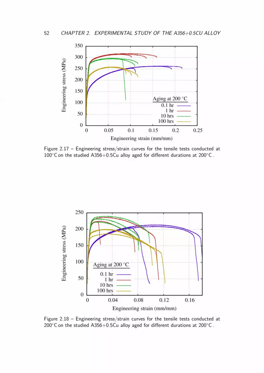
52 CHAPTER 2. EXPERIMENTAL STUDY OF THE A356+0.5CU ALLOY
100 hrs10 hrs
1 hr0.1 hr
Aging at 200 C
Engineering strain (mm/mm)
Eng
inee
ring
stre
ss(M
Pa)
0.250.20.150.10.050
350
300
250
200
150
100
50
0
Figure 2.17 – Engineering stress/strain curves for the tensile tests conducted at100Con the studied A356+0.5Cu alloy aged for different durations at 200C .
100 hrs10 hrs
1 hr0.1 hr
Aging at 200 C
Engineering strain (mm/mm)
Eng
inee
ring
stre
ss(M
Pa)
0.160.120.080.040
250
200
150
100
50
0
Figure 2.18 – Engineering stress/strain curves for the tensile tests conducted at200Con the studied A356+0.5Cu alloy aged for different durations at 200C .

2.5. CONCLUSION 53
200 C100 C
Room Temperature
Test temperature
Aging duration (hr)
Rp0
.2(M
Pa)
1001010.1
300
250
200
150
100
50
0
Figure 2.19 – Evolution of the measured 0.2 % offset proof yield stress for thestudied A356+Cu alloy as a function of aging duration at 200C for each testtemperature.
2.5 ConclusionThe studied alloy of type A356+0.5Cu was characterized using transmission
electron microscopy and tensile testing. This experimental study was conductedon this alloy subject to a solutionizing, quenching and aging heat treatment ofdifferent durations at 200C .
The objectives of the microstructural study were to investigate the precipitationsequence taking place and obtain statistically valid size distributions of precipitates.In summary the conclusions of this study are:
1. Homogeneously distributed precipitates in samples aged 0.1, 1 and 10 hrs at200Cwere characterized as rod-shaped β′′ by comparing experimental andsimulated SAD patterns.
2. Samples aged for 10 hrs were characterized by the coexistence of these rod-shaped β′′ with lath-shaped Q′ or Q′′ precipitates in significantly fewer num-bers.
3. When observed along a 〈100〉α zone axis, the β′′ precipitates appear alignedalong the 〈100〉Al directions. The ones aligned along the viewing directionare visible due to their round cross-sections. The others are visible edge-ondue to the elongated strain field around them.
4. Samples aged for 0.1 hr contained very small precipitates, therefore the strainfield around them is very small. This provided a contrast that is too low to

54 CHAPTER 2. EXPERIMENTAL STUDY OF THE A356+0.5CU ALLOY
allow them to be visible edge-on.
5. Quantitative measurement of precipitate size distributions of rod-shaped β′′in terms of diameter and length was conducted for samples aged for 0.1, 1and 10 hrs with the exception of length for samples aged for 0.1 hr.
6. Samples aged 100 hrs at 200Cpresented a complex microstructure with bothfine and coarse precipitates. The predominant homogeneously distributedfine precipitates have the characteristics of the Q′ phase, i.e. a rectangularcross-section with habit plane 10 to 12 away from 〈100〉α. Q′′ precipitateswith rectangular cross-sections with habit plane 〈100〉α are also observed infewer numbers. Coarse precipitates with various shapes were recognized asthe Si phase.
7. Very few β′′ (possibly β′) precipitates are observable in samples aged for 100hrs.
8. Some heterogeneous precipitation could also be observed in sample aged for100 hrs.
9. Quantitative measurement of precipitate size distribution of lath-shaped Q′and Q′′ in terms of length, thickness and width was conducted for this sample.
In addition to microstructural investigation, tensile tests were conducted forthe same aging conditions at room temperature, 100Cand 200C . The value ofyield stress was the mechanical property of interest and it was measured for eachcondition. The alloy showed a well expected behavior with measured yield stressesstarting at relatively low values for samples aged for 0.1 hr, going up to a peakbetween the cases aged for 1 and 10 hrs and then continuing the decrease for thecase aged for 100 hrs.
In the next chapters the precipitation kinetics and yield stress models will bepresented and they will be confronted to the results of this experimental study.These results will be used to validate and calibrate the parameter values of themodel.

Chapter 3
Precipitation kinetics model
RésuméLa cinétique de précipitation de la phase β′′-Mg2Si a été modélisée en utilisant
une approche théorique. Il s’agit d’une approche basée sur la théorie classique de lagermination et croissance et la méthode KWN (Kampmann-Wagner-Numerical).
Dans ce chapitre, les équations gouvernant ce modèle sont présentées etdéveloppées en explicitant les hypothèses et les simplifications adoptées. Les in-stances de couplage indirect avec le logiciel Thermo-Calc sont également décrites.La méthode de résolution numérique est ensuite détaillée.
Le modèle a été validé et calibré en comparant les distributions de tailles desprécipités simulées aux résultats expérimentaux du chapitre 2. La confrontationdu modèle à ces résultats expérimentaux est présentée. Les variables cinétiquescalculées par le modèle sont présentées et décrites.
55

56 CHAPTER 3. PRECIPITATION KINETICS MODEL
Precipitation kinetics models usually consist in describing three major processes:nucleation, growth and coarsening. In this chapter, each one of these processes willbe presented as well as its governing equations. The hypotheses and assumptionswill be discussed and the resulting choices will be determined.
It is worth recalling that the final aim of this work is engineering scale calcu-lations using the finite element method. It is therefore important that calculationcosts be kept as minimal as possible while keeping an acceptable level of represen-tativeness of physical phenomena.
Three major approaches to modelling precipitation kinetics can be found inliterature: phase field, molecular dynamics and particle size distribution models.For the purposes of this study, the calculation cost of the first two is not viable.Therefore, the modelling effort pursued a size distribution based model.
The input variables to the precipitation kinetics model are the thermal historyand certain thermodynamic quantities such as the driving force for precipitation,equilibrium concentrations and others. The values of these variables for the com-position of the studied A356+0.5Cu alloy were accessed through indirect couplingwith the Thermo-Calc software equipped with the TCAL5 database.
The model uses a number of physical parameters such as the diffusivities ofchemical elements. With the exception of the precipitate/matrix interfacial energy,the values for all these parameters are drawn from literature. The value chosen forthe interfacial energy was determined so as to provide the best possible fit to theexperimental values.
All output variables pertaining to the kinetics of precipitation are made avail-able by the model. Precipitate size distributions, volume fractions and soluteconcentrations are subsequently utilized in the yield stress model.
3.1 NucleationThe approaches used to model precipitate nucleation in literature are based on
classical nucleation theory in almost every case. It starts out by the expression ofthe free energy variation resulting from the precipitation of a β phase from a ho-mogeneous supersaturated α′ phase (Figure 3.1a). This variation ∆G is expressedusing equation 3.1 which splits into two terms: a volume term and a surface term:
∆G = ∆gvV + γS. (3.1)
The volume term consists of the volumetric chemical driving force for precipita-tion ∆gv and the volume V of the precipitating β phase. The surface term consistsof γ, the α/β interfacial energy, and the surface S of this interface. These termsare in competition with one another, as the former is a negative contribution (su-persaturation) and the latter a positive one (creation of an interface). Figure 3.1bshows a plot of ∆G with respect to the radius of the precipitate where these effectscan be observed. Therefore, sufficient chemical driving force and size are necessaryfor the overall free energy variation to be negative. A negative energy variation

3.1. NUCLEATION 57
α′
α
β
(a) (b)
Figure 3.1 – Nucleation of a particle of the β phase in an α matrix: (a) Schematicof the α′ → α + β transformation and (b) Plot of the corresponding variation inthe Gibbs free energy with respect to the radius of the precipitate.
implies that the transformation can occur and that the nucleus remains stable inequilibrium with the parent phase. It is important to note that equation 3.1 cangenerally have a third term accounting for elastic strain energy. In this work thiscontribution is considered negligible and is therefore omitted.
In order to express the critical size of nuclei, i.e. the size at which further growthminimizes the free energy must be determined. The critical size is therefore theroot of the derivative of ∆G with respect to size. If one assumes a spherical shapeof the β phase with a radius R, the critical radius for nucleation R∗ is expressedwith equation 3.2:
R? = −2γ∆gv
. (3.2)
The energy barrier ∆G∗, i.e. the free energy corresponding to a critical nucleus,can therefore be expressed using equation 3.3:
∆G? = 16πγ3
3∆g2v
. (3.3)
The number of stable nuclei that are added to the system at any given time isthe nucleation rate J . This nucleation rate is given by equation 3.4 [69, 70]:
J = Zβ?N exp(−∆G?
kBT
)exp
(−τt
)(3.4)
with kB being the Boltzmann constant and T the temperature.It is best viewed as the product of three factors. First, there is N exp
(−∆G?
kBT
)which expresses the total number of nucleation sites which may have critical nucleigrown around them. It consists of the temperature dependent energy barrier termon the one hand. On the other hand, we find N which is the nucleation site

58 CHAPTER 3. PRECIPITATION KINETICS MODEL
density in the matrix. If one assumes a homogeneous nucleation, i.e. the absenceof preferential nucleation sites within the matrix, it can be expressed by equation3.5. It simply considers that any atomic site in the crystal can be a potentialnucleation site for the precipitating phase:
N = NAV α
(3.5)
with NA being the Avogadro number and V α the molar volume of the matrix.In the case of heterogeneous nucleation, an additional heterogeneous nucelation
rate can be expressed with a number of nucleation sites depending on the nature ofthe heterogeneity (grain boundaries, inclusions, etc..). The term S(θ) in equation3.6:
∆G?,het = ∆G?S(θ) (3.6)
with θ being the wetting angle of the interface, is always smaller than 1 [71].This expresses how heterogeneous nucleation has a lower energy barrier in com-parison to homogeneous nucleation (Figure 3.2). This is due to the lowering ofthe positive surface term due to the pre-existence of an interface. In this work, inview of the homogeneous nature of the observed precipitation in the studied alloy,heterogeneous nucleation will be neglected.
Figure 3.2 – The difference in energy barriers for homogeneous and heterogeneousnucleation [71].
The second factor Zβ? in equation 3.4 concerns the stochastic aspect of nu-cleation. Nuclei that are exactly at the energy barrier for nucleation are at an

3.1. NUCLEATION 59
unstable equilibrium, they can either dissolve or grow. The Zeldovitch factor Z(equation 3.7) expresses the probability that such nuclei have of growing:
Z = V α∆g2v
8π(γ3kBT )1/2 . (3.7)
The condensation rate β? (equation 3.8) expresses the rate at which“monomers” of the precipitating phase attach to the growing nuclei:
β? = 16πγ2DC
∆g2va
4 (3.8)
with D being the diffusivity, C the mean solute molar fraction in the matrix anda the lattice parameter of the matrix.
The third and last factor, exp (−τ/t), where t is time, is an incubation functionthat accounts for the thermal inertia of the nucleation process. The incubationperiod τ expresses the time necessary for the system to begin the transformation(equation 3.9):
τ = 8kBTγa4
V α∆G2VDC
. (3.9)
In fact, time as such is not a relevant variable in a constitutive equation. It canonly appear by integrating an evolution equation along a particular path [72]. It iswell understood, for example, that interrupting a test for a longer or shorter periodof time should not change the result if this period is under conditions where thematerial does not evolve. A rigorous approach to taking incubation into accountwould be to introduce a specific variable with its own law of evolution, to beintegrated as a function of temperature history. In our work, back-to-back heattreatment transient sequences of quenching and aging will be simulated. Insertingtime explicitely in such an incubation function is therefore inconsistent as thephase transformation may occur in stages. Nevertheless simulations were carriedout with and without this term and hardly any difference could be noticed. It wasthen decided to omit this incubation term in the final simulation.
One can see, the evaluation of these equations requires knowledge of the val-ues of the volumetric precipitation driving force ∆gv. Thermo-Calc allows thecalculation of ∆gm, the molar precipitation driving force of a phase for any alloycomposition. It depends on temperature and the molar concentration of solute inthe matrix. This value is then normalized using the molar volume of the precipitat-ing phase in order to obtain the volumetric driving force ∆gv. Note that althoughthe precipitates were identified as the β′′ phase, the precipitation sequence will becollapsed into the equilibrium phase β for simplification. Thermodynamic data inTCAL5 is also far more reliable for stable phases than it is for metastable phases.
The model is given access to these values through indirect coupling. First, thevalues of the precipitation driving force of β-Mg2Si as a function of temperature andsolute content in the matrix are tabulated. Multiple calculations were performedin order to span a wide range of compositions and temperatures. Subsequently,

60 CHAPTER 3. PRECIPITATION KINETICS MODEL
0.0015 0.002
0.0025 0.003
0.0035 0.004 -14
-11
-8
-5
-3e+09
-2e+09
-1e+09
0
1e+09
Δgv(J/m3)
TCAL5 dataFit function
1/T(K)
log(Mgα)
Δgv(J/m3)
Figure 3.3 – Fit function of the precipitation driving force of β-Mg2Si in the alu-minum matrix extracted from Thermo-Calc/TCAL5.
all the results were mapped using a Taylor series fit function resulting in a simpleequation which was implemented in the model (Figure 3.3). This numerical fitfunction is given by equation 3.10 with x and y representing the temperatureinverse, 1/T (K), and the logarithm of the molar fraction of Mg in the matrix,log(Cα
Mg), respectively.
f(x, y) = ax−1 + by + cx−2 + dy2 + eyx−1 + f
a = −3.65× 10⁴ Jm−3K−1
b = −1.03× 10⁷ Jm−3
c = −4.45× 10² Jm−3K−2
d = −2.98× 10⁴ Jm−3
e = 4.46× 10⁵ Jm−3K−1
f = 2.04× 10⁹ Jm−3
(3.10)
This indirect coupling scheme is costless to compute, contrary to direct couplingto Thermo-Calc which would induce large calculation costs rendering it imprac-tical. Also, the process leading up to the determination of the indirect couplingfit equation was scripted and is straight forward. A commented example of aThermo-Calc macro can be found in Appendix B.
3.2 Growth
3.2.1 The growth rateA stable supercritical nucleus (R > R?) is capable of growing into increasingly
larger sizes. It is therefore important to express the rate at which growth occurs.

3.2. GROWTH 61
The growth rate is expressed with respect to the radius R of precipitates which areassumed to be spherical. The corrections necessary to take into account the realmorphology of precipitates will be addressed later on. At the atomic scale, growthis controlled by diffusion as atoms migrate to the precipitate/matrix interface. Thisprocess can therefore be described using Fick’s laws [73]. The first law allows theexpression of the diffusive flux Ji of solute element i as a function of the gradientof concentration Ci assuming an ideal solution (equation 3.11):
Ji = −Di.∇Ci. (3.11)
Fick’s second law expresses how diffusive flux of atoms changes the concentra-tion profile with respect to time. Assuming that the diffusivity is independent ofcoordinates, it can be written as equation 3.12:
∂Ci∂t
= Di∆Ci. (3.12)
In spherical coordinates, assuming steady-state (∂Ci/∂t = 0) and recalling thatthe concentration profile depends exclusively on the radius r (Ci(r, θ, φ) = Ci(r)),this law leads to a Cauchy ordinary differential equation 3.13:
∂2Ci∂r2 + 2
r
∂Ci∂r
= 0. (3.13)
The solution to such an equation takes the form given by equation 3.14 witha and b being constants to be determined using boundary conditions:
Ci(r) = a+ b
r. (3.14)
Setting:
- C∞i : concentration of element i in the matrix far from the interface;
- Cα/βi : concentration of element i in the matrix at the interface;
- Cβ/αi : concentration of element i in the precipitate at the interface. As-
suming a stoechiometric precipitate and no diffusion in the precipitate, thiswill be considered a constant Cβ
i .
We can formulate the following boundary conditions:
- Ci(r →∞, t) = C∞i ;
- Ci(r = R(t), t) = Cαi , R(t) being the radius of the precipitate at time t;
- Ci(r < R(t), t) = Cβi .

62 CHAPTER 3. PRECIPITATION KINETICS MODEL
This yields the expression of the concentration profile as a function of thedistance from the center of the spherical precipitate:
Ci(r) = C∞i + R(t)r
(Cα/βi − C∞i ) , r > R(t), (3.15)
Ci(r) = Cβi , 0 6 r < R(t). (3.16)
The total flux through the interface I in dt is responsible for the volume changedV of the particle according to equation 3.17 expressing mass conservation:
Idt = (Cα/βi − Cβ
i )dV (3.17)
with dV = 4πR(t)2dR(t). The total flux I is simply calculated by integrating theflux over the interface surface oriented along its normal (equation 3.18):
I =∫∫
int−Di
∂Ci(r)∂n
dS. (3.18)
Using equation 3.16 and considering the surface element dS of which thenormal is radial and oriented to the exterior, equation 3.19 is obtained:
I = 4πD(Cα/βi − C∞i )R(t). (3.19)
Finally, combining equations 3.17 and 3.19 leads to the growth rate expressionthat is widely used in literature (equation 3.20):
dR(t)dt
= D
R(t)(C∞i − C
α/βi )
(Cβi − C
α/βi )
. (3.20)
When modelling the precipitation of a phase where there is only one diffusingchemical element, equation 3.20 is sufficient. This was exemplified in the work ofMartinez et al. [13] where coarsening of θ-Al2Cu precipitates was modelled. Indeed,only the diffusion of Cu is to be considered when calculating the growth rate ofthese precipitates. Therefore, there is a single possible equilibrium concentrationof Cu in the matrix at any given temperature.
However, when two chemical elements must diffuse within the aluminum matrixin order to form the precipitate, other considerations apply. This is the case forthe β-Mg2Si around which this work is centered. While the growth rate equationis still valid for each one of the two elements participating in the formation of theprecipitate, there is a number of sets of possible equilibrium concentrations of Mgand Si in the matrix at any given temperature. This requires the addition of athermodynamic and a kinetic constraint to fully define the growth rate.
The thermodynamic constraint consist of the tie-line equations in the Al-Si-Mgdiagram expressing the equilibrium between α-Al and β-Mg2Si. Tie-lines calculatedusing Thermo-Calc are shown in Figure 3.4a for temperatures ranging from 273.15to 723.15 K. The solubility product Ks for the β-Mg2Si is expressed according

3.2. GROWTH 63
to equation 3.21 as a function of mole fractions of Mg and Si in the matrix atequilibrium, Cα,eq
Mg and Cα,eqSi respectively:
Ks = (Cα,eqMg )2.Cα,eq
Si . (3.21)
Plotting log(Ks) against the temperature inverse collapses these tie-lines intoone straight line that can be fitted with a simple linear function (Figure 3.4b).The obtained fit equation (equation 3.22) expresses the thermodynamic constraintthat the equilibrium concentrations must respect:
log(Ks) = −7144T
+ 2.7. (3.22)
The kinetic constraint consists of ensuring that solute flux is respective ofthe difference in diffusivities between Mg and Si and of the stœchiometry of theprecipitating phase. Therefore, the growth rate expressed by equation 3.20 mustbe the same whether it be calculated using the Mg or Si supersaturations (equation3.23):
dR(t)dt
= DMg
R(t)(C∞Mg − C
α/βMg )
(CβMg − C
α/βMg )
= DSi
R(t)(C∞Si − C
α/βSi )
(CβSi − C
α/βSi )
, (3.23)
where DMg and DSi are the diffusivities of Mg and Si respectively.One of the adopted simplifications used in this work is the collapse of the
precipitation sequence into a single equivalent phase considered to be β-Mg2Si.The metastable precursors to this phase are therefore not considered and all thepreviously mentioned thermodynamic data are extracted for the stable phase. Thissimplification was used in the pioneering implementations of precipitation mod-elling by Myhr et al. [74, 75], Deschamps et al. [76] and Bréchet et al. [77]. Also,this phase is considered stœchiometric which defines the interfacial concentrationson the precipitate side Cβ
Si and CβMg (0.334 and 0.666 respectively). The concen-
trations far from the interface C∞Mg and C∞Si , can be considered as the mean soluteconcentrations in the matrix at any given time step. Therefore, the unknowns re-maining to evaluate the growth rate are the matrix interfacial concentrations Cα/β
Si
and Cα/βMg .
3.2.2 Interfacial compositionsIn the case of a curved interface α/β, the equilibrium between the two phases
is modified due to capillarity effects, the so called Gibbs-Thomson effect. Whenassuming a local equilibrium modified by the Gibbs-Thomson effect, the interfacialcompositions are the equilibrium compositions corrected for curvature. Indeed,the solute concentrations in the matrix near the α/β interface and far from it aredifferent. The classical expression that is used in modelling precipitation kineticsis given in equation 3.24:

64 CHAPTER 3. PRECIPITATION KINETICS MODEL
β
Si
α
723.15 K
673.15 K
623.15 K
573.15 K
523.15 K
473.15 K423.15 K373.15 K
323.15 K
273.15 K
Log(Cα,eqMg )
Log
(Cα,
eqSi
)
0-1-2-3-4-5-6-7-8
-2-3-4-5-6-7-8-9
-10-11-12
(a)
Fit functionThermoCalc data
Log(Ks) =−7144
T+2.7
1/T (K−1)
Log(
Ks)
0.0040.00350.0030.00250.0020.00150.001
-6
-8
-10
-12
-14
-16
-18
-20
-22
-24
(b)
Figure 3.4 – Determination of the solubility product for β-Mg2Si using Thermo-Calc/TCAL5: (a) Mg and Si concentrations in the matrix for different temperaturesrepresenting the phase diagram tie-lines and (b) logarithm of the solubility productKs as a function of the temperature inverse with the corresponding fit functionimplemented in the model.
Cα/βi,R = C
α/βi,R=∞. exp
(2.γ.V β
R.kB.T
), (3.24)

3.2. GROWTH 65
with Cαi,R=∞ the concentration of solute i in the matrix for an infinite curvature
(planar interface), V β the molar volume of the precipitation β phase and R theprecipitate radius.
Although this expression is commonly used, it is worth noting that it is obtainedby using an approximation that does not always apply. Perez [78] showed how thatsolution of the Gibbs-Thomson equation is obtained under the assumption of a pureprecipitating phase (i.e. Cβ
i =1). In his publication the author also showed thatthere are other approximations that may be used to solve the Gibbs-Thomsonequation.
Under the assumption of a low curvature effect, i.e. Cα/βi,R ' C
α/βi,R=∞, there is
a different solution given by equation 3.25:
Cα/βi,R = C
α/βi,R=∞.
1 + 2.γ.V β
R.kB.T
1− Cα/βi,R=∞
Cβi − C
α/βi,R=∞
. (3.25)
Finally, by assuming a dilute solid solution whereby Cα/βi,R and Cα/β
i,R=∞ are smallcompared to unity, a third solution given by equation 3.26 is provided:
Cα/βi,R = C
α/βi,R=∞. exp
(2.γ.V β
Cβi .R.kB.T
). (3.26)
In this work, this expression of the Gibbs-Thomson effect was used as it is themost coherent with the modelled precipitates. It is noteworthy that setting if Cβ
i
= 1 in equations 3.26 and 3.25, the former becomes exactly equation 3.24 and thelatter becomes its first order Taylor expansion.
Du et al. [79] used a different approach to evaluate the effect of curvatureon interfacial equilibrium concentrations. It consisted in constructing what theyreferred to as a “Gibbs-Thomson phase diagram” using Thermo-Calc. It is obtainedby increasing the Gibbs free energy of the precipitating phase in the databaseby 2γκVm, with κ being the curvature and Vm the precipitate molar volume.The in-built energy minimization algorithm of Thermo-Calc then produces a newphase diagram taking into account curvature. Of course, this calculation is thenperformed for the whole range of curvature values to produce the full curvature-dependent diagram. The model then uses a table look-up technique to navigatethe diagram and access the required values.
Another approach was demonstrated in [80] where the authors numerically in-tegrated the differential form of the curvature-modified equilibrium condition of amulticomponent system. With knowledge of Gibbs energies of the matrix and theprecipitating phase, they numerically integrated the tie-line equations with incre-ments of curvature. Figure 3.5 demonstrates how the integration method producesresults that are consistent with the Gibbs-Thomson phase diagram method calcu-lated using Thermo-Calc.

66 CHAPTER 3. PRECIPITATION KINETICS MODEL
Figure 3.5 – Gibbs–Thomson phase diagram (surface showing matrix solute contentvs. curvature) of the Al–Mn–Si system at 600C calculated by the integrationmethod together with the solubility limit lines (markers) for various curvaturescalculated by Thermo-Calc [80].
3.2.3 Mean matrix compositionIn the model, the solute concentrations in the matrix far from the interface
C∞Mg and C∞Si are considered to be the mean matrix concentrations. The initialmean composition of the matrix is considered to be the equilibrium composition atthe solutionizing temperature. As the volume fraction of the precipitating phaseincreases, this mean composition must be updated. To update these values, themass balance equation 3.27 is used:
Cαi = C0
i − fβ.Cβi
1− fβ , (3.27)
with Cαi being the mean concentration in the matrix of solute i, C0
i its initialconcentration, Cβ
i its concentration in the precipitate and fβ the molar fractionof the β phase.
Figure 3.6 shows the evolution of the equilibrium concentrations of Mg and Siin the matrix with respect to temperature according to a Thermo-Calc calculationusing TCAL5 for the studied A356+0.5Cu alloy. The Mg content in the aluminummatrix is almost constant for temperatures above the solvus of β-Mg2Si. Theobserved decrease in Mg content below this solvus temperature is entirely dueto the formation of the β-Mg2Si. Therefore, since solutionizing temperatures arealways higher than the solvus temperature, C0
Mg is considered constant.The same cannot be said about Si because it contributes in the formation of

3.2. GROWTH 67
the Si phase alongside β-Mg2Si. This is shown in Figure 3.7 where the yellowcurve represents the equilibrium Si concentration in the matrix and the red curvethe equilibrium molar fraction of the Si phase. Therefore, the amount of Si thatis available to contribute in the formation of β-Mg2Si is not a constant. The bluecurve was obtained by eliminating the amount of Si that goes into the formationof the Si phase. This curve represents C0
Si which in this case is temperature-dependent. It was fitted and implemented in the model as such. It is worth notingthat this implies that the model considers that the Si phase forms and the matrixis depleted from Si instantaneously.
SiMg
β-M
g 2Si
solv
us
Temperature (C )
Mol
arfr
actio
nof
solu
tein
α-A
l
6005004003002001000
0.014
0.012
0.01
0.008
0.006
0.004
0.002
0
Figure 3.6 – Evolution of the equilibrium molar fraction of Mg and Si in thematrix with respect to temperature calculated using Thermo-Calc/TCAL5 for theA356+0.5Cu alloy.
3.2.4 Effect of precipitate morphologyAs seen in the chapter 2, all observations of the β′′-Mg2Si phase indicate an
elongated morphology (cf. Figure 2.7). This may lead to a breakdown in the resultsof the model when the aspect ratio of the precipitates becomes significantly large.However, the model as described so far is based on the assumption of a sphericalmorphology for the precipitating phase. Taking into account morphology has beenaddressed in literature in two different ways.
Considering a rod-shaped precipitate as given in Figure 3.8, the aspect ratiowill be given by equation 3.28:
λ = l
2.R (3.28)
with l and R being the length and radius of the precipitate respectively.The nucleation and growth theoretical equations can all be rewritten as a
function of λ and one of the dimensions (either l or R). This adds an unknown tothe problem and therefore requires the description of the evolution of the aspect

68 CHAPTER 3. PRECIPITATION KINETICS MODEL
fSi
EquilibriumAvailable to form β-Mg2Si
β-M
g 2Si
solv
us
Temperature (C )
Mol
arfr
actio
nof
the
Siph
ase,
f Si
Mol
arfr
actio
nof
Siin
α-A
l
0.01
0.008
0.006
0.004
0.002
06005004003002001000
0.016
0.014
0.012
0.01
0.008
0.006
0.004
0.002
0
Figure 3.7 – Concentration of Si available to form β-Mg2Si (blue curve) withrespect to temperature, obtained using the equilibrium concentration of Si (yellowcurve) and the molar fraction of the Si phase (red curve), calculated using Thermo-Calc/TCAL5.
ratio. It is for example possible to experimentally define a time-dependent functionλ(t) for a given isothermal heat treatment and implement it in the model. This ofcourse limits the non-isothermal capacity of the model.
Another possibility was exemplified by Bardel et al. [8] in their precipitationmodel for non-isothermal treatments of a 6061 aluminum alloy. According to theirexperimental findings using small angle neutron scattering (SANS) for a wide rangeof temperatures, the aspect ratio remained relatively close to an average value of11. Therefore, as a model simplification, they used a constant value for the aspectratio λ = 11. The same approach was used by Chen et al. [10] in modellingprecipitation in an Al-7Si-Mg alloy. In their work they measured the average radiiand lengths for a set of aging conditions using TEM imagery and calculated anaverage aspect ratio of 7.
Figure 3.8 – Schematic of the elongated morphology of the β′′-Mg2Si precipitates.
The second approach consists in introducing analytically derived correctionsto the growth rate (f in equation 3.29 ) and the Gibbs-Thomson effect (g inequation 3.30):
dR
dt= f
D
R(t)(C∞i − C
α/βi )
(Cβi − C
α/βi )
, (3.29)

3.2. GROWTH 69
Cα/βi,R = C
α/βi,R=∞. exp
(2.g.γ.V β
Cβi .R.kB.T
). (3.30)
Holmedal et al. [81] introduced a generalization of the Kampmann-Wagnernumerical (KWN) method to non-spherical precipitates. The shape of a prolatespheroid can be considered a good approximation of the rod morphology of theprecipitates (Figure 3.9a). Therefore, in order to calculate the correction factorf they developed an analytical solution to the diffusion problem in the prolatespheroidal coordinates (ξ,η,φ). In this coordinate system, they derived the soluteconcentration profile by assuming it dependent only on ξ. Indeed, surfaces of aconstant ξ form prolate spheroids and outward growth is represented by increases ofthis coordinate. Using that compositional profile they calculated the flux of solutethrough a prolate spheroidal interface according to Fick’s law. By equating this fluxto the flux through a volume-equivalent spherical interface mediating the correctionfactor f , an analytical expression for the latter was determined (equation 3.31):
f(λ) = 2√λ2 − 1
3√λln(2λ2 + 2λ
√λ2 − 1− 1)
. (3.31)
They also used the same approach for a needle-shaped cuboid (Figure 3.9b). Inthis case, although an analytical compositional profile can be expressed, calculatingthe flux through the surface had to be performed numerically. A different expressionfor the correction factor f was therefore derived (equation 3.32):
f(λ) = 0.1 exp(−0.091(λ− 1)) + 1.736√λ2 − 1
3√λln(2λ2 + 2λ
√λ2 − 1− 1)
. (3.32)
Both these factors degenerate to a value of 1 for spheres, i.e. λ= 1. Figure 3.10shows the evolution of these factors as a function of the aspect ratio. It shows howthere is a positive influence of the aspect ratio on the growth rate, i.e. as a particleelongates, it grows faster. The authors reported that this is in contradiction withthe results of the approach used by Bardel et al. and other studies they examinedwhere the influence is negative.
The second correction factor g, is obtained under the assumption of shapeconservation and quasi-constant evolution of the aspect ratio. The first assumptionmeans that the surface of the particle is related to its volume. The Gibbs-Thomsonmodified chemical potential of a given alloying element in the precipitating phasecan be written according to equation 3.33:
∂Gβ
∂nβ= µβm + γ.
∂Sβ
∂nβ(3.33)
with Sβ being the particle surface, nβ the number of atoms in the particle, µβm thechemical potential and γ the surface energy.

70 CHAPTER 3. PRECIPITATION KINETICS MODEL
(a) (b)
Figure 3.9 – Drawing of analytical shapes approximating the rod shaped β′′-Mg2Siprecipitates: (a) Prolate spheroid characterized by c>a and (b) Needle-shapedcuboid.
CuboidProlate spheroid
λ =L
2R
Aspect ratio, λ
Cor
rect
ion
fact
or,f
403530252015105
3.5
3
2.5
2
1.5
1
0.5
0
Figure 3.10 – Correction factor f [81], for different precipitate morphologies as afunction of the aspect ratio λ.
Using V β = nβ.V βm equation 3.34 can be obtained. The correction factor g
can therefore be obtained by equating the previous equation to its expression fora volume-equivalent sphere:
∂Gβ
∂nβ= µβm + γ.
∂Sβ
∂V βV βm = µβm + 2.g.γ.V β
m
R. (3.34)
The correction factor g is then scaled so as to degenerate to a value of 1 forspheres (λ=1) and is therefore given by equation 3.35:
g = 12R
∂Sβ
∂V β= 1
8πR.∂Sβ
∂R. (3.35)
Applying this equation to a prolate spheroid and a needle-shaped cuboid rendersequations 3.36 and 3.37 respectively. Figure 3.11 shows the evolution of thesefactors as a function of the aspect ratio:

3.2. GROWTH 71
g(λ) = 12λ2/3
(1 + λ2√λ2 − 1
sin−1(√
λ2 − 1λ
)), (3.36)
g(λ) = 2λ+ 12π
(4π3λ
)2/3. (3.37)
CuboidProlate spheroid
λ =L
2R
Aspect ratio, λ
Cor
rect
ion
fact
or,g
403530252015105
3.5
3
2.5
2
1.5
1
0.5
0
Figure 3.11 – Correction factor g [81], for different precipitate morphologies as afunction of the aspect ratio λ.
All these corrections depend on the aspect ratio and therefore the same limi-tation discussed for the previous approach applies here. It is necessary to have adescription of the evolution of the aspect ratio or treat is as a constant.
A subsequent paper by Du et al. [82] used this generalization to simulatean isothermal aging heat treatments of an Al-Mg-Si alloy. They performed threekinds of simulations : using the spherical assumption, using the corrections witha constant aspect ratio of 8 and using the corrections with a varying aspect ratio.Generally, they found that the introduction of the correction factors improvedthe agreement of the model with their TEM observations. It especially dealtwell with the onset of ripening after long durations of aging. Regarding the sizedistributions, the correction factors produce wider distributions compared to theclassical spherical case. Varying aspect ratio produces a faster evolution of themean radius in comparison to the constant aspect ratio case. This effect wasparticularly significant for long exposure durations.
Introducing both corrections to the model results in a size-dependent competi-tion between the diffusion acceleration and the suppression of the supersaturationby the modified Gibbs-Thomson effect. Figure 3.12 presents the growth rate nor-malized by the growth rate for a spherical particle as a function of the aspectratio for different equivalent particle sizes. It shows that for a small particle size,the attenuation of the supersaturation by the modified Gibbs-Thomson effect hasmore weight than the accelerated diffusion. There is therefore an overall negativeinfluence of the aspect ratio on the growth rate in comparison to the spherical
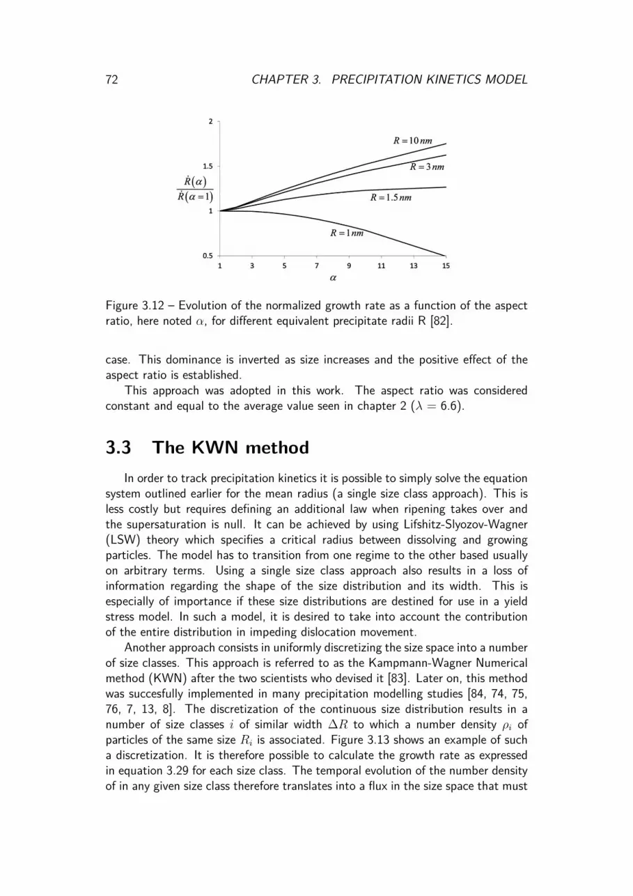
72 CHAPTER 3. PRECIPITATION KINETICS MODEL
Figure 3.12 – Evolution of the normalized growth rate as a function of the aspectratio, here noted α, for different equivalent precipitate radii R [82].
case. This dominance is inverted as size increases and the positive effect of theaspect ratio is established.
This approach was adopted in this work. The aspect ratio was consideredconstant and equal to the average value seen in chapter 2 (λ = 6.6).
3.3 The KWN methodIn order to track precipitation kinetics it is possible to simply solve the equation
system outlined earlier for the mean radius (a single size class approach). This isless costly but requires defining an additional law when ripening takes over andthe supersaturation is null. It can be achieved by using Lifshitz-Slyozov-Wagner(LSW) theory which specifies a critical radius between dissolving and growingparticles. The model has to transition from one regime to the other based usuallyon arbitrary terms. Using a single size class approach also results in a loss ofinformation regarding the shape of the size distribution and its width. This isespecially of importance if these size distributions are destined for use in a yieldstress model. In such a model, it is desired to take into account the contributionof the entire distribution in impeding dislocation movement.
Another approach consists in uniformly discretizing the size space into a numberof size classes. This approach is referred to as the Kampmann-Wagner Numericalmethod (KWN) after the two scientists who devised it [83]. Later on, this methodwas succesfully implemented in many precipitation modelling studies [84, 74, 75,76, 7, 13, 8]. The discretization of the continuous size distribution results in anumber of size classes i of similar width ∆R to which a number density ρi ofparticles of the same size Ri is associated. Figure 3.13 shows an example of sucha discretization. It is therefore possible to calculate the growth rate as expressedin equation 3.29 for each size class. The temporal evolution of the number densityof in any given size class therefore translates into a flux in the size space that must

3.3. THE KWN METHOD 73
Figure 3.13 – Schematic of the discretization of the continuous size distribution[7].
be defined.At any given time step, the mass in the system is regulated by equation 3.38:
dρ(R)dt
= −dFdR
(3.38)
with ρ(R) being the number density of particles of radius R and F the particleflux in the size space.
The flux F can therefore be expressed as ρ(R).vt(R), with vt(R) is the rate ofevolution for particles of size R. This rewrites equation 3.38 as:
dρ(R)dt
= −d(ρ(R).vt(R))dR
. (3.39)
Using the aforementioned discretization of the size space and by applying afinite differences scheme, equation 3.40 can be written:
ρt+∆t(R)− ρt(R)∆t = −
[ρ(R + ∆R).vt(R + ∆R)− ρ(R).vt(R)
∆R
]θ
. (3.40)
To ensure that the integration is stable and its convergence is not dependenton the value of the time step, a Euler implicit scheme is used (θ = t+ ∆t) and itis given by equation 3.41:
ρt+∆t(R)− ρt(R)∆t = −
[ρt+∆t(R + ∆R).vt(R + ∆R)− ρt+∆t(R).vt(R)
∆R
].
(3.41)This is simplified as follows:

74 CHAPTER 3. PRECIPITATION KINETICS MODEL
Figure 3.14 – Schematic of the particle flux management in the size space betweensize classes R−∆R and R + ∆R [13].
(a) (b)
Figure 3.15 – Schematic of the particle flux management in the size space for theboundary cases: (a) The smallest size class of size Rmin and (b) The biggest sizeclass of size Rmax [13].
ρt+∆t(R). [P ] = ρt+∆t(R−∆R). [G]+ρt+∆t(R+∆R) [D]+ρt(R).[P 0], (3.42)
with [P ], [G], [D], and [P 0] being computation parameters. It is important tonote at this point that each size class R exists in between two size classes R−∆Rand R + ∆R. There is however two boundary cases at the extremities wherethe smallest and biggest size classes, Rmin and Rmax respectively, have only oneneighboring size class.
For size classes within ]Rmin, Rmax[ there are four flux management possibil-ities as displayed in Figure 3.14. The corresponding computation parameters areobtained by appreciating the direction of the fluxes in the size class and its neigh-bours. A summary of the resulting parameters for each case is given in Table 3.1.
For the boundary cases Rmin and Rmax (represented in Figure 3.15a and 3.15brespectively), the finite differences scheme must be decentered on R + ∆R andR − ∆R respectively. The same treatment for non centered schemes as the onepresented in Table 3.1 is therefore used for these cases.
In order to solve equation 3.42 and obtain ρt+∆t(R) for each size class, thisequation is written in matrix form. Using the following notations:

3.3. THE KWN METHOD 75
Table 3.1 – Values of the parameters C, L, R and C0 of equation 3.42 as afunction of the directions of the fluxes for the particules in ]Rmin : Rmax[ [13].
Direction Direction Direction Finite P G D P 0
of flux in of flux in of flux in differencesR−∆R R R + ∆R schemepositive positive - decentered ∆R
∆t + vt(R) vt(R−∆R) 0 ∆R∆t
on R−∆R
- negative negative decentered ∆R∆t − vt(R) 0 −vt(R + ∆R) ∆R
∆t
on R + ∆R
positive - negative centered on R 2.∆R∆t vt(R−∆R) −vt(R + ∆R) 2.∆R
∆t
negative - positive centered on R 2.∆R∆t vt(R−∆R) −vt(R + ∆R) 2.∆R
∆t
ρt(R) = ρin,
ρt+∆t(R) = ρin+1,
ρt+∆t(R + ∆R) = ρi+1n+1,
ρt+∆t(R−∆R) = ρi−1n+1.
(3.43)
Equation 3.42 becomes:
ρin = ρi−1n+1.
[−G][P 0] + ρin+1.
[P ][P 0] + ρi+1
n+1.[−D][P 0] . (3.44)
It shows how it is possible to build the term on the right as the sum of threematrices (diagonal, lower diagonal and upper diagonal). It can therefore be writtenin matricial form:
∑j δ[i,j] = l1,∑j δ[i+1,j] = M sup
[i,j] ,∑j δ[i−1,j] = M inf
[i,j].
(3.45)
Matrix M sup[i,j] is a matrix where terms for which j = i + 1 are equal to 1
and 0 everywhere else. It is therefore associated to the upper diagonal term inequation 3.44. On the other hand M inf
[i,j] is associated to the lower diagonal matrixand l1 is associated to the diagonal term.
Factorising equation 3.44 leads to the general matrix form of the problemgiven by equation 3.46. Recall that the boundary conditions Rmin and Rmax
are automatically taken into account by properly evaluating the computation theparameters. The general matrix form of the problem becomes:
ρn = ρn+1
(−M inf
[i,j].[G][P 0] + l1. [P ]
[P 0] −Msup[i,j] .
[D][P 0]
). (3.46)
Which is equivalent to the following generic form:

76 CHAPTER 3. PRECIPITATION KINETICS MODEL
ρin =∑j
D[i,j]ρjn+1 (3.47)
where the matrix D[i,j] is a tridiagonal matrix defined as:
D[i,j] =
P [1]P [1]0 − R[1]
P [1]0 0 0
− L[2]P [2]0 . . 0
0 . . − R[n−1]P [n−1]0
0 0 − L[n]P [n]0
P [n]P [n]0
.
It is therefore possible to compute ρjn+1 by inverting the tridiagonal matrix.This can be achieved numerically using a tridiagonal matrix algorithm (TDMA)which is an efficient algorithm. This constitutes one of the main advantages ofthe KWN method in tracking the evolution of size distributions of precipitates.
Another major advantage is its compatibility with nucleation theory. The sizeclasses are filled using the particle flux described in the previous section. Themodel is therefore capable of handling the simultaneousness of the processes ofnucleation and growth. It allows simulations of anisothermal heat treatments wherenucleation events can occur multiple times during the treatment.
In addition to that, the transition to the ripening regime is done intrinsically.Even if the matrix supersaturation is close to 0, the Gibbs-Thomson effect stillmodifies the interfacial compositions in a size-dependent manner. Particles of smallsizes dissolve and those with bigger sizes continue growing. It is also importantto continuously evaluate the mean compositions as described earlier in order toensure mass conservation in the system.
Recall that central element of this model is the growth rate of the precipitatingparticle. In light of what was presented so far, the system of non linear equationsthat determine it is as follows:
dR(t)dt
=DαMg
R(t)(Cα
Mg − Cα/βMg )
(CβMg − C
α/βMg )
,
dR(t)dt
= DαSi
R(t)(Cα
Si − Cα/βSi )
(CβSi − C
α/βSi )
,
log[(Cα,eqMg )2.Cα,eq
Si ] = −7144.T−1 + 2.7,
Cα/βMg = Cα,eq
Mg . exp 2.g.γ.V β
CβMg.R.kB.T
,Cα/βSi = Cα,eq
Si . exp(
2.g.γ.V β
CβSi.R.kB.T
).
(3.48)
Solving this system for the growth rate relies on finding a set of equilibriumconcentrations Cα,eq
Si and Cα,eqMg that satisfy the kinetic and thermodynamic con-
straints. This is achieved using a Newton-Raphson numerical resolution scheme.

3.3. THE KWN METHOD 77
The equations in system 3.48 are combined to produce a single equation in whichthe only unknown is one of the equilibrium concentrations. This happens to comedown to finding the roots of a third degree polynomial. The function is thereforeregular and its derivative is simple. The algorithm is therefore set to find a rootbetween 0 and 1 which it is capable of achieving quite efficiently.
Regarding the discretization of the size space, a minimum radius is introduced.Essentially, a particle the size of which is smaller than the lattice parameter isconsidered non-existent. The minimum radius is therefore set to 0.2 nm (i.e. adiameter of 0.4 nm, which is about one lattice parameter).
An adaptive time step management was also necessary in order to ensure thatthe solver respects a 1D Courant–Friedrichs–Lewy (CFL) type condition. Thiscondition ensures that displacement in the size space, i.e. particles moving fromone class to another, within the ∆t timestep does not skip over classes. It isformulated according to inequality 3.49:
∆t ≤ ∆RR
(3.49)
where ∆R is the size space discretization step and R the calculated growth rate.Within the loop over the size classes, the maximal admissible value of the timestep, ∆tadm is defined according to this condition. The timestep is therefore setwith ∆t = u∆tadm, u being a precision coefficient between 0 and 1. An upperlimit, ∆tu, is systematically set to avoid large leaps in time when the conditionallows it. The solver algorithm for the entire precipitation model is presented inflow-chart form in Figure 3.16.
3.3.1 Model parametersThe model parameters and their values are compiled in Table 3.2. The dif-
fusion coefficients for Mg and Si are assumed to be given by an Arrhenius law(equation 3.50):
Di = D0i . exp
(Qi
RT
)(3.50)
with Di being the diffusivity of element i, D0i its pre-exponential factor and Qi its
activation energy for diffusion.The interfacial energy γ was split into two values, γnuc applying for the nu-
cleation theory equations and γgro applying for the Gibbs-Thomson effect. Thiswas found to make the model more capable of handling the transition from nucle-ation/growth to ripening.
There is a wide range of values in literature for the interfacial energies. Inthe publications where authors perform no comparison to experiments, this valueis chosen arbitrarily within an acceptable range taking into account the nature ofthe phase and its coherence. In other publications where experiments are used ascalibration, the values for the interfacial energy were chosen so as to give the best

78 CHAPTER 3. PRECIPITATION KINETICS MODEL
Start
Newton-Raphson resolution(Calculating the growth rate dR/dt for each size class)
Definition of ∆tadm
∆tadm < ∆tuYes No
∆t = ∆tadm ∆t = ∆tu
Homogeneous nucleation(Evaluation of ∆gv, R? and J )
Filling size classes(R > R? + ∆R)
Generation of the computation parameters([P ], [G], [D], and [P 0])
Filling the tridiagonal matrix
TDMA resoluttion(Inversion of the tridiagonal matrix)
Updating the system(size distribution, mass balance etc..)
t < tendYes
No
End
Figure 3.16 – Flow-chart describing the solver algorithm used for the precipitationmodel of β′′-Mg2Si in this work.
possible fit to said experiments. In this work, the values for the interfacial energywere chosen in this manner. The simulated size distributions were compared to

3.4. SIMULATION RESULTS 79
the experimental results presented in the previous chapter.
Table 3.2 – Summary of the precipitation model parameters and the values used in this work.
Model parameter Symbol Value Unit Sourceα-Al lattice parameter a 4.05×10⁻¹⁰ m [53]Molar volume of α-Al V α
m 1.02×10⁻⁵ m3.mol−1 TCAL51
Molar volume of β-Mg2Si V βm 1.29×10⁻⁵ m3.mol−1 TCAL51
Activation energy for diffusion of Mg in α-Al QMg 120500 J [85]Activation energy for diffusion of Si in α-Al QSi 117600 J [85]Pre-exponential factor of Mg diffusivity in α-Al D0
Mg 1.49×10⁻⁵ m2.s−1 [85]Pre-exponential factor of Si diffusivity in α-Al D0
Si 1.38×10⁻⁵ m2.s−1 [85]Molar fraction of Mg in β-Mg2Si Cp
Mg 0.666 - StoechiometryMolar fraction of Si in β-Mg2Si Cp
Si 0.334 - StoechiometryInterfacial energy for nucleation γnuc 142 mJ.m−2 This work2
Interfacial energy for growth γgro 54 mJ.m−2 This work2
1: averaged over temperatures between 20Cand 540C .2: fit parameters
3.4 Simulation resultsTo present the simulation results and compare them to the experiments, the
model was given as input the same thermal history that was studied experimentally.This thermal history is given in Figure 3.17. It consists in quenching from asolutionizing temperature of 540Cdown to room temperature with a cooling rateof 4.3C/s, followed by a natural aging period and then heating to the agingtemperature of 200Cwith a rate of 0.2C/s and holding for 100 hours. Thedotted lines refer to the end of quenching, the beginning of the heating ramp andthe beginning of the aging heat treatment. These dotted lines will be used in thesame order for all the graphs depicting kinetic variables output by the model.
The response of the nucleation model is given in Figure 3.18. It shows thatthe model predicts two nucleation peaks, the first one occuring during quenchingand the second one in the middle of the heating ramp from room temperatureto 200C . This explains the two-step increase in the total number density ofprecipitates, which is essentially the area under the nucleation peaks. The effectof these two nucleation rate peaks can also be observed in Figure 3.19. First,there is a two-step increase in the volume fraction as well which going hand inhand with the total number density of precipitates. Then there are two dips inthe mean radius, each occuring as a result of the nucleation rate peaks. Indeed,with each nucleation rate peak, the system is flooded by a considerable number ofprecipitates of small size which explains this dip.
According to Figure 3.19, the volume fraction evolves in two sharp steps. How-ever, right after the second step, there seems to be an episode of pure growth

80 CHAPTER 3. PRECIPITATION KINETICS MODEL
Agi
ngst
art
Hea
ting
star
t
Que
nch
end
Time (h)
Tem
pera
ture
(C
)
1001010.10.010.001
600
500
400
300
200
100
0
Figure 3.17 – Simulated thermal history for the solutionizing and aging heat treat-ment of the A356+0.5Cu alloy.
without any nucleation events. Volume fraction later stabilises at a value closeto 0.009 which is nearly exactly the equilibrium volume fraction of the β phasepredicted by Thermo-Calc at 200C (metastable calculation where the Q-phase issuppressed).
Judging by Figure 3.18, it appears that ripening starts to take place early inthe aging heat treatment. Indeed the total number density of precipitates startsto decrease progressively as aging duration increases. There is however no sharpdistinction between the regimes of growth and coarsening. This can be explainedby the fact that numerically, an actual equilibrium where the oversaturation is nulland the volume fraction is strictly constant is never reached. This can be observedin Figure 3.20 where the oversaturation both in terms of Mg and Si does decreaseas precipitation occurs, but without ever reaching zero.
As mentioned above, the interfacial energies were used as fitting parameters forthe model. This fit was performed by qualitatively comparing the simulated and theexperimental size distributions. The experimental size distributions were producedfor the diameter and length of the rod shaped β′′ precipitates. It is worth notingthat the diameter and length were not measured for the same particles (differentTEM viewing directions). This means that what is refered to here as the averageaspect ratio is the aspect ratio of the average particle (i.e. <λ>=<l>/<d>).
In order to produce simulation variables comparable to the experiments, westart by equating the volume of the rod shaped particle, V Rod, to that of a sphereof equivalent volume, V SEV (equation 3.51):
V Rod = V SEV . (3.51)
This leads to linking rod length l and diameter d to the radius of the sphereof equivalent volume R (i.e. the KWN radius) using equations 3.52 and 3.53. A

3.4. SIMULATION RESULTS 81
JNtot
Time (h)
Nuc
leat
ion
rate
,J(#/
m−
3 .s−
1 )
Tota
lnum
berd
ensi
ty,N
tot
(#/
m−
3 ) 1e+25
1e+20
1e+15
1e+10
100000
11001010.10.01
1e+25
1e+20
1e+15
1e+10
100000
1
Figure 3.18 – Simulated evolution of the nucleation rate, J , and the total numberdensity of precipitates, Ntot.
fv
R
Time (h)
Volu
me
Frac
tion
ofβ”
,f v
Mea
nra
dius
,R(n
m)
0.009
0.008
0.007
0.006
0.005
0.004
0.003
0.002
0.001
01001010.10.01
4.5
4
3.5
3
2.5
2
1.5
1
0.5
Figure 3.19 – Simulated evolution of the mean radius, R, and volume fraction, fv,of the precipitating phase β′′.

82 CHAPTER 3. PRECIPITATION KINETICS MODEL
i = Sii = Mg
Time (h)
Ove
rsat
urat
ion,
Cα i−
Ceq,α
i
1001010.10.01
0.0045
0.004
0.0035
0.003
0.0025
0.002
0.0015
0.001
0.0005
0
Figure 3.20 – Simulated evolution of the matrix oversaturation for solute elementsMg and Si.
simulated length and diameter can therefore be obtained by using the value of theaverage aspect ratio given in the previous chapter (λ = 6.6):
l = 2.R. 3
√23 < λ >2, (3.52)
d = 2.R. 3
√2
3. < λ >. (3.53)
The comparison between the experimental and simulated size distributions isgiven in figure 3.21. Recall that size distribution of length for the 0.1 hour agingduration was not determined experimentally. Overall, the model appears to be ingood agreement with the experiments. The early stages of aging (the 0.1 and 1hour cases) are very well represented. For the 10 hour case, the model gives goodagreement in terms of the mean radius and length. However, the model gives anarrower distribution of radius and length in comparison to the experiments. Thismay be an indication of a breakdown due to the assumption of a constant aspectratio. It was observed in the work of Du et al. [82] that using a varying aspectratio produced slightly wider size distributions.

3.4. SIMULATION RESULTS 83
SimulationExperiment
Diameter of precipitates (nm)
Prec
ipita
tenu
mbe
rfra
ctio
nN
f i=
ρ i ρ tot
76543210
0.35
0.3
0.25
0.2
0.15
0.1
0.05
0
(a) Aged for 0.1 hr
SimulationExperiment
Diameter of precipitates (nm)
Prec
ipita
tenu
mbe
rfra
ctio
nN
f i=
ρ i ρ tot
76543210
0.25
0.2
0.15
0.1
0.05
0
(b) Aged for 1 hr
SimulationExperiment
Length of precipitates (nm)
Prec
ipita
tenu
mbe
rfra
ctio
nN
f i=
ρ i ρ tot
6050403020100
0.4
0.35
0.3
0.25
0.2
0.15
0.1
0.05
0
(c) Aged for 1 hr
SimulationExperiment
Diameter of precipitates (nm)
Prec
ipita
tenu
mbe
rfra
ctio
nN
f i=
ρ i ρ tot
76543210
0.18
0.16
0.14
0.12
0.1
0.08
0.06
0.04
0.02
0
(d) Aged for 10 hr
SimulationExperiment
Length of precipitates (nm)
Prec
ipita
tenu
mbe
rfra
ctio
nN
f i=
ρ i ρ tot
6050403020100
0.3
0.25
0.2
0.15
0.1
0.05
0
(e) Aged for 10 hr
Figure 3.21 – Comparison between the experimental and simulated size distributions of β′′-Mg2Si precipitates: (a),(b) and (c) diameter size distributions for aging durations of 0.1, 1 and 10 hr respectively, (c) and (e) length sizedistributions for aging durations of 1 and 10 hours at 200C respectively.

84 CHAPTER 3. PRECIPITATION KINETICS MODEL
3.5 ConclusionThe precipitation kinetics of the hardening phase β′′-Mg2Si in the studied
A356+0.5Cu alloy was modelled using nucleation and growth theory. In the model,the precipitating phase was considered to be the stable β-Mg2Si for the sake ofsimplicity. Correction factors were introduced in the growth rate equation and theGibbs-Thomson effect equation to take into account the rod morphology of theprecipitates. Modelling of compound phases where two elements diffuse in thematrix necessitated the formulation of thermodynamic and kinetic constraints inorder to correctly evaluate the growth rate.
The precipitation driving force and the solubility product were both evalu-ated using Thermo-Calc/TCAL5. They were introduced in the model throughindirect coupling whereby prior thermodynamic calculations were performed andnumerically fitted. Parameters such as the molar volumes of precipitates were alsocalculated using Thermo-Calc.
The KWN method, paired with a Euler explicit finite differences scheme wereused to write a matrix form of the time dependent size distributions of precipitates.Prior to that, a Newton-Raphson algorithm is used to evaluate the growth ratesuch that it abides by the thermodynamic and kinetic constraints.
The model was then utilized to simulate the heat treatment sequence that wasexperimentally studied. It was therefore calibrated by comparing simulated andexperimental size distributions using the interfacial energy as fitting parameter.Two separate values of the interfacial energy were used, one for the nucleationequations and the other for the growth rate equations. Overall, the model wascapable of correctly representing the size distributions, especially in terms of themean diameter. The width of the distributions were slightly less well representedfor the long aging duration of 10 hr.
In the following chapter, the results of the precipitation kinetics model will beused as inputs for a yield stress model. Indeed, outputs of the precipitation modelsuch as the time-dependent size distributions, volume fraction and solute contentswill be used. An estimation of yield stress will be provided on the basis of differentcontributions that are fully dependent on the precipitation state.

Chapter 4
Yield stress model and finiteelement computations
RésuméLa limite d’élasticité a été modélisée avec un modèle additif, prenant en compte
la contribution de la résistance intrinsèque de la matrice aluminium, le durcisse-ment par solution solide et la précipitation. Les équations évaluant ces diversescontributions se basent sur les résultats du modèle de précipitation présenté auchapitre précédent.
Dans ce chapitre, les équations servant à l’estimation de la limite d’élasticitéde façon informée par l’évolution microstructurale sont présentées. Les simulationssont ensuite confrontées aux résultats expérimentaux de la limite d’élasticité afinde caler et valider la modélisation.
Le mode de couplage du modèle à la méthode des éléments finis est exposé. Lachaîne de calcul comprenant la thermique, le modèle de précipitation et de limited’élasticité et la mécanique est ensuite détaillée. Un calcul 2D a été effectué enutilisant cette chaîne pour démontrer sa capacité à représenter les gradients depropriétés et à estimer les contraintes résiduelles issues des traitements thermiquesde trempe.
85

86 CHAPTER 4. YIELD STRESS MODEL AND FE COMPUTATIONS
4.1 Origin of yield stressYield stress is the material property which expresses the stress at which the
material starts to deform irreversibly (plastic deformation). At the atomic scale,considering a monocrystal, applying shear stress results in the displacement ofdislocations within the crystal (Figure 4.1). Once a dislocation reaches a freesurface, a step appears and the material is therefore permanently deformed. Themovement of dislocations is activated by the applied shear stress and can alsobe assisted by temperature dependent diffusive mechanisms. It is worth notingthat dislocation motion is not the only plastic deformation mechanism that exists.Twinning and phase transformation induced plasticity are additional mechanismsthat will not be discussed in this work.
Figure 4.1 – Schematic of an elementary displacement of an edge dislocation underan applied shear stress τ . ~L is the dislocation line vector and ~b its Burgers vector[86].
Setting aside thermal activation, the applied shear stress required to move adislocation is called the critical resolved shear stress (CRSS), τc which is dependentonly on the crystal structure. The resolved shear stress is the projection of theapplied stress on the dislocation slip plane and along its slip direction (Figure 4.2).Considering a monocrystal under a simple unidirectional tensile stress, Schmid andBoas [87] write the well known projection given by equation 4.1:
τ = F
Scosφ cosλ (4.1)
with τ being the resolved shear stress, F the load, S the cross section normal tothe tensile direction, φ the angle between the tensile direction and the normal tothe slip plane and λ the angle between the tensile direction and the slip direction.
The Schmid factor, Ms, refers to the expression cosφ cosλ and has a maxi-mum value of 0.5 (corresponding to a value of 45 for θ and λ). Dislocation slipsystems in a crystal are characterized by a plane and a direction of slip. It is well

4.1. ORIGIN OF YIELD STRESS 87
Figure 4.2 – Schematic of the projection of a tensile stress σ on the slip planealong the dislocation slip direction [87].
established that for any given crystal structure, slip occurs in the dense planesalong dense directions. For FCC crystals, these systems consist of the 12 varia-tions of 1
2〈110〉111. For any given stress direction, it is the slip system with thehighest Schmid factor that will be engaged. A monocrystal is therefore inherentlyplastically anisotropic.
The transition from monocrystals to the polycrystals requires certain consider-ations. A polycrystal can be viewed as a collection of monocrystals (grains) havingdifferent crystallographic orientations. Therefore, in the absence of a strong tex-ture, a polycrystal can be considered isotropic. This is because it is no longerpossible to deform the material on only one slip system since grains of differentorientations would deform heterogeneously under a given applied stress. For adislocation to continue its movement across a grain boundary, the grains have tobe “compatible”, i.e. able to accommodate the dislocation. This constitutes ahindrance in the movement of dislocations meaning that the CRSS depends alsoon the geometric arrangement of crystals and texture.
The transition rules are based on hypotheses regarding the local stress anddeformation fields in a material subject to a load. One hypothesis attributed toSachs [88] is that of uniform stress across the polycrystal equal to the macroscopicapplied stress. Assuming a large enough number of distinct crystallographic orien-tations and the absence of texture it is inevitable for some grains to be orientedsuch that their Schmid factor is maximal. The CRSS can therefore be consideredas the stress required to activate the most favorably oriented slip systems in eachgrain. It can be shown that for a FCC material subject to unidirectional tensilestress, the ratio Ms between the applied stress and the resolved shear stress takesa value of 2.24. This value constitutes a lower limit to the yield stress.
A second hypothesis formulated by Taylor [89] is that of uniform plastic defor-mation across the polycrystal equal to the macroscopic plastic strain. This offersan upper limit to the yield stress and it can be shown that for an FCC materialsubject to unidirectional tensile stress Ms = 3.06.

88 CHAPTER 4. YIELD STRESS MODEL AND FE COMPUTATIONS
Since yield stress is linked to the stress required for dislocation motion, thepresence of obstacles to this motion provides strengthening. The effective yieldstress can therefore be considered as the stress required to overcome the sum ofthe contributions of these obstacles in resisting dislocation motion.
4.2 Contributions to yield stress
4.2.1 Peierls-Nabarro stressDislocation slip consists in breaking atomic bonds along the dislocation line
which requires energy [90]. This intrinsic resistance to dislocation motion is knownas the Peierls-Nabarro stress [91]. It is intrinsic in the sense that it depends onlyon the properties of the dislocation core which in turn depend on the nature of thecrystal. The Peierls-Nabarro stress, τpn, can be expressed using equation 4.2:
τpn = µb2
π(1− ν) exp(−2πω
b
)(4.2)
with µ being the shear modulus, b the magnitude of the Burgers vector, ν thePoisson ratio and ω the width of the dislocation core. In FCC materials thiscontribution is small, with reported orders of magnitude smaller than 10 MPa [92].This contribution becomes increasingly insignificant as temperature increases sincethermal agitation assists in breaking atomic bonds.
4.2.2 Solid solution strengtheningWhen solute atoms are introduced in a solid solution they represent point
defects in the matrix. The interaction of these solute atoms with dislocations onmultiple levels produces a strengthening effect. Firstly, the presence of an atom of adifferent size in a matrix creates an isotropic distortion of the crystal lattice aroundit. The magnitude of this distortion is characterized by the geometric misfit value,δ. The elastic strain field around the solute atom becomes more important as themisfit increases. Dislocations movement is hindered by the presence of these strainfields. Secondly, solute atoms change the interatomic bonding forces which locallychanges the elastic modulus. This also results in a disturbance for dislocationmotion. Thirdly, high solute concentrations can result in chemical segregation andclustering which makes for an even larger obstacle for dislocation motion. Finally,there can be electrostatic interactions between solute atoms and dislocations whichare comprised of matrix atoms. For most crystalline materials, this effect is not asdominant as the previously mentioned elastic interaction effects.
At temperatures high enough to activate the diffusion of solute atoms, theycan migrate to dislocation cores and produce a pinning effect. However, as hightemperatures also assist dislocation motion, this effect can only occur if the velocityof dislocation motion is close to that of the diffusing atoms [93, 94]. Increasingthe applied stress allows dislocations to gain in velocity and break free from the

4.2. CONTRIBUTIONS TO YIELD STRESS 89
solute atoms pinning them. Once free, the stress decreases and with it the velocityof the dislocation which allows solute atoms to regain its core and pin it anew.The repetition of this process known as the Portevin-Le Chatelier effect producesinstabilities in the plastic region of the stress-strain response of the material [95].
Evidently, the contribution of solid solution strengthening, τss, is more impor-tant when their concentration is increased [96]. For a dislocation of length Ld, τssis given by equation 4.3 where kss is a scaling factor dependent on the chemicalelement and C the atomic concentration of this element:
τss = kssµb
2LdC2/3. (4.3)
4.2.3 Precipitation hardeningPrecipitates are three dimensional defects in the crystal structure of the matrix
which constitute an obstacle for dislocation motion thus contributing in strength-ening the material. When a mobile dislocation meets a precipitate in its slip planeit can either shear it or bypass it. Multiple considerations determine which of thetwo mechanisms takes place.
Chief among these considerations is the coherence of the precipitates withthe matrix. Indeed, in order to shear a precipitate, the dislocation must be ableto continue its motion through the precipitate thus requiring continuity betweenthe atomic planes of the matrix and the precipitate. Coherent and semi-coherentprecipitates can present this crystallographic continuity thus allowing them to besheared. Incoherent precipitates cannot be sheared and are therefore bypassedaccording to the Orowan mechanism.
Even if a precipitate is shearable it is possible for the strain field around it toexert a repulsive force which acts at a distance [97]. This can prevent certaindislocations from reaching the matrix/precipitate interface. Also, considering apopulation of precipitates of a given size distribution and spacing in the slip plane,it is possible for it to be energetically favorable for a dislocation to bypass themrather than shear them.
Considering a normal distribution of equidistant spherical precipitates with amean radius R and a standard deviation of 0.25R, Deschamps et al. [98] showedthat the hardening contributions of shearable precipitates, τsh, and non-shearableprecipitates, τby, can be written according to equations 4.4 and 4.5 respectively:
τsh = 0.7k2/3µ
√fvR
b, (4.4)
and τby = 0.6µb√fv
R(4.5)
with fv the volume fraction and k a constant that can be determined by evaluatingthe critical radius Rcrit of transition between shearing and bypassing.

90 CHAPTER 4. YIELD STRESS MODEL AND FE COMPUTATIONS
By equating the shearing and bypassing forces given by equations 4.6 and 4.7for a critical particle of radius Rcrit, k can be written as per equation 4.8:
Fsh = kµbR, (4.6)
Fby = 2βµb2, (4.7)
k = 2βbRcrit
(4.8)
with β being a scaling factor between 0.2 and 0.5.
4.2.4 Work hardeningDislocations that are in motion in a crystal under shear stress interact via
their strain fields. When the Burgers vectors of two dislocations of equal moduliare of opposite signs, these two exert an attractive force on each other. If theyattract along a shared slip plane they can annihilate, i.e. the two half planes jointo form a full plane and eliminating the two dislocations. Conversly, dislocationsfor which the Burgers vectors have the same sign exert a repulsive force on oneanother. Therefore, dislocations can themselves be obstacles to the propagation ofother dislocations thus providing a strengthening effect. Evidently, the higher thenumber density of dislocations the more significant this strengthening becomes.
On the one hand, the number density of dislocations can decrease, as mentionedbefore, as a result of the annihilation of dislocations having opposite signs. Thiscan be practically induced by subjecting the material to annealing heat treatments.These treatments lead to a softening of the material. On the other hand, itis possible to increase the number density of dislocations through deformation.The mechanism of multiplication of dislocations was described by Charles Frankand Thornton Read after whom Frank-Read sources were named. A Frank-Readsource is represented in Figure 4.3 and it consists of a dislocation pinned in twopoints [99]. Subject to an increasing shear stress and its own line tension, thedislocation bows out into an arc and spirals around the pinning points. Thesespiralling edges eventually come together and cancel forming a dislocation loopand a new dislocation between the pinning points. A further increase in the shearstress expands the dislocation loop and repeats the multiplication process betweenthe pinning points for the newly created dislocation.
The contribution of work hardening to the yield stress, τw, is expressed usingequation 4.9 as a function of the dislocation number density, ρd, with α being aconstant representing the interaction between mobile and immobile dislocations (ittakes values between 0 and 1):
τw = αµb√ρd. (4.9)

4.3. THE YIELD STRESS MODEL 91
Figure 4.3 – Schematic of a Frank-Read source showing how applying shear stressτ on a pinned dislocation makes it multiply itself [8].
4.2.5 Grain size effectIn a polycrystal, grains have different orientations which can limit the range of
motion of dislocations. Grain boundaries have a large atomic mismatch making itdifficult for a dislocation to move from one grain to another. The grain boundariestherefore act as obstacles for dislocation motion. Once a dislocation is pinned at agrain boundary its repulsive stress field makes it more difficult for other dislocationsto move in the same plane. Reducing the free range of motion can speed up theonset of this effect and it can be obtained by decreasing the size of the grains.
This effect is given by the Hall-Petch equation [100, 101] (equation 4.10)which phenomenologically expresses the strengthening contribution of grain sizereduction, τhp, as a function of the average grain diameter, 〈D〉, and a materialand temperature dependent parameter, khp:
τhp = khp√〈D〉
. (4.10)
4.3 The yield stress modelThe objective of the yield stress model is to be able to correctly represent
the evolution of the yield stress of the studied A356+0.5Cu alloy subject to a heattreatment. The aim is to then reproduce in simulation the experimental aging curveobtained for the alloy for a temperature of 200C . The yield stress model will bedirectly coupled to the previously described precipitation model. The calculatedsize distributions of precipitate, the volume fraction and solute concentrations atevery time step will therefore serve as input variables for the yield stress model. Anumber of simplifications will be used to alleviate complexity and calculation cost.
Yield stress of a representative volume element of the FCC-Al phase will beconsidered as the macroscopic yield stress of the alloy. This means that the effect ofthe eutectic constituent will not be taken into account for simplification. As listed

92 CHAPTER 4. YIELD STRESS MODEL AND FE COMPUTATIONS
before, there are multiple strengthening effects that contribute in the yield stressof the FCC matrix. However, not all of them will be explicitly taken into account.The contribution of initial work hardening will be neglected since the alloy is castand heat treated without any applied plastic deformation. The Peierls-Nabarrostress and the Hall-Petch effect will be merged into a constant value σ0 which willbe chosen equal to 20 MPa.
The contributions that will be taken into account are those of precipitationhardening and solid solution strengthening. The superposition of these contri-butions will be done according to a simple additive rule given by equation 4.11[102]:
τ q = τ q1 + τ q2 . (4.11)
In this equation two contributions, τ1 and τ2 are summed according to apythagorean law of exponent q. De Vaucorbeil et al. [102] used a dislocation linetension model to simulate the CRSS obtained when combining two distributions ofobstacles of different strength. As shown in Figure 4.4, the authors constructed amap of values of q as a function of two different obstacle distribution strengths Φ1cand Φ2c. This strength is simply the breaking angle of the obstacle, i.e. the angleat which the dislocation must bow to around the obstacle to break free from it. Itcan be observed that when combining obstacle distributions of similar strength anexponent value of 2 must be used, and as the strength differential increases thisexponent decreases all the way to a value of 1.
Applying this to the contributions that will be taken into account in this work,the addition law for yield stress will be written according to equation 4.12:
σy = σ0 + (∑i
σ2i,ss)1/2 + (σ2
sh + σ2by)1/2 (4.12)
where σy is the yield stress, σi,ss is the individual solid solution strengthen-ing contribution of element i, σsh and σby are the contributions of shearable andbypassed precipitates respectively. Indeed, the solid solution strengthening contri-butions of different elements are added with an exponent of 2 as they are consid-ered similar. The same treatment is applied for the different types of precipitates.However, the overall addition rule uses an exponent of 1 as the difference be-tween precipitation hardening, intrinsic strength and solid solution strengtheningis significant.
The individual contribution of solid solution strengthening will be accountedfor according to Leyson et al. [103] who expressed it using equation 4.13:
σi,ss = MkiCi2/3 (4.13)
where M is the Taylor factor and Ci is the mean molar fractions of element i inthe matrix. The authors determined the values of the coefficients ki using firstprinciples and the discrete Fourier transform method. They reported values of 342,137, and 348 MPa/at%2/3 for Mg, Si and Cu, respectively.

4.3. THE YIELD STRESS MODEL 93
Figure 4.4 – The addition law exponent q as a function of the obstacle strength[102].
The strengthening effect due to precipitates will be calculated by assessing thecontributions of the entire size distribution as proposed by Deschamps et al. [98].Contrary to a mean radius approach, this approach is able to factor in the widthof distributions as well as bimodal distributions. The necessary stress, σp, requiredfor a dislocation to glide through a distribution of precipitates in its glide plane isgiven by equation 4.14:
σp = MF p
bL(4.14)
where F p is the mean precipitate strength and L the average spacing betweenprecipitates in the dislocation glide plane. The mean precipitate strength for adiscretized size distribution of n classes can be written according to equation 4.15:
F p =
n∑iρiF
pi
n∑iρi
(4.15)
where ρi is the number density of precipitates in the size class i of radius Ri andstrength F p
i . Since the strengths of shearable and non-shearable precipitates aredifferent (equations 4.6 and 4.7), the average strength of shearable precipitatesFsh and Fby can be written according to equations 4.16 and 4.17 respectively:
Fsh = kµb
∑i<ic
ρiRi∑i<ic
ρi, (4.16)
Fby = 2βµb2 (4.17)
where ic is the size class corresponding to the critical radius for shearing, Rcrit.

94 CHAPTER 4. YIELD STRESS MODEL AND FE COMPUTATIONS
L[001]α
[010]α[100]α
(a)
AL
(b)
l ′l111 type Glide plane
(c)
Figure 4.5 – Schematic representation of the β′′-Mg2Si precipitates : (a) cellconstituted of the three families of orientations, (b) a section view of a populationof precipitates cut with the dislocation glide plane of 111 type and (c) side viewof a population of precipitates of length l.
The average precipitate spacing in the glide plane L is determined by con-sidering a cell as shown in Figure 4.5a [11, 8]. In this figure, three precipitatesbelonging to each family of orientation (the three [100]α directions) are positionedsuch that the spacing between them in the dislocation glide plane (111) is L. Theconstituted triangle has an area given by equation 4.18 and it can be seen in Figure4.5b that each precipitate is shared by 6 unit triangles:
A =√
34 L2. (4.18)
The number of precipitates, nA, in any given triangle is therefore exactly threesixths, i.e. nA = 1/2. The precipitate number density per unit area is thereforeρA = nA/A. Combining this with equation 4.18 leads to the expression of theaverage spacing according to equation 4.19:
L =√
2√3ρA
. (4.19)
Figure 4.5c shows a population of precipitates of length l with a total numberdensity of ρ being intersected by the dislocation glide plane. The number densityper unit area can therefore be written according to equation 4.20, where P is theprobability of intersecting at any given height:

4.3. THE YIELD STRESS MODEL 95
ρ = PρA. (4.20)
The probability P is simply 1/l′, where l′ is the height of the unit parallelepiped.This height is oriented along the [111] direction while l is oriented along [100]direction. They are therefore linked according to equation 4.21:
l′ = l cos([111], [100]) = l√3. (4.21)
Combining equations 4.21 and 4.20 the number density per unit area can beexpressed as follows:
ρA = ρl√3. (4.22)
Using ρ = ∑ni ρi and l =
∑ni ρili∑ni ρi
, equation 4.19 writes :
L =√
2∑ni ρili
. (4.23)
This expression is valid only for bypassed precipitates as it is independent ofthe applied stress. Indeed, all bypassed particles have the same strength and thedislocation must form a complete loop around them to break free. The averagespacing is therefore simply the center-to-center distance between precipitates in thedislocation glide plane given by equation 4.23. However, in the case of shearableprecipitates, this average spacing depends on the precipitate strength.
According to the Friedel statistics [104, 105, 106] the average spacing betweenshearable precipitates is given by equation 4.24:
Lsh = 1√√√√ρA cos(
Φc
2
) (4.24)
where Φc is the strength of the precipitate expressed as its breaking angle, i.e.the critical angle to which a dislocation must bow out to unpin itself. Figure 4.6illustrates the equilibrium of forces acting on a precipitate about to be “broken”by a dislocation. Indeed the precipitate is subject to the dislocation tension, Γ, onboth sides and its own resistance, F . The dislocation forms an angle of Φc aroundthe precipitate at the unpinning moment. The equilibrium is such that equation4.25 can be written:
F = 2Γ cos(
Φc
2
). (4.25)
Combining equations 4.19, 4.24 and 4.25 leads to the expression of the averagespacing between precipitates for the case of shearable precipitates (equation 4.26):

96 CHAPTER 4. YIELD STRESS MODEL AND FE COMPUTATIONS
Lsh =√√
3ΓF
L. (4.26)
~F~Γ ~Γ
Φc2
Figure 4.6 – Schematic illustration of the equilibrium of forces when a dislocationis pinned by an obstacle.
Finally, the set of equations presented so far leads to the expression of thecontributions of shearable and bypassed precipitates to the yield stress of the ma-terial. By assuming a constant dislocation line tension Γ = βµb2, equations 4.27and 4.28 can be obtained to evaluate the hardening coming from sheared andbypassed precipitates:
σsh = Mµ
k∑i<ic
ρiRi∑i<ic
ρi
3/2
∑i<ic
ρili
2√
3βb
1/2
, (4.27)
σby =√
2Mβµb
∑i>ic
ρili
1/2
. (4.28)
4.4 Simulation resultsThe yield stress model was calibrated using the tensile test results presented in
chapter 2. The same thermal history used in the calibration of the precipitationmodel was simulated with the estimation of yield stress at each time-step (cf.Figure 3.17). The parameters of the yield stress model are summarized in Table4.1.
Figure 4.7a shows the comparison between the simulated evolution of yieldstress and the experimental results. Recall that the dotted lines represent, in orderfrom left to right, the end of quenching (from 540C to room temperature), thebeginning of heating (from room temperature to 200C ) and the beginning of thehold at the aging temperature (200C ). The fitting strategy focused on gettingthe model to adequately represent the states in which the dominant strengtheningprecipitates are β′′ (cf. Table 2.3). This corresponds to the first three data points

4.4. SIMULATION RESULTS 97
Table 4.1 – Yield stress model parameters and the values used in this work.
Model parameter Symbol Value Unit SourceBurgers vector magnitude b 2.86×10⁻¹⁰ m [53]Scale transition factor M 2.24 - [88]Scaling factor β 0.28 - [8, 107, 108]Intrinsic strength σ0 20 MPa This workMg SSSC1 scaling factor kMg 342 MPa/at%2/3 [103]Si SSSC1 scaling factor kSi 137 MPa/at%2/3 [103]Critical radius for shearing Rcrit 2.25 nm This work
1 solid solution strengthening contribution.
for which the durations of aging at 200Cwere 0.1, 1 and 10 hours. Indeed, itwas shown in the TEM study that the condition aged for 100 hours showed apredominance of the Q-phase hardening precipitates.
The fitting parameter here is the critical radius for shearing Rcrit which wasset at 2.25 nm to give the best possible fit. Figure 4.7a shows how, with theexception of the condition aged for 0.1 h, the model is in good agreement withthe experimental values and the aging curve is adequately represented. The modelpredicts a significantly lower yield stress for the condition aged for 100 hourscompared to the experiments. This is easily explained by the phase transformationoccuring at long aging durations which switches the main hardening system from β′′
to Q. The model does not contain any consideration of this phase transformationand the evolution of yield stress at longer aging durations is strictly controlled bythe ripening process. Peak hardness is reached after 3 hours of aging at 200Cwitha value of yield stress of approximately ∼280MPa. After the peak, yield stressdecreases to a value of ∼150 MPa after aging for 100 hours.
Yield stress follows the profile of the contribution of precipitates as they are thebiggest contributors. This contribution sharply increases in two stages which aresynchronized with the nucleation peaks. The less significant solid solution strength-ening contribution evolves oppositely since solute atoms take part in forming theprecipitates.
Figure 4.7b shows a breakdown of the contribution of precipitates into its twocomponents (shearable and bypassed). This breakdown helps further understandthe reason behind the inability of the model to fit the first experimental data point.Indeed, a very sharp peak in the contribution of shearable precipitates is observedin the first moments of the aging heat treatment. It corresponds with a large influxof small - and therefore shearable - precipitates into the system.
An alternative option is proposed which allows a perfect representation of theexperimental results. It consists in considering only the contribution of the bypassedprecipitates and completely dampening that of the shearable precipitates. For avalue of the critical shear radius Rcrit = 1.6 nm and a slightly adjusted value forβ = 0.26, the evolution of the simulated yield stress is shown in Figure 4.8. Inthis case, the model accurately represents the aging curves fitting perfectly with

98 CHAPTER 4. YIELD STRESS MODEL AND FE COMPUTATIONS
Exp.σss
σp
σy
Time (h)
σ(M
Pa)
10001001010.10.01
300
250
200
150
100
50
0
(a)
σby
σsh
σp
Time (h)
σ(M
Pa)
10001001010.10.01
300
250
200
150
100
50
0
(b)
Figure 4.7 – Fitting of the simulated yield stress (σy) to experimental values (inred) using an Rcrit=2.1 nm: (a) breakdown of the evolution of each contributionand (b) breakdown of the contribution of precipitates into shearable and bypassed.
the first three experimental data points. Peak hardness is reached earlier than theprevious case after approximately 2.2 h of aging and its value is slightly higher (∼290 MPa). After the peak, yield stress decreases to a value of ∼140 MPa after

4.5. COUPLING TO THE FINITE ELEMENT METHOD 99
aging for 100 h.
Exp.σss
σp
σy
Time (h)
σ(M
Pa)
10001001010.10.01
300
250
200
150
100
50
0
Figure 4.8 – Alternative fitting of the simulated yield stress (σy) to experimentalvalues (in red) obtained by eliminating the contribution of shearable precipitates(Rcrit = 1.6 nm).
4.5 Coupling to the finite element method
4.5.1 Coupling of the precipitation and yield stress modelsto FEM
The computation chain comprised of the precipitation and yield stress modelswas coupled to the finite element method. The aim is to perform calculations onparts in order to study the effect of heat treatment parameters on the yield stressgradient. As a result it will be possible to perform mechanical calculations whichresult in estimations of residual stresses induced by quenching and their subsequentrelaxation during aging. It is assumed that the precipitation does not affect thematerial parameters of the thermal computation. The effect on the mechanicalproblem is represented by σy only.
Coupling was introduced in the form of a so called “local” post-processingplugin to Z-Set which was named precipAlu. Elements of the stand alone codeare detailed in Appendix C. A local post-processing is a calculation that takesinformation on a given point (node or Gauss point), typically a stress and/orstrain history, and delivers a result on the same point, typically an history ofother variables, or a lifetime estimation (Figure 4.9). In the present case, it is to

100 CHAPTER 4. YIELD STRESS MODEL AND FE COMPUTATIONS
be performed on the results of a thermal finite element calculation. A detailedpresentation of the procedure is given in Appendix D.
Figure 4.9 – Schematic representation of finite element post-treatments from theZ-Set manual.
Subsequent mechanical calculations are carried out in the framework of a clas-sical unified elasto-viscoplastic model suitable for cyclic loading [109, 72]. Certainsymbols hereinafter will have appeared earlier in the manuscript, aside from σy,the reader is invited to consider the definitions presented in the following. Un-der the assumption of small deformations, the strain can be decomposed into athermoelastic component and an inelastic one ε∼ = εe∼ + εp∼ . The introduction ofisotropic and kinematic hardening leads to the following definition of the elasticdomain (equation 4.29):
f(σ∼ ,X∼ , R) = J(σ∼ −X∼ )−R− σy ≤ 0 (4.29)
where σ∼ is the applied stress tensor,X∼ is a non linear kinematic hardening variable,and R an isotropic hardening non-linear scalar. The second invariant J of thedeviatoric effective stress, denoted by (σ∼ −X∼ )d writes:
J(σ∼ −X∼ ) =√
32(σ∼ −X∼ )d : (σ∼ −X∼ )d. (4.30)
The viscoplastic potential Ω of this model is defined by equation 4.31:
Ω = K
n+ 1
(f
K
)n+1
. (4.31)
The plastic flow rate is determined by the normality rule as follows (where xdenotes the time derivative of x):
εp∼ = ∂Ω∂σ∼
= ∂Ω∂f
∂f
∂σ∼= pn∼ (4.32)
where p is the cumulated viscoplastic strain rate (equation 4.33):

4.5. COUPLING TO THE FINITE ELEMENT METHOD 101
p =√
23 ε
p∼ : εp∼ =
⟨f(σ∼ ,X∼ , R)
K
⟩n(4.33)
and n∼ defines the normality rule:
n∼ = 32
(σ∼ −X∼ )dJ(σ∼ −X∼ ) . (4.34)
Two state variables are defined, α∼ for the kinematic hardening and q for theisotropic hardening:
α∼ = εp∼ −3D2CX∼ p (4.35)
q = (1− bq) p. (4.36)
Hence, the hardening variables could be deduced:
X∼ = 23Cα∼ (4.37)
R = bQq. (4.38)
It is customary to introduce several kinematic hardening variables in this typeof model in order to allow it to precisely describe the shape of the stress-strainresponse of materials. For the sake of simplicity and CPU efficiency, the number ofthese variables here is restricted to two. In such a case, the stress-strain responseof the model for pure tension writes:
σ = σy+K (εp)1n +Q
(1− e−bεp
)+ C1
D1
(1− e−D1εp
)+ C2
D2
(1− e−D2εp
)(4.39)
where Ci, Di, b, K and n are parameters identified using cyclic tensile tests andare temperature dependent. The terms in the right hand side result respectivelyfrom the initial yield stress, the viscous effect, isotropic hardening, then kinematichardening (two terms). The values used here were formerly identified on the studiedaluminum alloy. Coupling to the precipitation and yield stress model concerns theyield stress parameter, σy.
The spatially heterogeneous temperature distribution resulting from the ther-mal finite element computation directly impacts the resulting yield stress maps.These maps are the output of the precipAlu post-processing and are used asan addition to the input material parameters file for the mechanical computation.The resulting finite element computation chain is represented in Figure 4.10 inthe form of a flow-chart. The first step is a classical thermal calculation, whichtakes a geometric mesh, boundary conditions, material parameters, and deliversthe history of the temperature fields at nodes (file therm.node) and Gauss points

102 CHAPTER 4. YIELD STRESS MODEL AND FE COMPUTATIONS
(therm.integ). The second step is a post-processing of these results by meansof the precipAlu code. The output consists in a file that contains the metallur-gical variables (nucleation rate, mean radius, volume fraction and number densityof precipitates), therm.nodep for nodes and/or therm.integp for Gauss points,together with the evolution of the initial yield stress. This value is used in the finalstep, where the mechanical calculation takes as inputs the yield stress history, thetemperature history, the mechanical boundary conditions on the geometrical meshand the material parameters of the elastoviscplastic behaviour. The final outputconsists in the stress and strain fields.

4.5. COUPLING TO THE FINITE ELEMENT METHOD 103
Z-Set thermal transient FEM computation + interpolation to integration pointstherm.inp
Temperature maps
therm.node therm.integ
Z-Set post-processing on nodes or integration pointsprecipAlu.inp
Maps of precipitation kinetics variables + yield stress
Nucleation rate Number densityVolume fractionMean radius Yield stressOther temperature dependent
mechanical behavior law parameters(C,D,Q,b..)
Material_file.mat
Z-Set mechanical computationmeca.inp
Maps of stress and strain
Cumulated plastic strain Von Mises stressStress field Strain Field
Figure 4.10 – Flow-chart describing the integrated FEM computation chain.

104 CHAPTER 4. YIELD STRESS MODEL AND FE COMPUTATIONS
4.5.2 2D calculation setup
In order to demonstrate the proper functioning of the computation chain pre-sented above, a simple 2D calculation is carried out. The geometry is a simplisticrepresentation of a firedeck for a 4-valve cylinder of an internal combustion engine.It consists of a rectangle with five circular holes, one in the center representing theopening for the spark plug or the injector and the other four for the intake andexhaust valves. For obvious symmetry considerations, it is possible to perform thiscalculation on a quarter of this geometry.
The geometry is presented in Figure 4.11, together with the mesh which ismade of 2D quadratic continuum elements with reduced integration (i.e. 8 nodesand 4 integration points per element).
A single boundary condition for the thermal transient calculation is appliedto the nodes highlighted in yellow in Figure 4.11a. These nodes represent allthe free surfaces that are in direct contact with the heat transfer fluids (waterfor quenching and the air circulating in the furnaces for heat treatments). Thisboundary condition is introduced in the form of a function depicting the heattreatment sequence that was used all throughout this work (cf. Figure 3.17). TheZ-Set input file for the thermal calculation can be found in Appendix E. Note thatthe material parameters for the thermal behavior are simply included in the inputfile (under ***behavior thermal).
Regarding the mechanical calculations, two boundary conditions were used torepresent the geometrical symmetry (Figure 4.11b). Indeed displacement in the x1direction is set to zero for the node set on the right side (highlighted in yellow).Similarly, the displacement in the x2 direction is set to zero for the node set onthe top (highlighted in blue). No additional mechanical stresses or displacementsare applied, thus depicting the effect of the heat treatment only. The mechanicalcomputation is carried out under the assumption of plane stress. The material fileused in this calculation can be found in Appendix F. All the material parametersof the constitutive equations are in this file with the exception of the initial yieldstress which is given by the precipAlu post-processing. The Z-Set input files forthe latter and the mechanical calculation can be found in Appendices G and Hrespectively.
In Appendix H, it can be noted that the mechanical computation readsthe history of thermal and σy fields respectively in files temperature.dat andsigmay.dat. These files are generated by a post-processing of the thermal calcu-lation and from the precipAlu results.
It is expected to have a significant difference in behavior between the core andthe edges. Indeed the edges will be subject to sharp temperature gradients whileat the core the gradients will naturally be more diffuse. In order to evaluate theeffect of this difference, metallurgical and mechanical data will be extracted fortwo integration points IP 678/1 and IP 473/1 (this notation stands for the elementnumber and the Gauss point rank in the element). Figure 4.12 shows the positionsof these integration points, IP 678/1 being in the edge and IP 473/1 in the core.

4.5. COUPLING TO THE FINITE ELEMENT METHOD 105
Valve
Spark plugor injector
(a)
Valve
Spark plugor injector
x1
x2
(b)
Figure 4.11 – Node sets on which boundary conditions are applied (a) in thethermal transient calculation and ,(b) in the mechanical calculation.
IP 678/1
IP 473/1
Figure 4.12 – Positions of integration points IP 678/1 and IP 473/1 for whichoutput is analyzed.
4.5.3 Analysis of the precipAlu post-processing resultsMaps of the interesting variables were extracted for three key moments in the
thermal sequence: right at the end of the quench, in the beginning of the aging heattreatment plateau and after 2 hours of aging. Figure 4.13a shows the temperaturedistribution right after quenching. While the boundaries are cooled down to roomtemperature, it can be observed that temperatures are still high in core areas(around 480C ). The opposite is observed in Figure 4.13b right after the heatingramp. The boundaries reach the aging temperature of 200Cwhile the core is

106 CHAPTER 4. YIELD STRESS MODEL AND FE COMPUTATIONS
lagging behind at around 80C . Finally, the temperature hold at 200C for 2 hourshomogenizes temperature over the entire structure as is shown by Figure 4.13c.
In terms of the nucleation rate, right after quenching Figure 4.13d shows stringsof nucleation events in areas where thermal conditions are optimal, i.e. below solvusof the precipitating phase and high enough for atomic mobility: the nucleation ratepeaks for temperatures between 450Cand 120C . This zone forms a ribbon whichprogresses inwardly from the edge to the core with the evolution of the tempera-ture. Along this ribbon, the order of magnitude of the nucleation rate is 1020. Inthe start of the aging heat treatment, nucleation is again activated as shown inFigure 4.13e. This reactivation is visible around the edges which are at a temper-ature of 200Cand the order of magnitude is the same as right after quenching(1020). Once again, this reactivation progresses inwardly, reaching the core withconsiderable latency. Finally, after enough time at the aging temperature and asthe oversaturation approaches zero, no more nucleation events are possible withthe exception of some areas where thermal latency was at a maximum. However,the order of magnitude at this point is significantly lower (105). In accordance withthe stand alone simulations shown in chapter 3, nucleation occurs in two peaks,one during quenching and the other during heating for the aging heat treatment.
The nucleation events directly impact the mean radius as can be observed in theglobal decreasing progression given by Figures 4.13g, 4.13h and 4.13i. Indeed, witheach nucleation event, the mean radius decreases. Although growth also factorsinto the evolution of the mean radius, the large changes are mainly due to influxes ofnuclei of small size into the system. Figure 4.13i clearly shows the contrast betweenareas where sharp temperature transients occured and others where transients weresmoother. The resulting mean radii in the former are significantly smaller thanthose for the latter. In the edges, this is in agreement with the simulation resultpresented in Figure 3.19 of chapter 3, where the mean radius remains below 2 nmfor low aging durations. At the core, the low temperature gradient significantlyincreases the mean radius where it reaches values around 7 nm.
Recall that the equilibrium volume fraction of the precipitating phase predictedby Thermo-Calc/TCAL5 at 200C is around 0.88%. As shown in Figure 4.13l, thisequilibrium value is reached after 2 hours of aging at 200C . The evolution ofthe volume fraction occurs in two stages, one at the end of the quench and theother during the heating ramp for the aging heat treatment. Figure 4.13j showsthat right after quenching, the areas close to the edges reach almost 50% of theequilibrium volume fraction. At the start of the aging heat treatment plateau, asharp increase in the volume fraction is observed at the core (Figure 4.13k). Itcan be stated that this increase is mainly controlled by growth since no nucleationevents occur in those areas as mentioned previously.
Regarding the total number density of precipitates, Figures 4.13m, 4.13nand 4.13o clearly show that areas with sharp temperature gradients contain afar greater number of precipitates that the areas with diffuse temperature gradi-ents. This observation is fully consistent with the aforementioned observationsrelated to the mean radius and volume fraction. Indeed, at the equilibrium volume

4.5. COUPLING TO THE FINITE ELEMENT METHOD 107
fraction, the edges are characterized by large number densities of very small pre-cipitates. The orders of magnitude, starting from zero and then ranking from 1022
to 1023 after the two-hour plateau, is in agreement with the evolution reported inFigure 3.18 for the stand alone calculation. Contrarily, the core is characterized bysmaller number densities of coarser precipitates.
It is therefore expected that the yield stress would be higher in the edgesthan it is at the core. This is exactly what is depicted by Figures 4.13p, 4.13qand 4.13r. The initial yield stress without precipitates is very low, as verified bythe large area at 40MPa at the end of quenching (Figure 4.13p). It increasesrapidly, as demonstrated by the external boundaries on the same figure whereit already reaches 100MPa. Since the number of precipitates is still increasing,the initial yield continues to increase, and reaches 150MPa at the beginning ofaging (Figure 4.13q). The hardening effect of the aging period can be checked inFigure 4.13r, that shows “hard zones” at 250MPa not far from the surface of thecomponent. Meanwhile, the core remains relatively soft, with values still in thevicinity of 100MPa.
The coherence of this finite element model is further accentuated by Fig-ure 4.14, where these variables are plotted with respect to time for the two integra-tion points IP 678/1 (near surface point) and IP 473/1 (core). Figure 4.14a showsthe difference in thermal history seen by these two integration points. Indeed, IP678/1 is subject to sharp thermal gradients while IP 473/1 is significantly morediffuse.
The impact of this on the nucleation rate is displayed in Figure 4.14b. Thenucleation rates are significantly bigger, narrower and occur sooner at IP 678/1compared to IP 473/1. This suggests that in the bulk, IP 473/1 evolves in amanner that is more near-equilibrium than IP 678/1 which is a near-surface point.This directly affects the mean radius and total number density in the previouslydiscussed manner. Figures 4.14c and 4.14d show how IP 678/1 ends up with a highnumber density of small precipitates in contrast with IP 473/1. The equilibriumvolume fraction is also reached a lot sooner at IP 678/1 than it is the case for IP473/1 as per Figure 4.14e. This precociousness quickly transits IP 678/1 into theripening regime where the total number density decreases. The aforementionedtwo stages of evolution of the volume fraction can also clearly be observed. Theresulting yield stress is therefore considerably higher at the near-surface point IP678/1 than in the core at IP 473/1. The onset of ripening at IP 678/1 decreasesthe yield stress.
4.5.4 Analysis of the mechanical calculation resultsThe mechanical calculation results are presented in Figure 4.15 in the same
manner as for the post-processing results. The temperature fields are first repro-duced (Figures 4.15a,4.15b and 4.15c) for the sake of comparison with the otherfields contours.
Figures 4.15d, 4.15e and 4.15f show maps of the σ11 stress tensor component.

108 CHAPTER 4. YIELD STRESS MODEL AND FE COMPUTATIONS
Along the vertical A-A line displayed on these figures, a case of self-balancingstresses can be observed. As a result of cooling, the middle of this line is undercompressive stress (about -55MPa) and its extremities are under tensile stress(about 110MPa). These stresses then invert as a result of heating. The mid-dle switches to a tensile stress of about 150MPa while the extremities have acompressive stress of about -170MPa. This stress distribution remains the sameafter aging for 2 hours at 200Cbut decreases in magnitude considerably (from150 to 80MPa in the areas in tension and from -170 to -90MPa in the areas incompression).
Figures 4.15g, 4.15h and 4.15i show maps of the εp11 deformation tensor com-ponent. As a result of cooling, plastic deformation is generated in accordance withthe previously discussed distribution. The bulk of plastic deformation is producedat this stage with values ranging from -0.61% to 0.69%. Heating also producesplastic deformation within a considerably smaller range (-0.2% to -0.16%) whichremains constant for the remaining aging time at 200C . This point to plasticityno longer becoming possible as a result of the material gaining in hardness thanksto precipitation and, to a lesser extent, work hardening. The thermal transientsare therefore responsible for generating stress and the subsequent aging heat treat-ment relaxes these stresses. The residual stresses in the x1 direction are greaterin regions close to the right boundary which is blocked in this direction.
The σ22 and εp22 components are presented in Figures 4.15j, 4.15k and 4.15l andFigures 4.15m, 4.15n and 4.15o respectively. Similar observations as before canbe made in the x2 direction. The stresses are self-balancing along the horizontalB-B line displayed on the figures. Cooling generates compressive stresses (about-65MPa) in the middle and tensile stresses (about 180MPa) at the extremities,which ends up inverting as a result of heating (-220MPa and 160MPa). Afteraging for 2 hours at 200C , stress decreases in the most compression loaded areasto -140MPa and to 87MPa the most tension loaded areas. Plastic deformationfollows the same trend observed for the x1 component, i.e. peaking after quenchingand remaining invariable during aging. Here, the residual stresses in the x2 directionare greater in regions close to the upper boundary which is blocked in this direction.
The von Mises stress, σmises, is presented in Figures 4.15p, 4.15q and 4.15r.Throughout its evolution it can be seen that overall, it increases as a result of thethermal transients during quenching and heating. As a result of the isothermalaging, the von Mises stress decreases significantly as relaxation takes place.
Further analysis is carried out by examining the response at the integrationpoints IP 678/1 and IP 473/1. Firstly, Figure 4.16a shows that the plastic strainis cumulated over two stages corresponding to the two thermal transients. Thecumulated plastic strain stabilizes as the aging heat treatment plateau is reached.Its magnitude is considerably higher at IP 678/1 in comparison to IP 473/1. Thisis due to the sharpness of the thermal transients seen by IP 678/1 being at theedge of the structure.
Figure 4.16b shows σ22 with respect to σ11. On the one hand, it can beobserved that IP 678/1 is clearly under uni-axial stress in the x2 direction ranging

4.6. CONCLUSION 109
from -175MPa to just under 150MPa. On the other hand, IP 473/1 is under bi-axial stress, dominated by the x2 component ranging from -60 to 150MPa versus-25 to 25MPa for the x1 component. At the end of the heat treatment, IP 473/1retains σ11 and σ22 stresses of around 12 and 90MPa respectively.
Figures 4.16c and 4.16d, presents the stress-plastic strain response at thesetwo integration points. The antithetical behavior of the edge and core can beobserved whereby tensile stresses at IP 678/1 are met with compressive stressesat IP 473/1 in both directions and vice versa. It is worth pointing out how yieldoccurs at significantly lower stress values during the quench in comparison toduring the heating. For example, at IP 678/1 which hardens the most, the firstyield point during the quench occurs at around 45MPa which essentially amountsto the intrinsic matrix strength and solide solution strengthening. However, thesecond yield point occurs at around 125MPa since the material benefits from thehardening effect of precipitation at this stage. At the end of the heat treatment,IP 678/1 retains σ22 stresses of around 40MPa.
Finally, Figures 4.16e and Figures 4.16f allow the tracking of the von Misesstress along with yield stress. It can be observed that relaxation occurs around thetime the aging heat treatment plateau is reached in both integration points. Ashardening occurs faster and more significantly in IP 678/1, relaxation occurs earlieras the von Mises stress dips below yield stress. The opposite is seen in IP 473/1where the von Mises stress remains above yield stress for a longer duration. Theresidual stress, in the von Mises sense, after heat treating for 2 hours is thereforesignificantly higher at IP 473/1 (around 80 MPa) in comparison with IP 678/1(around 25 MPa).
4.6 ConclusionThe evolution of yield stress was modelled as the summation of the contribu-
tions of intrinsic strength, solid solution strengthening and precipitation hardening.The equations estimating these contributions all involve output variables of theprecipitation model thus offering a microstructure-informed estimation. The con-tribution of precipitates was modelled such that their morphology and orientationin the matrix are taken into account. This model also splits the precipitates intotwo separate contributions of shearable and bypassed precipitates.
The results of the yield stress model were then confronted to the tensile testresults presented in chapter 2. A sufficiently adequate fit to the experiments wasachieved using a critical radius for shearing of Rcrit= 2.25 nm. Another optionconsisting in eliminating the contribution of shearable precipitates allowed a perfectfit with the experiments with a value of Rcrit= 1.6 nm.
The yield stress model breaks down for long aging durations and predicts consid-erably lower values than the experiments. This is due to the phase transformationoccuring at long thermal exposure durations which transition the microstructurefrom being β-dominated to Q-dominated.
Coupling to the FEM was achieved by means of a post-processing which was

110 CHAPTER 4. YIELD STRESS MODEL AND FE COMPUTATIONS
named precipAlu. This post-processing program takes as input thermal mapsand produces maps of precipitation kinetics variables and yield stress. The latterwere used as an input material behavior law parameter directly informed by thetemperature and time dependent microstructural evolution in the part.
A 2D demonstrator was setup and an example calculation was carried out. Theanalysis of the results of this calculation show coherent results in terms of all theoutput variables. This newly established computation chain allowed the evaluationof the yield stress gradient occuring as a result of a heat treatment sequence. Justas important, the residual stress created during quenching and their subsequentrelaxation can also be evaluated.
This offers a powerful tool for the optimization of heat treatments and geome-tries in industrial contexts. Of course, further fine tuning in terms of the timeand size-space discretization would be necessary to improve the results of suchcalculations.

4.6. CONCLUSION 111
End of quench Beginning of aging After 2h plateau
(a) (b) (c)
Temperature
(d) (e) (f)
Nucle
ationrate
(g) (h) (i)
Meanradius
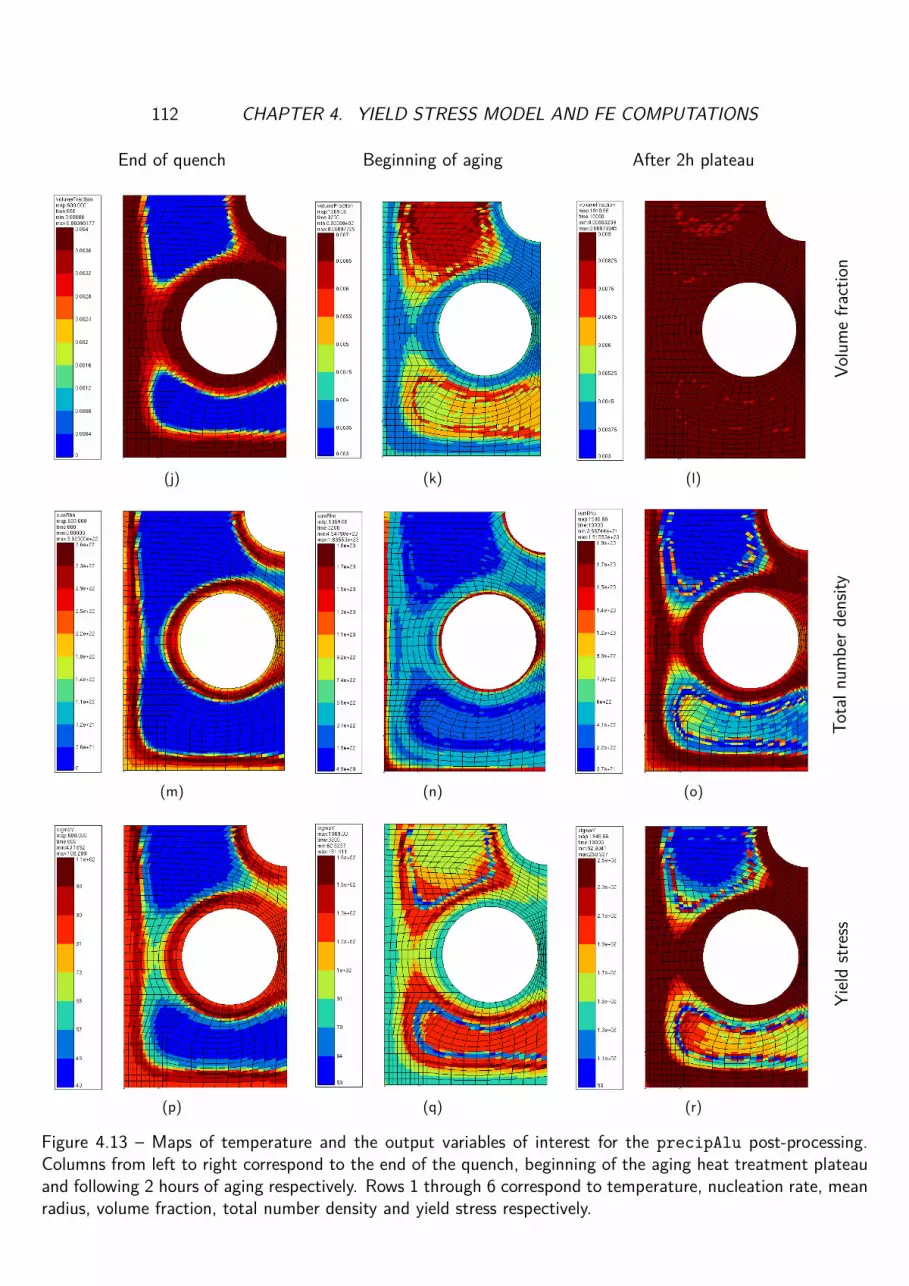
112 CHAPTER 4. YIELD STRESS MODEL AND FE COMPUTATIONS
End of quench Beginning of aging After 2h plateau
(j) (k) (l)
Volumefra
ction
(m) (n) (o)
Totaln
umberd
ensity
(p) (q) (r)
Yield
stress
Figure 4.13 – Maps of temperature and the output variables of interest for the precipAlu post-processing.Columns from left to right correspond to the end of the quench, beginning of the aging heat treatment plateauand following 2 hours of aging respectively. Rows 1 through 6 correspond to temperature, nucleation rate, meanradius, volume fraction, total number density and yield stress respectively.

4.6. CONCLUSION 113
IP 473/1IP 678/1
Time (h)
Tem
pera
ture
,T(
C)
43.532.521.510.50
600
500
400
300
200
100
0
(a)
IP 473/1IP 678/1
Time (h)
Nuc
leat
ion
rate
,J(#
.m−
3 .s−
1 )
43.532.521.510.50
1e+25
1e+20
1e+15
1e+10
100000
1
(b)
IP 473/1IP 678/1
Time (h)
Mea
nra
dius
,R(n
m)
43.532.521.510.50
14
12
10
8
6
4
2
0
(c)
IP 473/1IP 678/1
Time (h)
Tota
lnum
berd
ensi
ty,ρ
(#.m
−3 )
43.532.521.510.50
1e+24
1e+23
1e+22
1e+21
1e+20
(d)
IP 473/1IP 678/1
Time (h)
Volu
me
frac
tion,
f v
43.532.521.510.50
0.009
0.008
0.007
0.006
0.005
0.004
0.003
0.002
0.001
0
(e)
IP 473/1IP 678/1
Time (h)
Yie
ldst
ress
,σy
(MPa
)
43.532.521.510.50
300
250
200
150
100
50
0
(f)
Figure 4.14 – Behavior comparison between IP 678/1 and IP 473/1 through time in terms of (a) temperature,(b) nucleation rate (c) mean radius, (d) total number density, (e) volume fraction and (f) yield stress.

114 CHAPTER 4. YIELD STRESS MODEL AND FE COMPUTATIONS
End of quench Beginning of aging After 2h plateau
(a) (b) (c)
Temperature
A
A
(d)
A
A
(e)
A
A
(f)σ
11
(g) (h) (i)
εp 11

4.6. CONCLUSION 115
End of quench Beginning of aging After 2h plateau
B B
(j)
B B
(k)
B B
(l)
σ22
(m) (n) (o)εp 22
(p) (q) (r)
σmises
Figure 4.15 – Maps of temperature and the output variables of interest for the mechanical calculation. Columnsfrom left to right correspond to the end of the quench, beginning of the aging heat treatment plateau andfollowing 2 hours of aging respectively. Rows 1 through 6 correspond to temperature, σ11, ε11, σ22, ε22 andσmises.

116 CHAPTER 4. YIELD STRESS MODEL AND FE COMPUTATIONS
IP 473/1IP 678/1
Time (h)
εp cum
43.532.521.510.50
0.010.009
0.0080.0070.006
0.0050.0040.003
0.0020.001
0
(a)
IP 473/1IP 678/1
σ11 (MPa)
σ 22
(MPa
)
3020100-10-20-30
200
150
100
50
0
-50
-100
-150
-200
(b)
IP 473/1IP 678/1
εp11
σ 11
(MPa
)
0.0020.0010-0.001-0.002-0.003
30
20
10
0
-10
-20
-30
(c)
IP 473/1IP 678/1
εp22
σ 22
(MPa
)
0.0050.00250-0.0025-0.005
200
150
100
50
0
-50
-100
-150
-200
(d)
σmises IP 678/1σy IP 678/1
Time (h)
σ(M
Pa)
43.532.521.510.50
300
250
200
150
100
50
0
(e)
σmises IP 473/1σy IP 473/1
Time (h)
σ(M
Pa)
43.532.521.510.50
160
140
120
100
80
60
40
20
0
(f)
Figure 4.16 – Behavior comparison between IP 678/1 and IP 473/1: (a) cumulated plastic strain with respectto time, (b) σ22 with respect to σ11 (c) stress-plastic strain response in the x1 direction, (d) stress-plastic strainresponse in the x2 direction, (e) von Mises and yield stress with respect to time for IP 678/1 (f) mises and yieldstress with respect to time for IP 473/1.

Conclusion and perspectives
This work was centered around modelling precipitation hardening in anA356+0.5Cu cast aluminum alloy for cylinder head applications. The low-alloyednature of this alloy allows it to have an optimal thermal conductivity compared toits high-alloyed counterparts. This alloy benefits from adequate mechanical prop-erties resulting from heat treatments of solutionizing, quenching and aging. Theseheat treatment activate the precipitation of the β-Mg2Si hardening phase system,thus considerably raising the yield stress of the alloy.
The behavior of the studied A356+0.5Cu alloy when subject to a heat treat-ment sequence was studied. Indeed, samples were solutionized, quenched and agedat 200C for 0.1, 1, 10 and 100 hours. Then, a TEM characterization was con-ducted on these samples with qualitative and quantitative aims. It was shown thatfor the short aging durations (up to 10 hours), the dominating hardening precipi-tates were β′′ rods, while for the long aging duration (100 hours), the dominanceshifted to the Q-phase system (Q′, Q′′ precipitates). The length and diameter ofthe β′′ rods were measured on a sufficiently high number of precipitates to pro-duce size distributions. These size distributions later served for the calibration andvalidation of the precipitation kinetics model. In addition to that, tensile testswere carried out for these aging conditions in order to evaluate the evolution ofyield stress as a function of the duration of the aging heat treatment at 200C .Thus, the aging curve was produced which in its turn served for the calibrationand validation of the yield stress model.
The aim of the modelling effort was therefore to reproduce the experimentalresults both in terms of size distributions and yield stress by simulating the heattreatment sequence. A physics-based precipitation kinetics model was used whichrelied on classical nucleation theory equations and Fick’s laws of diffusion. Indi-rect coupling to the Thermo-Calc software was used to feed the model essentialthermodynamic variables such as the driving force for precipitation and the solu-bility product. These variables are extracted for a wide range of compositions andtemperature and then numerically fitted. Then, the model accesses their valuesby simply evaluating these numerical functions thus reducing computation time.Recent developments regarding the correction of the growth rate equations andthe curvature effect to take into account the elongated morphology of precipitateswere also implemented [81]. The KWN size class approach was used to track theevolution of the size distributions. This approach combined with a Euler implicitfinite differences scheme linearizes the integration problem and reduces it to the
117

118 CHAPTER 4. YIELD STRESS MODEL AND FE COMPUTATIONS
inversion of a tri-diagonal matrix which can be efficiently achieved thanks to anupper-lower type algorithm. The implementation of a Newton-Raphson solver algo-rithm was also made necessary by the multi-constituent nature of the precipitatingphase.
The precipitation model was then confronted to the measured size distributionsfor calibration and validation. As it is practiced for this type of approaches, thematrix/precipitate interfacial energy was used as a fitting parameter. In this worktwo separate values were used for the nucleation equations and growth equations.For reasonable values of these parameters the model was capable of reproducingthe experimental size distributions with good accuracy.
The yield stress was modelled as the pythagorean sum of the contributions ofintrinsic strength, solid solution strengthening and precipitation hardening. Themajor contribution there being precipitation hardening, it was modelled using anapproach originally proposed by Deschamps et al. [110]. Further developmentsintroduced by Esmaeili et al. [11] and Bardel et al. [8] which address the mor-phology and orientation of these precipitates in the matrix were implemented. Theresults of the yield stress model were also confronted to experiments using thecritical radius for shearing as a fitting parameter. Again, with reasonable values ofthis parameter, a good agreement with the experiments was obtained. However,a large underestimation of yield stress was obtained for a long aging duration at200C (100 hours). This is explained by the phase transformation observed in themicrostructural analysis after long aging. Indeed, the transition to the Q-phasehardening system allows the alloy to maintain a higher level of yield stress for asignificantly longer aging time. This is the result of the presence of Cu in the com-position which allows this phase transformation and increases the aging resistanceof the alloy.
Overall, this hybrid physics-based and phenomenological approach presents agood step in the direction of the integrated computational materials engineering.However, many assumptions are made all throughout in the adopted modellingscheme. They are accomodated by the use of fitting parameters, the values ofwhich are detached from physical considerations. Finally, the physical underpin-ning of many aspects of this modelling effort offers a good scope of application,especially when compared to purely phenomenological approaches [111, 112, 113].Indeed, thanks to this model, the effect of heat treatment parameters can bestudied, the ability to handle anisothermal states being at the core of the capabil-ities of this approach. It is also possible to study, to a certain extent, the effectof changes in the chemistry of the alloy. This is however limited by the neces-sity for the chemistry change to have no impact on the nature of the hardeningprecipitates.
This leads to the statement of the most important perspective of this work,which is the generalization to a multi-phase model. This should especially addressthe case where the precipitation of different phases is inter-dependent, such is thecase for alloys of type A356+0.5Cu. The KWN approach is intrinsically capable ofhandling multiple distributions of precipitates, but the thermodynamic description

4.6. CONCLUSION 119
of these phases and the transition from one to the other requires further work.Aside from remedying to the aforementioned discrepancy of the model and exper-iments for long aging durations, this would open the door for studying the effectof chemical composition, thus enabling tailor-made alloy development.
Another major perspective of this work consists in extending the effect ofmicrostructure dependence to the material parameters that represent isotropic andkinematic hardening. In the present state, only initial yield stress is informed by themicrostructural state while the hardening variables are experimentally identified.These variables are therefore dependent only on temperature and are identified foralloys in a given heat treated state. This limits the capability of the model in termsof representing the evolution of the plastic domain.
More immediate perspectives include the introduction of an evolution law forthe aspect ratio, considered constant in this work, compatible with isothermaltreatments. The nucleation stage also merits more consideration of elastic strainenergy and heterogeneous nucleation.
From a more fundamental point of view, the experimental or computationaldetermination of the matrix/precipitate interfacial energies would solve a majordrawback of these approaches. Also, the scale transition from dislocation/obstacleinteractions to macroscopic estimations of yield stress requires significant work.
Finally, the ultimate goal of this work was the construction of a finite elementsmethod computation chain integrating the precipitation kinetics and yield stressmodel. This has been achieved by means of the creation of a postprocessingoption called “precipAlu”. The process takes as its input the result of a FEMthermal calculation and produces maps of the precipitation kinetics variables andof the initial yield stress. The initial yield stress map is joined to the temperaturemap to be the input of the mechanical calculation. A 2D demonstrator has beenset up and was used to show the capability of the computation chain to trackthe property gradients produced by the heterogeneous temperature distributionin the structure. It was also shown that the FEM model properly represents theevolution of internal stresses induced by quenching and relaxed by aging. Thisallows the estimation and localization of the residual stresses which can be used tooptimize heat treatments and geometries. Further fine tuning is required in orderto transition to 3D calculations and experimental verification of the capability ofthe model to predict the levels and localization of residual stresses is of coursenecessary.

120 CHAPTER 4. YIELD STRESS MODEL AND FE COMPUTATIONS

Bibliography
[1] European Union. Climate action section of the official website of the euro-pean union.
[2] Mustafa Kemal Kulekci. Magnesium and its alloys applications in automotiveindustry. The International Journal of Advanced Manufacturing Technology,39(9-10):851–865, 2008.
[3] Neda Sarmady. The effect of quench rate and initial grain structure on themechanical behaviour of an al-mg-si-mn aluminum alloy. Master’s thesis,University of British Columbia, 2018.
[4] Anatomy Note. Car engine anatomical structure -https://www.anatomynote.com/transportation-anatomy/machinery-parts/car-engine-anatomical-structure/.
[5] Eric Nicouleau-Bourles. Etude experimentale et numerique du vieillissementd’un alliage d’aluminium. Application aux culasses automobiles. PhD thesis,École Nationale Supérieure des Mines de Paris, 1999.
[6] Bruno Barlas. Etude du comportement et de l’endommagement en fatigued’alliages d’aluminium de fonderie. PhD thesis, École Nationale Supérieuredes Mines de Paris, 2004.
[7] Rémi Martinez. Modélisation multi-échelles des propriétés mécaniques d’unalliage d’aluminium de fonderie. PhD thesis, Paris Est, 2012.
[8] D. Bardel, M. Perez, D. Nelias, A. Deschamps, C.R. Hutchinson, D. Maison-nette, T. Chaise, Josselin Garnier, and F. Bourlier. Coupled precipitation andyield strength modelling for non-isothermal treatments of a 6061 aluminiumalloy. Acta Materialia, 62:129–140, 2014.
[9] Yue Li, Bjørn Holmedal, Hongxiang Li, Linzhong Zhuang, Jishan Zhang,and Qiang Du. Precipitation and strengthening modeling for disk-shapedparticles in aluminum alloys: Size distribution considered. Materialia, 4:431–443, 2018.
[10] Rui Chen, Qingyan Xu, Huiting Guo, Zhiyuan Xia, Qinfang Wu, andBaicheng Liu. Modeling the precipitation kinetics and tensile properties
121

122 BIBLIOGRAPHY
in Al-7Si-Mg cast aluminum alloys. Materials Science and Engineering: A,685:403–416, 2017.
[11] Shahrzad Esmaeili. Precipitation hardening behaviour of AA6111. PhDthesis, University of British Columbia, 2002.
[12] John Allison, Dan Backman, and Leo Christodoulou. Integrated computa-tional materials engineering: a new paradigm for the global materials pro-fession. Jom, 58(11):25–27, 2006.
[13] R. Martinez, D. Larouche, G. Cailletaud, I. Guillot, and D. Massinon. Simu-lation of the concomitant process of nucleation-growth-coarsening of Al2Cuparticles in a 319 foundry aluminum alloy. MSMSE, 23(4), 2015.
[14] Encyclopedia Britannica, 2007.
[15] Joseph R. Davis et al. Aluminum and aluminum alloys. ASM international,1993.
[16] Country Granted Number Year. Bayer’s process for alumina production: ahistorical perspective. Bull. Hist. Chem, 17(18):15, 1995.
[17] Vinay Kumar and Linda Milewski. Charles martin hall and the great alu-minum revolution. Journal of Chemical Education, 64(8):690, 1987.
[18] Dietrich G. Altenpohl. Aluminum: Technology, applications, and environ-ment; a profile of a modern metal; aluminium from within. Warrendale,TMS., 1998.
[19] Aluminum Standards and Data. The Aluminum Association, 2009.
[20] P.S. Mohanty and J.E. Gruzleski. Grain refinement mechanisms of hypoeu-tectic Al–Si alloys. Acta materialia, 44(9):3749–3760, 1996.
[21] Günter Gottstein. Solidification. In Physical Foundations of Materials Sci-ence, pages 357–388. Springer, 2004.
[22] David A. Porter, Kenneth E. Easterling, and Mohamed Sherif. Phase Trans-formations in Metals and Alloys, (Revised Reprint). CRC press, 2009.
[23] D. Massinon and V. Constantin. Formation métallurgie et défauts defonderie. Montupet Châteauroux, 2002.
[24] F.T. Lee, J.F. Major, and F.H. Samuel. Effect of silicon particles on thefatigue crack growth characteristics of Al-12 Wt pct Si-0.35 Wt pct Mg-(0to 0.02) Wt pct Sr casting alloys. Metallurgical and Materials TransactionsA, 26(6):1553–1570, 1995.

BIBLIOGRAPHY 123
[25] M. Haghshenas, A. Zarei-Hanzaki, and S.M. Fatemi-Varzaneh. The effectsof thermo-mechanical parameters on the microstructure of thixocast A356aluminum alloy. Materials Science and Engineering: A, 480(1-2):68–74,2008.
[26] D.G. Eskin, V.I. Savran, L. Katgerman, et al. Effects of alloy composition andcasting speed on structure formation and hot tearing during direct-chill cast-ing of Al-Cu alloys. Metallurgical and Materials Transactions, 35(11):3551,2004.
[27] John A. Taylor. The effect of iron in Al-Si casting alloys. In 35th Australianfoundry institute national conference, Adelaide, South Australia, volume 31,pages 148–157, 2004.
[28] L. Lu and A.K. Dahle. Iron-rich intermetallic phases and their role in castingdefect formation in hypoeutectic Al–Si alloys. Metallurgical and MaterialsTransactions A, 36(3):819–835, 2005.
[29] L. Wang and S. Shivkumar. Strontium modification of aluminium alloycastings in the expendable pattern casting process. Journal of materialsScience, 30(6):1584–1594, 1995.
[30] Giulio Timelli and Daniele Caliari. Influence of process parameters on the mi-crostructure and casting defects of a LPDC engine block. In Shape Casting:6th International Symposium, pages 151–158. Springer, 2016.
[31] P. Ouellet and F.H. Samuel. Effect of Mg on the ageing behaviour ofAl-Si-Cu 319 type aluminium casting alloys. Journal of Materials Science,34(19):4671–4697, 1999.
[32] Bartłomiej Dybowski, Bogusława Adamczyk-Cieślak, Kinga Rodak, IwonaBednarczyk, Andrzej Kiełbus, and Jaroslaw Mizera. The microstructure ofAlSi7Mg alloy in as cast condition. In Solid State Phenomena, volume 229,pages 3–10. Trans Tech Publ, 2015.
[33] R. Martinez, V. Russier, Couzinié, I. Guillot, and G. Cailletaud. Modelingof the influence of coarsening on viscoplastic behaviour of a 319 foundryaluminum alloy. Mater. Sci. Eng. A, 559:40, 2013.
[34] M. Karlik and B. Jouffrey. High resolution electron microscopy studyof Guinier-Preston (GP1) zones in Al2Cu based alloys. Acta materialia,45(8):3251–3263, 1997.
[35] Delavand Ovono-Ovono. Recyclabilité des alliages d’aluminium de fonderie:Influence des éléments résiduels sur la microstructure et le comportementmécanique. PhD thesis, Université Technologique de Compiègne, 2004.

124 BIBLIOGRAPHY
[36] Emma Sjölander and Salem Seifeddine. The heat treatment of Al–Si–Cu–Mgcasting alloys. Journal of Materials Processing Technology, 210(10):1249–1259, 2010.
[37] Daniele Casari. The grain refinement and the Ni/V contamination in theA356 aluminium casting alloy: an experimental study on impact and tensileproperties. PhD thesis, Università degli Studi di Ferrara, 2014.
[38] M. Karlik, B. Jouffrey, and S. Belliot. The copper content of Guinier–Preston(GP1) zones in Al–1.84 at.% Cu alloy. Acta materialia, 46(5):1817–1825,1998.
[39] Katharina Teichmann, Calin D. Marioara, Sigmund J. Andersen, and KnutMarthinsen. Tem study of β’ precipitate interaction mechanisms with dis-locations and β’ interfaces with the aluminium matrix in Al–Mg–Si alloys.Materials Characterization, 75:1–7, 2013.
[40] Erhard Hornbogen. Hundred years of precipitation hardening. Journal oflight metals, 1(2):127–132, 2001.
[41] A. (Anthony) Kelly, R.B Nicholson, and ScienceDirect (Online service). Pre-cipitation hardening. Oxford : Pergamon Press, 1963.
[42] H. Liu, I. Papadimitriou, F.X. Lin, and J. LLorca. Precipitation during hightemperature aging of Al–Cu alloys: A multiscale analysis based on firstprinciples calculations. Acta Materialia, 167:121–135, 2019.
[43] S.K. Son, M. Takeda, M. Mitome, Y. Bando, and T. Endo. Precipitationbehavior of an Al–Cu alloy during isothermal aging at low temperatures.Materials letters, 59(6):629–632, 2005.
[44] S. Shivkumar, C. Keller, and D. Apelian. Aging behavior in cast Al-Si-Mgalloys. AFS Transactions, 98:905–911, 1990.
[45] I. Dutta and S.M. Allen. A calorimetric study of precipitation in commercialaluminium alloy 6061. Journal of Materials Science Letters, 10(6):323–326,1991.
[46] Eva A. Mørtsell, Feng Qian, Calin D. Marioara, and Yanjun Li. Precipi-tation in an A356 foundry alloy with Cu additions-A transmission electronmicroscopy study. Journal of Alloys and Compounds, 785:1106–1114, 2019.
[47] Takeshi Saito, Eva A. Mørtsell, Sigurd Wenner, Calin D. Marioara, Sig-mund J. Andersen, Jesper Friis, Kenji Matsuda, and Randi Holmestad.Atomic structures of precipitates in Al–Mg–Si alloys with small additionsof other elements. Advanced Engineering Materials, 20(7):1800125, 2018.
[48] G.A. Edwards, K. Stiller, G.L. Dunlop, and M.J. Couper. The precipitationsequence in Al–Mg–Si alloys. Acta materialia, 46(11):3893–3904, 1998.

BIBLIOGRAPHY 125
[49] W.F. Miao and D.E. Laughlin. Precipitation hardening in aluminum alloy6022. Scripta Materialia, 40(7):873–878, 1999.
[50] S.J. Andersen, C.D. Marioara, R. Vissers, A. Frøseth, and H.W. Zandber-gen. The structural relation between precipitates in Al–Mg–Si alloys, theAl-matrix and diamond silicon, with emphasis on the trigonal phase U1-MgAl2Si2. Materials Science and Engineering: A, 444(1-2):157–169, 2007.
[51] S.J. Andersen, C.D. Marioara, A. Frøseth, R. Vissers, and H.W. Zandbergen.Crystal structure of the orthorhombic U2-Al4Mg4Si4 precipitate in the Al–Mg–Si alloy system and its relation to the β’ and β" phases. MaterialsScience and Engineering: A, 390(1-2):127–138, 2005.
[52] C.D. Marioara, H. Nordmark, S.J. Andersen, and R. Holmestad. Post-β"phases and their influence on microstructure and hardness in 6xxx Al-Mg-Sialloys. Journal of materials science, 41(2):471–478, 2006.
[53] C. Ravi and C. Wolverton. First-principles study of crystal structure andstability of Al–Mg–Si–(Cu) precipitates. Acta materialia, 52(14):4213–4227,2004.
[54] C. Cayron and P.A. Buffat. Transmission electron microscopy study of theβ’ phase (Al–Mg–Si alloys) and QC phase (Al–Cu–Mg–Si alloys): orderingmechanism and crystallographic structure. Acta Materialia, 48(10):2639–2653, 2000.
[55] C.D. Marioara, S.J. Andersen, T.N. Stene, H. Hasting, J. Walmsley, A.T.J.Van Helvoort, and R. Holmestad. The effect of Cu on precipitation in Al–Mg–Si alloys. Philosophical Magazine, 87(23):3385–3413, 2007.
[56] S.J. Andersen, H.W. Zandbergen, J. Jansen, C. Traeholt, U. Tundal, andO. Reiso. The crystal structure of the β" phase in Al–Mg–Si alloys. ActaMaterialia, 46(9):3283–3298, 1998.
[57] R. Vissers, M.A. van Huis, J. Jansen, H.W. Zandbergen, C.D. Marioara,and S.J. Andersen. The crystal structure of the β’ phase in Al–Mg–Si alloys.Acta Materialia, 55(11):3815–3823, 2007.
[58] Chen Qian, Xie Quan, Zhao Feng-Juan, Cui Dong-Meng, and Li Xu-Zhen.First-principles calculation of electronic structure of Mg2Si with doping. In2009 International Forum on Information Technology and Applications, vol-ume 1, pages 338–341. IEEE, 2009.
[59] A. Perovic, D.D. Perovic, G.C. Weatherly, and D.J. Lloyd. Precipitation inaluminum alloys AA6111 and AA6016. Scripta Materialia, 41(7):703–708,1999.

126 BIBLIOGRAPHY
[60] Kenji Matsuda, Susumu Ikeno, Yasuhiro Uetani, and Tatsuo Sato.Metastable phases in an Al-Mg-Si alloy containing copper. Metallurgicaland Materials Transactions A, 32(6):1293–1299, 2001.
[61] C. Wolverton. Crystal structure and stability of complex precipitate phases inAl–Cu–Mg–(Si) and Al–Zn–Mg alloys. Acta Materialia, 49(16):3129–3142,2001.
[62] Kyoungdoc Kim, Andrew Bobel, Vuk Brajuskovic, Bi-Cheng Zhou, MikeWalker, Gregory B. Olson, and C. Wolverton. Energetics of native defects,solute partitioning, and interfacial energy of Q precipitate in Al-Cu-Mg-Sialloys. Acta Materialia, 154:207–219, 2018.
[63] S.I. Bakhtiyarov, R.A. Overfelt, and S.G. Teodorescu. Electrical and ther-mal conductivity of A319 and A356 aluminum alloys. Journal of MaterialsScience, 36(19):4643–4648, 2001.
[64] Thomas H. Ludwig, Paul L. Schaffer, and Lars Arnberg. Influence of vana-dium on the microstructure of A356 foundry alloy. Light Metals, 2013.
[65] George W. Smith. Precipitation kinetics in an air-cooled aluminum alloy: acomparison of scanning and isothermal calorimetry measurement methods.Thermochimica acta, 313(1):27–36, 1998.
[66] Yan Zheng, Wenlong Xiao, Sujing Ge, Weitao Zhao, Shuji Hanada, andChaoli Ma. Effects of Cu content and Cu/Mg ratio on the microstructureand mechanical properties of Al–Si–Cu–Mg alloys. Journal of Alloys andCompounds, 649:291–296, 2015.
[67] Xiang Wang, Shahrzad Esmaeili, and David J. Lloyd. The sequence ofprecipitation in the Al-Mg-Si-Cu alloy AA6111. Metallurgical and materialstransactions A, 37(9):2691–2699, 2006.
[68] D.J. Chakrabarti, Yingguo Peng, David E. Laughlin, et al. Precipitationin Al-Mg-Si alloys with Cu additions and the role of the Q’ and relatedphases. In Materials Science Forum, volume 396, pages 857–862. TranstecPublications; 1999, 2002.
[69] Kenneth C. Russell. Nucleation in solids: the induction and steady stateeffects. Advances in Colloid and Interface Science, 13(3-4):205–318, 1980.
[70] John Wyrill Christian. The theory of transformations in metals and alloys. I.equilibrium and general kinetic theory. 1975.
[71] D.A. Porter and K.E. Easterling. Phase transformations in metals and alloys.Chapman and Hall, Padstow, Cornwall, 1981.

BIBLIOGRAPHY 127
[72] Jacques Besson, Georges Cailletaud, Jean-Louis Chaboche, and Samuel For-est. Non-linear mechanics of materials, volume 167. Springer Science &Business Media, 2009.
[73] Boris S. Bokstein, Mikhail I. Mendelev, David J. Srolovitz, et al. Thermody-namics and kinetics in materials science: a short course. Oxford UniversityPress, 2005.
[74] O.R. Myhr, Ø Grong, and S.J. Andersen. Modelling of the age hardeningbehaviour of Al–Mg–Si alloys. Acta Materialia, 49(1):65–75, 2001.
[75] O.R. Myhr, Ø Grong, H.G. Fjaer, and C.D. Marioara. Modelling of themicrostructure and strength evolution in Al–Mg–Si alloys during multistagethermal processing. Acta Materialia, 52(17):4997–5008, 2004.
[76] Myriam Nicolas and Alexis Deschamps. Characterisation and modelling ofprecipitate evolution in an Al–Zn–Mg alloy during non-isothermal heat treat-ments. Acta Materialia, 51(20):6077–6094, 2003.
[77] Aude Simar, Yves Bréchet, B. De Meester, A. Denquin, and Thomas Par-doen. Sequential modeling of local precipitation, strength and strain hard-ening in friction stir welds of an aluminum alloy 6005A-T6. Acta Materialia,55(18):6133–6143, 2007.
[78] Michel Perez. Gibbs–Thomson effects in phase transformations. Scriptamaterialia, 52(8):709–712, 2005.
[79] Q. Du, W.J. Poole, M.A. Wells, and N.C. Parson. Microstructure evolutionduring homogenization of Al–Mn–Fe–Si alloys: Modeling and experimentalresults. Acta Materialia, 61(13):4961–4973, 2013.
[80] Qiang Du, Michel Perez, Warren J. Poole, and Mary Wells. Numericalintegration of the Gibbs–Thomson equation for multicomponent systems.Scripta Materialia, 66(7):419–422, 2012.
[81] Bjørn Holmedal, Elisa Osmundsen, and Qiang Du. Precipitation ofnon-spherical particles in aluminum alloys part I: generalization of theKampmann–Wagner numerical model. Metallurgical and Materials Transac-tions A, 47(1):581–588, 2016.
[82] Qiang Du, Bjørn Holmedal, Jesper Friis, and Calin D Marioara. Precipitationof non-spherical particles in aluminum alloys part II: numerical simulation andexperimental characterization during aging treatment of an Al-Mg-Si alloy.Metallurgical and Materials Transactions A, 47(1):589–599, 2016.
[83] Richard Wagner, Reinhard Kampmann, and Peter W Voorhees. Homoge-neous second-phase precipitation. Phase transformations in materials, 5:309,2001.

128 BIBLIOGRAPHY
[84] O.R. Myhr and Øystein Grong. Modelling of non-isothermal transformationsin alloys containing a particle distribution. Acta Materialia, 48(7):1605–1615,2000.
[85] Yong Du, LiJun Zhang, SenLin Cui, DongDong Zhao, DanDan Liu, WeiBinZhang, WeiHua Sun, and WanQi Jie. Atomic mobilities and diffusivities inal alloys. Science China Technological Sciences, 55(2):306–328, 2012.
[86] Joël Douin. Mécanique des milieux continus: introduction à la plasticité desmatériaux. Diderot éd., 1997.
[87] Erich Schmid and Walter Boas. Plasticity of crystals. 1950.
[88] G. Sachs and J. Weerts. Tensile tests on gold-silver crystals. Z. Physik,1930.
[89] Geoffrey Ingram Taylor. The mechanism of plastic deformation of crystals.part I.—theoretical. Proceedings of the Royal Society of London. Series A,Containing Papers of a Mathematical and Physical Character, 145(855):362–387, 1934.
[90] Derek Hull and David J Bacon. Introduction to dislocations, volume 37.Elsevier, 2011.
[91] FRN Nabarro. Dislocations in a simple cubic lattice. Proceedings of thePhysical Society, 59(2):256, 1947.
[92] Guillaume Fribourg. Couplages entre précipitation et plasticité dans un al-liage d’aluminium 7xxx: application à des traitements thermomécaniques deréduction des distorsions dans des composants aéronautiques. PhD thesis,Grenoble INPG, 2009.
[93] J.L. Martin. Dislocations et Plasticité des Cristaux, Presses Polytechniqueset Universitaires Romandes, Lausanne, 2000. Price: CHF34, h23, 10.
[94] Georges Saada et al. L’état métallique. déformation plastique. 1980.
[95] A. Portevin and F. Le Chatelier. The obtention, by thermal treatment, oflight aluminium alloys of high resistance not containing magnesium. C. R.Acad. Sci. Paris, 177:311, 1923.
[96] Ali Argon. Strengthening mechanisms in crystal plasticity, volume 4. OxfordUniversity Press on Demand, 2008.
[97] D. Hull and D.J. Bacon. Introduction to dislocations. Butterworth Heine-mann, Oxford, 1984.
[98] A. Deschamps and Y. Bréchet. Influence of predeformation and ageing ofan Al-Zn-Mg alloy - II. Modeling of precipitation kinetics and yield stress.Acta Mater., 47:293, 1999.

BIBLIOGRAPHY 129
[99] F.C. Frank and W.T. Read Jr. Multiplication processes for slow movingdislocations. Physical Review, 79(4):722, 1950.
[100] E.O. Hall. The deformation and ageing of mild steel: III discussion of results.Proceedings of the Physical Society. Section B, 64(9):747, 1951.
[101] N.J. Petch. The cleavage strength of polycrystals. Journal of the Iron andSteel Institute, 174:25–28, 1953.
[102] A. de Vaucorbeil, W.J. Poole, and C.W. Sinclair. The superposition ofstrengthening contributions in engineering alloys. Mater. Sci. Eng. A,582:147–154, 2013.
[103] G.P.M. Leyson, L.G. Hector Jr., and W.A. Curtin. Solute strengtheningfrom first principles and application to aluminum alloys. Acta Materialia,60(9):3873–3884, 2012.
[104] J. Friedel. Dislocations. Addison-Wesley Publishing Company Inc., Reading,Massachussets, USA, 1964.
[105] R.L. Fleischer and W.R. Hibbard. The relation between the structure andmechanical properties of metals. Her Majesty’s Stationary Office, London,261, 1963.
[106] A.J. Ardell. Precipitation hardening. Metall. Trans., 16A:2131, 1985.
[107] C. Gallais, A. Denquin, Y. Bréchet, and G. Lapasset. Precipitation mi-crostructures in an AA6056 aluminium alloy after friction stir welding: Char-acterisation and modelling. Materials Science and Engineering: A, 496(1-2):77–89, 2008.
[108] Aude Simar, Yves Bréchet, B. De Meester, Anne Denquin, Christophe Gal-lais, and Thomas Pardoen. Integrated modeling of friction stir welding of6xxx series Al alloys: process, microstructure and properties. Progress inMaterials Science, 57(1):95–183, 2012.
[109] Jean Lemaitre and Jean-Louis Chaboche. Mechanics of solid materials. Cam-bridge university press, 1994.
[110] A. Deschamps and Y. Brechet. Influence of predeformation and ageing ofan Al–Zn–Mg alloy - II. Modeling of precipitation kinetics and yield stress.Acta Materialia, 47(1):293–305, 1998.
[111] B. Barlas. Étude du comportement et de l’endommagement en fatigued’alliages d’aluminium de fonderie. PhD thesis, École Nationale Superieuredes Mines de Paris, France, 2004.

130 BIBLIOGRAPHY
[112] E. Nicouleau-Bourles. Étude expérimentale et numérique du vieillissementd’un alliage d’aluminium. Application aux culasses automobiles. PhD thesis,École Nationale Supérieure des Mines de Paris, France, 1999.
[113] François-Xavier Hoche. Vers une prise en compte du vieillissement thermiquedans la filière de dimensionnement des structures pour la fatigue thermomé-canique. PhD thesis, Paris Sciences et Lettres, 2016.

List of Figures
1 The Euro emission standards for diesel engines (lines) and petrolengines (points) [1]. . . . . . . . . . . . . . . . . . . . . . . . . . 6
2 Exploded view of an internal combustion engine showing the posi-tion of the cylinder head [4]. . . . . . . . . . . . . . . . . . . . . . 7
1.1 Schematic of the 4 strokes that make up a thermodynamic cycleof a petrol internal combustion engine [14]. . . . . . . . . . . . . . 10
1.2 Firedeck side of the cylinder head for the Ford 1.0L 3 cylinderengine with the integrated exhaust manifold (the red square showsthe sensitive intervalve area). . . . . . . . . . . . . . . . . . . . . 11
1.3 Al-Si binary phase diagram at atmospheric pressure, calculated us-ing Thermo-Calc (TCAL4 database). . . . . . . . . . . . . . . . . 15
1.4 Schematic of dendrite formation and morphology : (a) stages ofbreakdown of a planar solid/liquid interface which forms the den-dritic structure [22] and (b) a dendrite with its primary, secondaryand tertiary arms [23]. . . . . . . . . . . . . . . . . . . . . . . . . 16
1.5 Deep-etched micrographs of a 319 alloy : (a) SEM secondary elec-tron micrograph of non-modified as-cast alloy showing a lamel-lar eutectic Si-phase morphology, (b) SEM secondary electron ofa Strontium-modified as-cast alloy showing a fibrous eutectic Si-phase morphology [29] and (c) optical micrograph of a T7 heattreated 319 strontium-modified alloy showing the globular morphol-ogy of the eutectic Si-phase [7]. . . . . . . . . . . . . . . . . . . . 19
1.6 Optical micrographs showing the different iron-rich intermetallicphases and their different morphologies in an A356 alloy (Al-7%Si-0.4%Mg) : (a) Chinese-script shape of the α–Al15(Fe,Mn)3Si2, (b)platelet shape of the β–Al5FeSi and (c) blocky shape of the π-phase[28]. . . . . . . . . . . . . . . . . . . . . . . . . . . . . . . . . . 20
1.7 Micrographs of an Al-7%Si0.3%Mg alloy showing void defects : (a)shrinkage void and (b) gas porosity [30]. . . . . . . . . . . . . . . 21
1.8 Hardening phases in the as-cast state : (a) micrograph showing theθ-Al2Cu in an as-cast 319 alloy [31] and (b) micrograph showing abulky β-Mg2Si particle in an as-cast A356 alloy [32]. . . . . . . . . 21
131

132 LIST OF FIGURES
1.9 Hardening phases in heat-treated 3xx series aluminum alloys :(a) dark field TEM micrograph of θ′-Al2Cu precipitates in a heattreated 319 alloy [33] and (b) Bright field TEM micrograph of β′′-Mg2Si precipitates in a heat treated A356+0.5Cu alloy (this study). 22
1.10 High resolution transmission electron microscopy (HRTEM) micro-graph showing Guinier-Preston zones in an Al-1.84%at. Cu [34]. . . 24
1.11 Evolution of hardness in a 319 aluminum alloy as a function of agingduration at 210Cwith the corresponding precipitation sequence [35]. 25
1.12 Schematic representation of dislocation/precipitate interaction :(a) shearing, (b) bypassing and (c) the qualitative relationship be-tween particle size and the stress necessary to activate each mech-anism [36, 37]. . . . . . . . . . . . . . . . . . . . . . . . . . . . . 26
1.13 HRTEM micrographs showing precipitate crossing mechanisms :(a) sheared GP zone in an Al-1.84 at.% Cu alloy [38] and (b) dislo-cation bypassing two β′-Mg2Si precipitates in an Al-Si-Mg alloy, thedislocation line is pointed to by the dotted arrow, the areas pointedto by solid arrows are the dislocation loops around the precipitates[39]. . . . . . . . . . . . . . . . . . . . . . . . . . . . . . . . . . 26
1.14 Unit cells of FCC α-Al and the precipitates from the θ system [42]. 281.15 Unit cells of the precipitates from the β system : (a) β′′ [56], (b)
β′ [57, 50] and (c) β [58]. . . . . . . . . . . . . . . . . . . . . . . 301.16 Unit cell of Q and Q′ [62]. . . . . . . . . . . . . . . . . . . . . . . 30
2.1 Volume fraction of phases as a function of temperature for anA356+0.5Cu alloy calculated with Thermo-Calc using the TCAL5database. . . . . . . . . . . . . . . . . . . . . . . . . . . . . . . . 35
2.2 AFNOR cast aluminum alloy specimen in the experimental study. . 362.3 Schematic of the expected morphology and orientation of the pre-
cipitates as observed with TEM along a 〈001〉α zone axis. . . . . . 372.4 Micrographs showing the result of electrolytic jet polishing : (a)
in the studied A356+0.5Cu alloy and (b) in a typical 6xxx serieswrought alloy containing less Si. . . . . . . . . . . . . . . . . . . . 38
2.5 TEM observations along the 〈001〉α zone axis for samples aged0.1 hr at 200C (a) through (c): bright field images (d) through (f):dark field images (g) through (i): SAD patterns and the simulatedpattern for β′′. . . . . . . . . . . . . . . . . . . . . . . . . . . . . 39
2.6 TEM observations along the 〈001〉α zone axis for samples aged1 hr at 200C (a) through (c): bright field images (d) through (f):dark field images (g) through (i): SAD patterns and the simulatedpattern for β′′. . . . . . . . . . . . . . . . . . . . . . . . . . . . . 40
2.7 TEM observations along the 〈001〉α zone axis for samples aged10 hrs at 200C (a) through (c): bright field images (d) through (f):dark field images (g) through (i): SAD patterns and the simulatedpattern for β′′. . . . . . . . . . . . . . . . . . . . . . . . . . . . . 41

LIST OF FIGURES 133
2.8 TEM observations along the 〈001〉α zone axis for samples aged100 hrs at 200C (a) through (c): bright field images (d) through(f): dark field images (g) through (i): SAD patterns and the sim-ulated pattern for Q′. . . . . . . . . . . . . . . . . . . . . . . . . 43
2.9 EDS analysis of phase composition for the matrix and fine precipi-tate in sample aged for 100 hrs at 200C . . . . . . . . . . . . . . 44
2.10 Bright field images of heterogeneously distributed precipitates insample aged 100 hrs at 200C . . . . . . . . . . . . . . . . . . . . 44
2.11 Bright field TEM images of coarse Si phase precipitates and thecorresponding SAD pattern. . . . . . . . . . . . . . . . . . . . . . 45
2.12 EDS analysis for the matrix and a coarse cuboidal precipitate insample aged 100 hrs at 200C . . . . . . . . . . . . . . . . . . . . 45
2.13 Experimental size distributions of Q′ precipitates in the studiedA356+0.5Cu alloy aged 100 hrs at 200C ; bin sizes for thickness,width and length are 0.5, 0.5 and 10 nm respectively. . . . . . . . . 48
2.14 Tensile test sample geometry : (a) 3D model of the setup showingthe sample with the specially designed grips and (b) drawing of thesample. . . . . . . . . . . . . . . . . . . . . . . . . . . . . . . . . 49
2.15 Example of the data correction and interpretation procedure for theconducted tensile tests : (a) Raw Load/Position data, (b) Cleaned-up Load/Position data, (c) Correction for machine+grips compli-ance and (d) 0.2% offset proof stress reading on corrected plot. . . 50
2.16 Engineering stress/strain curves for the tensile tests conducted atroom temperature on the studied A356+0.5Cu alloy aged for dif-ferent durations at 200C . . . . . . . . . . . . . . . . . . . . . . . 51
2.17 Engineering stress/strain curves for the tensile tests conducted at100Con the studied A356+0.5Cu alloy aged for different durationsat 200C . . . . . . . . . . . . . . . . . . . . . . . . . . . . . . . 52
2.18 Engineering stress/strain curves for the tensile tests conducted at200Con the studied A356+0.5Cu alloy aged for different durationsat 200C . . . . . . . . . . . . . . . . . . . . . . . . . . . . . . . 52
2.19 Evolution of the measured 0.2 % offset proof yield stress for thestudied A356+Cu alloy as a function of aging duration at 200C foreach test temperature. . . . . . . . . . . . . . . . . . . . . . . . . 53
3.1 Nucleation of a particle of the β phase in an α matrix: (a)Schematic of the α′ → α + β transformation and (b) Plot of thecorresponding variation in the Gibbs free energy with respect to theradius of the precipitate. . . . . . . . . . . . . . . . . . . . . . . . 57
3.2 The difference in energy barriers for homogeneous and heteroge-neous nucleation [71]. . . . . . . . . . . . . . . . . . . . . . . . . 58
3.3 Fit function of the precipitation driving force of β-Mg2Si in thealuminum matrix extracted from Thermo-Calc/TCAL5. . . . . . . 60

134 LIST OF FIGURES
3.4 Determination of the solubility product for β-Mg2Si using Thermo-Calc/TCAL5: (a) Mg and Si concentrations in the matrix for dif-ferent temperatures representing the phase diagram tie-lines and(b) logarithm of the solubility product Ks as a function of the tem-perature inverse with the corresponding fit function implementedin the model. . . . . . . . . . . . . . . . . . . . . . . . . . . . . . 64
3.5 Gibbs–Thomson phase diagram (surface showing matrix solute con-tent vs. curvature) of the Al–Mn–Si system at 600C calculatedby the integration method together with the solubility limit lines(markers) for various curvatures calculated by Thermo-Calc [80]. . . 66
3.6 Evolution of the equilibrium molar fraction of Mg and Si in thematrix with respect to temperature calculated using Thermo-Calc/TCAL5 for the A356+0.5Cu alloy. . . . . . . . . . . . . . . . 67
3.7 Concentration of Si available to form β-Mg2Si (blue curve) withrespect to temperature, obtained using the equilibrium concentra-tion of Si (yellow curve) and the molar fraction of the Si phase (redcurve), calculated using Thermo-Calc/TCAL5. . . . . . . . . . . . 68
3.8 Schematic of the elongated morphology of the β′′-Mg2Si precipitates. 683.9 Drawing of analytical shapes approximating the rod shaped β′′-
Mg2Si precipitates: (a) Prolate spheroid characterized by c>a and(b) Needle-shaped cuboid. . . . . . . . . . . . . . . . . . . . . . . 70
3.10 Correction factor f [81], for different precipitate morphologies as afunction of the aspect ratio λ. . . . . . . . . . . . . . . . . . . . . 70
3.11 Correction factor g [81], for different precipitate morphologies as afunction of the aspect ratio λ. . . . . . . . . . . . . . . . . . . . . 71
3.12 Evolution of the normalized growth rate as a function of the aspectratio, here noted α, for different equivalent precipitate radii R [82]. 72
3.13 Schematic of the discretization of the continuous size distribution[7]. . . . . . . . . . . . . . . . . . . . . . . . . . . . . . . . . . . 73
3.14 Schematic of the particle flux management in the size space be-tween size classes R−∆R and R + ∆R [13]. . . . . . . . . . . . 74
3.15 Schematic of the particle flux management in the size space for theboundary cases: (a) The smallest size class of size Rmin and (b)The biggest size class of size Rmax [13]. . . . . . . . . . . . . . . 74
3.16 Flow-chart describing the solver algorithm used for the precipitationmodel of β′′-Mg2Si in this work. . . . . . . . . . . . . . . . . . . . 78
3.17 Simulated thermal history for the solutionizing and aging heat treat-ment of the A356+0.5Cu alloy. . . . . . . . . . . . . . . . . . . . 80
3.18 Simulated evolution of the nucleation rate, J , and the total numberdensity of precipitates, Ntot. . . . . . . . . . . . . . . . . . . . . . 81
3.19 Simulated evolution of the mean radius, R, and volume fraction,fv, of the precipitating phase β′′. . . . . . . . . . . . . . . . . . . 81
3.20 Simulated evolution of the matrix oversaturation for solute elementsMg and Si. . . . . . . . . . . . . . . . . . . . . . . . . . . . . . . 82

LIST OF FIGURES 135
3.21 Comparison between the experimental and simulated size distri-butions of β′′-Mg2Si precipitates: (a), (b) and (c) diameter sizedistributions for aging durations of 0.1, 1 and 10 hr respectively,(c) and (e) length size distributions for aging durations of 1 and 10hours at 200C respectively. . . . . . . . . . . . . . . . . . . . . . 83
4.1 Schematic of an elementary displacement of an edge dislocationunder an applied shear stress τ . ~L is the dislocation line vector and~b its Burgers vector [86]. . . . . . . . . . . . . . . . . . . . . . . . 86
4.2 Schematic of the projection of a tensile stress σ on the slip planealong the dislocation slip direction [87]. . . . . . . . . . . . . . . . 87
4.3 Schematic of a Frank-Read source showing how applying shearstress τ on a pinned dislocation makes it multiply itself [8]. . . . . 91
4.4 The addition law exponent q as a function of the obstacle strength[102]. . . . . . . . . . . . . . . . . . . . . . . . . . . . . . . . . . 93
4.5 Schematic representation of the β′′-Mg2Si precipitates : (a) cellconstituted of the three families of orientations, (b) a section viewof a population of precipitates cut with the dislocation glide planeof 111 type and (c) side view of a population of precipitates oflength l. . . . . . . . . . . . . . . . . . . . . . . . . . . . . . . . 94
4.6 Schematic illustration of the equilibrium of forces when a disloca-tion is pinned by an obstacle. . . . . . . . . . . . . . . . . . . . . 96
4.7 Fitting of the simulated yield stress (σy) to experimental values (inred) using an Rcrit=2.1 nm: (a) breakdown of the evolution of eachcontribution and (b) breakdown of the contribution of precipitatesinto shearable and bypassed. . . . . . . . . . . . . . . . . . . . . . 98
4.8 Alternative fitting of the simulated yield stress (σy) to experimentalvalues (in red) obtained by eliminating the contribution of shearableprecipitates (Rcrit = 1.6 nm). . . . . . . . . . . . . . . . . . . . . 99
4.9 Schematic representation of finite element post-treatments fromthe Z-Set manual. . . . . . . . . . . . . . . . . . . . . . . . . . . 100
4.10 Flow-chart describing the integrated FEM computation chain. . . . 1034.11 Node sets on which boundary conditions are applied (a) in the
thermal transient calculation and ,(b) in the mechanical calculation. 1054.12 Positions of integration points IP 678/1 and IP 473/1 for which
output is analyzed. . . . . . . . . . . . . . . . . . . . . . . . . . . 1054.13 Maps of temperature and the output variables of interest for the
precipAlu post-processing. Columns from left to right correspondto the end of the quench, beginning of the aging heat treatmentplateau and following 2 hours of aging respectively. Rows 1 through6 correspond to temperature, nucleation rate, mean radius, volumefraction, total number density and yield stress respectively. . . . . . 112
4.14 Behavior comparison between IP 678/1 and IP 473/1 through timein terms of (a) temperature ,(b) nucleation rate (c) mean radius,(d) total number density, (e) volume fraction and (f) yield stress. . 113

136 LIST OF FIGURES
4.15 Maps of temperature and the output variables of interest for themechanical calculation. Columns from left to right correspond tothe end of the quench, beginning of the aging heat treatmentplateau and following 2 hours of aging respectively. Rows 1 through6 correspond to temperature, σ11, ε11, σ22, ε22 and σmises. . . . . . 115
4.16 Behavior comparison between IP 678/1 and IP 473/1: (a) cumu-lated plastic strain with respect to time, (b) σ22 with respect toσ11 (c) stress-plastic strain response in the x1 direction, (d) stress-plastic strain response in the x2 direction, (e) von Mises and yieldstress with respect to time for IP 678/1 (f) mises and yield stresswith respect to time for IP 473/1. . . . . . . . . . . . . . . . . . . 116

List of Tables
1.1 Summary of the main wrought aluminum alloy series with theirmain alloying elements and their applications [19, 15]. . . . . . . . 14
1.2 Summary of the main cast aluminum alloy series with their mainalloying elements and their applications [19, 15]. . . . . . . . . . . 14
1.3 Cast aluminum alloy families of the 3xx series for automotive ap-plications. . . . . . . . . . . . . . . . . . . . . . . . . . . . . . . 18
1.4 Summary of the crystallographic characteristics of the phases be-longing to the θ-Al2Cu hardening system [42, 43]. . . . . . . . . . 27
1.5 Summary of the crystallographic characteristics of the phases be-longing to the β-Mg2Si hardening system [48, 49, 52, 53, 54, 55]. . 29
1.6 Summary of the crystallographic characteristics of the phases be-longing to the Q-phase hardening system [60, 54, 55, 61]. . . . . . 31
2.1 Chemical composition of the studied A356+0.5Cu alloy in %wt. . . 342.2 Comparison between calculated solvus temperatures of phases using
the TCAL5 database and experimental values from literature. . . . 342.3 Summary of precipitate predominance for each aging condition in
the studied A356+0.5Cu alloy. . . . . . . . . . . . . . . . . . . . . 422.4 Details of the procedure of measurement of precipitate size distri-
butions. . . . . . . . . . . . . . . . . . . . . . . . . . . . . . . . 462.5 Experimental size distributions of β′′ precipitates in the studied
A356+0.5Cu aged for 0.1, 1 and 10 hrs at 200C . . . . . . . . . . 472.6 Aspect ratio of the average β′′ precipitate. . . . . . . . . . . . . . 47
3.1 Values of the parameters C, L, R and C0 of equation 3.42 as afunction of the directions of the fluxes for the particules in ]Rmin :Rmax[ [13]. . . . . . . . . . . . . . . . . . . . . . . . . . . . . . . 75
3.2 Summary of the precipitation model parameters and the values usedin this work. . . . . . . . . . . . . . . . . . . . . . . . . . . . . . 79
4.1 Yield stress model parameters and the values used in this work. . . 97
137

138 LIST OF TABLES

Appendices
A Frost & Ashby properties of FCC metals
139

140 LIST OF TABLES

B. THERMO-CALC MACRO EXAMPLE 141
B Thermo-Calc macro example
The following is a Thermo-Calc macro example used to extract the drivingforce for precipitation of the MG2SI phase. A number of macro files are generatedspanning a wide range of Mg content in the alloy. The “DGM(phase)” variable inThermo-Calc represents the difference in the Gibbs free energy for a unit volumebetween the precipitating phase and the matrix. It is important to point outthat this value is normalized by R.T , R being the perfect gas constant and Tthe temperature in kelvin. Note in the following that comments in the Thermo-Calc console language are preceded by @@. They are colored in blue for ease ofinterpretation.
@@Opening the TCAL5 aluminum databaseGOTO_MODULE DATABASE
SWITCH_DATABASE
TCAL5
@@Definition of the alloy system, reduced for simplicityDEFINE_SYSTEM AL SI CU MG
@@All phases are rejected and only the phases of interest arerestored
REJECT PHASES *
RESTORE PHASES FCC_L12 AL2CU_C16 DIAMOND_A4 MG2SI LIQUID
@@Retrieval of date from the database for the selected phasesGET_DATA
GOTO_MODULE POLY-3
@@Setting thermodynamic conditions for a preliminary equilibriumconcentration. Compositions are set to the alloy compositionwith a varying Mg
SET-CONDITIONS N=1 P=1e5 T=300 w(cu)=0.5e-2 w(si)=7e-2 w(mg)=0.001421
@@Changing the phase status to dormant allows calculation of thedriving force
CHANGE_STATUS PHASEMG2SIDORMANT
COMPUTE-EQUILIBRIUM

142 LIST OF TABLES
@@Definition of a range of temperature over which calculations arecarried out
SET_AXIS_VARIABLE 1 t 273.15 923.15 1
STEP
NORMAL
@@Definition of the driving force variable deltaGvENTER FUNCTION deltaGv
DGM(Mg2Si)*8.314*T;
@@Tabulating the results: temperature, molar fraction of Mg inFCC-Al, deltaGv
ENTER TABLE dGvt x(fcc_l12,mg) deltaGv;
TABULATE dGv deltaGv_Mg2Si_1421_Mg.txt
EXIT
An excerpt of the resulting table is presented in the following :...col-1=T, col-3=X(FCC_L12#1,MG), col-4=DELTAGV,4.20000E+02 1.77548E-02 1.58391E+044.21000E+02 1.77546E-02 1.58081E+044.22000E+02 1.77544E-02 1.57771E+044.23000E+02 1.77542E-02 1.57461E+044.24000E+02 1.77540E-02 1.57151E+044.25000E+02 1.77538E-02 1.56841E+044.26000E+02 1.77536E-02 1.56531E+044.27000E+02 1.77534E-02 1.56221E+044.28000E+02 1.77532E-02 1.55911E+04...

C. SOURCE CODE FOR THE PRECIPITATION AND YIELD STRESS MODEL143
C Source code for the precipitation and yieldstress model
The following are commented snippets of the stand alone C++ code for theprecipitation and yield stress model. The aim is to highlight key elements ofthe code such that its functioning is further elucidated. Note that commentsin the C++ language are preceded by “//”. They are colored in blue for ease ofinterpretation. The three dots refer to skips in the code where variable declarationsand initialization take place which are not of great interest to the reader.
// These are the preamble code elements necessary for executing theNewton-Raphson algorithm. The third degree polynomial of theequiilbrium Mg concentration is defined. Then its derivative isalso defined and finally a Newton-Raphson resolution scheme isimplemented. The c0 to c3 coefficients will later be defined asa function of various model variables.
...struct fMgEq fMgEq(double c3, double c2, double c1, double c0): c3_f(c3), c2_f(c2), c1_f(c1), c0_f(c0)
double operator()(double MgEq) const return c3_f*pow(MgEq,3.0) + c2_f*pow(MgEq,2.0) + c1_f*MgEq + c0_f;private:double c3_f;double c2_f;double c1_f;double c0_f;;
struct fPrimeMgEq fPrimeMgEq(double c3, double c2, double c1): c3_f(c3), c2_f(c2), c1_f(c1)double operator()(double MgEq) const return 3.0*c3_f*pow(MgEq,2.0) + 2.0*c2_f*MgEq + c1_f;private:double c3_f;double c2_f;

144 LIST OF TABLES
double c1_f;;
double newtonRaphson(double x, double epsilon, double c3, double c2,double c1, double c0, double temperature)
fMgEq func(c3,c2,c1,c0);fPrimeMgEq derivFunc(c3,c2,c1);
double h = func(x) / derivFunc(x);
while (fabs(h) >= epsilon)h = func(x)/derivFunc(x);x = x - h;//cout << "residu=" << fabs(h) << endl;return x;...// Discretization parameters are defined. The time step upper limit
and the precision coefficient. The size space is discretizedinto nm equal size classes (dr) from the minimum radius to themaximum.
...double dt_u = 5.;double coefU = 0.9;
int nm = 296;double dr = 0.05e-09;double radMax = 15.0e-09;double radMin = 0.2e-09;...// The concentrations within Mg2Si, supposed stœchiometric, are
defined. Then the initial values of the concentration in thematrix at the solutionizing temperature according to Thermo-Calcare set.
...double MgPre = 0.666;double SiPre = 0.334;double Mg0 = 4.73404e-03;double Si0 = 1.11337e-02;
int main()
// The corrections dependent on the shape factor are defined here....

C. SOURCE CODE FOR THE PRECIPITATION AND YIELD STRESS MODEL145
shapeFactorBeta = 6.6;growthCorrectionBeta = (2*sqrt(pow(shapeFactorBeta,2.0)-1.0))/(pow(
shapeFactorBeta,(1.0/3.0))*log(2*pow(shapeFactorBeta,2.0)+2*shapeFactorBeta*sqrt(pow(shapeFactorBeta,2.0)-1.0)-1.0));
gThomsonCorrectionBeta = ((2*shapeFactorBeta+1.0)/(2*M_PI))*pow(((4*M_PI)/(3*shapeFactorBeta)),(2.0/3.0));
...
// Declaration of the maximum admissible time step, initialization oftime and definition of the total simulation time. Then the loopover time starts.
...double dt_Adm;double t = 0.;double totalTime = 38900.;
while (t <= totalTime)...
// Definition of the thermal history. This is an example where thetransients are time controlled. It is possible to do the same ina rate controlled manner.
double quenchTime = 120., quenchTemperatureStart = 813.15,quenchTemperatureEnd = 293.15;
double naturalAgingTime = 1880., naturalAgingTemperature = 293.15;double agingHeatingTime = 900., agingTemperature = 473.15;double quenchRate = (quenchTemperatureStart - quenchTemperatureEnd)/
quenchTime;double agingHeatingRate = (agingTemperature - naturalAgingTime)/
agingHeatingTime;double agingHeatingStartTime = quenchTime + naturalAgingTime;double agingStartTime = agingHeatingStartTime + agingHeatingTime;
//Quenchif (t <= Q_time) Temperature = Q_T_start - Q_rate*t;//Natural agingif (t > Q_time && t <= AHT_H_start) Temperature = NA_T;//Aging HT heatingif (t > AHT_H_start && t <= AHT_start) Temperature += AHT_rate*dt;//Aging HT holdif (t > AHT_start) Temperature = AHT_T;...
//Definition of the atomic diffusivities....DiffMg = D0Mg*exp(-qMg/(perfectGaz*Temperature));DiffSi = D0Si*exp(-qSi/(perfectGaz*Temperature));

146 LIST OF TABLES
...
//Definition of the available silicon concentration in the matrix.Contrary to Mg0 which is constant, Si0 varies as a function ofTemperature as Si participates in the formation of a phase otherthan Mg2Si (the Si phase). Then the conversion from volumefraction to molar fraction is made in order to introduce the massbalance equation calculating the mean solute content.coefAlphaInv is the ratio between the molar volume of Mg2Si andthat of the matrix.
...Si0 = (11.8823311456309*exp(-6004.36592881425/Temperature)
+0.00238605644562167)*((Temperature <= 7.58514E+02)?1:0)+(11.9334636957044*exp(-5670.5375376213/Temperature)+-3.97042147335617e-05)*((Temperature > 7.58514E+02)?1:0);
molarFractionBeta = volumeFractionBeta/(coefAlphaInv +volumeFractionBeta*(1. - coefAlphaInv));
MgBar = Mg0-(molarFractionBeta*MgPre))/(1.-molarFractionBeta);SiBar = Si0-(molarFractionBeta*SiPre))/(1.-molarFractionBeta);...
//Precipitation driving force for Mg2Si fitted on data extractedusing Thermo-Calc/TCAL5
...deltaGvBeta = -3.6516762664448237e+04/(1.0/Temperature)
-1.0300542835149117e+07*log(MgBar)-4.4530917064438512e+02/pow((1.0/Temperature),2.0)-2.9830189042941332e+04*pow(log(MgBar),2.0)+4.4579777571176417e+05*log(MgBar)/(1.0/Temperature)+2.0372938422416959e+09;
...
//Nucleation equations leading up to the evaluation of the nucleationrate jNucleationBeta.
...rStarNucleationBeta = 2.*surfaceEnergyBetaNuc/deltaGvBeta;zeldovitchBeta = vAlpha*pow(deltaGvBeta,2.)/(8.*M_PI*sqrt(pow(
surfaceEnergyBetaNuc,3.)*kB*Temperature));deltaGstarBeta = (16.*M_PI*pow(surfaceEnergyBetaNuc,3.))/(3.*pow(
deltaGvBeta,2.));betaStarBeta = (16.*M_PI*pow(surfaceEnergyBetaNuc,2.)*DiffMg*
MgBar)/(pow(deltaGvBeta,2.)*pow(latticeParam,4.));tauBeta = (8.*kB*Temperature*surfaceEnergyBetaNuc*pow(
latticeParam,4.))/(pow(vAlpha,2.)*pow(deltaGvBeta,2.)*DiffMg*MgBar);
jNucleationBeta = zeldovitchBeta*betaStarBeta*N0*exp(-1.*deltaGstarBeta/(kB*Temperature))*exp(-tauBeta/t);

C. SOURCE CODE FOR THE PRECIPITATION AND YIELD STRESS MODEL147
...
//Shear modulus according to Ashby and Frost Properties of FCCmetals.
...G = 2.64e+10*(1.-0.5*((Temperature - 300.0)/886.83));...
//Initialization of the admissible time step and a bool test....bool dtOK = 1;dtAdm = 1.0e+20;...
//Loop over the size classes calculating the growth rate and definingthe maximal admissible time step.
for (int i = 0 ; i <= nm-1; i++)
//Gibbs-Thomson curvature corrections.correctionSiGT = exp((2.*gThomsonCorrectionBeta*surfaceEnergyBetaGro*
molarVolumeBeta)/(SiPre*rBeta[i]*perfectGaz*Temperature));correctionMgGT = exp((2.*gThomsonCorrectionBeta*surfaceEnergyBetaGro*
molarVolumeBeta)/(MgPre*rBeta[i]*perfectGaz*Temperature));
//Definition of the polynomial parameters for the Newton-Raphsonalgorithm.
c3 = DiffSi*SiBar - DiffMg*SiPre*coefAlpha;c2 = DiffMg*MgBar*SiPre*coefAlpha - DiffSi*SiBar*MgPre*coefAlpha;c1 = (DiffMg - DiffSi)*pow(10.0,(-7144.83024258463/Temperature) +
2.69175189050442)*correctionMgGT*correctionSiGT;c0 = (DiffSi*MgPre*coefAlpha - DiffMg*MgBar)*pow
(10.0,(-7144.83024258463/Temperature) + 2.69175189050442)*correctionSiGT;
//Execution of the Newton-Raphson algorithm, the maximal residual isset by eps = 1.0e-12 and the root search occurs between 0 and 1.The result is the equilibrium Mg concentration satisfying thethermodynamic and kinetic constraints. The Si equilibriumconcentration is then calculated using the solubility product.
operMgEq = newtonRaphson(1.0, eps, c3, c2, c1, c0, Temperature);operSiEq = pow(10.0,(-7144.83024258463/Temperature) +
2.69175189050442)/pow(operMgEq,2.0);
MgInt[i] = operMgEq*correctionMgGT;SiInt[i] = operSiEq*correctionSiGT;

148 LIST OF TABLES
//The growth rate can therefore be calculated using either element Mgor Si.
growRateBetaMg[i] = growthCorrectionBeta*(DiffMg/rBeta[i])*(MgBar -MgInt[i])/(coefAlpha*MgPre - MgInt[i]);
growRateBetaSi[i] = growthCorrectionBeta*(DiffSi/rBeta[i])*(SiBar -SiInt[i])/(coefAlpha*SiPre - SiInt[i]);
growRateBeta[i] = growRateBetaMg[i] =;
//Definition of the maximal admissible time step. The treatment isonly made over classes with non null number densities.
if (rhoBeta[i] > 0.0)dtOK = 0;dtAdm = min(dtAdm, dr/fabs(growRateBeta[i]));
//Loop ends and the actual time step is defined. It is the minimumbetween the admissible time step, here multiplied by a precisioncoeffcient (coefU which is less than 1), and the upper limit setearlier. The time step is therefore validated and the time isthen incremented.
if(dtOK == 0)dt = min(coefU*dtAdm,dt_u);t = t + dt;
//The size classes right above the critical nucleation radius arefilled by the nucleating particles
...if (deltaGvBeta <= 0.0 || jNucleationBeta*dt/dr <= 1.0)jNucleationBeta = 0.0;
for (int i = 0 ; i <= nm-1; i++)if (jNucleationBeta*dt/dr > 1.0 && rStarNucleationBeta > rBeta[i] &&
rStarNucleationBeta < rBeta[i+1])rhoBeta[i+1] += jNucleationBeta*dt/dr;elserhoBeta[i+1] += 0.0;
//The tridiagonal matrix is hereby filled according to theconsiderations exposed in chapter 4.
for (int i = 0 ; i <= nm-1; i++)

C. SOURCE CODE FOR THE PRECIPITATION AND YIELD STRESS MODEL149
if (rhoBeta[i] >= 0 && i > 0 && i < nm-1 && growRateBeta[i-1] > 0. &&growRateBeta[i] > 0.) mark = 1;
if (rhoBeta[i] >= 0 && i > 0 && i < nm-1 && growRateBeta[i] < 0. &&growRateBeta[i+1] < 0.) mark = 2;
if (rhoBeta[i] >= 0 && i > 0 && i < nm-1 && growRateBeta[i-1] > 0. &&growRateBeta[i+1] < 0.) mark = 3;
if (rhoBeta[i] >= 0 && i > 0 && i < nm-1 && growRateBeta[i-1] < 0. &&growRateBeta[i+1] > 0.) mark = 4;
if (rhoBeta[i] >= 0 && i == 0)mark = 5;
if (rhoBeta[i] >= 0 && i == nm-1)mark = 6;
switch (mark) case 1:AeBeta[i] = 0.;AwBeta[i] = growRateBeta[i-1];Ap0Beta[i] = dr/dt;ApBeta[i] = dr/dt + growRateBeta[i];aBeta[i] = -1.*AwBeta[i]/Ap0Beta[i];bBeta[i] = ApBeta[i]/Ap0Beta[i];cBeta[i] = -1.*AeBeta[i]/Ap0Beta[i];break;
case 2:AeBeta[i] = -growRateBeta[i+1];AwBeta[i] = 0.;Ap0Beta[i] = dr/dt;ApBeta[i] = dr/dt - growRateBeta[i];aBeta[i] = -1.*AwBeta[i]/Ap0Beta[i];bBeta[i] = ApBeta[i]/Ap0Beta[i];cBeta[i] = -1.*AeBeta[i]/Ap0Beta[i];break;
case 3:AeBeta[i] = -growRateBeta[i+1];AwBeta[i] = growRateBeta[i-1];Ap0Beta[i] = 2.*dr/dt;ApBeta[i] = 2.*dr/dt;aBeta[i] = -1.*AwBeta[i]/Ap0Beta[i];bBeta[i] = ApBeta[i]/Ap0Beta[i];cBeta[i] = -1.*AeBeta[i]/Ap0Beta[i];break;
case 4:AeBeta[i] = -growRateBeta[i+1];AwBeta[i] = growRateBeta[i-1];

150 LIST OF TABLES
Ap0Beta[i] = 2.*dr/dt;ApBeta[i] = 2.*dr/dt;aBeta[i] = -1.*AwBeta[i]/Ap0Beta[i];bBeta[i] = ApBeta[i]/Ap0Beta[i];cBeta[i] = -1.*AeBeta[i]/Ap0Beta[i];break;
case 5:AeBeta[i] = -growRateBeta[i+1];AwBeta[i] = 0.;Ap0Beta[i] = dr/dt;ApBeta[i] = dr/dt - growRateBeta[i];aBeta[i] = -1.*AwBeta[i]/Ap0Beta[i];bBeta[i] = ApBeta[i]/Ap0Beta[i];cBeta[i] = -1.*AeBeta[i]/Ap0Beta[i];break;
case 6:AeBeta[i] = 0.;AwBeta[i] = growRateBeta[i-1];Ap0Beta[i] = dr/dt;ApBeta[i] = dr/dt + growRateBeta[i];aBeta[i] = -1.*AwBeta[i]/Ap0Beta[i];bBeta[i] = ApBeta[i]/Ap0Beta[i];cBeta[i] = -1.*AeBeta[i]/Ap0Beta[i];break;
default:break;
//The tridiagonal matrix is inverted thanks to the tridiagonal matrixalgorithm coded in the function tridiagsingle. This functiontakes as input the parameters above, the current number densityvector rhoBeta and outputs the number density resBeta after thetime increment. The code for this function can be found below.
tridiagSingle (aBeta, bBeta, cBeta, rhoBeta, resBeta, nm);
for (int i = 0 ; i <= nm-1; i++)rhoBeta[i] = resBeta[i];
//Integrating the size distribution to obtain the volume fraction,the total number density etc. The various sums over theshearable precipitates and bypasses precipitates are alsocalculated here to be subsequently used in calculating their

C. SOURCE CODE FOR THE PRECIPITATION AND YIELD STRESS MODEL151
contributions to the yield stress.for (int i = 0 ; i <= nm-1; i++)volumeFractionBeta += 4./3.*M_PI*pow(rBeta[i],3.0)*rhoBeta[i]*dr;sumRandRhoBeta += rBeta[i]*rhoBeta[i]*dr;sumRhoBeta += rhoBeta[i]*dr;totalRho += rhoBeta[i];
if (rBeta[i] <= criticRadiusForShearing)sumRhoBetaShear += rhoBeta[i]*dr;sumRandRhoShear += rBeta[i]*rhoBeta[i]*dr;sumLandRhoShear += lengthRodBeta[i]*rhoBeta[i]*dr;
if (rBeta[i] > criticRadiusForShearing)sumRandRhoBypass += rBeta[i]*rhoBeta[i]*dr;sumLandRhoBypass += lengthRodBeta[i]*rhoBeta[i]*dr;
//Updating the system in terms of molar fraction, mean radius andmean solute content. The cases with and without precipitates aredistinguished. The yield stress is then calculated accordinglyby adding up the various available contributions.
molarFractionBeta = volumeFractionBeta/(coefAlphaInv +volumeFractionBeta*(1. - coefAlphaInv));
if (sumRhoBeta == 0.)//Still no precipitation.MgBar = Mg0;SiBar = Si0;
meanRadiusBeta = 0.0;
sigmaMg = taylorFactor*kMg*pow(MgBar,(2./3.));sigmaSi = taylorFactor*kSi*pow(SiBar,(2./3.));sigmaSS = sqrt(pow(sigmaMg,2.0) + pow(sigmaSi,2.0));sigmaY = sigmaLattice + sigmaSS;
if (sumRhoBeta > 0.)//Precipitation has begun.MgBar = max((Mg0-(molarFractionBeta*MgPre))/(1.-
molarFractionBeta),1.1*MgEq);SiBar = max((Si0-(molarFractionBeta*SiPre))/(1.-
molarFractionBeta),1.1*SiEq);
meanRadiusBeta = sumRandRhoBeta/sumRhoBeta;

152 LIST OF TABLES
sigmaShear = (1.0e-06)*(taylorFactor*pow(k,1.5)*G/(sqrt(2.0*sqrt(3.0)*beta*burgers)))*sqrt(sumLandRhoShear)*pow((sumRandRhoShear/sumRhoBetaShear),1.5);
sigmaBypass = (1.0e-06)*taylorFactor*sqrt(2.0)*beta*G*burgers*sqrt(sumLandRhoBypass);
sigmaMg = taylorFactor*kMg*pow(MgBar,(2./3.));sigmaSi = taylorFactor*kSi*pow(SiBar,(2./3.));sigmaSS = sqrt(pow(sigmaMg,2.0) + pow(sigmaSi,2.0));sigmaP = pow((pow(sigmaBypass,q) + pow(sigmaShear,q)),(1./q));sigmaY = sigmaLattice + sigmaSS + sigmaP;
return 0;
The following is the code for the tridiagonal matrix inversion algorithm usedas a function in the code above. This code is included in a header file.void tridiagSingle (double* diagLow, double* diag, double* diagUpp,
double* input, double* result, int n)
double gam[n];double bet;if (diag[0] == 0.0) //cout << "Error 1 in TRIDIAG1"<< endl;bet = diag[0];result[0] = input[0]/bet;
for (int i = 1; i < n; i++) gam[i]= diagUpp[i-1]/bet;bet = diag[i]-diagLow[i]*gam[i];if (bet == 0.0) //cout << "Error 2 in TRIDIAG1" << endl;result[i] = (input[i] - diagLow[i]*result[i-1]) / bet;
for (int i = n-2; i >= 0; i--) result[i] -= gam[i+1]*result[i+1];

D. SOURCE CODE FOR THE PRECIPALU POSTPROCESSING 153
D Source code for the precipAlu postprocessing
The following are commented snippets of the manner in which the stand aloneC++ code for the preciptiation and yield stress model is coupled to the Z-Setlocal post-processing environment. The aim is to show the simple manner bywhich the code is utilized in the finite element framework. To avoid repetition,only the snippets pertaining to the Z-Set environment will be shown, the codewill be referred to in commentary. The reader can refer to Appendix C for thedetailed source code of the model. Recall that comments in the C++ languageare preceded by “//” and are hereby colored in blue for ease of interpretation.
#include <Local_post_computation.h>#include <Post_timer.h>
namespace ZSET
class PRECIPALU:public LOCAL_POST_COMPUTATION public :
//All the variables are declared here. var_name stands for the inputvariable name. This will be temperature.
STRING var_name;int nm;double radMin;double radMax;double dr;...
//The tridiagonal matrix inversion function and the Newton-Raphsonfunctions are declared here. In the Z-Set post-processingenvironment the function “input_i_need” is used to define andretrieve the input variables. “output_i_give” defines the outputvariables, and compute refers to the actual calculations whichlink the two. The MODIFY_INFO_RECORD is used in order tooverride parameter initializations made here using values enteredby the user in the input file.
void tridiagSingle (VECTOR& diagInf, VECTOR& diag, VECTOR& diagSup,VECTOR& input, VECTOR& result, int n);
void newtonRaphson (double x, double epsilon, double c3, double c2,double c1, double c0, double temperature);
PRECIPALU();~PRECIPALU()virtual MODIFY_INFO_RECORD* get_modify_info_record();virtual bool verify_info();virtual void input_i_need(int,ARRAY<STRING>&);virtual void output_i_give(bool&,ARRAY<STRING>&);

154 LIST OF TABLES
virtual void compute(const ARRAY<VECTOR>&,ARRAY<VECTOR>&);;
using namespace ZSET;
//The record modification function is used here for example to allowthe user to define their own size discretization parameters (nm,dr, radMax and radMin). Any other parameter can be allowed to bemodified directly by the user in the input file.
DECLARE_OBJECT(LOCAL_POST_COMPUTATION,PRECIPALU,precipAlu)MODIFY_INFO_RECORD* PRECIPALU::get_modify_info_record()MODIFY_INFO_RECORD* ret = new MODIFY_INFO_RECORD;ret->ptr = (void*)this;ret->info = "PRECIPALU";ADD_SINGLE_CMD_TO_MODIF_REC(var, var_name);ADD_SINGLE_CMD_TO_MODIF_REC(nm, nm);ADD_SINGLE_CMD_TO_MODIF_REC(dr, dr);ADD_SINGLE_CMD_TO_MODIF_REC(radMax, radMax);ADD_SINGLE_CMD_TO_MODIF_REC(radMin, radMin);return( ret );
PRECIPALU::PRECIPALU()//Here, all the fixed parameters are initialized. These values are
overridden with the record modification....avogadro = 6.0221413e+23;perfectGaz = 8.3144621;latticeParam = 4.0412e-10;...
bool PRECIPALU::verify_info() return TRUE;
//The required input is specified here by var_name. Thepost-processing considers therefore the variable name given bythe user in the input file after *var_name.
void PRECIPALU::input_i_need(int,ARRAY<STRING>& ret) ret.resize(1);ret[0]=var_name;

D. SOURCE CODE FOR THE PRECIPALU POSTPROCESSING 155
//The output vector is defined here. In this example, temperature,the nucleation rate, mean radius, volume fraction, total numberdensity and yield stress are output.
void PRECIPALU::output_i_give(bool& every_card,ARRAY<STRING>& ret) every_card=TRUE;ret.resize(6);ret[0]="temperature";ret[1]="jNucleation";ret[2]="meanRadius";ret[3]="volumeFraction";ret[4]="sumRho";ret[5]="sigmaY";
//The computation occurs here.void PRECIPALU::compute(const ARRAY<VECTOR>& in,ARRAY<VECTOR>& out)
//The time step is inherited from the input maps as the difference intime stamps between the current and the previous map. Artificialmaps are interpolated in order to satisfy the CFL condition ifneed be.
for (int icard = 0 ; icard <! in ; icard++) double time, _Dtime;time = TimePost(icard);if (icard == 0) _Dtime = TimePost(icard);
else _Dtime = TimePost(icard)-TimePost(icard-1);
//Temperature is read directly from the map at each time step.
temperature = in[icard][0];int mark = 0;
...//The stand alone code is inserted as is without any further
considerations....
//Output maps are hereby generated.out[icard][0] = temperature;out[icard][1] = jNucleation;out[icard][2] = meanRadius;out[icard][3] = volumeFraction;

156 LIST OF TABLES
out[icard][4] = sumRho;out[icard][5] = sigmaY;
//The tridiagonal matrix inversion and the Newton-Raphson algorithmsare coded here.
void PRECIPALU::tridiagSingle (VECTOR& diagInf, VECTOR& diag, VECTOR&diagSup, VECTOR& input, VECTOR& result, int n)
...
...
void PRECIPALU::newtonRaphson (double x, double epsilon, double c3,double c2, double c1, double c0, double temperature)
......

E. THERMAL CALCULATION INPUT FILE 157
E Thermal calculation input fileThe following is a simple input for a thermal transient finite element calculation
using Z-Set. Note that comments in the Z-Set environment are preceded by “%”.They are colored in blue for ease of interpretation.
****calcul thermal_transient% Calling the mesh file.***mesh **file ../GEOF/finemesh.geof***resolution**sequence
% Definition of the time sequence. A large number ofincrements is used for sequences where transients willtake place. A Newton-Raphson algorithm is used with anoption for dividing the time step to ensure convergence.*time 600. 2300. 3200. 10400. 12100. 14000.*increment 600 170 600 600 425 100*iteration 20*algorithm p1p2p3**automatic_time*divergence 2. 10*security 1.5
% Uniform temperature over the whole structure 813.15 K.***init_dof_value
TP uniform 813.15% The boundary conditions are applied to the node sets
according to the description made in chapter 4.***bc **impose_nodal_dof
Bottom TP 1.0 tabSparkPlug TP 1.0 tabValve TP 1.0 tabLeft TP 1.0 tab
% The heat treatment sequence is hereby defined.***table **name tab*time 0. 600. 2300. 3200. 10400. 12100. 14000.*value 813.15 293.15 293.15 473.15 473.15 293.15 293.15
***material *this_file****return
% The material file is simply defined in the input file.***behavior thermal**conductivity isotropick 217.6
**coefficientcapacity 950.
***return

158 LIST OF TABLES
F Material file for FEM mechanical calculationsThe following is the Z-Set mechanical behavior law file for the studied material.
Note that R0 stands for yield stress and it is defined as a parameter taken from theresults of the precipAlu postprocessing (see Appendix H). All the other variableswere identified thanks to cyclical tensile tests from previous studies. Note that thefile is written in two columns.
***behavior gen_evp**elasticity isotropicyoung temperature76000. 293.1575000. 423.1562000. 473.1557000. 553.1554778. 573.1553826. 593.1553826. 900.15poisson 0.3**thermal_strain isotropicalpha function (2.702e-08*
temperature + 8.459e-06);ref_temperature 293.15
**potential gen_evp ep*criterion mises*flow nortonn temperature5.58 293.154.49 423.154.06 473.153.22 573.153.22 593.153.22 900.15K temperature5. 293.15100. 423.1580. 473.1560. 573.1560. 593.1560. 900.15*kinematic nonlinearC temperature110000. 293.15110000. 423.1538000. 473.1525000. 553.1522000. 573.15
19000. 593.1519000. 900.15D temperature1100. 293.151800. 423.152000. 473.152300. 553.152800. 573.152000. 593.152000. 900.15*kinematic nonlinearC temperature25000. 293.1516000. 423.154500. 473.151700. 553.151600. 573.151200. 593.151200. 900.15D 100.*isotropic nonlinearR0 function sigmaY;Q temperature5.6 293.15-2.0 423.15-31.0 473.15-26.0 553.15-15.0 573.15-13.0 593.15-13.0 900.15b temperature2.0 293.152.0 423.151.2 473.150.8 553.150.3 573.150.2 593.150.2 900.15***return

G. PRECIPALU POST-PROCESSING INPUT FILE 159
G precipAlu post-processing input fileThe following is an example input file for the precipAlu Z-Set post-processing.
Recall that comments in the Z-Set environment are preceded by “%”. They arecolored in blue for ease of interpretation.
% The thermal calculation result file is opened here.****post_processing***data_source Z7**open ../THERM/thermique.ut***precision 6
% In this example the post-processing is applied tointegration points. The input variable is therefore givenhere and is named temperature. As mentioned in thepost-processing source code, the record is here modifiedby the input file in terms of the size discretizationparameters.
***local_post_processing**file integ**elset ALL_ELEMENT**process precipAlu*var temperature*nm 198*dr 0.1e-09*rayonMax 20.0e-09*rayonMin 0.2e-09
****return

160 LIST OF TABLES
H Mechanical calculation input fileThe following is an the input file for the mechanical Z-Set calculation. Recall
that comments in the Z-Set environment are preceded by “%”. They are coloredin blue for ease of interpretation.
****calcul***mesh plane_strain **file ../GEOF/finemesh.geof***resolution**automatic_time automatic_by_sequence global 3*divergence 2. 10 *security 1.2**sequence*time 600. 2300. 3200. 10400. 12100. 14000.*increment 600 170 600 600 425 100*algorithm p1p2p3*iteration 10*ratio absolu 1.
% The yield stress parameter is read from a file output by theprecipAlu post-processing (sigmay.dat). rec_size refersto the number of Gauss points in the mesh.
***parameter**file sigmaY*ip*rec_size 3344*table_file sigmay.dat
% Temperature is read from a file output by the thermalcalculation (temperature.dat). rec_size refers to thenumber of nodes in the mesh.
**file temperature*node*rec_size 2664*table_file temperature.dat
% The displacement boundary conditions are set according tothe description in chapter 4.
***bc **impose_nodal_dofRIGHT U1 0.TOP U2 0.
% The material file is called here. Aside from the yieldstress, all material the parameters of the constitutiveequations are found in this file.
***material*file Material_file.mat*integration theta_method_a 1. 1.e-09 200
***output **save_parameter****return


RÉSUMÉ
Les alliages d’aluminium du type A356+0.5Cu sont fortement utilisés en fonderie pour l’application culasses automobileen raison de leurs bonnes propriétés thermiques et mécaniques. La limite d’élasticité de ces alliages est étroitementreliée à la microstructure de précipitation dont la formation et l’évolution sont contrôlées par la diffusion. Dans ce travail,la cinétique de précipitation de la phase durcissante β”-Mg2Si et la limite d’élasticité associée ont été modélisées. Laprécipitation a été modélisée en se basant sur la théorie classique de la germination et la croissance contrôlée par ladiffusion. L’approche numérique KWN de discrétisation en classes de tailles a été employée afin de suivre l’évolutiondes distributions de tailles en réponse à un historique thermique. La limite d’élasticité a été modélisée en additionnantles contributions des précipités et le durcissement par solution solide de façon directement informée par le modèle deprécipitation. La contribution des précipités a été modélisée en prenant en compte leur morphologie en bâtonnets etleur orientation dans la matrice. Des échantillons ont été coulés et ont été assujettis à un traitement thermique de miseen solution, trempe et vieillissement pour des durées variables. Le modèle a ensuite été confronté à deux niveaux auxrésultats d’expériences conduites sur ces échantillons. D’une part, les distributions de tailles simulées ont été comparéesaux mesures effectuées grâce à des observations par microscopie électronique en transmission. D’autre part, la limited’élasticité simulée a été comparée aux résultats d’essais de traction. Finalement, une chaîne de calculs éléments-finisintégrant ces modèles a été mise au point dans le code de calcul Z-Set. Des simulations de traitement thermique detrempe et vieillissement ont été effectuées permettant la représentation des gradients de propriété ainsi que l’estimationet la localisation des contraintes résiduelles.
MOTS CLÉS
Durcissement par précipitation, KWN, alliages d’aluminium de fonderie, calcul par éléments finis, modélisa-tion multi-physique
ABSTRACT
Aluminum alloys of type A356+0.5Cu are widely used in casting cylinder heads for automotive applications due to theirgood thermal and mechanical properties. The yield stress in these alloys is closely related to precipitation microstructure,the formation and evolution of which are diffusion controlled. In this work, the precipitation kinetics of the β”-Mg2Sihardening phase and the associated evolution of yield stress are modelled. Precipitation is modelled based on classicalnucleation theory equations and diffusion controlled growth. The KWN size class discretization approach was used totrack the evolution of size distributions of precipitates in response to a given thermal history. Yield stress was modelledby adding up the contributions of precipitates and solid solution strengthening in a manner directly informed by theprecipitation model. The contribution of precipitates was modelled taking into account their rod morphology and theirorientation in the matrix. Samples were cast and were subject to a solutionizing, quenching and aging heat treatmentfor various durations. The model was then confronted, on two levels, to the results of experiments conducted on thesesamples. On the one hand, simulated size distributions were compared to measurements performed on precipitatesobserved using electron transmission microscopy. On the other hand, the simulated yield stress was compared to theresults of tensile tests. Finally, a finite-elements computation chain integrating these models was developed in the Z-Set framework. It was then used to simulate quenching and aging heat treatment making possible tracking of propertygradients as well as estimating and localizing residual stresses.
KEYWORDS
Precipitation hardening, KWN, cast aluminum alloy, finite-element computations, multi-physics modelling