modeling interferogram stacks

IEEE TRANSACTIONS ON GEOSCIENCE AND REMOTE SENSING, VOL. 45, NO. 10, OCTOBER 2007 3289

Modeling Interferogram StacksFabio Rocca

Abstract—Synthetic aperture radar interferometry is limitedby temporal and geometrical decorrelation. Permanent scatterers(PSs) are helpful to overcome these problems, but their densityin agricultural and out-of-town areas is not always sufficient. Theforthcoming availability of satellite platforms with thinner orbitaltubes and shorter revisit times will enhance the use of interfero-gram stacks, which are usable for distributed and progressivelydecorrelating targets, like those found in agricultural areas. Toestimate the possibilities of the interferogram stack technique, aMarkovian model for the temporal decorrelation is considered.ERS-1 data measured in C-band over Rome with a three-dayrepeat cycle are used to identify the parameters for this model,namely, the decorrelation time (estimated as 40 days) and theshort-term coherence (estimated as 0.6). In the hypothesis of smalldeviations from a model of the motion, the optimal weights to beused to combine a sequence of interferograms taken at intervalsthat are shorter than the decorrelation time are calculated in thecases of progressive and sinusoidal ground motion. The disper-sion of the optimal estimate of the motion is then determined.This model is extended to frequencies other than C-band. Theseevaluations are compared with the known results obtained forPSs. As an example, the case of a time interval between thetakes of T = 12 days is considered. With N consecutive images,interferogram stack results are equivalent to PSs if the pixel countin the window used to smooth the interferograms grows with N2.

Index Terms—Differential interferometric SAR (DInSAR),interferometric SAR (InSAR), synthetic aperture radar (SAR).

I. INTRODUCTION

S INCE 1991, synthetic aperture radar (SAR) data that aresystematically taken every 35 days have been made avail-

able by the European Space Agency (ESA) European Re-mote Sensing (ERS-1) satellite. The successive ESA satellitesERS-2 and ENVISAT and the availability of the Canadiansatellite Radarsat with its 24-day revisit time allowed moredata to be considered for multipass SAR interferometry. Thereader is referred to [1], [6], and [16] for a general view ofSAR interferometry. In this paper, I will try to identify theadvantages that will be obtained using shorter revisit timesatellites, like GMES Sentinel 1 [17], that should be orbitedin the next decade. With the current satellites, the usefulnessor, rather, the need [3] for long-term stable scatterers [the so-called permanent or persistent scatterers (PSs)] has long beenestablished to 1) reduce the effects of a) temporal decorrelationand b) geometric decorrelation [8] due to the wide orbital tubesand 2) abate the influence of the atmospheric phase screen(APS). However, as soon as new SAR satellites with shorter

Manuscript received December 14, 2006; revised March 25, 2007. Thiswork was supported in part by the European Space Agency under Contract19142/05/NL/CB.

The author is with the Dipartimento di Elettronica ed Informazione, Politec-nico di Milano, 20133 Milano, Italy (e-mail: [email protected]).

Digital Object Identifier 10.1109/TGRS.2007.902286

revisiting times, wider radio-frequency bandwidth, and thinnerorbital tubes will be available, distributed scatterer interferom-etry will also be an interesting tool to estimate slow terrainsubsidence, tectonic effects, and slow landslides. Subsidenceestimates based either on PSs or interferogram stacks will thusbe available. Here, I evaluate the dispersion of the groundmotion estimate using both techniques at different frequencies.For that, I model the scatterer’s temporal decorrelation law.I use a Brownian model of the scatterer change, i.e., I supposethat each scatterer within the cell will randomly walk along theline of sight. The parameters for this model are derived from thethree-day revisit interval data, which were obtained by ERS-1in the ice phase in 1993. The outcome is an exponentiallydecreasing correlation and the decorrelation time constant inC-band in lightly vegetated areas is estimated to be approxi-mately 40 days; this time constant can be easily extrapolatedto other frequencies. Then, any interferogram stack techniquebecomes a weighted stack of the interferograms at differentspans. The optimal weights to combine the interferogramsare then determined, taking also into account their mutualcorrelation. For a given revisit time, the weights depend onthe carrier frequency, and shorter spans are to be preferredat shorter wavelengths. Notice that the subsidence estimatecould be directly obtained from the N images, rather thanfrom the N(N − 1)/2 interferograms, apparently in a simplerway. However, the estimation becomes more difficult, and here,I propose the longer but easier way. For an analysis of thealternative technique, i.e., operating on the phases rather thanon the interferograms, please see [18].

After a brief summary of differential SAR (DInSAR) inter-ferometry, I assess the accuracy of the ground motion estimatewith conventional DInSAR and with the PS technique at differ-ent frequencies. I assume a simplified SAR acquisition, wherethe Earth is flat, and the sensor orbits are straight and parallel.This assumption is well justified on a local scale, i.e., forassessing performances in terms of the accuracy of the groundmotion estimate for progressive motion. Finally, I evaluate thequality of the estimate of periodical motion. I conclude thatin C-band, with a 12-day revisit interval, about 100 pixels,exponentially decorrelating with an average decorrelation timeof 40 days, should yield an estimate of progressive motion thatis as good as that yielded by a PS.

II. INTERFEROGRAM STACKS

Many targets in a SAR image are not coherent overlong temporal intervals; nevertheless, they can be exploitedfor motion estimation using “conventional” DInSAR tech-niques. Despite the widely developed literature on differentialinterferometry, starting from the very first InSAR references

0196-2892/$25.00 © 2007 IEEE

3290 IEEE TRANSACTIONS ON GEOSCIENCE AND REMOTE SENSING, VOL. 45, NO. 10, OCTOBER 2007

(see [7] and [9]), there has been a substantial lack of estimatesof the decorrelation of distributed targets, as well as optimaltechniques to provide an estimate of the motion field, afterthe paper by Zebker and Villasenor [21]. Most approachescan be generally defined as “interferogram stacks,” and newand appealing methodologies [12] that could be classified inthis category appear. However, there is no clear and formalassessment of the actual processing required. Even in the mostrecent papers (see, e.g., [5]), the motion estimate is, indeed,a somewhat heuristic exploitation of a set of interferogramsthat were taken with the shortest temporal baselines possible,where the choice of the interferograms to be combined isbased on a data-driven recipe that tries to get the best results,accounting for target decorrelation and atmospheric artifacts.This is also due to the fact that, up to now, no satellite hasbeen fully dedicated to interferometry; hence, no completesequences of interferometric images abound [2]. Further, themultiplication of modes offered by the current satellites addsanother complication, i.e., even if the same area is imaged insubsequent passes, the imaging will not be necessarily carriedout in the same mode. Furthermore, the wide orbital tubesused are beneficial to PS interferometry but hinder distributedscatterer coherence. In the future, narrower orbital tubes are tobe expected; thus, this becomes a further motivation to studyinterferogram stacks.

I establish a model for target decorrelation and provide astatistically consistent estimator to be mainly used for theassessment of the ground motion accuracy. I first focus onuniform subsidence. The optimal estimation of the subsidencerate in millimeter per year v is quite complicated because of thepresence of target decorrelation, additive noise (clutter morethan thermal), and multiplicative noise due to the APS, i.e.,the delay introduced by water vapor and ionospheric plasma[10]. In particular, the latter contributions make the probabilitydensity function of the observations non-Gaussian and difficultto express in a closed form. The presence of phase aliasingfurther jeopardizes the data statistics and the achievement ofa consistent solution. I approach the problem in a very simpleway: by approximating the APS as an additive noise, as it is rea-sonable for the expected phase dispersion on the order of 1 rad.However, unlike PS interferometry, DInSAR surveys can havelarge decorrelation and a small signal-to-noise ratio (SNR) (thereflection can be weak), and APS cannot be really approximatedas additive noise (its standard deviation may be, at times, largerthan 1 rad). In that case, an exact maximum-likelihood estimatecan be derived by a more refined statistical analysis. This hasbeen done and will be fully reported soon [18].

III. MODELING THE DECORRELATION

A. Exponential Model: Brownian Motion

I suppose that the time decorrelation mechanism is primarilydue to the motion of the scatterers in the resolution cell. Imodel this motion as a Brownian motion, or the sum of manysuccessive independent and equally distributed motions so thatthe normal approximation holds (see [21]). It is possible to sub-stitute the variable describing the motion (in the line of sight)

with the variable describing the (unwrapped) phase because ofthe linear relation between the two. The complex reflectivityξ(t) becomes ξ(t + nT ) after nT . The only difference betweenthe two is in the phase; thus, I can actually express the secondas a function of the first, i.e.,

ξ(t + nT ) = ξ(t) exp(−jϕ)

where ϕ is itself a real random variable that is normally distrib-uted and independent from ξ(t), with variance σ2

ϕ. Assumingthe motion to be Brownian implies that the phase variance σ2

ϕ

linearly increases with the time interval, i.e., σ2ϕ = σ2nT . The

decorrelation law is

γ(nT ) = E [ξ(t)ξ∗(t + nT )] = e−nTτ = ρn (3.1)

where τ = 2/σ2. For instance, for a Brownian motion in thelook direction with a standard deviation in a day of σBd/

√day,

with, e.g., σBd = 1 mm, the phase deviation would be

σ = σBd4πλ

rad · day− 12 . (3.2)

Hence, we have the following equations:

ρ = e−T/τ = e−1/M M =τ

T=

2Tσ2

Bd

(λ

4π

)2

(3.3)

which correspond to a time constant τ = 40 days in C-band.This was for a single scatterer. If the resolution cell containsmany scatterers so that the observed reflectivity is the sum ofelemental contributions, then the coherence shows the sameexponential decay with time, provided that each element isaffected by an independent Brownian motion.

B. Exponential Model: Markov

This alternative model makes the assumption that the ele-mental scatterers in the resolution cell suddenly change theirreflectivity, passing from complete coherence to zero. Oncea start time is set (t0 = 0), the scatterers are divided in twoclasses: those that have experienced at least one change andthose that have not. There are two populations: the unchangednUN and the changed ones nCH(t), with nUN(t) + nCH(t) =nTOT = const. At any given time, provided that the scatterershave similar amplitude statistics, the coherence is proportionalto the expected number of unchanged scatterers, i.e.,

γ(t) =E [nUN(t)]nTOT

. (3.4)

Suppose the change rate is constant and the process is withoutmemory other than the state. Then, the differential variationof the unchanged population is proportional to the currentunchanged population, i.e.,

dE [nUN(t)]dt

= −E [nUN(t)]τ

→ E [nUN(t)] = nTOT × e−t/τ

(3.5)

ROCCA: MODELING INTERFEROGRAM STACKS 3291

Fig. 1. Covariance matrices of Rome data, ordered with the acquisition dateand showing an approximately exponential decay.

which is equivalent to the Brownian motion model. Amore complex model could consider different populationsp1, p2, . . . , pN (

∑n pn = 1) that are characterized by different

time constants. In this case, the time evolution is

γ(nT ) =∑n

pne−nT/τn . (3.6)

In the case of only two populations with very different τ (e.g.,τ2 is very small compared to the acquisition time scale), thecoherence can be approximated with

γ(nT ) = p1e−nT/τ1 . (3.7)

The term p1 in (3.7) can range from 1 to 0 and representsthe fraction of the scatterers that did not suffer from a “quickdecorrelation” mechanism. The impact of decorrelation is thesame as that of thermal noise, i.e., a multiplication by

γSNR =1

1 + SNR−1 . (3.8)

Then, I account for all the multiplicative terms with a singleconstant γ0, and eventually, the model simply writes as follows:

γ(nT ) = γ0e−nT/τ = γ0ρ

n. (3.9)

C. Identification of Model Parameters

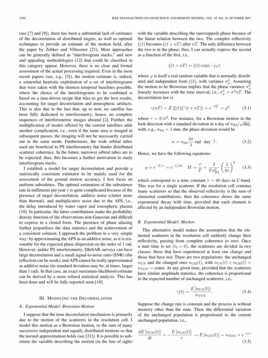
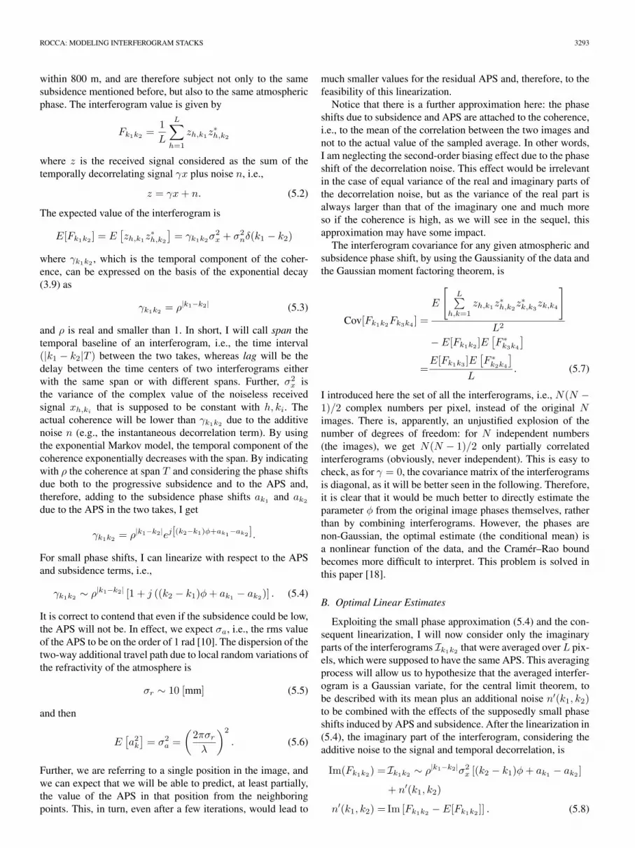
The parameters of the exponential models can be identifiedusing estimates of coherence. In the data sets that have beenexploited, the sampled estimate [14] has been applied to theinterferogram after removing the topographic contribution bymeans of a digital elevation model. The estimation window hasbeen made sufficiently large to minimize the bias of the estimate[19]. The result is a series of matrices, each of them represent-ing the correlation properties in a particular place in the scene(actually, the estimation window). Two examples are providedin Figs. 1 and 2. The images are arranged by the acquisitiondate (26 images are available), and each element in the matrixrepresents the coherence of a pair. The principal diagonal isalways unitary because every image is perfectly coherent withitself. In Fig. 2, it is easy to recognize three separate momentsin the scatterer’s “life.” To obtain the coherence as a functionof time separation, I take all the pairs in the data set, spanning

Fig. 2. Covariance matrices of Rome data, ordered with the acquisition dateand showing a Markovian behavior.

the same interval (for instance, all the pairs with a temporalbaseline of 15 days), and I average their coherence to make theestimates more robust, i.e.,

γ̂(nT ) =

∑t(k2)−t(k1)=nT γ̂(k1, k2)∑

t(k2)−t(k1)=nT 1(3.10)

where t(k) is the time of the kth acquisition. This is the inputto the next stage, which is the identification of the model.

The parameters of the model that can best justify the obser-vations can then be found. The identification process consists oftrying many combinations of the parameters and choosing thebest one according to some figure of merit Q. In this case, theL1 norm is minimized, i.e.,

Q(γ0, τ) =∑nT

∣∣∣γ̂(nT ) − γ0e−nT/τ

∣∣∣ . (3.11)

The sum is extended to all nT s for which an estimate γ̂(nT ) isavailable. The output of the identification step is the triple γ̂0,τ̂ , and Q(γ̂0, τ̂) for each processed window.

IV. VALIDATION WITH REAL DATA

The results discussed here are based on scenes from an ERS-1 ice-phase data set (Track 22, Frame 2763) that was acquiredover central Italy from the end of December 1993 to April1994 (26 scenes). During this acquisition phase, the revisit timeinterval was three days, whereas all the other orbital parame-ters remained basically unchanged. The images were focusedand oversampled by a factor of 2 (range only) and coregisteredon the master’s common grid (the image was taken on March 5,1994). Then, a portion of the entire scene was selected (20 ×15 km, range × azimuth). It is near the Fiumicino (Rome,Italy) airport and shows the last part of the Tevere Rivercourse. This C-band data set peculiarity stays with the reducedrevisit time, which is just three days. This characteristic is veryimportant in studying the decorrelation dynamics in the timespan of a few weeks: a task that is much harder with the morecommon 35-day data set. Although the maximum baselinespan is about 800 m, I chose to work with a reduced set of17 images in the range of ±250 m. This measure is an attemptto reduce the impact of geometric decorrelation. At the sametime, I applied spectral shift filtering in the range band common


Fig. 3. Map of the short-term coherence γ0.

Fig. 4. Map of the time constant τ .

Fig. 5. Histogram of the short-term coherence γ0, with and without spectralshift filtering.

to all images [8]. Approximately half the original bandwidthwas retained by this step, as one is limited by the worstcase (500 m).

A. Decorrelation Dynamics

Estimates have been made by spatial averaging on a 12 ×12 pixel window (range oversampled 2 : 1), and no overlapbetween any two windows was allowed to make every measureindependent. Figs. 3 and 4 show the maps for the short-termcoherence γ0 and for the estimated time constant τ . Thehistograms of the short-term coherence and the time constantτ , with and without spectral shift filtering, are shown in Figs. 5and 6.

The peak in the histogram is at about 40–50 days. As ex-pected, the coherence is increased if the common band-filteredimages are used, because a source of decorrelation is elimi-

Fig. 6. Histogram of the time constant τ , with and without spectral shiftfiltering.

nated. The histograms clearly indicate an increase in coherencewith filtering. The reason for not having any point with γ̂0 lowerthan 0.2 can be explained by the estimate bias discussed earlierin this paper. In fact, even for large time spans over totallydecorrelated areas, it would be usual to find coherence measureshigher than 0.15. Forcing an exponential model to explainsuch observations brings us to the conclusion that the “startingcoherence” γ̂0 must be greater than or equal to such a value.

B. Joint Distribution of the Estimates

The joint distribution of τ̂ and γ̂0 seemed to be separable,which makes the two parameters independent. To further ana-lyze the problem, I applied a singular value decomposition onthe matrix that approximates the joint probability density. If itwere a dyad, i.e., with a prevailing eigenvalue, the matrix wouldbe separable. In our case, the first eigenvalue is about ten timesthe second.

V. LINEAR ESTIMATES OF GROUND MOTION

A. Covariance Matrix of the Interferograms

In this section, I will deal with the approximate estimation ofthe progressive interferometric phase, namely, the subsidencevelocity correspondent to an additional phase shift φ that isidentical from one pass to the next. We have

φ =4πvTλ

(5.1)

where T is the interval between the takes, and λ is the wave-length. The interferogram is obtained by cross multiplyingtwo images at times k1T and k2T and then averaging over Lpixels. The removal of the scatterer’s phases is obtained bymultiplying one image times the conjugate of the other. Inthis derivation, I suppose that the baseline is systematicallyzero, and thus, I will not consider geometrical decorrelation.This impacts on the covariance of the decorrelation noiseas well, which is now dependent only on temporal decorre-lation. As the subsidence-induced phase shifts could creategeometrical decorrelation, if changing with the range, I haveassumed to have uniform subsidence in all the pixels to beconsidered. The value of L is determined by hypothesizing thatall pixels stay within the correlation radius of the APS, e.g.,


within 800 m, and are therefore subject not only to the samesubsidence mentioned before, but also to the same atmosphericphase. The interferogram value is given by

Fk1k2 =1L

L∑h=1

zh,k1z∗h,k2

where z is the received signal considered as the sum of thetemporally decorrelating signal γx plus noise n, i.e.,

z = γx + n. (5.2)

The expected value of the interferogram is

E[Fk1k2 ] = E[zh,k1z

∗h,k2

]= γk1k2σ

2x + σ2

nδ(k1 − k2)

where γk1k2 , which is the temporal component of the coher-ence, can be expressed on the basis of the exponential decay(3.9) as

γk1k2 = ρ|k1−k2| (5.3)

and ρ is real and smaller than 1. In short, I will call span thetemporal baseline of an interferogram, i.e., the time interval(|k1 − k2|T ) between the two takes, whereas lag will be thedelay between the time centers of two interferograms eitherwith the same span or with different spans. Further, σ2

x isthe variance of the complex value of the noiseless receivedsignal xh,ki

that is supposed to be constant with h, ki. Theactual coherence will be lower than γk1k2 due to the additivenoise n (e.g., the instantaneous decorrelation term). By usingthe exponential Markov model, the temporal component of thecoherence exponentially decreases with the span. By indicatingwith ρ the coherence at span T and considering the phase shiftsdue both to the progressive subsidence and to the APS and,therefore, adding to the subsidence phase shifts ak1 and ak2due to the APS in the two takes, I get

γk1k2 = ρ|k1−k2|ej[(k2−k1)φ+ak1−ak2 ].

For small phase shifts, I can linearize with respect to the APSand subsidence terms, i.e.,

γk1k2 ∼ ρ|k1−k2| [1 + j ((k2 − k1)φ + ak1 − ak2)] . (5.4)

It is correct to contend that even if the subsidence could be low,the APS will not be. In effect, we expect σa, i.e., the rms valueof the APS to be on the order of 1 rad [10]. The dispersion of thetwo-way additional travel path due to local random variations ofthe refractivity of the atmosphere is

σr ∼ 10 [mm] (5.5)

and then

E[a2k

]= σ2

a =(

2πσrλ

)2

. (5.6)

Further, we are referring to a single position in the image, andwe can expect that we will be able to predict, at least partially,the value of the APS in that position from the neighboringpoints. This, in turn, even after a few iterations, would lead to

much smaller values for the residual APS and, therefore, to thefeasibility of this linearization.

Notice that there is a further approximation here: the phaseshifts due to subsidence and APS are attached to the coherence,i.e., to the mean of the correlation between the two images andnot to the actual value of the sampled average. In other words,I am neglecting the second-order biasing effect due to the phaseshift of the decorrelation noise. This effect would be irrelevantin the case of equal variance of the real and imaginary parts ofthe decorrelation noise, but as the variance of the real part isalways larger than that of the imaginary one and much moreso if the coherence is high, as we will see in the sequel, thisapproximation may have some impact.

The interferogram covariance for any given atmospheric andsubsidence phase shift, by using the Gaussianity of the data andthe Gaussian moment factoring theorem, is

Cov[Fk1k2Fk3k4 ] =

E

[L∑

h,k=1

zh,k1z∗h,k2

z∗k,k3zk,k4

]L2

− E[Fk1k2 ]E[F ∗k3k4

]=E[Fk1k3 ]E

[F ∗k2k4

]L

. (5.7)

I introduced here the set of all the interferograms, i.e., N(N −1)/2 complex numbers per pixel, instead of the original Nimages. There is, apparently, an unjustified explosion of thenumber of degrees of freedom: for N independent numbers(the images), we get N(N − 1)/2 only partially correlatedinterferograms (obviously, never independent). This is easy tocheck, as for γ = 0, the covariance matrix of the interferogramsis diagonal, as it will be better seen in the following. Therefore,it is clear that it would be much better to directly estimate theparameter φ from the original image phases themselves, ratherthan by combining interferograms. However, the phases arenon-Gaussian, the optimal estimate (the conditional mean) isa nonlinear function of the data, and the Cramér–Rao boundbecomes more difficult to interpret. This problem is solved inthis paper [18].

B. Optimal Linear Estimates

Exploiting the small phase approximation (5.4) and the con-sequent linearization, I will now consider only the imaginaryparts of the interferograms Ik1k2 that were averaged over L pix-els, which were supposed to have the same APS. This averagingprocess will allow us to hypothesize that the averaged interfer-ogram is a Gaussian variate, for the central limit theorem, tobe described with its mean plus an additional noise n′(k1, k2)to be combined with the effects of the supposedly small phaseshifts induced by APS and subsidence. After the linearization in(5.4), the imaginary part of the interferogram, considering theadditive noise to the signal and temporal decorrelation, is

Im(Fk1k2) = Ik1k2 ∼ ρ|k1−k2|σ2x [(k2 − k1)φ + ak1 − ak2 ]

+ n′(k1, k2)

n′(k1, k2) = Im [Fk1k2 − E[Fk1k2 ]] . (5.8)


We indicate with n′(k1, k2) the random variate—real andzero mean—corresponding to the imaginary part of the inter-ferogram that is not dependent on APS or subsidence. Noticethat the variances of the real parts and the imaginary parts ofthe interferograms are different. For an intuitive confirmationof that, let us consider the case of no temporal decorrelation, nosubsidence, or no APS, i.e., a flat interferogram with coherencethat is equal to one. Although the phase and, therefore, theimaginary part of the interferogram is zero, the interferogramis a nonzero-mean random real variate, as it is the squaremodulus of a Gaussian variate. Hence, with good coherence,we expect, in general, many changes along the real partsof the interferograms and much smaller changes along theirimaginary parts.

Now, I construct a vector F with the imaginary parts of allthe N(N − 1)/2 interferograms, which were arranged usingthe first image in the interferograms first, then the second, etc.,without repetitions, as follows:

FT = [I12 I13 . . . I1N ; I23 I24 . . . I2N ; . . . IN−1,N ].(5.9)

Rather than indicate the entries of this vector with oneindex, for simplicity, I use the two indexes of the images thatcontributed to the interferogram. F is the sum of the threerandom vectors φM, (ak1 − ak2)A, and N, i.e.,

F = φM + (ak1 − ak2)A + N = φM + B

which is sorted like (5.9) and represents the following.1) φM is the progressive phase shifts, e.g., due to subsi-

dence, with entries φ(k1 − k2)ρ|k1−k2|σ2z .

2) (ak1 − ak2)A is the APS with entries (ak1 −ak2)ρ

|k1−k2|σ2z (for an easier check of the formulas).

3) N represents the contributions to the imaginary part ofthe interferograms due to instantaneous and progressivetemporal decorrelation. The covariance matrix relative toF is the sum of three covariance matrices, which arerelated to the three random vectors that have just beenintroduced. The matrix due to the random subsidence rateφ is a dyad, which is expressed by

E[φ2MM∗] → σ2φσ

4xρ

|k1−k2|+|k3−k4|(k1 − k2)(k3 − k4)

and that due to the APS is

E [(ak1−ak2)A(ak3−ak4)A∗]

= σ2aσ

4xρ

|k1−k2|+|k3−k4|(

+δ(k1−k2)+δ(k3−k4)−δ(k2−k4)−δ(k1−k3)

). (5.10)

It is possible to check that the entries of the correlationmatrix of the imaginary parts of the interferograms, without theadditional phase shifts due to APS or ground motion, are

E[NN∗]→

σ4x(γk1k2γk3k4 − γk1k4γk2k3)+

σ2xσ

2n

[+δ(k1 − k3)γk2k4 + δ(k1 − k4)γk2k3−δ(k2 − k4)γk1k3 − δ(k2 − k3)γk1k4

]+σ4

n (δ(k1−k3)δ(k2−k4)−δ(k1−k4)δ(k2−k3))2L

(5.11)

Fig. 7. Moduli of the interferogram weights as a function of time lags k1

and k2, k2 > k1: ρ = 0.74, γ0 = 0.6, and N = 30. Approximately five lagsare used.

For the real parts, the negative signs of the contributionsbecome positive, and thus, the sum is consistent with (5.7).The dispersion of the phases σ2

φ of an interferogram can beexpressed as the ratio between the dispersion of the imaginarypart over the squared mean as follows:

k1 = k3 k2 = k4 = k1 + 1 E[F ] = ρσ2x (5.12)

σ2φ =

1 − ρ2

2Lρ2(5.13)

which is consistent with [21] if σ2n is considered part of the

decorrelation mechanism. As mentioned before, for γ = 0,the covariance matrix E[FF∗] is diagonal, notwithstanding thedimensionality being much higher than the original data set.Notice that for N = 30 images, I have N(N − 1)/2 = 435interferograms, and this is the size of the covariance matrices.The optimal estimate of φ is a linear combination of theinterferograms weighted with the weight vector P∗, i.e.,

φ̂ = P∗F = P∗(φM + B).

The weights can be computed by imposing incorrelation be-tween the data (the interferograms) and the error, i.e.,

E [F(F∗P − φ)] = 0 (5.14)

By whitening the noise and imposing an unbiased estimate (i.e.,the limit of the previous one for σ2

φ → ∞), following [20], weare led to the following expression of the weight vector:

P =M∗Q−1

M∗Q−1MQ = E[BB∗]

which is represented in Fig. 7. The weight vector is representedas a function of the two indexes corresponding to the two takes;for this figure, the total number of takes is 30, and thus, thematrix is 30 × 30. However, the matrix is zero on and below themain diagonal, as the autointerferograms are irrelevant (pointson the main diagonal), and each interferogram is considered


only once. In the case of no instantaneous decorrelation, and noAPS, only the interferograms at span 1 (those on the first subdi-agonal) are used. The instantaneous decorrelation smoothes thismatrix. The APS induces smaller weights for the interferogramsat the beginning and the end of the takes, as the chaining ofthe interferograms (and, thus, the compensation of the APS) isbroken at both ends of the takes. Finally, the error variance is

limσ2

φ→∞

E[(φ− φ̂)2

]=

1M∗Q−1M

.

These equations will be revisited in Section V-C, in the cross-spectral domain, to simplify them and make them more directlyunderstandable. The final results will then be summarized inFig. 10.

Finally, before going further into the discussion, one hasto remember that the sample covariance matrix of the pixels,namely, the matrix of the cross correlations of the interfero-grams, as it is a sum of L dyads, has size N ×N and at mostrank L, whereas the sample covariance matrix of the inter-ferograms has size N(N − 1)/2 ×N(N − 1)/2 and rank 1.Therefore, one has to reduce the dimensionality of the problemto achieve some statistical estimate [13]. Indeed, one can alwaysintroduce spatiotemporal averaging procedures to augment therank of the matrices, but all averaging processes, unless datadependent and, therefore, nonlinear, hinder the identification ofPSs. Therefore, skillful averaging techniques should be found,where an optimal use is made of the temporal and spatial dimen-sions (like, e.g., averaging over seasons or target similarities).

C. Cross Spectra of Interferogram Sequences

I can simplify the problem by considering sequences of inter-ferograms F (p)

m with a given span 2p; the index m correspondsto the center time of the interferogram. The previously givenformulas simplify, in a symmetrical presentation, to

m =k1 + k2

2n =

k3 + k4

2

p =k2 − k1

2q =

k4 − k3

2, p, q > 0 (5.15)

where the indexes n and q correspond to the center time andspan 2q of the second interferogram, respectively.

By indicating further the lag between two interferogramswith l and with h and k the values

l = n−m h =p− q

2k =

p + q

2

we have

k1 = m− p k1 − k4 = l − 2k · · ·

and we gain the following simple relation:

L

σ4x

Cov[F (q)m F

(p)m+l

]= ρ2max(|l|,|h|) +

2δ(l)SNR

+δ(l)δ(h)

SNR2 .

(5.16)

Therefore, the complex covariance of two interferograms de-pends only on their lag l and on the span difference. The

covariances of the real and imaginary parts depend also onthe span sum. To find the estimator, rather than studying thecross correlations of the interferograms in the span and lagdomains, I look at their cross spectra, particularly at their low-frequency components that will be amplified by the interfero-gram stacks. As interferogram stacking is the low-pass filteringof the interferogram sequence, I move to the spectral domain,and I indicate with ψ the Fourier conjugate of the interferogramcenter times m and n. In this way, the analysis will be simplifiedas the interferograms center times m and n and the lags l =n−m disappear and instead of the initial four indexes (namely,the current ones k1, k2, k3, and k4 or the symmetrized ones, i.e.,lags and spans m, n, p, and q), we have just the two spans, i.e., pand q, and some behavior with the frequency ψ. As always, wesuppose that ρN ∼ 0, i.e., that the sequence is much longer thanthe decorrelation time. APS and temporal decorrelation effectsdecouple, allowing a general simplification.

The correlation between the zero-frequency components ofthe cross spectra of the imaginary parts of the interferogramsthat have spans p and q is indicated with Ndec,pq(ψ = 0). Thiscomponent of the cross spectrum is the sum of all the lags ofthe autocorrelation function (or mutual correlation function) ofthe imaginary parts between the interferograms at spans p andq. The sum is finite due to the previous hypothesis on the finitedecorrelation time. The elements of the cross-spectral matrixof the imaginary parts of the interferograms at zero frequencydepend on the difference and the sum of their spans (the lagsare averaged out) and are

2LNdec,pq(ψ = 0)σ4x

= ρ2|p−q|(

2|p− q| + 1 + ρ2

1 − ρ2

)− ρ2|p+q|

(2|p + q| + 1 + ρ2

1 − ρ2

)

+2(ρ2|p−q| − ρ2|p+q|)

SNR+

δ(p− q)SNR2 .

(5.17)

The cross spectra of the atmospheric perturbations at very lowfrequencies (at zero frequency, they are zero) are calculated asfollows. The atmospheric noise contribution correlation comesfrom terms like

σ4zσ

2aρ

2p+2q [(am−p − am+p)(an−q − an+q)] .

The cross correlations of the atmospheric contributions betweeninterferograms with spans p and q, termed ratm,pq(l), are in thecenter time domain, and for lag l, we have

ratm,pq(l) = σ4xσ

2aρ

2(p+q) [δ(l − 2h)

+ δ(l + 2h) − δ(l − 2k) + δ(l + 2k)] .

By Fourier transforming in ψ, we derive

Natm,pq(ψ)= ρ4kσ4xσ

2a(e

−j2ψh + ej2ψh − e−j2ψk − e−j2ψk)

= 2ρ4kσ4xσ

2a(cos 2ψh− cos 2ψk)


and approximating for low frequencies, we have

Natm,pq(ψ) = 4ρ4kσ4xσ

2aψ

2(k2 − h2)

= 4pqρ2(p+q)σ4xσ

2aψ

2, ψ � 1.

Hence, the cross-spectral matrix of the APS contribution at lowfrequencies is a dyad that increases with ψ2. Finally, the signalcomponents are expressed by

Nsig,pq(ψ) = 4pqρ2(p+q)σ2φσ

4xδ(ψ)

i.e., the same dyad but with a delta-like frequency behaviorinstead of ψ2 for the atmosphere. The estimate of the interfer-ometric phase φ in the presence of this colored noise can becarried by averaging over N samples of the interferograms, i.e.,windowing the spectrum. I approximate this windowing with anideal filter in the band as follows:∣∣∣∣ψN2

∣∣∣∣ < π

2→ |ψ| < π

N.

If the decorrelation time is much shorter than the integrationtime NT , then in the band of the filter, the cross spectrum of thedecorrelation can be considered as a constant. In conclusion, theentries of the cross-spectral matrices of the different sources ofnoise that are integrated in this band are indicated with N dec,pq,N atm,pq and are given by

2LNπσ4

x

N dec,pq = ρ2|p−q|(

2|p− q| + 1 + ρ2

1 − ρ2

)− ρ2|p+q|

(2|p + q| + 1 + ρ2

1 − ρ2

)

+2(ρ2|p−q| − ρ2(p+q)

)SNR

+δ(p− q)

SNR2

N

π

N atm,pq

σ4x

∼ 43

( π

N

)2

σ2apqρ

2(p+q). (5.18)

The signal vector s has the following components:

φsp = 2ρ2ppφσ2x sT = σ2

x[ρ, 2ρ2, 3ρ3, . . .].

The interferogram cross-spectral vector Ip (in slanted char-acters; its version in the time domain was in calligraphiccharacters) is now the vector of the interferogram stacks at spanp, and rather than N(N − 1)/2, it has a much smaller size Ncs,which corresponds to the maximum span to be used for theestimation, e.g., 5. Thus, we have

1 ≤ p ≤ Ncs < N

Ip = [I1, I2, . . . INcs ]

E[II∗] =N = N dec + N atm + σ2φss

∗. (5.19)

There is a misconception here that should be identified. Ifwe have N images, we have N − 1 samples of the 1 spaninterferogram sequence, but only one sample of the N − 1span interferogram sequence. To have the cross spectra of the

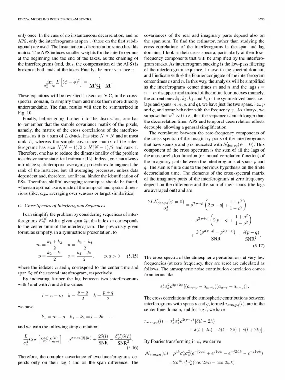
Fig. 8. Interferogram stack weights as a function of the lag: ρ = 0.74, SNR =1.5, and N = 30.

windowed sequences, we need an equal number of samples forthe sequences of interferograms at all spans p ≤ Ncs, and thisis what we do not have. However, as Ncs < N because thedecorrelation time for distributed scatterers is, in general, muchshorter than the observation time, this error in the cross-spectralanalysis is not very significant. Anyway, the previous analysisin the time domain does not have this problem. Proceeding asbefore, the unbiased optimal estimate of the subsidence rateleads to the following expression of the error:

E[(φ− φ̂)2

]=

1s∗(N dec + N atm)−1s

.

Then, exploiting the fact that

N atm =σ2a

3

( π

N

)3

ss∗ (5.20)

and using the matrix inversion lemma, I have

E[(φ− φ̂)2

]=

13

( π

N

)3

σ2a +

π

2LN1

s∗N −1decs

(5.21)

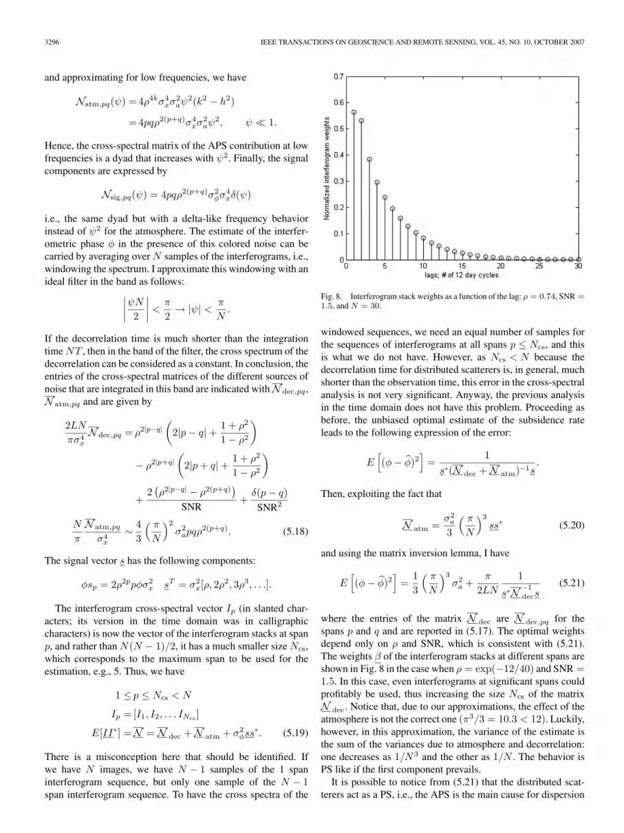
where the entries of the matrix N dec are N dec,pq for thespans p and q and are reported in (5.17). The optimal weightsdepend only on ρ and SNR, which is consistent with (5.21).The weights β of the interferogram stacks at different spans areshown in Fig. 8 in the case when ρ = exp(−12/40) and SNR =1.5. In this case, even interferograms at significant spans couldprofitably be used, thus increasing the size Ncs of the matrixN dec. Notice that, due to our approximations, the effect of theatmosphere is not the correct one (π3/3 = 10.3 < 12). Luckily,however, in this approximation, the variance of the estimate isthe sum of the variances due to atmosphere and decorrelation:one decreases as 1/N3 and the other as 1/N . The behavior isPS like if the first component prevails.

It is possible to notice from (5.21) that the distributed scat-terers act as a PS, i.e., the APS is the main cause for dispersion


of the subsidence rate estimate if the number of looks isgreater than

LPS =3

2π2

N2

σ2a

1s∗N−1

decs. (5.22)

If M is the number of revisits during the decorrelation timeconstant, i.e., from (3.3), we have

M =τ

T= − 1

log ρ(5.23)

it so happens that it results approximately to

s∗N−1decs ∼ 0.2M + γ0 − 1 = 0.2M − 1

1 + SNR. (5.24)

Then, the still rather complex formula (5.22) can be approx-imated with the following very simple one, even frequencyindependent, as it will be seen in the last section. To avoid(in)significant figures, then, if T is the repeat time in weeks,we have

LPS ∼ 0.75N2

Mσ2a

= 0.1N2T [in weeks]. (5.25)

1) Discussion: The result in (5.25) is reasonable in that thedispersion of the estimate of the subsidence rate decreaseswith N3 in the case of a PS. In the case of L distributedscatterers decorrelating in M revisits, we combine sequencesof N interferograms at M spans, on L pixels, and thus, thedispersion may well decrease with MNL. Then, to makethe two behaviors equivalent, one needs L increasing withN2/Mσ2

a. In our case, Mσ2a ∼ 3. This model, very crude and

overestimating LPS as the atmospheric contribution is verysmall, still captures the interesting behavior of LPS versusfrequency, as will be seen in Section VII. In fact, as long asthe product Mσ2

a is slowly varying with λ, the frequency willminimally create an impact on LPS. Further, it is easy to checkthat with a high SNR, one span suffices, and the others be-come redundant, as the unique source of noise is decorrelation.This corresponds to, e.g., the observation that the inverse ofa Toeplitz exponential matrix is tridiagonal, or that with first-order Markov processes, the memory to use for estimations isas short as possible. With a lower SNR, more spans are useful.Anyway, with the expected spatial resolution of 5 × 20 m, weexpect well more than 50 independent APS measurements persquare kilometer, which is not bad at all. This would allowa good estimate of the APS, its reduction, and, therefore, thejustification of the assumptions made, entering the PS regimeand yielding a further reduction of the dispersion of the velocityestimate.

D. Unbiased Estimates of Sinusoidal Motion Processes

The linear approximation that I have used allows to extendthe evaluation of the error to any motion, and it is not neces-sarily relative to a constant subsidence rate. It is enough to use,

Fig. 9. Noise level as a function of the temporal frequency, which is normal-ized to the seasonal variation.

as vector to be estimated, a sinusoidal change with time, at anygiven pulsation ψh. In this case, the vector φM becomes

φM = φh(ejk1ψh − ejk2ψh) ψh =2πN

h; h = 1, . . . , N.

The unbiased minimum variance estimate of the component ofthe motion φh at pulsation ψh is found with the same methodol-ogy as before, i.e., following the unbiased estimator that Caponuses for his spectral analysis [20]. In Fig. 9, I show the error asa function of the frequency, which is normalized to a seasonalvariation, in the case of 30 images per year and 50 looks.The behavior ramps up between 0.5 and 0.25 cycles/year. Forzero frequency, the dispersion is unlimited: a constant phase isirretrievable. As the noise due to temporal change is correlatedand, thus, low-pass, faster motions are less affected.

VI. PS INTERFEROMETRY

In PSs, the target is assumed to be a stable point scatterer.The sole meaningful information is then its complex amplitudein the nominal target location. The contribution due to thesubsidence for the nth image is

zn = |A| exp jψ exp(j4πλvnT

)+ wn (6.1)

where A is the amplitude of the scatterer, wn is the noisecontribution that mainly accounts for thermal noise, clutter, and(small) target decorrelation, and ψ is the intercept, i.e., the off-set in the subsidence linear law that is combined with the phaseof the scatterer. In PS interferometry, I assume that the am-plitude of the target’s return is much larger than the noise,so that I may approximate the phase of each single obser-vation as

∠zn = ψ +4πλvnT + φcn (6.2)

where φcn is a zero-mean normal noise that accounts for clutter,thermal noise, and target long-term coherence. Its variance is


half the ratio of the peak power of the target in the SLC SARimage to the noise power, i.e.,

σ2c =

σ2wn

2A2=

SNR−1s

2.

If I assume that phases due to APS are zero-mean normallydistributed, I get the following model:

∠zn =ψ +4πλvnT + φcn + φan + φtn (6.3)

=ψ +4πλvnT + φwn (6.4)

where φan is the APS noise. In (6.4), I have added all thenoise contributions in a single one, i.e., φwn , which is still zero-mean normal, and its variance is the superposition of all thecontributions, which is given as follows:

σ2w = σ2

c + σ2a + σ2

t .

Model (6.4) is the one assumed for estimating the subsidencerate v. Notice that the intercept ψ is a nuisance parameter in thesense that I do not explicitly require its estimate. Model (6.4)can be solved by linear regression. As a simple example, if Iassume N = 30 data takes, i.e., a one-year span, assuming aGMES-Sentinel 1 (GS1) d = 12 days repeat interval, I get thefollowing subsidence rate error:

σvp� λ

4π365d

σφ

√12

N3 −N� 3.6 mm/year (6.5)

σφ =√σ2a + σ2

SNR =

√(2πσrλ

)2

+1

2 · SNR(6.6)

where σφ is the phase dispersion of the PS and is due to thecontribution σ2

a of the APS, as σr = 10 mm is the two-waytravel path dispersion due to atmospheric effects (5.5) and (5.6)and to the phase dispersion due to SNR

σ2SNR � 1

2 · SNR. (6.7)

This last contribution is the cause of the higher dispersion atlonger carrier wavelengths (e.g., P-band). I have assumed forthe PS that usually have higher radar cross section that SNR→ 10 dB. Expression (6.3) is the fundamental one to be usedfor assessing the accuracy of the subsidence rate estimationin PS interferometry. Notice that this result accounts for anisolated PS, and I am not considering the possibility of abatingthe atmospheric noise by averaging its estimate on neighboringPSs. Further, the problem of phase unwrapping has not beenapproached. However, it is very unlikely to occur if the standarddeviation of the error is quite lower than π: in any case, ignoringunwrapping errors will give a lower bound on the rate estimate.

VII. EXTENSION OF THE MODEL TO

DIFFERENT FREQUENCIES

One advantage of the model that has been considered is thepossibility of its extension to different carrier wavelengths λ.

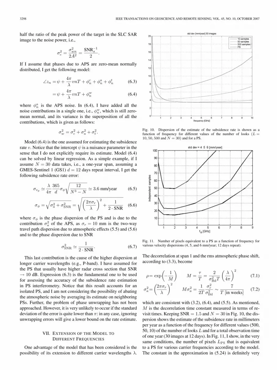
Fig. 10. Dispersion of the estimate of the subsidence rate is shown as afunction of frequency for different values of the number of looks (L =10, 50, 500 and N = 30) and for a PS.

Fig. 11. Number of pixels equivalent to a PS as a function of frequency forvarious velocity dispersions (4, 5, and 6 mm/year; 12 days repeat).

The decorrelation at span 1 and the rms atmospheric phase shift,according to (3.3), become

ρ= exp(− 1M

)M =

τ

T=

2σ2

BdT

(λ

4π

)2

(7.1)

σ2a=

(2πσrλ

)2

Mσ2a =

12T

σ2r

σ2Bd

∼ 7T [in weeks]

(7.2)

which are consistent with (3.2), (6.4), and (5.5). As mentioned,M is the decorrelation time constant measured in terms of re-visit times. Keeping SNR = 1.5 and N = 30 in Fig. 10, the dis-persion shows the estimate of the subsidence rate in millimetersper year as a function of the frequency for different values (500,50, 10) of the number of looks L and for a total observation timeof one year (30 images at 12 days). In Fig. 11, I show, in the verysame conditions, the number of pixels LPS that is equivalentto a PS for various carrier frequencies according to the model.The constant in the approximation in (5.24) is definitely very


high, but it captures the behavior of the broad minimum with thefrequency. I see from these figures that L = 100, for instance, isclose enough to ensure that, with 12 days repeat and 30 revisits,the average coherence is enough to enter the PS regime (1/N3),so that the atmospheric effect is prevailing, and there is no ap-preciable change with the carrier frequency. Indeed, higher car-rier frequencies behave worse, but practically big changes arenot to be expected until 8–10 GHz. On the very low frequencyside, the increment of the dispersion is due to the limited SNR,also as expected. With longer observation times, there would bea shift of the optimum toward lower frequencies while keepingthe variation of the dispersion of the estimate rather small. Interms of the area APS to be occupied by the distributed scatter-ers to look like a PS, indicating with δ the spatial resolution, wecan use (5.23) to say that APS is approximately independent ofthe frequency, as what is lost with M is gained with σa, i.e.,

APS =0.75σ2a

N2

Mδ2

=1.5N2δ2σ2BdT

σ2r

∼0.1N2T [in weeks] δ2. (7.3)

Further, as we can expect the resolution to improve with thecarrier frequency, we can expect this area to decrease.

VIII. CONCLUSION

An evaluation of the subsidence rate error budget has beencarried out for DInSAR interferometry using the three-day re-visit interval data of ERS-1 over Rome. The results of modelingtemporal decorrelation with a Brownian motion depend uponthe number N of successive images used and the revisit intervalT in weeks. Assuming a short-term target coherence of 0.6and averaging measures over L = 100 independent looks, thedispersion of the velocity estimate is lower than 4–4.5 mm/year.For a wide band of frequencies, including C-band, the numberof looks needed to make distributed scatterers as accurate as aPS is approximately on the order of 0.1N2T [in weeks].

ACKNOWLEDGMENT

The author would like to thank Dr. F. De Zan, Prof. A. M.Guarnieri, and Dr. S. Tebaldini for helpful discussions andnumerous contributions. Dr. De Zan carried out the analysesof the three-day Rome data. The author would also like tothank the reviewers for their very patient work, which helpeda lot in increasing the readability of this paper, correcting manymistakes, and improving my notation.

REFERENCES

[1] R. Bamler and P. Hartl, “Synthetic aperture radar interferometry,” Inv.Probl., vol. 14, no. 4, pp. R1–R54, 1998.

[2] P. M. L. Drezet and S. Quegan, “Environmental effects on the interfer-ometric repeat-pass coherence of forests,” IEEE Trans. Geosci. RemoteSens., vol. 44, no. 4, pp. 825–837, Apr. 2006.

[3] A. Ferretti, C. Prati, and F. Rocca, “Permanent scatterers in SAR inter-ferometry,” IEEE Trans. Geosci. Remote Sens., vol. 39, no. 1, pp. 8–20,Jan. 2001.

[4] A. Ferretti, D. Perissin, C. Prati, and F. Rocca, “On the physical nature ofSAR permanent scatterers,” in Proc. URSI Commission F Symp. Microw.Remote Sens. Earth, Oceans, Ice and Atmosphere, Ispra, Italy, Apr. 20–21,2005, p. 6.

[5] Y. Fialko, “Interseismic strain accumulation and the earthquake potentialon the southern San Andreas fault system,” Nature, vol. 441, no. 7096,pp. 968–971, Jun. 2006.

[6] G. Franceschetti and G. Fornaro, “Synthetic aperture radar interferom-etry,” in Synthetic Aperture Radar Processing, G. Franceschetti andR. Lanari, Eds. Boca Raton, FL: CRC Press, 1999, ch. 4, pp. 167–223.

[7] A. K Gabriel, R. M Goldstein, and H. A Zebker, “Mapping small elevationchanges over large areas: Differential radar interferometry,” J. Geophys.Res., vol. 94, no. B7, pp. 9183–9191, Jul. 10, 1989.

[8] F. Gatelli, A. Monti Guarnieri, F. Parizzi, P. Pasquali, C. Prati, andF. Rocca, “The wavenumber shift in SAR interferometry,” IEEE Trans.Geosci. Remote Sens., vol. 32, no. 4, pp. 855–865, Jul. 1994.

[9] R. M. Goldstein and H. A. Zebker, “Interferometric radar measure-ment of ocean surface currents,” Nature, vol. 328, no. 20, pp. 707–709,Aug. 1987.

[10] R. F. Hanssen, Radar Interferometry: Data Interpretation and ErrorAnalysis. Dordrecht, The Netherlands: Kluwer, 2001.

[11] R. F. Hanssen, “Satellite radar interferometry for deformation monitor-ing: A priori assessment of feasibility and accuracy,” Int. J. Appl. EarthObservation and Geoinformation, vol. 6, no. 3/4, pp. 253–260, Mar. 2005.

[12] A. Hooper, H. Zebker, P. Segall, and B. Kampes, “A new method formeasuring deformation on volcanoes and other natural terrains usingInSAR persistent scatterers,” Geophys. Res. Lett., vol. 31, no. 23, L23611,2004. DOI:10.1029/2004GL021737.

[13] O. Ledoit and M. Wolf, “Honey, I shrunk the sample covariance matrix,”J. Portf. Manage., vol. 31, no. 1, Fall 2004.

[14] F. Rocca, C. Prati, P. Pasquali, and A. Monti Guarnieri, “SAR interfer-ometry techniques and applications,” ESA, Noordwijk, The Netherlands,Tech. Rep. 7439/92/HGE-I, 1994.

[15] F. Rocca, “Diameters of the orbital tubes in long-term interferometricSAR surveys,” IEEE Geosci. Remote Sens. Lett., vol. 1, no. 3, pp. 224–227, Jul. 2004.

[16] P. Rosen, S. Hensley, I. R. Joughin, F. K. Li, S. Madsen, E. Rodríguez,and R. Goldstein, “Synthetic aperture radar interferometry,” Proc. IEEE,vol. 88, no. 3, pp. 333–382, Mar. 2000.

[17] Sentinel-1 MRD. [Online]. Available: http://esamultimedia.esa.int/docs/GMES/GMES_SENT1_MRD_1-4_approved_version.pdf

[18] S. Tebaldini and A. Monti Guarnieri, “Cramér–Rao lower bound forparametric phase estimation in multi-pass radar interferometry,” Analysisof Ambiguity Noise in the Sentinel-1 Interferometric Wideswath Mode.Personal Communication, Final report, ESA Contract 19142/05/NL/CB.

[19] R. Touzi, A. Lopes, J. Bruniquel, and P. W. Vachon“Coherence estimationfor SAR imagery,” IEEE Trans. Geosci. Remote Sens., vol. 37, no. 1,pp. 135–149, Jan. 1999.

[20] H. Van Trees, Optimum Array Processing. New York: Wiley-Interscience, 2002.

[21] H. A. Zebker and J. Villasenor, “Decorrelation in interferometric radarechoes,” IEEE Trans. Geosci. Remote Sens., vol. 30, no. 5, pp. 950–959,Sep. 1992.

Fabio Rocca received the Dottore degree in ingeg-neria elettronica from Politecnico di Milano, Milano,Italy, in 1962.

He is currently a Professor of digital signalprocessing with the Dipartimento di Elettronica edInformazione, Politecnico di Milano, Milano, Italy.He made research on digital signal processing fortelevision bandwidth compression, emission tomog-raphy, seismic data processing, and SAR. During1978–1988, he was a Visiting Professor at StanfordUniversity, Stanford, CA. He was a Department

Chair of the Istituto di Elettrotecnica ed Elettronica of the Politecnico di Milanoduring 1975–1978, a Cofounder of two small technological spin-off companiesfrom Politecnico di Milano, namely Telerilevamento Europa and Aresys, a pastPresident of the European Association of Exploration Geophysicists (EAEG),an Honorary Member of Society of Exploration Geophysicists (SEG) in 1989and European Association of Geoscientists and Engineers (EAGE) in 1998, thePresident of the Istituto Nazionale di Oceanografia e di Geofisica Sperimentale(OGS) Trieste during 1982–1983, a member of the Scientific Council of OGS,and a member of the SAR Advisory Group of the European Space Agency.

Dr. Rocca received an award from Italgas Telecommunications in 1995, aSpecial SEG Commendation in 1998, the Eduard Rhein Foundation Technol-ogy Award in 1999, and the Doctorat Honoris Causa in Geophysics, InstitutNational Polytechnique de Lorraine, Nancy, France, in 2001. He also receivedbest paper awards at the International Geoscience and Remote Sensing Sympo-sium in 1989 and 1999 and at the European Conference on Synthetic ApertureRadar in 2004.

modeling interferogram stacks

Documents