arX

iv:c

ond-

mat

/040

3706

v1 [

cond

-mat

.dis

-nn]

29

Mar

200

4 Memory effects in classical and quantum

mean-field disordered models

L. F. Cugliandolo1,2, G. Lozano3 and H. Lozza3

1 Laboratoire de Physique Theorique de l’Ecole Normale Superieure,

24 rue Lhomond, 75231 Paris Cedex 05, France

2 Laboratoire de Physique Theorique et Hautes Energies, Jussieu,

1er etage, Tour 16, 4 Place Jussieu, 75252 Paris Cedex 05, France

3 Departamento de Fısica, FCEyN, Universidad de Buenos Aires,

Pabellon I, Ciudad Universitaria, 1428 Buenos Aires, Argentina

February 2, 2008

Abstract

We apply the Kovacs experimental protocol to classical and quantum p-spin models. We show that these models have memory effects as those ob-served experimentally in super-cooled polymer melts. We discuss our resultsin connection to other classical models that capture memory effects. We pro-pose that a similar protocol applied to quantum glassy systems might be usefulto understand their dynamics.

1

1 Introduction

The Kovacs memory effect was first reported by this author in the 60s [1]. It

demonstrates that super-cooled liquids when taken out of equilibrium have a very

intricate dynamics that cannot be predicted on the basis of the knowledge of the

instantaneous value of the state variables (P, V, T ) right after the perturbation. More

precisely, Kovacs showed that the specific volume of a polymer melt in its super-

cooled liquid phase, has a rather non-trivial evolution that depends on the thermal

history of the sample [1, 2]. Non-trivial effects of temperature variations were also

observed in the evolution of (two-time) susceptibilities of dipolar glasses [3], spin-

glasses [4] and many other glassy systems [5, 6]. History-dependent phenomena

in granular compaction have been recently reported [7]. In this case, the control

parameter is the tapping strength and the observable is the density.

The experimental setup involved in the Kovacs effect is the following. In a first

step, one quenches an equilibrated liquid with a very fast cooling rate from a high

temperature T0 to a low temperature T2, at time t = 0. One then follows the

subsequent evolution of the quantity of interest that in Kovacs’ experiments is the

specific volume. In order to match what we shall study in this paper, we describe

the experiment using another one-time quantity, the energy density, as the example.

The energy density relaxes in time and it slowly approaches an asymptotic value

that may fall out of the experimental time-window. The time-dependent curve

E (T2)(t) constitutes a reference and we use a superscript (T2) to indicate that it has

been obtained using the first prescription, at fixed external temperature T2. The

extrapolated asymptotic value defines Eas(T2). In a second step, one first quenches

the sample from the same high temperature T0 to a lower temperature T1(< T2)

at time t = 0, waits until a carefully chosen time t1 and then heats the sample

to the final temperature T2. The value of t1 is chosen such that E (T1→T2)(t+1 ) =

Eas(T2), where the plus sign indicates that the one-time quantity should match the

asymptotic value obtained with the first procedure right after heating the sample

from T1 to T2. [In the experimental protocol the need to use E (T1→T2)(t+1 ) = Eas(T2)

is due to the fact that when changing the temperature there is a trivial response

due to the thermal expansion of the local degrees of freedom.] Since the initial

value of the energy density at the final temperature T2 is already the asymptotic

one, one could have expected that the energy remained constantly fixed to this

value for all subsequent times independently of the value of T1 (apart from very fast

rearrangements decaying exponentially). However, Kovacs demonstrated that after

2

t1 the energy-density, E (T1→T2)(t), has a slow non-monotic dependence on time, first

increasing and then decreasing back to its initial and asymptotic value Eas(T2):

E (T1→T2)(t) = Eas(T2) + ∆E(t) , (1)

with the “Kovacs hump” ∆E satisfying

∆E(t) > 0 , ∆E(t+1 ) = limt→∞

∆E(t) = 0 . (2)

The form of the hump depends on the values T2 and T1 used. Qualitatively, its

height is an increasing function of T2 − T1 and the time at which the maximum is

reached decreases when T2 − T1 increases.

It is interesting to note that Kovacs’ experiments have been performed in the

super-cooled liquid phase. While it would be no surprise to find nonequilibrium

effects in the glassy phase, the reason why one also finds a nonequilibrium behaviour

in the super-cooled liquid is that the jump in the external temperature drives the

system out of equilibrium and the relaxation occurs in a very long time-scale. This

experiment proves that the knowledge of the state variables, in Kovacs’ experiments

P, V and T at t+1 , is not sufficient to determine the subsequent evolution of the

same quantities in the glassy and super-cooled liquid phases (if the latter has been

recently strongly perturbed).

Recently, several authors presented analytical and numerical studies of this effect

using a variety of models with glassy dynamics. So far, apart from phenomenological

approaches [2], the Kovacs effect has been analysed numerically with molecular

dynamic simulations of a molecular model of a fragile glass former [8] and Montecarlo

simulations of the 3d Edwards-Anderson spin-glass [9], and analytically within the

ferromagnetic Ising chain [10], the critical 2d xy model [11], the trap model [12],

domain growth [12], 1d kinetically constrained spin models of fragile and strong

type [13], and the parking lot model of granular matter [14]. It has been suggested

that the quantitative analysis of the Kovacs effect may help distinguishing between

different glassy models and, perhaps, may also help identifying spatial properties

of glassy systems. In this paper we show that the main qualitative features of the

classical Kovacs effect are captured by the fully connected spherical p-spin disordered

system [15], a model with no spatial structure but with a slow dynamics leading to

very slow relaxations close to the transition to and in the glassy phase [16, 17].

This ‘negative’ result, as far as what can be deduced about spatial rearrangements

from the Kovacs effect, is reminiscent of the discussion [18] on the interpretation of

3

hole burning experiments [19]. We also discuss the scaling laws that describe the

behaviour of the hump and compare them to what found in other glassy models.

On the other hand, the analysis of quantum glassy systems is now starting to

call the attention of experimentalists and theoreticians. The slow, history-dependent

relaxation of a dipolar quantum system in its glassy phase has been reported [20].

The sample that entered the glassy phase following a quantum route (changing the

strength of quantum fluctuations at fixed low temperature) is always in advance

with respect to the one that arrived at the same point in parameter space following

a classical path (keeping the strength of quantum fluctuations fixed and cooling the

system). This has been demonstrated by the fact that the time-dependent dielectric

constant of the quantum-cooled sample is closer to its asymptotic value at any

finite, experimental time. Memory effects were also observed in glasses at ultralow

temperatures [21] and the electron glass [22].

A variant of the Kovacs procedure where the control parameter is the strength

of quantum fluctuations can be easily envisaged. The question then arises as to

whether a hump appears and which is its structure, scaling form, etc. We address

this question using a quantum extension of the p-spin model introduced and studied

in [23, 24] (see also [25]).

In short, in this paper we show that simple disordered mean-field models capture

the phenomenology of the Kovacs effect. With this aim, we analyse the nonequi-

librium relaxation of the spherical p-spin disordered model in its classical [16, 17]

and quantum [23] versions, see Sect. 2 for their definitions. First, we reproduce the

classical setup using temperature as the control parameter and we discuss the re-

sults in comparison with previous explanations of the same effect (Sect. 3). Second,

we switch on quantum fluctuations and use their strength as the control parameter

(Sect. 4). In both cases we follow the evolution in time of the potential energy-

density of the system. We present our conclusions in Sect. 5.

2 The spherical p-spin model

The spherical p spin model is defined by the Hamiltonian [15]

HJ [~S] = −∑

〈i1i2...ip〉

Ji1i2...ipsi1si2 . . . sip . (3)

The spins si are continuous variables si ∈ (−∞,∞) forced to satisfy the global

spherical constraint∑N

i=1 si = N with N their total number in the sample. The

4

exchange interaction Ji1i2...ip are quenched random variables drawn from a Gaus-

sian distribution with average [Ji1...ip ] = 0 and variance [J2i1...ip] = J2p!/(2Np−1).

We henceforth use square brackets to indicate the average over disorder. The in-

teractions occur between all groups of p spins in the sample. The model is then

fully-connected and mean-field in character. The scaling of the variance [J2i1...ip ] with

N has been chosen so as to ensure a good thermodynamic limit. The parameter p

takes integer values, p ≥ 2. Mixed models with a Hamiltonian with two terms of

the form (3) with p = 2 and p = 4 [26] are also of interest [17].

The classical dynamics is determined by the Langevin equation

si(t) = −∂E(t)

∂si(t)− µ(t)si(t) + ξi(t) (4)

where E(t) is the total energy, µ(t) is the Lagrange multiplier enforcing the spherical

constraint, and ξi(t) is a Gaussian white-noise with zero mean and correlations

〈ξi(t)ξj(t′)〉 = 2kBTδijδ(t − t′) . (5)

We assume that the system is prepared at t = 0 with an infinitely fast quench from

T0 → ∞ to the initial temperature T1. The dynamic equations for the macroscopic

order parameters are derived using standard functional techniques [17]. We discuss

them below, as the classical limit of the quantum extension of the same model. The

models with p = 2, p ≥ 3 have different dynamics; the former yields a mean-field

description of simple domain growth, while the latter case is related to the schematic

mode-coupling theory (mct) of super-cooled liquids and glasses. These models and

their generalizations are reviewed in detail in [17].

Quantum fluctuations can be introduced [23] by upgrading the spins si to coordinate-

like operators, adding a ‘kinetic term’

1

2M

N∑

i=1

Π2i (6)

to the Hamiltonian (3), and imposing canonical commutation relations

[Πi, sj ] = ih δij , [si, sj] = 0 , [Πi, Πj] = 0 . (7)

At time t = 0 we set the model in contact with an Ohmic bath of quantum harmonic

oscillators

Hb =N∑

l=1

1

2mlp2

l +N∑

l=1

1

2mlω

2l x

2l , (8)

Hsb = −N∑

i=1

szi

N∑

l=1

cilxl , (9)

5

where, for simplicity, we considered a bilinear coupling, Hsb. (Note that for the

spherical problem it is not necessary to introduce a counterterm). We assume that

this environment has a well-defined temperature and that it is not modified by

the interaction with the system. The initial density matrix is factorised and we

choose random initial conditions for the system. After integrating out the bath

degrees of freedom, and using the fully-connected character of (3), one arrives at a

dynamic generating functional from which one derives exact dynamic equations for

the macroscopic two-time dependent order parameters

C(t, t′) =1

N

N∑

i=1

[〈{si(t), si(t′)}〉] , R(t, t′) =

1

N

N∑

i=1

[〈si(t)〉]

hi(t′)

∣

∣

∣

∣

∣

h=0

. (10)

h is an infinitesimal field that couples linearly to the spins, modifying the Hamilto-

nian as H → H −∑

i=1 hisi. C is the symmetrized correlation function and R is the

linear response of the system.

The dynamic equations take the Schwinger-Dyson form

[M∂2t + µ(t)] R(t, t′) = δ(t − t′) +

∫ t

t′dt′′ Σ(t, t′′)R(t′′, t′) , (11)

[M∂2t + µ(t)] C(t, t′) =

∫ t

0dt′′ Σ(t, t′′)C(t′′, t′) +

∫ t′

0dt′′ D(t, t′′)R(t′, t′′) ,(12)

with the self-energy Σ and the vertex D given by

Σ(t, t′′) = −4η(t − t′) + σ(t, t′) , (13)

D(t, t′′) = 2hν(t − t′) + d(t, t′) . (14)

The first contributions originate in the interaction with the Ohmic bath of spectral

density [23, 24]

I(ω) =4γ

πωe−ω/Λ θ(ω) , (15)

where Λ is a cut-off included to avoid divergences. The kernels η and ν are functions

of the time-difference τ ≡ t − t′ and they are given by

η(τ) = −4γΛ2

π

2Λτ

(1 + (Λτ)2)2, (16)

ν(τ) =4γ

π

∫ ∞

0dω ωe−ω/Λcoth

(

βhω

2

)

cos(ωτ) . (17)

The second contributions, σ and d, are due to the interactions in the system and

read

σ(t, t′) ≡ −pJ2

hIm

[

C(t, t′) −ih

2R(t, t′)

]p−1

, (18)

6

d(t, t′) ≡pJ2

2Re

[

C(t, t′) −ih

2(R(t, t′) + R(t′, t))

]p−1

. (19)

An integral equation that fixes the Lagrange multiplier µ(t) supplements these equa-

tions and it is derived from the requirement C(t, t) = 1 for all times [23].

The classical limit is easily obtained by neglecting the kinetic term and by taking

the limit h → 0. Indeed, in this case, the effect of the coupling to the bath reduces

to the usual contributions originating in the friction and noise terms of the Langevin

equation and involving a first-order time-derivative of the correlation and response

when Λ is further taken to infinity.

In the quantum case, three contributions to the total energy density can be

identified: the kinetic part, the potential part and the interaction with the bath. In

the following we focus on the averaged potential energy density

E(t) ≡ N−1[〈HJ [~S]〉] = −1

N

⟨

∑

〈i1i2...ip〉

Ji1i2...ip si1(t)si2(t) . . . sip(t)

⟩

. (20)

With a simple calculation one finds

E(t) =∫ ∞

0dt′ [σ(t, t′)C(t, t′) + d(t, t′)R(t, t′)] (21)

that in the classical case becomes

E(t) = −J2p

2

∫ t

0dt′ Cp−1(t, t′)R(t, t′) . (22)

3 Classical case

In this Section we analyze the classical problem with p = 3. After recalling the value

of the asymptotic energy-density for the isothermal relaxation, we solve numerically

the dynamic equations for C and R following Kovacs’ protocol. We analyse the

Kovacs hump and we obtain its scaling with time and temperature in the three

regimes of short, intermediate and long times.

3.1 Analytic results

In the high-temperature phase the Fluctuation Dissipation Theorem (fdt) implies

Eas(T ) ≡ −p

2limt→∞

∫ t

0dt′ Cp−1(t, t′)

1

T

∂C(t, t′)

∂t′= −

1

2T, (23)

7

kB = J = 1 henceforth. We shall focus on the p = 3 model and use T2 = 0.75 as

the classical reference case for which Eas(T2) ≈ −0.67 (see Fig. 1).

This model undergoes a dynamic transition from an equilibrium (paramagnetic)

to a nonequilibrium (glassy) phase at

Td =

√

√

√

√

p(p − 2)p−2

2(p − 1)p−1. (24)

For p = 3, Td ≈ 0.61 and the asymptotic energy-density at the dynamic critical

temperature takes the value Eas(Td) ≈ −0.82.

In the low-temperature phase the solution of equations (11)-(19) involves a modi-

fication of the fdt [16, 17], Rs(t, t′) = T−1

eff∂t′Cs(t, t′)θ(t−t′), for the slow part of the

relaxation. The effective temperature [27] is given by Teff = (qeaT )/[(p−2)(1−qea)]

and the energy-density reads

Eas(T ) = −1

2T

[

(p − 2)(1 − qea)qp−1ea + (1 − qp

ea)]

(25)

with the Edwards-Anderson order parameter, qea, determined by

p(p − 1)

2qp−2ea (1 − qea)

2 = T 2 . (26)

At the dynamic transition Teff = T , qd = (p−2)/(p−1) and Td is given by Eq. (24).

The numerical solution of Eqs. (25) and (26) yields the value of the asymptotic

energy-density in the glassy phase.

3.2 Numerical results

The effect of temperature variations on the dynamics of the p spin models in the

glassy phase was studied in a couple of papers. The effect of small amplitude tem-

perature cycles on the nonequilibrium relaxation of the p = 2 model were discussed

in [28] while their influence on the dynamics of the p = 3 was analyzed in [29].

We show here that the p spin model with p ≥ 2 captures a similar phenomenology

in the sense that a hump with a slow relaxation is obtained when the Kovacs’ protocol

is applied. The model with p = 2 is related to ferromagnetic domain growth, as

described by the O(N) model in d = 3, and our results are intimately related to

the ones in [10, 12]. In the following we present the data for p = 3 (the schematic

mode-coupling-theory [17, 26]) only.

Figure 1 shows the time-evolution of the energy-density in the p = 3 classical

model using different temperature jumps chosen according to Kovacs’ rule. The

8

tE(t)

1400120010008006004002000

-0.6-0.62-0.64-0.66-0.68-0.7

1

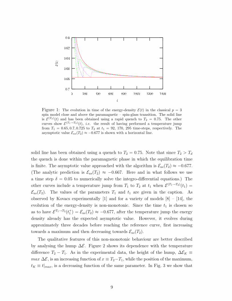
Figure 1: The evolution in time of the energy-density E(t) in the classical p = 3spin model close and above the paramagnetic – spin-glass transition. The solid lineis E(T2)(t) and has been obtained using a rapid quench to T2 = 0.75. The othercurves show E(T1→T2)(t), i.e. the result of having performed a temperature jumpfrom T1 = 0.65, 0.7, 0.725 to T2 at t1 = 92, 170, 295 time-steps, respectively. Theasymptotic value Eas(T2) ≈ −0.677 is shown with a horizontal line.

solid line has been obtained using a quench to T2 = 0.75. Note that since T2 > Td

the quench is done within the paramagnetic phase in which the equilibration time

is finite. The asymptotic value approached with the algorithm is Eas(T2) ≈ −0.677.

(The analytic prediction is Eas(T2) ≈ −0.667. Here and in what follows we use

a time step δ = 0.05 to numerically solve the integro-differential equations.) The

other curves include a temperature jump from T1 to T2 at t1 when E (T1→T2)(t1) =

Eas(T2). The values of the parameters T1 and t1 are given in the caption. As

observed by Kovacs experimentally [1] and for a variety of models [8] – [14], the

evolution of the energy-density is non-monotonic. Since the time t1 is chosen so

as to have ET1→T2(t+1 ) = Eas(T2) ≈ −0.677, after the temperature jump the energy

density already has the expected asymptotic value. However, it evolves during

approximately three decades before reaching the reference curve, first increasing

towards a maximum and then decreasing towards Eas(T2).

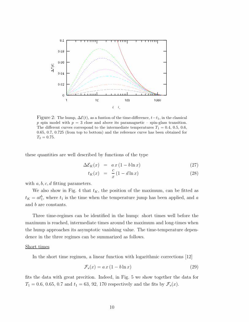
The qualitative features of this non-monotonic behaviour are better described

by analysing the hump ∆E . Figure 2 shows its dependence with the temperature

difference T2 − T1. As in the experimental data, the height of the hump, ∆EK ≡

max ∆E , is an increasing function of x ≡ T2−T1, while the position of the maximum,

tK ≡ t|max, is a decreasing function of the same parameter. In Fig. 3 we show that

9

t� t1�E(t)

1000100101

0.10.080.060.040.020

1

Figure 2: The hump, ∆E(t), as a funtion of the time-difference, t−t1, in the classicalp spin model with p = 3 close and above its paramagnetic – spin-glass transition.The different curves correspond to the intermediate temperatures T1 = 0.4, 0.5, 0.6,0.65, 0.7, 0.725 (from top to bottom) and the reference curve has been obtained forT2 = 0.75.

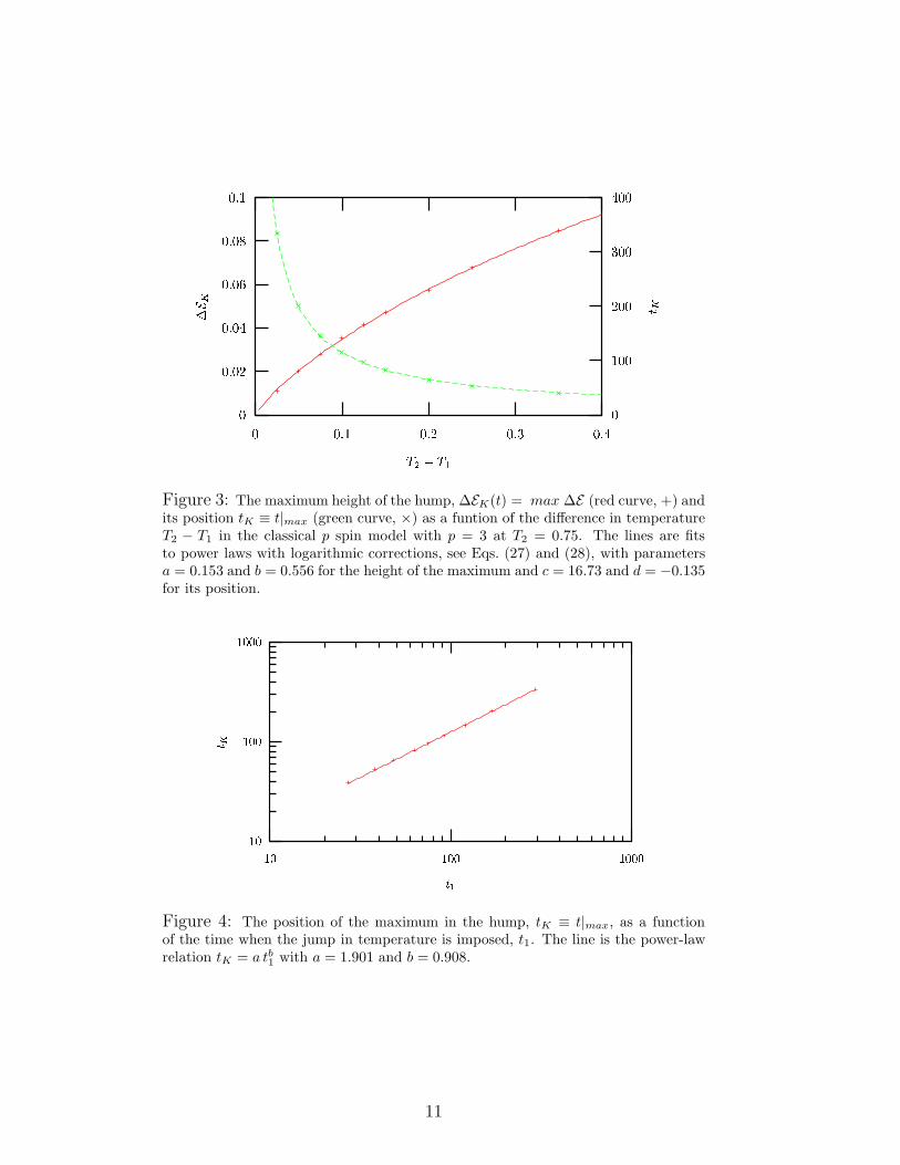
these quantities are well described by functions of the type

∆EK(x) = a x (1 − b ln x) (27)

tK(x) =c

x(1 − d lnx) (28)

with a, b, c, d fitting parameters.

We also show in Fig. 4 that tK , the position of the maximum, can be fitted as

tK = atb1, where t1 is the time when the temperature jump has been applied, and a

and b are constants.

Three time-regimes can be identified in the hump: short times well before the

maximum is reached, intermediate times around the maximum and long-times when

the hump approaches its asymptotic vanishing value. The time-temperature depen-

dence in the three regimes can be summarized as follows.

Short times

In the short time regimen, a linear function with logarithmic corrections [12]

Fs(x) = a x (1 − b ln x) (29)

fits the data with great precition. Indeed, in Fig. 5 we show together the data for

T1 = 0.6, 0.65, 0.7 and t1 = 63, 92, 170 respectively and the fits by Fs(x).

10

T2 � T1t K�E K

40030020010000.40.30.20.10

0.10.080.060.040.020

1

Figure 3: The maximum height of the hump, ∆EK(t) = max ∆E (red curve, +) andits position tK ≡ t|max (green curve, ×) as a funtion of the difference in temperatureT2 − T1 in the classical p spin model with p = 3 at T2 = 0.75. The lines are fitsto power laws with logarithmic corrections, see Eqs. (27) and (28), with parametersa = 0.153 and b = 0.556 for the height of the maximum and c = 16.73 and d = −0.135for its position.

t1t K

100010010

100010010

1

Figure 4: The position of the maximum in the hump, tK ≡ t|max, as a functionof the time when the jump in temperature is imposed, t1. The line is the power-lawrelation tK = a tb1 with a = 1.901 and b = 0.908.

11

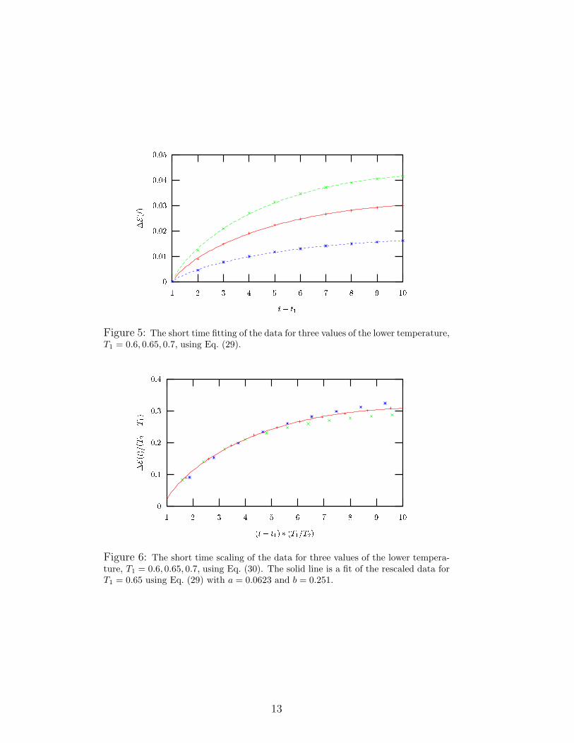
The data can also be scaled using

∆E(t) = (T2 − T1)Fs

(

(t − t1)T1

T2

)

. (30)

An accurate description of the rescaled data is achieved taking a = 0.0623 and

b = 0.251 for Fs(x), see Fig. 6.

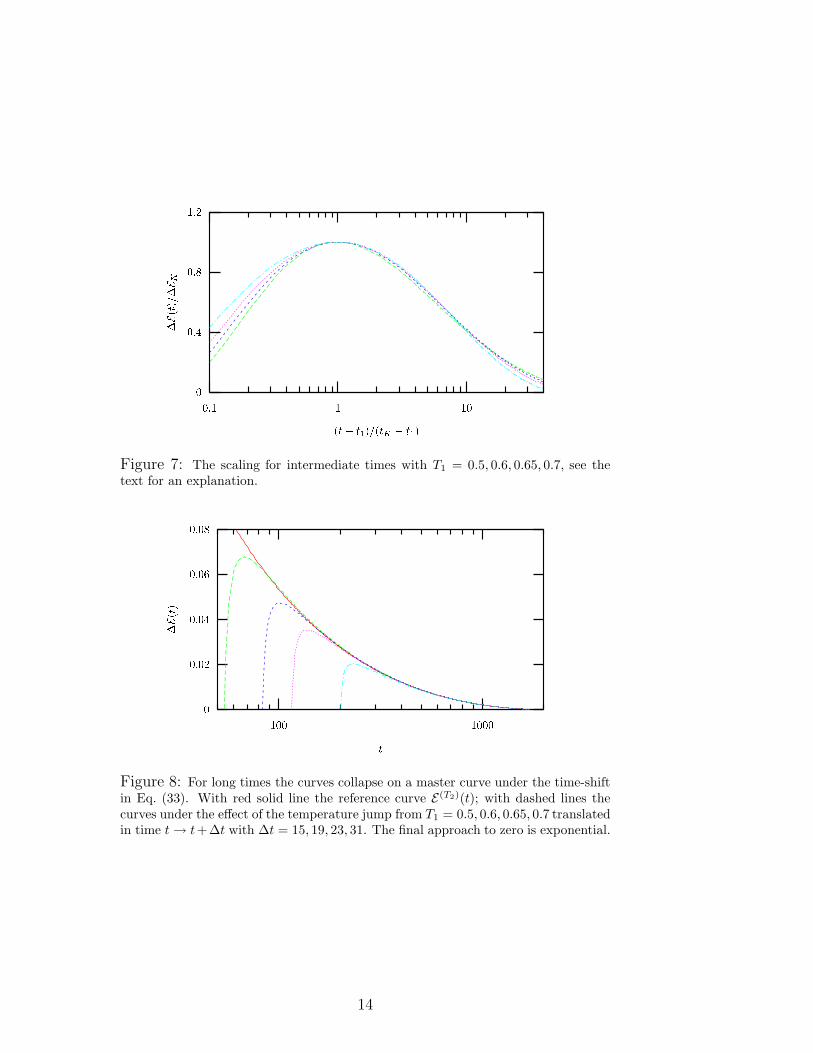
Intermediate times

The time-temperature dependence of the intermediate part of the relaxation is

well described with the scaling form

∆E(t) = ∆EK Fi

(

t − t1tK − t1

)

, (31)

see Fig. 7. This scaling law is of the class found in [9, 13].

Long times

The long times decay of the hump, i.e. for times well beyond tK , is exponential

∆E(t) = a e−bt . (32)

The curves ∆E(t) for different T1 can be made to collapse by shifting time according

to

t → t + (tK − t1) , (33)

that is to say that, the curves for the systems on which a temperature shift was

applied are in advance with respect to the reference one.

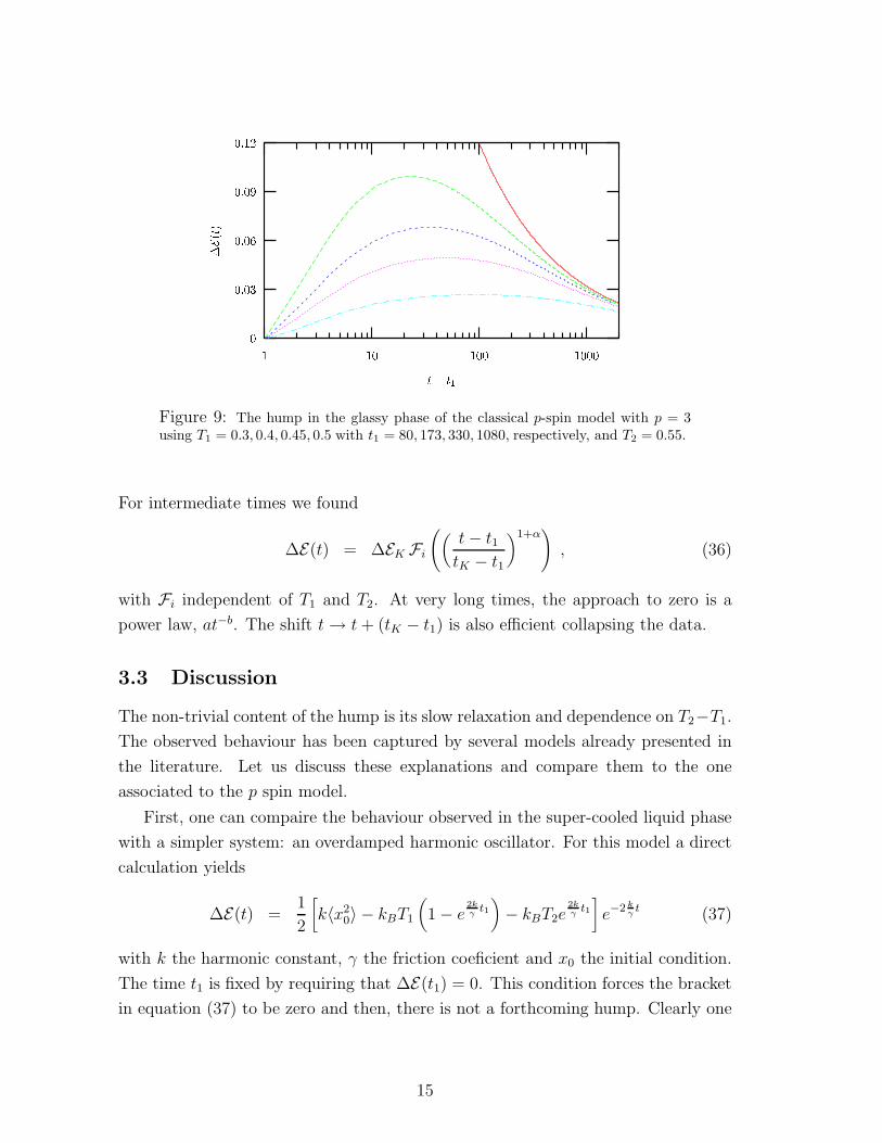
Finally, we implemented the same protocol using temperatures T1 and T2 that are

both below the dynamic critical temperature Td. As shown in Fig. 9 the qualitative

behaviour is the same as on the other side of the transition point. It is interesting

to note that the curves for the perturbed system join, and become independent of

T1 before reaching the reference curve (this is similar to what observed in [8]).

In the low temperature phase the scalings discussed above are modified as follows.

In the short-times regime, the scaling function (29) remains valid but the scaling

form is modified to

∆E(t) = (T2 − T1)Fs

(

(t − t1)(

T1

T2

)α)

, (34)

α =T2 − T1

Td. (35)

12

t� t1�E(t)

10987654321

0.050.040.030.020.010

1

Figure 5: The short time fitting of the data for three values of the lower temperature,T1 = 0.6, 0.65, 0.7, using Eq. (29).

(t� t1) � (T1=T2)�E(t)=(T 2�T1)

10987654321

0.40.30.20.10

1

Figure 6: The short time scaling of the data for three values of the lower tempera-ture, T1 = 0.6, 0.65, 0.7, using Eq. (30). The solid line is a fit of the rescaled data forT1 = 0.65 using Eq. (29) with a = 0.0623 and b = 0.251.

13

(t� t1)=(tK � t1)�E(t)=�E K

1010.1

1.20.80.40

1

Figure 7: The scaling for intermediate times with T1 = 0.5, 0.6, 0.65, 0.7, see thetext for an explanation.

t�E(t)

1000100

0.080.060.040.020

1

Figure 8: For long times the curves collapse on a master curve under the time-shiftin Eq. (33). With red solid line the reference curve E(T2)(t); with dashed lines thecurves under the effect of the temperature jump from T1 = 0.5, 0.6, 0.65, 0.7 translatedin time t → t+∆t with ∆t = 15, 19, 23, 31. The final approach to zero is exponential.

14

t� t1�E(t)

1000100101

0.120.090.060.030

1

Figure 9: The hump in the glassy phase of the classical p-spin model with p = 3using T1 = 0.3, 0.4, 0.45, 0.5 with t1 = 80, 173, 330, 1080, respectively, and T2 = 0.55.

For intermediate times we found

∆E(t) = ∆EK Fi

(

(

t − t1tK − t1

)1+α)

, (36)

with Fi independent of T1 and T2. At very long times, the approach to zero is a

power law, at−b. The shift t → t + (tK − t1) is also efficient collapsing the data.

3.3 Discussion

The non-trivial content of the hump is its slow relaxation and dependence on T2−T1.

The observed behaviour has been captured by several models already presented in

the literature. Let us discuss these explanations and compare them to the one

associated to the p spin model.

First, one can compaire the behaviour observed in the super-cooled liquid phase

with a simpler system: an overdamped harmonic oscillator. For this model a direct

calculation yields

∆E(t) =1

2

[

k〈x20〉 − kBT1

(

1 − e2kγ

t1

)

− kBT2e2kγ

t1

]

e−2 kγ

t (37)

with k the harmonic constant, γ the friction coeficient and x0 the initial condition.

The time t1 is fixed by requiring that ∆E(t1) = 0. This condition forces the bracket

in equation (37) to be zero and then, there is not a forthcoming hump. Clearly one

15

needs to go beyond this model to get the observed two-temperature dependence and

slow relaxation.

A simple next step is to study a model with a distribution of relaxation times that

depends on temperature. A simple realization is the 2d xy model in the spin-wave

approximation taking into account the contribution of vortices [11]. This model

is given by a Gaussian free field (the angle of the local magnetization) with a T -

dependent stiffness, ρ(T ). It has a slow dynamics characterised by the growth of a T -

dependent correlation length ℓT (t) = (ρ(T )t)1/2 and it captures the phenomenology

of the Kovacs’ effect, as discussed by Berthier and Holdsworth [11].

In slightly more general terms [9, 12] the Kovacs’ effect can be rationalized

in any system with a growing temperature-dependent dynamic correlation length,

that is shorter than the equilibrium one. When one shifts the temperature to T2

at t1, the length scales that are shorter than ℓT1(t1), and are hence equilibrated

at T1, have to reequilibrate at T2, where their equilibrium energy is higher. The

structure reached at T1 has to break up and allow for the nucleation of new structures

equilibrated at T2. Instead, the length scales that are longer than ℓT1(t1) are still

not equilibrated at T1 and they may continue their evolution to equilibrate now

at T2. The former processes involve shorter length-scales and should be faster and

dominate the first part of the relaxation after t1 hence leading to an energy increase.

The latter processes are slower and dominate the decay from the maximum towards

the asymptotic value Eas(T2). Within this picture, the time at which the maximum in

∆E is reached corresponds to the time when the small length scales have equilibrated

at the new temperature T2. A similar argument was put forward to explain the

overshoot observed in the time-dependent dielectric constant of dipolar glasses after

a temperature jump [3]. It is also behind the calculation presented by Brawer on

the ferromagnetic Ising chain at very low temperature [10].

However, it is not necessary to invoke a growing correlation length to capture

the qualitative features of the Kovacs’ effect. The main ingredient in the p-spin

model that leads to this effect is the slow – non-exponential – and temperature

dependent relaxation of the linear response after a strong perturbation. A scenario

with a wide spectrum of relaxation times that depends on temperature was used in

the past to explain the Kovacs’ effect [5]. Here we demonstrated that, as one could

have expected [12], the p-spin model or, equivalently, the mct with no equilibration

assumption, has this property.

The temperature and time dependence of the hump do depend on the model

considered but the main qualitative features of the effect are shared by all of them.

16

In the context of the spin models related to the mct these will be obviously modified

if one considers a mixture of p = 2 and p = 4 models (that corresponds to going

from the schematic mct to more refined versions).

Finally, let us discuss the relevance of the Kovacs’ effect for the development of

a thermodynamics of the nonequilibrium glassy state.

The attempts to use a thermodynamics for nonequilibrium glassy systems are

based on the introduction of effective state variables, basically temperature and

pressure. Initially, a (constant) fictive temperature that characterizes the glassy

structure was introduced by Tool [30]. As a consequence of Kovacs’ experiments it

was realized that this single parameter was not enough to describe the evolution of

the glass and the fictive temperature was upgraded to be a full history dependent

function measuring the departure from equilibrium [1, 2, 31]. Whether the fictive

temperature, as defined in [1, 30, 31] behaves as a thermodynamic temperature

remains to be proven. One can also translate the study of the Kovacs’ effect in

the parking lot model by Tarjus and Viot [14] in these terms: the second time-

dependent state variable introduced generalising Edwards’ prescrition [32] acts as a

fictive temperature.

More recently, an effective temperature was defined using the modification of the

fluctuation – dissipation theorem in slowly evolving nonequilibrium systems. The

interpretation of this quantity as a bonafide temperature was discussed, and some

conditions on the physical relevance of this definition were also given [27]. In partic-

ular, the need to have a system evolving slowly – characterized by a slow relaxation

of one time quantities – to be able to associate the properties of a temperature

to the fdt ratio was reckoned and stressed. The situation in Kovacs’ experiment

goes beyond this limit: the system is strongly perturbed and the one-time quantity

under study has a non-trivial, non-monotonic time-dependence. The Fluctuation

Dissipation Relation also depends on time in a non-trivial manner [34]. Thus one

cannot assert that it leads to a bonafide temperature and use it to construct a simple

extension of thermodynamics to describe the subsequent behaviour of the system.

A similar conclusion, though expressed in terms of the potential energy landscape

(pel) scenario was reached by Mossa and Sciortino [8]. These authors showed, with

molecular dynamic simulations of the fragile glass former otp, that two systems in

identical thermodynamic conditions (same values of T, V, P ) can be in very different

regions of their potential energy landscape if one of them has been strongly per-

turbed. Since the strongly perturbed system wanders in a region of the pel that

is never sampled in equilibrium, its configuration cannot be associated to that of

17

an equilibrated liquid at a different temperature. The region of the pel sampled

allows for a definition of a microcanonical temperature only when the variation of

the external conditions (temperature in this case) is small. Mossa and Sciortino

arrived at this conclusion by comparing the properties of the inherent structures

(closest local minimum in the pel) visited during aging after a temperature jump

of large magnitude to those sampled in equilibrium.

4 Quantum model

When quantum fluctuations are switched on one has to deal with the full Schwinger-

Dyson equations (11)-(19). As explained in [33] the parameter that plays the role

of the transverse field in trully quantum spin models is here the inverse of the

mass M . Indeed, this model undergoes a phase transition in the (T, Γ) plane with

Γ ≡ h2/(MJ) from an equilibrium paramagnetic phase to a non-equilibrium glassy

one. In order to test the memory effect in the quantum problem, we then apply the

Kovacs’ protocol using M−1 as the control parameter and we follow the evolution

of the averaged potential energy density E(t).

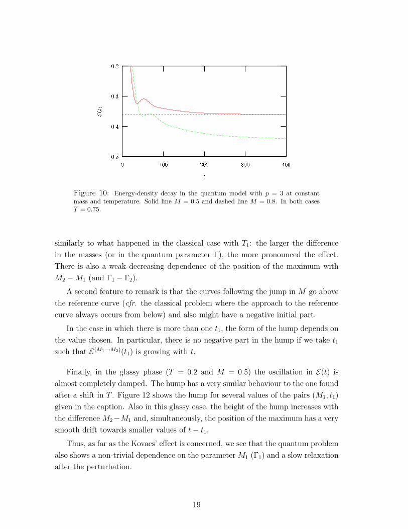
In the quantum problem the asymptotic value of the potential energy density

depends on M . (In the classical limit it does not.) The relaxation of the potential

energy density at constant M has (damped) oscillations whose magnitude depend

on the parameter M . For large values of the mass the oscillations have a suffi-

ciently large amplitude such that the asymptotic value falls within the oscillation,

i.e. E(t) < Eas(T2, Γ2) for some finite times t. In the following we choose a value

of M2 such that the system is close to the paramagnetic – glass transition and for

which Eas(T2, Γ2) < E(t) for all finite time t, see Fig. 10. Another feature to signal

is that the oscillation in the energy-density decay may be such that there is more

than one value of t1 for which EM1(t+1 ) = EM2

as , see the curve drawn with a dashed

line in Fig. 10 for which M = 0.8.

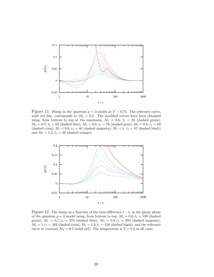
Figure 11 shows the result of applying Kovacs’ protocol to a system at T = 0.75

with the reference value of the mass, M2 = 0.5. We use four values of M1, M1 = 0.6,

0.8, 1 and 1.2 that satisfy M1 > M2, i.e. Γ1 < Γ2. For M1 = 0.6, 1 and 1.2 we find

a unique t1 satisfying EM1(t1) = EM2

as . For M1 = 0.8 instead three solutions to this

equation exist as shown in Fig. 10. Displayed in Fig. 11 are the reference energy

density E (T2,Γ2)(t) (solid red line) and the hump in the energy densities obtained by

shifting the mass.

The first thing to note in the figure is that the curves depend on the value of M1,

18

tE(t)

4003002001000

-0.2-0.3-0.4-0.5

1

Figure 10: Energy-density decay in the quantum model with p = 3 at constantmass and temperature. Solid line M = 0.5 and dashed line M = 0.8. In both casesT = 0.75.

similarly to what happened in the classical case with T1: the larger the difference

in the masses (or in the quantum parameter Γ), the more pronounced the effect.

There is also a weak decreasing dependence of the position of the maximum with

M2 − M1 (and Γ1 − Γ2).

A second feature to remark is that the curves following the jump in M go above

the reference curve (cfr. the classical problem where the approach to the reference

curve always occurs from below) and also might have a negative initial part.

In the case in which there is more than one t1, the form of the hump depends on

the value chosen. In particular, there is no negative part in the hump if we take t1

such that E (M1→M2)(t1) is growing with t.

Finally, in the glassy phase (T = 0.2 and M = 0.5) the oscillation in E(t) is

almost completely damped. The hump has a very similar behaviour to the one found

after a shift in T . Figure 12 shows the hump for several values of the pairs (M1, t1)

given in the caption. Also in this glassy case, the height of the hump increases with

the difference M2−M1 and, simultaneously, the position of the maximum has a very

smooth drift towards smaller values of t − t1.

Thus, as far as the Kovacs’ effect is concerned, we see that the quantum problem

also shows a non-trivial dependence on the parameter M1 (Γ1) and a slow relaxation

after the perturbation.

19

t� t1�E(t)

1000100101

0.150.10.050-0.05

1

Figure 11: Hump in the quantum p = 3 model at T = 0.75. The reference curve,solid red line, corresponds to M2 = 0.5. The modified curves have been obtainedusing, from bottom to top at the maximum, M1 = 0.6, t1 = 95 (dashed green);M1 = 0.7, t1 = 82 (dashed blue); M1 = 0.8, t1 = 76 (dashed gray); M1 = 0.8, t1 = 62(dashed cyan); M1 = 0.8, t1 = 46 (dashed magenta); M1 = 1, t1 = 47 (dashed black)and M1 = 1.2, t1 = 49 (dashed orange).

t� t1�E(t)

1000100101

0.20.150.10.050-0.05

1

Figure 12: The hump as a function of the time-difference t− t1 in the glassy phaseof the quantum p = 3 model using, from bottom to top, M1 = 0.6, t1 = 539 (dashedgreen), M1 = 0.7, t1 = 274 (dashed blue), M1 = 0.8, t1 = 204 (dashed magenta),M1 = 1, t1 = 163 (dashed cyan), M1 = 1.2, t1 = 150 (dashed black), and the referencecurve at constant M2 = 0.5 (solid red). The temperature is T = 0.2 in all cases.

20

5 Conclusions

We conclude that models with no spatial structure, like the p spin spherical model

that is intimately related to the schematic mode-coupling theory, can reproduce non-

trivial memory effects when their non-equilibrium dynamics is studied. Similarly to

what observed when reproducing the hole-burning protocol [18], we found here that

the Kovacs’ memory effect is captured by this model. In this sense, the Kovacs’

experiment is not able to prove the existence of a growing correlation length in

glassy systems. Assuming that a length scale exists one could, however, compare

the outcome of this and other experiments to what can be derived from a domain-

growth like picture for glassy dynamics.

The reason for having these non-trivial long-memory effects in these fully - con-

nected spin models is that close to their dynamic critical temperature (and below it)

their response function after strong perturbation has been applied is not given by a

simple exponential relaxation. The slow decay of the reponse implies that the effect

of non-linear perturbations takes very long to disappear. This is encoded in the

Schwinger-Dyson equations which describe the dynamical evolution of the system.

Acknowledegments We acknowledge financial support from the an Ecos-Sud travel

grant and the ACI project ”Optimisation algorithms and quantum disordered sys-

tems”. LFC is research associate at ICTP Trieste and a fellow of the J. S. Guggen-

heim Foundation. G. S. L. is supported by CONICET. This research was supported

in part by SECYT PICS 03-11609, PICS 03-05179 and by the National Science

Foundation under Grant No. PHYS99-07949. We thank J-P Bouchaud and D. R.

Grempel for very useful discussions.

References

[1] A. J. Kovacs, Adv. Polym. Sci (Fortschr. Hochpolym. Forsch.) 3, 394 (1963);

A. J. Kovacs, J. J. Aklonis, J. M. Hutchinson and A. R. Ramos, J. of Pol. Sci.

17, 1097 (1979).

[2] G. Mc Kenna, J. Res. NIST 99, 169 (1984); Glass formation and glassy behavior

in “Comprehensive polymer science” Vol. 12 (Polymer properties), C. Booth

21

and C. Price eds. (Pergamon, Oxford, 1989) and refs. therein.

[3] F. Alberici-Kious, J-P Bouchaud, L. F. Cugliandolo, P. Doussineau, and A.

Levelut, Phys. Rev. Lett. 81, 4987 (1998); Phys. Rev. B 62, 14766 (2000) .

[4] F. Lefloch, J. Hammann, M. Ocio, and E. Vincent, Europhys. Lett. 18, 647

(1992). M. Sasaki, V. Dupuis, J-P Bouchaud, and E. Vincent, Eur. Phys. J. B

29, 469 (2002).

[5] L. C. E. Struik, Aging in amorphous polymers and other materials (Elsevier,

Amsterdam) 1978.

[6] R. L. Leheny and S. R. Nagel, Phys. Rev. B 57, 5154 (1998). R. Hohler, S.

Cohen-Addad and A. Asnacios, Europhys. Lett. 48, 93 (1999). L. Bellon, S.

Ciliberto, and C. Laroche, Europhys. Lett. 51, 551 (2001). O. Kircher and R.

Bohmer, Eur. Phys. J. B 26, 329 (2002). F. Ozon et al, cond-mat/0210554. A.

Parker and V. Normand, cond-mat/0306056.

[7] C. Josserand, A. V. Thachenko, D. M. Mueth, and H. M. Jaeger, Phys. Rev.

Lett. 85, 3632 (2000).

[8] S. Mossa and F. Sciortino, Phys. rev. Lett. 92, 045504-1 (2004)

[9] L. Berthier and J-P Bouchaud, Phys. Rev. B 66, 054404 (2002).

[10] S. Brawer, Phys. and Chem. of Glasses 19, 48 (1978).

[11] L. Berthier and P. C. W. Holdsworth, Europhys. Lett. 58, 35 (2002).

[12] E. Bertin, J.-P. Bouchaud, J.-M. Drouffe, C. Godreche, J. Phys. A: Math. Gen.

36, 10701 (2003).

[13] A. Buhot, J. Phys. A 36, 12367 (2003).

[14] G. Tarjus and P. Viot, Memory and Kovacs effects in the parking-lot model: an

approximate statistical-mechanical treatment, cond-mat/0310738, Proceedings

from “Unifying concepts in granular media and glasses”, Capri 2003.

[15] A. Crisanti and H-J Sommers, Z. Phys. B 87, 341 (1992).

[16] L. F. Cugliandolo and J. Kurchan, Phys. Rev. Lett. 71, 173 (1993).

22

[17] L. F. Cugliandolo, cond-mat/0210312, Lecture notes in “Slow Relaxation and

non equilibrium dynamics in condensed matter”, Les Houches Session 77, J-L

Barrat et al Eds., (EDP-Springer, 2003).

[18] L. F. Cugliandolo and J. L. Iguain, Phys. Rev. Lett. 85, 3448 (2000), ibid 87,

129603 (2001). G. Diezemann, Phys. Rev. E 68 021105, 2003. U. Hberle, G.

Diezemann, Nonresonant holeburning in the Terahertz range: Brownian oscil-

lator model cond-mat/0308056.

[19] See, e.g. R. Richert, J. Phys. C 14 R703 (2002) and references therein.

[20] W. Wu, B. Ellmann, T. F. Rosenbaum, G. Aeppli, and D. H. Reich, Phys.

Rev. Lett. 67 2076 (1991); W. Wu, D. Bitko, T. F. Rosenbaum, and G. Aeppli,

Phys. Rev. Lett. 71 1919 (1993).

[21] S. Ludwig and D. D. Osheroff, Phys. Rev. Lett. 91, 105501 (2003). S. Ludwig,

P. Nalbach, D. Rosenberg, and D. D. Osheroff, Phys. Rev. Lett. 90, 105501

(2003). S. Rogge, D. Natelson, and D. D. Osheroff, Phys. Rev. Lett. 76, 3136

(1996).

[22] Z. Ovadyahu and M. Pollak, Phys. Rev. B 68, 184204 (2003). V. Orlyanchik

and Z. Ovadyahu, Phys. Rev. Lett. 92, 066801 (2004). A. Vaknin, Z. Ovadyahu

and M. Pollak, Phys. Rev. B 65, 134208 (2002).

[23] L. F. Cugliandolo and G. Lozano, Phys. Rev. Lett. 80, 4979 (1998), Phys. Rev.

B 59, 915 (1999). L. F. Cugliandolo, D. R. Grempel, G. Lozano, H. Lozza and

C. A. da Silva Santos, Phys. Rev. B 66, 014444 (2002).

[24] L. F. Cugliandolo, D. R. Grempel, G. Lozano and H. Lozza, cond-mat/0312064.

[25] M. Rokni and P. Chandra, Phys. Rev. B 69, 094403 (2004). R. Serral Gracias

and T. M. Nieuwenhuizen, cond-mat/0304150.

[26] W. Gotze, in Liquids, freezing and glass transition, Les Houches 1989, JP

Hansen, D. Levesque, J Zinn-Justin eds. North Holland. W. Gotze and L.

Sjogren, Rep. Prog. Phys. 55, 241 (1992).

[27] L. F. Cugliandolo, J. Kurchan and L. Peliti, Phys. Rev. E 55, 3898 (1997).

[28] L. F. Cugliandolo and D. S. Dean, J. Phys. A 28, 4213 (1995).

23

[29] L. F. Cugliandolo and J. Kurchan, Phys. Rev. B 60, 922 (1999).

[30] A. Q. Tool, J. Am. Ceram. Soc. 29, 240 (1946).

[31] O. S. Narayanaswamy, J. Am. Ceram. Soc. 54, 491 (1971).

[32] S. F. Edwards, in Granular Matter; an interdisciplinary approach, A. Mehta

ed. (Springer-Verlag, New York, 1994). A. Mehta and S. F. Edwards, Physica

A 157, 1091 (1989). S. F. Edwards amd R. Oakeshott, Physica A 157, 1080

(1989).

[33] L. F. Cugliandolo, D. R. Grempel and C. A. da Silva Santos, Phys. Rev. Lett.

85, 2589 (2000), Phys. Rev. B 64, 014403 (2001).

[34] Note the surprising result in [13] for two kinetically constrained models.

24