coherent transport in disordered metals out of equilibrium
TRANSCRIPT

arX
iv:c
ond-
mat
/010
6238
v1 [
cond
-mat
.mes
-hal
l] 1
3 Ju
n 20
01
Coherent transport in disordered metals out of equilibrium
P. Schwab(1) and R. Raimondi(2)(1)Institut fur Physik, Universitat Augsburg, D-86135 Augsburg
(2)NEST-INFM e Dipartimento di Fisica ”E. Amaldi”, Universita di Roma3, Via della Vasca Navale 84, 00146 Roma, Italy
(February 1, 2008)
We derive a formula for the quantum corrections to the electrical current for a metal out ofequilibrium. In the limit of linear current-voltage characteristics our formula reproduces the wellknown Altshuler-Aronov correction to the conductivity of a disordered metal. The current formula isobtained by a direct diagrammatic approach, and is shown to agree with what is obtained within theKeldysh formulation of the non-linear sigma model. As an application we calculate the current of amesoscopic wire. We find a current-voltage characteristics that scales with eV/kT , and calculate thedifferent scaling curves for a wire in the hot-electron regime and in the regime of full non-equilibrium.
I. INTRODUCTION
Quantum interference effects in disordered metals havebeen the subject of intensive investigation for over twentyyears. For general reviews see [1–3]. The interference ofthe scattered electrical waves in the presence of a randompotential leads to corrections [4–6] to the semi-classicalformula of the electrical conductivity known from theDrude-Boltzmann theory. The physical implications ofthese quantum corrections have been extensively dis-cussed in the literature mostly for the equilibrium prop-erties, for which experimental data were available, al-though a number of non-linear electric field effects havebeen predicted in the past [2,7–9].
In contrast, non-equilibrium electrical transport hasreceived considerable attention in the field of mesoscopicphysics. Examples are the transport in quantum dots[10], or the shot noise in mesoscopic conductors [11]. Inthis situation however the majority of the studied phe-nomena did not involve interference effects.
Our interest in the non-equilibrium properties of in-terference phenomena originated by the suggestion [12]that the non-equilibrium electric noise could be the ori-gin for the low temperature saturation of the weak lo-calization dephasing time observed in disordered filmsand wires [13]. Mohanty et al. [14] pointed out that inthe samples with the strongest dephasing rate also theinteraction correction (Altshuler-Aronov) to the conduc-tivity saturates at low temperature. This suggests thatalso the Altshuler-Aronov correction should be affectedby the non-equilibrium noise. Similar speculations con-cerning an electric field effect on the Altshuler-Aronovcorrection have also been made earlier by different au-thors in different contexts [15,16].
This motivated us to study the interaction correctionin the presence of an external field. In analogy to theanalysis performed in the literature for weak localization[2], we calculated the interaction correction to the cur-rent in the presence of a time dependent vector poten-tial, assuming a thermal distribution function [17]. In-deed we verified the above-mentioned speculations sincewe found an electric field effect. However, contrary to
what is known in the case of weak localization, where thestrongest effect occurs when the period of the AC field isof the order of the dephasing time, we found a suppres-sion of the interaction correction even by static electricfields. These findings have however raised the issues ofthe possibility of experimentally observing the effect andof its physical interpretation. Both these questions willbe addressed in this paper.
Let us comment first the problem concerning the inter-pretation of the effect. In Ref. [18] we demonstrated thatthe non-linear field effect can be understood in terms ofdephasing by calculating the phase shifts of the relevantclassical paths in the presence of a time dependent vec-tor potential. On the other hand, a static electric fieldcan also be described in terms of a static scalar poten-tial, and it is clear that a static scalar potential does notlead to dephasing. Therefore we think it is of interest topresent a version of our theory in the scalar gauge. Inthis paper we will explicitly show the gauge invariance ofour previous results.
The second problem concerns the scale of the effect andits experimental observability. We found in Ref. [17] thatthe temperature-dependent Altshuler-Aronov correctionto the conductivity saturates when the voltage drop onthe thermal length (LT =
√
D/T ) is comparable to thetemperature eELT ∼ kT . From this condition one canestimate the strength of the microwave field that is nec-essary to explain the saturation of the Altshuler-Aronovcorrection observed in the experimental data of Ref. [14].In so doing one arrives at a microwave field value that ismore than an order of magnitude larger than the opti-mistic estimate given in Ref. [12] to explain the saturationof the weak localization time. Furthermore it is ratherunlikely that the condition eELT ∼ kT can be reached atlow temperature, since strong heating is already assumedto set in when the voltage drop over the electron-phononlength is of order of the temperature. Strong heating onthe other hand is not observed in Ref. [14]. Similar prob-lems arise also in the attempt to explain the experimentaldata of Refs. [15,16].
Despite the above mentioned problems, we think wecannot rule out non-equilibrium noise as a reason for
1

the observed saturations. In fact, even in the absenceof strong heating, the distribution function may devi-ate from the equilibrium form and affect the interactioncorrection to the conductivity and possibly lead to sat-uration at considerably weaker electric fields. A theorywhich is valid even out of equilibrium will be developedin this paper.
In contrast to our previous work [17] we will avoidto guess the distribution function which could be rele-vant for the experiments of Refs. [13,14]. Instead we willcalculate the interaction correction in a more controlledsituation. Nowadays it is, indeed, possible to create non-equilibrium in a controlled way by, for instance, attachinga short mesoscopic wire to large metallic reservoirs (seee.g. [19]). In the absence of inelastic scattering processesthe distribution function in the wire is a linear super-position of the distribution functions of the leads. Theinteraction correction in such a situation has also beenconsidered in the recent paper by Gutmann and Gefen[20]. We verify their result that the I −V characteristicsscales as eV/kT . Going beyond, we calculate the I − Vcharacteristics explicitly and we will compare quantita-tively the wire in non-equilibrium with the wire in thehot electron regime. In addition we will also discuss theinteraction correction in the spin triplet channels.
Our paper is organized as follows. In the next sectionwe introduce the basic quantities and recall the main re-sults of the Drude-Boltzmann theory within the Keldyshformalism. In section III we consider the quantum cor-rections to the conductivity within the Keldysh diagram-matic approach. We derive, in particular, an expressionfor the current in the presence of an external electric field.In section IV we discuss the gauge invariance of the the-ory, while in section V we present a specific application:a mesoscopic wire. Finally in section VI we give ourconclusions. In the appendices we outline how to obtainthe same results using the Keldysh formulation of thenon-linear sigma model and we extend the calculationsin order to include also the spin effects.
II. BASIC DEFINITIONS AND THE
DRUDE-BOLTZMANN THEORY
In this section we will recall some basic relations ofthe quasi-classical approximation in its non-equilibrium(Keldysh) formulation [21]. Our notation will mainly fol-low Ref. [22]. We will write down the equation of mo-tion for the Green functions in the presence of impurityscattering in the case when quantum interference is com-pletely neglected. The Green functions have the matrixstructure
G =
(
GR GK
0 GA
)
, (1)
with
GR(x, x′) = −iΘ(t − t′)(
〈Ψ(x)Ψ†(x′)+Ψ†(x′)Ψ(x)〉)
(2)
GA(x, x′) = +iΘ(t′ − t)(
〈Ψ(x)Ψ†(x′)+Ψ†(x′)Ψ(x)〉)
(3)
GK(x, x′) = −i(
〈Ψ(x)Ψ†(x′)−Ψ†(x′)Ψ(x)〉)
, (4)
where Ψ and Ψ† are fermion operators and x = (x, t). Inequilibrium the Keldysh component of the Green func-tion is expressed in terms of the retarded and advancedcomponents by GK
ǫ = [1 − 2f(ǫ)](GRǫ − GA
ǫ ), where f(ǫ)is the Fermi function. The Keldysh component out ofequilibrium will be discussed later.
The Green function solves the differential equation
(
i∂
∂t+
1
2m(∇ + ieA)2 + eφ + µ
)
G(x, t;x′, t′)
−∫
dt1dx1Σ(x, t;x1, t1)G(x1, t1;x′, t′)
= δ(x − x′)δ(t − t′), (5)
where and φ, A are the scalar and vector potential. Sincethe self-energy Σ has the same triangular matrix struc-ture as the Green function, one can invert the inverseGreen function G−1 and finds for the Keldysh compo-nent the relation
GK = GRΣKGA. (6)
For a graphical representation see Fig.1.
���
���0 GA 0GR GK
FIG. 1. Graphical representation of the Green function;the shaded box in GK represents the Keldysh component ofthe self-energy, i.e., basically the distribution function.
We then introduce the ξ-integrated (quasi-classical)Green function
gtt′(p,R) =i
π
∫
dξdre−ip·rG(
R +r
2, t;R − r
2, t′
)
,
(7)
where ξ = p2/2m − µ and p is a unit vector along themomentum. The Green function in the energy domain is
gǫǫ′(p,x) =
∫
dtdt′eiǫt−iǫ′t′ gtt′(p,x). (8)
We will keep the notation of small g for the ξ-integratedGreen functions and capital G for the not integratedGreen functions all over this paper. When approximatingthe density of states as an energy independent constant,the ξ-integration is related to an integration over the mo-mentum p according to
2

∫
d3p
(2π)3→ N0
∫
dξ
∫
dp
4π. (9)
We will now recall some relations that are specific forimpurity scattering. By treating the impurity scatter-ing within the self-consistent Born approximation and as-suming a Gaussian, δ-correlated impurity potential with
〈U(x)U(x′)〉 =1
2πN0τδ(x − x′), (10)
the electron self-energy is local in space and is given by
Σimp(x, t;x′, t′) =1
2πN0τG(x, t;x, t′)δ(x − x′) (11)
= Σimptt′ (x)δ(x − x′). (12)
Notice that this equation has to be solved self-consistently for all the components of the Green func-tion. Using the above definition, one observes that theimpurity self-energy is related to the s-wave part of thequasi-classical function,
Σimptt′ (x) = − i
2τ
∫
dp
4πgtt′(p,x). (13)
The distribution function out of equilibrium is foundby solving the appropriate kinetic equation. Here we de-rive the kinetic equation for gK
ǫǫ′ from Eqs.(6) and (7).For simplicity we neglect external fields for the time be-ing. Under these conditions the retarded and advancedGreen functions are
GR(A)(p, ǫ) =1
ǫ − ξ ± i/2τ. (14)
Near the Fermi energy (ǫ, ǫ′ ≪ ǫF ) and for small mo-menta (q ≪ pF ) one finds
gKǫǫ′(p,q) =
i
π
∫
d3p
(2π)3GR(ǫ,p + q/2)
×ΣKǫǫ′(q)GA(ǫ′,p − q/2) (15)
≈ i
τ
1
ǫ − ǫ′ + i/τ − vF p · q
∫
dp
4πgK
ǫǫ′(p,q). (16)
The equation above reproduces the well-known kineticequation for impurity scattering
(
∂
∂t+
∂
∂t′+ vF p · ∇
)
gKtt′(p,x) =
1
τ
(
gKtt′(p,x) −
∫
dp
4πgK
tt′(p,x)
)
. (17)
In this work we will restrict to the case, where en-ergies and momenta are restricted even more, namelyǫτ, ǫ′τ, qvF τ ≪ 1. By expanding (16) for small energyand momentum and taking the angular average, one findsthe diffusive equation
(
∂
∂t+
∂
∂t′− D
∂2
∂x2
)∫
dp
4πgK
tt′(p,x) = 0, (18)
where the diffusion constant is D = v2F τ/3. Notice that
this equation is solved by any function gKtt′(p,x) which
is independent of position x and which depends on timedifferences (t − t′) only. This reflects the fact that anydistribution function is allowed for noninteracting elec-trons.
The charge density and current density are related tothe Keldysh component of the Green function,
ρ(x, t)=ieGK(x, t;x, t) (19)
j(x, t)=e
2m[∇x−∇x′ +2ieA(x, t)]GK(x, t;x′, t)|x′=x. (20)
In terms of the quasi-classical Green functions, the chargeand current read [22]
ρ(x, t) = 2eN0
(
π
2
∫
dp
4πgK
tt (p,x) − eφ(x, t)
)
(21)
j(x, t) = eπN0
∫
dp
4πvF pgK
tt (p,x). (22)
It is useful to consider the current density in the pres-ence of an electric field E(x) = −∇φ(x). By replacingGK in (20) with GRΣKGA we express the current densityas
j(q, ω) = ie
∫
dǫ
2π
∫
d3p
(2π)3p
mGR
(
ǫ +ω
2,p +
q
2
)
×ΣKǫ+ω/2,ǫ−ω/2(q)GA
(
ǫ − ω
2,p − q
2
)
, (23)
from which we obtain
j(x, t) = −eπDN0∇∫
dp
4πgK
tt (p,x) (24)
= −D∇ρ(x, t) + 2e2DN0E(x, t). (25)
Within the adopted approximations , i.e., a constant den-sity of states and a uniform diffusion coefficient, one ob-serves that the current is a linear function of the electricfield as long as the charge density ρ(x) stays uniform.
We close this section by commenting on Eq.(21). Ascalar field φ(x, t) shifts the entire Fermi surface, i.e., itaffects the Green function at all energies. This is lost inthe naive substitution of Eq.(9), when the ξ-integrationis extended to ±∞. The second term in eq.(21) is ob-tained by taking into account these high energy termscorrectly. The equilibrium response to a static field is,for instance, fully given by this second contribution. Forthis reason the second term is often referred to as the“static contribution” to the response, whereas the firstterm is referred to as the “dynamic contribution”.
3

III. QUANTUM CORRECTION TO THE
CURRENT
Quantum interference gives rise to corrections to thesemi-classical expression of the electrical conductivityof a metal. The so-called quantum corrections to theaverage conductivity are the weak localization correc-tion (WL), the interaction correction in the particle-hole channel (EEI), and the interaction correction in theCooper channel (EEIC). In this paper we will concen-trate on the interaction correction in the particle-holechannel. For non-linear effects in WL we refer to the lit-erature [2,3]. Interactions in the Cooper channel will notbe considered. This is justified for non-super-conductingmaterials since in that situation the relevant interactionparameter scales downwards under the renormalizationgroup.
A. Ladder diagrams
Before calculating the quantum corrections we intro-duce the ladder diagrams of repeated impurity scatteringwhich will appear at various places in the diagrammaticapproach. Technically speaking these ladder diagramsappear when averaging a product of a retarded and anadvanced Green function. Here we briefly recall how toderive the expressions for the ladder in the absence ofexternal fields and without spin effects. The inclusion ofexternal fields and spin structure is straightforward andone may refers to the reviews on the subject like Ref. [2].
The diffuson D(q, ω) or particle-hole ladder is foundby summing the sequence of diagrams shown in Fig.2:
D(q, ω) = 1 + ηRA + (ηRA)2 + · · · =1
1 − ηRA(26)
with
ηRA =1
2πN0τ
∫
d3p
(2π)3GR(ǫ + ω,p + q)GA(ǫ,p) (27)
≈ 1 − τ(−iω + Dq2) (28)
where we have used the condition that ωτ ≪ 1 andvF qτ ≪ 1 so that the diffuson reads
D(q, ω) =1
τ
1
−iω + Dq2. (29)
GR�+!p + q p0 + qp0p
GR�+!GR�+!GA� GA�GA�
FIG. 2. Graphical definition of the diffuson (particle-holeladder). GR and GA are the retarded and advanced Greenfunctions, which in the general case can depend on externalelectromagnetic fields.
For completeness we give the expression in the pres-ence of external electromagnetic fields. In this case it isconvenient to go a real space representation where thediffuson is defined by the equation
{
∂
∂t− D(∇x + ieAD)2 − ieφD
}
Dηtt′(x,x′)
=1
τδ(x − x′)δ(t − t′), (30)
with AD = A(x, t + η/2) − A(x, t − η/2) and φD =φ(x, t + η/2) − φ(x, t − η/2). In these equations t is thecenter-of-mass time, and η is the relative time, and aredefined in Fig.3.
D�tt0(x;x0) =GAGR
x0; t0 � �=2x0; t0 + �=2
x; t� �=2x; t + �=2
FIG. 3. The diffuson in the space/time domain.
Notice that the external field drops from the equationfor the diffuson when the relative time η equals zero.
B. Interaction correction to the current
We are now ready to allow for electron-electron inter-actions. Interactions will enter the kinetic equation anddetermine the form of the distribution function. We as-sume that the distribution function has been determinedself-consistently via the kinetic equation with the inclu-sion of the interaction. We will concentrate then on thecalculation of the interaction corrections to the currentdensity. To do so we need the expression for the KeldyshGreen function in the presence of interactions. FollowingRefs. [23,22] we start with the self-energy
Σ = Σimp + ΣV (31)
4
where Σimp is the previously defined impurity self-energyand
ΣVij(x, x′) = i
∑
i′j′kk′
∫
dx2dx3dx4dx5Γkii′(x5; x, x3)
× V kk′
(x5, x4)Gi′j′(x3, x2)Γk′
j′j(x4; x2, x′). (32)
The vertex functions are given by
Γkij(x; x1, x2) = γk
ij +1
2πN0τ
∑
i′j′
∫
dx′1dx′
2Gii′ (x1, x′1)
× Γki′j′ (x; x′
1, x′2)Gj′j(x
′2, x2). (33)
An analogous equation is valid for Γ. We recall that inthe Keldysh triangular representation the “absorption”and “emission” vertices differ. A diagrammatic repre-sentation of both the self-energy and vertex equations isshown in Figs.4 and 5.� = +
FIG. 4. The self-energy containing both disorder and in-teraction. +=
FIG. 5. Dressing of the interaction vertex with impuritylines.
The indices i, j, . . . denote matrix indices in Keldyshspace. The bare vertices γ, γ are local in space and time.The structure in Keldysh space is γ1
ij = γ2ij = δij/
√2
and γ2ij = γ1
ij = σxij/
√2. From Σimp + ΣV one may de-
rive a kinetic equation for the system with disorder andinteraction. The general expressions were already givenin the seminal paper, Ref. [23]. Explicit expressions forthe various components of Γ and Γ in terms of integralslike ηRA are also given in the appendix of Ref. [22]. Fullyevaluating the expressions in this or that limit remainsstill to be done. Even in thermal equilibrium we are notaware of any full self-consistent calculation.
In the following we will take into account only the non-interacting self-energy self-consistently, and restrict our-selves to the perturbation theory for the interacting partof the problem. The change in GK due to the interactionmay be written as
δGK = GRδΣRGK + GRδΣKGA + GKδΣAGA, (34)
where δΣ is a sum of the interaction self-energy plus theinteraction-induced change in the impurity self-energy
δΣ = δΣimp + ΣV . (35)
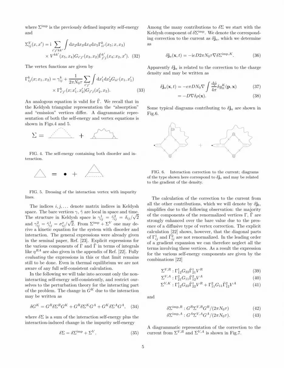
Among the many contributions to δΣ we start with theKeldysh component of δΣimp. We denote the correspond-ing correction to the current as δja, which we determineas
δja(x, t) = −ieD2πN0τ∇δΣimp,K . (36)
Apparently δja is related to the correction to the chargedensity and may be written as
δja(x, t) = −eπDN0∇∫
dp
4πδgK
tt (p,x) (37)
= −D∇δρ(x). (38)
Some typical diagrams contributing to δja are shown inFig.6.
��������
��������
��������
����
����
����
����
FIG. 6. Interaction correction to the current; diagramsof the type shown here correspond to δja and may be relatedto the gradient of the density.
The calculation of the correction to the current fromall the other contributions, which we will denote by δjb,simplifies due to the following observation: the majorityof the components of the renormalized vertices Γ, Γ arestrongly enhanced over the bare value due to the pres-ence of a diffusive type of vertex correction. The explicitcalculation [22] shows, however, that the diagonal partsof Γ1
ij and Γ2ij are not renormalized. In the leading order
of a gradient expansion we can therefore neglect all theterms involving these vertices. As a result the expressionfor the various self-energy components are given by thecombinations [22]
ΣV,R : Γ112G22Γ
121V
R (39)
ΣV,A : Γ221G11Γ
212V
A (40)
ΣV,K : Γ112G22Γ
122V
R + Γ211G11Γ
212V
A (41)
and
δΣimp,R : GRΣV,RGR/(2πN0τ) (42)
δΣimp,A : GAΣV,AGA/(2πN0τ). (43)
A diagrammatic representation of the correction to thecurrent from ΣV,R and ΣV,A is shown in Fig.7.
5

������
������
������
������
���������
���������
��������
��������
FIG. 7. Interaction correction to the current; these dia-grams contribute to δjb.
Going through the algebra one convinces one-self thatthe contributions from ΣV,K and δΣimp may be combinedas
ΣV,R + δΣimp,R + ΣV,Ka (44)
ΣV,A + δΣimp,A + ΣV,Kb (45)
where ΣV,Ka and ΣV,K
b refer to the two terms enteringthe expression for ΣV,K . These combinations of termsare taken into account in the diagrams of Fig.7 by com-pleting the “Hikami box” as shown in Fig.8.
FIG. 8. The three diagrams constituting the Hikami box;within the here-applied formalism the diagrams are gener-ated from the self-energies δΣimp + ΣV .
We can now proceed to the explicit calculation of thecorrection to the current. Let us start with the evalua-tion of the Hikami box. The first of the diagrams of theHikami box is shown in more detail in Fig.9.
��������
p + q1 �Q� q=2 ; t� �p� q=2 ; t p + q1 � q=2 ; t� �gKtt��(q1)
! Q# Q + q� q1p + q=2 ; tj(q; t)
FIG. 9. Labeling of momenta and times in the Hikamibox; within the here-applied approximations the retardedand advanced Green functions are local in time.
The evaluation of the diagram amounts to the inte-gration over the “fast” momentum entering the electronGreen function and is accomplished by
∫
d3p
(2π)3p
mGR(p + q/2)GA(p− q/2)
×GR(p − q/2 + q1)GA(p − q/2 + q1 − Q). (46)
The integration is performed under the assumption thatthe three momenta q, q1, and Q are small compared to1/l and that the energy in all the four Green functionsis small compared to 1/τ . After expanding the Greenfunctions to first order in q, q1, Q, the integration overp gives (−6πiN0τ
2)D(Q + q). Evaluating the other twodiagrams of Fig.8 analogously and summing up the threeof them one arrives at (−4πiN0τ
3)DQ.
After completing the evaluation of the Hikami box, wenow address our attention to the vertex functions Γ andΓ. From Ref. [22] we borrow the relevant expressions as
Γ112 =
1√2(1 − ηRA)−1(ηRK + ηKA) (47)
Γ121 =
1√2(1 − ηAR)−1, (48)
so that Γ121 is simply a diffusion operator, as it is also
manifest in Fig.7. The explicit space and time depen-dence is determined as
Γ121(x; x1, x2) =
1√2Dη=0
tt1 (x,x1)δ(x1 − x2)δ(t1 − t2).
(49)
The vertex Γ112 has a more complicated structure due to
the presence of a Keldysh Green function in the kernelof the corresponding integral equation. Its detailed dia-grammatic representation is shown in Fig.10.
������������
������������
p + q=2 Qq + q1FIG. 10. The interaction vertex; compare Fig.7.
The integral ηRK is given by
ηRK =1
2πN0τ
∫
d3p
(2π)3GR(p + q/2)
× GK(p + q/2 − Q;p + q1 − q/2 − Q). (50)
We replace GK by GR(−i/τ)FGA, with
6

Ftt′(x) =1
2
∫
dp
4πgK
tt′(p,x) (51)
and integrate over p in Eq.(50) to get ηRKtt′ (x) = Ftt′(x).
It can be easily shown that ηKA does not contribute tothe current; the (relevant part of the) vertex is then foundas
Γ112(x; x1, x2) =
1√2
∫
dηDηt1−η/2,t−η/2(x1,x)
× Ft,t−η(x)δ(x1 − x2)δ(t2 − t1 + η). (52)
The last ingredient entering the expression of the in-teracting self-energy is the electron-electron interactionpropagator V R,A. At the level of the approximation weare working, it is sufficient to confine to the standardrandom phase approximation (RPA). The retarded RPAscreened Coulomb interaction reads :
V R(x, x′) = V 0(x, x′)
−∫
dx1dx2V0(x, x1)Π
R(x1, x2)VR(x2, x
′), (53)
where
V 0(x, x′) = δ(t − t′)e2/|x− x′| (54)
and ΠR(x1, x2) is the retarded component of the densitycorrelation function. We write the density correlationfunction as the sum of a “static” and a “dynamic” part,ΠR = Πs + Πd. The “static” part is given by
Πs(x1, x2) = 2N0δ(x1 − x2)δ(t1 − t2), (55)
as it is seen directly from the quasi-classical expressionfor the electron density in Eq.(21).
������������
������������
������
������ �2 � (!2 + !3)=2�1 � !1=2 �2 + (!2 + !3)=2�1 � (!2 � !3)=2�2 + (!2 + !3)=2�1 + !1=2 �2 + (!2 � !3)=2�2 � (!2 + !3)=2
FIG. 11. The dynamical part of the density correlationfunction.
The “dynamic” part is determined from the ladder di-agrams as shown in Fig.11. The expression is given by
Πdtt′(x,x′) = 2πiN0τ
∫
dǫ12π
· · · dω2
2πe−iω1t+iω2t′
×D(
ǫ1 +ω1
2, ǫ1 −
ω1
2; ǫ3 +
ω2
2, ǫ2 −
ω2
2
)
×[
F(
ǫ3 +ω2
2, ǫ2 +
ω2
2
)
− F(
ǫ3 −ω2
2, ǫ2 −
ω2
2
)]
, (56)
where we suppressed the spatial indices. D(. . .) is thediffuson and F is the angular average over gK as de-fined in (51). For the frequencies in F we introduce
the center-of-mass and relative coordinates, F (ǫ1, ǫ2) →F(ǫ1+ǫ2)/2(ǫ1− ǫ2). In order to evaluate the frequency in-tegrals we assume that the time dependent distributionfunction Fǫ(t) deviates from the equilibrium distributionfunction only at small energies ǫ, i.e. Fǫ(t) → ±1 forǫ → ±∞. We then find
Πdt1t2(x1,x2) = 2N0τ
∂
∂t2D0
t1t2(x1,x2). (57)
Since here the diffuson enters with the relative timeη = 0, the density correlation function does not dependon the external fields. Adding the static and dynamicparts together and making use of the differential equa-tion for the diffuson, one finds
ΠR(x1, x2) = −2N0τD∂2x1
D0t1t2(x1,x2). (58)
In the case of a uniform system this reduces to the stan-dard expression
ΠR(q, ω) = 2N0Dq2
−iω + Dq2(59)
from which the dynamically screened Coulomb interac-tion is determined as
V (q, ω) =V 0(q)
1 + V 0(q)2N0Dq2/(−iω + Dq2)(60)
≈ 1
2N0
−iω + Dq2
Dq2. (61)
The second line is valid, when |ω| < V 0(q)2N0Dq2. Inthree dimensions, where V 0(q) = 4πe2/q2, this conditionreads |ω| < Dκ2. Since the inverse screening length κ isin a metal typically of the order of the Fermi wavelengththe approximation is well justified. In lower dimensionsa more careful analysis is sometimes necessary, see forexample Ref. [24,17].
If we now collect all the pieces of our analysis we maycome back to the quantum correction to the current. Forconvenience we switch from the energy/momentum do-main to the time/space domain. Remember that we haveneglected the energy dependence of the Green functionGR and GA in the calculation of the Hikami box. This isequivalent to approximate these Green functions as localin time. The resulting time dependencies are shown inFigs.9 and 10. The correction to the current δj = δja+δjbis finally found as
δja(x, t) = −D∇δρ(x, t) (62)
δjb(x, t) = e2πDN0τ2
∫
dηdx1dx2
×Ft−η,t(x)Dηt−η/2,t1−η/2(x,x1)Ft1,t1−η(x1)
×V Rt1,t2(x1,x2)(−i∇x)D0
t2,t−η(x2,x) + c.c.. (63)
This current formula is one of the central results of ourpaper. The nice feature is that is valid for arbitrary
7

form of the distribution function and diffuson propagator.This will allow us to examine the current in different ex-perimental and geometrical setups as well as more generalquestions concerning its physical interpretations. Specificapplications are discussed in Sections IV,V. The inter-acting disordered electron problem is often formulated interms of the field-theoretic non-linear sigma model andone may wonders how the presented diagrammatic ap-proach is related to it. To this end we explicitly show inthe appendix A at the end of the paper that the sameexpression for the current can be obtained from the fieldtheoretic approach of Ref. [25].
IV. GAUGE INVARIANCE
As a first application of the formula for the currentwe discuss in this section the issue of its physical inter-pretation and of gauge invariance. To begin with, webelieve useful to make contact with our earlier work inRefs. [17,18],
In Refs. [17,18] the quantum correction to the cur-rent was derived working in a vector gauge, A =−tE, φ = 0, under the assumption that the elec-tron distribution function had the equilibrium form,F (ǫ,x) = tanh(ǫ/2T ), or, equivalently, in the time do-main Ftt′(x) = −iT/ sinh[πT (t − t′)], and that we dealtwith a uniform system with a homogenous charge density.In this situation one has immediately that δja = 0 and byFourier transforming Eq.(63) with respect to the spatialvariables, the current formula of [17,18] is reproduced.
In [17,18] we showed that in the limit of weak elec-tric field our theory reproduces the well-known Altshuler-Aronov corrections to the conductivity. At larger fieldsnon-linear contributions to the current arise as a conse-quence of the nonlocal character of the current formula.
By working in the vector gauge, the electric field entersthe equation for the diffuson, Eq.(30), via the minimalsubstitution of the vector potential. Due to the quasi-classical nature of the equation governing the diffuson,one may interpret the non-linear conductivity in termsof phases. Let us recall the argument of Ref [18]. The in-teraction correction to the conductivity is related to thepropagation of a particle and a hole along closed paths.Pictorially one may think of this as one particle goingaround a closed path, starting for example at t = 0 andarriving at t = η. This particle is also interacting witha background particle which is retracing backwards-in-time the same closed path. Since the point of interactionx(t1) can be anywhere along the path, the particles tra-verse the loop at different times. In the presence of avector potential the accumulated phase difference of thetwo paths is ϕ1 − ϕ2 = e
∫ t1t1−η
dt′x1 ·A − e∫ η
0dt′x2 ·A.
This can be simplified using that x1(t) = x2(t) for0 < t < t1 and x1(t − η) = x2(t) for t1 < t < η
leading to ϕ1 − ϕ2 = e∫ 0
t1−η dt′x1 · [A(t′) − A(t′ + η)].For the particular case of a static electric field describedby A = −Et, the above given phase difference becomesϕ1 − ϕ2 = eη(x2 − x1) · E. This suggests that the inter-action correction should be sensitive to a static electricfield, leading to a non-linear conductivity.
One may object against this interpretation by observ-ing that the vector potential can be gauged away in sucha way that the static electric field is described by a staticscalar potential E(r) = −∇φ(r). A static scalar poten-tial, again according to Eq.(30), does no longer affect thediffuson propagator, so that the argument of the phasedifference along the two paths cannot be used. Of coursethis does not imply that the current formula is incorrect.
In fact we may demonstrate explicitly the gauge in-variance of the current formula. First one notices thatδja = −D∇ρ is gauge invariant. For δjb an explicit checkis necessary. Given the gauge transformation
A → A + ∇χ (64)
φ → φ − ∂tχ (65)
the diffuson and the distribution function transform ac-cording to
Ftt′(x) → Ftt′(x) exp{−ie[χ(x, t) − χ(x, t′)]} (66)
Dηtt′(x,x′) → Dη
tt′(x,x′) (67)
× exp{−ie[χ(x, t +η
2) − χ(x, t − η
2)]}
× exp{ie[χ(x′, t′ +η
2) − χ(x′, t′ − η
2)]}.
By applying the above transformation to Eq.(63), oneeasily verifies that the function χ(x, t) drops, so that theexpression is manifestly gauge invariant. For the spe-cial example of a static electric field with A = −Et wechoose χ(x, t) = tE · x. After the gauge transforma-tion the electric field appears in the distribution functiontanh(ǫ/2T ) → tanh[(ǫ − µx)/2T ], µx = eE · x but not inthe diffuson.
We conclude that although the correction to the cur-rent as derived in this paper is gauge invariant, the inter-pretation of the non-linear effects depends on the actualchoice of the potentials A or φ. With E = −∂tA, φ = 0we would interpret the non-linear conductivity as due todephasing. With E = −∇φ, A = 0 the reason of thenon-linear conductivity is attributed to the different lo-cal chemical potential felt by the particle and hole.
V. MESOSCOPIC WIRE
In this section we use the current formula to analyzethe non-linear electrical transport in a thin wire. Weassume that the temperature is low enough so that theDrude conductivity is dominated by the impurity scatter-ing and is therefore temperature independent. It is well
8

known that in one dimension the electron-electron inter-action leads to a 1/
√T correction to the conductivity.
The interesting question to ask concerns what happensat larger voltages and which are the relevant length andenergy scales in the problem.
For the calculation we need the diffuson propaga-tor and the distribution function in the wire. At theboundary with the vacuum or an insulator the deriva-tive of the diffuson normal to the boundary vanishes,(n · ∇)D(x,x′) = 0. In the case of an infinitely long wirewith cross section S the solution of the diffusion equationreads
D(x, t) =1
τ
1
S
1√4πDt
exp[−x2/(4Dt)]. (68)
In the above result we have averaged the diffuson overthe cross section. In a wire of finite length we impose theopen boundary conditions along the x axis
Dtt′(x, x′)∣
∣
x,x′=0,L= 0, (69)
corresponding to the fact that an electron arriving at theboundary escapes into the leads, where dissipation takesplace. Therefore it no longer contributes to the phasecoherent process of quantum interference. The diffusonin the finite system is related to the propagator for aninfinite system according to
Dtt′(x, x′) =∞∑
n=−∞
[
D(x − x′ + 2nL, t− t′)
−D(x + x′ + 2nL, t− t′)]
. (70)
For the actual calculations it is convenient to consideralso the product of the retarded interaction and the dif-fuson,
(V RD)tt′(x,x′) =
∫
dx1dt1VRtt1(x,x1)D
0t1t′(x1,x
′).
(71)
For the case of long range interaction this product solvesthe equation
[−D∇2x](V RD)tt′(x,x′) =
1
2N0τδ(x − x′)δ(t − t′), (72)
as it may be seen by comparing with Eq.(61). For aone dimensional wire with open boundary conditions weobtain then
(V RD)tt′ (x, x′) =
[
(L − x′)x
L− (x − x′)Θ(x − x′)
]
× 1
2DN0τδ(t − t′). (73)
Besides the boundary conditions for the diffuson and theinteraction we need the boundary condition for the distri-bution function. We assume that the leads of the wire are
in thermal equilibrium, so that the distribution functionis given by
F (ǫ,x)∣
∣
x=0,L= tanh
(
ǫ ± eV/2
2T
)
. (74)
The distribution function inside a mesoscopic wire hasbeen investigated both experimentally [19] and theoreti-cally [26,27]. In the theoretical analysis, in particular, asolution of the Boltzmann equation in the presence of dis-order, electron-electron interaction and electron-phononinteraction has been given. Here we borrow the approxi-mate solutions for the the distribution function found inRefs. [26,27].
The form of the distribution function depends on thevarious relaxation mechanisms governing the collision in-tegral. In the following we first consider a long wire,L ≫ Lph, and then subsequently reduce the length toLph ≫ L ≫ Lin and Lin ≫ L ≫ LT . Here we indicatewith Lph, Lin, and LT the electron-phonon, the inelasticand the thermal scattering lengths.
A. Long wire
In the case of a long wire, L ≫ Lph ≫ Lin, the elec-trons which traverse the wire scatter many times inelas-tically and exchange energy with the environment, forexample with the phonons. As a result the distributionfunction acquires the equilibrium form with a local chem-ical potential and temperature. Our ansatz for the dis-tribution function is
F (ǫ, x) = tanh
(
ǫ + eV (L − 2x)/2L
2Te(x)
)
. (75)
We assume that the temperature is constant in the bulkof the wire, and we also neglect the region near the leadswhere the electron temperature increases from the valuein the leads to the one in the bulk. The electron temper-ature in the bulk may be estimated with standard energybalance arguments [15,12]. For a stationary temperatureTe, the Joule heating power Pin = σE2 equals the powerwhich is transferred into the phonon system, Pout. Forweak heating, one has Pout = cV ∆T/τph, where cV isthe electron specific heat. One obtains then that thedifference of electron and phonon temperature may beestimated as
∆T ≈ 3
π2D(eV/L)2τph/T. (76)
For strong heating, on the other hand, the effective elec-tron temperature is of the order of the voltage drop overa phonon length
Te ∼ eV Lph/L. (77)
9
We are now ready to evaluate the quantum correctionto the current in the wire as
I =1
LS
∫ L
0
dxjx(x), (78)
where jx is the component of the current parallel to thewire. Recall that we separated the correction to the cur-rent density into two contributions δj = δja + δjb. Thefirst of the two terms does not contribute to the correc-tion to the current since
∫ L
0
dxδja ∝∫ L
0
dx∂
∂xδgK(x) (79)
= δgK(L) − δgK(0) (80)
and the boundary conditions impose that δgK vanisheson the leads. The correction to the current then reads
I =2πeτ
L
∫ L
0
dxdx1
∫
dηRe{
Ft−η,t(x)Ft−η,t−2η(x1)
× Dηt−η/2,t−3η/2(x, x1)(−i)
[
Θ(x1 − x) − x1
L
]}
. (81)
It is useful to introduce the center-of-mass and relativecoordinate R = (x + x1)/2, r = x1 − x. The lastterm in Eq.(81) above becomes then Θ(r)−R/L− r/2L.The term R/L vanishes upon integration due to theantisymmetry of the r-integral. The assumption thatthe thermal length is much shorter than the systemsize allows furthermore to approximate Θ(r) − r/2L byΘ(r), to neglect the boundary effect on the diffuson,i.e Dη
t−η/2,t−3η/2(x, x1) ≈ D(r, η), and to extend the r-
integration to infinity. By inserting the distribution func-tion we arrive at
δI = −2πeτ
∫ ∞
0
dr
∫ ∞
0
dη
(
Te
sinh(πTeη)
)2
× D(r, η) sin(eV rη/L). (82)
This is equivalent to what is obtained in Ref. [17]. In thelimit of low voltage the current becomes
δI(V ) ≈ e2
π2
√
D/Te
LV
(
−4.92 + 0.21D(eV/L)2
T 3e
+ · · ·)
,
(83)
where 4.92 and 0.21 are approximate numerical fac-tors. In order to obtain the full current, one has toadd the contribution of the Drude leading term, i.e.,I = 2e2DN0SV/L + δI. The low voltage expansionapplies when the voltage drop over a thermal length issmaller than the temperature, eV LT /L < Te. Since wehave assumed that Lph ≫ LT , the electron temperatureas a function of voltage rises so fast that the conditionalways holds. Finally we compare the heating and non-heating contribution to the non-linear conductivity at low
voltage. By taking the linear conductivity and the in-crease in temperature due to low voltages from Eq.(76),we find the heating contribution to the cubic term in thecurrent voltage characteristics in the form
δIheating ≈ 4.92e2
π2
LT
LV
3
2π2
D(eV/L)2
T 2(1/τph). (84)
This has to be compared with the corresponding non-heating cubic contribution
δInon−heating ≈ 0.21e2
π2
LT
LV
D(eV/L)2
T 3. (85)
One observes that the heating contribution is by a factorof the order of Tτph larger than the non-heating contri-bution.
B. Intermediate length
Now we consider a wire of intermediate length whereLph ≫ L ≫ Lin. One still expects to be near local equi-librium although the main mechanism which carries theenergy out of the wire is not due to the phonons, but tothe heat flow out of the wire. Under these conditions,a temperature profile over the wire develops. The localtemperature satisfies the equation [28]
d2
dx2T 2
e (x) = − 6
π2
(eV )2
L2(86)
which is solved by
T 2e (x) = T 2 +
3
π2
(
eV
L
)2
x(L − x). (87)
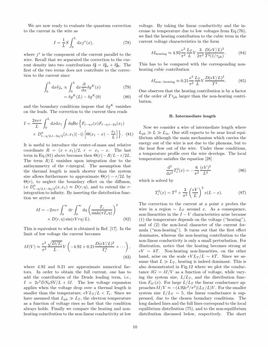
The correction to the current at a point x probes thewire in a region ∼ LT around x. As a consequence,non-linearities in the I − V characteristics arise because(1) the temperature depends on the voltage (“heating”),and of (2) the non-local character of the current for-mula (“non-heating”). It turns out that the first effectdominates, whereas the non-heating contribution to thenon-linear conductivity is only a small perturbation. Forillustration, notice that the heating becomes strong ateV ∼ kT . Non-heating non-linearities, on the otherhand, arise on the scale eV LT /L ∼ kT . Since we as-sume that L ≫ LT , heating is indeed dominant. This isalso demonstrated in Fig.12 where we plot the conduc-tance δG = δI/V as a function of voltage, while vary-ing the system size, L/LT , and the distribution func-tion Ftt′(x). For large L/LT the linear conductance ap-proaches δI/V ≈ −(4.92e2/π2)(LT /L)V . For the smallersystem size L/LT = 5, the linear conductance is sup-pressed, due to the chosen boundary conditions. Thelong dashed lines and the full lines correspond to the localequilibrium distribution (75), and to the non-equilibriumdistribution discussed below, respectively. The short
10
dashed line (L/LT = 5), instead, is obtained by takinginto account only the heating contribution, i.e. by calcu-lating from Eq.(81) the linear conductivity and averagingover the x-dependent temperature,
δIheating =1
L
∫ L
0
dxδσ(T (x))(V/L). (88)
One observes in Fig.12 that the “heating” contributionreproduces with a good accuracy the much more com-plicated full calculation. For the longer system withL/LT = 200, we do not plot the “heating” curve, be-cause in this case it is practically indistinguishable fromthe long dashed one. A slightly larger non-linear conduc-tivity is found in the non-equilibrium situation as it willbe discussed in the next section.
L=LT = 200L=LT = 5eV=kTconductance 100101
0-0.1-0.2-0.3-0.4-0.5FIG. 12. Interaction correction to the conductance I/V
for a mesoscopic wire as a function of voltage. I/V is plot-ted in units of (e2/h)LT /L. The full line corresponds tothe non-equilibrium distribution function (89). The longdashed line corresponds to the local equilibrium distributionfunction (75) with the x-dependent temperature. The shortdashed line (L/LT = 5) is the non-linear conductivity dueto the heating contribution only, Eq.(88).
C. Short wire
In a very short wire the inelastic length may exceedthe system size L. When one neglects the inelastic scat-tering, the distribution function inside the wire becomesa linear superposition of the distribution functions in theleads and reads
F (ǫ, x) = [(L − x)F (ǫ, 0) + xF (ǫ, L)] /L. (89)
In the limit L ≫ LT the analytic calculation of the cur-rent proceeds as in the case of subsection A. In analogyto (82) we arrive at
δI = −2πeτ
∫ ∞
0
dr
∫ ∞
0
dη
(
T
sinh(πTη)
)2
×D(r, η) sin(eV η)r/L. (90)
The numerical results for the current-voltage character-istics in the presence of such a distribution function areshown in Fig.12. Notice that we integrated numerically
Eq.(81), as it is appropriate when LT /L is not very large.The linear conductance is – of course – the same as in thelocal equilibrium situation, whereas the non-linear effectsare slightly larger.
D. The Spin-triplet channel
Up to now we have neglected all the spin effects. Asdemonstrated in appendix B, the current formula caneasily be generalized in order to include also the so calledspin triplet channels. The general equation for the cor-rection to the current is given in the appendix. With thetwo-step distribution function (89) and for L ≫ LT theequation for the current reads
δjb = −4πeDN0τ2
3∑
i=0
∫ ∞
−∞
dr
∫ ∞
0
dη
∫ η
0
dt1
×(
T
sinh(πTη)
)2
sin(eV η)r
L
× D(r, t1)∂
∂r(γiD)(r, η − t1), (91)
with
(γiD)(r, t) =γi
τ
√
1 − 2γi
4πDtexp
[
−r2(1 − 2γi)/4Dt]
,
(92)
and γi are the interaction amplitudes in the spin singlet(γ0 = 1/2) and spin triplet (γ1,2,3 = γt) channels. In thelow voltage limit this expression reproduces the standardresult for the linear conductivity,
δσ = −4.92e2
π2
LT
L
[
1 − 3(√
1 − 2γt − 1 + γt)/γt
]
. (93)
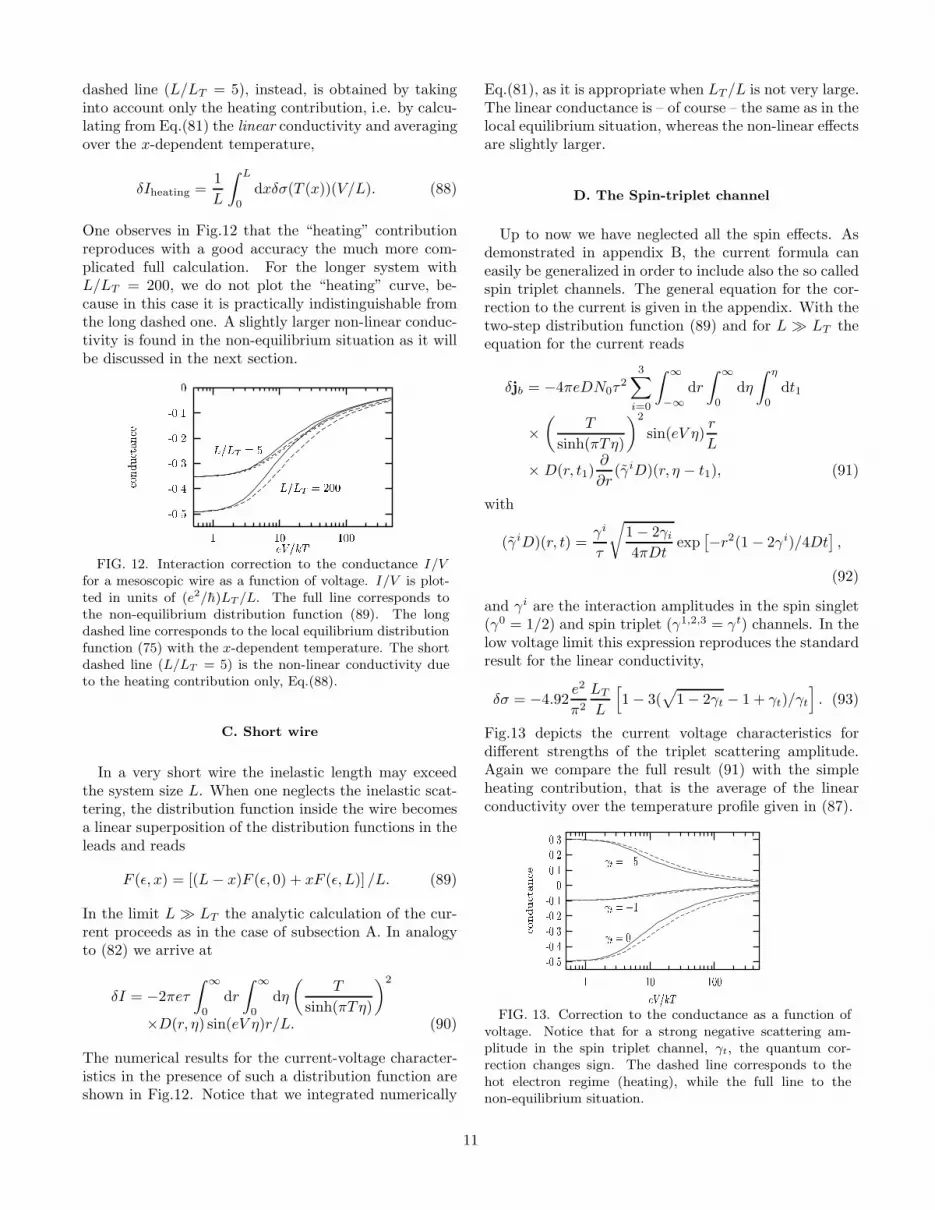
Fig.13 depicts the current voltage characteristics fordifferent strengths of the triplet scattering amplitude.Again we compare the full result (91) with the simpleheating contribution, that is the average of the linearconductivity over the temperature profile given in (87).
t = 0 t = �1 t = �5eV=kTconductanc
e100101
0.30.20.10-0.1-0.2-0.3-0.4-0.5FIG. 13. Correction to the conductance as a function of
voltage. Notice that for a strong negative scattering am-plitude in the spin triplet channel, γt, the quantum cor-rection changes sign. The dashed line corresponds to thehot electron regime (heating), while the full line to thenon-equilibrium situation.
11
For strong scattering in the triplet channel the quan-tum correction changes sign. As a function of voltage,the quantum corrections are suppressed. For the caseof a distribution function out of equilibrium, the non-heating non-linear contributions are stronger than thepure heating effects.
VI. CONCLUSIONS
We have calculated the interaction correction to theelectrical current for a disordered metal out of equilib-rium. In order to do so we have extended the diagram-matic approach of Refs. [17,18]. We have first demon-strated explicitly the gauge invariance of our current for-mula for the current density. In particular, we have dis-cussed how the physical interpretation of the non-linearcontribution may be described differently depending onthe gauge choice made. In the scalar gauge one maythink as the particle-hole pair lying on a different chemi-cal potential. In the vector gauge, the chemical potentialof the particle and hole are equal. In the latter case anargument based on phase differences leads to the conclu-sion that the electric field affects the correction to theconductivity.
We have successively discussed in some detail the cor-rection for the case of a mesoscopic wire. We have as-sumed that the wire is attached to “ideal leads” (infiniteconductance), which are described by means of bound-ary conditions for the distribution function and the dif-fusion propagator. We have distinguished three differentregimes. First we concentrated on a wire near local equi-librium, with a constant electron temperature. Besidesheating, there is a contribution to the non-linear conduc-tivity due to the nonlocal nature of the current response.
For short wires, where the electron-phonon length islonger than the system size, we found that the conduc-tance scales with voltage over temperature. Such a scal-ing behavior has been recently observed in a nanobridge[29]. However, the quantitative shape of the “scalingcurve” is not universal. We have found two differentcurves in the hot electron regime, where the inelasticscattering length is shorter than the system size, and innon-equilibrium.
We would like finally to emphasize that in this paperwe have concentrated on the quantum correction to thecurrent, and we have left aside a derivation of the chargedensity and the kinetic equation including the quantumcorrections. This latter task implies the evaluation ofthe quantum correction to the distribution function. Theevaluation of the distribution function and charge densityare directly connected as it is clear when one expressesthe distribution function in terms of the quasi-classicalGreen functions as gK = gRF − FgA, and recalls therelation of gK with the charge density. The inclusion of
quantum corrections into the kinetic equation for disor-dered electrons have been considered for the weak local-ization case without electron interaction in Refs. [31,32],and in the presence of interactions in Ref. [33]. In thelatter work, the non-linear electric field effects have notbeen included. We notice that the quantum correctionto the charge density out of equilibrium can be derivedfollowing the procedure described in this paper for thecurrent density in section III. This task is however moreinvolved for the following reason. Within the leading or-der in the gradient expansion, one finds from δΣimp,K , inanalogy to Eq.(38), the identity δρa = δρ. The diagramsin Fig.9, responsible for the contribution to the currentdenominated δjb, give in the case of the charge densityδρb = 0. This happens because, the evaluation of theHikami box with the density vertex is zero in the lead-ing order of the gradient expansion. In order to considerthe next-to-leading terms, one has to take into accounthigher powers in the inverse of ǫF τ and ql. This requiresthe evaluation of also the diagrams with only one vertex,Γ or Γ, renormalized by the diffusion pole. Therefore thefull expression of the electron self-energy is considerablymore complicated and such a calculation will be morelengthy than the one we presented here for the currentdensity. This task, although worth to be done, is beyondthe scope of the present paper.
ACKNOWLEDGMENTS
We acknowledge many discussions with C. Castellani.This work was supported by the DFG through SFB 484and Forschergruppe HO 955. R.R. acknowledges partialfinancial support from E.U. under Grant number RTN1-1999-00406.
APPENDIX A: FIELD THEORETIC APPROACH:
THE NON-LINEAR SIGMA MODEL
The field theoretic formulation of the interacting,disordered electron system was pioneered by Finkel-stein in the 80’s [30]. Recently, this formulation hasbeen extended to the non-equilibrium case by means ofthe Keldysh technique by Kamenev and Andreev [25]and Chamon, Ludwig and Nayak [34] for the case ofnormal-conducting metals and by Feigel’man, Larkin andSkvortsov [35] for superconductors. Gutmann and Gefen[20] have also used the field theoretic description to cal-culate the current and zero frequency shot noise.
Given the already extensive literature available on thesubject, we believe that, rather than repeating again thederivation of the non-linear sigma model, it is perhapsmore useful, instead, to show how to obtain our currentformula (63) within the non-linear sigma model. In thisappendix we will discuss the spinless version of the model,
12

following Ref. [25], postponing the spin effects to the fol-lowing appendix. In the absence of the electron interac-tion, the action of the non-linear sigma model is givenby
iS0 = −πN0
4
[
DTr(∂xQ)2 + 4iTrǫQ]
, (A1)
where the so-called long derivative ∂x is defined by
∂xQ = ∇Q + ie[A, Q]. (A2)
The field Q ≡ Qijtt′(x) must satisfy the constraints Q2 = 1
and TrQ = 0. The electron interaction is described bythe following term in the action
iS1 = −iπN0TrΦαγαQ, (A3)
with γ1 = σ0 and γ2 = σx. The fluctuations of the field Φare related to the statically screened Coulomb interactionand given by
− i〈Φi(x, t)Φj(x′, t′)〉 =
1
2V σij
x δ(x − x′)δ(t − t′). (A4)
In the case of long range Coulomb forces one findsV = 1/N0. Since Φ couples only linearly to Q it canbe integrated out:
〈e−iπN0TrΦαγαQ〉Φ
= exp
[
− iV (πN0)2
2
∫
dxdtTr(γ1Qtt(x))Tr(γ2Qtt(x))
]
. (A5)
Here the trace refers to the Keldysh space. The ap-pearance of the product of terms containing γ1 and γ2
stems from the σx structure of the interaction matrix inKeldysh space. In order to make contact with the dia-grammatic approach, we express the Green functions interms of the Q-fields. First we observe that [25]
Gtt′(x,x′) = 〈[
G−10 +
i
2τQ + Φαγα
]−1
〉Q,Φ, (A6)
where the brackets 〈. . .〉Q,Φ indicate that one has to av-erage over the fields Q and Φ. For the sake of simplicity,we drop the subscripts Q, Φ in the following. By usingthe condition that the fields Q and Φ are only slowlyvarying in space and time, one finds a relation betweenthe ξ-integrated Green function and the Q-matrix. Inparticular, upon taking the s-wave component of both,one finds
∫
dp
4πgtt′(p,x) = 〈Qtt′(x)〉. (A7)
In a similar way the p-wave part of the ξ-integrated Greenfunction is related to Q by
vF
∫
dp
4πpgǫǫ′(p,x) =
1
2D〈∂xQQ − Q∂xQ〉, (A8)
so that the current density reads
j =1
2eπDN0〈(∂xQQ − Q∂xQ)12〉. (A9)
At a first glance, this might differ from what is foundfollowing Ref. [25], where the current density is writtenas
j =1
2eπDN0〈Trγ2(∂xQQ − Q∂xQ)〉. (A10)
On the other hand, by comparing with the expression(A8) for the Green function, it is seen that Eq.(A10)sums the Keldysh component and the (21)-component ofthe Green function, whereas (A9) takes only the Keldyshcomponent. Since the (21)-component is zero the twoexpressions are equivalent.
1. Propagators
The saddle point approximation for the Q-field
Qsp =
(
1 2F0 −1
)
(A11)
reproduces the Drude-Boltzmann theory. The quantumcorrections are found when considering the fluctuationsabout the saddle point. We parameterize Q according to
Q = ue−W/2σzeW/2u (A12)
where u characterizes the saddle-point distribution func-tion
u =
(
1 F0 −1
)
, Qsp = uσzu, (A13)
and W parameterizes the fluctuations,
W =
(
0 ww 0
)
. (A14)
By expanding in powers of the W -field, one finds for thenon-interacting action, S0, up to the quadratic order
iS(2)0 = −πN0
2
{∫
dxdt1dt2wt1t2
(
∂t1 + ∂t2 + D∂2x
)
wt2t1
+
∫
dxdt1 · · · dt′2wt1t2(∂xFt2t′2)wt′
2t′1(∂xFt′
1t1)
}
. (A15)
The long derivative ∂xw = ∇w + ie[A, w] can here alsobe written as ∂x = ∇− ieAt1(x) + ieAt2(x). The 〈ωω〉correlations solve the differential equation
(
− ∂
∂t1− ∂
∂t2+ D∂2
x
)
〈wt2t1(x)wt3t4(x′)〉
=2
πN0δ(x − x′)δ(t1 − t3)δ(t2 − t4). (A16)
13
After introducing the relative times η = t2 − t1, η′ =t4 − t3 and the center-of-mass times, t = (t1 + t2)/2,t′ = (t3 + t4)/2, we identify this correlator with the dif-fuson,
〈wt2t1(x)wt3t4(x′)〉 = − 2τ
πN0Dη
tt′(x,x′)δ(η − η′), (A17)
as it may be seen by comparing with Eq.(30). Noticethat the relative time η is conserved during the propaga-tion so that η = η′. The 〈ww〉 correlator is the advancedcounterpart of the diffuson. 〈ww〉 = 0 since there is noterm proportional to ww in the action. Finally the 〈ww〉correlator is given by
〈wt2t1wt3t4〉 = −πN0
∫
dt′1 . . . dt′4〈wt2t1wt′1t′2〉〈wt′
4t′3wt3t4〉
×∂xFt′2t′4∂xFt′
3t′1. (A18)
This correlator is zero in equilibrium, when ∂xF = 0.Electron interactions modify these propagators. By ex-panding in (A5) each Q-field to first order in W , theinteracting part of the action becomes
= −i(πN0)2 1
2V
∫
dt(wF − Fw)tt(w − w − FwF )tt,
(A19)
which leads to non-trivial modifications of all the 〈ww〉correlators. Only 〈ωω〉 is not modified by the interactionand remains zero. We consider now 〈ww〉, which in theabsence of interaction is just the diffuson. We find
(
− ∂
∂t1− ∂
∂t2+ D∂2
x
)
〈wt2t1wt3t4〉Φ+ iπN0V Ft2t1 (〈wt2t2wt3t4〉Φ − 〈wt1t1wt3t4〉Φ)
=2
πN0δ(x − x′)δ(t1 − t3)δ(t2 − t4). (A20)
To understand the meaning of the above equation, let usconsider first the limit t2 → t1. The interaction depen-dent term does not drop from (A20) since the distributionfunction is singular in this limit, Ft2t1 ≈ −i/π(t2 − t1).Upon using this relation we arrive at the following simplediffusion equation
[
−(1 − N0V )∂
∂t+ D∂2
x
]
〈wttwt3t4〉Φ
=2
πN0δ(x − x′)δ(t − t3)δ(t − t4). (A21)
To make contact with the diagrammatic calculation, weidentify this correlation function with the product ofthe retarded interaction and diffusion propagators whichhave been defined in Eq.(71)
− π
2
N0V
2〈wttwt3t4〉Φ = (V RD)tt3δ(t3 − t4). (A22)
The propagator with four different time arguments is fi-nally given by
〈wt2t1wt3t4〉Φ = 〈wt2t1wt3t4〉 − iπN0V
∫
dx′dt′3dt′4[
×〈wt2t1wt′3t′4〉 Ft′
4t′3
(
〈wt′4t′4wt3t4〉Φ − 〈wt′
3t′3wt3t4〉Φ
)]
. (A23)
2. Correction to the current
Due to the fluctuations of Q there are corrections tothe charge and current density. Here we calculate thesecorrections by taking into account the Gaussian fluctu-ations. In the derivation, we parallel the lines of thediagrammatic approach. We begin by separating the cor-rection to the current in two contributions δj = δja + δjb,where δja is related to the gradient of the charge den-sity. We then proceed by expressing δjb in terms of thefields ω and ω. In the third step we will then explicitlyinclude the interaction and obtain the current formula.By writing Q = Qsp + δQ, the correction to the currentreads
δj(x, t) = −eπDN0
2〈Trγ2 {Qsp∂xδQ + δQ∂xQsp
+δQ∂xδQ − · · ·}〉. (A24)
The dots correspond to the terms which appear due to(∂xQ)Q. The term ja is proportional to the gradient ofthe charge density
δja(x, t) = −eπDN0∇〈δQ12tt (x)〉 (A25)
= −D∇δρ(x, t) (A26)
and we do not calculate explicitly here. The second term,δjb, contains all other contributions. By collecting thevarious summands, one gets
δjb = 2F∂x〈δQ22〉 + 〈δQ11〉∂x(2F )
+〈δQ11∂xδQ12〉 + 〈δQ12∂xδQ22〉 − · · · . (A27)
Now we expand Q in powers of W and we arrive at
δjb = eπDN0 [F 〈(∂xw)w〉Φ + 〈w(∂xw)〉ΦF ] (A28)
= 2πeDN0Re (〈w∂xw〉ΦF ) . (A29)
In the absence of interactions δjb vanishes, so that tak-ing the interactions into account is essential. Inserting〈ww〉Φ from eq.(A23) we find
δjb = 4πeDN0τ2
∫
dηdx1dx2Re{
Ft−η,t(x)
×Dηt−η/2,t1−η/2(x,x1)Ft1,t1−η(x1)
×V Rt1t2(x1,x2)(−i∇x)D0
t2,t−η(x2,x)}
, (A30)
which is identical to what we obtained in Eq.(62).Notice that the long derivative in the current formula
(A29) reduces to the gradient in the final result. Thishappens since the two time indices in the relevant ω fieldare always equal, 〈wttwt3t4〉Φ ∝ δ(t3 − t4).
14

APPENDIX B: SPIN-TRIPLET CHANNEL
Until now we have neglected the spin effects. Thesearise from the fact that the diffusion is described by theparticle-hole propagator, which may occurs in four spinstates depending on the relative spin of the particle andhole. In the case of Coulomb long range forces, the mostsingular contribution comes from the singlet channel thatwe have discussed throughout the paper. In addition tothe singlet channel, there are three triplet channels whichalso contribute to the quantum corrections to the current.In this appendix we extend our earlier work of Ref. [18]to non-equilibrium.
In order to take into account the spin-dependent inter-actions, we follow Refs. [30,34] and start from an inter-action which is local in space and time. The fermionicaction is of the type
iSee = − i
2N0Tr
{
ΓΨsΨs′Ψs′Ψs − Γ2ΨsΨs′ΨsΨs′
}
,
(B1)
where Γ and Γ2 are dimensionless static scattering am-plitudes, and Ψs is an operator for a Fermion with spins. The trace includes integration over space and timecontour, as well as summation over spin. The interactioncan be written in terms of the charge and spin densities,
iSee = − i
2N0Tr
{(
Γ − Γ2
2
)
ρρ − Γ2
2s · s
}
, (B2)
with ρ =∑
s ΨsΨs and si =∑
ss′ Ψsσiss′Ψs′ . At this
point it becomes convenient to introduce the interactionamplitudes in the charge (singlet) channel, Γs = Γ−Γ2/2and in the spin (triplet) channel, Γt = −Γ2/2. Thenwe decouple the interaction with the fields (Φ,B) forthe charge and spin. By going through the steps of thederivation of the σ-model one finds the following modifi-cations of the action
iS0 → −πN0
4[DTr∂xQss′∂xQs′s + 4iTrZǫQss] (B3)
iS1 → −iπN0Tr [(Φαδss′ + Bα · σss′ )γαQs′s] , (B4)
with
− i〈φαφβ〉 =1
2
Γs
N0σx
αβ (B5)
−i〈BiαBj
β〉 =1
2
Γt
N0σx
αβδij . (B6)
In (B3) we introduced the factor Z which arises in therenormalization of the σ-model [30]. One observes that Zcan be absorbed in a redefinition of the interaction am-plitudes, the quasi-particle diffusion constant, and thequasi-particle density of states according to
Γs,t → γs,t = Γs,t/Z (B7)
D → Dqp = D/Z (B8)
N0 → Nqp = N0Z (B9)
We are now ready to consider the fluctuations. In analogyto what has been done in the spinless case, we introducethe charge and spin components of the fields w and w,
wss′ =1√2
3∑
i=0
wiσiss′ (B10)
wi =1√2
∑
ss′
wss′σiss′ (B11)
where σ0ss′ = δss′ and σi
ss′ for i = 1, 2, 3 are the usualPauli matrices. In the quadratic fluctuations of the non-interacting action, S0, the spin and charge terms decou-ple, since the structure is of the type
∑
wss′ (. . .)ws′s =∑
i wi(. . .)wi. The coupling term iS1 is to first order inW given by
iS1 = −iπN0
√2
∑
i
Tr
{
Biαγαu
(
0 wi
−wi 0
)
u
}
+ · · ·
(B12)
where for brevity we denoted the scalar field Φ by B0.We assume that the saddle point, i.e. the distributionfunction and therefore the matrix u, does not depend onspin. The interaction field, Φ, is easily integrated out,with the result that at the level of the quadratic fluctu-ations, the spin and charge contributions are decoupledeven in the presence of the interaction.
The correction to the current is finally found as
δjb = eπDN0
3∑
i=0
Re〈wi∇xwi〉ΦF (B13)
= 4πeDqpτ2
3∑
i=0
∫
dηdx1dx2Re{
Ft−η,t(x)
×Di,ηt−η/2,t1−η/2(x,x1)Ft1,t1−η(x1)
× γit1t2(x1,x2)(−i∇x)Di,η′=0
t2,t−η(x2,x)}
, (B14)
where again i = 0 corresponds to the charge and i =1, 2, 3 correspond to spin channels. Di,η
tt′ (x,x′) is thequasi-particle diffusion propagator in the relevant spinor charge channel, which obeys the differential equationgiven in eq.(30), with the only difference that the diffu-sion constant D is replaced by the quasi-particle diffusionconstant Dqp. γi is the dynamically screened interaction,
γi(q, ω) = γi[1 + γiΠd/Nqp]−1 (B15)
= γi −iω + Dqpq2
−i(1 − 2γi)ω + Dqpq2. (B16)
For the explicit calculations it is convenient to considerthe product of the dynamically screened interaction andthe retarded diffuson,
15

(γiDi)tt′(x,x′) =
∫
dx1γitt1(x,x1)D
i,η=0t1,t′ (x1,x
′) (B17)
which solves the diffusion equation
[
(1 − 2γi)∂t − D∇2x
]
(γiDi)tt′(x,x′) =γi
τδ(x − x′)δ(t − t′).
(B18)
[1] P.A. Lee and T.V. Ramakrishnan, Rev. Mod. Phys. 57,287 (1985); D. Belitz and T.R. Kirkpatrick, Rev. Mod.Phys. 66, 261 (1994).
[2] B.L. Altshuler and A.G. Aronov, in Electron-Electron In-
teractions in Disordered Systems, edited by M. Pollakand A.L. Efros (North-Holland, Amsterdam, 1985), p. 1.
[3] G. Bergmann, Phys. Rep. 107, 1 (1984). S. Chakravartyand A. Schmid, Phys. Rep. 140, 193 (1986).
[4] L.P. Gorkov, A.I. Larkin, and D.E. Khmel’nitskii Pis’maZh. Eksp. Teor. 30, 248 (1979) [JETP Lett. 30, 228(1979)].
[5] E. Abrahams and T.V. Ramakrishnan, J. Non-Cryst. Sol.35, 15 (1980).
[6] B.L. Altshuler, A.G. Aronov, and P.A. Lee, Phys. Rev.Lett. 44, 1288 (1980); B.L. Altshuler, D. Khmel’nitzkii,A.I. Larkin, and P.A. Lee, Phys. Rev. B 22, 5141 (1980).
[7] A.I. Larkin, and D.E. Khmel’nitskii, Sov. Phys. JETP64, 1075 (1986).
[8] V.I. Fal’ko and D.E. Khmel’nitskii, Sov. Phys. JETP 68,186 (1989).
[9] V.E. Kravtsov and V.I. Yudson, Phys. Rev. Lett. 70, 210(1993).
[10] For a review on the experimental development see L.P. Kouwenhoven et al. in ” Proceeding of the NATOAdavnced Study Institute on Mesoscopic Electron Trans-port” edited by L.L. Sohn, L.P. Kouwenhoven, and G.Schon, Kluwer Academy Publishers, Dordrecht, 1997,pag.105; see also L.P. Kouwenhoven and C.M. MarcusPhysics World, pp35-39 june (1998); L.P. Kouwenhovenand L. Glazman Physics World, pp33-38 january (2001)and references therein.
[11] Ya.M. Blanter and M. Buttiker, Phys. Rep. 336, 1(2000).
[12] B.L. Altshuler, M.E. Gershenson, and I.L. Aleiner, Phys-ica E 3, 58 (1998).
[13] P. Mohanty, E.M.Q. Jariwala, and R.A. Webb, Phys.Rev. Lett. 78, 3366 (1997).
[14] P. Mohanty, E.M.Q. Jariwala, and R.A. Webb, Fortschr.Phys. 46, 779 (1998).
[15] G. Bergmann, Wei Wei, Yao Zou, and R.M. Mueller,Phys. Rev. B 41, 7386 (1990).
[16] J. Liu and N. Giordano, Phys. Rev. B 43, 1385 (1991).[17] R. Raimondi, P. Schwab, and C. Castellani, Phys. Rev.
B 60, 5818 (1999).[18] M. Leadbeater, R. Raimondi, P. Schwab, and C. Castel-
lani, Eur. Phys. J. B 15, 277 (2000).[19] H. Pothier, S. Gueron, N.O. Birge, D. Esteve, and M.H.
Devoret, Phys. Rev. Lett. 79, 3490 (1997).[20] D.B. Gutman and Y. Gefen, preprint, cond-mat/cond-
mat/0006468; cond-mat/0102134.[21] L.V. Keldysh Zh. Eksp. Teor. Fiz. 47, 1515 (1964) [Sov.
Phys. JETP 20, 1018 (1964)].[22] J. Rammer and H. Smith, Rev. Mod. Phys. 58, 323
(1986).[23] B.L. Altshuler, Sov. Phys. JETP 48, 670 (1978).[24] Ya.M. Blanter, Phys. Rev. B 54, 12807 (1996).[25] A. Kamenev and A. Andreev, Phys. Rev. B 60, 2218
(1999).[26] V.I. Kozub and A.M. Rudin, Phys. Rev. B 52, 7853
(1995).[27] Y. Naveh, D.V. Averin, and K.K. Likharev, Phys. Rev.
B 58, 15371 (1998); Y. Naveh, in XVIII Rencontres de
Moriond: Quantum Physics at Mesoscopic Scale, editedby D.C. Glattli and M. Sanquer (Editions Frontiers,France, 1999).
[28] K.E. Nagaev, Phys. Rev. B 52, 4740 (1995).[29] H.B. Weber, R. Haussler, H. v. Lohneysen, and J. Kroha
Phys. Rev. B 63 165426 (2001).[30] A.M. Finkelstein, Sov. Phys. JETP 57, 97 (1983); Z.
Phys. B 56, 189 (1984); in Electron Liquid in Disordered
Conductors, edited by I.M. Khalatnikov, Soviet ScientificReviews Vol 14 (Harwood, London, 1990).
[31] S. Hershfield and V. Ambegaokar Phys. Rev. B 34, 2147(1986).
[32] G. Strinati, C. Castellani, and C. Di Castro Phys. Rev.B 40, 12237 (1989).
[33] G. Strinati, C. Castellani, C. Di Castro, and G. Kotliar,Phys. Rev. B 44, 6078 (1991).
[34] C. Chamon, A.W.W. Ludwig, and C. Nayak, Phys. Rev.B 60, 2239 (1999).
[35] M.V. Feigel’man, A.I. Larkin, and M.A. Skvortsov, Phys.Rev. B 61, 12361 (2000).
16