coherent train of lfm pulses

7COHERENT TRAIN OF LFM PULSES

Good Doppler resolution requires a long coherent signal. To minimize eclips-ing requires a short transmission time (unless the radar is especially designed totransmit and receive simultaneously, as in CW radar). A solution that meets bothrequirements is a coherent train of pulses. The basic type of such a signal wasdiscussed in Sections 3.6 and 4.3, where the train was constructed from identicalconstant-frequency pulses. In many practical cases the pulses are modulated andare not identical. Modulation produces wider bandwidth, hence pulse compres-sion. The identicalness is violated by even the simple introduction of interpulseweighting, used to lower Doppler sidelobes. In some signals, significant diversityis introduced between the pulses in order to obtain additional advantages, suchas lower delay sidelobes or lower recurrent lobes.

In this and the following chapters we extend the discussion in two direc-tions: adding modulation and adding diversity. Adding modulation but keepingthe pulses identical still allows us to use the theoretical results regarding theperiodic ambiguity function (Section 3.6) and to obtain analytic expression forthe ambiguity function (within the duration of one pulse, i.e., |τ| ≤ T ). Addingdiversity in amplitude (i.e., weighting) or by different modulation in differentpulses within the coherent train will usually require numerical analysis, exceptfor a few simple cases in which theoretical analysis is available. Such is thecase for the subject of this chapter—a coherent train of LFM pulses—probablythe most popular radar signal in airborne radar (Rihaczek, 1969; Stimson, 1983;Nathanson et al., 1991).

Radar Signals, By Nadav Levanon and Eli MozesonISBN 0-471-47378-2 Copyright 2004 John Wiley & Sons, Inc.

168

COHERENT TRAIN OF IDENTICAL LFM PULSES 169

7.1 COHERENT TRAIN OF IDENTICAL LFM PULSES

A train of identical linear-FM pulses provides both range resolution and Dopplerresolution—hence its importance and popularity in radar systems. Its ambiguityfunction still suffers from significant sidelobes, both in delay (range) and inDoppler. Thus, modifications are usually applied to reduce these sidelobes. Inthis section we consider the basic signal without modifications. The coherencyis reflected in the expression of the real signal, given by

s(t) = Re[u(t) exp(j2πfct)] (7.1)

where the complex envelope is a train of N pulses with pulse repetition period Tr,

u(t) = 1√N

N∑n=1

un[t − (n − 1)Tr] (7.2)

The uniformity of the pulses is expressed by assuming that un(t) = u1(t). TheLFM nature of a pulse of duration T is expressed in its complex envelope,

u1(t) = 1√T

rect

(t

T

)exp(jπkt2), k = ±B

T(7.3)

An example of a real signal is shown in Fig. 7.1, where all the pulses beginwith the same initial phase. This is not a mandatory requirement for coherence.Coherency can be maintained as long as the initial phase of each pulse transmittedis known to the receiver.

Changes in phase from pulse to pulse will be expressed in the complex enve-lope of the nth pulse as

un(t) = 1√T

rect

(t

T

)exp[j (φn + πkt2)], k = ±B

T(7.4)

As long as T < Tr/2 (which will be assumed henceforth), the additional phaseelement has no effect on the ambiguity function for |τ| ≤ T . It will only affectthe recurrent lobes of the AF: namely, over |τ ± nTr| ≤ T (n = 1, 2, . . .). The

FIGURE 7.1 Coherent train of identical LFM pulses.

170 COHERENT TRAIN OF LFM PULSES

additional phase term can already be considered as some sort of diversity, butone that affects only recurrent lobes.

To get an analytic expression for the partial ambiguity function (AF) of oursignal, we start with the AF of a constant-frequency pulse, apply AF property 4to it, and obtain the AF of a single LFM pulse (as done in Section 4.2):

|χ(τ, ν)| = |χT (τ, ν)| =∣∣∣∣(

1 − |τ|T

)sin α

α

∣∣∣∣ , |τ| ≤ T (single pulse) (7.5)

where

α = πT(ν ∓ B

τ

T

)(1 − |τ|

T

)(7.6)

The first equality |χ(τ, ν)| = |χT (τ, ν)| stems from the fact that T < Tr/2. Todescribe the AF of the train, for the limited delay |τ| ≤ T , we now apply therelationship of the periodic AF:

|χ(τ, ν)| = |χT (τ, ν)|∣∣∣∣ sin NπνTr

N sin πνTr

∣∣∣∣ , |τ| ≤ T (train of pulses) (7.7)

0 1 2 3 4 5 6 7 8-6

-5

-4

-3

-2

-1

0

t / T r

Phas

e / π

0 1 2 3 4 5 6 7 8

-10

-5

0

5

10

t / T r

f T

FIGURE 7.2 Phase (top) and frequency (bottom) of a coherent train of eight LFMpulses (BT = 20).

COHERENT TRAIN OF IDENTICAL LFM PULSES 171

Using (7.5) in (7.7) yields the ambiguity function of a train of N identicalLFM pulses:

|χ(τ, ν)| =∣∣∣∣(

1 − |τ|T

)sin α

α

∣∣∣∣∣∣∣∣ sin NπνTr

N sin πνTr

∣∣∣∣ , |τ| ≤ T (7.8)

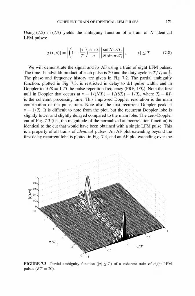
We will demonstrate the signal and its AF using a train of eight LFM pulses.The time–bandwidth product of each pulse is 20 and the duty cycle is T /Tr = 1

9 .The phase and frequency history are given in Fig. 7.2. The partial ambiguityfunction, plotted in Fig. 7.3, is restricted in delay to ±1 pulse width, and inDoppler to 10/8 = 1.25 the pulse repetition frequency (PRF, 1/Tr). Note the firstnull in Doppler that occurs at ν = 1/(NTr) = 1/(8Tr) = 1/Tc, where Tc = 8Tr

is the coherent processing time. This improved Doppler resolution is the maincontribution of the pulse train. Note also the first recurrent Doppler peak atν = 1/Tr. It is difficult to note from the plot, but the recurrent Doppler lobe isslightly lower and slightly delayed compared to the main lobe. The zero-Dopplercut of Fig. 7.3 (i.e., the magnitude of the normalized autocorrelation function) isidentical to the cut that would have been obtained with a single LFM pulse. Thisis a property of all trains of identical pulses. An AF plot extending beyond thefirst delay recurrent lobe is plotted in Fig. 7.4, and an AF plot extending over the

-1

-0.5

0

0.5

1

0

2

4

6

8

10

0

0.2

0.4

0.6

0.8

1

τ / T ν NT

r

|χ(τ

,ν)|

FIGURE 7.3 Partial ambiguity function (|τ| ≤ T ) of a coherent train of eight LFMpulses (BT = 20).


-1

-0.5

0

0.5

1

0

0.2

0.4

0.6

0.8

1

1.2

0

0.2

0.4

0.6

0.8

1

τ / T r ν T

r

|χ(τ

,ν)|

FIGURE 7.4 Partial ambiguity function (|τ| ≤ T + Tr) of a coherent train of eight LFMpulses (BT = 20).

-8-6

-4-2

02

46

8

0

0.5

1

1.5

2

2.5

0

0.2

0.4

0.6

0.8

1

τ / T r

ν T r

|χ(τ

,ν)|

FIGURE 7.5 Ambiguity function (|τ| ≤ 8Tr) of a coherent train of eight LFM pulses(BT = 20).

FILTERS MATCHED TO HIGHER DOPPLER SHIFTS 173

entire delay span appears in Fig. 7.5. The Doppler span displayed was doubledin Fig. 7.5, showing two Doppler recurrent lobes.

7.2 FILTERS MATCHED TO HIGHER DOPPLER SHIFTS

The ambiguity function displays the response of a filter matched to the origi-nal signal, without Doppler shift. As shown in Fig. 7.3, a coherent pulse trainachieves good Doppler resolution, and a matched filter will produce an outputonly when the Doppler shift of the received signal is within the Doppler reso-lution. A typical radar processor is likely to contain several filters, matched toseveral different Doppler shifts. In a coherent pulse train, implementing such aprocessor is relatively simple, especially if the intrapulse modulation is Dopplertolerant, as LFM is.

The principle of Doppler filter implementation is summarized inFigs. 7.6 and 7.7. Figure 7.6 shows that each pulse is processed by a zero-Doppler matched filter. The N outputs from the N pulses are then fed to anFFT. The first output of the FFT is equivalent to a zero-Doppler filter. For thatfirst output the FFT coherently sums the N inputs. For the second FFT output,the nth pulse n = 0, 1, . . . , N − 1 is first multiplied by the complex coefficientexp(j2πn/N), before being added to the outputs of the other N processed pulses.This complex coefficient is equivalent to a phase shift,

φn = 2πn

N= 2πνnTr ⇒ ν = 1

NTr(7.9)

0 T Tr

2Tr

(N-1)Tr

Complex envelopeof the signal u(t)

Pulsecompression

Pulsecompression

Pulsecompression

Pulsecompression

FFT

ν=0 ν=1/NTr

ν=1/Tr

FIGURE 7.6 Implementing several Doppler filters using FFT.


0 T Tr

2Tr

(N-1)Tr

Time

Phas

e Ideal Doppler compensation

Implemented Doppler compensation

FIGURE 7.7 Interpulse phase compensation for a higher Doppler filter.

The phase shift φn, added to the nth pulse which is delayed by nTr, is equalto the phase shift that would have been accumulated after a delay of nTr by aDoppler shift of ν = 1/NTr. We thus see that the second output of the FFT iseffectively a Doppler filter matched to the Doppler frequency at which the firstDoppler filter produces a null response. (The first Doppler filter is centered atzero Doppler.) The (k + 1) FFT filter sums the pulses after multiplying the nthpulse by the complex coefficient exp(j2πkn/N), and is therefore matched to aDoppler frequency ν = k/NTr or because of Doppler ambiguity (mod 1/Tr), toν = −(N − k)/NTr.

The Doppler compensation achieved by this method is represented by the solidline in Fig. 7.7. The ideal Doppler compensation is represented by the dashedline. The difference is that the FFT implementation lacks Doppler compensationwithin each pulse. If the output of a compressed pulse is relatively insensitiveto Doppler shift (like LFM), the performance of the FFT approach is nearly asgood as the performance of an ideal Doppler filter.

The expected response of the second Doppler filter (matched to ν = 1/NTr)of the train of eight LFM pulses studied in Section 7.1 is shown in Fig. 7.8. Theresponse was obtained by calculating a cross-ambiguity function between twosignals, one having the normal phase history of a train of identical LFM pulses(Fig. 7.9, top), and the other in which phase steps of 2π/N = π/4 were addedbetween pulses (Fig. 7.9, bottom). Note in Fig. 7.8 that the response was zero atzero Doppler and peaked at ν = 1/NTr, while in Fig. 7.3 the response peaks atzero Doppler and reaches a null at ν = 1/NTr = 1/(8Tr) = 1/Tc. Note that wedenote the cross-ambiguity or delay–Doppler response of a mismatched filter as

FILTERS MATCHED TO HIGHER DOPPLER SHIFTS 175

-1

-0.5

0

0.5

1

0

2

4

6

8

10

0

0.2

0.4

0.6

0.8

1

τ / T ν NT

r

|ψ(τ

,ν)|

FIGURE 7.8 Delay–Doppler response of the second Doppler filter, ν = 1/NTr.

0 1 2 3 4 5 6 7 8-6

-4

-2

0

2

t / T r

Phas

e / π

0 1 2 3 4 5 6 7 8-6

-4

-2

0

2

t / T r

Phas

e / π

FIGURE 7.9 Phase of the reference signal for the ν = 0 filter (top) and the ν = 1/NTr

filter (bottom).


ψ(τ, ν). As for the notations used for the (auto) ambiguity function in this book,a positive value of ν corresponds to a target with higher closing velocity, andpositive delay (τ) implies a target farther away from the radar.

Some targets may have a Doppler value that falls between successive FFT fil-ters. The return from those targets suffers a power loss according to the FFT filterresponse at the target Doppler. This power loss is usually referred to as straddleloss. To minimize straddle loss it is possible to either reduce the frequency separa-tion between consecutive Doppler filters or to widen the filter response such thatthe overlap between successive filters is higher. To reduce the frequency separa-tion between consecutive Doppler filters and thus achieve overlap between theirresponses, it is necessary to reduce the phase step between pulses of the referencesignal. This could be implemented by adding zero-padded inputs to the FFT. Thenumber of FFT outputs will grow accordingly, adding more Doppler filters. Widen-ing the filter response is achieved by introducing interpulse amplitude modulation,which is discussed in the next section. Finally, note that the imperfection of thiskind of FFT Doppler filtering grows as the center frequency of the Doppler filtergrows (the LFM Doppler tolerance has a stronger effect on the response).

7.3 INTERPULSE WEIGHTING

Figure 7.3 reveals high delay and Doppler sidelobes. As we learned with respectto the single LFM pulse, the delay sidelobes of the autocorrelation function ofa single LFM pulse can be reduced by shaping the spectrum according to aweight window. Because of the linear relationship between frequency and timein an LFM pulse, spectral shaping can be implemented by applying intrapulseamplitude weighting. In a dual way, the Doppler sidelobes, shown in Fig. 7.3,can be reduced by implementing interpulse amplitude weighting.

Figure 7.10 presents two versions of the amplitude of eight transmitted LFMpulses following a square root of a Hamming window. The reference signal inthe receiver will also have such a square-root weight window. Their product willyield a true Hamming window. In the top subplot the weight window has eightsteps, yielding flat-top pulses. In the bottom subplot the window is smooth overthe entire train duration (NTr), yielding variable-amplitude pulses. As long as theduty cycle is small, there is little difference in performances. Hence, the morepractical stepwise window is preferred. For a large duty cycle, and especially inperiodic CW signals (duty cycle = 1), the smooth window should be used. Thephase and frequency are identical in both signals and remain as in Fig. 7.2. Theresulting ambiguity function is shown in Fig. 7.11 and should be compared withFig. 7.3. The comparison clearly demonstrates the reduction in Doppler sidelobesand a widening of the Doppler mainlobe lobe (at ν = 0) and recurrent lobe (atν = 1/Tr or νNTr = 8).

The variable amplitude of the transmitted pulses could be a problem to ahigh-power RF amplifier, hence the readiness to implement the window only onreceive, despite the mismatch loss that this creates. Next we will demonstrate that

INTERPULSE WEIGHTING 177

0 1 2 3 4 5 6 7 80

0.2

0.4

0.6

0.8

1

t / T r

Am

plitu

de

0 1 2 3 4 5 6 7 80

0.2

0.4

0.6

0.8

1

t / T r

Am

plitu

de

FIGURE 7.10 Square root of Hamming interpulse amplitude weighting: stepwise (top)and smooth (bottom).

-1

-0.5

0

0.5

1

0

2

4

6

8

10

0

0.2

0.4

0.6

0.8

1

τ / T

ν NT r

|χ(τ

,ν)|

FIGURE 7.11 Ambiguity function of eight LFM pulses with a square root of Hamminginterpulse amplitude weighting.


0 1 2 3 4 5 6 7 80

0.2

0.4

0.6

0.8

1

t / T r

Am

plitu

de

0 1 2 3 4 5 6 7 80

0.2

0.4

0.6

0.8

1

t / T r

Am

plitu

de

FIGURE 7.12 Pulse amplitude of Hamming-weighted reference signal (top) and trans-mitted signal (bottom).

-1

-0.5

0

0.5

1

0

2

4

6

8

10

0

0.2

0.4

0.6

0.8

1

τ / T ν NT

r

|ψ(τ

,ν)|

FIGURE 7.13 Cross-ambiguity between two LFM pulse trains with amplitudes shownin Fig. 7.12.

INTRA- AND INTERPULSE WEIGHTING 179

other than SNR loss, implementing the interpulse amplitude weighting only onreceive, does not result in a different delay–Doppler response. Note that since thereference signal is not matched to the signal transmitted, we cannot use the phraseambiguity function. Instead, we use the phrases delay–Doppler response or cross-ambiguity to describe the output of a mismatched receiver. Figure 7.12 displaysthe amplitude of the eight pulses used in the train transmitted (bottom) and in thereference train (top). The phase and frequency are identical in both signals andwere shown in Fig. 7.2. Comparing the top of Fig. 7.12 with Fig. 7.10 showsthe difference between a Hamming window and a square root of a Hammingwindow. The resulting cross-ambiguity is shown in Fig. 7.13. It is practicallyindistinguishable from Fig. 7.11. We can conclude that with regard to interpulseweighting, there is hardly any difference in delay–Doppler response betweenmatched weighting and mismatched (on receive) weighting. A difference will beseen when intrapulse weight is introduced.

7.4 INTRA- AND INTERPULSE WEIGHTING

Interpulse weighting mitigates Doppler sidelobes, as demonstrated inFig. 7.11 or 7.13. Intrapulse weighting in LFM mitigates range sidelobes, aswas shown in Section 4.2.1. The weightings can be combined to reduce bothrange and Doppler sidelobes. Again, square-root weight windows can be applied

0 1 2 3 4 5 6 7 80

0.2

0.4

0.6

0.8

1

t / T r

Am

plitu

de

3.44 3.46 3.48 3.5 3.52 3.54 3.560

0.2

0.4

0.6

0.8

1

t / T

Am

plitu

de

FIGURE 7.14 Interpulse (top) and intrapulse (bottom) Hamming weight windows.


-1

-0.5

0

0.5

1

0

2

4

6

8

10

0

0.2

0.4

0.6

0.8

1

τ / T ν NT

r

|ψ(τ

,ν)|

FIGURE 7.15 Delay–Doppler response of eight LFM pulses with inter- and intrapulseHamming weight windows.

in both transmitter and receiver, maintaining match filtering. However, toallow fixed-amplitude transmission, the weighting can be concentrated in thereceiver, at a cost of SNR loss and some difference in delay–Doppler response.Figure 4.15 demonstrated the difference in the zero-Doppler response of asingle LFM pulse between matched and mismatched Hamming intrapulse weightwindows. That difference remains in the response of a train of LFM pulses withintrapulse weighting.

Figure 7.14 shows the amplitude of a reference signal in a receiver for a trainof eight LFM pulses. Hamming weight windows were implemented both betweenthe pulses (see the top) and within each pulse (see the zoom on a single pulseat the bottom). The resulting delay–Doppler response (BT = 20) is shown inFig. 7.15. The SNR loss due to mismatch is rather high in this case. It canbe calculated using Section 4.2.2. For simple weight windows such as Hann orHamming, the delay–Doppler response (plotted in Fig. 7.15) can be calculatedanalytically. An outline of the calculation is given in the next section.

7.5 ANALYTIC EXPRESSIONS OF THE DELAY–DOPPLERRESPONSE OF AN LFM PULSE TRAIN WITH INTRA- ANDINTERPULSE WEIGHTING

A simple analytic expression is presented here for the delay–Doppler responseof a coherent pulse-train radar waveform consisting of LFM pulses. The receiver

DELAY–DOPPLER RESPONSE OF AN LFM PULSE TRAIN 181

differs from a matched filter by intra- and interpulse weighting. The responsediffers from the ambiguity function of an unweighted pulse train by widenedlobes and reduced sidelobes, due to weightings, and by SNR loss due to themismatch. The analysis follows Getz and Levanon (1995). The analysis will belimited in delay to the pulse width T : namely, |τ| ≤ T . This will allow us to usethe periodic ambiguity function, which is simpler to develop and which is equalto the ambiguity function over that delay range. Recall from Section 3.6 that thetransmitted pulse train is not bounded in time. Only the reference signal in thereceiver is limited to N pulses.

7.5.1 Ambiguity Function of N LFM Pulses

The complex envelope of a single LFM pulse that starts at t = 0 can bedescribed as

uT (t) = 1√T

exp

[jπk

(t − 1

2T

)2]

, 0 ≤ t ≤ T (7.10)

where T is the pulse duration and k is the frequency sweep rate. The product|kT 2| = TB is known as the time–bandwidth product or compression ratio. Theenvelope of an infinitely long coherent pulse train is defined as

u(t) =∞∑

i=−∞uT (t − iTr) (7.11)

where Tr is the pulse repetition interval. At the receiver the number of processedpulses will be limited to N . For delay within the pulse duration |τ| ≤ T , whenthe receiver is matched to N pulses, the delay–Doppler response is equal to theperiodic ambiguity function of N pulses, which will be written slightly differentlyfrom its form in (3.37),

|χ(τ, ν)| = 1

NTr

∣∣∣∣∫ NTr

0u(t − τ)u∗(t) exp(j2πνt) dt

∣∣∣∣ , |τ| ≤ T (7.12)

As given by (7.6) and (7.8),

|χ(τ, ν)| =∣∣∣∣(

1 − |τ|T

)sin α

α

∣∣∣∣∣∣∣∣ sin NπνTr

N sin πνTr

∣∣∣∣ , |τ| ≤ T (7.13)

where

α = πT(ν ∓ B

τ

T

)(1 − |τ|

T

)(7.14)

This simple and well-known result will serve as a reference to which we willcompare the response of a more general processor that includes weighting.


7.5.2 Delay–Doppler Response of a Mismatched Receiver

Figure 7.16 summarizes the magnitude of the signals involved in a receiver mis-matched by introducing weight windows. It contains the periodic (and infinite)signal received, u(t − τ), the periodic reference signal r(t), which can be morecomplicated than just the complex conjugate of u(t), and an interpulse weightwindow, limited to the duration of N pulses:

wp(t) ={

w(t), 0 ≤ t ≤ NTr

0, elsewhere(7.15)

This interpulse weight window will reduce sidelobes along the Doppler axis.The receiver delay–Doppler response is the magnitude of the cross-correlationbetween the weighted reference and the received signal shifted in delay τ andDoppler ν:

|ψ(τ, ν)| =∣∣∣∣∫ ∞

−∞u(t − τ)r(t)wp(t) exp(j2πνt) dt

∣∣∣∣ (7.16)

Using the well-known property that the Fourier transform of a product is theconvolution between the individual Fourier transforms, (7.16) can be written as

|ψ(τ, ν)| =∣∣∣∣∫ ∞

−∞u(t − τ)r(t) exp(j2πνt) dt ⊗

∫ NT

0w(t) exp(j2πνt) dt

∣∣∣∣(7.17)

Since u(t) and r(t) are infinite and periodic with period T , the first transform onthe right-hand side of (7.17) can be written as an infinite sum:

∫ ∞

−∞u(t − τ)r(t) exp(j2πνt) dt =

∞∑n=−∞

δ(ν − n

T

)gn(τ) (7.18)

0 T Tr

2Tr

Complex envelope

of the signal u(t)

Reference

periodic signal r(t)

Inter-pulse

weigth window w(t)

FIGURE 7.16 Mismatched filter.


where

gn(τ)�= 1

T

∫ T

0u(t − τ)r(t) exp

(j2πnt

T

)dt (7.19)

When Tr > 2T , u and r in (7.19) can be replaced by their one-period versions,uT and rT , respectively.

The second transform is a Fourier transform of the external weight window

W(ν) =∫ NT

0w(t) exp(j2πνt) dt (7.20)

The convolution between (7.18) and (7.20) yields

|ψ(τ, ν)| =∣∣∣∣∣

N∞∑n=−N∞

gn(τ)W(ν − n

T

)∣∣∣∣∣ , N∞ → ∞ (7.21)

Rigorously, N∞ → ∞, but for most practical numerical calculations it issufficient to choose N∞ ≈ 5. Before we can obtain from (7.21) the specificdelay–Doppler response of the LFM pulses, we need to define the referenceperiodic signal r(t), which may include an intrapulse weight, and also choose aspecific interpulse weight function w(t).

We limit the weight windows to the family containing the uniform, Hann, andHamming windows. All three can be defined by

wp(t) =

1

NTr

[1 − 1 − c

ccos

2πt

NTr

], 0 ≤ t ≤ NTr

0, elsewhere(7.22)

with c = 1 for a uniform window, c = 0.5 for a Hann window, and c = 0.53836for a Hamming window. Their Fourier transform is given by

W(ν) = sin πνNTr

πνNTr

{1 + (1 − c)(νNTr)

2

c[1 − (νNTr)2]

}exp(j2πνNTr) (7.23)

Note that these are smooth windows that will create variable-top pulses (as in thebottom subplot of Fig. 7.10). For a small duty cycle, the delay–Doppler responseof variable-top pulses will be very similar to that of flat-top pulses. Flat-top pulsesare easier to implement and process but are more difficult to analyze analytically.

7.5.3 Adding Intrapulse Weighting

When the periodic reference in the receiver is simply the complex conjugate ofthe complex envelope of the transmitted signal: namely,

r(t) = u∗(t) (7.24)


then the gn(τ) function is found from (7.10) and (7.19) to be (up to a constant)

gn(τ) =(

1 − τ

T

) sin[πn(T /Tr)(1 − τ/T )]

πn(T /Tr)(1 − τ/T )exp

[jπn

T

Tr

(1 + τ

T

)], 0 ≤ τ ≤ T

(7.25)

During an LFM pulse the frequency is changing linearly with time. Addingan intrapulse weight window with a duration T is equivalent to implementing aweight window in the frequency domain. Such a window reduces sidelobes alongthe delay axis (Farnett and Stevens, 1990). We will therefore apply an intrapulseweight window:

wint(t)

={

1

T

[1 − 1 − c

ccos

2πt

T

]= 1

T

{1 − 1 − c

2c

[exp

(j

2πt

T

)+ exp

(−j

2πt

T

)]}, 0 ≤ t ≤ T

0, elsewhere

(7.26)For simplicity the intrapulse weight (7.26) was chosen to be similar to the inter-pulse weight (7.22). This is not a requirement, however. For example, c in (7.26)could be different from c in (7.22).

With intrapulse weighting, one period of the reference signal becomesthe product

rT (t) = u∗T (t)wint(t) (7.27)

which is clearly zero for t < 0 and t > T . With rT (t) defined through (7.10),(7.26), and (7.27), the final expression for the gn(τ) function of an LFM pulse,including intrapulse weighting, is

gn(τ) = g(0)n (τ) − 1 − c

2c[g(1)

n (τ) + g(−1)n (τ)] (7.28)

where

g(m)n (τ) =

(1 − τ

T

) sin β(m)n

β(m)n

exp

[jπT

(1 + τ

T

)(n

Tr+ m

T

)], m = −1, 0, 1

(7.29)

and

β(m)n = πT

(1 − τ

T

)(n

Tr+ m

T− kτ

), m = −1, 0, 1 (7.30)

The five equations (7.21), (7.23), and (7.28)–(7.30) fully define thedelay–Doppler response for 0 ≤ τ ≤ T . For negative delays we can sometimesassume symmetry with respect to the origin, borrowed from the ambiguityfunction, namely

|ψ(τ, ν)| = |ψ(−τ, −ν)| (7.31)


Note that (7.31) was not proved as (3.22) was. Figure 7.8 is an example wherethere is no symmetry. The number of terms in (7.28) can be increased, andtheir respective coefficients adjusted, to provide for intrapulse Taylor weight-ing (Farnett and Stevens, 1990).

7.5.4 Examples

Figure 7.17 presents the first quadrant of the cross-ambiguity function ofunweighted processing (top) and Hamming weighting (bottom). Identical typesof windows were used for both inter- and intrapulse weighting. The signalparameters were Tr/T = 5, TB = 20, and N = 16 pulses. Note from Fig. 7.17that at a Doppler of ν/Tr = 1, the recurrent peak is shifted in delay relative tothe peaks at zero Doppler. Note also that the direction of the shift agrees withour notations of the ambiguity function, where positive delay corresponds to atarget farther from the radar than the reference (τ = 0). Indeed, using an up-chirp LFM (as used for Fig. 7.17) implies that a target with negative Doppler1/Tr would appear as if the target location is farther from the radar than the truetarget location. The shift (typical of LFM) is

τ

T= 1

TB(Tr/T )(7.32)

0

0.2

0.4

0.6

0.8

1

0

5

10

15

200

0.2

0.4

0.6

0.8

1

τ / T

ν NT r

|ψ(τ

,ν)|

FIGURE 7.17 Cross-ambiguity function of 16 LFM pulses, with no weighting (above)and Hamming weighting (next page).


0

0.2

0.4

0.6

0.8

1

0

5

10

15

200

0.2

0.4

0.6

0.8

1

τ / T ν NT r

|ψ(τ

,ν)|

FIGURE 7.17 (continued )

The corresponding cuts along the Doppler axis (in dB) are presented in Fig. 7.18.The top plot (uniform window) behaves according to |(sin NπνT )/(N sin πνT )|.The bottom plot demonstrates the flat sidelobes level typical of a Hammingwindow.

The corresponding zero-Doppler cuts (in dB) are presented in Fig. 7.19. Thetop part (no weighting) is the well-known zero-Doppler AF cut of an unweightedsingle LFM pulse [see equation (4.10)]. The lower plot (Hamming weighting) wascalculated numerically using equations (7.28)–(7.30) for n = 0. The relativelyhigh delay sidelobes (≈ −30 dB), despite the Hamming weighting, will drop withhigher time–bandwidth product. An example for TB = 100 is given in Fig. 7.20,where the sidelobe level dropped to −42 dB.

Note the identity of Fig. 7.19 (bottom) and Fig. 4.15 (bottom). They bothdescribe the zero-Doppler cut of the delay–Doppler response of mismatched(only on receive) Hamming-weighted LFM pulse. However, Fig. 7.19 (bottom)was based on a numerical calculation of equations (7.28)–(7.30), whereasFig. 4.15 (bottom) was based on numerical cross-correlation between the(unweighted) transmitted signal and the (weighted) reference signal. This couldserve as some sort of confirmation of the analysis in Section 7.5.

Finally, we should point out that the analysis of Section 7.5 assumed that theintrapulse sampling rate is higher than twice the pulse bandwidth, meeting theNyquist criteria. In some very high bandwidth LFM pulses, hardware limitationsmay not allow high-enough sampling rate. Using a lower sampling rate will


0 2 4 6 8 10 12 14 16 18 20-60

-50

-40

-30

-20

-10

0

ν NT r

|ψ(0

,ν)|

0 2 4 6 8 10 12 14 16 18 20-60

-50

-40

-30

-20

-10

0

ν NT r

|ψ(0

,ν)|

FIGURE 7.18 Zero-delay cut of the cross-ambiguity function of 16 LFM pulses, withno weighting (top) and Hamming weighting (bottom).


0 0.1 0.2 0.3 0.4 0.5 0.6 0.7 0.8 0.9 1-60

-50

-40

-30

-20

-10

0

τ / T

|ψ(τ

,0)|

0 0.1 0.2 0.3 0.4 0.5 0.6 0.7 0.8 0.9 1-60

-50

-40

-30

-20

-10

0

τ / T

|ψ(τ

,0)|

FIGURE 7.19 Zero-Doppler cut of the cross-ambiguity function of 16 LFM pulses(TB = 20), with no weighting (top) and Hamming weighting (bottom).

PROBLEMS 189

0 0.1 0.2 0.3 0.4 0.5 0.6 0.7 0.8 0.9 1-60

-50

-40

-30

-20

-10

0

τ / T

|ψ(τ

,0)|

FIGURE 7.20 Zero-Doppler cut of the cross-ambiguity function of 16 LFM pulses withHamming weighting (TB = 100).

create spurious peaks in delay. This issue was discussed by Abatzoglou andGheen (1998).

PROBLEMS

7.1 Doppler toleranceConsider a pulse train of N = 8 pulses, pulse duration T = 100 µs, andrepetition period Tr = 10T .(a) What is the Doppler resolution (first null)?(b) For constant-frequency pulses, if the Doppler filter is matched to a

higher Doppler shift, at what (matched to) Doppler shift will thepeak response drop to 1

2 (relative to the peak response of a zero-Doppler filter)?

(c) Repeat part (b) for the case of LFM pulses with TB = 20.

7.2 SNR loss due to weighingCalculate the SNR loss for a train of eight LFM pulses when Hammingintrapulse and stepwise interpulse weightings are implemented only onreceive.


7.3 Opposite LFM slope doublet(a) In a train of two identical LFM pulses, what is the relative peak height

(in dB relative to the peak at the origin) of the zero-Doppler responseat the recurrent lobe?

(b) Repeat part (a) for the case when the two pulses are of opposite LFMslopes and TB = 20.

7.4 Frequency spectrum of a train of identical pulsesConsider a coherent train of eight identical pulses with Tr = 4T .(a) For a constant-frequency pulse, compare, discuss, and explain the sim-

ilarity between the ambiguity function’s zero-delay cut (in dB) withthe energy spectral density of the signal (in dB) over a Doppler orfrequency span of 0 ≤ f ≤ 6/Tr = 1.5/T .

(b) Qualitatively compare the energy spectral densities of the signal in part(a) with a similar train in which the pulses are LFM with TB = 10.Consider both the fine details of the spectrum plot in dB (over thefrequency span 0 ≤ f ≤ 6/Tr = 1.5/T ) and the overall spectral shape(over the frequency span 0 ≤ f ≤ 60/Tr = 15/T ).

7.5 AF of a train of LFM pulsesConsider a coherent train of eight identical (unweighted) LFM pulses withTr = 4T and TB = 50. Plot the ambiguity function with the followingzooms:(a) |τ| ≤ T , 0 ≤ ν ≤ 9T /8.(b) |τ| ≤ T /40, 0 ≤ ν ≤ 9T /8.Using the latter zoom, find how much has the first recurrent Dopplerpeak (at ν = 1/Tr) shifted in delay from τ = 0? Confirm your result withequation (7.32).

REFERENCES

Abatzoglou, T. J., and G. O. Gheen, Range, radial velocity, and acceleration MLE usingradar LFM pulse train, IEEE Transactions on Aerospace and Electronic Systems, vol.34, no. 4, October 1998, pp. 1070–1084.

Farnett, E. C., and G. H. Stevens, Pulse compression radar, in Skolnik, M. I. (ed.), RadarHandbook, 2nd ed., McGraw-Hill, New York, 1990, Chap. 10.

Getz, B., and N. Levanon, Weight effects on the periodic ambiguity function, IEEE Trans-actions on Aerospace and Electronic Systems, vol. 31, no. 1, January 1995, pp. 182–193.

Nathanson, F. E., J. P. Reilly, and M. N. Cohen, Radar Design Principles: Signal Pro-cessing and the Environment, 2nd ed., McGraw-Hill, New York, 1991.

Rihaczek A. W., Principles of High Resolution Radar, McGraw-Hill, New York, 1969.

Stimson, G. W., Introduction to Airborne Radar, Hughes Aircraft Co., El Segundo, CA,1983.

coherent train of lfm pulses

Documents