theory and experiments for disordered elastic manifolds
TRANSCRIPT
Theory and Experiments for Disordered ElasticManifolds, Depinning, Avalanches, and Sandpiles
Kay Jorg WieseLaboratoire de physique, Departement de physique de l’ENS, Ecole normale superieure,UPMC Univ. Paris 06, CNRS, PSL Research University, 75005 Paris, France
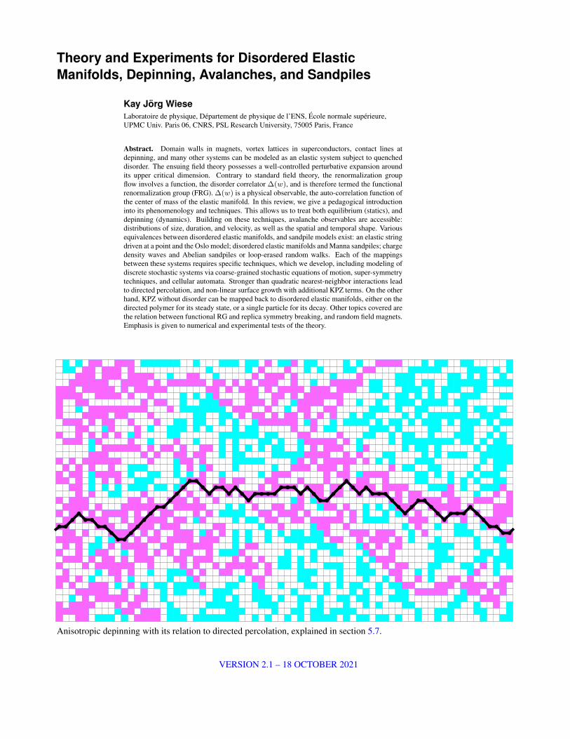
Abstract. Domain walls in magnets, vortex lattices in superconductors, contact lines atdepinning, and many other systems can be modeled as an elastic system subject to quencheddisorder. The ensuing field theory possesses a well-controlled perturbative expansion aroundits upper critical dimension. Contrary to standard field theory, the renormalization groupflow involves a function, the disorder correlator ∆(w), and is therefore termed the functionalrenormalization group (FRG). ∆(w) is a physical observable, the auto-correlation function ofthe center of mass of the elastic manifold. In this review, we give a pedagogical introductioninto its phenomenology and techniques. This allows us to treat both equilibrium (statics), anddepinning (dynamics). Building on these techniques, avalanche observables are accessible:distributions of size, duration, and velocity, as well as the spatial and temporal shape. Variousequivalences between disordered elastic manifolds, and sandpile models exist: an elastic stringdriven at a point and the Oslo model; disordered elastic manifolds and Manna sandpiles; chargedensity waves and Abelian sandpiles or loop-erased random walks. Each of the mappingsbetween these systems requires specific techniques, which we develop, including modeling ofdiscrete stochastic systems via coarse-grained stochastic equations of motion, super-symmetrytechniques, and cellular automata. Stronger than quadratic nearest-neighbor interactions leadto directed percolation, and non-linear surface growth with additional KPZ terms. On the otherhand, KPZ without disorder can be mapped back to disordered elastic manifolds, either on thedirected polymer for its steady state, or a single particle for its decay. Other topics covered arethe relation between functional RG and replica symmetry breaking, and random field magnets.Emphasis is given to numerical and experimental tests of the theory.
Anisotropic depinning with its relation to directed percolation, explained in section 5.7.
VERSION 2.1 – 18 OCTOBER 2021
CONTENTS 2
Contents
1 Disordered Elastic Manifolds: Phenomenology 41.1 Introduction . . . . . . . . . . . . . . . . . 41.2 Physical realizations, model and observables 51.3 Long-range elasticity (contact line of a
fluid, fracture, earthquakes, magnets withdipolar interactions) . . . . . . . . . . . . . 7
1.4 Flory estimates and bounds . . . . . . . . . 81.5 Replica trick and basic perturbation theory . 81.6 Dimensional reduction . . . . . . . . . . . 91.7 Larkin-length, and the role of temperature . 10
2 Equilibrium (statics) 112.1 General remarks about renormalization . . . 112.2 Derivation of the functional RG equations . 112.3 Statistical tilt symmetry . . . . . . . . . . . 132.4 Solution of the FRG equation, and cusp . . 132.5 Fixed points of the FRG equation . . . . . . 152.6 Random-field (RF) fixed point . . . . . . . 152.7 Random-bond (RB) and tricritical fixed points 152.8 Generic long-ranged fixed point . . . . . . 162.9 Charge-density wave (CDW) fixed point . . 162.10 The cusp and shocks: A toy model . . . . . 162.11 The effective disorder correlator in the
field-theory . . . . . . . . . . . . . . . . . 172.12 ∆(u) and the cusp in simulations . . . . . . 182.13 Beyond 1-loop order . . . . . . . . . . . . 182.14 Stability of the fixed point . . . . . . . . . 202.15 Thermal rounding of the cusp . . . . . . . . 212.16 Disorder chaos . . . . . . . . . . . . . . . 232.17 Finite N . . . . . . . . . . . . . . . . . . . 232.18 Large N . . . . . . . . . . . . . . . . . . . 242.19 Corrections at order 1/N . . . . . . . . . . 242.20 Relation to Replica Symmetry Breaking
(RSB) . . . . . . . . . . . . . . . . . . . . 252.21 Droplet picture . . . . . . . . . . . . . . . 262.22 Kida model . . . . . . . . . . . . . . . . . 272.23 Sinai model . . . . . . . . . . . . . . . . . 282.24 Random-energy model (REM) . . . . . . . 292.25 Complex disorder and localization . . . . . 302.26 Bragg glass and vortex glass . . . . . . . . 312.27 Bosons and fermions in d = 2, bosonization 322.28 Sine-Gordon model, Kosterlitz-Thouless
transition . . . . . . . . . . . . . . . . . . 332.29 Random-phase sine-Gordon model . . . . . 342.30 Multifractality . . . . . . . . . . . . . . . . 352.31 Simulations in equilibrium: polynomial
versus NP-hard . . . . . . . . . . . . . . . 372.32 Experiments in equilibrium . . . . . . . . . 37
3 Dynamics, and the depinning transition 373.1 Phenomenology . . . . . . . . . . . . . . . 373.2 Field theory of the depinning transition,
response function . . . . . . . . . . . . . . 383.3 Middleton theorem . . . . . . . . . . . . . 39
3.4 Loop expansion . . . . . . . . . . . . . . . 393.5 Depinning beyond leading order . . . . . . 423.6 Stability of the depinning fixed points . . . 433.7 Non-perturbative FRG . . . . . . . . . . . 433.8 Behavior at the upper critical dimension . . 433.9 Extreme-value statistics: The Discretized
Particle Model (DPM) . . . . . . . . . . . 443.10 Mean-field theories . . . . . . . . . . . . . 463.11 Effective disorder, and rounding of the cusp
by a finite driving velocity . . . . . . . . . 473.12 Simulation strategies . . . . . . . . . . . . 483.13 Characterization of the 1-dimensional string 483.14 Theory and numerics for long-range elas-
ticity: contact-line depinning and fracture . 503.15 Experiments on contact-line depinning . . . 503.16 Fracture . . . . . . . . . . . . . . . . . . . 503.17 Experiments for peeling and unzipping . . . 523.18 Creep, depinning and flow regime . . . . . 533.19 Quench . . . . . . . . . . . . . . . . . . . 543.20 Barkhausen noise in magnets (d = 2) . . . 553.21 Experiments on thin magnetic films (d = 1) 563.22 Hysteresis . . . . . . . . . . . . . . . . . . 573.23 Inertia, and a large-deviation function . . . 573.24 Plasticity . . . . . . . . . . . . . . . . . . 583.25 Depinning of vortex lines or charge-density
waves, columnar defects, and non-potentiality 583.26 Other universal distributions . . . . . . . . 59
4 Shocks and avalanches 594.1 Observables and scaling relations . . . . . . 594.2 A theory for the velocity . . . . . . . . . . 614.3 ABBM model . . . . . . . . . . . . . . . . 614.4 End of an avalanche, and an efficient
simulation algorithm . . . . . . . . . . . . 624.5 Brownian Force Model (BFM) . . . . . . . 624.6 Short-ranged rough disorder . . . . . . . . 634.7 Field theory . . . . . . . . . . . . . . . . . 634.8 FRG and scaling . . . . . . . . . . . . . . 634.9 Instanton equation . . . . . . . . . . . . . . 644.10 Avalanche-size distribution . . . . . . . . . 644.11 Watson-Galton process, and first-return
probability . . . . . . . . . . . . . . . . . . 644.12 Velocity distribution . . . . . . . . . . . . . 654.13 Duration distribution . . . . . . . . . . . . 654.14 Temporal shape of an avalanche . . . . . . 654.15 Local avalanche-size distribution . . . . . . 664.16 Spatial shape of avalanches . . . . . . . . . 664.17 Some theorems . . . . . . . . . . . . . . . 674.18 Loop corrections . . . . . . . . . . . . . . 684.19 Simulation results and experiments . . . . . 694.20 Correlations between avalanches . . . . . . 714.21 Avalanches with retardation . . . . . . . . . 724.22 Power-law correlated random forces, rela-
tion to fractional Brownian motion . . . . . 724.23 Higher-dimensional shocks . . . . . . . . . 73
4.24 Clusters of avalanches in systems withlong-range elasticity . . . . . . . . . . . . . 73
4.25 Earthquakes . . . . . . . . . . . . . . . . . 744.26 Avalanches in the SK model . . . . . . . . 74
5 Sandpile Models, and Anisotropic Depinning 755.1 From charge-density waves to sandpiles . . 755.2 Bak-Tang-Wiesenfeld, or Abelian sandpile
model . . . . . . . . . . . . . . . . . . . . 755.3 Oslo model . . . . . . . . . . . . . . . . . 755.4 Single-file diffusion, and ζdep
d=1 = 5/4 . . . . 765.5 Manna model . . . . . . . . . . . . . . . . 775.6 Hyperuniformity . . . . . . . . . . . . . . 775.7 A cellular automaton for fluid invasion, and
related models . . . . . . . . . . . . . . . . 775.8 Brief summary of directed percolation . . . 795.9 Fluid invasion fronts from directed percola-
tion . . . . . . . . . . . . . . . . . . . . . 805.10 Anharmonic depinning and FRG . . . . . . 805.11 Other models in the same universality class 815.12 Quenched KPZ with a reversed sign for the
non-linearity . . . . . . . . . . . . . . . . . 815.13 Experiments for directed Percolation and
quenched KPZ . . . . . . . . . . . . . . . 81
6 Modeling Discrete Stochastic Systems 826.1 Introduction . . . . . . . . . . . . . . . . . 826.2 Coherent-state path integral, imaginary
noise and its interpretation . . . . . . . . . 836.3 Stochastic noise as a consequence of the
discreteness of the state space . . . . . . . . 836.4 Reaction-annihilation process . . . . . . . . 846.5 Field theory for directed percolation . . . . 856.6 State variables of the Manna model . . . . . 856.7 Mean-field solution of the Manna model . . 866.8 Effective equations of motion for the
Manna model: CDP theory . . . . . . . . . 876.9 Mapping of the Manna model to disordered
elastic manifolds . . . . . . . . . . . . . . 88
7 KPZ, Burgers, and the directed polymer 897.1 Non-linear surface growth: KPZ equation . 897.2 Burgers equation . . . . . . . . . . . . . . 897.3 Cole-Hopf transformation . . . . . . . . . . 907.4 KPZ as a directed polymer . . . . . . . . . 907.5 Galilean-invariance, and scaling relations . 917.6 A field theory for the Cole-Hopf transform
of KPZ . . . . . . . . . . . . . . . . . . . 917.7 Decaying KPZ, and shocks . . . . . . . . . 927.8 All-order β-function for KPZ . . . . . . . . 927.9 Anisotropic KPZ . . . . . . . . . . . . . . 937.10 KPZ with spatially correlated noise . . . . . 947.11 An upper critical dimension for KPZ? . . . 947.12 The KPZ equation in dimension d = 1 . . . 947.13 KPZ, polynuclear growth, Tracey-Widom
and Baik-Rains distributions . . . . . . . . 95
7.14 Models in the KPZ universality class, andexperimental realizations . . . . . . . . . . 96
7.15 From Burgers’ turbulence to Navier-Stokesturbulence? . . . . . . . . . . . . . . . . . 96
8 Links between loop-erased random walks, CDWs,sandpiles, and scalar field theories 968.1 Supermathematics . . . . . . . . . . . . . . 968.2 Basic rules for Grassmann variables . . . . 968.3 Disorder averages with bosons and fermions 978.4 Renormalization of the disorder . . . . . . 988.5 Supersymmetry and dimensional reduction . 988.6 CDWs and their mapping onto φ4-theory
with two fermions and one boson . . . . . . 1008.7 Supermathematics: A critical discussion . . 1008.8 Mapping loop-erased random walks onto
φ4-theory with two fermions and one boson 1008.9 Other models equivalent to loop-erased
random walks, and CDWs . . . . . . . . . 1038.10 Conformal field theory for critical curves . 104
9 Further developments and ideas 1049.1 Non-perturbative RG (NPRG) . . . . . . . 1049.2 Random-field magnets . . . . . . . . . . . 1059.3 Dynamical selection of critical exponents . 1079.4 Conclusion and perspectives . . . . . . . . 108
10 Appendix: Basic Tools 10810.1 Markov chains, Langevin equation, inertia . 10810.2 Ito calculus . . . . . . . . . . . . . . . . . 10910.3 Fokker-Planck equation . . . . . . . . . . . 10910.4 Martin-Siggia-Rose (MSR) formalism . . . 11010.5 Gaussian theory with spatial degrees of
freedom . . . . . . . . . . . . . . . . . . . 11110.6 The inverse of the Laplace operator. . . . . 11210.7 Extreme-value statistics: Gumbel, Weibull
and Frechet distributions . . . . . . . . . . 11210.8 Gel’fand Yaglom method . . . . . . . . . . 114
Theory and Experiments forDisordered Elastic Manifolds,Depinning, Avalanches, andSandpiles
Foreword
This review grew out of lectures the author gave in theICTP master program at ENS Paris. While the beginning ofeach section is elementary, later parts are more specializedand can be skipped at first reading. Beginners wishing toenter the subject are encouraged to start reading sections1 (introduction), 2.1-2.13 (equilibrium/statics), and 3.1-3.4
Theory and Experiments for Disordered Elastic Manifolds, Depinning, Avalanches, and Sandpiles 4
(depinning/dynamics). An introduction to avalanches isgiven in sections 4.1-4.3, 4.5-4.10. The remaining sectionsare more specialized: Sandpile models and anisotropicdepinning are treated in sections 5 and 6. An introductionto the KPZ equation and its relation to disordered elasticsystems is given in section 7. Section 8 discusses linksbetween a class of theories encompassing loop-erasedrandom walks, charge density waves, Abelian sandpiles,and n-component φ4 theory with n = −2, linked bysupermathematics. Further developments and ideas arecollected in section 9. The appendix 10 contains usefulbasic tools.
1. Disordered Elastic Manifolds: Phenomenology
1.1. Introduction
Statistical mechanics is by now a rather mature branch ofphysics. For pure systems like a ferromagnet, it allowsone to calculate with precision details as the behavior ofthe specific heat on approaching the Curie-point. Weknow that it diverges as a function of the distance intemperature to the Curie-temperature, we know that thisdivergence has the form of a power-law, we can calculatethe exponent, and we can do this with at least 3 digits ofaccuracy using the perturbative renormalization group [1,2, 3, 4, 5, 6, 7, 8], and even more precisely with the newlydeveloped conformal bootstrap [9, 10, 11]. Best of all, thesefindings are in excellent agreement with the most precisesimulations [12, 13, 14], and experiments [15]. This is atrue success story of statistical physics. On the other hand,in nature no system is really pure, i.e. without at least somedisorder (“dirt”). As experiments (and theory) suggest, alittle bit of disorder does not change much. Otherwiseexperiments on the specific heat of Helium1 would not soextraordinarily well confirm theoretical predictions. Butwhat happens for strong disorder? By this we mean thatdisorder dominates over entropy, so effectively the systemis at zero temperature. Then already the question: “Whatis the ground-state?” is no longer simple. This goeshand in hand with the appearance of metastable states.States, which in energy are close to the ground-state,but which in configuration-space may be far apart. Anyrelaxational dynamics will take an enormous time to findthe correct ground-state, and may fail altogether, as canbe seen in computer-simulations as well as in experiments,particularly in glasses [17]. This means that our wayof thinking, taught in the treatment of pure systems, hasto be adapted to account for disorder. We will see thatin contrast to pure systems, whose universal large-scaleproperties can be “modeled by few parameters”, disorderedsystems demand to model the whole disorder-correlation1 Even though there is some tension between values obtained in aspace-shuttle experiment [15] on one side, and simulations [16] and theconformal bootstrap [11] on the other hand.
function (in contrast to its first few moments). We showhow universality nevertheless emerges.
Experimental realizations of strongly disordered sys-tems are glasses, or more specifically spin-glasses, vortex-glasses, electron-glasses and structural glasses [18, 19, 20,21, 22, 23, 24, 25, 17]. Furthermore random-field mag-nets [26, 27, 28, 29, 30, 31, 32, 33, 34, 35, 36, 37, 38, 39],and last not least elastic systems subject to disorder, some-times termed disordered elastic systems or disordered elas-tic manifolds [40, 41, 42, 43, 44, 45, 46, 47, 48, 49, 50, 51,52, 53, 54], on which we focus below.
What is our current understanding of disorderedsystems? There are a few exact solutions, mostly foridealized or toy systems [55], there are phenomenologicalapproaches (like the droplet-model [56], section 2.21), andthere is a mean-field approximation, involving a methodcalled replica-symmetry breaking (RSB) [57]. This methodpredicts the properties of infinitely connected systems, ase.g. the Sherrington-Kirkpatrick (SK) model [58, 59]. Thesolution proposed in 1979 by G. Parisi [60] is parameterizedby a function q(x), where x “lives between replica indices0 and 1”. Today we have a much better understanding ofthis solution [61, 62, 63], and many features can be provenrigorously [64, 65, 66, 67]. The most notable feature is thepresence of an extensive number of ground states arrangedin a hierarchic way (ultrametricity). On the other hand, thissolution is inappropriate for systems in which each degreeof freedom is coupled only to its neighbors, as is e.g. thecase in short-ranged magnetic systems.
While the RSB method mentioned above is intellectu-ally challenging and rewarding, its complexity makes intu-ition difficult, and performing a field theoretic expansionaround this mean-field solution has proven too challeng-ing a task. Random-field models, which can be recast ina φ4-type theory are seemingly more tractable, but still thenon-linearity of the φ4-interaction makes progress difficult.What one would like to have is a field theory which in ab-sence of disorder is as simple as possible. The simplest suchsystem certainly is a non-interacting, Gaussian, i.e. free the-ory, to which one could then add disorder. Actually, exper-imental systems of this type are abundant: Magnetic do-main walls in presence of disorder a.k.a. Barkhausen noise[68, 69, 70], a contact line wetting a disordered substrate[71], fracture in brittle heterogeneous systems [72, 73, 74],or earthquakes [75] are good examples for elastic systemssubject to quenched disorder. They have a quite differentphenomenology from mean-field models, with notably asingle ground state. Asking questions about this groundstate, or more generally the probability measure at a giventemperature, is termed equilibrium. It supposes that if ex-ternal parameters change, they change so slowly that thesystem has enough time to explore the full phase space (er-godicity), and find the ground state.
In the opposite limit, notably if there are no thermalfluctuations at all, is depinning: Increasing an external
Theory and Experiments for Disordered Elastic Manifolds, Depinning, Avalanches, and Sandpiles 5
applied field yields jumps in the center-of-mass of thesystem (the total magnetization in a magnet). These jumpsare termed shocks or avalanches. While one can showthat the sequence of avalanches is deterministic given aspecific disorder (see below), we are more interested intypical behavior, i.e. an average over disorder. The latteraverage can often be obtained by watching the system for anextended time; one says that the system is self-averaging2.
In these lectures combined with a review, I aimat explaining the field theory behind these phenomena.All key ingredients are in addition derived analyticallyin well-chosen toy models. Theoretically most excitingare the connections between seemingly unrelated models.Finally, all main theoretical concepts are checked inexperiments. While the field theory has been developed formore than thirty years, no comprehensive and pedagogicalintroduction is yet available. It is my aim to close thisgap. Despite the more than 700 references included inthis review, I am aware of omissions. My apologies to allcolleagues whose work is not covered in depth. Luckily,some of them have written reviews or lectures themselves,and we refer the reader to [77, 78, 79, 80, 19, 81, 82, 83] forcomplementary presentations.
1.2. Physical realizations, model and observables
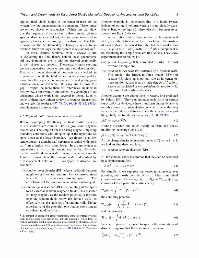
Before developing the theory to treat elastic systemsin a disordered environment, let us give some physicalrealizations. The simplest one is an Ising magnet. Imposingboundary conditions with all spins up at the upper and allspins down at the lower boundary (see figure 1), at lowtemperatures, a domain wall separates a region with spinsup from a region with spins down. In a pure system attemperature T = 0, this domain wall is flat. Disordercan deform the domain wall, making it eventually rough.Figure 1 shows, how the domain wall is described bya displacement field u(~x). Two types of disorder arecommon:
(i) random-bond disorder (RB), where the bonds betweenneighboring sites are random. On a course-grainedlevel this also represents missing spins. Thecorrelations of the random potential are short-ranged.
(ii) random-field disorder (RF), i.e. coupling of the spinsto an external random magnetic field. This disorderis “long-ranged”, as the random potential is the sumover the random fields below the domain wall, i.e.effectively has the statistics of a random walk. Takinga derivative of the potential, one obtains short-rangedcorrelated random forces.
2 In contrast to disordered elastic manifolds, some disordered systemssuch as long-range spin glasses are not self-averaging, which leads toreplica-symmetry breaking and a hierarchic organization of states, see [76]for a review, and section 2.20 for a discussion in our context. The presenceof a finite correlation length as given in Eqs. (34), (307) and (312) insuresself-averaging.
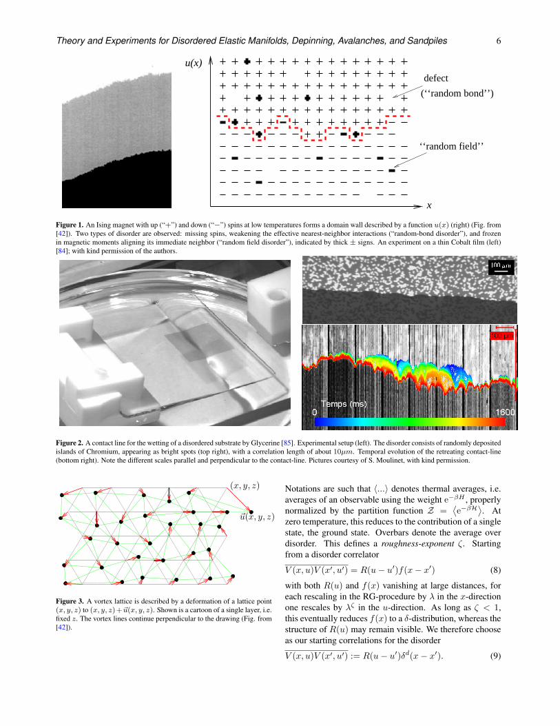
Another example is the contact line of a liquid (water,isobutanol, or liquid helium), wetting a rough (ideally scale-free) substrate, see figure 2. Here, elasticity becomes long-ranged, see Eq. (15) below.
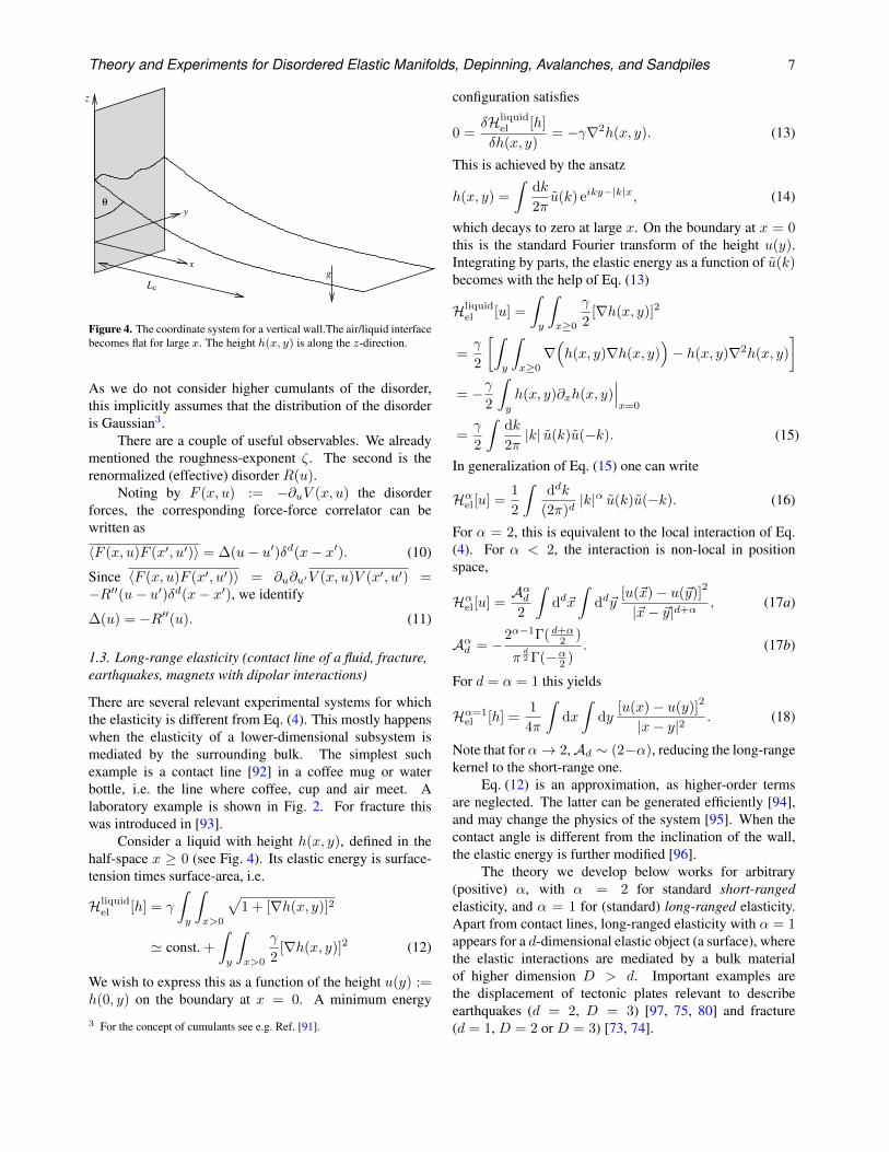
A realization with a 2-parameter displacement field~u(x, y, z) is the deformation of a vortex lattice: the positionof each vortex is deformed from the 3-dimensional vector~x = (x, y, z) to ~x+ ~u(~x), with ~u ∈ R2 (its z-component is0). Irradiating the sample produces line defects. They allowexperimentalists to realize [44]
(iii) generic long-range (LR) correlated disorder. The mostextreme example are
(iv) random forces with the statistics of a random walk.This model, the Brownian force model (BFM) ofsection 4.5, plays an important role as its center-of-mass motion advances as a single degree of freedom,known as the ABBM or mean-field model (section 4.3),often used to describe avalanches.
Another example are charge-density waves, first predictedby Peierls [86]: They can spontaneously form in certainsemiconductor devices, where a uniform charge density isunstable towards a super-lattice in which the underlyinglattice is periodically deformed, and the charge density ofthe globally neutral device becomes [87, 88, 89, 90].
ρ(~x) = ρ0 cos(~k~x). (1)
Adding disorder, the latter locally deforms the phase,modifying the charge density to
ρ(~x, u(~x)
)= ρ0 cos
(~k~x+ 2πu(~x)
). (2)
As the charge density is invariant under u(~x) → u(~x) + 1,we find another disorder class,
(v) random periodic disorder (RP).
All these models have in common that they can be describedby a displacement field
~x ∈ Rd −→ ~u(~x) ∈ RN . (3)
For simplicity, we suppress the vector notation whereverpossible, and mostly consider N = 1. After some initialcoarse-graining, the energy H = Hel + Hconf + Hdis
consists of three parts: the elastic energy
Hel[u] =
∫ddx
1
2[∇u(x)]
2, (4)
the confining potential
Hconf [u] =
∫
x
m2
2
∫
x
[u(x)− w]2, (5)
and the disorder
Hdis[u] =
∫ddxV
(x, u(x)
). (6)
In order to proceed, we need to specify the correlations ofdisorder. Suppose that fluctuations of u scale as⟨
[u(x)− u(y)]2⟩∼ |x− y|2ζ . (7)
Theory and Experiments for Disordered Elastic Manifolds, Depinning, Avalanches, and Sandpiles 6
(‘‘random bond’’)
defect
‘‘random field’’
x
u(x)
Figure 1. An Ising magnet with up (“+”) and down (“−”) spins at low temperatures forms a domain wall described by a function u(x) (right) (Fig. from[42]). Two types of disorder are observed: missing spins, weakening the effective nearest-neighbor interactions (“random-bond disorder”), and frozenin magnetic moments aligning its immediate neighbor (“random field disorder”), indicated by thick ± signs. An experiment on a thin Cobalt film (left)[84]; with kind permission of the authors.
Figure 2. A contact line for the wetting of a disordered substrate by Glycerine [85]. Experimental setup (left). The disorder consists of randomly depositedislands of Chromium, appearing as bright spots (top right), with a correlation length of about 10µm. Temporal evolution of the retreating contact-line(bottom right). Note the different scales parallel and perpendicular to the contact-line. Pictures courtesy of S. Moulinet, with kind permission.
~u(x, y, z)
(x, y, z)
Figure 3. A vortex lattice is described by a deformation of a lattice point(x, y, z) to (x, y, z)+~u(x, y, z). Shown is a cartoon of a single layer, i.e.fixed z. The vortex lines continue perpendicular to the drawing (Fig. from[42]).
Notations are such that 〈...〉 denotes thermal averages, i.e.averages of an observable using the weight e−βH , properlynormalized by the partition function Z =
⟨e−βH
⟩. At
zero temperature, this reduces to the contribution of a singlestate, the ground state. Overbars denote the average overdisorder. This defines a roughness-exponent ζ. Startingfrom a disorder correlator
V (x, u)V (x′, u′) = R(u− u′)f(x− x′) (8)
with both R(u) and f(x) vanishing at large distances, foreach rescaling in the RG-procedure by λ in the x-directionone rescales by λζ in the u-direction. As long as ζ < 1,this eventually reduces f(x) to a δ-distribution, whereas thestructure of R(u) may remain visible. We therefore chooseas our starting correlations for the disorder
V (x, u)V (x′, u′) := R(u− u′)δd(x− x′). (9)
Theory and Experiments for Disordered Elastic Manifolds, Depinning, Avalanches, and Sandpiles 7
L
θ
g
y
x
c
z
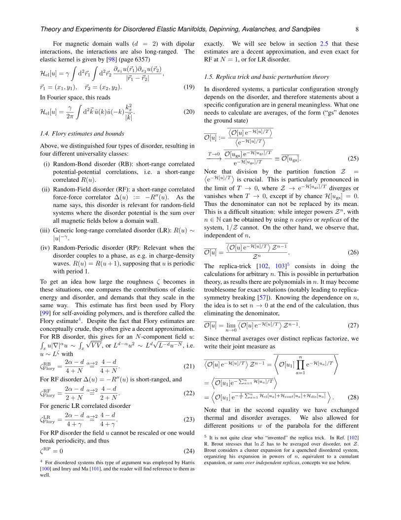
Figure 4. The coordinate system for a vertical wall.The air/liquid interfacebecomes flat for large x. The height h(x, y) is along the z-direction.
As we do not consider higher cumulants of the disorder,this implicitly assumes that the distribution of the disorderis Gaussian3.
There are a couple of useful observables. We alreadymentioned the roughness-exponent ζ. The second is therenormalized (effective) disorder R(u).
Noting by F (x, u) := −∂uV (x, u) the disorderforces, the corresponding force-force correlator can bewritten as
〈F (x, u)F (x′, u′)〉 = ∆(u− u′)δd(x− x′). (10)
Since 〈F (x, u)F (x′, u′)〉 = ∂u∂u′V (x, u)V (x′, u′) =−R′′(u− u′)δd(x− x′), we identify
∆(u) = −R′′(u). (11)
1.3. Long-range elasticity (contact line of a fluid, fracture,earthquakes, magnets with dipolar interactions)
There are several relevant experimental systems for whichthe elasticity is different from Eq. (4). This mostly happenswhen the elasticity of a lower-dimensional subsystem ismediated by the surrounding bulk. The simplest suchexample is a contact line [92] in a coffee mug or waterbottle, i.e. the line where coffee, cup and air meet. Alaboratory example is shown in Fig. 2. For fracture thiswas introduced in [93].
Consider a liquid with height h(x, y), defined in thehalf-space x ≥ 0 (see Fig. 4). Its elastic energy is surface-tension times surface-area, i.e.
Hliquidel [h] = γ
∫
y
∫
x>0
√1 + [∇h(x, y)]2
' const. +
∫
y
∫
x>0
γ
2[∇h(x, y)]2 (12)
We wish to express this as a function of the height u(y) :=h(0, y) on the boundary at x = 0. A minimum energy
3 For the concept of cumulants see e.g. Ref. [91].
configuration satisfies
0 =δHliquid
el [h]
δh(x, y)= −γ∇2h(x, y). (13)
This is achieved by the ansatz
h(x, y) =
∫dk
2πu(k) eiky−|k|x, (14)
which decays to zero at large x. On the boundary at x = 0this is the standard Fourier transform of the height u(y).Integrating by parts, the elastic energy as a function of u(k)becomes with the help of Eq. (13)
Hliquidel [u] =
∫
y
∫
x≥0
γ
2[∇h(x, y)]2
=γ
2
[∫
y
∫
x≥0
∇(h(x, y)∇h(x, y)
)− h(x, y)∇2h(x, y)
]
= −γ2
∫
y
h(x, y)∂xh(x, y)∣∣∣x=0
=γ
2
∫dk
2π|k| u(k)u(−k). (15)
In generalization of Eq. (15) one can write
Hαel[u] =1
2
∫ddk
(2π)d|k|α u(k)u(−k). (16)
For α = 2, this is equivalent to the local interaction of Eq.(4). For α < 2, the interaction is non-local in positionspace,
Hαel[u] =Aαd2
∫dd~x
∫dd~y
[u(~x)− u(~y)]2
|~x− ~y|d+α, (17a)
Aαd = −2α−1Γ(d+α2 )
πd2 Γ(−α2 )
. (17b)
For d = α = 1 this yields
Hα=1el [h] =
1
4π
∫dx
∫dy
[u(x)− u(y)]2
|x− y|2 . (18)
Note that for α→ 2,Ad ∼ (2−α), reducing the long-rangekernel to the short-range one.
Eq. (12) is an approximation, as higher-order termsare neglected. The latter can be generated efficiently [94],and may change the physics of the system [95]. When thecontact angle is different from the inclination of the wall,the elastic energy is further modified [96].
The theory we develop below works for arbitrary(positive) α, with α = 2 for standard short-rangedelasticity, and α = 1 for (standard) long-ranged elasticity.Apart from contact lines, long-ranged elasticity with α = 1appears for a d-dimensional elastic object (a surface), wherethe elastic interactions are mediated by a bulk materialof higher dimension D > d. Important examples arethe displacement of tectonic plates relevant to describeearthquakes (d = 2, D = 3) [97, 75, 80] and fracture(d = 1, D = 2 or D = 3) [73, 74].
Theory and Experiments for Disordered Elastic Manifolds, Depinning, Avalanches, and Sandpiles 8
For magnetic domain walls (d = 2) with dipolarinteractions, the interactions are also long-ranged. Theelastic kernel is given by [98] (page 6357)
Hel[u] = γ
∫d2~r1
∫d2~r2
∂x1u(~r1)∂x2
u(~r2)
|~r1 − ~r2|,
~r1 = (x1, y1), ~r2 = (x2, y2). (19)
In Fourier space, this reads
Hel[u] =γ
2π
∫d2~k u(k)u(−k)
k2x
|~k|. (20)
1.4. Flory estimates and bounds
Above, we distinguished four types of disorder, resulting infour different universality classes:
(i) Random-Bond disorder (RB): short-range correlatedpotential-potential correlations, i.e. a short-rangecorrelated R(u).
(ii) Random-Field disorder (RF): a short-range correlatedforce-force correlator ∆(u) := −R′′(u). As thename says, this disorder is relevant for random-fieldsystems where the disorder potential is the sum overall magnetic fields below a domain wall.
(iii) Generic long-range correlated disorder (LR): R(u) ∼|u|−γ .
(iv) Random-Periodic disorder (RP): Relevant when thedisorder couples to a phase, as e.g. in charge-densitywaves. R(u) = R(u+ 1), supposing that u is periodicwith period 1.
To get an idea how large the roughness ζ becomes inthese situations, one compares the contributions of elasticenergy and disorder, and demands that they scale in thesame way. This estimate has first been used by Flory[99] for self-avoiding polymers, and is therefore called theFlory estimate4. Despite the fact that Flory estimates areconceptually crude, they often give a decent approximation.For RB disorder, this gives for an N -component field u:∫xu|∇|αu ∼
∫x
√V V , or Ld−αu2 ∼ Ld
√L−du−N , i.e.
u ∼ Lζ with
ζRBFlory =
2α− d4 +N
α→2=
4− d4 +N
. (21)
For RF disorder ∆(u) = −R′′(u) is short-ranged, and
ζRFFlory =
2α− d2 +N
α→2=
4− d2 +N
. (22)
For generic LR correlated disorder
ζLRFlory =
2α− d4 + γ
α→2=
4− d4 + γ
. (23)
For RP disorder the field u cannot be rescaled or one wouldbreak periodicity, and thus
ζRP = 0 (24)4 For disordered systems this type of argument was employed by Harris[100] and Imry and Ma [101], and the reader will find reference to them aswell.
exactly. We will see below in section 2.5 that theseestimates are a decent approximation, and even exact forRF at N = 1, or for LR disorder.
1.5. Replica trick and basic perturbation theory
In disordered systems, a particular configuration stronglydepends on the disorder, and therefore statements about aspecific configuration are in general meaningless. What oneneeds to calculate are averages, of the form (“gs” denotesthe ground state)
O[u] :=
⟨O[u] e−H[u]/T
⟩⟨e−H[u]/T
⟩
T→0−−−→ O[ugs] e−H[ugs]/T
e−H[ugs]/T≡ O[ugs]. (25)
Note that division by the partition function Z =⟨e−H[u]/T
⟩is crucial. This is particularly pronounced in
the limit of T → 0, where Z → e−H[ugs]/T diverges orvanishes when T → 0, except if by chance H[ugs] = 0.Thus the denominator can not be replaced by its mean.This is a difficult situation: while integer powers Zn, withn ∈ N can be obtained by using n copies or replicas of thesystem, 1/Z cannot. On the other hand, we observe that,independent of n,
O[u] =
⟨O[u] e−H[u]/T
⟩Zn−1
Zn . (26)
The replica-trick [102, 103]5 consists in doing thecalculations for arbitrary n. This is possible in perturbationtheory, as results there are polynomials in n. It may becometroublesome for exact solutions (notably leading to replica-symmetry breaking [57]). Knowing the dependence on n,the idea is to set n → 0 at the end of the calculation, thuseliminating the denominator,
O[u] = limn→0
⟨O[u] e−H[u]/T
⟩Zn−1. (27)
Since thermal averages over distinct replicas factorize, wewrite their joint measure as
⟨O[u] e−H[u]/T
⟩Zn−1 =
⟨O[u1]
n∏
a=1
e−H[ua]/T
⟩
=⟨O[u1]e−
∑na=1H[ua]/T
⟩
=⟨O[u1] e−
1T
∑na=1Hel[ua]+Hconf [ua]+Hdis[ua]
⟩. (28)
Note that in the second equality we have exchangedthermal and disorder averages. We also allowed fordifferent positions w of the parabola for the different5 It is not quite clear who “invented” the replica trick. In Ref. [102]R. Brout stresses that lnZ has to be averaged over disorder, not Z .Brout considers a cluster expansion for a quenched disordered system,organizing his expansion in powers of n, equivalent to a cumulantexpansion, or sums over independent replicas, concepts we use below.
Theory and Experiments for Disordered Elastic Manifolds, Depinning, Avalanches, and Sandpiles 9
replicas, denoted wa6. Finally, we assume for simplicityof presentation that O[u] does not explicitly depend on thedisorder. Since only the last term in the exponential dependson V (x, u), and since V (x, u) which is Gauss distributed,
e−1T
∑na=1Hdis[ua] = exp
(− 1
T
∫
x
∑
a
V (x, ua(x))
)
= exp
1
2T 2
∫
x
∫
y
n∑
a,b=1
V (x, ua(x))V (y, ub(y))
= exp
1
2T 2
∫
x
n∑
a,b=1
R(ua(x)− ub(x)
) . (29)
In the second step we used that V is Gaussian; in the laststep we used the correlator (9).
To summarize: to evaluate the expectation of anobservable, we take averages with measure e−Srep[u] andreplica Hamiltonian or action
Srep[u] :=1
T
n∑
a=1
∫
x
1
2[∇ua(x)]2 +
m2
2[ua(x)− wa]2
− 1
2T 2
∫
x
n∑
a,b=1
R(ua(x)− ub(x)
). (30)
Note that each replica sum comes with a factor of 1/T . Ifthe disorder had a third cumulant, this would appear as atriple replica sum, and a factor3,5 of 1/T 3.
Let us now turn to perturbation theory. The freepropagator, constructed from the first line of Eq. (30), andindicated by the index “0”, is (first in Fourier, than in realspace)
〈ua(−k)ub(k)〉0 = TδabC(k), (31)〈ua(x)ub(y)〉0 = TδabC(x−y). (32)
Noting C(x − y) the Fourier transform of C(k), and Sd =2πd/2/Γ(d/2) the area of the d-sphere, we have
C(k) =1
k2 +m2, (33a)
C(x) =
∫ddk
(2π)deikx
k2 +m2
' 1
(d− 2)Sd|x|2−d for x→ 0. (33b)
On the other hand, for large x, the correlation functiondecays exponentially ∼ e−m|x|, which we associate witha correlation length
ξ =1
m. (34)
Eq. (33a) allows us to calculate expectation values in thefull theory. As an example consider⟨[u(x)− w1]
⟩w1
⟨[u(z)− w2]
⟩w2
c
6 The partition function for each of these replicas may be different. Theformalism takes this into account.
≡⟨[u1(x)− w1][u2(z)− w2]
⟩Srep
= −∫
y
C(x− y)C(z − y)R′′(w1 − w2) + ... (35)
Let us clarify the notations: Firstly,⟨[u(x) − w1]
⟩w1
isthe thermal average of u(x) − w1, obtained by evaluatingthe path integral for a fixed disorder configuration V , ata position of the parabola given by w1. This procedureis repeated for
⟨[u(z) − w2]
⟩w2
, with the same V , andparabola position w2. Finally the average over the disorderpotential V is taken. According to the calculations above,this can be evaluated with the help of the replica actionSrep[u], represented by
⟨[u1(x)−w1][u2(z)−w2]
⟩Srep . The
latter is already averaged over disorder. The last line showsthe leading order in perturbation theory, dropping terms oforder T and higher.
Finally, let us integrate this expression over x and z,and multiply by m4/Ld. This leads to
m4
Ld
∫
x,z
⟨[u(x)− w1]
⟩w1
⟨[u(z)− w2]
⟩w2
= −R′′(w1 − w2) + ... (36)
Let us understand the prefactor on the l.h.s.: Thecombination m2[u(x) − w1] is the force acting on point x(a density), its integral over x the total force acting on theinterface. Force correlations are short ranged in x, leadingto the factor of 1/Ld. Note that the thermal 2-point function(32) is absent, as we consider two distinct copies of thesystem.
1.6. Dimensional reduction
It is an interesting exercise to show that for w1 = w2 noperturbative corrections to Eq. (36) exist in the limit of T →0, as long as one supposes thatR(w) is an analytic function.Similarly, one shows that in the same limit 〈uuuu〉c = 0,and the same holds true for higher connected expectations.Thus u is a Gaussian field with correlations
〈u(k)〉 〈u(−k)〉 = 〈u(k)u(−k)〉
= u(k)u(−k) = − R′′(0)
(k2 +m2)2. (37)
In the third expression we suppressed the thermal expecta-tion values since at T = 0 only a single ground state sur-vives7. Fourier-transforming back to position space yields(with some amplitude A, and in the limit of mx→ 0)1
2
[u(x)− u(y)
]2= −R′′(0)A|x− y|4−d. (38)
This looks very much like the thermal expectation (32),except that the dimension of space has been shifted by 2.Further, both theories are seemingly Gaussian, i.e. highercumulants vanish.7 For disordered elastic manifolds with continuous disorder, the groundstate is almost surely unique. This is in strong contrast to mean-field spinglasses, where it is highly degenerate, see e.g. [57]
Theory and Experiments for Disordered Elastic Manifolds, Depinning, Avalanches, and Sandpiles 10
We have just given a simple version of a beautiful andrather mind-boggling theorem relating disordered systemsto pure ones (i.e. without disorder). The theorem appliesto a large class of systems, even when non-linearities arepresent in the absence of disorder. It is called dimensionalreduction [104, 105, 106]. We formulate it as follows:“Theorem”: A d-dimensional disordered system at zerotemperature is equivalent to all orders in perturbationtheory to a pure system in d − 2 dimensions at finitetemperature.
We give in section 8.1 a proof of this theorem usinga supersymmetric field theory introduced in Ref. [32].The proof implicitly assumes that R(u) is analytic, thusall derivatives can be taken. The equivalence is ratherpowerful, since the supersymmetric theory knows aboutdifferent replicas, and allows one to calculate even awayfrom the critical point.
However, evidence from experiments, simulations,and analytic solutions show that the above “theorem” isactually wrong. A prominent counter-example is the 3-dimensional random-field Ising model at zero temperature[30]; according to the theorem it should be equivalent tothe pure 1-dimensional Ising-model at finite temperature.While it was shown rigorously [30] that the former has anordered phase, the latter is disordered at finite temperature[107]. So what went wrong? Let us stress that there are nomissing diagrams or any such thing, but that the problemis more fundamental: As we will see later, the proof makesthe assumption thatR(u) is analytic. While this assumptionis correct in the microscopic model, it is not valid at largescales.
Nevertheless, the above “theorem” remains importantsince it has a devastating consequence for all perturbativecalculations in the disorder: However clever a procedurewe invent, as long as we perform a perturbative expansion,expanding the disorder in its moments, all our efforts arefutile: dimensional reduction tells us that we get a trivialand unphysical result. Before we try to understand why thisis so and how to overcome it, let us give one more counter-example. Dimensional reduction allowed us in Eq. (38) tocalculate the roughness-exponent ζ defined in equation (7),as
ζDR =4− d
2. (39)
On the other hand, the directed polymer in dimension d = 1does not have a roughness exponent of ζDR = 3/2, but[108]
ζRBd=1 =
2
3. (40)
Experiments and simulations for disordered elastic mani-folds discussed below in sections 2.31, 2.32, 3.12, 3.13,3.15, 3.16, 3.17, and 3.21 all violate dimensional reduction.
1.7. Larkin-length, and the role of temperature
To understand the failure of dimensional reduction, letus turn to crucial arguments given by Larkin [109]. Heconsiders a piece of an elastic manifold of size L. Ifthe disorder has correlation length r, and characteristicpotential energy E , there are (L/r)d independent degreesof freedom, and according to the central-limit theorem thispiece of size L will typically see a potential energy ofamplitude
Edis = E(L
r
)d2
. (41)
On the other hand, the elastic energy scales as
Eel = cLd−2. (42)
These energies are balanced at the Larkin-length L = Lc
with
Lc =
(c2
E2rd) 1
4−d
. (43)
More important than this value is the observation that in allphysically interesting dimensions d < dc = 4, and at scalesL > Lc, the disorder energy (41) wins; as a consequencethe manifold is pinned by disorder, whereas on small scalesthe elastic energy dominates. For long-ranged elasticity, thesame argument implies
dc = 2α, and disorder relevant for d < dc. (44)
Since the disorder has many minima which are far apartin configurational space but close in energy (metastability),the manifold can be in either of these minima, and localminimum does not imply global minimum. However, theexistence of exactly one minimum is assumed in e.g. theproof of dimensional reduction, even though formally, thefield theory sums over all saddle points.
Another important question is the role of temperature.In Eq. (7) we had supposed that u scales with thesystems size as u ∼ Lζ . Demanding that the action(30) be dimensionless, the first term in Eq. (30) scales asLd−2+2ζ/T . This implies that
T ∼ aθ, θ = d− 2 + 2ζ, (45)
where a is a microscopic cutoff with the dimension of L, tocompensate the factor of Ld−2+2ζ . For completeness, wealso give the result for generic LR-elasticity,
θα = d− α+ 2ζ. (46)
The thermodynamic limit is obtained by taking L → ∞.Temperature is thus irrelevant when θ > 0, which is thecase for d > 2, and when ζ > 0 even below. As aconsequence, the RG fixed point we are looking for is atzero temperature [110]. The same argument applies to thefree energy
F [u] = − 1
Tln(Z[u]) ∼
(L
a
)θ. (47)
Theory and Experiments for Disordered Elastic Manifolds, Depinning, Avalanches, and Sandpiles 11
We added u as an argument to F [u], as e.g. in thedirected polymer the partition function is the weight of alltrajectories arriving at u. This is important in section 7.1when considering the KPZ equation.
From the second term in Eq. (30) we conclude that the(microscopic) disorder scales as
R ∼ a2θ−d = ad−4+4ζ . (48)
For ζ = 0, this again implies that d = 4 is the uppercritical dimension. More thorough arguments are presentedin the next section, where we will construct an ε = 4 − dexpansion for the RG flow of R(u).
2. Equilibrium (statics)
2.1. General remarks about renormalization
In the next section 2.2 we derive the central renormalizationgroup equations for disordered elastic manifolds. Theseequations are obtained in a controlled ε = 4− d expansion[111] around the upper critical dimension. Retaining inthis expansion only the leading divergences which showup as poles in 1/ε, by using minimal subtraction, thisexpansion is unique. This is a deep result, ensured by therenormalizability of the theory (see e.g. [112, 113, 114, 115,116]). We consider it a gift: However we set up our RGscheme, we always get the same result. This allows us tochoose one scheme, and switch to a different one wheneverits particular features help us in our reasoning. The schemesin question are
(i) Wilson’s momentum-shell scheme. This scheme goesback to K. Wilson, who suggested to integrate overthe fast modes, i.e. modes k contained in a momentumshell between Λ(1− δ) and Λ, with δ 1. Doing thisincrementally is interpreted as a flow equation for theeffective parameters of the theory. The process stopswhen one reaches the scale one is interested in, whichis zero for correlations of the center of mass. Whileintuitive, this technique is cumbersome to implement,especially at subleading order. We refer to the classicaltext [117] for an introduction.
(ii) Field theory as used in high-energy physics. This isthe standard technique to treat critical phenomena, andis explained in many classical texts [1, 2, 4, 5, 6, 7].A well-oiled machinery, especially for higher-ordercalculations.
(iii) The operator product expansion as explained in [3],or section 3.4 of [118]. Realizing that the dominantcontributions in schemes (i) and (ii) come from largemomenta implies that they must come from shortdistances in position space. It is not only very efficientat leading order 8, it also explains why counter-termsare local (see below).
8 In φ4-theory it gives the 2-loop correction to η from a single integral,see section 3.4 of [118].
(iv) Non-perturbative functional RG: A rather heavymachinery, which we believe should be restricted tocases where other schemes fail (see section 9.2 onRandom-Field magnets).
(iv) The experimentalist’s point of view: If all RGprocedures are equivalent, then we can choose to studythe flow equations by reducing an experimentallyrelevant parameter, here the strength m2 of theconfining potential. As we show below in sections2.10-2.11, the theory can be defined at any m2, e.g. bydoing an experiment or simulation at this scale. Thisdefinition does not make reference to any perturbativecalculation. The latter can then be viewed as anefficient analytical tool to predict in an experimentor a simulation the consequences of a change of theparameter m2.
If we think about standard perturbative RG for φ4 theory,we remark that the parameter ε controls the order ofperturbation theory necessary9, and that at leading orderO(ε) the differences boil down to a choice of how toevaluate the elementary integral (58). For disorderedsystems, there is an additional quirk: The interactiontermed R(u) in Eq. (30) is a function of the fielddifferences, and we have no a-priory knowledge of its form.It will turn out in the next section 2.2 that we can writedown a flow equation for the function R(u) itself. Wewould already like to stress that similar to φ4-theory, thefixed point R∗(u) is of order ε, thus the calculation remainsperturbatively controlled.
2.2. Derivation of the functional RG equations
In section 1.7, we had seen that 4 is the upper criticaldimension for SR elasticity, which we treat now. As forstandard critical phenomena [1, 2, 3, 4, 5, 6, 7], we constructan ε = (4 − d)-expansion. Taking the dimensional-reduction result (39) in d = 4 dimensions tells us that thefield u is dimensionless there. Thus, the width σ = −R′′(0)of the disorder is not the only relevant coupling at small ε,but any function of u has the same scaling dimension inthe limit of ε = 0, and might equivalently contribute. Thenatural conclusion is to follow the full function R(u) underrenormalization, instead of just its second derivativeR′′(0).
Such an RG-treatment is most easily implementedin the replica approach: The n times replicated partitionfunction led after averaging over disorder to a path integralwith weight e−Srep[u], with action (30). Perturbation theoryis constructed as follows: The bare correlation function forreplicas a and b, graphically depicted as a solid line, is withmomentum k flowing through, see Eqs. (31)–(33a),
〈ua(k)ub(k)〉0 = T × a b = TδabC(k). (49)
Note that the factor of T is explicit in our graphicalnotation, and not included in the line. The disorder vertex9 As a rule of thumb: order n in ε necessitate order n in the interaction∫x φ
4(x).
Theory and Experiments for Disordered Elastic Manifolds, Depinning, Avalanches, and Sandpiles 12
is (we added an index R0 to R to indicate that this is themicroscopic (bare) disorder)
1
T 2×
xb
a
=1
T 2×R0
(ua(x)− ub(x)
). (50)
The rules of the game are to find all contributions whichcorrect R, and which survive in the limit of T → 0. Atleading order, i.e. order R2
0, counting of factors T showsthat we can use at most two correlators, as each contributesa factor of T . On the other hand,
∑a,bR0(ua − ub) has
two independent sums over replicas10. Thus at order R20
four independent sums over replicas appear, and in order toreduce them to two, one needs at least two correlators (eachcontributing a δab). Thus, at leading order, only diagramswith two propagators survive.
Before writing down these diagrams, we need to seewhat Wick-contractions do on functions of the field. To seethis, remind that a single Wick contraction (indicated by
sitting on top of the fields to be contracted)
ua(x)nub(y)m
= nua(x)n−1 ×mub(x)m−1 × TδabC(x− y). (51)
Realizing that nun−1 = ∂uun, we can write the Wick
contraction for an arbitrary function V (u) as
V(ua(x)
)V(ub(y)
)
= V ′(ua(x)
)× V ′
(ub(y)
)× TδabC(x− y). (52)
Graphically we have at second order for the correction ofdisorder
1
2T 2δR =
1
2!
[1
2T 2x
b
a]
T
T f
e
f
e
[1
2T 2y
d
c]
(53)
We have explicitly written all factors: a 1/2! from theexpansion of the exponential function exp(−Srep[u]), afactor of 1/(2T 2) per disorder vertex, and a factor of Tper propagator. Using these rules, we obtain two distinctcontributions
δR(1) =1
2x y
b
a
b
a
(54)
=1
2
∫
x
R′′0(ua(x)−ub(x)
)R′′0(ua(y)−ub(y)
)C(x−y)2,
δR(2) =x y
a
a
b
a
(55)
= −∫
x
R′′0(ua(x)−ua(x)
)R′′0(ua(y)−ub(y)
)C(x−y)2.
Note that all factors of T have disappeared, and onlytwo replica sums (not written explicitly) remain. EachR0(ua − ub) has been contracted twice, giving rise to twoderivatives. In the first diagram, since once ua and once10The concept of sums over independent replicas already appears in thework by R. Brout [102], see footnote 5.
ub has been contracted, each R′′0 comes with an additionalminus sign; these cancel. In the second diagram, there is aminus sign from the first R′′0 , but not from the second; thusthe overall sign is negative.
Note that the following diagram also contains twocorrelators (correct counting in powers of temperature), butis not a 2-replica but a 3-replica sum,
x yb
a
c
a
. (56)
In a renormalization program, we are looking for diver-gences of these diagrams. These divergences are localizedat x = y: indeed the integral over the difference z := y−x,is in radial coordinates with r = |z|, ε = 4 − d, and form→ 0 (up to a geometrical prefactor)∫
z
C(z)2 ∼∫ L
a
dr
rrdr2(2−d) =
∫ L
a
dr
rz4−d
=1
ε(Lε − aε) . (57)
Note that for ε → 0 each scale contributes the same: fromr = 1/2 to r = 1 the same as from r = 1/4 to r = 1/2, andagain the same for r = 1/8 to r = 1/4. Thus the divergencecomes from small scales, which allows us to approximateR′′0 (ua(y)−ub(y)) ≈ R′′0 (ua(x)−ub(x)). This is formallyan analysis of the theory via an operator product expansion.For an introduction and applications see [3, 118].
Eq. (57) is regularized with cutoffs a and L. It isconvenient to use ε > 0 (what we need anyway), whichallows us to take a → 0 and L → ∞ while keeping mfinite, as the latter appears as the harmonic well introducedin section 2.11. The integral in that limit becomes
I1 := =
∫
x−yC(x− y)2 =
∫
k
1
(k2 +m2)2
=m−ε
ε
2Γ(1 + ε2 )
(4π)d/2. (58)
It is the standard 1-loop diagram of massive φ4-theory11.Setting u = ua(x) − ub(x), we obtain for the
effective disorder correlator R(u) at 1-loop order with allcombinatorial factors as given above,
R(u) = R0(u) +
[1
2R′′0 (u)2 −R′′0 (u)R′′0 (0)
]I1 + ... (60)
We can now study its flow, by taking a derivative w.r.t. m,and replacing on the r.h.s. R0 with R, as given by the aboveequation. This leads to
−m ∂
∂mR(u) =
[1
2R′′(u)2 −R′′(u)R′′(0)
]εI1. (61)
11The trick to calculate integrals of this type is to write
1
(k2 +m2)2=
∫ ∞0
ds se−s(k2+m2). (59)
The integral over k is then the 1-dimensional integral to the power of d.Finally one integrates over s.
Theory and Experiments for Disordered Elastic Manifolds, Depinning, Avalanches, and Sandpiles 13
This equation still contains the factor of εI1, which hasboth a scale m−ε, as a finite amplitude. There are twoconvenient ways out of this: We can parameterize the flowby the integral I1 itself, defining
∂`R(u) := − ∂
∂I1R(u) =
1
2R′′(u)2 −R′′(u)R′′(0). (62)
This is convenient to study the flow numerically.To arrive at a fixed point one needs to rescale both R
and u, in order to make them dimensionless. The field u hasdimension u ∼ Lζ ∼ m−ζ , whereas the dimension of Rcan be read off from Eq. (54), namelyR(u) ∼ R′′(u)2m−ε,equivalent to R ∼ mε−4ζ . The dimensionless effectivedisorder R, as function of the dimensionless field u is thendefined as
R(u) := εI1m4ζR(u = um−ζ). (63)
Inserting this into Eq. (62), we arrive at12
∂`R(u) := −m ∂
∂mR(u) (64)
= (ε− 4ζ)R(u) + ζuR′(u) +1
2R′′(u)2 − R′′(u)R′′(0).
This is the functional RG flow equation for the renormal-ized dimensionless disorder R(u), first derived in Ref. [119]within the Wilson scheme13. We will in general set u→ uin the above equation, to simplify notations, and suppressthe tilde as long as this does not lead to confusion.
We would like to stress what we already said insection 2.1, namely that the flow-equations we derived asfunctions of m have a very intuitive interpretation: Sincethe strength m2 of the confining potential (5) is a parameterof the experimental system which does not renormalise(see the next section 2.3), the RG equation can be takenquite literally: what happens if in an experiment or asimulation the confining potential is weakened? In a peelingor unzipping experiment (sections 2.32 and 3.17) this evenhappens during the experiment. The answer is that form→∞, one sees the microscopic disorder, while for smaller man effective scale-dependent disorder is measured. This isexplained in detail in section 2.11. Before doing this, let usfirst ensure that m does not renormalize (next section 2.3),and then study what happens if m is lowered (section 2.4).
2.3. Statistical tilt symmetry
We claim that there are no renormalizations of the quadraticparts of the action which are replicated copies of
H0[u] := Hel[u] +Hconf [u] (65)
given in Eqs. (4) and (5). This is due to the statistical tiltsymmetry (STS)
ua(x)→ ua(x) + αx. (66)
12` in Eqs. (62) and (64) is different.13The RG flow equation (64) is at this order independent of the RGscheme. Universal quantities are scheme-independent to all orders [2, 112,113, 114, 118].
As the interaction is proportional to R(ua(x)− ub(x)), thelatter is invariant under the transformation (66). The changeinH0[u] becomes
δH0[u] = c
∫ddx
[∇u(x)α+
1
2α2
]
+ m2
∫ddx
[u(x)αx+
1
2α2x2
]. (67)
To render the presentation clearer, the elastic constant cset to c = 1 in equation (30) has been introduced. Theimportant observation is that all fields u involved are large-scale variables, which are also present in the renormalizedaction, where they change according to Hren[u] →Hren[u] + δHren[u]. Since one can either first renormalizeand then tilt, or first tilt and then renormalize, we obtainδHren
0 [u] = δHbare0 [u]. This means that neither the elastic
constant c, nor m change under renormalization.
2.4. Solution of the FRG equation, and cusp
We now analyze the FRG flow equations (62) and (64). Tosimplify our arguments, we first derive them twice w.r.t. u,to obtain flow equations for ∆(u) ≡ −R′′(u). This yields
no rescaling: ∂`∆(u) = −∂2u
1
2
[∆(u)−∆(0)
]2, (68)
with rescaling: ∂`∆(u) = (ε− 2ζ)∆(u) + ζu∆′(u)
− ∂2u
1
2
[∆(u)− ∆(0)
]2. (69)
For concreteness, consider Eq. (68), and start with ananalytic function,
∆`=0(u) = e−u2/2. (70)
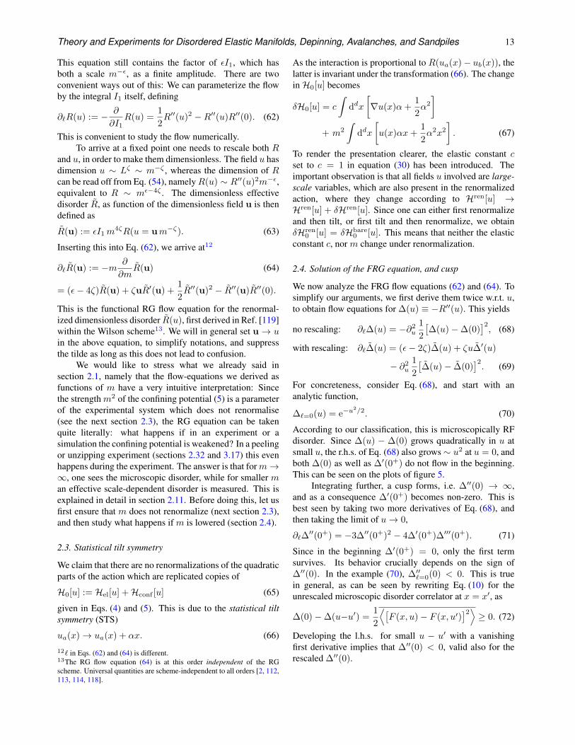
According to our classification, this is microscopically RFdisorder. Since ∆(u) − ∆(0) grows quadratically in u atsmall u, the r.h.s. of Eq. (68) also grows∼ u2 at u = 0, andboth ∆(0) as well as ∆′(0+) do not flow in the beginning.This can be seen on the plots of figure 5.
Integrating further, a cusp forms, i.e. ∆′′(0) → ∞,and as a consequence ∆′(0+) becomes non-zero. This isbest seen by taking two more derivatives of Eq. (68), andthen taking the limit of u→ 0,
∂`∆′′(0+) = −3∆′′(0+)2 − 4∆′(0+)∆′′′(0+). (71)
Since in the beginning ∆′(0+) = 0, only the first termsurvives. Its behavior crucially depends on the sign of∆′′(0). In the example (70), ∆′′`=0(0) < 0. This is truein general, as can be seen by rewriting Eq. (10) for theunrescaled microscopic disorder correlator at x = x′, as
∆(0)−∆(u−u′) =1
2
⟨[F (x, u)− F (x, u′)
]2⟩ ≥ 0. (72)
Developing the l.h.s. for small u − u′ with a vanishingfirst derivative implies that ∆′′(0) < 0, valid also for therescaled ∆′′(0).
Theory and Experiments for Disordered Elastic Manifolds, Depinning, Avalanches, and Sandpiles 14
1 2 3 4 5u
0.2
0.4
0.6
0.8
1.0
Δ(u)
0.1 0.2 0.3 0.4
0.90
0.92
0.94
0.96
0.98
1.00
1 2 3 4 5u
-0.6
-0.5
-0.4
-0.3
-0.2
-0.1
(u)
0.1 0.2 0.3 0.4 0.5 0.6 0.7ℓ
-0.5
-0.4
-0.3
-0.2
-0.1
Δ (0+)
1 2 3 4 5u
-0.5
0.5
1.0
(u)
0.1 0.2 0.3
0.90
0.92
0.94
0.96
0.98
1.00
1 2 3 4 5u
-1.0
-0.5
(u)
0.05 0.10 0.15 0.20ℓ
-1.0
-0.8
-0.6
-0.4
-0.2
Δ (0+)
Figure 5. Top: Change of ∆(u) := −R′′(u) under renormalization and formation of the cusp. Left: Explicit numerical integration of Eq. (62), startingfrom ∆(u) = e−u
2/2 (in solid black, top curve for u → 0). The function at scale ` is shown in steps of δ` = 1/20. Inset: blow-up. Right: plots of∆′(u). Inset: ∆′(0+) as a function of `. The cusp appears for ` = 1/3 (red dot); dashed lines are before appearance of the cusp, and solid lines after.Bottom: ibid for RB disorder, starting from R(u) = e−u
2/2; the cusp appears for ` = 1/9; δ` = 1/60.
Integrating Eq. (71) with this sign yields
∆′′` (0) =∆′′0(0)
1 + 3∆′′0(0)`= −1
3
1
`c − `,
`c = − 1
3∆′′0(0)
∆′′0 (0)=−1
−−−−−−−→ 1
3. (73)
In the last equality we used the initial condition (70). Withthis, ∆′′` (0) diverges at ` = 1
3 , thus ∆`(u) acquires a cups,i.e. ∆′`(0
+) 6= 0 for all ` > 1/3. Physically, this is the scalewhere multiple minima appear. In terms of the Larkin-scaleLc defined in section 1.7
`c = ln(Lc/a). (74)
Our numerical solution shows the appearance of the cusponly approximately, see the inset in the top right plot offigure 5. This discrepancy comes from discretization errors.It is indeed not simple to numerically integrate equation(68) for large times, as ∆′′` (0) diverges at ` = `c, andall further derivatives at u = 0+ were extracted fromnumerical extrapolations of the obtained functions, in thelimit of u→ 0.
Interpreting derivatives in this sense is an assumption,to be justified, without which one cannot continue tointegrate the flow equations. In this spirit, let us again look
at the flow equation for ∆(0), now including the rescalingterms,
∂`∆(0) = (ε− 2ζ)∆(0)− ∆′(0+)2. (75)
This equation tells us that as long as ∆′(0+) = 0,
ζ`<`c ' ζDR =ε
2=
4− d2
, (76)
the dimensional-reduction result. Beyond that scale, wehave (as long as we are at least close to a fixed point)
ζ`>`c =ε
2− ∆′(0+)2
∆(0)<ε
2, (77)
since both ∆′(0+)2 and ∆(0) are positive.Let us repeat our analysis for RB disorder, starting
from the microscopic disorder
R0(u) = e−u2/2 ⇐⇒ ∆(u) = e−u
2/2(1− u2). (78)
This is shown on the bottom of figure 5. Phenomenolog-ically, the scenario is rather similar, with a critical scale`c = 1/9 instead of 1/3.
Theory and Experiments for Disordered Elastic Manifolds, Depinning, Avalanches, and Sandpiles 15
2.5. Fixed points of the FRG equation
We had seen in the last section that integrating theflow-equation explicitly is rather cumbersome; moreover,an estimation of the critical exponent ζ will be ratherimprecise. For this purpose, it is better to directly search fora solution of the fixed-point equation (69), i.e. ∂`∆(u) = 0,
0 = (ε−2ζ)∆(u)+ζu∆′(u)−∂2u
1
2
[∆(u)− ∆(0)
]2. (79)
We start our analysis with situations where u is unbounded,as for the position of an interface. Then the fixed point isnot unique; indeed, if ∆(u) is solution of Eq. (79), so is
∆κ(u) := κ−2∆(κu). (80)
2.6. Random-field (RF) fixed point
There is one solution we can find analytically: To thispurpose integrate Eq. (79) from 0 to∞, assuming that ∆(u)has a cusp at u = 0, but no stronger singularity,
0 =
∫ ∞
0
(ε− 2ζ)∆(u) + ζu∆′(u)
− ∂2u
1
2
[∆(u)− ∆(0)
]2du. (81)
Integrating the second term by part, and using that the lastterm is a total derivative which vanishes both at 0 and at∞yields
0 = (ε− 3ζ)
∫ ∞
0
∆(u) du. (82)
This equation has two solutions: either the integralvanishes, which is the case for RB disorder14, or
ζRF =ε
3. (83)
This is the exponent (22) (at N = 1) predicted by a Floryargument. Let us remark that Eq. (81) remains valid to allorders in ε, as long as ∆(u) is the second derivative ofR(u),s.t. the additional terms at 2- and higher-loop order are alltotal derivatives, as is the last term in Eq. (79).
Let us pursue our analysis with the solution (83).Inserting Eq. (83) into Eq. (79), and setting
∆(u) =ε
3y(u) (84)
yields
∂u
[uy(u)− 1
2∂u
(y(u)− y(0)
)2]
= 0. (85)
This implies that the expression in the square bracket is aconstant, fixed to 0 by considering either the limit of u→ 0or u→∞. Simplifying yields
uy(u) +[y(0)− y(u)
]y′(u) = 0 . (86)
14For RB disorder∫ ∞0
du ∆(u) = −∫ ∞
0du R′′(u) = R′(0)− R′(∞) = 0.
Dividing by y(u) and integrating once again gives
u2
2− y(u) + y(0) ln(y(u)) = const. (87)
Let us now use Eq. (80) to set y(0) → 1. This fixes theconstant to −1. Dropping the argument of y, we obtain
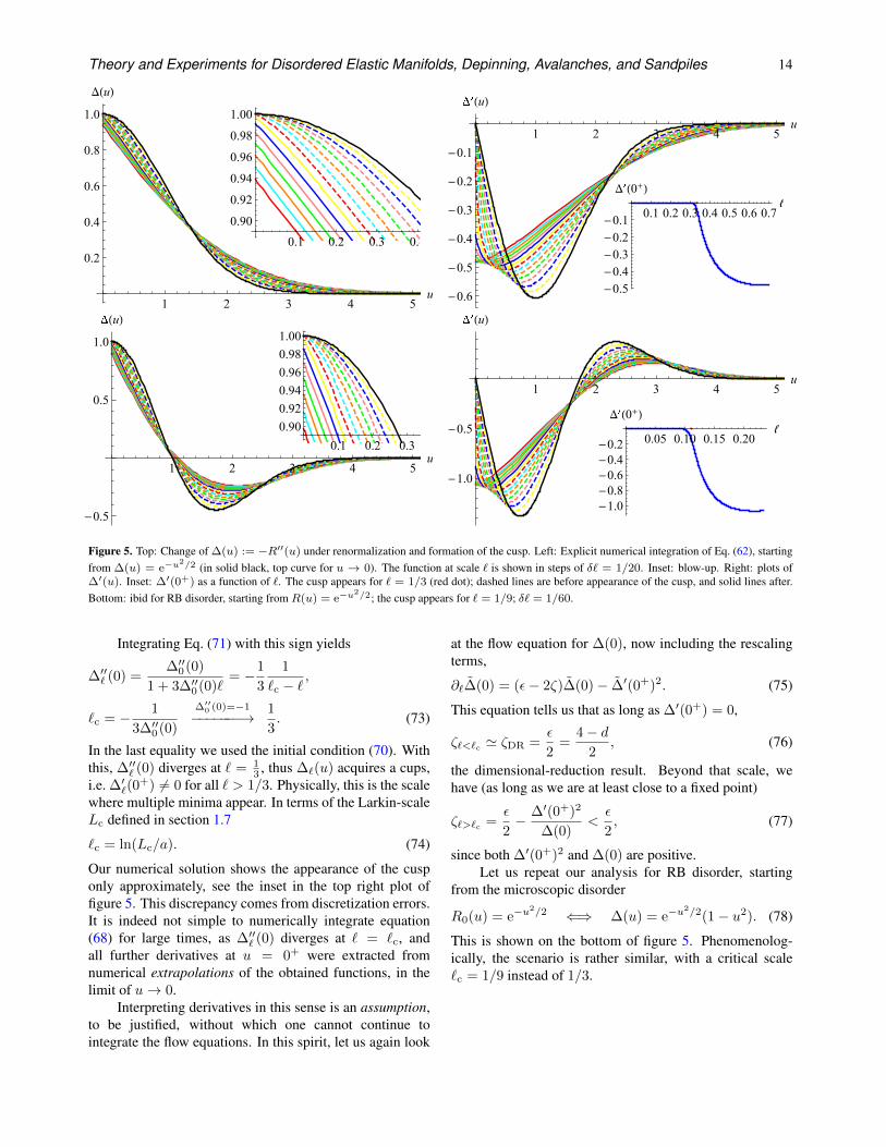
y − ln(y) = 1 +u2
2. (88)
This is plotted on figure 6.
2.7. Random-bond (RB) and tricritical fixed points
The other option for a fixed point is to have the integral inEq. (82) vanish,∫ ∞
0
∆RB(u) = 0. (89)
A numerical analysis of the fixed-point equation (79)proceeds as follows: Choose ∆(0) = 1; choose ζ; solvethe differential equation (79) for ∆′′(u). Integrate the latterfrom u = 0 to u = ∞. In practice, to avoid numericalproblems for u ≈ 0, one first solves the differential equationin a Taylor-expansion around 0; as the latter does notconverge for large u one then solves, with the informationfrom the Taylor series evaluated at u = 0.1, the differentialequation numerically up to u∞ ≈ 30. One then reports,as a function of ζ, the value of ∆(u∞). As in quantummechanics, one finds that there are several discrete valuesof ζ with ∆(u∞) = 0. The largest value of ζ is the onegiven in Eq. (83), where ∆(u) has no zero crossing. Thenext smaller value of ζ is
ζRB = 0.208298ε. (90)
The corresponding function is plotted on figure 6 (right).It has one zero-crossing. Consistent with Eq. (82), itintegrates to zero. This is the random-bond fixed point. Itis surprisingly close, but distinct, from the Flory estimate(21), ζ = ε/5.
For ε = 3 we have the directed polymer (d = 1) indimension N = 1, which has roughness ζRB
d=1 = 23 . Our
result (90) yields ζ(d = 1) = 0.624894 + O(ε2). Thisis quite good, knowing that ε = 3 is rather large. Thisvalue gets improved at 2-loop order (see section 2.13), withζ(d = 1) = 0.686616 +O(ε3). Despite the “strange cusp”,it seems the method works!
The next solution is at
ζ3crit = 0.14366ε. (91)
It has two zero-crossings, and corresponds to a tricriticalpoint. We do not know of any physical realization.
Theory and Experiments for Disordered Elastic Manifolds, Depinning, Avalanches, and Sandpiles 16
= ()
2 4 6 8 10u
-0.2
0.2
0.4
0.6
0.8
1.0
(u)
Figure 6. Left: The RF fixed point (88) with ζRF = ε3
. Right: The RB fixed point (90), with ζRB = 0.208298ε.
2.8. Generic long-ranged fixed point
If ζ is not one of these special values, then the solutionof the fixed-point Eq. (79) decays algebraically: Supposethat ∆(u) ∼ uα. Then the first two terms of Eq. (79) aredominant over the last one, as long as α < 2. Solving Eq.(79) in this limit one finds
∆ζ(u) ∼ u2− εζ for u→∞. (92)
An important application are the ABBM and BFM modelsdiscussed in sections 4.3 and 4.5, for which
ζABBM = ε, ∆ABBM(0)−∆ABBM(u) = σ|u|, (93)
such that the correlations of the random forces have thestatistics of a random walk. One easily checks that theflow equation (62) vanishes for all u > 0. In this case∆(0) is formally infinite, s.t. the bound (77) does notapply. Generically, however, Eq. (77) applies, implyingthat the exponent in Eq. (92) is negative, and ∆ζ(u) decaysalgebraically. This is what we mostly see in numericalsolutions of the fixed-point Eq. (79).
2.9. Charge-density wave (CDW) fixed point
In the above considerations, we had supposed that u cantake any real value. There are important applications wherethe disorder is periodic, or u is a phase between 0 and 2π.This is the case for the CDWs introduced above. To beconsistent with the standard conventions employed in theliterature [120, 121, 122, 123, 124, 125], we take the periodof the disorder to be 1. One checks that the following ansatzis a fixed point of the FRG equation (79)
ζRP = 0, ∆RP(u) =g
12− g
2u(1− u),
0 ≤ u ≤ 1. (94)
This ansatz is unique, due to the following three constraints:(i) ζ = 0, as the period is fixed and cannot change underrenormalization. (ii) ∆(u) = ∆(−u) = ∆(1 − u) due tothe symmetry u → −u, and periodicity. Thus ∆(u) is apolynomial in u(1 − u). (iii) a polynomial of degree 2 in
u closes under RG. (iv) the integral∫ 1
0du∆(u) = 0, since
∆(u) = −R′′(u), and R(u) itself is periodic. The fixedpoint has
g =ε
3+ ... (95)
Instead of a universal scaling exponent ζ, the lattervanishes, ζ = 0. As a consequence, the 2-point functionis logarithmic in all dimensions, with a universal amplitudegiven in Eqs. (119)-(120b). Apart from geometricprefactors, this amplitude is simply the fixed-point value g.
2.10. The cusp and shocks: A toy model
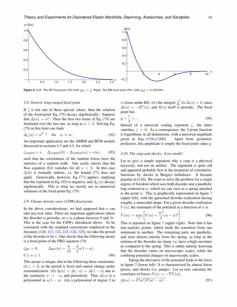
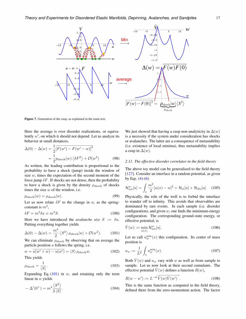
Let us give a simple argument why a cusp is a physicalnecessity, and not an artifact. The argument is quite oldand appeared probably first in the treatment of correlation-functions by shocks in Burgers turbulence. It becamepopular in [126]. We want to solve the problem for a singledegree of freedom which sees both disorder and a parabolictrap centered at w, which we can view as a spring attachedto the point w. This is graphically represented on figure 7(upper left), with the quenched disorder realization havingroughly a sinusoidal shape. For a given disorder realizationV (u), the minimum of the potential as a function of w is
V (w) := minu
[V (u) +
m2
2(u− w)2
]. (96)
This is reported on figure 7 (upper right). Note that it hasnon-analytic points, which mark the transition from oneminimum to another. The remaining parts are parabolic,and stem almost entirely from the spring, as long as theminima of the disorder are sharp, i.e. have a high curvatureas compared to the spring. This is rather natural, knowingthat the disorder varies on microscopic scales, while theconfining potential changes on macroscopic scales.
Taking the derivative of the potential leads to the forcein figure 7 (lower left). It is characterized by almost linearpieces, and shocks (i.e. jumps). Let us now calculate thecorrelator of forces F (u) := −∇V (u),
∆(w) := F (w′)F (w′ − w)c. (97)
Theory and Experiments for Disordered Elastic Manifolds, Depinning, Avalanches, and Sandpiles 17
formulasuw = wu
5
formulasuw = wu
5
formulasuw = wF(w)F(0) uˆ|w|
5
Why is a cusp necessary?. . . calculate effective action for single degree of freedom. . .
-10 -5 5 10
-1.5-1
-0.5
0.51
1.5V
u
Min
-10 -5 5 10
-1.5
-1.25
-1
-0.75
-0.5
-0.25
V u
-10 -5 5 10
-0.6
-0.4
-0.2
0.2
0.4
0.6 F
u average
-4 -2 2 4
0.2
0.4
0.6
0.8
1
7
formulasuw = wu
5
formulasuw = wu
5
formulasuw = wu
5
formulasuw =
u
5
(tuxt 2x +m2)uxt F(x,uxt) = 0
(tuxt 2x +m2)uxt tF(x,uxt) = 0
[F(w)F(0)]2 = shock|w| pshock
S2
(w) = F(w)F(0)
3
(tuxt 2x +m2)uxt F(x,uxt) = 0
(tuxt 2x +m2)uxt tF(x,uxt) = 0
[F(w)F(0)]2 = shock|w| pshock
S2
3
Figure 7. Generation of the cusp, as explained in the main text.
Here the average is over disorder realizations, or equiva-lently w′, on which it should not depend. Let us analyze itsbehavior at small distances,
∆(0)−∆(w) =1
2[F (w′)− F (w′ − w)]
2
=1
2pshock(w)
⟨δF 2
⟩+O(w2) (98)
As written, the leading contribution is proportional to theprobability to have a shock (jump) inside the window ofsize w, times the expectation of the second moment of theforce jump δF . If shocks are not dense, then the probabilityto have a shock is given by the density ρshock of shockstimes the size w of the window, i.e.
pshock(w) = ρshock|w|. (99)
Let us now relate δF to the change in u; as the spring-constant is m2,
δF = m2δu ≡ m2S. (100)
Here we have introduced the avalanche size S := δu.Putting everything together yields
∆(0)−∆(w) =m4
2
⟨S2⟩ρshock|w|+O(w2). (101)
We can eliminate ρshock by observing that on average theparticle position u follows the spring, i.e.
w = u(w′ + w)− u(w′) = 〈S〉 ρshockw. (102)
This yields
ρshock =1
〈S〉 . (103)
Expanding Eq. (101) in w, and retaining only the termlinear in w yields
−∆′(0+) = m4
⟨S2⟩
2 〈S〉 . (104)
We just showed that having a cusp non-analyticity in ∆(w)is a necessity if the system under consideration has shocksor avalanches. The latter are a consequence of metastability(i.e. existence of local minima), thus metastability impliesa cusp in ∆(w).
2.11. The effective disorder correlator in the field-theory
The above toy model can be generalized to the field theory[127]. Consider an interface in a random potential, as givenby Eqs. (4)-(6)
Hwtot[u] =
∫
x
m2
2[u(x)− w]2 +Hel[u] +Hdis[u]. (105)
Physically, the role of the well is to forbid the interfaceto wander off to infinity. This avoids that observables aredominated by rare events. In each sample (i.e. disorderconfiguration), and given w, one finds the minimum-energyconfiguration. The corresponding ground-state energy, oreffective potential, is
V (w) := minu(x)Hwtot[u]. (106)
Let us call uminw (x) this configuration. Its center of mass
position is
uw :=1
Ld
∫
x
uminw (x). (107)
Both V (w) and uw vary with w as well as from sample tosample. Let us now look at their second cumulants. Theeffective potential V (w) defines a function R(w),
R(w − w′) := L−d V (w)V (w′)c
. (108)
This is the same function as computed in the field theory,defined there from the zero-momentum action. The factor
Theory and Experiments for Disordered Elastic Manifolds, Depinning, Avalanches, and Sandpiles 18
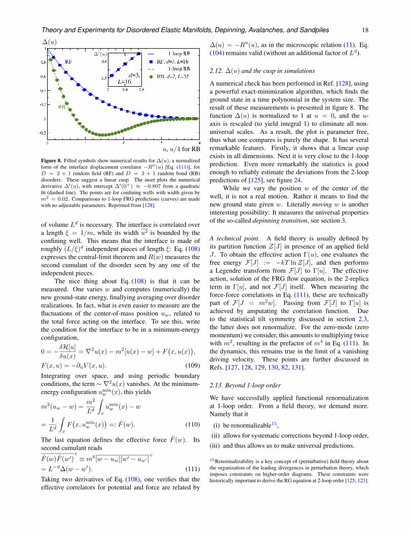
u, u/4 for RB
∆(u)
∆′(u)
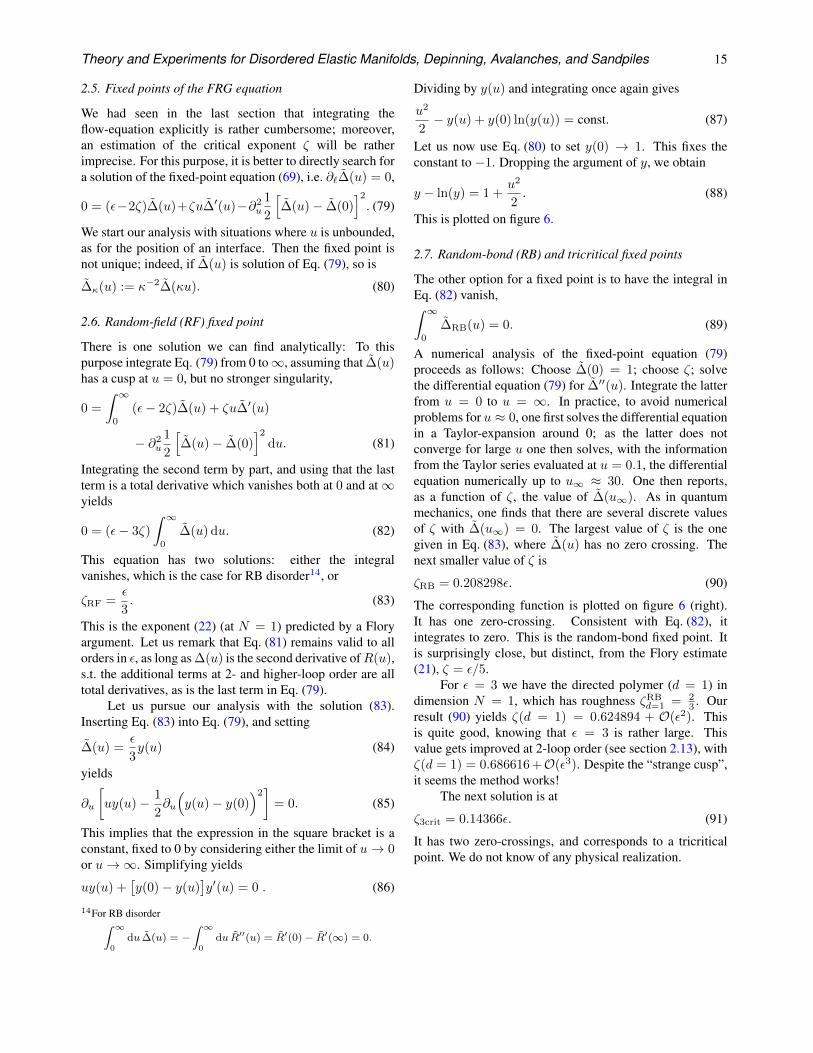
Figure 8. Filled symbols show numerical results for ∆(u), a normalizedform of the interface displacement correlator −R′′(u) [Eq. (111)], forD = 2 + 1 random field (RF) and D = 3 + 1 random bond (RB)disorders. These suggest a linear cusp. The inset plots the numericalderivative ∆′(u), with intercept ∆′(0+) ≈ −0.807 from a quadraticfit (dashed line). The points are for confining wells with width given bym2 = 0.02. Comparisons to 1-loop FRG predictions (curves) are madewith no adjustable parameters. Reprinted from [128].
of volume Ld is necessary. The interface is correlated overa length ξ = 1/m, while its width u2 is bounded by theconfining well. This means that the interface is made ofroughly (L/ξ)d independent pieces of length ξ: Eq. (108)expresses the central-limit theorem and R(w) measures thesecond cumulant of the disorder seen by any one of theindependent pieces.
The nice thing about Eq. (108) is that it can bemeasured. One varies w and computes (numerically) thenew ground-state energy, finallying averaging over disorderrealizations. In fact, what is even easier to measure are thefluctuations of the center-of-mass position uw, related tothe total force acting on the interface. To see this, writethe condition for the interface to be in a minimum-energyconfiguration,
0 = −δH[u]
δu(x)= ∇2u(x)−m2[u(x)− w] + F
(x, u(x)
),
F (x, u) = −∂uV (x, u). (109)
Integrating over space, and using periodic boundaryconditions, the term ∼ ∇2u(x) vanishes. At the minimum-energy configuration umin
w (x), this yields
m2(uw − w) =m2
Ld
∫
x
uminw (x)− w
=1
Ld
∫
x
F(x, umin
w (x))
=: F (w). (110)
The last equation defines the effective force F (w). Itssecond cumulant reads
F (w)F (w′)c
≡ m4[w − uw][w′ − uw′ ]c
= L−d∆(w − w′). (111)
Taking two derivatives of Eq. (108), one verifies that theeffective correlators for potential and force are related by
∆(u) = −R′′(u), as in the microscopic relation (11). Eq.(104) remains valid (without an additional factor of Ld).
2.12. ∆(u) and the cusp in simulations
A numerical check has been performed in Ref. [128], usinga powerful exact-minimization algorithm, which finds theground state in a time polynomial in the system size. Theresult of these measurements is presented in figure 8. Thefunction ∆(u) is normalized to 1 at u = 0, and the u-axis is rescaled (to yield integral 1) to eliminate all non-universal scales. As a result, the plot is parameter free,thus what one compares is purely the shape. It has severalremarkable features. Firstly, it shows that a linear cuspexists in all dimensions. Next it is very close to the 1-loopprediction. Even more remarkably the statistics is goodenough to reliably estimate the deviations from the 2-looppredictions of [125], see figure 24.
While we vary the position w of the center of thewell, it is not a real motion. Rather it means to find thenew ground state given w. Literally moving w is anotherinteresting possibility: It measures the universal propertiesof the so-called depinning transition, see section 3.
A technical point. A field theory is usually defined byits partition function Z[J ] in presence of an applied fieldJ . To obtain the effective action Γ(u), one evaluates thefree energy F [J ] := −kT lnZ[J ], and then performsa Legendre transform from F [J ] to Γ[u]. The effectiveaction, solution of the FRG flow equation, is the 2-replicaterm in Γ[u], and not F [J ] itself. When measuring theforce-force correlations in Eq. (111), these are technicallypart of F [J = m2w]. Passing from F [J ] to Γ[u] isachieved by amputating the correlation function. Dueto the statistical tilt symmetry discussed in section 2.3,the latter does not renormalize. For the zero-mode (zeromomentum) we consider, this amounts to multiplying twicewith m2, resulting in the prefactor of m4 in Eq. (111). Inthe dynamics, this remains true in the limit of a vanishingdriving velocity. These points are further discussed inRefs. [127, 128, 129, 130, 82, 131].
2.13. Beyond 1-loop order
We have successfully applied functional renormalizationat 1-loop order. From a field theory, we demand more.Namely that it
(i) be renormalizable15,(ii) allows for systematic corrections beyond 1-loop order,
(iii) and thus allows us to make universal predictions.
15Renormalizability is a key concept of (perturbative) field theory aboutthe organization of the leading divergences in perturbation theory, whichimposes constraints on higher-order diagrams. These constraints werehistorically important to derive the RG equation at 2-loop order [125, 123].
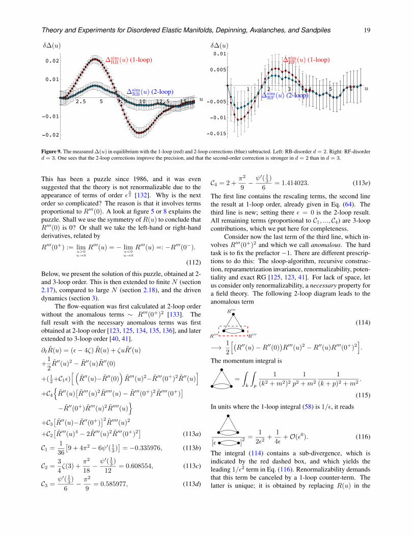
Theory and Experiments for Disordered Elastic Manifolds, Depinning, Avalanches, and Sandpiles 19
2.5 5 7.5 10 12.5 15
-0.02
-0.01
0.01
0.02
δ∆(u)
∆simRB(u) (1-loop)
∆simRB(u) (2-loop)
∆simRF (u) (1-loop)
∆simRF (u) (2-loop)
u
1 2 3 4 5 6
-0.015
-0.01
-0.005
0.005
0.01δ∆(u)
u
Figure 9. The measured ∆(u) in equilibrium with the 1-loop (red) and 2-loop corrections (blue) subtracted. Left: RB-disorder d = 2. Right: RF-disorderd = 3. One sees that the 2-loop corrections improve the precision, and that the second-order correction is stronger in d = 2 than in d = 3.
This has been a puzzle since 1986, and it was evensuggested that the theory is not renormalizable due to theappearance of terms of order ε
32 [132]. Why is the next
order so complicated? The reason is that it involves termsproportional to R′′′(0). A look at figure 5 or 8 explains thepuzzle. Shall we use the symmetry ofR(u) to conclude thatR′′′(0) is 0? Or shall we take the left-hand or right-handderivatives, related by
R′′′(0+) := limu>0u→0
R′′′(u) = − limu<0u→0
R′′′(u) =: −R′′′(0−).
(112)
Below, we present the solution of this puzzle, obtained at 2-and 3-loop order. This is then extended to finite N (section2.17), compared to large N (section 2.18), and the drivendynamics (section 3).
The flow-equation was first calculated at 2-loop orderwithout the anomalous terms ∼ R′′′(0+)2 [133]. Thefull result with the necessary anomalous terms was firstobtained at 2-loop order [123, 125, 134, 135, 136], and laterextended to 3-loop order [40, 41].
∂`R(u) = (ε− 4ζ) R(u) + ζuR′(u)
+1
2R′′(u)2 − R′′(u)R′′(0)
+( 12+C1ε)
[ (R′′(u)−R′′(0)
)R′′′(u)2−R′′′(0+)2R′′(u)
]
+C4R′′(u)
[R′′′(u)2R′′′′(u)− R′′′(0+)2R′′′′(0+)
]
−R′′(0+)R′′′(u)2R′′′′(u)
+C3[R′′(u)−R′′(0+)
]2R′′′′(u)2
+C2[R′′′(u)4 − 2R′′′(u)2R′′′(0+)2
](113a)
C1 =1
36
[9 + 4π2 − 6ψ′( 1
3 )]
= −0.335976, (113b)
C2 =3
4ζ(3) +
π2
18− ψ′( 1
3 )
12= 0.608554, (113c)
C3 =ψ′( 1
3 )
6− π2
9= 0.585977, (113d)
C4 = 2 +π2
9− ψ′( 1
3 )
6= 1.414023. (113e)
The first line contains the rescaling terms, the second linethe result at 1-loop order, already given in Eq. (64). Thethird line is new; setting there ε = 0 is the 2-loop result.All remaining terms (proportional to C1, ..., C4) are 3-loopcontributions, which we put here for completeness.
Consider now the last term of the third line, which in-volves R′′′(0+)2 and which we call anomalous. The hardtask is to fix the prefactor −1. There are different prescrip-tions to do this: The sloop-algorithm, recursive construc-tion, reparametrization invariance, renormalizability, poten-tiality and exact RG [125, 123, 41]. For lack of space, letus consider only renormalizability, a necessary property fora field theory. The following 2-loop diagram leads to theanomalous term
R′′′ R′′′
R′′′
(114)
−→ 1
2
[(R′′(u)−R′′(0)
)R′′′(u)2 −R′′(u)R′′′(0+)2
].
The momentum integral is
=
∫
k
∫
p
1
(k2 +m2)2
1
p2 +m2
1
(k + p)2 +m2.
(115)
In units where the 1-loop integral (58) is 1/ε, it reads
[ε ]2 =
1
2ε2+
1
4ε+O(ε0). (116)
The integral (114) contains a sub-divergence, which isindicated by the red dashed box, and which yields theleading 1/ε2 term in Eq. (116). Renormalizability demandsthat this term be canceled by a 1-loop counter-term. Thelatter is unique; it is obtained by replacing R(u) in the
Theory and Experiments for Disordered Elastic Manifolds, Depinning, Avalanches, and Sandpiles 20
1-loop correction δR(u) = 12R′′(u)2 − R′′(u)R′′(0) by
δR(u) itself; the last term then yields
δR′′(0) := limu→0
δR′′(u) = limu→0
R′′′(u)2 = R′′′(0+)2.(117)
This fixes the prefactor of the last (anomalous) term in thethird line of Eq. (113a).
A physical requirement is that the disorder correlationsremain potential, i.e. that forces are derivatives of apotential. The force-force correlations being −R′′(u), thismeans that the flow of R′(0+) has to vanish. (The simplestway to see this is to study a periodic potential.) FromEq. (113a) one can check that this does not remain true ifone changes the prefactor of the last term in the third line ofEq. (113a); thus fixing it.
RP disorder. Let us give results for cases of physicalinterest. First of all, for a periodic potential (RP), which isrelevant for charge-density waves, the fixed-point functioncan be calculated analytically. With the notations of Eqs.(94)-(95) this reads (with the choice of period 1, u ∈ [0, 1])
RRP(u) = −u2(1− u)2 g
24+ const., (118a)
∆RP(u) =g
12− g
2u(1− u), (118b)
g =ε
3+
2ε2
9+ε3
81
[9 + 2π2 − 18ζ(3)− 3ψ′( 1
3 )]
+O(ε4). (118c)
This gives a universal amplitude for the 2-point function at2-loop [123] and 3-loop order [40],
u(q)u(−q)∣∣∣q=0
=g
6md. (119)
This in turn leads to a logarithmic growth of the 2-point function in position space. The amplitude ismore complicated to extract, as one needs to extract theasymptotic behavior of scaling functions involved in thistransformation. Using Eqs. (4.13)-(4.18) of [40]16, it canbe written as1
2[u(x)− u(0)]2 =
gB(d)
6(4π)d2 Γ(d2 )
ln
( |x|L
), (120a)
B(d) =1 + 0.0.134567ε
1 + 1.134567ε+O(ε3). (120b)
RF disorder. For random-field disorder, the argumentgiven in Eq. (82) is still valid, and ζ = ε
3 remains valid,equivalent to the Flory estimate (22). The fixed-pointfunction ∆(u) changes, and can up to 3-loop order be givenanalytically [40].
RB disorder. For random-bond disorder (short-rangedpotential-potential correlation function) we have to solve16Eq. (4.15) of [40] should read Fd(0) = 1.
Eq. (113a) numerically, order by order in ε. The result is[40]
ζRB = 0.20829804ε+ 0.006858ε2 − 0.01075ε3 +O(ε4).
(121)
This compares well with numerical simulations, see figure10. It is also surprisingly close to, but distinct from, theFlory estimate (21), ζ = ε/5. For d = 1 (ε = 3) it getsclose to the exact value [108]
ζd=1RB =
2
3. (122)
The fixed-point function ∆(u) can be obtained up to 3-looporder numerically [40].
2.14. Stability of the fixed point
Having found a fixed point,
∂`∆(u) = β[∆](u) = 0, (123)
one has to ascertain that it is stable. Linear stability isanalyzed by considering infinitesimal perturbations of thefixed point
δβ[∆, z](u) :=d
dκβ[∆ + κz](u)
∣∣∣κ=0
. (124)
Assuming that ∆(u) is a solution of Eq. (123), theeigenvalue equation reads
δβ[∆, z](u) = −ωz(u). (125)
The exponent ω, if it exists, is the standard correction-to-scaling exponent [2] associated to the eigen-mode z(u). Incontrast to standard RG, more than one eigen-mode mayexist. The solutions to Eq. (125) depend on the universalityclass.
First, for the periodic fixed point (118a), there is adiscrete spectrum of solutions17,
ω−1 = −ε, z−1(u) = 1. (126a)
ω1 = ε− 2
3ε2 +
5 + 12ζ(3)
9ε3 +O(ε4), (126b)
z1(u) = 1− 6u(1− u).
ω2 = 4ε− 5ε2 +5
6[13 + 12ζ(3)]ε3 +O(ε4), (126c)
z2(u) = 1
−
15+5ε−5
6ε2[12ζ(3)+5+2π2 − 3ψ′( 1
3 )]u(1−u)
+
45+25ε−25
6ε2[12ζ(3)+5+2π2−3ψ′( 1
3 )]
[u(1−u)]2
ω3 =25ε
3− 140ε2
9+
70
9
[4ζ(3)+7
]ε3 +O(ε4) (126d)
...
The first solution ω−1 = −ε is relevant, and comeswith a constant perturbation for ∆(u). It is inadmissible17As in [140] we use the high-energy-physics conventions with ω > 0 foran IR-attractive fixed point. This is opposite to some earlier work, as theleading solution given in [40].
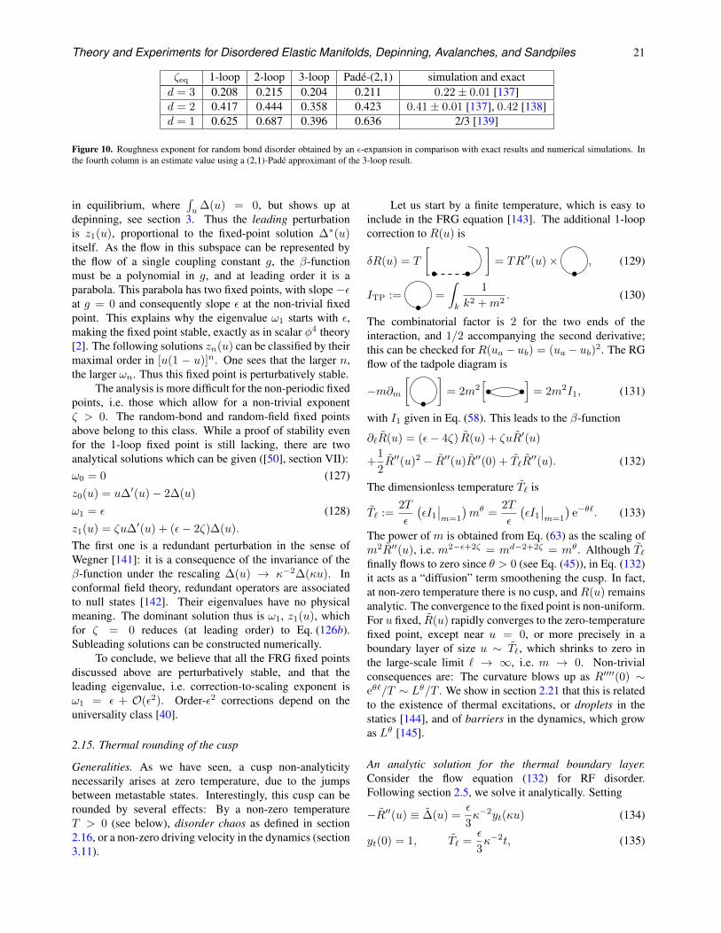
Theory and Experiments for Disordered Elastic Manifolds, Depinning, Avalanches, and Sandpiles 21
ζeq 1-loop 2-loop 3-loop Pade-(2,1) simulation and exactd = 3 0.208 0.215 0.204 0.211 0.22± 0.01 [137]d = 2 0.417 0.444 0.358 0.423 0.41± 0.01 [137], 0.42 [138]d = 1 0.625 0.687 0.396 0.636 2/3 [139]
Figure 10. Roughness exponent for random bond disorder obtained by an ε-expansion in comparison with exact results and numerical simulations. Inthe fourth column is an estimate value using a (2,1)-Pade approximant of the 3-loop result.
in equilibrium, where∫u
∆(u) = 0, but shows up atdepinning, see section 3. Thus the leading perturbationis z1(u), proportional to the fixed-point solution ∆∗(u)itself. As the flow in this subspace can be represented bythe flow of a single coupling constant g, the β-functionmust be a polynomial in g, and at leading order it is aparabola. This parabola has two fixed points, with slope −εat g = 0 and consequently slope ε at the non-trivial fixedpoint. This explains why the eigenvalue ω1 starts with ε,making the fixed point stable, exactly as in scalar φ4 theory[2]. The following solutions zn(u) can be classified by theirmaximal order in [u(1 − u)]n. One sees that the larger n,the larger ωn. Thus this fixed point is perturbatively stable.
The analysis is more difficult for the non-periodic fixedpoints, i.e. those which allow for a non-trivial exponentζ > 0. The random-bond and random-field fixed pointsabove belong to this class. While a proof of stability evenfor the 1-loop fixed point is still lacking, there are twoanalytical solutions which can be given ([50], section VII):ω0 = 0 (127)z0(u) = u∆′(u)− 2∆(u)
ω1 = ε (128)z1(u) = ζu∆′(u) + (ε− 2ζ)∆(u).
The first one is a redundant perturbation in the sense ofWegner [141]: it is a consequence of the invariance of theβ-function under the rescaling ∆(u) → κ−2∆(κu). Inconformal field theory, redundant operators are associatedto null states [142]. Their eigenvalues have no physicalmeaning. The dominant solution thus is ω1, z1(u), whichfor ζ = 0 reduces (at leading order) to Eq. (126b).Subleading solutions can be constructed numerically.
To conclude, we believe that all the FRG fixed pointsdiscussed above are perturbatively stable, and that theleading eigenvalue, i.e. correction-to-scaling exponent isω1 = ε + O(ε2). Order-ε2 corrections depend on theuniversality class [40].
2.15. Thermal rounding of the cusp
Generalities. As we have seen, a cusp non-analyticitynecessarily arises at zero temperature, due to the jumpsbetween metastable states. Interestingly, this cusp can berounded by several effects: By a non-zero temperatureT > 0 (see below), disorder chaos as defined in section2.16, or a non-zero driving velocity in the dynamics (section3.11).
Let us start by a finite temperature, which is easy toinclude in the FRG equation [143]. The additional 1-loopcorrection to R(u) is
δR(u) = T
[ ]= TR′′(u)× , (129)
ITP := =
∫
k
1
k2 +m2. (130)
The combinatorial factor is 2 for the two ends of theinteraction, and 1/2 accompanying the second derivative;this can be checked for R(ua − ub) = (ua − ub)2. The RGflow of the tadpole diagram is
−m∂m[ ]
= 2m2[ ]
= 2m2I1, (131)
with I1 given in Eq. (58). This leads to the β-function
∂`R(u) = (ε− 4ζ) R(u) + ζuR′(u)
+1
2R′′(u)2 − R′′(u)R′′(0) + T`R
′′(u). (132)
The dimensionless temperature T` is
T` :=2T
ε
(εI1∣∣m=1
)mθ =
2T
ε
(εI1∣∣m=1
)e−θ`. (133)
The power of m is obtained from Eq. (63) as the scaling ofm2R′′(u), i.e. m2−ε+2ζ = md−2+2ζ = mθ. Although T`finally flows to zero since θ > 0 (see Eq. (45)), in Eq. (132)it acts as a “diffusion” term smoothening the cusp. In fact,at non-zero temperature there is no cusp, and R(u) remainsanalytic. The convergence to the fixed point is non-uniform.For u fixed, R(u) rapidly converges to the zero-temperaturefixed point, except near u = 0, or more precisely in aboundary layer of size u ∼ T`, which shrinks to zero inthe large-scale limit ` → ∞, i.e. m → 0. Non-trivialconsequences are: The curvature blows up as R′′′′(0) ∼eθ`/T ∼ Lθ/T . We show in section 2.21 that this is relatedto the existence of thermal excitations, or droplets in thestatics [144], and of barriers in the dynamics, which growas Lθ [145].
An analytic solution for the thermal boundary layer.Consider the flow equation (132) for RF disorder.Following section 2.5, we solve it analytically. Setting
−R′′(u) ≡ ∆(u) =ε
3κ−2yt(κu) (134)
yt(0) = 1, T` =ε
3κ−2t, (135)
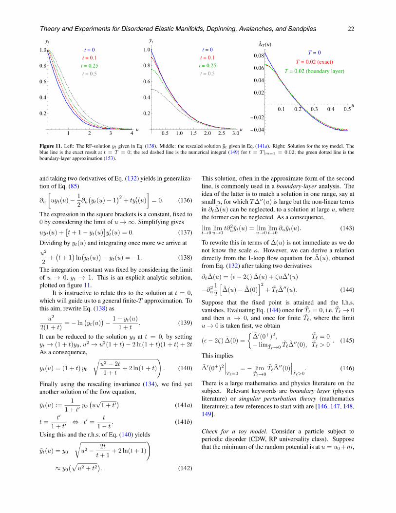
Theory and Experiments for Disordered Elastic Manifolds, Depinning, Avalanches, and Sandpiles 22
t = 0
t = 0.1
t = 0.25
t = 0.5
1 2 3 4u
0.2
0.4
0.6
0.8
1.0
yt
t = 0
t = 0.1
t = 0.25
t = 0.5
0.5 1.0 1.5 2.0 2.5 3.0u
0.2
0.4
0.6
0.8
1.0
y t
T = 0
T = 0.02 (exact)
T = 0.02 (boundary layer)
0.1 0.2 0.3 0.4 0.5u
-0.04
-0.02
0.02
0.04
0.06
0.08
ΔT(u)
Figure 11. Left: The RF-solution yt given in Eq. (138). Middle: the rescaled solution yt given in Eq. (141a). Right: Solution for the toy model. Theblue line is the exact result at t = T = 0; the red dashed line is the numerical integral (149) for t = T |m=1 = 0.02; the green dotted line is theboundary-layer approximation (153).
and taking two derivatives of Eq. (132) yields in generaliza-tion of Eq. (85)
∂u
[uyt(u)− 1
2∂u(yt(u)− 1
)2+ ty′t(u)
]= 0. (136)
The expression in the square brackets is a constant, fixed to0 by considering the limit of u→∞. Simplifying gives
uyt(u) +[t+ 1− yt(u)
]y′t(u) = 0. (137)
Dividing by yt(u) and integrating once more we arrive at
u2
2+(t+ 1
)ln(yt(u)
)− yt(u) = −1. (138)
The integration constant was fixed by considering the limitof u → 0, yt → 1. This is an explicit analytic solution,plotted on figure 11.
It is instructive to relate this to the solution at t = 0,which will guide us to a general finite-T approximation. Tothis aim, rewrite Eq. (138) as
u2
2(1 + t)= − ln
(yt(u)
)− 1− yt(u)
1 + t. (139)
It can be reduced to the solution y0 at t = 0, by settingyt → (1 + t)y0, u2 → u2(1 + t)− 2 ln(1 + t)(1 + t) + 2tAs a consequence,
yt(u) = (1 + t) y0
(√u2 − 2t
1 + t+ 2 ln(1 + t)
). (140)
Finally using the rescaling invariance (134), we find yetanother solution of the flow equation,
yt(u) :=1
1 + t′yt′(u√
1 + t′)
(141a)
t =t′
1 + t′⇔ t′ =
t
1− t . (141b)
Using this and the r.h.s. of Eq. (140) yields
yt(u) = y0
(√u2 − 2t
t+ 1+ 2 ln(t+ 1)
)
≈ y0
(√u2 + t2
). (142)
This solution, often in the approximate form of the secondline, is commonly used in a boundary-layer analysis. Theidea of the latter is to match a solution in one range, say atsmall u, for which T ∆′′(u) is large but the non-linear termsin ∂`∆(u) can be neglected, to a solution at large u, wherethe former can be neglected. As a consequence,
limt→0
limu→0
t∂2uyt(u) = lim
u→0limt→0
∂uyt(u). (143)
To rewrite this in terms of ∆(u) is not immediate as we donot know the scale κ. However, we can derive a relationdirectly from the 1-loop flow equation for ∆(u), obtainedfrom Eq. (132) after taking two derivatives
∂`∆(u) = (ε− 2ζ) ∆(u) + ζu∆′(u)
−∂2u
1
2
[∆(u)− ∆(0)
]2+ T`∆
′′(u). (144)
Suppose that the fixed point is attained and the l.h.s.vanishes. Evaluating Eq. (144) once for T` = 0, i.e. T` → 0and then u → 0, and once for finite T`, where the limitu→ 0 is taken first, we obtain
(ε− 2ζ) ∆(0) =
∆′(0+)2, T` = 0
− limT`→0 T`∆′′(0), T` > 0
. (145)
This implies
∆′(0+)2∣∣∣T`=0
= − limT`→0
T`∆′′(0)
∣∣∣T`>0
. (146)
There is a large mathematics and physics literature on thesubject. Relevant keywords are boundary layer (physicsliterature) or singular perturbation theory (mathematicsliterature); a few references to start with are [146, 147, 148,149].
Check for a toy model. Consider a particle subject toperiodic disorder (CDW, RP universality class). Supposethat the minimum of the random potential is at u = u0 +ni,
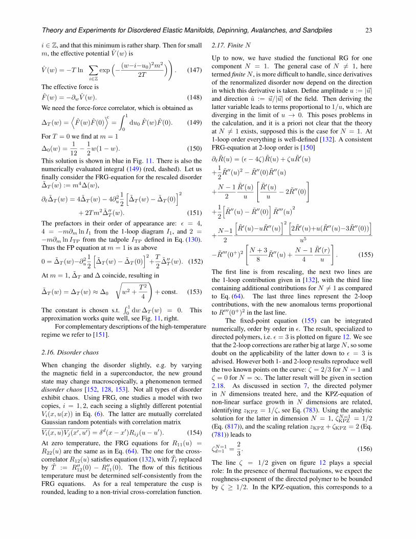
Theory and Experiments for Disordered Elastic Manifolds, Depinning, Avalanches, and Sandpiles 23
i ∈ Z, and that this minimum is rather sharp. Then for smallm, the effective potential V (w) is
V (w) = −T ln
(∑
i∈Zexp
(− (w−i−u0)2m2
2T
)). (147)
The effective force is
F (w) = −∂wV (w). (148)
We need the force-force correlator, which is obtained as
∆T (w) =⟨F (w)F (0)
⟩c=
∫ 1
0
du0 F (w)F (0). (149)
For T = 0 we find at m = 1
∆0(w) =1
12− 1
2w(1− w). (150)
This solution is shown in blue in Fig. 11. There is also thenumerically evaluated integral (149) (red, dashed). Let usfinally consider the FRG-equation for the rescaled disorder∆T (w) := m4∆(w),
∂`∆T (w) = 4∆T (w)− 4∂2u
1
2
[∆T (w)− ∆T (0)
]2
+ 2Tm2∆′′T (w). (151)
The prefactors in their order of appearance are: ε = 4,4 = −m∂m ln I1 from the 1-loop diagram I1, and 2 =−m∂m ln ITP from the tadpole ITP defined in Eq. (130).Thus the FP equation at m = 1 is as above
0 = ∆T (w)−∂2u
1
2
[∆T (w)− ∆T (0)
]2+T
2∆′′T (w). (152)
At m = 1, ∆T and ∆ coincide, resulting in
∆T (w) = ∆T (w) ≈ ∆0
(√w2 +
T 2
4
)+ const. (153)
The constant is chosen s.t.∫ 1
0dw∆T (w) = 0. This
approximation works quite well, see Fig. 11, right.For complementary descriptions of the high-temperature
regime we refer to [151].
2.16. Disorder chaos
When changing the disorder slightly, e.g. by varyingthe magnetic field in a superconductor, the new groundstate may change macroscopically, a phenomenon termeddisorder chaos [152, 128, 153]. Not all types of disorderexhibit chaos. Using FRG, one studies a model with twocopies, i = 1, 2, each seeing a slightly different potentialVi(x, u(x)) in Eq. (6). The latter are mutually correlatedGaussian random potentials with correlation matrix
Vi(x, u)Vj(x′, u′) = δd(x− x′)Rij(u− u′). (154)
At zero temperature, the FRG equations for R11(u) =R22(u) are the same as in Eq. (64). The one for the cross-correlator R12(u) satisfies equation (132), with T` replacedby T := R′′12(0) − R′′11(0). The flow of this fictitioustemperature must be determined self-consistently from theFRG equations. As for a real temperature the cusp isrounded, leading to a non-trivial cross-correlation function.
2.17. Finite N
Up to now, we have studied the functional RG for onecomponent N = 1. The general case of N 6= 1, heretermed finiteN , is more difficult to handle, since derivativesof the renormalized disorder now depend on the directionin which this derivative is taken. Define amplitude u := |~u|and direction u := ~u/|~u| of the field. Then deriving thelatter variable leads to terms proportional to 1/u, which arediverging in the limit of u → 0. This poses problems inthe calculation, and it is a priori not clear that the theoryat N 6= 1 exists, supposed this is the case for N = 1. At1-loop order everything is well-defined [132]. A consistentFRG-equation at 2-loop order is [150]
∂`R(u) = (ε− 4ζ)R(u) + ζuR′(u)
+1
2R′′(u)2 − R′′(0)R′′(u)
+N − 1
2
R′(u)
u
[R′(u)
u− 2R′′(0)
]
+1
2
[R′′(u)− R′′(0)
]R′′′(u)
2
+N−1
2
[R′(u)−uR′′(u)
]2 [2R′(u)+u(R′′(u)−3R′′(0))
]
u5
−R′′′(0+)2
[N + 3
8R′′(u) +
N − 1
4
R′(r)u
]. (155)
The first line is from rescaling, the next two lines arethe 1-loop contribution given in [132], with the third linecontaining additional contributions for N 6= 1 as comparedto Eq. (64). The last three lines represent the 2-loopcontributions, with the new anomalous terms proportionalto R′′′(0+)2 in the last line.
The fixed-point equation (155) can be integratednumerically, order by order in ε. The result, specialized todirected polymers, i.e. ε = 3 is plotted on figure 12. We seethat the 2-loop corrections are rather big at largeN , so somedoubt on the applicability of the latter down to ε = 3 isadvised. However both 1- and 2-loop results reproduce wellthe two known points on the curve: ζ = 2/3 for N = 1 andζ = 0 for N =∞. The latter result will be given in section2.18. As discussed in section 7, the directed polymerin N dimensions treated here, and the KPZ-equation ofnon-linear surface growth in N dimensions are related,identifying zKPZ = 1/ζ, see Eq. (783). Using the analyticsolution for the latter in dimension N = 1, ζN=1
KPZ = 1/2(Eq. (817)), and the scaling relation zKPZ + ζKPZ = 2 (Eq.(781)) leads to
ζN=1d=1 =
2
3. (156)
The line ζ = 1/2 given on figure 12 plays a specialrole: In the presence of thermal fluctuations, we expect theroughness-exponent of the directed polymer to be boundedby ζ ≥ 1/2. In the KPZ-equation, this corresponds to a
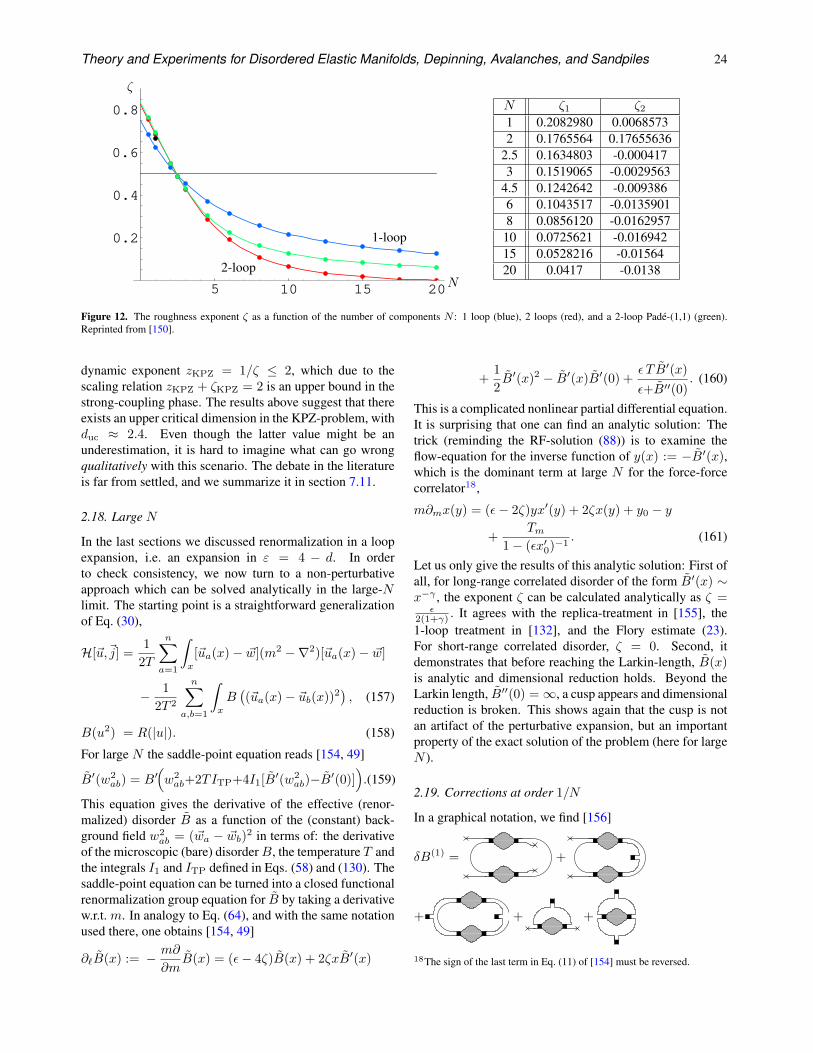
Theory and Experiments for Disordered Elastic Manifolds, Depinning, Avalanches, and Sandpiles 24
5 10 15 20
0.2
0.4
0.6
0.8
ζ
N
1-loop
2-loop
N ζ1 ζ21 0.2082980 0.00685732 0.1765564 0.17655636
2.5 0.1634803 -0.0004173 0.1519065 -0.0029563
4.5 0.1242642 -0.0093866 0.1043517 -0.01359018 0.0856120 -0.0162957
10 0.0725621 -0.01694215 0.0528216 -0.0156420 0.0417 -0.0138
Figure 12. The roughness exponent ζ as a function of the number of components N : 1 loop (blue), 2 loops (red), and a 2-loop Pade-(1,1) (green).Reprinted from [150].
dynamic exponent zKPZ = 1/ζ ≤ 2, which due to thescaling relation zKPZ + ζKPZ = 2 is an upper bound in thestrong-coupling phase. The results above suggest that thereexists an upper critical dimension in the KPZ-problem, withduc ≈ 2.4. Even though the latter value might be anunderestimation, it is hard to imagine what can go wrongqualitatively with this scenario. The debate in the literatureis far from settled, and we summarize it in section 7.11.
2.18. Large N
In the last sections we discussed renormalization in a loopexpansion, i.e. an expansion in ε = 4 − d. In orderto check consistency, we now turn to a non-perturbativeapproach which can be solved analytically in the large-Nlimit. The starting point is a straightforward generalizationof Eq. (30),
H[~u,~j] =1
2T
n∑
a=1
∫
x
[~ua(x)− ~w](m2 −∇2)[~ua(x)− ~w]
− 1
2T 2
n∑
a,b=1
∫
x
B((~ua(x)− ~ub(x))2
), (157)
B(u2) = R(|u|). (158)
For large N the saddle-point equation reads [154, 49]
B′(w2ab) = B′
(w2ab+2TITP+4I1[B′(w2
ab)−B′(0)]).(159)
This equation gives the derivative of the effective (renor-malized) disorder B as a function of the (constant) back-ground field w2
ab = (~wa − ~wb)2 in terms of: the derivative
of the microscopic (bare) disorderB, the temperature T andthe integrals I1 and ITP defined in Eqs. (58) and (130). Thesaddle-point equation can be turned into a closed functionalrenormalization group equation for B by taking a derivativew.r.t. m. In analogy to Eq. (64), and with the same notationused there, one obtains [154, 49]
∂`B(x) := − m∂
∂mB(x) = (ε− 4ζ)B(x) + 2ζxB′(x)
+1
2B′(x)2 − B′(x)B′(0) +
ε T B′(x)
ε+B′′(0). (160)
This is a complicated nonlinear partial differential equation.It is surprising that one can find an analytic solution: Thetrick (reminding the RF-solution (88)) is to examine theflow-equation for the inverse function of y(x) := −B′(x),which is the dominant term at large N for the force-forcecorrelator18,
m∂mx(y) = (ε− 2ζ)yx′(y) + 2ζx(y) + y0 − y
+Tm
1− (εx′0)−1. (161)
Let us only give the results of this analytic solution: First ofall, for long-range correlated disorder of the form B′(x) ∼x−γ , the exponent ζ can be calculated analytically as ζ =
ε2(1+γ) . It agrees with the replica-treatment in [155], the1-loop treatment in [132], and the Flory estimate (23).For short-range correlated disorder, ζ = 0. Second, itdemonstrates that before reaching the Larkin-length, B(x)is analytic and dimensional reduction holds. Beyond theLarkin length, B′′(0) =∞, a cusp appears and dimensionalreduction is broken. This shows again that the cusp is notan artifact of the perturbative expansion, but an importantproperty of the exact solution of the problem (here for largeN ).
2.19. Corrections at order 1/N
In a graphical notation, we find [156]
δB(1) = +
+ + +
18The sign of the last term in Eq. (11) of [154] must be reversed.
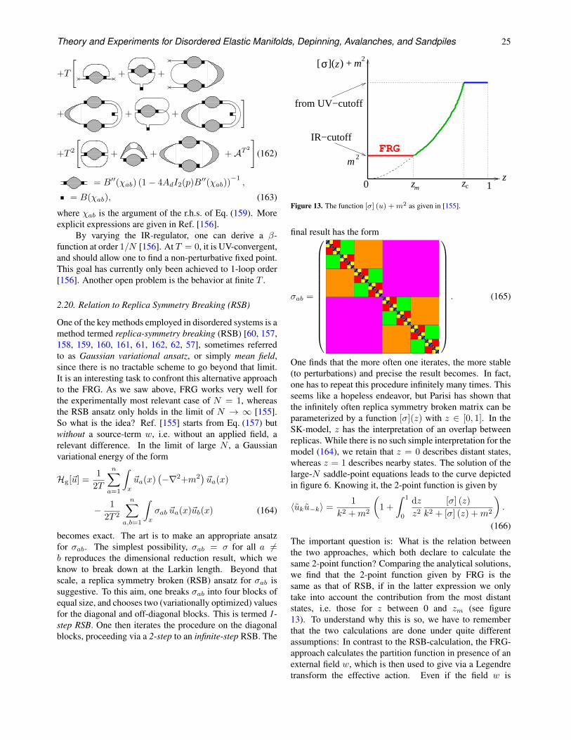
Theory and Experiments for Disordered Elastic Manifolds, Depinning, Avalanches, and Sandpiles 25
+T
[+ +
+ + +
]
+T 2
[+ + +AT 2
](162)
= B′′(χab) (1− 4AdI2(p)B′′(χab))−1,
= B(χab), (163)
where χab is the argument of the r.h.s. of Eq. (159). Moreexplicit expressions are given in Ref. [156].
By varying the IR-regulator, one can derive a β-function at order 1/N [156]. At T = 0, it is UV-convergent,and should allow one to find a non-perturbative fixed point.This goal has currently only been achieved to 1-loop order[156]. Another open problem is the behavior at finite T .
2.20. Relation to Replica Symmetry Breaking (RSB)
One of the key methods employed in disordered systems is amethod termed replica-symmetry breaking (RSB) [60, 157,158, 159, 160, 161, 61, 162, 62, 57], sometimes referredto as Gaussian variational ansatz, or simply mean field,since there is no tractable scheme to go beyond that limit.It is an interesting task to confront this alternative approachto the FRG. As we saw above, FRG works very well forthe experimentally most relevant case of N = 1, whereasthe RSB ansatz only holds in the limit of N → ∞ [155].So what is the idea? Ref. [155] starts from Eq. (157) butwithout a source-term w, i.e. without an applied field, arelevant difference. In the limit of large N , a Gaussianvariational energy of the form
Hg[~u] =1
2T
n∑
a=1
∫
x
~ua(x)(−∇2+m2
)~ua(x)
− 1
2T 2
n∑
a,b=1
∫
x
σab ~ua(x)~ub(x) (164)
becomes exact. The art is to make an appropriate ansatzfor σab. The simplest possibility, σab = σ for all a 6=b reproduces the dimensional reduction result, which weknow to break down at the Larkin length. Beyond thatscale, a replica symmetry broken (RSB) ansatz for σab issuggestive. To this aim, one breaks σab into four blocks ofequal size, and chooses two (variationally optimized) valuesfor the diagonal and off-diagonal blocks. This is termed 1-step RSB. One then iterates the procedure on the diagonalblocks, proceeding via a 2-step to an infinite-step RSB. The
from UV−cutoff
1
FRG
2[ ]( ) + σ z m
2m
0z
zcmz
IR−cutoff
Figure 13. The function [σ] (u) +m2 as given in [155].
final result has the form
σab =
. (165)
One finds that the more often one iterates, the more stable(to perturbations) and precise the result becomes. In fact,one has to repeat this procedure infinitely many times. Thisseems like a hopeless endeavor, but Parisi has shown thatthe infinitely often replica symmetry broken matrix can beparameterized by a function [σ](z) with z ∈ [0, 1]. In theSK-model, z has the interpretation of an overlap betweenreplicas. While there is no such simple interpretation for themodel (164), we retain that z = 0 describes distant states,whereas z = 1 describes nearby states. The solution of thelarge-N saddle-point equations leads to the curve depictedin figure 6. Knowing it, the 2-point function is given by
〈uku−k〉 =1
k2 +m2
(1 +
∫ 1
0
dz
z2
[σ] (z)
k2 + [σ] (z) +m2
).
(166)
The important question is: What is the relation betweenthe two approaches, which both declare to calculate thesame 2-point function? Comparing the analytical solutions,we find that the 2-point function given by FRG is thesame as that of RSB, if in the latter expression we onlytake into account the contribution from the most distantstates, i.e. those for z between 0 and zm (see figure13). To understand why this is so, we have to rememberthat the two calculations are done under quite differentassumptions: In contrast to the RSB-calculation, the FRG-approach calculates the partition function in presence of anexternal field w, which is then used to give via a Legendretransform the effective action. Even if the field w is
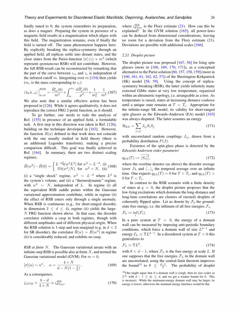
Theory and Experiments for Disordered Elastic Manifolds, Depinning, Avalanches, and Sandpiles 26
finally tuned to 0, the system remembers its preparation,as does a magnet: Preparing the system in presence of amagnetic field results in a magnetization which aligns withthis field. The magnetization remains, even if finally thefield is turned off. The same phenomenon happens here:By explicitly breaking the replica-symmetry through anapplied field, all replicas settle into distant states, and theclose states from the Parisi-function [σ] (z) + m2 (whichrepresent spontaneous RSB) will not contribute. However,the full RSB-result can be reconstructed by remarking thatthe part of the curve between zm and zc is independent ofthe infrared cutoff m. Integrating over m [154] then yields(mc is the mass corresponding to zc)
〈uku−k〉∣∣∣RSB
k=0=B′m(0)
m4+
∫ mc
m
dB′µ(0)
µ4+
1
m2c
− 1
m2.(167)
We also note that a similar effective action has beenproposed in [126]. While it agrees qualitatively, it does notreproduce the correct FRG 2-point function, as it should.
To go further, one needs to redo the analysis ofRef. [155] in presence of an applied field, a formidabletask. A first step in this direction was taken in Ref. [126],building on the technique developed in [163]. However,the function R(u) defined in that work does not coincidewith the one usually studied in field theory (there isan additional Legendre transform), making a precisecomparison difficult. This goal was finally achieved inRef. [164]. In summary, there are two distinct scalingregimes,
B(w2)− B(0) =
L−db(w2Ld) for w2 ∼ L−d, (i)Nb(w2/N) for w2 ∼ N, (ii)
(168)
(i) a “single shock” regime, w2 ∼ L−d where Ld isthe system’s volume, and (ii) a “thermodynamic” regime,with w2 ∼ N , independent of L. In regime (i) allthe equivalent RSB saddle points within the Gaussianvariational approximation contribute, while in regime (ii)the effect of RSB enters only through a single anomaly.When RSB is continuous (e.g., for short-ranged disorder,in dimension 2 ≤ d ≤ 4), regime (ii) yields the large-N FRG function shown above. In that case, the disordercorrelator exhibits a cusp in both regimes, though withdifferent amplitudes and of different physical origin. Whenthe RSB solution is 1-step and non-marginal (e.g. in d < 2for SR disorder), the correlator R(w) = B(w2) in regime(ii) is considerably reduced, and exhibits no cusp.
RSB at finite N . The Gaussian variational ansatz with aninfinite-step RSB is possible also at finiteN , and termed theGaussian variational model (GVM). For m = 0,
[σ](u) ∼ uα, α =4 +N
d−N(1− d2 ). (169)
As a consequence,
ζGVM =4− d4 +N
≡ ζRBFlory, (170)
where ζRBFlory is the Flory estimate (21). How can this be
explained? In the GVM solution [165], all power-lawscan be deduced from dimensional considerations, leavingno room for a deviation from the Flory estimate (21).Deviations are possible with additional scales [166].
2.21. Droplet picture
The droplet picture was proposed [167, 56] for Ising spinglasses (more in [168, 169, 170, 171]), as a conceptualalternative to the Parisi solution [60, 157, 158, 159] (more in[160, 161, 61, 162, 62, 57]) of the Sherrington-Kirkpatrick(SK) model [58, 59]. Using the concept of replica-symmetry breaking (RSB), the latter yields infinitely manyextremal Gibbs states at very low temperature, organizedwithin an ultrametric topology, i.e. arrangeable as a tree. Astemperature is raised, states at increasing distance coalesceuntil a unique state remains at T = Tc. Appropriate forthe infinite-range SK model, its validity for short-rangedspin glasses as the Edwards-Anderson (EA) model [103]was always disputed. The latter assumes an energy
HEA =∑
〈i,j〉JijSiSj (171)
with uncorrelated random couplings Jij , drawn from aprobability distribution P (J).
Existence of the spin-glass phase is detected by theEdwards-Anderson order parameter
qEA(T ) := 〈Si〉2t , (172)
where the overline denotes (as above) the disorder average(over J), and 〈...〉t the temporal average over an infinitetime. One expects qEA(T ) = 0 for T > Tc, and qEA(T ) >0 for T < Tc.
In contrast to the RSB scenario with a finite densityof states at q = 0, the droplet picture proposes that thelow-lying excitations which dominate the long-distance andlong-time correlations are clusters of (nested) droplets ofcoherently flipped spins. Let us denote by F0 the ground-state free energy, i.e. the infimum of all free energies Fi,F0 := inf
i(Fi). (173)
In a pure system at T = 0, the energy of a domainwall can be measured by imposing anti-periodic boundaryconditions, which force a domain wall of size Ld−1 andenergy EL ' ΥLd−1. In a disordered system at T > 0 thisgeneralizes to
FL ' ΥLθ, (174)
with θ < d − 1, where FL is the free energy at scale L. Ifone supposes that the free energies FL in the domain wallare uncorrelated, using the central-limit theorem improvesthe bound19 to θ ≤ d−1
2 . The probability of droplet
19One might argue that if a domain wall is rough, then its size scales asLdf with d − 1 ≤ df ≤ d, and we get a weaker bound for θ. Thisis incorrect. While the minimum-energy domain wall may be larger, itsenergy is lower; otherwise the minimal-energy interface would be flat.
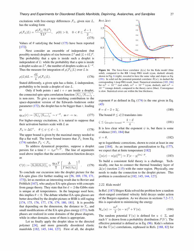
Theory and Experiments for Disordered Elastic Manifolds, Depinning, Avalanches, and Sandpiles 27
excitations with free-energy differences FL, given size L,has the scaling form
ρ(FL|L) =ρ(FL/ΥLθ)
ΥLθ, ρ(0) > 0, 0 < θ ≤ d− 1
2.
(175)
Values of θ satisfying the bond (175) have been reported[172].
Next consider an ensemble of independent (butpossibly nested) droplets of size between Ld and (L+δL)d.The probability that a spin is inside such a droplet isindependent of L: while the probability that a spin is insidea droplet scales asLd, the number of droplets scales asL−d.Thus the measure for integration of ρ(FL|L) over L is
ρ(L)dL =dL
Lρ(FL|L). (176)
Stated differently, a given spin has a finite, L-independent,probability to be inside a droplet of size L.
Only if both points i and i + r are inside a droplet,the connected spin-spin correlation function 〈Si〉t 〈Si+r〉t
c,
is non-zero. To give a non-vanishing contribution to thespace-dependent version of the Edwards-Anderson orderparameter (172), the droplet has to be bigger than r, leadingto
qEA(r) := 〈Si〉t 〈Si+r〉tc ∼ r−θ, as r →∞. (177)
For higher-energy excitations, it is natural to suppose thattheir activation barriers scale with L as
Fb ' ∆Lψ, θ ≤ ψ ≤ d− 1. (178)
The upper bound is given by the maximal energy needed toflip a flat wall. The lower bound insures that FL from Eq.(174) satisfies FL < Fb.
To address dynamical properties, suppose a dropletpersists for a time t = t0eFb/T . The line of argumentsused above implies that the autocorrelation function decaysas
C(t) := 〈Si(0)Si(t)〉t 'qEAT
Υ
[∆
T ln(t/t0)
] θψ
. (179)
To conclude our excursion into the droplet picture for theEA-spin glass (for further reading see [56, 169, 170, 171,173]), let us mention an interesting result due to Bovier andFrohlich [167], who analyze EA-spin glasses with conceptsfrom gauge theory. They state that for d = 2 the Gibbs stateis unique at all temperatures. In the language used here,this implies θ < 0. The debate whether EA-spin glasses arebetter described by the droplet picture or RSB is still raging[174, 175, 176, 177, 178, 179, 180, 181]. It is possiblethat depending on the dimension, the distance to Tc, andsmall modifications of the EA spin glass energy (171), bothphases are realized in some domains of the phase diagram,while in other domains, none of them is appropriate.
Let us finally apply the droplet ideas to the directedpolymer [24], and more generally disordered elasticmanifolds [182, 145, 144, 127]. First of all, the droplet
) Δ
)
Figure 14. The force-force correlator ∆(u) for the Kida model (bluesolid), compared to the RB 1-loop FRG result (cyan, dashed) alreadyshown in Fig. 6 (right), rescaled to have the same value and slopes as Eq.(191). In solid red the potential-potential correlator R(w), in dashed thecorresponding 1-loop FRG result. Inset: Numerical simulations [185, 186]for m2 = 10−1 (red solid), m2 = 10−2 (cyan, dashed), and m2 =10−4 (orange dotted), compared to the theory curve (blue). Convergenceis slow. Statistical errors are within the line thickness.
exponent θ as defined in Eq. (174) is the one given in Eq.(45)
θ = d− 2 + 2ζ. (180)
The bound θ ≤ d/2 translates into
ζ ≤ ζdroplet bound =4− d
4. (181)
It is less clear what the exponent ψ is, but there is someevidence [183, 184] that
ψ = θ, (182)
up to logarithmic corrections, shown to exist at least in onecase [184]. As an immediate generalization to Eq. (177),we expect that at finite temperature [182]⟨[u(x)− u(y)]2n
⟩' T |x− y|2nζ−θ. (183)
To build a consistent field theory is a challenge. Tech-nically, one has to connect the thermal boundary layer of∆(w) (section 2.15) with the outer region. Physically, oneneeds to make the connection to the droplet picture. Thisproblem is considered in [182, 145, 144, 127].
2.22. Kida model
In Ref. [187] Shigeo Kida solved the problem how a randomshort-ranged correlated velocity field decays under actionof the Burgers equation. As we discuss in sections 7.2–7.7,this is equivalent to minimizing the energy
Hw(u) :=m2
2(u− w)2 + V (u). (184)
The random potential V (u) is defined for u ∈ Z, andeach V is drawn from a probability distribution P (V ). Theeffective potential is defined as in Eq. (96). Kida’s solutionfor the V (w) correlations, rephrased in Refs. [188, 82] for
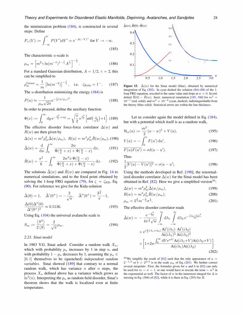
Theory and Experiments for Disordered Elastic Manifolds, Depinning, Avalanches, and Sandpiles 28
the minimization problem (184), is constructed in severalsteps: Define
P<(V ) :=
∫ V
−∞P (V ′)dV ′ ' e−A(−V )γ for V → −∞.
(185)
The characteristic u-scale is
ρm =[m2γ ln(m−1)1− 1
γA1γ
]− 12
. (186)
For a standard Gaussian distribution, A = 1/2, γ = 2, thiscan be simplified to
ρGaussm =
1
m
[ln(m−2)
]− 14 , i.e. ζKida = 1−. (187)
The u-distribution minimizing the energy (184) is
P (u) ≈ 1
ρm√
2πe−
12 (u/ρm)2 . (188)
In order to proceed, define the auxiliary function
Φ(x) :=
∫ ∞
0
dy e−y2
2 +xy =
√π
2ex2
2
[erf(x√2
)+1]. (189)
The effective disorder force-force correlator ∆(w) andR(w) are then given by
∆(u) = m4ρ2m∆(w/ρm), R(u) = m4ρ4
mR(w/ρm), (190)
∆(w) =d
dw
∫ ∞
0
2w
Φ(w2 + x) + Φ(w2 − x)dx, (191)
R(w) =π2
6−∫ ∞
0
2w2xΦ(w2 − x)
Φ(w2 + x) + Φ(w2 − x)dx. (192)
The solutions ∆(w) and R(w) are compared in Fig. 14 tonumerical simulations, and to the fixed point obtained bysolving the 1-loop FRG equation (79), for ζ = ζRB, Eq.(90). For reference we give for the Kida-solution
∆(0) = 1, ∆′(0+) = − 2√π, ∆′′(0+) =
332
π−1,
∆(0)∆′′(0)
∆′(0+)2≈ 0.5136. (193)
Using Eq. (104) the universal avalanche scale is
Sm :=
⟨S2⟩
2 〈S〉 =2√πρm. (194)
2.23. Sinai model
In 1983 Y.G. Sinai asked: Consider a random walk Xn,which with probability pn increases by 1 in step n, andwith probability 1− pn decreases by 1, assuming the pn ∈[0, 1] themselves to be (quenched) independent randomvariables. Sinai showed [189] that contrary to a normalrandom walk, which has variance n after n steps, theprocess Xn defined above has a variance which grows asln2(n). Interpreting the pn as random field disorder, Sinai’stheorem shows that the walk is localized even at finitetemperature.
Δ()
()-
()
Figure 15. ∆(w) for the Sinai model (blue), obtained by numericalintegration of Eq. (202). In cyan dashed the solution (84)-(88) of the 1-loop FRG equation, rescaled to the same value and slope at w = 0. In red,dotted R(0) − R(w). Inset: numerical simulation [185, 186] for m2 =10−1 (red, solid), andm2 = 10−2 (cyan, dashed), indistinguishable fromthe theory (blue solid). Statistical errors are within the line thickness.
Let us consider again the model defined in Eq. (184),but with a potential which itself is as a random walk,
Hw(u) :=m2
2(u− w)2 + V (u), (195)
V (u) = −∫ u
0
F (u′) du′, (196)
F (u)F (u′) = σδ(u− u′). (197)
Thus1
2[V (u)− V (u′)]2 = σ|u− u′|. (198)
Using the methods developed in Ref. [190], the renormal-ized disorder correlator ∆(w) for the Sinai model has beenobtained in Ref. [82]. Here we give a simplified version20:
∆(w) = m4ρ2m∆(w/ρm), (199)
R(w) = m4ρ4mR(w/ρm), (200)
ρm = 223m−
43σ
13 . (201)
The effective disorder correlator reads
∆(w) = − e−w3
12
4π32√w
∞∫
−∞
dλ1
∞∫
−∞
dλ2 e−(λ1−λ2)2
4w
× eiw2 (λ1+λ2) Ai′(iλ1)
Ai(iλ1)2
Ai′(iλ2)
Ai(iλ2)2
×[1+2w
∫∞0
dV ewV Ai(iλ1+V )Ai(iλ2+V )
Ai(iλ1)Ai(iλ2)
].
(202)20We simplify the result of [82] such that the only appearance of a =2−1/3 or b = 22/3 is in the scale ρm of Eq. (201). We further correctseveral misprints: First, the formulas given for a and b in [82] can onlybe used for m = σ = 1, or one would have to rescale the term ∼ w3 inthe exponential as well. The factor of w in the innermost integral for ∆ ismissing in Eq. (304) of [82], while it is there in Eq. (293) for R.
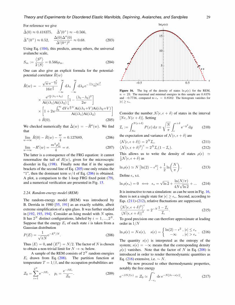
Theory and Experiments for Disordered Elastic Manifolds, Depinning, Avalanches, and Sandpiles 29
For reference we give
∆(0) ≈ 0.418375, ∆′(0+) ≈ −0.566,
∆′′(0+) ≈ 0.52,∆(0)∆′′(0)
∆′(0+)2≈ 0.68. (203)
Using Eq. (104), this predicts, among others, the universalavalanche scale,
Sm :=
⟨S2⟩
2 〈S〉 = 0.566ρm. (204)
One can also give an explicit formula for the potential-potential correlator R(w)
R(w) = −√w e−
w3
12
16π32
∞∫
−∞
dλ1
∞∫
−∞
dλ2 e−(λ1−λ2)2
4w
× eiw2 (λ1+λ2)
Ai(iλ1)Ai(iλ2)
[1− (λ1−λ2)2
2w
]
×[1 + 2w
∫∞0
dV ew2 V Ai(iλ1+V )Ai(iλ2+V )
Ai(iλ1)Ai(iλ2)
]
+ R(0). (205)
We checked numerically that ∆(w) = −R′′(w). We findthat
limw→∞
R(0)− R(w)− w
4= 0.127689, (206)
limw→∞
−R′(w) =m4ρ3
m
4= σ. (207)
The latter is a consequence of the FRG equation: it cannotrenormalize the tail of R(w), given for the microscopicdisorder in Eq. (198). Finally note that if in the squarebrackets of the second line of Eq. (205) one only retains the“1”, then the dominant term w/4 of Eq. (206) is obtained.A plot, a comparison to the 1-loop FRG fixed point (79),and a numerical verification are presented in Fig. 15.
2.24. Random-energy model (REM)
The random-energy model (REM) was introduced byB. Derrida in 1980 [55, 191] as an exactly soluble, albeitextreme simplification of a spin glass. It was further studiedin [192, 193, 194]. Consider an Ising model with N spins.It has 2N distinct configurations, labeled by i = 1, ..., 2N .Suppose that the energy Ei of each state i is taken from aGaussian distribution
P (E) =1√πN
e−E2/N . (208)
Thus 〈E〉 = 0, and⟨E2⟩
= N/2. The factor ofN is chosento obtain a non-trivial limit for N →∞ below.
A sample of the REM consists of 2N random energiesEi drawn from Eq. (208). The partition function attemperature T = 1/β, and the occupation probabilities are
Z0 =
2N∑
i=1
e−βEi , pi =e−βEi
Z0. (209)
-0.5 0.5ϵ
5
10
15
ln(ρ(ϵ))
Figure 16. The log of the density of states ln ρ(ε) for the REM,n = 23. The maximal and minimal energies in this sample are 0.8376and −0.7736, compared to ε∗ = 0.8582: The histogram vanishes for|ε| ≥ ε∗.
Consider the number N (ε, ε + δ) of states in the interval[Nε,N(ε+ δ)]. Setting
Iε :=
∫ N(ε+δ)
Nε
P (x) dx ≡√N
π
∫ ε+δ
ε
e−y2
dy (210)
the expectation and variance of N (ε, ε+ δ) are
〈N (ε, ε+ δ)〉 = 2NIε, (211)⟨N (ε, ε+ δ)2
⟩c= 2NIε(1− Iε). (212)
This allows us to write the density of states ρ(ε) '1δN (ε, ε+ δ) as
ln ρ(ε) ' N[ln(2)− ε2
]+
1
2ln
(N
π
). (213)
Define ε∗ s.t.
ln ρ(ε∗) = 0 ⇐⇒ ε∗ =√
ln 2 +ln(N/π)
4N√
ln 2+ ... (214)
It is instructive to run a simulation: as can be seen in Fig. 16,there is not a single state for |ε| ≥ ε∗. Second, according toEqs. (211)-(212), relative fluctuations are suppressed,⟨N (ε, ε+ δ)2
⟩c
〈N (ε, ε+ δ)〉2= 2−N
1− IεIε
. (215)
To good precision one can therefore approximate at leadingorder in 1/N
ln ρ(ε) = Ns(ε), s(ε) =
ln(2)− ε2 , |ε| ≤ ε∗−∞ , |ε| > ε∗
. (216)
The quantity s(ε) is interpreted as the entropy of thesystem; s(ε) = −∞ means that the corresponding densityρ(ε) vanishes. Note that the factor of N in Eq. (208) isintroduced in order to render thermodynamic quantities asEq. (216) extensive, i.e. ∼ N .
We now proceed to other thermodynamic properties,notably the free energy
e−βNf(ε) = Z0 '∫ ε∗
−ε∗dε e−N [βε−s(ε)], (217)
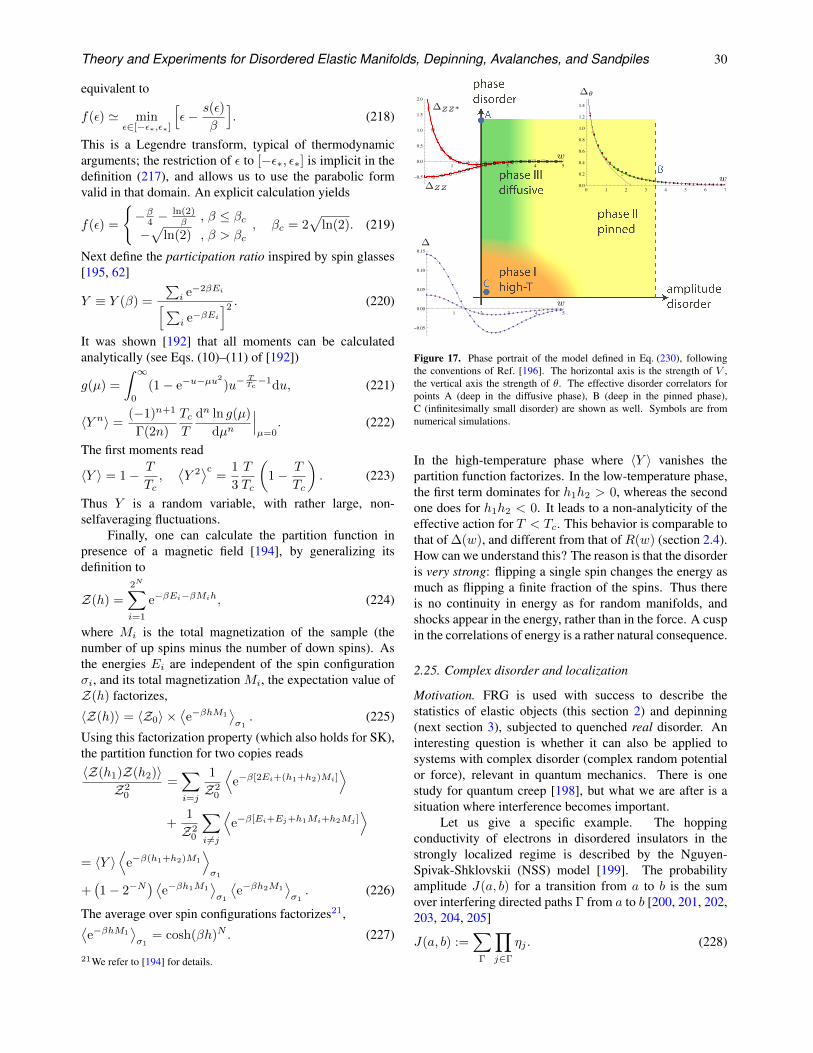
Theory and Experiments for Disordered Elastic Manifolds, Depinning, Avalanches, and Sandpiles 30
equivalent to
f(ε) ' minε∈[−ε∗,ε∗]
[ε− s(ε)
β
]. (218)
This is a Legendre transform, typical of thermodynamicarguments; the restriction of ε to [−ε∗, ε∗] is implicit in thedefinition (217), and allows us to use the parabolic formvalid in that domain. An explicit calculation yields
f(ε) =
−β4 −
ln(2)β , β ≤ βc
−√
ln(2) , β > βc, βc = 2
√ln(2). (219)
Next define the participation ratio inspired by spin glasses[195, 62]
Y ≡ Y (β) =
∑i e−2βEi
[∑i e−βEi
]2 . (220)
It was shown [192] that all moments can be calculatedanalytically (see Eqs. (10)–(11) of [192])
g(µ) =
∫ ∞
0
(1− e−u−µu2
)u−TTc−1du, (221)
〈Y n〉 =(−1)n+1
Γ(2n)
TcT
dn ln g(µ)
dµn
∣∣∣µ=0
. (222)
The first moments read
〈Y 〉 = 1− T
Tc,⟨Y 2⟩c
=1
3
T
Tc
(1− T
Tc
). (223)
Thus Y is a random variable, with rather large, non-selfaveraging fluctuations.
Finally, one can calculate the partition function inpresence of a magnetic field [194], by generalizing itsdefinition to
Z(h) =
2N∑
i=1
e−βEi−βMih, (224)
where Mi is the total magnetization of the sample (thenumber of up spins minus the number of down spins). Asthe energies Ei are independent of the spin configurationσi, and its total magnetization Mi, the expectation value ofZ(h) factorizes,
〈Z(h)〉 = 〈Z0〉 ×⟨e−βhM1
⟩σ1. (225)
Using this factorization property (which also holds for SK),the partition function for two copies reads〈Z(h1)Z(h2)〉
Z20
=∑
i=j
1
Z20
⟨e−β[2Ei+(h1+h2)Mi]
⟩
+1
Z20
∑
i 6=j
⟨e−β[Ei+Ej+h1Mi+h2Mj ]
⟩
= 〈Y 〉⟨
e−β(h1+h2)M1
⟩σ1
+(1− 2−N
) ⟨e−βh1M1
⟩σ1
⟨e−βh2M1
⟩σ1. (226)
The average over spin configurations factorizes21,⟨e−βhM1
⟩σ1
= cosh(βh)N . (227)
21We refer to [194] for details.
1 2 3 4 5w`
-0.5
0.0
0.5
1.0
1.5
2.0DHw` Lêbm2
∆ZZ∗
∆ZZ
w
0 1 2 3 4 5 6 7w`0.0
0.2
0.4
0.6
0.8
1.0
1.2
1.4
DqHw` Lêbm2∆θ
w
1 2 3 4 5w
-0.05
0.00
0.05
0.10
0.15DHwL∆
w
Figure 17. Phase portrait of the model defined in Eq. (230), followingthe conventions of Ref. [196]. The horizontal axis is the strength of V ,the vertical axis the strength of θ. The effective disorder correlators forpoints A (deep in the diffusive phase), B (deep in the pinned phase),C (infinitesimally small disorder) are shown as well. Symbols are fromnumerical simulations.
In the high-temperature phase where 〈Y 〉 vanishes thepartition function factorizes. In the low-temperature phase,the first term dominates for h1h2 > 0, whereas the secondone does for h1h2 < 0. It leads to a non-analyticity of theeffective action for T < Tc. This behavior is comparable tothat of ∆(w), and different from that of R(w) (section 2.4).How can we understand this? The reason is that the disorderis very strong: flipping a single spin changes the energy asmuch as flipping a finite fraction of the spins. Thus thereis no continuity in energy as for random manifolds, andshocks appear in the energy, rather than in the force. A cuspin the correlations of energy is a rather natural consequence.
2.25. Complex disorder and localization
Motivation. FRG is used with success to describe thestatistics of elastic objects (this section 2) and depinning(next section 3), subjected to quenched real disorder. Aninteresting question is whether it can also be applied tosystems with complex disorder (complex random potentialor force), relevant in quantum mechanics. There is onestudy for quantum creep [198], but what we are after is asituation where interference becomes important.
Let us give a specific example. The hoppingconductivity of electrons in disordered insulators in thestrongly localized regime is described by the Nguyen-Spivak-Shklovskii (NSS) model [199]. The probabilityamplitude J(a, b) for a transition from a to b is the sumover interfering directed paths Γ from a to b [200, 201, 202,203, 204, 205]
J(a, b) :=∑
Γ
∏
j∈Γ
ηj . (228)
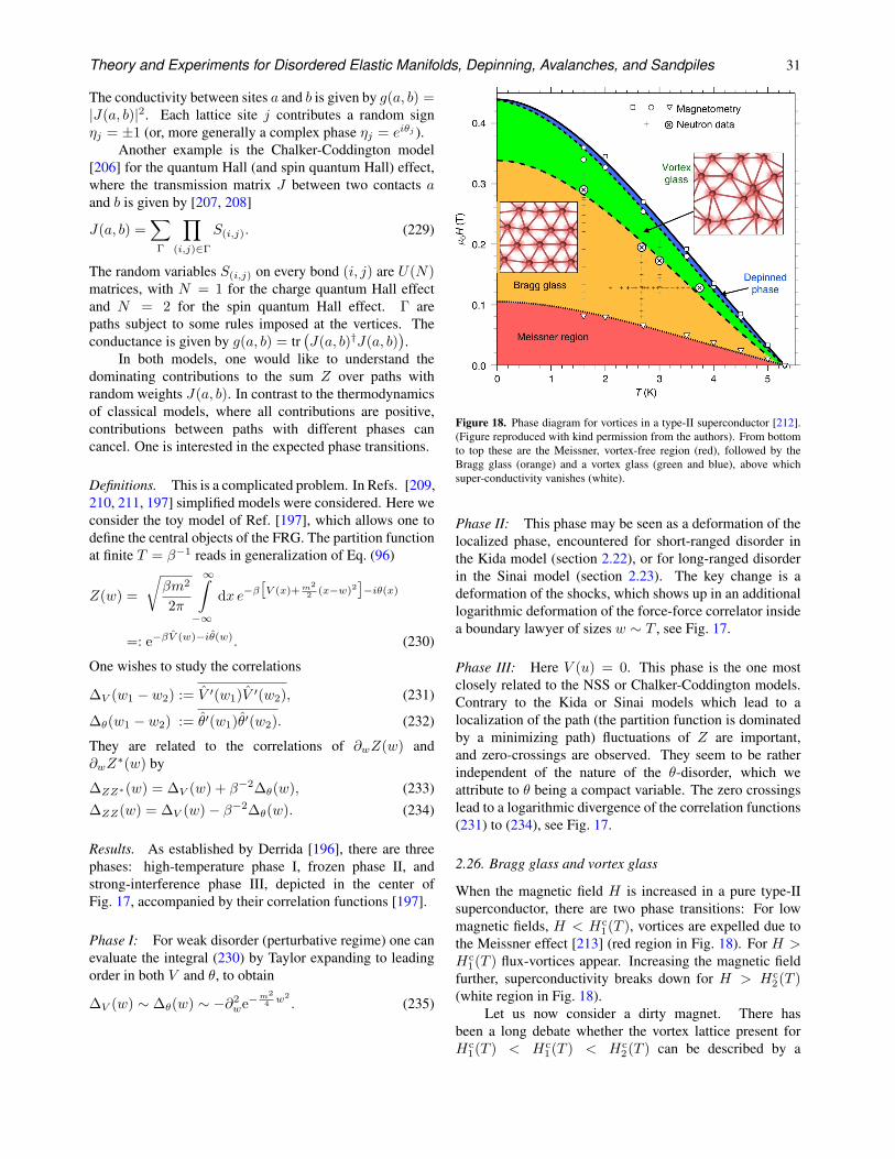
Theory and Experiments for Disordered Elastic Manifolds, Depinning, Avalanches, and Sandpiles 31
The conductivity between sites a and b is given by g(a, b) =|J(a, b)|2. Each lattice site j contributes a random signηj = ±1 (or, more generally a complex phase ηj = eiθj ).
Another example is the Chalker-Coddington model[206] for the quantum Hall (and spin quantum Hall) effect,where the transmission matrix J between two contacts aand b is given by [207, 208]
J(a, b) =∑
Γ
∏
(i,j)∈Γ
S(i,j). (229)
The random variables S(i,j) on every bond (i, j) are U(N)matrices, with N = 1 for the charge quantum Hall effectand N = 2 for the spin quantum Hall effect. Γ arepaths subject to some rules imposed at the vertices. Theconductance is given by g(a, b) = tr
(J(a, b)†J(a, b)
).
In both models, one would like to understand thedominating contributions to the sum Z over paths withrandom weights J(a, b). In contrast to the thermodynamicsof classical models, where all contributions are positive,contributions between paths with different phases cancancel. One is interested in the expected phase transitions.
Definitions. This is a complicated problem. In Refs. [209,210, 211, 197] simplified models were considered. Here weconsider the toy model of Ref. [197], which allows one todefine the central objects of the FRG. The partition functionat finite T = β−1 reads in generalization of Eq. (96)
Z(w) =
√βm2
2π
∞∫
−∞
dx e−β[V (x)+m2
2 (x−w)2]−iθ(x)
=: e−βV (w)−iθ(w). (230)
One wishes to study the correlations
∆V (w1 − w2) := V ′(w1)V ′(w2), (231)
∆θ(w1 − w2) := θ′(w1)θ′(w2). (232)
They are related to the correlations of ∂wZ(w) and∂wZ
∗(w) by
∆ZZ∗(w) = ∆V (w) + β−2∆θ(w), (233)∆ZZ(w) = ∆V (w)− β−2∆θ(w). (234)
Results. As established by Derrida [196], there are threephases: high-temperature phase I, frozen phase II, andstrong-interference phase III, depicted in the center ofFig. 17, accompanied by their correlation functions [197].
Phase I: For weak disorder (perturbative regime) one canevaluate the integral (230) by Taylor expanding to leadingorder in both V and θ, to obtain
∆V (w) ∼ ∆θ(w) ∼ −∂2we−
m2
4 w2
. (235)
Figure 18. Phase diagram for vortices in a type-II superconductor [212].(Figure reproduced with kind permission from the authors). From bottomto top these are the Meissner, vortex-free region (red), followed by theBragg glass (orange) and a vortex glass (green and blue), above whichsuper-conductivity vanishes (white).
Phase II: This phase may be seen as a deformation of thelocalized phase, encountered for short-ranged disorder inthe Kida model (section 2.22), or for long-ranged disorderin the Sinai model (section 2.23). The key change is adeformation of the shocks, which shows up in an additionallogarithmic deformation of the force-force correlator insidea boundary lawyer of sizes w ∼ T , see Fig. 17.
Phase III: Here V (u) = 0. This phase is the one mostclosely related to the NSS or Chalker-Coddington models.Contrary to the Kida or Sinai models which lead to alocalization of the path (the partition function is dominatedby a minimizing path) fluctuations of Z are important,and zero-crossings are observed. They seem to be ratherindependent of the nature of the θ-disorder, which weattribute to θ being a compact variable. The zero crossingslead to a logarithmic divergence of the correlation functions(231) to (234), see Fig. 17.
2.26. Bragg glass and vortex glass
When the magnetic field H is increased in a pure type-IIsuperconductor, there are two phase transitions: For lowmagnetic fields, H < Hc
1(T ), vortices are expelled due tothe Meissner effect [213] (red region in Fig. 18). For H >Hc
1(T ) flux-vortices appear. Increasing the magnetic fieldfurther, superconductivity breaks down for H > Hc
2(T )(white region in Fig. 18).
Let us now consider a dirty magnet. There hasbeen a long debate whether the vortex lattice present forHc
1(T ) < Hc1(T ) < Hc
2(T ) can be described by a
Theory and Experiments for Disordered Elastic Manifolds, Depinning, Avalanches, and Sandpiles 32
Bragg glass, or a vortex glass. In a Bragg glass favoredby [214, 215, 21, 216], the Abrikosov lattice of vortices(see sketch in Fig. 3) is elastically deformed, but thereare no topological defects and each vortex line retains sixnearest neighbors. According to the theory of disorderedelastic manifolds, the correlation function given in Eq.(120a) grows logarithmically with distance, preservingenough coherence to show up in a Bragg peak in neutronscattering experiments (hence the name). The alternativetheory, termed vortex glass and favored (for sometimesquite different reasons) in [217, 218, 219, 220, 221, 222,223, 224], assumes that topological defects destroy theorder, and as a consequence the Bragg peak in neutronscattering experiments.
The current experimental situation [212] shown inFig. 18 favors, in agreement with intuition, a Bragg glassfor smaller fields, and a vortex glass for larger ones, witha transition at Hc
B/V(T ), with Hc1(T ) < Hc
B/V(T ) <
Hc2(T ).
If the disorder contains columnar defects, it mayexhibit [25, 225] a transverse Meissner effect, for whichthe tilt ϑ to an applied field H vanishes up to Hc
tilt, afterwhich it grows as ϑ ∼ |H − Hc
tilt|φ, with φ < 1. One-dimensional quantum systems (Luttinger liquid) map totwo-dimensional classical systems with columnar disorder,thus can be understood in the same framework [225], oralternatively [226, 227, 228, 229, 230] within the NPFRGapproach (section 9.1). One further encounters a roundingof the cusp through quantum fluctuations, similar to thequantum creep regime of Ref. [198].
There are also situations where one of the two phasesis absent, as defects can destabilize the Bragg-glass phase[231]. Similar physics may be observed in charge-densitywaves [232]. For details we refer the reader to [19, 233].Discussion of a moving vortex lattice is referred to section3.25.
2.27. Bosons and fermions in d = 2, bosonization
To proceed, we need to establish connections betweentheories in two dimensions, including relations betweenfermions and bosons, known as bosonization. Dimensiond = 2 is special as the Gaussian free field is dimensionless,allowing for a number of constructions of which we showsome below. Our account is very condensed, and we referto [3, 234, 235, 236] for background reading.
Bosons.
Hboson =1
8π
∫d2~z [∇Φ(~z)]
2. (236)
Appendix 10.6 implies
〈Φ(~z)Φ(0)〉 = − ln |~z|2 = − ln z − ln z . (237)
This suggests that one can decompose Φ(~z) into aholomorphic and antiholomorphic part, Φ(~z) ≡ Φ(z, z) =
φ(z) + φ(z), with
〈φ(z)φ(w)〉 = − ln(z − w),⟨φ(z)φ(w)
⟩= − ln(z − w), (238)
⟨φ(z)φ(w)
⟩= 0.
Since φ(z) has logarithmic correlations, an infinity ofpower-law correlated vertex operators can be constructed(the dots indicate normal ordering, i.e. exclusion of self-contractions at the vertex),
Vα(z) = :eαφ(z) : (239)〈Vα(z)Vβ(w)〉 = e−αβ ln(z−w) = (z − w)−αβ . (240)
Majorana fermion. Consider a Majorana (real) fermion,constructed from anti-commuting Grassman fields (section8.2)
HMajorana =1
2π
∫d2~z
[ψ(z)∂ψ(z) + ψ(z)∂ψ(z)
]. (241)
Its correlation-functions are obtained from Eq. (992) as
〈ψ(z)ψ(w)〉 =1
z − w, (242)
⟨ψ(z)ψ(w)
⟩=
1
z − w . (243)
As for the bosons above, the theory can be split into aholomorphic and an antiholomorphic part.
Dirac fermion. A Dirac (complex) fermion is made out oftwo Majorana-fermions ψ1 = ψ∗1 and ψ2 = ψ∗2 ,
ψ = ψ1 + iψ2, ψ∗ = ψ1 − iψ2. (244)
Corresponding rules hold for the antiholomorphic fields.Choosing
HDirac =1
π
∫
z
ψ∗(z)∂ψ(z) + ψ∗(z)∂ψ(z), (245)
the correlation functions for the components ψ1 and ψ2
have an additional factor of 1/2 as compared to Eqs. (241)-(242), resulting in
〈ψ∗(z)ψ(w)〉 = 〈ψ(z)ψ∗(w)〉 =1
z − w, (246)
〈ψ(z)ψ(w)〉 = 〈ψ∗(z)ψ∗(w)〉 = 0. (247)
Similar relations hold for the anti-holomorphic parts ψ, andcorrelations vanish between ψ and ψ.
Bosonization. Since a Dirac-fermion and a free bosonhave both central charge22 c = 1, we may expect a closerrelation between objects in these theories. Indeed setting
ψ(z)= :eiφ(z) : ψ∗(z)= :e−iφ(z) : (248)
ψ(z)= :eiφ(z) : ψ∗(z)= :e−iφ(z) : (249)22The conformal charge c is the amplitude of the leading term in theOPE of the stress-energy tensor with itself. It can be measured from thefinite-size corrections of the free energy of a system [237, 234, 238, 3].The central charge is often used to identify or distinguish systems. Thishas to be taken with some precaution, as the total central charge of non-interacting systems is the sum of the central charges of its components.
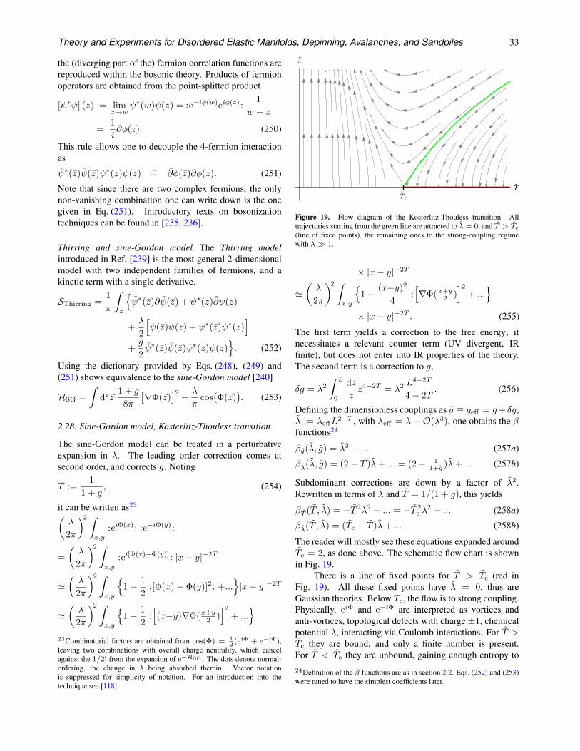
Theory and Experiments for Disordered Elastic Manifolds, Depinning, Avalanches, and Sandpiles 33
the (diverging part of the) fermion correlation functions arereproduced within the bosonic theory. Products of fermionoperators are obtained from the point-splitted product
[ψ∗ψ] (z) := limz→w
ψ∗(w)ψ(z) = :e−iφ(w)eiφ(z) :1
w − z=
1
i∂φ(z). (250)
This rule allows one to decouple the 4-fermion interactionas
ψ∗(z)ψ(z)ψ∗(z)ψ(z) = ∂φ(z)∂φ(z). (251)
Note that since there are two complex fermions, the onlynon-vanishing combination one can write down is the onegiven in Eq. (251). Introductory texts on bosonizationtechniques can be found in [235, 236].
Thirring and sine-Gordon model. The Thirring modelintroduced in Ref. [239] is the most general 2-dimensionalmodel with two independent families of fermions, and akinetic term with a single derivative.
SThirring =1
π
∫
z
ψ∗(z)∂ψ(z) + ψ∗(z)∂ψ(z)
+λ
2
[ψ(z)ψ(z) + ψ∗(z)ψ∗(z)
]
+g
2ψ∗(z)ψ(z)ψ∗(z)ψ(z)
. (252)
Using the dictionary provided by Eqs. (248), (249) and(251) shows equivalence to the sine-Gordon model [240]
HSG =
∫d2~z
1 + g
8π
[∇Φ(~z)
]2+λ
πcos(Φ(~z)
). (253)
2.28. Sine-Gordon model, Kosterlitz-Thouless transition
The sine-Gordon model can be treated in a perturbativeexpansion in λ. The leading order correction comes atsecond order, and corrects g. Noting
T :=1
1 + g, (254)
it can be written as23
(λ
2π
)2 ∫
x,y
:eiΦ(x) : :e−iΦ(y) :
=
(λ
2π
)2 ∫
x,y
:ei[Φ(x)−Φ(y)] : |x− y|−2T
'(λ
2π
)2 ∫
x,y
1− 1
2:[Φ(x)− Φ(y)]2 : +...
|x− y|−2T
'(λ
2π
)2 ∫
x,y
1− 1
2:[(x−y)∇Φ(x+y
2 )]2
+ ...
23Combinatorial factors are obtained from cos(Φ) = 12
(eiΦ + e−iΦ),leaving two combinations with overall charge neutrality, which cancelagainst the 1/2! from the expansion of e−HSG . The dots denote normal-ordering, the change in λ being absorbed therein. Vector notationis suppressed for simplicity of notation. For an introduction into thetechnique see [118].
λ
Figure 19. Flow diagram of the Kosterlitz-Thouless transition: Alltrajectories starting from the green line are attracted to λ = 0, and T > Tc
(line of fixed points), the remaining ones to the strong-coupling regimewith λ 1.
× |x− y|−2T
'(λ
2π
)2 ∫
x,y
1− (x−y)2
4:[∇Φ(x+y
2 )]2
+ ...
× |x− y|−2T . (255)
The first term yields a correction to the free energy; itnecessitates a relevant counter term (UV divergent, IRfinite), but does not enter into IR properties of the theory.The second term is a correction to g,
δg = λ2
∫ L
0
dz
zz4−2T = λ2 L
4−2T
4− 2T. (256)
Defining the dimensionless couplings as g ≡ geff = g+ δg,λ := λeffL
2−T , with λeff = λ + O(λ3), one obtains the βfunctions24
βg(λ, g) = λ2 + ... (257a)
βλ(λ, g) = (2− T )λ+ ... = (2− 11+g )λ+ ... (257b)
Subdominant corrections are down by a factor of λ2.Rewritten in terms of λ and T = 1/(1 + g), this yields
βT (T , λ) = −T 2λ2 + ... = −T 2c λ
2 + ... (258a)
βλ(T , λ) = (Tc − T )λ+ ... (258b)
The reader will mostly see these equations expanded aroundTc = 2, as done above. The schematic flow chart is shownin Fig. 19.
There is a line of fixed points for T > Tc (red inFig. 19). All these fixed points have λ = 0, thus areGaussian theories. Below Tc, the flow is to strong coupling.Physically, eiΦ and e−iΦ are interpreted as vortices andanti-vortices, topological defects with charge ±1, chemicalpotential λ, interacting via Coulomb interactions. For T >Tc they are bound, and only a finite number is present.For T < Tc they are unbound, gaining enough entropy to24Definition of the β functions are as in section 2.2. Eqs. (252) and (253)were tuned to have the simplest coefficients later.
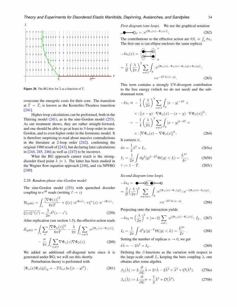
Theory and Experiments for Disordered Elastic Manifolds, Depinning, Avalanches, and Sandpiles 34
λ
Figure 20. The RG flow for λ as a function of T .
overcome the energetic costs for their core. The transitionat T = Tc is known as the Kosterlitz-Thouless transition[241].
Higher-loop calculations can be performed, both in theThirring model (241), as in the sine-Gordon model (253).As our treatment shows, they are rather straight-forward,and one should be able to go at least to 3-loop order in sine-Gordon, and to even higher order in the fermionic model. Itis therefore surprising to read about massive contradictionsin the literature at 2-loop order [242], confirming theoriginal 1980 result of [243], but declaring later calculationsin [244, 245, 246] as well as [247] to be incorrect.
What the RG approach cannot reach is the strong-disorder fixed point λ 1. The latter has been studied inthe Wegner flow-equation approach [248], and via NPFRG[249].
2.29. Random-phase sine-Gordon model
The sine-Gordon model (253) with quenched disordercoupling to eiΦ reads (writing ~z → z)
HrpSG =
∫
z
[∇Φ(z)
]2
8πT+ ξ(z) :eiΦ(z) : +ξ∗(z) :e−iΦ(z) :
ξ(z)ξ∗(z′) =λ
2πδ2(z − z′). (259)
After replication (see section 1.5), the effective action reads
SrpSG =
∫
z
∑
α
[∇Φα(z)]2
8πT− λ
2π
∫
z
∑
α6=β:ei[Φα(z)−Φβ(z)]:
− σ
4π
∫
z
∑
α 6=β∇Φα(z)∇Φβ(z). (260)
We added an additional off-diagonal term since it isgenerated under RG; we will see this shortly.
Perturbation theory is performed with
〈Φα(x)Φβ(y)〉0 = −Tδαβ ln(|x− y|2
). (261)
First diagram (one loop). We use the graphical notation
α β = :ei[Φα(x)−Φβ(x)] : (262)
The contributions to the effective action are δSi ≡∫xδsi.
The first one is (an ellipse encloses the same replica)
−δs1(x) =
x
y
=1
2!
(λ
2π
)2 ∑
α6=β
∫
y
: ei[Φα(x)−Φβ(x)−Φα(y)+Φβ(y)] :
×e−4T ln |x−y|. (263)
This term contains a strongly UV-divergent contributionto the free energy (which we do not need) and the sub-dominant term
−δs1 ≈ −1
4
(λ
2π
)2 ∑
α6=β
∫
y
|x− y|−4T ×
× : [(x− y) · ∇Φα(x)− (x− y) · ∇Φβ(x)]2
:
= − 1
4
(λ
2π
)2 ∑
α6=β
∫
y
|x− y|2−4T ×
× : [∇Φα(x)−∇Φβ(x)]2
: (264)
It corrects σ,
δσ =1
2λ2 × I1, (265a)
I1 =1
2π
∫dy2|y|2−2TΘ(|y| < L) =
L4τ
4τ, (265b)
τ := 1− T. (265c)
Second diagram (one loop).
−δs2 =
=2
2!
( λ2π
)2 ∑
α6=β 6=γ
∫
y
:ei[Φα(x)−Φγ(y)] :: e−i[Φβ(x)−θβ(y)] :
×e−2T ln |x−y|. (266)
Projecting onto the interaction yields
−δs2 ≈( λ
2π
)2× (n−2)
∑
α6=γ:ei[Φα(x)−Φγ(x)] : I2 , (267)
I2 =1
2π
∫d2y |y|−TΘ(|y| < L) =
L2τ
2τ. (268)
Setting the number of replicas n→ 0, we get
δλ = − 2λ2 × I2 . (269)
Defining the β-functions as the variation with respect tothe large-scale cutoff L, keeping the bare coupling λ, oneobtains after some algebra
βλ(λ) := L∂
∂Lλ = 2τ λ− 2λ2 + λ3 +O(λ4), (270a)
βσ(λ) := L∂
∂Lσ =
1
2λ2 +O(λ4). (270b)
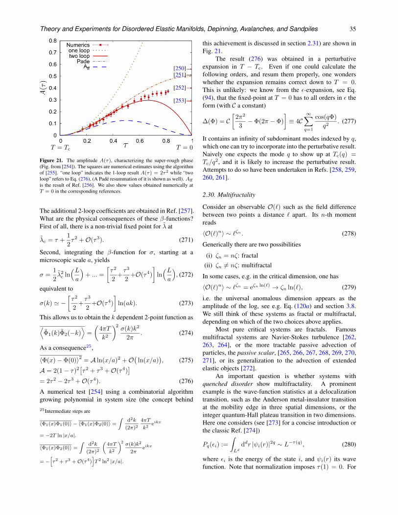
Theory and Experiments for Disordered Elastic Manifolds, Depinning, Avalanches, and Sandpiles 35
[250][251]
[252]
[253]
T = 0T = Tc
Figure 21. The amplitude A(τ), characterizing the super-rough phase(Fig. from [254]). The squares are numerical estimates using the algorithmof [255]. “one loop” indicates the 1-loop result A(τ) = 2τ2 while “twoloop” refers to Eq. (276), (A Pade resummation of it is shown as well). Aff
is the result of Ref. [256]. We also show values obtained numerically atT = 0 in the corresponding references.
The additional 2-loop coefficients are obtained in Ref. [257].What are the physical consequences of these β-functions?First of all, there is a non-trivial fixed point for λ at
λc = τ +1
2τ2 +O(τ3). (271)
Second, integrating the β-function for σ, starting at amicroscopic scale a, yields
σ =1
2λ2
c ln(La
)+ ... =
[τ2
2+τ3
2+O(τ4)
]ln(La
), (272)
equivalent to
σ(k) ' −[τ2
2+τ3
2+O(τ4)
]ln(ak). (273)
This allows us to obtain the k dependent 2-point function as⟨
Φ1(k)Φ2(−k)⟩
=
(4πT
k2
)2σ(k)k2
2π. (274)
As a consequence25,
〈Φ(x)− Φ(0)〉2 = A ln(x/a)2 +O(
ln(x/a)), (275)
A = 2(1− τ)2[τ2 + τ3 +O(τ4)
]
= 2τ2 − 2τ3 +O(τ4). (276)
A numerical test [254] using a combinatorial algorithmgrowing polynomial in system size (the concept behind25Intermediate steps are
〈Φ1(x)Φ1(0)〉 − 〈Φ1(x)Φ2(0)〉 =
∫d2k
(2π)2
4πT
k2eikx
= −2T ln |x/a|.
〈Φ1(x)Φ2(0)〉 =
∫d2k
(2π)2
(4πT
k2
)2 σ(k)k2
2πeikx
= −[τ2 + τ3 +O(τ4)
]T 2 ln2 |x/a|.
this achievement is discussed in section 2.31) are shown inFig. 21.
The result (276) was obtained in a perturbativeexpansion in T − Tc. Even if one could calculate thefollowing orders, and resum them properly, one wonderswhether the expansion remains correct down to T = 0.This is unlikely: we know from the ε-expansion, see Eq.(94), that the fixed-point at T = 0 has to all orders in ε theform (with C a constant)
∆(Φ) = C[
2π2
3− Φ(2π − Φ)
]≡ 4C
∞∑
q=1
cos(qΦ)
q2. (277)
It contains an infinity of subdominant modes indexed by q,which one can try to incorporate into the perturbative result.Naively one expects the mode q to show up at Tc(q) =Tc/q
2, and it is likely to increase the perturbative result.Attempts to do so have been undertaken in Refs. [258, 259,260, 261].
2.30. Multifractality
Consider an observable O(`) such as the field differencebetween two points a distance ` apart. Its n-th momentreads
〈O(`)n〉 ∼ `ζn . (278)
Generically there are two possibilities
(i) ζn = nζ: fractal(ii) ζn 6= nζ: multifractal
In some cases, e.g. in the critical dimension, one has
〈O(`)n〉 ∼ `ζn = eζn ln(`) → ζn ln(`), (279)
i.e. the universal anomalous dimension appears as theamplitude of the log, see e.g. Eq. (120a) and section 3.8.We still think of these systems as fractal or multifractal,depending on which of the two choices above applies.
Most pure critical systems are fractals. Famousmultifractal systems are Navier-Stokes turbulence [262,263, 264], or the more tractable passive advection ofparticles, the passive scalar, [265, 266, 267, 268, 269, 270,271], or its generalization to the advection of extendedelastic objects [272].
An important question is whether systems withquenched disorder show multifractality. A prominentexample is the wave-function statistics at a delocalizationtransition, such as the Anderson metal-insulator transitionat the mobility edge in three spatial dimensions, or theinteger quantum-Hall plateau transition in two dimensions.Here one considers (see [273] for a concise introduction orthe classic Ref. [274])
Pq(εi) :=
∫
Ldddr |ψi(r)|2q ∼ L−τ(q), (280)
where εi is the energy of the state i, and ψi(r) its wavefunction. Note that normalization imposes τ(1) = 0. For
Theory and Experiments for Disordered Elastic Manifolds, Depinning, Avalanches, and Sandpiles 36
extended states inside a band τ(q) = d(q − 1), while forlocalized states τ(q) = 0. At the band edge τ(q) is non-trivial. Define by f(α) its Legendre transform,
Legendreα↔q f(α) + τ(q) = αq. (281)
Then the set of points at which an eigenfunction takes thevalue |ψ(r)|2 = AL−α has weight Lf(α). Both f(α) andτ(q) are convex.
The question relevant for this review is whetherdisordered elastic manifolds show multifractality. As longas the roughness exponent ζ > 0, this does not seem to bethe case. The situation is different for ζ = 0, i.e. charge-density waves or vortex lattices. Technically, it can beaccessed either via a 4 − ε expansion [275] or directly intwo dimensions [276].
Multifractality of the random-phase sine-Gordon model indimension d = 2. The random-phase sine-Gordon modelwas introduced above in section 2.29. The object to beconsidered is
C(q, r) := 〈eiq[Φ(r)−Φ(0)]〉. (282)
It was shown in Ref. [276] that with A given in Eq. (276),
C(q, r) '(ar
)η(q)
exp
(−1
2Aq2 ln2(r/a)
). (283)
The anomalous exponent η defined in Eq. (283) reads
η(q) = 2q2(1− τ)[1 + 2(1− τ)σ′] + τ2ηg(q) +O(τ3).
(284)
Its nontrivial part ηg is [276]
ηg(q) =
q2[1− 2γE − ψ(q)− ψ(−q)], q < 1
−2, q = 1(285)
Here γE is Euler’s constant. The result for the correlationfunction (282) enables one to calculate the leading large-distance behavior of all higher powers of the connectedcorrelation functions in the super-rough phase, i.e., forT < Tc (τ > 0, see Fig. 20). Using
ηg(q) = q2 + 2
∞∑
n=2
ζ(2n− 1)q2n, (286)
one sees that odd moments vanish, the second moment isgiven by Eqs. (275)-(276), and higher even moments by
(−1)n
(2n)!
⟨[Φ(r)−Φ(0)]
2n⟩
c= −2τ2ζ(2n−1) ln
( ra
)+ ...
(287)
This system is multifractal.
FRG in dimension 4− ε. Following [275], define
G[λ] :=⟨
e∫xλ(x)u(x)
)⟩= limn→0
⟨e∫xλ(x)u1(x)
⟩S, (288)
λ(x) = iq[δ(x)− δ(x+ r)]. (289)
This can be calculated with methods similar to [277], usingfrom the action (30) only the cubic vertex,
1
2T 2
∫
x
∑
a,b
R(ua(x)−ub(x)
)
→ σ
12T 2
∑
a,b
|ua(x)−ub(x)|3, σ = R′′′(0+). (290)
The connected part of G[λ] reads (the correlation functionC(x) is defined in Eq. (33a))
ln(G[λ]) =1
2
1
3+ ...
= ln
(det(−∇2 + σU(x) +m2)
det(−∇2 +m2)
)(291)
U(x) =
∫
y
C(x− y)λ(y). (292)
Calculating the determinant (291) is a formidable task,usually only possible in perturbation theory in σ. Here wegive analytical results, using three consecutive tricks:
(i) Solve the problem for a spherically symmetric sourceλ(y), assuming a uniformly distributed positive unitcharge on a circle of radius a, and a compensatingnegative charge on a circle of radius L a. Thepotential is U(x) = (r−2 − L−2)/(2π)2 for a ≤ r ≤L, and constant beyond.
(ii) Write the Laplacian in distance and angle variables,
−∇2 → Hl := − d2
dr2+
(l + d−3
2
) (l + d−1
2
)
r2. (293)
(iii) ln(G[λ]) is written as a sum of the logarithms of the1-dimensional determinant ratios Bl for partial waves,weighted with the degeneracy of angular momenta l,
ln(G[λ]) =
∞∑
l=0
(2l+d−2)(l+d−3)!
l!(d−2)!ln(Bl). (294)
(iv) The Gel’fand-Yaglom method [278] explained inappendix 10.8 gives the ratio of the 1-dimensionalfunctional determinants for each partial wave l as
Bl :=det[Hl + σU(r) +m2
]
det [Hl +m2]=ψl(L)
ψl(L). (295)
Here ψl(r) is the solution of[Hl + σU(r) +m2
]ψl(r) = 0, (296)
satisfying ψl(r) ∼ rl+(d−1)/2 for r → 0; ψl(r) is thesolution for σ = 0.
(v) After some pages of algebra, one finds (modulo oddterms which cancel below)
ln(G[λ]) = F( σq
(2π)2
)+ terms odd in σ (297)
F(s) = −∞∑
l=0
(l + 1)2(√
(l + 1)2 + s− (l + 1)
− s
2(l + 1)+
s2
8(l + 1)3
). (298)
Theory and Experiments for Disordered Elastic Manifolds, Depinning, Avalanches, and Sandpiles 37
Resummation yields (dropping odd terms)
F(s) =
∞∑
n=2
s2nΓ(2n− 12 )ζ(4n− 3)
2√π(2n)!
. (299)
(vi) In a last step one proves perturbatively that all n-pointfunctions remain unchanged if one moves the chargeon the sphere at |r| = L to a single point at distance Lfrom the origin. The combinatorial analyses yields anadditional factor of 2.
Using the FRG fixed point (95), s = ε3q, the 2n-th cumulant
of relative displacements is obtained as
〈[u(r)− u(0)]2n〉c ' A2n ln(r/a) (300)
A2n = −( ε
3
)2nΓ(2n− 12 )ζ(4n− 3)√π
, n ≥ 2. (301)
This correlation function is multifractal.
2.31. Simulations in equilibrium: polynomial versusNP-hard
Finding the ground state of a disordered system is in generala very difficult problem, often even NP-hard, meaning noalgorithm exists which is guaranteed to find the groundstate in polynomial time, i.e. within a time which does notgrow faster than Np, with N the system size, and p a finitenumber. This statement should be viewed as “state of theart”: E.g. we know of no algorithm to find the ground stateof the SK model in polynomial time; but this does not implythat no such algorithm can exist. What computer scientistshave proven is that if one day an algorithm is found tosolve one NP-hard problem, all other NP-hard problemscan be solved as well. We refer the reader to the textbooks[279, 280] and collection [281] for a more precise definitionand further information on the subject.
While many ground-state calculations are consideredNP-hard, there are some notable exceptions: For the RNA-folding problem [282] a polynomial algorithm exists [283],which evaluates the partition function at all temperatures ina time growing as N3, allowing one not only to find theground state but even the phase transition from a frozen toa molten phase [284, 285, 286].
Another notable exception are disordered elasticmanifolds, or more specifically the ground state of an Isingferromagnet coupled to either random-bond or random-fielddisorder. It can be solved by the minimum-cut algorithm[287]. This has been used in numerous publications: Tofind the roughness exponent ζ in dimensions 2 and 3 [137],see Fig. 10; to measure the FRG-fixed point function [128],see Fig. 8. or avalanche-size distributions in equilibrium[288], see Fig. 51. Further for flux lines in a disorderedenvironment [289, 290]; or solid-on-solid models withdisordered substrates [250].
2.32. Experiments in equilibrium
There are few experiments which really are in equilibrium.The main reason is that in most cases the exponent θ definedin Eq. (45) is positive, restricting the energy fluctuationswhich according to Eq. (47) grow as Lθ. As a consequence,there is a maximal length Lmax
T up to which the system canequilibrate, i.e. find the minimum-energy configuration. Letus give a list of notable exceptions.
(i) domain walls in thin magnetic films with random-bonddisorder have long been interpreted [84, 291, 292] asshowing the roughness exponent of ζd=1
RB = 2/3 givenin Eq. (122). This interpretation probably holds onlyon small scales, see the discussion in section 3.21.
(ii) hairpin unzipping reported in [293] is consistent witha roughness exponent ζ = 4/3, in agreement withthe value predicted for a single degree of freedom, i.e.d = 0 or ε = 4 in Eq. (83). We discuss this experimentin detail in section 3.17. There it is confronted withan experiment using the much softer peeling mode,placing it in the different depinning universality classwith ζ = 2−.
(iii) Vortex lattices (section 2.26).
3. Dynamics, and the depinning transition
3.1. Phenomenology
Another important class of phenomena for elastic manifoldsin disorder is the so-called depinning transition: Applyinga constant force to the elastic manifold, e.g. a constantmagnetic field to the ferromagnet mentioned in theintroduction, the latter will move if, and only if, a certaincritical threshold force fc is surpassed, see figure 22. (Thisis fortunate, since otherwise the magnetic domain walls inthe hard-disc drive onto which this article is stored wouldmove, with the effect of deleting all information, deprivingyou from your reading.) At f = fc, the so-called depinningtransition, the manifold has a distinct roughness exponent ζ(see Eq. (7)) from the equilibrium (f = 0). The equationdescribing the movement of the interface is
∂tu(x, t) = (∇2−m2)u(x, t) + F(x, u(x, t)
)+ f(x, t),
(302)F (x, u) = −∂uV (x, u). (303)
There are two main driving protocols, depending onwhether one controls the applied force, or the mean drivingvelocity.
Force-controlled depinning. Let us impose a driving forcef(x, t) = f , and set m→ 0. For f > fc, the manifold thenmoves with velocity v. Close to the transition, new criticalexponents appear:
• a velocity-force relation given by (see figure 22)
v ∼ |f − fc|β for f > fc, (304)
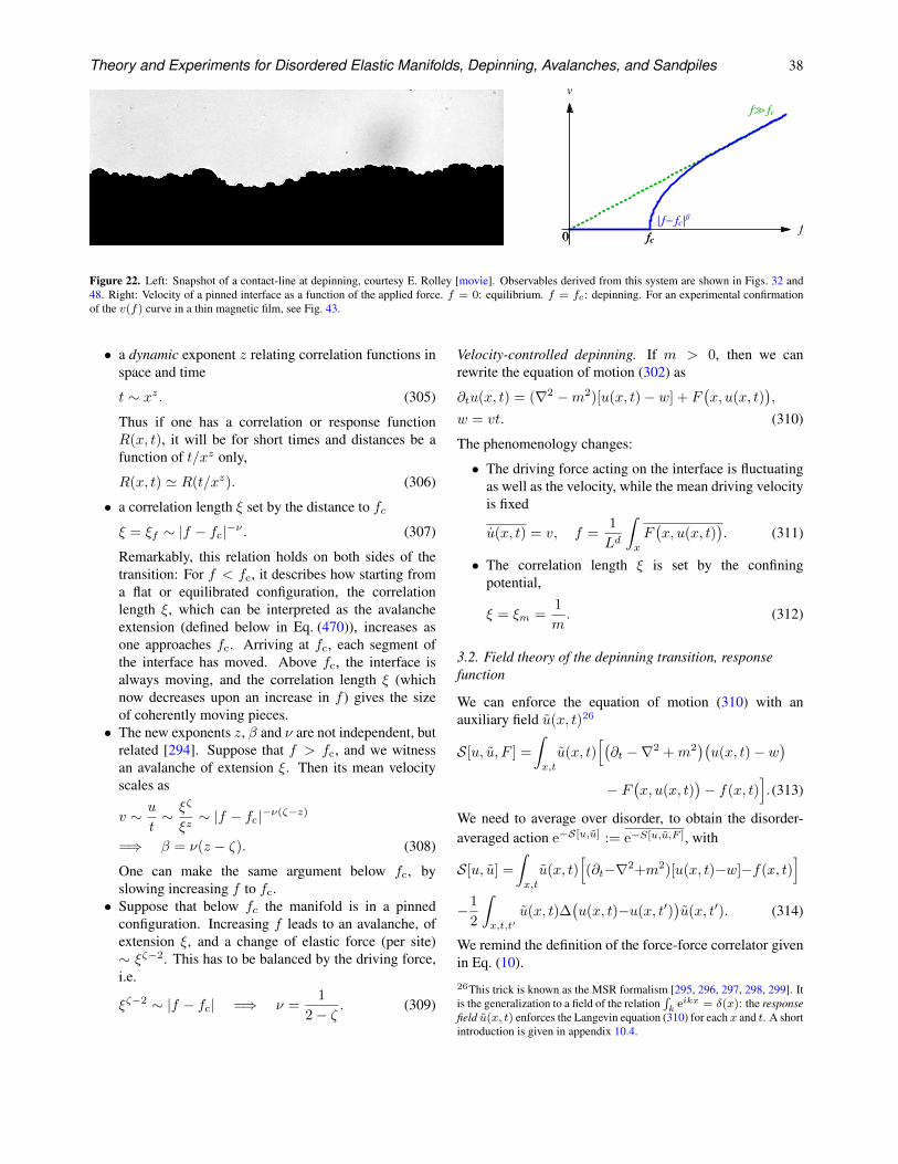
Theory and Experiments for Disordered Elastic Manifolds, Depinning, Avalanches, and Sandpiles 38
| - β
≫
Figure 22. Left: Snapshot of a contact-line at depinning, courtesy E. Rolley [movie]. Observables derived from this system are shown in Figs. 32 and48. Right: Velocity of a pinned interface as a function of the applied force. f = 0: equilibrium. f = fc: depinning. For an experimental confirmationof the v(f) curve in a thin magnetic film, see Fig. 43.
• a dynamic exponent z relating correlation functions inspace and time
t ∼ xz. (305)
Thus if one has a correlation or response functionR(x, t), it will be for short times and distances be afunction of t/xz only,
R(x, t) ' R(t/xz). (306)
• a correlation length ξ set by the distance to fc
ξ = ξf ∼ |f − fc|−ν . (307)
Remarkably, this relation holds on both sides of thetransition: For f < fc, it describes how starting froma flat or equilibrated configuration, the correlationlength ξ, which can be interpreted as the avalancheextension (defined below in Eq. (470)), increases asone approaches fc. Arriving at fc, each segment ofthe interface has moved. Above fc, the interface isalways moving, and the correlation length ξ (whichnow decreases upon an increase in f ) gives the sizeof coherently moving pieces.
• The new exponents z, β and ν are not independent, butrelated [294]. Suppose that f > fc, and we witnessan avalanche of extension ξ. Then its mean velocityscales as
v ∼ u
t∼ ξζ
ξz∼ |f − fc|−ν(ζ−z)
=⇒ β = ν(z − ζ). (308)
One can make the same argument below fc, byslowing increasing f to fc.
• Suppose that below fc the manifold is in a pinnedconfiguration. Increasing f leads to an avalanche, ofextension ξ, and a change of elastic force (per site)∼ ξζ−2. This has to be balanced by the driving force,i.e.
ξζ−2 ∼ |f − fc| =⇒ ν =1
2− ζ . (309)
Velocity-controlled depinning. If m > 0, then we canrewrite the equation of motion (302) as
∂tu(x, t) = (∇2 −m2)[u(x, t)− w] + F(x, u(x, t)
),
w = vt. (310)
The phenomenology changes:
• The driving force acting on the interface is fluctuatingas well as the velocity, while the mean driving velocityis fixed
u(x, t) = v, f =1
Ld
∫
x
F(x, u(x, t)
). (311)
• The correlation length ξ is set by the confiningpotential,
ξ = ξm =1
m. (312)
3.2. Field theory of the depinning transition, responsefunction
We can enforce the equation of motion (310) with anauxiliary field u(x, t)26
S[u, u, F ] =
∫
x,t
u(x, t)[(∂t −∇2 +m2
)(u(x, t)− w
)
− F(x, u(x, t)
)− f(x, t)
].(313)
We need to average over disorder, to obtain the disorder-averaged action e−S[u,u] := e−S[u,u,F ], with
S[u, u] =
∫
x,t
u(x, t)[(∂t−∇2+m2)[u(x, t)−w]−f(x, t)
]
−1
2
∫
x,t,t′u(x, t)∆
(u(x, t)−u(x, t′)
)u(x, t′). (314)
We remind the definition of the force-force correlator givenin Eq. (10).26This trick is known as the MSR formalism [295, 296, 297, 298, 299]. Itis the generalization to a field of the relation
∫k eikx = δ(x): the response
field u(x, t) enforces the Langevin equation (310) for each x and t. A shortintroduction is given in appendix 10.4.
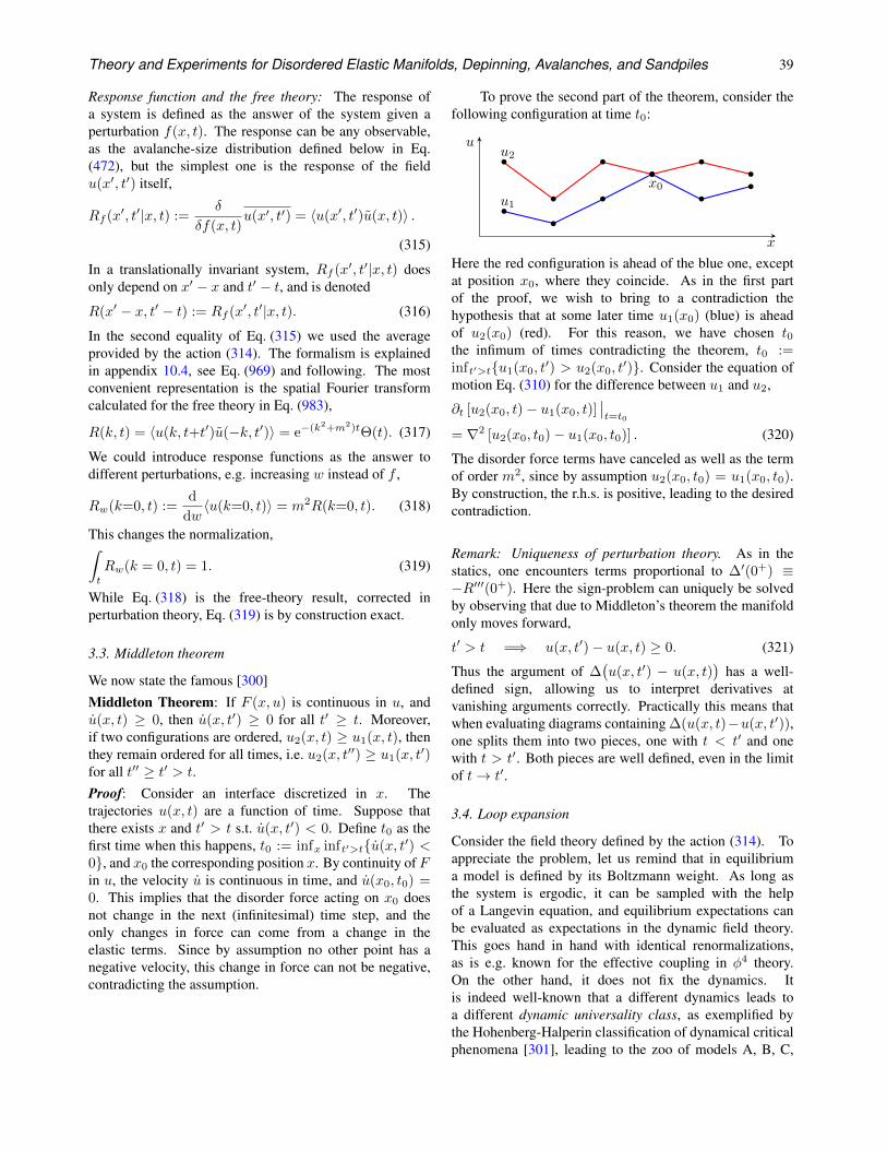
Theory and Experiments for Disordered Elastic Manifolds, Depinning, Avalanches, and Sandpiles 39
Response function and the free theory: The response ofa system is defined as the answer of the system given aperturbation f(x, t). The response can be any observable,as the avalanche-size distribution defined below in Eq.(472), but the simplest one is the response of the fieldu(x′, t′) itself,
Rf (x′, t′|x, t) :=δ
δf(x, t)u(x′, t′) = 〈u(x′, t′)u(x, t)〉 .
(315)
In a translationally invariant system, Rf (x′, t′|x, t) doesonly depend on x′ − x and t′ − t, and is denoted
R(x′ − x, t′ − t) := Rf (x′, t′|x, t). (316)
In the second equality of Eq. (315) we used the averageprovided by the action (314). The formalism is explainedin appendix 10.4, see Eq. (969) and following. The mostconvenient representation is the spatial Fourier transformcalculated for the free theory in Eq. (983),
R(k, t) = 〈u(k, t+t′)u(−k, t′)〉 = e−(k2+m2)tΘ(t). (317)
We could introduce response functions as the answer todifferent perturbations, e.g. increasing w instead of f ,
Rw(k=0, t) :=d
dw〈u(k=0, t)〉 = m2R(k=0, t). (318)
This changes the normalization,∫
t
Rw(k = 0, t) = 1. (319)
While Eq. (318) is the free-theory result, corrected inperturbation theory, Eq. (319) is by construction exact.
3.3. Middleton theorem
We now state the famous [300]Middleton Theorem: If F (x, u) is continuous in u, andu(x, t) ≥ 0, then u(x, t′) ≥ 0 for all t′ ≥ t. Moreover,if two configurations are ordered, u2(x, t) ≥ u1(x, t), thenthey remain ordered for all times, i.e. u2(x, t′′) ≥ u1(x, t′)for all t′′ ≥ t′ > t.Proof: Consider an interface discretized in x. Thetrajectories u(x, t) are a function of time. Suppose thatthere exists x and t′ > t s.t. u(x, t′) < 0. Define t0 as thefirst time when this happens, t0 := infx inft′>tu(x, t′) <0, and x0 the corresponding position x. By continuity of Fin u, the velocity u is continuous in time, and u(x0, t0) =0. This implies that the disorder force acting on x0 doesnot change in the next (infinitesimal) time step, and theonly changes in force can come from a change in theelastic terms. Since by assumption no other point has anegative velocity, this change in force can not be negative,contradicting the assumption.
To prove the second part of the theorem, consider thefollowing configuration at time t0:
x
x0
u1
u2u
Here the red configuration is ahead of the blue one, exceptat position x0, where they coincide. As in the first partof the proof, we wish to bring to a contradiction thehypothesis that at some later time u1(x0) (blue) is aheadof u2(x0) (red). For this reason, we have chosen t0the infimum of times contradicting the theorem, t0 :=inft′>tu1(x0, t
′) > u2(x0, t′). Consider the equation of
motion Eq. (310) for the difference between u1 and u2,
∂t [u2(x0, t)− u1(x0, t)]∣∣t=t0
= ∇2 [u2(x0, t0)− u1(x0, t0)] . (320)
The disorder force terms have canceled as well as the termof order m2, since by assumption u2(x0, t0) = u1(x0, t0).By construction, the r.h.s. is positive, leading to the desiredcontradiction.
Remark: Uniqueness of perturbation theory. As in thestatics, one encounters terms proportional to ∆′(0+) ≡−R′′′(0+). Here the sign-problem can uniquely be solvedby observing that due to Middleton’s theorem the manifoldonly moves forward,
t′ > t =⇒ u(x, t′)− u(x, t) ≥ 0. (321)
Thus the argument of ∆(u(x, t′) − u(x, t)
)has a well-
defined sign, allowing us to interpret derivatives atvanishing arguments correctly. Practically this means thatwhen evaluating diagrams containing ∆(u(x, t)−u(x, t′)),one splits them into two pieces, one with t < t′ and onewith t > t′. Both pieces are well defined, even in the limitof t→ t′.
3.4. Loop expansion
Consider the field theory defined by the action (314). Toappreciate the problem, let us remind that in equilibriuma model is defined by its Boltzmann weight. As long asthe system is ergodic, it can be sampled with the helpof a Langevin equation, and equilibrium expectations canbe evaluated as expectations in the dynamic field theory.This goes hand in hand with identical renormalizations,as is e.g. known for the effective coupling in φ4 theory.On the other hand, it does not fix the dynamics. Itis indeed well-known that a different dynamics leads toa different dynamic universality class, as exemplified bythe Hohenberg-Halperin classification of dynamical criticalphenomena [301], leading to the zoo of models A, B, C,
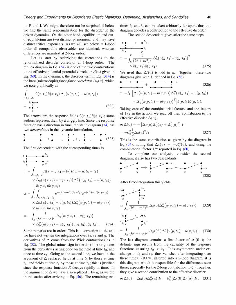
Theory and Experiments for Disordered Elastic Manifolds, Depinning, Avalanches, and Sandpiles 40
..., F, and J. We might therefore not be surprised if belowwe find the same renormalization for the disorder in thedriven dynamics. On the other hand, equilibrium and out-of-equilibrium are two distinct phenomena, and may havedistinct critical exponents. As we will see below, at 1-looporder all comparable observables are identical, whereasdifferences are manifest at 2-loop order.
Let us start by rederiving the corrections to therenormalized disorder correlator at 1-loop order. Thereplica diagram in Eq. (54) is one of the two contributionsto the effective potential-potential correlator R(u) given inEq. (60). In the dynamics, the disorder term in Eq. (314) isthe bare (microscopic) force-force correlator ∆0(u), whichwe note graphically as∫
x,t1,t2
u(x, t1)u(x, t2) ∆0
(u(x, t1)− u(x, t2)
)
=x
t1
t2
(322)
The arrows are the response fields u(x, t1)u(x, t2); someauthors represent them by a wiggly line. Since the responsefunction has a direction in time, the static diagram (54) hastwo descendants in the dynamic formulation,
x y
−→x y
+x y
(323)
The first descendant with the corresponding times is
x yt1
t2
t3
t4
= −∫
t1,t2,x
R(x− y, t4 − t2)R(x− y, t3 − t1)
×∆0
(u(x, t2)− u(x, t1)
)∆′′0(u(y, t4)− u(y, t3)
)
× u(y, t3)u(y, t4)
' −∫
k
∫
t1<t3,t2<t4
e−(k2+m2)(t4−t2)e−(k2+m2)(t3−t1)
×∆0
(u(y, t4)− u(y, t3)
)∆′′0(u(y, t4)− u(y, t3)
)
× u(y, t3)u(y, t4)
= −∫
k
1
(k2 +m2)2∆0
(u(y, t4)− u(y, t3)
)
×∆′′0(u(y, t4)− u(y, t3)
)u(y, t3)u(y, t4). (324)
Some remarks are in order: This is a correction to ∆, andwe have not written the integrations over t3, t4 and y. Thederivatives of ∆ come from the Wick contractions as inEq. (52). The global minus sign in the first line originatesfrom the derivatives acting once on the field at time t3, andonce at time t4. Going to the second line, we have in theargument of ∆ replaced fields at time t2 by those at timet4, and fields at time t1 by those at time t3; this is justifiedsince the response function R decays rapidly in time. Inthe argument of ∆ we have also replaced x by y, as we didin the statics after arriving at Eq. (56). The remaining two
times t3 and t4 can be taken arbitrarily far apart, thus thisdiagram encodes a contribution to the effective disorder.
The second descendant gives after the same steps
x yt1
t2
t3
t4
' −∫
k
1
(k2 +m2)2∆′0(u(y, t4)−u(y, t3)
)2
×u(y, t3)u(y, t4). (325)
We used that ∆′(u) is odd in u. Together, these twodiagrams give with I1 defined in Eq. (58)
+ (326)
' −I1[∆0
(u(y, t4)− u(y, t3)
)∆′′0(u(y, t4)− u(y, t3)
)
+ ∆′0(u(y, t4)− u(y, t3)
)2]u(y, t3)u(y, t4).
Taking care of the combinatorial factors, and the factorsof 1/2 in the action, we read off their contribution to theeffective disorder ∆(u),
δ1∆(u) = −[∆0(u)∆′′0(u) + ∆′0(u)2
]I1
= −∂2u
1
2∆0(u)2I1 (327)
This is the same contribution as given by the diagram inEq. (54), noting that ∆0(u) = −R′′0 (u), and using thecombinatorial factor 1/2 reported in Eq. (60).
To complete our analysis, consider the seconddiagram; it also has two descendants,
x y
−→x y
+x y
(328)
After time-integration this yields
x yt1
t2
t3
t4
'∫
k
1
(k2 +m2)2∆0(0)∆′′0
(u(y, t4)− u(y, t3)
). (329)
x yt1
t2
t3
t4
'∫
k
1
(k2 +m2)2∆′0(0+)∆′0
(u(y, t4)− u(y, t3)
). (330)
The last diagram contains a first factor of ∆′(0+); thedefinite sign results from the causality of the responsefunctions ensuring t2 < t1. It is asymmetric under ex-change of t3 and t4, thus vanishes after integrating overthese times. (B.t.w., inserted into a 2-loop diagram, it isthis diagram which is responsible for the differences seenthere, especially for the 2-loop contribution to ζ.) Together,they give a second contribution to the effective disorder
δ2∆(u) = ∆0(0)∆′′0(u) I1 = ∂2u [∆0(0)∆0(u)] I1. (331)
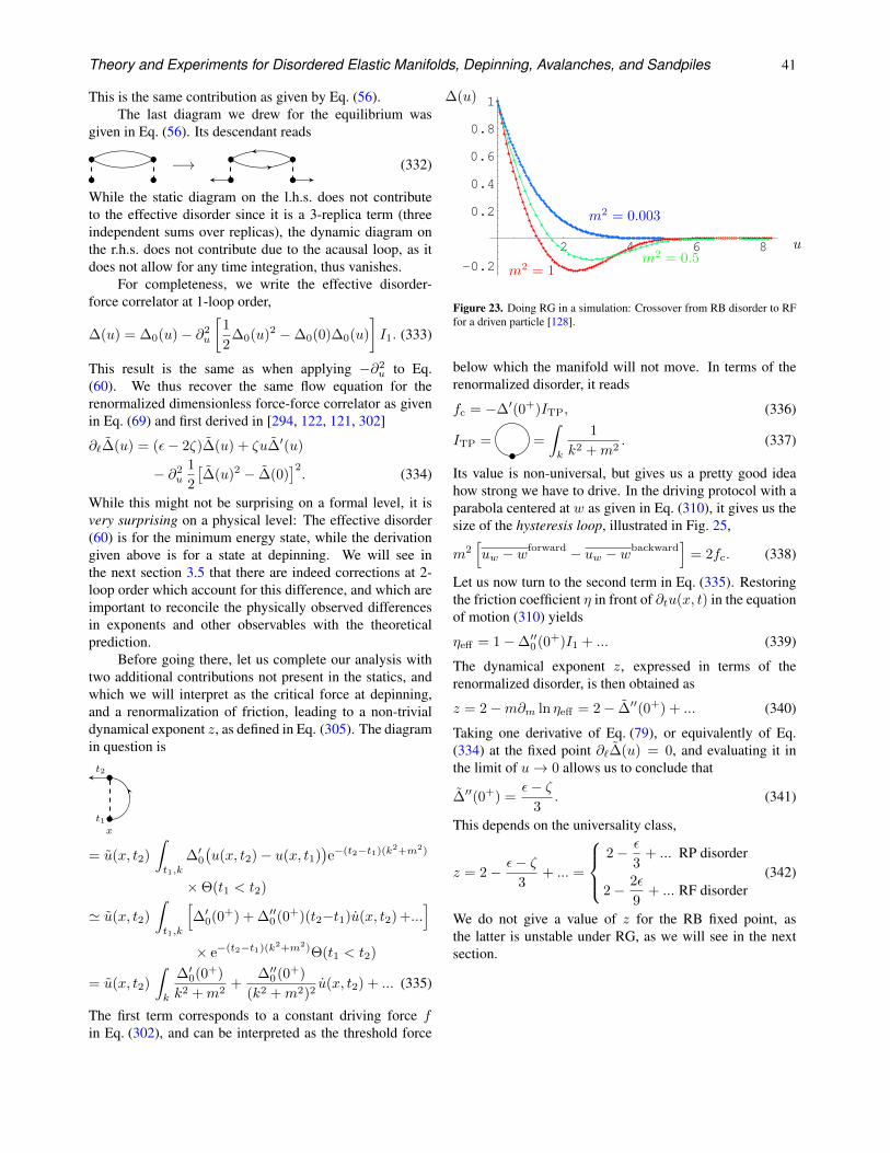
Theory and Experiments for Disordered Elastic Manifolds, Depinning, Avalanches, and Sandpiles 41
This is the same contribution as given by Eq. (56).The last diagram we drew for the equilibrium was
given in Eq. (56). Its descendant reads
−→ (332)
While the static diagram on the l.h.s. does not contributeto the effective disorder since it is a 3-replica term (threeindependent sums over replicas), the dynamic diagram onthe r.h.s. does not contribute due to the acausal loop, as itdoes not allow for any time integration, thus vanishes.
For completeness, we write the effective disorder-force correlator at 1-loop order,
∆(u) = ∆0(u)− ∂2u
[1
2∆0(u)2 −∆0(0)∆0(u)
]I1. (333)
This result is the same as when applying −∂2u to Eq.
(60). We thus recover the same flow equation for therenormalized dimensionless force-force correlator as givenin Eq. (69) and first derived in [294, 122, 121, 302]
∂`∆(u) = (ε− 2ζ)∆(u) + ζu∆′(u)
− ∂2u
1
2
[∆(u)2 − ∆(0)
]2. (334)
While this might not be surprising on a formal level, it isvery surprising on a physical level: The effective disorder(60) is for the minimum energy state, while the derivationgiven above is for a state at depinning. We will see inthe next section 3.5 that there are indeed corrections at 2-loop order which account for this difference, and which areimportant to reconcile the physically observed differencesin exponents and other observables with the theoreticalprediction.
Before going there, let us complete our analysis withtwo additional contributions not present in the statics, andwhich we will interpret as the critical force at depinning,and a renormalization of friction, leading to a non-trivialdynamical exponent z, as defined in Eq. (305). The diagramin question is
xt1
t2
= u(x, t2)
∫
t1,k
∆′0(u(x, t2)− u(x, t1)
)e−(t2−t1)(k2+m2)
×Θ(t1 < t2)
' u(x, t2)
∫
t1,k
[∆′0(0+) + ∆′′0(0+)(t2−t1)u(x, t2) +...
]
× e−(t2−t1)(k2+m2)Θ(t1 < t2)
= u(x, t2)
∫
k
∆′0(0+)
k2 +m2+
∆′′0(0+)
(k2 +m2)2u(x, t2) + ... (335)
The first term corresponds to a constant driving force fin Eq. (302), and can be interpreted as the threshold force
2 4 6 8
-0.2
0.2
0.4
0.6
0.8
1∆(u)
u
m2 = 1m2 = 0.5
m2 = 0.003
Figure 23. Doing RG in a simulation: Crossover from RB disorder to RFfor a driven particle [128].
below which the manifold will not move. In terms of therenormalized disorder, it reads
fc = −∆′(0+)ITP, (336)
ITP = =
∫
k
1
k2 +m2. (337)
Its value is non-universal, but gives us a pretty good ideahow strong we have to drive. In the driving protocol with aparabola centered at w as given in Eq. (310), it gives us thesize of the hysteresis loop, illustrated in Fig. 25,
m2[uw − wforward − uw − wbackward
]= 2fc. (338)
Let us now turn to the second term in Eq. (335). Restoringthe friction coefficient η in front of ∂tu(x, t) in the equationof motion (310) yields
ηeff = 1−∆′′0(0+)I1 + ... (339)
The dynamical exponent z, expressed in terms of therenormalized disorder, is then obtained as
z = 2−m∂m ln ηeff = 2− ∆′′(0+) + ... (340)
Taking one derivative of Eq. (79), or equivalently of Eq.(334) at the fixed point ∂`∆(u) = 0, and evaluating it inthe limit of u→ 0 allows us to conclude that
∆′′(0+) =ε− ζ
3. (341)
This depends on the universality class,
z = 2− ε− ζ3
+ ... =
2− ε
3+ ... RP disorder
2− 2ε
9+ ... RF disorder
(342)
We do not give a value of z for the RB fixed point, asthe latter is unstable under RG, as we will see in the nextsection.
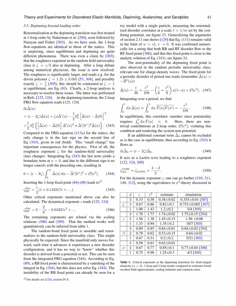
Theory and Experiments for Disordered Elastic Manifolds, Depinning, Avalanches, and Sandpiles 42
3.5. Depinning beyond leading order
Renormalization at the depinning transition was first treatedat 1-loop order by Natterman et al. [294], soon followed byNarayan and Fisher [303]. As we have seen, the 1-loopflow-equations are identical to those of the statics. Thisis surprising, since equilibrium and depinning are quitedifferent phenomena. There was even a claim by [303],that the roughness exponent in the random field universalityclass is ζ = ε/3 also at depinning. After a long debateamong numerical physicists, the issue is now resolved:The roughness is significantly larger, and reads e.g. for thedriven polymer ζ = 1.25 ± 0.005 [53, 304], and possiblyexactly ζ = 5
4 [305]; this should be contrasted to ζ = 1at equilibrium, see Eq. (83). Clearly, a 2-loop analysis isnecessary to resolve these issues. The latter was performedin Refs. [125, 124]. At the depinning transition, the 2-loopFRG flow equation reads [125, 124]
∂`∆(u)
= (ε− 2ζ)∆(u) + ζu∆′(u)− 1
2∂2u
[∆(u)− ∆(0)
]2
+1
2∂2u
[∆(u)− ∆(0)
]∆′(u)2 + ∆′(0+)2∆(u)
. (343)
Compared to the FRG-equation (113a) for the statics, theonly change is in the last sign on the second line ofEq. (343), given in red (bold). This “small change” hasimportant consequences for the physics. First of all, theroughness exponent ζ for the random-field universalityclass changes: Integrating Eq. (343) the last term yields aboundary term at u = 0, and due to the different sign it nolonger cancels with the preceding one, resulting in
0 = (ε− 3ζ)
∫ ∞
0
∆(u) du− ∆′(0+)3 +O(ε3). (344)
Inserting the 1-loop fixed point (84)-(88) leads to27
ζdepRF =
ε
3(1 + 0.143317ε+ . . .). (345)
Other critical exponents mentioned above can also becalculated. The dynamical exponent z reads [125, 124]
ζdepRF = 2− 2
9ε− 0.04321ε2 + . . . (346)
The remaining exponents are related via the scalingrelations (308) and (309). That the method works wellquantitatively can be inferred from table 1.
The random-bond fixed point is unstable and renor-malizes to the random-field universality class. This mightphysically be expected: Since the manifold only moves for-ward, each time it advances it experiences a new disorderconfiguration, and it has no way to “know” whether thisdisorder is derived from a potential or not. This can be seenfrom the integrated FRG equation (344): According to Eq.(89), a RB fixed point is characterized by a vanishing of theintegral in Eq. (344), but this does not solve Eq. (344). Theinstability of the RB fixed point can already be seen for a27For details see [124], section IV.A.
toy model with a single particle, measuring the renormal-ized disorder correlator at a scale ` = 1/m set by the con-fining potential, see figure 23. Generalizing the argumentsof section 2.11 one shows [129] that Eq. (111) remains validin the limit of w = vt, v → 0. It was confirmed numeri-cally for a string that both RB and RF disorder flow to theRF fixed point [306], and that this fixed point is close to theanalytic solution of Eq. (343), see figure 24.
The non-potentiality of the depinning fixed point isalso observed in the random periodic universality class,relevant one for charge-density waves. The fixed point fora periodic disorder of period one reads (remember ∆(u) =−R′′(u))
∆(u) =ε
36+
ε2
108−(ε
6+ε2
9
)u(1−u) +O(ε3). (347)
Integrating over a period, we find∫ 1
0
du ∆(u) ≡∫ 1
0
du F (u)F (u′) = − ε2
108. (348)
In equilibrium, this correlator vanishes since potentialityrequires
∫ 1
0du F (u) ≡ 0. Here, there are non-
trivial contributions at 2-loop order, O(ε2), violating thiscondition and rendering the system non-potential.
If an additional constant term ∆0 cannot be excludedas is the case in equilibrium, then according to Eq. (343) itflows as
∂`∆0 = (ε− 2ζ)∆0. (349)
It acts as a Larkin term leading to a roughness exponent[122, 124, 309]
ζCDWobs = ζLarkin =
4− d2
. (350)
For the dynamic exponent z, one can go further [310, 311,140, 312], using the equivalence to φ4-theory discussed in
d ε ε2 estimate simulation3 0.33 0.38 0.38±0.02 0.355±0.01 [307]
ζ 2 0.67 0.86 0.82±0.1 0.753±0.002 [307]1 1.00 1.43 1.2±0.2 5/4 [305]3 1.78 1.73 1.74±0.02 1.75±0.15 [294]
z 2 1.56 1.38 1.45±0.15 1.56 ±0.061 1.33 0.94 1.35±0.2 10/7 [305]3 0.89 0.85 0.84±0.01 0.84±0.02 [294]
β 2 0.78 0.62 0.53±0.15 0.64±0.021 0.67 0.31 0.2±0.2 5/21 [305]3 0.58 0.61 0.62±0.01
ν 2 0.67 0.77 0.85±0.1 0.77±0.04 [308]1 0.75 0.98 1.25±0.3 4/3 [305]
Table 1. Critical exponents at the depinning transition for short-rangedelasticity (α = 2). 1-loop and 2-loop results compared to estimates basedon three Pade approximants, scaling relations and common sense.
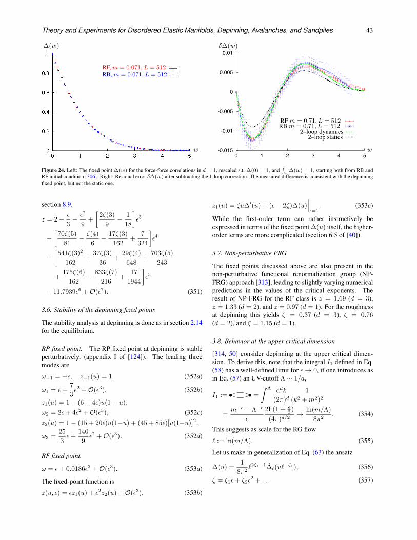
Theory and Experiments for Disordered Elastic Manifolds, Depinning, Avalanches, and Sandpiles 43
∆(w)
w
RF, m = 0.071, L = 512RB, m = 0.071, L = 512
3
-0.015
-0.01
-0.005
0
0.005
0.01
0 1 2 3 4 5
z
Y(z
)−
Y1(z
)
2–loop dynamics2–loop statics
RFm = 0 .71 , L = 512RBm = 0 .71 , L = 512
FIG. 3: The difference between the normalized correlator Y (z) andthe 1-loop prediction Y1(z).
We have studied the behaviour of the critical force f c(m)for the two classes of disorder. Because of (6), one has!
∆(0)m ∼ m2−ζ hence one obtains a parameter free linear
scaling shown in Fig.2. For large m the linear scaling does
not hold, while it holds for smaller m up to the point where
the correlation length becomes of the order of L (mL of order10 again ??). Note that c1< 0as discussed below.
We now turn to the FP function determination. Since there
are two scales in∆(u) hence we write:
∆(u) = ∆(0)Y (u/uξ) (7)
where Y (0) = 1and one determines uξ such that"
dzY (z) =1hence uξ =
"∆/∆(0). The function Y (z) is then fully uni-
versal and depends only on space dimension. We have deter-
mined the function Y (z) from our numerical data both for RFand RB disorder. For small masses the two function are found
to coincide within statistical errors. We also observe a cusp,
i.e. Y ′(0) = −... (show Y (z) ??). The predictions from theFRG is that Y (z) = Y1(z) + ϵY2(z) + O(ϵ2) with ϵ = 4− d.The one loop function is the same as for the statics and given
by the solution of Y = Y1(z) with γz =√
Y − 1− lnY
and γ =" 1
0 dy√
y − ln y − 1 ≈ 0.5482228893. Since themeasured Y (z) is numerically close to Y1(z), as was foundin the statics, we plot in Fig.3 the differential Y − Y1. The
overall shape of the difference function is very similar to the
one obtained for the RF statics in d = 3, 2, 0which was foundto exhibit only a weak dependence in d. However the over-all amplitude is larger by a factor of order 1.25. This factorbetween statics and dynamics is consistent with the two loop
prediction. We have plotted the function Y2(z) = ddϵY (z)|ϵ=0
which, as for the statics turns out to close to the numerical re-
sult **Alberto put the zero **
Examples of universal amplitudes are ∆ ′′(0+)cd/2,
∆(0)3/("
∆)2cx or ∆′(0+)2/∆(0)cy, check exponents of cgive one loop predictions ** see what we do about this, Kay
check the powers of c and one loop predictions **
0
0.2
0.4
0.6
0.8
1
0 0.2 0.4 0.6 0.8 1
∆(w)/∆(0)
S
1–loopRFRB
FIG. 4: Collapse of the 3 points function for RF and RB disorder.
Simlations has been performed for systems of size L = 512 andmassm = 0 .071 . The line represents the 1–loop predtiction f(x) =(1 − x)2
To investigate deeper the validity of FRG we measure the
third cumulant function, defined as:
m2p(w′ − u(w′) − (w − u(w)))3c
= L−2dS(w′ − w)(8)
The lowest order prediction [19] is S(w) =12m2 ∆′(w)(∆(w) − ∆(0)). Numerically one finds the
correct sign and to check the scaling in a parameter-free way
we define S =" w
0S(w)/
" ∞0
S(w) = F (∆(w)/∆(0)). Thefunction F (x) hereby defined is expected to be universal.Indeed we find, as can be seen in Fig.4, that RB and RF give
result identical within statistical errors.
The problem of characterizing the universality of the distri-
bution of the finite size fluctuations of the critical force bear
some similarity with the problem of the finite size fluctuations
of the ground state energy in the statics. There, for the directed
polymer several ”universal” distributions were found depend-
ing on the procedure and the geometry. The Tracy-Widom
distribution (for various β) was found for fixed endpoint oruniform KPZ field. On a cylinder the large deviation function
ln(eαF ) = L(κ1α − κ2G(κ3α)) where G(z) is universal.For the critical force problem there are several procedures.
Here we study the mass. Another procedure is the cylinder. A
third one is the fixed center of mass studied with FRG but hard
to study numerically. For each procedure there are fully uni-
versal quantities (different a priori in each procedure). Fully
universal means independent of microscopic details, and of
the model. It usually requires fixing two scales one in the udirection the other in the x direction. There are additional uni-versal quantities (usually amplitudes) however which depend
of the microscopic details only through renormalized elastic
constant cR and require fixing only one scale.
Here one measures:
m2p(w − u(w))pc
= L(1−p)dC(n)(0, ..0) (9)
with C(2)(0, 0) = ∆(0). Using the proper scaling
δ∆(w)
w
Figure 24. Left: The fixed point ∆(w) for the force-force correlations in d = 1, rescaled s.t. ∆(0) = 1, and∫w ∆(w) = 1, starting both from RB and
RF initial condition [306]. Right: Residual error δ∆(w) after subtracting the 1-loop correction. The measured difference is consistent with the depinningfixed point, but not the static one.
section 8.9,
z = 2− ε
3− ε2
9+
[2ζ(3)
9− 1
18
]ε3
−[
70ζ(5)
81− ζ(4)
6− 17ζ(3)
162+
7
324
]ε4
−[
541ζ(3)2
162+
37ζ(3)
36+
29ζ(4)
648+
703ζ(5)
243
+175ζ(6)
162− 833ζ(7)
216+
17
1944
]ε5
− 11.7939ε6 +O(ε7). (351)
3.6. Stability of the depinning fixed points
The stability analysis at depinning is done as in section 2.14for the equilibrium.
RP fixed point. The RP fixed point at depinning is stableperturbatively, (appendix I of [124]). The leading threemodes are
ω−1 = −ε, z−1(u) = 1. (352a)
ω1 = ε+7
3ε2 +O(ε3), (352b)
z1(u) = 1− (6 + 4ε)u(1− u).
ω2 = 2ε+ 4ε2 +O(ε3), (352c)z2(u) = 1− (15 + 20ε)u(1−u) + (45 + 85ε)[u(1−u)]2,
ω3 =25
3ε+
140
9ε2 +O(ε3). (352d)
RF fixed point.
ω = ε+ 0.0186ε2 +O(ε3). (353a)
The fixed-point function is
z(u, ε) = εz1(u) + ε2z2(u) +O(ε3), (353b)
z1(u) = ζu∆′(u) + (ε− 2ζ)∆(u)∣∣∣ε=1
. (353c)
While the first-order term can rather instructively beexpressed in terms of the fixed point ∆(u) itself, the higher-order terms are more complicated (section 6.5 of [40]).
3.7. Non-perturbative FRG
The fixed points discussed above are also present in thenon-perturbative functional renormalization group (NP-FRG) approach [313], leading to slightly varying numericalpredictions in the values of the critical exponents. Theresult of NP-FRG for the RF class is z = 1.69 (d = 3),z = 1.33 (d = 2), and z = 0.97 (d = 1). For the roughnessat depinning this yields ζ = 0.37 (d = 3), ζ = 0.76(d = 2), and ζ = 1.15 (d = 1).
3.8. Behavior at the upper critical dimension
[314, 50] consider depinning at the upper critical dimen-sion. To derive this, note that the integral I1 defined in Eq.(58) has a well-defined limit for ε→ 0, if one introduces asin Eq. (57) an UV-cutoff Λ ∼ 1/a,
I1 := =
∫ Λ ddk
(2π)d1
(k2 +m2)2
=m−ε − Λ−ε
ε
2Γ(1 + ε2 )
(4π)d/2→ ln(m/Λ)
8π2. (354)
This suggests as scale for the RG flow
` := ln(m/Λ). (355)
Let us make in generalization of Eq. (63) the ansatz
∆(u) =1
8π2`2ζ1−1∆`(u`
−ζ1), (356)
ζ = ζ1ε+ ζ2ε2 + ... (357)
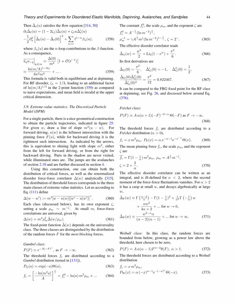
Theory and Experiments for Disordered Elastic Manifolds, Depinning, Avalanches, and Sandpiles 44
Then ∆`(u) satisfies the flow equation [314, 50]
∂`∆`(u) = (1− 2ζ1)∆`(u) + ζ1u∆′`(u)
−1
2∂2u
[∆`(u)− ∆`(0)
]2+∑
n>1
`1−nβn(u), (358)
where βn(u) are the n-loop contributions to the β-function.As a consequence,
uqu−q∣∣∣qm
' ∆(0)
m4
[1 +O(`−1)
]
' ln(m/Λ)1−2ζ1
8π2m4+ ... . (359)
This formula is valid both in equilibrium and at depinning.For RF disorder, ζ1 = 1/3, leading to an additional factorof ln(m/Λ)1/3 in the 2-point function (359) as comparedto naive expectations, and mean field is invalid at the uppercritical dimension.
3.9. Extreme-value statistics: The Discretized ParticleModel (DPM)
For a single particle, there is a nice geometrical constructionto obtain the particle trajectories, indicated in figure 25:For given w, draw a line of slope m2(u − w). Forforward driving, u(w) is the leftmost intersection with thepinning force F (u), while for backward driving it is therightmost such intersection. As indicated by the arrows,this is equivalent to shining light with slope m2, eitherfrom the left for forward driving, or from the right forbackward driving. Parts in the shadow are never visited,while illuminated ones are. The jumps are the avalanchesof section 2.10 and are further discussed in section 4.
Using this construction, one can obtain both thedistribution of critical forces, as well as the renormalizeddisorder force-force correlator ∆(w) analytically [315].The distribution of threshold forces corresponds to the threemain classes of extreme-value statistics. Let us according toEq. (111) define
∆(w − w′) := m4[w − u(w)][w′ − u(w′)]c. (360)
Each class (discussed below), has its own exponent ζ,setting a scale ρm ∼ m−ζ . At small m, force-forcecorrelations are universal, given by
∆(w) = m4ρ2m∆(w/ρm). (361)
The fixed-point function ∆(w) depends on the universalityclass. The three classes are distinguished by the distributionof the random forces F for the most blocking forces.
Gumbel class:
P (F ) ' e−A(−F )γ , as F → −∞. (362)
The threshold forces fc are distributed according to aGumbel distribution (tested in [131]),
PG(a) = exp(−a)Θ(a), (363)
fc =
[− ln(m2a)
A
] 1γ
= f0c − ln(a)m2ρm + ... (364)
The constant f0c , the scale ρm, and the exponent ζ are
f0c = A−
1γ (lnm−2)
1γ ,
ρ−1m = γA
1γmζ(lnm−2)1− 1
γ , ζ = 2−. (365)
The effective disorder correlator reads
∆G(w) =w2
2+ Li2(1− ew) +
π2
6. (366)
Its first derivatives are
∆G(0) =π2
6, ∆′G(0) = −1, ∆′′G(0) =
1
2,
∆G(0)∆′′G(0)
∆′G(0)2=π2
12= 0.822467. (367)
It can be compared to the FRG fixed point for the RF classat depinning, see Fig. 26, and discussed below around Eq.(376).
Frechet class:
P (F ) ' Aα(α+ 1)(−F )−2−α Θ(−F ) as F → −∞.(368)
The threshold forces fc are distributed according to aFrechet distribution (α > 0),
fc = xm2ρm, PF(x) = αx−α−1e−x−α
Θ(x). (369)
The mean pinning force fc, the scale ρm, and the exponentζ are
fc = Γ(1− 1α )m2ρm, ρm = A
1αm−ζ ,
ζ = 2 +2
α. (370)
The effective disorder correlator can be written as anintegral, and is ill-defined for α < 2, where the secondmoment of the force-force fluctuations vanishes. For α > 2it has a cusp at small w, and decays algebraically at largew,
∆F(w) ' Γ(α−2α
)− Γ(1− 1
α )2 + 1α2 Γ
(− 1α
)w
+αw2
4α+ 2+ ... for w → 0,
∆F(w) ' w2−αα(α− 2)(α− 1)
+ ... for w →∞. (371)
Weibull class: In this class, the random forces arebounded from below, growing as a power law above thethreshold, here chosen to be zero,
P (F ) = Aα(α− 1)Fα−2θ(F ), α > 1. (372)
The threshold forces are distributed according to a Weibulldistribution
fc = xm2ρm,
PW(x) = α (−x)α−1e−(−x)αΘ(−x). (373)
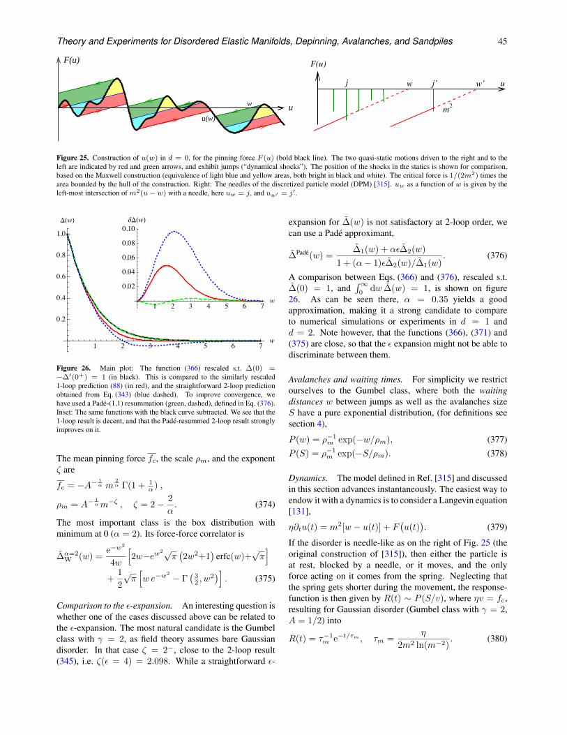
Theory and Experiments for Disordered Elastic Manifolds, Depinning, Avalanches, and Sandpiles 45
F(u)
uw
u(w)m
2
w j’
F(u)
j w’ u
Figure 25. Construction of u(w) in d = 0, for the pinning force F (u) (bold black line). The two quasi-static motions driven to the right and to theleft are indicated by red and green arrows, and exhibit jumps (“dynamical shocks”). The position of the shocks in the statics is shown for comparison,based on the Maxwell construction (equivalence of light blue and yellow areas, both bright in black and white). The critical force is 1/(2m2) times thearea bounded by the hull of the construction. Right: The needles of the discretized particle model (DPM) [315]. uw as a function of w is given by theleft-most intersection of m2(u− w) with a needle, here uw = j, and uw′ = j′.
Δ()
δΔ()
Figure 26. Main plot: The function (366) rescaled s.t. ∆(0) =−∆′(0+) = 1 (in black). This is compared to the similarly rescaled1-loop prediction (88) (in red), and the straightforward 2-loop predictionobtained from Eq. (343) (blue dashed). To improve convergence, wehave used a Pade-(1,1) resummation (green, dashed), defined in Eq. (376).Inset: The same functions with the black curve subtracted. We see that the1-loop result is decent, and that the Pade-resummed 2-loop result stronglyimproves on it.
The mean pinning force fc, the scale ρm, and the exponentζ are
fc = −A− 1α m
2α Γ(1 + 1
α ) ,
ρm = A−1αm−ζ , ζ = 2− 2
α. (374)
The most important class is the box distribution withminimum at 0 (α = 2). Its force-force correlator is
∆α=2W (w) =
e−w2
4w
[2w−ew2√
π(2w2+1
)erfc(w)+
√π]
+1
2
√π[w e−w
2 − Γ(
32 , w
2)]. (375)
Comparison to the ε-expansion. An interesting question iswhether one of the cases discussed above can be related tothe ε-expansion. The most natural candidate is the Gumbelclass with γ = 2, as field theory assumes bare Gaussiandisorder. In that case ζ = 2−, close to the 2-loop result(345), i.e. ζ(ε = 4) = 2.098. While a straightforward ε-
expansion for ∆(w) is not satisfactory at 2-loop order, wecan use a Pade approximant,
∆Pade(w) =∆1(w) + αε∆2(w)
1 + (α− 1)ε∆2(w)/∆1(w). (376)
A comparison between Eqs. (366) and (376), rescaled s.t.∆(0) = 1, and
∫∞0
dw ∆(w) = 1, is shown on figure26. As can be seen there, α = 0.35 yields a goodapproximation, making it a strong candidate to compareto numerical simulations or experiments in d = 1 andd = 2. Note however, that the functions (366), (371) and(375) are close, so that the ε expansion might not be able todiscriminate between them.
Avalanches and waiting times. For simplicity we restrictourselves to the Gumbel class, where both the waitingdistances w between jumps as well as the avalanches sizeS have a pure exponential distribution, (for definitions seesection 4),
P (w) = ρ−1m exp(−w/ρm), (377)
P (S) = ρ−1m exp(−S/ρm). (378)
Dynamics. The model defined in Ref. [315] and discussedin this section advances instantaneously. The easiest way toendow it with a dynamics is to consider a Langevin equation[131],
η∂tu(t) = m2[w − u(t)] + F(u(t)
). (379)
If the disorder is needle-like as on the right of Fig. 25 (theoriginal construction of [315]), then either the particle isat rest, blocked by a needle, or it moves, and the onlyforce acting on it comes from the spring. Neglecting thatthe spring gets shorter during the movement, the response-function is then given by R(t) ∼ P (S/v), where ηv = fc,resulting for Gaussian disorder (Gumbel class with γ = 2,A = 1/2) into
R(t) = τ−1m e−t/τm , τm =
η
2m2 ln(m−2). (380)
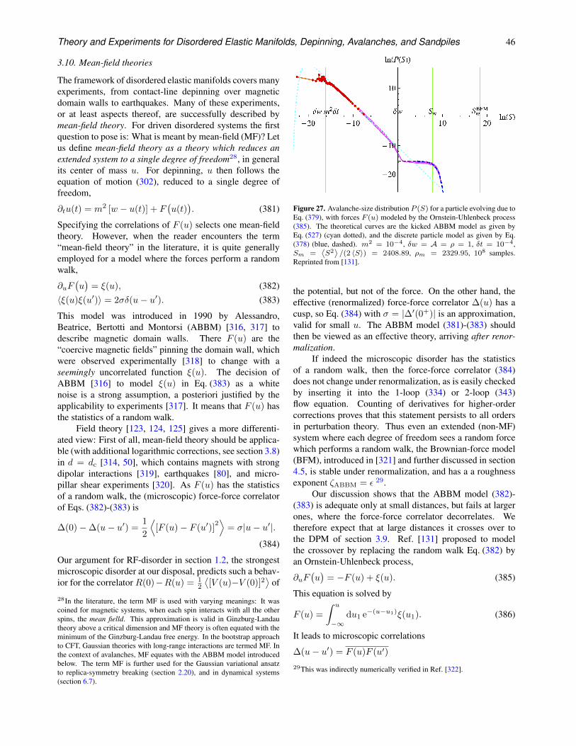
Theory and Experiments for Disordered Elastic Manifolds, Depinning, Avalanches, and Sandpiles 46
3.10. Mean-field theories
The framework of disordered elastic manifolds covers manyexperiments, from contact-line depinning over magneticdomain walls to earthquakes. Many of these experiments,or at least aspects thereof, are successfully described bymean-field theory. For driven disordered systems the firstquestion to pose is: What is meant by mean-field (MF)? Letus define mean-field theory as a theory which reduces anextended system to a single degree of freedom28, in generalits center of mass u. For depinning, u then follows theequation of motion (302), reduced to a single degree offreedom,
∂tu(t) = m2 [w − u(t)] + F(u(t)
). (381)
Specifying the correlations of F (u) selects one mean-fieldtheory. However, when the reader encounters the term“mean-field theory” in the literature, it is quite generallyemployed for a model where the forces perform a randomwalk,
∂uF(u)
= ξ(u), (382)〈ξ(u)ξ(u′)〉 = 2σδ(u− u′). (383)
This model was introduced in 1990 by Alessandro,Beatrice, Bertotti and Montorsi (ABBM) [316, 317] todescribe magnetic domain walls. There F (u) are the“coercive magnetic fields” pinning the domain wall, whichwere observed experimentally [318] to change with aseemingly uncorrelated function ξ(u). The decision ofABBM [316] to model ξ(u) in Eq. (383) as a whitenoise is a strong assumption, a posteriori justified by theapplicability to experiments [317]. It means that F (u) hasthe statistics of a random walk.
Field theory [123, 124, 125] gives a more differenti-ated view: First of all, mean-field theory should be applica-ble (with additional logarithmic corrections, see section 3.8)in d = dc [314, 50], which contains magnets with strongdipolar interactions [319], earthquakes [80], and micro-pillar shear experiments [320]. As F (u) has the statisticsof a random walk, the (microscopic) force-force correlatorof Eqs. (382)-(383) is
∆(0)−∆(u− u′) =1
2
⟨[F (u)− F (u′)]
2⟩
= σ|u− u′|.(384)
Our argument for RF-disorder in section 1.2, the strongestmicroscopic disorder at our disposal, predicts such a behav-ior for the correlator R(0)−R(u) = 1
2
⟨[V (u)−V (0)]2
⟩of
28In the literature, the term MF is used with varying meanings: It wascoined for magnetic systems, when each spin interacts with all the otherspins, the mean fielld. This approximation is valid in Ginzburg-Landautheory above a critical dimension and MF theory is often equated with theminimum of the Ginzburg-Landau free energy. In the bootstrap approachto CFT, Gaussian theories with long-range interactions are termed MF. Inthe context of avalanches, MF equates with the ABBM model introducedbelow. The term MF is further used for the Gaussian variational ansatzto replica-symmetry breaking (section 2.20), and in dynamical systems(section 6.7).
Figure 27. Avalanche-size distribution P (S) for a particle evolving due toEq. (379), with forces F (u) modeled by the Ornstein-Uhlenbeck process(385). The theoretical curves are the kicked ABBM model as given byEq. (527) (cyan dotted), and the discrete particle model as given by Eq.(378) (blue, dashed). m2 = 10−4, δw = A = ρ = 1, δt = 10−4,Sm =
⟨S2⟩/(2 〈S〉) = 2408.89, ρm = 2329.95, 108 samples.
Reprinted from [131].
the potential, but not of the force. On the other hand, theeffective (renormalized) force-force correlator ∆(u) has acusp, so Eq. (384) with σ = |∆′(0+)| is an approximation,valid for small u. The ABBM model (381)-(383) shouldthen be viewed as an effective theory, arriving after renor-malization.
If indeed the microscopic disorder has the statisticsof a random walk, then the force-force correlator (384)does not change under renormalization, as is easily checkedby inserting it into the 1-loop (334) or 2-loop (343)flow equation. Counting of derivatives for higher-ordercorrections proves that this statement persists to all ordersin perturbation theory. Thus even an extended (non-MF)system where each degree of freedom sees a random forcewhich performs a random walk, the Brownian-force model(BFM), introduced in [321] and further discussed in section4.5, is stable under renormalization, and has a a roughnessexponent ζABBM = ε 29.
Our discussion shows that the ABBM model (382)-(383) is adequate only at small distances, but fails at largerones, where the force-force correlator decorrelates. Wetherefore expect that at large distances it crosses over tothe DPM of section 3.9. Ref. [131] proposed to modelthe crossover by replacing the random walk Eq. (382) byan Ornstein-Uhlenbeck process,
∂uF(u)
= −F (u) + ξ(u). (385)
This equation is solved by
F (u) =
∫ u
−∞du1 e−(u−u1)ξ(u1). (386)
It leads to microscopic correlations
∆(u− u′) = F (u)F (u′)
29This was indirectly numerically verified in Ref. [322].
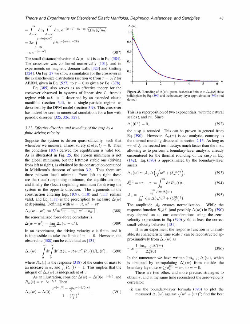
Theory and Experiments for Disordered Elastic Manifolds, Depinning, Avalanches, and Sandpiles 47
=
∫ u
−∞du1
∫ u′
−∞du2 e−(u+u′−u1−u2)ξ(u1)ξ(u2)
= 2σ
∫ min(u,u′)
−∞du e−(u+u′−2u)
= σ e−|u−u′|. (387)
The small-distance behavior of ∆(u−u′) is as in Eq. (384).The crossover was confirmed numerically [131], and inexperiments on magnetic domain walls [323] and knitting[324]. On Fig. 27 we show a simulation for the crossover inthe avalanche-size distribution (section 4) from τ = 3/2 forABBM, given in Eq. (527), to τ = 0 as given by Eq. (378).
Eq. (385) also serves as an effective theory for thecrossover observed in systems of linear size L, from aregime with mL 1 described by an extended elasticmanifold (section 3.4), to a single-particle regime asdescribed by the DPM model (section 3.9). This crossoverhas indeed be seen in numerical simulations for a line withperiodic disorder [325, 326, 327].
3.11. Effective disorder, and rounding of the cusp by afinite driving velocity
Suppose the system is driven quasi-statically, such thatwhenever we measure, almost surely ∂tu(x, t) = 0. Thenthe condition (109) derived for equilibrium is valid too.As is illustrated in Fig. 25, the chosen minimum is notthe global minimum, but the leftmost stable one (drivingfrom left to right), as obtained by the construction containedin Middleton’s theorem of section 3.2. Thus there arethree relevant local minima: From left to right theseare the (local) depinning minimum, the equilibrium one,and finally the (local) depinning minimum for driving thesystem in the opposite direction. The arguments in theconstruction entering Eqs. (109), (110) and (111) remainvalid, and Eq. (111) is the prescription to measure ∆(w)at depinning. Defining with w = vt, w′ = vt′
∆v(w − w′) := Ldm4[w − uw][w′ − uw′ ]c, (388)
the renormalized force-force correlator is
∆(w − w′) = limv→0
∆v(w − w′). (389)
In an experiment, the driving velocity v is finite, and itis impossible to take the limit of v → 0. However, theobservable (388) can be calculated as [131]
∆v(w) =
∞∫
0
dt
∞∫
0
dt′∆(w−vt+vt′)Rw(t)Rw(t′), (390)
where Rw(t) is the response (318) of the center of mass toan increase in w, and
∫tRw(t) = 1. This implies that the
integral of ∆v(w) is independent of v.As an illustration, consider ∆(w) = ∆(0)e−|w|/ξ, and
Rw(t) = τ−1e−t/τ . Then
∆v(w) = ∆(0)e−|w|/ξ − τv
ξ e−|w|/(τv)
1−(τvξ
)2 . (391)
Δ()
Figure 28. Rounding of ∆(w) (green, dashed) at finite v to ∆v(w) (bluesolid) given by Eq. (390) and the boundary-layer approximation (393) (reddotted).
This is a superposition of two exponentials, with the naturalscales ξ and τv. Since
∆′v(0+) = 0, (392)
the cusp is rounded. This can be proven in general fromEq. (390). However, ∆v(w) is not analytic, contrary tothe thermal rounding discussed in section 2.15. As long asτv ξ, the second term decays much faster than the first,allowing us to perform a boundary-layer analysis, alreadyencountered for the thermal rounding of the cusp in Eq.(142). Eq. (390) is approximated by the boundary-layeransatz
∆v(w) ' Av ∆(√
w2 + (δBLw )2
), (393)
δBLw = vτ, τ :=
∫ ∞
0
dtRw(t)t , (394)
Av =
∫∞0
dw∆(w)∫∞
0dw∆(
√w2 + (δBL
w )2). (395)
The amplitude Av ensures normalization. While theresponse function Rw(t) (and possibly ∆(w)) in Eq. (390)may depend on v, our considerations using the zero-velocity expressions in Eq. (390) yield at least the correctsmall-velocity behavior [131].
If in an experiment the response function is unavail-able, its characteristic time scale τ can be reconstructed ap-proximatively from ∆v(w) as
τ ' 1
v
limw→0 ∆′(w)
∆′′v(0). (396)
In the numerator we have written limw→0 ∆′(w), whichis obtained by extrapolating ∆′v(w) from outside theboundary layer, i.e w ≥ δBL
w = vτ , to w = 0.There are two other, and more precise, strategies to
obtain τ , and at the same time reconstruct the zero-velocitycorrelator:
(i) use the boundary-layer formula (393) to plot themeasured ∆v(w) against
√w2 + (vτ)2; find the best
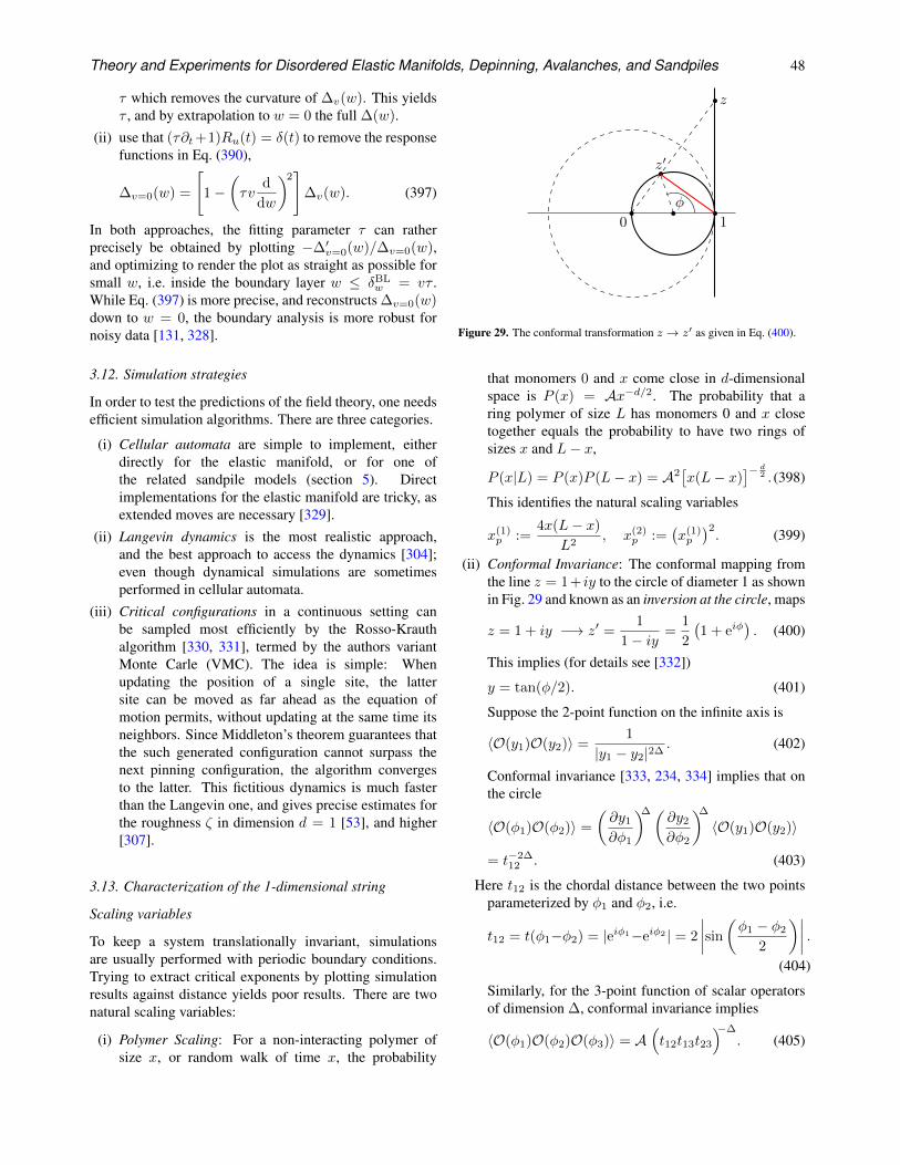
Theory and Experiments for Disordered Elastic Manifolds, Depinning, Avalanches, and Sandpiles 48
τ which removes the curvature of ∆v(w). This yieldsτ , and by extrapolation to w = 0 the full ∆(w).
(ii) use that (τ∂t+1)Ru(t) = δ(t) to remove the responsefunctions in Eq. (390),
∆v=0(w) =
[1−
(τv
d
dw
)2]
∆v(w). (397)
In both approaches, the fitting parameter τ can ratherprecisely be obtained by plotting −∆′v=0(w)/∆v=0(w),and optimizing to render the plot as straight as possible forsmall w, i.e. inside the boundary layer w ≤ δBL
w = vτ .While Eq. (397) is more precise, and reconstructs ∆v=0(w)down to w = 0, the boundary analysis is more robust fornoisy data [131, 328].
3.12. Simulation strategies
In order to test the predictions of the field theory, one needsefficient simulation algorithms. There are three categories.
(i) Cellular automata are simple to implement, eitherdirectly for the elastic manifold, or for one ofthe related sandpile models (section 5). Directimplementations for the elastic manifold are tricky, asextended moves are necessary [329].
(ii) Langevin dynamics is the most realistic approach,and the best approach to access the dynamics [304];even though dynamical simulations are sometimesperformed in cellular automata.
(iii) Critical configurations in a continuous setting canbe sampled most efficiently by the Rosso-Krauthalgorithm [330, 331], termed by the authors variantMonte Carle (VMC). The idea is simple: Whenupdating the position of a single site, the lattersite can be moved as far ahead as the equation ofmotion permits, without updating at the same time itsneighbors. Since Middleton’s theorem guarantees thatthe such generated configuration cannot surpass thenext pinning configuration, the algorithm convergesto the latter. This fictitious dynamics is much fasterthan the Langevin one, and gives precise estimates forthe roughness ζ in dimension d = 1 [53], and higher[307].
3.13. Characterization of the 1-dimensional string
Scaling variables
To keep a system translationally invariant, simulationsare usually performed with periodic boundary conditions.Trying to extract critical exponents by plotting simulationresults against distance yields poor results. There are twonatural scaling variables:
(i) Polymer Scaling: For a non-interacting polymer ofsize x, or random walk of time x, the probability
0 1
z
z′
φ
Figure 29. The conformal transformation z → z′ as given in Eq. (400).
that monomers 0 and x come close in d-dimensionalspace is P (x) = Ax−d/2. The probability that aring polymer of size L has monomers 0 and x closetogether equals the probability to have two rings ofsizes x and L− x,
P (x|L) = P (x)P (L− x) = A2[x(L− x)
]− d2 . (398)
This identifies the natural scaling variables
x(1)p :=
4x(L− x)
L2, x(2)
p :=(x(1)p
)2. (399)
(ii) Conformal Invariance: The conformal mapping fromthe line z = 1+ iy to the circle of diameter 1 as shownin Fig. 29 and known as an inversion at the circle, maps
z = 1 + iy −→ z′ =1
1− iy =1
2
(1 + eiφ
). (400)
This implies (for details see [332])
y = tan(φ/2). (401)
Suppose the 2-point function on the infinite axis is
〈O(y1)O(y2)〉 =1
|y1 − y2|2∆. (402)
Conformal invariance [333, 234, 334] implies that onthe circle
〈O(φ1)O(φ2)〉 =
(∂y1
∂φ1
)∆(∂y2
∂φ2
)∆〈O(y1)O(y2)〉
= t−2∆12 . (403)
Here t12 is the chordal distance between the two pointsparameterized by φ1 and φ2, i.e.
t12 = t(φ1−φ2) = |eiφ1−eiφ2 | = 2
∣∣∣∣sin(φ1 − φ2
2
)∣∣∣∣ .
(404)
Similarly, for the 3-point function of scalar operatorsof dimension ∆, conformal invariance implies
〈O(φ1)O(φ2)O(φ3)〉 = A(t12t13t23
)−∆
. (405)
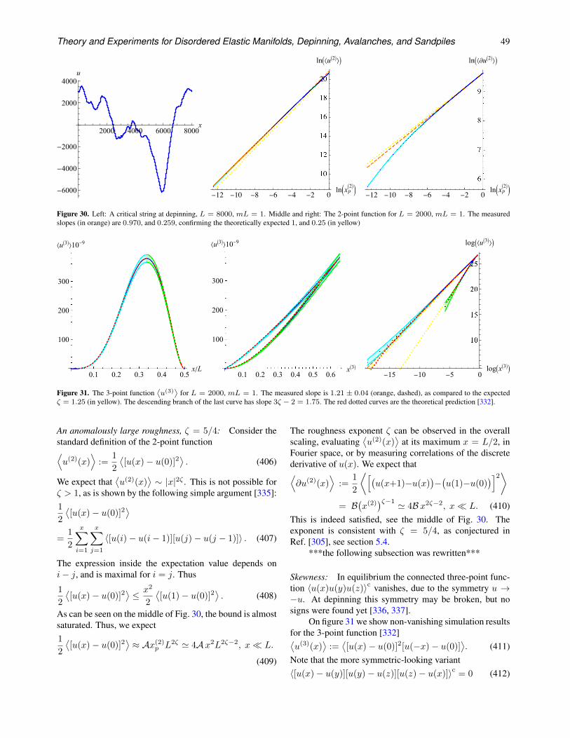
Theory and Experiments for Disordered Elastic Manifolds, Depinning, Avalanches, and Sandpiles 49
2000 4000 6000 8000x
-6000
-4000
-2000
2000
4000
u
-12 -10 -8 -6 -4 -2 0lnxp2
ln⟨u2⟩
-12 -10 -8 -6 -4 -2 0lnxp2
ln⟨∂u2⟩
Figure 30. Left: A critical string at depinning, L = 8000, mL = 1. Middle and right: The 2-point function for L = 2000, mL = 1. The measuredslopes (in orange) are 0.970, and 0.259, confirming the theoretically expected 1, and 0.25 (in yellow)
0.1 0.2 0.3 0.4 0.5x/L
100
200
300
⟨u3⟩10-9
0.1 0.2 0.3 0.4 0.5 0.6x3
100
200
300
⟨u3⟩10-9
-15 -10 -5 0logx3
log⟨u3⟩
Figure 31. The 3-point function⟨u(3)
⟩for L = 2000, mL = 1. The measured slope is 1.21 ± 0.04 (orange, dashed), as compared to the expected
ζ = 1.25 (in yellow). The descending branch of the last curve has slope 3ζ − 2 = 1.75. The red dotted curves are the theoretical prediction [332].
An anomalously large roughness, ζ = 5/4: Consider thestandard definition of the 2-point function⟨u(2)(x)
⟩:=
1
2
⟨[u(x)− u(0)]2
⟩. (406)
We expect that⟨u(2)(x)
⟩∼ |x|2ζ . This is not possible for
ζ > 1, as is shown by the following simple argument [335]:1
2
⟨[u(x)− u(0)]2
⟩
=1
2
x∑
i=1
x∑
j=1
〈[u(i)− u(i− 1)][u(j)− u(j − 1)]〉 . (407)
The expression inside the expectation value depends oni− j, and is maximal for i = j. Thus
1
2
⟨[u(x)− u(0)]2
⟩≤ x2
2
⟨[u(1)− u(0)]2
⟩. (408)
As can be seen on the middle of Fig. 30, the bound is almostsaturated. Thus, we expect1
2
⟨[u(x)− u(0)]2
⟩≈ Ax(2)
p L2ζ ' 4Ax2L2ζ−2, x L.
(409)
The roughness exponent ζ can be observed in the overallscaling, evaluating
⟨u(2)(x)
⟩at its maximum x = L/2, in
Fourier space, or by measuring correlations of the discretederivative of u(x). We expect that⟨∂u(2)(x)
⟩:=
1
2
⟨[(u(x+1)−u(x)
)−(u(1)−u(0)
)]2⟩
= B(x(2)
)ζ−1 ' 4B x2ζ−2, x L. (410)This is indeed satisfied, see the middle of Fig. 30. Theexponent is consistent with ζ = 5/4, as conjectured inRef. [305], see section 5.4.
***the following subsection was rewritten***
Skewness: In equilibrium the connected three-point func-tion 〈u(x)u(y)u(z)〉c vanishes, due to the symmetry u →−u. At depinning this symmetry may be broken, but nosigns were found yet [336, 337].
On figure 31 we show non-vanishing simulation resultsfor the 3-point function [332]⟨u(3)(x)
⟩:=⟨[u(x)− u(0)]2[u(−x)− u(0)]
⟩. (411)
Note that the more symmetric-looking variant〈[u(x)− u(y)][u(y)− u(z)][u(z)− u(x)]〉c = 0 (412)
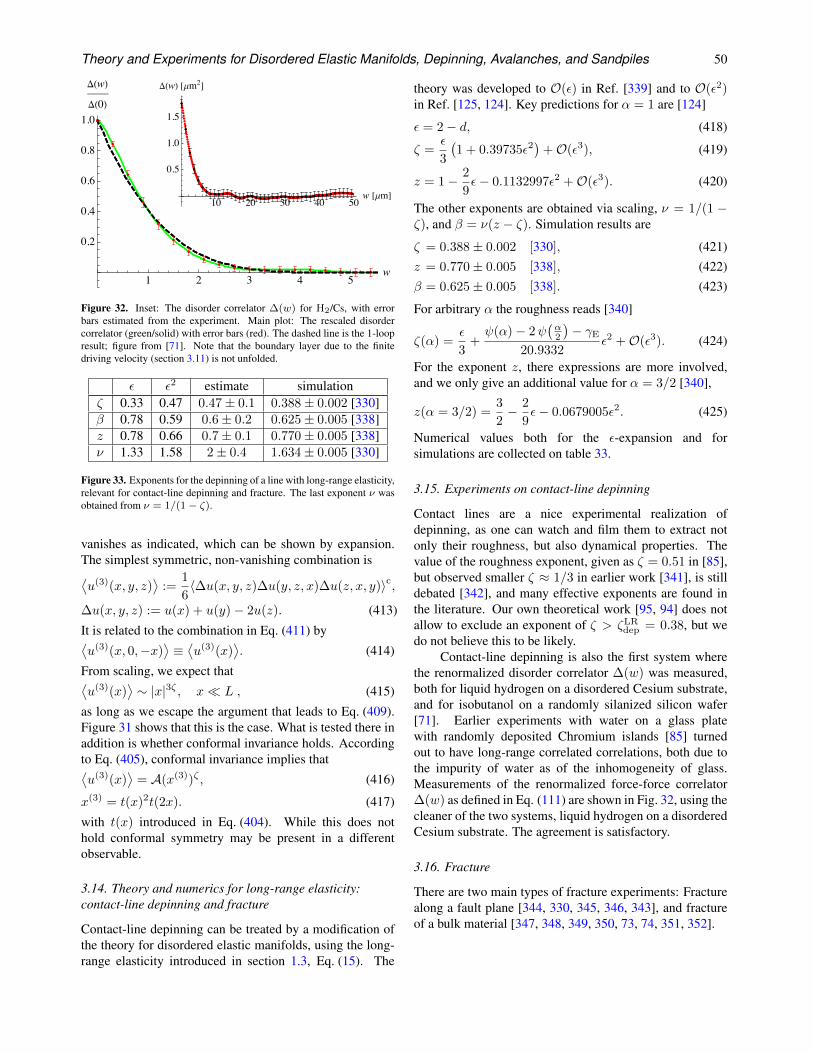
Theory and Experiments for Disordered Elastic Manifolds, Depinning, Avalanches, and Sandpiles 50
1 2 3 4 5w
0.2
0.4
0.6
0.8
1.0
Δ(w)
Δ(0)
10 20 30 40 50w [μm]
0.5
1.0
1.5
Δ(w) [μm2]
Figure 32. Inset: The disorder correlator ∆(w) for H2/Cs, with errorbars estimated from the experiment. Main plot: The rescaled disordercorrelator (green/solid) with error bars (red). The dashed line is the 1-loopresult; figure from [71]. Note that the boundary layer due to the finitedriving velocity (section 3.11) is not unfolded.
ε ε2 estimate simulationζ 0.33 0.47 0.47± 0.1 0.388± 0.002 [330]β 0.78 0.59 0.6± 0.2 0.625± 0.005 [338]z 0.78 0.66 0.7± 0.1 0.770± 0.005 [338]ν 1.33 1.58 2± 0.4 1.634± 0.005 [330]
Figure 33. Exponents for the depinning of a line with long-range elasticity,relevant for contact-line depinning and fracture. The last exponent ν wasobtained from ν = 1/(1− ζ).
vanishes as indicated, which can be shown by expansion.The simplest symmetric, non-vanishing combination is⟨u(3)(x, y, z)
⟩:=
1
6〈∆u(x, y, z)∆u(y, z, x)∆u(z, x, y)〉c,
∆u(x, y, z) := u(x) + u(y)− 2u(z). (413)
It is related to the combination in Eq. (411) by⟨u(3)(x, 0,−x)
⟩≡⟨u(3)(x)
⟩. (414)
From scaling, we expect that⟨u(3)(x)
⟩∼ |x|3ζ , x L , (415)
as long as we escape the argument that leads to Eq. (409).Figure 31 shows that this is the case. What is tested there inaddition is whether conformal invariance holds. Accordingto Eq. (405), conformal invariance implies that⟨u(3)(x)
⟩= A(x(3))ζ , (416)
x(3) = t(x)2t(2x). (417)
with t(x) introduced in Eq. (404). While this does nothold conformal symmetry may be present in a differentobservable.
3.14. Theory and numerics for long-range elasticity:contact-line depinning and fracture
Contact-line depinning can be treated by a modification ofthe theory for disordered elastic manifolds, using the long-range elasticity introduced in section 1.3, Eq. (15). The
theory was developed to O(ε) in Ref. [339] and to O(ε2)in Ref. [125, 124]. Key predictions for α = 1 are [124]
ε = 2− d, (418)
ζ =ε
3
(1 + 0.39735ε2
)+O(ε3), (419)
z = 1− 2
9ε− 0.1132997ε2 +O(ε3). (420)
The other exponents are obtained via scaling, ν = 1/(1 −ζ), and β = ν(z − ζ). Simulation results are
ζ = 0.388± 0.002 [330], (421)z = 0.770± 0.005 [338], (422)β = 0.625± 0.005 [338]. (423)
For arbitrary α the roughness reads [340]
ζ(α) =ε
3+ψ(α)− 2ψ
(α2
)− γE
20.9332ε2 +O(ε3). (424)
For the exponent z, there expressions are more involved,and we only give an additional value for α = 3/2 [340],
z(α = 3/2) =3
2− 2
9ε− 0.0679005ε2. (425)
Numerical values both for the ε-expansion and forsimulations are collected on table 33.
3.15. Experiments on contact-line depinning
Contact lines are a nice experimental realization ofdepinning, as one can watch and film them to extract notonly their roughness, but also dynamical properties. Thevalue of the roughness exponent, given as ζ = 0.51 in [85],but observed smaller ζ ≈ 1/3 in earlier work [341], is stilldebated [342], and many effective exponents are found inthe literature. Our own theoretical work [95, 94] does notallow to exclude an exponent of ζ > ζLR
dep = 0.38, but wedo not believe this to be likely.
Contact-line depinning is also the first system wherethe renormalized disorder correlator ∆(w) was measured,both for liquid hydrogen on a disordered Cesium substrate,and for isobutanol on a randomly silanized silicon wafer[71]. Earlier experiments with water on a glass platewith randomly deposited Chromium islands [85] turnedout to have long-range correlated correlations, both due tothe impurity of water as of the inhomogeneity of glass.Measurements of the renormalized force-force correlator∆(w) as defined in Eq. (111) are shown in Fig. 32, using thecleaner of the two systems, liquid hydrogen on a disorderedCesium substrate. The agreement is satisfactory.
3.16. Fracture
There are two main types of fracture experiments: Fracturealong a fault plane [344, 330, 345, 346, 343], and fractureof a bulk material [347, 348, 349, 350, 73, 74, 351, 352].
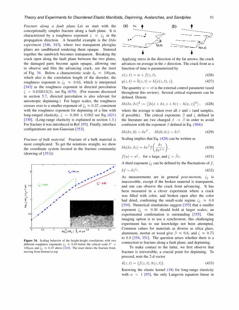
Theory and Experiments for Disordered Elastic Manifolds, Depinning, Avalanches, and Sandpiles 51
Fracture along a fault plane. Let us start with theconceptionally simpler fracture along a fault plane. It ischaracterized by a roughness exponent ζ ≡ ζ‖ in thepropagation direction. A beautiful example is the Osloexperiment [346, 343], where two transparent plexiglasplates are sandblasted rendering them opaque. Sinteredtogether the sandwich becomes transparent. Breaking thecrack open along the fault plane between the two plates,the damaged parts become again opaque, allowing oneto observe and film the advancing crack, see the insetof Fig. 34. Below a characteristic scale δ0 ≈ 100µm,which also is the correlation length of the disorder, theroughness exponent is ζ‖ ≈ 0.63, which is interpreted[343] as the roughness exponent in directed percolationζ = 0.632613(3), see Eq. (670). (For reasons discussedin section 5.7, directed percolation is also relevant foranisotropic depinning.) For larger scales, the roughnesscrosses over to a smaller exponent of ζ‖ ≈ 0.37, consistentwith the roughness exponent for depinning of a line withlong-ranged elasticity, ζ = 0.388 ± 0.002 see Eq. (421)[330]. (Long-range elasticity is explained in section 1.3.)For fracture it was introduced in Ref. [93]. Finally, interfaceconfigurations are non-Gaussian [353].
Fracture of bulk material. Fracture of a bulk material ismore complicated. To get the notations straight, we showthe coordinate system favored in the fracture community(drawing of [351]):
Figure 34. Scaling behavior of the height-height correlations with twodifferent roughness exponents ζ‖ ≈ 0.63 below the critical scale δ∗ =100µm and ζ‖ ≈ 0.37 above [343]. The inset shows the fracture front,moving from bottom to top.
Chapter 4: Fracture surfaces for model linear elastic disordered materials 73
lead to a planar fracture surface (the plane (z, x)). But the heterogeneities of thematerial induce both in-plane (along x) and out-of -plane (along y) perturbationsof the shape of the edge. Schematic views of the in-plane f(z, t) and out-of-plane
Figure 4.1: Geometry of perturbed cracks subject to mode I loading (large arrowsindicating the direction of macroscopic loading). (a): In-plane perturbations. (b):Out-of-plane perturbations. The shape of the fracture surface is effectively the historyof the out-of-plane perturbations of the crack front. (Taken from Ref. [40]).
h(x = x0 + f(z, t), z) displacements are shown in Fig. 4.1. For simplicity, the out-of-plane perturbations are represented for a crack front without in-plane perturbations(f(z, t) = 0). The fracture surface is the print of the out-of-plane perturbations h(x, z)of the crack front. In the following, we will see that, for small enough perturbations,the out-of-plane displacements are independent of the in-plane displacements so thatthe shape of the fracture surface can be predicted independently of f(z, t). Thisimplies that the dynamical properties of the crack – the local velocities of the crackfront ∂f
∂t(z, t) – are decoupled from the crack trajectory h(x, z). An experimental
argument based on the analysis of fracture surfaces will also support this statement(see Section 4.2 ).
Stress field in the vicinity of a slightly perturbed crack front : We considernow a point M of the crack front characterized by its position (x = x0 + f(z, t), y =h(x, z), z). The local stress field around M determines its trajectory. The stress at adistance r ahead of the point M in the direction θ can be written as the sum of thecontributions of each of the three fracture modes (see Section 1.1), each mode beingdeveloped as a rk/2 expansion with k ≥ −1
σij =
III!
p=I
Kp√2πr
gijp (θ) + Tpk
ijp (θ) + Apl
ijp (θ)
√r + ... (4.1)
where Kp (the so-called stress intensity factors), Tp (T -stress) and Ap are constantsdepending on the loading and the geometry of the sample. gij
p , kijp and lijp are universal
Applying stress in the direction of the fat arrows, the crackadvances on average in the x direction. The crack front as afunction of time is parameterized by
x(z, t) = w + f(z, t), (426)
y(z, t) = h(z, t) = h(x(z, t), z
). (427)
The quantity w = vt is the external control parameter (usedthroughout this review). Several critical exponents can bedefined. Denote
δh(δx, δz)2 :=⟨[h(x+ δx, z + δz)− h(x, z)]2
⟩, (428)
where the average is taken over all x and z (and samples,if possible). The critical exponents β and ζ defined inthe literature are (we changed β → β in order to avoidconfusion with the exponent β defined in Eq. (304))
δh(δx, 0) ∼ δxβ , δh(0, δz) ∼ δzζ . (429)
Scaling implies that Eq. (428) can be written as
δh(δx, δz) = δxβf
(δz
δx1/z
), (430)
f(u) ∼ uζ , for u large, and ζ = βz. (431)
A third exponent ζ‖ can be defined by the fluctuations of f ,
δf ∼ δzζ‖ . (432)
As measurements are in general post-mortem, ζ‖ isinaccessible, except if the broken material is transparent,and one can observe the crack front advancing. It hasbeen measured in a clever experiment where a crackwas filled with color, and broken open after the colorhad dried, confirming the small-scale regime ζ‖ ≈ 0.6[354]. Numerical simulations suggest [355] that a smallerexponent ζ‖ ≈ 0.38 should hold at larger scales; anexperimental confirmation is outstanding [355]. Oneimaging option is to use a synchrotron; this challengingexperiment has to our knowledge not been attempted.Common values for materials as diverse as silica glass,aluminum, mortar or wood give β ≈ 0.6, and ζ ≈ 0.75to 0.8 [354, 351]. The question arises whether there is aconnection to fracture along a fault plane, and depinning.
To make contact to the latter, we first observe thatfracture is irreversible, a crucial point for depinning. Toproceed, note the 2-d vector
~u(z, t) =(f(z, t), h(z, t)
). (433)
Knowing the elastic kernel (18) for long-range elasticitywith α = 1 [93], the only Langevin equation linear in
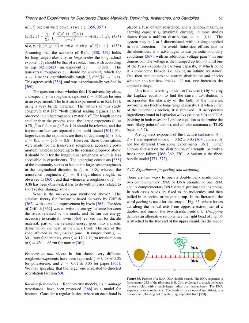
Theory and Experiments for Disordered Elastic Manifolds, Depinning, Avalanches, and Sandpiles 52
u(z, t) one can write down is (see e.g. [356, 357])
∂t~u(z, t) =γ
2π
∫
z′
~u(z′, t)−~u(z, t)
(z−z′)2+ η(~u(z, t), z
), (434)
η(x, y, z)η(x′, y′, z′) = σδ(x−x′)δ(y−y′)δ(z−z′). (435)
Assuming that the scenario of Refs. [358, 359] holdsfor long-ranged elasticity, at large scales the longitudinalexponent ζ‖ should be that of a contact line, with accordingto Eqs. (421)-(423) an exponent ζ‖ = 0.388. Thetransversal roughness ζ⊥ should be thermal, which forα = 1 means logarithmically rough (
∫k
eikz/|k| ∼ ln z).This agrees with [356], and was experimentally verified in[360].
The question arises whether this LR universality class,and especially the roughness exponent ζ = 0.38 can be seenin an experiment. The first such experiment is in Ref. [73],using a very brittle material. The authors of this studyconjecture that [73] “both critical scaling regimes can beobserved in all heterogeneous materials:” For length scalessmaller than the process zone, the larger exponents (ζ ≈0.75, β ≈ 0.6, z = ζ/β ≈ 1.2) should be relevant, and thefracture surface was reported to be multi-fractal [361]. Forlarger scales the exponents are those of depinning (ζ ≈ 0.4,β = 0.5, z = ζ/β ≈ 0.8). However, these observationswere made for the transversal roughness, accessible post-mortem, whereas according to the scenario proposed aboveit should hold for the longitudinal roughness which is lessaccessible in experiments. The emerging consensus [355]of the community seems to be that the large-scale roughnessin the longitudinal direction is ζ‖ ≈ 0.38, whereas thetransversal roughness ζ⊥ = 0 (logarithmic rough), asobserved in [360]; and that whenever a roughness of ζ⊥ ≈0.38 has been observed, it has to do with physics related toshort scales (damage zone).
What is the process-zone mentioned above? Thestandard theory for fracture is based on work by Griffith[362], with a crucial improvement by Irwin [363]. The ideaof Griffith [362] was to write an energy balance betweenthe stress released by the crack, and the surface energynecessary to create it. Irwin [363] realized that for ductilematerial, part of the released energy goes into a plasticdeformation, i.e. heat, at the crack front. The size of thezone affected is the process zone. It ranges from ξ =50±9µm for ceramics, over ξ = 170±12µm for aluminumto ξ = 450± 35µm for mortar [361].
Fracture in thin sheets. In thin sheets, very differentroughness exponents have been reported: ζ = 0.48 ± 0.05for polysterene, and ζ = 0.67 ± 0.05 for paper [365].We may speculate that the larger one is related to directedpercolation (section 5.8).
Random fuse models. Random fuse models, a.k.a. damagepercolation, have been proposed [366] as a model forfracture: Consider a regular lattice, where on each bond is
placed a fuse of unit resistance, and a random maximumcarrying capacity ic (maximal current), in most studiesdrawn from a uniform distribution, ic ∈ [0, 1]. Thesystem may be 2 or 3-dimensional, with a voltage appliedin one direction. To avoid finite-size effects due tothe electrodes, it is advantages to use periodic boundaryconditions [367], with an additional voltage gain V in onedimension. The voltage is then ramped up from 0, until oneof the fuses exceeds its carrying capacity, at which pointit is considered broken, i.e. having an infinite resistance.One then recalculates the current distribution and checkswhether another fuse breaks. If not, one increases theapplied voltage.
This is an interesting model for fracture: (i) by solvingthe Laplace equation to find the current distribution, itincorporates the elasticity of the bulk of the material,providing an effective long-range elasticity; (ii) when a partof the material is broken, it is removed. It incorporatesingredients found in Laplacian walks (section 8.9) and DLA(solving in both cases the Laplace equation to determine themost likely point of action), and cellular automata as TL92(section 5.7).
A roughness exponent of the fracture surface in d =2 + 1 was reported to be ζ = 0.62± 0.05 [367], apparentlynot too different from some experiments [367]. Otherauthors focused on the distribution of strength, or brokenfuses upon failure [368, 369, 370]. A variant is the fiber-bundle model [371, 372].
3.17. Experiments for peeling and unzipping
There are two ways to open a double helix made out oftwo complementary RNA or DNA strands, or one RNAand its complementary DNA strand: peeling and unzipping.In both cases beads are fixed to the molecules, and thenpulled in an optical or magnetic trap. In the literature, theword peeling is used for the setup of Fig. 35, where forcesact along the helical axis from opposite extremities of aduplex, and one of the two strands peels off. Unzippingdenotes an alternative setup where the right bead of Fig. 35is attached to the free end of the upper strand. As the reader
Partial anneal
Full anneal
No anneal
RNA
DNA
w
u
Figure 35. Peeling of a RNA-DNA double strand. The RNA sequence isfrom subunit 23S of the ribosome in E. Coli, prolonged to attach the beads(brown circles, with a much larger radius than drawn here). The DNAsequence is its complement. The beads sit in an optical trap (blue), at adistance w. (Drawing not to scale.) Fig. reprinted from [364].
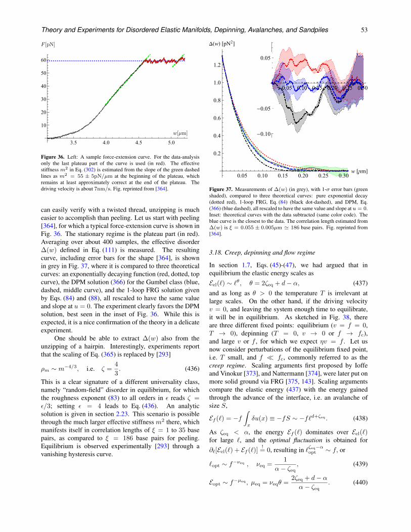
Theory and Experiments for Disordered Elastic Manifolds, Depinning, Avalanches, and Sandpiles 53
3.5 4.0 4.5 5.0
10
20
30
40
50
60
w[µm]
F [pN]
Figure 36. Left: A sample force-extension curve. For the data-analysisonly the last plateau part of the curve is used (in red). The effectivestiffness m2 in Eq. (302) is estimated from the slope of the green dashedlines as m2 = 55 ± 5pN/µm at the beginning of the plateau, whichremains at least approximately correct at the end of the plateau. Thedriving velocity is about 7nm/s. Fig. reprinted from [364].
can easily verify with a twisted thread, unzipping is mucheasier to accomplish than peeling. Let us start with peeling[364], for which a typical force-extension curve is shown inFig. 36. The stationary regime is the plateau part (in red).Averaging over about 400 samples, the effective disorder∆(w) defined in Eq. (111) is measured. The resultingcurve, including error bars for the shape [364], is shownin grey in Fig. 37, where it is compared to three theoreticalcurves: an exponentially decaying function (red, dotted, topcurve), the DPM solution (366) for the Gumbel class (blue,dashed, middle curve), and the 1-loop FRG solution givenby Eqs. (84) and (88), all rescaled to have the same valueand slope at u = 0. The experiment clearly favors the DPMsolution, best seen in the inset of Fig. 36. While this isexpected, it is a nice confirmation of the theory in a delicateexperiment.
One should be able to extract ∆(w) also from theunzipping of a hairpin. Interestingly, experiments reportthat the scaling of Eq. (365) is replaced by [293]
ρm ∼ m−4/3, i.e. ζ =4
3. (436)
This is a clear signature of a different universality class,namely “random-field” disorder in equilibrium, for whichthe roughness exponent (83) to all orders in ε reads ζ =ε/3; setting ε = 4 leads to Eq. (436). An analyticsolution is given in section 2.23. This scenario is possiblethrough the much larger effective stiffness m2 there, whichmanifests itself in correlation lengths of ξ = 1 to 35 basepairs, as compared to ξ = 186 base pairs for peeling.Equilibrium is observed experimentally [293] through avanishing hysteresis curve.
0.30
-0.10
-0.05
0.05
0.05 0.10 0.15 0.20 0.25 0.30w [ m]
0.2
0.4
0.6
0.8
1.0
1.2
(w) [pN2]
Figure 37. Measurements of ∆(w) (in grey), with 1-σ error bars (greenshaded), compared to three theoretical curves: pure exponential decay(dotted red), 1-loop FRG, Eq. (84) (black dot-dashed), and DPM, Eq.(366) (blue dashed), all rescaled to have the same value and slope at u = 0.Inset: theoretical curves with the data subtracted (same color code). Theblue curve is the closest to the data. The correlation length estimated from∆(w) is ξ = 0.055 ± 0.005µm ' 186 base pairs. Fig. reprinted from[364].
3.18. Creep, depinning and flow regime
In section 1.7, Eqs. (45)-(47), we had argued that inequilibrium the elastic energy scales asEel(`) ∼ `θ, θ = 2ζeq + d− α, (437)and as long as θ > 0 the temperature T is irrelevant atlarge scales. On the other hand, if the driving velocityv = 0, and leaving the system enough time to equilibrate,it will be in equilibrium. As sketched in Fig. 38, thereare three different fixed points: equilibrium (v = f = 0,T → 0), depinning (T = 0, v → 0 or f → fc),and large v or f , for which we expect ηv = f . Let usnow consider perturbations of the equilibrium fixed point,i.e. T small, and f fc, commonly referred to as thecreep regime. Scaling arguments first proposed by Ioffeand Vinokur [373], and Nattermann [374], were later put onmore solid ground via FRG [375, 143]. Scaling argumentscompare the elastic energy (437) with the energy gainedthrough the advance of the interface, i.e. an avalanche ofsize S,
Ef (`) = −f∫
x
δu(x) ≡ −fS ∼ −f`d+ζeq . (438)
As ζeq < α, the energy Ef (`) dominates over Eel(`)for large `, and the optimal fluctuation is obtained for∂`[Eel(`) + Ef (`)]
!= 0, resulting in `ζeq−αopt ∼ f, or
`opt ∼ f−νeq , νeq =1
α− ζeq, (439)
Eopt ∼ f−µeq , µeq = νeqθ =2ζeq + d− αα− ζeq
. (440)
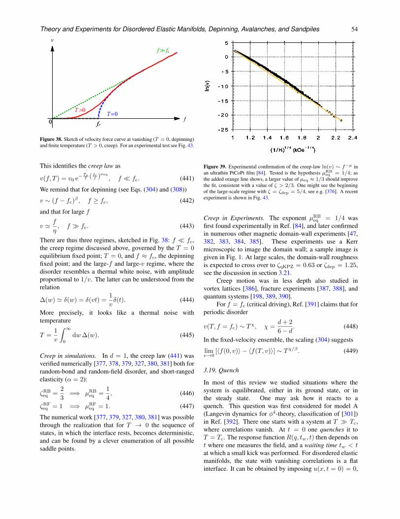
Theory and Experiments for Disordered Elastic Manifolds, Depinning, Avalanches, and Sandpiles 54
fc0
T=0T>0
fc0
f≫ fc
f
v
Figure 38. Sketch of velocity force curve at vanishing (T = 0, depinning)and finite temperature (T > 0, creep). For an experimental test see Fig. 43.
This identifies the creep law as
v(f, T ) = v0 e−T∗T ( fcf )
µeq
, f fc. (441)
We remind that for depinning (see Eqs. (304) and (308))
v ∼ (f − fc)β , f ≥ fc, (442)
and that for large f
v ' f
η, f fc. (443)
There are thus three regimes, sketched in Fig. 38: f fc,the creep regime discussed above, governed by the T = 0equilibrium fixed point; T = 0, and f ≈ fc, the depinningfixed point; and the large-f and large-v regime, where thedisorder resembles a thermal white noise, with amplitudeproportional to 1/v. The latter can be understood from therelation
∆(w) ' δ(w) = δ(vt) =1
vδ(t). (444)
More precisely, it looks like a thermal noise withtemperature
T =1
v
∫ ∞
0
dw∆(w). (445)
Creep in simulations. In d = 1, the creep law (441) wasverified numerically [377, 378, 379, 327, 380, 381] both forrandom-bond and random-field disorder, and short-rangedelasticity (α = 2):
ζRBeq =
2
3=⇒ µRB
eq =1
4, (446)
ζRFeq = 1 =⇒ µRF
eq = 1. (447)
The numerical work [377, 379, 327, 380, 381] was possiblethrough the realization that for T → 0 the sequence ofstates, in which the interface rests, becomes deterministic,and can be found by a clever enumeration of all possiblesaddle points.
Figure 39. Experimental confirmation of the creep-law ln(v) ∼ f−µ inan ultrathin PtCoPt film [84]. Tested is the hypothesis µRB
eq = 1/4; asthe added orange line shows, a larger value of µeq ≈ 1/3 should improvethe fit, consistent with a value of ζ > 2/3. One might see the beginningof the large-scale regime with ζ = ζdep = 5/4, see e.g. [376]. A recentexperiment is shown in Fig. 43.
Creep in Experiments. The exponent µRBeq = 1/4 was
first found experimentally in Ref. [84], and later confirmedin numerous other magnetic domain-wall experiments [47,382, 383, 384, 385]. These experiments use a Kerrmicroscopic to image the domain wall; a sample image isgiven in Fig. 1. At large scales, the domain-wall roughnessis expected to cross over to ζqKPZ = 0.63 or ζdep = 1.25,see the discussion in section 3.21.
Creep motion was in less depth also studied invortex lattices [386], fracture experiments [387, 388], andquantum systems [198, 389, 390].
For f = fc (critical driving), Ref. [391] claims that forperiodic disorder
v(T, f = fc) ∼ Tχ, χ =d+ 2
6− d . (448)
In the fixed-velocity ensemble, the scaling (304) suggests
limv→0
[〈f(0, v)〉 − 〈f(T, v)〉] ∼ Tχ/β . (449)
3.19. Quench
In most of this review we studied situations where thesystem is equilibrated, either in its ground state, or inthe steady state. One may ask how it reacts to aquench. This question was first considered for model A(Langevin dynamics for φ4-theory, classification of [301])in Ref. [392]. There one starts with a system at T Tc,where correlations vanish. At t = 0 one quenches it toT = Tc. The response function R(q, tw, t) then depends ont where one measures the field, and a waiting time tw < tat which a small kick was performed. For disordered elasticmanifolds, the state with vanishing correlations is a flatinterface. It can be obtained by imposing u(x, t = 0) = 0,
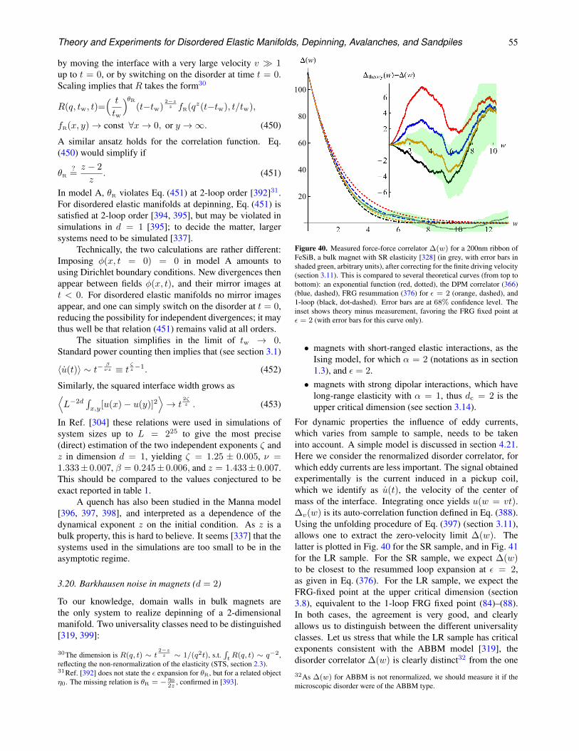
Theory and Experiments for Disordered Elastic Manifolds, Depinning, Avalanches, and Sandpiles 55
by moving the interface with a very large velocity v 1up to t = 0, or by switching on the disorder at time t = 0.Scaling implies that R takes the form30
R(q, tw, t)=( t
tw
)θR(t−tw)
2−zz fR(qz(t−tw), t/tw),
fR(x, y)→ const ∀x→ 0, or y →∞. (450)
A similar ansatz holds for the correlation function. Eq.(450) would simplify if
θR?=z − 2
z. (451)
In model A, θR violates Eq. (451) at 2-loop order [392]31.For disordered elastic manifolds at depinning, Eq. (451) issatisfied at 2-loop order [394, 395], but may be violated insimulations in d = 1 [395]; to decide the matter, largersystems need to be simulated [337].
Technically, the two calculations are rather different:Imposing φ(x, t = 0) = 0 in model A amounts tousing Dirichlet boundary conditions. New divergences thenappear between fields φ(x, t), and their mirror images att < 0. For disordered elastic manifolds no mirror imagesappear, and one can simply switch on the disorder at t = 0,reducing the possibility for independent divergences; it maythus well be that relation (451) remains valid at all orders.
The situation simplifies in the limit of tw → 0.Standard power counting then implies that (see section 3.1)
〈u(t)〉 ∼ t− βνz ≡ t ζz−1. (452)
Similarly, the squared interface width grows as⟨L−2d
∫x,y
[u(x)− u(y)]2⟩→ t
2ζz . (453)
In Ref. [304] these relations were used in simulations ofsystem sizes up to L = 225 to give the most precise(direct) estimation of the two independent exponents ζ andz in dimension d = 1, yielding ζ = 1.25 ± 0.005, ν =1.333± 0.007, β = 0.245± 0.006, and z = 1.433± 0.007.This should be compared to the values conjectured to beexact reported in table 1.
A quench has also been studied in the Manna model[396, 397, 398], and interpreted as a dependence of thedynamical exponent z on the initial condition. As z is abulk property, this is hard to believe. It seems [337] that thesystems used in the simulations are too small to be in theasymptotic regime.
3.20. Barkhausen noise in magnets (d = 2)
To our knowledge, domain walls in bulk magnets arethe only system to realize depinning of a 2-dimensionalmanifold. Two universality classes need to be distinguished[319, 399]:
30The dimension is R(q, t) ∼ t2−zz ∼ 1/(q2t), s.t.
∫tR(q, t) ∼ q−2,
reflecting the non-renormalization of the elasticity (STS, section 2.3).31Ref. [392] does not state the ε expansion for θR, but for a related objectη0. The missing relation is θR = − η0
2z, confirmed in [393].
10w
-6
-4
-2
2
4
6
theory(w)- (w)
2 4 6 8 10 12w
20
40
60
80
100
(w)
Figure 40. Measured force-force correlator ∆(w) for a 200nm ribbon ofFeSiB, a bulk magnet with SR elasticity [328] (in grey, with error bars inshaded green, arbitrary units), after correcting for the finite driving velocity(section 3.11). This is compared to several theoretical curves (from top tobottom): an exponential function (red, dotted), the DPM correlator (366)(blue, dashed), FRG resummation (376) for ε = 2 (orange, dashed), and1-loop (black, dot-dashed). Error bars are at 68% confidence level. Theinset shows theory minus measurement, favoring the FRG fixed point atε = 2 (with error bars for this curve only).
• magnets with short-ranged elastic interactions, as theIsing model, for which α = 2 (notations as in section1.3), and ε = 2.
• magnets with strong dipolar interactions, which havelong-range elasticity with α = 1, thus dc = 2 is theupper critical dimension (see section 3.14).
For dynamic properties the influence of eddy currents,which varies from sample to sample, needs to be takeninto account. A simple model is discussed in section 4.21.Here we consider the renormalized disorder correlator, forwhich eddy currents are less important. The signal obtainedexperimentally is the current induced in a pickup coil,which we identify as u(t), the velocity of the center ofmass of the interface. Integrating once yields u(w = vt).∆v(w) is its auto-correlation function defined in Eq. (388).Using the unfolding procedure of Eq. (397) (section 3.11),allows one to extract the zero-velocity limit ∆(w). Thelatter is plotted in Fig. 40 for the SR sample, and in Fig. 41for the LR sample. For the SR sample, we expect ∆(w)to be closest to the resummed loop expansion at ε = 2,as given in Eq. (376). For the LR sample, we expect theFRG-fixed point at the upper critical dimension (section3.8), equivalent to the 1-loop FRG fixed point (84)–(88).In both cases, the agreement is very good, and clearlyallows us to distinguish between the different universalityclasses. Let us stress that while the LR sample has criticalexponents consistent with the ABBM model [319], thedisorder correlator ∆(w) is clearly distinct32 from the one32As ∆(w) for ABBM is not renormalized, we should measure it if themicroscopic disorder were of the ABBM type.
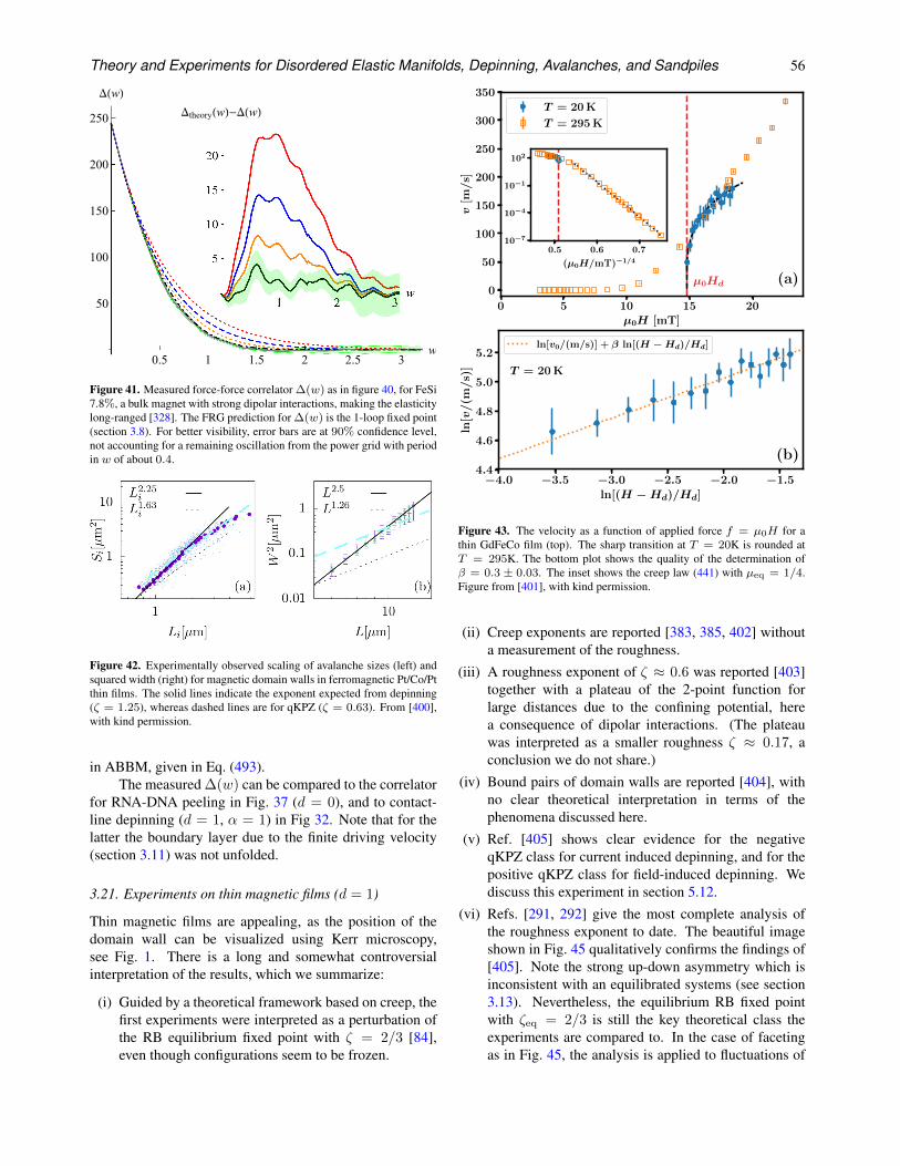
Theory and Experiments for Disordered Elastic Manifolds, Depinning, Avalanches, and Sandpiles 56
w
5
10
15
20
Δtheory(w)-Δ(w)
0.5 1 1.5 2 2.5 3w
50
100
150
200
250
Δ(w)
Figure 41. Measured force-force correlator ∆(w) as in figure 40, for FeSi7.8%, a bulk magnet with strong dipolar interactions, making the elasticitylong-ranged [328]. The FRG prediction for ∆(w) is the 1-loop fixed point(section 3.8). For better visibility, error bars are at 90% confidence level,not accounting for a remaining oscillation from the power grid with periodin w of about 0.4.
Figure 42. Experimentally observed scaling of avalanche sizes (left) andsquared width (right) for magnetic domain walls in ferromagnetic Pt/Co/Ptthin films. The solid lines indicate the exponent expected from depinning(ζ = 1.25), whereas dashed lines are for qKPZ (ζ = 0.63). From [400],with kind permission.
in ABBM, given in Eq. (493).The measured ∆(w) can be compared to the correlator
for RNA-DNA peeling in Fig. 37 (d = 0), and to contact-line depinning (d = 1, α = 1) in Fig 32. Note that for thelatter the boundary layer due to the finite driving velocity(section 3.11) was not unfolded.
3.21. Experiments on thin magnetic films (d = 1)
Thin magnetic films are appealing, as the position of thedomain wall can be visualized using Kerr microscopy,see Fig. 1. There is a long and somewhat controversialinterpretation of the results, which we summarize:
(i) Guided by a theoretical framework based on creep, thefirst experiments were interpreted as a perturbation ofthe RB equilibrium fixed point with ζ = 2/3 [84],even though configurations seem to be frozen.
2
pinning transition and allocate the studied model systemin the qEW universality class.
Experimental details - The studied sample consists ina Ta(5 nm)/Gd32Fe61.2Co6.8(10 nm)/Pt(5 nm) trilayerdeposited on a thermally oxidized silicon SiO2(100 nm)substrate by RF sputtering. The GdFeCo thin filmis a rare earth-transition metal (RE-TM) ferrimagneticcompound presenting perpendicular magnetic anisotropywith the RE and TM magnetic moments antiferromag-netically coupled. DW motion is measured using PolarMagneto-Optical Kerr E↵ect (PMOKE) microscopy. Weobtain images of DWs before and after the applicationof square-shaped magnetic field pulses of amplitude Hand duration t, and measure the resulting mean DWdisplacement x. The mean DW velocity v, characteriz-ing its collective motion, at a given field H is calculatedas x/t. The maximum investigated field is limitedby the nucleation of multiple magnetic domains, whichimpedes clear DW displacement measurements. Addi-tionally, the microscope is equipped with a cryostat anda temperature controller that give us access to a widetemperature range, from 4 K to 360 K.
Zero-temperature-like depinning transition - The con-tribution of thermal e↵ects on the depinning transitionis shown in Fig. 1(a), which compares two velocity-field curves with very similar depinning threshold (Hd 15 mT) measured at temperatures that di↵er in morethan one order of magnitude (20 K and 295 K). Asit can be observed, thermal activation blurs the depin-ning transition. Above Hd, velocities measured at bothtemperatures are rather similar. However, close to Hd
the velocity sharply decreases for T = 20 K while it re-mains finite, even well below Hd, for T = 295 K. [28].The curve obtained for T = 295 K (Fig. 1(a)) presentsboth the typical thermally activated behavior for lowfields and the thermal rounding around Hd, as has beenreported in the literature for most of the field- andcurrent-driven experiments [29, 30]. Below the depin-ning threshold (3 mT < H < Hd), the DWs follow athermally activated creep dynamics. The velocity obeysthe Arrhenius law v(H, T ) = v(Hd, T )eE/kBT , withkB the Boltzmann constant. The universal creep bar-
rier is given by E = kBTd
h(H/Hd)
µ 1i
[29], where
Td is the so-called depinning temperature and µ is thecreep exponent (µ = 1/4) [3, 10, 17]. As observed inFig. 1(a) (see the inset), the experimental data measuredat T = 295 K, which covers more than eight orders ofmagnitude, are in good agreement with the creep law.Remarkably, the depinning temperature estimated fromthe fit, Td 10000 K, is among the largest Td reportedin the literature [31]. Moreover, for the lowest temper-ature at which we can observe a clean creep dynamics,T = 100 K, the value of Td is close to 30000 K. Thiscorresponds to a ratio Td/T (> 300), which had neverbeen reached experimentally [31] so far.
0 5 10 15 20µ0H [mT]
0
50
100
150
200
250
300
350
v[m
/s]
µ0Hd (a)
T = 20 K
T = 295 K
0.5 0.6 0.7
(µ0H/mT)1/4
107
104
101
102
4.0 3.5 3.0 2.5 2.0 1.5ln[(H Hd)/Hd]
4.4
4.6
4.8
5.0
5.2
ln[v
/(m
/s)
] T = 20 K
(b)
ln[v0/(m/s)] + ln[(H Hd)/Hd]
Figure 1. High- and low-temperature velocity curves. (a)Domain wall velocity (v) as a function of the external mag-netic field (µ0H) for a GdFeCo thin film at T = 20 K (circles)and T = 295 K (squares). The depinning field µ0Hd corre-sponding to T = 20 K (vertical dashed red line), and the fitof Eq. (1) for that temperature (dashed black line) are indi-cated. In the inset, in semi-logarithmic scale, the thermallyactivated creep regime observed for T = 295 K is emphasizedwith the dotted line, a fit to the creep formula. (b) Resultsobtained at T = 20 K and plotted in a logarithmic scale toillustrate an excellent agreement with Eq. (1). The fittedparameters are = 0.28 ± 0.08, µ0Hd = 14.8 ± 0.2 mT andv0 = 270 ± 40 m/s.
The universal velocity depinning exponent - The ra-tio Td/T is strongly enhanced as the temperature de-creases, thus explaining the absence of creep regime andthe quasi-athermal depinning behavior observed for theTa/GdFeCo/Pt film at T = 20 K. Then the velocity-fielddata at T = 20 K can be analyzed as a zero temperature-like depinning transition. Quantitative information isthus obtained by fitting the data using [14, 17, 32–36]
v(H, T = 0 K) = v0
H Hd
Hd
. (1)
In Eq. (1), the depinning velocity v0 and Hd are ma-terial and temperature dependent parameters [14, 33].As shown in Fig. 1(b), the data presents a good quan-titative agreement with the prediction over the wholerange of measured magnetic fields (see [36] for detailson the fitting procedure). Our direct experimental mea-surement of (= 0.28±0.08) somehow justifies the valuesassumed in former experimental studies of depinning [14]( = 0.25), and, more importantly, matches the exponent
Figure 43. The velocity as a function of applied force f = µ0H for athin GdFeCo film (top). The sharp transition at T = 20K is rounded atT = 295K. The bottom plot shows the quality of the determination ofβ = 0.3 ± 0.03. The inset shows the creep law (441) with µeq = 1/4.Figure from [401], with kind permission.
(ii) Creep exponents are reported [383, 385, 402] withouta measurement of the roughness.
(iii) A roughness exponent of ζ ≈ 0.6 was reported [403]together with a plateau of the 2-point function forlarge distances due to the confining potential, herea consequence of dipolar interactions. (The plateauwas interpreted as a smaller roughness ζ ≈ 0.17, aconclusion we do not share.)
(iv) Bound pairs of domain walls are reported [404], withno clear theoretical interpretation in terms of thephenomena discussed here.
(v) Ref. [405] shows clear evidence for the negativeqKPZ class for current induced depinning, and for thepositive qKPZ class for field-induced depinning. Wediscuss this experiment in section 5.12.
(vi) Refs. [291, 292] give the most complete analysis ofthe roughness exponent to date. The beautiful imageshown in Fig. 45 qualitatively confirms the findings of[405]. Note the strong up-down asymmetry which isinconsistent with an equilibrated systems (see section3.13). Nevertheless, the equilibrium RB fixed pointwith ζeq = 2/3 is still the key theoretical class theexperiments are compared to. In the case of facetingas in Fig. 45, the analysis is applied to fluctuations of
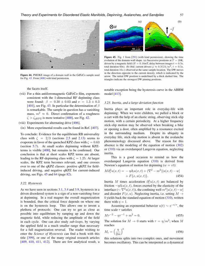
Theory and Experiments for Disordered Elastic Manifolds, Depinning, Avalanches, and Sandpiles 57
Figure 44. PMOKE image of a domain wall in the GdFeCo sample usedfor Fig. 43. From [408] with kind permission.
the facets itself.(vii) For a thin antiferromagnetic GdFeCo film, exponents
consistent with the 1-dimensinal RF depinning classwere found: β = 0.30 ± 0.03 and ν = 1.3 ± 0.3[401], see Fig. 43. In particular the determination of βis remarkable. The sample in question has a vanishingmass, m2 ≈ 0. Direct confirmation of a roughnessζ > ζqKPZ is more tentative [400], see Fig. 42.
(viii) Experiments for alternating drive [406].(ix) More experimental results can be found in Ref. [407].
To conclude: Evidence for the equilibrium RB universalityclass with ζ = 2/3 (sections 2.5 and 2.13) seems toevaporate in favor of the quenched KPZ class with ζ = 0.63(section 5.7). At small scales depinning without KPZ-terms is visible [400], but remains to be confirmed. Ourconclusion is that at short scales KPZ terms are absent,leading to the RF-depinning class with ζ = 1.25. At largerscales, the KPZ term becomes relevant, and one crossesover to one of the qKPZ classes: positive qKPZ for field-induced driving, and negative qKPZ for current-induceddriving, see Figs. 45 and 64 (page 82).
3.22. Hysteresis
As we have seen in sections 3.1, 3.4 and 3.9, hysteresis in adriven disordered system is a sign of a non-vanishing forceat depinning. In a real magnet the overall magnetizationis bounded, thus the critical force depends on where oneis on the hysteresis loop. This allows one to invent aplethora of protocols: One can try to get as close aspossible into equilibrium by ramping up and down themagnetic field, while reducing the amplitude of the fieldin each cycle. One can also study sub-loops, by varyingthe applied field in a much smaller range than necessaryfor a full magnetization reversal. The reader wishing toenter the Science of Hysteresis can find a book with thistitle [399], or one of the many original research articles[409, 410, 411, 412]. There are few analytical result, a
R. DÍAZ PARDO et al. PHYSICAL REVIEW B 100, 184420 (2019)
DWs produced by current and magnetic field remains an openquestion. Moreover, the origin of STT-induced DW tilting andits contribution to DW dynamics and universal behaviors arenot well understood.
In this paper, we propose an extensive and comparativestudy on DW motion driven by STT and magnetic field.Investigations were conducted with the ferromagnetic semi-conductor (Ga,Mn)As, which presents a sufficiently low de-pinning threshold [24] to cover the creep, depinning, and flowdynamical regimes [25], and to discuss, in particular, DWtilting without pinning. Our stringent test of universality relieson the verification that magnetic-field-driven DW motion inour sample shares the common universal (material and tem-perature independent) behaviors encountered in a variety ofother magnetic materials [4,5,9–11] and on the independentanalysis of DW dynamics and roughness, which are bothconsistent with the conclusion of common universal behaviorsfor STT and field-driven DW motion.
The paper is organized as follows. After a descriptionof the experimental techniques (Sec. II), we compare theshape evolution of DWs driven by STT and magnetic fieldand analyze their roughness (Sec. III). Section IV details acomparative study of DW dynamics. In Sec. V, we discuss theorigin of DW faceting produced by STT and its implicationsfor DW dynamics.
II. EXPERIMENTAL TECHNIQUES
The experiments were performed with rectangles of a4-nm-thick (Ga,Mn)(As,P)/(Ga,Mn)As bilayer film patternedby lithography. The film was grown on a (001) GaAs/AlAsbuffer [26]. It has an effective perpendicular anisotropy and aCurie temperature (Tc) of 65 K. The sizes of rectangles were133 × 210, 228 × 302, and 323 × 399 µm2 (see Appendix Afor the details). Two 40-µm-wide gold electrodes (separatedby 110, 204, and 300 µm, respectively) were deposited byevaporation parallel to the narrow sides of rectangles. Theywere used to generate a homogeneous current density drivingDW motion by STT. The pulse amplitude varied between0 and 11 GA/m2. We verified that the Joule effect had anegligible contribution on DW dynamics (see Appendix B).Perpendicular magnetic field pulses of adjustable amplitude(0–65 mT) were produced by a 75-turn small coil (diameter∼1 mm) mounted on the sample. The DW displacement isobserved using a magneto-optical Kerr microscope (resolution∼1 µm). The DW velocity is defined as the ratio between theaverage displacement ⟨u ⟩ and the pulse duration !t , whichvaries between 1 µs and 120 s. The setup was placed againstthe cold finger of an optical He-flow cryostat, which allowedthe temperature to be stabilized to between 5.7 K and Tc.
III. DOMAIN-WALL DISPLACEMENT AND ROUGHNESSIN THE CREEP REGIME
The time evolution of an initially almost flat DW drivenby magnetic field and STT is compared in Fig. 1. For field-driven DW motion, the average successive displacements arerelatively similar. The initial DW shape is almost conservedduring the motion. The DWs become sometimes stronglypinned and curved [see Fig. 1(a)] but are flattened again when
FIG. 1. Time evolution of DW shape. Successive positions of aDW, at T = 28 K, driven by (a) magnetic field (H = 0.16 mT, delaybetween images !t = 0.5 s, total duration 60 s) and (b) current( j ≈ 0.5 GA/m2, !t = 0.5 s, total duration 16 s) observed at thesame sample location. The DW move in the direction opposite tothe current density, which is indicated by the arrow. The initial DWposition is underlined by a thick dashed line. The triangles indicatethe strongest DW pinning positions.
depinned due to the combined effects of DW elasticity anddriving force, which acts as a pressure ( f ∝ H). In contrast,the initial DW shape is significantly altered by the current[see Fig. 1(b)]. DWs are tilted and form faceted structures.The faceting process seems to start close to “strong” pinningcenters [5] and to produce a reduction of DW displacementswith increasing tilting angle θ until DWs stop (on the ex-periment timescale), as already observed in Pt/Co/Pt films[5]. In Sec. V, we will show that the faceting results froman instability of the transverse alignment between current andthe DW, which can be triggered even without any contributionfrom pinning.
Let us start with investigations of universal behaviorswith a study on DW self-affinity using the displacement-displacement correlation function [4]:
w(L) =!
x
[u (x + L) − u (x)]2, (1)
where u (x) is the DW displacement measured parallel to thecurrent and L the length of DW segment along the x axis trans-verse to the current [see Fig. 2(a)]. For a self-affine interface,the function w(L) is expected to follow a power-law variationw(L) ∼ L2ζ , where ζ is the roughness exponent. Typicalvariations of w vs L obtained for field- and current-inducedmotion are compared in Fig. 2(b) in log-log scale. As it can beobserved, both curves present a linear variation with similarslopes (= 2ζ ), between the microscope resolution (≈ 1 µm)and L = 10 µm. In order to get more statistics, the slopes weresystematically determined for successions of DW positionsand a temperature varying over one decade (T = 4.5–59 K,see Appendix C for the statistical study). The mean and stan-dard deviation of the roughness exponent for current (ζ j)- andfield (ζH )-driven DW motion is reported in Fig. 2 as a functionof temperature. As expected for universal critical exponents,the values of ζ j and ζH do not vary significantly. Their meanvalues (ζ j = 0.60 ± 0.05 and ζH = 0.61 ± 0.04), calculatedfrom all measurements, agree well within experimental error,which is a signature of common universal behavior.
Here, it is important to discuss differences and sim-ilarities with the results reported for Pt/Co/Pt in Ref.[5]. For (Ga,Mn)(As,P), ζ j presents no significant variation
184420-2
Figure 45. Fig. 1 from [291] (with kind permission), showing the timeevolution of the domain-wall shape. (a) Successive positions at T = 28K,driven by a magnetic field (H = 0.16mT, delay between images t = 0.5s,total duration 60s). (b) ibid. current driven (j ≈ 0.5GA/m2, t = 0.5s,total duration 16s.) observed at the same sample location. The DW movesin the direction opposite to the current density, which is indicated by thearrow. The initial DW position is underlined by a thick dashed line. Thetriangles indicate the strongest DW pinning positions.
notable exception being the hysteresis curve in the ABBMmodel [413].
3.23. Inertia, and a large-deviation function
Inertia plays an important role in everyday-life withdepinning: When we were children, we pulled a block ora cart with the help of an elastic string, observing stick-slipmotion, with a certain periodicity. At a higher frequencystick-slip motion may be observed when breaking a bikeor opening a door, often amplified by a resonance excitedin the surrounding medium. Despite its ubiquity ineveryday life, stick-slip motion is absent in the avalanchephenomenology discussed above. The reason for thisabsence is the modeling of the equation of motion (302)or (310) via an overdamped Langevin equation, neglectinginertia.
This is a good occasion to remind us how theoverdamped Langevin equation (310) is derived fromNewton’s equation of motion for depinning (w = vt):
M∂2t u(x, t) = − η∂tu(x, t) + (∇2 −m2)[u(x, t)− w]
+ F(x, u(x, t)
). (454)
Inertia M times acceleration ∂2t u(x, t) are balanced by
friction −η∂tu(x, t), forces exerted by the elasticity of theinterface (∼ ∇2u(x, t)), the confining wellm2[u(x, t)−w]and disorder F (x, u). Neglecting inertia, i.e. setting M →0 yields back the standard equation of motion (310), writtenthere with η = 1.
Assuming an exponential behavior u(t) ∼ e−t/τ , thetime scale τ satisfies
Mτ−2 − ητ−1 +m2 = 0. (455)
The solution for M → 0 starts with τ = η/m2; when Mreaches
Mc =( η
2m
)2(456)
this solutions splits into two complex ones, and movementbecomes oscillatory. This can be interpreted as a dynamical
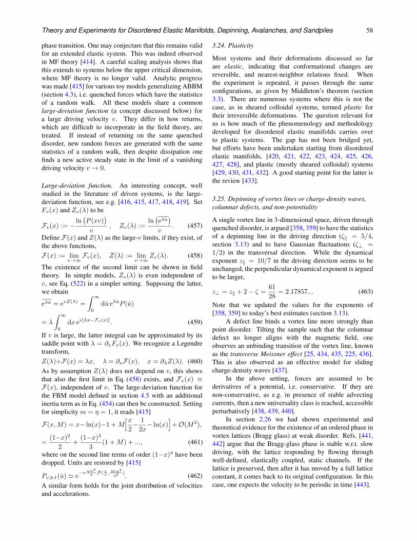
Theory and Experiments for Disordered Elastic Manifolds, Depinning, Avalanches, and Sandpiles 58
phase transition. One may conjecture that this remains validfor an extended elastic system. This was indeed observedin MF theory [414]. A careful scaling analysis shows thatthis extends to systems below the upper critical dimension,where MF theory is no longer valid. Analytic progresswas made [415] for various toy models generalizing ABBM(section 4.3), i.e. quenched forces which have the statisticsof a random walk. All these models share a commonlarge-deviation function (a concept discussed below) fora large driving velocity v. They differ in how returns,which are difficult to incorporate in the field theory, aretreated. If instead of returning on the same quencheddisorder, new random forces are generated with the samestatistics of a random walk, then despite dissipation onefinds a new active steady state in the limit of a vanishingdriving velocity v → 0.
Large-deviation function. An interesting concept, wellstudied in the literature of driven systems, is the large-deviation function, see e.g. [416, 415, 417, 418, 419]. SetFv(x) and Zv(λ) to be
Fv(x) := − ln(P (xv)
)
v, Zv(λ) :=
ln(eλu)
v. (457)
Define F(x) and Z(λ) as the large-v limits, if they exist, ofthe above functions,F(x) := lim
v→∞Fv(x), Z(λ) := lim
v→∞Zv(λ). (458)
The existence of the second limit can be shown in fieldtheory. In simple models, Zv(λ) is even independent ofv, see Eq. (522) in a simpler setting. Supposing the latter,we obtain
eλu = evZ(λ) =
∫ ∞
0
du eλuP (u)
= λ
∫ ∞
0
dx ev[λx−Fv(x)]. (459)
If v is large, the latter integral can be approximated by itssaddle point with λ = ∂xFv(x). We recognize a Legendretransform,Z(λ)+F(x) = λx, λ = ∂xF(x), x = ∂λZ(λ). (460)As by assumption Z(λ) does not depend on v, this showsthat also the first limit in Eq. (458) exists, and Fv(x) ≡F(x), independent of v. The large-deviation function forthe FBM model defined in section 4.5 with an additionalinertia term as in Eq. (454) can then be constructed. Settingfor simplicity m = η = 1, it reads [415]
F(x,M) = x− ln(x)−1 +M[x
2− 1
2x− ln(x)
]+O(M2),
=(1−x)2
2+
(1−x)3
3(1 +M) + ..., (461)
where on the second line terms of order (1−x)4 have beendropped. Units are restored by [415]
Pv1(u) ' e−v ηm2
σ F( uv ,Mm2
η2). (462)
A similar form holds for the joint distribution of velocitiesand accelerations.
3.24. Plasticity
Most systems and their deformations discussed so farare elastic, indicating that conformational changes arereversible, and nearest-neighbor relations fixed. Whenthe experiment is repeated, it passes through the sameconfigurations, as given by Middleton’s theorem (section3.3). There are numerous systems where this is not thecase, as in sheared colloidal systems, termed plastic fortheir irreversible deformations. The question relevant forus is how much of the phenomenology and methodologydeveloped for disordered elastic manifolds carries overto plastic systems. The gap has not been bridged yet,but efforts have been undertaken starting from disorderedelastic manifolds, [420, 421, 422, 423, 424, 425, 426,427, 428], and plastic (mostly sheared colloidal) systems[429, 430, 431, 432]. A good starting point for the latter isthe review [433].
3.25. Depinning of vortex lines or charge-density waves,columnar defects, and non-potentiality
A single vortex line in 3-dimensional space, driven throughquenched disorder, is argued [358, 359] to have the statisticsof a depinning line in the driving direction (ζ‖ = 5/4,section 3.13) and to have Gaussian fluctuations (ζ⊥ =1/2) in the transversal direction. While the dynamicalexponent z‖ = 10/7 in the driving direction seems to beunchanged, the perpendicular dynamical exponent is arguedto be larger,
z⊥ = z‖ + 2− ζ =61
28= 2.17857... (463)
Note that we updated the values for the exponents of[358, 359] to today’s best estimates (section 3.13).
A defect line binds a vortex line more strongly thanpoint disorder. Tilting the sample such that the columnardefect no longer aligns with the magnetic field, oneobserves an unbinding transition of the vortex line, knownas the transverse Meissner effect [25, 434, 435, 225, 436].This is also observed as an effective model for slidingcharge-density waves [437].
In the above setting, forces are assumed to bederivatives of a potential, i.e. conservative. If they arenon-conservative, as e.g. in presence of stable advectingcurrents, then a new universality class is reached, accessibleperturbatively [438, 439, 440].
In section 2.26 we had shown experimental andtheoretical evidence for the existence of an ordered phase invortex lattices (Bragg glass) at weak disorder. Refs. [441,442] argue that the Bragg-glass phase is stable w.r.t. slowdriving, with the lattice responding by flowing throughwell-defined, elastically coupled, static channels. If thelattice is preserved, then after it has moved by a full latticeconstant, it comes back to its original configuration. In thiscase, one expects the velocity to be periodic in time [443].
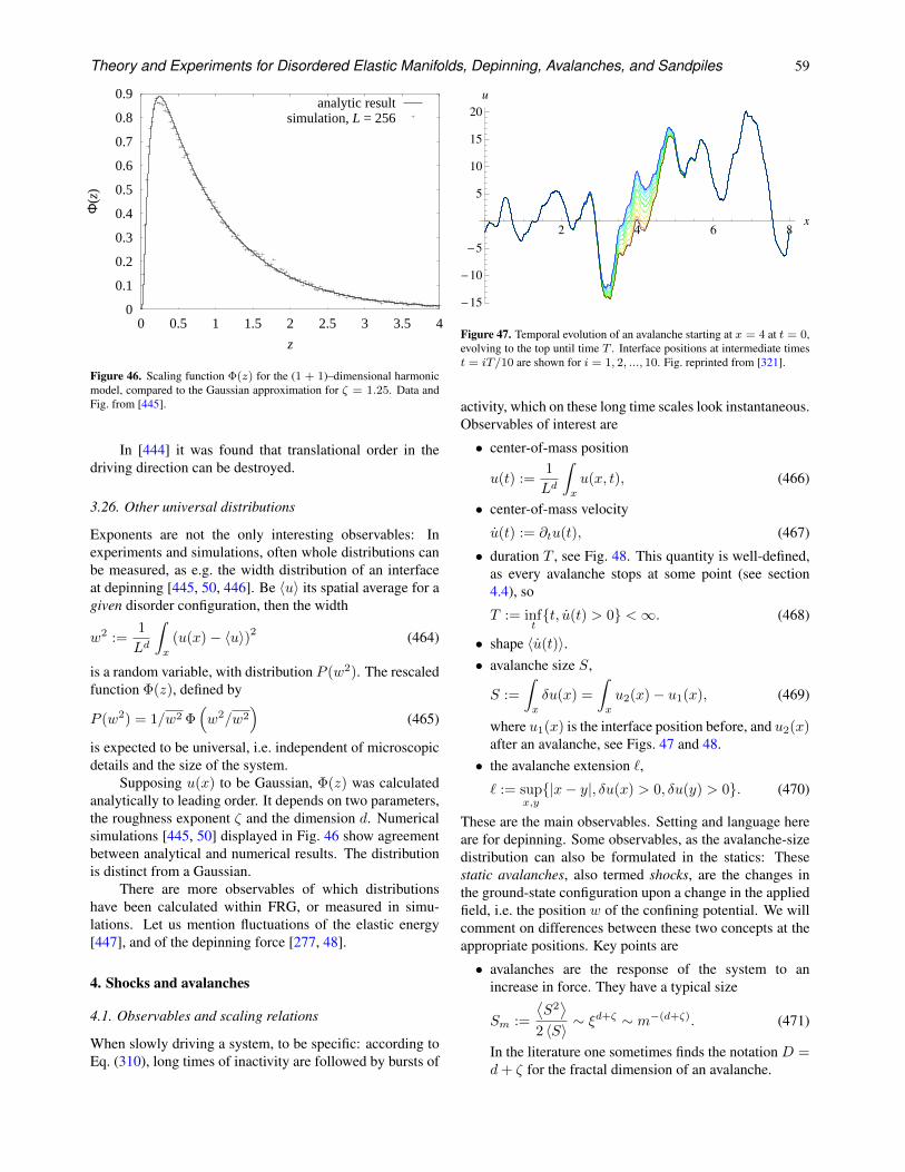
Theory and Experiments for Disordered Elastic Manifolds, Depinning, Avalanches, and Sandpiles 59
0
0.1
0.2
0.3
0.4
0.5
0.6
0.7
0.8
0.9
0 0.5 1 1.5 2 2.5 3 3.5 4
Φ(z
)
z
analytic resultsimulation, L = 256
Figure 46. Scaling function Φ(z) for the (1 + 1)–dimensional harmonicmodel, compared to the Gaussian approximation for ζ = 1.25. Data andFig. from [445].
In [444] it was found that translational order in thedriving direction can be destroyed.
3.26. Other universal distributions
Exponents are not the only interesting observables: Inexperiments and simulations, often whole distributions canbe measured, as e.g. the width distribution of an interfaceat depinning [445, 50, 446]. Be 〈u〉 its spatial average for agiven disorder configuration, then the width
w2 :=1
Ld
∫
x
(u(x)− 〈u〉)2 (464)
is a random variable, with distribution P (w2). The rescaledfunction Φ(z), defined by
P (w2) = 1/w2 Φ(w2/w2
)(465)
is expected to be universal, i.e. independent of microscopicdetails and the size of the system.
Supposing u(x) to be Gaussian, Φ(z) was calculatedanalytically to leading order. It depends on two parameters,the roughness exponent ζ and the dimension d. Numericalsimulations [445, 50] displayed in Fig. 46 show agreementbetween analytical and numerical results. The distributionis distinct from a Gaussian.
There are more observables of which distributionshave been calculated within FRG, or measured in simu-lations. Let us mention fluctuations of the elastic energy[447], and of the depinning force [277, 48].
4. Shocks and avalanches
4.1. Observables and scaling relations
When slowly driving a system, to be specific: according toEq. (310), long times of inactivity are followed by bursts of
2 4 6 8x
-15
-10
-5
5
10
15
20
u
Figure 47. Temporal evolution of an avalanche starting at x = 4 at t = 0,evolving to the top until time T . Interface positions at intermediate timest = iT/10 are shown for i = 1, 2, ..., 10. Fig. reprinted from [321].
activity, which on these long time scales look instantaneous.Observables of interest are
• center-of-mass position
u(t) :=1
Ld
∫
x
u(x, t), (466)
• center-of-mass velocity
u(t) := ∂tu(t), (467)
• duration T , see Fig. 48. This quantity is well-defined,as every avalanche stops at some point (see section4.4), so
T := inftt, u(t) > 0 <∞. (468)
• shape 〈u(t)〉.• avalanche size S,
S :=
∫
x
δu(x) =
∫
x
u2(x)− u1(x), (469)
where u1(x) is the interface position before, and u2(x)after an avalanche, see Figs. 47 and 48.
• the avalanche extension `,
` := supx,y|x− y|, δu(x) > 0, δu(y) > 0. (470)
These are the main observables. Setting and language hereare for depinning. Some observables, as the avalanche-sizedistribution can also be formulated in the statics: Thesestatic avalanches, also termed shocks, are the changes inthe ground-state configuration upon a change in the appliedfield, i.e. the position w of the confining potential. We willcomment on differences between these two concepts at theappropriate positions. Key points are
• avalanches are the response of the system to anincrease in force. They have a typical size
Sm :=
⟨S2⟩
2 〈S〉 ∼ ξd+ζ ∼ m−(d+ζ). (471)
In the literature one sometimes finds the notation D =d+ ζ for the fractal dimension of an avalanche.
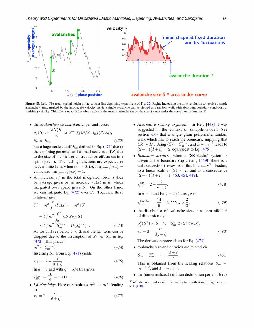
Theory and Experiments for Disordered Elastic Manifolds, Depinning, Avalanches, and Sandpiles 60
0
10
20
30
40
50
60
85 170 255 340
(µm)
(µ
m) sp
atia
lly
aver
aged
hei
ght
plate position
avalanches
S
mean shape at fixed duration
avalanche duration T
avalanche size S = area under curve
and its fluctuations
velocity
Figure 48. Left: The mean spatial height in the contact-line depinning experiment of Fig. 22. Right: Increasing the time resolution to resolve a singleavalanche (jump, marked by the arrow), the velocity inside a single avalanche can be viewed as a random walk with absorbing boundary conditions atvanishing velocity. This allows us to define observables as the mean avalanche shape, the size S (area under the curve), or its duration T .
• the avalanche-size distribution per unit force,
ρf (S) :=δN(S)
δf' S−τfS(S/Sm)gS(S/S0),
S0 Sm, (472)has a large-scale cutoff Sm defined in Eq. (471) due tothe confining potential, and a small-scale cutoff S0 dueto the size of the kick or discretization effects (as in aspin system). The scaling functions are expected tohave a finite limit when m → 0, i.e. limx→0 fS(x) =const, and limx→∞ gS(x) = 1.
• An increase δf in the total integrated force is thenon average given by an increase δu(x) in u, whichintegrated over space gives S. On the other hand,we can integrate Eq. (472) over S. Together, theserelations give
δf = m2
∫
x
〈δu(x)〉 = m2 〈S〉
= δf m2
∫ ∞
0
dS Sρf (S)
∼ δf m2[S2−τm −O(S2−τ
0 )]. (473)
As we will see below τ < 2, and the last term can bedropped due to the assumption of S0 Sm in Eq.(472). This yieldsm2 ∼ Sτ−2
m . (474)Inserting Sm from Eq. (471) yields
τSR = 2− 2
d+ ζ. (475)
In d = 1 and with ζ = 5/4 this gives
τd=1SR =
10
9= 1.111... (476)
• LR-elasticity: Here one replaces m2 → mα, leadingtoτα = 2− α
d+ ζ. (477)
• Alternative scaling argument: In Ref. [448] it wassuggested in the context of sandpile models (seesection 6.6) that a single grain performs a randomwalk which has to reach the boundary, implying that〈S〉 ∼ L2. Using 〈S〉 ∼ S2−τ
m , and L ∼ m−1 leads to(2− τ)(d+ ζ) = 2, equivalent to Eq. (475).
• Boundary driving: when a (SR-elastic) system isdriven at the boundary (tip driving [449]) there is adrift (advection) away from this boundary33, leadingto a linear scaling, 〈S〉 ∼ L, and as a consequence(2− τ)(d+ ζ) = 1 [450, 451, 449],
τ tipSR = 2− 1
d+ ζ. (478)
In d = 1 and for ζ = 5/4 this gives
τ tip,d=1SR =
14
9= 1.555... >
3
2. (479)
• the distribution of avalanche sizes in a submanifold φof dimension dφ,
ρφf (Sφ) ∼ S−τφ , Sφm Sφ Sφ0 ,
τφ = 2− α
dφ + ζ. (480)
The derivation proceeds as for Eq. (475).• avalanche size and duration are related via
Sm ∼ T γm, γ =d+ ζ
z. (481)
This is obtained from the scaling relations Sm ∼m−d−ζ , and Tm ∼ m−z .
• the (unnormalized) duration distribution per unit force33We do not understand the first-return-to-the-origin argument ofRef. [450].
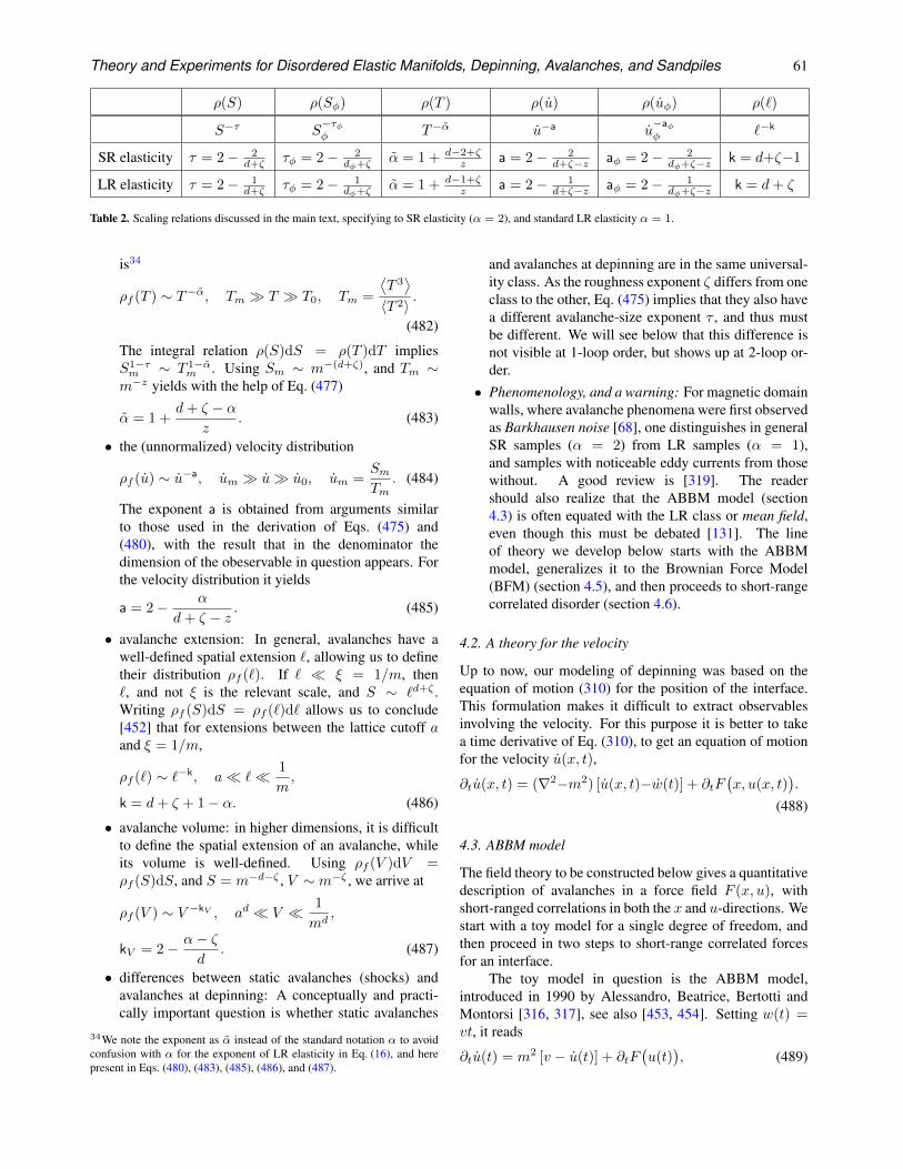
Theory and Experiments for Disordered Elastic Manifolds, Depinning, Avalanches, and Sandpiles 61
ρ(S) ρ(Sφ) ρ(T ) ρ(u) ρ(uφ) ρ(`)
S−τ S−τφφ T−α u−a u
−aφφ `−k
SR elasticity τ = 2− 2d+ζ τφ = 2− 2
dφ+ζ α = 1 + d−2+ζz a = 2− 2
d+ζ−z aφ = 2− 2dφ+ζ−z k = d+ζ−1
LR elasticity τ = 2− 1d+ζ τφ = 2− 1
dφ+ζ α = 1 + d−1+ζz a = 2− 1
d+ζ−z aφ = 2− 1dφ+ζ−z k = d+ ζ
Table 2. Scaling relations discussed in the main text, specifying to SR elasticity (α = 2), and standard LR elasticity α = 1.
is34
ρf (T ) ∼ T−α, Tm T T0, Tm =
⟨T 3⟩
〈T 2〉 .
(482)
The integral relation ρ(S)dS = ρ(T )dT impliesS1−τm ∼ T 1−α
m . Using Sm ∼ m−(d+ζ), and Tm ∼m−z yields with the help of Eq. (477)
α = 1 +d+ ζ − α
z. (483)
• the (unnormalized) velocity distribution
ρf (u) ∼ u−a, um u u0, um =SmTm
. (484)
The exponent a is obtained from arguments similarto those used in the derivation of Eqs. (475) and(480), with the result that in the denominator thedimension of the obeservable in question appears. Forthe velocity distribution it yields
a = 2− α
d+ ζ − z . (485)
• avalanche extension: In general, avalanches have awell-defined spatial extension `, allowing us to definetheir distribution ρf (`). If ` ξ = 1/m, then`, and not ξ is the relevant scale, and S ∼ `d+ζ .Writing ρf (S)dS = ρf (`)d` allows us to conclude[452] that for extensions between the lattice cutoff aand ξ = 1/m,
ρf (`) ∼ `−k, a ` 1
m,
k = d+ ζ + 1− α. (486)
• avalanche volume: in higher dimensions, it is difficultto define the spatial extension of an avalanche, whileits volume is well-defined. Using ρf (V )dV =ρf (S)dS, and S = m−d−ζ , V ∼ m−ζ , we arrive at
ρf (V ) ∼ V −kV , ad V 1
md,
kV = 2− α− ζd
. (487)
• differences between static avalanches (shocks) andavalanches at depinning: A conceptually and practi-cally important question is whether static avalanches
34We note the exponent as α instead of the standard notation α to avoidconfusion with α for the exponent of LR elasticity in Eq. (16), and herepresent in Eqs. (480), (483), (485), (486), and (487).
and avalanches at depinning are in the same universal-ity class. As the roughness exponent ζ differs from oneclass to the other, Eq. (475) implies that they also havea different avalanche-size exponent τ , and thus mustbe different. We will see below that this difference isnot visible at 1-loop order, but shows up at 2-loop or-der.
• Phenomenology, and a warning: For magnetic domainwalls, where avalanche phenomena were first observedas Barkhausen noise [68], one distinguishes in generalSR samples (α = 2) from LR samples (α = 1),and samples with noticeable eddy currents from thosewithout. A good review is [319]. The readershould also realize that the ABBM model (section4.3) is often equated with the LR class or mean field,even though this must be debated [131]. The lineof theory we develop below starts with the ABBMmodel, generalizes it to the Brownian Force Model(BFM) (section 4.5), and then proceeds to short-rangecorrelated disorder (section 4.6).
4.2. A theory for the velocity
Up to now, our modeling of depinning was based on theequation of motion (310) for the position of the interface.This formulation makes it difficult to extract observablesinvolving the velocity. For this purpose it is better to takea time derivative of Eq. (310), to get an equation of motionfor the velocity u(x, t),
∂tu(x, t) = (∇2−m2) [u(x, t)−w(t)] + ∂tF(x, u(x, t)
).
(488)
4.3. ABBM model
The field theory to be constructed below gives a quantitativedescription of avalanches in a force field F (x, u), withshort-ranged correlations in both the x and u-directions. Westart with a toy model for a single degree of freedom, andthen proceed in two steps to short-range correlated forcesfor an interface.
The toy model in question is the ABBM model,introduced in 1990 by Alessandro, Beatrice, Bertotti andMontorsi [316, 317], see also [453, 454]. Setting w(t) =vt, it reads
∂tu(t) = m2 [v − u(t)] + ∂tF(u(t)
), (489)
Theory and Experiments for Disordered Elastic Manifolds, Depinning, Avalanches, and Sandpiles 62
∂tF(u(t)
)=√u(t)ξ(t), (490)
〈ξ(t)ξ(t′)〉 = 2σδ(t− t′). (491)
The last equation implies thatF (u) is a random walk, as canbe seen as follows: As u is non-negative, t is an increasingfunction of u, and we can change variables from t to u,
∂uF (u) = ξ(u),⟨ξ(u)ξ(u′)
⟩= 2σδ(u− u′). (492)
As a random walk, F (u) has correlations
∆(0)−∆(u− u′) ≡ 1
2
⟨[F (u)− F (u′)]
2⟩
= σ|u− u′|.(493)
In the language introduced above, the (bare) disorder has acusp, with amplitude |∆′(0+)| = σ.
The ABBM model is traditionally treated [316, 317,453] via the associated Fokker-Planck equation (944) (for aderivation see appendix 10.3),
∂tP (u, t) = σ∂2
∂u2
[uP (u, t)
]+m2 ∂
∂u
[(u− v)P (u, t)
].
(494)
This approach is difficult for time-dependent quantities, butefficient for observables in the steady state. As an example,consider the steady-state distribution of velocities, obtainedby solving ∂tP (u, t) = 0,
P (u) =um2vσ −1e−u
m2
σ
Γ(m2vσ
)(m2
σ
)m2vσ
. (495)
Setting σ = m = 1 to simplify the expressions yields
P (u) =uv−1e−u
Γ(v). (496)
4.4. End of an avalanche, and an efficient simulationalgorithm
It is important to remark that an avalanche stops at a givenwell-defined time. To see this, we solve Eqs. (489)-(490)for m = 0, given that at time t = 0 the velocity is u0. Theassociated Fokker-Planck equation is
∂tP (u, t) = ∂2u [σuP (u, t)] . (497)
It can be solved analytically, for given initial distributionP (u, 0) = δ(u− u0), as
P (u, t) = δ(u) exp
(− u0
σt
)
+exp(− u0+u
σt )σt
√u0
u I1
(2√u0uσt
).
(498)
(I1 is the Bessel-function of the first kind.) This canbe checked by inserting the solution into the differentialequation (497). Eq. (498) teaches us that for an initialvelocity u0, with a finite probability exp(− u0
σt ) the velocitywill be (strictly) zero after time t. It also means that the endof an avalanche is well defined in time, which is crucial todefine its duration. This would not be the case for a particlein a smooth potential: Linearizing the potential close to the
endpoint assumed to be u(t = ∞) = 0 of the avalancheyields
∂tu(t) ' −αu(t) =⇒ u(t) ' u0e−αt. (499)
Eq. (498) can serve as an efficient simulation algorithm,replacing t by the time-discretization step δt, andalternately integrating the forcing term δu(t) = m2[v −u(t)]δt and the stochastic process according to Eq. (498).This is not straightforward, due to the appearance ofmultiplicative noise [455]. We can use an additional trick[456]: Observe that the solution (498) can be written as
P (u, t) = δ(u) exp
(− u0
σt
)
+
∞∑
n=1
(u0
σt
)nexp
(− u0
σt
)
n!× 1
σt
(uσt
)n−1exp
(− uσt
)
(n− 1)!
=
∞∑
n=0
pn1
σtPn
(u
σt
). (500)
Here, pn is a normalized probability vector, i.e.∑∞n=0 pn = 1, and each probability Pn(x) is normalized,∫∞
0dx Pn(x) = 1. Explicitly, we have
pn =
(u0
σt
)nexp
(− u0
σt
)
n!, (501)
P0(x) = δ(x), (502)
Pn(x) =xn−1 exp (−x)
(n− 1)!, n ≥ 1. (503)
Given u0, one obtains uwith probability P (u, t) as follows:
(i) draw an integer random number n, from the Poissondistribution pn; the latter has parameter u0/(σt),
(ii) if n = 0, return u = 0,(iii) else draw a positive real random number x, from the
Gamma distribution with parameter n.(iv) return u = σtx,
Contrary to a naive integration of the stochastic differentialequation which yields ∂tF
(u(t)
)δt = ξt
√δt, 〈ξtξt′〉 =
δt,t′ , this algorithm is linear in δt.This allows us to define the distribution of durations,
given below in Eq. (546), and the mean temporal shape(552), without introducing an (arbitrary) small-velocitycutoff.
4.5. Brownian Force Model (BFM)
The model defined in Eqs. (489) and (490) is a model for asingle degree of freedom, not for an interface. A model foran interface can be defined by [321]
∂tu(x, t) = ∇2u(x, t) +m2 [v − u(x, t)]
+ ∂tF(x, u(x, t)
), (504)
∂tF(x, u(x, t)
)=√u(x, t)ξ(x, t), (505)
〈ξ(x, t)ξ(x′, t′)〉 = 2σδ(t− t′)δd(x− x′). (506)
Theory and Experiments for Disordered Elastic Manifolds, Depinning, Avalanches, and Sandpiles 63
Since each degree of freedom sees a force which is arandom walk, this model is termed the Brownian ForceModel (BFM) [321].
4.6. Short-ranged rough disorder
Both the ABBM model as its spatial generalization, theBFM model, are pathologic in the sense that the force-force correlator grows for all distances instead of saturatingas expected in short-ranged correlated systems, and asis reflected in the FRG fixed points discussed in section2.5. To remedy this, one can keep the equation of motion(504), but add an additional damping term in the evolutionequation (505) of the force,
∂tF(x, u(x, t)
)= −γu(x, t)F
(x, u(x, t)
)
+√u(x, t)ξ(x, t), (507)
〈ξ(x, t)ξ(x′, t′)〉 = 2σδ(t− t′)δd(x− x′). (508)
As u(x, t) ≥ 0, the equation of motion for the force isequivalent to
∂uF (x, u) = −γF (x, u) + ξ(x, u), (509)⟨ξ(x, u)ξ(x′, u′)
⟩= 2σδ(u− u′)δd(x− x′). (510)
This system has the force-force correlator
〈F (u, x)F (u′, x′)〉c = σδd(x− x′)e−γ|u−u′|
γ. (511)
For u γ, we recover the correlations (493).
4.7. Field theory
Consider the equation of motion (488) with generic short-ranged force-force correlators. The dynamical actionis obtained by multiplying the equation of motion withu(x, t), and averaging over disorder35,
S =
∫
x,t
u(x, t)[(∂t−∇2)u(x, t) +m2
(u(x, t)−w
)]
−1
2
∫
x,t,t′u(x, t)u(x, t′)∂t∂t′∆
(u(x, t)−u(x, t′)
). (512)
The second line contains
∂t∂t′∆(u(x, t)− u(x, t′)
)
= u(x, t)∂t′∆′(u(x, t)− u(x, t′)
)
= u(x, t)[∆′(0+)∂t′sign(t− t′)−∆′′(0+)u(x, t′) + ...
]
= −2u(x, t)∆′(0+)δ(t− t′)−∆′′(0+)u(x, t)u(x, t′) + ... (513)
The terms dropped in this expansion are higher derivativesof ∆(u), and they come with higher powers of u(x, t),and its time-integral u(x, t) − u(x, t′) =
∫ tt′
dτ u(x, τ),
35The response field u(x, t) is different from that in Eqs. (313)-(314).One can derive Eq. (512) by substituting in Eq. (314) u(x, t) →−∂tu(x, t), and then integrating by parts in time.
reminding that u(x, t) and not u(x, t) is the variable forwhich we wrote down the equation of motion.
This expression is quite remarkable: The leading termis proportional to δ(t − t′), rendering the last term in Eq.(512) local in time. It is therefore appropriate to start ouranalysis of the theory with this term only. The action weobtain is
SBFM[u, u]
=
∫
x,t
u(x, t)[(∂t −∇2)u(x, t) +m2
(u(x, t)− w(x, t)
)]
+ ∆′(0+)u(x, t)2u(x, t). (514)
This is the action of the BFM introduced in Eqs. (504)-(506): as ∆(u) only has a first non-vanishing derivative,all subsequent terms in Eq. (513) vanish. Corrections areobtained by adding the omitted terms perturbatively. Thesubleading term is
S[u, u] = SBFM[u, u] (515)
+1
2
∫
x,t,t′u(x, t)u(x, t′)u(x, t)u(x, t′)∆′′(0+) + ....
We show below on page 68 several theorems, indicating thatat the upper critical dimension the action (512) leads to theresults of the BFM model, and that the additional term inEq. (515) is sufficient for the 1-loop corrections, of orderε = dc − d.
4.8. FRG and scaling
The FRG equation (343) for the disorder has the followingstructure
∂`∆(u) = (ε− 2ζ)∆(u) + ζu∆′(u)
+
∞∑
n=1
∂2nu
[∆(u)− ∆(0)
]n+1
. (516)
The n-loop terms are highly symbolic, since the derivativescan be distributed in different ways on the n + 1 disordercorrelators, and we have dropped all prefactors. We nowassume that the microscopic disorder has the form (493),thus ∆(0)− ∆(u) has only a term linear in u. This impliesthat the term of order n = 1 may contribute a constantto Eq. (516), while terms with n ≥ 2 vanish. Thus to allorders, the roughness exponent is given by
ζBFM = ε = 4− d. (517)
As a consequence, the unrescaled disorder is scaleindependent (does not renormalize), and
∆BFM(0)−∆BFM(u) ≡ σ|u|. (518)
Note that ∆(0) is not well-defined, since random forcesgrow unboundedly.
Similarly, the dynamical exponent z has correctionsproportional to ∆′′(0), which vanish. As a consequence,z = 2, and all exponents can be obtained analytically,
zBFM = 2, βBFM = aBFM = 1, γBFM = αBFM = 2,
τBFM =3
2, κBFM = 3 . (519)
Theory and Experiments for Disordered Elastic Manifolds, Depinning, Avalanches, and Sandpiles 64
4.9. Instanton equation
We want to construct observables for the BFM such as
Z[λ,w] :=⟨
e∫x,t
λ(x,t)u(x,t)⟩
=
∫D[u]D[u] e
∫x,t
λ(x,t)u(x,t)−SBFM[u,u]. (520)
This includes the avalanche-size distribution with λ(x, t) =λ, the velocity distribution with λ(x, t) = λδ(t), the localavalanche-size distribution with λ(x, t) = λδ(x), a.s.o.
The key observation is that u(x, t) appears linearly inthe exponent, thus the path integral over u can be performedexactly, enforcing an instanton equation for u(x, t),(−∂t −∇2 +m2
)uinst(x, t)− σuinst(x, t)
2 = λ(x, t).
(521)
Here σ ≡ −∆′(0+) > 0, see e.g. Eqs. (493) and (511). Theexpectation (520) simplifies to
Z[λ,w] = e∫x,t
m2w(x,t)u(x,t)∣∣∣u=uinst
. (522)
The term with w(x, t) in the exponential is the only one notproportional to u(x, t); the latter vanish due to the instantonequation (521). Let us consider some examples.
4.10. Avalanche-size distribution
The simplest example is the avalanche-size distribution.Noting that S =
∫x,tu(x, t), we have to solve the instanton
equation (521) for λ(x, t) = λ. The solution for u =uinst will be constant in space and time, thus the instantonequation (521) reduces to
m2u− σu2 = λ. (523)
This quadratic equation has two solutions. The relevant onevanishing at λ = 0 reads
u =m2 −
√m4 − 4λσ
2σ. (524)
We now insert this solution into Eq. (522). As u(x, t) isconstant in space and time, the integral on the r.h.s. of Eq.(522) is u times
w :=
∫
x,t
w(x, t) > 0. (525)
This yields with u given in Eq. (524)⟨eλS⟩
= em2wu. (526)
Taking the inverse Laplace transform gives
PSw (S) = m2we−
m4(S−w)2
4σS
2√πσS3/2
. (527)
One checks that PSw (S) is normalized, 〈1〉w =∫∞0
dS PSw (S) = 1, and that the first avalanche-size mo-ment is 〈S〉w =
∫∞0
dS SPw(S) = w. If w(x, t) is con-stant in x, then 〈S〉w = w is nothing but the displacementof the confining parabola.
Pw(S) is the response of the system to a displacementw, or equivalently to a force kick δf = m2w. We now takethe limit of an infinitesimally small displacement w, and tothis purpose define
PS(S) := limw→0
〈S〉ww
PSw (S)
= 〈S〉m2 e−m4S4σ
2√πσS3/2
≡ 〈S〉 e−S
4Sm
2√πSmSτ
, (528)
τ = τABBM =3
2, (529)
Sm :=
⟨S2⟩
2 〈S〉 =σ
m4. (530)
Since 〈S〉w = w, by construction all moments which do notnecessitate a small-S cutoff, i.e. 〈Sn〉w with n ≥ 1 have awell-defined small-w limit, given by Eq. (528). What onelooses when taking the limit of w → 0 is normalizability,as formally 〈1〉 = limw→0 w
−1 =∞.
4.11. Watson-Galton process, and first-return probability
The avalanche size-exponent τ = 3/2 observed in theABBM model appears in many contexts: It was first studiedin the survival probability of a noble man’s name (maledescendents) [457]. The latter has the equations of motion(489)-(491), where u(t) is the number of descendants ina generation, v = 0, and m2 the mean relative decrease inmale descendants in a generation (which could be negative),
∂tu(t) = −m2u(t) +√uξ(t), (531)
〈ξ(t)ξ(t′)〉 = 2σδ(t− t′). (532)
As u(t) > 0, the total number of descendants u(t) ismonotonically increasing, allowing us to write u(t) ≡u(u(t)). The equation of motion (531) then becomes
∂tu(u(t)) = u(u)∂uu(u) = −m2u(u)+√u(u) ξ(t). (533)
As long as u > 0, we can divide both sides by u to arrive at
∂uu(u) = −m2 + ξ(u), (534)⟨ξ(u)ξ(u′)
⟩= 2σδ(u− u′). (535)
Note the change of argument in the noise. Thus u(u)performs a random walk in “time” u with drift −m2 andabsorbing boundary conditions at u = 0. In absence of anabsorbing wall, the probability that u(u) starts close to zeroat u = 0, and returns to zero behaves for large u as
Preturn(u) ∼ e−m2u
√u
. (536)
In presence of an absorbing wall, we need the probabilityto arrive at zero for the first “time” u. The latter is obtainedby taking a “time”, i.e. u-derivative of Preturn(u),
Pfirst(u) = −∂uPreturn(u) ∼ e−m2u
u32
. (537)
This is again the ABBM avalanche-size distribution (528)with τ = 3/2, interpreted as first-return probability of arandom walk.
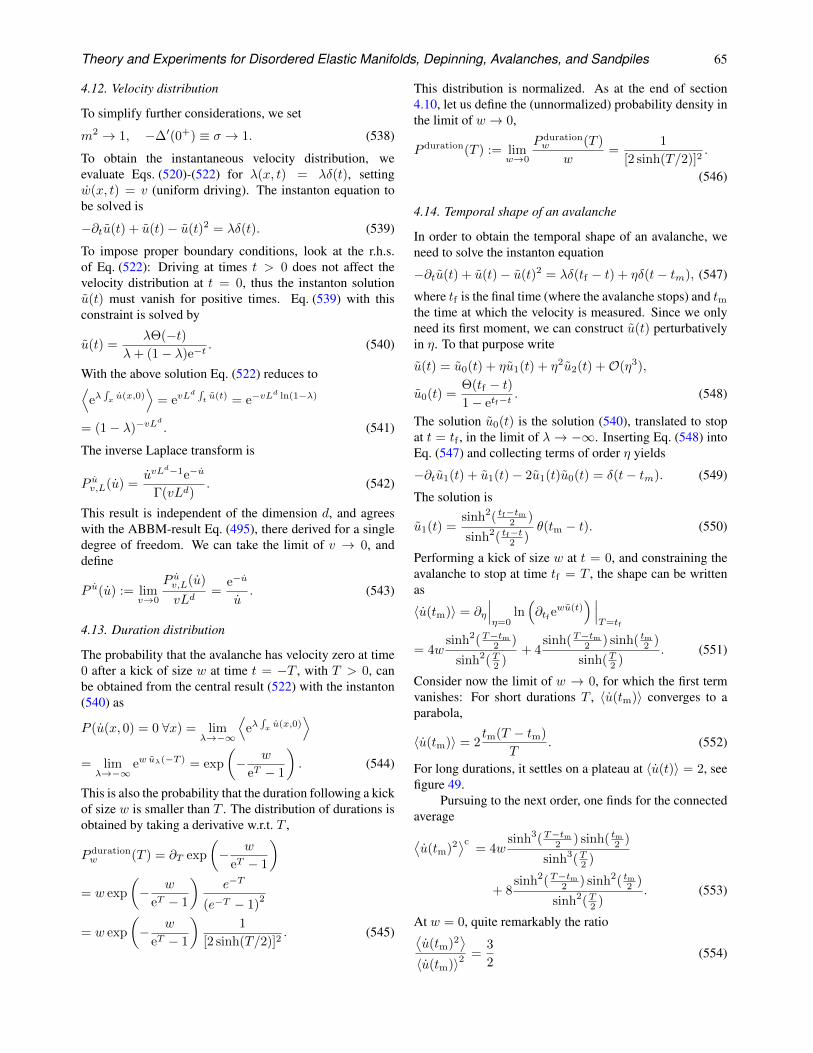
Theory and Experiments for Disordered Elastic Manifolds, Depinning, Avalanches, and Sandpiles 65
4.12. Velocity distribution
To simplify further considerations, we set
m2 → 1, −∆′(0+) ≡ σ → 1. (538)
To obtain the instantaneous velocity distribution, weevaluate Eqs. (520)-(522) for λ(x, t) = λδ(t), settingw(x, t) = v (uniform driving). The instanton equation tobe solved is
−∂tu(t) + u(t)− u(t)2 = λδ(t). (539)
To impose proper boundary conditions, look at the r.h.s.of Eq. (522): Driving at times t > 0 does not affect thevelocity distribution at t = 0, thus the instanton solutionu(t) must vanish for positive times. Eq. (539) with thisconstraint is solved by
u(t) =λΘ(−t)
λ+ (1− λ)e−t. (540)
With the above solution Eq. (522) reduces to⟨
eλ∫xu(x,0)
⟩= evL
d∫tu(t) = e−vL
d ln(1−λ)
= (1− λ)−vLd
. (541)
The inverse Laplace transform is
P uv,L(u) =uvL
d−1e−u
Γ(vLd). (542)
This result is independent of the dimension d, and agreeswith the ABBM-result Eq. (495), there derived for a singledegree of freedom. We can take the limit of v → 0, anddefine
P u(u) := limv→0
P uv,L(u)
vLd=
e−u
u. (543)
4.13. Duration distribution
The probability that the avalanche has velocity zero at time0 after a kick of size w at time t = −T , with T > 0, canbe obtained from the central result (522) with the instanton(540) as
P (u(x, 0) = 0 ∀x) = limλ→−∞
⟨eλ∫xu(x,0)
⟩
= limλ→−∞
ew uλ(−T ) = exp
(− w
eT − 1
). (544)
This is also the probability that the duration following a kickof size w is smaller than T . The distribution of durations isobtained by taking a derivative w.r.t. T ,
P durationw (T ) = ∂T exp
(− w
eT − 1
)
= w exp
(− w
eT − 1
)e−T
(e−T − 1)2
= w exp
(− w
eT − 1
)1
[2 sinh(T/2)]2. (545)
This distribution is normalized. As at the end of section4.10, let us define the (unnormalized) probability density inthe limit of w → 0,
P duration(T ) := limw→0
P durationw (T )
w=
1
[2 sinh(T/2)]2.
(546)
4.14. Temporal shape of an avalanche
In order to obtain the temporal shape of an avalanche, weneed to solve the instanton equation
−∂tu(t) + u(t)− u(t)2 = λδ(tf − t) + ηδ(t− tm), (547)
where tf is the final time (where the avalanche stops) and tmthe time at which the velocity is measured. Since we onlyneed its first moment, we can construct u(t) perturbativelyin η. To that purpose write
u(t) = u0(t) + ηu1(t) + η2u2(t) +O(η3),
u0(t) =Θ(tf − t)1− etf−t
. (548)
The solution u0(t) is the solution (540), translated to stopat t = tf , in the limit of λ→ −∞. Inserting Eq. (548) intoEq. (547) and collecting terms of order η yields
−∂tu1(t) + u1(t)− 2u1(t)u0(t) = δ(t− tm). (549)
The solution is
u1(t) =sinh2( tf−tm2 )
sinh2( tf−t2 )θ(tm − t). (550)
Performing a kick of size w at t = 0, and constraining theavalanche to stop at time tf = T , the shape can be writtenas
〈u(tm)〉 = ∂η
∣∣∣η=0
ln(∂tf e
wu(t)) ∣∣∣
T=tf
= 4wsinh2(T−tm2 )
sinh2(T2 )+ 4
sinh(T−tm2 ) sinh( tm2 )
sinh(T2 ). (551)
Consider now the limit of w → 0, for which the first termvanishes: For short durations T , 〈u(tm)〉 converges to aparabola,
〈u(tm)〉 = 2tm(T − tm)
T. (552)
For long durations, it settles on a plateau at 〈u(t)〉 = 2, seefigure 49.
Pursuing to the next order, one finds for the connectedaverage
⟨u(tm)2
⟩c= 4w
sinh3(T−tm2 ) sinh( tm2 )
sinh3(T2 )
+ 8sinh2(T−tm2 ) sinh2( tm2 )
sinh2(T2 ). (553)
At w = 0, quite remarkably the ratio⟨u(tm)2
⟩
〈u(tm)〉2=
3
2(554)
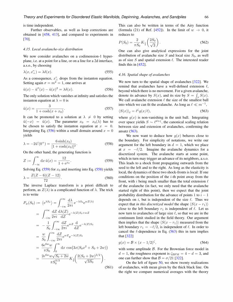
Theory and Experiments for Disordered Elastic Manifolds, Depinning, Avalanches, and Sandpiles 66
is time independent.Further observables, as well as loop corrections are
obtained in [458, 413], and compared to experiments in[70].
4.15. Local avalanche-size distribution
We now consider avalanches on a codimension-1 hyper-plane, i.e. at a point for a line, or on a line for a 2d interface,a.s.o., by choosing
λ(x, ~x⊥) = λδ(x). (555)
As a consequence, ~x⊥ drops from the instanton equation.Setting again σ = m2 = 1, one arrives at
u(x)− u′′(x)− u(x)2 = λδ(x). (556)
The only solution which vanishes at infinity and satisfies theinstanton equation at λ = 0 is
u(x) =3
1 + cosh(x+ x0). (557)
It can be promoted to a solution at λ 6= 0 by settingu(−x) = u(x). The parameter x0 = x0(λ) has tobe chosen to satisfy the instanton equation at x = 0.Integrating Eq. (556) within a small domain around x = 0yields
λ = −2u′(0+) =6 sinh(x0)
[1 + cosh(x0)]2. (558)
On the other hand, the generating function is
Z :=
∫ ∞
−∞dx u(x) =
12
1 + ex0. (559)
Solving Eq. (559) for x0 and inserting into Eq. (558) yields
λ =Z(Z − 6)(Z − 12)
72. (560)
The inverse Laplace transform is a priori difficult toperform, as Z(λ) is a complicated function of λ. The trickis to write
Pw(S0) :=⟨eλS0
⟩=
∫ i∞
−i∞
dλ
2πie−λS0ewZ(λ)
=
∫ i∞
−i∞
dZ
2πi
dλ(Z)
dZe−λ(Z)S0+wZ
= − 1
S0
∫ i∞
−i∞
dZ
2πiewZ
d
dZe−λ(Z)S0
=w
S0
∫ i∞
−i∞
dZ
2πiewZe−λ(Z)S0
=6e6ww
πS0
∫ ∞
0
dx cos(3x(S0x
2 + S0 + 2w))
=2e6ww
√S0 + 2w
πS3/20
K 13
(2(S0 + 2w)3/2
√3S0
).
(561)
This can also be written in terms of the Airy function(formula (21) of Ref. [452]). In the limit of w → 0, itreduces to
P (S0) =2
πS0K 1
3
(2S0√
3
). (562)
One can also give analytical expressions for the jointdistribution of avalanche size S and local size S0, as wellas of size S and spatial extension `. The interested readerfinds this in [452].
4.16. Spatial shape of avalanches
We now turn to the spatial shape of avalanches [322]. Weremind that avalanches have a well-defined extension `,beyond which there is no movement. For a given avalanche,denote its advance by S(x), and its size by S =
∫xS(x).
We call avalanche extension ` the size of the smallest ballinto which we can fit the avalanche. As long as ` m−1,
〈S(x)〉` = `ζg(x/`), (563)
where g(x) is non-vanishing in the unit ball. Integratingover space yields S ∼ `d+ζ , the canonical scaling relationbetween size and extension of avalanches, confirming theansatz (563).
We now want to deduce how g(x) behaves close tothe boundary. For simplicity of notations, we write ourargument for the left boundary in d = 1, which we placeat x = −`/2. Imagine the avalanche dynamics for adiscretized system. The avalanche starts at some point,which in turn may trigger an advance of its neighbors, a.s.o.This leads to a shock front propagating outwards from theseed to the left and to the right. As long as the elasticity islocal, the dynamics of these two shock-fronts is local: If oneconditions on the position of the i-th point away from thefront, with i being much smaller than the total extension `of the avalanche (in fact, we only need that the avalanchestarted right of this point), then we expect that the jointprobability distribution for the advance of points 1 to i − 1depends on i, but is independent of the size `. Thus weexpect that in this discretized model the shape 〈S(x− r1)〉close to the left boundary r1 is independent of `. Let usnow turn to avalanches of large size `, so that we are in thecontinuum limit studied in the field theory. Our argumentthen implies that the shape 〈S(x− r1)〉 measured from theleft boundary r1 = −`/2, is independent of `. In order tocancel the `-dependence in Eq. (563) this in turn impliesthat [322]
g(x) = B × (x− 1/2)ζ , (564)
with some amplitude B. For the Brownian force model ind = 1, the roughness exponent is ζBFM = 4 − d = 3, andone can further show that B = σ/21 [322].
On the left of figure 50, we show twenty realizationsof avalanches, with mean given by the thick black line. Onthe right we compare numerical averages with the theory
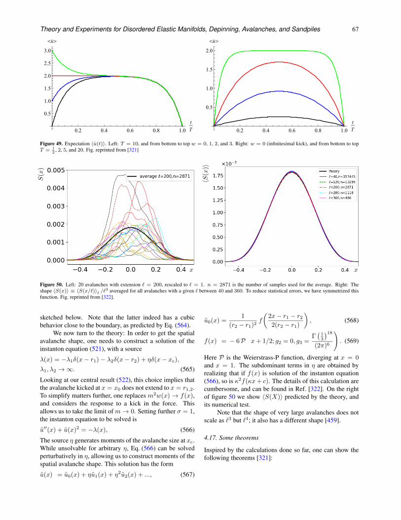
Theory and Experiments for Disordered Elastic Manifolds, Depinning, Avalanches, and Sandpiles 67
0.2 0.4 0.6 0.8 1.0
t
T
0.5
1.0
1.5
2.0
2.5
3.0
<u>
0.2 0.4 0.6 0.8 1.0
t
T
0.5
1.0
1.5
2.0
<u>
Figure 49. Expectation 〈u(t)〉. Left: T = 10, and from bottom to top w = 0, 1, 2, and 3. Right: w = 0 (infinitesimal kick), and from bottom to topT = 1
2, 2, 5, and 20. Fig. reprinted from [321]
S(x
)
x
〈S(x
)〉
x
Figure 50. Left: 20 avalanches with extension ` = 200, rescaled to ` = 1. n = 2871 is the number of samples used for the average. Right: Theshape 〈S(x)〉 ≡ 〈S(x/`)〉` /`3 averaged for all avalanches with a given ` between 40 and 360. To reduce statistical errors, we have symmetrized thisfunction. Fig. reprinted from [322].
sketched below. Note that the latter indeed has a cubicbehavior close to the boundary, as predicted by Eq. (564).
We now turn to the theory: In order to get the spatialavalanche shape, one needs to construct a solution of theinstanton equation (521), with a source
λ(x) = −λ1δ(x− r1)− λ2δ(x− r2) + ηδ(x− xc),
λ1, λ2 →∞. (565)
Looking at our central result (522), this choice implies thatthe avalanche kicked at x = x0 does not extend to x = r1,2.To simplify matters further, one replaces m2w(x)→ f(x),and considers the response to a kick in the force. Thisallows us to take the limit of m→ 0. Setting further σ = 1,the instanton equation to be solved is
u′′(x) + u(x)2 = −λ(x), (566)
The source η generates moments of the avalanche size at xc.While unsolvable for arbitrary η, Eq. (566) can be solvedperturbatively in η, allowing us to construct moments of thespatial avalanche shape. This solution has the form
u(x) = u0(x) + ηu1(x) + η2u2(x) + ..., (567)
u0(x) =1
(r2 − r1)2f
(2x− r1 − r2
2(r2 − r1)
), (568)
f(x) = − 6P(x+ 1/2; g2 = 0, g3 =
Γ(
13
)18
(2π)6
). (569)
Here P is the Weierstrass-P function, diverging at x = 0and x = 1. The subdominant terms in η are obtained byrealizing that if f(x) is solution of the instanton equation(566), so is κ2f(κx+ c). The details of this calculation arecumbersome, and can be found in Ref. [322]. On the rightof figure 50 we show 〈S(X)〉 predicted by the theory, andits numerical test.
Note that the shape of very large avalanches does notscale as `3 but `4; it also has a different shape [459].
4.17. Some theorems
Inspired by the calculations done so far, one can show thefollowing theorems [321]:
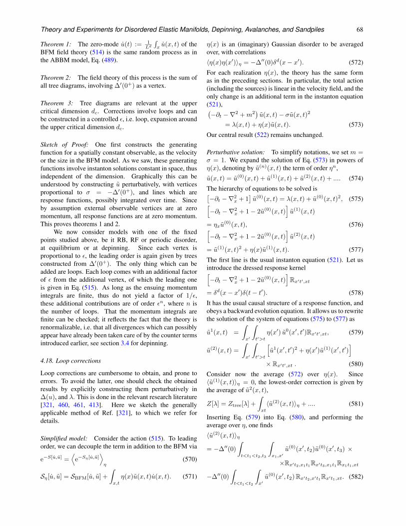
Theory and Experiments for Disordered Elastic Manifolds, Depinning, Avalanches, and Sandpiles 68
Theorem 1: The zero-mode u(t) := 1Ld
∫xu(x, t) of the
BFM field theory (514) is the same random process as inthe ABBM model, Eq. (489).
Theorem 2: The field theory of this process is the sum ofall tree diagrams, involving ∆′(0+) as a vertex.
Theorem 3: Tree diagrams are relevant at the uppercritical dimension dc. Corrections involve loops and canbe constructed in a controlled ε, i.e. loop, expansion aroundthe upper critical dimension dc.
Sketch of Proof: One first constructs the generatingfunction for a spatially constant observable, as the velocityor the size in the BFM model. As we saw, these generatingfunctions involve instanton solutions constant in space, thusindependent of the dimension. Graphically this can beunderstood by constructing u perturbatively, with verticesproportional to σ = −∆′(0+), and lines which areresponse functions, possibly integrated over time. Sinceby assumption external observable vertices are at zeromomentum, all response functions are at zero momentum.This proves theorems 1 and 2.
We now consider models with one of the fixedpoints studied above, be it RB, RF or periodic disorder,at equilibrium or at depinning. Since each vertex isproportional to ε, the leading order is again given by treesconstructed from ∆′(0+). The only thing which can beadded are loops. Each loop comes with an additional factorof ε from the additional vertex, of which the leading oneis given in Eq. (515). As long as the ensuing momentumintegrals are finite, thus do not yield a factor of 1/ε,these additional contributions are of order εn, where n isthe number of loops. That the momentum integrals arefinite can be checked; it reflects the fact that the theory isrenormalizable, i.e. that all divergences which can possiblyappear have already been taken care of by the counter termsintroduced earlier, see section 3.4 for depinning.
4.18. Loop corrections
Loop corrections are cumbersome to obtain, and prone toerrors. To avoid the latter, one should check the obtainedresults by explicitly constructing them perturbatively in∆(u), and λ. This is done in the relevant research literature[321, 460, 461, 413]. Here we sketch the generallyapplicable method of Ref. [321], to which we refer fordetails.
Simplified model: Consider the action (515). To leadingorder, we can decouple the term in addition to the BFM via
e−S[u,u] =⟨
e−Sη [u,u]⟩η
(570)
Sη[u, u] = SBFM[u, u] +
∫
x,t
η(x)u(x, t)u(x, t). (571)
η(x) is an (imaginary) Gaussian disorder to be averagedover, with correlations
〈η(x)η(x′)〉η = −∆′′(0)δd(x− x′). (572)
For each realization η(x), the theory has the same formas in the preceding sections. In particular, the total action(including the sources) is linear in the velocity field, and theonly change is an additional term in the instanton equation(521),(−∂t −∇2 +m2
)u(x, t)− σu(x, t)2
= λ(x, t) + η(x)u(x, t). (573)
Our central result (522) remains unchanged.
Perturbative solution: To simplify notations, we set m =σ = 1. We expand the solution of Eq. (573) in powers ofη(x), denoting by u(n)(x, t) the term of order ηn,
u(x, t) = u(0)(x, t) + u(1)(x, t) + u(2)(x, t) + .... (574)
The hierarchy of equations to be solved is[−∂t −∇2
x + 1]u(0)(x, t) = λ(x, t) + u(0)(x, t)2, (575)
[−∂t −∇2
x + 1− 2u(0)(x, t)]u(1)(x, t)
= ηxu(0)(x, t), (576)[
−∂t −∇2x + 1− 2u(0)(x, t)
]u(2)(x, t)
= u(1)(x, t)2 + η(x)u(1)(x, t). (577)
The first line is the usual instanton equation (521). Let usintroduce the dressed response kernel[−∂t −∇2
x + 1− 2u(0)(x, t)]Rx′t′,xt
= δd(x− x′)δ(t− t′). (578)
It has the usual causal structure of a response function, andobeys a backward evolution equation. It allows us to rewritethe solution of the system of equations (575) to (577) as
u1(x, t) =
∫
x′
∫
t′>t
η(x′) u0(x′, t′)Rx′t′,xt, (579)
u(2)(x, t) =
∫
x′
∫
t′>t
[u1(x′, t′)2 + η(x′)u(1)(x′, t′)
]
× Rx′t′,xt . (580)
Consider now the average (572) over η(x). Since〈u(1)(x, t)〉η = 0, the lowest-order correction is given bythe average of u2(x, t),
Z[λ] = Ztree[λ] +
∫
xt
〈u(2)(x, t)〉η + .... (581)
Inserting Eq. (579) into Eq. (580), and performing theaverage over η, one finds
〈u(2)(x, t)〉η= −∆′′(0)
∫
t<t1<t2,t3
∫
x1,x′u(0)(x′, t2)u(0)(x′, t3) ×
×Rx′t2,x1t1Rx′t3,x1t1Rx1t1,xt
−∆′′(0)
∫
t<t1<t2
∫
x′u(0)(x′, t2)Rx′t2,x′t1Rx′t1,xt. (582)
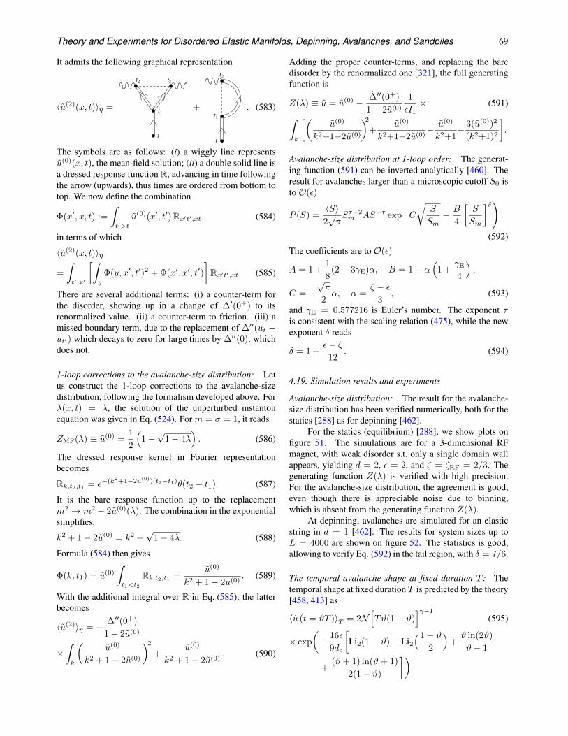
Theory and Experiments for Disordered Elastic Manifolds, Depinning, Avalanches, and Sandpiles 69
It admits the following graphical representation
〈u(2)(x, t)〉η =
3t2
t
t1
t
+
t
1
t2
t
. (583)
The symbols are as follows: (i) a wiggly line representsu(0)(x, t), the mean-field solution; (ii) a double solid line isa dressed response function R, advancing in time followingthe arrow (upwards), thus times are ordered from bottom totop. We now define the combination
Φ(x′, x, t) :=
∫
t′>t
u(0)(x′, t′)Rx′t′,xt, (584)
in terms of which
〈u(2)(x, t)〉η
=
∫
t′,x′
[∫
y
Φ(y, x′, t′)2 + Φ(x′, x′, t′)
]Rx′t′,xt. (585)
There are several additional terms: (i) a counter-term forthe disorder, showing up in a change of ∆′(0+) to itsrenormalized value. (ii) a counter-term to friction. (iii) amissed boundary term, due to the replacement of ∆′′(ut −ut′) which decays to zero for large times by ∆′′(0), whichdoes not.
1-loop corrections to the avalanche-size distribution: Letus construct the 1-loop corrections to the avalanche-sizedistribution, following the formalism developed above. Forλ(x, t) = λ, the solution of the unperturbed instantonequation was given in Eq. (524). For m = σ = 1, it reads
ZMF(λ) ≡ u(0) =1
2
(1−√
1− 4λ). (586)
The dressed response kernel in Fourier representationbecomes
Rk,t2,t1 = e−(k2+1−2u(0))(t2−t1)θ(t2 − t1). (587)
It is the bare response function up to the replacementm2 → m2 − 2u(0)(λ). The combination in the exponentialsimplifies,
k2 + 1− 2u(0) = k2 +√
1− 4λ. (588)
Formula (584) then gives
Φ(k, t1) = u(0)
∫
t1<t2
Rk,t2,t1 =u(0)
k2 + 1− 2u(0). (589)
With the additional integral over R in Eq. (585), the latterbecomes
〈u(2)〉η = − ∆′′(0+)
1− 2u(0)
×∫
k
(u(0)
k2 + 1− 2u(0)
)2
+u(0)
k2 + 1− 2u(0). (590)
Adding the proper counter-terms, and replacing the baredisorder by the renormalized one [321], the full generatingfunction is
Z(λ) ≡ u = u(0) − ∆′′(0+)
1− 2u(0)
1
εI1× (591)
∫
k
[(u(0)
k2+1−2u(0)
)2+
u(0)
k2+1−2u(0)− u(0)
k2+1− 3(u(0))2
(k2+1)2
].
Avalanche-size distribution at 1-loop order: The generat-ing function (591) can be inverted analytically [460]. Theresult for avalanches larger than a microscopic cutoff S0 isto O(ε)
P (S) =〈S〉2√πSτ−2m AS−τ exp
(C
√S
Sm− B
4
[S
Sm
]δ).
(592)
The coefficients are to O(ε)
A = 1 +1
8(2− 3γE)α, B = 1− α
(1 +
γE
4
),
C = −√π
2α, α =
ζ − ε3
, (593)
and γE = 0.577216 is Euler’s number. The exponent τis consistent with the scaling relation (475), while the newexponent δ reads
δ = 1 +ε− ζ
12. (594)
4.19. Simulation results and experiments
Avalanche-size distribution: The result for the avalanche-size distribution has been verified numerically, both for thestatics [288] as for depinning [462].
For the statics (equilibrium) [288], we show plots onfigure 51. The simulations are for a 3-dimensional RFmagnet, with weak disorder s.t. only a single domain wallappears, yielding d = 2, ε = 2, and ζ = ζRF = 2/3. Thegenerating function Z(λ) is verified with high precision.For the avalanche-size distribution, the agreement is good,even though there is appreciable noise due to binning,which is absent from the generating function Z(λ).
At depinning, avalanches are simulated for an elasticstring in d = 1 [462]. The results for system sizes up toL = 4000 are shown on figure 52. The statistics is good,allowing to verify Eq. (592) in the tail region, with δ = 7/6.
The temporal avalanche shape at fixed duration T : Thetemporal shape at fixed duration T is predicted by the theory[458, 413] as
〈u (t = ϑT )〉T = 2N[Tϑ(1− ϑ)
]γ−1
(595)
× exp
(− 16ε
9dc
[Li2(1− ϑ)− Li2
(1− ϑ2
)+ϑ ln(2ϑ)
ϑ− 1
+(ϑ+ 1) ln(ϑ+ 1)
2(1− ϑ)
]).
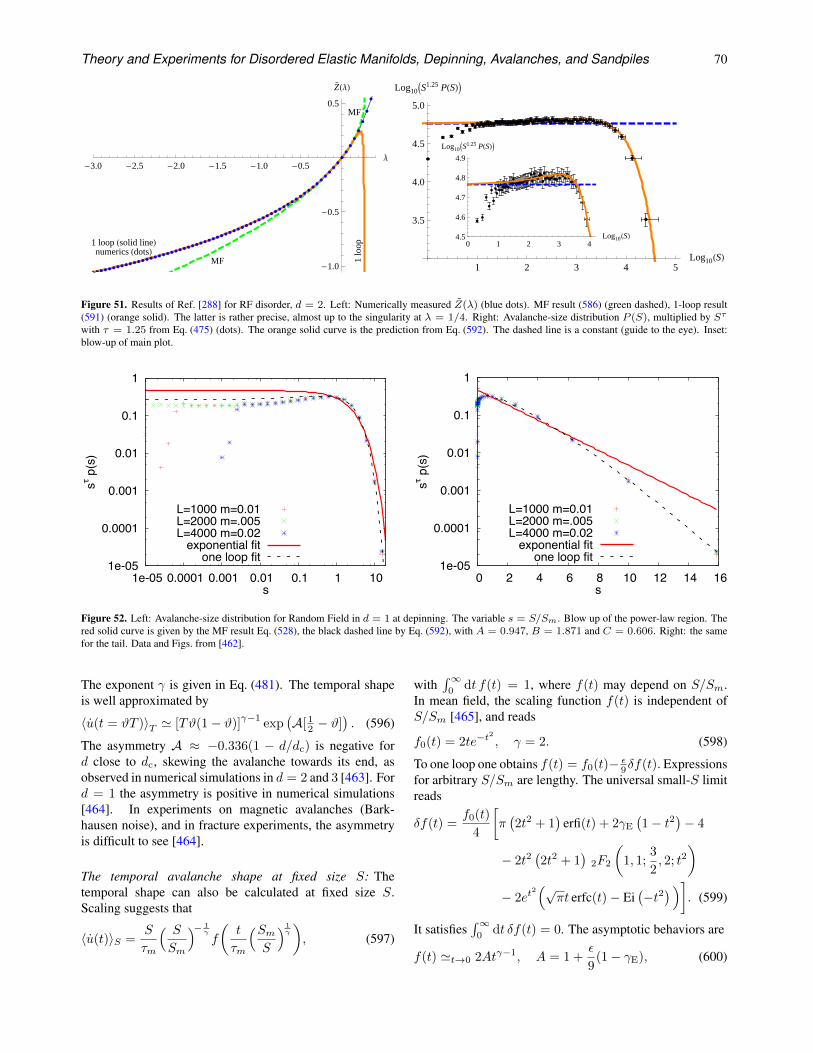
Theory and Experiments for Disordered Elastic Manifolds, Depinning, Avalanches, and Sandpiles 70
MF
MF
numerics HdotsL1 loop Hsolid lineL
1lo
op
-3.0 -2.5 -2.0 -1.5 -1.0 -0.5Λ
-1.0
-0.5
0.5
ZHΛL
1 2 3 4 5Log10HSL
3.5
4.0
4.5
5.0
Log10IS1.25 PHSLM
0 1 2 3 4Log10HSL4.5
4.6
4.7
4.8
4.9
Log10IS1.25 PHSLM
Figure 51. Results of Ref. [288] for RF disorder, d = 2. Left: Numerically measured Z(λ) (blue dots). MF result (586) (green dashed), 1-loop result(591) (orange solid). The latter is rather precise, almost up to the singularity at λ = 1/4. Right: Avalanche-size distribution P (S), multiplied by Sτ
with τ = 1.25 from Eq. (475) (dots). The orange solid curve is the prediction from Eq. (592). The dashed line is a constant (guide to the eye). Inset:blow-up of main plot.
1e-05
0.0001
0.001
0.01
0.1
1
1e-05 0.0001 0.001 0.01 0.1 1 10
sτ p
(s)
s
L=1000 m=0.01L=2000 m=.005L=4000 m=0.02
exponential fitone loop fit
1e-05
0.0001
0.001
0.01
0.1
1
0 2 4 6 8 10 12 14 16
sτ p
(s)
s
L=1000 m=0.01L=2000 m=.005L=4000 m=0.02
exponential fitone loop fit
Figure 52. Left: Avalanche-size distribution for Random Field in d = 1 at depinning. The variable s = S/Sm. Blow up of the power-law region. Thered solid curve is given by the MF result Eq. (528), the black dashed line by Eq. (592), with A = 0.947, B = 1.871 and C = 0.606. Right: the samefor the tail. Data and Figs. from [462].
The exponent γ is given in Eq. (481). The temporal shapeis well approximated by
〈u(t = ϑT )〉T ' [Tϑ(1− ϑ)]γ−1
exp(A[ 1
2 − ϑ]). (596)
The asymmetry A ≈ −0.336(1 − d/dc) is negative ford close to dc, skewing the avalanche towards its end, asobserved in numerical simulations in d = 2 and 3 [463]. Ford = 1 the asymmetry is positive in numerical simulations[464]. In experiments on magnetic avalanches (Bark-hausen noise), and in fracture experiments, the asymmetryis difficult to see [464].
The temporal avalanche shape at fixed size S: Thetemporal shape can also be calculated at fixed size S.Scaling suggests that
〈u(t)〉S =S
τm
( S
Sm
)− 1γ
f
(t
τm
(SmS
)1γ
), (597)
with∫∞
0dt f(t) = 1, where f(t) may depend on S/Sm.
In mean field, the scaling function f(t) is independent ofS/Sm [465], and reads
f0(t) = 2te−t2
, γ = 2. (598)
To one loop one obtains f(t) = f0(t)− ε9δf(t). Expressions
for arbitrary S/Sm are lengthy. The universal small-S limitreads
δf(t) =f0(t)
4
[π(2t2 + 1
)erfi(t) + 2γE
(1− t2
)− 4
− 2t2(2t2 + 1
)2F2
(1, 1;
3
2, 2; t2
)
− 2et2(√
πt erfc(t)− Ei(−t2
) )]. (599)
It satisfies∫∞
0dt δf(t) = 0. The asymptotic behaviors are
f(t) 't→0 2Atγ−1, A = 1 +ε
9(1− γE), (600)
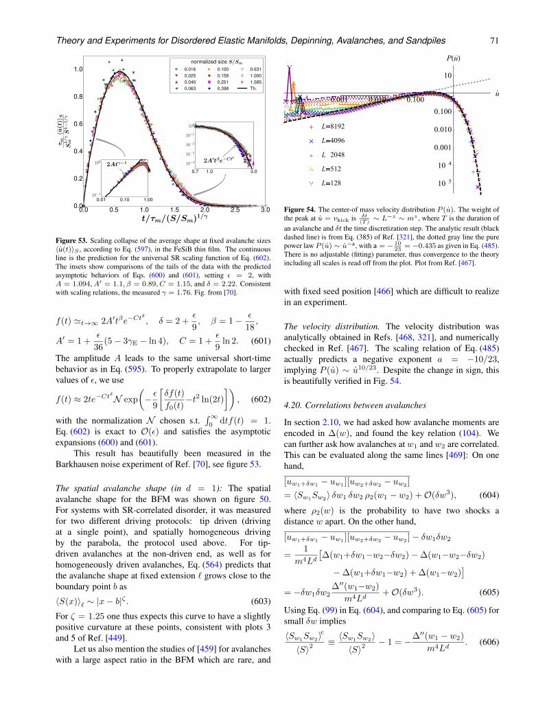
Theory and Experiments for Disordered Elastic Manifolds, Depinning, Avalanches, and Sandpiles 71
0.0 0.5 1.0 1.5 2.0 2.5 3.0t/m/(S/Sm)1/
0.0
0.2
0.4
0.6
0.8
1.0
m
S1/
m
hu(t
)iS
S1
1/
normalized size S/Sm
0.0160.0250.0400.063
0.1000.1580.2510.398
0.6311.0001.585Th.
0.01 0.10 1.00101
1002At1
0.7 1.0 3.0
104
103
102
101
100
2A0teCt
Figure 53. Scaling collapse of the average shape at fixed avalanche sizes〈u(t)〉S , according to Eq. (597), in the FeSiB thin film. The continuousline is the prediction for the universal SR scaling function of Eq. (602).The insets show comparisons of the tails of the data with the predictedasymptotic behaviors of Eqs. (600) and (601), setting ε = 2, withA = 1.094, A′ = 1.1, β = 0.89, C = 1.15, and δ = 2.22. Consistentwith scaling relations, the measured γ = 1.76. Fig. from [70].
f(t) 't→∞ 2A′tβe−Ctδ
, δ = 2 +ε
9, β = 1− ε
18,
A′ = 1 +ε
36(5− 3γE − ln 4), C = 1 +
ε
9ln 2. (601)
The amplitude A leads to the same universal short-timebehavior as in Eq. (595). To properly extrapolate to largervalues of ε, we use
f(t) ≈ 2te−CtδN exp
(− ε
9
[δf(t)
f0(t)−t2 ln(2t)
]), (602)
with the normalization N chosen s.t.∫∞
0dtf(t) = 1.
Eq. (602) is exact to O(ε) and satisfies the asymptoticexpansions (600) and (601).
This result has beautifully been measured in theBarkhausen noise experiment of Ref. [70], see figure 53.
The spatial avalanche shape (in d = 1): The spatialavalanche shape for the BFM was shown on figure 50.For systems with SR-correlated disorder, it was measuredfor two different driving protocols: tip driven (drivingat a single point), and spatially homogeneous drivingby the parabola, the protocol used above. For tip-driven avalanches at the non-driven end, as well as forhomogeneously driven avalanches, Eq. (564) predicts thatthe avalanche shape at fixed extension ` grows close to theboundary point b as
〈S(x)〉` ∼ |x− b|ζ . (603)
For ζ = 1.25 one thus expects this curve to have a slightlypositive curvature at these points, consistent with plots 3and 5 of Ref. [449].
Let us also mention the studies of [459] for avalancheswith a large aspect ratio in the BFM which are rare, and
+
+
+×
×
×*
*
*
+++++++
+
++++++++++++++++++++
+++++++++++
+++++++++++++++++++++++++
++++
+
+
+
××××××
×
××××××××××××××××××××××××
××××××××××××
×××××××××××××××××××××××××
×
×
×
*****
*
****************************
*****************************
****
*
*
+ L 8192
× L 4096
* L 2048
L 512
L 128
10-4
0.001 0.010 0.100u
10-5
10-4
0.001
0.010
0.100
10
P(u)
Figure 54. The center-of mass velocity distribution P (u). The weight ofthe peak at u = vkick is δt
〈T 〉 ∼ L−z ∼ mz , where T is the duration ofan avalanche and δt the time discretization step. The analytic result (blackdashed line) is from Eq. (385) of Ref. [321], the dotted gray line the purepower law P (u) ∼ u−a, with a = − 10
23= −0.435 as given in Eq. (485).
There is no adjustable (fitting) parameter, thus convergence to the theoryincluding all scales is read off from the plot. Plot from Ref. [467].
with fixed seed position [466] which are difficult to realizein an experiment.
The velocity distribution. The velocity distribution wasanalytically obtained in Refs. [468, 321], and numericallychecked in Ref. [467]. The scaling relation of Eq. (485)actually predicts a negative exponent a = −10/23,implying P (u) ∼ u10/23. Despite the change in sign, thisis beautifully verified in Fig. 54.
4.20. Correlations between avalanches
In section 2.10, we had asked how avalanche moments areencoded in ∆(w), and found the key relation (104). Wecan further ask how avalanches at w1 and w2 are correlated.This can be evaluated along the same lines [469]: On onehand,
[uw1+δw1 − uw1 ][uw2+δw2 − uw2 ]
= 〈Sw1Sw2〉 δw1 δw2 ρ2(w1 − w2) +O(δw3), (604)
where ρ2(w) is the probability to have two shocks adistance w apart. On the other hand,
[uw1+δw1 − uw1 ][uw2+δw2 − uw2 ]− δw1δw2
=1
m4Ld[∆(w1+δw1−w2−δw2)−∆(w1−w2−δw2)
−∆(w1+δw1−w2) + ∆(w1−w2)]
= −δw1δw2∆′′(w1−w2)
m4Ld+O(δw3). (605)
Using Eq. (99) in Eq. (604), and comparing to Eq. (605) forsmall δw implies
〈Sw1Sw2〉c
〈S〉2≡ 〈Sw1
Sw2〉
〈S〉2− 1 = −∆′′(w1 − w2)
m4Ld. (606)
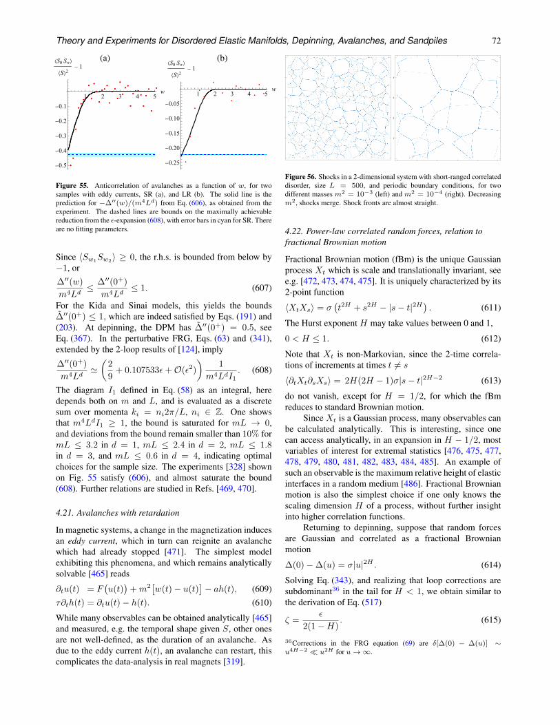
Theory and Experiments for Disordered Elastic Manifolds, Depinning, Avalanches, and Sandpiles 72
(a) (b)
1 2 3 4 5w
-0.5
-0.4
-0.3
-0.2
-0.1
⟨S0 Sw⟩
⟨S⟩2- 1
1 2 3 4 5w
-0.25
-0.20
-0.15
-0.10
-0.05
⟨S0 Sw⟩
⟨S⟩2- 1
Figure 55. Anticorrelation of avalanches as a function of w, for twosamples with eddy currents, SR (a), and LR (b). The solid line is theprediction for −∆′′(w)/(m4Ld) from Eq. (606), as obtained from theexperiment. The dashed lines are bounds on the maximally achievablereduction from the ε-expansion (608), with error bars in cyan for SR. Thereare no fitting parameters.
Since 〈Sw1Sw2〉 ≥ 0, the r.h.s. is bounded from below by−1, or
∆′′(w)
m4Ld≤ ∆′′(0+)
m4Ld≤ 1. (607)
For the Kida and Sinai models, this yields the bounds∆′′(0+) ≤ 1, which are indeed satisfied by Eqs. (191) and(203). At depinning, the DPM has ∆′′(0+) = 0.5, seeEq. (367). In the perturbative FRG, Eqs. (63) and (341),extended by the 2-loop results of [124], imply
∆′′(0+)
m4Ld'(
2
9+ 0.107533ε+O(ε2)
)1
m4LdI1. (608)
The diagram I1 defined in Eq. (58) as an integral, heredepends both on m and L, and is evaluated as a discretesum over momenta ki = ni2π/L, ni ∈ Z. One showsthat m4LdI1 ≥ 1, the bound is saturated for mL → 0,and deviations from the bound remain smaller than 10% formL ≤ 3.2 in d = 1, mL ≤ 2.4 in d = 2, mL ≤ 1.8in d = 3, and mL ≤ 0.6 in d = 4, indicating optimalchoices for the sample size. The experiments [328] shownon Fig. 55 satisfy (606), and almost saturate the bound(608). Further relations are studied in Refs. [469, 470].
4.21. Avalanches with retardation
In magnetic systems, a change in the magnetization inducesan eddy current, which in turn can reignite an avalanchewhich had already stopped [471]. The simplest modelexhibiting this phenomena, and which remains analyticallysolvable [465] reads
∂tu(t) = F(u(t)
)+m2
[w(t)− u(t)
]− ah(t), (609)
τ∂th(t) = ∂tu(t)− h(t). (610)
While many observables can be obtained analytically [465]and measured, e.g. the temporal shape given S, other onesare not well-defined, as the duration of an avalanche. Asdue to the eddy current h(t), an avalanche can restart, thiscomplicates the data-analysis in real magnets [319].
1 100 200 300 400 501
1
100
200
300
400
501
1 100 200 300 400 5011
100
200
300
400
501
1 100 200 300 400 501
1
100
200
300
400
501
1 100 200 300 400 5011
100
200
300
400
501
Figure 56. Shocks in a 2-dimensional system with short-ranged correlateddisorder, size L = 500, and periodic boundary conditions, for twodifferent masses m2 = 10−3 (left) and m2 = 10−4 (right). Decreasingm2, shocks merge. Shock fronts are almost straight.
4.22. Power-law correlated random forces, relation tofractional Brownian motion
Fractional Brownian motion (fBm) is the unique Gaussianprocess Xt which is scale and translationally invariant, seee.g. [472, 473, 474, 475]. It is uniquely characterized by its2-point function
〈XtXs〉 = σ(t2H + s2H − |s− t|2H
). (611)
The Hurst exponent H may take values between 0 and 1,
0 < H ≤ 1. (612)
Note that Xt is non-Markovian, since the 2-time correla-tions of increments at times t 6= s
〈∂tXt∂sXs〉 = 2H(2H − 1)σ|s− t|2H−2 (613)
do not vanish, except for H = 1/2, for which the fBmreduces to standard Brownian motion.
Since Xt is a Gaussian process, many observables canbe calculated analytically. This is interesting, since onecan access analytically, in an expansion in H − 1/2, mostvariables of interest for extremal statistics [476, 475, 477,478, 479, 480, 481, 482, 483, 484, 485]. An example ofsuch an observable is the maximum relative height of elasticinterfaces in a random medium [486]. Fractional Brownianmotion is also the simplest choice if one only knows thescaling dimension H of a process, without further insightinto higher correlation functions.
Returning to depinning, suppose that random forcesare Gaussian and correlated as a fractional Brownianmotion
∆(0)−∆(u) = σ|u|2H . (614)
Solving Eq. (343), and realizing that loop corrections aresubdominant36 in the tail for H < 1, we obtain similar tothe derivation of Eq. (517)
ζ =ε
2(1−H). (615)
36Corrections in the FRG equation (69) are δ[∆(0) − ∆(u)] ∼u4H−2 u2H for u→∞.
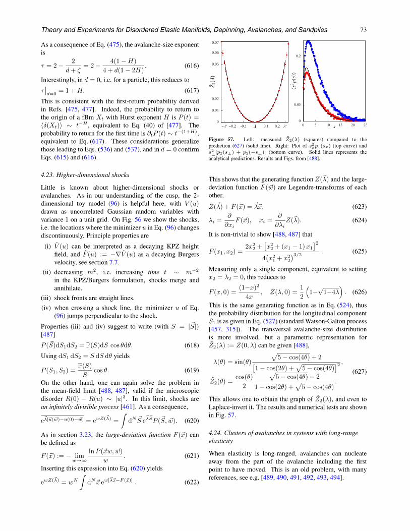
Theory and Experiments for Disordered Elastic Manifolds, Depinning, Avalanches, and Sandpiles 73
As a consequence of Eq. (475), the avalanche-size exponentis
τ = 2− 2
d+ ζ= 2− 4(1−H)
4 + d(1− 2H). (616)
Interestingly, in d = 0, i.e. for a particle, this reduces to
τ∣∣d=0
= 1 +H. (617)
This is consistent with the first-return probability derivedin Refs. [475, 477]. Indeed, the probability to return tothe origin of a fBm Xt with Hurst exponent H is P (t) =〈δ(Xt)〉 ∼ t−H , equivalent to Eq. (40) of [477]. Theprobability to return for the first time is ∂tP (t) ∼ t−(1+H),equivalent to Eq. (617). These considerations generalizethose leading to Eqs. (536) and (537), and in d = 0 confirmEqs. (615) and (616).
4.23. Higher-dimensional shocks
Little is known about higher-dimensional shocks oravalanches. As in our understanding of the cusp, the 2-dimensional toy model (96) is helpful here, with V (u)drawn as uncorrelated Gaussian random variables withvariance 1 on a unit grid. On Fig. 56 we show the shocks,i.e. the locations where the minimizer u in Eq. (96) changesdiscontinuously. Principle properties are
(i) V (u) can be interpreted as a decaying KPZ heightfield, and F (u) := −∇V (u) as a decaying Burgersvelocity, see section 7.7.
(ii) decreasing m2, i.e. increasing time t ∼ m−2
in the KPZ/Burgers formulation, shocks merge andannihilate.
(iii) shock fronts are straight lines.(iv) when crossing a shock line, the minimizer u of Eq.
(96) jumps perpendicular to the shock.
Properties (iii) and (iv) suggest to write (with S = |~S|)[487]
P (~S)dS1dS2 = P(S)dS cos θdθ. (618)
Using dS1 dS2 = S dS dθ yields
P (S1, S2) =P(S)
Scos θ. (619)
On the other hand, one can again solve the problem inthe mean-field limit [488, 487], valid if the microscopicdisorder R(0) − R(u) ∼ |u|3. In this limit, shocks arean infinitely divisible process [461]. As a consequence,
e~λ[~u(~w)−u(0)−~w] = ewZ(~λ) =
∫dN ~S e
~λ~SP (~S, ~w). (620)
As in section 3.23, the large-deviation function F (~x) canbe defined as
F (~x) := − limw→∞
lnP (~xw, ~w)
w. (621)
Inserting this expression into Eq. (620) yields
ewZ(~λ) = wN∫
dN~x ew[~λ~x−F (~x)] . (622)
0
0.01
0.02
0.05
0.06
0.07
−λ∗ −0.2 -0.1 0.1 0.2 λ∗
Z2(λ)
λ0
0.05
0.2
0 5 10 15 20 25
〈s2p(s)〉
s
Figure 57. Left: measured Z2(λ) (squares) compared to theprediction (627) (solid line). Right: Plot of s2xp1(sx) (top curve) ands2⊥[p2(s⊥) + p2(−s⊥)] (bottom curve). Solid lines represents theanalytical predictions. Results and Figs. from [488].
This shows that the generating function Z(~λ) and the large-deviation function F (~w) are Legendre-transforms of eachother,
Z(~λ) + F (~x) = ~λ~x, (623)
λi =∂
∂xiF (~x), xi =
∂
∂λiZ(~λ). (624)
It is non-trivial to show [488, 487] that
F (x1, x2) =2x2
2 +[x2
2 + (x1 − 1)x1
]2
4(x2
1 + x22
)3/2 . (625)
Measuring only a single component, equivalent to settingx2 = λ2 = 0, this reduces to
F (x, 0) =(1−x)2
4x, Z(λ, 0) =
1
2
(1−√
1−4λ). (626)
This is the same generating function as in Eq. (524), thusthe probability distribution for the longitudinal componentS1 is as given in Eq. (527) (standard Watson-Galton process[457, 315]). The transversal avalanche-size distributionis more involved, but a parametric representation forZ2(λ) := Z(0, λ) can be given [488],
λ(θ) = sin(θ)
√5− cos(4θ) + 2
[1− cos(2θ) +
√5− cos(4θ)
]2 ,
Z2(θ) =cos(θ)
2
√5− cos(4θ)− 2
1− cos(2θ) +√
5− cos(4θ).
(627)
This allows one to obtain the graph of Z2(λ), and even toLaplace-invert it. The results and numerical tests are shownin Fig. 57.
4.24. Clusters of avalanches in systems with long-rangeelasticity
When elasticity is long-ranged, avalanches can nucleateaway from the part of the avalanche including the firstpoint to have moved. This is an old problem, with manyreferences, see e.g. [489, 490, 491, 492, 493, 494].
Theory and Experiments for Disordered Elastic Manifolds, Depinning, Avalanches, and Sandpiles 74
Suppose that each avalanche of size S is composed ofNc(S) clusters, distributed as
P (Sc|S) ∼ S−τcc Θ(Sc < S), τc < 2. (628)
Then the typical size of clusters, given avalanche size S, is
〈Sc〉S =
∫ ∞
0
dSc ScP (Sc|S) ∼ S2−τc . (629)
There are
Nc(S) ' S
〈Sc〉∼ Sτc−1 (630)
clusters. Suppose that the number of clusters scales as
P (Nc) ∼ N−µc Θ(Nc < Nc(S)). (631)
On dimensional grounds, P (S)dS ∼ P (Nc)dNc. Insertingthe above relations yields
τc − 1 =τ − 1
µ− 1. (632)
If one further supposes [492, 493, 494] that the generationof a new cluster is a Galton-Watson process (section 4.11),then
µ = 3/2, (633)
simplifying Eq. (632) to [492, 493, 494]
τcluster = 2τ − 1. (634)
Numerically it was checked [492, 493] that this scalingrelation works for all 0 ≤ α < 2; it might actually continueto work for α = 2, if one keeps a finite value for Aαd inEq. (17b) avoiding to reduce the power-law kernel to short-ranged correlations in that limit (see section 1.3). Theseresults have recently been questioned [495].
4.25. Earthquakes
Gutenberg and Richter [97, 75] first reported that themagnitude of earthquakes in California follows a power-law, equivalent to an avalanche-size exponent37 of τ = 3/2.Due to its enormous impact on society, much research isdone in the domain, both by geophysicists with the aimof predicting the next big earthquake, and by theoreticalphysicists, trying to put earthquakes into the framework ofdisordered elastic manifolds. The latter is successful to acertain extend:
• the elastic object depinning is a 2-dimensional faultplane, to which the relative movement is confined,often with sub-mm precision (localization),
• driving is through the tectonic plates, equivalent to theparabolic confining potential of Eq. (5),
• the elastic interactions on the fault plane are long-ranged since elasticity is mediated by the bulk. Thecalculation is essentially the same as for contact linesin section 1.3, and yields α = 1 in Eq. (16),
37Geophysicist usually consider the cumulative distribution of magnitude.The magnitude was originally defined as “proportional to the log of themaximum amplitude on a standard torsion seismometer” [496].
• the critical dimension dc(α) = 2α = 2 is thedimension of the fault plane. The system is in itscritical dimension. As a consequence ζ = 0, z = 2,and τ = 3/2, which correctly predicts the Gutenberg-Richter law.
But there is an additional element: After an earthquake,the fault is damaged, rendering it less resistant to furthermovement before the damage is healed, which happens on amuch longer time scale (see e.g. [497]). As a consequence,immediately after a big earthquake, the likelihood ofanother earthquake is increased. It is indeed found that theprobability for an aftershock to appear decays (roughly) as1/t in time t, known today as Omori’s law [498].
For further reading, we refer to the original literature[499, 497, 500, 501, 502, 503, 504, 80, 505, 506, 507, 508,509, 510] and to some of the relevant concepts discussed inthis review, long-range correlated elasticity (section 4.24),and inertia (section 3.23).
4.26. Avalanches in the SK model
The ABBM model, the BFM, or any other approach basedon a random walk, and commonly summarized as “meanfield” gives an avalanche-size exponent τ = 3/2 (definedin Eq. (472)), bounding from above all experiments andsimulations on disordered elastic manifolds
ζABBM = ζBFM = ζMF =3
2≥ ζddep ≡ 2− 2
d+ ζ> 1.
(635)
On the other hand, since d + ζ > 2, even in dimensiond = 1, there seems to be a lower bound on τ as well,indicated above. Note that for τ ≤ 1 the avalanche-sizedistribution becomes non-integrable at large S in absenceof an IR cutoff.
It is thus quite surprising to learn that in the SK model[59] the exponent τ is smaller [511, 512],
τ equilibriumSK = τdynamic
SK = 1. (636)
This result for the equilibrium was obtained [511, 512]within a full-RSB scheme, relevant for SK. Curiously, ex-actly the same exponent is found in numerical simulations[513] out of equilibrium, where one simply increases themagnetic field until one spin becomes unstable, which isthen flipped. While finding the ground-state is an NP-hardproblem, this dynamic algorithm is trivial to implement.Still, the exponent τ is the same. It is also counterintuitiveto learn that avalanches in the SK model involve a finitefraction of its total of N spins, changing the magnetizationon average by
√N for an increase in external field by order
1/√N , i.e.
Styp :=
⟨S2⟩
〈2S〉 =√N. (637)
This means that on the complete hysteresis curve each spinflips on average an order of
√N times. This is very different
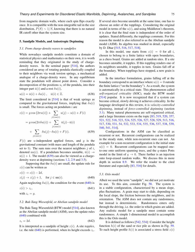
Theory and Experiments for Disordered Elastic Manifolds, Depinning, Avalanches, and Sandpiles 75
from magnetic domain walls, where each spin flips exactlyonce. It is compatible with the non-integrable tail in the sizedistribution, P (S) ∼ 1/S, knowing that there is no naturalIR cutoff other than the system size.
5. Sandpile Models, and Anisotropic Depinning
5.1. From charge-density waves to sandpiles
While nowadays sandpile models constitute a domain ofstatistical physics and mathematics on their own, it is worthreminding that they originated in the study of charge-density waves. In the seminal paper [514], the authorsconsidered an array of rotating pendula elastically coupledto their neighbors via weak torsion springs, a mechanicalanalogue of a charge-density wave. In any equilibriumstate the pendulum will almost point down. Consider adecomposition of the positions ui of the pendula, into theirinteger part u(i) and a rest δu(i),
u(i) = u(i) + δu(i) , u(i) ∈ Z. (638)
The limit considered in [514] is that of weak springs ascompared to the gravitational forces, implying that δu(i)is small. The forces acting on pendulum i are
z(i) = g cos(2πu(i)
)+
∑
j∈nn(i)
u(j)− u(i) + F (i)
= g cos(2πδu(i)) +∑
j∈nn(i)
u(j)−u(i)
+∑
j∈nn(i)
δu(j)−δu(i) + F (i). (639)
F (i) are u-independent applied forces, and g is thegravitational constant (with mass and length of the pendulaset to 1). The sum runs over the nearest neighbors j of i,denoted nn(i). If a pendulum becomes unstable, u(i) →u(i) + 1. The model (639) can also be viewed as a charge-density wave at depinning (sections 1.2, 2.9 and 3.5).
Supposing that the δu(i) are small, the update rule forz(i) can be written as
z(i)→ z(i)− 2d,
z(j)→ z(j) + 1, for j ∈ nn(i). (640)
Again neglecting δu(i), the condition for the event (640) is
z(i) > zc, (641)
with zc = g.
5.2. Bak-Tang-Wiesenfeld, or Abelian sandpile model
The Bak-Tang-Wiesenfeld (BTW) model [514], also knownas the Abelian sandpile model (ASM), uses the update rules(640) combined with
zc = 2d. (642)
It is interpreted as a sandpile of height z(i). A site topples,i.e. the rule (640) is performed, when its height exceeds zc.
If several sites become unstable at the same time, one has tochoose an order of the topplings. Considering the originalmodel in terms of the u(i), and using Middleton’s theorem,it is clear that the final state is independent of the order ofupdates. Stated differently, the topplings commute. For thisreason the model is also referred to as the Abelian sandpilemodel (ASM). Its algebra was studied in detail, especiallyby D. Dhar [515, 516, 517, 518].
In this model, one starts from z(i) = 0 for all i,chosen to belong to a finite lattice with open boundaries,as a chess board. Grains are added at random sites. If a sitebecomes unstable, it topples. If this toppling renders one ofits neighbors unstable, it topples in turn. Grains fall off atthe boundary. When topplings have stopped, a new grain isadded.
In the interface formulation, grains falling off at theboundary correspond to an interface where u(i) = 0 outsidethe finite lattice (“on the boundary”). As a result, the systemis automatically in a critical state. This phenomenon calledself-organized criticality (SOC), made the BTW model[514] popular. It is now recognized that if a system canbecome critical, slowly driving it achieves criticality. In thelanguage developed in this review, it is velocity-controlleddepinning, instead of force-controlled depinning (section3.1). Many natural phenomena are self-organized critical,and a large literature exists on the topic [83, 519, 520, 357,521, 522, 518, 523, 524, 525, 526, 527, 528, 529, 513, 516,517, 530, 531, 54, 532, 533, 534, 535, 536, 537, 538, 539,540, 541, 514].
Configurations in the ASM can be classified asrecurrent or not. Recurrent configurations can be realizedin the steady state, while non-recurrent ones can not. Anexample for a non-recurrent configuration is the initial stateu(i) = 0. Recurrent configurations can be mapped one-to-one onto uniform spanning trees, and the q-states Pottsmodel in the limit of q → 0. There further is an injectiononto loop-erased random walks. We discuss this in moredepth in section 8.9. We refer the reader to the citedliterature and especially [83, 516] for details.
5.3. Oslo model
Albeit we used the term “sandpile”, we did not yet motivateits use. To this aim, consider Fig. 58. The system isin a stable configuration, characterized by a mean slope,plus fluctuations. A grain may start to slide, depending onthe local slope, the friction between the neighbors, and itsorientation. The ASM does not contain any randomness,but instead is deterministic. Randomness enters onlythrough the driving, i.e. the order in which grains are added.Any realistic model for a sandpile must contain somerandomness. A simple 1-dimensional model to accomplishthis is the Oslo model.
It is defined as follows [542, 534]: Consider the heightfunction h(i) of the sand or rice pile as shown in Fig. 59.To each height profile h(i) is associated a stress field z(i)
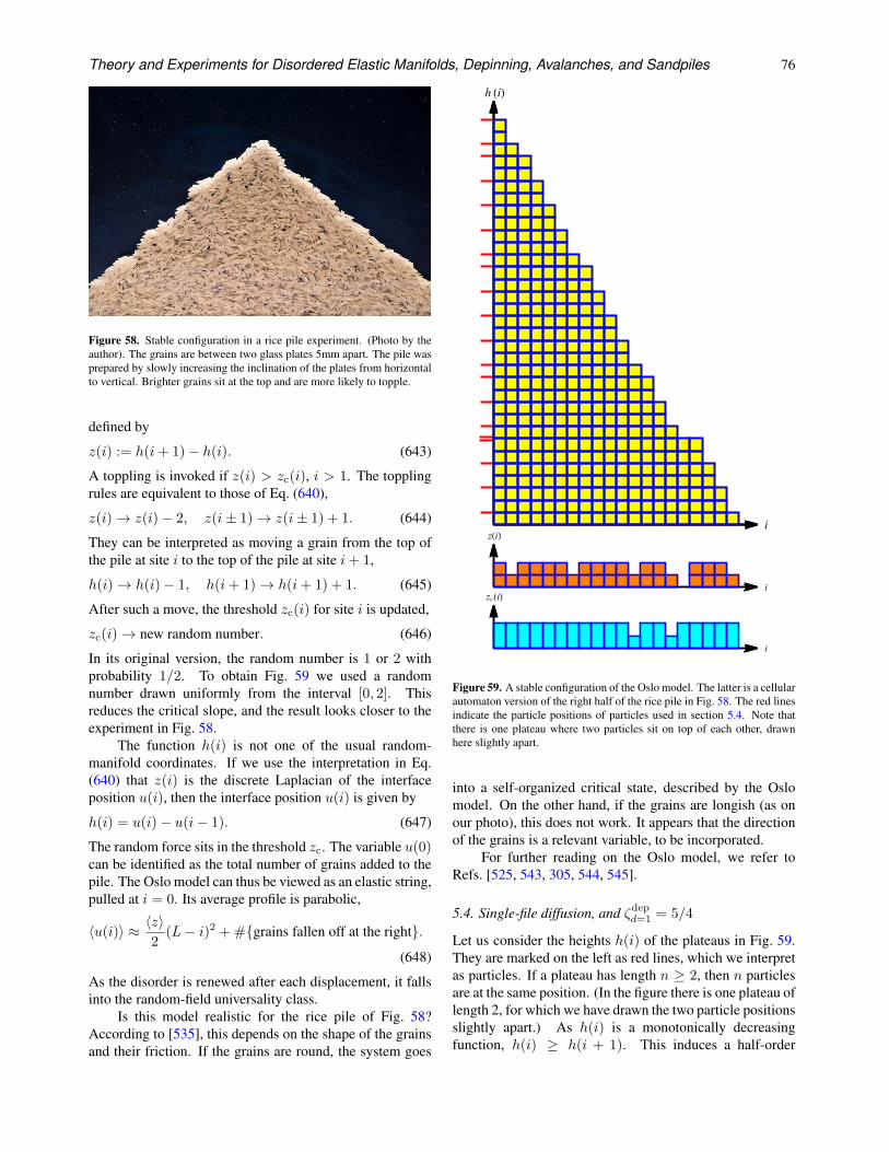
Theory and Experiments for Disordered Elastic Manifolds, Depinning, Avalanches, and Sandpiles 76
Figure 58. Stable configuration in a rice pile experiment. (Photo by theauthor). The grains are between two glass plates 5mm apart. The pile wasprepared by slowly increasing the inclination of the plates from horizontalto vertical. Brighter grains sit at the top and are more likely to topple.
defined by
z(i) := h(i+ 1)− h(i). (643)
A toppling is invoked if z(i) > zc(i), i > 1. The topplingrules are equivalent to those of Eq. (640),
z(i)→ z(i)− 2, z(i± 1)→ z(i± 1) + 1. (644)
They can be interpreted as moving a grain from the top ofthe pile at site i to the top of the pile at site i+ 1,
h(i)→ h(i)− 1, h(i+ 1)→ h(i+ 1) + 1. (645)
After such a move, the threshold zc(i) for site i is updated,
zc(i)→ new random number. (646)
In its original version, the random number is 1 or 2 withprobability 1/2. To obtain Fig. 59 we used a randomnumber drawn uniformly from the interval [0, 2]. Thisreduces the critical slope, and the result looks closer to theexperiment in Fig. 58.
The function h(i) is not one of the usual random-manifold coordinates. If we use the interpretation in Eq.(640) that z(i) is the discrete Laplacian of the interfaceposition u(i), then the interface position u(i) is given by
h(i) = u(i)− u(i− 1). (647)
The random force sits in the threshold zc. The variable u(0)can be identified as the total number of grains added to thepile. The Oslo model can thus be viewed as an elastic string,pulled at i = 0. Its average profile is parabolic,
〈u(i)〉 ≈ 〈z〉2
(L− i)2 + #grains fallen off at the right.(648)
As the disorder is renewed after each displacement, it fallsinto the random-field universality class.
Is this model realistic for the rice pile of Fig. 58?According to [535], this depends on the shape of the grainsand their friction. If the grains are round, the system goes
i
h (i)
i
z(i)
i
zc(i)
Figure 59. A stable configuration of the Oslo model. The latter is a cellularautomaton version of the right half of the rice pile in Fig. 58. The red linesindicate the particle positions of particles used in section 5.4. Note thatthere is one plateau where two particles sit on top of each other, drawnhere slightly apart.
into a self-organized critical state, described by the Oslomodel. On the other hand, if the grains are longish (as onour photo), this does not work. It appears that the directionof the grains is a relevant variable, to be incorporated.
For further reading on the Oslo model, we refer toRefs. [525, 543, 305, 544, 545].
5.4. Single-file diffusion, and ζdepd=1 = 5/4
Let us consider the heights h(i) of the plateaus in Fig. 59.They are marked on the left as red lines, which we interpretas particles. If a plateau has length n ≥ 2, then n particlesare at the same position. (In the figure there is one plateau oflength 2, for which we have drawn the two particle positionsslightly apart.) As h(i) is a monotonically decreasingfunction, h(i) ≥ h(i + 1). This induces a half-order
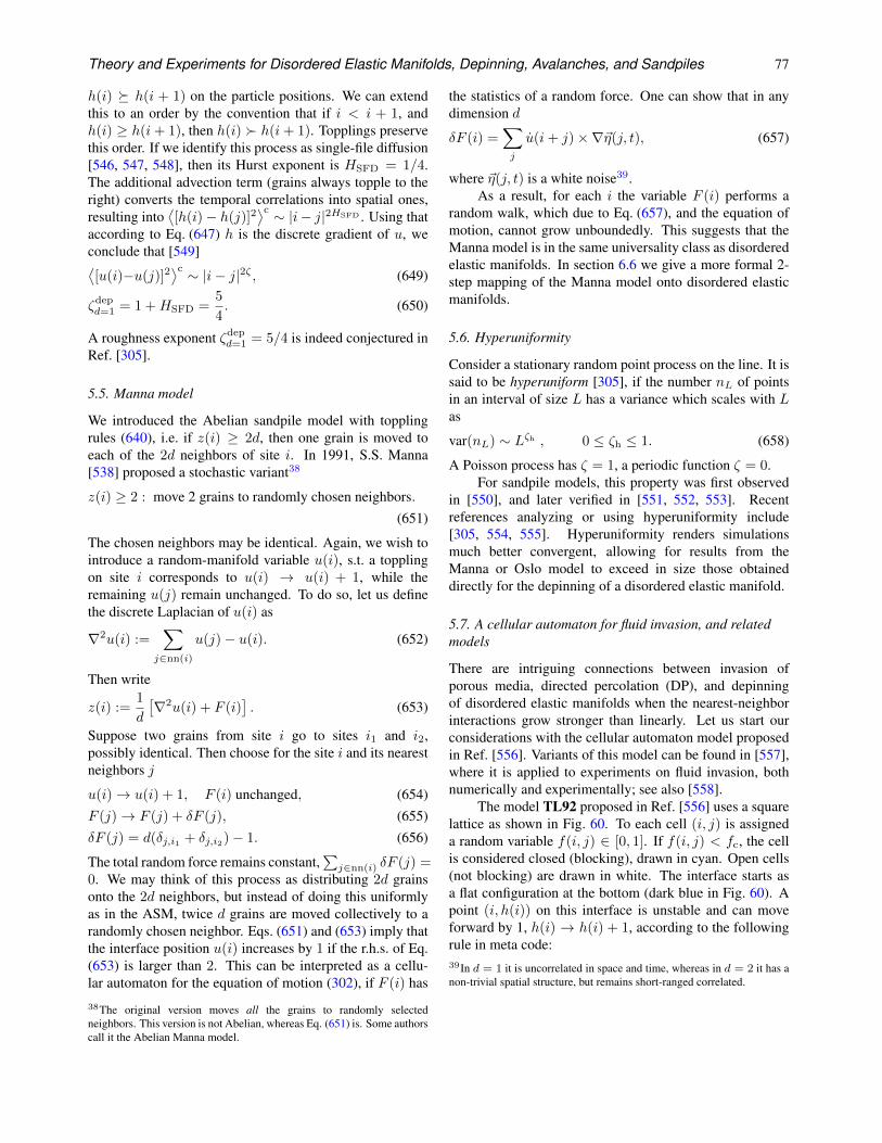
Theory and Experiments for Disordered Elastic Manifolds, Depinning, Avalanches, and Sandpiles 77
h(i) h(i + 1) on the particle positions. We can extendthis to an order by the convention that if i < i + 1, andh(i) ≥ h(i+ 1), then h(i) h(i+ 1). Topplings preservethis order. If we identify this process as single-file diffusion[546, 547, 548], then its Hurst exponent is HSFD = 1/4.The additional advection term (grains always topple to theright) converts the temporal correlations into spatial ones,resulting into
⟨[h(i)− h(j)]2
⟩c ∼ |i− j|2HSFD . Using thataccording to Eq. (647) h is the discrete gradient of u, weconclude that [549]⟨[u(i)−u(j)]2
⟩c ∼ |i− j|2ζ , (649)
ζdepd=1 = 1 +HSFD =
5
4. (650)
A roughness exponent ζdepd=1 = 5/4 is indeed conjectured in
Ref. [305].
5.5. Manna model
We introduced the Abelian sandpile model with topplingrules (640), i.e. if z(i) ≥ 2d, then one grain is moved toeach of the 2d neighbors of site i. In 1991, S.S. Manna[538] proposed a stochastic variant38
z(i) ≥ 2 : move 2 grains to randomly chosen neighbors.(651)
The chosen neighbors may be identical. Again, we wish tointroduce a random-manifold variable u(i), s.t. a topplingon site i corresponds to u(i) → u(i) + 1, while theremaining u(j) remain unchanged. To do so, let us definethe discrete Laplacian of u(i) as
∇2u(i) :=∑
j∈nn(i)
u(j)− u(i). (652)
Then write
z(i) :=1
d
[∇2u(i) + F (i)
]. (653)
Suppose two grains from site i go to sites i1 and i2,possibly identical. Then choose for the site i and its nearestneighbors j
u(i)→ u(i) + 1, F (i) unchanged, (654)F (j)→ F (j) + δF (j), (655)δF (j) = d(δj,i1 + δj,i2)− 1. (656)
The total random force remains constant,∑j∈nn(i) δF (j) =
0. We may think of this process as distributing 2d grainsonto the 2d neighbors, but instead of doing this uniformlyas in the ASM, twice d grains are moved collectively to arandomly chosen neighbor. Eqs. (651) and (653) imply thatthe interface position u(i) increases by 1 if the r.h.s. of Eq.(653) is larger than 2. This can be interpreted as a cellu-lar automaton for the equation of motion (302), if F (i) has
38The original version moves all the grains to randomly selectedneighbors. This version is not Abelian, whereas Eq. (651) is. Some authorscall it the Abelian Manna model.
the statistics of a random force. One can show that in anydimension d
δF (i) =∑
j
u(i+ j)×∇~η(j, t), (657)
where ~η(j, t) is a white noise39.As a result, for each i the variable F (i) performs a
random walk, which due to Eq. (657), and the equation ofmotion, cannot grow unboundedly. This suggests that theManna model is in the same universality class as disorderedelastic manifolds. In section 6.6 we give a more formal 2-step mapping of the Manna model onto disordered elasticmanifolds.
5.6. Hyperuniformity
Consider a stationary random point process on the line. It issaid to be hyperuniform [305], if the number nL of pointsin an interval of size L has a variance which scales with Las
var(nL) ∼ Lζh , 0 ≤ ζh ≤ 1. (658)
A Poisson process has ζ = 1, a periodic function ζ = 0.For sandpile models, this property was first observed
in [550], and later verified in [551, 552, 553]. Recentreferences analyzing or using hyperuniformity include[305, 554, 555]. Hyperuniformity renders simulationsmuch better convergent, allowing for results from theManna or Oslo model to exceed in size those obtaineddirectly for the depinning of a disordered elastic manifold.
5.7. A cellular automaton for fluid invasion, and relatedmodels
There are intriguing connections between invasion ofporous media, directed percolation (DP), and depinningof disordered elastic manifolds when the nearest-neighborinteractions grow stronger than linearly. Let us start ourconsiderations with the cellular automaton model proposedin Ref. [556]. Variants of this model can be found in [557],where it is applied to experiments on fluid invasion, bothnumerically and experimentally; see also [558].
The model TL92 proposed in Ref. [556] uses a squarelattice as shown in Fig. 60. To each cell (i, j) is assigneda random variable f(i, j) ∈ [0, 1]. If f(i, j) < fc, the cellis considered closed (blocking), drawn in cyan. Open cells(not blocking) are drawn in white. The interface starts asa flat configuration at the bottom (dark blue in Fig. 60). Apoint (i, h(i)) on this interface is unstable and can moveforward by 1, h(i) → h(i) + 1, according to the followingrule in meta code:39In d = 1 it is uncorrelated in space and time, whereas in d = 2 it has anon-trivial spatial structure, but remains short-ranged correlated.
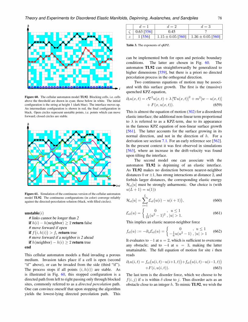
Theory and Experiments for Disordered Elastic Manifolds, Depinning, Avalanches, and Sandpiles 78
i
h
i
h
Figure 60. The cellular automaton model TL92. Blocking cells, i.e. cellsabove the threshold are drawn in cyan; those below in white. The initialconfiguration is the string at height 1 (dark blue). The interface moves up.An intermediate configuration is shown in red, the final configuration inblack. Open circles represent unstable points, i.e. points which can moveforward; closed circles are stable.
i=t
h
i=t
h
Figure 61. Simulation of the continuous version of the cellular automatonmodel TL92. The continuous configurations (in color) converge reliablyagainst the directed-percolation solution (black, with filled circles).
unstable(i)# links cannot be longer than 2if h(i)− h(neighbor) ≥ 2 return false# move forward if openif f(i, h(i)
)> fc return true
# move forward if a neighbor is 2 aheadif h(neighbor)− h(i) ≥ 2 return true
end
This cellular automaton models a fluid invading a porousmedium. Invasion takes place if a cell is open (second“if” above), or can be invaded from the side (third “if”).The process stops if all points (i, h(i)) are stable. Asis illustrated in Fig. 60, this stopped configuration is adirected path from left to right passing only through blockedsites, commonly referred to as a directed percolation path.One can convince oneself that upon stopping the algorithmyields the lowest-lying directed percolation path. This
d = 1 d = 2 d = 3ζ 0.63 [556] 0.45 ?z 1 [556] 1.15± 0.05 [560] 1.36± 0.05 [560]
Table 3. The exponents of qKPZ.
can be implemented both for open and periodic boundaryconditions. The latter are chosen in Fig. 60. Theautomaton TL92 can straightforwardly be generalized tohigher dimensions [559], but there is a priori no directedpercolation process in the orthogonal direction.
Two continuous equations of motion may be associ-ated with this surface growth. The first is the (massive)quenched KPZ equation,
∂tu(x, t) = c∇2u(x, t) + λ [∇u(x, t)]2
+m2[w − u(x, t)]
+ F (x, u(x, t)). (659)
This is almost the equation of motion (302) for a disorderedelastic interface; the additional non-linear term proportionalto λ is referred to as a KPZ-term, due to its appearancein the famous KPZ equation of non-linear surface growth[561]. The latter accounts for the surface growing in itsnormal direction, and not in the direction of h. For aderivation see section 7.1. For an early reference see [562].In the present context it was first observed in simulations[563], where an increase in the drift-velocity was foundupon tilting the interface.
The second model one can associate with theautomaton TL92 is depinning of an elastic interface.As TL92 makes no distinction between nearest-neighbordistances 0 or ±1, has strong interactions at distance 2, andforbids larger distances, the corresponding elastic energyHel[u] must be strongly anharmonic. Our choice is (withu(L+ 1) = u(1))
Hel[u] =
L∑
i=1
Eel
(u(i)− u(i+ 1)
), (660)
Eel(u) =
0 , u ≤ 1
124 (u2 − 1)2 , |u| > 1.
(661)
This implies an elastic nearest-neighbor force
fel(u) := −∂uEel(u) =
0 , u ≤ 1
− 16u(u2 − 1) , |u| > 1
(662)
It evaluates to −1 at u = 2, which is sufficient to overcomeany obstacle; and to −4 at u = 3, making the latterunattainable. The full equation of motion for site i thenreads
∂tu(i, t) = fel
(u(i, t)−u(i+1, t)
)+fel
(u(i, t)−u(i−1, t)
)
+F (i, u(i, t)). (663)
The last term is the disorder force, which we choose to bef(i, j) if u is within δ close to j. Thus disorder acts as anobstacle close to an integer h. To mimic TL92, we wish the
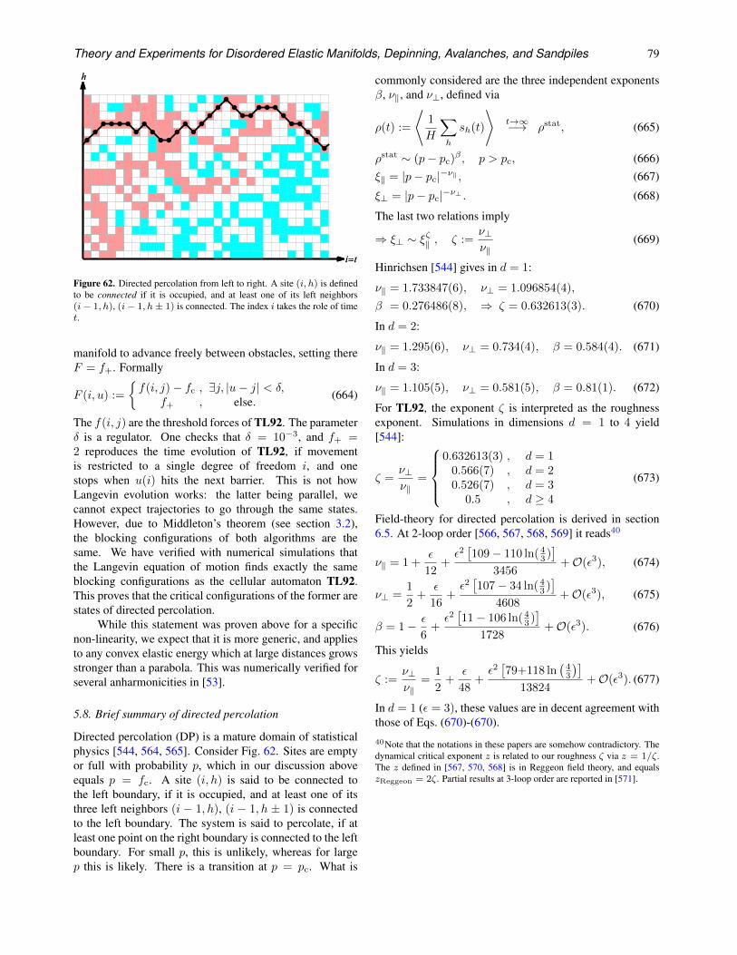
Theory and Experiments for Disordered Elastic Manifolds, Depinning, Avalanches, and Sandpiles 79
i=t
h
i=t
h
Figure 62. Directed percolation from left to right. A site (i, h) is definedto be connected if it is occupied, and at least one of its left neighbors(i− 1, h), (i− 1, h± 1) is connected. The index i takes the role of timet.
manifold to advance freely between obstacles, setting thereF = f+. Formally
F (i, u) :=
f(i, j)− fc , ∃j, |u− j| < δ,
f+ , else. (664)
The f(i, j) are the threshold forces of TL92. The parameterδ is a regulator. One checks that δ = 10−3, and f+ =2 reproduces the time evolution of TL92, if movementis restricted to a single degree of freedom i, and onestops when u(i) hits the next barrier. This is not howLangevin evolution works: the latter being parallel, wecannot expect trajectories to go through the same states.However, due to Middleton’s theorem (see section 3.2),the blocking configurations of both algorithms are thesame. We have verified with numerical simulations thatthe Langevin equation of motion finds exactly the sameblocking configurations as the cellular automaton TL92.This proves that the critical configurations of the former arestates of directed percolation.
While this statement was proven above for a specificnon-linearity, we expect that it is more generic, and appliesto any convex elastic energy which at large distances growsstronger than a parabola. This was numerically verified forseveral anharmonicities in [53].
5.8. Brief summary of directed percolation
Directed percolation (DP) is a mature domain of statisticalphysics [544, 564, 565]. Consider Fig. 62. Sites are emptyor full with probability p, which in our discussion aboveequals p = fc. A site (i, h) is said to be connected tothe left boundary, if it is occupied, and at least one of itsthree left neighbors (i − 1, h), (i − 1, h ± 1) is connectedto the left boundary. The system is said to percolate, if atleast one point on the right boundary is connected to the leftboundary. For small p, this is unlikely, whereas for largep this is likely. There is a transition at p = pc. What is
commonly considered are the three independent exponentsβ, ν‖, and ν⊥, defined via
ρ(t) :=
⟨1
H
∑
h
sh(t)
⟩t→∞−→ ρstat, (665)
ρstat ∼ (p− pc)β , p > pc, (666)ξ‖ = |p− pc|−ν‖ , (667)
ξ⊥ = |p− pc|−ν⊥ . (668)
The last two relations imply
⇒ ξ⊥ ∼ ξζ‖ , ζ :=ν⊥ν‖
(669)
Hinrichsen [544] gives in d = 1:
ν‖ = 1.733847(6), ν⊥ = 1.096854(4),
β = 0.276486(8), ⇒ ζ = 0.632613(3). (670)
In d = 2:
ν‖ = 1.295(6), ν⊥ = 0.734(4), β = 0.584(4). (671)
In d = 3:
ν‖ = 1.105(5), ν⊥ = 0.581(5), β = 0.81(1). (672)
For TL92, the exponent ζ is interpreted as the roughnessexponent. Simulations in dimensions d = 1 to 4 yield[544]:
ζ =ν⊥ν‖
=
0.632613(3) , d = 10.566(7) , d = 20.526(7) , d = 3
0.5 , d ≥ 4
(673)
Field-theory for directed percolation is derived in section6.5. At 2-loop order [566, 567, 568, 569] it reads40
ν‖ = 1 +ε
12+ε2[109− 110 ln( 4
3 )]
3456+O(ε3), (674)
ν⊥ =1
2+
ε
16+ε2[107− 34 ln(4
3 )]
4608+O(ε3), (675)
β = 1− ε
6+ε2[11− 106 ln(4
3 )]
1728+O(ε3). (676)
This yields
ζ :=ν⊥ν‖
=1
2+
ε
48+ε2[79+118 ln
(43
)]
13824+O(ε3). (677)
In d = 1 (ε = 3), these values are in decent agreement withthose of Eqs. (670)-(670).40Note that the notations in these papers are somehow contradictory. Thedynamical critical exponent z is related to our roughness ζ via z = 1/ζ.The z defined in [567, 570, 568] is in Reggeon field theory, and equalszReggeon = 2ζ. Partial results at 3-loop order are reported in [571].
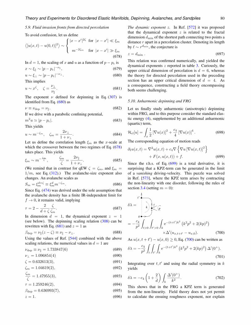
Theory and Experiments for Disordered Elastic Manifolds, Depinning, Avalanches, and Sandpiles 80
5.9. Fluid invasion fronts from directed percolation
To avoid confusion, let us define
⟨[u(x, t)− u(0, t)]2
⟩∼
|x− x′|2ζ for |x− x′| ξm
m−2ζm for |x− x′| ξm
(678)In d = 1, the scaling of x and u as a function of p− pc isx ∼ ξ‖ ∼ |p− pc|−ν‖ , (679)
u ∼ ξ⊥ ∼ |p− pc|−ν⊥ . (680)This implies
u ∼ xζ , ζ =ν⊥ν‖. (681)
The exponent ν defined for depinning in Eq. (307) isidentified from Eq. (680) asν ≡ νdep = ν‖. (682)If we drive with a parabolic confining potential,m2u ' |p− pc|. (683)This yields
u ∼ m−ζm , ζm =2ν⊥
1 + ν⊥. (684)
Let us define the correlation length ξm as the x-scale atwhich the crossover between the two regimes of Eq. (678)takes place. This yields
ξm ∼ m−ζmζ ,
ζmζ
=2ν‖
1 + ν⊥. (685)
(We remind that in contrast for qEW ζ = ζm, and ξm =1/m, see Eq. (312).) The avalanche-size exponent alsochanges. An avalanche scales asSm = ξd+ζ
m ≡ ξdmm−ζm . (686)Since Eq. (474) was derived under the sole assumption thatthe avalanche density has a finite IR-independent limit forf → 0, it remains valid, implying
τ = 2− 2
d+ ζ
ζ
ζm. (687)
In dimension d = 1, the dynamical exponent z = 1(see below). The depinning scaling relation (308) can berewritten with Eq. (681) and z = 1 asβdep = ν‖(z − ζ) ≡ ν‖ − ν⊥. (688)Using the values of Ref. [544] combined with the abovescaling relations, the numerical values in d = 1 areνdep ≡ ν‖ = 1.733847(6) (689)ν⊥ = 1.096854(4) (690)ζ = 0.632613(3), (691)ζm = 1.04619(2), (692)ζmζ
= 1.47955(3), (693)
τ = 1.259246(2), (694)βdep = 0.636993(7), (695)z = 1. (696)
The dynamic exponent z. In Ref. [572] it was proposedthat the dynamical exponent z is related to the fractaldimension dmin of the shortest path connecting two points adistance r apart in a percolation cluster. Denoting its lengthby ` ∼ rdmin , the conjecture is
z = dmin . (697)
This relation was confirmed numerically, and yielded thedynamical exponents z reported in table 3. Curiously, theupper critical dimension of percolation is d = 6, whereasthe theory for directed percolation used in the precedingsection has an upper critical dimension of d = 4. Asa consequence, constructing a field theory encompassingboth seems challenging.
5.10. Anharmonic depinning and FRG
Let us finally study anharmonic (anisotropic) depinningwithin FRG, and to this purpose consider the standard elas-tic energy (4), supplemented by an additional anharmonic(quartic) term,
Hel[u] =
∫
x
1
2[∇u(x)]
2+c44
[∇u(x)]4. (698)
The corresponding equation of motion reads
∂tu(x, t) = ∇2u(x, t) + c4∇∇u [∇u(x, t)]
2
+ F (x, u(x, t)) + f. (699)
Since the r.h.s. of Eq. (699) is a total derivative, it issurprising that a KPZ-term can be generated in the limitof a vanishing driving-velocity. This puzzle was solvedin Ref. [573], where the KPZ term arises by contractingthe non-linearity with one disorder, following the rules ofsection 3.4 (setting m = 0):
δλ =
t’
k p
0
t
= − c4p2
∫
t>0
∫
t′>0
∫
k
e−(t+t′)k2(k2p2 + 2(kp)2
)
×∆′(ux,t+t′ − ux,0). (700)
As u(x, t+ t′)− u(x, 0) ≥ 0, Eq. (700) can be written as
δλ = − c4p2
∫
t
∫
t′
∫
k
e−(t+t′)k2(k2p2 + 2(kp)2
)∆′(0+).
(701)
Integrating over t, t′ and using the radial symmetry in kyields
δλ = −c4(
1 +2
d
)∫
k
∆′(0+)
k2. (702)
This shows that in the FRG a KPZ term is generatedfrom the non-linearity. Field theory does not yet permitto calculate the ensuing roughness exponent, nor explain
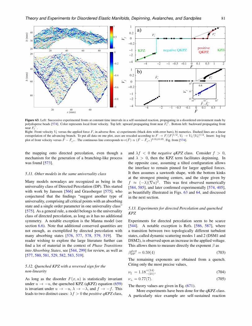
Theory and Experiments for Disordered Elastic Manifolds, Depinning, Avalanches, and Sandpiles 81
x (mm)
h (mm
)
20 40 60
20
40
60
80
!1
!0.8
!0.6
!0.4
!0.2
0
h (mm
)
20 40 60 8020
30
40
0
0.5
1
V f
F - Fc+
10!2 10!1 10010!2
10!1
1000.8
!4 !2 !1 !0.5 !0.1 0 0.1 0.5 1!4 !2 !1
!0.20 0.2 1
KPZ negative QKPZ positiveQKPZ
Fc Fc
!4 !2 !1 !0.5 !0.1 0 0.1 0.5 1 2 !4 !2 !1 !0.20 0.2 1
V fV f
KPZ
a)
b)Fc Fc
F
F
Figure 63. Left: Successive experimental fronts at constant time intervals in a self-sustained reaction, propagating in a disordered environment made bypolydisperse beads [574]. Color represents local front velocity. Top left: upward propagating front near F+
c . Bottom left: backward propagating frontnear F−c .Right: Front velocity Vf versus the applied force F , in adverse flow. a) experiments (black dots with error bars), b) numerics. Dashed lines are a linearextrapolation of the advancing branch. To put all data on one plot, axes are rescaled according to F → F/|F |1/2, Vf → Vf/|Vf |1/2. Insert: log-logplot of front velocity versus F − Fc+ . The continuous line corresponds to v(F ) ∝ (F − Fc+ )0.8±0.05. Fig. from [574].
the mapping onto directed percolation, even though amechanism for the generation of a branching-like processwas found [573].
5.11. Other models in the same universality class
Many models nowadays are recognized as being in theuniversality class of Directed Percolation (DP). This startedwith work by Janssen [566] and Grassberger [575], whoconjectured that the findings “suggest another type ofuniversality, comprising all critical points with an absorbingstate and a single order parameter in one universality class”[575]. As a general rule, a model belongs to the universalityclass of directed percolation, as long as it has no additionalsymmetry. A notable exception is the Manna model (seesection 6.6). Note that additional conserved quantities arenot enough, as exemplified by directed percolation withmany absorbing states [576, 577, 578, 579, 519]. Thereader wishing to explore the large literature further canfind a lot of material in the context of Phase Transitionsinto Absorbing States, see [544, 299] for review, as well as[577, 580, 581, 529, 582, 583, 519].
5.12. Quenched KPZ with a reversed sign for thenon-linearity
As long as the disorder F (x, u) is statistically invariantunder u → −u, the quenched KPZ (qKPZ) equation (659)is invariant under u → −u, λ → −λ, and f → −f . Thisleads to two distinct cases: λf > 0 the positive qKPZ class,
and λf < 0 the negative qKPZ class. Consider f > 0,and λ > 0, then the KPZ term facilitates depinning. Inthe opposite case, assuming a tilted configuration allowsthe interface to remain pinned for larger applied forces.It then assumes a sawtooth shape, with the bottom kinksat the strongest pinning centers, and the slope given byf ≈ (−λ)(∇u)2. This was first observed numerically[584, 585], and later confirmed experimentally [574, 405],as beautifully illustrated in Figs. 63 and 64, and discussedin the next section.
5.13. Experiments for directed Percolation and quenchedKPZ
Experiments for directed percolation seem to be scarce[544]. A notable exception is Refs. [586, 587], wherea transition between two topologically different turbulentstates, called dynamic scattering modes 1 and 2 (DSM1 andDSM2), is observed upon an increase in the applied voltage.This allows them to measure directly the exponent β as
βd=2DP = 0.59(4) (703)
The remaining exponents are obtained from a quench.Citing only the most precise values,
ν‖ = 1.18+(14)−(21), (704)
ν⊥ = 0.77(7). (705)
The theory values are given in Eq. (671).More experiments have been done for the qKPZ class.
A particularly nice example are self-sustained reaction
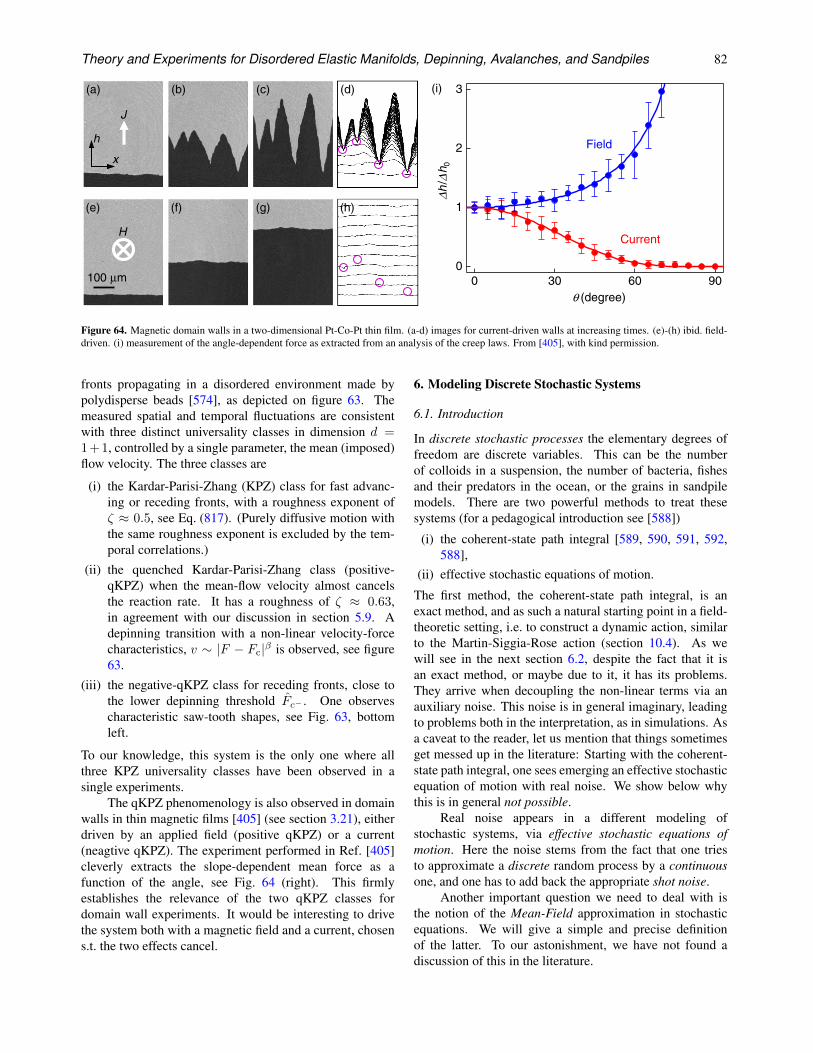
Theory and Experiments for Disordered Elastic Manifolds, Depinning, Avalanches, and Sandpiles 82
The current-driven roughness growth in these films isdepicted in Figs. 1(a)–1(d). Figure 1(a) shows a linear DWinitially created by the thermomagnetic writing scheme.By injecting current, the linear DW starts to develop theshape of mountains with a constant slope as seen byFigs. 1(b) and 1(c). Figure 1(d) summarizes this evolutionby superimposing the DW lines sequentially with a con-stant time step. We observe this behavior for more than 10samples under examination, over the range of J between0.7 and 2.2 times 1010 A=m2. This behavior is distinctfrom that of the field-driven roughness as shown byFigs. 1(e)–1(h), where the DW sweeps with a constant speedwithout a significant change in the shape of roughness.
These distinct DW shapes belong to different universal-ity classes. Figure 1(i) depicts the log-log plot between theDW segment length L along the x axis and the roughnessamplitude w along the h axis. The linear relation indicatesthe power-law scaling w / L! , where ! is labeled theroughness exponent [13]. The best fit quantifies that !J ¼0:99" 0:01 for the current and !H ¼ 0:68" 0:04 for thefield. The exponent !H (! 1) indicates the conventionalself-affinity of the field-driven DW roughness as alreadywell established in a number of studies with !H ¼ 2=3[4–6]. In contrast, the current-driven exponent !J (’ 1)corresponds to the self-similarity in the present scalingrange. Thus, very surprisingly, the same DW exhibitsdistinctive roughness scalings between the self-affinityand self-similarity in the same system depending ondriving forces.In the current-driven cases, the shape of the mountains is
developed by the pinning of DWs at several strong pinningsites as indicated by purple circles in Fig. 1(d). Once thestructure is fully developed, the strength of pinning is sostrong that the DW is barely depinned over the measure-ment time range of up to a few days. By contrast, suchstrong pinning does not appear in the field-driven case asshown by Fig. 1(h). This suggests that the DW respondsdifferently to pinning sites depending on what the drivingforce is.In quenched disorder systems such as magnetic media,
universal behaviors of the interface dynamics are governedby the quenched Kardar-Parisi-Zhang (KPZ) equation[13,14], which describes the temporal change of the inter-face height hðx; tÞ at the position x and time t by @h=@t ¼V0 þ "ð@2h=@x2Þ þ ð#=2Þð@h=@xÞ2 þ $q. The first term
denotes the mean speed. The second term describes relaxa-tion caused by the tension ". The third term is called theKPZ nonlinear term and induces growth (#> 0) or decay(#< 0) along the local normal to the interface, dependingon the sign of the coefficient #. The fourth term reflectsthe noise induced by the local disorders and thermalfluctuations.The KPZ equation predicts qualitatively different inter-
face dynamics depending on the sign of #. A scaling ana-lysis predicts the conventional self-affine roughness for apositive # [13,15]. However, for a negative #, the interfaceforms a typical roughness—called a facet [16,17]—in theshape of mountains with a constant slope, which is trulyaccordant with our observation. It is thus natural to deducethat the DW driven by the current (field) is described by theKPZ equation with a negative (positive) #.The opposite sign of # readily explains the different
pinning mechanisms [17]. When a driven interface meetsa pinning site, the interface bends at around the pinning siteand thus, the slope j@h=@xj adjacent to the pinning siteincreases accordingly. At this instant, for a positive #,the KPZ nonlinear term adds a force positively to thedriving force. It thus enhances the bending recursively
1 10 100
0.1
1
10
100
Field
Current
(i)
x
h
J
H
100 µm
(a) (b) (c) (d)
(e) (f) (g) (h)
x
h
L
w
L (µm)
w(µ
m)
FIG. 1 (color online). Magnetic domain images taken at(a) 0 s, (b) 20 min, and (c) 4 hr after the application of J (1:0&1010 A=m2). (d) Time-resolved DW lines superimposed sequen-tially with a constant time step (3 min). Images taken at (e) 0,(f) 10, and (g) 20 min after the application of H (1.0 mT).(h) Time-resolved DW lines superimposed sequentially with aconstant time step (3 min). The purple circles in (d) and (h)designate the strong pinning sites that appeared in the current-driven motion. (i) Log-log scaling plot between the DW segmentlength L along the x axis and the roughness amplitude w alongthe h axis for DWs driven by the current (red) and field (blue). wis defined as the standard deviation of the roughness fluctuationover the length L. Each symbol is obtained by sampling morethan 1000 times. The solid lines show the best linear fit.
PRL 110, 107203 (2013) P HY S I CA L R EV I EW LE T T E R Sweek ending
8 MARCH 2013
107203-2
and consequently, assists depinning. On the contrary, anegative ! suppresses the bending via the force oppositeto the driving force. Since more bending with a largerdriving force further enhances the negative KPZ force, asignificantly large force is required to overwhelm the KPZforce to trigger depinning.
Driving force dependence appears also in the slope-dependent DW displacement. For this, a linear DW isinitially prepared with an angle " (¼ tan"1½@h=@x$) andthen subjected to either a magnetic field or current pulse.Figure 2 depicts the results for the current (a)–(d) and field(e)–(h). Each image is obtained by adding two imagesbefore and after the translation and thus, each image showstwo DWs simultaneously. For the field-driven motion, thedisplacement !h? normal to the DW is found to be invari-ant irrespective of ". This behavior is due to the rotation
symmetry with respect to the axis parallel to the appliedfield H. On the contrary, for the current-driven motion,!h? decreases as " increases as we discuss further below.These angular dependences are summarized in Fig. 2(i).We observe the angular dependences for 3 differentsamples with the range of J between 1.0 and 3.4 times1010 A=m2. The ordinate is scaled as the displacement !halong the þh axis, normalized by !h0 for " ¼ 0. Theplot shows opposite dependences for the field (positive)and current (negative). For the field-driven case, the data fitto a 1= cos" function, which is attributed to the relation!h? ¼ !h cos" with a constant !h? ( ¼ !h0) as illus-trated in Fig. 2(f).The different slope dependence is a direct indicator of
the opposite sign of !. When !h is converted into the DWspeed Vð¼ !h=!tÞ using the pulse duration !t, the field-driven 1= cos" dependence indicates a positive !, since theTaylor expansion of V with respect to @h=@x gives the firstleading term as ðV0=2Þð@h=@xÞ2, which is identical to theKPZ nonlinear term with ! ¼ V0 (¼ !h0=!t > 0). Forthe current-driven case, on the other hand, the oppositeangle dependence implies a negative !. In both cases, theð@h=@xÞ1 term is forbidden due to inversion symmetry!hð"Þ ¼ !hð""Þ.We next consider the details of the current-driven
motion. As depicted in Fig. 2(b), J can be decomposedinto the vector components, parallel (Jk) and normal (J?)to the DW. Since Jk makes no macroscopic change alongthe normal direction, it is reasonable to assume that!h? ismainly driven by J?. Then, by defining the new axesparallel (x0) and normal (h0) to the DW, it becomes avery typical situation where the DW lies along the hori-zontal x0 axis and the DW is driven by J? along the verticalh0 axis as shown by the green window in Fig. 2(b). Thecreep scaling is then related to the DW roughness in the h0
axis, of which the scaling exponent # 0J is measured withrespect to the x0 axis. It is experimentally revealed that # 0Jis invariant ( ¼ 0:69( 0:04) irrespective of " for the rangeof L smaller than a few tens of micrometers. Note that# 0J!#J, which is a common symptom [18] of an interfacewith facet formation. Interestingly, # 0J is identical to #H[4–6]. It is thus natural to infer that the creep scaling in thex0-h0 coordinate system is independent of the driving forceswith the common creep scaling exponent $ (¼½2#"1$=½2"#$) given by 1=4 in both cases [3,4]. Therefore, thewell-established creep theory can be applied.For the case that the current is injected normal to the
DW in metallic ferromagnetic materials, it has been theo-retically proposed [19] and experimentally verified [12]that the DW speed V follows the creep law V ¼v0 exp½"%fH)g"$$, with respect to the effective field
H)ðH; JÞ ¼ H " &J " 'J2ffiffiffiffiffiffiffiffiffiffiffiffiffiffiffiffiH " &J
pþð2=5Þ'2J4 þ * * * ,
where v0 is the characteristic speed and % is the ratio of ascaling energy constant over the thermal energy. Here, &and ' are the efficiency constants of the nonadiabatic and
0 30 60 900
1
2
3
Field
θ (degree)
Current
(i)
h h
xh
J⊥
J
J ||
x’ h’ 30 µm
(a) (b) (c) (d)
(e) (f) (g) (h)
J
H
h/
h 0
∆
∆∆
∆θ
FIG. 2 (color online). Displacement driven by a current pulse(1:0+ 1010 A=m2, 150 s) for DWs with different ", (a) 0,(b) 30,, (c) 60,, and (d) 90,. Displacement driven by a magneticfield pulse (1.0 mT, 150 s) for DWs with different ", (e) 0,(f) 30,, (g) 60,, and (h) 90,. The purple arrows in (b) illustratethe decomposition of J into the parallel Jk and normal J?components. The green window in (b) exemplifies the newcoordinate axes—x0 and h0—parallel and perpendicular to theDW. The equilength green arrows in (e)–(h) guide !h?. Thewhite solid and dashed lines in (f) indicate the DWs before andafter the displacement, respectively. The black solid and dashedarrows in (f) depict the displacements !h and !h?, respectively.(i) Plot of !h=!h0 with respect to " for DW motion driven bythe current (red) and field (blue). The error bars correspond to thestandard deviation from data obtained by sampling 10 times.
PRL 110, 107203 (2013) P HY S I CA L R EV I EW LE T T E R Sweek ending
8 MARCH 2013
107203-3
Figure 64. Magnetic domain walls in a two-dimensional Pt-Co-Pt thin film. (a-d) images for current-driven walls at increasing times. (e)-(h) ibid. field-driven. (i) measurement of the angle-dependent force as extracted from an analysis of the creep laws. From [405], with kind permission.
fronts propagating in a disordered environment made bypolydisperse beads [574], as depicted on figure 63. Themeasured spatial and temporal fluctuations are consistentwith three distinct universality classes in dimension d =1+1, controlled by a single parameter, the mean (imposed)flow velocity. The three classes are
(i) the Kardar-Parisi-Zhang (KPZ) class for fast advanc-ing or receding fronts, with a roughness exponent ofζ ≈ 0.5, see Eq. (817). (Purely diffusive motion withthe same roughness exponent is excluded by the tem-poral correlations.)
(ii) the quenched Kardar-Parisi-Zhang class (positive-qKPZ) when the mean-flow velocity almost cancelsthe reaction rate. It has a roughness of ζ ≈ 0.63,in agreement with our discussion in section 5.9. Adepinning transition with a non-linear velocity-forcecharacteristics, v ∼ |F − Fc|β is observed, see figure63.
(iii) the negative-qKPZ class for receding fronts, close tothe lower depinning threshold Fc− . One observescharacteristic saw-tooth shapes, see Fig. 63, bottomleft.
To our knowledge, this system is the only one where allthree KPZ universality classes have been observed in asingle experiments.
The qKPZ phenomenology is also observed in domainwalls in thin magnetic films [405] (see section 3.21), eitherdriven by an applied field (positive qKPZ) or a current(neagtive qKPZ). The experiment performed in Ref. [405]cleverly extracts the slope-dependent mean force as afunction of the angle, see Fig. 64 (right). This firmlyestablishes the relevance of the two qKPZ classes fordomain wall experiments. It would be interesting to drivethe system both with a magnetic field and a current, chosens.t. the two effects cancel.
6. Modeling Discrete Stochastic Systems
6.1. Introduction
In discrete stochastic processes the elementary degrees offreedom are discrete variables. This can be the numberof colloids in a suspension, the number of bacteria, fishesand their predators in the ocean, or the grains in sandpilemodels. There are two powerful methods to treat thesesystems (for a pedagogical introduction see [588])
(i) the coherent-state path integral [589, 590, 591, 592,588],
(ii) effective stochastic equations of motion.
The first method, the coherent-state path integral, is anexact method, and as such a natural starting point in a field-theoretic setting, i.e. to construct a dynamic action, similarto the Martin-Siggia-Rose action (section 10.4). As wewill see in the next section 6.2, despite the fact that it isan exact method, or maybe due to it, it has its problems.They arrive when decoupling the non-linear terms via anauxiliary noise. This noise is in general imaginary, leadingto problems both in the interpretation, as in simulations. Asa caveat to the reader, let us mention that things sometimesget messed up in the literature: Starting with the coherent-state path integral, one sees emerging an effective stochasticequation of motion with real noise. We show below whythis is in general not possible.
Real noise appears in a different modeling ofstochastic systems, via effective stochastic equations ofmotion. Here the noise stems from the fact that one triesto approximate a discrete random process by a continuousone, and one has to add back the appropriate shot noise.
Another important question we need to deal with isthe notion of the Mean-Field approximation in stochasticequations. We will give a simple and precise definitionof the latter. To our astonishment, we have not found adiscussion of this in the literature.
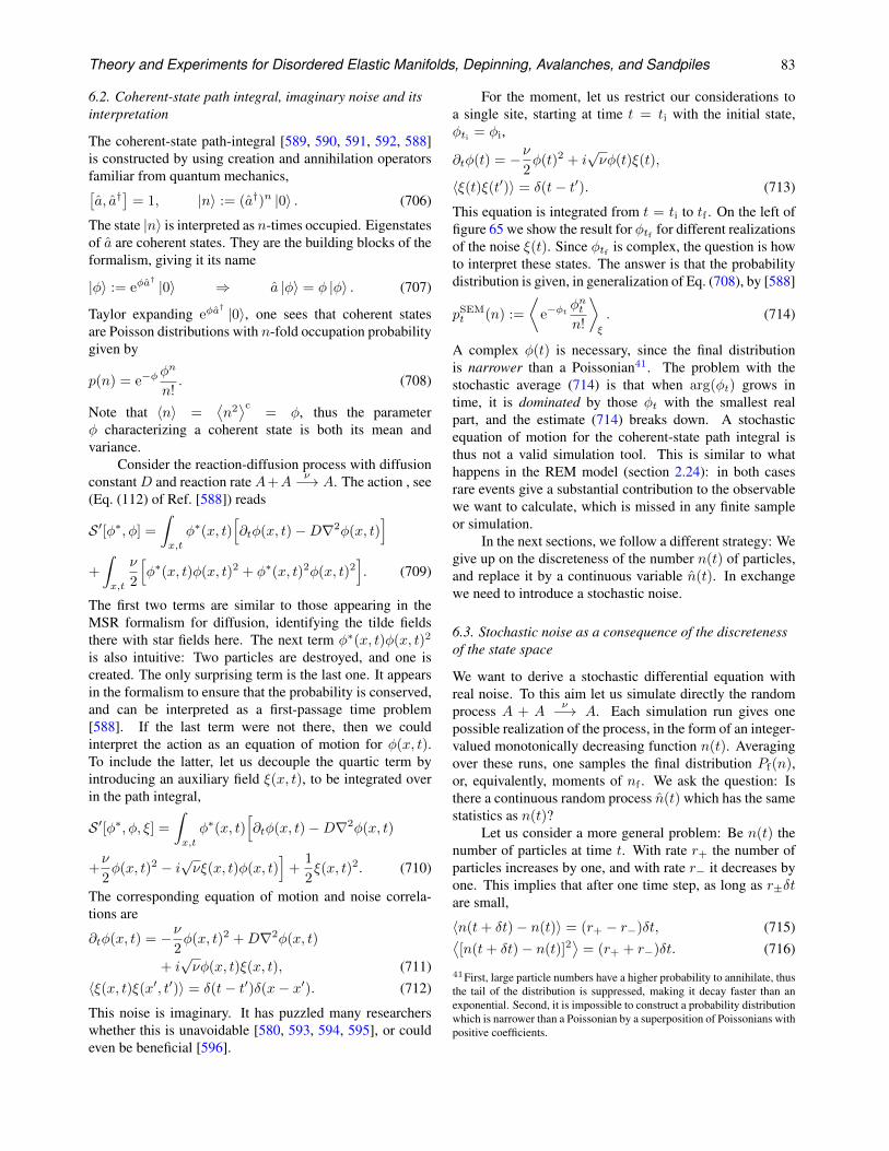
Theory and Experiments for Disordered Elastic Manifolds, Depinning, Avalanches, and Sandpiles 83
6.2. Coherent-state path integral, imaginary noise and itsinterpretation
The coherent-state path-integral [589, 590, 591, 592, 588]is constructed by using creation and annihilation operatorsfamiliar from quantum mechanics,[a, a†
]= 1, |n〉 := (a†)n |0〉 . (706)
The state |n〉 is interpreted as n-times occupied. Eigenstatesof a are coherent states. They are the building blocks of theformalism, giving it its name
|φ〉 := eφa† |0〉 ⇒ a |φ〉 = φ |φ〉 . (707)
Taylor expanding eφa† |0〉, one sees that coherent states
are Poisson distributions with n-fold occupation probabilitygiven by
p(n) = e−φφn
n!. (708)
Note that 〈n〉 =⟨n2⟩c
= φ, thus the parameterφ characterizing a coherent state is both its mean andvariance.
Consider the reaction-diffusion process with diffusionconstantD and reaction rateA+A
ν−→ A. The action , see(Eq. (112) of Ref. [588]) reads
S ′[φ∗, φ] =
∫
x,t
φ∗(x, t)[∂tφ(x, t)−D∇2φ(x, t)
]
+
∫
x,t
ν
2
[φ∗(x, t)φ(x, t)2 + φ∗(x, t)2φ(x, t)2
]. (709)
The first two terms are similar to those appearing in theMSR formalism for diffusion, identifying the tilde fieldsthere with star fields here. The next term φ∗(x, t)φ(x, t)2
is also intuitive: Two particles are destroyed, and one iscreated. The only surprising term is the last one. It appearsin the formalism to ensure that the probability is conserved,and can be interpreted as a first-passage time problem[588]. If the last term were not there, then we couldinterpret the action as an equation of motion for φ(x, t).To include the latter, let us decouple the quartic term byintroducing an auxiliary field ξ(x, t), to be integrated overin the path integral,
S ′[φ∗, φ, ξ] =
∫
x,t
φ∗(x, t)[∂tφ(x, t)−D∇2φ(x, t)
+ν
2φ(x, t)2 − i√νξ(x, t)φ(x, t)
]+
1
2ξ(x, t)2. (710)
The corresponding equation of motion and noise correla-tions are
∂tφ(x, t) = −ν2φ(x, t)2 +D∇2φ(x, t)
+ i√νφ(x, t)ξ(x, t), (711)
〈ξ(x, t)ξ(x′, t′)〉 = δ(t− t′)δ(x− x′). (712)
This noise is imaginary. It has puzzled many researcherswhether this is unavoidable [580, 593, 594, 595], or couldeven be beneficial [596].
For the moment, let us restrict our considerations toa single site, starting at time t = ti with the initial state,φti = φi,
∂tφ(t) = −ν2φ(t)2 + i
√νφ(t)ξ(t),
〈ξ(t)ξ(t′)〉 = δ(t− t′). (713)
This equation is integrated from t = ti to tf . On the left offigure 65 we show the result for φtf for different realizationsof the noise ξ(t). Since φtf is complex, the question is howto interpret these states. The answer is that the probabilitydistribution is given, in generalization of Eq. (708), by [588]
pSEMt (n) :=
⟨e−φt
φntn!
⟩
ξ
. (714)
A complex φ(t) is necessary, since the final distributionis narrower than a Poissonian41. The problem with thestochastic average (714) is that when arg(φt) grows intime, it is dominated by those φt with the smallest realpart, and the estimate (714) breaks down. A stochasticequation of motion for the coherent-state path integral isthus not a valid simulation tool. This is similar to whathappens in the REM model (section 2.24): in both casesrare events give a substantial contribution to the observablewe want to calculate, which is missed in any finite sampleor simulation.
In the next sections, we follow a different strategy: Wegive up on the discreteness of the number n(t) of particles,and replace it by a continuous variable n(t). In exchangewe need to introduce a stochastic noise.
6.3. Stochastic noise as a consequence of the discretenessof the state space
We want to derive a stochastic differential equation withreal noise. To this aim let us simulate directly the randomprocess A + A
ν−→ A. Each simulation run gives onepossible realization of the process, in the form of an integer-valued monotonically decreasing function n(t). Averagingover these runs, one samples the final distribution Pf(n),or, equivalently, moments of nf . We ask the question: Isthere a continuous random process n(t) which has the samestatistics as n(t)?
Let us consider a more general problem: Be n(t) thenumber of particles at time t. With rate r+ the number ofparticles increases by one, and with rate r− it decreases byone. This implies that after one time step, as long as r±δtare small,
〈n(t+ δt)− n(t)〉 = (r+ − r−)δt, (715)⟨[n(t+ δt)− n(t)]2
⟩= (r+ + r−)δt. (716)
41First, large particle numbers have a higher probability to annihilate, thusthe tail of the distribution is suppressed, making it decay faster than anexponential. Second, it is impossible to construct a probability distributionwhich is narrower than a Poissonian by a superposition of Poissonians withpositive coefficients.
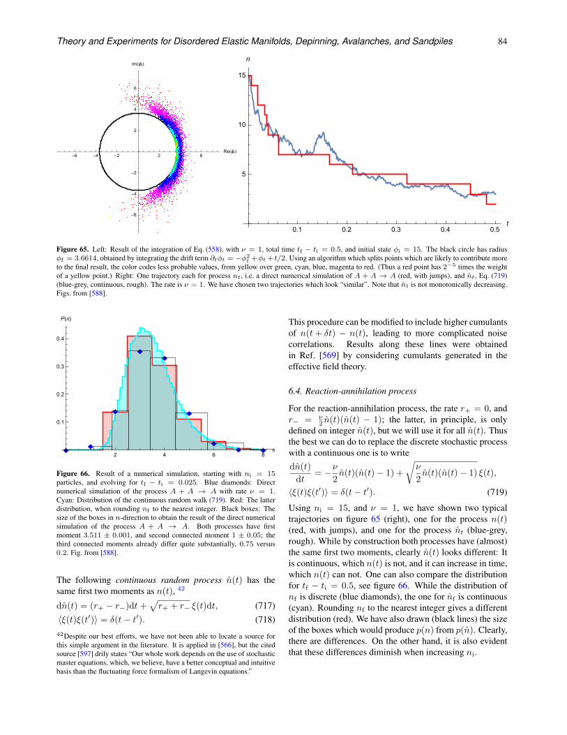
Theory and Experiments for Disordered Elastic Manifolds, Depinning, Avalanches, and Sandpiles 84
Figure 65. Left: Result of the integration of Eq. (558), with ν = 1, total time tf − ti = 0.5, and initial state φi = 15. The black circle has radiusφf = 3.6614, obtained by integrating the drift term ∂tφt = −φ2
t +φt+ t/2. Using an algorithm which splits points which are likely to contribute moreto the final result, the color codes less probable values, from yellow over green, cyan, blue, magenta to red. (Thus a red point has 2−5 times the weightof a yellow point.) Right: One trajectory each for process nt, i.e. a direct numerical simulation of A + A → A (red, with jumps), and nt, Eq. (719)(blue-grey, continuous, rough). The rate is ν = 1. We have chosen two trajectories which look “similar”. Note that nt is not monotonically decreasing.Figs. from [588].
2 4 6 8n
0.1
0.2
0.3
0.4
P(n)
Figure 66. Result of a numerical simulation, starting with ni = 15particles, and evolving for tf − ti = 0.025. Blue diamonds: Directnumerical simulation of the process A + A → A with rate ν = 1.Cyan: Distribution of the continuous random walk (719). Red: The latterdistribution, when rounding nf to the nearest integer. Black boxes: Thesize of the boxes in n-direction to obtain the result of the direct numericalsimulation of the process A + A → A. Both processes have firstmoment 3.511 ± 0.001, and second connected moment 1 ± 0.05; thethird connected moments already differ quite substantially, 0.75 versus0.2. Fig. from [588].
The following continuous random process n(t) has thesame first two moments as n(t), 42
dn(t) = (r+ − r−)dt+√r+ + r− ξ(t)dt, (717)
〈ξ(t)ξ(t′)〉 = δ(t− t′). (718)42Despite our best efforts, we have not been able to locate a source forthis simple argument in the literature. It is applied in [566], but the citedsource [597] drily states “Our whole work depends on the use of stochasticmaster equations, which, we believe, have a better conceptual and intuitivebasis than the fluctuating force formalism of Langevin equations.”
This procedure can be modified to include higher cumulantsof n(t+ δt) − n(t), leading to more complicated noisecorrelations. Results along these lines were obtainedin Ref. [569] by considering cumulants generated in theeffective field theory.
6.4. Reaction-annihilation process
For the reaction-annihilation process, the rate r+ = 0, andr− = ν
2 n(t)(n(t) − 1); the latter, in principle, is onlydefined on integer n(t), but we will use it for all n(t). Thusthe best we can do to replace the discrete stochastic processwith a continuous one is to writedn(t)
dt= −ν
2n(t)(n(t)− 1) +
√ν
2n(t)(n(t)− 1) ξ(t),
〈ξ(t)ξ(t′)〉 = δ(t− t′). (719)
Using ni = 15, and ν = 1, we have shown two typicaltrajectories on figure 65 (right), one for the process n(t)(red, with jumps), and one for the process nt (blue-grey,rough). While by construction both processes have (almost)the same first two moments, clearly n(t) looks different: Itis continuous, which n(t) is not, and it can increase in time,which n(t) can not. One can also compare the distributionfor tf − ti = 0.5, see figure 66. While the distribution ofnf is discrete (blue diamonds), the one for nf is continuous(cyan). Rounding nf to the nearest integer gives a differentdistribution (red). We have also drawn (black lines) the sizeof the boxes which would produce p(n) from p(n). Clearly,there are differences. On the other hand, it is also evidentthat these differences diminish when increasing ni.
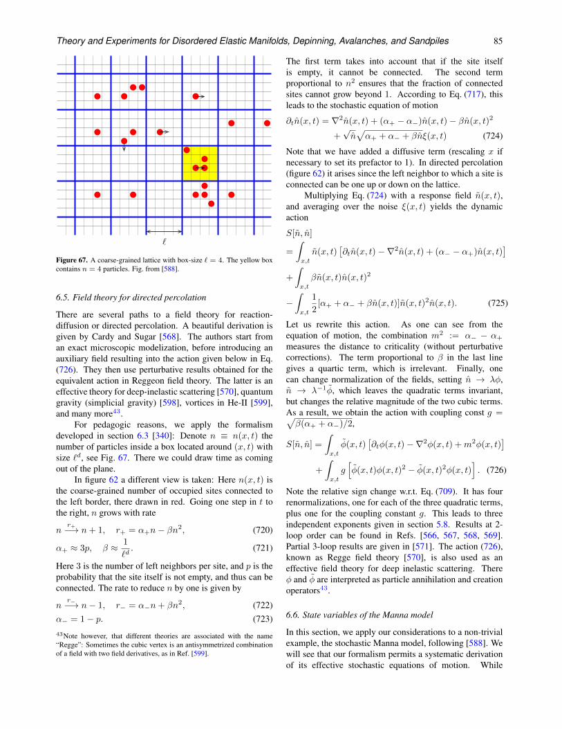
Theory and Experiments for Disordered Elastic Manifolds, Depinning, Avalanches, and Sandpiles 85
`
Figure 67. A coarse-grained lattice with box-size ` = 4. The yellow boxcontains n = 4 particles. Fig. from [588].
6.5. Field theory for directed percolation
There are several paths to a field theory for reaction-diffusion or directed percolation. A beautiful derivation isgiven by Cardy and Sugar [568]. The authors start froman exact microscopic modelization, before introducing anauxiliary field resulting into the action given below in Eq.(726). They then use perturbative results obtained for theequivalent action in Reggeon field theory. The latter is aneffective theory for deep-inelastic scattering [570], quantumgravity (simplicial gravity) [598], vortices in He-II [599],and many more43.
For pedagogic reasons, we apply the formalismdeveloped in section 6.3 [340]: Denote n ≡ n(x, t) thenumber of particles inside a box located around (x, t) withsize `d, see Fig. 67. There we could draw time as comingout of the plane.
In figure 62 a different view is taken: Here n(x, t) isthe coarse-grained number of occupied sites connected tothe left border, there drawn in red. Going one step in t tothe right, n grows with rate
nr+−→ n+ 1, r+ = α+n− βn2, (720)
α+ ≈ 3p, β ≈ 1
`d. (721)
Here 3 is the number of left neighbors per site, and p is theprobability that the site itself is not empty, and thus can beconnected. The rate to reduce n by one is given by
nr−−→ n− 1, r− = α−n+ βn2, (722)
α− = 1− p. (723)
43Note however, that different theories are associated with the name“Regge”: Sometimes the cubic vertex is an antisymmetrized combinationof a field with two field derivatives, as in Ref. [599].
The first term takes into account that if the site itselfis empty, it cannot be connected. The second termproportional to n2 ensures that the fraction of connectedsites cannot grow beyond 1. According to Eq. (717), thisleads to the stochastic equation of motion
∂tn(x, t) = ∇2n(x, t) + (α+ − α−)n(x, t)− βn(x, t)2
+√n√α+ + α− + βnξ(x, t) (724)
Note that we have added a diffusive term (rescaling x ifnecessary to set its prefactor to 1). In directed percolation(figure 62) it arises since the left neighbor to which a site isconnected can be one up or down on the lattice.
Multiplying Eq. (724) with a response field n(x, t),and averaging over the noise ξ(x, t) yields the dynamicaction
S[n, n]
=
∫
x,t
n(x, t)[∂tn(x, t)−∇2n(x, t) + (α− − α+)n(x, t)
]
+
∫
x,t
βn(x, t)n(x, t)2
−∫
x,t
1
2[α+ + α− + βn(x, t)]n(x, t)2n(x, t). (725)
Let us rewrite this action. As one can see from theequation of motion, the combination m2 := α− − α+
measures the distance to criticality (without perturbativecorrections). The term proportional to β in the last linegives a quartic term, which is irrelevant. Finally, onecan change normalization of the fields, setting n → λφ,n → λ−1φ, which leaves the quadratic terms invariant,but changes the relative magnitude of the two cubic terms.As a result, we obtain the action with coupling const g =√β(α+ + α−)/2,
S[n, n] =
∫
x,t
φ(x, t)[∂tφ(x, t)−∇2φ(x, t) +m2φ(x, t)
]
+
∫
x,t
g[φ(x, t)φ(x, t)2 − φ(x, t)2φ(x, t)
]. (726)
Note the relative sign change w.r.t. Eq. (709). It has fourrenormalizations, one for each of the three quadratic terms,plus one for the coupling constant g. This leads to threeindependent exponents given in section 5.8. Results at 2-loop order can be found in Refs. [566, 567, 568, 569].Partial 3-loop results are given in [571]. The action (726),known as Regge field theory [570], is also used as aneffective field theory for deep inelastic scattering. Thereφ and φ are interpreted as particle annihilation and creationoperators43.
6.6. State variables of the Manna model
In this section, we apply our considerations to a non-trivialexample, the stochastic Manna model, following [588]. Wewill see that our formalism permits a systematic derivationof its effective stochastic equations of motion. While
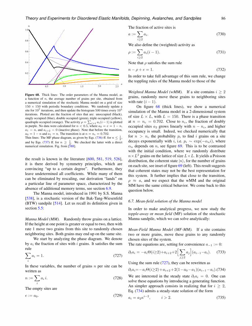
Theory and Experiments for Disordered Elastic Manifolds, Depinning, Avalanches, and Sandpiles 86
0.5 1.0 1.5 2.0 2.5
n
0.2
0.4
0.6
0.8
1.0
ai
Figure 68. Thick lines: The order parameters of the Manna model, asa function of n, the average number of grains per site, obtained froma numerical simulation of the stochastic Manna model on a grid of size150 × 150 with periodic boundary conditions. We randomly update asite for 107 iterations, and then update the histogram 500 times every 105
iterations. Plotted are the fraction of sites that are: unoccupied (black),singly occupied (blue), double occupied (green), triple occupied (yellow),quadruple occupied (orange). The activity ρ =
∑i>1 ai(i− 1) is plotted
in purple. No data were calculated for n < 0.5, where a0 = e = 1 − n,a1 = n, and ai>2 = 0 (inactive phase). Note that before the transition,a0 = 1− n and a1 = n. The transition is at n = nc = 0.702.Thin lines: The MF phase diagram, as given by Eqs. (736) ff. for n ≤ 1
2,
and by Eqs. (737) ff. for n ≥ 12
. We checked the latter with a directnumerical simulation. Fig. from [588].
the result is known in the literature [600, 581, 519, 526],it is there derived by symmetry principles, which areconvincing “up to a certain degree”. Furthermore, theyleave undetermined all coefficients. While many of themcan be eliminated by rescaling, our derivation “lands” ona particular line of parameter space, characterized by theabsence of additional memory terms, see section 6.9.
The Manna model, introduced in 1991 by S.S. Manna[538], is a stochastic version of the Bak-Tang-Wiesenfeld(BTW) sandpile [514]. Let us recall its definition given insection 5.5:
Manna Model (MM). Randomly throw grains on a lattice.If the height at one point is greater or equal to two, then withrate 1 move two grains from this site to randomly chosenneighboring sites. Both grains may end up on the same site.
We start by analyzing the phase diagram. We denoteby ai the fraction of sites with i grains. It satisfies the sumrule∑
i
ai = 1. (727)
In these variables, the number of grains n per site can bewritten as
n :=∑
i
ai i. (728)
The empty sites are
e := a0. (729)
The fraction of active sites is
a :=∑
i≥2
ai. (730)
We also define the (weighted) activity as
ρ :=∑
i≥2
ai(i− 1). (731)
Note that ρ satisfies the sum rule
n− ρ+ e = 1. (732)
In order to take full advantage of this sum rule, we changethe toppling rules of the Manna model to those of the
Weighted Manna Model (wMM). If a site contains i ≥ 2grains, randomly move these grains to neighboring siteswith rate (i− 1).
On figure 68 (thick lines), we show a numericalsimulation of the Manna model in a 2-dimensional systemof size L × L, with L = 150. There is a phase transitionat n = nc = 0.702. Close to nc, the fraction of doublyoccupied sites a2 grows linearly with n − nc, and higheroccupancy is small. Indeed, we checked numerically thatfor n > nc the probability pi to find i grains on a sitedecays exponentially with i, i.e. pi ∼ exp(−αni), whereαn depends on n, see figure 69. This is to be contrastedwith the initial condition, where we randomly distributen×L2 grains on the lattice of size L×L. It yields a Poissondistribution, the coherent state |n〉, for the number of grainson each site, see inset of figure 69 (left). This result suggeststhat coherent states may not be the best representation forthis system. It further implies that close to the transition,ρ ≈ a, and we expect that the wMM and the originalMM have the same critical behavior. We come back to thisquestion below.
6.7. Mean-field solution of the Manna model
In order to make analytical progress, we now study thetopple-away or mean field (MF) solution of the stochasticManna sandpile, which we can solve analytically:
Mean-Field Manna Model (MF-MM). If a site containstwo or more grains, move these grains to any randomlychosen sites of the system.The rate equations are, setting for convenience a−1 := 0:
∂tai = −aiΘ(i≥2)+ai+2+2[∑
j≥2
aj
](ai−1−ai). (733)
Using the sum rule (727), they can be rewritten as
∂tai=−aiΘ(i≥2)+ai+2+2(1−a0−a1)(ai−1−ai).(734)
We are interested in the steady state ∂tai = 0. One cansolve these equations by introducing a generating function.An simpler approach consists in realizing that for i ≥ 2,Eq. (734) admits a steady-state solution of the form
ai = a2κi−2, i > 2. (735)
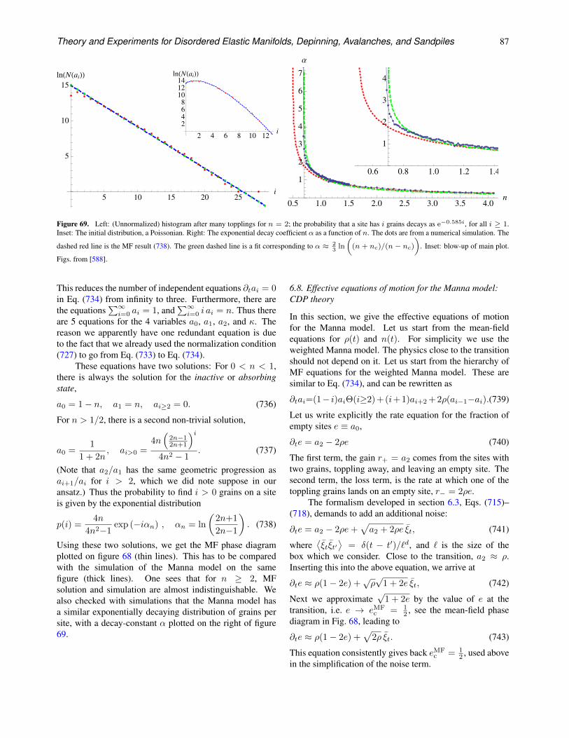
Theory and Experiments for Disordered Elastic Manifolds, Depinning, Avalanches, and Sandpiles 87
5 10 15 20 25i
5
10
15
lnHNHaiLL
2 4 6 8 10 12i
2
4
6
8
10
12
14
lnHNHaiLL
0.5 1.0 1.5 2.0 2.5 3.0 3.5 4.0n
1
2
3
4
5
6
7
Α
0.6 0.8 1.0 1.2 1.4
1
2
3
4
Figure 69. Left: (Unnormalized) histogram after many topplings for n = 2; the probability that a site has i grains decays as e−0.585i, for all i ≥ 1.Inset: The initial distribution, a Poissonian. Right: The exponential decay coefficient α as a function of n. The dots are from a numerical simulation. The
dashed red line is the MF result (738). The green dashed line is a fit corresponding to α ≈ 23
ln
((n + nc)/(n − nc)
). Inset: blow-up of main plot.
Figs. from [588].
This reduces the number of independent equations ∂tai = 0in Eq. (734) from infinity to three. Furthermore, there arethe equations
∑∞i=0 ai = 1, and
∑∞i=0 i ai = n. Thus there
are 5 equations for the 4 variables a0, a1, a2, and κ. Thereason we apparently have one redundant equation is dueto the fact that we already used the normalization condition(727) to go from Eq. (733) to Eq. (734).
These equations have two solutions: For 0 < n < 1,there is always the solution for the inactive or absorbingstate,
a0 = 1− n, a1 = n, ai≥2 = 0. (736)
For n > 1/2, there is a second non-trivial solution,
a0 =1
1 + 2n, ai>0 =
4n(
2n−12n+1
)i
4n2 − 1. (737)
(Note that a2/a1 has the same geometric progression asai+1/ai for i > 2, which we did note suppose in ouransatz.) Thus the probability to find i > 0 grains on a siteis given by the exponential distribution
p(i) =4n
4n2−1exp (−iαn) , αn = ln
(2n+1
2n−1
). (738)
Using these two solutions, we get the MF phase diagramplotted on figure 68 (thin lines). This has to be comparedwith the simulation of the Manna model on the samefigure (thick lines). One sees that for n ≥ 2, MFsolution and simulation are almost indistinguishable. Wealso checked with simulations that the Manna model hasa similar exponentially decaying distribution of grains persite, with a decay-constant α plotted on the right of figure69.
6.8. Effective equations of motion for the Manna model:CDP theory
In this section, we give the effective equations of motionfor the Manna model. Let us start from the mean-fieldequations for ρ(t) and n(t). For simplicity we use theweighted Manna model. The physics close to the transitionshould not depend on it. Let us start from the hierarchy ofMF equations for the weighted Manna model. These aresimilar to Eq. (734), and can be rewritten as
∂tai=(1− i)aiΘ(i≥2) + (i+ 1)ai+2 + 2ρ(ai−1−ai).(739)
Let us write explicitly the rate equation for the fraction ofempty sites e ≡ a0,
∂te = a2 − 2ρe (740)
The first term, the gain r+ = a2 comes from the sites withtwo grains, toppling away, and leaving an empty site. Thesecond term, the loss term, is the rate at which one of thetoppling grains lands on an empty site, r− = 2ρe.
The formalism developed in section 6.3, Eqs. (715)–(718), demands to add an additional noise:
∂te = a2 − 2ρe+√a2 + 2ρe ξt, (741)
where⟨ξtξt′
⟩= δ(t − t′)/`d, and ` is the size of the
box which we consider. Close to the transition, a2 ≈ ρ.Inserting this into the above equation, we arrive at
∂te ≈ ρ(1− 2e) +√ρ√
1 + 2e ξt, (742)
Next we approximate√
1 + 2e by the value of e at thetransition, i.e. e → eMF
c = 12 , see the mean-field phase
diagram in Fig. 68, leading to
∂te ≈ ρ(1− 2e) +√
2ρ ξt. (743)
This equation consistently gives back eMFc = 1
2 , used abovein the simplification of the noise term.
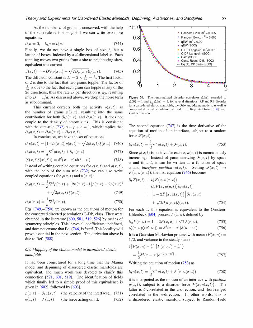
Theory and Experiments for Disordered Elastic Manifolds, Depinning, Avalanches, and Sandpiles 88
As the number n of grains is conserved, with the helpof the sum rule n + e = ρ + 1 we can write two moreequations,∂tn = 0, ∂tρ = ∂te. (744)Finally, we do not have a single box of size `, but alattice of boxes, indexed by a d-dimensional label x. Eachtoppling moves two grains from a site to neighboring sites,equivalent to a current
J(x, t) = −D∇ρ(x, t) +√
2Dρ(x, t)ξ(x, t). (745)The diffusion constant is D = 2× 1
2d = 1d . The first factor
of 2 is due to the fact that two grains topple. The factor of12d is due to the fact that each grain can topple in any of the2d directions, thus the rate D per direction is 1
2d , resultinginto D = 1/d. As discussed above, we drop the noise termas subdominant.
This current corrects both the activity ρ(x, t), asthe number of grains n(x, t), resulting into the samecontribution for both ∂tρ(x, t), and ∂tn(x, t). It does notcouple to the density of empty sites. This is consistentwith the sum-rule (732) n− ρ + e = 1, which implies that∂tρ(x, t) ≡ ∂tn(x, t) + ∂te(x, t).
In conclusion, we have the set of equations
∂te(x, t) = [1−2e(x, t)]ρ(x, t) +√
2ρ(x, t) ξ(x, t), (746)
∂tρ(x, t) =1
d∇2ρ(x, t) + ∂te(x, t), (747)
〈ξ(x, t)ξ(x′, t′)〉 = δd(x− x′)δ(t− t′). (748)Instead of writing coupled equations for e(x, t) and ρ(x, t),with the help of the sum rule (732) we can also writecoupled equations for ρ(x, t) and n(x, t):
∂tρ(x, t) =1
d∇2ρ(x, t) +
[2n(x, t)−1
]ρ(x, t)− 2ρ(x, t)2
+√
2ρ(x, t) ξ(x, t), (749)
∂tn(x, t) =1
d∇2ρ(x, t), (750)
Eqs. (749)–(750) are known as the equations of motion forthe conserved directed percolation (C-DP) class. They wereobtained in the literature [600, 581, 519, 526] by means ofsymmetry principles. This leaves all coefficients undefined,and does not ensure that Eq. (746) is local. This locality willprove essential in the next section. The derivation above isdue to Ref. [588].
6.9. Mapping of the Manna model to disordered elasticmanifolds
It had been conjectured for a long time that the Mannamodel and depinning of disordered elastic manifolds areequivalent, and much work was devoted to clarify thisconnection [521, 601, 519]. The identification of fieldswhich finally led to a simple proof of this equivalence isgiven in [602], followed by [603],ρ(x, t) = ∂tu(x, t) (the velocity of the interface), (751)e(x, t) = F(x, t) (the force acting on it). (752)
0 1 2 3 4 50
0.2
0.4
0.6
0.8
1Random Field, m
2 = 0.005
Random Bond, m2 = 0.005
qEW, m2 = 0.001
qEW (SOC)
C-DP Langevin, m2=0.001
C-DP Langevin (SOC)Oslo (SOC)Cons. React.-Diff. (SOC)Eq.(4), DP class (SOC)
w
∆(w)
Figure 70. The renormalized disorder correlator ∆(u), rescaled to∆(0) = 1 and
∫u ∆(u) = 1, for several situations: RF and RB disorder
for a disordered elastic manifolds, the Oslo and Manna models, as well asconserved directed percolation, all in d = 1. Reprinted from [519], withkind permission.
The second equation (747) is the time derivative of theequation of motion of an interface, subject to a randomforce F(x, t),
∂tu(x, t) =1
d∇2u(x, t) + F(x, t). (753)
Since ρ(x, t) is positive for each x, u(x, t) is monotonouslyincreasing. Instead of parameterizing F(x, t) by spacex and time t, it can be written as a function of spacex and interface position u(x, t). Setting F(x, t) →F(x, u(x, t)
), the first equation (746) becomes
∂tF(x, t)→ ∂tF(x, u(x, t)
)
= ∂uF(x, u(u, t)
)∂tu(x, t)
=[1− 2F
(x, u(x, t)
)]∂tu(x, t)
+√
2∂tu(x, t)ξ(x, t). (754)
For each x, this equation is equivalent to the Ornstein-Uhlenbeck [604] process F (x, u), defined by
∂uF (x, u) = 1− 2F (x, u) +√
2 ξ(x, u), (755)〈ξ(x, u)ξ(x′, u′)〉 = δd(x− x′)δ(u− u′). (756)
It is a Gaussian Markovian process with mean 〈F (x, u)〉 =1/2, and variance in the steady state of⟨[F (x, u)− 1
2
] [F (x′, u′)− 1
2
]⟩
=1
2δd(x− x′)e−2|u−u′|. (757)
Writing the equation of motion (753) as
∂tu(x, t) =1
d∇2u(x, t) + F
(x, u(x, t)
), (758)
it is interpreted as the motion of an interface with positionu(x, t), subject to a disorder force F
(x, u(x, t)
). The
latter is δ-correlated in the x-direction, and short-rangedcorrelated in the u-direction. In other words, this isa disordered elastic manifold subject to Random-Field
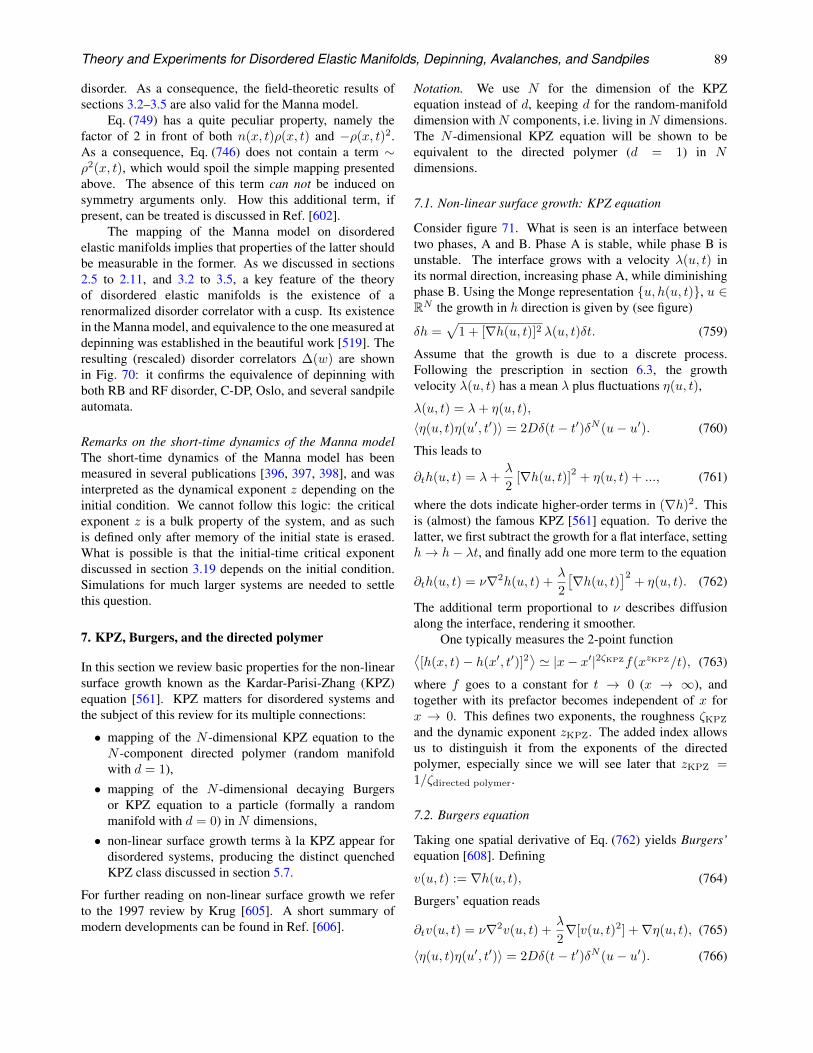
Theory and Experiments for Disordered Elastic Manifolds, Depinning, Avalanches, and Sandpiles 89
disorder. As a consequence, the field-theoretic results ofsections 3.2–3.5 are also valid for the Manna model.
Eq. (749) has a quite peculiar property, namely thefactor of 2 in front of both n(x, t)ρ(x, t) and −ρ(x, t)2.As a consequence, Eq. (746) does not contain a term ∼ρ2(x, t), which would spoil the simple mapping presentedabove. The absence of this term can not be induced onsymmetry arguments only. How this additional term, ifpresent, can be treated is discussed in Ref. [602].
The mapping of the Manna model on disorderedelastic manifolds implies that properties of the latter shouldbe measurable in the former. As we discussed in sections2.5 to 2.11, and 3.2 to 3.5, a key feature of the theoryof disordered elastic manifolds is the existence of arenormalized disorder correlator with a cusp. Its existencein the Manna model, and equivalence to the one measured atdepinning was established in the beautiful work [519]. Theresulting (rescaled) disorder correlators ∆(w) are shownin Fig. 70: it confirms the equivalence of depinning withboth RB and RF disorder, C-DP, Oslo, and several sandpileautomata.
Remarks on the short-time dynamics of the Manna modelThe short-time dynamics of the Manna model has beenmeasured in several publications [396, 397, 398], and wasinterpreted as the dynamical exponent z depending on theinitial condition. We cannot follow this logic: the criticalexponent z is a bulk property of the system, and as suchis defined only after memory of the initial state is erased.What is possible is that the initial-time critical exponentdiscussed in section 3.19 depends on the initial condition.Simulations for much larger systems are needed to settlethis question.
7. KPZ, Burgers, and the directed polymer
In this section we review basic properties for the non-linearsurface growth known as the Kardar-Parisi-Zhang (KPZ)equation [561]. KPZ matters for disordered systems andthe subject of this review for its multiple connections:
• mapping of the N -dimensional KPZ equation to theN -component directed polymer (random manifoldwith d = 1),
• mapping of the N -dimensional decaying Burgersor KPZ equation to a particle (formally a randommanifold with d = 0) in N dimensions,
• non-linear surface growth terms a la KPZ appear fordisordered systems, producing the distinct quenchedKPZ class discussed in section 5.7.
For further reading on non-linear surface growth we referto the 1997 review by Krug [605]. A short summary ofmodern developments can be found in Ref. [606].
Notation. We use N for the dimension of the KPZequation instead of d, keeping d for the random-manifolddimension withN components, i.e. living inN dimensions.The N -dimensional KPZ equation will be shown to beequivalent to the directed polymer (d = 1) in Ndimensions.
7.1. Non-linear surface growth: KPZ equation
Consider figure 71. What is seen is an interface betweentwo phases, A and B. Phase A is stable, while phase B isunstable. The interface grows with a velocity λ(u, t) inits normal direction, increasing phase A, while diminishingphase B. Using the Monge representation u, h(u, t), u ∈RN the growth in h direction is given by (see figure)
δh =√
1 + [∇h(u, t)]2 λ(u, t)δt. (759)
Assume that the growth is due to a discrete process.Following the prescription in section 6.3, the growthvelocity λ(u, t) has a mean λ plus fluctuations η(u, t),
λ(u, t) = λ+ η(u, t),
〈η(u, t)η(u′, t′)〉 = 2Dδ(t− t′)δN (u− u′). (760)
This leads to
∂th(u, t) = λ+λ
2[∇h(u, t)]
2+ η(u, t) + ..., (761)
where the dots indicate higher-order terms in (∇h)2. Thisis (almost) the famous KPZ [561] equation. To derive thelatter, we first subtract the growth for a flat interface, settingh→ h− λt, and finally add one more term to the equation
∂th(u, t) = ν∇2h(u, t) +λ
2
[∇h(u, t)
]2+ η(u, t). (762)
The additional term proportional to ν describes diffusionalong the interface, rendering it smoother.
One typically measures the 2-point function⟨[h(x, t)− h(x′, t′)]2
⟩' |x− x′|2ζKPZf(xzKPZ/t), (763)
where f goes to a constant for t → 0 (x → ∞), andtogether with its prefactor becomes independent of x forx → 0. This defines two exponents, the roughness ζKPZ
and the dynamic exponent zKPZ. The added index allowsus to distinguish it from the exponents of the directedpolymer, especially since we will see later that zKPZ =1/ζdirected polymer.
7.2. Burgers equation
Taking one spatial derivative of Eq. (762) yields Burgers’equation [608]. Defining
v(u, t) := ∇h(u, t), (764)
Burgers’ equation reads
∂tv(u, t) = ν∇2v(u, t) +λ
2∇[v(u, t)2] +∇η(u, t), (765)
〈η(u, t)η(u′, t′)〉 = 2Dδ(t− t′)δN (u− u′). (766)
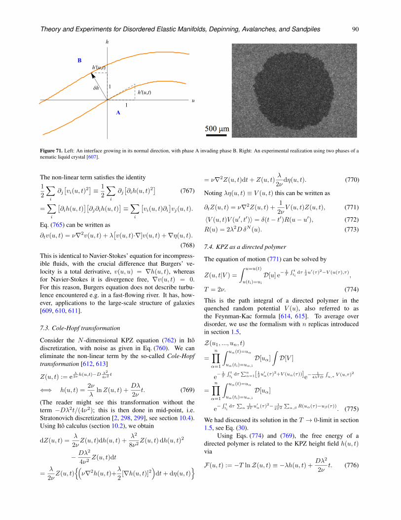
Theory and Experiments for Disordered Elastic Manifolds, Depinning, Avalanches, and Sandpiles 90
h'(u,t)
1
1
h'(u,t)
δh
A
B
u
h
Figure 71. Left: An interface growing in its normal direction, with phase A invading phase B. Right: An experimental realization using two phases of anematic liquid crystal [607].
The non-linear term satisfies the identity1
2
∑
i
∂j[vi(u, t)
2]≡ 1
2
∑
i
∂j[∂ih(u, t)2
](767)
=∑
i
[∂ih(u, t)
][∂j∂ih(u, t)
]≡∑
i
[vi(u, t)∂i
]vj(u, t).
Eq. (765) can be written as
∂tv(u, t) = ν∇2v(u, t) + λ[v(u, t)·∇]v(u, t) +∇η(u, t).
(768)
This is identical to Navier-Stokes’ equation for incompress-ible fluids, with the crucial difference that Burgers’ ve-locity is a total derivative, v(u, u) = ∇h(u, t), whereasfor Navier-Stokes it is divergence free, ∇v(u, t) = 0.For this reason, Burgers equation does not describe turbu-lence encountered e.g. in a fast-flowing river. It has, how-ever, applications to the large-scale structure of galaxies[609, 610, 611].
7.3. Cole-Hopf transformation
Consider the N -dimensional KPZ equation (762) in Itodiscretization, with noise as given in Eq. (760). We caneliminate the non-linear term by the so-called Cole-Hopftransformation [612, 613]
Z(u, t) := eλ2ν h(u,t)−D λ2
4ν2t
⇐⇒ h(u, t) =2ν
λlnZ(u, t) +
Dλ
2νt. (769)
(The reader might see this transformation without theterm −Dλ2t/(4ν2); this is then done in mid-point, i.e.Stratonovich discretization [2, 298, 299], see section 10.4).Using Ito calculus (section 10.2), we obtain
dZ(u, t) =λ
2νZ(u, t)dh(u, t) +
λ2
8ν2Z(u, t) dh(u, t)2
− Dλ2
4ν2Z(u, t)dt
=λ
2νZ(u, t)
(ν∇2h(u, t)+
λ
2[∇h(u, t)]2
)dt+ dη(u, t)
= ν∇2Z(u, t)dt+ Z(u, t)λ
2νdη(u, t). (770)
Noting λη(u, t) ≡ V (u, t) this can be written as
∂tZ(u, t) = ν∇2Z(u, t) +1
2νV (u, t)Z(u, t), (771)
〈V (u, t)V (u′, t′)〉 = δ(t− t′)R(u− u′), (772)R(u) = 2λ2D δN (u). (773)
7.4. KPZ as a directed polymer
The equation of motion (771) can be solved by
Z(u, t|V ) =
∫ u=u(t)
u(ti)=ui
D[u] e− 1T
∫ tti
dτ 12u′(τ)2−V (u(τ),τ)
,
T = 2ν. (774)
This is the path integral of a directed polymer in thequenched random potential V (u), also referred to asthe Feynman-Kac formula [614, 615]. To average overdisorder, we use the formalism with n replicas introducedin section 1.5,
Z(u1, ..., un, t)
=
n∏
α=1
∫ uα(t)=uα
uα(ti)=uα,i
D[uα]
∫D[V ]
e− 1T
∫ tti
dτ∑nα=1[ 1
2u′α(τ)2+V (uα(τ))]e−
14λ2D
∫u,τ
V (u,τ)2
=
n∏
α=1
∫ uα(t)=uα
uα(ti)=uα,i
D[uα]
e−∫ tti
dτ∑α
12T u
′α(τ)2− 1
2T2
∑α,β R(uα(τ)−uβ(τ))
. (775)
We had discussed its solution in the T → 0-limit in section1.5, see Eq. (30).
Using Eqs. (774) and (769), the free energy of adirected polymer is related to the KPZ height field h(u, t)via
F(u, t) := −T lnZ(u, t) ≡ −λh(u, t) +Dλ2
2νt. (776)
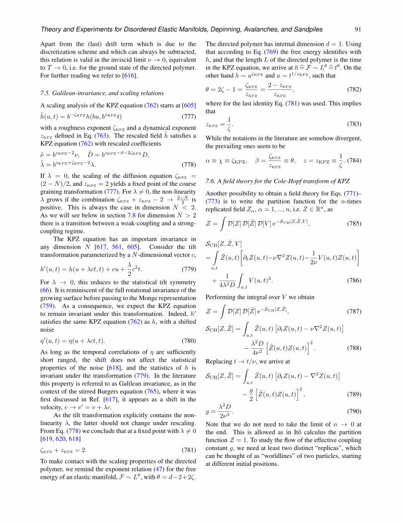
Theory and Experiments for Disordered Elastic Manifolds, Depinning, Avalanches, and Sandpiles 91
Apart from the (last) drift term which is due to thediscretization scheme and which can always be subtracted,this relation is valid in the inviscid limit ν → 0, equivalentto T → 0, i.e. for the ground state of the directed polymer.For further reading we refer to [616].
7.5. Galilean-invariance, and scaling relations
A scaling analysis of the KPZ equation (762) starts at [605]
h(u, t) = b−ζKPZh(bu, bzKPZt) (777)
with a roughness exponent ζKPZ and a dynamical exponentzKPZ defined in Eq. (763). The rescaled field h satisfies aKPZ equation (762) with rescaled coefficients
ν = bzKPZ−2ν, D = bzKPZ−d−2ζKPZD,
λ = bzKPZ+ζKPZ−2λ. (778)
If λ = 0, the scaling of the diffusion equation ζKPZ =(2−N)/2, and zKPZ = 2 yields a fixed point of the coarsegraining transformation (777). For λ 6= 0, the non-linearityλ grows if the combination ζKPZ + zKPZ − 2 → 2−N
2 ispositive. This is always the case in dimension N < 2.As we will see below in section 7.8 for dimension N > 2there is a transition between a weak-coupling and a strong-coupling regime.
The KPZ equation has an important invariance inany dimension N [617, 561, 605]. Consider the tilttransformation parameterized by a N -dimensional vector c,
h′(u, t) = h(u+ λct, t) + cu+λ
2c2t. (779)
For λ → 0, this reduces to the statistical tilt symmetry(66). It is reminiscent of the full rotational invariance of thegrowing surface before passing to the Monge representation(759). As a consequence, we expect the KPZ equationto remain invariant under this transformation. Indeed, h′
satisfies the same KPZ equation (762) as h, with a shiftednoise
η′(u, t) = η(u+ λct, t). (780)
As long as the temporal correlations of η are sufficientlyshort ranged, the shift does not affect the statisticalproperties of the noise [618], and the statistics of h isinvariant under the transformation (779). In the literaturethis property is referred to as Galilean invariance, as in thecontext of the stirred Burgers equation (765), where it wasfirst discussed in Ref. [617], it appears as a shift in thevelocity, v → v′ = v + λc.
As the tilt transformation explicitly contains the non-linearity λ, the latter should not change under rescaling.From Eq. (778) we conclude that at a fixed point with λ 6= 0[619, 620, 618]
ζKPZ + zKPZ = 2. (781)
To make contact with the scaling properties of the directedpolymer, we remind the exponent relation (47) for the freeenergy of an elastic manifold, F ∼ Lθ, with θ = d−2+2ζ.
The directed polymer has internal dimension d = 1. Usingthat according to Eq. (769) the free energy identifies withh, and that the length L of the directed polymer is the timein the KPZ equation, we arrive at h =F ∼ Lθ = tθ. On theother hand h ∼ uζKPZ and u ∼ t1/zKPZ , such that
θ = 2ζ − 1 =ζKPZ
zKPZ
=2− zKPZ
zKPZ
, (782)
where for the last identity Eq. (781) was used. This impliesthat
zKPZ =1
ζ. (783)
While the notations in the literature are somehow divergent,the prevailing ones seem to be
α ≡ χ ≡ ζKPZ, β =ζKPZ
zKPZ
≡ θ, z = zKPZ ≡1
ζ. (784)
7.6. A field theory for the Cole-Hopf transform of KPZ
Another possibility to obtain a field theory for Eqs. (771)–(773) is to write the partition function for the n-timesreplicated field Zα, α = 1, ..., n, i.e. Z ∈ Rn, as
Z =
∫D[Z]D[Z]D[V ] e−SCH[Z,Z,V ], (785)
SCH[Z, Z, V ]
=
∫
u,t
Z(u, t)
[∂tZ(u, t)−ν∇2Z(u, t)− 1
2νV (u, t)Z(u, t)
]
+1
4λ2D
∫
u,t
V (u, t)2. (786)
Performing the integral over V we obtain
Z =
∫D[Z]D[Z] e−SCH[Z,Z], (787)
SCH[Z, Z] =
∫
u,t
Z(u, t)[∂tZ(u, t)− ν∇2Z(u, t)
]
− λ2D
4ν2
[Z(u, t)Z(u, t)
]2. (788)
Replacing t→ t/ν, we arrive at
SCH[Z, Z] =
∫
u,t
Z(u, t)[∂tZ(u, t)−∇2Z(u, t)
]
− g
2
[Z(u, t)Z(u, t)
]2, (789)
g =λ2D
2ν3. (790)
Note that we do not need to take the limit of n → 0 atthe end. This is allowed as in Ito calculus the partitionfunction Z = 1. To study the flow of the effective couplingconstant g, we need at least two distinct “replicas”, whichcan be thought of as “worldlines” of two particles, startingat different initial positions.
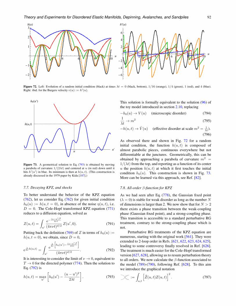
Theory and Experiments for Disordered Elastic Manifolds, Depinning, Avalanches, and Sandpiles 92
2 4 6 8 10u
-2
-1
1
2
3
h(u)
2 4 6 8 10u
-6
-4
-2
2
4
6
h (u)
Figure 72. Left: Evolution of a random initial condition (black) at times λt = 0 (black, bottom), 1/16 (orange), 1/4 (green), 1 (red), and 4 (blue).Right: ibid. for the Burgers velocity v(u) := h′(u).
h(u,t)
uu′
h0(u′)
Figure 73. A geometrical solution to Eq. (793) is obtained by movinga parabola of curvature 1/(2λt) and centered at u (in red) down until ithits h′(u′) in blue. Its minimum is then at h(u, t). (This construction isalready discussed in the 1979 paper by Kida [187].)
7.7. Decaying KPZ, and shocks
To better understand the behavior of the KPZ equation(762), let us consider Eq. (762) for given initial conditionh0(u) := h(u, t = 0), in absence of the noise η(u, t), i.e.D = 0. The Cole-Hopf transformed KPZ equation (771)reduces to a diffusion equation, solved as
Z(u, t) =
∫
u′
e−(u−u′)2
4νt
(4πνt)d/2Z(u′, 0). (791)
Putting back the definition (769) of Z in terms of h0(u) :=h(u, t = 0), we obtain, since D = 0,
eλ2ν h(u,t) =
∫
u′
eλ2ν
[h0(u′)− (u−u′)2
2λt
](4πνt)d/2
. (792)
It is interesting to consider the limit of ν → 0, equivalent toT → 0 for the directed polymer (774). Then the solution toEq. (792) is
h(u, t) = maxu′
[h0(u′)− (u− u′)2
2λt
]. (793)
This solution is formally equivalent to the solution (96) ofthe toy model introduced in section 2.10, replacing
−h0(u)→ V (u) (microscopic disorder) (794)1
λt→ m2 (795)
−h(u, t)→ V (u) (effective disorder at scale m2 = 1λt ).
(796)
As observed there and shown in Fig. 72 for a randominitial condition, the function h(u, t) is composed ofalmost parabolic pieces, continuous everywhere but notdifferentiable at the junctures. Geometrically, this can beobtained by approaching a parabola of curvature m2 =1/(λt) from the top, and reporting as a function of its centeru the position h(u, t) at which it first touches the initialcondition h0(u). This construction is shown in Fig. 73.More can be learned via this approach, see Ref. [82].
7.8. All-order β-function for KPZ
As we had seen after Eq. (778), the Gaussian fixed point(λ = 0) is stable for weak disorder as long as the numberNof dimensions is larger than 2. We now show that forN > 2there exists a phase transition between the weak-couplingphase (Gaussian fixed point), and a strong-coupling phase.This transition is accessible to a standard perturbative RGtreatment, contrary to the strong-coupling phase which isnot.
Perturbative RG treatments of the KPZ equation arenumerous, starting with the original work [561]. They wereextended to 2-loop order in Refs. [621, 622, 623, 624, 625],leading to some controversy finally resolved in Ref. [626].The treatment is much easier for the Cole-Hopf transformedversion [627, 628], allowing us to resum perturbation theoryto all orders. We now calculate the β-function associated tothe model (789)-(790), following Ref. [628]. To this aimwe introduce the graphical notation
:=
∫
u,t
[Z(u, t)Z(u, t)
]2. (797)
Theory and Experiments for Disordered Elastic Manifolds, Depinning, Avalanches, and Sandpiles 93
Then the only diverging diagrams are chains of , ofthe form , and so on. Higher-ordervertices are irrelevant in perturbation theory. As a result,the effective coupling constant is
geff = g + g2 + g3
+ g4 + . . .
+ higher order vertices. (798)
In Fourier-representation with incoming momentum p andfrequency ω, each chain in Eq. (798) factorizes, i.e. can bewritten as a product of the vertex times a power of theelementary loop diagram (which is a function of p and ω):p,ω−→
︸ ︷︷ ︸n loops
=(
p,ω
)n. (799)
Eq. (798) is a geometric sum which yields the effective 4-point function
geff = ΓZZZZ p,ω=
g
1− g p,ω
. (800)
The elementary diagram is
p,ω−→
ω2 +ν, p2 +k
ω2−ν,
p2−k
p,ω−→
=
∫dNk
(2π)N
∫dν
2π
1(p2 +k
)2+ i(ω2 +ν
)1
(p2−k
)2+i(ω2−ν
)
= a
(1
2p2+iω
)N/2−1
, a =1
(8π)N/2Γ
(1−N
2
). (801)
This integral is divergent for any p and ω when N → 2.Renormalization means to absorb this divergence into areparametrization of the coupling constant g: We claim thatthe 4-point function (the effective coupling geff ) is finite(renormalized) as a function of gr instead of g, upon setting
g = Zggrµ−ε , Zg =
1
1 + agr, ε = N − 2. (802)
µ is an arbitrary scale, the renormalization scale. As afunction of gr, the 4-point function reads
ΓZZZZ p,ω=
grµ−ε
1 +(a− µ−ε p,ω
)gr
. (803)
Since 1ε
(12p
2 + iω)ε/2
µ−ε is finite for ε > 0 as longas the combination 1
2p2 + iω is finite, it can be read off
from Eq. (803) that ΓZZZZ p,ωis finite even in the limit
of ε → 0. (If useful, either p = 0 or ω = 0 maysafely be taken.) This completes the proof. Note that thisensures that the model is renormalizable to all orders inperturbation-theory, what is normally a formidable task toshow [112, 113, 114, 115, 629, 630, 118].
The β-function that we calculate now is exact to allorders in perturbation theory. It is defined as the variation
of the renormalized coupling constant, keeping the bare onefixed
β(gr) = −µ ∂
∂µg
gr. (804)
From Eq. (803) we see that it gives the dependence of the4-point function on p and ω for fixed bare coupling. Therelation between g and gr is
g =grµ−ε
1 + agr⇔ gr =
g
µ−ε − ag , (805)
and hence
β(gr) = −εgr(1 + agr). (806)
Using a from Eq. (801), our final result is
β(gr) = (2−N)gr +2
(8π)N/2Γ
(2− N
2
)g2
r . (807)
This equation has a perturbative, IR repulsive, fixed point at
g∗r =2(8π)N/2
(N − 2)Γ(2− N
2
) . (808)
For N > 2 it describes the phase transition between theweak-coupling phase where the KPZ term is irrelevant (g =0), and a strong coupling phase, for which g → ∞. Thisis the only fixed point available for N ≤ 2; especially,the perturbative treatment above does not describe KPZ indimension N = 1.
As a consequence, standard perturbation theory fails toproduce a strong-coupling fixed point, a result which cannotbe overemphasized. This means that any treatment of thestrong coupling regime has to rely on non-perturbativemethods. The FRG approach discussed above qualifies asnon-perturbative in this sense, since FRG follows morethan the flow of a single coupling constant. It does ofcourse not rule out the possibility to find an exactly solvablemodel, distinct from KPZ, for which it is possible to expandtowards the strong-coupling regime of KPZ.
Let us also note that the β-function is divergent atN = 4, and therefore our perturbation expansion breaksdown at N = 4. To cure the problem, a lattice regularizedversion of Eq. (771) may be used. However, then the latticecut-off a will enter into the equations and the result isno longer model-independent. This may be interpreted asN = 4 being the upper critical dimension of KPZ, or as asign for a simple technical problem. See [631, 413], and thediscussion in section 7.11.
7.9. Anisotropic KPZ
A special case is the anisotropic KPZ equation in twodimensions, for which the KPZ-nonlinearity is positive inone direction, and negative in the other. This competitionproduces a perturbative fixed point [632].
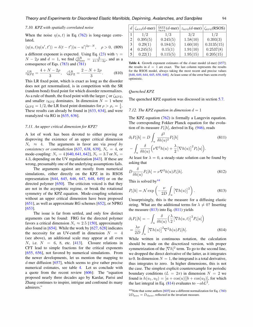
Theory and Experiments for Disordered Elastic Manifolds, Depinning, Avalanches, and Sandpiles 94
7.10. KPZ with spatially correlated noise
When the noise η(u, t) in Eq. (762) is long-range corre-lated,
〈η(u, t)η(u′, t′)〉 = δ(t− t′)|u− u′|2ρ−N , ρ > 0, (809)
a different exponent is expected. Using Eq. (23) with γ =N − 2ρ and d = 1, we find ζLR
Flory = 34+N−2ρ , and as a
consequence of Eqs. (783) and (781)
zLRKPZ =
4 +N − 2ρ
3, ζLR
KPZ =2−N + 2ρ
3. (810)
This LR fixed point, which is exact as long as the disorderdoes not get renormalized, is in competition with the SR(random bond) fixed point for which disorder renormalizes.As a rule of thumb, the fixed point with the larger ζ or ζKPZ,and smaller zKPZ dominates. In dimension N = 1 whereζKPZ = 1/2, the LR fixed point dominates for ρ > ρc = 1
4 .These results can already be found in [633, 634], and werereanalyzed via RG in [635, 636].
7.11. An upper critical dimension for KPZ?
A lot of work has been devoted to either proving ordisproving the existence of an upper critical dimensionNc ≈ 4. The arguments in favor are via proof byconsistency or contradiction [637, 638, 639], Nc = 4, ormode-coupling: Nc = 4 [640, 641, 642],Nc = 3.7 orNc =4.3, depending on the UV regularization [643]. If these arewrong, presumably one of the underlying assumptions fails.
The arguments against are mostly from numericalsimulations, either directly on the KPZ in its RSOSrepresentation [644, 645, 646, 647, 648, 649] or on thedirected polymer [650]. The criticism voiced is that theyare not in the asymptotic regime, or break the rotationalsymmetry of the KPZ equation. Mode-coupling solutionswithout an upper critical dimension have been proposed[651], as well as approximate RG schemes [652], or NPRG[653].
The issue is far from settled, and only few distinctarguments can be found: FRG for the directed polymerfavors a critical dimension Nc ≈ 2.5 [150], approximatelyalso found in [654]. While the work by [627, 628] indicatesthe necessity for an UV-cutoff in dimension N = 4(see above), an additional scale may appear at all evenN , i.e. N = 6, 8, etc. [413]. Closure relations inCFT lead to simple fractions for the critical exponents[655, 656], not favored by numerical simulations. Fromthe newer developments, let us mention the mapping tod-mer diffusion [657], which seems to give rather precisenumerical estimates, see table 4. Let us conclude witha quote from the recent review [606]: The “equationproposed nearly three decades ago by Kardar, Parisi andZhang continues to inspire, intrigue and confound its manyadmirers.”
d ζKPZ(d-mer) ζKPZ
zKPZ(d-mer) zKPZ(d-mer) ζKPZ(RSOS)
1 1/2 1/3 3/2 1/22 0.395(5) 0.245(5) 1.58(10) 0.393(3)3 0.29(1) 0.184(5) 1.60(10) 0.3135(15)4 0.245(5) 0.15(1) 1.91(10) 0.2537(8)5 0.22(1) 0.115(5) 1.95(15) 0.205(15)
Table 4. Growth exponent estimates of the d-mer model (d-mer) [657];the results in d = 1 are exact. The last column represents the resultsfor the RSOS model, always taking the most recent and precise values[648, 649, 644, 645, 658, 646]. At least some of the error bars seem overlyoptimistic.
Quenched KPZ
The quenched KPZ equation was discussed in section 5.7.
7.12. The KPZ equation in dimension d = 1
The KPZ equation (762) is formally a Langevin equation.The corresponding Fokker Planck equation for the evolu-tion of its measure Pt[h], derived in Eq. (946), reads
∂tPt[h] = D
∫
u
δ2
δh(u)2Pt[h] (811)
−∫
u
δ
δh(u)
(ν∇2h(u) +
λ
2
[∇h(u)
]2Pt[u]
).
At least for λ = 0, a steady-state solution can be found byasking that
Dδ
δh(u)Pt[h] = ν∇2h(u)Pt[h]. (812)
This is solved by44
Pt[h] = N exp
(− ν
2D
∫
u
[∇h(u)
]2). (813)
Unsurprisingly, this is the measure for a diffusing elasticstring. What are the additional terms for λ 6= 0? Insertingthe measure (813) into Eq. (811) yields
∂tPt[h] = −∫
u
δ
δh(u)
(λ2
[∇h(u, t)
]2Pt[u]
)
=λν
2D
∫
u
[∇h(u)
]2∇2h(u)Pt[h]. (814)
While written in continuous notation, the calculationshould be made on the discretized version, with propersymmetrization of the [∇h]2 term. To go to the second line,we dropped the direct derivative of the latter, as it integratesto 0. In dimensionN = 1, the integrand is a total derivative,thus integrates to zero. In higher dimensions, this is notthe case. The simplest explicit counterexample for periodicboundary conditions (L = 2π) in dimension N = 2 wefound is h(u1, u2) = [a + cos(u)][b + cos(u2)], for whichthe last integral in Eq. (814) evaluates to −abL2.44Note that some authors [605] use a different normalization for Eq. (760)2Dhere = Dthere, reflected in the invariant measure.
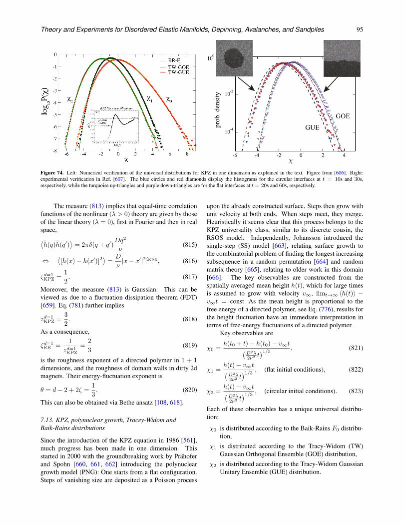
Theory and Experiments for Disordered Elastic Manifolds, Depinning, Avalanches, and Sandpiles 95
A KPZ Cocktail-Shaken, not Stirred... 797
Fig. 1 1+1 KPZ Euler: numerical integrations, for stationary-state (χ0), transient flat (χ1), and radial (χ2)geometries, stacked up against relevant universal limit distributions Baik–Rains, Tracy–Widom GOE, andGUE, respectively. Inset: skewness minimum, sT M ≈ 0.22, exhibited by KPZ equation as experimentalsignature of stationary-state statistics, recently observed in KPZ turbulent liquid-crystal kinetic rougheningwork [84]. Note, in particular, the asymptotic approach from below to TW-GOE skewness s(τ ≫ 1) = s1 =0.2935
runs, suitably averaged,we have extracted the asymptotic growth velocity v∞ = 0.195935 forthe KPZ equation, as simulated. Note that, in contrast to PNG, where the phenomenologicalparameters A, λ and v∞ are known exactly, pinning down these quantities represents theprimary challenge, beyond simply aggregating the height fluctuation statistics. In fact, asdone in experiment [82,83] and occasionally in numerics, we have matched the variance ofthe transient regime statistics (i.e., our 1+1 KPZ Euler pdf) to TW-GOE, fitting the secondmoment to ⟨χ2
1 ⟩ = 0.63805, which fixes $β = 0.23111. The resulting numerical dataset, when viewed against the known TW-GOE limit distribution, focusses attention uponthe skewness and kurtosis, as well as the finite-time correction to the universal mean. Inparticular, our extracted value for the 1+1 KPZ skewness, s = ⟨δh 3⟩c/⟨δh 2⟩3/2c = 0.279, ascomparedwith accepted result s1 = 0.2935. As emphasized recently [66],$ thus determined,can then be employed in the service of a genuine comparison to both the radial TW-GUE andstationary-state BR-F0 limit distributions. In other words, the KPZ scaling parameters, whilemodel-dependent, are not subclass dependent—in a given dimension, the same $ and v∞apply to flat, curved and stationary cases, as noted already in experiment [83]. Thus, here,we take the numerical short-cut, using TW-GOE to determine $β , privileging the greaterchallenges posed by BR-F0 & TW-GUE.
Hence, we have also included in Fig. 1 the centered, rescaled fluctuations of the h eigh tincrement,'h = h (to+'t)− h (to), casting the associated stationary-stateKPZ statistics interms of theO(1) Baik–Rains variable: χ0 = ('h − v∞'t)/($'t)1/3, integrating the KPZequation to a late time to = 5000, then investigating the temporal correlations at a later timeto + 't, with 1 ≤ 't ≤ 25 ≪ to, at a given site, sampling over the entire system of sizeL = 104, then averaging over 105 realizations, again yielding a statistical data set with 109
points. Here, for the skewness and kurtosis, we find 0.348 and 0.261, compared to Prähofer–Spohn’s oft-quoted BR-F0 values: s0 = 0.35941 and k0 = 0.28916, respectively, for these
123
866 K.A. Takeuchi, M. Sano
Fig. 8 Histogram of the rescaledlocal heightq ≡ (h − v∞t)/(Γ t)1/3 for thecircular (solid symbols) and flat(open symbols) interfaces. Theblue circles and red diamondsdisplay the histograms for thecircular interfaces at t = 10 s and30 s, respectively, while theturquoise up-triangles and purpledown-triangles are for the flatinterfaces at t = 20 s and 60 s,respectively. The dashed anddotted curves show the GUE andGOE TW distributions,respectively, defined by therandom variables χGUE andχGOE. (Color figure online)
For the flat interfaces, one in principle needs to impose a tilt u to measure v∞(u) [53], butsupposing the rotational invariance of the system, one again finds v∞(u) =
√1 + u2v∞ and
thus Eq. (13). This is justified by practically the same values of our estimates v∞ in Eq. (10).In passing, the rotational invariance also implies v0 = 0 in the KPZ equation (5), without theneed to invoke the comoving frame.
3.4 Distribution Function
Using the two experimentally determined parameter values (10) and (11), we shall directlycompare the interface fluctuations χ with the mathematically defined random variables χGUE
and χGOE. This is achieved by defining the rescaled local height
q ≡ h − v∞t
(Γ t)1/3≃ χ (14)
and producing its histogram for the circular and flat interfaces (solid and open symbols inFig. 8, respectively). The result clearly shows that the two cases exhibit distinct distribu-tions, which are not centered nor symmetric, and hence clearly non-Gaussian. Moreover,the histograms for the circular and flat interfaces are found, without any ad hoc fitting, veryclose to the GUE (dashed curve) and GOE (dotted curve) TW distributions, respectively, asanticipated from their values of the skewness and the kurtosis as well as from the theoreticalresults for the solvable models. The agreements are confirmed with resolution roughly downto 10−5 in the probability density.
A closer inspection of the experimental data in Fig. 8 reveals, however, a slight devia-tion from the theoretical curves, which is mostly a small horizontal translation that shrinksas time elapses. To quantify this effect, we plot in Fig. 9 the time series of the differencebetween the nth-order cumulants of the measured rescaled height q and those for the TWdistributions. We then find for both circular and flat interfaces [Fig. 9(a, b)] that, indeed, thesecond- to fourth-order cumulants quickly converge to the values for the corresponding TWdistributions, whereas the first-order cumulant ⟨q⟩, or the mean, shows a pronounced devia-tion as suggested in the histograms. This, however, decreases in time, showing a clear powerlaw proportional to t−1/3 [Fig. 9(c, e)], and thus vanishes in the asymptotic limit t → ∞.Similar finite-time corrections are in fact visible in other cumulants, though less clearly for
χ
Figure 74. Left: Numerical verification of the universal distributions for KPZ in one dimension as explained in the text. Figure from [606]. Right:experimental verification in Ref. [607]. The blue circles and red diamonds display the histograms for the circular interfaces at t = 10s and 30s,respectively, while the turquoise up-triangles and purple down-triangles are for the flat interfaces at t = 20s and 60s, respectively.
The measure (813) implies that equal-time correlationfunctions of the nonlinear (λ > 0) theory are given by thoseof the linear theory (λ = 0), first in Fourier and then in realspace,⟨h(q)h(q′)
⟩= 2πδ(q + q′)
Dq2
ν(815)
⇔⟨[h(x)− h(x′)]2
⟩=D
ν|x− x′|2ζKPZ , (816)
ζd=1KPZ =
1
2. (817)
Moreover, the measure (813) is Gaussian. This can beviewed as due to a fluctuation dissipation theorem (FDT)[659]. Eq. (781) further implies
zd=1KPZ =
3
2. (818)
As a consequence,
ζd=1RB =
1
zd=1KPZ
=2
3(819)
is the roughness exponent of a directed polymer in 1 + 1dimensions, and the roughness of domain walls in dirty 2dmagnets. Their energy-fluctuation exponent is
θ = d− 2 + 2ζ =1
3. (820)
This can also be obtained via Bethe ansatz [108, 618].
7.13. KPZ, polynuclear growth, Tracey-Widom andBaik-Rains distributions
Since the introduction of the KPZ equation in 1986 [561],much progress has been made in one dimension. Thisstarted in 2000 with the groundbreaking work by Prahoferand Spohn [660, 661, 662] introducing the polynucleargrowth model (PNG): One starts from a flat configuration.Steps of vanishing size are deposited as a Poisson process
upon the already constructed surface. Steps then grow withunit velocity at both ends. When steps meet, they merge.Heuristically it seems clear that this process belongs to theKPZ universality class, similar to its discrete cousin, theRSOS model. Independently, Johansson introduced thesingle-step (SS) model [663], relating surface growth tothe combinatorial problem of finding the longest increasingsubsequence in a random permutation [664] and randommatrix theory [665], relating to older work in this domain[666]. The key observables are constructed from thespatially averaged mean height h(t), which for large timesis assumed to grow with velocity v∞, limt→∞ 〈h(t)〉 −v∞t = const. As the mean height is proportional to thefree energy of a directed polymer, see Eq. (776), results forthe height fluctuation have an immediate interpretation interms of free-energy fluctuations of a directed polymer.
Key observables are
χ0 =h(t0 + t)− h(t0)− v∞t
(D2λ2ν2 t
)1/3 , (821)
χ1 =h(t)− v∞t(D2λ2ν2 t
)1/3 , (flat initial conditions), (822)
χ2 =h(t)− v∞t(D2λ2ν2 t
)1/3 , (circular initial conditions). (823)
Each of these observables has a unique universal distribu-tion:
χ0 is distributed according to the Baik-Rains F0 distribu-tion,
χ1 is distributed according to the Tracy-Widom (TW)Gaussian Orthogonal Ensemble (GOE) distribution,
χ2 is distributed according to the Tracy-Widom GaussianUnitary Ensemble (GUE) distribution.
Theory and Experiments for Disordered Elastic Manifolds, Depinning, Avalanches, and Sandpiles 96
The reader wishing to test these laws himself can find aMathematica implementation online [667].
The Bethe-ansatz for the directed polymer wasintroduced in 1987 by Kardar to obtain the roughnessexponent of a directed polymer, ζ = 2/3 and θ =1/3. A revival started in 2010, when physicists succeeded[668, 669, 670, 671, 672] to first reproduce the work of[660, 661, 662] via the Bethe ansatz, and then extendit to other situations [673]. At the same time, a newgeneration of mathematicians developed complementarytools [674, 675, 676, 677], joining the work of Spohn andcollaborators [678, 679].
Extraordinarily, Takeuchi and Sano [680, 607] suc-ceeded to extract the universal distributions from a turbulentliquid-crystal experiment. A snapshot is shown in Fig. 71,and the two Tracey-Widom distributions for circular and flatinitial conditions in Fig. 74.
Let us conclude by mentioning pedagogical presenta-tions [681, 682, 683], as well as attempts to port this at leastnumerically to higher dimensions [684, 685].
7.14. Models in the KPZ universality class, andexperimental realizations
In all dimensions:
• KPZ [561],• polynuclear growth (PNG) [660, 661, 662],• Rigid-solid-on-solid models (RSOS) [644, 645, 646,
647, 648, 649].• directed polymer in quenched disorder (section 7.4).
In one dimension:
• longest growing subsequence in a random permutation[664],
• the asymmetric simple exclusion process (ASEP)[686, 687, 688].
Experimental realizations (one dimension only):
• slow combustion of paper [689, 690],• turbulent liquid crystals [680, 607],• particle deposition (with crossover to qKPZ) [691],• bacterial growth [692],• chemical reaction fronts [574].
7.15. From Burgers’ turbulence to Navier-Stokesturbulence?
In Burgers’ turbulence velocity profiles are locally linear(see e.g. the right of Fig. 72), interrupted by jumps.Phenomenologically it is similar to the force field indisordered systems. This implies that, if non-vanishing, atsmall distances
〈[v(u, t)− v(u′, t)]n〉 ' An|u− u′|ζn , (824)
and for Burger ζn = 1, independent of n. In Navier-Stokes turbulence, the exponent ζ3 = 1, as predicted byKolmogorov in 1941 [693]. Other moments obey
ζn =n
3+ δζn, (825)
where δζn is small. Calculating δζn analytically is theoutstanding problem of turbulence research. One cantry to use FRG for this problem [694], but somethingcrucial is missing: While FRG correctly deals with shocks,the weaker singularities responsible for Eq. (825) are notcaptured by FRG. (It may work in dimension d = 2,though [694].) It is possible that the FRG fixed point whichtypically has a cusp, and which usually is implemented forthe second cumulant, instead applies to the third cumulant,as ζ3 = 1. How to implement this idea remains an openproblem.
8. Links between loop-erased random walks, CDWs,sandpiles, and scalar field theories
8.1. Supermathematics
Supermathematics, introduced in [695] and nicely reviewedin [696] is an alternative way to average over disorder.In this technique, additional fermionic or Grassmanniandegrees of freedom are introduced to normalize the partitionfunction to Z = 1, even before averaging over disorder. Westart by reviewing basic properties of Grassmann variables,before using them for disorder averages. Most of thematerial is standard, and the reader familiar with it, orwishing to advance may safely do so.
Two points should be retained: While supermathemat-ics is usually referred to as supersymmetry technique, thisis a misnomer as supersymmetry is broken at the Larkinscale, i.e. when a cusp appears. The name is due to histor-ical reasons, stemming from a time when people believedthat supersymmetry is not broken. To avoid this confusion,we prefer the term supermathematics.
Braking of supersymmetry, and the cusp, can be foundin this framework, as long as one considers at least twophysically distinct copies. The technical reason is that toassess the n-th cumulant of a distribution, one needs at leastn distinct copies. Even when supposing the disorder to beGaussian distributed, the variance, i.e. the second cumulantneeds to be assessed, thus two distinct replicas.
Apart from these more formal considerations, thetechnique has proven powerful in the mapping of charge-density waves onto a φ4-type theory (section 8.6).
8.2. Basic rules for Grassmann variables
Grassmann variables are anticommuting variables whichallow one to write a path-integral for bosons, in the sameway as one does for bosons. There are only few rules toremember. If χ and ψ are Grassmann variables, then
χψ = −ψ χ. (826)
Theory and Experiments for Disordered Elastic Manifolds, Depinning, Avalanches, and Sandpiles 97
This immediately implies that
χ2 = 0. (827)
One introduces derivatives, and integrals through the sameformula, known as Berezin integral [695],∫
dχχ ≡ d
dχχ = 1. (828)
One checks that they satisfy the usual properties associatedto “normal” derivatives, and integrals. An importantproperty is∫
dχdχ e−aχχ = a. (829)
This is easily proven upon Taylor expansion. The minussign in the exponential cancels the minus sign obtainedwhen exchanging χ with χ, which is necessary since anintegral or derivative is defined to act directly on thevariable following it. Eq. (829) can be generalized tointegrals over an n-component pair of vectors ~χ, and ~χ:∫
d~χd~χ e−~χA~χ :=
n∏
a=1
∫dχa dχa e−~χA~χ = det(A).
(830)
It is proven by changing coordinates s.t. A becomesdiagonal. For comparison we give the correspondingformula for normal (bosonic) fields, noting φa := φax+iφay ,φa := φax − iφay ,∫
d~φ d~φ e−
~φA~φ :=
n∏
a=1
∫dφax dφay
πe−~φA~φ =
1
det(A).
(831)
When combining normal and Grassmannian integralsover the same number of variables into a product, thecontributions from Eqs. (830) and (831) cancel. This willbe used below.
8.3. Disorder averages with bosons and fermions
The above formulas permit a different approach to averageover disorder. For concreteness, define
H[u, V ] =
∫
x
1
2[∇u(x)]
2+m2
2u(x)2 + U
(u(x)
)
+ V(x, u(x)
). (832)
The disorder-average of an observable O is defined as
O[u] :=
∫ r∏
a=1
D[ua]O[u1]e−1T H[ua,V ]
∫ r∏
a=1
D[ua]e−1T H[ua,V ]
. (833)
The function U(u) is an arbitrary potential, e.g. the non-linearity in φ4-theory, U(u) = g u4. The randompotential V (x, u) is the same one used in section 1.2, with
correlations given by Eq. (9). Its average is indicated bythe overline. We remind that the difficulty in evaluating(833) comes from the denominator. The replica trick usedin section 1.5 allowed us to set r = 0, effectively discardingthe denominator. Here we follow a different strategy.
In the limit of T → 0 only configurations whichminimize the energy survive. These configurations satisfyδH[ua,V ]δua(x) = 0, and we want to insert a δ-distribution
enforcing this condition into the path-integral. This hasto be accompanied by a factor of det
[δ2H[ua,V ]δua(x)δua(y)
], such
that the path integral is normalized to 1. The latter canbe achieved by an additional integral over Grassmannvariables, i.e. fermionic degrees of freedom, using that
det
(δ2H[u, V ]
δu(x)δu(y)
)(834)
=
∫D[ψa]D[ψa] exp
(−∫
x
ψ(x)δ2H[u, V ]
δu(x)δu(y)ψ(x)
).
This allows us to write the disorder average of anyobservable O[u] as
O[u] =
∫ r∏
a=1
D[ua]D[ua]D[ψa]D[ψa]O[u]
× exp
[−∫
x
ua(x)δH[ua]
δua(x)+ ψa(x)
δ2H[ua]
δua(x)δua(y)ψa(y)
].
(835)
This method was first introduced in [32, 697]. Analternative derivation and insight are offered by Cardy[698, 699, 700], see also [701, 702].
Averaging over disorder with the force-force correlator∆(u) := −R′′(u) yields
O[u] =
∫ ∏
a
D[ua]D[ua]D[ψa]D[ψa]
exp(−S[ua, ua, ψa, ψa]
)
S[ua, ua, ψa, ψa],
=
∫
x
r∑
a=1
ua(x)
[(−∇2+m2)ua(x) + U ′
(ua(x)
)]
+ ψa(x)[−∇2+m2+U ′′
(ua(x)
)]ψa(x)
−r∑
a,b=1
[1
2ua(x)∆
(ua(x)− ub(x)
)ub(x)
−ua(x)∆′(ua(x)− ub(x)
)ψb(x)ψb(x)
−1
2ψa(x)ψa(x)∆′′
(ua(x)− ub(x)
)ψb(x)ψb(x)
]. (836)
We first analyze the special case of n = 1. Suppose that∆(u) is even and analytic to start with, then few termssurvive from Eq. (836),
SSusy[u, u, ψ, ψ] =∫
x
u(x)
[(−∇2+m2)u(x) + U ′
(u(x)
)]
Theory and Experiments for Disordered Elastic Manifolds, Depinning, Avalanches, and Sandpiles 98
+ψ(x)[−∇2+m2+U ′′
(u(x)
)]ψ(x)− 1
2u(x)∆(0)u(x)
.
(837)
(We have used that ψ2a = ψ2
a = 0 to eliminate the4-fermion-term.) A particularly simple case are randommanifolds, for which U(u) = 0. Then bosons u andu, and fermions ψ and ψ do not interact, all expectationvalues are Gaussian, perturbation theory gives Eq. (38), anddimensional reduction holds. When U(u) 6= 0, things aremore complicated, but as we will see in the next section,dimensional reduction still holds, at least formally.
The reason is that the action (837) possesses anapparent supersymmetry, made manifest by grouping allfields into a (bosonic) superfield,
Φ(x, Θ,Θ) := u(x) + Θψ(x) + ψ(x)Θ− ΘΘu(x). (838)
Both Θ and Θ are Grassmann numbers. The action (837)can then be written with the super Laplacian ∆s as
SSusy =
∫dΘdΘ
∫
x
1
2Φ(x, Θ,Θ)(−∆s +m2)Φ(x, Θ,Θ)
+ U(Φ(x, Θ,Θ)), (839)
∆s := ∇2 + ∆(0)∂
∂Θ
∂
∂Θ. (840)
As we will see in section 8.5, the action is invariant underthe action of two supergenerators
Q := x∂
∂Θ− 2
∆(0)Θ∇, Q := x
∂
∂Θ+
2
∆(0)Θ∇,
Q, Q
= 0. (841)
This is sufficient to “prove” dimensional reduction.
8.4. Renormalization of the disorder
For more than r = 1 replicas, the theory is richer, and wecan recover the renormalization of ∆(u) itself. To simplifymatters, set U(u) = 0, and write
S[ua, ua, ψa, ψa] =∑
a
∫
x
[ua(x)(−∇2 +m2)ua(x)
+ ψa(x)(−∇2 +m2)ψa(x)− 1
2ua(x)∆(0)ua(x)
]
−∑
a 6=b
∫
x
[1
2ua(x)∆
(ua(x)− ub(x)
)ub(x)
−ua(x)∆′(ua(x)− ub(x)
)ψb(x)ψb(x)
−1
2ψa(x)ψa(x)∆′′
(ua(x)− ub(x)
)ψb(x)ψb(x)
].
(842)
Corrections to ∆(u) are constructed by remarking that theinteraction term quadratic in u is almost identical to thetreatment of the dynamics in the static limit (i.e. afterintegration over times). The diagrams in question are
+ +
+ , (843)
where an arrow indicates the correlation-function, x−→−−−y= 〈u(x)u(y)〉 = C(x−y). This leads to (in the order givenabove)
δ∆(u) =[−∆(u)∆′′(u)−∆′(u)2 + ∆′′(u)∆(0)
]
×∫
x−yC(x− y)2. (844)
The last term of Eq. (843) is odd, and vanishes. Eq. (844)is equal to the results of Eqs. (323)–(331).
A non-trivial ingredient is the cancellation of theacausal loop (332) in the dynamics, equivalent to the 3-replica term in the statics:
+ = 0. (845)
The first diagram comes from the contraction of two termsproportional to ua∆(ua − ub)ub. The second is obtainedfrom contracting all fermions in two terms proportional toua∆′(ua − ub)ψbψb. Since the fermionic loop (orientedwiggly line in the second diagram) contributes a factor of−1, both cancel.
One can treat the interacting theory completely in asuperspace formulation. The action is
S[Φ] =∑
a
∫
Θ,Θ
∫
x
1
2Φa(x, Θ,Θ)(−∆s+m
2)Φa(x, Θ,Θ)
− 1
2
∑
a6=b
∫
x
∫
Θ,Θ
∫
Θ′,Θ′
R(Φa(x, Θ,Θ)− Φb(x, Θ
′,Θ′)).
(846)
“Non-locality” in replica-space or in time is replaced by“non-locality” in superspace. Corrections to R(u) all stemfrom superdiagrams, which result into bilocal interactionsin superspace, not trilocal, or higher. The latter find theirequivalent in 3-local terms in replica-space in the replica-formulation, and 3-local terms in time, in the dynamicformulation.
Supersymmetry is broken, once ∆(0) changes, i.e. atthe Larkin length. A seemingly “effective supersymmetry”,or “scale-dependent supersymmetry” appears, in which theparameter ∆(0), which appears in the Susy-transformation,changes with scale, according to the FRG flow equations(64) for ∆(u), continued to u = 0.
8.5. Supersymmetry and dimensional reduction
Let us study invariants of the action. Since total derivativesboth in x and θ or θ vanish, the crucial term to focus on isthe super-Laplacian. To simplify notations, we set
ρ := ∆(0). (847)
By explicit inspection, we find that the two generators ofsuper-translations
Q := x∂
∂Θ+
2
ρΘ∇, Q := x
∂
∂Θ− 2
ρΘ∇ (848)
Theory and Experiments for Disordered Elastic Manifolds, Depinning, Avalanches, and Sandpiles 99
both commute with the Super-Laplacian, and anti-commutewith each other,
[∆s, Q] =[∆s, Q
]= 0,
Q, Q
= 0. (849)
The following combination is invariant under the action ofQ and Q,
Q
(x2 +
4
ρΘΘ
)= Q
(x2 +
4
ρΘΘ
)= 0. (850)
Applying the Super-Laplacian (840) gives45
∆s
(x2 +
4
ρΘΘ
)= 2(d− 2). (851)
To obtain the super-propagator, inverse of the super-Laplacian plus mass term in Eq. (839), we remark that(m2 −∇2 − ρ ∂
∂Θ
∂
∂Θ
)(m2 −∇2 + ρ
∂
∂Θ
∂
∂Θ
)
= (m2 −∇2)2. (852)
This implies that
(m2 −∆s
)−1=m2 −∇2 + ρ
∂
∂Θ
∂
∂Θ(m2 −∇2)2 . (853)
Therefore
C(x− x′,Θ−Θ′, Θ− Θ′) (854)
=m2 −∇2 + ρ
∂
∂Θ
∂
∂Θ(m2 −∇2)2 δ(x− x′)δ(Θ−Θ′)δ(Θ− Θ′).
The Grassmanian δ-functions are defined as∫dΘδ(Θ−Θ′)f(Θ) = f(Θ′). (855)
By direct calculation one finds
δ(Θ−Θ′) = Θ′ −Θ =
∫dχ eχ(Θ′−Θ). (856)
One can transform (854) into a representation in dual spacesof momentum (k-space) and super-coordinates (χ-space) as
C(k, χ, χ) =m2 + k2 + ρχχ
(m2 + k2)2≡ 1
m2 + k2 + ρχχ
≡∫ ∞
0
ds e−s(m2+k2+ρχχ). (857)
The final proof of dimensional reduction is performed withthis representation of the super-correlator46. Any diagramcan be written as∫
k1
∫
χ1χ1
...
∫
kn
∫
χnχn
n∏
i=1
[∫ ∞
0
dsi e−si(m2+k2i+ρχiχi)
],
(858)
where some δ-distributions have already been used toeliminate integrations over k’s, i.e. some of the ki’s45This relation comes out incorrectly in [32].46Note that one can also work in position-space [32]. Then the super-correlator is explicitly d-dependent, and one should check that this d-dependence comes out correctly.
appearing in the exponential are not independent variables,but linear combinations of other kj’s, and the same holdsfor the corresponding χi and χi. The product of exponentialfactors can be written as
n∏
i=1
[e−si(m
2+k2i+ρχiχi)]
= exp
−
k1
k2
. . .kn
W
k1
k2
. . .kn
× exp
−
χ1
χ2
. . .χn
W
χ1
χ2
. . .χn
. (859)
Integration over the k’s gives∫
k1
. . .
∫
kn
e−~k·W·~k =
(1
4π
)ld/2det(W)−d/2, (860)
where l is the number of loops. Integration over χ and χgives∫
χ1χ1
. . .
∫
χnχn
e−ρ~χ·W·~χ = (ρ)l det(W). (861)
The product of the two factors (860) and (861) is the sameas for a standard bosonic diagram in dimension d − 2.Remarking that the expansion is in powers of T , andcombining these relations, we obtain after integration overthe si:
l-loop super-diagram in dimension d (862)
=( ρ
4πT
)l× l-loop standard-diagram in dimension d− 2.
This implies that for any observable O(T )
Oddisordered(ρ) = Od−2thermal
(T =
ρ
4π
). (863)
The above proof can be extended to theories with derivativecouplings. The rules are as follows: Consider Hs[Φ]given in Eq. (839). To this we can add an interaction inderivatives, for a total of
Hs[Φ] =
∫
Θ,Θ
∫
x
[1
2Φ(x, Θ,Θ)(−∆s +m2)Φ(x, Θ,Θ)
+ U(Φ(x, Θ,Θ)
)
+A1
(Φ(x, Θ,Θ)
)(−∆s +m2)A2
(Φ(x, Θ,Θ)
)].
(864)
This theory is supersymmetric: Calculating diagrams inperturbation theory, we get additional vertices. Thecorresponding diagrams can be calculated from the sametype of generating function (859). The trick is to use insteadof an integral w.r.t. s a derivative w.r.t. s, taken at s = 0,(m2 + k2 + ρχχ
)= − d
ds
∣∣∣∣s=0
e−s(m2+k2+ρχχ). (865)
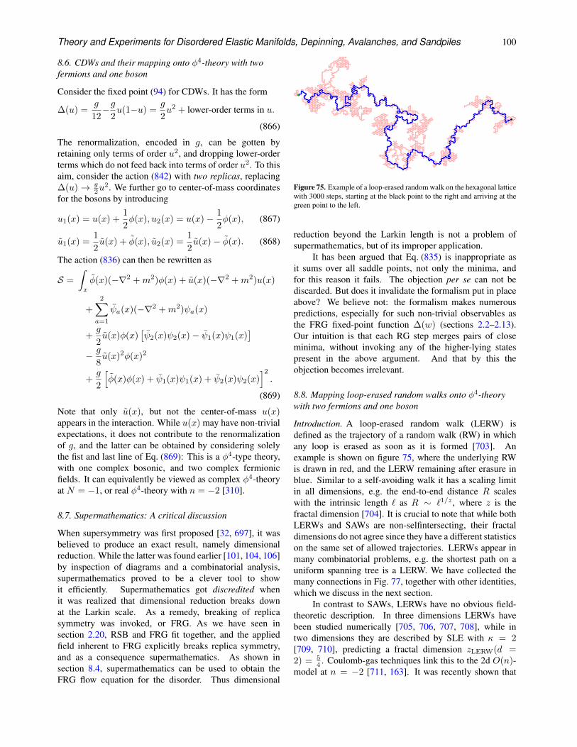
Theory and Experiments for Disordered Elastic Manifolds, Depinning, Avalanches, and Sandpiles 100
8.6. CDWs and their mapping onto φ4-theory with twofermions and one boson
Consider the fixed point (94) for CDWs. It has the form
∆(u) =g
12−g
2u(1−u) =
g
2u2 + lower-order terms in u.
(866)
The renormalization, encoded in g, can be gotten byretaining only terms of order u2, and dropping lower-orderterms which do not feed back into terms of order u2. To thisaim, consider the action (842) with two replicas, replacing∆(u)→ g
2u2. We further go to center-of-mass coordinates
for the bosons by introducing
u1(x) = u(x) +1
2φ(x), u2(x) = u(x)− 1
2φ(x), (867)
u1(x) =1
2u(x) + φ(x), u2(x) =
1
2u(x)− φ(x). (868)
The action (836) can then be rewritten as
S =
∫
x
φ(x)(−∇2 +m2)φ(x) + u(x)(−∇2 +m2)u(x)
+
2∑
a=1
ψa(x)(−∇2 +m2)ψa(x)
+g
2u(x)φ(x)
[ψ2(x)ψ2(x)− ψ1(x)ψ1(x)
]
− g
8u(x)2φ(x)2
+g
2
[φ(x)φ(x) + ψ1(x)ψ1(x) + ψ2(x)ψ2(x)
]2.
(869)
Note that only u(x), but not the center-of-mass u(x)appears in the interaction. While u(x) may have non-trivialexpectations, it does not contribute to the renormalizationof g, and the latter can be obtained by considering solelythe fist and last line of Eq. (869): This is a φ4-type theory,with one complex bosonic, and two complex fermionicfields. It can equivalently be viewed as complex φ4-theoryat N = −1, or real φ4-theory with n = −2 [310].
8.7. Supermathematics: A critical discussion
When supersymmetry was first proposed [32, 697], it wasbelieved to produce an exact result, namely dimensionalreduction. While the latter was found earlier [101, 104, 106]by inspection of diagrams and a combinatorial analysis,supermathematics proved to be a clever tool to showit efficiently. Supermathematics got discredited whenit was realized that dimensional reduction breaks downat the Larkin scale. As a remedy, breaking of replicasymmetry was invoked, or FRG. As we have seen insection 2.20, RSB and FRG fit together, and the appliedfield inherent to FRG explicitly breaks replica symmetry,and as a consequence supermathematics. As shown insection 8.4, supermathematics can be used to obtain theFRG flow equation for the disorder. Thus dimensional
Figure 75. Example of a loop-erased random walk on the hexagonal latticewith 3000 steps, starting at the black point to the right and arriving at thegreen point to the left.
reduction beyond the Larkin length is not a problem ofsupermathematics, but of its improper application.
It has been argued that Eq. (835) is inappropriate asit sums over all saddle points, not only the minima, andfor this reason it fails. The objection per se can not bediscarded. But does it invalidate the formalism put in placeabove? We believe not: the formalism makes numerouspredictions, especially for such non-trivial observables asthe FRG fixed-point function ∆(w) (sections 2.2–2.13).Our intuition is that each RG step merges pairs of closeminima, without invoking any of the higher-lying statespresent in the above argument. And that by this theobjection becomes irrelevant.
8.8. Mapping loop-erased random walks onto φ4-theorywith two fermions and one boson
Introduction. A loop-erased random walk (LERW) isdefined as the trajectory of a random walk (RW) in whichany loop is erased as soon as it is formed [703]. Anexample is shown on figure 75, where the underlying RWis drawn in red, and the LERW remaining after erasure inblue. Similar to a self-avoiding walk it has a scaling limitin all dimensions, e.g. the end-to-end distance R scaleswith the intrinsic length ` as R ∼ `1/z , where z is thefractal dimension [704]. It is crucial to note that while bothLERWs and SAWs are non-selfintersecting, their fractaldimensions do not agree since they have a different statisticson the same set of allowed trajectories. LERWs appear inmany combinatorial problems, e.g. the shortest path on auniform spanning tree is a LERW. We have collected themany connections in Fig. 77, together with other identities,which we discuss in the next section.
In contrast to SAWs, LERWs have no obvious field-theoretic description. In three dimensions LERWs havebeen studied numerically [705, 706, 707, 708], while intwo dimensions they are described by SLE with κ = 2[709, 710], predicting a fractal dimension zLERW(d =2) = 5
4 . Coulomb-gas techniques link this to the 2d O(n)-model at n = −2 [711, 163]. It was recently shown that
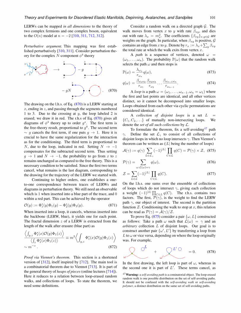
Theory and Experiments for Disordered Elastic Manifolds, Depinning, Avalanches, and Sandpiles 101
LERWs can be mapped in all dimensions to the theory oftwo complex fermions and one complex boson, equivalentto the O(n) model at n = −2 [310, 311, 712, 312].
Perturbative argument. This mapping was first estab-lished perturbatively [310, 311]. Consider perturbation the-ory for the complex N -component φ4 theory
x
y
1
2
3z
−→x
z
− gx
z
− gNx
z
. (870)
The drawing on the l.h.s. of Eq. (870) is a LERW starting atx, ending in z, and passing through the segments numbered1 to 3. Due to the crossing at y, the loop labeled 2 iserased; we draw it in red. The r.h.s of Eq. (870) gives alldiagrams of φ4 theory up to order gs. The first term isthe free-theory result, proportional to g0. The second term∼ g cancels the first term, if one puts g → 1. Here it iscrucial to have the same regularization for the interactionas for the conditioning. The third term is proportional toN , due to the loop, indicated in red. Setting N → −1compensates for the subtracted second term. Thus settingg → 1 and N → −1, the probability to go from x to zremains unchanged as compared to the free theory. This is anecessary condition to be satisfied. Since the first two termscancel, what remains is the last diagram, corresponding tothe drawing for the trajectory of the LERW we started with.
Continuing to higher orders, one establishes a one-to-one correspondence between traces of LERWs anddiagrams in perturbation theory. We still need an observablewhich is 1 when inserted into a blue part of the trace, and 0within a red part. This can be achieved by the operator
O(y) := Φ∗1(y)Φ1(y)− Φ∗2(y)Φ2(y). (871)
When inserted into a loop, it cancels, whereas inserted intothe backbone (LERW, blue), it yields one for each point.The fractal dimension z of a LERW is extracted from thelength of the walk after erasure (blue part) as⟨∫
y,zΦ∗1(x)O(y)Φ1(z)
⟩
⟨∫z
Φ∗1(x)Φ1(z)⟩ ≡ m2
⟨∫
y,z
Φ∗1(x)O(y)Φ1(z)
⟩
∼ m−z . (872)
Proof via Viennot’s theorem. This section is a shortenedversion of [312], itself inspired by [712]. The main tool isa combinatorial theorem due to Viennot [713]. It is part ofthe general theory of heaps of pieces (online lectures [714]).Here it reduces to a relation between loop-erased randomwalks, and collections of loops. To state the theorem, weneed some definitions.
Consider a random walk on a directed graph G. Thewalk moves from vertex x to y with rate βxy , and diesout with rate λx = m2
x. The coefficients βxyx,y∈G areweights on the graph. In particular, when βxy is positive, Gcontains an edge from x to y. Denote by rx := λx+
∑y βxy
the total rate at which the walk exits from vertex x.A path is a sequence of vertices, denoted ω =
(ω1, . . . , ωn). The probability P(ω) that the random walkselects the path ω and then stops is
P(ω) =λωnrωn
q(ω), (873)
q(ω) =βω1ω2
rω1
βω2ω3
rω2
. . .βωn−1ωn
rωn−1
. (874)
A loop is a path ω = (ω1, . . . , ωn−1, ωn = ω1) wherethe first and last points are identical, and all other verticesdistinct, so it cannot be decomposed into smaller loops.Loops obtained from each other via cyclic permutations areconsidered identical.
A collection of disjoint loops is a set L =C1, C2, . . . of mutually non-intersecting loops. Wedenote the set of all such collections by L.
To formulate the theorem, fix a self-avoiding47 pathγ. Define the set Lγ to consist of all collections ofdisjoint loops in which no loop intersects γ. Then Viennot’stheorem can be written as (|L| being the number of loops)
A(γ) := q(γ)∑
L∈Lγ(−1)|L|
∏
C∈Lq(C) = P(γ)×Z, (875)
P(γ) =∑
ω:L(ω)=γ
q(ω), (876)
Z =∑
L∈L(−1)|L|
∏
C∈Lq(C). (877)
On the l.h.s. one sums over the ensemble of collectionsof loops which do not intersect γ, giving each collectiona weight (−1)|L|
∏C∈L q(C). The r.h.s. contains two
factors. The first, P(γ), is the weight to find the LERWpath γ, our object of interest. The second is the partitionfunction Z . Conditioning the walk to stop at x, this relationcan be read as P(γ) = A(γ)/Z .
To prove Eq. (875) consider a pair ω,L constructedas follows: Take a path ω such that L(ω) = γ and anarbitrary collection L of disjoint loops. Our goal is toconstruct another pair ω′, L′ by transferring a loop fromL to ω or vice versa, depending on where the loop originallywas. For example,
+
ω
L
ω′
L′= 0. (878)
In the first drawing, the left loop is part of ω, whereas inthe second one it is part of L′. These terms cancel, as47Warning: a self-avoiding path is a cominatorial object. The loop-erasedrandom walk is one possible distribution on the set of self-avoiding paths.It should not be confused with the self-avoiding walk or self-avoidingpolymer, a distinct distribution on the same set of self-avoiding paths.
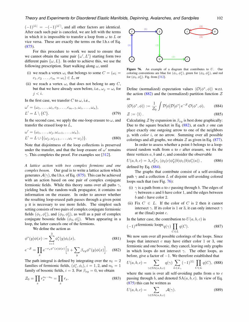
Theory and Experiments for Disordered Elastic Manifolds, Depinning, Avalanches, and Sandpiles 102
(−1)|L| = −(−1)|L′|, and all other factors are identical.
After each such pair is canceled, we are left with the termsin which it is impossible to transfer a loop from ω to L orvice versa. These are exactly the terms on the l.h.s of Eq.(875).
For this procedure to work we need to ensure thatwe cannot obtain the same pair ω′, L′ starting form twodifferent pairs ω,L. In order to achieve this, we use thefollowing prescription. Start walking along ω, until
(i) we reach a vertex ωi that belongs to some C = (ωi =c1, c2 . . . , cm = ωi) ∈ L, or
(ii) we reach a vertex ωi that does not belong to any C,but that we have already seen before, i.e., ωj = ωi forj < i.
In the first case, we transfer C to ω, i.e.,
ω′ = (ω1, . . . , ωi, c2, . . . , cm−1, ωi, . . . , ωn),
L′ = L \ C. (879)
In the second case, we apply the one-loop erasure to ω, andtransfer the erased loop to L,
ω′ = (ω1, . . . , ωj , ωi+1, . . . , ωn),
L′ = L ∪ (ωj , ωj+1, . . . , ωi = ωj). (880)
Note that disjointness of the loop collections is preservedunder the transfer, and that the loop erasure of ω′ remainsγ. This completes the proof. For examples see [312].
A lattice action with two complex fermions and onecomplex boson. Our goal is to write a lattice action whichgeneratesA(γ), the l.h.s. of Eq. (875). This can be achievedwith an action based on one pair of complex conjugatefermionic fields. While this theory sums over all paths γ,yielding back the random-walk propagator, it contains noinformation on the erasure. In order to answer whetherthe resulting loop-erased path passes through a given pointy it is necessary to use more fields. The simplest suchsetting consists of two pairs of complex conjugate fermionicfields (φ1, φ
∗1), and (φ2, φ
∗2), as well as a pair of complex
conjugate bosonic fields (φ3, φ∗3). When appearing in a
loop, the latter cancels one of the fermions.We define the action as
φ∗(y)φ(x) :=
3∑
i=1
φ∗i (y)φi(x), (881)
e−S =∏
x
e−rxφ∗(x)φ(x)
[1 +
∑
y
βxyφ∗(y)φ(x)
]. (882)
The path integral is defined by integrating over the nf = 2families of fermionic fields, (φ∗i , φi), i = 1, 2, and nb = 1family of bosonic fields, i = 3. For βxy = 0, we obtain
Z0 =∏
x
rnf−nbx =
∏
x
rx. (883)
a
b
c
x
y
z w
(1)
(1)
(2)
(2)
(3)
(3)
Figure 76. An example of a diagram that contributes to U . Ourcoloring conventions are blue for (φ1, φ∗1), green for (φ2, φ∗2), and redfor (φ3, φ∗3). Fig. from [312].
Define (normalized) expectation values 〈O(φ∗, φ)〉 w.r.t.the action (882) and the (normalized) partition function Zas
〈O(φ∗, φ)〉 :=1
Z0
∫D[φ]D[φ∗] e−S O(φ∗, φ), (884)
Z := 〈1〉 . (885)
CalculatingZ by expansion in βxy is best done graphically:Due to the square bracket in Eq. (882), at each x one canplace exactly one outgoing arrow to one of the neighborsy, with color i, or no arrow. Summing over all possiblecolorings and all graphs, we obtain Z as given in Eq. (877).
In order to assess whether a point b belongs to a loop-erased random walk from a to c after erasure, we fix thethree vertices a, b and c, and consider the observable
U(a, b, c) = λcr2brc 〈φ2(c)φ∗2(b)φ1(b)φ∗1(a)〉 , (886)
defined by Eq. (884).The graphs that contribute consist of a self-avoiding
path γ and a collection L of disjoint self-avoiding coloredloops such that (see Fig. 76):
(i) γ is a path from a to c passing through b. The edges ofγ between a and b have color 1, and the edges betweenb and c have color 2.
(ii) Fix C ∈ L. If the color of C is 2 then it cannotintersect γ. If its color is 1 or 3, it can only intersect γat the (final) point c.
In the latter case, the contribution to U(a, b, c) is
(−1)#fermionic loopsq(γ)∏
C∈Lq(C). (887)
We now sum over all possible colorings of the loops. Sinceloops that intersect c may have either color 1 or 3, onefermionic and one bosonic, they cancel, leaving only graphsin which loops do not intersect γ. The other loops, asbefore, give a factor of −1. We therefore established that
U(a, b, c) =∑
γ∈SA(a,b,c)
q(γ)∑
L∈Lγ(−1)|L|
∏
C∈Lq(C), (888)
where the sum is over all self-avoiding paths from a to cpassing through b, and denoted SA(a, b, c). In view of Eq.(875) this can be written as
U(a, b, c) =∑
γ∈SA(a,b,c)
A(γ). (889)
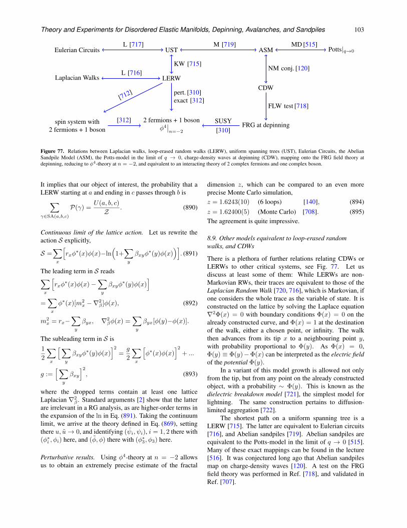
Theory and Experiments for Disordered Elastic Manifolds, Depinning, Avalanches, and Sandpiles 103
Eulerian Circuits
LERWLaplacian Walks
UST ASM Potts|q→0
CDW
FRG at depinning2 fermions + 1 boson
φ4∣∣n=−2
spin system with2 fermions + 1 boson
SUSY[310]
[312]
[712]
KW [715]L [716]
L [717]
pert. [310]exact [312]
MD [515]
NM conj. [120]
FLW test [718]
M [719]
Figure 77. Relations between Laplacian walks, loop-erased random walks (LERW), uniform spanning trees (UST), Eulerian Circuits, the AbelianSandpile Model (ASM), the Potts-model in the limit of q → 0, charge-density waves at depinning (CDW), mapping onto the FRG field theory atdepinning, reducing to φ4-theory at n = −2, and equivalent to an interacting theory of 2 complex fermions and one complex boson.
It implies that our object of interest, the probability that aLERW starting at a and ending in c passes through b is∑
γ∈SA(a,b,c)
P(γ) =U(a, b, c)
Z . (890)
Continuous limit of the lattice action. Let us rewrite theaction S explicitly,
S =∑
x
[rxφ∗(x)φ(x)−ln
(1+∑
y
βxyφ∗(y)φ(x)
)]. (891)
The leading term in S reads∑
x
[rxφ∗(x)φ(x)−
∑
y
βxyφ∗(y)φ(x)
]
=∑
x
φ∗(x)[m2x −∇2
β ]φ(x), (892)
m2x = rx−
∑
y
βyx, ∇2βφ(x) =
∑
y
βyx[φ(y)−φ(x)].
The subleading term in S is1
2
∑
x
[∑
y
βxyφ∗(y)φ(x)
]2=g
2
∑
x
[φ∗(x)φ(x)
]2+ ...
g :=[∑
y
βxy
]2, (893)
where the dropped terms contain at least one latticeLaplacian ∇2
β . Standard arguments [2] show that the latterare irrelevant in a RG analysis, as are higher-order terms inthe expansion of the ln in Eq. (891). Taking the continuumlimit, we arrive at the theory defined in Eq. (869), settingthere u, u→ 0, and identifying (ψi, ψi), i = 1, 2 there with(φ∗i , φi) here, and (φ, φ) there with (φ∗3, φ3) here.
Perturbative results. Using φ4-theory at n = −2 allowsus to obtain an extremely precise estimate of the fractal
dimension z, which can be compared to an even moreprecise Monte Carlo simulation,z = 1.6243(10) (6 loops) [140], (894)z = 1.62400(5) (Monte Carlo) [708]. (895)The agreement is quite impressive.
8.9. Other models equivalent to loop-erased randomwalks, and CDWs
There is a plethora of further relations relating CDWs orLERWs to other critical systems, see Fig. 77. Let usdiscuss at least some of them: While LERWs are non-Markovian RWs, their traces are equivalent to those of theLaplacian Random Walk [720, 716], which is Markovian, ifone considers the whole trace as the variable of state. It isconstructed on the lattice by solving the Laplace equation∇2Φ(x) = 0 with boundary conditions Φ(x) = 0 on thealready constructed curve, and Φ(x) = 1 at the destinationof the walk, either a chosen point, or infinity. The walkthen advances from its tip x to a neighbouring point y,with probability proportional to Φ(y). As Φ(x) = 0,Φ(y) ≡ Φ(y)−Φ(x) can be interpreted as the electric fieldof the potential Φ(y).
In a variant of this model growth is allowed not onlyfrom the tip, but from any point on the already constructedobject, with a probability ∼ Φ(y). This is known as thedielectric breakdown model [721], the simplest model forlightning. The same construction pertains to diffusion-limited aggregation [722].
The shortest path on a uniform spanning tree is aLERW [715]. The latter are equivalent to Eulerian circuits[716], and Abelian sandpiles [719]. Abelian sandpiles areequivalent to the Potts-model in the limit of q → 0 [515].Many of these exact mappings can be found in the lecture[516]. It was conjectured long ago that Abelian sandpilesmap on charge-density waves [120]. A test on the FRGfield theory was performed in Ref. [718], and validated inRef. [707].
Theory and Experiments for Disordered Elastic Manifolds, Depinning, Avalanches, and Sandpiles 104
It would be interesting to generalize loops to higher-dimensional surfaces, as was done for self-avoidingmanifolds in Refs. [723, 724].
8.10. Conformal field theory for critical curves
In d = 2, all critical exponents should be accessiblevia conformal field theory (CFT). The latter is basedon ideas proposed in the 80s by Belavin, Polyakov andZamolodchikov [725]. They constructed a series ofminimal models, indexed by an integerm ≥ 3, starting withthe Ising model at m = 3. These models are conformallyinvariant and unitary, equivalent to reflection positive inEuklidean theories. For details, see one of the manyexcellent textbooks on CFT [237, 234, 726, 238]. Theirconformal charge48 is given by
c = 1− 6
m(m+ 1). (896)
The list of conformal dimensions for allowed operators at agiven m is given by the Kac formula with integers r, s
hr,s =[r(m+ 1)− sm]2 − 1
4m(m+ 1), 1 ≤ r < m, 1 ≤ s ≤ m.
(897)
It was later realized that other values of m also correspondto physical systems, in particular m = 1 (loop-erasedrandom walks), and m = 2 (self-avoiding walks). Thesevalues can further be extended to non-integer n and m,using the identification
n = 2 cos( πm
). (898)
More strikingly, the table of dimensions allowed by Eq.(897) has to be extended to half-integer values, including0. This yields: the fractal dimension of the propagator line[727, 728, 729]
df = 2− 2h1,0 = 1 +π
2(arccos
(n2
)+ π
) . (899)
ν, i.e. the inverse fractal dimension of all lines, be itpropagator or loops ([729], inline after Eq. (2))
ν =1
2− 2h1,3=
1
4
(1 +
π
arccos(n2 )
). (900)
For η, there are two suggestive candidates from the Isingmodel, η = 4h1,2 = 4h2,2, which do not work for othervalues of n; instead [727, 728, 729]
η = 4h 12 ,0
=5
4− 3 arccos
(n2
)
4π− π
arccos(n2
)+ π
. (901)
It has a square-root singularity both for n = −2 and n = 2.There is no clear candidate for the exponent ω [140]. The48The conformal charge is the coefficient in the leading term of the OPEof the stress-energy tensor. It also gives the amplitude of finite-sizecorrections [3].
crossover exponent φc [1, 730, 140] (explained in [140],page 7) becomes
φc = νdf =1− h1,0
1− h1,3=
1
4+
3π
8 arccos(n2 ). (902)
To conclude, we remark that ideas identifying symplecticfermions with the ASM [731] are overly simplistic, as theydo not catch any of the above exponents.
9. Further developments and ideas
9.1. Non-perturbative RG (NPRG)
The renormalization transformation originally proposed byK. Wilson [117] consists in integrating out a specific rangeof fast modes, and following the effective action of theremaining modes under this transformation. While thisprocedure is exact by construction, its implementation isinfeasible, and one has to rely on approximation schemes.Several such schemes have been proposed:
(i) expansion in ε = 4 − d [111]. This scheme producesa divergent, albeit Borel-resummable series in ε, withhigh predictive power [2, 732, 733, 140].
(ii) expansion in the number of components N [734, 2].This works in general well forN ' 5, but gives mostlyqualitative information at N = 1.
(iii) the non-perturbative RG approach (NPRG). Thistechnique can be formulated for the free energyF(J) = lnZ(J) [735], or the effective action Γ[φ][736]. For the effective action it has the structure
∂`Γ[φ] =1
2tr
[(δ2Γ[φ]
δφ2+R`
)−1
∂`R`
]. (903)
The function Rl is a momentum cutoff function,optimized for convergence. The simplest truncation ofEq. (903) is the local potential approximation (LPA),sometimes followed by a gradient expansion (GE).(For historical work and a recent review see [737, 738,735, 736, 739, 740, 741]).
The FRG technique used in this review is perturbative inε = 4−d; keeping the exact field dependence is crucial. TheNPRG is an approximation (truncation) in the momentumdependence. Based on a numeric integration of the flowequations, keeping only the leading orders in the field isoften sufficient and accelerates the implementation. Thenon-perturbative FRG (NPFRG) (used for the RF Isingmodel in section 9.2) is approximate in the momentum,but aims at keeping the full field dependence as doesperturbative FRG. One sometimes encounters the termexact RG instead of NPRG, a notion better reservedfor the concept of RG than any of its approximateimplementations. The Heidelberg school [736] now usesFRG instead of NPRG, a notion we reserve to situationswhen the exact functional form is required.
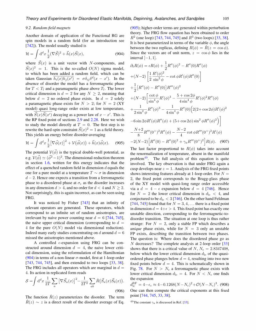
Theory and Experiments for Disordered Elastic Manifolds, Depinning, Avalanches, and Sandpiles 105
9.2. Random-field magnets
Another domain of application of the Functional RG arespin models in a random field (for an introduction see[742]). The model usually studied is
H =
∫ddx
1
2(∇~S)2 + ~h(x)~S(x), (904)
where ~S(x) is a unit vector with N -components, and~S(x)2 = 1. This is the so-called O(N) sigma model,to which has been added a random field, which can betaken Gaussian hi(x)hj(x′) = σδijδ
d(x − x′). In theabsence of disorder the model has a ferromagnetic phasefor T < Tf and a paramagnetic phase above Tf . The lowercritical dimension is d = 2 for any N ≥ 2, meaning thatbelow d = 2 no ordered phase exists. In d = 2 solelya paramagnetic phase exists for N > 2; for N = 2 (XYmodel) quasi long-range order exists at low temperature,with ~S(x)~S(x′) decaying as a power law of x− x′. This isthe RP fixed point of sections 2.9 and 2.28. Here we wishto study the model directly at T = 0. The first step is torewrite the hard-spin constraint ~S(x)2 = 1 as a field theory.This yields an energy before disorder-averaging
H =
∫ddx
1
2
[∇~φ(x)
]2+ V
(~φ(x)
)+ ~h(x)~φ(x). (905)
The potential V(~φ) is the typical double-well potential, ase.g. V(~φ) ' (~φ2−1)2. The dimensional-reduction theoremin section 1.6, written for this energy indicates that theeffect of a quenched random field in dimension d equals theone for a pure model at a temperature T ∼ σ in dimensiond− 2. Hence one expects a transition from a ferromagneticphase to a disordered phase at σc as the disorder increasesin any dimension d > 4, and no order for d < 4 andN ≥ 2.Not surprisingly, this is again incorrect, as can be seen usingFRG.
It was noticed by Fisher [743] that an infinity ofrelevant operators are generated. These operators, whichcorrespond to an infinite set of random anisotropies, areirrelevant by naive power counting near d = 6 [744, 745],the naive upper critical dimension (corresponding to d =4 for the pure O(N) model via dimensional reduction).Indeed many early studies concentrating on d around d = 6missed the anisotropies mentioned above.
A controlled ε-expansion using FRG can be con-structed around dimension d = 4, the naive lower criti-cal dimension, using the reformulation of the Hamiltonian(904) in terms of a non-linear σ-model, first at 1-loop order[743, 744, 745], and then extended to two loops [33, 38].The FRG includes all operators which are marginal in d =4. Its action in replicated form reads
S =
∫ddx
1
2T
∑
a
[∇~Sa(x)
]2− 1
2T 2
∑
ab
R(~Sa(x)~Sb(x)
).
(906)The function R(z) parameterizes the disorder. The termR(z) ∼ z is a direct result of the disorder average of Eq.
(905); higher-order terms are generated within perturbationtheory. The FRG flow equation has been obtained to orderR2 (one loop) [743, 744, 745] and R3 (two loops) [33, 38].It is best parameterized in terms of the variable φ, the anglebetween the two replicas, defining R(φ) = R(z = cosφ).Since the vectors are of unit norm, z = cosφ lies in theinterval [−1, 1].
∂`R(φ) = εR(φ) +1
2R′′(φ)2 −R′′(0)R′′(φ)
+(N−2)
[1
2
R′(φ)2
sin2 φ− cotφR′(φ)R′′(0)
]
+1
2
[R′′(φ)−R′′(0)
]R′′′(φ)2
+(N−2)
[cotφ
sin4 φR′(φ)3 − 5 + cos 2φ
4 sin4 φR′(φ)2R′′(φ)
+1
2 sin2 φR′′(φ)3 − 1
4 sin4 φR′′(0)
(2(2+ cos 2φ)R′(φ)2
−6 sin 2φR′(φ)R′′(φ) + (5+ cos 2φ) sin2 φR′′(φ)2)]
−N+2
8R′′′(0+)2R′′(φ)− N−2
4cotφR′′′(0+)2R′(φ)
−2(N−2)[R′′(0)−R′′(0)2 + γaR
′′′(0+)2]R(φ). (907)
The last factor proportional to R(φ) takes into accountthe renormalization of temperature, absent in the manifoldproblem49. The full analysis of this equation is quiteinvolved. The key observation is that under FRG again acusp develops near z = 1. Analysis of the FRG fixed pointsshows interesting features already at 1-loop order. For N =2, the fixed point corresponds to the Bragg-glass phaseof the XY model with quasi-long range order accessiblevia a d = 4 − ε expansion below d = 4 [746]. Hencefor N = 2 the lower critical dimension is dlc < 4, andconjectured to be dlc < 3 [746]. On the other hand Feldman[744, 745] found that for N = 3, 4, . . . there is a fixed pointin dimension d = 4+ε > 4. This fixed point has exactly oneunstable direction, corresponding to the ferromagnetic-to-disorder transition. The situation at one loop is thus ratherstrange: For N = 2, only a stable FP which describes aunique phase exists, while for N = 3 only an unstableFP exists, describing the transition between two phases.The question is: Where does the disordered phase go asN decreases? The complete analysis at 2-loop order [33]shows that there is a critical value of N , Nc = 2.8347408,below which the lower critical dimension dlc of the quasi-ordered phase plunges below d = 4, resulting into two newfixed points below d = 4. This is schematically shown inFig. 78. For N > Nc a ferromagnetic phase exists withlower critical dimension dlc = 4. For N < Nc one findsthe expansiondRF
lc = 4−εc ≈ 4−0.1268(N−Nc)2+O(N−Nc)3. (908)One can then compute the critical exponents at this fixedpoint [744, 745, 33, 38].49The constant γa is discussed in Ref. [33].
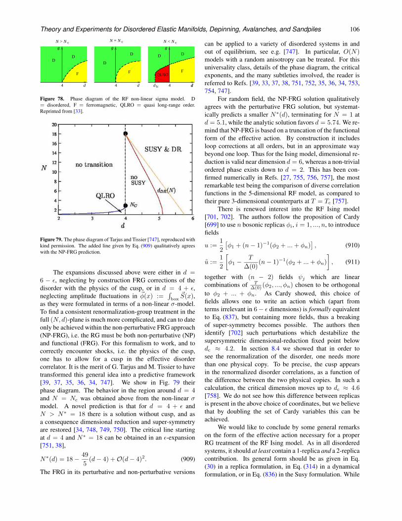
Theory and Experiments for Disordered Elastic Manifolds, Depinning, Avalanches, and Sandpiles 106
N = N cN > N c N < N c
dd dd 444 d lc
F F F
DD
D
D D D
QLRO
ggg
Figure 78. Phase diagram of the RF non-linear sigma model. D= disordered, F = ferromagnetic, QLRO = quasi long-range order.Reprinted from [33].
Figure 79. The phase diagram of Tarjus and Tissier [747], reproduced withkind permission. The added line given by Eq. (909) qualitatively agreeswith the NP-FRG prediction.
The expansions discussed above were either in d =6 − ε, neglecting by construction FRG corrections of thedisorder with the physics of the cusp, or in d = 4 + ε,neglecting amplitude fluctuations in ~φ(x) :=
∫box
~S(x),as they were formulated in terms of a non-linear σ-model.To find a consistent renormalization-group treatment in thefull (N, d)-plane is much more complicated, and can to dateonly be achieved within the non-perturbative FRG approach(NP-FRG), i.e. the RG must be both non-perturbative (NP)and functional (FRG). For this formalism to work, and tocorrectly encounter shocks, i.e. the physics of the cusp,one has to allow for a cusp in the effective disordercorrelator. It is the merit of G. Tarjus and M. Tissier to havetransformed this general idea into a predictive framework[39, 37, 35, 36, 34, 747]. We show in Fig. 79 theirphase diagram. The behavior in the region around d = 4and N = Nc was obtained above from the non-linear σmodel. A novel prediction is that for d = 4 + ε andN > N∗ = 18 there is a solution without cusp, and asa consequence dimensional reduction and super-symmetryare restored [34, 748, 749, 750]. The critical line startingat d = 4 and N∗ = 18 can be obtained in an ε-expansion[751, 38],
N∗(d) = 18− 49
5(d− 4) +O(d− 4)2. (909)
The FRG in its perturbative and non-perturbative versions
can be applied to a variety of disordered systems in andout of equilibrium, see e.g. [747]. In particular, O(N)models with a random anisotropy can be treated. For thisuniversality class, details of the phase diagram, the criticalexponents, and the many subtleties involved, the reader isreferred to Refs. [39, 33, 37, 38, 751, 752, 35, 36, 34, 753,754, 747].
For random field, the NP-FRG solution qualitativelyagrees with the perturbative FRG solution, but systemat-ically predicts a smaller N∗(d), terminating for N = 1 atd = 5.1, while the analytic solution favors d = 5.74. We re-mind that NP-FRG is based on a truncation of the functionalform of the effective action. By construction it includesloop corrections at all orders, but in an approximate waybeyond one loop. Thus for the Ising model, dimensional re-duction is valid near dimension d = 6, whereas a non-trivialordered phase exists down to d = 2. This has been con-firmed numerically in Refs. [27, 755, 756, 757], the mostremarkable test being the comparison of diverse correlationfunctions in the 5-dimensional RF model, as compared totheir pure 3-dimensional counterparts at T = Tc [757].
There is renewed interest into the RF Ising model[701, 702]. The authors follow the proposition of Cardy[699] to use n bosonic replicas φi, i = 1, ..., n, to introducefields
u :=1
2
[φ1 + (n− 1)−1(φ2 + ...+ φn)
], (910)
u :=1
2
[φ1 −
T
∆(0)(n− 1)−1(φ2 + ...+ φn)
], (911)
together with (n − 2) fields ψj which are linearcombinations of T
∆(0) (φ2, ..., φn) chosen to be orthogonalto φ2 + ... + φn. As Cardy showed, this choice offields allows one to write an action which (apart fromterms irrelevant in 6− ε dimensions) is formally equivalentto Eq. (837), but containing more fields, thus a breakingof super-symmetry becomes possible. The authors thenidentify [702] such perturbations which destabilize thesupersymmetric dimensional-reduction fixed point belowdc ≈ 4.2. In section 8.4 we showed that in order tosee the renormalization of the disorder, one needs morethan one physical copy. To be precise, the cusp appearsin the renormalized disorder correlations, as a function ofthe difference between the two physical copies. In such acalculation, the critical dimension moves up to dc ≈ 4.6[758]. We do not see how this difference between replicasis present in the above choice of coordinates, but we believethat by doubling the set of Cardy variables this can beachieved.
We would like to conclude by some general remarkson the form of the effective action necessary for a properRG treatment of the RF Ising model. As in all disorderedsystems, it should at least contain a 1-replica and a 2-replicacontribution. Its general form should be as given in Eq.(30) in a replica formulation, in Eq. (314) in a dynamicalformulation, or in Eq. (836) in the Susy formulation. While
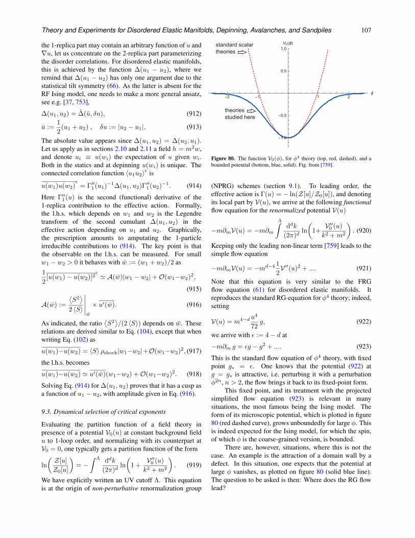
Theory and Experiments for Disordered Elastic Manifolds, Depinning, Avalanches, and Sandpiles 107
the 1-replica part may contain an arbitrary function of u and∇u, let us concentrate on the 2-replica part parameterizingthe disorder correlations. For disordered elastic manifolds,this is achieved by the function ∆(u1 − u2), where weremind that ∆(u1 − u2) has only one argument due to thestatistical tilt symmetry (66). As the latter is absent for theRF Ising model, one needs to make a more general ansatz,see e.g. [37, 753],
∆(u1, u2) = ∆(u, δu), (912)
u :=1
2(u1 + u2) , δu := |u2 − u1|. (913)
The absolute value appears since ∆(u1, u2) = ∆(u2, u1).Let us apply as in sections 2.10 and 2.11 a field h = m2w,and denote ui ≡ u(wi) the expectation of u given wi.Both in the statics and at depinning u(wi) is unique. Theconnected correlation function 〈u1u2〉c is
u(w1)u(w2)c
= Γ′′1(u1)−1∆(u1, u2)Γ′′1(u2)−1. (914)
Here Γ′′1(u) is the second (functional) derivative of the1-replica contribution to the effective action. Formally,the l.h.s. which depends on w1 and w2 is the Legendretransform of the second cumulant ∆(u1, u2) in theeffective action depending on u1 and u2. Graphically,the prescription amounts to amputating the 1-particleirreducible contributions to (914). The key point is thatthe observable on the l.h.s. can be measured. For smallw1 − w2 > 0 it behaves with w := (w1 + w2)/2 as1
2[u(w1)− u(w2)]2
c ' A(w)|w1 − w2|+O(w1−w2)2,
(915)
A(w) :=
⟨S2⟩
2 〈S〉
∣∣∣∣∣w
× u′(w). (916)
As indicated, the ratio⟨S2⟩/(2 〈S〉) depends on w. These
relations are derived similar to Eq. (104), except that whenwriting Eq. (102) as
u(w1)−u(w2) = 〈S〉 ρshock|w1−w2|+O(w1−w2)2, (917)
the l.h.s. becomes
u(w1)−u(w2) ' u′(w)(w1−w2) +O(w1−w2)2. (918)
Solving Eq. (914) for ∆(u1, u2) proves that it has a cusp asa function of u1 − u2, with amplitude given in Eq. (916).
9.3. Dynamical selection of critical exponents
Evaluating the partition function of a field theory inpresence of a potential V0(u) at constant background fieldu to 1-loop order, and normalizing with its counterpart atV0 = 0, one typically gets a partition function of the form
ln
( Z[u]
Z0[u]
)= −
∫ Λ ddk
(2π)dln
(1 +
V ′′0 (u)
k2 +m2
). (919)
We have explicitly written an UV cutoff Λ. This equationis at the origin of non-perturbative renormalization group
Figure 80. The function V0(φ), for φ4 theory (top, red, dashed), and abounded potential (bottom, blue, solid). Fig. from [759].
(NPRG) schemes (section 9.1). To leading order, theeffective action is Γ(u) = − ln(Z[u]/Z0[u]), and denotingits local part by V(u), we arrive at the following functionalflow equation for the renormalized potential V(u)
−m∂mV(u) = −m∂mΛ∫
ddk
(2π)dln
(1+V ′′0 (u)
k2 +m2
). (920)
Keeping only the leading non-linear term [759] leads to thesimple flow equation
−m∂mV(u) = −md−4 1
2V ′′(u)2 + .... (921)
Note that this equation is very similar to the FRGflow equation (61) for disordered elastic manifolds. Itreproduces the standard RG-equation for φ4 theory; indeed,setting
V(u) = m4−du4
72g, (922)
we arrive with ε := 4− d at
−m∂m g = εg − g2 + .... (923)
This is the standard flow equation of φ4 theory, with fixedpoint g∗ = ε. One knows that the potential (922) atg = g∗ is attractive, i.e. perturbing it with a perturbationφ2n, n > 2, the flow brings it back to its fixed-point form.
This fixed point, and its treatment with the projectedsimplified flow equation (923) is relevant in manysituations, the most famous being the Ising model. Theform of its microscopic potential, which is plotted in figure80 (red dashed curve), grows unboundedly for large φ. Thisis indeed expected for the Ising model, for which the spin,of which φ is the coarse-grained version, is bounded.
There are, however, situations, where this is not thecase. An example is the attraction of a domain wall by adefect. In this situation, one expects that the potential atlarge φ vanishes, as plotted on figure 80 (solid blue line).The question to be asked is then: Where does the RG flowlead?
Theory and Experiments for Disordered Elastic Manifolds, Depinning, Avalanches, and Sandpiles 108
As one sees from figure 80, the bounded potential V0
is negative. In order to deal with positive quantities, setV(u) ≡ −R(u). The flow equation to be studied is
−m∂mR(u) = m−ε1
2R′′(u)2 + .... (924)
As shown in [759], for generic smooth initial conditions asplotted on figure 80:
(i) The flow equation (924) develops a cusp at u = 0, anda cubic singularity at u = uc > 0.
(ii) The rescaled flow equation for the dimensionlessfunction R(u)
−m∂mR(u) = (ε− 4ζ)R(u) + ζuR′(u)
+1
2R′′(u)2 + .... (925)
has an infinity of fixed points −m∂mR(u) = 0,indexed by ζ ∈ [ ε4 ,∞].
(iii) The solution chosen dynamically when starting fromsmooth initial conditions is ζ = ε
3 . Its analyticexpression for 0 ≤ u ≤ 1 reads
Rζ= ε3(u) = ε
[1
18(1− u)3 − 1
72(1− u)4
]. (926)
It vanishes for u > 1, and is continued symmetricallyto u < 0.
This scenario is quite unusual: Normally, the perturbativelyaccessible fixed points of the RG flow have only one fixedpoint. In the few cases where there is more than onefixed point, the spectrum of fixed points is at least discrete.In contrast, here is a spectrum of fixed points. On theother hand, only one of them seems to be chosen. Thusexperiments would only see this one fixed point.
It is yet not clear to which physical system it applies.As discussed in the literature [760, 761, 762, 763, 764, 765],experiments describing wetting are usually attributed to aflow equation linear in R(u). Is a nonlinear fixed pointpossible? Let me cite Thierry Giamarchi, one of thepioneers of FRG: “Whenever there is a simple equation, itis somewhere realized in nature.”
9.4. Conclusion and perspectives
The aim of this review was to give a thorough overviewover the physics of disordered elastic manifolds, with itsnumerous connections to systems as diverse as sandpilesand loop-erased random walks. We covered all theoreticaltools developed to date, including FRG, replicas, replica-symmetry breaking, MSR dynamics, and super-symmetry.We put emphasis on applications, giving experimentaliststhe necessary tools to verify the theoretical concepts, andgoing beyond critical exponents.
Our aim at completeness was seriously challenged bythe shear amount of publications on the subject, and weapologize for any omissions. Please let us know, and wewill try to remedy.
While the presented methods are powerful, fundamen-tal questions remain: Can FRG be applied to other sys-tems such as spin glasses, sheared colloids, real glasses, orNavier-Stokes turbulence? Can FRG be applied beyond theelastic limit, i.e. to systems with overhangs or topologicaldefects, or to fractal curves that can not be represented bydirected interfaces?
The author is looking forward to exciting newdiscoveries, and the contributions of today’s PhD studentsand postdocs. As for this review, it needs to stop here.
Acknowledgments
It is a pleasure to thank all my collaborators over thepast years: Pierre Le Doussal for introducing me to thesubject and all his enthusiasm in the many projects weundertook together. A. Rosso, A. Kolton, L. Laurson,and A. Middleton for putting the theoretical concepts totest. M. Muller for all his insights in the connection toreplica-symmetry breaking. Many thanks go to my studentsM. Delorme, A. Dobrinevski, C. ter Burg, G. Mukerjee,T. Thierry, Z. Zhu, and postdocs C. Husemann, A.Petkovic, Z. Ristivojevic and A. Shapira, for their helpand pertinent questions. I am grateful to A.A. Fedorenkofor the many enjoyable common projects. S. Atis,F. Bohn, M. Correa, A. Douin, A.K. Dubey, G. Durin,F. Lechenault, S. Moulinet, M.R. Pasto, F. Ritort, P.Rissone, E. Rolley, D. Salin, R. Sommer, and L. Talonwere essential in testing the concepts in experiments.I have benefitted from collaborations with L. Aragon,C. Bachas, P. Chauve, R. Golestanian, E. Jagla, M. Kardar,M. Kompaniets, W. Krauth, A. Ludwig, C. Marchetti,A. Perret, E. Raphael, G. Schehr and J. Vannimenus.Many thanks for discussions go to M. Alava, C. Aron,E. Brezin, L. Balents, E. Bouchaud, J.P. Bouchaud,J. Cardy, F. David, H.W. Diehl, T. Giamarchi, P. Goldbart,D. Gross, F. Haake, A. Hartmann, J. Jacobsen, J. Krug,S. Majumdar, M. Mezard, T. Nattermann, G. Parisi,H. Rieger, L. Ponson, S. Rychkov, S. Santucci, L. Schafer,S. Stepanov, L. Sutterlin, G. Tarjus, M. Tissier, F. Wegner,J. Zinn-Justin and A. Zippelius. This review is based onlecture notes for the ICTP master program at ENS, and Ithank all students for their feedback.
10. Appendix: Basic Tools
10.1. Markov chains, Langevin equation, inertia
In Markov chains the state at time tN := Nτ is given bythe product of transition probabilities
P(xN , xN−1, ..., x1, x0) =
N∏
i=1
Pτ (xi|xi−1). (927)
Transition probabilities are drawn from a Gaussian distri-bution. The probability to be at x (the variable) given x′
Theory and Experiments for Disordered Elastic Manifolds, Depinning, Avalanches, and Sandpiles 109
(prime as previous), reads
Pτ (x|x′) =1√
4πτD(x′)e− [η(x−x′)−τF (x′)]2
4ητD(x′) . (928)
Both F and D depend on the previous position (Itodiscretization). As a stochastic process, this reads
η(xi+1 − xi) = τF (xi) +√τξi, (929)
〈ξi〉 = 0, 〈ξiξj〉 = 2δijηD(xi) (930)
The formal limit of τ → 0 is the Ito-Langevin equation,
ηx(t) = F(x(t)
)+ ξ(t), (931)
〈ξ(t)〉 = 0, 〈ξ(t)ξ(t′)〉 = 2ηδ(t− t′)D(x(t)
). (932)
The factor of η is the friction coefficient in Newton’sequation of motion. Indeed, for the problem at hand thelatter reads
M∂tx(t) = F(x(t)
)+ ξ(t)− ηx(t). (933)
On the l.h.s. is the mass M (or inertia) of the particle (notto be confounded with the mass m in field theory), times itsacceleration. This defines a characteristic time scale
τM =M
η. (934)
For times t τM , inertia plays no role, M can be set to 0,and we arrive at Eq. (931).
The situation is different, when the noise is correlatedon a time scale τ τM . Then in the equation of motionF (x(t)) changes, since x(t) changes, and it is better todiscretize this limit as
η(xi+1 − xi) = τF
(xi + xi+1
2
)+√τξi. (935)
This prescription is known as mid-point or Stratonovichdiscretization.
Let us finally rescale time, t → ηt, which effectivelysets η → 1. The friction coefficient η can always be restoredby multiplying each time derivative with η.
10.2. Ito calculus
Consider (with η = 1)
g(xi+1)− g(xi) = g(xi + τF (xi) +
√τξi)− g(xi)
= g′(xi)[τF (xi) +
√τξi]
+1
2g′′(xi)τξ
2i +O(τ3/2)
= g′(xi)[τF (xi) +
√τξi]
+ g′′(xi)τD(xi) +O(τ3/2).
(936)
The last relation is justified since in any time slicemaximally two powers of ξi can appear. (If there could be4 then one would have to use Wick’s theorem to decouplethem pairwise.) It is implicitly understood that the noiseis independent of x, thus 〈g(xi)ξi〉 = 0, and
⟨g(xi)ξ
2i
⟩=
2g(xi)D(xi)dt.
Mathematicians prefer setting xi → x, τ → dt,ξi√τ → dξ, and write the Langevin equation as
dx = F (x)dt+ dξ, (937)〈dξ〉 = 0, dξ2 =
⟨dξ2⟩
= 2D(x)dt. (938)
The stochastic evolution of a function g(x) can then bewritten with these “differentials” as
dg(x) = g′(x)dx+1
2g′′(x)dx2 + ...
= g′(x)[F (x)dt+ dξ] +1
2g′′(x)[F (x)dt+ dξ]2 + ...
= [g′(x)F (x) + g′′(x)D(x)] dt+ g′(x)dξ (939)
This is known as Ito calculus. The rule of thumb toremember is that when expanding to first order in the timedifferential dt, as dξ ∼
√dt, one has to keep all terms up
to second order in dξ.
10.3. Fokker-Planck equation
Derivation of (forward) Fokker-Planck equation using Ito’sformalism: The forward Fokker-Planck equation can bederived from Ito’s formalism. Consider the expectation of atest function g(x) at time t:
〈g(xt)〉 ≡∫
x
g(x)Pt(x). (940)
Taking the expectation of the first line of Eq. (939) yields
〈dg(xt)〉 = 〈g′(xt)dx〉+1
2
⟨g′′(xt)dx
2⟩
+ ... (941)
Averaging over the noise gives
d
dt〈g(xt)〉 = 〈g′(xt)F (xt)〉+ 〈g′′(xt)D(xt)〉 . (942)
Expressing the expectation values with the help of Eq.(940), we obtain∫
x
g(x)∂tPt(x)
=
∫
x
g′(x)F (x)Pt(x) + g′′(x)D(x)Pt(x). (943)
Integrating by part, and using that g(x) is an arbitrary testfunction, we obtain the forward Fokker-Planck equation
∂tPt(x) =∂2
∂x2
(D(x)Pt(x)
)− ∂
∂x
(F (x)Pt(x)
). (944)
Our derivation is valid for any initial condition, thus thepropagator P (xf , tf |xi, ti) also satisfies the forward FokkerPlanck-equation as a function of x = xf , t = tf .
If there are several degrees of freedom xu, u =1, ..., L, then Eq. (944) generalizes to an equation for thejoint probability Pt[x] ≡ Pt(x1, x2, ..., xL)
∂tPt[x] =
L∑
u=1
∂2
∂x2u
(Du[x]Pt[x]
)− ∂
∂xu
(Fu[x]Pt[x]
).
(945)
Theory and Experiments for Disordered Elastic Manifolds, Depinning, Avalanches, and Sandpiles 110
Passing to the continuum limit, this yields the functionalFokker-Planck equation
∂tPt[x] (946)
=
∫du
δ2
δx(u)2
(Du[x]Pt[x]
)− δ
δx(u)
(Fu[x]Pt[x]
).
The backward Fokker-Planck equation: Let us studyP (xf , tf |xi, ti) as a function of its initial time and position.To this purpose, write down the exact equation, using thenotations of Eq. (937),
P (xf , tf |x, t) = 〈P (xf , tf |x+ dx, t+ dt)〉 . (947)
The average is over all realizations of the noise η duringa time step dt. Expanding inside the expectation value tofirst order in dt and second order in dx, and taking theexpectation, we find
〈P (xf , tf |x+ dx, t+ dt)〉=⟨P (xf , tf |x, t) + dt ∂tP (xf , tf |x, t)
+ dx ∂xP (xf , tf |x, t) +dx2
2∂2xP (xf , tf |x, t)
⟩
= P (xf , tf |x, t) + dt[∂tP (xf , tf |x, t)
+ F (x) ∂xP (xf , tf |x, t) +D(x)∂2xP (xf , tf |x, t)
].
(948)
Comparing to Eq. (947) implies that the term of order dtvanishes, thus
−∂tP (xf , tf |x, t)
= F (x)∂
∂xP (xf , tf |x, t) +D(x)
∂2
∂x2P (xf , tf |x, t). (949)
This is the backward Fokker-Planck equation. Note thatcontrary to the forward equation, all derivatives act onP (xf , tf |y, t), not on F or D.
Remark on Consistency: The form of the backward andforward equations is constraint by an important consistencyrelation: Using that the process is Markovian, we can writethe Chapman-Kolmogorov equation
P (xf , tf |xi, ti) =
∫
x
P (xf , tf |x, t)P (x, t|xi, ti). (950)
This relation must hold for all t between ti and tf . Taking at derivative and using the backward Fokker-Planck equationfor the first propagator P (xf , tf |x, t), and the forwardequation for the second P (x, t|xi, ti), we find cancelationof all tems upon partial integration in x, due to the specificarrangement of the derivatives in Eqs. (944) and (949).
Remark on Steady State: Let us find a steady-statesolution of Eq. (944), i.e. a solution which does not dependon time. Integrating once and dropping the time argumentyields∂
∂x
[D(x)P (x)
]= F (x)P (x) + const. (951)
Let us suppose that the probability P (x) vanishes whenx → ∞. This implies that the constant vanishes. Thesolution is obtained as (x0 is arbitrary)
P (x) =ND(x)
exp
(∫ x
x0
F (y)
D(y)dy
), (952)
N−1 =
∫ ∞
−∞dx
1
D(x)exp
(∫ x
x0
F (y)
D(y)dy
). (953)
The simplest case is obtained for thermal noise, i.e.D(x) =T , and when the force F (x) is the derivative of a potential,F (x) = −V ′(x). Eq. (952) can then be written as
P (x) = N e−V (x)/T , N−1 =
∫ ∞
−∞dx e−V (x)/T . (954)
This is Boltzmann’s law [766].
10.4. Martin-Siggia-Rose (MSR) formalism
The path integral: The transition probability (928) fromx′ to x was
Pτ (x|x′)dx =dx√
4πτD(x′)e− [x−x′−τF (x′)]2
4τD(x′) . (955)
This is ugly: our standard field-theory calculations workwith polynomials in the exponential. We therefore rewritethis measure as
Pτ (x|x′)dx = dx
∫ i∞
−i∞
dx
2πie−Sτ [x,x], (956)
Sτ [x, x] = x(x− x′ − τF (x′)
)− τ x2D(x′). (957)
The term Sτ [x, x] is termed action. Reassembling all timeslices, it is normally written in the limit of τ → 0 as
P(x|x0)dx =
∫ x(N)=x
x(0)=x0
D[x]D[x]e−S[x,x], (958)
S[x, x] =
∫
t
x(t)[x(t)−F
(x(t)
)]− x(t)2D
(x(t)
), (959)
D[x]D[x] =
N∏
i=1
∫ ∞
−∞dxi
∫ i∞
−i∞
dxi2πi
. (960)
This is known as the MSR formalism (Martin-Siggia-Rose)[295], the action also as Martin-Siggia-Rose-Janssen-DeDominicis action, in honor of their respective work[296, 298, 767, 297] .
Changing the discretization: Let us turn back to a singletime slice, as given in Eq. (956). The variables x and x areconjugate, i.e.∫
dx dx
2πie−x(x−x′)xnf(x, x)
=
∫dx dx
2πie−x(x−x′)∂nxf(x, x) , (961)
∫dx dx
2πie−x(x−x′)(x− x′)nf(x, x)
=
∫dx dx
2πie−x(x−x′)∂nxf(x, x). (962)
Theory and Experiments for Disordered Elastic Manifolds, Depinning, Avalanches, and Sandpiles 111
We can thus change our discretization scheme, i.e. replaceF (x′)→ F (x), D(x′)→ D(x), where
x = αx+ (1− α)x′ , 0 ≤ α ≤ 1. (963)
There are cases where this change is advantageous. On theother hand, the microscopic dynamics may be such that Fand D depend on x instead of x′ (see end of section 10.1).
The consequences of the reparametrization (963) isunderstood from the following example: Expand eτxF (x)−1 to linear order in τ ,
τ
∫dx dx
2πie−x(x−x′)xF (x)f(x, x)
= τ
∫dxdx
2πie−x(x−x′)∂x [F (x)f(x, x)] . (964)
As the derivative acts on F (x), this depends on α, as∂xx = α. Luckily, we can compensate this by an explicit xderivative: Wherever we change x → x, we also replace xby x− ∂x. This yields for the action of a single time slice
Sτ [x, x]
= x(x− x′)− τ(x− ∂x)F (x)− τ(x− ∂x)2D(x)
= ατF ′(x)− α2τD′′(x)
+ x[x− x′ − τF (x) + 2ατD′(x)
]− τ x2D(x). (965)
The noise-correlator D(x) did not change, but there is anadditional contribution to the force
F (x′)→ F (x)− 2αD′(x). (966)
The first two terms, αF ′(x)− α2D′′(x) can be interpretedas a change in the integration measure. Let us stress thatthe change in the action leaves the physics of the probleminvariant. One may arrive at α = 1
2 also when the bath isevolving more slowly than the time scale set by viscosity(see end of section 10.1). Then the choice α = 1/2, knownas Stratanovich discretization, is natural; one can use theabove procedure to get back to Ito’s discretization.
Interpretation of the field x(t): Let us now turn to aninterpretation of the two fields x(t) and x(t), and modifyequation (931) to
x(t) = F(x(t)
)+ ξ(t) + fδ(t− t0). (967)
Thus at time t = t0, we kick the system with an infinitelysmall force f . Then, the probability changes by
∂f
∣∣∣f=0P(x|x0)dx = ∂f
∣∣∣f=0
∫ x(t)=x
x(0)=x0
D[x]D[x] e−S[x,x]
=
∫ x(t)=x
x0=x(0)
D[x]D[x] x(t0)e−S[x,x] (968)
Multiplying with x(t) and integrating over all finalconfigurations, we obtain
R(t, t0) = ∂f
∣∣∣f=0〈x(t)〉 = 〈x(t)x(t0)〉 . (969)
The expectation is w.r.t the measure D[x]D[x] e−S[x,x]. AsEq. (969) is the response of the system to a change in force,
x is called response field, and R(t, t0) response function.Correlation functions are similarly obtained as
C(t, t′) = 〈x(t)x(t′)〉 . (970)
Since the probability is normalized,∫P(x|x0) dx = 1, (971)
for all forces, one shows by taking derivatives w.r.t. forcesat different times that expectations of the sole response fieldvanish,
〈x(t)〉 = 〈x(t)x(t′)〉 = 〈x(t)x(t′)x(t′′)〉 = ... = 0. (972)
10.5. Gaussian theory with spatial degrees of freedom
Consider theories with spatial dependence, and let ussuppose that the energy is given by
H[u] =
∫
x
1
2[∇u(x)]
2+m2
2u(x)2. (973)
This corresponds to an elastic manifold inside a confiningpotential of curvature m2. The elastic forces acting on apiece of the manifold at position x are given by
F (x) = −δH[u]
δu(x)=(∇2 −m2
)u(x). (974)
Its Langevin dynamics reads
∂tu(x, t) =(∇2 −m2
)u(x, t) + ξ(x, t), (975)
〈ξ(t)ξ(t′)〉 = 2Tδ(t− t′)δ(x− x′). (976)
The action in Ito discretization is
S[u, u] =
∫
x,t
u(x, t)[∂t−∇2+m2
]u(x, t)− T u(x, t)2.
(977)
It can be diagonalized in momentum and frequency space,
S[u, u] =
∫
k,ω
u(−k,−ω)[iω + k2 +m2
]u(k, ω)
− T u(−k,−ω)u(k, ω)
=1
2
∫
k,ω
(u(−k,−ω)
u(−k,−ω)
)M(u(k, ω)
u(k, ω)
), (978)
M =
(0 −iω + k2 +m2
iω + k2 +m2 −2T
). (979)
This implies
M−1 =
(2T
(iω+k2+m2)(−iω+k2+m2)1
iω+k2+m2
1−iω+k2+m2 0
). (980)
As a consequence,
R(k, ω) := 〈u(−k,−ω)u(k, ω)〉 =1
iω+k2+m2, (981)
C(k, ω) := 〈u(−k,−ω)u(k, ω)〉 =2T
|iω + k2 +m2|2 .
(982)
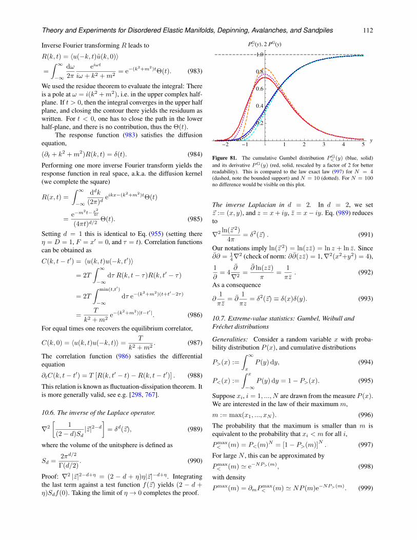
Theory and Experiments for Disordered Elastic Manifolds, Depinning, Avalanches, and Sandpiles 112
Inverse Fourier transforming R leads to
R(k, t) = 〈u(−k, t)u(k, 0)〉
=
∫ ∞
−∞
dω
2π
eiωt
iω + k2 +m2= e−(k2+m2)tΘ(t). (983)
We used the residue theorem to evaluate the integral: Thereis a pole at ω = i(k2 +m2), i.e. in the upper complex half-plane. If t > 0, then the integral converges in the upper halfplane, and closing the contour there yields the residuum aswritten. For t < 0, one has to close the path in the lowerhalf-plane, and there is no contribution, thus the Θ(t).
The response function (983) satisfies the diffusionequation,
(∂t + k2 +m2)R(k, t) = δ(t). (984)
Performing one more inverse Fourier transform yields theresponse function in real space, a.k.a. the diffusion kernel(we complete the square)
R(x, t) =
∫ ∞
−∞
ddk
(2π)deikx−(k2+m2)tΘ(t)
=e−m
2t− x24t
(4πt)d/2Θ(t). (985)
Setting d = 1 this is identical to Eq. (955) (setting thereη = D = 1, F = x′ = 0, and τ = t). Correlation functionscan be obtained as
C(k, t− t′) = 〈u(k, t)u(−k, t′)〉
= 2T
∫ ∞
−∞dτ R(k, t− τ)R(k, t′ − τ)
= 2T
∫ min(t,t′)
−∞dτ e−(k2+m2)(t+t′−2τ)
=T
k2 +m2e−(k2+m2)|t−t′|. (986)
For equal times one recovers the equilibrium correlator,
C(k, 0) = 〈u(k, t)u(−k, t)〉 =T
k2 +m2. (987)
The correlation function (986) satisfies the differentialequation
∂tC(k, t− t′) = T [R(k, t′ − t)−R(k, t− t′)] . (988)
This relation is known as fluctuation-dissipation theorem. Itis more generally valid, see e.g. [298, 767].
10.6. The inverse of the Laplace operator.
∇2
[1
(2− d)Sd|~z|2−d
]= δd(~z), (989)
where the volume of the unitsphere is defined as
Sd =2πd/2
Γ(d/2). (990)
Proof: ∇2 |~z|2−d+η = (2 − d + η)η|~z|−d+η . Integratingthe last term against a test function f(~z) yields (2 − d +η)Sdf(0). Taking the limit of η → 0 completes the proof.
- -
<
() ()
Figure 81. The cumulative Gumbel distribution PG< (y) (blue, solid)
and its derivative PG(y) (red, solid, rescaled by a factor of 2 for betterreadability). This is compared to the law exact law (997) for N = 4(dashed, note the bounded support) and N = 10 (dotted). For N = 100no difference would be visible on this plot.
The inverse Laplacian in d = 2. In d = 2, we set~z := (x, y), and z = x+ iy, z = x− iy. Eq. (989) reducesto
∇2 ln(~z 2)
4π= δ2(~z) . (991)
Our notations imply ln(~z 2) = ln(zz) = ln z + ln z. Since∂∂ = 1
4∇2 (check of norm: ∂∂(zz) = 1,∇2(x2+y2) = 4),
1
∂= 4
∂
∇2=∂ ln(zz)
π=
1
πz. (992)
As a consequence
∂1
πz= ∂
1
πz= δ2(~z) ≡ δ(x)δ(y). (993)
10.7. Extreme-value statistics: Gumbel, Weibull andFrechet distributions
Generalities: Consider a random variable x with proba-bility distribution P (x), and cumulative distributions
P>(x) :=
∫ ∞
x
P (y) dy, (994)
P<(x) :=
∫ x
−∞P (y) dy = 1− P>(x). (995)
Suppose xi, i = 1, ..., N are drawn from the measure P (x).We are interested in the law of their maximum m,
m := max(x1, ..., xN ). (996)
The probability that the maximum is smaller than m isequivalent to the probability that xi < m for all i,
Pmax< (m) = P<(m)N = [1− P>(m)]
N. (997)
For large N , this can be approximated by
Pmax< (m) ' e−NP>(m), (998)
with density
Pmax(m) = ∂mPmax< (m) ' NP (m)e−NP>(m). (999)
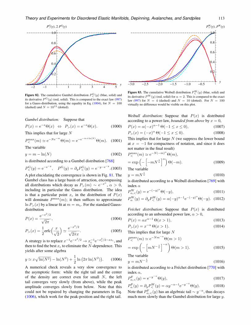
Theory and Experiments for Disordered Elastic Manifolds, Depinning, Avalanches, and Sandpiles 113
- -
<
() ()
Figure 82. The cumulative Gumbel distribution PG< (y) (blue, solid) and
its derivative PG(y) (red, solid). This is compared to the exact law (997)for a Gauss-distribution, using the equality in Eq. (1004), for N = 100(dashed) and N = 1013 (dotted).
Gumbel distribution: Suppose that
P (x) = e−xΘ(x) ⇔ P>(x) = e−xΘ(x). (1000)
This implies that for large N
Pmax< (m) ' e−Ne−mΘ(m) = e−e−m+ln(N)
Θ(m). (1001)
The variable
y = m− ln(N) (1002)
is distributed according to a Gumbel distribution [768]
PG< (y) = e−e−y , PG(y) = ∂yP
G< (y) = e−y−e−y .(1003)
A plot elucidating the convergence is shown in Fig. 81. TheGumbel class has a large basin of attraction, encompassingall distributions which decay as P>(m) ∼ e−x
α
, α > 0,including in particular the Gauss distribution. The ideais that a particular point xc in the distribution of P (x)will dominate Pmax(m); it then suffices to approximatelnP>(x) by a linear fit atm = mc. For the standard Gauss-distribution
P (x) =e−x
2/2
√2π
, (1004)
P>(x) =1
2erfc( x√
2
)' e−x
2/2
√2πx
. (1005)
A strategy is to replace x−1e−x2/2 → x−1
c e−x2c/2−xxc , and
then to find the best xc to eliminate theN -dependence. Thisyields after some algebra
y ' x√
ln(N2)− ln(N2) +1
2ln(2π ln(N2)
). (1006)
A numerical check reveals a very slow convergence tothe asymptotic form: while the right tail and the centerof the density are correct even for small N , the lefttail converges very slowly (from above), while the peakamplitude converges slowly from below. Note that thiscould not be repaired by changing the parameters in Eq.(1006), which work for the peak-position and the right tail.
- - - - - -
<
() ()
Figure 83. The cumulative Weibull distribution PW< (y) (blue, solid) and
its derivative PW(y) (red, solid) for α = 2. This is compared to the exactlaw (997) for N = 4 (dashed) and N = 10 (dotted). For N = 100virtually no difference would be visible on this plot.
Weibull distribution: Suppose that P (x) is distributedaccording to a power-law, bounded from above by x = 0,P (x) = α(−x)α−1 Θ(−1 ≤ x ≤ 0), (1007)P>(x) = (−x)α Θ(−1 ≤ x ≤ 0). (1008)This implies that for large N (we suppress the lower boundat x = −1 for compactness of notation, and since it doesnot matter in the final result)Pmax< (m) ' e−N(−m)αΘ(m),
= exp(−[−mN 1
α
]α)Θ(−m). (1009)
The variabley = mN
1α (1010)
is distributed according to a Weibull distribution [769] withindex αPWα,<(y) = e−(−y)αΘ(−y), (1011)
PWα (y) = ∂yP
W< (y) = α(−y)α−1e−(−y)αΘ(−y). (1012)
Frechet distribution: Suppose that P (x) is distributedaccording to an unbounded power law, α > 0,P (x) = αxα−1 Θ(x > 1), (1013)P>(x) = x−α Θ(x > 1). (1014)This implies that for large N
Pmax< (m) ' e−Nm
−αΘ(m > 1)
= exp
(−[mN−
1α
]−α)Θ(m > 1). (1015)
The variabley = mN−
1α (1016)
is distributed according to a Frechet distribution [770] withindex α,PFα,<(y) = e−y
−αΘ(y), (1017)
PFα (y) = ∂yP
W< (y) = αy−α−1e−y
−αΘ(y). (1018)
Note that PFα,<(y) has an algebraic tail ∼ y−α, thus decays
much more slowly than the Gumbel distribution for large y.
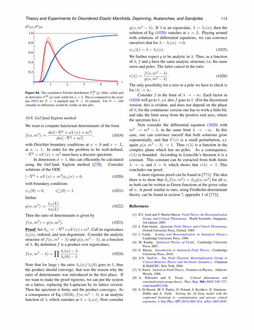
Theory and Experiments for Disordered Elastic Manifolds, Depinning, Avalanches, and Sandpiles 114
<() ()
Figure 84. The cumulative Frechet distribution PW< (y) (blue, solid) and
its derivative PW(y) (red, solid) for α = 2. This is compared to the exactlaw (997) for N = 4 (dashed) and N = 10 (dotted). For N = 100virtually no difference would be visible on this plot.
10.8. Gel’fand Yaglom method
We want to compute functional determinants of the form
f(α,m2) :=det[−∇2 + αV (x) +m2]
det[−∇2 +m2], (1019)
with Dirichlet boundary conditions at x = 0 and x = L,at α = 1. In order for the problem to be well-defined,−∇2 + αV (x) +m2 must have a discrete spectrum.
In dimension d = 1, this can efficiently be calculatedusing the Gel’fand Yaglom method [278]. Considersolutions of the ODE
[−∇2 + αV (x) +m2]ψα(x) = 0, (1020)
with boundary conditions
ψα(0) = 0, ψ′α(0) = 1. (1021)
Define
g(α,m2) :=ψα(L)
ψ0(L). (1022)
Then the ratio of determinants is given by
f(α,m2) = g(α,m2). (1023)
Proof: Set Λα := −∇2 +αV (x)+m2. Call its eigenvaluesλi(α), ordered, and non-degenerate. Consider the analyticstructure of f(α,m2 − λ) and g(α,m2 − λ), as a functionof λ. By definition f is a product over eigenvalues,
f(α,m2 − λ) =∏
i
λi(α)− λλi(0)− λ . (1024)
Note that for large i the ratio λi(α)/λi(0) goes to 1, thusthe product should converge; that was the reason why theratio of determinants was introduced in the first place. Ifwe want to make the proof rigorous, we can put the systemon a lattice, replacing the Laplacian by its lattice version.Then the spectrum is finite, and the product converges. Asa consequence of Eq. (1024), f(α,m2 − λ) is an analyticfunction of λ, which vanishes at λ = λi(α). Now consider
g(α,m2 − λ). If λ is an eigenvalue, λ = λi(α), then thesolution of Eq. (1020) vanishes at x = L. Playing aroundwith solutions of differential equations, we can convinceourselves that for λ− λi(α)→ 0,
ψα(L) ∼ λ− λi(α). (1025)
We further expect g to be analytic in λ. Thus, as a functionof λ, f and g have the same analytic structure, i.e. the samezeros and poles. The latter cancel in the ratio
r(λ) :=f(α,m2 − λ)
g(α,m2 − λ). (1026)
The only possibility for a zero or a pole we have to check isfor |λ| → ∞.
Consider f in the limit of λ → −∞: Each factor in(1024) will go to 1, s.t. also f goes to 1. (For the discretizedversion, this is evident, and does not depend on the phaseof λ; for the continuous version one has to work a little bit,and take the limit away from the positive real axes, wherethe spectrum lies.)
Now consider the differential equation (1020) withm2 → m2 − λ, in the same limit λ → −∞. In thiscase, one can convince oneself that both solutions growexponentially, and that V (x) is a small perturbation, s.t.again g(α,m2 − λ) → 1. Thus r(λ) is a function in thecomplex plane which has no poles. As a consequence,r(λ) is bounded. According to Liouville’s theorem it is aconstant. This constant can be extracted from both limitsλ → ∞ and λ = 0, which shows that r(λ) = 1. Thisconcludes our proof.
A more rigorous proof can be found in [771]: The ideathere is to show that ∂αf(α,m2) = ∂αg(α,m2) for all α,as both can be written as Green functions at the given valueof α. A proof similar to ours, using Fredholm-determinanttheory, can be found in section 7, appendix 1 of [772].
References
[1] D.J. Amit and V. Martin-Mayor, Field Theory, the RenormalizationGroup, and Critical Phenomena, World Scientific, Singapore,3rd edition, 2005.
[2] J. Zinn-Justin, Quantum Field Theory and Critical Phenomena,Oxford University Press, Oxford, 1989.
[3] J. Cardy, Scaling and Renormalization in Statistical Physics,Cambridge University Press, 1996.
[4] M. Kardar, Statistical Physics of Fields, Cambridge UniversityPress, 2007.
[5] E. Brezin, Introduction to Statistical Field Theory, CambridgeUniversity Press, 2010.
[6] A.N. Vasil’ev, The Field Theoretic Renormalization Group inCritical Behavior Theory and Stochastic Dynamics, Chapman& Hall/CRC, New York, 2004.
[7] G. Parisi, Statistical Field Theory, Frontiers in Physics, Addison-Wesely, 1988.
[8] A. Pelissetto and E. Vicari, Critical phenomena andrenormalization-group theory, Phys. Rep. 368 (2002) 549–727,cond-mat/0012164.
[9] S. El-Showk, M. F. Paulos, D. Poland, S. Rychkov, D. Simmons-Duffin and A. Vichi, Solving the 3d Ising model with theconformal bootstrap ii. c-minimization and precise criticalexponents, J. Stat. Phys. 157 (2014) 869–914, arXiv:1403.4545.
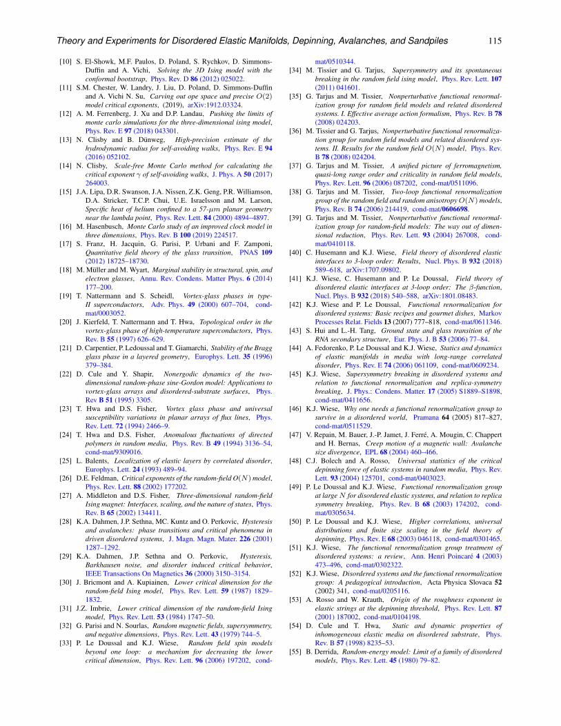
Theory and Experiments for Disordered Elastic Manifolds, Depinning, Avalanches, and Sandpiles 115
[10] S. El-Showk, M.F. Paulos, D. Poland, S. Rychkov, D. Simmons-Duffin and A. Vichi, Solving the 3D Ising model with theconformal bootstrap, Phys. Rev. D 86 (2012) 025022.
[11] S.M. Chester, W. Landry, J. Liu, D. Poland, D. Simmons-Duffinand A. Vichi N. Su, Carving out ope space and precise O(2)model critical exponents, (2019), arXiv:1912.03324.
[12] A. M. Ferrenberg, J. Xu and D.P. Landau, Pushing the limits ofmonte carlo simulations for the three-dimensional ising model,Phys. Rev. E 97 (2018) 043301.
[13] N. Clisby and B. Dunweg, High-precision estimate of thehydrodynamic radius for self-avoiding walks, Phys. Rev. E 94(2016) 052102.
[14] N. Clisby, Scale-free Monte Carlo method for calculating thecritical exponent γ of self-avoiding walks, J. Phys. A 50 (2017)264003.
[15] J.A. Lipa, D.R. Swanson, J.A. Nissen, Z.K. Geng, P.R. Williamson,D.A. Stricker, T.C.P. Chui, U.E. Israelsson and M. Larson,Specific heat of helium confined to a 57-µm planar geometrynear the lambda point, Phys. Rev. Lett. 84 (2000) 4894–4897.
[16] M. Hasenbusch, Monte Carlo study of an improved clock model inthree dimensions, Phys. Rev. B 100 (2019) 224517.
[17] S. Franz, H. Jacquin, G. Parisi, P. Urbani and F. Zamponi,Quantitative field theory of the glass transition, PNAS 109(2012) 18725–18730.
[18] M. Muller and M. Wyart, Marginal stability in structural, spin, andelectron glasses, Annu. Rev. Condens. Matter Phys. 6 (2014)177–200.
[19] T. Nattermann and S. Scheidl, Vortex-glass phases in type-II superconductors, Adv. Phys. 49 (2000) 607–704, cond-mat/0003052.
[20] J. Kierfeld, T. Nattermann and T. Hwa, Topological order in thevortex-glass phase of high-temperature superconductors, Phys.Rev. B 55 (1997) 626–629.
[21] D. Carpentier, P. Ledoussal and T. Giamarchi, Stability of the Braggglass phase in a layered geometry, Europhys. Lett. 35 (1996)379–384.
[22] D. Cule and Y. Shapir, Nonergodic dynamics of the two-dimensional random-phase sine-Gordon model: Applications tovortex-glass arrays and disordered-substrate surfaces, Phys.Rev B 51 (1995) 3305.
[23] T. Hwa and D.S. Fisher, Vortex glass phase and universalsusceptibility variations in planar arrays of flux lines, Phys.Rev. Lett. 72 (1994) 2466–9.
[24] T. Hwa and D.S. Fisher, Anomalous fluctuations of directedpolymers in random media, Phys. Rev. B 49 (1994) 3136–54,cond-mat/9309016.
[25] L. Balents, Localization of elastic layers by correlated disorder,Europhys. Lett. 24 (1993) 489–94.
[26] D.E. Feldman, Critical exponents of the random-field O(N) model,Phys. Rev. Lett. 88 (2002) 177202.
[27] A. Middleton and D.S. Fisher, Three-dimensional random-fieldIsing magnet: Interfaces, scaling, and the nature of states, Phys.Rev. B 65 (2002) 134411.
[28] K.A. Dahmen, J.P. Sethna, MC. Kuntz and O. Perkovic, Hysteresisand avalanches: phase transitions and critical phenomena indriven disordered systems, J. Magn. Magn. Mater. 226 (2001)1287–1292.
[29] K.A. Dahmen, J.P. Sethna and O. Perkovic, Hysteresis,Barkhausen noise, and disorder induced critical behavior,IEEE Transactions On Magnetics 36 (2000) 3150–3154.
[30] J. Bricmont and A. Kupiainen, Lower critical dimension for therandom-field Ising model, Phys. Rev. Lett. 59 (1987) 1829–1832.
[31] J.Z. Imbrie, Lower critical dimension of the random-field Isingmodel, Phys. Rev. Lett. 53 (1984) 1747–50.
[32] G. Parisi and N. Sourlas, Random magnetic fields, supersymmetry,and negative dimensions, Phys. Rev. Lett. 43 (1979) 744–5.
[33] P. Le Doussal and K.J. Wiese, Random field spin modelsbeyond one loop: a mechanism for decreasing the lowercritical dimension, Phys. Rev. Lett. 96 (2006) 197202, cond-
mat/0510344.[34] M. Tissier and G. Tarjus, Supersymmetry and its spontaneous
breaking in the random field ising model, Phys. Rev. Lett. 107(2011) 041601.
[35] G. Tarjus and M. Tissier, Nonperturbative functional renormal-ization group for random field models and related disorderedsystems. I. Effective average action formalism, Phys. Rev. B 78(2008) 024203.
[36] M. Tissier and G. Tarjus, Nonperturbative functional renormaliza-tion group for random field models and related disordered sys-tems. II. Results for the random field O(N) model, Phys. Rev.B 78 (2008) 024204.
[37] G. Tarjus and M. Tissier, A unified picture of ferromagnetism,quasi-long range order and criticality in random field models,Phys. Rev. Lett. 96 (2006) 087202, cond-mat/0511096.
[38] G. Tarjus and M. Tissier, Two-loop functional renormalizationgroup of the random field and random anisotropyO(N) models,Phys. Rev. B 74 (2006) 214419, cond-mat/0606698.
[39] G. Tarjus and M. Tissier, Nonperturbative functional renormal-ization group for random-field models: The way out of dimen-sional reduction, Phys. Rev. Lett. 93 (2004) 267008, cond-mat/0410118.
[40] C. Husemann and K.J. Wiese, Field theory of disordered elasticinterfaces to 3-loop order: Results, Nucl. Phys. B 932 (2018)589–618, arXiv:1707.09802.
[41] K.J. Wiese, C. Husemann and P. Le Doussal, Field theory ofdisordered elastic interfaces at 3-loop order: The β-function,Nucl. Phys. B 932 (2018) 540–588, arXiv:1801.08483.
[42] K.J. Wiese and P. Le Doussal, Functional renormalization fordisordered systems: Basic recipes and gourmet dishes, MarkovProcesses Relat. Fields 13 (2007) 777–818, cond-mat/0611346.
[43] S. Hui and L.-H. Tang, Ground state and glass transition of theRNA secondary structure, Eur. Phys. J. B 53 (2006) 77–84.
[44] A. Fedorenko, P. Le Doussal and K.J. Wiese, Statics and dynamicsof elastic manifolds in media with long-range correlateddisorder, Phys. Rev. E 74 (2006) 061109, cond-mat/0609234.
[45] K.J. Wiese, Supersymmetry breaking in disordered systems andrelation to functional renormalization and replica-symmetrybreaking, J. Phys.: Condens. Matter. 17 (2005) S1889–S1898,cond-mat/0411656.
[46] K.J. Wiese, Why one needs a functional renormalization group tosurvive in a disordered world, Pramana 64 (2005) 817–827,cond-mat/0511529.
[47] V. Repain, M. Bauer, J.-P. Jamet, J. Ferre, A. Mougin, C. Chappertand H. Bernas, Creep motion of a magnetic wall: Avalanchesize divergence, EPL 68 (2004) 460–466.
[48] C.J. Bolech and A. Rosso, Universal statistics of the criticaldepinning force of elastic systems in random media, Phys. Rev.Lett. 93 (2004) 125701, cond-mat/0403023.
[49] P. Le Doussal and K.J. Wiese, Functional renormalization groupat largeN for disordered elastic systems, and relation to replicasymmetry breaking, Phys. Rev. B 68 (2003) 174202, cond-mat/0305634.
[50] P. Le Doussal and K.J. Wiese, Higher correlations, universaldistributions and finite size scaling in the field theory ofdepinning, Phys. Rev. E 68 (2003) 046118, cond-mat/0301465.
[51] K.J. Wiese, The functional renormalization group treatment ofdisordered systems: a review, Ann. Henri Poincare 4 (2003)473–496, cond-mat/0302322.
[52] K.J. Wiese, Disordered systems and the functional renormalizationgroup: A pedagogical introduction, Acta Physica Slovaca 52(2002) 341, cond-mat/0205116.
[53] A. Rosso and W. Krauth, Origin of the roughness exponent inelastic strings at the depinning threshold, Phys. Rev. Lett. 87(2001) 187002, cond-mat/0104198.
[54] D. Cule and T. Hwa, Static and dynamic properties ofinhomogeneous elastic media on disordered substrate, Phys.Rev. B 57 (1998) 8235–53.
[55] B. Derrida, Random-energy model: Limit of a family of disorderedmodels, Phys. Rev. Lett. 45 (1980) 79–82.
Theory and Experiments for Disordered Elastic Manifolds, Depinning, Avalanches, and Sandpiles 116
[56] D.S. Fisher and D.A. Huse, Ordered phase of short-range Isingspin-glasses, Phys. Rev. Lett. 56 (1986) 1601–4.
[57] M. Mezard, G. Parisi and M.A. Virasoro, Spin Glas Theory andBeyond, World Scientific, Singapore, 1987.
[58] S. Kirkpatrick and D. Sherrington, Infinite-ranged models of spin-glasses, Phys. Rev. B 17 (1978) 4384–4403.
[59] D. Sherrington and S. Kirkpatrick, Solvable model of a spin-glass,Phys. Rev. Lett. 35 (1975) 1792–1796.
[60] G. Parisi, Infinite number of order parameters for spin-glasses,Phys. Rev. Lett. 43 (1979) 1754–1756.
[61] M. Mezard, G. Parisi, N. Sourlas, G. Toulouse and M. Virasoro,Nature of the spin-glass phase, Phys. Rev. Lett. 52 (1984) 1156–1159.
[62] M. Mezard, G. Parisi and M.A. Virasoro, Random free energies inspin glasses, J. Physique Lett. 46 (1985) 217–222.
[63] L.F. Cugliandolo and J. Kurchan, Analytical solution of the off-equilibrium dynamics of a long-range spin-glass model, Phys.Rev. Lett. 71 (1993) 173–6.
[64] F. Guerra, Broken replica symmetry bounds in the mean field spinglass model, Commun, Math. Phys. 233 (2003) 1–12.
[65] M. Talagrand, Mean Field Models for Spin Glasses, Volume I:Basic Examples, Springer Verlag, Berlin, Heidelberg, 2011.
[66] M. Talagrand, Mean Field Models for Spin Glasses, Volume II:Advanced Replica-Symmetry and Low Temperature, SpringerVerlag, Berlin, Heidelberg, 2011.
[67] D. Panchenko, The Sherrington-Kirkpatrick Model, Springer,Berlin, Heidelberg, 2013.
[68] H. Barkhausen, Zwei mit Hilfe der neuen Verstarker entdeckteErscheinungen, Phys. Ztschr. 20 (1919) 401–403.
[69] P. Cizeau, S. Zapperi, G. Durin and H. Stanley, Dynamics of aFerromagnetic Domain Wall and the Barkhausen Effect, Phys.Rev. Lett. 79 (1997) 4669–4672.
[70] G. Durin, F. Bohn, M.A. Correa, R.L. Sommer, P. Le Doussal andK.J. Wiese, Quantitative scaling of magnetic avalanches, Phys.Rev. Lett. 117 (2016) 087201, arXiv:1601.01331.
[71] P. Le Doussal, K.J. Wiese, S. Moulinet and E. Rolley, Heightfluctuations of a contact line: A direct measurement of therenormalized disorder correlator, EPL 87 (2009) 56001,arXiv:0904.4156.
[72] L. Ponson, D. Bonamy and E. Bouchaud, Method and system fordetermining the propagation path of at least one crack fromone or more fracture surfaces created by said crack(s), Frenchpatent FR:2892811 (2007).
[73] D. Bonamy, L. Ponson, S. Prades, E. Bouchaud and C. Guillot,Scaling exponents for fracture surfaces in homogenous glass andglassy ceramics, Phys. Rev. Lett. 97 (2006) 135504.
[74] L. Ponson, D. Bonamy and E. Bouchaud, Two-dimensional scalingproperties of experimental fracture surfaces, Phys. Rev. Lett. 96(2006) 035506.
[75] B. Gutenberg and C.F. Richter, Earthquake magnitude, intensity,energy, and acceleration, Bulletin of the Seismological Societyof America 46 (1956) 105–145.
[76] K. Binder and A.P. Young, Spin glasses: Experimental facts,theoretical concepts, and open questions, Rev. Mod. Phys. 58(1986) 801.
[77] A. McKane, M. Droz, J. Vannimenus and D. Wolf, editors, ScaleInvariance, Interfaces, and Non-Equilibrium Dynamics, NATOASI Series 344, Springer US, 1995.
[78] M. Kardar, Nonequilibrium dynamics of interfaces and lines, Phys.Rep. 301 (1998) 85–112.
[79] T. Giamarchi and P. Le Doussal, Statics and dynamics of disorderedelastic systems, in A.P. Young, editor, Spin glasses and randomfields, World Scientific, Singapore, 1997, cond-mat/9705096.
[80] D.S. Fisher, Collective transport in random media: Fromsuperconductors to earthquakes, Phys. Rep. 301 (1998) 113–150.
[81] S. Brazovskii and T. Nattermann, Pinning and sliding of drivenelastic systems: from domain walls to charge density waves,Adv. Phys. 53 (2004) 177–252, cond-mat/0312375.
[82] P. Le Doussal, Exact results and open questions in first
principle functional RG, Ann. Phys. (NY) 325 (2009) 49–150,arXiv:0809.1192.
[83] G. Pruessner, Self-Organised Criticality: Theory, Models andCharacterisation, Cambridge University Press, 2012.
[84] S. Lemerle, J. Ferre, C. Chappert, V. Mathet, T. Giamarchi and P. LeDoussal, Domain wall creep in an Ising ultrathin magnetic film,Phys. Rev. Lett. 80 (1998) 849.
[85] S. Moulinet, C. Guthmann and E. Rolley, Roughness and dynamicsof a contact line of a viscous fluid on a disordered substrate, Eur.Phys. J. E 8 (2002) 437–443.
[86] R.E. Peierls, Quantum Theory of Solids, Oxford University Press,London, 1955.
[87] H. Fukuyama and P.A. Lee, Dynamics of the charge-density wave.I. Impurity pinning in a single chain, Phys. Rev. B 17 (1978)535.
[88] P.A. Lee and T.M. Rice, Electric-field depinning of charge-densitywaves, Phys. Rev. B 19 (1979) 3970–3980.
[89] G. Gruner, The dynamics of charge-density waves, Rev. Mod.Phys. 60 (1988) 1129–81.
[90] P. Monceau, Electronic crystals: an experimental overview, Adv.Phys. 61 (2012) 325.
[91] M. Kardar, Lectures on directed paths in random media, inF. David, P. Ginsparg and J. Zinn-Justin, editors, FluctuatingGeometries in Statistical Mechanics and Field Theory, VolumeLXII of Les Houches, ecole d’ete de physique theorique 1994,Elsevier Science, Amsterdam, 1996, cond-mat/9411022.
[92] F. Brochard and P.G. De Gennes, Collective modes of a contactline, Langmuir 7 (1991) 3216–3218.
[93] J.R. Rice, First-order variation in elastic fields due to variationin location of a planar crack front, J. Appl. Mech. 52 (1985)571–579.
[94] C. Bachas, P. Le Doussal and K.J. Wiese, Wetting and minimalsurfaces, Phys. Rev. E 75 (2007) 031601, hep-th/0606247.
[95] P. Le Doussal, K.J. Wiese, E. Raphael and Ramin Golestanian,Can non-linear elasticity explain contact-line roughness atdepinning?, Phys. Rev. Lett. 96 (2006) 015702, cond-mat/0411652.
[96] P. Le Doussal and K.J. Wiese, Elasticity of a contact-line andavalanche-size distribution at depinning, Phys. Rev. E 82(2010) 011108, arXiv:0908.4001.
[97] B. Gutenberg and C.F. Richter, Frequency of earthquakes inCalifornia, Bulletin of the Seismological Society of America34 (1944) 185.
[98] S. Zapperi, P. Cizeau, G. Durin and H.E. Stanley, Dynamics of aferromagnetic domain wall: Avalanches, depinning transition,and the Barkhausen effect, Phys. Rev. B 58 (1998) 6353–6366.
[99] P.J. Flory, Principles of Polymer Chemistry, Cornell UniversityPress, 1953.
[100] A.B. Harris, Effect of random defects on the critical behaviour ofIsing models, J. Phys. C 7 (1974) 1671–1692.
[101] Y. Imry and S.K. Ma, Random-field instability of the ordered stateof continuous symmetry, Phys. Rev. Lett. 355 (1975) 1399–1401.
[102] R. Brout, Statistical mechanical theory of a random ferromagneticsystem, Phys. Rev. 115 (1959) 824–835.
[103] S.F. Edwards and P.W. Anderson, Theory of spin glasses, J. Phys.F Met. Phys. 5 (1975) 965–974.
[104] A. Aharony, J. Imry and S.-K. Ma, Lowering of dimensionality inphase transitions with random fields, Phys. Rev. Lett. 37 (1976)1364–1367.
[105] K.B. Efetov and A.I. Larkin, Charge-density wave in a randompotential, Sov. Phys. JETP 45 (1977) 1236.
[106] A.P. Young, On the lowering of dimensionality in phase transitionswith random fields, J. Phys. C 10 (1977) L257–L256.
[107] E. Ising, Beitrag zur Theorie des Ferromagnetismus, Z. Phys. 31(1925) 253–258.
[108] M. Kardar, Replica Bethe ansatz studies of two-dimensionalinterfaces with quenched random impurities, Nucl. Phys. B 290(1987) 582–602.
[109] A.I. Larkin, Sov. Phys. JETP 31 (1970) 784.
Theory and Experiments for Disordered Elastic Manifolds, Depinning, Avalanches, and Sandpiles 117
[110] T. Nattermann, Ising domain wall in a random pinning potential,J. Phys. C 18 (1985) 6661–79.
[111] K.G. Wilson and M.E. Fisher, Critical exponents in 3.99dimensions, Phys. Rev. Lett. 28 (1972) 240–243.
[112] N.N. Bogoliubov and O.S. Parasiuk, Uber die Multiplikation derKausalfunktionen in der Quantentheorie der Felder, Acta Math.97 (1957) 227.
[113] K. Hepp, Proof of the Bogoliubov-Parasiuk theorem onrenormalization, Comm. Math. Phys. 2 (1966) 301–326.
[114] W. Zimmermann, Convergence of Bogoliubov’s method ofrenormalization in monmentum space, Commun. Math. Phys.15 (1969) 208–234.
[115] M.C. Bergere and Y.-M.P. Lam, Bogoliubov-Parasiuk theoremin the α-parametric representation, J. Math. Phys. 17 (1976)1546–1557.
[116] V. Rivasseau, From perturbative to constructive renormalization,Princeton university press, Princeton, New Jersey, 1991.
[117] K. Wilson and J. Kogut, The renormalization group and the ε-expansion, Phys. Rep. 12 (1974) 75–200.
[118] K.J. Wiese, Polymerized membranes, a review, Volume 19 of PhaseTransitions and Critical Phenomena, Acadamic Press, London,1999.
[119] D.S. Fisher, Interface fluctuations in disordered systems: 5 − εexpansion, Phys. Rev. Lett. 56 (1986) 1964–97.
[120] O. Narayan and A.A. Middleton, Avalanches and therenormalization-group for pinned charge-density waves, Phys.Rev. B 49 (1994) 244–256.
[121] O. Narayan and D.S. Fisher, Critical behavior of sliding charge-density waves in 4-epsilon dimensions, Phys. Rev. B 46 (1992)11520–49.
[122] O. Narayan and D.S. Fisher, Dynamics of sliding charge-densitywaves in 4-epsilon dimensions, Phys. Rev. Lett. 68 (1992)3615–18.
[123] P. Le Doussal, K.J. Wiese and P. Chauve, Functional renormal-ization group and the field theory of disordered elastic systems,Phys. Rev. E 69 (2004) 026112, cond-mat/0304614.
[124] P. Le Doussal, K.J. Wiese and P. Chauve, 2-loop functionalrenormalization group analysis of the depinning transition,Phys. Rev. B 66 (2002) 174201, cond-mat/0205108.
[125] P. Chauve, P. Le Doussal and K.J. Wiese, Renormalization ofpinned elastic systems: How does it work beyond one loop?,Phys. Rev. Lett. 86 (2001) 1785–1788, cond-mat/0006056.
[126] L. Balents, J.P. Bouchaud and M. Mezard, The large scale energylandscape of randomly pinned objects, J. Phys. I (France) 6(1996) 1007–20, cond-mat/9601137.
[127] P. Le Doussal, Finite temperature Functional RG, droplets anddecaying Burgers turbulence, Europhys. Lett. 76 (2006) 457–463, cond-mat/0605490.
[128] A.A. Middleton, P. Le Doussal and K.J. Wiese, Measuringfunctional renormalization group fixed-point functions forpinned manifolds, Phys. Rev. Lett. 98 (2007) 155701, cond-mat/0606160.
[129] P. Le Doussal and K.J. Wiese, How to measure Functional RGfixed-point functions for dynamics and at depinning, EPL 77(2007) 66001, cond-mat/0610525.
[130] K.J. Wiese and P. Le Doussal, How to measure the effective actionfor disordered systems, in Wolfhard Janke and Axel Pelster,editors, Path Integrals - New Trends and Perspectives, WorldScientific, 2008, arXiv:0712.4286.
[131] C. ter Burg and K.J. Wiese, Mean-field theories for depinning andtheir experimental signatures, Phys. Rev. E 103 (2021) 052114,arXiv:2010.16372.
[132] L. Balents and D.S. Fisher, Large-N expansion of 4 − ε-dimensional oriented manifolds in random media, Phys. Rev.B 48 (1993) 5949–5963.
[133] O.S. Wagner, V.B. Geshkenbein, A.I. Larkin and G. Blatter,Renormalization-group analysis of weak collective pinning intype-II superconductors, Phys. Rev. B 59 (1999) 11551–62.
[134] S. Scheidl, Private communication about 2-loop calculations forthe random manifold problem. 2000-2004.
[135] Y. Dincer, Zur Universalitat der Struktur elastischer Mannig-faltigkeiten in Unordnung, Master’s thesis, Universitat Koln,1999.
[136] P. Chauve and P. Le Doussal, Exact multilocal renormalizationgroup and applications to disordered problems, Phys. Rev. E64 (2001) 051102/1–27, cond-mat/0006057.
[137] A.A. Middleton, Numerical results for the ground-state interfacein a random medium, Phys. Rev. E 52 (1995) R3337–40.
[138] M.J. Alava and P.M. Duxbury, Disorder-induced roughening in thethree-dimensional Ising model, Phys. Rev. B 54 (1996) 14990–14993.
[139] M. Kardar, D.A. Huse, C.L. Henley and D.S. Fisher, Rougheningby impurities at finite temperatures (comment and reply), Phys.Rev. Lett. 55 (1985) 2923–4.
[140] M. Kompaniets and K.J. Wiese, Fractal dimension of criticalcurves in theO(n)-symmetric φ4-model and crossover exponentat 6-loop order: Loop-erased random walks, self-avoidingwalks, Ising, XY and Heisenberg models, Phys. Rev. E 101(2019) 012104, arXiv:1908.07502.
[141] F.J. Wegner, Some invariance properties of the renormalizationgroup, J. Phys. C 7 (1974) 2098–2108.
[142] D. Poland, S. Rychkov and A. Vichi, The conformal bootstrap:Theory, numerical techniques, and applications, Rev. Mod.Phys. 91 (2019) 015002.
[143] P. Chauve, T. Giamarchi and P. Le Doussal, Creep and depinningin disordered media, Phys. Rev. B 62 (2000) 6241–67, cond-mat/0002299.
[144] L. Balents and P. Le Doussal, Thermal fluctuations in pinnedelastic systems: field theory of rare events and droplets, Ann.Phys. (NY) 315 (2005) 213–303, cond-mat/0408048.
[145] L. Balents and P. Le Doussal, Broad relaxation spectrum and thefield theory of glassy dynamics for pinned elastic systems, Phys.Rev. E 69 (2004) 061107, cond-mat/0312338.
[146] W. Wasow, Asymptotic expansions for ordinary differential equa-tions, Pure and Applied Mathematics, Vol. XIV, IntersciencePublishers John Wiley & Sons, Inc., New York-London-Sydney,1965.
[147] N.N. Bogolyubov, jr. (originator), Encyclopedia of Mathematics:Perturbation Theory. 2011.
[148] D.R. Smith, Singular-Perturbation Theory, Cambridge UniversityPress, 1985.
[149] E. Hairer and G. Wanner, Solving Ordinary Differential EquationsII: Stiff and Differential-Algebra Problems, Springer, Berlin,Heidelberg, 1996.
[150] P. Le Doussal and K.J. Wiese, 2-loop functional renormalizationfor elastic manifolds pinned by disorder inN dimensions, Phys.Rev. E 72 (2005) 035101 (R), cond-mat/0501315.
[151] A. Rosso S. Bustingorry, P. Le Doussal, The universal hightemperature regime of pinned elastic objects, Phys. Rev. B 82(2010) 140201, arXiv:1006.0603.
[152] P. Le Doussal, Chaos and residual correlations in pinneddisordered systems, Phys. Rev. Lett. 96 (2006), cond-mat/0505679.
[153] O. Duemmer and P. Le Doussal, Chaos in the thermal regime forpinned manifolds via functional RG, (2007), arXiv:0709.1378.
[154] P. Le Doussal and K.J. Wiese, Functional renormalization groupat large N for random manifolds, Phys. Rev. Lett. 89 (2002)125702, cond-mat/0109204.
[155] M. Mezard and G. Parisi, Replica field theory for randommanifolds, J. Phys. I (France) 1 (1991) 809–837.
[156] P. Le Doussal and K.J. Wiese, Derivation of the functionalrenormalization group β-function at order 1/N for manifoldspinned by disorder, Nucl. Phys. B 701 (2004) 409–480, cond-mat/0406297.
[157] G Parisi, A sequence of approximated solutions to the SK model forspin glasses, J. Phys. A 13 (1980) L115–L121.
[158] G Parisi, The order parameter for spin glasses: a function on theinterval 0-1, J. Phys. A 13 (1980) 1101–1112.
[159] G Parisi, Magnetic properties of spin glasses in a new mean fieldtheory, J. Phys. A 13 (1980) 1887–1895.
Theory and Experiments for Disordered Elastic Manifolds, Depinning, Avalanches, and Sandpiles 118
[160] G. Parisi and G. Toulouse, A simple hypothesis for the spin glassphase of the infinite-ranged SK model, J. Phys. (France) 41(1980) L361–4.
[161] G. Parisi and G. Toulouse, Erratum: A simple hypothesis for thespin glass phase of the infinite-ranged SK model, J. PhysiqueLett. 42 (1981) 71.
[162] M. Mezard, G. Parisi, N. Sourlas, G. Toulouse and M. Virasoro,Replica symmetry breaking and the nature of the spin glassphase, J. Phys. France 45 (1984) 843–854.
[163] B. Duplantier, Loop-erased self-avoiding walks in two dimensions:exact critical exponents and winding numbers, Physica A 191(1992) 516–522.
[164] P. Le Doussal, M. Muller and K.J. Wiese, Cusps and shocksin the renormalized potential of glassy random manifolds:How functional renormalization group and replica symmetrybreaking fit together, Phys. Rev. B 77 (2007) 064203,arXiv:0711.3929.
[165] E. Agoritsas and V. Lecomte, Power countings versus physicalscalings in disordered elastic systems—case study of the one-dimensional interface, J. Phys. A 50 (2017) 104001.
[166] E. Agoritsas and V. Lecomte, unpublished.[167] A. Bovier and J. Frohlich, A heuristic theory of the spin glass
phase, J. Stat. Phys. 44 (1986) 347–391.[168] D.S. Fisher and D.A. Huse, Absence of many states in realistic spin
glasses, J. Phys. A 20 (1987) L1005–10.[169] D.A. Huse and D.S. Fisher, Dynamics of droplet fluctuations in
pure and random Ising systems, Phys. Rev. B 35 (1987) 6841–6.
[170] D.S. Fisher and D.A. Huse, Equilibrium behavior of the spin-glassordered phase, Phys. Rev. B 38 (1988) 386–11.
[171] D.S. Fisher and D.A. Huse, Nonequilibrium dynamics of spinglasses, Phys. Rev. B 38 (1988) 373–85.
[172] A.J. Bray and M A. Moore, Critical behavior of the three-dimensional Ising spin glass, Phys. Rev. B 31 (1985) 631–633.
[173] C.M. Newman and D.L. Stein, Metastate approach to thermody-namic chaos, Phys. Rev. E 55 (1997) 5194–211.
[174] M.A. Moore, H. Bokil and B. Drossel, Evidence for the dropletpicture of spin glasses, Phys. Rev. Lett. 81 (1998) 4252–4255.
[175] E. Marinari, G. Parisi, J. Ruiz-Lorenzo and F. Ritort, Numericalevidence for spontaneously broken replica symmetry in 3d spinglasses, Phys. Rev. Lett. 76 (1996) 843–846.
[176] E. Marinari, G. Parisi, F. Ricci-Tersenghi, J. J. Ruiz-Lorenzo andF. Zuliani, Replica symmetry breaking in short-range spinglasses: Theoretical foundations and numerical evidences, J.Stat. Phys. 98 (2000) 973–1074.
[177] T. Aspelmeier, Wenlong Wang, M. A. Moore and Helmut G.Katzgraber, Interface free-energy exponent in the one-dimensional ising spin glass with long-range interactions in boththe droplet and broken replica symmetry regions, Phys. Rev. E94 (2016) 022116.
[178] P. Charbonneau and S. Yaida, Nontrivial critical fixed point forreplica-symmetry-breaking transitions, Phys. Rev. Lett. 118(2017) 215701.
[179] M.A. Moore, Why replica symmetry breaking does not occur belowsix dimensions in ising spin glasses, (2019), arXiv:1902.07099.
[180] J. Yeo and M. A. Moore, Possible instability of one-step replicasymmetry breaking in p-spin ising models outside mean-fieldtheory, Phys. Rev. E 101 (2020) 032127.
[181] J. Holler and N. Read, One-step replica-symmetry-breaking phasebelow the de Almeida–Thouless line in low-dimensional spinglasses, Phys. Rev. E 101 (2020) 042114.
[182] L. Balents and P. Le Doussal, Field theory of statics and dynamicsof glasses: Rare events and barrier distributions, Europhys.Lett. 65 (2004) 685–691, cond-mat/0205358.
[183] B. Drossel and M. Kardar, Scaling of energy barriers for flux linesand other random systems, Phys. Rev. E 52 (1995) 4841–4852.
[184] L.V. Mikheev, B. Drossel and M. Kardar, Energy barriers to motionof flux lines in random media, Phys. Rev. Lett. 75 (1995) 1170–1173.
[185] C. ter Burg, to appear, PhD thesis, PSL Research University, 2021.
[186] C. ter Burg and K.J. Wiese, unpublished.[187] S. Kida, Asymptotic properties of Burgers turbulence, J. Fluid
Mech. 93 (1979) 337–377.[188] J.-P. Bouchaud and M. Mezard, Universality classes for extreme-
value statistics, J. Phys. A 30 (1997) 7997–8015, arXiv:cond-mat/9707047.
[189] Y.G. Sinai, The limiting behaviour of a one-dimensional randomwalk in a random environments, Theory Probab. Appl. 27(1983) 256–268.
[190] P. Le Doussal and C. Monthus, Exact solutions for the statisticsof extrema of some random 1d landscapes, application to theequilibrium and the dynamics of the toy model, Physica A 317(2003) 140–98, cond-mat/0204168.
[191] B. Derrida, Random-energy model: An exactly solvable model ofdisordered systems, Phys. Rev. B 24 (1981) 2613–2626.
[192] B. Derrida and G. Toulouse, Sample to sample fluctuations in therandom energy model, J. Physique Lett. 46 (1985) 223–228.
[193] D. Ruelle, A mathematical reformulation of derrida’s rem andgrem, Commun. Math. Phys. 108 (1987) 225–239.
[194] H. Mukaida, Non-differentiability of the effective potential and thereplica symmetry breaking in the random energy model, J. Phys.A 49 (2015) 045002.
[195] D.J. Gross and M. Mezard, The simplest spin glass, Nucl. Phys. B240 (1984) 431 – 452.
[196] B. Derrida, The zeroes of the partition function of the randomenergy model, Physica A 177 (1991) 31 – 37.
[197] A. Dobrinevski, P. Le Doussal and K.J. Wiese, Interference indisordered systems: A particle in a complex random landscape,Phys. Rev. E 83 (2011) 061116, arXiv:1101.2411.
[198] D.A. Gorokhov, D.S. Fisher and G. Blatter, Quantum collectivecreep: a quasiclassical Langevin equation approach, Phys. Rev.B 66 (2002) 214203.
[199] V.L. Nguen, B.Z. Spivak and B.I. Shklovskii, Tunnel hopping indisordered systems, JETP 62 (1985) 1021.
[200] E. Medina and M. Kardar, Spin-orbit scattering and magnetocon-ductance of strongly localized electrons, Phys. Rev. Lett. 66(1991) 3187–3190.
[201] E. Medina and M. Kardar, Quantum interference effects forstrongly localized electrons, Phys. Rev. B 46 (1992) 9984–10006.
[202] E. Medina, M. Kardar, Y. Shapir and X.R. Wang, Interference ofdirected paths in disordered systems, Phys. Rev. Lett. 62 (1989)941–944.
[203] E. Medina, M. Kardar, Y. Shapir and X.R. Wang, Magnetic-fieldeffects on strongly localized electrons, Phys. Rev. Lett. 64(1990) 1816–1819.
[204] A. M. Somoza, M. Ortuno and J. Prior, Universal distributionfunctions in two-dimensional localized systems, Phys. Rev. Lett.99 (2007) 116602.
[205] J. Prior, A. M. Somoza and M. Ortuno, Conductance distributionin two-dimensional localized systems with and without magneticfields, EPJB 70 (2009) 513–521.
[206] J.T. Chalker and P.D. Coddington, Percolation, quantum tunnellingand the integer hall effect, 21 (1988) 2665–2679.
[207] J. Cardy, Quantum network models and classical localizationproblems, Int. J. Mod. Phys. B 24 (2010) 1989–2014,https://doi.org/10.1142/S0217979210064678.
[208] E.J. Beamond, J. Cardy and J.T. Chalker, Quantum and classicallocalization, the spin quantum hall effect, and generalizations,Phys. Rev. B 65 (2002) 214301.
[209] J. Cook and B. Derrida, Lyapunov exponents of large, sparserandom matrices and the problem of directed polymers withcomplex random weights, Journal of Statistical Physics 61(1990) 961–986.
[210] B. Derrida, Mean field theory of directed polymers in a randommedium and beyond, Physica Scripta T38 (1991) 6–12.
[211] B. Derrida, M.R. Evans and E.R. Speer, Mean field theory ofdirected polymers with random complex weights, Comm. Math.Phys. 156 (1993) 221–244.
[212] R. Toft-Petersen, A.B. Abrahamsen, S. Balog, L. Porcar and
Theory and Experiments for Disordered Elastic Manifolds, Depinning, Avalanches, and Sandpiles 119
M. Laver, Decomposing the bragg glass and the peak effect ina type-ii superconductor, Nat. Commun. 9 (2018) 901.
[213] W. Meissner and R. Ochsenfeld, Ein neuer Effekt bei Eintritt derSupraleitfahigkeit, Naturwissenschaften 21 (1933) 787–788.
[214] T. Giamarchi and P. Le Doussal, Elastic theory of pinned fluxlattices, Phys. Rev. Lett. 72 (1994) 1530–3.
[215] T. Giamarchi and P. Le Doussal, Variational theory ofelastic manifolds with correlated disorder and localization ofinteracting quantum particles, Phys. Rev. B 53 (1996) 15206,cond-mat/9509008.
[216] T. Klein, I. Joumard, S. Blanchard, J. Marcus, R. Cubitt,T. Giamarchi and P. Le Doussal, A Bragg glass phase in thevortex lattice of a type II superconductor, Nature 413 (2001)404–406.
[217] M.P.A. Fisher, Vortex-glass superconductivity: A possible newphase in bulk high-tc oxides, Phys. Rev. Lett. 62 (1989) 1415–1418.
[218] R. H. Koch, V. Foglietti, W. J. Gallagher, G. Koren, A. Guptaand M. P. A. Fisher, Experimental evidence for vortex-glasssuperconductivity in Y-Ba-Cu-O, Phys. Rev. Lett. 63 (1989)1511–1514.
[219] J. D. Reger, T. A Tokuyasu, A. P. Young and Matthew P. A. Fisher,Vortex-glass transition in three dimensions, Phys. Rev. B 44(1991) 7147–7150.
[220] A. Moser, H. J. Hug, I. Parashikov, B. Stiefel, O. Fritz, H. Thomas,A. Baratoff, H.-J. Guntherodt and P. Chaudhari, Observation ofsingle vortices condensed into a vortex-glass phase by magneticforce microscopy, Phys. Rev. Lett. 74 (1995) 1847–1850.
[221] L. Balents, MC. Marchetti and L. Radzihovsky, Nonequilibriumsteady states of driven periodic media, Phys. Rev. B 57 (1998)7705–7739, cond-mat/9707302.
[222] I.S. Aranson, S. Scheidl and V.M. Vinokur, Nonequilibriumdislocation dynamics and instability of driven vortex lattices intwo dimensions, Phys. Rev. B 58 (1998) 14541–14547, cond-mat/9805400.
[223] S. Scheidl and V.M. Vinokur, Driven dynamics of periodic elasticmedia in disorder, Phys. Rev. E 57 (1998) 2574–2593, cond-mat/9708222.
[224] F.O. Pfeiffer and H. Reiger, Numerical study of the stronglyscreened vortex-glass model in an external field, Phys. Rev. B60 (1999) 6304–6307.
[225] A.A. Fedorenko, Elastic systems with correlated disorder:Response to tilt and application to surface growth, Phys. Rev.B 77 (2008) 094203, arXiv:0712.0801.
[226] N. Dupuis, Glassy properties of the Bose-glass phase of a one-dimensional disordered Bose fluid, Phys. Rev. E 100 (2019)030102.
[227] N. Dupuis and R. Daviet, Bose-glass phase of a one-dimensionaldisordered Bose fluid: Metastable states, quantum tunneling,and droplets, Phys. Rev. E 101 (2020) 042139.
[228] N. Dupuis, Is there a Mott-glass phase in a one-dimensionaldisordered quantum fluid with linearly confining interactions?,EPL 130 (2020) 56002.
[229] R. Daviet and N. Dupuis, Mott-glass phase of a one-dimensionalquantum fluid with long-range interactions, Phys. Rev. Lett. 125(2020) 235301.
[230] R. Daviet and N. Dupuis, Chaos in the Bose-glass phase of a one-dimensional disordered Bose fluid, (2021), arXiv:2101.12487.
[231] T. Emig and T. Nattermann, Effect of planar defects on the stabilityof the Bragg glass phase of type-II superconductors, Phys. Rev.Lett. 97 (2006) 177002.
[232] T. Emig and T. Nattermann, A new disorder-driven rougheningtransition of charge-density waves and flux-line lattices, Phys.Rev. Lett. 79 (1997) 5090–5093, cond-mat/9708116.
[233] P. Le Doussal, Novel phases of vortices in superconductors, Int. J.Mod. Phys. B 24 (2010) 3855–3914.
[234] P. Di Francesco, P. Mathieu and D. Senechal, Conformal FieldTheory, Springer, New York, 1997.
[235] J. von Delft and H. Schoeller, Bosonization for beginners –refermionization for experts, Ann. Phys. 7 (1998) 225–305,
cond-mat/9805275.[236] T. Giamarchi, Quantum Physics in One Dimension, Oxford
University Press, 2004.[237] Vl. S. Dotsenko, Serie de cours sur la theorie conforme, Lecture
notes, Universites Paris VI and VII.[238] M. Henkel, Conformal Invariance and Critical Phenomena,
Springer, Berlin, Heidelberg, 1999.[239] W.E. Thirring, A soluble relativistic field theory, Annals of Physics
3 (1958) 91 – 112.[240] S. Coleman, Quantum sine-Gordon equation as the massive
Thirring model, Phys. Rev. D 11 (1975) 2088–2097.[241] J.M. Kosterlitz and D.J. Thouless, Ordering, metastability and
phase transitions in two-dimensional systems, 6 (1973) 1181–1203.
[242] J. Balog and A. Hegedus, Two-loop beta-functions of the sine-Gordon model, J. Phys. A 33 (2000) 6543.
[243] D.J. Amit, Y.Y. Goldschmidt and S. Grinstein, Renormalisationgroup analysis of the phase transition in the 2d Coulomb gas,sine-Gordon theory and XY-model, J. Phys. A 13 (1980) 585.
[244] C. Lovelace, Stability of string vacua: (i). a new picture of therenormalization group, Nucl. Phys. B 273 (1986) 413–467.
[245] D. Boyanovsky, Field-theoretical renormalisation and fixed-pointstructure of a generalised coulomb gas, J. Phys. A 22 (1989)2601–2614.
[246] S. Naik, The exact mass gap of the chiral SU(n)×SU(n) model,Nucl. Phys. B Proc. Suppl. 30 (1993) 232–235.
[247] R.M. Konik and A. LeClair, Short-distance expansions ofcorrelation functions in the sine-Gordon theory, Nucl. Phys. B479 (1996) 619–653.
[248] S. Kehrein, Flow equation approach to the sine-Gordon model,Nucl. Phys. B 592 (2001) 512 – 562.
[249] R. Daviet and N. Dupuis, Nonperturbative functionalrenormalization-group approach to the sine-Gordon modeland the Lukyanov-Zamolodchikov conjecture, Phys. Rev. Lett.122 (2019) 155301.
[250] H. Rieger and U. Blasum, Ground-state properties of solid-on-solid models with disordered substrates, Phys. Rev. B 55 (1997)R7394–R7397.
[251] C. Zeng, A.A. Middleton and Y. Shapir, Ground-state roughnessof the disordered substrate and flux lines in d = 2, Phys. Rev.Lett. 77 (1996) 3204–3207.
[252] R. Kenyon, Dominos and the gaussian free field, Ann. Probab. 29(2001) 1128–1137.
[253] P. Le Doussal and G. Schehr, Disordered free fermions and theCardy-Ostlund fixed line at low temperature, Phys. Rev. B 75(2007) 184401, cond-mat/0607657.
[254] A. Perret, A. Ristivojevic, P. Le Doussal, Gregory Schehr andK. J. Wiese, Super-rough glassy phase of the random field XYmodel in two dimensions, Phys. Rev. Lett. 109 (2012) 157205,arXiv:1204.5685.
[255] J. Propp, Generalized domino-shuffling, Theoretical ComputerScience 303 (2003) 267 – 301.
[256] S. Guruswamy, A. LeClair and A.W.W. Ludwig, gl(N |N)super-current algebras for disordered Dirac fermions in twodimensions, Nucl. Phys. B 583 (2000) 475–512, cond-mat/9909143.
[257] Z. Ristivojevic, P. Le Doussal and K.J. Wiese, Super-rough phaseof the random-phase sine-Gordon model: Two-loop results,Phys. Rev. B 86 (2012) 054201, arXiv:1204.6221.
[258] D. Carpentier and P. Le Doussal, Disordered XY models andCoulomb gases: renormalization via traveling waves, Phys.Rev. Lett. 81 (1998) 2558–61.
[259] D. Carpentier and P. Le Doussal, Topological transitions andfreezing in XY models and Coulomb gases with quencheddisorder: renormalization via traveling waves, Nucl. Phys. B588 (2000) 565–629, cond-mat/9908335.
[260] D. Carpentier and P. Le Doussal, Glass transition of a particle ina random potential, front selection in nonlinear renormalizationgroup, and entropic phenomena in Liouville and sinh-Gordonmodels, Phys. Rev. E 63 (2001) 026110, cond-mat/0003281.
Theory and Experiments for Disordered Elastic Manifolds, Depinning, Avalanches, and Sandpiles 120
[261] D. Carpentier and P. Le Doussal, Electromagnetic Coulomb gaswith vector charges and “elastic” potentials: Renormalizationgroup equations, Nucl. Phys. B 795 (2008) 491–518,arXiv:0707.2667.
[262] U. Frisch, Turbulence, Cambridge University Press, 1995.[263] M. Lesieur, Turbulence in Fluids, Kluwer Academic Publishers,
Dordrecht/Boston/London, third edition, 1995.[264] K. Gawedzki, Stochastic processes in turbulent transport, (2008),
arXiv:0806.1949.[265] R.H. Kraichnan, V. Yakhot and S. Chen, Scaling relations for a
randomly advected passive scalar field, Phys. Rev. Lett. 75(1995) 240–3.
[266] K. Gawedzki and A. Kupiainen, Anomalous scaling of the passivescalar, Phys. Rev. Lett. 75 (1995) 3834.
[267] D. Bernard, K. Gawedzki and A. Kupiainen, Slow modes in passiveadvection, J. Stat. Phys. 90 (1998) 519–69.
[268] N.V. Antonov, Anomalous scaling regimes of a passive scalaradvected by the synthetic velocity field, Phys. Rev. E 60 (1999)6691–707.
[269] L.T. Adzhemyan, N.V. Antonov and A.N. Vasil’ev, Renormaliza-tion group, operator product expansion, and anomalous scalingin a model of advected passive scalar, Phys. Rev. E 58 (1998)1823–1835.
[270] L.Ts. Adzhemyan, N.V. Antonov, V.A. Barinov, Yu. S. Kabrits andA.N. Vasil’ev, Anomalous exponents to order ε3 in the rapid-change model of passive scalar advection, Phys. Rev. E 63(2001) 025303.
[271] L. Ts. Adzhemyan, N. V. Antonov, V. A. Barinov, Yu. S. Kabritsand A. N. Vasil’ev, Erratum: Anomalous exponents to orderε3 in the rapid-change model of passive scalar advection [Phys.Rev. E 63, 025303 (2001)], Phys. Rev. E 64 (2001) 019901.
[272] K.J. Wiese, The passive polymer problem, J. Stat. Phys. 101 (2000)843–891, chao-dyn/9911005.
[273] M.S. Foster, S. Ryu and A.W.W. Ludwig, Termination oftypical wave-function multifractal spectra at the Andersonmetal-insulator transition: Field theory description using thefunctional renormalization group, Phys. Rev. B 80 (2009)075101.
[274] T.C. Halsey, M.H. Jensen, L.P. Kadanoff, I. Procaccia and B.I.Shraiman, Fractal measures and their singularities: Thecharacterization of strange sets, Phys. Rev. A 33 (1986) 1141–1151.
[275] A.A. Fedorenko, P. Le Doussal and K.J. Wiese, Non-Gaussianeffects and multifractality in the Bragg glass, EPL 105 (2014)16002, arXiv:1309.6529.
[276] P. Le Doussal, Z. Ristivojevic and K.J. Wiese, Exact form ofthe exponential correlation function in the glassy super-roughphase, Phys. Rev. B 87 (2013) 214201, arXiv:1304.4612.
[277] A. Fedorenko, P. Le Doussal and K.J. Wiese, Universal distributionof threshold forces at the depinning transition, Phys. Rev. E 74(2006) 041110, cond-mat/0607229.
[278] I. M. Gel’fand and A. M. Yaglom, Integration in functional spacesand its applications in quantum physics, J. Phys. A 1 (1960) 48.
[279] A.K. Hartmann and H. Rieger, Optimization Algorithms in Physics,WILEY-VCH Verlag, Berlin, 2002.
[280] W. Krauth, Statistical Mechanics: Algorithms and Computations,Oxford University Press, 2006.
[281] A.K. Hartmann and H. Rieger, editors, New OptimizationAlgorithms in Physics, Wiley-VCH Verlag, Berlin, 2002.
[282] I. Tinoco and C. Bustamante, How RNA folds, Journal ofMolecular Biology 293 (1999) 271–281.
[283] J.S. McCaskill, The equilibrium partition function and base pairbinding probabilities for rna secondary structure, Biopolymers29 (1990) 1105–1119.
[284] R. Bundschuh and T. Hwa, RNA secondary structure formation:a solvable model of heteropolymer folding, Phys. Rev. Lett. 83(1999) 1479–82, cond-mat/9903089.
[285] P.G. Higgs, RNA secondary structure: physical and computationalaspects, Q. Rev. Biophys. 33 (2000) 199.
[286] William D. Baez, Kay Jorg Wiese and Ralf Bundschuh, Behavior
of random rna secondary structures near the glass transition,Phys. Rev. E 99 (2019) 022415, arXiv:1808.02351.
[287] R. Sedgewick, Algorithms in C, Addison-Wesely, 1990.[288] P. Le Doussal, A.A. Middleton and K.J. Wiese, Statistics of static
avalanches in a random pinning landscape, Phys. Rev. E 79(2009) 050101 (R), arXiv:0803.1142.
[289] H. Rieger, Ground state properties of fluxlines in a disorderedenvironment, Phys. Rev. Lett. 81 (1998) 4488–4491.
[290] N.D. Jae and H. Rieger, Disorder-driven critical behavior ofperiodic elastic media in a crystal potential, Phys. Rev. Lett.87 (2001) 176102.
[291] R. Dıaz Pardo, N. Moisan, L. J. Albornoz, A. Lemaıtre, J. Curialeand V. Jeudy, Common universal behavior of magnetic domainwalls driven by spin-polarized electrical current and magneticfield, Phys. Rev. B 100 (2019) 184420.
[292] R. Diaz Pardo, Universal behaviors of magnetic domain walls inthin ferromagnets, PhD thesis, Universite Paris Saclay, 2018, .
[293] J.M. Huguet, N. Forns and F. Ritort, Statistical properties ofmetastable intermediates in DNA unzipping, Phys. Rev. Lett.103 (2009) 248106.
[294] T. Nattermann, S. Stepanow, L.-H. Tang and H. Leschhorn,Dynamics of interface depinning in a disordered medium, J.Phys. II (France) 2 (1992) 1483–8.
[295] P.C. Martin, E.D. Siggia and H.A. Rose, Statistical dynamics ofclassical systems, Phys. Rev. A 8 (1973) 423–437.
[296] H.-K. Janssen, On a Lagrangean for classical field dynamicsand renormalization group calculations of dynamical criticalproperties, Z. Phys. B 23 (1976) 377–380.
[297] C. De Dominicis, Techniques de renormalisation de la theoriedes champs et dynamique des phenomenes critiques, J. Phys.Colloques 37 (1976) C1–247–253.
[298] H.K. Janssen, Feldtheoretische Methoden in der StatistischenMechanik, Vorlesungsmanuskript Uni Dusseldorf (1985).
[299] U. Tauber, Critical dynamics: A field theory approach toequilibrium and non-equilibrium scaling behavior, CambridgeUniversity Press, 2012.
[300] A.A. Middleton, Asymptotic uniqueness of the sliding state forcharge-density waves, Phys. Rev. Lett. 68 (1992) 670–673.
[301] P.C. Hohenberg and B.I. Halperin, Theory of dynamical criticalphenomena, Rev. Mod. Phys. 49 (1977) 435.
[302] H. Leschhorn, T. Nattermann, S. Stepanow and L.-H. Tang, Driveninterface depinning in a disordered medium, Annalen derPhysik 509 (1997) 1–34, arXiv:cond-mat/9603114.
[303] O. Narayan and D.S. Fisher, Threshold critical dynamics of driveninterfaces in random media, Phys. Rev. B 48 (1993) 7030–42.
[304] E.E. Ferrero, S. Bustingorry and A.B. Kolton, Non-steadyrelaxation and critical exponents at the depinning transition,Phys. Rev. E 87 (2013) 032122, arXiv:1211.7275.
[305] P. Grassberger, D. Dhar and P. K. Mohanty, Oslo model,hyperuniformity, and the quenched Edwards-Wilkinson model,Phys. Rev. E 94 (2016) 042314.
[306] A. Rosso, P. Le Doussal and K.J. Wiese, Numerical calculation ofthe functional renormalization group fixed-point functions at thedepinning transition, Phys. Rev. B 75 (2007) 220201, cond-mat/0610821.
[307] A. Rosso, A.K. Hartmann and W. Krauth, Depinning of elasticmanifolds, Phys. Rev. E 67 (2003) 021602, cond-mat/0207288.
[308] L. Roters, A. Hucht, S. Lubeck, U. Nowak and K.D. Usadel,Depinning transition and thermal fluctuations in the random-field Ising model, Phys. Rev. E 60 (1999) 5202.
[309] D.C. Kaspar and M. Mungan, Subthreshold behavior andavalanches in an exactly solvable charge density wave system,EPL 103 (2013) 46002.
[310] K.J. Wiese and A.A. Fedorenko, Field theories for loop-erased random walks, Nucl. Phys. B 946 (2019) 114696,arXiv:1802.08830.
[311] K.J. Wiese and A.A. Fedorenko, Depinning transition of charge-density waves: Mapping onto O(n) symmetric φ4 theory withn → −2 and loop-erased random walks, Phys. Rev. Lett. 123(2019) 197601, arXiv:1908.11721.
Theory and Experiments for Disordered Elastic Manifolds, Depinning, Avalanches, and Sandpiles 121
[312] A. Shapira and K.J. Wiese, An exact mapping between loop-erasedrandom walks and an interacting field theory with two fermionsand one boson, SciPost Phys. 9 (2020) 063, arXiv:2006.07899.
[313] I. Balog, G. Tarjus and M. Tissier, Benchmarking the nonperturba-tive functional renormalization group approach on the randomelastic manifold model in and out of equilibrium, J. Stat. Mech.2019 (2019) 103301.
[314] A. Fedorenko and S. Stepanow, Depinning transition at the uppercritical dimension, Phys. Rev. E 67 (2003) 057104, cond-mat/0209171.
[315] P. Le Doussal and K.J. Wiese, Driven particle in a randomlandscape: disorder correlator, avalanche distribution andextreme value statistics of records, Phys. Rev. E 79 (2009)051105, arXiv:0808.3217.
[316] B. Alessandro, C. Beatrice, G. Bertotti and A. Montorsi, Domain-wall dynamics and Barkhausen effect in metallic ferromagneticmaterials. I. Theory, J. Appl. Phys. 68 (1990) 2901.
[317] B. Alessandro, C. Beatrice, G. Bertotti and A. Montorsi, Domain-wall dynamics and Barkhausen effect in metallic ferromagneticmaterials. II. Experiments, J. Appl. Phys. 68 (1990) 2908.
[318] R. Vergne, J.C. Cotillard and J.L. Porteseil, Quelques aspectsstatistiques des processus d’aimantation dans les corps ferro-magnetiques. Cas du deplacement d’une seule paroi de Blocha 180 dans un milieu monocristallin aleatoirement perturbe,Rev. Phys. Appl. (Paris) 16 (1981) 449–476.
[319] G. Durin and S. Zapperi, The Barkhausen effect, in G. Bertottiand I. Mayergoyz, editors, The Science of Hysteresis, page 51,Amsterdam, 2006, cond-mat/0404512.
[320] F. F. Csikor, C. Motz, D. Weygand, M. Zaiser and S. Zapperi,Dislocation avalanches, strain bursts, and the problem of plasticforming at the micrometer scale, Science 318 (2007) 251–254.
[321] P. Le Doussal and K.J. Wiese, Avalanche dynamics of elasticinterfaces, Phys. Rev. E 88 (2013) 022106, arXiv:1302.4316.
[322] Z. Zhu and K.J. Wiese, The spatial shape of avalanches, Phys.Rev. E 96 (2017) 062116, arXiv:1708.01078.
[323] G. Durin, C. ter Burg and K.J. Wiese, unpublished.[324] A. Douin, C. ter Burg, F. Lechenault and K.J. Wiese, unpublished.[325] S. Bustingorry, A. B. Kolton and T. Giamarchi, Random-manifold
to random-periodic depinning of an elastic interface, Phys. Rev.B 82 (2010) 094202.
[326] S. Bustingorry and A. Kolton, Anisotropic finite-size scaling of anelastic string at the depinning threshold in a random-periodicmedium, Papers in Physics 020008 (2010).
[327] A.B. Kolton, S. Bustingorry, E.E. Ferrero and A. Rosso,Uniqueness of the thermodynamic limit for driven disorderedelastic interfaces, J. Stat. Mech. 2013 (2013) P12004,arXiv:1308.4329.
[328] C. ter Burg, F. Bohn, G. Durin, R. Sommer and K.J. Wiese,Universal force-force correlations in Barkhausen experiments,(2021), arXiv:2109.01197.
[329] A. Rosso and W. Krauth, Monte Carlo dynamics of driven stringsin disordered media, Phys. Rev. B 65 (2001) 012202, cond-mat/0102017.
[330] A. Rosso and W. Krauth, Roughness at the depinning threshold fora long-range elastic string, Phys. Rev. E 65 (2002) 025101.
[331] A. Rosso, Depiegeage de varietes elastiques en milieu aleatoire,PhD thesis, Universite Pierre et Marie Curie, tel.archives-ouvertes.fr/tel-00002097, 2002, .
[332] J. Sparfel and K.J. Wiese, Skewness at depinning, and conformalinvariance, unpublished (2021).
[333] P. Ginsparg, Applied conformal field theory, in E. Brezin andJ. Zinn-Justin, editors, Fields, strings and critical phenomena,Volume XLIX of Les Houches, ecole d’ete de physique theorique1988, North Holland, Amsterdam, 1988.
[334] J. Cardy, Conformal invariance. Volume 11 of Phase Transitionsand Critical Phenomena, pages 55–126, Academic PressLondon, 1987.
[335] H. Leschhorn and L.-H. Tang, Comment on “Elastic string in arandom potential”, Phys. Rev. Lett. 70 (1993) 2973–2973.
[336] A. Rosso and W. Krauth, private communication.
[337] A.B. Kolton, private communication.[338] O. Dummer and W. Krauth, Depinning exponents of the driven
long-range elastic string, J. Stat. Mech. (2007) P01019, cond-mat/0612323.
[339] D. Ertas and M. Kardar, Critical dynamics of contact linedepinning, Phys. Rev. E 49 (1994) 2532.
[340] K.J. Wiese, Original reserch done for this review, yet unpublished.[341] E. Rolley, C. Guthmann, R. Gombrowicz and V. Repain,
Roughness of the Contact Line on a Disordered Substrate, Phys.Rev. Lett. 80 (1998) 2865–2868.
[342] P. Iliev, N. Pesheva and S. Iliev, Roughness of the contact lineon random self-affine rough surfaces, Phys. Rev. E 98 (2018)060801.
[343] S. Santucci, M. Grob, R. Toussaint, J. Schmittbuhl, A. Hansen andK. J. Maløy, Fracture roughness scaling: A case study on planarcracks, EPL 92 (2010) 44001, arXiv:1007.1188.
[344] S. Ramanathan and DS. Fisher, Dynamics and instabilities ofplanar tensile cracks in heterogeneous media, Phys. Rev. Lett.79 (1997) 877–880.
[345] E. Katzav, M. Adda-Bedia, M. Ben Amar and A. Boudaoud,Roughness of moving elastic lines: Crack and wetting fronts,Phys. Rev. E 76 (2007) 051601.
[346] S. Santucci, K.J. Maløy, A. Delaplace, J. Mathiesen, A. Hansen,J.Ø. Haavig Bakke, J Schmittbuhl, L. Vanel and P. Ray,Statistics of fracture surfaces, Phys. Rev. E 75 (2007) 016104.
[347] E Bouchaud, G Lapasset and J Planes, Fractal dimension offractured surfaces: A universal value?, EPL 13 (1990) 73–79.
[348] B. Lawn, Fracture of Brittle Solids, Cambridge University Press,Cambridge, UK, 2nd edition, 1993.
[349] A. Parisi, G. Caldarelli and L. Piotronero, Roughness of fracturesurfaces, Europhys. Lett. 52 (2000) 304–10.
[350] P.F. Arndt and T. Nattermann, Criterion for crack formation indisordered materials, Phys. Rev. B 63 (2001) 134204.
[351] L. Ponson, Crack propagation in disordered materials: How todecipher fracture surfaces, Ann. Phys. 32 (2007) 1–128.
[352] L. Ponson, Depinning transition in failure of inhomogeneousbrittle materials, Phys. Rev. Lett. 103 (2009) 055501,arXiv:0805.1802.
[353] R. Tallakstad, K.T.and Toussaint, S. Santucci and K.J. Maløy, Non-gaussian nature of fracture and the survival of fat-tail exponents,Phys. Rev. Lett. 110 (2013) 145501.
[354] E. Bouchaud, Scaling properties of cracks, J. Phys. Cond. Mat. 9(1997) 4319–4344.
[355] L. Ponson, private communication.[356] S. Ramanathan, D. Ertas and D.S. Fisher, Quasistatic crack
propagation in heterogeneous media, Phys. Rev. Lett. 79 (1997)873–876.
[357] D. Bonamy, S. Santucci and L. Ponson, Crackling dynamics inmaterial failure as the signature of a self-organized dynamicphase transition, Phys. Rev. Lett. 101 (2008) 045501.
[358] D. Ertas and M. Kardar, Anisotropic scaling in depinning of a fluxline, Phys. Rev. Lett. 73 (1994) 1703–6.
[359] D. Ertas and M. Kardar, Anisotropic scaling in threshold criticaldynamics of driven directed lines, Phys. Rev. B 53 (1996) 3520–42.
[360] D. Dalmas, A. Lelarge and D. Vandembroucq, Crack propagationthrough phase-separated glasses: Effect of the characteristicsize of disorder, Phys. Rev. Lett. 101 (2008) 255501.
[361] S. Vernede, L. Ponson and J.-P. Bouchaud, Turbulent fracturesurfaces: A footprint of damage percolation?, Phys. Rev. Lett.114 (2015) 215501.
[362] A.A. Griffith, The phenomena of rupture and flow in solids, Phil.Trans. R. Soc. A (1921).
[363] G Irwin, Analysis of stresses and strains near the end of a cracktraversing a plate, Journal of Applied Mechanics 24 (1957)361–364.
[364] K.J. Wiese, M. Bercy, L. Melkonyan and T. Bizebard, Universalforce correlations in an RNA-DNA unzipping experiment, Phys.Rev. Research 2 (2020) 043385, arXiv:1909.01319.
[365] L. Ponson, Statistical aspects in crack growth phenomena: how
Theory and Experiments for Disordered Elastic Manifolds, Depinning, Avalanches, and Sandpiles 122
the fluctuations reveal the failure mechanisms, Int. J. Fract. 201(2016) 11–27.
[366] L. de Arcangelis, S. Redner and H.J. Herrmann, A random fusemodel for breaking processes, J. Physique Lett. 46 (1985) 585–590.
[367] G.G. Batrouni and A. Hansen, Fracture in three-dimensional fusenetworks, Phys. Rev. Lett. 80 (1998) 325–328.
[368] P.K.V.V. Nukala, S. Simunovi and S. Zapperi, Percolation andlocalization in the random fuse model, J. Stat. Mech. 2004(2004) P08001.
[369] S. Zapperi, P.K.V.V. Nukala and S. Simunovic, Crack avalanchesin the three-dimensional random fuse model, Physica A 357(2005) 129 – 133.
[370] S. Zapperi and P.K.V.V Nukala, Fracture statistics in the three-dimensional random fuse model, Int. J. Fract. 140 (2006) 99–111.
[371] K.S. Gjerden, A. Stormo and A. Hansen, Local dynamics of arandomly pinned crack front: a numerical study, Frontiers inPhysics 2 (2014) 66.
[372] A. Stormo, O. Lengline, J. Schmittbuhl and A. Hansen, Soft-clampfiber bundle model and interfacial crack propagation: Com-parison using a non-linear imposed displacement, Frontiers inPhysics 4 (2016) 18.
[373] L.B. Ioffe and V.M. Vinokur, Dynamics of interfaces anddislocations in disordered media, J. Phys. C 20 (1987) 6149–6158.
[374] T. Nattermann, Scaling approach to pinning - charge-density wavesand giant flux creep in superconductors, Phys. Rev. Lett. 64(1990) 2454–2457.
[375] P. Chauve, T. Giamarchi and P. Le Doussal, Creep via dynamicalfunctional renormalization group, Europhys. Lett. 44 (1998)110–15.
[376] E.E. Ferrero, L. Foini, T. Giamarchi, A.B. Kolton and A. Rosso,Creep motion of elastic interfaces driven in a disorderedlandscape, Ann. Rev. Cond. Mat. Phys. 12 (2020) 111–134,arXiv:2001.11464.
[377] A.B. Kolton, A. Rosso and T. Giamarchi, Creep motion of anelastic string in a random potential, Phys. Rev. Lett. 94 (2005)047002, cond-mat/0408284.
[378] A.B. Kolton, A. Rosso, T. Giamarchi and W. Krauth, Dynamicsbelow the depinning threshold in disordered elastic systems,Phys. Rev. Lett. 97 (2006) 057001.
[379] A.B. Kolton, A. Rosso, T. Giamarchi and W. Krauth, Creepdynamics of elastic manifolds via exact transition pathways,Phys. Rev. B 79 (2009) 184207.
[380] E.E. Ferrero, S. Bustingorry, A.B. Kolton and A. Rosso, Numericalapproaches on driven elastic interfaces in random media,Comptes Rendus Physique 14 (2013) 641 – 650.
[381] E.E. Ferrero, L. Foini, T. Giamarchi, A.B. Kolton and A. Rosso,Spatiotemporal patterns in ultraslow domain wall creepdynamics, Phys. Rev. Lett. 118 (2017) 147208.
[382] P. J. Metaxas, J. P. Jamet, A. Mougin, M. Cormier, J. Ferre, V. Baltz,B. Rodmacq, B. Dieny and R. L. Stamps, Creep and flowregimes of magnetic domain-wall motion in ultrathin Pt/Co/Ptfilms with perpendicular anisotropy, Phys. Rev. Lett. 99 (2007)217208.
[383] J. Gorchon, S. Bustingorry, J. Ferre, V. Jeudy, A.B. Koltonand T. Giamarchi, Pinning-dependent field-driven domainwall dynamics and thermal scaling in an ultrathin Pt/Co/Ptmagnetic film, Phys. Rev. Lett. 113 (2014) 027205.
[384] V. Jeudy, A. Mougin, S. Bustingorry, W. Savero Torres, J. Gorchon,A. B. Kolton, A. Lemaıtre and J.-P. Jamet, Universal pinningenergy barrier for driven domain walls in thin ferromagneticfilms, Phys. Rev. Lett. 117 (2016) 057201.
[385] R. Diaz Pardo, W. Savero Torres, A.B. Kolton, S. Bustingorry andV. Jeudy, Universal depinning transition of domain walls inultrathin ferromagnets, Phys. Rev. B 95 (2017) 184434.
[386] AM. Troyanovski, J. Aarts and P.H. Kes, Collective and plasticvortex motion in superconductors at high flux densities, Nature399 (1999) 665–668.
[387] K.T. Tallakstad, R. Toussaint, S. Santucci, J. Schmittbuhl and K.J.Maløy, Local dynamics of a randomly pinned crack front duringcreep and forced propagation: An experimental study, Phys.Rev. E 83 (2011) 046108.
[388] T. Vincent-Dospital, A. Cochard, S. Santucci, K.J. Maloy andR. Toussaint, Thermally activated intermittent dynamicsof creeping crack fronts along disordered interfaces 2020,arXiv:2010.06865.
[389] T. Nattermann, T. Giamarchi and P. Le Doussal, Variable-rangehopping and quantum creep in one dimension, Phys. Rev. Lett.91 (2003) 056603, cond-mat/0303233.
[390] A. Andreanov and A.A. Fedorenko, Localization of spin waves indisordered quantum rotors, Phys. Rev. B 90 (2014) 014205.
[391] A. B. Kolton and E. A. Jagla, Thermally rounded depinningof an elastic interface on a washboard potential, (2020),arXiv:2008.00534.
[392] H. K. Janssen, B. Schaub and B. Schmittmann, New universalshort-time scaling behaviour of critical relaxation processes, Z.Phys. B 73 (1989) 539–549.
[393] Y. Chen, S.H. Guo, Z.B. Li, S. Marculescu and L. Schulke, Theshort-time critical behaviour of the Ginzburg-Landau modelwith long-range interaction, EPJB 18 (2000) 289–296.
[394] G. Schehr and P. Le Doussal, Functional renormalization forpinned elastic systems away from their steady states, Europhys.Lett. 71 (2005) 290–296, cond-mat/0501199.
[395] A.B. Kolton, G. Schehr and P. Le Doussal, Universal non-stationary dynamics at the depinning transition, Phys. Rev. Lett.103 (2009) 160602, arXiv:0906.2494.
[396] R. Dickman, M. Alava, M.A. Munoz, J. Peltola, A. Vespignani andS. Zapperi, Critical behavior of a one-dimensional fixed-energystochastic sandpile, Phys. Rev. E 64 (2001) 056104.
[397] S. Kwon and Ji.M. Kim, Critical behavior for random initialconditions in the one-dimensional fixed-energy manna sandpilemodel, Phys. Rev. E 94 (2016) 012113.
[398] D. Tapader, P. Pradhan and D. Dhar, Density relaxation inconserved Manna sandpiles, (2020), arXiv:2011.01173.
[399] G. Bertotti and I. Mayergoyz, editors, The science of hysteresis,Volume 1-3, Elsevier, 2005.
[400] M.P. Grassi, A B. Kolton, V. Jeudy, A. Mougin, S. Bustingorry andJ. Curiale, Intermittent collective dynamics of domain walls inthe creep regime, Phys. Rev. B 98 (2018) 224201.
[401] L.J. Albornoz, E.E. Ferrero, A.B. Kolton, V. Jeudy, S. Bustingorryand J. Curiale, Universal critical exponents of the magneticdomain wall depinning transition, (2021), arXiv:2101.06555.
[402] V. Jeudy, R. Dıaz Pardo, W. Savero Torres, S. Bustingorry and A. B.Kolton, Pinning of domain walls in thin ferromagnetic films,Phys. Rev. B 98 (2018) 054406.
[403] T. Shibauchi, L. Krusin-Elbaum, V. M. Vinokur, B. Argyle,D. Weller and B. D. Terris, Deroughening of a 1d domain wallin an ultrathin magnetic film by a correlated defect, Phys. Rev.Lett. 87 (2001) 267201.
[404] M. Bauer, A. Mougin, J. P. Jamet, V. Repain, J. Ferre, R. L. Stamps,H. Bernas and C. Chappert, Deroughening of domain wall pairsby dipolar repulsion, Phys. Rev. Lett. 94 (2005) 207211.
[405] K.-W. Moon, D.-H. Kim, S.-C. Cheol Yoo, C.-G. Cho, S. Hwang,B. Kahng, B.-C. Min, K.-H. Shin and S.-B. Choe, Distinct uni-versality classes of domain wall roughness in two-dimensionalPt/Co/Pt films, Phys. Rev. Lett. 110 (2013) 107203.
[406] P. Domenichini, C.P. Quinteros, M. Granada, S. Collin, J.-M. George, J. Curiale, S. Bustingorry, M.G. Capeluto andG. Pasquini, Transient magnetic-domain-wall ac dynamics bymeans of magneto-optical Kerr effect microscopy, Phys. Rev. B99 (2019) 214401.
[407] J. Ferre, P.J. Metaxas, A. Mougin, J.-P. Jamet, J. Gorchon andV. Jeudy, Universal magnetic domain wall dynamics in thepresence of weak disorder, Comptes Rendus Physique 14(2013) 651 – 666.
[408] L.J. Albornoz, Dynamics and morphology of driven domain wallsin magnetic thin films from the standpoint of statistical physics,PhD thesis, Universite Paris-Saclay and Universidad Nacional
Theory and Experiments for Disordered Elastic Manifolds, Depinning, Avalanches, and Sandpiles 123
de Cuyo, 2021.[409] I.F. Lyuksyutov, T. Nattermann and V. Pokrovsky, Theory of the
hysteresis loop in ferromagnets, Phys. Rev. B 59 (1999) 4260–4272.
[410] T. Nattermann, V. Pokrovsky and V.M. Vinokur, Hystereticdynamics of domain walls at finite temperatures, Phys. Rev.Lett. 87 (2001) 197005.
[411] A. Glatz, T. Nattermann and V. Pokrovsky, Domain wall depinningin random media by ac fields, Phys. Rev. Lett. 90 (2000)047201.
[412] W. Kleemann, J. Rhensius, O. Petracic, J. Ferre, J. P. Jamet andH. Bernas, Modes of periodic domain wall motion in ultrathinferromagnetic layers, Phys. Rev. Lett. 99 (2007) 097203.
[413] A. Dobrinevski, Field theory of disordered systems – avalanchesof an elastic interface in a random medium, PhD Thesis, ENSParis (2013), arXiv:1312.7156.
[414] J.M. Schwarz and D.S. Fisher, Depinning with dynamic stressovershoots: Mean field theory, Phys. Rev. Lett. 87 (2001)096107.
[415] P. Le Doussal, A. Petkovic and K.J. Wiese, Distribution ofvelocities and acceleration for a particle in Brownian correlateddisorder: Inertial case, Phys. Rev. E 85 (2012) 061116,arXiv:1203.5620.
[416] J.L. Lebowitz and H. Spohn, A Gallavotti–Cohen-type symmetry inthe large deviation functional for stochastic dynamics, J. Stat.Phys. 95 (1999) 333–365.
[417] S.N. Majumdar and G. Schehr, Top eigenvalue of a random matrix:large deviations and third order phase transition, J. Stat. Mech.(2014) P01012.
[418] P. L. Krapivsky, K. Mallick and T. Sadhu, Large deviations insingle-file diffusion, Phys. Rev. Lett. 113 (2014) 078101.
[419] T. Sadhu and B. Derrida, Large deviation function of a tracerposition in single file diffusion, J. Stat. Mech. 2015 (2015)P09008.
[420] V.M. Vinokur and T. Nattermann, Hysteretic depinning ofanisotropic charge density waves, Phys. Rev. Lett. 79 (1997)3471–3474.
[421] MC. Marchetti, AA. Middleton and T. Prellberg, Viscoelasticdepinning of driven systems: Mean-field plastic scallops, Phys.Rev. Lett. 85 (2000) 1104–1107.
[422] M.C. Marchetti and K. Saunders, Viscoelasticity from amicroscopic model of dislocation dynamics, Phys. Rev. B 66(2002) 224113.
[423] M.C. Marchetti and K.A. Dahmen, Hysteresis in driven disorderedsystems: From plastic depinning to magnets, Phys. Rev. B 66(2002) 214201.
[424] K. Saunders, J.M. Schwarz, M.C. Marchetti and A.A. Middleton,Mean-field theory of collective transport with phase slips, Phys.Rev. B 70 (2004) 024205.
[425] M.C. Marchetti, Models of plastic depinning of driven disorderedsystems, Pramana 64 (2005) 1097–1107.
[426] M.C. Marchetti, Depinning and plasticity of driven disorderedlattices, in Jamming, Yielding, and Irreversible Deformationsin Condensed Matter, Springer-Verlag, Berlin, 2006.
[427] P. Le Doussal, M.C. Marchetti and K.J. Wiese, Depinning in a two-layer model of plastic flow, Phys. Rev. B 78 (2008) 224201,arXiv:0801.0137.
[428] E. E. Ferrero and E. A. Jagla, Elastic interfaces on disorderedsubstrates: From mean-field depinning to yielding, Phys. Rev.Lett. 123 (2019) 218002.
[429] A. Nicolas, K. Martens, L. Bocquet and J.-L. Barrat, Universaland non-universal features in coarse-grained models of flow indisordered solids, Soft Matter 10 (2014) 4648–4661.
[430] E. Agoritsas, E. Bertin, K. Martens and J.-L. Barrat, On therelevance of disorder in athermal amorphous materials undershear, EPJB 38 (2015) 71.
[431] V.V. Vasisht, M. Le Goff, K. Martens and J.-L. Barrat, Permanentshear localization in dense disordered materials due tomicroscopic inertia, (2018), arXiv:1812.03948.
[432] B. Tyukodi, S. Patinet, S. Roux and D. Vandembroucq, From
depinning transition to plastic yielding of amorphous media: Asoft-modes perspective, Phys. Rev. E 93 (2016) 063005.
[433] A. Nicolas, E.E. Ferrero, K. Martens and J.-L. Barrat, Deformationand flow of amorphous solids: Insights from elastoplasticmodels, Rev. Mod. Phys. 90 (2018) 045006.
[434] L. Balents and M. Kardar, Delocalization of flux lines fromextended defects by bulk randomness, Europhys. Lett. 23 (1993)503–509, cond-mat/9303015.
[435] P. Chauve, P. Le Doussal and T. Giamarchi, Dynamical transverseMeissner effect and transition in moving Bose glass, Phys. Rev.B 61 (2000) 11906–11909.
[436] E. Olive, J.C. Soret, P.L. Doussal and T. Giamarchi, Numericalsimulation evidence of dynamical transverse Meissner effect andmoving Bose glass phase, Phys. Rev. Lett. 91 (2003) 037005,cond-mat/0301471.
[437] L.W. Chen, L. Balents, M.P.A. Fisher and M.C. Marchetti,Dynamical transition in sliding charge-density waves withquenched disorder, Phys. Rev. B 54 (1996) 12798–12806,cond-mat/9605007.
[438] P. Le Doussal, L.F. Cugliandolo and L. Peliti, Dynamics ofparticles and manifolds in a quenched random force field,Europhys. Lett. 39 (1997) 111, cond-mat/9612079.
[439] P. Le Doussal and K.J. Wiese, Glassy trapping of elastic manifoldsin nonpotential static random flows, Phys. Rev. Lett. 80 (1998)2362, cond-mat/9708112.
[440] K.J. Wiese and P. Le Doussal, Polymers and manifolds in staticrandom flows: a RG study, Nucl. Phys. B 552 (1999) 529–598,cond-mat/9808330.
[441] T. Giamarchi and P. Le Doussal, Moving glass phases of drivenlattices, Phys. Rev. Lett. 76 (1996) 3408.
[442] P. Le Doussal and T. Giamarchi, Moving glass theory of drivenlattices with disorder, Phys. Rev. B 57 (1998) 11356–11403,cond-mat/9708085.
[443] L. Balents and M.P.A. Fisher, Temporal order in dirty drivenperiodic media, Phys. Rev. Lett. 75 (1995) 4270, cond-mat/9504082.
[444] L. Balents, M.C. Marchetti and L. Radzihovsky, Moving glassphase of driven lattices - comment, Phys. Rev. Lett. 78 (1997)751–751.
[445] A. Rosso, W. Krauth, P. Le Doussal, J. Vannimenus and K.J.Wiese, Universal interface width distributions at the depinningthreshold, Phys. Rev. E 68 (2003) 036128, cond-mat/0301464.
[446] S. Moulinet, A. Rosso, W. Krauth and E. Rolley, Width distributionof contact lines on a disordered substrate, Phys. Rev. E 69(2004) 035103, cond-mat/0310173.
[447] A. Fedorenko and S. Stepanow, Universal energy distributionfor interfaces in a random-field environment, Phys. Rev. E 68(2003) 056115.
[448] L.P. Kadanoff, S.R. Nagel, L. Wu and S. Zhou, Scaling anduniversality in avalanches, Phys. Rev. A 39 (1989) 6524–6537.
[449] L.E. Aragon, A.B. Kolton, P. Le Doussal, K.J. Wiese and E. Jagla,Avalanches in tip-driven interfaces in random media, EPL 113(2016) 10002, arXiv:1510.06795.
[450] M. Paczuski and S. Boettcher, Universality in sandpiles, interfacedepinning, and earthquake models, Phys. Rev. Lett. 77 (1996)111.
[451] H. Nakanishi and K. Sneppen, Universal versus drive-dependentexponents for sandpile models, Phys. Rev. E 55 (1997) 4012–4016.
[452] M. Delorme, P. Le Doussal and K.J. Wiese, Distribution ofjoint local and total size and of extension for avalanches inthe Brownian force model, Phys. Rev. E 93 (2016) 052142,arXiv:1601.04940.
[453] F. Colaiori, Exactly solvable model of avalanches dynamicsfor Barkhausen crackling noise, Adv. Phys. 57 (2008) 287,arXiv:0902.3173.
[454] A. Dobrinevski, P. Le Doussal and K.J. Wiese, Non-stationarydynamics of the Alessandro-Beatrice-Bertotti-Montorsi model,Phys. Rev. E 85 (2012) 031105, arXiv:1112.6307.
[455] M.A. Munoz, Multiplicative noise in non-equilibrium phase
Theory and Experiments for Disordered Elastic Manifolds, Depinning, Avalanches, and Sandpiles 124
transitions: A tutorial, in Advances in Condensed Matter andStatistical Physics, pages 37–68, Nova Science Publishers, Inc.,E. Korutcheva and R. Cuerno eds., 2004.
[456] I. Dornic, H. Chate and M.A. Munoz, Integration of Langevinequations with multiplicative noise and the viability of fieldtheories for absorbing phase transitions, Phys. Rev. Lett. 94(2005) 100601.
[457] H.W. Watson and F. Galton, On the probability of the extinctionof families, Journal of the Anthropological Institute of GreatBritain 4 (1875) 138–144.
[458] A. Dobrinevski, P. Le Doussal and K.J. Wiese, Avalanche shapeand exponents beyond mean-field theory, EPL 108 (2014)66002, arXiv:1407.7353.
[459] T. Thiery, P. Le Doussal and K.J. Wiese, Spatial shape ofavalanches in the Brownian force model, J. Stat. Mech. 2015(2015) P08019, arXiv:1504.05342.
[460] P. Le Doussal and K.J. Wiese, Size distributions of shocks and staticavalanches from the functional renormalization group, Phys.Rev. E 79 (2009) 051106, arXiv:0812.1893.
[461] P. Le Doussal and K.J. Wiese, First-principle derivation of staticavalanche-size distribution, Phys. Rev. E 85 (2011) 061102,arXiv:1111.3172.
[462] A. Rosso, P. Le Doussal and K.J. Wiese, Avalanche-sizedistribution at the depinning transition: A numerical test of thetheory, Phys. Rev. B 80 (2009) 144204, arXiv:0904.1123.
[463] L. Laurson, private communication.[464] L. Laurson, X. Illa, S. Santucci, K.T. Tallakstad, K.J. Maløy and
M.J. Alava, Evolution of the average avalanche shape with theuniversality class, Nat. Commun. 4 (2013) 2927.
[465] A. Dobrinevski, P. Le Doussal and K.J. Wiese, Statistics ofavalanches with relaxation and Barkhausen noise: A solvablemodel, Phys. Rev. E 88 (2013) 032106, arXiv:1304.7219.
[466] T. Thiery and P. Le Doussal, Universality in the mean spatial shapeof avalanches, EPL 114 (2016) 36003, arXiv:1601.00174.
[467] A. Kolton, P. Le Doussal and K.J. Wiese, Distribution of velocitiesin an avalanche, and related quantities: Theory and numericalverification, EPL 127 (2019) 46001, arXiv:1904.08657.
[468] P. Le Doussal and K.J. Wiese, Distribution of velocities in anavalanche, EPL 97 (2012) 46004, arXiv:1104.2629.
[469] T. Thiery, P. Le Doussal and K.J. Wiese, Universal correlationsbetween shocks in the ground state of elastic interfacesin disordered media, Phys. Rev. E 94 (2016) 012110,arXiv:1604.05556.
[470] P. Le Doussal and T. Thiery, Correlations between avalanches inthe depinning dynamics of elastic interfaces, Phys. Rev. E 101(2020) 032108.
[471] S. Zapperi, C. Castellano, F. Colaiori and G. Durin, Signatureof effective mass in crackling-noise asymmetry, Nat. Phys. 1(2005) 46–49.
[472] V.I. Piterbarg, Asymptotic Methods in the Theory of Gaussian Pro-cesses and Fields, Translations of Mathematical Monographs,v.148, American Mathematical Society, Providence, Rhode Is-land, 1995.
[473] V.I. Piterbarg, Twenty Lectures About Gaussian Processes,Atlantic Financial Press, London, New York, 2015.
[474] Z. Michna, Remarks on Pickands theorem, Probability and Math-ematical Statististics 37 (2017) 373–393, arXiv:0904.3832.
[475] M. Delorme and K.J. Wiese, Maximum of a fractional Brownianmotion: Analytic results from perturbation theory, Phys. Rev.Lett. 115 (2015) 210601, arXiv:1507.06238.
[476] K.J. Wiese, S.N. Majumdar and A. Rosso, Perturbation theoryfor fractional Brownian motion in presence of absorbingboundaries, Phys. Rev. E 83 (2011) 061141, arXiv:1011.4807.
[477] M. Delorme and K.J. Wiese, Extreme-value statistics of fractionalBrownian motion bridges, Phys. Rev. E 94 (2016) 052105,arXiv:1605.04132.
[478] M. Delorme and K.J. Wiese, Perturbative expansion for themaximum of fractional Brownian motion, Phys. Rev. E 94(2016) 012134, arXiv:1603.00651.
[479] M. Delorme, A. Rosso and K.J. Wiese, Pickands’ constant at first
order in an expansion around Brownian motion, J. Phys. A 50(2017) 16LT04, arXiv:1609.07909.
[480] K.J. Wiese, First passage in an interval for fractional Brownianmotion, Phys. Rev. E 99 (2018) 032106, arXiv:1807.08807.
[481] T. Sadhu, M. Delorme and K.J. Wiese, Generalized arcsine lawsfor fractional Brownian motion, Phys. Rev. Lett. 120 (2018)040603, arXiv:1706.01675.
[482] L. Benigni, C. Cosco, A. Shapira and K.J. Wiese, Hausdorffdimension of the record set of a fractional Brownian motion,Electron. Commun. Probab. 23 (2018) 1–8, arXiv:1706.09726.
[483] B. Walter and K.J. Wiese, Monte Carlo sampler of first passagetimes for fractional Brownian motion using adaptive bisections:Source code, hal-02270046 (2019).
[484] B. Walter and K.J. Wiese, Sampling first-passage times offractional Brownian motion using adaptive bisections, Phys.Rev. E 101 (2020) 043312, arXiv:1908.11634.
[485] M. Arutkin, B. Walter and K.J. Wiese, Extreme eventsfor fractional Brownian motion with drift: Theory andnumerical validation, Phys. Rev. E 102 (2020) 022102,arXiv:1908.10801.
[486] J. Rambeau, S. Bustingorry, A.B. Kolton and G. Schehr, Maximumrelative height of elastic interfaces in random media, Phys. Rev.E 84 (2011) 041131.
[487] P. Le Doussal and K.J. Wiese, unpublished.[488] P. Le Doussal, A. Rosso and K.J. Wiese, Shock statistics in
higher-dimensional Burgers turbulence, EPL 96 (2011) 14005,arXiv:1104.5048.
[489] K.J. Maløy, S. Santucci, J. Schmittbuhl and R. Toussaint, Localwaiting time fluctuations along a randomly pinned crack front,Phys. Rev. Lett. 96 (2006) 045501.
[490] L. Laurson, S. Santucci and S. Zapperi, Avalanches and clusters inplanar crack front propagation, Phys. Rev. E 81 (2010) 046116.
[491] Z. Budrikis and S. Zapperi, Avalanche localization and crossoverscaling in amorphous plasticity, Phys. Rev. E 88 (2013) 062403.
[492] C. Le Priol, J. Chopin, P. Le Doussal, L. Ponson and A. Rosso,Universal scaling of the velocity field in crack front propagation,Phys. Rev. Lett. 124 (2020) 065501.
[493] C. Le Priol, P. Le Doussal and A. Rosso, Spatial clustering ofdepinning avalanches in presence of long-range interactions,(2020), arXiv:2008.10025.
[494] C. Le Priol, Long-range interactions in the avalanches ofelastic interfaces, PhD thesis, PSL Research University, 2020,arXiv:2103.07701.
[495] W. Terrot, Avalanches en presence d’interactions a longue portee,internship report, universite Paris-Saclay (2021).
[496] Frequency of earthquakes in California, Nature 156 (1945) 371–371.
[497] J.H. Dieterich, Earthquake nucleation on faults with rate-and state-dependent strength, Tectonophysics 211 (1992) 115–134.
[498] F. Omori, On the aftershocks of earthquakes, Journal of theCollege of Science, Imperial University of Tokyo. 7 (1894) 111–200.
[499] R. Burridge and L. Knopoff, Model and theoretical seismicity,Bulletin of the Seismological Society of America 57 (1967)341–371.
[500] Y. Ben-Zion and J.R. Rice, Earthquake failure sequences alonga cellular fault zone in a three-dimensional elastic solidcontaining asperity and nonasperity regions, J. Geophys. Res.98 (1993) 14109–14131.
[501] A. Ruina, Slip instability and state variable friction laws, J.Geophys. Res. 88 (1983) 359–10.
[502] J.M. Carlson, J.S. Langer and B.E. Shaw, Dynamics of earthquakefaults, Rev. Mod. Phys. 66 (1994) 657–670.
[503] Y. Ben-Zion and J.R. Rice, Dynamic simulations of slip on asmooth fault in an elastic solid, J. Geophys. Res. 102 (1997)17–17.
[504] D. Fisher, K. Dahmen, S. Ramanathan and Y. Ben-Zion, Statisticsof Earthquakes in Simple Models of Heterogeneous Faults,Phys. Rev. Lett. 78 (1997) 4885–4888.
[505] C.H. Scholz, Earthquakes and friction laws, Nature 391 (1998)
Theory and Experiments for Disordered Elastic Manifolds, Depinning, Avalanches, and Sandpiles 125
37–42.[506] N. Shome, C.A. Cornell, P. Bazzurro and J.E. Carballo,
Earthquakes, records, and nonlinear responses, EarthquakeSpectra 14 (1998) 469–500.
[507] E. Monte-Moreno and M. Hernandez-Pajares, Occurrence ofsolar flares viewed with GPS: Statistics and fractal nature, J.Geophys. Res. 119 (2014) 9216–9227.
[508] Y.Y. Kagan, Seismic moment distribution revisited: I. Statisticalresults, Geophys. J. Int. 148 (2002) 520–541.
[509] J.M. Schwarz and D.S. Fisher, Depinning with dynamic stressovershoots: A hybrid of critical and pseudohysteretic behavior,Phys. Rev. E 67 (2003) 021603, cond-mat/0204623.
[510] E.A. Jagla and A.B. Kolton, The mechanisms of spatial andtemporal earthquake clustering, J. Geophys. Res. 115 (2009)B05312, arXiv:0901.1907.
[511] P. Le Doussal, M. Muller and K.J. Wiese, Avalanches in mean-field models and the Barkhausen noise in spin-glasses, EPL 91(2010) 57004, arXiv:1007.2069.
[512] P. Le Doussal, M. Muller and K.J. Wiese, Equilibriumavalanches in spin glasses, Phys. Rev. B 85 (2012) 214402,arXiv:1110.2011.
[513] F. Pazmandi, G. Zarand and G.T. Zimanyi, Self-organizedcriticality in the hysteresis of the Sherrington-Kirkpatrick model,Phys. Rev. Lett. 83 (1999) 1034–1037.
[514] P. Bak, C. Tang and K. Wiesenfeld, Self-organized criticality - anexplanation of 1/f noise, Phys. Rev. Lett. 59 (1987) 381–384.
[515] S.N. Majumdar and D. Dhar, Equivalence between the Abeliansandpile model and the q → 0 limit of the Potts-model, PhysicaA 185 (1992) 129–145.
[516] D. Dhar, Studying self-organized criticality with exactly solvedmodels, (1999), cond-mat/9909009.
[517] D. Dhar, The Abelian sandpile and related models, Physica A 263(1999) 4, ond-mat/9808047.
[518] D. Dhar, Theoretical studies of self-organized criticality, PhysicaA 369 (2006) 29–70.
[519] J.A. Bonachela, M. Alava and M.A. Munoz, Cusps in systems with(many) absorbing states, Phys. Rev. E 79 (2009) 050106(R),arXiv:0810.4395.
[520] J.A. Bonachela, Universality in self-organized criticality, PhDthesis, University of Granada, Spain, 2008.
[521] J.A. Bonachela, H. Chate, I. Dornic and M.A. Munoz, Absorbingstates and elastic interfaces in random media: Two equivalentdescriptions of self-organized criticality, Phys. Rev. Lett. 98(2007) 155702.
[522] V.M. Uritsky, M. Paczuski, J.M. Davila and S.I. Jones, Coexistenceof self-organized criticality and intermittent turbulence in thesolar corona, Phys. Rev. Lett. 99 (2007) 025001.
[523] M. Jeng, Conformal field theory correlations in the Abeliansandpile model, Phys. Rev. E 71 (2005) 016140, cond-mat/0407115.
[524] M. Stapleton and K. Christensen, Mean-field theory and sandpilemodels, (2005), cond-mat/0510626.
[525] D. Dhar, Steady state and relaxation spectrum of the Oslo rice-pilemodel, Physica A 340 (2004) 535–543.
[526] M. Alava, Self-organized criticality as a phase transition, pages69–102, Nova Science Publishers, New York, NY, USA, 2003,cond-mat/0307688.
[527] M. Alava, Scaling in self-organized criticality from interfacedepinning?, J. Phys. Cond. Mat. 14 (2002) 2353, cond-mat/0204226.
[528] K.E. Bassler, M. Paczuski and E. Altshuler, Simple model forplastic dynamics of a disordered flux-line lattice, Phys. Rev.B 64 (2001) 224517, cond-mat/0009278.
[529] R. Dickman, M.A. Munoz, A. Vespignani and S. Zapperi, Pathsto self-organized criticality, Braz. J. Phys. 30 (2000) 27–41,cond-mat/9910454.
[530] R. Dickman, A. Vespignani and S. Zapperi, Self-organizedcriticality as an absorbing-state phase transition, Phys. Rev.E 57 (1998) 5095–5105.
[531] K.E. Bassler and M. Paczuski, Simple model of superconducting
vortex avalanches, Phys. Rev. Lett. 81 (1998) 3761–3764,cond-mat/9804249.
[532] H.J. Jensen, Self-Organized Criticality, Cambridge UniversityPress, Cambridge, UK, 1998.
[533] A. Tanguy, M. Gounelle and S. Roux, From individual to collectivepinning: Effect of long-range elastic interactions, Phys. Rev. E58 (1998) 1577–90, cond-mat/9804105.
[534] K. Christensen, A. Corral, V. Frette, J. Feder and T. Jøssang, Tracerdispersion in a self-organized critical system, Phys. Rev. Lett.77 (1996) 107–110.
[535] V. Frette, K. Christensen, A. Malthe-Sørenssen, J. Feder, T. Jøssangand P. Meakin, Avalanche dynamics in a pile of rice, Nature 379(1996) 49–52.
[536] J.S. Urbach, R.C. Madison and J.T. Markert, Interface depinning,self-organized criticality, and the Barkhausen effect, Phys. Rev.Lett. 75 (1995) 276–279.
[537] K. Sneppen, Self-organized pinning and interface growth in arandom medium, Phys. Rev. Lett. 69 (1992) 3539–3542.
[538] S.S. Manna, Two-state model of self-organized critical phenomena,J. Phys. A 24 (1991) L363–L369.
[539] D. Dhar and S.N. Majumdar, Abelian sandpile model on the Bethelattice, J. Phys. A 23 (1990) 4333–4350.
[540] D. Dhar and R. Ramaswamy, Exactly solved model of self-organized critical phenomena, Phys. Rev. Lett. 63 (1989) 1659–1662.
[541] C. Tang and P. Bak, Mean field-theory of self-organized criticalphenomena, J. Stat. Phys. 51 (1988) 797–802.
[542] V. Frette, Sandpile models with dynamically varying critical slopes,Phys. Rev. Lett. 70 (1993) 2762–2765.
[543] H.N. Huynh, G. Pruessner and L.Y. Chew, The Abelian Mannamodel on various lattices in one and two dimensions, J. Stat.Mech. 2011 (2011) P09024, arXiv:1106.0406.
[544] H. Hinrichsen, Non-equilibrium critical phenomena and phasetransitions into absorbing states, Adv. Phys. 49 (2000) 815–958, cond-mat/0001070.
[545] M. Henkel, H. Hinrichsen and S. Lubeck, Non-Equilibrium PhaseTransitions, Springer, Dordrecht, 2008.
[546] Q.-H. Wei, C. Bechinger and P. Leiderer, Single-file diffusion ofcolloids in one-dimensional channels, Science 287 (2000) 625–627.
[547] P.L. Krapivsky, K. Mallick and T. Sadhu, Dynamical propertiesof single-file diffusion, J. Stat. Mech. (2015) P09007,arXiv:1505.01287.
[548] P. L. Krapivsky, K. Mallick and T. Sadhu, Tagged particle in single-file diffusion, J. Stat. Phys. 160 (2015) 885–925.
[549] A. Shapira and K.J. Wiese, unpublished.[550] M. Basu, U. Basu, S. Bondyopadhyay, P. Mohanty and H. Hin-
richsen, Fixed-energy sandpiles belong generically to directedpercolation, Phys. Rev. Lett. 109 (2012) 015702.
[551] D. Hexner and D. Levine, Hyperuniformity of critical absorbingstates, Phys. Rev. Lett. 114 (2015) 110602.
[552] S.B. Lee, Universality class of the conserved Manna model in onedimension, Phys. Rev. E 89 (2014) 060101.
[553] R. Dickman and S.D. da Cunha, Particle-density fluctuations anduniversality in the conserved stochastic sandpile, Phys. Rev. E92 (2015) 020104.
[554] R. Garcia-Millan, G. Pruessner, L. Pickering and K. Christensen,Correlations and hyperuniformity in the avalanche size of theOslo model, EPL 122 (2018) 50003.
[555] L. Berthier, P. Chaudhuri, C. Coulais, O. Dauchot and P. Sollich,Suppressed compressibility at large scale in jammed packings ofsize-disperse spheres, Phys. Rev. Lett. 106 (2011) 120601.
[556] L.-H. Tang and H. Leschhorn, Pinning by directed percolation,Phys. Rev. A 45 (1992) R8309–12.
[557] S.V. Buldyrev, A.-L. Barabasi, F. Caserta, S. Havlin, H.E. Stanleyand T. Vicsek, Anomalous interface roughening in porousmedia: experiment and model, Phys. Rev. A 45 (1992) R8313–16.
[558] S.C. Glotzer, M.F. Gyure, F. Sciortino, A. Coniglio and H.E.Stanley, Pinning in phase-separating systems, Phys. Rev. E
Theory and Experiments for Disordered Elastic Manifolds, Depinning, Avalanches, and Sandpiles 126
49 (1994) 247–58.[559] A.-L. Barabasi, G. Grinstein and M.A. Munoz, Directed surfaces
in disordered media, Phys. Rev. Lett. 76 (1996) 1481–4.[560] L.A.N. Amaral, A.-L. Barabasi and H.E. Stanley, Critical dynamics
of contact line depinning, Phys. Rev. Lett. 73 (1994) 62.[561] M. Kardar, G. Parisi and Y.-C. Zhang, Dynamic scaling of growing
interfaces, Phys. Rev. Lett. 56 (1986) 889–892.[562] C. Lee and J.M. Kim, Depinning transition of the quenched
Kardar-Parisi-Zhang equation, J. Korean Phys. Soc. 47 (2005)13–17.
[563] L.-H. Tang, M. Kardar and D. Dhar, Driven depinning inanisotropic media, Phys. Rev. Lett. 74 (1995) 920–3.
[564] N. Araujo, P. Grassberger, B. Kahng, K. J. Schrenk and R. M. Ziff,Recent advances and open challenges in percolation, Eur. Phys.J. Spec. Top. 223 (2014) 2307–2321, arXiv:1404.5325.
[565] D. Dhar, Directed percolation and directed animals, (2017),arXiv:1703.07541.
[566] H.K. Janssen, On the nonequilibrium phase transition in reaction-diffusion systems with an absorbing stationary state, Z. Phys. B42 (1981) 151–154.
[567] J.B. Bronzan and J.W. Dash, Higher order ε-terms in therenormalization group approach to Reggeon field theory, Phys.Lett. B 51 (1974) 496 – 498.
[568] J.L. Cardy and R.L. Sugar, Directed percolation and Reggeon fieldtheory, J. Phys. A 13 (1980) L423.
[569] H.K. Janssen and U.C. Tauber, The field theory approach topercolation processes, Ann. Phys. (NY) 315 (2005) 147 – 192.
[570] H.D.I. Abarbanel, J.D. Bronzan, R.L. Sugar and A.R. White,Reggeon field theory: Formulation and use, Phys. Rep. 21(1975) 119 – 182.
[571] L.T. Adzhemyan, M. Hnatic, M.V. Kompaniets, T. Lucivjanskyand L. Mizisin, Renormalization Group Approach of DirectedPercolation: Three-Loop Approximation, in Christos H. Skiadasand Ihor Lubashevsky, editors, 11th Chaotic Modeling andSimulation International Conference, pages 195–204, SpringerInternational Publishing, Cham, 2019.
[572] S. Havlin, L.A.N. Amaral, S.V. Buldyrev, S.T. Harrington andH.E. Stanley, Dynamics of surface roughening with quencheddisorder, Phys. Rev. Lett. 74 (1995) 4205–8.
[573] P. Le Doussal and K.J. Wiese, Functional renormalization groupfor anisotropic depinning and relation to branching processes,Phys. Rev. E 67 (2003) 016121, cond-mat/0208204.
[574] S. Atis, A.K. Dubey, D. Salin, L. Talon, P. Le Doussal and K.J.Wiese, Experimental evidence for three universality classes forreaction fronts in disordered flows, Phys. Rev. Lett. 114 (2015)234502, arXiv:1410.1097.
[575] P. Grassberger, On phase-transitions in Schlogl’s second model, Z.Phys. B 47 (1982) 365.
[576] I. Jensen, Critical behavior of the pair contact process, Phys. Rev.Lett. 70 (1993) 1465–1468.
[577] M.A. Munoz, G. Grinstein, R. Dickman and R. Livi, Criticalbehavior of systems with many absorbing states, Phys. Rev.Lett. 76 (1996) 451–454.
[578] M.A. Munoz, G. Grinstein, R. Dickman and R. Livi, Infinitenumbers of absorbing states: Critical behavior, Physica D 103(1997) 485–490.
[579] M.A. Munoz, G. Grinstein and R. Dickman, Phase structure ofsystems with infinite numbers of absorbing states, J. Stat. Phys.91 (1998) 541–569.
[580] M.A. Munoz, Nature of different types of absorbing states, Phys.Rev. E 57 (1998) 1377–1383.
[581] A. Vespignani, R. Dickman, M.A. Munoz and S. Zapperi, Driving,conservation, and absorbing states in sandpiles, Phys. Rev.Lett. 81 (1998) 5676–5679.
[582] A. Vespignani, R. Dickman, M.A. Munoz and S. Zapperi,Absorbing-state phase transitions in fixed-energy sandpiles,Phys. Rev. E 62 (2000) 4564–4582.
[583] M. Alava and M.A. Munoz, Interface depinning versus absorbing-state phase transitions, Phys. Rev. E 65 (2002) 026145.
[584] H. Jeong, B. Kahng and D. Kim, Anisotropic surface growth model
in disordered media, Phys. Rev. Lett. 77 (1996) 5094–5097.[585] H. Jeong, B. Kahng and D. Kim, Facet formation in the negative
quenched Kardar-Parisi-Zhang equation, Phys. Rev. E 59(1999) 1570–1573.
[586] K.A. Takeuchi, M. Kuroda, H. Chate and M. Sano, Directedpercolation criticality in turbulent liquid crystals, Phys. Rev.Lett. 99 (2007) 234503.
[587] K.A. Takeuchi, F. Kuroda, H. Chate and M. Sano, Experimentalrealization of directed percolation criticality in turbulent liquidcrystals, Phys. Rev. E 80 (2009) 051116.
[588] K.J. Wiese, Coherent-state path integral versus coarse-grainedeffective stochastic equation of motion: From reaction diffusionto stochastic sandpiles, Phys. Rev. E 93 (2016) 042117,arXiv:1501.06514.
[589] M. Doi, Second quantization representation for classical many-particle system, J. Phys. A 9 (1976) 1465–1477.
[590] M. Doi, Stochastic theory of diffusion-controlled reaction, J. Phys.A 9 (1976) 1479.
[591] L. Peliti, Path integral approach to birth-death processes on alattice, J. Phys. (France) 46 (1985) 1469–1483.
[592] J. Cardy, Reaction-diffusion processes, Lectures held at WarwickUniversity, unpublished (2006).
[593] A. Andreanov, G. Biroli, J.P. Bouchaud and A. Lefevre, Fieldtheories and exact stochastic equations for interacting particlesystems, Phys. Rev. E 74 (2006) 030101.
[594] D. Gredat, I. Dornic and J.M. Luck, On an imaginary exponentialfunctional of Brownian motion, J. Phys. A 44 (2011) 175003,arXiv:1101.1173.
[595] U.C. Tauber, Critical Dynamics: A Field Theory Approach to Equi-librium and Non-Equilibrium Scaling Behavior, CambridgeUniversity Press, 2014.
[596] O. Deloubriere, L. Frachebourg, H.J. Hilhorst and K. Kitahara,Imaginary noise and parity conservation in the reaction A +A↔ 0, Physica A 308 (2002) 135–147.
[597] C.W. Gardiner, K.J. McNeil, D.F. Walls and I.S. Matheson,Correlations in stochastic theories of chemical reactions, J. Stat.Phys. 14 (1976) 307–331.
[598] R.M. Williams and P.A. Tuckey, Regge calculus: a brief reviewand bibliography, 9 (1992) 1409–1422.
[599] M. Rasetti and T. Regge, Vortices in He II, current algebras andquantum knots, Physica A 80 (1975) 217–233.
[600] R. Pastor-Satorras and A. Vespignani, Field theory of absorbingphase transitions with a nondiffusive conserved field, Phys. Rev.E 62 (2000) R5875–R5878.
[601] J.A. Bonachela and M.A. Munoz, Confirming and extending thehypothesis of universality in sandpiles, Phys. Rev. E 78 (2008)041102.
[602] P. Le Doussal and K.J. Wiese, An exact mapping of the stochasticfield theory for Manna sandpiles to interfaces in random media,Phys. Rev. Lett. 114 (2014) 110601, arXiv:1410.1930.
[603] H.-K. Janssen and O. Stenull, Directed percolation with aconserved field and the depinning transition, Phys. Rev. E(2016) 042138, arXiv:607.01635.
[604] G. E. Uhlenbeck and L. S. Ornstein, On the theory of the Brownianmotion, Phys. Rev. 36 (1930) 823–841.
[605] J. Krug, Origins of scale invariance in growth processes, Adv.Phys. 46 (1997) 139–282.
[606] T. Halpin-Healy and K.A. Takeuchi, A KPZ cocktail – shaken, notstirred..., J. Stat. Phys. 160 (2015) 794–814.
[607] K.A. Takeuchi and M. Sano, Evidence for geometry-dependentuniversal fluctuations of the Kardar-Parisi-Zhang interfaces inliquid-crystal turbulence, J. Stat. Phys. 147 (2012) 853–890.
[608] J.M. Burgers, The non-linear diffusion equation, Dordrecht, 1974.[609] S.N. Gurbatov, A.I. Saichev and S.F. Shandarin, The large-
scale structure of the universe in the frame of the modelequation of non-linear diffusion, Monthly Notices of the RoyalAstronomical Society 236 (1989) 385–402.
[610] E. Bertschinger, Simulations of structure formation in the universe,Annu. Rev. Astron. Astrophys. 36 (1998) 599–654.
[611] F. Bernardeau, S. Colombi, E. Gaztanaga and R. Scoccimarro,
Theory and Experiments for Disordered Elastic Manifolds, Depinning, Avalanches, and Sandpiles 127
Large-scale structure of the universe and cosmological pertur-bation theory, Phys. Rep. 367 (2002) 1–248.
[612] E. Hopf, The partial differential equation ut + uux = µxx,Comm. Pure Appl. Math. 3 (1950) 201–230.
[613] J.D. Cole, On a quasi-linear parabolic equation occurring inaerodynamics, Q. Appl. Math. 9 (1951) 225–236.
[614] R.P. Feynman, Space-time approach to non-relativistic quantummechanics, Rev. Mod. Phys. 20 (1948) 367–387.
[615] M. Kac, On distributions of certain Wiener functionals, Trans.Amer. Math. Soc. 65 (1949) 1–13.
[616] E. Brunet and B. Derrida, Probability distribution of the free energyof a directed polymer in a random medium, Phys. Rev. E 61(2000) 6789–801.
[617] D. Forster, D.R. Nelson and M.J. Stephen, Large-distance andlong-time properties of a randomly stirred fluid, Phys. Rev. A16 (1977) 732–749.
[618] E. Medina, T. Hwa, M. Kardar and Y.C. Zhang, Burgers equationwith correlated noise: Renormalization-group analysis andapplications to directed polymers and interface growth, Phys.Rev. A 39 (1989) 3053.
[619] P. Meakin, P. Ramanlal, L.M. Sander and R.C. Ball, Ballisticdeposition on surfaces, Phys. Rev. A 34 (1986) 5091–5103.
[620] J. Krug, Scaling relation for a growing interface, Phys. Rev. A 36(1987) 5465–5466.
[621] E. Frey and U.C. Tauber, Two-loop renormalization group analysisof the Burgers-Kardar-Parisi-Zhang equation, Phys. Rev. E 50(1994) 1024–1045.
[622] E. Frey and U.C. Tauber, Reply to “Comment on ‘Two-looprenormalization group analysis of the Burgers-Kardar-Parisi-Zhang equation’ ”, Phys. Rev. E 51 (1995) 6319–6322.
[623] T. Sun and M. Plischke, Field-theory renormalization approachto the Kardar-Parisi-Zhang equation, Phys. Rev. E 49 (1994)5046–5057.
[624] T. Sun, Comment on ‘Two-loop renormalization group analysis ofthe Burgers-Kardar-Parisi-Zhang equation”, Phys. Rev. E 51(1995) 6316–6318.
[625] E.V. Teodorovich, Anomalous dimensions in the Burgers-Kardar-Parisi-Zhang equation, JETP 82 (1996) 268–277.
[626] K.J. Wiese, Critical discussion of the 2-loop calculations for theKPZ-equation, Phys. Rev. E 56 (1997) 5013–5017, cond-mat/9706009.
[627] M. Lassig, On the renormalization of the Kardar-Parisi-Zhangequation, Nucl. Phys. B 448 (1995) 559–574, cond-mat/9501094.
[628] K.J. Wiese, On the perturbation expansion of the KPZ-equation,J. Stat. Phys. 93 (1998) 143–154, cond-mat/9802068.
[629] F. David, B. Duplantier and E. Guitter, Renormalization theory forinteracting crumpled manifolds, Nucl. Phys. B 394 (1993) 555–664, hep-th/9211038.
[630] F. David, B. Duplantier and E. Guitter, Renormalization theoryfor the self-avoiding polymerized membranes, (1997), cond-mat/9702136.
[631] R. Bundschuh and M. Lassig, Directed polymers in highdimensions, Phys. Rev. E 54 (1996) 304–320, cond-mat/9602045.
[632] E. Frey, U.C. Tauber and H.K. Janssen, Scaling regimes and criticaldimensions in the Kardar-Parisi-Zhang problem, Europhys.Lett. 47 (1999) 14–20.
[633] M. Kardar, Domain walls subject to quenched impuri-ties (invited), J. Appl. Phys. 61 (1987) 3601–3604,https://doi.org/10.1063/1.338687.
[634] T. Nattermann, Interface roughening in systems with quenchedrandom impurities, Europhys. Lett. 4 (1987) 1241–6.
[635] H.K. Janssen, U.C. Tauber and E. Frey, Exact results for theKardar-Parisi-Zhang equation with spatially correlated noise,Eur. Phys. J. B 9 (1999) 491–511.
[636] U.C. Tauber and E. Frey, Universality classes in the anisotropicKardar-Parisi-Zhang model, Europhys. Lett. 59 (2002) 655–61.
[637] M. Lassig and H. Kinzelbach, Upper critical dimension of theKardar-Parisi-Zhang equation, Phys. Rev. Lett. 78 (1997) 903–
6.[638] H.C. Fogedby, Localized growth modes, dynamic textures, and
upper critical dimension for the Kardar-Parisi-Zhang equationin the weak-noise limit, Phys. Rev. Lett. 94 (2005) 195702.
[639] T.J. Newman and H. Kallabis, Strong coupling probe for theKardar-Parisi-Zhang equation, J. Phys. I France 6 (1996) 373–383.
[640] J.K. Bhattacharjee, Upper critical dimension of the Kardar-Parisi-Zhang equation, J. Phys. A 31 (1998) L93–L96.
[641] F. Colaiori and M.A. Moore, Upper critical dimension, dynamicexponent, and scaling functions in the mode-coupling theory forthe Kardar-Parisi-Zhang equation, Phys. Rev. Lett. 86 (2001)3946–3949.
[642] L. Canet and M.A. Moore, Universality classes of the Kardar-Parisi-Zhang equation, Phys. Rev. Lett. 98 (2007) 200602.
[643] E. Katzav and M. Schwartz, Existence of the upper criticaldimension of the Kardar–Parisi–Zhang equation, Physica A 309(2002) 69–78, cond-mat/0012103.
[644] E. Marinari, A. Pagnani and G. Parisi, Critical exponents of theKPZ equation via multi-surface coding numerical simulations,J. Phys. A 33 (2000) 8181–92.
[645] E. Marinari, A. Pagnani, G. Parisi and Z. Racz, Width distributionsand the upper critical dimension of Kardar-Parisi-Zhanginterfaces, Phys. Rev. E 65 (2002) 026136.
[646] S.G. Alves, T.J. Oliveira and S.C. Ferreira, Universality offluctuations in the Kardar-Parisi-Zhang class in high dimensionsand its upper critical dimension, Phys. Rev. E 90 (2014)020103.
[647] W.P. Gomes, A.L.A. Penna and F.A. Oliveira, From cellularautomata to growth dynamics: The Kardar-Parisi-Zhanguniversality class, Phys. Rev. E 100 (2019) 020101.
[648] T. Ala-Nissila, Comment on “Upper critical dimension of theKardar-Parisi-Zhang equation”, Phys. Rev. Lett. 80 (1998)887–887.
[649] T. Ala-Nissila, Erratum: Comment on “Upper Critical Dimensionof the Kardar-Parisi-Zhang Equation” [Phys. Rev. Lett. 80, 887(1998)], Phys. Rev. Lett. 80 (1998) 5459–5459.
[650] M. Schwartz and E. Perlsman, Upper critical dimension of theKardar-Parisi-Zhang equation, Phys. Rev. E 85 (2012) 050103.
[651] Y. Tu, Absence of finite upper critical dimension in the sphericalKardar-Parisi-Zhang model, Phys. Rev. Lett. 73 (1994) 3109–3112.
[652] C. Castellano, M. Marsili and L. Pietronero, Nonperturbativerenormalization of the Kardar-Parisi-Zhang growth dynamics,Phys. Rev. Lett. 80 (1998) 3527–3530.
[653] L. Canet, H. Chate, B. Delamotte and N. Wschebor, Nonperturba-tive renormalization group for the Kardar-Parisi-Zhang equa-tion, Phys. Rev. Lett. 104 (2010) 150601.
[654] J.P. Bouchaud and M.E. Cates, Self-consistent approach to theKardar-Parisi-Zhang equation, Phys. Rev. E 47 (1993) R1455–R1458.
[655] M. Lassig, Quantized scaling of growing surfaces, Phys. Rev. Lett.80 (1998) 2366–2369.
[656] M. Lassig, On growth, disorder, and field theory, J. Phys. C 10(1998) 9905.
[657] G. Odor, B. Liedke and K.-H. Heinig, Directed d-mer diffusiondescribing the Kardar-Parisi-Zhang-type surface growth, Phys.Rev. E 81 (2010) 031112.
[658] A. Pagnani and G. Parisi, Multisurface coding simulations of therestricted solid-on-solid model in four dimensions, Phys. Rev.E 87 (2013) 010102.
[659] V.Ss L’vov, V.V. Lebedev, M. Paton and I. Procaccia, Proofof scale invariant solutions in the Kardar-Parisi-Zhang andKuramoto-Sivashinsky equations in 1+1 dimensions: analyticaland numerical results, Nonlinearity 6 (1993) 25–47.
[660] M. Prahofer and H. Spohn, Statistical self-similarity of one-dimensional growth processes, Physica A 279 (2000) 342–52,cond-mat/9910273.
[661] M. Prahofer and H. Spohn, Universal distributions for growthprocesses in 1 + 1 dimensions and random matrices, Phys. Rev.
Theory and Experiments for Disordered Elastic Manifolds, Depinning, Avalanches, and Sandpiles 128
Lett. 84 (2000) 4882–4885, cond-mat/9912264.[662] M. Prahofer and H. Spohn, Scale invariance of the PNG droplet
and the Airy process, J. Stat. Phys. 108 (2002) 1071–1106.[663] K. Johansson, Universality of the local spacing distribution in
certain ensembles of hermitian wigner matrices, Commun,Math. Phys. 215 (2001) 683–705.
[664] J. Baik, P. Deift and K. Johansson, On the distribution ofthe length of the longest increasing subsequence of randompermutations, J. Amer. Math. Soc. 12 (1999) 1119–1178,arXiv:math/9810105.
[665] K. Johansson, Shape fluctuations and random matrices, Commun,Math. Phys. 209 (2000) 437–76, math/9903134.
[666] R.M. Baer and P. Brock, Natural sorting over permutation spaces,Math. Comput. 22 (1968) 385.
[667] A. Dobrinevski, Simulating directed polymers and the Tracy-Widom distribution, inordinatum.wordpress.com.
[668] P. Calabrese, P. Le Doussal and A. Rosso, Free-energy distributionof the directed polymer at high temperature, EPL 90 (2010)20002, arXiv:1002.4560.
[669] V. Dotsenko, Bethe ansatz derivation of the Tracy-Widomdistribution for one-dimensional directed polymers, EPL 90(2010) 20003.
[670] V. Dotsenko, Replica Bethe ansatz derivation of the Tracy-Widomdistribution of the free energy fluctuations in one-dimensionaldirected polymers, J. Stat. Mech. 2010 (2010) P07010.
[671] P. Calabrese and P. Le Doussal, Exact solution for the Kardar-Parisi-Zhang equation with flat initial conditions, Phys. Rev.Lett. 106 (2011) 250603.
[672] P. Le Doussal and P. Calabrese, The KPZ equation with flat initialcondition and the directed polymer with one free end, 2012(2012) P06001.
[673] T. Gueudre and P. Le Doussal, Directed polymer near a hard walland KPZ equation in the half-space, EPL 100 (2012) 26006.
[674] I. Corwin, The Kardar-Parisi-Zhang equation and universalityclass, Random Matrices: Theory and Applications 01 (2012)1130001.
[675] G. Amir, I. Corwin and J. Quastel, Probability distribution of thefree energy of the continuum directed random polymer in 1 + 1dimensions, Commun. Pur. Appl. Math. 64 (2011) 466–537.
[676] A. Borodin and I. Corwin, Macdonald processes, Probab. Th. Rel.Fields 158 (2014) 225–400.
[677] T. Imamura and T. Sasamoto, Exact solution for the stationaryKardar-Parisi-Zhang equation, Phys. Rev. Lett. 108 (2012)190603.
[678] T. Sasamoto and H. Spohn, One-dimensional Kardar-Parisi-Zhangequation: An exact solution and its universality, Phys. Rev. Lett.104 (2010) 230602.
[679] T. Sasamoto and H. Spohn, Exact height distributions for the KPZequation with narrow wedge initial condition, Nucl. Phys. B834 (2010) 523–542.
[680] K.A. Takeuchi and M. Sano, Universal fluctuations of growinginterfaces: Evidence in turbulent liquid crystals, Phys. Rev.Lett. 104 (2010) 230601.
[681] T. Kriecherbauer and J. Krug, A pedestrian’s view on interactingparticle systems, KPZ universality and random matrices, J.Phys. A 43 (2010) 403001.
[682] J. Quastel, Introduction to KPZ, Current Developments inMathematics 2011 (2013).
[683] J. Quastel and H. Spohn, The one-dimensional KPZ equation andits universality class, J. Stat. Phys. 160 (2015) 965–984.
[684] T. Halpin-Healy, (2+1)-dimensional directed polymer in a randommedium: Scaling phenomena and universal distributions, Phys.Rev. Lett. 109 (2012) 170602.
[685] T. Halpin-Healy, Extremal paths, the stochastic heat equation, andthe three-dimensional Kardar-Parisi-Zhang universality class,Phys. Rev. E 88 (2013) 042118.
[686] F. Spitzer, Interaction of Markov processes, Adv. Math. 5 (1970)246 – 290.
[687] J. Krug, Boundary-induced phase transitions in driven diffusivesystems, Phys. Rev. Lett. 67 (1991) 1882–1885.
[688] B. Derrida, An exactly soluble non-equilibrium system: Theasymmetric simple exclusion process, Phys. Rep. 301 (1998)65 – 83.
[689] M. Myllys, J. Maunuksela, M. Alava, T. Ala-Nissila, J. Merikoskiand J. Timonen, Kinetic roughening in slow combustion ofpaper, Phys. Rev. E 64 (2001) 036101.
[690] L. Miettinen, M. Myllys, J. Merikoski and J. Timonen, Experimen-tal determination of KPZ height-fluctuation distributions, EPJB46 (2005) 55–60.
[691] C.S. Dias, P.J. Yunker, A.G. Yodh, N.A.M. Araujo and M.M.Telo da Gama, Interaction anisotropy and the KPZ to KPZQtransition in particle deposition at the edges of drying drops,Soft Matter 14 (2018) 1903–1907.
[692] O. Hallatschek, P. Hersen, S. Ramanathan and D.R. Nelson,Genetic drift at expanding frontiers promotes gene segregation,PNAS 104 (2007) 19926–19930.
[693] A.N. Kolmogorov, On the energy distribution in the spectrum of aturbulent flow, C.R. Acad. Sci. URSS 30 (1941) 301–305.
[694] A. Fedorenko, P. Le Doussal and K.J. Wiese, Functionalrenormalization-group approach to decaying turbulence, J. Stat.Mech. (2013) P04014, arXiv:1212.2117.
[695] F. Berezin, The Method of Second Quantization, Academic Press,1965.
[696] F. Wegner, Supermathematics and its Applications in StatisticalPhysics, Springer-Verlag, Berlin, Heidelberg, 2016.
[697] G. Parisi and N. Sourlas, Supersymmetric field theories andstochastic differential equations, Nucl. Phys. B B206 (1982)321–32.
[698] J.L. Cardy, Nonperturbative effects in a scalar supersymmetrictheory, Phys. Lett. 125 B (1983) 470–2.
[699] J.L. Cardy, Nonperturbative aspects of supersymmetry in statisticalmechanics, Physica D 15 (1985) 123–128.
[700] J.L. Cardy and A.J. McKane, Field theoretic approach to the studyof Yang-Lee and Griffiths singularities in the randomly dilutedIsing model, Nucl. Phys. B 257 (1985) 383–396.
[701] A. Kaviraj, S. Rychkov and E. Trevisani, Random field Ising modeland Parisi-Sourlas supersymmetry. Part I. Supersymmetric CFT,JHEP 2020 (2019) 1–49, arXiv:1912.01617.
[702] A. Kaviraj, S. Rychkov and E. Trevisani, Random field Ising modeland Parisi-Sourlas supersymmetry II. Renormalization group,(2020), arXiv:2009.10087.
[703] G.F. Lawler, A self-avoiding random walk, Duke Math. J. 47(1980) 655–693.
[704] G. Kozma, The scaling limit of loop-erased random walk in threedimensions, Acta Mathematica 199 (2007) 29–152.
[705] A.J. Guttmann and R.J. Bursill, Critical exponent for the looperased self-avoiding walk by monte carlo methods, J. Stat. Phys.59 (1990) 1–9.
[706] H. Agrawal and D. Dhar, Distribution of sizes of erased loops ofloop-erased random walks in two and three dimensions, Phys.Rev. E 63 (2001) 056115.
[707] P. Grassberger, Scaling of loop-erased walks in 2 to 4 dimensions,J. Stat. Phys. 136 (2009) 399–404, arXiv:0905.3440.
[708] D.B. Wilson, Dimension of the loop-erased random walk in threedimensions, Phys. Rev. E 82 (2010) 062102, arXiv:1008.1147.
[709] O. Schramm, Scaling limits of loop-erased random walks anduniform spanning trees, Israel J. Math. 118 (2000) 221–288,arXiv:math/9904022.
[710] G.F. Lawler, O. Schramm and W. Werner, Conformal invariance ofplanar loop-erased random walks and uniform spanning trees,Ann. Probab. 32 (2004) 939–995, arXiv:math/0112234.
[711] B. Nienhuis, Exact critical point and critical exponents of O(n)models in two dimensions, Phys. Rev. Lett. 49 (1982) 1062–1065.
[712] T. Helmuth and A. Shapira, Loop-erased random walk as aspin system observable, J. Stat. Phys. 181 (2020) 1306–1322,arXiv:2003.10928.
[713] G.X. Viennot, Heaps of pieces, I : Basic definitions andcombinatorial lemmas, in Gilbert Labelle and Pierre Leroux,editors, Combinatoire enumerative, pages 321–350, Springer,
Theory and Experiments for Disordered Elastic Manifolds, Depinning, Avalanches, and Sandpiles 129
Berlin, Heidelberg, 1986.[714] X. Viennot, The Art of Bijective Combinatorics, Online Lectures,
2017.[715] R.W. Kenyon and D.B. Wilson, Spanning trees of graphs on
surfaces and the intensity of loop-erased random walk onplanar graphs, J. Amer. Math. Soc. 28 (2015) 985–1030,arXiv:1107.3377.
[716] G.F. Lawler, The Laplacian-b random walk and the Schramm-Loewner evolution, Illinois J. Math. 50 (2006) 701–746.
[717] P.W. Kasteleyn, in F. Harary, editor, Graph Theory and TheoreticalPhysics, Academic Press, London and New York, 1967.
[718] A.A. Fedorenko, P. Le Doussal and K.J. Wiese, Field theoryconjecture for loop-erased random walks, J. Stat. Phys. 133(2008) 805–812, arXiv:0803.2357.
[719] S.N. Majumdar, Exact fractal dimension of the loop-erased self-avoiding walk in two dimensions, Phys. Rev. Lett. 68 (1992)2329–2331.
[720] J. W. Lyklema, C. Evertsz and L. Pietronero, The Laplacianrandom walk, EPL 2 (1986) 77.
[721] L. Niemeyer, L. Pietronero and H. J. Wiesmann, Fractal dimensionof dielectric breakdown, Phys. Rev. Lett. 52 (1984) 1033–1036.
[722] T.A. Witten and L.M. Sander, Diffusion-limited aggregation, akinetic critical phenomenon, Phys. Rev. Lett. 47 (1981) 1400–1403.
[723] K.J. Wiese and M. Kardar, Generalizing the O(N)-field theory toN -colored manifolds of arbitrary internal dimension D, Nucl.Phys. B 528 (1998) 469–522, cond-mat/9803389.
[724] K.J. Wiese and M. Kardar, A geometric generalization of fieldtheory to manifolds of arbitrary dimension, Eur. Phys. J. B 7(1998) 187–190, cond-mat/9803279.
[725] A.A. Belavin, A.M. Polyakov and A.B. Zamolodchikov, Infiniteconformal symmetry in two-dimensional quantum field theory,Nucl. Phys. B 241 (1984) 333–380.
[726] C. Itzykson and J.-M. Drouffe, Statistical Field Theory, Volume 2,Cambridge University Press, 1989.
[727] I. Rushkin, E. Bettelheim, I.A. Gruzberg and P. Wiegmann, Criticalcurves in conformally invariant statistical systems, J. Phys. A 40(2007) 2165–2195, cond-mat/0610550.
[728] H.W.J. Blote, Y.M.M. Knops and B. Nienhuis, Geometrical aspectsof critical Ising configurations in 2 dimensions, Phys. Rev. Lett.68 (1992) 3440–3443.
[729] W. Janke and A.M.J. Schakel, Holographic interpretation of two-dimensionalO(N) models coupled to quantum gravity, (2010),arXiv:1003.2878.
[730] J.E. Kirkham, Calculation of crossover exponent from Heisenbergto Ising behaviour using the fourth-order ε expansion, J. Phys.A 14 (1981) L437–L442.
[731] S. Moghimi-Araghi, M.A. Rajabpour and S. Rouhani, Abeliansandpile model: A conformal field theory point of view, Nucl.Phys. B 718 (2005) 362–370, cond-mat/0410434.
[732] M.V. Kompaniets and E. Panzer, Minimally subtracted six-looprenormalization of O(n)-symmetric φ4 theory and criticalexponents, Phys. Rev. D 96 (2017) 036016, arXiv:1705.06483.
[733] H. Mera, T. G. Pedersen and B.K. Nikolic, Fast summationof divergent series and resurgent transseries from Meijer-Gapproximants, Phys. Rev. D 97 (2018) 105027.
[734] G.’t Hooft, A planar diagram theory for strong interactions, Nucl.Phys. B 72 (1974) 461–473.
[735] J. Polchinski, Renormalization and effective Lagrangians, Nucl.Phys. B 231 (1984) 269–95.
[736] C. Wetterich, Exact evolution equation for the effective potential,Phys. Lett. B 301 (1993) 90–94.
[737] A. Hasenfratz and P. Hasenfratz, Renormalization group study ofscalar field theory, Nucl. Phys. B 270 (1986) 687–701.
[738] F.J. Wegner and A. Houghton, Renormalization group equation forcritical phenomena, Phys. Rev. A 8 (1973) 401–12.
[739] T.R. Morris, The exact renormalization group and approximatesolutions, Int. J. Mod. Phys. A 09 (1994) 2411.
[740] J. Berges, N. Tetradis and C. Wetterich, Non-perturbativerenormalization flow in quantum field theory and statistical
physics, Phys. Rep. 363 (2002) 223–386.[741] N. Dupuis, L. Canet, A. Eichhorn, W. Metzner, J.M. Pawlowski,
M. Tissier and N. Wschebor, The nonperturbative functionalrenormalization group and its applications, Phys. Rep. (2021),arXiv:2006.04853.
[742] T. Nattermann, Theory of the random field Ising model, in A.P.Young, editor, Spin glasses and random fields, World Scientific,Singapore, 1997, cond-mat/9705295.
[743] D.S. Fisher, Random fields, random anisotropies, nonlinear sigmamodels and dimensional reduction, Phys. Rev. B 31 (1985)7233–51.
[744] D.E. Feldman, Quasi-long-range order in the random anisotropyHeisenberg model: Functional renormalization group in 4-epsilon dimensions, Phys. Rev. B 61 (2000) 382–90.
[745] D.E. Feldman, Quasi-long range order in glass states of impureliquid crystals, magnets, and superconductors, Int. J. Mod.Phys. B 15 (2001) 2945, cond-mat/0201243.
[746] T. Giamarchi and P. Le Doussal, Elastic theory of flux lattices inthe presence of weak disorder, Phys. Rev. B 52 (1995) 1242–70,cond-mat/9501087.
[747] G. Tarjus and M. Tissier, Random-field Ising and O(N) models:theoretical description through the functional renormalizationgroup, Eur. Phys. J. B 93 (2020) 50.
[748] M. Tissier and G. Tarjus, Nonperturbative functional renormal-ization group for random field models and related disorderedsystems. III. Superfield formalism and ground-state dominance,Phys. Rev. B 85 (2012) 104202.
[749] M. Tissier and G. Tarjus, Nonperturbative functional renormaliza-tion group for random field models and related disordered sys-tems. IV. Supersymmetry and its spontaneous breaking, Phys.Rev. B 85 (2012) 104203.
[750] M. Baczyk, G. Tarjus, M. Tissier and I. Balog, Fixed points andtheir stability in the functional renormalization group of randomfield models, J. Stat. Mech. 2014 (2014) P06010.
[751] P. Le Doussal and K.J. Wiese, Stability of random-field andrandom-anisotropy fixed points at large N , Phys. Rev. Lett. 98(2007) 269704, cond-mat/0612310.
[752] A.A. Fedorenko and F. Kuhnel, Long-range correlated randomfield and random anisotropy O(N) models: A functionalrenormalization group study, Phys. Rev. B 75 (2007) 174206,cond-mat/0701256.
[753] G. Tarjus, M. Baczyk and M. Tissier, Avalanches and dimensionalreduction breakdown in the critical behavior of disorderedsystems, Phys. Rev. Lett. 110 (2013) 135703, arXiv:1209.3161.
[754] D. Mouhanna and G. Tarjus, Phase diagram and criticality of therandom anisotropy model in the large-n limit, Phys. Rev. B 94(2016) 214205.
[755] N.G. Fytas, V. Martın-Mayor, M. Picco and N. Sourlas, Restorationof dimensional reduction in the random-field Ising model at fivedimensions, Phys. Rev. E 95 (2017) 042117.
[756] N.G. Fytas, V. Martın-Mayor, M. Picco and N. Sourlas, Reviewof recent developments in the random-field Ising model, J. Stat.Phys. 172 (2018) 665–672.
[757] N.G. Fytas, V. Martın-Mayor, G. Parisi, M. Picco and N. Sourlas,Evidence for supersymmetry in the random-field Ising model atd = 5, Phys. Rev. Lett. 122 (2019) 240603.
[758] G. Tarjus and M. Tissier, Avalanches and perturbation theory in therandom-field Ising model, J. Stat. Mech. 2016 (2016) 023207.
[759] K.J. Wiese, Dynamical selection of critical exponents, Phys. Rev.E 93 (2016) 042105, arXiv:1602.00601.
[760] E. Brezin, B.I. Halperin and S. Leibler, Critical wetting: thedomain of validity of mean field theory, J. Phys. (France) 44(1983) 775–783.
[761] E. Brezin, B.I. Halperin and S. Leibler, Critical wetting in threedimensions, Phys. Rev. Lett. 50 (1983) 1387.
[762] D.S. Fisher and D.A. Huse, Wetting transitions: A functionalrenormalization-group approach, Phys. Rev. B 32 (1985) 247–256.
[763] E. Brezin and T. Halpin-Healy, Scaling functions for 3d criticalwetting, J. Phys. (France) 48 (1987) 757–761.
Theory and Experiments for Disordered Elastic Manifolds, Depinning, Avalanches, and Sandpiles 130
[764] R. Lipowsky and M.E. Fisher, Scaling regimes and functionalrenormalization for wetting transitions, Phys. Rev. B 36 (1987)2126–2241.
[765] G. Forgas, R. Lipowsky and T.M. Nieuwenhuizen, The behaviourof interfaces in ordered and disordered systems. Volume 14of Phase Transitions and Critical Phenomena, pages 136–376,Academic Press London, 1991.
[766] L. Boltzmann, Studien uber das Gleichgewicht der lebendigenKraft zwischen bewegten materiellen Punkten, Wiener Berichte58 (1868) 517–560.
[767] H.K. Janssen, On the renormalized field theory of nonlinear criticalrelaxation, in From Phase Transitions to Chaos, Topics inModern Statistical Physics, pages 68–117, World Scientific,Singapore, 1992.
[768] E.J. Gumbel, Les valeurs extremes des distributions statistiques,Ann. Inst. Henri Poincare 5 (1935) 115–118.
[769] W. Weibull, A statistical distribution function of wide applicability,J. Appl. Mech. 18 (1951) 293–297.
[770] M. Frechet, Sur la loi de probabilite de l’ecart maximum, Ann.Soc. Math. Polon. 6 (1927) 93.
[771] S. Levit and U. Smilansky, A theorem on infinite products ofeigenvalues of Sturm-Liouville type operators, Proceedings ofthe American Mathematical Society 65 (1977) 299–302.
[772] S. Colemann, Aspects of Symmetry, Cambridge University Press,1985.