Sleep Signal Processing forDisordered Breathing Event Detection and

Severity Estimation

Brian R. SniderB. S., Computer and Information Science, George Fox University, 2008

Presented to theCenter for Spoken Language Understanding

within the Oregon Health & Science UniversitySchool of Medicine

in partial fulfillment ofthe requirements for the degree

Doctor of Philosophyin

Computer Science & Engineering

August 2020

Copyright © 2020 Brian R. SniderAll rights reserved

ii

Center for Spoken Language UnderstandingSchool of Medicine

Oregon Health & Science University

CERTIFICATE OF APPROVAL

This is to certify that the Ph. D. dissertation of

Brian R. Snider

has been approved.

Alexander Kain, Ph. D., Thesis AdvisorAssociate Professor

Xubo Song, Ph. D.Professor

Peter Heeman, Ph. D.Associate Professor

Miranda M. Lim, M. D., Ph. D.Associate Professor

Meysam Asgari, Ph. D.Assistant Professor

iii

Dedication

To my patient and loving wife and our dear children

iv

Acknowledgements

This body of work would not be possible without the support of many colleagues and friends at

Oregon Health & Science University, whom I graciously acknowledge:

To Alex, my thesis advisor and mentor: thank you for challenging me intellectually and

for guiding me on this long and arduous path. I will always treasure the many times spent

brainstorming at the whiteboard, the rigorous academic discussions, the hours poring over plots

and figures and reviewing papers, and debating the merits of writing pure LATEX over using the

lesser LYX with me over the past many years.

To Jan: thank you for the opportunities you created for me to pursue research within OHSU

and BioSpeech. I am grateful for the experience and am a better, more well-rounded scientist and

researcher because of it. To the members of my dissertation advisory committee and the rest of the

faculty: thank you for your guidance and tutelage and your pursuit of academic excellence. You all

contribute to fostering an atmosphere of discovery through sound research. And to Brian, Shiran,

Géza, Hamid, Mahsa, Meysam, Masoud, Mahsa, Alireza, and the rest of my fellow graduate

students at OHSU: thank you for listening to my research talks, reviewing my papers, and for

your friendship over the years.

To Chad: thank you for all of the time you spent sharing your wealth of clinical knowledge of

sleep, and helping me gain access to clinical sleep data. I appreciate your willingness to support

my work and to invest your time despite your busy clinical practice. To James, Stacy, Justin, and

rest of the OHSU sleep lab staff: thank you for your willingness to help beyond your day-to-day

work, for all of the time and effort you put into identifying and consenting patients for my studies

in the sleep lab, and for sharing your expertise on polysomnography equipment and procedures.

To Julianne: thank you for all of your help with everything we worked on together, and, most

of all, for your friendship. To Katina and Rosemary: thank you for your tireless efforts triaging,

labeling, and managing the piles of study data and associated records—your hard work made

mine possible. To Allison and Peter: thank you for all of your assistance to help me finish my

dissertation research. And finally, to Pat: thank you for answering my many questions over the

years, and helping me—and others—navigate the process.

v

Table of Contents

Dedication . . . . . . . . . . . . . . . . . . . . . . . . . . . . . . . . . . . . . . . . . . . . . iv

Acknowledgements . . . . . . . . . . . . . . . . . . . . . . . . . . . . . . . . . . . . . . . . v

List of Tables . . . . . . . . . . . . . . . . . . . . . . . . . . . . . . . . . . . . . . . . . . . . x

List of Figures . . . . . . . . . . . . . . . . . . . . . . . . . . . . . . . . . . . . . . . . . . . xii

Abstract . . . . . . . . . . . . . . . . . . . . . . . . . . . . . . . . . . . . . . . . . . . . . . . xiii

1 Introduction . . . . . . . . . . . . . . . . . . . . . . . . . . . . . . . . . . . . . . . . . . 11.1 Sleep Disordered Breathing . . . . . . . . . . . . . . . . . . . . . . . . . . . . . . . . 1

1.1.1 Prevalence . . . . . . . . . . . . . . . . . . . . . . . . . . . . . . . . . . . . . . 11.1.2 Longitudinal Outcomes and Comorbidities . . . . . . . . . . . . . . . . . . . 21.1.3 Cost . . . . . . . . . . . . . . . . . . . . . . . . . . . . . . . . . . . . . . . . . . 21.1.4 Clinical Polysomnography . . . . . . . . . . . . . . . . . . . . . . . . . . . . . 31.1.5 Alternatives to Clinical Polysomnography . . . . . . . . . . . . . . . . . . . . 3

1.2 Problem and Thesis Statements . . . . . . . . . . . . . . . . . . . . . . . . . . . . . . 41.3 Contributions of the Thesis . . . . . . . . . . . . . . . . . . . . . . . . . . . . . . . . 51.4 Organization of the Thesis . . . . . . . . . . . . . . . . . . . . . . . . . . . . . . . . . 7

2 Physiology of Sleep . . . . . . . . . . . . . . . . . . . . . . . . . . . . . . . . . . . . . . 92.1 Introduction . . . . . . . . . . . . . . . . . . . . . . . . . . . . . . . . . . . . . . . . . 92.2 Sleep Stages . . . . . . . . . . . . . . . . . . . . . . . . . . . . . . . . . . . . . . . . . 9

2.2.1 Wakefulness . . . . . . . . . . . . . . . . . . . . . . . . . . . . . . . . . . . . . 102.2.2 Non-Rapid Eye Movement (NREM) Sleep . . . . . . . . . . . . . . . . . . . . 102.2.3 Rapid Eye Movement (REM) Sleep . . . . . . . . . . . . . . . . . . . . . . . . 10

2.3 Physiological Systems . . . . . . . . . . . . . . . . . . . . . . . . . . . . . . . . . . . 112.3.1 Respiratory System . . . . . . . . . . . . . . . . . . . . . . . . . . . . . . . . . 112.3.2 Nervous System . . . . . . . . . . . . . . . . . . . . . . . . . . . . . . . . . . . 112.3.3 Cardiovascular System . . . . . . . . . . . . . . . . . . . . . . . . . . . . . . . 11

2.4 Sleep-Disordered Breathing . . . . . . . . . . . . . . . . . . . . . . . . . . . . . . . . 122.4.1 Obstructive Hypopnea . . . . . . . . . . . . . . . . . . . . . . . . . . . . . . . 122.4.2 Obstructive Apnea . . . . . . . . . . . . . . . . . . . . . . . . . . . . . . . . . 122.4.3 Central Apnea . . . . . . . . . . . . . . . . . . . . . . . . . . . . . . . . . . . . 122.4.4 Complex Apnea . . . . . . . . . . . . . . . . . . . . . . . . . . . . . . . . . . . 13

vi

3 Clinical Polysomnography . . . . . . . . . . . . . . . . . . . . . . . . . . . . . . . . . . 143.1 Introduction . . . . . . . . . . . . . . . . . . . . . . . . . . . . . . . . . . . . . . . . . 143.2 Brief History of Polysomnography . . . . . . . . . . . . . . . . . . . . . . . . . . . . 143.3 Sensors . . . . . . . . . . . . . . . . . . . . . . . . . . . . . . . . . . . . . . . . . . . . 16

3.3.1 Electroencephalography . . . . . . . . . . . . . . . . . . . . . . . . . . . . . . 163.3.2 Electrooculography . . . . . . . . . . . . . . . . . . . . . . . . . . . . . . . . . 163.3.3 Electromyography . . . . . . . . . . . . . . . . . . . . . . . . . . . . . . . . . 173.3.4 Electrocardiography . . . . . . . . . . . . . . . . . . . . . . . . . . . . . . . . 173.3.5 Oronasal Airflow . . . . . . . . . . . . . . . . . . . . . . . . . . . . . . . . . . 173.3.6 Ventilatory Effort . . . . . . . . . . . . . . . . . . . . . . . . . . . . . . . . . . 183.3.7 Pulse Oximetry . . . . . . . . . . . . . . . . . . . . . . . . . . . . . . . . . . . 18

3.4 Typical Procedures . . . . . . . . . . . . . . . . . . . . . . . . . . . . . . . . . . . . . 183.4.1 Sensor Placement . . . . . . . . . . . . . . . . . . . . . . . . . . . . . . . . . . 183.4.2 Sensor Calibration . . . . . . . . . . . . . . . . . . . . . . . . . . . . . . . . . 193.4.3 Split-Night Studies . . . . . . . . . . . . . . . . . . . . . . . . . . . . . . . . . 19

3.5 Sleep Staging . . . . . . . . . . . . . . . . . . . . . . . . . . . . . . . . . . . . . . . . . 203.6 Event Scoring . . . . . . . . . . . . . . . . . . . . . . . . . . . . . . . . . . . . . . . . 20

3.6.1 Event Duration Rule . . . . . . . . . . . . . . . . . . . . . . . . . . . . . . . . 213.6.2 Adult Apnea Rule . . . . . . . . . . . . . . . . . . . . . . . . . . . . . . . . . 21

3.6.2.1 Apnea Classification . . . . . . . . . . . . . . . . . . . . . . . . . . . 213.6.3 Adult Hypopnea Rule . . . . . . . . . . . . . . . . . . . . . . . . . . . . . . . 21

3.7 Reported Measures . . . . . . . . . . . . . . . . . . . . . . . . . . . . . . . . . . . . . 223.7.1 Total Sleep Time . . . . . . . . . . . . . . . . . . . . . . . . . . . . . . . . . . 223.7.2 Sleep Onset Latency . . . . . . . . . . . . . . . . . . . . . . . . . . . . . . . . 223.7.3 Sleep Efficiency . . . . . . . . . . . . . . . . . . . . . . . . . . . . . . . . . . . 223.7.4 Percent Time per Sleep Stage . . . . . . . . . . . . . . . . . . . . . . . . . . . 233.7.5 Apnea–Hypopnea Index . . . . . . . . . . . . . . . . . . . . . . . . . . . . . . 233.7.6 Respiratory Disturbance Index . . . . . . . . . . . . . . . . . . . . . . . . . . 233.7.7 Overall Severity . . . . . . . . . . . . . . . . . . . . . . . . . . . . . . . . . . . 233.7.8 Additional Metrics . . . . . . . . . . . . . . . . . . . . . . . . . . . . . . . . . 23

3.8 Accreditation . . . . . . . . . . . . . . . . . . . . . . . . . . . . . . . . . . . . . . . . 243.8.1 Inter-Rater Reliability . . . . . . . . . . . . . . . . . . . . . . . . . . . . . . . 24

4 Previous Approaches . . . . . . . . . . . . . . . . . . . . . . . . . . . . . . . . . . . . . 254.1 Introduction . . . . . . . . . . . . . . . . . . . . . . . . . . . . . . . . . . . . . . . . . 254.2 Brief History of Alternative Approaches . . . . . . . . . . . . . . . . . . . . . . . . . 264.3 Alternative Approaches . . . . . . . . . . . . . . . . . . . . . . . . . . . . . . . . . . 28

4.3.1 Acoustics-Based Approaches . . . . . . . . . . . . . . . . . . . . . . . . . . . 284.3.1.1 Advantages . . . . . . . . . . . . . . . . . . . . . . . . . . . . . . . . 304.3.1.2 Disadvantages . . . . . . . . . . . . . . . . . . . . . . . . . . . . . . 31

4.3.2 Movement-Based Approaches . . . . . . . . . . . . . . . . . . . . . . . . . . 324.3.2.1 Advantages . . . . . . . . . . . . . . . . . . . . . . . . . . . . . . . . 34

vii

4.3.2.2 Disadvantages . . . . . . . . . . . . . . . . . . . . . . . . . . . . . . 354.3.3 Other Approaches . . . . . . . . . . . . . . . . . . . . . . . . . . . . . . . . . 35

4.4 Automated Scoring . . . . . . . . . . . . . . . . . . . . . . . . . . . . . . . . . . . . . 374.5 Related Topics . . . . . . . . . . . . . . . . . . . . . . . . . . . . . . . . . . . . . . . . 40

5 Sleep Signal Corpora . . . . . . . . . . . . . . . . . . . . . . . . . . . . . . . . . . . . . 435.1 Introduction . . . . . . . . . . . . . . . . . . . . . . . . . . . . . . . . . . . . . . . . . 435.2 Polysomnography Corpus . . . . . . . . . . . . . . . . . . . . . . . . . . . . . . . . . 44

5.2.1 Data Collection . . . . . . . . . . . . . . . . . . . . . . . . . . . . . . . . . . . 445.2.2 Polysomnography Sensor Data . . . . . . . . . . . . . . . . . . . . . . . . . . 455.2.3 Manual Sleep Staging and Event Scoring . . . . . . . . . . . . . . . . . . . . 465.2.4 Corpus Analysis . . . . . . . . . . . . . . . . . . . . . . . . . . . . . . . . . . 48

5.3 Audio Corpus . . . . . . . . . . . . . . . . . . . . . . . . . . . . . . . . . . . . . . . . 485.3.1 Data Collection . . . . . . . . . . . . . . . . . . . . . . . . . . . . . . . . . . . 485.3.2 Manual Ventilatory Effort Labeling . . . . . . . . . . . . . . . . . . . . . . . . 505.3.3 Corpus Analysis . . . . . . . . . . . . . . . . . . . . . . . . . . . . . . . . . . 51

6 Rule-Based Event Detection and Severity Estimation . . . . . . . . . . . . . . . . . . . 546.1 Introduction . . . . . . . . . . . . . . . . . . . . . . . . . . . . . . . . . . . . . . . . . 546.2 Event Detection from Polysomnography . . . . . . . . . . . . . . . . . . . . . . . . . 54

6.2.1 Sensor Preprocessing . . . . . . . . . . . . . . . . . . . . . . . . . . . . . . . . 556.2.1.1 Baseline Estimation . . . . . . . . . . . . . . . . . . . . . . . . . . . 576.2.1.2 Peak Excursion from Baseline . . . . . . . . . . . . . . . . . . . . . 586.2.1.3 Sensor Confidence Measures . . . . . . . . . . . . . . . . . . . . . . 586.2.1.4 Ideal SpO2 Sensor Delay . . . . . . . . . . . . . . . . . . . . . . . . 59

6.2.2 Event Detection Rules . . . . . . . . . . . . . . . . . . . . . . . . . . . . . . . 606.2.3 Event Confidence Measures . . . . . . . . . . . . . . . . . . . . . . . . . . . . 616.2.4 Event Integration . . . . . . . . . . . . . . . . . . . . . . . . . . . . . . . . . . 626.2.5 Results . . . . . . . . . . . . . . . . . . . . . . . . . . . . . . . . . . . . . . . . 62

6.3 Optimal Hyperparameter Search . . . . . . . . . . . . . . . . . . . . . . . . . . . . . 646.3.1 Results . . . . . . . . . . . . . . . . . . . . . . . . . . . . . . . . . . . . . . . . 65

6.4 Severity Estimation from SpO2 . . . . . . . . . . . . . . . . . . . . . . . . . . . . . . 666.4.1 Results . . . . . . . . . . . . . . . . . . . . . . . . . . . . . . . . . . . . . . . . 69

6.5 Discussion . . . . . . . . . . . . . . . . . . . . . . . . . . . . . . . . . . . . . . . . . . 69

7 Two-Stage HMM-Based Event Detection . . . . . . . . . . . . . . . . . . . . . . . . . . 727.1 Introduction . . . . . . . . . . . . . . . . . . . . . . . . . . . . . . . . . . . . . . . . . 727.2 Stage I: Ventilatory Effort Tracking from Audio . . . . . . . . . . . . . . . . . . . . . 73

7.2.1 Acoustic Feature Extraction . . . . . . . . . . . . . . . . . . . . . . . . . . . . 747.2.2 Ventilatory Effort Tracking Model Architecture . . . . . . . . . . . . . . . . . 757.2.3 Automatic Label Remapping . . . . . . . . . . . . . . . . . . . . . . . . . . . 767.2.4 Training and Testing . . . . . . . . . . . . . . . . . . . . . . . . . . . . . . . . 777.2.5 Results . . . . . . . . . . . . . . . . . . . . . . . . . . . . . . . . . . . . . . . . 80

viii

7.3 Stage II: Event Detection from Ventilatory Effort and SpO2 . . . . . . . . . . . . . . 837.3.1 Ventilatory Cycle Feature Extraction . . . . . . . . . . . . . . . . . . . . . . . 847.3.2 Event Detection Model Architecture . . . . . . . . . . . . . . . . . . . . . . . 877.3.3 Training and Testing . . . . . . . . . . . . . . . . . . . . . . . . . . . . . . . . 877.3.4 Results . . . . . . . . . . . . . . . . . . . . . . . . . . . . . . . . . . . . . . . . 87

7.4 Discussion . . . . . . . . . . . . . . . . . . . . . . . . . . . . . . . . . . . . . . . . . . 89

8 DNN-Based Event Detection and Severity Estimation . . . . . . . . . . . . . . . . . . . 918.1 Introduction . . . . . . . . . . . . . . . . . . . . . . . . . . . . . . . . . . . . . . . . . 918.2 Feed-Forward Event Detection . . . . . . . . . . . . . . . . . . . . . . . . . . . . . . 92

8.2.1 Preprocessing . . . . . . . . . . . . . . . . . . . . . . . . . . . . . . . . . . . . 928.2.2 Feature Extraction . . . . . . . . . . . . . . . . . . . . . . . . . . . . . . . . . 938.2.3 Feed-Forward Model Architecture . . . . . . . . . . . . . . . . . . . . . . . . 948.2.4 Training and Testing . . . . . . . . . . . . . . . . . . . . . . . . . . . . . . . . 968.2.5 Results . . . . . . . . . . . . . . . . . . . . . . . . . . . . . . . . . . . . . . . . 98

8.3 Sequence-to-Sequence Event Detection . . . . . . . . . . . . . . . . . . . . . . . . . . 1038.3.1 Preprocessing . . . . . . . . . . . . . . . . . . . . . . . . . . . . . . . . . . . . 1038.3.2 Encoder–Decoder Model Architecture . . . . . . . . . . . . . . . . . . . . . . 1048.3.3 Training and Testing . . . . . . . . . . . . . . . . . . . . . . . . . . . . . . . . 1098.3.4 Results . . . . . . . . . . . . . . . . . . . . . . . . . . . . . . . . . . . . . . . . 111

8.4 Full-Night Severity Estimation . . . . . . . . . . . . . . . . . . . . . . . . . . . . . . 1138.4.1 Severity Estimation Model Architecture . . . . . . . . . . . . . . . . . . . . . 1148.4.2 Training and Testing . . . . . . . . . . . . . . . . . . . . . . . . . . . . . . . . 1158.4.3 Results . . . . . . . . . . . . . . . . . . . . . . . . . . . . . . . . . . . . . . . . 115

8.5 Discussion . . . . . . . . . . . . . . . . . . . . . . . . . . . . . . . . . . . . . . . . . . 117

9 Conclusions and Future Direction . . . . . . . . . . . . . . . . . . . . . . . . . . . . . . 1199.1 Summary of Results . . . . . . . . . . . . . . . . . . . . . . . . . . . . . . . . . . . . . 119

9.1.1 Event Detection Results . . . . . . . . . . . . . . . . . . . . . . . . . . . . . . 1199.1.2 Severity Estimation Results . . . . . . . . . . . . . . . . . . . . . . . . . . . . 123

9.2 Suitability of Our Approaches . . . . . . . . . . . . . . . . . . . . . . . . . . . . . . . 1249.2.1 Strengths . . . . . . . . . . . . . . . . . . . . . . . . . . . . . . . . . . . . . . . 1249.2.2 Weaknesses . . . . . . . . . . . . . . . . . . . . . . . . . . . . . . . . . . . . . 1269.2.3 Challenges . . . . . . . . . . . . . . . . . . . . . . . . . . . . . . . . . . . . . . 126

9.3 Summary of Contributions . . . . . . . . . . . . . . . . . . . . . . . . . . . . . . . . . 1289.4 Outline of Future Work . . . . . . . . . . . . . . . . . . . . . . . . . . . . . . . . . . . 129

Glossary . . . . . . . . . . . . . . . . . . . . . . . . . . . . . . . . . . . . . . . . . . . . . . 132

Bibliography . . . . . . . . . . . . . . . . . . . . . . . . . . . . . . . . . . . . . . . . . . . . 134

Colophon . . . . . . . . . . . . . . . . . . . . . . . . . . . . . . . . . . . . . . . . . . . . . . 153

Biographical Note . . . . . . . . . . . . . . . . . . . . . . . . . . . . . . . . . . . . . . . . . 154

ix

List of Tables

5.1 PSG corpus: sensors . . . . . . . . . . . . . . . . . . . . . . . . . . . . . . . . . . . . 465.2 PSG corpus: subject statistics . . . . . . . . . . . . . . . . . . . . . . . . . . . . . . . 485.3 Audio corpus: subject statistics . . . . . . . . . . . . . . . . . . . . . . . . . . . . . . 52

6.1 Rule-based event detection confusion matrix . . . . . . . . . . . . . . . . . . . . . . 636.2 Optimal hyperparameter grid search constraints . . . . . . . . . . . . . . . . . . . . 646.3 Working subset of hyperparameter grid search constraints . . . . . . . . . . . . . . 656.4 Rule-based PSG optimal hyperparameter search results . . . . . . . . . . . . . . . . 666.5 Rule-based SpO2 severity estimation results . . . . . . . . . . . . . . . . . . . . . . . 69

7.1 Stage I HMM state confusion matrix . . . . . . . . . . . . . . . . . . . . . . . . . . . 817.2 Stage I HMM confusion matrices by granularity . . . . . . . . . . . . . . . . . . . . 837.3 Stage II HMM confusion matrices by granularity . . . . . . . . . . . . . . . . . . . . 89

8.1 DNN-based event detection sensors . . . . . . . . . . . . . . . . . . . . . . . . . . . 938.2 Feed-forward event detection DNN model capacities and trainable parameters . . 978.3 Feed-forward event detection results . . . . . . . . . . . . . . . . . . . . . . . . . . . 988.4 Feed-forward event detection confusion matrix, all severities . . . . . . . . . . . . . 998.5 Feed-forward event detection confusion matrix, by severity group . . . . . . . . . . 1008.6 Sequence-to-sequence event detection confusion matrix, all severities . . . . . . . . 1118.7 Sequence-to-sequence event detection confusion matrix, by severity group . . . . . 113

9.1 Event detection model accuracies . . . . . . . . . . . . . . . . . . . . . . . . . . . . . 1209.2 Event detection confusion matrices . . . . . . . . . . . . . . . . . . . . . . . . . . . . 1219.3 Event detection measures and metrics . . . . . . . . . . . . . . . . . . . . . . . . . . 1229.4 Severity estimation correlations . . . . . . . . . . . . . . . . . . . . . . . . . . . . . . 124

x

List of Figures

3.1 EEG electrode placement . . . . . . . . . . . . . . . . . . . . . . . . . . . . . . . . . . 163.2 EOG electrode placement . . . . . . . . . . . . . . . . . . . . . . . . . . . . . . . . . 17

5.1 Corpus–approach–task data flow . . . . . . . . . . . . . . . . . . . . . . . . . . . . . 435.2 PSG corpus: CONSORT flow diagram . . . . . . . . . . . . . . . . . . . . . . . . . . 455.3 PSG corpus: data sample . . . . . . . . . . . . . . . . . . . . . . . . . . . . . . . . . . 475.4 PSG corpus: subject statistics . . . . . . . . . . . . . . . . . . . . . . . . . . . . . . . 495.5 Audio corpus: CONSORT flow diagram . . . . . . . . . . . . . . . . . . . . . . . . . 515.6 Audio corpus: data sample . . . . . . . . . . . . . . . . . . . . . . . . . . . . . . . . 525.7 Audio corpus: subject statistics . . . . . . . . . . . . . . . . . . . . . . . . . . . . . . 53

6.1 Rule-based event detection data flow . . . . . . . . . . . . . . . . . . . . . . . . . . . 556.2 Rule-based event detection system architecture . . . . . . . . . . . . . . . . . . . . . 566.3 SpO2 sensor preprocessing . . . . . . . . . . . . . . . . . . . . . . . . . . . . . . . . . 576.4 Local SpO2 sensor delay cross-correlation . . . . . . . . . . . . . . . . . . . . . . . . 596.5 Full-night SpO2 sensor delay . . . . . . . . . . . . . . . . . . . . . . . . . . . . . . . 606.6 Full-night SpO2 sensor delay histogram . . . . . . . . . . . . . . . . . . . . . . . . . 616.7 Components of hypopnea detection rule . . . . . . . . . . . . . . . . . . . . . . . . . 626.8 Inter-labeler agreement by severity group . . . . . . . . . . . . . . . . . . . . . . . . 636.9 Rule-based severity estimation data flow . . . . . . . . . . . . . . . . . . . . . . . . . 676.10 AHI correlations . . . . . . . . . . . . . . . . . . . . . . . . . . . . . . . . . . . . . . . 686.11 Mean desaturation ROC curves . . . . . . . . . . . . . . . . . . . . . . . . . . . . . . 70

7.1 Two-stage HMM-based event detection data flow . . . . . . . . . . . . . . . . . . . . 737.2 Audio waveform, spectrogram, and ventilatory effort labels . . . . . . . . . . . . . . 747.3 Spectral reconstruction of LPC-based acoustic features . . . . . . . . . . . . . . . . 757.4 Stage I HMM topology . . . . . . . . . . . . . . . . . . . . . . . . . . . . . . . . . . . 767.5 Ventilatory effort label remapping . . . . . . . . . . . . . . . . . . . . . . . . . . . . 777.6 Stage I transition matrix . . . . . . . . . . . . . . . . . . . . . . . . . . . . . . . . . . 787.7 Stage I Gaussian mixture models . . . . . . . . . . . . . . . . . . . . . . . . . . . . . 797.8 Stage I true versus predicted state sequence . . . . . . . . . . . . . . . . . . . . . . . 807.9 Stage I model prediction accuracy by label granularity . . . . . . . . . . . . . . . . . 827.10 Ventilatory effort label durations by SDB event type . . . . . . . . . . . . . . . . . . 857.11 Stage II duration/desaturation feature vector . . . . . . . . . . . . . . . . . . . . . . 867.12 Stage II HMM topology . . . . . . . . . . . . . . . . . . . . . . . . . . . . . . . . . . 87

xi

7.13 Stage II model prediction accuracy by label granularity . . . . . . . . . . . . . . . . 88

8.1 DNN-based event detection data flow . . . . . . . . . . . . . . . . . . . . . . . . . . 928.2 Feed-forward event detection feature extraction . . . . . . . . . . . . . . . . . . . . 948.3 Feed-forward event detection DNN architecture . . . . . . . . . . . . . . . . . . . . 958.4 Feed-forward epoch-level accuracy by severity group . . . . . . . . . . . . . . . . . 998.5 Feed-forward softmax class probabilities and true versus predicted events . . . . . 1018.6 Overall feed-forward event probability versus true events . . . . . . . . . . . . . . . 1028.7 Sequence-to-sequence data preprocessing . . . . . . . . . . . . . . . . . . . . . . . . 1058.8 CNN encoder architecture . . . . . . . . . . . . . . . . . . . . . . . . . . . . . . . . . 1068.9 LSTM decoder architecture . . . . . . . . . . . . . . . . . . . . . . . . . . . . . . . . 1088.10 Sequence-to-sequence epoch-level accuracy by severity group . . . . . . . . . . . . 1118.11 Sequence-to-sequence softmax class probabilities . . . . . . . . . . . . . . . . . . . . 1128.12 DNN-based severity estimation data flow . . . . . . . . . . . . . . . . . . . . . . . . 1148.13 AHI–severity estimation correlation . . . . . . . . . . . . . . . . . . . . . . . . . . . 116

xii

Abstract

Sleep Signal Processing forDisordered Breathing Event Detection and

Severity Estimation

Brian R. Snider

Doctor of PhilosophyCenter for Spoken Language Understanding

within the Oregon Health & Science UniversitySchool of Medicine

August 2020Thesis Advisor: Alexander Kain, Ph. D.

Sleep-disordered breathing (SDB) is recognized as a widespread, under-diagnosed condition

associated with many detrimental health problems. The condition places a significant burden

on the individual and the healthcare system alike, with untreated SDB patients utilizing national

health resources at twice the usual rate. The most common form of SDB is obstructive sleep apnea,

characterized by frequent transient reductions of oxygen saturation, cessations of ventilatory

airflow, and collapse or obstruction of the upper airway. Other forms of SDB include hypopnea,

characterized by a reduction of ventilatory airflow; central apnea, with a cessation of ventilatory

effort and airflow; and mixed apnea, a combination of central and obstructive apnea.

The current gold standard for diagnosis of sleep-disordered breathing is a full-night sleep

study, or polysomnography. This overnight procedure takes place in a sleep laboratory and is ob-

trusive, typically recording twelve or more physiological processes (including electroencephalog-

raphy, electrocardiography, electrooculography, electromyography, blood oxygen saturation, and

oronasal airflow) requiring 22–40 sensor leads to be attached to the patient. Scoring of study

results is time-consuming and expensive, as an entire full-night study must be manually assessed

by a registered polysomnography technician, then reviewed by a board-certified sleep medicine

xiii

physician to determine a diagnosis. Moreover, studies show that patients sleep differently at a

hospital or clinic than at home. Some at-home polysomnography systems exist, but these still

require sensor attachments (e. g., face mask to measure airflow) and a degree of training to operate.

We determine that a machine learning-based system can detect individual sleep-disordered

breathing events with an acceptable level of inter-rater reliability with human experts, and predict

overall sleep-disordered breathing severity with a strong correlation to the clinically-derived

apnea–hypopnea index. In this work, we present three approaches: (i) an algorithmic rule-based

approach for disordered breathing event detection and severity estimation based on American

Academy of Sleep Medicine event scoring criteria; (ii) a two-stage hidden Markov model-based

approach for ventilatory cycle tracking and disordered breathing event detection; and (iii) a deep

neural network (DNN)-based approach for disordered breathing event detection and severity

estimation. Our three approaches explore a continuum that varies from most aligned with

established clinical practices and informed by human expertise—the rule-based system—to fully

automated with discriminating features learned by the machinery—the DNN-based system.

We apply these approaches to two new corpora we collected at the Oregon Health & Science

University sleep lab, a large full-night clinical polysomnography corpus and a smaller corpus

of high-quality, time-aligned sleep breathing audio collected during clinical polysomnography.

We find that our algorithmic, rule-based event detection system achieves 86.4% agreement with

human experts, surpassing the threshold set for by the AASM for accreditation. We also find

that our feature-learning DNN-based approach also achieves a high level of agreement, falling

below 80% only for the most severe of subjects, while operating on the raw sensor data rather than

hand-engineered features. We present our work on these approaches, including additional work

on specific issues that pertain to event scoring such as sensor failure, oximetry sensor desaturation

delay, and sensor baseline estimation, and outline remaining work toward our goal of automatic,

objective, and accurate event scoring and severity estimation.

xiv

Chapter 1

Introduction

1.1 Sleep Disordered Breathing

Sleep-disordered breathing (SDB) is recognized as a widespread, under-diagnosed condition as-

sociated with many detrimental health problems [41, 73, 144, 164, 168]. Young et al. describe the

total burden of sleep-disordered breathing on the health system and society as “staggering” [168].

The most common form of sleep-disordered breathing is obstructive sleep apnea (OSA), charac-

terized by frequent transient reductions of blood oxygen saturation corresponding to cessations of

breathing airflow due to collapse or obstruction of the upper airway, despite continued breathing

effort [92, 168]. Other forms of sleep-disordered breathing include hypopnea (partial airway col-

lapse or obstruction), central apnea (cessation of breathing effort and airflow), and mixed apnea

(a combination of central and obstructive apnea). These forms of disordered breathing—and the

related physiological processes—are presented in detail in Chapter 2.

1.1.1 Prevalence

The first large-scale longitudinal population study of sleep-disordered breathing, the Wisconsin

Sleep Cohort Study by Young et al., estimated that approximately 15% of the U. S. population is

affected by the disorder [168]. The long-term findings of this ongoing study were published in 2009,

reporting on a cohort of 1,500 subjects recruited from state employee records as a representative

sample of the general population who underwent full-night polysomnography (PSG) every four

years starting with a baseline PSG in 1998. Subjects in the cohort exhibited a wide range of severity

of disordered breathing during sleep, with the number of disordered breathing events per hour (a

clinically-derived metric known as the apnea–hypopnea index, or AHI, introduced more formally

in Section 3.7.5) ranging from 0 to 92. The study authors found a prevalence of at least mild SDB

(i. e., AHI ≥ 5 events per hour) of 9% for women and 24% for men, and a prevalence of at least

moderate SDB (i. e., AHI ≥ 15) was 4% for women and 9% for men [168].

1

2

Other significant studies published in the U. S. during the same timeframe reported a similar

prevalence of sleep-disordered breathing. A study of 741 males aged 20–100 years by Bixler

et al. in Pennsylvania found an overall prevalence of at least moderate SDB of 7.2% [26]. Further

work by this same team added 1,000 females to the study and found an overall prevalence of

at least moderate SDB in women of 2.2% [27]. Deeper investigation by prominent researchers

noted consistent prevalence among similar studies in other regions [114, 162, 164, 166], and raised

concern that many individuals have not been diagnosed with or treated for SDB by their healthcare

providers [163].

1.1.2 Longitudinal Outcomes and Comorbidities

Longitudinal and retrospective studies are consistent in their findings that sleep-disordered

breathing is associated with many serious health conditions [87, 116, 164, 167]. Some of the

health problems associated with sleep-disordered breathing include daytime sleepiness [154],

motor vehicle accidents [150, 163], hypertension [63, 97, 113, 144], insulin resistance [70], cardiac

arrhythmia [111, 144] or other cardiovascular disease [64, 167], and stroke [10, 133, 144, 161]. More

recently, the 2016 U. S. National Health and Wellness Survey found that individuals with obstruc-

tive sleep apnea experienced a “higher prevalence of comorbidities, reduced health-related quality

of life, and greater impairment in productivity” compared to individuals without OSA [147]. Be-

yond the obvious detriment to the well-being and quality of life of affected individuals, the overall

impact of these serious conditions also includes a significant cost to the healthcare system.

1.1.3 Cost

Given the high prevalence of sleep-disordered breathing within the population mentioned in

Section 1.1.1 coupled with the myriad of related health problems listed in Section 1.1.2, the

burden on the healthcare system is immense. Early investigation by Ronald et al. into the cost of

sleep-disordered breathing revealed that untreated SDB patients utilize national health resources

at twice the usual rate [127]. After reviewing cost data for 238 clinical cases in 1999, Kapur

et al. concluded that “patients with undiagnosed sleep apnea had considerably higher medical

costs than age and sex matched individuals” in terms of mean annual medical cost the year

prior to diagnosis of sleep-disordered breathing [72]. A more recent study of U. S. Medicare

data published in 2020 representing nearly 290,000 claims spanning 2006–2013 found a significant

increase in healthcare utilization and mean annual costs during the year prior to a diagnosis of

OSA, as compared to matched control subjects without sleep-disordered breathing [48, 158].

3

In 2016, the American Academy of Sleep Medicine (AASM) commissioned an independent

analysis of the economic impact of obstructive sleep apnea in the U. S. The resulting report,

published as a white paper on the AASM’s website [9], revealed an estimated annual economic

burden of $149.6 billion. This figure included $86.9 billion in lost productivity (which includes

absenteeism, underperformance, and negative workplace behavior), $26.2 billion in motor vehicle

accidents, $6.5 billion in workplace accidents, and $30 billion in costs related to healthcare utiliza-

tion and medication for the comorbidities noted earlier [58]. An editorial published in the Journal

of Clinical Sleep Medicine, authored by the immediate past president of the AASM, commented

on key findings of the report, noting both the immense cost as well as the high prevalence of

obstructive sleep apnea—an estimated 29.4 million adults in the U. S., or 12% of the adult popula-

tion [156]. The report itself also notes that of those 29.4 million, only 5.9 million individuals have

been diagnosed, leaving 80% of cases undiagnosed [58]. The report also calculates that properly

treating every affected individual would result in an annual savings of $100 billion.

1.1.4 Clinical Polysomnography

The current gold standard for diagnosis of sleep-disordered breathing is a full-night sleep study,

or polysomnography (PSG). This overnight procedure takes place in a sleep laboratory and is ob-

trusive, typically recording twelve or more physiological processes (including electroencephalog-

raphy, electrooculography, electromyography, blood oxygen saturation, and oronasal airflow) re-

quiring 22–40 sensor leads to be attached to the patient. Scoring of study results is time-consuming

and expensive, as an entire full-night study must be manually assessed by a human expert, then

reviewed by a clinician to determine a diagnosis. Moreover, studies show that patients sleep

differently at a hospital or clinic than at home [109]. Some at-home PSG systems exist, but these

still require sensor attachments (e. g., face mask to measure airflow) and a degree of training to

operate. We present more complete discussion of polysomnography in Chapter 3.

1.1.5 Alternatives to Clinical Polysomnography

The complex clinical nature and high cost of polysomnography make the procedure ill-suited

for mass screening of the population. Consequently, there is a tremendous unmet need for an

alternative method to screen for sleep-disordered breathing, as indicated by the large percentage

of undiagnosed cases outlined above. In recent years, several studies have investigated alternative

approaches to full-night clinical polysomnography for SDB screening. Much of this work is

motivated by the high cost and obtrusive, clinical nature of polysomnography and seeks low-cost,

4

minimally-obtrusive methods that can be used in the home sleep environment. These methods use

a variety of sensors and techniques to track the ventilatory cycle during sleep to detect SDB-related

events or predict overall SDB severity.

We survey the existing work in this area in Chapter 4, and note that all of these approaches

feature the use of algorithms, statistics, or machine learning to automate the tedious tasks of event

detection and severity estimation. These approaches generally operate on some subset of the

full polysomnography sensor array; some focus purely on automating the scoring of full-night

PSG using existing attached sensors, while others introduce alternative, less obtrusive sensors or

mechanisms to quantify the underlying physiological phenomena at the core of sleep-disordered

breathing. For approaches that introduce alternatives to traditional PSG sensors, three broad

classes emerge from the literature: methods that focus solely on the acoustics of sleep breathing

sounds, based on the high incidence of snoring sounds exhibited by individuals with obstructive

sleep apnea; methods that use non-acoustic, movement-based sensors to track fine movement

of the body during ventilation; and methods that use some minimal subset of traditional PSG

sensors or other novel mechanisms to quantify physiological changes during sleep. As part of our

review, we also discuss other related topics, such as automatic PSG scoring functions built into

the polysomnography system’s software suite, as well as the rise of commercially-available home

sleep monitoring devices in recent years.

1.2 Problem and Thesis Statements

We frame our work in terms of the following problem and thesis statements:

Problem Statement: Sleep-disordered breathing is a highly prevalent, under-diagnosed condi-

tion associated with many detrimental health problems, one that places a significant bur-

den on the individual and the healthcare system alike. Due to the significant cost and

shortcomings of diagnosing sleep-disordered breathing using traditional full-night clinical

polysomnography, alternative approaches must be considered.

Thesis Statement: A machine learning-based system can: (i) detect individual sleep-disordered

breathing events with acceptable inter-rater reliability with trained human experts, and

(ii) predict overall sleep-disordered breathing severity with a strong correlation to the clin-

ically-derived apnea–hypopnea index, automatically and objectively, given data from a full

polysomnography sensor array down to a minimal subset of sensors.

5

Our computational approaches use proven digital signal processing techniques and machine

learning architectures to extract essential information from sensor data about the underlying

physiological phenomena during sleep-disordered breathing, allowing our machine learning-

based systems to learn to recognize subtle changes that are indicative of atypical physiology.

Notably, through our use of deep learning in one of our machine learning-based systems, we are

able to move beyond hand-engineered features based on human expert knowledge to state-of-the-

art, fully-automatic feature learning, a significant departure from the vast majority of previous

work in the area.

1.3 Contributions of the Thesis

Our contributions to the field are multi-faceted, representing a comprehensive body of work to

not only rigorously evaluate and illuminate shortcomings of the existing clinical gold standard

for diagnosis of sleep-disordered breathing—manual scoring of polysomnography—but move

beyond it to automated approaches that address these shortcomings. Our contributions manifest

at the intersection of computer science, electrical engineering, and sleep medicine—a truly inter-

disciplinary endeavor that also has applications to other related efforts that attempt to quantify

physiological phenomena through the use of digital signal processing and machine learning on

vast volumes of sensor data.

Our first contribution is a thorough investigation of the American Academy of Sleep Medicine’s

published event scoring rules, which we accomplish by the use of our straightforward, algorithmic

rule-based event detection system to automatically score disordered breathing events. Through

our analysis of the output of our rule-based system in comparison with the manually-annotated

output, we uncover significant shortcomings inherent in the codified criteria, particularly with

respect to the ambiguity of critical event detection thresholds. We find that these ambiguities

introduce subjectivity to the event scoring process, leading to lower levels of inter-rater reliability,

or agreement, between human experts as they visually integrate many signals. We note that

these ambiguities also substantially impair the ability of any automated approach to precisely

follow the accepted clinical standard. To further investigate the concept of subjectivity in event

scoring, we contribute a methodical exploration of slight changes to the precise threshold values

and corresponding impact of those changes on the resulting event detection accuracy, further

highlighting the inherent fuzziness of the current manual process.

Our next contribution is a set of techniques to address the aforementioned ambiguities in the

codified clinical standard and to handle other related issues that arise during event scoring—all

6

aspects that human experts subjectively handle through training or intuition. Our most important

technique is an automatic method for per-sensor baseline estimation, as the baseline value is

used as the fundamental measure of each underlying physiological process. Despite its crucial

role in the formulation of all aspects of the event detection criteria, the concept of baseline is

ill-defined in the official AASM scoring manual. We note that this baseline measure is subjectively

estimated by human experts in the current clinical standard of care, further complicating attempts

at automatic event detection. We also contribute our automatic method to estimate the delay in

peripherial oxygen saturation (SpO2) as measured by a pulse oximeter, allowing us to time-align

oxygen desaturations with the changes in ventilatory effort that actually cause them. Without

this alignment, desaturations appear approximately 10–20 seconds after the causal event in the

recorded PSG sensor traces; human experts visually scan forward and backward during manual

scoring to identify these dependent yet temporally-disjoint occurrences. In 2017, we presented

this automatic approach for determining SpO2 delay during a poster session at SLEEP, the premier

clinical and scientific conference in the field, following acceptance of our submitted abstract [141].

In addition to these contributions, we also include automatic methods for identifying and handling

sensor failure—again, a task currently handled by human experts during the scoring process.

Our third contribution is our investigation of sleep breathing sounds as a surrogate for

physically-attached sensors for quantifying ventilatory effort throughout the night. This investiga-

tion is comprised of our initial work in the field of sleep-disordered breathing, where we explore

the acoustics of sleep breathing, various feature extraction and noise removal techniques, and

machine learning model architectures to classify those sounds into various types of ventilatory

effort to track the ventilatory cycle during sleep. In 2013, we presented the peer-reviewed findings

of our work in this area at the International Conference on Acoustics, Speech, and Signal Process-

ing (ICASSP) [139]. Our efforts originally focused on portable monitoring and screening, leading

us to pursue a Small Business Innovation Research grant to further explore a potential at-home,

acoustics-based screening system. We were subsequently awarded a Phase I grant by the National

Institutes of Health (Project Number: 1R43DA037588-01A1, Principal Investigator: B. R. Snider),

enabling us to collect high-quality audio recordings of breath and snore sounds concurrently with

full-night polysomnography at the Oregon Health & Science University sleep lab to further our

work to track ventilatory effort using sleep breathing sounds [142]. Through this multi-year effort,

we extended our acoustics-based ventilatory effort tracking model to also predict SDB events,

and presented our findings at the 2016 ICASSP conference [140]. We also filed an institutional

technical report on acoustic noise reduction in the sleep environment, presenting a method to

minimize environmental noise present in audio recordings of sleep breathing sounds [138].

7

Our fourth contribution is our set of deep neural network (DNN)-based event detection and

severity estimation approaches. Notably, we use a convolutional neural network (CNN) to learn

filters that yield discriminating features directly from a subset of PSG sensors, rather than hand-

engineered features. Our feature-learning approach is a significant departure from the vast

majority of the existing published methods for these tasks, greatly reducing or even eliminating

the dependence on domain knowledge, in particular the ill-defined and somewhat subjective

aspects such as baseline estimation. We contribute our hybrid DNN architecture that uses a series

of convolutional layers to encode relevant information from the raw sensor data, followed by

a series of long short-term memory-based recurrent layers to predict the corresponding sleep-

disordered breathing event type to describe 30-second epochs of data. We note that our hybrid

CNN-LSTM model appears to be the first of its kind in the SDB event scoring literature, and

we plan to submit a manuscript for publication to the relevant clinical journals detailing our

approach—specifically, the feature-learning aspects—and corresponding promising results.

Our final contribution is our manually-curated sleep signal corpora. Due to the lack of avail-

ability of full-night PSG recordings that also include manually-annotated sleep staging and event

scoring labels for the entire night, rather than just summary metrics, we undertook the task of

clinical data collection to support our research. We designed two different research studies to

permit us to gather both full-night polysomnography sensor data and high-quality, time-aligned

sleep breathing audio recordings, and provide us access to the ground-truth sleep stage and SDB

event labels and corresponding clinical findings. For each of these studies, we worked with our

clinical counterparts and our institutional review board (IRB) to carefully consider patient safety,

privacy, and data stewardship concerns as part of the approval and continuing review process.

We contribute these two corpora in hopes that, through increased access, they enable further

research at our own institution and beyond, noting that our clinical counterparts have explicitly

expressed interest in proposing their own longitudinal studies of the 167 subjects we included

in our polysomnography corpus in the coming years as subjects age and comorbities of sleep-

disordered breathing begin to manifest. These corpora are available to other researchers affiliated

with Oregon Health & Science University, given proper IRB approval to obtain access.

1.4 Organization of the Thesis

We lay the foundation for our work by first introducing the physiology of sleep and relevant

disordered breathing types (Chapter 2). We then discuss facets of clinical polysomnography,

including a brief history, description of sensors used, typical study procedures, and reported

8

measures (Chapter 3). We also discuss accreditation guidelines presented by the governing body,

the aforementioned American Academy of Sleep Medicine. We then review previous approaches

for automatic assessment of sleep-disordered breathing (Chapter 4).

Given this background, we then present our contributions, which include our own curated

sleep signal corpora (Chapter 5) and automatic approaches for sleep-disordered breathing event

detection and overall severity estimation using three different architectures: an algorithmic rule-

based event detection system based on the AASM’s standardized event scoring criteria for clinical

polysomnography (Chapter 6); a two-stage, hidden Markov model (HMM)-based ventilatory cycle

tracking system (Chapter 7); and a series of deep neural network-based systems (Chapter 8). Our

three approaches explore a continuum that varies from most aligned with established clinical

practices and informed by human expertise—the rule-based system—to fully automated with

discriminating features learned by the machinery—the DNN-based systems. Finally, we close

with our conclusions and discuss future directions for our research (Chapter 9).

Chapter 2

Physiology of Sleep

2.1 Introduction

Sleep is a complex phenomenon that consists of a variety of stages, and involves several key

systems of the body. As the focus of our work is on sleep-disordered breathing (SDB), we are

primarily concerned with ventilation—the mechanical movement of the chest or thorax during

breathing. However, the effects of disordered breathing during sleep manifest in other physiologi-

cal systems beyond the respiratory system, notably, a drop in blood oxygen saturation, motivating

an understanding of the basic function of the circulatory system. Moreover, some of the causes of

sleep-disordered breathing have ties to other systems, such as the central nervous system in the

case of central apnea. To properly inform the reader of the essential aspects of sleep and disordered

breathing during sleep, we present an overview of the stages of sleep (Section 2.2), the principal

physiological systems involved in sleep-disordered breathing and its diagnosis (Section 2.3), and

the various forms of sleep-disordered breathing (Section 2.4).

2.2 Sleep Stages

As early as 1937, sleep researchers recognized that sleep was composed of a variety of stages.

Loomis et al. first described features of non-rapid eye movement (NREM) sleep, introducing

the notion of sleep stages characterized by unique electroencephalography (EEG) patterns [88].

In 1957, Dement and Kleitman published widely-adopted descriptions of sleep stages used by

sleep researchers analyzing clinical sleep recordings [46]. As part of a larger effort to codify a

terminology and scoring system for use by all sleep researchers, Rechtschaffen and Kales published

A Manual of Standardized Terminology, Techniques and Scoring System for Sleep Stages of Human Subjects

in 1968 [121]. This manual presented the first codified rules for categorizing periods of sleep into

stages based on the EEG, electrooculography (EOG), and electromyography (EMG) recordings.

9

10

The foundational concepts described in these rules form the underpinnings of our current

understanding of the stages of sleep, and continue to be refined as part of the official American

Academy of Sleep Medicine sleep staging and event scoring criteria [137]. For the interested reader,

we discuss the history of sleep research and polysomnography in greater detail in Section 3.2.

As the actual task of sleep staging is not addressed by our work, we only provide a brief

summary of each of the various stages, and point to the scoring manual for a more complete

technical description. We also note that experts in the field have commented on the need to

reassess sleep staging due to the advent of digital recording equipment [132]. The summaries that

follow in this section are paraphrased from the AASM scoring manual [24, 25, 69].

2.2.1 Wakefulness

Wakefulness is defined as anything from full alertness all the way through early states of drowsi-

ness. This stage is primarily identified by a specific pattern of activity in the occipital region of the

brain evident in the EEG sensor data known as an alpha rhythm. This stage is also characterized,

in the absence of alpha rhythm, by eye blinks at a frequency of 0.5–2.0 Hz and reading or scanning

eye movements [69].

2.2.2 Non-Rapid Eye Movement (NREM) Sleep

Non-rapid eye movement (NREM) sleep is a period of non-wakefulness characterized by slow eye

movements, defined as “conjugate, reasonably regular, sinusoidal eye movements with an initial

deflection usually lasting greater than 500 milliseconds” [69]. NREM sleep is further categorized

into three stages, known as N1, N2, and N3. Stage N3 is also known as slow-wave sleep. These

stages are identified by distinguishing characteristics evident in the EEG, EMG, and EOG sensor

data, such as vertex sharp (“V”) waves, K complex waves, and sleep spindles. Further discussion

of these and other sensors used in clinical polysomnography is presented in Section 3.3.

2.2.3 Rapid Eye Movement (REM) Sleep

Rapid eye movement (REM) sleep is a period of non-wakefulness characterized by “conjugate,

irregular, sharply-peaked eye movements with an initial deflection usually lasting less than 500

milliseconds” [69]. For SDB event scoring purposes, only periods of REM and NREM sleep are

considered; periods of wakefulness are excluded from event scoring, but may be used to determine

whether an arousal from sleep occurred following an event.

11

2.3 Physiological Systems

Sleep is influenced by, and also influences, all of the major systems of the body. In this section,

we provide a brief overview of these relationships to provide context for our discussion of the

specific types of sleep-disordered breathing we present in Section 2.4, focusing on those systems

that we directly measure via polysomnography.

2.3.1 Respiratory System

The respiratory system includes both ventilation—the mechanical movement of air into and out of

the lungs, and respiration—the transport of oxygen into the bloodstream and carbon dioxide out of

the bloodstream. Individuals that suffer from sleep-disordered breathing experience reductions

or pauses in respiration, leading to desaturations in blood oxygen levels. These abnormalities can

be obstructive in nature, where the airway is partially or completely obstructed or collapsed, and

airflow is inhibited despite continued ventilation. They can also be non-obstructive, and instead

caused by a defect in the function of the nervous system that inhibits ventilation. We discuss

specific types of disordered breathing during sleep in the next section (Section 2.4).

2.3.2 Nervous System

The alternating cycle of sleep and wakefulness are regulated in part by the nervous system. The

nervous system orchestrates several aspects of sleep, from inhibiting wakefulness to activating

mechanical ventilation. Beyond control, the nervous system is negatively impacted by sleep

loss; without restoration during sleep, regions of the brain involved in alertness, attention, and

higher-order cognitive function exhibit decreased activity and function [151]. This much-needed

restoration aspect of sleep is most associated with slow-wave NREM sleep.

2.3.3 Cardiovascular System

As part of the larger circulatory system (which also includes the lymphatic system), the cardio-

vascular system transports oxygen from the lungs to the rest of the body, and carbon dioxide from

the body back to the lungs. Beyond transport, the cardiovascular system is also directly impacted

by sleep. Heart rate and blood pressure both vary during sleep, lowering during sleep and rising

in the hours before waking. Disordered sleep is also associated with cardiac events, including

arrhythmia [111, 144] and stroke [10, 133, 144, 161], as well as hypertension [63, 97, 113, 144] other

cardiovascular disease [64, 167]. Some of these studies have found that even a single night of sleep

loss can result in increased blood pressure in otherwise healthy individuals.

12

2.4 Sleep-Disordered Breathing

Sleep-disordered breathing (SDB) is a general term that refers to several types of disordered

breathing that occur during sleep. The AASM scoring manual fully specifies how these different

types of breathing are identified; we discuss those criteria in Section 3.6. In this section, we provide

brief descriptions of the physiology of the specific types of SDB relevant to our work, to motivate

further discussion in Chapter 3 of the sensors and techniques used in clinical polysomnography

to diagnose these disorders.

2.4.1 Obstructive Hypopnea

Obstructive sleep hypopnea, from the prefix hypo- (“under”) and the suffix -pnea (“breath”), is a

form of disordered breathing characterized by a reduction, but not complete cessation, of airflow

despite continued ventilatory effort. Clinically-significant hypopnea events typically exhibit a

noticeable drop in blood oxygen saturation, and last for several seconds. The precise clinical

criteria for scoring hypopnea events is discussed in Section 3.6.3.

2.4.2 Obstructive Apnea

Obstructive sleep apnea (OSA), from the prefix a- (“not” or “without”) and the suffix -pnea

(“breath”), is a form of disordered breathing characterized by a complete cessation of airflow

despite continued ventilatory effort. The precise clinical criteria for scoring apnea events and

distinguishing between the various types of events is specified in Section 3.6.2. Obstructive sleep

apnea is the most common form of sleep-disordered breathing, and is frequently accompanied by

loud snoring [168]. OSA is most common in overweight individuals [165].

2.4.3 Central Apnea

Central apnea is another type of apnea with a completely different etiology than that of obstruc-

tive apnea. The sub-types of central apnea can be roughly categorized into two groups: those

characterized by excessive ventilatory drive (such as Cheyne–Stokes breathing), and those with

reduced or impaired ventilatory drive (such as sleep hypoventilation syndrome) [93, 169]. In

some variants of central apnea, the pre-Bötzinger complex—the region of the medulla that helps

regulate inspiratory rhythm [124]—fails to correctly initiate or propagate the signal instructing

the body to inhale.

Individuals afflicted by central apnea can exhibit long cessations of breathing effort and airflow.

Despite the different underlying causes, all forms of central apnea still result in the same immediate

13

change in the body as other forms of sleep-disordered breathing—a significant drop in blood

oxygen saturation [93]. However, due to the lack of ventilatory effort, central apnea is fairly

straightforward to distinguish from obstructive apnea.

2.4.4 Complex Apnea

Complex apnea, sometimes referred to as mixed apnea, is a curious phenomenon that arises in

some individuals presenting with obstructive sleep apnea upon the administration of positive

airway pressure [101]. There is much debate amongst sleep researchers on whether complex sleep

apnea is a disease in its own right [60], or simply a group of loosely related conditions of varying

etiologies [94]. Regardless, this type of treatment-emergent central apnea typically persists even

after the original OSA-related symptoms have been resolved, for as long as interventions such as

continuous positive airway pressure (CPAP) are administered [94].

Chapter 3

Clinical Polysomnography

3.1 Introduction

The current gold standard for diagnosis of sleep-disordered breathing is a full-night sleep study

known as polysomnography (PSG). This overnight procedure takes place in a sleep laboratory,

typically recording twelve or more physiological processes (including electroencephalography,

electrooculography, electromyography, blood oxygen saturation, and oronasal airflow) requiring

many sensor leads to be attached to the patient. These full-night recordings are reviewed to

determine sleep staging throughout the night and to identify sleep-disordered breathing events.

In this chapter, we present a brief history of polysomnography and prototypical scoring cri-

teria (Section 3.2), followed by an introduction to the sensors (Section 3.3) and procedures (Sec-

tion 3.4) used in modern clinical polysomnography. Next, we review sleep staging and event

scoring rules (Sections 3.5 and 3.6) prescribed by the American Academy of Sleep Medicine, or

AASM, the accrediting body for sleep medicine in the United States. We then present measures

typically reported post-clinical study, including the apnea–hypopnea index (Section 3.7). Finally,

we discuss AASM accreditation requirements (Section 3.8), which focus on an acceptable level of

inter-rater reliability.

3.2 Brief History of Polysomnography

The first successful recording of electrical activity in the human brain was made in 1929 by

German physicist Hans Berger, introducing the term electroencephalography (EEG) to describe

these recordings [22]. In the following decade, others used EEG to describe electrical activity in

the human brain. Loomis et al. first described features of non-rapid eye movement (NREM) sleep,

introducing the notion of sleep stages characterized by unique EEG patterns [88]. Closely related

work by Davis et al. explored changes in EEG patterns at the onset of sleep [44]. Blake et al. refined

14

15

this idea by determining that these characteristic patterns of activity were most evident in specific

locations of the brain [28].

In 1953, Kleitman and Aserinsky noted distinct periods of eye movement and non-movement

while observing sleeping infants [11]. After observing the same phenomenon in sleeping adults,

they devised electrooculography (EOG) to measure eye movements during sleep, leading to the

discovery of rapid eye movement (REM) sleep. Through experimental study, they concluded that

rapid eye movements represented physiological changes associated with dreaming.

Despite these advances, the periodicity and ordering of sleep stages were not yet known.

Experiments at this time were typically very short in duration or sampled only occasionally

throughout the night, due to resource constraints [45]. In 1957, Kleitman and Dement used EEG,

EOG, and movement channels in the first large-scale study of full nights of uninterrupted sleep,

leading to the discovery of the human sleep cycle [46]. They characterized the sleep cycle as a

recurring sequence of sleep stages and set a new precedent for EEG recordings [45].

After Kleitman and Dement published their findings in 1957, sleep researchers widely adopted

their description of sleep stages when analyzing clinical sleep recordings. Over the next decade,

concern about the reproducibility and inter-rater reliability of sleep scoring grew among sleep

researchers. Analysis by Monroe validated this concern, finding an alarmingly low level of inter-

rater reliability [100]. A committee of investigators, led by Rechtschaffen and Kales, was formed

in 1967 to codify a terminology and scoring system for use by all sleep researchers, leading to the

publication of A Manual of Standardized Terminology, Techniques and Scoring System for Sleep Stages

of Human Subjects in 1968 [121]. The manual codified rules for sleep staging based on the EEG,

EOG, and EMG recordings as observed in 30-second epochs.

The Rechtschaffen and Kales manual was accepted by the sleep community as the gold standard

for sleep staging and remained in service for nearly four decades [45, 135]. Despite the intention

of the original authors, the manual was not revised as the field changed over time. Beyond the

limited scope of physiological phenomena included in the manual, the manual pre-dated the

widespread adoption of digital recording equipment. Starting in 2004, the American Academy

of Sleep Medicine commissioned work to create a new scoring manual covering a wide variety

of topics, including visual and digital scoring, arousal from sleep, movement, respiratory issues,

and cardiac issues, resulting in the publication in 2007 of the AASM Manual for the Scoring of Sleep

and Associated Events: Rules, Terminology, and Technical Specifications [69, 122]. This manual saw

another substantial revision from version 1.0 to version 2.0 in 2012 [24], followed by planned annual

updates bringing it to version 2.5 as of April 2018 [25], with version 2.6 due for implementation

by all AASM-accredited sleep facilities by July 1, 2020.

16

nasion

inion

F3Fz F4

M1 C3 Cz C4 M2

P3 PzP4

O1 O2

Figure 3.1: Top-down view of typical EEG electrode placement locations on the head. Someelectrode locations (used in full EEG, but not in PSG) omitted for clarity.

3.3 Sensors

In this section, we introduce the sensors used during modern, full-night clinical polysomnography.

These sensors are an essential part of PSG, providing insight into the wakefulness of the patient

as well as the underlying physiological phenomena that accompany sleep-disordered breathing.

3.3.1 Electroencephalography

Electroencephalography (EEG) records electrical signals in the brain over time via electrodes

attached to the scalp. EEG is used during polysomnography for determining sleep staging

and arousals from sleep. The AASM-recommend derivations are F4–M1, C4–M1, and O2–M1,

at minimum, to sample activity from the frontal, central, and occipital regions of the brain,

respectively (where M1 and M2 are the left and right mastoid processes) [69]. Additional electrodes

are typically placed at F3, C3, O1, and M2 to accommodate alternative derivations, providing

redundancy in the event of an electrode malfunction during the PSG study. Figure 3.1 depicts the

locations of these electrodes, placed according to the International 10–20 System [82].

3.3.2 Electrooculography

Electrooculography (EOG) records electrical signals related to eye movement via electrodes placed

near the eye. EOG is used during polysomnography to identify periods of rapid eye movement

17

R L

E1

E2

Figure 3.2: Typical EOG electrode placement locations (anterior view)

(REM) sleep and to help determine the onset of sleep. The AASM-recommended derivations are

E1–M2 (where E1 is placed 1 cm below the left outer canthus, i. e., the point where the upper

and lower eyelid meet) and E2–M2 (where E2 is placed 1 cm above the right outer canthus) [69].

Figure 3.2 depicts an anterior view of the locations of these electrodes.

3.3.3 Electromyography

Electromyography (EMG) records electrical signals related to muscle tension in the body. EMG

is used during polysomnography as a measure of relaxation typically associated with sleep,

specifically near the chin above and below the inferior edge of the mandible. It is also used on the

anterior tibialis of each leg to detect periodic limb movements.

3.3.4 Electrocardiography

Electrocardiography (ECG) records electrical signals in the heart as it expands and contracts. Typ-

ical ECG uses ten electrodes; however, only two or three are typically used in polysomnography,

primarily to identify any abnormal activity that may indicate an underlying cardiac condition.

3.3.5 Oronasal Airflow

Oronasal airflow is typically measured using a thermal sensor and an air pressure transducer,

quantifying the flow of air through the mouth and nose during inhalation and exhalation. The

oronasal thermal sensor is used to detect the absence of airflow for identification of an apnea, and

the nasal air pressure transducer is used to detect changes in airflow for the identification of a

hypopnea [69]. In the event of an unreliable thermal sensor, the nasal air pressure transducer may

be used for the identification of an apnea.

18

3.3.6 Ventilatory Effort

Ventilatory effort—that is, the mechanical movement of the thorax or abdomen—is measured

using respiratory inductance plethysmography (RIP). In typical PSG studies, two effort bands are

worn about the torso, one about the thoracic cavity and the other about the abdominal cavity.

These bands quantify the amount of inspiratory breathing effort, informing the scoring process

when identifying obstructive, central, or mixed apnea when a cessation of airflow is observed [69].

3.3.7 Pulse Oximetry

Blood oxygen is measured using a pulse oximeter, typically fastened to the fingertip or toe and

reported as the peripherial oxygen saturation (SpO2) in percent. The AASM manual prescribes a

maximum acceptable signal averaging time of three seconds [69]. Desaturations of 3–4% are used

during event scoring to help identify hypopnea events.

3.4 Typical Procedures

As polysomnography is a fairly complicated approach requiring the use of many different types

of sensors, several procedures are typically used to ensure the correctness of the recorded sensor

data as well as provide diagnostic information about the efficacy of possible treatment options. In

this section, we describe typical sensor placement (Section 3.4.1), sensor calibration (Section 3.4.2),

and split-night studies (Section 3.4.3).

3.4.1 Sensor Placement

After checking a patient in and obtaining informed consent to proceed with the full-night PSG

study, a registered polysomnography technician (RPSGT) must then correctly position and affix

each sensor on the patient’s body. Electrodes for EEG, EOG, EMG, and ECG are positioned

according to the guidelines outlined in Section 3.3 using careful measurements, and are typically

affixed with adhesive tape or paste. A nasal cannula is placed in the patient’s nostrils (much like

when administering oxygen) to measure airflow pressure and temperature. The RIP bands used

to measure ventilatory effort are wrapped around the patient’s thorax and abdomen and snugly

fastened. A pulse oximeter is clipped or taped to the patient’s fingertip to measure peripherial

oxygen saturation. Commonly, additional sensor leads are also affixed at various other locations

of the patient’s body to measure other physiological aspects; for example, electrode leads are

attached to the legs to measure periodic leg movements.

19

Beyond the initial setup, technicians often are required to reaffix or reposition sensors during

the full-night study, due to patient movement during sleep, such as when the patient turns over in

the bed and an electrode lead detaches, or the RIP belt slides up or down too far. Such corrections

are dutifully noted in the PSG system to provide context during later review, as the recorded

sensor data will likely show spurious extreme deviations in these instances.

3.4.2 Sensor Calibration

Once all of the sensors are correctly and securely attached, the patient is instructed to lay down

in the bed and prepare for sensor calibration. This critical step is required to properly tune each

sensor to the patient’s body according to the AASM guidelines, and allows the technician to verify

that sensor data is being correctly recorded by the PSG system before the full-night study begins.

During calibration, the RPSGT instructs the patient to perform various physical tasks such as

blinking one’s eyes, coughing, taking a deep breath in, and so on, to verify that each sensor is

placed and functioning correctly. Autonomous processes such as brain activity and heart function

are assessed as well. If one or more sensors are not providing valid data, the technician then

adjusts the positioning or calibration as needed.

3.4.3 Split-Night Studies

As mentioned earlier, a secondary goal of full-night polysomnography, beyond providing suf-

ficient evidence to accurately diagnose a sleep disorder, is to determine the efficacy of possible

treatment options. During a PSG study, a technician may determine that a patient is frequently

exhibiting symptoms of sleep-disordered breathing, as evidenced by trends in the recorded sen-

sor data. In such a case, the technician may employ a so-called “split-night” study once enough

evidence (i. e., recorded sensor data) has been gathered to justify the decision.

In a split-night study, the first portion of the study is used for diagnostic purposes, and

generally lasts for at least one hour after sleep onset. The technician then “splits” the full-night

into a second portion. In the second portion of the night, the technician administers some type of

intervention based on the exhibited symptoms, typically in the form of positive airway pressure or

oxygen. During this second, intervention-focused portion, the technician titrates air pressure, for

example using a continuous positive airway pressure (CPAP) machine, and observes the response

from the patient’s physiological systems.

For example, a technician might observe a significant reduction in airflow due to complete

or partial airway collapse despite continued ventilatory effort, consistent with obstructive apnea

20

or hypopnea. In this situation, the RPSGT might administer CPAP and gradually adjust the

amount of airway pressure up until the airflow reductions are minimized or eliminated, while

also noting the effect on the patient’s SpO2 level. After review by a physician, the patient may

then be prescribed long-term use of a CPAP machine at home, with the machine set to the titrated

pressure determined during the split-night PSG study.

3.5 Sleep Staging

The next important aspect of a polysomnography study is the review and interpretation of the

recorded sensor data. This review is typically conducted in two steps: sleep staging, to determine

which stage of sleep the patient is in throughout the night, and event scoring, where individual

instances of apnea and hypopnea events are identified in regions of sleep (discussed in the next

section). Sleep staging is an essential first step before disordered breathing events can be scored.

During staging, the completed PSG study is first segmented into uniform 30-second sequential

epochs. Each epoch is then categorized with its corresponding sleep stage: wakefulness (Stage

W), non-rapid eye movement sleep (Stages N1–N3), or rapid eye movement sleep (Stage R), as

introduced in Section 2.2. In the event of a single epoch consisting of more than one sleep stage,

the AASM scoring manual recommends assigning the stage that comprises the greatest portion

of the epoch [69]. Epochs that are labeled as Stage W are not usually considered for diagnosing

sleep-disordered breathing.

3.6 Event Scoring

Once the sleep staging is complete, disordered breathing events are identified using standard-

ized rules. These rules are codified in the AASM scoring manual and are reproduced here for

reference [69]. In general, events must meet a minimum duration criteria, and exhibit significant

changes in sensor data to qualify as a disordered event.

One important aspect of the event scoring rules we discuss in this section is the notion of

“baseline” values for each of the various sensors. Disordered breathing events are generally

identified by sensor values that deviate from some determined baseline value, typically based

on some summarization of recently-seen values for that sensor. Despite the integral nature of

baseline values in the official scoring rules, the AASM scoring manual curiously does not explicitly

specify how to determine the baseline. We discuss our own approach to baseline estimation in

Section 6.2.1.1, based on discussions with sleep medicine physicians here at our institution.

21

3.6.1 Event Duration Rule

For a candidate event to be considered a true event, it must meet a minimum duration of ten

seconds. The event duration is measured from the nadir (i. e., lowest point) preceding the first

breath that is clearly reduced; it is measured to the beginning of the first breath that approximates

baseline amplitude.

3.6.2 Adult Apnea Rule

An apnea event is scored when there is a drop in peak oronasal thermal sensor signal excursion

by greater than or equal to 90% of the pre-event baseline. The duration of the 90% drop must be

greater than or equal to ten seconds. In this work, we focus solely on sleep-disordered breathing

in adults; separate rules for pediatric patients are also presented in the AASM scoring manual.

3.6.2.1 Apnea Classification

Once an apnea event is identified, it is further classified as obstructive, central, or mixed, based

on the ventilatory effort. If inspiratory effort is continued or increased throughout the event,

the apnea is obstructive (that is, the patient is mechanically trying to breathe, but the airway is

obstructed). Conversely, if inspiratory effort is absent throughout the event, the apnea is central

(that is, the patient is not mechanically trying to breathe). The apnea is considered mixed if

evidence of both central and obstructive is present, typically when inspiratory effort is absent

at the onset of the event (as in central apnea), but resumes before the end of the event (as in

obstructive apnea).

3.6.3 Adult Hypopnea Rule

Similar to the apnea rule, a hypopnea event is scored when there is a drop in peak nasal airflow

pressure sensor signal excursion by greater than or equal to 30% of pre-event baseline. The

duration of the 90% drop must be greater than or equal to ten seconds. Furthermore, the SpO2

sensor must show a desaturation of at least 3–4% from the pre-event baseline, or the event must

be associated with an arousal. Due to the impreciseness of this desaturation range, we further

explore the effect of different desaturation thresholds in Section 6.3.

22

3.7 Reported Measures

In addition to the sleep staging and event scoring information, polysomnography studies typically

provide a sleep study report containing additional standard metrics for the physician to review.

In this section, we briefly introduce the measures that are typically calculated and reported for a

full-night polysomnography study.

3.7.1 Total Sleep Time

Total sleep time (TST), in the context of a PSG study, is simply defined as the total elapsed time

(measured in hours) from the beginning of the first epoch of Stage N1 sleep (known as the

“sleep onset”) to waking the following morning (“sleep offset”), excluding the duration of epochs

identified as Stage W. It is calculated as the time in stages N1–N3 plus the time in REM sleep:

tTST � tN1 + tN2 + tN3 + tREM . (3.1)

Similarly, the total recording time (TRT) is the total elapsed time the patient is in bed with the PSG

sensor equipment in place and recording physiological signals.

3.7.2 Sleep Onset Latency

Originally conceived as an objective measure of daytime sleepiness [47], sleep onset latency

is the time in minutes it takes for a person to fall asleep. The first test of sleep latency, the

Multiple Sleep Latency Test, formalized this duration into the following levels of sleepiness: 0–5

minutes, severe; 5–10 minutes, troublesome; 10–15 minutes, manageable; and 15–20 minutes,

excellent [32, 33, 123, 152].

3.7.3 Sleep Efficiency

Sleep efficiency is expressed as the percentage of the total recording time that the patient was

actually asleep during the study. It is calculated as the total sleep time (defined in Equation 3.1)

divided by the total recording time, multiplied by 100:

ηsleep �tTSTtTRT

× 100 . (3.2)

23

3.7.4 Percent Time per Sleep Stage

As various sleep stages are associated with different physiological and neurochemical changes,

the percent of time spent in each stage of sleep is also reported. These percentages are simply

calculated as the time in a given stage divided by the total sleep time, multiplied by 100; for

example, for REM sleep:

%tREM �tREMtTST

× 100 . (3.3)

3.7.5 Apnea–Hypopnea Index

The apnea–hypopnea index (AHI) is computed as the sum of the number of apnea events and

number of hypopnea events divided by the total sleep time:

AHI �napnea + nhypopnea

tTST. (3.4)

The AHI is the most commonly used metric in sleep-disordered breathing assessment, essentially

indicating the average number of events per hour, and is used to compute the overall severity (see

Section 3.7.7).

3.7.6 Respiratory Disturbance Index

The respiratory disturbance index (RDI) is similar to the apnea–hypopnea index, but also includes

disordered breathing events known as respiratory effort-related arousals (RERAs) that do not

fully meet the scoring criteria for apnea or hypopnea events:

RDI �napnea + nhypopnea + nRERA

tTST. (3.5)

3.7.7 Overall Severity

The overall measure of severity of sleep-disordered breathing is determined directly from the

apnea–hypopnea index, such that an AHI of 0–5 corresponds to a severity of “none,” 5–15 is mild,

15–30 is moderate, and over 30 is considered severe. In general, the more events per hour, the

more severe the condition is considered.

3.7.8 Additional Metrics

Beyond the primary metrics described above, PSG typically reports additional metrics or data

points. These include: “lights out,” the time of day the patient first fell asleep; “lights on,” the

24

time of day the patient woke in the morning; the number of apnea, hypopnea, and respiratory

effort-related arousal events; the number of periodic leg movements with and without arousals;

mean, minimum, and maximum duration of contiguous NREM and REM sleep episodes; mean,

minimum, and maximum oxygen saturation in wake, NREM, and REM sleep; and other relevant

information such as the patient’s body position throughout the night [74, 84].

3.8 Accreditation

Many, if not all, sleep centers and clinics in the U. S. seek to attain accreditation with the American

Academy of Sleep Medicine on an annual basis. To do so, registered polysomnography technicians

employed by the facility must score polysomnography studies with a high level of agreement

with each other during a formal assessment. Typically, a senior RPSGT or a physician will score

selected studies; their results (i. e., sleep staging and event scoring labels) are considered the “gold

standard” for the facility for that accreditation cycle. All other technicians then score the same

PSG studies, and their results are compared with the gold standard.

3.8.1 Inter-Rater Reliability

To attain accreditation with the AASM, personnel at a facility must generally achieve 85% agree-

ment, or inter-rater reliability (IRR), with the gold standard scorers at that facility [89]. AASM

guidelines provide some relevant guidance here: if individual epochs contain more than one sleep

stage or event label, use the predominant label to describe the entire epoch, and, when determin-

ing agreement between two different labelers, epochs are considered to be in agreement if their

labels match [69]. Due to differing interpretations of the rules, scoring variability is a recognized

concern; researchers continue to examine areas of disagreement to further refine both the staging

and scoring rules [39, 79, 129].

The overall inter-rater reliability for a given study is defined as the number of scored epochs

in agreement divided by the total number of scored epochs in the study, multiplied by 100:

IRR �nepochs in agreement

nepochs total× 100 . (3.6)

As we look toward more automatic approaches to sleep-disordered breathing event detection and

severity estimation, we consider a high level of inter-rater reliability between human experts and

our own automated approaches a viable measure of success.

Chapter 4

Previous Approaches

4.1 Introduction

Over the past several decades, an increasing number of studies have been conducted to investigate

alternative approaches to full-night clinical polysomnography for sleep-disordered breathing

screening and diagnosis. Much of this work is motivated by the high cost and obtrusive, clinical

nature of polysomnography and seeks low-cost, minimally-obtrusive methods that can be used in

the home sleep environment. These methods use a variety of sensors and classification techniques

to track the ventilatory cycle and other relevent phenomena during sleep to detect sleep-disordered

breathing-related events or estimate overall sleep-disordered breathing severity.

In this chapter, we review the previously published literature on sleep-disordered breathing

event detection and severity estimation. We note that these previous approaches generally operate

on some subset of the full polysomnography sensor array, with an emphasis on those sensors

traditionally used for sleep-disordered breathing event detection, per the American Academy of

Sleep Medicine scoring guidelines. Many of these approaches introduce alternative, less obtrusive

sensors or mechanisms to quantify the underlying physiological phenomena at the core of sleep-

disordered breathing; we review the history of the rise of these alternatives in Section 4.2. We

also note that, in addition to the introduction of alternative sensors, several researchers focus on

automating event scoring, with a variety of techniques applied to both traditional PSG sensors

as well as alternative or minimal subsets of sensors. We review the numerous alternative sensor

types and approaches in Section 4.3, and further discuss automated scoring in Section 4.4. As part

of our review, we also discuss other related topics in Section 4.5, such as automatic PSG scoring

functions built into the polysomnography system’s software suite by the vendor, as well as the

rise of commercially-available home sleep monitoring devices in recent years.

25

26

4.2 Brief History of Alternative Approaches

In 1994, the American Sleep Disorders Association (ASDA; now the American Academy of Sleep

Medicine) published standards of practice recommendations guiding the use of portable monitor-

ing devices [53]. In the published recommendations, the ASDA committee members categorized

the various monitoring approaches into four groups, or types, largely based on the number of

sensor channels used. Per their original definitions, Type 1 monitoring is full-night polysomnog-

raphy, with the typical sensor array we describe in Section 3.3, conducted in a sleep center or lab

and attended by a registered polysomnography technician; types 2–4 are considered “portable.”

Type 2 monitoring uses an equivalent number and type of sensors as Type 1 in an ambulatory

setting, with the additional difference being that the study is not supervised by a technician.

Type 3 monitoring uses at least four sensor channels, with two for ventilatory effort and one for

cardiac monitoring. Type 4 monitoring includes only one or two sensor channels, where venti-

latory airflow or oxygen saturation are commonly used. For all types of monitoring, the ASDA

recommended a minimum of 6 hours of sensor data recording time during sleep.

In 2003, the American Academy of Sleep Medicine published updated practice parameters re-

garding the use of portable monitoring devices for diagosing obstructive sleep apnea (OSA) [36].

This update further refined the definition of Type 2 monitoring as methods that use a minimum

of seven channels, including electroencephalography (EEG), electrooculography (EOG), chin elec-

tromyography (EMG), electrocardiography (ECG) or heart rate, ventilatory effort or airflow, and

oxygen saturation. The updated standard made several specific recommendations, first noting

insufficient evidence to formally recommend the use of Type 2 portable monitoring devices for

diagnosis in attended or unattended settings. The authors further recognized the potential for

Type 3 monitoring to be used in an attended setting to assess severity through the detection of

sleep-disordered breathing events leading to an AHI greater than 15, while also recommending

that Type 3 monitoring not be used in an unattended setting to actually diagnose OSA.

However, the authors of the updated standard did acknowledge some evidence supporting

the use of Type 3 monitoring in an attended, in-clinic setting, given more stringent criteria—

namely, manual event scoring rather than fully-automatic scoring, only using such approaches for

patients without significant comorbidities, the need to refer symptomatic patients for full-night

polysomnography regardless of Type 3 monitoring results, and not using monitoring for titrating

positive airway pressure or conducting split-night studies (introduced in Section 3.4.3). Finally,

they concluded with the recommendation that Type 4 devices not be used in either attended or

unattended settings for diagnosis.

27

That same year, a large, systematic review of alternative methods was published by Flemons

et al., co-sponsored by the American Academy of Sleep Medicine, the American College of Chest

Physicians, and the American Thoracic Society [57]. This comprehensive, evidence-based review

of 51 studies further reinforced the recommendations, assessing the study design, repeatability,

avoidance of bias, and reporting of results, summarizing the efficacy of various Type 2, 3, and 4

portable monitoring devices and methods. They noted a diversity of approaches for Type 4

monitoring, with a variety of sensor types, including several mechanisms for assessing oxygen

saturation, heart rate, ventilatory airflow, and even esophageal pressure. They also noted that

16 of the 51 studies used automated scoring as part of the monitoring approach, rather than

manual scoring. Beyond the comprehensive analysis and corresponding recommendations for

future studies, the authors clearly pointed out the need for consistency and standardization of

polysomnography procedures and scoring in all forms, whether using a full PSG sensor array

in an attended clinical setting with manual scoring, or some minimal subset of sensors in an

unattended at-home environment with fully-automated scoring.

In 2007, the AASM Portable Monitoring Task Force again updated the clinical guidelines for

the use of unattended portable monitoring to diagnose OSA [40]. The updated guidelines advise

that portable monitoring should only be used in conjunction with a comprehensive evaluation,

supervised by a board-certified sleep medicine clinician. Furthermore, the authors advise that

portable monitoring is “not appropriate” for diagnosis of OSA in individuals with comorbid sleep

disorders or other significant medical conditions. However, they do note that alternative mon-

itoring approaches may be indicated for individuals with immobility, safety, or illness concerns

that prevent them from being seen for full-night clinical polysomnography. In such cases, the

guidelines clearly advise that such alternative approaches must, at a minimum, include ventila-

tory effort, ventilatory airflow, and blood oxygen saturation, recorded via the same sensors used

in clinical PSG. Furthermore, strict requirements related to the ability to display and manually

review the recorded raw sensor data are mentioned, with the stated intention that a certified

professional conduct a review using scoring criteria from the current AASM standards. These

updated recommendations followed an update to the official scoring criteria that same year [69].

Ahmed et al. published a shorter, independent review of the use of portable monitoring ap-

proaches later that year, noting that such methods had been in use for over two decades [7]. In that

time, the authors report, portable monitoring approaches had been found to correlate well with

clinical PSG, but with misclassification of a significant number of patients, and increased sensor

failure compared to PSG. They note that, despite these shortcomings, such approaches may yet

prove their worth due to increased availability and reduced cost compared to polysomnography.

28

The current guidance on alternative approaches to full-night clinical polysomnography is

outlined in an official American Academy of Sleep Medicine position statement published in 2017

in the Journal of Clinical Sleep Medicine. This statement reiterates that “the diagnosis and effective

treatment of obstructive sleep apnea in adults is an urgent health priority” [128]. It continues on

to state that “only a physician can diagnose medical conditions,” while reiterating its previous

guidance that home or portable sleep tests must provide access to the raw sensor data for review

and interpretation by a trained and certified clinician. Furthermore, the position statement outlines

the specific circumstances where alternative methods are warranted—in summary, by physician

order for diagnosis, or evaluation of treatment efficacy, for adults without further complications

who present with OSA symptoms.

4.3 Alternative Approaches

With the historical and current perspective on alternatives to clinical polysomnography in mind,

we turn to our review of the alternative approaches. For approaches that introduce alternatives to

traditional PSG sensors, three broad classes emerge from the literature. The first is comprised of

methods that focus solely on the acoustics of sleep breathing sounds, based on the high incidence

of snoring sounds exhibited by individuals with obstructive sleep apnea, which we explore in

Section 4.3.1. The second group includes those methods that use non-acoustic, movement-based

sensors to track fine movement of the body during ventilation; we survey this group in Section 4.3.2.

A third, more diverse group includes all other mechanisms and sensor types, whether a minimal

subset of existing PSG sensors or close approximants, or some other novel approach for quantifying

the physiological changes during sleep. We review the varied approaches comprising this third

group in Section 4.3.3.

4.3.1 Acoustics-Based Approaches

In the aforementioned 2003 review by Flemons et al., only two of 51 papers between 1990 and 2001

utilized sleep sounds for sleep-disordered breathing diagnosis [57]. Since then, many studies

using portable acoustic sensors and digital signal processing techniques have been conducted.

These studies explore ways to automate SDB screening and diagnosis by analyzing sleep breathing

sounds, based on the widely-proposed hypothesis that snore signals carry relevant information

about the state of the upper airways, especially the partial or full collapse thereof [3, 19, 43, 55,

71, 86, 117, 143]. Several studies focus on robust snore detection, as snoring is commonly seen as

a possible indicator for the most common form of sleep-disordered breathing, obstructive sleep

29

apnea [66, 115]. These studies report on the incidence of snoring, as predicted by a classification

system. Additionally, some attempt to predict the overall sleep-disordered breathing severity,

with varying degrees of success.

Beyond snore detection, numerous studies investigate or otherwise discuss the acoustic and

temporal properties of snoring, to various ends. Wilson conducts a broad assessment of snoring

sound intensity and its correlation to a variety clinical indicators [159]. Similarly, Hunsaker and

Riffenburgh explore the relation between the duration and loudness of snoring and the apnea–

hypopnea index [67]. Matsiki et al. performs wavelet analysis of snoring sounds made during

episodes of obstructive sleep apnea to better understand the nature of changes to the acoustic

signal during disordered breathing [96]. Independent efforts by Hill et al. and Saunders et al.

both attempt to identify the location and manner of snoring—specifically, palatal snoring—from

acoustics alone, rather than via the more invasive nasendoscopy [62, 131]. More generally, Fiz

and Jane survey a wide variety methods for assessing snoring, ranging from clinical procedures

to acoustics-based analysis [56].

These acoustic-based alternative methods use a variety of feature extraction techniques to

generate a compact representation of the underlying acoustic signal. One group of methods

emphasizes the energy of the acoustic signal. Most methods in this group, such as those proposed

by Abeyratne et al. and Karunajeewa et al., compute the root-mean-square (RMS) energy of the

signal as a feature for classification, as it can distinguish ventilatory effort sounds from silence,

or loud snoring from quiet breathing [4, 75]. The RMS energy alone is insufficient, however, to

distinguish quiet snoring from loud, raspy breathing. To reduce confusability among different

ventilatory cycle events with similar RMS energy evident in the corresponding breathing sounds,

several methods consider the energy distribution across frequency partitions, or sub-bands.

For example, methods by Cavusoglu et al., and later, Azarbarzin and Moussavi, calculate

the energy of 500 Hz sub-bands across a 0–7500 Hz frequency range, then calculate the average

normalized energy in each sub-band for each snore episode [14, 34]. These methods use principal

component analysis to reduce the dimensionality of the computed features, and ultimately perform

classification into snore and no-snore classes. Related work by Yadollahi and Moussavi presents

formant analysis of breath and snore sounds, focusing on the energy in much narrower, specific

frequencies rather than wider bands [160].

Another group of acoustic methods extracts energy-independent features from the acoustic

signal. These features are borrowed from automatic speech recognition (ASR) and speech signal

processing techniques, as the underlying signal source (i. e., the upper airway) is common between

speech and sleep breathing sound production. One such method, by Duckitt et al., calculates

30

thirteen Mel-frequency cepstral coefficients (MFCCs) with delta and acceleration coefficients, then

uses these extracted features to train a hidden Markov model (HMM)-based machine learning

classifier [49]. The trained HMM is then used classify unseen portions of the signal as breathing,

snoring, silence, or noise. Another method by Ng et al. calculates the first three formant values

using 14th-order linear predictive coding (LPC). The mean and standard deviation of the formant

values are used to estimate a linear decision boundary; the boundary is then used to classify

portions of the signal into snore and no-snore classes [104]. A third method introduced by

Karunajeewa et al. calculates the energy, number of zero crossings, and first LPC coefficient,

then determines the minimum Euclidean distance from a probability density function to classify

portions of the acoustic signal into silence, breathing, and snore classes [75].

Some methods go beyond using traditional ASR features to classify snores, instead using novel

acoustic features to directly predict sleep-disordered breathing events. A prime example is the

“intra-snore pitch jump” (ISPJ) probability feature introduced by Abeyratne et al. [4]. This new

feature captures the pitch jump that occurs when the upper airway collapses during a snoring

episode. This particular system uses the log energy and number of zero crossings to segment the

signal into snore and no-snore segments, then computes the ISPJ probability in the snore segments

to detect sleep-disordered breathing events at sensitivities of 86–100% while holding specificity at

50–80%. Their novel ISPJ feature is based on their own previous work on pitch-jitter analysis of

snoring sounds for OSA event detection [155].

4.3.1.1 Advantages

An acoustics-based approach to sleep-disordered breathing event detection or severity estimation

has significant advantages over clinical polysomnography in terms of cost, patient comfort, and

suitability for more accessible screening of the population. The use of ambient microphones

eliminates the need to physically attach any sensors to the patient’s body. While traditional PSG

sensors require the use of adhesive paste or tape, or elastic bands, cuffs, or other such mechanisms,

to ensure proper placement of a sensor, an ambient microphone can be simply be positioned within

a few feet of the patient, such as on a nightstand or affixed to the wall or ceiling above the bed.

Physically-attached sensors like those used in clinical polysomnography can cause patient

discomfort in several ways. For instance, patients often experience increased localized pressure

when lying directly on a sensor attached to the head, chest, or leg. Additionally, the numerous

wires and tubes connecting the sensors to the PSG data collection system tether the patient to

the bed, restricting movement, potentially inhibiting one’s typical sleep posture or preferred

positioning. Finally, some individuals are susceptible to skin irritation from adhesive paste or

31

tape. Clinical experts note that physical discomfort may be a reason why patients sleep differently

at a hospital than at home [109].

In addition to increasing patient comfort, the simple nature of an acoustic data collection

system enables the use of portable analysis devices. Clinical polysomnography is a highly complex

procedure, requiring a substantial amount of training to administer. Some ambulatory, reduced-

functionality PSG devices exist, but still require the use of physically attached sensors and a degree

of training to properly configure and use. In stark contrast, a portable acoustic system could simply

be placed on a nightstand, oriented toward the patient’s head, and operated with a simple on/off

button. Furthermore, many individuals are familiar with basic audio recording devices, and are

capable of performing basic verification of the success of recorded audio by playing back their

own recording and confirming that sleep breathing sounds are indeed audible.

A simple acoustics-based system that is unobtrusive, portable, and easy to operate is well-suited

for more accessible screening or monitoring efforts, potentially reaching a much larger portion of

the population in a cost-effective manner than is currently possible with clinical polysomnography.

The full-night PSG procedure is prohibitively expensive for some, requiring costly equipment,

training, and clinical bed space to administer. At-home acoustic assessment addresses all of these

deficiencies. Portable acoustic equipment is low-cost in comparison and requires minimal training

to operate. Furthermore, performing the assessment in the patient’s home saves hospital bed space

and enables multiple-night studies or even long-term monitoring at minimal additional expense.

Furthermore, the acoustics-based approaches found in the literature typically employ auto-

mated methods of extracting relevant information from the collected data to predict physiological

events. The resulting predictions may be used to identify patients that, for example, have se-

vere snoring and are likely to have obstructive sleep apnea, and would benefit from full clinical

polysomnography. Alternatively, the automatic predictions from acoustic data may be used in

conjunction with PSG as a diagnostic aid, to assist human experts in quickly identifying problem-

atic regions of the overnight study to focus their manual investigation efforts on.

4.3.1.2 Disadvantages

Despite significant advantages, acoustics-based methods also have weaknesses that should be ad-

dressed in future studies. The non-contact nature of acoustic signal collection, while unobtrusive,

is a potential point of failure. The quality of the collected data can be highly dependent on the

position of the patient during sleep. For example, a patient may toss and turn during the night

and end up facing away from the microphone, or otherwise muffle his breathing and snoring

sounds with bedding. This potential liability was considered early on by Lee et al., who further

32

explored and reported on the nuanced details of snore loudness, microphone placement, and

at-home audio collection for screening [85].

Additionally, ambient microphones are susceptible to many sources of noise, such as that from

an air conditioner, a television, or nearby automobile traffic. Special care must be taken to eliminate

potential noise sources from the home sleep environment during the screening procedure. Some

forms of noise, such as stationary noise produced by constant-rate fans, can be reduced or removed

during pre-processing; others cannot. Early work in the speech recognition field by Berouti et al.

and others produced relevant methods for spectral subtraction of noise for speech enhancement,

which are promising for the enhancement of sleep breathing noises as well [23, 29].

Furthermore, the use of ambient microphones generally requires that a patient sleep alone dur-

ing the screening procedure. Clinical polysomnography mandates the same solitude, but does not

take place in the patient’s home (where a patient’s bed partner has a reasonable expectation to sleep

in the same bed), and may therefore more tolerable. Here again, techniques from ASR may prove

useful in isolating breathing sounds from one individual in a complex acoustic environment. For

example, work on beamforming by Fischer and Simmer and Mitianoudis and Davies has enabled

audio source separation and speech acquisition in noisy environments [54, 98]. Furthermore,

machine learning approaches paired with specifically-chosen acoustic features have been shown

to improve speech recognition in noisy environments, such as the HMM-based approach using

MFCC features [59].

4.3.2 Movement-Based Approaches

The second major group of alternative approaches we review consists of methods that use various

types of movement-based sensors to track physical movement of the body during sleep to identify

disordered breathing. These methods measure the movement of the upper body during ventila-

tory effort using sensors such as load cells under the bed, capacitive fabric electronics in a shirt or

other wearable garment, or even accelerometers embedded in a blanket. As with the acoustics-

based methods, these methods focus on low cost and increased patient comfort as compared to

clinical polysomnography, and are suitable for at-home or portable monitoring use.

The most common sensor in this group is the load cell. Load cells are high-resolution force

sensors that can measure the fine movement of the body caused by the thorax or abdomen

expanding during inhalation, and are even capable of detecting the percussion of the heart beat.

These sensors are typically used in multiples, and positioned under each bedpost (or alternatively,

under the mattress) and continuously measure the applied force at each point. As the patient’s

body makes fine movements during ventilation, the slight differences in force at each point are

33

registered by the load cells. After full-night data collection, the data is analyzed to identify periods

of reduced or otherwise atypical breathing effort.

Work by Brink et al. in 2006 introduced the use of load cells under the bed as a viable alternative

to conventional ventilatory effort contact sensors, such as respiratory inductance plethysmography

belts, used in polysomnography for full-night sleep studies [31]. Following studies used load cell

sensor data to track the ventilatory cycle to characterize ventilatory effort during sleep. For

example, Paalasmaa et al. use filtered load cell sensor data to predict the respiratory rate with

high accuracy when compared to a reference airflow pressure signal from polysomnography [110].

This method predicted 95.9% of the individual ventilatory cycle lengths within 0.5 seconds and

98.5% within 1.0 seconds, as compared to the corresponding lengths in the reference PSG signal.

The investigators note the variation in respiratory rate, with periods of disordered breathing

exhibiting higher variability than adjacent periods of typical sleep breathing.

Later studies use the load cell sensor data to train a classification system to identify actual sleep-

disordered breathing events. Similar to the acoustics-based approaches reviewed in Section 4.3.1,

the movement-based methods used in these studies use digital signal processing techniques to

extract features to generate a compact representation of the underlying signals. One such method,

presented by Beattie et al., first calculates the variance, range, and peak amplitude of the sensor

data for each of six load cell sensors. Using class-conditional probabilities learned from fitting

the features from each disordered breathing event class with a multivariate normal density, this

system correctly classified individual disordered breathing samples with a sensitivity of 0.77 and

a specificity of 0.91 [16]. In further work by this same team, a human expert manually scored load

cell-derived ventilatory effort channels, and then corresponding PSG ventilatory effort channels,

with a high level of agreement in the resulting apnea–hypopnea index [18]. This study showed

that load cell sensor data may be used interchangeably with typical PSG ventilatory effort sensor

data, and still give accurate SDB event scoring and severity estimation results.

Beyond event detection, load cells have also proven useful for other related tasks. Along with

the aforementioned work, Beattie et al. demonstrates the use of load cell data for prediction of

sleeper position in the bed, recognizing prone, supine, and left or right lateral decubitus (i. e.,

laying on one’s side or the other) positions [17]. This method depends on the differences in force

measured at different corners or edges of the bed, where, for example, increased force on the left

side as compared to the right side of the bed likely indicates that a sleeping individual is laying on

her right side in a fetal or recovery position, and her thorax and abdomen are applying force from

right to left (as viewed from a top-down perspective, with the head of the bed being “up”) during

inhalation effort. Related work by Austin et al. demonstrates the use of load cells for sleep/wake

34

detection, with a sensitivity of 0.808 and a specificity of 0.812, when compared to gold-standard

sleep/wake annotations from polysomnography [13].

Moving on from load cells, recent advances in materials science have opened the door to

comfortable, more contemporary wearable form factors with embedded sensors. Bello et al.

present an approach that uses a tightly-fitted shirt with capacitive sensors embedded in the

fabric [21]. The shirt uses one chest sensor and two abdominal sensors to gather ventilatory

effort data. The sensors are comprised of two conductive plates with a small gap of elastic

fabric between them, forming a co-planar plate capacitor. When the individual wearing the shirt

inhales, the chest expands, increasing the distance between the conductive plates and decreasing

the capacitance. With minimal post-processing, the shirt-based system gathered nearly identical

ventilatory effort data as traditional PSG sensors. Another method that shows promise introduces

a blanket with embedded accelerometer sensors to track the position and movement of the body

during sleep [102]. The blanket is still in the intermediate stages of design; it has not yet appeared

in the scientific literature as part of a classification system. According to its designers, future

versions may include additional sensors, monitoring biological signals such as temperature or

heart rate in addition to body movement.

4.3.2.1 Advantages

Movement-based sensor methods precisely and accurately measure the patient’s body movement

as it relates to the ventilatory cycle. These methods can detect sleep-disordered breathing events

by determining when the chest or abdomen is not moving in a typical manner during ventilation,

capable of quantifying the reductions or cessations of effort that accompany some forms of dis-

ordered breathing. These methods exhibit the same advantages as the acoustics-based methods

with respect to portability, cost, and ease of use in an at-home screening paradigm.

Load cell sensors placed under the feet of the patient’s bed afford a high level of patient comfort,

and are equally suited to a clinic or home environment. While still effectively in contact with the

patient, other types of movement-based sensors worn as part of a garment or blanket are a marked

improvement over the taped, cinched, or glued sensors from clinical polysomnography due to

their form factor and materials, both in terms of patient comfort and in potential for compliance in

recurring use in an unattended monitoring scenario. Furthermore, compared to the microphones

used in acoustics-based methods, the sensors used in these movement-based methods are more

robust to environmental noise.

35

4.3.2.2 Disadvantages

Like the acoustics-based methods, movement-based methods face the challenge of patient move-

ment during sleep. The patient may change position many times during the night. This may

require special consideration by the system processing the sensor data, requiring the use of accu-

rate position detection. The system cannot safely assume that the patient is oriented in a traditional

supine position, and must handle cases where the patient has assumed a non-typical sleep posture

(e. g., entire body rotated to a different orientation on the mattress, curled up in a fetal position).

Furthermore, a worn garment or blanket may become twisted, folded, or otherwise distorted

as the patient moves during sleep. In the case of a blanket, it may even shift to the point of falling

off of the bed, or, in the case of a bed partner, record the ventilatory effort data of both individuals,

further complicating the signal processing and confounding following attempts to use the data

for event detection. Any worn sensor may be susceptible to loss of calibration or sensor failure

in such an event, as the sensor may lose contact with the body or otherwise become improperly

situated; in clinical polysomnography, this risk is mitigated by full-night studies being attended

by a technician. Finally, wearables are likely to have a shorter lifespan due to repeated laundering,

potentially raising long-term costs, and perhaps more importantly, reducing sensor reliability as

garments age and embedded electronics or materials degrade before true failure.

4.3.3 Other Approaches

The third broad category we review includes a wide variety of approaches that use a variety of

sensor types and mechanisms to quantify relevant physiological phenomena during sleep. As

with the acoustics- and movement-based approaches, these approaches generally seek to identify

individual sleep-disordered breathing events, generally describe entire 30-second epochs by event

type, or estimate overall SDB severity. Many of these methods explore the use of minimal subsets

of sensors already included in clinical polysomnography or introduce potential surrogates, and

often include some form of automated analysis.

In our review of the literature, we note that several approaches explore the use of a mini-

mal subset of sensors that provides only the data required to adhere the existing AASM event

scoring guidelines; as we outline in Section 3.6, hypopnea and apnea events are scored based on

reductions in ventilatory airflow, with or without effort, and a corresponding drop in oxygen sat-

uration. Accordingly, we find several approaches based on the use of an oronasal airflow pressure

transducer and pulse oximeter, whether as part of a polysomnography sensor array or a portable,

purpose-built device. For example, Rathnayake et al. perform mixture discriminant analysis of

36

single-channel airflow pressure to categorize epochs according to SDB event type [120]. They

note sensitivities and specificities of 71.5 and 89.5% for disease classification for patients with a

respiratory disturbance index (RDI) ≥ 15, and 63.3 and 100.0% for those with an RDI ≥ 5, as

determined from manual scoring of the PSG studies the airflow pressure data was sourced from.

Given the interest in portable monitoring using this specific subset of sensor types, purpose-

built devices, such as the single-channel ApneaLink™ and two-channel ApneaLink Ox™, have

been introduced means of data collection, rather than full-night clinical polysomnography. These

specific devices consist of a nasal cannula attached to a pressure transducer to measure ventilatory

airflow, held in place by a belt worn about the chest; the latter device adds a pulse oximeter to

measure oxygen saturation. Chai-Coetzer et al. and Nigro et al. use these devices for event

detection and severity estimation, with a goal of evaluating their potential for at-home assessment

of sleep-disordered breathing.

Another often-mentioned aspect of polysomnography in the sleep research literature is elec-

troencephalography (EEG), which measures brain activity during wake and sleep. As mentioned

in Section 3.5, EEG data is primarily used for sleep staging; however, researchers have explored

EEG-based approaches for other purposes related to sleep quality or overall severity estimation.

One such method, by Balakrishnan et al., generates a “sleep index” measure based on the time

spent in the various sleep stages (outlined in Section 2.2) throughout the night [15]. Other meth-

ods, such as those reported by Ebrahimi et al. and Mariani et al., use machine learning on EEG

data for automated sleep stage classification [50, 95].

Similarly, the use of electrocardiography (ECG) data has expanded from assessment of cardiac

function to SDB event detection. Roche et al. use wavelet analysis of heart rate variability for OSA

screening; Khandoker et al. similarly use a neural network trained on wavelet-based ECG features

for event detection [77, 126]. In a different approach, Tan-a-ram and Thanawattano perform

apnea event detection via statistical analysis of ECG-derived features [149]. As in the case of the

aforementioned ApneaLink™ devices that offer portable monitoring of ventilatory effort, similiar

devices have been introduced to enable cardiac-related data collection. One such example is the

WatchPAT®, a wrist-worn device that records peripheral arterial tone (PAT), heart rate, pulse

oximetry, and wrist movement data. The peripheral arterial tone is a measure of arterial pulsatile

volume changes, which the device detects via a sensor held in place around the fingertip. In

their published work with the device, Choi et al. note that the automated event detection system

included in the device’s software suite detects sleep-disordered breathing events such as apnea

and hypopnea from the arterial tone data without conventional measurements of airflow and

ventilatory effort, finding this aspect “remarkable” [38].

37

In the literature, we also find numerous examples of attempts to enhance—or address specific

weaknesses of—previous approaches. For example, to counter the difficulty of separating sleep

breathing audio from environmental noise, Nobuyuki et al. replace ambient microphones with

a bone conduction microphone in their event detection system based on snoring incidence and

changes in oxygen saturation [106]. Zhang et al. improve wearables by adding ECG, SpO2, and

other sensors to their shirt [172]. In a departure from wrist- or body-worn devices, Westbrook

introduces a forehead-attached multichannel device featuring a pulse oximeter, microphone, and

accelerometer for oxygen saturation and pulse rate, snoring intensity, and head position and

movement, respectively [157].

Finally, some researchers further pursue more exotic techniques to not just reduce sensor

contact during monitoring, but eliminate it completely. One such technique, reported by Falie and

Ichim, uses a depth-mapping time-of-flight camera to monitor sleep and detect OSA events [52]. In

a similarly-motivated fashion, work by Zeng et al. uses Doppler radar and video image analysis for

non-contact sleep/wake detection in rodents [171]. This technology quantifies differences in the

frequencies of reflected microwaves caused by small changes in body position due to movement

during ventilatory effort and translates them into velocity-of-movement information, which is then

fed into a support vector machine-based system as a measure of ventilatory effort to automatically

predict sleep stages.

4.4 Automated Scoring

Current work seeks to not simply supplement typical polysomnography sensors with less obtru-

sive alternatives, but to also explore automated and computer-assisted manual sleep-disordered

breathing event scoring of clinical and home sleep recordings, with an eye toward “scoring as

a service” rather than in-house scoring. This point is apparent from our review of the various

alternative approaches in the previous section, where many investigators introduce algorithmic,

statistical, or machine learning-based methods to identify disordered breathing events or estimate

severity, with or without alternative sensors.

Beyond the specific methods themselves, several published works also address other important

facets of automated approaches, many of which are framed in terms of inter-rater reliability (IRR).

As early as 1986, investigators have conducted reliability studies on automated event scoring, com-

paring the IRR between such methods and traditional manual scoring of polysomnography [145].

Penzel et al. discuss several problems with automatic scoring of sleep-disordered breathing events;

Zammit later concludes there is insufficient evidence for the use of automated and semi-automated

38

PSG scoring [112, 170]. These concerns reach beyond event detection, as Norman et al. explore the

impact of omitting SDB events manually scored during epochs of wakefulness on auto-calculated

AHI measures, a circumstance exacerbated by the rise of computer-assisted scoring [107]. To fur-

ther investigate, Malhotra et al. survey the performance of automated polysomnography scoring

versus computer-assisted manual scoring in a clinical setting [91]. Likewise, Alvarez-Estevez and

Moret-Bonillo conduct a comprehensive survey of the numerous “state of the art” methods for

computer-assisted SDB event scoring [8]. Outside of the clinical setting, others focus on assessing

the accuracy of automated scoring of home sleep studies, and more generally, the efficacy of

portable sleep testing [12, 81]. Aside from SDB event scoring, similar also work exists in related

areas, where researchers compare manual versus automated scoring of biosignals [30, 146]. These

and other related investigations commonly use inter-rater reliability as their primary measure of

success of the automated methods.

Inter-rater reliability concerns manifest for reasons beyond misgivings about automated ap-

proaches, however. Sleep medicine professionals also express concern around manual scoring,

as Magalang et al. and Kuna et al. do regarding inter-rater reliability across sleep centers [83, 89].

Even with continuous training and annual accreditation testing to validate reliability, the some-

what frequent updates to the American Academy of Sleep Medicine sleep staging and event

scoring rules open the door to differing interpretations. For example, Ruehland et al. discuss the

impact of the 2007 scoring rule update on the apnea–hypopnea index [130].

Despite this history of concern related to automated methods, more recent literature highlights

new successes that are eroding earlier impressions. With the rise of deep neural networks (DNNs)

and the appropriate technology to greatly accelerate their computational efficiency, researchers are

applying deep learning to tasks previously only possible for humans to do, such as autonomously

driving an automobile on the highway, or completely revolutionizing fields previously dominated

by other automated methods, as seen by the dethroning of hidden Markov models in the field of

automatic speech recognition.

One specific advancement that the use of deep neural networks has enabled is the possibility

of feature learning, as opposed to feature engineering. Specific DNN architectures called convo-

lutional neural networks (CNNs) use a series of convolutional layers to effectively learn filters

that propagate the most discriminating features of the input data. Rather than depending on

hand-curated features based on human expert domain knowledge, the machinery independently

learns what in the data is discriminating, without one necessarily knowing how it relates to the

task at hand. Other DNN architectures can use the output of CNNs—the learned features—and

use them to predict relevant conditions, such as sleep-disordered breathing events.

39

One such example is a hybrid architecture that uses a specific type of recurrent neural network

called a long short-term memory (LSTM) network, where a layer in such a network may have many

long short-term memory cells or nodes. A recurrent LSTM cell is able to remember information

across many steps in a sequence of input, unlike other types of models that are generally only

influenced by the current or one-previous step, allowing longer-term trends in the data to be

learned, and later, recognized by the cell. This architecture, commonly referred to as a CNN-

LSTM network, has proven especially useful for time-series data, where the output or ground

truth label of a given time step is dependent on several previous time steps.

For example, Ordóñez and Roggen use this type of CNN-LSTM network to independently

learn relevant features from the accelerometer data from a study subject’s smartphone for human

activity recognition, rather than hand-coding frequency-based features as others have historically

done [108]. Supratak et al. present a similar approach for feature learning from EEG data for sleep

staging, noting high levels of agreement with manually-annotated staging by trained human

experts on the same corpus [148]. These and numerous other successes draw attention to the

ability of DNN-based automated approaches to make new inferences of clinical significance

without explicit knowledge of the specific domain they are operating in; they simply need a large

body of data with sufficient examples of the pertinent types or classes to learn from.

In recent years, the number of published works related to problems centered around physio-

logical signals that use deep neural networks has rapidly increased, as expected, given the success

in several domains. In 2018, Craik et al. performed a comprehensive search of published literature

related to EEG classification tasks using deep learning methods, initially resulting in nearly 300

results. After a preliminary review to identify the most complete works, the authors compiled a

survey of the remaining 90 published papers, noting the type of task, signal processing techniques,

and DNN architectures used by each. They noted the application of CNNs to 43% of the tasks,

which included emotion recognition, motor imagery classification, mental workload classification,

seizure detection, event-related potential classification, and sleep stage scoring [42]. Notably, 39%

of all the DNN-based approaches they reviewed used raw or averaged signal values as input,

primarily in more complex CNN-based approaches; other approaches with simpler architectures

(e. g., multi-layer perceptrons or shallow stacked autoencoders) favored the calculated features. At

the end of their review, the authors conclude that deep learning had been “successfully applied”

to these varied EEG classification tasks, and take care point out that hybrid designs incorporating

convolutional layers with recurrent layers, such as in the CNN-LSTM architecture mentioned

above, performed well compared to standard (non-convolutional) designs, especially when given

raw or minimally preprocessed sensor data as input. [42]

40

A second large, independent survey of deep learning in physiological signal data by Rim

et al. in 2020 reviewed 147 papers published between January 2018 and October 2019. In their

survey, the authors report that 79 of the works used EEG, 47 used ECG, 15 used electromyography

(EMG), 1 used electrooculography (EOG), and 5 used some combination of those signals for their

classification tasks [125]. Given these findings, we note the success of DNN-based approaches

when applied to closely-related classification tasks using physiological signal data, and—perhaps

more importantly—recognize the need to apply these same deep learning approaches to ventila-

tory effort, ventilatory airflow, and peripherial oxygen saturation data for the task of automated

sleep-disordered breathing event detection.

4.5 Related Topics

We conclude our review of previous approaches in the published literature by briefly addressing

selected related topics that play a part in the clinical acceptance of alternative methods and

devices. These include screening questionnaires, automated scoring functions built into PSG

system software packages, and finally, commercially-available, consumer-oriented home sleep

monitoring devices.

One of the earliest alternatives to full-night polysomnography found in the literature is a paper-

based screening instrument or questionnaire. A systematic review of screening questionnaires by

Abrishami et al. in 2010 concluded that the reviewed instruments yield “promising but inconsis-

tent” results for identifying obstructive sleep apnea [5]. Ramachandran and Josephs offer further

comparison of clinical screening tests for OSA in a similar review [119]. One such questionnaire,

the Berlin questionnaire, has been shown to exhibit many false postives and negatives, leading

Ahmadi et al. to conclude that it “is not an appropriate instrument for identifying patients with

sleep apnea in a sleep clinic population” [6]. Despite known concerns, the Berlin questionnaire

has been used in an attempt to identify at-risk patients [103, 134]. As an alternative, Epstein

et al. recommend that OSA-related screening questions should be integrated into routine health

evaluations by primary care providers [51]. Along related lines, Shrivastava et al. prepared and

published work promoting the value of understanding technical and clinical information in sleep

study reports, in a journal intended for primary care physicians [136].

On the topic of automated scoring functions built into various PSG systems, there is little to

say, as little is published on the inner workings of these tools. We do note the general impression

left on us after inquiring about the existence of such utilities, where RPSGTs anecdotally explain

that some of these tools work well (for example, periodic leg movement detectors), while others

41

such as disordered breathing event detectors produce so many false positives that the time and

effort required to review and correct the automatically-generated output is greater than simply

scoring a study manually. This reported underwhelming performance perhaps explains the lack

of mention in the literature, as these tools appear to be largely ignored by their intended audience.

Finally, we address the rise in commercially-available, consumer-oriented home sleep moni-

toring devices. Since their introduction, individual clinicians have generally encouraged the use

of computing technology to promote healthy sleep behaviors [37]. Over the past decade, these

devices have become increasingly available, whether as standalone, single-purpose devices, or

as one of many functionalities of a more general-purpose device. One well-known standalone

device is the Beddit™ Sleep Monitor, which features a slim sensor strip the user places on top

of the mattress underneath the bedding. It uses force sensors—similar to load cells—to quantify

several aspects of sleep, promising “a full picture of your night so you have the information you

need to better your sleep” through “automatic and accurate” tracking of body movements [20].

Such devices are available as commercial, off-the-shelf products at major electronics retailers and

are promoted in marketing materials to the health- or fitness-oriented individual as well as the

casual consumer simply looking to improve their quality of life.

The other, more pervasive variant of such technology is the general-purpose device; the two

most common manifestations are the smartphone with a sleep tracking application installed, and

the smartwatch or smartband. The former is nearly ubiquitious, with the promise of self-service,

à la carte health monitoring and advice—beyond just sleep assessment—just a small purchase

away. The latter is becoming increasingly commonplace, with prime examples being numerous

types of FitBit® devices and the Apple Watch®, offering an increasing repertoire of sleep tracking

functionality with each new product version, in addition to the existing fitness-related features.

Some healthcare institutions and even health insurance providers offer such devices as incentives

to join self-paced fitness or weight loss programs, or lower premiums on coverage if one is willing

to share recorded activity data.

The American Academy of Sleep Medicine directly addresses these types of devices in their

2018 position statement on consumer sleep technology published in the Journal of Clinical Sleep

Medicine. In their statement, the authors introduce consumer sleep technologies (CSTs) as

“widespread applications and devices that purport to measure and even improve sleep” [78].

They note that CSTs are (as of the time of publication) unvalidated against the gold standard of

clinical polysomnography, and lack U. S. Food and Drug Administration (FDA) clearance, yet so

pervasive that patients expect their providers to be familiar with them. As such, the statement

offers guidance to sleep clinicians on approaching patient-generated health data from CSTs in a

42

clinical setting. After outlining the disadvantages of CSTs, the statement acknowledges their po-

tential to enhance the patient–clinician interaction in appropriate settings, and suggest that their

ubiquitous nature may “further research and practice” [78]. They ultimately conclude with the

recommendation that additional validation, access to raw data and algorithms, and FDA oversight

are needed to further their acceptance in clinical practice.

Chapter 5

Sleep Signal Corpora

5.1 Introduction

We use two sleep signal corpora of our own creation in this work: a large full-night clinical

polysomnography corpus (described in Section 5.2), and a high-quality, time-aligned audio corpus

collected in parallel with full-night clinical polysomnography (Section 5.3). Figure 5.1 illustrates

these corpora and their relation to approaches presented in this work to accomplish specific tasks.

We highlight the relevant portions of this figure at the beginning of the following chapters and

high-level experiment sections to clearly identify the corpus, approach, and task used in each

chapter or section.

Rule-based

ClinicalPSG

Eventdetection

Two-stageHMM

Audio+ SpO2

Severityestimation

Deep neuralnetwork

Corpus Approach Task

Figure 5.1: Corpus–approach–task data flow diagram

43

44

5.2 Polysomnography Corpus

5.2.1 Data Collection

We created a large corpus comprised of historical polysomnography (PSG) studies conducted

at the Oregon Health & Science University sleep lab from March 2013 to April 2014. This date

range was specifically recommend by the attending physician for our historical chart review, as

it corresponded to a period of time with increased physician involvement to ensure high study

scoring quality, increased inter-rater reliability, and adherence to established standards. All

study subjects were patients reporting for scheduled full-night polysomnography, with apnea–

hypopnea index (AHI)-based severity ranging from none to severe.

We reviewed the sleep lab technician summary report for every study in the specified date

range to determine eligibility for inclusion. Our inclusion criteria were: (i) subject age 21–89

years (inclusive) on the day of the study, to align with the National Institutes of Health policy, as

both younger and older patients require additional institutional review board oversight on patient

ability to consent; (ii) subject weight and height at time of study included in the PSG technician

report; (iii) diagnostic (i. e., no oxygen or positive airway pressure titrated) study duration of one

hour or greater, to ensure an adequate amount of unassisted sleep breathing; and (iv) total sleep

time of two hours or greater, as indicated in the PSG technician report. We worked from the most

recent study in the specified date range backwards to the oldest study in the range, assessing 1,000

studies for eligibility. This search yielded 172 studies for inclusion in our corpus. As our historical

chart review was deemed minimal risk by our institutional review board, the requirement for

patient consent was waived.

During later analysis, we excluded an additional five studies due to sensor failure during the

diagnostic portion of the study. Figure 5.2 depicts a modified Consolidated Standards of Reporting

Trials (CONSORT) flow diagram to illustrate the flow of subjects considered for inclusion in the

corpus and later analysis [99]. As our work represents purely diagnostic predictions, and not

true intervention, we omit portions of the flow diagram that are not relevant to our work. Here,

we note that approximately 60% of the patients seen at the sleep lab were pediatric patients

and therefore excluded from further consideration; the remainder of those excluded during our

historical chart review generally did not have a sufficiently-long diagnostic portion of their split-

night polysomnography study.

We used a software utility provided by the PSG system vendor to export the raw sensor data

from the PSG system’s proprietary format to a well-defined open binary file format—the European

Data Format (EDF) [76]. This format is widely used by diagnostic and theraputic medical devices

45

Assessed for eligibility (n � 1000)

Randomized (n � 172)

Analyzed (n � 167)· Excluded from analysis due to sensor failure (n � 5)

Excluded (n � 828)· Did not meet inclusion criteria (n � 828)

Figure 5.2: CONSORT flow diagram for the polysomnography corpus

and related software as a default archival file format, or otherwise available as an export file format

option. We also manually recorded the following attributes for each subject during our review of

the PSG technician report: anatomical sex, age in years, height in inches, weight in pounds, and

body mass index (BMI), which is expressed in kg/m2.

5.2.2 Polysomnography Sensor Data

Each full-night polysomnography study used a wide array of sensors attached to the body to

collect data about the subject over the course of the night. Table 5.1 exhaustively lists the actual

sensors used in the collected data in this corpus. Our corpus includes a typical array of sensors

(e. g., EEG, EOG, EMG, ECG, ventilatory effort, peripherial oxygen saturation) commmonly used

in clinical polysomnography; see Section 3.3 for more detailed descriptions of each specific sensor

type and the underlying physiological phenomena they are intended to capture.

Figure 5.3 depicts a 60-second excerpt of relevant sensor data and corresponding disordered

breathing event labels from an actual polysomnography study included in the corpus. This small

subset of five channels—thoracic ventilatory effort (“Direct Thorax”), abdominal ventilatory ef-

fort (“Direct Abd”), oronasal airflow pressure (“PFlow”), oronasal airflow temperature (“Direct

Therm”), and peripherial oxygen saturation (“SpO2”)—are those used by human experts to score

sleep-disordered breathing events, as discussed in Chapter 3. In this excerpt, the central ap-

nea (“CA”) event label visibly aligns with the cessation of ventilatory effort evident in the Direct

Thorax and Direct Abd channels; the small, regular peaks in this time region are the patient’s

heartbeat being detected by the respiratory inductance plethysmography belts. The PFlow chan-

nel indicates little airflow throughout, while the Direct Therm channel indicates a corresponding

46

Channel Description Unit Rate (Hz)F3, F4 Electroencephalography left, right frontal µV 200T3, T4 Electroencephalography left, right temporal µV 200C3, C4 Electroencephalography left, right central µV 200O1, O2 Electroencephalography left, right occipital µV 200M1, M2 Electroencephalography left, right mastoid µV 200E1, E2 Electrooculography left, right µV 200Chin, Chin1, Chin2 Electromyography chin µV 200LLeg, RLeg Electromyography left, right leg µV 200LArm, RArm Electromyography left, right arm µV 200EKG Electrocardiography µV 200HR Heart rate beats/min 10Direct Thorax Thoracic ventilatory effort µV 200Direct Abd Abdominal ventilatory effort µV 200Tidal Volume Ventilatory air volume displacement mL 100Direct Snore Snore sensor µV 200PFlow Oronasal airflow pressure mbar 200Direct Therm Oronasal airflow temperature µV 200SpO2 Peripherial oxygen saturation % 10Ext SpO2 Peripherial oxygen saturation (external) % 100tcpO2 Transcutaneous oxygen pressure mmHg 10tcpCO2 Transcutaneous carbon dioxide pressure mmHg 10EtCO2 End tidal carbon dioxide pressure mmHg 10CFlow Continuous positive airway pressure airflow - 100Plesmo Plethysmography air volume - 100

Table 5.1: Channel name, description, unit of measure, and sample rate for sensors included inthe polysomnography corpus

reduction in temperature variation due to the lack of airflow during the event. Note that the SpO2

channel depicts a desaturation in peripherial oxygen saturation—delayed by several seconds after

the actual cessation of breathing. While the changes in effort and airflow are time aligned with the

SDB event label, the change in SpO2 is clearly not. We discuss our specific approach for handling

this issue in Section 6.2.1.4, as an integral part of our first approach at automatic event detection.

5.2.3 Manual Sleep Staging and Event Scoring

As each subject in our polysomnography corpus was an actual patient in the university’s hospital

system, each study was manually interpreted by a trained registered polysomnography technician

(RPSGT) per typical study procedures (listed in Section 3.4), including applying sleep staging

(e. g., wakefulness, REM sleep) and disordered breathing event (e. g., apnea, hypopnea) labels

47

Dire

ctTh

orax

Dire

ctAbd

PFlow

Dire

ctTh

erm

SpO

2

340 350 360 370 380 390 400Time (s)

Even

tLa

bel

CA MH OA MH

Figure 5.3: PSG sensor data sample for a subset of sensors, from top to bottom: thoracic ventila-tory effort, abdominal ventilatory effort, oronasal airflow pressure, oronasal airflow temperature,peripherial oxygen saturation, and disordered breathing event labels. The visible cessation ofventilatory effort is clear evidence of central apnea (labeled “CA”).

in accordance with the American Academy of Sleep Medicine sleep staging and event scoring

rules in effect at the time of the study [69]. The RPSGT first annotated the sleep stage for each 30-

second epoch of the study. Then, disordered breathing event labels were identified and annotated.

Finally, each study was reviewed by a senior RPSGT or physician for correctness and archived for

long-term storage, completing the PSG study.

As with the sensor data, we exported the sleep staging and event scoring annotations from

the proprietary PSG system format to a well-defined, machine-parseable plain-text format. The

sleep staging and event scoring files contain precise stage or event start and end times, along with

a corresponding sleep stage (e. g., “W” for wake, “1” for stage 1) or sleep-disordered breathing

event (e. g., “H” for hypopnea, “OA” for obstructive apnea) label. We later use these event times

and labels as the ground truth for supervised learning in several machine learning-based event

detection and severity estimation experiments, which we present in the next several chapters.

48

Sex Count Age (yr) Height (in) Weight (lb) BMI (kg/m2)Male 79 53.95 (14.71) 70.21 (2.94) 223.14 (64.41) 31.85 (9.04)Female 93 48.22 (13.60) 64.82 (2.71) 219.62 (71.24) 36.81 (11.71)All 172 50.85 (14.41) 67.30 (3.89) 221.24 (68.21) 34.53 (10.85)

Table 5.2: Mean age, height, weight, and body mass index (with standard deviations) at time ofstudy for subjects included in the polysomnography corpus, grouped by anatomical sex

5.2.4 Corpus Analysis

After assembling our corpus, we calculated basic descriptive statistics for the attributes of the

subjects included in the corpus. Table 5.2 lists the mean subject age, height, weight, and body

mass index (with standard deviations in parentheses) for all of the subjects included in the

polysomnography corpus. We then plotted each of these attributes for all subjects grouped by

anatomical sex to get a better feel for the distribution of age, height, weight, and BMI in our corpus.

Figure 5.4 depicts the distribution of each of these attributes for male, female, and all subjects

in the corpus. Figure 5.4a depicts the subject age; recall that our inclusion criteria limits subject

age to 21–89 years, inclusive, at the time of study. Figure 5.4b depicts the subject height in inches;

5.4c, the subject weight in pounds; and 5.4d, the body mass index. Note that the body mass index

classification cutoff values for underweight (< 18.5), normal weight (18.5–24.9), overweight (25.0–

29.9), and obese (≥ 30.0) are indicated by dotted horizontal lines at BMI values of 18.5, 25.0,

and 30.0 kg/m2, respectively. As all of the study subjects were being seen at OHSU’s sleep lab

for existing conditions related to sleep-disordered breathing, the majority of the subjects were

unsurprisingly overweight to obese according to their body mass index.

5.3 Audio Corpus

5.3.1 Data Collection

As one of our approaches uses acoustic data not typically collected during full-night polysomnog-

raphy, we also created a corpus of time-aligned high-quality audio recorded in parallel with clinical

polysomnography sensor data. We collected the data during routine clinical polysomnography

studies at Oregon Health & Science University’s sleep lab. Trained registered polysomnography

technicians scored each study per the AASM guidelines in effect at the time of the study [69].

A total of 24 adult subjects were recruited by the sleep lab staff over a period of several months

and consented to participate in our data collection effort while being seen in the lab for existing

sleep-disordered breathing-related conditions.

49

Male (79) Female (93) All (172)Anatomical sex (n)

20

30

40

50

60

70

80

90Age

(yr)

(a) Subject age

Male (79) Female (93) All (172)Anatomical sex (n)

55

60

65

70

75

80

Heigh

t(in)

(b) Subject height

Male (79) Female (93) All (172)Anatomical sex (n)

100

200

300

400

500

Weigh

t(lb)

(c) Subject weight

Male (79) Female (93) All (172)Anatomical sex (n)

10

20

30

40

50

60

70

80

BMI(kg

/m2 )

(d) Subject BMI

Figure 5.4: Subject age, height, weight, and BMI values for male (red), female (blue), and all (pur-ple) subjects in the PSG corpus. BMI classification cutoff values for underweight, normal weight,overweight, and obese indicated by dotted horizontal lines; subject count per group indicated inparentheses.

50

We recorded uncompressed 16-bit audio at a sampling rate of 16 kHz using a highly directional

microphone (Audio-Technica AT8035). The microphone was affixed to an articulated microphone

stand in the subject’s room and oriented toward the subject’s head when in a supine position.

Audio recordings were made in parallel with typical PSG sensor data during each overnight study.

We manually time-aligned the separate, high-quality audio recordings with the low-quality audio

synchronously recorded by the polysomnography system’s passive infrared video camera with

built-in microphone, thereby time-aligning the high-quality audio with the PSG sensor data. We

further verified the manual alignment by visually inspecting the PSG sensor data during the sensor

calibration process (see Section 3.4.2), as some of the calibration activities (specifically, coughing

or deeply inhaling) produce obvious evidence in the sensor waveforms as well as in the audio

recording, allowing us to confirm the precise alignment of the timing of the two separate sources.

As a critical part of our creation of the audio corpus, we referred to technician annotations on

the scored PSG studies to exclude audio recorded before each subject fell asleep or after he or she

woke up to constrain our analysis to only those ventilatory sounds made during actual sleep. We

also excluded audio that was captured after remedial measures were taken (e. g., positive airway

pressure was titrated or oxygen was administered), as these measures introduce additional airflow

noise in the sleep environment near the subject’s mouth and nose, confounding any attempt to

track airflow from actual ventilatory effort. During later review, we unfortunately noted that

many subjects had very little time asleep before remedial measures were taken, greatly reducing

the amount of audio available for us to include in our corpus. Finally, we also excluded audio

that contained air conditioner, fan, furnace, or television background noise, as these sounds also

hinder our ability to discern actual ventilatory airflow sounds. After considering these factors,

only 6 of the 24 subjects had usable sleep breathing audio. Figure 5.5 depicts the CONSORT flow

diagram for our audio corpus.

5.3.2 Manual Ventilatory Effort Labeling

For each of the six subjects with usable audio, we identified four continuous regions of sleep

breathing audio, each approximately four minutes in duration. We selected these regions from

various times during the night to cover possible differences due to stage of sleep, bed posture,

varied breathing patterns and rates, and episodes of snoring. Additionally, we consulted the

polysomnography data to ensure that a variety of disordered breathing event types—and also

typical, non-disordered breathing—were present in the selected regions of audio for each subject.

We then listened to each region of audio while visually inspecting the corresponding spectro-

gram and manually annotated ventilatory effort labels. Research assistants on our team labeled

51

Assessed for eligibility (n � 90)

Randomized (n � 24)

Analyzed (n � 6)· Excluded from analysis due to background noise (n � 12)· Excluded from analysis due to multiple sleepers (n � 2)· Excluded from analysis due to indiscernible breathing (n � 4)

Excluded (n � 66)· Did not meet inclusion criteria (n � 30)· Declined to participate (n � 36)

Figure 5.5: CONSORT flow diagram for the audio corpus

inhalation as either breathing in (Bi) or snoring in (Si), and exhalation as either breathing out (Bo)

or snoring out (So). Finally, we labeled the remaining portions as no effort (N). Portions with no

visible (in the waveform or the spectrogram) or audible breathing were labeled as N, despite that

the subject was indeed quite likely breathing out at some point before the next inhalation.

Figure 5.6 depicts a brief excerpt of an actual region of high-quality audio and the correspond-

ing spectrogram and manually-annotated ventilatory effort labels from our audio corpus. Note

that a single inhalation or exhalation may consist of more than one constituent type, such as an

inhalation that is characterized by both breathing in and snoring in. Particularly, we observed

many instances of Bi turning into Si, and of Si transitioning to Bi. During manual ventilatory effort

labeling, we restricted a single inhalation or exhalation to include up to three constituent portions.

For example, an inhalation may be as complex as Si-Bi-Si (see Figure 5.6, 1.2–3.0 seconds), but

not Bi-Si-Bi-Si; we based this restriction on the phenomena evident in the spectrogram, where the

relatively short durations of inhalation and exhalation did not exhibit such vascillations between

types within a matter of seconds. We also noted that only one of the six subjects exhibited snoring

during exalation (i. e., So) in the selected regions.

5.3.3 Corpus Analysis

As in Section 5.2.4 for the polysomnography corpus, we calculated basic descriptive statistics

for the attributes of the subjects included in the audio corpus. Table 5.3 lists the mean subject

age, height, weight, and body mass index (with standard deviations in parentheses) for subjects

52

−0.2

0.0

0.2Waveform

0

2000

4000

6000

8000

Freq

uenc

y(H

z)

0 1 2 3 4 5 6 7 8 9 10Time (s)

Effort

Labe

l

N Si Bi Si Bo N Si Bo N

Figure 5.6: Original high-quality waveform, spectrogram, and manually-annotated ventilatoryeffort labels for a brief excerpt from the audio corpus.

Sex Count Age (yr) Height (in) Weight (lb) BMI (kg/m2)Male 4 43.50 (8.99) 72.33 (1.89) 232.67 (90.13) 30.71 (10.11)Female 2 44.50 (9.50) 64.00 (0.00) 150.00 (17.00) 25.74 (2.92)All 6 43.83 (9.17) 69.00 (4.34) 199.60 (81.42) 28.72 (8.41)

Table 5.3: Mean age, height, weight, and body mass index (with standard deviations) at time ofstudy for subjects included in the audio corpus, grouped by anatomical sex

included in the corpus, grouped by anatomical sex. We again plotted the distributions of each of

these attributes for all subjects.

Similar to the figure for the PSG corpus, Figure 5.7 depicts the distribution of each of these

attributes for male (red), female (blue), and all (purple) subjects in the audio corpus, with median

values indicated by horizontal red lines. Figure 5.7a depicts the subject age; 5.7b, the subject height

in inches; 5.7c, the subject weight in pounds; and 5.7d, the body mass index. Note that again,

the body mass index classification cutoff values for underweight, normal weight, overweight, and

obese are indicated by dotted horizontal lines. The technician report for one of the male subjects

did not include the subject’s height, weight, or BMI; the corresponding subfigures of Figure 5.7

therefore reflect the values for the remaining five subjects with complete technician reports.

53

Male (4) Female (2) All (6)Anatomical sex (n)

20

30

40

50

60

70

80

90Age

(yr)

(a) Subject age

Male (3) Female (2) All (5)Anatomical sex (n)

55

60

65

70

75

80

Heigh

t(in)

(b) Subject height

Male (3) Female (2) All (5)Anatomical sex (n)

100

200

300

400

500

Weigh

t(lb)

(c) Subject weight

Male (3) Female (2) All (5)Anatomical sex (n)

10

20

30

40

50

60

70

80

BMI(kg

/m2 )

(d) Subject BMI

Figure 5.7: Subject age, height, weight, and BMI values for male (red), female (blue), and all (pur-ple) subjects in the audio corpus. BMI classification cutoff values for underweight, normal weight,overweight, and obese indicated by dotted horizontal lines; subject count per group indicated inparentheses.

Chapter 6

Algorithmic Rule-BasedEvent Detection and Severity Estimation

6.1 Introduction

In this chapter, we apply straightforward rule-based approaches to the tasks of sleep-disordered

breathing (SDB) event detection and severity estimation, using the well-established standard:

the American Academy of Sleep Medicine (AASM) event scoring criteria [69], as presented in

Section 3.6. We first apply our algorithmic rules to the same polysomnography sensor data used

during manual event scoring (Section 6.2). Next, we investigate the performance of the rules when

running a grid search of the rule hyperparameters (Section 6.3). Then, we estimate the overall

SDB severity by generalizing the AASM event scoring criteria to calculate the mean desaturation

from baseline SpO2 across the full night (Section 6.4). Finally, we discuss our results and address

the shortcomings of our straightforward, rule-based implementation of the AASM scoring criteria

and our mean desaturation metric (Section 6.5).

6.2 Event Detection from Polysomnography

In this section, we present our rule-based approach for detecting sleep-disordered breathing events

from polysomnography sensor data from our PSG corpus of 172 subjects (described in Section 5.2),

with sleep-disordered breathing severities ranging from none to severe. Figure 6.1 depicts our

corpus–approach–task data flow, and Figure 6.2 depicts the overall architectural design of our

rule-based event detection system. Note that we use the same sensor channels in this approach

that are used in clinical PSG event scoring by human experts: oronasal airflow temperature and

pressure, thoracic and abdominal ventilatory effort, and pulse oximetry to measure peripherial

oxygen saturation, as presented in Section 3.6.

54

55

Rule-based

ClinicalPSG

Eventdetection

Two-stageHMM

Audio+ SpO2

Severityestimation

Deep neuralnetwork

Corpus Approach Task

Figure 6.1: Rule-based polysomnography event detection data flow diagram

First, we discuss the preprocessors we use for each type of sensor (Section 6.2.1). These

preprocessors take the raw data from a sensor and transform it into two channels: a processed

sensor data feature and a corresponding sensor confidence measure. Next, we apply event

scoring rules to the extracted features to generate candidate hypopnea and apnea event label

tracks (Section 6.2.2) along with event confidence measures based on the underlying sensor values

and sensor confidences (Section 6.2.3). We then use an event integrator to merge the separate

hypopnea and apnea event label tracks into one integrated label track, given the corresponding

event confidence measures (Section 6.2.3). Finally, we report and discuss our rule-based event

detection results (Section 6.2.5).

6.2.1 Sensor Preprocessing

Before feeding the sensor data to the event detection rules, we first preprocess each sensor’s data

using multiple steps: estimation of baseline (Section 6.2.1.1); calculation of the peak excursion

from baseline (Section 6.2.1.2); and calculation of sensor confidence (Section 6.2.1.3). Additionally,

the peripherial oxygen saturation sensor requires additional calculation to determine the ideal

delay per subject to correctly time-align the SpO2 sensor data with the rest of the sensor data (Sec-

tion 6.2.1.4). The resulting peak excursion and confidence channels are then passed to the relevant

rules for event detection.

56

Thoraciceffort

Excursionfrom baseline

Abdominaleffort

Excursionfrom baseline

Apneaclassification

Oronasalthermistor

Excursionfrom baseline

Apneadetection

Eventintegrator

Oronasalairflow pressure

Excursionfrom baseline

Hypopneadetection

Pulseoximeter

Desaturationfrom baseline

Sensor Preprocessor Rule Integrator

µV

200 Hz

µV

200 Hz

µV

200 Hz

mbar200 Hz

% SpO2

10 Hz

chest

abd

therm

pflow

(alternate)

desa

t

even

t A

eventA ∗

even

t H

Figure 6.2: Rule-based event detection system architecture

57

0 50 100 150 200 250 300 350

80

100Ra

w

0 50 100 150 200 250 300 350

80

100

Processed

0 50 100 150 200 250 300 350−10

0

Desaturation

0 50 100 150 200 250 300 350Time (s)

0

1

Con

fiden

ce

Figure 6.3: Raw (blue, with 70% sensor failure threshold in dotted red) and processed (green)SpO2 sensor data, with estimated baseline (dotted gray) and corresponding desaturation (red)and confidence (solid gray) measures

6.2.1.1 Baseline Estimation

We use a sliding window percentile-based method to estimate baseline values for several sensor

types. This method is robust to transient spikes due to patient movement or arousal from sleep.

For the oronasal airflow temperature and pressure sensors (see Section 3.3.5) and the thoracic and

abdominal ventilatory effort bands (Section 3.3.6), we calculate the 67th-percentile in the running

prior five minutes and record it as the baseline value. Similarly, for the SpO2 sensor (Section 3.3.7)

we calculate the 95th-percentile in the running prior two minutes and record it as the baseline

SpO2 value. The SpO2 sensor samples at a much lower rate (10 Hz; see Table 5.1) as the peripherial

oxygen saturation changes very slowly, therefore a shorter window duration is sufficient. Similarly,

we use a different percentile here due to the steady, non-periodic nature of the underlying signal.

Figure 6.3 depicts the preprocessed SpO2 sensor value and the estimated baseline SpO2 for

a sample portion of PSG sensor data. The first subplot depicts the raw SpO2 sensor data (blue

58

solid line) along with the 70% sensor failure threshold (dotted red line). The failure threshold

is empirically derived from non-failure values in the corpus, where values rarely dropped below

80%, and true sensor failure was consistently observed as a 0% SpO2 reading. The second subplot

depicts the processed SpO2 data after eliminating data where the values dropped below the failure

threshold, along with the baseline (dotted gray line) estimated by using the running two-minute

window. The third and fourth subplot depict the desaturation and sensor confidence measures,

further described in the following subsections.

6.2.1.2 Peak Excursion from Baseline

Using the estimated baseline values, we compute the peak excursion (termed “desaturation” for

SpO2) by first subtracting the preprocessed sensor values from the baseline values. As the event

scoring rules are defined in terms of a percentage drop from baseline (e. g., a 30% drop in peak signal

excursion from pre-event baseline for hypopnea events), we then divide the differences by the baseline

values to yield a percentage, expressed in values ranging from 0.0 to 1.0, where, for example, 0.3

indicates a 30% excursion. From the baseline SpO2 estimation, the desaturation value is simply

determined by subtracting the recorded SpO2 value from the baseline, as both values are already

percentages. Figure 6.3 depicts this resulting desaturation from baseline (third subplot, red line)

given the preprocessed and baseline values (see second subplot, as described in Section 6.2.1.1).

6.2.1.3 Sensor Confidence Measures

We estimate per-sensor confidence using a posteriori thresholds combined with a slope parameter

to smoothly transition between full confidence (1.0) and no confidence (0.0) when a threshold is

crossed. Figure 6.3 depicts the raw SpO2 sensor data (first subplot, solid blue line) with a 70%

threshold superimposed (dotted red line). Where values drop below the threshold, the raw values

are discarded (middle, solid green line). Accordingly, the sensor confidence values reflect failure

by dropping quickly to zero, and rise once the sensor value again exceeds the threshold (fourth

subplot, solid gray line). For the effort sensors, we use a threshold of 97% drop in peak excursion

from baseline to indicate no confidence, as the RIP belts typically drop to zero (i. e., 100% drop)

when they move out of position. During development of our sensor confidence measures, we

found that 5 of the 172 subjects in our PSG corpus had catastrophic failure of one or both RIP belts;

we therefore omit these subjects from the remainder of our work, leaving us with 167 subjects.

59

0 500 1000 1500 2000 2500 3000Time (samples @ 10 Hz)

0

2

4

6

8

10Desaturation(%

SpO

2) EventDesat

0 100 200 300 400Delay (samples @ 10 Hz)

0.00

0.25

0.50

0.75

1.00

Cross-correlatio

n

XCorrIdeal

Figure 6.4: Event pulse wave–SpO2 desaturation cross-correlation

6.2.1.4 Ideal SpO2 Sensor Delay

The SpO2 sensor requires additional calculation to determine the ideal delay to correctly time-

align the SpO2 sensor data with the rest of the sensor data. We calculate the mean localized

ideal SpO2 delay, τ, for each subject in the corpus [141]. For each disordered breathing event, we

generate an aperiodic pulse wave with a duration equal to the event duration. Next, we compute

the cross-correlation between the pulse wave and the SpO2 desaturation in a five-minute window,

and store the location of the maximum correlation as the localized ideal τ. Finally, we compute

the per-subject mean τ and use it during preprocessing to shift the SpO2 sensor data to time-align

it with the rest of the sensor data.

Figure 6.4 depicts the generated pulse waves and desaturation, and the cross-correlation and

corresponding ideal delay (located at approximately 220 samples at 10 Hz, or 22 seconds). Fig-

ure 6.5 depicts the calculated ideal delay for each manually labeled event across an entire night of

data (approximately 31000 seconds, or 8.6 hours). Figure 6.6 illustrates the distribution of delay

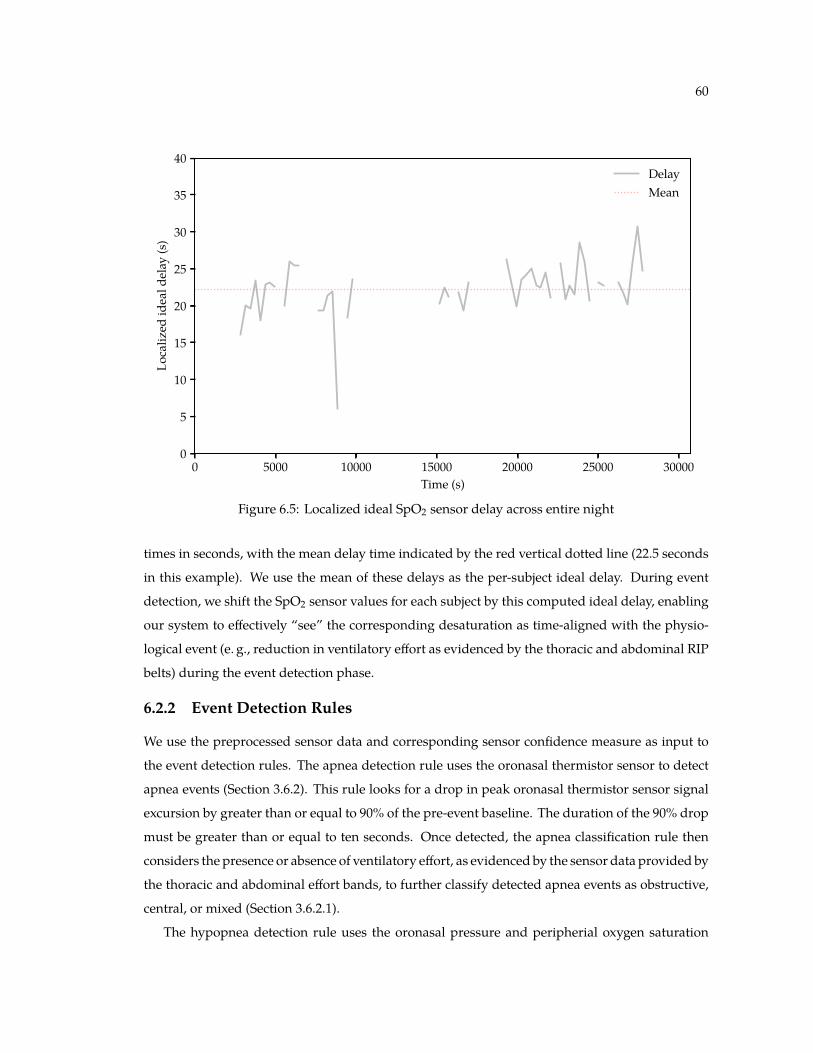
60

0 5000 10000 15000 20000 25000 30000Time (s)

0

5

10

15

20

25

30

35

40Lo

caliz

edideald

elay

(s)

DelayMean

Figure 6.5: Localized ideal SpO2 sensor delay across entire night

times in seconds, with the mean delay time indicated by the red vertical dotted line (22.5 seconds

in this example). We use the mean of these delays as the per-subject ideal delay. During event

detection, we shift the SpO2 sensor values for each subject by this computed ideal delay, enabling

our system to effectively “see” the corresponding desaturation as time-aligned with the physio-

logical event (e. g., reduction in ventilatory effort as evidenced by the thoracic and abdominal RIP

belts) during the event detection phase.

6.2.2 Event Detection Rules

We use the preprocessed sensor data and corresponding sensor confidence measure as input to

the event detection rules. The apnea detection rule uses the oronasal thermistor sensor to detect

apnea events (Section 3.6.2). This rule looks for a drop in peak oronasal thermistor sensor signal

excursion by greater than or equal to 90% of the pre-event baseline. The duration of the 90% drop

must be greater than or equal to ten seconds. Once detected, the apnea classification rule then

considers the presence or absence of ventilatory effort, as evidenced by the sensor data provided by

the thoracic and abdominal effort bands, to further classify detected apnea events as obstructive,

central, or mixed (Section 3.6.2.1).

The hypopnea detection rule uses the oronasal pressure and peripherial oxygen saturation

61

0 5 10 15 20 25 30 35Lag (s)

0

2

4

6

8

10

12

14

16

18Cou

nt

Figure 6.6: Histogram of localized ideal SpO2 sensor delay across entire night

sensor to detect hypopnea events, according to the AASM scoring criteria as discussed in Sec-

tion 3.6.3. This rule looks for a drop in peak nasal airflow pressure sensor signal excursion by

greater than or equal to 30% of pre-event baseline. The duration of the 30% drop must be greater

than or equal to ten seconds. Furthermore, the SpO2 sensor must show a desaturation of at least

3–4% from the pre-event baseline, or the event must be associated with an arousal.

Figure 6.7 depicts the components of the hypopnea detection rule. A reduction in peak

excursion of nasal airflow pressure (labeled “PFlow” in this example) from baseline by at least

30% lasting at least 10 seconds, combined with 3–4% desaturation from baseline SpO2 triggers the

detection of hypopnea events.

6.2.3 Event Confidence Measures

Along with the detected events, the hypopnea and apnea detection rules each provide an event

confidence measure, much like the sensor confidence measures provided by the sensor preproces-

sors mentioned in Section 6.2.1.3. The event confidence measures are based on the proximity of

the preprocessed sensor value to the decision boundary. If the sensor value is close to the decision

boundary—whether above or below threshold—the confidence is lower. If the sensor value is well

above or below the threshold, the confidence is higher. We use the event confidence measures in

62

0

1000PF

low raw

peakbaseline

−10

0

SpO

2Desat

1500 1510 1520 1530 1540 1550 1560 1570 1580 1590 1600Time (s)

Hyp

opne

aRu

le

Figure 6.7: Components of the hypopnea detection rule. Reduction in peak excursion of PFlowfrom baseline (top subplot) by ≥ 30% for at least 10 seconds, combined with 3–4% SpO2 desatu-ration (middle subplot), triggers detection of hypopnea events.

the next step, event integration.

6.2.4 Event Integration

We use an event integrator to merge the independently-detected hypopnea and apnea events

into a single, unified series of events. We adhere to the AASM criteria and consider potential

events meeting both the hypopnea and apnea event scoring criteria as an apnea event, unless the

corresponding confidence measure of the apnea event is below a given threshold (typically set at

0.5, or 50%), in which case it becomes a hypopnea event. If the confidence of hypopnea and apnea

are both below threshold, the potential event is discarded and the corresponding region of time is

then labeled as no event.

6.2.5 Results

Using the methodology described in Section 6.2, we used our rule-based event detection system on

each study in the polysomnography corpus. Table 6.1 depicts the resulting epoch-level confusion

matrix for all subjects in the PSG corpus. Note that both hypopnea and apnea events are frequently

63

PredictedNo event Hypopnea Apnea

True

No event 16451 1124 84Hypopnea 1172 852 0Apnea 135 219 3

Table 6.1: Rule-based epoch-level event detection confusion matrix for all subjects in the PSGcorpus. Note high confusability between no event and hypopnea.

none (17) mild (33) moderate (51) severe (66)Severity group (n)

0.3

0.4

0.5

0.6

0.7

0.8

0.9

1.0

Agreemen

t(%)

Figure 6.8: Inter-labeler epoch-level agreement by severity group, using standard AASM eventscoring rules. AASM accreditation standard of 85% agreement indicated by dotted gray line.

reported as false negatives; apnea events are also incorrectly identified as hypopnea events, or

completely misclassified as no event. We find that our straightforward algorithmic implementation

of the AASM event scoring rules exhibits high specificity (i. e., the probability of true negatives

being correctly predicted), as expected given the ratio of true negative to true positive epochs in

the corpus. Overall, we find that our rule-based system predicts epoch-level SDB event labels

with 86.4% agreement with human experts.

Figure 6.8 depicts our results by SDB severity group. Breaking out agreement by severity

group reveals our system predicts epoch-level event labels for subjects with few true events with

a high level of agreement, easily exceeding the AASM-directed 85% agreement standard for

64

Type Channel Hyperparameter Value SearchStart Stop Step N

Baseline Thoracic effort baseline percentile 67 % 50 80 5 7estimator baseline window length 300 s 120 480 30 12

Abdominal effort baseline percentile 67 % 50 80 5 7baseline window length 300 s 120 480 30 12

Airflow pressure baseline percentile 67 % 50 80 5 7baseline window length 300 s 120 480 30 12

Thermistor baseline percentile 67 % 50 80 5 7baseline window length 300 s 120 480 30 12

Pulse oximeter baseline percentile 95 % 80 95 5 4baseline window length 120 s 120 240 30 4

Hypopnea Airflow pressure sensor confidence 50 % 35 65 5 7detector peak excursion 30 % 20 30 5 3

excursion duration 10 s 6 12 2 4Pulse oximeter sensor confidence 50 % 35 65 5 7

desaturation 3 % 2 4 0.5 5Apnea Thermistor sensor confidence 50 % 35 65 5 7detector peak excursion 90 % 80 90 5 3

excursion duration 10 s 5 15 1 11Apnea Thoracic effort sensor confidence 50 % 35 65 5 7classifier peak excursion 90 % 50 95 5 10

Abdominal effort sensor confidence 50 % 35 65 5 7peak excursion 90 % 50 95 5 10

Event Event sequence apnea confidence 50 % 40 60 5 5integrator hypopnea confidence 50 % 40 60 5 5

Total 6.6272 × 1019 combinations

Table 6.2: Optimal hyperparameter grid search constraints

accreditation. However, as the number of sleep-disordered breathing events per hour increases,

the system yields lower and lower epoch-level agreement results. Epoch-level accuracy for subjects

with moderate SDB is close to the 85% threshold; accuracy for subjects with severe SDB falls short

of acceptable agreement with human experts, with several falling even below 50% agreement.

6.3 Optimal Hyperparameter Search

Given the results of our straightforward algorithmic implementation of the event scoring rules,

we design a secondary experiment using the same rule-based event detection system from the

previous section. We hypothesize that there is an inherent fuzziness to event scoring when

65

Type Channel Hyperparameter Value SearchStart Stop Step N

Hypopnea Airflow pressure peak excursion 30 % 20 30 5 3Pulse oximeter desaturation 3 % 2 4 0.5 5

Apnea Thermistor peak excursion 90 % 80 90 5 3Total 45 combinations

Table 6.3: Working subset of hyperparameter grid search constraints. Note that only hypopneaand apnea event detection thresholds are searched; baseline estimator, sensor/event confidence,apnea classifier, and excursion duration parameters are fixed.

human experts visually integrate the PSG sensor values and apply the AASM scoring rules. In

this experiment, we perform a grid search of the system hyperparameters to identify the optimal

combination of hyperparameters to maximize the accuracy of our rule-based system, specifically

to increase the detection rate of true positive hypopnea and apnea events—a clear shortcoming in

our initial results. Table 6.2 depicts the boundaries of the proposed hyperparameter search space.

Note that the space used by just the baseline estimators is 796,594,176 combinations; the space

used by the hypopnea and apnea detectors is 679,140 combinations. All together, the space used

by the baseline estimators, hypopnea and apnea detectors, apnea classifier, and event integrator is

6.6272×1019 combinations. Interestingly, the notion of baseline estimation is the least well-defined

aspect of event scoring.

6.3.1 Results

Given the significant runtime and massive result set from such a search, we present the results for

a more reasonable fixed subset of the hyperparameter search space in Table 6.4. For this subset, we

fix the baseline estimator, sensor and event confidence, apnea classifier, and excursion duration

parameters at the values listed in Table 6.2 (column 4, “Value”). This yields the greatly reduced

working subset depicted in Table 6.3, representing a much more computationally-tractable 45

combinations of hyperparameter values to search, given an average runtime of 20 minutes per

searched combination on all 167 subjects in our polysomnography corpus.

Table 6.4 lists our hyperparameter search results. Starting from a base configuration of a 90%

reduction in oronasal thermistor temperature, 30% reduction in oronasal airflow pressure, and

a 3.0% desaturation, we find statistically-significant 1.2% inter-labeler agreement improvement

when increasing the SpO2 desaturation threshold to 3.5 or 4.0%. We surmise that this is indicative

of human expert labelers erring on the 4% side of the “3–4% desaturation” guidance given by

66

Type Hyperparameters AgreementTherm (%) PFlow (%) SpO2 (%)

Hypopnea 90 20 2.0 0.778 (0.170)detector 90 20 2.5 0.813 (0.174)

90 20 3.0 0.813 (0.174)90 20 3.5 *0.837 (0.171)90 20 4.0 *0.837 (0.171)90 25 2.0 0.806 (0.165)90 25 2.5 0.830 (0.167)90 25 3.0 0.830 (0.167)90 25 3.5 *0.846 (0.165)90 25 4.0 *0.846 (0.165)90 30 2.0 0.824 (0.161)90 30 2.5 0.841 (0.163)90 30 3.0 0.841 (0.163)90 30 3.5 *0.853 (0.161)90 30 4.0 *0.853 (0.161)

Apnea 80 30 3.0 0.841 (0.164)detector 85 30 3.0 0.841 (0.163)

90 30 3.0 0.841 (0.163)

Table 6.4: Rule-based optimal hyperparameter search results. Agreement results represent mean(with standard deviation) epoch-level inter-labeler agreement across subjects (n � 169) in the PSGcorpus. Asterisk (*) indicates significant difference (p ≤ 0.00001) for dependent t-test for pairedsamples against base criteria approximant in same grouping.

the AASM scoring criteria outlined in Section 3.3.7, also reinforcing our perception of the manual

event scoring process as somewhat subjective.

6.4 Severity Estimation from SpO2

As an extension of our rule-based approach, we consider the minimal subset of sensor information

most relevant to not only the AASM event scoring rules, but to the true underlying issue mani-

festing in sleep-disordered breathing: oxygen desaturation. As some degree of desaturation from

baseline SpO2 is common to all forms of sleep-disordered breathing, we hypothesize that there

may be a correlation between the full-night mean desaturation and the apnea–hypopnea index.

To explore this hypothesis, we first estimate the baseline SpO2 as described in Section 6.2.1.1.

Next, we compute the desaturation from baseline SpO2 (Section 6.2.1.2). This step produces a

continuous desaturation channel, sampled at 10 Hz, across the entire night. Then, we calculate

the mean desaturation for each study in the PSG corpus. Finally, we calculate the correlation (i. e.,

the Pearson product-moment correlation, r) between the mean desaturation from baseline SpO2

67

Rule-based

ClinicalPSG

Eventdetection

Two-stageHMM

Audio+ SpO2

Severityestimation

Deep neuralnetwork

Corpus Approach Task

Figure 6.9: Rule-based severity estimation data flow diagram

and the clinically-determined apnea–hypopnea index, to assess the feasibility of estimating overall

SDB severity from the mean desaturation alone. Figure 6.9 depicts this approach at a high level,

notably omitting the detection of individual events. We include this approach in this chapter as it

is highly related to our algorithmic, rule-based approach focusing on domain knowledge, rather

than the machine learning-based approaches we present in later chapters.

As part of this exploration, we also calculate the correlation between constituents of the apnea–

hypopnea index, namely the number of events and the total sleep time (TST), to better understand

which aspect of the accepted clinical measurement of severity is more significant: the frequency

of event, or the amount of time spent asleep. Figure 6.10a depicts the correlation between AHI

and the total number of sleep-disordered breathing events; Figure 6.10b depicts the correlation

between AHI and TST. Notably, the AHI–number-of-events correlation is quite strong (r � 0.942),

independent of the total sleep time. The AHI–TST correlation exhibited only a marginal negative

correlation (r � −0.215). These correlations clearly indicate that the severity measure is dominated

by the average number of events, with little regard to variation in time spent asleep.

Figure 6.10c depicts the correlation between AHI and mean desaturation from baseline SpO2.

We observe a much stronger correlation between AHI and mean desaturation from baseline

(r � 0.356) than between AHI and baseline SpO2 itself (r � −0.189, Figure 6.10d). While not

conclusive, the AHI–mean desaturation from baseline correlation depicted in Figure 6.10c appears

strong enough to have potential for discriminating between subjects with no sleep-disordered

68

0 25 50 75 100Apnea–hypopnea index

0

100

200

300

400

500

600Num

bero

fevents

r = 0.941

(a) AHI–number-of-events correlation

0 25 50 75 100Apnea–hypopnea index

3

4

5

6

7

8

Totalsleep

time(hr)

r = -0.216

(b) AHI–TST correlation

0 25 50 75 100Apnea–hypopnea index

2

4

6

8

10

12

Meande

saturatio

nfrom

baselin

eSp

O2(%

)

r = 0.353

(c) AHI–mean desat from baseline correlation

0 25 50 75 100Apnea–hypopnea index

92

94

96

98

100

Baselin

eSp

O2(%

)

r = -0.192

(d) AHI–baseline correlation

Figure 6.10: Correlation between AHI and total number of SDB events, total sleep time, meandesaturation from baseline SpO2, and baseline SpO2. Pearson product-moment correlation (r)noted for each pair; individual values colored by SDB severity, with thresholds indicated byvertical dotted lines.

69

SpO2 (%) Accuracy Precision Recall AUC MCC2.0 0.888 0.907 0.974 0.570 0.2172.5 0.846 0.908 0.921 0.571 0.1503.0 0.817 0.923 0.868 0.628 0.2163.5 0.763 0.937 0.788 0.672 0.2454.0 0.633 0.941 0.629 0.648 0.1864.5 0.521 0.961 0.483 0.658 0.1965.0 0.414 0.964 0.358 0.623 0.162

Table 6.5: Rule-based SpO2 severity estimation results. Note that a decision threshold of 3.5%mean desaturation from baseline SpO2 yields the highest AUC and MCC.

breathing issues, and those with some degree of severity as indicated by the AHI. We further

explore this possibility by running a straightforward decision boundary classification experiment.

For each study in the PSG corpus, we compare the mean desaturation from baseline SpO2 to a

pre-determined threshold ranging from 2.0 to 5.0%. Studies with a mean at or above the threshold

are predicted as indicative of SDB.

6.4.1 Results

We compare the predicted and actual classification, where the actual SDB classification was

determined by comparing the actual AHI to the clinical standard for mild SDB (as discussed in

Section 3.7.7). We compute accuracy, precision, recall, area under the curve (AUC) for receiver

operating characteristic (ROC) curves, and Matthews correlation coefficient (MCC) for all studies

for each SDB decision threshold. These results are listed in Table 6.5.

To more readily interpret our findings, we also plot the receiver operating characteristic curves

for prediction of SDB severity from mean desaturation from baseline SpO2. Figure 6.11 depicts

these ROC curves; each individual curve represents one SpO2 decision threshold. For example, the

green curve, labeled “3.5” in the legend, indicates a decision threshold of 3.5% mean desaturation

from baseline SpO2. The corresponding AUC value for each threshold’s curve is in noted in

parentheses in the legend.

6.5 Discussion

We find that our rule-based system using straightforward algorithmic implementation of the

American Academy of Sleep Medicine event scoring rules reliably meets the 85% inter-labeler

agreement threshold for accreditation, even before our tuning of the hyperparameters, but leaves

many aspects unexplained. For example, true apnea events are correctly detected less than 1% of

70

0.0 0.2 0.4 0.6 0.8 1.0False positive rate

0.0

0.2

0.4

0.6

0.8

1.0True

positiv

erate

2.0 (0.575)2.5 (0.578)3.0 (0.639)3.5 (0.687)4.0 (0.640)4.5 (0.655)5.0 (0.621)

Figure 6.11: Receiver operating characteristic curves for prediction of SDB severity from meandesaturation from baseline SpO2. Individual curves represent various SpO2 decision thresholds(e. g., “3.5” indicates a decision threshold of 3.5% mean desaturation); corresponding area underthe curve in parentheses.

the time using our base configuration that precisely replicates AASM scoring criteria; however,

hypopnea events are detected somewhat more reliably, at 42%. Even with the introduction of

more flexibility in the scoring criteria, our hyperparameter search only increases the inter-labeler

agreement by approximately 2% over our base configuration that precisely adheres to the peak

excursion thresholds codified in the AASM scoring manual. Further exploration of the vast

hyperparameter search space might yield further improvements. We also note that we focus

our assessment on the more stringent epoch-level agreement, rather than the predicted severity

group agreement, based on the use of the former in the published literature in the field. We do

recognize, however, that some clinical decision-making is based on the severity; for example, in

an admittedly gross simplification, a patient with an AHI anywhere between 5 and 30 may be

prescribed the use of a CPAP machine, regardless of precise AHI, while a patient with an AHI

less than 5 would not.

Moving on to our straightforward decision boundary classification experiment, we find that a

decision threshold of 3.5% mean desaturation from baseline SpO2 yields both the highest ROC area

under the curve and the highest Matthews correlation coefficient. Incidentally, this desaturation

71

value also aligns nicely with the clinical PSG event detection threshold of 3–4%; while not directly

comparable, the similarity between individual event desaturation threshold and full-night mean

desaturation threshold is a curious finding. The overall accuracy of the system with the decision

threshold set at 3.5% is marginally acceptable at 76.3%—meaning one in four patients would be

assessed at the incorrect severity level—but does yield good precision at 93.7%.

We surmise that it may be possible to extend the notion of mean desaturation from baseline

SpO2 to a more fine-grained approach, for example, extrapolating some measure of the ratio of

threshold-exceeding epochs to non-threshold-exceeding epochs, rather than a single, full-night

mean desaturation measure. Such an approach would likely be well-received by clinicians, as it

more closely adheres to the epoch-by-epoch nature of the existing scoring guidelines. However, it

is not immediately clear that such an approach would provide any advantage over the full-night

measure without introducing additional machine learning algorithms—which still must work to

overcome the “black box” stigma commonly associated with them to gain widespread clinical

acceptance.

Chapter 7

Two-Stage Hidden Markov Model-BasedEvent Detection

7.1 Introduction

In this chapter, we build on our earlier work with sleep breathing audio [138, 139, 140], using

minimally-obtrusive sensors and an automatic, two-stage method for (i) classifying breathing

sounds during sleep to track ventilatory effort, and (ii) predicting disordered breathing events

using featured derived directly from the tracked ventilatory cycle, along with the corresponding

oxygen desaturations evident during disordered breathing events. Figure 7.1 provides a high-level

overview of our approach. As discussed at length in Chapter 4, much attention has been paid to

the acoustics of snoring and other sleep breathing sounds by other researchers; we likewise direct

our own attention here in this chapter to explore the possibility of assessing sleep-disordered

breathing without the patient burden of the myriad of physically-attached sensors required for

typical clinical polysomnography.

In the first stage, which we refer to as Stage I, we use acoustic features extracted from high-

quality audio to classify sleep breathing sounds into ventilatory effort classes. We describe our

acoustic feature extraction, ventilatory effort tracking model, automatic effort label remapping,

and Stage I training and testing procedures and results in Section 7.2. Then, in Stage II, we use

features extracted from the output of our Stage I ventilatory effort tracking model, in conjunction

with additional features extracted from pulse oximetry data (in this case, peripherial oxygen

saturation, or SpO2) for use in a separate classifier. We describe our Stage II feature extraction,

event detection model, and training and testing procedures and results in Section 7.3. Finally, we

discuss the overall results of our two-stage approach in Section 7.4.

72

73

Rule-based

ClinicalPSG

Eventdetection

Two-stageHMM

Audio+ SpO2

Severityestimation

Deep neuralnetwork

Corpus Approach Task

Figure 7.1: Two-stage HMM-based event detection data flow diagram

7.2 Stage I: Ventilatory Effort Tracking from Audio

For this experiment, we use our own manually-curated audio-plus-SpO2 corpus (more fully

described in Section 5.3). This corpus contains high-quality sleep breathing audio recordings made

synchronously during full-night clinical polysomnography for six subjects, allowing us to relate

the acoustics of disordered breathing and snoring with the corresponding oxygen desaturations

recorded by the PSG sensor array, using clinically-derived sleep-disordered breathing event labels

as the ground truth of the underlying physiological state. From the start of this work, we have

envisioned a hypothetical nightstand device with a microphone paired with a small, unobtrusive

wrist-worn pulse oximeter as the eventual data collection mechanism; however, for this actual

experiment, we simply use the SpO2 data from the existing PSG system.

Figure 7.2 depicts a brief example from our audio corpus. Recall that we manually labeled the

ventilatory effort evident in the recorded audio as breathing in (Bi), breathing out (Bo), snoring

in (Si), snoring out (So), or no effort (N), as described in Section 5.3.2, while listening to the audio

and visually inspecting the audio waveform and spectrogram. Figure 7.2 depicts the waveform,

corresponding spectrogram, and manually-annotated ventilatory effort labels for a 10-second

example from one of the subjects in the corpus. Note the increased energy and voicing during Si

events due to vibration of soft tissues along the airway during snoring.

74

−0.2

0.0

0.2Waveform

0

2000

4000

6000

8000

Freq

uenc

y(H

z)

0 1 2 3 4 5 6 7 8 9 10Time (s)

Effort

Labe

l

N Si Bi Si Bo N Si Bo N

Figure 7.2: Original high-quality waveform, spectrogram, and manually-annotated ventilatoryeffort labels for a brief excerpt from the audio corpus.

7.2.1 Acoustic Feature Extraction

In our early published work with a similar, smaller audio corpus for a related task, we investigated

classical features from acoustic signal processing [139]. The corpus contained high-quality single-

channel audio recordings made using a directional microphone oriented toward the head of the

bed, sampled at 16 kHz and stored as original, uncompressed waveforms. We extracted these

features from the audio waveforms using non-overlapping 150-ms frames and a Hanning analysis

window. For each frame, we independently calculated thirteen cepstral coefficients (CC), Mel-

frequency cepstral coefficients (MFCCs), and reflection coefficients from linear predictive coding

(LPC). We then excluded the first coefficient from the resulting CC and MFCC feature vectors,

to make the features energy-independent. In addition, we also calculated and appended first-

order delta features derived from the static coefficient features, yielding a length-26 feature vector

for each 150-ms frame of audio, a common approach in related tasks such as automatic speech

recognition (ASR).

As in our previous work, we find reflection coefficients from linear predictive coding to be

the highest-performing acoustic features in sleep breathing classification; we therefore focus our

75

0 1000 2000 3000 4000 5000 6000 7000 8000Frequency (Hz)

2.0

2.5

3.0

3.5

4.0

4.5

5.0

5.5

6.0Amplitu

de(dB)

BiBoNSiSo

Figure 7.3: Spectral reconstruction of LPC-based features for examples of each ventilatory efforttype. Note similarities in spectral peak locations, and slight shift to lower frequencies duringexhalation.

attention in this current experiment on these features, and refer the interested reader to our

earlier published findings for further analysis of the other types. Figure 7.3 illustrates the spectral

reconstruction of our chosen LPC-based features for representative instances of each ventilatory

effort event type from one subject in our audio corpus. Note that the features focus on modeling

the spectral peaks, with similarities in peak location evident across event types. Also note the

slight shift to lower frequencies during exhalation. We use these LPC-based features as input to

our Stage I model.

7.2.2 Ventilatory Effort Tracking Model Architecture

The first stage of our two-stage event detection system uses acoustic features from sleep breathing

audio to track ventilatory effort. We use a hidden Markov model (HMM) to predict ventilatory

effort state sequences to capitalize on the repetitive sequential nature of typical ventilation, charac-

terized by an infinite cycle of inhalation and exhalation. HMMs model both transition probabilities

from one state to the next, as well as observation probabilities—the probability of observing ev-

idence that supports being in a given state of the underlying hidden Markov process [118]. We

76

⋆

Bi1 Bi2 Bi3

Si1 Si2 Si3

� N �

Bo1 Bo2 Bo3

So1 So2 So3

N ⋆

Figure 7.4: Stage I HMM topology with three states per ventilatory effort label type (Bi, Bo, Si, So)and one state for the no-effort type (N). Stars (⋆) denote the null state at the start of a ventilatorycycle. Nulls (�) denote intermediate null states.

assume a priori that ventilatory effort states evidenced by the acoustic features can be learned and

predicted by the HMM, much like phone states in automatic speech recognition applications.

Figure 7.4 illustrates the topology of our Stage I effort tracking model. Each ventilatory effort

type consists of three states per label, while the no-effort type consists of one state, which is

shared following both inhalation and exhalation. Note that the N state is sometimes optional; null

states enable skipping N between inhalation and exhalation. However, N is always present after

exhalation, and before the following inhalation. We arrive at this specific model topology after

preliminary exploration of various numbers of states per effort label, subtypes of no-effort states,

and related aspects in our aforementioned early related work. [139]

When originally creating our audio corpus, we observed many interesting phenomena during

manual ventilatory effort labeling, motivating our Stage I HMM architecture. For example, within

a single inhalation, a breath in may turn into a snore in; likewise, during an exhalation, a snore out

may degrade into a breath out. Additionally, we observed that an inhalation may be immediately

followed by an exhalation, with no intermediate no-effort state. Finally, we account for multiple

short inhalation attempts in rapid succession, separated by brief no-effort states. We observed this

type of phenomenon during obstructive apnea events, when a subject tried repeatedly to breathe

in with limited success. We designed our model to capture these various phenomena, learning

the relevant probabilities during training.

7.2.3 Automatic Label Remapping

We use an automatic label remapping algorithm to transform our manually-applied ventilatory

effort labels into the specific ventilatory effort state names used by our model depicted in Figure 7.4.

Similar to our previous work, we divide individual episodes of inhalation and exhalation according

77

Effort

Labe

l

N Si Bi Si N Bo N

0 1 2 3 4Time (s)

State

Nam

e

N Si1 Bi2 Si3 N Bo1 Bo2 Bo3 N

Figure 7.5: Resulting state names after automatic remapping of ventilatory effort labels

to the following rules: (i) if an episode consists of one constituent label, divide the label into three

equal-duration states; (ii) if an episode consists of two constituent labels, divide the longer-duration

label into two equal-duration states, and assign the shorter-duration label to a third state; and (iii) if

an episode consists of three constituent labels, assign each label to a single state, preserving the

original durations of the constituent labels. Figure 7.5 illustrates the resulting ventilatory effort

state names for one inhalation–exhalation cycle after automatic remapping from our manually-

applied ventilatory effort labels. Note that the inhalation, labeled Si–Bi–Si, is a single episode

with three constituent labels; we therefore assign each label to its own state (Si1, Bi2, and Si3,

respectively), preserving the original durations. The exhalation episode, labeled Bo, contains one

constituent label, and is split into three equal-duration states, Bo1, Bo2, and Bo3. Note that N labels

remain unchanged by the remapping algorithm.

7.2.4 Training and Testing

To train and test our Stage I model, we use a leave-one-out cross-validation scheme, separating

the data into training and testing sets. For each fold, we hold out one subject’s data for testing,

using the remaining five subjects’ data for training. As each subject in the corpus has 16 minutes

of manually-labeled sleep breathing audio, each training set contains 80 minutes of audio, with

16 minutes held out for testing. We cycle through all six subjects, with a different held-out subject

78

Bi1 Bi2 Bi3 Bo1 Bo2 Bo3 N Si1 Si2 Si3

Bi1

Bi2

Bi3

Bo1

Bo2

Bo3

N

Si1

Si2

Si3

Figure 7.6: Stage I transition matrix (A) for one training fold

per fold. For each fold, we use the resulting training set to initialize and train a new instance of

the Stage I HMM, and then use the trained model to predict the ventilatory effort state sequence

for the test set.

To initialize the HMM, we first calculate the start probability values π, representing the prob-

ability of starting in each state, and transition probability matrix A using observed sequences

from the training set. Figure 7.6 depicts an example computed transition matrix for one training

fold. Row labels indicate the current state, and column labels indicate the possible next states.

Transition probabilities from the current state to the possible next state are visually depicted at

row–column intersections, ranging from 0.0 to 1.0; all rows sum to 1.0. Note that So is not present

in this particular training fold, as it is very rare in the corpus; we omit those rows and columns in

the figure for brevity.

Next, using the state-labeled data, we group the frame-level feature vectors (described in

Section 7.2.1) from the training set by state. For each state, we calculate the mean and covariance

of the feature vectors for that state. We use these statistics to fit a Gaussian mixture model (GMM)

for each state, each with two mixture components and full covariance, to model the observation

probabilities B. Figure 7.7 depicts the GMMs for Bi and Si states for the first five (of twenty-six)

features for each state. For each feature, we plot a histogram of the values for that feature, and

79

Feature1

Feature2

Feature3

Feature4

Bi1

Feature5

Bi2 Bi3

(a) Breath in

Feature1

Feature2

Feature3

Feature4

Si1

Feature5

Si2 Si3

(b) Snore in

Figure 7.7: Gaussian mixture models for Bi states (top) and Si states (bottom) for the first five LPCfeatures. Histogram of feature values depicted in light gray; Mixture component KDEs depictedin light blue, with resulting mixture density estimate in dark blue.

80

True N Si1 Si2 Si3 NBo1 Bo2 Bo3 N Bi1 Si2 Si3 NBo1Bo2Bo3 N

0 1 2 3 4 5 6 7 8 9 10Time (s)

Pred N Bi1Si2 Si3 NBo1 Bo2 Bo3 N Bi1 Si2 Si3 NBo1 Bo2Bo3 N

Figure 7.8: True and predicted ventilatory effort state sequences. Smallest individual labelsrepresent 150-millisecond frames.

overlay the kernel density estimate (KDE) from the two mixture components in the GMM for

possible values in the feature’s range. We then plot the resulting mixture KDE, which depicts the

combined density estimate of the individual components.

We create a new instance of the HMM and initialize it with the precomputed π, A, and B

from the training set. We then perform supervised training of the model using the Baum-Welch

expectation-maximization algorithm, feeding the model with frame-by-frame LPC-based features

and corresponding ventilatory effort-based state labels. We train the model for a maximum of

50 iterations, stopping early if the probability of the model given the training sequence does not

improve beyond a pre-defined threshold. Once trained, we use the HMM to predict the most

probable ventilatory effort state sequence for the test set, given the model, using the Viterbi search

algorithm. We record the predicted state sequences, and also map model state names back to

ventilatory effort labels and then merge identical adjacent labels to enable direct comparison to

the original, manually-labeled sequences.

7.2.5 Results

Figure 7.8 depicts the true (top) and predicted (bottom) ventilatory effort state sequences for a

10-second example from one test subject. We find that our Stage I model tracks appears to track the

81

True PredictedBi1 Bi2 Bi3 Bo1 Bo2 Bo3 N Si1 Si2 Si3

Bi1 204 20 7 66 27 17 289 349 535 313Bi2 9 18 13 22 24 64 109 19 73 253Bi3 1 13 11 10 11 70 266 0 22 182Bo1 83 78 31 223 138 183 882 123 276 115Bo2 6 33 112 33 125 383 1065 3 81 306Bo3 7 12 75 90 45 381 1791 0 18 43

N 849 798 339 570 281 1147 14994 472 505 35Si1 50 1 3 25 6 7 165 169 1184 349Si2 6 0 16 8 2 17 246 90 1630 1363Si3 2 5 35 16 1 8 1225 6 732 1458

Table 7.1: Aggregate confusion matrix of true versus predicted frame-by-frame HMM states. Noteconfusability of N with various forms of quiet breathing.

ventilatory cycle fairly well. We observe some confusability at the edges of effort types, and also

where very quiet breathing is indistinguishable from no effort. We also note some mistracking of

the cycle, with one episode of inhalation incorrectly predicted as following another, without an

intermediary exhalation, rather than correctly as an inhalation followed by an exhalation.

In previous work, we introduced discrete no-effort labels to describe N between an inhalation

and exhalation (Nio) and between exhalation and inhalation (Noi), to help address this tracking

issue by increasing the probability of preferred transitions. We also introduced Nii to describe

N between successive attempts at inhalation (as discussed in Section 7.2.2), and Noo for the same

during exhalation. However, when replicating this extended topology in this experiment with

tied GMM emission probabilities for all types of N, we observed lower frame-by-frame accuracy.

During review of the development data set producing these results, we noted many instances

in the labeled audio where very quiet exhalation (i. e., Bo) was simply not discernable, and was

labeled as some form of N. In these circumstances, a true Bi–Nio–Bo–Noi–Bi cycle was labeled as

Bi–Nii–Bi (with the Nii label having a duration of many seconds, rather than milliseconds), despite

the episode not corresponding to a disordered breathing event and it in all likelihood simply being

very quiet breathing out followed by breathing in. We found that the transition probabilities biased

the model, leading us to eliminate the four discrete no-effort states, and simply use one N state.

Table 7.1 depicts the aggregate confusion matrix across all subjects, compiled from the longer

frame-by-frame state sequence predictions by our Stage I HMM. We find that N is frequently

incorrectly predicted as breathing in or out (row labeled by N); likewise, breathing in and out is

incorrectly predicted as N (column labeled by N). We also find that breathing in (rows labeled by

Bi) is quite frequently predicted as snoring in (columns labeled by Si). We hypothesize that this is

82

State Label B/S I/O E/NGranularity

0.0

0.2

0.4

0.6

0.8

1.0Fram

eaccu

racy

(%)

Figure 7.9: Stage I model prediction accuracy by label granularity. Distributions reflect predictionaccuracies for 24 four-minute recordings (6 subjects times 4 sequences per subject). Medianaccuracies indicated by red lines.

due to breathing in some subjects looking more (in feature space) like snoring in other subjects in

the training set. However, we do also observe that snoring is generally predicted well as snoring

(bottom right cells of the table), with some blurring of the constituent state lines. Finally, we

find that our Stage I model is well-behaved, with few unexpected spurious transitions, such as an

inhalation abruptly turning into exhalation mid-episode.

To better understand the confusion results, we move beyond the state-level predictions and

report our model prediction accuracy for several groupings, or granularities, of states: state

granularity, the actual fine-grained HMM state names listed in Table 7.1; ventilatory effort label

granularity, where HMM state names are merged into one effort label (e. g., Bi1, Bi2, and Bi3 become

Bi); breath/snore granularity, where Bi and Bo effort labels are grouped into a more generic B

label, and Si and So into S; inhale/exhale granularity, where Bi and Si are grouped into a more

generic I label, and Bo and So into O; and finally, a very coarse effort/no-effort granularity, where

all effort types aside from N are grouped into a high-level E label. By grouping related labels, we

are able to better assess the model’s ability to track ventilatory effort, beyond what the individual

HMM state sequence prediction indicates.

83

True PredictedBi Bo N Si

Bi 374 319 733 1591Bo 689 1513 3827 712N 2095 2030 15287 578Si 124 103 1916 6682

(a) Ventilatory effort label granularity

True PredictedB S N

B 2895 2303 4560S 227 6682 1916N 4125 578 15287

(b) Breath/snore granularity

True PredictedI O N

I 8771 422 2649O 1401 1513 3827N 2673 2030 15287

(c) Inhale/exhale granularity

True PredictedE N

E 12107 6476N 4703 15287

(d) Effort/no-effort granularity

Table 7.2: Confusion matrices for ventilatory effort label, breath/snore, inhale/exhale, andeffort/no-effort granularites

Figure 7.9 summarizes our mean Stage I model prediction accuracy by label granularity. Each

distribution reflects the prediction accuracies for all six subjects in the audio corpus, each with four

audio recordings of approximately four minutes in duration. Our Stage I model yields mean frame-

by-frame accuracy of 0.505 at the HMM state sequence granularity (labeled “State” in the figure).

Our grouped label granularities yield the following mean accuracies: 0.618 for the ventilatory

effort label granularity (labeled “Label”); 0.645 for the breath/snore (“B/S”) granularity; 0.663

for the inhale/exhale (“I/O”) granularity; and 0.710 for the effort/no-effort (“E/N”) granularity.

Table 7.2 depicts the corresponding confusion matrices for each of these granularities. In all of

these alternative groupings, confusability between quiet breathing and no effort accounts for a

majority of the frame-by-frame prediction error.

7.3 Stage II: Event Detection from Ventilatory Effort and SpO2

As our ultimate goal is not ventilatory effort tracking, but rather disordered breathing event

detection, we build upon Stage I and add a second stage that uses features extracted from the

output of our Stage I ventilatory effort tracking model, in conjunction with additional features

extracted from peripherial oxygen saturation (SpO2) sensor data. Recall that our high-quality

audio recordings of sleep breathing sounds were recorded synchronously during full-night clin-

ical polysomnography (as described in Section 5.3.1), giving us time-aligned SpO2 sensor data

84

and corresponding sleep-disordered breathing (SDB) event labels. In Stage II, we use a second

hidden Markov model to predict these SDB event labels using features derived from the predicted

ventilatory effort labels from Stage I and corresponding changes in SpO2.

7.3.1 Ventilatory Cycle Feature Extraction

When scoring polysomnography studies, trained clinicians and PSG technicians evaluate ventila-

tory effort, airflow, and peripherial oxygen saturation (SpO2) data to identify disordered breathing

events, looking for a reduction in or cessation of breathing effort or airflow and a correspond-

ing drop in blood oxygen saturation, in accordance with American Academy of Sleep Medicine

guidelines, as presented in Section 3.6. With these criteria in mind, we create new feature vec-

tors for Stage II by extracting ventilatory effort features from the output of Stage I, incorporating

additional SpO2 features extracted from the polysomnography data.

During manual labeling of respiratory effort (described in Section 5.3.2), we noted changes

in ventilatory effort label duration during disordered breathing events such as hypopnea (H),

obstructive apnea (OA), or central apnea (CA), when compared to typical breathing (“-” for no

event) of that same effort type. Figure 7.10 depicts ventilatory effort label durations wholly

contained within a given disordered breathing event. The numbers in parentheses next to each

SDB event label on the x-axes indicate the number of instances of that ventilatory effort type

within the corresponding type of event. Note the shortening of inhalation and exhalation episode

duration during disordered breathing events. The ventilatory effort durations during central

apnea events represent effort at the beginning or end of the event, as there is no effort during the

majority of the labeled event.

Based on this finding, we create duration-related ventilatory effort features for use by our

Stage II model. Using the predicted ventilatory effort labels from Stage I, we extract the duration

of the current ventilatory effort label to create a one-hot duration vector for each 150-millisecond

frame. In this design, only one of the five possible effort labels (Bi, Bo, N, Si, So) can be “hot”

(i. e., non-zero) per frame. The value of the one “hot” feature is the duration of the current “hot”

ventilatory effort label; the values of the remaining four “cold” effort duration features for the

frame are set to zero.

Along with the duration features, we extract SpO2 desaturation features from the time-aligned

polysomnography data. First, we estimate a single baseline SpO2 value per subject by computing

the 95th-percentile SpO2 value in a running two-minute window, as we describe in Section 6.2.1.1

for our rule-based system. Next, we compute a desaturation from baseline value for each frame,

where desaturation is defined as the baseline minus the observed SpO2 value. Finally, we append

85

- (1078) H (18) OA (14) CA (11)0.0

0.5

1.0

1.5

2.0

2.5

3.0

3.5

4.0Duration(s)

(a) Breath in

- (1659) H (69) OA (25) CA (12)0.0

0.5

1.0

1.5

2.0

2.5

3.0

3.5

4.0

Duration(s)

(b) Breath out

- (1441) H (61) OA (21) CA (13)0.0

0.5

1.0

1.5

2.0

2.5

3.0

3.5

4.0

Duration(s)

(c) Snore in

- (3683) H (127) OA (47) CA (30)

0

2

4

6

8

10

Duration(s)

(d) No effort

Figure 7.10: Ventilatory effort label durations for breath in, breath out, snore in, and no effortepisodes, grouped by containing disordered breathing event type. Note shortening of episodeduration during disordered breathing events (H, OA, CA) compared to during no event (“-”).

86

Effort

−8−6−4−2

0

Desat

BiBoNSiSo

SpO2

Features

450 500 550 600 650Frame

Even

t

Figure 7.11: Stage I ventilatory effort labels, SpO2 desaturation, corresponding Stage II durationand desaturation feature vector, and disordered breathing event labels (hypopnea in orange,surrounded by no event) for a 30-second (i. e., 200-frame) excerpt of training data

this desaturation value to the one-hot duration vector to form the feature vector for each frame,

yielding six feature values per frame. We normalize the features on a per-feature basis by dividing

by the maximum value for each feature.

Figure 7.11 illustrates the Stage I ventilatory effort labels, desaturation from baseline SpO2,

corresponding Stage II duration and desaturation feature vector, and disordered breathing event

labels for a 30-second excerpt of training data. Note the shorter-duration episodes of snore in (Si)

during the hypopnea event, indicated visually in the feature vector by lighter blue Si compared to

the darker blue Si preceeding and following the disordered breathing event; a similar shortening

of no effort (N) between exhalation and inhalation is also evident during the event. The shortening

of the Si appears when the snoring in changes to a different variant of inhalation, characterized by

an initial few frames of breath in immediately changing into snore in. Once the event concludes,

the inhalation pattern returns to the pre-event variant. The hypopnea event also corresponds to a

3–4% desaturation, meeting the AASM scoring guidelines for hypopnea presented in Section 3.6.3.

87

⋆ - � OA

H

CA

⋆

Figure 7.12: Stage II HMM topology with one state per disordered breathing event type (H, OA,CA) and one state for typical breathing with no event (“-”).

7.3.2 Event Detection Model Architecture

We create a new, second-stage hidden Markov model to predict disordered breathing events during

sleep. Figure 7.12 illustrates the topology of our Stage II model. In this stage, the possible states

represent observed disordered breathing event types: no event (“-”), hypopnea (H), obstructive

apnea (OA), and central apnea (CA). Other event types, such as mixed apnea or hypopnea, are

possible but are not present in our audio corpus. We use one state per event type, with null states

allowing one disordered type to transition to another without an intermediate no event. Likewise,

self-loops permit staying in one state for many frames in a row. As in our Stage I HMM, we use a

Gaussian mixture model with two mixture components to model the observation probabilities in

our Stage II model.

7.3.3 Training and Testing

As in Stage I, we use a leave-one-out cross-validation scheme, replacing the Stage I ventilatory

effort HMM with the Stage II disordered breathing event HMM, and using the Stage II duration

and desaturation feature vectors as input. For each fold, we hold out data from one subject

for testing, and use the data from the remaining five subjects to initialize and train the model

in a similar fashion as we describe for our Stage I model in Section 7.2.4, for a maximum of 50

iterations. Once trained, we predict the disordered breathing event label sequence for the held-out

test subject and record the results for comparison with the true event labels.

7.3.4 Results

We evaluate Stage II model accuracy in a similar manner as in Stage I, with two levels of granularity:

fine- and coarse-grain accuracy. For fine-grain accuracy, we leave events as is, allowing all four

possible event labels. For coarse-grain accuracy, we combine all disordered events into one generic

88

Fine CoarseGranularity

0.0

0.2

0.4

0.6

0.8

1.0Fram

eaccu

racy

(%)

Figure 7.13: Stage II model prediction accuracy for fine granularity (with discrete disorderedbreathing event types) and coarse granularity (with all event types collapsed into one genericevent). Median accuracies indicated by red lines.

disordered event label, to evaluate the potential for identifying typical breathing versus disordered

breathing. Figure 7.13 depicts our Stage II model prediction fine- and coarse-grain accuracy. We

find essentially no difference between the two granularities, with mean accuracies of 0.658 and

0.659, respectively. This indicates that the various types of disordered breathing events—i. e., the

labels being collapsed in the coarse granularity—are generally not confusable for each other.

In reviewing the true and predicted event labels for individual sequences in the test set, we

find that our Stage II model generally predicts (i) entire (approximately) four-minute contiguous

sequences as entirely no event, which is largely accurate for those sequences; (ii) mostly no event,

with very few sporadic frames of the correct disordered event type; or (iii) mostly some form of

disordered event type, with very few sporadic frames of no event. In the first case, subjects with

little to no disordered breathing exhibit high accuracy, raising the overall mean accuracy. In the

second case, subjects with one or more disordered breathing events (each at least 10 seconds in

duration) have some frames correctly predicted during actual events, but not for the entire duration

of each event. In the third case, subjects with or without disordered breathing events have large

portions incorrectly predicted as disordered, when in truth there is no event, lowering the overall

89

True Predicted- CA H OA

- 23272 3302 8320 0CA 121 0 7 0

H 309 30 0 0OA 0 0 0 0

(a) Fine granularity

True Predicted- E- E

- 23272 11622E 430 37

(b) Coarse granularity

Table 7.3: Confusion matrices for fine and coarse granularites

mean accuracy of the system. Given that our audio corpus has a fairly uniform distribution of

sleep-disordered breathing severities among subjects, with corresponding incidence of disordered

breathing events, our Stage II event prediction accuracies fairly uniformly range from 33 to 100%.

Overall, we find that our Stage II model exhibits a high incidence of false positives, with no

event very frequently being predicted as some form of disordered breathing event; however, there

are relatively few false negatives. Table 7.3 depicts the confusion matrices for the fine- and coarse-

grained variants. Note the large number of no event (row labeled “-” in Table 7.3a) predicted

as central apnea (column labeled “CA”) or hypopnea (“H”). Moreover, note the tendency of the

model to confuse true CA and H events with no event, rather than with some other type of

disordered breathing event.

7.4 Discussion

We find that our Stage I ventilatory effort model tracks the ventilatory cycle fairly well, with 71%

frame-level accuracy. Given that some slight alignment differences at the start or end of individual

episodes of inhalation or exhalation lower accuracy, but do not constitute a significant issue, we

find that our chosen linear predictive coding-based acoustic features are sufficient to characterize

different types of ventilatory effort. Overall, our system detects episodes of ventilatory effort

with acceptable accuracy. Except in the case of very quiet breathing, an acoustic-only monitoring

system may prove capable at detecting cessations of breathing evident during central apnea with

high accuracy.

We also find that, for our specific audio corpus, very quiet breathing is acoustically indistin-

guishable from no effort at all. Despite selecting purpose-built audio recording equipment with

a low noise floor and highly-directional microphones to help reject off-axis environmental noise,

human labelers and our hidden Markov model-based classifier alike cannot reliably discern the

difference between these two types. For individuals with no disordered breathing events who also

90

exhibit no snoring or snore-like breathing, our system would have difficulty correctly tracking the

ventilatory effort cycle with any degree of accuracy.

We do note that our system accurately identifies snoring over 75% of the time, outperforming

identification of non-snore breathing. As snoring is often associated with obstructive sleep ap-

nea, this finding is encouraging. We also find that our system does distinguish inhalation from

exhalation quite well; however, exhalation is often confused with inhalation—specifically, slightly

louder, more audible breathing out is confused with typical, non-snore breathing in. Given these

two desirable attributes of our system, we speculate that an HMM-based system using acoustic

features that primarily focuses on tracking inhalation characterized by snoring-like sounds may

yield better overall tracking of the ventilatory cycle than our existing system that tries to model

both breathing and snoring during both inhalation and exhalation. As sleep-disordered breath-

ing generally manifests during inhalation, the need to carefully track exhalation is possibly less

necessary than we anticipated when first designing our model.

Moving on to our Stage II classifier, we find that the durations of various types of ventilatory

effort are somewhat informative (as evidenced by the shortening of some types, as depicted

in Figure 7.10), but perhaps not distinguishing enough—especially across subjects—to clearly

identify disordered breathing. We speculate that the desaturation of peripherial oxygen saturation

is the most distinguishing factor when predicting SDB events, as it is consistent across subjects.

Recalling the AASM event scoring criteria, we further speculate that the difference from some

baseline duration, or even the rate of change of the effort durations, may prove more useful. We

also recognize the need for additional data with labeled ventilatory effort that also coincides with

true disordered breathing events. Due to the nature of the clinical environment our subjects were

in during data collection for our audio corpus, the dearth of noise-free regions of audio negatively

impacted the amount of usable audio, reducing our corpus from 23 subjects to 6.

Finally, we address the possibility of sleep breathing audio standing in as a surrogate for ven-

tilatory effort measurements made using respiratory inductance plethysmography belts fastened

about the thorax and abdomen. We find that, when audible, breathing sounds are sufficient to

quantify ventilatory effort, such that episodes of effort are distinguishable from no effort. This

gives support for pursuing unobtrusive, non-contact methods that increase patient comfort by

reducing the number of attached sensors required to assess sleep-disordered breathing. Further

work is required, however, to determine if an acoustics-based method is sensitive enough to repli-

cate the combination of a RIP belt and oronasal airflow sensor to indicate reduction in effort or a

reduction in airflow.

Chapter 8

Deep Neural Network-BasedEvent Detection and Severity Estimation

8.1 Introduction

In this chapter, we present three deep neural network (DNN)-based approaches for event detection

and overall sleep-disordered breathing (SDB) severity estimation. First, we present two distinct

approaches for event detection: a feed-forward DNN model that predicts the dominant SDB event

label for each 30-second epoch (Section 8.2), and a sequence-to-sequence DNN model that maps

the time-series sequence of input sensor data to the corresponding SDB event labels (Section 8.3).

Then, we present an SDB severity predictor that considers large portions of the entire night

of sensor data to make an overall sleep-disordered breathing severity prediction, similar to the

apnea–hypopnea index (Section 8.4).

Our three DNN-based approaches explore a continuum that varies from most aligned with

established clinical practices and informed by human expertise, to fully automated with dis-

criminating features learned by the machinery. Our feed-forward model uses the same human-

engineered features used in our rule-based system that are in turn derived from the American

Academy of Sleep Medicine (AASM) scoring guidelines. Conversely, our sequence-to-sequence

model uses feature learning, using a convolutional neural network (CNN) to learn and encode

features directly from the raw polysomnography (PSG) sensor data, combined with a long short-

term memory (LSTM)-based model to decode those features and translate them into disordered

breathing event labels. This second approach eliminates feature engineering, but still predicts

individual event labels much like human expert event scoring. Finally, our full-night severity

predictor translates raw PSG sensor data directly to a single severity estimation value, without

predicting individual event labels en route.

91

92

Rule-based

ClinicalPSG

Eventdetection

Two-stageHMM

Audio+ SpO2

Severityestimation

Deep neuralnetwork

Corpus Approach Task

Figure 8.1: DNN-based event detection data flow diagram

8.2 Feed-Forward Event Detection

In this experiment, we use a feed-forward deep neural network to predict sleep-disordered breath-

ing events on an epoch-by-epoch basis from full-night clinical polysomnography, as depicted by

Figure 8.1. Starting with basic preprocessing (Section 8.2.1), we extract features from the PSG sen-

sor data (Section 8.2.2) based on the clinical scoring standard. Next, we construct a fully-connected

feed-forward DNN model (Section 8.2.3) and train it using the extracted features (Section 8.2.4).

Then, we use the trained model to predict SDB events for unseen subject data and report the

results (Section 8.2.5).

8.2.1 Preprocessing

As the data used in this experiment were collected during routine full-night clinical PSG, we

minimally preprocess the data to exclude time before lights out and after lights on (see Section 3.7.8)

to eliminate atypical noise from the audio recordings (e. g., verbal instructions from the technician

during PSG sensor calibration, post-study discussion).

Additionally, we only include data from the first hour of sleep starting at the sleep onset (i. e.,

the start time of the first clinically-scored 30-second epoch of sleep). As many of the patients

presenting to the sleep lab for polysomnography studies had some degree of sleep-disordered

breathing, a substantial number of the PSG studies in our corpus found sufficient evidence of SDB

93

Channel Description Unit Rate (Hz)Direct Thorax Thoracic ventilatory effort µV 200Direct Abd Abdominal ventilatory effort µV 200PFlow Oronasal airflow pressure mbar 200Direct Therm Oronasal airflow temperature µV 200SpO2 Peripherial oxygen saturation % 10

Table 8.1: Channel name, description, unit of measure, and sample rate for sensors used in thefeed-forward event detection experiment

within the first hour or two of sleep, and then quickly transitioned to determining the efficacy of

intervention (e. g., repositioning the body to keep the airway open, titration of continuous positive

airway pressure or oxygen). We discuss these split-night studies in greater detail in Section 3.4.3.

8.2.2 Feature Extraction

For this experiment, we extract straightforward features from the sensor channels listed in Table 8.1

based on the AASM event scoring rules, using the same approach presented in Section 6.2.1 in

our rule-based system. First, we estimate the running baseline for the thoracic and abdominal

ventilatory effort, the oronasal airflow pressure and temperature, and the peripherial oxygen

saturation sensor channels (Section 6.2.1.1). We then calculate the peak excursion from baseline

for each of these channels (Section 6.2.1.2). As before, the peripherial oxygen saturation sensor

requires additional calculation to determine the ideal delay per subject to correctly time-align the

SpO2 sensor data with the rest of the sensor data (Section 6.2.1.4).

Given a sample rate of 10 Hz for the SpO2 sensor, we consider 100 milliseconds the minimum

window length for feature analysis to ensure we include at least one sample from the oximeter per

analysis window. We analyze the computed ventilatory effort (thorax and abdomen) and oronasal

airflow (pressure and temperature) sensor peak excursion values using a non-overlapping 100 ms

sliding window on these four 200 Hz channels, yielding 20 discrete values per sensor channel,

and summarize those values by computing the root-mean-square (RMS) energy and absolute peak

of the analysis window. We create a feature vector for each 100 ms analysis window consisting

of the resulting eight values (RMS energy and peak, for each of the four sensor channels) plus

the corresponding single SpO2 desaturation value, yielding a vector of nine values per 100 ms

window. Figure 8.2 depicts this approach.

As we intend to predict SDB events on an epoch-by-epoch basis in this experiment, we gather

9 values per 100 ms window times 10 windows per second, yielding 90 values per second. Using

a standard event scoring epoch duration of 30 seconds, we arrive at 2,700 values per 30-second

94

−250

25Th

orax

−2500

250

Abd

omen

−10000

1000

PFlow

−25000

2500

Therm

600 605 610 615 620 625 630Time (s)

859095

SpO

2

600.1 600.2Time (s)

Figure 8.2: Raw sensor data for one 30-second epoch, with 100 ms analysis window (at dotted linein left subplot) depicted in the right subplot (between dotted lines). The peak and RMS energyof the 20 values in the analysis window are calculated for the four effort and airflow sensors, andcombined with the single SpO2 value to form the feature vector.

epoch. We then use each epoch consisting of 2,700 values as a single input vector to our DNN

model during training and testing. We record the longest label present in the epoch as the event

label for the epoch.

8.2.3 Feed-Forward Model Architecture

Figure 8.3 depicts our feed-forward event detection DNN model architecture. Our model generally

uses an input layer fully connected to one or more dense hidden layers, where each hidden layer

uses a rectified linear unit (ReLU) activation function, ultimately connected to an output layer that

uses a softmax activation function to predict disordered breathing event probabilities. We use the

softmax probabilities to determine the most likely SDB event for each epoch; the event type with

the highest probability is recorded as the predicted event for that epoch.

We explore several model capacities to determine the optimal topology for our event detection

task. During our exploration, we vary both the number of hidden layers in the DNN as well as

the number of nodes per layer. Table 8.2 lists the various capacities we explore. Note that, in

95

x1

x2

x3

x4

xn

...

L1

input

a1

a2

a3

a4

an

...

L2

hidden

a1

a2

a3

an

...

ReLU

L3

hidden

a1

a2

a3

an

...

ReLU

L4

hidden

a1

a2

a3

an

...

ReLU

L5

output

a1

a2

an

...

softmax

y

Figure 8.3: Feed-forward event detection DNN architecture

this experiment, we fix the number of nodes in the input layer L1 at 2,700—one per value in the

input vector, per Section 8.2.2 above. We use a guideline of a minimum of 10 input values per

node to determine the upper limit on the number of nodes in the first hidden layer (L2), giving

a maximum of 270 nodes. For each additional hidden layer, we explore 1:1, 2:1, and 4:1 ratios,

giving 270, 135, and 67 nodes respectively. We use these three capacities in the first hidden layer

as well, giving L1–L2 node ratios of 10:1, 20:1, and 40:1. Finally, we also fix the number of nodes in

the output layer L5 at 6—one per possible disordered breathing event type present in our corpus,

where the six possible event types are obstructive hypopnea, mixed hypopnea, obstructive apnea,

central apnea, mixed apnea, and no event.

Table 8.2 also lists the number of trainable parameters P for each explored model capacity. To

compute the number of trainable parameters, we count the number of connections between layers

plus the number of nodes in each layer. In a model with an input layer L1, one hidden layer L2,

and an output layer L3, we calculate:

P � (|L1 | × |L2 | + |L2 |) + (|L2 | × |L3 | + |L3 |) (8.1)

where |Ln | indicates the size (i. e., number of nodes) of some layer n. In Equation 8.1, the quantity

|L1 | × |L2 | is the number of connections between layers between L1 and L2, and |L2 | × |L3 | is the

96

number of connections between layers between L2 and L3. For example, given an input layer L1

with 2,700 nodes, a hidden layer L2 with 270 nodes, and an output layer L3 with 6 nodes, we can

compute the number of trainable parameters P as follows:

P � (2700 × 270 + 270) + (270 × 6 + 6)

� 729270 + 1626

� 730896 .

More generally, we can compute the number of trainable parameters for any model with n

layers via the following:

P �

i<n∑i�1

|Li | × |Li+1 | + |Li+1 | . (8.2)

Using Equation 8.2, we compute P for each of the model capacities listed in Table 8.2. Note that P

is largely dominated by the number of nodes in the first hidden layer, due to our constraints on the

output–input ratio between layers and the large number of connections between the 2,700-node

input layer and the first hidden layer.

8.2.4 Training and Testing

For this experiment, we use a stratified k-fold cross-validation approach for training and testing.

We set k � 10 folds, yielding approximately 150 subjects for training and 17 subjects for testing in

each fold. We stratify the folds according the SDB severity group, determined from the clinically-

derived apnea–hypopnea index. For each fold, we hold out the 17 test subjects, and train a new

instance of our DNN using the rest of the subjects. Then, we use the trained DNN to predict

events for the held out subjects one at a time. For each test subject, we record the true versus

predicted disordered breathing event label for each 30-second epoch.

Our DNN experiments are written in Python 3 using the TensorFlow 2 API [1, 2], and run on an

NVIDIA Quadro® RTX™ 5000 graphics processing unit (GPU) with 16 GB of dedicated memory.

This GPU provides 3,072 compute cores and 384 tensor cores to accelerate DNN training. Once

our model and training and testing data are copied from the host system memory to the GPU

device memory, our DNN training and inference algorithms run on the GPU rather than on the

CPU, allowing us to more quickly evaluate various model architectures and capacities.

In preparation for training, we configure our feed-forward DNN model to use the Adam

optimization method, an efficient stochastic gradient descent method named due to its use of

adaptive moment estimation [80], with categorical cross-entropy as our loss measure. Addition-

ally, we specify early stopping after 10 training iterations without improved loss via TensorFlow’s

97

Hidden layers Nodes per layer Trainable parametersL2 L3 L4

1 67 - - 73,095135 - - 365,451270 - - 730,896

2 67 67 - 185,931135 67 - 374,155135 135 - 383,811270 67 - 747,835270 135 - 766,671270 270 - 804,066

3 67 67 67 190,487135 67 67 378,711135 135 67 392,515135 135 135 402,171270 67 67 752,391270 135 67 775,375270 135 135 785,031270 270 67 821,005270 270 135 839,841270 270 270 877,236

Table 8.2: Number of hidden layers, number of nodes per hidden layer, and corresponding numberof trainable parameters for each explored model capacity

provided training callback mechanism. Once configured, we fit our model on the training set us-

ing a maximum of 50 training iterations (typically referred to as epochs; however, we use iterations

here to avoid confusion with the 30-second epochs our polysomnography studies are segmented

into). We also specify class weights for each of the six possible SDB event types, based on the

prevalence of each type in the corpus, as some event types are relatively rare and would otherwise

never be predicted by our model.

Given our feature vectors of 2,700 values per 30-second epoch of data (described in Section 8.2.2)

and inclusion of just the first hour of sleep (for reasons motivated in Section 8.2.1), each subject

included in the training set provides 324,000 values (i. e., 2,700 values per epoch, times 2 epochs

per minute, times 60 minutes). As each training set in our k-fold cross-validation scheme consists

of 160 subjects (i. e., 167 subjects minus 10% held out for training), our DNN model is learning P

trainable parameters from 48,600,000 values. From our computed P listed in Table 8.2, our model

should be provided with sufficient data to learn the parameters from during training.

98

Hidden layers Nodes per layer AccuracyL2 L3 L4 None Mild Moderate Severe All

1 67 - - 0.815 0.745 0.692 0.510 0.643135 - - 0.772 0.682 0.612 0.466 0.584270 - - 0.738 0.664 0.605 0.479 0.580

2 67 67 - 0.777 0.707 0.639 0.480 0.604135 67 - 0.815 0.742 0.654 0.477 0.618135 135 - 0.779 0.692 0.641 0.463 0.595270 67 - 0.772 0.741 0.639 0.448 0.597270 135 - 0.862 0.777 0.705 0.519 0.662270 270 - 0.750 0.666 0.598 0.449 0.568

3 67 67 67 0.792 0.710 0.636 0.447 0.592135 67 67 0.814 0.738 0.664 0.475 0.619135 135 67 0.811 0.699 0.606 0.443 0.581135 135 135 0.731 0.628 0.561 0.391 0.524270 67 67 0.824 0.755 0.675 0.468 0.624270 135 67 0.712 0.642 0.561 0.396 0.527270 135 135 0.754 0.674 0.584 0.409 0.550270 270 67 0.702 0.612 0.525 0.321 0.480270 270 135 0.822 0.756 0.644 0.449 0.607270 270 270 0.770 0.690 0.596 0.423 0.564

Table 8.3: Mean prediction accuracy by SDB severity group for each explored model capacity.Note that the 270 × 135 model exhibits the best overall accuracy.

8.2.5 Results

Table 8.3 depicts the mean prediction accuracy across all subjects for each explored model capacity.

For each capacity, we report the accuracy by sleep-disordered breathing severity group: none,

mild, moderate, and severe. We also report the overall mean prediction accuracy. The accuracy

measures are determined according to the same epoch-by-epoch inter-rater reliability guidelines

as clinical polysomnography, as described in Section 3.8.1. We find that a model with two hidden

layers, with |L2 | � 270 and |L3 | � 135—which we refer to as the “270 × 135 model”—exhibits

the best overall accuracy, standing out when specifically considering just the none and mild SDB

severity groups, but also outperforming all other models for the moderate and severe severity

groups as well.

Table 8.4 depicts the aggregate confusion matrix across all subjects for the 270×135 model. We

find that no event (“-”) is frequently incorrectly predicted as obstructive or mixed hypopnea (“H”

or “MH”, respectively). We also find that obstructive hypopnea is often predicted as no event or

99

Event True Predicted- H MH OA CA MA

No event - 12415 3055 1738 309 50 92Hypopnea H 413 391 312 50 8 11Mixed hypopnea MH 145 184 352 108 18 32Obstructive apnea OA 13 34 138 102 4 4Central apnea CA 1 10 21 8 0 1Mixed apnea MA 1 2 8 7 1 2

Table 8.4: Aggregate confusion matrix of true versus predicted SDB events across all subjects forthe 270 × 135 model

none (17) mild (33) moderate (51) severe (66)Severity group (n)

0.0

0.2

0.4

0.6

0.8

1.0

Epochaccu

racy

(%)

Figure 8.4: Epoch-level accuracy for the 270 × 135 model by SDB severity group, with medianvalues indicated by solid red lines. AASM accreditation standard of 85% agreement indicated bydotted gray line.

as mixed hypopnea. Obstructive apnea (“OA”) appears highly confusable for mixed hypopnea;

central and mixed apnea (“CA” and “MA”) occur infrequently, and are rarely correctly predicted.

To better understand the nature of the prediction errors, we break subject results out by SDB

severity: none, characterized by 0–5 disordered breathing events per hour; mild, 5–15 events per

hour; moderate, 15–30 events per hour; and severe, greater than 30 events per hour. Figure 8.4

depicts the epoch-level prediction accuracy for the 270 × 135 model by severity group. We find

100

Severity True Predicted- H MH OA CA MA

None - 1756 205 65 5 2 2H 2 2 1 0 0 0

MH 0 0 0 0 0 0OA 0 0 0 0 0 0CA 0 0 0 0 0 0MA 0 0 0 0 0 0

Mild - 3049 571 189 21 5 8H 53 25 14 2 0 3

MH 7 5 4 0 0 0OA 0 2 2 0 0 0CA 0 0 0 0 0 0MA 0 0 0 0 0 0

Moderate - 4174 867 459 78 14 20H 126 76 63 11 2 3

MH 43 52 57 25 7 14OA 1 1 12 6 0 1CA 1 2 3 1 0 1MA 0 0 0 0 0 0

Severe - 3436 1412 1025 205 29 62H 232 288 234 37 6 5

MH 95 127 291 83 11 18OA 12 31 124 96 4 3CA 0 8 18 7 0 0MA 1 2 8 7 1 2

Table 8.5: Aggregate confusion matrices of true versus predicted SDB events across all subjectsfor each severity group for the 270 × 135 feed-forward model

that the inter-rater reliability of our DNN-based model generally decreases as sleep-disordered

breathing severity increases, with subjects in the “none” severity group surpassing the 85%

AASM agreement threshold on average, and mild, moderate and severe subjects falling further

and further below the threshold while also exhibiting more deviation from the mean. The mean

accuracy of each severity group is none, 86.2%; mild, 77.7%; moderate, 70.5%; and severe, 51.9%.

Table 8.5 depicts the aggregate confusion matrix across all subjects for each severity group for

the 270 × 135 model. Here, we note that subjects falling in the none and mild severity groups

largely only exhibit hypopnea events, which are generally correctly predicted as hypopnea of

some type, rather than as apnea. We also note that epochs with no event are predicted as false

positive hypopnea events in all severity groups, and increasingly so as SDB severity increases,

with none, 13.3%; mild, 19.9%; moderate, 24.1%; and severe, 41.5% false positive for hypopnea

of some type. We speculate that it is possible that typical (n. b., not “normal”) breathing during

101

-

CA

H

MA

MH

OASo

ftmax

classp

roba

bility

0 20 40 60 80 100Epoch (duration = 30s)

True

Pred

Figure 8.5: Softmax class probabilities (top subplot) and corresponding true and predicted events(bottom subplot) for each epoch for one subject with severe sleep-disordered breathing

sleep by individuals suffering from severe SDB may indeed look more like atypical breathing in

less afflicted individuals.

Furthermore, we investigate the DNN model predictions for individual subjects within each

severity group. For example, consider one subject from our polysomnography corpus with

severe sleep-disordered breathing. Figure 8.5 depicts the softmax class probabilities from the

DNN output layer for each 30-second epoch (top subplot), along with the corresponding true

and predicted events for the epoch (bottom subplot). The true and predicted event colors in the

figure correspond to: white, no event (“-”); orange, obstructive hypopnea (“H”); pink, mixed

hypopnea (“MH”); red, obstructive apnea (“OA”); and purple, mixed apnea (“MA”). Note that

this particular subject did not exhibit central apnea (“CA”); however, other subjects in the training

set did exhibit this type, hence the small probability of central apnea.

Figure 8.5 demonstrates that our DNN model detects regions of sleep-disordered breathing

throughout the hour of sleep with some degree of precision in time, though with imperfect

accuracy in specific event type. First, consider the true hypopnea events in epochs 9–10. The

softmax class probability of no event (top subplot, “-” label) clearly shows a decrease down to near

zero, followed by an increase back to highly probable during this timeframe. The softmax class

102

0 20 40 60 80 100Epoch (duration = 30s)

0.0

0.2

0.4

0.6

0.8

1.0Ev

entp

roba

bility

Figure 8.6: Overall disordered breathing event probability (blue line) and corresponding trueevents (horizontal color spans) for each epoch for one subject with severe sleep-disordered breath-ing. Overall probability computed as the sum of the softmax probabilities depicted in Figure 8.5.

probabilities for hypopnea and mixed hypopnea show a corresponding increase, then decrease,

during this same timeframe. A similar occurrence can be seen for the true obstructive apnea event

at epochs 26–27, albeit with an incorrect hypopnea event prediction rather than a correct apnea

event prediction.

We also observe that the DNN model confidently and correctly predicts long sequences of

epochs of no event, with only a few spurious false positives from epochs 30–99. Note that, in most

of these false positive instances, the probability of no event is nearly as high as the probablity of

hypopnea. Finally, starting at epoch 100, the softmax probabilities clearly indicate a much higher

likelihood of disordered breathing than of no event for the remainder of the hour, in accordance

with the ground truth. Here we see the model more consistently predict obstructive apnea (“OA”,

indicated by the red color in the figure), with some confusion for mixed hypopnea, mixed apnea,

and obstructive hypopnea—and even central apnea. The resulting epoch-by-epoch agreement

for this subject is 76.7%; other subjects in the severe group either exhibited more spurious false

positives, or more true positive sleep-disordered breathing events, just of the incorrect specific

event type.

103

Given that our model does exhibit confusability between similar types of SDB events, we also

investigate the overall probability of any type of disordered breathing event in each epoch. To do

so, we take the sum of the softmax probabilities for all event types (that are not “no event”) for

each epoch, and compare those probabilities with the true events. Figure 8.6 depicts the overall

probability of any type of SDB event, with true events indicated by horizontal spans of color,

for the same subject depicted in Figure 8.5. We observe that the overall probability generally

correlates well with the incidence of true events.

8.3 Sequence-to-Sequence Event Detection

In this experiment, we use a more complex type of deep neural network to translate the time series

sensor data to corresponding sleep-disordered breathing event labels, mapping one sequence to

another, framing our event detection task as a “sequence-to-sequence” problem. Notably, this

approach eliminates the domain-specific feature engineering common in other areas of machine

learning, instead relying on the DNN to learn the salient features from the input data itself during

training. DNN-based sequence-to-sequence approaches have proven useful in other domains that

use time series data, including sleep staging using EEG data [90, 148].

Starting with basic preprocessing (Section 8.3.1), we feed the polysomnography sensor data

directly into the first half of our sequence-to-sequence model, a convolutional neural network

(CNN)-based series of layers that encodes the PSG data into a compact internal representation.

This internal represenation passes directly from the CNN encoder into the second half of our

model, a long short-term memory (LSTM)-based recurrent neural network (RNN) that decodes

the internal representation into SDB event labels, completing the sequence-to-sequence translation

from PSG sensor data to disordered breathing event labels. We fully describe this model in

Section 8.3.2, and describe our approach for training and testing the model in Section 8.3.3.

We then use the trained model to predict SDB events for unseen subject data and report the

results (Section 8.3.4).

8.3.1 Preprocessing

For this experiment, we perform the same minimal preprocessing as in the feed-forward DNN

experiment described in Section 8.2.1, namely only including the first hour of sleep during the

full-night PSG study, starting at sleep onset. As we do not extract any manually-engineered

features as in previous experiments, we use a robust scaler that centers and scales the sample

data using median values and interquartile ranges for each channel of data. This approach helps

104

avoid issues with extreme outliers in the sensor values (e. g., due to sensor slippage or failure,

or erratic patient movement during the PSG study) that can hinder traditional scaling based on

the mean and variance. We apply this scaling on a per-subject basis. We further discuss sensor

positioning in Section 3.4.1, and our related approaches for dealing with the resulting outlier

values in Section 6.2.1.3.

Unlike the feed-forward model from our previous DNN experiment, our sequence-to-sequence

model operates on continuous overlapping subsequences of the training data, rather than atomic

snapshots of discrete, non-overlapping windows. To this end, we supply the model with not one

feature vector per 30-second epoch, but with a sequence of PSG sensor data samples per 5-second

analysis window. Given the 200 Hz sample rate of the ventilatory effort and oronasal airflow

sensors (see Table 8.1 in Section 8.2.2), we upsample the SpO2 sensor data from 10 Hz to 200 Hz.

We then apply a 5-second sliding window with a 1-second window shift to the five channels,

yielding a new subsequence after each shift of the analysis window. Each subsequence consists

of five 1-second time steps, in turn each consisting of 200 samples per sensor. For the first four

seconds, we zero-pad the left end of the sliding window, as there are less than five time steps to

include. The majority disordered breathing event label for the corresponding 5-second window

is recorded as the ground truth label for the subsequence.

Figure 8.7 depicts this subsequence generation approach, as applied to a 10-second example

from our polysomnography corpus. The first subsequence, for t � 5, includes the sensor values

from 0–5 seconds, and is described by the majority event label from the corresponding 5-second

window (no event, indicated in the figure as “-”). The second subsequence, for t � 6, includes

the sensor values from 1–6 seconds, and is described by the majority event label from its 5-second

window (no event). The third subsequence, for t � 7, is also described as no event, despite the

presence of the beginning of a true obstructive apnea (“OA”) event. Note that, for t � 9, the

subsequence is finally described as obstructive apnea once it becomes the dominant label in the

corresponding 5-second window.

8.3.2 Encoder–Decoder Model Architecture

As briefly introduced at the beginning of Section 8.3, our model architecture is based on an

encoder—the first half of the model—that encodes the input PSG sensor data into a compact

internal representation using a convolutional neural network (CNN)-based series of layers, and

a decoder—the second half of the model—that decodes the encoded internal representation

into disordered breathing event labels. Notably, the CNN encoder provides feature learning,

as opposed to feature engineering; the convolutional layers learn filters over the time-series

105

Thorax

Abd

omen

PFlow

Therm

SpO

2

0 5 10Time (s)

Even

t

- OA

0 5t = 5

-

1 6t = 6

-

2 7t = 7

-

3 8t = 8

-

4 9t = 9

OA

5 10t = 10

OA

Figure 8.7: Subsequence generation for the sequence-to-sequence event detection model. Each 5-second window is used to train the model to predict the majority event label of the correspondingsubsequence.

input data, weighing salient features derived from trends in the data itself over time in each

input subsequence, and preserving the most relevant as output. For example, the reduction in

amplitude in the effort and airflow sensors, along with the corresponding drop in SpO2 at t � 9

and t � 10 in Figure 8.7 might lead the model to predict the corresponding obstructive event

based on repeatedly seeing similar phenomena during training.

To learn the relevant discriminative features, our encoder, depicted in Figure 8.8, uses two

different series of convolution layers operating on the input data in parallel. We feed the CNN

encoder sequences of length 1,000 (i. e., 5 seconds times 200 samples per second) at a time, along

with the corresponding ground truth event label from preprocessing, as described in Section 8.3.1.

These input sequences are processed by both a series of small filter convolutional layers (indicated

by the red dotted outline in Figure 8.8) and large filter convolutional layers (indicated by the

blue dotted outline). The small filter layers are designed to learn temporal information, such as

106

5 × 1000input

64 × 62convolution 64 × 47

64 × 31max pooling

64 × 23

64 × 31dropout

64 × 23

64 × 25convolution 64 × 19

64 × 19convolution 64 × 15

64 × 13convolution 64 × 12

64 × 6max pooling

64 × 6

64 × 6dropout

64 × 6

384flatten 384

768concatenate

- H MH OA CA MA6dense

16/16 256/16

2/2 2/2

0.5 0.5

7/1 5/1

7/1 5/1

7/1 4/1

2/2 2/2

0.5 0.5

Figure 8.8: CNN encoder architecture, with small (red dotted outline on left) and large (blue dottedoutline on right) filters. Each 1-D convolution layer uses batch normalization and ReLU activation.Convolution filter/stride sizes, pooling sizes, and dropout rates are noted in gray; layer outputdimensionality is noted in black. Small and large filter outputs are flattened and concatenatedfor decoding by the LSTM decoder. After pre-training the CNN encoder, the temporary densesoftmax activation layer (purple dotted outline at bottom) is discarded.

107

reductions in amplitude over time characteristic of disordered breathing events, while the large

filter layers are designed to learn frequency information.

Each one-dimensional (1-D) convolution layer uses batch normalization and rectified linear

unit (ReLU) activation, with 64 filters per layer. We use varying filter sizes and strides (i. e., amount

to shift by during the convolution operation) for each layer, indicated next to each convolution

operation in the figure in grey text. For example, we use a filter size of 16 and a stride length of 16

for the first small filter layer, and a filter size of 256 and stride length of 16 for the first large filter

layer. The output of these first filter layers is a tensor of the 64 filter outputs over the convolution of

the inputs. Each successive layer maintains the 64-filter dimension, but yields smaller and smaller

output lengths due to repeated convolution operations. This effect is depicted in Figure 8.8, with

the dimensionality of each layer indicated as 64 × L, where L is the output length.

Following the first convolutional layer, we use a max pooling layer with a pool size of 2 and

stride of 2 to keep only the most relevant features from the first filter layer. Then, we apply

dropout with a dropout rate of 0.5, which sets the weights of the outputs to zero randomly with

50% probability, to prevent overfitting of our model. We then use three successive convolution

layers, followed again by max pooling and dropout. The series of small and large filter layers in

the CNN encoder operate in parallel, and ultimately each yield a 64 × 6 tensor of salient features.

We then flatten the 64 × 6 output from each series of layers into 1-D vectors of length 384 and

then concatentate them, yielding a single 1-D vector of length 768 as the output of the encoder, as

depicted at the bottom of Figure 8.8.

Each length-768 vector is a compact encoded representation of the original 5-second window of

sensor data—5 seconds times 200 samples per second times 5 sensor channels, or 5,000 values—

used to describe one second of sleep, and is accompanied by the corresponding disordered

breathing event label for that one second. Note that the final layer, a dense layer with six nodes,

one for each possible disordered breathing event type, is only used during model training to

pre-train the CNN encoder, and is not used during full encoder–decoder operation. We further

discuss our specific approach to training both the encoder and the decoder in Section 8.3.3.

The second part of our model, the decoder, translates the encoded representation into event

label probabilities, allowing us to predict disordered breathing event labels for each input subse-

quence. The decoder uses a type of recurrent neural network (RNN) consisting of long short-term

memory (LSTM) cells to remember useful information over longer input sequences than classic

RNNs [65]. The decoder operates on entire 30-second epochs of data, allowing the LSTM layers

to consider longer sequences of features to when making a prediction, and intentionally aligning

with the accepted clinical practice of scoring epochs of this duration. We discuss our approach

108

30 × 768input

30 × (384 + 384)LSTM

30 × (384 + 384)dropout

384 + 384LSTM

384 + 384dropout

- H MH OA CA MA6dense

384 384

0.5

384 384

0.5

Figure 8.9: LSTM decoder architecture. Each bidirectional LSTM layer processes its input in theforward ( ) and backward ( ) direction, feeding the combined output to the next layer.LSTM cell counts and dropout rates are noted in gray; layer output dimensionality is noted inblack. The final dense softmax activation layer predicts the probability of each SDB event type forthe given input sequence.

for feeding the output of the CNN encoder to the LSTM decoder in greater detail in Section 8.3.3.

Figure 8.9 depicts our LSTM decoder architecture. Our decoder accepts sequences of multiple

length-768 vectors as input; recall that this is precisely the output of our CNN encoder. We

use a bidirectional LSTM layer, which processes the entire input sequence both forwards and

backwards, allowing the decoder to learn long-term relationships across individual subsequences

in the input to predict a single output. We use 384 cells in each direction of the bidirectional layer,

for a total of 768 cells. We apply dropout with a dropout rate of 0.5 and feed the sequence output

of the first LSTM layer to a second bidirectional LSTM layer. The sequence output contains a series

of vectors, equal in length to the length of the input sequence of vectors; each vector contains one

output value from each of the 384 forward-processing cells and 384 backward-processing cells,

for a total of 768 values in each vector. We again apply dropout and feed the output of the second

layer to a dense layer of six nodes, one for each disordered breathing event type. This final layer

uses softmax activation to predict the probability of each event type for each of the sequences

provided to the model; in our case, the sequences are length-30 sequences of length-768 vectors,

109

where each length-768 vector represents one second of CNN-encoded input, and each length-30

sequence of vectors represents one 30-second epoch of input described by a single SDB event label.

8.3.3 Training and Testing

We train our sequence-to-sequence model using the same general approach as for our feed-forward

model, described in Section 8.2.4. We again use a stratified k-fold cross-validation approach for

training and testing, stratifying the folds according to the SDB severity group determined from

the clinically-derived AHI. From our PSG corpus of 167 subjects, we generate 10 folds, with

approximately 150 subjects for training and 17 subjects for testing in each fold. For each fold, we

use a two-part training procedure: first, we pre-train the CNN encoder using a balanced version

of the training set; then, we train the entire CNN-LSTM encoder–decoder model on the original

unaltered training set for the fold.

To prevent overfitting to the most common label, no event, we create a balanced version of

the training set for the fold for pre-training. We determine the number of occurrences for each

of the true disordered breathing event labels, and set N as the number of occurrences in the

most frequently-appearing label. We then sample the data for each of the remaining event labels

with replacement—including for the no event label—N times, generating a balanced corpus of

size 6 × N , with N occurrences of each of the six possible event labels. We use this approach

rather than simply oversampling the five disordered breathing event labels to match the number

of occurrences of no event labels due to the sheer volume of data that would be generated for each

fold. During early testing, we noted that this growth increased the size of an original training set

consisting of 150 subjects from 20 GB to over 60 GB on average, leading us to design an alternate

approach to creating the balanced training set.

To pre-train the CNN encoder, we feed it batches of 5-second subsequences of PSG sensor data

and corresponding 1-second event labels from the balanced training set, which are in the format

described in Section 8.3.1 and depicted in Figure 8.7. We also add a temporary dense softmax

activation output layer after the concatenation layer, as depicted at the bottom of Figure 8.8,

to permit prediction of SDB event labels for each input sequence. We use Adam optimization

with categorical cross-entropy as our loss measure, and train our encoder for a maximum of 50

iterations. Once trained, we remove the temporary softmax layer, and attach the pre-trained CNN

encoder to the LSTM decoder, using the output of the encoder as input for the decoder.

As our goal is to predict disordered breathing event labels for entire 30-second epochs, we

supply the entire CNN-LSTM model with a restructured version of the original (unbalanced)

110

training set. We group the original 3,600 seconds (representing the first hour of sleep) into 30-

second epochs, yielding 120 epochs per subject. The CNN-LSTM operates on one 30-second epoch

at a time, first encoding each one-second time step in the epoch (consisting of 5 seconds’ worth

of sensor data) using the CNN encoder into a length-768 vector. The resulting 30 × 768 tensor is

then fed to the LSTM decoder to generate SDB event probabilities for the epoch.

To train the decoder, we must also provide a single event label per 30-second epoch, as opposed

to the existing 30 individual event labels from the underlying time steps fed to the CNN encoder.

Rather than just taking the most frequently-occurring (i. e., “predominant”) label in the epoch,

which might omit true disordered event labels that would otherwise be used to describe the epoch

in a clinical scoring setting, we attempt to procedurally derive the one best descriptive label to

complement the feature learning approach of our convolutional and recurrent layers, as we depart

from hand-engineered features and ill-defined aspects of the event scoring rules. For example,

consider an epoch that consists of 18 seconds of no event followed by a 12-second hypopnea

event. A naïve approach that simply uses the most frequently-occurring label would choose

the more prevalent no event over hypopnea to describe the epoch, counter to clinical guidance

for describing SDB events at the epoch level—briefly mentioned in Section 3.8.1, with respect to

inter-rater reliability, but otherwise not defined in the scoring manual. In contrast, our approach

retains the hypopnea event label in this example. The net effect of our approach is a larger number

of epochs being labeled as containing disordered breathing than would be indicated by strict

interpretation of the “predominant” terminology in the AASM scoring manual.

To determine the best descriptive label, we identify the longest true event label within the

30-second epoch that exceeds five seconds in duration, if one exists. We base this decision on the

minimum 10-second duration for event scoring, and the possibility of a single scored event being

split perfectly into a 5-second label at the end of one epoch and a second 5-second label at the

beginning of the next epoch. Where multiple SDB event labels are present, only the longest is

considered. We record the event label that meets our criteria—if such a label is present—as the

label for the entire 30-second epoch, else, we record no event as the label.

We train the entire CNN-LSTM model using the generated descriptive labels and correspond-

ing encoded data for each epoch, using Adam optimization with categorical cross-entropy as our

loss measure, and train our model for for a maximum of 100 iterations. We then use the trained

model to predict event labels for each subject in the test set for the fold. The output of the model

prediction is the resulting softmax probability of the six possible event types for each 30-second

epoch. We record both the probabilities and the label of the one most probable event for each

epoch, for comparison with the true event labels from clinical scoring by a human expert.

111

Event True Predicted- H MH OA CA MA

No event - 14837 689 83 70 135 0Hypopnea H 2000 233 17 26 72 2Mixed hypopnea MH 952 206 25 63 40 0Obstructive apnea OA 280 32 4 93 63 0Central apnea CA 52 0 2 8 22 0Mixed apnea MA 21 2 1 2 8 0

Table 8.6: Aggregate confusion matrix of true versus predicted SDB events across all subjects forthe sequence-to-sequence model

8.3.4 Results

none (17) mild (33) moderate (51) severe (66)Severity group (n)

0.0

0.2

0.4

0.6

0.8

1.0

Epochaccu

racy

(%)

Figure 8.10: Epoch-level accuracy for the sequence-to-sequence model by SDB severity group,with median values indicated by solid red lines. AASM accreditation standard of 85% agreementindicated by dotted gray line.

Table 8.6 depicts the aggregate confusion matrix across all subjects for the sequence-to-

sequence model. We find that our model generally predicts individual epochs with good accuracy,

with some degree of false negatives for all disordered breathing types, most notably for hypopnea.

We find that no event (“-”) is correctly predicted reliably well, with a false positive rate of just

over 6%, largely for hypopnea. Correspondingly, we also find that both obstructive and mixed

112

-

CA

H

MA

MH

OASo

ftmax

classp

roba

bility

0 20 40 60 80 100Epoch (duration = 30s)

True

Pred

Figure 8.11: Softmax class probabilities (top subplot) and corresponding true and predicted events(bottom subplot) for each epoch for one subject with severe sleep-disordered breathing

hypopnea are often incorrectly predicted as no event, indicating high confusability between no

event and hypopnea. We also observe some degree of confusability between various forms of

disordered breathing. To better understand the nature of the prediction errors, we again break

subject results out by SDB severity. Figure 8.10 depicts the epoch-level prediction accuracy for the

sequence-to-sequence model by severity group. Similar to our feed-forward DNN results, we find

that the inter-rater reliability of our CNN-LSTM model generally decreases as sleep-disordered

breathing severity increases. However, for this model, subjects in the none and mild severity

groups both surpass the 85% AASM agreement threshold. The mean accuracy of each severity

group is none, 94.9%; mild, 88.9%; moderate, 80.6%; and severe, 60.8%. For each severity group,

the sequence-to-sequence model handily outperforms the feed-forward model. Table 8.7 depicts

the corresponding confusion matrices by severity group. Note the increasing confusion amongst

event types (and no event) as severity increases, again, with hypopnea and no event exhibiting

the most confusability.

Figure 8.11 depicts the output softmax probabilities for each epoch for one subject from our

polysomnography corpus (n. b.: the same subject as depicted in Figure 8.5). Note that the model

does indicate some probability of the correct event, even when predicting the incorrect event. We

113

Severity True Predicted- H MH OA CA MA

None - 1936 51 29 1 9 0H 12 1 0 0 1 0

MH 0 0 0 0 0 0OA 0 0 0 0 0 0CA 0 0 0 0 0 0MA 0 0 0 0 0 0

Mild - 3479 217 10 17 5 0H 156 41 1 0 1 0

MH 14 4 3 0 0 0OA 5 0 0 1 1 0CA 5 0 0 0 0 0MA 0 0 0 0 0 0

Moderate - 4871 195 21 4 61 0H 536 49 4 6 10 0

MH 248 46 2 6 4 0OA 24 2 0 5 4 0CA 11 0 1 2 5 0MA 2 0 0 0 1 0

Severe - 4551 226 23 48 60 0H 1296 142 12 20 60 2

MH 690 156 20 57 36 0OA 251 30 4 87 58 0CA 36 0 1 6 17 0MA 19 2 1 2 7 0

Table 8.7: Aggregate confusion matrices of true versus predicted SDB events across all subjectsfor each severity group for the sequence-to-sequence model

find that the model also generally exhibits good precision, only predicting disordered breathing

at times during the hour when true disordered breathing events actually exist. Some explanation

for the lower accuracy for more severe subjects is evident in Figure 8.11; the last twenty epochs

primarily indicate disordered breathing, but only two of the twenty epochs are actually of the

correct type at the correct time, with high confusability amongst event types. We do note that the

model generates high probability of no event correctly in the long middle region, with hypopnea

appearing as a somewhat probable alternative following the events in the initial thirty epochs.

8.4 Full-Night Severity Estimation

In this experiment, we reframe our task from an event detection task to a severity estimation one.

We reuse our sequence-to-sequence model from Section 8.3 and repurpose it to predict a full-night

114

Rule-based

ClinicalPSG

Eventdetection

Two-stageHMM

Audio+ SpO2

Severityestimation

Deep neuralnetwork

Corpus Approach Task

Figure 8.12: DNN-based severity estimation data flow diagram

sleep-disordered breathing severity measure analogous to the clinically-derived apnea–hypopnea

index (AHI), expressed as the number of events per hour. We describe our modifications to the

CNN-LSTM model in Section 8.4.1, where we combine the disordered breathing event probabilities

from the final softmax activation output layer to generate a single severity estimate for the entire

hour of sleep, rather than per-epoch, per-event-type probabilities. We then briefly discuss our

training and testing procedures in Section 8.4.2, and our severity estimation results in Section 8.4.3,

where we assess the correlation between our severity estimates and the AHI. Figure 8.12 depicts a

high-level overview of our approach. As in our full-night severity estimation approach presented

in Section 6.4, we directly estimate severity for an entire episode of sleep, without concern for

specific event instances.

8.4.1 Severity Estimation Model Architecture

To repurpose our CNN-LSTM model (described in detail in Section 8.3.2) for severity estimation

rather than event detection, we apply a transformation to the output of the final softmax activation

layer of the LSTM-based decoder, originally used to predict individual event type probabilities

on an epoch-by-epoch basis. For each epoch, we compute the sum of the disordered breathing

event probabilities, excluding the probability of no event for the epoch, to yield a single floating-

point value in the range 0.0–1.0 per epoch. We then compute the sum of the resulting per-epoch

probability-of-disordered-event values across all 120 epochs in the hour of sleep, and divide the

115

sum by the number of epochs to yield a mean probability-of-disordered-event value, also in the

range 0.0–1.0. We use this value as the severity estimate for the entire series of epochs, without

concern for which specific epochs correspond to individual disordered breathing event instances.

8.4.2 Training and Testing

For severity estimation, we train our CNN-LSTM model using the same approach as for our feed-

forward and sequence-to-sequence event detection models, described in Sections 8.2.4 and 8.3.3,

respectively. We again use a stratified k-fold cross-validation approach for training and testing,

stratifying the folds according to the SDB severity group determined from the clinically-derived

AHI, to ensure that subject data corresponding to all sleep-disordered breathing severities are

included in each training and testing fold. We hold out 10% of the corpus for testing, yielding

approximately 150 subjects for training and 17 subjects for testing for each fold. Once trained

using the training set, we use the model to predict a severity estimate for each subject in the test

set, and record this estimate for comparison with the true severity, as indicated by the AHI.

8.4.3 Results

We review our severity estimate prediction results for each test subject with respect to both the

first-hour AHI, which we compute based on the number of epochs in the first hour of sleep—

i. e., the actual data the estimate is based on—containing true disordered breathing events, as

well as the full-night AHI, which is computed across the entire night of sleep (as described in

Section 3.7.5) during the full-night polysomnography study we extract the first-hour data from for

this experiment. Note that, for any given subject, the first-hour AHI may differ significantly from

the actual full-night AHI, simply due to the number of events in the first hour of sleep differing

from the average number per hour throughout the night.

Figure 8.13 depicts the clinically-derived apnea–hypopnea index and predicted severity esti-

mate for each subject in the polysomnography corpus, for both the first-hour AHI (8.13a) and

the full-night AHI (8.13b). Individual values are colored by true SDB severity group; vertical

dotted lines indicate severity thresholds. To assess the predicted severity estimates, we compute

the Pearson’s product-moment correlation, r, between the AHI and our severity estimate for all

subjects, finding a fairly strong positive correlation (r � 0.616) between the first-hour AHI and

our estimate. We find a moderately strong, somewhat lesser correlation (r � 0.468) between the

full-night AHI and the severity estimate. As evident in Figures 8.13a and 8.13b, there are no clear

decision boundaries (i. e., horizontal lines) for severity estimate values that clearly separates the

116

0 20 40 60 80 100 120

0.0

0.2

0.4

0.6

0.8

1.0

Severit

yestim

ate

r = 0.616

(a) First-hour AHI

0 20 40 60 80 100 120

0.0

0.2

0.4

0.6

0.8

1.0

Severit

yestim

ate

r = 0.468

(b) Full-night AHI

Figure 8.13: Correlation between first-hour and full-night AHI and predicted severity estimates.Pearson product-moment correlation (r) noted for each pair; individual values colored by SDBseverity, with thresholds indicated by vertical dotted lines.

117

none, mild, moderate, or severe groups, as there are for the apnea–hypopnea index, despite the

promising correlation. We do note, however, that the general trend of a higher estimate indicating

higher true severity holds for both the first hour as well as the full night.

8.5 Discussion

Our feed-forward DNN-based event detection model predicts disordered breathing events with

reasonable accuracy, ranging from 51.9 to 86.2% epoch-level accuracy for specific event types,

depending on severity; accuracy falls below 70% only for the most severe subjects, where we

see many false positive events predicted by our model. We find that hypopnea is by far the

most common event type predicted for these numerous false positives, which we consider well-

explained by the fact that it is the least severe form of disordered breathing, with changes in

ventilatory effort and peripherial oxygen saturation looking most like no event in feature space

due to the lesser excursion from sensor baseline. However, this model is still reliant on features

engineered by human experts, requiring additional domain knowledge as well as machine runtime

on top of the already computationally-expensive deep neural network training.

Our sequence-to-sequence event detection model eschews the engineered features, instead

learning relevant features from the data itself during training. Here, our CNN-LSTM model

achieves 60.8–94.9% epoch-level accuracy, outperforming the fully-connected feed-forward model

by nearly 10% at each severity level. Notably, epoch-level event prediction accuracy falls below

80% only for the most severe subjects in our polysomnography corpus. As with the feed-forward

model using engineered features, prediction errors predominantly manifest as false positives for

hypopnea when there is no true event, and false negatives when there is a true hypopnea event.

Given this similarity between the two models, in addition to the increased event detection accuracy,

we find that our sequence-to-sequence model does indeed learn discriminating features that are

useful for predicting sleep-disordered breathing events. Further work is required, however, to

more thoroughly investigate the cause of non-hypopnea mispredictions.

Moving on to our DNN-based severity estimation model, we note promising correlations be-

tween the clinically-derived apnea–hypopnea index and our predicted severity estimates. We

note that the severity estimates derived from only the first hour of sleep correlate well with both

the first-hour AHI and the full-night AHI, with the first-hour correlation appearing stronger, as

expected. Further work remains to determine if a true severity estimate decision boundary exists,

such that a patient might be recommended for further consulation or full-night polysomnography.

118

We further discuss our deep neural network-based event detection and severity estimation ap-

proaches, and compare them with our rule-based and hidden Markov model-based approaches,

in Chapter 9.

Chapter 9

Conclusions and Future Direction

In this final chapter, we conclude this body of work by first summarizing the results from our

event detection and severity estimation experiments in Section 9.1, followed by discussion of the

suitability of our approaches for their intended purpose in Section 9.2, including discussion of

challenges inherent in automatic approaches such as our own and in event scoring in general. We

then summarize the contributions of the thesis in Section 9.3, and finally, outline several areas for

further exploration and future work in Section 9.4.

9.1 Summary of Results

We compile event detection and severity estimation results here from Chapters 6, 7, and 8, reporting

both event-level confusion as well as overall prediction accuracy. We summarize the results of

our experiments with our various approaches, and compare the performance of each approach

with our other approaches, with an eye toward the American Academy of Sleep Medicine inter-

labeler agreement guideline of 85% agreement (discussed in Section 3.8.1) when evaluating the

performance of each approach.

9.1.1 Event Detection Results

We begin our summary with the results of our disordered breathing event detection approaches,

which include: (i) our rule-based system, a straightforward algorithmic implementation of the

AASM event scoring guidelines; (ii) our two-stage HMM-based system, which uses hidden Markov

models to track the ventilatory effort cycle from sleep breathing audio; (iii) our feed-forward

DNN-based system, which uses a deep neural network consisting of a series of dense and fully–

connected layers of nodes; and (iv) our sequence-to-sequence DNN-based system, which features

a convolutional encoder coupled with a long short-term memory decoder. Our four event detec-

tion approaches explore a continuum ranging from most informed by the AASM event scoring

119

120

Severity Subjects ApproachRule-based Feed-forward Sequence-to-sequence

None 17 0.972 0.862 0.950Mild 33 0.947 0.782 0.891Moderate 51 0.907 0.724 0.815Severe 66 0.761 0.568 0.639All 167 0.864 0.688 0.774

Table 9.1: Rule-based, feed-forward DNN, and sequence-to-sequence DNN mean event detectionaccuracy by severity group for subjects from the PSG corpus

guidelines, with manually-engineered features based on domain knowledge, to least informed,

with features learned by the model from the data itself.

Table 9.1 summarizes the mean event prediction accuracy for our rule-based system, our

feed-forward DNN, and our sequence-to-sequence DNN. We omit the two-stage HMM here, as

it uses a much smaller audio corpus, rather than the full-night polysomnography corpus, and

does not predict events at the epoch level as the other approaches do. We break the results

out by sleep-disordered breathing severity group to highlight differences in the results for each

approach. We find that our algorithmic rule-based system reliably exceeds the 85% epoch-level

agreement threshold when comparing our event detection output with the true event labels scored

by clinicians as part of each polysomnography study for all but the most severe subjects in our

corpus. We note here that, despite the lower level of agreement for subjects in the severe group,

the high number of correctly detected events in agreement still likely provides sufficient evidence

to identify those subjects as having a more severe underlying condition.

Moving on to the DNN-based approaches, we find that our sequence-to-sequence event pre-

diction model, which uses features learned from the polysomnography data, is fairly competitive

with our straightforward algorithmic implementation of the AASM event scoring rules in our

rule-based system, given that it has no explicit knowledge of the actual scoring rules. Notably,

it consistently and handily outperforms the feed-forward model. We find this significant, as the

feed-forward model operates on the same hand-engineered features as the algorithmic rule-based

system. However, the sequence-to-sequence model only exceeds the 85% agreement threshold

for subjects in the none and mild severity groups; it falls just short at 81.5% for subjects in the

moderate severity group, and under-performs for subjects in the most severe group.

To further explore the epoch-level event detection accuracies, we compare the event confus-

ability for each approach, and further analyze these epoch-level predictions by computing several

statistical measures. Table 9.2 depicts a simplified version of the confusion matrices first presented

121

Approach True PredictedNo event Hypopnea Apnea

Rule-based No event 16451 1124 84Hypopnea 1172 852 0Apnea 135 219 3

Feed-forward No event 12415 4793 451Hypopnea 558 1239 227Apnea 15 213 129

Sequence-to-sequence No event 14837 772 205Hypopnea 2952 481 203Apnea 353 41 196

Table 9.2: Simplified rule-based, feed-forward, and sequence-to-sequence event detection confu-sion matrices. Note that the sequence-to-sequence model uses an alternative approach (describedin Section 8.3.3) to determine the best true event label per 30-second epoch; per-row subtotals arecorrespondingly different.

in Tables 6.1, 8.4, and 8.6. Each matrix represents 20,040 epochs (i. e., 167 subjects times 1 hour,

times 60 minutes per hour, times 2 epochs per minute), each 30 seconds in duration, from the

first hour of sleep. Here, we note high confusability between no event and hypopnea for all three

approaches, accounting for 84.0, 85.5, and 82.3% of the prediction error for the rule-based, feed-

forward, and sequence-to-sequence approaches, respectively. We also note the relatively high

false positive hypopnea detection rate for the feed-forward model, and the relatively high false

negative rate for the sequence-to-sequence model, as compared to the rule-based system. For the

rule-based and feed-forward systems, note that the true event labels are determined according to

the terminology used in the AASM scoring manual, where the ill-defined “predominant” label is

used to describe the entire epoch. Conversely, recall that our sequence-to-sequence model uses

an alternative approach as part of our departure from the manual scoring process, as described

in Section 8.3.3, to determine the most representative true event label per 30-second epoch for

training and testing; per-row subtotals are correspondingly different for the sequence-to-sequence

model, while the total number of epochs remains the same.

The feed-forward model does exhibit the highest true positive hypopnea detection rate of

the three at 65.9%, compared to 42.1% for the rule-based system and 13.2% for the sequence-to-

sequence model. The apparent cost—and possibly, the cause—of this increased detection rate is

the over-prediction of hypopnea by the model. As we note in Section 8.5, further work is required

to more thoroughly investigate the underlying cause of these mispredictions. Finally, despite the

overall higher event detection accuracy of the rule-based system, we find that it does not predict

apnea well. Rather, nearly two-thirds of true positive apnea events are mispredicted as hypopnea,

122

Measure/metric ApproachRule-based Feed-forward Sequence-to-sequence

Condition positives 2381 2381 4226Condition negatives 17659 17659 15814True positives 1074 1808 921True negatives 16451 12415 14837False positives 1208 5244 977False negatives 1307 573 3305True positive rate/sensitivity/recall 0.451 0.759 0.218True negative rate/specificity 0.932 0.703 0.938Positive predictive value/precision 0.471 0.256 0.485Negative predictive value 0.926 0.956 0.818False negative rate 0.549 0.241 0.782False positive rate 0.068 0.297 0.062Accuracy 0.875 0.710 0.786Balanced accuracy 0.691 0.731 0.578F1 score 0.461 0.383 0.301Matthews correlation coefficient 0.390 0.313 0.218

Table 9.3: Event detection measures and metrics for all subjects in the PSG corpus. Condition,true, and false positive and negative measures indicate the number of corresponding 30-secondepochs; all following metrics are calculated from these measures.

with the remainder being mispredicted as false negatives (i. e., no event). Again, further work is

required to determine the underlying cause; we find this peculiar given our strict adherence to

the published AASM event scoring criteria, and a best-effort attempt at ill-defined aspects of the

otherwise well-codified rules, such as baseline estimation.

Table 9.3 lists the measures and metrics we derive from the confusion matrices in Table 9.2.

We list the number of condition positive and negative epochs, where condition positives include

all epochs actually labeled as a disordered breathing event of any type, and condition negatives

include all those actually labeled as no event. The true and false positive and negative epoch

counts are determined from the epoch-level predictions for each approach. We calculate several

metrics from these measures to better assess the performance of each approach, as accuracy alone

can be misleading due to class imbalance. Here, we note that our rule-based and sequence-to-

sequence systems exhibit high specificity (or true negative rates) but moderate to low sensitivity

(or true positive rates), while our feed-forward system achieves better balance between the two.

Correspondingly, the rule-based and sequence-to-sequence systems also exhibit low false positive

rates, but moderate to high false negative rates.

123

We also note that while the total accuracy indicates that our rule-based system achieves the

highest agreement with the human-expert labels, the balanced accuracy reveals that our feed-

forward system is perhaps more performant, due to normalizing the true positives and negatives

by the condition positives and negatives, respectively. Here, the increased sensitivity of the feed-

forward system is more fairly reflected, given the smaller percentage of condition positive epochs.

Meanwhile, despite having a higher total accuracy, our sequence-to-sequence system is penalized

more fairly for its lower sensitivity in the balanced accuracy metric. However, the sequence-to-

sequence system does exhibit substantially higher precision (or positive predictive value) than the

feed-forward system, while slightly outpeforming the rule-based system.

Finally, we note that the resulting F1 score and Matthews correlation coefficient metrics both

indicate that our rule-based system is the most performant, followed by our feed-forward system,

then our sequence-to-sequence system. This finding is somewhat unsurprising, given that this or-

dering of systems also ranges from most informed by human-expert knowledge to least informed,

despite the higher total accuracy of the sequence-to-sequence system and the higher balanced

accuracy of the feed-forward system. However, one must consider the cost of false positives and

false negatives, which, in a diagnostic paradigm, may both ultimately lead to misdiagnosis. In a

screening scenario to identify potential at-risk patients for more comprehensive clinical follow-up,

the high specificity of the rule-based and sequence-to-sequence systems may be preferred, even

if the systems are less sensitive. Conversely, in a long-term monitoring scenario for a patient with

an established degree of sleep-disordered breathing severity, the higher sensitivity and overall

more balanced event detection accuracy of the feed-forward system might be preferable, despite

a substantially higher false positive rate.

9.1.2 Severity Estimation Results

Our second high-level task, after event detection, is overall sleep-disordered breathing severity

estimation. We summarize our results from our two estimation approaches, which are based

on (i) mean desaturation from baseline SpO2, as part of our rule-based system, and (ii) mean

probability of disordered breathing event, as part of one of our DNN-based systems. Table 9.4 lists

the correlations (i. e., Pearson’s product-moment correlation coefficient, r) between the severity

estimates produced by these two methods and the clinically-accepted measure of severity, the

apnea–hypopnea index (AHI). Note that we report the correlation with the full-night AHI for

both methods; we also report the correlation with the AHI determined from the first hour of sleep

for the mean probability of event estimate, as that method uses only data from the first hour of

sleep for its prediction.

124

Severity estimation method AHI Correlation (r)Mean desaturation from baseline SpO2 full-night 0.353Mean probability of SDB event full-night 0.468

first hour 0.616

Table 9.4: Correlations between mean desaturation and mean event probability severity estima-tions and clinically-derived AHI

We find that both of our severity estimation approaches have a positive correlation with the

clinically-derived AHI, with the mean probability of SDB event estimation exhibiting a stronger

positive correlation than the mean desaturation one. Moreover, the probability of event estimation

has an even stronger correlation with the AHI derived from the first hour only, providing a more

representative assessment of its relationship to the true severity. Given our sample size (n � 167)

and underlying distribution of true severity values in our polysomnography corpus, we find that

both of our severity estimates are useful for approximating true severity, with the mean probability

of event estimate clearly being more performant.

9.2 Suitability of Our Approaches

We frame our assessment of the suitability of our sleep-disordered breathing event detection

and severity estimation approaches for their intended purpose by revisiting our original problem

and thesis statements. In Section 1.2, we state that alternative approaches to diagnosing sleep-

disordered breathing using traditional full-night clinical polysomnography with manual event

scoring must be considered, in large part to increase the amount of screening for and diagnosis of

sleep-disordered breathing and related conditions being done in an effort to reduce the overall bur-

den on the individual and the healthcare system alike. We hypothesize that our machine-learning

based systems can detect disordered breathing events with acceptable inter-rater reliability (IRR)

with trained human experts, and predict overall SDB severity with a strong correlation to the

clinically-derived AHI. In this section, we present our assessment in terms of strengths of our

approaches, weaknesses or shortcomings of our approaches, and discuss challenges related to our

automatic approaches and to event detection in general.

9.2.1 Strengths

For our first intended purpose, disordered breathing event detection, we conclude that our rule-

based algorithmic implementation of the American Academy of Sleep Medicine event scoring

125

rules clearly succeeds at predicting SDB events with acceptable IRR with trained human experts,

as it achieves an average of 86.4% agreement over all 167 subjects. Furthermore, it exceeds 90%

agreement for all but the most severe subjects.

Moving on to our two-stage hidden Markov model-based system, we conclude that it succeeds

at tracking ventilatory effort in general, with the caveat that very quiet, audibly-indiscernable

breathing sounds are problematic for our system and human labelers alike. Given our Stage I

results (presented in Section 7.2.5), we conclude that sleep breathing audio is a viable candidate

as a surrogate for ventilatory effort, especially in a home sleep environment for initial screening

purposes. However, we are unable to report any substantial measure of success at detecting

actual disordered breathing events using sleep breathing audio, given our current approach using

ventilatory effort label durations. We discuss possible directions for related lines of research that

use non-obtrusive alternatives to attached sensors, including sleep breathing audio, in Section 9.4.

Finally, for our deep neural network-based systems, we conclude that our sequence-to-sequence

model presents a viable alternative to manually-engineered features, based on the very good event

detection accuracy for subjects with less severe sleep-disordered breathing, and promising accu-

racy for those more severe SDB. The overall IRR of this system falls short of the 85% agreement

threshold, achieving an average of 77.4% agreement with trained human experts, as reported in

Table 9.1. However, as indicated by Table 9.2 and discussed in Section 9.1.1, our sequence-to-

sequence model exhibits a higher true positive apnea event detection rate than our rule-based

system, prompting the need for further discussion of the merits of the AASM event scoring

rules—which our rule-based system directly implements—versus learned features. We consider

our sequence-to-sequence model a success, with room for improvement in reducing false negatives

for more severe subjects to sufficiently raise agreement to meet or exceed the 85% threshold. Ad-

ditionally, while it exhibits the lowest agreement, our feed-forward model does yield the highest

balanced accuracy, due to its better balance between sensitivity and specificity; we also consider

this a success.

For our second intended purpose, sleep-disordered breathing severity estimation, we con-

clude that our mean probability of sleep-disordered breathing event method predicts overall SDB

severity with a strong correlation to the clinically-derived AHI. We find that our other severity

estimation method, based on the mean desaturation from baseline SpO2, shows promise, but

exhibits a weaker correlation as currently designed. Although a clear decision boundary between

typical and disordered breathing is not evident, we see value in our more performant severity

estimation method for screening purposes, or as a diagnostic aid in a clinical monitoring scenario,

to prioritize further investigative efforts by identifying potentially-afflicted patients.

126

We also note that any reasonable replacement ventilatory effort sensor can be used by our

method due to the feature learning aspect of the CNN encoder component, further extending

its usefulness beyond clinical polysomnography to a variety of less-obtrusive data collection

mechanisms. Finally, given the advancements in technology in the last several years, a pre-trained

DNN model such as ours can efficiently be used on hand-held portable devices—including recent

smartphones—in the field, making at-home and point-of-care screening an inexpensive, routine

occurrence rather than a costly, infrequent one.

9.2.2 Weaknesses

As summarized in Section 9.1, our event detection and severity estimation approaches are not

without their weaknesses. Starting with event detection, the most significant issue affecting all

of our approaches is the high degree of confusability between no event and hypopnea. For our

algorithmic rule-based system, we note equal, moderate amounts of both false positives and false

negatives; for our feed-forward DNN, a large amount of false positives; and for our sequence-

to-sequence DNN, a moderate amount of false negatives. Beyond lowering overall accuracy, the

mispredictions point out that hypopnea itself is inherently more difficult to cleanly distinguish

from no event, a challenge that we discuss further in Section 9.2.3. Furthermore, we also note the

inability of our most performant event detection model to successfully predict true apnea events.

For severity estimation, even our most performant method does not achieve exceptionally high

linear correlation with the true severity as measured by the apnea–hypopnea index. Perhaps less

encouraging is the lack of a clear decision boundary in the estimated severity values to distinguish

between typical and disordered breathing. This lack of a clear decision boundary is an obvious

weakness of our severity estimation methods, as without it, any attempt to use the measure as a

replacement for the full-night AHI will lead to under- or over-estimation of disordered breathing,

depending on the chosen threshold and one’s preference for sensitivity or specificity.

9.2.3 Challenges

We recognize several challenges in our work on our own automated methods, and in SDB event

detection in general. Our first major challenge is the lack of availability of corpora with scored

events, which we address by creating our own corpora—in turn leading to several other challenges,

including the significant amount of time and effort required to design, propose, receive approval

for, and carry out a data collection study in a clinical environment, all without interrupting the

critical patient-facing care being provided. Over the past several years, related corpora have

127

become available; however, none appear to include the sensor data used for disordered breathing

event scoring, or the corresponding event labels and timestamps needed to properly train a

machine learning model. We do note the existence of several EEG corpora, a few of which provide

sleep staging information on an epoch-by-epoch basis; most appear oriented toward epilepsy or

seizure detection research.

More specific to our sleep breathing audio corpus, confounding factors such as body position

changing throughout the night, environmental noise from entertainment and heating or cooling

systems, and the presence of another person sleeping in the same room or bed make acquisition

of noise-free audio a near-impossible task. Something as simple as a person rolling over in the

bed often results in the person’s face no longer being oriented toward a microphone, reducing the

amplitude of any recorded sounds. Aside from this situation, we also note significant difficulty

in labeling ventilatory effort containing very quiet breathing, further complicating the tedious

task of fine-grained labeling of each breath. To truly assess the use of sleep breathing audio as a

representative surrogate for ventilatory effort, a much larger corpus of labeled audio on the scale

of our polysomnography is required. We expect similar difficulties would arise for any similar

surrogate for ventilatory effort that might be used in a screening or monitoring scenario.

More generally, any automatic approach that deviates from the official AASM guidance faces

the challenge of clinical acceptance. As we note in Chapter 4, much work is being done on such

methods, but remain predominantly in the realm of research, not yet part of the clinical stan-

dard of care. In conversations with sleep medicine physicians and registered polysomnography

technicians on staff at the Oregon Health & Science University sleep lab, as well as in the larger

community at various professional conferences, we take away the impression of a healthy skepti-

cism for automatic sleep staging and event scoring alike. We note that is quite frequently based

on the underwhelming performance of automated utilities built into larger polysomnography

software systems, with RPSGTs anecdotally explaining that some of these tools work well (for

example, periodic leg movement detectors), while others such as disordered breathing event de-

tectors produce so many false positives that the time and effort required to review and correct the

automatically-generated output is greater than simply scoring a sleep study manually.

The most common—and quite understandable—recurring theme amidst this skepticism is the

perceived opaqueness of the internals of machine learning methods and corresponding learned

features. Without the ability to truly understand and clearly articulate precisely what the machine

is learning and modeling (e. g., rate of change of some sensor’s values), and how it is using that

learned or modeled information to predict events, we believe researchers will continue to face

challenges gaining clinical support for acceptance into the routine standard of care. We take

128

care to frame our work as part of an effort to enable mass screening, or to augment human

expertise as a diagnostic tool, not an attempt to promote a new gold standard. However, one

must recognize that the historical dependence on domain-specific knowledge, leading to features

engineered by human experts, is slowly eroding in many fields, as the ability of machine learning-

based systems—and an exponentially-growing amount of data and ability to store and efficiently

process it—continues to increase.

We recognize and highlight one last challenge inherent in all of our work on automated

approaches: the relatively subjective nature of manual event scoring. We first discuss this issue

in Section 3.6, where we introduce the AASM event scoring rules, noting the lack of clear and

definitive explanation of the notion of baseline; this is especially troubling for the computer

scientist or engineer who greatly prefers precise, formal specifications. Most troubling is the

fact that this ill-defined notion of baseline is at the core of the event scoring rules, where “peak

excursion from baseline” or “desaturation from baseline” exceeding some threshold is an essential

part of detecting disordered breathing events.

The situation is further compounded by what we consider inherent fuzziness in the manual

event scoring process when human experts visually integrate the PSG sensor values and apply

the AASM scoring rules. PSG software systems do include on-screen measurement tools to aid

in the quantification of differences in amplitude in the recorded ventilatory effort sensor values,

but there is no expectation that PSG technicians use these tools to score each and every event

throughout a full-night study. Rather, humans rely on expertise and innate ability to subjectively

assess baselines and excursions from baseline as they review 30-second epochs of sensor data.

We attempt to address this fuzziness in Section 6.3, where we loosen the decision boundaries

prescribed by the scoring manual in our own rule-based system. Despite a comprehensive grid

search of many combinations of the space, we only achieve a slight improvement in agreement

with the ground truth event labels.

9.3 Summary of Contributions

With this body of work, we contribute a collection of automated sleep-disordered breathing event

detection and severity estimation approaches that explore a continuum that varies from most

aligned with established clinical practices and informed by human expertise—our rule-based event

detection system and related mean desaturation from baseline SpO2 severity estimation method—

to fully automated with discriminating features learned by the machinery—our DNN-based event

detection and severity estimation systems, where our hybrid, feature-learning CNN-LSTM system

129

using raw sensor data significantly outperforms our feed-forward DNN using hand-engineered

features based on the AASM event scoring criteria.

We also contribute two new corpora collected at the Oregon Health & Science University sleep

lab, a large full-night clinical polysomnography corpus and a smaller corpus of high-quality,

time-aligned sleep breathing audio collected during clinical polysomnography. It is our hope that

these corpora enable further research at the university and beyond, with appropriate institutional

review board approval and oversight, including longitudinal studies of the patients included

as study subjects in our corpora. Furthermore, we contribute our automated approaches for

threshold-based handling of sensor failure, estimation of peripherial oxygen saturation sensor

delay, and estimation of sensor baseline, all necessary aspects of event detection and severity

estimation that any system must address to ensure proper functioning, and more importantly,

accurate results.

9.4 Outline of Future Work

We draw this body of work to a close by briefly outlining relevant areas for further exploration

and future work. Beyond simply improving the event prediction accuracy of our approaches,

we propose applying our CNN-LSTM system to closely-related tasks, such as automated sleep

staging or detection of other phenomena occuring during sleep like Cheyne–Stokes breathing or

periodic leg movements. Given the demonstrated ability of the convolutional neural network to

learn filters that, in effect, extract relevant features from the underlying sensor data, we anticipate

a degree of success using this specific approach on related tasks.

We also see great value in working closely with trained human experts to manually review the

results of our event detection systems, particularly those epochs where our machinery predicts

a disordered breathing event with high confidence, yet no event was manually scored. Beyond

helping us understand our system’s prediction errors, we optimistically consider that we might

discover that our system is picking up on some change evident the sensor data that is indicative

of a departure from typical physiological function. To that end, we conclude by quoting from

the American Academy of Sleep Medicine position statement on artificial intelligence in sleep

medicine, published in the Journal of Clinical Sleep Medicine on April 15, 2020:

Sleep medicine is well positioned to benefit from advances that use big data to cre-

ate artificially intelligent computer programs. One obvious initial application in the

sleep disorders center is the assisted (or enhanced) scoring of sleep and associated

events during polysomnography (PSG). This position statement outlines the potential

130

opportunities and limitations of integrating artificial intelligence (AI) into the practice

of sleep medicine.

Additionally, although the most apparent and immediate application of AI in our field

is the assisted scoring of PSG, we propose potential clinical use cases that transcend

the sleep laboratory and are expected to deepen our understanding of sleep disorders,

improve patient-centered sleep care, augment day-to-day clinical operations, and in-

crease our knowledge of the role of sleep in health at a population level [61].

Though we do not personally anticipate redefining the gold standard through our own such effort,

we do aspire to better inform those charged with refining and improving it.

Glossary

AASM American Academy of Sleep Medicine

AHI apnea–hypopnea index

ASDA American Sleep Disorders Association

ASR automatic speech recognition

AUC area under the curve

BMI body mass index

CC cepstral coefficient

CNN convolutional neural network

CPAP continuous positive airway pressure

CPU central processing unit

CST consumer sleep technology

DNN deep neural network

ECG electrocardiography

EDF European Data Format

EEG electroencephalography

EMG electromyography

EOG electrooculography

EtCO2 end tidal carbon dioxide pressure

GMM Gaussian mixture model

GPU graphics processing unit

HMM hidden Markov model

IRB institutional review board

IRR inter-rater reliability

KDE kernel density estimate

LPC linear predictive coding

LSTM long short-term memory

MCC Matthews correlation coefficient

132

133

MFCC Mel-frequency cepstral coefficient

NREM non-rapid eye movement

OSA obstructive sleep apnea

PaCO2 partial pressure of carbon dioxide

PAT peripheral arterial tone

PLM periodic leg movement

PSG polysomnography

RDI respiratory disturbance index

ReLU rectified linear unit

REM rapid eye movement

RERA respiratory effort-related arousal

RIP respiratory inductance plethysmography

RMS root-mean-square

RNN recurrent neural network

ROC receiver operating characteristic

RPSGT registered polysomnography technician

RR respiratory rate

SaO2 arterial oxygen saturation

SDB sleep-disordered breathing

SpO2 peripherial oxygen saturation

TcPCO2 transcutaneous carbon dioxide pressure

TcPO2 transcutaneous oxygen pressure

TRT total recording time

TST total sleep time

Bibliography

[1] M. Abadi, A. Agarwal, P. Barham, E. Brevdo, Z. Chen, C. Citro, G. S. Corrado,

A. Davis, J. Dean, M. Devin, S. Ghemawat, I. Goodfellow, A. Harp, G. Irving,

M. Isard, Y. Jia, R. Jozefowicz, L. Kaiser, M. Kudlur, J. Levenberg, D. Mané, R. Monga,

S. Moore, D. Murray, C. Olah, M. Schuster, J. Shlens, B. Steiner, I. Sutskever, K. Talwar,

P. Tucker, V. Vanhoucke, V. Vasudevan, F. Viégas, O. Vinyals, P. Warden, M. Wattenberg,

M. Wicke, Y. Yu, and X. Zheng. (2015) TensorFlow: Large-Scale Machine Learning on

Heterogeneous Systems. Google. Mountain View, CA. Accessed: June 9, 2020. Online:

https://www.tensorflow.org/about/bib

[2] M. Abadi, P. Barham, Z. Chen, A. Davis, J. Dean, M. Devin, S. Ghemawat, G. Irving,

M. Isard, M. Kudlur, J. Levenberg, R. Monga, S. Moore, D. G. Murray, B. Steiner, P. Tucker,

V. Vasudevan, P. Warden, M. Wicke, Y. Yu, and X. Zheng, “TensorFlow: A System for Large-

Scale Machine Learning,” in Proceedings of the 12th USENIX Symposium on Operating Systems

Design and Implementation. Savannah, GA: USENIX—The Advanced Computing Systems

Association, Nov. 2016, pp. 265–283.

[3] U. R. Abeyratne, C. K. K. Patabandi, and K. Puvanendran, “Pitch-Jitter Analysis of Snoring

Sounds for the Diagnosis of Sleep Apnea,” in Proceedings of the 23rd International Conference of

the IEEE Engineering in Medicine and Biology Society. Istanbul, Turkey: Institute of Electrical

and Electronics Engineers, Oct. 2001, pp. 2072–2075.

[4] U. R. Abeyratne, A. S. Wakwella, and C. Hukins, “Pitch Jump Probability Measures for the

Analysis of Snoring Sounds in Apnea,” Physiological Measurement, vol. 26, no. 5, pp. 779–798,

Oct. 2005.

[5] A. Abrishami, A. Khajehdehi, and F. Chung, “A Systematic Review of Screening Ques-

tionnaires for Obstructive Sleep Apnea,” Canadian Journal of Anesthesia, vol. 57, no. 5, pp.

423–438, Feb. 2010.

[6] N. Ahmadi, S. A. Chung, A. Gibbs, and C. M. Shapiro, “The Berlin Questionnaire for Sleep

134

BIBLIOGRAPHY 135

Apnea in a Sleep Clinic Population: Relationship to Polysomnographic Measurement of

Respiratory Disturbance,” Sleep and Breathing, vol. 12, no. 1, pp. 39–45, Aug. 2007.

[7] M. Ahmed, N. P. Patel, and I. Rosen, “Portable Monitors in the Diagnosis of Obstructive

Sleep Apnea,” Chest, vol. 132, no. 5, pp. 1672–1677, Nov. 2007.

[8] D. Alvarez-Estevez and V. Moret-Bonillo, “Computer-Assisted Diagnosis of the Sleep

Apnea-Hypopnea Syndrome: A Review,” Sleep Disorders, vol. 2015, 2015.

[9] American Academy of Sleep Medicine. (2016) Economic Impact of Obstructive Sleep

Apnea. American Academy of Sleep Medicine. Darien, IL. Accessed: May 12, 2020. Online:

https://aasm.org/advocacy/initiatives/economic-impact-obstructive-sleep-apnea

[10] M. Arzt, T. Young, L. Finn, J. B. Skatrud, and T. D. Bradley, “Association of Sleep-Disordered

Breathing and the Occurrence of Stroke,” American Journal of Respiratory and Critical Care

Medicine, vol. 172, no. 11, pp. 1447–1451, Dec. 2005.

[11] E. Aserinsky and N. Kleitman, “Regularly Occurring Periods of Eye Motility, and Concomi-

tant Phenomena, During Sleep,” Science, vol. 118, no. 3062, pp. 273–274, Sep. 1953.

[12] R. N. Aurora, R. Swartz, and N. M. Punjabi, “Misclassification of OSA Severity with Auto-

mated Scoring of Home Sleep Recordings,” Chest, vol. 147, no. 3, pp. 719–727, Mar. 2015.

[13] D. Austin, Z. T. Beattie, T. Riley, A. M. Adami, C. C. Hagen, and T. L. Hayes, “Unobtrusive

Classification of Sleep and Wakefulness Using Load Cells under the Bed,” in Proceedings of the

34th International Conference of the IEEE Engineering in Medicine and Biology Society. San Diego,

California: Institute of Electrical and Electronics Engineers, Aug. 2012, pp. 5254–5257.

[14] A. Azarbarzin and Z. M. K. Moussavi, “Automatic and Unsupervised Snore Sound Extrac-

tion from Respiratory Sound Signals,” IEEE Transactions on Biomedical Engineering, vol. 58,

no. 5, pp. 1156–1162, May 2011.

[15] G. Balakrishnan, D. Burli, J. R. Burk, E. A. Lucas, and K. Behbehani, “Comparison of a Sleep

Quality Index between Normal and Obstructive Sleep Apnea Patients,” in Proceedings of the

27th International Conference of the IEEE Engineering in Medicine and Biology Society. Institute

of Electrical and Electronics Engineers, 2005, pp. 1154–1157.

[16] Z. T. Beattie, C. C. Hagen, M. Pavel, and T. L. Hayes, “Classification of Breathing Events

Using Load Cells Under the Bed,” in Proceedings of the 31st International Conference of the IEEE

BIBLIOGRAPHY 136

Engineering in Medicine and Biology Society. Minneapolis, MN: Institute of Electrical and

Electronics Engineers, 2009, pp. 3921–3924.

[17] Z. T. Beattie, C. C. Hagen, and T. L. Hayes, “Classification of Lying Position Using Load Cells

Under the Bed,” in Proceedings of the 33rd International Conference of the IEEE Engineering in

Medicine and Biology Society. Boston, MA: Institute of Electrical and Electronics Engineers,

2011, pp. 474–477.

[18] Z. T. Beattie, T. L. Hayes, C. Guilleminault, and C. C. Hagen, “Accurate Scoring of the

Apnea–Hypopnea Index Using a Simple Non-Contact Breathing Sensor,” Journal of Sleep

Research, Jan. 2013.

[19] R. Beck, M. Odeh, A. Oliven, and N. Gavriely, “The Acoustic Properties of Snores,” European

Respiratory Journal, vol. 8, no. 12, pp. 2120–2128, Dec. 1995.

[20] Beddit. (2019) Beddit Sleep Monitor. Apple Inc. Cupertino, CA. Accessed: July 26, 2020.

Online: https://www.beddit.com

[21] P. J. Bello, C. J. Darling, and T. S. Lipoma, “Somnus: A Sleep Diagnostics Shirt Employing

Respiratory Patterns Through Chest Expansion,” in Proceedings of the 2011 Design of Medical

Devices Conference, 2011. Online: http://web.mit.edu/2.75/past_projects/DMD2011-

5225.pdf

[22] H. Berger, “Über das Elektrenkephalogramm des Menschen,” Archiv für Psychiatrie und

Nervenkrankheiten, vol. 87, no. 1, pp. 527–570, Dec. 1929.

[23] M. Berouti, R. Schwartz, and J. Makhoul, “Enhancement of Speech Corrupted by Acoustic

Noise,” in IEEE International Conference on Acoustics, Speech, and Signal Processing. Institute

of Electrical and Electronics Engineers, 1979, pp. 208–211.

[24] R. B. Berry, R. Budhiraja, D. J. Gottlieb, D. Gozal, C. Iber, V. K. Kapur, C. L. Marcus, R. Mehra,

S. Parthasarathy, and S. F. Quan, “Rules for Scoring Respiratory Events in Sleep: Update of

the 2007 AASM Manual for the Scoring of Sleep and Associated Events: Deliberations of the

Sleep Apnea Definitions Task Force of the American Academy of Sleep Medicine,” Journal

of Clinical Sleep Medicine, vol. 8, no. 5, p. 597, 2012.

[25] R. B. Berry, C. L. Albertario, S. M. Harding, R. M. Lloyd, D. T. Plante, S. F. Quan, M. M.

Troester, and B. V. Vaughn, The AASM Manual for the Scoring of Sleep and Associated Events:

Rules, Terminology and Technical Specifications. Version 2.5., C. Iber, S. Ancoli-Israel, A. Chesson,

and S. F. Quan, Eds. Darien, IL: American Academy of Sleep Medicine, 2018.

BIBLIOGRAPHY 137

[26] E. O. Bixler, A. N. Vgontzas, T. Ten Have, K. Tyson, and A. Kales, “Effects of Age on Sleep

Apnea in Men: Prevalence and Severity,” American Journal of Respiratory and Critical Care

Medicine, vol. 157, no. 1, pp. 144–148, 1998.

[27] E. O. Bixler, A. N. Vgontzas, H.-M. Lin, T. Ten Have, J. Rein, A. Vela-Bueno, and A. Kales,

“Prevalence of Sleep-Disordered Breathing in Women: Effects of Gender,” American Journal

of Respiratory and Critical Care Medicine, vol. 163, no. 3, pp. 608–613, 2001.

[28] H. Blake, R. W. Gerard, and N. Kleitman, “Factors Influencing Brain Potentials During

Sleep,” Journal of Neurophysiology, vol. 2, no. 1, pp. 48–60, 1939.

[29] S. F. Boll, “Suppression of Acoustic Noise in Speech Using Spectral Subtraction,” IEEE

Transactions on Acoustics, Speech, and Signal Processing, vol. 27, no. 2, pp. 113–120, 1979.

[30] K. Boyne, D. D. Sherry, P. R. Gallagher, M. Olsen, and L. J. Brooks, “Accuracy of computer

algorithms and the human eye in scoring actigraphy,” Sleep and Breathing, May 2012.

[31] M. Brink, C. H. Müller, and C. Schierz, “Contact-Free Measurement of Heart Rate, Respira-

tion Rate, and Body Movements During Sleep,” Behavior Research Methods, vol. 38, no. 3, pp.

511–521, Aug. 2006.

[32] M. A. Carskadon, W. C. Dement, M. M. Mitler, T. Roth, P. R. Westbrook, and S. Keenan,

“Guidelines for the Multiple Sleep Latency Test (MSLT): A Standard Measure of Sleepiness,”

SLEEP: Journal of Sleep and Sleep Disorders Research, vol. 9, pp. 519–524, 1986.

[33] M. A. Carskadon and W. C. Dement, “Sleep Tendency: An Objective Measure of Sleep Loss,”

Sleep Research, vol. 6, p. 200, 1977.

[34] M. Cavusoglu, M. Kamasak, O. Erogul, T. Ciloglu, Y. Serinagaoglu, and T. Akcam, “An

Efficient Method for Snore/Nonsnore Classification of Sleep Sounds,” Physiological Mea-

surement, vol. 28, no. 8, pp. 841–853, 2007.

[35] C. L. Chai-Coetzer, N. A. Antic, L. S. Rowland, P. G. Catcheside, A. Esterman, R. L. Reed,

H. Williams, S. Dunn, and R. D. McEvoy, “A Simplified Model of Screening Questionnaire

and Home Monitoring for Obstructive Sleep Apnoea in Primary Care,” Thorax, vol. 66, no. 3,

pp. 213–219, Feb. 2011.

[36] A. L. Chesson, Jr., R. B. Berry, and A. Pack, “Practice Parameters for the Use of Portable

Monitoring Devices in the Investigation of Suspected Obstructive Sleep Apnea in Adults,”

SLEEP: Journal of Sleep and Sleep Disorders Research, vol. 26, no. 7, pp. 907–913, Oct. 2003.

BIBLIOGRAPHY 138

[37] E. K. Choe, S. Consolvo, N. F. Watson, and J. A. Kientz, “Opportunities for computing

technologies to support healthy sleep behaviors,” in Proceedings of the 2011 Annual Conference

on Human Factors in Computing Systems. Association for Computing Machinery, May 2011.

[38] J. H. Choi, E. J. Kim, Y. S. Kim, J. Choi, T. H. Kim, S. Y. Kwon, H. M. Lee, S. H. Lee, C. Shin, and

S. H. Lee, “Validation Study of Portable Device for the Diagnosis of Obstructive Sleep Apnea

According to the New AASM Scoring Criteria: Watch-PAT 100,” Acta Oto-Laryngologica, vol.

130, no. 7, pp. 838–843, Jul. 2010.

[39] N. A. Collop, “Scoring Variability Between Polysomnography Technologists in Different

Sleep Laboratories,” Sleep Medicine, vol. 3, no. 1, pp. 43–47, Jan. 2002.

[40] N. A. Collop, W. M. Anderson, B. Boehlecke, D. Claman, R. Goldberg, D. J. Gottlieb,

D. Hudgel, M. Sateia, and R. J. Schwab, “Clinical Guidelines for the Use of Unattended

Portable Monitors in the Diagnosis of Obstructive Sleep Apnea in Adult Patients,” Journal of

Clinical Sleep Medicine, vol. 3, no. 7, pp. 737–747, Dec. 2007.

[41] H. R. Colten and the Institute of Medicine Committee on Sleep Medicine and Research, Sleep

Disorders and Sleep Deprivation: An Unmet Public Health Problem, ser. The National Academies

Collection: Reports funded by National Institutes of Health, H. R. Colten and B. M. Altevogt,

Eds. Washington, DC: National Academies Press, 2006.

[42] A. Craik, Y. He, and J. L. Contreras-Vidal, “Deep Learning for Electroencephalogram (EEG)

Classification Tasks: A Review,” Journal of Neural Engineering, vol. 16, Apr. 2019.

[43] F. Dalmasso and R. Prota, “Snoring: Analysis, Measurement, Clinical Implications and

Applications,” European Respiratory Journal, vol. 9, pp. 146–159, 1996.

[44] H. Davis, P. A. Davis, A. L. Loomis, E. N. Harvey, and G. Hobart, “Changes In Human Brain

Potentials During The Onset Of Sleep,” Science, vol. 86, no. 2237, pp. 448–450, Nov. 1937.

[45] M. Deak and L. J. Epstein, “The History of Polysomnography,” Sleep Medicine Clinics, vol. 4,

no. 3, pp. 313–321, Sep. 2009.

[46] W. Dement and N. Kleitman, “Cyclic Variations in EEG During Sleep and Their Relation to

Eye Movements, Body Motility, and Dreaming,” Electroencephalography and Clinical Neuro-

physiology, vol. 9, no. 4, pp. 673–690, 1957.

BIBLIOGRAPHY 139

[47] W. C. Dement, The Promise of Sleep: A Pioneer in Sleep Medicine Explores the Vital Connection

Between Health, Happiness, and a Good Night’s Sleep. New York, NY: Dell Trade Paperbacks,

2000.

[48] Q. Ding and M. Kryger, “Greater Health Care Utilization and Cost Associated with Un-

treated Sleep Apnea,” Journal of Clinical Sleep Medicine, vol. 16, no. 1, pp. 5–6, 2020.

[49] W. D. Duckitt, S. K. Tuomi, and T. R. Niesler, “Automatic Detection, Segmentation, and

Assessment of Snoring from Ambient Acoustic Data,” Physiological Measurement, vol. 27,

no. 10, pp. 1047–1056, 2006.

[50] F. Ebrahimi, M. Mikaeili, E. Estrada, and H. Nazeran, “Automatic sleep stage classification

based on eeg signals by using neural networks and wavelet packet coefficients,” in Proceed-

ings of the 30th International Conference of the IEEE Engineering in Medicine and Biology Society.

Institute of Electrical and Electronics Engineers, 2008, pp. 1151–1154.

[51] L. J. Epstein, D. Kristo, P. J. Strollo, N. Friedman, A. Malhotra, S. P. Patil, K. Ramar, R. Rogers,

R. J. Schwab, E. M. Weaver, M. D. Weinstein, and Adult Obstructive Sleep Apnea Task

Force of the American Academy of Sleep Medicine, “Clinical Guideline for the Evaluation,

Management, and Long-Term Care of Obstructive Sleep Apnea in Adults,” Journal of Clinical

Sleep Medicine, vol. 5, no. 3, pp. 263–276, Jun. 2009.

[52] D. Falie and M. Ichim, “Sleep Monitoring and Sleep Apnea Event Detection Using a 3D

Camera,” in Proceedings of the 8th International Conference on Communications, 2010, pp. 177–

180.

[53] R. Ferber, R. Millman, M. Coppola, J. Fleetham, C. F. Murray, C. Iber, V. McCall, G. Nino-

Murcia, M. Pressman, M. Sanders, K. Strohl, B. Votteri, and A. Williams, “Portable Recording

in the Assessment of Obstructive Sleep Apnea: ASDA Standards of Practice,” SLEEP: Journal

of Sleep and Sleep Disorders Research, vol. 17, no. 4, pp. 378–392, Jun. 1994.

[54] S. Fischer and K. U. Simmer, “Beamforming microphone arrays for speech acquisition in

noisy environments,” Speech Communication, vol. 20, no. 3–4, pp. 215–227, 1996.

[55] J. A. Fiz, “Acoustic analysis of snoring sound in patients with simple snoring and obstructive

sleep apnea,” European Respiratory Journal, vol. 9, pp. 2365–2370, 1996.

[56] J. A. Fiz and R. Jane, “Snoring Analysis: A Complex Question,” Journal of Sleep Disorders:

Treatment & Care, vol. 1, no. 1, Jul. 2012.

BIBLIOGRAPHY 140

[57] W. W. Flemons, M. R. Littner, J. A. Rowley, P. Gay, W. M. Anderson, D. W. Hudgel, R. D.

McEvoy, and D. I. Loube, “Home Diagnosis of Sleep Apnea: A Systematic Review of the

Literature: An Evidence Review Cosponsored by the American Academy of Sleep Medicine,

the American College of Chest Physicians, and the American Thoracic Society,” Chest, vol.

124, no. 4, pp. 1543–1579, 2003.

[58] Frost & Sullivan, “Hidden Health Crisis Costing America Billions: Underdiagnosing and

Undertreating Obstructive Sleep Apnea Draining Healthcare System,” American Academy

of Sleep Medicine, Darien, IL, White Paper, 2016.

[59] M. J. F. Gales and S. Young, “An improved approach to the hidden Markov model decom-

position of speech and noise,” in Proceedings of the 17th International Conference on Acoustics,

Speech, and Signal Processing. San Francisco, CA: Institute of Electrical and Electronics

Engineers, Mar. 1992, pp. 233–236.

[60] P. C. Gay, “Complex Sleep Apnea: It Really Is a Disease,” Journal of Clinical Sleep Medicine,

vol. 4, no. 5, pp. 403–405, 2008.

[61] C. A. Goldstein, R. B. Berry, D. T. Kent, D. A. Kristo, A. A. Seixas, S. Redline, M. B. Westover,

F. Abbasi-Feinberg, R. N. Aurora, K. A. Carden, D. B. Kirsch, R. K. Malhotra, J. L. Martin,

E. J. Olson, K. Ramar, C. L. Rosen, J. A. Rowley, and A. V. Shelgikar, “Artificial Intelligence

in Sleep Medicine: An American Academy of Sleep Medicine Position Statement,” Journal

of Clinical Sleep Medicine, vol. 16, no. 4, pp. 605–607, Apr. 2020.

[62] P. D. Hill, B. W. V. Lee, J. E. Osborne, and E. Z. Osman, “Palatal Snoring Identified by

Acoustic Crest Factor Analysis,” Physiological Measurement, vol. 20, no. 2, pp. 167–174, May

1999.

[63] K. M. Hla, T. Young, T. Bidwell, M. Palta, J. B. Skatrud, and J. Dempsey, “Sleep Apnea and

Hypertension: A Population-Based Study,” Annals of Internal Medicine, vol. 120, no. 5, pp.

382–388, Mar. 1994.

[64] K. M. Hla, T. Young, L. Finn, P. E. Peppard, M. Szklo-Coxe, and M. Stubbs, “Longitudinal

Association of Sleep-Disordered Breathing and Nondipping of Nocturnal Blood Pressure

in the Wisconsin Sleep Cohort Study,” SLEEP: Journal of Sleep and Sleep Disorders Research,

vol. 31, no. 6, pp. 795–800, Jun. 2008.

[65] S. Hochreiter and J. Schmidhuber, “Long Short-Term Memory,” Neural Computation, vol. 9,

no. 8, pp. 1735–1780, Nov. 1997.

BIBLIOGRAPHY 141

[66] V. Hoffstein, Snoring—The Principles and Practice of Sleep Medicine, 3rd ed. Philadelphia, PA:

Saunders, 2000.

[67] D. Hunsaker and R. Riffenburgh, “Snoring Significance in Patients Undergoing Home Sleep

Studies,” Otolaryngology: Head and Neck Surgery, vol. 134, no. 5, pp. 756–760, May 2006.

[68] J. D. Hunter, “Matplotlib: A 2D Graphics Environment,” IEEE Computing in Science and

Engineering, vol. 9, no. 3, pp. 90–95, May 2007.

[69] C. Iber, S. Ancoli-Israel, A. Chesson, and S. F. Quan, The AASM Manual for the Scoring of

Sleep and Associated Events: Rules, Terminology and Technical Specifications, 1st ed., C. Iber, Ed.

Westchester, IL: American Academy of Sleep Medicine, 2007.

[70] M. S. M. Ip, B. Lam, M. M. T. Ng, W. K. Lam, K. W. T. Tsang, and K. S. L. Lam, “Obstructive

Sleep Apnea is Independently Associated with Insulin Resistance,” American Journal of

Respiratory and Critical Care Medicine, vol. 165, no. 5, pp. 670–676, 2002.

[71] I. Kalam, “Objective Assessment of Nasal Obstruction in Snoring and Obstructive Sleep

Apnea Patients: Experience of a Police Authority Hospital,” Annals of Saudi Medicine, vol. 22,

no. 3–4, pp. 158–162, May 2002.

[72] V. Kapur, D. K. Blough, R. E. Sandblom, R. Hert, J. B. de Maine, S. D. Sullivan, and B. M.

Psaty, “The Medical Cost of Undiagnosed Sleep Apnea,” SLEEP: Journal of Sleep and Sleep

Disorders Research, vol. 22, no. 6, pp. 749–755, Sep. 1999.

[73] V. Kapur, K. P. Strohl, S. Redline, C. Iber, G. O Connor, and J. Nieto, “Underdiagnosis of

Sleep Apnea Syndrome in U. S. Communities,” Sleep and Breathing, vol. 6, no. 2, pp. 49–54,

2002.

[74] V. K. Kapur, D. H. Auckley, S. Chowdhuri, D. C. Kuhlmann, R. Mehra, K. Ramar, and C. G.

Harrod, “Clinical Practice Guideline for Diagnostic Testing for Adult Obstructive Sleep

Apnea: An American Academy of Sleep Medicine Clinical Practice Guideline,” Journal of

Clinical Sleep Medicine, vol. 13, no. 3, pp. 479–504, Mar. 2017.

[75] A. S. Karunajeewa, U. R. Abeyratne, and C. Hukins, “Silence-Breathing-Snore Classification

from Snore-Related Sounds,” Physiological Measurement, vol. 29, no. 2, pp. 227–243, 2008.

[76] B. Kemp, A. Värri, A. C. Rosa, K. D. Nielsen, and J. Gade, “A Simple Format for Exchange

of Digitized Polygraphic Recordings,” Electroencephalography and Clinical Neurophysiology,

vol. 5, no. 82, pp. 391–393, 1992.

BIBLIOGRAPHY 142

[77] A. H. Khandoker, J. Gubbi, and M. Palaniswami, “Automated Scoring of Obstructive Sleep

Apnea and Hypopnea Events Using Short-Term Electrocardiogram Recordings,” IEEE Trans-

actions on Information Technology in Biomedicine, vol. 13, no. 6, pp. 1057–1067, Sep. 2009.

[78] S. Khosla, M. C. Deak, D. Gault, C. A. Goldstein, D. Hwang, Y. Kwon, D. O’Hearn, S. Schutte-

Rodin, M. Yurcheshen, I. M. Rosen, D. B. Kirsch, R. D. Chervin, K. A. Carden, K. Ramar,

R. N. Aurora, D. A. Kristo, R. K. Malhotra, J. L. Martin, E. J. Olson, C. L. Rosen, and J. A.

Rowley, “Consumer Sleep Technology: An American Academy of Sleep Medicine Position

Statement,” Journal of Clinical Sleep Medicine, vol. 14, no. 5, pp. 877–880, May 2018.

[79] Y. Kim, M. Kurachi, M. Horita, K. Matsuura, and Y. Kamikawa, “Agreement in Visual

Scoring of Sleep Stages Among Laboratories in Japan,” Journal of Sleep Research, vol. 1, no. 1,

pp. 58–60, 1992.

[80] D. P. Kingma and J. Ba, “Adam: A Method for Stochastic Optimization,” in 3rd International

Conference on Learning Representations, Y. Bengio and Y. LeCun, Eds., San Diego, CA, May

2015.

[81] D. B. Kirsch, “PRO: Sliding Into Home: Portable Sleep Testing is Effective for Diagnosis of

Obstructive Sleep Apnea,” Journal of Clinical Sleep Medicine, vol. 9, no. 1, pp. 5–7, 2013.

[82] G. H. Klem, H. O. Lüders, H. H. Jasper, and C. Elger, “The Ten-Twenty Electrode System

of the International Federation of Clinical Neurophysiology,” Electroencephalography and

Clinical Neurophysiology, vol. 52, pp. 3–6, 1999.

[83] S. Kuna, R. Benca, C. Kushida, J. Walsh, M. Younes, B. Staley, A. Hanlon, A. Pack, G. Pien,

and A. Malhotra, “Agreement in Computer-Assisted Manual Scoring of Polysomnograms

Across Sleep Centers,” SLEEP: Journal of Sleep and Sleep Disorders Research, vol. 36, no. 4, pp.

583–589, 2013.

[84] C. A. Kushida, M. R. Littner, T. Morgenthaler, C. A. Alessi, D. Bailey, J. Coleman, Jack,

L. Friedman, M. Hirshkowitz, S. Kapen, M. Kramer, T. Lee-Chiong, D. L. Loube, J. Owens,

J. P. Pancer, and M. Wise, “Practice Parameters for the Indications for Polysomnography

and Related Procedures: An Update for 2005,” SLEEP: Journal of Sleep and Sleep Disorders

Research, vol. 28, no. 4, pp. 499–523, Apr. 2005.

[85] B. W. V. Lee, P. D. Hill, J. E. Osborne, and E. Z. Osman, “A Simple Audio Data Logger for

Objective Assessment of Snoring in the Home,” Physiological Measurement, vol. 20, no. 2, pp.

119–127, May 1999.

BIBLIOGRAPHY 143

[86] T. H. Lee, U. R. Abeyratne, K. Puvanendran, and K. L. Goh, “Formant-Structure and Phase-

Coupling Analysis of Human Snoring Sounds for the Detection of Obstructive Sleep Apnea,”

Computer Methods in Biomechanics and Biomedical Engineering, vol. 3, 2000.

[87] W. Lee, S. Nagubadi, M. H. Kryger, and B. Mokhlesi, “Epidemiology of Obstructive Sleep

Apnea: A Population-Based Perspective,” Expert Review of Respiratory Medicine, vol. 2, no. 3,

pp. 349–364, 2008.

[88] A. L. Loomis, E. N. Harvey, and G. A. Hobart, “Cerebral States During Sleep, as Studied by

Human Brain Potentials,” Journal of Experimental Psychology, vol. 21, no. 2, p. 127, 1937.

[89] U. J. Magalang, N. H. Chen, P. A. Cistulli, A. C. Fedson, T. Gíslason, D. Hillman, T. Penzel,

R. Tamisier, S. Tufik, G. Phillips, and A. I. Pack, “Agreement in the Scoring of Respiratory

Events and Sleep Among International Sleep Centers,” SLEEP: Journal of Sleep and Sleep

Disorders Research, vol. 36, no. 4, pp. 591–596, 2013.

[90] A. Malafeev, D. Laptev, S. Bauer, X. Omlin, A. Wierzbicka, A. Wichniak, W. Jernajczyk,

R. Riener, J. Buhmann, and P. Achermann, “Automatic Human Sleep Stage Scoring Using

Deep Neural Networks,” Frontiers in Neuroscience, vol. 12, no. 781, Nov. 2018.

[91] A. Malhotra, M. Younes, S. T. Kuna, R. Benca, C. A. Kushida, J. Walsh, A. Hanlon, B. Staley,

A. I. Pack, and G. W. Pien, “Performance of an Automated Polysomnography Scoring System

Versus Computer-Assisted Manual Scoring,” SLEEP: Journal of Sleep and Sleep Disorders

Research, vol. 36, no. 4, pp. 573–582, 2013.

[92] A. Malhotra, “Obstructive Sleep Apnoea,” The Lancet, vol. 360, pp. 237–245, 2002.

[93] A. Malhotra and R. L. Owens, “What Is Central Sleep Apnea?” Respiratory Care, vol. 55,

no. 9, pp. 1168–1178, 2010.

[94] A. Malhotra, S. Bertisch, and A. Wellman, “Complex Sleep Apnea: It Isn’t Really a Disease,”

Journal of Clinical Sleep Medicine, vol. 4, no. 5, pp. 406–408, 2008.

[95] S. Mariani, E. Manfredini, V. Rosso, A. Grassi, M. O. Mendez, A. Alba, M. Matteucci,

L. Parrino, M. G. Terzano, S. Cerutti, and A. M. Bianchi, “Efficient Automatic Classifiers for

the Detection of A Phases of the Cyclic Alternating Pattern in Sleep,” Medical & Biological

Engineering & Computing, vol. 50, no. 4, pp. 359–372, Mar. 2012.

BIBLIOGRAPHY 144

[96] D. Matsiki, X. Deligianni, E. Vlachogianni-Daskalopoulou, and L. J. Hadjileontiadis,

“Wavelet-Based Analysis of Nocturnal Snoring in Apneic Patients Undergoing Polysomnog-

raphy,” in Proceedings of the 29th International Conference of the IEEE Engineering in Medicine

and Biology Society, 2007, pp. 1912–1915.

[97] W. T. McNicholas, J. Krieger, P. Levy, W. De Backer, N. Douglas, O. Marrone, J. Montserrat,

J. H. Peter, D. Rodenstein, and ERS Task Force. European Respiratory Society, “Public Health

and Medicolegal Implications of Sleep Apnoea,” European Respiratory Journal, vol. 20, no. 6,

pp. 1594–1609, 2002.

[98] N. Mitianoudis and M. E. Davies, “Using Beamforming in the Audio Source Separation

Problem,” in Proceedings of the 7th International Symposium on Signal Processing and Its Ap-

plications. Paris, France: Institute of Electrical and Electronics Engineers, Jul. 2003, pp.

89–92.

[99] D. Moher, K. F. Schulz, and D. Altman, “The CONSORT Statement: Revised Recommenda-

tions for Improving the Quality of Reports of Parallel-Group Randomized Trials,” JAMA:

The Journal of the American Medical Association, vol. 285, no. 15, pp. 1987–1991, Apr. 2001.

[100] L. J. Monroe, “Inter-Rater Reliability and the Role of Experience in Scoring EEG Sleep

Records: Phase 1,” Psychophysiology, vol. 5, no. 4, pp. 376–384, 1969.

[101] T. I. Morgenthaler, V. Kagramanov, V. Hanak, and P. A. Decker, “Complex Sleep Apnea

Syndrome: Is It a Unique Clinical Syndrome?” SLEEP: Journal of Sleep and Sleep Disorders

Research, vol. 29, no. 9, pp. 1203–1209, 2006.

[102] C. Moukheiber, C. Marcopoulos, and R. el Khoury. (2011, Feb.) IM Blanky.

University of Toronto. Toronto, ON, Canada. Accessed: February 25, 2013. Online:

http://rad.daniels.utoronto.ca/2012/02/im-blanky

[103] N. C. Netzer, R. A. Stoohs, and C. M. Netzer, “Using the Berlin Questionnaire To Identify

Patients at Risk for the Sleep Apnea Syndrome,” Annals of Internal Medicine, vol. 131, no. 7,

pp. 485–491, 1999.

[104] A. K. Ng, T. S. Koh, E. Baey, T. H. Lee, U. R. Abeyratne, and K. Puvanendran, “Could Formant

Frequencies of Snore Signals be an Alternative Means for the Diagnosis of Obstructive Sleep

Apnea?” Sleep Medicine, vol. 9, no. 8, pp. 894–898, 2008.

BIBLIOGRAPHY 145

[105] C. A. Nigro, E. Dibur, S. Malnis, S. Grandval, and F. Nogueira, “Validation of Ap-

neaLink Ox™ for the Diagnosis of Obstructive Sleep Apnea,” Sleep and Breathing, Mar.

2012.

[106] A. Nobuyuki, N. Yasuhiro, T. Taiki, Y. Miyae, M. Kiyoko, and H. Terumasa, “Trial of Mea-

surement of Sleep Apnea Syndrome with Sound Monitoring and SpO2 at Home,” in 11th

IEEE International Conference on E-Health Networking, Applications and Services. Institute of

Electrical and Electronics Engineers, 2009, pp. 66–69.

[107] M. B. Norman, S. Middleton, and C. E. Sullivan, “The Use of Epochs to Stage Sleep Results in

Incorrect Computer-Generated AHI Values,” Sleep and Breathing, vol. 15, no. 3, pp. 385–392,

Apr. 2010.

[108] F. J. Ordóñez and D. Roggen, “Deep Convolutional and LSTM Recurrent Neural Networks

for Multimodal Wearable Activity Recognition,” Sensors, vol. 16, no. 115, Jan. 2016.

[109] E. Z. Osman, J. E. Osborne, P. D. Hill, and B. W. V. Lee, “Snoring Assessment: Do Home Stud-

ies and Hospital Studies Give Different Results?” Clinical Otolaryngology & Allied Sciences,

vol. 23, pp. 524–527, 1998.

[110] J. Paalasmaa, L. Leppäkorpi, and M. Partinen, “Quantifying respiratory variation with

force sensor measurements.” in Proceedings of the 33rd International Conference of the IEEE

Engineering in Medicine and Biology Society. Institute of Electrical and Electronics Engineers,

2011, pp. 3812–3815.

[111] M. Partinen and A. Jamieson, “Long-Term Outcome for Obstructive Sleep Apnea Syndrome

Patients,” Chest, vol. 94, no. 6, pp. 1200–1204, 1988.

[112] T. Penzel, K. Kesper, V. Gross, H. F. Becker, and C. Vogelmeier, “Problems in automatic sleep

scoring applied to sleep apnea,” in Proceedings of the 25th International Conference of the IEEE

Engineering in Medicine and Biology Society. Institute of Electrical and Electronics Engineers,

2003, pp. 358–361.

[113] P. E. Peppard, T. Young, M. Palta, and J. Skatrud, “Prospective Study of the Association be-

tween Sleep-Disordered Breathing and Hypertension,” The New England Journal of Medicine,

vol. 342, no. 19, pp. 1378–1384, 2000.

[114] P. E. Peppard, T. Young, J. H. Barnet, M. Palta, E. W. Hagen, and K. M. Hla, “Increased

Prevalence of Sleep-Disordered Breathing in Adults,” American Journal of Epidemiology, vol.

177, no. 9, pp. 1006–1014, 2013.

BIBLIOGRAPHY 146

[115] D. Pevernagie, R. M. Aarts, and M. De Meyer, “The Acoustics of Snoring,” Sleep Medicine

Reviews, vol. 14, no. 2, pp. 131–144, 2010.

[116] N. M. Punjabi, “The Epidemiology of Adult Obstructive Sleep Apnea,” Proceedings of the

American Thoracic Society, vol. 5, no. 2, pp. 136–143, Feb. 2008.

[117] K. Puvanendran and K. L. Goh, “From Snoring to Sleep Apnea in a Singapore Population,”

Sleep Research Online, vol. 2, no. 1, pp. 11–14, 1999.

[118] L. R. Rabiner, “A Tutorial on Hidden Markov Models and Selected Applications in Speech

Recognition,” in Proceedings of the IEEE. Institute of Electrical and Electronics Engineers,

1989, pp. 257–286.

[119] S. K. Ramachandran and L. A. Josephs, “A Meta-Analysis of Clinical Screening Tests for

Obstructive Sleep Apnea,” Anesthesiology, vol. 110, no. 4, pp. 928–939, Apr. 2009.

[120] S. I. Rathnayake, I. A. Wood, U. R. Abeyratne, and C. Hukins, “Nonlinear Features for

Single-Channel Diagnosis of Sleep-Disordered Breathing Diseases,” IEEE Transactions on

Biomedical Engineering, vol. 57, no. 8, pp. 1973–1981, Mar. 2010.

[121] A. Rechtschaffen and A. Kales, Eds., A Manual of Standardized Terminology, Techniques and

Scoring System for Sleep Stages of Human Subjects. Bethesda, MD: National Institute of

Neurological Disease and Blindness, 1968.

[122] S. Redline, R. Budhiraja, V. Kapur, C. L. Marcus, J. H. Mateika, R. Mehra, S. Parthasarthy,

V. K. Somers, K. P. Strohl, L. G. Sulit, D. Gozal, M. S. Wise, and S. F. Quan, “The Scoring

of Respiratory Events in Sleep: Reliability and Validity,” Journal of Clinical Sleep Medicine,

vol. 3, no. 2, pp. 169–200, Mar. 2007.

[123] G. S. Richardson, M. A. Carskadon, W. Flagg, J. Van den Hoed, W. C. Dement, and M. M.

Mitler, “Excessive Daytime Sleepiness in Man: Multiple Sleep Latency Measurement in Nar-

coleptic and Control Subjects,” Electroencephalography and Clinical Neurophysiology, vol. 45,

no. 5, pp. 621–627, Nov. 1978.

[124] D. W. Richter and J. C. Smith, “Respiratory Rhythm Generation In Vivo,” Physiology, vol. 29,

no. 1, pp. 58–71, 2014.

[125] B. Rim, N.-J. Sung, S. Min, and M. Hong, “Deep Learning in Physiological Signal Data: A

Survey,” Sensors, vol. 20, no. 969, Feb. 2020.

BIBLIOGRAPHY 147

[126] F. Roche, V. Pichot, E. Sforza, I. Court-Fortune, D. Duverney, F. Costes, M. Garet, and J.-C.

Barthelemy, “Predicting Sleep Apnoea Syndrome from Heart Period: A Time-Frequency

Wavelet Analysis,” European Respiratory Journal, vol. 22, no. 6, pp. 937–942, Dec. 2003.

[127] J. Ronald, K. Delaive, L. Roos, J. Manfreda, A. Bahammam, and M. H. Kryger, “Health

Care Utilization in the 10 Years Prior to Diagnosis in Obstructive Sleep Apnea Syndrome

Patients,” SLEEP: Journal of Sleep and Sleep Disorders Research, vol. 22, no. 2, pp. 225–229, 1999.

[128] I. M. Rosen, D. B. Kirsch, R. D. Chervin, K. A. Carden, K. Ramar, R. N. Aurora, D. A. Kristo,

R. K. Malhotra, J. L. Martin, E. J. Olson, C. L. Rosen, and J. A. Rowley, “Clinical Use of a

Home Sleep Apnea Test: An American Academy of Sleep Medicine Position Statement,”

Journal of Clinical Sleep Medicine, vol. 13, no. 10, pp. 1205–1207, Oct. 2017.

[129] R. S. Rosenberg and S. Van Hout, “The American Academy of Sleep Medicine Inter-Scorer

Reliability Program: Respiratory Events,” Journal of Clinical Sleep Medicine, vol. 10, no. 4, pp.

447–454, 2014.

[130] W. R. Ruehland, P. D. Rochford, F. J. O’Donoghue, R. J. Pierce, P. Singh, and A. T. Thornton,

“The New AASM Criteria for Scoring Hypopneas: Impact on the Apnea–Hypopnea Index,”

SLEEP: Journal of Sleep and Sleep Disorders Research, vol. 32, no. 2, pp. 150–157, Feb. 2009.

[131] N. C. Saunders, P. Tassone, G. Wood, A. Norris, M. Harries, and B. Kotecha, “Is Acoustic

Analysis of Snoring an Alternative to Sleep Nasendoscopy?” Clinical Otolaryngology & Allied

Sciences, vol. 29, no. 3, pp. 242–246, Jun. 2004.

[132] H. Schulz, “Rethinking Sleep Analysis,” Journal of Clinical Sleep Medicine, vol. 4, no. 2, pp.

99–103, Apr. 2008.

[133] N. A. Shah, N. A. Botros, N. K. Yaggi, and V. Mohsenin, “Sleep Apnea Increases Risk of

Heart Attack or Death by 30%,” American Thoracic Society, May 2007.

[134] S. K. Sharma, C. Vasudev, S. Sinha, A. Banga, R. M. Pandey, and K. K. Handa, “Validation

of the Modified Berlin Questionnaire to Identify Patients at Risk for the Obstructive Sleep

Apnoea Syndrome,” The Indian Journal of Medical Research, vol. 124, no. 3, pp. 281–290, Sep.

2006.

[135] J. W. Shepard Jr., D. J. Buysse, A. L. Chesson Jr., W. C. Dement, R. Goldberg, C. Guilleminault,

C. D. Harris, C. Iber, E. Mignot, M. M. Mitler, K. E. Moore, B. A. Phillips, S. F. Quan, R. S.

Rosenberg, T. Roth, H. S. Schmidt, M. H. Silber, J. K. Walsh, and D. P. White, “History of

BIBLIOGRAPHY 148

the Development of Sleep Medicine in the United States,” Journal of Clinical Sleep Medicine,

vol. 1, no. 1, pp. 61–82, Jan. 2005.

[136] D. Shrivastava, S. Jung, M. Saadat, R. Sirohi, and K. Crewson, “How to Interpret the Results

of a Sleep Study,” Journal of Community Hospital Internal Medicine Perspectives, vol. 4, no. 5,

2014.

[137] M. H. Silber, S. Ancoli-Israel, M. H. Bonnet, S. Chokroverty, M. M. Grigg-Damberger, M. Hir-

shkowitz, S. Kapen, S. A. Keenan, M. H. Kryger, T. Penzel et al., “The Visual Scoring of Sleep

in Adults,” Journal of Clinical Sleep Medicine, vol. 3, no. 2, pp. 121–131, 2007.

[138] B. R. Snider and A. Kain, “Adaptive reduction of additive noise from sleep breathing

sounds,” Oregon Health & Science University, Portland, OR, Technical Report CSLU-2012-

001, Jun. 2012.

[139] B. R. Snider and A. Kain, “Automatic Classification of Breathing Sounds During Sleep,”

in Proceedings of the 38th International Conference on Acoustics, Speech, and Signal Processing.

Vancouver, Canada: Institute of Electrical and Electronics Engineers, 2013, pp. 699–703.

[140] B. R. Snider and A. Kain, “Classification of Respiratory Effort and Disordered Breathing

During Sleep from Audio and Pulse Oximetry Signals,” in Proceedings of the 41st International

Conference on Acoustics, Speech, and Signal Processing. Shanghai, China: Institute of Electrical

and Electronics Engineers, 2016, pp. 794–798.

[141] B. R. Snider and A. Kain, “Estimation of Localized Ideal Oximetry Sensor Lag via Oxygen

Desaturation–Disordered Breathing Event Cross-Correlation,” SLEEP: Journal of Sleep and

Sleep Disorders Research, vol. 40, no. Abstract Supplement, p. A232, Apr. 2017.

[142] B. R. Snider, A. Kain, and van Santen, Jan P. H., “Screening for Sleep-Disordered

Breathing with Minimally-Obtrusive Sensors,” Project Number 1R43DA037588-01A1,

National Institutes of Health, Sep. 2013. Online: https://projectreporter.nih.gov/project_

info_details.cfm?aid=8648375&icde=17801918

[143] J. Sola-Soler, R. Jane, J. A. Fiz, and J. Morera, “Pitch analysis in snoring signals from simple

snorers and patients with obstructive sleep apnea,” in Proceedings of the 24th International

Conference of the IEEE Engineering in Medicine and Biology Society. Institute of Electrical and

Electronics Engineers, 2002, pp. 1527–1528.

BIBLIOGRAPHY 149

[144] V. K. Somers, D. P. White, R. Amin, W. T. Abraham, F. Costa, A. Culebras, S. Daniels, J. S.

Floras, C. E. Hunt, L. J. Olson, T. G. Pickering, R. Russell, M. Woo, and T. Young, “Sleep

Apnea and Cardiovascular Disease: An American Heart Association/American College of

Cardiology Foundation Scientific Statement From the American Heart Association Council

for High Blood Pressure Research Professional Education Committee, Council on Clinical

Cardiology, Stroke Council, and Council on Cardiovascular Nursing In Collaboration With

the National Heart, Lung, and Blood Institute National Center on Sleep Disorders Research

(National Institutes of Health),” Circulation, vol. 118, no. 10, pp. 1080–1111, Sep. 2008.

[145] E. Stanus, B. Lacroix, M. Kerkhofs, and J. Mendlewicz, “Automated Sleep Scoring: A Com-

parative Reliability Study of Two Algorithms,” Electroencephalography and Clinical Neurophys-

iology, vol. 66, no. 4, pp. 448–456, Apr. 1987.

[146] G. Stege, P. J. E. Vos, P. N. R. Dekhuijzen, P. H. E. Hilkens, M. J. T. Ven, Y. F. Heijdra, and F. J. J.

Elshout, “Manual vs. Automated Analysis of Polysomnographic Recordings in Patients with

Chronic Obstructive Pulmonary Disease,” Sleep and Breathing, May 2012.

[147] C. Stepnowsky, K. F. Sarmiento, S. Bujanover, K. F. Villa, V. W. Li, and N. M. Flores, “Co-

morbidities, Health-Related Quality of Life, and Work Productivity Among People With

Obstructive Sleep Apnea With Excessive Sleepiness: Findings From the 2016 US National

Health and Wellness Survey,” Journal of Clinical Sleep Medicine, vol. 15, no. 02, pp. 235–243,

2019.

[148] A. Supratak, H. Dong, C. Wu, and Y. Guo, “DeepSleepNet: A Model for Automatic Sleep

Stage Scoring Based on Raw Single-Channel EEG,” IEEE Transactions on Neural Systems and

Rehabilitation Engineering, vol. 25, no. 11, pp. 1998–2008, Nov. 2017.

[149] S. Tan-a-ram and C. Thanawattano, “Procedure to Identify Sleep Apnea Events from Statis-

tical Features,” in Proceedings of the 3rd International Conference on Biomedical Engineering and

Informatics. Yantai, China: Institute of Electrical and Electronics Engineers, Oct. 2010, pp.

996–1001.

[150] J. Teran-Santos and A. Jimenez-Gomez, “The Association between Sleep Apnea and the Risk

of Traffic Accidents,” The New England Journal of Medicine, vol. 340, no. 11, pp. 847–851, 1999.

[151] M. Thomas, H. Sing, G. Belenky, H. Holcomb, H. Mayberg, R. Dannals, H. Wagner Jr.,

D. Thorne, K. Popp, L. Rowland, A. Welsh, S. Balwinski, and D. Redmond, “Neural Basis

BIBLIOGRAPHY 150

of Alertness and Cognitive Performance Impairments During Sleepiness,” Journal of Sleep

Research, vol. 9, no. 4, pp. 335–352, 2000.

[152] M. J. Thorpy, P. Westbrook, R. Ferber, P. Fredrickson, M. Mahowald, F. Perez-Guerra, M. Re-

ite, and P. Smith, “The Clinical Use of the Multiple Sleep Latency Test,” SLEEP: Journal of

Sleep and Sleep Disorders Research, vol. 15, pp. 268–276, 1992.

[153] G. van Rossum, “Python Tutorial,” Centrum voor Wiskunde en Informatica, Amsterdam,

Netherlands, Technical Report CS-R9526, May 1995.

[154] A. N. Vgontzas and D. A. Papanicolaou, “Sleep Apnea and Daytime Sleepiness and Fatigue:

Relation to Visceral Obesity, Insulin Resistance, and Hypercytokinemia,” The Journal of

Clinical Endocrinology & Metabolism, vol. 85, no. 3, pp. 1151–1158, 2000.

[155] A. S. Wakwella, U. R. Abeyratne, and Y. Kinouchi, “Automatic Segmentation and Pitch/Jitter

Tracking of Sleep Disturbed Breathing Sounds,” in 8th International Conference on Control,

Automation, Robotics, and Vision. Kunming, China: Institute of Electrical and Electronics

Engineers, Dec. 2004, pp. 936–941.

[156] N. F. Watson, “Health Care Savings: The Economic Value of Diagnostic and Therapeutic

Care for Obstructive Sleep Apnea,” Journal of Clinical Sleep Medicine, vol. 12, no. 08, pp.

1075–1077, 2016.

[157] P. R. Westbrook, “Description and Validation of the Apnea Risk Evaluation System: A

Novel Method To Diagnose Sleep Apnea-Hypopnea in the Home,” Chest, vol. 128, no. 4, pp.

2166–2175, Oct. 2005.

[158] E. M. Wickwire, S. E. Tom, A. Vadlamani, M. Diaz-Abad, L. M. Cooper, A. M. Johnson,

S. M. Scharf, and J. S. Albrecht, “Older Adult U. S. Medicare Beneficiaries with Untreated

Obstructive Sleep Apnea are Heavier Users of Health Care than Matched Control Patients,”

Journal of Clinical Sleep Medicine, vol. 16, no. 1, pp. 81–89, 2020.

[159] K. Wilson, “The Snoring Spectrum: Acoustic Assessment of Snoring Sound Intensity in

1,139 Individuals Undergoing Polysomnography,” Chest, vol. 115, no. 3, pp. 762–770, Mar.

1999.

[160] A. Yadollahi and Z. M. K. Moussavi, “Formant Analysis of Breath and Snore Sounds,” in

Proceedings of the 31st International Conference of the IEEE Engineering in Medicine and Biology

Society. Minneapolis, MN: Institute of Electrical and Electronics Engineers, Sep. 2009, pp.

2563–2566.

BIBLIOGRAPHY 151

[161] H. K. Yaggi, J. Concato, and W. N. Kernan, “Obstructive Sleep Apnea as a Risk Factor for

Stroke and Death,” The New England Journal of Medicine, vol. 353, no. 19, pp. 2034–2041, 2005.

[162] T. Young, M. Palta, J. Dempsey, J. Skatrud, S. Weber, and S. Badr, “The Occurrence of Sleep-

Disordered Breathing among Middle-Aged Adults,” The New England Journal of Medicine,

vol. 328, no. 17, pp. 1230–1235, 1993.

[163] T. Young, J. Blustein, and L. Finn, “Sleepiness, Driving and Accidents: Sleep-Disordered

Breathing and Motor Vehicle Accidents in a Population Based Sample of Employed Adults,”

SLEEP: Journal of Sleep and Sleep Disorders Research, vol. 20, no. 8, pp. 608–613, 1997.

[164] T. Young, P. E. Peppard, and D. J. Gottlieb, “Epidemiology of Obstructive Sleep Apnea: A

Population Health Perspective,” American Journal of Respiratory and Critical Care Medicine,

vol. 165, no. 9, pp. 1217–1239, 2002.

[165] T. Young, J. Skatrud, and P. E. Peppard, “Risk Factors for Obstructive Sleep Apnea in Adults,”

JAMA: The Journal of the American Medical Association, vol. 291, no. 16, pp. 2013–2016, Apr.

2004.

[166] T. Young, P. E. Peppard, and S. Taheri, “Excess Weight and Sleep-Disordered Breathing,”

Journal of Applied Physiology, vol. 99, no. 4, pp. 1592–1599, Oct. 2005.

[167] T. Young, L. Finn, P. E. Peppard, M. Szklo-Coxe, D. Austin, J. Nieto, R. Stubbs, and K. M.

Hla, “Sleep Disordered Breathing and Mortality: Eighteen-Year Follow-Up of the Wisconsin

Sleep Cohort,” SLEEP: Journal of Sleep and Sleep Disorders Research, vol. 31, no. 8, pp. 1071–

1078, Aug. 2008.

[168] T. Young, M. Palta, J. Dempsey, P. E. Peppard, F. J. Nieto, and K. M. Hla, “Burden of

Sleep Apnea: Rationale, Design, and Major Findings of the Wisconsin Sleep Cohort Study,”

Wisconsin Medical Journal: Official Publication of the State Medical Society of Wisconsin, vol. 108,

no. 5, pp. 246–249, 2009.

[169] D. Yumino and T. D. Bradley, “Central Sleep Apnea and Cheyne–Stokes Respiration,” Pro-

ceedings of the American Thoracic Society, vol. 5, no. 2, pp. 226–236, 2008.

[170] G. K. Zammit, “Insufficient Evidence for the Use of Automated and Semi-Automated Scoring

of Polysomnographic Recordings,” SLEEP: Journal of Sleep and Sleep Disorders Research, vol. 31,

no. 4, pp. 449–451, Apr. 2008.

BIBLIOGRAPHY 152

[171] T. Zeng, C. Mott, D. Mollicone, and L. D. Sanford, “Automated Determination of Wake-

fulness and Sleep in Rats Based on Non-Invasively Acquired Measures of Movement and

Respiratory Activity,” Journal of Neuroscience Methods, vol. 204, no. 2, pp. 276–287, Mar. 2012.

[172] Z.-B. Zhang, Y.-H. Shen, W.-D. Wang, B.-Q. Wang, and J.-W. Zheng, “Design and Implemen-

tation of Sensing Shirt for Ambulatory Cardiopulmonary Monitoring,” Journal of Medical

and Biological Engineering, vol. 31, no. 3, pp. 207–216, 2011.

Colophon

This work was drafted in GNOME LATEX version 3.36.0 and vim version 8.2. It was typeset

using X ELATEX version 3.14159265-2.6-0.999991, BIBTEX version 0.99d, makeindex version 2.15, and

makeglossaries version 4.41 (as part of the TEX Live 2019 distribution), along with GNU make

version 4.2.1 and latekmk version 4.69a for build management. The TEX class used is cslu-thesis,

created by the author. The interior fonts used are TEX Gyre Pagella, based on URW Palladio L

(from Palatino, designed by Hermann Zapf), and Inconsolata, designed by Raph Levien.

The sensor placement figures, data flow diagrams, and model topology figures that appear in

this work were created by the author and generated during typesetting using TikZ version 3.1.4b.

All other figures and plots were produced using Python [153] version 3.8.1 and matplotlib [68]

version 3.2.2, using conda version 4.8.2 to manage the Python package dependencies.

153

Biographical Note

Brian R. Snider was born on June 14, 1977 in Portland, Oregon. He received his Bachelor of

Science degree in Computer and Information Science from George Fox University in Newberg,

Oregon in 2008. He joined Oregon Health & Science University in September 2010, working on

sleep signal processing as a graduate research assistant. While at the university, he also served as

a teaching assistant in the Department of Medical Informatics and Clinical Epidemiology and a

senior research assistant in the Department of Behavioral Neuroscience.

Brian joined BioSpeech, Inc. in 2012, working on biomedical applications of signal processing

and speech technology. In 2013, he was awarded a Small Business Innovation Research grant by

the National Institutes of Health to develop automatic approaches for detecting sleep disordered

breathing. He served as Chief Engineer at BioSpeech until 2017.

Brian is currently an Assistant Professor of Computer Science and Information Systems in the

Department of Electrical Engineering and Computer Science within the College of Engineering at

George Fox University. His professional interests include artificial intelligence and data science

ethics and policy, and applications of machine learning to a wide variety of problem domains.

He also greatly enjoys teaching computer science and mentoring students as they prepare for

careers in research and industry. He has mentored three funded undergraduate researchers, and

two National Academy of Engineering Grand Challenge Scholars. He is the first author of three

conference publications, and a contributing author of three journal publications.

154