arX

iv:0

911.

3957

v1 [

quan

t-ph

] 2

0 N

ov 2

009

Rhodopsin Photoisomerization:

Coherent vs. Incoherent Excitation

Kunihito Hoki and Paul Brumer

Chemical Physics Theory Group, Department of Chemistry,

and Center for Quantum Information and Quantum Control,

University of Toronto, Toronto, Canada M5S 3H6

(Dated: May 4, 2006)

2

Abstract

A uniform minimal model of rhodopsin photoisomerization induced by either coherent

laser light or low level incoherent light (e.g. moonlight) is provided. Realistic timescales for

both processes, which differ by ten orders of magnitude, are obtained. Further, a kinetic

scheme involving rates for both coherent and incoherent light excitation is introduced, plac-

ing all timescales into a uniform framework.

Keyword: rhodopsin, isomerization, femtosecond laser, incoherent light

3

I. INTRODUCTION

Developments in fast pulsed lasers have allowed for the detailed study of photobiological

processes such as laser induced cis/trans isomerization of rhodopsin, a process of interest

due to the large quantum yield (∼ 65%), high speed (∼ 200 fs) of reaction, and importance

in the function of living organisms [1, 2, 3]. However, photoinduced processes such as this

occur naturally in the presence of weak incoherent light, rather than in the strong coherent

light that emanates from laser sources. For example, photoabsorption in rhodopsin initiates

vertebrate visual transduction in dim light, such as moonlight [4]. Since the processes

induced by these two types of sources are qualitatively different, e.g. pulsed coherent light

induces time dependent molecular dynamics, whereas purely incoherent light does not [5, 6],

it is important to establish the relationship between them.

In this paper, we provide a uniform minimal model for photoisomerization induced by

either of these light sources and demonstrate: (a) a computed dynamics timescale for fem-

tosecond laser pulse excitation in agreement with experiment, (b) realistic dynamics for

time scales on the order of milliseconds for moonlight induced processes, and (c) a kinetic

scheme involving rates of both incoherent and coherent excitation that places all timescales

within a unified framework. Specifically, in the natural visual process, the femtosecond co-

herent timescales provide the initial rise of the cis/trans isomerization and the millisecond

incoherent timescale gives the rate of the process at longer times.

4

II. THEORY

Our theoretical treatment of the photoisomerization is based on a one dimensional system

with two electronic states (see Fig. 1a) connecting the cis and trans configurations, coupled

through a strength parameter η to a “bath” that models the effects of the remaining degrees

of freedom and of the external environment. Isomerization occurs via rotation about an

angle α. The interaction potential between the system and the coherent external field

E(t) is treated by means of the dipole approximation. In the case of low level incoherent

light, E(t) = 0 and a second bath describing the incoherent light is included. That is, our

Hamiltonian is

HT = HS − µE(t) + HIenv + Henv + HIrad + Hrad, (1)

where HS is system Hamiltonian, µ is transition dipole moment of the system, E(t) is

electric field of the laser pulse, Henv is the environment Hamiltonian, HIenv is the interaction

Hamiltonian between the system and environment, Hrad describes blackbody radiation, and

HIrad is interaction Hamiltonian between the system and the radiation field. Eigenstates |i〉

of the system HS satisfy

HS |i〉 = λi |i〉 , (2)

and the density matrix accounted with evolution of the (system + bath) is denoted ρT. The

system density matrix is ρ = TrBρT , where TrB denotes a trace over the bath. The time

propagation of the density matrix elements of the system ρij(t) = 〈i| ρ(t) |j〉 is described by

5

Redfield theory within a secular approximation [7, 8, 9, 10] as,

∂

∂tρii =

∑

j 6=i

wijρjj − ρii

∑

j 6=i

wji

− iE(t)

~

∑

m

[ρim(t) µmi − µimρmi(t)] (3)

∂

∂tρij = −iωijρij(t) − γijρij(t)

− iE(t)

~

∑

m

[ρim(t) µmj − µimρmj(t)] (i 6= j), (4)

where wji = Γ+ijji + Γ−

ijji is transition probability per unit time from ith to jth eigen state

of HS, and γij =∑

k

(

Γ+ikki + Γ−

jkkj

)

− Γ+jjii − Γ−

jjii is dephasing rate. Here,

Γ+ljik =

1

~2

∫ ∞

0

dτe−iωikτ⟨

HIenvlj(τ) HIenvik

⟩

env

+1

~2

∫ ∞

0

dτe−iωikτ⟨

HIradlj(τ) HIradik

⟩

rad(5)

Γ−ljik =

(

Γ+kijl

)∗, (6)

where the brackets 〈. . . 〉B represent a trace over degrees of freedom in B, where B is either the

environment “env” or the incoherent radiation field “rad”, and HIB(t) = eiHBt/~HIBe−iHBt/~.

The system Hamiltonian HS is given in terms of two diabatic electronic states by

HS =

T + Vg(α) Vge(α)

Veg(α) T + Ve(α)

, (7)

where T = − ~2

2m∂2

∂α2 is the kinetic energy, Vg(α) and Ve(α) are the potential energy surfaces

in ground and excited electronic state, and Vge(α) = Veg(α) is the coupling potential between

ground and excited states (see Fig. 1a).

6

The environment is described as a set of harmonic oscillators of frequency ω′n and the

system–environment coupling is HIenv = Q∑

n ~κn

(

b†n + bn

)

, where b†n and bn are the

creation and annihilation operators pertaining to the nth harmonic oscillator. The op-

erator Q is a diagonal 2 × 2 matrix with cosα on the diagonal, and the coupling con-

stants κn and spectrum of the bath are chosen in accord with an Ohmic spectral density

J(ω) = 2π∑

n κ2nδ(ω − ω′

n) = ηωe−ω/ωc, where the strength of the system–environment cou-

pling is determined by the dimensionless parameter η, and ωc = 300 cm−1. After some

algebra, we obtain first term of Eq. (5) as,

1

~2

∫ ∞

0

dτe−iωikτ⟨

HIenvlj(τ) HIenvik

⟩

env

=1

2πQljQik

∫ ∞

0

dτ

∫ ∞

0

dωJ(ω) ·

·{

[n(ω) + 1] e−i(ωik+ω)τ + n(ω) e−i(ωik−ω)τ}

, (8)

where n(ω) = {exp(~ω/kbT ) − 1}−1 is the Bose distribution at temperature T = 300K ,

ωji = (λj − λi) /~, and λi is an eigenenergy of HS.

As a typical situation of scotopic vision, we consider moonlight, which is well characterized

as a blackbody source at 4100K [11]. The radiation field is also described as a set of harmonic

oscillators of frequency ω′′n and the system–radiation field coupling is treated by means of

dipole approximation as,

HIrad = µ∑

k

i

√

~ω′′k

2ǫ0Vsin θ

{

ak exp (ik · r) − ak† exp (−ik · r)

}

, (9)

where k is a wave number vector, ǫ0 is the permittivity of vacuum, r is a position inside of

7

a cavity, V is volume of the cavity, and θ is an angle between the transition dipole moment

vector and k [12]. By assuming the large cavity limit the summation of k can be replaced

with integrals, and second term of Eq. (5) is written as,

1

~2

∫ ∞

0

dτe−iωikτ⟨

HIradlj(τ) HIradik

⟩

rad

= Cµljµik

2~ǫ0π3

∫ ∞

0

dτ

∫ ∞

0

dk

∫ π2

0

dθ

∫ π2

0

dφk2 sin θ3·

·[

(n(ω′′k) + 1) e−i(ω′′

k+ωik)τ + n(ω′′

k) ei(ω′′

k−ωik)τ

]

. (10)

A component of the imaginary part of Eq. (10) describes the Lamb shift. The integration

with respect to k does not converge, and this difficulty can be avoided by renormalization

theory [13]. However, since the effect of Lamb shift is generally less than 0.1 cm−1, the

divergent term in Eq. (10) is neglected in this paper. The coefficient C in Eq. (10) is

introduced to adjust density of blackbody radiation to that of light incident on our retina.

Specifically, by assuming that one is looking at a surface lit by moonlight, with a color

temperature of 4100K and a luminance LCd·m−2, the ratio of the intensity of light falling

on the retina over the light falling on the cornea as 0.5, the pupil area 3.8 × 10−5 m2, and

the distance from the lens to the retina of 0.0167m, we obtain C = L/4.0 × 1010. Here,

a conversion from luminous flux in Cd·sr to radiant flux in W·m−1 was done by using the

spectral luminous efficiency function for scotopic vision [14].

From Eqs. (8) and (10), we obtain the transition probability in (3) as,

wji =

CBjiW (−ωji) + Aji + |Qji|2 J(−ωji) [n(−ωji) + 1] for ωji < 0

CBjiW (ωji) + |Qji|2 J(ωji) n(ωji) for ωji > 0

, (11)

8

where Aij and Bij are Einstein A and B coefficient in between the ith and jth eigenstate of

HS, and W (ω) is the Planck’s energy density. The dephasing ratio γij in (4) is evaluated by

numerical integration of Eq. (8).

III. RESULTS AND DISCUSSION

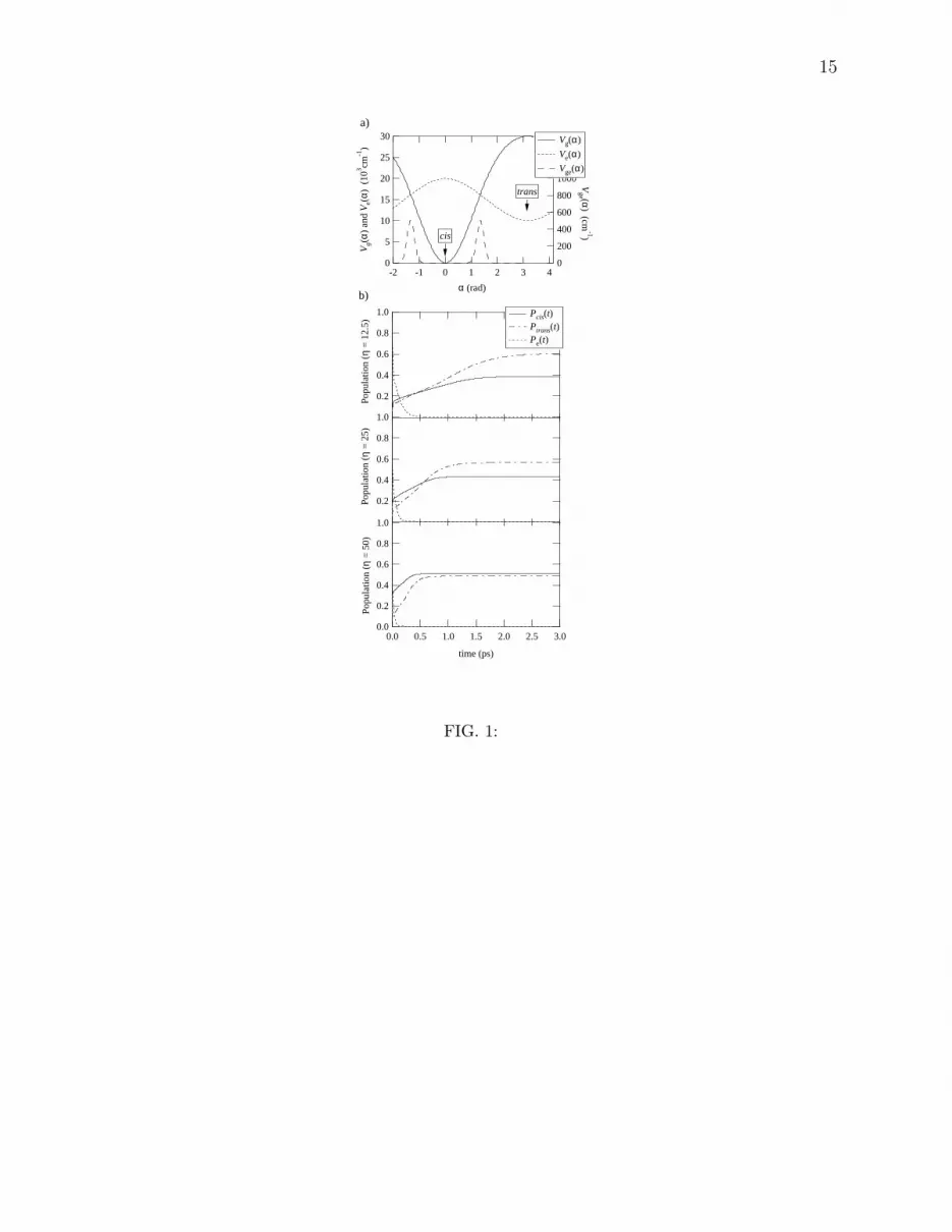
Figure 1b shows the time propagation of molecular populations under a typical laser

pulse of time duration 5 fs, amplitude 4 × 109 V/m, and a carrier frequency of 2 × 104 cm−1

that is resonant with the excitation to the electronic excited state around the Franck–

Condon region. The transition dipole moment, set at 10Debye, corresponds to an oscillator

strength f ≈ 1. At time t = 0, the cis population Pcis(t = 0) is almost unity, and after

t = 10 fs, probability is created in the excited state. Each panel in the Fig. 1b shows the

relaxation process with a different degree of system–environment coupling: η = 12.5, 25 and

50. Evident is the fact that the trans yield is lower, and the isomerization is faster, with

increasing coupling η to the bath. We note that the time scale of the reaction in Fig. 1 is in

accord with that observed experimentally using coherent light excitation of rhodopsin, i.e.

on the order of 200 fs [1, 2].

By contrast, the time dependence of the molecular populations for the case of excitation

by incoherent light is shown in Fig. 2. Here we examine the problem in a context relevant

to realistic biological systems. As seen in Fig. 2, for all η the rate of increase of Ptrans is

linear in time after a time that we denote as tc(η). Subsequent to that time the slope of

Ptrans vs. t is s = 9.4 × 10−8 s−1, corresponding to a cis/trans isomerization timescale of

9

almost one year. Note that the slope s is independent of the speed of photoisomerization

observed under pulsed laser conditions, as evidenced by the fact that it is independent of η.

Rather, this rate of transformation is dictated by the photon flux, which is the rate limiting

reagent in the process. By contrast, the time tc, which corresponds well to the time scale of

photoisomerization under the laser pulse, relates directly to η as tcη ≈ 20 ps. For example,

for the case of η = 12.5, tc = 1.5 ps, in accord with Fig. 1b.

Figure 2b shows the time dependence of Ptrans as a function of the luminance L of the

incoherent light source. The slope s is seen to be proportional to the luminance L as

s/L ≈ 3.1 × 10−6 Cd−1·m2·s−1.

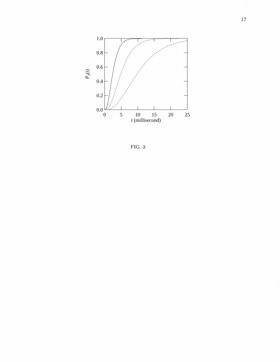
Since the isomerization of only a few molecules are necessary to induce hyperpolarization

in a rod cell [4], we compute P3, the probability that at least three from among all of the

cis molecules in a rod cell are converted to trans. The probability would then correspond

to the rate of our initial visual process under moonlight conditions. The probability P3(t)

that at time t at least three from among N molecules are trans is given by 1− p0 − p1 − p2,

where

pn = CnNpn(1 − p)N−n (12)

is a probability that n from among N molecules are converted to trans. Here, p = Ptrans(t) is

the probability that a molecule is trans at time t, and CnN is the binomial coefficient. For the

case of vision, we take the number of rhodopsin molecules in a rod cell to be N = 4×109 [15],

and assume that the time dependence of Ptrans maintains a constant slope s until t = 25 msec.

The resultant P3 values are shown in Fig. 3, where the time scale to obtain at least three

10

trans molecules is on the order of a few tens of milliseconds. This finding is consistent with

experimental time scales of 10 msec for dim flash response of a rod cell [4]. We note, as

in the previous results, that the speed of photoisomerization under pulsed laser conditions

bears no relation to the far longer time scales associated with the evolution of probability

P3, since the photon flux is rate-determining in the latter case. Note further that the times

at which P3(t) reaches the value of 0.5, a measure of the biological response, is virtually a

linear function of the irradiance.

Thus far, molecular time evolution in incoherent light was considered using the Redfield

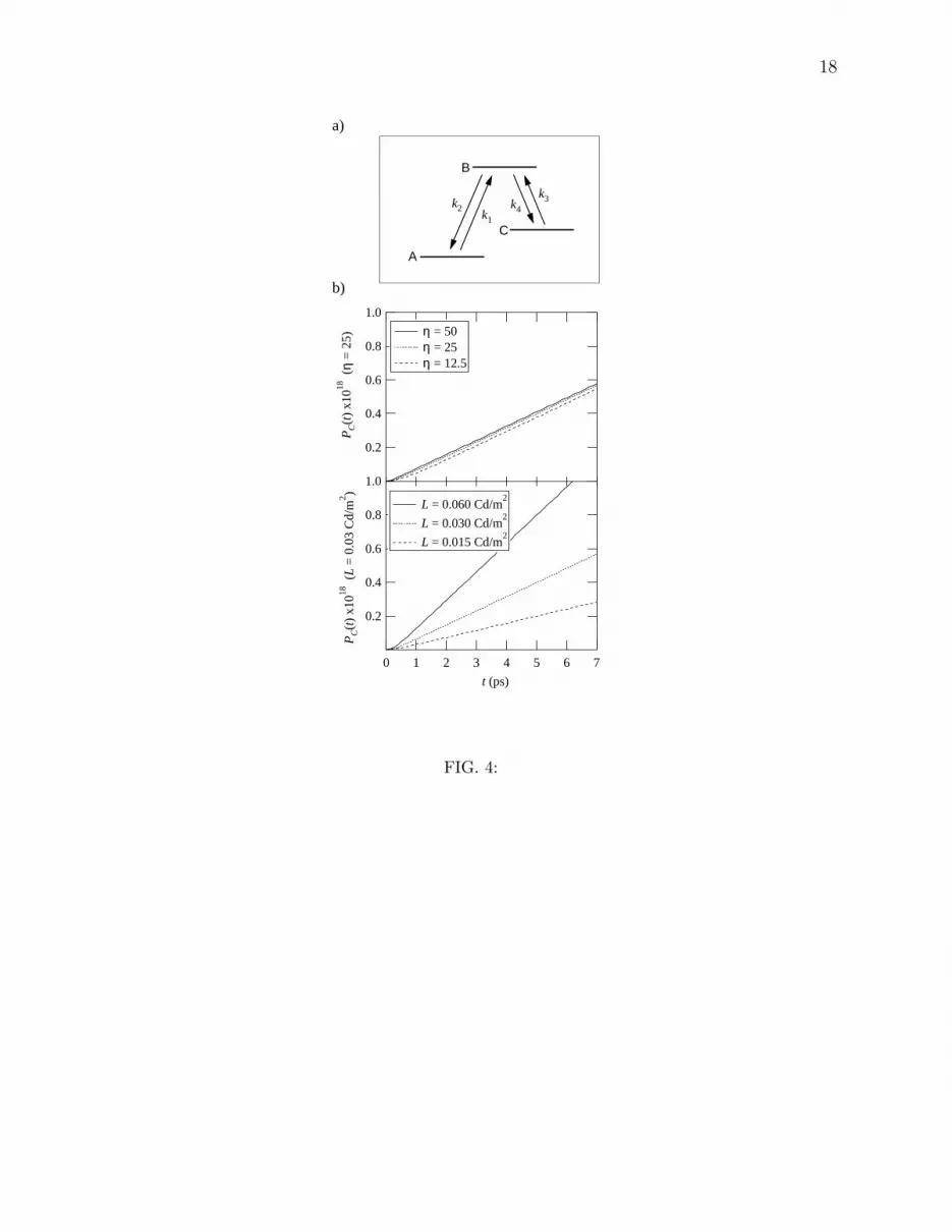
approach. We also find that the population transfer can be modeled analytically by solving

the simple three state model with the four reaction rates shown in Fig. 4. A comparison with

the computed Fig. 2 gives excellent results. Here, states A, B, and C represent cis, excited,

and trans conformations of the molecule, respectively. The values of k2 and k4 correspond

to rates of population transfer from Pe to Pcis and Ptrans, which are mainly caused by the

system–environment coupling. Values obtained from the coherent pulse studies of Fig. 1

give k2 = k4 = 0.08η ps−1. The k1 and k3 represent rates of population transfer from

Pcis and Ptrans to Pe, caused by both system–environment coupling and photoabsorption.

The rates of system–environment coupling can be assigned using detailed balance, and the

rates of photoabsorption are given by the Einstein transition probability from the electronic

ground state to the electronic excited state. In the case of k1, the primary contribution is

photoabsorption, giving k1 = BW = L × 5.6 × 10−6 Cd−1·m2·s−1, where B is the Einstein

B coefficient, and W is density of energy of the radiation field. The densities of the field

11

used in Fig. 4 correspond to the luminescence values used in Fig. 2 [16]. On the other

hand, in the case of k3, the dominant term is system–environment coupling, and we obtain

k3 = k4 × 1.87 × 10−9. With the resultant k1, k3 << k2, k4, the rate equations give

the reaction rate for isomerization under incoherent light as k1/2 = BW/2. Further, these

equations establish the existence of a linear region for Ptrans vs. t with an η independent slope

s = k1/2 after a time tc = 3/(k2 + k4), relating the rate approach to both the computed

coherent and incoherent results.

We note that the reaction rate obtained by the three state model is ≈10% smaller than

that given by the Redfield equation. The difference mainly comes from the simplifying

assumption that k2 = k4, and the evaluation of the rate of photoabsorption at the torsional

angle α set to zero. Nonetheless, all of the trends seen in the Redfield computed results are

also evident in the rate equation results.

IV. SUMMARY

We have presented a unified theoretical model of photoisomerization under both a co-

herent light source such as a femtosecond laser pulse and an incoherent light source such as

the moonlight. A minimal model of the isomerization process that gives the same timescale

as the femtosecond laser experiment was obtained. It was shown that the time scale for

photoisomerization under coherent light corresponds to the initial rise time tc of the photoi-

somerization under incoherent light. Further, we introduced a simple three state model that

incorporates all of the relevant rates obtained from both the femtosecond and millisecond

12

time domains.

This approach provides a connection between the time domain of the femtosecond laser

experiment and that of biologically relevant response time scales. A dynamical behavior

is seen even for the case of incoherent light source, since sudden irradiation of the light at

t = 0 introduces partial coherence into the system. The very earliest dynamics correlate

with the primary event of isomerization as identified in femtosecond laser experiments. The

exact response observed reflects the combined effect of the characteristics of the radiation

field and the underlying dynamics.

Acknowledgment: This work was carried out with partial support from Photonics Re-

search Ontario and NSERC Canada. We thank Professor R.J. Dwayne Miller for extensive

comments on a earlier version of this manuscript.

13

[1] Q. Wang, W. Schoenlein, L. A. Peteanu, R. A. Mathies, and C. V. Shand, Science 266, 422

(1994).

[2] H. Kandori, Y. Shichida, and T. Yoshizawa, Biochemistry(Moscow) 66, 1483 (2001).

[3] T. Kobayashi, T. Saito, and H. Ohtani, Nature 414, 531 (2001).

[4] N. Sperelakis, ed., Cell Physiology Source Book (Academic Press, San Diego, 1998), chap. 47,

2nd ed.

[5] X.-P. Jiang and P. Brumer, J. Chem. Phys. 94, 5833 (1991).

[6] X.-P. Jiang and P. Brumer, Chem. Phys. Lett. 180, 222 (1991).

[7] R. G. Redfield, IBM J. Res. Dev. 1, 19 (1957).

[8] K. Blum, Density Matrix Theory and Applications (Plenum Press, New York, 1981).

[9] V. May and O. Kuhn, Charge and Energy Transfer Dynamics in Molecular Systems (Wily-

VCH, Berlin, 2000).

[10] W. T. Pollard, A. K. Felts, and R. A. Friesner, Adv. Chem. Phys. 93, 77 (1996).

[11] H. Davison, Physiology of the Eye (Macmillan Press, London, 1990), 5th ed.

[12] R. Loudon, The Quantum Theory of Light (Oxford University Press, 1983), 2nd ed.

[13] W. H. Louisell, Quantum Statistical Properties of Radiation (John Wiley & Sons, 1990).

[14] ISO/CIE 10527 (1991) CIE Standard Colorimetric Observers.

[15] C. N. Graymore, ed., Biochemistry of the Eye (Academic Press, London, 1970), chap. 9.

[16] Here W = 2.5 × 10−11w(ω)L, where the coefficient is estimated by using the radius of pupil,

the distance between the lens and a surface, etc., L is luminance of the surface in Cd·m−2, and

w(ω) is the black body energy density at 4100K. Here, W and w(ω) have units of Joule·sec·m−3.

14

Figure Captions

FIG. 1: a) Potential energy surfaces for the two state model for cis to trans photoisomer-

ization. The solid curve and dotted curve show diabatic potentials Vg and Ve, respectively.

The dashed curve shows a coupling potential between two diabatic electronic states. b) Time

propagation of cis and trans populations under a short intense pulse for different values of

η. Pcis is the population in the range −π3

≤ α ≤ π3

on Vg, Ptrans is that in the range

−π ≤ α ≤ −2π3

on Ve, and Pe = 1−Pcis−Ptrans. Note that in Panels b and c, the very short

time dynamics, which includes the excitation from the cis, is not evident due to the short

time over which it occurs.

FIG. 2: a) Time dependence of Ptrans for three η values with incoherent light luminescence

L = 0.03Cd·m−2. b) Time dependence of Ptrans for various values of L, with system–

environment coupling η = 25. In all cases there is a deviation from strictly linear behavior

at the early times that corresponds to timescales of isomerization dynamics.

FIG. 3: Time dependence of the probability P3 that at least three from among 4×109 cis

molecules become trans for various values of L: 0.060Cd/m2 (solid); 0.030Cd/m2 (dotted);

0.015Cd/m2 (dashed).

FIG. 4: a) Three states model with reaction rates k1, k2, k3, and k4. Time propagation

of PC for each luminance L and strength parameter of system–environment coupling η.

Compare with results shown in Fig. 2.

15

30

25

20

15

10

5

0

Vg(

α) a

nd V

e(α)

(10

3 cm-1

)

43210-1-2

α (rad)

1400

1200

1000

800

600

400

200

0

Vge (α

) (cm-1)

Vg(α)

Ve(α)

Vge(α)

cis

trans

1.0

0.8

0.6

0.4

0.2

0.0

Popu

latio

n (η

= 5

0)

3.02.52.01.51.00.50.0

time (ps)

1.0

0.8

0.6

0.4

0.2Popu

latio

n (η

= 2

5)

1.0

0.8

0.6

0.4

0.2Popu

latio

n (η

= 1

2.5)

Pcis(t) Ptrans(t) Pe(t)

a)

b)

FIG. 1:

16

1.0

0.8

0.6

0.4

0.2

0.0

Ptr

ans(

t) x

1018

(η

= 2

5)

76543210time (ps)

1.0

0.8

0.6

0.4

0.2P

tran

s(t)

x10

18 (

L =

0.0

3 C

d/m

2 )

η = 50 η = 25 η = 12.5

L = 0.060 Cd/m2

L = 0.030 Cd/m2

L = 0.015 Cd/m2

(a)

(b)

FIG. 2:

17

1.0

0.8

0.6

0.4

0.2

0.0

P3(

t)

2520151050t (millisecond)

FIG. 3:

18

1.0

0.8

0.6

0.4

0.2

PC(t

) x1

018 (

η =

25)

76543210

t (ps)

1.0

0.8

0.6

0.4

0.2

PC(t

) x1

018 (

L =

0.0

3 C

d/m

2 )

L = 0.060 Cd/m2

L = 0.030 Cd/m2

L = 0.015 Cd/m2

η = 50 η = 25 η = 12.5

k2k1

k4

k3

A

B

C

a)

b)

FIG. 4: