dephasing in disordered systems at low temperatures
TRANSCRIPT
Dephasing in disordered systemsat low temperatures
Maximilian Treiber
München 2013

Dephasing in disordered systemsat low temperatures
Maximilian Treiber
Dissertationan der Fakultät für Physik
der Ludwig–Maximilians–UniversitätMünchen
vorgelegt vonMaximilian Treiber
aus Göttingen
München, den 25.04.2013
Erstgutachter: Prof. Dr. Jan von DelftZweitgutachter: Prof. Dr. Igor V. LernerTag der mündlichen Prüfung: 06.06.2013
Table of Contents
Deutsche Zusammenfassung 1
List of publications 3
1 Introduction, motivation and overview 5
2 Dephasing in disordered systems 92.1 Electrons in disordered systems . . . . . . . . . . . . . . . . . . . . . . . . . . . . . 9
2.1.1 Diagrammatic approach to disorder . . . . . . . . . . . . . . . . . . . . . . 102.1.2 Disorder averaged correlation functions . . . . . . . . . . . . . . . . . . . . 112.1.3 Magnetic field dependence and time-reversal symmetry . . . . . . . . . . . . 192.1.4 Validity of the loop-expansion . . . . . . . . . . . . . . . . . . . . . . . . . 212.1.5 Field theoretical approaches . . . . . . . . . . . . . . . . . . . . . . . . . . 222.1.6 Comparison with random matrix theory . . . . . . . . . . . . . . . . . . . . 23
2.2 Dephasing due to electron interactions . . . . . . . . . . . . . . . . . . . . . . . . . 282.2.1 Keldysh perturbation theory . . . . . . . . . . . . . . . . . . . . . . . . . . 282.2.2 Electron interactions in disordered systems . . . . . . . . . . . . . . . . . . 292.2.3 Quasi-particle lifetime of electrons in disordered systems . . . . . . . . . . . 322.2.4 Diagrammatic calculation of the dephasing time . . . . . . . . . . . . . . . . 372.2.5 Regimes of dephasing . . . . . . . . . . . . . . . . . . . . . . . . . . . . . 432.2.6 Electronic noise and the semi-classical picture of dephasing . . . . . . . . . 45
2.3 To be published: Two-loop calculation of the generalized diffusion propagator . . . 492.3.1 Dimensional regularization . . . . . . . . . . . . . . . . . . . . . . . . . . . 492.3.2 Ballistic regularization . . . . . . . . . . . . . . . . . . . . . . . . . . . . . 522.3.3 Conclusions . . . . . . . . . . . . . . . . . . . . . . . . . . . . . . . . . . . 57
2.4 Publication: Thermal noise and dephasing due to electron interactions in nontrivialgeometries . . . . . . . . . . . . . . . . . . . . . . . . . . . . . . . . . . . . . . . . 61
3 Quantum corrections to the conductance 713.1 The conductance of disordered metals . . . . . . . . . . . . . . . . . . . . . . . . . 71
3.1.1 The classical conductance . . . . . . . . . . . . . . . . . . . . . . . . . . . 713.1.2 Quantum corrections to the conductance: weak localization . . . . . . . . . 753.1.3 Universal conductance fluctuations . . . . . . . . . . . . . . . . . . . . . . 78
3.2 The random matrix theory of quantum transport . . . . . . . . . . . . . . . . . . . . 803.2.1 Conductance as a scattering problem . . . . . . . . . . . . . . . . . . . . . . 803.2.2 Quantum corrections . . . . . . . . . . . . . . . . . . . . . . . . . . . . . . 813.2.3 Models of dephasing . . . . . . . . . . . . . . . . . . . . . . . . . . . . . . 83
3.3 Dephasing in non-trivial geometries . . . . . . . . . . . . . . . . . . . . . . . . . . 84
3.3.1 Confined geometries . . . . . . . . . . . . . . . . . . . . . . . . . . . . . . 853.3.2 Networks of wires . . . . . . . . . . . . . . . . . . . . . . . . . . . . . . . 86
3.4 Publication: Dimensional crossover of the dephasing time in disordered mesoscopicrings . . . . . . . . . . . . . . . . . . . . . . . . . . . . . . . . . . . . . . . . . . . 91
3.5 Publication: Dimensional Crossover of the Dephasing Time in Disordered Meso-scopic Rings: From Diffusive through Ergodic to 0D Behavior . . . . . . . . . . . . 97
3.6 Publication: Transport and dephasing in a quantum dot: Multiply connected graphmodel . . . . . . . . . . . . . . . . . . . . . . . . . . . . . . . . . . . . . . . . . . 125
4 Quantum corrections to the polarizability 1374.1 Isolated systems: Realizing the canonical ensemble . . . . . . . . . . . . . . . . . . 1374.2 The polarizability in the random phase approximation . . . . . . . . . . . . . . . . . 1394.3 Results from RMT and the sigma-model . . . . . . . . . . . . . . . . . . . . . . . . 1404.4 Overview of recent experiments . . . . . . . . . . . . . . . . . . . . . . . . . . . . 1464.5 Preprint: Quantum Corrections to the Polarizability of Isolated Disordered Metals . 149
5 Summary and conclusions 163
A Source code listings 167A.1 Calculation of the two-loop Hikami boxes . . . . . . . . . . . . . . . . . . . . . . . 167
Bibliography 177
Acknowledgments 187
Curriculum vitae 189
AbstractThe transition from quantum to classical behavior of complex systems, known as dephasing, has fas-
cinated physicists during the last decades. Disordered systems provide an insightful environment to studythe dephasing time τϕ , since electron interference leads to quantum corrections to classical quantities,such as the weak-localization correction ∆g to the conductance, whose magnitude is governed by τϕ . Inthis thesis, we study one of the fundamental questions in this field: How does Pauli blocking influencethe interaction-induced dephasing time at low temperatures? In general, Pauli blocking limits the energytransfer ω of electron interactions to ω� T , which leads to an increase of τϕ . However, the so-called 0Dregime of dephasing, reached at T � ETh , is practically the only relevant regime, in which Pauli blockingsignificantly influences the temperature dependence of τϕ . Despite of its fundamental physical importance,0D dephasing has not been observed experimentally in the past. We investigate several possible scenariosfor verifying its existence: (1) We analyze the temperature dependence of ∆g in open and confined systemsand give detailed instructions on how the crossover to 0D dephasing can be reliably detected. Two concreteexamples are studied: an almost isolated ring and a new quantum dot model. However, we conclude thatin transport experiments, 0D dephasing unavoidably occurs in the universal regime, in which all quantumcorrections to the conductance depend only weakly on τϕ , and hence carry only weak signatures of 0Ddephasing. (2) We study the quantum corrections to the polarizability ∆α of isolated systems, and derivetheir dependence on τϕ and temperature. We show that 0D dephasing occurs in a temperature range, inwhich ∆α depends strongly (as a power-law) on τϕ , making the quantum corrections to the polarizabilityan ideal candidate to study dephasing at low temperatures and the influence of Pauli blocking.
A detailed summary of the of the contents of this thesis may be found at the end of Chapter 1, and inthe concluding Chapter 5.
Deutsche Zusammenfassung 1
Deutsche Zusammenfassung
Diese Doktorarbeit beschäftigt sich mit der Theorie der Dephasierung in ungeordneten mesoskopi-schen Systemen. Bei niedrigen Temperaturen wird das Pauli’sche Ausschlussprinzip wichtig und be-wirkt eine Schwächung der Wirkung von Elektronenwechselwirkungen, da Streuprozesse mit Energi-en ω� T aufgrund des Nichtvorhandenseins möglicher Streuendzustände ausgeschlossen sind. Wiranalysieren den Einfluss des Pauli-Prinzips auf die wechselwirkungsinduzierte Dephasierungsrate γund diskutieren mögliche Experimente, die den Einfluss des Pauli-Prinzips demonstrieren.
Die Arbeit ist in 4 Kapitel aufgeteilt, in denen wir zunächst den aktuellen Stand der Forschung be-schreiben und eine kurze Zusammenfassung unserer Ergebnisse präsentieren. Details unserer Ergeb-nisse finden sich in Veröffentlichungen am Ende jedes Kapitels. Eine graphische Zusammenfassungunserer Haupterkenntnisse findet sich in dem abschliessenden Kapitel 5, siehe Fig. 5.1.
Kapitel 1 beinhaltet eine allgemeine Einführung in die Thematik, gefolgt von einer Diskussion unsererMotiviation. Des weiteren findet sich hier eine kurze Darstellung der Gliederung dieser Arbeit.
In Kapitel 2 stellen wir die Standardmethoden der mesoskopischen Physik vor: die perturbative Schlei-fenentwicklung in diffusiven Propagatoren und die nicht-perturbative Theorie der Zufallsmatrizen.Wir besprechen die üblichen Herleitungen der Dephasierungsrate: (1) mittels einer Störungstheoriein der Elektronenwechselwirkung und (2) mittels eines Pfadintegrals mit effektivem Rauschpotential.Wir kommen zu dem Schluss, dass die Temperaturabhängigkeit der Dephasierungsrate durch eine ein-fache selbstkonsistente Integralgleichung hinreichend beschrieben wird. Des weiteren stellen wir fest,dass nur in dem sog. 0D Dephasierungsregime, erreicht bei Temperaturen T � ETh , das Pauli-Prinzipeinen signifikaten Einfluss auf das Temperaturverhalten der Dephasierungsrate hat. Dieses 0D Re-gime konnte jedoch trotz zahlreicher Versuche bisher nicht experimentell nachgewiesen werden. ImFolgenden haben wir uns daher auf die Beschreibung eines solchen Nachweises konzentriert. Von be-sonderer Bedeutung sind die folgenden Eigenschaften des 0D Regimes: (1) Es beschreibt ein Systemmit diskreten Energieniveaus, welches im Allgemeinen nicht mehr mit Hilfe der Schleifenentwicklungbeschrieben werden kann. (2) Die 0D Dephasierungsrate ist so klein, dass die relevanten Elektronen-trajektorien das ganze System ausfüllen und daher von der Geometrie des Systems abhängig werden.Unser erstes Hauptergebnis in diesem Kapitel ist die Berechnung der Zwei-Schleifen-Korrektur zumverallgemeinerten Diffusionspropagator, in der wir eine neue Methode zur Berechnung der kurzreich-weitigen Teile (die sogenannten Hikami-Boxen) der zugehörigen Diagramme vorschlagen. Die neueMethode kann direkt auf die Berechnung von Diagrammen höherer Ordnung und verwandte phy-sikalische Probleme ausgedehnt werden. Unser zweites Hauptergebnis ist die Herleitung eines neu-artigen Dephasierungsratenfunktionals, welches Dephasierung bei beliebigen Temperaturen und innicht-trivialen Geometrien, insbesondere Netzwerken von Drähten, beschreibt.
Kapitel 3 befasst sich mit der Leitwertkorrektur ∆g aufgrund von schwacher Lokalisierung, welchein offenen Systemen einen universellen Wert ∼ 1 annimmt, sobald γ� ETh . Da zudem T � γ gilt,liegt das 0D Dephasierungsregime in einem Temperaturbereich, in dem ∆g praktisch nicht mehr von
2 Deutsche Zusammenfassung
γ abhängt. Nichtsdestotrotz kann ein Nachweis von 0D Dephasierung in solchen Systemen gelingen,indem die Kurve ∆g(T ) vom universellen Leitwert bei T → 0 abgezogen wird. Wir argumentieren,dass ein verhältnismäßig kleiner Leitwert in Verbindung mit stark absorbierenden Zuleitungen einenNachweis von 0D Dephasierung ermöglichen könnte. Des weiteren befassen wir uns mit der Trans-porttheorie der Zufallsmatrizen, welche “eingeschlossene” Systeme beschreibt, in denen die Elek-tronentrajektorien den gesamten Raum des Systems ergodisch ausfüllen. Solche Systeme lassen sichmit Hilfe einer sogenannten Verweilzeit τdw beschreiben, und wir schlagen ein Modell vor, welchesDephasierung in annähernd isolierten Systemen beschreibt. Unser erstes Hauptergebnis in diesem Ka-pitel ist eine detaillierte Beschreibung der Temperaturabhängigkeit von ∆g eines annähernd isoliertenRings. Wir zeigen, dass die Ringgeometrie besonders gut geeignet ist, um den Übergang zu 0D Ver-halten zu untersuchen, da aufgrund des Aharonov-Bohm-Effekts die Beiträge zum Leitwert vom Ringvon den störenden Beiträgen der Zuleitungen getrennt werden können. Unser zweites Hauptergebnisist die Beschreibung der Dephasierung in einem Quantenpunktmodell, welches (1) auf der Theorieder Diffusion in Graphen und (2) auf dem Dephasierungsratenfunktional, hergeleitet in Kapitel 2,basiert. Unser Modell beschreibt die Leitwertkorrektur aufgrund von schwacher Lokalisierung bei be-liebigen Temperaturen und kann ohne Umschweife auf kompliziertere Geometrien erweitert werden.Wir folgern, dass eingeschlossene Systeme sich besser eignen, um den Übergang zu 0D Verhalten zuuntersuchen, jedoch tritt 0D Dephasierung unausweichlich im universellen Regime auf, solange derLeitwert der Kontakte zu den Zuleitungen größer als 1 ist.
In Kapitel 4 beschäftigen wir uns mit isolierten Systemen, in denen τdw→ ∞. Insbesondere befassenwir uns mit den Quantenkorrekturen zur Polarisierbarkeit ∆α eines Ensembles von isolierten und-geordneten Metallen. Bisherige Beschreibungen von ∆α, die auf einer Kombination der Theorie derZufallsmatrizen und dem nicht-linearen σ-Modell basierten, konnten die Frequenzabhängigkeit er-klären, beschrieben jedoch nicht die Dephasierung bei endlichen Temperaturen. Unser Hauptergebnisist eine Herleitung von ∆α mittels der Schleifenentwicklung, welche uns ermöglicht, die Tempera-turabhängigkeit zu beschreiben, und welche sowohl für verbundene (Großkanonisches Ensemble) alsauch isolierte (Kanonisches Ensemble) Systeme anwendbar ist. Wir konnten zeigen, dass, im Gegen-satz zu ∆g, der Übergang zum 0D Regime in einem Temperaturbereich auftritt, im dem ∆α einemPotenzgesetz in γ folgt. Unsere Ergebnisse stimmen gut mit vorherigen Experimenten überein undlegen nahe, dass 0D Dephasierung in den beobachteten Magnetooszillationen gefunden wurde. Auf-grund der kleinen Zahl an relevanten Datenpunkten bleibt dies jedoch derzeit eine Hypothese, dieerst in zukünftigen Experimenten hinreichend belegt werden kann. Nichtsdestotrotz folgern wir, dasssich die Quantenkorrekturen zur Polarisierbarkeit besonders für die Untersuchung von Dephasierungbei niedrigen Temperaturen eignen. Insbesondere lässt sich der Übergang zum 0D Regime und derEinfluss des Pauli-Prinzips hervorragend untersuchen. Es bleibt zu hoffen, dass unsere theoretischenErgebnisse zu neuen Experimenten in dieser Richtung führen werden.
List of publications 3
List of publications
During the work for this thesis the following articles have been published in peer-reviewed journals,as a chapter in a book, or made available as preprints:
1. Dimensional crossover of the dephasing time in disordered mesoscopic rings,MT, O. M. Yevtushenko, F. Marquardt, J. von Delft, and I. V. Lerner,published in Physical Review B 80, 201305(R) (2009),see Section 3.4.
2. Dimensional Crossover of the Dephasing Time in Disordered Mesoscopic Rings: From Diffu-sive through Ergodic to 0D Behavior,MT, O. M. Yevtushenko, F. Marquardt, J. von Delft, and I. V. Lerner,published as Chapter 20 in the bookPerspectives of Mesoscopic Physics: Dedicated to Yoseph Imry’s 70th Birthday,edited by A. Aharony and O. Entin-Wohlman (World Scientific, Singapore, 2010),see Section 3.5.
3. Thermal noise and dephasing due to electron interactions in nontrivial geometries,MT, C. Texier, O. M. Yevtushenko, J. von Delft, and I. V. Lerner,published in Physical Review B 84, 054204 (2011),see Section 2.4.
4. Transport and dephasing in a quantum dot: Multiply connected graph model,MT, O. M. Yevtushenko, F. Marquardt, J. von Delft, and I. V. Lerner,published in Annalen der Physik (Berlin) 524, 188 (2012),see Section 3.6.
5. Quantum Corrections to the Polarizability and Dephasing in Isolated Disordered Metals,MT, P. M. Ostrovsky, O. M. Yevtushenko, J. von Delft, and I. V. Lerner,available as preprint at arXiv:1304.4342,see Section 4.5.

1. Introduction, motivation and overview 5
Chapter 1
Introduction, motivation and overview
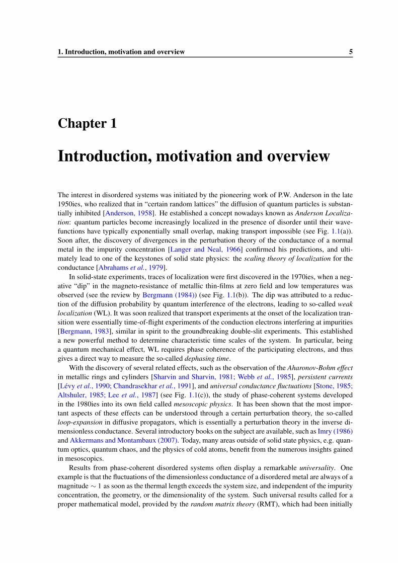
The interest in disordered systems was initiated by the pioneering work of P.W. Anderson in the late1950ies, who realized that in “certain random lattices” the diffusion of quantum particles is substan-tially inhibited [Anderson, 1958]. He established a concept nowadays known as Anderson Localiza-tion: quantum particles become increasingly localized in the presence of disorder until their wave-functions have typically exponentially small overlap, making transport impossible (see Fig. 1.1(a)).Soon after, the discovery of divergences in the perturbation theory of the conductance of a normalmetal in the impurity concentration [Langer and Neal, 1966] confirmed his predictions, and ulti-mately lead to one of the keystones of solid state physics: the scaling theory of localization for theconductance [Abrahams et al., 1979].
In solid-state experiments, traces of localization were first discovered in the 1970ies, when a neg-ative “dip” in the magneto-resistance of metallic thin-films at zero field and low temperatures wasobserved (see the review by Bergmann (1984)) (see Fig. 1.1(b)). The dip was attributed to a reduc-tion of the diffusion probability by quantum interference of the electrons, leading to so-called weaklocalization (WL). It was soon realized that transport experiments at the onset of the localization tran-sition were essentially time-of-flight experiments of the conduction electrons interfering at impurities[Bergmann, 1983], similar in spirit to the groundbreaking double-slit experiments. This establisheda new powerful method to determine characteristic time scales of the system. In particular, beinga quantum mechanical effect, WL requires phase coherence of the participating electrons, and thusgives a direct way to measure the so-called dephasing time.
With the discovery of several related effects, such as the observation of the Aharonov-Bohm effectin metallic rings and cylinders [Sharvin and Sharvin, 1981; Webb et al., 1985], persistent currents[Lévy et al., 1990; Chandrasekhar et al., 1991], and universal conductance fluctuations [Stone, 1985;Altshuler, 1985; Lee et al., 1987] (see Fig. 1.1(c)), the study of phase-coherent systems developedin the 1980ies into its own field called mesoscopic physics. It has been shown that the most impor-tant aspects of these effects can be understood through a certain perturbation theory, the so-calledloop-expansion in diffusive propagators, which is essentially a perturbation theory in the inverse di-mensionless conductance. Several introductory books on the subject are available, such as Imry (1986)and Akkermans and Montambaux (2007). Today, many areas outside of solid state physics, e.g. quan-tum optics, quantum chaos, and the physics of cold atoms, benefit from the numerous insights gainedin mesoscopics.
Results from phase-coherent disordered systems often display a remarkable universality. Oneexample is that the fluctuations of the dimensionless conductance of a disordered metal are always of amagnitude ∼ 1 as soon as the thermal length exceeds the system size, and independent of the impurityconcentration, the geometry, or the dimensionality of the system. Such universal results called for aproper mathematical model, provided by the random matrix theory (RMT), which had been initially
6 1. Introduction, motivation and overview
Figure 1.1: Effects in disordered systems:(a) STM images of GaMnAs for different Mn concentrations, showing the evolution of the local den-sity of states (LDOS) close to the Anderson transition: from weakly insulating (1.5%) to relativelyconducting (5%). [picture from Richardella et al. (2010)](b) The resistance of metallic films decreases as a function of the external magnetic field due to areduction of the weak localization effect. In the geometry of a cylinder with perpendicular magneticfield (lower picture), oscillations with a flux-period of hc/2e are superimposed due to the Aharonov-Bohm effect. (In this context they are also called Altshuler-Aronov-Spivak oscillations [Altshuleret al., 1981b]) [pictures from Bergmann (1984) and Altshuler et al. (1982b)](c) The dimensionless conductance g (G in units of e/h) of two samples in the mesoscopic regimeshows universal conductance fluctuations as a function of magnetic field: Although the samplesshown are totally different in shape and material, and their conductance differs by almost one order ofmagnitude, the fluctuations are ∼ 1. [pictures from Lee et al. (1987)]
used in the study of nuclear energy levels. Using RMT, exact universal results for quantities, suchas the energy level correlation function, have been found. These results had been known from theloop-expansion only in some restricted parameter range.
This thesis deals with disordered electronic systems at low temperatures. Such systems can beconsidered as being at the edge of mesoscopic universality since the dephasing time increases withdecreasing temperature. This is due to the fact that the temperature determines the magnitude of theenvironmental noise of the electrons, which in turn determines the inelastic scattering rate responsiblefor randomizing the phase of the electrons.
In a seminal work, Altshuler et al. (1982a) determined the dephasing time of electrons in a clas-sical Johnson-Nyquist noise environment (i.e. assuming white noise) using a path integral approach.Soon after, their results were confirmed by Fukuyama and Abrahams (1983) by means of a diagram-matic perturbation theory in the screened electron interaction propagators. Since then, numerousexperiments have shown their predicted dependence of the dephasing time on temperature, namelyτϕ ∼ T−2/3 for 1D - and τϕ ∼ T−1 for 2D -systems. However, both calculations assumed that thetemperature is still relatively high, so that the dephasing length is shorter than the system size.
At lower temperatures, a 0D regime of dephasing has been predicted by Sivan et al. (1994), where
1. Introduction, motivation and overview 7
dephasing is substantially weaker and the dephasing time depends on temperature as τϕ ∼ T−2 . Itis called “0D ” since it is reached independently of the geometry and real dimensionality of the sys-tem, while the results of Altshuler et al. (1982a); Fukuyama and Abrahams (1983) show a distinctdependence on dimensionality. The increase of the dephasing time in this regime is essentially due tothe Pauli principle. The Pauli principle prevents the electrons from exchanging energies larger thantemperature with their environment, and thus reduces the scattering rate. An environment where sucha behavior is observed is often referred to as quantum noise, and in contrast to classical white noise,it is characterized by a finite correlation time τT ∼ 1/T . However, despite of its physical importance,attempts to observe this 0D regime experimentally in mesoscopic systems have been unsuccessful so-far. From a fundamental point of view, this is somewhat unsatisfactory: since the difference betweenclassical and quantum noise has a very fundamental origin, namely the Pauli principle, our under-standing of dephasing is incomplete as long as the “deep quantum limit”, in which Pauli blockinginfluences dephasing in an essential way, remains hidden from experimental observation. An exper-imental verification of the existence of the 0D regime has been identified by Aleiner et al. (2002) asone of the major open challenges in the physics of disordered systems.
Therefore, the overall goal of this thesis is to theoretically analyze experimental scenarios thatwould allow the difference between classical and quantum noise to be probed experimentally.
In the following, we give a brief overview of the contents of this thesis. It is organized in threemain chapters, with our original results presented in publications at the end of each of them:
• Chapter 2 starts with a review of the disordered systems in general. We give a detailed derivationof the perturbative loop-expansion of quantum-corrections to important correlation functions,discuss their dependence on time-reversal symmetry, and give a comparison to non-perturbativeresults from RMT. We then introduce the concept of dephasing in this setting. Based on theapproach developed by von Delft et al. (2007), which uses the Keldysh diagrammatic techniqueand takes into account Pauli blocking, we discuss the influence of quantum noise on dephasingdue to electron interactions. By generalizing the calculations to arbitrary system sizes, we showhow all known regimes of the dephasing time, and in particular the 0D regime, can be describedon an equal footing.
We will see that for closed systems and in the absence of other sources of dephasing (besideselectron interactions), the weakness of dephasing in the 0D regime necessarily leads to a formalbreakdown of the loop-expansion, which is characterized by the onset of a discreteness in theenergy levels of the system. We provide a better understanding of the crossover regime, bycalculating the two-loop correction to the generalized diffusion propagator.
For transport experiments in open systems, we establish that 0D dephasing always occurs atthe edge of the universal regime, where the quantum corrections depend only weakly on thedephasing time. To make quantitative predictions on the dephasing time in this parameter range,one has to model the geometry of the system explicitly.
To achieve this, we derive the noise correlations for multiply-connected systems and use thisresult in order to develop a theory of dephasing by electronic noise applicable for arbitrarygeometries and arbitrary temperatures, which we formulate in terms of a trajectory-dependentfunctional.
• Chapter 3 is devoted to quantum corrections to the conductivity of disordered metals. Aftergiving a detailed derivation of the WL correction using the loop-expansion, we analyze itsdependence on the dephasing time. Moreover, we review the RMT of quantum transport anddiscuss the currently-known possibilities to incorporate dephasing in this theory.
8 1. Introduction, motivation and overview
In order to analyze the possibility to observe 0D dephasing in a conductance experiment, wediscuss two concrete scenarios:
(1) For a ring weakly coupled to leads in an external magnetic field, we show that 0D dephas-ing also governs the magnitude of the Altshuler-Aronov-Spivak oscillations at sufficiently lowtemperatures. This allows signatures of dephasing in the ring to be cleanly extracted by filteringout those of the leads.
(2) We propose a novel quantum dot model based on results from the theory of diffusion ingraphs, and using the functional derived in Chapter 2. We will see that in this model, whichis complementary to the RMT models, interaction-induced dephasing can be accounted for indetail, and we make qualitative predictions on the observability of 0D dephasing.
• In Chapter 4, we investigate the polarizability α of isolated metals. After briefly discussing theimplications of the fixed particle number in isolated systems, and the role of screening in thisproblem, we derive an expression for the quantum corrections of α.
In contrast to previous approaches which used a model based on RMT, we show how the cor-rections can be calculated by means of the loop-expansion. Using the two-loop correction to thegeneralized diffusion propagator derived in Chapter 2, we show that this perturbative calculationadequately reproduces the RMT result in the zero temperature limit. Importantly, our approachalso allows us to determine the dependence of α on the dephasing time, the temperature andthe magnetic field, and we compare our findings with recent experiments.
Finally, we show that quantum corrections to the polarizability might be the key to eventuallyobserve 0D dephasing in an experiment.
2. Dephasing in disordered systems 9
Chapter 2
Dephasing in disordered systems
2.1 Electrons in disordered systems
The goal of this section is a description of the electron dynamics in a disordered metal. Remarkably,an approximation in terms of free particles with kinetic energy H0 in a static disorder potential V (tobe specified further below) of the form
H = H0 +V , (2.1)
is usually sufficient. This is mainly due to two profound achievements of solid state theory, namelyelectronic band theory, which describes the influence of the periodic lattice potential of an underlyingcrystal, see e.g. Madelung (1978), and Landau-Fermi liquid theory, which includes the interactionsbetween the electrons, see e.g. Pines and Nozieres (1989). It is shown that most of the effects of thelattice-potential and the interactions can be accounted for, by shifting and rescaling parameters of thedispersion relation ε(k) of the electrons. As a result, the system is formally described by free quasi-particles with a finite lifetime, which have, however, essentially the same properties as free electrons.1
Importantly, due to the fermionic statistics of the quasi-particles, all excitations occur in the vicinityof the Fermi edge, characterized by a Fermi energy εF . In metals, εF is very large compared to thetypical excitation energies, which are usually of the order of temperature [εF & 104K ]. In fact, in thefollowing, we will always assume that εF is the largest energy scale, and we will measure particleenergies relative to εF .
For the disorder potential, we assume that at each point in space V (x) is an independent realGaussian random variable characterized by the probability distribution
P[V ] =1Z
∫DV exp
(− 1
2γ
∫ddx [V (x)]2
), (2.2)
where γ is a measure of the disorder strength and Z is a normalization constant. We denote thedisorder average of a quantity “A” with respect to the probability distribution function (2.2) by “ A ”.In particular, the lowest order correlation functions of V are given by
V (x) = 0 , V (x)V (y) = γδ(x−y) , (2.3)
and all higher correlation functions can be obtained from Eq. (2.3) using Wick’s theorem. A randompotential characterized by Eq. (2.3) is also called white noise.
1. We will discuss the lifetime τee of the quasi-particles in more details in Section 2.2, and simply assume that τee issufficiently large in the following.
10 2. Dephasing in disordered systems
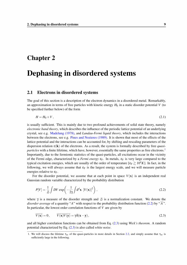
Figure 2.1: Diagrammatic representation of Eq. (2.6) and Eq. (2.7).
Eq. (2.2) is the simplest possible model of disorder, nevertheless, it accurately describes the long-range physics of many disordered systems. For a metal, it can be justified from a microscopic point ofview as follows: Assume that N impurities with potential u(x) are distributed randomly in the system(so-called Edwards model). E.g. u(x) might describe the real microscopic potential of impurities,dislocations, vacancies, etc. Then the total disorder potential is given by
V (x) =N
∑i=1
u(x−xi) . (2.4)
On scales larger than the range of u, the position xi of the microscopic potential should be irrelevant.After taking an average over all xi and taking the limit of a high density (N/V → ∞) of weak scatterers(u→ 0), one recovers Eq. (2.3), up to a shift of the electron energy.
A powerful tool to describe the dynamics of the system are the resolvents of the correspondingSchrödinger equation, called retarded/advanced Green’s functions, which are given for V = 0 by
GR/Aε (k) =
1ε− ε(k)± i0
. (2.5)
The regularizer, ±i0, is added to ensure that the Fourier transform of GR vanishes for times t < 0,while GA vanishes for t > 0. In the following we will calculate the disorder average of Eq. (2.5) andsee how important correlation functions can be calculated by using GR/A .
2.1.1 Diagrammatic approach to disorder
The standard way to study the system described by Eq. (2.1) is a perturbation theory in the disorderpotential. A detailed derivation of all results given in this section can be found, for example, in Leeand Ramakrishnan (1985) or Akkermans and Montambaux (2007). Diagrammatically expanding theretarded or advanced Green’s functions in powers of V results in the diagram shown in Fig. 2.1(a).Upon averaging according to Eq. (2.3), the term linear in V , as well as all other odd power termsvanish, while the even terms are paired according to Wick’s theorem. Each pair of potentials isrepresented by a dotted line in Fig. 2.1(b), called impurity line, and brings an additional factor ofγ, according to Eq. (2.3). Formally, we can sum up all diagrams using Dyson’s equation shown inFig. 2.1(c), with the result
GR/Aε (k) =
1ε− ε(k)± i/2τ
, (2.6)
2. Dephasing in disordered systems 11
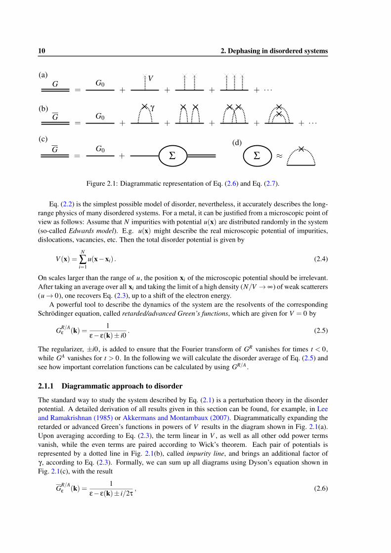
Figure 2.2: Diagramatic representation of the correlation functions P and K .
where −1/2τ is defined as the imaginary part of the irreducible self-energy Σ. [The real part gives anunimportant shift of the electron energy.] The calculation of the self-energy is in principle a difficultproblem since it contains an infinite number of terms. In the so-called first Born approximation, it isgiven by the diagram shown in Fig. 2.1(d). It is given by a momentum sum over an electron Green’sfunction (GR ) and an impurity line (γ):
12τ
=−Im[ΣR
ε (k)]≈−Im
[1V ∑
k′GR
ε (k−k′)γ
]= πρε γ . (2.7)
One can show that the higher order diagrams, which involve crossed and nested impurity lines, aresmall in terms of the parameter (εFτ)−1 . Note that in Eq. (2.6), τ determines the lifetime of theelectron in a momentum eigen-state k, and is often called momentum relaxation time or impurityscattering time. The corresponding length scale, defined via `= vFτ, where vF is the Fermi velocityof the electrons, is called the mean free path. Thus, (εFτ)−1� 1 describes a “classical limit” wherethe wavelength of the electrons is much shorter than the distance between two scattering events, whichis usually the case in a disordered metal.
In Eq. (2.7), we have introduced the density of states per unit volume,
ρε ≡1V ∑
kδ(ε− εk) (2.8)
=− 1πV ∑
kIm[GR
ε (k)]=
i2π[GR
ε (x,x)−GAε (x,x)
]. (2.9)
For a continuous energy spectrum, ρε is typically a slowly varying function of energy. Thus, in thefollowing we will often neglect its energy dependence and simple denote it by ρ≡ ρ0 . Furthermore,we see from substituting Eq. (2.6) in Eq. (2.9), that the density of states itself depends only weakly ondisorder for (εFτ)−1� 1, such that ρε ≈ ρ.
2.1.2 Disorder averaged correlation functions
In a classical disordered system, particle propagation in a random potential is diffusive for distanceslarger than ` and times larger than τ. To see that the same characteristic behavior survives in thequantum picture, we consider the probability of an electron of energy ε to propagate from x to y in
12 2. Dephasing in disordered systems
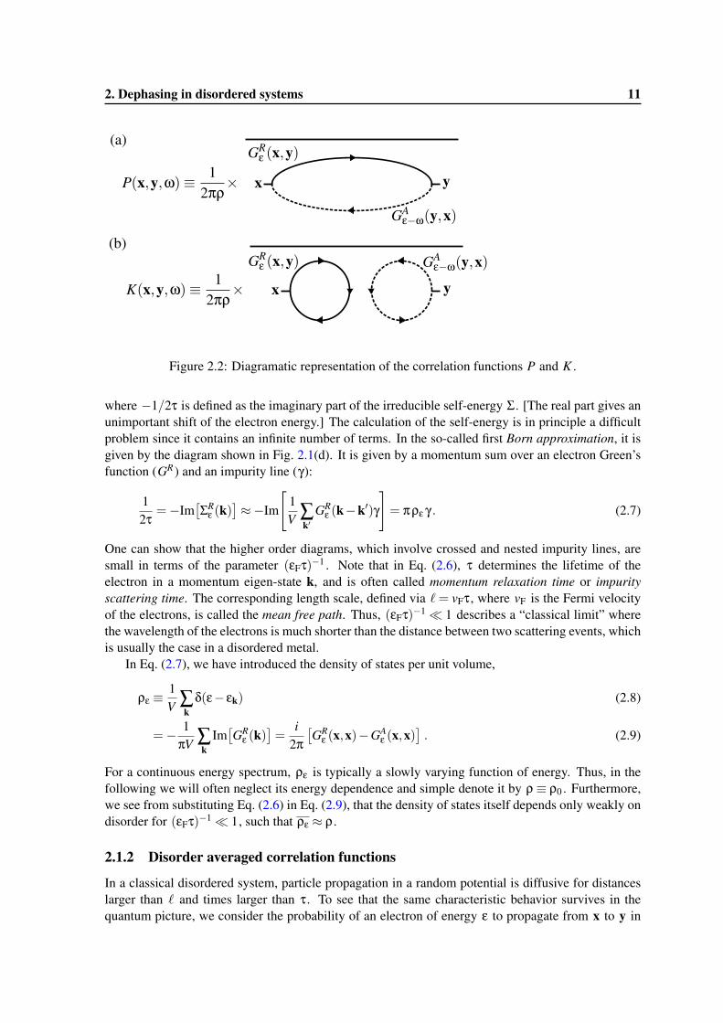
Figure 2.3: The ladder appromation to the generalized diffusion propagator.
time t . For large ε, it can be expressed as follows in terms of a correlation function of the retardedand advanced Green’s functions [Akkermans and Montambaux, 2007]:1
P(x,y, t) =∫ ∞
−∞
dω2π
e−iωt 12πρ
GRε (x,y)GA
ε−ω(y,x) . (2.10)
P is also called the generalized diffusion propagator, and plays an important role in the description ofthe transport properties of the metal, such as the conductivity considered in Chapter 3. Diagrammati-cally, we can represent Eq. (2.10) as a bubble shown in Fig. 2.2(a).
The second important correlation function which we consider here is shown in Fig. 2.2(b) anddefined as
K(x,y, t) =∫ ∞
−∞
dω2π
e−iωt 12πρ
GRε (x,x)GA
ε−ω(y,y) . (2.11)
Evidently, K is directly related to the fluctuations of the density of states, cf. Eq. (2.8). Thus, itdescribes spectral characteristics of the metal, such as the energy level correlations.
Note that we have suppressed the argument ε in the definitions of P and K , since the disorder av-eraged product of Green’s functions depends only weakly on their common energy, see e.g. Eq. (2.18)below.
Generalized diffusion propagator
Let us first consider P in a disordered system. The ”classical“ contribution to Eq. (2.10) is given bythe so-called ladder diagram, shown in Fig. 2.3. It is called “classical” due to the following argument:P can be interpreted as the interfering amplitudes of an electron, GR
ε , and a hole, GAε−ω , propagating
through a disorder landscape. In the limit (εFτ)−1� 1, their wavelengths are much shorter than themean free path, and we may visualize their trajectories as being two independent random walks chang-ing directions only at impurity positions. After averaging over the random disorder potential V (x),the quantum-mechanical phase difference of electron and hole is randomized. However, constructiveinterference is guaranteed if both, electron and hole, scatter at the same impurities in the same order.This process is precisely described by Fig. 2.3.
1. Formally, Eq. (2.10) follows from a description of the electron as wave-packed with energy-width ∆ε in the limit∆ε� εF .
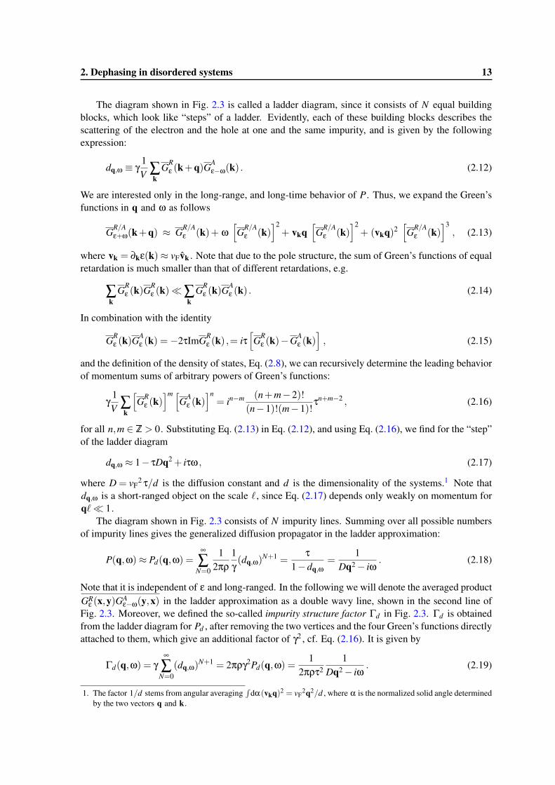
2. Dephasing in disordered systems 13
The diagram shown in Fig. 2.3 is called a ladder diagram, since it consists of N equal buildingblocks, which look like “steps” of a ladder. Evidently, each of these building blocks describes thescattering of the electron and the hole at one and the same impurity, and is given by the followingexpression:
dq,ω ≡ γ1V ∑
kGR
ε (k+q)GAε−ω(k) . (2.12)
We are interested only in the long-range, and long-time behavior of P. Thus, we expand the Green’sfunctions in q and ω as follows
GR/Aε+ω(k+q) ≈ GR/A
ε (k)+ ω[GR/A
ε (k)]2
+ vkq[GR/A
ε (k)]2
+ (vkq)2[GR/A
ε (k)]3
, (2.13)
where vk = ∂kε(k)≈ vFvk . Note that due to the pole structure, the sum of Green’s functions of equalretardation is much smaller than that of different retardations, e.g.
∑k
GRε (k)G
Rε (k)�∑
kGR
ε (k)GAε (k) . (2.14)
In combination with the identity
GRε (k)G
Aε (k) =−2τImGR
ε (k) ,= iτ[GR
ε (k)−GAε (k)
], (2.15)
and the definition of the density of states, Eq. (2.8), we can recursively determine the leading behaviorof momentum sums of arbitrary powers of Green’s functions:
γ1V ∑
k
[GR
ε (k)]m [
GAε (k)
]n= in−m (n+m−2)!
(n−1)!(m−1)!τn+m−2 , (2.16)
for all n,m ∈ Z> 0. Substituting Eq. (2.13) in Eq. (2.12), and using Eq. (2.16), we find for the “step”of the ladder diagram
dq,ω ≈ 1− τDq2 + iτω , (2.17)
where D = vF2 τ/d is the diffusion constant and d is the dimensionality of the systems.1 Note that
dq,ω is a short-ranged object on the scale `, since Eq. (2.17) depends only weakly on momentum forq`� 1.
The diagram shown in Fig. 2.3 consists of N impurity lines. Summing over all possible numbersof impurity lines gives the generalized diffusion propagator in the ladder approximation:
P(q,ω)≈ Pd(q,ω) =∞
∑N=0
12πρ
1γ(dq,ω)
N+1 =τ
1−dq,ω=
1Dq2− iω
. (2.18)
Note that it is independent of ε and long-ranged. In the following we will denote the averaged productGR
ε (x,y)GAε−ω(y,x) in the ladder approximation as a double wavy line, shown in the second line of
Fig. 2.3. Moreover, we defined the so-called impurity structure factor Γd in Fig. 2.3. Γd is obtainedfrom the ladder diagram for Pd , after removing the two vertices and the four Green’s functions directlyattached to them, which give an additional factor of γ2 , cf. Eq. (2.16). It is given by
Γd(q,ω) = γ∞
∑N=0
(dq,ω)N+1 = 2πργ2Pd(q,ω) =
12πρτ2
1Dq2− iω
. (2.19)
1. The factor 1/d stems from angular averaging∫
dα(vkq)2 = vF2q2/d , where α is the normalized solid angle determined
by the two vectors q and k .
14 2. Dephasing in disordered systems
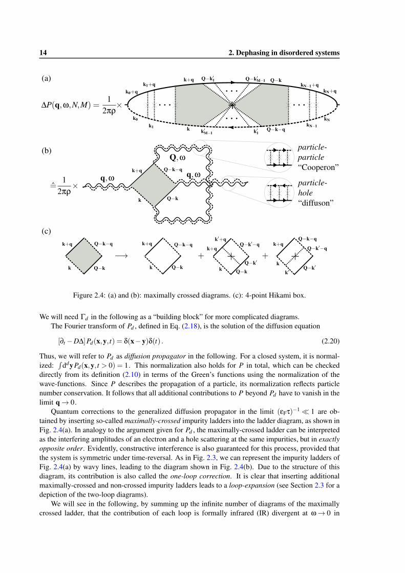
Figure 2.4: (a) and (b): maximally crossed diagrams. (c): 4-point Hikami box.
We will need Γd in the following as a “building block” for more complicated diagrams.The Fourier transform of Pd , defined in Eq. (2.18), is the solution of the diffusion equation
[∂t −D∆]Pd(x,y, t) = δ(x−y)δ(t) . (2.20)
Thus, we will refer to Pd as diffusion propagator in the following. For a closed system, it is normal-ized:
∫ddyPd(x,y, t > 0) = 1. This normalization also holds for P in total, which can be checked
directly from its definition (2.10) in terms of the Green’s functions using the normalization of thewave-functions. Since P describes the propagation of a particle, its normalization reflects particlenumber conservation. It follows that all additional contributions to P beyond Pd have to vanish in thelimit q→ 0.
Quantum corrections to the generalized diffusion propagator in the limit (εFτ)−1� 1 are ob-tained by inserting so-called maximally-crossed impurity ladders into the ladder diagram, as shown inFig. 2.4(a). In analogy to the argument given for Pd , the maximally-crossed ladder can be interpretedas the interfering amplitudes of an electron and a hole scattering at the same impurities, but in exactlyopposite order. Evidently, constructive interference is also guaranteed for this process, provided thatthe system is symmetric under time-reversal. As in Fig. 2.3, we can represent the impurity ladders ofFig. 2.4(a) by wavy lines, leading to the diagram shown in Fig. 2.4(b). Due to the structure of thisdiagram, its contribution is also called the one-loop correction. It is clear that inserting additionalmaximally-crossed and non-crossed impurity ladders leads to a loop-expansion (see Section 2.3 for adepiction of the two-loop diagrams).
We will see in the following, by summing up the infinite number of diagrams of the maximallycrossed ladder, that the contribution of each loop is formally infrared (IR) divergent at ω→ 0 in
2. Dephasing in disordered systems 15
dimensions d < 3 [Langer and Neal, 1966]. Thus the loop-expansion can be considered as a groupingof all possible crossed and non-crossed impurity lines in the most divergent contributions. We give adetailed discussion of this divergence and the validity of the loop-expansion in Section 2.1.4. For now,we simply assume that the contribution of each loop gives rise to a small factor, and that the leadingcorrection to P≈ Pd is given by the one-loop diagram shown in Fig. 2.4(a/b).
In Fig. 2.4(b), we see that the direction of the Green’s functions in the maximally-crossed impurityladder constituting the inner loop are reversed: This ladder thus expresses propagation in the so-called particle-particle channel, and is described by the so-called Cooperon propagator Pc (a notationadopted from superconductivity). This is in contrast to the diffuson propagator Pd , calculated inEq. (2.18), which describes propagation in the particle-hole channel. Correspondingly, we denoteeach “step” of an impurity ladder in the particle-particle channel as dc
q,ω , and note that it is given bydq,ω , calculated in Eq. (2.17), only if the system has time-reversal symmetry.
In the representation of Fig. 2.4(b), the short range part connecting the crossed to the regular im-purity ladders is highlighted as a shaded square consisting of two retarded and two advanced averagedGreen’s functions. This short-range part of the diagram is called Hikami box [Hikami, 1981]. Addinga single impurity line connecting two of the Green’s functions of equal retardation (also called dress-ing of the Hikami box), as shown in Fig. 2.4(c), one finds two more diagrams of the same order in(εFτ)−1� 1. Denoting this short-range part by H4 , we find for the diagram shown in Fig. 2.4(a):
∆P(q,ω,N,M) =1
2πρε× (dq,ω)
N× 1V ∑
Qγ(dc
Q,ω)M−1×H4(q,Q,ω) . (2.21)
Summing over all possible numbers of impurities and positions of the crossed ladder (N +1 possibil-ities), we find
∆P(q,ω) =∞
∑N=0
∞
∑M=1
(N +1)∆P(q,ω,N,M)
=1
2πρ1
(1−dq,ω)21V ∑
Q
γ1−dc
Q,ω×H4(q,Q,ω)
≈ 12πρ
1(Dq2− iω)2
1V ∑
QPc(Q,ω)× 1
2πρτ4 H4(q,Q,ω) , (2.22)
where Pc(Q,ω) = Pd(Q,ω) = (DQ2− iω)−1 only if the system has time-reversal symmetry. We willdiscuss the Q-sum and appropriate cutoffs in more detail in Section 2.1.4 below.
Let us now turn to a calculation of the Hikami box first. Naively writing down the expressionfollowing from the diagram in Fig. 2.4(c), it is given by the following sum of Green’s functions:
H4(q,Q,ω) ?= ∑
kGA
ε−ω(k)GRε (k+q)GA
ε−ω(Q−k−q)GRε (Q−k) (2.23)
+∑k
GRε (Q−k)GA
ε−ω(k)GRε (k+q)∑
k′GR
ε (k′+q)GA
ε−ω(Q−k′−q)GRε (Q−k′)
+∑k
GAε−ω(Q−k−q)GR
ε (Q−k)GAε−ω(k)G
Rε (k+q)∑
k′GR
ε (Q−k′)GAε−ω(k
′) .
Expanding in the transferred momenta and energies (q, Q, ω), using Eq. (2.13), and calculating thesums using Eq. (2.16) shows that all three diagrams are of the same order in τDq2 , τDQ2 , and τω,
16 2. Dephasing in disordered systems
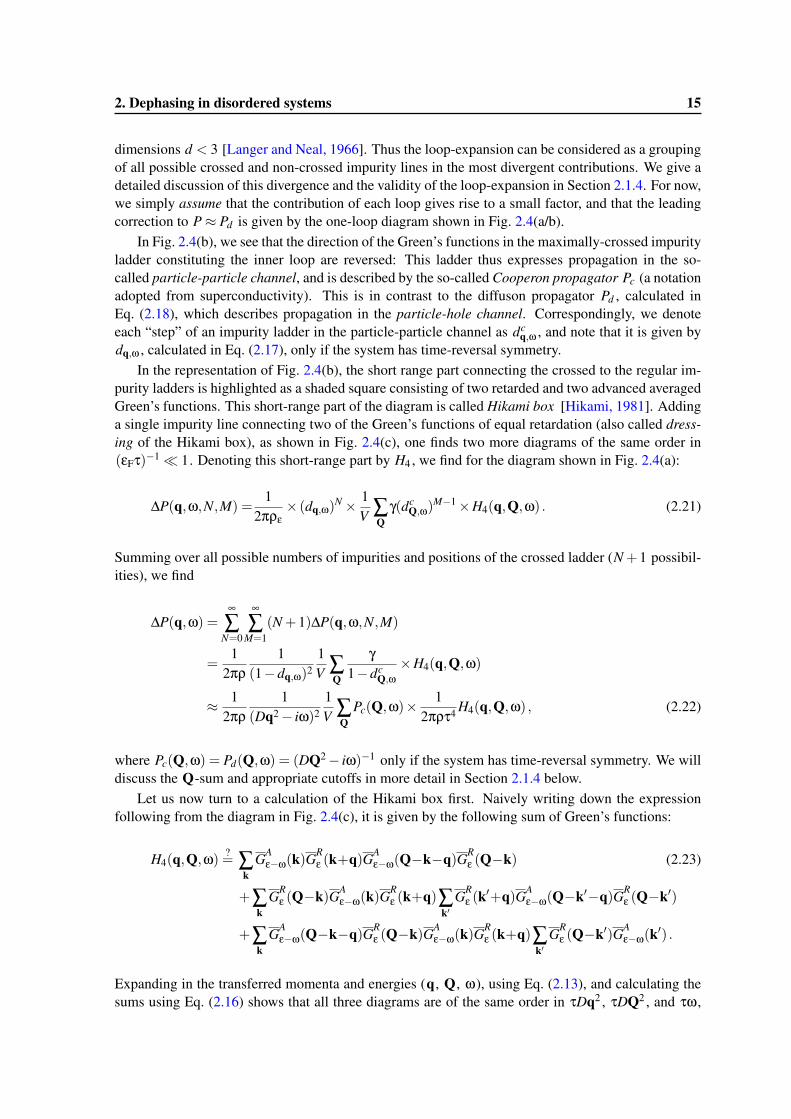
Figure 2.5: Illustration of the idea of Hastings et al. (1994): Moving a vertex with q = 0 around animpurity ladder generates a set of diagrams that cancels each other.
and that the leading terms cancel each other:
WRONG : H4(q,Q)≈ (2πρτ3)[2−2τD(q2 +Q2)+6iτω
](2.24)
+(2πρτ3)[−1+2τD(q2 +qQ+Q2)−4iτω
]
+(2πρτ3)[−1+2τD(q2−qQ+Q2)−4iτω
]
≈ 4πρτ4 [Dq2 +DQ2− iω]. (2.25)
Evidently, Eq. (2.23) has to be wrong, since inserting Eq. (2.25) in Eq. (2.22) leads to an UV-divergentQ-sum in any dimension. Moreover, the terms [DQ2− iω] violate particle number conservation, sincethey give a non-zero contribution to the generalized diffusion propagator at q = 0.
The problem can be resolved by the following argument: We assumed in Eq. (2.22), that themaximally crossed impurity ladder can have only one single impurity line (M = 1). However, asingle line together with an undressed Hikami box gives no new contribution to P, since it is alreadyincluded in the diffusion propagator Pd . On the other hand, a single line does give a new contribution,if the Hikami box is dressed! Thus, the maximally crossed ladder has an additional “step” wheneverthe Hikami box is undressed. Consequently, the first diagram of Fig. 2.4(c) should be multiplied byan additional factor of dQ,ω ≈ 1− τDQ2 + iτω. Multiplying the first line of Eq. (2.24) by dQ,ω , andcollecting terms to lowest order in τ gives instead of Eq. (2.25):1
CORRECT : H4(q,Q)≈ 4πρτ4Dq2 . (2.26)
Finally, substituting Eq. (2.26) in Eq. (2.22) gives the leading quantum correction to the generalizeddiffusion propagator:
∆P(q,ω)≈ 1πρ
Dq2
(Dq2− iω)21V ∑
QPc(Q,ω) . (2.27)
Note that ∆P(q→ 0,ω) = 0 as expected.
1. Remarkably, our argument for the calculation of H4 cannot, to the best of our knowledge, be found in the literature,albeit the final result for ∆P is well-known, see e.g. Aleiner et al. (1999).
2. Dephasing in disordered systems 17
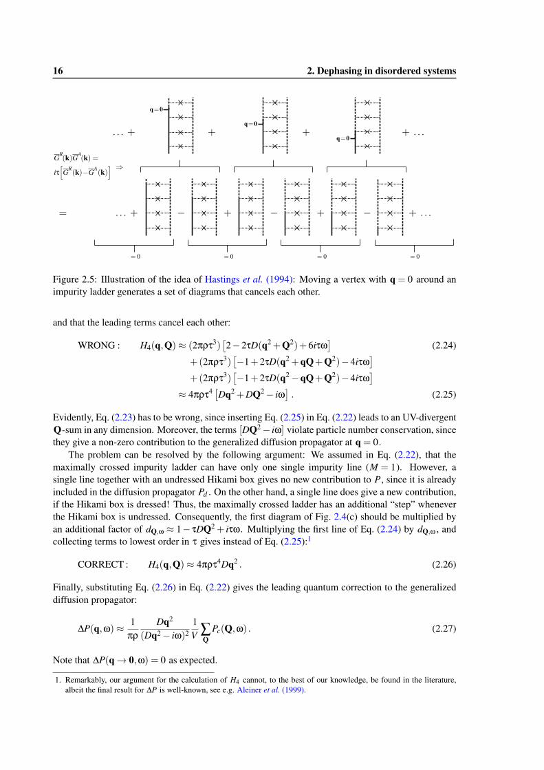
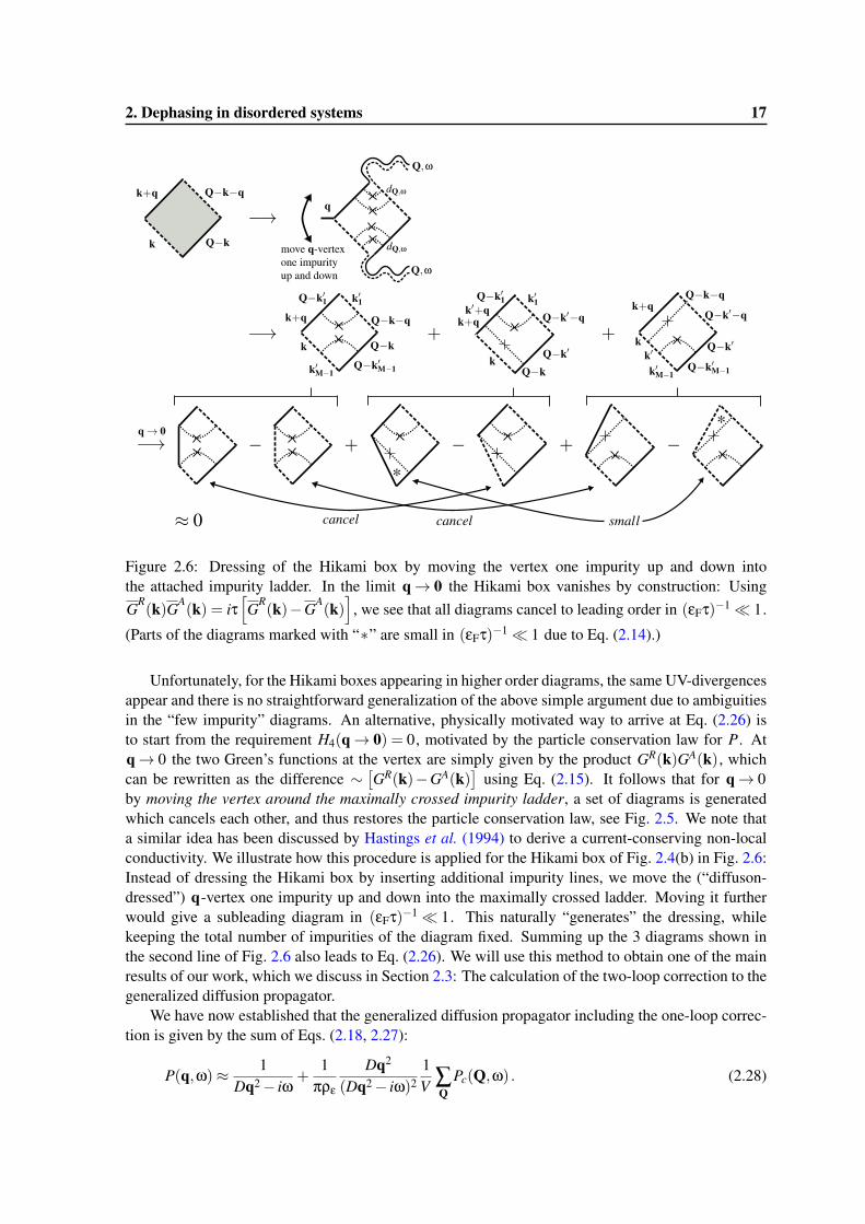
Figure 2.6: Dressing of the Hikami box by moving the vertex one impurity up and down intothe attached impurity ladder. In the limit q→ 0 the Hikami box vanishes by construction: UsingGR
(k)GA(k) = iτ
[GR
(k)−GA(k)]
, we see that all diagrams cancel to leading order in (εFτ)−1� 1.
(Parts of the diagrams marked with “∗” are small in (εFτ)−1� 1 due to Eq. (2.14).)
Unfortunately, for the Hikami boxes appearing in higher order diagrams, the same UV-divergencesappear and there is no straightforward generalization of the above simple argument due to ambiguitiesin the “few impurity” diagrams. An alternative, physically motivated way to arrive at Eq. (2.26) isto start from the requirement H4(q→ 0) = 0, motivated by the particle conservation law for P. Atq→ 0 the two Green’s functions at the vertex are simply given by the product GR(k)GA(k), whichcan be rewritten as the difference ∼
[GR(k)−GA(k)
]using Eq. (2.15). It follows that for q→ 0
by moving the vertex around the maximally crossed impurity ladder, a set of diagrams is generatedwhich cancels each other, and thus restores the particle conservation law, see Fig. 2.5. We note thata similar idea has been discussed by Hastings et al. (1994) to derive a current-conserving non-localconductivity. We illustrate how this procedure is applied for the Hikami box of Fig. 2.4(b) in Fig. 2.6:Instead of dressing the Hikami box by inserting additional impurity lines, we move the (“diffuson-dressed”) q-vertex one impurity up and down into the maximally crossed ladder. Moving it furtherwould give a subleading diagram in (εFτ)−1� 1. This naturally “generates” the dressing, whilekeeping the total number of impurities of the diagram fixed. Summing up the 3 diagrams shown inthe second line of Fig. 2.6 also leads to Eq. (2.26). We will use this method to obtain one of the mainresults of our work, which we discuss in Section 2.3: The calculation of the two-loop correction to thegeneralized diffusion propagator.
We have now established that the generalized diffusion propagator including the one-loop correc-tion is given by the sum of Eqs. (2.18, 2.27):
P(q,ω)≈ 1Dq2− iω
+1
πρε
Dq2
(Dq2− iω)21V ∑
QPc(Q,ω) . (2.28)
18 2. Dephasing in disordered systems
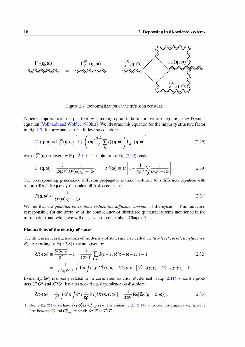
Figure 2.7: Renormalization of the diffusion constant.
A better approximation is possible by summing up an infinite number of diagrams using Dyson’sequation [Vollhardt and Wölfle, 1980b,a]. We illustrate this equation for the impurity structure factorin Fig. 2.7. It corresponds to the following equation:
Γd(q,ω) = Γ(0)d (q,ω)
[1+
(Dq2 2τ2
V ∑Q
Pc(q,ω)
)Γ(0)
d (q,ω)
], (2.29)
with Γ(0)d (q,ω) given by Eq. (2.19). The solution of Eq. (2.29) reads
Γd(q,ω) =1
2πρτ21
D∗(ω)q2− iω, D∗(ω) ≡ D
[1− 1
πρV ∑Q
1DQ2− iω
]. (2.30)
The corresponding generalized diffusion propagator is thus a solution to a diffusion equation withrenormalized, frequency-dependent diffusion constant:
P(q,ω)≈ 1D∗(ω)q2− iω
. (2.31)
We see that the quantum corrections reduce the diffusion constant of the system. This reductionis responsible for the decrease of the conductance of disordered quantum systems mentioned in theintroduction, and which we will discuss in more details in Chapter 3.
Fluctuations of the density of states
The dimensionless fluctuations of the density of states are also called the two-level correlation functionR2 . According to Eq. (2.8) they are given by
δR2(ω)≡ρερε−ω
ρ2 −1 =1
(ρV )2 ∑k,k′
δ(ε− εk)δ(ε−ω− εk′)−1 (2.32)
=− 1(2πρV )2
∫ddx
∫ddy [GR
ε (x,x)−GAε (x,x)]
[GR
ε−ω(y,y)−GAε−ω(y,y)
]−1 .
Evidently, δR2 is directly related to the correlation function K , defined in Eq. (2.11), since the prod-ucts GRGR and GAGA have no non-trivial dependence on disorder:1
δR2(ω) =1
V 2
∫ddx
∫ddy
1πρ
Re[δK(x,y,ω) ] =1
πρVRe[δK(q = 0,ω) ] . (2.33)
1. Due to Eq. (2.14), we have γ∑k GRε (k)GR
ε−ω(k)� 1 in contrast to Eq. (2.17). It follows that diagrams with impuritylines between GR
ε and GRε−ω are small: GRGR ≈ GR GR .
2. Dephasing in disordered systems 19
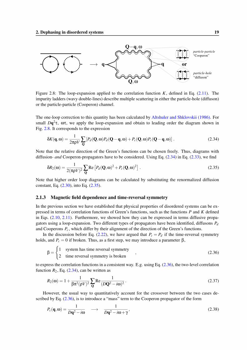
Figure 2.8: The loop-expansion applied to the correlation function K , defined in Eq. (2.11). Theimpurity ladders (wavy double-lines) describe multiple scattering in either the particle-hole (diffuson)or the particle-particle (Cooperon) channel.
The one-loop correction to this quantity has been calculated by Altshuler and Shklovskii (1986). Forsmall Dq2τ, ωτ, we apply the loop-expansion and obtain to leading order the diagram shown inFig. 2.8. It corresponds to the expression
δK(q,ω) =1
2πρV ∑Q[Pd(Q,ω)Pd(Q−q,ω)+Pc(Q,ω)Pc(Q−q,ω)] . (2.34)
Note that the relative direction of the Green’s functions can be chosen freely. Thus, diagrams withdiffusion- and Cooperon-propagators have to be considered. Using Eq. (2.34) in Eq. (2.33), we find
δR2(ω) =1
2(πρV )2 ∑Q
Re[Pd(Q,ω)2 +Pc(Q,ω)2] . (2.35)
Note that higher order loop diagrams can be calculated by substituting the renormalized diffusionconstant, Eq. (2.30), into Eq. (2.35).
2.1.3 Magnetic field dependence and time-reversal symmetry
In the previous section we have established that physical properties of disordered systems can be ex-pressed in terms of correlation functions of Green’s functions, such as the functions P and K definedin Eqs. (2.10, 2.11). Furthermore, we showed how they can be expressed in terms diffusive propa-gators using a loop-expansion. Two different types of propagators have been identified, diffusons Pdand Cooperons Pc , which differ by their alignment of the direction of the Green’s functions.
In the discussion before Eq. (2.22), we have argued that Pc = Pd if the time-reversal symmetryholds, and Pc = 0 if broken. Thus, as a first step, we may introduce a parameter β,
β =
{1 system has time reversal symmetry2 time reversal symmetry is broken
, (2.36)
to express the correlation functions in a consistent way. E.g. using Eq. (2.36), the two-level correlationfunction R2 , Eq. (2.34), can be written as
R2(ω) = 1+1
βπ2(ρV )2 ∑Q
Re1
(DQ2− iω)2 . (2.37)
However, the usual way to quantitatively account for the crossover between the two cases de-scribed by Eq. (2.36), is to introduce a “mass” term to the Cooperon propagator of the form
Pc(q,ω) =1
Dq2− iω−→ 1
Dq2− iω+ γ, (2.38)
20 2. Dephasing in disordered systems
or in real time:
Pc(q, t) = θ(t)e−Dq2 t −→ θ(t)e−Dq2 te−γ t . (2.39)
γ plays the role of an infrared cutoff to the sums appearing in the loop-expansion, such as Eq. (2.22).The diffuson propagator Pd calculated in Eq. (2.18), on the other hand, cannot acquire a mass dueto the requirement of particle conservation.1 Since the “mass” term γ describes the dephasing of theelectron and the hole of the Cooperon it is called the dephasing rate, and the corresponding time-scaleτϕ = 1/γ the dephasing time. In Section 2.2, we will calculate the contribution of electron interactionsto the mass of the Cooperon.
To explicitly see how a finite value of γ can appear, it is instructive to consider the influence of amagnet field on Pd and Pc . The Hamiltonian for a free electron in a random potential and an externalmagnetic field described by the vector potential A can be written as
H =− 12m
(∇+ i
ec
A)2
+V (x) . (2.40)
Assuming that the magnetic field is sufficiently weak, such that it does not affect the dynamics ofthe electron2, it’s sole effect is to modify the phase of the wave functions. For a sufficiently slowlyvarying field, it can be shown that the Green’s functions acquire an additional phase factor (see e.g.the discussion in Fetter and Walecka (1971)):
GR/Aε (x,y,A) = GR/A
ε (x,y)eiφ(x,y) , (2.41)
where the phase φ is given by a line integral over the vector potential:
φ(x,y) =−e∮ y
xdz ·A(z) . (2.42)
For diffuson propagators, which are given by geometric series of the products GR(x,y)GA
(y,x), thephase factors of Eq. (2.41) cancel exactly, such that Pd is unaffected by the magnetic field, and stilldescribed by the diffusion equation Eq. (2.20). For Cooperon propagators, on the other hand, whichare described by the products GR
(x,y)GA(x,y), the phases add up and lead to a total phase difference
of 2φ. Thus, the Cooperon in a magnetic field obeys a covariant diffusion equation given by[−iω−D(∇y +2ieA(y))2
]Pc(x,y,ω) = δ(x−y) , (2.43)
see Aronov and Sharvin (1987) for details. One consequence of the substitution ∇→ ∇+2ieA isthat in the geometry of a ring or a cylinder with perpendicular magnetic field B, the Cooperon be-comes a φ0/2-periodic function of the flux, where φ0 = 2πc/e is the flux quantum [Altshuler et al.,1981a]. Furthermore, the phase difference leads to a decay of the Cooperon at sufficiently large B.The characteristic time of the decay, τB , can be estimated from the condition
∆φ =BA(τB)
φ0' 1 , (2.44)
where A(t) is the typical area perpendicular to the magnetic field strength B, which is covered by theelectron trajectory in time t . For an infinite plane A(t) ∝ (
√Dt)2 , such that τB ∝ 1/B [Altshuler et al.,
1. The situation is different for the diffuson propagators appearing in the calculation of fluctuations, such as Eq. (2.34). Inthis case, the Green’s functions correspond to measurements of the density of states at different times and thus correspondto different realizations of disorder.
2. This is the case for rc� ` , where rc = mvF/eB is the cyclotron radius.
2. Dephasing in disordered systems 21
1980]. The case of a longitudinal magnetic field B, as well as quasi-1D wires, have been investigatedby Altshuler et al. (1980). The corresponding Cooperon propagator is thus of the form suggested inEq. (2.38):
Pc(q,ω) =1
Dq2− iω+1/τB. (2.45)
2.1.4 Validity of the loop-expansion
The one-loop quantum correction to the diffusion constant, Eq. (2.30), breaks down if
1ρV π ∑
Q
1DQ2− iω+ γ
� 1 , (2.46)
where we used expression (2.38) for the Cooperon propagator with a dephasing rate γ. Note that theprefactor of the sum, the inverse density of states, is often called level spacing:
∆≡ 1ρV
. (2.47)
Evidently, including higher order loop diagrams leads to additional terms on the l.h.s of Eq. (2.46)which are of the same form as the one-loop term, albeit raised to a higher power1, cf. Section 2.3.Moreover, the quantum corrections to other correlation functions, such as K , can be constructed bysubstituting the renormalized diffusion constant for D. Thus, the criterion (2.46) applies to the loop-expansion in general.
The summation in Eq. (2.46) runs over all diffusive modes Qα,n , where α = x,y,z and n ∈ Z.For example, in an open (not confined, connected) system of size Lα in direction α, the modes areQα,n ∼ n
Lα. Evidently, the sum is dominated by large momenta (UV) in dimensions d ≥ 2 and by small
momenta (IR) in d ≤ 2.2 Thus, we do not consider the case d = 3 in the following, where quantumcorrections are generally weak and independent of γ. Furthermore, we follow the general practice tointroduce an upper cutoff 1/` for d = 2, effectively assuming no quantum corrections from ballisticscales. The IR behavior on the other hand, is governed by ω and γ for a closed system. For connectedsystems, the sum has no zero mode in the connected direction and may also be dominated by theso-called Thouless energy ETh = D/L2 , representing the smallest diffusive mode. The inverse of theThouless energy, the so-called Thouless time τTh = L2/D is the average time needed to diffusivelytraverse the whole sample.
The implications of these findings to two types of experiments, typical conducted with disorderedsystems, are as follows:
• In transport experiments on open systems, which we will analyze (along with confined systems)in more detail in Chapter 3, the energy ω corresponds to the AC-frequency of the current source,and is typically small. In this case, for weak dephasing γ� ETh , the quantum corrections arecontrolled by the small parameter
1g≡ ∆
2πETh� 1 , (2.48)
1. Note that the Cooperon propagator in Eq. (2.46) may be replaced by a diffuson propagator in higher loops. But sincethe diffusion propagator has no dependence on a magnetic field, see Section 2.1.3, and quantum effects in disorderedsystems are often measured via the magnetic field dependent parts of observables, this is usually not a problem.
2. Note that d is the effective “quasi” dimension of the diffusive process, for which ` is the shortest length scale. Thedimension of the underlying electronic system might be larger.
22 2. Dephasing in disordered systems
where g is the so-called dimensionless conductance of the system, which is always large for adisordered metal (see Eq. (3.21)), implying that the loop-expansion is always valid. This regimeis often called mesoscopic, since the sample is completely phase coherent due to τϕ� τTh .Simultaneously, this regime is often called universal, since the quantum corrections to the con-ductance g become g× 1
g ∼ 1.
For strong dephasing ETh� γ, on the other hand, the corrections are controlled by the ratio∆/γ. In this regime, the temperature dependence of the dephasing time can be determineddirectly from the amplitude of the quantum corrections.
• Isolated systems can be studied by measuring their response to external electric or magneticfields, and we will give a detailed discussion of the polarizability of disordered metals in Chap-ter 4. In this case, ω is the frequency of the external field, and the quantum corrections arecontrolled by the parameter ∆/max(γ,ω). Evidently, at sufficiently low temperatures and fre-quencies, the loop-expansion can break down in this case. Since the level broadening γ becomessmaller than the level spacing ∆ in this limit, it can be interpreted as a transition to a discretelevel regime. The preferred theoretical method to study systems in this regime is the so-calledrandom matrix theory (RMT), which we discuss briefly in Section 2.1.6. However, there is nostraightforward way to include dephasing in RMT.
2.1.5 Field theoretical approaches
The field theoretical approach to disordered systems starts from a representation of the Green’s func-tion of Eq. (2.1) as an integral over a complex vector field φ(x), see Feynman and Hibbs (1965):
GRε (x,y) = 〈x|
1ε− H0−V ± i0
|y〉=−i∫
DφDφ∗ (φ(x)φ∗(y)) exp(iS [φ∗,φ])∫DφDφ∗exp(iS [φ∗,φ])
, (2.49)
with the action
S [φ∗,φ] =∫
ddz φ∗(z)[(ε+ i0)− H0−V
]φ(z) . (2.50)
Averaging over the random potential V with the probability distribution function (2.2) presents atechnical challenge often called the problem of denominator: Due to the appearance of V in the nu-merator and the denominator, the integral over fluctuating variables is largely intractable (see e.g. thediscussion in Altland and Simons (2006)). Different approaches have been identified to circumventthis problem, the most prominent beeing the replica trick [Edwards and Anderson, 1975], the Keldyshtechnique [Kamenev, 2005], and the supersymmetry approach [Efetov, 1983, 1997]. They share thefeature that the propagator, Eq. (2.49), is expressed as a field-integral without the necessity of a nor-malization factor in the denominator. As a result the disorder average is doable and leads to a quarticterm in the fields of the following form:
S [ψ∗,ψ]−→ S [ψ∗,ψ] =∫
ddz ψ∗(z)[(ε+ i0)− H0
]ψ(z)+
γ2[ψ∗(z)ψ(z)]2 . (2.51)
In Eq. (2.51), we wrote ψ instead of φ to make clear that this field must have a non-trivial internalstructure to avoid the denominator, e.g. in the replica formalism it carries an additional replica indexand in the supersymmetry approach it is a so-called supervector field which includes bosonic andfermionic degrees of freedom. The usual strategy to describe systems far from localization is now todecouple the disorder-generated quartic term by the Hubbard-Stratonovich transformation [Hubbard,
2. Dephasing in disordered systems 23
1959]. This is done by introducing an auxiliary field Q(x) and applying the identity
exp(−1
2[ψ∗(z)ψ(z)]2
)=
√1
2π
∫DQ exp
(−1
2Q(z)2− iQ(z)ψ∗(z)ψ(z)
)(2.52)
to the quartic term of Eq. (2.51). Importantly, due to the structure of the field ψ, the Hubbart-Stratonovich field Q must be matrix valued. After this transformation, the ψ field can be integratedout and one obtains an effective action that depends only on Q. However, minimizing this effectiveaction is not straightforward, since it is characterized by a whole manifold of saddle points such that Qand has to obey non-linear constraints. Performing a gradient expansion and expanding in excitationenergy ω to linear order and integrating out massive modes, one can derive an action describing thelow-lying excitations, which is known as the non-linear sigma model:
Sω[Q]∼∫
ddz Tr[−D[∇Q(z)]2−2iωQ(z)] , with Q(z)2 = 1 . (2.53)
In the context of the replica trick Eq. (2.53) was first derived by Schäfer and Wegner (1980); Efetovet al. (1980), and in the context of the supersymmetric technique by Efetov (1983).
The results for correlation functions calculated by using this low-energy field theory are identicalto those discussed in the previous sections. In particular, a similar loop-expansion can be generated,and the same limitations as discussed in Section 2.1.4 apply. Furthermore, Hikami (1981) has shownthat a certain parametrization of the Q matrix field exists, where the results of the Hikami boxesare identical to those obtained in perturbation theory, including the unphysical divergences discussedafter Eq. (2.24). In the field theoretical representation, a dimensional regularization scheme is usuallyapplied (see Brezin et al. (1980)) to obtain the physical results, and we show in Section 2.3, that theresults obtained in this way are identical, up to and including the second loop, to those obtained bythe “moving vertex”-procedure discussed in Fig. 2.6.
2.1.6 Comparison with random matrix theory
We have seen in the previous sections that only perturbative results for correlation functions of theGreen’s functions of our Hamiltonian (2.1) are known. In this section, we consider a simpler systemwhere non-perturbative results can be found: We assume that the Hamiltonian is simply given by arandom matrix H. In comparison to Eq. (2.1), this means that all spatial degrees of freedom in theproblem are neglected. Strictly speaking, these results are only relevant for effectively 0D systems,such as isolated quantum-dots. Nevertheless, we will discuss such a system here to gain insights onthe validity of the loop-expansion.
Random matrix theory (RMT) is a broad topic with an extremely wide range of applications inphysics and mathematics, such as: condensed matter physics, chaotic systems, spectra of complexnuclei, number theory, quantum gravity, traffic networks, stock movement in the financial markets,etc. An overview on the main ideas, results and applications can be found in Mehta (2004). However,the literature on this topic is often very mathematically oriented, for which reason we find it necessaryto discuss several aspects of RMT related to our work in this section.
The celebrated Gaussian random matrix ensemble of Wigner and Dyson is defined by the proba-bility distribution function (cf. Eq. (2.2))
P(H) ∝N
∏n,m=1
exp(−a|Hnm|2
). (2.54)
24 2. Dephasing in disordered systems
Eq. (2.54) describes N×N hermitian matrices H = H† , where each entry is an independent Gaussianrandom variable. H is identified as the Hamiltonian of a system, having N energy levels. Depend-ing on the global symmetry, the matrix elements Hnm are restricted: with time reversal symmetry,Hnm ∈ R, while Hnm ∈ C, if time reversal symmetry is broken. The symmetry is usually encoded inthe parameter β as follows
β =
{1 for Hnm ∈ R Gaussian orthogonal ensemble (GOE)2 for Hnm ∈ C Gaussian unitary ensemble (GUE)
, (2.55)
which is in analogy to the parameter introduced in Eq. (2.55). Note that the situation is more compli-cated if spin degrees of freedom are considered, but we restrict ourselves here to the symmetry classesdefined in Eq. (2.55).
Other probability distribution functions than Eq. (2.54) are the subject of active research. Inparticular, the model originally devised by Anderson (1958) to describe the localization transition canbe studied by a banded RMT, where the matrix elements in the exponential of Eq. (2.54) are weightedwith respect to their distance to the diagonal. Remarkably, many of these models can be solved in abroad range of parameters, see e.g. Fyodorov and Mirlin (1991); Bunder et al. (2007); Yevtushenkoand Kravtsov (2003); Yevtushenko and Ossipov (2007).
In the following we derive the density of states and the n-level correlation functions (loosely fol-lowing Kravtsov (2009)), which will be used in Chapter 4. We use the so-called method of orthogonalpolynomials here, and note that the same results can be obtained from a field-theoretical approach,namely, a 0D limit of the non-linear sigma model, see e.g. Mirlin (2000). We restrict our derivation tothe simpler unitary ensemble (β = 2), and then discuss briefly the generalization to β = 1. As a firststep, we rewrite the probability distribution function (2.54) in terms of the eigen-energies {εn} of Has follows
P({εn}) =C · J (εn) · exp
(−a
N
∑i=1
ε2i
). (2.56)
where C is a normalization constant, and J is the Jacobian of the transformation H = UDU† , whereU is a unitary matrix and D is a diagonal matrix containing the eigen-energies. The Jacobian is givenby the square of the so-called Vandermonde determinant VN :
J = |VN |β , VN = ∏1≤i< j≤N
|εi− ε j|=
∣∣∣∣∣∣∣∣∣∣
1 1 . . . 1ε1 ε2 . . . εN
ε21 ε2
2 . . . ε2N
. . . . . . . . . . . .εN
1 εN2 . . . εN
N
∣∣∣∣∣∣∣∣∣∣
. (2.57)
The result (2.57) can be explained by the following two arguments: (1) J must be a polynomialof degree N(N−1) since U has N(N−1)/2 independent complex variables, with independent realand imaginary part, and (2), since the Jacobian is a determinant, which is an alternating form, J hasto vanish whenever two eigen-values are identical. The latter is a fundamental property of randommatrices called level repulsion.
Using Eq. (2.56), we can directly evaluate quantities such as the averaged density of states ρε ,which is defined in analogy to Eq. (2.8) as
ρε =N
∑n=1
δ(ε− εn) , (2.58)
2. Dephasing in disordered systems 25
with the average being now calculated with respect to probability distribution (2.54). To do this, weconsider a seemingly unrelated problem: The wave-function of a system of N non-interacting 1Dfermions in a parabolic potential V (x) ∝ x2 is given by the Slater determinant:
Ψ({xn}) ∝
∣∣∣∣∣∣∣∣
ϕ0(x1) ϕ0(x2) . . . ϕ0(xN)ϕ1(x1) ϕ1(x2) . . . ϕ1(xN). . . . . . . . . . . .
ϕN(x1) ϕN(x2) . . . ϕN(xN)
∣∣∣∣∣∣∣∣, (2.59)
where ϕn(x) = Hn(x)exp(−x2/2
)and Hn(x) are the Hermite polynomials. As orthogonal polynomi-
als, they can be defined via a three-term recursive relation:
H0(x) = 1 , H1(x) = x , Hn+1(x) = 2xHn(x)−2nHn−1(x) . (2.60)
We immediately note the similarity between the slater determinant (2.59) and the Vandermonde de-terminant (2.57). In fact, using Eq. (2.60) it is easy to show that the absolute value squared of thewave-function (2.59) is equal to the probability density function (2.56), after substituting the coordi-nates xn by εn :
P({εn}) = |Ψ({εn})|2 . (2.61)
In the language of non-interacting fermions, the density of states (2.58) is nothing but the expec-tation value of the N-particle density operator n(x) = ∑N
i=1 δ(x− xi). In its second quantized formit is given by n(x) = ψ†(x)ψ(x), where the field operators are defined as ψ(x)≡ ∑n ϕn(x)an andψ†(x)≡ ∑n ϕn(x)a†
n . Thus, the expectation value of ψ†(x)ψ(x) in the N-particle ground state de-scribed by Ψ({εn}) is equal to the density of states averaged with respect to the probability distribu-tion function P({εn}). It directly follows that
ρε =N−1
∑n=0
ϕn(ε)2 . (2.62)
Eq. (2.62) relates the density of states of a unitary random matrix to a sum of products of orthogonalpolynomials. The advantage of this representation is due to the famous Christoffel-Darboux formula,which allows to calculate sums of this type very efficiently:
KN(x,y)≡N−1
∑n=0
ϕn(x)ϕn(y) =
√N2
ϕN−1(x)ϕN(y)−ϕN−1(y)ϕN(x)x− y
. (2.63)
The large-n limit of the Hermite polynomials is well-known in the physical literature, in particular inthe context of the WKB approximation [Schwabl, 2002]:
limn→∞x→0
(−1)nn1/4ϕ2n(x) =cos(2n1/2x)√
π, lim
n→∞x→0
(−1)nn1/4ϕ2n+1(x) =sin(2n1/2x)√
π. (2.64)
Using Eq. (2.64) in Eq. (2.63) for large N , we immediately obtain
KN→∞(x,y) =1π
sin(√
2N(x− y))
x− y. (2.65)
26 2. Dephasing in disordered systems
As a result the density of states of a unitary random matrix with large N and ε close to the band centeris given by:1
ρε = KN→∞(ε,ε) =1π√
2N , (2.66)
independent of ε, in full analogy to the density of states at the Fermi energy considered in Eq. (2.8).In the following we will denote it simply as ρ≡ ρε .
Correlation functions of higher order can be calculated in the same way: For example, the two-level correlation function R2 can be expressed by four fermionic field operators, ψ†(x)ψ(x)ψ†(y)ψ(y),and thus, can also be represented in terms of the wave-functions ϕn and the functions KN defined inEq. (2.63):2
R2(ε,ε′) =ρερε′
ρ2 =1ρ2
N−1
∑n=0
N−1
∑m=0
[ϕ2
n(ε)ϕ2m(ε′)−ϕn(ε)ϕn(ε′)ϕm(ε′)ϕm(ε)
](2.67)
=1ρ2
[KN(ε,ε)KN(ε′,ε′)−K2
N(ε,ε′)]. (2.68)
It is easy to show that the general n-level correlation function is given by the following determinant:
Rn(ε1,ε2, . . . ,εn) =1ρn
∣∣∣∣∣∣∣∣
KN(ε1,ε1) KN(ε1,ε2) . . . KN(ε1,εn)KN(ε2,ε1) KN(ε2,ε2) . . . KN(ε2,εn)
. . . . . . . . . . . .KN(εn,ε1) KN(εn,ε2) . . . KN(εn,εn)
∣∣∣∣∣∣∣∣. (2.69)
Using Eq. (2.65) in Eq. (2.68) we find R2 in the limit N→ ∞
RGUE2 (ε,ε′) = 1− sin2(πs)
(πs)2 , s≡ ε− ε′
∆, (2.70)
where the mean level spacing is defined in analogy to Eq. (2.47) as ∆ = 1/ρ = π/√
2N .In the orthogonal ensemble (β = 1), the Jacobian J in Eq. (2.56) is proportional to |VD| instead
of |VD|2 . In this case, there is a similar analogy to interacting particles: the so-called Calogero-Sutherland model [García-García and Verbaarschot, 2003]. However, instead of orthogonal polyno-mials (such as the Hermite polynomials), so-called skew-orthogonal polynomials of real type haveto be considered [Mehta, 2004]. Nevertheless it can be shown that the average density of states andthe n-level correlation functions are still given by Eqs. (2.66, 2.69), when replacing the real-valuedfunction KN with a different, biquaternion3-valued function. The result for the two-level correlationfunction in the orthogonal ensemble is
RGOE2 (ε,ε′) = 1− sin2(πs)
(πs)2 −[∫ ∞
sdu
sin(πu)πu
][dds
sin(πs)πs
]. (2.71)
In the limits of large energy separations, the envelope of Eqs. (2.70, 2.71) yield
R2 (ω/∆→ ∞) = 1− ∆2
βπ2ω2 . (2.72)
1. Since the limits N→ ∞ and x→ y in Eq. (2.63) do not commute, Eq. (2.66) is only valid for 2N� ε2 . For arbitraryN , the result for ρε is Wigner’s celebrated semi-circle: ρε =
√2N− ε2/π , see Mehta (2004).
2. In Eq. (2.67) and further expressions for R2 we assume ε 6= ε′ , and neglect a trivial contribution R2(ε,ε′) ∝ δ(ε− ε′)stemming from one and the same level n in Eq. (2.58).
3. Biquaternions are quaternions where all 4 coefficients are complex numbers.
2. Dephasing in disordered systems 27
-0.1
0
0.1
0.20.3
0.4
0.5
0 0.5 1 1.5 2 2.5 3
R2(
ω,β=
1)−
R2(
ω,β=
2)
s = ω/∆
RMTone-loop, γ = ∆/π
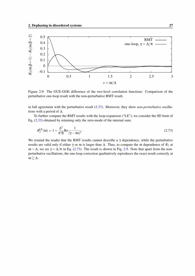
Figure 2.9: The GUE-GOE difference of the two-level correlation functions: Comparison of theperturbative one-loop result with the non-perturbative RMT result.
in full agreement with the perturbative result (2.37). Moreover, they show non-perturbative oscilla-tions with a period of ∆.
To further compare the RMT results with the loop-expansion (“LE”), we consider the 0D limit ofEq. (2.33) obtained by retaining only the zero-mode of the internal sum:
RLE2 (ω) = 1+
∆2
π2βRe
1(γ− iω)2 . (2.73)
We remind the reader that the RMT results cannot describe a γ dependence, while the perturbativeresults are valid only if either γ or ω is larger than ∆. Thus, to compare the ω dependence of R2 atω∼ ∆, we set γ = ∆/π in Eq. (2.73). The result is shown in Fig. 2.9. Note that apart from the non-perturbative oscillations, the one-loop correction qualitatively reproduces the exact result correctly atω & ∆.
28 2. Dephasing in disordered systems
2.2 Dephasing due to electron interactions
We have argued in Section 2.1.3, that all processes that break the time-reversal symmetry of the systemlead to a reduction of the quantum corrections described by Cooperon propagators. Moreover, we haveintroduced the dephasing time τϕ in terms of the inverse “Cooperon mass” γ = 1/τϕ in Eq. (2.38).The goal of this section is a description of dephasing due to inelastic scattering events.
Inelastic scattering of electrons in a disordered metal is typically due to interactions with phononsor other electrons. However, experiments in mesoscopic systems are usually conducted at tempera-tures T . 1K , where the lattice vibrations of the underlying crystal are effectively “frozen” [Altshuleret al., 1981c]. Thus, in the following, we will concentrate solely on electron interactions and neglectthe influence of phonons.
2.2.1 Keldysh perturbation theory
In contrast to the perturbation theory in the static potential V (x) used in the first part of this Chapter,electron interactions in disordered metals are time-dependent due to dynamical screening, which wewill discuss in the following section. Moreover, we have so far not accounted for the influence oftemperature, which plays an important role in the description of inelastic scattering.
Two well-established formalisms have been developed to describe problems of this type: TheMastsubara technique and the Keldysh technique. Both have their advantages and disadvantages (seee.g. Zagoskin (1998) for a detailed comparison): The former introduces discrete Matsubara frequen-cies, and requires to calculate a non-trivial analytic continuation to real frequencies in the end. Inthe latter, which we will employ here, the propagators become matrices. The reason for the matrixstructure in the Keldysh technique is that the time evolution of the field operators is calculated byintegrating the Hamiltonian over times along a closed contour from −∞ to +∞ and back to −∞.This is in contrast to the integration over an inverse temperature interval in the Matsubara formalismor the real axis for T = 0. Since one needs to keep track of the location of the time arguments ofthe field operators in the perturbative expansions, and since each of them can be on the forward orbackward contour, this leads to a 2×2 matrix structure for the propagators. The main advantagesof the Keldysh technique are (i) that it can describe non-equilibrium situations, (ii) that the occur-rence of a normalization factor (partition function) is avoided, and (iii) that a finite temperature isautomatically accounted for. Note that the Keldysh technique has been developed primarily to dealwith non-equilibrium processes, but we will restrict ourselves exclusively to thermal equilibrium inthe following.
However, we will not give a detailed discussion or derivation of the Keldysh technique here andrestrict ourselves purely to the “user perspective”. The interested reader is referred to the books byRammer (2007) and Kamenev (2011). Note that the matrix structure is not unique and many differentconventions can be found in the literature. In the following, we strictly follow the notations of Rammerand Smith (1986), who use a representation originally introduced by Larkin and Ovchinnikov (1975).
In Section 2.1 we have introduced the retarded and advanced Green’s functions as electron prop-agators, and argued that they have a simple perturbative expansion in a static potential V (x), cf.Eq. (2.1). In the Keldysh perturbation theory, the propagators of the electrons G and electron interac-tions U are represented as upper triangular matrices, defined as:
Gε(x,y) =(
GRε(x,y) GK
ε (x,y)0 GA
ε (x,y)
), U ω(x,y) =
(UR
ω(x,y) UKω (x,y)
0 UAω(x,y)
), (2.74)
where the so-called Keldysh Green’s functions are given in thermal equilibrium by
GKε (x,y) = hε
[GR
ε (x,y)−GAε (x,y)
], UK
ω (x,y) = gω[UR
ω(x,y)−UAω(x,y)
], (2.75)
2. Dephasing in disordered systems 29
with
hε = tanh( ε
2T
), gω = coth
( ω2T
). (2.76)
The information on the occupation of the energy levels at temperature T is fully contained in thefunctions h and g, defined in Eq. (2.76).
The relations of Eq. (2.75) are also known as fluctuation dissipation theorem (FDT), since theKeldysh Green’s function effectively describes the fluctuations of the electron field operators, whilethe retarded and advanced functions describe their response to an external perturbation.
Let us now briefly summarize the rules of this perturbation theory: The perturbation expansionof the propagators (as described by Wick’s theorem) at finite temperature is equivalent to the usualFeynman diagrams at T = 0, when replacing the time ordered Green’s functions by the matricesdefined in Eq. (2.74). In particular, multiplying Green’s functions and expanding in scalar potentials isrepresented by the usual matrix multiplication. However, interaction vertices have to be distinguishedby absorption, γ i
a and emission γ je vertices, and they have a tensor structure with the additional indices
i, j ∈ {1,2} denoting the i, j’th component of the matrix U to which the Green’s functions G couple:
γa1 = γe
2 =1√2
(1 00 1
), γa
2 = γe1 =
1√2
(0 11 0
). (2.77)
Moreover, matrix multiplication has to be carried out opposite to the propagation direction, which wewill denote by arrows on the propagators. The tensor structure will become more clear in the examplesbelow, see e.g. Eqs. (2.82, 2.113). The other rules are identical to the T = 0 theory. In particular,the diagrammatic n’th order expansion of the electron Green’s function in interaction propagators ismultiplied by in(−1)F , where F is the number of electron loops [Abrikosov et al., 1965].
2.2.2 Electron interactions in disordered systems
In this section, we will begin our discussion of electron interactions by analyzing the influence ofdiffusive screening. Interactions between free electrons are described by a potential U0 given byCoulomb’s law [Jackson, 1962]:1
U0(x,y) =e2
|x−y| , U0(q) =
4πe2/|q|2 (d = 3)2πe2/|q| (d = 2)−2e2 ln |q|W (d = 1)
. (2.78)
In a metal, the interaction is substantially screened due to the high electron density. This is usu-ally accounted for in the random phase approximation (RPA), where the creation and annihilationof electron-hole pairs by the interaction are taken into account [Gell-Mann and Brueckner, 1957](see e.g. Bruus and Flensberg (2004) for a detailed discussion). As a result, the effective Coulombpotential becomes short ranged:
U(x,y) =U0(x,y)e−κ|x−y| , (2.79)
where the Thomas-Fermi screening wave-vector is given by
κ =
{√8πe2ρ (d = 3)
4πe2ρ (d = 2). (2.80)
1. We follow the usual sign convention in Eq. (2.78). As a result, all diagrams are multiplied by (−1)I , where I is thenumber of interaction lines.
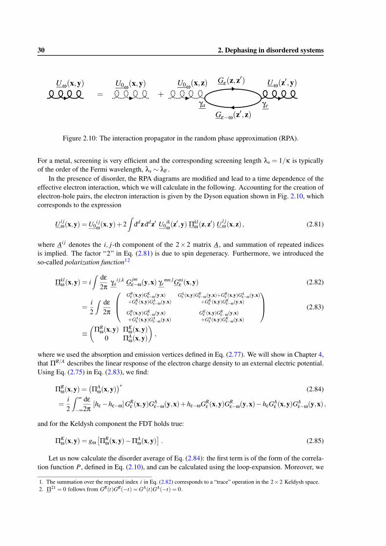
30 2. Dephasing in disordered systems
Figure 2.10: The interaction propagator in the random phase approximation (RPA).
For a metal, screening is very efficient and the corresponding screening length λs = 1/κ is typicallyof the order of the Fermi wavelength, λs ∼ λF .
In the presence of disorder, the RPA diagrams are modified and lead to a time dependence of theeffective electron interaction, which we will calculate in the following. Accounting for the creation ofelectron-hole pairs, the electron interaction is given by the Dyson equation shown in Fig. 2.10, whichcorresponds to the expression
U i jω(x,y) =U0
i jω(x,y)+2
∫ddzddz′ U0
ikω(z′,y) Πkl
ω (z,z′) U l j
ω(x,z) , (2.81)
where Ai j denotes the i, j-th component of the 2×2 matrix A, and summation of repeated indicesis implied. The factor “2” in Eq. (2.81) is due to spin degeneracy. Furthermore, we introduced theso-called polarization function12
Πklω (x,y) = i
∫ dε2π
γai j,k G jm
ε−ω(y,x) γemn,lGni
ε (x,y) (2.82)
=i2
∫ dε2π
GRε (x,y)GK
ε−ω(y,x)+GK
ε (x,y)GAε−ω(y,x)
GAε (x,y)GR
ε−ω(y,x)+GRε (x,y)GA
ε−ω(y,x)+GK
ε (x,y)GKε−ω(y,x)
GRε (x,y)GR
ε−ω(y,x)+GA
ε (x,y)GAε−ω(y,x)
GKε (x,y)GR
ε−ω(y,x)+GA
ε (x,y)GKε−ω(y,x)
(2.83)
≡(
ΠRω(x,y) ΠK
ω(x,y)0 ΠA
ω(x,y)
),
where we used the absorption and emission vertices defined in Eq. (2.77). We will show in Chapter 4,that ΠR/A describes the linear response of the electron charge density to an external electric potential.Using Eq. (2.75) in Eq. (2.83), we find:
ΠRω(x,y) =
(ΠA
ω(x,y))∗
(2.84)
=i2
∫ ∞
−∞
dε2π
[hε−hε−ω]GRε (x,y)G
Aε−ω(y,x)+hε−ωGR
ε (x,y)GRε−ω(y,x)−hεGA
ε (x,y)GAε−ω(y,x) ,
and for the Keldysh component the FDT holds true:
ΠKω(x,y) = gω
[ΠR
ω(x,y)−ΠAω(x,y)
]. (2.85)
Let us now calculate the disorder average of Eq. (2.84): the first term is of the form of the correla-tion function P, defined in Eq. (2.10), and can be calculated using the loop-expansion. Moreover, we
1. The summation over the repeated index i in Eq. (2.82) corresponds to a “trace” operation in the 2×2 Keldysh space.2. Π21 = 0 follows from GR(t)GR(−t) = GA(t)GA(−t) = 0.
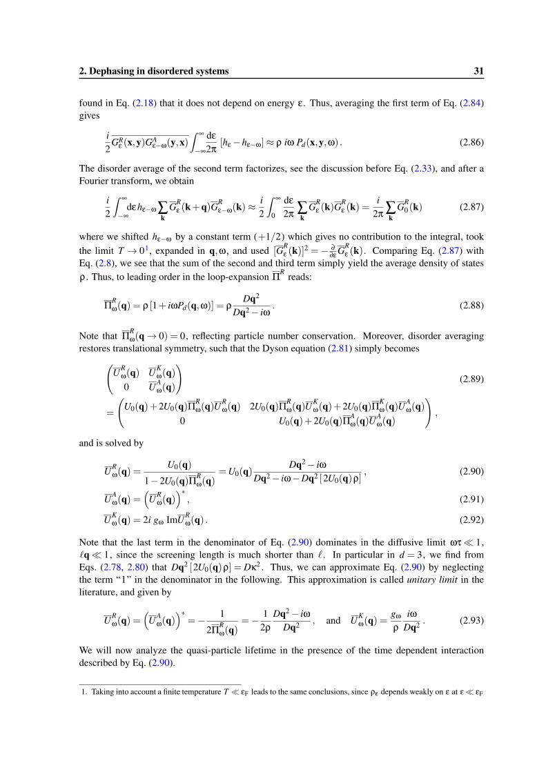
2. Dephasing in disordered systems 31
found in Eq. (2.18) that it does not depend on energy ε. Thus, averaging the first term of Eq. (2.84)gives
i2
GRε (x,y)GA
ε−ω(y,x)∫ ∞
−∞
dε2π
[hε−hε−ω]≈ ρ iω Pd(x,y,ω) . (2.86)
The disorder average of the second term factorizes, see the discussion before Eq. (2.33), and after aFourier transform, we obtain
i2
∫ ∞
−∞dεhε−ω ∑
kGR
ε (k+q)GRε−ω(k)≈
i2
∫ ∞
0
dε2π ∑
kGR
ε (k)GRε (k) =
i2π ∑
kGR
0 (k) (2.87)
where we shifted hε−ω by a constant term (+1/2) which gives no contribution to the integral, tookthe limit T → 01, expanded in q,ω, and used [GR
ε (k)]2 =− ∂∂ε GR
ε (k). Comparing Eq. (2.87) withEq. (2.8), we see that the sum of the second and third term simply yield the average density of statesρ. Thus, to leading order in the loop-expansion ΠR reads:
ΠRω(q) = ρ [1+ iωPd(q,ω)] = ρ
Dq2
Dq2− iω. (2.88)
Note that ΠRω(q→ 0) = 0, reflecting particle number conservation. Moreover, disorder averaging
restores translational symmetry, such that the Dyson equation (2.81) simply becomes(
URω(q) UK
ω(q)0 UA
ω(q)
)(2.89)
=
(U0(q)+2U0(q)Π
Rω(q)U
Rω(q) 2U0(q)Π
Rω(q)U
Kω(q)+2U0(q)Π
Kω(q)U
Aω(q)
0 U0(q)+2U0(q)ΠAω(q)U
Aω(q)
),
and is solved by
URω(q) =
U0(q)
1−2U0(q)ΠRω(q)
=U0(q)Dq2− iω
Dq2− iω−Dq2 [2U0(q)ρ], (2.90)
UAω(q) =
(UR
ω(q))∗
, (2.91)
UKω(q) = 2i gω ImUR
ω(q) . (2.92)
Note that the last term in the denominator of Eq. (2.90) dominates in the diffusive limit ωτ� 1,`q� 1, since the screening length is much shorter than `. In particular in d = 3, we find fromEqs. (2.78, 2.80) that Dq2 [2U0(q)ρ] = Dκ2 . Thus, we can approximate Eq. (2.90) by neglectingthe term “1” in the denominator in the following. This approximation is called unitary limit in theliterature, and given by
URω(q) =
(UA
ω(q))∗
=− 1
2ΠRω(q)
=− 12ρ
Dq2− iωDq2 , and UK
ω(q) =gω
ρiω
Dq2 . (2.93)
We will now analyze the quasi-particle lifetime in the presence of the time dependent interactiondescribed by Eq. (2.90).
1. Taking into account a finite temperature T � εF leads to the same conclusions, since ρε depends weakly on ε at ε� εF
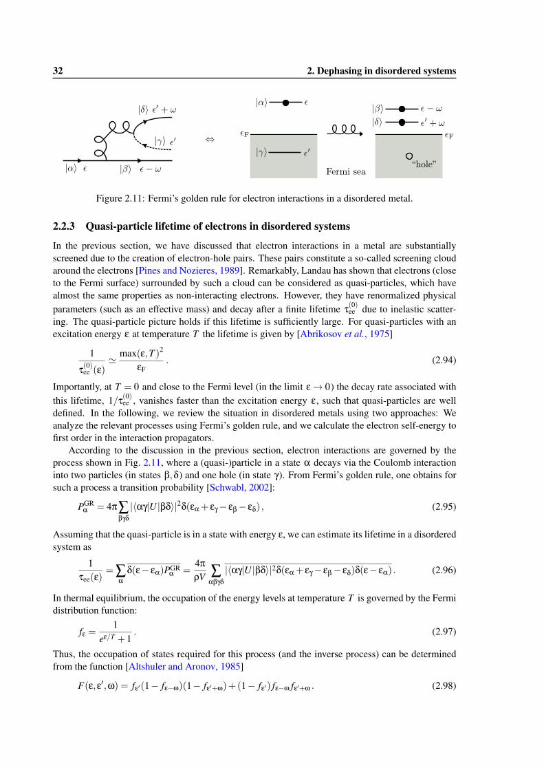
32 2. Dephasing in disordered systems
Figure 2.11: Fermi’s golden rule for electron interactions in a disordered metal.
2.2.3 Quasi-particle lifetime of electrons in disordered systems
In the previous section, we have discussed that electron interactions in a metal are substantiallyscreened due to the creation of electron-hole pairs. These pairs constitute a so-called screening cloudaround the electrons [Pines and Nozieres, 1989]. Remarkably, Landau has shown that electrons (closeto the Fermi surface) surrounded by such a cloud can be considered as quasi-particles, which havealmost the same properties as non-interacting electrons. However, they have renormalized physicalparameters (such as an effective mass) and decay after a finite lifetime τ(0)ee due to inelastic scatter-ing. The quasi-particle picture holds if this lifetime is sufficiently large. For quasi-particles with anexcitation energy ε at temperature T the lifetime is given by [Abrikosov et al., 1975]
1
τ(0)ee (ε)' max(ε,T )2
εF. (2.94)
Importantly, at T = 0 and close to the Fermi level (in the limit ε→ 0) the decay rate associated withthis lifetime, 1/τ(0)ee , vanishes faster than the excitation energy ε, such that quasi-particles are welldefined. In the following, we review the situation in disordered metals using two approaches: Weanalyze the relevant processes using Fermi’s golden rule, and we calculate the electron self-energy tofirst order in the interaction propagators.
According to the discussion in the previous section, electron interactions are governed by theprocess shown in Fig. 2.11, where a (quasi-)particle in a state α decays via the Coulomb interactioninto two particles (in states β,δ) and one hole (in state γ). From Fermi’s golden rule, one obtains forsuch a process a transition probability [Schwabl, 2002]:
PGRα = 4π∑
βγδ|〈αγ|U |βδ〉|2δ(εα + εγ− εβ− εδ) , (2.95)
Assuming that the quasi-particle is in a state with energy ε, we can estimate its lifetime in a disorderedsystem as
1τee(ε)
= ∑α
δ(ε− εα)PGRα =
4πρV ∑
αβγδ|〈αγ|U |βδ〉|2δ(εα + εγ− εβ− εδ)δ(ε− εα) . (2.96)
In thermal equilibrium, the occupation of the energy levels at temperature T is governed by the Fermidistribution function:
fε =1
eε/T +1. (2.97)
Thus, the occupation of states required for this process (and the inverse process) can be determinedfrom the function [Altshuler and Aronov, 1985]
F(ε,ε′,ω) = fε′(1− fε−ω)(1− fε′+ω)+(1− fε′) fε−ω fε′+ω . (2.98)
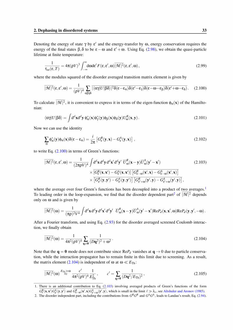
2. Dephasing in disordered systems 33
Denoting the energy of state γ by ε′ and the energy-transfer by ω, energy conservation requires theenergy of the final states β,δ to be ε−ω and ε′+ω. Using Eq. (2.98), we obtain the quasi-particlelifetime at finite temperature:
1τee(ε,T )
= 4π(ρV )3∫ ∞
−∞dωdε′F(ε,ε′,ω)|M |2(ε,ε′,ω) , (2.99)
where the modulus squared of the disorder averaged transition matrix element is given by
|M |2(ε,ε′,ω) = 1(ρV )4 ∑
αβγδ|〈αγ|U |βδ〉|2δ(ε−εα)δ(ε′−εγ)δ(ε−ω−εβ)δ(ε′+ω−εδ) . (2.100)
To calculate |M |2 , it is convenient to express it in terms of the eigen-function φα(x) of the Hamilto-nian:
〈αγ|U |βδ〉=∫
ddxddy φ∗α(x)φ∗γ(y)φβ(x)φδ(y)UR
ω(x,y) . (2.101)
Now we can use the identity
∑α
φ∗α(y)φα(x)δ(ε− εα) =i
2π[GR
ε (y,x)−GAε (y,x)
], (2.102)
to write Eq. (2.100) in terms of Green’s functions:
|M |2(ε,ε′,ω) = 1(2πρV )4
∫ddxddyddx′ ddy′ UR
ω(x−y)UAω(y′−x′) (2.103)
× [GRε (x,x′)−GA
ε (x,x′)][GR
ε−ω(x′,x)−GAε−ω(x′,x)
]
×[GR
ε′(y,y′)−GAε′(y,y′)
][GR
ε′+ω(y′,y)−GAε′+ω(y′,y)
],
where the average over four Green’s functions has been decoupled into a product of two averages.1
To leading order in the loop-expansion, we find that the disorder dependent part2 of |M |2 dependsonly on ω and is given by
|M |2(ω) = 1(πρ)2V 4
∫ddxddyddx′ ddy′ UR
ω(x−y)UAω(y′−x′)RePd(x,x′,ω)RePd(y,y′,−ω) .
After a Fourier transform, and using Eq. (2.93) for the disorder averaged screened Coulomb interac-tion, we finally obtain
|M |2(ω) = 14π2(ρV )4 ∑
q 6=0
1(Dq2)2 +ω2 . (2.104)
Note that the q = 0 mode does not contribute since RePd vanishes at q→ 0 due to particle conserva-tion, while the interaction propagator has to remain finite in this limit due to screening. As a result,the matrix element (2.104) is independent of ω at ω� ETh :
|M |2(ω) ETh�ω≈ c′
4π2(ρV )41
E2Th
, c′ = ∑q6=0
1(Dq2/ETh)2 , (2.105)
1. There is an additional contribution to Eq. (2.103) involving averaged products of Green’s functions of the formGR
ε (x,x′)GAε′(y,y′) and GR
ε−ω(x′,x)GAε′+ω(y′,y) , which is small in the limit `� λs , see Altshuler and Aronov (1985).
2. The disorder independent part, including the contributions from GRGR and GAGA , leads to Landau’s result, Eq. (2.94).
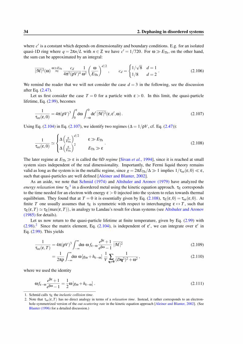
34 2. Dephasing in disordered systems
where c′ is a constant which depends on dimensionality and boundary conditions. E.g. for an isolatedquasi-1D ring where q = 2πn/L with n ∈ Z we have c′ = 1/720. For ω� ETh , on the other hand,the sum can be approximated by an integral:
|M |2(ω) ω�ETh≈ cd
4π2(ρV )41
ω2
(ω
ETh
)d/2
, cd =
{1/√
8 d = 11/8 d = 2
. (2.106)
We remind the reader that we will not consider the case d = 3 in the following, see the discussionafter Eq. (2.47).
Let us first consider the case T = 0 for a particle with ε > 0. In this limit, the quasi-particlelifetime, Eq. (2.99), becomes
1τee(ε,0)
= 4π(ρV )3∫ ε
0dω
∫ 0
−ωdε′ |M |2(ε,ε′,ω) . (2.107)
Using Eq. (2.104) in Eq. (2.107), we identify two regimes (∆ = 1/ρV , cf. Eq. (2.47)):
1τee(ε,0)
'
∆(
εETh
)d/2ε� ETh
∆(
εETh
)2ETh� ε
. (2.108)
The later regime at ETh� ε is called the 0D regime [Sivan et al., 1994], since it is reached at smallsystem sizes independent of the real dimensionality. Importantly, the Fermi liquid theory remainsvalid as long as the system is in the metallic regime, since g = 2πETh/∆� 1 implies 1/τee(ε,0)� ε,such that quasi-particles are well defined [Aleiner and Blanter, 2002].
As an aside, we note that Schmid (1974) and Altshuler and Aronov (1979) have analyzed theenergy relaxation time τE
1 in a disordered metal using the kinetic equation approach. τE correspondsto the time needed for an electron with energy ε > 0 injected into the system to relax towards thermalequilibrium. They found that at T = 0 it is essentially given by Eq. (2.108), τE(ε,0) = τee(ε,0). Atfinite T one usually assumes that τE is symmetric with respect to interchanging ε↔ T , such thatτE(ε,T )' τE(max(ε,T )), in analogy to Landau’s result for clean systems (see Altshuler and Aronov(1985) for details).
Let us now return to the quasi-particle lifetime at finite temperature, given by Eq. (2.99) with(2.98).2 Since the matrix element, Eq. (2.104), is independent of ε′ , we can integrate over ε′ inEq. (2.99). This yields
1τee(ε,T )
= 4π(ρV )3∫ ∞
−∞dω ω fε−ω
eβε +1eβω−1
|M |2 (2.109)
=1
2πρ
∫ ∞
−∞dω ω [gω +hε−ω]
1V ∑
q 6=0
1(Dq2)2 +ω2 , (2.110)
where we used the identity
ω fε−ωeβε +1eβω−1
=12
ω [gω +hε−ω] . (2.111)
1. Schmid calls τE the inelastic collision time.2. Note that τee(ε,T ) has no direct analogy in terms of a relaxation time. Instead, it rather corresponds to an electron-
hole-symmetrized version of the out-scattering rate in the kinetic equation approach [Aleiner and Blanter, 2002]. (SeeBlanter (1996) for a detailed discussion.)
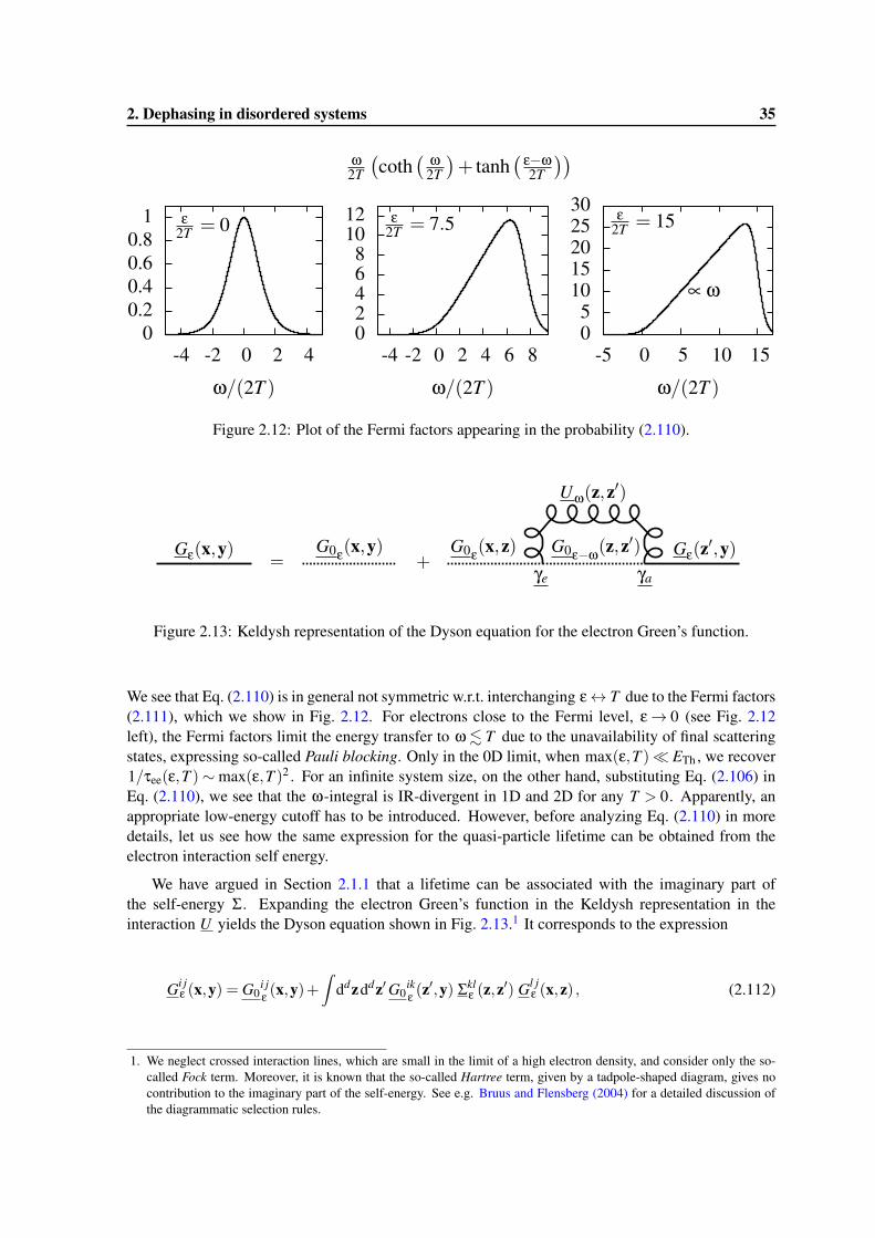
2. Dephasing in disordered systems 35
ω
2T
(coth
(ω
2T
)+ tanh
(ε−ω
2T
))
00.20.40.60.8
1
-4 -2 0 2 4
ω/(2T )
ε
2T = 0
02468
1012
-4 -2 0 2 4 6 8
ω/(2T )
ε
2T = 7.5
05
1015202530
-5 0 5 10 15
ω/(2T )
ε
2T = 15
∝ ω
Figure 2.12: Plot of the Fermi factors appearing in the probability (2.110).
Figure 2.13: Keldysh representation of the Dyson equation for the electron Green’s function.
We see that Eq. (2.110) is in general not symmetric w.r.t. interchanging ε↔ T due to the Fermi factors(2.111), which we show in Fig. 2.12. For electrons close to the Fermi level, ε→ 0 (see Fig. 2.12left), the Fermi factors limit the energy transfer to ω . T due to the unavailability of final scatteringstates, expressing so-called Pauli blocking. Only in the 0D limit, when max(ε,T )� ETh , we recover1/τee(ε,T )∼max(ε,T )2 . For an infinite system size, on the other hand, substituting Eq. (2.106) inEq. (2.110), we see that the ω-integral is IR-divergent in 1D and 2D for any T > 0. Apparently, anappropriate low-energy cutoff has to be introduced. However, before analyzing Eq. (2.110) in moredetails, let us see how the same expression for the quasi-particle lifetime can be obtained from theelectron interaction self energy.
We have argued in Section 2.1.1 that a lifetime can be associated with the imaginary part ofthe self-energy Σ. Expanding the electron Green’s function in the Keldysh representation in theinteraction U yields the Dyson equation shown in Fig. 2.13.1 It corresponds to the expression
Gi jε (x,y) = G0
i jε (x,y)+
∫ddzddz′G0
ikε (z′,y) Σkl
ε (z,z′) Gl j
ε (x,z) , (2.112)
1. We neglect crossed interaction lines, which are small in the limit of a high electron density, and consider only the so-called Fock term. Moreover, it is known that the so-called Hartree term, given by a tadpole-shaped diagram, gives nocontribution to the imaginary part of the self-energy. See e.g. Bruus and Flensberg (2004) for a detailed discussion ofthe diagrammatic selection rules.
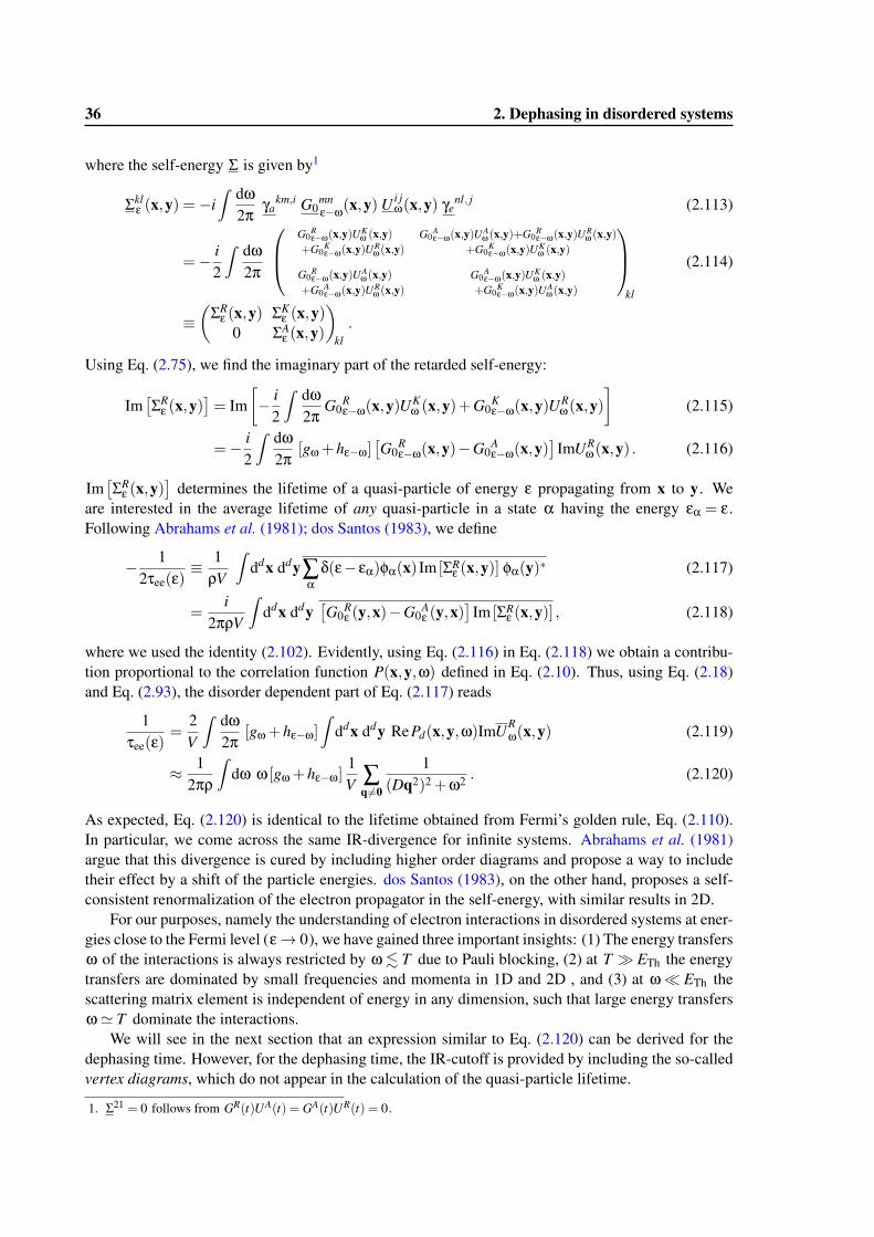
36 2. Dephasing in disordered systems
where the self-energy Σ is given by1
Σklε (x,y) =−i
∫ dω2π
γakm,i G0
mnε−ω(x,y) U i j
ω(x,y) γenl, j (2.113)
=− i2
∫ dω2π
G0Rε−ω(x,y)UK
ω (x,y)+G0
Kε−ω(x,y)UR
ω (x,y)G0
Aε−ω(x,y)UA
ω (x,y)+G0Rε−ω(x,y)UR
ω (x,y)+G0
Kε−ω(x,y)UK
ω (x,y)
G0Rε−ω(x,y)UA
ω (x,y)+G0
Aε−ω(x,y)UR
ω (x,y)G0
Aε−ω(x,y)UK
ω (x,y)+G0
Kε−ω(x,y)UA
ω (x,y)
kl
(2.114)
≡(
ΣRε (x,y) ΣK
ε (x,y)0 ΣA
ε (x,y)
)
kl.
Using Eq. (2.75), we find the imaginary part of the retarded self-energy:
Im[ΣR
ε (x,y)]= Im
[− i
2
∫ dω2π
G0Rε−ω(x,y)U
Kω (x,y)+G0
Kε−ω(x,y)U
Rω(x,y)
](2.115)
=− i2
∫ dω2π
[gω +hε−ω][G0
Rε−ω(x,y)−G0
Aε−ω(x,y)
]ImUR
ω(x,y) . (2.116)
Im[ΣR
ε (x,y)]
determines the lifetime of a quasi-particle of energy ε propagating from x to y. Weare interested in the average lifetime of any quasi-particle in a state α having the energy εα = ε.Following Abrahams et al. (1981); dos Santos (1983), we define
− 12τee(ε)
≡ 1ρV
∫ddx ddy∑
αδ(ε− εα)φα(x) Im [ΣR
ε (x,y)] φα(y)∗ (2.117)
=i
2πρV
∫ddx ddy
[G0
Rε (y,x)−G0
Aε (y,x)
]Im [ΣR
ε (x,y)] , (2.118)
where we used the identity (2.102). Evidently, using Eq. (2.116) in Eq. (2.118) we obtain a contribu-tion proportional to the correlation function P(x,y,ω) defined in Eq. (2.10). Thus, using Eq. (2.18)and Eq. (2.93), the disorder dependent part of Eq. (2.117) reads
1τee(ε)
=2V
∫ dω2π
[gω +hε−ω]∫
ddx ddy RePd(x,y,ω)ImURω(x,y) (2.119)
≈ 12πρ
∫dω ω [gω +hε−ω]
1V ∑
q6=0
1(Dq2)2 +ω2 . (2.120)
As expected, Eq. (2.120) is identical to the lifetime obtained from Fermi’s golden rule, Eq. (2.110).In particular, we come across the same IR-divergence for infinite systems. Abrahams et al. (1981)argue that this divergence is cured by including higher order diagrams and propose a way to includetheir effect by a shift of the particle energies. dos Santos (1983), on the other hand, proposes a self-consistent renormalization of the electron propagator in the self-energy, with similar results in 2D.
For our purposes, namely the understanding of electron interactions in disordered systems at ener-gies close to the Fermi level (ε→ 0), we have gained three important insights: (1) The energy transfersω of the interactions is always restricted by ω . T due to Pauli blocking, (2) at T � ETh the energytransfers are dominated by small frequencies and momenta in 1D and 2D , and (3) at ω� ETh thescattering matrix element is independent of energy in any dimension, such that large energy transfersω' T dominate the interactions.
We will see in the next section that an expression similar to Eq. (2.120) can be derived for thedephasing time. However, for the dephasing time, the IR-cutoff is provided by including the so-calledvertex diagrams, which do not appear in the calculation of the quasi-particle lifetime.
1. Σ21 = 0 follows from GR(t)UA(t) = GA(t)UR(t) = 0.
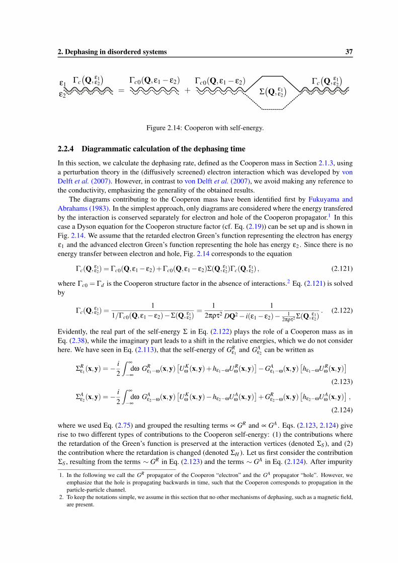
2. Dephasing in disordered systems 37
Figure 2.14: Cooperon with self-energy.
2.2.4 Diagrammatic calculation of the dephasing time
In this section, we calculate the dephasing rate, defined as the Cooperon mass in Section 2.1.3, usinga perturbation theory in the (diffusively screened) electron interaction which was developed by vonDelft et al. (2007). However, in contrast to von Delft et al. (2007), we avoid making any reference tothe conductivity, emphasizing the generality of the obtained results.
The diagrams contributing to the Cooperon mass have been identified first by Fukuyama andAbrahams (1983). In the simplest approach, only diagrams are considered where the energy transferedby the interaction is conserved separately for electron and hole of the Cooperon propagator.1 In thiscase a Dyson equation for the Cooperon structure factor (cf. Eq. (2.19)) can be set up and is shown inFig. 2.14. We assume that the retarded electron Green’s function representing the electron has energyε1 and the advanced electron Green’s function representing the hole has energy ε2 . Since there is noenergy transfer between electron and hole, Fig. 2.14 corresponds to the equation
Γc(Q, ε1ε2) = Γc0(Q,ε1− ε2)+Γc0(Q,ε1− ε2)Σ(Q, ε1ε2)Γc(Q, ε1ε2) , (2.121)
where Γc0 = Γd is the Cooperon structure factor in the absence of interactions.2 Eq. (2.121) is solvedby
Γc(Q, ε1ε2) =1
1/Γc0(Q,ε1− ε2)−Σ(Q, ε1ε2)=
12πρτ2
1DQ2− i(ε1− ε2)− 1
2πρτ2 Σ(Q, ε1ε2). (2.122)
Evidently, the real part of the self-energy Σ in Eq. (2.122) plays the role of a Cooperon mass as inEq. (2.38), while the imaginary part leads to a shift in the relative energies, which we do not considerhere. We have seen in Eq. (2.113), that the self-energy of GR
ε1and GA
ε2can be written as
ΣRε1(x,y) =− i
2
∫ ∞
−∞dω GR
ε1−ω(x,y)[UK
ω (x,y)+hε1−ωURω(x,y)
]−GA
ε1−ω(x,y)[hε1−ωUR
ω(x,y)]
(2.123)
ΣAε2(x,y) =− i
2
∫ ∞
−∞dω GA
ε2−ω(x,y)[UK
ω (x,y)−hε2−ωUAω(x,y)
]+GR
ε2−ω(x,y)[hε2−ωUA
ω(x,y)],
(2.124)
where we used Eq. (2.75) and grouped the resulting terms ∝ GR and ∝ GA . Eqs. (2.123, 2.124) giverise to two different types of contributions to the Cooperon self-energy: (1) the contributions wherethe retardation of the Green’s function is preserved at the interaction vertices (denoted ΣS ), and (2)the contribution where the retardation is changed (denoted ΣH ). Let us first consider the contributionΣS , resulting from the terms ∼ GR in Eq. (2.123) and the terms ∼ GA in Eq. (2.124). After impurity
1. In the following we call the GR propagator of the Cooperon “electron” and the GA propagator “hole”. However, weemphasize that the hole is propagating backwards in time, such that the Cooperon corresponds to propagation in theparticle-particle channel.
2. To keep the notations simple, we assume in this section that no other mechanisms of dephasing, such as a magnetic field,are present.
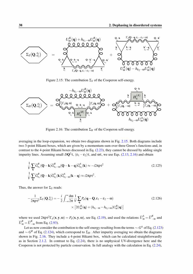
38 2. Dephasing in disordered systems
Figure 2.15: The contribution ΣS of the Cooperon self-energy.
Figure 2.16: The contribution ΣH of the Cooperon self-energy.
averaging in the loop-expansion, we obtain two diagrams shown in Fig. 2.15. Both diagrams includetwo 3-point Hikami boxes, which are given by a momentum-sum over three Green’s functions and, incontrast to the 4-point Hikami boxes discussed in Eq. (2.23), they cannot be dressed by adding singleimpurity lines. Assuming small DQ2τ, (ε1− ε2)τ, and ωτ, we use Eqs. (2.13, 2.16) and obtain
1V ∑
kGR
ε1(Q−k)GR
ε1−ω(Q−k−q)GAε2(k)≈−i2πρτ2 (2.125)
1V ∑
kGR
ε1(Q−k)GA
ε2(k)GA
ε2−ω(k−q)≈ i2πρτ2 .
Thus, the answer for ΣS reads:
− 12πρτ2 ΣS (Q, ε1ε2) =−
i2
∫ ∞
−∞
dω2π
1V ∑
qPd(q−Q,ε1− ε2−ω) (2.126)
×[2UK
ω (q)+(hε1−ω−hε2+ω)URω(q)
]
where we used 2πρτ2Γd(x,y,ω) = Pd(x,y,ω), see Eq. (2.19), and used the relations UAω =UR
−ω andUK
ω =UK−ω from Eq. (2.93).
Let us now consider the contribution to the self-energy resulting from the terms ∼ GA of Eq. (2.123)and ∼ GR of Eq. (2.124), which correspond to ΣH . After impurity averaging we obtain the diagramsshown in Fig. 2.16. They include a 4-point Hikami box, which can be calculated straightforwardlyas in Section 2.1.2. In contrast to Eq. (2.24), there is no unphysical UV-divergence here and theCooperon is not protected by particle conservation. In full analogy with the calculation in Eq. (2.24),
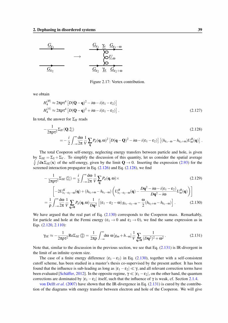
2. Dephasing in disordered systems 39
Figure 2.17: Vertex contribution.
we obtain
H(R)4 ≈ 2πρτ4 [D(Q−q)2− iω− i(ε1− ε2)
]
H(A)4 ≈ 2πρτ4 [D(Q−q)2 + iω− i(ε1− ε2)
]. (2.127)
In total, the answer for ΣH reads
− 12πρτ2 ΣH (Q, ε1ε2) (2.128)
=− i2
∫ ∞
−∞
dω2π
1V ∑
qPd(q,ω)2 [D(q−Q)2− iω− i(ε1− ε2)
][(hε1−ω−hε2+ω)UR
ω(q)].
The total Cooperon self-energy, neglecting energy transfers between particle and hole, is givenby ΣSE = ΣS +ΣV . To simplify the discussion of this quantity, let us consider the spatial average1V
∫dxΣSE(x) of the self-energy, given by the limit Q→ 0. Inserting the expression (2.93) for the
screened interaction propagator in Eq. (2.126) and Eq. (2.128), we find
− 12πρτ2 ΣSE (
ε1ε2) =i2
∫ ∞
−∞
dω2π
1V ∑
qPd(q,ω)× (2.129)
[−2UK
ε1−ε2−ω(q)+(hε2+ω−hε1−ω)
(UR
ε1−ε2−ω(q)−Dq2− iω− i(ε1− ε2)
Dq2− iωUR
ω(q))]
=1ρ
∫ ∞
−∞
dω2π
1V ∑
q6=0Pd(q,ω)
1Dq2
[(ε1− ε2−ω)gε1−ε2−ω−
ω2(hε2+ω−hε1−ω)
]. (2.130)
We have argued that the real part of Eq. (2.130) corresponds to the Cooperon mass. Remarkably,for particle and hole at the Fermi energy (ε1→ 0 and ε2→ 0), we find the same expression as inEqs. (2.120, 2.110):
γSE ≈−1
2πρτ2 ReΣSE (00) =
12πρ
∫ ∞
−∞dω ω [gω +h−ω]
1V ∑
q6=0
1(Dq2)2 +ω2 . (2.131)
Note that, similar to the discussion in the previous section, we see that Eq. (2.131) is IR-divergent inthe limit of an infinite system size.
The case of a finite energy difference (ε1− ε2) in Eq. (2.130), together with a self-consistentcutoff scheme, has been studied in a master’s thesis co-supervised by the present author. It has beenfound that the influence is sub-leading as long as |ε1− ε2| � γ, and all relevant correction terms havebeen evaluated [Schäffer, 2012]. In the opposite regime, γ� |ε1− ε2|, on the other hand, the quantumcorrections are dominated by |ε1− ε2| itself, such that the influence of γ is weak, cf. Section 2.1.4.
von Delft et al. (2007) have shown that the IR-divergence in Eq. (2.131) is cured by the contribu-tion of the diagrams with energy transfer between electron and hole of the Cooperon. We will give
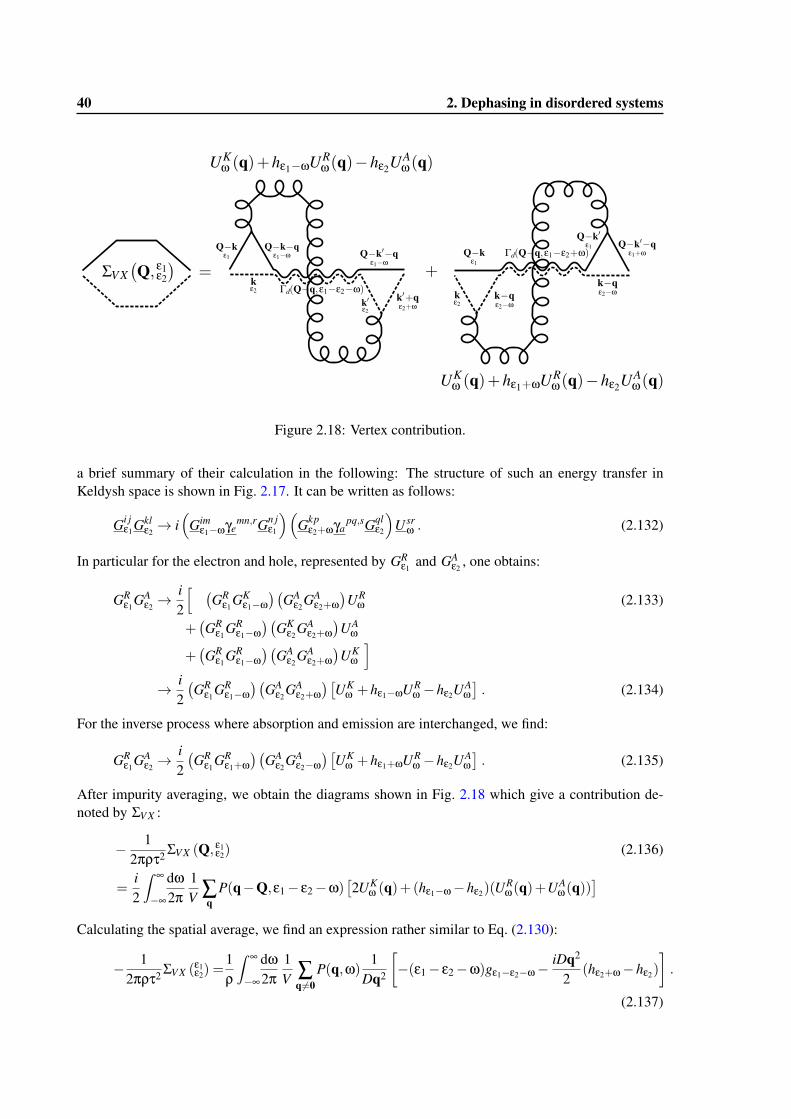
40 2. Dephasing in disordered systems
Figure 2.18: Vertex contribution.
a brief summary of their calculation in the following: The structure of such an energy transfer inKeldysh space is shown in Fig. 2.17. It can be written as follows:
Gi jε1Gkl
ε2→ i
(Gim
ε1−ωγemn,rGn j
ε1
)(Gkp
ε2+ωγapq,sGql
ε2
)U sr
ω . (2.132)
In particular for the electron and hole, represented by GRε1
and GAε2
, one obtains:
GRε1
GAε2→ i
2
[ (GR
ε1GK
ε1−ω)(
GAε2
GAε2+ω
)UR
ω (2.133)
+(GR
ε1GR
ε1−ω)(
GKε2
GAε2+ω
)UA
ω
+(GR
ε1GR
ε1−ω)(
GAε2
GAε2+ω
)UK
ω
]
→ i2(GR
ε1GR
ε1−ω)(
GAε2
GAε2+ω
)[UK
ω +hε1−ωURω −hε2U
Aω]. (2.134)
For the inverse process where absorption and emission are interchanged, we find:
GRε1
GAε2→ i
2(GR
ε1GR
ε1+ω)(
GAε2
GAε2−ω
)[UK
ω +hε1+ωURω −hε2U
Aω]. (2.135)
After impurity averaging, we obtain the diagrams shown in Fig. 2.18 which give a contribution de-noted by ΣV X :
− 12πρτ2 ΣV X (Q, ε1ε2) (2.136)
=i2
∫ ∞
−∞
dω2π
1V ∑
qP(q−Q,ε1− ε2−ω)
[2UK
ω (q)+(hε1−ω−hε2)(URω(q)+UA
ω(q))]
Calculating the spatial average, we find an expression rather similar to Eq. (2.130):
− 12πρτ2 ΣV X (ε1ε2) =
1ρ
∫ ∞
−∞
dω2π
1V ∑
q6=0P(q,ω)
1Dq2
[−(ε1− ε2−ω)gε1−ε2−ω−
iDq2
2(hε2+ω−hε2)
].
(2.137)
2. Dephasing in disordered systems 41
However, since energy is not conserved for each Green’s function, we cannot formulate the problemin terms of a Dyson equation of the form Eq. (2.121) any more. Instead, the Cooperon structure factoris described by a so-called Bethe-Salpether equation,
Γc(Q, ε11ε21ε12ε22) = Γc0(Q, ε11ε21)
[δ(ε11−ε12)δ(ε21−ε22)+
∫ ∞
−∞dω1dω2Σ(ε11ε21
ω1ω2)Γc (Q,ω1ω2ε12ε22)
], (2.138)
with a self-energy which depends on four energy arguments and is given by a combination of Eq. (2.130)and Eq. (2.137):
− 12πρτ2 Σ(ε11ε21
ε12ε22) =1ρ
∫ ∞
−∞
dω2π
1V ∑
q6=0Pd(q,ω)
1Dq2 (2.139)
×[(
(ε11− ε21−ω)gε11−ε21−ω−ω2(hε21+ω−hε11−ω)
)δ(ε11−ε12)δ(ε21−ε22)
+
(−(ε11− ε21−ω)gε11−ε21−ω−
iDq2
2(hε21+ω−hε21)
)δ(ε11−ε12−ω)δ(ε21−ε22+ω)
].
In general, Eq. (2.138) with Eq. (2.139) cannot be solved exactly. However, we can make two impor-tant observations: (a) In the limit of small energy transfers, ω→ 0, the contributions from ΣSE andΣV X , represented by the second and third line of Eq. (2.139), cancel exactly. (b) As in Eq. (2.130),only energy transfers ω . T contribute to the real part of Eq. (2.139) at energies close to the Fermienergy (ε11→ 0 and ε21→ 0).1
von Delft et al. (2007) have suggested to transform Eq. (2.138) to real space and time, and thento solve it approximately with an exponential ansatz. Since the corresponding calculation is ratherlengthy, we restrict ourselves here to a discussion of the final results. For electron and hole at theFermi level, the solution has the following form
Γc (x,y, t) = Γc0 (x,y, t) exp[−F(x,y, t)] . (2.140)
F is called the Cooperon decay function and is given by
F (x,y, t) =∫ t
0dτdτ′
1V
∫ddzddz′K(z− z′,τ− τ′) (2.141)
×
Px,y,t(z,z′,τ,τ′)︸ ︷︷ ︸
from ΣSE
−Px,y,t(z,z′,τ, t− τ′)︸ ︷︷ ︸from ΣV X
,
where the Fourier transform of K is given by
K(q,ω) =1
2ρ1
Dq2 ω [gω +h−ω] (2.142)
and Px,y,t(z,τ,τ′) corresponds to the probability of diffusive propagation from x to y in time t passingthrough point z at time τ and point z′ at time τ′ . For 0 < τ < t and τ < τ′ < t it is given by:2
Px,y,t(z,z′,τ,τ′) =Pd(x,z,0,τ)Pd(z,z′,τ,τ′)Pd(z′,y,τ′, t)
Pd(x,y, t). (2.143)
1. Note that Re [iPd(q,ω)] = −ω(Dq2)2+ω2 .
2. For τ′ < τ , we should interchange (z,τ) and (z′,τ′) in Eq. (2.143).
42 2. Dephasing in disordered systems
We will recover a relation similar to Eq. (2.141) in the path integral approach discussed in Sec-tion 2.2.6. To see that Eq. (2.141) is free of infrared divergences it is instructive to approximate theprobability (2.143), which is restricted to follow a trajectory from x to y in time t , by the unrestricteddiffusion probability between z and z′ :
1V
∫ddzddz′ eiq(z−z′)Px,y,t(z,z′,τ,τ′)≈
1V
∫ddzddz′ eiq(z−z′)Pd(z− z′, |τ− τ′|) = e−Dq2|τ′−τ| .
(2.144)
It has been shown that the approximation Eq. (2.144) merely leads to a different prefactor ∼ 1 of thefinal result, see Marquardt et al. (2007) for a detailed discussion. In this approximation, the decayfunction becomes independent of coordinates:
F (t) =∫ t
0dτdτ′
∫ dω2π
eiω(τ−τ′) 1V ∑
q6=0K(q,ω)
[e−Dq2|τ−τ′|− e−Dq2|t−τ−τ′|
]. (2.145)
After integrating over time one obtains a result similar to Eq. (2.131) [von Delft et al., 2007; Akker-mans and Montambaux, 2007]:
F (t) =t
2πρ
∫dω ω [gω +h−ω]
(1− sin(ω t)
ω t
)1V ∑
q6=0
1(Dq2)2 +ω2 (2.146)
However, Eq. (2.146) contains the additional factor 1− sin(ωt)/(ωt) which is absent in Eq. (2.131).It effectively cuts the ω integral in IR at ω' 1/t . Large energy transfers, on the other hand, arerestricted to ω . T due to the factor gω +h−ω , cf. Fig. 2.12. Extracting the corresponding dephasingtime from the relation F
(τϕ)' 1, we finally obtain the self-consistent equation
1τϕ≈ 2T
πρ
∫ T
1/τϕ
dω1V ∑
q6=0
1(Dq2)2 +ω2 . (2.147)
We see that the IR-divergence is effectively cut by the inverse dephasing time itself. This correspondsto the very plausible assumption that energies cannot be transferred on time scales larger than thedephasing time.
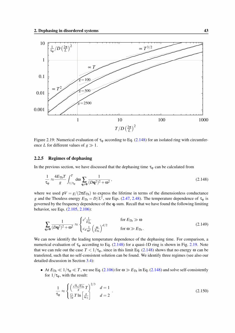
2. Dephasing in disordered systems 43
0.001
0.01
0.1
1
10
1 10 100 1000
T/D( 2π
L
)2
1τϕ/D
( 2π
L
)2
∝ T 2
∝ T
∝ T 3/2
g=100
g=500
g=2500
Figure 2.19: Numerical evaluation of τϕ according to Eq. (2.148) for an isolated ring with circumfer-ence L for different values of g� 1.
2.2.5 Regimes of dephasing
In the previous section, we have discussed that the dephasing time τϕ can be calculated from
1τϕ≈4EThT
g
∫ T
1/τϕ
dω ∑q 6=0
1(Dq2)2 +ω2 , (2.148)
where we used ρV = g/(2πETh) to express the lifetime in terms of the dimensionless conductanceg and the Thouless energy ETh = D/L2 , see Eqs. (2.47, 2.48). The temperature dependence of τϕ isgoverned by the frequency dependence of the q-sum. Recall that we have found the following limitingbehavior, see Eqs. (2.105, 2.106):
∑q6=0
1(Dq2)2 +ω2 ≈
c′ 1E2
Thfor ETh� ω
cd1
ω2
(ω
ETh
)d/2for ω� ETh .
(2.149)
We can now identify the leading temperature dependence of the dephasing time. For comparison, anumerical evaluation of τϕ according to Eq. (2.148) for a quasi-1D ring is shown in Fig. 2.19. Notethat we can rule out the case T < 1/τϕ , since in this limit Eq. (2.148) shows that no energy ω can betransfered, such that no self-consistent solution can be found. We identify three regimes (see also ourdetailed discussion in Section 3.4):
• At ETh� 1/τϕ� T , we use Eq. (2.106) for ω� ETh in Eq. (2.148) and solve self-consistentlyfor 1/τϕ , with the result:
1τϕ≈
(√8√
EThg T
)2/3d = 1
c22g T ln
[g
4c2
]d = 2
. (2.150)
44 2. Dephasing in disordered systems
We call this the diffusive regime in the following, since the electron dynamics are governed byfree diffusive trajectories much shorter than the system size.
Similar to the inelastic processes governing the quasi-particle lifetime, which we discussed inSection 2.2.3, dephasing is dominated by small energy and momentum transfers in this regime.
The diffusive regime has been first derived in the form of Eq. (2.150) by Altshuler et al. (1981c)by means of a dimensional estimation. The predicted temperature dependence, Eq. (2.150), hasbeen observed in numerous experiments.
• At 1/τϕ� ETh� T , we split the ω integral into parts smaller and larger than ETh , such thatapproximately
1τϕ≈ 4EThT
g
[∫ ETh
1/τϕ
dωc′1
E2Th
+∫ T
ETh
dωcd1
ω2
(ω
ETh
)d/2], (2.151)
and find
1τϕ≈{
4Tg [c′+1/4] d = 1
4Tg [c′+ c2 ln [T/ETh]] d = 2
. (2.152)
We call this the ergodic regime in the following, since the quasi-particles explore the wholesystem before they dephase, τϕ� 1/ETh . Note that the size of the temperature range where1/τϕ� ETh� T depends on g and the coefficients c′ and cd . We see in Fig. 2.19 that for aquasi-1D ring (without a magnetic field) a rather large conductance is required.
For open and unconfined systems, we have discussed in Section 2.1.4, that the quantum correc-tions are controlled by max(ETh,1/τϕ). At 1/τϕ� ETh , they become temperature independentand universal. Thus, a dephasing time of the form Eq. (2.152) can only contribute as a sub-leading correction in this case. However, we will see in Chapter 3, that the situation is differentfor confined systems, such as quantum dots.
The ergodic regime has been first discussed by Ludwig and Mirlin (2004) in the context ofthe Aharonov-Bohm effect: The trajectories contributing to dephasing of the AB-oscillationsare always ergodic, such that the diffusive regime is absent. For the situation described here,it has been discussed first by Texier and Montambaux (2005). Moreover, it has been recentlyconfirmed experimentally by Capron et al. (2013) (see also Ferrier et al. (2008)).
• At 1/τϕ� T � ETh , using Eq. (2.105) for ETh� ω in Eq. (2.148), we find
1τϕ≈ 4c′
gEThT 2 , (2.153)
independent of dimensionality. This is the so-called 0D regime first discussed in Sivan et al.(1994). Only in this regime, the upper limit of the integral in Eq. (2.148), which is due to Pauliblocking, has a significant influence on the temperature dependence of τϕ . Thus, dephasing isgoverned by large energy transfers ω' T , cf. Section 2.2.3.
However, dephasing is even weaker than in the ergodic regime. As a result, the quantum cor-rections in open and unconfined systems depend only weakly on temperature. We will establishin Chapter 3, that even in confined geometries 0D dephasing can be observed in a transportexperiment only as a sub-leading correction to the quantum corrections.
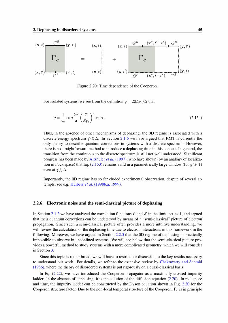
2. Dephasing in disordered systems 45
Figure 2.20: Time dependence of the Cooperon.
For isolated systems, we see from the definition g = 2πETh/∆ that
γ =1τϕ≈ ∆
2c′
π
(T
ETh
)2
� ∆ , (2.154)
Thus, in the absence of other mechanisms of dephasing, the 0D regime is associated with adiscrete energy spectrum γ� ∆. In Section 2.1.6 we have argued that RMT is currently theonly theory to describe quantum corrections in systems with a discrete spectrum. However,there is no straightforward method to introduce a dephasing time in this context. In general, thetransition from the continuous to the discrete spectrum is still not well understood. Significantprogress has been made by Altshuler et al. (1997), who have shown (by an analogy of localiza-tion in Fock space) that Eq. (2.153) remains valid in a parametrically large window (for g� 1)even at γ . ∆.
Importantly, the 0D regime has so far eluded experimental observation, despite of several at-tempts, see e.g. Huibers et al. (1998b,a, 1999).
2.2.6 Electronic noise and the semi-classical picture of dephasing
In Section 2.1.2 we have analyzed the correlation functions P and K in the limit εFτ� 1, and arguedthat their quantum corrections can be understood by means of a “semi-classical” picture of electronpropagation. Since such a semi-classical picture often provides a more intuitive understanding, wewill review the calculation of the dephasing time due to electron interactions in this framework in thefollowing. Moreover, we have argued in Section 2.2.5 that the 0D regime of dephasing is practicallyimpossible to observe in unconfined systems. We will see below that the semi-classical picture pro-vides a powerful method to study systems with a more complicated geometry, which we will considerin Section 3.
Since this topic is rather broad, we will have to restrict our discussion to the key results necessaryto understand our work. For details, we refer to the extensive review by Chakravarty and Schmid(1986), where the theory of disordered systems is put rigorously on a quasi-classical basis.
In Eq. (2.22), we have introduced the Cooperon propagator as a maximally crossed impurityladder. In the absence of dephasing, it is the solution of the diffusion equation (2.20). In real spaceand time, the impurity ladder can be constructed by the Dyson equation shown in Fig. 2.20 for theCooperon structure factor. Due to the non-local temporal structure of the Cooperon, Γc is in principle
46 2. Dephasing in disordered systems
a function of four time arguments, cf. Eq. (2.138):1
Γc(x,y, t
t ′t ′t
)= γδ(x−y)δ(t− t ′) (2.155)
+∫
ddx∗dt∗Γc(x,x∗, t
t ′t ′−t∗t−t∗)
GR(x∗,y, t ′− t∗, t ′)GA
(x∗,y, t− t∗, t) .
The diffusive limit (q`� 1,ωτ� 1) corresponds in real space and time to the assumptions that theGreen’s functions in Eq. (2.155) decay much faster than Γc , such that we can expand Γc in the integralaround x∗ ≈ y and t∗ ≈ 0. The term linear in (x∗−y) of the expansion vanishes due to symmetry,and after integrating over x∗ and t∗ and a re-arrangement of the terms of Eq. (2.155) one obtains thediffusion equation for Γc ,
τ(∂t ′−D∆y)Γc(x,y, t
t ′t ′t
)= γδ(x−y)δ(t− t ′) , (2.156)
in full analogy to Eq. (2.19). Now, let us assume the presence of a slowly-varying smooth2 time-dependent noise potential V , which describes the interactions with the surrounding electrons.3 In thiscase the Green’s functions acquire an additional phase,
GR(x,y, t, t ′)→ GR
(x,y, t, t ′)ei∫ t′
t dτV (x,τ) , (2.157)
and GA(y,x, t ′, t) acquires the opposite phase. Thus, when deriving the diffusion equation (2.156), not
only Γc, but also the phase-factor has to be expanded around (y, t ′). As a result, an additional term,
∂∂t
ei∫ t′
t dτV (x,τ) ∝−iV (x, t) , (2.158)
appears, and the diffusion equation becomes:
γδ(x−y)δ(t− t ′) =(− τD∆y + τ∂t ′− iτ
[V (y, t ′)︸ ︷︷ ︸from GR
−V (y, t)︸ ︷︷ ︸from GA
])Γc(x,y, t
t ′t ′t
). (2.159)
It is important to note that the noise potential from the advanced Green’s function enters this equationat time t and not t ′, which is due to the time-reversed structure of the Cooperon, see Fig. 2.20. Thus,the difference of noise potentials, δV ≡−i [V (y, t ′)−V (y, t)], is local in space but not in time, anddepends on the long-range nature of the Cooperon.
δV is directly associated with the dephasing rate γ = 1/τϕ, as we will see in the following: Ac-cording to Feynman and Hibbs (1965), the solution to Eq. (2.159) can be written as a path-integral,
τγ
Γc(x,y, tt ′
t ′t ) = Pc(x,y, t− t ′) (2.160)
=∫ z(t ′)=y
z(t)=xDz exp
(−∫ t ′
tdτ[ .
z4D− i(V (z(τ),τ)−V (z(τ), t + t ′− τ)
)]),
where the noise potentials V in the action of Eq. (2.160) are taken at reversed times. Since V variesonly slowly on the scale of the mean-free path, the path integral can be approximated by
Pc(x,y, t)≈ Pc0(x,y, t) 〈ei∫ t
0dτ(V (z(τ),τ)−V (z(τ),t−τ))〉{z(τ)} (2.161)
≡ Pc0(x,y, t) 〈e−tΓ[z(τ)]〉{z(τ)} , (2.162)
1. Note that in principle, two different times, τ∗R for GR , and τ∗A for GA , have to be considered, such that the secondterm on the r.h.s. of Eq. (2.155) comprises a double time integral. However, we have shown in the momentum-energyrepresentation, Eq. (2.17), that the corresponding term is independent of the common energy ε , which is equivalent tosetting τ∗R = τ∗A .
2. The noise potential V is assumed to be slowly varying on the scale of the mean free path `, i.e. V (x+ `, t)≈V (x, t).3. V (x, t) should not be confused with the static disorder potential V (x) , introduced in Section 2.1.
2. Dephasing in disordered systems 47
where 〈. . .〉{z(τ)} denotes an average over diffusive trajectories from z(t) = x to z(t ′) = y, and Pc0 isthe Cooperon in the absence of the noise potential. In Eq. (2.162), we have defined the dephasing ratefunctional Γ[z(τ)], in full analogy to the dephasing rate in Eq. (2.39):
Γ[z(τ)]≡−i1t
∫ t
0dτ (V (z(τ),τ)−V (z(τ), t− τ)) . (2.163)
Typically, the noise potential is a random function with Gaussian probability distribution. Averagingover the realizations of V and using 〈exp(iΦ)〉V = exp
(−1
2〈Φ2〉V)
we find
Γ[z(τ)]=1t
∫ t
0dτ1dτ2
(〈|V |2〉V (z(τ1),z(τ2), t−τ1−τ2)−〈|V |2〉V (z(τ1),z(τ2),τ1−τ2)
), (2.164)
where we introduced the noise correlation function 〈|V |2〉V (x,y,t).In Section 2.4 we give a detailed microscopic derivation of 〈|V |2〉V . We will show that it is
directly related to the interaction propagator in the random phase approximation, Eq. (2.93):
〈|V |2〉V (x,y,ω) = Fω Im[UR
ω(x,y)], (2.165)
with an energy distribution function
Fω =2
1− e−ω/T . (2.166)
Moreover, we show that it can be expressed in terms of the solution of the diffusion equation of thesystem at ω = 0:
〈|V |2〉V (x,y,ω) =1
2ρωFωPd(x,y,0) . (2.167)
Powerful methods are available to calculate this quantity in systems with a non-homogeneous geom-etry. In Section 3.6, we will use Eq. (2.167) to describe dephasing in a confined system, namely aquantum dot.
In the limit of small frequencies, the distribution function is given by
limω/T→0
[ωFω] = 2T . (2.168)
As a result, the r.h.s. of Eq. (2.167) becomes independent of frequency and describes white noisein time. In this limit, the average over random walks in Eq. (2.162) has been calculated exactly foran infinite quasi-1D wire by Altshuler et al. (1982a) and for a finite quasi-1D ring by Texier andMontambaux (2005).
The great advantage of a description of dephasing using Eq. (2.162) and Eq. (2.164) is that it isfree of any IR-divergencies. We will show in Section 2.4 that this can be easily understood fromthe following argument: Due to the difference in noise correlators in Eq. (2.164), we can add anyadditional terms to Eq. (2.167), which do not depend on the difference in coordinates. In particluar,we can substitute
Pd(x,y,0)→ Pd(x,y,0)−12[Pd(x,x,0)+Pd(y,y,0)] =−
σ0
2DR (x,y) , (2.169)
where σ0 is the Drude bulk conductivity and R (x,y) is the classical dc resistance between the pointsx and y of the metal. Since the resistance R (x,y) is not singular for any x and y and τ,τ′ ∈ [0, t],there cannot be an IR-divergence in Eq. (2.164).
48 2. Dephasing in disordered systems
However, at low temperatures T . ETh , using Eq. (2.167) in Eq. (2.164) to calculate the dephasingrate cannot be correct, since energy transfers larger than temperature would be exchanged with thenoise field due to limω→∞ Fω = 2 6= 0. We have discussed in Section 2.2.3 and Section 2.2.4 that suchprocesses are excluded due to Pauli blocking. The reason why Eqs. (2.167, 2.164) fail to describe thislimit is clear: The path integral approach describes the Cooperon in the presence of quantum noise,but in the absence of a Fermi sea [Marquardt et al., 2007]. Remarkably, after doing the replacement
Fω −→ [gω +h−ω] (2.170)
in Eq. (2.167), the correlation function Eq. (2.167) exactly corresponds to the function K, definedin Eq. (2.142). Moreover, the contribution of the first and second terms of Eq. (2.164) are directlyrelated to the contribution from ΣSE and ΣV X in Eq. (2.141), after lifting the average over diffusivetrajectories into the exponent:
〈e−tΓ[z(τ)]〉{z(τ)} ≈ e−t〈Γ[z(τ)]〉{z(τ)} = e−F(t) . (2.171)
Thus, by comparing both approaches, it is conjectured by Marquardt et al. (2007); von Delft et al.(2007) that the Fermi sea can be accounted for in the path integral approach via the substitution(2.170). See also Cohen et al. (2009) for a detailed discussion of this substitution. As a result,Eq. (2.164) reproduces precisely the three regimes for the dephasing time described in Section 2.2.5.We refer to our detailed discussion of this point in “VII” of Section 2.4.
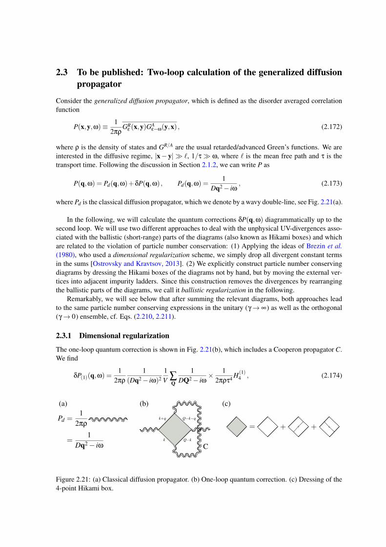
2.3 To be published: Two-loop calculation of the generalized diffusionpropagator
Consider the generalized diffusion propagator, which is defined as the disorder averaged correlationfunction
P(x,y,ω)≡ 12πρ
GRε (x,y)GA
ε−ω(y,x) , (2.172)
where ρ is the density of states and GR/A are the usual retarded/advanced Green’s functions. We areinterested in the diffusive regime, |x− y| � `, 1/τ� ω, where ` is the mean free path and τ is thetransport time. Following the discussion in Section 2.1.2, we can write P as
P(q,ω) = Pd(q,ω)+δP(q,ω) , Pd(q,ω) =1
Dq2− iω, (2.173)
where Pd is the classical diffusion propagator, which we denote by a wavy double-line, see Fig. 2.21(a).
In the following, we will calculate the quantum corrections δP(q,ω) diagrammatically up to thesecond loop. We will use two different approaches to deal with the unphysical UV-divergences asso-ciated with the ballistic (short-range) parts of the diagrams (also known as Hikami boxes) and whichare related to the violation of particle number conservation: (1) Applying the ideas of Brezin et al.(1980), who used a dimensional regularization scheme, we simply drop all divergent constant termsin the sums [Ostrovsky and Kravtsov, 2013]. (2) We explicitly construct particle number conservingdiagrams by dressing the Hikami boxes of the diagrams not by hand, but by moving the external ver-tices into adjacent impurity ladders. Since this construction removes the divergences by rearrangingthe ballistic parts of the diagrams, we call it ballistic regularization in the following.
Remarkably, we will see below that after summing the relevant diagrams, both approaches leadto the same particle number conserving expressions in the unitary (γ→ ∞) as well as the orthogonal(γ→ 0) ensemble, cf. Eqs. (2.210, 2.211).
2.3.1 Dimensional regularization
The one-loop quantum correction is shown in Fig. 2.21(b), which includes a Cooperon propagator C.We find
δP(1)(q,ω) =1
2πρ1
(Dq2− iω)21V ∑
Q
1DQ2− iω
× 12πρτ4 H(1)
4 , (2.174)
Figure 2.21: (a) Classical diffusion propagator. (b) One-loop quantum correction. (c) Dressing of the4-point Hikami box.
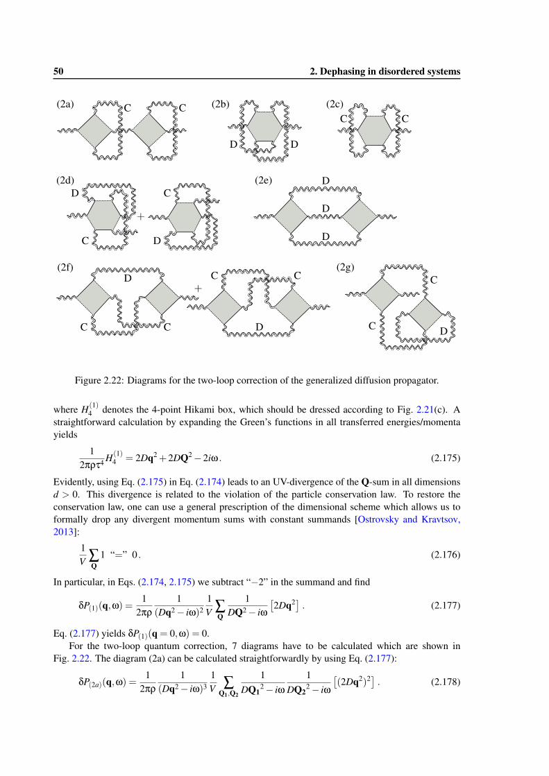
50 2. Dephasing in disordered systems
Figure 2.22: Diagrams for the two-loop correction of the generalized diffusion propagator.
where H(1)4 denotes the 4-point Hikami box, which should be dressed according to Fig. 2.21(c). A
straightforward calculation by expanding the Green’s functions in all transferred energies/momentayields
12πρτ4 H(1)
4 = 2Dq2 +2DQ2−2iω . (2.175)
Evidently, using Eq. (2.175) in Eq. (2.174) leads to an UV-divergence of the Q-sum in all dimensionsd > 0. This divergence is related to the violation of the particle conservation law. To restore theconservation law, one can use a general prescription of the dimensional scheme which allows us toformally drop any divergent momentum sums with constant summands [Ostrovsky and Kravtsov,2013]:
1V ∑
Q1 “=” 0 . (2.176)
In particular, in Eqs. (2.174, 2.175) we subtract “−2” in the summand and find
δP(1)(q,ω) =1
2πρ1
(Dq2− iω)21V ∑
Q
1DQ2− iω
[2Dq2] . (2.177)
Eq. (2.177) yields δP(1)(q = 0,ω) = 0.For the two-loop quantum correction, 7 diagrams have to be calculated which are shown in
Fig. 2.22. The diagram (2a) can be calculated straightforwardly by using Eq. (2.177):
δP(2a)(q,ω) =1
2πρ1
(Dq2− iω)31V ∑
Q1,Q2
1DQ1
2− iω1
DQ22− iω
[(2Dq2)2] . (2.178)
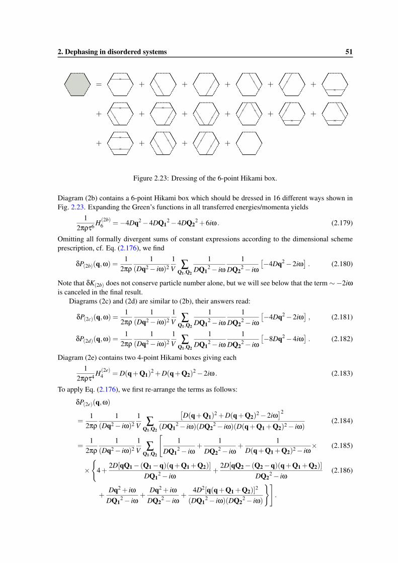
2. Dephasing in disordered systems 51
Figure 2.23: Dressing of the 6-point Hikami box.
Diagram (2b) contains a 6-point Hikami box which should be dressed in 16 different ways shown inFig. 2.23. Expanding the Green’s functions in all transferred energies/momenta yields
12πρτ6 H(2b)
6 =−4Dq2−4DQ12−4DQ2
2 +6iω . (2.179)
Omitting all formally divergent sums of constant expressions according to the dimensional schemeprescription, cf. Eq. (2.176), we find
δP(2b)(q,ω) =1
2πρ1
(Dq2− iω)21V ∑
Q1,Q2
1DQ1
2− iω1
DQ22− iω
[−4Dq2−2iω
]. (2.180)
Note that δK(2b) does not conserve particle number alone, but we will see below that the term∼−2iωis canceled in the final result.
Diagrams (2c) and (2d) are similar to (2b), their answers read:
δP(2c)(q,ω) =1
2πρ1
(Dq2− iω)21V ∑
Q1,Q2
1DQ1
2− iω1
DQ22− iω
[−4Dq2−2iω
], (2.181)
δP(2d)(q,ω) =1
2πρ1
(Dq2− iω)21V ∑
Q1,Q2
1DQ1
2− iω1
DQ22− iω
[−8Dq2−4iω
]. (2.182)
Diagram (2e) contains two 4-point Hikami boxes giving each1
2πρτ4 H(2e)4 = D(q+Q1)
2 +D(q+Q2)2−2iω . (2.183)
To apply Eq. (2.176), we first re-arrange the terms as follows:
δP(2e)(q,ω)
=1
2πρ1
(Dq2− iω)21V ∑
Q1,Q2
[D(q+Q1)
2 +D(q+Q2)2−2iω
]2
(DQ12− iω)(DQ2
2− iω)(D(q+Q1 +Q2)2− iω)(2.184)
=1
2πρ1
(Dq2− iω)21V ∑
Q1,Q2
[1
DQ12− iω
+1
DQ22− iω
+1
D(q+Q1 +Q2)2− iω× (2.185)
×{
4+2D[qQ1− (Q1−q)(q+Q1 +Q2)]
DQ12− iω
+2D[qQ2− (Q2−q)(q+Q1 +Q2)]
DQ22− iω
(2.186)
+Dq2 + iω
DQ12− iω
+Dq2 + iω
DQ22− iω
+4D2[q(q+Q1 +Q2)]
2
(DQ12− iω)(DQ2
2− iω)
}].
52 2. Dephasing in disordered systems
Evidently, when applying Eq. (2.176), the first two terms in the rectangular brackets of (2.185) arezero. After re-defining q+Q1 +Q2 as either Q1 or Q2, it is evident that the same is true for the firstterm in curly brackets of line (2.186), while the second and third terms vanish after angular averaging.In total, we find:
δP(2e)(q,ω) (2.187)
=1
2πρ1
(Dq2− iω)21V ∑
Q1,Q2
1DQ1
2− iω1
DQ22− iω
[2Dq2+2iω+
4D2[q(q+Q1+Q2)]2
D(q+Q1+Q2)2− iω
].
Diagram (2f) contains two 4-point Hikami boxes giving
1(2πρτ4)2
[H(2 f )
4 ×H(2 f )4
](2.188)
=[D(q+Q1)
2 +D(Q1+Q2)2−2iω
]×[D(q+Q2)
2 +D(Q1+Q2)2−2iω
].
Again rearranging the terms similar to Eq. (2.184) and using Eq. (2.176), we find:
δP(2 f )(q,ω) (2.189)
=1
2πρ1
(Dq2− iω)21V ∑
Q1,Q2
1DQ1
2− iω1
DQ22− iω
[10Dq2+2iω+
8D2(qQ1)(qQ2)
D(q+Q1+Q2)2− iω
].
Finally, for diagram (2g), we find
1(2πρτ4)2
[H(2g)
4 ×H(2g)4
]=[2Dq2 +2DQ1
2−2iω]×[2DQ1
2 +2DQ22−2iω
], (2.190)
and
δP(2g)(q,ω) (2.191)
=1
2πρ1
(Dq2− iω)21V ∑
Q1,Q2
1DQ1
2− iω1
DQ22− iω
[4Dq2+4iω+
4iωDq2
DQ12− iω
].
Collecting all parts together, we find the answers (2.210, 2.211), see Section 2.3.3.
2.3.2 Ballistic regularization
In this section we construct particle number conserving diagrams by moving the external verticesinto adjacent impurity ladders [Hastings et al., 1994]. We have already discussed this procedure inSection 2.1.2, cf. Fig. 2.5 and Fig. 2.6.
To illustrate the idea, we have drawn an external vertex close to an impurity ladder in Fig. 2.24(a):By moving the external vertex (on the left) up, into the ladder, we generate a diagram which re-sembles the dressing of a Hikami box, while keeping the total number of impurities of the diagramfixed. Applying this to the diagram of Fig. 2.21(b), see Fig. 2.24(b), where an impurity ladder withmomentum-transfer Q is attached at the top and bottom of the Hikami box, we can generate both re-quired dressings of the 4 point Hikami box. Note that calculating the diagrams in this way means thatthe undressed box is effectively multiplied by an extra factor of [1+ iτω− τDQ2], since it containsone extra “step” of the ladder, cf. Fig. 2.24(d).
Importantly, all dressings shown in Fig. 2.21(c) and Fig. 2.23 have to be generated in this way,and we will see below that this is not immediately possible for the diagrams involving 6-point Hikami
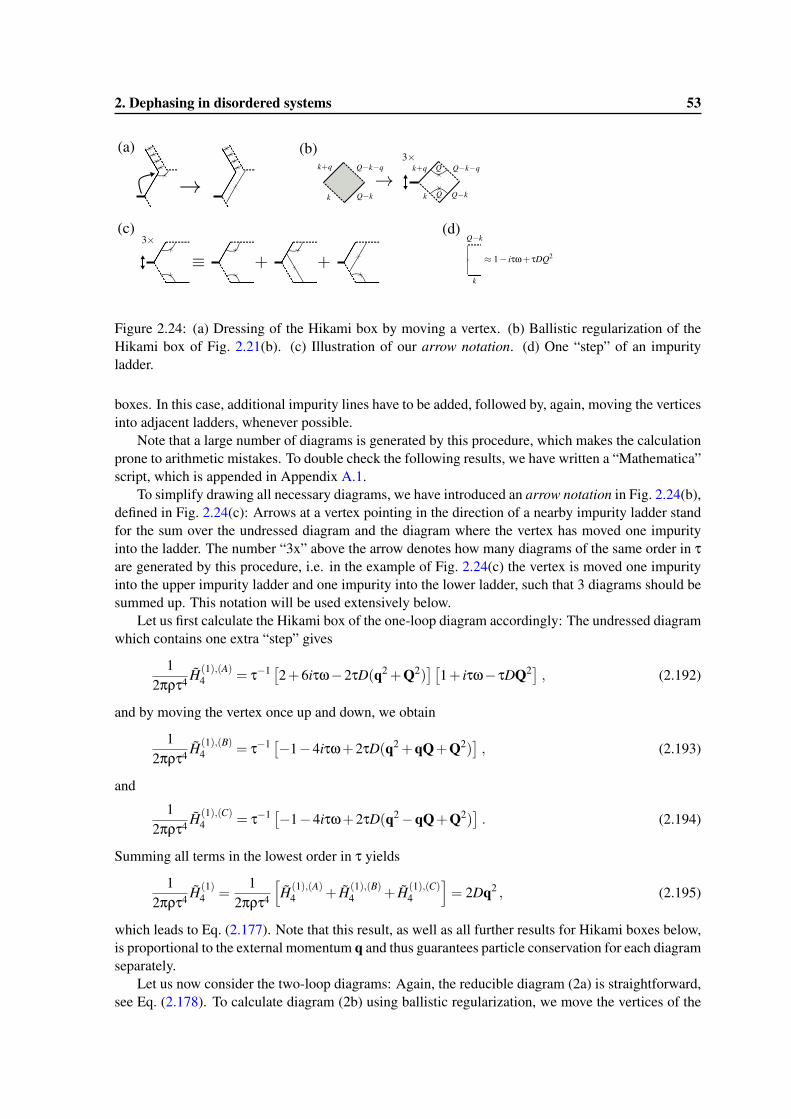
2. Dephasing in disordered systems 53
Figure 2.24: (a) Dressing of the Hikami box by moving a vertex. (b) Ballistic regularization of theHikami box of Fig. 2.21(b). (c) Illustration of our arrow notation. (d) One “step” of an impurityladder.
boxes. In this case, additional impurity lines have to be added, followed by, again, moving the verticesinto adjacent ladders, whenever possible.
Note that a large number of diagrams is generated by this procedure, which makes the calculationprone to arithmetic mistakes. To double check the following results, we have written a “Mathematica”script, which is appended in Appendix A.1.
To simplify drawing all necessary diagrams, we have introduced an arrow notation in Fig. 2.24(b),defined in Fig. 2.24(c): Arrows at a vertex pointing in the direction of a nearby impurity ladder standfor the sum over the undressed diagram and the diagram where the vertex has moved one impurityinto the ladder. The number “3x” above the arrow denotes how many diagrams of the same order in τare generated by this procedure, i.e. in the example of Fig. 2.24(c) the vertex is moved one impurityinto the upper impurity ladder and one impurity into the lower ladder, such that 3 diagrams should besummed up. This notation will be used extensively below.
Let us first calculate the Hikami box of the one-loop diagram accordingly: The undressed diagramwhich contains one extra “step” gives
12πρτ4 H(1),(A)
4 = τ−1 [2+6iτω−2τD(q2 +Q2)][
1+ iτω− τDQ2] , (2.192)
and by moving the vertex once up and down, we obtain
12πρτ4 H(1),(B)
4 = τ−1 [−1−4iτω+2τD(q2 +qQ+Q2)], (2.193)
and
12πρτ4 H(1),(C)
4 = τ−1 [−1−4iτω+2τD(q2−qQ+Q2)]. (2.194)
Summing all terms in the lowest order in τ yields
12πρτ4 H(1)
4 =1
2πρτ4
[H(1),(A)
4 + H(1),(B)4 + H(1),(C)
4
]= 2Dq2 , (2.195)
which leads to Eq. (2.177). Note that this result, as well as all further results for Hikami boxes below,is proportional to the external momentum q and thus guarantees particle conservation for each diagramseparately.
Let us now consider the two-loop diagrams: Again, the reducible diagram (2a) is straightforward,see Eq. (2.178). To calculate diagram (2b) using ballistic regularization, we move the vertices of the
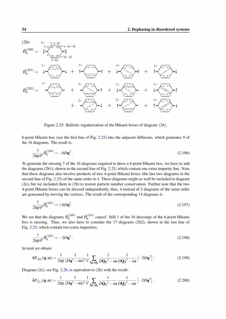
54 2. Dephasing in disordered systems
Figure 2.25: Ballistic regularization of the Hikami boxes of diagram (2b).
6-point Hikami box (see the first line of Fig. 2.25) into the adjacent diffusons, which generates 9 ofthe 16 diagrams. The result is:
12πρτ6 H(2b0)
6 =−6Dq2 . (2.196)
To generate the missing 7 of the 16 diagrams required to dress a 6-point Hikami box, we have to addthe diagrams (2b1), shown in the second line of Fig. 2.25, which contain one extra impurity line. Notethat these diagrams also involve products of two 4-point Hikami boxes (the last two diagrams in thesecond line of Fig. 2.25) of the same order in τ. These diagrams might as well be included in diagram(2e), but we included them in (2b) to restore particle number conservation. Further note that the two4-point Hikami boxes can be dressed independently, thus, 4 instead of 3 diagrams of the same orderare generated by moving the vertices. The result of the corresponding 14 diagrams is
12πρτ6 H(2b1)
6 =+6Dq2 . (2.197)
We see that the diagrams H(2b0)6 and H(2b1)
6 cancel. Still 1 of the 16 dressings of the 6-point Hikamibox is missing. Thus, we also have to consider the 17 diagrams (2b2), shown in the last line ofFig. 2.25, which contain two extra impurities:
12πρτ6 H(2b2)
6 =−2Dq2 . (2.198)
In total we obtain:
δP(2b)(q,ω) =1
2πρ1
(Dq2− iω)21V ∑
Q1,Q2
1DQ1
2− iω1
DQ22− iω
[−2Dq2] . (2.199)
Diagram (2c), see Fig. 2.26, is equivalent to (2b) with the result:
δP(2c)(q,ω) =1
2πρ1
(Dq2− iω)21V ∑
Q1,Q2
1DQ1
2− iω1
DQ22− iω
[−2Dq2] . (2.200)
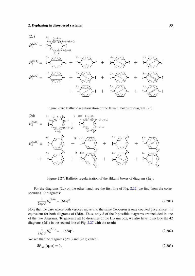
2. Dephasing in disordered systems 55
Figure 2.26: Ballistic regularization of the Hikami boxes of diagram (2c).
Figure 2.27: Ballistic regularization of the Hikami boxes of diagram (2d).
For the diagrams (2d) on the other hand, see the first line of Fig. 2.27, we find from the corre-sponding 17 diagrams:
12πρτ6 H(2d0)
6 = 16Dq2 . (2.201)
Note that the case where both vertices move into the same Cooperon is only counted once, since it isequivalent for both diagrams of (2d0). Thus, only 8 of the 9 possible diagrams are included in oneof the two diagrams. To generate all 16 dressings of the Hikami box, we also have to include the 42diagrams (2d1) in the second line of Fig. 2.27 with the result:
12πρτ6 H(2d1)
6 =−16Dq2 . (2.202)
We see that the diagrams (2d0) and (2d1) cancel:
δP(2d)(q,ω) = 0 . (2.203)
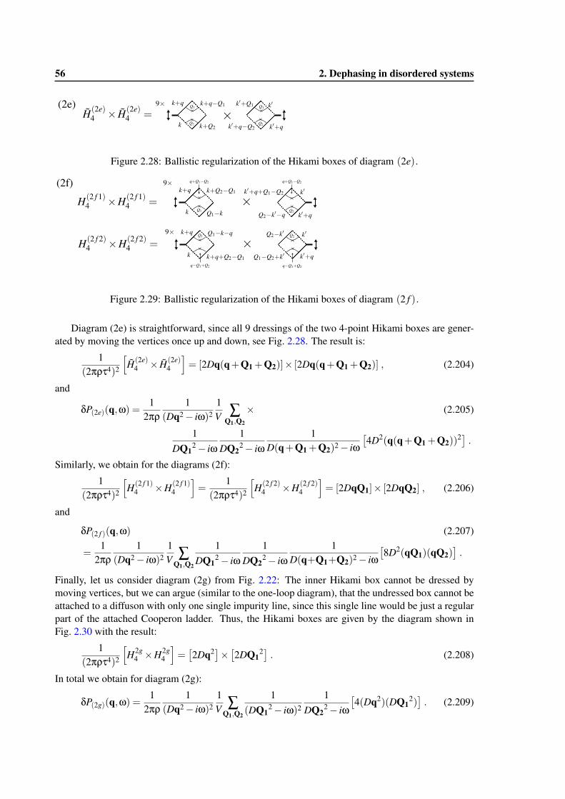
56 2. Dephasing in disordered systems
Figure 2.28: Ballistic regularization of the Hikami boxes of diagram (2e).
Figure 2.29: Ballistic regularization of the Hikami boxes of diagram (2 f ).
Diagram (2e) is straightforward, since all 9 dressings of the two 4-point Hikami boxes are gener-ated by moving the vertices once up and down, see Fig. 2.28. The result is:
1(2πρτ4)2
[H(2e)
4 × H(2e)4
]= [2Dq(q+Q1 +Q2)]× [2Dq(q+Q1 +Q2)] , (2.204)
and
δP(2e)(q,ω) =1
2πρ1
(Dq2− iω)21V ∑
Q1,Q2
× (2.205)
1DQ1
2− iω1
DQ22− iω
1D(q+Q1 +Q2)2− iω
[4D2(q(q+Q1 +Q2))
2] .
Similarly, we obtain for the diagrams (2f):
1(2πρτ4)2
[H(2 f 1)
4 ×H(2 f 1)4
]=
1(2πρτ4)2
[H(2 f 2)
4 ×H(2 f 2)4
]= [2DqQ1]× [2DqQ2] , (2.206)
and
δP(2 f )(q,ω) (2.207)
=1
2πρ1
(Dq2− iω)21V ∑
Q1,Q2
1DQ1
2− iω1
DQ22− iω
1D(q+Q1+Q2)2− iω
[8D2(qQ1)(qQ2)
].
Finally, let us consider diagram (2g) from Fig. 2.22: The inner Hikami box cannot be dressed bymoving vertices, but we can argue (similar to the one-loop diagram), that the undressed box cannot beattached to a diffuson with only one single impurity line, since this single line would be just a regularpart of the attached Cooperon ladder. Thus, the Hikami boxes are given by the diagram shown inFig. 2.30 with the result:
1(2πρτ4)2
[H2g
4 ×H2g4
]=[2Dq2]×
[2DQ1
2] . (2.208)
In total we obtain for diagram (2g):
δP(2g)(q,ω) =1
2πρ1
(Dq2− iω)21V ∑
Q1,Q2
1(DQ1
2− iω)2
1DQ2
2− iω[4(Dq2)(DQ1
2)]. (2.209)
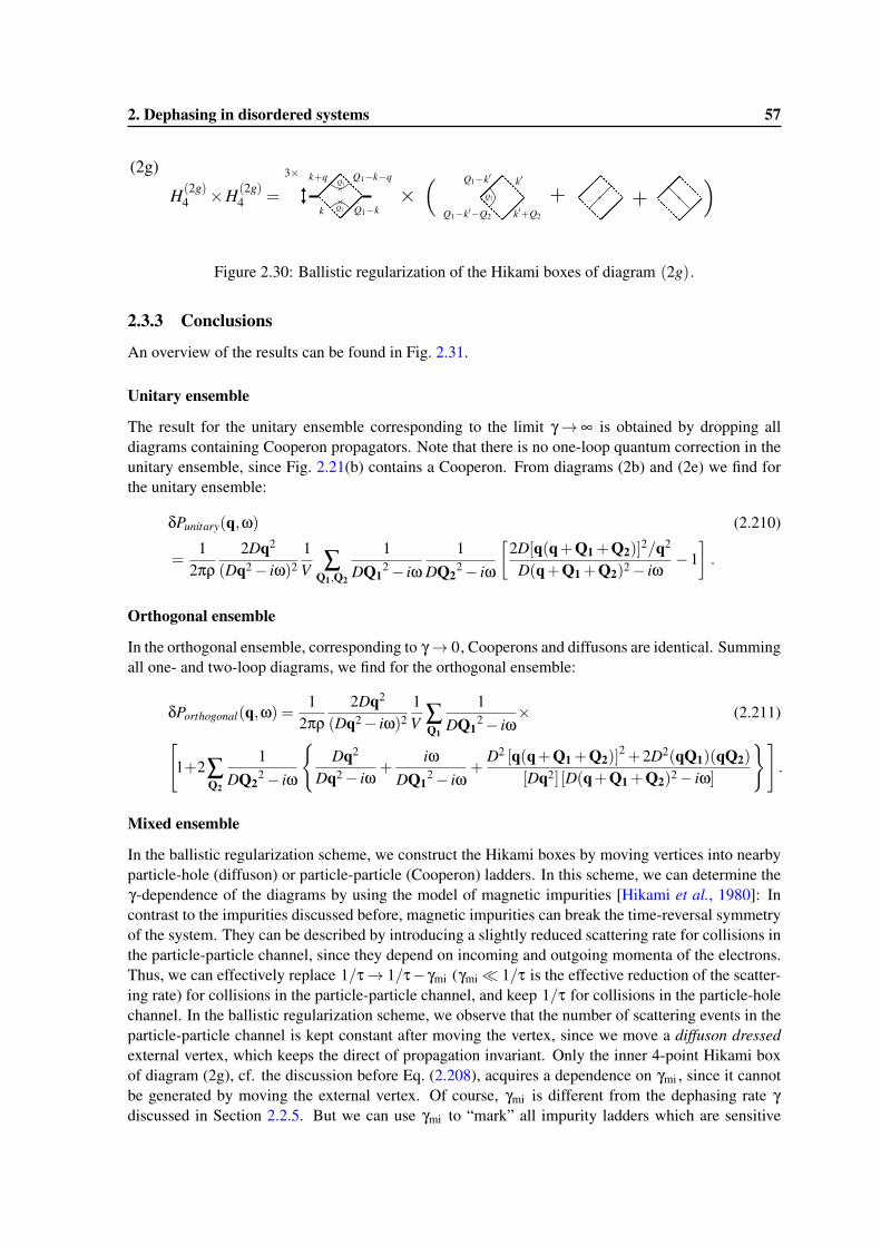
2. Dephasing in disordered systems 57
Figure 2.30: Ballistic regularization of the Hikami boxes of diagram (2g).
2.3.3 Conclusions
An overview of the results can be found in Fig. 2.31.
Unitary ensemble
The result for the unitary ensemble corresponding to the limit γ→ ∞ is obtained by dropping alldiagrams containing Cooperon propagators. Note that there is no one-loop quantum correction in theunitary ensemble, since Fig. 2.21(b) contains a Cooperon. From diagrams (2b) and (2e) we find forthe unitary ensemble:
δPunitary(q,ω) (2.210)
=1
2πρ2Dq2
(Dq2− iω)21V ∑
Q1,Q2
1DQ1
2− iω1
DQ22− iω
[2D[q(q+Q1 +Q2)]
2/q2
D(q+Q1 +Q2)2− iω−1].
Orthogonal ensemble
In the orthogonal ensemble, corresponding to γ→ 0, Cooperons and diffusons are identical. Summingall one- and two-loop diagrams, we find for the orthogonal ensemble:
δPorthogonal(q,ω) =1
2πρ2Dq2
(Dq2− iω)21V ∑
Q1
1DQ1
2− iω× (2.211)
[1+2∑
Q2
1DQ2
2− iω
{Dq2
Dq2− iω+
iωDQ1
2− iω+
D2 [q(q+Q1 +Q2)]2 +2D2(qQ1)(qQ2)
[Dq2] [D(q+Q1 +Q2)2− iω]
}].
Mixed ensemble
In the ballistic regularization scheme, we construct the Hikami boxes by moving vertices into nearbyparticle-hole (diffuson) or particle-particle (Cooperon) ladders. In this scheme, we can determine theγ-dependence of the diagrams by using the model of magnetic impurities [Hikami et al., 1980]: Incontrast to the impurities discussed before, magnetic impurities can break the time-reversal symmetryof the system. They can be described by introducing a slightly reduced scattering rate for collisions inthe particle-particle channel, since they depend on incoming and outgoing momenta of the electrons.Thus, we can effectively replace 1/τ→ 1/τ− γmi (γmi� 1/τ is the effective reduction of the scatter-ing rate) for collisions in the particle-particle channel, and keep 1/τ for collisions in the particle-holechannel. In the ballistic regularization scheme, we observe that the number of scattering events in theparticle-particle channel is kept constant after moving the vertex, since we move a diffuson dressedexternal vertex, which keeps the direct of propagation invariant. Only the inner 4-point Hikami boxof diagram (2g), cf. the discussion before Eq. (2.208), acquires a dependence on γmi , since it cannotbe generated by moving the external vertex. Of course, γmi is different from the dephasing rate γdiscussed in Section 2.2.5. But we can use γmi to “mark” all impurity ladders which are sensitive
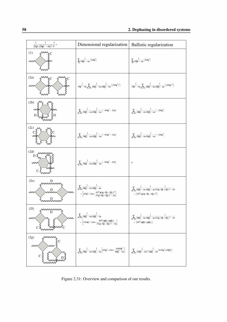
58 2. Dephasing in disordered systems
Dimensional regularization Ballistic regularization
Figure 2.31: Overview and comparison of our results.
2. Dephasing in disordered systems 59
to time-reversal symmetry. After rearranging the terms, and substituting DQ21,2→ DQ2
1,2 + γ in allimpurity ladders which contain γmi , we obtain:
δP(q,ω) =1
2πρ2Dq2
(Dq2− iω)21V ∑
Q1,Q2
(Pd(Q1,ω)Pd(Q2,ω)
[2D[q(q+Q1 +Q2)]
2/q2
D(q+Q1 +Q2)2− iω−1]
+Pc(Q1,ω)Pc(Q2,ω)[
Dq2 + iωDq2− iω
+4D(qQ1)(qQ2)/Dq2
D(q+Q1 +Q2)2− iω
]
+Pc(Q1,ω)Pd(Q2,ω) [2+2iωPc(Q1,ω)]
). (2.212)
Only the Cooperon propagators, Pc , in Eq. (2.212) acquire a dependence on γ.

2. Dephasing in disordered systems 61
2.4 Publication: Thermal noise and dephasing due to electron interac-tions in nontrivial geometries
The following 8 pages have been published in the journal Physical Review B.
PHYSICAL REVIEW B 84, 054204 (2011)
Thermal noise and dephasing due to electron interactions in nontrivial geometries
M. Treiber,1 C. Texier,2 O. M. Yevtushenko,1 J. von Delft,1 and I. V. Lerner3
1Ludwig Maximilians University, Arnold Sommerfeld Center and Center for Nano-Science, Munich, DE-80333, Germany2Univ. Paris Sud, CNRS, LPTMS, UMR 8626 & LPS, UMR 8502, Orsay FR-91405, France
3School of Physics and Astronomy, University of Birmingham, Birmingham, B15 2TT, United Kingdom(Received 5 May 2011; published 5 August 2011)
We study Johnson-Nyquist noise in macroscopically inhomogeneous disordered metals and give a microscopicderivation of the correlation function of the scalar electric potentials in real space. Starting from the interactingHamiltonian for electrons in a metal and the random phase approximation, we find a relation between thecorrelation function of the electric potentials and the density fluctuations, which is valid for arbitrary geometryand dimensionality. We show that the potential fluctuations are proportional to the solution of the diffusionequation, taken at zero frequency. As an example, we consider networks of quasi-one-dimensional disorderedwires and give an explicit expression for the correlation function in a ring attached via arms to absorbing leads.We use this result in order to develop a theory of dephasing by electronic noise in multiply-connected systems.
DOI: 10.1103/PhysRevB.84.054204 PACS number(s): 07.50.Hp, 42.50.Lc, 73.63.−b
I. INTRODUCTION
Electronic noise generated by the thermal excitation ofcharge carriers has been observed and explained by Johnsonand Nyquist more than 80 years ago1 and discussed ingreat detail in the literature since then. More recently, ithas been found that this so-called Johnson-Nyquist noise isthe main source of dephasing in mesoscopic systems at lowtemperatures of a few Kelvins where phonons are frozen out.Dephasing puts an IR cut-off for interference phenomena, suchas quantum corrections to the classical conductivity.2
The current interest in this topic arises from studies ofdephasing in mesoscopic systems which consist of connectedquasi-one-dimensional (1D) disordered wires, see Fig. 1,including connected rings and grids.3,4 It has been found (bothexperimentally5 and theoretically6–10) that dephasing dependsnot only on the dimensionality, but also on the geometry of thesystem. The noise correlation function is well-understood formacroscopically homogeneous systems such as infinite wiresor isolated rings, but has so-far not been studied in multiply-connected networks with leads attached at arbitrary points.The goal of this paper is to give a transparent and systematicdescription of the thermal noise properties for such systems. Inparticular, we will derive an expression for the fluctuations ofthe scalar electric potentials for arbitrary geometries, Eq. (31),and a general expression for the corresponding dephasingrate, Eq. (45). Throughout, we assume that a description ofthe noise in terms of scalar potentials is sufficient, i.e., weneglect the fluctuations of the transverse component of theelectromagnetic field (for a detailed discussion of the latter,see Ref. 2).
Let us start by reviewing simplified arguments to derive thenoise correlation function: Johnson and Nyquist concludedthat thermal noise in electrical conductors is approximatelywhite, meaning that the power spectral density is nearlyconstant throughout the whole frequency spectrum. If, inaddition, the fluctuations are uncorrelated for different pointsin space, a correlation function for the random thermal currentsin the classical limit is independent of frequency ω andmomentum q. The power spectrum of the current density reads
〈| j |2〉(q,ω) = 2T σ0 . (1)
Here, σ0 = e2νD is the Drude conductivity of the disorderedsystem, D and ν are the diffusion constant and the densityof states, respectively. Naively applying Ohm’s law, j (q) =σ0 E(q), to Eq. (1) and using the relation between the electricfield and the scalar potential, eE(q) = −iqV (q), we find
〈|V |2〉(q,ω) = 2T e2
σ0
1
q2. (2)
The correlation function, Eq. (2), corresponds to the couplingof a given electron to the bath of the surrounding electrons.2
Thus 〈|V |2〉 describes the process of successive emission andreabsorption of a photon, which is described effectively by thescalar potential V . The factor 1/q2 coincides with the solutionof a diffusion equation in an infinite system, which reflects thefact that the currents, Eq. (1), are uncorrelated in space.
These simple arguments are based on the homogeneity ofthe system and have assumed a local relation between potentialand current, whereas transport properties in disordered metalsare substantially nonlocal.10–13 In this paper, we derive ananalogy of Eq. (2) for disordered systems with arbitrarygeometry and dimensionality; this will in particular apply tonetworks of disordered wires. A detailed calculation, whichtakes into account all properties of the mesoscopic samples,has to be done in the real-space representation. Starting pointsare the usual linear response formalism and the fluctuation-dissipation theorem (FDT).14 Although most ingredients ofthe following discussion will be familiar to experts, we hopethat the manner in which they have been assembled here willbe found not only to be pedagogically useful, but also helpfulfor further theoretical studies.
The paper is organized as follows: in Sec. II, we propose aheuristic description of the potential fluctuations. In Sec. III,we review a microscopic approach to the noise correlationfunction, based on a relation of the fluctuations of the scalarpotentials to the fluctuations of the density, using the randomphase approximation (RPA). In Sec. IV, we evaluate thedensity response function χ for disordered systems by usinga real-space representation for arbitrary geometries. We applythis result to the noise correlation function in Sec. V. In Sec. VI,we show how the noise correlation function can be calculatedfor networks of disordered wires. Finally, in Sec. VII, we
054204-11098-0121/2011/84(5)/054204(8) ©2011 American Physical Society
62 2. Dephasing in disordered systems
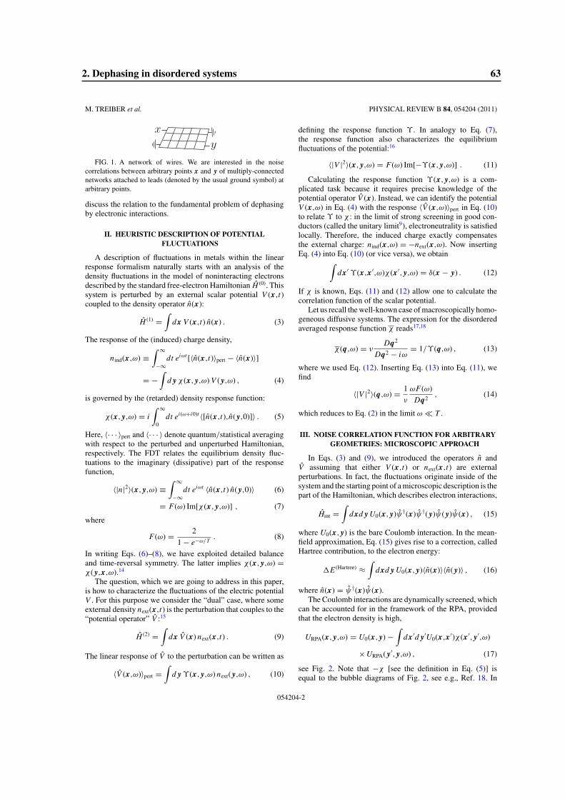
M. TREIBER et al. PHYSICAL REVIEW B 84, 054204 (2011)
FIG. 1. A network of wires. We are interested in the noisecorrelations between arbitrary points x and y of multiply-connectednetworks attached to leads (denoted by the usual ground symbol) atarbitrary points.
discuss the relation to the fundamental problem of dephasingby electronic interactions.
II. HEURISTIC DESCRIPTION OF POTENTIALFLUCTUATIONS
A description of fluctuations in metals within the linearresponse formalism naturally starts with an analysis of thedensity fluctuations in the model of noninteracting electronsdescribed by the standard free-electron Hamiltonian H (0). Thissystem is perturbed by an external scalar potential V (x,t)coupled to the density operator n(x):
H (1) =∫
dx V (x,t) n(x) . (3)
The response of the (induced) charge density,
nind(x,ω) ≡∫ ∞
−∞dt eiωt [〈n(x,t)〉pert − 〈n(x)〉]
= −∫
d y χ (x, y,ω) V ( y,ω) , (4)
is governed by the (retarded) density response function:
χ (x, y,ω) = i
∫ ∞
0dt ei(ω+i0)t 〈[n(x,t),n( y,0)]〉 . (5)
Here, 〈· · · 〉pert and 〈· · · 〉 denote quantum/statistical averagingwith respect to the perturbed and unperturbed Hamiltonian,respectively. The FDT relates the equilibrium density fluc-tuations to the imaginary (dissipative) part of the responsefunction,
〈|n|2〉(x, y,ω) ≡∫ ∞
−∞dt eiωt 〈n(x,t) n( y,0)〉 (6)
= F (ω) Im[χ (x, y,ω)] , (7)
where
F (ω) = 2
1 − e−ω/T. (8)
In writing Eqs. (6)–(8), we have exploited detailed balanceand time-reversal symmetry. The latter implies χ (x, y,ω) =χ ( y,x,ω).14
The question, which we are going to address in this paper,is how to characterize the fluctuations of the electric potentialV . For this purpose we consider the “dual” case, where someexternal density next(x,t) is the perturbation that couples to the“potential operator” V :15
H (2) =∫
dx V (x) next(x,t) . (9)
The linear response of V to the perturbation can be written as
〈V (x,ω)〉pert =∫
d y ϒ(x, y,ω) next( y,ω) , (10)
defining the response function ϒ . In analogy to Eq. (7),the response function also characterizes the equilibriumfluctuations of the potential:16
〈|V |2〉(x, y,ω) = F (ω) Im[−ϒ(x, y,ω)] . (11)
Calculating the response function ϒ(x, y,ω) is a com-plicated task because it requires precise knowledge of thepotential operator V (x). Instead, we can identify the potentialV (x,ω) in Eq. (4) with the response 〈V (x,ω)〉pert in Eq. (10)to relate ϒ to χ : in the limit of strong screening in good con-ductors (called the unitary limit9), electroneutrality is satisfiedlocally. Therefore, the induced charge exactly compensatesthe external charge: nind(x,ω) = −next(x,ω). Now insertingEq. (4) into Eq. (10) (or vice versa), we obtain∫
dx′ ϒ(x,x′,ω)χ (x′, y,ω) = δ(x − y) . (12)
If χ is known, Eqs. (11) and (12) allow one to calculate thecorrelation function of the scalar potential.
Let us recall the well-known case of macroscopically homo-geneous diffusive systems. The expression for the disorderedaveraged response function χ reads17,18
χ(q,ω) = νDq2
Dq2 − iω= 1/ϒ(q,ω) , (13)
where we used Eq. (12). Inserting Eq. (13) into Eq. (11), wefind
〈|V |2〉(q,ω) = 1
ν
ωF (ω)
Dq2, (14)
which reduces to Eq. (2) in the limit ω � T .
III. NOISE CORRELATION FUNCTION FOR ARBITRARYGEOMETRIES: MICROSCOPIC APPROACH
In Eqs. (3) and (9), we introduced the operators n andV assuming that either V (x,t) or next(x,t) are externalperturbations. In fact, the fluctuations originate inside of thesystem and the starting point of a microscopic description is thepart of the Hamiltonian, which describes electron interactions,
Hint =∫
dxd y U0(x, y)ψ†(x)ψ†( y)ψ( y)ψ(x) , (15)
where U0(x, y) is the bare Coulomb interaction. In the mean-field approximation, Eq. (15) gives rise to a correction, calledHartree contribution, to the electron energy:
E(Hartree) ≈∫
dxd y U0(x, y)〈n(x)〉〈n( y)〉 , (16)
where n(x) = ψ†(x)ψ(x).The Coulomb interactions are dynamically screened, which
can be accounted for in the framework of the RPA, providedthat the electron density is high,
URPA(x, y,ω) = U0(x, y) −∫
dx′d y′U0(x,x′)χ (x′, y′,ω)
×URPA( y′, y,ω) , (17)
see Fig. 2. Note that −χ [see the definition in Eq. (5)] isequal to the bubble diagrams of Fig. 2, see e.g., Ref. 18. In
054204-2
2. Dephasing in disordered systems 63
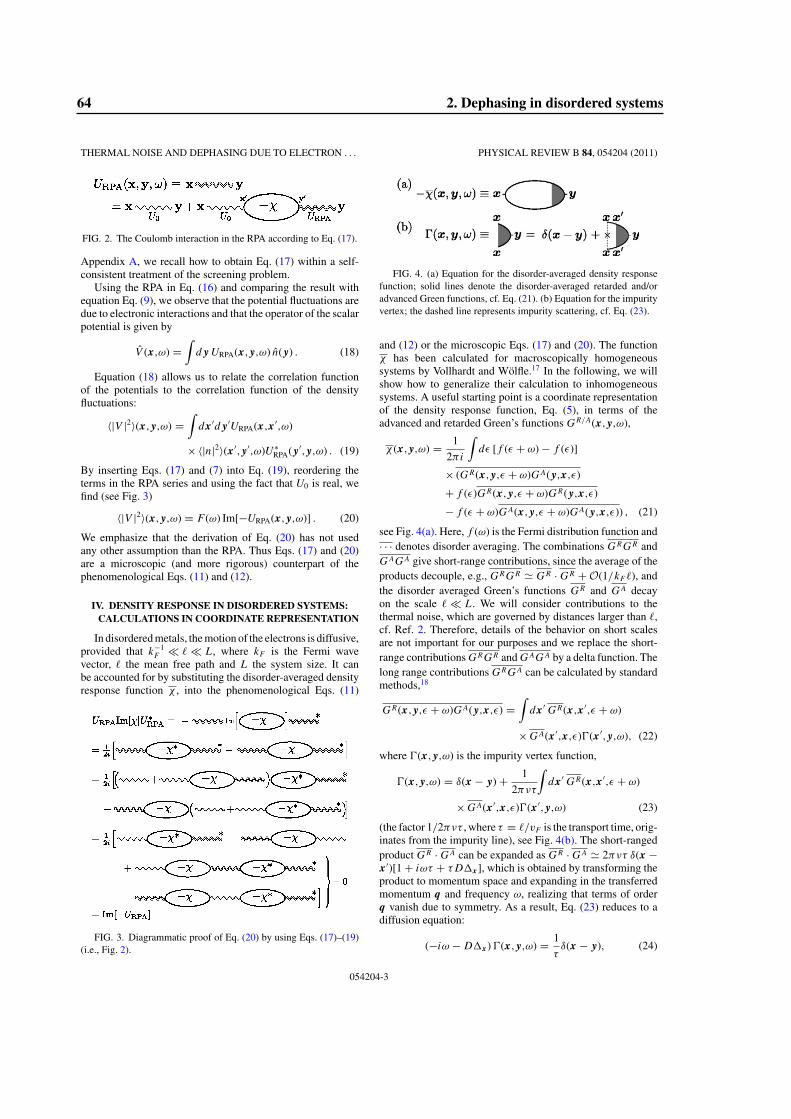
THERMAL NOISE AND DEPHASING DUE TO ELECTRON . . . PHYSICAL REVIEW B 84, 054204 (2011)
FIG. 2. The Coulomb interaction in the RPA according to Eq. (17).
Appendix A, we recall how to obtain Eq. (17) within a self-consistent treatment of the screening problem.
Using the RPA in Eq. (16) and comparing the result withequation Eq. (9), we observe that the potential fluctuations aredue to electronic interactions and that the operator of the scalarpotential is given by
V (x,ω) =∫
d y URPA(x, y,ω) n( y) . (18)
Equation (18) allows us to relate the correlation functionof the potentials to the correlation function of the densityfluctuations:
〈|V |2〉(x, y,ω) =∫
dx′d y′URPA(x,x′,ω)
×〈|n|2〉(x′, y′,ω)U ∗RPA( y′, y,ω) . (19)
By inserting Eqs. (17) and (7) into Eq. (19), reordering theterms in the RPA series and using the fact that U0 is real, wefind (see Fig. 3)
〈|V |2〉(x, y,ω) = F (ω) Im[−URPA(x, y,ω)] . (20)
We emphasize that the derivation of Eq. (20) has not usedany other assumption than the RPA. Thus Eqs. (17) and (20)are a microscopic (and more rigorous) counterpart of thephenomenological Eqs. (11) and (12).
IV. DENSITY RESPONSE IN DISORDERED SYSTEMS:CALCULATIONS IN COORDINATE REPRESENTATION
In disordered metals, the motion of the electrons is diffusive,provided that k−1
F � � L, where kF is the Fermi wavevector, the mean free path and L the system size. It canbe accounted for by substituting the disorder-averaged densityresponse function χ , into the phenomenological Eqs. (11)
FIG. 3. Diagrammatic proof of Eq. (20) by using Eqs. (17)–(19)(i.e., Fig. 2).
FIG. 4. (a) Equation for the disorder-averaged density responsefunction; solid lines denote the disorder-averaged retarded and/oradvanced Green functions, cf. Eq. (21). (b) Equation for the impurityvertex; the dashed line represents impurity scattering, cf. Eq. (23).
and (12) or the microscopic Eqs. (17) and (20). The functionχ has been calculated for macroscopically homogeneoussystems by Vollhardt and Wolfle.17 In the following, we willshow how to generalize their calculation to inhomogeneoussystems. A useful starting point is a coordinate representationof the density response function, Eq. (5), in terms of theadvanced and retarded Green’s functions GR/A(x, y,ω),
χ (x, y,ω) = 1
2πi
∫dε [f (ε + ω) − f (ε)]
× (GR(x, y,ε + ω)GA( y,x,ε)
+ f (ε)GR(x, y,ε + ω)GR( y,x,ε)
− f (ε + ω)GA(x, y,ε + ω)GA( y,x,ε)) , (21)
see Fig. 4(a). Here, f (ω) is the Fermi distribution function and· · · denotes disorder averaging. The combinations GRGR andGAGA give short-range contributions, since the average of theproducts decouple, e.g., GRGR GR · GR + O(1/kF ), andthe disorder averaged Green’s functions GR and GA decayon the scale � L. We will consider contributions to thethermal noise, which are governed by distances larger than ,cf. Ref. 2. Therefore, details of the behavior on short scalesare not important for our purposes and we replace the short-range contributions GRGR and GAGA by a delta function. Thelong range contributions GRGA can be calculated by standardmethods,18
GR(x, y,ε + ω)GA( y,x,ε) =∫
dx′ GR(x,x′,ε + ω)
×GA(x′,x,ε) (x′, y,ω), (22)
where (x, y,ω) is the impurity vertex function,
(x, y,ω) = δ(x − y) + 1
2πντ
∫dx′ GR(x,x′,ε + ω)
×GA(x′,x,ε) (x′, y,ω) (23)
(the factor 1/2πντ , where τ = /vF is the transport time, orig-inates from the impurity line), see Fig. 4(b). The short-rangedproduct GR · GA can be expanded as GR · GA 2πντ δ(x −x′)[1 + iωτ + τDx], which is obtained by transforming theproduct to momentum space and expanding in the transferredmomentum q and frequency ω, realizing that terms of orderq vanish due to symmetry. As a result, Eq. (23) reduces to adiffusion equation:
(−iω − Dx) (x, y,ω) = 1
τδ(x − y), (24)
054204-3
64 2. Dephasing in disordered systems
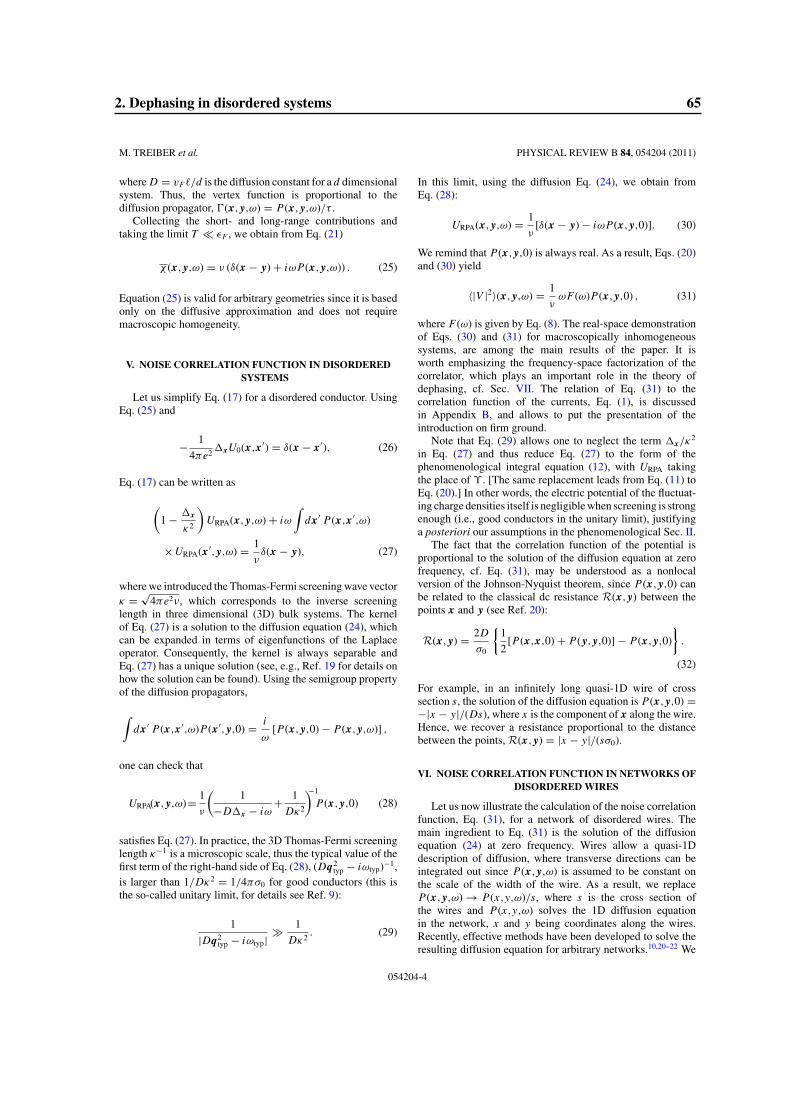
M. TREIBER et al. PHYSICAL REVIEW B 84, 054204 (2011)
where D = vF /d is the diffusion constant for a d dimensionalsystem. Thus, the vertex function is proportional to thediffusion propagator, (x, y,ω) = P (x, y,ω)/τ .
Collecting the short- and long-range contributions andtaking the limit T � εF , we obtain from Eq. (21)
χ(x, y,ω) = ν (δ(x − y) + iωP (x, y,ω)) . (25)
Equation (25) is valid for arbitrary geometries since it is basedonly on the diffusive approximation and does not requiremacroscopic homogeneity.
V. NOISE CORRELATION FUNCTION IN DISORDEREDSYSTEMS
Let us simplify Eq. (17) for a disordered conductor. UsingEq. (25) and
− 1
4πe2xU0(x,x′) = δ(x − x′), (26)
Eq. (17) can be written as
(1 − x
κ2
)URPA(x, y,ω) + iω
∫dx′ P (x,x′,ω)
×URPA(x′, y,ω) = 1
νδ(x − y), (27)
where we introduced the Thomas-Fermi screening wave vectorκ =
√4πe2ν, which corresponds to the inverse screening
length in three dimensional (3D) bulk systems. The kernelof Eq. (27) is a solution to the diffusion equation (24), whichcan be expanded in terms of eigenfunctions of the Laplaceoperator. Consequently, the kernel is always separable andEq. (27) has a unique solution (see, e.g., Ref. 19 for details onhow the solution can be found). Using the semigroup propertyof the diffusion propagators,
∫dx′ P (x,x′,ω)P (x′, y,0) = i
ω[P (x, y,0) − P (x, y,ω)] ,
one can check that
URPA(x, y,ω)= 1
ν
(1
−Dx − iω+ 1
Dκ2
)−1
P (x, y,0) (28)
satisfies Eq. (27). In practice, the 3D Thomas-Fermi screeninglength κ−1 is a microscopic scale, thus the typical value of thefirst term of the right-hand side of Eq. (28), (Dq2
typ − iωtyp)−1,is larger than 1/Dκ2 = 1/4πσ0 for good conductors (this isthe so-called unitary limit, for details see Ref. 9):
1
|Dq2typ − iωtyp|
� 1
Dκ2. (29)
In this limit, using the diffusion Eq. (24), we obtain fromEq. (28):
URPA(x, y,ω) = 1
ν[δ(x − y) − iωP (x, y,0)]. (30)
We remind that P (x, y,0) is always real. As a result, Eqs. (20)and (30) yield
〈|V |2〉(x, y,ω) = 1
νωF (ω)P (x, y,0) , (31)
where F (ω) is given by Eq. (8). The real-space demonstrationof Eqs. (30) and (31) for macroscopically inhomogeneoussystems, are among the main results of the paper. It isworth emphasizing the frequency-space factorization of thecorrelator, which plays an important role in the theory ofdephasing, cf. Sec. VII. The relation of Eq. (31) to thecorrelation function of the currents, Eq. (1), is discussedin Appendix B, and allows to put the presentation of theintroduction on firm ground.
Note that Eq. (29) allows one to neglect the term x/κ2
in Eq. (27) and thus reduce Eq. (27) to the form of thephenomenological integral equation (12), with URPA takingthe place of ϒ . [The same replacement leads from Eq. (11) toEq. (20).] In other words, the electric potential of the fluctuat-ing charge densities itself is negligible when screening is strongenough (i.e., good conductors in the unitary limit), justifyinga posteriori our assumptions in the phenomenological Sec. II.
The fact that the correlation function of the potential isproportional to the solution of the diffusion equation at zerofrequency, cf. Eq. (31), may be understood as a nonlocalversion of the Johnson-Nyquist theorem, since P (x, y,0) canbe related to the classical dc resistance R(x, y) between thepoints x and y (see Ref. 20):
R(x, y) = 2D
σ0
{1
2[P (x,x,0) + P ( y, y,0)] − P (x, y,0)
}.
(32)
For example, in an infinitely long quasi-1D wire of crosssection s, the solution of the diffusion equation is P (x, y,0) =−|x − y|/(Ds), where x is the component of x along the wire.Hence, we recover a resistance proportional to the distancebetween the points, R(x, y) = |x − y|/(sσ0).
VI. NOISE CORRELATION FUNCTION IN NETWORKS OFDISORDERED WIRES
Let us now illustrate the calculation of the noise correlationfunction, Eq. (31), for a network of disordered wires. Themain ingredient to Eq. (31) is the solution of the diffusionequation (24) at zero frequency. Wires allow a quasi-1Ddescription of diffusion, where transverse directions can beintegrated out since P (x, y,ω) is assumed to be constant onthe scale of the width of the wire. As a result, we replaceP (x, y,ω) → P (x,y,ω)/s, where s is the cross section ofthe wires and P (x,y,ω) solves the 1D diffusion equationin the network, x and y being coordinates along the wires.Recently, effective methods have been developed to solve theresulting diffusion equation for arbitrary networks.10,20–22 We
054204-4
2. Dephasing in disordered systems 65
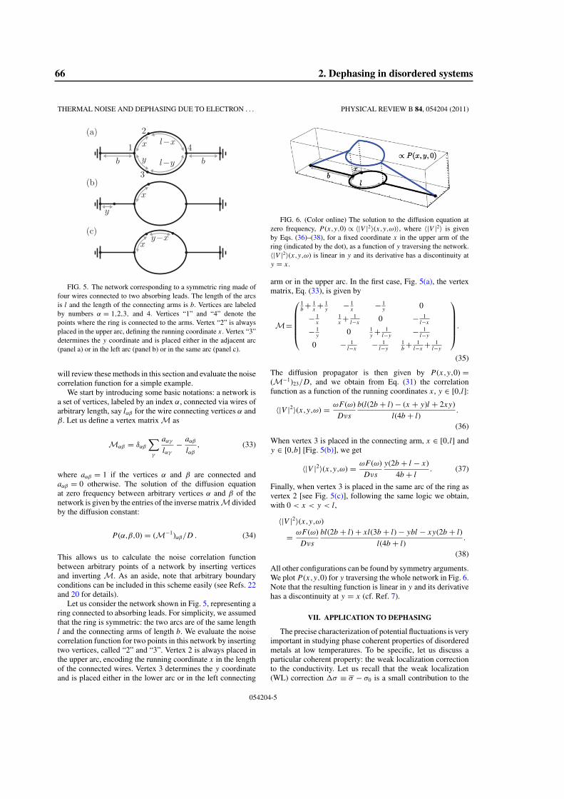
THERMAL NOISE AND DEPHASING DUE TO ELECTRON . . . PHYSICAL REVIEW B 84, 054204 (2011)
FIG. 5. The network corresponding to a symmetric ring made offour wires connected to two absorbing leads. The length of the arcsis l and the length of the connecting arms is b. Vertices are labeledby numbers α = 1,2,3, and 4. Vertices “1” and “4” denote thepoints where the ring is connected to the arms. Vertex “2” is alwaysplaced in the upper arc, defining the running coordinate x. Vertex “3”determines the y coordinate and is placed either in the adjacent arc(panel a) or in the left arc (panel b) or in the same arc (panel c).
will review these methods in this section and evaluate the noisecorrelation function for a simple example.
We start by introducing some basic notations: a network isa set of vertices, labeled by an index α, connected via wires ofarbitrary length, say lαβ for the wire connecting vertices α andβ. Let us define a vertex matrix M as
Mαβ = δαβ
∑γ
aαγ
lαγ
− aαβ
lαβ
, (33)
where aαβ = 1 if the vertices α and β are connected andaαβ = 0 otherwise. The solution of the diffusion equationat zero frequency between arbitrary vertices α and β of thenetwork is given by the entries of the inverse matrix M dividedby the diffusion constant:
P (α,β,0) = (M−1)αβ/D . (34)
This allows us to calculate the noise correlation functionbetween arbitrary points of a network by inserting verticesand inverting M. As an aside, note that arbitrary boundaryconditions can be included in this scheme easily (see Refs. 22and 20 for details).
Let us consider the network shown in Fig. 5, representing aring connected to absorbing leads. For simplicity, we assumedthat the ring is symmetric: the two arcs are of the same lengthl and the connecting arms of length b. We evaluate the noisecorrelation function for two points in this network by insertingtwo vertices, called “2” and “3”. Vertex 2 is always placed inthe upper arc, encoding the running coordinate x in the lengthof the connected wires. Vertex 3 determines the y coordinateand is placed either in the lower arc or in the left connecting
FIG. 6. (Color online) The solution to the diffusion equation atzero frequency, P (x,y,0) ∝ 〈|V |2〉(x,y,ω)〉, where 〈|V |2〉 is givenby Eqs. (36)–(38), for a fixed coordinate x in the upper arm of thering (indicated by the dot), as a function of y traversing the network.〈|V |2〉(x,y,ω) is linear in y and its derivative has a discontinuity aty = x.
arm or in the upper arc. In the first case, Fig. 5(a), the vertexmatrix, Eq. (33), is given by
M=
⎛⎜⎜⎜⎜⎝
1b+ 1
x+ 1
y− 1
x− 1
y0
− 1x
1x+ 1
l−x0 − 1
l−x
− 1y
0 1y+ 1
l−y− 1
l−y
0 − 1l−x
− 1l−y
1b+ 1
l−x+ 1
l−y
⎞⎟⎟⎟⎟⎠.
(35)
The diffusion propagator is then given by P (x,y,0) =(M−1)23/D, and we obtain from Eq. (31) the correlationfunction as a function of the running coordinates x, y ∈ [0,l]:
〈|V |2〉(x,y,ω) = ωF (ω)
Dνs
b(l(2b + l) − (x + y)l + 2xy)
l(4b + l).
(36)
When vertex 3 is placed in the connecting arm, x ∈ [0,l] andy ∈ [0,b] [Fig. 5(b)], we get
〈|V |2〉(x,y,ω) = ωF (ω)
Dνs
y(2b + l − x)
4b + l. (37)
Finally, when vertex 3 is placed in the same arc of the ring asvertex 2 [see Fig. 5(c)], following the same logic we obtain,with 0 < x < y < l,
〈|V |2〉(x,y,ω)
= ωF (ω)
Dνs
bl(2b + l) + xl(3b + l) − ybl − xy(2b + l)
l(4b + l).
(38)
All other configurations can be found by symmetry arguments.We plot P (x,y,0) for y traversing the whole network in Fig. 6.Note that the resulting function is linear in y and its derivativehas a discontinuity at y = x (cf. Ref. 7).
VII. APPLICATION TO DEPHASING
The precise characterization of potential fluctuations is veryimportant in studying phase coherent properties of disorderedmetals at low temperatures. To be specific, let us discuss aparticular coherent property: the weak localization correctionto the conductivity. Let us recall that the weak localization(WL) correction σ ≡ σ − σ0 is a small contribution to the
054204-5
66 2. Dephasing in disordered systems
M. TREIBER et al. PHYSICAL REVIEW B 84, 054204 (2011)
averaged conductivity arising from quantum interference ofreversed diffusive electronic trajectories.23
At low temperatures, dephasing is dominated by electroninteractions, that can be accounted for through a contributionto the phase accumulated by two time-reversed interferingtrajectories in a fluctuating electric field2:
�[x(τ )] =∫ t
0dτ [V (x(τ ),τ ) − V (x(τ ),t − τ )]. (39)
When averaged over the Gaussian fluctuations of the electricfield, 〈ei�〉V = e− 1
2 〈�2〉V yields a phase difference that cutsoff the contributions of long electronic trajectories. Intro-ducing the trajectory- dependent dephasing rate [x(τ )] =12t
〈�[x(τ )]2〉V , the weak localization correction takes theform:7,20,24,25
σ (x) = −2e2D
π
∫ ∞
0dt P (x,x,t) 〈e−t [x(τ )]〉{x(τ )}, (40)
where 〈· · · 〉{x(τ )} is the average with respect to closed diffusivetrajectories of duration t starting from x (not to be confusedwith the thermal average 〈· · · 〉V over the electric potentialV ). The phase fluctuations can then be related to the potentialfluctuations:
1
2〈�[x]2〉 =
∫ t
0dτdτ ′
∫ ∞
−∞
dω
2π[e−iω(τ−τ ′) − e−iω(τ+τ ′−t)]
×〈|V |2〉ϕ(x(τ ),x(τ ′,ω). (41)
Here, we have introduced a new noise correlator,
〈|V |2〉ϕ(x, y,ω) = 1
νωFϕ(ω)P (x, y,0), (42)
obtained from Eq. (31) by replacing F (ω) with a modifiedfunction Fϕ(ω) (given below), on the origin of which wenow comment. Equation (20) is well-known in the theoryof dephasing: its version symmetrized with respect to fre-quency arises naturally when comparing the diagrammaticcalculation of the dephasing time26,27 with the influencefunctional approach describing electrons moving in a randomGaussian field V .24,28,29 Diagrammatically, the symmetrizedEq. (20) represents the Keldysh component of the screened-electron-interaction propagator, the only substantial differencebeing that the diagrammatically calculated correlation functioninvolved in the dephasing process acquires so-called Paulifactors that account for the fact that the Fermi sea limits thephase space available for inelastic transitions.28 These factorslead to the following replacement of the function F (ω) inEq. (20) and also in Eq. (31):
F (ω)sym−→ coth(ω/2T )
Pauli−→ ω/2T
sinh2(ω/2T )≡ Fϕ(ω). (43)
This restricts the energy transfer to |ω| < T ,24,27 but does notaffect the factorization of the correlator. Inserting Eq. (42) intoEq. (41) leads to
1
2〈�[x]2〉 = 2T
ν
∫ t
0dτdτ ′ P (x(τ ),x(τ ′),0)
∫ ∞
−∞
dω
2π
× [e−iω(τ−τ ′) − e−iω(τ+τ ′−t)]ω
2TFϕ(ω). (44)
The fact that the frequency dependent function ω2T
Fϕ(ω) issymmetric allows us to add to P (x(τ ),x(τ ′),0) the term
− 12 [P (x(τ ),x(τ ),0) + P (x(τ ′),x(τ ′),0)], which does not con-
tribute to the integral (44). Therefore, we finally end up withthe following expression for the dephasing rate,
[x(τ )] = e2T
∫ t
0
dτ
t
∫ t
0dτ ′ [δT (τ + τ ′ − t) − δT (τ − τ ′)]
×R(x(τ ),x(τ ′)), (45)
written in terms of the resistance R, defined in Eq. (32). Thefunction δT (t), a broadened delta function of width 1/T andheight T , is the Fourier transform of ω
2TFϕ(ω), which is given
by
δT (τ ) = πT w(πT τ ), w(y) = y coth y − 1
sinh2 y. (46)
Equation (45), which is one of the main results of our paper,generalizes the results obtained in Refs. 8,9,24, and 28 for aninfinite wire and an isolated ring to arbitrary geometry. In theclassical noise limit T → ∞, δT (τ ) may be replaced by a δ(τ )function: the second term of Eq. (45) vanishes and we recoverthe results of Refs. 7 and 20.
Let us now illustrate Eq. (45) by calculating the dephasingtime for the well-understood case of one and two-dimensionalisolated simply-connected samples. The dephasing time canbe extracted from the condition
1 ≡ (τϕ)τϕ, (47)
where (t) is given by the functional Eq. (45), averaged overthe typical closed random walks x(τ ) of duration t in thesystem. The problem is governed by the interplay of threetime scales: the Thouless time τTh = L2/D, depending onthe system size L, the thermal time τT = 1/T (related to thethermal length LT = √
D/T ), and the dephasing time τϕ .(i) Diffusive regime, τT � τϕ � τTh (LT � Lϕ � L):
this is the regime considered in Refs. 2 and 25, where thewidth of the broadened delta functions in Eq. (45), τT , isthe shortest time scale. Thus, when averaging over pathsx(τ ), the characteristic length scale |x − y| entering theresistance R(x,y) can be determined as follows: for the firstδT term, this length is governed by free diffusion, since|x(τ ) − x(t − τ )| ∼ √
Dτ , hence |x − y| ∼ √Dτ . For the
second term, the characteristic length is set by the width of thedelta function, |x − y| ∼ √
DτT . In 1D, where R(x,y) ∼ |x −y|/σ0s, the first term dominates and we immediately obtainfrom Eq. (47) 1/τϕ ∼ (e2
√DT/σ0s)2/3. In 2D, the diffuson
at zero frequency is logarithmic as well as the resistance (32),R(x,y) ∼ ln(|x − y|)/σ0d, where d is the width of the sample,which can be understood from the fact that the resistance of aplane connected at two corners scales logarithmically with thesystem size. Equation (47) gives 1 ∼ e2T τϕ ln(T τϕ)/σ0d, andfor the dephasing time, 1/τϕ ∼ e2T ln(e2/σ0d)/σ0d.
(ii) Ergodic regime, τT � τTh � τϕ (LT � L � Lϕ): thewidth of δT (τ ) in Eq. (45) is still the shortest time scalebut, in contrast to (i), the typical trajectories x(τ ) explorethe whole system, setting the length scale of diffusion tothe system size L, cf. Refs. 6 and 7. In full analogy to thediffusive regime, but replacing
√Dτ by L, we find for 1D,
1/τϕ ∼ e2LT/σ0s, and for 2D, 1/τϕ ∼ e2T ln(τTh/τT )/σ0d.30
These examples show that for nontrivial geometries, dephasingdue to electron interactions cannot be accounted for through
054204-6
2. Dephasing in disordered systems 67
THERMAL NOISE AND DEPHASING DUE TO ELECTRON . . . PHYSICAL REVIEW B 84, 054204 (2011)
a unique dephasing rate depending only on dimensionality,but must be described by a functional of the trajectories x(τ )since the qualitative behavior of τϕ follows from the geometrydependent typical distance |x(τ ) − x(τ ′)|.
For sufficiently low temperatures, on the other hand,Eq. (45) is capable to describe the crossover to a 0D regime,where, apart from a dependence on the total system size,geometry becomes unimportant.
(iii) 0D regime, τTh � τT � τϕ (L � LT � Lϕ): here,the width of the delta functions in Eq. (45), τT , is largerthan τTh. Hence, the trajectories reach the ergodic limitx(τ � τTh) ∼ L before the electric potential has significantlychanged: dephasing is strongly reduced. Let us denote themaximal resistance reached at the ergodic limit as Rerg
and replace the resistance in Eq. (45) by R → R − Rerg,without changing the result, since Rerg is constant and itscontribution vanishes after integrating over τ and τ ′. Thedifference R − Rerg is nonzero only during time differencesτ − τ ′ � τTh before reaching ergodicity. Thus the leadingcontribution comes from the second δT term in Eq. (45),which is constant at its maximum T during such short timescales. We find 1 ∼ −e2T 2τϕ
∫ τTh
0 dτ [R(x(τ ),0) − Rerg] andsince the Rerg term dominates, we obtain a dephasing time1/τϕ ∼ e2T 2τThRerg, independent of geometry and with thecharacteristic ∼T 2 behavior.31
VIII. CONCLUSIONS
In this paper, we have considered fluctuations of the scalarelectric potentials in macroscopically inhomogeneous metals.We have shown how to relate the density fluctuations tothe potential fluctuations, emphasizing the role of electronicinteractions, provided a real space derivation of the densityresponse function, and illustrated these general ideas for thecase of networks of metallic wires. Finally, we have obtaineda trajectory-dependent functional, Eq. (45), which describesdephasing by electron interactions for arbitrary geometries andaccounts for the quantum noise contribution. When applied tonetworks, Eq. (45) can describe the full crossover from the 0Dto the 1D and the 2D regime.
ACKNOWLEDGMENTS
We acknowledge illuminating discussions with F. Mar-quardt and support from the DFG through SFB TR-12(O. Ye.), DE 730/8-1 (M. T.) and the Cluster of Excellence,Nanosystems Initiative, Munich.
APPENDIX A: SELF CONSISTENT ANALYSIS OFSCREENING
We recall here how to obtain Eq. (17) using a self-consistenttreatment of screening in real space.32 Starting points are thefollowing three equations: (i) the excess charge density isdecomposed into external and induced contributions
δn(x,ω) = next(x,ω) + nind(x,ω). (A1)
(ii) The induced charge is related to the potential V (x,ω) bythe density response function, cf. Eq. (4):
nind(x,ω) = −∫
d y χ (x, y,ω) V ( y,ω). (A2)
(iii) The Poisson equation
V (x,ω) = −4πe2 δn(x,ω). (A3)
Self-consistency lies in the fact that the response involvesthe screened potential V (x,ω) and not the bare “external”potential related to next(x,ω). The screened effective interac-tion between electrons URPA(x, y,ω) is obtained by placingan external charge at y, so that the external density isnext(x,ω) = δ(x − y), and associating the resulting screenedpotential V (x,ω) in Eq. (A3) with URPA(x, y,ω). We obtain
− 1
4πe2xURPA(x, y,ω) +
∫dx′ χ (x,x′,ω)URPA(x′, y,ω)
= δ(x − y). (A4)
Convolution with the Coulomb interaction gives Eq. (17).
APPENDIX B: CURRENT DENSITY CORRELATIONS
We discuss here the relation between the density and thecurrent density correlations. The response of the (induced)current density is characterized by the conductivity tensor σ ,
〈jα(x,ω)〉neq =∫
d y σαβ(x, y,ω) Eβ( y,ω), (B1)
which is related to Eq. (5) by current conservation:
∇α∇′βσαβ(x,x′,ω) = −iωe2χ (x,x′,ω). (B2)
The thermal fluctuations of the current density can be obtainedfrom 〈jαj
†β〉(x, y,ω) = ωF (ω) Re[σαβ(x, y,ω)], in analogy to
the discussion in Sec. II, assuming time-reversal symmetry,σαβ(x, y,ω) = σβα( y,x,ω).
Let us now examine the case of disordered metals. Theclassical contribution to the averaged nonlocal dc conductivityhas been derived in Ref. 12. Their result can be generalizedstraightforwardly to nonzero frequencies,
σαβ(x,x′,ω) = σ0 [δαβδ(x − x′) − D∇α∇′βP (x,x′,ω)], (B3)
which obeys the condition (B2) with Eq. (25) substituted forχ . For the current correlations, we find33
〈jαj†β〉(x,x′,ω) = σ0 ωF (ω) {δαβδ(x − x′)
−D∇α∇′βRe[P (x,x′,ω)]}. (B4)
Since the diffuson P (x,x′,ω) decays exponentially on alength scale Lω = √
D/ω, this expression shows that currentcorrelations can be considered as purely local over the scale||x − x′|| � Lω, i.e., 〈|j |2〉(x,x′,ω) σ0ωF (ω)δ(x − x′). Inthe limit of classical noise, F (ω) ω 2T , we recover preciselyEq. (1).
054204-7
68 2. Dephasing in disordered systems
M. TREIBER et al. PHYSICAL REVIEW B 84, 054204 (2011)
1J. B. Johnson, Phys. Rev. 32, 97 (1928); H. Nyquist, ibid. 32, 110(1928).
2B. L. Altshuler, A. G. Aronov, and D. E. Khmelnitsky, J. Phys. C15, 7367 (1982).
3M. Ferrier, L. Angers, A. C. H. Rowe, S. Gueron, H. Bouchiat,C. Texier, G. Montambaux, and D. Mailly, Phys. Rev. Lett. 93,246804 (2004).
4F. Schopfer, F. Mallet, D. Mailly, C. Texier, G. Montambaux,C. Bauerle, and L. Saminadayar, Phys. Rev. Lett. 98, 026807 (2007).
5M. Ferrier, A. C. H. Rowe, S. Gueron, H. Bouchiat, C. Texier, andG. Montambaux, Phys. Rev. Lett. 100, 146802 (2008).
6T. Ludwig and A. D. Mirlin, Phys. Rev. B 69, 193306 (2004).7C. Texier and G. Montambaux, Phys. Rev. B 72, 115327 (2005).8M. Treiber, O. M. Yevtushenko, F. Marquardt, J. von Delft, andI. V. Lerner, Phys. Rev. B 80, 201305(R) (2009).
9M. Treiber, O. M. Yevtushenko, F. Marquardt, J. von Delft, and I. V.Lerner, in Perspectives of Mesoscopic Physics: Dedicated to YosephImry’s 70th Birthday, edited by A. Aharony, O. Entin-Wohlman(World Scientific, Singapore, 2010), Chap. 20.
10C. Texier and G. Montambaux, Phys. Rev. Lett. 92, 186801 (2004).11A. Yu. Zyuzin and B. Z. Spivak, Sov. Phys. JETP 66, 560 (1987);
[Zh. Eksp. Teor. Fiz. 93, 994 (1987)].12C. L. Kane, R. A. Serota, and P. A. Lee, Phys. Rev. B 37, 6701
(1988).13I. V. Lerner, Sov. Phys. JETP 68, 143 (1989) [Zh. Eksp. Teor. Fiz.
95, 253 (1989)].14L. D. Landau and E. M. Lifshitz, Statistical Physics, 3rd ed.
(Butterworth-Heinemann, 1980), Vol. 5.15In general, if the electromagnetic field is not quantized, as is the case
here, the potential is not an operator; the assumption of a potentialoperator arises from electronic interactions that relate the internalelectronic density operator to the electric potential.
16The different signs in Eqs. (7) and (11) reflect the different signconventions in Eqs. (4) and (10).
17D. Vollhardt and P. Wolfle, Phys. Rev. B 22, 4666 (1980).18E. Akkermans and G. Montambaux, Mesoscopic Physics of Elec-
trons and Photons (Cambridge University Press, Cambridge, 2007).19R. P. Kanwal, Linear Integral Equations: Theory & Technique
(Birkenhauser, Boston, 1997).20C. Texier, P. Delplace, and G. Montambaux, Phys. Rev. B 80,
205413 (2009).21M. Pascaud and G. Montambaux, Phys. Rev. Lett. 82, 4512
(1999).22E. Akkermans, A. Comtet, J. Desbois, G. Montambaux, and
C. Texier, Ann. Phys. (NY) 284, 10 (2000).23D. E. Khmelnitskii, Physica B & C 126, 235 (1984).24F. Marquardt, J. von Delft, R. Smith, and V. Ambegaokar, Phys.
Rev. B 76, 195331 (2007).25G. Montambaux and E. Akkermans, Phys. Rev. Lett. 95, 016403
(2005).26I. L. Aleiner, B. L. Altshuler, and M. E. Gershenson, Waves in
Random and Complex Media 9, 201 (1999).27J. von Delft, F. Marquardt, R. Smith, and V. Ambegaokar, Phys.
Rev. B 76, 195332 (2007).28J. von Delft, Int. J. Mod. Phys. B 22, 727 (2008).29S. Chakravarty and A. Schmid, Phys. Rep. 140, 193
(1986).30Compare with Y. Takane, Anomalous Behavior of the Dephasing
Time in Open Diffusive Cavities, J. Phys. Soc. Jpn. 72, 233 (2003),where vertex diagrams27,28 have not been considered.
31U. Sivan, Y. Imry, and A. G. Aronov, Europhys. Lett. 28, 115(1994).
32T. Christen and M. Buttiker, Europhys. Lett. 35, 523 (1996).33Note that the FDT expresses thermal correlations 〈 j2〉(x, y,ω) ≡
〈j (x,ω)j ( y, − ω)〉 ∼ Re[σ (x, y,ω)], dominated by short-rangecontributions; this should not be confused with the mesoscopiccorrelations 〈j (x,ω)〉〈j (x′,ω′)〉 ∼ σ (x, y,ω)σ (x′, y′,ω′) studied inRefs. 11–13, dominated by long-range contributions.
054204-8
2. Dephasing in disordered systems 69

3. Quantum corrections to the conductance 71
Chapter 3
Quantum corrections to the conductance
In Chapter 2, we have discussed the loop-expansion in diffusive propagators of disorder averagedcorrelation functions. We have argued that, in open systems, the relative magnitude of the quantumcorrections is controlled by the inverse dimensionless conductance, which we defined as
g≡ 2πETh
∆, (3.1)
cf. Section 2.1.4. The distinction between open and confined systems will play an important role inthe following: In the former, the electrons leave the system as soon as they have traversed it once,i.e. after the Thouless time τTh . In the latter, they dwell in the system much longer than τTh . Inthis chapter, we will show that g actually corresponds to the conductance measured in a transportexperiment on an open system. We calculate g from the current response function and derive theso-called weak-localization correction and the universal conductance fluctuations. Their dependenceon dephasing due to electron interactions at low T is analyzed in detail. We compare the perturbativecalculation with the results from RMT valid for confined system. Finally, we discuss the situationin two particular confined systems, namely an almost isolated quasi-1D ring and a quantum-dot, andshow that the elusive 0D regime of dephasing can be observed at the onset of mesoscopic universalityin such systems.
3.1 The conductance of disordered metals
3.1.1 The classical conductance
The conductivity of disordered metals at finite temperatures can be calculated using the Keldyshperturbation theory which we have introduced in Section 2.2.1 [Rammer and Smith, 1986]. Startingpoint is the expectation value of the current density operator in the absence of an external electricfield:
jα(x, t) =e
im
⟨ψ†(x, t)(∂α
x ψ(x, t +0))+(∂α
x ψ†(x, t))
ψ(x, t +0)⟩, (3.2)
where ∂αx denotes the directional derivative of x in the direction α = x,y,z and we assumed spin-
degeneracy. The expectation value of the field operators is directly related to the Green’s functions,see [Rammer and Smith, 1986]:
〈ψ†(x, t)ψ(x, t)〉=−i[GK(x, t;x, t +0)−GR(x, t;x, t +0)+GA(x, t;x, t +0)
]. (3.3)
72 3. Quantum corrections to the conductance
Let us now include a weak external electric field Eω(x), which we conveniently express in terms of avector potential Aω(x) = Eω(x)/iω. Expanding Eq. (3.2) to linear order in A using Eq. (3.3) yields
jα (1)ω (x) =− e
m
∫ dε2π
limx′→x
(∂αx −∂α
x′)[GK (1)
ε−ω,ε(x,x′)]− ne2
mAα
ω(x) , (3.4)
where the second term is the diamagnetic contribution1 (n is the average electron density), see e.g.Bruus and Flensberg (2004), and GK (1)
ε1,ε2 (x,y) is the first order term of the expansion of the Fouriertransform of GK(x, t1;y, t2) in A:2
GK (1)ε−ω,ε(x,y) =
ie2m
∫ddz ∑
βAβ
ω(z) (3.5)
× limz′→z
(∂β
z −∂βz′
)[GK
ε−ω(x,z)GRε (z′,y)+GA
ε−ω(x,z)GKε (z′,y)].
The Green’s functions on the r.h.s of Eq. (3.5) are taken at A = 0. Using Eq. (3.5) in Eq. (3.4), wefind:
jα (1)ω (x) =
∫ddy ∑
βσαβ
ω (x,y) iωAβω(y) . (3.6)
with the non-local conductivity tensor
σαβω (x,y) =− ne2
iωmδαβδ(x−y) (3.7)
− 2e2
ωm2
∫ dε2π
[GK
ε−ω(x,y)↔∂
α
x
↔∂
β
y GRε (y,x)+GA
ε−ω(x,y)↔∂
α
x
↔∂
β
y GKε (y,x)
],
where we introduced the symmetrized directional derivative
f (x)↔∂
α
x g(x)≡ 12
limx′→x
(∂αx −∂α
x′) f (x)g(x′) . (3.8)
In thermal equilibrium, the Keldysh Green’s function, GK , can be related to the retarded/advancedGreen’s functions via Eq. (2.75). As a result, we obtain products of Green’s functions with equalretardation, GRGR and GAGA , and terms with different retardation GRGA . The former terms have nonontrivial dependence on disorder, cf. the discussion after Eq. (2.32), in the absence of interactions3.It can be shown, similar to Eq. (2.87) (for details see e.g. Rammer and Smith (1986)), that they cancelthe diamagnetic term in Eq. (3.7), which restores gauge invariance. As a result Eq. (3.7) simplifies to
σαβω (x,y) =
2e2
m2
∫ dε2π
hε−ω−hε
ωGA
ε−ω(x,y)↔∂
α
x
↔∂
β
y GRε (y,x) . (3.9)
In the following, we are only interested in spatially homogeneous electric fields in Eq. (3.6).4 More-over, we concentrate on the current component in the direction of the field, described by the so-called
1. Note that the diamagnetic contribution alone is unphysical since it violates gauge invariance and diverges in the directcurrent (DC) limit, ω→ 0. Thus, it should be canceled by a contribution from the first terms in Eq. (3.4).
2. Note that GR and GA in Eq. (3.3) do not depend on A to linear order due to GR(t)GR(−t) = GA(t)GA(−t) = 0.3. In the presence of electron interactions, the terms with equal retardation play an important role in the description of the
so-called Altshuler-Aronov interaction corrections. These corrections are temperature dependent, however, they do notdepend on magnetic field or the dephasing time discussed in Section 2.2.
4. The case of arbitrary fields has been studied in detail in Kane et al. (1988).
3. Quantum corrections to the conductance 73
longitudial conductivity, and neglect the transverse components. The transverse components are re-lated to the Hall effect, which we do not consider here. Therefore, we can integrate over y in Eq. (3.6)and obtain after symmetrization:
σω =1d ∑
α
1V 2
∫ddx
∫ddy σαα
ω (x,y) . (3.10)
The quantity measured in a transport experiment is the conductance, which is related to the conduc-tivity by Ohm’s law:
Gω = Ld−2σω . (3.11)
Eq. (3.11) is a generalization of the usual form G = σS/L for a sample of length L and cross-sectionS to arbitrary dimensions. We obtain
Gω =1
dL2 ∑α
1V
∫ddx
∫ddy σαα
ω (x,y) (3.12)
=2e2
dm2L2
∫ dε2π
hε−ω−hε
ω1V
∫ddx
∫ddyGR
ε (y,x)↔∇x↔∇y GA
ε−ω(x,y) ,
where↔∇x is defined in analogy to Eq. (3.8), but with the directional derivative replaced by gradients.
At small frequencies ω� T , we can use the following approximation
limω�T
hε−ω−hε
ω=−∂ fε
∂ε, fε =
1eε/T +1
, (3.13)
where fε is the Fermi distribution function. Note that − ∂ fε∂ε is a broadened delta function of width
T � εF , centered around εF . After impurity averaging, the product of Green’s functions depends onlyweakly on ε in this energy range, see the discussion after Eq. (2.86). Thus, we can integrate over εand obtain for the disorder averaged conductance:
Gω =e2
πdm2L21V
∫ddx
∫ddyGR
ε (y,x)↔∇x↔∇y GA
ε−ω(x,y) . (3.14)
Note that the r.h.s of Eq. (3.14) does not depend on ε, but we keep ε here just as in Section 2.1.2.After a Fourier transform, we finally obtain
Gω =e2
πdL2m21V ∑
k,k′kk′ GR
ε (k,k′)GAε−ω(k′,k) . (3.15)
Let us now evaluate the disorder average of Eq. (3.15) in analogy to our discussion in Section 2.1.2.In the limit (εFτ)−1� 1 the disorder average GRGA is given by the ladder approximation, which isshown in Fig. 3.1. However, in contrast to the generalized diffusion propagator, there are additionalfactors k and k′ in Eq. (3.15). These vector-valued factors correspond to the momentum of theGreen’s functions at the vertices in Fig. 3.1, which are often called vector vertices in this context. Dueto the symmetry of the disorder averaged Green’s functions, GR/A(k) = GR/A(−k), the following sumvanishes:
∑k
kGR(k)GA
(k) = 0 . (3.16)
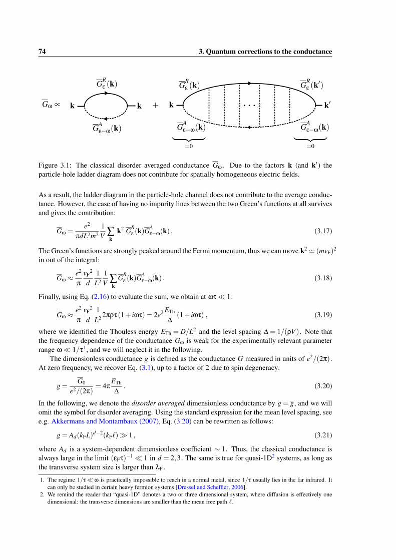
74 3. Quantum corrections to the conductance
Figure 3.1: The classical disorder averaged conductance Gω . Due to the factors k (and k′ ) theparticle-hole ladder diagram does not contribute for spatially homogeneous electric fields.
As a result, the ladder diagram in the particle-hole channel does not contribute to the average conduc-tance. However, the case of having no impurity lines between the two Green’s functions at all survivesand gives the contribution:
Gω =e2
πdL2m21V ∑
kk2 GR
ε (k)GAε−ω(k) . (3.17)
The Green’s functions are strongly peaked around the Fermi momentum, thus we can move k2 ' (mvF)2
in out of the integral:
Gω ≈e2
πvF
2
d1L2
1V ∑
kGR
ε (k)GAε−ω(k) . (3.18)
Finally, using Eq. (2.16) to evaluate the sum, we obtain at ωτ� 1:
Gω ≈e2
πvF
2
d1L2 2πρτ(1+ iωτ) = 2e2 ETh
∆(1+ iωτ) , (3.19)
where we identified the Thouless energy ETh = D/L2 and the level spacing ∆ = 1/(ρV ). Note thatthe frequency dependence of the conductance Gω is weak for the experimentally relevant parameterrange ω� 1/τ1, and we will neglect it in the following.
The dimensionless conductance g is defined as the conductance G measured in units of e2/(2π).At zero frequency, we recover Eq. (3.1), up to a factor of 2 due to spin degeneracy:
g =G0
e2/(2π)= 4π
ETh
∆. (3.20)
In the following, we denote the disorder averaged dimensionless conductance by g = g, and we willomit the symbol for disorder averaging. Using the standard expression for the mean level spacing, seee.g. Akkermans and Montambaux (2007), Eq. (3.20) can be rewritten as follows:
g = Ad(kFL)d−2(kF`)� 1 , (3.21)
where Ad is a system-dependent dimensionless coefficient ∼ 1. Thus, the classical conductance isalways large in the limit (εFτ)−1� 1 in d = 2,3. The same is true for quasi-1D2 systems, as long asthe transverse system size is larger than λF .
1. The regime 1/τ� ω is practically impossible to reach in a normal metal, since 1/τ usually lies in the far infrared. Itcan only be studied in certain heavy fermion systems [Dressel and Scheffler, 2006].
2. We remind the reader that “quasi-1D” denotes a two or three dimensional system, where diffusion is effectively onedimensional: the transverse dimensions are smaller than the mean free path ` .
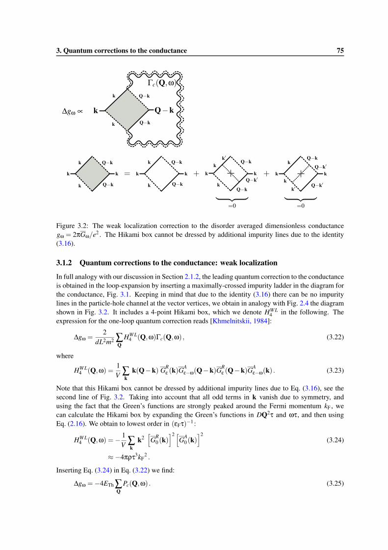
3. Quantum corrections to the conductance 75
Figure 3.2: The weak localization correction to the disorder averaged dimensionless conductancegω = 2πGω/e2 . The Hikami box cannot be dressed by additional impurity lines due to the identity(3.16).
3.1.2 Quantum corrections to the conductance: weak localization
In full analogy with our discussion in Section 2.1.2, the leading quantum correction to the conductanceis obtained in the loop-expansion by inserting a maximally-crossed impurity ladder in the diagram forthe conductance, Fig. 3.1. Keeping in mind that due to the identity (3.16) there can be no impuritylines in the particle-hole channel at the vector vertices, we obtain in analogy with Fig. 2.4 the diagramshown in Fig. 3.2. It includes a 4-point Hikami box, which we denote HWL
4 in the following. Theexpression for the one-loop quantum correction reads [Khmelnitskii, 1984]:
∆gω =2
dL2m2 ∑Q
HWL4 (Q,ω)Γc(Q,ω) , (3.22)
where
HWL4 (Q,ω) =
1V ∑
kk(Q−k) GR
ε (k)GAε−ω(Q−k)GR
ε (Q−k)GAε−ω(k) . (3.23)
Note that this Hikami box cannot be dressed by additional impurity lines due to Eq. (3.16), see thesecond line of Fig. 3.2. Taking into account that all odd terms in k vanish due to symmetry, andusing the fact that the Green’s functions are strongly peaked around the Fermi momentum kF , wecan calculate the Hikami box by expanding the Green’s functions in DQ2τ and ωτ, and then usingEq. (2.16). We obtain to lowest order in (εFτ)−1 :
HWL4 (Q,ω) =− 1
V ∑k
k2[GR
0 (k)]2 [
GA0 (k)
]2(3.24)
≈−4πρτ3kF2 .
Inserting Eq. (3.24) in Eq. (3.22) we find:
∆gω =−4ETh ∑Q
Pc(Q,ω) . (3.25)
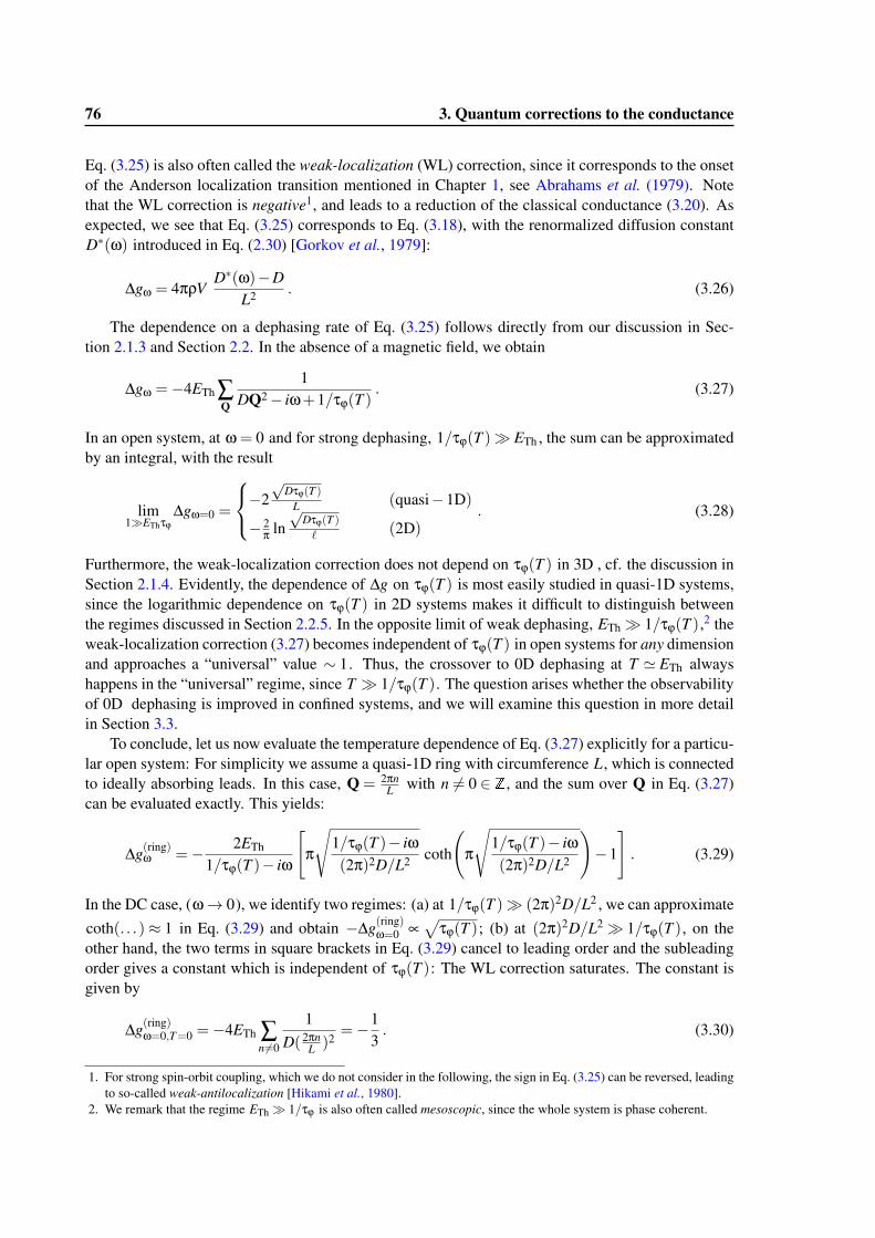
76 3. Quantum corrections to the conductance
Eq. (3.25) is also often called the weak-localization (WL) correction, since it corresponds to the onsetof the Anderson localization transition mentioned in Chapter 1, see Abrahams et al. (1979). Notethat the WL correction is negative1, and leads to a reduction of the classical conductance (3.20). Asexpected, we see that Eq. (3.25) corresponds to Eq. (3.18), with the renormalized diffusion constantD∗(ω) introduced in Eq. (2.30) [Gorkov et al., 1979]:
∆gω = 4πρVD∗(ω)−D
L2 . (3.26)
The dependence on a dephasing rate of Eq. (3.25) follows directly from our discussion in Sec-tion 2.1.3 and Section 2.2. In the absence of a magnetic field, we obtain
∆gω =−4ETh ∑Q
1DQ2− iω+1/τϕ(T )
. (3.27)
In an open system, at ω = 0 and for strong dephasing, 1/τϕ(T )� ETh , the sum can be approximatedby an integral, with the result
lim1�EThτϕ
∆gω=0 =
−2√
Dτϕ(T )L (quasi−1D)
− 2π ln√
Dτϕ(T )` (2D)
. (3.28)
Furthermore, the weak-localization correction does not depend on τϕ(T ) in 3D , cf. the discussion inSection 2.1.4. Evidently, the dependence of ∆g on τϕ(T ) is most easily studied in quasi-1D systems,since the logarithmic dependence on τϕ(T ) in 2D systems makes it difficult to distinguish betweenthe regimes discussed in Section 2.2.5. In the opposite limit of weak dephasing, ETh� 1/τϕ(T ),2 theweak-localization correction (3.27) becomes independent of τϕ(T ) in open systems for any dimensionand approaches a “universal” value ∼ 1. Thus, the crossover to 0D dephasing at T ' ETh alwayshappens in the “universal” regime, since T � 1/τϕ(T ). The question arises whether the observabilityof 0D dephasing is improved in confined systems, and we will examine this question in more detailin Section 3.3.
To conclude, let us now evaluate the temperature dependence of Eq. (3.27) explicitly for a particu-lar open system: For simplicity we assume a quasi-1D ring with circumference L, which is connectedto ideally absorbing leads. In this case, Q = 2πn
L with n 6= 0 ∈ Z, and the sum over Q in Eq. (3.27)can be evaluated exactly. This yields:
∆g(ring)ω =− 2ETh
1/τϕ(T )− iω
[π
√1/τϕ(T )− iω(2π)2D/L2 coth
(π
√1/τϕ(T )− iω(2π)2D/L2
)−1
]. (3.29)
In the DC case, (ω→ 0), we identify two regimes: (a) at 1/τϕ(T )� (2π)2D/L2 , we can approximatecoth(. . .)≈ 1 in Eq. (3.29) and obtain −∆g(ring)
ω=0 ∝√
τϕ(T ); (b) at (2π)2D/L2� 1/τϕ(T ), on theother hand, the two terms in square brackets in Eq. (3.29) cancel to leading order and the subleadingorder gives a constant which is independent of τϕ(T ): The WL correction saturates. The constant isgiven by
∆g(ring)ω=0,T=0 =−4ETh ∑
n6=0
1D(2πn
L )2=−1
3. (3.30)
1. For strong spin-orbit coupling, which we do not consider in the following, the sign in Eq. (3.25) can be reversed, leadingto so-called weak-antilocalization [Hikami et al., 1980].
2. We remark that the regime ETh� 1/τϕ is also often called mesoscopic, since the whole system is phase coherent.
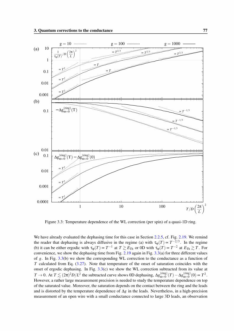
3. Quantum corrections to the conductance 77
0.001
0.01
0.1
1
10
0.01
0.1 −Δg(ring)ω=0 (T)
0.0001
0.001
0.01
0.1
1 10 100 1000
Δg(ring)ω=0 (T)−Δg(ring)ω=0 (0)
(a)
(b)
(c)
g= 10 g= 100 g= 1000
Figure 3.3: Temperature dependence of the WL correction (per spin) of a quasi-1D ring.
We have already evaluated the dephasing time for this case in Section 2.2.5, cf. Fig. 2.19. We remindthe reader that dephasing is always diffusive in the regime (a) with τϕ(T ) ∝ T−2/3 . In the regime(b) it can be either ergodic with τϕ(T ) ∝ T−1 at T & ETh or 0D with τϕ(T ) ∝ T−2 at ETh & T . Forconvenience, we show the dephasing time from Fig. 2.19 again in Fig. 3.3(a) for three different valuesof g. In Fig. 3.3(b) we show the corresponding WL correction to the conductance as a function ofT calculated from Eq. (3.27). Note that temperature of the onset of saturation coincides with theonset of ergodic dephasing. In Fig. 3.3(c) we show the WL correction subtracted from its value atT → 0. At T . (2π)2D/L2 the subtracted curve shows 0D dephasing, ∆g(ring)
ω=0 (T )−∆g(ring)ω=0 (0) ∝ T 2 .
However, a rather large measurement precision is needed to study the temperature dependence on topof the saturated value. Moreover, the saturation depends on the contact between the ring and the leadsand is distorted by the temperature dependence of ∆g in the leads. Nevertheless, in a high-precisionmeasurement of an open wire with a small conductance connected to large 3D leads, an observation
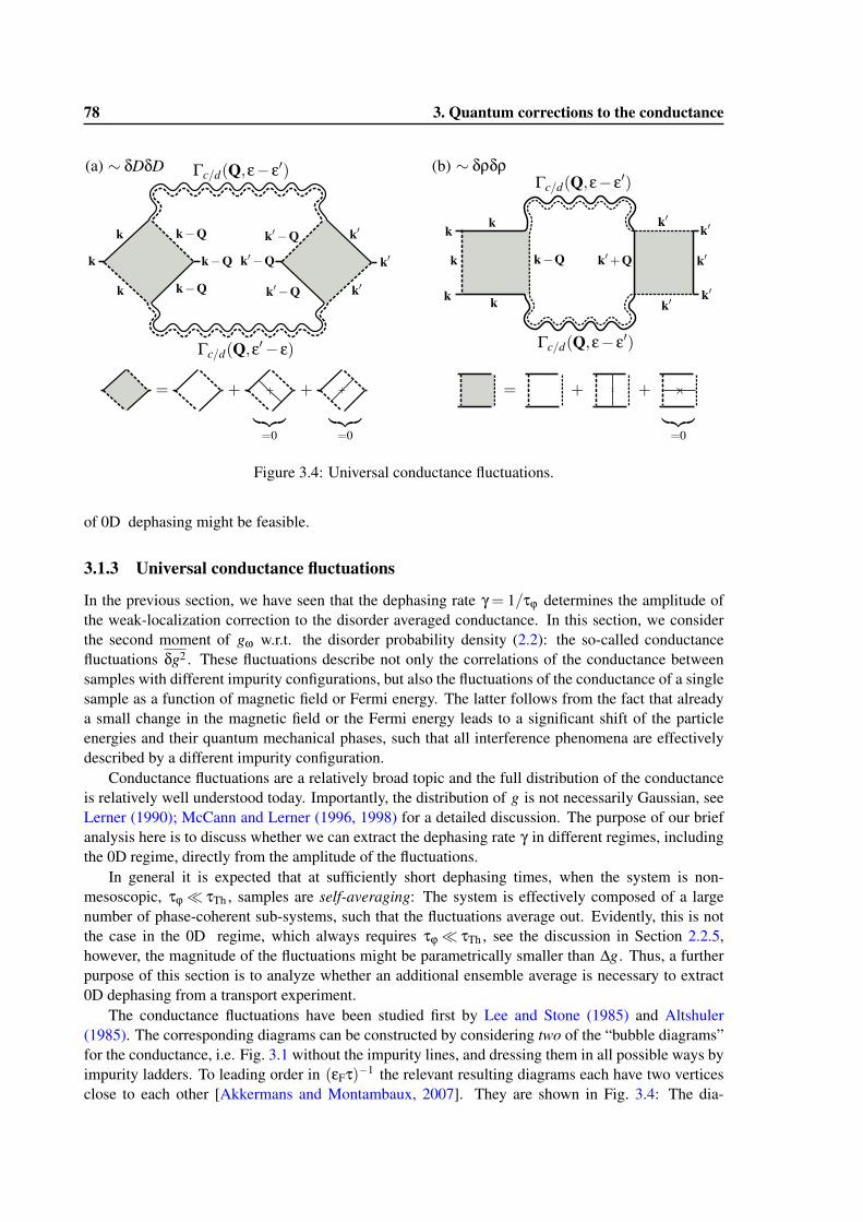
78 3. Quantum corrections to the conductance
Figure 3.4: Universal conductance fluctuations.
of 0D dephasing might be feasible.
3.1.3 Universal conductance fluctuations
In the previous section, we have seen that the dephasing rate γ = 1/τϕ determines the amplitude ofthe weak-localization correction to the disorder averaged conductance. In this section, we considerthe second moment of gω w.r.t. the disorder probability density (2.2): the so-called conductancefluctuations δg2 . These fluctuations describe not only the correlations of the conductance betweensamples with different impurity configurations, but also the fluctuations of the conductance of a singlesample as a function of magnetic field or Fermi energy. The latter follows from the fact that alreadya small change in the magnetic field or the Fermi energy leads to a significant shift of the particleenergies and their quantum mechanical phases, such that all interference phenomena are effectivelydescribed by a different impurity configuration.
Conductance fluctuations are a relatively broad topic and the full distribution of the conductanceis relatively well understood today. Importantly, the distribution of g is not necessarily Gaussian, seeLerner (1990); McCann and Lerner (1996, 1998) for a detailed discussion. The purpose of our briefanalysis here is to discuss whether we can extract the dephasing rate γ in different regimes, includingthe 0D regime, directly from the amplitude of the fluctuations.
In general it is expected that at sufficiently short dephasing times, when the system is non-mesoscopic, τϕ� τTh , samples are self-averaging: The system is effectively composed of a largenumber of phase-coherent sub-systems, such that the fluctuations average out. Evidently, this is notthe case in the 0D regime, which always requires τϕ� τTh , see the discussion in Section 2.2.5,however, the magnitude of the fluctuations might be parametrically smaller than ∆g. Thus, a furtherpurpose of this section is to analyze whether an additional ensemble average is necessary to extract0D dephasing from a transport experiment.
The conductance fluctuations have been studied first by Lee and Stone (1985) and Altshuler(1985). The corresponding diagrams can be constructed by considering two of the “bubble diagrams”for the conductance, i.e. Fig. 3.1 without the impurity lines, and dressing them in all possible ways byimpurity ladders. To leading order in (εFτ)−1 the relevant resulting diagrams each have two verticesclose to each other [Akkermans and Montambaux, 2007]. They are shown in Fig. 3.4: The dia-
3. Quantum corrections to the conductance 79
gram of Fig. 3.4(a) is often interpreted as the correlation function of the diffusion constant (δDδD),and Fig. 3.4(b) as the correlation function of the density of states (δρδρ) [Altshuler and Shklovskii,1986]. Both diagrams are structurally similar and consist of two impurity ladders (in the particle-holeor particle-particle channel, corresponding to diffuson, Pd , or Cooperon, Pc , propagators) attachedto two 4-point Hikami boxes. Note that due to the factors k and k′ , the Hikami boxes have “vectorvertices”, and can be dressed only partially, cf. the Hikami box for ∆g in Fig. 3.2. In Fig. 3.4(a) onlythe undressed Hikami box contributes, and the impurity ladders are taken at opposite energies ε− ε′and ε′− ε. Thus, they are complex conjugates and their contribution includes a modulus square of thediffusive propagators:
δgεδgε′(δDδD)
= 8E2Th ∑
Q|Pc(Q,ε− ε′)|2 + |Pd(Q,ε− ε′)|2 . (3.31)
In Fig. 3.4(b), on the other hand, one of the dressings of the Hikami box is non-zero, since itincludes an even number of k-factors. As a result, the contribution of the Hikami box in Fig. 3.4(a) istwice as large as that of Fig. 3.4(b). The diagram shown in Fig. 3.4(b) and its complex conjugate givetwice the real part. In total, one obtains from Fig. 3.4(b):
δgεδgε′(δρδρ)
= 8E2Th ∑
QRe[
Pc(Q,ε− ε′)2 +Pd(Q,ε− ε′)2 ] . (3.32)
The Cooperon propagators in Eqs. (3.31, 3.32) depend on τϕ in the same way as the weak-localizationcorrection, Eq. (3.27). In addition, the diffusons can also be sensitive to dephasing since they are notprotected by particle conservation, see e.g. the detailed discussion in Akkermans and Montambaux(2007). The relation between the dephasing rates appearing in the Cooperons and in the diffusons isdiscussed in Blanter (1996) and Aleiner and Blanter (2002).
The dependence of δg2 on temperature and a magnetic field has been analyzed in Lee et al. (1987).At finite temperature we obtain from Eqs. (3.12, 3.13) at ω� T � εF :
δg2(T ) =∫
dεdε′∂ f∂ε
∂ f∂ε′
δgεδgε′ . (3.33)
Since the fluctuations depend only on the difference in energies, Eq. (3.33) can be rewritten as fol-lows:
δg2(T ) =∫ dω
2TF( ω
2T
)δg2(ω) F(x) =
xcothx−1sinh2 x
, (3.34)
where F(ω/2T ) restrict the energy transfer ω to |ω|. T . Substituting Eq. (3.31) and Eq. (3.32) intoEq. (3.34), we see that the fluctuations reach a “universal” value as soon as T � ETh , which alsoimplies 1/τϕ(T )� ETh :
δg2(T � ETh)∼ 1 . (3.35)
For open systems, Eq. (3.35) directly follows from Pc(ω = 0)∼ Pd(ω = 0)∼ 1/ETh at 1/τϕ(T )� ETh ,but Eq. (3.35) also holds for confined geometries, see Serota et al. (1987). At higher temperatures,T & ETh , on the other hand, Eq. (3.34) predicts that the fluctuations become temperature dependentdue to the function F . In fact, it has been shown in Aleiner and Blanter (2002)1 that the fluctuationscan be written directly in terms of the weak-localization correction (3.25):
δg2 =−2π3
ETh
T[∆g+∆gPc→Pd ]`→
√D/T , (3.36)
1. See also the more general proof in appendix E of Texier and Montambaux (2005).
80 3. Quantum corrections to the conductance
where the second term in rectangular brackets is obtained by replacing the Cooperon propagator inEq. (3.25) by a diffuson propagator. Moreover the short distance cutoff `, which is relevant in di-mensions d > 1 in Eq. (3.25) is be replaced by
√D/T in both terms. We see from Eq. (3.36) that in
the intermediate temperature range 1/τϕ(T )� ETh� T , the fluctuations are smaller than the weak-localization correction by a factor of ETh/T . However, at the crossover to 0D dephasing, T . ETh ,the magnitude of ∆g and of δgδg are of the same order, since they are both “universal” and with mag-nitude ∼ 1. Since the samples cannot be self-averaging in this temperature range either, 0D dephasingcan be observed from ∆g only by averaging over a large number of samples.
We conclude with the observation that the magnitude of the fluctuations is not well suited to studythe crossover to 0D : The intrinsic temperature dependence described by Eq. (3.34) and the changeof the temperature dependence of τϕ(T ), which both occur at T ' ETh , interfere with each other andmake a clear observation of the crossover more difficult. Thus, in the following, we will not considerthe fluctuations in more details, and always assume a suitable ensemble average.
3.2 The random matrix theory of quantum transport
In Section 2.1.6 we have argued that the properties of disordered metals where spatial degrees offreedom can be neglected (such as a disordered quantum dot) show a remarkable universality, suchthat their properties only depend on the symmetry class described by the parameter β. These systemscan be described by assuming that the Hamiltonian is a random matrix from one of the Wigner-Dysonensembles. As a result, certain quantities, such as the average energy-level correlation functions, canbe calculated non-perturbatively. However, our discussion was so-far restricted to isolated systems.
Using RMT in the calculation of the conductance is possible by relating the conductance to a so-called scattering matrix S via the celebrated Landauer formula [Landauer, 1957; Imry, 1986; Büttiker,1986a], as we will see in the following.
3.2.1 Conductance as a scattering problem
In this section we give a brief derivation of the Landauer formula for a quasi-1D system followingFisher and Lee (1981), and then discuss how the formalism can be extended to arbitrary systems.Consider a disordered conductor of Length L and cross-section A connected to ideal reservoirs in aparallel electric field. According to Eq. (3.14), we can write the dimensionless conductance (at ω = 0)as follows:
g =− 1m2L2
∫ddxddx′ GR
ε (x⊥,x′⊥,x|,x
′|)↔∂ x|
↔∂ x′|
GAε (x′⊥,x⊥,x′|,x|) (3.37)
where x⊥ are the perpendicular components of x, and x| is its parallel component. The next step is toFourier transform the Green’s functions with respect to the perpendicular coordinates:
GRab(x|,x
′|) = GR
ε (ka,kb,x|,x′|) =
1A
∫dd−1x⊥dd−1x′⊥GR
ε (x⊥,x′⊥,x|,x
′|)e
i(kax⊥−kbx′⊥) , (3.38)
where we denote the transverse modes by a and b. Note that in the assumed geometry the number oftransverse modes (which are often called channels in this context) is finite since they are quantized inunits of 2π/W and restricted by the Fermi momentum kF . Thus, the number of transverse channelscan be estimated by
N ≈ πkF2
2π(2π/W )2 =kF
2S4π
. (3.39)
3. Quantum corrections to the conductance 81
Recent advances in nanofabrication have made it possible to create samples with W ' λF , such thatthe number of transverse channels can be as low as N ' 1.
Using Eq. (3.38) in Eq. (3.37) we find:
g =− e2
2πm2L2
∫dx|dx′| ∑
a,bGR
ab(x|,x′|)↔∂ x|
↔∂ x′|
GAab(x
′|,x|) . (3.40)
In Eq. (3.40), the integrand cannot depend on x| due to current conservation [Imry, 2002]. Thus, wecan equally set x| = 0 and x| = L in the contact region. Assuming non-interacting ballistic leads, thex| -dependence of the Green’s functions in this region is simply exp
(ikax|
), see Datta (1997) for a
detailed discussion. As a result, we obtain the Landauer formula:
g =− e2
2π ∑a,b
Tab , Tab = vavb|GRab(0,L)|2 , (3.41)
where va/b = ka/b/m are the longitudinal velocities and Tab are the so-called transmission coefficients.We emphasize that the number of transmission coefficients depends only on the transverse size of thewire at the contacts.
Evidently, one can generalize Eq. (3.41) for arbitrary systems which have a left and a right con-tact: the entire inner structure of the system is then fully included in the transmission coefficients.Thus, Eq. (3.41) constitutes a reformulation of the conductance problem in terms of the modes of theincoming and outgoing electrons. Eq. (3.41) can also be expressed in terms of a transmission matrix,
Tab = i√
vavbGRab(0,L) , (3.42)
such that
g =e2
2π ∑ab|Tab|2 . (3.43)
The transmission matrix describes the amplitude of transmission of a particle entering the left contactin channel a to propagate through the sample and exit through the right contact in channel b. Usually,one also analogously defines a transmission matrix from right to left, T′ , and corresponding reflectionmatrices R and R′ . All 4 matrices constitute the so-called scattering matrix:
S =
(R T′T R′
)(3.44)
Note that particle conservation requires unitarity of the S matrix:
S†S = SS† = 1 . (3.45)
3.2.2 Quantum corrections
With Eqs. (3.43, 3.44), we have expressed the conductance in terms of a scattering matrix S. Al-though, we have considered an open wire in the derivation, the formalism can be straightforwardlygeneralized to arbitrary systems. The number of rows and columns of S depends only on the size ofthe contacts. In particular, we can consider a confined system with small contacts. In such systems,the electrons spend a much larger time in the system than the Thouless time, τTh , which is the averagetime needed to traverse the system once. We denote the time spend in the system in the following asdwelling time τdw . If
τdw� τTh = 1/ETh (3.46)
82 3. Quantum corrections to the conductance
the electrons explore the inner part of the system ergodically before they leave the system. In thislimit, it is expected that the scattering matrix becomes universal, i.e. independent of the actual size,shape, or impurity concentration of the system. Such a system is usually called a quantum dot, sinceit effectively has no spatial degrees of freedom, and can be described by a universal Hamiltonian[Kurland et al., 2000].
To obtain a random matrix theory of the scattering matrix of such a quantum dot, two approachescan be found in the literature: (1) One applies random directly to the Hamiltonian of the system,and then analyses how the corresponding S-matrix can be constructed. This approach uses a stan-dard extension to scattering theory, the so-called R-matrix theory [Wigner and Eisenbud, 1947]. Adetailed review of this approach can be found in Verbaarschot et al. (1985) or Weidenmüller (1990).(2) One applies random matrix theory directly to the scattering matrix S and ignores the underlyingHamiltonian. In particular, Blümel and Smilansky (1988) proposed to use a constant distribution:
P(S) = const . (3.47)
Eq. (3.47) characterizes a system where all scattering processes are equally probable. Of course,additionally, S has to be a unitary matrix if a strong magnetic field B is applied (β = 2, unitaryensemble); and a unitary symmetric matrix if B = 0 (β = 1, orthogonal ensemble)1. Note that therandom matrix ensemble for the unitary matrix S is called Dyson’s circular ensemble, which is incontrast to the so-called Wigner-Dyson ensemble for the Hamiltonian H.
The implications of Eq. (3.47) for quantum transport have been discussed in Baranger and Mello(1994); Jalabert et al. (1994), see also the extensive review Beenakker (1997) and the introductionin Brouwer (1997). Note that the conductance is related to the transmission matrix T, (3.42), andnot directly to the scattering matrix S. S and T are related by Eq. (3.44) and one can employ thefollowing decomposition,
S =
(u 00 v′
)(√1−T i
√T
i√
T√
1−T
)(u′ 00 v
), (3.48)
where u,u′,v,v′ are N×N unitary matrices and T = diag(T1,T2, . . .) includes the transmission co-efficients Ti , cf. Eq. (3.41). The distribution of the Ti can be found from the Jacobian of the transfor-mation (3.48), and is given by:
P({Ti}) = ∏i< j|Ti−Tj|β
N
∏j=1
T β/2−1j . (3.49)
Note the similarity between Eq. (3.49) and the Vandermonde determinant (2.57).In the RMT for the Hamiltonian we were mainly interested in the limit N→ ∞. The RMT for the
scattering matrix, on the other hand, is useful for all values of N . In particular, the case of single-modeleads N = 1 is described by the probability distribution
P(T ) = β2 T β/2−1 . (3.50)
Note that this distribution is highly non-Gaussian. The average transmission value can be obtainedstraightforwardly:
g∼ T =∫ 1
0dT T P(T ) =
ββ+2
=
{1/2−1/6 (GOE,β = 1)1/2 (GUE,β = 2)
. (3.51)
1. Note that we assume the absence of spin-orbit scattering for simplicity.
3. Quantum corrections to the conductance 83
The value 1/2 in the GUE (β = 2) reflects the fact that on average only half of the electrons aretransmitted through a perfectly symmetric quantum dot, while the other half is reflected. The weak-localization correction is given by the difference of the GOE and the GUE. We see from Eq. (3.51) thatit is given by the universal value −1/6 for single-mode quantum dots. For spin-degenerate systems,the result (3.51) should be multiplied by an additional factor of 2. Thus, the WL correction of theconfined quantum dot is (coincidentally1) identical to that of the open ring calculated in Eq. (3.30).
The situation is more complicated for arbitrary N. In the limiting case of many-mode leads,N� 1, the distribution becomes Gaussian and one obtains [Brouwer, 1997]:
g∼N
∑i=1
Ti =N2+
β−24β
+O(1/N)≈{
N/2−1/4 (GOE,β = 1)N/2 (GUE,β = 2)
. (3.52)
We conclude that the RMT predicts a WL correction ∆g∼ 1, and the precise value depends on thecontacts, in particular the number of channels.
We note in passing that also the fluctuations of the conductance have been calculated using theRMT for the scattering matrix, however, they are not well suited to study the 0D crossover due to theirintrinsic temperature dependence, cf. Section 3.1.3. The latter is discussed in the context of the RMTin Efetov (1995).
3.2.3 Models of dephasing
Two methods have been used in the past to include the loss of phase coherence in the random matrixtheory of quantum transport: (1) In the first method the quantum dot is coupled to an additionalfictitious lead to a phase-randomizing reservoir [Büttiker, 1986b]. The distribution of the conductancefor single- and multi-channel systems has been evaluated for this case by Brouwer and Beenakker(1995). The conductance of the “dephasing lead”, gϕ , is assumed to be related to the dephasing rateγ = 1/τϕ via:
gϕ = γ/∆ , (3.53)
where ∆ is the level spacing of the dot defined in Eq. (2.47), see e.g. Brouwer and Beenakker (1997)for a discussion. (2) In the second method, an additional imaginary potential is included to the Hamil-tonian of the quantum dot, which is of the form [McCann and Lerner, 1996]:
H ′ =−iγ/2 , (3.54)
and then its effect on the scattering matrix is studied.At first glance, both approaches seem to describe very different physical situations. In particular,
it seems not plausible that the additional localized lead can serve as a model for dephasing by electroninteractions, which occur uniformly inside of the quantum dot. However, Brouwer and Beenakker(1997) have proposed a version of the dephasing lead model which is equivalent to the imaginarypotential model: After introducing an additional tunnel barrier with transparency Γϕ , and taking thelimit of infinitely many “dephasing channels” Nϕ of the dephasing lead, while simultaneously fixinggϕ = NϕΓϕ , both approaches lead to the same dependence of the conductance on γ.
The result can be summed up in terms of an interpolation formula suggested in Baranger andMello (1995):
g =N2
(1− 1
(2N +1)+2πγ/∆
). (3.55)
1. Since the open ring is equivalent to two open wires connected in parallel, the weak-localization correction of an openwire is twice as large as that of the single lead quantum dot.
84 3. Quantum corrections to the conductance
Note that Eq. (3.55) is valid for arbitrary N (see also Brouwer and Beenakker (1997) for a detailedderivation of the case N� 1), and reproduces the γ→ 0 results, Eqs. (3.52, 3.51).
Several experiments have tried to extract the dependence of γ on temperature using Eq. (3.55), andto provide evidence for 0D dephasing, see e.g. Clarke et al. (1995); Huibers et al. (1999). However,we stress that 0D dephasing always requires γ . ∆, cf. Section 2.2.5 and thus cannot dominate theamplitude of g according to Eq. (3.55). The differences between the RMT result, Eq. (3.55), and theperturbative result, Eq. (3.27), are discussed in more details in the following section.
3.3 Dephasing in non-trivial geometries
So far, we have considered only simple geometries. For simplicity, we have assumed in our deriva-tion of the weak-localization correction in Section 3.1 that the system is effectively rectangular, andconnected with one surface to ideal absorbing leads (i.e. open): This allowed us (a) to use a simpleform Ohm’s law, G = σLd−2 , relating conductance and conductivity, Eq. (3.11), and (b) to define aThouless time of the form τTh = L2/D. To calculate the classical conductance for more complicatedgeometries, this description is usually sufficient: The system can be divided into simple rectangularsub-systems and the conductance of the total system is then obtained using Kirchhoff’s circuit laws.
In Section 3.2, on the other hand, we have seen how confined systems (in the limit τdw� τTh ) canbe effectively described in terms of a random matrix ensemble for the scattering matrix S. However,this approach neither tries to give an accurate description of the contacts, nor of the inner geometry. Itrelies on the assumption that electrons can be described as plane waves before and after they traversethe system; and that the inner spatial structure of the system is irrelevant. The dephasing rate γ = 1/τϕis introduced in this description phenomenologically, cf. Eq. (3.53), and, in contrast to the perturbativetreatment of Section 3.1, it is not guaranteed that the γ introduced in Eq. (3.53) corresponds to thesame dephasing rate discussed in Section 2.2.5. Importantly, we have found that for few-channelcontacts, N ' 1, the weak-localization correction saturates at γ . ∆, see Eq. (3.55), while in opensystems the saturation occurs at γ . ETh . Thus, we expect that confined systems are better suited tostudy the 0D crossover.
In the following Section 3.3.1 we propose a simplified model to describe dephasing in a confinedsystem. Namely, we study an almost isolated ring with a phenomenologically introduced dwellingtime τdw . We discuss the temperature dependence of the weak-localization correction in all details inSection 3.4 and Section 3.5. We argue that the ring geometry is particularly well suited to study the0D crossover, since distorting contributions of the leads can be effectively filtered from contributionsof the ring by applying an additional magnetic field.
The description of the quantum corrections in more complicated geometries is a difficult task,since the diffusive propagators describe long-range electron trajectories. The typical length of thecontributing trajectories is governed by the dephasing length and can exceed all of the characteristiclength scales of the system at sufficiently low temperatures. To systematically study non-trivial ge-ometries, several effective methods have been developed, which describe the full system in terms ofsimpler sub-systems. One example is an effective description in terms of a network of quantum dots,see Kupferschmidt and Brouwer (2008). Another method, which we discuss in Section 3.3.2, is aneffective description in terms of quasi-1D wires connected at vertices, which constitute a so-calledgraph. We have developed a general procedure to include dephasing in their description with the helpof our results in Section 2.4, and we apply this procedure to calculate the weak-localization correctionfor a disordered quantum dot in Section 3.6.
Note that we do not consider the case of tunneling contacts in our work, which would lead to afurther complication of the problem due to electric repulsion of the electrons in the confined part of
3. Quantum corrections to the conductance 85
the system: the so-called Coulomb blockade [Aleiner et al., 2002; Blanter et al., 2006].
3.3.1 Confined geometries
The random matrix theory discussed in Section 3.2 describes a confined quantum dot with N channelcontacts. One assumes that the spatial degrees of freedom of the inner part are unimportant and canbe neglected. We can picture such a system as being composed of three open metals: A left andright contact with conductance gc ∼ N and a central region with a conductance g1� gc . Note thatg1 determines the average level spacing inside of the dot: g1 = 2πETh/∆. In this language, the weak-localization correction (3.55) of the system assumes the form:
∆g∼−EThgc
g1
1ETh
gcg1+ γ
, (3.56)
for spin degenerate systems. The ratio gc/g1 determines the effectivity of the confinement. Thus, a“natural” definition of the dwelling time is as follows:
τdw ≡ τThg1
gc. (3.57)
Using Eq. (3.57) in Eq. (3.56), we obtain:
∆g∼− 1τdw
11/τdw + γ
. (3.58)
We see that the RMT result Eq. (3.58) for confined systems predicts a dependence of ∆g on γ assoon as γ� 1/τdw . Note that this is in full agreement with the perturbative result for open systems,Eq. (3.27), where τTh ' τdw .
This observation allows us to formulate a simple effective perturbative model for dephasing in con-fined systems: The RMT describes the spatially homogeneous part of the weak-localization correctioncorresponding to the Q = 0 mode of the Cooperon. Thus, the IR-divergence, present in isolated sys-tems at small γ is regularized by 1/τdw according to Eq. (3.58). As a consequency, Eq. (3.27) shouldbe replaced in a confined system, τdw� τTh , as follows:
∆g'−ETh ∑Q 6=0
1DQ2 + γ
confinement−→ ∆g'−EThgc
g1∑
all Q
1DQ2 +1/τdw + γ
. (3.59)
This model is equivalent to a closed system with a homogeneous electron dissipation rate 1/τdw . Thereduction of the overall amplitude due to Eq. (3.56) reflects the fact that contact and dot are connectedin series, g = (2/gc +1/g1)
−1 ' gc/2. Note that the dephasing rate γ in Eq. (3.59) is equal to the ratediscussed in Section 2.2.5 and independent of τdw . The reason is that the constant mode 1/τdw doesnot contribute in Eq. (2.148), since it cannot lead to a finite phase difference. The dwelling time justprovides an additional effective source of dephasing,1 which should be added to the dephasing ratevia Matthiessen’s rule:
γ→ γ+1/τdw . (3.60)
We study the consequences of this model applied to a quasi-1D ring in detail in Section 3.4. Inparticular, we discuss the observability of 0D dephasing and argue that an additional perpendicular
1. The independence of γ on τdw also follows from the path integral picture discussed in Section 2.2.6: The dephasing rateis obtained by calculating the phase difference acquired by a path of given duration t . Provided that such a path exists,an average over its spatial probability density, cf. Eq. (2.143), is independent of τdw .
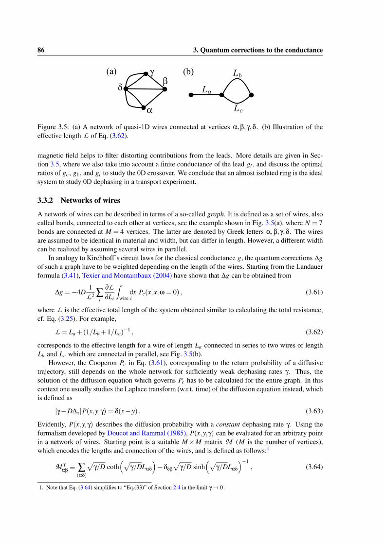
86 3. Quantum corrections to the conductance
(a) (b)
Figure 3.5: (a) A network of quasi-1D wires connected at vertices α,β,γ,δ. (b) Illustration of theeffective length L of Eq. (3.62).
magnetic field helps to filter distorting contributions from the leads. More details are given in Sec-tion 3.5, where we also take into account a finite conductance of the lead gl , and discuss the optimalratios of gc , g1 , and gl to study the 0D crossover. We conclude that an almost isolated ring is the idealsystem to study 0D dephasing in a transport experiment.
3.3.2 Networks of wires
A network of wires can be described in terms of a so-called graph. It is defined as a set of wires, alsocalled bonds, connected to each other at vertices, see the example shown in Fig. 3.5(a), where N = 7bonds are connected at M = 4 vertices. The latter are denoted by Greek letters α,β,γ,δ. The wiresare assumed to be identical in material and width, but can differ in length. However, a different widthcan be realized by assuming several wires in parallel.
In analogy to Kirchhoff’s circuit laws for the classical conductance g, the quantum corrections ∆gof such a graph have to be weighted depending on the length of the wires. Starting from the Landauerformula (3.41), Texier and Montambaux (2004) have shown that ∆g can be obtained from
∆g =−4D1
L2 ∑i
∂L∂Li
∫
wire idx Pc(x,x,ω = 0) , (3.61)
where L is the effective total length of the system obtained similar to calculating the total resistance,cf. Eq. (3.25). For example,
L = La +(1/Lb +1/Lc)−1 , (3.62)
corresponds to the effective length for a wire of length La connected in series to two wires of lengthLb and Lc which are connected in parallel, see Fig. 3.5(b).
However, the Cooperon Pc in Eq. (3.61), corresponding to the return probability of a diffusivetrajectory, still depends on the whole network for sufficiently weak dephasing rates γ. Thus, thesolution of the diffusion equation which governs Pc has to be calculated for the entire graph. In thiscontext one usually studies the Laplace transform (w.r.t. time) of the diffusion equation instead, whichis defined as
[γ−D∆x]P(x,y,γ) = δ(x− y) . (3.63)
Evidently, P(x,y,γ) describes the diffusion probability with a constant dephasing rate γ. Using theformalism developed by Doucot and Rammal (1985), P(x,y,γ) can be evaluated for an arbitrary pointin a network of wires. Starting point is a suitable M×M matrix M (M is the number of vertices),which encodes the lengths and connection of the wires, and is defined as follows:1
M γαβ ≡ ∑
(αδ)
√γ/D coth
(√γ/DLαδ
)−δδβ
√γ/D sinh
(√γ/DLαδ
)−1, (3.64)
1. Note that Eq. (3.64) simplifies to “Eq.(33)” of Section 2.4 in the limit γ→ 0.
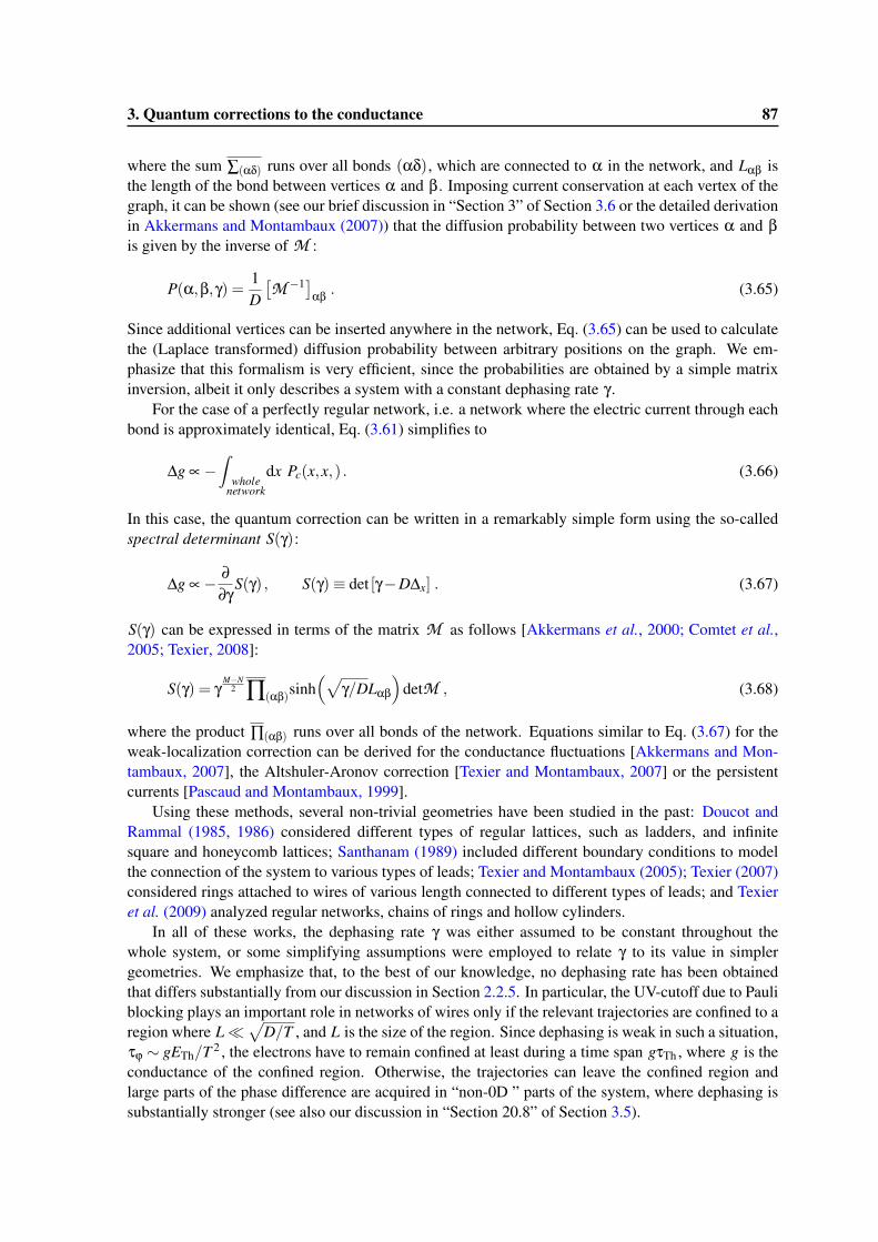
3. Quantum corrections to the conductance 87
where the sum ∑(αδ) runs over all bonds (αδ), which are connected to α in the network, and Lαβ isthe length of the bond between vertices α and β. Imposing current conservation at each vertex of thegraph, it can be shown (see our brief discussion in “Section 3” of Section 3.6 or the detailed derivationin Akkermans and Montambaux (2007)) that the diffusion probability between two vertices α and βis given by the inverse of M :
P(α,β,γ) =1D
[M −1]
αβ . (3.65)
Since additional vertices can be inserted anywhere in the network, Eq. (3.65) can be used to calculatethe (Laplace transformed) diffusion probability between arbitrary positions on the graph. We em-phasize that this formalism is very efficient, since the probabilities are obtained by a simple matrixinversion, albeit it only describes a system with a constant dephasing rate γ.
For the case of a perfectly regular network, i.e. a network where the electric current through eachbond is approximately identical, Eq. (3.61) simplifies to
∆g ∝−∫
wholenetwork
dx Pc(x,x,) . (3.66)
In this case, the quantum correction can be written in a remarkably simple form using the so-calledspectral determinant S(γ):
∆g ∝− ∂∂γ
S(γ) , S(γ)≡ det [γ−D∆x] . (3.67)
S(γ) can be expressed in terms of the matrix M as follows [Akkermans et al., 2000; Comtet et al.,2005; Texier, 2008]:
S(γ) = γM−N
2 ∏(αβ)sinh(√
γ/DLαβ
)detM , (3.68)
where the product ∏(αβ) runs over all bonds of the network. Equations similar to Eq. (3.67) for theweak-localization correction can be derived for the conductance fluctuations [Akkermans and Mon-tambaux, 2007], the Altshuler-Aronov correction [Texier and Montambaux, 2007] or the persistentcurrents [Pascaud and Montambaux, 1999].
Using these methods, several non-trivial geometries have been studied in the past: Doucot andRammal (1985, 1986) considered different types of regular lattices, such as ladders, and infinitesquare and honeycomb lattices; Santhanam (1989) included different boundary conditions to modelthe connection of the system to various types of leads; Texier and Montambaux (2005); Texier (2007)considered rings attached to wires of various length connected to different types of leads; and Texieret al. (2009) analyzed regular networks, chains of rings and hollow cylinders.
In all of these works, the dephasing rate γ was either assumed to be constant throughout thewhole system, or some simplifying assumptions were employed to relate γ to its value in simplergeometries. We emphasize that, to the best of our knowledge, no dephasing rate has been obtainedthat differs substantially from our discussion in Section 2.2.5. In particular, the UV-cutoff due to Pauliblocking plays an important role in networks of wires only if the relevant trajectories are confined to aregion where L�
√D/T , and L is the size of the region. Since dephasing is weak in such a situation,
τϕ ∼ gETh/T 2 , the electrons have to remain confined at least during a time span gτTh , where g is theconductance of the confined region. Otherwise, the trajectories can leave the confined region andlarge parts of the phase difference are acquired in “non-0D ” parts of the system, where dephasing issubstantially stronger (see also our discussion in “Section 20.8” of Section 3.5).
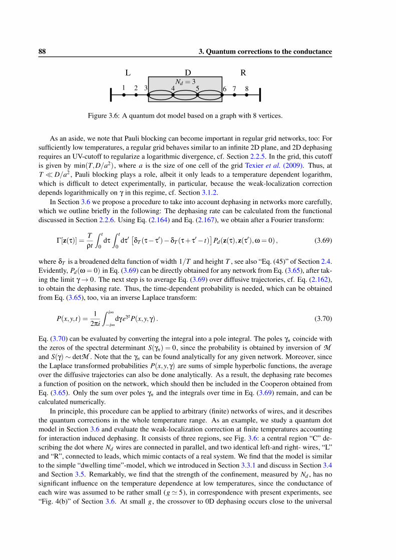
88 3. Quantum corrections to the conductance
Figure 3.6: A quantum dot model based on a graph with 8 vertices.
As an aside, we note that Pauli blocking can become important in regular grid networks, too: Forsufficiently low temperatures, a regular grid behaves similar to an infinite 2D plane, and 2D dephasingrequires an UV-cutoff to regularize a logarithmic divergence, cf. Section 2.2.5. In the grid, this cutoffis given by min(T,D/a2), where a is the size of one cell of the grid Texier et al. (2009). Thus, atT � D/a2 , Pauli blocking plays a role, albeit it only leads to a temperature dependent logarithm,which is difficult to detect experimentally, in particular, because the weak-localization correctiondepends logarithmically on γ in this regime, cf. Section 3.1.2.
In Section 3.6 we propose a procedure to take into account dephasing in networks more carefully,which we outline briefly in the following: The dephasing rate can be calculated from the functionaldiscussed in Section 2.2.6. Using Eq. (2.164) and Eq. (2.167), we obtain after a Fourier transform:
Γ[z(τ)] =Tρt
∫ t
0dτ
∫ t
0dτ′[δT (τ− τ′)−δT (τ+ τ′− t)
]Pd(z(τ),z(τ′),ω = 0) , (3.69)
where δT is a broadened delta function of width 1/T and height T , see also “Eq. (45)” of Section 2.4.Evidently, Pd(ω = 0) in Eq. (3.69) can be directly obtained for any network from Eq. (3.65), after tak-ing the limit γ→ 0. The next step is to average Eq. (3.69) over diffusive trajectories, cf. Eq. (2.162),to obtain the dephasing rate. Thus, the time-dependent probability is needed, which can be obtainedfrom Eq. (3.65), too, via an inverse Laplace transform:
P(x,y, t) =1
2πi
∫ i∞
−i∞dγeγ tP(x,y,γ) . (3.70)
Eq. (3.70) can be evaluated by converting the integral into a pole integral. The poles γn coincide withthe zeros of the spectral determinant S(γn) = 0, since the probability is obtained by inversion of Mand S(γ)∼ detM . Note that the γn can be found analytically for any given network. Moreover, sincethe Laplace transformed probabilities P(x,y,γ) are sums of simple hyperbolic functions, the averageover the diffusive trajectories can also be done analytically. As a result, the dephasing rate becomesa function of position on the network, which should then be included in the Cooperon obtained fromEq. (3.65). Only the sum over poles γn and the integrals over time in Eq. (3.69) remain, and can becalculated numerically.
In principle, this procedure can be applied to arbitrary (finite) networks of wires, and it describesthe quantum corrections in the whole temperature range. As an example, we study a quantum dotmodel in Section 3.6 and evaluate the weak-localization correction at finite temperatures accountingfor interaction induced dephasing. It consists of three regions, see Fig. 3.6: a central region “C” de-scribing the dot where Nd wires are connected in parallel, and two identical left-and right- wires, “L”and “R”, connected to leads, which mimic contacts of a real system. We find that the model is similarto the simple “dwelling time”-model, which we introduced in Section 3.3.1 and discuss in Section 3.4and Section 3.5. Remarkably, we find that the strength of the confinement, measured by Nd , has nosignificant influence on the temperature dependence at low temperatures, since the conductance ofeach wire was assumed to be rather small (g' 5), in correspondence with present experiments, see“Fig. 4(b)” of Section 3.6. At small g, the crossover to 0D dephasing occurs close to the universal
3. Quantum corrections to the conductance 89
regime of the weak-localization correction even in completely open systems, cf. Section 3.1.2. How-ever, we stress that this observation is based on the assumption of strongly absorbing leads. Thisassumptions is in particular questionable in unconfined system, since the electron trajectories mightbe able to return into the system if it is not sufficiently confined. A better model of the leads is highlydesirable, albait difficult to achieve.
In any case, 0D dephasing can be observed only after subtracting the quantum corrections fromtheir universal value at low temperature. Unfortunately, the conductance is very sensitive to the type ofcontacts and leads in the particular experiment in this temperature range, which makes the observationof the crossover very difficult in a transport experiment. However, we show in the following Chapter 4that 0D dephasing is also accessible in isolated systems, where these problems do not appear.

3. Quantum corrections to the conductance 91
3.4 Publication: Dimensional crossover of the dephasing time in disor-dered mesoscopic rings
The following 4 pages have been published in the journal Physical Review B.
Dimensional crossover of the dephasing time in disordered mesoscopic rings
M. Treiber,1 O. M. Yevtushenko,1 F. Marquardt,1 J. von Delft,1 and I. V. Lerner2
1Arnold Sommerfeld Center and Center for Nano-Science, Ludwig-Maximilians-University, Munich D-80333, Germany2School of Physics and Astronomy, University of Birmingham, Birmingham B15 2TT, United Kingdom
�Received 13 October 2009; published 10 November 2009�
We study dephasing by electron interactions in a small disordered quasi-one-dimensional �1D� ring weaklycoupled to leads. We use an influence functional for quantum Nyquist noise to describe the crossover for thedephasing time ���T� from diffusive or ergodic 1D ���
−1�T2/3 ,T1� to zero-dimensional �0D� behavior���
−1�T2� as T drops below the Thouless energy. The crossover to 0D, predicted earlier for two-dimensionaland three-dimensional systems, has so far eluded experimental observation. The ring geometry holds promiseof meeting this long-standing challenge, since the crossover manifests itself not only in the smooth part of themagnetoconductivity but also in the amplitude of Altshuler-Aronov-Spivak oscillations. This allows signaturesof dephasing in the ring to be cleanly extracted by filtering out those of the leads.
DOI: 10.1103/PhysRevB.80.201305 PACS number�s�: 73.63.�b, 72.10.�d, 72.15.Rn
I. INTRODUCTION
Over the last 20 years numerous theoretical1–8 andexperimental10–15 works have studied the mechanism ofdephasing in electronic transport and its dependence on tem-perature T and dimensionality in disordered condensed-matter systems. At low temperatures dephasing is mainly dueto electron interactions, with the dephasing time ���T� in-creasing as T−a when T→0.
The dephasing time controls the scale of a negative weaklocalization �WL� correction to the magnetoconductivity and�under certain conditions� the magnitude of universal con-ductance fluctuations �UCFs�. If T is so low that �� exceeds�Th=� /ETh, the time required for an electron to cross �diffu-sively or ballistically� a mesoscopic sample �ETh is the Thou-less energy�, UCFs become T independent. This leaves WLas the only tool to measure the T dependence of dephasing inmesoscopic wires or quantum dots at very low T. For quan-tum dots, a dimensional crossover was predicted4 from���T−1, typical for a two-dimensional �2D� electron gas,1 to���T−2 when the temperature is lowered into the zero-dimensional �0D� regime,
�/�� � T � ETh, �1�
where the coherence length and the thermal length are bothlarger than the system size independent of geometry and realdimensionality of the sample. Although the ���T−2 behavioris quite generic, arising from the fermionic statistics of con-duction electrons, experimental efforts13 to observe it have sofar been unsuccessful. The reasons for this are unclear. Con-ceivably dephasing mechanisms other than electron interac-tions were dominant, or the regime of validity of the 0Ddescription had not been reached. In any case, other ways oftesting the dimensional crossover for �� are desirable.
Here we study dephasing in a quasi-1D mesoscopic ringweakly coupled to two well-conducting leads through narrowpoint contacts. We find a dimensional crossover for ���T�from diffusive or ergodic 1D ��T−2/3 ,T−1� to 0D ��T−2� be-havior as T is decreased below ETh and propose a detailedexperimental scenario for observing this behavior. It revealsitself not only via the WL corrections to the smooth part ofmagnetoconductivity but also via the amplitude of the
Altshuler-Aronov-Spivak �AAS� oscillations16 that resultfrom closed trajectories with a nonzero winding number ac-quiring the Aharonov-Bohm phase. For sufficiently weaklead-ring coupling �specified below�, the magnitude of AASoscillations will be independent of dephasing in the leads.Thus, the ring geometry provides a more promising setup forthe observation of the dimensional crossover than 2D or 3Dsettings.
II. DEPHASING IN WEAK LOCALIZATION
The WL correction to the conductivity is governed bycoherent backscattering of the electrons from static disorderand, to the lowest order, is due to the enhancement of thereturn probability caused by constructive interference of twotime reversed trajectories described by the so-called Coop-eron C.17,18 In this order, the WL correction to the conduc-tivity, in units of the Drude conductivity �0, is given by19
�g =��
�0= −
1
�
0
�
dt�C�t�� . �2�
Here is the electron density of states per spin at the Fermisurface and �=1 henceforward. Dephasing limits the scale ofthis contribution and effectively results in the suppression ofthe Cooperon at long times:
C�t� � C0�t�exp�− t/�H − t/�dw − F�t�� . �3�
We consider here low temperatures where the phonon con-tribution to dephasing is negligible and three main sourcescontribute to the Cooperon decay with time: an applied mag-netic field H characterized by the time scale �H �Ref. 20�; theleakage of particles from the ring characterized by the dwelltime �dw �Ref. 21�; and electron interactions, whose effectscan be described in terms of the decay function F�t�,1,3
which grows with time and may be used to define a dephas-ing time via F����=1.
F�t� can be obtained using the influence functionalapproach,6,7 which gives results for the magnetoconductivitythat are practically equivalent to those originally obtained inRef. 1. Roughly speaking, an electron traversing a randomwalk trajectory x�t1� of duration t acquires a random phase
PHYSICAL REVIEW B 80, 201305�R� �2009�
RAPID COMMUNICATIONS
1098-0121/2009/80�20�/201305�4� ©2009 The American Physical Society201305-1
92 3. Quantum corrections to the conductance
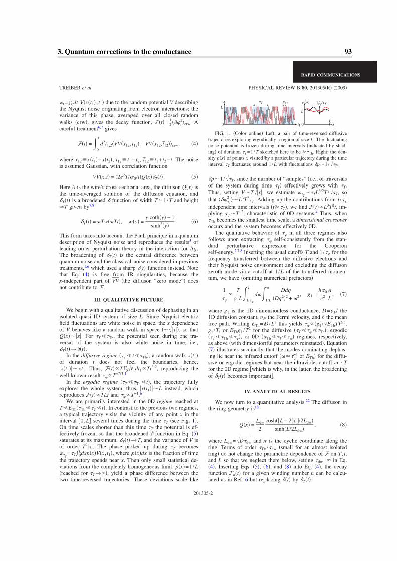
�t=�0t dt1V�x�t1� , t1� due to the random potential V describing
the Nyquist noise originating from electron interactions; thevariance of this phase, averaged over all closed randomwalks �crw�, gives the decay function, F�t�= 1
2 ���t2crw. A
careful treatment6,7 gives
F�t� = �0
t
d2t1,2�VV�x12,t12� − VV�x12, t12�crw, �4�
where x12�x�t1�−x�t2�; t12� t1− t2; t12� t1+ t2− t. The noiseis assumed Gaussian, with correlation function
VV�x,t� = �2e2T/�0A�Q�x��T�t� . �5�
Here A is the wire’s cross-sectional area, the diffuson Q�x� isthe time-averaged solution of the diffusion equation, and�T�t� is a broadened � function of width T1 /T and heightT given by7,8
�T�t� = Tw�Tt�, w�y� =y coth�y� − 1
sinh2�y�. �6�
This form takes into account the Pauli principle in a quantumdescription of Nyquist noise and reproduces the results5 ofleading order perturbation theory in the interaction for �g.The broadening of �T�t� is the central difference betweenquantum noise and the classical noise considered in previoustreatments,1,6 which used a sharp ��t� function instead. Notethat Eq. �4� is free from IR singularities, because thex-independent part of VV �the diffuson “zero mode”� doesnot contribute to F.
III. QUALITATIVE PICTURE
We begin with a qualitative discussion of dephasing in anisolated quasi-1D system of size L. Since Nyquist electricfield fluctuations are white noise in space, the x dependenceof V behaves like a random walk in space ��� x �, so thatQ�x�� x . For �T��Th, the potential seen during one tra-versal of the system is also white noise in time, i.e.,�T�t�→��t�.
In the diffusive regime ��T� t��Th�, a random walk x�t1�of duration t does not feel the boundaries, hence, x�t1� ��t1. Thus, F�t��T�0
t �t1dt1�Tt3/2, reproducing thewell-known result ���T−2/3.1
In the ergodic regime ��T��Th� t�, the trajectory fullyexplores the whole system, thus, x�t1� �L instead, whichreproduces F�t��TLt and ���T−1.6
We are primarily interested in the 0D regime reached atT�ETh��Th��T� t�. In contrast to the previous two regimes,a typical trajectory visits the vicinity of any point x in theinterval �0,L� several times during the time �T �see Fig. 1�.On time scales shorter than this time �T the potential is ef-fectively frozen, so that the broadened � function in Eq. �5�saturates at its maximum, �T�t�→T, and the variance of V isof order T2 x . The phase picked up during �T becomes��T
=�T�0Ldxp�x�V�x , t1�, where p�x�dx is the fraction of time
the trajectory spends near x. Then only small statistical de-viations from the completely homogeneous limit, p�x�=1 /L�reached for �T→��, yield a phase difference between thetwo time-reversed trajectories. These deviations scale like
�p�1 /��T, since the number of “samples” �i.e., of traversalsof the system during time �T� effectively grows with �T.Thus, setting V�T� x , we estimate ��T
��TL3/2T /��T, sothat ����T
2 �L3T2�T. Adding up the contributions from t /�T
independent time intervals �t �T�, we find F�t��L3T2t, im-plying ���T−2, characteristic of 0D systems.4 Thus, when�Th becomes the smallest time scale, a dimensional crossoveroccurs and the system becomes effectively 0D.
The qualitative behavior of �� in all three regimes alsofollows upon extracting �� self-consistently from the stan-dard perturbative expression for the Cooperonself-energy.2,7,8 Inserting the usual cutoffs T and 1 /�� for thefrequency transferred between the diffusive electrons andtheir Nyquist noise environment and excluding the diffusonzeroth mode via a cutoff at 1 /L of the transferred momen-tum, we have �omitting numerical prefactors�
1
��
�T
g1L�
1/��
T
d��1/L
� Ddq
�Dq2�2 + �2 , g1 =h�0
e2
A
L, �7�
where g1 is the 1D dimensionless conductance, D=vFl the1D diffusion constant, vF the Fermi velocity, and � the meanfree path. Writing ETh=D /L2 this yields ��� �g1 /�EThT�2/3,g1 /T, or EThg1 /T2 for the diffusive ��T�����Th�, ergodic��T��Th����, or 0D ��Th��T���� regimes, respectively,as above �with dimensionful parameters reinstated�. Equation�7� illustrates succinctly that the modes dominating dephas-ing lie near the infrared cutoff ����
−1 or ETh� for the diffu-sive or ergodic regimes but near the ultraviolet cutoff �Tfor the 0D regime �which is why, in the latter, the broadeningof �T�t� becomes important�.
IV. ANALYTICAL RESULTS
We now turn to a quantitative analysis.22 The diffuson inthe ring geometry is18
Q�x� =Ldw
2
cosh��L − 2 x �/2Ldw�sinh�L/2Ldw�
, �8�
where Ldw=�D�dw and x is the cyclic coordinate along thering. Terms of order �Th /�dw �small for an almost isolatedring� do not change the parametric dependence of F on T , t,and L so that we neglect them below, setting �dw=� in Eq.�4�. Inserting Eqs. �5�, �6�, and �8� into Eq. �4�, the decayfunction Fn�t� for a given winding number n can be calcu-lated as in Ref. 6 but replacing ��t� by �T�t�:
�
�L
0 t1
x
�
�
0 x
p(x)
L
��
1/√
τT� �τT ��τTh
1L
FIG. 1. �Color online� Left: a pair of time-reversed diffusivetrajectories exploring ergodically a region of size L. The fluctuatingnoise potential is frozen during time intervals �indicated by shad-ing� of duration �T=1 /T sketched here to be �Th. Right: the den-sity p�x� of points x visited by a particular trajectory during the timeinterval �T fluctuates around 1 /L with fluctuations �p�1 /��T.
TREIBER et al. PHYSICAL REVIEW B 80, 201305�R� �2009�
RAPID COMMUNICATIONS
201305-2
3. Quantum corrections to the conductance 93
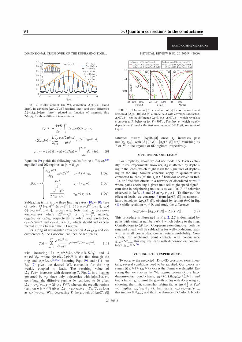
Fn�t� = −4Tt
g1L�
0
1
du z�u��Qcrw�u� ,
�Qcrw�u� =L
2 �k=1
�cos�2knu�
�k�2 e−�2k�2EThtu�1−u�,
z�u� = − 2Tt�1 − u�w�Ttu� + �−Ttu
Ttu
dv w�v� . �9�
Equation �9� yields the following results for the diffusive,1,23
ergodic,6 and 0D regimes at n �ETht:
Fn�t� ��n,03/2
2g1
�EThTt3/2, �T � t � �Th �10a�
Tt
3g1, �T � �Th � t �10b�
2
270g1
T2t
ETh, �Th � �T � t . �10c�
Subleading terms in the three limiting cases �10a�–�10c� areof order O���T / t�1/2 , �t /�Th�1/2�, O���T /�Th�1/2 ,�Th / t�, andO���Th /�T�2 , ��T / t��, respectively. Note that the crossovertemperatures where ��
diff��erg or ��
erg��0D, namely,
c1g1ETh or c2ETh, respectively, involve large prefactors,c1=27 /47 and c2=90 /30, which should aid experi-mental efforts to reach the 0D regime.
For a ring of rectangular cross section A=LWLH and cir-cumference L, the Cooperon can then be written as
C�t� �n=−�
+�e−�nL�2/4Dt
�4Dte−t/�H−Fn�t�−t/�dwein�, �11�
with �restoring �� �H=9.5��c /eH�2� �l /DLW3 � and �
=4� /�0, where �=�L /2�2H is the flux through thering and �0=hc /e.15,16,24 Inserting Eqs. �9� and �11� intoEq. �2� gives the desired WL correction for the ringweakly coupled to leads. The resulting value of �g�T ,�� increases with decreasing T, Fig. 2, in a mannergoverned by ��: since only trajectories with n �2�t /�Thcontribute, the diffusive regime �n restricted to 0� gives �g ���� /�Th /g1� �ETh /g1
2T�1/3, whereas the ergodic regime�sum on n is �t1/2� gives �g � ��� /�Th� /g1�ETh /T, as longas ����H ,�dw. With decreasing T, the growth of �g�T ,��
saturates toward �g�0,�� once �� increases pastmin��H ,�dw�, with �g�0,�� − �g�T ,�� ���
−1 vanishing asT or T2 in the ergodic or 0D regimes, respectively.
V. FILTERING OUT LEADS
For simplicity, above we did not model the leads explic-itly. In real experiments, however, �g is affected by dephas-ing in the leads, which might mask the signatures of dephas-ing in the ring. Similar concerns apply to quantum dotsconnected to leads �cf. the ���T−1 behavior observed in Ref.13�, or finite-size effects in a network of disordered wires,15
where paths encircling a given unit cell might spend signifi-cant time in neighboring unit cells as well �cf. T−1/3 behaviorobserved in Refs. 15 and 25 at �� /�Th�1�. To filter out theeffect of leads, we construct15 from �g�T ,�� its nonoscil-latory envelope �gen�T ,�� , obtained by setting �=0 in Eq.�11� while retaining �H�0, and study the difference
�g�T,�� = �gen�T,�� − �g�T,�� . �12�
This procedure is illustrated in Fig. 2. �g is dominated bypaths with winding numbers n�1 which belong to the ring.Contributions to �g from Cooperons extending over both thering and a lead will be subleading for well-conducting leadswith a small contact-lead-contact return probability. Con-cretely, for N-channel point contacts with conductancegcont=NTcont, this requires leads with dimensionless conduc-tance glead N.26
VI. SUGGESTED EXPERIMENTS
To observe the predicted 1D-to-0D crossover experimen-tally, several conditions need to be satisfied. Our theory as-sumes �i� L � LW �F ��F is the Fermi wavelength�. En-suring that we stay in the WL regime requires �ii� a largedimensionless conductance, g1� �� /L��LWLH /�F
2� 1, and�iii� a finite �dw to limit the growth of �g with decreasing T;choosing the limit, somewhat arbitrarily, as �g�
12 at T ,H
=0 implies �dw /�Th�g1 /8. Estimating �dw /�Thg1 /gcont,this implies 8�gcont and thus the absence of Coulomb block-
0
0.1
0.2
0.3
0.4
0.5
0.6
0.7
-6 -4 -2 0 2 4 6
|∆g(
T,φ
)|
2φ/φ0
τdw/τTh = 3
ETh = 40mKL = 10.0µmLW = 0.3µm
l = 2µmg1 = 25
T = 1EThT = 10EThT =100ETh
0.5
0-4 -2 2 4
∆g(T
,φ)
φ1
FIG. 2. �Color online� The WL correction �g�T ,�� �solidlines�, its envelope �gen�T ,�� �dashed lines�, and their difference�g= �gen − �g �inset�, plotted as function of magnetic flux2� /�0, for three different temperatures.
0.01
0.1
100 1000
|∆g(
T,0
)|
T mK
0.6
25
∝ T −1/3
∝T −
1
(a)
�ETh� ETh
100 1000
∆g(T
,φ1)
T mK25
∝T −
1
(b)
�ETh� ETh
100T mK
25
∝T
2
�ETh �ETh
(c)
∆g(0
,φ1)−∆
g(T,φ
1)
l=2µm,g1=25,τdw/τTh=3:(L,LW)=(10,0.3)µm,ETh=40mK(L,LW)=(40,1.2)µm,ETh=2.5mK
l=4µm,g1=100,τdw/τTh=13:(L,LW)=(10,0.6)µm,ETh=80mK(L,LW)=(40,2.4)µm,ETh=5.0mK
( ) ( ) ( )
FIG. 3. �Color online� T dependence of �a� the WL correction atzero field, �g�T ,0� and �b� at finite field with envelope subtracted,�g�T ,�1�; �c� the difference �g�0,�1�−�g�T ,�1�, which reveals acrossover to T2 behavior for T�30ETh. The flux �1, which weaklydepends on T, marks the first maximum of �g�T ,��; see inset ofFig. 2.
DIMENSIONAL CROSSOVER OF THE DEPHASING TIME… PHYSICAL REVIEW B 80, 201305�R� �2009�
RAPID COMMUNICATIONS
201305-3
94 3. Quantum corrections to the conductance
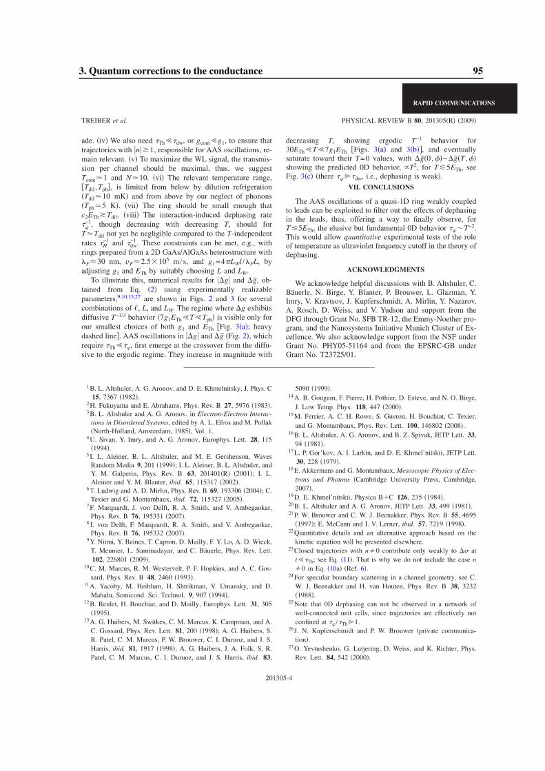
ade. �iv� We also need �Th��dw, or gcont�g1, to ensure thattrajectories with n �1, responsible for AAS oscillations, re-main relevant. �v� To maximize the WL signal, the transmis-sion per channel should be maximal, thus, we suggestTcont1 and N10. �vi� The relevant temperature range,�Tdil ,Tph�, is limited from below by dilution refrigeration�Tdil10 mK� and from above by our neglect of phonons�Tph5 K�. �vii� The ring should be small enough thatc2ETh�Tdil. �viii� The interaction-induced dephasing rate��
−1, though decreasing with decreasing T, should forTTdil not yet be negligible compared to the T-independentrates �H
−1 and �dw−1 . These constraints can be met, e.g., with
rings prepared from a 2D GaAs/AlGaAs heterostructure with�F�30 nm, vF�2.5�105 m /s, and g1=4LWl /�FL, byadjusting g1 and ETh by suitably choosing L and LW.
To illustrate this, numerical results for �g and �g, ob-tained from Eq. �2� using experimentally realizableparameters,9,10,15,27 are shown in Figs. 2 and 3 for severalcombinations of �, L, and LW. The regime where �g exhibitsdiffusive T−1/3 behavior �7g1ETh�T�Tph� is visible only forour smallest choices of both g1 and ETh �Fig. 3�a�; heavydashed line�. AAS oscillations in �g and �g �Fig. 2�, whichrequire �Th���, first emerge at the crossover from the diffu-sive to the ergodic regime. They increase in magnitude with
decreasing T, showing ergodic T−1 behavior for30ETh�T�7g1ETh �Figs. 3�a� and 3�b��, and eventuallysaturate toward their T=0 values, with �g�0,��−�g�T ,��showing the predicted 0D behavior, �T2, for T�5ETh, seeFig. 3�c� �there �� �dw, i.e., dephasing is weak�.
VII. CONCLUSIONS
The AAS oscillations of a quasi-1D ring weakly coupledto leads can be exploited to filter out the effects of dephasingin the leads, thus, offering a way to finally observe, forT�5ETh, the elusive but fundamental 0D behavior ���T−2.This would allow quantitative experimental tests of the roleof temperature as ultraviolet frequency cutoff in the theory ofdephasing.
ACKNOWLEDGMENTS
We acknowledge helpful discussions with B. Altshuler, C.Bäuerle, N. Birge, Y. Blanter, P. Brouwer, L. Glazman, Y.Imry, V. Kravtsov, J. Kupferschmidt, A. Mirlin, Y. Nazarov,A. Rosch, D. Weiss, and V. Yudson and support from theDFG through Grant No. SFB TR-12, the Emmy-Noether pro-gram, and the Nanosystems Initiative Munich Cluster of Ex-cellence. We also acknowledge support from the NSF underGrant No. PHY05-51164 and from the EPSRC-GB underGrant No. T23725/01.
1 B. L. Altshuler, A. G. Aronov, and D. E. Khmelnitsky, J. Phys. C15, 7367 �1982�.
2 H. Fukuyama and E. Abrahams, Phys. Rev. B 27, 5976 �1983�.3 B. L. Altshuler and A. G. Aronov, in Electron-Electron Interac-
tions in Disordered Systems, edited by A. L. Efros and M. Pollak�North-Holland, Amsterdam, 1985�, Vol. 1.
4 U. Sivan, Y. Imry, and A. G. Aronov, Europhys. Lett. 28, 115�1994�.
5 I. L. Aleiner, B. L. Altshuler, and M. E. Gershenson, WavesRandom Media 9, 201 �1999�; I. L. Aleiner, B. L. Altshuler, andY. M. Galperin, Phys. Rev. B 63, 201401�R� �2001�; I. L.Aleiner and Y. M. Blanter, ibid. 65, 115317 �2002�.
6 T. Ludwig and A. D. Mirlin, Phys. Rev. B 69, 193306 �2004�; C.Texier and G. Montambaux, ibid. 72, 115327 �2005�.
7 F. Marquardt, J. von Delft, R. A. Smith, and V. Ambegaokar,Phys. Rev. B 76, 195331 �2007�.
8 J. von Delft, F. Marquardt, R. A. Smith, and V. Ambegaokar,Phys. Rev. B 76, 195332 �2007�.
9 Y. Niimi, Y. Baines, T. Capron, D. Mailly, F. Y. Lo, A. D. Wieck,T. Meunier, L. Saminadayar, and C. Bäuerle, Phys. Rev. Lett.102, 226801 �2009�.
10 C. M. Marcus, R. M. Westervelt, P. F. Hopkins, and A. C. Gos-sard, Phys. Rev. B 48, 2460 �1993�.
11 A. Yacoby, M. Heiblum, H. Shtrikman, V. Umansky, and D.Mahalu, Semicond. Sci. Technol. 9, 907 �1994�.
12 B. Reulet, H. Bouchiat, and D. Mailly, Europhys. Lett. 31, 305�1995�.
13 A. G. Huibers, M. Switkes, C. M. Marcus, K. Campman, and A.C. Gossard, Phys. Rev. Lett. 81, 200 �1998�; A. G. Huibers, S.R. Patel, C. M. Marcus, P. W. Brouwer, C. I. Duruoz, and J. S.Harris, ibid. 81, 1917 �1998�; A. G. Huibers, J. A. Folk, S. R.Patel, C. M. Marcus, C. I. Duruoz, and J. S. Harris, ibid. 83,
5090 �1999�.14 A. B. Gougam, F. Pierre, H. Pothier, D. Esteve, and N. O. Birge,
J. Low Temp. Phys. 118, 447 �2000�.15 M. Ferrier, A. C. H. Rowe, S. Gueron, H. Bouchiat, C. Texier,
and G. Montambaux, Phys. Rev. Lett. 100, 146802 �2008�.16 B. L. Altshuler, A. G. Aronov, and B. Z. Spivak, JETP Lett. 33,
94 �1981�.17 L. P. Gor’kov, A. I. Larkin, and D. E. Khmel’nitskii, JETP Lett.
30, 228 �1979�.18 E. Akkermans and G. Montambaux, Mesoscopic Physics of Elec-
trons and Photons �Cambridge University Press, Cambridge,2007�.
19 D. E. Khmel’nitskii, Physica B�C 126, 235 �1984�.20 B. L. Altshuler and A. G. Aronov, JETP Lett. 33, 499 �1981�.21 P. W. Brouwer and C. W. J. Beenakker, Phys. Rev. B 55, 4695
�1997�; E. McCann and I. V. Lerner, ibid. 57, 7219 �1998�.22 Quantitative details and an alternative approach based on the
kinetic equation will be presented elsewhere.23 Closed trajectories with n�0 contribute only weakly to �� at
t��Th; see Eq. �11�. That is why we do not include the case n�0 in Eq. �10a� �Ref. 6�.
24 For specular boundary scattering in a channel geometry, see C.W. J. Beenakker and H. van Houten, Phys. Rev. B 38, 3232�1988�.
25 Note that 0D dephasing can not be observed in a network ofwell-connected unit cells, since trajectories are effectively notconfined at �� /�Th 1.
26 J. N. Kupferschmidt and P. W. Brouwer �private communica-tion�.
27 O. Yevtushenko, G. Lutjering, D. Weiss, and K. Richter, Phys.Rev. Lett. 84, 542 �2000�.
TREIBER et al. PHYSICAL REVIEW B 80, 201305�R� �2009�
RAPID COMMUNICATIONS
201305-4
3. Quantum corrections to the conductance 95

3. Quantum corrections to the conductance 97
3.5 Publication: Dimensional Crossover of the Dephasing Time in Dis-ordered Mesoscopic Rings: From Diffusive through Ergodic to 0DBehavior
The following 26 pages have been published as Chapter 20 in the book Perspectives of MesoscopicPhysics: Dedicated to Yoseph Imry’s 70th Birthday, edited by A. Aharony and O. Entin-Wohlman(World Scientific, Singapore, 2010).
March 31, 2010 16:48 World Scientific Review Volume - 9in x 6in chapter 20
Chapter 20
Dimensional Crossover of the Dephasing Time in
Disordered Mesoscopic Rings: From Diffusive through
Ergodic to 0D Behavior
M. Treiber, O.M. Yevtushenko, F. Marquardt and J. von Delft
Arnold Sommerfeld Center and Center for Nano-Science, Ludwig
Maximilians University, Munich, D-80333, Germany
I.V. Lerner
School of Physics and Astronomy, University of Birmingham,
Birmingham, B15 2TT, UK
We analyze dephasing by electron interactions in a small disorderedquasi-one dimensional (1D) ring weakly coupled to leads, where we re-cently predicted a crossover for the dephasing time τϕ(T ) from diffusiveor ergodic 1D (τ−1
ϕ ∝ T 2/3, T 1) to 0D behavior (τ−1ϕ ∝ T 2) as T drops
below the Thouless energy ETh.1 We provide a detailed derivation of our
results, based on an influence functional for quantum Nyquist noise, andcalculate all leading and subleading terms of the dephasing time in thethree regimes. Explicitly taking into account the Pauli blocking of theFermi sea in the metal allows us to describe the 0D regime on equal foot-ing as the others. The crossover to 0D, predicted by Sivan, Imry andAronov for 3D systems,2 has so far eluded experimental observation.We will show that for T � ETh, 0D dephasing governs not only theT -dependence for the smooth part of the magnetoconductivity but alsofor the amplitude of the Altshuler-Aronov-Spivak oscillations, which re-sult only from electron paths winding around the ring. This observationcan be exploited to filter out and eliminate contributions to dephasingfrom trajectories which do not wind around the ring, which may tend tomask the T 2 behavior. Thus, the ring geometry holds promise of finallyobserving the crossover to 0D experimentally.
20.1. Introduction
Over the last twenty-five years many theoretical and experimental works
addressed quantum phenomena in mesoscopic disordered metallic rings.3
371
98 3. Quantum corrections to the conductance
March 31, 2010 16:48 World Scientific Review Volume - 9in x 6in chapter 20
372 M. Treiber et al.
This subject was launched in part by several seminal papers by Joe Imry
and his collaborators 4–11, and continues to be of great current interest. One
intensively-studied topic involves persistent currents, which can flow with-
out dissipation due to quantum interference in rings prepared from normal
metals.4,12–15 Attention was also paid to Aharonov-Bohm oscillations in the
conductance through a mesoscopic ring attached to two leads,5–7,10,16 and
the closely related oscillations of the negative weak localization (WL) cor-
rection to the magnetoconductivity.17,18 These oscillations result from the
interference of closed trajectories which have a non-zero winding number
acquiring the Aharonov-Bohm phase. Both persistent currents and magne-
tooscillations require the ring to be phase coherent, since any uncertainty
of the quantum phase due to the environment or interactions immediately
suppresses all interference phenomena.19
The mechanism of dephasing in electronic transport and its dependence
on temperature T in disordered conductors was studied in numerous theo-
retical2,19–27 and experimental28–35 works. The characteristic time scale of
dephasing is called the dephasing time τϕ. At low temperatures phonons
are frozen out and dephasing is mainly due to electron interactions, with
the dephasing time τϕ(T ) increasing as T−a when T → 0 , a > 0.
The scaling of the dephasing time with temperature depends on the
dimensionality of the sample.20 It was predicted in a pioneering paper by
Sivan, Imry and Aronov2 that the dephasing time in a disordered quantum
dot shows a dimensional crossover from τϕ ∝ T−1, typical for a 2D electron
gas,20 to τϕ ∝ T−2 when the temperature is lowered into the 0D regime:
�/τϕ � T � �/τTh , (20.1)
where τTh = �/ETh is the Thouless time, i.e. the time required for an
electron to cross (diffusively or ballistically) the mesoscopic sample; ETh
is the Thouless energy. In this low-T , 0D regime, the coherence length
and the thermal length are both larger than the system size, independent
of geometry and real dimensionality of the sample. In this regime WL
is practically the only tool to measure the T -dependence of dephasing in
mesoscopic wires or quantum dots (the mesoscopic conductance fluctuations
go over to a universal value of order e2/h for T � ETh3).
Although the τϕ ∝ T−2 behavior is quite generic, arising from the
fermionic statistics of conduction electrons, experimental efforts31–33 to
observe it have so far been unsuccessful. The reasons for this are today
still unclear. Conceivably dephasing mechanisms other than electron in-
teractions were dominant, or the regime of validity of the 0D description
3. Quantum corrections to the conductance 99
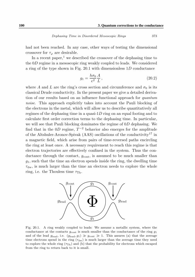
March 31, 2010 16:48 World Scientific Review Volume - 9in x 6in chapter 20
Dephasing Time in Disordered Mesoscopic Rings 373
had not been reached. In any case, other ways of testing the dimensional
crossover for τϕ are desirable.
In a recent paper,1 we described the crossover of the dephasing time to
the 0D regime in a mesoscopic ring weakly coupled to leads. We considered
a ring of the type shown in Fig. 20.1 with dimensionless 1D conductance
g1 =hσ0
e2A
L, (20.2)
where A and L are the ring’s cross section and circumference and σ0 is its
classical Drude conductivity. In the present paper we give a detailed deriva-
tion of our results based on an influence functional approach for quantum
noise. This approach explicitly takes into account the Pauli blocking of
the electrons in the metal, which will allow us to describe quantitatively all
regimes of the dephasing time in a quasi-1D ring on an equal footing and to
calculate first order correction terms to the dephasing time. In particular,
we will see that Pauli blocking dominates the regime of 0D dephasing. We
find that in the 0D regime, T−2 behavior also emerges for the amplitude
of the Altshuler-Aronov-Spivak (AAS) oscillations of the conductivity17 in
a magnetic field, which arise from pairs of time-reversed paths encircling
the ring at least once. A necessary requirement to reach this regime is that
electron trajectories are effectively confined in the system. Thus the con-
ductance through the contact, gcont, is assumed to be much smaller than
g1, such that the time an electron spends inside the ring, the dwelling time
τdw, is much larger than the time an electron needs to explore the whole
ring, i.e. the Thouless time τTh.
Fig. 20.1. A ring weakly coupled to leads: We assume a metallic system, where theconductance at the contacts gcont is much smaller than the conductance of the ring g1and of the lead glead, i.e. (glead, g1) � gcont � 1. This assures (a) that the averagetime electrons spend in the ring (τdw) is much larger than the average time they needto explore the whole ring (τTh) and (b) that the probability for electrons which escapedfrom the ring to return back to it is small.
100 3. Quantum corrections to the conductance
March 31, 2010 16:48 World Scientific Review Volume - 9in x 6in chapter 20
374 M. Treiber et al.
We will show below that after subtracting from the amplitude of the
AAS-oscillations the non-oscillating background, only contributions to de-
phasing from paths encircling the ring will contribute. However, some of
these paths may involve loops which not only encircle the ring, but along
the way also enter the lead and reenter the ring (see Fig. 20.6(b) below).
Such lead-ring cross-contributions to dephasing will contribute a non-0D
T -dependence to the conductance and hence tend to mask the 0D behav-
ior. We shall argue that by additionally choosing the conductance of the
connected leads, glead, to be larger than gcont, dephasing due to lead-ring
cross-contributions, can be neglected, and the remaining contributions will
be characterized by 0D dephasing.
20.2. Dephasing and Weak Localization
In a disordered metal, the conductivity is reduced by coherent backscatter-
ing of the electrons from impurities, an effect known as weak localization
(WL). In a semi-classical picture it can be understood as the constructive
interference of closed, time-reversed random-walks through the metal’s im-
purity landscape. It is most pronounced in systems of low dimensionality d
where the integrated return probability becomes large for long times. For
an infinite system characterized by the diffusion constant D = vF l/d (vF is
the Fermi velocity and l is the mean free path), the probability of a random
walk of duration t to return back to its origin is given by
C0(t) = (4πDt)−d/2 . (20.3)
To leading order in 1/g1, the relative correction to the conductance (20.2)
can be written as
Δg =Δσ
σ0= − 1
πν
∫ ∞
0
dt C(t) , (20.4)
where ν is the density of states per volume in the ring and we have set
� = 1 henceforth. The function C(t) is the so called Cooperon propagator
corresponding to the interference amplitude of the time-reversed random
walks. C(t) reduces to Eq. (20.3) if time-reversal symmetry is fully pre-
served. Processes which destroy this symmetry lead to a suppression of this
contribution at long times, since the random walks and their time-reversed
counterparts acquire a different phase. The model we are considering as-
sumes a suppression of the Cooperon of the following form
C(t) ≡ C0(t) exp [−t/τH − t/τdw − F(t)] . (20.5)
3. Quantum corrections to the conductance 101
March 31, 2010 16:48 World Scientific Review Volume - 9in x 6in chapter 20
Dephasing Time in Disordered Mesoscopic Rings 375
In Eq. (20.5), we consider dephasing due to the effect of an external mag-
netic field leading to the cutoff τH ∼ 1/H of the integral in Eq. (20.4).43
Furthermore, our model of an almost isolated ring assumes an average
dwelling time, τdw, of the electrons in the ring.45
Our primary interest is the effect of electron interactions, which we
describe in terms of the Cooperon decay function F(t), which grows with
time and may be used to define a dephasing time via
F(τϕ) = 1 . (20.6)
Dephasing due to electron interactions can be understood roughly as fol-
lows: At finite temperatures the interactions lead to thermal fluctuations
(noise) of the electron’s potential energy V (x, t). Then the closed paths
contributing to WL and their time-reversed counterparts effectively “see” a
different local potential, leading to a phase difference. This is most clearly
seen in a path integral representation of the Cooperon in a time-dependent
potential,20 which is given by
C(t) ∝∫ x(t)=x0
x(0)=x0
Dx eiϕ(t)e−∫ t0dt1 L(t1) . (20.7)
Here the Lagrangian L(t1) = x2(t1)/4D describes diffusive propagation,
and ϕ(t) is a phase corresponding to the time-reversed structure of the
Cooperon:
ϕ(t) =
∫ t
0
dt1 [V (x(t1), t1) − V (x(t1), t − t1)] . (20.8)
Assuming that the noise induced by electron interactions is Gaussian, the
decay function F(t) in Eq. (20.5) can be estimated from F(t) = 12 〈ϕ2〉crw,
where · · · denotes averaging over realizations of the noise and 〈. . . 〉crw over
closed random walks of duration t from x0 back to x0. F(t) is then given
in terms of a difference of the noise correlation functions, taken at reversed
instances of time:
F(t) =
∫ t
0
d2t1,2
⟨V V (x12, t12) − V V (x12, t12)
⟩crw
. (20.9)
Here t12 = t1 − t2 and t12 = t1 + t2 − t, while x12 = x(t1) − x(t2) is the
distance of two points of the closed random walk taken at times t1 and
t2. For an infinite wire and the case of classical Nyquist noise (defined in
Eq. (20.11) below), Eq. (20.9) has been shown26,27 to give results practically
equivalent to the exact results obtained in Ref. [20].
102 3. Quantum corrections to the conductance
March 31, 2010 16:48 World Scientific Review Volume - 9in x 6in chapter 20
376 M. Treiber et al.
20.3. Thermal Noise due to Electron Interactions
Electron interactions in the metal lead to thermal fluctuations of the electric
field E, producing so-called Nyquist noise. In the high temperature limit, it
can be obtained from the classical Fluctuation-Dissipation Theorem leading
to a field-field correlation function in 3D of the form
EE(q, ω)|ω|�T−−−−→ 2T
σ0. (20.10)
Note that the fluctuations of the fields do not depend on q or ω, i.e. they
correspond to white noise in space and time. To describe dephasing in a
quasi-1D wire, we need the correlation function of the corresponding scalar
potentials V in a quasi-1D wire. Since E = 1e∇V , the noise correlator that
corresponds to the classical limit (20.10) has the form
V V class(q, ω) =2Te2
σ0
1
q2. (20.11)
This so-called classical Nyquist noise is frequency independent, i.e. cor-
responds to “white noise”. For present purposes, however, we need its
generalization to the case of quantum noise, valid for arbitrary ratios of
|ω|/T . In particular, V V is expected to become frequency-dependent: it
should go to zero for |ω| T , since the Pauli principle prevents scattering
processes into final states occupied by other electrons in the Fermi sea.38
A careful analysis of quantum noise has been given recently in Ref. [26]
and Ref. [27]. The authors derived an effective correlation function for the
quantum noise potentials that properly accounts for the Pauli principle. It
is given by
V V (q, ω) = ImLR(q, ω)ω/2T
sinh (ω/2T )2(20.12)
with
LR(q, ω) = − Dq2 − iω
2νDq2 + (Dq2 − iω)/V (q); (20.13)
V (q) is the Fourier-transformed bare Coulomb potential (not renormalized
due to diffusion) in the given effective dimensionality.
If the momentum and energy transfer which dominates dephasing is
small then the second term of the denominator of Eq. (20.13) can be ne-
glected so that Eq. (20.13) reduces to
ImLR(q, ω) � ω
2νDq2. (20.14)
3. Quantum corrections to the conductance 103
March 31, 2010 16:48 World Scientific Review Volume - 9in x 6in chapter 20
Dephasing Time in Disordered Mesoscopic Rings 377
This simplification holds true, in particular, in the high temperature
(diffusive) regime where ω � T .20 We will argue below (see Eqs. (20.54)
to (20.57)) that the same simplification can be used in the low temperature
regime where |ω| ∼ T � ETh.1
Inserting Eq. (20.14) in Eq. (20.12) with σ0 = 2e2νD/A, where A is the
cross-section perpendicular to the current direction, we obtain
V V (q, ω) =2e2 T
σ0A
1
q2
(ω/2T
sinh(ω/2T )
)2
. (20.15)
In the time and space domain, this correlator factorizes into a product
of time- and space-dependent parts:
V V (x, t) =2e2 T
σ0AQ(x) δT (t) , (20.16)
where δT (t) is a broadened delta function of width 1/T and height T :
δT (t) = πTw(π T t) , w(y) =y coth(y) − 1
sinh2(y). (20.17)
The fact that the noise correlator (20.16) is proportional to a broadened
peak δT (t) is a direct consequence of the effects of Pauli blocking. Previous
approaches often used a sharp Dirac-delta peak instead. In the frequency
domain this corresponds to white noise and leads to (20.11), instead of our
frequency-dependent form (20.12). Such a “classical” treatment reproduces
correct results for the dephasing time when processes with small energy
transfers |ω| � T dominate. However, it has been shown in Ref. [2] that this
is in fact not the case in the 0D limit T � ETh, where the main contribution
to dephasing is due to processes with |ω| � T . Thus, the results become
dependent on the form of the cutoff that eliminates modes with |ω| > T
to account for the Pauli principle. For such purposes, previous treatments
typically introduced a sharp cutoff, θ(T − |ω|), by hand. However, the
precise form of the cutoff becomes important in an analysis interested not
only in qualitative features, but quantitative details. The virtue of (20.11) is
that it encodes the cutoff in a quantitatively reliable fashion. (For example,
it was shown26 to reproduce a result first obtained in Ref. [23], namely the
subleading term in an expansion of the large-field magnetoconductance (for
quasi-1D wires) in powers of the small parameter 1/√TτH .)
The position-dependent part of Eq. (20.16), the so-called diffuson at zero
frequency Q(x), is the time-integrated solution of the diffusion equation.
In the isolated system, it satisfies
−ΔQ(x) = δ(x) , (20.18)
104 3. Quantum corrections to the conductance
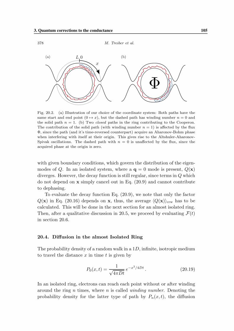
March 31, 2010 16:48 World Scientific Review Volume - 9in x 6in chapter 20
378 M. Treiber et al.
Fig. 20.2. (a) Illustration of our choice of the coordinate system: Both paths have thesame start and end point (0 �→ x), but the dashed path has winding number n = 0 andthe solid path n = 1. (b) Two closed paths in the ring contributing to the Cooperon.The contribution of the solid path (with winding number n = 1) is affected by the fluxΦ, since the path (and it’s time-reversed counterpart) acquire an Aharonov-Bohm phasewhen interfering with itself at their origin. This gives rise to the Altshuler-Aharonov-Spivak oscillations. The dashed path with n = 0 is unaffected by the flux, since theacquired phase at the origin is zero.
with given boundary conditions, which govern the distribution of the eigen-
modes of Q. In an isolated system, where a q = 0 mode is present, Q(x)
diverges. However, the decay function is still regular, since terms inQ which
do not depend on x simply cancel out in Eq. (20.9) and cannot contribute
to dephasing.
To evaluate the decay function Eq. (20.9), we note that only the factor
Q(x) in Eq. (20.16) depends on x, thus, the average 〈Q(x)〉crw has to be
calculated. This will be done in the next section for an almost isolated ring.
Then, after a qualitative discussion in 20.5, we proceed by evaluating F(t)
in section 20.6.
20.4. Diffusion in the almost Isolated Ring
The probability density of a randomwalk in a 1D, infinite, isotropic medium
to travel the distance x in time t is given by
P0(x, t) =1√4πDt
e−x2/4Dt . (20.19)
In an isolated ring, electrons can reach each point without or after winding
around the ring n times, where n is called winding number. Denoting the
probability density for the latter type of path by Pn(x, t), the diffusion
3. Quantum corrections to the conductance 105
March 31, 2010 16:48 World Scientific Review Volume - 9in x 6in chapter 20
Dephasing Time in Disordered Mesoscopic Rings 379
probability density can be expanded in n as
P (x, t) =
+∞∑
n=−∞Pn(x, t) , Pn(x, t) =
1√4πDt
e−(x+nL)2/4Dt , (20.20)
where L is the circumference of the ring and x ∈ [0, L] is the cyclic coordi-
nate along the ring, see Fig. 20.2(a). To model the effect of the two contacts
of the ring, we assume that an electron, on average, stays inside the ring
only for the duration of the dwelling time τdw, introduced in Eq. (20.5), and
then escapes with a vanishing return probability. This simplified model of
homogeneous dissipation, strictly applicable only in the limit τTh � τdwand for a very large lead conductance, captures all the essential physics of
the 0D crossover we are interested in. Our present assumptions lead to the
following replacement of the diffusion probability density:
P (x, t) → P (x, t) e−t/τdw . (20.21)
Furthermore, the spatial dependence of the noise correlation function
(20.13) acquires an additional dissipation term in the denominator. Thus,
in contrast to the isolated case, Q(x) now satisfies the Laplace transform
of the diffusion equation, given by[
1
L2dw
− Δ
]Q(x) = δ(x) , (20.22)
where Ldw =√τdwD. For a ring with circumference L we obtain
Q(x) =Ldw
2
cosh([L − 2|x|]/2Ldw
)
sinh(L/2Ldw). (20.23)
We can expand Eq. (20.23) for the almost isolated ring in powers of
τTh/τdw � 1:
Q(x) ≈ C − |x|2
(1 − |x|
L
)+ O
(τTh
τdw
), (20.24)
where the x-independent first term, C = Lτdw/τTh, describes the contribu-
tion of the zero mode. As expected, see the discussion after Eq. (20.18), it
diverges in the limit τTh/τdw → 0.
Having described the diffuson in our model of the almost isolated ring,
we can proceed by calculating the closed random walk average (crw) of
Eq. (20.24). We will see below that we need to consider the random walk
106 3. Quantum corrections to the conductance
March 31, 2010 16:48 World Scientific Review Volume - 9in x 6in chapter 20
380 M. Treiber et al.
average with respect to closed paths with a specific winding number n only.
For an isolated ring, using Eq. (20.20), it can be written as
〈Q〉crw(t12, n) =∫ L
0
d2x1,2 Q(x12)Pcrw(x12, t12, n) , (20.25)
with
Pcrw(x12, t12, n) =∑
i+j+k=n
Pi(x01, t1)Pj(x12, t21)Pk(x20, t − t2)
Pn(0, t), (20.26)
where we used the notation xαβ = xα − xβ and tαβ = tα − tβ . Obviously,
the replacement (20.21) does not affect this averaging procedure, so that
it remains valid in our model of homogeneous dissipation. Note that the
expression (20.26) depends in fact only on x12 and not on x0, as can be
verified by integrating both sides of the equation over x0 using the following
semi-group property in the ring:∫ L
0
dx2 Pl(x12, t1)Pm(x23, t2) = Pl+m(x13, t1 + t2) . (20.27)
Doing the average of Eq. (20.23) according to Eq. (20.25), we finally obtain
〈Q〉crw(t12, n) = C − L
2
∞∑
k=1
cos(2πknu)
(πk)2e−(2πk)2 ETh t12(1−t12/t) . (20.28)
It follows that a finite dissipation rate does not affect the decay function to
leading order in τTh/τdw.
For the Cooperon, an expansion similar to Eq. (20.20) can be done. In
addition to that, the dependence of the Cooperon on an external magnetic
field changes due to the ring geometry. It not only leads to the suppres-
sion of the Cooperon at long times, but also, due to the Aharonov-Bohm
effect, to Altshuler-Aronov-Spivak oscillations17 of the WL-correction, see
Fig. 20.2(b). Combining these remarks with Eq. (20.5) and inserting
Eq. (20.3) with d = 1, we write the Cooperon in our model as
C(t) =+∞∑
n=−∞
e−(nL)2/4Dt
√4πDt
e−t/τH−t/τdw−Fn(t)einθ , (20.29)
where θ = 4πφ/φ0 and φ = π(L/2π)2H is the flux through the ring (φ0 =
2πc/e is the flux quantum). Note that the decay function F is now a
function of n: Since we used an expansion in winding numbers n, we should
consider the phase (20.8) acquired by paths with the winding number n
only. Thus, the crw-average in Eq. (20.9) has to be performed with respect
to paths with given winding number n only, as anticipated in Eq. (20.25).
3. Quantum corrections to the conductance 107
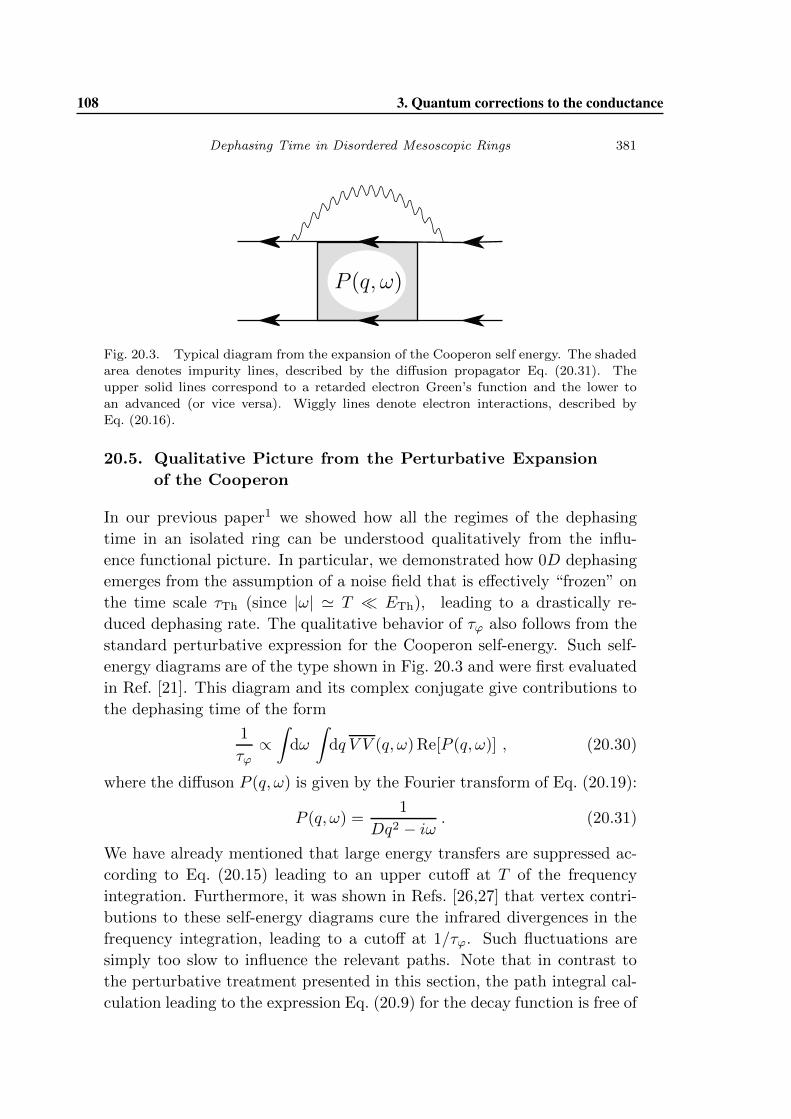
March 31, 2010 16:48 World Scientific Review Volume - 9in x 6in chapter 20
Dephasing Time in Disordered Mesoscopic Rings 381
P (q, ω)
Fig. 20.3. Typical diagram from the expansion of the Cooperon self energy. The shadedarea denotes impurity lines, described by the diffusion propagator Eq. (20.31). Theupper solid lines correspond to a retarded electron Green’s function and the lower to
an advanced (or vice versa). Wiggly lines denote electron interactions, described byEq. (20.16).
20.5. Qualitative Picture from the Perturbative Expansion
of the Cooperon
In our previous paper1 we showed how all the regimes of the dephasing
time in an isolated ring can be understood qualitatively from the influ-
ence functional picture. In particular, we demonstrated how 0D dephasing
emerges from the assumption of a noise field that is effectively “frozen” on
the time scale τTh (since |ω| � T � ETh), leading to a drastically re-
duced dephasing rate. The qualitative behavior of τϕ also follows from the
standard perturbative expression for the Cooperon self-energy. Such self-
energy diagrams are of the type shown in Fig. 20.3 and were first evaluated
in Ref. [21]. This diagram and its complex conjugate give contributions to
the dephasing time of the form
1
τϕ∝∫dω
∫dq V V (q, ω)Re[P (q, ω)] , (20.30)
where the diffuson P (q, ω) is given by the Fourier transform of Eq. (20.19):
P (q, ω) =1
Dq2 − iω. (20.31)
We have already mentioned that large energy transfers are suppressed ac-
cording to Eq. (20.15) leading to an upper cutoff at T of the frequency
integration. Furthermore, it was shown in Refs. [26,27] that vertex contri-
butions to these self-energy diagrams cure the infrared divergences in the
frequency integration, leading to a cutoff at 1/τϕ. Such fluctuations are
simply too slow to influence the relevant paths. Note that in contrast to
the perturbative treatment presented in this section, the path integral cal-
culation leading to the expression Eq. (20.9) for the decay function is free of
108 3. Quantum corrections to the conductance
March 31, 2010 16:48 World Scientific Review Volume - 9in x 6in chapter 20
382 M. Treiber et al.
these IR divergences. In fact, it was shown that the first term of Eq. (20.9)
corresponds, when compared to a diagrammatic evaluation of the Cooperon
self-energy, to the so-called self-energy contributions (shown in Fig. 20.3),
while the second term corresponds to the so-called vertex contributions.
In the ring geometry, the diffuson has quantized momenta and the q = 0
mode can not contribute. For a qualitative discussion we may take this into
account by inserting a lower cutoff 1/L of the momentum integration.
Taking into account the above remarks, we can estimate the dephasing
time as
1
τϕ∝ T
g1L
∫ T
1/τϕ
dω
∫ ∞
1/L
dqD
(Dq2)2 + ω2. (20.32)
Eq. (20.32) illustrates succinctly that the modes dominating dephasing lie
near the infrared cutoff (ω � τ−1ϕ or ETh) for the diffusive or ergodic
regimes, but near the ultraviolet cutoff ω � T for the 0D regime, which is
why, in the latter, the broadening of δT (t) becomes important. Performing
the integrals in Eq. (1.28) and solving for τϕ self-consistently, we find three
regimes:
(1) The diffusive regime, for τT � τϕ � τTh, with
τϕ ∝ (g1/√EThT )
2/3 ; (20.33)
(2) the ergodic regime, for τT � τTh � τϕ, with
τϕ ∝ g1/T ; (20.34)
(3) and the 0D regime, reached at τTh � τT � τϕ, with
τϕ ∝ g1ETh/T2 . (20.35)
Here, τT =√D/T is the thermal time. Expressing (20.35) in terms of the
level spacing δ = ETh/g1 we find τϕδ ∝ E2Th/T
2. This ratio is 1 in
the 0D regime, implying that dephasing is so weak that the dephasing rate
1/τϕ is smaller than the level spacing.
20.6. Results for the Cooperon Decay Function
For a systematic analysis of the Cooperon decay function, we rewrite
Eq. (20.9) in terms of an integral over the dimensionless variable u = t12/t:
Fn(t) =4πT t
g1
∫ 1
0
du z(u) qn(u) , (20.36)
3. Quantum corrections to the conductance 109
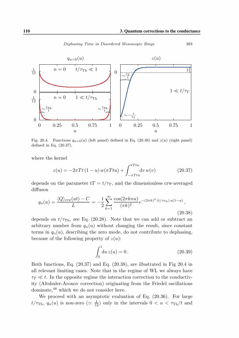
March 31, 2010 16:48 World Scientific Review Volume - 9in x 6in chapter 20
Dephasing Time in Disordered Mesoscopic Rings 383
qn=0(u) z(u)
0
112
n = 0 t/τTh � 1
0
112
0 0.25 0.5 0.75 1u
∼τTht
∼τTht{ {
n = 0 1 � t/τTh
0
0 0.25 0.5 0.75 1u
{1
{∼τTt
∼− tτT
1 � t/τT
Fig. 20.4. Functions qn=0(u) (left panel) defined in Eq. (20.38) and z(u) (right panel)defined in Eq. (20.37).
where the kernel
z(u) = −2πT t (1 − u)w(πT tu) +
∫ πTtu
−πTtu
dv w(v) (20.37)
depends on the parameter tT = t/τT , and the dimensionless crw-averaged
diffuson
qn(u) =〈Q〉crw(ut) − C
L= −1
2
∞∑
k=1
cos(2πknu)
(πk)2e−(2πk)2 (t/τTh) u(1−u) ,
(20.38)
depends on t/τTh, see Eq. (20.28). Note that we can add or subtract an
arbitrary number from qn(u) without changing the result, since constant
terms in qn(u), describing the zero mode, do not contribute to dephasing,
because of the following property of z(u):
∫ 1
0
du z(u) = 0 . (20.39)
Both functions, Eq. (20.37) and Eq. (20.38), are illustrated in Fig 20.4 in
all relevant limiting cases. Note that in the regime of WL we always have
τT � t. In the opposite regime the interaction correction to the conductiv-
ity (Altshuler-Aronov correction) originating from the Friedel oscillations
dominate,48 which we do not consider here.
We proceed with an asymptotic evaluation of Eq. (20.36). For large
t/τTh, qn(u) is non-zero (� 112 ) only in the intervals 0 < u < τTh/t and
110 3. Quantum corrections to the conductance
March 31, 2010 16:48 World Scientific Review Volume - 9in x 6in chapter 20
384 M. Treiber et al.
1− τTh/t < u < 1, see Fig. 20.4. For small t/τTh and n = 0 we can use the
expansion
qn=0(u) ≈ 1
12− 1√
π
√t
τTh(u(1 − u)) +
t
τTh(u(1 − u)) . (20.40)
For larger n the exponential function in Eq. (20.38) can be expanded since
the sum converges at k � 1.
For τT � t, z(u) is large (∼ −t/τT ) in the interval 0 < u < τT /t
and z(u) ≈ 1 otherwise. Thus, it will be convenient to decompose z(u) =
z + z(u) into a constant part z = +1 and a peaked part z(u) = z(u) − 1.
For contributions of the peaked type one observes that
∫ 1
0
du z(u)us =
⎧⎪⎪⎨⎪⎪⎩
−1, s = 0 ;
−√
τTt
√2π4 |ζ
(12
)|, s = 1/2 ;
− τTt , s = 1 .
(20.41)
We identify the following 3 regimes:
Diffusive regime τT � t � τTh and n = 0: Here we can use the
expansion Eq. (20.40). The constant term does not contribute, due to
Eq. (20.39). The main contribution to the integral comes from values of u
where z(u) ≈ 1. Thus, we decompose z(u) = z + z(u) as suggested above.
The leading result and corrections ∝√t/τTh due to the second and third
term in Eq. (20.40) stem from z. Corrections ∝√t/τT can be calculated
with the help of Eq. (20.41) with s = 1/2 from the z(u) part. In total we
obtain for n = 0:
Fn=0(t) =π3/2
√ETh
2g1T t3/2
(1 +
23/2ζ(12
)
π
1√tT
− 4
3√π
√t
τTh
).
(20.42)
Diffusive regime τT � t � τTh and |n| > 0: For winding numbers
larger than zero, we expand the exponential function in (20.38). In contrast
to the case of n = 0, the leading result comes here from the peaked part
z(u). After expanding the exponential function and doing the sum over k,
we can apply Eq. (20.41) with s = 0 and s = 1 to find the leading result and
a correction ∼ τT /t. For z, we observe that the first term vanishes since
the integral is over n full periods of cos. The second term of the expansion
gives a correction ∼ t/τTh and in total for 0 < |n| � t/τT :
Fn(t) =π
3g1T t
(1 − 2
n2
t
τTh− 6
πn
τTt
). (20.43)
3. Quantum corrections to the conductance 111
March 31, 2010 16:48 World Scientific Review Volume - 9in x 6in chapter 20
Dephasing Time in Disordered Mesoscopic Rings 385
Note that in the diffusive regime, winding numbers |n| > 0 only contribute
weakly to the conductivity, see Eq. (20.29).
Ergodic regime τT � τTh � t: In this regime, the main contribution
to the conductivity will not depend on n, since we may neglect the cos-
term of qn(u) as long as |n| � t/τTh. This restriction on n is justified by
the fact that large values of |n| give contributions smaller by a factor of
∼ exp(−n2t/τTh), see Eq. (20.29).
Again, we decompose z(u) = z + z(u). For the z(u) part, we use the
expansion of qn=0(u), Eq. (20.40), where the constant term 1/12 will yield
the main result. Corrections due to the second term of Eq. (20.40) are
∼√τT /τTh, because of Eq. (20.41) with s = 1/2. For z, we do the integral
over u directly using∫ 1
0du exp(−xu(1−u))
x→∞−−−−→ 2/x. From this we obtain
a correction ∼ τTh/t and in total
Fn(t) =π
3g1T t
(1 − 6√
2π
√τTτTh
− 1
30
τTh
t
). (20.44)
It is not surprising that the case |n| > 0 in the diffusive regime gives, to
leading order, the same results as all n of the ergodic regime (compare
Eq. (20.44) to (20.43)), since higher winding numbers are by definition
always ergodic: The electron paths explore the system completely.
0D regime τTh � τT � t: In this regime, qn(u) is more sharply peaked
than z(u), since τT /t τTh/t. This means that the electron reaches the
fully ergodic limit (where q(u) = const and no dephasing can occur) be-
fore the fluctuating potential changes significantly. Thus, the potential is
effectively frozen and only small statistical deviations from the completely
ergodic limit yield a phase difference between the two time-reversed trajec-
tories. The width of the peak of z(u) becomes unimportant, instead, we
can expand z(u) around u = 0 and u = 1. Furthermore, we can expand the
argument of the exponential function in qn(u) and then extend the integral
to +∞ and scale u by kπ:
Fn(t) =4πT t
g1
∫ ∞
0
du
[2πT t
3− 1 − 4π3
15(tT )3u2
] ∞∑
k=1
cos(2nu)
(kπ)3e−4kπEThtu
(20.45)
(the −1 in the integrand stems from the region u ≈ 1). Now, assuming
|n| � t/τTh, the integral over u can be done and then the sum over k
112 3. Quantum corrections to the conductance
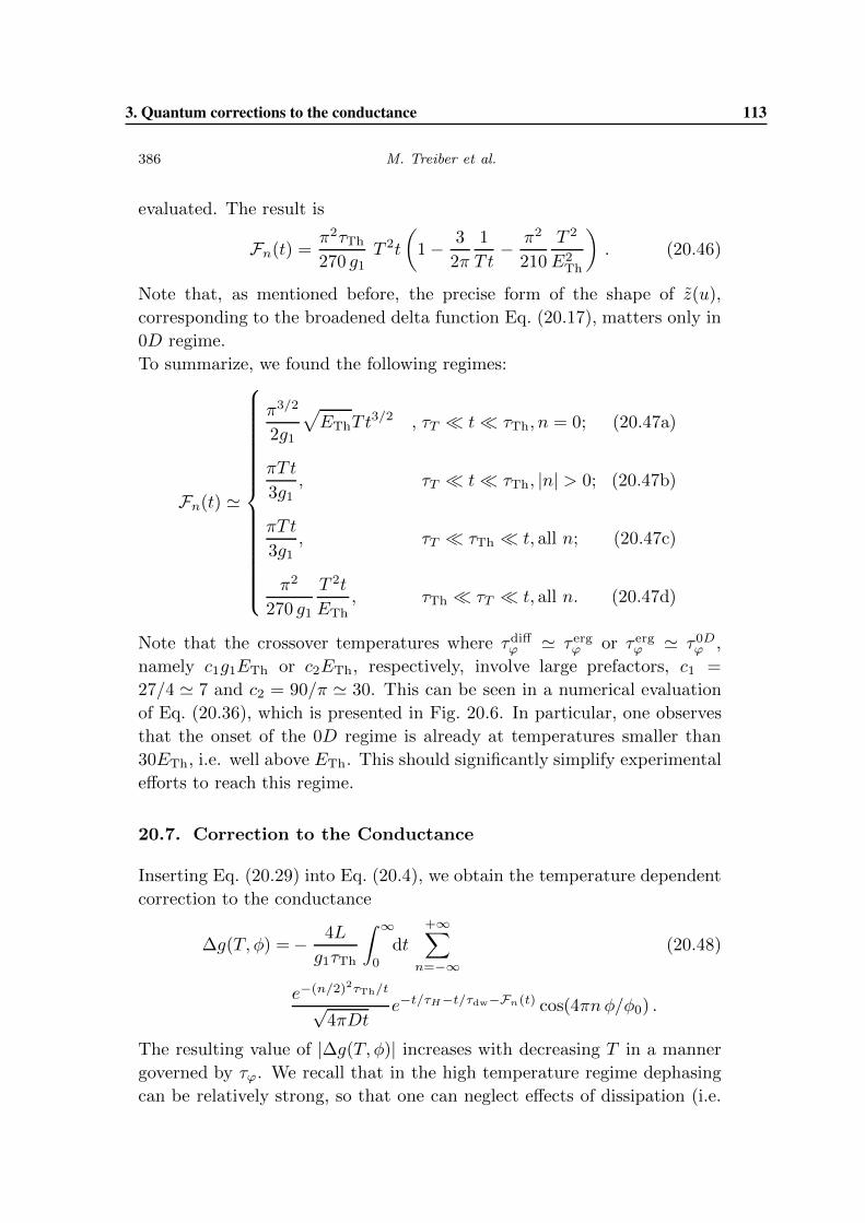
March 31, 2010 16:48 World Scientific Review Volume - 9in x 6in chapter 20
386 M. Treiber et al.
evaluated. The result is
Fn(t) =π2τTh
270 g1T 2t
(1 − 3
2π
1
T t− π2
210
T 2
E2Th
). (20.46)
Note that, as mentioned before, the precise form of the shape of z(u),
corresponding to the broadened delta function Eq. (20.17), matters only in
0D regime.
To summarize, we found the following regimes:
Fn(t) �
⎧⎪⎪⎪⎪⎪⎪⎪⎪⎪⎪⎪⎪⎪⎪⎪⎨⎪⎪⎪⎪⎪⎪⎪⎪⎪⎪⎪⎪⎪⎪⎪⎩
π3/2
2g1
√EThT t
3/2 , τT � t � τTh, n = 0; (20.47a)
πT t
3g1, τT � t � τTh, |n| > 0; (20.47b)
πT t
3g1, τT � τTh � t, all n; (20.47c)
π2
270 g1
T 2t
ETh, τTh � τT � t, all n. (20.47d)
Note that the crossover temperatures where τdiffϕ � τergϕ or τergϕ � τ0Dϕ ,
namely c1g1ETh or c2ETh, respectively, involve large prefactors, c1 =
27/4 � 7 and c2 = 90/π � 30. This can be seen in a numerical evaluation
of Eq. (20.36), which is presented in Fig. 20.6. In particular, one observes
that the onset of the 0D regime is already at temperatures smaller than
30ETh, i.e. well above ETh. This should significantly simplify experimental
efforts to reach this regime.
20.7. Correction to the Conductance
Inserting Eq. (20.29) into Eq. (20.4), we obtain the temperature dependent
correction to the conductance
Δg(T, φ) = − 4L
g1τTh
∫ ∞
0
dt
+∞∑
n=−∞(20.48)
e−(n/2)2τTh/t
√4πDt
e−t/τH−t/τdw−Fn(t) cos(4πnφ/φ0) .
The resulting value of |Δg(T, φ)| increases with decreasing T in a manner
governed by τϕ. We recall that in the high temperature regime dephasing
can be relatively strong, so that one can neglect effects of dissipation (i.e.
3. Quantum corrections to the conductance 113
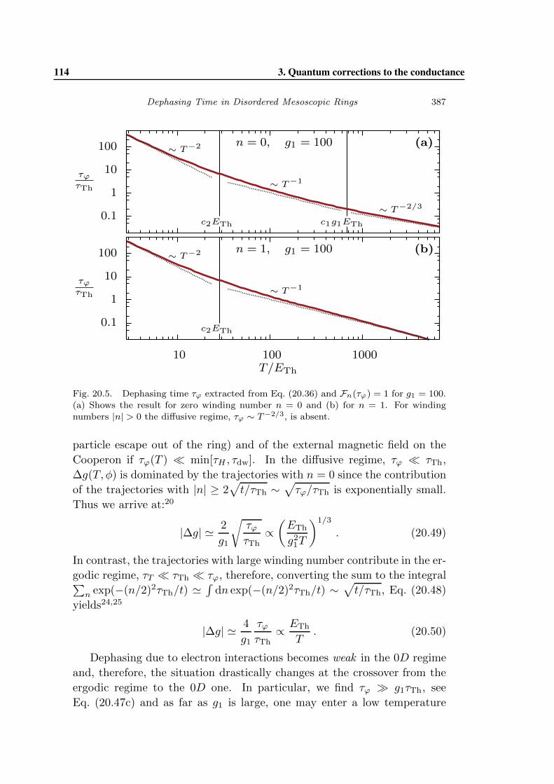
March 31, 2010 16:48 World Scientific Review Volume - 9in x 6in chapter 20
Dephasing Time in Disordered Mesoscopic Rings 387
0.1
1
10
100
τϕτTh
(a)
c2ETh c1g1ETh
∼ T−2
∼ T−1
∼ T−2/3
n = 0, g1 = 100
0.1
1
10
100
10 100 1000
τϕτTh
T/ETh
(b)
c2ETh
∼ T−2
∼ T−1
n = 1, g1 = 100
Fig. 20.5. Dephasing time τϕ extracted from Eq. (20.36) and Fn(τϕ) = 1 for g1 = 100.(a) Shows the result for zero winding number n = 0 and (b) for n = 1. For windingnumbers |n| > 0 the diffusive regime, τϕ ∼ T−2/3, is absent.
particle escape out of the ring) and of the external magnetic field on the
Cooperon if τϕ(T ) � min[τH , τdw]. In the diffusive regime, τϕ � τTh,
Δg(T, φ) is dominated by the trajectories with n = 0 since the contribution
of the trajectories with |n| ≥ 2√t/τTh ∼
√τϕ/τTh is exponentially small.
Thus we arrive at:20
|Δg| � 2
g1
√τϕτTh
∝(ETh
g21T
)1/3
. (20.49)
In contrast, the trajectories with large winding number contribute in the er-
godic regime, τT � τTh � τϕ, therefore, converting the sum to the integral∑n exp(−(n/2)2τTh/t) �
∫dn exp(−(n/2)2τTh/t) ∼
√t/τTh, Eq. (20.48)
yields24,25
|Δg| � 4
g1
τϕτTh
∝ ETh
T. (20.50)
Dephasing due to electron interactions becomes weak in the 0D regime
and, therefore, the situation drastically changes at the crossover from the
ergodic regime to the 0D one. In particular, we find τϕ g1τTh, see
Eq. (20.47c) and as far as g1 is large, one may enter a low temperature
114 3. Quantum corrections to the conductance
March 31, 2010 16:48 World Scientific Review Volume - 9in x 6in chapter 20
388 M. Treiber et al.
regime where τϕ ≥ τdw. In this case, the temperature independent parts
of the Cooperon decay must be taken into account. In our model, with
decreasing T , the growth of |Δg(T, φ)| saturates towards |Δg(0, φ)| once τϕincreases past min[τH , τdw] (a more quantitative consideration is given in
the next section). Nevertheless, the temperature dependence of Δg is still
governed by τϕ(T ) and we can single it out by subtracting the conductance
from its limiting value at T = 0. Then the difference
|Δg(0, φ)| − |Δg(T, φ)| � 4
g1
τ2dwτThτϕ
∝(τdwT
g1
)2
(20.51)
shows T 2-behavior in the 0D regime.
20.8. Suggested Experiments
Our theoretical predictions should be observable in real experiments, pro-
vided that several requirements are met. We list these conditions in accor-
dance with their physical causes, focusing below on the example of a ring
prepared from a quasi-1D wire of width LW on a 2D surface.
20.8.1. Validity of theoretical predictions
1D diffusion: We have used the theory of 1D diffusion which calls for
the following inequalities
L (�, LW ) λF ; (20.52)
λF is the Fermi wavelength.
Weak localization regime: Eq. (20.48) describes the leading weak lo-
calization correction to the conductance. Subleading corrections can be
neglected if (a) the classical conductance of the ring is large
g1 ∝ (�/L)(LW/λF) 1 ; (20.53)
and (b) the leading correction to the conductivity is smaller than its classical
value, |Δg| < 1. The former condition can be assured by a proper choice of
the ring geometry and of the material while, in the low temperature regime,
the latter is provided by finite dissipation.
3. Quantum corrections to the conductance 115
March 31, 2010 16:48 World Scientific Review Volume - 9in x 6in chapter 20
Dephasing Time in Disordered Mesoscopic Rings 389
Time-/spatial-dependence of the noise correlation function: We
have used the noise correlation function (20.16) where dependencies on
time- and space-coordinates are factorized. This simplified form requires
the following condition (see Section 20.3):
2νDq2 (Dq2 − iω)/V (q) . (20.54)
In the 0D regime we can roughly estimate typical values, Dq2 ∼ ω ∼ ETh,
arriving at the inequality
νV (q) 1 . (20.55)
For a quasi-1D wire on a 2D structure, ν and V can be written as (restoring
�)
ν2D =me
2π�2, (20.56)
where me is the electron mass, and
V1D(q) =e2LW
4πε0| ln(L2
W q2)| (20.57)
(in SI units). Thus, (20.55) implies that LW cannot be taken to be overly
small. Inserting material parameters, however, this condition turns out not
to be very restrictive, as long as ν2D is reasonably large.
Contacts (dissipation and absence of the Coulomb blockade):
The presence of contacts, through which electrons can escape into leads, is
mimicked in our model through the homogeneous dissipation rate 1/τdw.
We have assumed weak dissipation:
τTh � τdw . (20.58)
This ensures that the winding trajectories with |n| ≥ 1, responsible for
AAS oscillations, are relevant. On the other hand, τdw cannot be taken
to be arbitrarily large, since the growth of the WL correction to the con-
ductance with decreasing temperature is cut off mainly due to this tem-
perature independent dissipation, and this cutoff has to occur sufficiently
soon that the relative correction remains small, else we would leave the
WL regime. Choosing the zero temperature limit, somewhat arbitrary, as
|Δg(0, φ)| = 1/2, we find from Eq. (20.50)
τdw/τTh � g1/8 . (20.59)
116 3. Quantum corrections to the conductance
March 31, 2010 16:48 World Scientific Review Volume - 9in x 6in chapter 20
390 M. Treiber et al.
We note that our assumptions imply τϕ g1τTh > τdw in the 0D regime,
i.e., dephasing due to electron interactions is weak (each electron con-
tributing to transport through the ring is dephased only a little bit during
the course of its stay in the ring). Nevertheless, we demonstrate below
(see Fig. 20.8) that the T 2 -dependence of the conductance should be visi-
ble in real experiments.
To choose a suitable value for the conductance at the contacts, we esti-
mate τdw/τTh � g1/gcont, which results in
8 � gcont . (20.60)
We suppose that the contacts are open and have a maximal transmission
per channel at the contact
Tcont = 1 ⇒ gcont = TcontN = N , (20.61)
(N is the number of transmitting reflectionless channels at the contact).
This choice allows one to maximize the WL effect and, simultaneously, to
minimize any Coulomb blockade effects, which we have neglected.
20.8.2. Possible experimental setup
Temperature range: The relevant temperature range, [Tdil, Tph], is lim-
ited from below by dilution refrigeration (Tdil � 10mK) and from above by
our neglect of phonons (Tph � 5K). Furthermore, the ring should be small
enough that c2ETh � Tdil; c2ETh is the upper estimate for the temperature
of the crossover to the 0D regime, see the discussion after Eq. (20.47).
Contributions from the leads: We have considered an ideal situation
and calculated the Cooperon decay function for the isolated ring, where
the finite dissipation rate 1/τdw does not affect the decay function up to
leading order in τTh/τdw. This means that the Cooperons are assumed to
live completely inside the ring and not influenced by dephasing in the leads,
i.e. it corresponds to the situation shown in Fig. 20.6(a).
In real experiments, the correction to the conductance, Δg, is sensitive
to dephasing in the leads because Cooperons exist which either belong to
the lead (e.g. the situation shown in Fig. 20.6(c)) or extend over both the
ring and the lead (Fig. 20.6(b))49. (Note that in contrast to Ref. [51] or
Ref. [49], we do not consider Cooperons with a Hikami-box directly at the
contact, since we chose Tcont = 1.)
3. Quantum corrections to the conductance 117
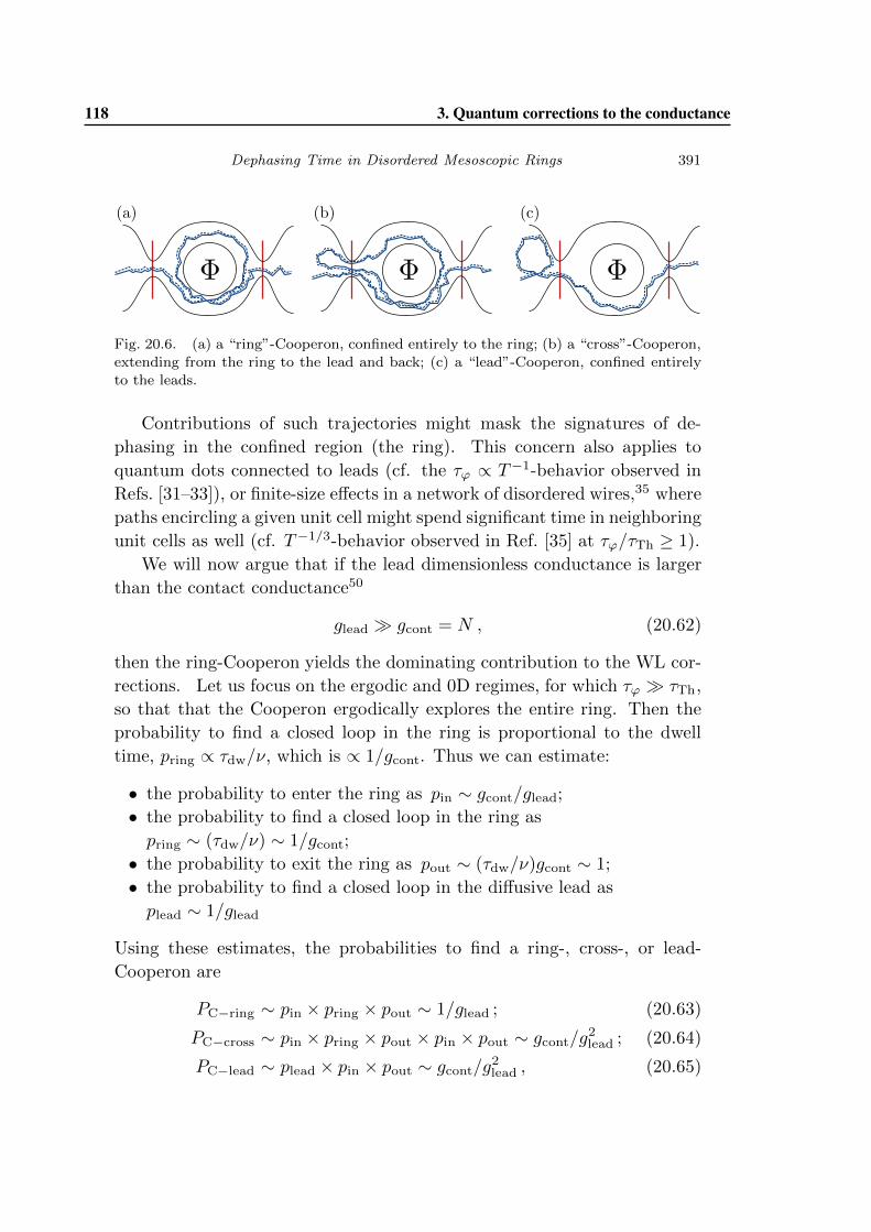
March 31, 2010 16:48 World Scientific Review Volume - 9in x 6in chapter 20
Dephasing Time in Disordered Mesoscopic Rings 391
Fig. 20.6. (a) a “ring”-Cooperon, confined entirely to the ring; (b) a “cross”-Cooperon,extending from the ring to the lead and back; (c) a “lead”-Cooperon, confined entirelyto the leads.
Contributions of such trajectories might mask the signatures of de-
phasing in the confined region (the ring). This concern also applies to
quantum dots connected to leads (cf. the τϕ ∝ T−1-behavior observed in
Refs. [31–33]), or finite-size effects in a network of disordered wires,35 where
paths encircling a given unit cell might spend significant time in neighboring
unit cells as well (cf. T−1/3-behavior observed in Ref. [35] at τϕ/τTh ≥ 1).
We will now argue that if the lead dimensionless conductance is larger
than the contact conductance50
glead gcont = N , (20.62)
then the ring-Cooperon yields the dominating contribution to the WL cor-
rections. Let us focus on the ergodic and 0D regimes, for which τϕ τTh,
so that that the Cooperon ergodically explores the entire ring. Then the
probability to find a closed loop in the ring is proportional to the dwell
time, pring ∝ τdw/ν, which is ∝ 1/gcont. Thus we can estimate:
• the probability to enter the ring as pin ∼ gcont/glead;
• the probability to find a closed loop in the ring as
pring ∼ (τdw/ν) ∼ 1/gcont;
• the probability to exit the ring as pout ∼ (τdw/ν)gcont ∼ 1;
• the probability to find a closed loop in the diffusive lead as
plead ∼ 1/glead
Using these estimates, the probabilities to find a ring-, cross-, or lead-
Cooperon are
PC−ring ∼ pin × pring × pout ∼ 1/glead ; (20.63)
PC−cross ∼ pin × pring × pout × pin × pout ∼ gcont/g2lead ; (20.64)
PC−lead ∼ plead × pin × pout ∼ gcont/g2lead , (20.65)
118 3. Quantum corrections to the conductance
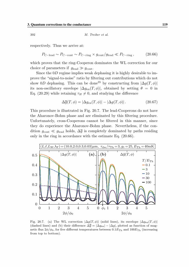
March 31, 2010 16:48 World Scientific Review Volume - 9in x 6in chapter 20
392 M. Treiber et al.
respectively. Thus we arrive at:
PC−lead ∼ PC−cont ∼ PC−ring × gcont/glead � PC−ring , (20.66)
which proves that the ring-Cooperon dominates the WL correction for our
choice of parameters if glead gcont.
Since the 0D regime implies weak dephasing it is highly desirable to im-
prove the “signal-to-noise” ratio by filtering out contributions which do not
show 0D dephasing. This can be done35 by constructing from |Δg(T, φ)|its non-oscillatory envelope |Δgen(T, φ)|, obtained by setting θ = 0 in
Eq. (20.29) while retaining τH �= 0, and studying the difference
Δg(T, φ) = |Δgen(T, φ)| − |Δg(T, φ)| . (20.67)
This procedure is illustrated in Fig. 20.7. The lead-Cooperons do not have
the Aharonov-Bohm phase and are eliminated by this filtering procedure.
Unfortunately, cross-Cooperons cannot be filtered in this manner, since
they do experience the Aharonov-Bohm phase. Nevertheless, if the con-
dition gcont � glead holds, Δg is completely dominated by paths residing
only in the ring in accordance with the estimate Eq. (20.66).
0
0.1
0.2
0.3
0.4
0.5
0 1 2 3 4 5
2φ/φ0
|Δg(T, φ)| (a)
0 1 2 3 4 5
2φ/φ0
Δg(T, φ)(b)
φ1
(L,�,LW,λF)=(10.0,2.0,0.3,0.03)μm, τdw/τTh=3, g1=25, ETh=40mK
T/ETh
0.13
1030
100
Fig. 20.7. (a) The WL correction |Δg(T, φ)| (solid lines), its envelope |Δgen(T, φ)|(dashed lines) and (b) their difference Δg = |Δgen| − |Δg|, plotted as function of mag-netic flux 2φ/φ0, for five different temperatures between 0.1ETh and 100ETh (increasingfrom top to bottom).
3. Quantum corrections to the conductance 119
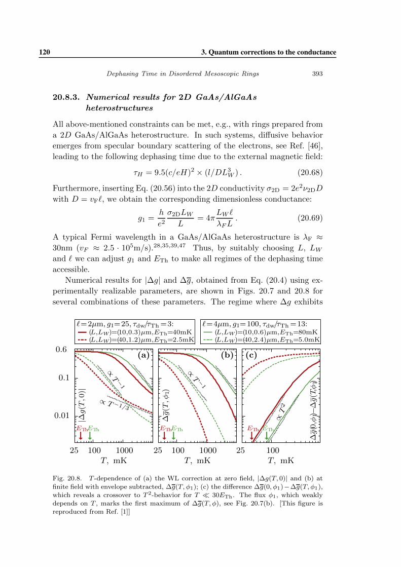
March 31, 2010 16:48 World Scientific Review Volume - 9in x 6in chapter 20
Dephasing Time in Disordered Mesoscopic Rings 393
20.8.3. Numerical results for 2D GaAs/AlGaAs
heterostructures
All above-mentioned constraints can be met, e.g., with rings prepared from
a 2D GaAs/AlGaAs heterostructure. In such systems, diffusive behavior
emerges from specular boundary scattering of the electrons, see Ref. [46],
leading to the following dephasing time due to the external magnetic field:
τH = 9.5(c/eH)2 × (l/DL3W ) . (20.68)
Furthermore, inserting Eq. (20.56) into the 2D conductivity σ2D = 2e2ν2DD
with D = vF�, we obtain the corresponding dimensionless conductance:
g1 =h
e2σ2DLW
L= 4π
LW �
λFL. (20.69)
A typical Fermi wavelength in a GaAs/AlGaAs heterostructure is λF ≈30nm (vF ≈ 2.5 · 105m/s).28,35,39,47 Thus, by suitably choosing L, LW
and � we can adjust g1 and ETh to make all regimes of the dephasing time
accessible.
Numerical results for |Δg| and Δg, obtained from Eq. (20.4) using ex-
perimentally realizable parameters, are shown in Figs. 20.7 and 20.8 for
several combinations of these parameters. The regime where Δg exhibits
0.01
0.1
100 1000
|Δg(T
,0)|
T, mK
0.6
25
∝ T −1/3
∝T −
1
(a)
�ETh�ETh
100 1000
Δg(T
,φ1)
T, mK25
∝T −
1
(b)
�ETh�ETh
100T, mK
25
∝T
2
�ETh �ETh
(c)
Δg(0,φ
1)−Δg(T,φ
1)
�=2μm, g1=25, τdw/τTh=3:(L,LW)=(10,0.3)μm,ETh=40mK(L,LW)=(40,1.2)μm,ETh=2.5mK
�=4μm, g1=100, τdw/τTh=13:(L,LW)=(10,0.6)μm,ETh=80mK(L,LW)=(40,2.4)μm,ETh=5.0mK
Fig. 20.8. T -dependence of (a) the WL correction at zero field, |Δg(T, 0)| and (b) at
finite field with envelope subtracted, Δg(T, φ1); (c) the difference Δg(0, φ1)−Δg(T, φ1),which reveals a crossover to T 2-behavior for T � 30ETh. The flux φ1, which weaklydepends on T , marks the first maximum of Δg(T, φ), see Fig. 20.7(b). [This figure isreproduced from Ref. [1]]
120 3. Quantum corrections to the conductance
March 31, 2010 16:48 World Scientific Review Volume - 9in x 6in chapter 20
394 M. Treiber et al.
diffusive T−1/3 behavior (7g1ETh � T � Tph) is visible only for our small-
est choices of both g1 and ETh (Fig. 20.8(a), heavy dashed line). AAS
oscillations in |Δg| and Δg (Fig. 20.7), which require τTh � τϕ, first
emerge at the crossover from the diffusive to the ergodic regime. They
increase in magnitude with decreasing T , showing ergodic T−1 behavior for
30ETh � T � 7g1ETh (Figs. 20.8(a),(b)), and eventually saturate towards
their T = 0 values, with Δg(0, φ) − Δg(T, φ) showing the predicted 0D
behavior, ∝ T 2, for T � 5ETh, see Fig. 20.8(c).
20.9. Conclusions
For an almost isolated disordered quasi-1D ring with T ETh, the T -
dependence of the dephasing time has been known to behave as τϕ ∝ T−2/3
(Ref. [20]) or ∝ T−1 (Refs. [24,25]) in the diffusive or ergodic regimes,
respectively. Here we showed how it crosses over, for T � 30ETh, to
τϕ ∝ T−2, in agreement with the theory of dephasing in 0D systems
(Ref. [2]). This crossover manifests itself in both the smooth part of the
magnetoconductivity and the amplitude of the AAS oscillations. Impor-
tantly, the latter fact can be exploited to decrease the effects of dephasing
in the leads, by subtracting from the magnetoconductivity its smooth en-
velope. While we did not give an exhaustive study of all contributions to
dephasing in the connected ring, we were able to show that the leading
contribution results only from trajectories confined to the ring. Thus, an
analysis of the T -dependence of the AAS oscillation amplitude may offer
a way to finally observe, for T � 5ETh, the elusive but fundamental 0D
behavior τϕ ∼ T−2. Its observation, moreover, would allow quantitative
experimental tests of the role of temperature as ultraviolet frequency cut-
off in the theory of dephasing. An interesting challenge for future works
consists in a more realistic model of the connection to the leads. Work on
the model of an N -channel ring attached via two arms with fewer channels
to absorbing boundaries is currently in progress.52
Acknowledgments
We acknowledge illuminating discussions with B. L. Altshuler, C. Bauerle,
N. O. Birge, Ya. M. Blanter, P. W. Brouwer, L. I. Glazman, Y. Imry,
V. E. Kravtsov, J. Kupferschmidt, A. D. Mirlin, Y. V. Nazarov, A. Rosch,
D. Weiss and V. I. Yudson. We acknowledge support from the DFG through
SFB TR-12, the Emmy-Noether program and the Nanosystems Initiative
3. Quantum corrections to the conductance 121
March 31, 2010 16:48 World Scientific Review Volume - 9in x 6in chapter 20
Dephasing Time in Disordered Mesoscopic Rings 395
Munich Cluster of Excellence; from the NSF, Grant No. PHY05-51164;
and from the EPSRC, Grant No. T23725/01.
References
1. M. Treiber, O. M. Yevtushenko, F. Marquardt, J. von Delft, and I. V. Lerner,Phys. Rev. B 80, 201305(R) (2009).
2. U. Sivan, Y. Imry, and A. G. Aronov, Europhys. Lett. 28, 115 (1994).3. Y. Imry, in Introduction to Mesoscopic Physics, Oxford University Press
(1997)4. M. Buttiker, Y. Imry, and R. Landauer, Phys. Rev. A 96, 365 (1983).5. M. Buttiker, Y. Imry, and M. Ya. Azbel, Phys. Rev. A 30, 1982 (1984).6. Y. Gefen, Y. Imry, and M. Ya. Azbel, Phys. Rev. Lett. 52, 129 (1984).7. M. Buttiker, Y. Imry, R. Landauer, and S. Pinhas, Phys. Rev. B 31, 6207
(1984).8. M. Murat, Y. Gefen, and Y. Imry, Phys. Rev. B 34, 659 (1985).9. Y. Imry, and N. S. Shiren, Phys. Rev. B 33, 7992 (1986).
10. A. D. Stone, and Y. Imry, Phys. Ref. Lett. 56, 189 (1986).11. B. L. Altshuler, Y. Gefen, and Y. Imry, Phys. Rev. Lett. 66, 88 (1990).12. L. P. Levy, G. Dolan, J. Dunsmuir, and H. Bouchiat, Phys. Rev. Lett. 64,
2074 (1990).13. H. Bluhm, N. C. Koshnick, J. A. Bert, M. E. Huber, and K. A. Moler, Phys.
Rev. Lett. 102, 136802 (2009).14. A. C. Bleszynski-Jayich, W. E. Shanks, B. Peaudecerf, E. Ginossar, F. von
Oppen, L. I. Glazman, and J. G. E. Harris, arXiv:0906.4780 (2009).15. Y. Imry, Physics 2, 24 (2009).16. R. A. Webb, S. Washburn, C. P. Umbach, and R. B. Laibowitz, Phys. Rev.
Lett. 54, 2696 (1985).17. B. L. Altshuler, A. G. Aronov, and B. Z. Spivak, JETP Lett. 33, 94 (1981).18. D. Y. Sharvin, and Y. V. Sharvin, Pis’ma Zh. Teor. Eksp. Fiz. 34, 285 (1981).19. A. Stern, Y. Aharonov, and Y. Imry, Phys. Rev. A 41, 3436 (1990).20. B. L. Altshuler, A. G. Aronov, and D. E. Khmelnitsky, J. Phys. C 15, 7367
(1982).21. H. Fukuyama and E. Abrahams, Phys. Rev. B, 27, 5976 (1983).22. B. L. Altshuler and A. G. Aronov, in Electron-Electron Interactions in Dis-
ordered Systems, edited by A. L. Efros and M. Pollak, North-Holland, Ams-terdam, 1 (1985).
23. I. L. Aleiner, , B. L. Altshuler, and M. E. Gershenson, Waves in RandomMedia 9, 201 (1999).
24. T. Ludwig and A. D. Mirlin, Phys. Rev. B 69, 193306 (2004).25. C. Texier and G. Montambaux, Phys. Rev. B 72, 115327 (2005).26. F. Marquardt, J. von Delft, R. A. Smith, and V. Ambegaokar, Phys. Rev. B
76, 195331 (2007).27. J. von Delft, F. Marquardt, R. A. Smith, and V. Ambegaokar, Phys. Rev. B
76, 195332 (2007).
122 3. Quantum corrections to the conductance
March 31, 2010 16:48 World Scientific Review Volume - 9in x 6in chapter 20
396 M. Treiber et al.
28. C. M. Marcus, R. M. Westervelt, P. F. Hopkins, and A. C. Gossard, Phys.Rev. B 48, 2460 (1993).
29. A. Yacoby, M. Heiblum, H. Shtrikman, V. Umansky, and D. Mahalu, Semi-cond. Sci. Tech. 9, 907 (1994).
30. B. Reulet, H. Bouchiat, and D. Mailly, Europhys. Lett. 31, 305 (1995).31. A. G. Huibers, M. Switkes, C. M. Marcus, K. Campman, and A. C. Gossard,
Phys. Rev. Lett. 81, 200 (1998);32. A. G. Huibers, S. R. Patel, C. M. Marcus, P. W. Brouwer, C. I. Duruoz, and
J. S. Harris, Jr., Phys. Rev. Lett. 81, 1917 (1998);33. A. G. Huibers, J. A. Folk, S. R. Patel, C. M. Marcus, C. I. Duruoz and J. S.
Harris, Jr., Phys. Rev. Lett. 83, 5090 (1999).34. A. B. Gougam, F. Pierre, H. Pothier, D. Esteve, and N. O. Birge, J. Low
Temp. Phys. 118, 447 (2000).35. M. Ferrier, A. C. H. Rowe, S. Gueron, H. Bouchiat, C. Texier, and G. Mon-
tambaux, Phys. Rev. Lett. 100, 146802 (2008).36. I. L. Aleiner, B. L. Altshuler, and Y. M. Galperin, Phys. Rev. B 63, 201401
(2001).37. I. L. Aleiner and Y. M. Blanter, Phys. Rev. B 65, 115317 (2002).38. Y. Imry, arXiv: cond-mat/0202044 (2002)39. Y. Niimi, Y. Baines, T. Capron, D. Mailly, F.-Y. Lo, A. D. Wieck, T. Meu-
nier, L. Saminadayar, and C. Bauerle, Phys. Rev. Lett. 102, 226801 (2009).40. L. P. Gor’kov, A. I. Larkin, and D. E. Khmel’nitskii, JETP Lett. 30, 228
(1979).41. E. Akkermans and G. Montambaux, Mesoscopic physics of electrons and
photons (Cambridge University Press, Cambridge, 2007).42. D. E. Khmelnitskii, Physica B&C 126, 235 (1984).43. B. L. Altshuler and A. G. Aronov, JETP Lett. 33, 499 (1981).44. P. W. Brouwer and C. W. J. Beenakker, Phys. Rev. B 55, 4695 (1997);45. E. McCann and I. V. Lerner, Phys. Rev. B 57, 7219 (1998).46. C. W. J. Beenakker and H. van Houten, Phys. Rev. B 38, 3232 (1988).47. O. Yevtushenko, G. Lutjering, D. Weiss, and K. Richter, Phys. Rev. Lett.
84, 542 (2000).48. B. L. Altshuler, A. G. Aronov, and P. A. Lee, Phys. Rev. Lett. 44, 1288
(1980).49. Ya. M. Blanter, V. M. Vinokur, and L. I. Glazman, Phys. Rev. B 73, 165322
(2006).50. J. N. Kupferschmidt, and P. W. Brouwer, (private communication).51. R. S. Whitney, Phys. Rev. B 75, 235404 (2007).52. M. Treiber, O. M. Yevtushenko, F. Marquardt, J. von Delft, and I. V. Lerner,
to be published.
3. Quantum corrections to the conductance 123


3. Quantum corrections to the conductance 125
3.6 Publication: Transport and dephasing in a quantum dot: Multiplyconnected graph model
The following 11 pages have been published in the journal Annalen der Physik (Berlin).
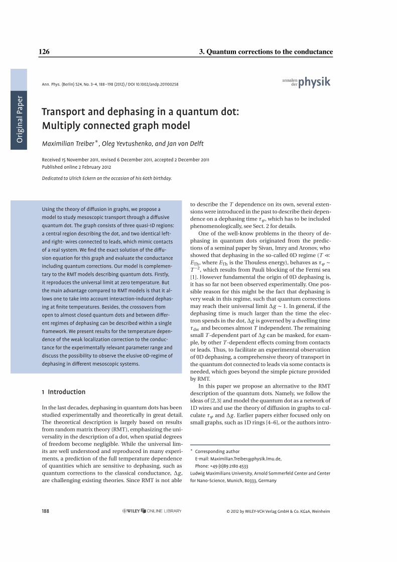
Orig
inalPaper
Ann. Phys. (Berlin) 524, No. 3–4, 188–198 (2012) / DOI 10.1002/andp.201100258
Transport and dephasing in a quantum dot:Multiply connected graph modelMaximilian Treiber∗, Oleg Yevtushenko, and Jan von Delft
Received 15 November 2011, revised 6 December 2011, accepted 2 December 2011Published online 2 February 2012
Dedicated to Ulrich Eckern on the occasion of his 60th birthday.
Using the theory of diffusion in graphs, we propose amodel to study mesoscopic transport through a diffusivequantum dot. The graph consists of three quasi-1D regions:a central region describing the dot, and two identical left-and right- wires connected to leads, which mimic contactsof a real system. We find the exact solution of the diffu-sion equation for this graph and evaluate the conductanceincluding quantum corrections. Our model is complemen-tary to the RMTmodels describing quantum dots. Firstly,it reproduces the universal limit at zero temperature. Butthe main advantage compared to RMTmodels is that it al-lows one to take into account interaction-induced dephas-ing at finite temperatures. Besides, the crossovers fromopen to almost closed quantum dots and between differ-ent regimes of dephasing can be described within a singleframework. We present results for the temperature depen-dence of the weak localization correction to the conduc-tance for the experimentally relevant parameter range anddiscuss the possibility to observe the elusive 0D-regime ofdephasing in different mesoscopic systems.
1 Introduction
In the last decades, dephasing in quantum dots has beenstudied experimentally and theoretically in great detail.The theoretical description is largely based on resultsfrom random matrix theory (RMT), emphasizing the uni-versality in the description of a dot, when spatial degreesof freedom become negligible. While the universal lim-its are well understood and reproduced in many experi-ments, a prediction of the full temperature dependenceof quantities which are sensitive to dephasing, such asquantum corrections to the classical conductance, Δg ,are challenging existing theories. Since RMT is not able
to describe the T dependence on its own, several exten-sions were introduced in the past to describe their depen-dence on a dephasing time τϕ, which has to be includedphenomenologically, see Sect. 2 for details.
One of the well-know problems in the theory of de-phasing in quantum dots originated from the predic-tions of a seminal paper by Sivan, Imry and Aronov, whoshowed that dephasing in the so-called 0D regime (T �ETh, where ETh is the Thouless energy), behaves as τϕ ∼T −2, which results from Pauli blocking of the Fermi sea[1]. However fundamental the origin of 0D dephasing is,it has so far not been observed experimentally. One pos-sible reason for this might be the fact that dephasing isvery weak in this regime, such that quantum correctionsmay reach their universal limit Δg ∼ 1. In general, if thedephasing time is much larger than the time the elec-tron spends in the dot,Δg is governed by a dwelling timeτdw and becomes almost T independent. The remainingsmall T -dependent part of Δg can be masked, for exam-ple, by other T -dependent effects coming from contactsor leads. Thus, to facilitate an experimental observationof 0D dephasing, a comprehensive theory of transport inthe quantum dot connected to leads via some contacts isneeded, which goes beyond the simple picture providedby RMT.
In this paper we propose an alternative to the RMTdescription of the quantum dots. Namely, we follow theideas of [2,3] and model the quantum dot as a network of1D wires and use the theory of diffusion in graphs to cal-culate τϕ and Δg . Earlier papers either focused only onsmall graphs, such as 1D rings [4–6], or the authors intro-
∗ Corresponding authorE-mail: [email protected],Phone: +49 (0)89 2180 4533
LudwigMaximilians University, Arnold Sommerfeld Center and Centerfor Nano-Science, Munich, 80333, Germany
188 © 2012 by WILEY-VCH Verlag GmbH & Co. KGaA, Weinheim
126 3. Quantum corrections to the conductance
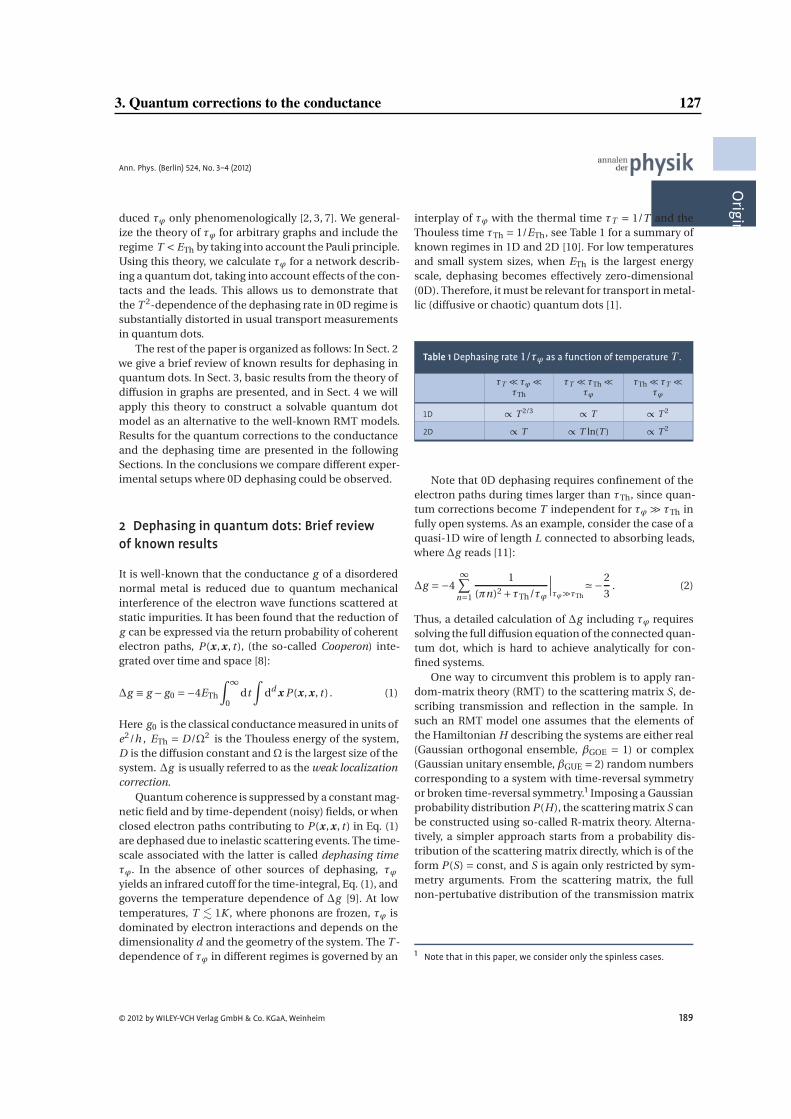
Ann. Phys. (Berlin) 524, No. 3–4 (2012)
OriginalPaper
duced τϕ only phenomenologically [2, 3, 7]. We general-ize the theory of τϕ for arbitrary graphs and include theregime T < ETh by taking into account the Pauli principle.Using this theory, we calculate τϕ for a network describ-ing a quantum dot, taking into account effects of the con-tacts and the leads. This allows us to demonstrate thatthe T 2-dependence of the dephasing rate in 0D regime issubstantially distorted in usual transport measurementsin quantum dots.
The rest of the paper is organized as follows: In Sect. 2we give a brief review of known results for dephasing inquantum dots. In Sect. 3, basic results from the theory ofdiffusion in graphs are presented, and in Sect. 4 we willapply this theory to construct a solvable quantum dotmodel as an alternative to the well-known RMT models.Results for the quantum corrections to the conductanceand the dephasing time are presented in the followingSections. In the conclusions we compare different exper-imental setups where 0D dephasing could be observed.
2 Dephasing in quantum dots: Brief reviewof known results
It is well-known that the conductance g of a disorderednormal metal is reduced due to quantum mechanicalinterference of the electron wave functions scattered atstatic impurities. It has been found that the reduction ofg can be expressed via the return probability of coherentelectron paths, P(x , x , t ), (the so-called Cooperon) inte-grated over time and space [8]:
Δg ≡ g − g0 =−4ETh
∫∞
0dt
∫dd x P(x , x , t ) . (1)
Here g0 is the classical conductance measured in units ofe2/h , ETh = D/Ω2 is the Thouless energy of the system,D is the diffusion constant andΩ is the largest size of thesystem. Δg is usually referred to as the weak localizationcorrection.
Quantum coherence is suppressed by a constant mag-netic field and by time-dependent (noisy) fields, or whenclosed electron paths contributing to P(x , x , t ) in Eq. (1)are dephased due to inelastic scattering events. The time-scale associated with the latter is called dephasing timeτϕ. In the absence of other sources of dephasing, τϕyields an infrared cutoff for the time-integral, Eq. (1), andgoverns the temperature dependence of Δg [9]. At lowtemperatures, T � 1K , where phonons are frozen, τϕ isdominated by electron interactions and depends on thedimensionality d and the geometry of the system. The T -dependence of τϕ in different regimes is governed by an
interplay of τϕ with the thermal time τT = 1/T and theThouless time τTh = 1/ETh, see Table 1 for a summary ofknown regimes in 1D and 2D [10]. For low temperaturesand small system sizes, when ETh is the largest energyscale, dephasing becomes effectively zero-dimensional(0D). Therefore, it must be relevant for transport in metal-lic (diffusive or chaotic) quantum dots [1].
Table 1 Dephasing rate 1/τϕ as a function of temperature T .
τT � τϕ �τTh
τT � τTh �τϕ
τTh � τT �τϕ
1D ∝ T 2/3 ∝ T ∝T 2
2D ∝ T ∝ T ln(T ) ∝T 2
Note that 0D dephasing requires confinement of theelectron paths during times larger than τTh, since quan-tum corrections become T independent for τϕ � τTh infully open systems. As an example, consider the case of aquasi-1D wire of length L connected to absorbing leads,where Δg reads [11]:
Δg =−4∞∑
n=1
1
(πn)2+τTh/τϕ
∣∣∣τϕ�τTh
−2
3. (2)
Thus, a detailed calculation of Δg including τϕ requiressolving the full diffusion equation of the connected quan-tum dot, which is hard to achieve analytically for con-fined systems.
One way to circumvent this problem is to apply ran-dom-matrix theory (RMT) to the scattering matrix S, de-scribing transmission and reflection in the sample. Insuch an RMT model one assumes that the elements ofthe Hamiltonian H describing the systems are either real(Gaussian orthogonal ensemble, βGOE = 1) or complex(Gaussian unitary ensemble, βGUE = 2) random numberscorresponding to a system with time-reversal symmetryor broken time-reversal symmetry.1 Imposing a Gaussianprobability distribution P(H), the scattering matrix S canbe constructed using so-called R-matrix theory. Alterna-tively, a simpler approach starts from a probability dis-tribution of the scattering matrix directly, which is of theform P(S) = const, and S is again only restricted by sym-metry arguments. From the scattering matrix, the fullnon-pertubative distribution of the transmission matrix
1 Note that in this paper, we consider only the spinless cases.
© 2012 by WILEY-VCH Verlag GmbH & Co. KGaA, Weinheim 189
3. Quantum corrections to the conductance 127
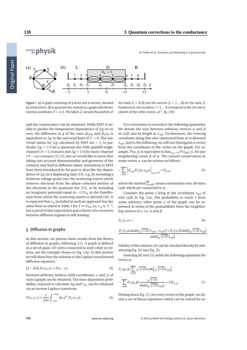
Orig
inalPaper
M. Treiber et al.: Transport and dephasing in a quantum dot
Figure 1 (a) A graph consisting of 9 wires and 6 vertices, denotedby Greek letters. (b) A quantumdot realized as a graph with dimen-sionless coordinate Z = x/L. The labels Zi denote the position of
the leads (i = 0,9) and the vertices (i = 1. . . 8) on the scale Z .Furthermore, the numbers i = 1. . . 8 correspond to the i th row orcolumn of the vertex matrixM γ, Eq. (10)
and the conductance can be obtained. While RMT is un-able to predict the temperature dependence of Δg on itsown, the difference in g of the cases βGOE and βGUE isequivalent to Δg in the universal limit of T → 0. The uni-versal values for Δg calculated by RMT are ∼ 1, in par-ticular Δg = 1/3 for a quantum dot with spinfull single-channel (N = 1) contacts andΔg = 1/4 for many-channel(N →∞) contacts [12,13], but we would like to stress thattaking into account dimensionality and geometry of thecontacts may lead to different values. Extensions to RMThave been introduced in the past to describe the depen-dence of Δg on a dephasing time [14], e.g. by including afictitious voltage probe into the scattering matrix whichremoves electrons from the phase-coherent motion ofthe electrons in the quantum dot [15], or by includingan imaginary potential equal to −i /2τϕ in the Hamilto-nian from which the scattering matrix is derived [16]. Itis expected that τϕ included in such an approach has thesame form as stated in Table 1 for T � ETh, i.e. τϕ∝ T −2,but a proof of this expectation and a theory of a crossoverbetween different regimes is still missing.
3 Diffusion in graphs
In this section, we present basic results from the theoryof diffusion in graphs, following [11]. A graph is definedas a set of quasi-1D wires connected to each other at ver-tices, see the example shown in Fig. 1(a). In this sectionwe will show how the solution to the Laplace transformeddiffusion equation,(γ−DΔ
)Pγ(x, y) = δ(x − y) , (3)
between arbitrary vertices (with coordinates x and y) ofsuch a graph can be obtained. The time-dependent prob-ability, required to calculate Δg and τϕ, can be obtainedvia an inverse Laplace transform:
P(x, y, t ) = 1
2πi
∫+i∞
−i∞dγeγt Pγ(x, y) . (4)
It is convenient to introduce the following quantities:We denote the wire between arbitrary vertices α and β
as (αβ) and its length as Lαβ. Furthermore, the runningcoordinate along this wire (measured from α) is denotedxαβ, and in the following, we will not distinguish a vertexfrom the coordinate of the vertex on the graph: For ex-ample, P(α, y) is equivalent to limxαβ→0 P(xαβ, y), for anyneighboring vertex β of α. The current conservation atsome vertex α can be written as follows:
−∑
(αβ)
[∂xαβPγ(μ, xαβ)
]xαβ=0
= δα,μ , (5)
where the symbol∑
(αβ) means summation over all wires(αβ) which are connected to α.
Consider the point x lying at the coordinate xαβ ofwire (αβ) in Fig. 1(a). The probability to reach x fromsome arbitrary other point y of the graph can be ex-pressed in terms of the probabilities from the neighbor-ing vertices of x, i.e. α and β:
Pγ(y, x) = (6)
Pγ(y,α)sinh(√
γ/D (Lαβ−xαβ))+Pγ(y,β)sinh
(√γ/D xαβ
)
sinh(√
γ/D Lαβ) .
Validity of the solution (6) can be checked directly by sub-stituting Eq. (6) into Eq. (3).
Inserting (6) into (5) yields the following equations forvertexα:
Pγ(μ,α)∑
(αβ)
√γ/D coth
(√γ/DLαβ
)
−∑
(αβ)Pγ(μ,β)
√γ/D
sinh(√
γ/DLαβ) = Dδα,μ . (7)
Writing down Eq. (7), for every vertex of the graph, we ob-tain a set of linear equations which can be solved for ar-
190 www.ann-phys.org © 2012 by WILEY-VCH Verlag GmbH & Co. KGaA, Weinheim
128 3. Quantum corrections to the conductance
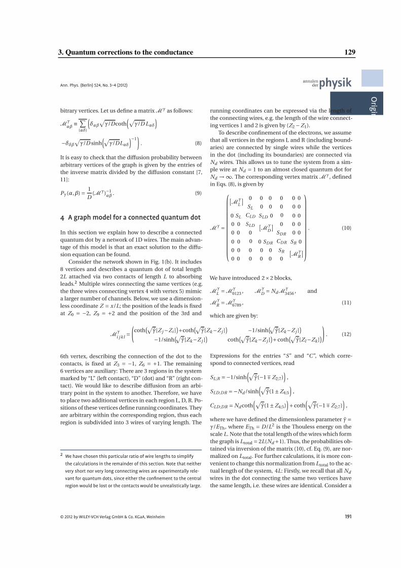
Ann. Phys. (Berlin) 524, No. 3–4 (2012)
OriginalPaper
bitrary vertices. Let us define a matrix M γ as follows:
Mγ
αβ≡
∑
(αδ)
(δαβ
√γ/Dcoth
(√γ/D Lαδ
)
−δδβ√γ/D sinh
(√γ/DLαδ
)−1)
. (8)
It is easy to check that the diffusion probability betweenarbitrary vertices of the graph is given by the entries ofthe inverse matrix divided by the diffusion constant [7,11]:
Pγ(α,β) = 1
D(M γ)−1
αβ . (9)
4 A graph model for a connected quantum dot
In this section we explain how to describe a connectedquantum dot by a network of 1D wires. The main advan-tage of this model is that an exact solution to the diffu-sion equation can be found.
Consider the network shown in Fig. 1(b). It includes8 vertices and describes a quantum dot of total length2L attached via two contacts of length L to absorbingleads.2 Multiple wires connecting the same vertices (e.g.the three wires connecting vertex 4 with vertex 5) mimica larger number of channels. Below, we use a dimension-less coordinate Z = x/L; the position of the leads is fixedat Z0 = −2, Z9 = +2 and the position of the 3rd and
6th vertex, describing the connection of the dot to thecontacts, is fixed at Z3 = −1, Z6 = +1. The remaining6 vertices are auxiliary: There are 3 regions in the systemmarked by “L” (left contact), “D” (dot) and “R” (right con-tact). We would like to describe diffusion from an arbi-trary point in the system to another. Therefore, we haveto place two additional vertices in each region L, D, R. Po-sitions of these vertices define running coordinates. Theyare arbitrary within the corresponding region, thus eachregion is subdivided into 3 wires of varying length. The
2 We have chosen this particular ratio of wire lengths to simplifythe calculations in the remainder of this section. Note that neithervery short nor very long connecting wires are experimentally rele-vant for quantum dots, since either the confinement to the centralregion would be lost or the contacts would be unrealistically large.
running coordinates can be expressed via the length ofthe connecting wires, e.g. the length of the wire connect-ing vertices 1 and 2 is given by (Z2 −Z1).
To describe confinement of the electrons, we assumethat all vertices in the regions L and R (including bound-aries) are connected by single wires while the verticesin the dot (including its boundaries) are connected viaNd wires. This allows us to tune the system from a sim-ple wire at Nd = 1 to an almost closed quantum dot forNd → ∞. The corresponding vertex matrix M γ, definedin Eqs. (8), is given by
M γ =
⎛⎜⎜⎜⎜⎜⎜⎜⎜⎜⎜⎜⎜⎜⎜⎝
[M
γL
] 0
SL
0 0
0 0
0
0
0 0
0 0
0 SL CLD SLD 0 0 0 0
0 0
0 0
SLD
0
[M
γD
] 0
SDR
0 0
0 0
0 0 0 0 SDR CDR SR 0
0 0
0 0
0
0
0 0
0 0
SR
0
[M
γR
]
⎞⎟⎟⎟⎟⎟⎟⎟⎟⎟⎟⎟⎟⎟⎟⎠
. (10)
We have introduced 2×2 blocks,
MγL =M
γ0123 , M
γD = NdM
γ3456 , and
MγR =M
γ6789 , (11)
which are given by:
Mγ
i j kl =(
coth(√
γ[Z j −Zi ])+coth
(√γ[Zk−Z j ]
)−1/sinh
(√γ[Zk−Z j ]
)
−1/sinh(√γ[Zk−Z j ]
)coth
(√γ[Zk−Z j ]
)+coth(√
γ[Zl −Zk ]))
. (12)
Expressions for the entries “S” and “C”, which corre-spond to connected vertices, read
SL;R =−1/sinh(√
γ(−1∓Z2;7))
,
SLD ;DR =−Nd /sinh(√
γ(1±Z4;5
),
CLD ;DR = Nd coth(√
γ(1±Z4;5))+coth
(√γ(−1∓Z2;7)
),
where we have defined the dimensionless parameter γ=γ/ETh, where ETh = D/L2 is the Thouless energy on thescale L. Note that the total length of the wires which formthe graph is Ltotal = 2L(Nd+1). Thus, the probabilities ob-tained via inversion of the matrix (10), cf. Eq. (9), are nor-malized on Ltotal. For further calculations, it is more con-venient to change this normalization from Ltotal to the ac-tual length of the system, 4L: Firstly, we recall that all Nd
wires in the dot connecting the same two vertices havethe same length, i.e. these wires are identical. Consider a
© 2012 by WILEY-VCH Verlag GmbH & Co. KGaA, Weinheim 191
3. Quantum corrections to the conductance 129
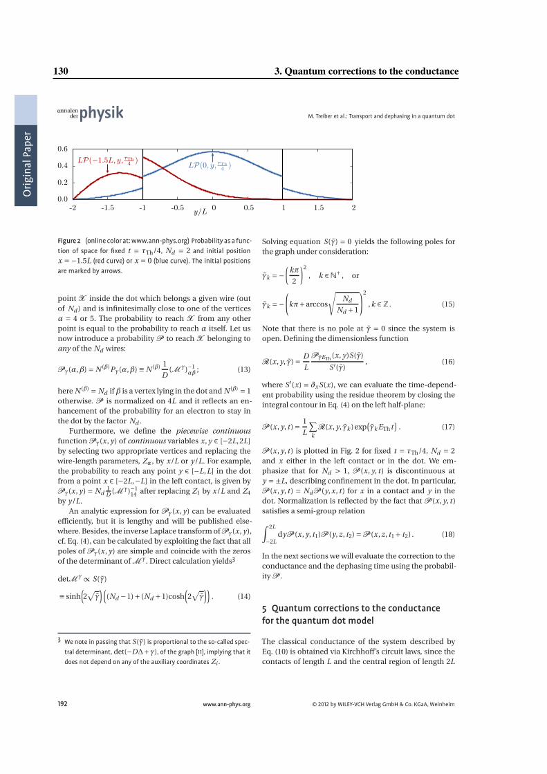
Orig
inalPaper
M. Treiber et al.: Transport and dephasing in a quantum dot
0.0
0.2
0.4
0.6
-2 -1.5 -1 -0.5 0 0.5 1 1.5 2y/L
LP(−1.5L, y, τTh
4 )LP(0, y, τTh
4 )
Figure 2 (online color at:www.ann-phys.org) Probability as a func-tion of space for fixed t = τTh/4, Nd = 2 and initial positionx = −1.5L (red curve) or x = 0 (blue curve). The initial positionsare marked by arrows.
point X inside the dot which belongs a given wire (outof Nd ) and is infinitesimally close to one of the verticesα = 4 or 5. The probability to reach X from any otherpoint is equal to the probability to reach α itself. Let usnow introduce a probability P to reach X belonging toany of the Nd wires:
Pγ(α,β) = N (β)Pγ(α,β) ≡ N (β) 1
D(M γ)−1
αβ ; (13)
here N (β) = Nd ifβ is a vertex lying in the dot and N (β) = 1otherwise. P is normalized on 4L and it reflects an en-hancement of the probability for an electron to stay inthe dot by the factor Nd .
Furthermore, we define the piecewise continuousfunction Pγ(x, y) of continuous variables x, y ∈ [−2L,2L]by selecting two appropriate vertices and replacing thewire-length parameters, Zα, by x/L or y/L. For example,the probability to reach any point y ∈ [−L,L] in the dotfrom a point x ∈ [−2L,−L] in the left contact, is given byPγ(x, y) = Nd
1D (M γ)−1
14 after replacing Z1 by x/L and Z4
by y/L.An analytic expression for Pγ(x, y) can be evaluated
efficiently, but it is lengthy and will be published else-where. Besides, the inverse Laplace transform ofPγ(x, y),cf. Eq. (4), can be calculated by exploiting the fact that allpoles of Pγ(x, y) are simple and coincide with the zerosof the determinant of M γ. Direct calculation yields3
detM γ∝ S(γ)
≡ sinh(2√γ)(
(Nd −1)+ (Nd +1)cosh(2√γ))
. (14)
3 We note in passing that S(γ) is proportional to the so-called spec-tral determinant, det(−DΔ+γ), of the graph [11], implying that itdoes not depend on any of the auxiliary coordinates Zi .
Solving equation S(γ) = 0 yields the following poles forthe graph under consideration:
γk =−(
kπ
2
)2
, k ∈N+ , or
γk =−(
kπ+arccos
√Nd
Nd +1
)2
,k ∈Z . (15)
Note that there is no pole at γ = 0 since the system isopen. Defining the dimensionless function
R(x, y, γ) = D
L
P γETh (x, y)S(γ)
S′(γ), (16)
where S′(x) = ∂x S(x), we can evaluate the time-depend-ent probability using the residue theorem by closing theintegral contour in Eq. (4) on the left half-plane:
P (x, y, t )= 1
L
∑
kR(x, y, γk )exp
(γk ETht
). (17)
P (x, y, t ) is plotted in Fig. 2 for fixed t = τTh/4, Nd = 2and x either in the left contact or in the dot. We em-phasize that for Nd > 1, P (x, y, t ) is discontinuous aty = ±L, describing confinement in the dot. In particular,P (x, y, t ) = NdP (y, x, t ) for x in a contact and y in thedot. Normalization is reflected by the fact that P (x, y, t )satisfies a semi-group relation
∫2L
−2LdyP (x, y, t1)P (y, z, t2) =P (x, z, t1+ t2) . (18)
In the next sections we will evaluate the correction to theconductance and the dephasing time using the probabil-ity P .
5 Quantum corrections to the conductancefor the quantum dot model
The classical conductance of the system described byEq. (10) is obtained via Kirchhoff’s circuit laws, since thecontacts of length L and the central region of length 2L
192 www.ann-phys.org © 2012 by WILEY-VCH Verlag GmbH & Co. KGaA, Weinheim
130 3. Quantum corrections to the conductance
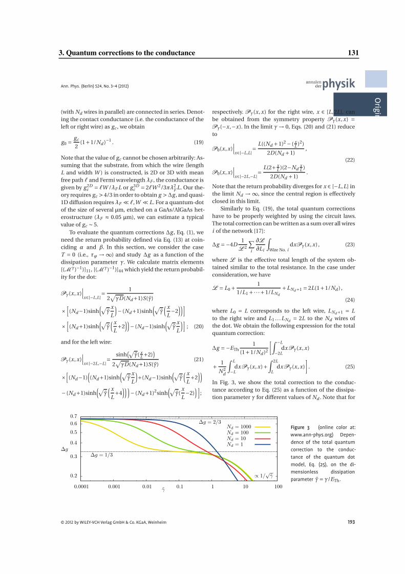
Ann. Phys. (Berlin) 524, No. 3–4 (2012)
OriginalPaper
(with Nd wires in parallel) are connected in series. Denot-ing the contact conductance (i.e. the conductance of theleft or right wire) as gc , we obtain
g0 =gc
2(1+1/Nd )−1 . (19)
Note that the value of gc cannot be chosen arbitrarily: As-suming that the substrate, from which the wire (lengthL and width W ) is constructed, is 2D or 3D with meanfree path and Fermi wavelengthλF , the conductance isgiven by g 2D
c = W /λF L or g 3Dc = 2W 2/3πλ2
F L. Our the-ory requires gc > 4/3 in order to obtain g >Δg , and quasi-1D diffusion requires λF � ,W � L. For a quantum-dotof the size of several µm, etched on a GaAs/AlGaAs het-erostructure (λF ≈ 0.05 µm), we can estimate a typicalvalue of gc ∼ 5.
To evaluate the quantum corrections Δg , Eq. (1), weneed the return probability defined via Eq. (13) at coin-ciding α and β. In this section, we consider the caseT = 0 (i.e., τϕ → ∞) and study Δg as a function of thedissipation parameter γ. We calculate matrix elements[(M γ)−1)]11, [(M γ)−1)]44 which yield the return probabil-ity for the dot:
Pγ(x, x)∣∣∣x∈[−L,L]
= 1
2√γD(Nd+1)S(γ)
×[
(Nd−1)sinh(√
γx
L
)− (Nd+1)sinh
(√γ
( x
L−2
))]
×[
(Nd+1)sinh(√
γ( x
L+2
))− (Nd−1)sinh
(√γ
x
L
)]; (20)
and for the left wire:
Pγ(x, x)∣∣∣x∈[−2L,−L]
=sinh
(√γ( x
L +2))
2√γD(Nd+1)S(γ)
(21)
×[
(Nd−1)((Nd+1)sinh
(√γ
x
L
)+(Nd−1)sinh
(√γ
( x
L+2
))
− (Nd+1)sinh(√
γ( x
L+4
)))− (Nd+1)2sinh
(√γ(
x
L−2)
)];
respectively. Pγ(x, x) for the right wire, x ∈ [L,2L], canbe obtained from the symmetry property Pγ(x, x) =Pγ(−x,−x). In the limit γ→ 0, Eqs. (20) and (21) reduceto
P0(x, x)∣∣∣x∈[−L,L]
=L((Nd +1)2 − ( x
L )2)
2D(Nd +1),
(22)
P0(x, x)∣∣∣x∈[−2L,−L]
=L(2+ x
L )(2−NdxL )
2D(Nd +1).
Note that the return probability diverges for x ∈ [−L,L] inthe limit Nd → ∞, since the central region is effectivelyclosed in this limit.
Similarly to Eq. (19), the total quantum correctionshave to be properly weighted by using the circuit laws.The total correction can be written as a sum over all wiresi of the network [17]:
Δg =−4D1
L 2
∑
i
∂L
∂Li
∫
Wire No. idxPγ(x, x) , (23)
where L is the effective total length of the system ob-tained similar to the total resistance. In the case underconsideration, we have
L = L0 +1
1/L1 +·· ·+1/LNd
+LNd+1 = 2L(1+1/Nd ) ,
(24)
where L0 = L corresponds to the left wire, LNd+1 = Lto the right wire and L1 . . . LNd = 2L to the Nd wires ofthe dot. We obtain the following expression for the totalquantum correction:
Δg =−ETh1
(1+1/Nd )2
[∫−L
−2LdxPγ(x, x)
+ 1
N 2d
∫L
−LdxPγ(x, x)+
∫2L
LdxPγ(x, x)
]. (25)
In Fig. 3, we show the total correction to the conduc-tance according to Eq. (25) as a function of the dissipa-tion parameter γ for different values of Nd . Note that for
0.2
0.3
0.4
0.5
0.6
0.7
0.0001 0.001 0.01 0.1 1 10 100
Δg
γ
Δg = 2/3
Δg = 1/3
∝ 1/√γ
Nd = 1000Nd = 100Nd = 10Nd = 1
Figure 3 (online color at:www.ann-phys.org) Depen-dence of the total quantumcorrection to the conduc-tance of the quantum dotmodel, Eq. (25), on the di-mensionless dissipationparameter γ= γ/ETh.
© 2012 by WILEY-VCH Verlag GmbH & Co. KGaA, Weinheim 193
3. Quantum corrections to the conductance 131
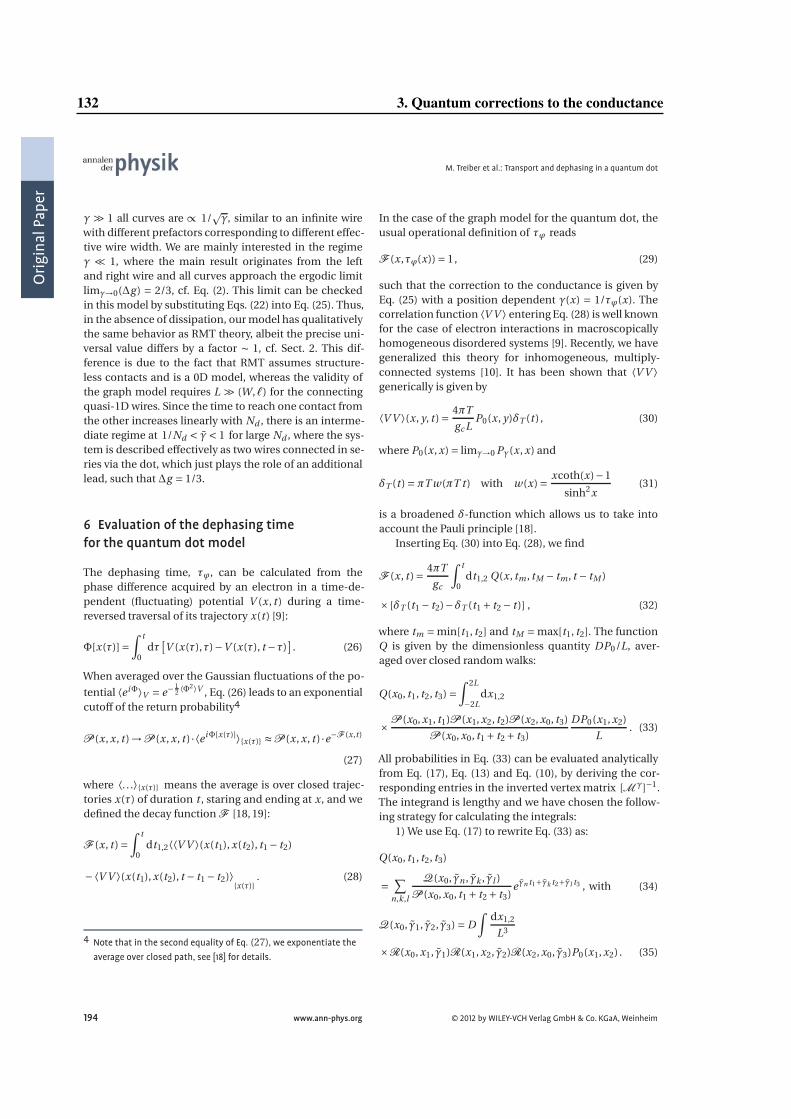
Orig
inalPaper
M. Treiber et al.: Transport and dephasing in a quantum dot
γ� 1 all curves are ∝ 1/�γ, similar to an infinite wire
with different prefactors corresponding to different effec-tive wire width. We are mainly interested in the regimeγ � 1, where the main result originates from the leftand right wire and all curves approach the ergodic limitlimγ→0(Δg ) = 2/3, cf. Eq. (2). This limit can be checkedin this model by substituting Eqs. (22) into Eq. (25). Thus,in the absence of dissipation, our model has qualitativelythe same behavior as RMT theory, albeit the precise uni-versal value differs by a factor ∼ 1, cf. Sect. 2. This dif-ference is due to the fact that RMT assumes structure-less contacts and is a 0D model, whereas the validity ofthe graph model requires L � (W ,) for the connectingquasi-1D wires. Since the time to reach one contact fromthe other increases linearly with Nd , there is an interme-diate regime at 1/Nd < γ< 1 for large Nd , where the sys-tem is described effectively as two wires connected in se-ries via the dot, which just plays the role of an additionallead, such that Δg = 1/3.
6 Evaluation of the dephasing timefor the quantum dot model
The dephasing time, τϕ, can be calculated from thephase difference acquired by an electron in a time-de-pendent (fluctuating) potential V (x, t ) during a time-reversed traversal of its trajectory x(t ) [9]:
Φ[x(τ)]=∫t
0dτ
[V (x(τ),τ)−V (x(τ), t −τ)
]. (26)
When averaged over the Gaussian fluctuations of the po-
tential ⟨eiΦ⟩V = e−12 ⟨Φ2⟩V , Eq. (26) leads to an exponential
cutoff of the return probability4
P (x, x, t )→P (x, x, t )·⟨eiΦ[x(τ)]⟩{x(τ)} ≈P (x, x, t )·e−F (x,t)
(27)
where ⟨. . .⟩{x(τ)} means the average is over closed trajec-tories x(τ) of duration t , staring and ending at x, and wedefined the decay function F [18, 19]:
F (x, t )=∫t
0dt1,2⟨⟨V V ⟩(x(t1), x(t2), t1− t2)
−⟨V V ⟩(x(t1), x(t2), t − t1 − t2)⟩{x(τ)}
. (28)
4 Note that in the second equality of Eq. (27), we exponentiate theaverage over closed path, see [18] for details.
In the case of the graph model for the quantum dot, theusual operational definition of τϕ reads
F (x,τϕ(x))= 1, (29)
such that the correction to the conductance is given byEq. (25) with a position dependent γ(x) = 1/τϕ(x). Thecorrelation function ⟨V V ⟩ entering Eq. (28) is well knownfor the case of electron interactions in macroscopicallyhomogeneous disordered systems [9]. Recently, we havegeneralized this theory for inhomogeneous, multiply-connected systems [10]. It has been shown that ⟨V V ⟩generically is given by
⟨V V ⟩(x, y, t )= 4πT
gc LP0(x, y)δT (t ) , (30)
where P0(x, x)= limγ→0 Pγ(x, x) and
δT (t )=πT w(πT t ) with w(x)= xcoth(x)−1
sinh2x(31)
is a broadened δ-function which allows us to take intoaccount the Pauli principle [18].
Inserting Eq. (30) into Eq. (28), we find
F (x, t )= 4πT
gc
∫t
0dt1,2 Q(x, tm , tM − tm, t − tM )
× [δT (t1 − t2)−δT (t1 + t2 − t )] , (32)
where tm = min[t1, t2] and tM = max[t1, t2]. The functionQ is given by the dimensionless quantity DP0/L, aver-aged over closed random walks:
Q(x0, t1, t2, t3) =∫2L
−2Ldx1,2
× P (x0, x1, t1)P (x1, x2, t2)P (x2, x0, t3)
P (x0, x0, t1 + t2 + t3)
DP0(x1, x2)
L. (33)
All probabilities in Eq. (33) can be evaluated analyticallyfrom Eq. (17), Eq. (13) and Eq. (10), by deriving the cor-responding entries in the inverted vertex matrix [M γ]−1.The integrand is lengthy and we have chosen the follow-ing strategy for calculating the integrals:
1) We use Eq. (17) to rewrite Eq. (33) as:
Q(x0, t1, t2, t3)
=∑
n,k ,l
Q(x0, γn , γk , γl )
P (x0, x0, t1 + t2 + t3)eγn t1+γk t2+γl t3 , with (34)
Q(x0, γ1, γ2, γ3) = D∫
dx1,2
L3
×R(x0, x1, γ1)R(x1, x2, γ2)R(x2, x0, γ3)P0(x1, x2) . (35)
194 www.ann-phys.org © 2012 by WILEY-VCH Verlag GmbH & Co. KGaA, Weinheim
132 3. Quantum corrections to the conductance
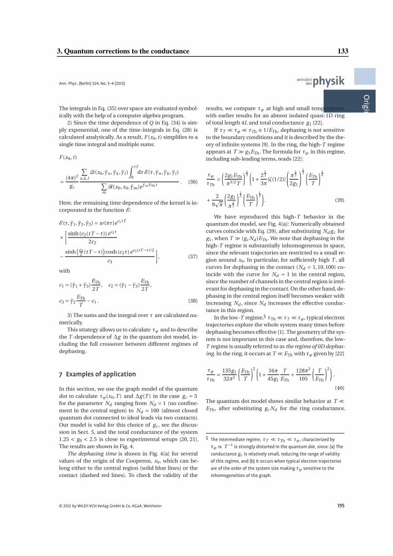
Ann. Phys. (Berlin) 524, No. 3–4 (2012)
OriginalPaper
The integrals in Eq. (35) over space are evaluated symbol-ically with the help of a computer algebra program.
2) Since the time dependence of Q in Eq. (34) is sim-ply exponential, one of the time-integrals in Eq. (28) iscalculated analytically. As a result, F (x0, t ) simplifies to asingle time integral and multiple sums:
F (x0, t )
= (4π)2
gc
∑
n,k ,lQ(x0, γn , γk , γl )
∫tT
0dτE (τ, γn , γk , γl )
∑m
R(x0, x0, γm )eγm ETht. (36)
Here, the remaining time dependence of the kernel is in-corporated in the function E :
E (τ, γ1, γ2, γ3) = w(πτ)ec1tT
×[
sinh (c2(t T −τ))ec3τ
2c2
−sinh
( c32 (t T −τ)
)cosh(c2τ)ec3(tT−τ)/2
c3
], (37)
with
c1 = (γ1 + γ3)ETh
2T, c2 = (γ1 − γ3)
ETh
2T,
c3 = γ2ETh
T−c1 . (38)
3) The sums and the integral over τ are calculated nu-merically.
This strategy allows us to calculate τϕ and to describethe T -dependence of Δg in the quantum dot model, in-cluding the full crossover between different regimes ofdephasing.
7 Examples of application
In this section, we use the graph model of the quantumdot to calculate τϕ(x0,T ) and Δg (T ) in the case gc = 5for the parameter Nd ranging from Nd = 1 (no confine-ment in the central region) to Nd = 100 (almost closedquantum dot connected to ideal leads via two contacts).Our model is valid for this choice of gc , see the discus-sion in Sect. 5, and the total conductance of the system1.25 < g0 < 2.5 is close to experimental setups [20, 21].The results are shown in Fig. 4.
The dephasing time is shown in Fig. 4(a) for severalvalues of the origin of the Cooperon, x0, which can be-long either to the central region (solid blue lines) or thecontact (dashed red lines). To check the validity of the
results, we compare τϕ at high and small temperatureswith earlier results for an almost isolated quasi-1D ringof total length 4L and total conductance g1 [22].
If τT � τϕ � τTh ≡ 1/ETh, dephasing is not sensitiveto the boundary conditions and it is described by the the-ory of infinite systems [9]. In the ring, the high-T regimeappears at T � g1ETh. The formula for τϕ in this regime,including sub-leading terms, reads [22]:
τϕ
τTh=
(2g1ETh
π3/2T
) 23(1+ 2
52
3π|ζ(1/2)|
(π
32
2g1
) 13 (
ETh
T
) 16
+ 2
9�π
(2g1
π32
) 13(
ETh
T
) 13)
. (39)
We have reproduced this high-T behavior in thequantum dot model, see Fig. 4(a): Numerically obtainedcurves coincide with Eq. (39), after substituting Nd gc forg1, when T � (gc Nd )ETh. We note that dephasing in thehigh-T regime is substantially inhomogeneous in space,since the relevant trajectories are restricted to a small re-gion around x0. In particular, for sufficiently high T , allcurves for dephasing in the contact (Nd = 1,10,100) co-incide with the curve for Nd = 1 in the central region,since the number of channels in the central region is irrel-evant for dephasing in the contact. On the other hand, de-phasing in the central region itself becomes weaker withincreasing Nd , since Nd increases the effective conduc-tance in this region.
In the low-T regime,5 τTh � τT � τϕ, typical electrontrajectories explore the whole system many times beforedephasing becomes effective [1]. The geometry of the sys-tem is not important in this case and, therefore, the low-T regime is usually referred to as the regime of 0D dephas-ing. In the ring, it occurs at T � ETh with τϕ given by [22]
τϕ
τTh= 135g1
32π2
(ETh
T
)2 (1+ 16π
45g1
T
ETh+ 128π2
105
(T
ETh
)2).
(40)
The quantum dot model shows similar behavior at T �ETh, after substituting gc Nd for the ring conductance.
5 The intermediate regime, τT � τTh � τϕ , characterized byτϕ ∝ T −1 is strongly distorted in the quantum dot, since: (a) Theconductance gc is relatively small, reducing the range of validityof this regime, and (b) it occurs when typical electron trajectoriesare of the order of the system size making τϕ sensitive to theinhomogeneities of the graph.
© 2012 by WILEY-VCH Verlag GmbH & Co. KGaA, Weinheim 195
3. Quantum corrections to the conductance 133
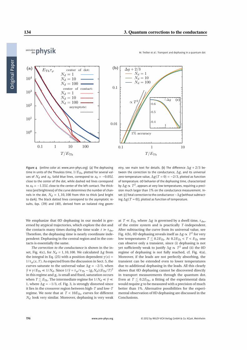
Orig
inalPaper
M. Treiber et al.: Transport and dephasing in a quantum dot
100
101
102
103
104
0.1 1 10 100
T/ETh
EThτϕ(a) center of dot:
Nd = 1Nd = 10Nd = 100center of contact:
Nd = 1Nd = 10Nd = 100
asymptote:
0.01
0.1
0.1 1 10
T/ETh
1% accuracy
(b)
∝ T 2
Δg + 2/3Nd = 1Nd = 10Nd = 100
0.4
0.5
0.6
1
(c)−Δg
Figure 4 (online color at: www.ann-phys.org) (a) The dephasingtime in units of the Thouless time, 1/ETh, plotted for several val-ues of Nd and x0. Solid blue lines, correspond to x0 = −0.05Lclose to the center of the dot, while dashed red lines correspondto x0 = −1.55L close to the center of the left contact. The thick-ness (and brightness) of the curve determines the number of chan-nels in the dot, Nd = 1,10,100 from thin to thick (and brightto dark). The black dotted lines correspond to the asymptotic re-sults, Eqs. (39) and (40), derived from an isolated ring geom-
etry, see main text for details. (b) The difference Δg + 2/3 be-tween the correction to the conductance, Δg , and its universalzero-temperature value, Δg (T = 0) =−2/3, plotted as functionof temperature. 0D behavior of the dephasing time, characterizedbyΔg ∝ T 2, appears at very low temperatures, requiring a preci-sion much larger than 1% on the conductance measurement. In-set: (c) Total correction to the conductance−Δg (without subtract-ingΔg (T = 0)), plotted as function of temperature.
We emphasize that 0D dephasing in our model is gov-erned by atypical trajectories, which explore the dot andthe contacts many times during the time scale t � τdw.Therefore, the dephasing time is nearly coordinate inde-pendent: Dephasing in the central region and in the con-tacts is essentially the same.
The correction to the conductance is shown in the in-set, Fig. 4(c), for Nd = 1,10,100. We calculated Δg fromthe integral in Eq. (25) with a position dependent γ(x) =1/τϕ(x,T ). As expected from the discussion in Sect. 5, thecurves saturate to the universal value Δg = −2/3, whenγ≡ γ/ETh � 1/Nd . Since 1/γ= τϕ/τTh ∼ (gc Nd )(ETh/T )2
in this regime and gc is small and fixed, saturation occurswhen T � ETh. The intermediate regime for 1/Nd � γ�1, where Δg = −1/3, cf. Fig. 3, is strongly distorted sinceit lies in the crossover region between high-T and low-Tregime. We note that at T < 10ETh, curves for differentNd look very similar. Moreover, dephasing is very weak
at T � ETh where Δg is governed by a dwell time, τdw,of the entire system and is practically T -independent.After subtracting the curve from its universal value, seeFig. 4(b), 0D dephasing reveals itself as Δg ∝ T 2 for verylow temperatures T � 0.2ETh. At 0.2ETh < T < ETh onecan observe only a transient, since (i) dephasing is notyet sufficiently weak to justify Δg ∝ T 2 and (ii) the 0Dregime of dephasing is not fully reached, cf. Fig. 4(a).Moreover, if the leads are not perfectly absorbing, thetransient can be extended even to lower temperaturesdue to additional dephasing in the leads. All this clearlyshows that 0D dephasing cannot be discovered directlyin transport measurements through the quantum dot.Even at T � 0.2ETh, a fitting of the experimental datawould require g to be measured with a precision of muchbetter than 1%. Alternative possibilities for the experi-mental observation of 0D dephasing are discussed in theConclusions.
196 www.ann-phys.org © 2012 by WILEY-VCH Verlag GmbH & Co. KGaA, Weinheim
134 3. Quantum corrections to the conductance
Ann. Phys. (Berlin) 524, No. 3–4 (2012)
OriginalPaper
8 Conclusions
We have suggested a graph model, which allows one todescribe transport through mesoscopic quantum dots.The graph includes three quasi-1D regions: identical left-and right- wires and a central region. The identical wiresare connected to ideally absorbing leads and mimic thecontacts of a real system. The number of conductingchannels in the central region can be of the order of- orsubstantially larger than the number of channels in thecontacts. The latter case corresponds to a strong confine-ment of electrons in the central region. Thus the graphmodel is able to describe a crossover from opened toclosed quantum dots.
The model which we suggest can be viewed as com-plementary to the seminal RMT model. Firstly, the exactsolution to the diffusion equation can be found for thegraph model. Secondly, we have shown that our modelcorrectly reproduces the universal regime of transport infull analogy with the RMT solution. Even more impor-tantly, the graph model allows us to take into accountinteraction induced dephasing in a broad temperaturerange, i.e., we can describe the full crossover from 1D to0D regimes.
Using the solution to the diffusion equation on thegraph, we have described in detail how to calculate thedephasing time and the weak localization correction tothe conductance. Though the intermediate equations arerather lengthy, we have suggested an efficient combi-nation of analytical steps (involving computer algebra)and numerical integration, which helped us to overcometechnical difficulties.
The general approach has been illustrated for the sys-tem with gc = 5. We have demonstrated that 0D dephas-ing (∼ T 2), which is governed by the Pauli principle andis very generic, occurs in the system at T � ETh at arbi-trary ratio of the channel numbers in the dots and leads.In this regime, dephasing is governed by atypical trajecto-ries which explore the dot and the contacts many timesduring the time scale t � τdw where the conductanceis governed mainly by the dwell time and is almost T -independent. Our results confirm that weak 0D dephas-ing is substantially distorted by the influence of the con-tacts and the leads. Therefore, its direct experimental ob-servation in transport through the quantum dot wouldrequire not only very low temperatures but also unrealis-tically precise measurements. We conclude that alterna-tive experimental approaches are needed, where eitherthe effects from the environment are reduced or the sys-tem is closed. One possibility to improve the effective pre-cision of the measurements is related to extracting τϕfrom the T -dependence of the Aronov-Altshuler-Spivak
oscillations of the magnetoconductivity in almost closedmesoscopic rings. This option was discussed in recentpapers [6, 22] where all effects of the environment weretaken into account via a constant dwelling time. We planto study in more detail the sensitivity of the AAS oscil-lations on the distortions from the environment usinga ring model similar to the model of the dot presentedhere [23]. The other option is to extract τϕ from experi-mental measurements of the electric or magnetic suscep-tibility of closed mesoscopic systems, e.g. by measuringthe properties of resonators in which mesoscopic sam-ples are deposited [24]. In closed systems, there is no uni-versal limit of the quantum corrections at τϕ� τdw, typi-cal for transport through opened systems. Therefore, thesaturation in the closed system can occur at much lowerT , making them more suitable for an experimental obser-vation of 0D dephasing. A theoretical description of suchexperiments will be published elsewhere.
Acknowledgements. We acknowledge illuminating discussionswith C. Texier, and support from the DFG through SFB TR-12 (O. Ye.),DE 730/8-1 (M. T.) and the Cluster of Excellence, Nanosystems Ini-tiative Munich.
Key words. Dephasing, quantumdot, weak localization, diffusionin graphs.
References
[1] U. Sivan, Y. Imry, and A. G. Aronov, Europhys. Lett. 28,115 (1994).
[2] B. Doucot and R. Rammal, Phys. Rev. Lett. 55, 1148(1985).
[3] B. Doucot and R. Rammal, J. Phys. (Paris) 47, 973(1986).
[4] T. Ludwig and A. D. Mirlin, Phys. Rev. B 69, 193306(2004).
[5] C. Texier and G. Montambaux, Phys. Rev. B 72,115327 (2005).
[6] M. Treiber et al., Phys. Rev. B 80, 201305 (2009).[7] C. Texier, P. Delplace, and G. Montambaux, Phys. Rev.
B 80, 205413 (2009).[8] D. E. Khmel’nitskii, Physica B + C 126, 235 (1984)[9] B. L. Altshuler, A. G. Aronov, and D. E. Khmelnitsky, J.
Phys. C 15, 7367 (1982).[10] M. Treiber et al., Phys. Rev. B 84, 054204 (2011).[11] E. Akkermans and G. Montambaux, in: Mesoscopic
Physics of Electrons and Photons (Cambridge Univer-sity Press, Cambridge, 2007).
[12] H. U. Baranger and P. A. Mello, Phys. Rev. Lett. 73, 142(1994).
[13] R. A. Jalabert, J.-L. Pichard, and C. W. J. Beenakker,Europhys. Lett. 27, 255 (1994).
© 2012 by WILEY-VCH Verlag GmbH & Co. KGaA, Weinheim 197
3. Quantum corrections to the conductance 135
Orig
inalPaper
M. Treiber et al.: Transport and dephasing in a quantum dot
[14] P. W. Brouwer and C. W. J. Beenakker, Phys. Rev. B 55,4695 (1997).
[15] M. Büttiker, Phys. Rev. B 33, 3020 (1986).[16] E. McCann and I. V. Lerner, J. Phys. Condens. Matter
8, 6719 (1996).[17] C. Texier and G. Montambaux, Phys. Rev. Lett. 92,
186801 (2004).[18] F. Marquardt, J. von Delft, R. Smith, and V. Ambe-
gaokar, Phys. Rev. B 76, 195331 (2007).[19] J. von Delft, F. Marquardt, R. Smith, and V. Ambe-
gaokar, Phys. Rev. B 76, 195332 (2007).[20] A. G. Huibers et al., Phys. Rev. Lett. 81, 200 (1998).
[21] S. Amasha et al., arXiv:1009.5348 (unpublished).[22] M. Treiber et al., Dimensional Crossover of the De-
phasing Time in Disordered Mesoscopic Rings: FromDiffusive Through Ergodic to 0D Behavior, in: Per-spectives of Mesoscopic Physics – Dedicated toYoseph Imry’s 70th Birthday, Chap. 20, edited byA. Aharony and O. Entin-Wohlman (World Scientific,Singapore, 2010); arXiv:1001.0479.
[23] M. Treiber, O. M. Yevtushenko, and J. von Delft, to bepublished.
[24] R. Deblock et al., Phys. Rev. B 65, 075301 (2002).
198 www.ann-phys.org © 2012 by WILEY-VCH Verlag GmbH & Co. KGaA, Weinheim
136 3. Quantum corrections to the conductance
4. Quantum corrections to the polarizability 137
Chapter 4
Quantum corrections to the polarizability
In Chapter 3, we have discussed dephasing at low temperatures in the context of the weak-localizationcorrection to the conductance. We found that the elusive 0D regime of dephasing can be observedonly in the universal regime, where the weak-localization correction is dominated by a dwelling timeτdw and the system’s real dimensionality is not important. Thus, the characteristic 1/τϕ ∝ T 2 behav-ior of the dephasing time is difficult to observe and heavily depends on the contacts controlling theconfinement. In isolated systems, on the other hand, we have effectively τdw→ ∞, making them anideal candidate to study 0D dephasing.
Furthermore, we have discussed in Section 2.2.5 that in the isolated systems, and in the absence ofother sources of dephasing, the 0D regime is characterized by a discreteness of the energy levels. Incontrast to the conductivity of a good metal, which is well described by the loop-expansion, discretelevel systems are rather described by the non-perturbative random matrix theory (RMT). Thus, ananalysis of quantum corrections in isolated systems also provides the unique opportunity to study thecrossover from perturbative to non-perturbative regimes.
4.1 Isolated systems: Realizing the canonical ensemble
One of the recent and important results of mesoscopic physics was the realization that the employedstatistical ensemble plays an important role in the description of observables [Kamenev and Gefen,1993; Kamenev et al., 1994; Kamenev and Gefen, 1997b]. Usually the grand-canonical ensemble(GCE), where the chemical potential µ is fixed, is used to describe quantum corrections, cf. Section 2.On the other hand, isolated systems are characterized by a fixed number of particles N and are ratherdescribed by the canonical ensemble (CE). Remarkably, a qualitative difference between the CE andthe GCE can persist up to energy scales much larger than the level spacing ∆ [Kamenev and Gefen,1997a].
Initiated by the seminal work of Büttiker et al. (1983), who predicted a so-called persistent currentin disordered phase-coherent metallic rings, a large effort has been made to describe the magnetic re-sponse of isolated samples, see e.g. Cheung et al. (1988); Schmid (1991). However, the experimentalobservation of the persistent current is difficult due to its weakness. In fact, experimental results oftendiffered in sign and magnitude with theoretical predictions [Reulet et al., 1995; Deblock et al., 2002a].In spite of recent advances in measurement techniques, see Bluhm et al. (2009); Bleszynski-Jayichet al. (2009), persistent currents remain a rather controversial subject in mesoscopic physics. Thus, inthe following, we will solely concentrate on the electric response of mesoscopic samples, namely, wewill investigate the electrical polarizability of isolated samples in the CE.
To realize the CE, we employ the ideas of Altland et al. (1992a,b); Lehle and Schmid (1995):
138 4. Quantum corrections to the polarizability
When the number of particles N in the system is fixed, the chemical potential µ fluctuates. However,the precise value of µ∼ εF is not relevant in the quantum corrections, e.g. the correlation functionssuch as P and K , defined in Eqs. (2.10, 2.11), do not depend on energy ε. In fact, this is a rathergeneral observation for disorder averaged correlation functions, since we have seen in Eq. (2.12) thateach “step” of any impurity ladder dq,ω is independent of the common energy of particle and holein the limit (εFτ)−1� 1. From a semi-classical picture, the independence of dq,ω on ε is intuitivelyclear, since it corresponds to the requirement that the propagation time of particle and hole betweentwo scattering events has to be identical to guarantee constructive interference. However, we stressthat the independence on ε does not mean that the statistical ensemble is irrelevant. Instead, thefluctuations of the chemical potential induce correlations of the density of states with the correlationfunctions, i.e. three-level correlations become important, as we will see in the following.
For a fixed number of electrons and low temperatures T � εF , all of the lowest electron states ofthe Fermi sea up to the N ’th state εk are occupied. Following Lehle and Schmid (1995), we can thus“pin” the chemical potential to this particular level by setting µ = εk +0. However the level εk is notfixed and we should describe its distribution by a normalized weight function P(εk) centered aroundεF and with a support much smaller than εF but much larger than the level spacing ∆.1
To give a concrete example, let us consider the correlation function K introduced in Eq. (2.11).Before impurity averaging and for a fixed chemical potential is given by:
KGCE =1
2πρGR
µ+ε(x,x)GAµ+ε−ω(y,y) . (4.1)
Pinning the chemical potential to εk to describe the canonical ensemble, we instead have
KCE =1
2πρ∑k P(εk)GR
εk+ε(x,x)GAεk+ε−ω(y,y)
∑k P(εk). (4.2)
Using the definition of the density of states, Eq. (2.8), the normalization constant in Eq. (4.2) can bewritten as
∑k
P(εk) =V∫ ∞
−∞dεP(ε)ρε ≈ ρV , (4.3)
since the ρε depends only weakly on ε at ε� εF . Therefore, Eq. (4.2) can be written as
KCE =1
2πρ2
∫ ∞
−∞dE P(E)ρEGR
E+ε(x,x)GAE+ε−ω(y,y) (4.4)
=i
(2πρ)2
∫ ∞
−∞dE P(E)
[GR
E(z,z)−GAE(z,z)
]GR
E+ε(x,x)GAE+ε−ω(y,y) .
Since the disorder average of the product of Green’s functions does not depend on their commonenergy, we can integrate over E using the normalization
∫ ∞−∞dE P(E) = 1. As a result, we find for K
in the canonical ensemble:
KCE(x,y,ω) =i
(2πρ)2V
∫ddz[GR
E(z,z)−GAE(z,z)
]GR
E+ε(x,x)GAE+ε−ω(y,y) . (4.5)
1. After disorder averaging, this “Fermi-level pinning ensemble” describes an ensemble average of a large number ofisolated samples where the number of particles is fixed per sample. However, the particle number is not necessarilythe same in different samples of the ensemble, see the discussion in Altland et al. (1992a,b) and Kamenev and Gefen(1993).
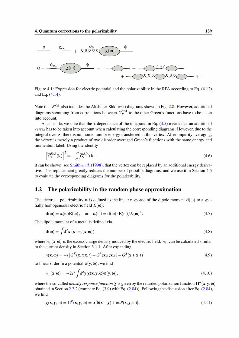
4. Quantum corrections to the polarizability 139
Figure 4.1: Expression for electric potential and the polarizability in the RPA according to Eq. (4.12)and Eq. (4.14).
Note that KCE also includes the Altshuler-Shklovski diagrams shown in Fig. 2.8. However, additionaldiagrams stemming from correlations between GR/A
E to the other Green’s functions have to be takeninto account.
As an aside, we note that the z dependence of the integrand in Eq. (4.5) means that an additionalvertex has to be taken into account when calculating the corresponding diagrams. However, due to theintegral over z, there is no momentum or energy transferred at this vertex. After impurity averaging,the vertex is merely a product of two disorder averaged Green’s functions with the same energy andmomentum label. Using the identity
[GR/A
ε (k)]2
=− ∂∂ε
GR/Aε (k) , (4.6)
it can be shown, see Smith et al. (1998), that the vertex can be replaced by an additional energy deriva-tive. This replacement greatly reduces the number of possible diagrams, and we use it in Section 4.5to evaluate the corresponding diagrams for the polarizability.
4.2 The polarizability in the random phase approximation
The electrical polarizability α is defined as the linear response of the dipole moment d(ω) to a spa-tially homogeneous electric field E(ω):
d(ω) = α(ω)E(ω) , or α(ω) = d(ω) ·E(ω)/E(ω)2 . (4.7)
The dipole moment of a metal is defined via
d(ω) =∫
ddx (x ·nin(x,ω)) , (4.8)
where nin(x,ω) is the excess charge density induced by the electric field. nin can be calculated similarto the current density in Section 3.1.1. After expanding
n(x,ω) =−i[GK(x, t;x, t)−GR(x, t;x, t)+GA(x, t;x, t)
](4.9)
to linear order in a potential φ(y,ω), we find
nin(x,ω) =−2e2∫
ddy χ(x,y,ω)φ(y,ω) , (4.10)
where the so-called density response function χ is given by the retarded polarization function ΠR(x,y,ω)obtained in Section 2.2.2 (compare Eq. (3.9) with Eq. (2.84)). Following the discussion after Eq. (2.84),we find
χ(x,y,ω) = ΠR(x,y,ω) = ρ [δ(x−y)+ iωP(x,y,ω)] , (4.11)
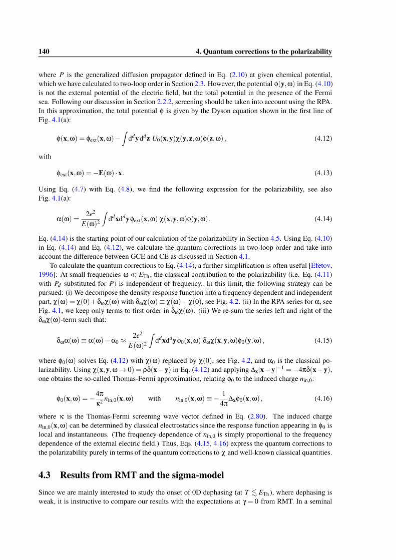
140 4. Quantum corrections to the polarizability
where P is the generalized diffusion propagator defined in Eq. (2.10) at given chemical potential,which we have calculated to two-loop order in Section 2.3. However, the potential φ(y,ω) in Eq. (4.10)is not the external potential of the electric field, but the total potential in the presence of the Fermisea. Following our discussion in Section 2.2.2, screening should be taken into account using the RPA.In this approximation, the total potential φ is given by the Dyson equation shown in the first line ofFig. 4.1(a):
φ(x,ω) = φext(x,ω)−∫
ddyddz U0(x,y)χ(y,z,ω)φ(z,ω) , (4.12)
with
φext(x,ω) =−E(ω) ·x . (4.13)
Using Eq. (4.7) with Eq. (4.8), we find the following expression for the polarizability, see alsoFig. 4.1(a):
α(ω) =2e2
E(ω)2
∫ddxddyφext(x,ω) χ(x,y,ω)φ(y,ω) . (4.14)
Eq. (4.14) is the starting point of our calculation of the polarizability in Section 4.5. Using Eq. (4.10)in Eq. (4.14) and Eq. (4.12), we calculate the quantum corrections in two-loop order and take intoaccount the difference between GCE and CE as discussed in Section 4.1.
To calculate the quantum corrections to Eq. (4.14), a further simplification is often useful [Efetov,1996]: At small frequencies ω� ETh , the classical contribution to the polarizability (i.e. Eq. (4.11)with Pd substituted for P) is independent of frequency. In this limit, the following strategy can bepursued: (i) We decompose the density response function into a frequency dependent and independentpart, χ(ω) = χ(0)+δωχ(ω) with δωχ(ω)≡ χ(ω)−χ(0), see Fig. 4.2. (ii) In the RPA series for α, seeFig. 4.1, we keep only terms to first order in δωχ(ω). (iii) We re-sum the series left and right of theδωχ(ω)-term such that:
δωα(ω)≡ α(ω)−α0 ≈2e2
E(ω)2
∫ddxddyφ0(x,ω) δωχ(x,y,ω)φ0(y,ω) , (4.15)
where φ0(ω) solves Eq. (4.12) with χ(ω) replaced by χ(0), see Fig. 4.2, and α0 is the classical po-larizability. Using χ(x,y,ω→ 0) = ρδ(x−y) in Eq. (4.12) and applying ∆x|x−y|−1 =−4πδ(x−y),one obtains the so-called Thomas-Fermi approximation, relating φ0 to the induced charge nin,0:
φ0(x,ω) =−4πκ2 nin,0(x,ω) with nin,0(x,ω)≡−
14π
∆xφ0(x,ω) , (4.16)
where κ is the Thomas-Fermi screening wave vector defined in Eq. (2.80). The induced chargenin,0(x,ω) can be determined by classical electrostatics since the response function appearing in φ0 islocal and instantaneous. (The frequency dependence of nin,0 is simply proportional to the frequencydependence of the external electric field.) Thus, Eqs. (4.15, 4.16) express the quantum corrections tothe polarizability purely in terms of the quantum corrections to χ and well-known classical quantities.
4.3 Results from RMT and the sigma-model
Since we are mainly interested to study the onset of 0D dephasing (at T . ETh ), where dephasing isweak, it is instructive to compare our results with the expectations at γ = 0 from RMT. In a seminal
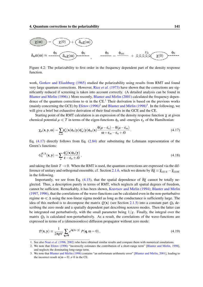
4. Quantum corrections to the polarizability 141
Figure 4.2: The polarizability to first order in the frequency dependent part of the density responsefunction.
work, Gorkov and Eliashberg (1965) studied the polarizability using results from RMT and foundvery large quantum corrections. However, Rice et al. (1973) have shown that the corrections are sig-nificantly reduced if screening is taken into account correctly. (A detailed analysis can be found inBlanter and Mirlin (1996).) More recently, Blanter and Mirlin (2001) calculated the frequency depen-dence of the quantum corrections to α in the CE.1 Their derivation is based on the previous works(mainly concerning the GCE) by Efetov (1996)2 and Blanter and Mirlin (1998)3. In the following, wewill give a brief but exhaustive derivation of their final results in the GCE and the CE.
Starting point of the RMT calculation is an expression of the density response function χ at givenchemical potential µ� T in terms of the eigen-functions φn and -energies εn of the Hamiltonian:
χµ(x,y,ω) = ∑n,m
φ∗n(x)φn(y)φ∗m(y)φm(x)θ(µ− εn)−θ(µ− εm)
ω+ εm− εn + i0. (4.17)
Eq. (4.17) directly follows from Eq. (2.84) after substituting the Lehmann representation of theGreen’s functions:
GR/Aε (x,y) = ∑
n
φ∗n(x)φn(y)ε− εn± i0
, (4.18)
and taking the limit T → 0. When the RMT is used, the quantum corrections are expressed via the dif-ference of unitary and orthogonal ensemble, cf. Section 2.1.6, which we denote by δχ≡ χGUE −χGOEin the following.
Importantly, we see from Eq. (4.15), that the spatial dependence of δχ cannot be totally ne-glected. Thus, a description purely in terms of RMT, which neglects all spatial degrees of freedom,cannot be sufficient. Remarkably, it has been shown, Kravtsov and Mirlin (1994); Blanter and Mirlin(1997, 1996), that the correlations of the wave-functions can be calculated even in the non-perturbativeregime ω� ∆ using the non-linear sigma model as long as the conductance is sufficiently large. Theidea of this method is to decompose the matrix Q(x) (see Section 2.1.5) into a constant part Q0 de-scribing the zero mode and a spatially dependent part describing nonzero modes. Then the latter canbe integrated out perturbatively, with the small parameter being 1/g. Finally, the integral over thematrix Q0 is calculated non-perturbatively. As a result, the correlations of the wave-functions areexpressed in terms of a (dimensionless) diffusion propagator without zero mode:
P (x,y)≡ 12πρV ∑
q6=0eiq(x−y) P(q,ω = 0) , (4.19)
1. See also Noat et al. (1996, 2002) who have obtained similar results and compare them with numerical simulations.2. We note that Efetov (1996) “incorrectly estimates the contribution of a short-range term” [Blanter and Mirlin, 1998],
and neglects the dominating long-range term.3. We note that Blanter and Mirlin (1998) contains “an unfortunate arithmetic error” [Blanter and Mirlin, 2001], leading to
the incorrect result α(ω = 0) 6= 0 in the CE.
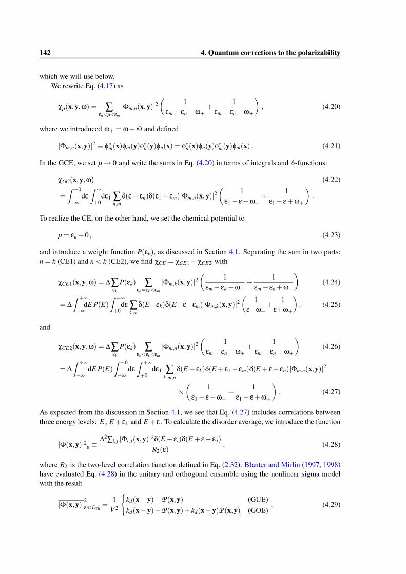
142 4. Quantum corrections to the polarizability
which we will use below.We rewrite Eq. (4.17) as
χµ(x,y,ω) = ∑εn<µ<εm
|Φm,n(x,y)|2(
1εm− εn−ω+
+1
εm− εn +ω+
), (4.20)
where we introduced ω+ = ω+ i0 and defined
|Φm,n(x,y)|2 ≡ φ∗m(x)φm(y)φ∗n(y)φn(x) = φ∗n(x)φn(y)φ∗m(y)φm(x) . (4.21)
In the GCE, we set µ→ 0 and write the sums in Eq. (4.20) in terms of integrals and δ-functions:
χGC(x,y,ω) (4.22)
=∫ −0
−∞dε
∫ ∞
+0dε1 ∑
n,mδ(ε− εn)δ(ε1− εm)|Φm,n(x,y)|2
(1
ε1− ε−ω++
1ε1− ε+ω+
).
To realize the CE, on the other hand, we set the chemical potential to
µ = εk +0 , (4.23)
and introduce a weight function P(εk), as discussed in Section 4.1. Separating the sum in two parts:n = k (CE1) and n < k (CE2), we find χCE = χCE1 +χCE2 with
χCE1(x,y,ω) = ∆∑εk
P(εk) ∑εn=εk<εm
|Φm,k(x,y)|2(
1εm− εk−ω+
+1
εm− εk +ω+
)(4.24)
= ∆∫ +∞
−∞dE P(E)
∫ +∞
+0dε ∑
k,mδ(E−εk)δ(E+ε−εm)|Φm,k(x,y)|2
(1
ε−ω++
1ε+ω+
), (4.25)
and
χCE2(x,y,ω) = ∆∑εk
P(εk) ∑εn<εk<εm
|Φm,n(x,y)|2(
1εm− εn−ω+
+1
εm− εn +ω+
)(4.26)
= ∆∫ +∞
−∞dE P(E)
∫ −0
−∞dε
∫ +∞
+0dε1 ∑
k,m,nδ(E− εk)δ(E + ε1− εm)δ(E + ε− εn)|Φm,n(x,y)|2
×(
1ε1− ε−ω+
+1
ε1− ε+ω+
). (4.27)
As expected from the discussion in Section 4.1, we see that Eq. (4.27) includes correlations betweenthree energy levels: E , E + ε1 and E + ε. To calculate the disorder average, we introduce the function
|Φ(x,y)|2ε ≡∆2∑i, j |Φi, j(x,y)|2δ(E− εi)δ(E + ε− ε j)
R2(ε), (4.28)
where R2 is the two-level correlation function defined in Eq. (2.32). Blanter and Mirlin (1997, 1998)have evaluated Eq. (4.28) in the unitary and orthogonal ensemble using the nonlinear sigma modelwith the result
|Φ(x,y)|2ε�ETh=
1V 2
{kd(x−y)+P (x,y) (GUE)kd(x−y)+P (x,y)+ kd(x−y)P (x,y) (GOE)
, (4.29)
4. Quantum corrections to the polarizability 143
where P is defined in Eq. (4.19) and kd is a short-range function on the scale `. Since the polarizabil-ity is governed by the long-range behavior of χ, see Eq. (4.14), we can neglect the contribution ∼ kdand use the approximation
|Φ(x,y)|2ε�ETh≈ 1
V 2 P (x,y) (GUE) and (GOE) (4.30)
in the following. Importantly, the matrix element (4.30) is independent of ε at ε� ETh . Moreover,we define the matrix element with two energy indices as follows:
|Φ(x,y)|2ε1,ε ≡∆3∑i, j,k |Φi, j(x,y)|2δ(E− εi)δ(E + ε1− ε j)δ(E + ε− εk)
R3(ε1,ε). (4.31)
where the three-level correlation function is defined as
R3(ε1,ε)≡ ∆3 ∑i, j,k
δ(E− εi)δ(E + ε1− ε j)δ(E + ε− εk) . (4.32)
Blanter and Mirlin (2001) have argued that the same long-range behavior as described by Eq. (4.30)can be expected for this quantity at ε,ε1� ETh .
Using the definition (4.28), and integrating out E , by using∫
dE P(E) = 1, one obtains fromEq. (4.22) for the GCE:
χGCE(x,y,ω) =1
∆2
∫ ∞
+0dε ε R2(ε)|Φ(x,y)|2ε
(1
ε−ω++
1ε+ω+
), (4.33)
and from Eqs. (4.25, 4.27) for the CE:
χCE(x,y,ω) (4.34)
=1
∆2
∫ ∞
+0dε(
∆R2(ε)|Φ(x,y)|2ε +∫ ε−0
+0dε1 R3(ε,ε1)|Φ(x,y)|2ε,ε1
) (1
ε−ω++
1ε+ω+
).
It is instructive to split the quantum corrections, δχ = χGUE −χGOE , to Eqs. (4.33, 4.34) into 4 parts:
δχGCE(x,y,ω) = δχGCE1(x,y,ω)+δχGCE2(x,y,ω) (4.35)
δχCE(x,y,ω) = δχGCE(x,y,ω)+δχCE1(x,y,ω)+δχCE2(x,y,ω) ,
with
δχGCE1(x,y,ω) =1
∆2
∫ ∞
+0dε2δ
[R2(ε)|Φ(x,y)|2ε
](4.36)
δχGCE2(x,y,ω) =1
∆2
∫ ∞
+0dε
2ω2+
ε2−ω2+
δ[R2(ε)|Φ(x,y)|2ε
](4.37)
δχCE1(x,y,ω) =1
∆2
∫ ∞
+0dε
2εε2−ω2
+
∆δ[R2(ε)|Φ(x,y)|2ε
](4.38)
δχCE2(x,y,ω) =1
∆2
∫ ∞
+0dε
2εε2−ω2
+
∫ ε−0
+0dε1 δ
[R3(ε,ε1)|Φ(x,y)|2ε,ε1
], (4.39)
where R3(ε,ε1) = R3(ε,ε1)−R2(ε).
144 4. Quantum corrections to the polarizability
Let us first consider the contribution δχGCE1 . Using the definition of the matrix element (4.28) inEq. (4.36), and symmetrizing the ε-integral, we obtain:
δχGCE1(x,y,ω) =∫ ∞
−∞dε δ
[∑i 6= j|Φi, j(x,y)|2δ(E− εi)δ(E + ε− ε j)
]
= δ
[∑i6= j|Φi, j(x,y)|2δ(E− εi)
]
= δ
[∑i j|Φi, j(x,y)|2δ(E− εi)−∑
i|Φi,i(x,y)|2δ(E− εi)
].
After summing over j, the first term is just a density of states and does not depend on the ensemble,cf. Eq. (2.66). The second term has been evaluated in Blanter and Mirlin (1997, 1998) using thenon-linear sigma model:
|Φi,i(x,y)|2ε ≡ ∆∑i|Φi,i(x,y)|2δ(ε− εi)≈
1V 2
{[1+ P (x,y)] [1+ kd(x,y)] (GUE)[1+2P (x,y)] [1+2kd(x,y)] (GOE)
. (4.40)
Neglecting the short-range contribution, we find
δχGCE1(x,y,ω) =1
∆V 2 P (x,y) . (4.41)
We will see below that the contribution (4.41) dominates the polarizability in the range ∆� ω� EThfor both statistical ensembles, the GCE and the CE. In the second contribution, δχGCE2 , the integralis dominated by small ε ∼ ω� ETh. At these values of ε, the matrix element δ|Φ|2ε is constant, andwe can write:
δχGCE2(x,y,ω) =1
∆2 |Φ(x,y)|20
∫ ∞
+0dε[
2ω2
ε2−ω2+
]δ[R2(ε)] . (4.42)
Moreover, since∫ ∞
+0dεδR2(ε) = 0 , (4.43)
one can add any constant term in the square brackets of Eq. (4.42). In particular, we can write:
δχGCE2(x,y,ω) =1
∆2 |Φ(x,y)|20
∫ ∞
+0dε(
1ε−ω+
+1
ε+ω+
)εδ [R2(ε)] (4.44)
=1
∆2V 2 P (x,y)∫ ∞
+0dε(
1ε−ω+
+1
ε+ω+
)εδ [R2(ε)] , (4.45)
where we used Eq. (4.30). Similarly, we can neglect the ε dependence of |Φ(x,y)|2ε and |Φ(x,y)|2ε,ε1
in the terms χCE1 and χCE2 and find
δχCE1(x,y,ω) =1
∆2V 2 P (x,y)∫ ∞
+0dε(
1ε−ω+
+1
ε+ω+
)∆ δ [R2(ε)] (4.46)
δχCE2(x,y,ω) =1
∆2V 2 P (x,y)∫ ∞
+0dε(
1ε−ω+
+1
ε+ω+
)∫ ε−0
+0dε1 δ
[R3(ε,ε1)
].
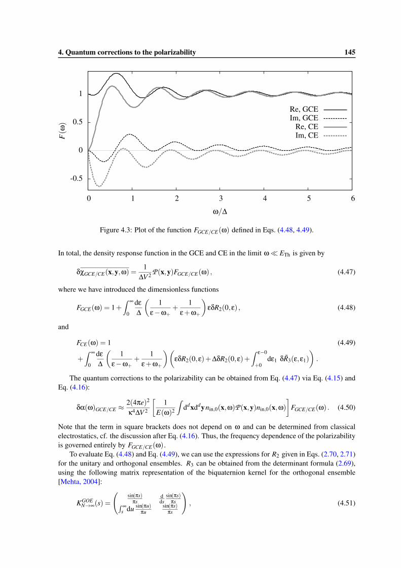
4. Quantum corrections to the polarizability 145
-0.5
0
0.5
1
0 1 2 3 4 5 6
F(ω
)
ω/∆
Re, GCEIm, GCE
Re, CEIm, CE
Figure 4.3: Plot of the function FGCE/CE(ω) defined in Eqs. (4.48, 4.49).
In total, the density response function in the GCE and CE in the limit ω� ETh is given by
δχGCE/CE(x,y,ω) =1
∆V 2 P (x,y)FGCE/CE(ω) , (4.47)
where we have introduced the dimensionless functions
FGCE(ω) = 1+∫ ∞
0
dε∆
(1
ε−ω++
1ε+ω+
)εδR2(0,ε) , (4.48)
and
FCE(ω) = 1 (4.49)
+∫ ∞
0
dε∆
(1
ε−ω++
1ε+ω+
)(εδR2(0,ε)+∆δR2(0,ε)+
∫ ε−0
+0dε1 δR3(ε,ε1)
).
The quantum corrections to the polarizability can be obtained from Eq. (4.47) via Eq. (4.15) andEq. (4.16):
δα(ω)GCE/CE ≈2(4πe)2
κ4∆V 2
[1
E(ω)2
∫ddxddynin,0(x,ω)P (x,y)nin,0(x,ω)
]FGCE/CE(ω) . (4.50)
Note that the term in square brackets does not depend on ω and can be determined from classicalelectrostatics, cf. the discussion after Eq. (4.16). Thus, the frequency dependence of the polarizabilityis governed entirely by FGCE/CE(ω).
To evaluate Eq. (4.48) and Eq. (4.49), we can use the expressions for R2 given in Eqs. (2.70, 2.71)for the unitary and orthogonal ensembles. R3 can be obtained from the determinant formula (2.69),using the following matrix representation of the biquaternion kernel for the orthogonal ensemble[Mehta, 2004]:
KGOEN→∞(s) =
(sin(πs)
πsdds
sin(πs)πs∫ ∞
s du sin(πu)πu
sin(πs)πs
), (4.51)
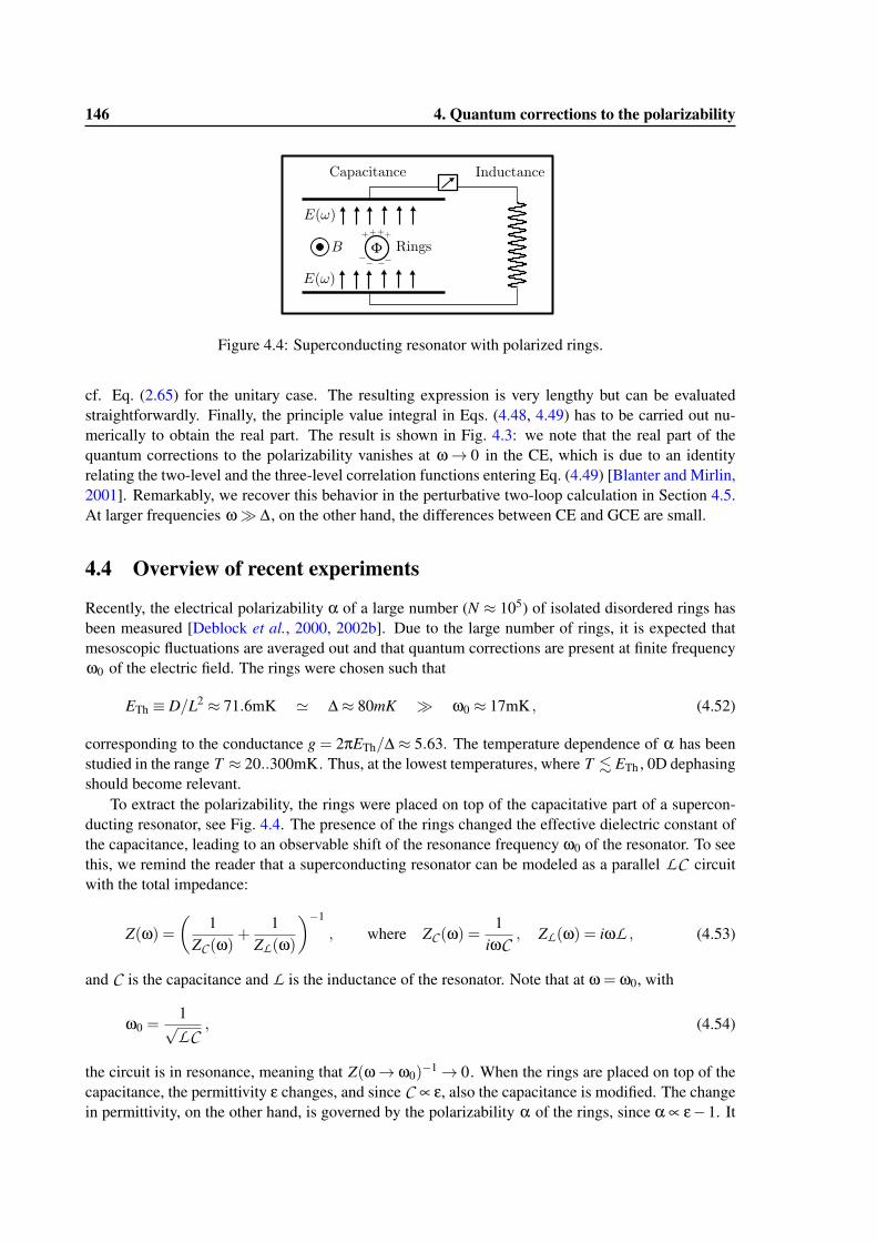
146 4. Quantum corrections to the polarizability
Figure 4.4: Superconducting resonator with polarized rings.
cf. Eq. (2.65) for the unitary case. The resulting expression is very lengthy but can be evaluatedstraightforwardly. Finally, the principle value integral in Eqs. (4.48, 4.49) has to be carried out nu-merically to obtain the real part. The result is shown in Fig. 4.3: we note that the real part of thequantum corrections to the polarizability vanishes at ω→ 0 in the CE, which is due to an identityrelating the two-level and the three-level correlation functions entering Eq. (4.49) [Blanter and Mirlin,2001]. Remarkably, we recover this behavior in the perturbative two-loop calculation in Section 4.5.At larger frequencies ω� ∆, on the other hand, the differences between CE and GCE are small.
4.4 Overview of recent experiments
Recently, the electrical polarizability α of a large number (N ≈ 105) of isolated disordered rings hasbeen measured [Deblock et al., 2000, 2002b]. Due to the large number of rings, it is expected thatmesoscopic fluctuations are averaged out and that quantum corrections are present at finite frequencyω0 of the electric field. The rings were chosen such that
ETh ≡ D/L2 ≈ 71.6mK ' ∆≈ 80mK � ω0 ≈ 17mK , (4.52)
corresponding to the conductance g = 2πETh/∆ ≈ 5.63. The temperature dependence of α has beenstudied in the range T ≈ 20..300mK. Thus, at the lowest temperatures, where T . ETh , 0D dephasingshould become relevant.
To extract the polarizability, the rings were placed on top of the capacitative part of a supercon-ducting resonator, see Fig. 4.4. The presence of the rings changed the effective dielectric constant ofthe capacitance, leading to an observable shift of the resonance frequency ω0 of the resonator. To seethis, we remind the reader that a superconducting resonator can be modeled as a parallel LC circuitwith the total impedance:
Z(ω) =(
1ZC (ω)
+1
ZL(ω)
)−1
, where ZC (ω) =1
iωC, ZL(ω) = iωL , (4.53)
and C is the capacitance and L is the inductance of the resonator. Note that at ω = ω0, with
ω0 =1√LC
, (4.54)
the circuit is in resonance, meaning that Z(ω→ ω0)−1→ 0. When the rings are placed on top of the
capacitance, the permittivity ε changes, and since C ∝ ε, also the capacitance is modified. The changein permittivity, on the other hand, is governed by the polarizability α of the rings, since α ∝ ε−1. It
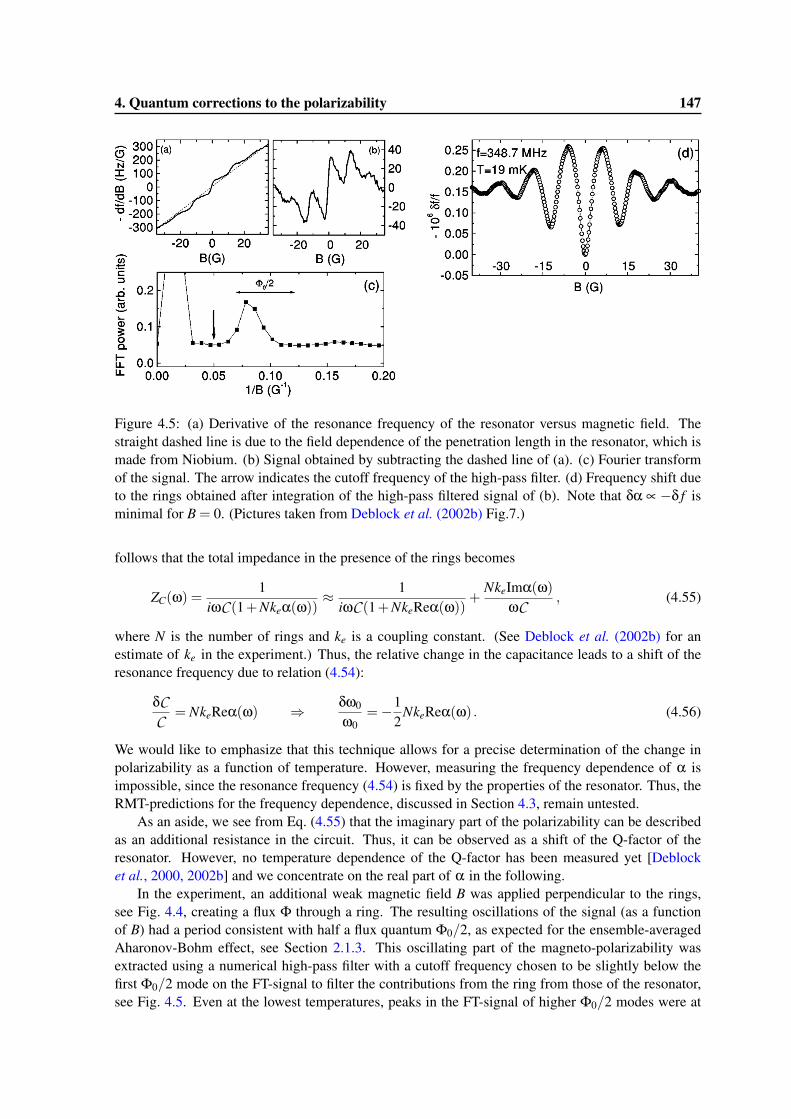
4. Quantum corrections to the polarizability 147
Figure 4.5: (a) Derivative of the resonance frequency of the resonator versus magnetic field. Thestraight dashed line is due to the field dependence of the penetration length in the resonator, which ismade from Niobium. (b) Signal obtained by subtracting the dashed line of (a). (c) Fourier transformof the signal. The arrow indicates the cutoff frequency of the high-pass filter. (d) Frequency shift dueto the rings obtained after integration of the high-pass filtered signal of (b). Note that δα ∝ −δ f isminimal for B = 0. (Pictures taken from Deblock et al. (2002b) Fig.7.)
follows that the total impedance in the presence of the rings becomes
ZC(ω) =1
iωC (1+Nkeα(ω))≈ 1
iωC (1+NkeReα(ω))+
NkeImα(ω)ωC
, (4.55)
where N is the number of rings and ke is a coupling constant. (See Deblock et al. (2002b) for anestimate of ke in the experiment.) Thus, the relative change in the capacitance leads to a shift of theresonance frequency due to relation (4.54):
δCC
= NkeReα(ω) ⇒ δω0
ω0=−1
2NkeReα(ω) . (4.56)
We would like to emphasize that this technique allows for a precise determination of the change inpolarizability as a function of temperature. However, measuring the frequency dependence of α isimpossible, since the resonance frequency (4.54) is fixed by the properties of the resonator. Thus, theRMT-predictions for the frequency dependence, discussed in Section 4.3, remain untested.
As an aside, we see from Eq. (4.55) that the imaginary part of the polarizability can be describedas an additional resistance in the circuit. Thus, it can be observed as a shift of the Q-factor of theresonator. However, no temperature dependence of the Q-factor has been measured yet [Deblocket al., 2000, 2002b] and we concentrate on the real part of α in the following.
In the experiment, an additional weak magnetic field B was applied perpendicular to the rings,see Fig. 4.4, creating a flux Φ through a ring. The resulting oscillations of the signal (as a functionof B) had a period consistent with half a flux quantum Φ0/2, as expected for the ensemble-averagedAharonov-Bohm effect, see Section 2.1.3. This oscillating part of the magneto-polarizability wasextracted using a numerical high-pass filter with a cutoff frequency chosen to be slightly below thefirst Φ0/2 mode on the FT-signal to filter the contributions from the ring from those of the resonator,see Fig. 4.5. Even at the lowest temperatures, peaks in the FT-signal of higher Φ0/2 modes were at
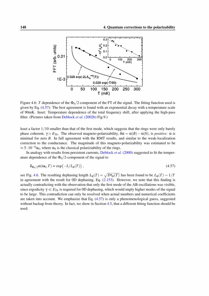
148 4. Quantum corrections to the polarizability
Figure 4.6: T dependence of the Φ0/2 component of the FT of the signal. The fitting function used isgiven by Eq. (4.57): The best agreement is found with an exponential decay with a temperature scaleof 90mK. Inset: Temperature dependence of the total frequency shift, after applying the high-passfilter. (Pictures taken from Deblock et al. (2002b) Fig.9.)
least a factor 1/10 smaller than that of the first mode, which suggests that the rings were only barelyphase coherent, γ' ETh . The observed magneto-polarizability, δα = α(B)−α(0), is positive: α isminimal for zero B. In full agreement with the RMT results, and similar to the weak-localizationcorrection to the conductance. The magnitude of this magneto-polarizability was estimated to be≈ 5 ·10−4α0, where α0 is the classical polariziability of the rings.
In analogy with results from persistent currents, Deblock et al. (2000) suggested to fit the temper-ature dependence of the Φ0/2-component of the signal to
δΦ0/2α(ω0,T ) ∝ exp(−L/Lϕ(T )
), (4.57)
see Fig. 4.6. The resulting dephasing length Lϕ(T ) =√
Dτϕ(T ) has been found to be Lϕ(T )∼ 1/Tin agreement with the result for 0D dephasing, Eq. (2.153). However, we note that this finding isactually contradicting with the observation that only the first mode of the AB-oscillations was visible,since ergodicity γ� ETh is required for 0D dephasing, which would imply higher modes of the signalto be large. This contradiction can only be resolved when actual numbers and numerical coefficientsare taken into account. We emphasize that Eq. (4.57) is only a phenomenological guess, suggestedwithout backup from theory. In fact, we show in Section 4.5, that a different fitting function should beused.
4.5 Preprint: Quantum Corrections to the Polarizability of IsolatedDisordered Metals
The following 12 pages have been made available as a preprint at arXiv:1304.4342.
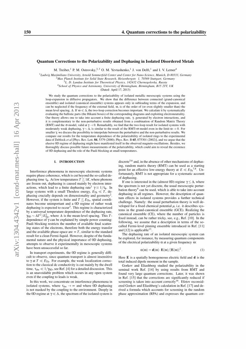
Quantum Corrections to the Polarizability and Dephasing in Isolated Disordered Metals
M. Treiber,1 P. M. Ostrovsky,2, 3 O. M. Yevtushenko,1 J. von Delft,1 and I. V. Lerner4
1Ludwig Maximilians University, Arnold Sommerfeld Center and Center for Nano-Science, Munich, D-80333, Germany2Max Planck Institute for Solid State Research, Heisenbergstr. 1, 70569 Stuttgart, Germany
3L. D. Landau Institute for Theoretical Physics, 142432 Chernogolovka, Russia4School of Physics and Astronomy, University of Birmingham, Birmingham, B15 2TT, UK
(Dated: April 17, 2013)
We study the quantum corrections to the polarizability of isolated metallic mesoscopic systems using theloop-expansion in diffusive propagators. We show that the difference between connected (grand-canonicalensemble) and isolated (canonical ensemble) systems appears only in subleading terms of the expansion, andcan be neglected if the frequency of the external field, ω, is of the order of (or even slightly smaller than) themean level spacing, ∆. If ω� ∆, the two-loop correction becomes important. We calculate it by systematicallyevaluating the ballistic parts (the Hikami boxes) of the corresponding diagrams and exploiting electroneutrality.Our theory allows one to take into account a finite dephasing rate, γ, generated by electron interactions, andit is complementary to the non-perturbative results obtained from a combination of Random Matrix Theory(RMT) and the σ-model, valid at γ→ 0. Remarkably, we find that the two-loop result for isolated systems withmoderately weak dephasing, γ ∼ ∆, is similar to the result of the RMT+σ-model even in the limit ω→ 0. Forsmaller γ, we discuss the possibility to interpolate between the perturbative and the non-perturbative results. Wecompare our results for the temperature dependence of the polarizability of isolated rings to the experimentaldata of Deblock et al [Phys. Rev. Lett. 84, 5379 (2000); Phys. Rev. B 65, 075301 (2002)], and we argue that theelusive 0D regime of dephasing might have manifested itself in the observed magneto-oscillations. Besides, wethoroughly discuss possible future measurements of the polarizability, which could aim to reveal the existenceof 0D dephasing and the role of the Pauli blocking at small temperatures.
I. INTRODUCTION
Interference phenomena in mesoscopic electronic systemsrequire phase coherence, which is cut beyond the so-called de-phasing time τφ. At low temperatures T . 1K, where phononsare frozen out, dephasing is caused mainly by electron inter-actions, which lead to a finite dephasing rate1 γ ≡ 1/τφ. Inlarge systems with a small Thouless energy, ETh � T , de-phasing crucially depends on dimensionality and geometry2.However, if the system is finite and T . ETh, spatial coordi-nates become unimportant and a 0D regime of rather weakdephasing is expected to occur3. This regime is characterizedby a universal temperature dependence of the dephasing rate,γ0D ∼ ∆T 2/E2
Th, where ∆ is the mean-level spacing. This T -dependence of γ can be explained by simple power counting:Pauli blocking restricts the number of available final scatter-ing states of the electrons, therefore both the energy transferand the available phase-space are ∝ T , similar to the standardresult for a clean Fermi-liquid. However, despite of the funda-mental nature and the physical importance of 0D dephasing,attempts to observe it experimentally in mesoscopic systemshave been unsuccessful so far.
In transport experiments, the 0D regime is generally diffi-cult to observe, since quantum transport is almost insensitiveto γ at T � ETh. For example, the weak localization correc-tion to the classical dc conductivity is cut mainly by the dwelltime, τdw� 1/γ0D, see Ref. [4] for a detailed discussion. Thisis an unavoidable problem which occurs in any open systemeven if the coupling to leads is weak.
In this work, we concentrate on interference phenomena inisolated systems, where τdw → ∞ and where 0D dephasingis not masked by the coupling to the environment. Deeply inthe 0D regime at γ� ∆ , the spectrum of the isolated system is
discrete5,6 and, in the absence of other mechanisms of dephas-ing, random matrix theory (RMT) can be used as a startingpoint for an effective low-energy theory at E � ETh
7,8. Un-fortunately, RMT is not appropriate for a systematic accountof dephasing.
If one is interested in the (almost 0D) regime γ≤ ∆, wherethe spectrum is not yet discrete, the usual mesoscopic pertur-bation theory9 can be used, which is able to take into accountdephasing in all regimes. However, the description of quan-tum effects in isolated systems provides a further technicalchallenge. Namely: the usual perturbation theory is well de-veloped for a fixed chemical potential µ, i.e. it describes sys-tems in the grand-canonical ensemble (GCE). Realizing thecanonical ensemble (CE), where the number of particles isfixed instead, can be rather tricky, see, e.g., Ref. [10]. In thefollowing, we assume that a description in terms of the so-called Fermi-level pinning ensemble introduced in Ref. [11]and [12] is applicable13.
The dephasing rate of an isolated mesoscopic system canbe explored, for instance, by measuring quantum componentsof the electrical polarizability α at a given frequency ω:
α(ω) = d(ω) ·E(ω)/|E(ω)|2 . (1)
Here E is a spatially homogeneous electric field and d is thetotal induced dipole moment in the sample.
Gorkov and Eliashberg studied the polarizability in theseminal work Ref. [14] by using results from RMT andfound very large quantum corrections. Later, it was shownin Ref. [15] that the corrections are significantly reduced ifscreening is taken into account correctly16. Efetov reconsid-ered Gorkov and Eliashberg’s calculation in Ref. [17] and de-rived a formula which accounts for screening in the randomphase approximation (RPA) and expresses the quantum cor-
arX
iv:1
304.
4342
v1 [
cond
-mat
.mes
-hal
l] 1
6 A
pr 2
013
150 4. Quantum corrections to the polarizability
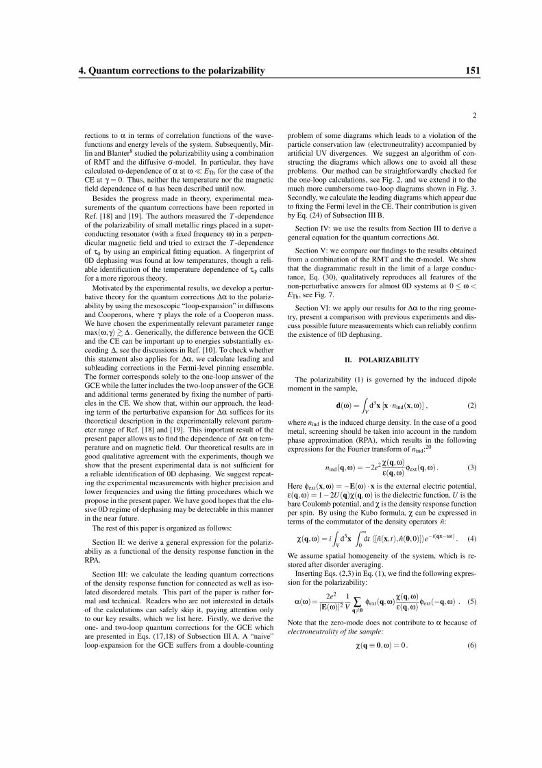
2
rections to α in terms of correlation functions of the wave-functions and energy levels of the system. Subsequently, Mir-lin and Blanter8 studied the polarizability using a combinationof RMT and the diffusive σ-model. In particular, they havecalculated ω-dependence of α at ω� ETh for the case of theCE at γ = 0. Thus, neither the temperature nor the magneticfield dependence of α has been described until now.
Besides the progress made in theory, experimental mea-surements of the quantum corrections have been reported inRef. [18] and [19]. The authors measured the T -dependenceof the polarizability of small metallic rings placed in a super-conducting resonator (with a fixed frequency ω) in a perpen-dicular magnetic field and tried to extract the T -dependenceof τφ by using an empirical fitting equation. A fingerprint of0D dephasing was found at low temperatures, though a reli-able identification of the temperature dependence of τϕ callsfor a more rigorous theory.
Motivated by the experimental results, we develop a pertur-bative theory for the quantum corrections ∆α to the polariz-ability by using the mesoscopic “loop-expansion” in diffusonsand Cooperons, where γ plays the role of a Cooperon mass.We have chosen the experimentally relevant parameter rangemax(ω,γ) & ∆ . Generically, the difference between the GCEand the CE can be important up to energies substantially ex-ceeding ∆, see the discussions in Ref. [10]. To check whetherthis statement also applies for ∆α, we calculate leading andsubleading corrections in the Fermi-level pinning ensemble.The former corresponds solely to the one-loop answer of theGCE while the latter includes the two-loop answer of the GCEand additional terms generated by fixing the number of parti-cles in the CE. We show that, within our approach, the lead-ing term of the perturbative expansion for ∆α suffices for itstheoretical description in the experimentally relevant param-eter range of Ref. [18] and [19]. This important result of thepresent paper allows us to find the dependence of ∆α on tem-perature and on magnetic field. Our theoretical results are ingood qualitative agreement with the experiments, though weshow that the present experimental data is not sufficient fora reliable identification of 0D dephasing. We suggest repeat-ing the experimental measurements with higher precision andlower frequencies and using the fitting procedures which wepropose in the present paper. We have good hopes that the elu-sive 0D regime of dephasing may be detectable in this mannerin the near future.
The rest of this paper is organized as follows:
Section II: we derive a general expression for the polariz-abiliy as a functional of the density response function in theRPA.
Section III: we calculate the leading quantum correctionsof the density response function for connected as well as iso-lated disordered metals. This part of the paper is rather for-mal and technical. Readers who are not interested in detailsof the calculations can safely skip it, paying attention onlyto our key results, which we list here. Firstly, we derive theone- and two-loop quantum corrections for the GCE whichare presented in Eqs. (17,18) of Subsection III A. A “naive”loop-expansion for the GCE suffers from a double-counting
problem of some diagrams which leads to a violation of theparticle conservation law (electroneutrality) accompanied byartificial UV divergences. We suggest an algorithm of con-structing the diagrams which allows one to avoid all theseproblems. Our method can be straightforwardly checked forthe one-loop calculations, see Fig. 2, and we extend it to themuch more cumbersome two-loop diagrams shown in Fig. 3.Secondly, we calculate the leading diagrams which appear dueto fixing the Fermi level in the CE. Their contribution is givenby Eq. (24) of Subsection III B.
Section IV: we use the results from Section III to derive ageneral equation for the quantum corrections ∆α.
Section V: we compare our findings to the results obtainedfrom a combination of the RMT and the σ-model. We showthat the diagrammatic result in the limit of a large conduc-tance, Eq. (30), qualitatively reproduces all features of thenon-perturbative answers for almost 0D systems at 0 ≤ ω <ETh, see Fig. 7.
Section VI: we apply our results for ∆α to the ring geome-try, present a comparison with previous experiments and dis-cuss possible future measurements which can reliably confirmthe existence of 0D dephasing.
II. POLARIZABILITY
The polarizability (1) is governed by the induced dipolemoment in the sample,
d(ω) =∫
Vd3x [x ·nind(x,ω)] , (2)
where nind is the induced charge density. In the case of a goodmetal, screening should be taken into account in the randomphase approximation (RPA), which results in the followingexpressions for the Fourier transform of nind:20
nind(q,ω) =−2e2 χ(q,ω)ε(q,ω)
φext(q,ω) . (3)
Here φext(x,ω) = −E(ω) · x is the external electric potential,ε(q,ω) = 1−2U(q)χ(q,ω) is the dielectric function, U is thebare Coulomb potential, and χ is the density response functionper spin. By using the Kubo formula, χ can be expressed interms of the commutator of the density operators n:
χ(q,ω) = i∫
Vd3x
∫ ∞
0dt 〈[n(x, t), n(0,0)]〉e−i(qx−ωt) . (4)
We assume spatial homogeneity of the system, which is re-stored after disorder averaging.
Inserting Eqs. (2,3) in Eq. (1), we find the following expres-sion for the polarizability:
α(ω)=2e2
|E(ω)|21V ∑
q6=0φext(q,ω)
χ(q,ω)ε(q,ω)
φext(−q,ω) . (5)
Note that the zero-mode does not contribute to α because ofelectroneutrality of the sample:
χ(q≡ 0,ω) = 0 . (6)
4. Quantum corrections to the polarizability 151
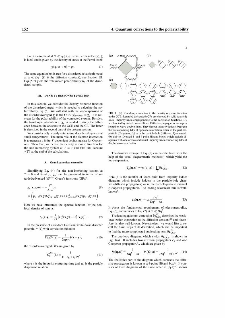
3
For a clean metal at ω� vFq (vF is the Fermi velocity), χis local and is given by the density of states at the Fermi level:
χ(q,ω→ 0) = ρ0 . (7)
The same equation holds true for a disordered (classical) metalat ω � Dq2 (D is the diffusion constant), see Section III.Eqs.(5,7) yield the ”classical“ polarizability α0 of the disor-dered sample.
III. DENSITY RESPONSE FUNCTION
In this section, we consider the density response functionof the disordered metal which is needed to calculate the po-larizability, Eq. (5). We will start with the loop-expansion ofthe disorder-averaged χ in the GCE: χ|µ=const ≡ χµ. It is rel-evant for the polarizability of the connected system. Besides,the two-loop contribution to χµ is needed to study the differ-ence between the answers in the GCE and the CE. The latteris described in the second part of the present section.
We consider only weakly-interacting disordered systems atsmall temperatures. The main role of the electron interactionis to generate a finite T -dependent dephasing rate for Cooper-ons. Therefore, we derive the density response function forthe non-interacting system at T = 0 and take into accountγ(T ) at the end of the calculations.
A. Grand canonical ensemble
Simplifying Eq. (4) for the non-interacting system atT = 0 and fixed µ, χµ can be presented in terms of re-tarded/advanced (GR/A) Green’s functions (GFs)9:
χµ(x,y,ω) =−∫ 0
−∞dε (8)
×(
ρµ+ε(x,y)GAµ+ε−ω(y,x)+GR
µ+ε+ω(x,y)ρµ+ε(y,x)).
Here we have introduced the spectral function (or the non-local density of states):
ρε(x,y)≡i
2π[GR
ε (x,y)−GAε (x,y)
]. (9)
In the presence of a random Gaussian white-noise disorderpotential V (x) with correlation function
V (x)V (y) =1
2πρ0τδ(x−y) , (10)
the disorder-averaged GFs are given by
GR/Aε (k) =
1ε− εk± i/2τ
, (11)
where τ is the impurity scattering time and εk is the particledispersion relation.
FIG. 1. (a): One-loop correction to the density response functionin the GCE. Retarded (advanced) GFs are denoted by solid (dashed)lines. Impurity lines, corresponding to the correlation function (10),are denoted by dotted crossed lines. Diffusive propagators are repre-sented by wavy double lines. They denote impurity ladders betweenthe corresponding GFs of opposite retardation either in the particle-particle (Cooperon, Pc) or in the particle-hole (diffuson, Pd) channel.(b) and (c): Dressed 4- and 6-point Hikami boxes which include di-agrams with one or two additional impurity lines connecting GFs ofthe the same retardation.
The disorder average of Eq. (8) can be calculated with thehelp of the usual diagrammatic methods,1 which yield theloop-expansion:
χµ(q,ω) = χ0(q,ω)+∑j
δχ( j)GCE . (12)
Here j is the number of loops built from impurity ladderdiagrams which include ladders in the particle-hole chan-nel (diffuson propagators) or in the particle-particle channel(Cooperon propagators). The leading (classical) term is well-known1:
χ0(q,ω) = ρ0Dq2
Dq2− iω. (13)
It obeys the fundamental requirement of electroneutrality,Eq. (6), and reduces to Eq. (7) at ω� Dq2.
The leading quantum correction δχ(1)GCE describes the weak-
localization correction to the diffusion constant21 and, there-fore, is also well-known. Nevertheless, we would like to re-call the basic steps of its derivation, which will be importantto find the more complicated subleading term δχ(2)
GCE.
The one-loop diagram, which yields δχ(1)GCE, is shown in
Fig. 1(a). It includes two diffuson propagators Pd and oneCooperon propagator Pc, which are given by
Pd(q,ω) =1
Dq2− iω, Pc(Q,ω) =
1DQ2− iω+ γ
. (14)
The (ballistic) part of the diagram which connects the diffu-sive propagators is known as a 4-point Hikami box22. It con-sists of three diagrams of the same order in (εFτ)−1 shown
152 4. Quantum corrections to the polarizability
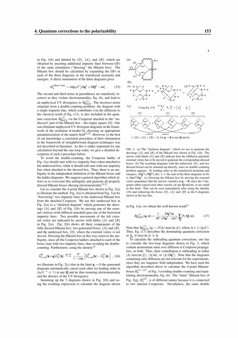
4
in Fig. 1(b) and labeled by {0}, {A}, and {B}, which areobtained by inserting additional impurity lines between GFsof the same retardation (“dressing” the Hikami box). TheHikami box should be calculated by expanding the GFs ineach of the three diagrams in the transferred momenta andenergies. A direct summation of the three diagrams gives
H(direct sum)4 = 4πρ0τ4 [Dq2 +DQ2− iω
]. (15)
The second and third terms in parentheses are manifestly in-correct as they violate electroneutrality, Eq. (6), and lead toan unphysical UV divergence in δχ(1)
GCE. The incorrect termsoriginate from a double-counting problem: the diagram witha single impurity line, which contributes (via the diffuson) tothe classical result of Eq. (13), is also included in the quan-tum correction δχ(1)
GCE via the Cooperon attached to the “un-dressed” part of the Hikami box – the empty square {0}. Onecan eliminate unphysical UV divergent diagrams in the frame-work of the nonlinear σ-model by choosing an appropriateparameterization of the matrix field23,25. However, to the bestof our knowledge a consistent procedure of their eliminationin the framework of straightforward diagram techniques wasnot described in literature. As this is rather important for anycalculation beyond the one-loop order, we give a detailed de-scription of such a procedure below.
To avoid the double-counting, the Cooperon ladder ofFig. 1(a) should start with two impurity lines when attached tothe undressed box, while it should still start with one impurityline when attached to the dressed box. Thus, there is an am-biguity in the independent definition of the Hikami boxes andthe ladder diagrams. We suggest a general algorithm which al-lows us to overcome this ambiguity and generate all properlydressed Hikami boxes obeying electroneutrality24,25.
Let us consider the 4-point Hikami box shown in Fig. 2(a)to illustrate the method. Fig. 2(a) is obtained from Fig. 1(a) by“borrowing” two impurity lines to the undressed Hikami boxfrom the attached Cooperon. We use this undressed box inFig. 2(a) as a “skeleton diagram” which generates the dress-ings {A} and {B} of Fig. 1(b) by moving one of the exter-nal vertices (with diffuson attached) past one of the borrowedimpurity lines. Two possible movements of the left exter-nal vertex are indicated by arrows with lables {A} and {B}in Fig. 2(a). Fig. 2(b) shows all three components of thefully dressed Hikami box: two generated boxes, {A} and {B},and the undressed box, {0}, where the external vertex is notmoved. Dressing the Hikami box in this way removes the am-biguity, since all the Cooperon ladders attached to each of theboxes start with two impurity lines, thus avoiding the double-counting. Furthermore, using the identity24
GRε+ω(k+q)GA
ε (k)q→0−→ iτ
1− iτω
[GR
ε+ω(k)−GAε (k)
], (16)
we illustrate in Fig. 2(c) that in the limit q→ 0 the generateddiagrams automatically cancel each other (to leading order in(εFτ)−1� 1) at any Q and ω, thus ensuring electroneutralityand the absence of the UV divergence.
Summing up the 3 diagrams drawn in Fig. 2(b) and us-ing the resulting expression to calculate the diagram shown
FIG. 2. (a) The “skeleton diagram”, which we use to generate thedressings {A} and {B} of the Hikami box shown in Fig. 1(b). Thearrows with labels {A} and {B} indicate how the (diffuson attached)external vertex has to be moved to generate the correponding dressedboxes. (b) The resulting diagrams with the undressed, {0}, and twodressed boxed can be summed up directly, since no double-countingproblem appears. To leading order in the transferred momenta andenergies, (Dq2τ,DQ2τ,ωτ)� 1, the sum of the three diagrams in (b)is 4πρτ4Dq2. (c) Dressing the Hikami box by moving the externalvertex guarantees that the answer vanishes at q→ 0, since the 3 dia-grams either cancel each other exactly (at any Q and ω), or are smallin this limit. This can be seen immediately after using the identity(16) and redrawing the boxes {0}, {A} and {B} as the 6 diagramsshown in the last line.
in Fig. 1(a), we obtain the well-known result21
δχ(1)GCE(q,ω) =
1πV
Dq2iω(Dq2− iω)2 ∑
QPc(Q,ω) . (17)
Note that δχ(1)GCE/χ0 ∼ O(∆/max(ω,γ)), where ∆≡ 1/(ρ0V ).
Thus, Eq. (17) describes the dominating quantum correctionto χµ if max(ω,γ)� ∆.
To calculate the subleading quantum corrections, one hasto consider the two-loop diagrams shown in Fig. 3, whichcontain momentum sums over diffuson or Cooperon propaga-tors, or both. Thus, their contribution is subleading in either(∆/max(ω,γ)), (∆/ω), or (∆/Dq2). Note that the diagramscontaining only diffusons are not relevant for the experiments,since they are magnetic field independent. We have used thealgorithm described above to calculate the 4-point Hikami-boxes H(a)−(g1)
4 of Fig. 3 avoiding double-counting and main-taining electroneutrality, Eq. (6). The “inner” Hikami box ofFig. 3(g), H(g2)
4 , is of different nature because it is connectedto two internal Cooperons. Nevetheless, the same double
4. Quantum corrections to the polarizability 153
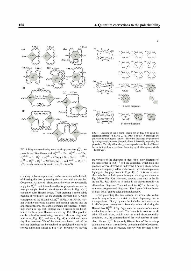
5
FIG. 3. Diagrams contributing to the two-loop correction χ(2)GCE. An-
swers for the Hikami boxes read: H(a,g1)4 = Dq2, H(b,c)
6 =−τ2Dq2,
H(d1,d2)6 = 0, H(e1)
4 ×H(e2)4 = (D(q(q + Q1 + Q2)))
2, H(f1)4 ×
H(f2)4 = H(f3)
4 ×H(f4)4 = 2D2(qQ1)(qQ2), and H(g2)
4 = D(Q12 +
γ/D), see the main text for details; here D = 4πρτ4D.
counting problem appears and can be overcome with the helpof dressing this box by moving the vertices with the attachedCooperons. As a result, electroneutrality does not necessarilyapply for H(g2)
4 , which is reflected by its γ-dependence, see thenext paragraph. Besides, the diagrams shown in Fig. 3(b-d)contain 6-point Hikami boxes. Their dressing is more subtlebecause of two issues, see the example shown in Fig. 4, whichcorresponds to the Hikami box H(b)
6 of Fig. 3(b): Firstly, start-ing with the undressed diagram and moving vertices into theattached diffusons, one cannot generate all required 15 dress-ings shown in Fig. 1(c). Instead, only 8 dressings can be ob-tained for the 6-point Hikami box, cf. Fig. 4(a). That problemcan be solved by considering two more “skeleton diagrams”with one-, Fig. 4(b), and two-, Fig. 4(c), additional impu-rity lines between GFs of the same retardation. All of themissing dressings can be obtained by applying the above de-scribed algorithm similar to Fig. 4(a). Secondly, by moving
FIG. 4. Dressing of the 6-point Hikami box of Fig. 3(b) using thealgorithm introduced in Fig. 2. (a) Only 8 of the 15 dressings aregenerated by moving the vertices. The other dressings are generatedby adding one (b) or two (c) impurity lines, followed by repeating theprocedure. This algorithm also generates products of 4-point Hikamiboxes, indicated by a grey box. Summing up all 40 diagrams yields−12πρτ6Dq2.
the vertices of the diagrams in Figs. 4(b,c) new diagrams ofthe same order in (εFτ)−1� 1 are generated, which look likeproducts of two dressed or undressed 4-point Hikami boxeswith a few-impurity ladder in-between. Several examples arehighlighted by grey boxes in Figs. 4(b,c). It is not a prioriclear whether such diagrams belong to the diagram shown inFig. 3(b) or Fig. 3(e). However, keeping them only in the di-agram Fig. 3(b) allows us to maintain the electroneutrality inall two-loop diagrams. The total result for H(b)
6 is obtained bysumming 40 generated diagrams. The 6-point Hikami boxesof Figs. 3(c,d) can be calculated analogously.
Before presenting the final answer, we would like to dis-cuss the way of how to reinstate the finite dephasing rate inthe equations. Firstly, γ must be included as a mass termin all Cooperon propagators. Secondly, when calculating theHikami box H(g2)
4 of Fig. 3(g), only the number of coherentmodes has to be conserved. The latter is in contrast to allother Hikami boxes, which obey the usual electroneutralitycondition, i.e., the conservation of the total number of parti-cles. Hence, H(g2)
4 is the only Hikami box of the two-loopcalculations which is sensitive to dephasing of the Cooperons.This statement can be checked directly with the help of the
154 4. Quantum corrections to the polarizability
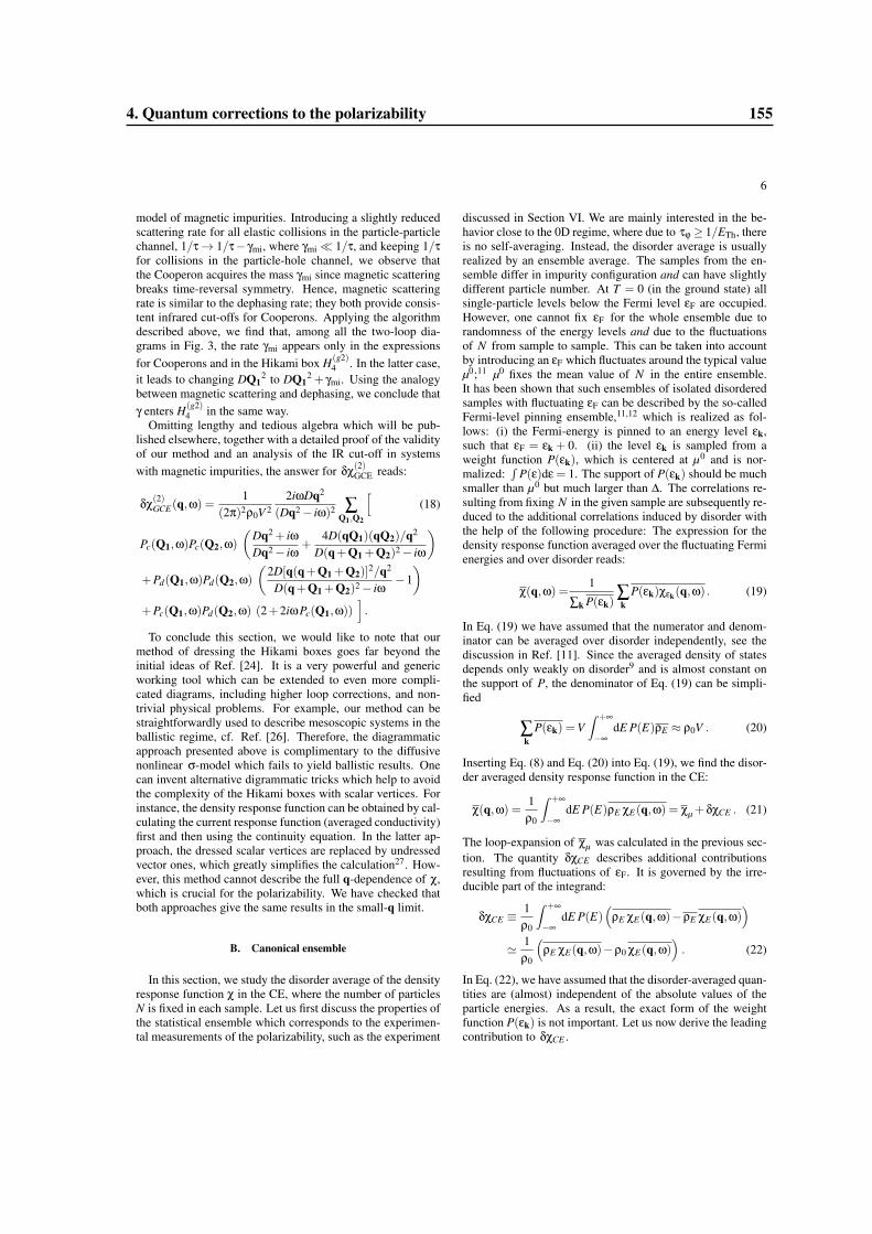
6
model of magnetic impurities. Introducing a slightly reducedscattering rate for all elastic collisions in the particle-particlechannel, 1/τ→ 1/τ− γmi, where γmi� 1/τ, and keeping 1/τfor collisions in the particle-hole channel, we observe thatthe Cooperon acquires the mass γmi since magnetic scatteringbreaks time-reversal symmetry. Hence, magnetic scatteringrate is similar to the dephasing rate; they both provide consis-tent infrared cut-offs for Cooperons. Applying the algorithmdescribed above, we find that, among all the two-loop dia-grams in Fig. 3, the rate γmi appears only in the expressionsfor Cooperons and in the Hikami box H(g2)
4 . In the latter case,it leads to changing DQ1
2 to DQ12 + γmi. Using the analogy
between magnetic scattering and dephasing, we conclude thatγ enters H(g2)
4 in the same way.Omitting lengthy and tedious algebra which will be pub-
lished elsewhere, together with a detailed proof of the validityof our method and an analysis of the IR cut-off in systemswith magnetic impurities, the answer for δχ(2)
GCE reads:
δχ(2)GCE(q,ω) =
1(2π)2ρ0V 2
2iωDq2
(Dq2− iω)2 ∑Q1,Q2
[(18)
Pc(Q1,ω)Pc(Q2,ω)(
Dq2 + iωDq2− iω
+4D(qQ1)(qQ2)/q2
D(q+Q1 +Q2)2− iω
)
+Pd(Q1,ω)Pd(Q2,ω)(
2D[q(q+Q1 +Q2)]2/q2
D(q+Q1 +Q2)2− iω−1)
+Pc(Q1,ω)Pd(Q2,ω) (2+2iωPc(Q1,ω))].
To conclude this section, we would like to note that ourmethod of dressing the Hikami boxes goes far beyond theinitial ideas of Ref. [24]. It is a very powerful and genericworking tool which can be extended to even more compli-cated diagrams, including higher loop corrections, and non-trivial physical problems. For example, our method can bestraightforwardly used to describe mesoscopic systems in theballistic regime, cf. Ref. [26]. Therefore, the diagrammaticapproach presented above is complimentary to the diffusivenonlinear σ-model which fails to yield ballistic results. Onecan invent alternative digrammatic tricks which help to avoidthe complexity of the Hikami boxes with scalar vertices. Forinstance, the density response function can be obtained by cal-culating the current response function (averaged conductivity)first and then using the continuity equation. In the latter ap-proach, the dressed scalar vertices are replaced by undressedvector ones, which greatly simplifies the calculation27. How-ever, this method cannot describe the full q-dependence of χ,which is crucial for the polarizability. We have checked thatboth approaches give the same results in the small-q limit.
B. Canonical ensemble
In this section, we study the disorder average of the densityresponse function χ in the CE, where the number of particlesN is fixed in each sample. Let us first discuss the properties ofthe statistical ensemble which corresponds to the experimen-tal measurements of the polarizability, such as the experiment
discussed in Section VI. We are mainly interested in the be-havior close to the 0D regime, where due to τϕ ≥ 1/ETh, thereis no self-averaging. Instead, the disorder average is usuallyrealized by an ensemble average. The samples from the en-semble differ in impurity configuration and can have slightlydifferent particle number. At T = 0 (in the ground state) allsingle-particle levels below the Fermi level εF are occupied.However, one cannot fix εF for the whole ensemble due torandomness of the energy levels and due to the fluctuationsof N from sample to sample. This can be taken into accountby introducing an εF which fluctuates around the typical valueµ0;11 µ0 fixes the mean value of N in the entire ensemble.It has been shown that such ensembles of isolated disorderedsamples with fluctuating εF can be described by the so-calledFermi-level pinning ensemble,11,12 which is realized as fol-lows: (i) the Fermi-energy is pinned to an energy level εk,such that εF = εk + 0. (ii) the level εk is sampled from aweight function P(εk), which is centered at µ0 and is nor-malized:
∫P(ε)dε = 1. The support of P(εk) should be much
smaller than µ0 but much larger than ∆. The correlations re-sulting from fixing N in the given sample are subsequently re-duced to the additional correlations induced by disorder withthe help of the following procedure: The expression for thedensity response function averaged over the fluctuating Fermienergies and over disorder reads:
χ(q,ω) =1
∑k P(εk)∑k
P(εk)χεk(q,ω) . (19)
In Eq. (19) we have assumed that the numerator and denom-inator can be averaged over disorder independently, see thediscussion in Ref. [11]. Since the averaged density of statesdepends only weakly on disorder9 and is almost constant onthe support of P, the denominator of Eq. (19) can be simpli-fied
∑k
P(εk) =V∫ +∞
−∞dE P(E)ρE ≈ ρ0V . (20)
Inserting Eq. (8) and Eq. (20) into Eq. (19), we find the disor-der averaged density response function in the CE:
χ(q,ω) =1ρ0
∫ +∞
−∞dE P(E)ρE χE(q,ω) = χµ +δχCE . (21)
The loop-expansion of χµ was calculated in the previous sec-tion. The quantity δχCE describes additional contributionsresulting from fluctuations of εF. It is governed by the irre-ducible part of the integrand:
δχCE ≡1ρ0
∫ +∞
−∞dE P(E)
(ρE χE(q,ω)−ρE χE(q,ω)
)
' 1ρ0
(ρE χE(q,ω)−ρ0 χE(q,ω)
). (22)
In Eq. (22), we have assumed that the disorder-averaged quan-tities are (almost) independent of the absolute values of theparticle energies. As a result, the exact form of the weightfunction P(εk) is not important. Let us now derive the leadingcontribution to δχCE .
4. Quantum corrections to the polarizability 155
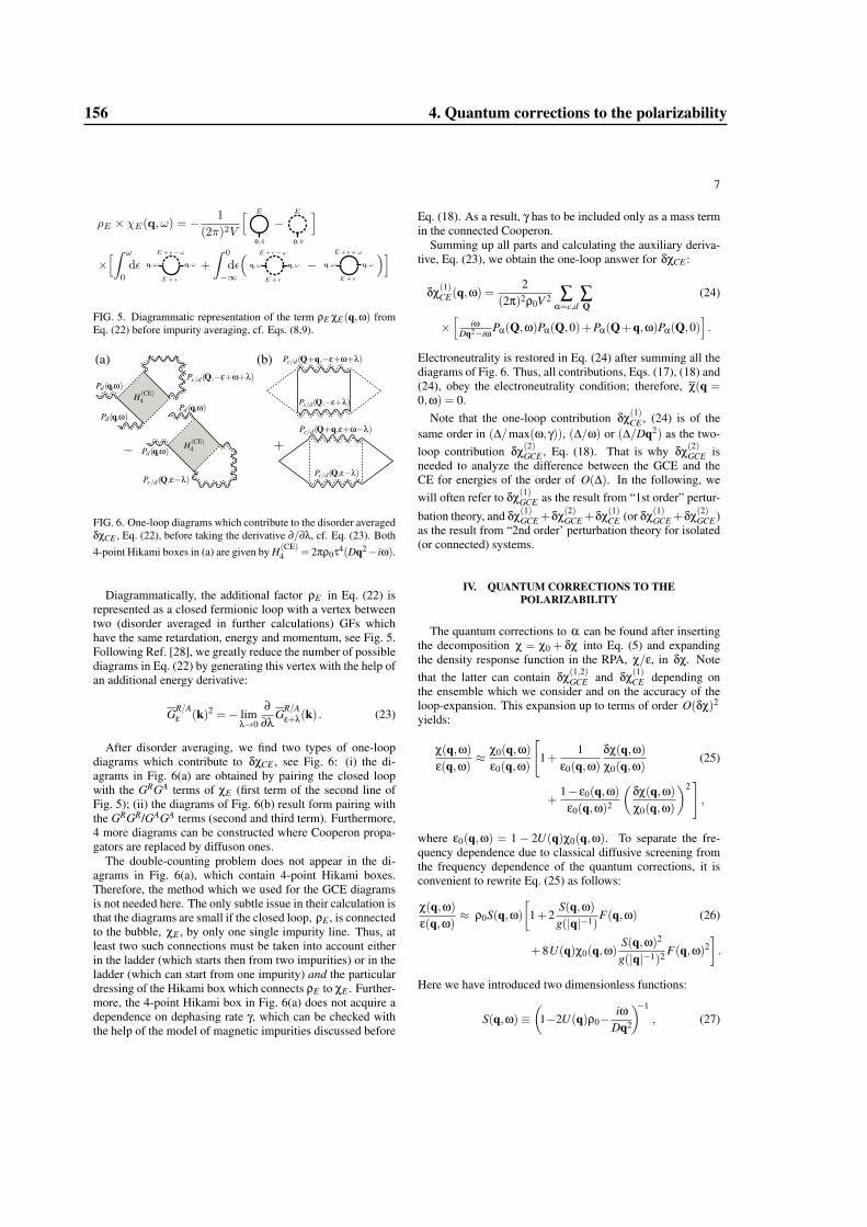
7
FIG. 5. Diagrammatic representation of the term ρE χE(q,ω) fromEq. (22) before impurity averaging, cf. Eqs. (8,9).
FIG. 6. One-loop diagrams which contribute to the disorder averagedδχCE , Eq. (22), before taking the derivative ∂/∂λ, cf. Eq. (23). Both4-point Hikami boxes in (a) are given by H(CE)
4 = 2πρ0τ4(Dq2− iω).
Diagrammatically, the additional factor ρE in Eq. (22) isrepresented as a closed fermionic loop with a vertex betweentwo (disorder averaged in further calculations) GFs whichhave the same retardation, energy and momentum, see Fig. 5.Following Ref. [28], we greatly reduce the number of possiblediagrams in Eq. (22) by generating this vertex with the help ofan additional energy derivative:
GR/Aε (k)2 =− lim
λ→0
∂∂λ
GR/Aε+λ(k) . (23)
After disorder averaging, we find two types of one-loopdiagrams which contribute to δχCE , see Fig. 6: (i) the di-agrams in Fig. 6(a) are obtained by pairing the closed loopwith the GRGA terms of χE (first term of the second line ofFig. 5); (ii) the diagrams of Fig. 6(b) result form pairing withthe GRGR/GAGA terms (second and third term). Furthermore,4 more diagrams can be constructed where Cooperon propa-gators are replaced by diffuson ones.
The double-counting problem does not appear in the di-agrams in Fig. 6(a), which contain 4-point Hikami boxes.Therefore, the method which we used for the GCE diagramsis not needed here. The only subtle issue in their calculation isthat the diagrams are small if the closed loop, ρE , is connectedto the bubble, χE , by only one single impurity line. Thus, atleast two such connections must be taken into account eitherin the ladder (which starts then from two impurities) or in theladder (which can start from one impurity) and the particulardressing of the Hikami box which connects ρE to χE . Further-more, the 4-point Hikami box in Fig. 6(a) does not acquire adependence on dephasing rate γ, which can be checked withthe help of the model of magnetic impurities discussed before
Eq. (18). As a result, γ has to be included only as a mass termin the connected Cooperon.
Summing up all parts and calculating the auxiliary deriva-tive, Eq. (23), we obtain the one-loop answer for δχCE :
δχ(1)CE(q,ω) =
2(2π)2ρ0V 2 ∑
α=c,d∑Q
(24)
×[
iωDq2−iω Pα(Q,ω)Pα(Q,0)+Pα(Q+q,ω)Pα(Q,0)
].
Electroneutrality is restored in Eq. (24) after summing all thediagrams of Fig. 6. Thus, all contributions, Eqs. (17), (18) and(24), obey the electroneutrality condition; therefore, χ(q =0,ω) = 0.
Note that the one-loop contribution δχ(1)CE , (24) is of the
same order in (∆/max(ω,γ)), (∆/ω) or (∆/Dq2) as the two-loop contribution δχ(2)
GCE , Eq. (18). That is why δχ(2)GCE is
needed to analyze the difference between the GCE and theCE for energies of the order of O(∆). In the following, wewill often refer to δχ(1)
GCE as the result from “1st order” pertur-
bation theory, and δχ(1)GCE +δχ(2)
GCE +δχ(1)CE (or δχ(1)
GCE +δχ(2)GCE )
as the result from “2nd order’ perturbation theory for isolated(or connected) systems.
IV. QUANTUM CORRECTIONS TO THEPOLARIZABILITY
The quantum corrections to α can be found after insertingthe decomposition χ = χ0 + δχ into Eq. (5) and expandingthe density response function in the RPA, χ/ε, in δχ. Notethat the latter can contain δχ(1,2)
GCE and δχ(1)CE depending on
the ensemble which we consider and on the accuracy of theloop-expansion. This expansion up to terms of order O(δχ)2
yields:
χ(q,ω)ε(q,ω)
≈ χ0(q,ω)ε0(q,ω)
[1+
1ε0(q,ω)
δχ(q,ω)χ0(q,ω)
(25)
+1− ε0(q,ω)
ε0(q,ω)2
(δχ(q,ω)χ0(q,ω)
)2],
where ε0(q,ω) = 1− 2U(q)χ0(q,ω). To separate the fre-quency dependence due to classical diffusive screening fromthe frequency dependence of the quantum corrections, it isconvenient to rewrite Eq. (25) as follows:
χ(q,ω)ε(q,ω)
≈ ρ0S(q,ω)[
1+2S(q,ω)g(|q|−1)
F(q,ω) (26)
+8U(q)χ0(q,ω)S(q,ω)2
g(|q|−1)2 F(q,ω)2].
Here we have introduced two dimensionless functions:
S(q,ω)≡(
1−2U(q)ρ0−iω
Dq2
)−1
, (27)
156 4. Quantum corrections to the polarizability
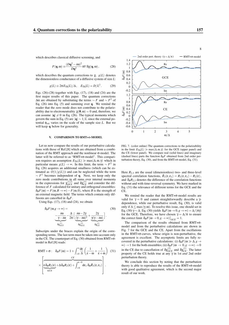
8
which describes classical diffusive screening, and
F(q,ω)≡ (Dq2− iω)2
Dq2 πV δχ(q,ω) , (28)
which describes the quantum corrections to χ. g(L) denotesthe dimensionless conductance of a diffusive system of size L:
g(L)≡ 2πETh(L)/∆ , ETh(L) = D/L2 . (29)
Eqs. (26)-(28) together with Eqs. (17), (18) and (24) are thefirst major results of this paper. The quantum corrections∆α are obtained by substituting the terms ∼ F and ∼ F2 ofEq. (26) into Eq. (5) and summing over q. We remind thereader that the zero mode does not contribute to the polariz-ability due to electroneutrality χ(0,ω) = 0 and, therefore, wecan assume |q| 6= 0 in Eq. (26). The typical momenta whichgovern the sum in Eq. (5) are |q| ∼ 1/L since the external po-tential φext varies on the scale of the sample size L. But wewill keep q below for generality.
V. COMPARISON TO RMT+σ-MODEL
Let us now compare the results of our perturbative calcula-tions with those of Ref.[8] which are obtained from a combi-nation of the RMT approach and the nonlinear σ-model. Thelatter will be referred to as “RMT+σ-model”. This compari-son requires an assumption ETh(L)� max(∆,ω,γ) which inparticular means g(L)→ ∞. In this limit, the term ∼ F2 inEq. (26) acquires an additional smallness (which can be es-timated as O(1/g(L))) and can be neglected while the term∼ F1 becomes independent of q. Next, we keep only thezero mode contributions in all sums over internal momentain the expressions for χ(1,2)
GCE and δχ(1)CE and consider the dif-
ference of F calculated for unitary and orthogonal ensembles:δBF(ω) = F(ω,B→ ∞)−F(ω,0), where B is the strength ofan external magnetic field. The terms which contain only dif-fusons are cancelled in δBF .
Using Eqs. (17), (18) and (24), we obtain
δBF(ω,g→ ∞) = (30)
− iωγ− iω︸ ︷︷ ︸
δχ(1)GCE
− ∆2π
[ iω−2γ(γ− iω)2︸ ︷︷ ︸
δχ(2)GCE
+2γ
γ(γ− iω)︸ ︷︷ ︸δχ(1)CE
].
Subscripts under the braces explain the origin of the corre-sponding terms. The last term must be taken into account onlyin the CE. The counterpart of Eq. (30) obtained from RMT+σ-model in Ref.[8] reads:
RMT+σ : δBF(ω) = 1+∫ ∞
+0
dε∆
(1
ε−ω+
1ε+ω
)(31)
×
CE︷ ︸︸ ︷εδBR2(ε)︸ ︷︷ ︸
GCE
+∆δBR2(ε)+∫ ε−0
+0dε1 δBR3(ε,ε1)
.
-0.20
0.20.40.60.81
1.21.4
GCE
Re
Im
2nd-Ord.-Pert.-Theory ( ) RMT+σ-model
-0.6-0.4-0.2
00.20.40.60.81
1.2
0 1 2 3 4 5
CE
Re
Im
2nd order pert. theory
FIG. 7. (color online) The quantum corrections to the polarizabilityin the limit ETh(L)� max(∆,ω,γ) for the GCE (upper panel) andthe CE (lower panel). We compare real (solid lines) and imaginary(dashed lines) parts the function δBF obtained from 2nd order per-turbation theory, Eq. (30), and from the RMT+σ-model, Eq. (31).
Here R2,3 are the usual (dimensionless) two- and three-levelspectral correlation functions, R3(ε,ε1) = R3(ε,ε1)−R2(ε) ,and δBR2,3 denotes the difference of the correlation functionswithout and with time-reversal symmetry. We have marked inEq. (31) the relevance of different terms for the GCE and theCE.
We remind the reader that the RMT+σ-model results arevalid for γ = 0 and cannot straightforwardly describe a γ-dependence, while our perturbative result, Eq. (30), is validonly if ∆ . max(γ,ω). To resolve this issue, one should set inEq. (30) γ∼ ∆. Eq. (30) yields δBF(ω→ 0,g→∞) = ∆/(πγ)for the GCE. Therefore, we have chosen γ = ∆/π to ensurethe correct limit δBF(ω→ 0,g→ ∞)
∣∣GCE = 1.
The comparison of the results obtained from RMT+σ-model and from the perturbative calculations are shown inFig. 7 for the GCE and the CE. Apart from the oscillationsin the RMT+σ-curves, whose origin is non-perturbative, theagreement is excellent. The asymptotic limits are fully re-covered in the perturbative calculations: (i) δBF(ω� ∆,g→∞)→ 1 for the both ensembles; (ii) δBF(ω → 0,g→∞)→ 0in the CE due to cancellation of δχ(2)
GCE and δχ(1)CE . The latter
property of the CE holds true at any γ in 1st and 2nd orderperturbation theory.
We conclude this section by noting that the perturbationtheory is able to reproduce the results of the RMT+σ-modelwith good qualitative agreement, which is the second majorresult of our work.
4. Quantum corrections to the polarizability 157
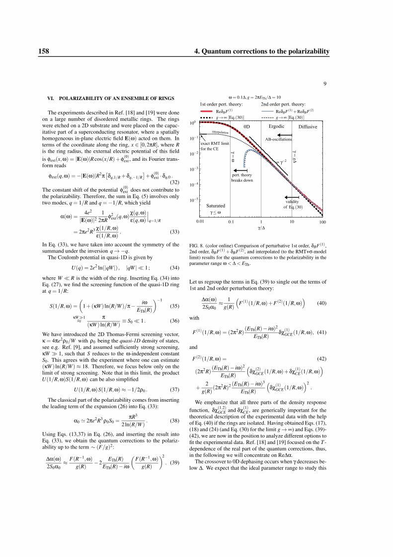
9
VI. POLARIZABILITY OF AN ENSEMBLE OF RINGS
The experiments described in Ref. [18] and [19] were doneon a large number of disordered metallic rings. The ringswere etched on a 2D substrate and were placed on the capac-itative part of a superconducting resonator, where a spatiallyhomogeneous in-plane electric field E(ω) acted on them. Interms of the coordinate along the ring, x ∈ [0,2πR], where Ris the ring radius, the external electric potential of this fieldis φext(x,ω) = |E(ω)|Rcos(x/R)+φ(0)ext , and its Fourier trans-form reads
φext(q,ω) =−|E(ω)|R2π[δq,1/R +δq,−1/R
]+φ(0)ext ·δq,0 .
(32)The constant shift of the potential φ(0)ext does not contribute tothe polarizability. Therefore, the sum in Eq. (5) involves onlytwo modes, q = 1/R and q =−1/R, which yield
α(ω) =4e2
|E(ω)|21
2πRφ2
ext(q,ω)χ(q,ω)ε(q,ω)
∣∣∣q=1/R
= 2πe2R3 χ(1/R,ω)ε(1/R,ω)
. (33)
In Eq. (33), we have taken into account the symmetry of thesummand under the inversion q→−q.
The Coulomb potential in quasi-1D is given by
U(q) = 2e2 ln(|qW |) , |qW | � 1; (34)
where W � R is the width of the ring. Inserting Eq. (34) intoEq. (27), we find the screening function of the quasi-1D ringat q = 1/R:
S(1/R,ω) =(
1+(κW ) ln(R/W )/π− iωETh(R)
)−1
(35)
κW�1≈ π(κW ) ln(R/W )
≡ S0� 1 . (36)
We have introduced the 2D Thomas-Fermi screening vector,κ = 4πe2ρ0/W with ρ0 being the quasi-1D density of states,see e.g. Ref. [9], and assumed sufficiently strong screening,κW � 1, such that S reduces to the ω-independent constantS0. This agrees with the experiment where one can estimate(κW ) ln(R/W ) ≈ 18. Therefore, we focus below only on thelimit of strong screening. Note that in this limit, the productU(1/R,ω)S(1/R,ω) can be also simplified
U(1/R,ω)S(1/R,ω)≈−1/2ρ0 . (37)
The classical part of the polarizability comes from insertingthe leading term of the expansion (26) into Eq. (33):
α0 ' 2πe2R3 ρ0S0 =πR3
2ln(R/W ). (38)
Using Eqs. (13,37) in Eq. (26), and inserting the result intoEq. (33), we obtain the quantum corrections to the polariz-ability up to the term ∼ (F/g)2:
∆α(ω)2S0α0
≈ F(R−1,ω)g(R)
−2ETh(R)
ETh(R)− iω
(F(R−1,ω)
g(R)
)2
. (39)
DiffusiveErgodic0D
Saturated
pert. theorybreaks down
1st order pert. theory: 2nd order pert. theory:
exact RMT limitfor the CE
interpolation
validityof
AB-oscillations
FIG. 8. (color online) Comparison of perturbative 1st order, δBF(1),2nd order, δBF(1)+δBF(2), and interpolated (to the RMT+σ-modellimit) results for the quantum corrections to the polarizability in theparameter range ω < ∆ < ETh.
Let us regroup the terms in Eq. (39) to single out the terms of1st and 2nd order perturbation theory:
∆α(ω)2S0α0
≈ 1g(R)
(F(1)(1/R,ω)+F(2)(1/R,ω)
)(40)
with
F(1)(1/R,ω) = (2π2R)(ETh(R)− iω)2
ETh(R)δχ(1)
GCE(1/R,ω), (41)
and
F(2)(1/R,ω) = (42)
(2π2R)(ETh(R)− iω)2
ETh(R)
(δχ(2)
GCE(1/R,ω)+δχ(1)CE(1/R,ω)
)
+2
g(R)(2π2R)2 (ETh(R)− iω)3
ETh(R)
(δχ(1)
GCE(1/R,ω))2
.
We emphasize that all three parts of the density responsefunction, δχ(1,2)
GCE and δχ(1)CE , are generically important for the
theoretical description of the experimental data with the helpof Eq. (40) if the rings are isolated. Having obtained Eqs. (17),(18) and (24) (and Eq. (30) for the limit g→∞) and Eqs. (39)-(42), we are now in the position to analyze different options tofit the experimental data. Ref. [18] and [19] focused on the T -dependence of the real part of the quantum corrections, thus,in the following we will concentrate on Re∆α.
The crossover to 0D dephasing occurs when γ decreases be-low ∆. We expect that the ideal parameter range to study this
158 4. Quantum corrections to the polarizability
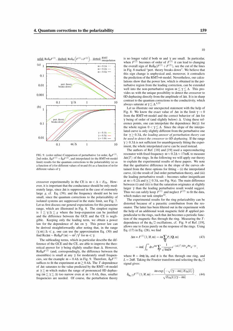
10
0.001
0.01
0.1
1
0.1 1 10
solid/dashed: one-loop/two-loop pert. theory
(a)
0.01
0.1
1
0.1 1 10
(b)
solid: dashed: dotted: RMTinterpolation
pert. theorybreaks down
pert. theorybreaks down
FIG. 9. (color online) Comparison of perturbative 1st order, δBF(1),2nd order, δBF(1)+δBF(2), and interpolated (to the RMT+σ-modellimit) results for the quantum corrections to the polarizability (a) asa function of γ for different values of ω and (b) as a function of ω fordifferent values of γ.
crossover experimentally in the CE is ω < ∆ < ETh. How-ever, it is important that the conductance should be only mod-erately large, since ∆α is suppressed in the case of extremelylarge g, cf. Eq. (39); and the frequency should not be toosmall, since the quantum corrections to the polarizability ofisolated systems are suppressed in the static limit, see Fig. 7.Let us first discuss our general expectations for this parameterrange, which are illustrated in Fig. 8. The simplest regimeis 1 . γ/∆ . g where the loop-expansion can be justifiedand the difference between the GCE and the CE is negli-gible. Keeping only the leading term, we obtain a powerlaw for the dependence of ∆α on γ. This power law canbe derived straightforwardly after noting that, in the range(γ,ω)/∆ � g, one can use the approximation Eq. (30) andfind Re∆α∼ ReδBF(ω)∼ ω2/γ2 for ω� γ.
The subleading terms, which in particular describe the dif-ference of the GCE and the CE, are able to improve the theo-retical answer for γ being slightly smaller than ∆. However,ReδBF(2) (and, correspondingly, the difference between theensembles) is small at any γ for moderately small frequen-cies, see the example ω = 0.4∆ in Fig. 9. Therefore, δBF(1)
suffices to fit the experiment at ω & 0.4∆. The T -dependenceof ∆α saturates to the value predicted by the RMT+σ-modelat γ . ω which makes the range of pronounced 0D dephas-ing (ω . γ . ∆) too narrow even at ω ' 0.4∆, thus, smallerfrequencies are needed. Of course, the perturbation theory
is no longer valid if both ω and γ are small. In particular,when F(2) becomes of order of F(1) it can lead to changingthe overall sign of ReδB(F(1)+F(2)), see the cut of the linesin Fig. 8 marked “pert. theory breaks down”. We believe thatthis sign change is unphysical and, moreover, it contradictsthe prediction of the RMT+σ-model. Nevertheless, our calcu-lations show that the power law, which is obtained in the per-turbative region from the leading correction, can be extendedwell into the non-perturbative region ω . γ . ∆. This pro-vides us with the unique possibility to detect the crossover to0D dephasing directly from the amplitude of ∆α. It is in sharpcontrast to the quantum corrections to the conductivity, whichalways saturate at γ . ∆.4,33
Let us illustrate our unexpected statement with the help ofFig. 8: We know the exact value of ∆α in the limit γ→ 0from the RMT+σ-model and the correct behavior of ∆α forγ being of order of (and slightly below) ∆. Using these ref-erence points, one can interpolate the dependence δα(γ) forthe whole region 0 < γ . ∆. Since the slope of the interpo-lated curve is only slightly different from the perturbative onefor γ ≥ 0.3∆, the leading answer of perturbation theory canbe used to detect the crossover to 0D dephasing. If the rangeγ≥ 0.3∆ is not sufficient for unambiguously fitting the exper-iment, the whole interpolated curve can be used instead.
The authors of Ref. [18] and [19] used a superconductingresonator with fixed frequency ω' 0.2∆' 17mK to measure∆α(T ) of the rings. In the following we will apply our theoryto explain the experimental results of these papers. We notethat the qualitative difference in the slope of the curves ob-tained from the three options for fitting – (i) the interpolatedcurve, (ii) the result of 2nd order perturbation theory, and (iii)the leading perturbative result – becomes rather insignificantat ω' 0.2∆ and γ & 0.3∆, see Fig. 9(a). The main differencebetween (i) and (iii) is that the saturation originates at slightlylarger γ than the leading perturbative result would suggest.Thus we can safely keep F(1) and neglect F(2) to fit the data,which makes our task simpler32.
The experimental results for the ring polarizability can bedistorted because of a parasitic contribution from the res-onator. The latter has been filtered out in the experiment withthe help of an additional weak magnetic field B applied per-pendicular to the rings, such that ∆α becomes a periodic func-tion of the magnetic flux through the ring. Measuring the T -dependence of the φ0/2 oscillations, cf. Fig. 9 of Ref. [19],allows one to focus purely on the response of the rings. UsingEq. (17) in Eq. (28), we find
∆α ∝ F(1)(1/R,ω) = iω∑Q
Pc(Q,ω) (43)
= iωL∫ ∞
0dt eiωt ∑
n
1√4πDt
e−(nL)2/4Dteiθne−γ t ,
where θ = 4πφ/φ0 and φ is the flux through one ring, andL = 2πR. Taking the Fourier transform and selecting the φ0/2signal gives:
δφ0/2F(1)(1/R,ω) =iω exp
(−√(γ− iω)/ETh(L)
)
√ETh(L)(γ− iω)
. (44)
4. Quantum corrections to the polarizability 159
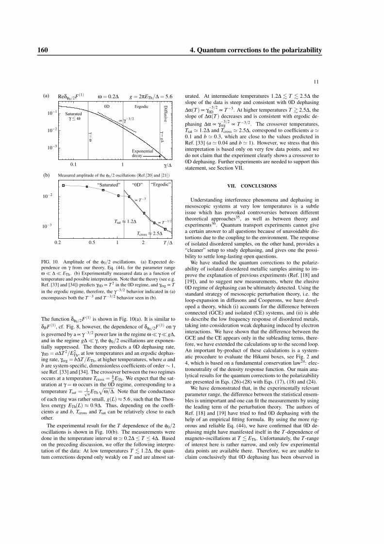
11
(a)
(b)
“Saturatedˮ “0D” “Ergodic”
Saturated
Ergodic0D Diffusive
Exponentialdecay
FIG. 10. Amplitude of the φ0/2 oscillations. (a) Expected de-pendence on γ from our theory, Eq. (44), for the parameter rangeω� ∆� ETh. (b) Experimentally measured data as a function oftemperature and possible interpretation. Note that the theory (see e.g.Ref. [33] and [34]) predicts γ0D ∝ T 2 in the 0D regime, and γerg ∝ Tin the ergodic regime, therefore, the γ−3/2 behavior indicated in (a)encompasses both the T−3 and T−3/2 behavior seen in (b).
The function δφ0/2F(1) is shown in Fig. 10(a). It is similar toδBF(1), cf. Fig. 8, however, the dependence of δφ0/2F(1) on γis governed by a ∝ γ−3/2 power law in the regime ω� γ� g∆,and in the regime g∆� γ, the φ0/2 oscillations are exponen-tially suppressed. The theory predicts a 0D dephasing rate,γ0D = a∆T 2/E2
Th, at low temperatures and an ergodic dephas-ing rate, γerg = b∆T/ETh, at higher temperatures, where a andb are system-specific, dimensionless coefficients of order∼ 1,see Ref. [33] and [34]. The crossover between the two regimesoccurs at a temperature Tcross =
ba ETh. We expect that the sat-
uration at γ = ω occurs in the 0D regime, corresponding to atemperature Tsat =
1√a ETh
√ω/∆. Note that the conductance
of each ring was rather small, g(L)≈ 5.6, such that the Thou-less energy ETh(L) ≈ 0.9∆. Thus, depending on the coeffi-cients a and b, Tcross and Tsat can be relatively close to eachother.
The experimental result for the T dependence of the φ0/2oscillations is shown in Fig. 10(b). The measurements weredone in the temperature interval ω ' 0.2∆ ≤ T ≤ 4∆. Basedon the preceding discussion, we offer the following interpre-tation of the data: At low temperatures T . 1.2∆, the quan-tum corrections depend only weakly on T and are almost sat-
urated. At intermediate temperatures 1.2∆ . T . 2.5∆ theslope of the data is steep and consistent with 0D dephasing∆α(T ) ∝ γ−3/2
0D ∝ T−3. At higher temperatures T & 2.5∆, theslope of ∆α(T ) decreases and is consistent with ergodic de-phasing ∆α ∝ γ−3/2
erg ∝ T−3/2. The crossover temperatures,Tsat ' 1.2∆ and Tcross ' 2.5∆, correspond to coefficients a '0.1 and b ' 0.3, which are close to the values predicted inRef. [33] (a ' 0.04 and b ' 1). However, we stress that thisinterpretation is based only on very few data points, and wedo not claim that the experiment clearly shows a crossover to0D dephasing. Further experiments are needed to support thisstatement, see Section VII.
VII. CONCLUSIONS
Understanding interference phenomena and dephasing inmesoscopic systems at very low temperatures is a subtleissue which has provoked controversies between differenttheoretical approaches35, as well as between theory andexperiments36. Quantum transport experiments cannot givea certain answer to all questions because of unavoidable dis-tortions due to the coupling to the environment. The responseof isolated disordered samples, on the other hand, provides a“cleaner” setup to study dephasing, and gives one the possi-bility to settle long-lasting open questions.
We have studied the quantum corrections to the polariz-ability of isolated disordered metallic samples aiming to im-prove the explanation of previous experiments (Ref. [18] and[19]), and to suggest new measurements, where the elusive0D regime of dephasing can be ultimately detected. Using thestandard strategy of mesoscopic perturbation theory, i.e. theloop-expansion in diffusons and Cooperons, we have devel-oped a theory, which (i) accounts for the difference betweenconnected (GCE) and isolated (CE) systems, and (ii) is ableto describe the low frequency response of disordered metals,taking into consideration weak dephasing induced by electroninteractions. We have shown that the difference between theGCE and the CE appears only in the subleading terms, there-fore, we have extended the calculations up to the second loop.An important by-product of these calculations is a system-atic procedure to evaluate the Hikami boxes, see Fig. 2 and4, which is based on a fundamental conservation law24: elec-troneutrality of the density response function. Our main ana-lytical results for the quantum corrections to the polarizabilityare presented in Eqs. (26)-(28) with Eqs. (17), (18) and (24).
We have demonstrated that, in the experimentally relevantparameter range, the difference between the statistical ensem-bles is unimportant and one can fit the measurements by usingthe leading term of the perturbation theory. The authors ofRef. [18] and [19] have tried to find 0D dephasing with thehelp of an empirical fitting formula. By using the more rig-orous and reliable Eq. (44), we have confirmed that 0D de-phasing might have manifested itself in the T -dependence ofmagneto-oscillations at T . ETh. Unfortunately, the T -rangeof interest here is rather narrow, and only few experimentaldata points are available there. Therefore, we are unable toclaim conclusively that 0D dephasing has been observed in
160 4. Quantum corrections to the polarizability
12
the experiments. However, we can straightforwardly suggestseveral experiments which might yield conclusive evidenceof 0D dephasing: Firstly, one can repeat the measurement ofRef. [18] and [19], but with a larger number of data pointsaround the crossover temperature Tcross, see Fig. 10, while si-multaneously improving the measurements precision. Sincethe theory predicts a drastic increase in slope of the φ0/2-oscillations at the crossover (from T−3/2 to T−3), even suchmeasurements should be able to reliably confirm the existenceof 0D dephasing, thereby uncovering the role of the Pauliblocking at low T . Secondly, it is highly desirable to extendthe T -range where the crossover to 0D dephasing is expectedto appear, which can be achieved by decreasing ω and/or in-creasing g. However, a very large conductance and ultra-smallfrequencies are nevertheless undesirable, because in these lim-its the quantum corrections to the polarizability are reduced.Thus, improving the precision of the measurement is neededanyway. Besides, fitting with the help of the leading pertur-bative result fails at very small frequencies, see Fig. 9. This
difficulty can be overcome by taking into account our two-loop results and/or using an interpolation to the γ→ 0 limitfrom the RMT+σ-model, see Fig. 8.
To summarize, we have shown that the quantum correctionsto the polarizability are an ideal candidate to study dephasingat low T and the crossover to 0D dephasing. We very muchhope that our theoretical results will stimulate new measure-ments in this direction.
ACKNOWLEDGMENTS
We acknowledge illuminating discussions with C. Texier,H. Bouchiat, G. Montambaux, and V. Kravtsov, and supportfrom the DFG through SFB TR-12 (O. Ye.), DE 730/8-1(M. T.) and the Cluster of Excellence, Nanosystems Initia-tive Munich. O. Ye. and M. T. acknowledge hospitality ofthe ICTP (Trieste) where part of the work for this paper wascarried out.
1 B. L. Altshuler, and A. G. Aronov, in Electron-Electron Interac-tions in Disordered Systems, edited by A. L. Efros and M. Pollak(North-Holland, Amsterdam, 1985), Vol. 1.
2 B. L. Altshuler, A. G. Aronov, and D. E. Khmelnitsky, J. Phys. C15, 7367 (1982).
3 U. Sivan and Y. Imry and A. G. Aronov, Europhys. Lett. 28, 115(1994).
4 M. Treiber, O. M. Yevtushenko, and J. von Delft, Ann. Physik524, 188 (2012).
5 B. L. Altshuler, Y. Gefen, A. Kamenev, and L. S. Levitov, Phys.Rev. Lett. 78, 2803 (1997).
6 Ya. M. Blanter, Phys. Rev. B54, 12807 (1996).7 V. E. Kravtsov, and A. D. Mirlin, JETP Lett. 60, 656 (1994).8 Ya. M. Blanter, and A. D. Mirlin, Phys. Rev. B 57, 4566 (1998);
ibid 63, 113315 (2001).9 G. Montambaux, and E. Akkermans, Mesoscopic Physics of Elec-
trons and Photons, Cambridge University Press (2007).10 A. Kamenev and Y. Gefen, Phys. Rev. Lett.70, 1976 (1993); Phys.
Rev. B 56, 1025 (1997); A. Kamenev, B. Reulet, H. Bouchiat, andY. Gefen, Europhys. Lett. 28, 391 (1994).
11 W. Lehle, and A. Schmid, Ann. Physik 507, 451 (1995).12 A. Altland and S. Iida and A. Muller-Groeling and H. A. Wei-
denmuller, Europhys. Lett. 20, 155 (1992); Ann. Phys. (N.Y.) 219,148 (1992).
13 This approach has also been used in Ref. [8] to describe the po-larizability in the non-perturbative regime.
14 L. P. Gorkov, and G. M. Eliashberg, Sov. Phys. JETP 21, 940(1965).
15 M. J. Rice, W. R. Schneider, and S. Strassler Phys. Rev. B 8, 474(1973).
16 A detailed discussion of the assumptions of Ref. [14] can be foundin: Ya. M. Blanter, and A. D. Mirlin Phys. Rev. B 53, 12601(1996).
17 K. B. Efetov, Phys. Rev. Lett. 76, 1908 (1996).18 R. Deblock, Y. Noat, H. Bouchiat, B. Reulet, and D. Mailly, Phys.
Rev. Lett. 84, 5379 (2000).19 R. Deblock, Y. Noat, B. Reulet, H. Bouchiat, and D. Mailly, Phys.
Rev. B 65, 075301 (2002).20 H. Bruus and K. Flensberg, Many-Body Quantum Theory in Con-
densed Matter Physics, Oxford graduate texts in mathematics(2004).
21 D. Vollhardt and P. Wolfle, Phys. Rev. B 22, 4666 (1980).22 S. Hikami, Phys. Rev. B 24, 2671 (1981).23 K. B. Efetov, Adv. Phys. 32, 53 (1983); B. L. Altshuler, V. E.
Kravtsov, and I. V. Lerner, Zh. Eksp. Teor. Fiz. 91, 2276 (1986).24 A similar idea has been discussed in the derivation of a current-
conserving non-local conductivity: M. B. Hastings, A. D. Stone,and H. U. Baranger , Phys. Rev. B 50, 8230 (1994).
25 P. M. Ostrovsky, and V. Kravtsov, unpublished.26 G. Zala, B. N. Narozhny, and I. L. Aleiner, Phys. Rev. B 64,
214204 (2001).27 L. P. Gorkov, A. I. Larkin, and D. E. Khmelnitskii, JETP Lett. 30,
228 (1979).28 R. A. Smith, I. V. Lerner, and B. L. Altshuler, Phys. Rev. B 58,
10343 (1998).29 H. Bouchiat, private communication.30 T. Ludwig, and A. D. Mirlin, Phys. Rev. B 69, 193306 (2004).31 C. Texier, and G. Montambaux, Phys. Rev. B 72, 115327 (2005).32 The smallness of the contribution of 2nd order perturbation the-
ory is also confirmed by the absence of φ0-periodic oscillationsin the experimental data. We remind the reader that the φ0-periodic oscillations result from contributions of diffusons [seeA. G. Aronov, and Yu. V. Sharvin, Rev. Mod. Phys. 59, 755(1987)] which exists only in F(2) due to δχ(2)
GCE and δχ(1)CE ; For
a discussion of this point, see A. Kamenev, and Y. Gefen, Phys.Rev. B 49, 14474 (1994).
33 M. Treiber, O. M. Yevtushenko, F. Marquardt, J. von Delft, andI. V. Lerner, Phys. Rev. B 80, 201305(R) (2009).
34 M. Treiber, C. Texier, O. M. Yevtushenko, J. von Delft, andI. V. Lerner, Phys. Rev. B 84, 054204 (2011).
35 F. Marquardt, J. von Delft, R. A. Smith, and V. Ambegaokar,Phys. Rev. B 76, 195331 (2007); J. von Delft, F. Marquardt,R. A. Smith, and V. Ambegaokar, ibid 76, 195332 (2007).
36 A. G. Huibers, M. Switkes, C. M. Marcus, K. Campman, andA. C. Gossard, Phys. Rev. Lett. 81, 200 (1998).
4. Quantum corrections to the polarizability 161

5. Summary and conclusions 163
Chapter 5
Summary and conclusions
In this thesis we have contributed to the theory of dephasing in disordered mesoscopic systems. Atlow temperatures, Pauli blocking becomes important and limits the energy transfer ω of electroninteractions to ω� T due to a lack of final scattering states. We have analyzed its effect on theinteraction-induced dephasing rate γ, and discussed possible experiments to demonstrate the influenceof Pauli blocking.
The thesis is divided into four main chapters, where we have reviewed the current state of researchand presented a brief overview of our original results in the main text. More details on the originalresults can be found in the papers attached at the end of each chapter.
In Chapter 1, we have given a general introduction to the field, followed by a discussion of ourmotivation, and we have provided a brief outline of this thesis.
In Chapter 2, we have introduced the standard methods of mesoscopic physics, namely, the pertur-bative loop-expansion in diffusive propagators, and the non-perturbative random matrix theory. Wehave reviewed the usual derivations of the dephasing rate: (1) using a perturbation theory in theelectron interactions and (2) using a path integral with an effective noise potential, and we have con-cluded that the temperature dependence of γ can be obtained from a self-consistent integral equationshown in Table 5 below. We have established that the so-called 0D regime of dephasing, reached atT � ETh , is practically the only regime (in the relevant dimensions d ≤ 2), where Pauli blocking sig-nificantly influences the temperature dependence of γ. Importantly, attempts to observe the 0D regimeof dephasing experimentally have been unsuccessful so far, and we have concentrated on a possibleexperimental verification in the following. We have emphasized that the 0D regime is characterizedby (1) a discreteness of the energy levels, accompanied with a breakdown of the perturbative loop-expansion, and (2) a relative weakness of the dephasing rate, such that electron trajectories, whichprobe the whole geometry of the system, become important. Our first main new result in this sectionhas been the calculation of the two-loop expansion of the generalized diffusion propagator, wherewe have introduced a new method to calculate the short-range parts (so-called Hikami boxes) of thecorresponding diagrams, which can be extended straightforwardly to more complicated diagrams, in-cluding higher loop corrections, and non-trivial physical problems. The second main result has beenthe derivation of a new dephasing rate functional, valid at arbitrary temperatures, which describesdephasing in non-trivial geometries, in particular, networks of quasi-1D wires.
In Chapter 3, we have considered the weak-localization correction ∆g to the conductance, and dis-cussed that ∆g assumes a universal value ∼ 1 in open systems, as soon as γ� ETh , see Fig. 5.1(a)below. Since T � γ, the 0D regime occurs deep in the universal regime, where the weak-localizationcorrection is practically independent of γ. However, a signature of 0D dephasing can still be extracted
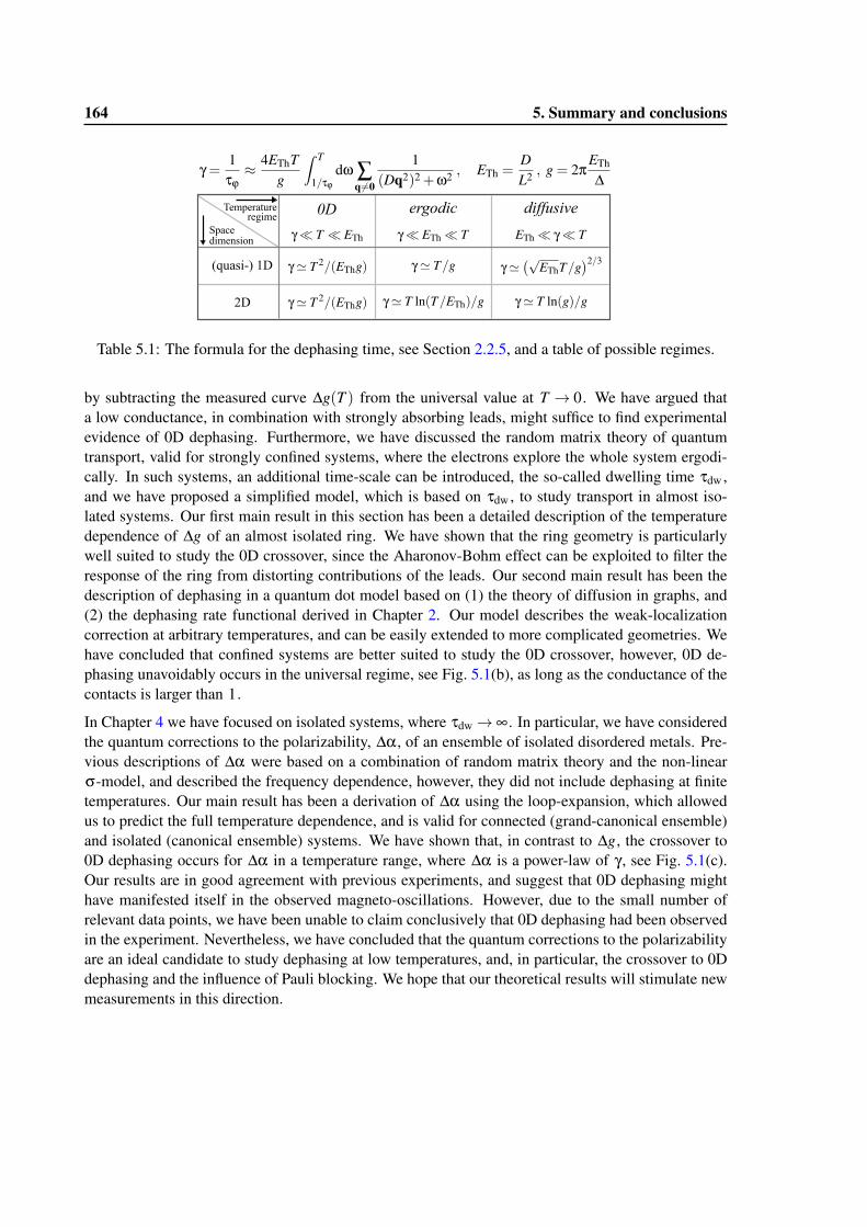
164 5. Summary and conclusions
(quasi-) 1D
2D
diffusiveergodic0DSpacedimension
Temperatureregime
Table 5.1: The formula for the dephasing time, see Section 2.2.5, and a table of possible regimes.
by subtracting the measured curve ∆g(T ) from the universal value at T → 0. We have argued thata low conductance, in combination with strongly absorbing leads, might suffice to find experimentalevidence of 0D dephasing. Furthermore, we have discussed the random matrix theory of quantumtransport, valid for strongly confined systems, where the electrons explore the whole system ergodi-cally. In such systems, an additional time-scale can be introduced, the so-called dwelling time τdw ,and we have proposed a simplified model, which is based on τdw , to study transport in almost iso-lated systems. Our first main result in this section has been a detailed description of the temperaturedependence of ∆g of an almost isolated ring. We have shown that the ring geometry is particularlywell suited to study the 0D crossover, since the Aharonov-Bohm effect can be exploited to filter theresponse of the ring from distorting contributions of the leads. Our second main result has been thedescription of dephasing in a quantum dot model based on (1) the theory of diffusion in graphs, and(2) the dephasing rate functional derived in Chapter 2. Our model describes the weak-localizationcorrection at arbitrary temperatures, and can be easily extended to more complicated geometries. Wehave concluded that confined systems are better suited to study the 0D crossover, however, 0D de-phasing unavoidably occurs in the universal regime, see Fig. 5.1(b), as long as the conductance of thecontacts is larger than 1.
In Chapter 4 we have focused on isolated systems, where τdw→ ∞. In particular, we have consideredthe quantum corrections to the polarizability, ∆α, of an ensemble of isolated disordered metals. Pre-vious descriptions of ∆α were based on a combination of random matrix theory and the non-linearσ-model, and described the frequency dependence, however, they did not include dephasing at finitetemperatures. Our main result has been a derivation of ∆α using the loop-expansion, which allowedus to predict the full temperature dependence, and is valid for connected (grand-canonical ensemble)and isolated (canonical ensemble) systems. We have shown that, in contrast to ∆g, the crossover to0D dephasing occurs for ∆α in a temperature range, where ∆α is a power-law of γ, see Fig. 5.1(c).Our results are in good agreement with previous experiments, and suggest that 0D dephasing mighthave manifested itself in the observed magneto-oscillations. However, due to the small number ofrelevant data points, we have been unable to claim conclusively that 0D dephasing had been observedin the experiment. Nevertheless, we have concluded that the quantum corrections to the polarizabilityare an ideal candidate to study dephasing at low temperatures, and, in particular, the crossover to 0Ddephasing and the influence of Pauli blocking. We hope that our theoretical results will stimulate newmeasurements in this direction.
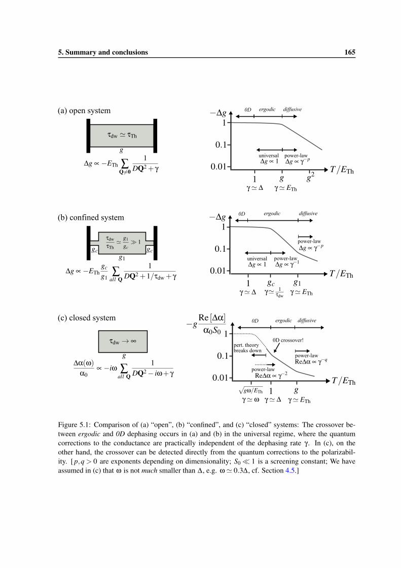
5. Summary and conclusions 165
(a) open system
(b) confined system
(c) closed system
0D
power-law
diffusiveergodic
power-law
universal
0D
power-law
diffusiveergodic
universal
0D
power-law
diffusiveergodic
power-law
pert. theorybreaks down
0D crossover!
Figure 5.1: Comparison of (a) “open”, (b) “confined”, and (c) “closed” systems: The crossover be-tween ergodic and 0D dephasing occurs in (a) and (b) in the universal regime, where the quantumcorrections to the conductance are practically independent of the dephasing rate γ. In (c), on theother hand, the crossover can be detected directly from the quantum corrections to the polarizabil-ity. [ p,q > 0 are exponents depending on dimensionality; S0� 1 is a screening constant; We haveassumed in (c) that ω is not much smaller than ∆, e.g. ω' 0.3∆, cf. Section 4.5.]

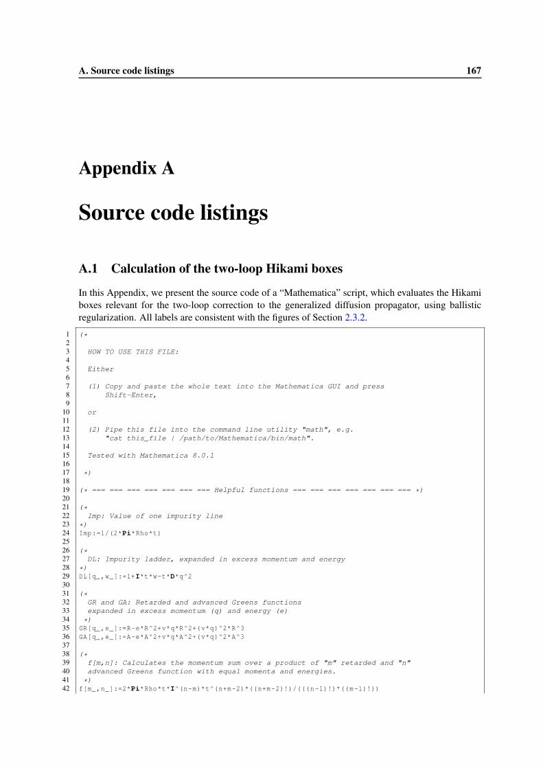
A. Source code listings 167
Appendix A
Source code listings
A.1 Calculation of the two-loop Hikami boxes
In this Appendix, we present the source code of a “Mathematica” script, which evaluates the Hikamiboxes relevant for the two-loop correction to the generalized diffusion propagator, using ballisticregularization. All labels are consistent with the figures of Section 2.3.2.
1 (*23 HOW TO USE THIS FILE:45 Either67 (1) Copy and paste the whole text into the Mathematica GUI and press8 Shift-Enter,9
10 or1112 (2) Pipe this file into the command line utility "math", e.g.13 "cat this_file | /path/to/Mathematica/bin/math".1415 Tested with Mathematica 8.0.11617 *)1819 (* === === === === === === === Helpful functions === === === === === === === *)2021 (*22 Imp: Value of one impurity line23 *)24 Imp:=1/(2*Pi*Rho*t)2526 (*27 DL: Impurity ladder, expanded in excess momentum and energy28 *)29 DL[q_,w_]:=1+I*t*w-t*D*q^23031 (*32 GR and GA: Retarded and advanced Greens functions33 expanded in excess momentum (q) and energy (e)34 *)35 GR[q_,e_]:=R-e*R^2+v*q*R^2+(v*q)^2*R^336 GA[q_,e_]:=A-e*A^2+v*q*A^2+(v*q)^2*A^33738 (*39 f[m,n]: Calculates the momentum sum over a product of "m" retarded and "n"40 advanced Greens function with equal momenta and energies.41 *)42 f[m_,n_]:=2*Pi*Rho*t*I^(n-m)*t^(n+m-2)*((n+m-2)!)/(((n-1)!)*((m-1)!))
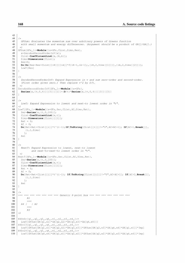
168 A. Source code listings
4344 (*45 GFSum: Evaluates the momentum sum over arbitrary powers of Greens function46 with small momentum and energy differences. (Argument should be a product of GR[]/GA[].)47 *)48 GFSum[GFs_]:=Module[{x=GFs,CList ,Dims ,Res},49 x=ZeroAndSecondOrderInV[x];50 CList=CoefficientList[x,{R,A}];51 Dims=Dimensions[CList];52 Res=0;53 Do[Do[Res=Res+CList[[iR]][[iA]]*f[iR-1,iA -1];,{iR,2,Dims[[1]]}],{iA,2,Dims[[2]]}];54 LowT[Res]55 ]5657 (*58 ZeroAndSecondOrderInV: Expand Expression in v and sum zero-order and second-order.59 (First order gives zero.) Then replace v^2 by D/t.60 *)61 ZeroAndSecondOrderInV[GFs_]:=Module[{x=GFs},62 Series[x,{v,0 ,4}][[3]][[1]]+(D/t)*Series[x,{v,0 ,4}][[3]][[3]]63 ]6465 (*66 LowT: Expand Expression to lowest and next-to lowest order in "t".67 *)68 LowT[GFs_]:=Module[{x=GFs,Ser,CList ,AC,Dims ,Ret},69 Ser=Series[x,{t,0,100}];70 CList=CoefficientList[x,t];71 Dims=Dimensions[CList ][[1]];72 Ret = 0;73 AC = 0;74 Do[Ret=Ret+CList[[i]]*t^(i-1);If[ToString[CList[[i]]]!="0",AC=AC+1]; If[AC>1,Break[]],75 {i,1,Dims}76 ];77 Ret78 ]7980 (*81 NextT: Expand Expression to lowest, next-to lowest82 and next-to-next-to lowest order in "t".83 *)84 NextT[GFs_]:=Module[{x=GFs,Ser,CList ,AC,Dims ,Ret},85 Ser=Series[x,{t,0,100}];86 CList=CoefficientList[x,t];87 Dims=Dimensions[CList ][[1]];88 Ret = 0;89 AC = 0;90 Do[Ret=Ret+CList[[i]]*t^(i-1); If[ToString[CList[[i]]]!="0",AC=AC+1]; If[AC>2,Break[]],91 {i,1,Dims}92 ];93 Ret94 ]9596 (*97 === === === === === === === Generic 4-point box === === === === === === ===98 R199 ===
100 A4 | | A2101 ===102 R3103 *)104105 H4UnDr[q1_,q2_ ,q3_,q4_,e1_,e2_,e3_,e4_]:=106 LowT[GFSum[GR[q1,e1]*GA[q2,e2]*GR[q3,e3]*GA[q4,e4]]]107 H4Dr13[q1_,q2_ ,q3_,q4_,e1_,e2_,e3_,e4_]:=108 LowT[GFSum[GR[q1,e1]*GA[q2,e2]*GR[q3,e3]]*GFSum[GR[q3,e3]*GA[q4,e4]*GR[q1,e1]]*Imp]109 H4Dr24[q1_,q2_ ,q3_,q4_,e1_,e2_,e3_,e4_]:=110 LowT[GFSum[GA[q4,e4]*GR[q1,e1]*GA[q2,e2]]*GFSum[GA[q2,e2]*GR[q3,e3]*GA[q4,e4]]*Imp]
A. Source code listings 169
111112 Print["Generic 4-point Hikami box:"]113 FullSimplify[114 H4UnDr[q1,q2,q3,q4,e1,e2,e3,e4]+115 H4Dr13[q1,q2,q3,q4,e1,e2,e3,e4]+116 H4Dr24[q1,q2,q3,q4,e1,e2,e3,e4]117 ]118119 (*120 === === === === === === === Generic 6-point box === === === === === === ===121 A2122 -------123 R1// \\ R3124 // \\125 \ /126 A6\ /A4127 =======128 R5129 *)130131 H6UnDr[q1_,q2_,q3_,q4_,q5_,q6_,e1_,e2_,e3_,e4_,e5_,e6_]:=132 LowT[GFSum[GR[q1,e1]*GA[q2,e2]*GR[q3,e3]*GA[q4,e4]*GR[q5,e5]*GA[q6,e6]]]133 H6Dr24[q1_,q2_,q3_,q4_,q5_,q6_,e1_,e2_,e3_,e4_,e5_,e6_]:=134 LowT[Imp*GFSum[GA[q2,e2]*GR[q3,e3]*GA[q4,e4]]*135 GFSum[GR[q1,e1]*GA[q2,e2]*GA[q4,e4]*GR[q5,e5]*GA[q6,e6]]]136 H6Dr26[q1_,q2_,q3_,q4_,q5_,q6_,e1_,e2_,e3_,e4_,e5_,e6_]:=137 LowT[Imp*GFSum[GA[q6,e6]*GR[q1,e1]*GA[q2,e2]]*138 GFSum[GA[q2,e2]*GR[q3,e3]*GA[q4,e4]*GR[q5,e5]*GA[q6,e6]]]139 H6Dr46[q1_,q2_,q3_,q4_,q5_,q6_,e1_,e2_,e3_,e4_,e5_,e6_]:=140 LowT[Imp*GFSum[GA[q4,e4]*GR[q5,e5]*GA[q6,e6]]*141 GFSum[GA[q6,e6]*GR[q1,e1]*GA[q2,e2]*GR[q3,e3]*GA[q4,e4]]]142 H6Dr13[q1_,q2_,q3_,q4_,q5_,q6_,e1_,e2_,e3_,e4_,e5_,e6_]:=143 LowT[Imp*GFSum[GR[q1,e1]*GA[q2,e2]*GR[q3,e3]]*144 GFSum[GR[q1,e1]*GR[q3,e3]*GA[q4,e4]*GR[q5,e5]*GA[q6,e6]]]145 H6Dr15[q1_,q2_,q3_,q4_,q5_,q6_,e1_,e2_,e3_,e4_,e5_,e6_]:=146 LowT[Imp*GFSum[GR[q5,e5]*GA[q6,e6]*GR[q1,e1]]*147 GFSum[GR[q1,e1]*GA[q2,e2]*GR[q3,e3]*GA[q4,e4]*GR[q5,e5]]]148 H6Dr35[q1_,q2_,q3_,q4_,q5_,q6_,e1_,e2_,e3_,e4_,e5_,e6_]:=149 LowT[Imp*GFSum[GR[q3,e3]*GA[q4,e4]*GR[q5,e5]]*150 GFSum[GR[q1,e1]*GA[q2,e2]*GR[q3,e3]*GR[q5,e5]*GA[q6,e6]]]151 H6Dr1315[q1_,q2_,q3_,q4_,q5_,q6_,e1_,e2_,e3_,e4_,e5_,e6_]:=152 LowT[Imp^2*GFSum[GR[q1,e1]*GA[q2,e2]*GR[q3,e3]]*153 GFSum[GR[q1,e1]*GR[q3,e3]*GA[q4,e4]*GR[q5,e5]]*154 GFSum[GR[q5,e5]*GA[q6,e6]*GR[q1,e1]]]155 H6Dr3135[q1_,q2_,q3_,q4_,q5_,q6_,e1_,e2_,e3_,e4_,e5_,e6_]:=156 LowT[Imp^2*GFSum[GR[q1,e1]*GA[q2,e2]*GR[q3,e3]]*157 GFSum[GR[q3,e3]*GR[q5,e5]*GA[q6,e6]*GR[q1,e1]]*158 GFSum[GR[q3,e3]*GA[q4,e4]*GR[q5,e5]]]159 H6Dr5153[q1_,q2_,q3_,q4_,q5_,q6_,e1_,e2_,e3_,e4_,e5_,e6_]:=160 LowT[Imp^2*GFSum[GR[q3,e3]*GA[q4,e4]*GR[q5,e5]]*161 GFSum[GR[q5,e5]*GR[q1,e1]*GA[q2,e2]*GR[q3,e3]]*162 GFSum[GR[q5,e5]*GA[q6,e6]*GR[q1,e1]]]163 H6Dr2426[q1_,q2_,q3_,q4_,q5_,q6_,e1_,e2_,e3_,e4_,e5_,e6_]:=164 LowT[Imp^2*GFSum[GA[q6,e6]*GR[q1,e1]*GA[q2,e2]]*165 GFSum[GA[q2,e2]*GA[q4,e4]*GR[q5,e5]*GA[q6,e6]]*166 GFSum[GA[q2,e2]*GR[q3,e3]*GA[q4,e4]]]167 H6Dr6264[q1_,q2_,q3_,q4_,q5_,q6_,e1_,e2_,e3_,e4_,e5_,e6_]:=168 LowT[Imp^2*GFSum[GA[q6,e6]*GR[q1,e1]*GA[q2,e2]]*169 GFSum[GA[q6,e6]*GA[q2,e2]*GR[q3,e3]*GA[q4,e4]]*170 GFSum[GA[q4,e4]*GR[q5,e5]*GA[q6,e6]]]171 H6Dr4246[q1_,q2_,q3_,q4_,q5_,q6_,e1_,e2_,e3_,e4_,e5_,e6_]:=172 LowT[Imp^2*GFSum[GA[q2,e2]*GR[q3,e3]*GA[q4,e4]]*173 GFSum[GA[q4,e4]*GA[q6,e6]*GR[q1,e1]*GA[q2,e2]]*174 GFSum[GA[q4,e4]*GR[q5,e5]*GA[q6,e6]]]175 H6Dr1346[q1_,q2_,q3_,q4_,q5_,q6_,e1_,e2_,e3_,e4_,e5_,e6_]:=176 LowT[Imp^2*GFSum[GR[q1,e1]*GA[q2,e2]*GR[q3,e3]]*177 GFSum[GA[q6,e6]*GR[q1,e1]*GR[q3,e3]*GA[q4,e4]]*178 GFSum[GA[q4,e4]*GR[q5,e5]*GA[q6,e6]]]
170 A. Source code listings
179 H6Dr1524[q1_,q2_,q3_,q4_,q5_,q6_,e1_,e2_,e3_,e4_,e5_,e6_]:=180 LowT[Imp^2*GFSum[GR[q5,e5]*GA[q6,e6]*GR[q1,e1]]*181 GFSum[GA[q4,e4]*GR[q5,e5]*GR[q1,e1]*GA[q2,e2]]*182 GFSum[GA[q2,e2]*GR[q3,e3]*GA[q4,e4]]]183 H6Dr2635[q1_,q2_,q3_,q4_,q5_,q6_,e1_,e2_,e3_,e4_,e5_,e6_]:=184 LowT[Imp^2*GFSum[GR[q3,e3]*GA[q4,e4]*GR[q5,e5]]*185 GFSum[GA[q2,e2]*GR[q3,e3]*GR[q5,e5]*GA[q6,e6]]*186 GFSum[GA[q6,e6]*GR[q1,e1]*GA[q2,e2]]]187188 Print["Generic 6-point Hikami box:"]189 FullSimplify[190 H6UnDr[q1,q2,q3,q4,q5,q6,e1,e2,e3,e4,e5,e6]+191 H6Dr24[q1,q2,q3,q4,q5,q6,e1,e2,e3,e4,e5,e6]+192 H6Dr26[q1,q2,q3,q4,q5,q6,e1,e2,e3,e4,e5,e6]+193 H6Dr46[q1,q2,q3,q4,q5,q6,e1,e2,e3,e4,e5,e6]+194 H6Dr13[q1,q2,q3,q4,q5,q6,e1,e2,e3,e4,e5,e6]+195 H6Dr15[q1,q2,q3,q4,q5,q6,e1,e2,e3,e4,e5,e6]+196 H6Dr35[q1,q2,q3,q4,q5,q6,e1,e2,e3,e4,e5,e6]+197 H6Dr1315[q1,q2,q3,q4,q5,q6,e1,e2,e3,e4,e5,e6]+198 H6Dr3135[q1,q2,q3,q4,q5,q6,e1,e2,e3,e4,e5,e6]+199 H6Dr5153[q1,q2,q3,q4,q5,q6,e1,e2,e3,e4,e5,e6]+200 H6Dr2426[q1,q2,q3,q4,q5,q6,e1,e2,e3,e4,e5,e6]+201 H6Dr6264[q1,q2,q3,q4,q5,q6,e1,e2,e3,e4,e5,e6]+202 H6Dr4246[q1,q2,q3,q4,q5,q6,e1,e2,e3,e4,e5,e6]+203 H6Dr1346[q1,q2,q3,q4,q5,q6,e1,e2,e3,e4,e5,e6]+204 H6Dr1524[q1,q2,q3,q4,q5,q6,e1,e2,e3,e4,e5,e6]+205 H6Dr2635[q1,q2,q3,q4,q5,q6,e1,e2,e3,e4,e5,e6]206 ]207208 (* === === === === === Calculation of 2-loop diagram Hikami boxes === === === === === *)209210 Print["=== Results for diagram (b) ==="]211212 Print["(b1) = "]213 FullSimplify[214 LowT[H6UnDr[q,q-Q1,q-Q1+Q2,-Q1+Q2,Q2,0,w,0,w,0,w,0]*DL[Q1,w]^2*DL[Q2,w]^2]+215 LowT[H6Dr15[q,q-Q1,q-Q1+Q2,-Q1+Q2,Q2,0,w,0,w,0,w,0]*DL[Q1,w]^2*DL[Q2,w]^1]+216 LowT[H6Dr35[q,q-Q1,q-Q1+Q2,-Q1+Q2,Q2,0,w,0,w,0,w,0]*DL[Q1,w]^1*DL[Q2,w]^2]+217 LowT[H6Dr26[q,q-Q1,q-Q1+Q2,-Q1+Q2,Q2,0,w,0,w,0,w,0]*DL[Q1,w]^1*DL[Q2,w]^2]+218 LowT[H6Dr24[q,q-Q1,q-Q1+Q2,-Q1+Q2,Q2,0,w,0,w,0,w,0]*DL[Q1,w]^2*DL[Q2,w]^1]+219 LowT[H6Dr5153[q,q-Q1,q-Q1+Q2,-Q1+Q2,Q2,0,w,0,w,0,w,0]*DL[Q1,w]^1*DL[Q2,w]^1]+220 LowT[H6Dr2426[q,q-Q1,q-Q1+Q2,-Q1+Q2,Q2,0,w,0,w,0,w,0]*DL[Q1,w]^1*DL[Q2,w]^1]+221 LowT[H6Dr1524[q,q-Q1,q-Q1+Q2,-Q1+Q2,Q2,0,w,0,w,0,w,0]*DL[Q1,w]^2*DL[Q2,w]^0]+222 LowT[H6Dr2635[q,q-Q1,q-Q1+Q2,-Q1+Q2,Q2,0,w,0,w,0,w,0]*DL[Q1,w]^0*DL[Q2,w]^2]223 ]224225 Print["(b2) = "]226 FullSimplify[227 LowT[H6Dr13[q,q-Q1,q-Q1+Q2,-Q1+Q2,Q2,0,w,0,w,0,w,0]*DL[Q1,w]^2*DL[Q2,w]^2]+228 LowT[H6Dr1315[q,q-Q1,q-Q1+Q2,-Q1+Q2,Q2,0,w,0,w,0,w,0]*DL[Q1,w]^2*DL[Q2,w]^1]+229 LowT[H6Dr3135[q,q-Q1,q-Q1+Q2,-Q1+Q2,Q2,0,w,0,w,0,w,0]*DL[Q1,w]^1*DL[Q2,w]^2]+230 LowT[H6Dr46[q,q-Q1,q-Q1+Q2,-Q1+Q2,Q2,0,w,0,w,0,w,0]*DL[Q1,w]^2*DL[Q2,w]^2]+231 LowT[H6Dr6264[q,q-Q1,q-Q1+Q2,-Q1+Q2,Q2,0,w,0,w,0,w,0]*DL[Q1,w]^1*DL[Q2,w]^2]+232 LowT[H6Dr4246[q,q-Q1,q-Q1+Q2,-Q1+Q2,Q2,0,w,0,w,0,w,0]*DL[Q1,w]^2*DL[Q2,w]^1]+233 LowT[Imp*H4UnDr[q,Q2-Q1,Q2,0,w,0,w,0]*234 H4UnDr[q,q-Q1,q-Q1+Q2,Q2-Q1,w,0,w,0]*DL[Q1,w]^2*DL[Q2,w]^2]+235 LowT[Imp*H4Dr13[q,Q2-Q1,Q2,0,w,0,w,0]*236 H4UnDr[q,q-Q1,q-Q1+Q2,Q2-Q1,w,0,w,0]*DL[Q1,w]^2*DL[Q2,w]^1]+237 LowT[Imp*H4UnDr[q,Q2-Q1,Q2,0,w,0,w,0]*238 H4Dr24[q,q-Q1,q-Q1+Q2,Q2-Q1,w,0,w,0]*DL[Q1,w]^2*DL[Q2,w]^1]+239 LowT[Imp*H4Dr13[q,Q2-Q1,Q2,0,w,0,w,0]*240 H4Dr24[q,q-Q1,q-Q1+Q2,Q2-Q1,w,0,w,0]*DL[Q1,w]^2*DL[Q2,w]^0]+241 LowT[Imp*H4UnDr[q,q-Q1,q-Q1+Q2,0,w,0,w,0]*242 H4UnDr[q-Q1+Q2,Q2-Q1,Q2,0,w,0,w,0]*DL[Q1,w]^2*DL[Q2,w]^2]+243 LowT[Imp*H4Dr24[q,q-Q1,q-Q1+Q2,0,w,0,w,0]*244 H4UnDr[q-Q1+Q2,Q2-Q1,Q2,0,w,0,w,0]*DL[Q1,w]^1*DL[Q2,w]^2]+245 LowT[Imp*H4UnDr[q,q-Q1,q-Q1+Q2,0,w,0,w,0]*246 H4Dr13[q-Q1+Q2,Q2-Q1,Q2,0,w,0,w,0]*DL[Q1,w]^1*DL[Q2,w]^2]+
A. Source code listings 171
247 LowT[Imp*H4Dr24[q,q-Q1,q-Q1+Q2,0,w,0,w,0]*248 H4Dr13[q-Q1+Q2,Q2-Q1,Q2,0,w,0,w,0]*DL[Q1,w]^0*DL[Q2,w]^2]249 ]250251 Print["(b3) = "]252 FullSimplify[253 LowT[H6Dr1346[q,q-Q1,q-Q1+Q2,-Q1+Q2,Q2,0,w,0,w,0,w,0]*DL[Q1,w]^2*DL[Q2,w]^2]+254 LowT[Imp*H4Dr24[q,Q2-Q1,Q2,0,w,0,w,0]*255 H4UnDr[q,q-Q1,q-Q1+Q2,Q2-Q1,w,0,w,0]*DL[Q1,w]^2*DL[Q2,w]^2]+256 LowT[Imp*H4Dr24[q,Q2-Q1,Q2,0,w,0,w,0]*257 H4Dr24[q,q-Q1,q-Q1+Q2,Q2-Q1,w,0,w,0]*DL[Q1,w]^2*DL[Q2,w]^1]+258 LowT[Imp*H4UnDr[q,Q2-Q1,Q2,0,w,0,w,0]*259 H4Dr13[q,q-Q1,q-Q1+Q2,Q2-Q1,w,0,w,0]*DL[Q1,w]^2*DL[Q2,w]^2]+260 LowT[Imp*H4Dr13[q,Q2-Q1,Q2,0,w,0,w,0]*261 H4Dr13[q,q-Q1,q-Q1+Q2,Q2-Q1,w,0,w,0]*DL[Q1,w]^2*DL[Q2,w]^1]+262 LowT[Imp*H4UnDr[q,Q2-Q1,Q2,0,w,0,w,0]*263 H4UnDr[q,q-Q1,q-Q1+Q2,Q2-Q1,w,0,w,0]*DL[Q1,w]^2*DL[Q2,w]^2*DL[q-Q2+Q1,w]]+264 LowT[Imp*H4Dr13[q,Q2-Q1,Q2,0,w,0,w,0]*265 H4UnDr[q,q-Q1,q-Q1+Q2,Q2-Q1,w,0,w,0]*DL[Q1,w]^2*DL[Q2,w]^1*DL[q-Q2+Q1,w]]+266 LowT[Imp*H4UnDr[q,Q2-Q1,Q2,0,w,0,w,0]*267 H4Dr24[q,q-Q1,q-Q1+Q2,Q2-Q1,w,0,w,0]*DL[Q1,w]^2*DL[Q2,w]^1*DL[q-Q2+Q1,w]]+268 LowT[Imp*H4Dr13[q,Q2-Q1,Q2,0,w,0,w,0]*269 H4Dr24[q,q-Q1,q-Q1+Q2,Q2-Q1,w,0,w,0]*DL[Q1,w]^2*DL[Q2,w]^0*DL[q-Q2+Q1,w]]+270 LowT[Imp*H4Dr13[q,q-Q1,q-Q1+Q2,0,w,0,w,0]*271 H4UnDr[q-Q1+Q2,Q2-Q1,Q2,0,w,0,w,0]*DL[Q1,w]^2*DL[Q2,w]^2]+272 LowT[Imp*H4Dr13[q,q-Q1,q-Q1+Q2,0,w,0,w,0]*273 H4Dr13[q-Q1+Q2,Q2-Q1,Q2,0,w,0,w,0]*DL[Q1,w]^1*DL[Q2,w]^2]+274 LowT[Imp*H4UnDr[q,q-Q1,q-Q1+Q2,0,w,0,w,0]*275 H4Dr24[q-Q1+Q2,Q2-Q1,Q2,0,w,0,w,0]*DL[Q1,w]^2*DL[Q2,w]^2]+276 LowT[Imp*H4Dr24[q,q-Q1,q-Q1+Q2,0,w,0,w,0]*277 H4Dr24[q-Q1+Q2,Q2-Q1,Q2,0,w,0,w,0]*DL[Q1,w]^1*DL[Q2,w]^2]+278 LowT[Imp*H4UnDr[q,q-Q1,q-Q1+Q2,0,w,0,w,0]*279 H4UnDr[q-Q1+Q2,Q2-Q1,Q2,0,w,0,w,0]*DL[Q1,w]^2*DL[Q2,w]^2*DL[q-Q1+Q2,w]]+280 LowT[Imp*H4UnDr[q,q-Q1,q-Q1+Q2,0,w,0,w,0]*281 H4Dr13[q-Q1+Q2,Q2-Q1,Q2,0,w,0,w,0]*DL[Q1,w]^1*DL[Q2,w]^2*DL[q-Q1+Q2,w]]+282 LowT[Imp*H4Dr24[q,q-Q1,q-Q1+Q2,0,w,0,w,0]*283 H4UnDr[q-Q1+Q2,Q2-Q1,Q2,0,w,0,w,0]*DL[Q1,w]^1*DL[Q2,w]^2*DL[q-Q1+Q2,w]]+284 LowT[Imp*H4Dr24[q,q-Q1,q-Q1+Q2,0,w,0,w,0]*285 H4Dr13[q-Q1+Q2,Q2-Q1,Q2,0,w,0,w,0]*DL[Q1,w]^0*DL[Q2,w]^2*DL[q-Q1+Q2,w]]286 ]287288 Print["=== Results for diagram (c) ==="]289290 Print["(c1) = "]291 FullSimplify[292 LowT[H6UnDr[q,q-Q1,q-Q1+Q2,-Q1+Q2,-Q1,0,w,0,w,0,w,0]*DL[Q1,w]^2*DL[Q2,w]^2]+293 LowT[H6Dr15[q,q-Q1,q-Q1+Q2,-Q1+Q2,-Q1,0,w,0,w,0,w,0]*DL[Q1,w]^1*DL[Q2,w]^2]+294 LowT[H6Dr35[q,q-Q1,q-Q1+Q2,-Q1+Q2,-Q1,0,w,0,w,0,w,0]*DL[Q1,w]^2*DL[Q2,w]^1]+295 LowT[H6Dr26[q,q-Q1,q-Q1+Q2,-Q1+Q2,-Q1,0,w,0,w,0,w,0]*DL[Q1,w]^1*DL[Q2,w]^2]+296 LowT[H6Dr24[q,q-Q1,q-Q1+Q2,-Q1+Q2,-Q1,0,w,0,w,0,w,0]*DL[Q1,w]^2*DL[Q2,w]^1]+297 LowT[H6Dr5153[q,q-Q1,q-Q1+Q2,-Q1+Q2,-Q1,0,w,0,w,0,w,0]*DL[Q1,w]^1*DL[Q2,w]^1]+298 LowT[H6Dr2426[q,q-Q1,q-Q1+Q2,-Q1+Q2,-Q1,0,w,0,w,0,w,0]*DL[Q1,w]^1*DL[Q2,w]^1]+299 LowT[H6Dr1524[q,q-Q1,q-Q1+Q2,-Q1+Q2,-Q1,0,w,0,w,0,w,0]*DL[Q1,w]^1*DL[Q2,w]^1]+300 LowT[H6Dr2635[q,q-Q1,q-Q1+Q2,-Q1+Q2,-Q1,0,w,0,w,0,w,0]*DL[Q1,w]^1*DL[Q2,w]^1]301 ]302303 Print["(c2) = "]304 FullSimplify[305 LowT[H6Dr13[q,q-Q1,q-Q1+Q2,-Q1+Q2,-Q1,0,w,0,w,0,w,0]*DL[Q1,w]^2*DL[Q2,w]^2]+306 LowT[H6Dr1315[q,q-Q1,q-Q1+Q2,-Q1+Q2,-Q1,0,w,0,w,0,w,0]*DL[Q1,w]^1*DL[Q2,w]^2]+307 LowT[H6Dr3135[q,q-Q1,q-Q1+Q2,-Q1+Q2,-Q1,0,w,0,w,0,w,0]*DL[Q1,w]^2*DL[Q2,w]^1]+308 LowT[H6Dr46[q,q-Q1,q-Q1+Q2,-Q1+Q2,-Q1,0,w,0,w,0,w,0]*DL[Q1,w]^2*DL[Q2,w]^2]+309 LowT[H6Dr6264[q,q-Q1,q-Q1+Q2,-Q1+Q2,-Q1,0,w,0,w,0,w,0]*DL[Q1,w]^1*DL[Q2,w]^2]+310 LowT[H6Dr4246[q,q-Q1,q-Q1+Q2,-Q1+Q2,-Q1,0,w,0,w,0,w,0]*DL[Q1,w]^2*DL[Q2,w]^1]+311 LowT[Imp*H4UnDr[q,Q2-Q1,-Q1,0,w,0,w,0]*312 H4UnDr[q,q-Q1,q-Q1+Q2,Q2-Q1,w,0,w,0]*DL[Q1,w]^2*DL[Q2,w]^2]+313 LowT[Imp*H4Dr13[q,Q2-Q1,-Q1,0,w,0,w,0]*314 H4UnDr[q,q-Q1,q-Q1+Q2,Q2-Q1,w,0,w,0]*DL[Q1,w]^1*DL[Q2,w]^2]+
172 A. Source code listings
315 LowT[Imp*H4UnDr[q,Q2-Q1,-Q1,0,w,0,w,0]*316 H4Dr24[q,q-Q1,q-Q1+Q2,Q2-Q1,w,0,w,0]*DL[Q1,w]^2*DL[Q2,w]^1]+317 LowT[Imp*H4Dr13[q,Q2-Q1,-Q1,0,w,0,w,0]*318 H4Dr24[q,q-Q1,q-Q1+Q2,Q2-Q1,w,0,w,0]*DL[Q1,w]^1*DL[Q2,w]^1]+319 LowT[Imp*H4UnDr[q,q-Q1,q-Q1+Q2,0,w,0,w,0]*320 H4UnDr[q-Q1+Q2,Q2-Q1,-Q1,0,w,0,w,0]*DL[Q1,w]^2*DL[Q2,w]^2]+321 LowT[Imp*H4Dr24[q,q-Q1,q-Q1+Q2,0,w,0,w,0]*322 H4UnDr[q-Q1+Q2,Q2-Q1,-Q1,0,w,0,w,0]*DL[Q1,w]^1*DL[Q2,w]^2]+323 LowT[Imp*H4UnDr[q,q-Q1,q-Q1+Q2,0,w,0,w,0]*324 H4Dr13[q-Q1+Q2,Q2-Q1,-Q1,0,w,0,w,0]*DL[Q1,w]^2*DL[Q2,w]^1]+325 LowT[Imp*H4Dr24[q,q-Q1,q-Q1+Q2,0,w,0,w,0]*326 H4Dr13[q-Q1+Q2,Q2-Q1,-Q1,0,w,0,w,0]*DL[Q1,w]^1*DL[Q2,w]^1]327 ]328329 Print["(c3) = "]330 FullSimplify[331 LowT[H6Dr1346[q,q-Q1,q-Q1+Q2,-Q1+Q2,-Q1,0,w,0,w,0,w,0]*DL[Q1,w]^2*DL[Q2,w]^2]+332 LowT[Imp*H4Dr24[q,Q2-Q1,-Q1,0,w,0,w,0]*333 H4UnDr[q,q-Q1,q-Q1+Q2,Q2-Q1,w,0,w,0]*DL[Q1,w]^2*DL[Q2,w]^2]+334 LowT[Imp*H4Dr24[q,Q2-Q1,-Q1,0,w,0,w,0]*335 H4Dr24[q,q-Q1,q-Q1+Q2,Q2-Q1,w,0,w,0]*DL[Q1,w]^2*DL[Q2,w]^1]+336 LowT[Imp*H4UnDr[q,Q2-Q1,-Q1,0,w,0,w,0]*337 H4Dr13[q,q-Q1,q-Q1+Q2,Q2-Q1,w,0,w,0]*DL[Q1,w]^2*DL[Q2,w]^2]+338 LowT[Imp*H4Dr13[q,Q2-Q1,-Q1,0,w,0,w,0]*339 H4Dr13[q,q-Q1,q-Q1+Q2,Q2-Q1,w,0,w,0]*DL[Q1,w]^1*DL[Q2,w]^2]+340 LowT[Imp*H4UnDr[q,Q2-Q1,-Q1,0,w,0,w,0]*341 H4UnDr[q,q-Q1,q-Q1+Q2,Q2-Q1,w,0,w,0]*DL[Q1,w]^2*DL[Q2,w]^2*DL[q-Q2+Q1,w]]+342 LowT[Imp*H4Dr13[q,Q2-Q1,-Q1,0,w,0,w,0]*343 H4UnDr[q,q-Q1,q-Q1+Q2,Q2-Q1,w,0,w,0]*DL[Q1,w]^1*DL[Q2,w]^2*DL[q-Q2+Q1,w]]+344 LowT[Imp*H4UnDr[q,Q2-Q1,-Q1,0,w,0,w,0]*345 H4Dr24[q,q-Q1,q-Q1+Q2,Q2-Q1,w,0,w,0]*DL[Q1,w]^2*DL[Q2,w]^1*DL[q-Q2+Q1,w]]+346 LowT[Imp*H4Dr13[q,Q2-Q1,-Q1,0,w,0,w,0]*347 H4Dr24[q,q-Q1,q-Q1+Q2,Q2-Q1,w,0,w,0]*DL[Q1,w]^1*DL[Q2,w]^1*DL[q-Q2+Q1,w]]+348 LowT[Imp*H4Dr13[q,q-Q1,q-Q1+Q2,0,w,0,w,0]*349 H4UnDr[q-Q1+Q2,Q2-Q1,-Q1,0,w,0,w,0]*DL[Q1,w]^2*DL[Q2,w]^2]+350 LowT[Imp*H4Dr13[q,q-Q1,q-Q1+Q2,0,w,0,w,0]*351 H4Dr13[q-Q1+Q2,Q2-Q1,-Q1,0,w,0,w,0]*DL[Q1,w]^2*DL[Q2,w]^1]+352 LowT[Imp*H4UnDr[q,q-Q1,q-Q1+Q2,0,w,0,w,0]*353 H4Dr24[q-Q1+Q2,Q2-Q1,-Q1,0,w,0,w,0]*DL[Q1,w]^2*DL[Q2,w]^2]+354 LowT[Imp*H4Dr24[q,q-Q1,q-Q1+Q2,0,w,0,w,0]*355 H4Dr24[q-Q1+Q2,Q2-Q1,-Q1,0,w,0,w,0]*DL[Q1,w]^1*DL[Q2,w]^2]+356 LowT[Imp*H4UnDr[q,q-Q1,q-Q1+Q2,0,w,0,w,0]*357 H4UnDr[q-Q1+Q2,Q2-Q1,-Q1,0,w,0,w,0]*DL[Q1,w]^2*DL[Q2,w]^2*DL[q-Q1+Q2,w]]+358 LowT[Imp*H4UnDr[q,q-Q1,q-Q1+Q2,0,w,0,w,0]*359 H4Dr13[q-Q1+Q2,Q2-Q1,-Q1,0,w,0,w,0]*DL[Q1,w]^2*DL[Q2,w]^1*DL[q-Q1+Q2,w]]+360 LowT[Imp*H4Dr24[q,q-Q1,q-Q1+Q2,0,w,0,w,0]*361 H4UnDr[q-Q1+Q2,Q2-Q1,-Q1,0,w,0,w,0]*DL[Q1,w]^1*DL[Q2,w]^2*DL[q-Q1+Q2,w]]+362 LowT[Imp*H4Dr24[q,q-Q1,q-Q1+Q2,0,w,0,w,0]*363 H4Dr13[q-Q1+Q2,Q2-Q1,-Q1,0,w,0,w,0]*DL[Q1,w]^1*DL[Q2,w]^1*DL[q-Q1+Q2,w]]364 ]365366 Print["=== Results for diagrams (d) ==="]367368 Print["(d1) = "]369 FullSimplify[370 LowT[H6UnDr[q,q-Q1,-Q1,Q2-Q1,Q2,0,w,0,w,0,w,0]*DL[Q1,w]^2*DL[Q2,w]^2]+371 LowT[H6Dr13[q,q-Q1,-Q1,Q2-Q1,Q2,0,w,0,w,0,w,0]*DL[Q1,w]^1*DL[Q2,w]^2]+372 LowT[H6Dr15[q,q-Q1,-Q1,Q2-Q1,Q2,0,w,0,w,0,w,0]*DL[Q1,w]^2*DL[Q2,w]^1]+373 LowT[H6Dr24[q,q-Q1,-Q1,Q2-Q1,Q2,0,w,0,w,0,w,0]*DL[Q1,w]^2*DL[Q2,w]^1]+374 LowT[H6Dr26[q,q-Q1,-Q1,Q2-Q1,Q2,0,w,0,w,0,w,0]*DL[Q1,w]^1*DL[Q2,w]^2]+375 LowT[H6Dr1315[q,q-Q1,-Q1,Q2-Q1,Q2,0,w,0,w,0,w,0]*DL[Q1,w]^1*DL[Q2,w]^1]+376 LowT[H6Dr2426[q,q-Q1,-Q1,Q2-Q1,Q2,0,w,0,w,0,w,0]*DL[Q1,w]^1*DL[Q2,w]^1]+377 LowT[H6Dr1524[q,q-Q1,-Q1,Q2-Q1,Q2,0,w,0,w,0,w,0]*DL[Q1,w]^2*DL[Q2,w]^0]+378 LowT[H6UnDr[q,q-Q2,q-Q1-Q2,q-Q1,-Q1,0,w,0,w,0,w,0]*DL[Q1,w]^2*DL[Q2,w]^2]+379 LowT[H6Dr15[q,q-Q2,q-Q1-Q2,q-Q1,-Q1,0,w,0,w,0,w,0]*DL[Q1,w]^1*DL[Q2,w]^2]+380 LowT[H6Dr46[q,q-Q2,q-Q1-Q2,q-Q1,-Q1,0,w,0,w,0,w,0]*DL[Q1,w]^1*DL[Q2,w]^2]+381 LowT[H6Dr35[q,q-Q2,q-Q1-Q2,q-Q1,-Q1,0,w,0,w,0,w,0]*DL[Q1,w]^2*DL[Q2,w]^1]+382 LowT[H6Dr26[q,q-Q2,q-Q1-Q2,q-Q1,-Q1,0,w,0,w,0,w,0]*DL[Q1,w]^2*DL[Q2,w]^1]+
A. Source code listings 173
383 LowT[H6Dr5153[q,q-Q2,q-Q1-Q2,q-Q1,-Q1,0,w,0,w,0,w,0]*DL[Q1,w]^1*DL[Q2,w]^1]+384 LowT[H6Dr6264[q,q-Q2,q-Q1-Q2,q-Q1,-Q1,0,w,0,w,0,w,0]*DL[Q1,w]^1*DL[Q2,w]^1]+385 LowT[H6Dr2635[q,q-Q2,q-Q1-Q2,q-Q1,-Q1,0,w,0,w,0,w,0]*DL[Q1,w]^2*DL[Q2,w]^0]+386 LowT[Imp*H4UnDr[q,q-Q1,-Q1,0,w,0,w,0]*387 H4UnDr[-Q1,0,Q2,Q2-Q1,w,0,w,0]*DL[Q1,w]^1*DL[Q2,w]^2]388 ]389390 Print["(d2) = "]391 FullSimplify[392 LowT[H6Dr35[q,q-Q1,-Q1,Q2-Q1,Q2,0,w,0,w,0,w,0]*DL[Q1,w]^2*DL[Q2,w]^2]+393 LowT[H6Dr5153[q,q-Q1,-Q1,Q2-Q1,Q2,0,w,0,w,0,w,0]*DL[Q1,w]^2*DL[Q2,w]^1]+394 LowT[H6Dr2635[q,q-Q1,-Q1,Q2-Q1,Q2,0,w,0,w,0,w,0]*DL[Q1,w]^1*DL[Q2,w]^2]+395 LowT[H6Dr3135[q,q-Q1,-Q1,Q2-Q1,Q2,0,w,0,w,0,w,0]*DL[Q1,w]^1*DL[Q2,w]^2]+396 LowT[Imp*H4UnDr[q,q-Q1,Q2,0,w,0,w,0]*397 H4UnDr[-Q1,Q2-Q1,Q2,q-Q1,w,0,w,0]*DL[Q1,w]^2*DL[Q2,w]^2]+398 LowT[Imp*H4Dr13[q,q-Q1,Q2,0,w,0,w,0]*399 H4UnDr[-Q1,Q2-Q1,Q2,q-Q1,w,0,w,0]*DL[Q1,w]^2*DL[Q2,w]^1]+400 LowT[Imp*H4Dr24[q,q-Q1,Q2,0,w,0,w,0]*401 H4UnDr[-Q1,Q2-Q1,Q2,q-Q1,w,0,w,0]*DL[Q1,w]^1*DL[Q2,w]^2]+402 LowT[Imp*H4UnDr[q,q-Q1,Q2,0,w,0,w,0]*403 H4Dr24[-Q1,Q2-Q1,Q2,q-Q1,w,0,w,0]*DL[Q1,w]^2*DL[Q2,w]^1]+404 LowT[Imp*H4Dr13[q,q-Q1,Q2,0,w,0,w,0]*405 H4Dr24[-Q1,Q2-Q1,Q2,q-Q1,w,0,w,0]*DL[Q1,w]^2*DL[Q2,w]^0]+406 LowT[Imp*H4Dr24[q,q-Q1,Q2,0,w,0,w,0]*407 H4Dr24[-Q1,Q2-Q1,Q2,q-Q1,w,0,w,0]*DL[Q1,w]^1*DL[Q2,w]^1]+408 LowT[H6Dr13[q,q-Q2,q-Q1-Q2,q-Q1,-Q1,0,w,0,w,0,w,0]*DL[Q1,w]^2*DL[Q2,w]^2]+409 LowT[H6Dr1315[q,q-Q2,q-Q1-Q2,q-Q1,-Q1,0,w,0,w,0,w,0]*DL[Q1,w]^1*DL[Q2,w]^2]+410 LowT[H6Dr1346[q,q-Q2,q-Q1-Q2,q-Q1,-Q1,0,w,0,w,0,w,0]*DL[Q1,w]^1*DL[Q2,w]^2]+411 LowT[H6Dr3135[q,q-Q2,q-Q1-Q2,q-Q1,-Q1,0,w,0,w,0,w,0]*DL[Q1,w]^2*DL[Q2,w]^1]+412 LowT[Imp*H4UnDr[q,q-Q2,q-Q1-Q2,0,w,0,w,0]*413 H4UnDr[q-Q1-Q2,q-Q1,-Q1,0,w,0,w,0]*DL[Q1,w]^2*DL[Q2,w]^2]+414 LowT[Imp*H4UnDr[q,q-Q2,q-Q1-Q2,0,w,0,w,0]*415 H4Dr13[q-Q1-Q2,q-Q1,-Q1,0,w,0,w,0]*DL[Q1,w]^2*DL[Q2,w]^1]+416 LowT[Imp*H4UnDr[q,q-Q2,q-Q1-Q2,0,w,0,w,0]*417 H4Dr24[q-Q1-Q2,q-Q1,-Q1,0,w,0,w,0]*DL[Q1,w]^1*DL[Q2,w]^2]+418 LowT[Imp*H4Dr24[q,q-Q2,q-Q1-Q2,0,w,0,w,0]*419 H4UnDr[q-Q1-Q2,q-Q1,-Q1,0,w,0,w,0]*DL[Q1,w]^2*DL[Q2,w]^1]+420 LowT[Imp*H4Dr24[q,q-Q2,q-Q1-Q2,0,w,0,w,0]*421 H4Dr13[q-Q1-Q2,q-Q1,-Q1,0,w,0,w,0]*DL[Q1,w]^2*DL[Q2,w]^0]+422 LowT[Imp*H4Dr24[q,q-Q2,q-Q1-Q2,0,w,0,w,0]*423 H4Dr24[q-Q1-Q2,q-Q1,-Q1,0,w,0,w,0]*DL[Q1,w]^1*DL[Q2,w]^1]+424 LowT[Imp*H4UnDr[q,q-Q1,-Q1,0,w,0,w,0]*425 H4Dr13[-Q1,Q2-Q1,Q2,0,w,0,w,0]*DL[Q1,w]^1*DL[Q2,w]^2]426 ]427428 Print["(d3) = "]429 FullSimplify[430 LowT[H6Dr46[q,q-Q1,-Q1,Q2-Q1,Q2,0,w,0,w,0,w,0]*DL[Q1,w]^2*DL[Q2,w]^2]+431 LowT[H6Dr1346[q,q-Q1,-Q1,Q2-Q1,Q2,0,w,0,w,0,w,0]*DL[Q1,w]^1*DL[Q2,w]^2]+432 LowT[H6Dr4246[q,q-Q1,-Q1,Q2-Q1,Q2,0,w,0,w,0,w,0]*DL[Q1,w]^2*DL[Q2,w]^1]+433 LowT[H6Dr6264[q,q-Q1,-Q1,Q2-Q1,Q2,0,w,0,w,0,w,0]*DL[Q1,w]^1*DL[Q2,w]^2]+434 LowT[Imp*H4UnDr[q,Q2-Q1,Q2,0,w,0,w,0]*435 H4UnDr[q,q-Q1,-Q1,Q2-Q1,w,0,w,0]*DL[Q1,w]^2*DL[Q2,w]^2]+436 LowT[Imp*H4UnDr[q,Q2-Q1,Q2,0,w,0,w,0]*437 H4Dr13[q,q-Q1,-Q1,Q2-Q1,w,0,w,0]*DL[Q1,w]^1*DL[Q2,w]^2]+438 LowT[Imp*H4UnDr[q,Q2-Q1,Q2,0,w,0,w,0]*439 H4Dr24[q,q-Q1,-Q1,Q2-Q1,w,0,w,0]*DL[Q1,w]^2*DL[Q2,w]^1]+440 LowT[Imp*H4Dr13[q,Q2-Q1,Q2,0,w,0,w,0]*441 H4UnDr[q,q-Q1,-Q1,Q2-Q1,w,0,w,0]*DL[Q1,w]^2*DL[Q2,w]^1]+442 LowT[Imp*H4Dr13[q,Q2-Q1,Q2,0,w,0,w,0]*443 H4Dr13[q,q-Q1,-Q1,Q2-Q1,w,0,w,0]*DL[Q1,w]^1*DL[Q2,w]^1]+444 LowT[Imp*H4Dr13[q,Q2-Q1,Q2,0,w,0,w,0]*445 H4Dr24[q,q-Q1,-Q1,Q2-Q1,w,0,w,0]*DL[Q1,w]^2*DL[Q2,w]^0]+446 LowT[H6Dr24[q,q-Q2,q-Q1-Q2,q-Q1,-Q1,0,w,0,w,0,w,0]*DL[Q1,w]^2*DL[Q2,w]^2]+447 LowT[H6Dr1524[q,q-Q2,q-Q1-Q2,q-Q1,-Q1,0,w,0,w,0,w,0]*DL[Q1,w]^1*DL[Q2,w]^2]+448 LowT[H6Dr2426[q,q-Q2,q-Q1-Q2,q-Q1,-Q1,0,w,0,w,0,w,0]*DL[Q1,w]^2*DL[Q2,w]^1]+449 LowT[H6Dr4246[q,q-Q2,q-Q1-Q2,q-Q1,-Q1,0,w,0,w,0,w,0]*DL[Q1,w]^1*DL[Q2,w]^2]+450 LowT[Imp*H4UnDr[q,q-Q2,-Q1,0,w,0,w,0]*
174 A. Source code listings
451 H4UnDr[q-Q1-Q2,q-Q1,-Q1,q-Q2,w,0,w,0]*DL[Q1,w]^2*DL[Q2,w]^2]+452 LowT[Imp*H4Dr13[q,q-Q2,-Q1,0,w,0,w,0]*453 H4UnDr[q-Q1-Q2,q-Q1,-Q1,q-Q2,w,0,w,0]*DL[Q1,w]^1*DL[Q2,w]^2]+454 LowT[Imp*H4Dr24[q,q-Q2,-Q1,0,w,0,w,0]*455 H4UnDr[q-Q1-Q2,q-Q1,-Q1,q-Q2,w,0,w,0]*DL[Q1,w]^2*DL[Q2,w]^1]+456 LowT[Imp*H4UnDr[q,q-Q2,-Q1,0,w,0,w,0]*457 H4Dr13[q-Q1-Q2,q-Q1,-Q1,q-Q2,w,0,w,0]*DL[Q1,w]^2*DL[Q2,w]^1]+458 LowT[Imp*H4Dr13[q,q-Q2,-Q1,0,w,0,w,0]*459 H4Dr13[q-Q1-Q2,q-Q1,-Q1,q-Q2,w,0,w,0]*DL[Q1,w]^1*DL[Q2,w]^1]+460 LowT[Imp*H4Dr24[q,q-Q2,-Q1,0,w,0,w,0]*461 H4Dr13[q-Q1-Q2,q-Q1,-Q1,q-Q2,w,0,w,0]*DL[Q1,w]^2*DL[Q2,w]^0]+462 LowT[Imp*H4UnDr[q,q-Q1,-Q1,0,w,0,w,0]*463 H4Dr24[-Q1,Q2-Q1,Q2,0,w,0,w,0]*DL[Q1,w]^1*DL[Q2,w]^2]464 ]465466 Print["=== Results for diagrams (e) ==="]467468 Print["(e) = "]469 FullSimplify[470 NextT[Imp*H4UnDr[q,q-Q1,Q2,0,w,0,w,0]*471 H4UnDr[Q1,0,q,q-Q2,w,0,w,0]*DL[Q1,w]^2*DL[Q2,w]^2]+472 NextT[Imp*H4UnDr[q,q-Q1,Q2,0,w,0,w,0]*473 H4Dr13[Q1,0,q,q-Q2,w,0,w,0]*DL[Q1,w]^1*DL[Q2,w]^2]+474 NextT[Imp*H4UnDr[q,q-Q1,Q2,0,w,0,w,0]*475 H4Dr24[Q1,0,q,q-Q2,w,0,w,0]*DL[Q1,w]^2*DL[Q2,w]^1]+476 NextT[Imp*H4Dr13[q,q-Q1,Q2,0,w,0,w,0]*477 H4UnDr[Q1,0,q,q-Q2,w,0,w,0]*DL[Q1,w]^2*DL[Q2,w]^1]+478 NextT[Imp*H4Dr13[q,q-Q1,Q2,0,w,0,w,0]*479 H4Dr13[Q1,0,q,q-Q2,w,0,w,0]*DL[Q1,w]^1*DL[Q2,w]^1]+480 NextT[Imp*H4Dr13[q,q-Q1,Q2,0,w,0,w,0]*481 H4Dr24[Q1,0,q,q-Q2,w,0,w,0]*DL[Q1,w]^2*DL[Q2,w]^0]+482 NextT[Imp*H4Dr24[q,q-Q1,Q2,0,w,0,w,0]*483 H4UnDr[Q1,0,q,q-Q2,w,0,w,0]*DL[Q1,w]^1*DL[Q2,w]^2]+484 NextT[Imp*H4Dr24[q,q-Q1,Q2,0,w,0,w,0]*485 H4Dr13[Q1,0,q,q-Q2,w,0,w,0]*DL[Q1,w]^0*DL[Q2,w]^2]+486 NextT[Imp*H4Dr24[q,q-Q1,Q2,0,w,0,w,0]*487 H4Dr24[Q1,0,q,q-Q2,w,0,w,0]*DL[Q1,w]^1*DL[Q2,w]^1]488 ]489490 Print["=== Results for diagrams (f) ==="]491492 Print["(f1) = "]493 FullSimplify[494 NextT[Imp*H4UnDr[q,Q2-Q1,-Q1,0,w,0,w,0]*495 H4UnDr[q+Q1-Q2,0,q,q-Q2,w,0,w,0]*DL[Q1,w]^1*DL[Q2,w]^1*DL[q+Q1-Q2,w]^2]+496 NextT[Imp*H4Dr13[q,Q2-Q1,-Q1,0,w,0,w,0]*497 H4UnDr[q+Q1-Q2,0,q,q-Q2,w,0,w,0]*DL[Q1,w]^0*DL[Q2,w]^1*DL[q+Q1-Q2,w]^2]+498 NextT[Imp*H4Dr24[q,Q2-Q1,-Q1,0,w,0,w,0]*499 H4UnDr[q+Q1-Q2,0,q,q-Q2,w,0,w,0]*DL[Q1,w]^1*DL[Q2,w]^1*DL[q+Q1-Q2,w]^1]+500 NextT[Imp*H4UnDr[q,Q2-Q1,-Q1,0,w,0,w,0]*501 H4Dr13[q+Q1-Q2,0,q,q-Q2,w,0,w,0]*DL[Q1,w]^1*DL[Q2,w]^1*DL[q+Q1-Q2,w]^1]+502 NextT[Imp*H4Dr13[q,Q2-Q1,-Q1,0,w,0,w,0]*503 H4Dr13[q+Q1-Q2,0,q,q-Q2,w,0,w,0]*DL[Q1,w]^0*DL[Q2,w]^1*DL[q+Q1-Q2,w]^1]+504 NextT[Imp*H4Dr24[q,Q2-Q1,-Q1,0,w,0,w,0]*505 H4Dr13[q+Q1-Q2,0,q,q-Q2,w,0,w,0]*DL[Q1,w]^1*DL[Q2,w]^1*DL[q+Q1-Q2,w]^0]+506 NextT[Imp*H4UnDr[q,Q2-Q1,-Q1,0,w,0,w,0]*507 H4Dr24[q+Q1-Q2,0,q,q-Q2,w,0,w,0]*DL[Q1,w]^1*DL[Q2,w]^0*DL[q+Q1-Q2,w]^2]+508 NextT[Imp*H4Dr13[q,Q2-Q1,-Q1,0,w,0,w,0]*509 H4Dr24[q+Q1-Q2,0,q,q-Q2,w,0,w,0]*DL[Q1,w]^0*DL[Q2,w]^0*DL[q+Q1-Q2,w]^2]+510 NextT[Imp*H4Dr24[q,Q2-Q1,-Q1,0,w,0,w,0]*511 H4Dr24[q+Q1-Q2,0,q,q-Q2,w,0,w,0]*DL[Q1,w]^1*DL[Q2,w]^0*DL[q+Q1-Q2,w]^1]512 ]513514 Print["(f2) = "]515 FullSimplify[516 NextT[Imp*H4UnDr[q,q-Q1,q+Q2-Q1,0,w,0,w,0]*517 H4UnDr[-Q2,0,q,Q1-Q2,w,0,w,0]*DL[Q1,w]^1*DL[Q2,w]^1*DL[q-Q1+Q2,w]^2]+518 NextT[Imp*H4Dr13[q,q-Q1,q+Q2-Q1,0,w,0,w,0]*
A. Source code listings 175
519 H4UnDr[-Q2,0,q,Q1-Q2,w,0,w,0]*DL[Q1,w]^1*DL[Q2,w]^1*DL[q-Q1+Q2,w]^1]+520 NextT[Imp*H4Dr24[q,q-Q1,q+Q2-Q1,0,w,0,w,0]*521 H4UnDr[-Q2,0,q,Q1-Q2,w,0,w,0]*DL[Q1,w]^0*DL[Q2,w]^1*DL[q-Q1+Q2,w]^2]+522 NextT[Imp*H4UnDr[q,q-Q1,q+Q2-Q1,0,w,0,w,0]*523 H4Dr13[-Q2,0,q,Q1-Q2,w,0,w,0]*DL[Q1,w]^1*DL[Q2,w]^0*DL[q-Q1+Q2,w]^2]+524 NextT[Imp*H4Dr13[q,q-Q1,q+Q2-Q1,0,w,0,w,0]*525 H4Dr13[-Q2,0,q,Q1-Q2,w,0,w,0]*DL[Q1,w]^1*DL[Q2,w]^0*DL[q-Q1+Q2,w]^1]+526 NextT[Imp*H4Dr24[q,q-Q1,q+Q2-Q1,0,w,0,w,0]*527 H4Dr13[-Q2,0,q,Q1-Q2,w,0,w,0]*DL[Q1,w]^0*DL[Q2,w]^0*DL[q-Q1+Q2,w]^2]+528 NextT[Imp*H4UnDr[q,q-Q1,q+Q2-Q1,0,w,0,w,0]*529 H4Dr24[-Q2,0,q,Q1-Q2,w,0,w,0]*DL[Q1,w]^1*DL[Q2,w]^1*DL[q-Q1+Q2,w]^1]+530 NextT[Imp*H4Dr13[q,q-Q1,q+Q2-Q1,0,w,0,w,0]*531 H4Dr24[-Q2,0,q,Q1-Q2,w,0,w,0]*DL[Q1,w]^1*DL[Q2,w]^1*DL[q-Q1+Q2,w]^0]+532 NextT[Imp*H4Dr24[q,q-Q1,q+Q2-Q1,0,w,0,w,0]*533 H4Dr24[-Q2,0,q,Q1-Q2,w,0,w,0]*DL[Q1,w]^0*DL[Q2,w]^1*DL[q-Q1+Q2,w]^1]534 ]535536537 Print["=== Results for diagrams (g) ==="]538539 Print["(g) = "]540 FullSimplify[541 NextT[Imp*H4UnDr[q,q-Q1,-Q1,0,w,0,w,0]*542 H4UnDr[-Q1,0,Q2,Q2-Q1,w,0,w,0]*DL[Q1,w]^1*DL[Q2,w]^1]+543 NextT[Imp*H4UnDr[q,q-Q1,-Q1,0,w,0,w,0]*544 H4Dr13[-Q1,0,Q2,Q2-Q1,w,0,w,0]*DL[Q1,w]^1*DL[Q2,w]^0]+545 NextT[Imp*H4UnDr[q,q-Q1,-Q1,0,w,0,w,0]*546 H4Dr24[-Q1,0,Q2,Q2-Q1,w,0,w,0]*DL[Q1,w]^1*DL[Q2,w]^0]+547 NextT[Imp*H4Dr13[q,q-Q1,-Q1,0,w,0,w,0]*548 H4UnDr[-Q1,0,Q2,Q2-Q1,w,0,w,0]*DL[Q1,w]^0*DL[Q2,w]^1]+549 NextT[Imp*H4Dr13[q,q-Q1,-Q1,0,w,0,w,0]*550 H4Dr13[-Q1,0,Q2,Q2-Q1,w,0,w,0]*DL[Q1,w]^0*DL[Q2,w]^0]+551 NextT[Imp*H4Dr13[q,q-Q1,-Q1,0,w,0,w,0]*552 H4Dr24[-Q1,0,Q2,Q2-Q1,w,0,w,0]*DL[Q1,w]^0*DL[Q2,w]^0]+553 NextT[Imp*H4Dr24[q,q-Q1,-Q1,0,w,0,w,0]*554 H4UnDr[-Q1,0,Q2,Q2-Q1,w,0,w,0]*DL[Q1,w]^0*DL[Q2,w]^1]+555 NextT[Imp*H4Dr24[q,q-Q1,-Q1,0,w,0,w,0]*556 H4Dr13[-Q1,0,Q2,Q2-Q1,w,0,w,0]*DL[Q1,w]^0*DL[Q2,w]^0]+557 NextT[Imp*H4Dr24[q,q-Q1,-Q1,0,w,0,w,0]*558 H4Dr24[-Q1,0,Q2,Q2-Q1,w,0,w,0]*DL[Q1,w]^0*DL[Q2,w]^0]559 ]

BIBLIOGRAPHY 177
Bibliography
Abrahams, E., P. W. Anderson, P. A. Lee, and T. V. Ramakrishnan, 1981, Quasiparticle lifetime indisordered two-dimensional metals, Phys. Rev. B 24, 6783.
Abrahams, E., P. W. Anderson, D. C. Licciardello, and T. V. Ramakrishnan, 1979, Scaling theory oflocalization: Absence of quantum diffusion in two dimensions, Phys. Rev. Lett. 42, 673.
Abrikosov, A.A., I.E. Dzyaloshinski, and L.P. Gorkov, 1965, Quantum Field Theoretical Methods inStatistical Physics, International series of monographs in natural philosophy, v.4.
Abrikosov, A.A., L.P. Gorkov, and I.E. Dzyaloshinski, 1975, Methods of Quantum Field Theory inStatistical Physics, Dover Books on Physics Series (Dover Publ.) ISBN 9780486632285.
Akkermans, E., A. Comtet, J. Desbois, G. Montambaux, and C. Texier, 2000, Spectral determinanton quantum graphs, Annals of Physics 284 (1), 10 , ISSN 0003-4916.
Akkermans, E., and G. Montambaux, 2007, Mesoscopic Physics of Electrons and Photons (CambridgeUniv. Press) ISBN 9780521855129.
Aleiner, I. L., B. L. Altshuler, and M. E. Gershenson, 1999, Interaction effects and phase relaxationin disordered systems, Waves in Random Media 9 (2), 201.
Aleiner, I. L., and Ya. M. Blanter, 2002, Inelastic scattering time for conductance fluctuations, Phys.Rev. B 65, 115317.
Aleiner, I.L., P.W. Brouwer, and L.I. Glazman, 2002, Quantum effects in coulomb blockade, PhysicsReports 358 (5-6), 309.
Altland, A., S. Iida, A. Müller-Groeling, and H. A. Weidenmüller, 1992a, Persistent currents in anensemble of isolated, mesoscopic rings at zero temperature: a nonperturbative approach, EPL(Europhysics Letters) 20 (2), 155.
Altland, A., S. Iida, A. Müller-Groeling, and H.A. Weidenmüller, 1992b, Persistent currents in anensemble of isolated mesoscopic rings, Annals of Physics 219 (1), 148.
Altland, A., and B. Simons, 2006, Condensed Matter Field Theory (Cambridge University Press)ISBN 9780521845083.
Altshuler, B. L., 1985, Fluctuations in the extrinsic conductivity of disordered conductors, Sov. Phys.JETP Lett. 41, 648.
Altshuler, B. L., A. G. Aronov, and D. E. Khmelnitsky, 1982a, Effects of electron-electron collisionswith small energy transfers on quantum localisation, Journal of Physics C: Solid State Physics15 (36), 7367.
178 BIBLIOGRAPHY
Altshuler, B. L., A. G. Aronov, and B. Z. Spivak, 1981a, The aaronov-bohm effect in disorderedconductors, JETP Lett. 33, 94.
Altshuler, B. L., A. G. Aronov, and B. Z. Spivak, 1981b, Magnetoresistance of thin films and of wiresin a longitudinal magnetic field, JETP Lett. 33, 499.
Altshuler, B. L., A. G. Aronov, B. Z. Spivak, D. Yu. Sharvin, and Yu. V. Sharvin, 1982b, Observationof the aharonov-bohm effect in hollow metal cylinders, JETP Lett. 35, 588.
Altshuler, B. L., Y. Gefen, A. Kamenev, and L. S. Levitov, 1997, Quasiparticle lifetime in a finitesystem: A nonperturbative approach, Phys. Rev. Lett. 78, 2803.
Altshuler, B. L., D. Khmel’nitzkii, A. I. Larkin, and P. A. Lee, 1980, Magnetoresistance and halleffect in a disordered two-dimensional electron gas, Phys. Rev. B 22, 5142.
Altshuler, B. L., and B. Shklovskii, 1986, Repulsion of energy levels and conductivity of disorderedconductors, Sov. Phys. JETP Lett. 64, 127.
Altshuler, B.L., and A.G. Aronov, 1979, Damping of one-electron excitations in metals, JETP Lett.30, 482.
Altshuler, B.L., and A.G. Aronov, 1985, Electron-electron interactions in disordered systems, Modernproblems in condensed matter sciences (North-Holland) ISBN 9780444869166.
Altshuler, B.L., A.G. Aronov, and D.E. Khmelnitsky, 1981c, Suppression of localization effects by thehigh frequency field and the nyquist noise, Solid State Communications 39 (5), 619 .
Anderson, P. W., 1958, Absence of diffusion in certain random lattices, Phys. Rev. 109, 1492.
Aronov, A. G., and Yu. V. Sharvin, 1987, Magnetic flux effects in disordered conductors, Rev. Mod.Phys. 59, 755.
Baranger, H. U., and P. A. Mello, 1994, Mesoscopic transport through chaotic cavities: A randoms-matrix theory approach, Phys. Rev. Lett. 73, 142.
Baranger, H. U., and P. A. Mello, 1995, Effect of phase breaking on quantum transport through chaoticcavities, Phys. Rev. B 51, 4703.
Beenakker, C. W. J., 1997, Random-matrix theory of quantum transport, Rev. Mod. Phys. 69, 731.
Bergmann, G., 1983, Physical interpretation of weak localization: A time-of-flight experiment withconduction electrons, Phys. Rev. B 28, 2914.
Bergmann, G., 1984, Weak localization in thin films: a time-of-flight experiment with conductionelectrons, Physics Reports 107 (1), 1 .
Blanter, Ya. M., 1996, Electron-electron scattering rate in disordered mesoscopic systems, Phys. Rev.B 54, 12807.
Blanter, Ya. M., and A. D. Mirlin, 1996, Gor’kov and eliashberg linear-response theory: Rigorousderivation and limits of applicability, Phys. Rev. B 53, 12601.
Blanter, Ya. M., and A. D. Mirlin, 1997, Correlations of eigenfunctions in disordered systems, Phys.Rev. E 55, 6514.
BIBLIOGRAPHY 179
Blanter, Ya. M., and A. D. Mirlin, 1998, Electron-electron interaction in disordered mesoscopic sys-tems: Weak localization and mesoscopic fluctuations of polarizability and capacitance, Phys. Rev.B 57, 4566.
Blanter, Ya. M., and A. D. Mirlin, 2001, Frequency dependence of the magnetopolarizability of meso-scopic grains, Phys. Rev. B 63, 113315.
Blanter, Ya. M., V. M. Vinokur, and L. I. Glazman, 2006, Weak localization in metallic granularmedia, Phys. Rev. B 73, 165322.
Bleszynski-Jayich, A. C., W. E. Shanks, B. Peaudecerf, E. Ginossar, F. von Oppen, L. Glazman, andJ. G. E. Harris, 2009, Persistent currents in normal metal rings, Science 326 (5950), 272.
Bluhm, Hendrik, Nicholas C. Koshnick, Julie A. Bert, Martin E. Huber, and Kathryn A. Moler, 2009,Persistent currents in normal metal rings, Phys. Rev. Lett. 102, 136802.
Blümel, R., and U. Smilansky, 1988, Classical irregular scattering and its quantum-mechanical im-plications, Phys. Rev. Lett. 60, 477.
Brezin, E., S. Hikami, and J. Zinn-Justin, 1980, Generalized non-linear σ-models with gauge invari-ance„ Nucl. Phys. B 165, 528.
Brouwer, P. W., and C. W. J. Beenakker, 1995, Effect of a voltage probe on the phase-coherent con-ductance of a ballistic chaotic cavity, Phys. Rev. B 51, 7739.
Brouwer, P. W., and C. W. J. Beenakker, 1997, Voltage-probe and imaginary-potential models fordephasing in a chaotic quantum dot, Phys. Rev. B 55, 4695.
Brouwer, P.W., 1997, On the Random-Matrix Theory of Quantum Transport, Ph.D. thesis (LeidenUniversity, Leiden, Netherlands).
Bruus, H., and K. Flensberg, 2004, Many-Body Quantum Theory in Condensed Matter Physics: AnIntroduction, Oxford graduate texts in mathematics (OUP Oxford) ISBN 9780198566335.
Bunder, J.E., K.B. Efetov, V.E. Kravtsov, O.M. Yevtushenko, and M.R. Zirnbauer, 2007, Super-bosonization formula and its application toÂarandom matrix theory, Journal of Statistical Physics129, 809.
Büttiker, M., 1986a, Four-terminal phase-coherent conductance, Phys. Rev. Lett. 57, 1761.
Büttiker, M., 1986b, Role of quantum coherence in series resistors, Phys. Rev. B 33, 3020.
Büttiker, M., Y. Imry, and R. Landauer, 1983, Josephson behavior in small normal one-dimensionalrings, Physics Letters A 96 (7), 365 .
Capron, T., C. Texier, G. Montambaux, D. Mailly, A. D. Wieck, and L. Saminadayar, 2013, Ergodicversus diffusive decoherence in mesoscopic devices, Phys. Rev. B 87, 041307.
Chakravarty, S., and A. Schmid, 1986, Weak localization: The quasiclassical theory of electrons in arandom potential, Physics Reports 140 (4), 193.
Chandrasekhar, V., R. A. Webb, M. J. Brady, M. B. Ketchen, W. J. Gallagher, and A. Kleinsasser,1991, Magnetic response of a single, isolated gold loop, Phys. Rev. Lett. 67, 3578.
180 BIBLIOGRAPHY
Cheung, H. F., Y. Gefen, E. K. Riedel, and W. H. Shih, 1988, Persistent currents in small one-dimensional metal rings, Phys. Rev. B 37, 6050.
Clarke, R. M., I. H. Chan, C. M. Marcus, C. I. Duruöz, J. S. Harris, K. Campman, and A. C. Gossard,1995, Temperature dependence of phase breaking in ballistic quantum dots, Phys. Rev. B 52, 2656.
Cohen, Doron, Jan von Delft, Florian Marquardt, and Yoseph Imry, 2009, Dephasing rate formula inthe many-body context, Phys. Rev. B 80, 245410.
Comtet, A., J. Desbois, and C. Texier, 2005, Functionals of brownian motion, localization and metricgraphs, Journal of Physics A: Mathematical and General 38 (37), R341.
Datta, S., 1997, Electronic Transport in Mesoscopic Systems, Cambridge Studies in SemiconductorPhysics and Microelectronic Engineering (Cambridge University Press) ISBN 9780521599436.
Deblock, R., R. Bel, B. Reulet, H. Bouchiat, and D. Mailly, 2002a, Diamagnetic orbital response ofmesoscopic silver rings, Phys. Rev. Lett. 89, 206803.
Deblock, R., Y. Noat, H. Bouchiat, B. Reulet, and D. Mailly, 2000, Measurements of flux-dependentscreening in aharonov-bohm rings, Phys. Rev. Lett. 84, 5379.
Deblock, R., Y. Noat, B. Reulet, H. Bouchiat, and D. Mailly, 2002b, ac electric and magnetic re-sponses of nonconnected aharonov-bohm rings, Phys. Rev. B 65, 075301.
von Delft, J., F. Marquardt, R. A. Smith, and V. Ambegaokar, 2007, Decoherence in weak localization.ii. bethe-salpeter calculation of the cooperon, Phys. Rev. B 76, 195332.
Doucot, B., and R. Rammal, 1985, Quantum oscillations in normal-metal networks, Phys. Rev. Lett.55, 1148.
Doucot, B., and R. Rammal, 1986, Interference effects and magnetoresistance oscillations in normal-metal networks: 1 - weak localization approach, J. Phys. (Paris) 47, 973.
Dressel, M., and M. Scheffler, 2006, Verifying the drude response, Annalen der Physik 15 (7-8), 535.
Edwards, S. F., and P. W. Anderson, 1975, Theory of spin glasses, Journal of Physics F: Metal Physics5 (5), 965.
Efetov, K. B., 1995, Temperature effects in quantum dots in the regime of chaotic dynamics, Phys.Rev. Lett. 74, 2299.
Efetov, K. B., 1996, Polarizability of small metal particles: “weak localization” effects, Phys. Rev.Lett. 76, 1908.
Efetov, K. B., 1997, Supersymmetry in Disorder and Chaos (Cambridge Univ. Press) ISBN9780521663823.
Efetov, K. B., A. I. Larkin, and D. E. Khemlnitskii, 1980, Interaction of diffusion modes in the theoryof localization, Sov. Phys. JETP 52, 568.
Efetov, K.B., 1983, Supersymmetry and theory of disordered metals, Advances in Physics 32 (1), 53.
Ferrier, M., A. C. H. Rowe, S. Guéron, H. Bouchiat, C. Texier, and G. Montambaux, 2008, Geomet-rical dependence of decoherence by electronic interactions in a GaAs/GaAlAs square network,Phys. Rev. Lett. 100, 146802.
BIBLIOGRAPHY 181
Fetter, A.L., and J.D. Walecka, 1971, Quantum Theory of Many-Particle Systems, Dover Books onPhysics (Dover Publications) ISBN 9780486428277.
Feynman, R. P., and A. R. Hibbs, 1965, Quantum Mechanics and Path Integrals (McGraw-Hill Com-panies) ISBN 0070206503.
Fisher, Daniel S., and Patrick A. Lee, 1981, Relation between conductivity and transmission matrix,Phys. Rev. B 23, 6851.
Fukuyama, H., and E. Abrahams, 1983, Inelastic scattering time in two-dimensional disordered met-als, Phys. Rev. B 27, 5976.
Fyodorov, Y. V., and A. D. Mirlin, 1991, Scaling properties of localization in random band matrices:A σ-model approach, Phys. Rev. Lett. 67, 2405.
García-García, A. M., and J. J. M. Verbaarschot, 2003, Critical statistics in quantum chaos andcalogero-sutherland model at finite temperature, Phys. Rev. E 67, 046104.
Gell-Mann, M., and K. A. Brueckner, 1957, Correlation energy of an electron gas at high density,Phys. Rev. 106, 364.
Gorkov, L. P., and G. M. Eliashberg, 1965, Minute metallic particles in an electromagnetic field, Sov.Phys. JETP 21, 940.
Gorkov, L.P., A.I. Larkin, and D.E. Khmelnitskii, 1979, Particle conductivity in a two-dimensionalrandom potential, JETP Lett. 30, 228.
Hastings, M. B., A. D. Stone, and H. U. Baranger, 1994, Inequivalence of weak localization andcoherent backscattering, Phys. Rev. B 50, 8230.
Hikami, S., 1981, Anderson localization in a nonlinear-σ-model representation, Phys. Rev. B 24,2671.
Hikami, S., A. I. Larkin, and Y. Nagaoka, 1980, Spin-orbit interaction and magnetoresistance in thetwo dimensional random system, Progress of Theoretical Physics 63 (2), 707.
Hubbard, J., 1959, Calculation of partition functions, Phys. Rev. Lett. 3, 77.
Huibers, A. G., J. A. Folk, S. R. Patel, C. M. Marcus, C. I. Duruöz, and J. S. Harris, 1999, Low-temperature saturation of the dephasing time and effects of microwave radiation on open quantumdots, Phys. Rev. Lett. 83, 5090.
Huibers, A. G., S. R. Patel, C. M. Marcus, P. W. Brouwer, C. I. Duruöz, and J. S. Harris, 1998a,Distributions of the conductance and its parametric derivatives in quantum dots, Phys. Rev. Lett.81, 1917.
Huibers, A. G., M. Switkes, C. M. Marcus, K. Campman, and A. C. Gossard, 1998b, Dephasing inopen quantum dots, Phys. Rev. Lett. 81, 200.
Imry, Y., 1986, Directions in Condensed Matter Physics (World Scientific) ISBN 9971978423.
Imry, Y., 2002, Introduction to Mesoscopic Physics (Oxford University Press) ISBN 0198507380.
Jackson, J.D., 1962, Classical electrodynamics (Wiley).
182 BIBLIOGRAPHY
Jalabert, R. A., J.-L. Pichard, and C. W. J. Beenakker, 1994, Universal quantum signatures of chaosin ballistic transport, EPL (Europhysics Letters) 27 (4), 255.
Kamenev, A., 2005, Many-body theory of non-equilibrium systems, arXiv:cond-mat/0412296v2.
Kamenev, A., 2011, Field Theory of Non-Equilibrium Systems (Cambridge University Press) ISBN9781139500296.
Kamenev, A., and Y. Gefen, 1997a, Differences between statistical mechanics and thermodynamicson the mesoscopic scale, Phys. Rev. B 56, 1025.
Kamenev, A., and Y. Gefen, 1997b, Statistical ensembles and spectral correlations in mesoscopicsystems, Chaos, Solitons & Fractals 7/8, 1229.
Kamenev, A., B. Reulet, H. Bouchiat, and Y. Gefen, 1994, Conductance of aharonov-bohm rings:From the discrete to the continuous spectrum limit, EPL (Europhysics Letters) 28 (6), 391.
Kamenev, Alex, and Yuval Gefen, 1993, Static versus adiabatic response of mesoscopic systems: Therole of the statistical ensemble, Phys. Rev. Lett. 70, 1976.
Kane, C. L., R. A. Serota, and P. A. Lee, 1988, Long-range correlations in disordered metals, Phys.Rev. B 37, 6701.
Khmelnitskii, D.E., 1984, Localization and coherent scattering of electrons, Physica B+C 126 (1-3),235 .
Kravtsov, V. E., 2009, Random Matrix Theory: Wigner-Dyson statistics and beyond. Lecture notesgiven at SISSA (Trieste, Italy), arXiv:0911.0639.
Kravtsov, V. E., and A. D. Mirlin, 1994, Level statistics in a metallic sample: corrections to thewigner-dyson distribution, JETP Lett. 60, 656.
Kupferschmidt, J. N., and P. W. Brouwer, 2008, Temperature and magnetic-field dependence of thequantum corrections to the conductance of a network of quantum dots, Phys. Rev. B 78, 125313.
Kurland, I. L., I. L. Aleiner, and B. L. Altshuler, 2000, Mesoscopic magnetization fluctuations formetallic grains close to the stoner instability, Phys. Rev. B 62, 14886.
Landauer, R., 1957, Spatial variation of currents and fields due to localized scatterers in metallicconduction, IBM Journal of Research and Development 1 (3), 223 .
Langer, J. S., and T. Neal, 1966, Breakdown of the concentration expansion for the impurity resistivityof metals, Phys. Rev. Lett. 16, 984.
Larkin, A.I., and Yu. N. Ovchinnikov, 1975, Nonlinear conductivity of superconductors in the mixedstate, Sov. Phys. JETP 41, 960.
Lee, P. A., and T. V. Ramakrishnan, 1985, Disordered electronic systems, Rev. Mod. Phys. 57, 287.
Lee, P. A., A. D. Stone, and H. Fukuyama, 1987, Universal conductance fluctuations in metals: Effectsof finite temperature, interactions, and magnetic field, Phys. Rev. B 35, 1039.
Lee, P. A., and A. Douglas Stone, 1985, Universal conductance fluctuations in metals, Phys. Rev.Lett. 55, 1622.
BIBLIOGRAPHY 183
Lehle, W., and A. Schmid, 1995, Mesoscopic systems with fixed number of electrons, Annalen derPhysik 507 (5), 451.
Lerner, I.V., 1990, Distribution functions of mesoscopic fluctuations and applicability of the one-parameter scaling, Physica A: Statistical Mechanics and its Applications 167 (1), 1 .
Lévy, L. P., G. Dolan, J. Dunsmuir, and H. Bouchiat, 1990, Magnetization of mesoscopic copperrings: Evidence for persistent currents, Phys. Rev. Lett. 64, 2074.
Ludwig, T., and A. D. Mirlin, 2004, Interaction-induced dephasing of aharonov-bohm oscillations,Phys. Rev. B 69, 193306.
Madelung, O., 1978, Introduction to Solid-State Theory (Springer-Verlag) ISBN 354060443X.
Marquardt, F., J. von Delft, R. A. Smith, and V. Ambegaokar, 2007, Decoherence in weak localization.i. pauli principle in influence functional, Phys. Rev. B 76, 195331.
McCann, E., and I. V. Lerner, 1996, Mesoscopic conductance fluctuations in dirty quantum dots withsingle channel leads, Journal of Physics: Condensed Matter 8 (36), 6719.
McCann, E., and I. V. Lerner, 1998, Effect of dephasing on mesoscopic conductance fluctuations inquantum dots with single-channel leads, Phys. Rev. B 57, 7219.
Mehta, M.L., 2004, Random Matrices, Pure and Applied Mathematics (Elsevier Science) ISBN9780080474113.
Mirlin, A. D., 2000, Statistics of energy levels and eigenfunctions in disordered and chaotic systems:Supersymmetry approach, arXiv:cond-mat/0006421.
Noat, Y., R. Deblock, B. Reulet, and H. Bouchiat, 2002, Magnetopolarizability of mesoscopic systems,Phys. Rev. B 65, 075305.
Noat, Y., B. Reulet, and H. Bouchiat, 1996, Magneto-polarisability of mesoscopic rings, EPL (Euro-physics Letters) 36, 701.
Ostrovsky, P. M., and V. E. Kravtsov, 2013, unpublished.
Pascaud, M., and G. Montambaux, 1999, Persistent currents on networks, Phys. Rev. Lett. 82, 4512.
Pines, D., and P. Nozieres, 1989, The Theory of Quantum Liquids (Adison-Wesley) ISBN0201094290.
Rammer, J., 2007, Quantum field theory of non-equilibrium states, revised ed. (Cambridge Univ.Press) ISBN 9780486632285.
Rammer, J., and H. Smith, 1986, Quantum field-theoretical methods in transport theory of metals,Rev. Mod. Phys. 58, 323.
Reulet, Bertrand, Michel Ramin, Hélène Bouchiat, and Dominique Mailly, 1995, Dynamic responseof isolated aharonov-bohm rings coupled to an electromagnetic resonator, Phys. Rev. Lett. 75, 124.
Rice, M. J., W. R. Schneider, and S. Strässler, 1973, Electronic polarizabilities of very small metallicparticles and thin films, Phys. Rev. B 8, 474.
184 BIBLIOGRAPHY
Richardella, A., P. Roushan, S. Mack, B. Zhou, D. A. Huse, D. D. Awschalom, and A. Yazdani,2010, Visualizing critical correlations near the metal-insulator transition in ga1-xmnxas, Science327 (5966), 665.
Santhanam, P., 1989, Weak localization in normal-metal loops: Influence of boundary conditions,Phys. Rev. B 39, 2541.
dos Santos, J. M. B. Lopes, 1983, Self-consistent calculation of the quasiparticle lifetime in two-dimensional disordered metals, Phys. Rev. B 28, 1189.
Schäfer, L., and F. Wegner, 1980, Disordered system with n orbitals per site: Lagrange formulation,hyperbolic symmetry, and goldstone modes, Zeitschrift für Physik B: Condensed Matter 38, 113.
Schäffer, M., 2012, Interactions-induced dephasing in AC-driven disordered normal metals, Master’sthesis (Ludwig-Maximilians-Universität München, Munich, Germany).
Schmid, A., 1974, On the dynamics of electrons in an impure metal, Zeitschrift für Physik 271, 251.
Schmid, A., 1991, Persistent currents in mesoscopic rings by suppression of charge fluctuations, Phys.Rev. Lett. 66, 80.
Schwabl, F., 2002, Quantum Mechanics, Advanced Texts in Physics (Springer) ISBN9783540431091.
Serota, R. A., Shechao Feng, C. Kane, and P. A. Lee, 1987, Conductance fluctuations in small disor-dered conductors: Thin-lead and isolated geometries, Phys. Rev. B 36, 5031.
Sharvin, D. Yu., and Yu. V. Sharvin, 1981, Magnetic-flux quantization in a cylindrical film of a normalmetal, JETP Lett. 34, 272.
Sivan, U., Y. Imry, and A. G. Aronov, 1994, Quasi-particle lifetime in a quantum dot, EPL (Euro-physics Letters) 28 (2), 115.
Smith, R. A., I. V. Lerner, and B. L. Altshuler, 1998, Spectral statistics in disordered metals: Atrajectories approach, Phys. Rev. B 58, 10343.
Stone, A. Douglas, 1985, Magnetoresistance fluctuations in mesoscopic wires and rings, Phys. Rev.Lett. 54, 2692.
Texier, C., 2007, Effect of connecting wires on the decoherence due to electron-electron interaction ina metallic ring, Phys. Rev. B 76, 153312.
Texier, C., 2008, On the spectrum of the laplace operator of metric graphs attached at a vertex-spectral determinant approach, Journal of Physics A: Mathematical and Theoretical 41 (8),085207.
Texier, C., P. Delplace, and G. Montambaux, 2009, Quantum oscillations and decoherence due toelectron-electron interaction in metallic networks and hollow cylinders, Phys. Rev. B 80, 205413.
Texier, C., and G. Montambaux, 2004, Weak localization in multiterminal networks of diffusive wires,Phys. Rev. Lett. 92, 186801.
Texier, C., and G. Montambaux, 2005, Dephasing due to electron-electron interaction in a diffusivering, Phys. Rev. B 72, 115327.
Bibliography 185
Texier, C., and G. Montambaux, 2007, Altshuler-aronov correction to the conductivity of a largemetallic square network, Phys. Rev. B 76, 094202.
Verbaarschot, J.J.M., H.A. Weidenmüller, and M.R. Zirnbauer, 1985, Grassmann integration instochastic quantum physics: The case of compound-nucleus scattering, Physics Reports 129 (6),367 .
Vollhardt, D., and P. Wölfle, 1980a, Anderson localization in d ∼ 2 dimensions: A self-consistentdiagrammatic theory, Phys. Rev. Lett. 45, 842.
Vollhardt, D., and P. Wölfle, 1980b, Diagrammatic, self-consistent treatment of the anderson local-ization problem in d ≤ 2 dimensions, Phys. Rev. B 22, 4666.
Webb, R. A., S. Washburn, C. P. Umbach, and R. B. Laibowitz, 1985, Observation of he aharonov-
bohm oscillations in normal-metal rings, Phys. Rev. Lett. 54, 2696.
Weidenmüller, H. A., 1990, Scattering theory and conductance fluctuations in mesoscopic systems,Physica A: Statistical Mechanics and its Applications 167 (1), 28 .
Wigner, E. P., and L. Eisenbud, 1947, Higher angular momenta and long range interaction in reso-nance reactions, Phys. Rev. 72, 29.
Yevtushenko, Oleg, and Vladimir E Kravtsov, 2003, Virial expansion for almost diagonal randommatrices, Journal of Physics A: Mathematical and General 36 (30), 8265.
Yevtushenko, Oleg, and Alexander Ossipov, 2007, A supersymmetry approach to almost diagonalrandom matrices, Journal of Physics A: Mathematical and Theoretical 40 (18), 4691.
Zagoskin, A.M., 1998, Quantum Theory of Many-Body Systems: Techniques and Applications, Grad-uate Texts in Contemporary Physics Series (Springer Verlag) ISBN 9780387983844.

Acknowledgments 187
Acknowledgments
Foremost, I would like to thank Oleg M. Yevtushenko, who guided me through most of thiswork. Without his patience and experience this would not have been possible.
Also, I want to thank Jan von Delft for the opportunity to pursue my Ph.D. in his group, andhis constant support in every aspect of this work.
I owe my deepest gratitude to my collaborators, Igor V. Lerner, Christophe Texier, Pavel M.Ostrovski, and Florian Marquardt. It was a great pleasure working with you.
Many thanks to Bärbel, Dietmar, Matthias, Markus, Sandra, and all my colleagues at theArnold Sommerfeld Center for Theoretical Physics.
Furthermore, I acknowledge the generous financial support from the DFG through DE 730/8-1,SFB-TR-12 and the Cluster of Excellence, Nanosystems Initiative Munich.


Curriculum vitae 189
Curriculum Vitae
Dipl.-Phys. Maximilian Treiber
Date of Birth: 22.03.1981
Place of Birth: Göttingen, Germany
Academic Education
2009 – 2013 Ph. D. studies of theoretical solid state physics,Ludwig-Maximilians-University, Munich
2008 Diploma in physics,Technical University of Munich
2004 – 2005 ERASMUS student exchange program in Paris, France,“University Paris 6: Pierre et Marie Curie”
2001 – 2008 Academic studies of physics,Technical University of Munich
2000 – 2001 Compulsory community service in Hann. Münden,“Mobile Kranken- und Seniorenpflege Salzmann”
2000 Allgemeine Hochschulreife
1993 – 2000 Grotefend-Gymnasium Münden, Hann. Münden
1992 – 1993 Orientierungsstufe 2., Hann. Münden
1991 – 1992 Orientierungsstufe Lutherschule, Göttingen
1990 – 1991 Hölty-Grundschule, Göttingen
1989 – 1990 Wilhelm-Busch-Grundschule, Göttingen
1987 – 1989 Hölty-Grundschule, Göttingen