negative kelvin temperatures in stock markets

Negative Kelvin temperatures in stock markets J. L. Subias Departamento de Ingenieria de Diseno y Fabricacion, Universidad de Zaragoza, C/Maria de Luna 3, 50018-Zaragoza, Spain E-mail: [email protected] Abstract A spin model relating physical to financial variables is presented. This work is the first to introduce the concept of negative absolute temperature into stock market dynamics by establishing a rigorous formal analogy between physical and financial variables. Based on this model, an algorithm evaluating negative temperatures was applied to an analysis of New York Stock Exchange quotations from November 2002 up to the present. We found that the magnitude of negative temperature peaks correlates with subsequent index movement. Moreover, a certain autocorrelation function decays as temperature increases. An effort was directed to the search for patterns similar to known physical processes, since the model hypotheses pointed to the possibility of such a similarity. A number of cases resembling known processes in phenomenological thermodynamics were found, namely, population inversion and the magneto-caloric effect. PACS numbers: 89.65.Gh, 05.50.+q, 05.70.-a, 05.45.Tp 1. Introduction During recent years there has been increasing interest in the application of statistical mechanics to the study of financial markets and macroeconomic systems in general [1–3]. Hence it is that the neologism ‘econophysics’ has become well-known at the present time. A variety of theoretical models have been proposed, from stochastic to deterministic [4], trying to explain market dynamics using agent-based and stochastic models. In particular, spin models have been the focus of important research work [5–8]. However, a model establishing a nexus between physical and financial variables, between pure theory and real finance, is lacking. As a precedent, the analogy energy-money has previously been investigated [1], and the concept of ‘market temperature’ has been established as ‘positive mean temperature’ assuming that the market is in ‘statistical equilibrium’ [1, 9]. Hence, there is a lack of the concepts of ‘local’ or ‘negative temperature’ for a market that is not in rigorous equilibrium. Returns, trading volume, and volatility (see Appendix A) are the main financial concepts that we will deal with, from which we derive the analogy of physical variables (temperature and magnetic energy). Therefore, the primary aim of this work is to interpret the variables of a spin model and their mathematical transcription into financial terms. On the other hand, in sociophysics or econophysics, any researcher using spin models might wonder whether a social system can experience the same phenomena as the corresponding physical system, i.e., whether a social system can experience the magneto-caloric effect, population inversion, Barkhausen jumps, etc. Hence, a secondary aim was the search for patterns that, in the financial field, were formally analogous to these in physics, since the model hypotheses suggested that their occurrence should be possible. In light of the results presented in the current study, we conjecture that an unobservable population inversion underlies very many events in financial markets. The importance of this conjecture is its implications in other disciplines, such as the stability of financial markets. 1.1 Required background and terminology As an interdisciplinary work, this paper will probably be of interest to a broad spectrum of readers. In order to make its reading more comprehensive, all of the concepts and terminology appearing in this paper are defined in Appendix A. There, the interested reader will also find

mailto:[email protected]

Negative Kelvin temperatures in stock markets

bibliographic references providing the necessary background, whether the reader approaches from the standpoint of economics, physics, mathematics, etc. 2. The model Explicitly, we will consider a stock market as a set of agents or traders similar to spins with a value of . Spins are distributed on a lattice whose topology we have not considered so far. Hence, the total system is made up of two subsystems: spins and lattice. Since this model is established in order to describe market behaviour in the short term, we assume the total number of traders to be constant. The opinion position adopted by the mass media is equivalent to an external magnetic field

1

B [5, 10]. We assume an interaction constant between spins. Hence, the energy of a configuration ,

Jis Ni ,,1 is specified by:

N

i jijiii ssJsBsE

1 ,

The spin subsystem is mathematically equivalent to a lattice gas with nodes whose occupation variable is defined by

N2/)1(ˆ ii ss , i.e., 1ˆ is if a node is occupied and if

it is unoccupied. This consideration is useful when it comes to analyzing some issues, such as price time series, to be modelled by means of a one-dimensional Brownian motion of a particle suspended in the lattice gas. In other words, we consider a time series of prices or indexes to be a Brownian motion of a hypothetical particle suspended into the spin system considered as lattice gas. Such a particle would be equivalent to a thermometer that allows us to measure the absolute temperature of the system in which it is suspended. Indeed, assuming such a particle is in approximate thermodynamic equilibrium with the lattice gas, by combining Einstein’s

equation for mean square displacement [11]

0ˆ is

2/2xD with the Einstein-Smoluchowski

relation [12] TkD B , we obtain:

B

2

2 k

xT

, (1)

where T is the absolute temperature, 2x is the mean square displacement, is the mean time

between collisions, is the mobility, and is the Boltzmann’s constant. Now, let us set the

equivalence between Brownian and financial concepts. The relative changes in quotes

(prices ) are the so-called returns in the financial literature:

Bk

tir ,

tip ,

1,1

,

,1

,1,,

ti

ti

ti

tititi p

p

p

ppr , (2)

i,t stand for the i-th intraday price or return on t-th trading day. Formula (2) can also be rewritten as follows:

tititi

titi pp

p

pr ,1,

,1

,, lnln1

, (3)

provided that << 1. tir ,


Returns calculated in such a way are the so-called logarithmic returns (log-returns). From this point of view, the stock market is a source of a geometric Brownian motion, returns being elemental displacements or ‘kicks’ received by the Brownian particle. Hence, the mean time between collisions equals the total elapsed time divided by the number of returns (on a

trading day): tn

tn/1 given that the total elapsed time equals one day. The mean square

displacement t

x2 would be represented by the square average of returns:

tn

iti

ttr

nx

1

2,

2 1

The term

2/1

1

2,

1

tn

iti

tt r

n (4)

is known as (historical) volatility in the financial literature [13]. Accordingly, we define the absolute temperature of the spin system on the t-th trading day as:

2

B

2

1,1,

B

2

B 2

1lnln

2

1

2

1tt

n

itititt n

kpp

kxn

kT

t

, (5)

This definition agrees with [2], where the second moments of returns are stated to relate to the

system temperature. We take B2 k to equal for our particular temperature scale. 310

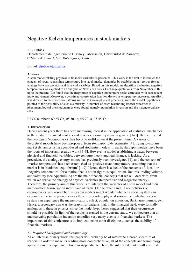
Figure 1. Entropy vs. energy for a magnetic system. If 0 and E 01 tt TT , then

the temperature sign is negative

Under these conditions, the entropy and mean energy S E per spin are bounded from above:

and max0 SS maxmin EEE . Also, the entropy is a function of energy S E with an arched shape [14], as shown in figure 1. Next, we define the energy increment E on the t-th day to be:

11 1,1,,1 ,

tt ni tititi

ni tit vpvpE , (6)

where is the i-th lot of shares on the t-th day. Such a definition agrees with [1], where

money and energy are treated as equivalent concepts. It is also consistent with [7], where tiv ,


logarithmic relative changes of price depend on magnetization increments, and therefore on energy per spin. 2.1 Negative Kelvin temperatures Readers with a general background in physics may find it paradoxical title of this section since Kelvin scale is an absolute temperature scale without negative values. However, for some particular systems, negative Kelvin temperatures are mathematically consistent [14, 15].

Temperature sign can be characterized by [15]: XEST /1

W

. Let us revisit such an

equation for our spin subsystem. The magnetic work relating to a magnetic state change of a system, is [16]:

BHVW d , (7) where V is the system volume, H the external magnetic field, and the induction variation. Magnetic work

Bd

mW performed by the system is the difference between magnetic work (7) and

the work needed for creating a magnetic field in the vacuum HHW dV0 [16], i.e.:

MHVWWW d00m (8) where is the magnetization variation and Md 0 the vacuum permeability. From (8) we may rewrite the fundamental equation of thermodynamics as follows:

nm0nmm dddd WMHVSTWWSTE , (9) where E is the internal energy and the non-magnetic work performed by the system. On

the other hand, magnetic potential energy for a system in a magnetic field is determined by [16]:

nmW

mE

HMVE 0m , (10)

The total energy will be the sum of internal energy TE E and potential energy : mE

mT EEE , (11) By combining (9), (10), and (11) we get:

nm0T ddd WHMVSTE , (12) where the entropy equals magnetic entropy plus non-magnetic entropy . S mS nmSNow, assuming that the spin subsystem has no degrees of freedom other than those associated with dipole orientation, i.e., , mSS mT EE and 0nm W , equation (12) leads to:

HE

ST

m

m1 . (13)

It is important to remark that equation (13) holds strictly for 0J and approximately for

. As treated in Section 2.4, in our model, we assume that a paramagnetism or weak ferromagnetism holding equation (13) is enough.

0J


In short, for certain magnetic systems, the entropy , after reaching a maximum, becomes

decreasing and the corresponding temperature is negative since is no other than the slope of entropy curve [14]. Hence, if a positive entropy increment corresponds to a negative energy increment, additional thermodynamic variables

S1T

H being constant, then the temperature is negative. Hence, it follows that 0E and 01 tT tT imply 0T (as shown in figure 1).

Correlatively, 0E and 01 tt TT imply 0T .

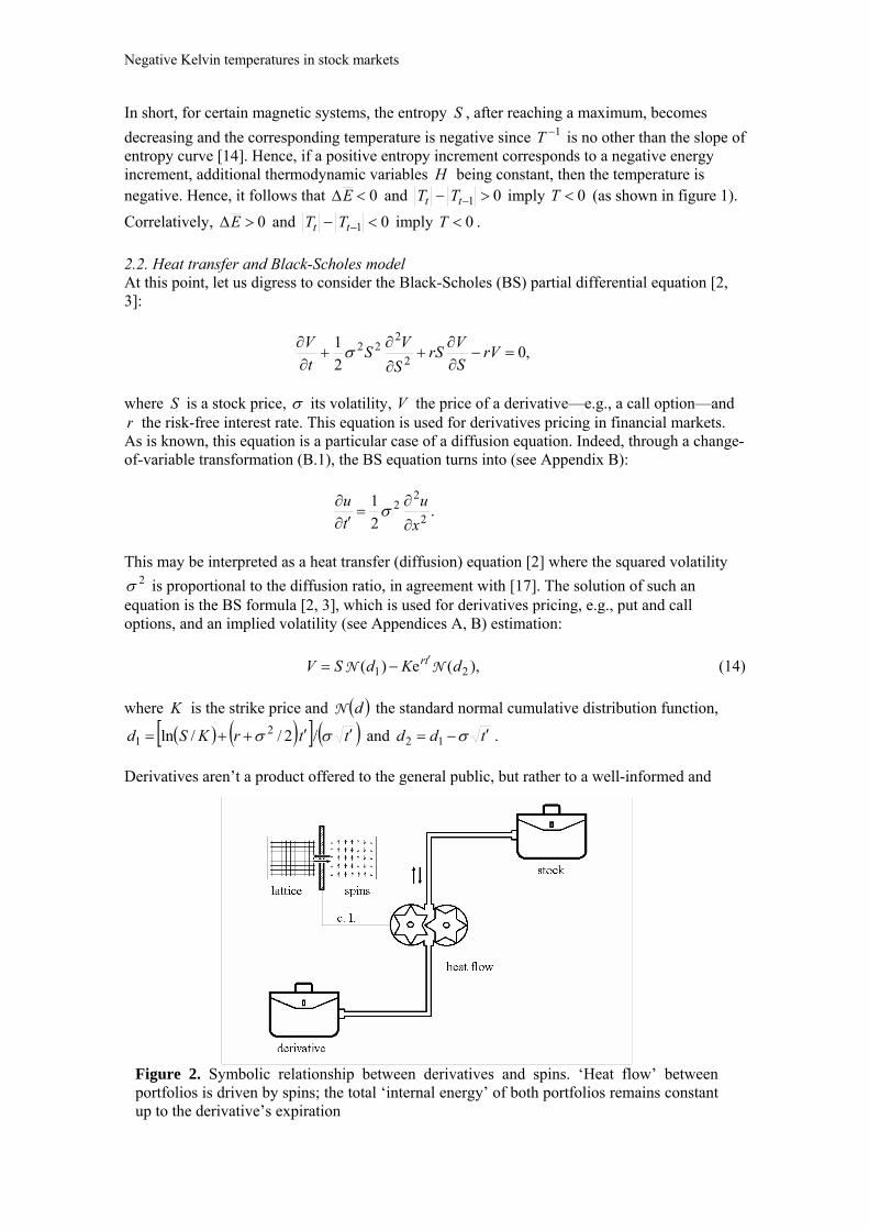
2.2. Heat transfer and Black-Scholes model At this point, let us digress to consider the Black-Scholes (BS) partial differential equation [2, 3]:

,02

12

222

rVS

VrS

S

VS

t

V

where is a stock price, S its volatility, V the price of a derivative—e.g., a call option—and r the risk-free interest rate. This equation is used for derivatives pricing in financial markets. As is known, this equation is a particular case of a diffusion equation. Indeed, through a change-of-variable transformation (B.1), the BS equation turns into (see Appendix B):

.2

12

22

x

u

t

u

This may be interpreted as a heat transfer (diffusion) equation [2] where the squared volatility

is proportional to the diffusion ratio, in agreement with [17]. The solution of such an equation is the BS formula [2, 3], which is used for derivatives pricing, e.g., put and call options, and an implied volatility (see Appendices A, B) estimation:

2

),(e)( 21 dKdSV tr NN (14) where K is the strike price and the standard normal cumulative distribution function, dN

ttrKd /2// 21 Sln and tdd 12 .

Derivatives aren’t a product offered to the general public, but rather to a well-informed and

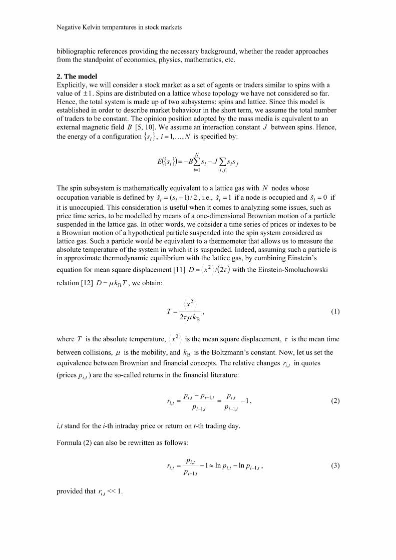
Figure 2. Symbolic relationship between derivatives and spins. ‘Heat flow’ between portfolios is driven by spins; the total ‘internal energy’ of both portfolios remains constant up to the derivative’s expiration


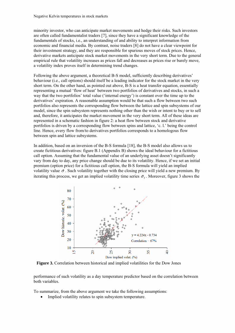
minority investor, who can anticipate market movements and hedge their risks. Such investors are often called fundamentalist traders [7], since they have a significant knowledge of the fundamentals of stocks, i.e., an understanding of and ability to interpret information from economic and financial media. By contrast, noise traders [8] do not have a clear viewpoint for their investment strategy, and they are responsible for spurious moves of stock prices. Hence, derivative markets anticipate stock market movements in the very short term. Due to the general empirical rule that volatility increases as prices fall and decreases as prices rise or barely move, a volatility index proves itself in determining trend changes. Following the above argument, a theoretical B-S model, sufficiently describing derivatives’ behaviour (i.e., call options) should itself be a leading indicator for the stock market in the very short term. On the other hand, as pointed out above, B-S is a heat transfer equation, essentially representing a mutual ‘flow of heat’ between two portfolios of derivatives and stocks, in such a way that the two portfolios’ total value (‘internal energy’) is constant over the time up to the derivatives’ expiration. A reasonable assumption would be that such a flow between two such portfolios also represents the corresponding flow between the lattice and spin subsystems of our model, since the spin subsystem represents nothing other than the wish or intent to buy or to sell and, therefore, it anticipates the market movement in the very short term. All of these ideas are represented in a schematic fashion in figure 2: a heat flow between stock and derivative portfolios is driven by a corresponding flow between spins and lattice, ‘c. l.’ being the control line. Hence, every flow from/to derivatives portfolios corresponds to a homologous flow between spin and lattice subsystems.

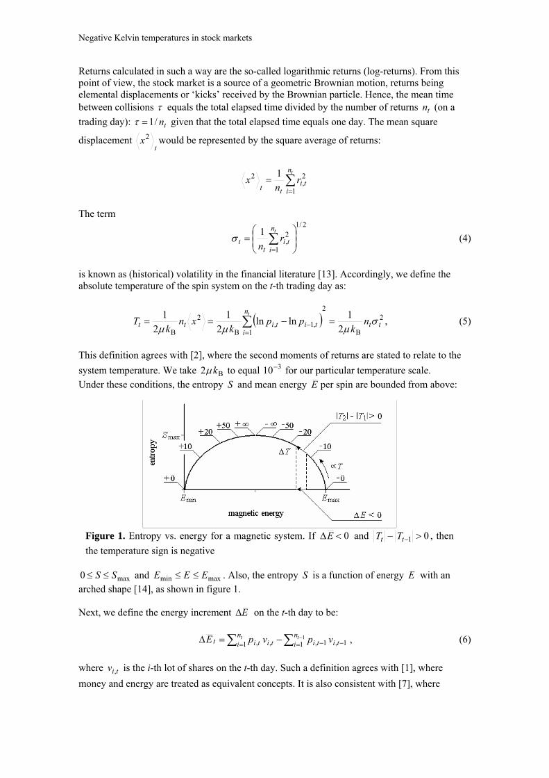
Figure 3. Correlation between historical and implied volatilities for the Dow Jones

In addition, based on an inversion of the B-S formula [18], the B-S model also allows us to create fictitious derivatives: figure B.1 (Appendix B) shows the ideal behaviour for a fictitious call option. Assuming that the fundamental value of an underlying asset doesn’t significantly vary from day to day, any price change should be due to its volatility. Hence, if we set an initial premium (option price) for a fictitious call option, the B-S formula will yield an implied volatility value . Such volatility together with the closing price will yield a new premium. By iterating this process, we get an implied volatility time series t . Moreover, figure 3 shows the

performance of such volatility as a day temperature predictor based on the correlation between both variables. To summarize, from the above argument we take the following assumptions:

Implied volatility relates to spin subsystem temperature.


Spin and lattice subsystems are in thermal contact and may fluctuate around an equilibrium point. Hence, energy may flow between them; e.g., when the spins experience a negative temperature, energy flows from the spins to the lattice, since negative temperatures are hotter than positive ones [15].

There is no upper limit for the lattice energy; therefore, its Kelvin temperature is always positive.

Hence, historical volatility would be a good estimation of spin temperature whenever both subsystems are in mutual equilibrium; however, if they fluctuate, it would be necessary to introduce implied volatility for a good estimation of the spin temperature. 2.3. Spin-field and spin-lattice relaxation times For a fluctuating system, relaxation time depends on the nature of the interaction between its particles (spins). In fact, relaxation time for the spin subsystem should be very brief, since such a subsystem models the mental attitude of the investor (i.e., his or her wish or intent to buy or to sell), and it is clear that such a mental position might change in seconds as he or she reads or hears some news in the financial media. However, sending the corresponding order to the market and its subsequent execution takes a period longer than the mental position change; i.e., in physical terms the typical interaction between spins and lattice is very much longer than the interaction between spins and the external magnetic field. This holds true despite telematic sending of market orders, since such a process is not direct but indirect through an intermediary broker. Automatic orders (on-stop orders) are an exception that should not confuse us: an automatic order doesn’t represent a brief interaction but rather a delayed interaction, since the investor’s mental change took place some time ago. On the other hand, financial time series are considered to be heteroskedastic random processes [19]. If we assume such a major property, then spin-lattice relaxation should be correlated with the relaxation time of the variance which, for the Dow Jones, ranged from a few hours to a few weeks in previous studies [20-22]. In this context, spin-lattice relaxation time presumably being very much longer than spin-field relaxation time, one may expect to population inversion phenomena to occur, since they occur in the event of very different relaxation times. 2.4. Magnetic behaviour and collaborative phenomena In general, stock markets are competitive (non-collaborative) systems, in which agents dispute a limited resource: what one agent loses is what another gains. In game theory, the so-called minority game [23-25] illustrates such a competitive feature very well. In this game, at each step of play, each player has to secretly choose one of two alternatives (e.g., ‘to buy’ or ‘to sell’). A counting of total choices is done: the winners are the players that are up on the minority side. And so the game is repeated. A player does not know anything about the others’ choices, but he must outguess what everyone else is guessing. One peculiar aspect of this game is that, no matter what strategy each agent uses for taking their position, if a majority uses the same mathematical strategy, then its failure is guaranteed; e.g., in stock markets, if all agents decide to sell, then prices suddenly drop, the majority is harmed, and only the minority outguessing such an event benefits. This fact in itself constitutes a fundamental limit of the game, so that massive collaboration is impossible because it is in contradiction to the nature of the game. Certainly, collaborative phenomena may spontaneously emerge, but they are limited [24]. In physical terms, ‘non-collaborative’ means ‘non-interactive with nearest neighbour’. This, in turn, means paramagnetic or very weak ferromagnetic behaviour. In other words, massive ferromagnetism is impossible because it is in contradiction to the nature of interaction. Hence, only very limited or weak ferromagnetism should be possible, as we indeed assumed in our model. In this context, one can expect, in financial markets, to turn up phenomena similar to those associated with physical paramagnetism, in particular, the magneto-caloric effect or adiabatic demagnetization. As it is known, materials increasing their temperature when they are exposed to a strong external magnetic field suffer a magneto-caloric effect: the larger their temperature increment, the stronger their magneto-caloric effect [26]. In consequence, in a search for hypothetical ‘magneto-caloric patterns’ in stock markets, a good strategy would be to


select those stocks suffering the strongest increment of their ‘temperature’, as appearing in the relevant news in the financial media. 3. The algorithm Following the above prolegomena, we devised an algorithm characterizing the temperature sign as follows: (i) First, we calculate tE by (6) on the t-th trading day. Then, we calculate temperatures and

using Eq. (5). tT

1tT(ii) Next, we estimate the temperature trend as follows:

(iia) We calculate intraday volatilities 1t , t corresponding to the (t−1)th and t-th

trading days using Eq. (4). Next, by entering 1t , 1c, tpKS

4

( being the closing

price on the [t−1]th trading day) and an initial value of

1c, tp

tVt

days into the BS formula (14), we get a fictitious price of a fictitious derivative p ˆ

(iib) We enter tpV ˆ and into the BS formula (14) again, and by a numerical

method, e.g., Newton-Raphson, we obtain the implied volatility

tpS c,

tˆ . Note that the volatility obtained from Eq. (4) is the so-called historical volatility, whereas that obtained from the BS formula (14) is referred to as implied

(iii) Finally, having evaluated the following conditions:

0 0 1 tt TTE (15)

0 0 1 tt TTE (16)

0ˆ tt (17)

if [(15) or (16)] and (17) hold, then we will conclude the temperature sign to be negative. 4. Some statistics As intraday data prove difficult to obtain, we used end-of-day data and a reasonably accurate approximation of formulae (4), (5), (6) as follows:

2/12min,max,

2o,c,

2

3/)ln(ln)ln(ln

tttt

t

pppp ,

11c,c, ttttt vpvpE ,

2

)ln(ln3)ln(ln 2min,max,

2o,c, tttt

t

ppppT

,

where subscripts o, max, min, c stand for open, maximum, minimum, and close. As a ticker to be studied, we selected the Dow Jones Industrial Average for a period between 15 November 2002 and 7 December 2012. The data set contains 2,542 points, forming a time series

, where the subscript t is the trading day number. By applying the above algorithm to the data set, we obtained a time series of signed temperatures, whose further analysis led to the results shown in this section and in Appendix C.

tS


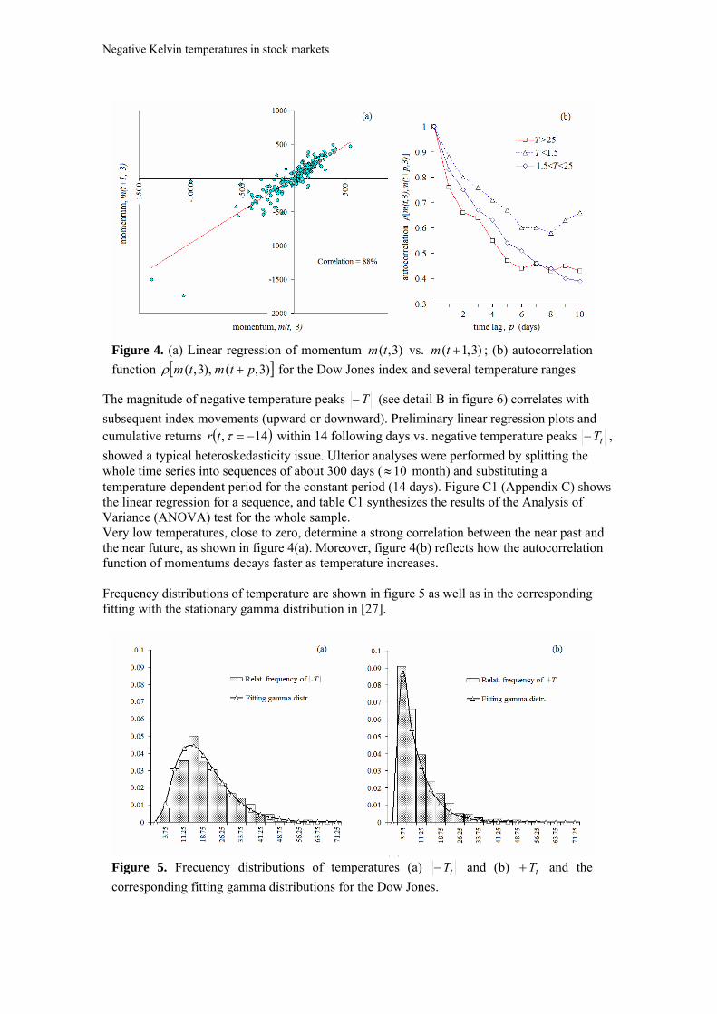
Figure 4. (a) Linear regression of momentum vs. )3,(tm )3,1( tm ; (b) autocorrelation

function )3,(),3,( ptmtm for the Dow Jones index and several temperature ranges

The magnitude of negative temperature peaks T (see detail B in figure 6) correlates with

subsequent index movements (upward or downward). Preliminary linear regression plots and cumulative returns 14, tr within 14 following days vs. negative temperature peaks tT ,

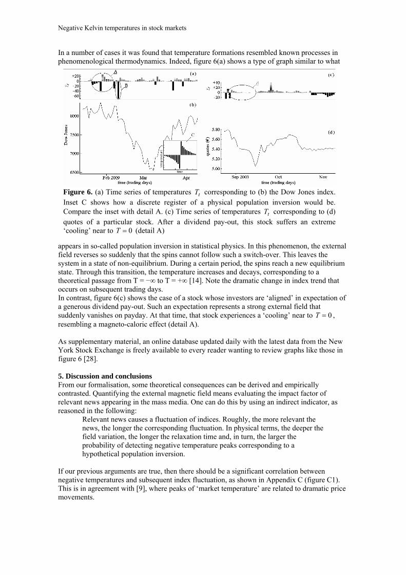
showed a typical heteroskedasticity issue. Ulterior analyses were performed by splitting the whole time series into sequences of about 300 days ( 10 month) and substituting a temperature-dependent period for the constant period (14 days). Figure C1 (Appendix C) shows the linear regression for a sequence, and table C1 synthesizes the results of the Analysis of Variance (ANOVA) test for the whole sample. Very low temperatures, close to zero, determine a strong correlation between the near past and the near future, as shown in figure 4(a). Moreover, figure 4(b) reflects how the autocorrelation function of momentums decays faster as temperature increases. Frequency distributions of temperature are shown in figure 5 as well as in the corresponding fitting with the stationary gamma distribution in [27].

Figure 5. Frecuency distributions of temperatures (a) tT and (b) and the

corresponding fitting gamma distributions for the Dow Jones. tT


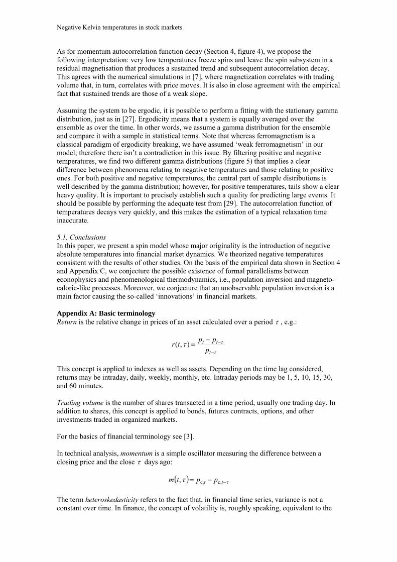
Figure 6. (a) Time series of temperatures T corresponding to (b) the Dow Jones index. Inset C shows how a discrete register of a physical population inversion would be. Compare the inset with detail A. (c) Time series of temperatures T corresponding to (d) quotes of a particular stock. After a dividend pay-out, this stock suffers an extreme ‘cooling’ near to

t

t

0T (detail A)

In a number of cases it was found that temperature formations resembled known processes in phenomenological thermodynamics. Indeed, figure 6(a) shows a type of graph similar to what

appears in so-called population inversion in statistical physics. In this phenomenon, the external field reverses so suddenly that the spins cannot follow such a switch-over. This leaves the system in a state of non-equilibrium. During a certain period, the spins reach a new equilibrium state. Through this transition, the temperature increases and decays, corresponding to a theoretical passage from T = −∞ to T = +∞ [14]. Note the dramatic change in index trend that occurs on subsequent trading days. In contrast, figure 6(c) shows the case of a stock whose investors are ‘aligned’ in expectation of a generous dividend pay-out. Such an expectation represents a strong external field that suddenly vanishes on payday. At that time, that stock experiences a ‘cooling’ near to T , resembling a magneto-caloric effect (detail A).

0

As supplementary material, an online database updated daily with the latest data from the New York Stock Exchange is freely available to every reader wanting to review graphs like those in figure 6 [28]. 5. Discussion and conclusions From our formalisation, some theoretical consequences can be derived and empirically contrasted. Quantifying the external magnetic field means evaluating the impact factor of relevant news appearing in the mass media. One can do this by using an indirect indicator, as reasoned in the following:

Relevant news causes a fluctuation of indices. Roughly, the more relevant the news, the longer the corresponding fluctuation. In physical terms, the deeper the field variation, the longer the relaxation time and, in turn, the larger the probability of detecting negative temperature peaks corresponding to a hypothetical population inversion.

If our previous arguments are true, then there should be a significant correlation between negative temperatures and subsequent index fluctuation, as shown in Appendix C (figure C1). This is in agreement with [9], where peaks of ‘market temperature’ are related to dramatic price movements.


As for momentum autocorrelation function decay (Section 4, figure 4), we propose the following interpretation: very low temperatures freeze spins and leave the spin subsystem in a residual magnetisation that produces a sustained trend and subsequent autocorrelation decay. This agrees with the numerical simulations in [7], where magnetization correlates with trading volume that, in turn, correlates with price moves. It is also in close agreement with the empirical fact that sustained trends are those of a weak slope. Assuming the system to be ergodic, it is possible to perform a fitting with the stationary gamma distribution, just as in [27]. Ergodicity means that a system is equally averaged over the ensemble as over the time. In other words, we assume a gamma distribution for the ensemble and compare it with a sample in statistical terms. Note that whereas ferromagnetism is a classical paradigm of ergodicity breaking, we have assumed ‘weak ferromagnetism’ in our model; therefore there isn’t a contradiction in this issue. By filtering positive and negative temperatures, we find two different gamma distributions (figure 5) that implies a clear difference between phenomena relating to negative temperatures and those relating to positive ones. For both positive and negative temperatures, the central part of sample distributions is well described by the gamma distribution; however, for positive temperatures, tails show a clear heavy quality. It is important to precisely establish such a quality for predicting large events. It should be possible by performing the adequate test from [29]. The autocorrelation function of temperatures decays very quickly, and this makes the estimation of a typical relaxation time inaccurate. 5.1. Conclusions In this paper, we present a spin model whose major originality is the introduction of negative absolute temperatures into financial market dynamics. We theorized negative temperatures consistent with the results of other studies. On the basis of the empirical data shown in Section 4 and Appendix C, we conjecture the possible existence of formal parallelisms between econophysics and phenomenological thermodynamics, i.e., population inversion and magneto-caloric-like processes. Moreover, we conjecture that an unobservable population inversion is a main factor causing the so-called ‘innovations’ in financial markets. Appendix A: Basic terminology Return is the relative change in prices of an asset calculated over a period , e.g.:

t

tt

p

pptr ),(

This concept is applied to indexes as well as assets. Depending on the time lag considered, returns may be intraday, daily, weekly, monthly, etc. Intraday periods may be 1, 5, 10, 15, 30, and 60 minutes. Trading volume is the number of shares transacted in a time period, usually one trading day. In addition to shares, this concept is applied to bonds, futures contracts, options, and other investments traded in organized markets. For the basics of financial terminology see [3]. In technical analysis, momentum is a simple oscillator measuring the difference between a closing price and the close days ago:

tt pptm c,c,,

The term heteroskedasticity refers to the fact that, in financial time series, variance is not a constant over time. In finance, the concept of volatility is, roughly speaking, equivalent to the


concept of standard deviation in mathematical statistics. To learn more about the concepts of implied and historical volatilities, see [2, 3]. For a comprehensive survey of time series and its mathematical treatment see [19]. Appendix B: The Black-Scholes model By a change-of-variable transformation as follows:

rt Sx ln , trxz

2

2, t ttuV e , e , (B.1)

where is a stock price, S its volatility, V the price of a derivative, r the risk-free interest rate, t the remaining time until derivative expiration and t expiry date, the Black-Scholes (BS) partial differential equation [2, 3]:

e

,02

12

222

rVS

VrS

S

VS

t

V (B.2)

turns into a one-dimensional heat transfer equation:

.2

12

22

x

u

t

u

(B.3)

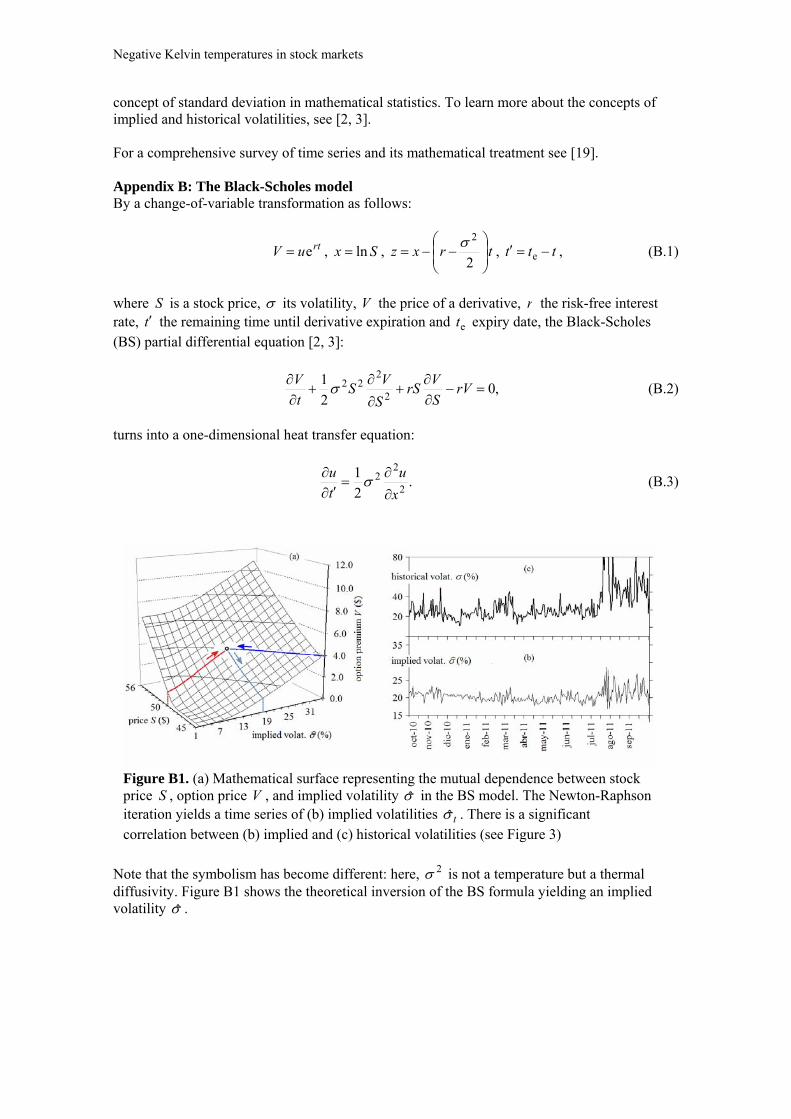
Note that the symbolism has become different: here, is not a temperature but a thermal diffusivity. Figure B1 shows the theoretical inversion of the BS formula yielding an implied volatility

2

.

Figure B1. (a) Mathematical surface representing the mutual dependence between stock price , option price V , and implied volatility S in the BS model. The Newton-Raphson iteration yields a time series of (b) implied volatilities t . There is a significant correlation between (b) implied and (c) historical volatilities (see Figure 3)


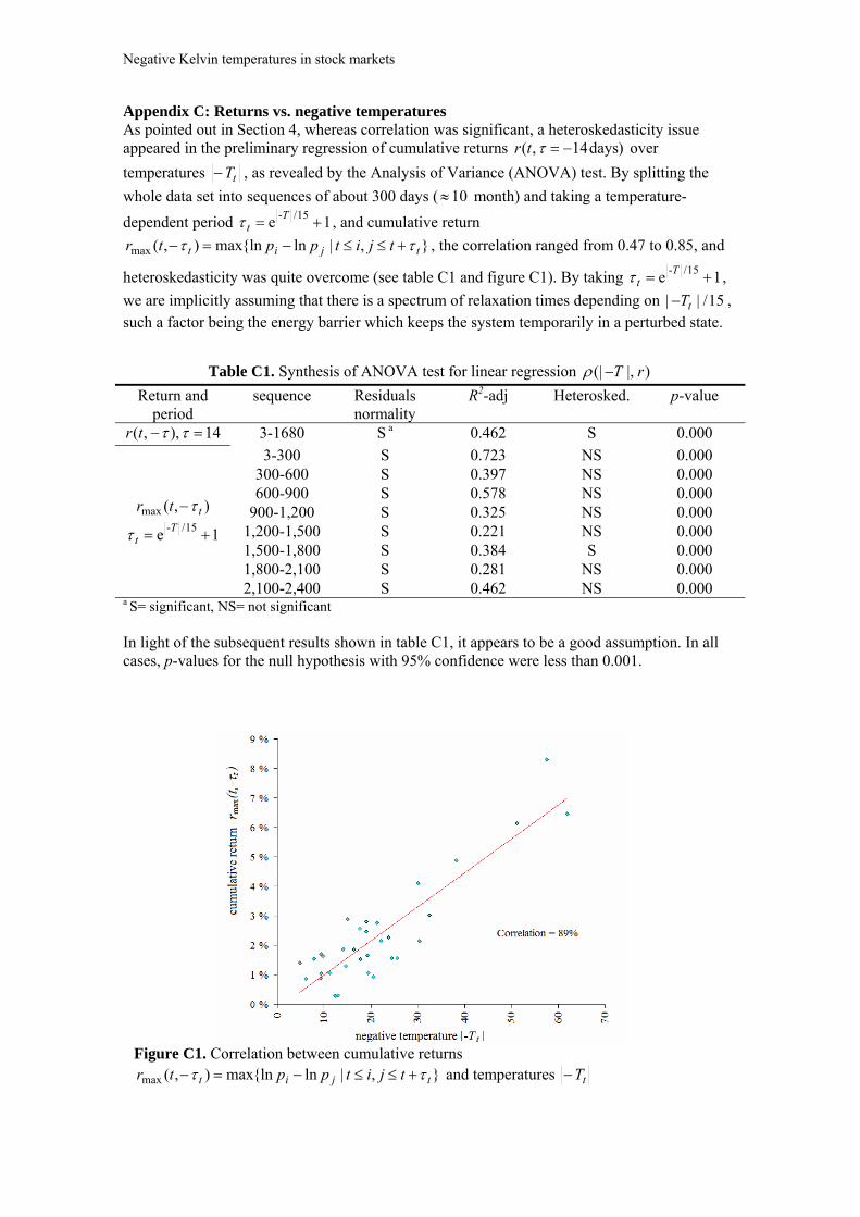
Appendix C: Returns vs. negative temperatures As pointed out in Section 4, whereas correlation was significant, a heteroskedasticity issue appeared in the preliminary regression of cumulative returns )days14,( tr over

temperatures tT , as revealed by the Analysis of Variance (ANOVA) test. By splitting the

whole data set into sequences of about 300 days ( 10 month) and taking a temperature-

dependent period 1e 15/- Tt , and cumulative return

},|ln{lnmax),(max tjit tjitpptr , the correlation ranged from 0.47 to 0.85, and

heteroskedasticity was quite overcome (see table C1 and figure C1). By taking 1e 15/- Tt ,

we are implicitly assuming that there is a spectrum of relaxation times depending on , such a factor being the energy barrier which keeps the system temporarily in a perturbed state.

15/|| tT

Table C1. Synthesis of ANOVA test for linear regression )|,(| rT

Return and period

sequence Residuals normality

R2-adj Heterosked. p-value

14),,( tr 3-1680 S a 0.462 S 0.000

3-300 S 0.723 NS 0.000 300-600 S 0.397 NS 0.000 600-900 S 0.578 NS 0.000

900-1,200 S 0.325 NS 0.000 1,200-1,500 S 0.221 NS 0.000 1,500-1,800 S 0.384 S 0.000 1,800-2,100 S 0.281 NS 0.000

),(max ttr

1e 15/- Tt

2,100-2,400 S 0.462 NS 0.000 a S= significant, NS= not significant

In light of the subsequent results shown in table C1, it appears to be a good assumption. In all cases, p-values for the null hypothesis with 95% confidence were less than 0.001.

Figure C1. Correlation between cumulative returns

},|ln{lnmax),(max tjit tjitpptr and temperatures tT


References [1] V. M. Yakovenko and J. Barkley, Statistical mechanics of money, wealth, and income Rev.

Mod. Phys. 81 1703-25 (2009) A. Dragulescu and V. M. Yakovenko, Statistical mechanics of money Eur. Phys. J. B 17 723-729 (2000)

[2] R. N. Mantegna and H. E. Stanley, An Introduction to Econophysiscs: Correlations and Complexity in Finance (Cambridge University Press, Cambridge, 1999) pp 120-127

[3] J. Voit, The Statistical Mechanics of Financial Markets (Springer-Verlag, Berlin, 2003) pp 70-79

[4] A. Kononovicius, V. Gontis and V. Daniunas, Agent-based versus macroscopic modeling of competition and business processes in economics and finance International journal on advances in intelligent systems 5 111-126 (2012)

[5] T. Kaizoji, An interacting-agent model of financial markets from the viewpoint of nonextensive statistical mechanics Physica A 370, 109-113 (2006)

[6] T. Kaizoji, Speculative bubbles and crashes in stock markets: an interacting-agent model of speculative activity Physica A 287 493-506 (2000)

[7] T. Kaizoji, S. Bornholdt and Y Fujiwara, Dynamics of price and trading volume in a spin model of stock markets with heterogeneous agents Physica A 316 441-452 (2002)

[8] D. Chowdhury and D. Stauffer, A generalized spin model of financial markets Eur. Phys. J. B 8 477-482 (1999)

[9] H. Kleinerta and X. J. Chen, Boltzmann distribution and market temperature Physica A 383 513-518 (2007)

[10] A. Krawiecki, J. A. Holyst and D. Helbing, Volatility Clustering and Scaling for Financial Time Series due to Attractor Bubbling Phys. Rev. Lett. 89 158701 (2002)

[11] R. Newburgh, J. Peidle and W. Rueckner, Einstein, Perrin, and the reality of atoms: 1905 revisited Am. J. Phys. 74 478-481 (2006)

[12] U. M. B. Marconi, A. Puglisi, L. Rondoni and A. Vulpiani, Fluctuation–dissipation: Response theory in statistical physics Physics Reports 461 111-195 (2008)

[13] B. Bollen and B. Inder, Estimating daily volatility in financial markets utilizing intraday data Journal of Empirical Finance 9 551-562 (2002)

[14] R. K. Pathria and P. D. Beale, Statistical Mechanics (Elsevier, Oxford, 2011) pp 88-92 [15] N. F. Ramsey, Thermodynamics and Statistical Mechanics at Negative Absolute

Temperatures Phys. Rev. 103 20-28 (1956) [16] J. J. Brey, P. Rubia and S. Rubia, Mecanica Estadistica (UNED, Madrid, 2001) pp 295-298 [17] M. G.Daniels, J. D. Farmer, L. Gillemot, G. Iori and E. Smith, Quantitative model of price

diffusion and market friction based on trading as a mechanistic random process Phys. Rev. Lett. 90 108102 (2003)

[18] Minqiang Le, Approximate inversion of the Black–Scholes formula using rational functions European Journal of Operational Research 185 743-759 (2008)

[19] C. Chatfield Time Series Forecasting (Chapman & Hall/CRC, Boca Raton, 2000) pp 11-148

[20] J. P. Fouque, G. Papanicolaou, and K. R. Sircar, Mean-reverting stochastic volatility, International Journal of Theoretical and Applied Finance 3 101-142 (2000)

[21] R. F. Engle and A. J. Patton, What good is a volatility model? Quantitative Finance 1 237-241 (2001)

[22] J. Masoliver and J. Perello, A correlated stochastic volatility model measuring leverage and other stylized facts International Journal of Theoretical and Applied Finance 5 541-562 (2002)

[23] E. Moro, The minority game: An introductory guide Advances in Condensed Matter and Statistical Physics edited by Shohov T, Boriotti S and Dennis D (Nova Science Publishers, New York, 2004) pp 263-286

[24] D. Challet and Y. C. Zhang, Emergence of cooperation and organization in an evolutionary game Physica A 246 407-418 (1997)


[25] C. A. Zapart, On entropy, financial markets and minority games Physica A 388 1157-72 (2009)

[26] D. Serantes, D. Baldomir, M. Pereiro, J. Botana, V. M. Prida, B. Hernando, J. E. Arias, J. Rivas Magnetocaloric effect in magnetic nanoparticle systems: How to choose the best magnetic material? Journal of nanoscience and nanotechnology 10 2512-17 (2010)

[27] D. Dragulescu and V. M. Yakovenko, Probability distribution of returns in the Heston model with stochastic volatility Quantitative Finance 2 443-453 (2002)

[28] Http://www.didyf.unizar.es/info/jlsubias/econophysical-trend-indicator.htm [29] J. Franke, G. Wergen and J. Krug, Correlations of record events as a test for heavy-tailed

distributions Phys. Rev. Lett. 108 064101 (2012)

http://www.didyf.unizar.es/info/jlsubias/econophysical-trend-indicator.htm

negative kelvin temperatures in stock markets

Documents