material point method applied to multiphase flows

Available online at www.sciencedirect.com

Journal of Computational Physics 227 (2008) 3159–3173

www.elsevier.com/locate/jcp

Material point method applied to multiphase flows

Duan Z. Zhang *, Qisu Zou, W. Brian VanderHeyden 1, Xia Ma

Theoretical Division, Fluid Dynamics Group (T-3, B216), Los Alamos National Laboratory, Los Alamos, NM 87545, USA

Received 5 June 2007; received in revised form 9 November 2007; accepted 19 November 2007Available online 22 Janauary 2008

Abstract

The particle-in-cell method (PIC), especially the latest version of it, the material point method (MPM), has shown sig-nificant advantage over the pure Lagrangian method or the pure Eulerian method in numerical simulations of problemsinvolving large deformations. It avoids the mesh distortion and tangling issues associated with Lagrangian methods andthe advection errors associated with Eulerian methods. Its application to multiphase flows or multi-material deformations,however, encounters a numerical difficulty of satisfying continuity requirement due to the inconsistence of the interpola-tion schemes used for different phases. It is shown in Section 3 that current methods of enforcing this requirement eitherleads to erroneous results or can cause significant accumulation of errors. In the present paper, a different numericalmethod is introduced to ensure that the continuity requirement is satisfied with an error consistent with the discretizationerror and will not grow beyond that during the time advancement in the calculation. This method is independent of phys-ical models. Its numerical implementation is quite similar to the common method used in Eulerian calculations of multi-phase flows. Examples calculated using this method are presented.� 2007 Elsevier Inc. All rights reserved.

Keywords: Particle-in-cell; Material point method; Multiphase flow; Fluid–structure interaction

1. Introduction

Particle-in-cell (PIC) method has been used in computational fluid mechanics since 1960s [1,2]. Since thenmany have used, improved and generalized the method to various cases. The work of Sulsky et al. [3] providesa mathematical foundation for the improved version of the method. The method is regarded as a numericalapproach of seeking a weak solution to the governing equations. The numerical schemes described in thatwork and the sequential extensions of it are often referred as the material point methods (MPM). A materialpoint method uses both Eulerian meshes and Lagrangian (material) points to represent a material. In suchmethods Eulerian meshes stay fixed and the Lagrangian points move through the Eulerian meshes duringthe material motion and deformation.

0021-9991/$ - see front matter � 2007 Elsevier Inc. All rights reserved.

doi:10.1016/j.jcp.2007.11.021

* Corresponding author. Tel.: +1 505 665 4428; fax: +1 505 665 5926.E-mail address: [email protected] (D.Z. Zhang).

1 Present address: BP North America, 150 West Warrenville Road, Naperville, IL 60563, USA.

mailto:[email protected]

3160 D.Z. Zhang et al. / Journal of Computational Physics 227 (2008) 3159–3173

A distinguished advantage of the particle-in-cell method is its capability of tracking motion of materialundergoing large deformation while avoid mesh tangling issues associated with Lagrangian meshes. Theuse of Lagrangian points in the method avoids the need to advect state variables, such as stress and strainof the material through the Eulerian mesh and avoids the numerical diffusion issues associated with suchadvection. One of the disadvantages of the material point method is its computational cost. It is more com-putationally expensive compared to both pure Eulerian and Lagrangian methods because it has to tracemotions of the material points and to update quantities on mesh nodes at the same time. Despite this disad-vantage, often it is the only credible choice for a practical problem that involves large deformations and com-plex moving boundaries [4].

The advantage of the material point method is highly desired for solving problems involving interactions ofdifferent materials or fluids. Materials involved in such cases often have different constitutive relations. Forinstance, in the case of porous solid materials filled with fluid, the fluid in the pores can often be modeledas Newtonian and its stress can be calculated from the strain rate. The stress in the solid is often related tostrain, which needs to be calculated accumulatively following the path of the material deformation. In thiscase, we often choose to calculate the fluid motion using an Eulerian mesh and to calculate the solid motionusing both the Eulerian mesh and Lagrangian material points, so that the stress and the deformation history ofthe solid can be traced using the material points. The method has been used to calculate fluid–structure inter-actions [5] and to calculate the interaction between a tungsten projectile and a steel block [6].

In all of these calculations, materials are regarded as interpenetrating continua. The location of the mate-rials is described by the spatial distribution of the volume fractions of the materials. The continuity conditionrequires that the volume fractions of all the materials sum to one. This continuity requirement is used to deter-mine the pressure in many calculations of multiphase flows using Eulerian methods [7]. As we shall see in Sec-tion 3, due to the difference in the approximations between the material point method and the Eulerianmethod, erroneous results for pressure will be obtained if the same scheme as used in Eulerian methods formultiphase flows is used to calculate the pressure. To avoid such numerical error, evolution equations for pres-sure and specific volume are developed [5] based on the assumption of the pressure equilibriums, so that thedirect enforcement of the continuity condition can be circumvented by directly advancing these quantitiesusing the evolution equations. It is proved [8] that the set of evolution equations for pressure and specific vol-ume is equivalent to one of the models that satisfies the continuity requirement. Other models are possible.

Many of the problems to be solved using the material point method are continuous multiphase or multi-mate-rial problems where the characteristic length scales of the materials are comparable to the length scale of theproblem domain. This type of problems is beyond the regime of disperse multiphase flows or particle reinforcedcomposite materials, where there is only one continuous phase, or material, and all other phases or materials arein the form of particles, droplets or bubbles with the characteristic size small compared to the problem domain.Compared to disperse multiphase problems, the models for continuous multiphase flows are still in theirinfancy. Even for disperse multiphase flows, there are still unsettled issues related to pressure calculations. Evo-lution equations [5,8] for pressure, the material densities and volume fractions are used to compute physicalinteractions involved in deformations that determine volume fractions. However, using these equations directlyto advance these quantities in time can lead to significant error accumulation as we show in Section 3.

In this paper we introduce a numerical scheme that satisfies the continuity requirement to higher order ofaccuracy in the sense of weak solutions for the evolution equations for the volume fractions. The nature ofweak solutions is consistent with the material point method.

In the following section we briefly describe the material point method. The approach described is not newand has been used by many others [3,4,9]. The reason we list them here is to rewrite them in the context ofmultiphase flows and to provide the basis for our discussion of the new method of satisfying the continuityconstraint. Many of the equations listed are used in later discussions. By briefly describing the method herewe also provide a complete description of the method as a convenience to the readers.

2. The material point method

Let qk be an average quantity contained in a unit mass of phase k at location x and time t. The averagedtransport equation for this quantity qk can be written in the following Lagrangian form [8]:

D.Z. Zhang et al. / Journal of Computational Physics 227 (2008) 3159–3173 3161

hkq0k

dqk

dt¼ qk

oqk

otþ uk � rqk

� �¼ r � ðhkLkÞ þ qkGk; ð1Þ

where hk is the volume fraction, q0k is the average material density, qk ¼ hkq0

k is the macroscopic density, uk isthe average velocity of phase k, Lk is the qk-flux tensor that is one order higher than qk, and qkGk is the sourcedensity for qk.

After taking inner product with a continuous trial function, hk, Eq. (1) can be written as

qkdqk

dt; hk

� �¼ r � ðhkLkÞ þ qkGk; hkð Þ; ð2Þ

where ð�; �Þ denotes the inner product. The inner product of two functions qk and hk is defined as

ðqk; hkÞ ¼Z

Xqkhk dv; ð3Þ

where the integration is over the entire computational domain X, and v is the volume in the domain.The material point method seeks an approximate weak solution to (1) in a subspace of continuous func-

tions in which all functions take the following form:

qkðx; tÞ ¼XN

j¼1

qkjðtÞSjðxÞ; ð4Þ

where N is the number of mesh nodes in the domain, qkj is the value of qk at node j and Sj is the shape functionassociated with the node.

By taking the trial function hk in the same form as (4)

hk ¼XN

‘¼1

dqk‘S‘ðxÞ; ð5Þ

we can define the weak solution to (1) in this subspace as qk in form (4) with qkj satisfying the following equa-tion for any trial function of form (5):
XN
‘¼1

XN

j¼1

mk‘jdqkj

dtdqk‘ ¼

XN

‘¼1

dqk‘ ðqk Gk; S‘Þ � ðhkLk;rS‘Þ þZ

oXhkLk � nS‘ðxÞdS

� �; ð6Þ

where n is the outward normal on the boundary of the domain X, and

mk‘j ¼Z

XqkS‘ðxÞSjðxÞdv: ð7Þ

Since dqk‘ is arbitrary, we have
XN
j¼1

mk‘jdqkj

dt¼ ðqkGk; S‘Þ � ðhkLk;rS‘Þ þ

ZoX

hkLk � nS‘ðxÞdS� �

: ð8Þ

This is a system of linear equations for the rate of change of qk at the nodes. To avoid solving this system ofcoupled equations, we note that mk‘j is non-zero only for the nodes (j’s) that are within the support (non-zeroregion) of the shape function S‘. Since these nodes are in the vicinity of node ‘, the rate dqkj=dt can be approx-imated as dqk‘=dt with a spatial discretization error O½ðDxÞd �, where d ¼ 1 if the rate is continuous in the spaceor node ‘ is a boundary node; and d ¼ 2 if the rate is smooth (first order differentiable), in the space. With thisapproximation the system of the linear equations is decoupled and can then be solved as

dqk‘

dt¼ 1

mk‘ðqkGk; S‘Þ � hkLk;rS‘ð Þ þ

ZoX

hkLk � nS‘ðxÞdS� �

þO½ðDxÞd �; ð9Þ

where

mk‘ ¼XN

j¼1

mk‘j ¼Z

XqkS‘ðxÞdv; ð10Þ


sincePN

j¼1SjðxÞ ¼ 1. This approximate way of decoupling the system of equations is equivalent to approxi-mating the matrix formed by elements mk‘jð‘; j ¼ 1; 2; . . . ;NÞ with a diagonal matrix in which the diagonal ele-ments are the sum of the elements in the corresponding rows of the original matrix. The error introduced bythis approximation is of order ðDxÞd . Because of this error, only the linear or bi-linear shape functions are usu-ally used in a material point method. In the present paper, we also restrict ourselves in using these shape func-tions. This approximation is also known to cause artificial energy dissipation of order ðDtÞ2 in a dynamicsystem [9].

To calculate the inner product in the first term on the right-hand side of (9), we again write Gk in the form of(4) to find

ðqkGk; S‘Þ ¼Z

Xqk

XN

j¼1

GkjSjðxÞS‘ðxÞdv

¼ Gk‘

ZX

qk

XN

n¼1

SnðxÞS‘ðxÞdvf1þO½ðDxÞd �g

¼ Gk‘mk‘f1þO½ðDxÞd �g: ð11Þ

We have again taken advantage of local support of the shape function as in (9) and approximated Gkj with Gk‘

within the support of S‘. This equation enables the source term Gk, such as the interaction force betweenphases, to be calculated at the nodes.

To calculate the second inner product on the right-hand side of (9), we now introduce an approximatescheme to calculate the inner product using material point quantities. In a material point method, the domainoccupied by phase k material is divided into non-overlapping Lagrangian regions. The union of these regionscovers entire domain occupied by phase k material. In principle, these Lagrangian regions are independent ofthe mesh in the computational domain, but for the convenience often these Lagrangian regions are formed bydividing a mesh cell into several such regions based on the domain occupied by phase k material specified inthe initial condition. The sizes of these regions are fractions of the typical mesh size Dx. Initially, the materialpoints are centroids of these Lagrangian regions. The mass and the volume of the region are assigned to thematerial point. These Lagrangian regions move and deform with the material and hence the material pointsalso move with the material. Although the material point may not be the centroid of the Lagrangian regionafter a deformation, the distance between them is of order O½ðDxÞd �, where d ¼ 1 for continuous and d ¼ 2 forsmooth displacement fields. Because the region is a Lagrangian region, the mass of the material point is con-stant during the material deformation without a phase change. In this way the shape of the Lagrangian regionis not tracked in the computation, but the volume vkp of the region for phase k represented by material point p

can be calculated by vkp ¼ mkp=q0kp, where mkp is the mass of the material point and q0

kp is the material density atthe material point. With the material points so constructed, the inner product ðqkqk; hkÞ can be approximatelycalculated based on the Lagrangian regions as

ðqkqk; hkÞ ¼XNkp

p¼1

mkpqkphkp þO½ðDxÞd �; ð12Þ

where N kp is the number of material points for phase k material in the domain, and qkp and hkp are the values ofqk and hk evaluated at material point p. The error estimate in (12) is obtained from the relation between thematerial points and the centroids of the Lagrangian regions.

In this way to seek a weak solution for (1) as defined in (6), the second inner product on the right-hand sideof (9) is approximated as

ðhkLk;rS‘Þ ¼ ðqkLk=q0k ;rS‘Þ �

XNkp

p¼1

vkpLkðxkp; tÞ � rS‘ðxkpÞ: ð13Þ

For the case where there are not enough material points in the elements surrounding node ‘, the accuracy ofthis approximation could be reduced. For more accurate and stable calculation, this inner product could becalculated using Gaussian integration scheme, but this subject is beyond the scope of the present work and we


will not discuss it further. Since S‘ has a local support, the summation only needs to be carried out for thematerial points in the elements surrounding node ‘.

With the right-hand side calculated using (11) and (13) we can write (9) as

dqk‘

dt� Gk‘ �

1

mk‘

XNkp

p¼1

vkpLkðxkp; tÞ � rS‘ðxkpÞ þ1

mk‘

ZoX

hkLk � nS‘ðxÞdS: ð14Þ

The last term in (14) represents the effect of boundaries.With the rate of change for qk calculated we can advance qk to the next time step as

qLk‘ ¼ qn

k‘ þdqk‘

dtDt; ð15Þ

where the superscript n denotes time step n and the superscript L denotes that this time advancement followsthe material point, the Lagrangian value, since the derivative is the solution to the evolution equation (1) in theLagrangian form. To update qk values on material points we interpolate the rate of change, or the materialderivative, from the nodes to material points as

qnþ1kp ¼ qn

kp þXN

‘¼1

ðqLk‘ � qn

k‘ÞS‘ðxnkpÞ: ð16Þ

It is important to note that we interpolate the change qLk‘ � qn

k‘, not qLk , to the material points. In this way, the

change of material point values is only caused by the right-hand side of (14). If the right-hand side of (14)vanishes, the material point value does not change. Therefore, such node to material point interpolation doesnot introduce numerical diffusion to the solution. If we interpolate Lagrangian node values qL

k‘ to materialpoints, significant numerical diffusion would occur. We also note that the value for the shape function S‘ isevaluated at the time step n. This is because material points are Lagrangian points. In this Lagrangian stepthey follow the motion of the material and the shape function is defined in the coordinate system that movesand deforms with the material. Therefore there is no relative motion between the material points and the coor-dinate system during the time advancement, and the values of the shape functions remain unchanged at thematerial point locations. Following the motion of the material, the new positions xkp of the material pointsrepresenting phase k are calculated as

xnþ1kp ¼ xn

kp þ ukpDt; ð17Þ

where velocity ukp is the velocity uk for phase k material at the location of material point p,

ukp ¼XN

‘¼1

uLk‘S‘ðxn

kpÞ; ð18Þ

with uLk‘ calculated using qk ¼ uk in (15). Again, the value for the shape function S‘ in (18) is evaluated at the

time step n for the same reason as in (16). The velocity ukp used to advance the material point positions is notthe material point velocity, but rather the velocity interpolated from the nodes, because material points areLagrangian points following the motion and deformation of the material, while a material point velocityshould be regarded as the averaged momentum per unit mass carried by the material point. The velocity gra-dient used to calculate the stresses or to advance the strains on material points is calculated by differentiatingthe shape functions in (18).

Note that the change rate dqk‘=dt calculated in (14) is the Lagrangian rate following the motion of the mate-rial. The time advanced qnþ1

k‘ on a fixed node needs to be calculated using the updated values qLkp on material

points. To obtain the scheme of calculating node values using material point values, we note that the innerproduct ðqq; hÞ can also be calculated using (4) to find

ðqkqk; hkÞ ¼XN

‘¼1

XN

j¼1

mk‘jqkjhk‘; ð19Þ

where mk‘j is defined in (7).


Comparing (12) with (19) and then using (4) for hk we find

XN

‘¼1

XN

j¼1

mk‘jqkjhk‘ ¼XN

‘¼1

XNkp

p¼1

mkpqkphk‘S‘ðxkpÞ þO½ðDxÞd �: ð20Þ

Since hk is an arbitrary smooth function, we have

XN

j¼1

mk‘jqkj ¼XNkp

p¼1

mkpqkpS‘ðxkpÞf1þOw½ðDxÞd �g; ð21Þ

where the subscript w in the error term reminds that this error estimate is given in the sense of the weaksolution. A common mistake is to treat (21) as a pointwise approximation with d ¼ 2 thinking that (21)can be derived from (20) by letting hk‘ ¼ 1 and hkj ¼ 0ðj 6¼ ‘Þ. The problem with this derivation is thatsuch defined function hk is not a smooth function, whereas (20) only holds for a smooth function ifd ¼ 2. Therefore we have only d ¼ 1 if (21) is regarded as a pointwise approximation. Instead of treat-ing both sides of (21) as pointwise individual values, we should regard the values specified by both sidesof (21) as an approximate way of representing two smooth functions by their values on the mesh nodes.The error estimate Ow½ðDxÞd � in (21) states that, for the two functions represented by both sides of (21),the inner products of these two functions with another smooth function approach each other quadrat-ically as mesh size decreases. As a consequence of this, if the values of both sides of (21) are averagedover the mesh nodes within a fixed physical domain, the difference between the averages approaches zeroquadratically as mesh refines.

For qk ¼ 1 in (21), we find that mk‘ defined in (10), can be approximately calculated using

mk‘ ¼XN

j¼1

mk‘j ¼XNkp

p¼1

mkpS‘ðxkpÞf1þOw½ðDxÞd �g: ð22Þ

Eq. (21) is a set of coupled equations for qkj at the nodes. Again because of the local support of the shapefunctions, by approximating qkj with qk‘ we have

qk‘ ¼PNkp

p¼1mkpqkpS‘ðxkpÞmk‘

f1þO½ðDxÞd �g ¼PNkp

p¼1mkpqkpS‘ðxkpÞPNkp

p¼1mkpS‘ðxkpÞf1þO½ðDxÞd �g: ð23Þ

By letting qk ¼ 1=q0k in (23), we find

q0k‘ ¼

PNkp

p¼1mkpS‘ðxkpÞPNkp

p¼1vkpS‘ðxkpÞf1þO½ðDxÞd �g; ð24Þ

for the material density at node ‘, where vkp ¼ mkp=q0k is the volume of the material point. Although for d ¼ 2

the error estimates in (21) and (22) are only in the sense of weak solution, the error estimates in (23) and (24)are pointwise provided that the displacements from the initial material point positions are spatially smooth,because the node quantity is approximated as the mass weighted mean of its surrounding material points andthe distance between a material point and the centroid of the Lagrangian region is of order O½ðDxÞ2�. The firstorder errors in Dx in the numerator and in the denominator cancel each other in this case.

Because the main subject of this paper is about the material point method, which seeks a weak solution tothe equations, and also because the second order spatial accuracy can be simply obtained by averaging overseveral neighboring nodes for smooth fields, there is little advantage to distinguish whether an error estimate ispointwise or is in the sense of weak solution. We will not distinguish them further, and drop the subscript w inthe error estimate.


3. Calculation of volume fractions and pressures

Using (10) and (22), the macroscopic density qk‘ at node ‘ can be approximated as

qk‘ ¼mk‘

V ‘

þO½ðDxÞd � ¼PNkp

p¼1mkpS‘ðxkpÞV ‘

f1þO½ðDxÞd �g; ð25Þ

where

V ‘ ¼Z

XS‘ðxÞdv ð26Þ

is the volume associated with the node. The volume fraction hk can be approximately calculated as

hk‘ ¼qk‘

q0k‘

¼PNkp

p¼1vkpS‘ðxkpÞV ‘

f1þO½ðDxÞd �g: ð27Þ

For phases that are not represented by material points, the macroscopic density is calculated from the massconservation equation [7,8]:

oqk

otþr � ðukqkÞ ¼ q0

kc_/k; ð28Þ

where _/k is the average rate of volume generation due to phase change and q0kc is the material density at phase

change. The volume fractions, hk‘, at node ‘ for those phases are approximated as the ratio qk‘=q0k‘ with the

same order of the spatial discretization error O½ðDxÞd �. Since the material densities are functions of pressures ofthe phases, the pressures can be found by enforcing the continuity condition
XM
k¼1

hk ¼ 1; ð29Þ

where M is the number of the phases in the calculation. In many computations of multiphase flows using Eule-rian methods [7], this equation is indeed used to find the pressures. However using the volume fraction approx-imately calculated using (27) for the phases represented by material points in this equation will result in failureof the calculation. To show this, we define a function

f ðDp; tÞ �XM

k¼1

qk

q0k

¼XM

k¼1

hkðDp; tÞ; ð30Þ

where Dp is the pressure increment. In this definition for function f, the material density q0k is a function of the

pressure increment through the equation of state. If a time explicit method is used, the macroscopic density isindependent of the pressure increment. If a time implicit method is used the macroscopic density is a functionof the pressure increment through the pressure gradient term in the momentum equation. The pressures for thephases may be the same or different, depending on the physical models used.

If an Eulerian method is used for all the phases as in many multiphase flow calculations [7], the consistencein spatial discretization for all the phases ensures that f ð0; tnÞ ¼ 1 is exact at the beginning of the time stepfrom n to nþ 1. For the cases where calculations of the volume fractions are different as described above,one can only have f ð0; tnÞ ¼ 1þO½ðDxÞd �. In other words, the sum of the volume fractions is not exactlyone if the volume fractions are calculated using different sets of material points for different phases, or if someof the volume fractions are calculated using an Eulerian method and the others are calculated using the mate-rial point method. We now show that this numerical error propagates and eventually contaminates the solu-tion if we require the function defined in (30) to be one in finding the pressure increment Dp, even though allthe methods of calculating the volume fractions are equally valid and have the same order of accuracy indi-vidually. The use of (30) to find Dp is equivalent to solving the following equation:

f ð0; tnÞ þ ofot

Dt þ ofoDp

Dp ¼ 1; ð31Þ


where, according to the Taylor theorem, the partial derivatives are evaluated at a point between tn and tn þ Dtfor time and between 0 and Dp for the pressure increment. Since f ð0; tnÞ ¼ 1þO½ðDxÞd �, we have

ofotþ of

oDpDpDt¼ O½ðDxÞd �

Dtð32Þ

for Dp. In many calculations of dynamical problems the time step is proportional to the mesh size Dx; there-fore the error on the right-hand side of (32), or Dp=Dt is ½OðDxÞd�1�. In this way, the pressure calculated usingpnþ1

k ¼ pnk þ Dp accumulates such errors. For a problem with characteristic time T, within T=Dt time steps, or

at the end of period T, the accuracy of the pressure reduces to O½ðDxÞd�1�, and in d such periods the pressurecalculation fails. The material point method described in Section 1 has a second order spatial accuracy in theregion where relevant quantities vary smoothly. For sharp interface regions or boundaries the accuracy re-duces to first order. For such cases the pressure calculated using (32) is erroneous (i.e. the error is zeroth or-der). Indeed, if this method were used to calculate the pressure in the case of an elastic body translatingthrough a mesh with the same uniform velocity as the surrounding air, one would see pressure changes wherenone should exist. For problems involving diffusion, if an explicit method is used, the problem will be evenworse because Dt is restricted by ðDxÞ2.

To satisfy the continuity requirement while avoiding the numerical error, efforts [5] have been made todirectly solve the evolution equations for material density or pressures. This approach is proved to be equiv-alent to directly solving the evolution equations for the volume fractions [8] and has been practiced for theequilibrium pressures model [5]. The evolution equations for the volume fraction and the average materialdensity can be written as [8]

ohk

otþr � ðhkukÞ ¼ hkhr � uki þ _/k; ð33Þ

hkoq0

k

otþ uk � rq0

k

� �¼ hkq

0khr � uki þ ðq0

kc � q0kÞ _/k; ð34Þ

where hr � uki is the average rate of the volumetric expansion in the material of phase k. The angular bracket,h�i represents the ensemble average [8]. The divergence of the averaged velocity r � uk is not necessary equal tothe average rate of the volumetric expansion in a multiphase flow. For instance, in a multiphase flow contain-ing air and sand grains, the divergence of the velocity field for sand is quite different from the volumetricexpansion of sand grains. In fact, in most practical situations the sand grains can be regarded as rigid withzero volumetric expansion, while the divergence of the average velocity of sand is not usually zero as sandgrains accumulate or disperse in the flow.

The summation of (33) over all the phases leads to

o

ot

XM

k¼1

hk þr � ðumÞ ¼XM

k¼1

ðhkhr � uki þ _/kÞ; ð35Þ

where

um ¼XM

k¼1

hkuk ð36Þ

is the mixture velocity and M is the number of phases. The continuity condition (29), is equivalent to

r � um �XM

k¼1

ðhkhr � uki þ _/kÞ ¼ 0; ð37Þ

since if this equation is satisfied the sum of the volume fractions is one if it is initially so. Using this relation,models for the average rate hr � uki of the volumetric expansion have been derived [5,8]. For a multipressuremodel

hr � uki ¼ akr � uk þ Bk; ð38Þ


where ak is a parameter specified by the model and the term Bk is related to compressibilities of the phases

Bk ¼1=ðhq0

kic2kÞPN

i¼1hi=ðhq0i ic2

i ÞXM

i¼1

r � ðhieuiÞ � aihir � eui � _/i

h i; ð39Þ

with ck being the speed of sound in phase k material. The equilibrium pressure or the single pressure model canbe treated [8] as a special case of the multipressure model by setting ak ¼ 0.

Using (38) and (39) one can calculate hr � uki at time level n (or at time level nþ 1, if an implicit method isused) and advance the volume fractions and the material densities in time according to (33) and (34). In thisscheme, Eq. (37) is only exactly satisfied at time tn (or tnþ1 for an implicit method) since the models are derivedbased on this equation. During time interval between tn and tnþ1, Eq. (37) is not exactly satisfied but with anerror OðDtÞ. Using (35), after a time integration, we find that the sum of the volume fractions at time levelnþ 1 is

XM

k¼1

hnþ1k ¼

XM

k¼1

hnk þO½ðDxÞdDt� þO½ðDtÞ2�; ð40Þ

where the error term O½ðDxÞdDt� results from the calculation of hr � uki using approximated volume fractionsand the error term O½ðDtÞ2� results from the OðDtÞ error in satisfying (37) during the time interval from tn totnþ1. Although such scheme is usable to find the pressures and volume fractions, the error accumulation couldbe significant. The OðDtÞ error in continuity constraint (37) leads to an error in the pressure. This error in pres-sure can be estimated as Oðqkc2

kDt=T Þ, where T is the characteristic time scale of the problem. Comparing theadvection terms in the momentum equation with this error, we find that this error in pressure can only be ne-glected if O½ðDt=T Þ=M2

k � is small, where Mk is the Mach number for phase k. For low Mach number flows thiserror could be significant although it decreases with the time step Dt.

According to this analysis, the most important error is not the error in the sum of the volume fractions butthe error in satisfying (37), because the later error carries significant dynamical consequence while the error inthe volume fraction sum is kinematic. In the time advancing scheme directly using the evolution equations, thekinematic error can be generated, because the sum of the volume fractions at time level tnþ1 can deviate fromunity even if the sum is exactly one at the previous time level and the motion of the material point does notintroduce any additional error. This volume fraction error causes error in the mixture compressibility asimplied by (39). To regulate this error, the volume fractions need to be normalized by redefining the volumefractions as hk=

PMi¼1hi. However such normalization does not affect the error already contained in the material

densities and pressures. In this way the kinematic error generated in the time advancing scheme spreads andbecomes the dynamical error. Indeed, this is the reason for using (29) instead of this scheme for pressure cal-culations in modern Eulerian methods for multiphase flow.

In a numerical calculation, although it is difficult to isolate errors and to prevent the kinematic error fromspreading into and becoming dynamical errors, such error spreading can be minimized. To do so, we nowintroduce a numerical method that spreads the kinematic error less than the scheme of directly advancingthe volume fractions or material densities using the values for hr � uki calculated at some specific time levels.The new method does not generate kinematic errors during the enforcement of the continuity constraintalthough it cannot prevent the generation of the error of OðDtÞ due to the motion of the material points.In this scheme, if the volume fraction sum is one at the beginning of a time step, the volume fraction wouldremain to be one if the motion of the material points were not to create a kinematic error. In other words, inthe new scheme, although the kinematic process still introduces an error of OðDtÞ, Eq. (37) is satisfied withinthe error limited to O½ðDxÞdDt�, instead of OðDtÞ, and then the pressure error caused by the kinematic errorbecomes O½ðDx=LÞdDt=T =M2

k �, where L is the characteristic length scale in the problem. In this way, althoughthe scheme is still first order in the time step, the extra factor ðDx=LÞd reduces the error in pressure caused bythe kinematic error resulting from using different but equivalently valid approaches to approximate the vol-ume fractions. This new scheme is based on the weak solution to the evolution equations for the volume frac-tions and is model independent. Its numerical implementation is quite similar to the commonly used methodsin pure Eulerian calculations.


4. Weak solution for volume fraction equations

To derive this scheme, we add and subtract r � ðhkumÞ from the left-hand side of (33), and rewrite the equa-tion as

dmhk

dmtþr � ½hkðuk � umÞ� þ hkr � um ¼ hkhr � uki þ _/k; ð41Þ

where

dmhk

dmt¼ ohk

otþ um � rhk ð42Þ

is the material derivative following the mixture velocity. To seek an approximate weak solution, we multiplyboth sides of (41) by a trial function h in the form of (4) defined on the frame moving with the mixture velocityum, and then integrate the resulting equation over the entire computational domain to find
XN
j¼1

hjdmvkj

dmt¼ �

XN

j¼1

hj

ZX

SjðxÞr � ½hkðuk � umÞ�dvþZ

XSjðxÞ hkhr � uki þ _/k � hkr � um

� �dv

� ; ð43Þ

where

vkj ¼Z

Xhkðx; tÞSjðxÞdv ð44Þ

and

dmvkj

dmt¼ ovkj

otþZ

XSjðxÞum � rhkdv: ð45Þ

Since hj is arbitrary, we then have

dmvkj

dmt¼ �

ZX

SjðxÞr � ½hkðuk � umÞ�dvþZ

XSjðxÞ hkhr � uki þ _/k � hkr � um

� �dv: ð46Þ

Summing (46) over all phases, we find that, in the sense of a weak solution, to satisfy (37) within an error ofO½ðDxÞdDt� is equivalent to satisfying the following equation within the same order of error:

dm

dmt

XM

k¼1

vkj ¼ �Z

XSjðxÞr �

XM

k¼1

½hkðuk � umÞ�dvþ V j O½ðDxÞdDt�; ð47Þ

where V j is defined in (26). Using (36), we find that the first term on the right-hand side of (47) is zero ifthe continuity condition (29) is satisfied exactly. When the approximated volume fractions are used,PM

k¼1½hkðuk � umÞ� is a quantity of O½ðDxÞd �. To avoid this error, we now change the way of calculating themixture velocity as

um ¼XM

k¼1

hkuk

XM

k¼1

hk:

,ð48Þ

This mixture velocity is, of course, the same as the definition (36) for the mixture velocity if the continuitycondition (29) is satisfied exactly and has the same order of accuracy as that calculated using the original def-inition (36) when (29) is only satisfied with an error O½ðDxÞd �. In this way the first term on the right and side of(47) vanishes identically; and (47) becomes

dm

dmt

XM

k¼1

vkj ¼o

ot

XM

k¼1

vkj þZ

XSjðxÞum � r

XM

k¼1

hkdv ¼ V jO½ðDxÞdDt�: ð49Þ

To calculate vkj defined in (44) for the phases represented by the material points, we can approximate the vol-ume integral by the sum over all material point volumes as in (21) with qk ¼ 1=q0

k and then use (27) to find


vkj ¼ ðqk=q0k ; SjÞ ¼ f1þO½ðDxÞd �g

XNkp

p¼1

vkpSjðxkpÞ ¼ hkjV jf1þO½ðDxÞd �g: ð50Þ

For the phases that are calculated using an Eulerian method we can simply approximate vkj by

vkj ¼ hkjV jf1þO½ðDxÞd �g ð51Þ
for d 6 2.
Since V j is a constant in time, by dividing V j across (49), the equation becomes

o

ot

XM

k¼1

hkj þ um � rXM

k¼1

hk

!j

24 35f1þO½ðDxÞd �g ¼ O½ðDxÞdDt�; ð52Þ

where the subscript j outside the round brackets denotes that it is evaluated at node j. By integrating this equa-tion from time tn to tnþ1 we have

XM

k¼1

hnþ1kj �

XM

k¼1

hnkj þ

Z tnþ1

tnum � r

XM

k¼1

hk

!j

dt

24 35f1þO½ðDxÞd �g ¼ O½ðDxÞdðDtÞ2�: ð53Þ

Within an error OðDtÞ, the integrand in the time integral can be approximated as ðugm � r

PMk¼1h

gkjÞ

½1þOðDtÞ�, where g ¼ n for a time explicit method and g ¼ nþ 1 for a time implicit method. Substituting thisinto (53), we find

XM

k¼1

hnþ1kj �

XM

k¼1

hnkj þ ug

m � rXM

k¼1

hgkjDt

!f1þO½ðDxÞd �g þ ug

m � rXM

k¼1

hgkjOðDtÞ2 ¼ O½ðDxÞdðDtÞ2�: ð54Þ

NotingPM

k¼1hgkj ¼ 1þO½ðDxÞd �, we find that r

PMk¼1h

gkj ¼ O½ðDxÞd �, and that the last term on the left-hand side

can be combined into the right-hand side. Therefore, with the mixture velocity um calculated using (48), if
XM
k¼1

hnþ1kj �

XM

k¼1

hnkj þ ug

m � rXM

k¼1

hgkjDt ¼ O½ðDxÞdðDtÞ2� ð55Þ

holds, then Eq. (37) is satisfied within an error of O½ðDxÞdDt�. Interestingly, Eq. (55) implies that the sum of thevolume fractions is ‘‘incompressible” following the mixture velocity calculated using (48).

In the numerical implementation described in the following section, Eq. (55) is used to enforce the conti-nuity condition (37).

5. Numerical implementation

After substituting (38) into (34), the evolution equation of the material density becomes

hkoq0

k

otþ uk � rq0

k

� �¼ hkq

0kakr � uk þ ðq0

kc � q0kÞ _/k þ hkq

0kBk: ð56Þ

With this evolution equation for the material density, the numerical scheme introduced in the present papercan be implemented in the time advancement from tn to tnþ1 as follows:

(1) For phases calculated using the Eulerian method, qk is the value of macroscopic density solved from themass conservation equation (28).

(2) For the phases calculated using the material point method, the macroscopic density qk is calculated using(25). The volume V ‘ defined in (26) is not typically calculated in a material point method. In manymeshes, such as triangle and quadrilateral elements in two dimensional problems and tetrahedral andhexahedral elements in three dimensional problem, this volume can be approximated by the control vol-ume, V C

‘ , of node ‘, provided that the meshes are not significantly distorted.


(3) For the phases calculated using the material point method, calculate interim microscopic density hq0kni�

on material points using (56) by neglecting the effects of Bk, and with the velocity divergence calculatedby taking the divergence of velocity (18). Then interpolate such calculated interim material density tonodes using (24).

(4) For phases calculated using the Eulerian method, the material density at the node is calculated by solv-ing (56) with the Bk term neglected.

(5) Use the equation of state for the phase to find an interim pressure p�k for all the phases according to thecalculated interim material densities at the nodes.

(6) Find a common pressure increment Dp such that the volume fractions, calculated as the ratioqkjðp�k þ DpÞ=q0

kjðp�k þ DpÞ between the macroscopic density and the material density, satisfy (55), orequivalently

XM

k¼1

qkjðp�k þ DpÞq0

kjðp�k þ DpÞ

" #nþ1

¼XM

k¼1

hkj

" #n

� ugm � r

XM

k¼1

hgk

!j

Dt: ð57Þ

The right-hand side of (57) can be regarded as a predicted volume fraction sum at time tnþ1 using (52). Thelast term in this equation can be evaluated at time tnþ1 or tn (g ¼ nþ 1 or n), depending on whether an implicitor explicit method is used. For numerical codes equipped with a good divergence operator, it is often conve-nient to calculate the factor in the last term as

ugm � r

XM

k¼1

hgk

!j

¼ r � ugm

XM

k¼1

hgk

!j

�XM

k¼1

hgkr � ug

m

!j

: ð58Þ

In this approach the effects of Bk in (56) is accounted for by finding Dp and then changing the material den-sities and volume fractions accordingly to satisfy (57). In an explicit time advancing scheme Eq. (57) is pointwise and involves only the local variables at the node j, and therefore can be solved easily. For implicitschemes, a mesh wide system must be solved.

The method of satisfying the continuity requirement introduced here is independent of physical models.The equilibrium pressure model can be implemented as a special case of the procedures outlined above byskipping steps 3–5. This method is similar to the typical pressure calculation procedures in an Eulerian codefor multiphase flows; therefore it can be implemented without significant modification of an Eulerian code.

Using (57) we also find that the change of the volume fraction sum during this procedure of finding thepressures is O½ðDxÞdDt�. Therefore, the error accumulation due to this pressure calculation is limited toO½ðDxÞd �, the same order of error due to the spatial discretization. In the case of spatially smoothly varyingvolume fractions, d ¼ 2 and the error in the sum of the volume fractions is second order in Dx.

6. Numerical examples

The numerical procedures outlined in Section 5 have been implemented into a numerical code. Several casesof fluid–structure interactions and multi-material interactions have been calculated. In our recent paper [8] wehave presented a numerical example of multiphase flow involving spalling of porous material with air filledpores calculated by the new method described here. In this example, the air flow around the porous solidand inside the pores of the solid is calculated using the Eulerian approach and the motion of the solid is cal-culated using the material point method. Good agreement between the numerical result and the theoreticalresults is observed.

To confirm the error analysis presented in this paper we perform a one-dimensional calculation of a poroussolid bar immersed in a heavy gas in domain [0, 1] cm with periodic boundary conditions on both ends. Thematerial properties of the solid bar are set as copper with initial density of 8:9 g=cm3. The initial volume frac-tion for the solid is set as 0:5þ 0:4 sinð2pxÞ (0 6 x 6 1). The solid bar is modeled as an elastic material withYoung’s modulus 125 GPa. The gas is assumed to be an ideal gas, with density calculated as Bp, where

B ¼ 1:15� 10�5 g=cm3=Pa. The initial pressure is set to be one atmosphere (p ¼ 1:013� 105 Pa). In this exam-ple, the gas is 1000 times heavier and stiffer than the air so that appreciable gas–solid interactions can take


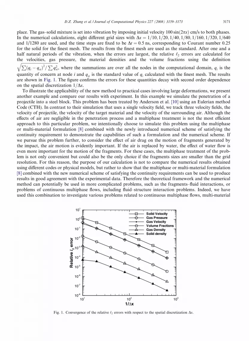
place. The gas–solid mixture is set into vibration by imposing initial velocity 100 sinð2pxÞ cm/s to both phases.In the numerical calculations, eight different grid sizes with Dx ¼ 1=10; 1=20; 1=40; 1=80; 1=160; 1=320; 1=640and 1/1280 are used, and the time steps are fixed to be Dt ¼ 0:5 ns, corresponding to Courant number 0.25for the solid for the finest mesh. The results from the finest mesh are used as the standard. After one and ahalf natural periods of the vibration, when the errors are largest, the relative ‘2 errors are calculated forthe velocities, gas pressure, the material densities and the volume fractions using the definitionffiffiffiffiffiffiffiffiffiffiffiffiffiffiffiffiffiffiffiffiffiffiffiffiffiffiffiffiffiffiffiffiffiffiffiffiffiffiffiP

ðqi � qsiÞ2=P

q2si

q, where the summations are over all the nodes in the computational domain, qi is the

quantity of concern at node i and qsi is the standard value of qi calculated with the finest mesh. The resultsare shown in Fig. 1. The figure confirms the errors for these quantities decay with second order dependenceon the spatial discretization 1=Dx.

To illustrate the applicability of the new method to practical cases involving large deformations, we presentanother example and compare our results with experiment. In this example we simulate the penetration of aprojectile into a steel block. This problem has been treated by Anderson et al. [10] using an Eulerian methodCode (CTH). In contrast to their simulation that uses a single velocity field, we track three velocity fields, thevelocity of projectile, the velocity of the target material and the velocity of the surrounding air. Although theeffects of air are negligible in the penetration process and a multiphase treatment is not the most efficientapproach to this particular problem, we intentionally choose to simulate this problem using the multiphaseor multi-material formulation [8] combined with the newly introduced numerical scheme of satisfying thecontinuity requirement to demonstrate the capabilities of such a formulation and the numerical scheme. Ifwe pursue this problem further, to consider the effect of air drag on the motion of fragments generated bythe impact, the air motion is evidently important. If the air is replaced by water, the effect of water flow iseven more important for the motion of the fragments. For these cases, the multiphase treatment of the prob-lem is not only convenient but could also be the only choice if the fragments sizes are smaller than the gridresolution. For this reason, the purpose of our calculation is not to compare the numerical results obtainedusing different codes or physical models, but rather to show that the multiphase or multi-material formulation[8] combined with the new numerical scheme of satisfying the continuity requirements can be used to produceresults in good agreement with the experimental data. Therefore the theoretical framework and the numericalmethod can potentially be used in more complicated problems, such as the fragments–fluid interactions, orproblems of continuous multiphase flows, including fluid–structure interaction problems. Indeed, we haveused this combination to investigate various problems related to continuous multiphase flows, multi-material

1/Δx

Rel

ativ

el 2

erro

r

101 102 10310-8

10-7

10-6

10-5

10-4

10-3

10-2

10-1

100

101

Solid VelocityGas PressureGas VelocityVolume FractionsGas DensitySolid density

Fig. 1. Convergence of the relative ‘2 errors with respect to the spatial discretization Dx.


interactions and fluid–structure interactions. Because of the complexity involved, direct comparison to eithertheoretical result and experiment are non-trivial. Fortunately, the projectile–target interaction problem treatedin this work is an exception and direct comparison to experimental results is possible for this case.

In this example of projectile–target interaction, a 5 cm tungsten rod is shot into a steel block of 4.95 cm inthickness. The steel block is initially at rest and the impact velocity of the tungsten rod is 1.7 km/s. The con-stitutive relation of both the tungsten and the steel are described using the Johnson–Cook model [11], in whichthe yield stresses of the metals are functions of the effective plastic strain and the temperature. The modelparameters used in this simulation are the same as those used by Anderson et al. [10]. Fig. 2 shows a snapshot of the penetration process. Our numerical results are compared with experimental data in Fig. 3.

Fig. 2. A snapshot of the projectile–target interaction. The region left to the symmetry axis shows the relative locations of the air, thetungsten rod and the steel block. In region right to the symmetry axis, we plot contours of air pressure, tungsten velocity and stress ryy inthe steel block in the corresponding regions.

Time (μs)

Hei

ght(

cm)

0 10 20 30 40 50 60 700

1

2

3

4

5

6

7

8

9

10

11Experiment (tail)Experiment (nose)Mesh size: 115x31Mesh size: 230x62Mesh size: 460x124

Tail position

Nose position

Upper steel surface

Lower steel surface

Fig. 3. Comparison with experimental results. Results calculated using different mesh sizes are plotted.


7. Conclusions

The material point method has been successfully applied in many calculations of solid material undergoinglarge deformations. Its direct application to physical systems described by multi-velocity fields, such as mul-tiphase flows and fluid–structure interactions, encounters a numerical difficulty of satisfying the continuityrequirement due to the spatial discretization error. Although there is an approach to circumvent this difficultyby solving an evolution equation for the pressure or the material density based on the models for volumetricdeformation rate, this approach is restricted to the single pressure model and is shown to cause significanterror accumulation. The error in satisfying the continuity requirement in the approach is OðDtÞ; and the errorin pressure is O½ðDt=T Þ=M2

k �, where Mk is the Mach number in phase k, T is the characteristic time scale of theproblem and Dt is the time step in the calculation. For low Mach number flows this error could be significantalthough it decreases with the time step.

Based on the weak solution to the evolution equations for volume fractions, in the present paper, we intro-duced another method of enforcing the continuity requirement within the error O½ðDx=LÞdDt=T �, where Dx isthe typical mesh size, L is the characteristic length scale of the problem, and d is the order of the discretizationerror. For a smoothly spatial varying field d ¼ 2. Although this method is still first order in the time step, thereis an extra factor ðDx=LÞd in it to reduce the error, and the error in the pressure caused by different but equiv-alently valid methods used to approximate the volume fractions can be maintained at O½ðDx=LÞdDt=T =M2

k �.The new approach is independent of physical models and is quite similar to the method of satisfying the con-tinuity requirement in an Eulerian method for multiphase flows; therefore it can be implemented easily with-out significant change to that part of an Eulerian code. Numerical examples calculated using this newapproach are presented and show good agreement with theoretical and experimental results.

Acknowledgment

This work was performed under the auspices of the United States Department of Energy with support fromthe Army Research Office.

References

[1] F.H. Harlow, The particle-in-cell computing method for fluid dynamics, Methods Comput. Phys. 3 (1963) 219.[2] F.H. Harlow, A.A. Amsden, Fluid Dynamics, A LASL Monograph, Los Alamos National Laboratory Report LA-4700, 1991.[3] D. Sulsky, S.-J. Zhou, H.L. Schreyer, Application of a particle-in-cell method to solid mechanics, Comput. Phys. Commun. 87 (1995)

236.[4] S.G. Bardenhagen, J.U. Brackbill, D. Sulsky, The material-point method for granular materials, Comput. Methods Appl. Mech. Eng.

187 (2000) 529.[5] B.A. Kashiwa, A Multifield Model and Method for Fluid–Structure Interaction Dynamics, Los Alamos Technical Report LA-UR-

01-1136, Los Alamos National Laboratory, Los Alamos, NM, 2001.[6] X. Ma, Q. Zou, D.Z. Zhang, W.B. VanderHeyden, G.W. Wathugala, T.K. Hasselman, Application of a FILP-MPM-MFM method

for simulating weapon–target interaction, in: Proceedings of the 12th International Symposium on Interaction of the Effects ofMunitions with Structures, New Orleans, Louisiana, September 13–16, 2005.

[7] A. Prosperetti, G. Tryggvason, Computational Methods for Multiphase Flow, Cambridge University Press, 2006 (Chapter 10).[8] D.Z. Zhang, W.B. VanderHeyden, Q. Zou, Nely T. Padial-Collins, Pressure calculations in disperse and continuous multiphase flows,

Int. J. Multiphase Flow. 33 (2007) 86.[9] S.J. Cummins, J.U. Brackbill, An implicit particle-in-cell method for granular materials, J. Comput. Phys. 180 (2002) 506.

[10] C.E. Anderson, V. Hohler, J.D. Walker, A.J. Stilp, Time-resolved penetration of long rods into steel targets, Int. J. Impact Eng. 16 (1)(1995) 1.

[11] G.R. Johnson, W.H. Cook, Fracture characteristic of three metals subjected to various strains, strain rates, temperature and pressure,Eng. Fract. Mech. 21 (1985) 31.

material point method applied to multiphase flows

Documents