masters thesis: numerical simulation of crack development
TRANSCRIPT
Department of Maritime & Transport Technology
Numerical simulation of crackdevelopmentfor Leak-Before-Break applications
Marjolein Bransen
Mas
tero
fScie
nce
Thes
is

Numerical simulation of crackdevelopment
for Leak-Before-Break applications
Master of Science Thesis
For the degree of Master of Science in Offshore and DredgingEngineering at Delft University of Technology
Marjolein Bransen
November 21, 2016
Faculty of Mechanical, Maritime and Materials Engineering (3mE) · Delft University ofTechnology

The work in this thesis was supported by Lloyd’s Register EMEA. Their cooperation is herebygratefully acknowledged.
Copyright c© Lloyd’s Register Global Technology CentreAll rights reserved.
Abstract
The term Leak-Before-Break (LBB) refers to a well-established safety criterion used to assesswhether cracked tanks or pipes can leak detectable amounts of fluid as a warning beforecatastrophic failure occurs. In this research The LBB criterion was applied to the safetyassessment of spherical Liquefied Natural Gas (LNG) containment systems on ships. Forthis type of LNG tanks, the International Code for the Construction and Equipment of ShipsCarrying Liquefied Gases in Bulk (IGC) requires several fracture mechanics analyses of fatiguecrack growth.
Details on how these analyses should be carried out can be found in industry codes. Al-though these codes provide guidance on most aspects of an LBB assessment, they are notfully satisfactory with regard to their recommendations on how to calculate the growth ofdeep semi-elliptical surface cracks, on how to estimate the crack shape when the crack snapsthrough the tank wall and how to assess these through-thickness cracks in the stage rightafter breakthrough.
The aim of this research was to more accurately simulate the development of cracks for LBBapplications. To do so, a new numerical calculation model have been developed for the estima-tion of crack growth, crack shape development and crack propagation after wall penetration.In addition, Finite Element Models (FEM) have been developed to predict the Stress Inten-sity Factor (SIF), a parameter that characterises the local stress distribution in the vicinity ofa crack-tip and is commonly used in fracture mechanics. Finite Element (FE) analyses wereconducted to evaluate existing, approximative SIF solutions for deep, semi-elliptical surfacecracks and to find a new, FE-derived SIF solution for through-thickness cracks after break-through. Both the new FE-derived and existing SIF solutions were used in the numericalmodel. The results of different SIF solutions and numerical model configurations were thencompared to experimental data from the literature in order to find recommendations for theenhancement of existing LBB procedures.
i

ii
ii
Table of Contents
Glossary ixList of Acronyms . . . . . . . . . . . . . . . . . . . . . . . . . . . . . . . . . . . ixList of Symbols . . . . . . . . . . . . . . . . . . . . . . . . . . . . . . . . . . . ix
Preface xiii
1 Introduction 11-1 State of the art . . . . . . . . . . . . . . . . . . . . . . . . . . . . . . . . . . . 31-2 Scope of work . . . . . . . . . . . . . . . . . . . . . . . . . . . . . . . . . . . . 101-3 Research objective . . . . . . . . . . . . . . . . . . . . . . . . . . . . . . . . . . 12
2 Numerical modelling of crack development 152-1 Calculation procedure, phases, steps and calculation steps . . . . . . . . . . . . . 152-2 Phase 1: Presence of an initial semi-elliptical surface flaw . . . . . . . . . . . . . 162-3 Phase 2: Crack growth . . . . . . . . . . . . . . . . . . . . . . . . . . . . . . . 162-4 Phase 3: Re-characterisation of the crack at breakthrough . . . . . . . . . . . . 202-5 Phase 4: Crack propagation after breakthrough . . . . . . . . . . . . . . . . . . 21
3 Modelling cracks with finite elements 233-1 Validation of the finite element method and software . . . . . . . . . . . . . . . 233-2 FEM of semi-elliptical surface cracks . . . . . . . . . . . . . . . . . . . . . . . . 263-3 FEM of semi-elliptical through-thickness cracks . . . . . . . . . . . . . . . . . . 32
4 The accuracy of predictive models in comparison with experiments 454-1 Comparison between the estimated breakthrough shape and experiments . . . . . 454-2 Comparison between the predicted N and experiments . . . . . . . . . . . . . . 484-3 Comparison between the predicted crack propagation and experiments . . . . . . 50
iii
iv Table of Contents
5 Analysis of the data, conclusions and recommendations 555-1 Analysis of the data taken from external sources . . . . . . . . . . . . . . . . . . 555-2 Estimating surface crack growth and breakthrough shape . . . . . . . . . . . . . 585-3 Estimating crack propagation after wall penetration . . . . . . . . . . . . . . . . 605-4 Recommendations for further research . . . . . . . . . . . . . . . . . . . . . . . 61
A Fracture mechanics 63A-1 Stress intensities . . . . . . . . . . . . . . . . . . . . . . . . . . . . . . . . . . . 63A-2 Energy release rate and the J integral . . . . . . . . . . . . . . . . . . . . . . . 65A-3 Linear and non-linear fracture mechanics . . . . . . . . . . . . . . . . . . . . . . 67A-4 Relation between the SIF and crack growth . . . . . . . . . . . . . . . . . . . . 68
B Stress intensity factor solutions 71B-1 Newman-Raju solution for a semi-elliptical surface crack . . . . . . . . . . . . . 71B-2 Wang solution for a deep semi-elliptical surface crack . . . . . . . . . . . . . . . 74B-3 AFNTO solution for a semi-elliptical through-thickness crack . . . . . . . . . . . 77B-4 Solution for a centre crack in a finite width-plate . . . . . . . . . . . . . . . . . 78
C Ansys script for the validation models 81
D The finite element method 93
E Ansys script for a semi-elliptical surface crack 97
F Ansys script for a semi-elliptical through-thickness crack 105
G Input for the numerical model 113
H Dealing with incomplete data-sets 115
iv
List of Figures
1-1 Leak-before-break diagram . . . . . . . . . . . . . . . . . . . . . . . . . . . . . 21-2 Steps to calculate the crack size versus number of stress cycles . . . . . . . . . . 51-3 Numbering of the calculation steps in the numerical procedure . . . . . . . . . . 51-4 Semi-elliptical surface crack . . . . . . . . . . . . . . . . . . . . . . . . . . . . . 61-5 Crack growth . . . . . . . . . . . . . . . . . . . . . . . . . . . . . . . . . . . . 61-6 Weigth function notation . . . . . . . . . . . . . . . . . . . . . . . . . . . . . . 71-7 Re-characterisation of the crack at breakthrough . . . . . . . . . . . . . . . . . . 81-8 Re-characterisation of the crack at breakthrough when a∗/c∗ is fixed. . . . . . . 91-9 LNG spherical tank . . . . . . . . . . . . . . . . . . . . . . . . . . . . . . . . . 10
2-1 Integration methods to find ∆N . . . . . . . . . . . . . . . . . . . . . . . . . . 182-2 Flowchart . . . . . . . . . . . . . . . . . . . . . . . . . . . . . . . . . . . . . . 192-3 Re-characterisation of the crack at breakthrough . . . . . . . . . . . . . . . . . . 20
3-1 Infinite sheet with an infinite row of collinear cracks . . . . . . . . . . . . . . . . 243-2 Three different mesh types . . . . . . . . . . . . . . . . . . . . . . . . . . . . . 253-3 Model of an embedded ellipse and a semi-elliptical surface crack . . . . . . . . . 283-4 Stress distribution σ(X) applied to the FEM . . . . . . . . . . . . . . . . . . . . 293-5 Comparison between the BCFs predicted by formulae and by FEM for a/c = 0.2 . 303-6 Comparison between the BCFs predicted by formulae and by FEM for a/c = 0.4 . 313-7 Semi-elliptical through-thickness cracks . . . . . . . . . . . . . . . . . . . . . . 323-8 Crack volumes created by extruding a spider web mesh along a semi-elliptical line 343-9 Crack volumes created by extruding a ’spider web’ mesh along straight lines . . . 343-10 Model and validation model for a/c = c2/c = 0.4 . . . . . . . . . . . . . . . . . 353-11 Crack-tip mesh used for all FEM . . . . . . . . . . . . . . . . . . . . . . . . . . 36
v
vi List of Figures
3-12 KFEM/Kref for the validation model of Figure 3-10 . . . . . . . . . . . . . . . 373-13 KFEM/Kref for validation models with a small and a large crack w.r.t. t . . . . 383-14 FEM with a small and a large crack w.r.t. t . . . . . . . . . . . . . . . . . . . . 393-15 KFEM/Kref for the semi-elliptical through-thickness crack model . . . . . . . . 403-16 BCF curves for point C . . . . . . . . . . . . . . . . . . . . . . . . . . . . . . . 423-17 BCF curves for point D . . . . . . . . . . . . . . . . . . . . . . . . . . . . . . . 43
4-1 Relation between ∆σB/∆σF and the shape at breakthrough . . . . . . . . . . . 474-2 Close-up of Figure 4-1 . . . . . . . . . . . . . . . . . . . . . . . . . . . . . . . . 484-3 Prediction and experimental data of crack growth for data-sets TH-1 and TH-3 . 494-4 Prediction and experimental data of crack growth for data-sets THL-1 and TB-7 504-5 Legend . . . . . . . . . . . . . . . . . . . . . . . . . . . . . . . . . . . . . . . . 514-6 Predicted and measured data of crack growth for c and c2 after breakthrough . . 524-7 Predicted and measured crack growth after breakthrough (tension and bending)-I 534-8 Predicted and measured crack growth after breakthrough (tension and bending)-II 54
5-1 Relation between da/dN versus ∆KA . . . . . . . . . . . . . . . . . . . . . . . 57
A-1 Local and global coordinate system for an arbitrary crack face . . . . . . . . . . 64A-2 Mode I, II and III . . . . . . . . . . . . . . . . . . . . . . . . . . . . . . . . . . 65A-3 Relation between P and u for a cracked plate . . . . . . . . . . . . . . . . . . . 66A-4 Arbitrary contour around a crack-tip . . . . . . . . . . . . . . . . . . . . . . . . 67A-5 Small scale plasticity correction . . . . . . . . . . . . . . . . . . . . . . . . . . . 68A-6 Crack growth rate as a function of ∆K . . . . . . . . . . . . . . . . . . . . . . 70
B-1 Nominal stress distribution . . . . . . . . . . . . . . . . . . . . . . . . . . . . . 71B-2 Semi-elliptical surface crack . . . . . . . . . . . . . . . . . . . . . . . . . . . . . 72B-3 Definitions for a semi-elliptical surface crack in a finite plate . . . . . . . . . . . 73B-4 Definitions for a semi-elliptical through-thickness surface crack . . . . . . . . . . 78B-5 Approximated Φ(1) . . . . . . . . . . . . . . . . . . . . . . . . . . . . . . . . . 79B-6 Definitions for a centre crack in a finite plate . . . . . . . . . . . . . . . . . . . 79
D-1 Crack-tip elements . . . . . . . . . . . . . . . . . . . . . . . . . . . . . . . . . . 94D-2 Surface for computing a J integral in 3-D. . . . . . . . . . . . . . . . . . . . . . 95D-3 Illustration of an issue with the J integral at the breakthrough side . . . . . . . . 96D-4 Stress field extrapolation . . . . . . . . . . . . . . . . . . . . . . . . . . . . . . 96
H-1 Relation between crack length at the initiation side and bending stress ratio. . . 116H-2 Crack shape development before breakthrough . . . . . . . . . . . . . . . . . . . 117
vi
List of Tables
1-1 Phases of crack development . . . . . . . . . . . . . . . . . . . . . . . . . . . . 4
2-1 Input for the numerical model . . . . . . . . . . . . . . . . . . . . . . . . . . . . 17
3-1 Ratio between the SIF from FEM and analytical SIF . . . . . . . . . . . . . . . . 26
4-1 Input for the prediction model for the breakthrough shape . . . . . . . . . . . . 464-2 r2 of the numerical models for crack growth . . . . . . . . . . . . . . . . . . . . 47
5-1 r2 of the fitted relations between da/dN versus ∆KA . . . . . . . . . . . . . . 56
G-1 Input for the models . . . . . . . . . . . . . . . . . . . . . . . . . . . . . . . . . 113G-2 Other model input . . . . . . . . . . . . . . . . . . . . . . . . . . . . . . . . . . 114
H-1 Eccentricity and load ratio for the specimens loaded by bending and tension . . . 115
vii

viii List of Tables
viii
Glossary
List of Acronyms
AFNTO Ando, Fujibayashi, Nam, Takahashi and Ogura
API American Petroleum Institute
BCF Boundary Correction Factor
BS British Standard
FE Finite Element
FEM Finite Element Model(s)
IGC International Code for the Construction and Equipment of Ships CarryingLiquefied Gases in Bulk
LBB Leak-Before-Break
LEFM Linear Elastic Fracture Mechanics
LNG Liquefied Natural Gas
LR Lloyd’s Register
NR Newman and Raju
NRC Newman and Raju Correction
SIF Stress Intensity Factor
SINTAP Structural Integrity Assessment Procedures for European Industry
TU Delft Delft University of Technology
ix
x Glossary
List of Symbols
Greek SymbolsΓ Integration contourε Strainη Ratio length over width, c/Wθ Angleµ Shear modulusν Poisson’s ratioΠ Potential energyσ Nominal stressσy Yield stress∆σ σmax − σminϕ Parametric angle of the ellipse
Latin SymbolsA Deepest point of a semi-elliptical crackA Crack areaa General crack size/ depth of a semi-elliptical cracka1 Initial crack depthabb Assumed depth of the crack at ligament instabilityC Surface point of a semi-elliptical crackC Constant in Paris relationC Compliancec Half surface length of the crackc1 Initial crack half lengthc2 Half length of the back side of the crack after breakthroughE Youngs’ modulusE′ E (plane stress) ; E/(1− ν2) (plane strain)e EccentricityF Work done by external forcesfR(.) Function depending on Rfw Finite width correction factorfϕ Embedded elliptical crack boundary correction factorG Linear elastic energy release rateH (Half-) heigthi Iteration step numberJ Energy release rateK Stress intensity factor
x

xi
Kc Critical stress intensity factor (plane stress)Keff Effective stress intensityKIc Critical stress intensity factor (plane strain)∆K Kmax −Kmin
∆Kth Threshold stress intensity factor rangek Step numberm Exponent in Paris relationm(x, a) Weight functionN Number of load cyclesn Total number of steps/ order of the stress fieldni Normal vector componentsP LoadQ Square of the complete elliptic integral of the second kindR Load ratio (= σmin/σmax = Kmin/Kmax)r Radiusr2 Coefficient of determinationrp Radius of the plastic zone around the crack-tipT Thickness of a solid bodyTi Stress vector componentst Plate thicknessU Elastic strain energyu DisplacementW (Half-)widthW Strain energy density{X,Y, Z} Global coordinates{x, y, z} Local coordinatesY Boundary correction factor
Subscripts/SuperscriptsA At point Aa Along direction abb Before breakthroughbt Breakthroughb BendingC At point Cc Along direction c/criticalD At point Dmax Maximummin Minimumm Membrane∗ Condition at breakthrough
xi

xii Glossary
xii

Preface
During my first days of my internship at the Global Technology Centre of Lloyd’s Register(LR) in Southampton, I was given the opportunity to join a multi-day workshop on fracturemechanics related topics. A group of Lloyd’s experts from all over the world shared theirknowledge of a wide range of topics within this field. Some of them gave examples of thechallenges they had encountered and how they had managed to deal with these issues. Theyalso raised some current unresolved questions related to their work. One of these problems,on how to deal with crack propagation in spherical LNG tanks after a crack had appeared atthe tank surface, became the starting point for a research exercise and this thesis.The idea to apply for a graduate internship at LR came after doing an internship at a shipyardwhere the largest vessel in the world, the Pioneering Spirit was being build. Not only didthis experience aroused my interest for marine engineering, it also introduced me to theimportance of the work of classification societies like LR and their contribution to the safetyof vessels.I would like to express my gratitude to Rob Pijper of LR for giving me the great opportunityto work on my thesis at the Southampton office were I was surrounded by experts in marineengineering. In addition, his genuine interest in my research and my personal well-beingwhile living in England is greatly appreciated. Of the many helpful and welcoming colleaguesin Southampton, I would like to mention in particular my supervisors Richard Villavicencioand Shengmin Zhang. Their encouragements and efforts to improve my research have beena welcoming assistance to my work and it has been a great pleasure to work with them.Richard has not only helped me to retrieve data from the figures from external resources,he also spend much of his own time to read all chapters and gave valuable comments on mywork. This welcoming and productive environment greatly contributed to the completion ofthe thesis.Furthermore, I am also grateful for the useful translation of the article of Shingai et al. fromJapanese to Dutch made by Lei Hendriks. He does not only have a degree in Japanese studiesbut also works as an engineer, which made him a great translator for this article. I am verythankful that he dedicated his free time to translate this for me.On a more personal level, I would like to thank my friends Laurens, Moniek, Roos and myfellow students from ’the Parrotzone’ for their mental support during the course of my study.Their encouragements, sense of humour and friendship have been an indispensable factor ofsuccess to the completion of my study during these seven vette years in Delft.
xiii

xiv Preface
More than anyone else, I would like to thank my parents. They supported me in all possiblekinds of ways. They encouraged me from a very young age to make my own choices and gaveme the self-confidence that I was able to make my own decisions. The choices I made werequite often not their choices - quite the opposite in fact. My decision to study Korean Studiescame to them as a surprise but nevertheless, they were proud that I became a languagestudent. When I started taking evening classes in mathematics and physics at an adulteducation centre and subsequently enrolled as a student at the TU Delft, they were evenmore surprised. While some parents hope that their child becomes an engineer, mine mighthave had their doubts whether this plan would stand a chance. They might have thought thatstudying Dutch, history or economics would be more suitable for me. If your child followsprecisely the career path that you have in mind, it is easy to be enthusiast and encouraging.But I truly admire my parents because they did so regardless of what I choose to do. Byreassuring me countless times that I could count on them even if I would completely fail, Iwas able to flourish.
Delft, University of Technology Marjolein BransenNovember 21, 2016
xiv

“On ne découvre pas de terre nouvelle sans consentir à perdre de vue, d’abord etlongtemps, tout rivage.”— André Gide

Chapter 1
Introduction
A well-established safety assessment criterion in the nuclear and (petro-) chemical industryis to check that tanks and pipes have the ability to leak for a certain period of time as awarning before catastrophic failure occurs [1]. The objective of this so-called Leak-Before-Break (LBB)1 assessment is to analyse:
1) How and how fast an initial flaw develops into an unstable crack and whether thisinstability occurs before or after penetrating through a tank or pipeline wall;
2) Whether a breakthrough crack leaks enough to get detected before becoming unstable;3) Whether sufficient time is available after leakage detection to take emergency measures.
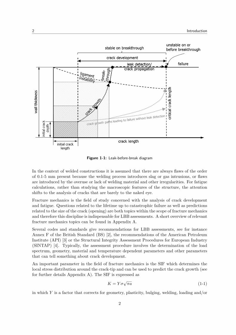
Figure 1-1 illustrates the stages of crack development in the wall of a tank or pipe. Aninitial crack is present in the structure, and the first step is to establish the initial crack sizeand shape. These could be known from inspection or could be assumed to be equal to theminimum detectable size. The next step is to determine how the shape of the crack developswhile growing towards wall penetration, i.e. the crack growth phase. A sufficiently large crackbecomes unstable, resulting in a sudden rupture of the material. If the crack re-stabilises afterwall penetration an LBB case could be made, provided there is enough time for leak detectionbefore the crack reaches a critical length at which the tank or pipe catastrophically fails. Thecrack growth phase after breakthrough is referred to as the crack propagation phase. Crackdevelopment refers to both the crack growth and propagation phase.
Under normal operating conditions the nominal stresses in tanks and pipes, taken into accounta safety factor, should stay well below the yield strength of the material and failure shouldnot occur when a small flaw is present. Furthermore, in these predominantly tensile loadedstructures, buckling is not an issue either. Hence, apart from accidental loads, the mainthreat to cyclically loaded constructions is fatigue, damaging metallic structures even whenloaded well below the yield stress. What initially may start as a small flaw, could grow intoa potentially dangerous crack.
1It would have been more appropriate to refer to this criterion as ’Leak-Before-Failure’ but this researchfollows the more commonly used ’Leak-Before-Break’ terminology.
1
2 Introduction
Figure 1-1: Leak-before-break diagram
In the context of welded constructions it is assumed that there are always flaws of the orderof 0.1-5 mm present because the welding process introduces slag or gas intrusions, or flawsare introduced by the overuse or lack of welding material and other irregularities. For fatiguecalculations, rather than studying the macroscopic features of the structure, the attentionshifts to the analysis of cracks that are barely to the naked eye.
Fracture mechanics is the field of study concerned with the analysis of crack developmentand fatigue. Questions related to the lifetime up to catastrophic failure as well as predictionsrelated to the size of the crack (opening) are both topics within the scope of fracture mechanicsand therefore this discipline is indispensable for LBB assessments. A short overview of relevantfracture mechanics topics can be found in Appendix A.
Several codes and standards give recommendations for LBB assessments, see for instanceAnnex F of the British Standard (BS) [2], the recommendations of the American PetroleumInstitute (API) [3] or the Structural Integrity Assessment Procedures for European Industry(SINTAP) [4]. Typically, the assessment procedure involves the determination of the loadspectrum, geometry, material and temperature dependent parameters and other parametersthat can tell something about crack development.
An important parameter in the field of fracture mechanics is the SIF which determines thelocal stress distribution around the crack-tip and can be used to predict the crack growth (seefor further details Appendix A). The SIF is expressed as
K = Y σ√πa (1-1)
in which Y is a factor that corrects for geometry, plasticity, bulging, welding, loading and/or
2
1-1 State of the art 3
other factors, σ is the nominal stress and a refers to a crack size in general, like the length ordepth of a crack. When reaching KIc, the critical SIF, a linear elastic material under plainstrain conditions2 starts to propagate in an unstable manner. Plasticity effects decrease thecritical crack size but for stress levels well below the yield stress, it is a reasonable assumptionto apply a Linear Elastic Fracture Mechanics (LEFM) model. The critical SIF depends on thetemperature, material properties and production techniques and is obtained by standardisedtests. From Eq. (1-1), the critical crack size is determined as
ac = 1π
(KIc
Y σ
)2(1-2)
In a recent update of the International Code for the Construction and Equipment of ShipsCarrying Liquefied Gases in Bulk (IGC), section 4.18.2.6 in [5], it is required to carry out afracture mechanics analysis of flaws in LNG containment systems. It should be verified thata crack will not reach critical dimensions before breakthrough and that it can leak detectableamounts of LNG under a recommended 15-day load spectrum before becoming critical. ThisIGC update underlines the importance of fracture mechanics for LBB assessments and therelevance of it for the industry, including classification societies like Lloyd’s Register.
1-1 State of the art
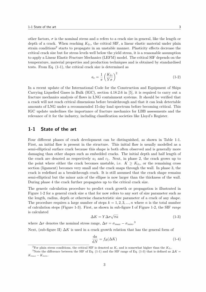
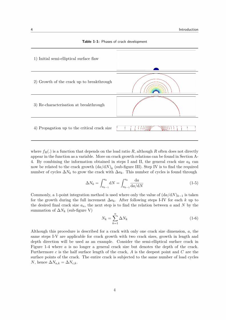
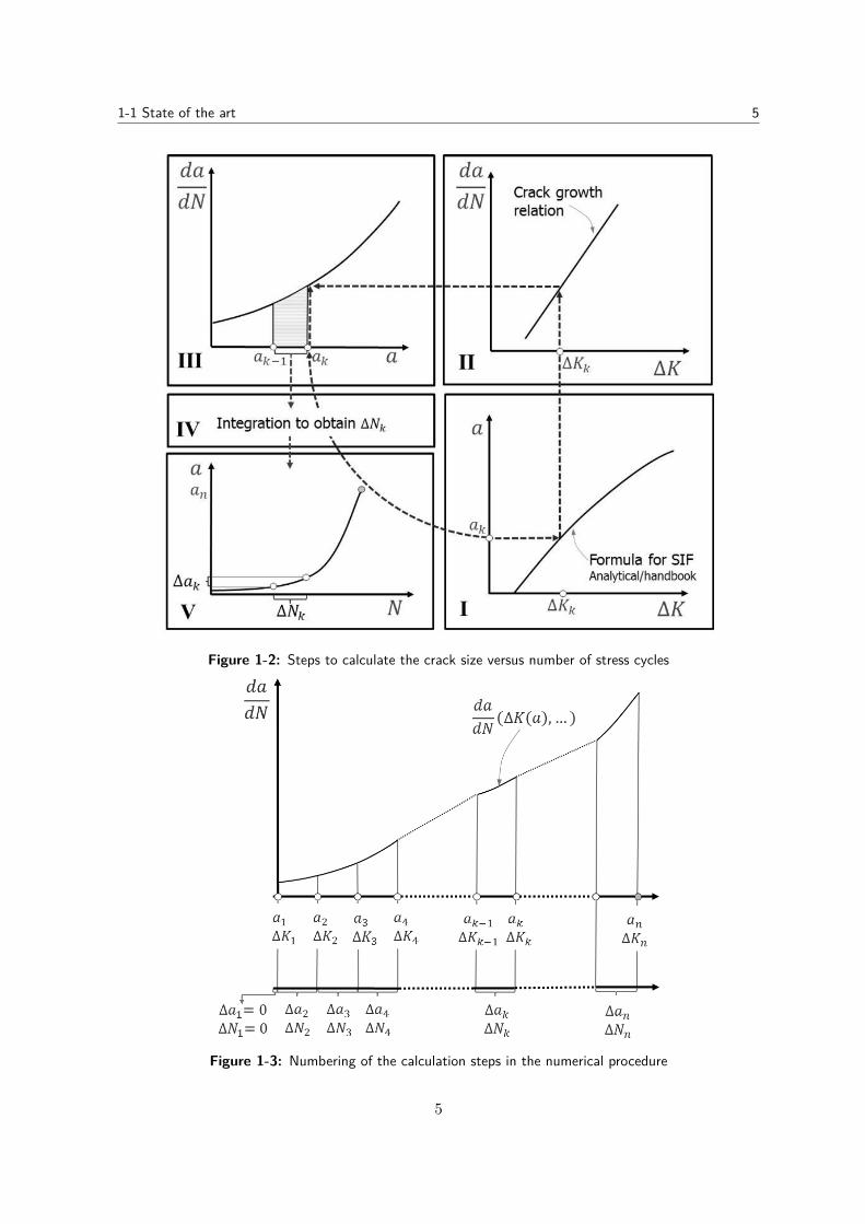
Four different phases of crack development can be distinguished, as shown in Table 1-1.First, an initial flaw is present in the structure. This initial flaw is usually modelled as asemi-elliptical surface crack because this shape is both often observed and is generally moredamaging than other shapes such as embedded cracks. The initial depth and half length ofthe crack are denoted as respectively a1 and c1. Next, in phase 2, the crack grows up tothe point where either the crack becomes unstable, i.e. K ≥ KIc, or the remaining crosssection (ligament) becomes very small and the crack snaps through the wall. In phase 3, thecrack is redefined as a breakthrough crack. It is still assumed that the crack shape remainssemi-elliptical but the minor axis of the ellipse is now larger than the thickness of the wall.During phase 4 the crack further propagates up to the critical crack size.The generic calculation procedure to predict crack growth or propagation is illustrated inFigure 1-2 for a general crack size a that for now refers to any sort of size parameter such asthe length, radius, depth or otherwise characteristic size parameter of a crack of any shape.The procedure requires a large number of steps k = 1, 2, 3, ..., n where n is the total numberof calculation steps (Figure 1-3). First, as shown in sub-figure I of Figure 1-2, the SIF rangeis calculated
∆K = Y∆σ√πa (1-3)
where ∆σ denotes the nominal stress range, ∆σ = σmax − σmin.3
Next, (sub-figure II) ∆K is used in a crack growth relation that has the general form of
dadN = fR(∆K) (1-4)
2For plain stress conditions, the critical SIF is denoted as Kc and is somewhat higher than the KIc.3Note the difference between the SIF of Eq. (1-1) and the SIF range of Eq. (1-3) that is defined as ∆K =
Kmax −Kmin.
3
4 Introduction
Table 1-1: Phases of crack development
1) Initial semi-elliptical surface flaw
2) Growth of the crack up to breakthrough
3) Re-characterisation at breakthrough
4) Propagation up to the critical crack size
where fR(.) is a function that depends on the load ratio R, although R often does not directlyappear in the function as a variable. More on crack growth relations can be found in Section A-4. By combining the information obtained in steps I and II, the general crack size ak cannow be related to the crack growth (da/dN)k (sub-figure III). Step IV is to find the requirednumber of cycles ∆Nk to grow the crack with ∆ak. This number of cycles is found through
∆Nk =∫ ak
ak−1dN =
∫ ak
ak−1
dada/dN (1-5)
Commonly, a 1-point integration method is used where only the value of (da/dN)k−1 is takenfor the growth during the full increment ∆ak. After following steps I-IV for each k up tothe desired final crack size an, the next step is to find the relation between a and N by thesummation of ∆Nk (sub-figure V)
Nk =n∑k=1
∆Nk (1-6)
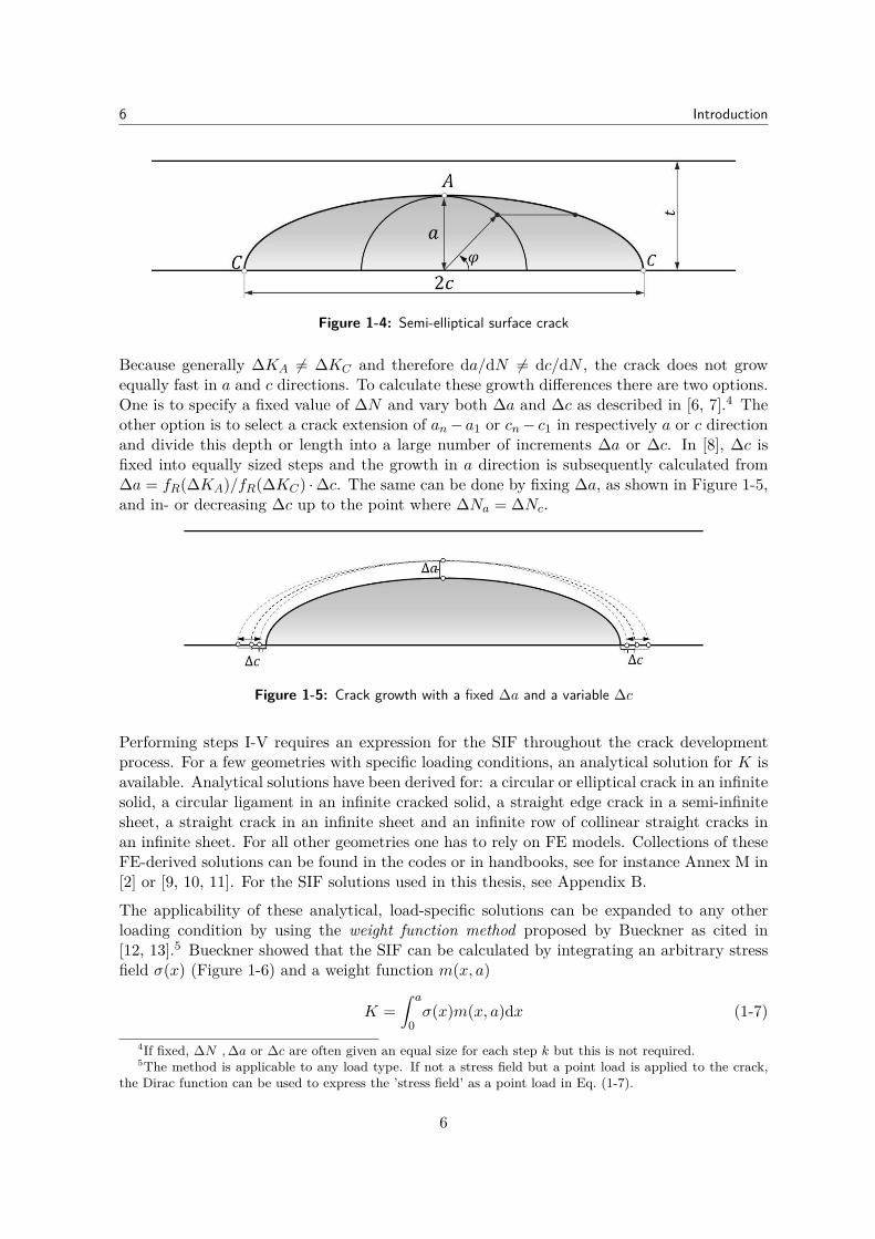
Although this procedure is described for a crack with only one crack size dimension, a, thesame steps I-V are applicable for crack growth with two crack sizes, growth in length anddepth direction will be used as an example. Consider the semi-elliptical surface crack inFigure 1-4 where a is no longer a general crack size but denotes the depth of the crack.Furthermore c is the half surface length of the crack, A is the deepest point and C are thesurface points of the crack. The entire crack is subjected to the same number of load cyclesN , hence ∆Na,k = ∆Nc,k.
4
1-1 State of the art 5
Figure 1-2: Steps to calculate the crack size versus number of stress cycles
Figure 1-3: Numbering of the calculation steps in the numerical procedure
5
6 Introduction
Figure 1-4: Semi-elliptical surface crack
Because generally ∆KA 6= ∆KC and therefore da/dN 6= dc/dN , the crack does not growequally fast in a and c directions. To calculate these growth differences there are two options.One is to specify a fixed value of ∆N and vary both ∆a and ∆c as described in [6, 7].4 Theother option is to select a crack extension of an− a1 or cn− c1 in respectively a or c directionand divide this depth or length into a large number of increments ∆a or ∆c. In [8], ∆c isfixed into equally sized steps and the growth in a direction is subsequently calculated from∆a = fR(∆KA)/fR(∆KC) ·∆c. The same can be done by fixing ∆a, as shown in Figure 1-5,and in- or decreasing ∆c up to the point where ∆Na = ∆Nc.
Figure 1-5: Crack growth with a fixed ∆a and a variable ∆c
Performing steps I-V requires an expression for the SIF throughout the crack developmentprocess. For a few geometries with specific loading conditions, an analytical solution for K isavailable. Analytical solutions have been derived for: a circular or elliptical crack in an infinitesolid, a circular ligament in an infinite cracked solid, a straight edge crack in a semi-infinitesheet, a straight crack in an infinite sheet and an infinite row of collinear straight cracks inan infinite sheet. For all other geometries one has to rely on FE models. Collections of theseFE-derived solutions can be found in the codes or in handbooks, see for instance Annex M in[2] or [9, 10, 11]. For the SIF solutions used in this thesis, see Appendix B.
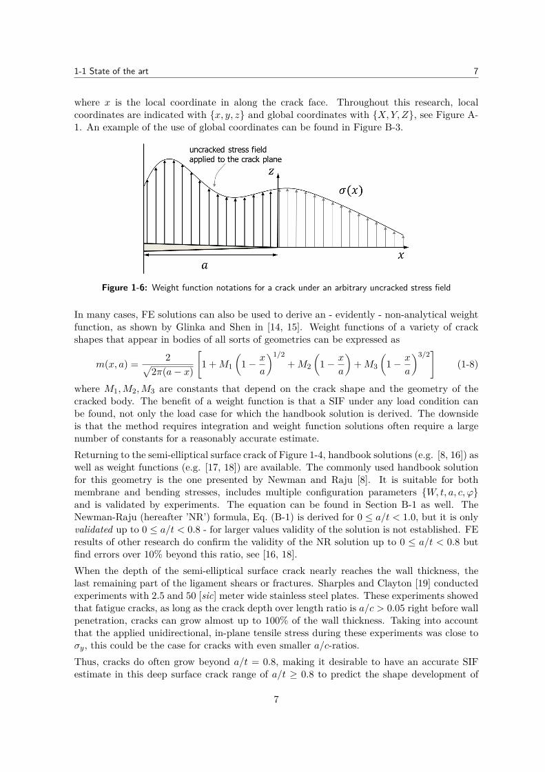
The applicability of these analytical, load-specific solutions can be expanded to any otherloading condition by using the weight function method proposed by Bueckner as cited in[12, 13].5 Bueckner showed that the SIF can be calculated by integrating an arbitrary stressfield σ(x) (Figure 1-6) and a weight function m(x, a)
K =∫ a
0σ(x)m(x, a)dx (1-7)
4If fixed, ∆N ,∆a or ∆c are often given an equal size for each step k but this is not required.5The method is applicable to any load type. If not a stress field but a point load is applied to the crack,
the Dirac function can be used to express the ’stress field’ as a point load in Eq. (1-7).
6
1-1 State of the art 7
where x is the local coordinate in along the crack face. Throughout this research, localcoordinates are indicated with {x, y, z} and global coordinates with {X,Y, Z}, see Figure A-1. An example of the use of global coordinates can be found in Figure B-3.
Figure 1-6: Weight function notations for a crack under an arbitrary uncracked stress field
In many cases, FE solutions can also be used to derive an - evidently - non-analytical weightfunction, as shown by Glinka and Shen in [14, 15]. Weight functions of a variety of crackshapes that appear in bodies of all sorts of geometries can be expressed as
m(x, a) = 2√2π(a− x)
[1 +M1
(1− x
a
)1/2+M2
(1− x
a
)+M3
(1− x
a
)3/2]
(1-8)
where M1,M2,M3 are constants that depend on the crack shape and the geometry of thecracked body. The benefit of a weight function is that a SIF under any load condition canbe found, not only the load case for which the handbook solution is derived. The downsideis that the method requires integration and weight function solutions often require a largenumber of constants for a reasonably accurate estimate.Returning to the semi-elliptical surface crack of Figure 1-4, handbook solutions (e.g. [8, 16]) aswell as weight functions (e.g. [17, 18]) are available. The commonly used handbook solutionfor this geometry is the one presented by Newman and Raju [8]. It is suitable for bothmembrane and bending stresses, includes multiple configuration parameters {W, t, a, c, ϕ}and is validated by experiments. The equation can be found in Section B-1 as well. TheNewman-Raju (hereafter ’NR’) formula, Eq. (B-1) is derived for 0 ≤ a/t < 1.0, but it is onlyvalidated up to 0 ≤ a/t < 0.8 - for larger values validity of the solution is not established. FEresults of other research do confirm the validity of the NR solution up to 0 ≤ a/t < 0.8 butfind errors over 10% beyond this ratio, see [16, 18].When the depth of the semi-elliptical surface crack nearly reaches the wall thickness, thelast remaining part of the ligament shears or fractures. Sharples and Clayton [19] conductedexperiments with 2.5 and 50 [sic] meter wide stainless steel plates. These experiments showedthat fatigue cracks, as long as the crack depth over length ratio is a/c > 0.05 right before wallpenetration, cracks can grow almost up to 100% of the wall thickness. Taking into accountthat the applied unidirectional, in-plane tensile stress during these experiments was close toσy, this could be the case for cracks with even smaller a/c-ratios.Thus, cracks do often grow beyond a/t = 0.8, making it desirable to have an accurate SIFestimate in this deep surface crack range of a/t ≥ 0.8 to predict the shape development of
7
8 Introduction
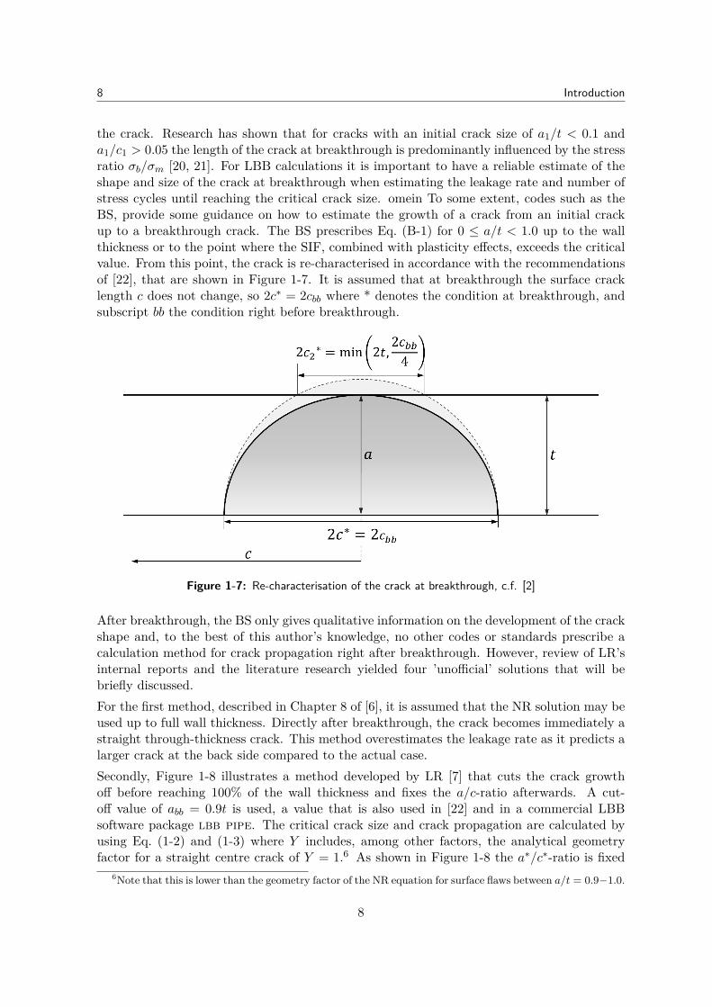
the crack. Research has shown that for cracks with an initial crack size of a1/t < 0.1 anda1/c1 > 0.05 the length of the crack at breakthrough is predominantly influenced by the stressratio σb/σm [20, 21]. For LBB calculations it is important to have a reliable estimate of theshape and size of the crack at breakthrough when estimating the leakage rate and number ofstress cycles until reaching the critical crack size. omein To some extent, codes such as theBS, provide some guidance on how to estimate the growth of a crack from an initial crackup to a breakthrough crack. The BS prescribes Eq. (B-1) for 0 ≤ a/t < 1.0 up to the wallthickness or to the point where the SIF, combined with plasticity effects, exceeds the criticalvalue. From this point, the crack is re-characterised in accordance with the recommendationsof [22], that are shown in Figure 1-7. It is assumed that at breakthrough the surface cracklength c does not change, so 2c∗ = 2cbb where * denotes the condition at breakthrough, andsubscript bb the condition right before breakthrough.
Figure 1-7: Re-characterisation of the crack at breakthrough, c.f. [2]
After breakthrough, the BS only gives qualitative information on the development of the crackshape and, to the best of this author’s knowledge, no other codes or standards prescribe acalculation method for crack propagation right after breakthrough. However, review of LR’sinternal reports and the literature research yielded four ’unofficial’ solutions that will bebriefly discussed.For the first method, described in Chapter 8 of [6], it is assumed that the NR solution may beused up to full wall thickness. Directly after breakthrough, the crack becomes immediately astraight through-thickness crack. This method overestimates the leakage rate as it predicts alarger crack at the back side compared to the actual case.Secondly, Figure 1-8 illustrates a method developed by LR [7] that cuts the crack growthoff before reaching 100% of the wall thickness and fixes the a/c-ratio afterwards. A cut-off value of abb = 0.9t is used, a value that is also used in [22] and in a commercial LBBsoftware package lbb pipe. The critical crack size and crack propagation are calculated byusing Eq. (1-2) and (1-3) where Y includes, among other factors, the analytical geometryfactor for a straight centre crack of Y = 1.6 As shown in Figure 1-8 the a∗/c∗-ratio is fixed
6Note that this is lower than the geometry factor of the NR equation for surface flaws between a/t = 0.9−1.0.
8
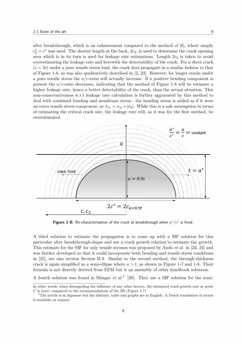
1-1 State of the art 9
after breakthrough, which is an enhancement compared to the method of [6], where simplyc∗2 = c∗ was used. The shorter length at the back, 2c2, is used to determine the crack openingarea which is in its turn is used for leakage rate estimations. Length 2c2 is taken to avoidoverestimating the leakage rate and herewith the detectability of the crack. For a short crack(c < 5t) under a pure tensile stress load, the crack does propagate in a similar fashion to thatof Figure 1-8, as was also qualitatively described in [2, 22]. However, for longer cracks undera pure tensile stress the a/c-ratio will actually increase. If a positive bending component ispresent the a/c-ratio decreases, indicating that the method of Figure 1-8 will be estimate ahigher leakage rate, hence a better detectability of the crack, than the actual situation. Thisnon-conservativeness w.r.t leakage rate calculation is further aggravated by this method todeal with combined bending and membrane stress - the bending stress is added as if it werean extra tensile stress component, so σm = σm+ |σb|. While this is a safe assumption in termsof estimating the critical crack size, the leakage rate will, as it was for the first method, beoverestimated.
Figure 1-8: Re-characterisation of the crack at breakthrough when a∗/c∗ is fixed.
A third solution to estimate the propagation is to come up with a SIF solution for thisparticular after breakthrough-shape and use a crack growth relation to estimate the growth.This estimate for the SIF for only tensile stresses was proposed by Ando et al. in [23, 24] andwas further developed so that it could incorporate both bending and tensile stress conditionsin [25], see also section Section B-3. Similar to the second method, the through-thicknesscrack is again simplified as a semi-ellipse where a > t, as shown in Figure 1-7 and 1-8. Theirformula is not directly derived from FEM but is an assembly of other handbook solutions.
A fourth solution was found in Shingai et al.7 [20]. They use a SIF solution for the semi-
In other words, when disregarding the influence of any other factors, the estimated crack growth rate at pointC is lower compared to the recommendations of the BS (Figure 1-7)
7The article is in Japanese but the abstract, table and graphs are in English. A Dutch translation of articleis available on request.
9
10 Introduction
elliptical surface crack that was proposed by Shah and Kobayashi, cited in [20]. The approachfollowed by Shingai et al. is to use this SIF solution for point A and C at breakthroughthroughout the propagation phase, i.e. using a/t = 1.0 and ϕ = 90 for point A and ϕ = 0 forpoint C of Figure 1-7. Since the Shah and Kobayashi formula was not intended to be usedafter breakthrough and their approach is not validated with test results either, this methodis not considered further.
To summarise, the industrial codes offer only limited guidance for LBB assessments on howto deal with deep surface cracks or semi-elliptical through-thickness cracks. In absence ofthis, other solutions that are not fully satisfactory either have been proposed.
1-2 Scope of work
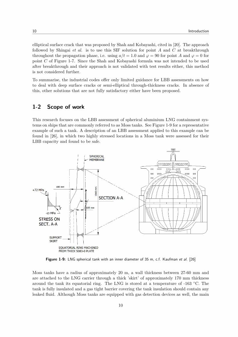
This research focuses on the LBB assessment of spherical aluminium LNG containment sys-tems on ships that are commonly referred to as Moss tanks. See Figure 1-9 for a representativeexample of such a tank. A description of an LBB assessment applied to this example can befound in [26], in which two highly stressed locations in a Moss tank were assessed for theirLBB capacity and found to be safe.
Figure 1-9: LNG spherical tank with an inner diameter of 35 m, c.f. Kaufman et al. [26]
Moss tanks have a radius of approximately 20 m, a wall thickness between 27-60 mm andare attached to the LNG carrier through a thick ’skirt’ of approximately 170 mm thicknessaround the tank its equatorial ring. The LNG is stored at a temperature of -163 ◦C. Thetank is fully insulated and a gas tight barrier covering the tank insulation should contain anyleaked fluid. Although Moss tanks are equipped with gas detection devices as well, the main
10
1-2 Scope of work 11
leakage warning system is a so-called ’drip tray’ which is installed under the tank and wherethe liquefied gas is collected and detected.
Fatigue damage is primarily induced by the inertial loading of the liquefied gas under themovements of the ship and by the deformation (hogging or sagging etc.) of the ship. Repeatedfilling and emptying of the tank barely contributes to the fatigue damage and neither issloshing an issue because it a requirement that the tank is filled to almost 100% of its capacity.
When performing an LBB assessment, calculation steps like the determination of the stressspectrum or the estimation of material parameters, are all equally important but are con-sidered to be given input parameters within the scope of this research. The emphasis willbe on the prediction of the crack (shape) development, the first of the aforementioned threeaspects of an LBB assessment. In an indirect way this also touches upon the second and thirdaspect: the amount of leakage is related to the crack opening area, so it is necessary to havea reliable estimate of c2, and to determine whether there will be enough time to detect theleak or take emergency measures depends on the accuracy of the estimated relation betweenc and N . Howver, topics directly related to aspects 2.) and 3.) such as the estimation of theleakage rate, assessing the adequacy of the leak detection, or the expected crack propagationunder a 15-day load spectrum, will not be considered. Calculations for these two aspectsrely heavily on the accuracy of the assumed stress spectrum in the tank, local geometry andthe availability of a reliable, experimentally obtained crack growth relation and many othervalues that are material-depend and situation-specific.
For this research, both a numerical calculation scheme and an FE model are developed. Inorder to keep the models manageable, the following simplifications are made:
– The geometry in the vicinity of the crack is simplified as an infinite, straight plate.Locally, the curvature of the tank is negligible given the large diameter of the sphericaltank.
– The plate material is considered to be linear-elastic. The design stresses for platedstructures like this are much lower than the yield stress, hence plasticity is not consid-ered to have major impact unless the depth of a surface crack almost reaches the wallthickness or when high residual stresses are present.
– Damage mechanisms other than fatigue and fracture, like corrosion or impact load ordynamic effects are not considered.
– There are no other discontinuities, like welds or attachments, other than the fatiguecrack.
– No multi-axial stresses but only σZ , the nominal stress in-plane of the plate material, isconsidered and it varies only in X (depth) direction, see Figure 1-9 or B-3. For brevity,subscript Z is hereafter omitted.
– The effects of nominal higher order stresses are not considered because their contributionis small w.r.t the nominal membrane and bending stresses in LNG tanks. No externalpressures are modelled.
– The stresses are either of constant amplitude throughout the crack development or theamplitude is a function of the crack length at the crack initiation side.
– No crack closure effects are taken into account. A plastic zone around a crack-tip canact as a compressive, crack closing stress even when the nominal stresses are tensile.
11
12 Introduction
– Differences in the crack propagation rate that exist along the thickness (in X-direction)are ignored.8
– Cracks grow symmetrically.
– The crack will be fully opened during all stress cycles. Roughly said, this means thatthe nominal stress acting on the crack area is tensile, i.e. σmin ≥ 0.
A minor caveat to the last point should be made: it is not true that a crack can only befully opened when σmin ≥ 0. As an example of this, consider a semi-elliptical surface crackthat is predominately subjected to a large nominal bending stress and possibly a minor -either tensile or compressive - membrane stress component. In this case, the entire crack canbe opened despite that a small part of the crack face is subjected to a compressive stress.’Membrane stress’ can therefore refer to both a relatively small uniform compressive stressor a uniform tensile stress. If only the latter is considered, it is explicitly referred to as a(uniform) tensile stress.
1-3 Research objective
The first aim of this research is to predict the crack shape of surface cracks more accuratelyby using a different numerical calculation method than the ones described above. This newscheme will be introduced in Chapter 2 where the perceived shortcomings of other methodswill be addressed. In Chapter 4 the performance of the new numerical calculation scheme isassessed in comparison with experimentally determined results of the crack shape at break-through. The objective is to:
1-a) Solve perceived shortcomings of other numerical calculations methods.
1-b) Improve the numerical calculation method so that it performs well in comparison withexperimentally determined results.
In order to estimate crack growth before breakthrough more accurately, several FEM arebuild to assess the validity of two different expressions to predict the SIF. In Chapter 3,semi-elliptical surface crack FEM results of the SIF are compared to two other solutions.One is a commonly used SIF solution proposed by Newman and Raju [8], the other one wasproposed by Wang [18] and is only applicable to deep surface cracks with a depth in the rangeof (0.6 ∼ 0.8) ≤ a/t < 0.95. In Chapter 4 the crack shapes at breakthrough estimated by firstonly using the NR solution and then by replacing the NR solution by the one of Wang in therange of 0.6 ≤ a/t < 0.95, will be compared to experimental results found in the literature.The goal is then to:
1-c) Assess the influence on the accuracy of the estimations for crack shape and growth whenthe SIF is not only predicted by the NR solution, but also by the Wang solution in therange of 0.6 ≤ a/t < 0.95.
8This crack closure effect is a 3-D phenomenon influenced by plasticity: at the material surfaces whereplane stress conditions prevail, a larger plastic zone around the crack-tip is present compared to the innermaterial under plane strain. Hence, a closed crack opens first mid-thickness and propagates faster. Undervariable amplitude loading, this effect is considerable. More on this thickness effect can be found in Chapter11 of [6].
12
1-3 Research objective 13
The second aim is to improve the accuracy of the estimated crack propagation after break-through. Of the four aforementioned solutions (straight through-thickness immediately afterbreakthrough; cutting growth off at abb = 0.9t and fixing a∗/c∗; using an assembly of hand-book SIF equations to estimate the SIF for the crack after breakthrough; using the Shahand Kobayashi formula), the second and third will be further evaluated for their accuracy incomparison with experimental data in Chapter 4. In addition to these two methods, a newSIF formula will be proposed in Chapter 3, one that is based upon FEM of this particularsemi-elliptical through-thickness shape. So the objective is to:
2) Develop a new FE-derived SIF solution for a crack after wall penetration and asses theaccuracy to estimate crack propagation of both this new as well as two existing solutionsin comparison with experimentally obtained data.
The results will then be used to make recommendations for improving existing LBB proce-dures.
13

14 Introduction
14
Chapter 2
Numerical modelling of crackdevelopment
The generic calculation procedure to predict crack development that was briefly introduced inthe previous chapter, will be discussed in more detail for each phase shown in Table 1-1 andthe specific features of the numerical calculation procedure that is developed for this researchwill be highlighted. The next section first introduces some terminology and general aspectsfor the numerical modelling of crack development.
2-1 Calculation procedure, phases, steps and calculation steps
The entire process of 1.) selecting input parameters, 2.) numerically calculating crack growth,3.) specifying the rules for re-characterisation of the breakthrough crack and 4.) numericallycalculating crack propagation, is referred to as the numerical modelling of crack development.If only the last three aspects are considered, this is referred to as carrying out a numericalcalculation procedure or numerical calculation scheme. The numerical calculation procedureis carried out by matlab, a program that can quickly process a large number of numericalcalculations and can easily generate graphical output. The numerical model is subdividedin 4 phases (Table 1-1). Phase 2 and 4, respectively crack growth and propagation, can bemodelled with the steps of Figure 1-2. The incremental steps, k = 1, 2, 3...n, as illustrated inFigure 1-3 are referred to as calculation steps to distinguish them from the steps of Figure 1-2.Within a calculation step, it is often necessary to use iteration steps to obtain a new value,these are denoted in the matlab program by i.The basic assumption to calculate crack development, is that the crack is loaded by the samenumber of load cycles, i.e. Na = Nc or Nc = Nc2. The number of load cycles may vary eachcalculation step k.As shown in Figure 1-3, ∆a1,∆N1 and also ∆c1 are added as virtual increments with a valueof 0 to be consistent with the matlab program. matlab does not recognize a syntax withcalculation step number 0 and therefore a0,∆K0 cannot be attached to a value.
15
16 Numerical modelling of crack development
The specific method followed for each step of Figure 1-2 will now be further explained for thefour phases.
2-2 Phase 1: Presence of an initial semi-elliptical surface flaw
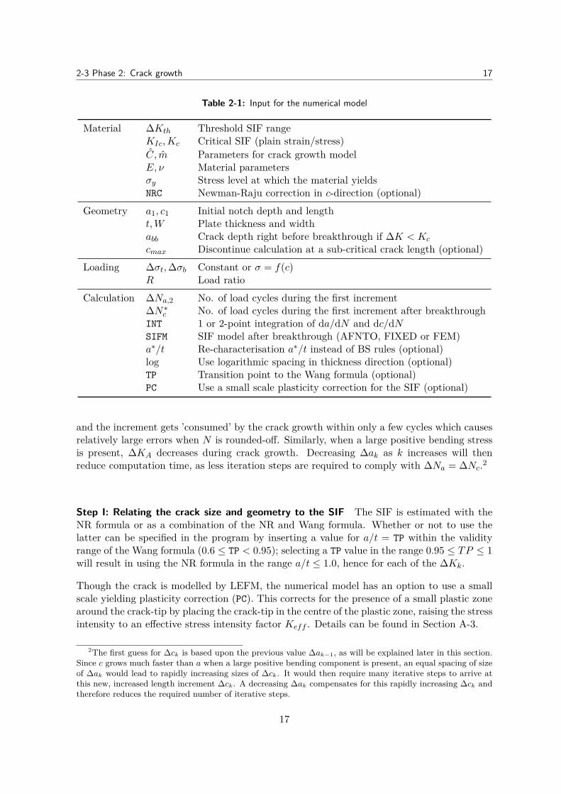
Before any growth can be modelled, some input regarding crack dimensions and other inputsare required. An overview is given in Table 2-1. More input and calculation options will bediscussed in the next sections.
The experimental data that will later be used to assess the numerical model, is given forfinite width specimens, therefore a value for W is required to correct for a finite width. Whenmodelling a spherical tank, the value of W should be given a value much larger than the finalcrack size so that is will not affect the outcome.
As pointed out in the introduction, ligament failure can occur when the crack depth reachesalmost the wall thickness or when KA,max = Kc or KC,max = KIc. Because the scheme onlyuses SIF ranges and not Kmax, the values of Kc and KIc are converted into something thatone could unofficially call ’critical SIF ranges’
∆Kc = Kc −R ·Kc (2-1a)∆KIc = KIc −R ·KIc (2-1b)
If ∆KA is still smaller than ∆Kc at a = abb it is assumed that this very thin remaining part ofthe cross section fails anyhow. This research adopted abb = 0.995t for all calculations, exceptwhen using the ’fixed a/c ratio’ model of Figure 1-8 where it is abb = 0.9t.
2-3 Phase 2: Crack growth
As mentioned in the introduction, either ∆ak, ∆ck or ∆Nk should be known to calculate thecrack growth for a two-dimensional crack. ∆ak is selected as the ’known’ parameter in thisprocedure, because the distance abb− a1 is known in advance, unlike cbb− c1.1 Using ∆Nk asa known can be troublesome because the growth rate may vary considerable between that ofan initial flaw and one that approaches criticality. Increasing ∆Nk as k increases, would solvethis problem although it is hard to estimate the increase rate beforehand. Another solutionis to use a small ∆Nk throughout the calculation but this is requires more computation timeas the increments become increasingly small as well. Moreover, averaging the crack growthover a reasonable number of cycles better reflects the empirical nature of growth relationsand the error margin of the approximative SIF solution. Again, it can be difficult to judgein advance whether a selected ∆Nk is indeed small enough yet not too small for a reliablegrowth estimate.
This considered, the size of ∆ak is fixed and is in most cases given an equal value for each k.Though an equal spacing rarely causes problems for growth calculations, there is an optionin the model to use a logarithmically in- or decreasing ∆ak. For a rapidly increasing ∆KA,the first option prevents that ∆ak becomes too small when approaching the wall thickness
1When ∆Kc is reached before the initially selected abb, the algorithm decreases abb until ∆KA < ∆Kc.
16
2-3 Phase 2: Crack growth 17
Table 2-1: Input for the numerical model
Material ∆Kth Threshold SIF rangeKIc,Kc Critical SIF (plain strain/stress)C, m Parameters for crack growth modelE, ν Material parametersσy Stress level at which the material yieldsNRC Newman-Raju correction in c-direction (optional)
Geometry a1, c1 Initial notch depth and lengtht,W Plate thickness and widthabb Crack depth right before breakthrough if ∆K < Kc
cmax Discontinue calculation at a sub-critical crack length (optional)
Loading ∆σt,∆σb Constant or σ = f(c)R Load ratio
Calculation ∆Na,2 No. of load cycles during the first increment∆N∗c No. of load cycles during the first increment after breakthroughINT 1 or 2-point integration of da/dN and dc/dNSIFM SIF model after breakthrough (AFNTO, FIXED or FEM)a∗/t Re-characterisation a∗/t instead of BS rules (optional)log Use logarithmic spacing in thickness direction (optional)TP Transition point to the Wang formula (optional)PC Use a small scale plasticity correction for the SIF (optional)
and the increment gets ’consumed’ by the crack growth within only a few cycles which causesrelatively large errors when N is rounded-off. Similarly, when a large positive bending stressis present, ∆KA decreases during crack growth. Decreasing ∆ak as k increases will thenreduce computation time, as less iteration steps are required to comply with ∆Na = ∆Nc.2
Step I: Relating the crack size and geometry to the SIF The SIF is estimated with theNR formula or as a combination of the NR and Wang formula. Whether or not to use thelatter can be specified in the program by inserting a value for a/t = TP within the validityrange of the Wang formula (0.6 ≤ TP < 0.95); selecting a TP value in the range 0.95 ≤ TP ≤ 1will result in using the NR formula in the range a/t ≤ 1.0, hence for each of the ∆Kk.
Though the crack is modelled by LEFM, the numerical model has an option to use a smallscale yielding plasticity correction (PC). This corrects for the presence of a small plastic zonearound the crack-tip by placing the crack-tip in the centre of the plastic zone, raising the stressintensity to an effective stress intensity factor Keff . Details can be found in Section A-3.
2The first guess for ∆ck is based upon the previous value ∆ak−1, as will be explained later in this section.Since c grows much faster than a when a large positive bending component is present, an equal spacing of sizeof ∆ak would lead to rapidly increasing sizes of ∆ck. It would then require many iterative steps to arrive atthis new, increased length increment ∆ck. A decreasing ∆ak compensates for this rapidly increasing ∆ck andtherefore reduces the required number of iterative steps.
17
18 Numerical modelling of crack development
Step II: Relating the SIF to the crack growth The Paris relations [27]dadN = CA(∆K)m (2-2a)
dcdN = CC(∆K)m (2-2b)
are used to estimate the crack growth rates. One of the options is to use a different CCin length direction in Eq. (2-2b) as suggested in [8]. It is therefore here referred to as the’Newman-Raju correction’ (NRC).
CC = 0.9m · CA (2-3)Only the Paris relation is for now considered in the calculation scheme because the materialparameters C, m of the experiments that will be used for validation, have been publishedfor this relation as well. Adding other relations does not require much effort should this beneeded for a later research.
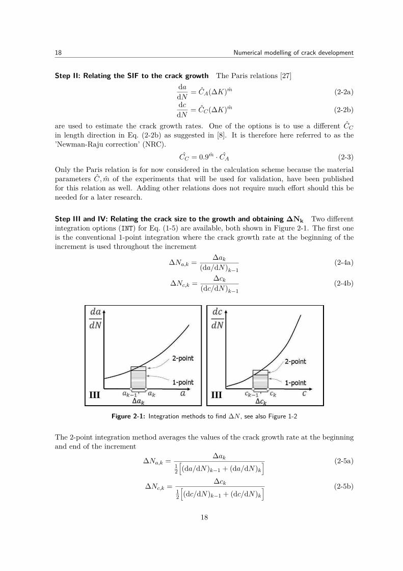
Step III and IV: Relating the crack size to the growth and obtaining ∆Nk Two differentintegration options (INT) for Eq. (1-5) are available, both shown in Figure 2-1. The first oneis the conventional 1-point integration where the crack growth rate at the beginning of theincrement is used throughout the increment
∆Na,k = ∆ak(da/dN)k−1
(2-4a)
∆Nc,k = ∆ck(dc/dN)k−1
(2-4b)
Figure 2-1: Integration methods to find ∆N , see also Figure 1-2
The 2-point integration method averages the values of the crack growth rate at the beginningand end of the increment
∆Na,k = ∆ak12
[(da/dN)k−1 + (da/dN)k
] (2-5a)
∆Nc,k = ∆ck12
[(dc/dN)k−1 + (dc/dN)k
] (2-5b)
18
2-3 Phase 2: Crack growth 19
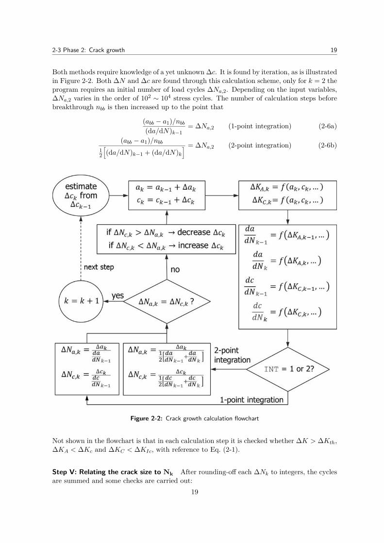
Both methods require knowledge of a yet unknown ∆c. It is found by iteration, as is illustratedin Figure 2-2. Both ∆N and ∆c are found through this calculation scheme, only for k = 2 theprogram requires an initial number of load cycles ∆Na,2. Depending on the input variables,∆Na,2 varies in the order of 102 ∼ 104 stress cycles. The number of calculation steps beforebreakthrough nbb is then increased up to the point that
(abb − a1)/nbb(da/dN)k−1
= ∆Na,2 (1-point integration) (2-6a)
(abb − a1)/nbb12
[(da/dN)k−1 + (da/dN)k
] = ∆Na,2 (2-point integration) (2-6b)
Figure 2-2: Crack growth calculation flowchart
Not shown in the flowchart is that in each calculation step it is checked whether ∆K > ∆Kth,∆KA < ∆Kc and ∆KC < ∆KIc, with reference to Eq. (2-1).
Step V: Relating the crack size to Nk After rounding-off each ∆Nk to integers, the cyclesare summed and some checks are carried out:
19
20 Numerical modelling of crack development
– The difference between Na and Nc may not exceed 0.1% of the total N ,
|Na −Nc| < max(Na, Nc) · 10−3
– The difference between ∆Na,k and ∆Nc,k may not exceed 0.1 on average,∣∣∣∣∣∑nbbk=2 ∆Na,k −∆Nc,k
nbb
∣∣∣∣∣ < 0.1
– The minimum number of N is 10 in each calculation step;– The error due to the rounding to integers in each k may not exceed 0.01 on average,∣∣∣∣∣
∑nbbk=2 ∆Nk −∆Nk,rounded
nbb
∣∣∣∣∣ < 0.01
If all conditions are met, the calculation continues to the next phase.
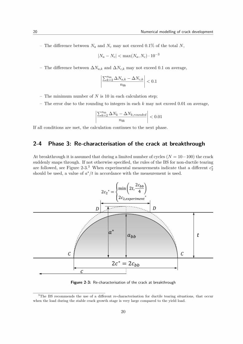
2-4 Phase 3: Re-characterisation of the crack at breakthrough
At breakthrough it is assumed that during a limited number of cycles (N = 10−100) the cracksuddenly snaps through. If not otherwise specified, the rules of the BS for non-ductile tearingare followed, see Figure 2-3.3 When experimental measurements indicate that a different c∗2should be used, a value of a∗/t in accordance with the measurement is used.
Figure 2-3: Re-characterisation of the crack at breakthrough
3The BS recommends the use of a different re-characterisation for ductile tearing situations, that occurwhen the load during the stable crack growth stage is very large compared to the yield load.
20
2-5 Phase 4: Crack propagation after breakthrough 21
2-5 Phase 4: Crack propagation after breakthrough
After breakthrough, the length of ∆c2,k is the unknown variable and ∆ck is now fixed. Lengthcc−c∗ is known as the difference between the critical crack length cc (Eq. (1-2)) and the lengthat breakthrough. Optionally, a different value for cmax can be used to cut-off the calculationbefore cc. For most loading conditions, a linear spacing of ∆ck is recommended.
Step I: Relating the crack size and geometry to the SIF After breakthrough, three optionscan be used for the SIF estimate. The first is to use the approximative equation of Ando,Fujibayashi, Nam, Takahashi and Ogura (AFNTO), the authors of the first paper with thissolution [23]. Their solution is hereafter referred to as the AFNTO solution. Alternativelyone can use the ’fixed a∗/c∗ model’ or the equation that is found by FE modelling for thisresearch. This FEM based equation will be treated in Section 3-3.
Step II - V: Relating the SIF and crack length to the crack to the propagation rate,obtaining ∆Nk and summation The Paris relation Eq. (2-2) is again used to estimatecrack propagation. The steps for crack propagation after breakthrough are similar to those ofcrack growth. An initial ∆N∗c should be selected for the first step after breakthrough, usuallyit is in the order of 80 ∼ 400.
The same procedure as shown in Figure 2-2 is followed, but {a,∆a,∆KA,∆Na} are nowreplaced by respectively {c2,∆c2,∆KD,∆Nc2}, with reference to Figure 2-3. The checks areidentical to the ones for the crack growth phase.
21

22 Numerical modelling of crack development
22
Chapter 3
Modelling cracks with finite elements
As mentioned in Chapter 2, crack growth can be estimated with an empirical formula thatrelates the SIF range to the crack growth rate. The SIF, and subsequently the SIF range inthis relation, can be obtained through an FE analysis.
Three models that are relevant for crack growth modelling will be introduced in the nextsections. The first model shows, by comparison with an analytical solution, that the FEmethod and software package are indeed suitable to accurately approximate the SIF. Thesecond model of a semi-elliptical surface crack compares the FEM results of the SIF to pre-dicted SIF values by the formulae of NR and Wang. Thirdly, in order to derive a ’handbook’solution, a set of FEM of semi-elliptical through-thickness cracks are build and used to derivea approximative solution. This solution is then compared to the AFNTO formula, which isonly an assembly of other FE-derived handbook solutions.
All FE analyses are carried out with ansys, release 16.1. The models use three-dimensionalisoparametric solid elements with reduced integration to increase the computation speed, andare linear-elastic.
3-1 Validation of the finite element method and software
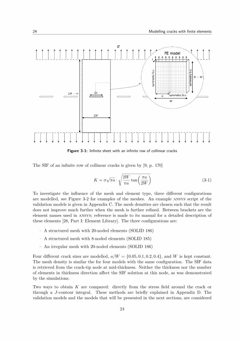
A validation model serves two purposes: (1) it validates the FE method and software packageansys and (2) it shows which mesh and/or element types can give the most accurate solutionin comparison with an analytical solution. As said, only a few analytical solutions existsand all analytical solution are derived for a geometry with one or multiple boundaries at aninfinite distance from the crack. The first issue that arises is that the FE method can onlymodel (anti-) symmetry boundaries. The analytical solution of infinite row of collinear cracks(Figure 3-1) limits the problem of modelling infinity to only one boundary: the infinite heightH at which the nominal stress acts. This geometry is therefore selected to validate the FEsoftware and model. H in the FEM is selected as H = W in order to study the effects of thefinite height.
23
24 Modelling cracks with finite elements
Figure 3-1: Infinite sheet with an infinite row of collinear cracks
The SIF of an infinite row of collinear cracks is given by [9, p. 170]
K = σ√πa ·
√2Wπa
tan(πa
2W
)(3-1)
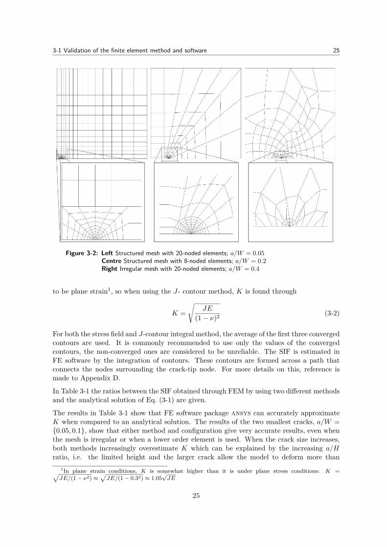
To investigate the influence of the mesh and element type, three different configurationsare modelled, see Figure 3-2 for examples of the meshes. An example ansys script of thevalidation models is given in Appendix C. The mesh densities are chosen such that the resultdoes not improve much further when the mesh is further refined. Between brackets are theelement names used in ansys; reference is made to its manual for a detailed description ofthese elements [28, Part I: Element Library]. The three configurations are:
– A structured mesh with 20-noded elements (SOLID 186)
– A structured mesh with 8-noded elements (SOLID 185)
– An irregular mesh with 20-noded elements (SOLID 186)
Four different crack sizes are modelled, a/W = {0.05, 0.1, 0.2, 0.4}, and W is kept constant.The mesh density is similar the for four models with the same configuration. The SIF datais retrieved from the crack-tip node at mid-thickness. Neither the thickness nor the numberof elements in thickness direction affect the SIF solution at this node, as was demonstratedby the simulations.
Two ways to obtain K are compared: directly from the stress field around the crack orthrough a J-contour integral. These methods are briefly explained in Appendix D. Thevalidation models and the models that will be presented in the next sections, are considered
24
3-1 Validation of the finite element method and software 25
Figure 3-2: Left Structured mesh with 20-noded elements; a/W = 0.05Centre Structured mesh with 8-noded elements; a/W = 0.2Right Irregular mesh with 20-noded elements; a/W = 0.4
to be plane strain1, so when using the J- contour method, K is found through
K =√
JE
(1− ν)2 (3-2)
For both the stress field and J-contour integral method, the average of the first three convergedcontours are used. It is commonly recommended to use only the values of the convergedcontours, the non-converged ones are considered to be unreliable. The SIF is estimated inFE software by the integration of contours. These contours are formed across a path thatconnects the nodes surrounding the crack-tip node. For more details on this, reference ismade to Appendix D.
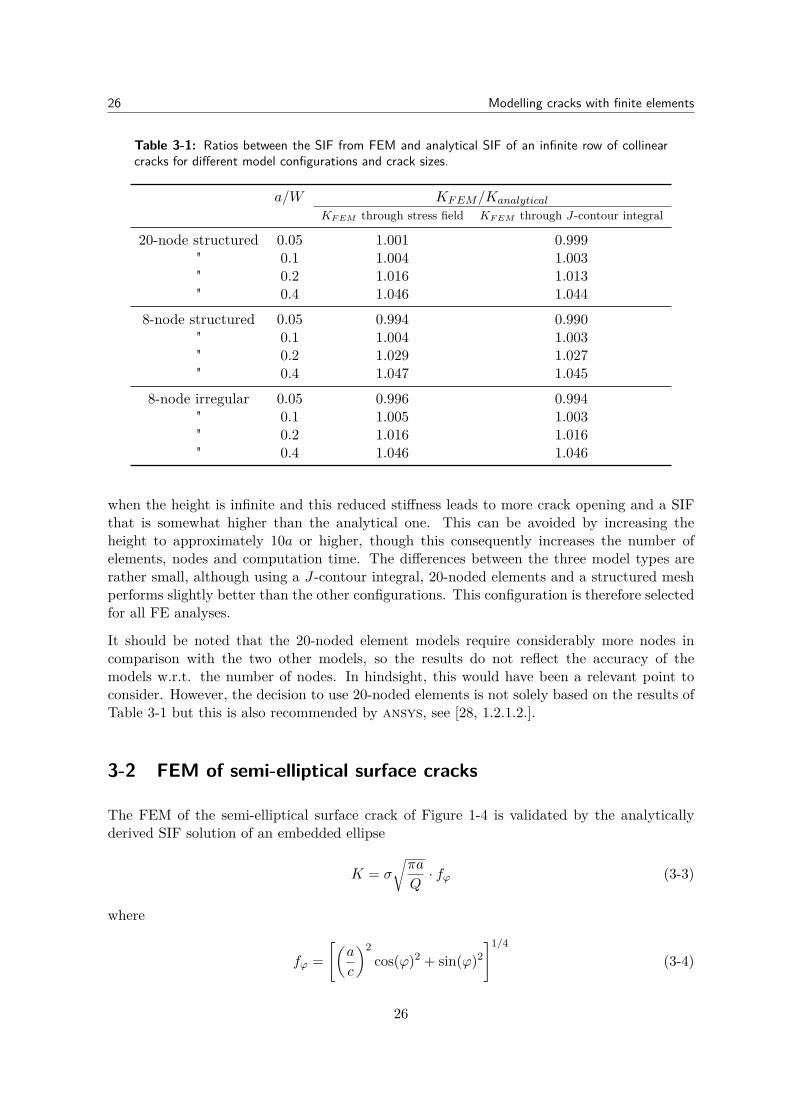
In Table 3-1 the ratios between the SIF obtained through FEM by using two different methodsand the analytical solution of Eq. (3-1) are given.
The results in Table 3-1 show that FE software package ansys can accurately approximateK when compared to an analytical solution. The results of the two smallest cracks, a/W ={0.05, 0.1}, show that either method and configuration give very accurate results, even whenthe mesh is irregular or when a lower order element is used. When the crack size increases,both methods increasingly overestimate K which can be explained by the increasing a/Hratio, i.e. the limited height and the larger crack allow the model to deform more than
1In plane strain conditions, K is somewhat higher than it is under plane stress conditions: K =√JE/(1− ν2) ≈
√JE/(1− 0.32) ≈ 1.05
√JE
25
26 Modelling cracks with finite elements
Table 3-1: Ratios between the SIF from FEM and analytical SIF of an infinite row of collinearcracks for different model configurations and crack sizes.
a/W KFEM/Kanalytical
KF EM through stress field KF EM through J-contour integral
20-node structured 0.05 1.001 0.999" 0.1 1.004 1.003" 0.2 1.016 1.013" 0.4 1.046 1.044
8-node structured 0.05 0.994 0.990" 0.1 1.004 1.003" 0.2 1.029 1.027" 0.4 1.047 1.045
8-node irregular 0.05 0.996 0.994" 0.1 1.005 1.003" 0.2 1.016 1.016" 0.4 1.046 1.046
when the height is infinite and this reduced stiffness leads to more crack opening and a SIFthat is somewhat higher than the analytical one. This can be avoided by increasing theheight to approximately 10a or higher, though this consequently increases the number ofelements, nodes and computation time. The differences between the three model types arerather small, although using a J-contour integral, 20-noded elements and a structured meshperforms slightly better than the other configurations. This configuration is therefore selectedfor all FE analyses.
It should be noted that the 20-noded element models require considerably more nodes incomparison with the two other models, so the results do not reflect the accuracy of themodels w.r.t. the number of nodes. In hindsight, this would have been a relevant point toconsider. However, the decision to use 20-noded elements is not solely based on the results ofTable 3-1 but this is also recommended by ansys, see [28, 1.2.1.2.].
3-2 FEM of semi-elliptical surface cracks
The FEM of the semi-elliptical surface crack of Figure 1-4 is validated by the analyticallyderived SIF solution of an embedded ellipse
K = σ
√πa
Q· fϕ (3-3)
where
fϕ =[(
a
c
)2cos(ϕ)2 + sin(ϕ)2
]1/4
(3-4)
26
3-2 FEM of semi-elliptical surface cracks 27
and
Q =∫ π/2
0
√√√√1−[1−
(a
c
)2]
sin2 ϕ dϕ (3-5)
A closed form solution of Q does not exist but a close approximation to Eq. (3-5) is given by
Q = 1 + 1.464(a
c
)1.65(3-6)
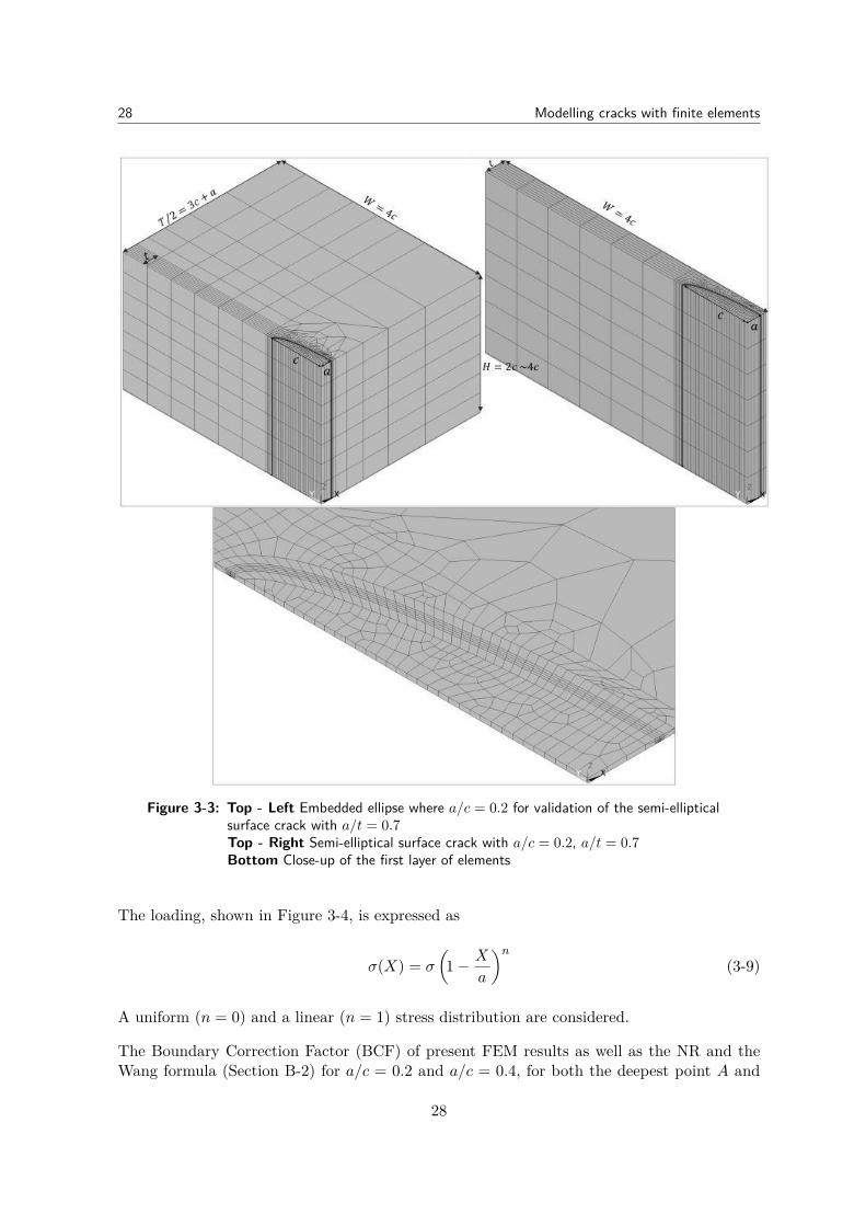
Figure 3-3 shows both an example mesh of a validation model and a semi-elliptical surfacecrack. Because of its symmetry, only 1/8th of the geometry of the embedded ellipse and 1/4th
of the surface crack needs to be modelled. The mesh of the semi-elliptical surface crack isalmost identical to the validation model, except that only the thickness t is modelled. Anexample ansys script file can be found in Appendix E.
The licence type of ansys limits the number of nodes of each model to 32,000. This isenough to obtain reasonably accurate results compared to the analytical solution but thislimitation forces the user to find a balance between accepting some poorly shaped elementsand compromising on the distance of the boundaries that should ideally be at H/a > 10,W/c > 10 and t/a > 10. An element is for instance poorly shaped when the aspect ratiobecomes too large (i.e. one of the three dimensions is much smaller or larger than the othertwo dimensions) or when it is very skewed. To avoid a large number of poorly shaped elements,the distance of the boundaries is less than ideal in each direction. For all models W = 4c andthe half height is of the order H = 2c ∼ 4c. The thickness of the model of an embedded ellipseis T = 6c+2a. W,H and T are selected such that they barely affect the stress field around thecrack-tip. Nevertheless, the models still have a less-than-ideal thickness, height and width,and therefore a correction factor for this is applied as well. The following correction factor isoriginally only used for the NR solution (see Eq. (B-4) or [8]), but is here considered to be areasonable approximation for an embedded ellipse as well
fw =[cos
(πc
2W
√a
t
)]−1/2(3-7)
To make a comparison with the plots in [18], a/c = {0.2, 0.4}. Correcting Eq. (3-3) with fwof Eq. (3-7), the reference solution for the elliptical validation models becomes2
Kref = σ
√πa
Q· fφ · fw (3-8)
The SIFs of the elliptical validation models are within 1.0% error with respect to Kref foreach node along the crack-tip when obtained through the J-contour integral. When K isretrieved through the stress field, K has a maximum 1.2% error with respect to Kref for eachnode.
2Inserting W = 4c; t = T/2 = 3c + a and a/c in Eq. (3-7), fw = cos (π/32)−1/2 ≈ 1.0024 and fw =cos{(π/8)
√2/17}−1/2 ≈ 1.0046 for respectively a/c = 0.2 and a/c = 0.4, hence the impact of the finite
boundaries on the SIF is still rather small and is even smaller if the actual thickness T instead of T/2 hadbeen used.
27
28 Modelling cracks with finite elements
Figure 3-3: Top - Left Embedded ellipse where a/c = 0.2 for validation of the semi-ellipticalsurface crack with a/t = 0.7Top - Right Semi-elliptical surface crack with a/c = 0.2, a/t = 0.7Bottom Close-up of the first layer of elements
The loading, shown in Figure 3-4, is expressed as
σ(X) = σ
(1− X
a
)n(3-9)
A uniform (n = 0) and a linear (n = 1) stress distribution are considered.
The Boundary Correction Factor (BCF) of present FEM results as well as the NR and theWang formula (Section B-2) for a/c = 0.2 and a/c = 0.4, for both the deepest point A and
28
3-2 FEM of semi-elliptical surface cracks 29
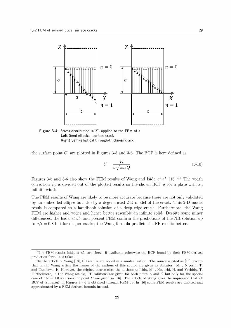
Figure 3-4: Stress distribution σ(X) applied to the FEM of aLeft Semi-elliptical surface crackRight Semi-elliptical through-thickness crack
the surface point C, are plotted in Figures 3-5 and 3-6. The BCF is here defined as
Y = K
σ√πa/Q
(3-10)
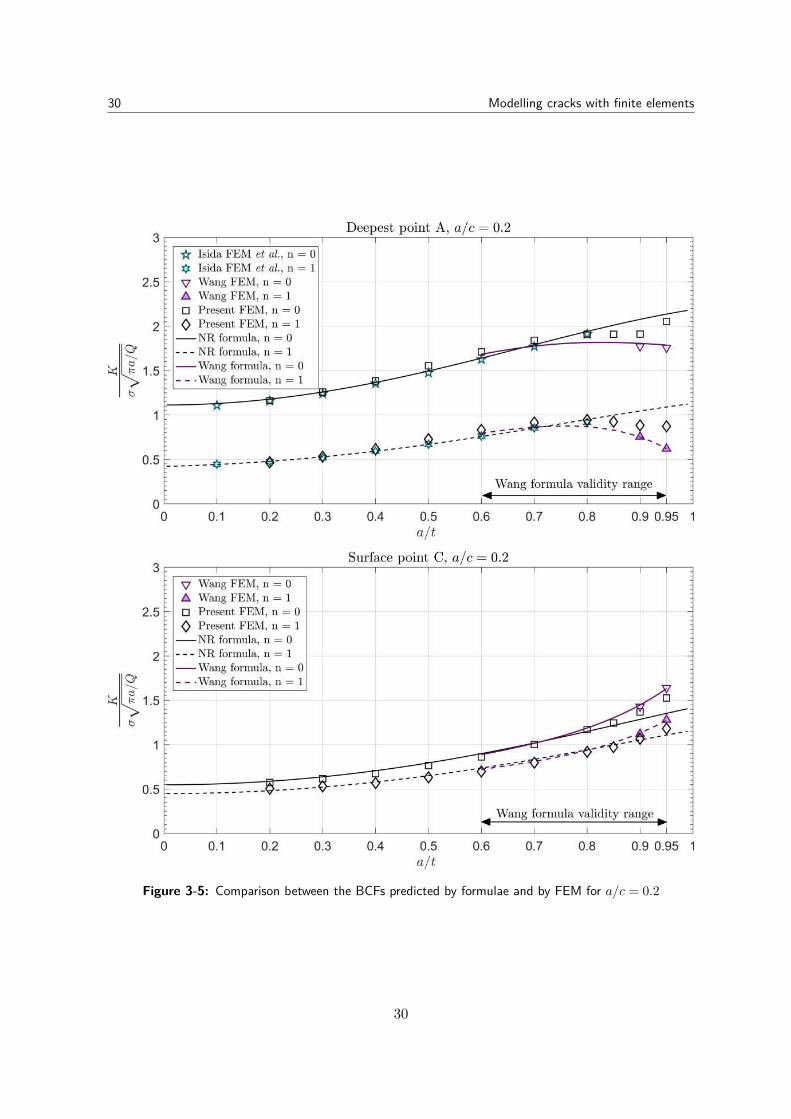
Figures 3-5 and 3-6 also show the FEM results of Wang and Isida et al. [16].3,4 The widthcorrection fw is divided out of the plotted results so the shown BCF is for a plate with aninfinite width.
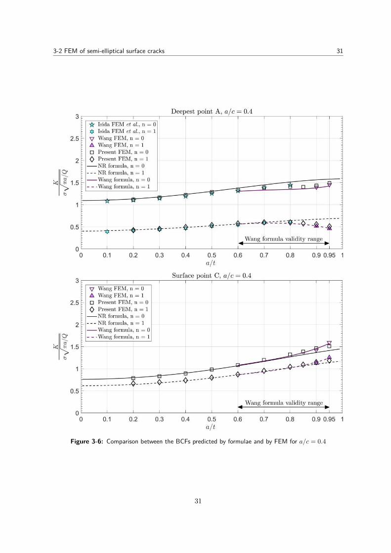
The FEM results of Wang are likely to be more accurate because these are not only validatedby an embedded ellipse but also by a degenerated 2-D model of the crack. This 2-D modelresult is compared to a handbook solution of a deep edge crack. Furthermore, the WangFEM are higher and wider and hence better resemble an infinite solid. Despite some minordifferences, the Isida et al. and present FEM confirm the predictions of the NR solution upto a/t = 0.8 but for deeper cracks, the Wang formula predicts the FE results better.
3The FEM results Isida et al. are shown if available, otherwise the BCF found by their FEM derivedprediction formula is taken.
4In the article of Wang [18], FE results are added in a similar fashion. The source is cited as [16], exceptthat in the Wang article the names of the authors of this source are given as Shiratori, M. , Niyoshi, T.and Tanikawa, K. However, the original source cites the authors as Isida, M. , Noguchi, H. and Yoshida, T.Furthermore, in the Wang article, FE solutions are given for both point A and C but only for the specialcase of a/c = 1.0 solutions for point C are given in [16]. The article of Wang gives the impression that allBCF of ’Shiratori’ in Figures 3 - 6 is obtained through FEM but in [16] some FEM results are omitted andapproximated by a FEM derived formula instead.
29
30 Modelling cracks with finite elements
Figure 3-5: Comparison between the BCFs predicted by formulae and by FEM for a/c = 0.2
30
3-2 FEM of semi-elliptical surface cracks 31
Figure 3-6: Comparison between the BCFs predicted by formulae and by FEM for a/c = 0.4
31
32 Modelling cracks with finite elements
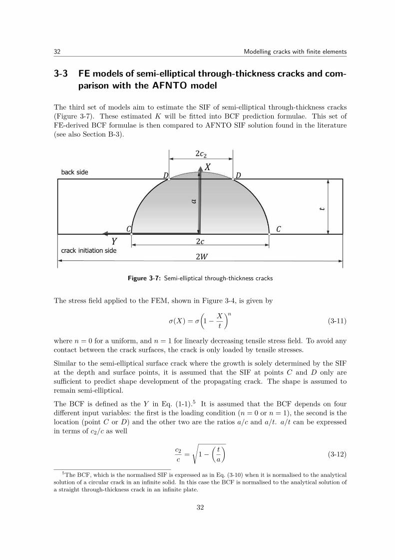
3-3 FE models of semi-elliptical through-thickness cracks and com-parison with the AFNTO model
The third set of models aim to estimate the SIF of semi-elliptical through-thickness cracks(Figure 3-7). These estimated K will be fitted into BCF prediction formulae. This set ofFE-derived BCF formulae is then compared to AFNTO SIF solution found in the literature(see also Section B-3).
Figure 3-7: Semi-elliptical through-thickness cracks
The stress field applied to the FEM, shown in Figure 3-4, is given by
σ(X) = σ
(1− X
t
)n(3-11)
where n = 0 for a uniform, and n = 1 for linearly decreasing tensile stress field. To avoid anycontact between the crack surfaces, the crack is only loaded by tensile stresses.
Similar to the semi-elliptical surface crack where the growth is solely determined by the SIFat the depth and surface points, it is assumed that the SIF at points C and D only aresufficient to predict shape development of the propagating crack. The shape is assumed toremain semi-elliptical.
The BCF is defined as the Y in Eq. (1-1).5 It is assumed that the BCF depends on fourdifferent input variables: the first is the loading condition (n = 0 or n = 1), the second is thelocation (point C or D) and the other two are the ratios a/c and a/t. a/t can be expressedin terms of c2/c as well
c2c
=√
1−(t
a
)(3-12)
5The BCF, which is the normalised SIF is expressed as in Eq. (3-10) when it is normalised to the analyticalsolution of a circular crack in an infinite solid. In this case the BCF is normalised to the analytical solution ofa straight through-thickness crack in an infinite plate.
32
3-3 FEM of semi-elliptical through-thickness cracks 33
The following ratios are analysed: a/c = {0.4, 0.6, 0.8, 1.0, 1.25, 1.5, 1.75, 2.0} and c2/c ={0.24, 0.28, ..., 0.92}, c2/c = {0.94, 0.95, ..., 0.99} so a total of 8 × 24 = 192 models are usedfor curve fitting a BCF-relation.
The models are validated by the analytical solution for a straight, through-thickness centrecrack that is corrected for its finite width, see also Section B-4. The reference solution for thevalidation model is then given by
Kref = σ√πc · fw
(c
W
)(3-13)
where the width correction fw for a straight centre crack is given by
fw
(c
W
)=[1− 0.025
(c
W
)2+ 0.06
(c
W
)4] [
cos(π
2c
W
)]−1/2(3-14)
All models have a width of W = 6c. For the (straight) validation models the correction istherefore constant at fw = 1.01683. Hence, also Kref remains uniform along the thickness.For the semi-elliptical through-thickness models fw varies along the crack-tip because insteadof c in Eq. (3-14), the ’local’ c is used, i.e. the respective Y -coordinates of each of the crack-tipnodes.
The SIF values are obtained by the J-contour integral. This method is not suitable to retrievethe SIF value at the nodes where three free surfaces meet (i.e. point C and D), see AppendixD for a brief explanation why this is the case. The SIFs at these points are therefore assumedto have the same value as the first neighbouring crack-tip node.
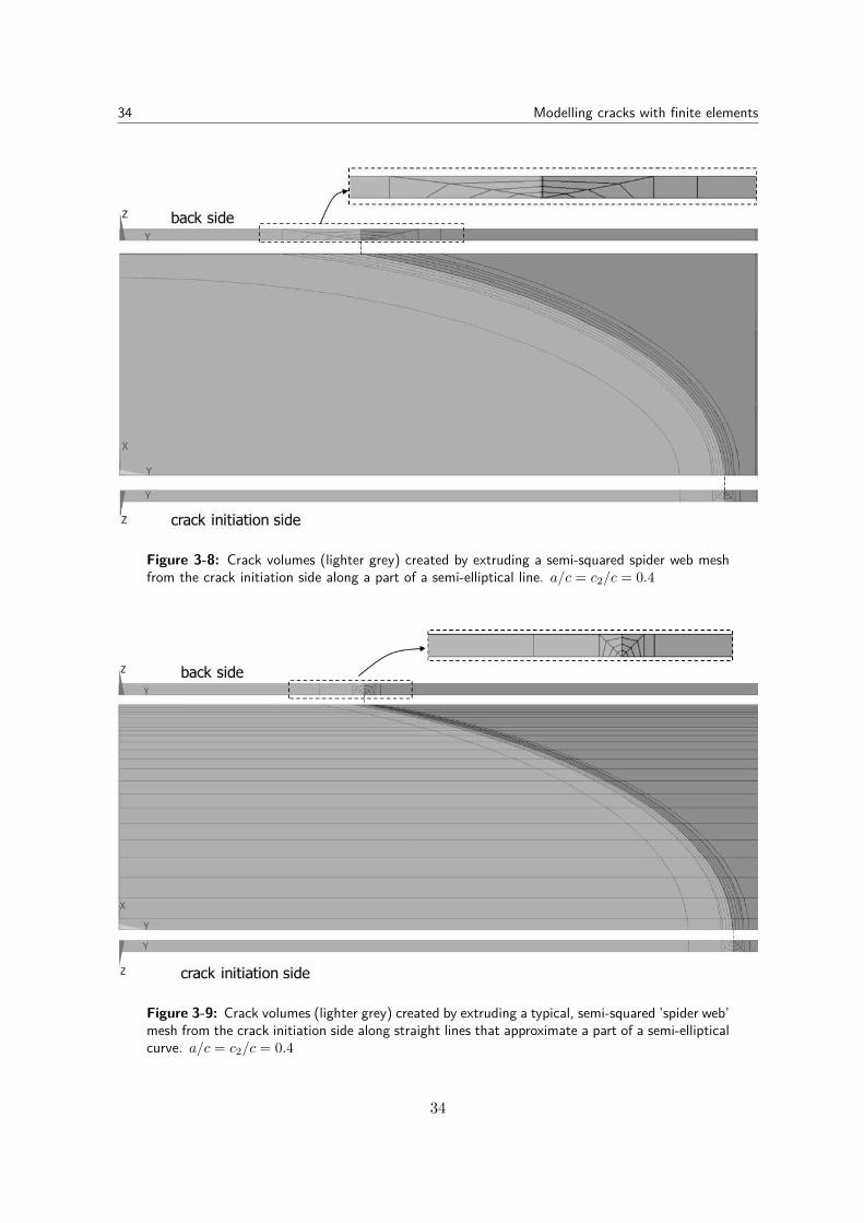
The through-thickness models cannot be constructed in a similar way as the surface crackmodels, i.e. by extruding a typical, semi-squared ’spider web’ type of mesh from the crackinitiation side along (a part of) a semi-elliptical line, as for instance shown in the close-up inFigure 3-3. However, as shown in Figure 3-8, this extrusion heavily distorts the spider-webshape at the back side and is therefore not suitable for sharply curved through-thicknesscracks. To avoid this distortion, the elliptical lines at and around the crack-tip are approxi-mated by a reasonably large number of straight lines, see Figure 3-9.
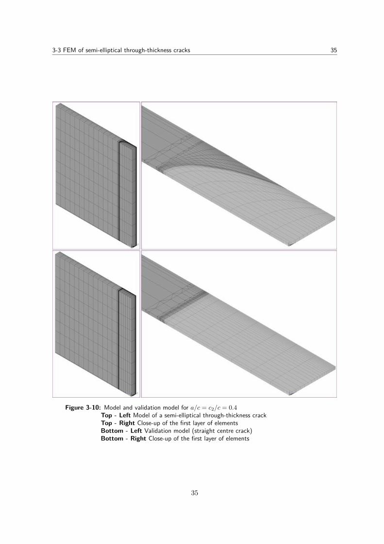
This latter model can be modified into a validation model when the crack-tip mesh is extrudedalong a straight line perpendicular to the surface and not along the curved ’elliptical’ line.In Figure 3-10 an example can be found of the model and its validation mesh. An exampleansys script file can be found in Appendix F.
This mesh type is by no means the best mesh possible but it does allow for a - at leastsome sort of - comparison with a validation model. Models similar to that of Figure 3-10 aretherefore used for all FEM.
33
34 Modelling cracks with finite elements
Figure 3-8: Crack volumes (lighter grey) created by extruding a semi-squared spider web meshfrom the crack initiation side along a part of a semi-elliptical line. a/c = c2/c = 0.4
Figure 3-9: Crack volumes (lighter grey) created by extruding a typical, semi-squared ’spider web’mesh from the crack initiation side along straight lines that approximate a part of a semi-ellipticalcurve. a/c = c2/c = 0.4
34
3-3 FEM of semi-elliptical through-thickness cracks 35
Figure 3-10: Model and validation model for a/c = c2/c = 0.4Top - Left Model of a semi-elliptical through-thickness crackTop - Right Close-up of the first layer of elementsBottom - Left Validation model (straight centre crack)Bottom - Right Close-up of the first layer of elements
35
36 Modelling cracks with finite elements
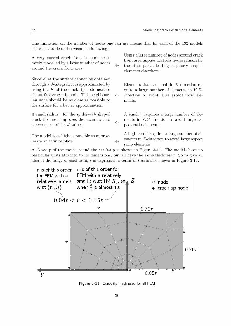
The limitation on the number of nodes one can use means that for each of the 192 modelsthere is a trade-off between the following:
A very curved crack front is more accu-rately modelled by a large number of nodesaround the crack front area. ⇔
Using a large number of nodes around crackfront area implies that less nodes remain forthe other parts, leading to poorly shapedelements elsewhere.
Since K at the surface cannot be obtainedthrough a J-integral, it is approximated byusing the K of the crack-tip node next tothe surface crack-tip node. This neighbour-ing node should be as close as possible tothe surface for a better approximation.
⇔
Elements that are small in X-direction re-quire a large number of elements in Y,Z-direction to avoid large aspect ratio ele-ments.
A small radius r for the spider-web shapedcrack-tip mesh improves the accuracy andconvergence of the J values. ⇔
A small r requires a large number of ele-ments in Y,Z-direction to avoid large as-pect ratio elements.
The model is as high as possible to approx-imate an infinite plate ⇔
A high model requires a large number of el-ements in Z-direction to avoid large aspectratio elements
A close-up of the mesh around the crack-tip is shown in Figure 3-11. The models have noparticular units attached to its dimensions, but all have the same thickness t. So to give anidea of the range of used radii, r is expressed in terms of t as is also shown in Figure 3-11.
Figure 3-11: Crack-tip mesh used for all FEM
36
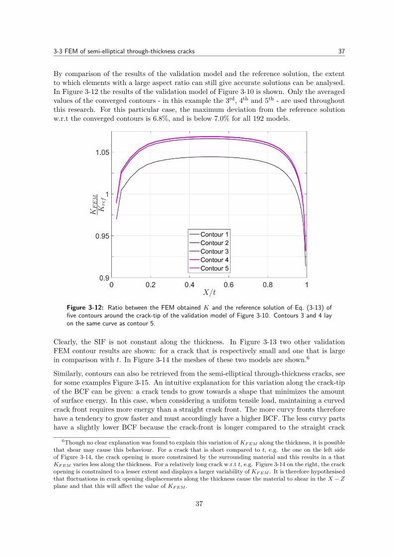
3-3 FEM of semi-elliptical through-thickness cracks 37
By comparison of the results of the validation model and the reference solution, the extentto which elements with a large aspect ratio can still give accurate solutions can be analysed.In Figure 3-12 the results of the validation model of Figure 3-10 is shown. Only the averagedvalues of the converged contours - in this example the 3rd, 4th and 5th - are used throughoutthis research. For this particular case, the maximum deviation from the reference solutionw.r.t the converged contours is 6.8%, and is below 7.0% for all 192 models.
Figure 3-12: Ratio between the FEM obtained K and the reference solution of Eq. (3-13) offive contours around the crack-tip of the validation model of Figure 3-10. Contours 3 and 4 layon the same curve as contour 5.
Clearly, the SIF is not constant along the thickness. In Figure 3-13 two other validationFEM contour results are shown: for a crack that is respectively small and one that is largein comparison with t. In Figure 3-14 the meshes of these two models are shown.6
Similarly, contours can also be retrieved from the semi-elliptical through-thickness cracks, seefor some examples Figure 3-15. An intuitive explanation for this variation along the crack-tipof the BCF can be given: a crack tends to grow towards a shape that minimizes the amountof surface energy. In this case, when considering a uniform tensile load, maintaining a curvedcrack front requires more energy than a straight crack front. The more curvy fronts thereforehave a tendency to grow faster and must accordingly have a higher BCF. The less curvy partshave a slightly lower BCF because the crack-front is longer compared to the straight crack
6Though no clear explanation was found to explain this variation of KF EM along the thickness, it is possiblethat shear may cause this behaviour. For a crack that is short compared to t, e.g. the one on the left sideof Figure 3-14, the crack opening is more constrained by the surrounding material and this results in a thatKF EM varies less along the thickness. For a relatively long crack w.r.t t, e.g. Figure 3-14 on the right, the crackopening is constrained to a lesser extent and displays a larger variability of KF EM . It is therefore hypothesisedthat fluctuations in crack opening displacements along the thickness cause the material to shear in the X −Zplane and that this will affect the value of KF EM .
37
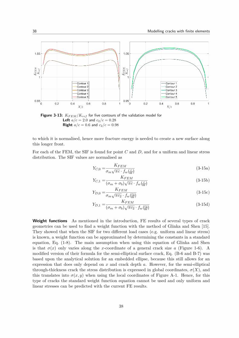
38 Modelling cracks with finite elements
Figure 3-13: KF EM/Kref for five contours of the validation model forLeft a/c = 2.0 and c2/c = 0.28Right a/c = 0.6 and c2/c = 0.98
to which it is normalised, hence more fracture energy is needed to create a new surface alongthis longer front.
For each of the FEM, the SIF is found for point C and D, and for a uniform and linear stressdistribution. The SIF values are normalised as
YC,0 = KFEM
σm√πc · fw
(cW
) (3-15a)
YC,1 = KFEM
(σm + σb)√πc · fw
(cW
) (3-15b)
YD,0 = KFEM
σm√πc2 · fw
(c2W
) (3-15c)
YD,1 = KFEM
(σm + σb)√πc2 · fw
(c2W
) (3-15d)
Weight functions As mentioned in the introduction, FE results of several types of crackgeometries can be used to find a weight function with the method of Glinka and Shen [15].They showed that when the SIF for two different load cases (e.g. uniform and linear stress)is known, a weight function can be approximated by determining the constants in a standardequation, Eq. (1-8). The main assumption when using this equation of Glinka and Shenis that σ(x) only varies along the x-coordinate of a general crack size a (Figure 1-6). Amodified version of their formula for the semi-elliptical surface crack, Eq. (B-6 and B-7) wasbased upon the analytical solution for an embedded ellipse, because this still allows for anexpression that does only depend on x and crack depth a. However, for the semi-ellipticalthrough-thickness crack the stress distribution is expressed in global coordinates, σ(X), andthis translates into σ(x, y) when using the local coordinates of Figure A-1. Hence, for thistype of cracks the standard weight function equation cannot be used and only uniform andlinear stresses can be predicted with the current FE results.
38
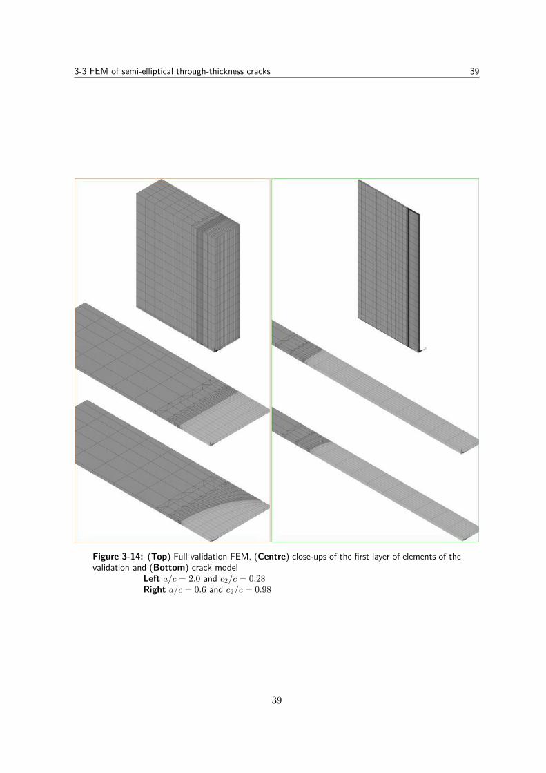
3-3 FEM of semi-elliptical through-thickness cracks 39
Figure 3-14: (Top) Full validation FEM, (Centre) close-ups of the first layer of elements of thevalidation and (Bottom) crack model
Left a/c = 2.0 and c2/c = 0.28Right a/c = 0.6 and c2/c = 0.98
39
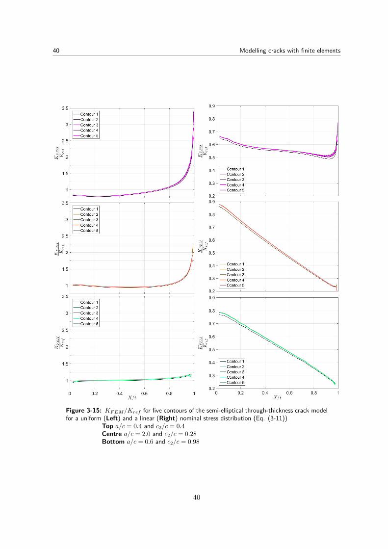
40 Modelling cracks with finite elements
Figure 3-15: KF EM/Kref for five contours of the semi-elliptical through-thickness crack modelfor a uniform (Left) and a linear (Right) nominal stress distribution (Eq. (3-11))
Top a/c = 0.4 and c2/c = 0.4Centre a/c = 2.0 and c2/c = 0.28Bottom a/c = 0.6 and c2/c = 0.98
40
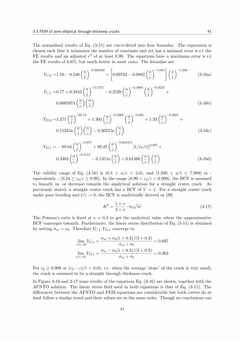
3-3 FEM of semi-elliptical through-thickness cracks 41
The normalised results of Eq. (3-15) are curve-fitted into four formulae. The expression ischosen such that it minimises the number of constants and yet has a minimal error w.r.t theFE results and an adjusted r2 of at least 0.99. The equations have a maximum error w.r.tthe FE results of 6.6%, but much better in most cases. The formulae are
YC,0 =1.50− 0.536(a
t
)−0.008246+[0.09782− 0.0882
(a
c
)−1.081](
a
t
)−1.289(3-16a)
YC,1 =0.77 + 0.2843(a
t
)−0.7473− 0.2529
(a
c
)−0.4966 (at
)−0.9227+
0.0005974(a
c
)(a
t
)(3-16b)
YD,0 =1.271(a
t
)−26.73+ 1.304
(a
c
)−0.4908 (at
)−3.082+ 1.33
(a
c
)−0.2891+
0.1523 ln(a
t
)(a
c
)− 0.3052 ln
(a
t
)(3-16c)
YD,1 =− 89.04(a
t
)−3.857+ 89.25
(a
c
)−0.003415[1/(a/t)]3.867 +
0.3383(a
c
)−0.4113− 0.135 ln
(a
t
)+ 0.01466
(a
c
)(a
t
)(3-16d)
The validity range of Eq. (3-16) is (0.4 ≤ a/c ≤ 2.0), and (1.030 ≤ a/t ≤ 7.089) or -equivalently - (0.24 ≤ c2/c ≤ 0.99). In the range (0.99 < c2/c < 0.999), the BCF is assumedto linearly in- or decrease towards the analytical solution for a straight centre crack. Aspreviously stated, a straight centre crack has a BCF of Y = 1. For a straight centre crackunder pure bending and t/c→ 0, the BCF is analytically derived as [29]
Kb = 1 + ν
3 + ν· σb√πc (3-17)
The Poisson’s ratio is fixed at ν = 0.3 to get the analytical value where the approximativeBCF converges towards. Furthermore, the linear stress distribution of Eq. (3-11) is obtainedby setting σm = σb. Therefore YC,1, YD,1 converge to
limt/c→0
YC,1 = σm + σb(1 + 0.3)/(3 + 0.3)σm + σb
= 0.697
limt/c→0
YD,1 = σm − σb(1 + 0.3)/(3 + 0.3)σm + σb
= 0.303
For c2 ≥ 0.999 or (c2 − c)/t < 0.01, i.e. when the average ’slope’ of the crack is very small,the crack is assumed to be a straight through thickness crack.
In Figure 3-16 and 3-17 some results of the equations Eq. (3-16) are shown, together with theAFNTO solution. The linear stress field used in both equations is that of Eq. (3-11). Thedifferences between the AFNTO and FEM equations are considerable but both curves do atleast follow a similar trend and their values are in the same order. Though no conclusions can
41
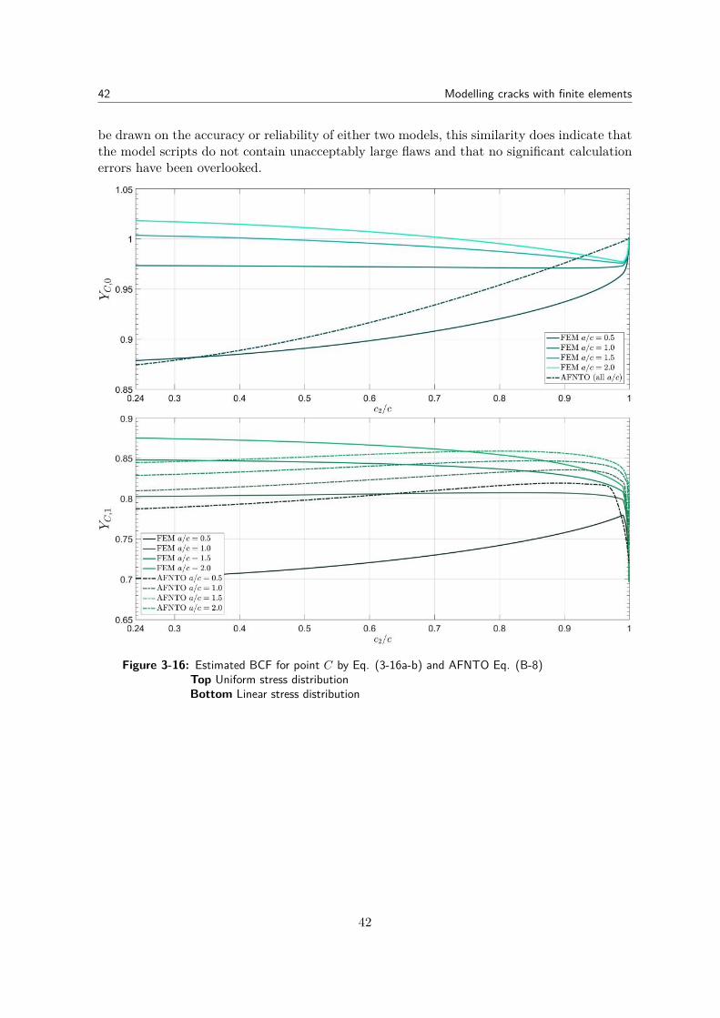
42 Modelling cracks with finite elements
be drawn on the accuracy or reliability of either two models, this similarity does indicate thatthe model scripts do not contain unacceptably large flaws and that no significant calculationerrors have been overlooked.
Figure 3-16: Estimated BCF for point C by Eq. (3-16a-b) and AFNTO Eq. (B-8)Top Uniform stress distributionBottom Linear stress distribution
42
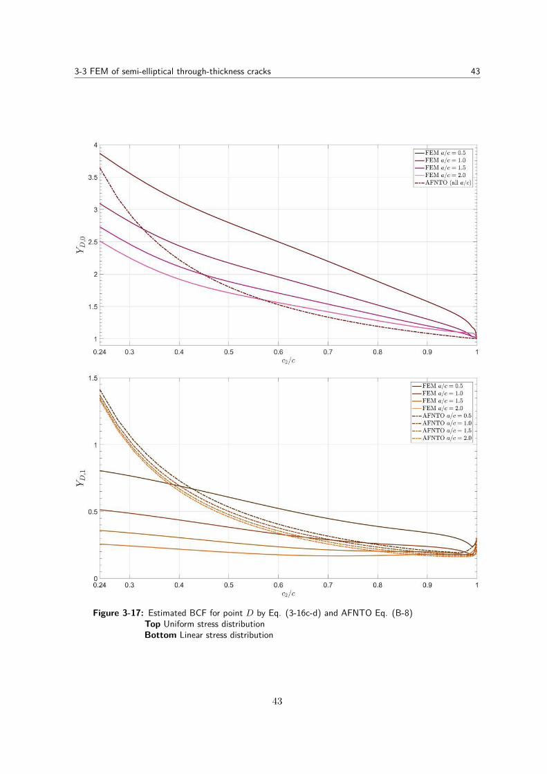
3-3 FEM of semi-elliptical through-thickness cracks 43
Figure 3-17: Estimated BCF for point D by Eq. (3-16c-d) and AFNTO Eq. (B-8)Top Uniform stress distributionBottom Linear stress distribution
43

44 Modelling cracks with finite elements
44

Chapter 4
The accuracy of predictive models incomparison with experiments
For an LBB analysis, both the estimation of the number of stress cycles to attain a certaincrack shape as well as the prediction of the crack shape at and after breakthrough duringthe crack development are of primary interest to calculate the leakage rate and the numberof cycles before reaching the critical crack size. In this chapter the models to estimate thecrack shape at and after breakthrough will be compared to experimental data found in theliterature. In Appendix G the input values for all experimental data-sets are given. Notall of these sets were complete in the sense that all information was available to run thenumerical model. Educated guesses have been made to fill in missing information so thatthese experiments could nonetheless be used. The methods used to fill the gaps are furtherexplained in Appendix H.
4-1 Comparison between the estimated breakthrough shape andexperiments
Numerical simulations of other research [21, 22] indicated that the breakthrough shape ispredominantly affected by the ratio between membrane and bending stresses. The numericalmodel of [21] has been validated with experimental crack shape development data. Thecalculation scheme of this previous research is essentially identical to the numerical calculationprocedure described in Chapter 2. Calculations of this experimentally validated numericalmodel indicated that the shape up to and at breakthrough is largely insensitive to the:
– Material constants, like C and m in Eq. (2-2)
– Initial crack size, as long as a1/c1 > 0.1
– Initial crack depth, as long as it is not too deep a1/t < 0.1 yet large enough for the SIFand growth models to be applicable.
45
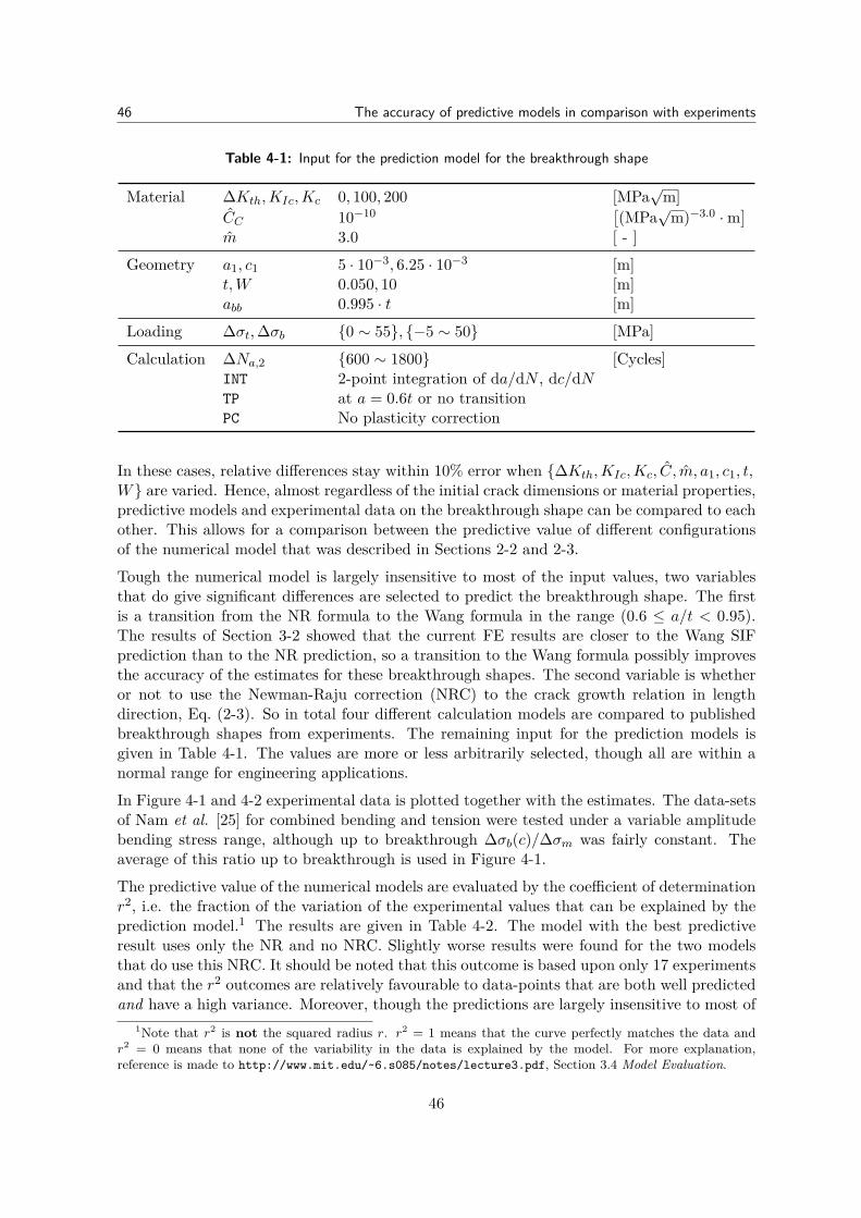
46 The accuracy of predictive models in comparison with experiments
Table 4-1: Input for the prediction model for the breakthrough shape
Material ∆Kth,KIc,Kc 0, 100, 200 [MPa√m]
CC 10−10 [(MPa
√m)−3.0 ·m
]m 3.0 [ - ]
Geometry a1, c1 5 · 10−3, 6.25 · 10−3 [m]t,W 0.050, 10 [m]abb 0.995 · t [m]
Loading ∆σt,∆σb {0 ∼ 55}, {−5 ∼ 50} [MPa]
Calculation ∆Na,2 {600 ∼ 1800} [Cycles]INT 2-point integration of da/dN , dc/dNTP at a = 0.6t or no transitionPC No plasticity correction
In these cases, relative differences stay within 10% error when {∆Kth,KIc,Kc, C, m, a1, c1, t,W} are varied. Hence, almost regardless of the initial crack dimensions or material properties,predictive models and experimental data on the breakthrough shape can be compared to eachother. This allows for a comparison between the predictive value of different configurationsof the numerical model that was described in Sections 2-2 and 2-3.
Tough the numerical model is largely insensitive to most of the input values, two variablesthat do give significant differences are selected to predict the breakthrough shape. The firstis a transition from the NR formula to the Wang formula in the range (0.6 ≤ a/t < 0.95).The results of Section 3-2 showed that the current FE results are closer to the Wang SIFprediction than to the NR prediction, so a transition to the Wang formula possibly improvesthe accuracy of the estimates for these breakthrough shapes. The second variable is whetheror not to use the Newman-Raju correction (NRC) to the crack growth relation in lengthdirection, Eq. (2-3). So in total four different calculation models are compared to publishedbreakthrough shapes from experiments. The remaining input for the prediction models isgiven in Table 4-1. The values are more or less arbitrarily selected, though all are within anormal range for engineering applications.
In Figure 4-1 and 4-2 experimental data is plotted together with the estimates. The data-setsof Nam et al. [25] for combined bending and tension were tested under a variable amplitudebending stress range, although up to breakthrough ∆σb(c)/∆σm was fairly constant. Theaverage of this ratio up to breakthrough is used in Figure 4-1.
The predictive value of the numerical models are evaluated by the coefficient of determinationr2, i.e. the fraction of the variation of the experimental values that can be explained by theprediction model.1 The results are given in Table 4-2. The model with the best predictiveresult uses only the NR and no NRC. Slightly worse results were found for the two modelsthat do use this NRC. It should be noted that this outcome is based upon only 17 experimentsand that the r2 outcomes are relatively favourable to data-points that are both well predictedand have a high variance. Moreover, though the predictions are largely insensitive to most of
1Note that r2 is not the squared radius r. r2 = 1 means that the curve perfectly matches the data andr2 = 0 means that none of the variability in the data is explained by the model. For more explanation,reference is made to http://www.mit.edu/~6.s085/notes/lecture3.pdf, Section 3.4 Model Evaluation.
46
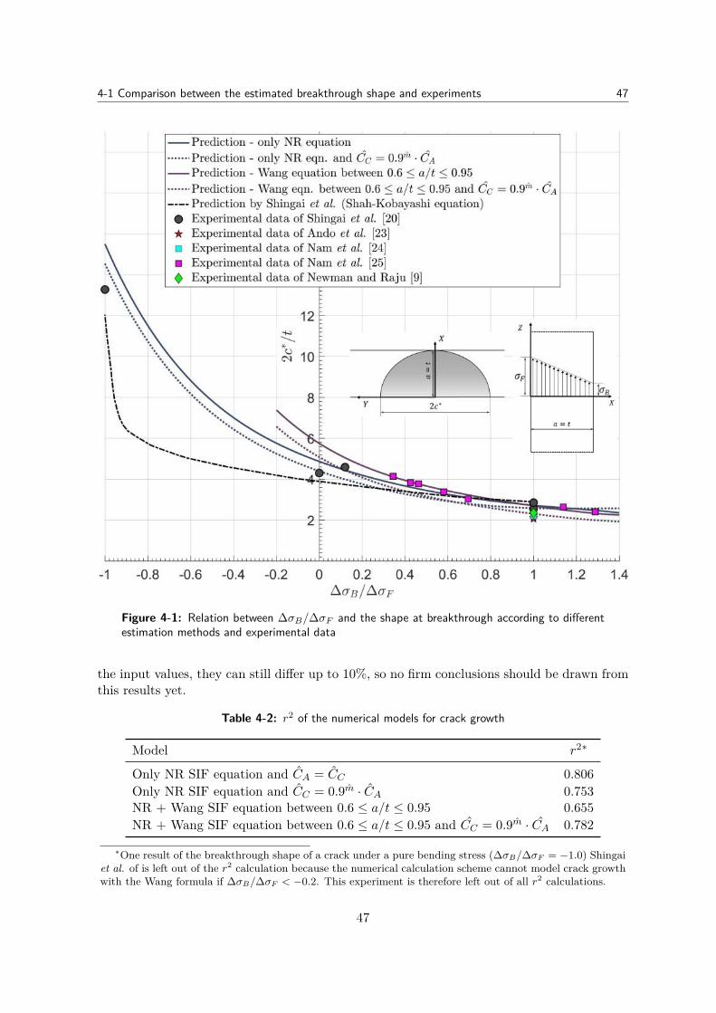
4-1 Comparison between the estimated breakthrough shape and experiments 47
Figure 4-1: Relation between ∆σB/∆σF and the shape at breakthrough according to differentestimation methods and experimental data
the input values, they can still differ up to 10%, so no firm conclusions should be drawn fromthis results yet.
Table 4-2: r2 of the numerical models for crack growth
Model r2∗
Only NR SIF equation and CA = CC 0.806Only NR SIF equation and CC = 0.9m · CA 0.753NR + Wang SIF equation between 0.6 ≤ a/t ≤ 0.95 0.655NR + Wang SIF equation between 0.6 ≤ a/t ≤ 0.95 and CC = 0.9m · CA 0.782
∗One result of the breakthrough shape of a crack under a pure bending stress (∆σB/∆σF = −1.0) Shingaiet al. of is left out of the r2 calculation because the numerical calculation scheme cannot model crack growthwith the Wang formula if ∆σB/∆σF < −0.2. This experiment is therefore left out of all r2 calculations.
47
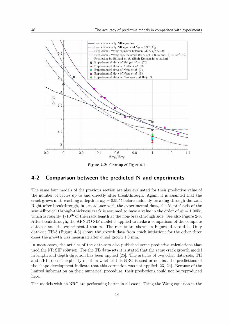
48 The accuracy of predictive models in comparison with experiments
Figure 4-2: Close-up of Figure 4-1
4-2 Comparison between the predicted N and experiments
The same four models of the previous section are also evaluated for their predictive value ofthe number of cycles up to and directly after breakthrough. Again, it is assumed that thecrack grows until reaching a depth of abb = 0.995t before suddenly breaking through the wall.Right after breakthrough, in accordance with the experimental data, the ’depth’ axis of thesemi-elliptical through-thickness crack is assumed to have a value in the order of a∗ = 1.005t,which is roughly 1/10th of the crack length at the non-breakthrough side. See also Figure 2-3.After breakthrough, the AFNTO SIF model is applied to make a comparison of the completedata-set and the experimental results. The results are shown in Figures 4-3 to 4-4. Onlydata-set TH-3 (Figure 4-3) shows the growth data from crack initiation; for the other threecases the growth was measured after c had grown 1.3 mm.
In most cases, the articles of the data-sets also published some predictive calculations thatused the NR SIF solution. For the TB data-sets it is stated that the same crack growth modelin length and depth direction has been applied [25]. The articles of two other data-sets, THand THL, do not explicitly mention whether this NRC is used or not but the predictions ofthe shape development indicate that this correction was not applied [23, 24]. Because of thelimited information on their numerical procedure, their predictions could not be reproducedhere.
The models with an NRC are performing better in all cases. Using the Wang equation in the
48
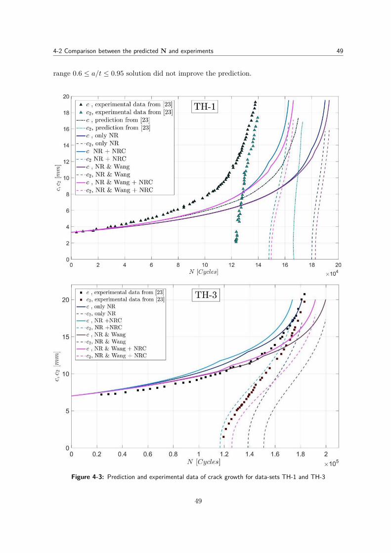
4-2 Comparison between the predicted N and experiments 49
range 0.6 ≤ a/t ≤ 0.95 solution did not improve the prediction.
Figure 4-3: Prediction and experimental data of crack growth for data-sets TH-1 and TH-3
49
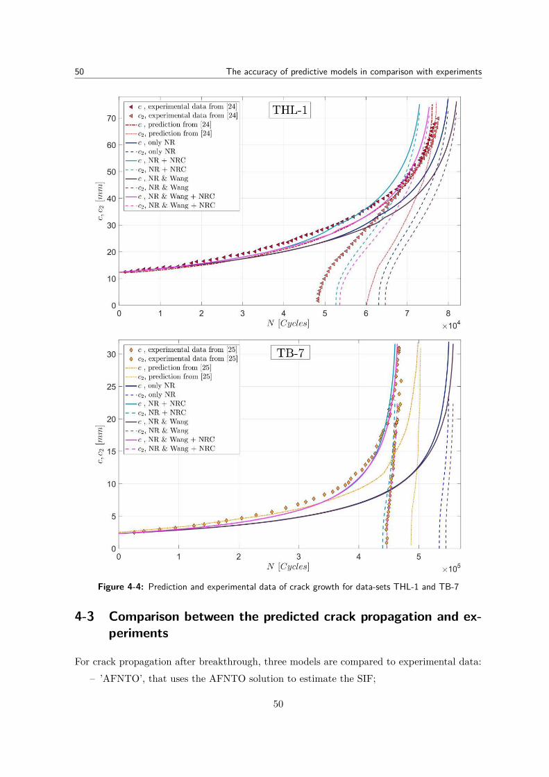
50 The accuracy of predictive models in comparison with experiments
Figure 4-4: Prediction and experimental data of crack growth for data-sets THL-1 and TB-7
4-3 Comparison between the predicted crack propagation and ex-periments
For crack propagation after breakthrough, three models are compared to experimental data:– ’AFNTO’, that uses the AFNTO solution to estimate the SIF;
50
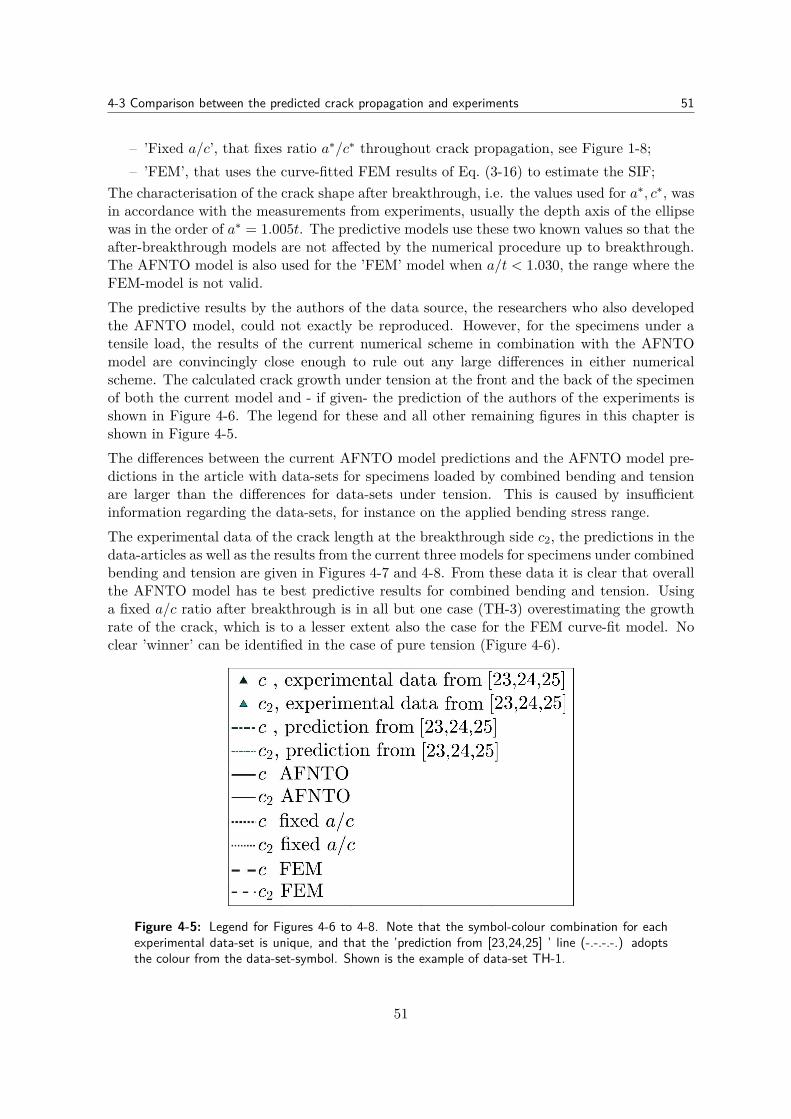
4-3 Comparison between the predicted crack propagation and experiments 51
– ’Fixed a/c’, that fixes ratio a∗/c∗ throughout crack propagation, see Figure 1-8;– ’FEM’, that uses the curve-fitted FEM results of Eq. (3-16) to estimate the SIF;
The characterisation of the crack shape after breakthrough, i.e. the values used for a∗, c∗, wasin accordance with the measurements from experiments, usually the depth axis of the ellipsewas in the order of a∗ = 1.005t. The predictive models use these two known values so that theafter-breakthrough models are not affected by the numerical procedure up to breakthrough.The AFNTO model is also used for the ’FEM’ model when a/t < 1.030, the range where theFEM-model is not valid.The predictive results by the authors of the data source, the researchers who also developedthe AFNTO model, could not exactly be reproduced. However, for the specimens under atensile load, the results of the current numerical scheme in combination with the AFNTOmodel are convincingly close enough to rule out any large differences in either numericalscheme. The calculated crack growth under tension at the front and the back of the specimenof both the current model and - if given- the prediction of the authors of the experiments isshown in Figure 4-6. The legend for these and all other remaining figures in this chapter isshown in Figure 4-5.The differences between the current AFNTO model predictions and the AFNTO model pre-dictions in the article with data-sets for specimens loaded by combined bending and tensionare larger than the differences for data-sets under tension. This is caused by insufficientinformation regarding the data-sets, for instance on the applied bending stress range.The experimental data of the crack length at the breakthrough side c2, the predictions in thedata-articles as well as the results from the current three models for specimens under combinedbending and tension are given in Figures 4-7 and 4-8. From these data it is clear that overallthe AFNTO model has te best predictive results for combined bending and tension. Usinga fixed a/c ratio after breakthrough is in all but one case (TH-3) overestimating the growthrate of the crack, which is to a lesser extent also the case for the FEM curve-fit model. Noclear ’winner’ can be identified in the case of pure tension (Figure 4-6).
Figure 4-5: Legend for Figures 4-6 to 4-8. Note that the symbol-colour combination for eachexperimental data-set is unique, and that the ’prediction from [23,24,25] ’ line (-.-.-.-.) adoptsthe colour from the data-set-symbol. Shown is the example of data-set TH-1.
51
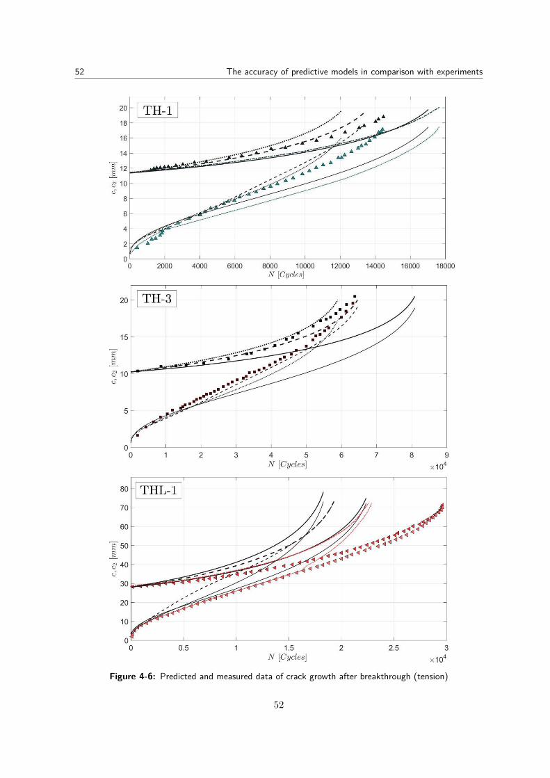
52 The accuracy of predictive models in comparison with experiments
Figure 4-6: Predicted and measured data of crack growth after breakthrough (tension)
52
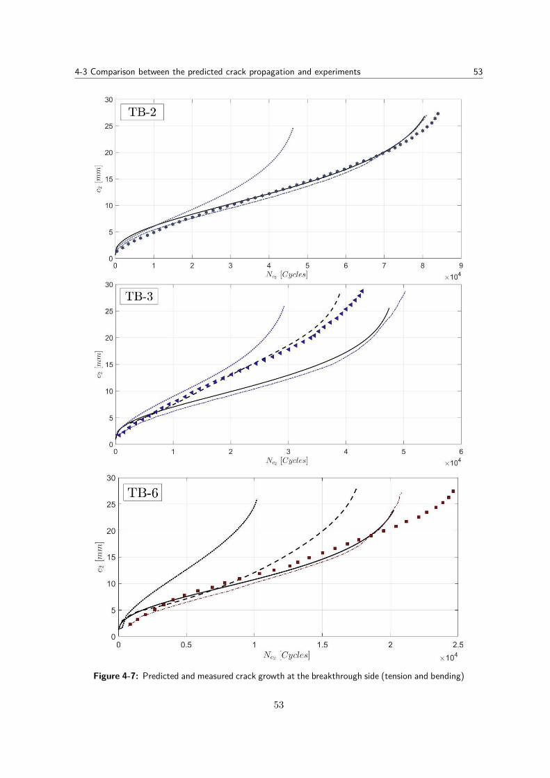
4-3 Comparison between the predicted crack propagation and experiments 53
Figure 4-7: Predicted and measured crack growth at the breakthrough side (tension and bending)
53
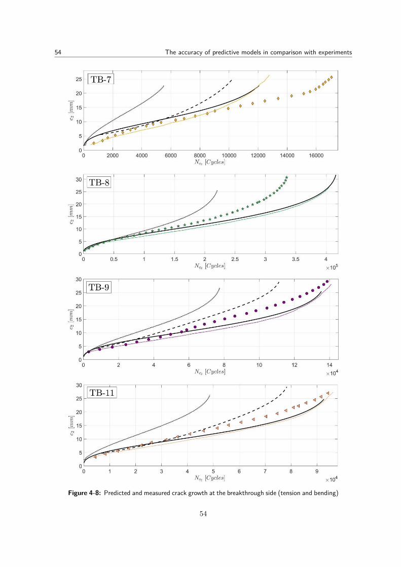
54 The accuracy of predictive models in comparison with experiments
Figure 4-8: Predicted and measured crack growth at the breakthrough side (tension and bending)
54
Chapter 5
Analysis of the data, conclusions andrecommendations
5-1 Analysis of the data taken from external sources
The present thesis relies heavily on three publications from the same group of researchers thatalso introduced the AFNTO SIF model, these articles will first be reviewed in this chapter. Fora brief discussion on a smaller issue related to the AFNTO formula for combined membraneand bending stress, reference is made to Section B-3. Hereafter, the authors of [23, 24, 25]will be referred to as ’the authors’, and the research of these articles is referred to as ’their’research or experiments.Unfortunately, their experiments have a different configuration for each new experiment, thusnone of the experiments was repeated. This repeating is necessary to estimate the scatter ofthe results and to assess the performance of the models when more than one test result isavailable. As a consequence, the unknown confidence level for the outcomes is a limitation.As mentioned, crack growth can be estimated by using a crack growth relation. The authorsuse the commonly applied Paris relation, but their method to find C and m in Eq. (2-2)is questionable. As pointed out in Section A-4, one cannot simply obtain C and m from amanufacturer’s specification but one has to conduct experiments for each batch of materialin order to reliably estimate these. These experiments had been carried out by the authorsbut in such a way that the values they obtained for C and m may be unreliable.Before breakthrough, they use the NR equation to estimate ∆K using their measured crackdepth and length. Some criticism can be given to this:
– The NR equation in itself has an error margin of 5.0% up to a/t ≤ 0.8, and, as discussedin Section 3-2, possibly larger error margins beyond this ratio. For other crack shapes∆K can be found with much higher or even analytical precision.
– The crack depth was determined afterwards from the typical ’beach marks’ that fatiguecracks sometimes leave on the crack surface. These marks may be hard to identify ormeasure precisely.
55
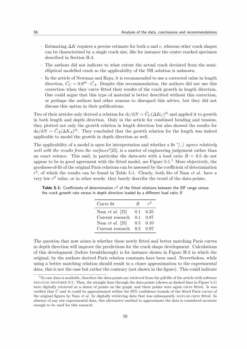
56 Analysis of the data, conclusions and recommendations
– Estimating ∆K requires a precise estimate for both a and c, whereas other crack shapescan be characterised by a single crack size, like for instance the centre cracked specimendescribed in Section B-4.
– The authors did not indicate to what extent the actual crack deviated from the semi-elliptical modelled crack so the applicability of the NR solution is unknown.
– In the article of Newman and Raju, it is recommended to use a corrected value in lengthdirection, CC = 0.9m · CA. Despite this recommendation, the authors did not use thiscorrection when they curve fitted their results of the crack growth in length direction.One could argue that this type of material is better described without this correction,or perhaps the authors had other reasons to disregard this advice, but they did notdiscuss this option in their publications.
Two of their articles only derived a relation for dc/dN = CC(∆KC)m and applied it to growthin both length and depth direction. Only in the article for combined bending and tension,they plotted not only the growth relation in length direction but also showed the results forda/dN = CA(∆KA)m. They concluded that the growth relation for the length was indeedapplicable to model the growth in depth direction as well.
The applicability of a model is open for interpretation and whether a fit "[..] agrees relativelywell with the results from the surfaces"[25], is a matter of engineering judgement rather thanan exact science. This said, in particular the data-sets with a load ratio R = 0.5 do notappear to be in good agreement with the fitted model, see Figure 5-1.1 More objectively, thegoodness-of-fit of the original Paris relations can be assessed by the coefficient of determinationr2, of which the results can be found in Table 5-1. Clearly, both fits of Nam et al. have avery low r2 value, or in other words: they barely describe the trend of the data-points.
Table 5-1: Coefficients of determination r2 of the fitted relations between the SIF range versusthe crack growth rate versus in depth direction loaded by a different load ratio R
Curve fit R r2
Nam et al. [25] 0.1 0.35Current research 0.1 0.87Nam et al. [25] 0.5 0.10Current research 0.5 0.97
The question that now arises is whether these newly fitted and better matching Paris curvesin depth direction will improve the predictions for the crack shape development. Calculationsof this development (before breakthrough) is for instance shown in Figure H-2 in which theoriginal, by the authors derived Paris relation constants have been used. Nevertheless, whileusing a better matching relation should result in a closer approximation to the experimentaldata, this is not the case but rather the contrary (not shown in the figure). This could indicate
1No raw data is available, therefore the data-points are retrieved from the pdf-file of the article with softwareengauge digitizer 9.5. Thus, the straight lines through the data-points (shown as dashed lines in Figure 5-1)were digitally retrieved as a dozen of points on the graph, and these points were again curve fitted. Is wasverified that C and m could be approximated within the 95% confidence bounds of the fitted Paris curves ofthe original figures by Nam et al. by digitally retrieving data that was subsequently matlab curve fitted. Inabsence of any raw experimental data, this alternative method to approximate the data is considered accurateenough to be used for this research.
56
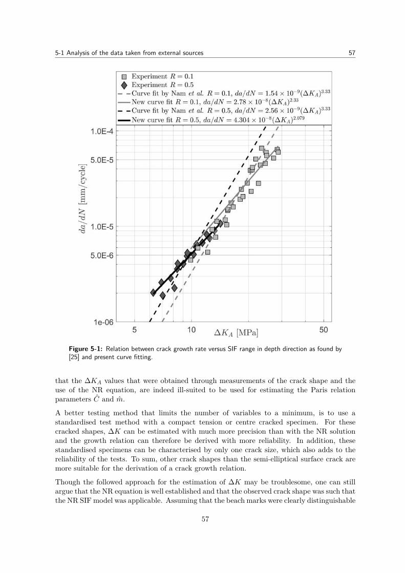
5-1 Analysis of the data taken from external sources 57
Figure 5-1: Relation between crack growth rate versus SIF range in depth direction as found by[25] and present curve fitting.
that the ∆KA values that were obtained through measurements of the crack shape and theuse of the NR equation, are indeed ill-suited to be used for estimating the Paris relationparameters C and m.
A better testing method that limits the number of variables to a minimum, is to use astandardised test method with a compact tension or centre cracked specimen. For thesecracked shapes, ∆K can be estimated with much more precision than with the NR solutionand the growth relation can therefore be derived with more reliability. In addition, thesestandardised specimens can be characterised by only one crack size, which also adds to thereliability of the tests. To sum, other crack shapes than the semi-elliptical surface crack aremore suitable for the derivation of a crack growth relation.
Though the followed approach for the estimation of ∆K may be troublesome, one can stillargue that the NR equation is well established and that the observed crack shape was such thatthe NR SIF model was applicable. Assuming that the beach marks were clearly distinguishable
57
58 Analysis of the data, conclusions and recommendations
and precisely measured, their method could, in this best case scenario, give usable ∆K values.
However, after breakthrough, the authors used their own, non-validated and newly developedSIF formula to estimate C and m. For one of their test materials, SS 41 steel, they actuallyfound a considerably higher value for m in the Paris relation after breakthrough but thiswas "thought to be attributable to the fact that the [...] sample of the SS 41 steel suffered anoverall general yielding prior to penetration of the crack" [23]. Though this could indeed bean explanation, they did not consider the option that their formula for the SIF might not bea proper one to be used. For the other material used in their experiments, high tension steel,they did fit the data into a single Paris relation and concluded that it was therefore appropriateto predict crack growth and propagation with their new formula. Because the calculated andmeasured results agreed fairly well, they also concluded that "[...] the behaviour of fatiguecracks after through-thickness can be evaluated quantitatively using the stress intensity factorassessment method proposed in this report." [23].
Their conclusion is highly questionable: fitting a line through data-points does not provethat their SIF model is correct, it merely shows that the parameters of a fitted curve can beadjusted in such a way that the data-points on a graph can be reasonably well approximatedby a single line. In other words, C and m are chosen such that the NR and AFNTO modelaccurately predict crack growth and propagation. The growth rate from actual measurements(∆c/∆N) is attached to a value ∆K from the NR or AFNTO SIF, which in its turn is laterused to estimate this growth or propagation. It is therefore no surprise that the AFNTOmodel performs well for crack propagation estimations but this could equally well be causedby the chosen values for C and m. It does not yet say anything about the validity of theAFNTO SIF model.
5-2 Conclusions I: Estimating surface crack growth and break-through shape
The first aim of this research, developing a numerical calculation scheme to predict surfacecrack growth more accurately compared to existing numerical methods, can now be assessedby answering the following questions:
1-a) To what extent does the numerical calculation scheme developed in this research solvesperceived shortcomings of other methods?
1-b) How does this numerical calculation scheme perform in comparison with experimentallydetermined results of the breakthrough shape?
1-c) What is the influence on the accuracy of the estimations for crack shape and growthwhen the SIF is not only estimated by the NR solution, but also by the Wang solutionin the range of (0.6 ≤ a/t < 0.95)?
1-a The ’other methods’ in 1-a, refer to numerical calculation schemes that were brieflymentioned in the Chapter 1, i.e. Chapter 8 of [6] and [8, 7, 22, 25]. Because these methodsare only described in a broad outline, the real limitations or inaccuracies remain unidentified,hence the wording ’perceived shortcomings’ is preferred.
58
5-2 Estimating surface crack growth and breakthrough shape 59
The numerical scheme of Chapter 2 solves the issue of selecting values for the ’knowns’ tosolve the ’unknowns’ in two dimensional crack growth models. Experimental results of [19]indicate that in most practical cases the crack can grow up to almost 100% of the thickness.With this information, it is convenient to divide the remaining cross section in depth directionabb−a1 into a large number of increments ∆ak to serve as a known to solve the unknowns ∆ckand ∆Nk. To solve both unknowns, an extra requirement is necessary: ∆Na,k = ∆Nc,k. Oneof the shortcomings of the other methods is that they require that ∆Nk is known in advanceas well, but this number of cycles is difficult to estimate beforehand. Selecting a small ∆Nk
may result in a large number of calculation steps. On the other hand, a large ∆Nk resultsin large increments ∆ak,∆ck and this weakens the assumption that the increment is smallenough to assume that ∆KA,k and ∆KC,k remain constant. The current numerical schemelimits the selection of knowns and the build-in checks verify that the selected input results inan outcome that is within pre-set limits for errors.Besides this assistance with the selection of input values, the current numerical model offerssome other benefits. One of the options is the 2-point integration. This option does notonly averages between the growth rates at the beginning and end of the increment, but alsoiteratively finds new values for ∆KA,k,∆KC,k that are consistent with the new values of ak, ck.Other options include a logarithmically in- or decreasing spacing of ∆ak or the use of a smallscale plasticity correction factor.
1-b The accuracy of the prediction depends on much more than just the numerical scheme.Selecting an appropriate crack growth relation and determining the material constants in theseempirical relations make the difference between a reliable prediction or an entirely inadequateestimate of the number of load cycles up to breakthrough.On the other hand, it was found that the predictions of the crack shape at breakthrough isin most cases not much affected by the growth relation or material constants. In comparisonwith the breakthrough shapes from experiments that were reported in the literature, thepredictions of the numerical models were reasonably accurate. The best estimates are foundfor the model with only the NR SIF equation and the same material constants in respectivelylength and depth direction. The difference with two other models that use the NRC is small.The number of experiments is limited so no firm conclusions should be drawn from theseresults yet. It does show, however, that the numerical calculation model can be used toroughly estimate the shape at breakthrough.As said, the growth model and material parameters do affect the prediction of load cyclesand the growth during and up to breakthrough to a large extent. The material values C, mand the used crack growth model were taken from the literature and used as an input in thenumerical model. As highlighted in the previous section, the reliability of these values is opento doubts, but presuming they were correct, it is found that using a different value for thegrowth rate in length direction, i.e. the NRC, improved the accuracy of the estimated numberof load cycles versus crack length. The use of the Wang SIF equation did not improve theresults, but this could equally well be attributed to the applied method to obtain C, m.It is known that the rolling direction of the material and other inhomogeneities affect thegrowth rate of the crack. An interesting question would be if the results could be furtherenhanced by using different growth models in length and depth direction that are based onactual measurements instead of the empirical NRC. The NRC is only a roughly estimated
59
60 Analysis of the data, conclusions and recommendations
correction from crack growth data of a broad range of materials. In absence of these tests, itis recommended to use the NRC.
1-c No evidence is found that the Wang formula is more accurate than the sole use of theNR SIF equation, despite the finding that the SIFs from current FE analysis are closer tothe SIF values obtained by the FEM of Wang and Isida et al.. The effect was negligiblewhen considering the estimated number of load cycles versus crack growth. Although againan explanation can be sought in the applied method to obtain the material values, neitherthe largely C, m independent breakthrough shape predictions did improve with the Wangsolution. Only the combination with an NRC gave reasonable results. Overall, consideringthe experimental data of this research, no clear advantages of using the Wang equation fordeep surface cracks have been found.
5-3 Conclusions II: Estimating crack propagation after wall pene-tration
2) How do the newly FE-derived SIF solution and two existing methods that consider acrack after wall penetration perform in comparison with experimentally obtained data?
Unfortunately, due to the used methods to obtain C, m, no firm statements or conclusionscan be drawn. As said, the values of C, m are such that, regardless of the actual accuracy ofthe model, the results will be biased towards the AFNTO SIF model. A slight modificationof C, m affects the results considerably. This means that these reported material valuesare neither suitable as provisional, educated guesses. Because of this, neither model can berecommended or rejected at this point. Instead of a comparison with experimental data, whichwould have been much more relevant when making recommendations for a LBB assessment,all that remains is therefore a comparison on how the models perform relative to each other.
The fixed a/c model predicts the highest crack growth rate at the front and back side ofthe specimens. It predicts that the crack reaches criticality within much less cycles than theAFNTO and FEM solutions. Presuming that the reported C, m are more or less realistic, itwould also mean that the growth rate is overestimated by a factor two or more in most cases.When taking into account that the mean material values are used in the current predictionswhereas for LBB calculations often design values will be used, this will lead to an unnecessarycautious estimate that is perhaps not viable from an economical perspective. For leakage ratepredictions, which depend on the crack length at the back side, it is the other way around:the crack is not leaking as much as estimated and will likely get detected later than predicted.Similar conclusions can be drawn for the FEM model, though to a lesser extent. The AFNTOSIF equations tend to estimate c2 the best. To emphasise: this is only true if the crack growthconstants happen to be accurate.
In absence of any official recommendations regarding crack shape propagation, it is probablysafe - not to say very safe - to use the fixed a/c model for the determination of crack propaga-tion and herewith for estimations of the number of cycles before the crack reaches criticality.It is furthermore advised to use the AFNTO SIF model for leakage rate predictions, as thismodel is likely to give a safer estimate for the crack opening area at the back of the wall.
60
5-4 Recommendations for further research 61
5-4 Recommendations for further research
It is highly recommended to carry out new experiments in a different test set-up so that thesethree solutions can be evaluated for their performance on crack propagation estimates. Itappears that the fixed a/c model overestimates the actual growth rate. New experiments canprovide a reliable crack propagation rate estimate, which in its turn can identify a model thatpredicts crack propagation both safe and economically viable.
It is recommended that these new experiments are carried out with large, rectangular, Mosstank-aluminium test samples under a temperature that is -163 ◦C so that it resembles theactual environment. The crack growth relation should be obtained with a standardised testsample and testing procedure, preferably with different test samples that correspond withthe depth and length direction of the crack, for any likely orientation a crack may have ina spherical tank. It is furthermore recommended that both tensile and bending stresses areapplied and that the amplitude of the stress range remains constant during the test. The sametest configuration must be repeated at least a couple of times to determine the variabilityof the experiments. With this experimental data it can then be assessed which - if any - ofthe three suggested models give a reasonable estimate. Once this is known, other influencingfactors such as multi-axial loading, the presence of welds or the curvature of the plates canbe further researched and added to the models.
61

62 Analysis of the data, conclusions and recommendations
62
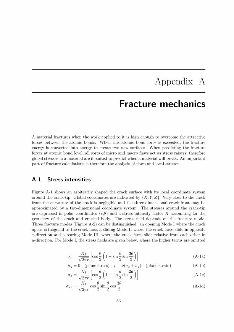
Appendix A
Fracture mechanics
A material fractures when the work applied to it is high enough to overcome the attractiveforces between the atomic bonds. When this atomic bond force is exceeded, the fractureenergy is converted into energy to create two new surfaces. When predicting the fractureforces at atomic bond level, all sorts of micro and macro flaws act as stress raisers, thereforeglobal stresses in a material are ill-suited to predict when a material will break. An importantpart of fracture calculations is therefore the analysis of flaws and local stresses.
A-1 Stress intensities
Figure A-1 shows an arbitrarily shaped the crack surface with its local coordinate systemaround the crack-tip. Global coordinates are indicated by {X,Y, Z}. Very close to the crackfront the curvature of the crack is negligible and the three-dimensional crack front may beapproximated by a two-dimensional coordinate system. The stresses around the crack-tipare expressed in polar coordinates {r,θ} and a stress intensity factor K accounting for thegeometry of the crack and cracked body. The stress field depends on the fracture mode.Three fracture modes (Figure A-2) can be distinguished: an opening Mode I where the crackopens orthogonal to the crack face, a sliding Mode II where the crack faces slide in oppositex-direction and a tearing Mode III, where the crack faces slide relative from each other iny-direction. For Mode I, the stress fields are given below, where the higher terms are omitted
σx = KI√2πr
[cos θ2
(1− sin θ2 sin 3θ
2
)](A-1a)
σy = 0 (plane stress) ; ν(σx + σz) (plane strain) (A-1b)
σz = KI√2πr
[cos θ2
(1 + sin θ2 sin 3θ
2
)](A-1c)
σxz = KI√2πr
cos θ2 sin θ2 cos 3θ2 (A-1d)
63
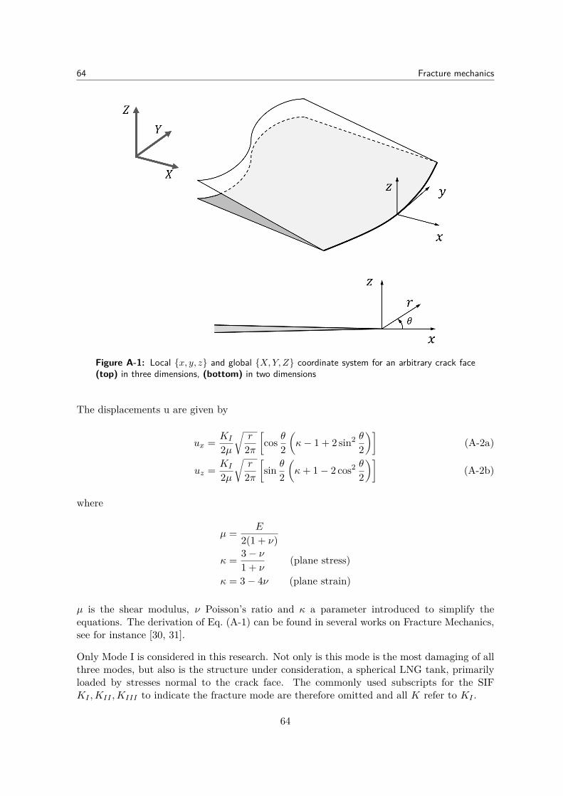
64 Fracture mechanics
Figure A-1: Local {x, y, z} and global {X,Y, Z} coordinate system for an arbitrary crack face(top) in three dimensions, (bottom) in two dimensions
The displacements u are given by
ux = KI
2µ
√r
2π
[cos θ2
(κ− 1 + 2 sin2 θ
2
)](A-2a)
uz = KI
2µ
√r
2π
[sin θ2
(κ+ 1− 2 cos2 θ
2
)](A-2b)
where
µ = E
2(1 + ν)
κ = 3− ν1 + ν
(plane stress)
κ = 3− 4ν (plane strain)
µ is the shear modulus, ν Poisson’s ratio and κ a parameter introduced to simplify theequations. The derivation of Eq. (A-1) can be found in several works on Fracture Mechanics,see for instance [30, 31].
Only Mode I is considered in this research. Not only is this mode is the most damaging of allthree modes, but also is the structure under consideration, a spherical LNG tank, primarilyloaded by stresses normal to the crack face. The commonly used subscripts for the SIFKI ,KII ,KIII to indicate the fracture mode are therefore omitted and all K refer to KI .
64
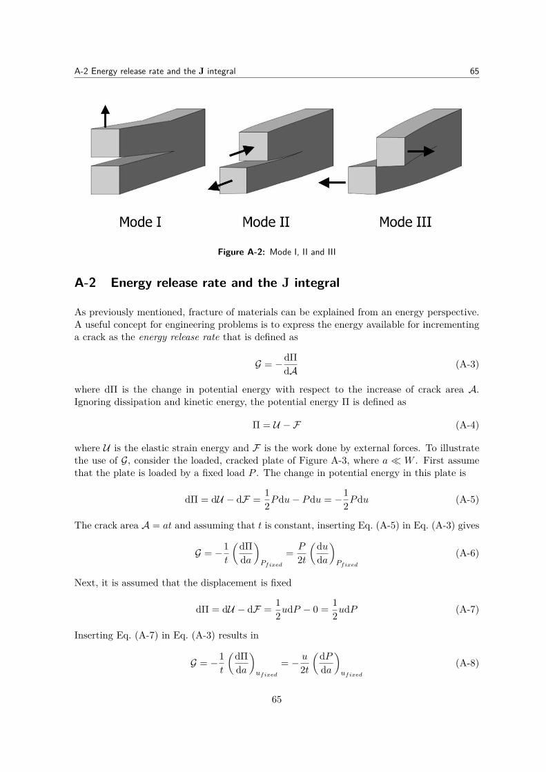
A-2 Energy release rate and the J integral 65
Figure A-2: Mode I, II and III
A-2 Energy release rate and the J integral
As previously mentioned, fracture of materials can be explained from an energy perspective.A useful concept for engineering problems is to express the energy available for incrementinga crack as the energy release rate that is defined as
G = −dΠdA (A-3)
where dΠ is the change in potential energy with respect to the increase of crack area A.Ignoring dissipation and kinetic energy, the potential energy Π is defined as
Π = U − F (A-4)
where U is the elastic strain energy and F is the work done by external forces. To illustratethe use of G, consider the loaded, cracked plate of Figure A-3, where a � W . First assumethat the plate is loaded by a fixed load P . The change in potential energy in this plate is
dΠ = dU − dF = 12Pdu− Pdu = −1
2Pdu (A-5)
The crack area A = at and assuming that t is constant, inserting Eq. (A-5) in Eq. (A-3) gives
G = −1t
(dΠda
)Pfixed
= P
2t
(duda
)Pfixed
(A-6)
Next, it is assumed that the displacement is fixed
dΠ = dU − dF = 12udP − 0 = 1
2udP (A-7)
Inserting Eq. (A-7) in Eq. (A-3) results in
G = −1t
(dΠda
)ufixed
= − u2t
(dPda
)ufixed
(A-8)
65
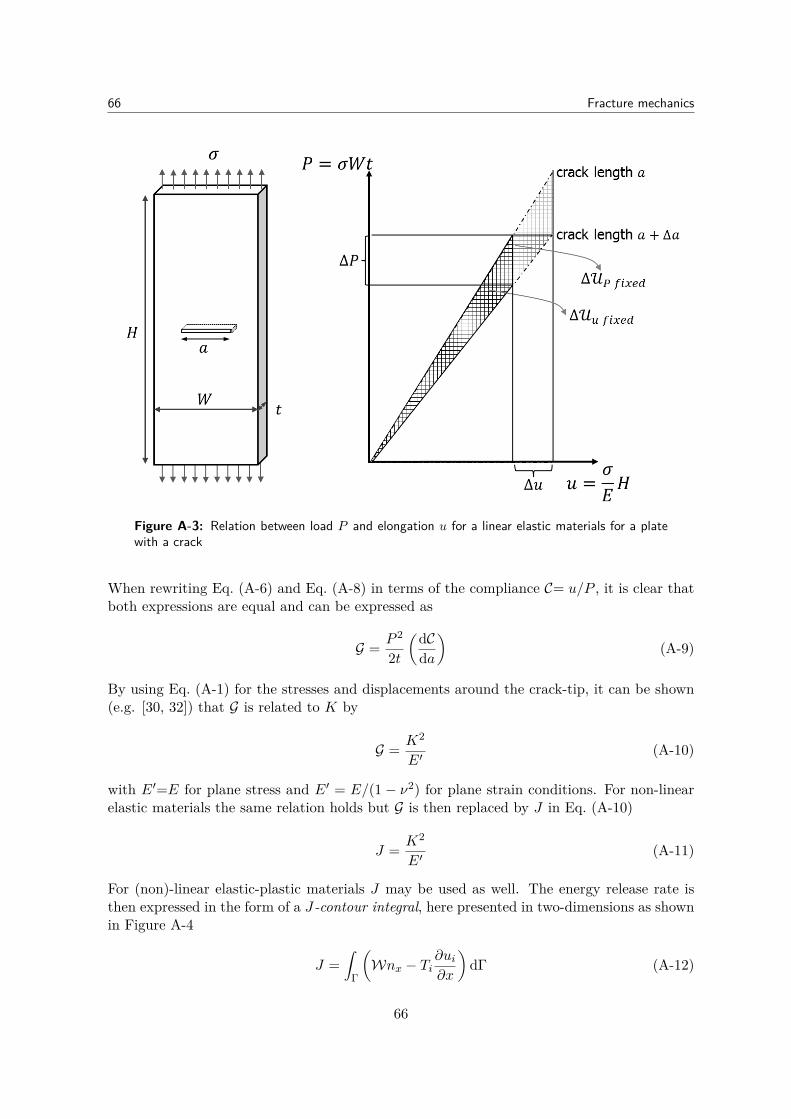
66 Fracture mechanics
Figure A-3: Relation between load P and elongation u for a linear elastic materials for a platewith a crack
When rewriting Eq. (A-6) and Eq. (A-8) in terms of the compliance C= u/P , it is clear thatboth expressions are equal and can be expressed as
G = P 2
2t
(dCda
)(A-9)
By using Eq. (A-1) for the stresses and displacements around the crack-tip, it can be shown(e.g. [30, 32]) that G is related to K by
G = K2
E′(A-10)
with E′=E for plane stress and E′ = E/(1 − ν2) for plane strain conditions. For non-linearelastic materials the same relation holds but G is then replaced by J in Eq. (A-10)
J = K2
E′(A-11)
For (non)-linear elastic-plastic materials J may be used as well. The energy release rate isthen expressed in the form of a J-contour integral, here presented in two-dimensions as shownin Figure A-4
J =∫
Γ
(Wnx − Ti
∂ui∂x
)dΓ (A-12)
66
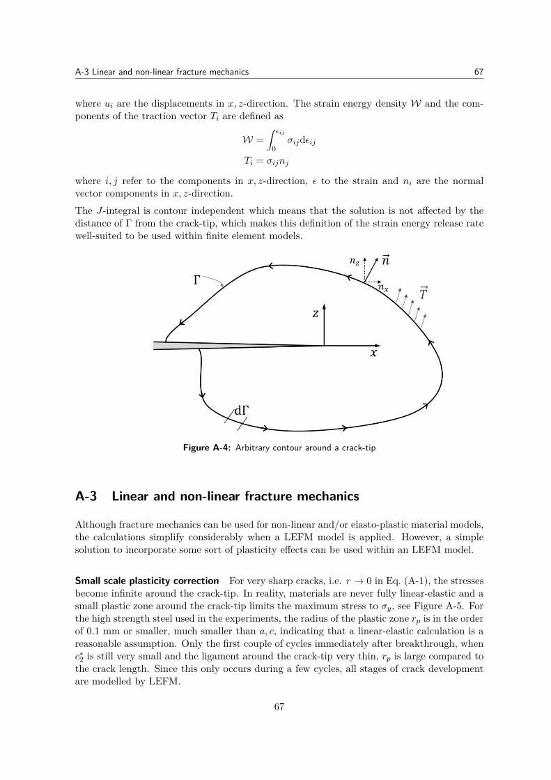
A-3 Linear and non-linear fracture mechanics 67
where ui are the displacements in x, z-direction. The strain energy density W and the com-ponents of the traction vector Ti are defined as
W =∫ εij
0σijdεij
Ti = σijnj
where i, j refer to the components in x, z-direction, ε to the strain and ni are the normalvector components in x, z-direction.The J-integral is contour independent which means that the solution is not affected by thedistance of Γ from the crack-tip, which makes this definition of the strain energy release ratewell-suited to be used within finite element models.
Figure A-4: Arbitrary contour around a crack-tip
A-3 Linear and non-linear fracture mechanics
Although fracture mechanics can be used for non-linear and/or elasto-plastic material models,the calculations simplify considerably when a LEFM model is applied. However, a simplesolution to incorporate some sort of plasticity effects can be used within an LEFM model.
Small scale plasticity correction For very sharp cracks, i.e. r → 0 in Eq. (A-1), the stressesbecome infinite around the crack-tip. In reality, materials are never fully linear-elastic and asmall plastic zone around the crack-tip limits the maximum stress to σy, see Figure A-5. Forthe high strength steel used in the experiments, the radius of the plastic zone rp is in the orderof 0.1 mm or smaller, much smaller than a, c, indicating that a linear-elastic calculation is areasonable assumption. Only the first couple of cycles immediately after breakthrough, whenc∗2 is still very small and the ligament around the crack-tip very thin, rp is large compared tothe crack length. Since this only occurs during a few cycles, all stages of crack developmentare modelled by LEFM.
67
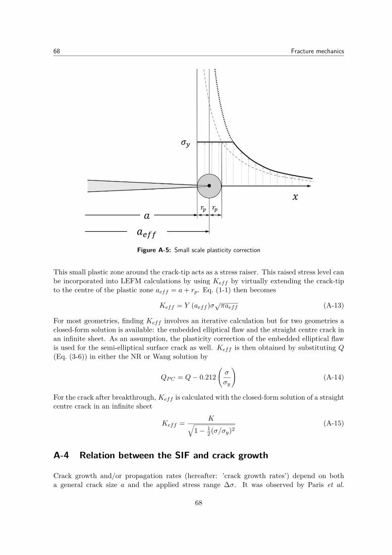
68 Fracture mechanics
Figure A-5: Small scale plasticity correction
This small plastic zone around the crack-tip acts as a stress raiser. This raised stress level canbe incorporated into LEFM calculations by using Keff by virtually extending the crack-tipto the centre of the plastic zone aeff = a+ rp. Eq. (1-1) then becomes
Keff = Y (aeff )σ√πaeff (A-13)
For most geometries, finding Keff involves an iterative calculation but for two geometries aclosed-form solution is available: the embedded elliptical flaw and the straight centre crack inan infinite sheet. As an assumption, the plasticity correction of the embedded elliptical flawis used for the semi-elliptical surface crack as well. Keff is then obtained by substituting Q(Eq. (3-6)) in either the NR or Wang solution by
QPC = Q− 0.212(σ
σy
)(A-14)
For the crack after breakthrough, Keff is calculated with the closed-form solution of a straightcentre crack in an infinite sheet
Keff = K√1− 1
2(σ/σy)2(A-15)
A-4 Relation between the SIF and crack growth
Crack growth and/or propagation rates (hereafter: ’crack growth rates’) depend on botha general crack size a and the applied stress range ∆σ. It was observed by Paris et al.
68
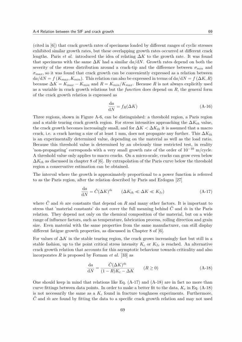
A-4 Relation between the SIF and crack growth 69
(cited in [6]) that crack growth rates of specimens loaded by different ranges of cyclic stressesexhibited similar growth rates, but these overlapping growth rates occurred at different cracklengths. Paris et al. introduced the idea of relating ∆K to the growth rate. It was foundthat specimens with the same ∆K had a similar da/dN . Growth rates depend on both theseverity of the stress distribution around a crack-tip and the difference between σmin andσmax, so it was found that crack growth can be conveniently expressed as a relation betweenda/dN = f (Kmax,Kmin). This relation can also be expressed in terms of da/dN = f (∆K,R)because ∆K = Kmax −Kmin and R = Kmin/Kmax. Because R is not always explicitly usedas a variable in crack growth relations but the function does depend on R, the general formof the crack growth relation is expressed as
dadN = fR(∆K) (A-16)
Three regions, shown in Figure A-6, can be distinguished: a threshold region, a Paris regionand a stable tearing crack growth region. For stress intensities approaching the ∆Kth value,the crack growth becomes increasingly small, and for ∆K < ∆Kth it is assumed that a macrocrack, i.e. a crack having a size of at least 1 mm, does not propagate any further. This ∆Kth
is an experimentally determined value, depending on the material as well as the load ratio.Because this threshold value is determined by an obviously time restricted test, in reality’non-propagating’ corresponds with a very small growth rate of the order of 10−10 m/cycle.A threshold value only applies to macro cracks. On a micro-scale, cracks can grow even below∆Kth as discussed in chapter 8 of [6]. By extrapolation of the Paris curve below the thresholdregion a conservative estimation can be obtained.
The interval where the growth is approximately proportional to a power function is referredto as the Paris region, after the relation described by Paris and Erdogan [27]
dadN = C(∆K)m (∆Kth � ∆K � KIc) (A-17)
where C and m are constants that depend on R and many other factors. It is important tostress that ’material constants’ do not cover the full meaning behind C and m in the Parisrelation. They depend not only on the chemical composition of the material, but on a widerange of influence factors, such as temperature, fabrication process, rolling direction and grainsize. Even material with the same properties from the same manufacturer, can still displaydifferent fatigue growth properties, as discussed in Chapter 8 of [6].
For values of ∆K in the stable tearing region, the crack grows increasingly fast but still in astable fashion, up to the point critical stress intensity Kc or KIc is reached. An alternativecrack growth relation that accounts for this asymptotic behaviour towards criticality and alsoincorporates R is proposed by Forman et al. [33] as
dadN = C(∆K)m
(1−R)Kc −∆K (R ≥ 0) (A-18)
One should keep in mind that relations like Eq. (A-17) and (A-18) are in fact no more thancurve fittings between data points. In order to make a better fit to the data, Kc in Eq. (A-18)is not necessarily the same as a Kc found in fracture toughness experiments. Furthermore,C and m are found by fitting the data to a specific crack growth relation and may not used
69
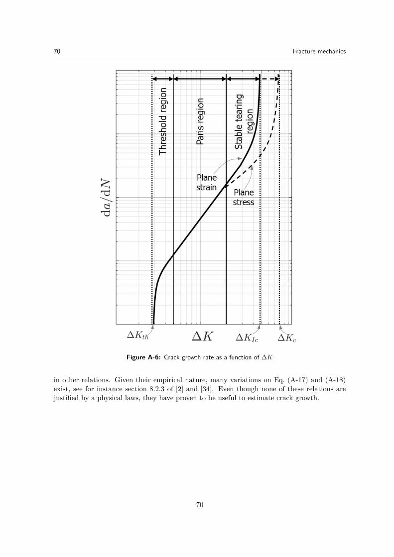
70 Fracture mechanics
Figure A-6: Crack growth rate as a function of ∆K
in other relations. Given their empirical nature, many variations on Eq. (A-17) and (A-18)exist, see for instance section 8.2.3 of [2] and [34]. Even though none of these relations arejustified by a physical laws, they have proven to be useful to estimate crack growth.
70
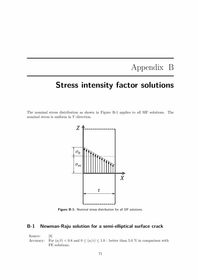
Appendix B
Stress intensity factor solutions
The nominal stress distribution as shown in Figure B-1 applies to all SIF solutions. Thenominal stress is uniform in Y -direction.
Figure B-1: Nominal stress distribution for all SIF solutions.
B-1 Newman-Raju solution for a semi-elliptical surface crack
Source: [8]Accuracy: For (a/t) < 0.8 and 0 ≤ (a/c) ≤ 1.0 : better than 5.0 % in comparison with
FE solutions.
71
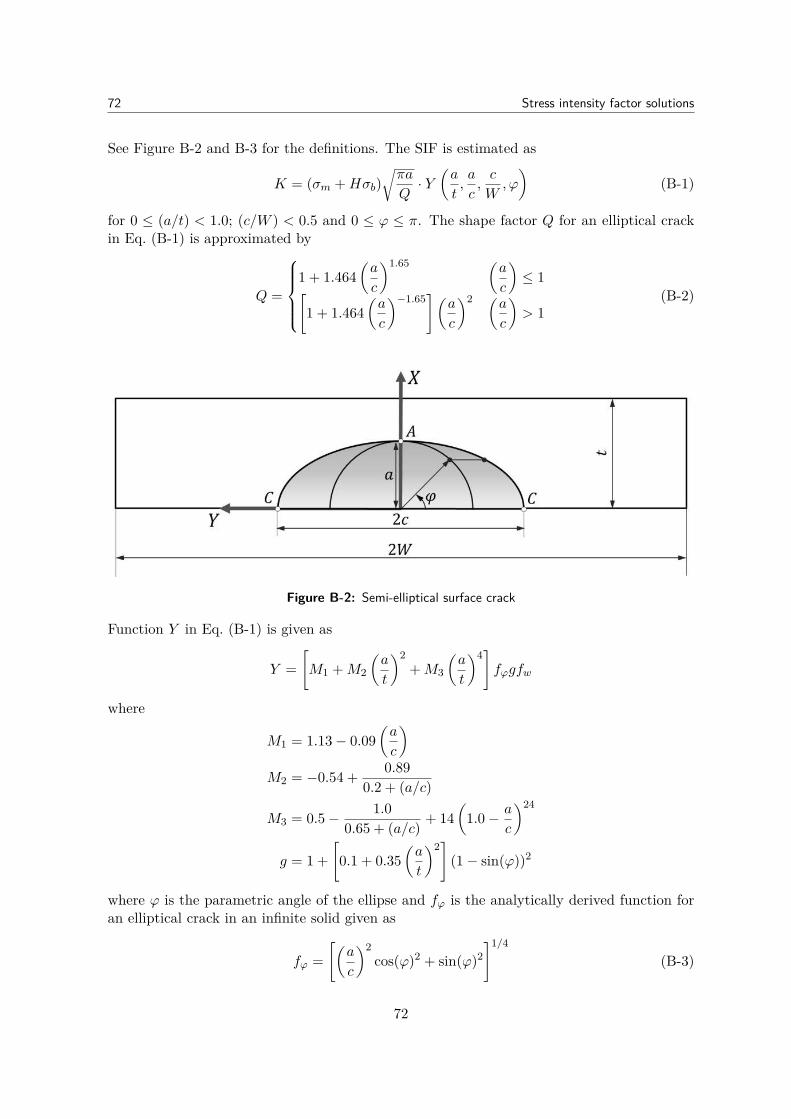
72 Stress intensity factor solutions
See Figure B-2 and B-3 for the definitions. The SIF is estimated as
K = (σm +Hσb)√πa
Q· Y
(a
t,a
c,c
W,ϕ
)(B-1)
for 0 ≤ (a/t) < 1.0; (c/W ) < 0.5 and 0 ≤ ϕ ≤ π. The shape factor Q for an elliptical crackin Eq. (B-1) is approximated by
Q =
1 + 1.464
(a
c
)1.65 (a
c
)≤ 1[
1 + 1.464(a
c
)−1.65](
a
c
)2 (a
c
)> 1
(B-2)
Figure B-2: Semi-elliptical surface crack
Function Y in Eq. (B-1) is given as
Y =[M1 +M2
(a
t
)2+M3
(a
t
)4]fϕgfw
where
M1 = 1.13− 0.09(a
c
)M2 = −0.54 + 0.89
0.2 + (a/c)
M3 = 0.5− 1.00.65 + (a/c) + 14
(1.0− a
c
)24
g = 1 +[0.1 + 0.35
(a
t
)2]
(1− sin(ϕ))2
where ϕ is the parametric angle of the ellipse and fϕ is the analytically derived function foran elliptical crack in an infinite solid given as
fϕ =[(
a
c
)2cos(ϕ)2 + sin(ϕ)2
]1/4
(B-3)
72
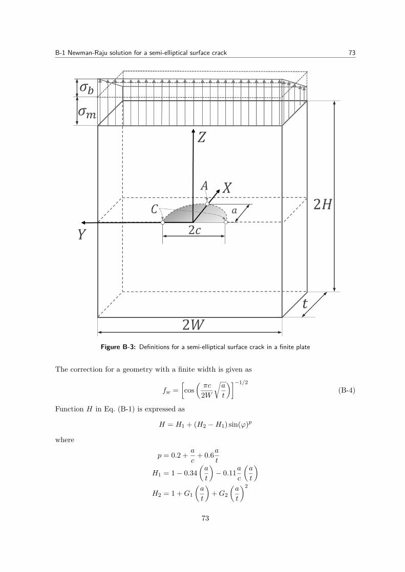
B-1 Newman-Raju solution for a semi-elliptical surface crack 73
Figure B-3: Definitions for a semi-elliptical surface crack in a finite plate
The correction for a geometry with a finite width is given as
fw =[cos
(πc
2W
√a
t
)]−1/2(B-4)
Function H in Eq. (B-1) is expressed as
H = H1 + (H2 −H1) sin(ϕ)p
where
p = 0.2 + a
c+ 0.6a
t
H1 = 1− 0.34(a
t
)− 0.11a
c
(a
t
)H2 = 1 +G1
(a
t
)+G2
(a
t
)2
73
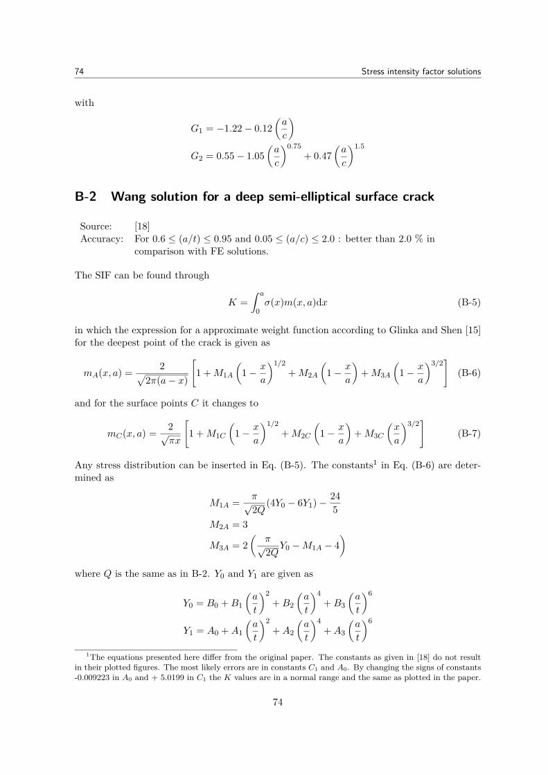
74 Stress intensity factor solutions
with
G1 = −1.22− 0.12(a
c
)G2 = 0.55− 1.05
(a
c
)0.75+ 0.47
(a
c
)1.5
B-2 Wang solution for a deep semi-elliptical surface crack
Source: [18]Accuracy: For 0.6 ≤ (a/t) ≤ 0.95 and 0.05 ≤ (a/c) ≤ 2.0 : better than 2.0 % in
comparison with FE solutions.
The SIF can be found through
K =∫ a
0σ(x)m(x, a)dx (B-5)
in which the expression for a approximate weight function according to Glinka and Shen [15]for the deepest point of the crack is given as
mA(x, a) = 2√2π(a− x)
[1 +M1A
(1− x
a
)1/2+M2A
(1− x
a
)+M3A
(1− x
a
)3/2]
(B-6)
and for the surface points C it changes to
mC(x, a) = 2√πx
[1 +M1C
(1− x
a
)1/2+M2C
(1− x
a
)+M3C
(x
a
)3/2]
(B-7)
Any stress distribution can be inserted in Eq. (B-5). The constants1 in Eq. (B-6) are deter-mined as
M1A = π√2Q
(4Y0 − 6Y1)− 245
M2A = 3
M3A = 2(
π√2Q
Y0 −M1A − 4)
where Q is the same as in B-2. Y0 and Y1 are given as
Y0 = B0 +B1
(a
t
)2+B2
(a
t
)4+B3
(a
t
)6
Y1 = A0 +A1
(a
t
)2+A2
(a
t
)4+A3
(a
t
)6
1The equations presented here differ from the original paper. The constants as given in [18] do not resultin their plotted figures. The most likely errors are in constants C1 and A0. By changing the signs of constants-0.009223 in A0 and + 5.0199 in C1 the K values are in a normal range and the same as plotted in the paper.
74
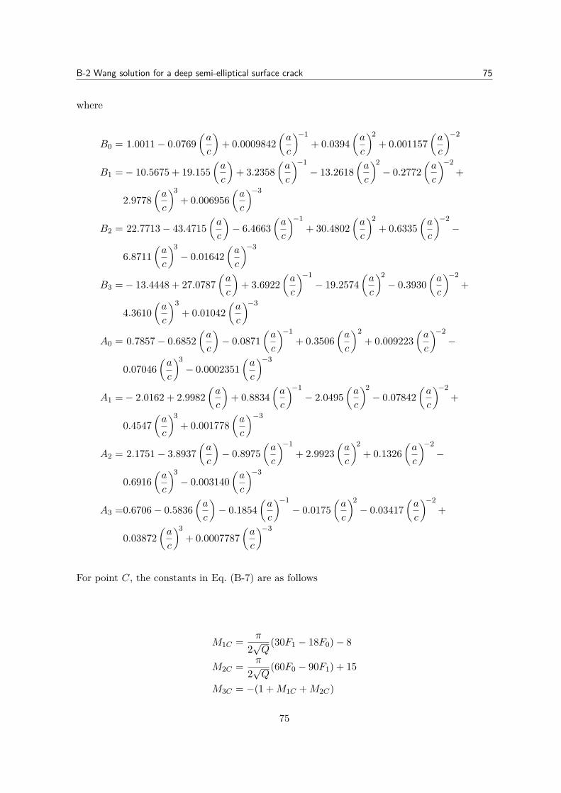
B-2 Wang solution for a deep semi-elliptical surface crack 75
where
B0 = 1.0011− 0.0769(a
c
)+ 0.0009842
(a
c
)−1+ 0.0394
(a
c
)2+ 0.001157
(a
c
)−2
B1 =− 10.5675 + 19.155(a
c
)+ 3.2358
(a
c
)−1− 13.2618
(a
c
)2− 0.2772
(a
c
)−2+
2.9778(a
c
)3+ 0.006956
(a
c
)−3
B2 = 22.7713− 43.4715(a
c
)− 6.4663
(a
c
)−1+ 30.4802
(a
c
)2+ 0.6335
(a
c
)−2−
6.8711(a
c
)3− 0.01642
(a
c
)−3
B3 =− 13.4448 + 27.0787(a
c
)+ 3.6922
(a
c
)−1− 19.2574
(a
c
)2− 0.3930
(a
c
)−2+
4.3610(a
c
)3+ 0.01042
(a
c
)−3
A0 = 0.7857− 0.6852(a
c
)− 0.0871
(a
c
)−1+ 0.3506
(a
c
)2+ 0.009223
(a
c
)−2−
0.07046(a
c
)3− 0.0002351
(a
c
)−3
A1 =− 2.0162 + 2.9982(a
c
)+ 0.8834
(a
c
)−1− 2.0495
(a
c
)2− 0.07842
(a
c
)−2+
0.4547(a
c
)3+ 0.001778
(a
c
)−3
A2 = 2.1751− 3.8937(a
c
)− 0.8975
(a
c
)−1+ 2.9923
(a
c
)2+ 0.1326
(a
c
)−2−
0.6916(a
c
)3− 0.003140
(a
c
)−3
A3 =0.6706− 0.5836(a
c
)− 0.1854
(a
c
)−1− 0.0175
(a
c
)2− 0.03417
(a
c
)−2+
0.03872(a
c
)3+ 0.0007787
(a
c
)−3
For point C, the constants in Eq. (B-7) are as follows
M1C = π
2√Q
(30F1 − 18F0)− 8
M2C = π
2√Q
(60F0 − 90F1) + 15
M3C = −(1 +M1C +M2C)
75
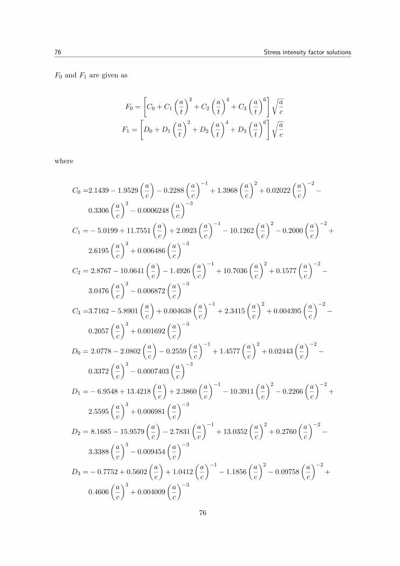
76 Stress intensity factor solutions
F0 and F1 are given as
F0 =[C0 + C1
(a
t
)2+ C2
(a
t
)4+ C3
(a
t
)6]√
a
c
F1 =[D0 +D1
(a
t
)2+D2
(a
t
)4+D3
(a
t
)6]√
a
c
where
C0 =2.1439− 1.9529(a
c
)− 0.2288
(a
c
)−1+ 1.3968
(a
c
)2+ 0.02022
(a
c
)−2−
0.3306(a
c
)3− 0.0006248
(a
c
)−3
C1 =− 5.0199 + 11.7551(a
c
)+ 2.0923
(a
c
)−1− 10.1262
(a
c
)2− 0.2000
(a
c
)−2+
2.6195(a
c
)3+ 0.006486
(a
c
)−3
C2 = 2.8767− 10.0641(a
c
)− 1.4926
(a
c
)−1+ 10.7036
(a
c
)2+ 0.1577
(a
c
)−2−
3.0476(a
c
)3− 0.006872
(a
c
)−3
C3 =3.7162− 5.8901(a
c
)+ 0.004638
(a
c
)−1+ 2.3415
(a
c
)2+ 0.004395
(a
c
)−2−
0.2057(a
c
)3+ 0.001692
(a
c
)−3
D0 = 2.0778− 2.0802(a
c
)− 0.2559
(a
c
)−1+ 1.4577
(a
c
)2+ 0.02443
(a
c
)−2−
0.3372(a
c
)3− 0.0007403
(a
c
)−3
D1 =− 6.9548 + 13.4218(a
c
)+ 2.3860
(a
c
)−1− 10.3911
(a
c
)2− 0.2266
(a
c
)−2+
2.5595(a
c
)3+ 0.006981
(a
c
)−3
D2 = 8.1685− 15.9579(a
c
)− 2.7831
(a
c
)−1+ 13.0352
(a
c
)2+ 0.2760
(a
c
)−2−
3.3388(a
c
)3− 0.009454
(a
c
)−3
D3 =− 0.7752 + 0.5602(a
c
)+ 1.0412
(a
c
)−1− 1.1856
(a
c
)2− 0.09758
(a
c
)−2+
0.4606(a
c
)3+ 0.004009
(a
c
)−3
76
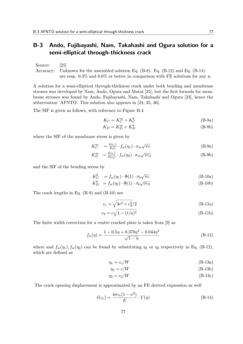
B-3 AFNTO solution for a semi-elliptical through-thickness crack 77
B-3 Ando, Fujibayashi, Nam, Takahashi and Ogura solution for asemi-elliptical through-thickness crack
Source: [25]Accuracy: Unknown for the assembled solution Eq. (B-8). Eq. (B-12) and Eq. (B-14)
are resp. 0.3% and 0.6% or better in comparison with FE solutions for any η.
A solution for a semi-elliptical through-thickness crack under both bending and membranestresses was developed by Nam, Ando, Ogura and Matui [25], but the first formula for mem-brane stresses was found by Ando, Fujibayashi, Nam, Takahashi and Ogura [23], hence theabbreviation ’AFNTO’. This solution also appears in [24, 35, 36].
The SIF is given as follows, with reference to Figure B-4
KC = KmC +Kb
C (B-8a)KD = Km
D +KbD (B-8b)
where the SIF of the membrane stress is given by
KmC = δ(ce)
δ(c) · fw(η1) · σm√πc (B-9a)
KmD = δ(ce)
δ(c2) · fw(η2) · σm√πc2 (B-9b)
and the SIF of the bending stress by
KbC = fw(η1) · Φ(1) · σb
√πc (B-10a)
KbD = fw(η2) · Φ(1) · σb
√πc2 (B-10b)
The crack lengths in Eq. (B-9) and (B-10) are
ce =√
3c2 + c22/2 (B-11a)
c2 = c√
1− (t/a)2 (B-11b)
The finite width correction for a centre cracked plate is taken from [9] as
fw(η) = 1− 0.5η + 0.370η2 − 0.044η3√
1− η (B-12)
where and fw(η1), fw(η2) can be found by substituting η1 or η2 respectively in Eq. (B-12),which are defined as
ηe = ce/W (B-13a)η1 = c/W (B-13b)η2 = c2/W (B-13c)
The crack opening displacement is approximated by an FE derived expression as well
δ(ce) = 4σce(1− ν2)E
· V (η) (B-14)
77
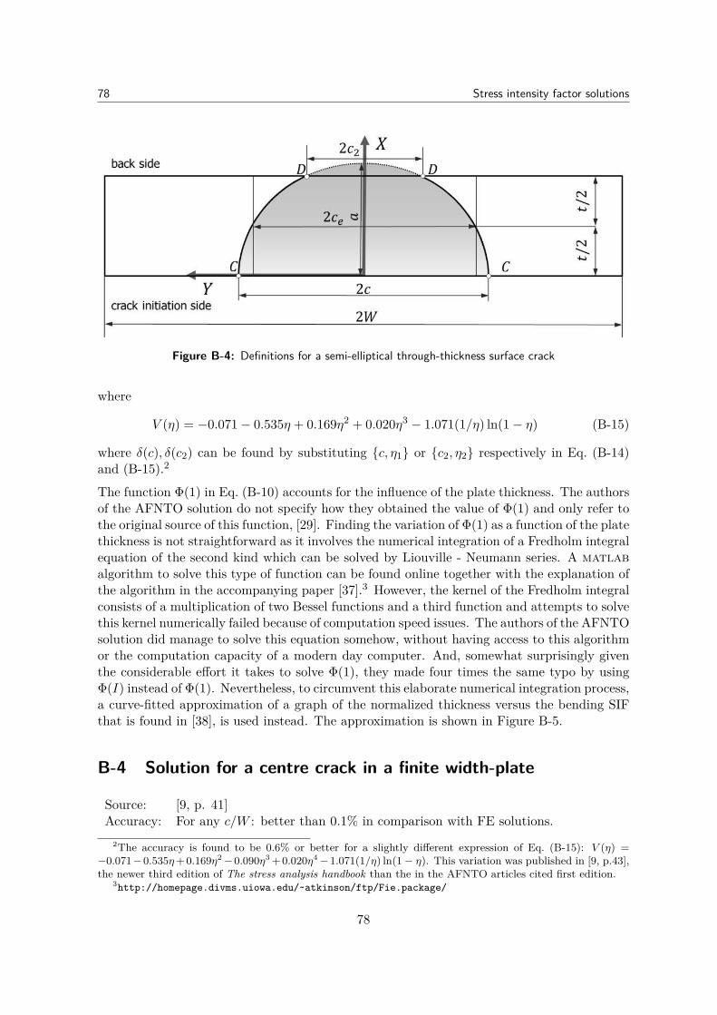
78 Stress intensity factor solutions
Figure B-4: Definitions for a semi-elliptical through-thickness surface crack
where
V (η) = −0.071− 0.535η + 0.169η2 + 0.020η3 − 1.071(1/η) ln(1− η) (B-15)
where δ(c), δ(c2) can be found by substituting {c, η1} or {c2, η2} respectively in Eq. (B-14)and (B-15).2
The function Φ(1) in Eq. (B-10) accounts for the influence of the plate thickness. The authorsof the AFNTO solution do not specify how they obtained the value of Φ(1) and only refer tothe original source of this function, [29]. Finding the variation of Φ(1) as a function of the platethickness is not straightforward as it involves the numerical integration of a Fredholm integralequation of the second kind which can be solved by Liouville - Neumann series. A matlabalgorithm to solve this type of function can be found online together with the explanation ofthe algorithm in the accompanying paper [37].3 However, the kernel of the Fredholm integralconsists of a multiplication of two Bessel functions and a third function and attempts to solvethis kernel numerically failed because of computation speed issues. The authors of the AFNTOsolution did manage to solve this equation somehow, without having access to this algorithmor the computation capacity of a modern day computer. And, somewhat surprisingly giventhe considerable effort it takes to solve Φ(1), they made four times the same typo by usingΦ(I) instead of Φ(1). Nevertheless, to circumvent this elaborate numerical integration process,a curve-fitted approximation of a graph of the normalized thickness versus the bending SIFthat is found in [38], is used instead. The approximation is shown in Figure B-5.
B-4 Solution for a centre crack in a finite width-plate
Source: [9, p. 41]Accuracy: For any c/W : better than 0.1% in comparison with FE solutions.
2The accuracy is found to be 0.6% or better for a slightly different expression of Eq. (B-15): V (η) =−0.071−0.535η+0.169η2−0.090η3 +0.020η4−1.071(1/η) ln(1− η). This variation was published in [9, p.43],the newer third edition of The stress analysis handbook than the in the AFNTO articles cited first edition.
3http://homepage.divms.uiowa.edu/~atkinson/ftp/Fie.package/
78
B-4 Solution for a centre crack in a finite width-plate 79
Figure B-5: Approximation of the analytical BCF Φ(1) for an infinite plate under bending
For a straight centre crack in a finite width-plate (Figure B-6) a solution for fw, is given by
Y = fw(η) =(1− 0.025η2 + 0.06η4
) [cos(π
2 η)]−1/2
(B-16)
where η = c/W .
Figure B-6: Definitions for a centre crack in a finite plate
79

80 Stress intensity factor solutions
80
Appendix C
Ansys script for the validation models
Parts of the following code are copied from the verification manual ’VM256’ of ansys [28].The example code is for a crack of size a = 1.
FINISH/CLEAR!!!!!!!!!!!!!!!!!!!!!!!!!!!!!!!!!!!!!!!!!!!!!!!!!!!!!!!!!!!!!!!!!!!!!! PLATE WITH COLLINEAR CRACKS, SOLID 186 ELEMENT, Structured mesh!!!!!!!!!!!!!!!!!!!!!!!!!!!!!!!!!!!!!!!!!!!!!!!!!!!!!!!!!!!!!!!!!!!!!/TITLE, STRESS INTENSITY - WIDE PLATE WITH COLLINEAR CRACKS, A = 1/PREP7SMRT,OFF/COM,*** PLATE WITH COLLINEAR CRACKS IN 3-D USING SOLID186/COM,!--------------------! INPUT VARIABLES!--------------------A = 1 ! HALF CRACK SIZEW = 20 ! HALF WIDTH OF THE PLATEH = W ! HALF HEIGHT OF THE PLATET = 0.5 ! PLATE THICKNESSPI = 3.141592654
EMOD = 30E6 ! YOUNGS MODULUSNU = 0.3 ! POISSONS RATIOET,1,PLANE183 ! PLATE ELEMENT 183 (will be deleted later)ET,2,186 ! SOLID ELEMENT 186MP,EX,1,EMODMP,NUXY,1,NU
!--------------------! MODEL GEOMETRY!--------------------CSYS,1 ! CYLINDRICAL COORDINATE SYSTEMK,1,0,0,0KGEN,6,1,,,,,,10,0 ! 6 x KP AT (0,0,0) NUMBERED 1,11,21,31,41,51K,6,1
81
82 Ansys script for the validation models
K,46,1,180KFILL,6,46,3,16,10 ! FILL LINE BETWEEN NODE 6 AND 46 WITH A NODE AT
! 1/4 OF THE DISTANCE FROM 16 (+10) TO 46CSYS,0 ! CARTESIAN COORDINATE SYSTEMKFILL,1,6,4,2,1,3CSYS,1 ! CYLINDRICAL COORDINATE SYSTEMKGEN,5,1,5,1,0,180/4,0,10,1,0CSYS,0 ! CARTESIAN COORDINATE SYSTEMK,27,0 ,H,0K,7 ,W-A,0,0KMODIF,15, 0.82*cos(PI/4),0.82*sin(PI/4),0KMODIF,35,-0.82*cos(PI/4),0.82*sin(PI/4),0K,16, A,tan(PI/4),0K,36,-A,tan(PI/4),0A,2 ,12, 1,1A,12,22,11,11A,22,32,21,21A,32,42,31,31A,2 , 3,13,12,A,12,13,23,22,A,22,23,33,32,A,32,33,43,42,A,3 ,13,14,4,A,13,23,24,14,A,23,33,34,24,A,33,43,44,34,A,4 ,14,15,5A,14,24,25,15A,24,34,35,25A,34,44,45,35A,5 ,15,16,6A,15,25,26,16A,25,35,36,26A,35,45,46,36ASEL,ALLAGLUE,ALLL,26,27L,6,7LSEL,S,LOC,Y,1ADRAG,ALL,,,,,,5ALLSEL,ALLLSEL,S,LOC,X,AADRAG,ALL,,,,,,6ASEL,ALLAGLUE,ALL
!-----------------------------------------! MESH AREAS!-----------------------------------------NUMMRG, KP,,,,LSEL,S,LOC,X,A+0.1,W-A-0.1LESIZE,ALL,,,11,4LSEL,S,LOC,Y,1.1 ,H-0.1LSEL,R,LOC,X,-A-0.1,W-A-0.1LESIZE,ALL,,,11,4ALLSEL,ALLLESIZE,53,,,11,1/4
82
83
LESIZE,12,,,2,1LESIZE,8,,,2,1LESIZE,41,,,2,1LESIZE,44,,,2,1LESIZE,46,,,2,1LESIZE,48,,,2,1LESIZE,56,,,2,1ASEL,ALLCM,REMOVEAREAS,AREAMSHKEY,1AMESH,ALL
!---------------------------------------------! EXTRUDE TO VOLUME AND MESH!---------------------------------------------TYPE,2ESIZE,,2 ! Specifies the default number of line divisionsVEXT,all,,,0,0,T ! Extrude areas to volumesALLSELESEL,S,ENAME,,183 ! Select elements of type plane 183ACLEAR,REMOVEAREAS ! Delete these elementsALLSEL
!-----------------------------! DEFINING CRACKTIP!-----------------------------NSEL,S,LOC,X,0NSEL,R,LOC,Y,0CM,CRACKTIP,NODE ! CRACK TIP NODE COMPONENT
!-------------------------------------------------! BOUNDARY CONDITIONS!-------------------------------------------------ALLSEL,ALLNSEL,S,LOC,X,-ADSYM,SYMM,X ! SYMMETRY BOUNDARY CONDITIONSNSEL,S,LOC,X,0,WNSEL,R,LOC,Y,0DSYM,SYMM,Y ! SYMMETRY BOUNDARY CONDITIONSNSEL,S,LOC,X,W-ADSYM,SYMM,X ! SYMMETRY BOUNDARY CONDITIONS
!-------------------------------------------------! LOADS!-------------------------------------------------ALLSEL,ALLD,ALL,UZ,ALLSEL,ALLNSEL,S,LOC,Y,HSF,ALL,PRES,-1/((A*PI)**0.5) ! SURFACE PRESSUREALLSEL,ALLFINI/SOLU
!-------------------------------------------------! SOLVE SYSTEM AND RETRIEVE K AND J-INTEGRAL DATA!-------------------------------------------------
83
84 Ansys script for the validation models
AUTOTS,ONNSUBST,10OUTRES,ALL,ALLCINT,NEW,1 ! CRACK IDCINT,TYPE,SIFS ! DEFINE CRACK TYPECINT,CTNC,CRACKTIP,NODE(-1,0,0) ! DEFINE CRACK TIP COMPONENTCINT,NCON,6 ! NO OF CONTOURSCINT,SYMM,ON ! SYMMETRY ONCINT,NORM,0,2 ! CRACK PLANE NORMALCINT,LISTCINT,NEW,2 ! CRACK IDCINT,TYPE,JINT ! DEFINE CRACK TYPECINT,CTNC,CRACKTIP,NODE(-1,0,0) ! DEFINE CRACK TIP COMPONENTCINT,NCON,6 ! NO OF CONTOURSCINT,SYMM,ON ! SYMMETRY ONCINT,NORM,0,2 ! CRACK PLANE NORMALCINT,LISTALLSEL,ALL/NERR,0,,,,SOLVEFINI/POST1/OUT,PRCINT,1,NODE(0,0,T/2),K1 ! PRINT K VALUESPRCINT,2,NODE(0,0,T/2),JINT ! PRINT J-INTEGRAL VALUES*GET,K1_3,CINT,1,CTIP,NODE(0,0,T/2),CONTOUR,3,DTYPE,K1*GET,K1_4,CINT,1,CTIP,NODE(0,0,T/2),CONTOUR,4,DTYPE,K1*GET,K1_5,CINT,1,CTIP,NODE(0,0,T/2),CONTOUR,5,DTYPE,K1*GET,J1,CINT,2,CTIP,NODE(0,0,T/2),CONTOUR,1,,*GET,J3,CINT,2,CTIP,NODE(0,0,T/2),CONTOUR,3,,*GET,J4,CINT,2,CTIP,NODE(0,0,T/2),CONTOUR,4,,*GET,J5,CINT,2,CTIP,NODE(0,0,T/2),CONTOUR,5,,K = (K1_3 + K1_4 + K1_5)/3*STATUS,K ! Lists the current parameters and abbreviationsJ = (ABS(J3)+ABS(J4)+ABS(J5))/3K_J = (J*(EMOD/(1-NU*NU)))**0.5K_J1 = (ABS(J1)*(EMOD/(1-NU*NU)))**0.5
!--------------------------! WRITE DATA TO TABLE!--------------------------*STATUS,J*DIM,LABEL,CHAR,3,*DIM,VALUE,,3,3LABEL(1,1) = ’K SIF’,LABEL(2,1) = ’K J-INT’LABEL(3,1) = ’K J1-INT’TARGET = (TAN(PI*A/(2*W))/(PI*A/(2*W)))**0.5*VFILL,VALUE(1,1),DATA,TARGET ! STRESS INTENSITY FROM REFERENCE*VFILL,VALUE(1,2),DATA,K*VFILL,VALUE(1,3),DATA,ABS(K/TARGET)*VFILL,VALUE(2,1),DATA,TARGET*VFILL,VALUE(2,2),DATA,K_J*VFILL,VALUE(2,3),DATA,ABS(K_J/TARGET)*VFILL,VALUE(3,1),DATA,TARGET*VFILL,VALUE(3,2),DATA,K_J1*VFILL,VALUE(3,3),DATA,ABS(K_J1/TARGET)
84
85
SAVE,TABLE_1!PLCINT,front,2,,,JINT ! Plot J-contours
FINISH/CLEAR, NOSTART ! CLEAR DATABASE FOR 2nD SOLUTION/OUT,
!!!!!!!!!!!!!!!!!!!!!!!!!!!!!!!!!!!!!!!!!!!!!!!!!!!!!!!!!!!!!!!!!!!!! PLATE WITH COLLINEAR CRACKS, SOLID 185 ELEMENT, Structured mesh!!!!!!!!!!!!!!!!!!!!!!!!!!!!!!!!!!!!!!!!!!!!!!!!!!!!!!!!!!!!!!!!!!!!/CLEAR/TITLE, STRESS INTENSITY - WIDE PLATE WITH COLLINEAR CRACKS A = 1/PREP7SMRT,OFF/COM, *** PLATE WITH COLLINEAR CRACKS IN 3-DIMENSIONS USING SOLID185/COM,!--------------------! INPUT VARIABLES!--------------------A = 1 ! HALF CRACK SIZEW = 20 ! HALF WIDTH OF THE PLATEH = W ! HALF HEIGHT OF THE PLATET = 0.5 ! PLATE THICKNESSPI = 3.141592654
EMOD = 30E6 ! YOUNGS MODULUSNU = 0.3 ! POISSONS RATIOET,1,SOLID185 ! SOLID 185 ELEMENTET,2,SOLID185 ! ELEMENTS AROUND THE CRACK-TIPMP,EX,1,EMODMP,NUXY,1,NU
!--------------------! MODEL GEOMETRY!--------------------CSYS,1 ! CYLINDRICAL COORDINATE SYSTEMN,1,0,0,0NGEN,9,20,1 ! Generates additional nodes from a pattern of nodes,
! 9 x node at 0,0,0 with numbers 1, 21, 41 , 61 ... ,161N,11,0.8N,171,0.8,180FILL,11,171,7,31,20 ! Fill line between node 11 and 171 with a node
! at 1/7 of the distance, from 31 (+20) to 151CSYS,0 ! CARTESIAN COORDINATE SYSTEMFILL,1,11,9,2,1,9,20,4 ! 4 is last step/first step, unequal spacingN,19,W-A,0,0N,79,W-A,H,0FILL,19,79,2,39,20N,159,-A,H,0FILL,79,159,3,99,20N,172,-A,0FILL,159,172,9,181,-1,,,.034 ! Increment is -1. decreasing divisionsFILL,11,19,7,,,7,20,15NGEN,2,200,1,181,,,,TE,2,22,1,1,202,222,201,201EGEN,8,20,-1E,2,3,23,22,202,203,223,222
85
86 Ansys script for the validation models
EGEN,8,20,-1EGEN,9,1,-8EGEN,9,1,73,78E,171,151,173,172,371,351,373,372 ! 111E,151,131,174,173,351,331,374,373 ! 112E,131,132,175,174,331,332,375,374 ! 113EGEN,7,1,-1E,138,139,159,181,338,339,359,381TYPE,2EMODIF,1 ! MODIFY ELEMENTS 1 TO 8 FROM TYPE 1 TO TYPE 2*REPEAT,8,1NUMMRG,NODE ! MERGE COINCIDENT NODESALLSEL,ALL
!-----------------------------! DEFINING CRACKTIP!-----------------------------NSEL,S,LOC,X,0NSEL,R,LOC,Y,0NLIST ! node 1 and 201CM,CRACKTIP,NODE ! CRACK TIP NODE COMPONENT, name is cracktip
!-------------------------------------------------! BOUNDARY CONDITIONS!-------------------------------------------------ALLSEL,ALLNSEL,S,LOC,X,-ADSYM,SYMM,X ! SYMMETRY BOUNDARY CONDITIONSNSEL,S,LOC,X,0,WNSEL,R,LOC,Y,0DSYM,SYMM,Y ! SYMMETRY BOUNDARY CONDITIONSNSEL,S,LOC,X,W-ADSYM,SYMM,X ! SYMMETRY BOUNDARY CONDITIONSALLSEL,ALLD,ALL,UZ,0
!-------------------------------------------------! LOADS!-------------------------------------------------ALLSEL,ALLNSEL,S,LOC,Y,HSF,ALL,PRES,-1/((A*PI)**0.5) ! SURFACE PRESSUREALLSEL,ALLFINI
!-------------------------------------------------! SOLVE SYSTEM AND RETRIEVE K AND J-INTEGRAL DATA!-------------------------------------------------/SOLUAUTOTS,ON ! Is default, automatic time steppingNSUBST,10 ! Specifies the number of substepsOUTRES,ALL,ALLCINT,NEW,1 ! CRACK IDCINT,TYPE,SIFS ! DEFINE CRACK TYPECINT,CTNC,CRACKTIP,NODE(-1,0,0) ! DEFINE CRACK-TIP COMPONENT
! any node on the open side of the crackCINT,NCON,6 ! NO OF CONTOURS
86
87
CINT,SYMM,ON ! SYMMETRY ONCINT,NORM,0,2 ! CRACK PLANE NORMALCINT,LISTCINT,NEW,2 ! CRACK IDCINT,TYPE,JINT ! DEFINE CRACK TYPECINT,CTNC,CRACKTIP,NODE(-1,0,0) ! DEFINE CRACK-TIP COMPONENTCINT,NCON,6 ! NO OF CONTOURSCINT,SYMM,ON ! SYMMETRY ONCINT,NORM,0,2 ! CRACK PLANE NORMALCINT,LISTALLSEL,ALLSAVE/NERR,0,,,,! supresses warningsSOLVEFINI
/POST1/OUT,PRCINT,1,NODE(0,0,T/2),K1 ! PRINT K VALUESPRCINT,2,NODE(0,0,T/2),JINT ! PRINT J-INTEGRAL*GET,K1_3,CINT,1,CTIP,NODE(0,0,T/2),CONTOUR,3,DTYPE,K1*GET,K1_4,CINT,1,CTIP,NODE(0,0,T/2),CONTOUR,4,DTYPE,K1*GET,K1_5,CINT,1,CTIP,NODE(0,0,T/2),CONTOUR,5,DTYPE,K1*GET,J1,CINT,2,CTIP,NODE(0,0,T/2),CONTOUR,1,,*GET,J3,CINT,2,CTIP,NODE(0,0,T/2),CONTOUR,3,,*GET,J4,CINT,2,CTIP,NODE(0,0,T/2),CONTOUR,4,,*GET,J5,CINT,2,CTIP,NODE(0,0,T/2),CONTOUR,5,,K = (K1_3 + K1_4 + K1_5)/3*STATUS,K ! Lists the current parameters and abbreviationsJ = (ABS(J3)+ABS(J4)+ABS(J5))/3K_J = (J*(EMOD/(1-NU*NU)))**0.5K_J1 = (ABS(J1)*(EMOD/(1-NU*NU)))**0.5
!--------------------------! WRITE DATA TO TABLE!--------------------------*STATUS,J*DIM,LABEL,CHAR,3,*DIM,VALUE,,3,3LABEL(1,1) = ’K SIF’,LABEL(2,1) = ’K J-INT’LABEL(3,1) = ’K J1-INT’TARGET = (TAN(PI*A/(2*W))/(PI*A/(2*W)))**0.5*VFILL,VALUE(1,1),DATA,TARGET ! STRESS INTENSITY FROM REFERENCE*VFILL,VALUE(1,2),DATA,K*VFILL,VALUE(1,3),DATA,ABS(K/TARGET)*VFILL,VALUE(2,1),DATA,TARGET*VFILL,VALUE(2,2),DATA,K_J*VFILL,VALUE(2,3),DATA,ABS(K_J/TARGET)*VFILL,VALUE(3,1),DATA,TARGET*VFILL,VALUE(3,2),DATA,K_J1*VFILL,VALUE(3,3),DATA,ABS(K_J1/TARGET)SAVE,TABLE_2
FINISH/CLEAR, NOSTART ! CLEAR DATABASE FOR 3RD SOLUTION/OUT,
87
88 Ansys script for the validation models
!!!!!!!!!!!!!!!!!!!!!!!!!!!!!!!!!!!!!!!!!!!!!!!!!!!!!!!!!!!!!!!!!!!!! PLATE WITH COLLINEAR CRACKS, SOLID 186 ELEMENT, irregular mesh!!!!!!!!!!!!!!!!!!!!!!!!!!!!!!!!!!!!!!!!!!!!!!!!!!!!!!!!!!!!!!!!!!!!/PREP7SMRT,OFF/TITLE, STRESS INTENSITY - PLATE WITH COLLINEAR CRACKS A = 1/COM,*** PLATE WITH COLLINEAR CRACKS IN 3-D USING SOLID186
!--------------------! INPUT VARIABLES!--------------------A = 1 ! HALF CRACK SIZEW = 20 ! HALF WIDTH OF THE PLATEH = W ! HALF HEIGHT OF THE PLATEPI = 3.141592654T = 0.5 ! PLATE THICKNESSEMOD = 30E6 ! YOUNGS MODULUSNU = 0.3 ! POISSONS RATIOET,1,PLANE183 ! PLATE ELEMENT 183, WILL BE REMOVED LATERET,2,186 ! SOLID ELEMENT 186MP,EX,1,EMODMP,NUXY,1,NU
!--------------------! MODEL GEOMETRY!--------------------K,1,0 ,0,0 ! DEFINE KEYPOINTS AND LINE SEGMENTSK,2,W-A,0,0K,3,W-A,H,0K,4,-A ,H,0K,5,-A ,0,0L,1,2L,2,3LESIZE,2,,,4L,3,4LESIZE,3,,,4L,4,5,LESIZE,4,,,6,.2L,5,1
!-----------------------------------------! MESH AREAS!-----------------------------------------ESIZE,,5KSCON,1,.125,0,8 ! DEFINE CRACK-TIP with singular elementsAL,1,2,3,4,5AMESH,1TYPE,2ESIZE,,2 ! Specifies the default number of line divisionsVEXT,1,,,0,0,TALLSELESEL,S,ENAME,,183 ! Select elements of type plane 183ACLEAR,1 ! Delete these elements
!-----------------------------! DEFINING CRACKTIP!-----------------------------
88
89
ALLSELNSEL,S,LOC,X,0NSEL,R,LOC,Y,0NLISTCM,CRACKTIP,NODE ! CRACK-TIP NODE COMPONENT
!-------------------------------------------------! BOUNDARY CONDITIONS!-------------------------------------------------ALLSEL,ALLNSEL,S,LOC,X,-ADSYM,SYMM,X ! SYMMETRY BOUNDARY CONDITIONSNSEL,S,LOC,X,0,WNSEL,R,LOC,Y,0DSYM,SYMM,Y ! SYMMETRY BOUNDARY CONDITIONSNSEL,S,LOC,X,W-ADSYM,SYMM,X ! SYMMETRY BOUNDARY CONDITIONSALLSEL,ALLD,ALL,UZ,0
!-------------------------------------------------! LOADS!-------------------------------------------------ALLSEL,ALLNSEL,S,LOC,Y,HSF,ALL,PRES,-1/((A*PI)**0.5) ! SURFACE PRESSUREALLSEL,ALLFINI
!-------------------------------------------------! SOLVE SYSTEM AND RETRIEVE K AND J-INTEGRAL DATA!-------------------------------------------------/SOLUAUTOTS,ONNSUBST,10OUTRES,ALL,ALLCINT,NEW,1 ! CRACK IDCINT,TYPE,SIFS ! DEFINE CRACK TYPECINT,CTNC,CRACKTIP,NODE(-1,0,0) ! DEFINE CRACK TIP COMPONENTCINT,NCON,6 ! NO OF CONTOURSCINT,SYMM,ON ! SYMMETRY ONCINT,NORM,0,2 ! CRACK PLANE NORMALCINT,LISTCINT,NEW,2 ! CRACK IDCINT,TYPE,JINT ! DEFINE CRACK TYPECINT,CTNC,CRACKTIP,NODE(-1,0,0) ! DEFINE CRACK TIP COMPONENTCINT,NCON,6 ! NO OF CONTOURSCINT,SYMM,ON ! SYMMETRY ONCINT,NORM,0,2 ! CRACK PLANE NORMALCINT,LISTALLSEL,ALLSAVE/NERR,0,,,,SOLVEFINI/POST1PLNSOL, S,INT
89
90 Ansys script for the validation models
/OUT,PRCINT,1,NODE(0,0,T/2),K1 ! PRINT K VALUES ID = 1PRCINT,2,NODE(0,0,T/2),JINT ! PRINT J-INTEGRAL VALUES ID = 1PRCINT,1,NODE(0,0,T/2),K1 ! PRINT K VALUES ID = 2PRCINT,2,NODE(0,0,T/2),JINT ! PRINT J-INTEGRAL VALUES ID = 2*GET,K1_3,CINT,1,CTIP,NODE(0,0,T/2),CONTOUR,3,DTYPE,K1*GET,K1_4,CINT,1,CTIP,NODE(0,0,T/2),CONTOUR,4,DTYPE,K1*GET,K1_5,CINT,1,CTIP,NODE(0,0,T/2),CONTOUR,5,DTYPE,K1*GET,J1,CINT,2,CTIP,NODE(0,0,T/2),CONTOUR,1,,*GET,J3,CINT,2,CTIP,NODE(0,0,T/2),CONTOUR,3,,*GET,J4,CINT,2,CTIP,NODE(0,0,T/2),CONTOUR,4,,*GET,J5,CINT,2,CTIP,NODE(0,0,T/2),CONTOUR,5,,K = (K1_3 + K1_4 + K1_5)/3*STATUS,K ! Lists the current parameters and abbreviationsJ = (ABS(J3)+ABS(J4)+ABS(J5))/3K_J = (J*(EMOD/(1-NU*NU)))**0.5K_J1 = (ABS(J1)*(EMOD/(1-NU*NU)))**0.5
!--------------------------! WRITE DATA TO TABLE!--------------------------*STATUS,J*DIM,LABEL,CHAR,3,*DIM,VALUE,,3,3LABEL(1,1) = ’K SIF’,LABEL(2,1) = ’K J-INT’LABEL(3,1) = ’K J1-INT’TARGET = (TAN(PI*A/(2*W))/(PI*A/(2*W)))**0.5*VFILL,VALUE(1,1),DATA,TARGET ! STRESS INTENSITY FROM REFERENCE*VFILL,VALUE(1,2),DATA,K*VFILL,VALUE(1,3),DATA,ABS(K/TARGET)*VFILL,VALUE(2,1),DATA,TARGET*VFILL,VALUE(2,2),DATA,K_J*VFILL,VALUE(2,3),DATA,ABS(K_J/TARGET)*VFILL,VALUE(3,1),DATA,TARGET*VFILL,VALUE(3,2),DATA,K_J1*VFILL,VALUE(3,3),DATA,ABS(K_J1/TARGET)SAVE,TABLE_3FINISH
90
91
!--------------------------! WRITE DATA TO .TXT FILE!--------------------------RESUME,TABLE_1/COM/OUT,Results_collinearcrack,txt/COM,---RESULTS COMPARISON PLATE WITH COLLINEAR CRACKS A = 1 ---/COM,/COM, | TARGET | Mechanical APDL | RATIO/COM,/COM, **********************************************************/COM, USING SOLID 186 ELEMENT - Structured mesh/COM, **********************************************************/COM,*VWRITE,LABEL(1,1),VALUE(1,1),VALUE(1,2),VALUE(1,3)(1X,A8,’ ’,F10.5,’ ’,F14.5,’ ’,F15.4)/NOPRRESUME,TABLE_2/GOPR/COM,/COM, **********************************************************/COM, USING SOLID 185 ELEMENT - Structured mesh/COM, **********************************************************/COM,*VWRITE,LABEL(1,1),VALUE(1,1),VALUE(1,2),VALUE(1,3)(1X,A8,’ ’,F10.5,’ ’,F14.5,’ ’,F15.4)/NOPRRESUME,TABLE_3/GOPR/COM,/COM, **********************************************************/COM, USING SOLID 186 ELEMENT - Irregular mesh/COM, **********************************************************/COM,*VWRITE,LABEL(1,1),VALUE(1,1),VALUE(1,2),VALUE(1,3)(1X,A8,’ ’,F10.5,’ ’,F14.5,’ ’,F15.4)/NOPR/COM,/COM,-----------------------------------------------------------/OUTFINISH*LIST,Results_collinearcrack,txt
91

92 Ansys script for the validation models
92
Appendix D
The finite element method
For many engineering problems where no analytical solution is available, one has to resortto numerical methods such as the boundary element method or the finite element method toapproximate a field quantity, (e.g. stresses, displacements, strain etc.) in a body or region.Both can be used for fracture mechanics but he boundary element method is more suitablefor problems with a small surface/volume ratio. For the geometries in this thesis, this is notreally the case, hence using the FEM is considered to be more appropriate.The FEM essentially comes down to the subdivision of a body into a large number of smallerelements. It is assumed that the actual field quantity within these elements can be approx-imated by expressions that are not very complex such as a constant, linear or quadraticexpression. Elements are connected to each other at their points through nodes and thisassembly of nodes and elements forms the mesh. If a large gradient of a field quantity is ex-pected, the mesh needs to be more refined in these areas so that the simple expressions withinan element can still approximate the field quantity reasonably well. Alternatively, a specialelement type can be used. For a cracked body, stress, strain and displacement gradients arevery high around the crack-tip and therefore special crack-tip elements can be considered forfracture problems.Three methods to find the SIF will also be briefly discussed here: the virtual crack extensionmethod, the J-integral method and crack-tip field methods.
Element types The analysis of a curved crack front is a 3-D problem which needs to bemodelled with solid elements. Of these, a variety of shapes are available, such as tetrahedra,pyramids, prisms and hexahedra. The first two shapes are not recommended to be used inansys. The predominantly rectangular shape of the model in this thesis is best modelledby brick elements, prismatic elements are only used to connect the fine brick elements withthe coarser ones. A lower order brick element is the 8-node solid, which is the 3-D versionof the 4-node plane element shown bottom left in Figure D-1. Correspondingly, the 20-nodehigher order solid is the 3-D equivalent of the 8-node plane element shown at the top-left ofFigure D-1. Varieties such as a 27-node element with an extra node mid-plane and mid-bodyexist but are not widely applied in FE analysis.
93
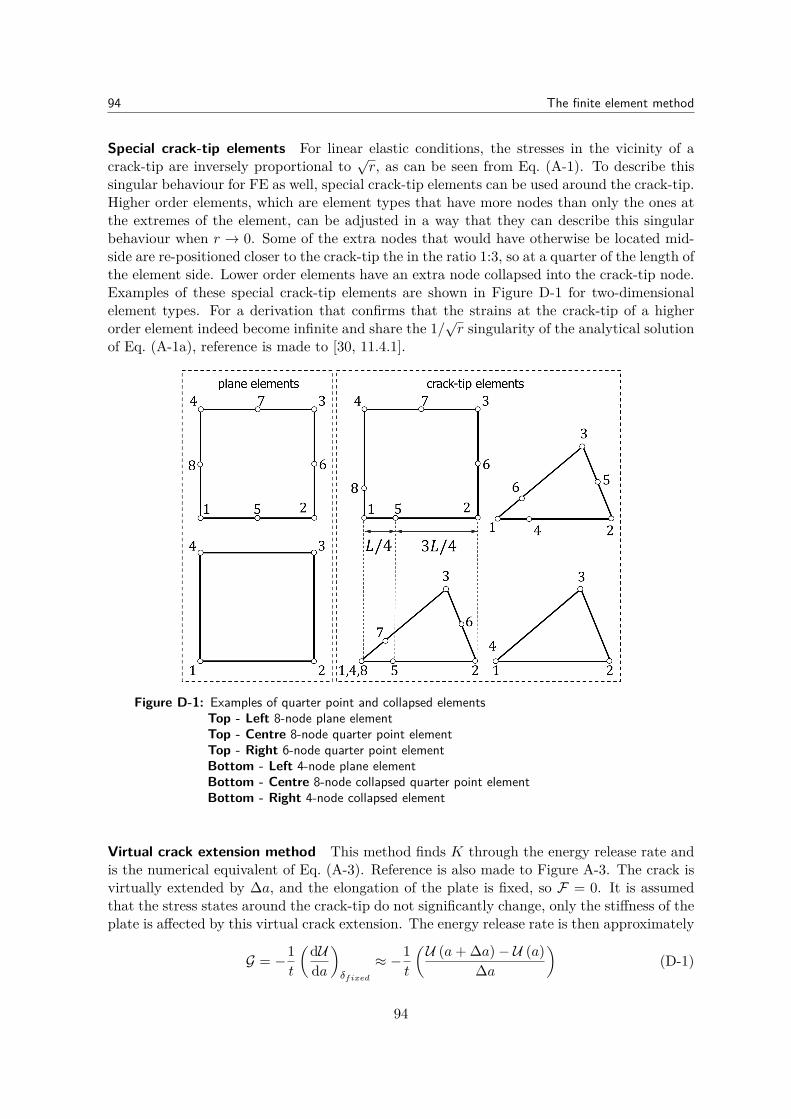
94 The finite element method
Special crack-tip elements For linear elastic conditions, the stresses in the vicinity of acrack-tip are inversely proportional to
√r, as can be seen from Eq. (A-1). To describe this
singular behaviour for FE as well, special crack-tip elements can be used around the crack-tip.Higher order elements, which are element types that have more nodes than only the ones atthe extremes of the element, can be adjusted in a way that they can describe this singularbehaviour when r → 0. Some of the extra nodes that would have otherwise be located mid-side are re-positioned closer to the crack-tip the in the ratio 1:3, so at a quarter of the length ofthe element side. Lower order elements have an extra node collapsed into the crack-tip node.Examples of these special crack-tip elements are shown in Figure D-1 for two-dimensionalelement types. For a derivation that confirms that the strains at the crack-tip of a higherorder element indeed become infinite and share the 1/
√r singularity of the analytical solution
of Eq. (A-1a), reference is made to [30, 11.4.1].
Figure D-1: Examples of quarter point and collapsed elementsTop - Left 8-node plane elementTop - Centre 8-node quarter point elementTop - Right 6-node quarter point elementBottom - Left 4-node plane elementBottom - Centre 8-node collapsed quarter point elementBottom - Right 4-node collapsed element
Virtual crack extension method This method finds K through the energy release rate andis the numerical equivalent of Eq. (A-3). Reference is also made to Figure A-3. The crack isvirtually extended by ∆a, and the elongation of the plate is fixed, so F = 0. It is assumedthat the stress states around the crack-tip do not significantly change, only the stiffness of theplate is affected by this virtual crack extension. The energy release rate is then approximately
G = −1t
(dUda
)δfixed
≈ −1t
(U (a+ ∆a)− U (a)∆a
)(D-1)
94
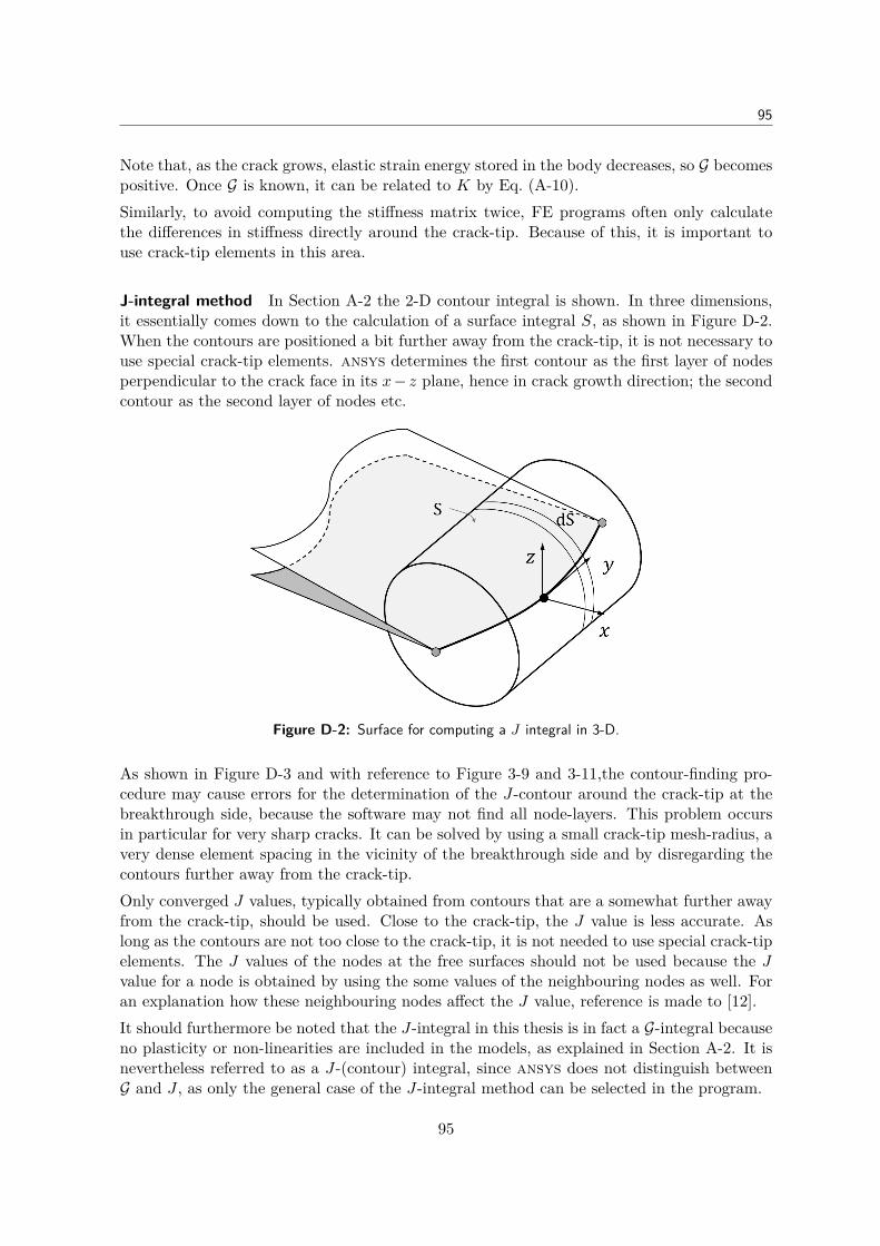
95
Note that, as the crack grows, elastic strain energy stored in the body decreases, so G becomespositive. Once G is known, it can be related to K by Eq. (A-10).Similarly, to avoid computing the stiffness matrix twice, FE programs often only calculatethe differences in stiffness directly around the crack-tip. Because of this, it is important touse crack-tip elements in this area.
J-integral method In Section A-2 the 2-D contour integral is shown. In three dimensions,it essentially comes down to the calculation of a surface integral S, as shown in Figure D-2.When the contours are positioned a bit further away from the crack-tip, it is not necessary touse special crack-tip elements. ansys determines the first contour as the first layer of nodesperpendicular to the crack face in its x− z plane, hence in crack growth direction; the secondcontour as the second layer of nodes etc.
Figure D-2: Surface for computing a J integral in 3-D.
As shown in Figure D-3 and with reference to Figure 3-9 and 3-11,the contour-finding pro-cedure may cause errors for the determination of the J-contour around the crack-tip at thebreakthrough side, because the software may not find all node-layers. This problem occursin particular for very sharp cracks. It can be solved by using a small crack-tip mesh-radius, avery dense element spacing in the vicinity of the breakthrough side and by disregarding thecontours further away from the crack-tip.Only converged J values, typically obtained from contours that are a somewhat further awayfrom the crack-tip, should be used. Close to the crack-tip, the J value is less accurate. Aslong as the contours are not too close to the crack-tip, it is not needed to use special crack-tipelements. The J values of the nodes at the free surfaces should not be used because the Jvalue for a node is obtained by using the some values of the neighbouring nodes as well. Foran explanation how these neighbouring nodes affect the J value, reference is made to [12].It should furthermore be noted that the J-integral in this thesis is in fact a G-integral becauseno plasticity or non-linearities are included in the models, as explained in Section A-2. It isnevertheless referred to as a J-(contour) integral, since ansys does not distinguish betweenG and J , as only the general case of the J-integral method can be selected in the program.
95
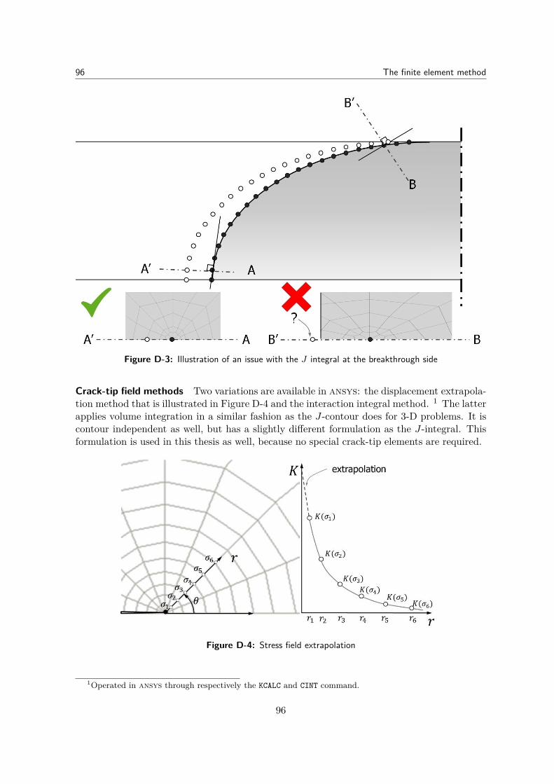
96 The finite element method
Figure D-3: Illustration of an issue with the J integral at the breakthrough side
Crack-tip field methods Two variations are available in ansys: the displacement extrapola-tion method that is illustrated in Figure D-4 and the interaction integral method. 1 The latterapplies volume integration in a similar fashion as the J-contour does for 3-D problems. It iscontour independent as well, but has a slightly different formulation as the J-integral. Thisformulation is used in this thesis as well, because no special crack-tip elements are required.
Figure D-4: Stress field extrapolation
1Operated in ansys through respectively the KCALC and CINT command.
96
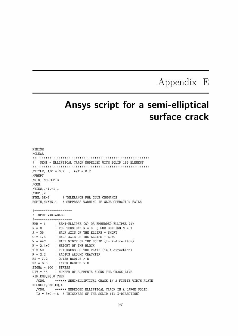
Appendix E
Ansys script for a semi-ellipticalsurface crack
FINISH/CLEAR!!!!!!!!!!!!!!!!!!!!!!!!!!!!!!!!!!!!!!!!!!!!!!!!!!!!!!!!!!!!!!! SEMI - ELLIPTICAL CRACK MODELLED WITH SOLID 186 ELEMENT!!!!!!!!!!!!!!!!!!!!!!!!!!!!!!!!!!!!!!!!!!!!!!!!!!!!!!!!!!!!!!/TITLE, A/C = 0.2 ; A/T = 0.7/PREP7/UIS, MSGPOP,3/COM,/VIEW,,-1,-1,1/VUP,,ZBTOL,3E-4 ! TOLERANCE FOR GLUE COMMANDSBOPTN,NWARN,1 ! SUPPRESS WARNING IF GLUE OPERATION FAILS
!--------------------! INPUT VARIABLES!--------------------EMB = 1 ! SEMI-ELLIPSE (0) OR EMBEDDED ELLIPSE (1)N = 0 ! FOR TENSION: N = 0 ; FOR BENDING N = 1A = 35 ! HALF AXIS OF THE ELLIPS - SHORTC = 175 ! HALF AXIS OF THE ELLIPS - LONGW = 4*C ! HALF WIDTH OF THE SOLID (in Y-direction)H = 2.4*C ! HEIGHT OF THE BLOCKT = 50 ! THICKNESS OF THE PLATE (in X-direction)R = 2.2 ! RADIUS AROUND CRACKTIPR2 = 7.2 ! OUTER RADIUS > RR3 = 6.8 ! INNER RADIUS > RSIGMA = 100 ! STRESSDIV = 46 ! NUMBER OF ELEMENTS ALONG THE CRACK LINE*IF,EMB,EQ,0,THEN
/COM, ****** SEMI-ELLIPTICAL CRACK IN A FINITE WIDTH PLATE*ELSEIF,EMB,EQ,1
/COM, ****** EMBEDDED ELLIPTICAL CRACK IN A LARGE SOLIDT2 = 3*C + A ! THICKNESS OF THE SOLID (IN X-DIRECTION)
97
98 Ansys script for a semi-elliptical surface crack
*ENDIFPI = 3.141592654ET,1,186 ! SOLID ELEMENT 186 - 20 NODE HEXAGONALEMOD = 207E3 ! YOUNGS MODULUSNU = 0.3 ! POISSONS RATIOMP,EX,1,EMODMP,NUXY,1,NU
!--------------------! MODELLING GEOMETRY!--------------------WPOFFS, 0, C, 0WPROTA,-90,90,0 ! ROTATE THE WORKING PLANCSWPLA,11,1 ! DEFINE LOCAL COORDINATE SYSTEM 11K,1,0,0,0KGEN,5,1,,,,,,10,0 ! 5 x KP AT (0,0,0) NUMBERED 1,11,21,31,...
K,4,R*0.8,0,0K,44,R*0.8,180,0KFILL,4,44,3,14,10 ! FILL THE ’LINE’ BETWEEN NODE 4 AND 44 WITH A NODE
! AT 1/4 OF THE DISTANCE NUMBERED FROM 14 (+10) TO 44KFILL,1,4,2,2,1,1.0KGEN,5,1,4,1,0,180/4,0,10,1,0
CSWPLA,12,0 ! DEFINE LOCAL COORDINATE SYSTEM 12, CARTHESIANK, 5, R,0,0K, 6, R3,0,0K,15, R,R,0K,16, R3,R,0K,25, 0,R,0K,35, -R,R,0K,45, -R,0,0K,46,-R2,0,0KMODIF,14, R*0.62,R*0.62,0KMODIF,34,-R*0.62,R*0.62,0A, 2,12, 1, 1 !A,12,22,11,11A,22,32,21,21A,32,42,31,31A, 2, 3,13,12, !A,12,13,23,22,A,22,23,33,32,A,32,33,43,42,A, 3,13,14, 4, !A,13,23,24,14,A,23,33,34,24,A,33,43,44,34,A, 4,14,15, 5 !A,14,24,25,15A,24,34,35,25A,34,44,45,35A, 5, 6,16,15 !
K,36,-R2,R,0A,45, 46,36,35
ASEL,ALL
98
99
AGLUE,ALL
WPSTYL,DEFAWPSTYL, , , , , , 0, 0, 0,CSYS,0K, 7,0,0,0K,100,A,0,0
LOCAL,13,1,0,0,0,,,,C/A ! ELLIPTICAL COORDINATE SYSTEML,1,100
CSYS,0ASEL,ALLVDRAG,ALL,,,,,,5 ! EXTRUDE AREAS TO VOLUMESLDELE,5 ! REMOVE LINE
L, 6,7L,49,7NUMMRG,KP, , , ,AL,5,99,111VDRAG,79,,,,,,41,VGLUE,14,19 ! GLUE VOLUMES
BLOCK, 0, T, 0, C+3*R2, 0, RVSEL,S,VOLU,,19CM,BOTTOMVOLUME1,VOLU
BLOCK, 0, T, C+3*R2,W , 0, RVSEL,D,VOLU,,21CM,BOTTOMVOLUME2,VOLU
ALLSEL,ALLVSEL,U,VOLU,,BOTTOMVOLUME1,VSEL,U,VOLU,,BOTTOMVOLUME2,CM,SUBTRACTVOLUME,VOLU
VSEL,ALL ! SUBTRACT VOLUMES FROM VOLUMESVSBV,BOTTOMVOLUME1,SUBTRACTVOLUME,,DELETE,KEEPCMDELE,SUBTRACTVOLUME
VSEL,S,VOLU,,20CM,CORNERVOLUME,VOLUVSEL,S,VOLU,,14CM,INNERRAD,VOLUVSEL,S,VOLU,,15CM,OUTERRAD,VOLUVSEL,S,VOLU,,22CM,BOTTOMVOLUME1,VOLUVSEL,S,VOLU,,21CM,BOTTOMVOLUME2,VOLU
*IF,EMB,EQ,0,THENVSEL,ALLVGLUE,ALLALLSEL,ALLNUMMRG,kp, , , ,
*ELSEIF,EMB,EQ,1
99
100 Ansys script for a semi-elliptical surface crack
BLOCK, T, T2, 0,C+3*R2,0,RBLOCK, T, T2,C+3*R2, W,0,RVSEL,ALLVGLUE,ALLALLSEL,ALLNUMMRG,KP, ,VSEL,S,VOLU,,19CM,BOTTOMVOLUME3,VOLUVSEL,S,VOLU,,23CM,BOTTOMVOLUME4,VOLU
*ENDIF
!-----------------------------! MESH CRACK AREA!-----------------------------LSEL,S,LOC,X,0.1,A+RLSEL,R,LOC,Y,0.1,C+RLESIZE,ALL,,,DIV,1.0 ! DIVIDE CRACK TIP LINEESIZE,,1VSEL,ALLVSEL,U,VOLU,,CORNERVOLUMEVSEL,U,VOLU,,INNERRADVSEL,U,VOLU,,OUTERRADVSEL,U,VOLU,,BOTTOMVOLUME1VSEL,U,VOLU,,BOTTOMVOLUME2*IF,EMB,EQ,1,THEN
VSEL,U,VOLU,,BOTTOMVOLUME3VSEL,U,VOLU,,BOTTOMVOLUME4
*ENDIFMSHKEY,1 ! MAPPED MESHINGVMESH,ALL
ALLSEL,ALLKSEL,S,KP,,1LSLK,S,0LSEL,R,LOC,X,0.01,A+R ! SELECT LINE AT CRACK TIPNSLL,S,1CM,CRACKTIP,NODE ! DEFINE COMPONENT FOR CRACK TIPALLSEL
!-----------------------------! MESH THE OTHER VOLUMES!-----------------------------SMRT,OFFLSEL,S,LOC,X,0LSEL,R,LOC,Y,C+R2LESIZE,ALL,,,1LSEL,S,LOC,X,0LSEL,R,LOC,Y,C+R+0.1,C+R2-0.1LSEL,R,LOC,Z,0,RLESIZE,ALL,,,1,VSWEEP,OUTERRAD ! MESH OUTER RADIUS
LSEL,S,LOC,X,0LSEL,R,LOC,Y,C-R3LESIZE,ALL,,,1LSEL,S,LOC,X,0
100
101
LSEL,R,LOC,Y,C-R3+0.1,C-R-0.1LSEL,R,LOC,Z,0,RLESIZE,ALL,,,1,VSWEEP,INNERRAD ! MESH INNER RADIUS
SMRT,10LSEL,S,LOC,Y,0.1,C-R-0.1LSEL,R,LOC,X,0LESIZE,ALL,,,DIV-13,1.1,,,,0LSEL,S,LOC,X,0.1,A-R3-0.1LSEL,R,LOC,Y,0LESIZE,ALL,,,3,1.0,,,,0VSWEEP,CORNERVOLUME ! MESH VOLUMES ABOVE THE CRACK
LSEL,S,LOC,X,0.1,T-0.1LSEL,R,LOC,Y,C+3*R2,LESIZE,ALL,,,8LSEL,S,LOC,X,TLSEL,R,LOC,Y,0.1,C+R2-0.1LESIZE,ALL,,,24,,,,,0VSWEEP,BOTTOMVOLUME1 ! MESH VOLUMES IN LENGTH DIRECTION
ESIZE,,1LSEL,S,LOC,X,0LSEL,A,LOC,X,TLSEL,R,LOC,Y,C+3*R2+0.1, W-0.1,LESIZE,ALL,,,6,ALLSEL, ALLVSWEEP,BOTTOMVOLUME2 ! MESH VOLUMES IN DEPTH DIRECTION
*IF,EMB,EQ,1,THENLSEL,S,LOC,X,T+0.1,T2-0.1LSEL,R,LOC,Y,0,LESIZE,ALL,,,5,5,,,,0LSEL,S,LOC,X,T+0.1,T2-0.1LSEL,R,LOC,Y,C+3*R2,WLESIZE,ALL,,,5,1/5,,,,0LSEL,S,LOC,X,T2 ! LONG SIDE, AWAY FROM CRACKLSEL,R,LOC,Y,0.1,C+3*R2-0.1LESIZE,ALL,,,1,,,,,0VSWEEP,BOTTOMVOLUME3VSWEEP,BOTTOMVOLUME4 ! MESH REMAINING VOLUMES IN DEPTH DIRECTION
*ENDIF
!---------------------------------------------! EXTRUDE TO FULL HEIGHT AND MESH OTHER AREAS!---------------------------------------------ALLSEL,ALLESIZE,,7ALLSEL,ALLASEL,S,LOC,Z,RVEXT,ALL, , , , ,H-RALLSEL,ALLVSEL,S,LOC,Z,R,HVSWEEP,ALLALLSEL,ALL
101
102 Ansys script for a semi-elliptical surface crack
!----------------------------------! BOUNDARY CONDITIONS!----------------------------------*IF,EMB,EQ,0,THEN
*IF,N,EQ,0,THENNSEL,S,LOC,X,T/2-1,T/2+0.1NSEL,R,LOC,Z,HD,ALL,UX,0
*ELSEIF,N,EQ,1NSEL,S,LOC,X,ANSEL,R,LOC,z,HNSEL,R,LOC,Y,0D,ALL,UX,0 ! CONSTRAIN UX DOF
*ENDIF*ELSEIF,EMB,EQ,1
NSEL,S,LOC,X,0D,ALL,UX,0 ! CONSTRAIN UX DOF
*ENDIF
ALLSELNSEL,S,LOC,Y,0D,ALL,UY,0 ! CONSTRAIN UY DOFALLSEL
KSEL,S,KP,,42,46 ! CONSTRAIN AREAS THAT ARE NOT PART OF THE CRACKLSLK,S,0LSEL,R,LOC,Z,0ASLL,S,0ASEL,A,LOC,Y,C+R,W
*IF,EMB,EQ,0,THENASEL,A,LOC,X,A+R,T
*ELSEIF,EMB,EQ,1ASEL,A,LOC,X,A+R,T2
*ENDIF
ASEL,R,LOC,Z,0CM,CONSTRAINAREAS,AREACMSEL,S,CONSTRAINAREAS,AREANSLA,S,1D,ALL,UZ,0 ! CONSTRAIN UZ DOF
!-------------------------------------------------! LOADS!-------------------------------------------------*IF,N,EQ,0,THEN ! TENSION
ALLSELNSEL,S,LOC,Z,HSF,ALL,PRES,-SIGMA ! SURFACE PRESSURE LOADING
*ELSEIF,N,EQ,1P = (SIGMA+SIGMA*(T-A)/A)/T ! BENDINGALLSELSFGRAD,PRES,0,X,A,P ! PRESSURE LOAD GRADIENTNSEL,S,LOC,Z,HSF,ALL,PRES,0 ! SURFACE PRESSURE LOADING
*ENDIFALLSEL
102
103
FINISH
!-------------------------------------------------! SOLVE SYSTEM AND RETRIEVE K AND J-INTEGRAL DATA!-------------------------------------------------/SOLUAUTOTS,ONNSUBST,10OUTRES,ALL,ALLCINT,NEW,1 ! CRACK IDCINT,TYPE,SIFS ! DEFINE CRACK TYPECINT,CTNC,CRACKTIP,NODE(0,0,0),0 ! DEFINE CRACK-TIP COMPONENTCINT,NORM,0,3 ! CRACK PLANE NORMAL - ZCINT,NCON,5 ! NO. OF CONTOURSCINT,SYMM,ON ! SYMMETRY ONCINT,LISTCINT,NEW,2 ! CRACK IDCINT,TYPE,JINT ! DEFINE CRACK TYPECINT,CTNC,CRACKTIP,NODE(0,0,0),0 ! DEFINE CRACK TIP COMPONENTCINT,NORM,0,3 ! CRACK PLANE NORMAL - ZCINT,NCON,5 ! NO. OF CONTOURSCINT,SYMM,ON ! SYMMETRY ONCINT,LISTALLSEL,ALL
SAVE/NERR,0,,,,SOLVEFINI
/POST1EPLOT!PLCINT,FRONT,1,,,K1
SET,LAST,LASTCMSEL,S,CRACKTIP,NODE*GET,NNUM,NODE,0,COUNT*GET,NMIN,NODE,0,NUM,MIN*DIM,VALUE,ARRAY,NNUM,4I = 1
*DO,I,1,NNUMNCUR = NMIN*GET,X_COOR,NODE,NCUR,LOC,XVALUE(I,1) = X_COOR*GET,Y_COOR,NODE,NCUR,LOC,yVALUE(I,2) = Y_COOR*GET,K2,CINT,1,CTIP,NCUR,,2,,K1*GET,K3,CINT,1,CTIP,NCUR,,3,,K1*GET,K4,CINT,1,CTIP,NCUR,,4,,K1K = ABS(K2+K3+K4)/3VALUE(I,3) = K*GET,J2,CINT,2,CTIP,NCUR,,2,,JINT*GET,J3,CINT,2,CTIP,NCUR,,3,,JINT*GET,J4,CINT,2,CTIP,NCUR,,4,,JINTJ = ABS(J2+J3+J4)/3KJ = (J*EMOD/(1-NU*NU))**0.5
103
104 Ansys script for a semi-elliptical surface crack
VALUE(I,4) = KJI = I+1*GET,NMIN,NODE,NCUR,NXTH
*ENDDO
!-----------------------------! WRITE K VALUES TO .TXT FILE!-----------------------------*CFOPEN,X_Y_K_KJ,TXT ! CREATE FILE*VWRITE,VALUE(1,1),VALUE(1,2),VALUE(1,3),VALUE(1,4) ! WRITE ARRAY TO FILE(f10.6,3x,f10.6,3x,f10.5,3x,f10.5) ! FORMAT 3X (3X A BLANK SPACE)*CFCLOSE ! CLOSE FILE
NSEL,ALLESEL,ALL
FINISH
104
Appendix F
Ansys script for a semi-ellipticalthrough-thickness crack
FINISH/CLEAR!!!!!!!!!!!!!!!!!!!!!!!!!!!!!!!!!!!!!!!!!!!!!!!!!!!!!!!!!!!!!!! VERY FINE - 24 ELEMENTS IN X-DIRECTION!!!!!!!!!!!!!!!!!!!!!!!!!!!!!!!!!!!!!!!!!!!!!!!!!!!!!!!!!!!!!!/TITLE, A/C = 0.4 ; C2 = 0.40*C/PREP7/UIS, MSGPOP,3/COM,/VIEW,,-1,-1,1/VUP,,Z!--------------------! INPUT VARIABLES!--------------------CENTRE = 1 ! BREAKTHROUGH (0) OR CENTRE (1) CRACKN = 0 ! TENSION: N = 0 ; BENDING N = 1A = 109.1089451 ! HALF AXIS OF THE ELLIPS - SHORTC = A/0.4 ! HALF AXIS OF THE ELLIPS - LONGW = 6*C ! HALF WIDTH OF THE SOLID (IN Y-DIRECTION)H = 7.3*C ! HEIGHT OF THE PLATET = 100 ! THICKNESS OF THE PLATER = 5.00 ! RADIUS AROUND CRACKTIPRO = 1.45*R ! OUTER RADIUS > RROO = 2.18*RO ! TRANSITION TO COARSER MESH > RORT = 1.50*ROO ! TRANSITION TO COARSER MESH IIRI = A/5.55 ! INNER RADIUS > R (towards crack area)SIGMA = 10 ! STRESSET,1,186 ! SOLID ELEMENT 186 - 20 NODE HEXAGONALEMOD = 207E3 ! YOUNGS MODULUSNU = 0.3 ! POISSONS RATIOMP,EX,1,EMODMP,NUXY,1,NU
!--------------------
105
106 Ansys script for a semi-elliptical through-thickness crack
! MODEL GEOMETRY!--------------------WPOFFS, 0, C, 0WPROTA,-90,90,0 ! ROTATE THE WORKING PLANECSWPLA,11,1 ! DEFINE LOCAL COORDINATE SYSTEM 11KGEN,5,1,,,,,,10,0 ! 4 x KP AT (0,0,0) NUMBERED 1,11,21,31,...K,1,0,0,0K,4,R*0.85,0,0K,44,R*0.85,180,0KFILL,4,44,3,14,10 ! FILLS THE ’LINE’BETWEEN NODE 4 AND 44KFILL,1,4,2,2,1,1.0KGEN,5,1,4,1,0,180/4,0,10,1,0CSWPLA,12,0 ! DEFINE LOCAL COORDINATE SYSTEM 12, CARTHESIANK, 5, R,0,0K, 6, RI,0,0K,15, R,R,0K,16, RI,R,0K,25, 0,R,0K,35, -R,R,0K,36,-RO,R,0K,45, -R,0,0K,46,-RO,0,0KMODIF,14, R*0.70,R*0.70,0KMODIF,34,-R*0.70,R*0.70,0A, 2,12, 1, 1 !A,12,22,11,11A,22,32,21,21A,32,42,31,31A, 2, 3,13,12,!A,12,13,23,22,A,22,23,33,32,A,32,33,43,42,A, 3,13,14, 4,!A,13,23,24,14,A,23,33,34,24,A,33,43,44,34,A, 4,14,15, 5 !A,14,24,25,15A,24,34,35,25A,34,44,45,35A, 5, 6,16,15 !A,45,46,36,35ASEL,ALLAGLUE,ALLWPSTYL,DEFAWPSTYL,,,,,,0,0,0,CSYS,0*IF,CENTRE,EQ,0,THEN
K,100,A,0,0K,101,T,0,0K,102,T,C,0LOCAL,13,1,0,0,0,,,,C/A ! ELLIPTICAL COORDINATE SYSTEML,1,100CSYS,0L,101,102LPTN,5,6LDELE,11,12
106
107
LDELE, 8,9 ! TO GET THE SAME NUMBERING AS FOR A CENTRE CRACKLOCAL,13,1,0,0,0,,,,C/A ! ELLIPTICAL COORDINATE SYSTEML,1,7KDELE,100,102
*ELSEIF,CENTRE,EQ,1K,7,T,C,0L,1,7
*ENDIFWPROTA,,,90 ! ROTATE THE WORKING PLANEWPOFFS,,,0.050*T ! DIVIDE THE LINELSBW,5, , ! the divisions are different for almost all modelsWPOFFS,,,0.090*TLSBW,8, ,WPOFFS,,,0.089*TLSBW,5, ,WPOFFS,,,0.088*TLSBW,8, ,WPOFFS,,,0.080*TLSBW,5, ,WPOFFS,,,0.074*TLSBW,8, ,WPOFFS,,,0.069*TLSBW,5, ,WPOFFS,,,0.061*TLSBW,8, ,WPOFFS,,,0.0575*TLSBW,5, ,WPOFFS,,,0.0515*TLSBW,8, ,WPOFFS,,,0.0455*TLSBW,5, ,WPOFFS,,,0.040*TLSBW,8, ,WPOFFS,,,0.035*TLSBW,5, ,WPOFFS,,,0.028*TLSBW,8, ,WPOFFS,,,0.021*TLSBW,5, ,WPOFFS,,,0.0172*TLSBW,8, ,WPOFFS,,,0.016*TLSBW,5, ,WPOFFS,,,0.014*TLSBW,8, ,WPOFFS,,,0.013*TLSBW,5, ,WPOFFS,,,0.0125*TLSBW,8, ,WPOFFS,,,0.0122*TLSBW,5, ,WPOFFS,,,0.012*TLSBW,8, ,WPOFFS,,,0.0118*TLSBW,5, ,WPSTYL,DEFAWPSTYL, , , , , , 0, 0, 0,
107
108 Ansys script for a semi-elliptical through-thickness crack
CSYS,0LSEL,U,LOC,X,0LDELE,ALL,,,0L,1,8 ! CREATE LINES FOR THE CRACK-TIPL,8,9L,9,10L,10,11L,11,17L,17,18L,18,19L,19,20L,20,21L,21,26L,26,27L,27,28L,28,29L,29,30L,30,31L,31,37L,37,38L,38,39L,39,40L,40,47L,47,48L,48,49L,49,50L,50,7ASEL,ALLCM,EXTRUDEAREAS,AREA ! DEFINE COMPONENTLSEL,S,LOC,X,0.01,TCM,DRAGLINE,LINEVDRAG,EXTRUDEAREAS,,,,,,DRAGLINE ! EXTRUDE AREAS TO VOLUMES (cracktip area)VEXT,66,1446,60,0,-C, ! EXTRUDE AREAS TO VOLUMES (crack area)WPOFFS, 0,0, 0WPROTA,0,90,0 ! ROTATE THE WORKING PLANEVSBW,ALL,,DELETEWPSTYL,DEFAWPSTYL,,,,,,0,0,0,VSEL,S,LOC,Y,0,-CVDELE,ALL,,,1
!-----------------------------------------------------------! FROM 24 TO 12 LANES OF VOLUMES!------------------------------------------------------------ASEL,S,AREA,,70,1450,60VEXT,ALL,,,0,ROO-ROKSEL,S,KP,,653,697,4KSEL,A,KP,,654,698,4KMODIF, ALL, ,C+ROO-0.04*T,KSEL,S,KP,,655,699,4KSEL,A,KP,,656,700,4KMODIF, ALL, , C+ROO,BLOCK, 0, T, C+ROO-0.04*T, C + ROO, 0, RVSEL,S,VOLU,,433,456,1VSEL,A,VOLU,,481VSBA, ALL, 1655, , DELETE, DELETE ! SUBTRACT AREA FROM VOLUMESVSEL,S,LOC,Y,C+ROO-0.04*T-0.01,C+ROO
108
109
VSBV,481,ALL,,DELETE,KEEP ! SUBTRACT VOLUMES FROM VOLUMESASEL,S,LOC,Y,C+ROO-0.01,C+ROO+0.01VEXT,ALL,,,0,RT
!------------------------------! FROM 12 TO 6 LANES OF VOLUMES!-------------------------------KSEL,S,KP,,784,804,4KSEL,A,KP,,787,803,4KSEL,A,KP,,781KMODIF,ALL,,C+ROO+RT-0.08*T,BLOCK,0,T,C+ROO+RT-0.08*T,C+ROO+RT, 0, RVSEL,S,VOLU,,445,456,1VSEL,A,VOLU,,481VSBA, ALL, 1827, , DELETE, DELETE ! SUBTRACT AREA FROM VOLUMESVSEL,S,LOC,Y,C+ROO+RT-0.08*T-0.01,C+ROO+RTVSBV,481,ALL,,DELETE,KEEP ! SUBTRACT VOLUMES FROM VOLUMESASEL,S,LOC,Y,C+ROO+RT-0.01,C+ROO+RT+0.01VEXT,ALL,,,0,W-C-ROO-RTALLSELNUMMRG, KP,
!-----------------------------------------! MESH AREA AROUND THE CRACK-TIP!-----------------------------------------VSEL,S,VOLU,,1,432,VSEL,U,VOLU,,14,428,18VSEL,U,VOLU,,15,429,18ESIZE,,1MSHKEY,1 ! MAPPED MESHINGVMESH,ALL
!-----------------------------! MESH THE INNER RADIUS!-----------------------------LSEL,S,LOC,Y,C-R-0.01,C-RI-0.01LSEL,R,LOC,X,0,LSEL,R,LOC,Z,0,LESIZE,ALL,,,1LSEL,S,LOC,Y,C-R-0.01,C-RI-0.01LSEL,R,LOC,X,0,LSEL,R,LOC,Z,R,LESIZE,ALL,,,1LSEL,S,LINE,,123,1664,67LSEL,A,LINE,,41LESIZE,ALL,,,1,VSEL,S,VOLU,,14,428,18VSWEEP,ALL
!-----------------------------! MESH THE OUTER RADIUS!-----------------------------LSEL,S,LINE,,126,1667,67LSEL,A,LINE,,43LESIZE,ALL,,,1,LSEL,S,LINE,,128,1669,67LSEL,A,LINE,,44
109
110 Ansys script for a semi-elliptical through-thickness crack
LESIZE,ALL,,,1,LSEL,S,LINE,,130,1671,67LSEL,A,LINE,,45LESIZE,ALL,,,1,VSEL,S,VOLU,,15,429,18VSWEEP,ALL
!------------------------------! MESHING THE CRACK AREA!------------------------------LSEL,S,LOC,Y,0.1,C-RI-0.1LSEL,R,LOC,X,0LESIZE,ALL,,,6,VSEL,S,VOLU,,457,480VSWEEP,ALL
!-----------------------------! MESH THE OTHER AREAS!-----------------------------LSEL,S,LOC,Y,C+RO+0.1,C+ROO-0.06*T-0.01LSEL,R,LOC,X,0LESIZE,ALL,,,6,,,,, ! ROOVSEL,S,VOLU,,506,529VSWEEP,ALLLSEL,S,LOC,Y,C+ROO+0.1,C+ROO+RT-0.08*T-0.1LESIZE,ALL,,,1,,,,, ! RTVSEL,S,LOC,Y,C+ROO+0.1,C+ROO+RT-0.08*T-0.1VSWEEP,ALLLSEL,S,LOC,Y,C+ROO+RT+0.1,W-0.1LESIZE,ALL,,,13,,,,, ! WVSEL,S,LOC,Y,C+ROO+RT+0.1,WVSWEEP,ALLVSEL,S,LOC,Y,C+ROO-0.04*T-0.01,C+ROO+0.01MSHKEY,0MSHAPE, 1,3DVMESH,ALLVSEL,S,LOC,Y,C+ROO+RT-0.08*T-0.01,C+ROO+RT+0.01MSHKEY,0MSHAPE, 1,3DVMESH,ALL
!---------------------------------------------! EXTRUDE TO FULL HEIGHT AND MESH!---------------------------------------------ASEL,S,LOC,Z,RVEXT,ALL, , , , ,RESIZE,,9ASEL,S,LOC,Z,2*RVEXT,ALL, , , , ,H-2*R
!-----------------------------! DEFINE CRACK-TIP!-----------------------------CMSEL,S,DRAGLINE,LINENSLL,S,1CM,CRACKTIP,NODE ! DEFINE COMPONENT FOR CRACKTIP
110
111
!-------------------------------------------------! BOUNDARY CONDITIONS!-------------------------------------------------NSEL,S,LOC,Y,0D,ALL,UY,0 ! CONSTRAIN UY DOF*GET,X_CONSTR,KP,20,LOC,X ! LOCATION TO CONSTRAIN X AT KP 20, more or less halfway TNSEL,S,LOC,X,X_CONSTR ! CONSTRAIN UX DOFNSEL,R,LOC,Z,H ! CONSTRAIN UX DOFD,ALL,UX,0*IF,CENTRE,EQ,0,THEN
ASEL,S,AREA,,77,1457,60ASEL,A,AREA,,36,1416,60ASEL,A,AREA,,49,1429,60ASEL,A,AREA,,62,1442,60ASEL,A,AREA,,69,1449,60ASEL,A,AREA,,1745,1800,5ASEL,A,AREA,,1747,1802,5ASEL,A,LOC,Y,C,W ! CONSTRAIN AREAS THAT ARE NOT PART OF THE CRACKASEL,R,LOC,Z,0CM,CONSTRAINAREAS,AREACMSEL,S,CONSTRAINAREAS,AREANSLA,S,1D,ALL,UZ,0 ! CONSTRAIN UZ DOF
*ELSEIF,CENTRE,EQ,1NSEL,S,LOC,Y,C-0.1,WNSEL,R,LOC,Z,0D,ALL,UZ,0 ! CONSTRAIN UZ DOF
*ENDIF
!-------------------------------------------------! LOADS!-------------------------------------------------*IF,N,EQ,0,THEN ! TENSION
NSEL,S,LOC,Z,HSF,ALL,PRES,-SIGMA ! SURFACE PRESSURE LOADING
*ELSEIF,N,EQ,1 ! BENDINGSFGRAD,PRES,0,X,T,SIGMA/T ! PRESSURE LOAD GRADIENTNSEL,S,LOC,Z,HSF,ALL,PRES,0 ! SURFACE PRESSURE LOADING
*ENDIFALLSELFINISH
!-------------------------------------------------! SOLVE SYSTEM AND RETRIEVE K AND J-INTEGRAL DATA!-------------------------------------------------/SOLUCINT,NEW,1 ! CRACK IDCINT,TYPE,SIFS ! DEFINE CRACK TYPECINT,CTNC,CRACKTIP,NODE(0,0,0),0 ! DEFINE CRACK TIP COMPONENTCINT,NORM,0,3 ! CRACK PLANE NORMAL - ZCINT,NCON,5 ! NO OF CONTOURSCINT,SYMM,ON ! SYMMETRY ONCINT,LISTCINT,NEW,2 ! CRACK IDCINT,TYPE,JINT ! DEFINE CRACK TYPECINT,CTNC,CRACKTIP,NODE(0,0,0),0 ! DEFINE CRACK TIP COMPONENT
111
112 Ansys script for a semi-elliptical through-thickness crack
CINT,NORM,0,3 ! CRACK PLANE NORMAL - ZCINT,NCON,5 ! NO OF CONTOURSCINT,SYMM,ON ! SYMMETRY ONCINT,LISTALLSEL,ALLSAVE/NERR,0,,,,SOLVEFINI/POST1EPLOTSET,LAST,LASTCMSEL,S,CRACKTIP,NODE*GET,NNUM,NODE,0,COUNT*GET,NMIN,NODE,0,NUM,MIN*DIM,VAL,ARRAY,NNUM,8 ! CREATE ARRAY FOR VALUESI = 1*DO,I,1,NNUM
NCUR = NMIN*GET,X_COOR,NODE,NCUR,LOC,XVAL(I,1) = X_COOR*GET,Y_COOR,NODE,NCUR,LOC,YVAL(I,2) = Y_COOR*GET,K1,CINT,1,CTIP,NCUR,,1,,K1*GET,K2,CINT,1,CTIP,NCUR,,2,,K1*GET,K3,CINT,1,CTIP,NCUR,,3,,K1*GET,K4,CINT,1,CTIP,NCUR,,4,,K1*GET,K5,CINT,1,CTIP,NCUR,,5,,K1K = (K3+K4+K5)/3VAL(I,3) = K*GET,J1,CINT,2,CTIP,NCUR,,1,,JINT*GET,J2,CINT,2,CTIP,NCUR,,2,,JINT*GET,J3,CINT,2,CTIP,NCUR,,3,,JINT*GET,J4,CINT,2,CTIP,NCUR,,4,,JINT*GET,J5,CINT,2,CTIP,NCUR,,5,,JINTKJ1 = (J1*EMOD/(1-NU*NU))**0.5VAL(I,4) = KJ1KJ2 = (J2*EMOD/(1-NU*NU))**0.5VAL(I,5) = KJ2KJ3 = (J3*EMOD/(1-NU*NU))**0.5VAL(I,6) = KJ3KJ4 = (J4*EMOD/(1-NU*NU))**0.5VAL(I,7) = KJ4KJ5 = (J5*EMOD/(1-NU*NU))**0.5VAL(I,8) = KJ5I = I+1*GET,NMIN,NODE,NCUR,NXTH
*ENDDO
!--------------------------! WRITE DATA TO .TXT FILE!--------------------------*CFOPEN,X_Y_K_KJ1_KJ2_KJ3_KJ4_KJ5,TXT ! CREATE FILE*VWRITE,VAL(1,1),VAL(1,2),VAL(1,3),VAL(1,4),VAL(1,5),VAL(1,6),VAL(1,7),VAL(1,8)(f10.6,3x,f10.6,3x,f10.5,3x,f10.5,3x,f10.5,3x,f10.5,3x,f10.5,3x,f10.5) ! 3X BLANK SPACE*CFCLOSE ! CLOSE FILEFINISH
112
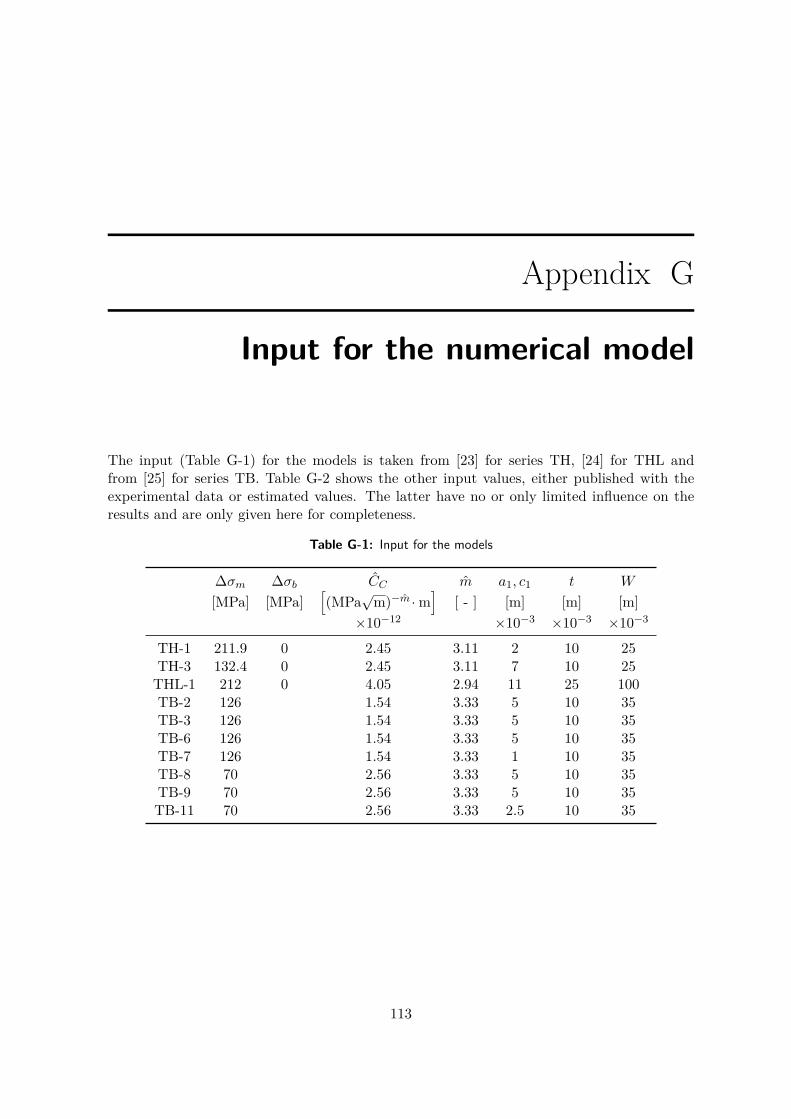
Appendix G
Input for the numerical model
The input (Table G-1) for the models is taken from [23] for series TH, [24] for THL andfrom [25] for series TB. Table G-2 shows the other input values, either published with theexperimental data or estimated values. The latter have no or only limited influence on theresults and are only given here for completeness.
Table G-1: Input for the models
∆σm ∆σb CC m a1, c1 t W
[MPa] [MPa][(MPa
√m)−m ·m
][ - ] [m] [m] [m]
×10−12 ×10−3 ×10−3 ×10⁻³
TH-1 211.9 0 2.45 3.11 2 10 25TH-3 132.4 0 2.45 3.11 7 10 25THL-1 212 0 4.05 2.94 11 25 100TB-2 126 1.54 3.33 5 10 35TB-3 126 1.54 3.33 5 10 35TB-6 126 1.54 3.33 5 10 35TB-7 126 1.54 3.33 1 10 35TB-8 70 2.56 3.33 5 10 35TB-9 70 2.56 3.33 5 10 35TB-11 70 2.56 3.33 2.5 10 35
113
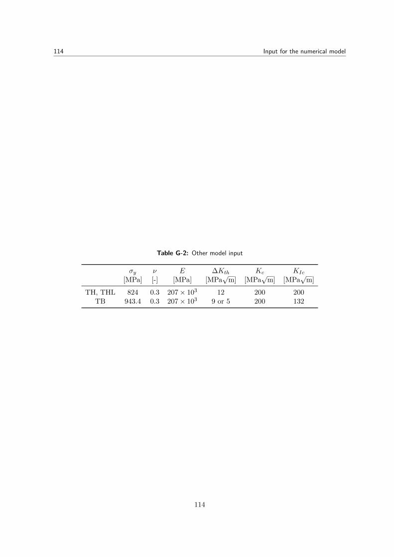
114 Input for the numerical model
Table G-2: Other model input
σy ν E ∆Kth Kc KIc
[MPa] [-] [MPa] [MPa√m] [MPa
√m] [MPa
√m]
TH, THL 824 0.3 207× 103 12 200 200TB 943.4 0.3 207× 103 9 or 5 200 132
114
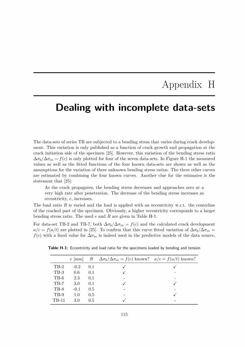
Appendix H
Dealing with incomplete data-sets
The data-sets of series TB are subjected to a bending stress that varies during crack develop-ment. This variation is only published as a function of crack growth and propagation at thecrack initiation side of the specimen [25]. However, this variation of the bending stress ratio∆σb/∆σm = f(c) is only plotted for four of the seven data-sets. In Figure H-1 the measuredvalues as well as the fitted functions of the four known data-sets are shown as well as theassumptions for the variation of three unknown bending stress ratios. The three other curvesare estimated by combining the four known curves. Another clue for the estimates is thestatement that [25]:
As the crack propagates, the bending stress decreases and approaches zero at avery high rate after penetration. The decrease of the bending stress increases aseccentricity, e, increases.
The load ratio R is varied and the load is applied with an eccentricity w.r.t. the centrelineof the cracked part of the specimen. Obviously, a higher eccentricity corresponds to a largerbending stress ratio. The used e and R are given in Table H-1.
For data-set TB-2 and TB-7, both ∆σb/∆σm = f(c) and the calculated crack developmenta/c = f(a/t) are plotted in [25]. To confirm that this curve fitted variation of ∆σb/∆σm =f(c) with a fixed value for ∆σm is indeed used in the predictive models of the data source,
Table H-1: Eccentricity and load ratio for the specimens loaded by bending and tension
e [mm] R ∆σb/∆σm = f(c) known? a/c = f(a/t) known?
TB-2 -0.2 0.1 X XTB-3 0.6 0.1 X -TB-6 2.3 0.1 - -TB-7 3.0 0.1 X XTB-8 -0.1 0.5 - -TB-9 1.0 0.5 - XTB-11 3.0 0.5 X -
115
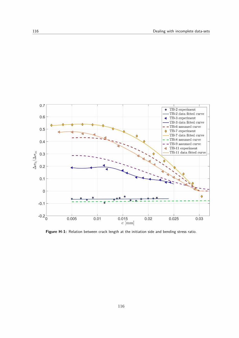
116 Dealing with incomplete data-sets
Figure H-1: Relation between crack length at the initiation side and bending stress ratio.
116
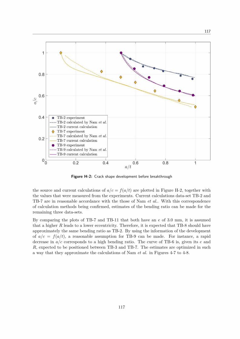
117
Figure H-2: Crack shape development before breakthrough
the source and current calculations of a/c = f(a/t) are plotted in Figure H-2, together withthe values that were measured from the experiments. Current calculations data-set TB-2 andTB-7 are in reasonable accordance with the those of Nam et al.. With this correspondenceof calculation methods being confirmed, estimates of the bending ratio can be made for theremaining three data-sets.
By comparing the plots of TB-7 and TB-11 that both have an e of 3.0 mm, it is assumedthat a higher R leads to a lower eccentricity. Therefore, it is expected that TB-8 should haveapproximately the same bending ratio as TB-2. By using the information of the developmentof a/c = f(a/t), a reasonable assumption for TB-9 can be made. For instance, a rapiddecrease in a/c corresponds to a high bending ratio. The curve of TB-6 is, given its e andR, expected to be positioned between TB-3 and TB-7. The estimates are optimized in sucha way that they approximate the calculations of Nam et al. in Figures 4-7 to 4-8.
117

118 Dealing with incomplete data-sets
118
Bibliography
[1] R. Bourga, P. Moore, Y.-J. Janin, B. Wang, and J. Sharples, “Leak-before-break: Globalperspectives and procedures,” International Journal of Pressure Vessels and Piping,vol. 129 - 130, pp. 43 – 49, 2015.
[2] The British Standards Institution, “Guide to methods for assessing the acceptability offlaws in metallic structures,” 31 July 2015. BS 7910:2013+A1:2015.
[3] American and Petroleum Institute, Recommended practice 579 Fitness-For-Service. API579-1/ASME FFS-1 ed., June 5 2007.
[4] Structural Integrity Assessment Procedures for European Industry, SINTAP Procedure.November 1999. Chapter IV.5.
[5] The Marine Safety Committee, Amendments to the international code for the construc-tion and equipment of ships carrying liquefied gases in bulk. Resolution MSC.370(93) ed.,22 May 2014.
[6] J. Schijve, Fatigue of Structures and Materials. Springer Netherlands, 2nd ed., 2009.
[7] D. Cudeiro and S. Osuna, “Engineering critical analysis of LNG cargo containments,”June 2016. Lloyd’s Register Marine Internal report.
[8] J. C. Newman and I. S. Raju, “An empirical stress-intensity factor equation for thesurface crack,” Engineering Fracture Mechanics, vol. 15, no. 1-2, pp. 185–192, 1981.
[9] H. Tada, P. C. Paris, and G. Irwin, The stress analysis of cracks handbook. ASME Press,3rd ed., 2000.
[10] D. P. Rooke and D. J. Cartwright, Compendium of stress intensity factors. H.M.S.O.,1976.
[11] Y. Murakami, Stress Intensity factors handbook. Pergamon Oxford, 1992.
[12] T. Anderson, Fracture Mechanics. CRC Press, Inc., 1991.
119
120 Bibliography
[13] H. F. Bueckner, “Weight functions and fundamental fields for the penny-shaped and thehalf-plane crack in three-space,” International Journal of Solids and Structures, vol. 23,no. 1, pp. 57 – 93, 1987.
[14] G. Shen and G. Glinka, “Determination of weight functions from reference stress intensityfactors,” Theoretical and Applied Fracture Mechanics, no. 15, pp. 237–245, 1991.
[15] G. Shen and G. Glinka, “Universal features of weight functions of cracks in mode I,”Engineering Fracture Mechanics, vol. 40, no. 6, pp. 1135–1146, 1991.
[16] M. Isida, H. Noguchi, and T. Yoshida, “Analysis of stress intensity factors for sur-face cracks subjected to arbitrarily distributed surface stress,” in Stress Intensity FactorHandbook (Y. Murakami, ed.), vol. 2, pp. 698–705, Pergamon, 1987.
[17] G. Shen and G. Glinka, “Weight functions for a surface semi-elliptical crack in a finitethickness plate,” Theoretical and Applied Fracture Mechanics, vol. 15, pp. 247–255, 1991.
[18] X. Wang, “Stress intensity factors and weight functions for deep semi-elliptical surfacecracks in finite-thickness plates,” Fatigue & Fracture of Engineering Materials & Struc-tures, vol. 25, no. 3, pp. 291–304, 2002.
[19] J. Sharples and A. Clayton, “A leak-before-break assessment method for pressure vesselsand some current unresolved issues.,” International Journal of Pressure Vessels & Piping,vol. 43, pp. 317 – 327, 1990.
[20] K. Shingai, N. Imamura, T. Hirata, M. Ushijima, and D. Sakai, “The fatigue crackpropagation of 9% Ni-steel for the tank of LNG carriers,” Collection of papers of TheSociety of Naval Architects of Japan, 1974. (in Japanese).
[21] M. Bransen, “On the crack shape development in spherical LNG tanks for a Leak-Before-Break assessment,” March 2016. Research Exercise.
[22] B. Brickstad and I. Sattari-Far, “Crack shape developments for LBB applications,” En-gineering Fracture Mechanics, vol. 67, no. 6, pp. 625 – 646, 2000.
[23] K. Ando, S. Fujibashi, K. W. Nam, M. Takahashi, and N. Ogura, “The fatigue lifeand crack through thickness behavior of a surface-cracked plate (for the case of tensileload),” Japan Society of Mechanical Engineers International Journal, vol. 30, no. 270,pp. 1898–1905, 1987.
[24] K. W. Nam, K. Ando, and N. Ogura, “The effect of specimen size on the behaviour ofpenetrating fatigue cracks,” Fatigue and Fracture of Engineering Materials and Struc-tures, vol. 16, no. 7, pp. 767–779, 1993.
[25] K. W. Nam, K. Ando, N. Ogura, and K. Matui, “Fatigue life and penetration behaviourof a surface cracked plate under combined tension and bending,” Fatigue and Fractureof Engineering Materials and Structures, vol. 17, no. 8, pp. 873–882, 1994.
[26] J. G. Kaufman, R. J. Bucci, and R. A. Kelsey, “Fracture mechanics aspects of the struc-tural integrity technology of spherical aluminium containment vessels for LNG tankers,”Journal of Engineering Materials and Technology, vol. 102, pp. 303–314, 1980.
120
121
[27] P. C. Paris and F. Erdogan, “A critical analysis of crack propagation law,” Transac-tions of the American Society of Mechanical Engineering; Journal of Basic Engineering,vol. 85, pp. 528–539, 1963.
[28] ANSYS Help - Mechanical APDL Documentation, 16 March 2015. Version 16.1.0, onlineaccessible through https://www.sharcnet.ca/Software/Ansys/16.2.3/en-us/help/ai_sinfo/mech_intro.html.
[29] R. J. Hartranft and G. C. Sih, “Effect of plate thickness on the bending stress distributionaround through cracks,” Studies in applied mathematics, vol. 47, no. 1-4, pp. 276–291,April 1968.
[30] P. Schreurs, Fracture Mechanics. Eindhoven University of Technology Department ofMechanical Engineering, Augustus 2014. http://www.mate.tue.nl/~piet/edu/frm/pdf/frmsyl1415.pdf.
[31] A. T. Zehnder, Fracture Mechanics. No. 62 in Lecture Notes in Applied and Computa-tional Mechanics, Springer Netherlands.
[32] J. Knott, Fundamentals of Fracture Mechanics. Butterworth & Co Publishers Ltd, 1973.
[33] R. G. Forman, V. E. Kearney, and R. M. Engle, “Numerical analysis of crack propa-gation in cyclic loaded structures,” Transactions of the American Society of MechanicalEngineering; Journal of Basic Engineering, vol. 89, pp. 459–464, 1967.
[34] S. Y. Yarema, “Correlation of the parameters of the paris equation and the cyclic crackresistance characteristics of materials,” Strength of Materials, vol. 13, no. 9, pp. 1090–1098, 1981.
[35] K. W. Nam, F. S., K. Ando, and N. Ogura, “The fatigue life and fatigue crack through-thickness behavior of a surface-cracked plate (effect of stress concentration),” JapanSociety of Mechanical Engineers International Journal, vol. 31, no. 2, pp. 272–279, 1988.
[36] K. W. Nam, K. Iwase, and K. Ando, “Fatigue life and surface crack penetration behaviourof an aluminium alloy,” Fatigue and Fracture of Engineering Materials and Structures,vol. 18, no. 2, pp. 179–187, 1995.
[37] K. E. Atkinson and L. F. Shampine, “Solving Fredholm Integral Equations of the SecondKind in matlab,” May 5 2007. http://homepage.divms.uiowa.edu/~atkinson/ftp/Fie_paper.pdf.
[38] M. Murthy, K. Raju, and S. Viswanath, “On the bending stress distribution at the tipof a stationarycrack from reissner’s theory,” International Journal of Fracture, vol. 17,no. 6, December 1981.
121

122 Bibliography
122