masters thesis: persistent surveillance of a greenhouse
TRANSCRIPT

Delft Center for Systems and Control
Persistent Surveillance of aGreenhouseEvolved neural network controllers for a swarm of UAVs
T.A. Fijen
Mas
tero
fScie
nce
Thes
is

Persistent Surveillance of aGreenhouse
Evolved neural network controllers for a swarm of UAVs
Master of Science Thesis
For the degree of Master of Science in Systems and Control at DelftUniversity of Technology
T.A. Fijen
December 28, 2018
Faculty of Mechanical, Maritime and Materials Engineering (3mE) · Delft University ofTechnology

Copyright c© Delft Center for Systems and Control (DCSC)All rights reserved.
Abstract
With the growing population the agricultural industry needs to find and implement newmethods for enhancing food production. Using a Micro Aerial Vehicle (MAV) in PrecisionAgriculture (PA) offers a large number of benefits such as enabling the farmer to createtargeted strategies to increase crop yield, reduced waste and halt the spread of diseases.Despite these advantages, the use of MAVs, particularly in greenhouses, is still very limited.To this end, this thesis seeks to combine, improve and implement existing strategies to solvethe persistent surveillance task for a swarm of MAVs operating in a greenhouse environment.
Broadly speaking, the persistent surveillance task seeks to find the optimal paths for a swarmof MAVs such that every point within the Mission Space (MS) is visited and they mustminimise the time between successive visits. This will ensure that the MAVs are able flythrough the entire greenhouse to collect up-to-date data about all the crops and the localenvironment. Naturally, on a physical system one has to deal with the limited flight timesof the MAVs. This factor becomes very important to the effectiveness of the solution and iscritical to the continuous operation of the MAVs.
In literature, many methods have be proposed to solve this task, but the majority are still onlytested in simulation. As a result, many works do not consider some physical constraints thatwill be applied to the system during implementation in a real-world setting. For example, inmost cases the authors do not consider the limited fuel available to the agents or they do notconsider a practical alternative indoor positioning system to GPS. In this work the problemhas been divided into two main sub-tasks, namely; the persistent surveillance task and therefuelling task.
For the persistent surveillance task it was decided to implement a reactive controller, in theform of an evolved Neural Network (NN), which was run on-board the MAVs. The NN usedpositional information from the other members of the swarm along with limited environmentalinformation to supply its MAV with a command velocity. These NN controllers could achievecoverage levels of over 95% while simultaneously avoiding collisions between 8 MAVs in a25m× 25m MS. Later, this method was shown to be robust to failures and scalable in termsof both MS and swarm size.
When dealing with the fuel constraints, a Behaviour Tree (BT) was used to determine when
Master of Science Thesis T.A. Fijen
ii
the MAV should return to the depot. Surprisingly, when combined with the NN controllers thesystem experienced an increase in performance across all the defined metrics. No MAV faileddue to low fuel levels, coverage increased to 97.41%, average cell age to 52.39s and the numberof tests were no collisions were recorded more than doubled. This increase in performancewas attributed to the fact that the refuelling periodically drew the MAV towards the centre ofthe MS. This is counter to the evolved behaviours of the NN where the MAVs would mainlyfocus their attention around the edges of the MS.
T.A. Fijen Master of Science Thesis
Table of Contents
Acknowledgements xiii
1 Introduction 11-1 Precision Agriculture . . . . . . . . . . . . . . . . . . . . . . . . . . . . . . . . 21-2 Persistent Surveillance . . . . . . . . . . . . . . . . . . . . . . . . . . . . . . . . 21-3 Thesis Outline . . . . . . . . . . . . . . . . . . . . . . . . . . . . . . . . . . . . 4
2 Problem Outline 52-1 Problem Statement . . . . . . . . . . . . . . . . . . . . . . . . . . . . . . . . . 5
2-1-1 Controller Architecture . . . . . . . . . . . . . . . . . . . . . . . . . . . 52-1-2 Problem Formulation . . . . . . . . . . . . . . . . . . . . . . . . . . . . 62-1-3 Reducing the Problem . . . . . . . . . . . . . . . . . . . . . . . . . . . . 7
2-2 Problem Analysis . . . . . . . . . . . . . . . . . . . . . . . . . . . . . . . . . . 92-3 Hardware Setup . . . . . . . . . . . . . . . . . . . . . . . . . . . . . . . . . . . 9
2-3-1 CyberZoo . . . . . . . . . . . . . . . . . . . . . . . . . . . . . . . . . . 102-3-2 Parrot Bebop 2 . . . . . . . . . . . . . . . . . . . . . . . . . . . . . . . 102-3-3 Positioning and Communication System . . . . . . . . . . . . . . . . . . 11
2-4 Conclusion . . . . . . . . . . . . . . . . . . . . . . . . . . . . . . . . . . . . . . 16
3 The NEAT Algorithm 193-1 NEAT Background . . . . . . . . . . . . . . . . . . . . . . . . . . . . . . . . . 19
3-1-1 Encoding Scheme . . . . . . . . . . . . . . . . . . . . . . . . . . . . . . 193-1-2 Key Aspects of the NEAT Algorithm . . . . . . . . . . . . . . . . . . . . 203-1-3 Mutations . . . . . . . . . . . . . . . . . . . . . . . . . . . . . . . . . . 22
3-2 Implementation . . . . . . . . . . . . . . . . . . . . . . . . . . . . . . . . . . . 233-2-1 Fitness Function . . . . . . . . . . . . . . . . . . . . . . . . . . . . . . . 233-2-2 Neural Network Inputs and Outputs . . . . . . . . . . . . . . . . . . . . 25
Master of Science Thesis T.A. Fijen
iv Table of Contents
3-2-3 Simulated Environment for Evolution . . . . . . . . . . . . . . . . . . . . 293-3 Simulation Results . . . . . . . . . . . . . . . . . . . . . . . . . . . . . . . . . . 31
3-3-1 Test Procedure . . . . . . . . . . . . . . . . . . . . . . . . . . . . . . . 313-3-2 Input Case Results . . . . . . . . . . . . . . . . . . . . . . . . . . . . . . 323-3-3 Results for Selected Input Case . . . . . . . . . . . . . . . . . . . . . . . 35
3-4 Summary . . . . . . . . . . . . . . . . . . . . . . . . . . . . . . . . . . . . . . . 50
4 Fuel Monitoring Policy 534-1 Fixed Threshold Scheduling Method . . . . . . . . . . . . . . . . . . . . . . . . 544-2 Behaviour Trees . . . . . . . . . . . . . . . . . . . . . . . . . . . . . . . . . . . 554-3 Implemented Behaviour Tree . . . . . . . . . . . . . . . . . . . . . . . . . . . . 564-4 Simulation Results . . . . . . . . . . . . . . . . . . . . . . . . . . . . . . . . . . 62
4-4-1 Avoidance Behaviour . . . . . . . . . . . . . . . . . . . . . . . . . . . . 624-4-2 Refuelling . . . . . . . . . . . . . . . . . . . . . . . . . . . . . . . . . . 654-4-3 Performance with Real World Fuel Constraints . . . . . . . . . . . . . . . 71
4-5 Summary . . . . . . . . . . . . . . . . . . . . . . . . . . . . . . . . . . . . . . . 73
5 Practical Implementation 755-1 UWB Positioning Results . . . . . . . . . . . . . . . . . . . . . . . . . . . . . . 755-2 High Fidelity Simulation . . . . . . . . . . . . . . . . . . . . . . . . . . . . . . . 785-3 NN Results . . . . . . . . . . . . . . . . . . . . . . . . . . . . . . . . . . . . . . 815-4 BT Results . . . . . . . . . . . . . . . . . . . . . . . . . . . . . . . . . . . . . . 845-5 Summary . . . . . . . . . . . . . . . . . . . . . . . . . . . . . . . . . . . . . . . 86
6 Conclusions 876-1 Summary . . . . . . . . . . . . . . . . . . . . . . . . . . . . . . . . . . . . . . . 876-2 Future Work . . . . . . . . . . . . . . . . . . . . . . . . . . . . . . . . . . . . . 89
6-2-1 UWB Positioning . . . . . . . . . . . . . . . . . . . . . . . . . . . . . . 896-2-2 NN Performance . . . . . . . . . . . . . . . . . . . . . . . . . . . . . . . 906-2-3 Refuelling . . . . . . . . . . . . . . . . . . . . . . . . . . . . . . . . . . 90
A Input Case Results 91A-1 Input Case 1 . . . . . . . . . . . . . . . . . . . . . . . . . . . . . . . . . . . . . 91A-2 Input Case 2 . . . . . . . . . . . . . . . . . . . . . . . . . . . . . . . . . . . . . 92A-3 Input Case 3 . . . . . . . . . . . . . . . . . . . . . . . . . . . . . . . . . . . . . 93A-4 Input Case 4 . . . . . . . . . . . . . . . . . . . . . . . . . . . . . . . . . . . . . 94A-5 Input Case 5 . . . . . . . . . . . . . . . . . . . . . . . . . . . . . . . . . . . . . 95
B Baseline Persistent Coverage Methods 99B-1 Sweep Planner . . . . . . . . . . . . . . . . . . . . . . . . . . . . . . . . . . . . 99
B-1-1 Boustrophedon Decomposition . . . . . . . . . . . . . . . . . . . . . . . 99B-1-2 Extension to the Multiple UAV Case . . . . . . . . . . . . . . . . . . . . 101
B-2 Random Walk . . . . . . . . . . . . . . . . . . . . . . . . . . . . . . . . . . . . 102
T.A. Fijen Master of Science Thesis
Table of Contents v
C Collision Avoidance Proof 103
Glossary 113List of Acronyms . . . . . . . . . . . . . . . . . . . . . . . . . . . . . . . . . . . 113List of Symbols . . . . . . . . . . . . . . . . . . . . . . . . . . . . . . . . . . . 114
Master of Science Thesis T.A. Fijen

vi Table of Contents
T.A. Fijen Master of Science Thesis
List of Figures
2-1 Example of a discretised MS . . . . . . . . . . . . . . . . . . . . . . . . . . . . 82-2 Parameter estimation and validation . . . . . . . . . . . . . . . . . . . . . . . . 112-3 Schematic description of 2-D multilateration . . . . . . . . . . . . . . . . . . . . 132-4 Comparison between OptiTrack and UWB positioning . . . . . . . . . . . . . . . 142-5 UWB module . . . . . . . . . . . . . . . . . . . . . . . . . . . . . . . . . . . . 152-6 Example of the ranging messages . . . . . . . . . . . . . . . . . . . . . . . . . . 15
3-1 Genotype mapping example, [1] . . . . . . . . . . . . . . . . . . . . . . . . . . . 203-2 Crossover example, [1] . . . . . . . . . . . . . . . . . . . . . . . . . . . . . . . . 213-3 Mutation examples . . . . . . . . . . . . . . . . . . . . . . . . . . . . . . . . . 233-4 Comparison of cost functions: Cell age . . . . . . . . . . . . . . . . . . . . . . . 243-5 Comparison of cost functions: Coverage . . . . . . . . . . . . . . . . . . . . . . 253-6 Sensor examples from [2] . . . . . . . . . . . . . . . . . . . . . . . . . . . . . . 263-7 Average age input example . . . . . . . . . . . . . . . . . . . . . . . . . . . . . 263-8 Feeler input example . . . . . . . . . . . . . . . . . . . . . . . . . . . . . . . . 273-9 Simulation MS shapes . . . . . . . . . . . . . . . . . . . . . . . . . . . . . . . . 303-10 Comparison of input cases . . . . . . . . . . . . . . . . . . . . . . . . . . . . . . 333-11 Input case comparison: Average cell age . . . . . . . . . . . . . . . . . . . . . . 343-12 Input case comparison: Average coverage percentage . . . . . . . . . . . . . . . 343-13 Input case comparison: Tick counters . . . . . . . . . . . . . . . . . . . . . . . 353-14 Final NN controller: Coverage performance . . . . . . . . . . . . . . . . . . . . 363-15 Final NN controller: Crash results . . . . . . . . . . . . . . . . . . . . . . . . . 373-16 Final NN controller: Average cell age . . . . . . . . . . . . . . . . . . . . . . . . 373-17 Final NN controller: Tick counter examples . . . . . . . . . . . . . . . . . . . . 383-18 Coverage levels for scaled up MS (8 MAVs) . . . . . . . . . . . . . . . . . . . . 39
Master of Science Thesis T.A. Fijen
viii List of Figures
3-19 Crash results for scaled up MS (8 MAVs) . . . . . . . . . . . . . . . . . . . . . . 393-20 Coverage levels for scaled up MS (16 MAVs) . . . . . . . . . . . . . . . . . . . . 403-21 Crash results for scaled up MS (16 MAVs) . . . . . . . . . . . . . . . . . . . . . 413-22 Average cell age results for simulated CyberZoo . . . . . . . . . . . . . . . . . . 423-23 Coverage levels for simulated CyberZoo . . . . . . . . . . . . . . . . . . . . . . 423-24 Crash results for simulated CyberZoo . . . . . . . . . . . . . . . . . . . . . . . . 433-25 Average cell age results for simulated CyberZoo: 3 Agents . . . . . . . . . . . . 443-26 Coverage levels for simulated CyberZoo: 3 Agents . . . . . . . . . . . . . . . . . 443-27 Crash results for simulated CyberZoo: 3 Agents . . . . . . . . . . . . . . . . . . 453-28 Baseline cell age comparison . . . . . . . . . . . . . . . . . . . . . . . . . . . . 463-29 Baseline coverage percentage . . . . . . . . . . . . . . . . . . . . . . . . . . . . 473-30 Line sweep tick counter . . . . . . . . . . . . . . . . . . . . . . . . . . . . . . . 473-31 Robustness test 1: Cell age comparison to baseline . . . . . . . . . . . . . . . . 483-32 Robustness test 1: Coverage percentage comparison to baseline . . . . . . . . . 493-33 Robustness test 2: Cell age comparison to baseline . . . . . . . . . . . . . . . . 493-34 Robustness test 2: Coverage percentage comparison to baseline . . . . . . . . . 50
4-1 Behaviour tree example . . . . . . . . . . . . . . . . . . . . . . . . . . . . . . . 554-2 Node type examples . . . . . . . . . . . . . . . . . . . . . . . . . . . . . . . . . 564-3 Implemented behaviour tree . . . . . . . . . . . . . . . . . . . . . . . . . . . . . 584-4 Charging decision process . . . . . . . . . . . . . . . . . . . . . . . . . . . . . . 594-5 Avoidance decision process . . . . . . . . . . . . . . . . . . . . . . . . . . . . . 604-6 Example of adjusted flight path for collision avoidance . . . . . . . . . . . . . . 614-7 Example of collision avoidance behaviour . . . . . . . . . . . . . . . . . . . . . . 614-8 Coverage levels with avoidance measures . . . . . . . . . . . . . . . . . . . . . . 624-9 Average cell ages with avoidance measures . . . . . . . . . . . . . . . . . . . . . 634-10 Crash instances with avoidance measures . . . . . . . . . . . . . . . . . . . . . . 634-11 MAV fuel levels . . . . . . . . . . . . . . . . . . . . . . . . . . . . . . . . . . . 664-12 Coverage levels with refuelling . . . . . . . . . . . . . . . . . . . . . . . . . . . 674-13 6 MAV flight path examples . . . . . . . . . . . . . . . . . . . . . . . . . . . . . 684-14 Average cell ages with refuelling . . . . . . . . . . . . . . . . . . . . . . . . . . 684-15 Number of crash instances with refuelling . . . . . . . . . . . . . . . . . . . . . 694-16 Coverage levels with refuelling . . . . . . . . . . . . . . . . . . . . . . . . . . . 704-17 Average cell ages with refuelling . . . . . . . . . . . . . . . . . . . . . . . . . . 714-18 4 MAV refuelling flight results: coverage percentage . . . . . . . . . . . . . . . . 724-19 4 MAV refuelling flight results: average cell age . . . . . . . . . . . . . . . . . . 724-20 4 MAV refuelling flight results: crash percentage . . . . . . . . . . . . . . . . . . 73
5-1 UWB position noise example . . . . . . . . . . . . . . . . . . . . . . . . . . . . 765-2 Kalman filter performance: Stationary MAV . . . . . . . . . . . . . . . . . . . . 77
T.A. Fijen Master of Science Thesis
List of Figures ix
5-3 Kalman filter performance: Mobile MAV . . . . . . . . . . . . . . . . . . . . . . 785-4 Model comparison for a circular flight pattern . . . . . . . . . . . . . . . . . . . 795-5 Model comparison for square flight pattern . . . . . . . . . . . . . . . . . . . . . 805-6 Model comparison for a circular flight pattern . . . . . . . . . . . . . . . . . . . 805-7 Model comparison for square flight pattern . . . . . . . . . . . . . . . . . . . . . 815-8 Physical Flight Results: Average Age . . . . . . . . . . . . . . . . . . . . . . . . 825-9 Physical Flight Results: Coverage Percentage . . . . . . . . . . . . . . . . . . . 835-10 3 MAV flight Results: Average Age . . . . . . . . . . . . . . . . . . . . . . . . . 835-11 3 MAV flight Results: Coverage Percentage . . . . . . . . . . . . . . . . . . . . 845-12 2 MAV refuelling flight paths . . . . . . . . . . . . . . . . . . . . . . . . . . . . 855-13 Individual controller comparisons . . . . . . . . . . . . . . . . . . . . . . . . . . 85
A-1 Input case 1 results . . . . . . . . . . . . . . . . . . . . . . . . . . . . . . . . . 92A-2 Input case 2 results . . . . . . . . . . . . . . . . . . . . . . . . . . . . . . . . . 93A-3 Input case 3 results . . . . . . . . . . . . . . . . . . . . . . . . . . . . . . . . . 94A-4 Input case 4 results . . . . . . . . . . . . . . . . . . . . . . . . . . . . . . . . . 95A-5 Input case 5 results . . . . . . . . . . . . . . . . . . . . . . . . . . . . . . . . . 96A-6 Input case 5 results . . . . . . . . . . . . . . . . . . . . . . . . . . . . . . . . . 97
B-1 Lawnmower search pattern . . . . . . . . . . . . . . . . . . . . . . . . . . . . . 100B-2 Boustrophedon decomposition example, [3] . . . . . . . . . . . . . . . . . . . . 100B-3 Example of IN and OUT events given in [3] . . . . . . . . . . . . . . . . . . . . 101
Master of Science Thesis T.A. Fijen

x List of Figures
T.A. Fijen Master of Science Thesis
List of Tables
2-1 Ranging update frequencies . . . . . . . . . . . . . . . . . . . . . . . . . . . . . 16
4-1 Node types and their statuses, [4] . . . . . . . . . . . . . . . . . . . . . . . . . 564-2 Number of tests with no collisions . . . . . . . . . . . . . . . . . . . . . . . . . 644-3 Parrot Bebop 2 refuelling parameter values . . . . . . . . . . . . . . . . . . . . . 664-4 Real-world refuelling parameter values . . . . . . . . . . . . . . . . . . . . . . . 71
Master of Science Thesis T.A. Fijen

xii List of Tables
T.A. Fijen Master of Science Thesis
Acknowledgements
First, I would like to thank my both of my supervisors. To Dr Guido de Croon, my dailysupervisor, your guidance and enthusiasm during our meetings were enormously helpful inkeeping me focused throughout my thesis. To my departmental supervisor dr.ir. TamásKeviczky, I found your insights into my topic and your feedback invaluable during my thesis.Together you helped me something that I am proud of and that I enjoyed working on. I trulyowe a great deal to both of you. Further, I would like to thank Mario Coppola for all theadvice that he offered and the hours that he set aside to help me understand the issues that Iran into while working with Paparazzi. He was always willing to make time for me no matterthe problem.
To my hockey team, Hudito H10, our trainings and games together were the ideal way todistract me from my thesis for a while and the camaraderie you offered helped keep me saneover the years. In addition I would like to thank my friends Chris, Michen, Andre and Gregfor all their support, their good humour and their willingness to listen as I described my latestround of issues.
Finally I would like to thank my parents and sisters for their love and support over the years,and in particular for inspiring me pursue my masters degree abroad. None of this would havebeen possible without them.
Delft, University of Technology T.A. FijenDecember 28, 2018
Master of Science Thesis T.A. Fijen

xiv Acknowledgements
T.A. Fijen Master of Science Thesis
Chapter 1
Introduction
In recent years, the global population has increased drastically which, in turn, has led to alarge increase in agricultural consumption [5]. As a result, the agricultural industry must findmethods for increasing their productivity while reducing their harmful environmental impacts.One such method is Precision Agriculture (PA). PA, also known as precision farming, is afarming management strategy that focuses on utilizing site specific crop and environmentalinformation to maximise crop yield while reducing inputs and wastage [6, 7, 8]. The quasi-realtime nature of the information gathered allows the farmer to identify and quickly react toany harmful changes to their crop.
There are many methods used in practice for obtaining the necessary information but aerialimagery is one of the most commonly used techniques [7]. It has been successfully usedto, amongst others, identify weeds ([9, 10]), locate infections ([5]) and for monitoring waterstress ([11, 12]). Traditionally there are three methods for obtaining these aerial images,namely; satellite imagery, a commercial aircraft or a Unmanned Aerial Vehicle (UAV). UAVsare becoming the preferred method due to their lower costs, their ability to deliver highresolution images, their availability and their flexibility [13]. Most importantly, UAVs areable to operate in indoor environments such as greenhouses.
To date, most UAV solutions currently available for PA focus on the collection of aerial imagesby covering the area, once, using predefined back and forth sweeps ([14, 15, 16, 17]). Othersolutions include [6, 13] where the UAV was controlled by a pilot, [18] where vision was used toidentify target points and [9] where a random walk like approach was used. However, all thesepapers dealt with using UAVs in outdoor fields, while research focussing on the applicationof UAVs in greenhouses is far more limited. The only works found dealing with this are thepapers by Roldan et al. ([19, 20]) which use a single UAV to collect data in a greenhouse byperforming back and forth sweeps.
Master of Science Thesis T.A. Fijen
2 Introduction
1-1 Precision Agriculture
While PA has received a great deal of interest in outdoor farming applications, it has only beensparsely implemented in a greenhouse environment [19]. In modern greenhouses, the farmercan create different climates and seasons allowing them to grow a variety of different cropsthroughout the year. However, this can be very complicated as the environmental conditionsinside a greenhouse are influenced by a number of strongly coupled factors [21]. Hence, for thisto be effective, farmers will be required to obtain regular climate measurements from multiplepoints around the greenhouse to create an objective representation of the climate gradient[22]. A poorly controlled climate gradient can severely decrease the yield and productivityof the crop and can facilitate the development of several diseases [21, 22]. A Wireless SensorNetwork (WSN) offered one method for data collection in a greenhouse and has been used inmany agricultural applications.
A WSN is built up of a collection of individual sensor nodes that are used to periodicallyrecord the environmental conditions in its immediate surrounding. This real-time data is thenused to control the climate inside the greenhouse to increase the yield, reduce energy inputsand for Integrated Pest Management (IPM). In [23] the authors made use of temperature,humidity, illumination and CO2 sensors to collect real-time data to automatically control thegreenhouse to improve the farmers’ convenience and productivity. This stored data couldalso then be used to create an optimal environmental plan for future harvests. Similar tothis are the works [24, 25]. In these papers, the WSN were used to create decision supportstructures specifically for IPM through the use of extensive WSN that collected data everyfour minutes for [24] and every minute for [25]. In [26] environmental data was again capturedin four minute intervals but this can be reduced further depending on the application. Thesemeasurements are then transmitted to a central computer which is usually located outsidethe greenhouse due to the high water content in the air [26].
Unfortunately there are many limitations that have prevented WSNs from being widely de-ployed in greenhouses. For example, creating the WSN for a 70m × 150m field can requireapproximately 40 to 50 nodes, [27], which leads to high costs for large greenhouses. Of coursethis number can vary greatly depending on the goal of the WSN. In [28] further limitations ofWSNs were listed as; determining the optimum deployment scheme, routing protocols, energyefficiency, communication range, scalability and fault tolerance.
Due to their high degree of mobility and small size, a Micro Aerial Vehicle (MAV) can offer analternative to WSN but their use in greenhouses is still very limited [19]. For environmentalcontrol and IPM, swarms of MAVs can be equipped with a variety of temperature, humidityand CO2 sensors and used to collect data throughout the greenhouse. In addition, MAVscan use digital imaging to monitor leaf temperature and water stress which traditional WSNgenerally cannot incorporate.
1-2 Persistent Surveillance
To replace a WSN with a MAV swarm will require the MAVs to continuously move throughthe greenhouse obtaining the necessary environmental readings. As mentioned in the previoussection, these measurements have to be captured on a regular basis to allow for precise control
T.A. Fijen Master of Science Thesis
1-2 Persistent Surveillance 3
of the climate conditions. Thus, obtaining these measurements for use in PA can be describedas a persistent surveillance task.
Persistent surveillance, is similar to Coverage Path Planning (CPP) in that both methods seekto find trajectories that visit every point in the given area. However, the persistent surveillancetask has the added goal of attempting to minimise the time elapsed between successive visitsto the different regions in the mission space. In other words, it seeks to continuously cover themission space while CPP seeks to cover the mission space only once, [29]. In literature, thisproblem is also referred to as the persistent monitoring or the persistent coverage problemand has received significant interest over the last few years. One of the simplest methods forachieving complete coverage of an area is through the use of a predefined exhaustive searchmethod such as the line sweep method implemented in [30, 16, 31, 14, 17]. These can theneasily be adapted to achieve persistence by restarting the algorithm each time the area hasbeen fully searched. The main drawback here is that the method is not able to adapt tochanges in the environment. To combat this draw back, other authors relied on reactivecontrollers. In [32] Nigam developed a Multi-agent Reactive Policy (MRP) that selected thenext point for an agent to visit based on the time since that point was last visited and thedistance to the other agents. Other works that implemented a reactive control method include[9] which made use of a random-walk like approach, [33] which again used a type of MRP,a Model Predictive Control (MPC) approach used in [34, 35, 36] and an optimal controlapproach for 1- and 2-D given in [37, 38].
Despite the interest in the subject, there are still a number of issues that require furtherinvestigation. First, most of the proposed solutions to this problem do not consider the effectof communication constraints on the performance. For example, the works [32, 39, 33, 36, 40]all assume that each agent has full knowledge of the system. However, there are exceptionssuch as [34] which compares the performance of its controller for the full, limited and nocommunication cases and [41] which implements decentralised persistent surveillance in 1Dfor agents with limited local knowledge.
Next, the problem of fuel management in CPP and persistent surveillance is often not in-corporated. In CPP it is usually assumed that the agents can cover the area before runningout of fuel, but in [16, 17] the authors made an attempt to include fuel constraints intotheir problem. Here agents were forced to return to a fuel depot as soon as their fuel leveldropped below a certain point. However, the authors did not schedule the refuelling taskto avoid congestion at the depot. For persistent surveillance, in his final work [32], Nigamformulated the refuelling task as a Linear Programming (LP) problem which determined theoptimal refuelling schedule to limit the congestion at the fuel depot. This approach requireda centralised controller with full communication with all the agents.
Other papers, not dealing with persistent surveillance, where fuel management was consideredinclude [42, 43] and the work by How et al. ([44, 45, 46, 47]) where the agent hands off itstask to another agent when its fuel level drops too low.
From a review of the current literature it was decide to implement an evolved Neural Net-work (NN) controller. As this is a reactive method, it is able to adapt to changes in theenvironment which methods that rely on predefined flight paths struggle to do. This is im-portant as the harsh environment inside the greenhouses could cause hardware failures, whichmust be accounted for. In addition, the NN approach has the added benefit of being morecomputationally efficient than determining a complete flight path for each MAV. This is
Master of Science Thesis T.A. Fijen
4 Introduction
important as it allows the controller to be run on-board the MAV instead of on a separate,more powerful computing platform.
Of course, these advantages are shared by most other reactive methods. An evolutionary al-gorithm was selected as Evolutionary Robotics (ER) offers a promising approach to designingcontrollers for swarms of agents performing complex tasks, [48]. This approach results in scal-able controllers that are computationally efficient, flexible and requires little prior knowledgeabout the problem, [2, 48, 49]. Evolution also offers an alternative method for determiningthe structure of the NN. Naturally the NNs performance is highly dependent on their chosenstructure. Selecting the number of hidden layers in the system by hand can be a very difficultprocess that mostly relies upon trial-and-error and personal experience. Lastly, there is alsovery little work that focusses on using NN for the persistent surveillance task. During theliterature review only the work by Miguel Duarte et al., [2, 50, 51], was found that dealt withthis topic. Later, during the course of this thesis, an extended abstract was published thatalso made use of evolved NN to control MAVs performing a persistent surveillance task. Bothof these works were mainly focussed on showing that NNs, particularly those created withthe NEAT algorithm, were applicable to the problem of persistent surveillance. They did notgive an indication to how well their controllers compared to other methods.
1-3 Thesis Outline
The remainder of this thesis is structured as follows. In the next chapter, the mathematicalformulation of the problem is given accompanied by a description of the hardware used totest the final solution. In Chapter 3, the evolutionary approach used in this work is described.The Neuro Evolution of Augmenting Topologies (NEAT) method was used to evolve a NNcontroller that was implemented on each of the MAVs. The fourth chapter deals with thereal-world fuel level constraints that are applied to the system. Here, a Behaviour Tree (BT)is used to coordinate the refuelling task between the MAVs while relying on limited inter-MAV communication. Finally this thesis concludes with a summary of the results obtainedand a description of possible future avenues of research.
T.A. Fijen Master of Science Thesis
Chapter 2
Problem Outline
The goal of this chapter is to provide a detailed description of the tasks that were solvedduring the course of this work. Further, the method of analysing the performance of thesolutions is given along with a description of the hardware that was used throughout thethesis.
2-1 Problem Statement
Through a careful analysis of the current literature, the author has found a lack of informationdealing with certain aspects of the persistent surveillance task. These are: decentralisedcontrol for the persistent surveillance task, inclusion of fuel management and scheduling(especially for use in a distributed/decentralised approach) and incorporation of methods forindoor localisation.
In light of the aforementioned gaps in the current literature, this thesis project seeks to finda solution to the multi-agent persistent surveillance problem that:
1. Does not rely on a centralised controller. Instead it should be implemented in a dis-tributed or hierarchical manner.
2. Imposes real world fuel constraints onto the MAVs. In addition, the MAVs should makeuse of limited knowledge about the other MAVs and the refuel station (or depot) toplan their own refuelling schedule. This is done so as to avoid congestion at the depotsand failure of MAVs to due low energy levels.
2-1-1 Controller Architecture
In the problem statement it is mentioned that the solution must not rely on a centralisedcontroller. This subsection seeks to briefly motivate why this is the case.
Master of Science Thesis T.A. Fijen
6 Problem Outline
For the centralised control structure, there is a single controller that coordinates the actionsof the other components (in this case the MAVs) in the system. The main strength of acentralised approach is that it can determine globally optimum solutions. However, for this,the controller needs full knowledge of the system and must have enough processing powerto control all the agents, [52, 53, 54]. Due to this, centralised control is not suited to largeteams, dynamic environments and has high communication demands. Further drawbacks ofthis method are that it has a central point of failure and, especially for predefined paths,it cannot quickly respond to changes in the system. This could be an issue as the harshenvironment of the greenhouse may lead to a number of agent failures.
When using a decentralised approach, each agent makes use of local knowledge to formulateits own decisions. This type of control is characterised by its reliability, flexibility, robustnessand adaptability [54, 53]. This is especially useful as the harmful environment could lead toa number of MAVs failing during operation. Unfortunately, as a result of agents basing theirdecisions on local knowledge, globally optimal solutions cannot be achieved, [54]. In light ofthis, the distributed control structure is most suited to applications where a large number ofagents are required to perform simple tasks with no strict bounds placed on their efficiency,[54].
The Hierarchical architecture lies in-between the centralised and distributed approaches andattempts to utilise the strengths of both. With this controller structure, there is no centralcontrol point for all agents. Rather, one or more agents will act as a local central controllerfor a small cluster of agents, [53]. This allows the structure to retain some of the flexibility,robustness and adaptability of the distributed controllers as the decision making is distributedamongst the team. This has the added benefit of giving the agents access to slightly moreglobal information than the pure distributed case, improving the performance of the globalsolution. Naturally this sharing of information amongst members of the cluster gives rise tohigher communication requirements.
For this particular problem, there are no strict limits placed on the data collection rate,multiple agents will be used and there is a need for robustness against failure of agents.Hence, a distributed or hierarchical controller is more suited to the problem than a centralisedcontroller.
2-1-2 Problem Formulation
More specifically, the general persistent surveillance problem can be formulated as such;Given:
• A known rectangular mission space G= [0,L1]× [0,L2] ⊂ R2 that can contain obstaclesO⊂ G that may not be occupied by a MAV
• M MAVs (or agents), A= {A1, . . . , AM}, with
– Initial position Pm(0), ∀m ∈ {1, 2, . . . ,M}– An energy level Em(t), ∀m ∈ {1, 2, . . . ,M}– A maximum energy level Em,max, ∀m ∈ {1, 2, . . . ,M}– A velocity vx,m and vy,m, ∀m ∈ {1, 2, . . . ,M}
T.A. Fijen Master of Science Thesis
2-1 Problem Statement 7
– An energy depletion rate em, ∀m ∈ {1, 2, . . . ,M}
• Q depots with
– A known position Pdepot,q, ∀q ∈ {1, 2, . . . , Q}– A recharge rate edepot
Determine:
• The set of flight plans, FP ( one for each MAV), where MAVs cannot occupy thesame position at the same time and each depot can refuel one MAV at any given time.This is defined as FP = {FP1,FP2, · · · ,FPM} where FPm = {Pm(0), · · · , Pm(tf )},∀m ∈ {1, 2, · · · ,M}.
• The age of each point, age(x, y,FP, t), where in (x,y) ∈ G are the coordinates of thepoints and t is the time. This age is the time since data was last collected at the givenpoint, and is formally defined in Section 2-1-3.
• The information age, Iage, defined in Equation (2-1) which is taken from [55]. This isused to indicate how often new data is collected by the system.
Iage(FP, ts, tf ) =∫ tf
ts
[∫ L2
0
∫ L1
0age(x, y,FP, t)dx · dy
]dt (2-1)
Such that the following optimisation problem is solved:
arg minFP
( Iage(FP, ts, tf )) (2-2)
S.T. Em,max ≥ Em(t) > 0, ∀m ∈ {1, 2, . . . ,M} (2-3)||Pi(t)− Pj(t)||2 > 0, ∀i, j ∈ {1, 2, . . . ,M}, i 6= j (2-4)
2-1-3 Reducing the Problem
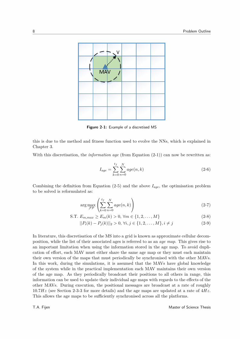
First, to reduce the computational complexity of the problem, it is solved in discrete time andthe MS is discretised into a 2-D grid, G(N). Each cell, g(n) |n ∈ {0, 1, . . . , N}, in this grid isthen assigned an age, age(n, k), which represents the time since the cell was last visited by aMAV. This age is defined by Equation (2-5), where ∆T is the discrete time step, Dist(n,m)is the distance between MAV m and the centre of the current cell and V is the radius of theMAVs camera footprint. This is shown visually in Figure 2-1. If the centre of a cell lies withinthe MAVs camera footprint, illustrated by the dotted line, then that cell is said to have beenvisited by a MAV and its age is reset to 100. This is indicated by the green cells in the image.
age(n, k) =
0 , k = 0max(0, age(n, k − 1)−∆T ) , Dist(n,m) > V
100 , Dist(n,m) ≤ V(2-5)
At first glance it may seem counter intuitive to have the age counting down from 100, whenthe definition of the persistent surveillance task is given as a minimisation problem. However,
Master of Science Thesis T.A. Fijen
8 Problem Outline
Figure 2-1: Example of a discretised MS
this is due to the method and fitness function used to evolve the NNs, which is explained inChapter 3.
With this discretisation, the information age (from Equation (2-1)) can now be rewritten as:
Iage =tf∑
k=0
N∑n=0
age(n, k) (2-6)
Combining the definition from Equation (2-5) and the above Iage, the optimisation problemto be solved is reformulated as:
arg maxFP
tf∑k=0
N∑n=0
age(n, k)
(2-7)
S.T. Em,max ≥ Em(k) > 0, ∀m ∈ {1, 2, . . . ,M} (2-8)||Pi(k)− Pj(k)||2 > 0, ∀i, j ∈ {1, 2, . . . ,M}, i 6= j (2-9)
In literature, this discretisation of the MS into a grid is known as approximate cellular decom-position, while the list of their associated ages is referred to as an age map. This gives rise toan important limitation when using the information stored in the age map. To avoid dupli-cation of effort, each MAV must either share the same age map or they must each maintaintheir own version of the maps that must periodically be synchronised with the other MAVs.In this work, during the simulations, it is assumed that the MAVs have global knowledgeof the system while in the practical implementation each MAV maintains their own versionof the age map. As they periodically broadcast their positions to all others in range, thisinformation can be used to update their individual age maps with regards to the effects of theother MAVs. During execution, the positional messages are broadcast at a rate of roughly10.7Hz (see Section 2-3-3 for more details) and the age maps are updated at a rate of 4Hz.This allows the age maps to be sufficiently synchronised across all the platforms.
T.A. Fijen Master of Science Thesis
2-2 Problem Analysis 9
Finally, as a reactive controller is used in this thesis instead of a global planner, it is notnecessary to determine the complete flight plan for the entire duration. All that is needed isthe MAVs position for the next time-step.
2-2 Problem Analysis
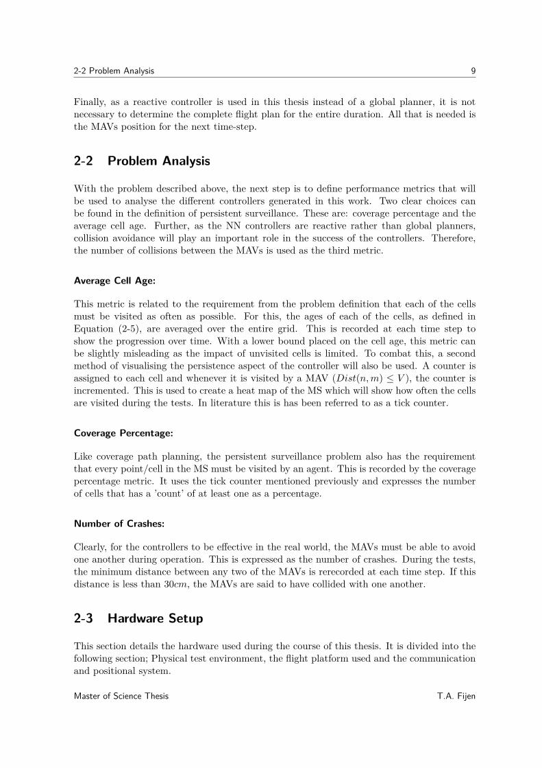
With the problem described above, the next step is to define performance metrics that willbe used to analyse the different controllers generated in this work. Two clear choices canbe found in the definition of persistent surveillance. These are: coverage percentage and theaverage cell age. Further, as the NN controllers are reactive rather than global planners,collision avoidance will play an important role in the success of the controllers. Therefore,the number of collisions between the MAVs is used as the third metric.
Average Cell Age:
This metric is related to the requirement from the problem definition that each of the cellsmust be visited as often as possible. For this, the ages of each of the cells, as defined inEquation (2-5), are averaged over the entire grid. This is recorded at each time step toshow the progression over time. With a lower bound placed on the cell age, this metric canbe slightly misleading as the impact of unvisited cells is limited. To combat this, a secondmethod of visualising the persistence aspect of the controller will also be used. A counter isassigned to each cell and whenever it is visited by a MAV (Dist(n,m) ≤ V ), the counter isincremented. This is used to create a heat map of the MS which will show how often the cellsare visited during the tests. In literature this is has been referred to as a tick counter.
Coverage Percentage:
Like coverage path planning, the persistent surveillance problem also has the requirementthat every point/cell in the MS must be visited by an agent. This is recorded by the coveragepercentage metric. It uses the tick counter mentioned previously and expresses the numberof cells that has a ’count’ of at least one as a percentage.
Number of Crashes:
Clearly, for the controllers to be effective in the real world, the MAVs must be able to avoidone another during operation. This is expressed as the number of crashes. During the tests,the minimum distance between any two of the MAVs is rerecorded at each time step. If thisdistance is less than 30cm, the MAVs are said to have collided with one another.
2-3 Hardware Setup
This section details the hardware used during the course of this thesis. It is divided into thefollowing section; Physical test environment, the flight platform used and the communicationand positional system.
Master of Science Thesis T.A. Fijen
10 Problem Outline
2-3-1 CyberZoo
The real-world testing was done in the CyberZoo of TU Delft. This is an enclosed, 10m ×10m× 7m research and test laboratory in the faculty of Aerospace Engineering. This area isequipped with a 12 camera OptiTrack system to provide accurate measurement of an objectsposition, velocity and heading through the use of reflective IR markers. These measurementsare used as ground truth data.
During the validation tests, the MAVs will operate within a 7m×7m flight area at an altitudeof 1m. As it is desired that the MAVs learn to stay within the boundary of the MS duringoperation, there is no high level controller that will force the MAVs to remain within the areaduring evolution of the NNs. However, during physical testing the MAVs will be required toland if they leave this MS to prevent them from colliding with the edges of the CyberZoo.
2-3-2 Parrot Bebop 2
The flight platform used during this work is the Parrot Bebop 2, which is controlled by thePaparazzi MAV software1 (v5.13). The Parrot Bebop 2 is a lightweight MAV equipped with anultrasound sensor to measure altitude, a 3-axis gyroscope, magnetometer and accelerometer,a front facing (14 mega-pixel fish-eye lens) camera and a bottom camera [56, 57]. In additionit is equipped with an ARM Cortex-A9 processor, a low-tier GPU and 8 GB of flash memory.
As mentioned, the existing, pre-installed autopilot software was overwritten and replaced withPaparazzi. This is an open-source autopilot software developed for hobby and professionaluse, [58]. For the inner-loop controller of the MAV, an existing controller from Paparazziwas used as this was considered beyond the scope of this project. This controller used thefollowing input variables: the commanded x and y velocities (in the North, East, Downcoordinate frame), the flight altitude and the heading.
Simplified MAV Dynamical Model
A core component of this work is the evolution of the NN that will control the MAVs. Nat-urally, this evolution cannot be done on the actual flight platform as this would damage theMAVs. Therefore, an accurate model of the dynamics of the MAV is needed for the simula-tion environment. At the same time, a simplified model is desirable as this will decrease thecomputational complexity of the simulation, thereby reducing the time needed to perform anevolutionary run. With this in mind, the model used by Szabo in [59] was implemented asthis was shown to be applicable for an Evolutionary Algorithm (EA).
The dynamics for this platform have six degrees of freedom which relates to the translationand rotation along the three axis of the MAV. This is combined with four inputs representingthe rotational speeds of the four motors which gives a nonlinear dynamic model. A decoupledlinear system can provide a reasonable approximation of the platform under normal flightconditions, [59]. This models the dynamics of the MAV together with the inner-loop control.The approximation used in this work is a linear, 2nd order velocity model in the X and Y
1Freely available from: https://github.com/paparazzi/paparazzi
T.A. Fijen Master of Science Thesis
2-3 Hardware Setup 11
directions, with no axis coupling [59]. This is given in Equation (2-10). As the MAVs willonly operate in a 2-D plane, the altitude state was not included in the model.
...XX...YY
X
Y
=
−2ζω −ω2 0 0 0 01 0 0 0 0 00 0 −2ζω −ω2 0 00 0 1 0 0 00 1 0 0 0 00 0 0 1 0 0
X
X
Y
YXY
+
ω2 00 00 ω2
0 00 00 0
[vx
vy
](2-10)
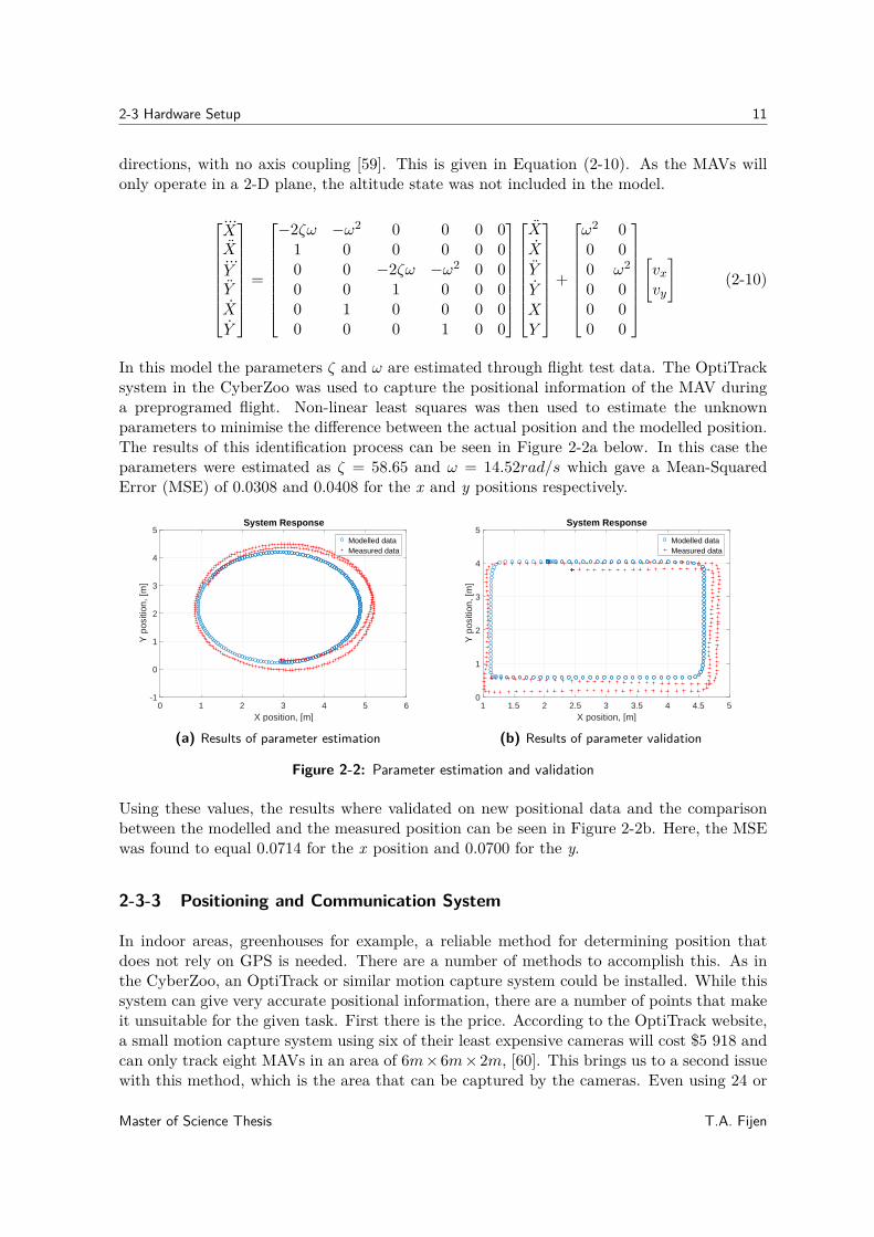
In this model the parameters ζ and ω are estimated through flight test data. The OptiTracksystem in the CyberZoo was used to capture the positional information of the MAV duringa preprogramed flight. Non-linear least squares was then used to estimate the unknownparameters to minimise the difference between the actual position and the modelled position.The results of this identification process can be seen in Figure 2-2a below. In this case theparameters were estimated as ζ = 58.65 and ω = 14.52rad/s which gave a Mean-SquaredError (MSE) of 0.0308 and 0.0408 for the x and y positions respectively.
0 1 2 3 4 5 6X position, [m]
-1
0
1
2
3
4
5
Y p
ositi
on, [
m]
System Response
Modelled dataMeasured data
(a) Results of parameter estimation
1 1.5 2 2.5 3 3.5 4 4.5 5X position, [m]
0
1
2
3
4
5
Y p
ositi
on, [
m]
System Response
Modelled dataMeasured data
(b) Results of parameter validation
Figure 2-2: Parameter estimation and validation
Using these values, the results where validated on new positional data and the comparisonbetween the modelled and the measured position can be seen in Figure 2-2b. Here, the MSEwas found to equal 0.0714 for the x position and 0.0700 for the y.
2-3-3 Positioning and Communication System
In indoor areas, greenhouses for example, a reliable method for determining position thatdoes not rely on GPS is needed. There are a number of methods to accomplish this. As inthe CyberZoo, an OptiTrack or similar motion capture system could be installed. While thissystem can give very accurate positional information, there are a number of points that makeit unsuitable for the given task. First there is the price. According to the OptiTrack website,a small motion capture system using six of their least expensive cameras will cost $5 918 andcan only track eight MAVs in an area of 6m×6m×2m, [60]. This brings us to a second issuewith this method, which is the area that can be captured by the cameras. Even using 24 or
Master of Science Thesis T.A. Fijen
12 Problem Outline
their most advanced cameras, this capture area is only 15m × 15m × 6m (and will cost you$147 849) [60]. As a result of these drawbacks, this method was not considered as a viablealternative to GPS.
Next, Simultaneous Localization and Mapping (SLAM) was considered. This would allowthe MAV to use its sensor readings to create a map of the environment while at the same tolocalise itself within that map [61]. The SLAM problem can be implemented using a widearray of sensors, such as LiDAR, laser range finders, vision and RGBD cameras. However,many of these are not applicable for use on small MAVs due to their limited payload andpower supply [62]. As a result, the authors of [62] proposed that the best sensor for MAVbased SLAM is a single camera. Recently, real-time monocular SLAM has gained popularityas a result of their use in robotics, [62, 63], but there are still some drawbacks. This methodis very sensitive to photometric changes, the captured image must contain varying texturesand depths, and pure rotational motion causes tracking failures [62, 63].
In the end, position estimation through the use of Two Way Ranging (TWR) and multilatera-tion was chosen. This can be achieved through the use of a system of Ultra-wideband (UWB)transceivers. These small, lightweight modules have a communication range of up to 300m,they can achieve a positional accuracy of 10cm in an indoor environment and they have alow power consumption [64]. As an added benefit, these modules can be used for inter-MAVcommunication as well as for localisation, reducing the number of sensors needed on the flightplatform. Finally, the module are also inexpensive, with a single module costing roughly$262. For these reasons, the UWB localisation system was selected over a monocular SLAMapproach. For UWB localisation, a system of anchors and tags are used. Here, anchors (orbeacons) are UWB modules that are placed at four known locations throughout the missionspace while the tags are mobile nodes that are placed on the MAVs. The four distancesbetween the tag and each of the anchors can then be used to calculate the current positionof the MAV. This will be explained in more detail in the next subsection.
Position Estimation
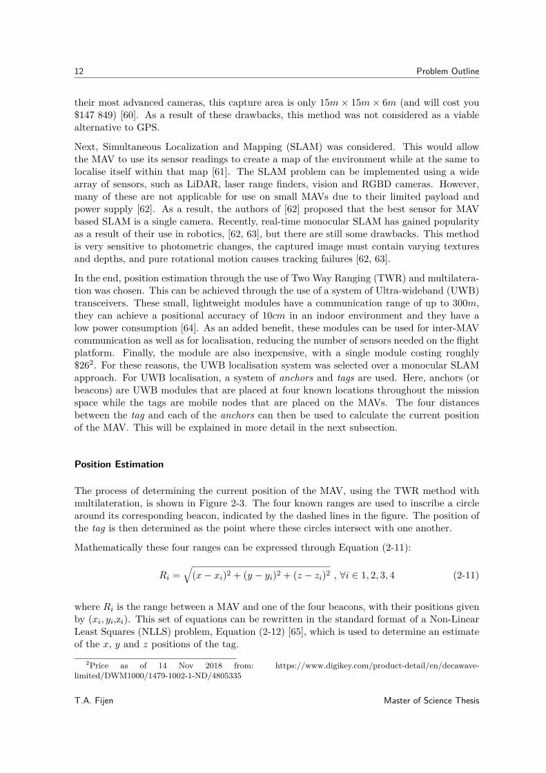
The process of determining the current position of the MAV, using the TWR method withmultilateration, is shown in Figure 2-3. The four known ranges are used to inscribe a circlearound its corresponding beacon, indicated by the dashed lines in the figure. The position ofthe tag is then determined as the point where these circles intersect with one another.
Mathematically these four ranges can be expressed through Equation (2-11):
Ri =√
(x− xi)2 + (y − yi)2 + (z − zi)2 , ∀i ∈ 1, 2, 3, 4 (2-11)
where Ri is the range between a MAV and one of the four beacons, with their positions givenby (xi, yi,zi). This set of equations can be rewritten in the standard format of a Non-LinearLeast Squares (NLLS) problem, Equation (2-12) [65], which is used to determine an estimateof the x, y and z positions of the tag.
2Price as of 14 Nov 2018 from: https://www.digikey.com/product-detail/en/decawave-limited/DWM1000/1479-1002-1-ND/4805335
T.A. Fijen Master of Science Thesis
2-3 Hardware Setup 13
Figure 2-3: Schematic description of 2-D multilateration
minX||e(X)||22 = min
X
4∑i=1
e2i (X) = min
x,y,z
4∑i=1
(Ri −
√(x− xi)2 + (y − yi)2 + (z − zi)2
)2(2-12)
In the above equation, e(X) is the error vector and is given by
e(X) =[e1(X) e2(X) · · · e4(X)
]T(2-13)
When the initial estimate of the position is near the optimum, the Hessian of the functionthat is minimised, H(Xk), can be approximated by Equation (2-14) [66].
H(Xk) = 2∇e(Xk)e(Xk) (2-14)
where ∇e(Xk) is the Jacobian of e(Xk). When updating the current position of the MAV,its previous position is used as the initial starting point for the new least squares problem.This ensures that the above approximation will hold as the update rate is fast enough andthe MAV speed is slow enough that there will not be a large jump in the position betweenupdates. Now, through the use of Equation (2-14), the NLLS problem can be solved throughthe Gauss-Newton algorithm shown in Equation (2-15).
Xk+1 = Xk −(∇e(Xk)∇T e(Xk)
)−1∇e(Xk)e(Xk) (2-15)
As this is an iterative process that will not provide the optimal solution within a finitenumber of steps, relevant stopping criteria are needed. In this work the following was used:||Xk+1 − Xk||2 < 0.01 along with an upper bound placed on the number of iterations of 20iterations.
Master of Science Thesis T.A. Fijen
14 Problem Outline
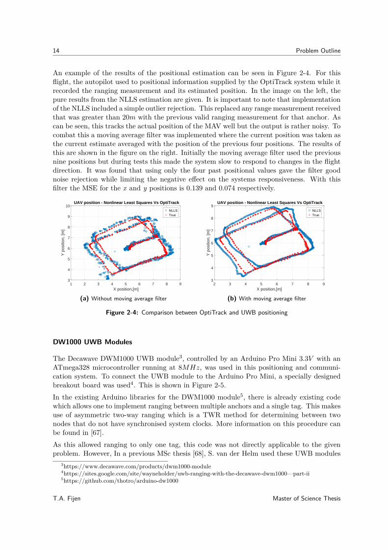
An example of the results of the positional estimation can be seen in Figure 2-4. For thisflight, the autopilot used to positional information supplied by the OptiTrack system while itrecorded the ranging measurement and its estimated position. In the image on the left, thepure results from the NLLS estimation are given. It is important to note that implementationof the NLLS included a simple outlier rejection. This replaced any range measurement receivedthat was greater than 20m with the previous valid ranging measurement for that anchor. Ascan be seen, this tracks the actual position of the MAV well but the output is rather noisy. Tocombat this a moving average filter was implemented where the current position was taken asthe current estimate averaged with the position of the previous four positions. The results ofthis are shown in the figure on the right. Initially the moving average filter used the previousnine positions but during tests this made the system slow to respond to changes in the flightdirection. It was found that using only the four past positional values gave the filter goodnoise rejection while limiting the negative effect on the systems responsiveness. With thisfilter the MSE for the x and y positions is 0.139 and 0.074 respectively.
1 2 3 4 5 6 7 8 9X position,[m]
3
4
5
6
7
8
9
10
Y p
ositi
on, [
m]
UAV position - Nonlinear Least Squares Vs OptiTrack
NLLSTrue
(a) Without moving average filter
2 3 4 5 6 7 8 9X position,[m]
3
4
5
6
7
8
9Y
pos
ition
, [m
]UAV position - Nonlinear Least Squares Vs OptiTrack
NLLSTrue
(b) With moving average filter
Figure 2-4: Comparison between OptiTrack and UWB positioning
DW1000 UWB Modules
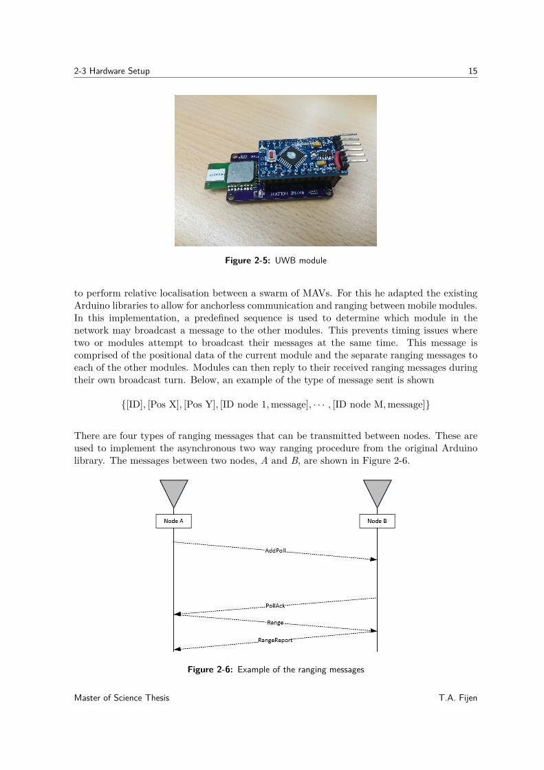
The Decawave DWM1000 UWB module3, controlled by an Arduino Pro Mini 3.3V with anATmega328 microcontroller running at 8MHz, was used in this positioning and communi-cation system. To connect the UWB module to the Arduino Pro Mini, a specially designedbreakout board was used4. This is shown in Figure 2-5.In the existing Arduino libraries for the DWM1000 module5, there is already existing codewhich allows one to implement ranging between multiple anchors and a single tag. This makesuse of asymmetric two-way ranging which is a TWR method for determining between twonodes that do not have synchronised system clocks. More information on this procedure canbe found in [67].As this allowed ranging to only one tag, this code was not directly applicable to the givenproblem. However, In a previous MSc thesis [68], S. van der Helm used these UWB modules
3https://www.decawave.com/products/dwm1000-module4https://sites.google.com/site/wayneholder/uwb-ranging-with-the-decawave-dwm1000—part-ii5https://github.com/thotro/arduino-dw1000
T.A. Fijen Master of Science Thesis
2-3 Hardware Setup 15
Figure 2-5: UWB module
to perform relative localisation between a swarm of MAVs. For this he adapted the existingArduino libraries to allow for anchorless communication and ranging between mobile modules.In this implementation, a predefined sequence is used to determine which module in thenetwork may broadcast a message to the other modules. This prevents timing issues wheretwo or modules attempt to broadcast their messages at the same time. This message iscomprised of the positional data of the current module and the separate ranging messages toeach of the other modules. Modules can then reply to their received ranging messages duringtheir own broadcast turn. Below, an example of the type of message sent is shown
{[ID], [Pos X], [Pos Y], [ID node 1,message], · · · , [ID node M,message]}
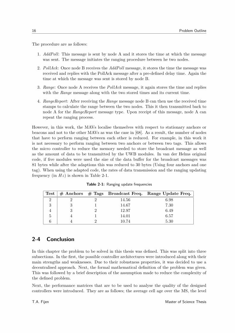
There are four types of ranging messages that can be transmitted between nodes. These areused to implement the asynchronous two way ranging procedure from the original Arduinolibrary. The messages between two nodes, A and B, are shown in Figure 2-6.
Figure 2-6: Example of the ranging messages
Master of Science Thesis T.A. Fijen
16 Problem Outline
The procedure are as follows:
1. AddPoll: This message is sent by node A and it stores the time at which the messagewas sent. The message initiates the ranging procedure between he two nodes.
2. PollAck: Once node B receives the AddPoll message, it stores the time the message wasreceived and replies with the PollAck message after a pre-defined delay time. Again thetime at which the message was sent is stored by node B.
3. Range: Once node A receives the PollAck message, it again stores the time and replieswith the Range message along with the two stored times and its current time.
4. RangeReport: After receiving the Range message node B can then use the received timestamps to calculate the range between the two nodes. This it then transmitted back tonode A for the RangeReport message type. Upon receipt of this message, node A canrepeat the ranging process.
However, in this work, the MAVs localise themselves with respect to stationary anchors orbeacons and not to the other MAVs as was the case in [68]. As a result, the number of nodesthat have to perform ranging between each other is reduced. For example, in this work itis not necessary to perform ranging between two anchors or between two tags. This allowsthe micro controller to reduce the memory needed to store the broadcast message as wellas the amount of data to be transmitted by the UWB modules. In van der Helms originalcode, if five modules were used the size of the data buffer for the broadcast messages was81 bytes while after the adaptions this was reduced to 30 bytes (Using four anchors and onetag). When using the adapted code, the rates of data transmission and the ranging updatingfrequency (in Hz) is shown in Table 2-1.
Table 2-1: Ranging update frequencies
Test # Anchors # Tags Broadcast Freq. Range Update Freq.2 2 2 14.56 6.983 3 1 14.67 7.304 3 2 12.97 6.495 4 1 14.01 6.576 4 2 10.74 5.30
2-4 Conclusion
In this chapter the problem to be solved in this thesis was defined. This was split into threesubsections. In the first, the possible controller architectures were introduced along with theirmain strengths and weaknesses. Due to their robustness properties, it was decided to use adecentralised approach. Next, the formal mathematical definition of the problem was given.This was followed by a brief description of the assumption made to reduce the complexity ofthe defined problem.Next, the performance matrices that are to be used to analyse the quality of the designedcontrollers were introduced. They are as follows; the average cell age over the MS, the level
T.A. Fijen Master of Science Thesis

2-4 Conclusion 17
of coverage over the MS that is achieved and lastly the controllers ability to avoid collisionsis represented by the number of crashes metric.
In the remainder of this chapter, the hardware used throughout the thesis was given. The testswill be performed in the CyberZoo using the Parrot Bebop 2 MAV. Inter-MAV communica-tions will rely on the Decawave UWB modules. This will allow the MAVs to broadcast theircurrent positions to all other MAVs in the MS. The UWB modules also serve another pur-pose, they are used to perform ranging to four stationary nodes (anchors) placed throughoutthe MS. This will allow the MAVs to localise themselves with respect to the anchors.
With the definitions given in this chapter, we can now move onto the method for creating theNN controllers.
Master of Science Thesis T.A. Fijen

18 Problem Outline
T.A. Fijen Master of Science Thesis
Chapter 3
The NEAT Algorithm
This section describes the evolutionary approach used to create the NNs used to control theindividual drones. This relied upon the Neuro Evolution of Augmenting Topologies (NEAT)algorithm first presented in [1]. This is a method for evolving not only the weights of a NNbut also its structure to find a good balance between the fitness and the diversity of thesolution.Due to the nature of the persistent surveillance task, a training data set cannot be generated.As a result of this, methods that rely on optimising the connection weights of the NN, likeback-propagation, are not applicable. To overcome this shortcoming, the training processmust rely on finding an (near) optimal set that is defined by a fitness function. Using thisview point, GAs can be used to train evolved NNs effectively [69]. Traditionally, GAs areused to evolve only the connection weighs for an existing NN structure, however, they can beused to evolve the structure as well as the weights of the connections [1].A key reason for selecting a method that evolves the structure as well as the weight is toeliminate the expert knowledge and trial-and-error based approaches to formulating the NNstopology. In his paper, [1], Stanley showed that his NEAT method also resulted in increasedperformance and was able to generate an effective solution five times faster than a fixed-topology method like Enforced Sub Populations. Lastly, the NEAT algorithm is well suitedto escape from local minimum which can trap fixed-topology methods as the NEAT algorithmcan add additional structure to its topology [1].The basic steps for the NEAT algorithm are outlined below, but a more detailed explanationcan be found in [1, 70].
3-1 NEAT Background
3-1-1 Encoding Scheme
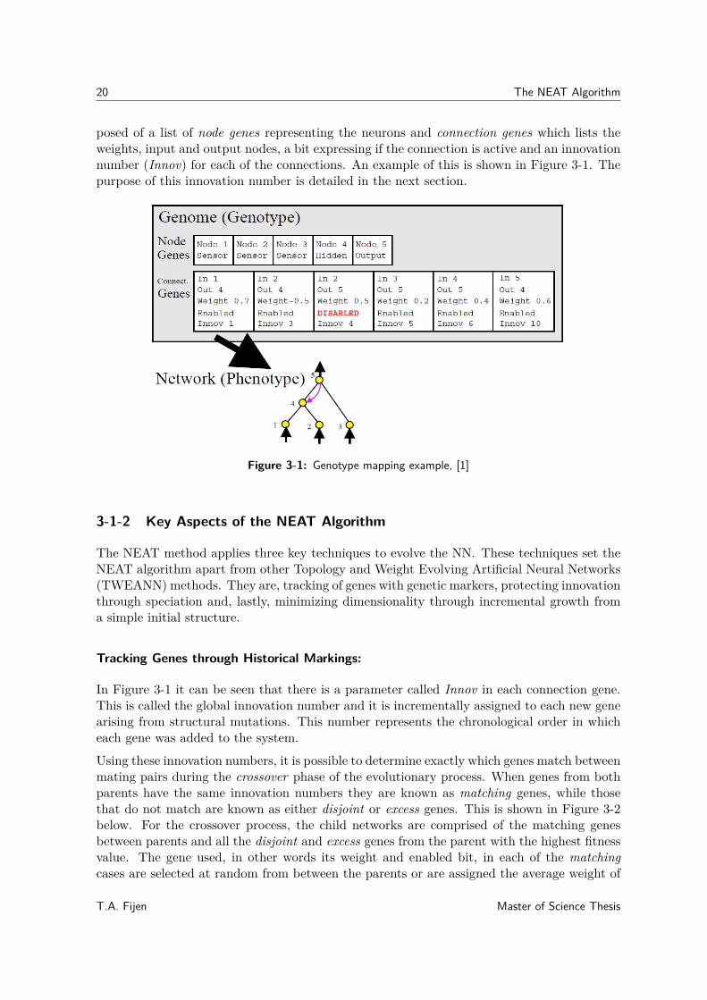
The genetic encoding scheme used in the NEAT translates the structure of the NN intogenomes, which are linear representations of the network connectivity. Each genome is com-
Master of Science Thesis T.A. Fijen
20 The NEAT Algorithm
posed of a list of node genes representing the neurons and connection genes which lists theweights, input and output nodes, a bit expressing if the connection is active and an innovationnumber (Innov) for each of the connections. An example of this is shown in Figure 3-1. Thepurpose of this innovation number is detailed in the next section.
Figure 3-1: Genotype mapping example, [1]
3-1-2 Key Aspects of the NEAT Algorithm
The NEAT method applies three key techniques to evolve the NN. These techniques set theNEAT algorithm apart from other Topology and Weight Evolving Artificial Neural Networks(TWEANN) methods. They are, tracking of genes with genetic markers, protecting innovationthrough speciation and, lastly, minimizing dimensionality through incremental growth froma simple initial structure.
Tracking Genes through Historical Markings:
In Figure 3-1 it can be seen that there is a parameter called Innov in each connection gene.This is called the global innovation number and it is incrementally assigned to each new genearising from structural mutations. This number represents the chronological order in whicheach gene was added to the system.
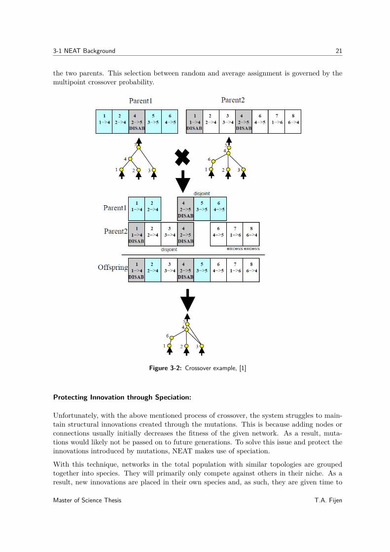
Using these innovation numbers, it is possible to determine exactly which genes match betweenmating pairs during the crossover phase of the evolutionary process. When genes from bothparents have the same innovation numbers they are known as matching genes, while thosethat do not match are known as either disjoint or excess genes. This is shown in Figure 3-2below. For the crossover process, the child networks are comprised of the matching genesbetween parents and all the disjoint and excess genes from the parent with the highest fitnessvalue. The gene used, in other words its weight and enabled bit, in each of the matchingcases are selected at random from between the parents or are assigned the average weight of
T.A. Fijen Master of Science Thesis
3-1 NEAT Background 21
the two parents. This selection between random and average assignment is governed by themultipoint crossover probability.
Figure 3-2: Crossover example, [1]
Protecting Innovation through Speciation:
Unfortunately, with the above mentioned process of crossover, the system struggles to main-tain structural innovations created through the mutations. This is because adding nodes orconnections usually initially decreases the fitness of the given network. As a result, muta-tions would likely not be passed on to future generations. To solve this issue and protect theinnovations introduced by mutations, NEAT makes use of speciation.
With this technique, networks in the total population with similar topologies are groupedtogether into species. They will primarily only compete against others in their niche. As aresult, new innovations are placed in their own species and, as such, they are given time to
Master of Science Thesis T.A. Fijen
22 The NEAT Algorithm
optimise their structure before competing with others. During each generation, every networkis sequentially placed into a species through the use of a compatibility distance, δ(i, j). Here,each existing species is represented by a random network from its previous generation andthe δ(i, j), for the given network from the current generation, is calculated according toEquation (3-1). In this equation, Egene and Dgene are used to represent the number of excessand disjoint genes respectively, Wgene is the average weight differences of matching genes andNgene is the number of genes in the larger network. Lastly, the parameters ci (∀i ∈ 1, 2, 3) areweighting factors that influence the impact of the Egene, Dgene and Wgene on the speciationcompatibility distance. If this distance is less than a compatibility threshold, δt, the currentnetwork is placed in that species, otherwise it is compared to the representative for the nextspecies. If it is not placed in any existing species, a new species is created with the currentnetwork as its representative.
δ(i, j) = c1Egene
Ngene+ c2Dgene
Ngene+ c3 · Wgene (3-1)
With the population divided into species, explicit fitness sharing is used as the reproductionmechanism. Here, networks in each species share the fitness value for their niche. Thisprevents any one species from completely taking over the entire population. The adjustedfitness, f ′
i , is calculated as:
f′i = fi∑Npop
j=1 sh(δ(i, j))(3-2)
where
sh(δ(i, j)) ={
0 , δ(i, j) > δt
1 , otherwise(3-3)
and Npop is the number of NN in the total population. Each species then produces a numberof children for the next generation, which is proportional to the sum of the f ′
i of its membernetworks.
Minimizing Dimensionality through Incremental Growth from a Simple Initial Structure:
The NEAT method biases the resulting controller towards a minimal-dimensional space. Thisis done by staring out with a uniform network configuration with no neurons in the hiddenlayer. This means that each input is directly connected to each of the outputs. New structures(i.e. hidden layers) are introduced incrementally through mutations, where only the usefulmutations survive.
3-1-3 Mutations
A further component of the NEAT algorithm are the mutations applied to the child networksto create the new population. There are two main types of mutations that can be applied tothe networks. The first is a mutation of the connection weights where each of the connectionsare either perturbed or not based on a predefined probability. These perturbations can changethe weight of the connection (governed by the weight mutation probability) or whether theconnection is enabled or disabled (Gene re-enable probability).
T.A. Fijen Master of Science Thesis
3-2 Implementation 23
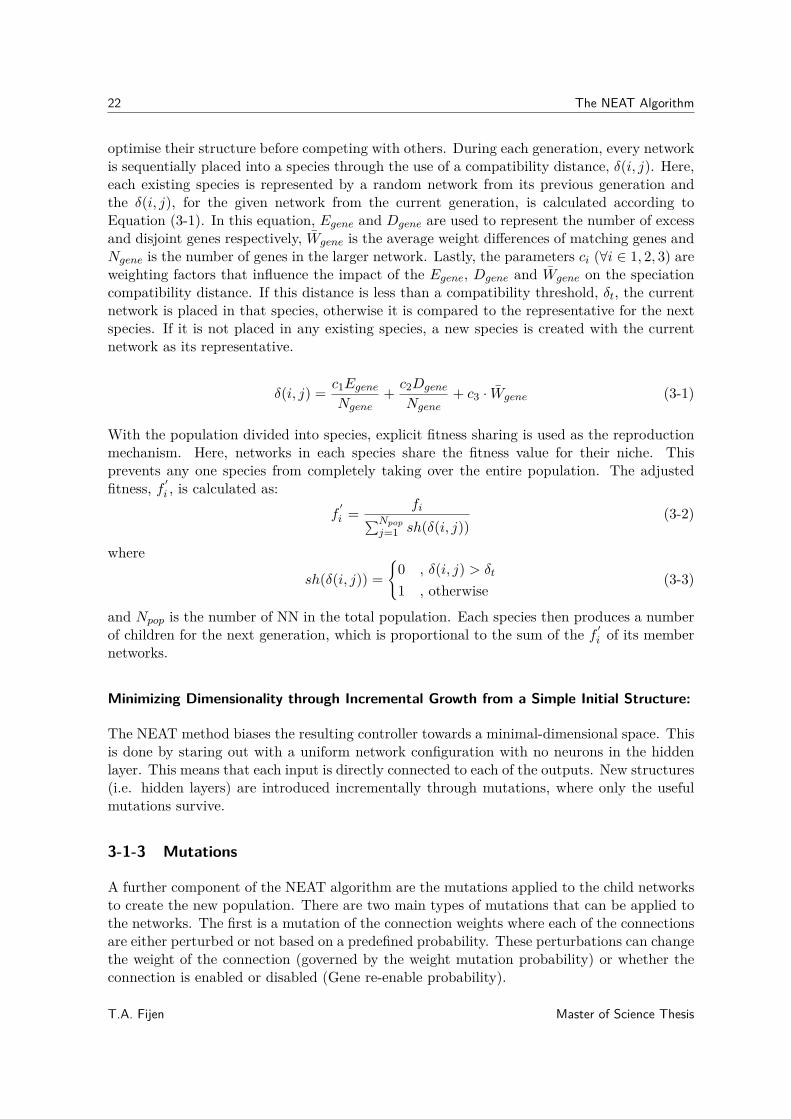
The second type of mutation is a structural mutation. This can be further divided intotwo subtypes namely; ’add connection’ or ’add node’. In ’add connection’, a new connectionbetween two previously unconnected nodes is added, with a random weight. For the ’add node’subtype, a new node is inserted into an existing connection. Here, the original connectionis set to disabled and two new connections are added, one entering the new node, which isassigned a weight of 1, and the other leaves the node with a weight equal to that of theoriginal connection. Examples of these two mutation types can be seen in Figure 3-3.
(a) Example of ’add connection’ mutation (b) Example of ’add node’ mutation
Figure 3-3: Mutation examples
3-2 Implementation
In this section, details are given for the specific implementation of the NEAT algorithm forthe problem given in Section 2-1. For this, the MATLAB version of Kenneth Stanley’s NEATalgorithm was used 1. The evolutionary process was implemented using MathWorks MATLABR2016b 64-bit running on a workstation with an Intel(R) Core i7-4700MQ CPU (2.4GHz),8 GB of RAM and a Windows 8.1 64-bit operating system.
3-2-1 Fitness Function
A key component to Evolutionary Robotics (ER) is the fitness function, f . This is the meansby which the solver determines which solutions are more capable of solving the given problem[71]. This is often the limiting factor in the quality of the generated solutions when evolvingcontrollers for complex tasks, [71].
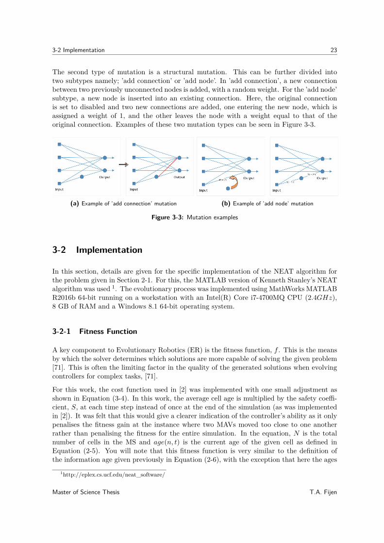
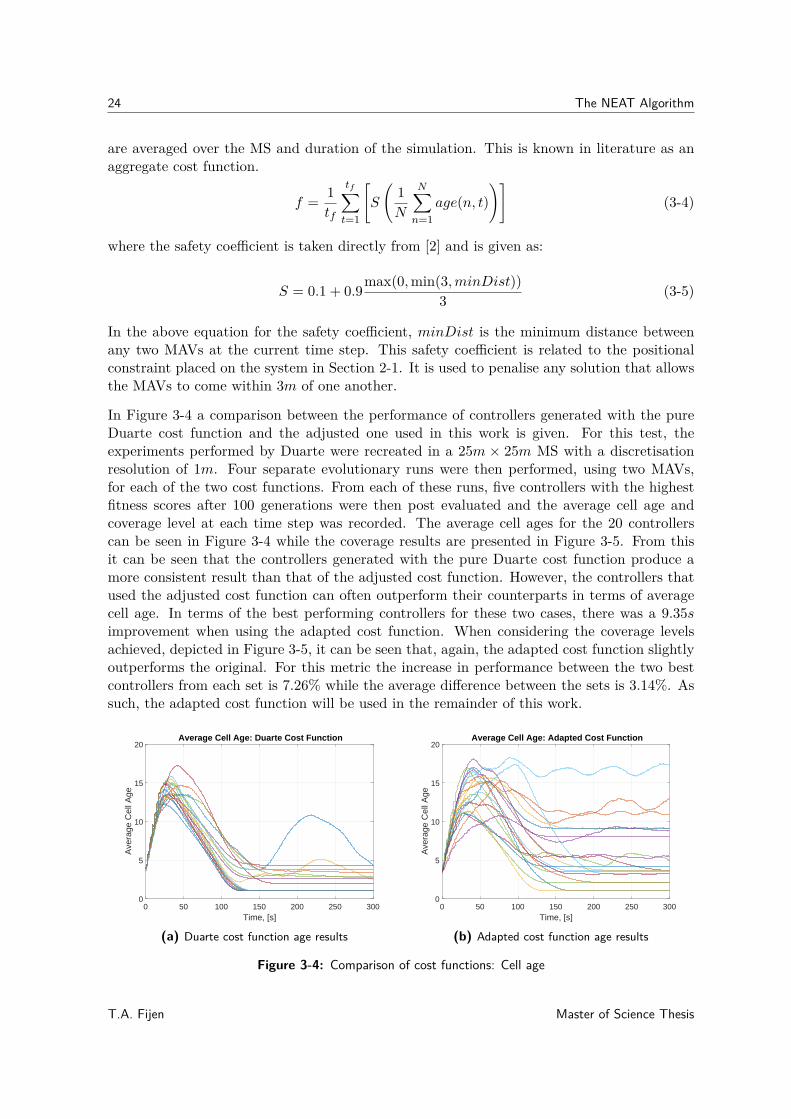
For this work, the cost function used in [2] was implemented with one small adjustment asshown in Equation (3-4). In this work, the average cell age is multiplied by the safety coeffi-cient, S, at each time step instead of once at the end of the simulation (as was implementedin [2]). It was felt that this would give a clearer indication of the controller’s ability as it onlypenalises the fitness gain at the instance where two MAVs moved too close to one anotherrather than penalising the fitness for the entire simulation. In the equation, N is the totalnumber of cells in the MS and age(n, t) is the current age of the given cell as defined inEquation (2-5). You will note that this fitness function is very similar to the definition ofthe information age given previously in Equation (2-6), with the exception that here the ages
1http://eplex.cs.ucf.edu/neat_software/
Master of Science Thesis T.A. Fijen
24 The NEAT Algorithm
are averaged over the MS and duration of the simulation. This is known in literature as anaggregate cost function.
f = 1tf
tf∑t=1
[S
(1N
N∑n=1
age(n, t))]
(3-4)
where the safety coefficient is taken directly from [2] and is given as:
S = 0.1 + 0.9max(0,min(3,minDist))3 (3-5)
In the above equation for the safety coefficient, minDist is the minimum distance betweenany two MAVs at the current time step. This safety coefficient is related to the positionalconstraint placed on the system in Section 2-1. It is used to penalise any solution that allowsthe MAVs to come within 3m of one another.
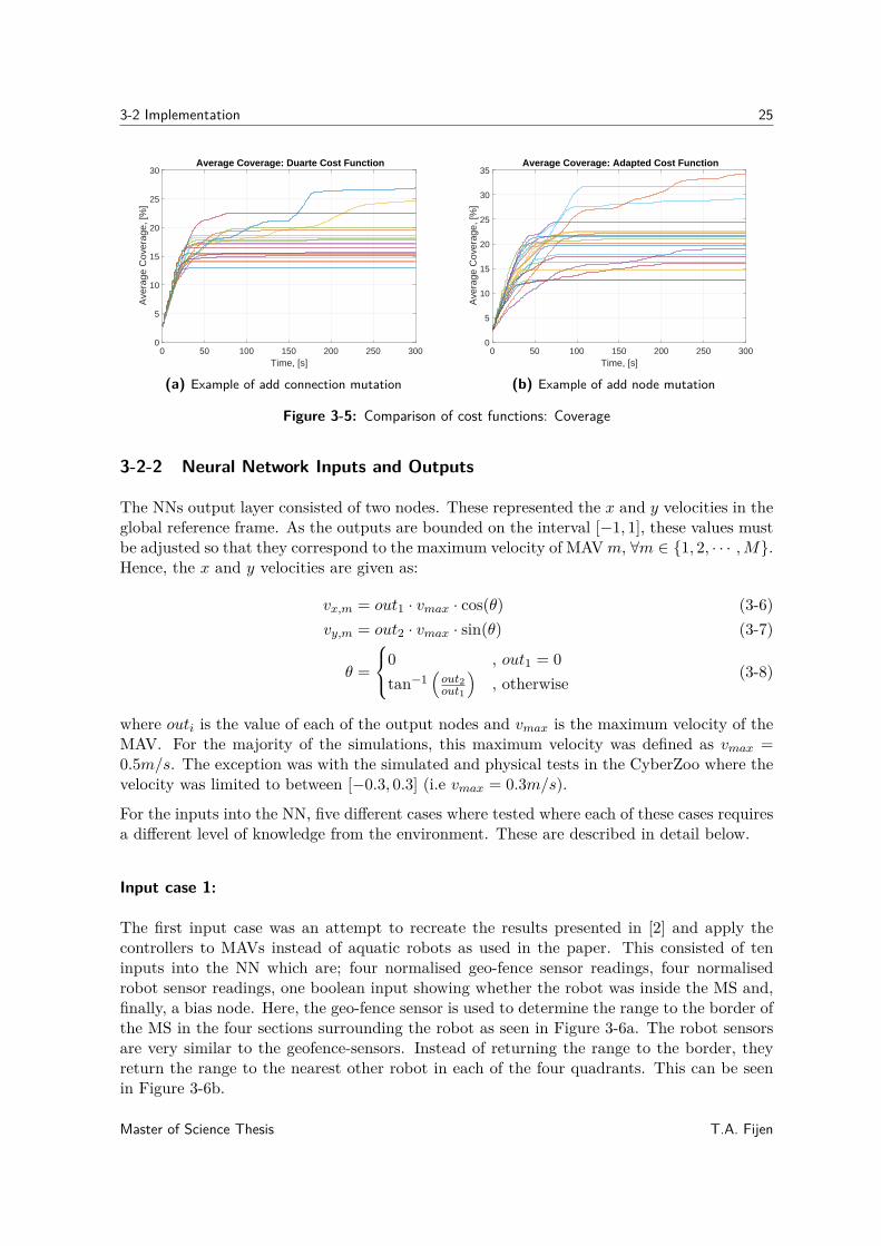
In Figure 3-4 a comparison between the performance of controllers generated with the pureDuarte cost function and the adjusted one used in this work is given. For this test, theexperiments performed by Duarte were recreated in a 25m × 25m MS with a discretisationresolution of 1m. Four separate evolutionary runs were then performed, using two MAVs,for each of the two cost functions. From each of these runs, five controllers with the highestfitness scores after 100 generations were then post evaluated and the average cell age andcoverage level at each time step was recorded. The average cell ages for the 20 controllerscan be seen in Figure 3-4 while the coverage results are presented in Figure 3-5. From thisit can be seen that the controllers generated with the pure Duarte cost function produce amore consistent result than that of the adjusted cost function. However, the controllers thatused the adjusted cost function can often outperform their counterparts in terms of averagecell age. In terms of the best performing controllers for these two cases, there was a 9.35simprovement when using the adapted cost function. When considering the coverage levelsachieved, depicted in Figure 3-5, it can be seen that, again, the adapted cost function slightlyoutperforms the original. For this metric the increase in performance between the two bestcontrollers from each set is 7.26% while the average difference between the sets is 3.14%. Assuch, the adapted cost function will be used in the remainder of this work.
0 50 100 150 200 250 300Time, [s]
0
5
10
15
20
Ave
rage
Cel
l Age
Average Cell Age: Duarte Cost Function
(a) Duarte cost function age results
0 50 100 150 200 250 300Time, [s]
0
5
10
15
20
Ave
rage
Cel
l Age
Average Cell Age: Adapted Cost Function
(b) Adapted cost function age results
Figure 3-4: Comparison of cost functions: Cell age
T.A. Fijen Master of Science Thesis
3-2 Implementation 25
0 50 100 150 200 250 300Time, [s]
0
5
10
15
20
25
30
Ave
rage
Cov
erag
e, [%
]
Average Coverage: Duarte Cost Function
(a) Example of add connection mutation
0 50 100 150 200 250 300Time, [s]
0
5
10
15
20
25
30
35
Ave
rage
Cov
erag
e, [%
]
Average Coverage: Adapted Cost Function
(b) Example of add node mutation
Figure 3-5: Comparison of cost functions: Coverage
3-2-2 Neural Network Inputs and Outputs
The NNs output layer consisted of two nodes. These represented the x and y velocities in theglobal reference frame. As the outputs are bounded on the interval [−1, 1], these values mustbe adjusted so that they correspond to the maximum velocity of MAVm, ∀m ∈ {1, 2, · · · ,M}.Hence, the x and y velocities are given as:
vx,m = out1 · vmax · cos(θ) (3-6)vy,m = out2 · vmax · sin(θ) (3-7)
θ =
0 , out1 = 0tan−1
(out2out1
), otherwise
(3-8)
where outi is the value of each of the output nodes and vmax is the maximum velocity of theMAV. For the majority of the simulations, this maximum velocity was defined as vmax =0.5m/s. The exception was with the simulated and physical tests in the CyberZoo where thevelocity was limited to between [−0.3, 0.3] (i.e vmax = 0.3m/s).
For the inputs into the NN, five different cases where tested where each of these cases requiresa different level of knowledge from the environment. These are described in detail below.
Input case 1:
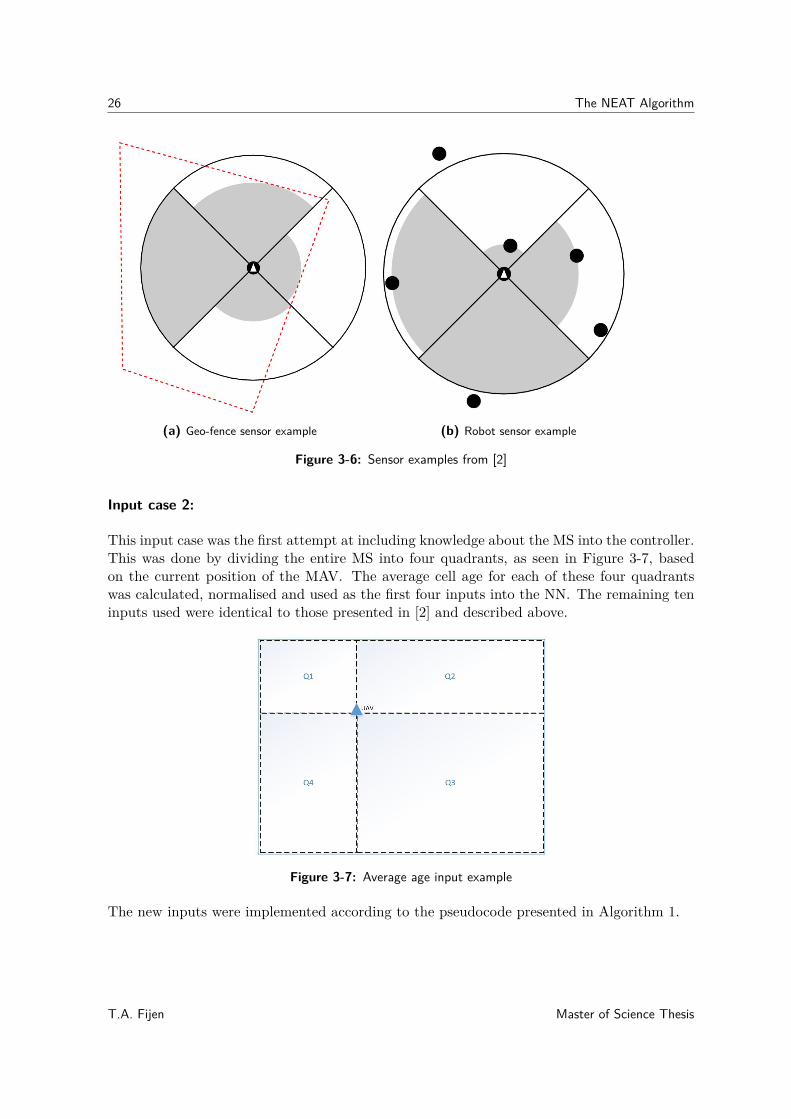
The first input case was an attempt to recreate the results presented in [2] and apply thecontrollers to MAVs instead of aquatic robots as used in the paper. This consisted of teninputs into the NN which are; four normalised geo-fence sensor readings, four normalisedrobot sensor readings, one boolean input showing whether the robot was inside the MS and,finally, a bias node. Here, the geo-fence sensor is used to determine the range to the border ofthe MS in the four sections surrounding the robot as seen in Figure 3-6a. The robot sensorsare very similar to the geofence-sensors. Instead of returning the range to the border, theyreturn the range to the nearest other robot in each of the four quadrants. This can be seenin Figure 3-6b.
Master of Science Thesis T.A. Fijen
26 The NEAT Algorithm
(a) Geo-fence sensor example (b) Robot sensor example
Figure 3-6: Sensor examples from [2]
Input case 2:
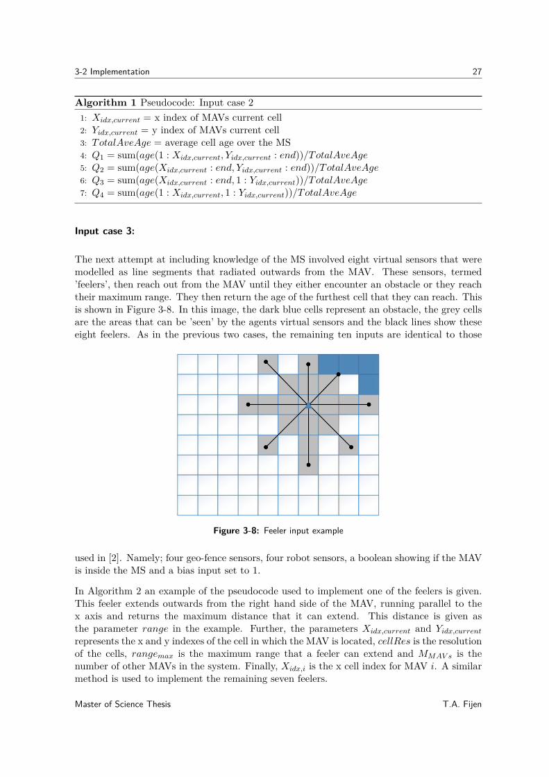
This input case was the first attempt at including knowledge about the MS into the controller.This was done by dividing the entire MS into four quadrants, as seen in Figure 3-7, basedon the current position of the MAV. The average cell age for each of these four quadrantswas calculated, normalised and used as the first four inputs into the NN. The remaining teninputs used were identical to those presented in [2] and described above.
Figure 3-7: Average age input example
The new inputs were implemented according to the pseudocode presented in Algorithm 1.
T.A. Fijen Master of Science Thesis
3-2 Implementation 27
Algorithm 1 Pseudocode: Input case 21: Xidx,current = x index of MAVs current cell2: Yidx,current = y index of MAVs current cell3: TotalAveAge = average cell age over the MS4: Q1 = sum(age(1 : Xidx,current, Yidx,current : end))/TotalAveAge5: Q2 = sum(age(Xidx,current : end, Yidx,current : end))/TotalAveAge6: Q3 = sum(age(Xidx,current : end, 1 : Yidx,current))/TotalAveAge7: Q4 = sum(age(1 : Xidx,current, 1 : Yidx,current))/TotalAveAge
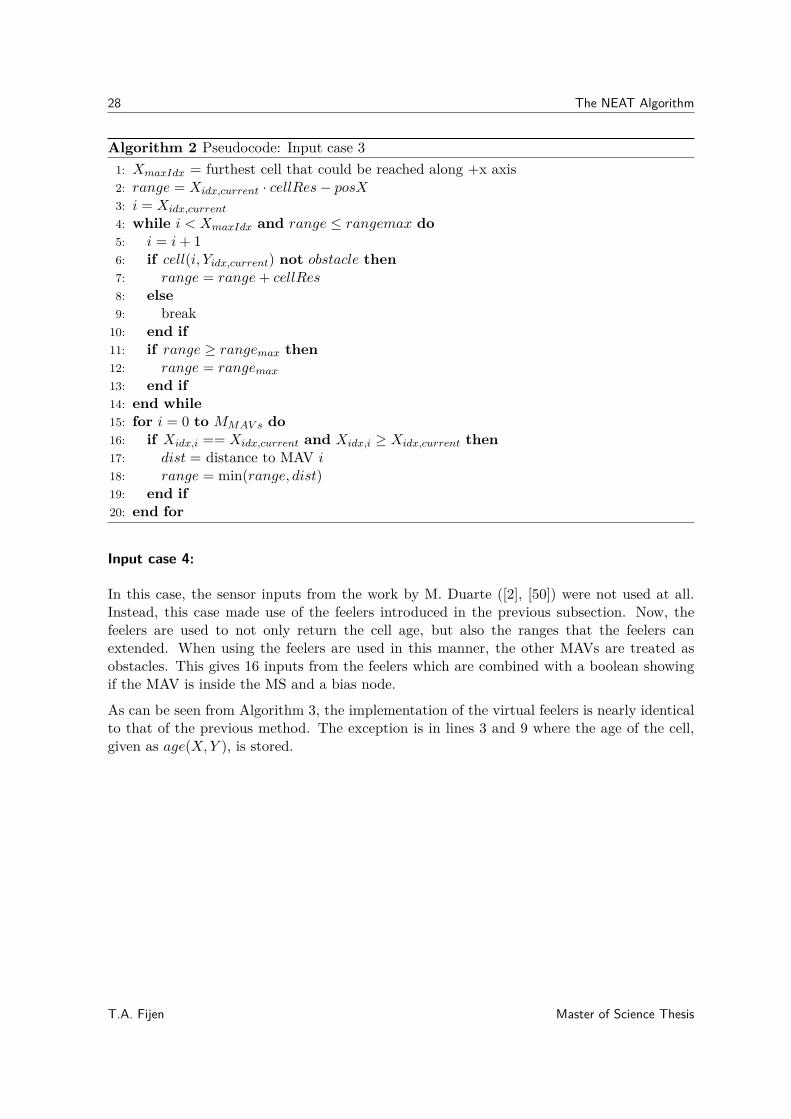
Input case 3:
The next attempt at including knowledge of the MS involved eight virtual sensors that weremodelled as line segments that radiated outwards from the MAV. These sensors, termed’feelers’, then reach out from the MAV until they either encounter an obstacle or they reachtheir maximum range. They then return the age of the furthest cell that they can reach. Thisis shown in Figure 3-8. In this image, the dark blue cells represent an obstacle, the grey cellsare the areas that can be ’seen’ by the agents virtual sensors and the black lines show theseeight feelers. As in the previous two cases, the remaining ten inputs are identical to those
Figure 3-8: Feeler input example
used in [2]. Namely; four geo-fence sensors, four robot sensors, a boolean showing if the MAVis inside the MS and a bias input set to 1.
In Algorithm 2 an example of the pseudocode used to implement one of the feelers is given.This feeler extends outwards from the right hand side of the MAV, running parallel to thex axis and returns the maximum distance that it can extend. This distance is given asthe parameter range in the example. Further, the parameters Xidx,current and Yidx,current
represents the x and y indexes of the cell in which the MAV is located, cellRes is the resolutionof the cells, rangemax is the maximum range that a feeler can extend and MMAV s is thenumber of other MAVs in the system. Finally, Xidx,i is the x cell index for MAV i. A similarmethod is used to implement the remaining seven feelers.
Master of Science Thesis T.A. Fijen
28 The NEAT Algorithm
Algorithm 2 Pseudocode: Input case 31: XmaxIdx = furthest cell that could be reached along +x axis2: range = Xidx,current · cellRes− posX3: i = Xidx,current
4: while i < XmaxIdx and range ≤ rangemax do5: i = i+ 16: if cell(i, Yidx,current) not obstacle then7: range = range+ cellRes8: else9: break
10: end if11: if range ≥ rangemax then12: range = rangemax
13: end if14: end while15: for i = 0 to MMAV s do16: if Xidx,i == Xidx,current and Xidx,i ≥ Xidx,current then17: dist = distance to MAV i18: range = min(range, dist)19: end if20: end for
Input case 4:
In this case, the sensor inputs from the work by M. Duarte ([2], [50]) were not used at all.Instead, this case made use of the feelers introduced in the previous subsection. Now, thefeelers are used to not only return the cell age, but also the ranges that the feelers canextended. When using the feelers are used in this manner, the other MAVs are treated asobstacles. This gives 16 inputs from the feelers which are combined with a boolean showingif the MAV is inside the MS and a bias node.
As can be seen from Algorithm 3, the implementation of the virtual feelers is nearly identicalto that of the previous method. The exception is in lines 3 and 9 where the age of the cell,given as age(X,Y ), is stored.
T.A. Fijen Master of Science Thesis
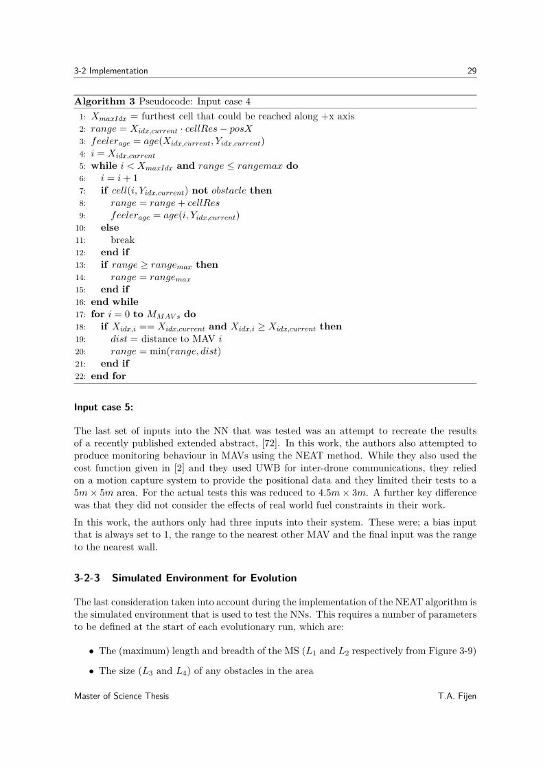
3-2 Implementation 29
Algorithm 3 Pseudocode: Input case 41: XmaxIdx = furthest cell that could be reached along +x axis2: range = Xidx,current · cellRes− posX3: feelerage = age(Xidx,current, Yidx,current)4: i = Xidx,current
5: while i < XmaxIdx and range ≤ rangemax do6: i = i+ 17: if cell(i, Yidx,current) not obstacle then8: range = range+ cellRes9: feelerage = age(i, Yidx,current)
10: else11: break12: end if13: if range ≥ rangemax then14: range = rangemax
15: end if16: end while17: for i = 0 to MMAV s do18: if Xidx,i == Xidx,current and Xidx,i ≥ Xidx,current then19: dist = distance to MAV i20: range = min(range, dist)21: end if22: end for
Input case 5:
The last set of inputs into the NN that was tested was an attempt to recreate the resultsof a recently published extended abstract, [72]. In this work, the authors also attempted toproduce monitoring behaviour in MAVs using the NEAT method. While they also used thecost function given in [2] and they used UWB for inter-drone communications, they reliedon a motion capture system to provide the positional data and they limited their tests to a5m× 5m area. For the actual tests this was reduced to 4.5m× 3m. A further key differencewas that they did not consider the effects of real world fuel constraints in their work.
In this work, the authors only had three inputs into their system. These were; a bias inputthat is always set to 1, the range to the nearest other MAV and the final input was the rangeto the nearest wall.
3-2-3 Simulated Environment for Evolution
The last consideration taken into account during the implementation of the NEAT algorithm isthe simulated environment that is used to test the NNs. This requires a number of parametersto be defined at the start of each evolutionary run, which are:
• The (maximum) length and breadth of the MS (L1 and L2 respectively from Figure 3-9)
• The size (L3 and L4) of any obstacles in the area
Master of Science Thesis T.A. Fijen
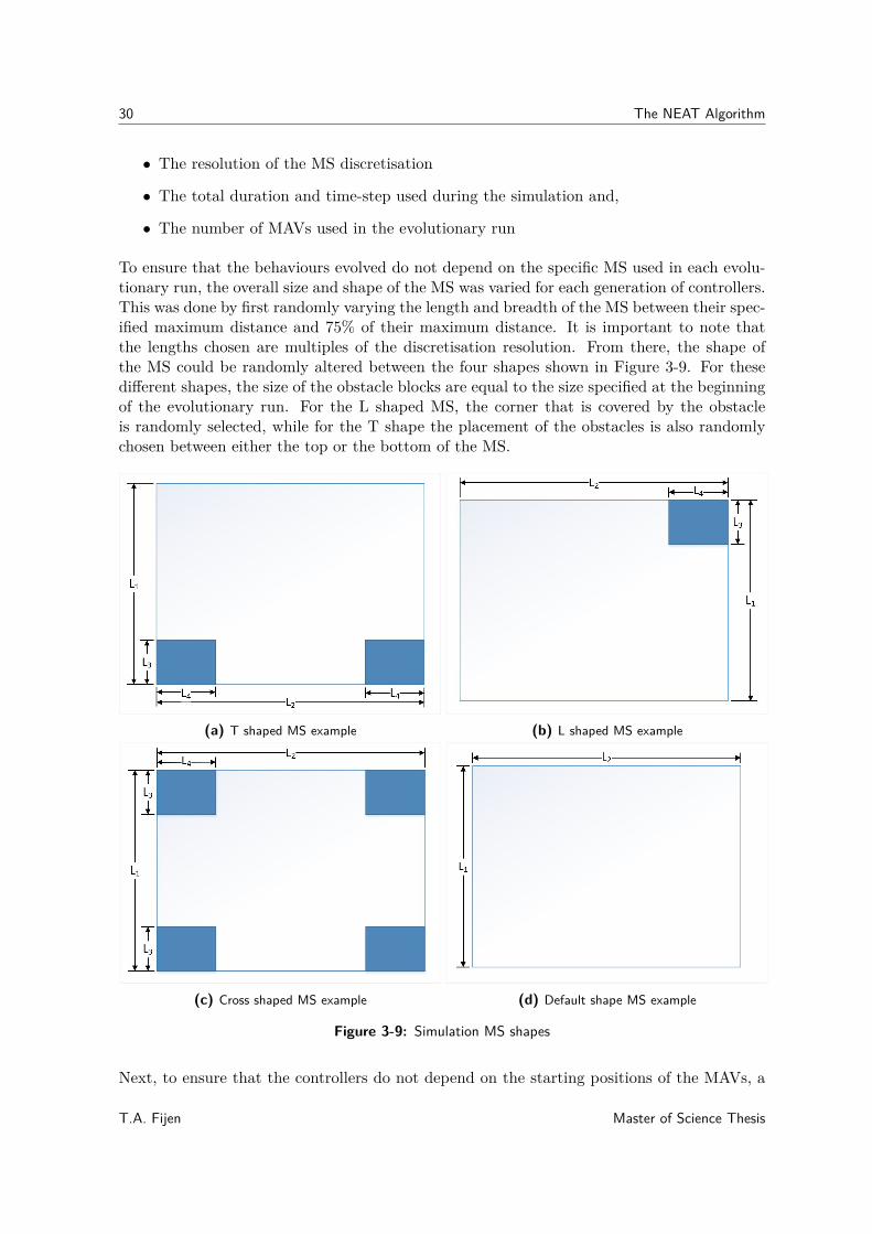
30 The NEAT Algorithm
• The resolution of the MS discretisation
• The total duration and time-step used during the simulation and,
• The number of MAVs used in the evolutionary run
To ensure that the behaviours evolved do not depend on the specific MS used in each evolu-tionary run, the overall size and shape of the MS was varied for each generation of controllers.This was done by first randomly varying the length and breadth of the MS between their spec-ified maximum distance and 75% of their maximum distance. It is important to note thatthe lengths chosen are multiples of the discretisation resolution. From there, the shape ofthe MS could be randomly altered between the four shapes shown in Figure 3-9. For thesedifferent shapes, the size of the obstacle blocks are equal to the size specified at the beginningof the evolutionary run. For the L shaped MS, the corner that is covered by the obstacleis randomly selected, while for the T shape the placement of the obstacles is also randomlychosen between either the top or the bottom of the MS.
(a) T shaped MS example (b) L shaped MS example
(c) Cross shaped MS example (d) Default shape MS example
Figure 3-9: Simulation MS shapes
Next, to ensure that the controllers do not depend on the starting positions of the MAVs, a
T.A. Fijen Master of Science Thesis
3-3 Simulation Results 31
set of 3 initial positions for each of the MAVs were randomly generated at the beginning ofeach generation of the evolutionary run. Every controller in the current population was thenapplied and tested in 3 simulations were the starting positions for each of the iterations wasgiven by one of the sets of initial positions. The controllers final fitness given as the averagefitness generated by Equation (3-4) averaged over all the iterations.
Lastly, to reduce the time taken to perform each evolutionary run, a simulation could bestopped if the MAVs left the MS and did not attempt to return. This was accomplished bytracking the time each MAV spent outside of the MS and if this was greater than 0.2×tf thenthe simulation was terminated. Each time a MAV re-entered the MS its tracking time wasreset to 0. To ensure that this did not positively influence the fitness of the given controller,the cost function still averaged the cell ages over the entire simulation time, tf , and not overjust the reduced simulation time.
3-3 Simulation Results
In this section, the performance of the evolved controllers for each of the input cases are given.
3-3-1 Test Procedure
For each of the input cases mentioned previously, four evolutionary runs were performed with3 MAVs used for the first run, followed by 4, 6, and 8 for the remaining runs. The parametersused during the evolution are as follows, for the simulation environment:
• Length and width of the MS were L1 = 25m and L2 = 25m respectively.
• Size of obstacles: L3 = 3m and L4 = 3m.
• MS was discretised into 1m× 1m cells.
• A simulation time of 300s with a 0.5s time-step was used.
The NEAT parameters are as follows:
• Number of generations = 100
• Initial population size = 150
• Recurrency was disabled
• Add node probability = 3%
• Add connection probability = 5%
• Weight mutation probability = 25%
• Multipoint crossover probability = 60%
• Probability of gene becoming re-enabled = 25%
Master of Science Thesis T.A. Fijen
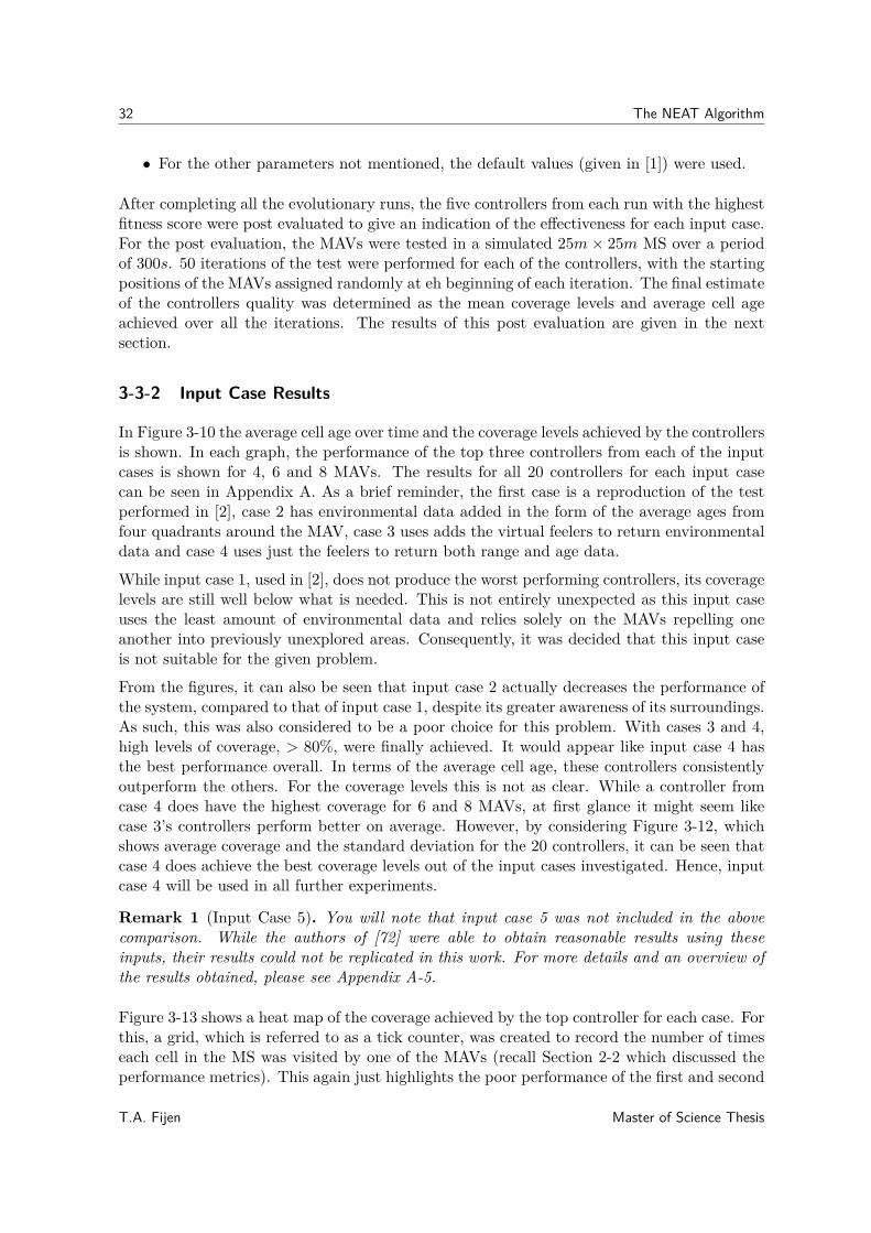
32 The NEAT Algorithm
• For the other parameters not mentioned, the default values (given in [1]) were used.
After completing all the evolutionary runs, the five controllers from each run with the highestfitness score were post evaluated to give an indication of the effectiveness for each input case.For the post evaluation, the MAVs were tested in a simulated 25m× 25m MS over a periodof 300s. 50 iterations of the test were performed for each of the controllers, with the startingpositions of the MAVs assigned randomly at eh beginning of each iteration. The final estimateof the controllers quality was determined as the mean coverage levels and average cell ageachieved over all the iterations. The results of this post evaluation are given in the nextsection.
3-3-2 Input Case Results
In Figure 3-10 the average cell age over time and the coverage levels achieved by the controllersis shown. In each graph, the performance of the top three controllers from each of the inputcases is shown for 4, 6 and 8 MAVs. The results for all 20 controllers for each input casecan be seen in Appendix A. As a brief reminder, the first case is a reproduction of the testperformed in [2], case 2 has environmental data added in the form of the average ages fromfour quadrants around the MAV, case 3 uses adds the virtual feelers to return environmentaldata and case 4 uses just the feelers to return both range and age data.
While input case 1, used in [2], does not produce the worst performing controllers, its coveragelevels are still well below what is needed. This is not entirely unexpected as this input caseuses the least amount of environmental data and relies solely on the MAVs repelling oneanother into previously unexplored areas. Consequently, it was decided that this input caseis not suitable for the given problem.
From the figures, it can also be seen that input case 2 actually decreases the performance ofthe system, compared to that of input case 1, despite its greater awareness of its surroundings.As such, this was also considered to be a poor choice for this problem. With cases 3 and 4,high levels of coverage, > 80%, were finally achieved. It would appear like input case 4 hasthe best performance overall. In terms of the average cell age, these controllers consistentlyoutperform the others. For the coverage levels this is not as clear. While a controller fromcase 4 does have the highest coverage for 6 and 8 MAVs, at first glance it might seem likecase 3’s controllers perform better on average. However, by considering Figure 3-12, whichshows average coverage and the standard deviation for the 20 controllers, it can be seen thatcase 4 does achieve the best coverage levels out of the input cases investigated. Hence, inputcase 4 will be used in all further experiments.
Remark 1 (Input Case 5). You will note that input case 5 was not included in the abovecomparison. While the authors of [72] were able to obtain reasonable results using theseinputs, their results could not be replicated in this work. For more details and an overview ofthe results obtained, please see Appendix A-5.
Figure 3-13 shows a heat map of the coverage achieved by the top controller for each case. Forthis, a grid, which is referred to as a tick counter, was created to record the number of timeseach cell in the MS was visited by one of the MAVs (recall Section 2-2 which discussed theperformance metrics). This again just highlights the poor performance of the first and second
T.A. Fijen Master of Science Thesis
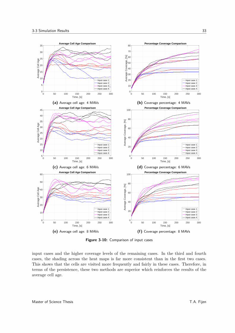
3-3 Simulation Results 33
0 50 100 150 200 250 300Time, [s]
0
5
10
15
20
25
30
35
Ave
rage
Cel
l Age
Average Cell Age Comparison
Input case 1Input case 2Input case 3Input case 4
(a) Average cell age: 4 MAVs
0 50 100 150 200 250 300Time, [s]
0
10
20
30
40
50
60
70
80
Ave
rage
Cov
erag
e, [%
]
Percentage Coverage Comparison
Input case 1Input case 2Input case 3Input case 4
(b) Coverage percentage: 4 MAVs
0 50 100 150 200 250 300Time, [s]
5
10
15
20
25
30
35
40
45
Ave
rage
Cel
l Age
Average Cell Age Comparison
Input case 1Input case 2Input case 3Input case 4
(c) Average cell age: 6 MAVs
0 50 100 150 200 250 300Time, [s]
0
20
40
60
80
100
Ave
rage
Cov
erag
e, [%
]
Percentage Coverage Comparison
Input case 1Input case 2Input case 3Input case 4
(d) Coverage percentage: 6 MAVs
0 50 100 150 200 250 300Time, [s]
0
10
20
30
40
50
60
Ave
rage
Cel
l Age
Average Cell Age Comparison
Input case 1Input case 2Input case 3Input case 4
(e) Average cell age: 8 MAVs
0 50 100 150 200 250 300Time, [s]
0
20
40
60
80
100
Ave
rage
Cov
erag
e, [%
]
Percentage Coverage Comparison
Input case 1Input case 2Input case 3Input case 4
(f) Coverage percentage: 8 MAVs
Figure 3-10: Comparison of input cases
input cases and the higher coverage levels of the remaining cases. In the third and fourthcases, the shading across the heat maps is far more consistent than in the first two cases.This shows that the cells are visited more frequently and fairly in these cases. Therefore, interms of the persistence, these two methods are superior which reinforces the results of theaverage cell age.
Master of Science Thesis T.A. Fijen
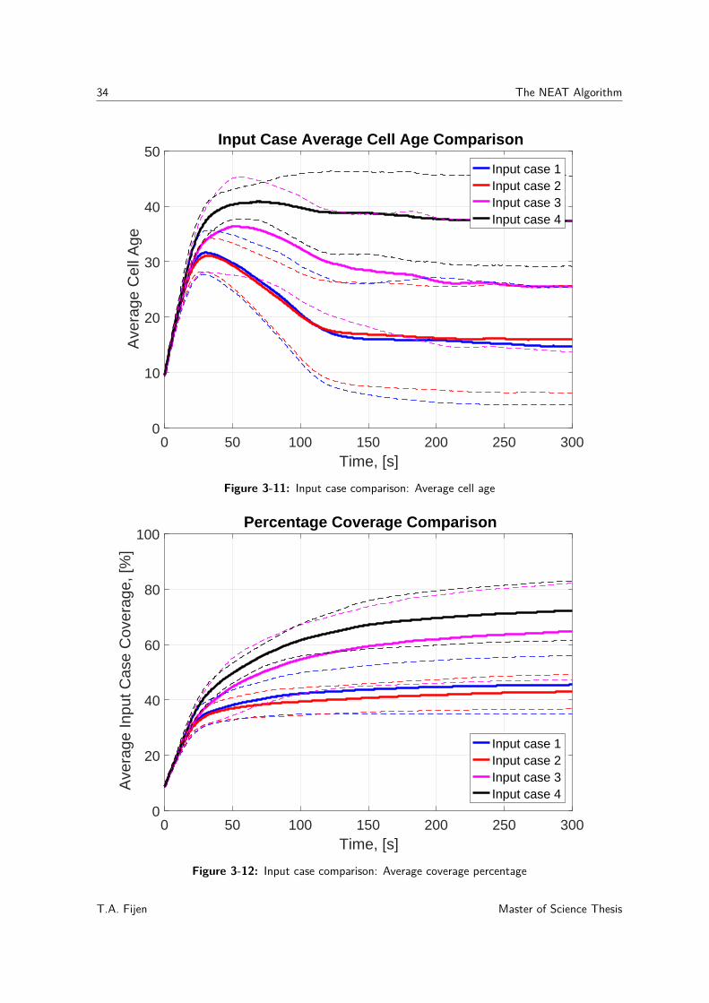
34 The NEAT Algorithm
0 50 100 150 200 250 300Time, [s]
0
10
20
30
40
50A
vera
ge C
ell A
geInput Case Average Cell Age Comparison
Input case 1Input case 2Input case 3Input case 4
Figure 3-11: Input case comparison: Average cell age
0 50 100 150 200 250 300Time, [s]
0
20
40
60
80
100
Ave
rage
Inpu
t Cas
e C
over
age,
[%]
Percentage Coverage Comparison
Input case 1Input case 2Input case 3Input case 4
Figure 3-12: Input case comparison: Average coverage percentage
T.A. Fijen Master of Science Thesis
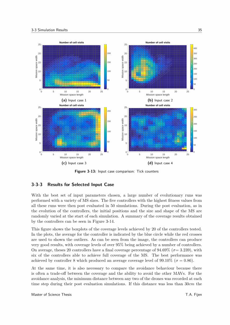
3-3 Simulation Results 35
0 5 10 15 20 25Mission space length
0
5
10
15
20
25
Mis
sion
spa
ce w
idth
Number of cell visits
0
50
100
150
200
(a) Input case 1
0 5 10 15 20 25Mission space length
0
5
10
15
20
25
Mis
sion
spa
ce w
idth
Number of cell visits
0
50
100
150
200
250
300
350
400
(b) Input case 2
0 5 10 15 20 25Mission space length
0
5
10
15
20
25
Mis
sion
spa
ce w
idth
Number of cell visits
0
50
100
150
200
(c) Input case 3
0 5 10 15 20 25Mission space length
0
5
10
15
20
25
Mis
sion
spa
ce w
idth
Number of cell visits
0
50
100
150
200
250
300
(d) Input case 4
Figure 3-13: Input case comparison: Tick counters
3-3-3 Results for Selected Input Case
With the best set of input parameters chosen, a large number of evolutionary runs wasperformed with a variety of MS sizes. The five controllers with the highest fitness values fromall these runs were then post evaluated in 50 simulations. During the post evaluation, as inthe evolution of the controllers, the initial positions and the size and shape of the MS arerandomly varied at the start of each simulation. A summary of the coverage results obtainedby the controllers can be seen in Figure 3-14.
This figure shows the boxplots of the coverage levels achieved by 20 of the controllers tested.In the plots, the average for the controller is indicated by the blue circle while the red crossesare used to shown the outliers. As can be seen from the image, the controllers can producevery good results, with coverage levels of over 95% being achieved by a number of controllers.On average, theses 20 controllers have a final coverage percentage of 94.69% (σ= 3.239), withsix of the controllers able to achieve full coverage of the MS. The best performance wasachieved by controller 8 which produced an average coverage level of 99.10% (σ = 0.86).
At the same time, it is also necessary to compare the avoidance behaviour because thereis often a trade-off between the coverage and the ability to avoid the other MAVs. For theavoidance analysis, the minimum distance between any two of the drones was recorded at eachtime step during their post evaluation simulations. If this distance was less than 30cm the
Master of Science Thesis T.A. Fijen
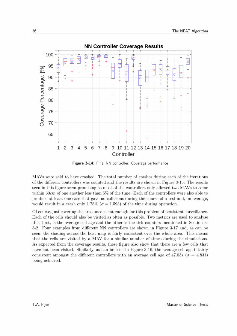
36 The NEAT Algorithm
1 2 3 4 5 6 7 8 9 10 11 12 13 14 15 16 17 18 19 20Controller
65
70
75
80
85
90
95
100
Cov
erag
e P
erce
ntag
e, [%
]NN Controller Coverage Results
Figure 3-14: Final NN controller: Coverage performance
MAVs were said to have crashed. The total number of crashes during each of the iterationsof the different controllers was counted and the results are shown in Figure 3-15. The resultsseen in this figure seem promising as most of the controllers only allowed two MAVs to comewithin 30cm of one another less than 5% of the time. Each of the controllers were also able toproduce at least one case that gave no collisions during the course of a test and, on average,would result in a crash only 1.78% (σ = 1.593) of the time during operation.
Of course, just covering the area once is not enough for this problem of persistent surveillance.Each of the cells should also be visited as often as possible. Two metrics are used to analysethis, first, is the average cell age and the other is the tick counters mentioned in Section 3-3-2. Four examples from different NN controllers are shown in Figure 3-17 and, as can beseen, the shading across the heat map is fairly consistent over the whole area. This meansthat the cells are visited by a MAV for a similar number of times during the simulations.As expected from the coverage results, these figure also show that there are a few cells thathave not been visited. Similarly, as can be seen in Figure 3-16, the average cell age if fairlyconsistent amongst the different controllers with an average cell age of 47.03s (σ = 4.831)being achieved.
T.A. Fijen Master of Science Thesis
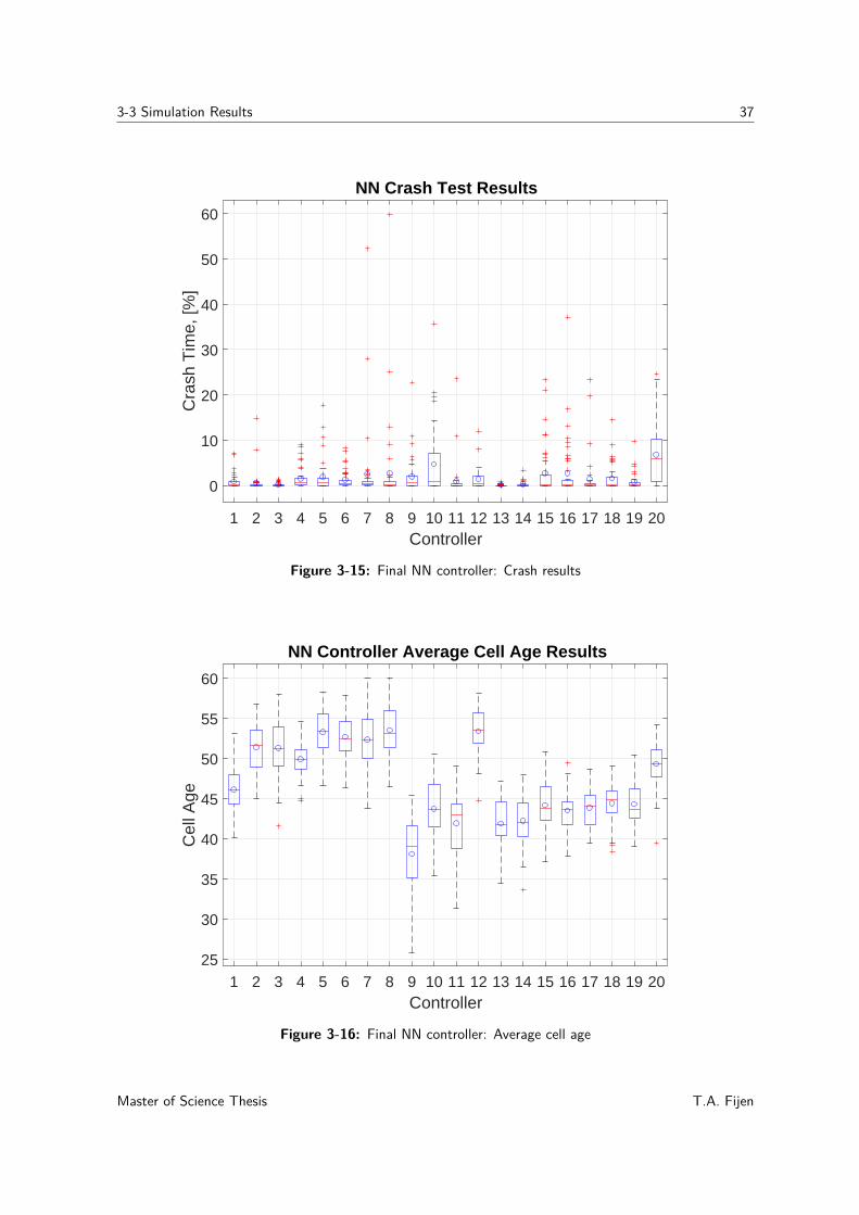
3-3 Simulation Results 37
1 2 3 4 5 6 7 8 9 10 11 12 13 14 15 16 17 18 19 20Controller
0
10
20
30
40
50
60
Cra
sh T
ime,
[%]
NN Crash Test Results
Figure 3-15: Final NN controller: Crash results
1 2 3 4 5 6 7 8 9 10 11 12 13 14 15 16 17 18 19 20Controller
25
30
35
40
45
50
55
60
Cel
l Age
NN Controller Average Cell Age Results
Figure 3-16: Final NN controller: Average cell age
Master of Science Thesis T.A. Fijen
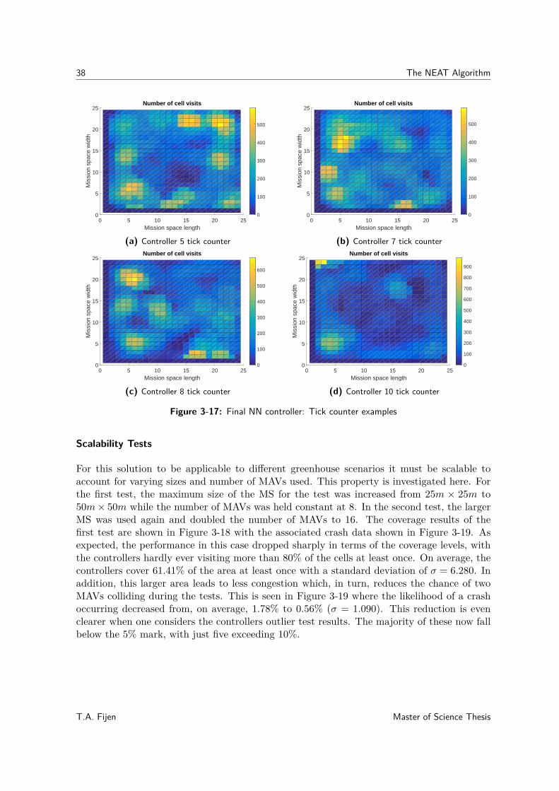
38 The NEAT Algorithm
0 5 10 15 20 25Mission space length
0
5
10
15
20
25
Mis
sion
spa
ce w
idth
Number of cell visits
0
100
200
300
400
500
(a) Controller 5 tick counter
0 5 10 15 20 25Mission space length
0
5
10
15
20
25
Mis
sion
spa
ce w
idth
Number of cell visits
0
100
200
300
400
500
(b) Controller 7 tick counter
0 5 10 15 20 25Mission space length
0
5
10
15
20
25
Mis
sion
spa
ce w
idth
Number of cell visits
0
100
200
300
400
500
600
(c) Controller 8 tick counter
0 5 10 15 20 25Mission space length
0
5
10
15
20
25
Mis
sion
spa
ce w
idth
Number of cell visits
0
100
200
300
400
500
600
700
800
900
(d) Controller 10 tick counter
Figure 3-17: Final NN controller: Tick counter examples
Scalability Tests
For this solution to be applicable to different greenhouse scenarios it must be scalable toaccount for varying sizes and number of MAVs used. This property is investigated here. Forthe first test, the maximum size of the MS for the test was increased from 25m × 25m to50m× 50m while the number of MAVs was held constant at 8. In the second test, the largerMS was used again and doubled the number of MAVs to 16. The coverage results of thefirst test are shown in Figure 3-18 with the associated crash data shown in Figure 3-19. Asexpected, the performance in this case dropped sharply in terms of the coverage levels, withthe controllers hardly ever visiting more than 80% of the cells at least once. On average, thecontrollers cover 61.41% of the area at least once with a standard deviation of σ = 6.280. Inaddition, this larger area leads to less congestion which, in turn, reduces the chance of twoMAVs colliding during the tests. This is seen in Figure 3-19 where the likelihood of a crashoccurring decreased from, on average, 1.78% to 0.56% (σ = 1.090). This reduction is evenclearer when one considers the controllers outlier test results. The majority of these now fallbelow the 5% mark, with just five exceeding 10%.
T.A. Fijen Master of Science Thesis
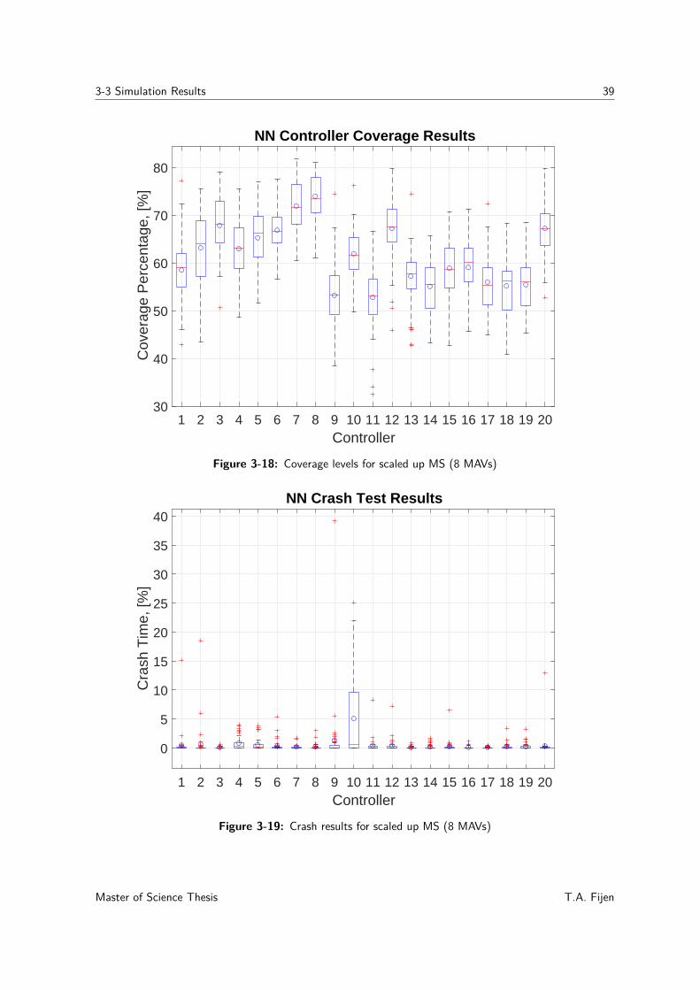
3-3 Simulation Results 39
1 2 3 4 5 6 7 8 9 10 11 12 13 14 15 16 17 18 19 20Controller
30
40
50
60
70
80
Cov
erag
e P
erce
ntag
e, [%
]NN Controller Coverage Results
Figure 3-18: Coverage levels for scaled up MS (8 MAVs)
1 2 3 4 5 6 7 8 9 10 11 12 13 14 15 16 17 18 19 20Controller
0
5
10
15
20
25
30
35
40
Cra
sh T
ime,
[%]
NN Crash Test Results
Figure 3-19: Crash results for scaled up MS (8 MAVs)
Master of Science Thesis T.A. Fijen
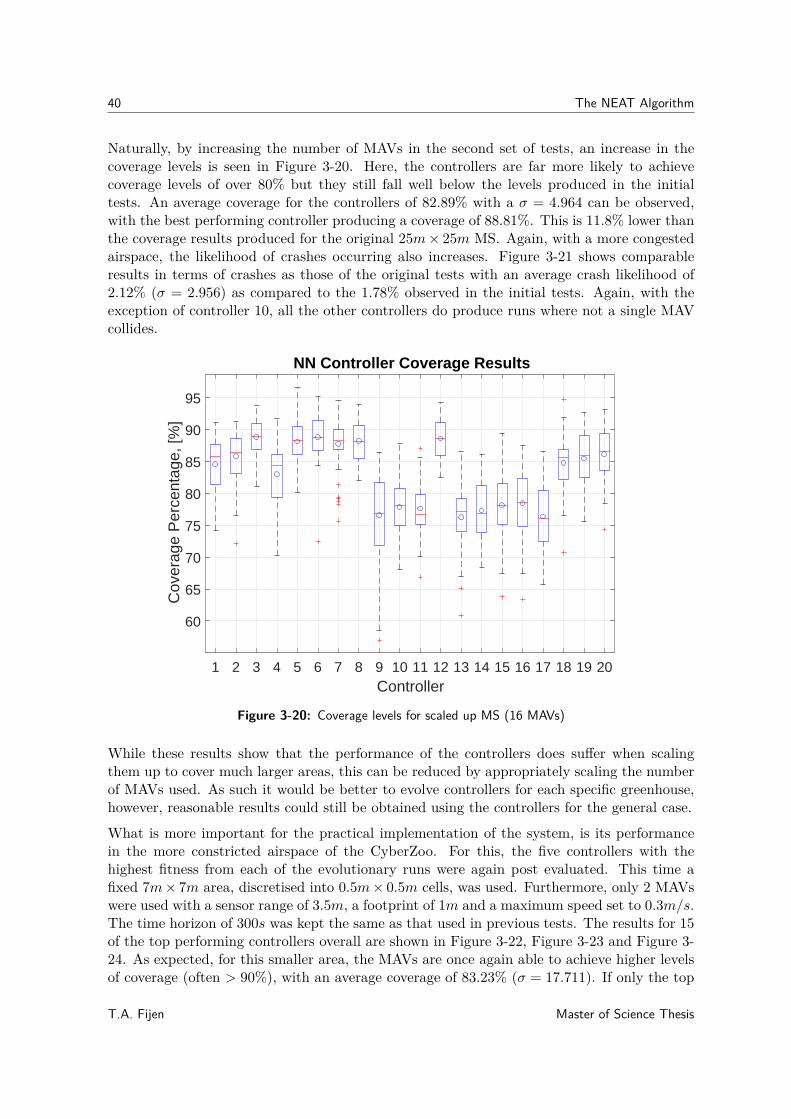
40 The NEAT Algorithm
Naturally, by increasing the number of MAVs in the second set of tests, an increase in thecoverage levels is seen in Figure 3-20. Here, the controllers are far more likely to achievecoverage levels of over 80% but they still fall well below the levels produced in the initialtests. An average coverage for the controllers of 82.89% with a σ = 4.964 can be observed,with the best performing controller producing a coverage of 88.81%. This is 11.8% lower thanthe coverage results produced for the original 25m× 25m MS. Again, with a more congestedairspace, the likelihood of crashes occurring also increases. Figure 3-21 shows comparableresults in terms of crashes as those of the original tests with an average crash likelihood of2.12% (σ = 2.956) as compared to the 1.78% observed in the initial tests. Again, with theexception of controller 10, all the other controllers do produce runs where not a single MAVcollides.
1 2 3 4 5 6 7 8 9 10 11 12 13 14 15 16 17 18 19 20Controller
60
65
70
75
80
85
90
95
Cov
erag
e P
erce
ntag
e, [%
]
NN Controller Coverage Results
Figure 3-20: Coverage levels for scaled up MS (16 MAVs)
While these results show that the performance of the controllers does suffer when scalingthem up to cover much larger areas, this can be reduced by appropriately scaling the numberof MAVs used. As such it would be better to evolve controllers for each specific greenhouse,however, reasonable results could still be obtained using the controllers for the general case.
What is more important for the practical implementation of the system, is its performancein the more constricted airspace of the CyberZoo. For this, the five controllers with thehighest fitness from each of the evolutionary runs were again post evaluated. This time afixed 7m× 7m area, discretised into 0.5m× 0.5m cells, was used. Furthermore, only 2 MAVswere used with a sensor range of 3.5m, a footprint of 1m and a maximum speed set to 0.3m/s.The time horizon of 300s was kept the same as that used in previous tests. The results for 15of the top performing controllers overall are shown in Figure 3-22, Figure 3-23 and Figure 3-24. As expected, for this smaller area, the MAVs are once again able to achieve higher levelsof coverage (often > 90%), with an average coverage of 83.23% (σ = 17.711). If only the top
T.A. Fijen Master of Science Thesis
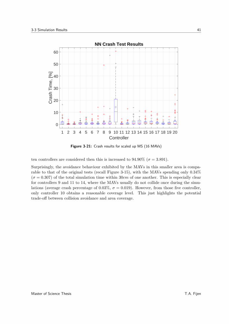
3-3 Simulation Results 41
1 2 3 4 5 6 7 8 9 10 11 12 13 14 15 16 17 18 19 20Controller
0
10
20
30
40
50
60C
rash
Tim
e, [%
]NN Crash Test Results
Figure 3-21: Crash results for scaled up MS (16 MAVs)
ten controllers are considered then this is increased to 94.90% (σ = 3.891).
Surprisingly, the avoidance behaviour exhibited by the MAVs in this smaller area is compa-rable to that of the original tests (recall Figure 3-15), with the MAVs spending only 0.34%(σ = 0.307) of the total simulation time within 30cm of one another. This is especially clearfor controllers 9 and 11 to 14, where the MAVs usually do not collide once during the simu-lations (average crash percentage of 0.03%, σ = 0.019). However, from those five controller,only controller 10 obtains a reasonable coverage level. This just highlights the potentialtrade-off between collision avoidance and area coverage.
Master of Science Thesis T.A. Fijen
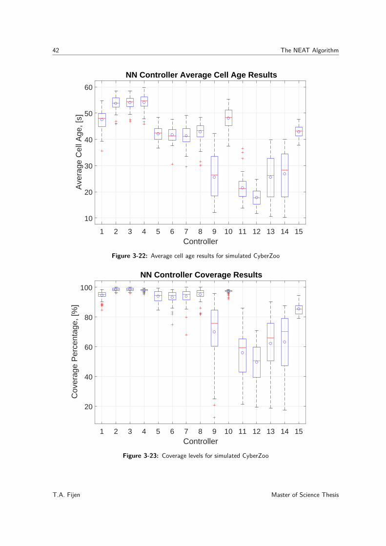
42 The NEAT Algorithm
1 2 3 4 5 6 7 8 9 10 11 12 13 14 15Controller
10
20
30
40
50
60A
vera
ge C
ell A
ge, [
s]NN Controller Average Cell Age Results
Figure 3-22: Average cell age results for simulated CyberZoo
1 2 3 4 5 6 7 8 9 10 11 12 13 14 15Controller
20
40
60
80
100
Cov
erag
e P
erce
ntag
e, [%
]
NN Controller Coverage Results
Figure 3-23: Coverage levels for simulated CyberZoo
T.A. Fijen Master of Science Thesis
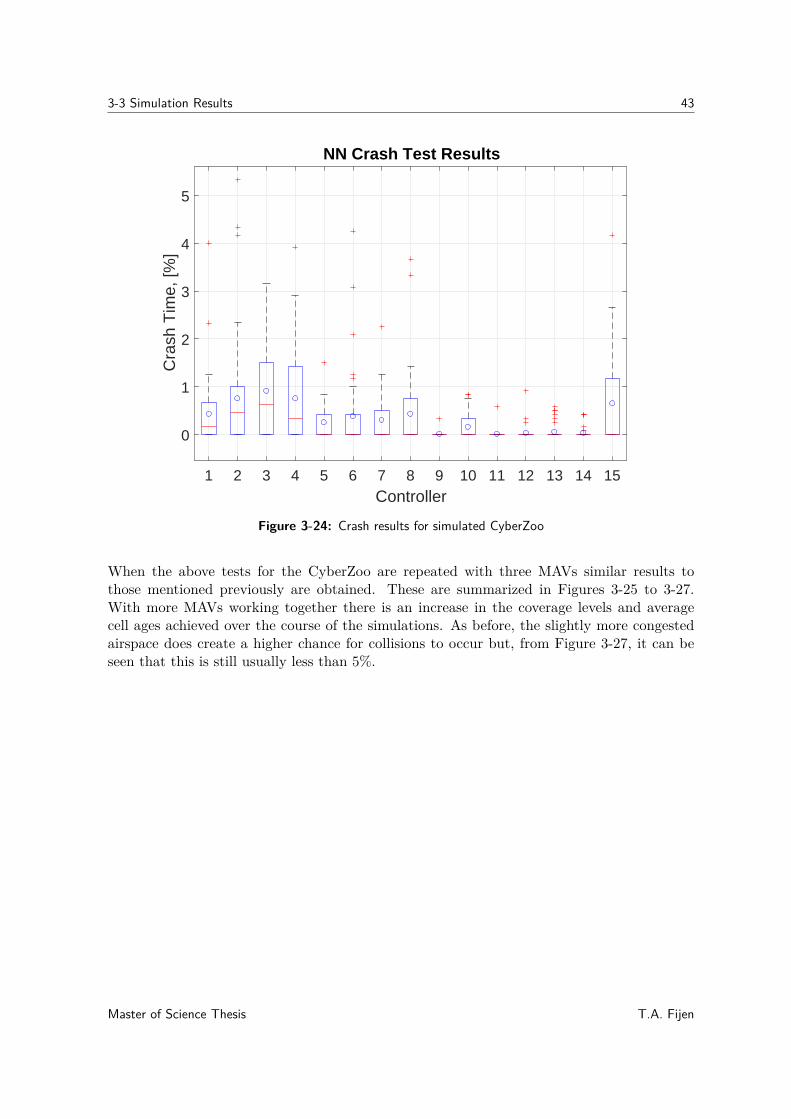
3-3 Simulation Results 43
1 2 3 4 5 6 7 8 9 10 11 12 13 14 15Controller
0
1
2
3
4
5
Cra
sh T
ime,
[%]
NN Crash Test Results
Figure 3-24: Crash results for simulated CyberZoo
When the above tests for the CyberZoo are repeated with three MAVs similar results tothose mentioned previously are obtained. These are summarized in Figures 3-25 to 3-27.With more MAVs working together there is an increase in the coverage levels and averagecell ages achieved over the course of the simulations. As before, the slightly more congestedairspace does create a higher chance for collisions to occur but, from Figure 3-27, it can beseen that this is still usually less than 5%.
Master of Science Thesis T.A. Fijen
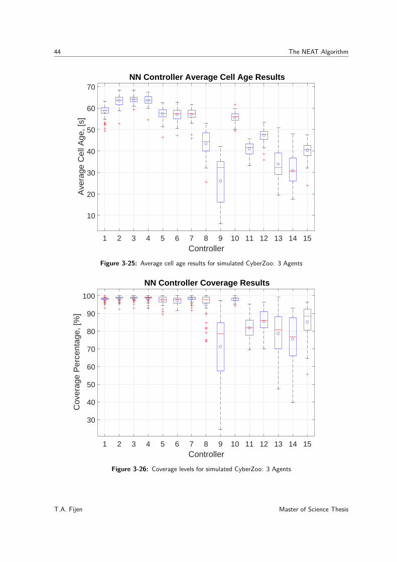
44 The NEAT Algorithm
1 2 3 4 5 6 7 8 9 10 11 12 13 14 15Controller
10
20
30
40
50
60
70A
vera
ge C
ell A
ge, [
s]NN Controller Average Cell Age Results
Figure 3-25: Average cell age results for simulated CyberZoo: 3 Agents
1 2 3 4 5 6 7 8 9 10 11 12 13 14 15Controller
30
40
50
60
70
80
90
100
Cov
erag
e P
erce
ntag
e, [%
]
NN Controller Coverage Results
Figure 3-26: Coverage levels for simulated CyberZoo: 3 Agents
T.A. Fijen Master of Science Thesis
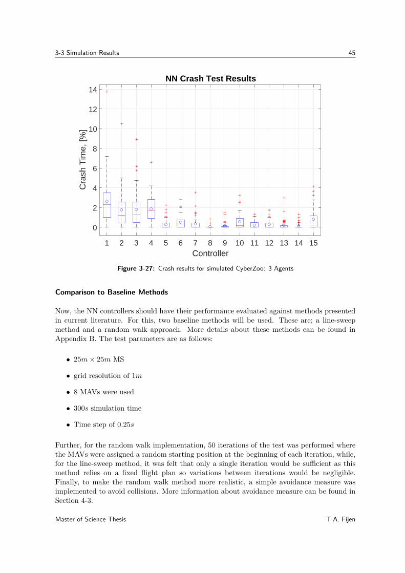
3-3 Simulation Results 45
1 2 3 4 5 6 7 8 9 10 11 12 13 14 15Controller
0
2
4
6
8
10
12
14C
rash
Tim
e, [%
]NN Crash Test Results
Figure 3-27: Crash results for simulated CyberZoo: 3 Agents
Comparison to Baseline Methods
Now, the NN controllers should have their performance evaluated against methods presentedin current literature. For this, two baseline methods will be used. These are; a line-sweepmethod and a random walk approach. More details about these methods can be found inAppendix B. The test parameters are as follows:
• 25m× 25m MS
• grid resolution of 1m
• 8 MAVs were used
• 300s simulation time
• Time step of 0.25s
Further, for the random walk implementation, 50 iterations of the test was performed wherethe MAVs were assigned a random starting position at the beginning of each iteration, while,for the line-sweep method, it was felt that only a single iteration would be sufficient as thismethod relies on a fixed flight plan so variations between iterations would be negligible.Finally, to make the random walk method more realistic, a simple avoidance measure wasimplemented to avoid collisions. More information about avoidance measure can be found inSection 4-3.
Master of Science Thesis T.A. Fijen
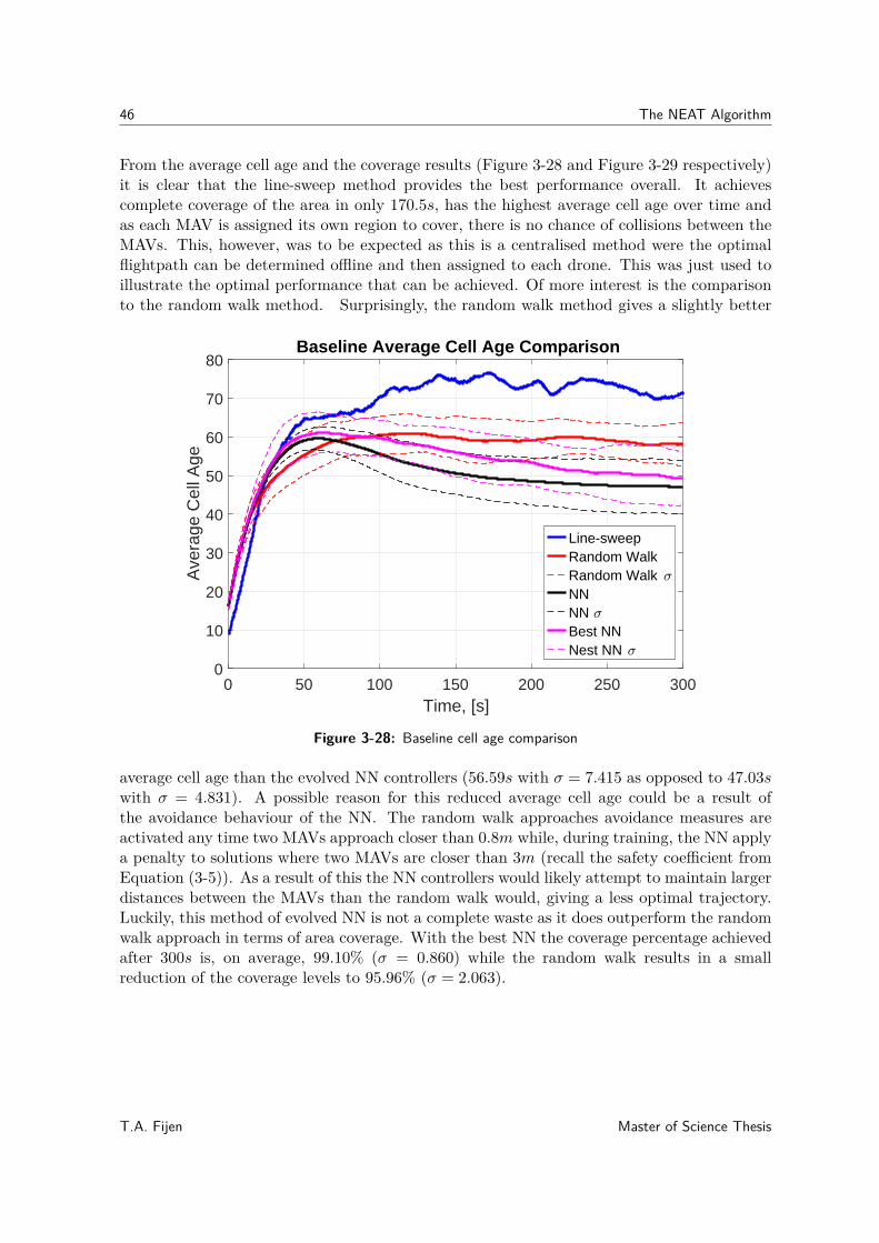
46 The NEAT Algorithm
From the average cell age and the coverage results (Figure 3-28 and Figure 3-29 respectively)it is clear that the line-sweep method provides the best performance overall. It achievescomplete coverage of the area in only 170.5s, has the highest average cell age over time andas each MAV is assigned its own region to cover, there is no chance of collisions between theMAVs. This, however, was to be expected as this is a centralised method were the optimalflightpath can be determined offline and then assigned to each drone. This was just used toillustrate the optimal performance that can be achieved. Of more interest is the comparisonto the random walk method. Surprisingly, the random walk method gives a slightly better
0 50 100 150 200 250 300Time, [s]
0
10
20
30
40
50
60
70
80
Ave
rage
Cel
l Age
Baseline Average Cell Age Comparison
Line-sweepRandom WalkRandom Walk NNNN Best NNNest NN
Figure 3-28: Baseline cell age comparison
average cell age than the evolved NN controllers (56.59s with σ = 7.415 as opposed to 47.03swith σ = 4.831). A possible reason for this reduced average cell age could be a result ofthe avoidance behaviour of the NN. The random walk approaches avoidance measures areactivated any time two MAVs approach closer than 0.8m while, during training, the NN applya penalty to solutions where two MAVs are closer than 3m (recall the safety coefficient fromEquation (3-5)). As a result of this the NN controllers would likely attempt to maintain largerdistances between the MAVs than the random walk would, giving a less optimal trajectory.Luckily, this method of evolved NN is not a complete waste as it does outperform the randomwalk approach in terms of area coverage. With the best NN the coverage percentage achievedafter 300s is, on average, 99.10% (σ = 0.860) while the random walk results in a smallreduction of the coverage levels to 95.96% (σ = 2.063).
T.A. Fijen Master of Science Thesis
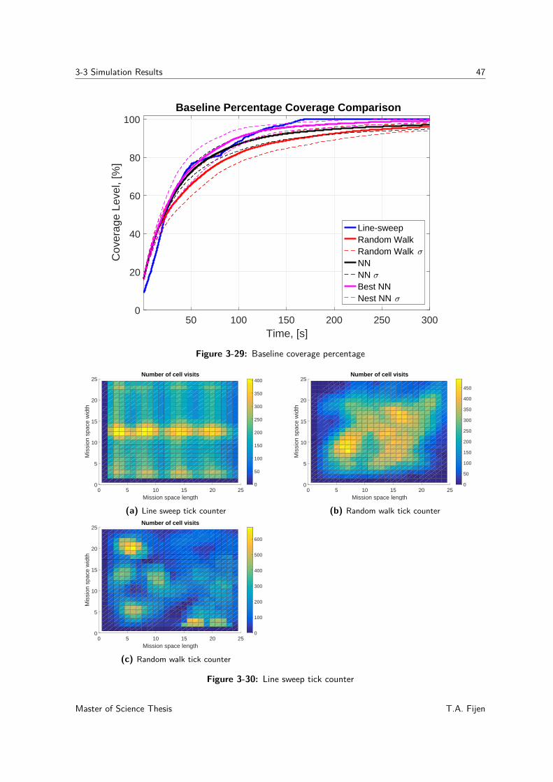
3-3 Simulation Results 47
50 100 150 200 250 300Time, [s]
0
20
40
60
80
100C
over
age
Leve
l, [%
]Baseline Percentage Coverage Comparison
Line-sweepRandom WalkRandom Walk NNNN Best NNNest NN
Figure 3-29: Baseline coverage percentage
0 5 10 15 20 25Mission space length
0
5
10
15
20
25
Mis
sion
spa
ce w
idth
Number of cell visits
0
50
100
150
200
250
300
350
400
(a) Line sweep tick counter
0 5 10 15 20 25Mission space length
0
5
10
15
20
25
Mis
sion
spa
ce w
idth
Number of cell visits
0
50
100
150
200
250
300
350
400
450
(b) Random walk tick counter
0 5 10 15 20 25Mission space length
0
5
10
15
20
25
Mis
sion
spa
ce w
idth
Number of cell visits
0
100
200
300
400
500
600
(c) Random walk tick counter
Figure 3-30: Line sweep tick counter
Master of Science Thesis T.A. Fijen
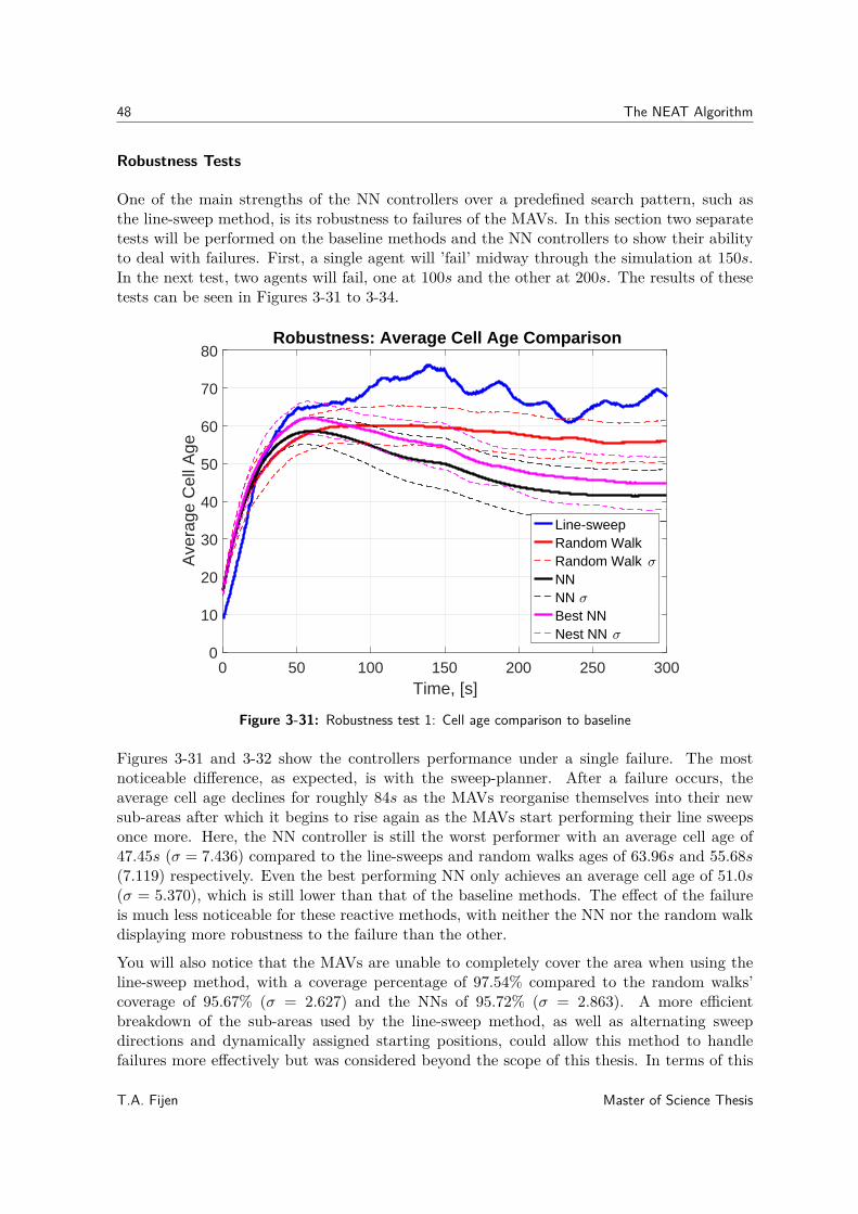
48 The NEAT Algorithm
Robustness Tests
One of the main strengths of the NN controllers over a predefined search pattern, such asthe line-sweep method, is its robustness to failures of the MAVs. In this section two separatetests will be performed on the baseline methods and the NN controllers to show their abilityto deal with failures. First, a single agent will ’fail’ midway through the simulation at 150s.In the next test, two agents will fail, one at 100s and the other at 200s. The results of thesetests can be seen in Figures 3-31 to 3-34.
0 50 100 150 200 250 300Time, [s]
0
10
20
30
40
50
60
70
80
Ave
rage
Cel
l Age
Robustness: Average Cell Age Comparison
Line-sweepRandom WalkRandom Walk NNNN Best NNNest NN
Figure 3-31: Robustness test 1: Cell age comparison to baseline
Figures 3-31 and 3-32 show the controllers performance under a single failure. The mostnoticeable difference, as expected, is with the sweep-planner. After a failure occurs, theaverage cell age declines for roughly 84s as the MAVs reorganise themselves into their newsub-areas after which it begins to rise again as the MAVs start performing their line sweepsonce more. Here, the NN controller is still the worst performer with an average cell age of47.45s (σ = 7.436) compared to the line-sweeps and random walks ages of 63.96s and 55.68s(7.119) respectively. Even the best performing NN only achieves an average cell age of 51.0s(σ = 5.370), which is still lower than that of the baseline methods. The effect of the failureis much less noticeable for these reactive methods, with neither the NN nor the random walkdisplaying more robustness to the failure than the other.
You will also notice that the MAVs are unable to completely cover the area when using theline-sweep method, with a coverage percentage of 97.54% compared to the random walks’coverage of 95.67% (σ = 2.627) and the NNs of 95.72% (σ = 2.863). A more efficientbreakdown of the sub-areas used by the line-sweep method, as well as alternating sweepdirections and dynamically assigned starting positions, could allow this method to handlefailures more effectively but was considered beyond the scope of this thesis. In terms of this
T.A. Fijen Master of Science Thesis
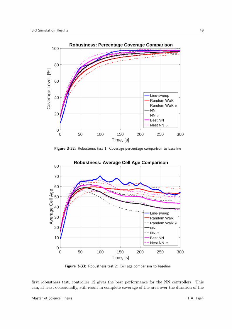
3-3 Simulation Results 49
0 50 100 150 200 250 300Time, [s]
0
20
40
60
80
100C
over
age
Leve
l, [%
]Robustness: Percentage Coverage Comparison
Line-sweepRandom WalkRandom Walk NNNN Best NNNest NN
Figure 3-32: Robustness test 1: Coverage percentage comparison to baseline
0 50 100 150 200 250 300Time, [s]
0
10
20
30
40
50
60
70
80
Ave
rage
Cel
l Age
Robustness: Average Cell Age Comparison
Line-sweepRandom WalkRandom Walk NNNN Best NNNest NN
Figure 3-33: Robustness test 2: Cell age comparison to baseline
first robustness test, controller 12 gives the best performance for the NN controllers. Thiscan, at least occasionally, still result in complete coverage of the area over the duration of the
Master of Science Thesis T.A. Fijen
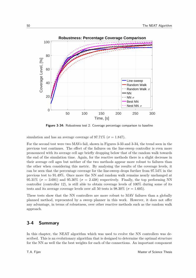
50 The NEAT Algorithm
50 100 150 200 250 300Time, [s]
0
20
40
60
80
100C
over
age
Leve
l, [%
]Robustness: Percentage Coverage Comparison
Line-sweepRandom WalkRandom Walk NNNN Best NNNest NN
Figure 3-34: Robustness test 2: Coverage percentage comparison to baseline
simulation and has an average coverage of 97.71% (σ = 1.847).
For the second test were two MAVs fail, shown in Figures 3-33 and 3-34, the trend seen in theprevious test continues. The effect of the failures on the line-sweep controller is even morepronounced with its average cell age briefly dropping below that of the random walk towardsthe end of the simulation time. Again, for the reactive methods there is a slight decrease intheir average cell ages but neither of the two methods appear more robust to failures thanthe other when considering this metric. By analysing the results of the coverage levels, itcan be seen that the percentage coverage for the line-sweep drops further from 97.54% in theprevious test to 91.49%. Once more the NN and random walk remains nearly unchanged at95.31% (σ = 3.691) and 95.30% (σ = 2.438) respectively. Finally, the top performing NNcontroller (controller 12), is still able to obtain coverage levels of 100% during some of itstests and its average coverage levels over all 50 tests is 98.30% (σ = 1.605).
These tests show that the NN controllers are more robust to MAV failures than a globallyplanned method, represented by a sweep planner in this work. However, it does not offerany advantage, in terms of robustness, over other reactive methods such as the random walkapproach.
3-4 Summary
In this chapter, the NEAT algorithm which was used to evolve the NN controllers was de-scribed. This is an evolutionary algorithm that is designed to determine the optimal structurefor the NN as well the the best weights for each of the connections. An important component
T.A. Fijen Master of Science Thesis
3-4 Summary 51
to this algorithm is the cost function used to evaluate the performance of the NNs from eachnew generation. In this thesis, the cost function presented by Duarte in [2] was used with asmall adaption. Instead of penalising the total fitness over the entire duration of the simula-tion when two MAVs come within 3m of one another, the function used here only penalisesthe fitness gain for the specific time step where the positional constraint was violated. Thiswas shown to produce controllers that resulted in a significant increase in the average cell ageover time, in many instances it more than doubled, while also offering a slight increase to thecoverage levels.
The next major design choice was selecting the inputs into the NN. For this, two examples ofinputs from current literature were tested along with three additional input cases that madeuse of varying levels of environmental knowledge. Through the post evaluation of these NNcontrollers it was found that by increasing the amount of environmental knowledge used bythe NN the performance of the system could be noticeably improve, which was to be expected.In the end, the best performance was achieved by the fourth input case. This relied on a seriesof eight virtual feelers (or antennae) that reached outwards from each MAV. These antennaereturned the distance to the nearest obstacle and the age of the furthest cell that it couldreach. On average, the controllers generated with this input case gave a coverage level of94.5% with a crash percentage of 1.78%. In addition, these controllers were shown to berobust to failures of MAVs and could be successfully scaled to both larger and smaller MSsand was applicable to varying number of MAVs.
Lastly, the NN controllers were compared to two baseline methods identified from currentliterature. These were the random walk and the line-sweep method. As expected, the line-sweep method gave the best performance in terms of coverage levels, average cell age andas each of the MAVs are assigned their own subregions, there are no collisions. However,as this is a centralised method that relies on predefined flight paths it is not as robust tofailures as the other two methods. Surprisingly, the purely random approach implementedin the random walk controller also outperformed the NN controller in terms of average cellage. Luckily the NN did offer better performance than a random approach in terms of areacoverage. As both of these methods are reactive, their ability to deal with failures is nearlyidentical.
As of yet, the fuel level constraint has not been addressed. This expanded upon in the nextchapter where a high level controller is used to determine when the MAV should return tothe depot for refuelling.
Master of Science Thesis T.A. Fijen

52 The NEAT Algorithm
T.A. Fijen Master of Science Thesis
Chapter 4
Fuel Monitoring Policy
Up until this point the constraint on the MAVs fuel, Equation (2-3), has not been addressed.This leads to an important component of this system, namely, the method for refuelling asthe MAVs have a limited flight time. For the MAVs used in this system, this amounts toeither charging the battery, or replacing the depleted battery with a charged one while theMAV is stationed at the depot. In this work, it was assumed that the depleted batteries couldbe manually replaced at the depots.
Next, the aspect of when a MAV must refuel itself forms a vital part of any fuel monitoringpolicy. Two common methods for achieving this are task assignment and task hand-off. Intask assignment ([73, 74, 75, 76], a single flight path that covers the entire MS is created, usinga sweep-planner for example. This path is then divided into separate sections that can becompletely transversed by a MAV before it returns for refuelling. Covering all these sections,along with the refuelling can be seen as tasks that must be completed. A global planner is thenused to efficiently assign MAVs to tasks with the goal of reducing the total time to completethe mission. Similar to this is task hand-off presented in [43, 77, 42, 45]. Again, completeflight paths that cover the area are generated but these paths may require more fuel than theMAVs have available. When a MAV is low on fuel, it will hand off its task to a MAV that iswaiting for an assignment who will than continue following the path while the original MAVreturns to the depot. Naturally, these methods require a complete flight path to be availablefor the duration of the mission so they will not be applicable with the reactive nature of theNN controllers presented in this work. In addition, these methods are usually formulated asa Mixed Integer Linear Programming (MILP) which are computationally expensive to solve(they are typically NP-hard [53, 78]). Therefore, these methods were not appropriate for usein this work.
Other methods of refuel scheduling include using motives and artificial emotions [79], anauction based task allocation process [80], formulating the times to start refuelling as a LinearProgramming (LP) problem where the goal is to reduce the overlap in refuel times betweenall the MAVs [32] and fixed threshold scheduling. In the end, the fixed-threshold method wasselected as this is highly scalable, it is the most computationally efficient and it requires littleto no communication between the MAVs.
Master of Science Thesis T.A. Fijen
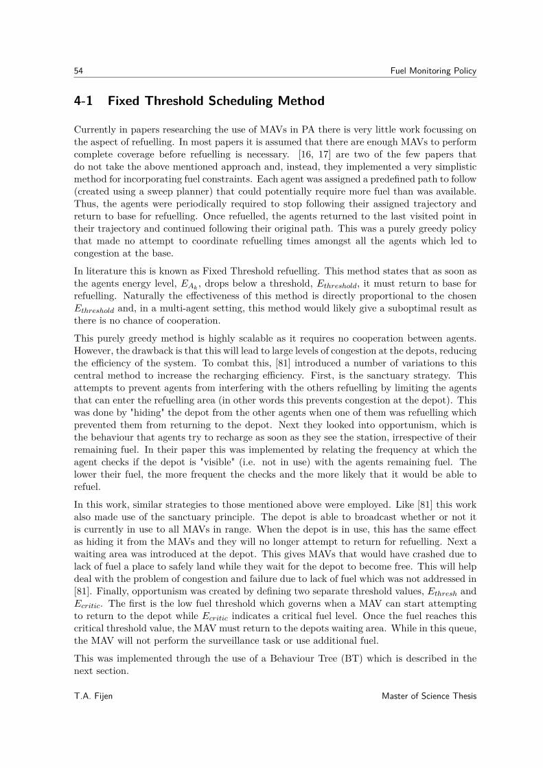
54 Fuel Monitoring Policy
4-1 Fixed Threshold Scheduling Method
Currently in papers researching the use of MAVs in PA there is very little work focussing onthe aspect of refuelling. In most papers it is assumed that there are enough MAVs to performcomplete coverage before refuelling is necessary. [16, 17] are two of the few papers thatdo not take the above mentioned approach and, instead, they implemented a very simplisticmethod for incorporating fuel constraints. Each agent was assigned a predefined path to follow(created using a sweep planner) that could potentially require more fuel than was available.Thus, the agents were periodically required to stop following their assigned trajectory andreturn to base for refuelling. Once refuelled, the agents returned to the last visited point intheir trajectory and continued following their original path. This was a purely greedy policythat made no attempt to coordinate refuelling times amongst all the agents which led tocongestion at the base.
In literature this is known as Fixed Threshold refuelling. This method states that as soon asthe agents energy level, EAk
, drops below a threshold, Ethreshold, it must return to base forrefuelling. Naturally the effectiveness of this method is directly proportional to the chosenEthreshold and, in a multi-agent setting, this method would likely give a suboptimal result asthere is no chance of cooperation.
This purely greedy method is highly scalable as it requires no cooperation between agents.However, the drawback is that this will lead to large levels of congestion at the depots, reducingthe efficiency of the system. To combat this, [81] introduced a number of variations to thiscentral method to increase the recharging efficiency. First, is the sanctuary strategy. Thisattempts to prevent agents from interfering with the others refuelling by limiting the agentsthat can enter the refuelling area (in other words this prevents congestion at the depot). Thiswas done by "hiding" the depot from the other agents when one of them was refuelling whichprevented them from returning to the depot. Next they looked into opportunism, which isthe behaviour that agents try to recharge as soon as they see the station, irrespective of theirremaining fuel. In their paper this was implemented by relating the frequency at which theagent checks if the depot is "visible" (i.e. not in use) with the agents remaining fuel. Thelower their fuel, the more frequent the checks and the more likely that it would be able torefuel.
In this work, similar strategies to those mentioned above were employed. Like [81] this workalso made use of the sanctuary principle. The depot is able to broadcast whether or not itis currently in use to all MAVs in range. When the depot is in use, this has the same effectas hiding it from the MAVs and they will no longer attempt to return for refuelling. Next awaiting area was introduced at the depot. This gives MAVs that would have crashed due tolack of fuel a place to safely land while they wait for the depot to become free. This will helpdeal with the problem of congestion and failure due to lack of fuel which was not addressed in[81]. Finally, opportunism was created by defining two separate threshold values, Ethresh andEcritic. The first is the low fuel threshold which governs when a MAV can start attemptingto return to the depot while Ecritic indicates a critical fuel level. Once the fuel reaches thiscritical threshold value, the MAV must return to the depots waiting area. While in this queue,the MAV will not perform the surveillance task or use additional fuel.
This was implemented through the use of a Behaviour Tree (BT) which is described in thenext section.
T.A. Fijen Master of Science Thesis
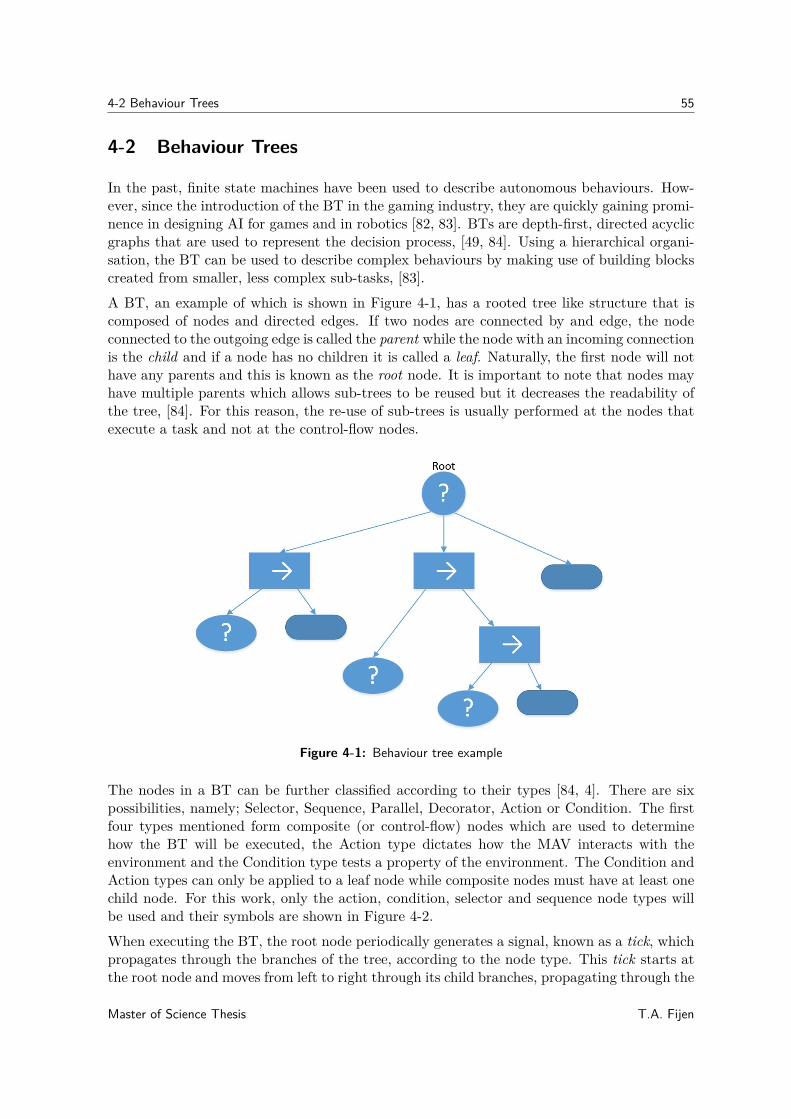
4-2 Behaviour Trees 55
4-2 Behaviour Trees
In the past, finite state machines have been used to describe autonomous behaviours. How-ever, since the introduction of the BT in the gaming industry, they are quickly gaining promi-nence in designing AI for games and in robotics [82, 83]. BTs are depth-first, directed acyclicgraphs that are used to represent the decision process, [49, 84]. Using a hierarchical organi-sation, the BT can be used to describe complex behaviours by making use of building blockscreated from smaller, less complex sub-tasks, [83].
A BT, an example of which is shown in Figure 4-1, has a rooted tree like structure that iscomposed of nodes and directed edges. If two nodes are connected by and edge, the nodeconnected to the outgoing edge is called the parent while the node with an incoming connectionis the child and if a node has no children it is called a leaf. Naturally, the first node will nothave any parents and this is known as the root node. It is important to note that nodes mayhave multiple parents which allows sub-trees to be reused but it decreases the readability ofthe tree, [84]. For this reason, the re-use of sub-trees is usually performed at the nodes thatexecute a task and not at the control-flow nodes.
Figure 4-1: Behaviour tree example
The nodes in a BT can be further classified according to their types [84, 4]. There are sixpossibilities, namely; Selector, Sequence, Parallel, Decorator, Action or Condition. The firstfour types mentioned form composite (or control-flow) nodes which are used to determinehow the BT will be executed, the Action type dictates how the MAV interacts with theenvironment and the Condition type tests a property of the environment. The Condition andAction types can only be applied to a leaf node while composite nodes must have at least onechild node. For this work, only the action, condition, selector and sequence node types willbe used and their symbols are shown in Figure 4-2.
When executing the BT, the root node periodically generates a signal, known as a tick, whichpropagates through the branches of the tree, according to the node type. This tick starts atthe root node and moves from left to right through its child branches, propagating through the
Master of Science Thesis T.A. Fijen
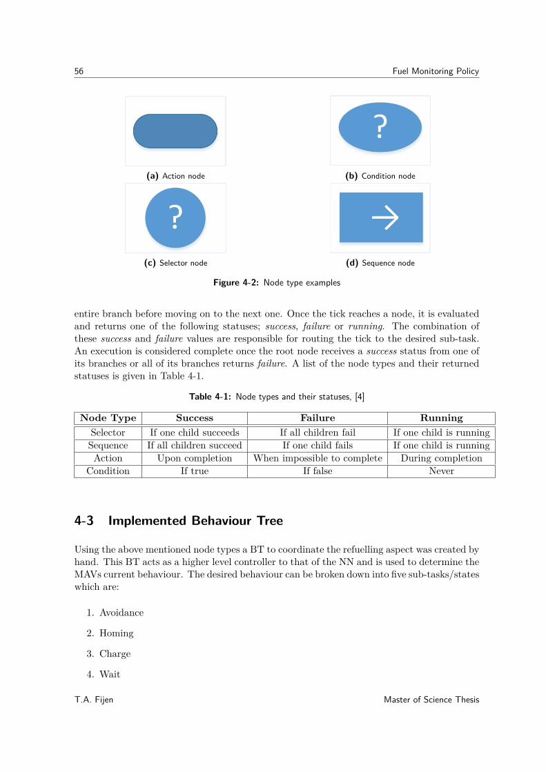
56 Fuel Monitoring Policy
(a) Action node (b) Condition node
(c) Selector node (d) Sequence node
Figure 4-2: Node type examples
entire branch before moving on to the next one. Once the tick reaches a node, it is evaluatedand returns one of the following statuses; success, failure or running. The combination ofthese success and failure values are responsible for routing the tick to the desired sub-task.An execution is considered complete once the root node receives a success status from one ofits branches or all of its branches returns failure. A list of the node types and their returnedstatuses is given in Table 4-1.
Table 4-1: Node types and their statuses, [4]
Node Type Success Failure RunningSelector If one child succeeds If all children fail If one child is runningSequence If all children succeed If one child fails If one child is runningAction Upon completion When impossible to complete During completion
Condition If true If false Never
4-3 Implemented Behaviour Tree
Using the above mentioned node types a BT to coordinate the refuelling aspect was created byhand. This BT acts as a higher level controller to that of the NN and is used to determine theMAVs current behaviour. The desired behaviour can be broken down into five sub-tasks/stateswhich are:
1. Avoidance
2. Homing
3. Charge
4. Wait
T.A. Fijen Master of Science Thesis

4-3 Implemented Behaviour Tree 57
5. Surveillance
The full BT is seen in Figure 4-3 and more a more detailed explanation of the differentbranches of the tree follows below.
Master of Science Thesis T.A. Fijen
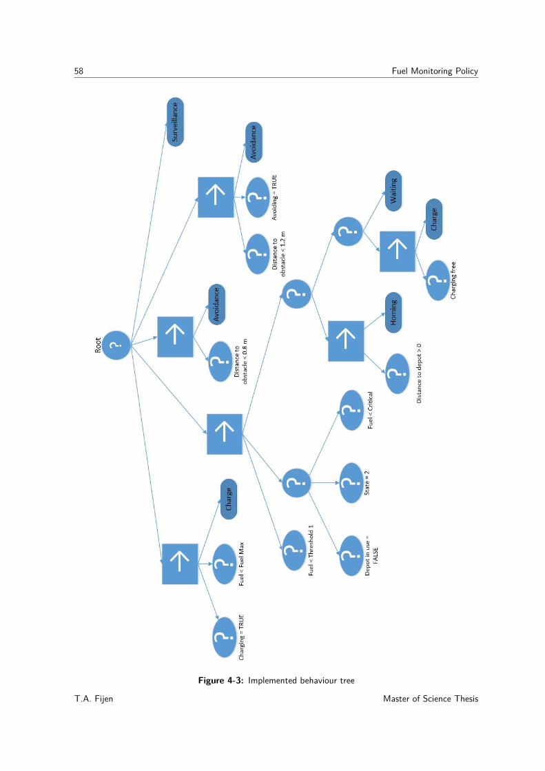
58 Fuel Monitoring Policy
Figure 4-3: Implemented behaviour tree
T.A. Fijen Master of Science Thesis
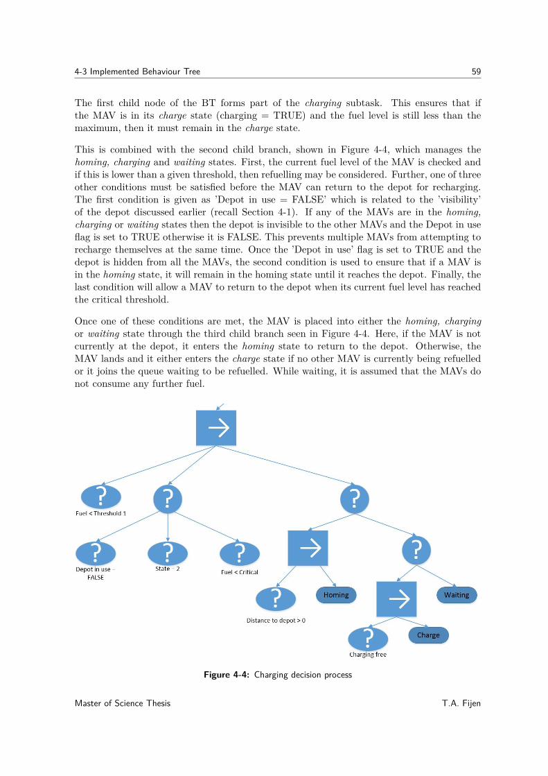
4-3 Implemented Behaviour Tree 59
The first child node of the BT forms part of the charging subtask. This ensures that ifthe MAV is in its charge state (charging = TRUE) and the fuel level is still less than themaximum, then it must remain in the charge state.
This is combined with the second child branch, shown in Figure 4-4, which manages thehoming, charging and waiting states. First, the current fuel level of the MAV is checked andif this is lower than a given threshold, then refuelling may be considered. Further, one of threeother conditions must be satisfied before the MAV can return to the depot for recharging.The first condition is given as ’Depot in use = FALSE’ which is related to the ’visibility’of the depot discussed earlier (recall Section 4-1). If any of the MAVs are in the homing,charging or waiting states then the depot is invisible to the other MAVs and the Depot in useflag is set to TRUE otherwise it is FALSE. This prevents multiple MAVs from attempting torecharge themselves at the same time. Once the ’Depot in use’ flag is set to TRUE and thedepot is hidden from all the MAVs, the second condition is used to ensure that if a MAV isin the homing state, it will remain in the homing state until it reaches the depot. Finally, thelast condition will allow a MAV to return to the depot when its current fuel level has reachedthe critical threshold.
Once one of these conditions are met, the MAV is placed into either the homing, chargingor waiting state through the third child branch seen in Figure 4-4. Here, if the MAV is notcurrently at the depot, it enters the homing state to return to the depot. Otherwise, theMAV lands and it either enters the charge state if no other MAV is currently being refuelledor it joins the queue waiting to be refuelled. While waiting, it is assumed that the MAVs donot consume any further fuel.
Figure 4-4: Charging decision process
Master of Science Thesis T.A. Fijen
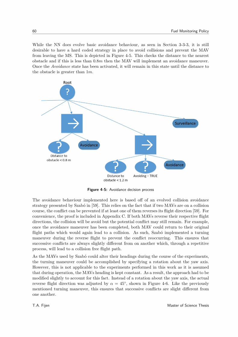
60 Fuel Monitoring Policy
While the NN does evolve basic avoidance behaviour, as seen in Section 3-3-3, it is stilldesirable to have a hard coded strategy in place to avoid collisions and prevent the MAVfrom leaving the MS. This is depicted in Figure 4-5. This checks the distance to the nearestobstacle and if this is less than 0.8m then the MAV will implement an avoidance maneuver.Once the Avoidance state has been activated, it will remain in this state until the distance tothe obstacle is greater than 1m.
Figure 4-5: Avoidance decision process
The avoidance behaviour implemented here is based off of an evolved collision avoidancestrategy presented by Szabó in [59]. This relies on the fact that if two MAVs are on a collisioncourse, the conflict can be prevented if at least one of them reverses its flight direction [59]. Forconvenience, the proof is included in Appendix C. If both MAVs reverse their respective flightdirections, the collision will be avoid but the potential conflict may still remain. For example,once the avoidance maneuver has been completed, both MAV could return to their originalflight paths which would again lead to a collision. As such, Szabó implemented a turningmaneuver during the reverse flight to prevent the conflict reoccurring. This ensures thatsuccessive conflicts are always slightly different from on another which, through a repetitiveprocess, will lead to a collision free flight path.
As the MAVs used by Szabó could alter their headings during the course of the experiments,the turning maneuver could be accomplished by specifying a rotation about the yaw axis.However, this is not applicable to the experiments performed in this work as it is assumedthat during operation, the MAVs heading is kept constant. As a result, the approach had to bemodified slightly to account for this fact. Instead of a rotation about the yaw axis, the actualreverse flight direction was adjusted by α = 45◦, shown in Figure 4-6. Like the previouslymentioned turning maneuver, this ensures that successive conflicts are slight different fromone another.
T.A. Fijen Master of Science Thesis
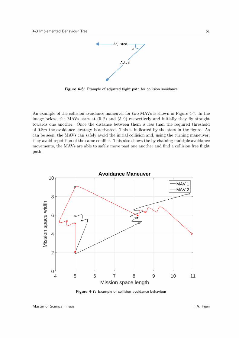
4-3 Implemented Behaviour Tree 61
Figure 4-6: Example of adjusted flight path for collision avoidance
An example of the collision avoidance maneuver for two MAVs is shown in Figure 4-7. In theimage below, the MAVs start at (5, 2) and (5, 9) respectively and initially they fly straighttowards one another. Once the distance between them is less than the required thresholdof 0.8m the avoidance strategy is activated. This is indicated by the stars in the figure. Ascan be seen, the MAVs can safely avoid the initial collision and, using the turning maneuver,they avoid repetition of the same conflict. This also shows the by chaining multiple avoidancemovements, the MAVs are able to safely move past one another and find a collision free flightpath.
4 5 6 7 8 9 10 11Mission space length
0
2
4
6
8
10
Mis
sion
spa
ce w
idth
Avoidance Maneuver
MAV 1MAV 2
Figure 4-7: Example of collision avoidance behaviour
Master of Science Thesis T.A. Fijen
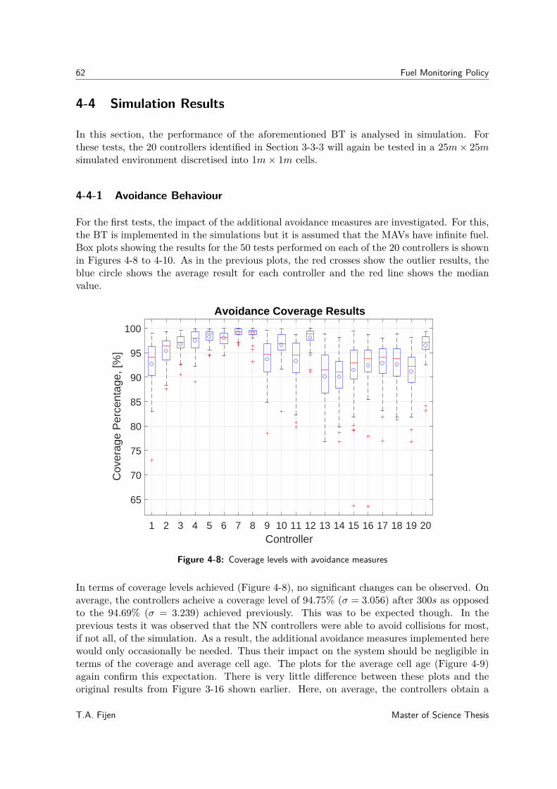
62 Fuel Monitoring Policy
4-4 Simulation Results
In this section, the performance of the aforementioned BT is analysed in simulation. Forthese tests, the 20 controllers identified in Section 3-3-3 will again be tested in a 25m× 25msimulated environment discretised into 1m× 1m cells.
4-4-1 Avoidance Behaviour
For the first tests, the impact of the additional avoidance measures are investigated. For this,the BT is implemented in the simulations but it is assumed that the MAVs have infinite fuel.Box plots showing the results for the 50 tests performed on each of the 20 controllers is shownin Figures 4-8 to 4-10. As in the previous plots, the red crosses show the outlier results, theblue circle shows the average result for each controller and the red line shows the medianvalue.
1 2 3 4 5 6 7 8 9 10 11 12 13 14 15 16 17 18 19 20Controller
65
70
75
80
85
90
95
100
Cov
erag
e P
erce
ntag
e, [%
]
Avoidance Coverage Results
Figure 4-8: Coverage levels with avoidance measures
In terms of coverage levels achieved (Figure 4-8), no significant changes can be observed. Onaverage, the controllers acheive a coverage level of 94.75% (σ = 3.056) after 300s as opposedto the 94.69% (σ = 3.239) achieved previously. This was to be expected though. In theprevious tests it was observed that the NN controllers were able to avoid collisions for most,if not all, of the simulation. As a result, the additional avoidance measures implemented herewould only occasionally be needed. Thus their impact on the system should be negligible interms of the coverage and average cell age. The plots for the average cell age (Figure 4-9)again confirm this expectation. There is very little difference between these plots and theoriginal results from Figure 3-16 shown earlier. Here, on average, the controllers obtain a
T.A. Fijen Master of Science Thesis
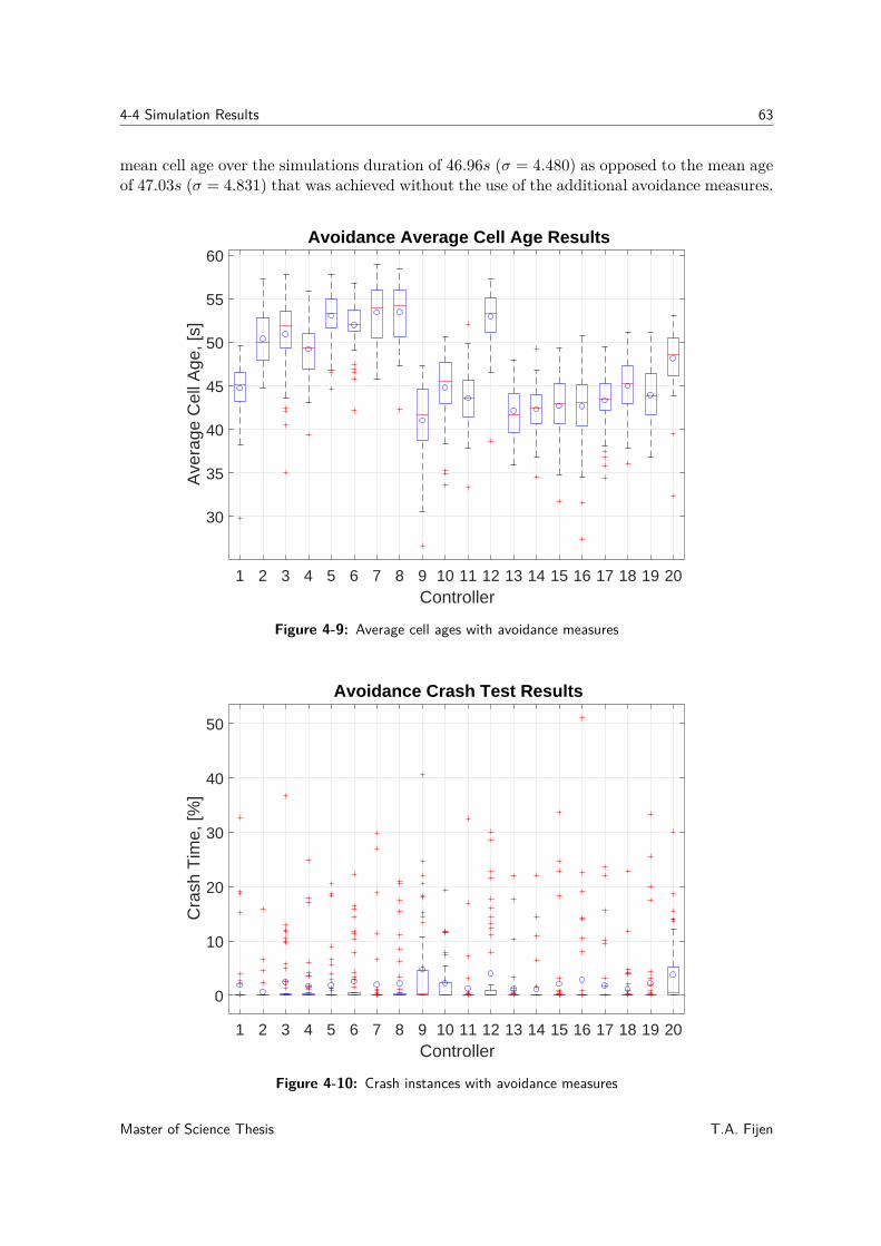
4-4 Simulation Results 63
mean cell age over the simulations duration of 46.96s (σ = 4.480) as opposed to the mean ageof 47.03s (σ = 4.831) that was achieved without the use of the additional avoidance measures.
1 2 3 4 5 6 7 8 9 10 11 12 13 14 15 16 17 18 19 20Controller
30
35
40
45
50
55
60
Ave
rage
Cel
l Age
, [s]
Avoidance Average Cell Age Results
Figure 4-9: Average cell ages with avoidance measures
1 2 3 4 5 6 7 8 9 10 11 12 13 14 15 16 17 18 19 20Controller
0
10
20
30
40
50
Cra
sh T
ime,
[%]
Avoidance Crash Test Results
Figure 4-10: Crash instances with avoidance measures
Master of Science Thesis T.A. Fijen
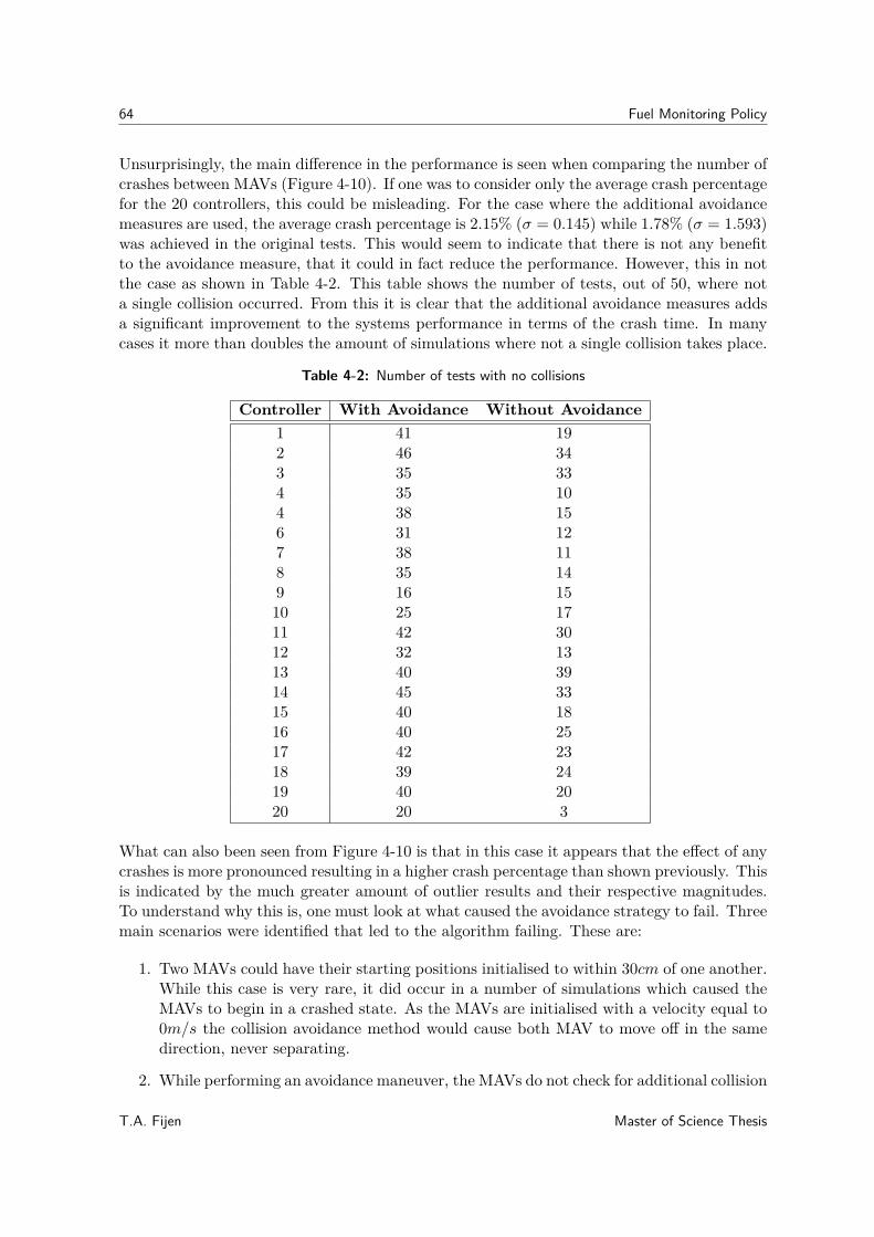
64 Fuel Monitoring Policy
Unsurprisingly, the main difference in the performance is seen when comparing the number ofcrashes between MAVs (Figure 4-10). If one was to consider only the average crash percentagefor the 20 controllers, this could be misleading. For the case where the additional avoidancemeasures are used, the average crash percentage is 2.15% (σ = 0.145) while 1.78% (σ = 1.593)was achieved in the original tests. This would seem to indicate that there is not any benefitto the avoidance measure, that it could in fact reduce the performance. However, this in notthe case as shown in Table 4-2. This table shows the number of tests, out of 50, where nota single collision occurred. From this it is clear that the additional avoidance measures addsa significant improvement to the systems performance in terms of the crash time. In manycases it more than doubles the amount of simulations where not a single collision takes place.
Table 4-2: Number of tests with no collisions
Controller With Avoidance Without Avoidance1 41 192 46 343 35 334 35 104 38 156 31 127 38 118 35 149 16 1510 25 1711 42 3012 32 1313 40 3914 45 3315 40 1816 40 2517 42 2318 39 2419 40 2020 20 3
What can also been seen from Figure 4-10 is that in this case it appears that the effect of anycrashes is more pronounced resulting in a higher crash percentage than shown previously. Thisis indicated by the much greater amount of outlier results and their respective magnitudes.To understand why this is, one must look at what caused the avoidance strategy to fail. Threemain scenarios were identified that led to the algorithm failing. These are:
1. Two MAVs could have their starting positions initialised to within 30cm of one another.While this case is very rare, it did occur in a number of simulations which caused theMAVs to begin in a crashed state. As the MAVs are initialised with a velocity equal to0m/s the collision avoidance method would cause both MAV to move off in the samedirection, never separating.
2. While performing an avoidance maneuver, the MAVs do not check for additional collision
T.A. Fijen Master of Science Thesis
4-4 Simulation Results 65
courses with other MAVs. As a result, two MAVs that are currently performing anavoidance movement could collide with one another while trying to avoid their originalconflicts.
3. In the last case, two MAVs could be commanded to travel in a similar flight directionas a result of the avoidance maneuver. While in theory they will never collide, they willalso never separate from one another and resolve the conflict. This can occur when twoMAVs are approaching one another and the first is already performing an avoidancemovement. Depending on the second MAV’s original flight direction, it could be placedon a parallel flight path by the avoidance strategy. Alternatively, as the method works onthe MAVs commanded velocity, it is also possible for the NN inputs to give two MAVsroughly the same velocity outputs just before the avoidance measures are activated.This will also cause the MAVs to perform the same avoidance motion.
These cases can cause the MAV to never resolve their collision courses, resulting in the highercrash times seen in the boxplot.
4-4-2 Refuelling
Arguably, the most important factor for determining the success of this solution is the MAVsfuel level over the duration of the mission. When the BT is implemented, this should remainabove 0 at all times. In Figure 4-11 the fuel levels for each of the eight MAVs is shown over thecourse of a typical persistent surveillance mission. It is important to note that the dischargeand refuelling rates were exaggerated in this figure so that multiple refuelling cycles could beillustrated. This figure shows that none of the MAVs become completely discharged over thecourse of the simulated mission. You will notice that all MAVs begin with the same fuel level,then, as they reach the first fuel threshold they start attempting to refuel. With the largenumber of MAVs sharing the depot, initially, not all MAVs will be able to charge themselvesbefore running out of fuel. This is where the queueing feature comes in, which is representedby the sections where the fuel level is held constant for one or more MAVs. As mentioned,this prevents crashed due to low fuel levels while it has the added benefit of staggering therefuel times of all the MAVs which will make future refuelling cycles more efficient.
As mentioned earlier, exaggerated charging and discharging rates were used for the simulatedtests. These were edepot = 5units/s and em = 0.5units/s while Ethresh = 50% and Ecritic =34% were used as the first and second refuelling thresholds. For the physical implementationon the other hand, the refuelling was based on the batteries current voltage. Table 4-3 showsthe actual values used for the physical tests on the Parrot bebop 2. Here, the threshold valuescorrespond to the low battery voltage warning given by Paparazzi. It is also important tonote that for the physical tests, the batteries are not charged while the MAV is at the depotbut, rather, they are replaced by new batteries. Therefore, in the physical tests, the depotrecharging rate is replaced with a fixed refuelling time of roughly 40s.
Master of Science Thesis T.A. Fijen
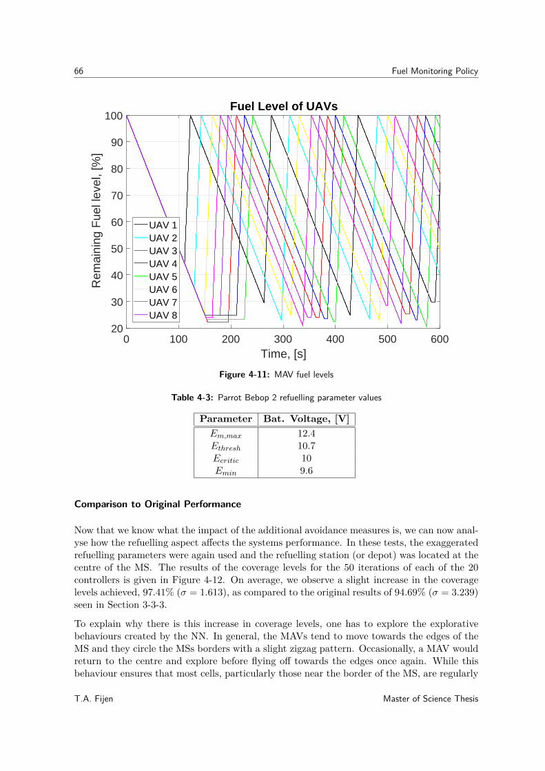
66 Fuel Monitoring Policy
0 100 200 300 400 500 600Time, [s]
20
30
40
50
60
70
80
90
100
Rem
aini
ng F
uel l
evel
, [%
]Fuel Level of UAVs
UAV 1UAV 2UAV 3UAV 4UAV 5UAV 6UAV 7UAV 8
Figure 4-11: MAV fuel levels
Table 4-3: Parrot Bebop 2 refuelling parameter values
Parameter Bat. Voltage, [V]Em,max 12.4Ethresh 10.7Ecritic 10Emin 9.6
Comparison to Original Performance
Now that we know what the impact of the additional avoidance measures is, we can now anal-yse how the refuelling aspect affects the systems performance. In these tests, the exaggeratedrefuelling parameters were again used and the refuelling station (or depot) was located at thecentre of the MS. The results of the coverage levels for the 50 iterations of each of the 20controllers is given in Figure 4-12. On average, we observe a slight increase in the coveragelevels achieved, 97.41% (σ = 1.613), as compared to the original results of 94.69% (σ = 3.239)seen in Section 3-3-3.
To explain why there is this increase in coverage levels, one has to explore the explorativebehaviours created by the NN. In general, the MAVs tend to move towards the edges of theMS and they circle the MSs borders with a slight zigzag pattern. Occasionally, a MAV wouldreturn to the centre and explore before flying off towards the edges once again. While thisbehaviour ensures that most cells, particularly those near the border of the MS, are regularly
T.A. Fijen Master of Science Thesis
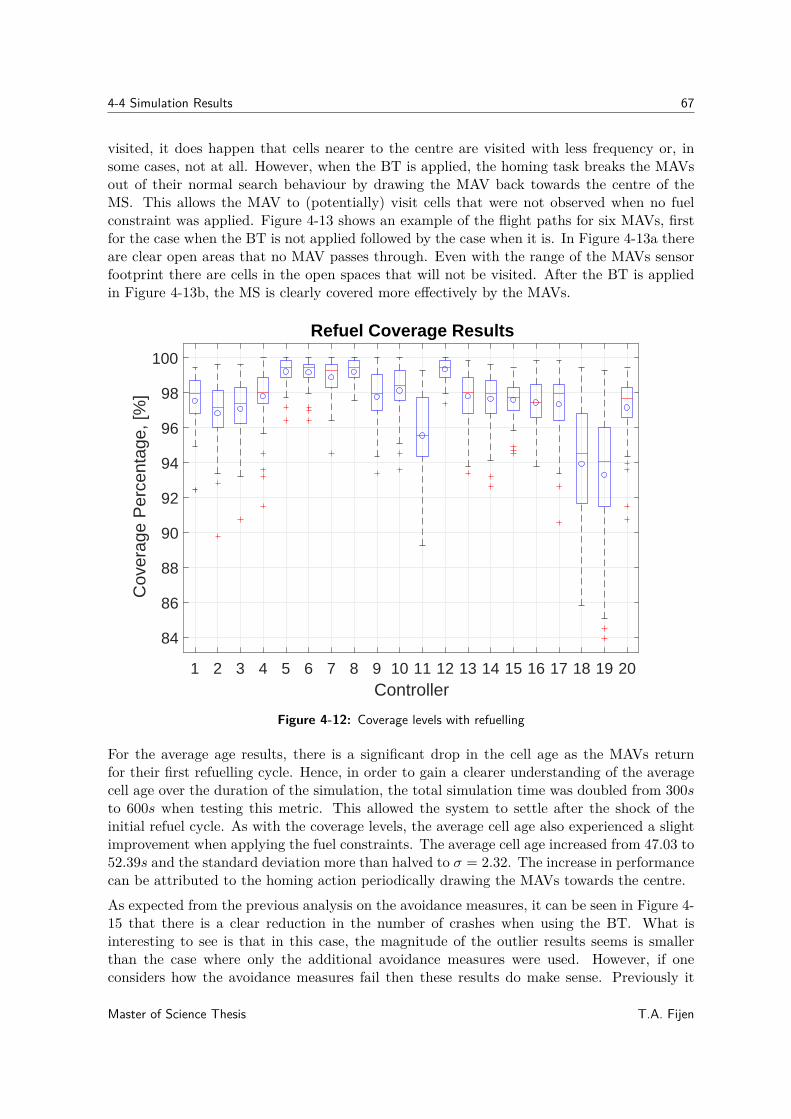
4-4 Simulation Results 67
visited, it does happen that cells nearer to the centre are visited with less frequency or, insome cases, not at all. However, when the BT is applied, the homing task breaks the MAVsout of their normal search behaviour by drawing the MAV back towards the centre of theMS. This allows the MAV to (potentially) visit cells that were not observed when no fuelconstraint was applied. Figure 4-13 shows an example of the flight paths for six MAVs, firstfor the case when the BT is not applied followed by the case when it is. In Figure 4-13a thereare clear open areas that no MAV passes through. Even with the range of the MAVs sensorfootprint there are cells in the open spaces that will not be visited. After the BT is appliedin Figure 4-13b, the MS is clearly covered more effectively by the MAVs.
1 2 3 4 5 6 7 8 9 10 11 12 13 14 15 16 17 18 19 20Controller
84
86
88
90
92
94
96
98
100
Cov
erag
e P
erce
ntag
e, [%
]
Refuel Coverage Results
Figure 4-12: Coverage levels with refuelling
For the average age results, there is a significant drop in the cell age as the MAVs returnfor their first refuelling cycle. Hence, in order to gain a clearer understanding of the averagecell age over the duration of the simulation, the total simulation time was doubled from 300sto 600s when testing this metric. This allowed the system to settle after the shock of theinitial refuel cycle. As with the coverage levels, the average cell age also experienced a slightimprovement when applying the fuel constraints. The average cell age increased from 47.03 to52.39s and the standard deviation more than halved to σ = 2.32. The increase in performancecan be attributed to the homing action periodically drawing the MAVs towards the centre.As expected from the previous analysis on the avoidance measures, it can be seen in Figure 4-15 that there is a clear reduction in the number of crashes when using the BT. What isinteresting to see is that in this case, the magnitude of the outlier results seems is smallerthan the case where only the additional avoidance measures were used. However, if oneconsiders how the avoidance measures fail then these results do make sense. Previously it
Master of Science Thesis T.A. Fijen
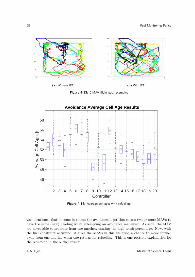
68 Fuel Monitoring Policy
(a) Without BT (b) With BT
Figure 4-13: 6 MAV flight path examples
1 2 3 4 5 6 7 8 9 10 11 12 13 14 15 16 17 18 19 20Controller
46
48
50
52
54
56
58
Ave
rage
Cel
l Age
, [s]
Avoidance Average Cell Age Results
Figure 4-14: Average cell ages with refuelling
was mentioned that in some instances the avoidance algorithm causes two or more MAVs tohave the same (new) heading when attempting an avoidance maneuver. As such, the MAVare never able to separate from one another, causing the high crash percentage. Now, withthe fuel constraint activated, it gives the MAVs in this situation a chance to move furtheraway from one another when one returns for refuelling. This is one possible explanation forthe reduction in the outlier results.
T.A. Fijen Master of Science Thesis
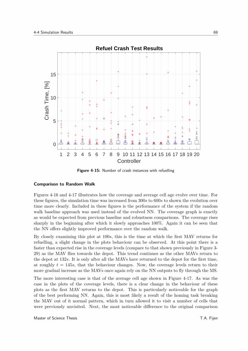
4-4 Simulation Results 69
1 2 3 4 5 6 7 8 9 10 11 12 13 14 15 16 17 18 19 20Controller
0
5
10
15
Cra
sh T
ime,
[%]
Refuel Crash Test Results
Figure 4-15: Number of crash instances with refuelling
Comparison to Random Walk
Figures 4-16 and 4-17 illustrates how the coverage and average cell age evolve over time. Forthese figures, the simulation time was increased from 300s to 600s to shown the evolution overtime more clearly. Included in these figures is the performance of the system if the randomwalk baseline approach was used instead of the evolved NN. The coverage graph is exactlyas would be expected from previous baseline and robustness comparisons. The coverage risessharply in the beginning after which it slowly approaches 100%. Again it can be seen thatthe NN offers slightly improved performance over the random walk.By closely examining this plot at 100s, this is the time at which the first MAV returns forrefuelling, a slight change in the plots behaviour can be observed. At this point there is afaster than expected rise in the coverage levels (compare to that shown previously in Figure 3-29) as the MAV flies towards the depot. This trend continues as the other MAVs return tothe depot at 132s. It is only after all the MAVs have returned to the depot for the first time,at roughly t = 145s, that the behaviour changes. Now, the coverage levels return to theirmore gradual increase as the MAVs once again rely on the NN outputs to fly through the MS.The more interesting case is that of the average cell age shown in Figure 4-17. As was thecase in the plots of the coverage levels, there is a clear change in the behaviour of theseplots as the first MAV returns to the depot. This is particularly noticeable for the graphof the best performing NN. Again, this is most likely a result of the homing task breakingthe MAV out of it normal pattern, which in turn allowed it to visit a number of cells thatwere previously unvisited. Next, the most noticeable difference to the original comparison
Master of Science Thesis T.A. Fijen
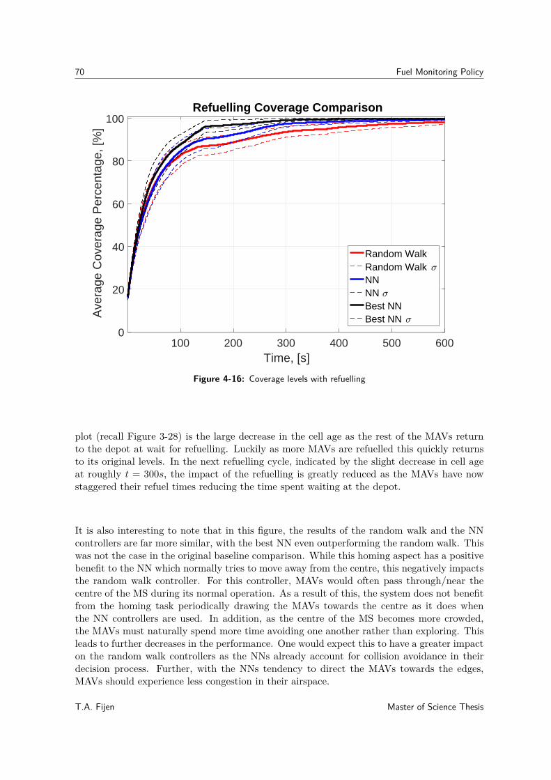
70 Fuel Monitoring Policy
100 200 300 400 500 600Time, [s]
0
20
40
60
80
100
Ave
rage
Cov
erag
e P
erce
ntag
e, [%
]Refuelling Coverage Comparison
Random WalkRandom Walk NNNN Best NNBest NN
Figure 4-16: Coverage levels with refuelling
plot (recall Figure 3-28) is the large decrease in the cell age as the rest of the MAVs returnto the depot at wait for refuelling. Luckily as more MAVs are refuelled this quickly returnsto its original levels. In the next refuelling cycle, indicated by the slight decrease in cell ageat roughly t = 300s, the impact of the refuelling is greatly reduced as the MAVs have nowstaggered their refuel times reducing the time spent waiting at the depot.
It is also interesting to note that in this figure, the results of the random walk and the NNcontrollers are far more similar, with the best NN even outperforming the random walk. Thiswas not the case in the original baseline comparison. While this homing aspect has a positivebenefit to the NN which normally tries to move away from the centre, this negatively impactsthe random walk controller. For this controller, MAVs would often pass through/near thecentre of the MS during its normal operation. As a result of this, the system does not benefitfrom the homing task periodically drawing the MAVs towards the centre as it does whenthe NN controllers are used. In addition, as the centre of the MS becomes more crowded,the MAVs must naturally spend more time avoiding one another rather than exploring. Thisleads to further decreases in the performance. One would expect this to have a greater impacton the random walk controllers as the NNs already account for collision avoidance in theirdecision process. Further, with the NNs tendency to direct the MAVs towards the edges,MAVs should experience less congestion in their airspace.
T.A. Fijen Master of Science Thesis
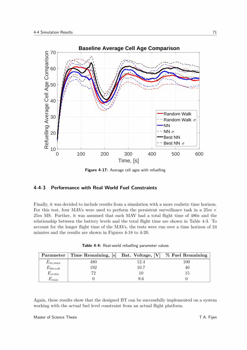
4-4 Simulation Results 71
0 100 200 300 400 500 600Time, [s]
10
20
30
40
50
60
70R
efue
lling
Ave
rage
Cel
l Age
Com
paris
onBaseline Average Cell Age Comparison
Random WalkRandom Walk NNNN Best NNBest NN
Figure 4-17: Average cell ages with refuelling
4-4-3 Performance with Real World Fuel Constraints
Finally, it was decided to include results from a simulation with a more realistic time horizon.For this test, four MAVs were used to perform the persistent surveillance task in a 25m ×25m MS. Further, it was assumed that each MAV had a total flight time of 480s and therelationship between the battery levels and the total flight time are shown in Table 4-3. Toaccount for the longer flight time of the MAVs, the tests were run over a time horizon of 24minutes and the results are shown in Figures 4-18 to 4-20.
Table 4-4: Real-world refuelling parameter values
Parameter Time Remaining, [s] Bat. Voltage, [V] % Fuel RemainingEm,max 480 12.4 100Ethresh 192 10.7 40Ecritic 72 10 15Emin 0 9.6 0
Again, these results show that the designed BT can be successfully implemented on a systemworking with the actual fuel level constraint from an actual flight platform.
Master of Science Thesis T.A. Fijen
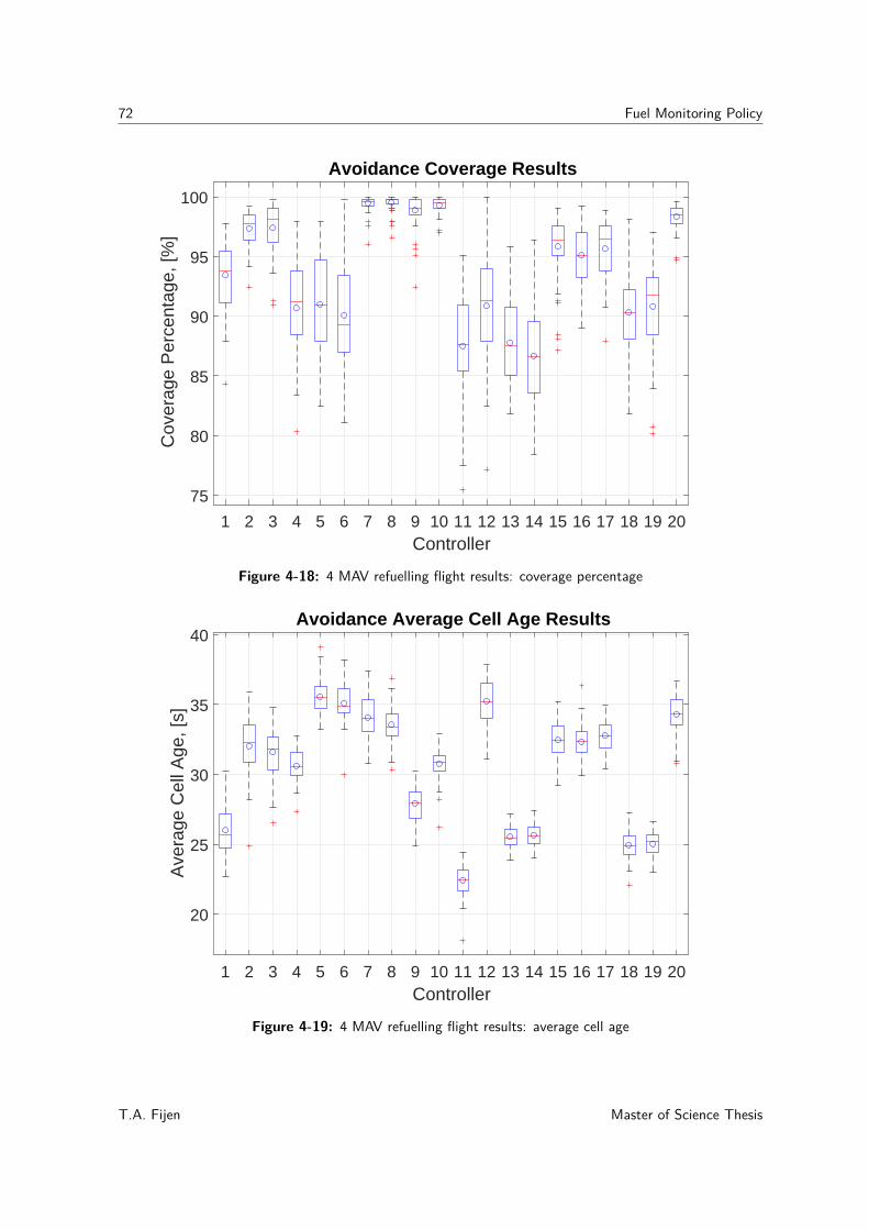
72 Fuel Monitoring Policy
1 2 3 4 5 6 7 8 9 10 11 12 13 14 15 16 17 18 19 20Controller
75
80
85
90
95
100
Cov
erag
e P
erce
ntag
e, [%
]Avoidance Coverage Results
Figure 4-18: 4 MAV refuelling flight results: coverage percentage
1 2 3 4 5 6 7 8 9 10 11 12 13 14 15 16 17 18 19 20Controller
20
25
30
35
40
Ave
rage
Cel
l Age
, [s]
Avoidance Average Cell Age Results
Figure 4-19: 4 MAV refuelling flight results: average cell age
T.A. Fijen Master of Science Thesis
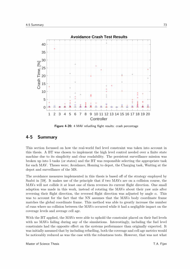
4-5 Summary 73
1 2 3 4 5 6 7 8 9 10 11 12 13 14 15 16 17 18 19 20Controller
0
5
10
15
20
25
30
35
40
Cra
sh T
ime,
[%]
Avoidance Crash Test Results
Figure 4-20: 4 MAV refuelling flight results: crash percentage
4-5 Summary
This section focussed on how the real-world fuel level constraint was taken into account inthis thesis. A BT was chosen to implement the high level control needed over a finite statemachine due to its simplicity and clear readability. The persistent surveillance mission wasbroken up into 5 tasks (or states) and the BT was responsible selecting the appropriate taskfor each MAV. Theses were; Avoidance, Homing to depot, the Charging task, Waiting at thedepot and surveillance of the MS.
The avoidance measures implemented in this thesis is based off of the strategy employed bySzabó in [59]. It makes use of the principle that if two MAVs are on a collision course, theMAVs will not collide it at least one of them reverses its current flight direction. One smalladaption was made in this work, instead of rotating the MAVs about their yaw axis afterreversing their flight direction, the reversed flight direction was adjusted by angle α. Thiswas to account for the fact that the NN assumes that the MAVs body coordinate framematches the global coordinate frame. This method was able to greatly increase the numberof runs where no collision between the MAVs occurred while it had a negligible impact on thecoverage levels and average cell age.
With the BT applied, the MAVs were able to uphold the constraint placed on their fuel levelswith no MAVs failing during any of the simulations. Interestingly, including the fuel levelconstraints had the opposite effect on the systems performance than originally expected. Itwas initially assumed that by including refuelling, both the coverage and cell age metrics wouldbe noticeably reduced as was the case with the robustness tests. However, that was not what
Master of Science Thesis T.A. Fijen
74 Fuel Monitoring Policy
was observed during the tests. These showed that both metrics experienced improvements.This was attributed to the flight paths created by the homing behaviour. During normaloperation, the NN controllers tended to command the MAVs to circle near the border of theMS. By including the homing behaviour, the MAVs would move towards the centre of theMS far more frequently allowing them to survey the centre cells more frequently and to visitcells that might have remained unobserved.
Now that the separate components to the system have been tested and verified in simulation,they can now be implemented in the physical system. This process and the results will beexplained in the next chapter.
T.A. Fijen Master of Science Thesis
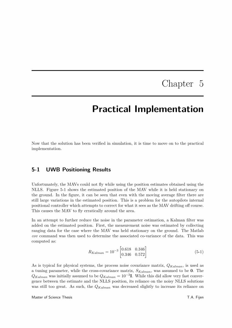
Chapter 5
Practical Implementation
Now that the solution has been verified in simulation, it is time to move on to the practicalimplementation.
5-1 UWB Positioning Results
Unfortunately, the MAVs could not fly while using the position estimates obtained using theNLLS. Figure 5-1 shows the estimated position of the MAV while it is held stationary onthe ground. In the figure, it can be seen that even with the moving average filter there arestill large variations in the estimated position. This is a problem for the autopilots internalpositional controller which attempts to correct for what it sees as the MAV drifting off course.This causes the MAV to fly erratically around the area.
In an attempt to further reduce the noise in the parameter estimation, a Kalman filter wasadded on the estimated position. First, the measurement noise was estimated by collectingranging data for the case where the MAV was held stationary on the ground. The Matlabcov command was then used to determine the associated co-variance of the data. This wascomputed as:
RKalman = 10−3[0.618 0.3460.346 0.572
](5-1)
As is typical for physical systems, the process noise covariance matrix, QKalman, is used asa tuning parameter, while the cross-covariance matrix, SKalman, was assumed to be 0. TheQKalman was initially assumed to be QKalman = 10−3I. While this did allow very fast conver-gence between the estimate and the NLLS position, its reliance on the noisy NLLS solutionswas still too great. As such, the QKalman was decreased slightly to increase its reliance on
Master of Science Thesis T.A. Fijen
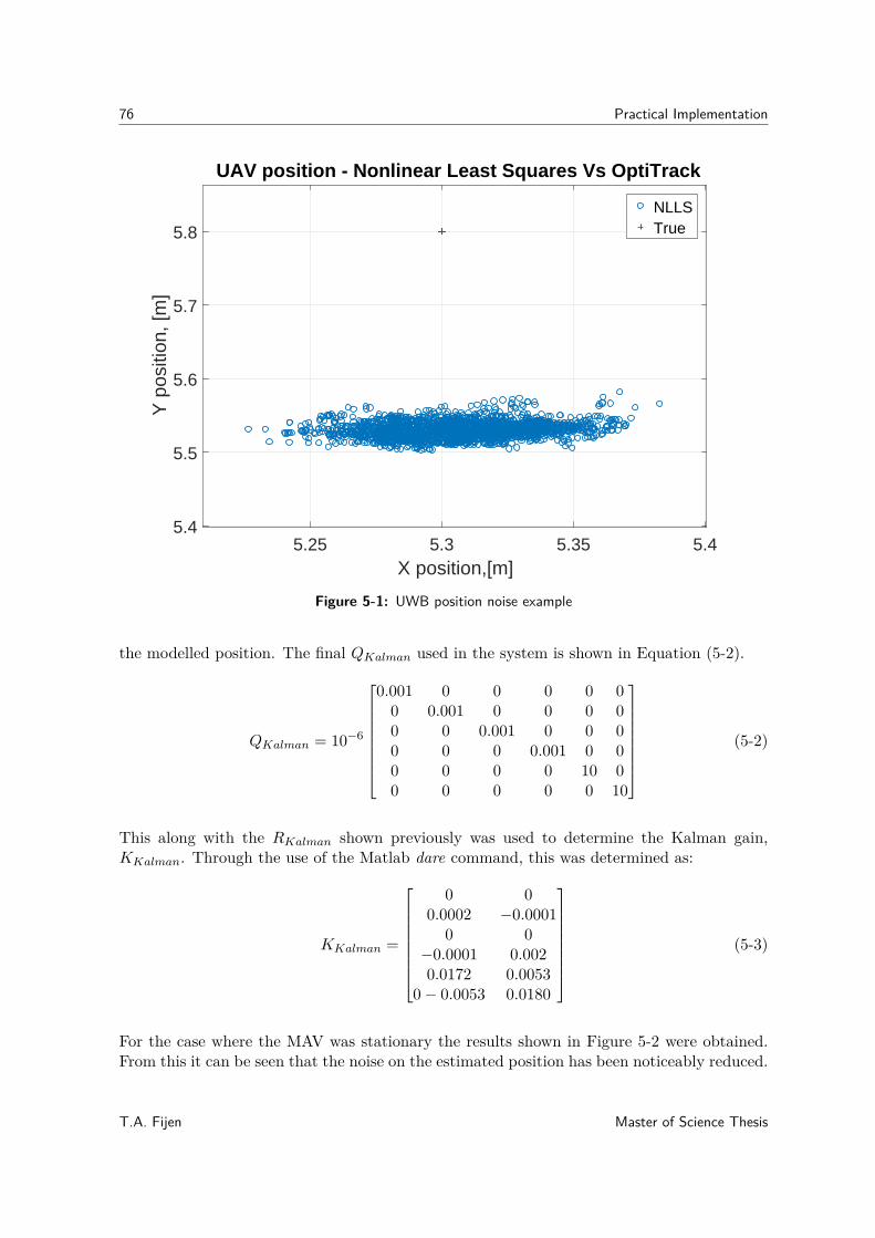
76 Practical Implementation
5.25 5.3 5.35 5.4X position,[m]
5.4
5.5
5.6
5.7
5.8
Y p
ositi
on, [
m]
UAV position - Nonlinear Least Squares Vs OptiTrack
NLLSTrue
Figure 5-1: UWB position noise example
the modelled position. The final QKalman used in the system is shown in Equation (5-2).
QKalman = 10−6
0.001 0 0 0 0 00 0.001 0 0 0 00 0 0.001 0 0 00 0 0 0.001 0 00 0 0 0 10 00 0 0 0 0 10
(5-2)
This along with the RKalman shown previously was used to determine the Kalman gain,KKalman. Through the use of the Matlab dare command, this was determined as:
KKalman =
0 00.0002 −0.0001
0 0−0.0001 0.0020.0172 0.0053
0− 0.0053 0.0180
(5-3)
For the case where the MAV was stationary the results shown in Figure 5-2 were obtained.From this it can be seen that the noise on the estimated position has been noticeably reduced.
T.A. Fijen Master of Science Thesis
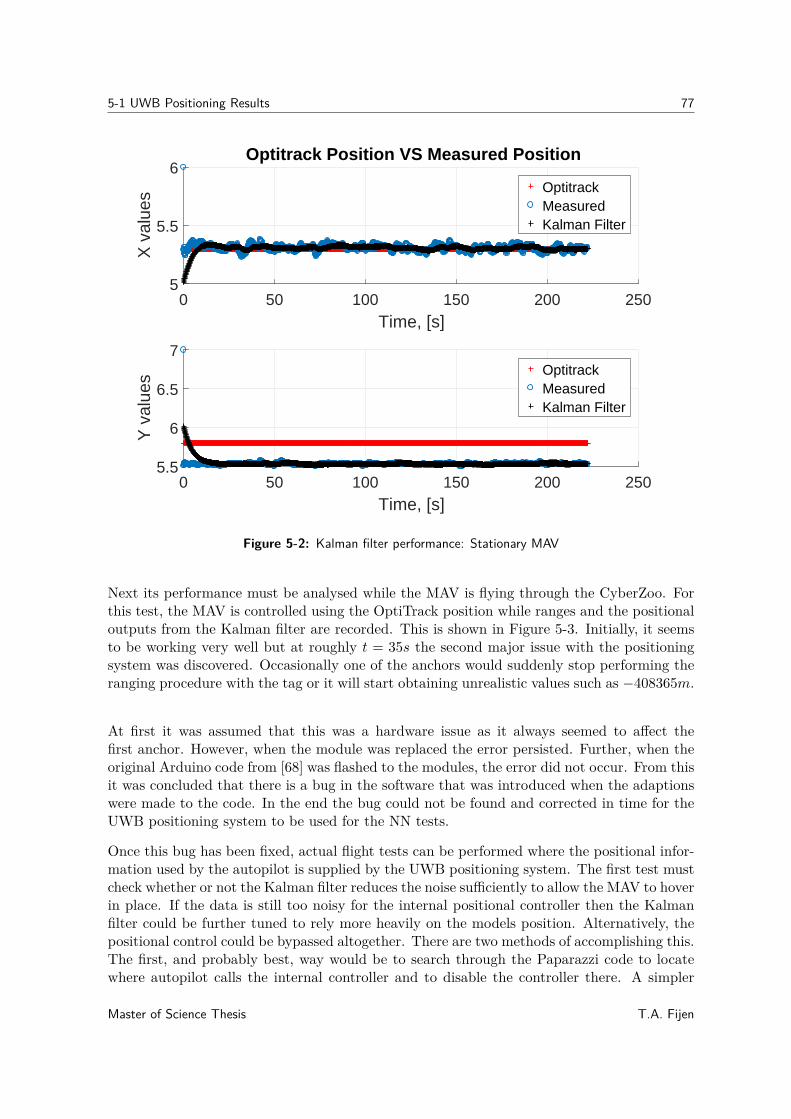
5-1 UWB Positioning Results 77
0 50 100 150 200 250Time, [s]
5
5.5
6
X v
alue
sOptitrack Position VS Measured Position
OptitrackMeasuredKalman Filter
0 50 100 150 200 250Time, [s]
5.5
6
6.5
7
Y v
alue
s OptitrackMeasuredKalman Filter
Figure 5-2: Kalman filter performance: Stationary MAV
Next its performance must be analysed while the MAV is flying through the CyberZoo. Forthis test, the MAV is controlled using the OptiTrack position while ranges and the positionaloutputs from the Kalman filter are recorded. This is shown in Figure 5-3. Initially, it seemsto be working very well but at roughly t = 35s the second major issue with the positioningsystem was discovered. Occasionally one of the anchors would suddenly stop performing theranging procedure with the tag or it will start obtaining unrealistic values such as −408365m.
At first it was assumed that this was a hardware issue as it always seemed to affect thefirst anchor. However, when the module was replaced the error persisted. Further, when theoriginal Arduino code from [68] was flashed to the modules, the error did not occur. From thisit was concluded that there is a bug in the software that was introduced when the adaptionswere made to the code. In the end the bug could not be found and corrected in time for theUWB positioning system to be used for the NN tests.
Once this bug has been fixed, actual flight tests can be performed where the positional infor-mation used by the autopilot is supplied by the UWB positioning system. The first test mustcheck whether or not the Kalman filter reduces the noise sufficiently to allow the MAV to hoverin place. If the data is still too noisy for the internal positional controller then the Kalmanfilter could be further tuned to rely more heavily on the models position. Alternatively, thepositional control could be bypassed altogether. There are two methods of accomplishing this.The first, and probably best, way would be to search through the Paparazzi code to locatewhere autopilot calls the internal controller and to disable the controller there. A simpler
Master of Science Thesis T.A. Fijen
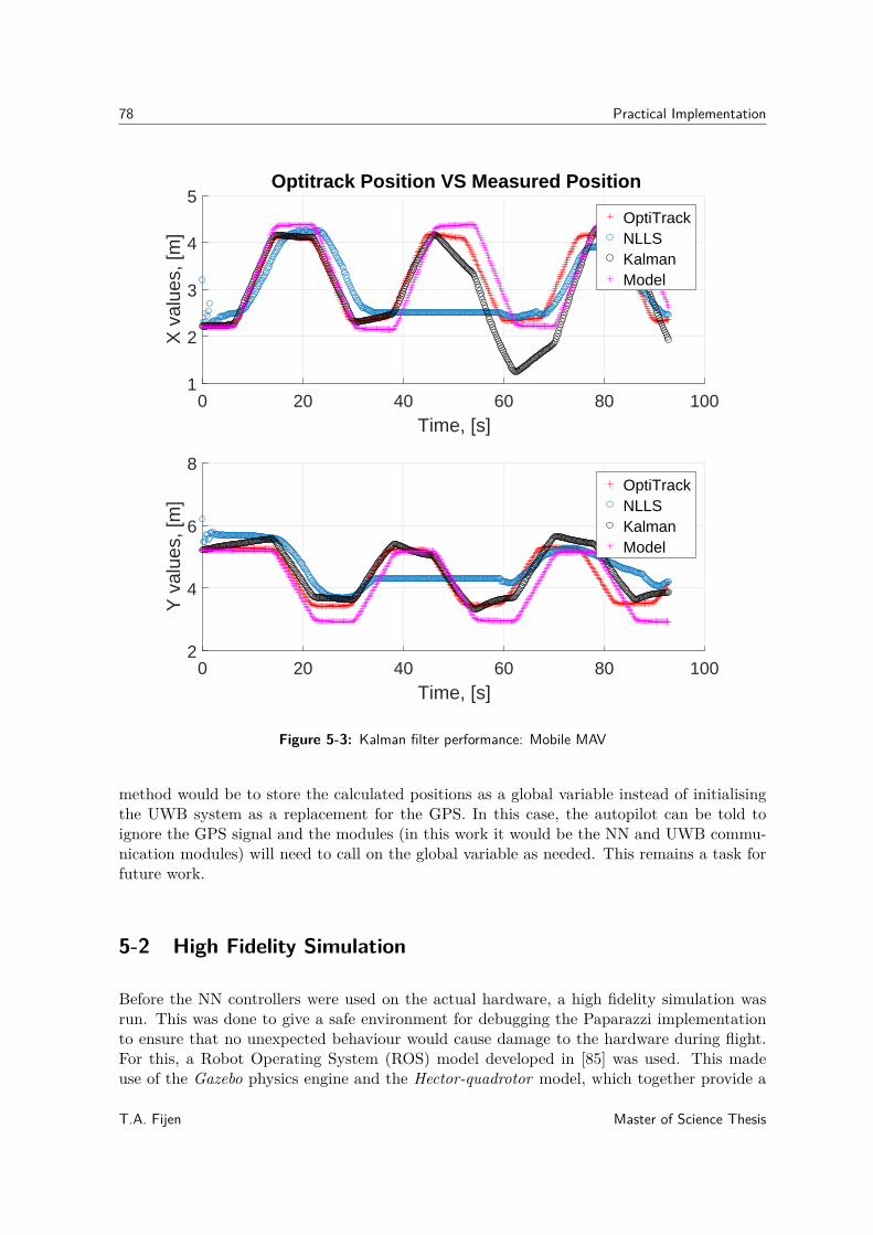
78 Practical Implementation
0 20 40 60 80 100Time, [s]
1
2
3
4
5X
val
ues,
[m]
Optitrack Position VS Measured Position
OptiTrackNLLSKalmanModel
0 20 40 60 80 100Time, [s]
2
4
6
8
Y v
alue
s, [m
]
OptiTrackNLLSKalmanModel
Figure 5-3: Kalman filter performance: Mobile MAV
method would be to store the calculated positions as a global variable instead of initialisingthe UWB system as a replacement for the GPS. In this case, the autopilot can be told toignore the GPS signal and the modules (in this work it would be the NN and UWB commu-nication modules) will need to call on the global variable as needed. This remains a task forfuture work.
5-2 High Fidelity Simulation
Before the NN controllers were used on the actual hardware, a high fidelity simulation wasrun. This was done to give a safe environment for debugging the Paparazzi implementationto ensure that no unexpected behaviour would cause damage to the hardware during flight.For this, a Robot Operating System (ROS) model developed in [85] was used. This madeuse of the Gazebo physics engine and the Hector-quadrotor model, which together provide a
T.A. Fijen Master of Science Thesis
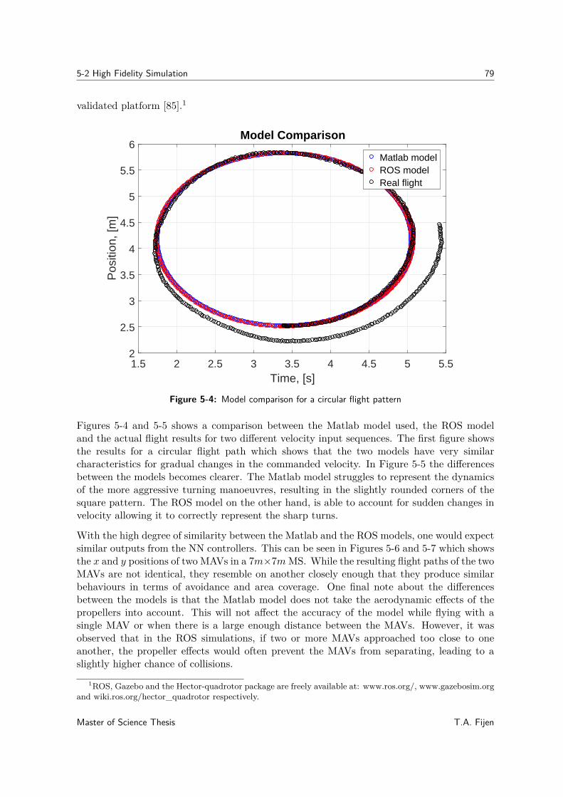
5-2 High Fidelity Simulation 79
validated platform [85].1
1.5 2 2.5 3 3.5 4 4.5 5 5.5Time, [s]
2
2.5
3
3.5
4
4.5
5
5.5
6
Pos
ition
, [m
]
Model Comparison
Matlab modelROS modelReal flight
Figure 5-4: Model comparison for a circular flight pattern
Figures 5-4 and 5-5 shows a comparison between the Matlab model used, the ROS modeland the actual flight results for two different velocity input sequences. The first figure showsthe results for a circular flight path which shows that the two models have very similarcharacteristics for gradual changes in the commanded velocity. In Figure 5-5 the differencesbetween the models becomes clearer. The Matlab model struggles to represent the dynamicsof the more aggressive turning manoeuvres, resulting in the slightly rounded corners of thesquare pattern. The ROS model on the other hand, is able to account for sudden changes invelocity allowing it to correctly represent the sharp turns.
With the high degree of similarity between the Matlab and the ROS models, one would expectsimilar outputs from the NN controllers. This can be seen in Figures 5-6 and 5-7 which showsthe x and y positions of two MAVs in a 7m×7mMS. While the resulting flight paths of the twoMAVs are not identical, they resemble on another closely enough that they produce similarbehaviours in terms of avoidance and area coverage. One final note about the differencesbetween the models is that the Matlab model does not take the aerodynamic effects of thepropellers into account. This will not affect the accuracy of the model while flying with asingle MAV or when there is a large enough distance between the MAVs. However, it wasobserved that in the ROS simulations, if two or more MAVs approached too close to oneanother, the propeller effects would often prevent the MAVs from separating, leading to aslightly higher chance of collisions.
1ROS, Gazebo and the Hector-quadrotor package are freely available at: www.ros.org/, www.gazebosim.organd wiki.ros.org/hector_quadrotor respectively.
Master of Science Thesis T.A. Fijen
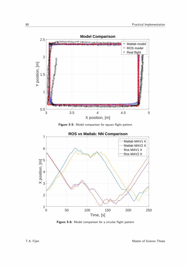
80 Practical Implementation
3 3.5 4 4.5 5X position, [m]
0.5
1
1.5
2
2.5Y
pos
ition
, [m
]Model Comparison
Matlab modelROS modelReal flight
Figure 5-5: Model comparison for square flight pattern
0 50 100 150 200 250Time, [s]
1
2
3
4
5
6
7
X p
ositi
on, [
m]
ROS vs Matlab: NN Comparison
Matlab MAV1 XMatlab MAV2 XRos MAV1 XRos MAV2 X
Figure 5-6: Model comparison for a circular flight pattern
T.A. Fijen Master of Science Thesis
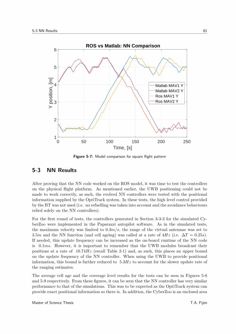
5-3 NN Results 81
0 50 100 150 200 250Time, [s]
1
2
3
4
5
6Y
pos
ition
, [m
]ROS vs Matlab: NN Comparison
Matlab MAV1 YMatlab MAV2 YRos MAV1 YRos MAV2 Y
Figure 5-7: Model comparison for square flight pattern
5-3 NN Results
After proving that the NN code worked on the ROS model, it was time to test the controllerson the physical flight platform. As mentioned earlier, the UWB positioning could not bemade to work correctly, as such, the evolved NN controllers were tested with the positionalinformation supplied by the OptiTrack system. In these tests, the high level control providedby the BT was not used (i.e. no refuelling was taken into account and the avoidance behavioursrelied solely on the NN controllers).
For the first round of tests, the controllers generated in Section 3-3-3 for the simulated Cy-berZoo were implemented in the Paparazzi autopilot software. As in the simulated tests,the maximum velocity was limited to 0.3m/s, the range of the virtual antennae was set to3.5m and the NN function (and cell ageing) was called at a rate of 4Hz (i.e. ∆T = 0.25s).If needed, this update frequency can be increased as the on-board runtime of the NN codeis 0.1ms. However, it is important to remember that the UWB modules broadcast theirpositions at a rate of 10.74Hz (recall Table 2-1) and, as such, this places an upper boundon the update frequency of the NN controller. When using the UWB to provide positionalinformation, this bound is further reduced to 5.3Hz to account for the slower update rate ofthe ranging estimates.
The average cell age and the coverage level results for the tests can be seen in Figures 5-8and 5-9 respectively. From these figures, it can be seen that the NN controller has very similarperformance to that of the simulations. This was to be expected as the OptiTrack system canprovide exact positional information so there is. In addition, the CyberZoo is an enclosed area
Master of Science Thesis T.A. Fijen
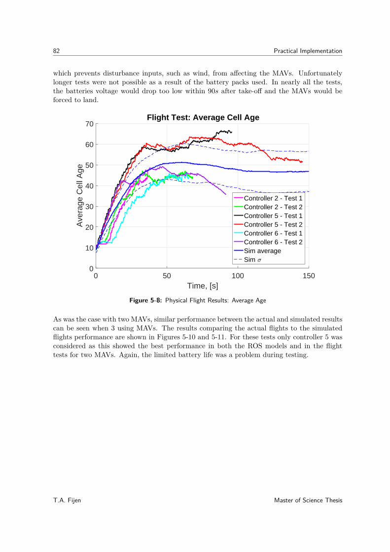
82 Practical Implementation
which prevents disturbance inputs, such as wind, from affecting the MAVs. Unfortunatelylonger tests were not possible as a result of the battery packs used. In nearly all the tests,the batteries voltage would drop too low within 90s after take-off and the MAVs would beforced to land.
0 50 100 150Time, [s]
0
10
20
30
40
50
60
70
Ave
rage
Cel
l Age
Flight Test: Average Cell Age
Controller 2 - Test 1Controller 2 - Test 2Controller 5 - Test 1Controller 5 - Test 2Controller 6 - Test 1Controller 6 - Test 2Sim averageSim
Figure 5-8: Physical Flight Results: Average Age
As was the case with two MAVs, similar performance between the actual and simulated resultscan be seen when 3 using MAVs. The results comparing the actual flights to the simulatedflights performance are shown in Figures 5-10 and 5-11. For these tests only controller 5 wasconsidered as this showed the best performance in both the ROS models and in the flighttests for two MAVs. Again, the limited battery life was a problem during testing.
T.A. Fijen Master of Science Thesis
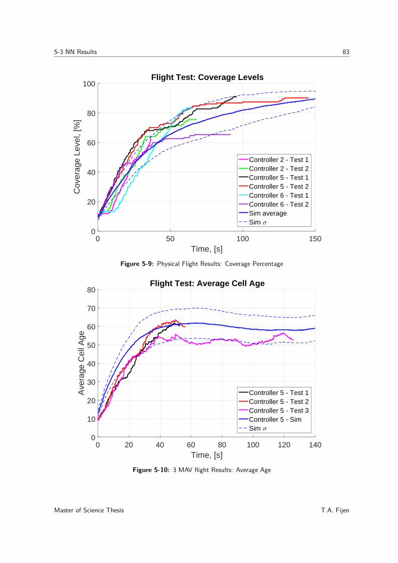
5-3 NN Results 83
0 50 100 150Time, [s]
0
20
40
60
80
100C
over
age
Leve
l, [%
]Flight Test: Coverage Levels
Controller 2 - Test 1Controller 2 - Test 2Controller 5 - Test 1Controller 5 - Test 2Controller 6 - Test 1Controller 6 - Test 2Sim averageSim
Figure 5-9: Physical Flight Results: Coverage Percentage
0 20 40 60 80 100 120 140Time, [s]
0
10
20
30
40
50
60
70
80
Ave
rage
Cel
l Age
Flight Test: Average Cell Age
Controller 5 - Test 1Controller 5 - Test 2Controller 5 - Test 3Controller 5 - SimSim
Figure 5-10: 3 MAV flight Results: Average Age
Master of Science Thesis T.A. Fijen
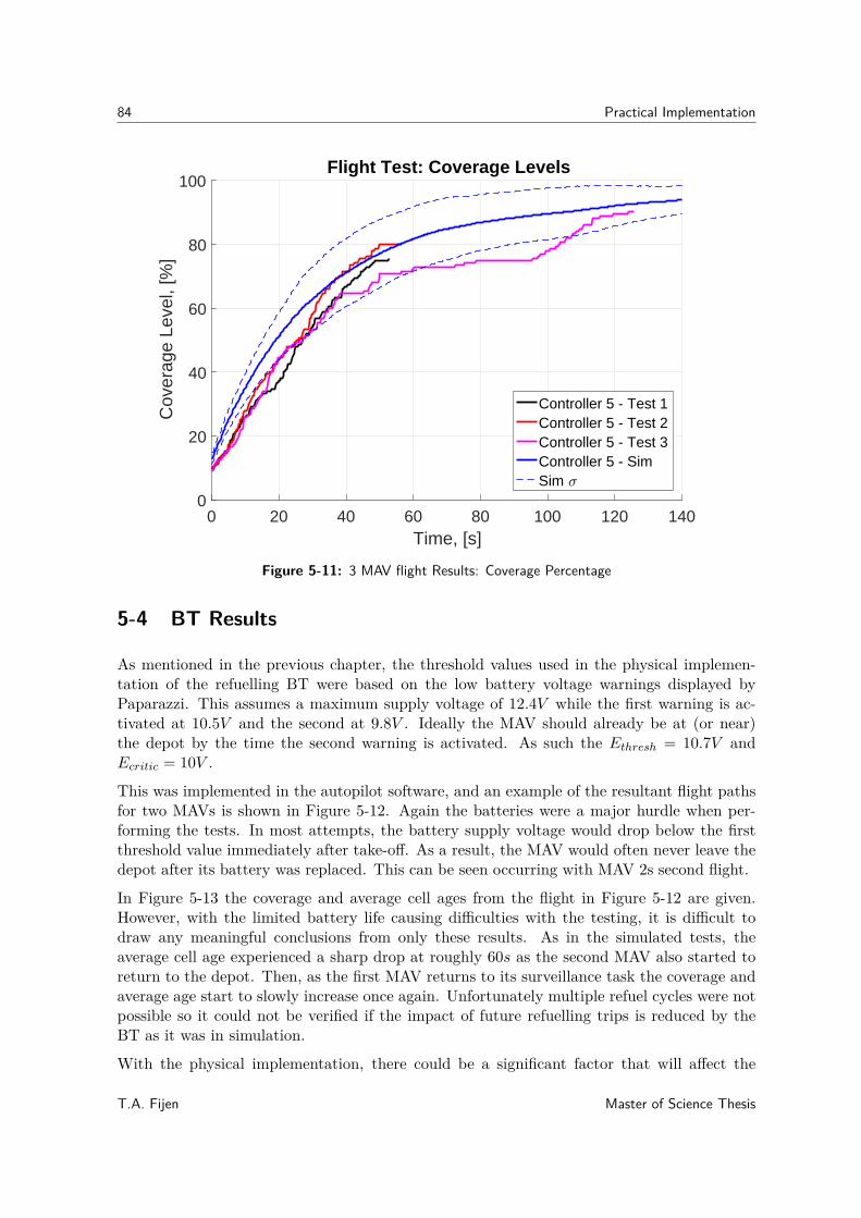
84 Practical Implementation
0 20 40 60 80 100 120 140Time, [s]
0
20
40
60
80
100C
over
age
Leve
l, [%
]Flight Test: Coverage Levels
Controller 5 - Test 1Controller 5 - Test 2Controller 5 - Test 3Controller 5 - SimSim
Figure 5-11: 3 MAV flight Results: Coverage Percentage
5-4 BT Results
As mentioned in the previous chapter, the threshold values used in the physical implemen-tation of the refuelling BT were based on the low battery voltage warnings displayed byPaparazzi. This assumes a maximum supply voltage of 12.4V while the first warning is ac-tivated at 10.5V and the second at 9.8V . Ideally the MAV should already be at (or near)the depot by the time the second warning is activated. As such the Ethresh = 10.7V andEcritic = 10V .
This was implemented in the autopilot software, and an example of the resultant flight pathsfor two MAVs is shown in Figure 5-12. Again the batteries were a major hurdle when per-forming the tests. In most attempts, the battery supply voltage would drop below the firstthreshold value immediately after take-off. As a result, the MAV would often never leave thedepot after its battery was replaced. This can be seen occurring with MAV 2s second flight.
In Figure 5-13 the coverage and average cell ages from the flight in Figure 5-12 are given.However, with the limited battery life causing difficulties with the testing, it is difficult todraw any meaningful conclusions from only these results. As in the simulated tests, theaverage cell age experienced a sharp drop at roughly 60s as the second MAV also started toreturn to the depot. Then, as the first MAV returns to its surveillance task the coverage andaverage age start to slowly increase once again. Unfortunately multiple refuel cycles were notpossible so it could not be verified if the impact of future refuelling trips is reduced by theBT as it was in simulation.
With the physical implementation, there could be a significant factor that will affect the
T.A. Fijen Master of Science Thesis
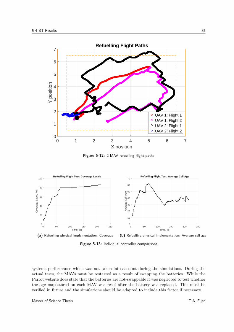
5-4 BT Results 85
0 1 2 3 4 5 6 7X position
0
1
2
3
4
5
6
7Y
pos
ition
Refuelling Flight Paths
UAV 1: Flight 1UAV 1: Flight 2UAV 2: Flight 1UAV 2: Flight 2
Figure 5-12: 2 MAV refuelling flight paths
0 50 100 150 200 250Time, [s]
0
20
40
60
80
100
Cov
erag
e Le
vel,
[%]
Refuelling Flight Test: Coverage Levels
(a) Refuelling physical implementation: Coverage
0 50 100 150 200 250Time, [s]
0
10
20
30
40
50
60
70
Ave
rage
Cel
l Age
Refuelling Flight Test: Average Cell Age
(b) Refuelling physical implementation: Average cell age
Figure 5-13: Individual controller comparisons
systems performance which was not taken into account during the simulations. During theactual tests, the MAVs must be restarted as a result of swapping the batteries. While theParrot website does state that the batteries are hot-swappable it was neglected to test whetherthe age map stored on each MAV was reset after the battery was replaced. This must beverified in future and the simulations should be adapted to include this factor if necessary.
Master of Science Thesis T.A. Fijen
86 Practical Implementation
5-5 Summary
The UWB positioning and communication system was partially successful. The inter-MAVcommunication of the current positions and the status of the depot were reliably transmittedby the UWB module. In addition, the NLLS position estimation, a Kalman filter on theposition and an UWB GPS structure were programmed in C and verified for the Paparazziautopilot software. The main issue with this positioning system was in the adaptions madeto the Arduino code that controlled the UWB modules. There is a bug in the code thatperiodically causes one of the modules to stop performing the ranging procedure. This madethe system too unreliable for the physical tests.
The NN controllers were successfully implemented and tested on the actual flight platform.During the tests comparable results in terms of the performance metrics were recorded. Inaddition, the MAVs exhibited the same explorative behaviours as those recorded in the simu-lated tests. This was to be expected as the OptiTrack system used to determine the positionof the MAVs offers a high degree of accuracy which eliminates the noise being input into theNN. Further, the enclosed are of the CyberZoo limits the disturbance forces that act on theMAVs.
The BT designed in the previous chapter was successfully implemented on the physical system.However, further testing will be needed to thoroughly verify that the performance on theactual setup is comparable to that of the simulations.
The main issue faced when performing the physical tests was with the batteries used to powerthe MAVs. The short flight times made it difficult to draw meaningful conclusions about theoverall performance of the controllers.
T.A. Fijen Master of Science Thesis
Chapter 6
Conclusions
In this final chapter, the work presented in this thesis and the main results will be summarised.This is followed by an outline of the potential aspects for future work.
6-1 Summary
The main goal of this thesis was to design and implement a controller that could be used toperform a multi-agent persistent surveillance task. The solution could not rely on a centralisedcontroller and had to account for the limitations placed on the system by the flight platformsfuel constraints. It was decided to use the NEAT algorithm to evolve NN controllers thatwere responsible for solving the persistent surveillance task while a BT was used to accountfor the limited fuel level. The NN controller and BT could then be implemented on a swarmof MAVs which would then be used to constantly fly throughout a greenhouse, collectingenvironmental data as they go for use in PA. Further, as this system is originally intended tooperate in indoor environments, an inexpensive and reliable alternative to GPS is needed tosupply the MAVs with their positional data. This thesis investigated the use of an OptiTrackmotion capture system and an UWB localisation system that gave the position relative to aset of fixed anchors.
In Chapter 2 the chapter started by giving a detailed explanation of the problem, and itssimplifying assumptions, that was solved during this thesis. It concluded with a descriptionof the physical hardware that was used during the testing phase of this work. Here, the UWBpositioning system was introduced and its performance was further described in Section 5-1.For this system a series of four stationary anchor modules were installed at known locationsaround the perimeter of the test area while each MAV was equipped with its own module.By measuring the time of flight for messages sent between the modules, the ranges betweenthe MAVs and the stationary nodes could be determined. A NLLS algorithm was then usedto estimate the positions of the MAVs based on these ranges.
This proved to be able to obtain reasonable (MSEx = 0.139 and MSEy = 0.074) positionalestimates provided that the autopilot software used positional information supplied by the
Master of Science Thesis T.A. Fijen
88 Conclusions
OptiTrack system in the flight controller. When attempting to use the positional informationsupplied by the UWB system it was found that there was too much noise on the estimatedposition. This caused the flight controller to try correct for what it saw as the MAV drifting.This resulted in the MAV moving erratically around the test area instead of hovering in place.To combat this, a Kalman filter was added to reduce the noise present in the positioningsystem. However, an issue with the module prevented this from being further tuned andtested to ensure that it does solve the problem. Due to the problems faced with this systemit was decided to rely on the OptiTrack system for all physical tests.
The NEAT algorithm was selected to generate the NN controllers. This is an evolutionaryalgorithm that optimises the structure of the NN as well as the connection weights betweennodes. In current literature, this method has not been widely used in the field of persistentsurveillance. The few papers that do make use of this focus on showing that it is applicableas a method for solving the persistent surveillance problem and do not present comparisonsto existing strategies or possible improvements.
The first change made in this work compared to the current literature was with the fitnessfunction used to analyse the performance of the NN controllers. Instead of multiplying thetotal average fitness, over the entire duration, by the safety coefficient, in this work the safetycoefficient was multiplied by the individual fitness scores for each time step. This penalisedthe system each time the positional constraint was violated instead of penalising it only onceat the end. For the test case, this produced an average increase in the coverage levels of 3.14%while the difference between th best performing controller for each case was 9.35s and 7.26%for the average cell age and coverage percentage respectively.
Next, five different sets of input values for the NN were tested. Two of the input sets werefrom current literature, while the remaining three used varying levels of information retrievedfrom the surrounding environment. This was done in an attempt to increase the controller’sperformance. During the testing procedure, it was found that the fourth set of input valuesproduced the best controllers in terms of the performance metrics identified in Chapter 2.This made use of 18 inputs comprised of the ranges returned by the 8 virtual antennae, thecell ages of the furthest cell reached by each of the 8 antenna, a boolean input that was setto 1 if the MAV was inside the MS and a bias node. With these inputs, the post evaluationof the controllers showed that the best controller had an average coverage of 99.1%, cell ageof 53.46s and a crash percentage of 2.6% over the 50 tests. The average values over the 20controllers tested were 94.96% for the coverage, 47.03s for the average cell age and 1.78% forthe crash percentage.
The performance of the NN controllers compared to the baseline methods was somewhatdisappointing. As expected, the (near) optimal performance obtained from the centralisedline-sweep method clearly gave the best performance. However, the NN and the random walkoffered greater robustness to MAV failures. For the random walk, this method showed betterresults in terms of the average cell age (56.59s). However, its ability to completely cover thearea was slightly lower than that of the NN, with an average coverage level of 95.96%.
In Chapter 4 a BT was created by hand to assign the MAV to one of five tasks. Thesewere avoidance, homing, charging, waiting or surveillance. During testing this was shown toensure that the real-world fuel constraints that the MAVs were never violated. In addition,the added avoidance measures further reduced the crash percentage more than doubling thenumber of tests that did not result in a single collision. Surprisingly the inclusion of the fuel
T.A. Fijen Master of Science Thesis
6-2 Future Work 89
constraints and the BT actually improved the performance of the system as a whole whenconsidering the coverage and cell age. On average, these were increased to 97.41% and 52.39srespectively. This increased performance was attributed to the fact that the homing task’broke’ the MAVs out of their flight patterns around the border of the MS and periodicallydrew them back to the centre.
Finally, in Chapter 5 the BT and the NN controllers were implemented in Paparazzi for theactual flight tests in the CyberZoo. These tests showed that the NN controllers offered similarperformance on the physical flight platform as they did in simulation. However, the length ofthe tests were relatively short as a result of the batteries used during testing. This made itdifficult to draw conclusions of the controller’s avoidance ability. Further, this also hinderedthe refuelling tests. Here, the MAVs fuel would immediately drop below the first thresholdas soon as they took-off. As a result, the MAVs would usually not move away from the depotafter their batteries were swapped out.
In conclusion, this thesis presented an evolved NN controller that could be implemented oneach individual MAV. By using the adapted fitness function and the new input values, a clearimprovement was observed compared to the NNs presented in current literature. While thiswork focussed on applying this system to PA in greenhouses, it is also directly applicable tosecurity related tasks such as crowd monitoring or patrolling an area.
6-2 Future Work
In this last section, a few topics for future research are described.
6-2-1 UWB Positioning
Research into UWB positioning systems have been well documented in current literature[86, 87, 65, 88]. However, as mentioned in Section 5-1 more work is needed to further de-velop the Arduino code controlling the ranging procedure between modules. Specifically, thisshould focus on implementing a more reliable ranging procedure between multiple anchorsand multiple tags.
A further issue with the current UWB system is the update rate of the range estimates.Currently the system is based on the TWR method where asynchronous two way ranging isused to determine the distance between two modules. However, this requires the modules tobroadcast a total of four messages before it can calculate the range. As more modules areadded, this can greatly reduce the system’s ability to produce results in (near) real-time. Inaddition, this can introduce more errors to the range estimates as the increasing time betweenthe ranging messages give the MAVs more time to change their positions during the rangingprocess [67]. An alternative would be to implement a system based on TDOA, for example.In this case, the position is determined using the difference in propagation times betweensignal sent by the anchors [68]. As a result, only the anchors are required to broadcast signalsand the position can be determined after each anchor broadcasts a single message. This willallow the system to operate with a much larger swarm of MAVs. The main drawback is thatthis method requires the anchors system clocks to be synchronised with on another [68, 89].
Master of Science Thesis T.A. Fijen
90 Conclusions
6-2-2 NN Performance
During evolution the NNs usually evolved behaviour where they would fly around near theedge of the MS and would only occasionally pass through the centre of the area. Whenanalysing the performance of the system with the BT implemented, it was observed thatby breaking the MAVs out of their naturally formed flight patterns an increase in the areacoverage and cell age could be obtained. As a topic for future work it would be useful todetermine whether the same benefit could be obtained by including an element of randomnessinto the NNs inputs. In addition an analysis between the performance of the system usingthe standard feedforward structure (as in this work) and the performance when recurrentconnections are allowed in the NN will be beneficial.
Further, research into the impact of differing age maps is necessary and has not been addressedin current literature. During refuelling, as the batteries are swapped, the MAV must berestarted this could cause it to lose the information currently stored in its age map. This canlead to a duplication of effort as the MAVs survey areas that were recently visited insteadof flying towards the unvisited areas. This can also be related to communication constraintsplaced on the system. Differences between the age maps will start developing as the MAVsmove out of communication range, or if the period of communication is longer that the NNsupdate rate.
6-2-3 Refuelling
While this thesis focussed on a single refuelling station, the method should be directly appli-cable to the multiple depot case. A minor topic for future research could look into the effectthat this will have on the overall systems performance. Related to this, one could then lookfurther to determine the ideal placement for the depots.
Lastly, this work assumed that each MAV must be completely recharged before it is allowedto leave the depot. While this makes sense for the case where the MAVs have their batteriesreplaced at the depot, future research could look into recharging the MAVs at the depotinstead. In this case it would then be possible to only partially recharge a MAV before itcontinues with the surveillance mission. This has not received much attention in currentliterature and may offer increased system performance, particularly during the first rechargecycle where a long queue forms at the depot.
T.A. Fijen Master of Science Thesis

Appendix A
Input Case Results
This appendix gives the individual results of the average cell age and coverage levels achieveby each of the 20 controllers analysed for the different input cases.
A-1 Input Case 1
Master of Science Thesis T.A. Fijen
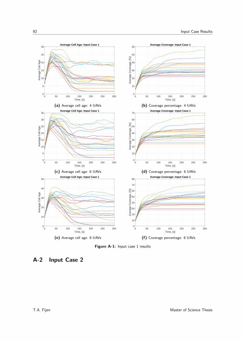
92 Input Case Results
0 50 100 150 200 250 300Time, [s]
0
5
10
15
20
25
30
Ave
rage
Cel
l Age
Average Cell Age: Input Case 1
(a) Average cell age: 4 UAVs
0 50 100 150 200 250 300Time, [s]
0
10
20
30
40
50
60
Ave
rage
Cov
erag
e, [%
]
Average Coverage: Input Case 1
(b) Coverage percentage: 4 UAVs
0 50 100 150 200 250 300Time, [s]
0
5
10
15
20
25
30
35
Ave
rage
Cel
l Age
Average Cell Age: Input Case 1
(c) Average cell age: 6 UAVs
0 50 100 150 200 250 300Time, [s]
0
10
20
30
40
50
60
70
Ave
rage
Cov
erag
e, [%
]
Average Coverage: Input Case 1
(d) Coverage percentage: 6 UAVs
0 50 100 150 200 250 300Time, [s]
0
10
20
30
40
50
Ave
rage
Cel
l Age
Average Cell Age: Input Case 1
(e) Average cell age: 8 UAVs
0 50 100 150 200 250 300Time, [s]
0
10
20
30
40
50
60
70
80
Ave
rage
Cov
erag
e, [%
]
Average Coverage: Input Case 1
(f) Coverage percentage: 8 UAVs
Figure A-1: Input case 1 results
A-2 Input Case 2
T.A. Fijen Master of Science Thesis
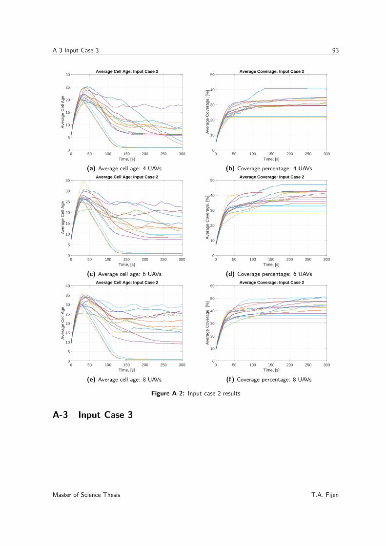
A-3 Input Case 3 93
0 50 100 150 200 250 300Time, [s]
0
5
10
15
20
25
30
Ave
rage
Cel
l Age
Average Cell Age: Input Case 2
(a) Average cell age: 4 UAVs
0 50 100 150 200 250 300Time, [s]
0
10
20
30
40
50
Ave
rage
Cov
erag
e, [%
]
Average Coverage: Input Case 2
(b) Coverage percentage: 4 UAVs
0 50 100 150 200 250 300Time, [s]
0
5
10
15
20
25
30
35
Ave
rage
Cel
l Age
Average Cell Age: Input Case 2
(c) Average cell age: 6 UAVs
0 50 100 150 200 250 300Time, [s]
0
10
20
30
40
50
Ave
rage
Cov
erag
e, [%
]
Average Coverage: Input Case 2
(d) Coverage percentage: 6 UAVs
0 50 100 150 200 250 300Time, [s]
0
5
10
15
20
25
30
35
40
Ave
rage
Cel
l Age
Average Cell Age: Input Case 2
(e) Average cell age: 8 UAVs
0 50 100 150 200 250 300Time, [s]
0
10
20
30
40
50
60
Ave
rage
Cov
erag
e, [%
]
Average Coverage: Input Case 2
(f) Coverage percentage: 8 UAVs
Figure A-2: Input case 2 results
A-3 Input Case 3
Master of Science Thesis T.A. Fijen
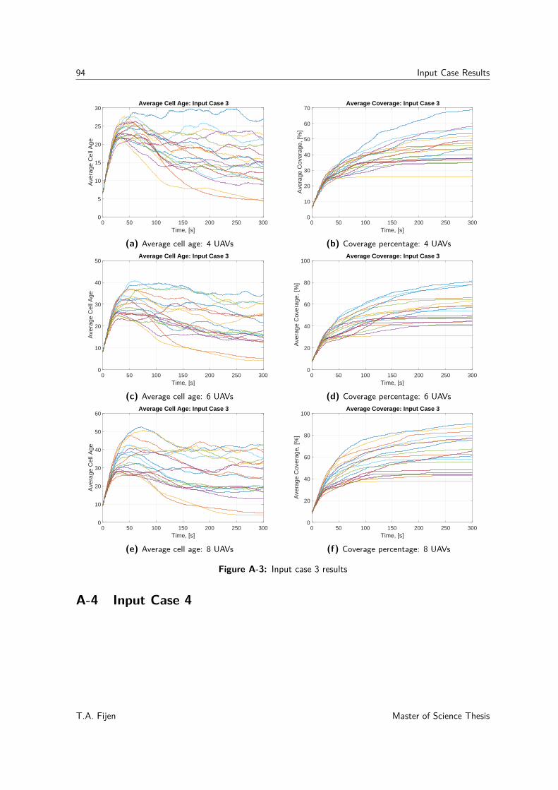
94 Input Case Results
0 50 100 150 200 250 300Time, [s]
0
5
10
15
20
25
30
Ave
rage
Cel
l Age
Average Cell Age: Input Case 3
(a) Average cell age: 4 UAVs
0 50 100 150 200 250 300Time, [s]
0
10
20
30
40
50
60
70
Ave
rage
Cov
erag
e, [%
]
Average Coverage: Input Case 3
(b) Coverage percentage: 4 UAVs
0 50 100 150 200 250 300Time, [s]
0
10
20
30
40
50
Ave
rage
Cel
l Age
Average Cell Age: Input Case 3
(c) Average cell age: 6 UAVs
0 50 100 150 200 250 300Time, [s]
0
20
40
60
80
100
Ave
rage
Cov
erag
e, [%
]
Average Coverage: Input Case 3
(d) Coverage percentage: 6 UAVs
0 50 100 150 200 250 300Time, [s]
0
10
20
30
40
50
60
Ave
rage
Cel
l Age
Average Cell Age: Input Case 3
(e) Average cell age: 8 UAVs
0 50 100 150 200 250 300Time, [s]
0
20
40
60
80
100
Ave
rage
Cov
erag
e, [%
]
Average Coverage: Input Case 3
(f) Coverage percentage: 8 UAVs
Figure A-3: Input case 3 results
A-4 Input Case 4
T.A. Fijen Master of Science Thesis
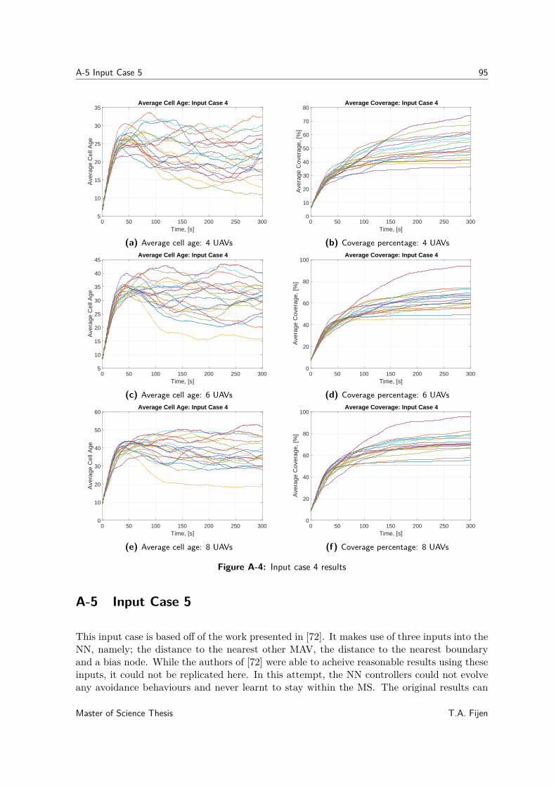
A-5 Input Case 5 95
0 50 100 150 200 250 300Time, [s]
5
10
15
20
25
30
35
Ave
rage
Cel
l Age
Average Cell Age: Input Case 4
(a) Average cell age: 4 UAVs
0 50 100 150 200 250 300Time, [s]
0
10
20
30
40
50
60
70
80
Ave
rage
Cov
erag
e, [%
]
Average Coverage: Input Case 4
(b) Coverage percentage: 4 UAVs
0 50 100 150 200 250 300Time, [s]
5
10
15
20
25
30
35
40
45
Ave
rage
Cel
l Age
Average Cell Age: Input Case 4
(c) Average cell age: 6 UAVs
0 50 100 150 200 250 300Time, [s]
0
20
40
60
80
100
Ave
rage
Cov
erag
e, [%
]
Average Coverage: Input Case 4
(d) Coverage percentage: 6 UAVs
0 50 100 150 200 250 300Time, [s]
0
10
20
30
40
50
60
Ave
rage
Cel
l Age
Average Cell Age: Input Case 4
(e) Average cell age: 8 UAVs
0 50 100 150 200 250 300Time, [s]
0
20
40
60
80
100
Ave
rage
Cov
erag
e, [%
]
Average Coverage: Input Case 4
(f) Coverage percentage: 8 UAVs
Figure A-4: Input case 4 results
A-5 Input Case 5
This input case is based off of the work presented in [72]. It makes use of three inputs into theNN, namely; the distance to the nearest other MAV, the distance to the nearest boundaryand a bias node. While the authors of [72] were able to acheive reasonable results using theseinputs, it could not be replicated here. In this attempt, the NN controllers could not evolveany avoidance behaviours and never learnt to stay within the MS. The original results can
Master of Science Thesis T.A. Fijen
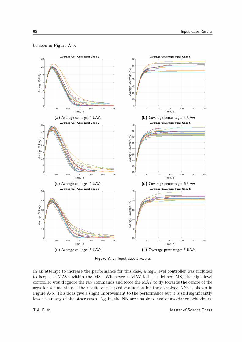
96 Input Case Results
be seen in Figure A-5.
0 50 100 150 200 250 300Time, [s]
0
5
10
15
20
25
30
Ave
rage
Cel
l Age
Average Cell Age: Input Case 5
(a) Average cell age: 4 UAVs
0 50 100 150 200 250 300Time, [s]
5
10
15
20
25
30
35
40
Ave
rage
Cov
erag
e, [%
]
Average Coverage: Input Case 5
(b) Coverage percentage: 4 UAVs
0 50 100 150 200 250 300Time, [s]
0
5
10
15
20
25
30
35
Ave
rage
Cel
l Age
Average Cell Age: Input Case 5
(c) Average cell age: 6 UAVs
0 50 100 150 200 250 300Time, [s]
10
15
20
25
30
35
40
45
50
Ave
rage
Cov
erag
e, [%
]
Average Coverage: Input Case 5
(d) Coverage percentage: 6 UAVs
0 50 100 150 200 250 300Time, [s]
0
10
20
30
40
50
Ave
rage
Cel
l Age
Average Cell Age: Input Case 5
(e) Average cell age: 8 UAVs
0 50 100 150 200 250 300Time, [s]
10
20
30
40
50
60
Ave
rage
Cov
erag
e, [%
]
Average Coverage: Input Case 5
(f) Coverage percentage: 8 UAVs
Figure A-5: Input case 5 results
In an attempt to increase the performance for this case, a high level controller was includedto keep the MAVs within the MS. Whenever a MAV left the defined MS, the high levelcontroller would ignore the NN commands and force the MAV to fly towards the centre of thearea for 4 time steps. The results of the post evaluation for these evolved NNs is shown inFigure A-6. This does give a slight improvement to the performance but it is still significantlylower than any of the other cases. Again, the NN are unable to evolve avoidance behaviours.
T.A. Fijen Master of Science Thesis
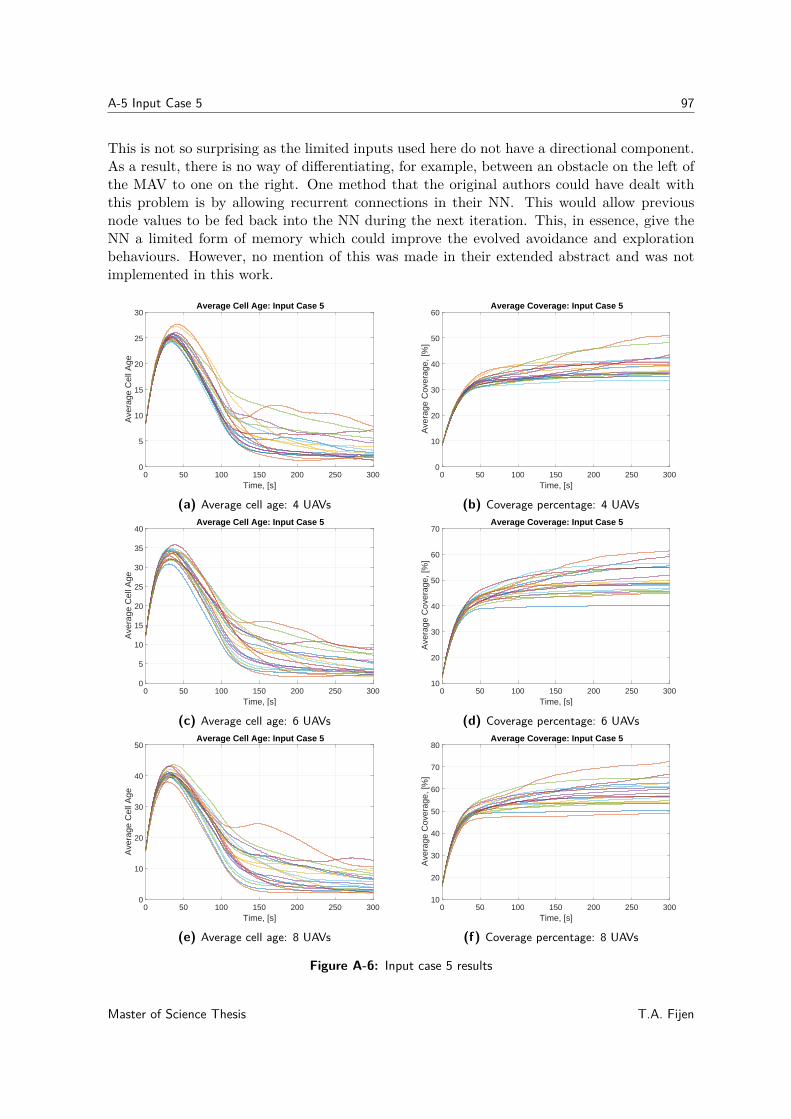
A-5 Input Case 5 97
This is not so surprising as the limited inputs used here do not have a directional component.As a result, there is no way of differentiating, for example, between an obstacle on the left ofthe MAV to one on the right. One method that the original authors could have dealt withthis problem is by allowing recurrent connections in their NN. This would allow previousnode values to be fed back into the NN during the next iteration. This, in essence, give theNN a limited form of memory which could improve the evolved avoidance and explorationbehaviours. However, no mention of this was made in their extended abstract and was notimplemented in this work.
0 50 100 150 200 250 300Time, [s]
0
5
10
15
20
25
30
Ave
rage
Cel
l Age
Average Cell Age: Input Case 5
(a) Average cell age: 4 UAVs
0 50 100 150 200 250 300Time, [s]
0
10
20
30
40
50
60
Ave
rage
Cov
erag
e, [%
]
Average Coverage: Input Case 5
(b) Coverage percentage: 4 UAVs
0 50 100 150 200 250 300Time, [s]
0
5
10
15
20
25
30
35
40
Ave
rage
Cel
l Age
Average Cell Age: Input Case 5
(c) Average cell age: 6 UAVs
0 50 100 150 200 250 300Time, [s]
10
20
30
40
50
60
70
Ave
rage
Cov
erag
e, [%
]
Average Coverage: Input Case 5
(d) Coverage percentage: 6 UAVs
0 50 100 150 200 250 300Time, [s]
0
10
20
30
40
50
Ave
rage
Cel
l Age
Average Cell Age: Input Case 5
(e) Average cell age: 8 UAVs
0 50 100 150 200 250 300Time, [s]
10
20
30
40
50
60
70
80
Ave
rage
Cov
erag
e, [%
]
Average Coverage: Input Case 5
(f) Coverage percentage: 8 UAVs
Figure A-6: Input case 5 results
Master of Science Thesis T.A. Fijen

98 Input Case Results
T.A. Fijen Master of Science Thesis
Appendix B
Baseline Persistent Coverage Methods
This appendix contains the extracts from the literature review that deals with the two typesof baseline methods that were used as a comparison to the evolved NN. The methods are; asweep planner and the random walk.
B-1 Sweep Planner
Current solutions in PA lean heavily towards a sweep planner approach as seen in [30, 16,31, 14, 17] for example. This method, also known as a lawnmower search pattern or theline-sweep method, searches the given area using the zig-zag trajectory shown in Figure B-1. However, if there are obstacles or no-go areas present, it is first necessary to decomposethe area into smaller subregions (known as exact cellular decomposition) which are thenindividually searched with these back and forth sweeps. A common approach to decomposethe target area is given in subsection B-1-1 and the order in which they are searched can beseen as a Vehicle Routing Problem (VRP).
B-1-1 Boustrophedon Decomposition
For simple environments, rectangular with no obstacles for example, it is very easy to deter-mine the coverage path using this line sweep method. In practice, however, the algorithm willneed to account for more complex environments. This is done by decomposing the originalarea into smaller subregions (or cells) as seen in Figure B-2, which can then be covered withthe back and forth sweeps. In literature, the most common method for creating these subre-gions is know as Boustrophedon Decomposition, which is an improvement on the trapezoidaldecomposition method.
In the trapezoidal decomposition method described in [3], a vertical line, known as a slice,moves from left to right over the entire area to be considered. The cells are then formed usinga sequence of open and close operations which occur when the slice intersects a vertex of a
Master of Science Thesis T.A. Fijen
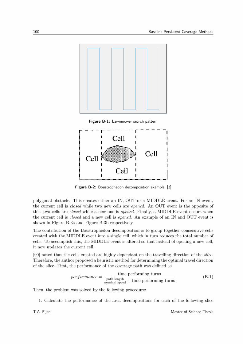
100 Baseline Persistent Coverage Methods
Figure B-1: Lawnmower search pattern
Figure B-2: Boustrophedon decomposition example, [3]
polygonal obstacle. This creates either an IN, OUT or a MIDDLE event. For an IN event,the current cell is closed while two new cells are opened. An OUT event is the opposite ofthis, two cells are closed while a new one is opened. Finally, a MIDDLE event occurs whenthe current cell is closed and a new cell is opened. An example of an IN and OUT event isshown in Figure B-3a and Figure B-3b respectively.
The contribution of the Boustrophedon decomposition is to group together consecutive cellscreated with the MIDDLE event into a single cell, which in turn reduces the total number ofcells. To accomplish this, the MIDDLE event is altered so that instead of opening a new cell,it now updates the current cell.
[90] noted that the cells created are highly dependant on the travelling direction of the slice.Therefore, the author proposed a heuristic method for determining the optimal travel directionof the slice. First, the performance of the coverage path was defined as
performance = time performing turnspath length
nominal speed + time performing turns(B-1)
Then, the problem was solved by the following procedure:
1. Calculate the performance of the area decompositions for each of the following slice
T.A. Fijen Master of Science Thesis
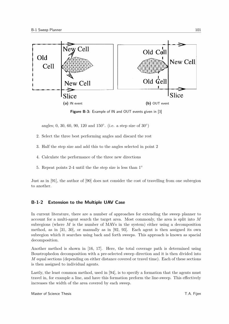
B-1 Sweep Planner 101
(a) IN event (b) OUT event
Figure B-3: Example of IN and OUT events given in [3]
angles; 0, 30, 60, 90, 120 and 150◦. (i.e. a step size of 30◦)
2. Select the three best performing angles and discard the rest
3. Half the step size and add this to the angles selected in point 2
4. Calculate the performance of the three new directions
5. Repeat points 2-4 until the the step size is less than 1◦
Just as in [91], the author of [90] does not consider the cost of travelling from one subregionto another.
B-1-2 Extension to the Multiple UAV Case
In current literature, there are a number of approaches for extending the sweep planner toaccount for a multi-agent search the target area. Most commonly, the area is split into Msubregions (where M is the number of MAVs in the system) either using a decompositionmethod, as in [31, 30], or manually as in [92, 93]. Each agent is then assigned its ownsubregion which it searches using back and forth sweeps. This approach is known as spacialdecomposition.
Another method is shown in [16, 17]. Here, the total coverage path is determined usingBoustrophedon decomposition with a pre-selected sweep direction and it is then divided intoM equal sections (depending on either distance covered or travel time). Each of these sectionsis then assigned to individual agents.
Lastly, the least common method, used in [94], is to specify a formation that the agents musttravel in, for example a line, and have this formation preform the line-sweep. This effectivelyincreases the width of the area covered by each sweep.
Master of Science Thesis T.A. Fijen
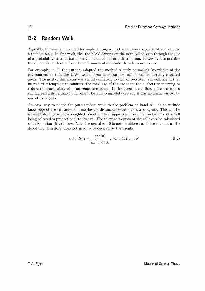
102 Baseline Persistent Coverage Methods
B-2 Random Walk
Arguably, the simplest method for implementing a reactive motion control strategy is to usea random walk. In this work, the, the MAV decides on the next cell to visit through the useof a probability distribution like a Gaussian or uniform distribution. However, it is possibleto adapt this method to include environmental data into the selection process.
For example, in [9] the authors adapted the method slightly to include knowledge of theenvironment so that the UAVs would focus more on the unexplored or partially exploredareas. The goal of this paper was slightly different to that of persistent surveillance in thatinstead of attempting to minimise the total age of the age map, the authors were trying toreduce the uncertainty of measurements captured in the target area. Successive visits to acell increased its certainty and once it became completely certain, it was no longer visited byany of the agents.
An easy way to adapt the pure random walk to the problem at hand will be to includeknowledge of the cell ages, and maybe the distances between cells and agents. This can beaccomplished by using a weighted roulette wheel approach where the probability of a cellbeing selected is proportional to its age. The relevant weights of the cells can be calculatedas in Equation (B-2) below. Note the age of cell 0 is not considered as this cell contains thedepot and, therefore, does not need to be covered by the agents.
weight(n) = age(n)∑Ni=1 age(i)
, ∀n ∈ 1, 2, . . . , N (B-2)
T.A. Fijen Master of Science Thesis
Appendix C
Collision Avoidance Proof
As mentioned in Section 4-3 the avoidance strategy used in this work is based off of [59].It relies on the principle that if two MAVs are flying on a collision course with an identicalspeed V , then the MAVs will not collide provided that at least one MAV reverses its flightdirection. It must continue along this reversed path, flying with a speed of v, until it reachesthe point where it entered into the conflict. The proof for this statement is taken from [59]and is given in below for two MAVs operating on 2-D plane.
Collision Avoidance Proof. If there are two MAVs, Am ∈ {1, 2}, where their initial positionsare given by ~Pm(0) and they are flying at a constant velocity vector where |~v1| = |~v2|. Theirpositions over time and the relative position vector ~D(t) is given as:
~P1(t) = ~P1(0) + ~v1t
~P2(t) = ~P2(0) + ~v2t
~D(t) = ~P1(t)− ~P2(t) = (~P1(0)− ~P2(0)) + (~v1 − ~v2)t
By splitting the vectors into their x and y components, the magnitude of ~D(t), d(t), is givenas
d(t) =√
(Dx + vxt)2 + (Dy + vyt)2
where
Dx = Px,1(0)− Px,1(0)Dy = Py,1(0)− Py,1(0)vx = vx,1 − vx,1
vy = vy,1 − vy,1
Now, let tc denote the time where d(t) is at its minimum (i.e. the point where the two MAVs
Master of Science Thesis T.A. Fijen
104 Collision Avoidance Proof
are closest). This equals the time at which d(t) = 0.
d(t) = vx(Dx + Vxtc) + vy(Dy + vytc)√(Dx + vxt)2 + (Dy + vyt)2
tc = −Dxvx +Dyvy
v2x + v2
y
thus
d(tc) =
√√√√(Dx − VxDxvx +Dyvy
v2x + v2
y
)2
+(Dy + vy
Dxvx +Dyvy
v2x + v2
y
)2
For a collision between the MAVs to occur, the distance between them must be less than thediameter of the MAVs defined as D. As the minimum distance between the MAV occurs attc, this translates to d(tc) ≤ D, or:√√√√(Dx − Vx
Dxvx +Dyvy
v2x + v2
y
)2
+(Dy + vy
Dxvx +Dyvy
v2x + v2
y
)2
≤ D
∴ D2x +D2
y −(Dxvx +Dyvy)2
v2x + v2
y
≤ D
from this it follows that:vx
vy=DxDy ±D
√D2
x +D2y −D2
D2y −D2
Now, since the terms on the left hand side of the inequality are constant and one of the andone of the solutions corresponds to a negative value of tc, the following relationship betweenthe velocities can be determined
vx ≤ Cvy
By substituting the original velocity vectors back into this equation we get:
vx,1 − vx,2 = C(vy,1 − vy,2)
If MAV2 was to reverse its velocity vector such that ~v2,new = −~v2. In this case, for the MAVsto remain on a collision course, the following equations must be true:
vx,1 − vx,2 ≤ C(vy,1 − vy,2)vx,1 − vx,2,new ≤ C(vy,1 − vy,2,new)⇒ vx,1 + vx,2 ≤ C(vy,1 + vy,2)
This can only be true ifvx,1vy,1
= vx,2vy,2
Using the earlier definition that |~v1| = |~v2| and the above equation it follows that ~v1 = ~v2.Therefore, if the initial positions were different then the two MAVs could not have initiallybeen on a collision course. AS this violate the initial assumption, this shows that reversingthe velocity of one MAV will prevent the collision.
T.A. Fijen Master of Science Thesis
Bibliography
[1] K. O. Stanley and R. Miikkulainen, “Evolving neural networks through augmentingtopologies,” Evolutionary computation, vol. 10, no. 2, pp. 99–127, 2002.
[2] M. Duarte, V. Costa, J. Gomes, T. Rodrigues, F. Silva, S. M. Oliveira, and A. L. Chris-tensen, “Evolution of collective behaviors for a real swarm of aquatic surface robots,”PloS one, vol. 11, no. 3, p. e0151834, 2016.
[3] H. Choset, “Coverage of known spaces: The boustrophedon cellular decomposition,”Autonomous Robots, vol. 9, no. 3, pp. 247–253, 2000.
[4] P. Ogren, “Increasing modularity of UAV control systems using computer game behaviortrees,” in Aiaa guidance, navigation, and control conference, p. 4458, 2012.
[5] M. Mazur, R. Abadie, J. Smith, A. Wisniewski, V. Huff, and S. Stroh, Clarity from above:PwC global report on the commercial applications of drone technology. PwC Polska Sp,2016.
[6] C. A. Rokhmana, “The potential of UAV-based remote sensing for supporting precisionagriculture in indonesia,” Procedia Environmental Sciences, vol. 24, pp. 245–253, 2015.
[7] A. Barrientos, J. Colorado, J. d. Cerro, A. Martinez, C. Rossi, D. Sanz, and J. Valente,“Aerial remote sensing in agriculture: A practical approach to area coverage and pathplanning for fleets of mini aerial robots,” Journal of Field Robotics, vol. 28, no. 5, pp. 667–689, 2011.
[8] D. J. Mulla, “Twenty five years of remote sensing in precision agriculture: Key advancesand remaining knowledge gaps,” Biosystems engineering, vol. 114, no. 4, pp. 358–371,2013.
[9] D. Albani, J. IJsselmuiden, R. Haken, and V. Trianni, “Monitoring and mapping withrobot swarms for agricultural applications,” in Advanced Video and Signal Based Surveil-lance (AVSS), 2017 14th IEEE International Conference on, pp. 1–6, IEEE, 2017.
Master of Science Thesis T.A. Fijen
106 Bibliography
[10] D. Gómez-Candón, A. De Castro, and F. López-Granados, “Assessing the accuracy ofmosaics from unmanned aerial vehicle (UAV) imagery for precision agriculture purposesin wheat,” Precision Agriculture, vol. 15, no. 1, pp. 44–56, 2014.
[11] J. A. Berni, P. J. Zarco-Tejada, L. Suárez, and E. Fereres, “Thermal and narrowbandmultispectral remote sensing for vegetation monitoring from an unmanned aerial vehicle,”IEEE Transactions on Geoscience and Remote Sensing, vol. 47, no. 3, pp. 722–738, 2009.
[12] M. Erena, S. Montesinos, D. Portillo, J. Alvarez, C. Marin, L. Fernandez, J. Henarejos,and L. Ruiz, “Configuration and specifications of an unmanned aerial vehicle for precisionagriculture.,” International Archives of the Photogrammetry, Remote Sensing & SpatialInformation Sciences, vol. 41, 2016.
[13] J. Primicerio, S. F. Di Gennaro, E. Fiorillo, L. Genesio, E. Lugato, A. Matese, andF. P. Vaccari, “A flexible unmanned aerial vehicle for precision agriculture,” PrecisionAgriculture, vol. 13, no. 4, pp. 517–523, 2012.
[14] G. Ristorto, P. D’Incalci, R. Gallo, F. Mazzetto, and G. Guglieri, “Mission planning forthe estimation of the field coverage of unmanned aerial systems in monitoring mission inprecision farming,” CHEMICAL ENGINEERING TRANSACTIONS, vol. 58, pp. 649–654, 2017.
[15] T. Oksanen and A. Visala, “Coverage path planning algorithms for agricultural fieldmachines,” Journal of Field Robotics, vol. 26, no. 8, pp. 651–668, 2009.
[16] D. Richards, T. Patten, R. Fitch, D. Ball, and S. Sukkarieh, “User interface and coverageplanner for agricultural robotics,” in Proceedings of ARAA Australasian Conference onRobotics and Automation (ACRA), 2015.
[17] D. Ball, P. Ross, A. English, T. Patten, B. Upcroft, R. Fitch, S. Sukkarieh, G. Wyeth,and P. Corke, “Robotics for sustainable broad-acre agriculture,” in Field and ServiceRobotics, pp. 439–453, Springer, 2015.
[18] B. H. Y. Alsalam, K. Morton, D. Campbell, and F. Gonzalez, “Autonomous UAV withvision based on-board decision making for remote sensing and precision agriculture,” inAerospace Conference, 2017 IEEE, pp. 1–12, IEEE, 2017.
[19] J. J. Roldán, G. Joossen, D. Sanz, J. del Cerro, and A. Barrientos, “Mini-UAV basedsensory system for measuring environmental variables in greenhouses,” Sensors, vol. 15,no. 2, pp. 3334–3350, 2015.
[20] J. J. Roldán, P. Garcia-Aunon, M. Garzón, J. de León, J. del Cerro, and A. Barrientos,“Heterogeneous multi-robot system for mapping environmental variables of greenhouses,”Sensors, vol. 16, no. 7, p. 1018, 2016.
[21] K. Ferentinos, N. Katsoulas, A. Tzounis, C. Kittas, and T. Bartzanas, “A climate controlmethodology based on wireless sensor networks in greenhouses,” in XXIX InternationalHorticultural Congress on Horticulture: Sustaining Lives, Livelihoods and Landscapes(IHC2014): 1107, pp. 75–82, 2014.
T.A. Fijen Master of Science Thesis
107
[22] K. P. Ferentinos, N. Katsoulas, A. Tzounis, T. Bartzanas, and C. Kittas, “Wirelesssensor networks for greenhouse climate and plant condition assessment,” BiosystemsEngineering, vol. 153, pp. 70–81, 2017.
[23] J. Hwang, C. Shin, and H. Yoe, “A wireless sensor network-based ubiquitous paprikagrowth management system,” Sensors, vol. 10, no. 12, pp. 11566–11589, 2010.
[24] G. Aiello, I. Giovino, M. Vallone, P. Catania, and A. Argento, “A decision support systembased on multisensor data fusion for sustainable greenhouse management,” Journal ofCleaner Production, vol. 172, pp. 4057–4065, 2018.
[25] K. Langendoen, A. Baggio, and O. Visser, “Murphy loves potatoes: Experiences froma pilot sensor network deployment in precision agriculture,” in Parallel and DistributedProcessing Symposium, 2006. IPDPS 2006. 20th International, pp. 8–pp, IEEE, 2006.
[26] T. Ahonen, R. Virrankoski, and M. Elmusrati, “Greenhouse monitoring with wirelesssensor network,” in Mechtronic and Embedded Systems and Applications, 2008. MESA2008. IEEE/ASME International Conference on, pp. 403–408, IEEE, 2008.
[27] D. Chaudhary, S. Nayse, and L. Waghmare, “Application of wireless sensor networks forgreenhouse parameter control in precision agriculture,” International Journal of Wireless& Mobile Networks (IJWMN) Vol, vol. 3, no. 1, pp. 140–149, 2011.
[28] H. M. Jawad, R. Nordin, S. K. Gharghan, A. M. Jawad, and M. Ismail, “Energy-efficientwireless sensor networks for precision agriculture: A review,” Sensors, vol. 17, no. 8,p. 1781, 2017.
[29] N. Nigam, “The multiple unmanned air vehicle persistent surveillance problem: A re-view,” Machines, vol. 2, no. 1, pp. 13–72, 2014.
[30] G. S. Avellar, G. A. Pereira, L. C. Pimenta, and P. Iscold, “Multi-UAV routing for areacoverage and remote sensing with minimum time,” Sensors, vol. 15, no. 11, pp. 27783–27803, 2015.
[31] I. Maza and A. Ollero, “Multiple UAV cooperative searching operation using polygon areadecomposition and efficient coverage algorithms,” in Distributed Autonomous RoboticSystems 6, pp. 221–230, Springer, 2007.
[32] N. Nigam, S. Bieniawski, I. Kroo, and J. Vian, “Control of multiple UAVs for persistentsurveillance: algorithm and flight test results,” IEEE Transactions on Control SystemsTechnology, vol. 20, no. 5, pp. 1236–1251, 2012.
[33] A. Wallar, E. Plaku, and D. A. Sofge, “Reactive motion planning for unmanned aerialsurveillance of risk-sensitive areas,” IEEE Transactions on Automation Science and En-gineering, vol. 12, no. 3, pp. 969–980, 2015.
[34] P. Trodden and A. Richards, “Multi-vehicle cooperative search using distributed modelpredictive control,” in AIAA Guidance, Navigation and Control Conference and Exhibit,p. 7138, 2008.
Master of Science Thesis T.A. Fijen
108 Bibliography
[35] M. M. Polycarpou, Y. Yang, and K. M. Passino, “A cooperative search framework fordistributed agents,” in Intelligent Control, 2001.(ISIC’01). Proceedings of the 2001 IEEEInternational Symposium on, pp. 1–6, IEEE, 2001.
[36] Y. Yang, M. M. Polycarpou, and A. A. Minai, “Opportunistically cooperative neurallearning in mobile agents,” in Neural Networks, 2002. IJCNN’02. Proceedings of the2002 International Joint Conference on, vol. 3, pp. 2638–2643, IEEE, 2002.
[37] X. Lin and C. G. Cassandras, “An optimal control approach to the multi-agent persis-tent monitoring problem in two-dimensional spaces,” IEEE Transactions on AutomaticControl, vol. 60, no. 6, pp. 1659–1664, 2015.
[38] C. G. Cassandras, X. Lin, and X. Ding, “An optimal control approach to the multi-agentpersistent monitoring problem,” IEEE Transactions on Automatic Control, vol. 58, no. 4,pp. 947–961, 2013.
[39] C. Franco, G. López-Nicolás, C. Sagüés, and S. Llorente, “Adaptive action for multi-agentpersistent coverage,” Asian Journal of Control, vol. 18, no. 2, pp. 419–432, 2016.
[40] M. D. Richards, D. Whitley, J. R. Beveridge, T. Mytkowicz, D. Nguyen, and D. Rome,“Evolving cooperative strategies for UAV teams,” in Proceedings of the 7th annual con-ference on Genetic and evolutionary computation, pp. 1721–1728, ACM, 2005.
[41] N. Zhou, C. G. Cassandras, X. Yu, and S. B. Andersson, “Decentralized event-driven al-gorithms for multi-agent persistent monitoring,” arXiv preprint arXiv:1708.06432, 2017.
[42] B. D. Song, J. Kim, and J. R. Morrison, “Rolling horizon path planning of an autonomoussystem of UAVs for persistent cooperative service: Milp formulation and efficient heuris-tics,” Journal of Intelligent & Robotic Systems, vol. 84, no. 1-4, pp. 241–258, 2016.
[43] J. Kim, B. D. Song, and J. R. Morrison, “On the scheduling of systems of UAVs andfuel service stations for long-term mission fulfillment,” Journal of Intelligent & RoboticSystems, pp. 1–13, 2013.
[44] B. Bethke, J. P. How, and J. Vian, “Multi-UAV persistent surveillance with communica-tion constraints and health management,” in AIAA Guidance, Navigation, and ControlConference (GNC), 2009.
[45] M. Valenti, D. Dale, J. How, D. Pucci de Farias, and J. Vian, “Mission health man-agement for 24/7 persistent surveillance operations,” in AIAA guidance, navigation andcontrol conference and exhibit, p. 6508, 2007.
[46] B. Bethke, M. Valenti, and J. P. How, “UAV task assignment,” IEEE robotics & automa-tion magazine, vol. 15, no. 1, 2008.
[47] N. K. Ure, G. Chowdhary, Y. F. Chen, M. Cutler, J. P. How, and J. Vian, “Decentralizedlearning-based planning for multiagent missions in the presence of actuator failures,” inUnmanned Aircraft Systems (ICUAS), 2013 International Conference on, pp. 1125–1134,IEEE, 2013.
[48] V. Trianni and S. Nolfi, “Engineering the evolution of self-organizing behaviors in swarmrobotics: A case study,” Artificial life, vol. 17, no. 3, pp. 183–202, 2011.
T.A. Fijen Master of Science Thesis
109
[49] K. Y. Scheper, S. Tijmons, C. C. de Visser, and G. C. de Croon, “Behavior trees forevolutionary robotics,” Artificial life, vol. 22, no. 1, pp. 23–48, 2016.
[50] M. Duarte, S. M. Oliveira, and A. L. Christensen, “Hybrid control for large swarms ofaquatic drones,” in Proceedings of the 14th International Conference on the Synthesis &Simulation of Living Systems. MIT Press, Cambridge, MA, pp. 785–792, Citeseer, 2014.
[51] M. Duarte, J. Gomes, V. Costa, S. M. Oliveira, and A. L. Christensen, “Hybrid controlfor a real swarm robotics system in an intruder detection task,” in European Conferenceon the Applications of Evolutionary Computation, pp. 213–230, Springer, 2016.
[52] Y. Cao, W. Yu, W. Ren, and G. Chen, “An overview of recent progress in the studyof distributed multi-agent coordination,” IEEE Transactions on Industrial informatics,vol. 9, no. 1, pp. 427–438, 2013.
[53] Z. Yan, N. Jouandeau, and A. A. Cherif, “A survey and analysis of multi-robot coor-dination,” International Journal of Advanced Robotic Systems, vol. 10, no. 12, p. 399,2013.
[54] S. Gezici, Z. Tian, G. B. Giannakis, H. Kobayashi, A. F. Molisch, H. V. Poor, andZ. Sahinoglu, “Localization via ultra-wideband radios: a look at positioning aspects forfuture sensor networks,” IEEE signal processing magazine, vol. 22, no. 4, pp. 70–84, 2005.
[55] P. Volf, D. Šišlák, D. Pavlíček, and M. Pěchouček, “Surveillance of unmanned aerial vehi-cles using probability collectives,” Holonic and Multi-Agent Systems for Manufacturing,pp. 235–245, 2011.
[56] Parrot, “Parrot bebop 2.” https://www.parrot.com/us/drones/parrot-bebop-2#lightweight, 2018. Accessed: 2018-11-14.
[57] J. Lipsky, “Parrot unveils bebop 2 drone.” https://www.eetimes.com/document.asp?doc_id=1328291, 2015. Accessed: 2018-11-14.
[58] Paparazzi, “Paparazzi: The free autopilot.” https://wiki.paparazziuav.org/wiki/General, 2016. Accessed: 2018-11-14.
[59] T. Szabo, “Autonomous collision avoidance for swarms of MAVs,” MSc thesis, DelftUniversity of Technology, 2015.
[60] OptiTrack, “OptiTrack sytems.” https://optitrack.com/systems/#robotics, 2018.Accessed: 2018-11-14.
[61] A. Pancham, N. Tlale, and G. Bright, “Literature review of SLAM and DATMO,” 2011.
[62] A. Nemra, L. M. Bergasa, E. López, R. Barea, A. Gómez, and Á. Saltos, “Robust visualsimultaneous localization and mapping for MAV using smooth variable structure filter,”in Robot 2015: Second Iberian Robotics Conference, pp. 557–569, Springer, 2016.
[63] K. Tateno, F. Tombari, I. Laina, and N. Navab, “CNN-SLAM: Real-time dense monoc-ular SLAM with learned depth prediction,” in Proceedings of the IEEE Conference onComputer Vision and Pattern Recognition (CVPR), vol. 2, 2017.
Master of Science Thesis T.A. Fijen
110 Bibliography
[64] DecaWave Ltd, Product Information: DWM 1000, 2018. V. 1.2.
[65] K. Guo, Z. Qiu, C. Miao, A. H. Zaini, C.-L. Chen, W. Meng, and L. Xie, “Ultra-wideband-based localization for quadcopter navigation,” Unmanned Systems, vol. 4, no. 01, pp. 23–34, 2016.
[66] B. D. Schutter and T. van den Boom, Optimization in Systems and Control. TU Delft,2015.
[67] Y. Jiang and V. C. Leung, “An asymmetric double sided two-way ranging for crystaloffset,” in Signals, Systems and Electronics, 2007. ISSSE’07. International Symposiumon, pp. 525–528, IEEE, 2007.
[68] S. van der Helm, “On-board range-based relative localization,” (The Netherlands), MScthesis, Delft University of Technology, 2018.
[69] X. Yao, “A review of evolutionary artificial neural networks,” International journal ofintelligent systems, vol. 8, no. 4, pp. 539–567, 1993.
[70] M. Buckland and M. Collins, AI techniques for game programming. Premier press, 2002.
[71] A. L. Nelson, G. J. Barlow, and L. Doitsidis, “Fitness functions in evolutionary robotics:A survey and analysis,” Robotics and Autonomous Systems, vol. 57, no. 4, pp. 345–370,2009.
[72] J. Butterworth, B. Broecker, K. Tuyls, and P. Paoletti, “Evolving coverage behavioursfor MAVs using NEAT,” in Proceedings of the 17th International Conference on Au-tonomous Agents and MultiAgent Systems, pp. 1886–1888, International Foundation forAutonomous Agents and Multiagent Systems, 2018.
[73] M. Darrah, W. Niland, and B. M. Stolarik, “Increasing UAV task assignment performancethrough parallelized genetic algorithms,” in Proceedings from, 2007.
[74] T. Shima and C. Schumacher, “Assignment of cooperating UAVs to simultaneous tasksusing genetic algorithms,” in AIAA Guidance, Navigation, and Control Conference andExhibit, p. 5829, 2005.
[75] A. Richards, J. Bellingham, M. Tillerson, and J. How, “Coordination and control ofmultiple UAVs,” in AIAA guidance, navigation, and control conference, Monterey, CA,2002.
[76] P. Goyal, E. Smeur, and G. de Croon, “Mission planning for sensor network deploymentusing a fleet of drones,” Delft University of Technology, Delft, Zuid-Holland, vol. 2629,2016.
[77] J. Kim, B. D. Song, and J. R. Morrison, “On the scheduling of systems of UAVs andfuel service stations for long-term mission fulfilment,” Journal of Intelligent & RoboticSystems, pp. 1–13, 2013.
[78] M. B. Dias, R. Zlot, N. Kalra, and A. Stentz, “Market-based multirobot coordination:A survey and analysis,” Proceedings of the IEEE, vol. 94, no. 7, pp. 1257–1270, 2006.
T.A. Fijen Master of Science Thesis
111
[79] F. Michaud, E. Robichaud, and J. Audet, “Using motives and artificial emotions forprolonged activity of a group of autonomous robots,” in Proceedings of the AAAI FallSymposium on Emotions. Cape Code Massachussetts, 2001.
[80] J. Leonard, A. Savvaris, and A. Tsourdos, “Energy management in swarm of unmannedaerial vehicles,” Journal of Intelligent & Robotic Systems, vol. 74, no. 1-2, pp. 233–250,2014.
[81] F. Sempé, A. Munoz, and A. Drogoul, “Autonomous robots sharing a charging stationwith no communication: a case study,” in Distributed Autonomous Robotic Systems 5,pp. 91–100, Springer, 2002.
[82] C.-U. Lim, R. Baumgarten, and S. Colton, “Evolving behaviour trees for the commercialgame defcon,” in European Conference on the Applications of Evolutionary Computation,pp. 100–110, Springer, 2010.
[83] A. Klöckner, “Interfacing behavior trees with the world using description logic,” in AIAAGuidance, Navigation, and Control (GNC) Conference, p. 4636, 2013.
[84] A. Marzinotto, M. Colledanchise, C. Smith, and P. Ögren, “Towards a unified behaviortrees framework for robot control,” in Robotics and Automation (ICRA), 2014 IEEEInternational Conference on, pp. 5420–5427, IEEE, 2014.
[85] M. Coppola, K. Mcguire, K. Scheper, and G. Croon, “On-board bluetooth-based relativelocalization for collision avoidance in micro air vehicle swarms,” 09 2016.
[86] J. Li, Y. Bi, K. Li, K. Wang, F. Lin, and B. M. Chen, “Accurate 3D localization forMAV swarms by UWB and IMU fusion,” in 2018 IEEE 14th International Conferenceon Control and Automation (ICCA), pp. 100–105, IEEE, 2018.
[87] M. W. Mueller, M. Hamer, and R. D’Andrea, “Fusing ultra-wideband range measure-ments with accelerometers and rate gyroscopes for quadrocopter state estimation,” inRobotics and Automation (ICRA), 2015 IEEE International Conference on, pp. 1730–1736, IEEE, 2015.
[88] T. M. Nguyen, A. H. Zaini, K. Guo, and L. Xie, “An ultra-wideband-based multi-UAVlocalization system in GPS-denied environments,” in Proc. Int. Micro Air Vehicle Conf.Competition, pp. 1–6, 2016.
[89] A. M. Khalel, “Position location techniques in wireless communication systems,” 2010.
[90] T. Oksanen et al., Path planning algorithms for agricultural field machines. HelsinkiUniversity of Technology, 2007.
[91] W. H. Huang, “Optimal line-sweep-based decompositions for coverage algorithms,” inRobotics and Automation, 2001. Proceedings 2001 ICRA. IEEE International Conferenceon, vol. 1, pp. 27–32, IEEE, 2001.
[92] R. Bähnemann, D. Schindler, M. Kamel, R. Siegwart, and J. Nieto, “A decentralizedmulti-agent unmanned aerial system to search, pick up, and relocate objects,” arXivpreprint arXiv:1707.03734, 2017.
Master of Science Thesis T.A. Fijen
112 Bibliography
[93] R. Bähnemann, M. Pantic, M. Popvić, D. Schindler, M. Tranzatto, M. Kamel, M. Grimm,J. Widauer, R. Siegwart, and J. Nieto, “The ETH-MAV team in the MBZ internationalrobotics challenge,” arXiv preprint arXiv:1710.08275, 2017.
[94] P. Vincent and I. Rubin, “A framework and analysis for cooperative search using UAVswarms,” in Proceedings of the 2004 ACM symposium on Applied computing, pp. 79–86,ACM, 2004.
T.A. Fijen Master of Science Thesis
Glossary
List of Acronyms
BT Behaviour Tree
CPP Coverage Path Planning
EA Evolutionary Algorithm
ER Evolutionary Robotics
GA Genetic Algorithm
IPM Integrated Pest Management
LP Linear Programming
MAV Micro Aerial Vehicle
MILP Mixed Integer Linear Programming
MPC Model Predictive Control
MRP Multi-agent Reactive Policy
MS Mission Space
MSE Mean-Squared Error
NEAT Neuro Evolution of Augmenting Topologies
NLLS Non-Linear Least Squares
NN Neural Network
PA Precision Agriculture
ROS Robot Operating System
SLAM Simultaneous Localization and Mapping
Master of Science Thesis T.A. Fijen
114 Glossary
TDOA Time Difference of Arrival
TWR Two Way Ranging
TU Delft Delft University of Technology
TWEANN Topology and Weight Evolving Artificial Neural Networks
UAV Unmanned Aerial Vehicle
UWB Ultra-wideband
VRP Vehicle Routing Problem
WSN Wireless Sensor Network
List of Symbols
α Adjustment angle for collision avoidanceδ(i, j) Specisation compatibility distanceδt Compatibility thresholdω Natural frequencyσ Standard deviationθ Direction of travelζ Model damping factor
H(Xk) Hessian of current stateWgene Average weight differences of matching genes∆T Time stepedepot Depot recharge rateem MAV energy depletion rateFP Set of flight plansG Continuous mission spaceIage Information ageO Set of obstacles in MS∇e(Xk) Jacobian matrix~D(t) Relative position vectorA Set of agents or MAVsage(n, k) Cell age, discretised MSage(x, y,FP, t) Age of a point in the mission space, continuous spaceci Speciation weighting factorsDgene Number of disjoint genesDist(n,m) Distance between MAV k and cell ne(Xk) Error vector for current state
T.A. Fijen Master of Science Thesis
115
Ecritic Critical fuel thresholdEgene Number of excess genesEm,max Maximum MAV energy levelEm(t) MAV energy level at time tEthresh Low fuel thresholdf NN fitness (or cost) functionf
′i Adjusted fitnessG(N) Approximate cellular decomposition of mission spaceg(n) Cell in discretised age gridL1 Length of MSL2 Breadth of MSL3 Obstacle lengthL4 Obstacle breadthM Number of MAVsm MAV index, m ∈ {1, 2, . . . ,M}minDist Minimum distance between any two MAVsN Total number of cells in discretised MSNgene Number of genesouti NN output iPdepot,q Depot positionPm(0) Initial position of MAV mQ Number of depotsq Depot index, q ∈ {1, 2, . . . , Q}QKalman Process noise covariance matrixRi Range between beacon i and a MAVRKalman Measurement noise covariance matrixS Safety coefficientSKalman Cross covariance matrixt Timetf Final timets Start timeV MAV footprintvmax MAV maximum velocityvx,m MAV x velocityvy,m MAV y velocityx X positionXk Current StateXk+1 Future statey Y positionz Altitude (or position along the z axis)
Master of Science Thesis T.A. Fijen

116 Glossary
T.A. Fijen Master of Science Thesis