masters thesis: uncertainty quantification and representativity analysis of the lwr-proteus phase ii...
TRANSCRIPT
Ecole Polytechnique Federale de Lausanne
Eidgenossische Technische Hochschule Zurich
For Obataining the degree of Master’s of Science inNuclear Engineering
Uncertainty Quantification andRepresentativity Analysis of the
LWR-PROTEUS Phase II ExperimentalCampaign
Author:Daniel J. Siefman
Supervisors:Professor Andreas Pautz
Dr. Mathieu Hursin
August 14, 2015


Abstract
The LWR-PROTEUS Phase II experimental program was conducted at the Proteus re-search reactor at the Paul Scherrer Institute (PSI) in the early 2000s. One of its purposeswas to gain more insight into the reactivity changes caused by fuel burnup and to developa sense of confidence in modern codes’ ability to predict these changes. The presentedproject reexamines the experimental campaign using SHARK-X. SHARK-X is a set ofPerl-based tools developed at PSI and built around the lattice physics code CASMO-5. Itis used to perform sensitivity analysis (SA), uncertainty quantification (UQ), and repre-sentativity analysis (RA). This report discusses how SHARK-X was used to quantify theeffect of input uncertainties when modeling the LWR-PROTEUS Phase II experimentsand to evaluate the representativity of the experiments to a spent fuel pool of the nuclearpower plant Gosgen (KKG).
The first objective of the analysis was to apply and assess the performance of SHARK-X for UQ analysis using the stochastic sampling and direct perturbation methods. Thisprocess involved modeling the experimental campaign in CASMO-5 and then evaluatingthe uncertainties in calculated criticality-relevant parameters (e.g. keff , reactivity) dueto input uncertainties. These input uncertainties are associated with nuclear data andfuel compositions. The results of the UQ analysis gave a quantification of the statisticalspread about the mean of these calculated criticality parameters. The mean values andstatistical spreads were then compared to their respective experimentally measured valuesto calculate the bias and bias uncertainty of CASMO-5 for this application. CASMO-5was then validated by using the bias and bias uncertainty in a z-score comparison analysis.Of the eleven samples from the H2O moderated portion of the experimental campaignanalyzed, only one did not have a successful validation.
The second objective was to apply SHARK-X to do uncertainty-based, RA of theexperimental campaign to the application of an industrial spent fuel pool. This testedthe abilities of SHARK-X to validate a CASMO-5 model of a given application, which inthis project was the spent fuel pool of the nuclear power plant Gosgen. Additionally thisanalysis can help to allow for burnup credit to be taken in the design of spent fuel pools andthus ameliorate financial penalties that can occur due to conservative assumptions appliedduring criticality safety. The representativity of the experiment to the spent fuel poolwas evaluated using a representativity index calculated from the UQ and SA for absolutereactivity worth. When this representativity index has a value of 0.9 or greater, there isa high degree of similarity between an application and an experiment. This means thatthe experiment can be used as a benchmark for establishing the bias and bias uncertaintyof CASMO-5 for a given application which can then be used to validate the application’smodel. For the spent fuel pool and the LWR-PROTEUS Phase II experimental campaign,the representativity index was calculated for a UO2 and MOX sample of intermediate
i

burnup. With H2O moderation conditions the representativity indices were 0.761 and0.861 for the UO2 and MOX samples respectively. With an H2O moderator containing2,023 ppm of boric acid, the representativity indices were calculated to be 0.847 and 0.780respectively. Therefore no sample had the sufficiently high representativity value of 0.9to be declared representative of the KKG spent fuel pool.
Keywords: Proteus, uncertainty quantification, sensitivity analysis, representativity,validation, spent fuel pool
ii

Contents
Abstract i
List of Figures vii
List of Tables ix
1 Introduction 1
1.1 Validation . . . . . . . . . . . . . . . . . . . . . . . . . . . . . . . . . . . . 1
1.2 Bias . . . . . . . . . . . . . . . . . . . . . . . . . . . . . . . . . . . . . . . 3
1.3 Representativity Analysis . . . . . . . . . . . . . . . . . . . . . . . . . . . 5
2 The LWR-PROTEUS Phase II Experiments 6
2.1 Proteus Description . . . . . . . . . . . . . . . . . . . . . . . . . . . . . . 6
2.2 The Experimental Campaign . . . . . . . . . . . . . . . . . . . . . . . . . 7
2.2.1 Sample Compositions . . . . . . . . . . . . . . . . . . . . . . . . . 8
2.2.2 Radiochemical Analyses . . . . . . . . . . . . . . . . . . . . . . . . 8
2.3 Reactivity Worth Measurements . . . . . . . . . . . . . . . . . . . . . . . 9
2.4 CASMO-4E Analyses . . . . . . . . . . . . . . . . . . . . . . . . . . . . . . 11
3 Uncertainty Quantification and Sensitivity Analysis Methods 13
3.1 Stochastic Sampling (SS) . . . . . . . . . . . . . . . . . . . . . . . . . . . 13
3.2 Direct Perturbation (DP) . . . . . . . . . . . . . . . . . . . . . . . . . . . 14
3.3 Implementation of SS and DP in SHARK-X . . . . . . . . . . . . . . . . . 15
3.4 Nuclear Data Input Uncertainties . . . . . . . . . . . . . . . . . . . . . . . 16
3.5 Variance Decomposition . . . . . . . . . . . . . . . . . . . . . . . . . . . . 16
3.6 Representativity Analysis . . . . . . . . . . . . . . . . . . . . . . . . . . . 17
4 CASMO-5 and SHARKX Calculations 19
4.1 CASMO-5 and SHARK-X Simulation Parameters . . . . . . . . . . . . . . 19
4.2 The Uncertain Inputs . . . . . . . . . . . . . . . . . . . . . . . . . . . . . 20
4.3 CASMO Models of LWR-PROTEUS Phase II . . . . . . . . . . . . . . . . 20
4.4 Spent Fuel Rack Model . . . . . . . . . . . . . . . . . . . . . . . . . . . . 21
5 UQ/SA and Validation Results 24
iii
Contents
5.1 H2O Moderator UQ/SA With SS . . . . . . . . . . . . . . . . . . . . . . . 24
5.1.1 kinf and keff UQ/SA . . . . . . . . . . . . . . . . . . . . . . . . . . 24
5.1.2 Absolute Reactivity Worth (∆ρ) UQ/SA . . . . . . . . . . . . . . 27
5.1.3 Relative Reactivity Worth (∆ρrel) UQ . . . . . . . . . . . . . . . . 31
5.2 Bias (bc) UQ and Validation . . . . . . . . . . . . . . . . . . . . . . . . . . 32
5.2.1 Comparison of CASMO-4E and CASMO-5 bc Values Without andWith UQ . . . . . . . . . . . . . . . . . . . . . . . . . . . . . . . . 33
5.3 Comparison of SS and DP Results . . . . . . . . . . . . . . . . . . . . . . 36
5.3.1 DP vs. SS for ∆ρrel . . . . . . . . . . . . . . . . . . . . . . . . . . 36
5.3.2 DP vs. SS for ∆ρ . . . . . . . . . . . . . . . . . . . . . . . . . . . . 37
5.4 Effect of Using Experimental Fuel Compositions . . . . . . . . . . . . . . 38
5.5 Borated (H2O/H3BO3) and D2O/H2O Moderator Validation Results . . . 39
5.5.1 σbc UQ Results . . . . . . . . . . . . . . . . . . . . . . . . . . . . . 39
5.5.2 Summary . . . . . . . . . . . . . . . . . . . . . . . . . . . . . . . . 45
6 Representativity Analysis Results 46
6.1 keff Representativity Index, ck . . . . . . . . . . . . . . . . . . . . . . . . . 46
6.2 Absolute Reactivity Worth Representativity Index, c∆ρ . . . . . . . . . . 47
7 Conclusions 52
Bibliography 53
Appendix A: Uncertainty Quantification Example Exercise 55
A.1 Mean, Variance, and Covariance of x1 and x2 . . . . . . . . . . . . . . . . 55
A.2 Variance with Taylor Series Expansion . . . . . . . . . . . . . . . . . . . . 57
A.3 Linear Example: f1(x1, x2) = x1 + x2 . . . . . . . . . . . . . . . . . . . . . 58
A.3.1 Analytical Solution . . . . . . . . . . . . . . . . . . . . . . . . . . . 58
A.3.2 Direct Perturbation Solution . . . . . . . . . . . . . . . . . . . . . 59
A.3.3 Stochastic Sampling . . . . . . . . . . . . . . . . . . . . . . . . . . 59
A.4 Nonlinear Example: f2(x1, x2) = x1 ∗ x2 . . . . . . . . . . . . . . . . . . . 61
A.4.1 Analytical Solution . . . . . . . . . . . . . . . . . . . . . . . . . . . 61
A.4.2 Direct Perturbation . . . . . . . . . . . . . . . . . . . . . . . . . . 63
A.4.3 Stochastic Sampling . . . . . . . . . . . . . . . . . . . . . . . . . . 63
A.5 Summary . . . . . . . . . . . . . . . . . . . . . . . . . . . . . . . . . . . . 64
Appendix B: Derivation of Criticality Parameters and Non-linearity Ef-fects 66
B.1 Absolute Reactivity Worth . . . . . . . . . . . . . . . . . . . . . . . . . . 66
B.1.1 ∆ρ sensitivity coefficient . . . . . . . . . . . . . . . . . . . . . . . . 67
B.1.2 Linearity of ∆ρ . . . . . . . . . . . . . . . . . . . . . . . . . . . . . 67
B.2 Relative Reactivity Worth . . . . . . . . . . . . . . . . . . . . . . . . . . . 69
B.2.1 ∆ρrel Sensitivity Coefficient . . . . . . . . . . . . . . . . . . . . . . 69
iv

Contents
B.2.2 Linearity of ∆ρrel . . . . . . . . . . . . . . . . . . . . . . . . . . . 70
Appendix C: Numerical Precision of Sensitivity Coefficients and Represen-tativity Indices 72
v

List of Figures
1.1 Relation of z-scores to other grading methods for a normal distribution [9]. 4
2.1 Proteus’ configuration during the LWR-PROTEUS programs [11]. . . . . 7
2.2 Central test region during the experimental campaign [10]. . . . . . . . . . 7
2.3 CASMO-4E bias values for relative reactivity [10]. . . . . . . . . . . . . . 12
4.1 CASMO-5 model of the PWR test region (dimensions in mm) [10]. . . . . 21
4.2 Depiction of one quarter of the KKG spent fuel rack. . . . . . . . . . . . . 22
5.1 Cross section vs. incident inergy for 238U/σs,in [24]. . . . . . . . . . . . . . 26
5.2 235U and 239Pu weight percents and ∆ρ 1σrel values. . . . . . . . . . . . . 29
5.3 Cross section vs. incident energy for 103Rh/(n,γ) [24]. . . . . . . . . . . . 30
5.4 103Rh and 237Np normalized number densities and ∆ρ σrel values fromtechnological input UQ. . . . . . . . . . . . . . . . . . . . . . . . . . . . . 31
5.5 Comparison of CASMO-4E and CASMO-5 bc without UQ. . . . . . . . . 34
5.6 Comparison of CASMO-4E and CASMO-5 bc with UQ. . . . . . . . . . . 35
5.7 Comparison of bc for each calculation type. Error bars seen are 2σrel andare from nuclear data UQ only. . . . . . . . . . . . . . . . . . . . . . . . . 39
5.8 M1 neutron flux spectra for all moderating conditions and their respectivesensitivity coefficients of 239Pu/ν for the response ∆ρrel. . . . . . . . . . 41
5.9 239Pu/σf . Sensitivity coefficient of 239Pu/ν for each moderator for theresponse ∆ρrel. . . . . . . . . . . . . . . . . . . . . . . . . . . . . . . . . 42
5.10 Difference in M1 neutron flux spectra between moderators. Sensitivitycoefficient of 239Pu/ν for each moderator for the response ∆ρrel. . . . . . 43
6.1 Sensitivity coefficient of 239Pu/ν for H2O moderator for the response ∆ρ. 49
6.2 Sensitivity coefficient of 235U/ν for H2O for the response ∆ρ. . . . . . . . 49
A.1 Hypothetical uniform distribution. . . . . . . . . . . . . . . . . . . . . . . 56
A.2 SS method applied to example f1(x1, x2) with fully correlated variables. . 60
A.3 SS method applied to example f1(x1, x2) with fully uncorrelated variables. 61
A.4 SS MATLAB script for f2(x1, x2) with fully correlated variables. . . . . . 64
A.5 SS MATLAB script for f2(x1, x2) with fully uncorrelated variables. . . . . 64
vi

List of Figures
B.1 Evolution of the first and second order term of absolute reactivity’s Taylorexpansion with respect to the relative input uncertainty, for U-238 capture 68
B.2 Evolution of the first and second order term of relative reactivity’s Taylorexpansion with respect to the relative input uncertainty, for U-238 capture. 71
vii
List of Tables
2.1 Descriptions of the fuel samples [14]. . . . . . . . . . . . . . . . . . . . . . 8
2.2 Nuclides selected for radiochemical analysis [14]. . . . . . . . . . . . . . . 9
5.1 U2 decomposition of DP 1σrel sensitivity coefficients (SC) for kinf and keff .Nuclear data UQ only. . . . . . . . . . . . . . . . . . . . . . . . . . . . . . 25
5.2 ∆ρ relative standard deviations, 1σrel. For nuclear data UQ. . . . . . . . 27
5.3 Decomposition of sample U2 and M1’s DP-calculated σrel for ∆ρ. Nucleardata UQ only . . . . . . . . . . . . . . . . . . . . . . . . . . . . . . . . . . 27
5.4 ∆ρ sample composition relative standard deviations, 1σrel, values. . . . . 30
5.5 SS-calculated ∆ρrel relative standard deviations, 1σrel. For nuclear dataUQ only. . . . . . . . . . . . . . . . . . . . . . . . . . . . . . . . . . . . . . 32
5.6 SS 1σbc values. For nuclear data UQ and for total UQ. . . . . . . . . . . . 33
5.7 Validation procedure for H2O moderated samples. . . . . . . . . . . . . . 35
5.8 SS and DP ∆ρrel relative standard deviations, 1σrel, and the differencebetween SS and DP 1σrel values. For nuclear data UQ only. . . . . . . . . 37
5.9 SS and DP ∆ρ relative standard deviations, 1σrel, and the absolute differ-ence between SS and DP 1σrel values. For nuclear data UQ only. . . . . . 37
5.10 SS-calculated total (nuclear data + sample composition + experiment) 1σbcvalues for each moderator. . . . . . . . . . . . . . . . . . . . . . . . . . . . 40
5.11 Decomposition of M1’s DP-calculated 1σbc for each moderating condition.Nuclear Data UQ Only. . . . . . . . . . . . . . . . . . . . . . . . . . . . . 40
5.12 Validation procedure for Proteus with H2O/H3BO3 and D2O/H2O moder-ating conditions. . . . . . . . . . . . . . . . . . . . . . . . . . . . . . . . . 44
6.1 ck for Uref and U2 with each moderating condition. . . . . . . . . . . . . . 47
6.2 c∆ρ of U2 for each moderating condition. . . . . . . . . . . . . . . . . . . 47
6.3 Decomposition of U2 and M2’s c∆ρ by nuclide. . . . . . . . . . . . . . . . 48
6.4 c∆ρ for each sample with H2O moderator. . . . . . . . . . . . . . . . . . . 50
A.1 Expected values, variances, and covariance for the random variables x1 andx2. . . . . . . . . . . . . . . . . . . . . . . . . . . . . . . . . . . . . . . . . 57
A.2 Summary of variance calculation exercise. . . . . . . . . . . . . . . . . . . 65
B.1 Typical values for λ and Sk,α values for 238U/σc for a reference state andtwo perturbed states. . . . . . . . . . . . . . . . . . . . . . . . . . . . . . . 68
viii

List of Tables
C.1 Uncertainty associated with SC with varying relative perturbations for sys-tems 1 and 2. . . . . . . . . . . . . . . . . . . . . . . . . . . . . . . . . . . 73
C.2 Calculated ck for each system with varying relative perturbations. . . . . 73
ix

Chapter 1
Introduction
This report summarizes an application of the uncertainty quantification and sensitivityanalysis (UQ/SA) tool SHARK-X developed at the Paul Scherrer Institut (PSI). SHARK-X was applied to an experiment and an application: the LWR-PROTEUS Phase II ex-perimental campaign and the spent fuel pool of the nuclear power plant Gosgen (KKG,or Kernkraftwerk Gosgen). First SHARK-X was used to validate the lattice physicscode CASMO-5 with the experiments done at the Proteus research reactor. Addition-ally SHARK-X was used to perform representativity analysis with UQ/SA, which is aquantitative method for evaluating the similarity of Proteus’ reactivity experiments toone of KKG’s spent fuel pools. The main purpose of this work was to successfully applythe SHARK-X tool and create practices and methodologies for validation and represen-tativity analysis. Additionally, the results allow for conclusions to be made concerningthe validation of CASMO-5 and the representativity of the experimental campaign to theKKG spent fuel pool.
The first chapter of the report gives an introduction into the concepts of UQ/SA,validation, bias, and representativity analysis. The second chapter describes the LWR-PROTEUS Phase II experimental campaign. Chapter 3 describes SHARK-X’s UQ meth-ods called stochastic sampling (SS) and direct perturbation (DP) along with representa-tivity analysis (RA) using representativity indices. Chapter 4 describes the SHARK-X’sSS and DP utilities and the CASMO-5 models of Proteus and the KKG spent fuel pool.Chapter 5 presents the results of the UQ analysis for the parameters kinf , keff , absolutereactivity worth, and relative reactivity worth. Additionally this chapter contains a dis-cussion of the bias and bias uncertainty of the relative reactivity worth parameter anda validation study based on these results. Chapter 6 presents the representativity anal-ysis of the KKG spent fuel pool based on the use of representativity indices. Chapter7 gives a conclusion and summary of the report along with recommendations for futureimprovements.
1.1 ValidationA key part of the design and safety assessment of nuclear systems is computer model-
ing. The modern trend in nuclear engineering modeling is based upon best-estimate codes.Best-estimate codes are desirable because they allow to reduce the costs of redundantsafety margins, to improve the quality of safety analysis, to help extend the operationof existing nuclear power plants, and to ease the design of complicated Generation IVsystems. A best-estimate code must
1

1.1. Validation
1. Avoid the purposeful introduction of conservatism.2. Minimize the use of expert judgement to tune models.3. Use state-of-the-art methods.
To help objectively classify a code as best-estimate, the accuracy of the code mustbe proven by validation against experiments. Validation is the process in which a code’soutputs are compared to experimental results to assess the code’s accuracy. The necessityof validation can be seen in many state-of-the-art neutron transport codes (e.g. SCALE[1], MCNP [2], CASMO [3]). These codes can predict keff with a high degree of precision,or with repeatability and reproducibility. However problems exist with these codes’ ac-curacies, or how close the value they calculate is to the true value in experiment, that is,there is always a difference between the calculated and true value. Thus when modelingcritical systems (e.g. spent fuel pools) with one of these codes, it is impossible to perfectlyand consistently calculate the criticality of systems.
The accuracy of the simulation, or the difference between the calculated value andthe real-world value measured in application, is called the bias and is due to differentcontributions:
• Uncertainties of the input parameters (e.g. geometry, compositions, and especiallynuclear data)
• Computational methods used to solve the neutron transport equation (e.g. diffusiontheory, Monte Carlo method)
• Modeling approximations (e.g. homogenizing regions or simplifying geometry)
This bias is why standards for nuclear criticality safety analysis (e.g. ANSI/ANS-8.1-1998 [4] and ANSI/ANS-8.24-2007 [5]) require the validation of the analytical methodsand nuclear data used in calculations. Validation establishes the credibility of a code foran application by quantifying the bias and the bias’ uncertainty. Often when simulating agiven application, experimental results do not exist and thus cannot be used to calculatethe bias of the code system for the application. In instances like this, validation is done bycomparing computed results with critical benchmarks, which are based on experimentaldata from critical systems1.
Choosing a benchmark for validation is typically undertaken using similarity studiesbetween the benchmark and the application of interest. Traditionally the benchmarkchoice is based off of finding its physical characteristics that are similar to the application.These characteristics can be the fissile elements present, the fissile concentration, themoderator type, the geometrical configuration, the hydrogen-to-fissile atom ratio, theaverage energy of neutrons causing fission, or the average neutron lethargy causing fission[8]. A series of benchmarks are then selected and trending analysis applied to their biasesas a function of the previously described physical characteristics (fissile concentration,etc.). Once a benchmark is found to be suitable, it is then chosen as the basis forestablishing the application’s bias [6]. The next step in validation is to model the chosenbenchmark in the same code with the same cross-section data as the application. Thenthe difference between the experimental quantity (e.g. keff) of the benchmark is compared
1There is a difference between critical benchmarks and critical experiments. Critical benchmarksare critical experiments that have been peer reviewed. They have relatively detailed descriptions ofexperimental conditions and can be repeatedly and consistently modeled by qualified specialists. In otherwords, all critical benchmarks are critical experiments, however not all critical experiments are criticalbenchmarks.
2

1.2. Bias
to the benchmark’s calculated value with the code. This establishes the computationalbias for the experimental benchmark. Next the benchmark’s bias is used to calculate theapplication’s computational bias.
Modern approaches used in SHARK-X and the TSUNAMI sequence of SCALE-6 [1]use advanced tools to assess the similarity of applications to benchmarks. The basisof these tools is that the computational biases seen are mainly caused by uncertaintiesin nuclear data. The nuclear data uncertainties are propagated through the system tofind the uncertainty in the computed value. Sensitivity coefficients are also calculatedand used with uncertainties to compute correlation coefficients between the benchmarkand the application, which are used as the basis for choosing a given benchmark. Thistechnique of quantifying the similarity between a benchmark and the application is calledrepresentativity analysis (RA) and is discussed further in Section 1.3.
1.2 BiasThe bias, bc, between a calculated value, C, and an experimental value, E, is quantified
as shown in Equation 1.1. A perfectly unbiased result (i.e. the code perfectly predictsthe experimental value) would have a bc value of 1.0.
bc =C
E(1.1)
Left out of this calculation of the bias in Equation 1.1 is the fact there are uncertaintiesassociated with both C and E. In criticality safety analysis, the uncertainties associatedwith C could be the composition of the fissile material input into the code, or the nucleardata used in the neutron transport calculations. The experimental value will always haveexperimental uncertainties associated with it, which in nuclear systems can come frommany sources (e.g. detector efficiencies and statistics). This means that C and E reallyexist with associated uncertainties as C±σC and E±σE and thus the uncertainty of biasbetween the calculated and experimental result is given by Equation 1.2.
σbc = bc
√(σCC
)2
+
(σEE
)2
(1.2)
Without access to UQ, and thus without knowledge of σC , the validation procedurehas three possible outcomes [7]:
1. Complete success: C is within a number of standard deviations (often two standarddeviations of σE) from the experimental result,
|C − E| ≤ 2σE (1.3)
2. Partial success: C is within some expert defined tolerance, ε, but outside the pre-vious two-standard-deviation bounds,
|C − E| ≤ ε (1.4)
3. Failure: C is outside the defined tolerance ε,
|C − E| > ε (1.5)
3

1.2. Bias
A major problem with this procedure is the definition of ε. This tolerance is based onexpert experience with the given type of prediction. The subjectivity involved in definingthis parameter violates the “no expert judgement” criteria for best-estimate codes. Thedegree of subjectivity necessary in choosing a benchmark can be decreased with the useof UQ/SA. By using UQ/SA, the calculation uncertainty, σC , is quantified and then usedfor calculating σbc . Then bc and σbc are used in a different validation test, where thecalculation is validated to a z-score tolerance, εz, as shown in Equation 1.6 [7].
|bc − 1|σbc
≤ εz (1.6)
The meaning of a z-score for a normal distribution is shown in Figure 1.1 in relation tostandard deviations, cumulative percentages, and percentiles. A two standard deviationlevel of validation, or a z-score of 2.0 level of validation, means that εz is equal to 2.0 andthe term seen in Equation 1.6 must be less than or equal to 2.0. The advantage of thisz-score tolerance approach is fast validation and easy comparison between many casesbecause the methodology is straightforward and the comparison between cases is relative.
Figure 1.1 – Relation of z-scores to other grading methods for a normal distribution [9].
The importance of knowing σbc can be seen when examining the validation of a hypo-thetical critical system both with and without UQ: Measurements by engineers show thatthe system is critical, that the measured value, E, of keff is equal to 1.00000. Calculationsby engineers with their favorite code show that the system is not critical, that C of keff isequal to 0.97000. If bc is evaluated without considering uncertainties (Equation 1.1), theengineers may derive the conclusion that the bias is significant, that bc is far from 1.0.
But what if the uncertainty associated with C and E is large? There can be significantuncertainties associated with the nuclear data (e.g. cross sections, ν, fission spectra)that are used in computational simulations. There can also be significant uncertaintiesassociated with the experimental value. If these uncertainties are accounted for, error barscould be placed on bc that indicate that its value could be 1.0 given its own statisticalspread. This means that what the engineers previously believed was a significant bias,may not be significant due to inherent uncertainties in the inputs of the calculation andthe experiment.
4

1.3. Representativity Analysis
1.3 Representativity AnalysisRepresentativity analysis is employed in validation to discern how representative an
integral experiment, like the LWR-PROTEUS Phase II campaign, is of a NPP application,e.g. a spent fuel pool. In other words, it helps to determine the applicability of anexperiment as a benchmark in validating code systems for a given application. When anexperiment is deemed representative of an application, it is then possible to validate theapplication’s model in a given code system by determining the application’s bias and biasuncertainty by using the experiment as a benchmark [8].
To quantitatively determine the representativity of an experiment to an application,it is necessary to use integral indices based UQ/SA. Validation could be done withoutintegral indices using vectors of sensitivity coefficients for a given response to nuclear data.These vectors however are cumbersome and the large volume of information associatedwith them is often too large for general use. Therefore the integral indices are used asa parameter to synthesise this information and turn it into an easily understood andcalculated value [6].
The integral index used in this report is uncertainty and sensitivity based and repre-sented by the variable cres, where res is a given response. Typically in criticality analyseskeff is used as the response that leads to the calculation of ck. Other responses can beused as well, which in this analysis includes reactivity coefficients, c∆ρ. This is the pre-ferred index for representativity quantification and is excellent for reducing the use ofexpert judgement, a requirement in the use of best-estimate code systems. A value ofzero for cres represents no correlation between the systems. A value of 1.0 indicates fullcorrelation. For benchmark selection purposes, if cres has a value greater than 0.9, theexperiment is considered to be highly representative of the given application.
5

Chapter 2
The LWR-PROTEUS Phase IIExperiments
Phase II of the LWR-PROTEUS campaign was dedicated to experimentally investigatingthe reactor physics of well-characterised, high-burnup fuel samples from Swiss NPPs.Reactivity measurements were performed with samples cut from the fuel rods of theseSwiss NPPs to investigate the effect of burnup upon reactivity. The reactivity worth ofeach sample was measured by inserting it into the core of Proteus. Afterwards, chemicalassays were done at the PSI hot laboratory to identify the concentrations of actinides andfission products in the irradiated fuel. The results were and are now, in this report, beingused to validate codes for predicting the composition and reactivity of fuel with burnup[13] [10].
2.1 Proteus Description
Proteus is a zero-power (maximum 1 kW and flux of 5×10⁹ n/s-cm2) nuclear researchreactor that operated from 1968 to 2011 at PSI [11]. During its operation history, it wasused for several experimental campaigns investigating reactor concepts like the gas-cooledfast reactor, the high-conversion light water reactor, the high temperature reactor, and thelight water reactor (LWR). Its use in the 21st century was mainly devoted to studying fuelsused in LWRs. These groups of experiments are called the LWR-PROTEUS campaigns,of which the second campaign, Phase II [13], is investigated in this report.
Proteus in Greek mythology is the son of Poseidon and a god of seas, rivers, and ingeneral water. Often he was ascribed to be the god of “elusive sea change”, suggestingthat he was behind the capriciousness of the sea. The adjective “protean” is derivedfrom Proteus, with the general meaning of “versatile,” “mutable,” or “capable of assum-ing many forms” [12]. “Protean” has positive connotations of flexibility, versatility andadaptability and is thus a excellent derivation of the moniker for this research reactor.This is because the reactor has a cavity at its center (1.2 m in diameter) which can befilled with the desired experimental configuration. Around the cavity, seen in Figure 2.1,is a graphite region with 5 w.% enriched UO2 pins that drive the criticality of the reactor.
6

2.2. The Experimental Campaign
Figure 2.1 – Proteus’ configuration during the LWR-PROTEUS programs [11].
2.2 The Experimental CampaignProteus was configured during this experimental campaign to represent a LWR. In the
reactor’s central cavity was a test zone consisting of an Al tank in which there were ninefull-length assemblies arranged in a 3×3 matrix. Eight of these were full-sized, Optima2,BWR assemblies (10×10 pins, 5 w.% enriched UO2) and the central assembly was an11×11 array of fresh, 4.3 w.% enriched, UO2, PWR fuel rods. The center pin of the PWRassembly was removed and existed as a guide tube through which the previously discussedsamples were inserted and withdrawn to vary reactivity. This central core region can beseen in Figure 2.2.
Figure 2.2 – Central test region during the experimental campaign [10].
The PWR assembly was placed in a stainless steel tank allowing for different moder-ating conditions to exist there than in the BWR assemblies. The moderating conditionsof the PWR assembly investigated in the experiment were
• Full-density H2O at atmospheric temperature and pressure (ATP),
7

2.2. The Experimental Campaign
• A mixture of H2O and D2O (37.0 w% D2O at ATP),• And borated H2O (2,023 ± 46 ppm of boric acid) at ATP.
The full-density H2O moderator was used to produce a standard neutron spectrumthat might be seen in criticality safety situations at ATP. The D2O/H2O moderator wasused to simulate the H number density that exists during PWR operations, and thus theharder neutron spectrum at these conditions. The BWR assemblies were all moderatedby pure H2O at ATP.
2.2.1 Sample Compositions
This report discusses eleven burnt fuel rod samples (seven UO2, four MOX) thatwere taken from the Gosgen-Daniken PWR (KKG). The samples varied in their degreeof burnup, ranging from ∼21 to ∼121 MWd/kg, and provided a spectrum of burnups forwhich experimental data could be obtained. The samples were prepared at the PSI hotlaboratory and enclosed in a Zircaloy over-clad. Each sample was approximately 40 cmlong and cut from the center of the fuel rods to avoid gradients in burnup that may existat the axial rod extremities.
In this document, the samples are identified either as “U” for the UO2 samples or “M”for the MOX samples. Each sample within a class (U or M) then has a correspondingidentification number that corresponds to increasing values of burnup. Thus for the sevenU samples, 1 indicates the lowest burnup and 7 the highest. A summary of the samplesin this identification system is given in Table 2.1. A different nomenclature is used withProteus’ documentation, where each sample is named UR and then a number (e.g. UR1)with the numbers based on the chronological order of the sample’s use in the experiment.The problem with this system is that it gives no indication of fuel type or burnup andmakes the analyses harder to understand. A complete history of each sample’s irradiationcan be found in Ref. [10].
Table 2.1 – Descriptions of the fuel samples [14].
ID Proteus ID Type # of CyclesBurnup
(MWd/kg)U1 UR7 UO2 3 ∼38U2 UR3 UO2 3 ∼54U3 UR5 UO2 5 ∼71U4 UR4 UO2 5 ∼75U5 UR2 UO2 3 ∼91U6 UR1 UO2 7 ∼92U7 UR11 UO2 10 ∼121
M1 UR6 MOX 1 ∼21M2 UR8 MOX 2 ∼44M3 UR9 MOX 3 ∼64M4 UR10 MOX 4 ∼72
2.2.2 Radiochemical Analyses
Radiochemical, post-irradiation analytical investigations on the fuel samples were per-formed in the PSI hot laboratory during the experimental campaign. The experimentsmeasured the concentrations of the 17 actinides and 40 fission products seen in Table 2.2.
8

2.3. Reactivity Worth Measurements
The data gained by these studies has been and will be used to validate computer codesfor high burnup and MOX fuels [10] [14].
Table 2.2 – Nuclides selected for radiochemical analysis [14].
Major Actinides:234U, 235U, 236U, 238U238Pu, 239Pu, 240Pu, 241Pu, 242Pu
Minor Actinides:237Np241Am, 242mAm, 243Am242Cm, 243Cm, 244Cm, 245Cm, 246Cm
Fission Products:Volatiles: 133Cs, 134Cs, 135Cs, 137CsMetallics: 90Sr, 95Mo, 99Tc, 101Ru, 106Ru, 103Rh, 109Ag, 125SbLanthanides: 144Ce, 147Pm, 155Gd
142Nd, 143Nd, 144Nd, 145Nd, 146Nd, 148Nd, 150Nd147Sm, 148Sm, 149Sm, 150Sm, 151Sm, 152Sm, 154Sm151Eu, 153Eu, 154Eu, 155Eu
The chemical analyses were done using a combination of high-performance liquid chro-matography (HPLC) and multicollector inductively coupled plasma mass spectrometry(MC-ICP-MS). The chromatography was done to separate chemical elements and massspectroscopy was done to analyze the isotopic compositions of the elements. Mass spec-troscopy cannot be used alone because it cannot separate isobars (nuclides having thesame mass number, but different atomic numbers). The nuclides 106Ru, 125Sb, 144Ce,and 243Cm existed in small concentrations in the fuel samples and needed to be measuredwith γ-ray spectroscopy using a high-purity germanium detector. The uncertainty associ-ated with the experimental measurement of the nuclides using MC-ICP-MS and HPLC is0.3-1%. The uncertainty of the isotopes measured with γ-ray spectroscopy is 5-10% [13].
The burnup of each sample was measured using the 148Nd technique. This isotope is afission product and its concentration increases with burnup. By measuring its concentra-tion in the fuel samples, it is possible to approximate a sample’s burnup. The assumptionmade in this technique is that the only phenomenon affecting the concentration of 148Nd isthe fission reaction. In reality, there is a significant amount of 148Nd produced by neutroncapture in 147Nd and a significant amount of 148Nd destroyed by its own reactions withneutrons. The concentration of 148Nd generated by neutron capture is approximately in-dependent of burnup (but dependent on the magnitude of the flux) because 147Nd reachessaturation quickly as its half-life is ∼11 days. The fraction of 148Nd destroyed howeverincreases linearly with burnup. This means that with the previously stated assumption,samples with low burnups have their burnups overestimated and those with high burnupshave their values underestimated. The net uncertainty therefore associated with the bur-nups of the samples is ±2.3-2.5% for the UO2 samples and less than 1% for the MOXsamples [10].
2.3 Reactivity Worth MeasurementsThe reactivity worth of each sample was experimentally measured by inserting them
one-by-one into the center of the PWR assembly. For each measurement, the reactivityworths were measured against a fresh, 3.5 w.% enriched, UO2 reference sample. The
9

2.3. Reactivity Worth Measurements
enrichment of this sample is the same as the initial value for all of the U samples, exceptU1. The experimental results obtained with this method show the effect on reactivityof replacing a reference sample with a burnt sample. It allows to directly measure thereactivity loss of fuel due to exposure in a reactor.
The reactivity was measured by using the compensation method with an automatically-driven fine control rod and the inverse kinetics method. The two methods provide com-plementary results, but the compensation method is more precise. Therefore during theexperiment, the compensation technique was primarily used, with the inverse kineticsmethod used as a cross check. The experimental precision of the compensation techniquemeasurements was approximately 0.5% at one standard deviation [15].
Relative Reactivity
In each measurement, the absolute reactivity worth, ∆ρ, of a sample was evaluatedagainst that of the reference sample (Uref ) of fresh, 3.5 w.% enriched UO2 as calculatedin Equation 2.1. In addition, ∆ρ of a naturally enriched sample (Unat) was also evaluatedwith this method. This ∆ρ of Unat is then used to create a ratio of reactivity worthscalled relative reactivity as seen in Equation 2.2. This parameter, ∆ρrel was used and not∆ρ so that accurate comparisons can be made between calculated values from CASMO1
and measured experimental values. Two things are accomplished by using ∆ρrel. Thefirst is to cancel out possible inherent errors in the experimental design and measurementtechniques. The second is to help correct for a neglected importance shift that occurs inCASMO when measuring ∆ρ by being independent of the size of the system, which the∆ρ is not.
∆ρ =1
kref− 1
kpert(2.1)
∆ρrel =∆ρ(Uref → sample)
∆ρ(Uref → Unat)(2.2)
The importance shift can be conceptualized when considering the effects that occurwhen a sample is inserted into PROTEUS. The keff response calculated during the ex-periment is the result of global effects in the reactor; Neutron production and neutronlosses in all regions of the core determine keff . Each region can then be thought of ascontributing with varying degrees of importance to the resulting global keff . For examplea fuel pin at the center of the core has a higher importance to the measured keff than apiece of steel at the core extremity.
Upon insertion of the sample, a global shift in the reactor’s flux and the energyspectrum of the flux occurs. In other words, this alteration of the flux is not isolatedlocally in the PWR assembly. The issue is then that in the CASMO simulations, globalchanges in the reactor’s flux are not taken into account due to the 2D, infinite-assemblycalculation. Virtually inserting the sample into the PWR assembly in CASMO effectsthe change in keff due to changes in the flux in that assembly alone. In reality thesituation is different. The PWR assembly is coupled neutronically to the whole core andthe importance of each region shifts relative to each other due to the insertion of a sample.
1When the code system in general is referenced, with no specificity on its version number, the term“CASMO” will be used. When content is version specific, the code system will be referred to as either“CASMO-5” or “CASMO-4E.”
10

2.4. CASMO-4E Analyses
In addition to the use of relative reactivity to account for the importance shift, a 2Dwhole core simulation was made in the code BOXER [16]. The ratio of the fission reactionrate in the PWR assembly to the whole core was calculated for the reference case withthe reference sample ands the given experimental sample, seen in Equation 2.3. Thiswas then used as an importance correction factor by which each reactivity coefficient ismultiplied. Overall this effect is very small, but has been included in this analysis forcompleteness in its comparison to previous work done with CASMO-4E [10].
∆F s =
∫PWR ΦΣs
fdV∫Proteus ΦΣs
fdV(2.3)
2.4 CASMO-4E AnalysesThe fuel composition analyses and reactivity worth data acquired during the experi-
mental campaign were compared in previous analyses [10][14] to calculations done withthe CASMO-4E fuel assembly code with the ENDF/B-VI nuclear data library. This com-parison was done to test the ability of CASMO-4E to predict the changes in fuel thatoccur during exposure and how these changes affect the fuel’s reactivity worth.
First burnup calculations were done with CASMO-4E version 2.10.13. Each samplewas depleted to the experimentally measured burnup with their appropriate state param-eters, i.e. specific power, water temperature and density, fuel temperature, and solubleboron concentration. The outputs of these calculations were the fuel compositions afterexposure, which were then used as the sample compositions in the reactivity analyses.The decay of radioactive nuclides was calculated until a time point which was in themiddle of the experiment, which was either July 2002 or March 2003 depending on thesample.
The results were deemed to be satisfactory with an average bias, or calculated toexperiment ratio, of 1.00 ± 0.02. Here the uncertainty quoted is the sample uncertaintybased off of the sample size of eleven. It does not include any uncertainty quantification.The bias for each sample that was calculated in the previous analysis is shown in Figure 2.3along with the sample’s burnup. These results showed a slight trend of biases increasingtowards 1.0 with increased burnup.
11

2.4. CASMO-4E Analyses
U 1 U 2 U 3 U 4 U 5 U 6 U 7 M 1 M 2 M 3 M 40
2 0
4 0
6 0
8 0
1 0 0
1 2 0
1 4 0
U O 2
Burnu
p (MW
d/kg)
B i a s B u r n u p
M O X0 . 9 0
0 . 9 2
0 . 9 4
0 . 9 6
0 . 9 8
1 . 0 0
1 . 0 2
1 . 0 4
Bias
S a m p l e
Figure 2.3 – CASMO-4E bias values for relative reactivity [10].
12

Chapter 3
Uncertainty Quantification andSensitivity Analysis Methods
Several uncertainty quantification and sensitivitiy analysis (UQ/SA) methods are appli-cable for use in reactor physics codes and can be generally divided into statistical anddeterministic methods. In the SHARK-X utility a version of each of these methods isimplemented for use with CASMO-5. The statistical method is called stochastic sam-pling (SS) and the deterministic method is called direct perturbation (DP) [23]. Eachof these methods is applied in this analysis to quantify the uncertainty associated withcriticality parameters due to nuclear data and technological parameter input uncertain-ties. Furthermore, the methods are used in sensitivity analysis which provides input forrepresentativity analysis (see Sections 1.3 and 3.6).
The use of multiple UQ/SA methods is an important part of the methodology andcalculation scheme applied in this project. A single UQ/SA method cannot satisfactorilysatisfy every need for UQ/SA, which includes the ability to
• Handle any uncertain inputs and outputs.• Generate output variance-covariance matrices (VCM) from input VCMs.• Decompose the output uncertainty into its contributions from individual inputs.• Include (or estimate) greater than first-order effects.
By using multiple methods concurrently, it is possible to compensate for weaknesses inone method with the strengths of another. The DP method for example has weaknessesmodeling higher than first-order effects. SS compensates for this weakness by being able toevaluate highly non-linear systems. This is detailed with example functions in AppendixA. Similarly SS is efficient and expeditious for quantifying total uncertainties, but hasdifficulties in calculating the contributions to output uncertainty due to its individualinputs. DP, being a local method, perturbs each input individually and is thus bettersuited for identifying individual contributions to total uncertainty because of its ease ofuse.
3.1 Stochastic Sampling (SS)Stochastic sampling (SS) is a global UQ/SA method based on the assignment of
probability density functions (PDFs) to uncertain inputs. These PDFs are based onthe knowledge of the actual distribution of the given parameter or are approximatedwhen not available. In the sampling scheme implemented in SHARK-X, simple random
13

3.2. Direct Perturbation (DP)
sampling (SRS) is used to sample the PDFs of uncertain inputs to create a number, N ,of independent input samples. For the N samples created, the model is run N timeswith these samples’ inputs and N outputs are generated. Then the output is interpretedin terms of its sample distribution and its statistical properties are calculated (e.g. thesample mean and standard deviation). This method is often known by other names suchas statistical sampling, sampling-based UQ, or Monte Carlo.
With the SS method, the standard deviation of the given output sample set is esti-mated from sample statistics using the unbiased, standard deviation estimator seen inEquation 3.1, where N is the number of samples, y(i) is the ith output of y, and y is thesample mean which is directly available from the nominal, unperturbed case.
σyc ≈
√√√√ 1
N − 1
N∑i=1
(y(i) − y)2 (3.1)
The SS method can be applied to both nuclear data and technological parameter (e.g.material composition) uncertainty quantification. SS is considered to be a global methodbecause all of the uncertain inputs are concurrently perturbed for each simulation.
3.2 Direct Perturbation (DP)The deterministic method for UQ, direct perturbation (DP), is based on the calcula-
tion of sensitivity coefficients. A sensitivity coefficient, Sij , is a measure of the changein an output yj with respect to a relative change in an input xi with the superscript (0)being the reference state of the parameter.
Sij =x
(0)i
y(0)j
δyjδxi
∣∣∣xi=x
(0)i
=δqjδpi
∣∣∣pi=1
(3.2)
where qj is the relative change in the output y,
qj =yj
y(0)j
(3.3)
and pi is the relative change in the input x, or the perturbation applied to input,
pi =xi
x(0)i
(3.4)
A single sensitivity coefficient thus describes the change in a response relative tochanges in an input parameter. A single sensitivity coefficient (not the entire matrix)in criticality analyses can be thought of as a triplet. The triplet is the given nuclide,the cross section for the given reaction, and the neutron energy group for which it iscalculated. For the response of keff , the sensitivity coefficient describes the importance ofthe nuclide-reaction-energy group triplet to the computed keff [6].
Once a set of sensitivity coefficients, Sij , is obtained, it can be combined with variance-covariance data, in the form of VCMs, to quantify the uncertainty in the outputs to thefirst-order. This calculation is done using the Taylor-series-derived sandwich rule seenin Equation 3.5, where Vin is the input (relative) VCM, S is the matrix of sensitivitycoefficients, Vout is the output (relative) VCM, and T denotes the transpose.
14

3.3. Implementation of SS and DP in SHARK-X
Vout = STVinS (3.5)
For the propagation of nuclear data uncertainty, the number of neutron energy groups(NG) dictates the dimensions of the VCM and sensitivity coefficient matrix. Thus fora single input reaction and NR output responses, S has dimensions of NG × NR, Vin isNG ×NG, and Vout is NR ×NR. The standard deviation of the output is given as σ~yc , avector of standard deviation of size NR.
σ~yc =√diag(Vout) (3.6)
The size of the problem increases proportionally to the number of nuclides. Thusfor 44-energy groups, 200 nuclides, and approximately three reactions per nuclide, Vinwill have dimensions of approximately 26,400×26,400. A normal sensitivity coefficientcalculation requires three points, or transport calculations with corresponding outputs,and thus roughly 80,000 inputs would be required for nuclear data uncertainty propagationfor this problem [7].
The definition of the sandwich rule (Equation 3.5) is derived with a Taylor seriesexpansion truncated to the first order, which can create problems in nonlinear systems towhich the DP method is applied. This means that for lattice physics codes (which can benon-linear), Equation 3.5 is a first-order approximation. Although the neutron transportequation is linear with respect to the angular flux, lattice physics codes are difficultto linearize especially with resonance self-shielding and depletion calculations. In thisanalysis however, the UQ/SA skips resonance treatment and is not applied to depletioncalculations and therefore does not present problems in terms of linearity. In fact, themultiplication factor, k, is a linear response, while the responses absolute reactivity andrelative reactivity are not. The effect of non-linearities on absolute reactivity worth andrelative reactivity worth are discussed in Appendix B. For simple and general cases, thesefirst-order problems are discussed with example problems in Appendix A.
3.3 Implementation of SS and DP in SHARK-XThe SS method’s sequence in SHARK-X begins with each input being sampled N
times according to the input’s underlying probability distribution. This sampling is donewith respect to correlation that may exist to other inputs if it exists. For nuclear data, theprobability distributions come from the SCALE-6.0 VCMs and for the non-nuclear datathe PDFs come from user defined distributions. For example in this report’s analysis,UQ is performed for uncertainty associated with fuel composition. The PDFs for thefuel composition are normal distributions based off of experimental analyses of the fuelcompositions [13].
The DP method as implemented in SHARK-X begins with a perturbation of unity, orp = 1.0, for the nominal calculation. This finds the nominal value of the response, y0, usedin calculating sensitivity coefficients. The DP driver then selects and performs additionalperturbed cases to create a perturbed response that is neither too big nor too small tocalculate the sensitivity coefficient, S. Once sensitivity coefficients are available, UQ maybe performed using standard, first-order uncertainty propagation via the sandwich ruleand with the SCALE-6.0 VCMs described in Section 3.4. More detailed explanations ofthis implementation can be found in Ref. [23].
The SS method implemented in SHARK-X is very similar to the DP method’s frame-work. The major differences between the implementations are
15

3.4. Nuclear Data Input Uncertainties
1. In SS, all input parameters are varied simultaneously. The DP method varies asingle input parameter at a time.
2. The DP method is a sensitivity analysis technique which then allows for UQ withthe sandwich rule. The SS method is first a UQ technique which can later be usedto calculate sensitivity coefficients.
3. The SS method is inherently parallel. Meanwhile the adaptive nature of the DPmethod limits the degree to which the calculation of a sensitivity coefficient can beparallelized. The sensitivities of different inputs however can be found simultane-ously and therefore parallelization can be implemented there.
3.4 Nuclear Data Input UncertaintiesUncertainties associated with group-wise nuclear data are typically described by vari-
ance/covariance matrices (VCMs). A VCM has variance terms along the diagonal of thematrix and covariance terms at the off-diagonal elements. The VCM allows for the inter-pretation of variance in multiple dimensions, showing how a given variables varies itselfand with other variables.
When used with nuclear data uncertainties, a VCM implies a normal distribution ofthe data. For a single nuclide and single reaction with G energy groups, the VCM matrix’ssize is G×G. The diagonal elements of the matrix give the group-wise variance and theoff-diagonal elements give the covariance between two groups. Uncertainty data for theENDF/B-VII.R0, 586-group nuclear data library used in CASMO-5 was not available atthe time that SHARK-X was developed. Therefore this uncertainty data in the currentimplementation is borrowed from the SCALE-6.0 VCM library [1],[23]. This data existsfor 401 nuclides/materials and in 44 energy groups. Nuclides are described by ZAIDnumbers and reactions are described by ENDF-style MT numbers.
3.5 Variance DecompositionPart of UQ/SA involves reducing the sandwich rule, or decomposing the variance,
to compute the variance on a given response due to just a single nuclide/reaction pair.By decomposing the variance, it is then possible to identify the varying degrees whichinput parameters contribute to the total variance. For the DP method, the sensitivitycoefficient for this decomposition is then SXi where Xi is a given input parameter. Thesandwich rule is used serially for each Xi with an input VCM, Vα, to calculate the outputvariance, VXi as shown in Equation 3.7.
VXi = STXiVαSXi (3.7)
Because this expression calculates VXi individually, one at a time, it calculates onlycovariance between energy groups within a given input parameter (e.g. nuclear data) andignores possible covariance between two or more input parameters. In reality covariancebetween variables is possible, meaning that the decomposed variance calculated in Equa-tion 3.7 may be over or underestimated to a certain degree. To illustrate the problem ofneglecting covariances, Equation 3.7 is shown for the total variance, Vtot, calculated fortwo input parameters X1 and X2. The variances of VX1 and VX2 as individually calculatedwith Equation 3.7 are shown in Equations 3.9 and 3.10 [19]. If VX1 and VX2 were addedtogether to calculate Vtot, the 2SX1SX2σX1,X2 would be missing. This shows the possibleerror that neglecting covariance may cause with this variance decomposition method.
16

3.6. Representativity Analysis
Vtot = SX1SX1σ2X1
+ SX2SX2σ2X2
+ 2SX1SX2σX1,X2 (3.8)
VX1 = SX1SX1σ2X1
(3.9)
VX2 = SX2SX2σ2X2
(3.10)
A set of MATLAB scripts are used to decompose the SS-calculated variance into itscomponent parts. The scripts infer from input parameter samples and the correspondingresponse samples the sensitivity coefficient of a given response due to the individual inputparameters. The sensitivity coefficients are computed using the least square solver inMATLAB. These sensitivity coefficients are then used with the sandwich rule as describedin Equation 3.7 [19].
The performance of the least square solver is improved by limiting the number ofinput parameters. This is done by integrating the energy dependence of the neutron flux.Because this is done in SHARK-X after the CASMO-5 calculation, the local neutron fluxcannot be used and 1/E dependence is approximated. This approximation introducesfurther errors in the variance decomposition for the SS method. Additionally, becauseof the stochastic nature of the calculation, each sensitivity coefficient has an uncertaintyassociated with it. The combination of these two effects leads to the variance decomposi-tion with the SS method to be less reliable than with the DP method. Therefore the DPvariance decomposition is used in parts of the analyses presented later in this report.
Part of the variance decomposition done in SHARK-X includes computing the variancefraction. The variance fraction is simply the fraction of the total variance that the variancefrom a single input contributes. The variance fraction from a given input parameter, Xi,is computed as seen in Equation 3.11.
Variance− Fraction =VXi∑Nn=1 VXn
(3.11)
3.6 Representativity AnalysisThe quantification of the representativity of a benchmark to an application is done in
this analysis with representativity indices. These indices are useful because they provide asingle quantity which summarizes the similarity between two systems. These can be basedoff of sensitivity coefficients or the combination of sensitivity coefficients and uncertainty.In this analysis, the indices based off of both sensitivity coefficients and uncertainty arepreferred. The other indices that are based solely on sensitivity coefficients and notuncertainty are not used. This is because previous studies [17] have shown that theyare not effective for systems containing Pu due to the anti-correlation between certaincomponents in its cross-section data. As some of the samples used in the LWR-PROTEUSPhase II campaign contain high quantities of Pu, these sensitivity-based indices wereavoided.
The uncertainty and sensitivity-based index used in this study, cres, is useful becauseit is calculated from both uncertainty and sensitivity information. The benefit of derivingcres like this is that the correlation in the bias between systems tends to mimic thecorrelation between the uncertainties of the systems, with the assumption that the biasis mainly due to uncertainties in nuclear data [18]. The sensitivity-based indices can be
17

3.6. Representativity Analysis
useful to determine the underlying reasons why poor representativity to an applicationexists. By comparing the sensitivity coefficients, the responsible nuclide-reaction pair canbe identified.
To compute cres, the sandwich rule as presented in Equation 3.5 is used with expandedsensitivity coefficient matrices of the response of interest, Sres. The matrix Sres hasdimensions of N ×L, where L is the number of systems considered in the representativityanalysis and N is the number of nuclear data parameters considered. Usually N is thenumber of nuclide-reaction pairs times the number of energy groups. The input VCM,Vα is a N ×N matrix. When Sres and Vα are used in the sandwich rule, the result is asymmetrical L× L response matrix Vres, as shown in Equation 3.12.
Vres = STresVαSres (3.12)
The diagonal elements of the Vres matrix are the variance values, σ2i for each of the
critical systems in the representativity analysis. The off-diagonal terms are the covariancebetween the systems, σi,j . The covariances, σi,j , are then divided by the product of thestandard deviations of the responses of each system, σi and σj , to obtain a correlationcoefficient matrix, or the representativity matrix, cres. This is shown for a single index,cijres, in Equation 3.13.
cijres =σi,jσiσj
(3.13)
Each cijres value is a correlation coefficient between input parameters of systems i andj and the response res. A typical response is keff and thus the integral index is ck.Additionally in this analysis, the response of reactivity, ∆ρ, will be considered and itsintegral index is c∆ρ
18

Chapter 4
CASMO-5 and SHARKXCalculations
This chapter discusses the implementation of the SS and DP methods in the utilitySHARK-X along with the input parameters considered when using the utility. Addi-tionally it discusses the two reactivity responses that were considered during the LWRPROTEUS Phase II campaign, that of absolute reactivity worth and relative reactivityworth. Additionally, the Proteus and spent fuel rack models are discussed, which are usedin UQ/SA and representativity analyses.
4.1 CASMO-5 and SHARK-X Simulation ParametersThe calculations for UQ/SA and RA for all samples and the spent fuel pool models
were carried out using the CASMO-5 fuel assembly code driven by SHARK-X. SHARK-X uses a modified version of CASMO-5 version 1.07.01 and is part of the SHARK-Xutility [23]. It uses the E7R0 125 cross-section library, 586-group cross-section library(file e7r0.125.586.bin), based on ENDF/B-VII release 1 nuclear data [20].
For all UQ/SA results presented in Chapter 5, the neutron transport calculationsin CASMO-5 are done with the CASMO-5, 19-energy-group structure [3]. The spentfuel pool calculations for RA use 95-energy-groups because this is the default calculationin CASMO-5 for spent fuel pools and is the structure that would be used in industrialapplications. For the UQ/SA with both the SS and DP methods, the uncertainties comefrom 19-energy-group VCMs for all nuclides. Originally the VCMs are in a 44-energy-group structure, but they are then collapsed in 19-energy groups (see Ref. [23] for moreinformation).
Significant Digits on SHARK-X Results
CASMO-5 has numerical precision to the fifth digit after the decimal point, or at 1pcm if the given value is keff or kinf . Sensitivity coefficients and the representativity indicesare derived from keff , which has this said numerical uncertainty below 1 pcm. Thereforethese numerical uncertainties have to be considered when results are reported. If a uniformdistribution from [0,1E-6] is assumed to exist that describes the uncertainty of keff below1E-5, the uncertainty below the fifth digit after the decimal point can be propagated.When this is done, it is seen that for sensitivity coefficients, numerical accuracy is givenonly to the fourth digit after the decimal and for representativity indices, only to thethird digit. A detailed summary of this analysis is given in Appendix C.
19

4.2. The Uncertain Inputs
4.2 The Uncertain InputsCurrently the SHARK-X utility allows for nuclear data perturbations to the following
parameters (ENDF MT numbers shown in parentheses):
1. Elastic scattering, σs,el (MT = 2)2. Inelastic scattering, σs,in (MT = 4)3. The (n,2n) reaction, σn,2n (MT = 16)4. Fission, σf (MT = 18)5. Capture, σc (MT = 101)6. Average number of neutrons per fission, ν (MT = 452)7. Average fission spectrum, χ (MT = 1018)
In this analysis, the uncertainty associated with nuclear data of 41 isotopes is investi-gated. For low atomic number nuclides (e.g. H, O, Zr, Nd) only σs and σc uncertaintiesare considered. No distinction was made between inelastic and elastic scattering, only to-tal scattering, or MT = 13, was used. For fissile and fertile nuclides, all of the previouslyenumerated reactions are considered for UQ/SA.
Additionally, UQ was performed with SS for uncertainties associated with the com-position of the fuel samples inserted and removed from the core. The experimentallymeasured compositions of the samples were used as the nominal values of the sampleinput composition. The uncertainties associated with their experimental measurementwere then used as the PDFs for sampling in the SS method. The uncertainty associatedwith the isotopic compositions of elements comes from the post-irradiation measurementsin the hot laboratory (see Section 2.2.2). For very rare isotopes, this number can belarger. For elemental concentrations, and therefore isotopic concentrations, the uncer-tainties range between 0.3% and 1% for most isotopes. For isotopes that could only bemeasured with γ-ray spectroscopy, uncertainties are as large as 5%. For elements mea-sured with MC-ICP-MS without chromatographic separation, uncertainties are ∼10%.These isotopes are the metallic fission products and 237Np [14].
4.3 CASMO Models of LWR-PROTEUS Phase IIThe CASMO models of Proteus simulate only the PWR assembly, which is formally
defined as a BWR assembly. This means that the CASMO feature that allows modelingof a BWR channel box can be used to represent the stainless steel tank containing theBWR assembly.
The model is seen in Figure 4.1 consists of, in addition to the central PWR assembly,
• The stainless steel tank,• The moderator between the outermost pins and the tank,• And the moderator that exists in the one-half distance between the PWR and BWR
peripheral pins (ignoring the BWR assemblies’ Zircaloy boxes).
The model is 2D and uses reflective boundary conditions upon its outer surfaces.The effect of this modeling approximation on the bias of reactivity responses may besignificant for the borated water and D2O/H2O moderated Proteus configurations. Thisis because in the real experiment only the central assembly has this adaptable moderatingcondition and there are seven BWR assemblies surrounding the central assembly with anunchangeable H2O moderator. By using the reflective boundary condition for the borated
20

4.4. Spent Fuel Rack Model
water and D2O/H2O moderated configurations, the whole system is simulated as havingthis moderator, while in reality it is only the central assembly. Therefore the neutron fluxin the CASMO model is not truly representative of what existed during the experimentalcampaign. The effect that this has upon bias is investigated in Chapter 5.
Figure 4.1 – CASMO-5 model of the PWR test region (dimensions in mm) [10].
The samples compositions in the models use experimental values measured at thePSI hotlab for the composition of each sample in the CASMO input decks. Due totechnical limitations at the hotlab, experimental compositions were only available for 72isotopes. For isotopes where experimental values were not available, the values from theCASMO-4E calculations were used. The effect of using experimental compositions theCASMO-5 input decks versus compositions from burnup calculations with CASMO-4Ewas investigated and is presented in Section 5.4.
Criticality is achieved (keff = 1.0) for the reference sample of 3.5%-enriched UO2 bysearching for the critical axial buckling. This buckling is then fixed constant and used asinput for the rest of the models where the various samples are inserted into the core. Thebuckling is also fixed for the perturbations to input parameters that occur during UQ/SAwith SHARK-X. These inputs were made for previous analyses with CASMO-4E [10] andwere slightly adapted for compatibility with CASMO-5.
4.4 Spent Fuel Rack ModelThe model of the spent fuel rack is for the Kompaktlager spent fuel pool, one of three
spent fuel pools at KKG. The model was based off of previous analyses done at PSI [21]and direct communications done with the KKG fuel management division. The previousstudy was a criticality safety analysis using 2D calculations. Figure 4.2 shows a horizontalcross-section of a quarter of the spent fuel rack.
21

4.4. Spent Fuel Rack Model
Figure 4.2 – Depiction of one quarter of the KKG spent fuel rack.
The fuel assembly is 15×15 array with water rods dispersed through the lattice. Afterthe assembly is a 0.475 cm thick inner water gap channel which is surrounded by thefollowing zones, going from inside to outside:
• A 0.1 cm thick zone of stainless steel SS-304,• A 0.025 cm thick zone of Al,• A 0.43 cm thick Boral plate with a B concentration of 60 mg/cm2,• A 0.025 cm thick zone of Al,• A 0.3 cm thick zone of SS-304,• And the outermost zone, a water channel gap, whose thickness is 1.42 cm.
The model is developed in CASMO-5 using the FSS and FSC cards that allow themodeling of spent fuel racks. With these cards, only full symmetry is allowed in modeling[3]. Additionally, CASMO-5 automatically used its 95-energy-group structure for thesecalculations. While this energy-group structure can be overridden and changed back tothe 19 groups typically used in its lattice physics calculations, this was not done for therepresentativity analyses. This is because it was desired to keep the simulation conditionsas similar as possible to those that would be used in industrial applications of CASMO-5. Therefore the results of the representativity analysis would be most interesting andapplicable to these types of analyses.
The SHARK-X utility is incompatible with the M×N functionality in CASMO-5,which allows for modeling of an array of assemblies of different compositions. In thisSFP model, reflective boundary conditions are used on the rack’s outer surfaces. Thismeans that effectively being modeled is an infinite array of identical fuel racks. Thecomposition of the fuel assembly takes the exact form of that of the samples in Proteusmodels. The entire assembly is either the reference, 3.5 w.% enriched UO2, or it isthe given sample composition. Therefore, when absolute or relative reactivity worth iscalculated, what is being measured is the change in reactivity that occurs when an infinitepool of fresh assemblies becomes an infinite pool of burnt assemblies. While this modelingis unrealistic, it serves as a starting point for developing the RA methodology during asix-month masters thesis.
22

4.4. Spent Fuel Rack Model
For consistency with the Proteus CASMO models, criticality is achieved (keff = 1.0)for the assembly of 3.5 w.% enriched UO2 by searching for the critical axial buckling.This buckling is then used as an input parameter for the given burned assembly. Thebuckling from the 3.5 w.% enriched UO2 assembly is fixed constant for the fuel rackneutron transport calculations and thus allows for the determination of deviations fromcriticality when the hypothetical assembly is inserted into the spent fuel pool. In otherwords, it assumed that axial leakage is not modified when a fresh assembly is replaced bya burned assembly because the axial buckling is fixeds for the simulations.
23

Chapter 5
UQ/SA and Validation Results
The results for the UQ/SA and validation analyses of LWR-PRTOEUS Phase II campaignare summarized and analyzed in this chapter. First the SS results with H2O moderatingconditions are presented. The UQ/SA is presented by response type starting with kinf
and keff , then ∆ρ, and finally ∆ρrel. Then the nuclear data, technological parameter, andexperimental uncertainties are combined to quantify the bias uncertainty of ∆ρrel andconclusions are drawn concerning the validation of CASMO-5. Next the SS and DP resultsare compared and their similarities and differences are analyzed. The difference betweenCASMO-4 and CASMO-5 bias results is then discussed along with the effect of usingthe experimentally measured isotopic inventory of the samples vs. compositions fromCASMO-4 burnup calculations. Finally the results for borated and D2O/H2O moderatingconditions are summarized to highlight the differences in UQ/SA results resulting fromdifferent moderators and thus different neutron flux spectra.
In summary, UQ analysis was performed for the following response parameters:
• kinf : Infinite multiplication factor• keff : Effective multiplication factor• ∆ρ : Absolute reactivity worth, calculated with keff (Equation 2.1)• ∆ρrel: Relative reactivity worth, calculated with keff (Equation 2.2)• bc : Computational bias, calculated with ∆ρrel
Each response’s uncertainty value is presented for all eleven samples to highlight howits magnitude may change with burnup and fuel composition (i.e. UO2 vs. MOX). Themean values for kinf , keff , ρinf , ∆ρ, and ∆ρrel are omitted because they are proprietary.Only their relative standard deviations are given.
5.1 H2O Moderator UQ/SA With SS
5.1.1 kinf and keff UQ/SA
The nuclear data UQ results for the responses of kinf and keff were calculated with theSS method, using 1,000 samples of the input parameters. The samples’ relative standarddeviations, 1σrel, for each response do not vary between samples; 1σrel is equal to 0.46%for each and every sample’s kinf response and is constant for keff as well at 0.55%. Thisindicates that the uncertainty associated with kinf and keff is driven by the fuel pinssurrounding the sample pin, not the sample pin itself.
A noticeable and interesting phenomenon seen in the results is a large difference in1σrel between kinf and keff , increasing from 0.46% to 0.55%. This behavior is thought to be
24

5.1. H2O Moderator UQ/SA With SS
the result of leakage effects and the concurrently harder spectra that exist in each samples’criticality flux in comparison to their infinite-medium fluxes1. Shown in Stammler andAbbate [22] is that for kinf > 1, the critical spectrum for a given calculation is harder thanthat of the infinite-medium spectrum. Concurrently, for kinf < 1, the critical spectrum issofter.
To understand these differences, the 1σrel values of kinf and keff for a representativesample of intermediate burnup, U2, are analyzed. To test for a spectral shift and toquantify its change, the spectrum index, r, was used as in Equation 5.1 where φ2 is thethermal flux integrated over all energies from 0 eV to the thermal energy boundary andφ1 is the fast flux integrated over all energies from the thermal energy boundary to higher.
r =φ2
φ1(5.1)
Larger values of r indicate that a larger portion of the neutron flux is in the thermalregion, or in other words, that the φ2 term in the numerator is larger. Equation 5.1 wasapplied to data taken from CASMO-5 results to analyse the spectral effects in sample U2.The calculated spectrum indices for the critical spectrum, rcrit, and the infinite-mediumspectrum, r∞, were calculated to be 0.1738 and 0.1885 respectively. The smaller value ofrcrit indicates that indeed the critical neutron-flux spectrum is harder than that of theinfinite-medium spectrum.
To explain what spectral changes do to affect the total uncertainty, U2’s DP-calculated2
1σrel values are decomposed into each of its contributing nuclide/reaction pairs. This de-composition is ordered in Table 5.1 as the top five nuclide/reaction pairs contributing tothe responses’ total uncertainty, along with each of these nuclide/reaction pair’s sensitivitycoefficient. First seen in Table 5.1 is the appearance in the top five of the nuclide/reactionpair 238U/σs,in for keff ; its sensitivity coefficient (SC) increases from -3.2E-3 for kinf to1.34E-2 and its 1σrel increases from 0.06% to 0.23% for kinf to keff respectively. Addi-tionally, the 235U/χ pair’s SC increases from -4E-4 to 3.5E-3 and its 1σrel value increasesfrom 0.06% to 0.17% for kinf to keff respectively.
Table 5.1 – U2 decomposition of DP 1σrel sensitivity coefficients (SC) for kinf and keff .Nuclear data UQ only.
Nuc./Reac. kinf 1σrel SC Nuc./Reac. keff 1σrel SC235U/ν 0.28% 0.9421 235U/ν 0.27% 0.9417238U/σc 0.25% -0.1895 238U/σc 0.25% -0.1818235U/σc 0.21% -0.1338 238U/σs,in 0.23% 0.0134235U/σf 0.13% 0.2970 235U/σc 0.21% -0.1295235U/χ 0.06% 0.0004 235U/χ 0.17% 0.0035
Beginning with the effect seen for 238U/σs,in, its change is thought to be the resultof the harder spectrum seen in the criticality flux in comparison to the infinite-mediumflux. A harder spectrum has such a significant effect because of two factors:
1. The input relative variance for 238U/σs,in is large at 16%, which is approximately
1Uncertainty in the axial buckling is not considered in this study, which could also introduce spectraldifferences from sample to sample.
2The DP method’s decomposition is used instead of SS’s because its higher accuracy, because of reasonsexplained in Section 3.5.
25

5.1. H2O Moderator UQ/SA With SS
one order of magnitude larger than the other nuclide/reaction pairs seen in Table5.1.
2. The energy dependence of 238U/σs,in behaves such that its cross section increaseswith increasing energy, as seen in Figure 5.1.
The combination of these two factors means that 238U/σs,in is extremely importantwhen considering spectral changes in the multiplication factor. This is because a harderspectrum, or the average neutron having a higher energy, compounds the effect of thelarger input variance. The higher neutron energies mean higher magnitudes of σs,in,which have high relative uncertainties. This makes this nuclide/reaction pair’s effect onthe uncertainty associated with keff sensitive to changes in the neutron flux spectrum.This higher sensitivity in harder spectra conditions can be seen in the increase in thenuclide/reaction pair’s SC from -3.0E-3 to 1.3E2 for kinf to keff respectively.
Figure 5.1 – Cross section vs. incident inergy for 238U/σs,in [24].
Returning to the 235U/χ pair’s increased 1σrel, this effect can be explained by theintroduction of leakage to the system in the calculation of keff . When there is no leakagein the system, the distribution of the fission neutrons’ energy is not as important to theoverall neutron balance. In the infinite system, neutron deaths only occur by parasiticabsorption while down-scattering to lower energies during the moderation process. Thusthe spectrum of energies does not matter greatly when scattering down through theresonance absorption regions. However when the system does have leakage, the spectrumof fast neutron energies is important because it is predominantly fast neutrons that arelost from leakage. Therefore if a fission neutron has more or less than a given energy, itcan greatly affect the probability that it leaks from the system, and thus greatly increasethe importance of 235U/χ to keff . This can be seen in its SC increase from -4.0E-4 to3.5E-3.
26

5.1. H2O Moderator UQ/SA With SS
5.1.2 Absolute Reactivity Worth (∆ρ) UQ/SA
Nuclear Data UQ
UQ results for absolute reactivity worth, ∆ρ (as defined in Equation 2.1), are summa-rized in Table 5.2 for nuclear data input uncertainty. First comparing the ∆ρ UQ resultsto those for kinf and keff , the magnitude of 1σrel now varies from sample to sample andwith burnup. This indicates a dependence upon burnup and fuel type. Furthermore, theuncertainty associated with ∆ρ is larger, varying from ∼0.9% to ∼4.1%.
Table 5.2 – ∆ρ relative standard deviations, 1σrel. For nuclear data UQ.
Sample ID 1σrelBurnup
(MWd/kg)
U1 1.45% ∼38U2 1.11% ∼54U3 0.94% ∼71U4 0.95% ∼75U5 0.88% ∼91U6 0.89% ∼92U7 0.95% ∼121
M1 4.12% ∼21M2 2.63% ∼44M3 1.94% ∼64M4 1.66% ∼72
The decomposition of sample U2 and M1’s DP-calculated 1σrel values was inspectedto determine the origin of the differences in σrel values between the ranges of samples’burnup and between fuel type. These samples were chosen because they are consideredto be representative examples of the UO2 and MOX samples. This decomposition, seenin Table 5.33, revealed that for ∆ρ, σrel is dominated by reactions involving the isotopes235U and 239Pu.
Table 5.3 – Decomposition of sample U2 and M1’s DP-calculated σrel for ∆ρ. Nucleardata UQ only .
U2 M1
Nuc./Reac. ∆ρ 1σrelVarianceFraction
Nuc./Reac. ∆ρ 1σrelVarianceFraction
239Pu/ν 0.80% 38% 239Pu/ν 3.02% 65%235U/ν 0.66% 26% 235U/ν 1.39% 14%238U/σs,in 0.56% 18% 239Pu/σf 0.86% 5%239Pu/σf 0.25% 4% 239Pu/σc 0.82% 5%239Pu/σc 0.24% 3% 235U/χ 0.62% 3%
The average number of neutrons per fission, ν, is particularly important for both 235Uand 239Pu making up 38% and 26% of the relative variance for U2 respectively and 65%and 14% of the variance for M1 respectively. Here the variance fraction is calculated
3The 1σrel and variance fraction data reported for each nuclide reaction pair are equivalent, i.e. thevariance fraction is derived from 1σrel. Variance fraction is shown to emphasize the proportion that agiven nuclide/reaction pair contributes to the total 1σrel value.
27

5.1. H2O Moderator UQ/SA With SS
as seen in Equation 3.11. The 238U/σs,in nuclide/reaction pair appears in U2’s ranking,but not in the M1’s. The absence in the M1’s ranking is likely due to the much lowerconcentration of 238U, which is about 5 w.% less in the MOX sample.
The large influence of 239Pu content on reactivity is interesting considering that no239Pu/reaction pair appeared in the top five of contributors to σrel for kinf and keff , seenin Table 5.1. These contributors were composed of only nuclide/reaction pairs involving235U and 238U. The differences seen are the result of the nature of the different responses.For both kinf and keff the uncertainty is mainly driven by the unburnt fuel pins withinthe assembly, not the inserted sample. This is because the given sample is only a smallcomponent of the system contributing to the overall integral value of k. In contrast ∆ρ isa response measuring the difference in two systems, or the difference in k caused by thesample. This response is therefore sensitive to differences between the systems, which inthis case is primarily the difference in sample compositions (which thus cause differencesin k).
When this is considered in context of the sandwich rule, it explains the high uncertain-ties associated with 239Pu and 235U nuclide reaction pair: ∆ρ is sensitive to differencesin sample compositions, especially those important to criticality. Additionally input un-certainties are high with nuclide/reaction pairs like 239Pu/ν and 235U/ν. When largesensitivity coefficients and large input uncertainties are used in the sandwich rule, theresult is large output uncertainties, as is seen in Table 5.3.
With reactions with 235U and 239Pu identified as being large contributors to the un-certainty associated with ∆ρ, the differences in their compositions and the effect of thesedifferences on σrel was investigated and is presented in Figure 5.2. A strong trend isvisible between the magnitude of the weight percent of both 235U and 239Pu and the sizeof 1σrel for ∆ρ. Higher quantities of both 235U and 239Pu lead to larger σrel values. TheUO2 samples have approximately equivalent 239Pu concentrations (239Pu saturates withburnup) but the concentration of 235U decreases as it is consumed with burnup. The UO2
samples thus show decreasing 1σrel values with increased burnup as 235U is consumed,and then approximately constant σrel at high burnups when most of the fissile materialis 239Pu. The small variations in σrel for the high burnup samples (U5, U6, and U7) arelikely due to small variations in the 239Pu content due to varying conditions seen by thesamples during their irradiation histories.
28

5.1. H2O Moderator UQ/SA With SS
U 1 U 2 U 3 U 4 U 5 U 6 U 7 M 1 M 2 M 3 M 40 . 0 0 0
0 . 5 0 0
1 . 0 0 0
1 . 5 0 0
2 . 0 0 0
2 . 5 0 0
3 . 0 0 0
3 . 5 0 0
4 . 0 0 0
2 3 5 U
wt% HM
2 3 9 P u
0 . 0 0
0 . 5 0
1 . 0 0
1 . 5 0
2 . 0 0
2 . 5 0
3 . 0 0
3 . 5 0
4 . 0 0
4 . 5 0
S a m p l eU O 2 M O X
Relat
ive St
anda
rd De
viatio
n (%)
S S ρ
U O 2Figure 5.2 – 235U and 239Pu weight percents and ∆ρ 1σrel values.
The MOX samples also show a strong trend towards decreasing σrel values with in-creased burnup, due to decreased 239Pu content as it is consumed during fission. SampleM1 with the largest 239Pu content correspondingly has the largest 1σrel value at 4.12%.The MOX values have uniformly larger σrel values than UO2 as their 239Pu contents arelarger. Thus the quantity of fissile material (either 235U or 239Pu) in a sample can beidentified as a determining factor in the uncertainty associated with ∆ρ.
Sample Composition UQ
Sample composition UQ is presented in Table 5.4 for ∆ρ. The uncertainty associatedwith sample compositions is smaller than that from nuclear data, with relative standarddeviations of 0.31 to 0.59%. The uncertainty is dominated largely by one isotope, 103Rh,which makes up ∼75% of the total uncertainty. The cause of the large dominance of103Rh is founded in its large capture cross section at thermal energies and its large inputuncertainty at 10%. This can be seen in Figure 5.3 where the nuclide/reaction pair103Rh/(n,γ) is plotted. This reaction makes up most of 103Rh’s total capture cross section.Because this cross section is so large, especially in the thermal region, uncertainties in itsvalue will have large effects on the total response’s uncertainty.
29

5.1. H2O Moderator UQ/SA With SS
Table 5.4 – ∆ρ sample composition relative standard deviations, 1σrel, values.
Sample ID 1σrelBurnup
(MWd/kg)
U1 0.42% ∼38U2 0.47% ∼54U3 0.44% ∼71U4 0.45% ∼75U5 0.44% ∼91U6 0.46% ∼92U7 0.45% ∼121
M1 0.31% ∼21M2 0.42% ∼44M3 0.39% ∼64M4 0.59% ∼72
Figure 5.3 – Cross section vs. incident energy for 103Rh/(n,γ) [24].
Table 5.4 shows a slight trend of increasing σrel with increasing burnup, but therelation is deeper than just a dependency on the magnitude of burnup. Figure 5.4 showsan investigation into the effect that the concentration of two isotopes, 103Rh and 237Np,have upon σrel.
237Np is important because it has a large uncertainty at 10%, it changeswith burnup, and has a significant capture cross section. Here the samples are organizedby fuel type and by increasing burnup. The concentrations of 103Rh and 237Np arecompared between samples by using their normalized number densities. The numberdensity of the lowest burnup sample for each fuel type, U1 for UO2 samples and M1 forMOX samples, of 103Rh or 237Np is used as the normalization factor for each sample’s103Rh or 237Np number density. Real number densities cannot be shown because they areproprietary information.
30

5.1. H2O Moderator UQ/SA With SS
U 1 U 2 U 3 U 4 U 5 U 6 U 7 M 1 M 2 M 3 M 40 . 0
0 . 5
1 . 0
1 . 5
2 . 0
2 . 5
3 . 0 N o r m a l i s e d 1 0 3 R h N u m b e r D e n s i t y
Norm
alised
Numb
er De
nsity
S a m p l e
N o r m a l i s e d 2 3 7 N p N u m b e r D e n s i t y
U 1 U 2 U 3 U 4 U 5 U 6 U 7 M 1 M 2 M 3 M 40 . 0 0
0 . 1 0
0 . 2 0
0 . 3 0
0 . 4 0
0 . 5 0
0 . 6 0
0 . 7 0
U O 2
Relat
ive St
anda
rd De
viatio
n (%)
M O X
R e l a t i v e S D ( % )
Figure 5.4 – 103Rh and 237Np normalized number densities and ∆ρ σrel values fromtechnological input UQ.
The general trend seen is that with increased burnup, more 103Rh and 237Np is yieldedfrom fission and decay processes. With higher concentrations of these isotopes, the σrelincreases. For samples U3 to U7 whose burnups range from ∼71 to ∼121 MWd/kg, theconcentration of these isotopes plateaus as their creation by fission and their destructionby neutron absorption reaches equilibrium. The result of this concentration equilibriumis a plateau of σrel. Small variations in σrel are likely due to variations in conditions thateach sample saw during its exposure periods, causing small variations in their composi-tions. The MOX samples which have lower burnup values never reach equilibrium in theirconcentration of 103Rh and 237Np and therefore show continually increasing σrel valueswith increased burnup.
The concentration of 103Rh is likely a first-order effect, as it contributes most to thetotal uncertainty, at around 55% for the UO2 samples and around 43% for the MOX. The237Np concentration is likely a second-order effect, accounting for some of the differencesin σrel seen between samples with similar 103Rh concentrations.
5.1.3 Relative Reactivity Worth (∆ρrel) UQ
Nuclear Data UQ
UQ results for relative reactivity worth, ∆ρrel (as defined in Equation 2.2), are sum-marized in Table 5.5 for nuclear data input uncertainty. Comparing the ∆ρrel UQ in Table5.5 to the ∆ρ UQ in Table 5.2 the magnitudes of 1σrel have increased by approximately0.5 to 0.6%.
31

5.2. Bias (bc) UQ and Validation
Table 5.5 – SS-calculated ∆ρrel relative standard deviations, 1σrel. For nuclear data UQonly.
Sample ID SS 1σrelBurnup
(MWd/kg)
U1 1.93% ∼38U2 1.61% ∼54U3 1.47% ∼71U4 1.48% ∼75U5 1.44% ∼91U6 1.45% ∼92U7 1.54% ∼121
M1 4.58% ∼21M2 3.17% ∼44M3 2.53% ∼64M4 2.28% ∼72
The decomposition of sample U2 and M1’s 1σrel values show behavior similar to thatof ∆ρ’s, presented in Table 5.3, with ν of 235U and 239Pu dominating the uncertaintyassociated with ∆ρrel for all of the samples. For U2, 235U/ν and 239Pu/ν make up 47%and 9% of σrel respectively. For M1, 235U/ν and 239Pu/ν make up 29% and 46% of σrelrespectively.
The response ∆ρrel shows a similar trend to ∆ρ between the magnitude of the weightpercent of both 235U and 239Pu and the size of the σrel. Higher quantities of both 235U and239Pu lead to larger σrel values. The UO2 samples have approximately equivalent 239Puconcentrations (239Pu saturates with burnup) but the concentration of 235U decreases asit is consumed with burnup. The UO2 samples thus show an approximately decreasingσrel values with increased burnup as 235U is consumed, and then approximately constantσrel at high burnups when most of the fissile material is 239Pu.
Sample Composition UQ
Sample composition UQ of ∆ρrel is identical to that of ∆ρ presented in Section 5.1.2.The Uref and Unat samples were references and thus their compositions were exactlyknown, unlike that of the samples. The uncertainty associated with their compositionis zero and thus uncertainty on all responses associated with them is zero. Thereforein the calculation of ∆ρrel seen in Equation 2.2, there is no uncertainty associatedwith the ∆ρ(Uref → Unat) term in the denominator, uncertainty only comes from the∆ρ(Uref → sample) term. When the uncertainty is calculated for ∆ρrel, only uncertaintyfrom ∆ρsample is propagated, and thus is identical that of ∆ρsample.
5.2 Bias (bc) UQ and ValidationFinally the bias, bc, and bias uncertainty, σbc , of the response ∆ρrel was calculated with
Equations 1.1 and 5.2 respectively. Equation 5.2 is used to propagate the uncertaintiesfrom nuclear data (σNuclearData), sample composition (σcomposition), and experimentalmeasurement (σE) to find a final, total uncertainty associated with bc. Additionally, thevalidation procedure outlined in Section 1.2 was done with a z-score tolerance, εz, of 2.0as the validation criteria.
32

5.2. Bias (bc) UQ and Validation
σbc = bc
√(σNuclearData
C
)2
+
(σcomposition
C
)2
+
(σEE
)2
(5.2)
Table 5.6 is presented as a summary of SS UQ for bc. First presented is 1σrel ofσbc due to only nuclear data input uncertainties. Therefore in these results the σE andσcomposition terms in Equation 5.2 were assumed to be zero. This illustrates the magnitudeof σbc that is made up of nuclear data input uncertainties. Next in Table 5.6, totaluncertainty is given, which is the combination of nuclear data, sample composition, andexperimental uncertainties. The 1σrel uncertainty associated with the experimental ∆ρrelmeasurements is 0.5% [15], and is thus the value used in the σbc uncertainty propagation.
Table 5.6 – SS 1σbc values. For nuclear data UQ and for total UQ.
Sample ID1σbc
Nuc. Data1σbcTotal
Burnup(MWd/kg)
U1 1.93% 2.03% ∼38U2 1.61% 1.75% ∼54U3 1.47% 1.62% ∼71U4 1.48% 1.55% ∼75U5 1.45% 1.60% ∼91U6 1.44% 1.59% ∼92U7 1.54% 1.68% ∼121
M1 4.58% 4.62% ∼21M2 3.17% 3.23% ∼44M3 2.53% 2.61% ∼64M4 2.28% 2.41% ∼72
Bias is a derived quantity of ∆ρrel, which is itself derived from ∆ρ, and thus showsvery similar UQ behavior with burnup and fuel type to each of those responses describedin Sections 5.1.2 and 5.1.3 respectively. At low burnups for both the UO2 and MOXsamples, the higher quantities of fissile material and thus the ν nuclear data uncertaintycontributes to larger uncertainties. For the UO2 samples, increased burnup leads to aflattening out of fissile material content and very similar σbc values for the high burnupsamples of U3 to U7. The MOX samples have larger uncertainties than the UO2 samplesdue to their larger 239Pu content. The MOX samples also show decreasing σbc values withthe decreased fissile content that accompanies increased burnup.
5.2.1 Comparison of CASMO-4E and CASMO-5 bc Values Without andWith UQ
Figure 5.5 helps to summarize the accomplishment of using UQ in the analysis ofbc. Here the original CASMO-4E simulations for bc done in [10] are compared to simula-tions done with CASMO-5. Each simulation used identical input parameters, particularlyidentical input sample compositions. When the CASMO-4E and CASMO-5 bc results arecompared in this figure without UQ, the conclusion could be made that they differ sig-nificantly from each other, especially for the MOX samples. With only the experimentaluncertainty available there is no explanation as to why the differences in bc exist. Isit because of changes made in the methods used from CASMO-4E to CASMO-5? Is itbecause of different cross-section libraries used in CASMO-4E and CASMO-5? Or, arethe differences due to simply uncertainties associated with cross-section data?
33

5.2. Bias (bc) UQ and Validation
Figure 5.5 – Comparison of CASMO-4E and CASMO-5 bc without UQ.
With the use of UQ, these questions can be answered. Figure 5.6 shows total 2σbc(two standard deviations of bc) associated with nuclear data, sample compositions, andexperiment. The size of the spread of each bc data point is such that it is not possible toeliminate the possibility that the CASMO-5 results agree well with those of CASMO-4E.In other words, the CASMO-5 bc statistical spreads each contain the CASMO-4E bc values,meaning that statistically the two values could be equivalent. If the uncertainty spreadfrom these input data was small and there was significant discrepancies in the comparisons,one could conclude that there are inherent differences between the two CASMO versions.Now with the aid of UQ it is concluded that the differences between the results of CASMO-4E and CASMO-5 are likely due to input uncertainties and experimental uncertainty,not due to inherent differences in their methodologies. This conclusion provides a goodexample of the power of UQ in bias analysis.
34

5.2. Bias (bc) UQ and Validation
Figure 5.6 – Comparison of CASMO-4E and CASMO-5 bc with UQ.
Validation
With UQ/SA giving σbc values, validation was then performed using Equation 1.2 tosee if a bc of 1.0 was covered within each sample’s two standard deviation uncertaintyspread. This validation procedure is summarized in Table 5.7. Every sample succeedsthe validation test except for U1, which has a large bias of 0.916 and validation score of4.5. This means that a bias of 1.0 is included in U1’s distribution only at 4.5 standarddeviations, or that only 4.22E-4% of the time is the bias’ distribution including the valueof 1.0.
Table 5.7 – Validation procedure for H2O moderated samples.
Sample ID bc ≤ εzBurnup
(MWd/kg)
U1 0.916 4.5 ∼38U2 1.000 0.0 ∼54U3 0.971 1.8 ∼71U4 0.988 0.8 ∼75U5 0.998 0.1 ∼91U6 0.985 1.0 ∼92U7 1.034 2.0 ∼121
M1 1.035 0.7 ∼21M2 1.007 0.2 ∼44M3 0.971 1.1 ∼64M4 1.046 1.8 ∼72
The validation failure of U1 is not the result of a very small uncertainty associatedwith bc. In fact as seen in Table 5.6, this sample has the largest uncertainty of the U
35

5.3. Comparison of SS and DP Results
samples at 2.03%. Furthermore the large bias of 0.916 for sample U1 is not likely due to amethod bias that is particularly strong for this sample composition. In previous analysesdone with CASMO-4E [10], burnup calculations were done to calculate the composition ofeach sample. When the CASMO-4E calculated U1 composition was used in the CASMO-5 input, a bc of 0.952 was calculated. This lead to a much smaller validation score of2.5 with this input’s respective σbc . This indicates that the low bc seen for this sample islikely due to the experimental sample composition used in the input. Furthermore, theuncertainty in the experimental composition does not explain the low bias because, if theuncertainty was large, it would be represented by larger σbc values and a better validationscore.
With methodology bias and composition uncertainty eliminated as the causes of thelow bc value for U1, the likely explanation lies in the experimental values used in theinput. Perhaps there is an error in their measurement at the time of the experimentalcampaign. Perhaps there is an error in their enumeration in the ensuing documentationthat this analysis was based off. Whatever errors that exist in this sample’s composition’sdescription lead to a combination of effects that skew the bias to this low value that isnot seen in the other samples’ results.
5.3 Comparison of SS and DP ResultsDP is a first-order UQ method and therefore has known limits in its applications.
Part of this analysis was to define where these limits are and determine the degree whichthis approximation affects the results. This section compares the SS and DP UQ resultsfor ∆ρ and ∆ρrel. Analytically the effects of these non-linearities on the responses arediscussed in Appendix B. The responses kinf and keff are not discussed because they arelinear and the UQ by each was identical. Shown in the following Sections 5.3.1 and 5.3.2is that the non-linearities of each response cause discrepancies between the uncertaintyquantified by the SS and DP methods. The discrepancies are larger for the more non-linear response ∆ρrel. Because of the higher degree of non-linearity of ∆ρrel, it is notused in the representativity analysis (see Chapter 6) of this work as it would have affectedthe DP-computed sensitivity coefficients used in calculating representativity indices.
5.3.1 DP vs. SS for ∆ρrelUQ results for relative reactivity worth, ∆ρrel, calculated with SS and DP are shown
in Table 5.8. These results showed that the differences between the σrel values calculatedby the SS and DP methods are large, particularly for the UO2 samples. The averageabsolute difference between the SS and DP 1σrel values of the U samples was 0.57%. TheMOX samples show smaller divergences, with the average absolute difference between theSS and DP 1σrel values of being 0.14%.
The differences between the SS and DP σrel values can be attributed to errors in-troduced by the first-order approximation used in the DP method, which is described indetail in Section B.1.2. The equation used to calculate ∆ρrel, Equation 2.2, is non-linearand thus has higher than first-order terms. The application of the DP method ignoresthese higher-than-first-order terms and their contributions to the total uncertainty quan-tification. Variations between σrel values are therefore seen in Table 5.8, with the DPmethod sometimes over-predicting and other times under-predicting the SS σrel value.These discrepancies thus show a limitation when applying the DP method for UQ in areal-world application.
36

5.3. Comparison of SS and DP Results
Table 5.8 – SS and DP ∆ρrel relative standard deviations, 1σrel, and the difference betweenSS and DP 1σrel values. For nuclear data UQ only.
Sample ID SS 1σrel DP 1σrel SS-DPBurnup
(MWd/kg)
U1 1.93% 2.65% -0.72% ∼38U2 1.61% 2.34% -0.74% ∼54U3 1.47% 2.16% -0.69% ∼71U4 1.48% 2.04% -0.56% ∼75U5 1.44% 1.62% -0.18% ∼91U6 1.45% 1.89% -0.45% ∼92U7 1.54% 2.20% -0.66% ∼121
M1 4.58% 4.47% 0.12% ∼21M2 3.17% 3.03% 0.14% ∼44M3 2.53% 2.60% -0.07% ∼64M4 2.28% 2.50% -0.22% ∼72
5.3.2 DP vs. SS for ∆ρ
A comparison of the SS and DP UQ results for absolute reactivity, ∆ρ, is given inTable 5.9 for nuclear data input uncertainty. Evident in Table 5.9 are the discrepanciesbetween the DP and SS-calculated σrel values, however these are less than are seen for∆ρrel. The σrel values for the U samples calculated with the DP method over-predict σrelby an average absolute difference of 0.12%, smaller than 0.57% seen for ∆ρrel. Meanwhilethe M samples’ DP-calculated σrel values under-predict σrel by and average absolutedifference of 0.23%.
Table 5.9 – SS and DP ∆ρ relative standard deviations, 1σrel, and the absolute differencebetween SS and DP 1σrel values. For nuclear data UQ only.
Sample ID SS 1σrel DP 1σrel SS-DPBurnup
(MWd/kg)
U1 1.45% 1.63% -0.18% ∼38U2 1.11% 1.31% -0.20% ∼54U3 0.94% 1.07% -0.13% ∼71U4 0.95% 0.98% -0.03% ∼75U5 0.88% 1.00% -0.12% ∼91U6 0.89% 0.90% -0.01% ∼92U7 0.95% 1.12% -0.17% ∼121
M1 4.12% 3.76% 0.36% ∼21M2 2.63% 2.35% 0.28% ∼44M3 1.94% 1.78% 0.16% ∼64M4 1.66% 1.54% 0.12% ∼72
The smaller differences between SS and DP for ∆ρ occur because ∆ρ is less non-linearthan ∆ρrel. This means that the first-order approximation in the DP method introducesless error into σrel when applied to ∆ρ. Because σrel is calculated from sensitivity coef-ficients in the DP method this means that the error exists in the sensitivity coefficients.Therefore in RA where the sensitivity coefficients are used to compute representativityindices, the ∆ρ response was used in this analysis, not the ∆ρrel response so that non-
37

5.4. Effect of Using Experimental Fuel Compositions
linearity errors could be minimized.
5.4 Effect of Using Experimental Fuel CompositionsThe results previously presented use experimental values measured at the PSI hotlab
for the composition of each sample in the CASMO input decks. Due to technical limita-tions at the hotlab, experimental compositions were only available for 72 isotopes. Forisotopes where experimental values were not available, the values from the CASMO-4Ecalculations were used. To test the effect of using the experimental isotopic values, threedifferent sets of calculations for the bc of ∆ρrel were compared:
1. CASMO-4E/CASMO-4E: CASMO-4E is used as the transport code and the isotopicinventory of the samples comes from CASMO-4E burnup calculations.
2. CASMO-5/CASMO-4E: CASMO-5 is used as the transport code and the isotopicinventory of the samples comes from CASMO-4E burnup calculations.
3. CASMO-5/Experiment: CASMO-5 is used as the transport code and the isotopicinventory of the samples comes from PSI hotlab experimental measurements.
The CASMO-4E/CASMO-4E calculations were done during previous analyses at PSI[10]. These analyses are included and compared to CASMO-5/CASMO-4E calculationsto highlight changes in bc that can be seen from code to code. These changes can occurfrom the different nuclear data libraries used or changes in methodologies. The CASMO-5/CASMO-4E and CASMO-5/Experiment calculations are compared to investigate theeffect that using experimental isotopic compositions has upon bc and σbc . This comparisonis shown in Figure 5.7 where the uncertainties are 1σbc and from nuclear data inputuncertainties only, no isotopic or experimental uncertainties are included.
First examining the bc values of CASMO-4E/CASMO-4E vs. CASMO-5/CASMO-4E, the difference in bc ranges from -2.7% to 0.6%. Considering the 2σbc error barsfor CASMO-5/CASMO-4E, these differences cannot be judged to be significant as the2σbc values associated with σbc range from 2.7% to 9.2% and thus include the CASMO-4E/CASMO-4E bc mean values. Therefore it is concluded that the difference betweenCASMO-4E and CASMO-5 do not significantly affect the bias of ∆ρrel in comparison tothe effect of uncertainties of input nuclear data.
For CASMO-5/CASMO-4E vs. CASMO-5/Experiment calculations, the differencesσbc values are large ranging from -4.9% to 4.5%, however the uncertainties associatedare also large. The 2σbc values range from 3.10% to to as high as 9.24% for sample M1.The conclusion drawn from this data is that differences between the three calculation setslikely exist, but they are not significant when considering the uncertainties due to inputnuclear data alone. Thus the use of the experimental data as the fuel sample compositioninput is considered to be a consistent modeling choice in comparison to other modelingmethodologies. Because of this, the experimental fuel compositions were used in all ofthe simulations done in the project.
38

5.5. Borated (H2O/H3BO3) and D2O/H2O Moderator Validation Results
U 1 U 2 U 3 U 4 U 5 U 6 U 7 M 1 M 2 M 3 M 40 . 8 5 0
0 . 9 0 0
0 . 9 5 0
1 . 0 0 0
1 . 0 5 0
1 . 1 0 0
S a m p l e s
Bias
C A S M O - 4 / C A S M O - 4 C A S M O - 5 / C A S M O - 4 C A S M O - 5 / E x p
M O XU O 2
Figure 5.7 – Comparison of bc for each calculation type. Error bars seen are 2σrel and arefrom nuclear data UQ only.
5.5 Borated (H2O/H3BO3) and D2O/H2O Moderator Valida-tion Results
This section summarizes the validation results (i.e. the calculation of bias, bias un-certainty, and then subsequent z-score analysis) for the other two moderating condi-tions that existed during the experimental campaign: H2O with 2,023 ppm of boric acid(H2O/H3BO3) and a D2O/H2O mixture. UQ results for kinf , keff , ∆ρ, and ∆ρrel are notgiven. For kinf and keff , the results are not given because they are very similar to theH2O results; The calculated relative standard deviations for kinf and keff are equal fromsample to sample and the keff relative standard deviations are slightly larger than the kinf
values, as summarized for H2O results in Section 5.1.1.
The ∆ρ, and ∆ρrel UQ results are not given because their behavior is similar to thatof bias’ (see Section 5.2). Therefore a summary of the bias UQ results is considered akinto that of ∆ρ and ∆ρrel UQ results. All results presented are calculated with the SSmethod and with sample compositions based off the experimental values.
5.5.1 σbc UQ Results
The bias uncertainties, σbc , of the response ∆ρrel for each sample with each moderatingcondition are given in Table 5.10. No measurements were done with U4 during theH2O/H3BO3 moderated part of the experimental campaign and thus data are omittedfor U4.
39

5.5. Borated (H2O/H3BO3) and D2O/H2O Moderator Validation Results
Table 5.10 – SS-calculated total (nuclear data + sample composition + experiment) 1σbcvalues for each moderator.
Sample IDH2O/H3BO3
1σbc
D2O/H2O1σbc
H2O1σbc
Burnup(MWd/kg)
U1 1.74% 1.73% 2.03% ∼38U2 1.37% 1.16% 1.75% ∼54U3 1.19% 1.13% 1.62% ∼71U4 - 1.13% 1.55% ∼75U5 1.58% 1.14% 1.60% ∼91U6 1.14% 1.12% 1.59% ∼92U7 1.24% 1.19% 1.68% ∼121
M1 7.82% 2.74% 4.62% ∼21M2 4.10% 2.09% 3.23% ∼44M3 2.80% 1.75% 2.61% ∼64M4 2.42% 1.66% 2.41% ∼72
First examining the UO2 samples results in Table 5.10, the 1σbc values are very similarfrom moderator to moderator, with the H2O results being generally higher. Additionallythey all show similar trends with burnup, with the highest 1σbc values at low burnupfor U1 and U2 and then a flattening of values at increased burnup due to saturation of239Pu content and consumption of 235U. The MOX samples in contrast show differentbehavior between the moderators especially for samples M1 and M2, with the H2O/H3BO3
moderated M1 having a particularly high 1σbc of 7.82%. Meanwhile for the D2O/H2Omoderating conditions, samples M1 and M2 have smaller 1σbc values at 2.74% and 2.09%respectively. The cause of the different σbc values for M1 was investigated by decomposingits variance into its respective nuclide/reaction pairs in Table 5.11.
Table 5.11 – Decomposition of M1’s DP-calculated 1σbc for each moderating condition.Nuclear Data UQ Only.
H2O/H3BO3 D2O/H2O H2ONuc./Reac. 1σbc Nuc./Reac. 1σbc Nuc./Reac. 1σbc239Pu/ν 5.69% 239Pu/ν 1.95% 239Pu/ν 3.02%235U/ν 2.05% 235U/ν 0.78% 235U/ν 2.40%235U/σc 1.83% 239Pu/σc 0.72% 239Pu/σf 0.86%239Pu/σf 1.77% 238U/σc 0.63% 238U/σc 0.84%239Pu/σc 1.42% 239Pu/σf 0.60% 235U/σc 0.82%
The differences in variance can be largely attributed to 239Pu/ν. For H2O/H3BO3 itsindividual decomposed 1σbc is 5.69%, or 65% of the total variance. Meanwhile with H2Omoderating conditions, its individual decomposed 1σbc is 3.02%, or 46% of the total vari-ance. Meanwhile the D2O/H2O decomposition shows the bias uncertainity from 239Pu/νto be only 1.95%. Shifts can be seen in the other nuclide/reaction pairs as well, especiallyfor H2O/H3BO3 results, where the other four nuclide/reaction pairs are all above 1.4%. Alikely source of the different UQ for each moderator is a shift in the neutron flux spectrumthat exists between each system. The different neutron flux spectra affect the sensitivityof the system to these nuclide/reaction pairs, especially 239Pu/ν, and cause the differentUQ values seen.
40

5.5. Borated (H2O/H3BO3) and D2O/H2O Moderator Validation Results
The existence of a spectral shift was investigated and is presented in Figure 5.8 alongwith the sensitivity coefficient per unit lethargy of 239Pu/ν for each system. Here thenormalized flux per unit lethargy inside sample M1 is presented for each moderating con-dition. Figure 5.8 shows that the H2O spectrum is the softest, i.e. in the thermal energyrange there is a larger portion of its neutron population. The next hardest spectrum isthat of H2O/H3BO3 which is caused by the large thermal absorption cross section of B,which decreases the thermal neutron population. The D2O/H2O system has the hardestspectrum caused by poorer moderation with the D2O/H2O mixture.
1 E - 0 3 1 E - 0 2 1 E - 0 1 1 E + 0 0 1 E + 0 10 . 0 0 0
0 . 0 0 5
0 . 0 1 0
0 . 0 1 5
0 . 0 2 0
0 . 0 2 5
0 . 0 3 0
0 . 0 3 5
1 E - 0 3 1 E - 0 2 1 E - 0 1 1 E + 0 0 1 E + 0 1- 2 . 0
- 1 . 8
- 1 . 6
- 1 . 4
- 1 . 2
- 1 . 0
- 0 . 8
- 0 . 6
- 0 . 4
- 0 . 2
0 . 0 H 2 O M 1
Norm
alized
Flux
per U
nit Le
thargy
E n e r g y ( e V )
( H 2 O / H 3 B O 3 ) M 1 ( D 2 O / H 2 O ) M 1 H 2 O S C / l e t h
Sens
itised
Coeff
icient
per U
nit Le
thargy
( H 2 O / H 3 B O 3 ) S C / l e t h ( D 2 O / H 2 O ) S C / l e t h
Figure 5.8 – M1 neutron flux spectra for all moderating conditions and their respectivesensitivity coefficients of 239Pu/ν for the response ∆ρrel.
The sensitivity profiles of 239Pu/ν are largest in the thermal range, which is wherethe majority of fissions in 239Pu occur. The sensitivity coefficient from 0.3 to 0.35 eVis particularly large, where all neutron flux spectra show a large dip. The H2O/H3BO3
sensitivity profile is largest in magnitude (more negative) and the D2O/H2O sensitivityprofile is the smallest. The effect that larger in magnitude sensitivity coefficients hason UQ can be considered with respect to the sandwich rule. H2O/H3BO3 had largersensitivity coefficients than H2O and D2O/H2O, but each system has equal input VCMs.Therefore larger sensitivity coefficients being input into the sandwich rule with equal inputVCMs resulted in larger output uncertainties being calculated. Likewise the D2O/H2Osensitivity profile being the smallest resulted in the smallest UQ calculated with thesandwich rule.
Focusing on the thermal energy range (especially at 0.3 to 0.35 eV), the higher sensi-tivity coefficients are believed to be related to the 239Pu fission cross section resonance.The fission cross section resonance of 239Pu is quite large, with its peak being ∼3,250barns. Therefore neutrons in this energy range are very important to the fission chainreaction, or to criticality, because they are very likely to cause fission. Because these
41

5.5. Borated (H2O/H3BO3) and D2O/H2O Moderator Validation Results
neutrons are so important, this means that criticality parameters are very sensitive todifferences in the neutron flux spectra in this energy range. The sensitivity in this energyrange is reflected in the sensitivity profiles of 239Pu/ν. Each moderator’s sensitivity pro-file for 239Pu/ν is plotted in Figure 5.9 along with the fission cross section of 239Pu. Thesensitivity profiles peak in the cross section’s resonance, indicating the importance of theenergy range in the profile.
0
5 0 0
1 0 0 0
1 5 0 0
2 0 0 0
2 5 0 0
3 0 0 0
3 5 0 0
1 E - 0 3 1 E - 0 2 1 E - 0 1 1 E + 0 0 1 E + 0 1- 2 . 0
- 1 . 8
- 1 . 6
- 1 . 4
- 1 . 2
- 1 . 0
- 0 . 8
- 0 . 6
- 0 . 4
- 0 . 2
0 . 0 2 3 9 P u σf
Cros
s Sec
tion (
barns
)
E n e r g y ( e V )
Sens
itised
Coeff
icient
per U
nit Le
thargy
( H 2 O / H 3 B O 3 ) S C / l e t h ( D 2 O / H 2 O ) S C / l e t h
H 2 O S C / l e t h
Figure 5.9 – 239Pu/σf . Sensitivity coefficient of 239Pu/ν for each moderator for theresponse ∆ρrel.
The cause of the different 239Pu/ν sensitivity profiles in the 239Pu fission cross sectionresonance was investigated by comparing each system’s neutron flux spectrum withinthat energy range. The comparison between spectra is done by calculating the differencein normalized neutron flux spectra between the systems. The normalized flux per unitlethargy inside sample M1 moderated by H2O/H3BO3 or D2O/H2O is subtracted fromthe normalized flux per unit lethargy inside sample M1 moderated by H2O. If there is nodifference between the spectra, this value is zero for the given energy group. If the value isgreater than unity, it means that for this energy group the H2O moderator’s spectra hasa higher normalized flux per unit lethargy at that energy range. By subtracting the twospectra, small differences between them are easier to find which cannot be distinguishedin plots like Figure 5.8.
The difference between the two moderator’s normalized neutron flux spectra in thefission cross section energy range is shown in Figure 5.10. The H2O/H3BO3 moderatedsample, in comparison to the H2O sample, has a greater portion of its neutron fluxspectrum (i.e. the difference in spectra is less than 0) in the energy range between thehigh energy tail of the resonance and up to its peak. This means that a larger numberof its fissions are occurring in this energy and in particular, a larger number of fissionsare occurring in 239Pu in general because of the large cross section at the energy range.Because more fissions are occurring in 239Pu, criticality parameters like ∆ρrel are more
42

5.5. Borated (H2O/H3BO3) and D2O/H2O Moderator Validation Results
sensitive to nuclear data associated with 239Pu, of which ν is particularly important.This higher sensitivity caused by a larger proportion of the neutron density being inthe 239Pu fission cross section resonance is reflected in the larger sensitivity coefficientsfor H2O/H3BO3. These large sensitivity coefficients lead to larger uncertainties (whenconsidered with respect to the sandwich rule). Therefore the larger σbc values in theH2O/H3BO3 moderated system’s MOX samples are likely associated with a fine spectralshift around the 239Pu fission cross section’s resonance.
- 0 . 0 0 0 2
- 0 . 0 0 0 1
0 . 0 0 0 0
0 . 0 0 0 1
0 . 0 0 0 2
0 . 0 0 0 3
0 . 0 0 0 4
0 . 0 0 0 5
0 . 0 0 0 6
1 E + 0 00
5 0 0
1 0 0 0
1 5 0 0
2 0 0 0
2 5 0 0
3 0 0 0
3 5 0 0 ( H 2 O - H 2 O / H 3 B O 3 ) M 1
Differ
ence
in No
rmaliz
ed Fl
ux pe
r Unit
Letha
rgy
( H 2 O - D 2 O / H 2 O ) M 1
Cros
s Sec
tion (
barns
)
E n e r g y ( e V )
2 3 9 P u σf
Figure 5.10 – Difference in M1 neutron flux spectra between moderators. Sensitivitycoefficient of 239Pu/ν for each moderator for the response ∆ρrel.
In contrast to the difference between H2O and H2O/H3BO3, the difference withD2O/H2O is greater than 0.0 at the entrance of and into the resonance. This meansthat in comparison to the H2O spectrum, a smaller portion of its neutron population isin the energy range of this resonance. This means that less of its fissions are occurringhere and its criticality parameters are less sensitive to uncertainties in 239Pu/ν. The totaleffect is then smaller sensitivity coefficients for 239Pu/ν that were seen in Figure 5.8 andultimately the smaller σbc values seen in Table 5.10. The spectral shift also affected othernuclide/reaction pairs (as seen in Table 5.11) but these are secondary effects comparedto 239Pu/ν and are not discussed here.
Bias and Validation Results
The validation results for the H2O/H3BO3 and D2O/H2O moderated samples arepresented in Figure 5.12. First examining bc, all CASMO-5 simulations or each moderatorover-predict the experimental value (i.e. bc > 1.0) for relative reactivity except for U1.For the H2O/H3BO3 moderator, the average bc for this moderator is 1.061 ± 0.017 withthe quoted uncertainty being that of the distribution of ten bc values in the sample set.The average bc for the D2O/H2O and H2O moderators is 1.034 ± 0.009 and 0.996 ± 0.011respectively.
43

5.5. Borated (H2O/H3BO3) and D2O/H2O Moderator Validation Results
Table 5.12 – Validation procedure for Proteus with H2O/H3BO3 and D2O/H2O moder-ating conditions.
H2O/H3BO3 D2O/H2O
Sample ID bc ≤ εz bc ≤ εzBurnup
(MWd/kg)
U1 0.990 0.6 0.963 2.2 ∼38U2 1.042 3.0 1.043 3.5 ∼54U3 1.025 2.0 1.020 1.8 ∼71U4 N/A N/A 1.056 4.7 ∼75U5 1.056 3.4 1.051 4.2 ∼91U6 1.030 2.6 1.015 1.3 ∼92U7 1.045 3.5 1.041 3.3 ∼121
M1 1.184 2.0 1.068 2.3 ∼21M2 1.130 2.8 1.059 2.7 ∼44M3 1.021 0.7 1.004 0.3 ∼64M4 1.089 3.4 1.051 2.9 ∼72
The larger biases seen for the H2O/H3BO3 and D2O/H2O moderating conditionsmay be the result of modeling approximations described in Section 4.3. The reflectiveboundary condition on the outer surfaces of the central PWR assembly means that forthe H2O/H3BO3 or D2O/H2O models, the simulated Proteus core is moderated entirelyby H2O/H3BO3 or D2O/H2O respectively. In reality it is only the central assemblythat has this moderator, the others are moderated by pure H2O. This means that forthis configuration, the neutron flux spectrum in the core is harder than it is in reality.The harder spectrum means that more parasitic absorptions by the fission products andactinides in the inserted samples will occur during the thermalization of neutrons. Thiscauses an over-prediction of the ∆ρrel with respect to the experimental value and leadsto the bc > 1.0 seen here.
Concerning the validation tests, only four out of ten samples passed for H2O/H3BO3
and three out of eleven for D2O/H2O. This means that in a 2.0 z-score tolerance interval,only four and three samples respectively contain a perfect bc of 1.0 with their statisticalspread. U1, which for the H2O conditions had a bc of 0.916 and a validation score of4.5, now has a bc of 0.990 and a passing validation score of 0.6 for H2O/H3BO3, and abc of 0.963 and a failing validation score of 2.2 for D2O/H2O. With an identical samplecomposition, the bc results improve greatly just by the spectral shift with a new moderator.This further supports the explanation that the low bc for U1 with the H2O moderatoris likely a combination of effects related to the experimental sample composition thatuniquely stacked up to give this outlying result. Samples U4 and U5 with the D2O/H2Omoderator show particularly large validation scores for the D2O/H2O cases at 4.7 and 4.2respectively as a result of their small σbc values (0.98% and 0.97% respectively).
Overall the conclusion of the validation test for this moderator is that with this system,the differences between experiment and CASMO-5 calculation are significant even whenthe effect of input uncertainties is considered. In other words, the difference betweencalculation and experiment cannot be explained only by uncertainties associated withnuclear data, sample composition, and experimental methods because a majority of thesamples failed the validation test.
For the H2O/H3BO3 moderated samples, another possible source of bias comes fromneglecting the uncertainty in the concentration of boric acid measured during the experi-
44

5.5. Borated (H2O/H3BO3) and D2O/H2O Moderator Validation Results
mental campaign. During the experiment there was an uncertainty of ±46 ppm associatedwith the boric acid. As the absolute reactivity worth of the samples is low at ∼150 to∼300 pcm, this uncertainty could have significant effects in the calculated ∆ρ and ∆ρrelvalues.
To improve the bias results for this moderator, an M×N model of the Proteus con-figuration in CASMO-5 could be created to eliminate the reflective boundary conditionson the PWR assembly and to assess its effect upon the bias. To address the boric aciduncertainty, modifications could be made to SHARK-X. In the SS method, the boric acidconcentration could be treated identically to the sample composition uncertainty that waspresented in this report. A PDF could be assigned to the boric acid concentration andthis PDF could be randomly sampled to see how this uncertainty would contribute to σbc .
5.5.2 Summary
The three moderating conditions delivered differing results for their UQ and validationstudies. The H2O/H3BO3 moderating conditions in particular gave high calculated σbcvalues for samples M1 and M2. The higher uncertainty is related to larger sensitivitycoefficients for 239Pu/ν in this sample. These larger sensitivity coefficients are believedto result from the harder neutron flux spectrum in the H2O/H3BO3 moderated samplesaround the energy range of the resonance of the fission cross section of 239Pu. TheD2O/H2O moderated samples show smaller σbc values which is believed to related to thecomparatively softer neutron spectrum at the resonance of the fission cross section of239Pu.
The validation results with a 2.0 z-score criteria showed that for H2O/H3BO3 4/10samples passed the test and for D2O/H2O 3/11 samples passed the test. The likelycause of the higher number of failures for these moderators (where with H2O 9/11 sam-ples passed) was their larger bc values, which the averages are 1.061 ± 0.017 and 1.034 ±0.009 for H2O/H3BO3 and D2O/H2O respectively. The larger biases for these moderatingconditions may result from the reflective boundary conditions placed on the central as-sembly in the CASMO model. This modeling approximation can cause artificially harderneutron flux spectra and an over-prediction of ∆ρ. Creating an M×N model for theseconfigurations may help to improve the bias by eliminating this modeling approximation.Additionally for the H2O/H3BO3 models, performing UQ/SA for the uncertainty in inputboric acid concentration may reveal that a large part of the bias between experiment andcalculation comes from this source.
45

Chapter 6
Representativity Analysis Results
This chapter describes the results of the representativity analysis (RA) between a modelof KKG’s spent fuel pool (SFP) and the Proteus research reactor. It uses the methodologyand theory described in Sections 1.3 and 3.6. Two representativity indices were calculated:ck and c∆ρ, which correspond to the responses keff and ∆ρ. Relative reactivity worth,∆ρrel, was not used because representativity analysis must be done with the DP methodto obtain accurate sensitivity coefficients. Because the DP method is used, the response∆ρrel cannot be used because it is too highly non-linear and would lead to non-negligibleerrors in the sensitivity coefficients used to calculate the representativity index. Thisnon-linearity was seen in the comparison between the SS and DP methods in Section 5.3.Additionally in Appendix B there are further discussions of the non-linearity of ∆ρrelwith its derivation given and a discussion of the implications of using it with UQ/SA.
The ck and c∆ρ results are shown for the reference sample Uref and samples U2 andM2 for H2O and H2O/H3BO3 moderating conditions. Samples U2 and M2 were chosenbecause they have intermediate burnups of ∼54 MWd/kg and ∼44 MWd/kg respectively,which are the burnups most likely to be seen of fuel in a SFP. These samples’ compositionswere used as the burned assemblies’ compositions in the CASMO-5 model of the KKGSFP. Representativity indices for D2O/H2O moderating conditions were not calculatedbecause this moderating condition is unrealistic for the given application, a SPF. Nextthe c∆ρ results are presented for each moderating condition, where ∆ρ is the differencein reactivity between the Uref system and the U2/M2 systems.
In the following sections, first the representativity indices are presented for keff , ck,for each moderating condition. Then representativity indices results are given for ∆ρ,c∆ρ, along with a breakdown of c∆ρ into the major nuclide/reaction pair players. Finally,conclusions are made considering the representativity of the LWR-PROTEUS Phase IIexperimental campaign to KKG’s spent fuel pool.
6.1 keff Representativity Index, ckFirst ck of the samples is evaluated for each of the experimental campaign’s moderat-
ing conditions. Each ck value is given in Table 6.1. No sample with any of the moderatingconditions satisfies the requirement of ck > 0.9 for high representativity. The low repre-sentativity is expected for keff because of how different the Proteus and SPF models are.The Proteus model has only one pin with the sample composition at the center of thePWR assembly. The rest of the pins are 4.3 w.% enriched, fresh pins. Meanwhile in theSFP model, every pin has the given sample’s composition with the addition of the fuel
46

6.2. Absolute Reactivity Worth Representativity Index, c∆ρ
rack surrounding the material. The higher ck values of the Uref systems are related to thesimilarity of the Uref pin to that of the 4.3 w.% enriched pins in the Proteus model. Thefresh 3.5 w.% enriched SFP assembly is more similar in composition to the 4.3% enrichedProteus assembly (with the exception of the sample) than the burnt assembly, leading tohigher ck values for the Uref SFP assembly.
Table 6.1 – ck for Uref and U2 with each moderating condition.
Moderator Uref ck U2 ck M2 ckH2O 0.565 0.130 0.017H2O/H3BO3 0.500 0.234 0.127
6.2 Absolute Reactivity Worth Representativity Index, c∆ρ
The next step in the analysis was to quantify c∆ρ for ∆ρ. The response ∆ρ is calculatedas seen in Section 2.3 with Equation 2.1. The keff value from a given system with a givensample composition (e.g. U2 or M2) is compared to that of a reference composition,Uref , of 3.5% enriched UO2 to measure the change in reactivity. This was done for eachmoderating condition and is shown in Table 6.2.
Table 6.2 – c∆ρ of U2 for each moderating condition.
Moderator U2 c∆ρ M2 c∆ρ
H2O 0.762 0.861H2O/H3BO3 0.847 0.780
First evident is the much higher values of c∆ρ in comparison to ck. The explanationof the higher c∆ρ is very similar to that of why ∆ρ has higher uncertainty than keff
discussed in Section 5.1.2. The response ∆ρ is a parameter that effectively quantifies thedifference between two systems, it is not a direct comparison of two systems. Thereforewhen measuring c∆ρ, the similarity between the difference between the fresh and burntSFP to the difference between the reference and sample-inserted Proteus system is beingevaluated. In contrast ck is a direct comparison between the entire SFP and Proteusmodels. Therefore the higher c∆ρ values come from the fact that what is different betweenthe the fresh and burnt SFP (i.e. the presence of fission products and major and minoractinides) is very similar to what is different between the reference and sample-insertedProteus systems (again the presence of fission products and actinides). In summary,because these differences between fresh/burnt SFP and reference/sample-inserted Proteussystems are similar, the corresponding c∆ρ value is much higher.
U2 and M2 c∆ρ values were then decomposed into their constituent nuclide/reactionpairs to determine from where the similarity between Proteus and the SFP originated.This decomposition is shown in Table 6.3 for H2O and H2O/H3BO3 moderated samples.These decomposition show that 239Pu/ν dominates c∆ρ at 0.466 for U2 and 0.590 for M2with H2O moderation and 0.555 for U2 and 0.538 for M2 with H2O/H3BO3 moderation.The other contributors are an order of magnitude smaller.
47
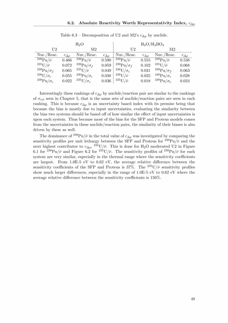
6.2. Absolute Reactivity Worth Representativity Index, c∆ρ
Table 6.3 – Decomposition of U2 and M2’s c∆ρ by nuclide.
H2O H2O/H3BO3
U2 M2 U2 M2
Nuc./Reac. c∆ρ Nuc./Reac. c∆ρ Nuc./Reac. c∆ρ Nuc./Reac. c∆ρ239Pu/ν 0.466 239Pu/ν 0.590 239Pu/ν 0.555 239Pu/ν 0.538235U/ν 0.072 239Pu/σf 0.059 239Pu/σf 0.102 235U/ν 0.068239Pu/σf 0.065 235U/ν 0.049 238U/σc 0.031 239Pu/σf 0.063238U/σc 0.055 240Pu/σc 0.038 238U/ν 0.025 240Pu/σc 0.028239Pu/σc 0.022 235U/σc 0.036 235U/ν 0.018 239Pu/σc 0.024
Interestingly these rankings of c∆ρ by nuclide/reaction pair are similar to the rankingsof σrel seen in Chapter 5, that is the same sets of nuclide/reaction pairs are seen in eachranking. This is because c∆ρ is an uncertainty based index with its premise being thatbecause the bias is mostly due to input uncertainties, evaluating the similarity betweenthe bias two systems should be based off of how similar the effect of input uncertainties isupon each system. Thus because most of the bias for the SFP and Proteus models comesfrom the uncertainties in these nuclide/reaction pairs, the similarity of their biases is alsodriven by these as well.
The dominance of 239Pu/ν in the total value of c∆ρ was investigated by comparing thesensitivity profiles per unit lethargy between the SFP and Proteus for 239Pu/ν and thenext highest contributor to c∆ρ,
235U/ν. This is done for H2O moderated U2 in Figure6.1 for 239Pu/ν and Figure 6.2 for 235U/ν. The sensitivity profiles of 239Pu/ν for eachsystem are very similar, especially in the thermal range where the sensitivity coefficientsare largest. From 1.0E-5 eV to 0.62 eV, the average relative difference between thesensitivity coefficients of the SFP and Proteus is 37%. The 235U/ν sensitivity profilesshow much larger differences, especially in the range of 1.0E-5 eV to 0.62 eV where theaverage relative difference between the sensitivity coefficients is 156%.
48

6.2. Absolute Reactivity Worth Representativity Index, c∆ρ
1 E - 0 5 1 E - 0 3 1 E - 0 1 1 E + 0 1 1 E + 0 3 1 E + 0 5 1 E + 0 7- 0 . 6
- 0 . 5
- 0 . 4
- 0 . 3
- 0 . 2
- 0 . 1
0 . 0
Sens
itised
Coeff
icient
per U
nit Le
thargy
E n e r g y ( e V )
S F P P r o t e u s
Figure 6.1 – Sensitivity coefficient of 239Pu/ν for H2O moderator for the response ∆ρ.
1 E - 0 5 1 E - 0 3 1 E - 0 1 1 E + 0 1 1 E + 0 3 1 E + 0 5 1 E + 0 7- 0 . 2
0 . 0
0 . 2
0 . 4
0 . 6
0 . 8
1 . 0
Sens
itised
Coeff
icient
per U
nit Le
thargy
E n e r g y ( e V )
S F P P r o t e u s
Figure 6.2 – Sensitivity coefficient of 235U/ν for H2O for the response ∆ρ.
This sensitivity profile comparison highlights the second duality of c∆ρ as a representa-tivity index: it is also sensitivity based. To have a high c∆ρ, two systems must have similarsensitivities to a given input parameter as well, not only high uncertainties. The 1σreluncertainties associated with 235U/ν and 239Pu/ν for H2O moderated U2 are 0.66% and
49

6.2. Absolute Reactivity Worth Representativity Index, c∆ρ
0.80% (see Table 5.3). 239Pu/ν does have higher uncertainty, but not significantly enoughto explain the large difference in c∆ρ. The large difference results from how dissimilar thesensitivity profiles of 235U/ν are between the SFP model and the Proteus model. Thisillustrates how cres behaves as both a sensitivity and uncertainty based representativityindex: high representativity for evaluating similar bias behavior occurs when the systemshave similar large uncertainties and similar sensitivities for a given parameter.
In summary different c∆ρ values from sample to sample and from nuclide/reactionpair to nuclide/reaction pair are caused by both varying magnitudes of uncertainty andby differences between sensitivity profiles. A nuclide/reaction pair that causes a highuncertainty in a given response for each system and of which each system has similarsensitivities will have a high cres value. However nuclide/reaction pairs with high uncer-tainties for each systems but differing sensitivity profiles will have smaller cres values, aswas seen for 235U/ν.
Representativity Results for all H2O Samples
The c∆ρ index was calculated for all H2O moderated samples to illustrate how theindex changes with burnup and with fuel type. Larger c∆ρ values are found for lowerburnup samples and for the MOX samples in comparison to the UO2 samples. This trendis similar to that of UQ, which is a logical result as c∆ρ is uncertainty based. The lowburnup samples U1 and M1 have the highest uncertainties for their fuel types at 1.63%and 3.76% and also the largest c∆ρ values at 0.841 and 0.873 respectively.
Table 6.4 – c∆ρ for each sample with H2O moderator.
Sample ID c∆ρ DP σbcBurnup
(MWd/kg)
U1 0.841 1.63% ∼38U2 0.762 1.31% ∼54U3 0.705 1.07% ∼71U4 0.766 0.98% ∼75U5 0.740 1.00% ∼91U6 0.733 0.90% ∼92U7 0.682 1.12% ∼121
M1 0.873 3.76% ∼21M2 0.861 2.35% ∼44M3 0.841 1.78% ∼64M4 0.841 1.54% ∼72
For this moderating condition, none of the samples had sufficiently high c∆ρ valuesfor Proteus to be deemed representative of the SFP model. Or in other words, no c∆ρ
value was greater than 0.9. The conclusion is that based on this methodology, the LWR-PROTEUS phase II campaign currently cannot be used as a benchmark for the KKGSFP as both systems are modeled with CASMO-5 in the manner described in Chapter 4.This does not eliminate the possibility of the experimental campaign being able to be abenchmark for the SFP with a different code system or with CASMO-5 using a differentmodeling scheme.
If the M×N methodology was available for use in SHARK-X, a more realistic model ofa SFP could be made without reflective boundary conditions on a single assembly. Thiscould improve the representativity results by allowing the action that causes the change
50

6.2. Absolute Reactivity Worth Representativity Index, c∆ρ
in reactivity to be more similar to that in the Proteus system. In Proteus, a single pinis removed/inserted which introduces the change in reactivity. The rest of the systemis static, i.e. it has a constant, fresh fuel composition. In the current SFP model, thereflective boundary conditions on the central fuel rack unit mean that when the freshassembly is “replaced” with burnt assembly in the CASMO-5 models, what effectivelyoccurs is a SFP of all fresh assemblies becomes all burnt assemblies, which is differentbehavior than is seen in Proteus. If an M×N model could be made, the models wouldsimulate replacing a single fresh assembly with a single burnt assembly, the surroundingassemblies would be static with fresh composition. This modelling would more closelyresemble the Proteus experiments. Additionally the modeling would be more realistic offuel handling that would occur in the real SFP.
51

Chapter 7
Conclusions
This project successfully achieved many of the goals declared at its outset:
1. The literature concerning the SHARK-X utility, UQ/SA methodologies, and theLWR-PROTEUS Phase II experimental campaign were reviewed and synthesized.
2. CASMO-5 models of the LWR Proteus configuration were made by adapting ex-isting CASMO-4E models. Additionally a comparison between their results wasperformed.
3. Stochastic sampling was applied to quantify the uncertainty due to input nucleardata and sample compositions uncertainties for all eleven samples and for each ofthe three moderating conditions.
4. Direct perturbation was successfully applied to quantify the uncertainty associatedwith input nuclear data for all experimental configurations.
5. Validation studies were done identifying that
• Nine out of eleven H2O moderated samples passed the validation test.• Four out of ten H2O/H3BO3 moderated samples passed the validation test.• Three out of eleven D2O/H2O moderated samples passed the validation test.
6. A model of the KKG spent fuel pool was made based off of communications withthe KKG fuel analysis team.
7. The UQ/SA results with DP calculations were successfully used to perform repre-sentativity analyses for evaluating the similarity of the Proteus experiments to theKKG spent fuel pool model.
8. The representativity analysis results for this modeling methodology were analyzedand found to be unsuccessful, but promising given the modeling approximationsused.
Overall, the project was successful in its primary goal of applying the SHARK-X toolto a real world problem to perform UQ/SA for validation and representativity analysis.The validation studies showed good results for H2O moderated samples and intimated thatbetter results could be possible for the H2O/H3BO3 and D2O/H2O moderated samplesby using more accurate modelling methodologies. Likewise, the representativity analysisresults could also be improved with more accurate modeling. A particularly interestingpath for future work to improve the modeling would involve implementing compatibilityin SHARK-X with the M×N feature in CASMO-5. If the representativity analysis resultswere sufficiently improved, the LWR-PROTEUS Phase II experimental campaign couldthen possibly be used as a benchmark for the KKG spent fuel pool or other spent fuelpools.
52

Bibliography
[1] “SCALE: A Modular Code System for Performing Standardized Computer Analysesfor Licensing Evaluation.” ORNL/TM-2005/39, Version 5.1, Vols. I–III, Oak RidgeNational Laboratory, Oak Ridge, Tenn., November 2006.
[2] “MCNP–A General Monte Carlo N Particle Transport Code.” Version 5, Vols. I–III,Oak Ridge National Laboratory, Oak Ridge, Tenn., February 2008.
[3] “CASMO-5 User’s Manual Rev. 5.” J. Rhodes, N. Gheorghiu, R.M. Ferrer, J. Hykes,T. Smed. SSP-07/431 Rev. 5, (2012)
[4] “American National Standard for Nuclear Criticality Safety in Operations with Fis-sionable Materials Outside Reactors, ANSI/ANS-8.1-1998.” American Nuclear Soci-ety, La Grange Park, Ill., 1998.
[5] “American National Standard for Validation of Neutron Transport Methods for Nu-clear Criticality Safety Calculations, ANSI/ANS-8.24-2007.” American Nuclear Soci-ety, La Grange Park, Ill., 2007.
[6] “TSUNAMI Primer: A Primer for Sensitivity/Uncertainty Calculations withSCALE.” B. T. Rearden, D. E. Mueller, S. M. Bowman, R. D. Busch, S. J. Emerson.ORNL/TM-2009/027. Oak Ridge National Laboratory, Oak Ridge, Tenn., January2009.
[7] “CASMO-5MX: Tools for Sensitivity Analysis and Uncertainty Quantification withrespect to Nuclear Data in CASMO-5M.” W. Wieselquist. TM-41-12-09, Paul ScherrerInstitut, Villigen, CH.
[8] “Application of Sensitivity/Uncertainty Methods to Burnup Credit Validation.” D.E. Mueller and J. C. Wagner. Presented at the International Atomic Energy Agency(IAEA) Technical Committee Meeting on Advances in Applications of Burnup Creditto Enhance Spent Fuel Transportation, Storage, Reprocessing and Disposition. August29 – September 2, 2005. London, UK
[9] Normal distribution and scales.gif. Wikipedia, The Free Encyclopedia.Wikimedia Foundation, Inc. 19 December 2005. Web. 1 June 2015.https://commons.wikimedia.org/wiki/File:Normal distribution and scales.gif
[10] “CASMO-4E Analysis of Reactivity Worths of Burnt Fuel Samples Measured inLWR-PROTEUS Phase II.” P. Grimm. TM-41-11–15, Paul Scherrer Institut, Villigen,CH. November 5, 2011.
[11] “PROTEUS FACILITY.” Paul Scherrer Institut. 16 July 2012. Web. 18 June 2015.http://proteus.web.psi.ch/facility/
53

Bibliography
[12] “Proteus”. Wikipedia, The Free Encyclopedia. Wikimedia Foundation, Inc. 3 June2015. Web. 18 June 2015. https://en.wikipedia.org/?title=Proteus
[13] “LWR-PROTEUS PROGRAMME, PHASE II, FINAL REPORT.” Ines Gunther-Leopold, Judith Kobler Waldis, Niko Kivel, Hans-Peter Linder, Beat Wernli. TM-43-06-05, Paul Scherrer Institut, Villigen, CH. December, 2007.
[14] “Comparison of Calculated and Measured Isotopic Inventories for the LWR-PROTEUS Phase II Irradiated Fuel Samples.” P. Grimm. TM-41-09-03, Paul ScherrerInstitut, Villigen, CH. September 16, 2009.
[15] “LWR-PROTEUS PROGRAMME, Phase II Experimental Results.” M.F. Murphy,G. Perret. TM-41-11-14, Paul Scherrer Institut, Villigen, CH. 26 July 2012.
[16] “ELCOS, The PSI Code System for LWR Core Analysis. Part II: User’s Manual forthe Fuel Assembly Code BOXER.”J.M. Paratte, K. Foskolos, P. Grimm, J.M. Hollard.PSI Bericht Nr. 96-08 (1996).
[17] “Criticality Safety Applications of S/U Validation Methods.” B. L. Broadhead, C.M. Hopper, K. R. Elam, B. T. Rearden, and R. L. Childs. Trans. Am. Nuc WinterMeeting, 2000, pp. 107–113.
[18] “Extended Interpretation of Sensitivity Data for Benchmark Areas of Applicabil-ity.” S. Goluoglu, C. M. Hopper, and B. T. Rearden. Trans. Am. Nuc. “The NuclearTechnology Expansion: Unlimited Opportunities,” 2003, pp. 77–79.
[19] “Uncertainty Quantification and Representativity Analysis of LWR-PROTEUSPhase III Experiments using CASMO-5MX.” M. Hursin, M. Scriven. TM-41-13-26,Paul Scherrer Institut, Villigen, CH. 2013.
[20] “ENDF/B-VII.1 nuclear data for science and technology: cross sections, covariances,fission product yields and decay data.” M.B. Chadwick et al. Nuclear Data Sheets,112, 2887–2996 (2011).
[21] “Bestimmung der hochstuzlassigen Anreicherung im Kompaktlager des KKWGosgen-Daniken mit Uran-Brennelementen.” S. Pelloni. TM-41-00-30, Paul ScherrerInstitut, Villigen, CH. October, 24 2000.
[22] “Methods of Steady-State Reactor Physics in Nuclear Design.’ ’Stammler A.J.J.,Abbate M.J.. Academic Press, 1983.
[23] “PSI Methodologies for Nuclear Data Uncertainty Propagation with CASMO-5Mand MCNPX: Results for OECD/NEA UAM Benchmark Phase I.” W. Wieselquist,T. Zhu, A. Vasiliev, H. Ferroukhi. Science and Technology of Nuclear Installations,Volume 2013.
[24] “Janis — A New Java-based Nuclear Data Display Program,” OECD Nuclear EnergyAgency (2001).
54

Appendix A: UncertaintyQuantification Example Exercise
An exercise is presented in this chapter to help develop an understanding of the SS andDP methods and where and why discrepancies between their results arise. Two examplefunctions are used to highlight what happens when the methods are applied to linearand non-linear systems both with and without covariance between their variables. Thevariance of the functions is calculated in three ways:
1. Analytically,2. With direct perturbation (DP),3. And with stochastic sampling (SS).
The chosen example functions are Equations 1 and 2. Equation 1 is a linear applicationof the methods and Equation 2 is a non-linear application. The variables x1 and x2 areimplemented as both fully correlated and fully uncorrelated random variables of uniformdistributions. Fully uncorrelated variables means that their covariance is zero. With non-zero covariance, the calculations are more complex and the differences between SS andDP become more prominent.
f1(x1, x2) = x1 + x2 (1)
f2(x1, x2) = x1 ∗ x2 (2)
A.1 Mean, Variance, and Covariance of x1 and x2
The expected value (mean) and variance of any continuous random variable are givenby Equations 3 and 4 respectively, where x is a given random variable and p(x) is thatvariable’s probability density function (PDF).
E(x) =
∫ ∞−∞
xp(x)dx (3)
V ar(x) = ∆2x = E
[(x− E(x)
)2](4)
Equations 3 and 4 can then be applied to a hypothetical uniform distribtuion, f(x),seen in Figure A.1 and defined with the PDF given by Equation 5. The random variablesx1 and x2 in Equations 1 and 2 are defined with αx1 and βx1 being equal to 1.0 and 2.0respectively, and αx2 and βx2 3.0 and 5.0 respectively.
55

A.1. Mean, Variance, and Covariance of x1 and x2
Figure A.1 – Hypothetical uniform distribution.
f(x) =
{1
β−α , if α ≤ x ≤ β.
0, otherwise.(5)
In the case where there are two or more variables like in Equations 1 and 2, a covariancebetween any two of these variables exists, which is a measure of how much the two variableschange together. For two random variables x and y, their covariance is given by Equation6. If their covariance is positive, the variables show similar behavior, i.e. greater values inone variable correspond to greater values in the second variable, or vice versa. Negativecovariance indicates greater values in one variable correspond to smaller values in thesecond variable. The degree of this correlation between the variables is described by acorrelation coefficient, ρx,y, seen in Equation 7. Here ∆x,y is the covariance between x andy and ∆x and ∆y are the standard deviations of x and y respectively. If ρx,y is equal to 1.0there is a total positive correlation between the variables, if it is 0 there is no correlation,and 1.0 there is total negative correlation. A ρx,y = 0, or fully uncorrelated variables,implies that the the covariance is 0. A ρx,y = 1.0, or positively and fully correlatedvariables, means that the covariance is equal to the product of each variable’s standarddeviation.
cov(x, y) = ∆x,y = E[(x− E(x)
)(y − E(y)
)](6)
ρx,y =∆x,y
∆x∆y(7)
Thus for the random variables x1 and x2, Equations 3, 4, and 6 are used to calculatetheir corresponding mean values, variances, and the covariance between the variables.These values for x1 and x2 are shown in Table A.1.
56

A.2. Variance with Taylor Series Expansion
Table A.1 – Expected values, variances, and covariance for the random variables x1 andx2.
x1 x2
Expected Value, E(x) 32 4
Variance, ∆2x
112
13
Covariance, ∆x1,x216
A.2 Variance with Taylor Series ExpansionThe DP method introduces error into the calculation of a function’s variance because
it is a first-order approximation. Using a Taylor series expansion to analytically calculatethe variance is interesting because it highlights which terms are first order and whichare second order, and thus it is easy to identify which terms are being neglected in theDP method’s approximation. The Taylor series expansion for a function’s variance isexplained in this section and is later applied in Sections A.3 and A.4 to calculate thevariances of the given linear and nonlinear examples.
The variance of a function of multiple random variables can be calculated with Equa-tion 4 by using the function as the main argument x. However an alternative methodusing a Taylor series expansion can be done by supposing that there is a function x of atleast two variables, u and v, shown in Equation 8. The function x has a most probablevalue, x, that comes from the most probable values of its variables, u and v, shown inEquation 9. The value x has an associated uncertainty due to the spread of its individualvalues, xi shown in Equation 10, which is caused by the combination of the spread of itsvariables, ui and vi.
x = f(u, v, ...) (8)
x = f(u, v, ...) (9)
xi = f(ui, vi, ...) (10)
In the limit of an infinite number of measurements, the distribution of x about itsmean can be quantified by its variance, ∆2
x, shown in Equation 11.
∆2x = lim
N→∞
[1
N
∑(xi − x)2
](11)
An expression for the variance as a function of the component variables, u and v, isdesired rather than with the term xi − x, which is the error in that individual xi value.This can be found by doing a Taylor series expansion on x, shown in Equation 12. Thisis done about the point of the averages of u and v, meaning that each partial derivative isevaluated while the other variable is fixed at its mean. This new expression for the errorof x can then be plugged in to Equation 11 to calculate the variance seen in Equation 13which is then expanded to Equation 14.
xi − x ≈ (ui − u)δx
δu
∣∣∣u,y
+ (vi − v)δx
δv
∣∣∣u,y
+ . . . (12)
57

A.3. Linear Example: f1(x1, x2) = x1 + x2
∆2x ≈ lim
N→∞
1
N
[(ui − u)
δx
δu
∣∣∣u,y
+ (vi − v)δx
δv
∣∣∣u,y
+ . . .
]2
(13)
∆2x ≈ lim
N→∞
1
N
[(ui − u)2
(δxδu
∣∣∣u,y
)2+ (vi − v)2
(δxδv
∣∣∣u,y
)2+
2(ui − u)(vi − v)δx
δu
∣∣∣u,y
δx
δv
∣∣∣u,y
+ . . .
] (14)
Next, the terms in Equation 14 can be replaced by the definitions for the variance ofu and v, ∆u and ∆v, as seen in Equation 15, and for the covariance between u and v,∆u,v, as seen in Equation 16. This gives a new expression, Equation 17, for the varianceof x with only the first-order terms of the Taylor expansion shown. Equation 17 can thenbe used for functions that are represented by x to calculate the variance of the givenfunction, which will be done for the example functions f1(x1, x2) and f2(x1, x2) in thefollowing sections.
∆2u = lim
N→∞
[1
N
∑(ui − u)2
]∆2v = lim
N→∞
[1
N
∑(vi − v)2
] (15)
∆uv = limN→∞
[1
N
∑(ui − u)(vi − v)
](16)
∆2x ≈ ∆2
u
(δxδu
∣∣∣u,y
)2+ ∆2
v
(δxδv
∣∣∣u,y
)2+ 2∆uv
δx
δu
∣∣∣u,y
δx
δv
∣∣∣u,y
+ . . . (17)
A.3 Linear Example: f1(x1, x2) = x1 + x2
Presented in this section are the analytical, DP, and SS solutions for the variance ofthe function f1(x1, x2), or Equation 1. The variance is calculated for when the variablesx1 and x2 are fully uncorrelated and positively, fully correlated. This example shows thatthe analytical, DP, and SS solutions for the variance of f1(x1, x2) are equivalent for alinear function.
A.3.1 Analytical Solution
The mean of f1(x1, x2) is calculated with Equation 1 and is shown as Equation 18. Thevariance of f1(x1, x2) is calculated using the Taylor series seen in Equation 17, evaluatedat the means of x1 and x2. Because the function is linear, the Taylor series expansion hasonly first-order terms, as is shown in Equation 19. Evaluating the derivatives in Equation19 leads to Equation 20 for the variance of f1(x1, x2). The mean and variance of f1(x1, x2)with correlated x1 and x2 variables are calculated using the values found in Table A.1and are 5.50 and 0.75 respectively.
f1(x1, x2) = x1 + x2 (18)
∆2f1 = ∆2
x1
( δf1
δx1
∣∣∣x1,x2
)2+ ∆2
x2
( δf1
δx2
∣∣∣x1,x2
)2+ 2∆x1,x2
δf1
δx1
∣∣∣x1,x2
δf1
δx2
∣∣∣x1,x2
(19)
58

A.3. Linear Example: f1(x1, x2) = x1 + x2
∆2x = ∆2
x1 + ∆2x2 + 2∆x1,x2 (20)
If the variables x1 and x2 are assumed to be uncorrelated and thus their covarianceis 0, the 2∆x1,x2 term vanishes from Equation 20 leading to Equation 21. The variancecalculated with Equation 21 is 0.42. The decreased variance from 0.75 to 0.42 shows thatconsidering covariance (if it exists) between variables is very important in evaluating theuncertainty of a system.
∆2x = ∆2
x1 + ∆2x2 (21)
A.3.2 Direct Perturbation Solution
With the DP method, the variance of f1(x1, x2) is taken from the output VCM ob-tained from the sandwich rule, or Equation 3.5. The sensitivity coefficient vector, S, usedin the sandwich rule is evaluated at the mean values for x1 and x2 as seen in Equation22. The input VCM, Vin, is made up of the variance and covariance terms of f1(x1, x2).
S =[δfδx1
∣∣∣x1,x2
δfδx2
∣∣∣x1,x2
](22)
Vin =
[∆2x1 ∆x1,x2
∆x1,x2 ∆2x2
](23)
The evaluation of S for f1(x1, x2) gives Equation 24. The sandwich rule can thenbe applied for f1(x1, x2) and gives Equation 25. The solution for the variance seen inEquation 25 is identical to the analytical one seen in Equation 20. This shows that forthis linear, fully and positively correlated function, the first-order approximation usedwith the DP method reproduces the analytical solution for the variance. The evaluationof Equation 25 using the values found in Table A.1 gives a variance of 0.75, equivalent tothe analytically calculated variance.
S =[δf1δx1
∣∣∣x1,x2
δf1δx2
∣∣∣x1,x2
]=[1 1
](24)
Vout =
[11
]×[
∆2x1 ∆x1,x2
∆x1,x2 ∆2x2
]×[1 1
]= ∆2
x1 + ∆2x2 + 2∆x1,x2 (25)
If the variables are uncorrelated, the Vin matrix is simplified by making the covarianceterm, ∆x1,x2 , equal to 0. The sandwich rule is applied again to f1(x1, x2) with uncorrelatedvariables giving Equation 26. This solution is also identical to the analytical solution seenin Equation 21, showing again that the DP method reproduces the analytical solution.The evaluation of Equation 26 using the values found in Table A.1 gives a variance of0.42, equivalent to analytically calculated variance.
Vout =
[11
]×[∆2x1 00 ∆2
x2
]×[1 1
]= ∆2
x1 + ∆2x2 (26)
A.3.3 Stochastic Sampling
Next the variance of f1(x1, x2) is evaluated using an implementation of the SS methodin MATLAB. The correlation between the variables is important in determining how each
59

A.3. Linear Example: f1(x1, x2) = x1 + x2
will be randomly sampled. If the samples are fully and positively correlated (i.e. thecorrelation coefficient, ρx,y = 1.0), they will use the same random number, u, as seen inEquation 27, where i is the ith random sample from the sample set. The parameters αxand βx are the limits of the uniform distribution PDFs described in Section A.1, Equation5. If the variables are fully uncorrelated (i.e. ρx,y = 0), separate random numbers, u1
and u2, for each variable must be generated as in Equation 28. Generating partiallycorrelated, random uniform variables (i.e. −1.0 < ρx,y < 0 and 0 < ρx,y < 1.0) is moredifficult and requires the use of copulas to approximate the correlation during the randomsampling. This is not done in this analysis.
xi1 = αx1 + (βx1 − αx1) ∗ u, xi2 = αx2 + (βx2 − αx2) ∗ u (27)
xi1 = αx1 + (βx1 − αx1) ∗ u1, xi2 = αx2 + (βx2 − αx2) ∗ u2 (28)
The MATLAB scripts for the simulations with fully correlated and fully uncorrelatedvariables are shown in Figures A.2 and A.3 respectively. The values for the mean andthe variance of f1(x1, x2) produced with fully correlated variables are converging towards5.5 and 0.75 after 1E6 samples. For the simulation with fully uncorrelated variables, themean and variance converge towards 5.5 and 0.42 after 1E6 samples. This illustrates thatfor this linear example, the analytical, DP, and SS methods agree and both reproduce theanalytical solution for the variance of the function.
Figure A.2 – SS method applied to example f1(x1, x2) with fully correlated variables.
60

A.4. Nonlinear Example: f2(x1, x2) = x1 ∗ x2
Figure A.3 – SS method applied to example f1(x1, x2) with fully uncorrelated variables.
A.4 Nonlinear Example: f2(x1, x2) = x1 ∗ x2
Presented in this section are the analytical, DP, and SS solutions for the variance ofthe function f2(x1, x2), or Equation 2. This example shows that for a simple, nonlinearfunction already there are divergences between the variance calculated analytically/withthe SS method and the variance calculated by the DP method. Additionally, the timeconsuming analytical solution for the variance shows why the use of the DP and SSmethods is valuable, especially if it were to be applied to more complicated, higher-orderfunctions.
A.4.1 Analytical Solution
The mean of the product of two variables, for example xy, is described with thefollowing derivation. First the terms ∆x and ∆y seen in Equation 29 are substitutedfor the values x and y as seen in Equation 30. Next in Equation 31, the expected valueE(xy) of the product of x and y is taken. Equation 31 is then simplified because the terms,E(∆x)E(y) and E(∆y)E(x) evaluate to zero as seen in Equation 32. Finally the mean ofxy is given by Equation 33, with the covariance term, cov(x, y), being described previouslyin Equation 6. This is then used to describe the mean of f2(x1, x2) as given by Equation34, where the term ∆x1,x2 is the covariance between x1 and x2. For fully correlated andfully uncorrelated variables, the mean of f2(x1, x2) is 6.16 and 6.0 respectively.
∆x = x− E(x), ∆y = y − E(y) (29)
xy =[∆x+ E(x)
][∆y + E(y)
]= ∆x∆y + ∆xE(y) + ∆yE(x) + E(x)E(y) (30)
E(xy) = E[∆x∆y
]+ E
[∆xE(y)
]+ E
[∆yE(x)
]+ E
[E(x)E(y)
](31)
61

A.4. Nonlinear Example: f2(x1, x2) = x1 ∗ x2
E(∆x)E(y) = E[x− E(x)
]E(y) =
[E(x)− E(x)
]E(y) = 0 (32)
E(xy) = E(x)E(y) + E(∆x∆y) = E(x)E(y) + cov(x, y) (33)
f2(x1, x2) = x1x2 + ∆x1,x2 (34)
Next the variance, ∆2f2
, can be calculated with a Taylor series expansion, as seenin Equation 35. In this nonlinear case, the Taylor expansion around x1 and x2 includessecond order terms, unlike in the linear Equation 19, which contains only first order terms.These second order terms are what will be later ignored in the DP method’s predictionof the variance.
∆2f2 ≈ lim
N→∞
[(x1,i − x1)
δf2
δx1
∣∣∣x1,x2
+ (x2,i − x2)δf2
δx2
∣∣∣x1,x2
+
1
2!
[(x1,i − x1)2 δ
2f2
δx21
∣∣∣x1,x2
+ (x2,i − x2)2 δ2f2
δx22
∣∣∣x1,x2
+
2(x1,i − x1)(x2,i − x2)δ2f2
δx1x2
∣∣∣x1,x2
]]2
(35)
Expanding Equation 35 leads to Equation 36. For this function, the second derivative
terms, δ2f2δx21
and δ2f2δx22
, evaluate to zero and are not shown. This leaves only the first
derivative terms, δf2δx1
and δf2δx2
, and the mixed derivative term δ2f2δx1x2
.
Then the definitions of variance and covariance given in Equations 15 and 16 areplugged in to Equation 36 to give Equation 37. Finally the derivatives are evaluated togive an analytical solution for the variance of f2(x1, x2) shown in Equation 38.
∆2f2 ≈ lim
N→∞
[(x1,i − x1)2
( δf2
δx1
∣∣∣x1,x2
)2+ (x2,i − x2)2
( δf2
δx2
∣∣∣x1,x2
)2+
2(x1,i − x1)(x2,i − x2)δf2
δx1
∣∣∣x1,x2
δf2
δx2
∣∣∣x1,x2
+
2(x1,i − x1)δf2
δx1
∣∣∣x1,x2
(x1,i − x1)(x2,i − x2)δ2f2
δx1x2
∣∣∣x1,x2
+
2(x2,i − x2)δf2
δx2
∣∣∣x1,x2
(x1,i − x1)(x2,i − x2)δ2f2
δx1x2
∣∣∣x1,x2
+
(x1,i − x1)2(x2,i − x2)2( δ2f2
δx1x2
∣∣∣x1,x2
)2]
(36)
∆2f2 = ∆2
x1
( δf2
δx1
∣∣∣x1,x2
)2+ ∆2
x2
( δf2
δx2
∣∣∣x1,x2
)2+ 2∆x1,x2
δf2
δx1
∣∣∣x1,x2
δf2
δx2
∣∣∣x1,x2
+
2∆x1∆x1,x2
δf2
δx1
∣∣∣x1,x2
δf2
δx1x2
∣∣∣x1,x2
+ 2∆x2∆x1,x2
δf2
δx2
∣∣∣x1,x2
δ2f2
δx1x2
∣∣∣x1,x2
+
∆2x1∆2
x2
( δ2f2
δx1x2
∣∣∣x1,x2
)2(37)
∆2f2 = ∆2
x1 x22 + ∆2
x2 x12 + 2∆x1,x2 x1x2 + ∆2
x1∆2x2 (38)
62
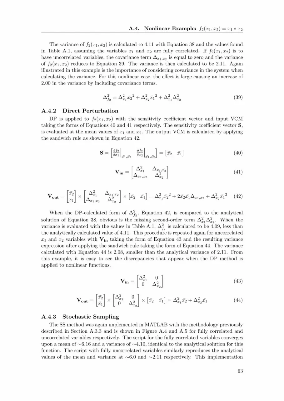
A.4. Nonlinear Example: f2(x1, x2) = x1 ∗ x2
The variance of f2(x1, x2) is calculated to 4.11 with Equation 38 and the values foundin Table A.1, assuming the variables x1 and x2 are fully correlated. If f2(x1, x2) is tohave uncorrelated variables, the covariance term ∆x1,x2 is equal to zero and the varianceof f2(x1, x2) reduces to Equation 39. The variance is then calculated to be 2.11. Againillustrated in this example is the importance of considering covariance in the system whencalculating the variance. For this nonlinear case, the effect is large causing an increase of2.00 in the variance by including covariance terms.
∆2f2 = ∆2
x1 x22 + ∆2
x2 x12 + ∆2
x1∆2x2 (39)
A.4.2 Direct Perturbation
DP is applied to f2(x1, x2) with the sensitivity coefficient vector and input VCMtaking the forms of Equations 40 and 41 respectively. The sensitivity coefficient vector S,is evaluated at the mean values of x1 and x2. The output VCM is calculated by applyingthe sandwich rule as shown in Equation 42.
S =[δf2δx1
∣∣∣x1,x2
δf2δx2
∣∣∣x1,x2
]=[x2 x1
](40)
Vin =
[∆2x1 ∆x1,x2
∆x1,x2 ∆2x2
](41)
Vout =
[x2
x1
]×[
∆2x1 ∆x1,x2
∆x1,x2 ∆2x2
]×[x2 x1
]= ∆2
x1 x22 + 2x2x1∆x1,x2 + ∆2
x2 x12 (42)
When the DP-calculated form of ∆2f2
, Equation 42, is compared to the analytical
solution of Equation 38, obvious is the missing second-order term ∆2x1∆2
x2 . When thevariance is evaluated with the values in Table A.1, ∆2
f2is calculated to be 4.09, less than
the analytically calculated value of 4.11. This procedure is repeated again for uncorrelatedx1 and x2 variables with Vin taking the form of Equation 43 and the resulting varianceexpression after applying the sandwich rule taking the form of Equation 44. The variancecalculated with Equation 44 is 2.08, smaller than the analytical variance of 2.11. Fromthis example, it is easy to see the discrepancies that appear when the DP method isapplied to nonlinear functions.
Vin =
[∆2x1 00 ∆2
x2
](43)
Vout =
[x2
x1
]×[∆2x1 00 ∆2
x2
]×[x2 x1
]= ∆2
x1 x2 + ∆2x2 x1 (44)
A.4.3 Stochastic Sampling
The SS method was again implemented in MATLAB with the methodology previouslydescribed in Section A.3.3 and is shown in Figure A.4 and A.5 for fully correlated anduncorrelated variables respectively. The script for the fully correlated variables convergesupon a mean of ∼6.16 and a variance of ∼4.10, identical to the analytical solution for thisfunction. The script with fully uncorrelated variables similarly reproduces the analyticalvalues of the mean and variance at ∼6.0 and ∼2.11 respectively. This implementation
63

A.5. Summary
shows the power of SS when the given problem is non-linear. With 1E6 samples thevariance is converging upon the analytical values of the variance. This accuracy is possiblebecause unlike with DP, no approximations are made in the SS calculation.
Figure A.4 – SS MATLAB script for f2(x1, x2) with fully correlated variables.
Figure A.5 – SS MATLAB script for f2(x1, x2) with fully uncorrelated variables.
A.5 SummaryThis exercise, presenting a linear and nonlinear function, shows in a simple way the
discrepancies that exist between the variance quantified by the SS and DP methods. Thevariance results are summarized for each example function in Table A.2 as calculatedanalytically and with the SS and DP methods. For the linear application f1(x1, x2), theanalytical, SS, and DP variance results agree. When the function is linear, the first-orderapproximation introduces no error, as there are no higher-order terms being neglected.
64

A.5. Summary
For the nonlinear application f1(x1, x2), differences between the analytical and SS resultsand the DP results emerge. This is due to terms ignored in the first-order approximationused in the DP method. It is easy to project to more complicated, nonlinear functionsthat the DP method’s error can become larger and larger.
Additionally the effect of correlation between the variables in the example functionwas investigated. If the variables are fully correlated vs fully uncorrelated, the magnitudeof the variance changes, no matter the method used to calculate it. With fully correlatedvariables, the variance is larger at 0.75 and 4.11 for f1(x1, x2) and f2(x1, x2) respectively.Meanwhile, for the fully uncorrelated variables, the variance is 0.42 and 2.11 respectively.These differences show the importance of considering correlation between variables whenquantifying the uncertainty associated with a system.
Table A.2 – Summary of variance calculation exercise.
f1(x1, x2) f2(x1, x2)Corr. Uncorr. Corr. Uncorr.
Analytical 0.75 0.42 4.11 2.11SS ∼0.75 ∼0.42 ∼4.10 ∼2.11DP 0.75 0.42 4.09 2.08
65

Appendix B: Derivation ofCriticality Parameters andNon-linearity Effects
B.1 Absolute Reactivity WorthThe neutron transport equation for a multiplying medium can be described in its
lambda-eigenvalue form as Equation 45. In this equation, L and P are the loss andproduction operators respectively in the Boltzmann equation, φ is the neutron flux, andλ is the fundamental lambda-eigenvalue for the multiplying medium, which by definitiontakes the form of Equation 46, where k is kinf or keff .
(L− λP)φ = 0 (45)
λ =1
k(46)
During the LWR-PROTEUS Phase II campaign, samples were inserted into the coreto measure change in the reactivity, ∆ρ, due to burnup products. The system, the Proteusreactor, is in a reference state before a sample is inserted and has a reference lambda-eigenvalue of λref . This reference state is when the reference sample of 3.5% enriched UO2
is in the core. The reactivity at this reference state is defined as Equation 47. A perturbedstate is then created when when the reference sample is removed and a burnt sample isinserted into the core. The different composition of the sample causes a change in the Land P terms in Equation 45. These changes in the loss and production of neutrons leadsto a new lambda-eigenvalue, λpert, of the perturbed system. The static reactivity of thisperturbed system is then Equation 48. The absolute change in reactivity between thereference and perturbed states is therefore described by Equation 49.
ρref = 1− λref (47)
ρpert = 1− λpert (48)
∆ρ = ρpert − ρref = λref − λpert (49)
Equation 49 gives the absolute reactivity worth (∆ρ) which is a response parameterinvestigated in the experimental campaign and in the UQ/SA presented in this report.The UQ/SA analysis requires the calculation of sensitivity coefficients of ∆ρ (and thus of
66

B.1. Absolute Reactivity Worth
k/λ as well) with respect to perturbations of an input parameter, α. Given a perturbationto α, the sensitivity coefficients of k and λ, Sk,α and Sλ,α, to this perturbation are definedas Equations 50 and 51 respectively. Replacing k in Equation 50 with λ leads to therelation seen in Equation 52, that Sk,λ is equal to but opposite of Sλ,α.
Sk,α =α0
k0
δk
δα
∣∣∣∣α0
(50)
Sλ,α =α0
λ0
δλ
δα
∣∣∣∣α0
(51)
Sk,α =α0
k0
δ
δα
(k)∣∣∣∣α0
= α0λ0δ
δα0
( 1
λ0
)∣∣∣∣α0
= −α0λ0
λ20
δλ
δα
∣∣∣∣α0
= −α0
λ0
δλ
δα
∣∣∣∣α0
= −Sλ,α (52)
B.1.1 ∆ρ sensitivity coefficient
The sensitivity coefficient of ∆ρ, S∆ρ,α, is written in Equation 53. The outputs ofCASMO-5 are the responses kinf and keff and are thus only inputs into SHARK-X tocalculate sensitivity coefficients. Therefore in order to calculate S∆ρ,α, Equation 53 needsto be rewritten in terms of k. To do this, the definition of ∆ρ given in Equation 49 isused in Equation 54 to obtain S∆ρ,α in terms of the reference and perturbed sensitivity
coefficients of k, Srefk,α and Spertk,α respectively. Equation 54 is what is implemented inSHARK-X to calculate S∆ρ,α for use in UQ/SA.
S∆ρ,α =α0
∆ρ0
δ∆ρ
δα
∣∣∣∣α0
=α0
∆ρ0
(δρpertδα
∣∣∣∣α0
−δρrefδα
∣∣∣∣α0
)(53)
S∆ρ,α =α0
∆ρ0
(δλrefδα
∣∣∣∣α0
− δλpertδα
∣∣∣∣α0
)=
1
∆ρ
(λ0,pertS
pertk,α − λ0,refS
refk,α
)(54)
B.1.2 Linearity of ∆ρ
As seen in Appendix 7, the DP method introduces some error in the calculationof variance due the first-order approximation in its definition. Because of this, it isimportant to assess the degree of non-linearity in response of interest when doing UQ/SA.SA applied to representativity analysis in particular can only been done with the DPmethod because the sensitivity coefficients created with the SS method have often largedegrees of uncertainty associated with them. This section assesses the degree of non-linearity of ∆ρ. First the Taylor series expansion of ∆ρ about the reference state of theinput parameter, α0, is done and is shown truncated to the third order in Equation 55.
∆ρ(α)−∆ρ(α0) = (α− α0)δ∆ρ
δα
∣∣∣∣α0
+1
2!(α− α0)2 δ
2∆ρ
δα2
∣∣∣∣α0
+ ... (55)
The first and second derivatives of ∆ρ are given by Equations 56 and 57 respectively.The second derivative of ∆ρ requires the use of the product rule. In the DP method, theresponse of k is assumed to be linear with respect to α. The second derivative is therefore
reduced to 58, as theδ2kpertδα2 and
δ2krefδα2 terms are zero in a linear system.
δ∆ρ
δα= − 1
k2ref
δkrefδα
+1
k2pert
δkpertδα
(56)
67

B.1. Absolute Reactivity Worth
δ2∆ρ
δα2=
2
k3ref
(δkrefδα
)2
− 1
k2ref
δ2krefδα2
− 2
k3pert
(δkpertδα
)2
− 1
k2ref
δ2krefδα2
+1
k2pert
δ2kpertδα2
(57)
δ2∆ρ
δα2=
2
k3ref
(δkrefδα
)2
− 2
k3pert
(δkpertδα
)2
(58)
The importance of the second-order term, or Equation 58, and thus the non-linearityof the response is considered by comparing the magnitude of the first-order term to thesecond-order term with example values for λ and Sk,α. These values are given in TableB.1 for a reference state and two perturbed states, where the perturbations are done upon238U/σc nuclide reaction pair, and thus the sensitivity coefficient is Sk,238U/σc .
Table B.1 – Typical values for λ and Sk,α values for 238U/σc for a reference state and twoperturbed states.
State λ Sk,238U/σc
Reference 0.76182 -0.292Pert1 0.76426 -0.290Pert2 0.76245 -0.291
This comparison is shown in Figure B.1 for relative perturbations of -10% to 10% of238U/σc. The second derivative term of absolute reactivity is much smaller than the firstderivative term in all ranges of perturbations. Therefore, despite having non-linearitiesin its formulation, the absolute reactivity response can be assumed to behave as a linearfunction for small perturbations of a given parameter α. Therfore in the UQ presentedin this report, the SS and DP methods should return close UQ results for this response.
Figure B.1 – Evolution of the first and second order term of absolute reactivity’s Taylorexpansion with respect to the relative input uncertainty, for U-238 capture
68

B.2. Relative Reactivity Worth
B.2 Relative Reactivity WorthDuring the experimental campaign, the absolute reactivity worth was normalized to
a parameter called relative reactivity worth (∆ρrel) shown in Equation 2.2.
B.2.1 ∆ρrel Sensitivity Coefficient
The sensitivity coefficient of relative reactivity, S∆ρrel,α, is also used in the UQ/SAdone in this report. The SHARK-X utility calculates S∆ρrel,α from given the kinf or keff
response of the CAMSO-5 output. S∆ρrel,α is derived from Equation 3.2 and given asEquation 59, where α is a given input parameter that is perturbed from its referencestate of α0.
S∆ρrel,α =α0
∆ρrel0
δ∆ρrel
δα
∣∣∣∣α0
(59)
The derivative of term in S∆ρrel,α is given as Equation 60, where λr is from thereference state of the system, and λ1 and λ2 are two different perturbed states. Thederivative is then evaluated using the quotient rule in Equation 61 and simplified toEquation 62
δ∆ρrel
δα
∣∣∣∣α0
=δ
δα
(λr − λ1
λr − λ2
)∣∣∣∣α0
(60)
δ∆ρrel
δα
∣∣∣∣α0
=1
(λr − λ2)2
[(λ0,r−λ0,2)
δ
δα
(λr−λ1
)∣∣∣∣α0
−(λ0,r−λ0,1)δ
δα
(λr−λ2
)∣∣∣∣α0
](61)
δ∆ρrel
δα
∣∣∣∣α0
=λ0,1 − λ0,2
(λr − λ0,2)2
δλrδα
∣∣∣∣α0
+λ0,r − λ0,2
(λr − λ0,2)2
δλ2
δα
∣∣∣∣α0
− 1
(λ0,r − λ0,2)
δλ1
δα
∣∣∣∣α0
(62)
Equation 62 is then plugged into the definition of S∆ρrel,α, or Equation 59, to obtainEquation 63. This allows for S∆ρrel,α to be calcualted in terms of λ. Next the sensitivity
coefficient of λ, or Equation 51, and the definition of ∆ρrel, Equation 2.2, are pluggedinto Equation 63 to obtain Equation 64. The relation between Sλ,α and Sk,α shownin Equation 52 is then used to obtain Equation 65. Equation 65 is implemented intoSHARK-X to calculate the sensitivity coefficients for relative reactivity with DP.
S∆ρrel,α =α0
∆ρrel0
[λ0,1 − λ0,2
(λ0,r − λ0,2)2
δλrδα
∣∣∣∣α0
+λ0,r − λ0,2
(λr − λ0,2)2
δλ2
δα
∣∣∣∣α0
− 1
λ0,r − λ0,2
δλ1
δα
∣∣∣∣α0
](63)
S∆ρrel,α =λ0,r(λ0,1 − λ0,2)
(λ0,r − λ0,1)(λ0,r − λ0,2)Sλr,α −
λ0,1
λ0,r − λ0,1Sλ1,α +
λ0,2
λ0,r − λ0,2Sλ2,α (64)
S∆ρrel,α = − λ0,r(λ0,1 − λ0,2)
(λ0,r − λ0,1)(λ0,r − λ0,2)Skr,α +
λ0,1
λ0,r − λ0,1Sk1,α −
λ0,2
λ0,r − λ0,2Sk2,α (65)
69

B.2. Relative Reactivity Worth
B.2.2 Linearity of ∆ρrel
The definition of relative reactivity seen in Equation 2.2 shows that this parameter isnonlinear. Therefore there will be error introduced by the first-order approximation usedin the DP method. The degree of this nonlinearity and the effect it has on the absolutevalue of ∆ρrel is investigated in this section. First, A Taylor series expansion of ∆ρrel(α)truncated to the second order and evaluated at α0 is done and is showed in Equation 66.
∆ρrel(α)−∆ρrel(α0) = (α− α0)δ∆ρrel
δα
∣∣∣∣α0
+1
2!(α− α0)2 δ
2∆ρrel
δα2
∣∣∣∣α0
+ ... (66)
δλ
δα
∣∣∣∣α
= −λ2 δk
δα
∣∣∣∣α
(67)
The second derivative term in Equation 66 is redefined with the definition of relativereactivity, Equation 2.2, in Equation 68. The derivatives are then evaluated using thequotient rule and Equation 68 becomes Equation 69.
δ2∆ρrel
δα2
∣∣∣∣α0
=δ2
δ2α
(∆ρ1
∆ρ2
)∣∣∣∣α0
(68)
δ2∆ρrel
δα2
∣∣∣∣α0
=1
∆ρ0,2
δ2∆ρ1
δα2
∣∣∣∣α0
− ∆ρ0,1
∆ρ20,2
δ2∆ρ2
δα2
∣∣∣∣α0
+ 2∆ρ0,1
∆ρ30,2
(δ∆ρ2
δα
∣∣∣∣α0
)2
(69)
Using Equation 56 for the first derivative term of ∆ρ and Equation 58 for the secondderivative terms, each of the derivative terms in Equation 69 are evaluated giving Equation70
δ2∆ρrel
δα2
∣∣∣∣α0
=1
∆ρ0,2
(− 2
k30,1
(δk1
δα
∣∣∣∣α0
)2
+2
k30,r
(δk2
δα
∣∣∣∣α0
)2)−
∆ρ0,1
∆ρ20,2
(− 2
k30,2
(δk2
δα
∣∣∣∣α0
)2
+2
k30,r
(δkrδα
∣∣∣∣α0
)2)
+2∆ρ0,1
∆ρ30,2
(− 1
k20,2
δk2
δα
∣∣∣∣α0
+1
k20,r
δkrδα
∣∣∣∣α0
)(70)
The ∆ρ terms in Equation 70 can be then replaced by their expressions as a functionof λ to give Equation 71.
δ2∆ρrel
δα2= −
2λ30,1
(λ0,r − λ0,2)
(δk1
δα
∣∣∣∣α0
)2
+2λ3
0,2
(λ0,r − λ0,2)
(δkrδα
∣∣∣∣α0
)2
+2(λ0,r − λ0,1)λ3
0,2
(λ0,r − λ0,2)2
(δk2
δα
∣∣∣∣α0
)2
−2(λ0,r − λ0,2)λ3
0,2
(λ0,r − λ0,2)2
(δk2
δα
∣∣∣∣α0
)2
+
2(λ0,r − λ0,1)
(λ0,r − λ0,2)3
(λ4
0,2
(δk2
δα
∣∣∣∣α0
)2
λ40,2
(δkrδα
∣∣∣∣α0
)2
+ 2λ40,2
(δk2
δα
∣∣∣∣α0
)2
+ λ20,rλ
20,2
δk2
δα
∣∣∣∣α0
δkrδα
∣∣∣∣α0
)(71)
α20
δ2∆ρrel
δα2=
2
λr − λ2
(λrS
2kr − λ1S
2k1
)2+
2λrλ2(λr − λ1)
(λr − λ2)3
(λrSkr − λ2Sk2) (72)
70

B.2. Relative Reactivity Worth
The importance of the second-order term of ∆ρrel and thus the non-linearity of theresponse is considered by comparing the magnitude of the first-order term to the second-order term with example values for λ and Sk,α previously seen in Table B.1. Using thesevalues, the magnitude of the first and second order terms of Equation 66 are evaluated tobe 1.5 and -31.6 respectively for a 1% perturbation to the 238U/σc pair. Additionally thebehaviour of these terms for perturbations of -10% to 10% is shown in Figure B.2. Thesecond derivative term is significant even for small perturbation ( 1%) with respect to itsfirst derivative term. This means that the relative reactivity response is not behaving asa linear function for small perturbations and therefore errors will be introduced when theUQ is performed for this term with the DP method. Thus the SS and DP methods willcalculate different UQ results for relatice reactivity.
Figure B.2 – Evolution of the first and second order term of relative reactivity’s Taylorexpansion with respect to the relative input uncertainty, for U-238 capture.
71

Appendix C: Numerical Precisionof Sensitivity Coefficients andRepresentativity Indices
CASMO-5 has numerical precision to the fifth digit after the decimal point, or at 1 pcm ifthe given value is keff . Sensitivity coefficients and representativity indices are derived fromkeff , and will therefore have the numerical uncertainty associated with keff propagatedto their values. These numerical uncertainties had to be considered when results werereported in this analysis.
A simple exercise was done to propagate the uncertainty associated with keff at thesixth decimal place through to sensitivity coefficients and representativity indices. Todo this, two systems were chosen, called 1 and 2. Both systems start at a reference keff
value, kref , of 1.00000. Hypothetical perturbations were then applied to 1 and 2 thatchanged their keff value to k1 = 0.99940 and k2 = 0.99910. The sensitivity coefficient isthen calculated as seen in Equation 3.2 for a given relative perturbation.
Next a uniform distribution probability density function (PDF) was assumed to existfrom [0, 1E-6] that describes the probability of the value that the sixth digit after thedecimal point will assume. The PDF was then randomly sampled 1,000 times usingEquation 73 to generate the sixth digit of keff , xi, for kref , k1, and k2. Here 1,000 randomnumbers, ui, were generated and the limits of the uniform distribution α = 0 and β =1E-6 were used. This created a sample set of 1,000 keff values for each keff parameter.Equation 3.2 is then used with these sample sets to create two sets of 1,000 sensitivitycoefficients for keff , Si. The relative perturbations were arbitrarily chosen to be 1.00%,5.00%, 10.00%, and 0.10%.
xi = α+ (β − α) ∗ ui (73)
The mean and standard deviation of the sensitivity coefficients were then calculatedand are presented in Table C.1. Seen is that the magnitude of absolute uncertainty, σ,associated with the the sensitivity coefficients is dependent on the size of the perturbation.Because in the DP method in SHARK-X the perturbations are the order of 1.00-10.00%,the quoted uncertainty for sensitivity coefficients was chosen to be reported at the thirddigit after the fourth digit after the decimal.
72

Table C.1 – Uncertainty associated with SC with varying relative perturbations for sys-tems 1 and 2.
k1 k2
Rel. Pert. SC 1σ SC 1σ
1.00% 0.06000 0.00125 0.09000 0.000825.00% 0.01200 0.00025 0.01800 0.0001610.00% 0.00600 0.00013 0.00900 0.000080.10% 0.60000 0.01251 0.90000 0.00817
Next the representativity of systems 1 to itself and to system 2 was evaluated usingEquation 3.13, where i and j are systems 1 and 1 or systems 1 and 2 respectively. Becausethe two systems are fully uncorrelated, the covariance term σi,j in the numerator is equalto the multiplication term of the standard deviations term, σiσj in the denominator and ckevaluates to 1.0. Therefore the uncertainty associated with ck is just that associated withthe propagation of the the sensitivity coefficients through the sandwich rule to calculateσ1 and σ2. This was done assuming an input uncertainty of 10.00% (which is used inthe input VCM in the sandwich rule) and the results for each perturbation are shown inTable C.2. Evident is that for ck, uncertainty is given to the third digit after the decimalplace on its value. Additionally the uncertainties are independent of the perturbation sizefor these simple, uncorrelated systems.
Table C.2 – Calculated ck for each system with varying relative perturbations.
Rel. Pert.k1 vs. k1
ck 1σk1 vs. k2
ck 1σ
1.00% 0.00293 0.002605.00% 0.00293 0.0026010.00% 0.00293 0.002600.10% 0.00293 0.00260
73