kpca plus lda: a complete kernel fisher discriminant framework for feature extraction and...

KPCA Plus LDA: A Complete KernelFisher Discriminant Framework forFeature Extraction and Recognition

Jian Yang, Alejandro F. Frangi, Jing-yu Yang, David Zhang, Senior Member, IEEE, and Zhong Jin

Abstract—This paper examines the theory of kernel Fisher discriminant analysis (KFD) in a Hilbert space and develops a two-phase

KFD framework, i.e., kernel principal component analysis (KPCA) plus Fisher linear discriminant analysis (LDA). This framework

provides novel insights into the nature of KFD. Based on this framework, the authors propose a complete kernel Fisher discriminant

analysis (CKFD) algorithm. CKFD can be used to carry out discriminant analysis in “double discriminant subspaces.” The fact that, it

can make full use of two kinds of discriminant information, regular and irregular, makes CKFD a more powerful discriminator. The

proposed algorithm was tested and evaluated using the FERET face database and the CENPARMI handwritten numeral database.

The experimental results show that CKFD outperforms other KFD algorithms.

Index Terms—Kernel-based methods, subspace methods, principal component analysis (PCA), Fisher linear discriminant analysis

(LDA or FLD), feature extraction, machine learning, face recognition, handwritten digit recognition.

�

1 INTRODUCTION

OVER the last few years, kernel-based learning machines,e.g., support vector machines (SVMs) [1], kernel

principal component analysis (KPCA), and kernel Fisherdiscriminant analysis (KFD), have aroused considerableinterest in the fields of pattern recognition and machinelearning [2]. KPCA was originally developed by Scholkopfet al. in 1998 [3], while KFDwas first proposed byMika et al.in 1999 [4], [5]. Subsequent research saw the development ofa series of KFD algorithms (see Baudat and Anouar [6], Rothand Steinhage [7], Mika et al. [8], [9], [10], Yang [11], Lu et al.[12], Xu et al. [13], Billings and Lee [14], Gestel et al. [15],Cawley and Talbot [16], and Lawrence and Scholkopf [17]).The KFD algorithms developed byMika et al. are formulatedfor two classes, while those of Baudat and Anouar areformulated for multiple classes. Because of its ability toextract themost discriminatory nonlinear features [4], [5], [6],[7], [8], [9], [10], [11], [12], [13], [14], [15], [16], [17], KFD hasbeen found to be very effective in many real-worldapplications.

KFD, however, always encounters the ill-posed problem inits real-world applications [10], [18]. A number of regulariza-tion techniques that might alleviate this problem have been

suggested. Mika et al. [4], [10] used the technique of makingthe inner product matrix nonsingular by adding a scalarmatrix. Baudat and Anouar [6] employed the QR decom-position technique to avoid the singularity by removing thezero eigenvalues. Yang [11] exploited the PCA plus LDAtechniqueadopted inFisherface [20] todealwith theproblem.Unfortunately, all of these methods discard the discriminantinformation contained in the null space of the within-classcovariance matrix, yet this discriminant information is veryeffective for “small sample size” (SSS) problem [21], [22], [23],[24], [25]. Lu et al. [12] have taken this issue into account andpresented kernel direct discriminant analysis (KDDA) bygeneralization of the direct-LDA [23].

In real-world applications, particularly in image recogni-tion, therearea lotofSSSproblems inobservationspace (inputspace). In such problems, the number of training samples isless than the dimension of feature vectors. For kernel-basedmethods, due to the implicit high-dimensional nonlinearmapping determined by kernel, many typical “large samplesize” problems in observation space, such as handwrittendigit recognition, are turned intoSSSproblems in feature space.These problems can be called generated SSS problems. SinceSSSproblems are common, it is necessary to developnewandmore effective KFD algorithms to deal with them.

Fisher linear discriminant analysis has been well studiedand widely applied to SSS problems in recent years. ManyLDA algorithms have been proposed [19], [20], [21], [22],[23], [24], [25], [26], [27], [28], [29]. The most famous methodis Fisherface [19], [20], which is based on a two-phaseframework: PCA plus LDA. The effectiveness of thisframework in image recognition has been broadly demon-strated [19], [20], [26], [27], [28], [29]. Recently, the theoreticalfoundation for this framework has been laid [24], [25].Besides, many researchers have been dedicated to searchingfor more effective discriminant subspaces [21], [22], [23],[24], [25]. A significant result is the finding that there existscrucial discriminative information in the null space of the

230 IEEE TRANSACTIONS ON PATTERN ANALYSIS AND MACHINE INTELLIGENCE, VOL. 27, NO. 2, FEBRUARY 2005

. J. Yang, J.-y. Yang, and Z. Jin are with the Department of ComputerScience, Nanjing University of Science and Technology, Nanjing 210094,PR China.E-mail: [email protected], [email protected].

. A.F. Frangi is with the Computational Imaging Lab, Department ofTechnology, Pompeu Fabra University, Pg Circumvallacio 8, E08003Barcelona, Spain. E-mail: [email protected].

. D. Zhang and J. Yang are with the Department of Computing, Hong KongPolytechnic University, Kowloon, Hong Kong, PR China.E-mail: [email protected].

. Z. Jin is with the Centre of Computer vision, University Autonoma ofBarcelona, E-08193 Barcelona, Spain. E-mail: [email protected].

Manuscript received 6 Aug. 2003; revised 21 Apr. 2004; accepted 19 July2004; published online 13 Dec. 2004.Recommended for acceptance by J. Weng.For information on obtaining reprints of this article, please send e-mail to:[email protected], and reference IEEECS Log Number TPAMI-0212-0803.

0162-8828/05/$20.00 � 2005 IEEE Published by the IEEE Computer Society

within-class scatter matrix [21], [22], [23], [24], [25]. In thispaper, we call this kind of discriminative informationirregular discriminant information, in contrast with regulardiscriminant information outside of the null space.

Kernel Fisher discriminant analysis would be likely tobenefit in twoways from the state-of-the-art LDA techniques.One is the adoption of a more concise algorithm frameworkand the other is that it would allow the use of irregulardiscriminant information. This paper seeks to improve KFDin these ways, first of all developing a new KFD framework,KPCAplusLDA,basedona rigorous theoretical derivation inHilbert space. Then, a complete KFD algorithm (CKFD) isproposed based on the framework. Unlike current KLDalgorithms, CKFD can take advantage of two kinds dis-criminant information: regular and irregular. Finally, CKFDwas used in face recognition and handwritten numeralrecognition. The experimental results are encouraging.

The remainder of the paper is organized as follows: InSection 2, the idea of KPCA and KFD is given. A two-phaseKFD framework, KPCA plus LDA, is developed in Section 3and a complete KFD algorithm (CKFD) is proposed inSection 4. In Section 5, the experiments are performed onthe FERET face database and CENPARMI handwrittennumeral database whereby the proposed algorithm isevaluated and compared to other methods. Finally, aconclusion and discussion are offered in Section 6.

2 OUTLINE OF KPCA AND KFD

For a given nonlinear mapping �, the input data space IRn

can be mapped into the feature space H:

� : IRn ! Hx 7! �ðxÞ:

ð1Þ

As a result, a pattern in the original input space IRn is mappedinto a potentially much higher dimensional feature vector inthe feature spaceH. Since the feature spaceH is possibly infinite-dimensional and the orthogonality needs to be characterizedin sucha space, it is reasonable to viewH as aHilbert space. Inthis paper,H is always regarded as a Hilbert space.

An initial motivation of KPCA (or KFD) is to performPCA (or LDA) in the feature space H. However, it is difficultto do so directly because it is computationally veryintensive to compute the dot products in a high-dimen-sional feature space. Fortunately, kernel techniques can beintroduced to avoid this difficulty. The algorithm can beactually implemented in the input space by virtue of kerneltricks. The explicit mapping process is not required at all.Now, let us describe KPCA as follows.

Given a set of M training samples x1; x2; . . . ;xM in IRn,the covariance operator on the feature space H can beconstructed by

S�t ¼ 1

M

XM

j¼1

�ðxjÞ �m�0

� ��ðxjÞ �m�

0

� �T; ð2Þ

where m�0 ¼ 1

M

PMj¼1 �ðxjÞ. In a finite-dimensional Hilbert

space, this operator is generally called covariance matrix.The covariance operator satisfies the following properties:

Lemma 1. S�t is a

1. bounded operator,2. compact operator,

3. positive operator, and4. self-adjoint (symmetric) operator on Hilbert space H.

The proof is given in Appendix A.Since every eigenvalue of a positive operator is nonnega-

tive in a Hilbert space [48], from Lemma 1, it follows that allnonzero eigenvalues of S�

t are positive. It is these positiveeigenvalues that are of interest to us. Scholkopf et al. [3] havesuggested the following way to find them.

It is easy to show that every eigenvector of S�t , �, can be

linearly expanded by

� ¼XM

i¼1

ai�ðxiÞ: ð3Þ

To obtain the expansion coefficients, let us denote Q ¼�ðx1Þ; . . . ;�ðxMÞ½ � and form an M �M Gram matrix~RR ¼ QTQ, whose elements can be determined by virtue ofkernel tricks:

~RRij ¼ �ðxiÞT�ðxjÞ ¼ �ðxiÞ � �ðxjÞ� �

¼ kðxi;yjÞ: ð4Þ

Centralize ~RR by

R ¼ ~RR� 1M~RR� ~RR 1M þ 1M

~RR 1M;

where the matrix 1M ¼ ð1=MÞM�M:ð5Þ

Calculate the orthonormal eigenvectors �1; �2; . . . ; �m of Rcorresponding to the m largest positive eigenvlaues, �1 ��2 � . . . � �m. Theorthonormal eigenvectors�1; �2; . . . ; �m ofS�t corresponding to the m largest positive eigenvlaues, �1;

�2; . . . ; �m, then are

�j ¼1ffiffiffiffiffi�j

p Q �j; j ¼ 1; . . . ;m: ð6Þ

After the projection of the mapped sample �ðxÞ onto theeigenvector system �1; �2; . . . ; �m, we can obtain the KPCA-transformed feature vector y ¼ ðy1; y2; . . . ; ymÞT by

y ¼ PT�ðxÞ; where P ¼ ð�1; �2; . . . ; �mÞ: ð7Þ

Specifically, the jth KPCA feature (component) yj isobtained by

yj ¼ �Tj�ðxÞ ¼ 1ffiffiffiffiffi

�j

p �Tj QT�ðxÞ

¼ 1ffiffiffiffiffi�j

p �Tj kðx1;xÞ; kðx2;xÞ; . . . ;kðxM;xÞ½ �; j ¼ 1; . . . ;m:

ð8Þ

In the formulation of KFD, a similar technique is adoptedagain. That is, expand the Fisher discriminant vector using(3) and then formulate the problem in a space spanned by allmapped training samples. For more details, please refer to[4], [6], [11].

3 A NEW KFD ALGORITHM FRAMEWORK: KPCAPLUS LDA

In this section,wewill build a rigorous theoretical frameworkfor kernel Fisher discriminant analysis. This framework isimportant because it provides a solid theoretical foundationfor our two-phased KFD algorithm that will be presented in

YANG ET AL.: KPCA PLUS LDA: A COMPLETE KERNEL FISHER DISCRIMINANT FRAMEWORK FOR FEATURE EXTRACTION AND... 231

Section 4. That is, the presented two-phasedKFDalgorithm isnot empirically-based but theoretically-based.

To provide more theoretical insights into KFD, we wouldlike to examine the problems in a whole Hilbert space ratherthan in the space spanned by training samples. Here, aninfinite-dimensional Hilbert space is preferred because anyproposition that holds in an infinite-dimensional Hilbertspace will hold in a finite-dimensional Hilbert space (but, thereverse might be not true). So, in this section, we will discussthe problems in an infinite-dimensional Hilbert spaceH.

3.1 Fundamentals

Suppose there are c known pattern classes. The between-class scatter operator S�

b and the within-class scatteroperator S�

w in the feature space H are defined below:

S�b ¼ 1

M

Xc

i¼1

li m�i �m�

0

� �m�

i �m�0

� �T; ð9Þ

S�w ¼ 1

M

Xc

i¼1

Xli

j¼1

�ðxijÞ �m�i

� ��ðxijÞ �m�

i

� �T; ð10Þ

where xij denotes the jth training sample in class i, li is thenumber of training samples in class i, m�

i is the mean of themapped training samples in class i, m�

0 is the mean acrossall mapped training samples.

From the above definitions, we have S�t ¼ S�

b þ S�w.

Following along with the proof of Lemma 1, it is easy toprove that the two operators satisfy the following properties:

Lemma 2. S�b and S�

w are both

1. bounded operators,2. compact operators,3. self-adjoint (symmetric) operators, and4. positive operators on Hilbert space H.

Since S�b is a self-adjoint (symmetric) operator in Hilbert

space H, the inner product between ’ and S�b ’ satisfies

’;S�b ’

� �¼ S�

b ’; ’� �

. So, we canwrite it as ’;S�b ’

� �¼�’TS�

b ’.

Note that, if S�b is not self-adjoint, this denotation is mean-

ingless. Since S�b is also a positive operator, we have ’TS�

b ’

� 0. Similarly, we have ’;S�w’

� �¼ S�

w’; ’� �

¼�’TS�w’ � 0.

Thus, in Hilbert spaceH, the Fisher criterion function can be

defined by

J�ð’Þ ¼ ’TS�b ’

’TS�w’

; ’ 6¼ 0: ð11Þ

If the within-class scatter operator S�w is invertible,

’TS�w’ > 0 always holds for every nonzero vector ’. In

such a case, the Fisher criterion can be directly employed toextract a set of optimal discriminant vectors (projectionaxes) using the standard LDA algorithm [35]. Its physicalmeaning is that, after the projection of samples onto theseaxes, the ratio of the between-class scatter to the within-class scatter is maximized.

However, in a high-dimensional (even infinite-dimen-sional) feature space H, it is almost impossible to makeS�w invertible because of the limited amount of training

samples in real-world applications. That is, there alwaysexist vectors satisfying ’TS�

w’ ¼ 0 (actually, these vec-tors are from the null space of S�

w). These vectors turnout to be very effective if they satisfy ’TS�

b ’ > 0 at thesame time [22], [24], [25]. This is because the positive

between-class scatter makes the data become wellseparable when the within-class scatter is zero. In sucha case, the Fisher criterion degenerates into thefollowing between-class scatter criterion:

J�b ð’Þ ¼ ’TS�

b ’; ðjj’jj ¼ 1Þ: ð12Þ

As a special case of the Fisher criterion, the criterion given in(12) is very intuitive since it is reasonable to use the between-class scatter to measure the discriminatory ability of aprojection axis when the within-class scatter is zero [22], [24].

In thispaper,wewilluse thebetween-class scatter criteriondefined in (12) to derive the irregular discriminant vectors fromnullðS�

wÞ (i.e., the null space of S�w), while using the standard

Fisher criterion defined in (11) to derive the regular discrimi-nant vectors from the complementary setH� nullðS�

wÞ.

3.2 Strategy for Finding Fisher OptimalDiscriminant Vectors in Feature Space

Now, a problem is how to find the two kinds of Fisheroptimal discriminant vectors in feature space H. Since H isvery large (high or infinite-dimensional), it is computation-ally too intensive or even infeasible to calculate the optimaldiscriminant vectors directly. To avoid this difficulty, thepresent KFD algorithms [4], [6], [7] all formulate theproblem in the space spanned by the mapped trainingsamples. The technique is feasible when the irregular case isdisregarded, but the problem becomes more complicatedwhen the irregular discriminant information is taken intoaccount since the irregular discriminant vectors exist in thenull space of S�

w. Because the null space of S�w is possibly

infinite-dimensional, the existing techniques for dealingwith the singularity of LDA [22], [24] are inapplicable sincethey are all limited to a finite-dimensional space in theory.

In this section, wewill examine the problem in an infinite-dimensional Hilbert space and try to find a way to solve it.Our strategy is to reduce the feasible solution space (searchspace)where two kinds of discriminant vectorsmight hide. Itshould be stressed thatwewould not like to lose any effectivediscriminant information in the process of space reduction.To this end, some theory should be developed first.

Theorem 1 (Hilbert-Schmidt Theorem [49]). Let A be acompact and self-adjoint operator on Hilbert spaceH. Then, itseigenvector system forms an orthonormal basis for H.

Since S�t is compact and self-adjoint, it follows from

Theorem 1 that its eigenvector system f�ig forms anorthonormal basis forH. Suppose �1; . . . ; �m are eigenvectorscorresponding to positive eigenvalues of S�

t , wherem ¼ rankðS�

t Þ ¼ rankðRÞ. Generally, m ¼ M � 1, where Mis the number of training samples. Let us define the subspace�t ¼ span f�1; �2; . . . ; �mg. Suppose its orthogonal comple-mentary space isdenotedby�?

t .Actually,�?t is thenull space

of S�t . Since �t, due to its finite dimensionality, is a closed

subspace ofH, from the Projection theorem [50], we have

Corollary 1. H ¼ �t ��?t . That is, for an arbitrary vector ’ 2

H; ’ can be uniquely represented in the form ’ ¼ �þ � with� 2 �t and � 2 �?

t .

Now, let us define a mapping L : H ! �t by

’ ¼ �þ � ! �; ð13Þ

where � is called the orthogonal projection of ’ onto �t. It iseasy to verify that L is a linear operator from H onto itssubspace �t.


Theorem 2. Under the mapping L : H ! �t determined by’ ¼ �þ � ! �, the Fisher criterion satisfies the followingproperties:

J�b ð’Þ ¼ J�

b ð�Þ and J�ð’Þ ¼ J�ð�Þ: ð14Þ

The proof is given in Appendix B.According to Theorem 2, we can conclude that both

kinds of discriminant vectors can be derived from �t

without any loss of effective discriminatory informationwith respect to the Fisher criterion. Since the new searchspace �t is finite-dimensional and much smaller (lessdimensional) than nullðS�

wÞ and H� nullðS�wÞ, it is feasible

to derive discriminant vectors from it.

3.3 Idea of Calculating Fisher Optimal DiscriminantVectors

In this section, we will offer our idea of calculating Fisher

optimal discriminant vectors in the reduced search space�t.

Since the dimension of �t is m, according to functional

analysis theory [47], �t is isomorphic to m-dimensional

Euclidean space IRm Thecorresponding isomorphicmapping is

’ ¼ P�; where P ¼ ð�1; �2; . . . ; �mÞ; � 2 IRm; ð15Þ

which is a one-to-one mapping from IRm onto �t.Under the isomorphic mapping ’ ¼ P�, the criterion

functions J�ð’Þ and J�b ð’Þ in feature space are, respec-

tively, converted into

J� ’ð Þ ¼ �TðPTS�b PÞ�

�TðPTS�wPÞ�

and J�b ’ð Þ ¼ �TðPTS�

b PÞ�: ð16Þ

Now, based on (16), let us define two functions:

Jð�Þ¼ �TSb�

�TSw�; ð� 6¼ 0Þ and Jbð�Þ ¼ �TSb�; ðjj�jj¼1Þ; ð17Þ

where Sb ¼ PTS�b P and Sw ¼ PTS�

wP.It is easy to show that Sb and Sw are both

m�m semipositive definite matrices. This means that

Jð�Þ is a generalized Rayleigh quotient [34] and Jbð�Þ is

a Rayleigh quotient in the isomorphic space IRm. Note

that Jbð�Þ is viewed as a Rayleigh quotient because the

formula �TSb � ðjj�jj ¼ 1) is equivalent to �TSb��T�

[34].

Under the isomorphic mapping mentioned above, thestationary points (optimal solutions) of the Fisher criterionhave the following intuitive property:

Theorem 3. Let’ ¼P � be an isomorphic mapping from IRm onto�t. Then, ’� ¼ P� � is the stationary point of J�ð’Þ ðJ�

b ð’ÞÞif and only if � � is the stationary point of Jð�Þ ðJbð�ÞÞ.From Theorem 3, it is easy to draw the following

conclusion:

Corollary 2. If �1; . . . ; �d is a set of stationary points of thefunction Jð�ÞðJbð�ÞÞ, then, ’1 ¼ P�1; . . . ; ’d ¼ P�d is a setof regular (irregular) optimal discriminant vectors withrespect to the Fisher criterion J�ð’Þ ðJ�

b ð’ÞÞ.Now, the problem of calculating the optimal discriminant

vectors in subspace �t is transformed into the extremumproblem of the (generalized) Rayleigh quotient in theisomorphic space IRm.

3.4 A Concise KFD Framework: KPCA Plus LDA

The obtained optimal discriminant vectors are used forfeature extraction in feature space. Given a sample x and itsmapped image �ðxÞ, we can obtain the discriminant featurevector z by the following transformation:

z ¼ WT�ðxÞ; ð18Þ

where

WT ¼ ð’1; ’2; . . . ; ’dÞT ¼ ðP�1;P�2; . . . ;P�d ÞT

¼ ð�1; �2; . . . ; �d ÞTPT:

The transformation in (18) can be decomposed into twotransformations:

y ¼ PT�ðxÞ; where P ¼ ð�1; �2; . . . ; �mÞ; ð19Þ

and

z ¼ GTy; where G ¼ ð�1; �2; . . . ; �d Þ: ð20Þ

Since�1; �2; . . . ; �m areeigenvectorsofS�t correspondingto

positive eigenvalues, the transformation in (19) is exactlyKPCA; see (7) and (8). This transformation transforms theinput space IRn into space IRm.

Now, let us view the issues in the KPCA-transformedspace IRm. Looking back at (17) and considering the twomatrices Sb and Sw, it is easy to show that they are between-class and within-class scatter matrices in IRm. In fact, we canconstruct them directly by

Sb ¼1

M

Xc

i¼1

li mi �m0ð Þ mi �m0ð ÞT; ð21Þ

Sw ¼ 1

M

Xc

i¼1

Xli

j¼1

yij �mi

� �yij �mi

� �T; ð22Þ

where yij denotes the jth training sample in class i, li is thenumber of training samples in class i, mi is the mean of thetraining samples in class i, m0 the mean across all trainingsamples.

Since Sb and Sw are between-class andwithin-class scattermatrices in IRm, the functions Jð�Þ and Jbð�Þ can be viewed asFisher criterions and, their stationary points �1; . . . ; �d are theassociated Fisher optimal discriminant vectors. Correspond-ingly, the transformation in (20) is the Fisher lineardiscriminant transformation (LDA) in the KPCA-trans-formed space IRm.

Up to now, the essence of KFD has been revealed. That is,KPCAis first used to reduce (or increase) thedimensionof theinput space tom, wherem is the rank ofS�

t (i.e., the rank of thecentralized Gram matrix R). Next, LDA is used for furtherfeature extraction in the KPCA-transformed space IRm.

In summary, a newKFD framework, i.e., KPCAplus LDA,is developed in this section. This framework offers us a newinsight into the nature of kernel Fisher discriminant analysis.

4 COMPLETE KFD ALGORITHM

In this section, we will develop a complete KFD algorithmbased on the two-phase KFD framework. Two kinds ofdiscriminant information, regular and irregular, will bederived and fused for classification tasks.


4.1 Extraction of Two Kinds of DiscriminantFeatures

Our task is to explore how to perform LDA in the KPCA-transformed space IRm.After all, the standardLDAalgorithm[35] remains inapplicable since thewithin-class scattermatrixSw is still singular in IRm. Wewould rather take advantage ofthis singularity to extract more discriminant information thanavoid it by means of the previous regularization techniques[4], [6], [11]. Our strategy is to split the space IRm into twosubspaces: the null space and the range space of Sw. We thenuse the Fisher criterion to derive the regular discriminantvectors from the range space and use the between-classscatter criterion to derive the irregular discriminant vectorsfrom the null space.

Suppose �1; . . . ; �m are the orthonormal eigenvectors ofSw and assume that the first q ones corresponde to nonzeroeigenvalues, where q ¼ rank ðSwÞ. Let us define a subspace�w ¼ spanf�qþ1; . . . ; �mg. Its orthogonal complementaryspace is �?

w ¼ spanf�1; . . . ; �qg.Actually, �w is the null space and �?

w is the range spaceof Sw and IRm ¼ �w ��?

w . The dimension of the subspace�?

w is p. Generally, q ¼ M � c ¼ m� cþ 1. The dimensionof the subspace �w is p ¼ m� q. Generally, p ¼ c� 1.

Lemma 3. For every nonzero vector � 2 �w, the inequality�TSb� > 0 always holds.

The proof is given in Appendix C.Lemma 3 tells us there indeed exists irregular discrimi-

nant information in the null space of Sw;�w, since thewithin-class scatter is zero while the between-class scatter isalways positive. Thus, the optimal irregular discriminantvectors must be derived from this space. On the other hand,since every nonzero vector � 2 �?

w satisfies �TSw� > 0, it isfeasible to derive the optimal regular discriminant vectorsfrom �?

w using the standard Fisher criterion.The idea of isomorphic mapping discussed in Section 3.3

can still be used for calculations of the optimal regular andirregular discriminant vectors.

Let us first consider the calculation of the optimal regulardiscriminant vectors in �?

w . Since the dimension of �?w is q,

�?w is isomorphic to Euclidean space IRq and the corre-

sponding isomorphic mapping is

� ¼ P1�; where P1 ¼ ð�1; . . . ; �qÞ: ð23Þ

Under this mapping, the Fisher criterion Jð�Þ in (17) isconverted into

~JJð�Þ ¼ �T~SSb�

�T~SSw�; ð� 6¼ 0Þ; ð24Þ

where ~SSb ¼ PT1 SbP1 and ~SSw ¼ PT

1 SwP1. It is easy to verifythat ~SSb is semipositive definite and ~SSw is positive definite(must be invertible) in IRq. Thus, ~JJð�Þ is a standard general-ized Rayleigh quotient. Its stationary points u1; . . . ;ud ðd �c� 1Þ are actually the generalized eigenvectors of thegeneralized eigenequation ~SSb� ¼ �~SSw� corresponding to thed largest positive eigenvalues [34]. It is easy to calculate themusing the standard LDA algorithm [33], [35]. After workingout u1; . . . ;ud, we can obtain ~��j ¼ P1uj ðj ¼ 1; . . . ; dÞ using(23). From the property of isomorphic mapping, we know~��1; . . . ; ~��d are the optimal regular discriminant vectors withrespect to Jð�Þ.

In a similar way, we can calculate the optimal irregulardiscriminant vectors within �w. �w is isomorphic toEuclidean space IRp and the corresponding isomorphicmapping is

� ¼ P2�; where P2 ¼ ð�qþ1; . . . ; �mÞ: ð25Þ

Under this mapping, the criterion Jbð�Þ in (17) is converted

into

JJbð�Þ ¼ �TSSb�; ðjj�jj ¼ 1Þ; ð26Þ

where SSb ¼ PT2 SbP2. It is easy to verify that SSb is positive

definite in IRp. The stationary points v1; . . . ;vd ðd � c� 1Þ ofJJbð�Þ are actually the orthonormal eigenvectors of SSb

corresponding to d largest eigenvalues. After working outv1; . . . ;vd, we can obtain ��j ¼ P2vj ðj ¼ 1; . . . ; dÞ using (25).From the property of isomorphic mapping, we know��1; . . . ; ��d are the optimal irregular discriminant vectors withrespect to Jbð�Þ.

Based on the derived optimal discriminant vectors, thelinear discriminant transformation in (20) can be performedin IRm. Specifically, after the projection of the sample y ontothe regular discriminant vectors ~��1; . . . ; ~��d, we can obtain theregular discriminant feature vector:

z1 ¼ ð~��1; . . . ; ~��dÞTy ¼ UTPT1 y; ð27Þ

where U ¼ ðu1; . . . ;udÞ, P1 ¼ ð�1; . . . ; �qÞ.After the projection of the sample y onto the irregular

discriminant vectors ��1; . . . ; ��d, we can obtain the irregulardiscriminant feature vector:

z2 ¼ ð��1; . . . ; ��dÞTy ¼ VTPT2 y; ð28Þ

where V ¼ ðv1; . . . ;vdÞ, P2 ¼ ð�qþ1; . . . ; �mÞ.

4.2 Fusion of Two Kinds of Discriminant Featuresfor Classification

Since, for any given sample, we can obtain two d-dimensionaldiscriminant feature vectors, it is possible to fuse them in thedecision level. Here, we suggest a simple fusion strategybased on a summed normalized-distance.

Suppose the distance between two samples zi and zj isgiven by

gðzi; zjÞ ¼ jjzi � zjjj; ð29Þ

where jj � jj is the notation of norm. The norm determineswhat measure is used. For example, the Euclidean normjj � jj2 defines the usual Euclidean distance. For simplicity,the Euclidean measure is adopted in this paper.

Let us denote a pattern z ¼ ½z1; z2�, where z1; z2 areregular and irregular discriminant feature vectors of thesame pattern. The summed normalized-distance betweensample z and the training sample zi ¼ ½z1i ; z2i � ði ¼ 1; . . . ;MÞis defined by

�ggðz; ziÞ ¼ jjz1 � z1i jj

PM

j¼1

jjz1 � z1j jjþ jjz2 � z2i jj

PM

j¼1

jjz2 � z2j jj; ð30Þ

where is the fusion coefficient. This coefficient determinesthe weight of regular discriminant information in thedecision level.


When a nearest neighbor classifier is used, if a sample zsatisfies �ggðz; zjÞ ¼ mini�ggðz; ziÞ and zj belongs to class k, thenz belongs to class k. When a minimum distance classifier isused, the mean vector i ¼ ½1

i ; 2i � of class i is viewed as a

prototype of samples in such a class. If a sample z satisfies�ggðz; kÞ ¼ mini�ggðz; iÞ, then z belongs to class k.

4.3 Complete KFD Algorithm

In summary of the discussion so far, the complete KFDalgorithm is given below:

CKFD Algorithm

Step 1. Use KPCA to transform the input space IRn into anm-dimensional space IRm, where m ¼ rankðRÞ;R is thecentralized Gram matrix. Pattern x in IRn is transformedto be KPCA-based feature vector y in IRm.

Step 2. In IRm, construct the between-class and within-classscatter matrices Sb and Sw. Calculate Sw’s orthonormaleigenvectors, �1; . . . ; �m, assuming the first q ðq¼rankðSwÞÞ ones are corresponding to positive eigenvalues.

Step 3. Extract the regular discriminant features: LetP1 ¼ ð�1; . . . ; �qÞ. Define ~SSb ¼ PT

1 SbP1 and ~SSw ¼PT

1 SwP1 and calculate the generalized eigenvectorsu1; . . . ;ud ðd � c� 1Þ of ~SSb� ¼ �~SSw� corresponding tothe d largest positive eigenvalues using the algo-rithm in [33], [35]. Let U ¼ ðu1; . . . ;udÞ. The regulardiscriminant feature vector is z1 ¼ UTPT

1 y.

Step 4. Extract the irregular discriminant features: LetP2 ¼ ð�qþ1; . . . ; �mÞ. Define SSb ¼ PT

2 SbP2 and calculateSSb’s orthonormal eigenvectorsv1; . . . ;vd ðd � c� 1Þ corre-sponding to the d largest eigenvalues. LetV¼ ðv1; . . . ;vdÞ.The irregular discriminant feature vector is z2 ¼ VTPT

2 y.

Step 5. Fuse the regular and irregular discriminant featuresusing summed normalized-distance for classification.

Concerning the implementation of the CKFD algorithm, aremark should be made. For numerical robustness, in Step 2of the CKFD algorithm, q could be selected as a number thatis properly less than the real rank of Sw in practicalapplications. In this paper, we choose q as the number ofeigenvalues that are less than �max

2;000 , where �max is themaximaleigenvalue of Sw.

4.4 Relationship to Other KFD (or LDA) Algorithms

In this section, we will review some other KFD (LDA)methods and explicitly distinguish them from the proposedCKFD. Let us begin with the linear discriminant analysismethods. Liu et al. [21] first claimed that there exist two kindsof discriminant information for LDA in small sample sizecases, irregular discriminant information (within the nullspace of within-class scatter matrix) and regular discriminantinformation (beyond the null space). Chen et al. [22]emphasized the irregular information and proposed a moreeffective way to extract it, but overlooked the regularinformation. Yu and Yang [23] took two kinds of discrimina-tory information into account and suggested extracting themwithin the range space of the between-class scatter matrix.Since thedimensionof the range space isup to c� 1, Yuet al.’salgorithm (DLDA) is computationally more efficient for SSSproblems in that the computational complexity is reduced tobe Oðc3Þ.

DLDA, however, is suboptimal in theory. Althoughthere is no discriminatory information within the null space

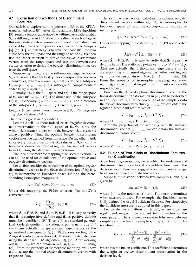
of the between-class scatter matrix, no theory (like Theorem 2)can guarantee that all discriminatory information mustexist in the range space because there is a large spacebeyond the null and the range space which may containcrucial discriminant information; see the shadow area inFig. 1. For two-class problems (such as gender recognition),the weakness of DLDA becomes more noticeable. The rangespace is only one-dimensional and spanned by thedifference of the two class mean vectors. This subspace istoo small to contain enough discriminant information.Actually, in such a case, the resulting discriminant vectorof DLDA is the difference vector itself, which is not optimalwith respect to the Fisher criterion, let alone the ability toextract two kinds of discriminant information.

Lu et al. [12] generalized DLDA using the idea of kernelsand presented kernel direct discriminant analysis (KDDA).KDDA was demonstrated effective for face recognition, but,as a nonlinear version of DLDA, KDDA unavoidably suffersthe weakness of DLDA. On the other hand, unlike DLDA,which can significantly reduce computational complexity ofLDA (as discussed above), KDDA has the same computa-tional complexity, i.e., OðM3Þ, as other KFD algorithms [4],[5], [6], [7], [8], [9], [10], [11] because KDDA still needs tocalculate the eigenvectors of an M �M Gram matrix.

Like Liu et al.’s [21] method, our previous LDA algorithm[24] can obtain more than c� 1 features, that is, allc� 1 irregular discriminant features plus some regular ones.This algorithm turned out to bemore effective thanChen andYu’s methods, which can extract at most c� 1 features. Inaddition, our LDA algorithm [24] is more powerful andsimpler thanLiu et al.’s [21]method [52]. The algorithm in theliterature [32] can be viewed as a nonlinear generalization ofthat in [24]. However, the derivation of the algorithm is basedon an assumption that the feature space is assumed to be afinite dimensional space. This assumption is no problem forpolynomial kernels, but is unsuitable for other kernels whichdetermine mappings that might lead to an infinite-dimen-sional feature space.

Compared to our previous idea [32] and Lu et al.’s KDDA,CKFD has two prominent advantages. One is in the theoryand other is in the algorithm itself. The theoretical derivationof the algorithm does not need any assumption. Thedeveloped theory in Hilbert space lays a solid foundationfor the algorithm. The derived discriminant information isguaranteednot only optimal but also complete (lossless)withrespect to the Fisher criterion. The completeness of discrimi-nant information enables CKFD to be used to performdiscriminant analysis in “double discriminant subspaces.”In each subspace, the number of discriminant features can beup to c� 1. This means 2ðc� 1Þ features can be obtained intotal. This is different from the KFD (or LDA) algorithmsdiscussed above and beyond [4], [5], [6], [7], [8], [9], [10], [11],


Fig. 1. Illustration the subspaces of DLDA.

[12], [13], [14], [15], [16], [17], [22], [23], which can yield onlyone discriminant subspace containing at most c� 1 discrimi-nant features. What is more, CKFD provides a new mechan-ism for decision fusion. This mechanismmakes it possible totake advantage of the two kinds of discriminant informationand to determine their contribution to decision bymodifyingthe fusion coefficient.

CKFD has a computational complexity ofOðM3Þ (M is thenumber of training samples),which is the sameas the existingKFD algorithms [4], [5], [6], [7], [8], [9], [10], [11], [12], [13],[14], [15], [16], [17]. The reason for this is that theKPCAphaseof CKFD is actually carried out in the space spanned byM training samples, so its computational complexity stilldepends on the operations of solving M �M sized eigenva-lue problems [3], [10]. Despite this, compared to other KFDalgorithms, CKFD indeed requires additional computationmainly owing to its space decomposition process performedin the KPCA-transformed space. In such a space, alleigenvectors of Sw should be calculated.

5 EXPERIMENTS

In this section, three experiments are designed to evaluatethe performance of the proposed algorithm. The firstexperiment is on face recognition and the second one ison handwritten digit recognition. Face recognition istypically a small sample size problem, while handwrittendigit classification is a “large sample size” problem inobservation space. We will demonstrate that the proposedCKFD algorithm is applicable to both of these kinds ofproblems. In the third experiment, CKFD is applied to two-class problems, i.e., the classification of digit-pairs. We willshow that CKFD is capable of exhibiting data in two-dimensional space for two-class problems.

5.1 Experiment on Face Recognition Using theFERET Database

The FERET face image database is a result of the FERETprogram, which was sponsored by the US Department ofDefense through the DARPA Program [36], [37]. It hasbecome a standard database for testing and evaluatingstate-of-the-art face recognition algorithms.

The proposed algorithm was tested on a subset of theFERET database. This subset includes 1,400 images of

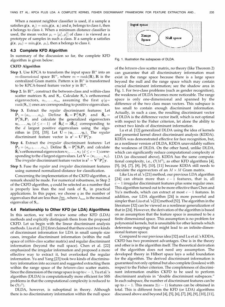
200 individuals (each individual has seven images). It iscomposed of the images whose names are marked with two-character strings: “ba,” “bj,” “bk,” “be,” “bf,” “bd,” and “bg”[51]. This subset involves variations in facial expression,illumination, and pose. In our experiment, the facial portionof each original image was automatically cropped based onthe location of eyes and the cropped image was resized to80� 80 pixels and preprocessed by histogram equalization.Some example images of one person are shown in Fig. 2.

Three images of each subject are randomly chosen fortraining, while the remaining four images are used fortesting. Thus, the training sample set size is 600 and thetesting sample set size is 800. In this way, we run the system20 times and obtain 20 different training and testing samplesets. The first 10 are used for model selection and the othersfor performance evaluation.

Two popular kernels are involved in our tests. One is thepolynomial kernel kðx;yÞ ¼ ðx � yþ 1Þr and the other is theGaussian RBF kernel kðx;yÞ ¼ expð�jjx� yjj2=�Þ . Threemethods, namely, Kernel Eigenface [11], Kernel Fisherface[11], and the proposed CKFD algorithm, are tested andcompared. In order to gain more insights into our algorithm,two additional versions, 1) CKFD: regular, where only theregulardiscriminant features are used, and 2)CKFD: irregular,where only the irregular discriminant features are used, arealso evaluated. Two simple classifiers, a minimum distanceclassifier (MD) and a nearest neighbor classifier (NN), areemployed in the experiments.

In the phase of model selection, our goal is to determineproper kernel parameters (i.e., the order r of the polynomialkernel and the width � of the Gaussian RBF kernel), thedimension of the projection subspace for each method, andthe fusion coefficient for CKFD. Since it is very difficult todetermine these parameters at the same time, a stepwiseselection strategy is more feasible and thus is adopted here[12]. Specifically, we fix the dimension and the fusioncoefficient (only for CKFD) in advance and try to find theoptimal kernel parameter for a given kernel function. Then,based on the chosen kernel parameters, the selection of thesubspace sizes is performed. Finally, the fusion coefficient ofCKFD isdeterminedwith respect to other chosenparameters.

To determine proper parameters for kernels, we use theglobal-to-local search strategy [2]. After globally searchingover awide range of theparameter space,we find a candidate


Fig. 2. Images of one person in the FERET database. (a) Original images. (b) Cropped images (after histogram equalization) corresponding

to images in (a).

interval where the optimal parameters might exist. Here, for

the polynomial kernel, the candidate order interval is from 1

to 7 and, for the Gaussian RBF kernel, the candidate width

interval is from 0.1 to 20. Then, we try to find the optimal

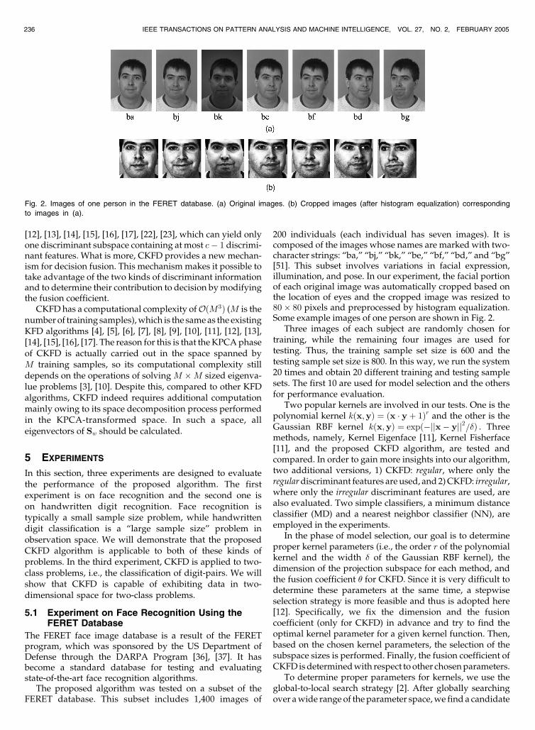
kernel parameterswithin these intervals. Figs. 3a and3c show

the recognition accuracy versus the variation of kernel

parameters corresponding to four methods with a fixed

dimension of 20 and ¼ 1 for CKFD. From these figures, we

candetermine theproperkernel parameters. For example, the

order of polynomial kernel should be two for CKFD with

respect to a minimum distance classifier and the width of

Gaussian kernel should be three for CKFD with respect to a

nearest neighbor classifier.By kernel parameter selection, we find that the nonlinear

kernels are really helpful for improving the performance of

CKFD. The results of CKFD with the linear kernel (i.e., the

first order polynomial kernel), second order polynomial

kernel, and Gaussian RBF kernel (� ¼ 3) are listed in Table 1.

From this table, it can be seen that CKFD with nonlinear

kernels achieves better results under two different classifiers.


Fig. 3. Illustration of the recognition rates over the variation of kernel parameters, subspace dimensions and fusion coefficients in the modelselection stage. (a) Recognition rates versus the order of the polynomial kernel, using minimum distance classifiers. (b) Recognition rates versusthe subspace dimension, using the polynomial kernel and minimum distance classifiers. (c) Recognition rates versus the width of the Gaussiankernel, using nearest neighbor classifiers, (d) Recognition rates versus the subspace dimension, using the Gaussian kernel and nearest neighborclassifiers. (e) Recognition rates of CKFD versus the fusion coefficients.

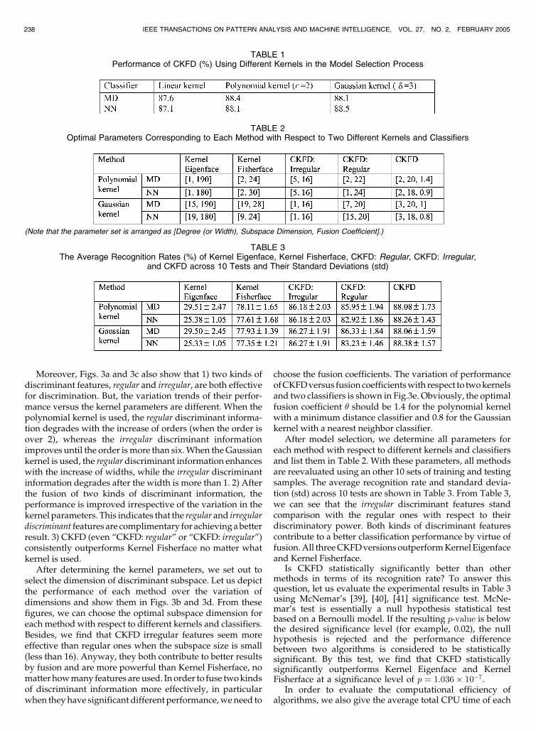
Moreover, Figs. 3a and 3c also show that 1) two kinds ofdiscriminant features, regular and irregular, are both effectivefor discrimination. But, the variation trends of their perfor-mance versus the kernel parameters are different. When thepolynomial kernel is used, the regular discriminant informa-tion degrades with the increase of orders (when the order isover 2), whereas the irregular discriminant informationimproves until the order ismore than six.When theGaussiankernel is used, the regular discriminant information enhanceswith the increase of widths, while the irregular discriminantinformation degrades after the width is more than 1. 2) Afterthe fusion of two kinds of discriminant information, theperformance is improved irrespective of the variation in thekernel parameters. This indicates that the regular and irregulardiscriminant features are complimentary for achievingabetterresult. 3) CKFD (even “CKFD: regular” or “CKFD: irregular”)consistently outperforms Kernel Fisherface no matter whatkernel is used.

After determining the kernel parameters, we set out toselect the dimension of discriminant subspace. Let us depictthe performance of each method over the variation ofdimensions and show them in Figs. 3b and 3d. From thesefigures, we can choose the optimal subspace dimension foreach method with respect to different kernels and classifiers.Besides, we find that CKFD irregular features seem moreeffective than regular ones when the subspace size is small(less than 16). Anyway, they both contribute to better resultsby fusion and are more powerful than Kernel Fisherface, nomatter howmany features areused. Inorder to fuse twokindsof discriminant information more effectively, in particularwhen they have significant different performance,weneed to

choose the fusion coefficients. The variation of performanceofCKFDversus fusioncoefficientswith respect to twokernelsand two classifiers is shown in Fig.3e. Obviously, the optimalfusion coefficient should be 1.4 for the polynomial kernelwith a minimum distance classifier and 0.8 for the Gaussiankernel with a nearest neighbor classifier.

After model selection, we determine all parameters foreach method with respect to different kernels and classifiersand list them in Table 2. With these parameters, all methodsare reevaluated using an other 10 sets of training and testingsamples. The average recognition rate and standard devia-tion (std) across 10 tests are shown in Table 3. From Table 3,we can see that the irregular discriminant features standcomparison with the regular ones with respect to theirdiscriminatory power. Both kinds of discriminant featurescontribute to a better classification performance by virtue offusion.All threeCKFDversions outperformKernel Eigenfaceand Kernel Fisherface.

Is CKFD statistically significantly better than othermethods in terms of its recognition rate? To answer thisquestion, let us evaluate the experimental results in Table 3using McNemar’s [39], [40], [41] significance test. McNe-mar’s test is essentially a null hypothesis statistical testbased on a Bernoulli model. If the resulting p-value is belowthe desired significance level (for example, 0.02), the nullhypothesis is rejected and the performance differencebetween two algorithms is considered to be statisticallysignificant. By this test, we find that CKFD statisticallysignificantly outperforms Kernel Eigenface and KernelFisherface at a significance level of p ¼ 1:036� 10�7.

In order to evaluate the computational efficiency ofalgorithms, we also give the average total CPU time of each


TABLE 1Performance of CKFD (%) Using Different Kernels in the Model Selection Process

TABLE 2Optimal Parameters Corresponding to Each Method with Respect to Two Different Kernels and Classifiers

(Note that the parameter set is arranged as [Degree (or Width), Subspace Dimension, Fusion Coefficient].)

TABLE 3The Average Recognition Rates (%) of Kernel Eigenface, Kernel Fisherface, CKFD: Regular, CKFD: Irregular,

and CKFD across 10 Tests and Their Standard Deviations (std)

method involved. Table 4 shows that CKFD (regular,irregular and fusion) algorithms are slightly slower thanKernel Fisherface and Kernel Eigenface.

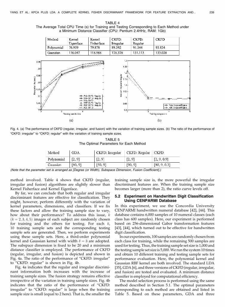
By far, we can conclude that both regular and irregulardiscriminant features are effective for classification. Theymight, however, perform differently with the variation ofkernel parameters, dimensions, and classifiers. If we fixthese factors and allow the training sample size to vary,how about their performance? To address this issue, kðk ¼ 2; 3; 4; 5Þ images of each subject are randomly chosenfor training and the others for testing. For each k,10 training sample sets and the corresponding testingsample sets are generated. Then, we perform experimentsusing these sample sets. Here, a third-order polynomialkernel and Gaussian kernel with width � ¼ 3 are adopted.The subspace dimension is fixed to be 20 and a minimumdistance classifier is employed. The performance of CKFD(regular, irregular, and fusion) is depicted and shown inFig. 4a. The ratio of the performance of “CKFD: irregular”to “CKFD: regular” is shown in Fig. 4b.

Fig. 4a indicates that the regular and irregular discrimi-nant information both increases with the increase oftraining sample sizes. The fusion strategy remains effectiveirrespective of the variation in training sample sizes. Fig. 4bindicates that the ratio of the performance of “CKFD:irregular” to “CKFD: regular” is large when the trainingsample size is small (equal to 2 here). That is, the smaller the

training sample size is, the more powerful the irregulardiscriminant features are. When the training sample sizebecomes larger (more than 2), the ratio curve levels off.

5.2 Experiment on Handwritten Digit ClassificationUsing CENPARMI Database

In this experiment, we use the Concordia UniversityCENPARMI handwritten numeral database [42], [44]. Thisdatabase contains 6,000 samples of 10 numeral classes (eachclass has 600 samples). Here, our experiment is performedbased on 256-dimensional Gabor transformation features[43], [44], which turned out to be effective for handwrittendigit classification.

Inourexperiments, 100samplesare randomlychosenfromeach class for training, while the remaining 500 samples areused for testing. Thus, the training sample set size is 1,000 andthe testing sample set size is 5,000.We run the system10 timesand obtain 10 different training and testing sample sets forperformance evaluation. Here, the polynomial kernel andGaussian RBF kernel are both involved. The standard LDA[35], GDA [6], and three versions of CKFD (regular, irregular,and fusion) are tested and evaluated. A minimum distanceclassifier is employed for computational efficiency.

The model selection process is performed using the samemethod described in Section 5.1. The optimal parameterscorresponding to each method are obtained and listed inTable 5. Based on these parameters, GDA and three


TABLE 4The Average Total CPU Time (s) for Training and Testing Corresponding to Each Method under

a Minimum Distance Classifier (CPU: Pentium 2.4HHz, RAM: 1Gb)

Fig. 4. (a) The performance of CKFD (regular, irregular, and fusion) with the variation of training sample sizes. (b) The ratio of the performance of

“CKFD: irregular” to “CKFD: regular” with the variation of training sample sizes.

TABLE 5The Optimal Parameters for Each Method

(Note that the parameter set is arranged as [Degree (or Width), Subspace Dimension, Fusion Coefficient].)

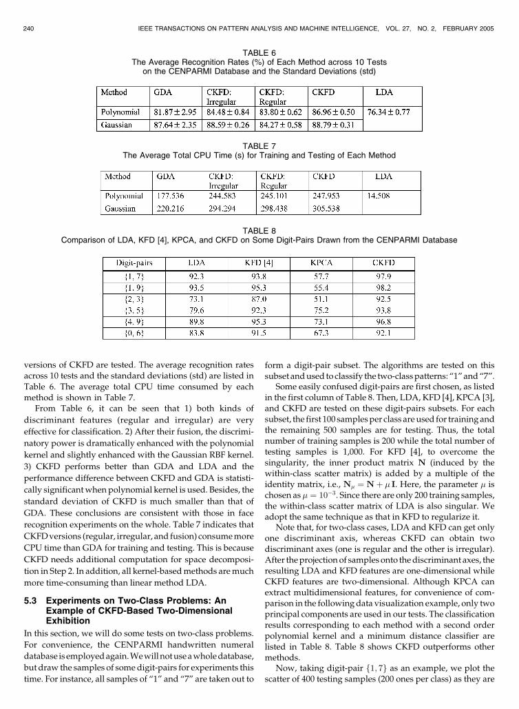
versions of CKFD are tested. The average recognition ratesacross 10 tests and the standard deviations (std) are listed in

Table 6. The average total CPU time consumed by eachmethod is shown in Table 7.

From Table 6, it can be seen that 1) both kinds of

discriminant features (regular and irregular) are very

effective for classification. 2) After their fusion, the discrimi-

natory power is dramatically enhanced with the polynomial

kernel and slightly enhanced with the Gaussian RBF kernel.

3) CKFD performs better than GDA and LDA and the

performance difference between CKFD and GDA is statisti-

cally significantwhen polynomial kernel is used. Besides, the

standard deviation of CKFD is much smaller than that of

GDA. These conclusions are consistent with those in face

recognition experiments on the whole. Table 7 indicates that

CKFDversions (regular, irregular, and fusion) consumemore

CPU time than GDA for training and testing. This is because

CKFD needs additional computation for space decomposi-

tion in Step 2. In addition, all kernel-basedmethods aremuch

more time-consuming than linear method LDA.

5.3 Experiments on Two-Class Problems: AnExample of CKFD-Based Two-DimensionalExhibition

In this section, we will do some tests on two-class problems.

For convenience, the CENPARMI handwritten numeral

database isemployedagain.Wewillnotuseawholedatabase,

but draw the samples of somedigit-pairs for experiments this

time. For instance, all samples of “1” and “7” are taken out to

form a digit-pair subset. The algorithms are tested on thissubset andused to classify the two-classpatterns: “1”and“7”.

Some easily confused digit-pairs are first chosen, as listedin the first column of Table 8. Then, LDA, KFD [4], KPCA [3],and CKFD are tested on these digit-pairs subsets. For eachsubset, the first 100 samplesper class areused for training andthe remaining 500 samples are for testing. Thus, the totalnumber of training samples is 200 while the total number oftesting samples is 1,000. For KFD [4], to overcome thesingularity, the inner product matrix N (induced by thewithin-class scatter matrix) is added by a multiple of theidentity matrix, i.e., N ¼ Nþ I. Here, the parameter ischosen as ¼ 10�3. Since there are only 200 training samples,the within-class scatter matrix of LDA is also singular. Weadopt the same technique as that in KFD to regularize it.

Note that, for two-class cases, LDA and KFD can get onlyone discriminant axis, whereas CKFD can obtain twodiscriminant axes (one is regular and the other is irregular).After theprojectionof samples onto thediscriminant axes, theresulting LDA and KFD features are one-dimensional whileCKFD features are two-dimensional. Although KPCA canextract multidimensional features, for convenience of com-parison in the followingdata visualization example, only twoprincipal components are used in our tests. The classificationresults corresponding to each method with a second orderpolynomial kernel and a minimum distance classifier arelisted in Table 8. Table 8 shows CKFD outperforms othermethods.

Now, taking digit-pair f1; 7g as an example, we plot thescatter of 400 testing samples (200 ones per class) as they are


TABLE 6The Average Recognition Rates (%) of Each Method across 10 Tests

on the CENPARMI Database and the Standard Deviations (std)

TABLE 7The Average Total CPU Time (s) for Training and Testing of Each Method

TABLE 8Comparison of LDA, KFD [4], KPCA, and CKFD on Some Digit-Pairs Drawn from the CENPARMI Database

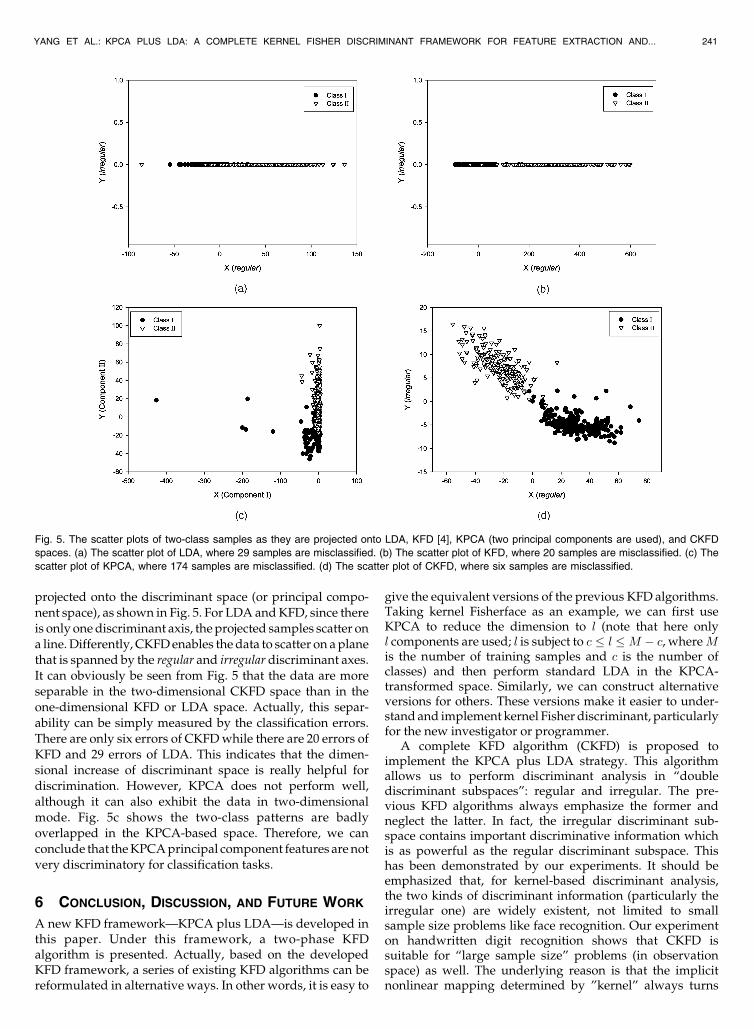
projected onto the discriminant space (or principal compo-nent space), as shown in Fig. 5. For LDA andKFD, since thereis only onediscriminant axis, the projected samples scatter ona line.Differently, CKFDenables the data to scatter on aplanethat is spanned by the regular and irregular discriminant axes.It can obviously be seen from Fig. 5 that the data are moreseparable in the two-dimensional CKFD space than in theone-dimensional KFD or LDA space. Actually, this separ-ability can be simply measured by the classification errors.There are only six errors of CKFDwhile there are 20 errors ofKFD and 29 errors of LDA. This indicates that the dimen-sional increase of discriminant space is really helpful fordiscrimination. However, KPCA does not perform well,although it can also exhibit the data in two-dimensionalmode. Fig. 5c shows the two-class patterns are badlyoverlapped in the KPCA-based space. Therefore, we canconclude that theKPCAprincipal component features arenotvery discriminatory for classification tasks.

6 CONCLUSION, DISCUSSION, AND FUTURE WORK

A new KFD framework—KPCA plus LDA—is developed inthis paper. Under this framework, a two-phase KFDalgorithm is presented. Actually, based on the developedKFD framework, a series of existing KFD algorithms can bereformulated in alternative ways. In other words, it is easy to

give the equivalent versions of the previous KFD algorithms.Taking kernel Fisherface as an example, we can first useKPCA to reduce the dimension to l (note that here onlyl components are used; l is subject to c � l � M � c, whereMis the number of training samples and c is the number ofclasses) and then perform standard LDA in the KPCA-transformed space. Similarly, we can construct alternativeversions for others. These versions make it easier to under-stand and implement kernel Fisher discriminant, particularlyfor the new investigator or programmer.

A complete KFD algorithm (CKFD) is proposed toimplement the KPCA plus LDA strategy. This algorithmallows us to perform discriminant analysis in “doublediscriminant subspaces”: regular and irregular. The pre-vious KFD algorithms always emphasize the former andneglect the latter. In fact, the irregular discriminant sub-space contains important discriminative information whichis as powerful as the regular discriminant subspace. Thishas been demonstrated by our experiments. It should beemphasized that, for kernel-based discriminant analysis,the two kinds of discriminant information (particularly theirregular one) are widely existent, not limited to smallsample size problems like face recognition. Our experimenton handwritten digit recognition shows that CKFD issuitable for “large sample size” problems (in observationspace) as well. The underlying reason is that the implicitnonlinear mapping determined by ”kernel” always turns


Fig. 5. The scatter plots of two-class samples as they are projected onto LDA, KFD [4], KPCA (two principal components are used), and CKFD

spaces. (a) The scatter plot of LDA, where 29 samples are misclassified. (b) The scatter plot of KFD, where 20 samples are misclassified. (c) The

scatter plot of KPCA, where 174 samples are misclassified. (d) The scatter plot of CKFD, where six samples are misclassified.

large sample size problems in observation space into smallsample size ones in feature space. More interestingly, the twodiscriminant subspaces of CKFD turn out to be mutuallycomplementary for discrimination despite the fact that eachof them can work well independently. The fusion of twokinds of discriminant information can achieve better results.

Especially for small sample size problems, CKFD isexactly in tune with the existing two-phase LDA algorithmsthat are based on PCA plus LDA framework. Actually, if alinear kernel, i.e., kðx;yÞ ¼ x � y, is adopted instead ofnonlinear kernels, CKFD would degenerate to be a PCA plusLDA algorithm like that in [24]. Therefore, the existing two-phase LDA (PCA plus LDA) algorithms can be viewed as aspecial case of CKFD.

Finally, we have to point out that the computationalefficiency of CKFD is a problem deserving further investiga-tion. Actually, all kernel-based methods, including KPCA[3], GDA [6], and KFD [4], encounter the same problem. Thisis because all kernel-based discriminant methods have tosolve an M �M sized eigenproblem (or generalized eigen-problem). When the sample sizeM is fairly large, it becomesvery computationally intensive [10]. Several ways suggestedbyMika et al. [10] and Burges and Scholkopf [45] can be usedto deal with this problem, but the optimal implementationscheme (e.g., developing a more efficient numerical algo-rithm for large scale eigenproblems) is still open.

APPENDIX A

THE PROOF OF LEMMA 1

Proof. For simplicity, let us denote T ¼ MS�t and

gj ¼ �ðxjÞ �m�0 . Then, T ¼

PMj¼1 gjg

Tj .

1. For every f 2 H , we have Tf ¼PM

j¼1 hgj; figj.Since

jjTf jj �XM

j¼1

jhgj; fij jjgjjj � jjfjjXM

j¼1

jjgjjj2 ;

T is bounded and jjTjj �PM

j¼1 jjgjjj2 .2. Let us consider the range of the operator T :

RðTÞ ¼ fTf; f 2 Hg.Since

Tf ¼XM

j¼1

hgj; figj;RðTÞ ¼ Lðg1; . . . ; gMÞ;

which is the generated space by g1; . . . ; gM . So,dim RðTÞ � M < 1, which implies that T is acompact operator [47].

3. For every f 2 H, we have

hTf; fi ¼XM

j¼1

hgj; fihgj; fi ¼XM

j¼1

hgj; fi2 � 0:

Thus, T is a positive operator on Hilbert space H.4. Since T is a positive operator, it must be self-

adjoint (symmetric) because its adjoint T� ¼ T(see [48]).

Since S�t has the same properties as T,

Lemma 1 is proven. tu

APPENDIX B

THE PROOF OF THEOREM 2

In order to verify Theorem 2, let us introduce two lemmasfirst.

Lemma B1. ’TS�t ’ ¼ 0 if and only if ’TS�

b ’ ¼ 0 and

’TS�w’ ¼ 0.

Proof. Since S�b and S�

w are both positive and S�t ¼ S�

b þ S�w,

it is easy to verify this. tuLemma B2 [47]. Suppose that A is a positive operator. Then,

xTAx ¼ 0 if and only if Ax ¼ 0.

Proof. IfAx ¼ 0, it is obvious thatxTAx¼0. So,weonlyneedto prove that xTAx ¼ 0 ) Ax ¼ 0. Since A is a positiveoperator, it must have a positive square root T [47], suchthat A ¼ T2. Thus, hTx;Txi ¼ hAx; xi ¼ xTAx ¼ 0. So,Tx ¼ 0, from which it follows thatAx ¼ TðTxÞ ¼ 0. tu

The Proof of Theorem 2. Since �?t is the null space of S�

t ,for every � 2 �?

t , we have �TS�t � ¼ 0.

From Lemma B1, it follows that �TS�b � ¼ 0. Since S�

b isa positive operator according to Lemma 2, we haveS�b � ¼ 0 by Lemma B2. Hence,

’TS�b ’ ¼ �TS�

b �þ 2�TS�b � þ �TS�

b � ¼ �TS�b �:

Similarly, we have

’TS�w’ ¼ �TS�

w�þ 2�TS�w� þ �TS�

w� ¼ �TS�w�:

So, J�b ð’Þ ¼ J�

b ð�Þ and J�ð’Þ ¼ J�ð�Þ. tu

APPENDIX C

THE PROOF OF LEMMA 3

Proof. Since S�t is a compact and positive operator from

Lemma 1, the total scatter matrix St in the KPCA-

transformation space IRm can be represented by

St¼PTS�t P¼diagð�1; �2; . . . ; �mÞ, where �1; �2; . . . ; �m

are the positive eigenvalues of S�t .

So, St is a positive definite matrix in IRm. This means

that, for every nonzero vector � 2 IRm, �TSt� > 0 always

holds.

Obviously, for every nonzero vector � 2 �w, �TSw� ¼ 0

always holds.Since St ¼ Sb þ Sw, for every nonzero vector � 2 �w,

we have �TSb� ¼ �TSt� � �TSw� > 0. tu

ACKNOWLEDGMENTS

This research was supported by the UGC/CRC fund fromthe HKSAR Government and the central fund from theHong Kong Polytechnic University, the National ScienceFoundation of China under Grant No. 60332010, 60472060,60473039, Grant TIC2002-04495-C02, from the SpanishMinistry of Science and Technology (MCyT), and GrantIM3-G03/185 from the Spanish ISCIII. Dr. Jin andDr. Frangi are also supported by RyC Research Fellow-ships from MCyT. The authors would also like to thankall of the anonymous reviewers and the editor for theirconstructive advice.


REFERENCES

[1] V. Vapnik, The Nature of Statistical Learning Theory. New York:Springer, 1995.

[2] K.-R. Muller, S. Mika, G. Ratsch, K. Tsuda, and B. Scholkopf, “AnIntroduction to Kernel-Based Learning Algorithms,” IEEE Trans.Neural Networks, vol. 12, no. 2, pp. 181-201, 2001.

[3] B. Scholkopf, A. Smola, and K.R. Muller, “Nonlinear ComponentAnalysis as a Kernel Eigenvalue Problem,” Neural Computation,vol. 10, no. 5, pp. 1299-1319, 1998.

[4] S.Mika,G.Ratsch, J.Weston,B. Scholkopf, andK.-R.Muller, “FisherDiscriminant Analysis with Kernels,” Proc. IEEE Int’l WorkshopNeural Networks for Signal Processing IX, pp. 41-48, Aug. 1999.

[5] S. Mika, G. Ratsch, B. Scholkopf, A. Smola, J. Weston, and K.-R.Muller, “Invariant Feature Extraction and Classification in KernelSpaces,” Advances in Neural Information Processing Systems 12,Cambridge, Mass.: MIT Press, 1999.

[6] G. Baudat and F. Anouar, “Generalized Discriminant AnalysisUsing a Kernel Approach,” Neural Computation, vol. 12, no. 10,pp. 2385-2404, 2000.

[7] V. Roth and V. Steinhage, “Nonlinear Discriminant AnalysisUsing Kernel Functions,” Advances in Neural Information ProcessingSystems, S.A. Solla, T.K. Leen, and K.-R. Mueller, eds., vol. 12,pp. 568-574, MIT Press, 2000.

[8] S. Mika, G. Ratsch, and K.-R. Muller, “A Mathematical Program-ming Approach to the Kernel Fisher Algorithm,” Advances inNeural Information Processing Systems 13, T.K. Leen, T.G. Dietterich,and V. Tresp, eds., pp. 591-597, MIT Press, 2001.

[9] S. Mika, A.J. Smola, and B. Scholkopf, “An Improved TrainingAlgorithm for Kernel Fisher Discriminants,” Proc. Eighth Int’lWorkshop Artificial Intelligence and Statistics, T. Jaakkola andT. Richardson, eds., pp. 98-104, 2001.

[10] S. Mika, G. Ratsch, J Weston, B. Scholkopf, A. Smola, and K.-R.Muller, “Constructing Descriptive and Discriminative NonlinearFeatures: Rayleigh Coefficients in Kernel Feature Spaces,” IEEETrans. Pattern Analysis and Machine Intelligence, vol. 25, no. 5,pp. 623-628, May 2003.

[11] M.H. Yang, “Kernel Eigenfaces vs. Kernel Fisherfaces: FaceRecognition Using Kernel Methods,” Proc. Fifth IEEE Int’l Conf.Automatic Face and Gesture Recognition, pp. 215-220, May 2002.

[12] J. Lu, K.N. Plataniotis, and A.N. Venetsanopoulos, “Face Recogni-tion Using Kernel Direct Discriminant Analysis Algorithms,” IEEETrans. Neural Networks, vol. 14, no. 1, pp. 117-126, 2003.

[13] J. Xu, X. Zhang, and Y. Li, “Kernel MSE Algorithm: A UnifiedFramework for KFD, LS-SVM, and KRR,” Proc. Int’l Joint Conf.Neural Networks, pp. 1486-1491, July 2001.

[14] S.A. Billings and K.L Lee, “Nonlinear Fisher DiscriminantAnalysis Using a Minimum Squared Error Cost Function andthe Orthogonal Least Squares Algorithm,”Neural Networks, vol. 15,no. 2, pp. 263-270, 2002.

[15] T.V. Gestel, J.A.K. Suykens, G. Lanckriet, A. Lambrechts, B.De Moor, and J. Vanderwalle, “Bayesian Framework for LeastSquares Support Vector Machine Classifiers, Gaussian Processesand Kernel Fisher Discriminant Analysis,” Neural Computation,vol. 15, no. 5, pp. 1115-1148, May 2002.

[16] G.C. Cawley and N.L.C. Talbot, “Efficient Leave-One-Out Cross-Validation of Kernel Fisher Discriminant Classifiers,” PatternRecognition, vol. 36, no. 11, pp. 2585-2592, 2003.

[17] N.D. Lawrence and B. Scholkopf, “Estimating a Kernel FisherDiscriminant in the Presence of Label Noise,” Proc. 18th Int’l Conf.Machine Learning, pp. 306-313, 2001.

[18] A.N. Tikhonov and V.Y. Arsenin, Solution of Ill-Posed Problems.New York: Wiley, 1997.

[19] D.L. Swets and J. Weng, “Using Discriminant Eigenfeatures forImage Retrieval,” IEEE Trans. Pattern Analysis and MachineIntelligence, vol. 18, no. 8, pp. 831-836, Aug. 1996.

[20] P.N. Belhumeur, J.P. Hespanha, and D.J. Kriengman, “Eigenfacesvs. Fisherfaces: Recognition Using Class Specific Linear Projec-tion,” IEEE Trans. Pattern Analysis and Machine Intelligence, vol. 19,no. 7, pp. 711-720, July 1997.

[21] K. Liu, Y.-Q. Cheng, J.-Y. Yang, and X. Liu, “An EfficientAlgorithm for Foley-Sammon Optimal Set of Discriminant Vectorsby Algebraic Method,” Int’l J. Pattern Recognition and ArtificialIntelligence, vol. 6, no. 5, pp. 817-829, 1992.

[22] L.F. Chen, H.Y.M. Liao, J.C. Lin, M.D. Kao, and G.J. Yu, “A NewLDA-Based Face Recognition System which Can Solve the SmallSample Size Problem,” Pattern Recognition, vol. 33, no. 10, pp. 1713-1726, 2000.

[23] H. Yu and J. Yang, “A Direct LDA Algorithm for High-Dimensional Data—With Application to Face Recognition,”Pattern Recognition, vol. 34, no. 10, pp. 2067-2070, 2001.

[24] J. Yang and J.Y. Yang, “Why Can LDA Be Performed in PCATransformed Space?” Pattern Recognition, vol. 36, no. 2, pp. 563-566, 2003.

[25] J. Yang and J.Y. Yang, “Optimal FLD Algorithm for Facial FeatureExtraction,” Proc. SPIE Intelligent Robots and Computer Vision XX:Algorithms, Techniques, and Active Vision, pp. 438-444, Oct. 2001.

[26] C.J. Liu and H. Wechsler, “A Shape- and Texture-Based EnhancedFisher Classifier for Face Recognition,” IEEE Trans. ImageProcessing, vol. 10, no. 4, pp. 598-608, 2001.

[27] C.J. Liu and H. Wechsler, “Robust Coding Schemes for Indexingand Retrieval from Large Face Databases,” IEEE Trans. ImageProcessing, vol. 9, no. 1, pp. 132-137, 2000.

[28] W. Zhao, R. Chellappa, and J. Phillips, “Subspace LinearDiscriminant Analysis for Face Recognition,” Technical ReportCS-TR4009, Univ. of Maryland, 1999.

[29] W. Zhao, A. Krishnaswamy, R. Chellappa, D. Swets, and J. Weng,“Discriminant Analysis of Principal Components for Face Recog-nition,” Face Recognition: From Theory to Applications, H. Wechsler,P. J. Phillips, V. Bruce, F. F. Soulie and T. S. Huang, eds., pp. 73-85,Springer-Verlag, 1998.

[30] M. Turk and A. Pentland, “Eigenfaces for Recognition,” J. CognitiveNeuroscience, vol. 3, no. 1, pp. 71-86, 1991.

[31] M. Kirby and L. Sirovich, “Application of the KL Procedure for theCharacterization of Human Faces,” IEEE Trans. Pattern Analysisand Machine Intelligence, vol. 12, no. 1, pp. 103-108, Jan. 1990.

[32] J. Yang, A.F. Frangi, and J.-Y. Yang, “A New Kernel FisherDiscriminant Algorithm with Application to Face Recognition,”Neurocomputing, vol. 56, pp. 415-421, 2004.

[33] G.H. Golub and C.F. Van Loan, Matrix Computations, third ed.Baltimore and London: The Johns Hopkins Univ. Press, 1996.

[34] P. Lancaster and M. Tismenetsky, The Theory of Matrices, seconded. Orlando, Fla.: Academic Press, 1985.

[35] K. Fukunaga, Introduction to Statistical Pattern Recognition, seconded. Boston: Academic Press, 1990.

[36] P.J. Phillips, H. Moon, S.A. Rizvi, and P.J. Rauss, “The FERETEvaluation Methodology for Face-Recognition Algorithms,” IEEETrans. Pattern Analysis and Machine Intelligence, vol. 22, no. 10,pp. 1090-1104, Oct. 2000.

[37] P.J. Phillips, “The Facial Recognition Technology (FERET)Database,” http://www.itl.nist.gov/iad/humanid/feret/feret_master.html, 2004.

[38] J. Yang, D. Zhang, and J.-y. Yang, “A Generalized K-L ExpansionMethod which Can Deal with Small Sample Size and High-Dimensional Problems,” Pattern Analysis and Application, vol. 6,no. 1, pp. 47-54, 2003.

[39] W. Yambor, B. Draper, and R. Beveridge, “Analyzing PCA-BasedFace Recognition Algorithms: Eigenvector Selection and DistanceMeasures,” Empirical Evaluation Methods in Computer Vision,H. Christensen and J. Phillips, eds., Singapore: World ScientificPress, 2002.

[40] J. Devore and R. Peck, Statistics: The Exploration and Analysis ofData, third ed. Brooks Cole, 1997.

[41] B.A. Draper, K. Baek, M.S. Bartlett, and J.R. Beveridge, “Recogniz-ing Faces with PCA and ICA,” Computer Vision and ImageUnderstanding, vol. 91, no. 1-2, pp. 115-137, 2003.

[42] Z. Lou, K. Liu, J.Y. Yang, and C.Y. Suen, “Rejection Criteria andPairwise Discrimination of Handwritten Numerals Based onStructural Features,” Pattern Analysis and Applications, vol. 2,no. 3, pp. 228-238, 1992.

[43] Y. Hamamoto, S. Uchimura, M. Watanabe, T. Yasuda, and S.Tomita, “Recognition of Handwritten Numerals Using GaborFeatures,” Proc. 13th Int’l Conf. Pattern Recognition, pp. 250-253,Aug. 1996.

[44] J. Yang, J.-y. Yang, D. Zhang, and J.F. Lu, “Feature Fusion: ParallelStrategy vs. Serial Strategy,” Pattern Recognition, vol. 36, no. 6,pp. 1369-1381, 2003.

[45] C.J.C. Burges and B. Scholkopf, “Improving the Accuracy andSpeed of Support Vector Learning Machines,” Advances in NeuralInformation Processing Systems 9, M. Mozer, M. Jordan, andT. Petsche, eds., pp. 375-381, Cambridge, Mass.: MIT Press, 1997.

[46] B. Scholkopf and A. Smola, Learning with Kernels. Cambridge,Mass.: MIT Press, 2002.

[47] E. Kreyszig, Introductory Functional Analysis with Applications. JohnWiley & Sons, 1978.


[48] W. Rudin, Functional Analysis. McGraw-Hill, 1973.[49] V. Hutson and J.S. Pym, Applications of Functional Analysis and

Operator Theory. London: Academic Press, 1980.[50] J. Weidmann, Linear Operators in Hilbert Spaces. New York:

Springer-Verlag, 1980.[51] J. Yang, J.-y. Yang, and A.F. Frangi, “Combined Fisherfaces

Framework,” Image and Vision Computing, vol. 21, no. 12, pp. 1037-1044, 2003.

[52] J. Yang, J.-y. Yang, and H. Ye, “Theory of Fisher LinearDiscriminant Analysis and Its Application,” Acta AutomaticaSinica, vol. 29, no. 4, pp. 481-494, 2003 (in Chinese).

Jian Yang received the BS degree in mathe-matics from the Xuzhou Normal University in1995. He received the MS degree in appliedmathematics from the Changsha Railway Uni-versity in 1998 and the PhD degree from theNanjing University of Science and Technology(NUST) Department of Computer Science, onthe subject of pattern recognition and intelli-gence systems in 2002. From March to Sep-tember 2002, he worked as a research assistant

in the Department of Computing, Hong Kong Polytechnic University.From January to December 2003, he was a postdoctoral researcher atthe University of Zaragoza and affiliated with the Division of Bioengi-neering of the Aragon Institute of Engineering Research (I3A). In thesame year, he was awarded the RyC program Research Fellowship,sponsored by the Spanish Ministry of Science and Technology. Now, heis a research associate at the Hong Kong Polytechnic University with thebiometrics center and a postdoctoral research fellow at NUST. He is theauthor of more than 30 scientific papers in pattern recognition andcomputer vision. His current research interests include pattern recogni-tion, computer vision, and machine learning.

Alejandro F. Frangi received the MSc degree intelecommunication engineering from the Univer-sitat Politecnica de Catalunya, Barcelona, in1996, where he subsequently did research onelectrical impedance tomography for imagereconstruction and noise characterization. In2001, he received the PhD degree from theImage Sciences Institute of the UniversityMedical Center Utrecht on model-based cardio-vascular image analysis. From 2001 to 2004, he

was an assistant professor and Ramon y Cajal Research Fellow at theUniversity of Zaragoza, Spain, where he cofounded and codirected theComputer Vision Group of the Aragon Institute of Engineering Research(I3A). He is now a Ramon y Cajal Research Fellow at the Pompeu FabraUniversity in Barcelona, Spain, where he directs the ComputationalImaging Lab in the Department of Technology. His main researchinterests are in computer vision and medical image analysis, withparticular emphasis on model and registration-based techniques. He isan associate editor of the IEEE Transactions on Medical Imaging andhas served twice as guest editor for special issues of the same journal.He is also member of the Biosecure European Excellence Network onBiometrics for Secure Authentication (www.biosecure.info).

Jing-yu Yang received the BS degree incomputer science from Nanjing University ofScience and Technology (NUST), Nanjing,China. From 1982 to 1984, he was a visitingscientist at the Coordinated Science Laboratory,University of Illinois at Urbana-Champaign.From 1993 to 1994, he was a visiting professorin the Department of Computer Science, Mis-suria University. And, in 1998, he acted as avisiting professor at Concordia University in

Canada. He is currently a professor and chairman in the Departmentof Computer Science at NUST. He is the author of more than 300scientific papers in computer vision, pattern recognition, and artificialintelligence. He has won more than 20 provincial and national awards.His current research interests are in the areas of pattern recognition,robot vision, image processing, data fusion, and artificial intelligence.

David Zhang graduated in computer sciencefrom Peking University in 1974 and received theMSc and PhD degrees in computer science andengineering from the Harbin Institute of Tech-nology (HIT) in 1983 and 1985, respectively. Hereceived a second PhD degree in electrical andcomputer engineering from the University ofWaterloo, Ontario, Canada, in 1994. After that,he was an associate professor at the CityUniversity of Hong Kong and a professor at the

Hong Kong Polytechnic University. Currently, he is a founder anddirector of the Biometrics Technology Centre supported by the UGC ofthe Government of the Hong Kong SAR. He is the founder and editor-in-chief of the International Journal of Image and Graphics and anassociate editor for some international journals such as the IEEETransactions on Systems, Man, and Cybernetics, Pattern Recognition,and International Journal of Pattern Recognition and Artificial Intelli-gence. His research interests include automated biometrics-basedidentification, neural systems and applications, and image processingand pattern recognition. So far, he has published more than 180 papersas well as 10 books, and won numerous prizes. He is a senior memberof the IEEE and the IEEE Computer Society.

Zhong Jin received the BS degree in mathe-matics, the MS degree in applied mathematics,and the PhD degree in pattern recognition andintelligence system from Nanjing University ofScience and Technology (NUST), China, in1982, 1984, and 1999, respectively. He is aprofessor in the Department of ComputerScience, NUST. He visited the Department ofComputer Science and Engineering, The Chi-nese University of Hong Kong from January

2000 to June 2000 and from November 2000 to August 2001 and visitedthe Laboratoire HEUDIASYC, UMR CNRS 6599, Universite deTechnologie de Compiegne, France, from October 2001 to July 2002.Dr. Jin is now visiting the Centre de Visio per Computador, UniversitatAutonoma de Barcelona, Spain, as the Ramon y Cajal programResearch Fellow. His current interests are in the areas of patternrecognition, computer vision, face recognition, facial expressionanalysis, and content-based image retrieval.

. For more information on this or any other computing topic,please visit our Digital Library at www.computer.org/publications/dlib.


kpca plus lda: a complete kernel fisher discriminant framework for feature extraction and...

Documents