jas: vol. 4, no. 1, march 2016, published
TRANSCRIPT

ISSN: 2166-0379
Journal of Agricultural Studies

Journal of Agricultural Studies
ISSN 2166-0379
2016, Vol. 4, No. 1
http://jas.macrothink.org
Editorial Team
Editor-in-Chief
Dr. Chenlin Hu, the Ohio State University, United States
Dr. Zhao Chen, Clemson University, United States
Associate Editors
Dr. Sahar Bahmani, University of Wisconsin at Parkside, United States
Dr. Hui Guo, University of Georgia, United States
Editor
Richard Williams, Macrothink Institute, United States
Editorial Board
Dr. Aftab Alam, Edenworks Inc. 234 Johnson Avenue, Brooklyn 11206 NY USA, United States
Mr. Ashit Kumar Paul, Patuakhali Science and Technology University, Babugonj, Barisal-8210, Bangladesh
Prof. Ph.D Carlos Alberto Zúniga González, Autonomous National University of Nicaragua, León, Nicaragua
Dr. Chenlin Hu, the Ohio State University, United States
Eliana Mariela Werbin, National University of Cordoba, Argentina
Ewa Moliszewska, Opole University, Poland
Dr. Ferdaous MANI, High Agronomic Institute Chott Mariem, Tunisia
Dr Gajanan T Behere, Indian Council of Agricultural Research (ICAR), India
Dr. Gerardo Ojeda, Universidad Nacional de Colombia, Palmira, Valle, Colombia
Dr. Gulzar Ahmad Nayik, SLIET Punjab, India
Dr. Hojjat Hasheminasab, College of Agriculture, Razi University, Iran, Islamic Republic of
Dr Hui Guo, University of Georgia, United States
Dr. Idress Hamad Attitalla, Molecular Evolution (Uppsala University, Sweden), Libya
Dr. Idin ZIBAEE, Department of Plant Protection College of Agriculture, University of Tehran
Dr. Luisa Pozzo, National Research Council, Italy
Dr. Martin Ernesto Quadro, Argentina
Dr. Muhammed Yuceer, Canakkale Onsekiz Mart University, Department of Food Processing, Turkey
Dr. Rasha Mousa, Assiut University, Egypt
Associate Professor Mohammad Reza Alizadeh, Rice Research Institute of Iran (RRII), Iran, Islamic Republic of
Dr. Mohamed Ahmed El-Esawi, Botany Department, Faculty of Science, Tanta University, Egypt
Dr. Pramod Kumar MishrA, GITAM School of International Business, GITAM University, India
Dr. Reham Ibrahim Abo-Shnaf, Plant Protection Research Institute, Agricultural research Center, Giza, Egypt
Dr. Richard R. E. Uwiera, University of Alberta, Canada
Dr. Sahar Bahmani, University of Wisconsin at Parkside, United States
Dr. Sait Engindeniz, Ege University Faculty of Agriculture, Turkey
Mr. Syed Rizwan Abbas, Research associate, Pakistan
Dr. Moses Iwatasia Olotu, Mkwawa University College of Education, Tanzania, United Republic of
Dr. Tran Dang Khanh, Agricultural Genetics Institute, Hanoi, Viet Nam
Dr. Zakaria Fouad Abdallah, National Research Centre, Egypt
Dr. Zhao Chen, Clemson University, United States
Dr. Zoubida Boumahdi, University Blida, Algeria
Dr. Zoi Parissi, Aristotle University of Thessaloniki, Greece

Journal of Agricultural Studies
ISSN 2166-0379
2016, Vol. 4, No. 1
www.macrothink.org/jas 1
The Use of ICT for Tertiary Education in Agriculture
and Research in Swaziland: The Case of University of
Swaziland (UNISWA) Students
Raufu, M.O.
Department of Agricultural Economics and Management, P. O. Luyengo, Luyengo. M205,
University of Swaziland, Swaziland.
Masuku, M. B. (Corresponding author)
Department of Agricultural Economics and Management, P. O. Luyengo, Luyengo. M205,
University of Swaziland, Swaziland.
Tijani, A. A.
Department of Agricultural Economics and Management, P. O. Luyengo, Luyengo. M205,
University of Swaziland, Swaziland.
Received: August 11, 2015 Accepted: August 27, 2015 Published: September 19, 2015
doi:10.5296/jas.v4i1.8142 URL: http://dx.doi.org/10.5296/jas.v4i1.8142
Abstract
The primary goal of universities is to teach, provide community service, and conduct research.
Empirical evidence has shown that innovative research can best be conducted with the aid of
ICT. This study therefore, examines factors affecting the use of ICT for tertiary education and
research for development among UNISWA students in the Faculty of Agriculture. Stratified
random sampling technique was employed to select 113 UNISWA undergraduate and
postgraduate students from whom data were obtained using structured questionnaires.
Descriptive statistics and Tobit regression model were used to analyse the data.
The results revealed that the radio and television, audio-graphic, email, computer file transfer
and multimedia products were the main ICT facilities available. Accessing research and
relevant materials online and the use of ICT in improving efficiency of communication
among students and lecturers were ranked high by the respondents. Weak wireless services
and unemployment were the greatest challenges to the use of ICT facilities by students.
Estimated Tobit regression results revealed that availability, accessibility and necessity for
ICT facilities significantly influenced their use for learning and research among the
undergraduate students while family size, availability, necessity and proficiency were the

Journal of Agricultural Studies
ISSN 2166-0379
2016, Vol. 4, No. 1
www.macrothink.org/jas 2
main factors affecting the use of ICT facilities among the postgraduate students.
In order to encourage the use of ICT among UNISWA students, the study is therefore
recommending that (i) The university authorities should make ICT facilities available and
accessible to all categories of students, (ii) Departments should incorporate the use of ICT
facilities into their curriculum, and (iii) lecturers should give ICT based assignments and use
ICT-based teaching methods.
Keywords: Agriculture and Research, ICT, Uniswa, Tertiary Education.
1. Introduction
1.1 Background
Education is the key to a knowledge economy. To compete effectively in global context, we
need an educated and skilled labour force so as to create, share and use knowledge; vibrant
system of research and innovation to be able to tap into global knowledge, assimilate and
adapt it to the local need. One cannot rule out that knowledge and human capital are
increasingly important to successful economies. The skills to productively transform
knowledge and information into innovative products and services will largely define
successful knowledge economies.
Telecommunication and the Internet are now on the policy “radar screen” in every nation and
multinational organisations. Over the past two decades, there has been considerable debate
over the extent to which ICT is transforming the economies of the world. Central
governments, businesses and international organisations have invested heavily on ICT in
anticipation of greater productivity increase and economic transformations. Since knowledge
and information have become the most important currency for productivity, competitiveness,
an increased wealth and prosperity, nations have and continue to place greater emphasis and
priority on human capital development. Learners learn better when learning experience and
activities are illustrated with use of ICT materials (Etiubong, 2011). The multi-purpose
application of ICT is now regarded as a Utility such as water and electricity and hence has
become a major factor in socio-economic development of every nation. ICT now plays a
major role in education, learning and research in general, agriculture, health, commerce and
even in poverty alleviation by generating or creating new jobs and investment
opportunities. It must be stressed that a country without systematic, coherent, innovative and
coordinated research culture rarely develops scientifically and economically.
Universities are considered to be the nerve centre of knowledge, innovation and their
application to real life situation because of their continued existence is to solve the needs of
society. This responsibility could be better served when these institutions of higher learning
are current in terms of modern ICT infrastructure. In no doubt Universities are research
centres and innovative research can best be conducted by the use of ICT. A relevant education
is more important because today’s networked world demands a workforce that understands
how to use technology as a tool to increase productivity and creativity. If Universities are to
play their role and contribute to national development through research and providing
innovative education then much effort has to be put in to integrate ICT as pedagogical tool

Journal of Agricultural Studies
ISSN 2166-0379
2016, Vol. 4, No. 1
www.macrothink.org/jas 3
and as a component of subject contents.
It is a common practice that students find it difficult to get the right study materials for their
respective programmes. Most students complete their chosen programmes without even
having the chance to read some of the internationally acclaimed articles and journals. It is
also usual to see that most dissertations and thesis by students never see any practical
implementation. They are rather kept on the shelves only to collect dust. This can be
attributed to the fact that the writing of these thesis and dissertations are not thoroughly
researched into due to lack of access to relevant information. With ICT, students during their
learning process can access different information and even know the paradigm shift in most
literature as this will make them current and know the dynamics of industry. It also offers
them to be trained in a way that meets the job market requirements and their final project can
be carried out in an innovative manner so that it becomes more practicable than before. The
resources used as input in instruction in a systematic and goal directed manner guarantee
better qualitative output from school (Etim, 2008).
To keep pace with what is taking place globally, education should be the passport to develop
a vibrant economy and ICT is capable to enhance education especially University education
so that they will be able to perform their mandated functions to the benefit of mankind.
Scientific research in many fields has also been revolutionised by the new possibilities
offered by ICTs, from digitisation of information to new recording, simulation and data
processing possibilities (Atkins et al., 2003). The education sector has so far been
characterised by rather slow progress in terms of innovation development which impact on
teaching activities. This article therefore seeks to look at the use of ICT by students for
tertiary agricultural education and agricultural research for development in Swaziland.
1.2 Objective of the Study
The main objective of the study was to access the use of ICT by post graduate students for
tertiary agricultural education and agricultural research for development in Swaziland. The
specific objectives were to:
(i) Highlight the source of ICTs available for learning and research to the respondents;
(ii) Determine the level of use of ICT for learning and research by respondents;
(iii) Identify the factors affecting the use of ICT in enhancing education and research
productivity; and
(iv) Identify the key challenges and constraints in the use of ICT for learning and
research by the respondents.
2. Methodology
2.1 Study Area
The University of Swaziland (UNISWA) is the only Government University and the only
University offering agricultural sciences at the post graduate level in Swaziland. The
University of Swaziland, which comprised of three Campuses at Kwaluseni, Luyengo and

Journal of Agricultural Studies
ISSN 2166-0379
2016, Vol. 4, No. 1
www.macrothink.org/jas 4
Mbabane, was established in 1982 by an Act of Parliament of the Kingdom of Swaziland with
a mandate to teach, conduct research and carry out community service. The University offers
Certificate programmes, Diplomas, Bachelor's degrees, Master's degrees and a PhD degree.
2.1 Sampling Procedure
The Luyengo campus of the University was purposively selected for the study because it is
the only campus that offers degrees in Agricultural Sciences at both the undergraduate and
postgraduate levels. Stratified random sampling technique was use. The student population in
the faculty of agricultural sciences were divided into undergraduate and postgraduate strata.
Out of the 1172 and 86 students that registered between 2013-2014 academic years for
undergraduate and postgraduate studies respectively, 10% (125 respondents) of the total
population were sampled. Seventy of the undergraduate students and 55 of the postgraduate
students were randomly sampled. Out of the total 125 questionnaires administered, 103 of
them, 63 and 40 questionnaires form the undergraduate and postgraduate strata respectively
were useful for the analysis.
2.2 Instrument and Measurement of Variables
Primary data were collected through the use of questionnaire. The questionnaire composed of
5 sections concerning the demographic features of the students, sources of ICT available for
learning and research, which were sub-divided into synchronous and asynchronous media
subsections and section for level of use of ICT for learning and research were measured with
statements weighed by a 5 points Likert scale. Other two sections also measured by 5 points
Likert scales were sections for factors affecting ICT role in enhancing educational and
research productivity, comprising of statements on availability, accessibility, necessity and
proficiency in use of ICT facilities for learning and research while the last section was on
challenges and constraint to the use of ICT.
2.3 Data Analyses
2.3.1 Descriptive Statistics
Weighted mean score (WMS) was used to rank the available sources of ICT for learning and
research, the level of use of the ICT for academic purposes, factors affecting ICT role as well
as challenges and constraint to ICT use. The weighted means score was calculated by
summing up the responses divided by the number of respondents. Also, standard deviations
of the respective items were calculated to determine the overall acceptance of the rank result
by the respondents.
2.3.2 Tobit Regression
The Tobit regression model was used to analyse the data collected. The dependent variable,
the use of ICT was captured through a five point likert scale, and was regressed against some
socioeconomic characteristics, which include the gender of the respondents, age, marital
status, and family size, average monthly and monthly income/stipends of the students. Other
independent variables are availability, accessibility, necessity and proficiency in use of ICT
facilities for learning and research.
According to Long (1997), Sigelman (1999) and Green, (2003), the structural equation for the

Journal of Agricultural Studies
ISSN 2166-0379
2016, Vol. 4, No. 1
www.macrothink.org/jas 5
Tobit model is:
yi*=Xiβ+εi
Where: εi=N (0,σ2
). yi* is a latent variable that is observed for values greater than т and censored
otherwise. The observed y is defined by the following measurement equation:
yi= yi* if yi*> т
yi= т if yi*≤ т
It is assumed that т=0 i.e the data are censored at zero. Thus, we have:
yi= yi* if yi*> 0
yi= 0 if yi*≤ 0
3. Results and Discussion
Table 1 revealed that radio broadcast and television as well as audio graphic ranked highest
among the synchronous media of ICT sources available for both undergraduate and
postgraduate students in the University, while use of email, computer file transfer and use of
multimedia products ranked highest among the asynchronous media. This could be because
these are easily accessible ICT sources. In the case of emails, students also communicate with
their lecturers on academic assignments.
Table1. Sources of ICT Available for Learning and Research
Synchronous Media Asynchronous Media
Sources Undergraduate
WMS*
Postgraduate
WMS
Sources Undergraduate
WMS
Postgraduate
WMS
Audio-graphics 0.16(2nd
) 0.15(2nd
) Audio, video tapes and
CDs
0.14(4th
) 0.10(3rd
)
Audio
conferencing
0.06(4th
) 0.13(3rd
) Email 0.84(1st) 0.95(1
st)
Broadcast
radio & TV
0.62(1st) 0.18(1
st) Computer file transfer 0.32(2
nd) 0.38(2
nd)
Computer
conferencing
0.10(3rd
) 0.10(4th
) Virtual conferences 0.05(6th
) 0.05(5th
)
Multimedia products 0.21(3rd
) 0.35(4th
)
Web based learning
format
0.13(5th
) 0.05(5th
)
Note: Respondents were asked to select the sources of ICT available to them for learning and
research. The figures indicate the mean scores of the selected sources and their rating.
* denotes weighted means
Source: Field Survey 2014
As regard the level of use of ICT in Table 2, accessing research and relevant study materials
online was ranked highest among uses of ICT for the undergraduate students, as compared
with its use to improve efficiency of communication with colleagues and lecturers was

Journal of Agricultural Studies
ISSN 2166-0379
2016, Vol. 4, No. 1
www.macrothink.org/jas 6
ranked highest by the postgraduate students. The fact that response on net to course relevant
information and assignments, and communication with colleagues on tutorials and research
issues ranked least in level of use of ICT for both the undergraduate and postgraduate
students shows that the high ranking of ICT in improving efficiency of communication is not
for academic learning and research purposes. Likewise, it can be inferred from the results that
though respondents do access research and relevant materials on line but they rarely shared
such information among themselves in their online communications.
Table 2. Level of Use of ICT’ use for Learning and Research
Level of Use Undergraduate
WMS
SD Postgraduate
WMS
SD
Course relevant information online 3.21(4th
) 1.42 3.33(4th
) 1.25
Communicating with colleagues on tutorials and
research
2.92(5th
) 1.21 3.30(5th
) 1.47
Accessing research and relevant study materials online 4.19(1st) 0.88 4.03(2
nd) 1.19
Use of ICT for efficiency in communication with
colleagues and lecturers
3.84(2nd
) 0.94 4.18(1st) 0.93
Use of ICT effectively for learning and research
evolved
3.38(3rd
) 1.18 3.68(3rd
) 1.19
Note: Respondents were asked to rate the level of use of ICT for learning and research on a 5
point Likert scale. The figures indicate the mean scores and their rating.
Source: Field Survey 2014
In terms of availability and accessibility, Table 3 revealed that not having wireless loop in the
university to allow internet in the university buildings and classrooms as well as having no
access to computers in class were ranked highest respectively by all the respondents. As
regards necessity and proficiency in use, problem of not integrating ICT in the curriculum
and having no skills to facilitate use of available packages for learning and research
respectively were ranked highest by the postgraduate students while not being referred to net
for further study/research and lack of pre-requisite knowledge for effective use of ICT were
the highest factors in terms of necessity and proficiency among the undergraduate
respondents. Their standard deviation of less than 2 indicated that many of the students at
both level agreed to the identified factors as highly affecting the role of ICT in enhancing
education and research productivity in agriculture.
Table3. Factors Affecting ICT Role in Enhancing Education and Research Productivity
Factors Affecting ICT Role Undergraduate
WMS
SD Postgraduate
WMS
SD
Availability
*No wireless loop in the University to allow internet
in University buildings and classrooms
3.57(1st)
1.51
3.23(1st)
1.52

Journal of Agricultural Studies
ISSN 2166-0379
2016, Vol. 4, No. 1
www.macrothink.org/jas 7
*The University ICT centre do not have enough ICT
facilities to enhance tertiary agricultural education
and research for development
3.46(2nd
) 1.32 2.68(2nd
) 1.36
*Multimedia are not always available in classroom
for presentations
2.83(3rd
) 1.16 2.63(3rd
) 1.37
Accessibility
*No access to computers in class
3.27(1st)
1.54
3.70(1st)
1.47
Necessity
*Lecturers do not refer students to net for further
study/research
2.24(1st)
1.36
1.93(2nd
)
1.29
*ICT is not integrated in the curriculum 2.40(2nd
) 1.04 2.98(1st) 1.49
Proficiency
*No required skills to facilitate use of available
packages for learning and research
2.71(2nd
)
1.11
3.63(1st)
1.44
*Required knowledge is not gotten from the
educational administrators/lecturers
2.40(3rd
) 0.96 2.10(3rd
) 1.26
*Have no enough background or pre-requisite
knowledge for effective use of ICT for tertiary
agricultural education and research for development
2.97(1st) 1.28 2.35(2
nd) 1.44
Note: Respondents were asked to rate factors affecting ICT role in enhancing education and
research productivity vis-a-vis availability, accessibility, necessity and proficiency in use on a
5 point Likert scale. The figures indicate the mean scores and their overall rating.
Source: Field Survey 2014
Table 4. shows that students at both levels see weak wireless service in the library and the
classrooms as well as working and learning that reduce the chance of learning and research
through ICT as the greatest challenges and constraints to the use of ICT.
Table4. Challenges and Constraints to the Use of ICT
Challenges and Constraints Undergraduate
WMS
SD Postgraduate
WMS
SD
High charged fees for the use of ICT 2.67(4th
) 1.28 1.98(5th
) 1.17
Other office services are not available 2.40(5th
) 1.21 2.68(4th
) 1.69
Working and learning reduce the chance of learning
and research through ICT
3.40(2nd
) 1.14 3.30(2nd
) 1.47
Space constraint of face-to-face learning experience
affect learning and research for development
3.16(3rd
) 0.81 2.95(3rd
) 1.01
The University internet wireless service is weak in the
library and the classrooms
4.20(1st) 1.08 4.00(1
st) 1.36
Note: Respondents were asked to rate the challenges and constraint to the use of ICT on a 5
point Likert scale. The figures indicate the mean scores and their rating.

Journal of Agricultural Studies
ISSN 2166-0379
2016, Vol. 4, No. 1
www.macrothink.org/jas 8
Source: Field Survey 2014
Table 5 revealed that for the undergraduate students, availability, accessibility and necessity
significantly affect the level of use of ICT for learning and research in the institution. Both
accessibility and necessity for ICT facilities negatively influenced the probability of use of
ICT for learning and research at 5% and 1% significant level respectively. This implies that
with increase in access there is a probability of 14.1% decrease in use of ICT facilities by the
undergraduate students as well as 27.8% probability of decrease in use for learning and
research with increase necessity. However, the availability of these facilities has a potential of
increasing their use by 20% and it is significant at 10% level. This buttress the fact that
students tend to misuse the technology for leisure time activities and have less time to learn
and study. Yousef and Dahmani (2008) described online gaming, use of face book, chat
rooms, and other communication channels as perceived drawbacks of ICT use in learning and
research, because, students easily switch to these sites at the expense of their study. Internet
access at home, for instance, may be a distraction because of chat rooms and online games,
reducing the time spent in doing assignments and learning (Kulik,1994). Therefore, the
impact of availability of ICT on student learning strongly depends on its specific uses.
Table 5. Tobit Analysis of Factors Affecting Use of ICT for Learning and Research Among
the Undergraduate Students
Variable Coefficient Standard Error t-value p-value
Constant 0.9946 0.1833 5.425 0.0000
Sex 0.3636E-04 0.3848E-01 0.001 0.9992
Age -0.4612E-02 0.5820E-02 -0.792 0.4281
MS -0.4474E-01 0.7303E-01 -0.613 0.5401
Fmlsz -0.2628E-02 0.6650E-02 -0.395 0.6927
Amt-Spnt -0.4025E-03 0.1452E-02 -0.277 0.7817
Ravail 0.2004* 0.1034 1.938 0.0526
Raccess -0.1405** 0.6355E-01 -2.211 0.0270
Rproficn -0.5484E-01 0.1017 -0.539 0.5898
Rnecess -0.2780*** 0.9017E-01 -3.083 0.0021
Source: Field Survey 2014
*, **, and *** indicate significance at 10%, 5%, and 1%
From Table 6, the postgraduate students’ family size and the availability of ICT facilities
positively influenced their use at 5% and 1% significant level respectively, while proficiency
in use and necessity of use negatively affect their use and are both significant at 1% level.
This likewise implies that increase in the students’ proficiency and necessity to use ICT
facilities does not necessarily result to the use of these facilities for research purposes but
rather for other uses. This confirmed Ma, Andersson, and Streith (2005) that the student
teachers’ perceived ease of use had only an indirect significant effect on intention to use.

Journal of Agricultural Studies
ISSN 2166-0379
2016, Vol. 4, No. 1
www.macrothink.org/jas 9
Table 6. Tobit Analysis of Factors Affecting Use of ICT for Learning and Research Among
the Postgraduate Students
Variable Coefficient Standard Error t-value p-value
Constant 0.6834 0.2161 3.163 0.0016
Sex 0.2192E-01 0.3986E-01 0.550 0.5824
Age -0.6260E-02 0.5295E-02 -1.182 0.2371
Job 0.5967E-01 0.5016E-01 -1.189 0.2343
MS -0.2825E-02 0.4666E-01 -0.061 0.9517
Fmlsz 0.3291E-01** 0.1155E-01 2.117 0.0343
Yrdeg Compl 0.4734E-02 0.8278E-02 0.572 0.5674
Amt-Spnt 0.4755E-04 0.3443E-04 1.381 0.1672
Ravail 0.3384*** 0.1168 2.898 0.0038
Raccess -0.4571E-01 0.7596E-01 -0.602 0.5473
Rprofic -0.3086*** 0.1149 -2.686 0.0072
Rnecess -0.3867*** 0.1172 -3.299 0.0010
Source: Field Survey 2014
*, **, and *** indicate significance at 10%, 5%, and 1%
Analysis of the pooled data in Table 7 revealed that age, being employed, monthly expenses
on the programme, and necessity are the factors that affect use of ICT and they all have a
negative relationship with the use of ICT at 1% significant level except age that is significant
at 10%. They all reduce the probability of ICT use by about 2%, 48.6%, 1% and 42.2%
respectively among all the respondents.
Table 7. Tobit Analysis of Factors Affecting the Use of ICT for Learning and Research for the
Pooled Data
Variable Coefficient Standard Error t-value p-value
Constant 2.013 2.784 7.231 0.0000
Sex 0.4464E-02 0.5871E-01 0.076 0.9394
Age -0.1698E-01* 0.9022E-02 -1.882 0.0598
Job -0.4865*** 0.1148 -4.239 0.0000
MS -0.9006E-01 0.9355E-01 -0.963 0.3357
Fmlsz 0.1205E-01 0.1053E-01 1.144 0.2526
Amt-Spnt -0.9330E-03*** 0.1767E-03 -5.281 0.0000
Ravail 0.8032E-01 0.1581 0.508 0.6118
Raccess -0.1408 0.9593E-01 -1.468 0.1421
Rprofic 0.1941 0.1509 1.286 0.1983
Rnecess -0.4223*** 0.1435 -2.944 0.0032
Source: Field Survey 2014
*, **, and *** indicate significance at 10%, 5%, and 1%
4. Conclusion and Recommendations
4.1 Conclusion
The results revealed that the radio and television, audio-graphic, email, computer file transfer

Journal of Agricultural Studies
ISSN 2166-0379
2016, Vol. 4, No. 1
www.macrothink.org/jas 10
and multimedia products were the main ICT facilities available online and the use of ICT in
improving efficiency of communication among students and lecturers were ranked high by
the respondents. Weak wireless services and employment were greatest challenges to the use
of ICT facilities by the students. The estimated Tobit regression results revealed that
availability, accessibility and necessity for ICT facilities significantly influenced their use for
learning and research among the undergraduate students while family size, availability,
necessity and proficiency were main factors affecting the use of ICT facilities among the
postgraduate students.
4.2 Recommendation
The study therefore recommended that students should be taught to use ICT not only for
social interactions, but also for educational and research purposes by incorporating the use of
ICT facilities into their curriculum. They should be trained on the use of both synchronous
and asynchronous media as well as relevant packages for research and development. The
university should make ICT facilities available and accessible to all categories of students.
The like of MTN cyber zone provided for the institution by the communication service
provider, MTN, should be upgraded and updated so that a ratio one to one student-computer
ratio will be possible. Likewise, similar Non-governmental organizations (NGOs) should be
approached on the provision of ICT centre for postgraduate students to enhance educational
and research productivity.
Reference
Atkins, D. E., Droegemeier, K. K., Feldman, S. I., Garcia-Molina, H., Klein, M. L.,
Messerschmitt, D. G., Messina, P., Ostriker, J. P., & Wright, M. H. (2003). Final Report of the
NSF Blue Ribbon Advisory Panel on Cyber infrastructure, available at
http://www.cise.nsf.gov/sci/reports/toc.cfm.
Etim, P. J. (2008). Effect of flexible learning in academic achievement of science education
students in the university of uyo, Nigeria. proceedings of Nigeria association for educational
media and technology.
Etiubong, L. U. (2011). Engaging technological resources to enhance students’ performance
in chemistry. Nigeria Journal of Education, 4(4), 230-240.
Green, W. H. (2003). Econometric Analysis. 5th edition. Upper Saddle River, N. J., Prentice
Hall.
Kulik, J. A. (1994). Meta-analytic studies of findings on computer-based instruction. In
J.E.L.Baker and H. F. O’ Neil (Ed.), Technology assessment in education and training.
Hillsdale, N. J: Lawrence Erlbaum.
Long, J. S. (1997). Regression models for categorical and limited dependent variables.
London, Sage Publications.
Ma, W. W., Andersson, R., & Streith, K.-O. (2005). Examining user acceptance of computer
technology: An empirical study of student teachers. Journal of Computer Assisted Learning,
21, 387–395.
Sigelman, L., & Langche, Z. (1999). Analysing Censored and Sample-Selected Data with
Tobit and Heckit Models. Political Analysis, 8, 167-182.

Journal of Agricultural Studies
ISSN 2166-0379
2016, Vol. 4, No. 1
www.macrothink.org/jas 11
Yousef, A. B., & Dahamini, M. (2008). The economics of E- Learning: The impact of ICT on
student performance in higher education: direct effects, indirect effects and organizational
change, (http://rusc.uoc.edu).
Copyright Disclaimer
Copyright for this article is retained by the author(s), with first publication rights granted to the journal.
This is an open-access article distributed under the terms and conditions of the Creative Commons Attribution license (http://creativecommons.org/licenses/by/3.0/).

Journal of Agricultural Studies
ISSN 2166-0379
2016, Vol. 4, No. 1
www.macrothink.org/jas 12
Factors Influencing the Choice of an Agriculture
Specialisation by Primary teachers’ Diploma College
Students in Swaziland
Alfred F. Tsikati
Lecturer: William Pitcher Teacher Training College
Barnabas M. Dlamini
Professor: Department of Agricultural Education and Extension, University of Swaziland
Micah B. Masuku (Corresponding author)
Associate Professor: Department of Agricultural Economics and Management, University of
Swaziland. E-mail: [email protected]
Received: August 13, 2015 Accepted: August 28, 2015 Published: September 19, 2015.
doi:10.5296/jas.v4i1.8153 URL: http://dx.doi.org/10.5296/jas.v4i1.8153
Abstract
The choice of a specialisation is one of the lifetime career decisions students have to make
when entering college. The purpose of the study was to determine factors that influence the
choice of Agriculture specialisation by college student teachers in Swaziland. A desk review
and a Modified Delphi technique were used to generate items used in the survey
questionnaire for data collection. A census of 351 student teachers from three teacher training
colleges was used. Data were analyzed by means of descriptive statistics and multinomial
logistic regression. The findings of the study revealed that students’ interest, department’s
image, sex and influence by professionals were the predictors for the choice of Agriculture
specialisation in the teacher training colleges in Swaziland. The study recommends that the
Agriculture departments in the colleges must stage campaigns and craft policies to promote
the choice of the Agriculture specialisation. A study should be conducted to determine the
influence of the subject combinations that make an area of specialisation on the choice of the
Agriculture specialisation.
Keywords: Agriculture, multinomial regression, logistic regression, specialisation, teacher
training colleges.

Journal of Agricultural Studies
ISSN 2166-0379
2016, Vol. 4, No. 1
www.macrothink.org/jas 13
1. Introduction
1.1 Background
Career choice including that of choosing a college major is one of the most important
decisions to be made by a college student (Begs, Bentham & Tyler, 2008). In some
institutions information is provided to advise students in making correct decisions about the
choice of a specialisation (Begs, Bentham & Tyler, 2008; Schuster & Costantino, 1986). The
2002 Guidelines and Regulations for Colleges Affiliated to the University of Swaziland
indicate that there are three teacher training institutions offering Primary Teachers’ Diploma
(PTD) in Swaziland, these are Ngwane Teacher Training College, William Pitcher Teacher
Training College and Nazarene Teacher Training College (now known as Southern Africa
Nazarene University). The Guidelines and Regulations for colleges affiliated to the
University of Swaziland provide information that guides students on the entrance
requirements to each of the specialisation for the Primary Teachers Diploma.
The PTD is a three-year program offered to prospective primary school teachers. In the first
two years of study, the student teachers are trained in all subjects taught at the primary
schools in Swaziland and then choose a specialisation in third year. A specialisation is an
option with a group of subjects, which the student teachers take in the teacher training
colleges.
The PTD programme comprises of three groups of subjects (A, B, & C). Group A is teaching
practice which is the main professional component. It is of six weeks duration in second and
third year respectively. Group B comprises core subjects taught at primary school level,
which include English, Mathematics, siSwati, Science, Health, Agriculture, Home Economics,
Education and Social Studies. Group C subjects include Arts and Craft, Physical Education,
Numerical Skills and Academic Communication Skills (Passaic, Ben bow & Simiane, 1990).
The choice of a college major or specialisation is one of the most important decisions a
student has to make (Begs, Bentham & Tyler, 2008). This decision has lifetime implications
as students tend to have academic challenges if they happen to choose a subject specialisation
in which they have no interest.
In Swaziland, several studies on specialisations and factors affecting the choice of a
specialisation have been conducted at high school and university levels (Dlamini, 1993; Dube
& Habedi, 1989; Xaba, 2003) and none at the college level. Hence, factors influencing the
choice of specialisation at teacher training college are not known. Findings of this study will
guide PTD students in choosing Agriculture specialisation at the college level.
1.2 Purpose and objectives of the study
The purpose of the study was to determine factors influencing the choice of Agriculture
specialisation by Primary Teachers Diploma student teachers in Swaziland. The specific
objectives of the study were to:
i) Describe student teachers enrolled in a Primary Teachers’ Diploma by college subject
specialisation.

Journal of Agricultural Studies
ISSN 2166-0379
2016, Vol. 4, No. 1
www.macrothink.org/jas 14
ii) Describe student teachers enrolled in a Primary Teacher Diploma by their background and
demographic characteristics.
iii) Compare the respondents’ choices of subject specialisation by selected background and
demographic variables.
iv) Predictor variables influencing student teachers enrolled in a Primary Teacher Diploma to
choose Agriculture specialisation.
1.3 Hypotheses of the study
1.3.1 Research hypothesis
Student’s interest is not a distinguishing factor in choosing Agriculture specialisation by the
Primary Teacher Diploma student teachers in Swaziland.
1.3.2 Alternative (plausible or rival) hypothesis
The choice of Agriculture specialisation by student teachers enrolled in Primary Teachers’
Diploma in Swaziland is not based on: student grade, outside college experience; college
experience, department’s image, professionals, subject combination, significant others,
attitude and impressions; and background and demographic characteristics.
2. Literature Review
Exposure to a subject specialisation such as agriculture draws student teachers towards that
particular specialisation (Wildman & Torres, 2001). Interaction with professionals such as
head teachers, teachers, lecturers, counsellors and school auxiliary staff positively influences
the choice of a profession by student teachers. Similarly, families and friends of students also
influence the choice of a subject specialisation (Wildman & Torres, 2001).
Student interest was identified as one of the main factors influencing the choice of a
specialisation (Dube & Habedi, 1989; Esters, 2007; Mokalake, 2005; Samela, 2010; Wildman
&Torres, 2001). However, Jackman and Smith-Attisan (1992) argue that, family members
only influence students to enrol in college without guiding them on the choice of a subject
specialisation.
The course content, pedagogical strategies, reputation, friendliness of the department affect
subject specialisation (Donnermeyer & Kreps, 1994; Sutphin & Newsom-Stewart, 1995).
Consequently, the experience gained by student teachers at the college plays a critical role in
the student’s choice of agriculture (Jones & Larke, 2001).
Beliefs and attitudes are good predictors for participation in an agricultural programme
(Sutphin & Newsom-Stewart, 1995). Beliefs and attitudes were reported to have an influence
on the success of the Pre-vocational programme in Swaziland (Mndebele & Dlamini, 1999).
Certain subject specialisations are associated with sex, as some are dominated by males,
while others are dominated by females (Begs, Bentham & Tyler, 2008; Samela, 2010).
Student’s locations are also considered important factors when choosing a subject
specialisation (Whiteley & Porter, 2000).

Journal of Agricultural Studies
ISSN 2166-0379
2016, Vol. 4, No. 1
www.macrothink.org/jas 15
3. Conceptual Framework
Figure 1 shows the conceptual framework of the study. The dependent variable in this study
was PTD student teachers’ subject specialisation. The dependent variable had four categories:
Agriculture, Languages, Pure Sciences and Social Sciences. Respondents were asked to circle
their subject specialisation. The major independent variable was student interest in choosing
any area of specialisation. Students’ specialisation choices are influenced by student interests
(Dube & Habedi, 1989; Edwards & Quinter, 2011; Sutphin & Newsom-Stewart, 1995).
Interest was measured by requesting respondents to indicate their level of interest in choosing
an area of specialisation. The scale used to rate each item was: 1 = No interest, 2 = Very low
interest, 3 = Low interest, 4 = Moderate interest, 5 = High interest, 6 = Very high interest. The
rival independent variables were student grade; outside-college exposure related to the
specialisation; professionals, significant others; image of the department, experience in the
college, and the influence of background and demographic characteristics.
Exposure to the related subject refers to prior student exposure related to a subject
specialisation. Student grade relates to a grade used to admit student to the teacher training
institution having an influence on the choice of a specialisation (Edwards & Quinter, 2011;
Whiteley & Porter, 2000). Professionals are teachers, counsellors influencing students’ choice
of specialisation (Jackman & Smith-Attisano, 1992). Significant others are other individuals
such as relatives and friends influencing students’ choice of programme or a specialisation
(Wildman & Torres, 2001). Department’s image is how the students perceive
the department offering the subject specialisation (Donnermeyer & Kreps, 1994). Subject
combination means the combination of courses making up the specialisation. College
experience is the experience gained by students at the college before choosing a
specialisation. Beliefs and attitudes are attitudes or values held by students prior to their
choice of specialisation. Demographic characteristics such as sex and student location are
important factors when choosing a subject specialisation (Begs, Bentham & Tyler, 2008;
Samela, 2010; Whiteley & Porter, 2000).
The rival independent variables were measured by requesting respondents to rate each item
on a scale: 1 = No influence, 2 = Low influence, 3 = Slightly low influence, 4 = Slightly High
influence, 5 = High influence, 6 = Very high influence. Background and demographic
characteristics were obtained by requesting respondents to tick or fill in the requested
information.

Journal of Agricultural Studies
ISSN 2166-0379
2016, Vol. 4, No. 1
www.macrothink.org/jas 16
Figure 1. Conceptual Framework
4. Methodology
The study was a descriptive predictive research employing multinomial logistic regression
procedures. Multinomial logistic regression is used when the dependent variable is a nominal
with more than two categories. A triangulation of desk review, modified Delphi technique and
a survey questionnaire were used for data collection. The outcomes from the desk review and
modified Delphi technique were used to develop the survey questionnaire. The questionnaire
was used for data collection to determine factors predicting the choice of Agriculture by PTD
student teachers.
The target population was a census of the 2012/2013 third year PTD students (N= 351) from
Ngwane Teacher Training College; Nazarene Teacher Training College and William Pitcher
Teacher Training College. The instrument was validated through the Delphi process.
Reliability coefficients ranged between 0.61 and 0.90 for the domains.
Data were collected in May 2013 using self-administered questionnaires. There were nine
non-respondents and non-response error was controlled by comparing the means of early and
late respondents (Miller & Smith, 1983). There was no significant difference between the
early and late respondents (t=0.63, p=0.54). Thus, the findings were generalizable to the
Major Independent
Variable
Student interest
Dependent Variable
Subject specialisations
(Agriculture;
Languages; Pure
Sciences and Social
Studies)
Rival Independent Variables
Students’ grades
Outside college
experience
Image of department
College experience
Professionals
Significant others
Attitude and impression
Sex
Age
Home location
Short term teaching
contract
Subject combination

Journal of Agricultural Studies
ISSN 2166-0379
2016, Vol. 4, No. 1
www.macrothink.org/jas 17
target population. Using SPSS Version 20 data were analysed through descriptive statistics,
and multinomial logistic regression. An a priori probability level of .05 was established to
determine the level of statistical significance of factors that influenced the choice of
agriculture specialisation. The multinomial regression model used was:
In [p/ (1-p)] = α + β1 X1 + β2 X2 + …. βkXk
Where: ln [p/ (1-p)] = is the log odds ratio, or "logit"
P/ (1-p) = is the "odds ratio"
p = probability that the event Y occurs, p(Y=1)
α = the Y intercept
β = the regression coefficient,
X1.k = variables of the study
5. Results and Discussion
The results are discussed in terms of the following: college subject specialisation: level of
interest in a specialisation, rival independent variables, background and demographic
characteristics of respondents, comparing the respondents’ choices of subject specialisation,
and predictors for choosing Agriculture specialisation.
5.1 Objective one - Distribution of respondents by subject specialisation
Table 1 indicates that a majority (29.6%) of the respondents specialized in Social Studies;
followed by respondents who specialized in Agriculture (24.6%) and then Pure Science
(23.7%). Languages had the least number of student teachers (22.2%).
Table 1. Distribution of student teachers by college subject specialisation
Specialisation
NTTC
N=149
SANU
N=135
WPC
N=58
Total
N=342
f % f % f % f %
Agriculture 39 11.4 25 7.3 20 5.8 84 24.6
Languages 36 10.5 32 9.4 8 2.3 76 22.2
Pure Sciences 32 9.4 33 9.6 16 4.7 81 23.7
Social Studies 42 12.3 45 13.2 14 4.1 101 29.5
149 43.6 135 39.5 58 16.9 342 100.0
Note. DV = Area of specialisation: 1 = Agriculture, 2 = Languages, 3 = Pure Sciences, 4 =
Social studies.
5.2 Objective two – Description of respondents by background and demographic
characteristics
Table 2 presents the demographic variables of the respondents. About two thirds (219 or
64.0%) of the respondents were females. This finding is consistent with previous findings

Journal of Agricultural Studies
ISSN 2166-0379
2016, Vol. 4, No. 1
www.macrothink.org/jas 18
that females dominate jobs in social sciences (Lackland, 2001). A majority of the respondents
were in the aged between 20-25 years (n=166, 48.5%). About 85% of the respondents were
living in rural areas. A few of the respondents (17.5%) had prior short-term teaching contract
before enrolling for the PTD programme. A majority (66.7%) of the student teachers were
influenced by the subject combination in choosing a subject specialisation at the college.
Table 2. Description of respondents’ background and demographic characteristics by
specialisation
Variable Agriculture
(N=84)
Languages
(N=76)
Pure Science
(N=81)
Social Studies
(N=101)
Overall
(N=342)
f % f % f % f % f %
Sex
Female 70 83.3 54 71.1 37 45.7 58 57.4 219 64.0
Male 14 16.7 22 28.9 44 54.3 43 42.6 123 36.0
Age
20 – 25 46 54.8 43 56.6 38 46.9 39 38.6 166 48.5
26 – 30 29 34.5 26 34.2 34 42.0 39 38.6 128 37.4
31 -35 9 10.5 6 7.9 8 9.9 20 19.8 43 12.6
36 – 40 0 0 1 1.3 1 1.2 3 3.0 5 1.5
Home location
Urban 16 19.0 19 25.0 15 18.5 17 16.8 67 19.6
Rural 68 81.0 57 75.0 66 81.5 84 83.2 275 80.4
Short term teaching contract
No 76 90.5 58 76.3 66 81.5 82 81.2 282 82.5
Yes 8 9.5 18 23.7 15 18.5 19 18.8 60 17.5
Influenced by subject combination
No 27 32.1 21 27.6 30 37.0 36 35.6 114 33.3
Yes 57 67.9 55 72.4 51 63.0 65 64.4 228 66.7
5.3 Objective three - Comparing the respondents’ choices of subject specialisation by selected
background and demographic variables
A Chi-square test was conducted to compare the frequencies between the dependent variable
and selected demographic and background variables (Table 3). A statistically significant
difference existed between college specialisation and sex (chi-square = 31.03, p<.01). Several
studies revealed that the representation of women in scientific majors was low (Lackland,
2001).
Table 3. Comparison between the specialisation with demographic and background variables
Variables X2
p
Sex 31.03 .00*
Age 13.72 .13
Home location 2.08 .55
Subject combination 1.75 .63
Short-term teaching contract 5.70 .13
*=p≤.001
5.4 Objective four - Explanatory and predictor variables for the choice of a specialisation
A multinomial logistic regression analysis was conducted to predict the choice of subject

Journal of Agricultural Studies
ISSN 2166-0379
2016, Vol. 4, No. 1
www.macrothink.org/jas 19
specialisation by 342 student teachers from three colleges in Swaziland (Table 4). Findings
revealed that predictors of a choice of subject specialisation by college students were image
of the college department, student interest in the specialisation and teaching experience (short
term teaching contract). In order for the multinomial logistic regression model to be true or
acceptable to explain and predict a dependent variable, the following conditions must be
satisfied to assess the success of the model: 1) the overall relationship must be statistically
significant – using the Test full model; 2) there must be no evidence of multi-collinearity; 3)
and the stated individual relationship must be statistically significant and interpreted correctly
(Agresti, 1996; Agresti & Finlay, 1997).
A logistic model is said to provide a better fit to the data if it demonstrates an improvement
over the intercept only model (null model). The test of the full model against the constant
only model was statistically significant (Chi square = 126.937, p <.01). The
Hosmer-Lemeshow (H-L) goodness-of-fit test also confirmed that the model was significant
(Chi-square = 9843.816, p>.05). The Nagelkerke’s R2 was 0.34. This value indicates that the
fitted model could account for 34% of the variance.
There was no evidence of multicollinearity problems in the solution of the choice of subject
specialisation as the standard errors for the ‘b coefficients’ were all less than 2.0. The model
of fit indicated that the model was acceptable.
The Likelihood ratio test statistics (Model Chi-Square) determines if there is a statistical
relationship between the dependent variable and the combination of the independent variables.
The Likelihood ratio tests for this study demonstrated that generally, significant factors for a
choice of Agriculture at the college were interest (Chi-square = 21.163, p < .01), department
image (Chi-square = 18.839, p < .01), professionals (Chi-square = 8.944, p < .05), and sex
(Chi-square = 28.319, p < .01). Interpretation is done only for independent variables that
significantly distinguish between pairs of groups and having an overall relationship with the
dependent variable in the likelihood ratio test.
Table 4. Parameter estimate for individual variable contribution
Languages Pure Sciences Social Studies
B Wald Exp(B) B Wald Exp(B) B Wald Exp(B)
X0 3.23 2.31 - 1.96 .79 - 1.73 .72 -
X 1 -.03 12.44* .41 -.56 4.39* .57 -.97 15.33* .38
X2 .30 2.28 1.36 .27 1.91 1.32 .09 .22 1.10
X3 -.04 .05 .95 -.12 .38 .88 -.04 .05 .95
X4 .45 3.18* 1.57 .41 2.70 1.51 .51 4.38 1.67
X5 -.60 5.91* .54 -.67 7.33* .51 -.94 14.49* .39
X6 .08 .14 1.08 .38 4.18* 1.48 .54 8.34 1.72
X7 -.12 .45 .88 .08 .20 .92 .11 .41 1.12
X8 .24 2.82 1.27 -.11 .31* 4.55 .28 3.94 1.32
X9 -.72 3.03 .44 -1.84 21.70* .16 -1.35 11.85* .26
X10 .03 .34 1.03 .03 .21 1.03 .11 3.81* 1.11
X11 .47 1.28 1.61 .14 .09 1.15 -.03 .04 .98

Journal of Agricultural Studies
ISSN 2166-0379
2016, Vol. 4, No. 1
www.macrothink.org/jas 20
X12 -1.06 4.26* .35 -.88 2.81 .42 -.72 2.01 .49
X13 -.13 .11 .88 .36 .99 1.44 .16 .20 1.17
Coding: Variables: X0 = Intercept; X1 = Student interest; X2 = College grades; X3 = Outside;
college experience; X4 = College experience; X5 = Department image; X6 = Professionals; X7=
Significant others; X8 = Attitude and impression; X9 = Sex; X10 = Age; X11 = Home location;
X12 = Short-term teaching contract; X13 = Subject combination.
Reference category: an Agriculture specialisation, *P ≤ .05 (alpha level).
The Wald criterion indicates that the interest (Wald = 12.44, p< .01); image of department
(Wald = 5.91, p< .05); and short-term teaching contract (Wald = 4.26, p< .05) were the only
independent variables that were significant in distinguishing between the choice of
Languages specialisation and Agriculture specialisation. Even though college experience
(Wald = 3.18, p< .05); and attitude and impressions (Wald = 4.82, p< .05) were also statistical
significant, they were not considered because they were not statistically significant in the
overall model.
The Exponential Beta (Exp (B)) was used to explain the effect of the independent variable on
the "odds ratio”. The Exponential Beta value indicates that student teachers with less interest
were less likely to choose the Languages specialisation, rather than Agriculture specialisation
at college. This finding that interest is the main factor in the choice of a specialisation is
consistent with Wildman and Torres (2001) findings. The Exponential Beta value further
shows that when the level of interest was raised by one unit the odds ratio decreased by .41. It
implies that for every unit increase in interest there is a decrease of 59% (.41 - 1 = 0.59) in
the probability of choosing languages specialisation.
Student teachers who had a low perception about the image of department were less likely to
choose Languages specialisation, rather than Agriculture specialisation. Donnermeyer and
Kreps (1994) found that the image of the department could either sway away or toward itself
students when making decisions on subject specialisation. For each unit increase in the image
of department, the odds ratio decreased by .54. This literally meant that a unit increase in the
perceived level of influence by the department image decreased the probability of choosing
Languages by 46%.
The Exponential Beta value indicates that student teachers who had no prior exposure to
teaching were less likely to choose Languages rather than Agriculture specialisation at the
college. Sutphin and Newsom-Stewart (1995) postulated that experience in a related
specialization drew students towards that particular subject area of specialisation. When short
term teaching contract was raised by one unit the odds ratio decreased by 35. In other words,
an increase of one year in the number of years student teachers were exposed to teaching
reduced the probability of choosing for Languages specialisation by 65%.
The Wald criterion also demonstrated that interest (Wald = 4.39, p< .05); department image
(Wald = 7.33, p <.01); professionals (Wald = 4.18, p<.05) and sex (Wald = 21.70, p= .00)
were statistically significant in differentiating between choosing Pure Sciences and an
Agriculture specialisation. However, attitude and impressions (Wald = .31, p< .05) were not

Journal of Agricultural Studies
ISSN 2166-0379
2016, Vol. 4, No. 1
www.macrothink.org/jas 21
considered because they were not statistically significant in the Likelihood ratio test.
The Exponential Beta value indicates that student teachers with less interest were less likely
to choose a Pure Sciences specialisation, rather than Agriculture specialisation. Esters (2007)
noted that interest in agriculture was one of the major factors influencing the decisions of
students to enrol in the subject. The Exponential Beta value further shows that when interest
was raised by one unit the odds ratio declined by 0.57. It implied that for a unit increase in
the level of interest the chances of choosing Pure Sciences at college decreased by 43%.
The Exponential Beta value also indicated that student teachers who had low perception of
the department image were less likely to choose a Pure Sciences specialisation, rather than
Agriculture specialisation. Wildman and Torres (2001) concluded that if the department was
friendly, students would select specialisation from that particular department. One unit
increase in the perceived influence level of the department image resulted in the odds ratio
for choosing Pure Sciences at the college decreasing by 0.51. Thus, for each unit increase in
the level of the department’s image, the odds declined by 49%.
The Exponential Beta value indicates that student teachers receiving advice from
professionals were likely to choose a Pure Sciences specialisation, rather than Agriculture
specialisation. A study by Jones and Larke (2001) revealed statistically significant differences
between the choice of agriculture by students associated with individuals employed in
agriculture related fields and those who were not associated with such individuals. However,
Dlamini (1993) reported that individuals working for an institution did not influence student
choice. The Exponential Beta value further shows that when the level of professional advice
was raised by one unit the odds ratio multiplied by 1.48. Thus, for a unit increase in the level
of professional advice the chances of choosing Pure Sciences instead of Agriculture increased
by 48%.
The Exponential Beta value also indicated that female student teachers were less likely to
choose Pure Sciences, rather than an Agriculture specialisation. Generally, female students
shun hard sciences (Lackland, 2001). When the number of respondents increased by a female
student teacher the odds ratio decreased by .16. It implied that when the respondents were
raised by a female, the female student teachers were 84% less likely to choose Pure Sciences
rather than Agriculture specialisation.
Finally, the Wald criterion demonstrated that interest (Wald = 15.33, p<.01), department
image (Wald = 14.49, p<.01); and, sex (Wald = 11.85, p<.01) were statistically significant in
differentiating between the choice of Social Studies specialisation than Agriculture
specialisation. Even though respondents’ age (Wald = 2.012, p< .05) was statistically
significant, it was not considered because it was not statistically significant in the Likelihood
ratio test.
The Exponential Beta values indicated that student teachers with less interest were less likely
to choose Social Studies specialisation, rather than Agriculture specialisation. This is
consistent with the findings of the study by Dube and Habedi (1989) that concluded that
student interest is the main factor for the choice of a specialisation. The Exponential Beta

Journal of Agricultural Studies
ISSN 2166-0379
2016, Vol. 4, No. 1
www.macrothink.org/jas 22
value further revealed that when interest level was raised by one unit the odds ratio declined
by .38. It implied that for each unit increase in the level of interest, the likelihood of choosing
Social Studies decreased by 62%.
The Exponential Beta value indicated that a student teacher who had a low perception of the
department image was less likely to choose Social Studies specialisation, rather than
Agriculture specialisation. Naylor and Sanford (1980) concluded that the strength of the
department was the most frequent reason cited by students to enrol in department. One unit
increase in the perceived influence level of department’s image resulted in the odds of
choosing Social Studies decreasing by .39. Thus, for a unit increase in the image of
department, the likelihood declined by 61%.
Lastly, Exponential Beta values indicated that male student teachers were less likely to
choose Social Studies, rather than an Agriculture specialisation. Generally, more male
students enrol for science related disciplines than their female counterparts (Lackland, 2001).
When the number of respondents was raised by a female student teacher the odds ratio
decreased by 0.26. It implied that the probability of female student teachers choosing Social
Studies was 74% less likely.
6. Conclusion and Recommendations
6.1 Conclusion
The conclusion drawn is that student teachers at teacher training colleges in Swaziland are
more interested in Agriculture than the other specialisations. Interestingly, the colleges are
producing more PTD teachers with Social Studies than the other subject specialisation
because agriculture caters for a limited number of students. Another conclusion drawn was
that interest and departmental image were the important predictors for choosing the
Agriculture specialisation by college students compared with other specialisations. Beliefs
and attitudes were also competing with student interest when students choose agriculture
specialisation. Professionals were likely to advise students to choose other specialisation i.e.
Pure Science than Agriculture. Student teachers with prior teaching practice exposure in
Agriculture are more likely to major in agriculture at the college. Female student teachers are
more likely to specialise in social sciences than to either applied or pure sciences. The male
student teachers choose applied or pure science than social sciences. A majority of student
teachers were from rural areas, hence their interest in the Agriculture. This could be attributed
to their possible exposure to farm activities at their homes.
The research hypothesis was accepted because student interest was the main factor
influencing the choice of agriculture specialisation, and the alternative hypotheses were
rejected.
6.2 Recommendations
The study recommended that colleges must use students’ interest as their benchmark when
advising students on the choice of their specialisation. The agriculture department should
maintain the good image as it has been found to attract more learners. It is also recommended

Journal of Agricultural Studies
ISSN 2166-0379
2016, Vol. 4, No. 1
www.macrothink.org/jas 23
that the Agriculture department markets itself by staging campaigns, and craft policies that
would promote the subject and attract more student teachers.
Furthermore, it is also recommended that further research must be conducted to establish the
effects of specializing in agriculture on the performance of student teachers in their first year
of teaching. There is a need for a tracer study on the progression of the student teachers on
completion of their diploma with their specialisation in agriculture.
References
Agresti, A. (1996). Categorical data analysis (2nd ed). New York: John Wiley and Sons Inc.
Agresti, A., & Finlay, B. (1997). Statistical methods for the social sciences (3rd ed). New
York. Upper Saddle River, NJ: Prentice Hall, Inc.
Begs, J. M., Bentham J. H., & Tyler, S. (2008). Distinguishing the factors Influencing College
Students' Choice of Major. College Student Journal, 4(22), 381-394. Retrieved from
http://www.eric.ed.gov.
Dlamini, M. P. (1993). Predictors of college students’ reasons for pursuing program of study
and enrolling in tertiary institutions in Swaziland. UNISWA Journal of Agriculture, 2, 64-69.
Donnermeyer, J. F., & Kreps, G. M. (1994). Assessing college of Agriculture freshmen.
NACTA Journal, 38(1), 45-48.
Dube, M. A., & Habedi, M. K. (1989). Factors influencing students to enrol in the Faculty of
Agriculture at the University of Swaziland. Research Project.
Edwards, K., & Quinter, M. (2011). Factors influencing students career choices among
secondary school students in Kisumu Municipality, Kenya. Journal of Emerging Trends in
Educational Research and Policy Studies, 2(2) 81-87.
Esters, L. T. (2007). Factors influencing post-secondary education enrolment behaviours of
urban Agriculture students. Career and Technical Education Research, 32(2), 79-98.
Jackman, W. J., & Smith-Attisan, O. R. A. (1992). Qualitative and quantitative methods add
depth to recruiting study. NACTA Journal, 3(1), 46-50.
Jones, W. A., & Larke, A. (2001).Factors influencing career choice of African American and
Hispanic Graduates of a Land Grant Institution. Journal of Agriculture, 42(1), 38-48.
Lackland, A. C. (2001). Students’ choices of college majors that are gender traditional and
non-traditional. Journal of College Student Development, 42(1), 39-47
Miller, L. E., & Smith, K. L. (September /October 1983). Handling nonresponse issues.
Journal of Extension, 21(5), 45-50.
Mndebele, C. B. S., & Dlamini, Z. C. (1999). Parent related problems associated with Home
based vocational Agriculture projects: the case of Swaziland. Journal of International
Agricultural and Extension Education, 6(1), 37-44.

Journal of Agricultural Studies
ISSN 2166-0379
2016, Vol. 4, No. 1
www.macrothink.org/jas 24
Mokalake, V. P. (2005). Perceptions of Botswana Senior Secondary Schools student regarding
the subject selection process in their schools. Unpublished Master’s Thesis, University of
Swaziland, Luyengo, Swaziland.
Multinomial logistic regression [Power Point slides]. (n.d.). Retrieved from
http://www.utexas.edu
Naylor, P. D., & Sanford, T. R. (1980). Educational maturity, race and the selection of a
college. AIR Forum 1980 paper, University of North Carolina. Chapel Hill NC.
Passaic, D., Ben bow, J. B., & Simelane, M. (1990). The final impact evaluation of the
Swaziland teacher training project. Washington, D. C. Britain. Creative Associates
International, Inc.
Samela, T. (2010).Who is joining physics and why? Factors influencing the choice of Physics
among Ethiopian university students. International Journal of Environmental and Science
education, 5(3), 319-340.Retrieved from http://www.ijese.com.
Schuster, C. P., & Costantino P (1986). Using marketing research to develop student
recruiting strategies. NACTA Journal, 30(10), 5-9.
Sutphin M., & Newsom-Stewart, H. D. (1995). Student’s rationale for selection of an
Agricultural related course in the high school by gender. Journal of Agriculture, 36(2), 55-61.
University of Swaziland (2002).Guidelines and regulations for colleges affiliated to the
University of Swaziland. Kwaluseni, Swaziland.
Wedeen, P. (2007). Student’s Perception of Geography: Decision making at age 14.
Education Matters, 92(1). Retrieved from http://www.geography.org.
Whitely, S., & Porter, J. (2000). Student perceptions on subject selection, longitudinal
perspectives from Queensland school. Retrieved from http://www.aare.edu.au/98262htm.
Wildman, M., & Torres, R. (2001). Factors identified when selecting a major in Agriculture.
Journal of Agriculture, 42(2), 46-56.
Xaba, S. K. (2003). Factors affecting academic selection of prevocational education subjects
in Swaziland High Schools. Unpublished Master’s Thesis, University of Swaziland, Luyengo,
Swaziland.
Copyright Disclaimer
Copyright for this article is retained by the author(s), with first publication rights granted to
the journal.
This is an open-access article distributed under the terms and conditions of the Creative
Commons Attribution license (http://creativecommons.org/licenses/by/3.0/).

Journal of Agricultural Studies
ISSN 2166-0379
2016, Vol. 4, No. 1
www.macrothink.org/jas 25
Vascular Hemostasis in Heifers on Rearing
Medvedev Ilya Nikolayevich (Corresponding author),
Kursk Institute of Social Education (branch) of Russian State Social Education,
Kursk, Russia
Zavalishina Svetlana Yur’evna
All-Russian Research Institute of Physiology, Biochemistry and Nutrition of Animals,
Borovsk, Russia
Received: August 11, 2015 Accepted: August 27, 2015 Available online: September 19, 2015.
doi:10.5296/jas.v4i1.8332 URL: http://dx.doi.org/10.5296/jas.v4i1.8332
Abstract
On investigation of 42 healthy black-and-white breed heifers on rearing the tendency for the
decrease of acylhydroperoxides and thiobarbituric acid content in their blood was stated as a
result of increase of plasma antioxidant protection activity in them. On the background of the
low level of endotheliocytemia in healthy heifers on rearing there was revealed a
considerable upward trend of the antiaggregational activity indices in the vascular wall with
all tested inductors and their combinations.
For endotheliocytes of heifers on rearing a tendency for gradual increase of antithrombin III
production, ensuring the necessary level of anticoagulant blood capacity is evident. In
animals from 12 to 15 months of life this was accompanied with increase of plasminogen
tissue activators secretion by the vascular wall.
Keywords: heifers; rearing; hemostasis; vascular wall; lipid peroxidation.
1. Introduction
Alongside with genetic potential (Amelina and Medvedev, 2008, 2009), vascular hemostasis,
provided with hemostatically significant substances produced in the vascular wall
(Zavalishina, 2012a; 2012b), is considered to be one of important elements for supporting the
homeostasis optimum in productive animals.
These substances are subdivided into compounds with antiaggregational, anticoagulant and
fibrinolytic activity, regulating liquid properties of blood and homeostasis functioning on the
whole, considerably determining the level of oxygen and nutrient substances supply to organs
and tissues (Medvedev and Zavalishina, 2014a; Zavalishina and Medvedev, 2012).
Having great physiological and biochemical significance, a vascular wall determines

Journal of Agricultural Studies
ISSN 2166-0379
2016, Vol. 4, No. 1
www.macrothink.org/jas 26
functional characteristics of an organism to a considerable state (Medvedev, Gromnatskij,
Volobuev, Osipova and Storozhenko, 2006; Medvedev, 2007; Simonenko, Medvedev,
Mezentseva and Tolmachev, 2007; Simonenko, Medvedev and Kumova, 2010).
There is no doubt, that on all stages of an organism growth and development vascular
hemostasis has an important role in providing the adaptation process (Medvedev, Zavalishina
and Krasnova, 2010; Medvedev and Zavalishina, 2015).
But, in spite of the significance of the vascular control in thrombocyte aggregation and
hemocoagulation (Krasnova and Medvedev, 2013a; Krasnova and Medvedev, 2013b;
Medvedev and Zavalishina, 2012), it is still not sufficiently investigated in heifers on rearing.
The capacity of the vascular wall to synthesize antiaggregants, antithrombin III (AT III) and
plasminogen tissue activators, which is significant for the future younger animals’
productivity, is still not elucidated.
The present investigation was planned and conducted due to the highlighted gaps in the
system of biological knowledge.
1.1 Purpose of the study
The aim is to determine functional capacities of the vascular wall hemostatic activity in
healthy heifers on rearing.
2. Methods
The investigation is conducted in the spring-summer period involving 42 healthy
black-and-white breed heifers on rearing, kept at the cattle breeding farm “Grand”, Kursk
region, Russia, which were inspected 4 times: at the age of about 12 months, about 13 months,
about 14 months and about 15 months.
The survey included the determination of plasma lipid peroxidation (PLP) activity according
to the acylhydroperoxides (AHP) (Gavrilov and Mishkorudnaja, 1983) and thiobarbituric acid
(TBA)-active products level using the “Agat-Med” set with the estimation of the antioxidant
activity (AOA) of the liquid part of blood (Volchegorskij, Dolgushin, Kolesnikov and
Cejlikman (2000).
Endotheliocytemia amount was recorded according to Zainulina M.S. method (Zainulina,
1999).
The state of the vascular wall antiaggregational ability was determined according to (Baluda,
Sokolov and Baluda, 1987) on the basis of visual micromethod of thrombocyte aggregation
(TA) recording (Medvedev, Zavalishina, Kutafina and Krasnova, 2015; Shitikova, 1999) with
ADF (0,5×10⁻⁴
М.), collagen (dilution 1:2 of the basic suspension), thrombin (0,125 u./ml),
ristomycin (0,8 mg/ml) and adrenalin (5,0×10⁻⁶
М), and also with their combinations: ADF +
adrenalin, ADF + collagen, collagen + adrenalin, ADF + thrombin, ADF + collagen +
adrenalin, ADF + thrombin + adrenalin and ADF + collagen + thrombin + adrenalin in
concentrations similar to standardized amount of thrombocytes (200×109thr.) in the
investigated plasma before and after temporary venous occlusion with determination of the
vascular wall antiaggregational index (VWAAI) by dividing TA time at temporary

Journal of Agricultural Studies
ISSN 2166-0379
2016, Vol. 4, No. 1
www.macrothink.org/jas 27
phlebostasis by TA development time without it.
Anticoagulational control of the vascular wall in animals was found out in accordance with
the value of the vascular wall anticoagulant activity index (VWACAI), which was counted by
dividing AT III activity (Barkagan and Momot, 1999) after venous occlusion by its value
before it (Baluda, Sokolov and Baluda, 1987). To find out the degree of the vascular wall
influence on the fibrinolytic blood activity the method of euglobulin lysis (Barkagan and
Momot, 1999) time determination before and after temporary venous occlusion, causing the
plasminogen tissue activator (Baluda, Sokolov and Baluda, 1987) discharge from vascular
wall into blood, was used with determination of the vascular wall fibrinolytic activity index
(VWFAI) by dividing euglobulin lysis time before the occlusion by the lysis time after it.
To determine the accounted biochemical data and TA, blood samples were taken from all
heifers in the morning before feeding without temporary venous occlusion through jugular
vein puncture.
In the sample with temporary venous occlusion, which allowed to estimate vascular wall
antiaggregational capacity, the blood was taken from animals’ popliteal vein 3 minutes
after fixing the tonometer cuff on the thigh with reaching the pressure 10 mm mc higher
than the systolic one.
The results of the investigation are processed using Student (td) criterion.
3. Results
The heifers under investigation demonstrated the downward trend of the content of primary
PLP – AHP products in the blood and of the secondary TBA-active compounds, which by
the 15th
month of life reached 1,29±0,11 Д233/1 ml and 3,05±0,21 mcmole/l, correspondingly,
(by the 12th
month of life1,36±0,16 Д233/1 ml and 3,20±0,13 mcmole/l, correspondingly).
The elucidated peroxidation intensity dynamics became possible as a result of the developing
tendency in animals to intensify the antioxidant protection of their organism during the
investigation period – their plasma antioxidant potential increased from 35,0±0,12% at the
age of 12 months up to 37,5±0,16% at the age of 15 months.
The investigated healthy heifers on rearing demonstrated high integrity of the endothelium
lining, which was estimated from the fact of keeping low endotheliocytemia level since 12
months (1,7±0,06 cells/ml) up to 15 months of age (1,4±0,04 cells/mcl) (see the table).
Table 1. Vascular indices in black-and-white breed heifers on rearing
(n=42, M±m, spring-summer period)
Value parameter Age, months Average values about 12 about 13 about 14 about 15
endotheliocytemia, cells/mcl
1,7±0,06 1,6±0,03 1,5±0,05 1,4±0,04 1,5±0,04
VWAAI with ADF 1,84±0,11 1,85±0,13 1,87±0,09 1,89±0,08 1,86±0,10 VWAAI with collagen
1,73±0,07 1,74±0,06 1,76±0,10 1,78±0,13 1,76±0,09
VWAAI with thrombin
1,62±0,03 1,62±0,02 1,63±0,06 1,64±0,07 1,63±0,04

Journal of Agricultural Studies
ISSN 2166-0379
2016, Vol. 4, No. 1
www.macrothink.org/jas 28
VWAAI with ristomycin
1,62±0,06 1,63±0,10 1,65±0,10 1,66±0,13 1,64±0,10
VWAAI with adrenalin
1,75±0,10 1,76±0,11 1,77±0,08 1,78±0,04 1,76±0,08
VWAAI with ADF +adrenalin
1,56±0,03 1,57±0,06 1,58±0,05 1,59±0,09 1,40±0,01
VWAAI with ADF + collagen
1,47±0,10 1,48±0,07 1,49±0,11 1,49±0,05 1,48±0,08
VWAAI with adrenalin + collagen
1,59±0,08 1,60±0,07 1,60±0,06 1,61±0,12 1,60±0,08
VWAAI with ADF +thrombin
1,47±0,04 1,48±0,08 1,49±0,05 1,50±0,07 1,48±0,06
VWAAI with ADF +collagen + adrenalin
1,41±0,06 1,42±0,11 1,43±0,09 1,44±0,08 1,42±0,08
VWAAI with ADF +thrombin + adrenalin
1,40±0,10 1,41±0,06 1,43±0,05 1,43±0,07 1,42±0,07
VWAAI with ADF +collagen + thrombin+ adrenalin
1,36±0,06 1,37±0,05 1,38±0,06 1,39±0,04 1,37±0,05
VWAAI 1,42±0,10 1,43±0,07 1,44±0,08 1,46±0,12 1,44±0,09 VWFAI 1,53±0,06 1,55±0,05 1,56±0,04 1,56±0,07 1,55±0,05
Note: valid dynamics of values is not obtained
In heifers on rearing the TA development time under collagen was 23,7±0,18 sec., in the
future having the tendency to decrease, reaching 23,0±0,20 sec. by the 15th month of life.
Similar TA dynamics in animals was found under ADF (32,7±0,12sec. and 32,0±0,19sec.,)
and under ristomycin (40,5±0,14 sec. and 39,7±0,18 sec., correspondingly), later thrombin
(45,6±0,22sec. and 44,8±0,13 sec., correspondingly) and adrenalin TA (87,8±0,26 sec. and
86,8±0,25sec., correspondingly) developed also having the tendency to acceleration during
the rearing period.
The downward trend of the TA development time in the investigated animals with the isolated
usage of inductors correlated with the decrease of the TA development time with the
application of their tested combinations, at the age of 12 and 15 months of life, which were:
for ADF+adrenalin – 30,2±0,07 sec. and 29,4±0,12 sec, for ADF+collagen – 21,3±0,08 sec.
and 20,6±0,11 sec., for adrenalin+collagen – 21,9±0,16 sec. and 21,1±0,14 sec., for
ADF+thrombin 21,6±0,08 sec. and 20,9±0,19 sec., for ADF+collagen+adrenalin 18,1±0,05
sec. and 17,3±0,08 sec., for ADF+thrombin+adrenalin 17,4±0,11 sec. and 16,8±0,09 sec., for
ADF+collagen+thrombin+adrenalin 15,1±0,06 sec. and 14,5±0,10 sec., correspondingly.
In investigated heifers at the age of about 12 months the TA development time on the
background of temporary venous occlusion was 41,0±0,17sec., remaining practically
unchangeable up to 15 months of age - 40,9±0,21sec.
The tendency for TA deceleration in the sample with temporary venous occlusion in the
heifers between 12 and 15 months of life was stated under the influence of ADF (60,2±0,19
sec. and 60,5±0,25 sec., correspondingly) and ristomycin (65,6±0,25 sec. and 65,9±0,28 sec.,
correspondingly), in the later period there developed thrombin (73,9±0,27 sec. and 73,5±0,23
sec., correspondingly) and adrenalin TA(153,6±0,23 sec. and 154,5±0,34 sec.,
correspondingly).

Journal of Agricultural Studies
ISSN 2166-0379
2016, Vol. 4, No. 1
www.macrothink.org/jas 29
The downward trend of the TA development time on the background of temporary venous
occlusion in the investigated animals with the isolated usage of inductors was accompanied
with a slight tendency for the acceleration of the TA development time in them with the
application of all tested combinations, at the age of 12 and 15 months of life, which were:
for ADF+adrenalin – 47,1±0,20 sec. and 46,7±0,22 sec., for ADF+collagen– 31,3±0,16 sec.
and 30,7±0,13 sec, for adrenalin+collagen – 34,8±0,16 sec. and 33,9±0,10 sec., for
ADF+thrombin 31,7±0,16 sec. and 31,3±0,19 sec., for ADF+collagen+adrenalin 25,5±0,11
sec. and 24,9±0,13 sec., for ADF+thrombin+adrenalin 24,4±0,13 sec. and 24,0±0,17 sec., for
ADF+collagen+thrombin+adrenalin 20,5±0,16 sec. and 20,1±0,10 sec., correspondingly.
In healthy investigated animals the upward trend for the VWAAI was recorded with all used
inductors and their combinations during all the period of observation (see the table). The
highest VWAAI was typical for ADF, as this inductor was characterized by maximum TA
impediment at venous occlusion. A somewhat lower VWAAI level was recorded with
adrenalin and collagen. VWAAI with thrombin (average 1,63±0,04) and ristomycin (average
1,64±0,10), also having the tendency for increase during all the period of observation,
yielded to them.
The values of vascular wall aggregational activity indices, obtained by application of all
tested combinations of inductors, though lower in absolute values, also demonstrated the
similar upward trend during all the period of observation.
During the study of the vascular wall anticoagulant activity in the blood of the heifers on
rearing the AT III level was estimated using the sample before temporary venous occlusion
and after it.
It was stated, that in the blood of healthy heifers between 12 and 15 months of life a slight AT
III increase from 128,6±0,08% up to 130,6±0,09% is evident. Besides, on the background of
temporary venous occlusion heifers demonstrate AT III activity increase in the blood from
182,6±0,16% up to 190,7±0,20%, accompanied with the upward trend for the VWACAI.
While studying the vascular wall fibrinolytic activity state in healthy heifers on rearing the
estimation of the plasminogen vascular activators intensity was conducted, this was recorded
in the euglobulin lysis test before and after the sample with dosaged venous occlusion. In
investigated animals a slight tendency for the reduction of the time of spontaneous euglobulin
lysis summing up to 4.3% was observed.
It was found out, that in investigated heifers on rearing the secretion of plasminogen tissue
activators, stimulated with the help of temporary venous wall ischemia creation, had the
general tendency for intensification – the time of euglobulin lysis after temporary venous
occlusion at 12 months was 223,4± 0,29 min., at 15 months – 214,5±0,22 min., providing
some VWFAI rise.
Thus, in healthy heifers on rearing on the background of some intensification of plasma
antioxidant protection and weakening of PLP in it, a slight rise of the vascular wall
antiaggregational, anticoagulant and fibrinolytic activity is stated, providing largely the
transition of hemostasis to the level, necessary for the conception and bearing of the posterity.

Journal of Agricultural Studies
ISSN 2166-0379
2016, Vol. 4, No. 1
www.macrothink.org/jas 30
4. Discussion
Being an anabolic stage in an organism development, the period of rearing of heifers is rather
significant for the completion of their development with most full preparation for the
pregnancy and realization of their productive qualities (Medvedev and Zavalishina, 2014b).
Vascular system (Medvedev and Zavalishina, 2012; 2014) is very important for bringing the
future cow organism together. It is polyfunctional and, through some mechanisms is closely
connected with all systems and organs, influencing in their turn the aggregational state of
blood (Medvedev, Savchenko and Kiperman, 2015).
Vascular wall activity, in younger productive animals also, determines the level of the factors
supporting optimal rheology of blood elements and, by that, the homeostasis of the growing
organism.
Low PLP level in heifers on rearing determines weak alteration of endothelium cells,
contributing to the optimal antiaggregational capacity of the vascular wall, having the
tendency to strengthen apparently due to the intensification of prostacyclin and NO synthesis
in it.
During the test with temporary venous wall ischemia in healthy heifers on rearing some
increase in the vessel control over adhesive ability of blood platelets, maintained through the
influence of desaggregants according to two mechanisms, was observed.
The first one – through the decrease of the density of Iа – IIа and VI collagen
receptors-glykoproteides on the thrombocyte membrane under their influence, which was
stated in the research indirectly from the tendency for intensification of inhibition in TA with
collagen in the sample with temporary venous ischemia.
The second mechanism of control over thrombocyte adhesive capacity in heifers on rearing
is connected with the decrease of the Villebrand factor production by the structures of the
vessels under the influence of antiaggregants with the decrease on this background of the
number of receptors to it (GPI) on the surface of blood platelets (Medvedev, Lapshina and
Zavalishina, 2010; Zavalishina, 2013).
In the conditions of intensification of discharge of physiological antiaggregants from blood
vessels of heifers on rearing the restriction of the fixation of strong aggregation agonists -
collagen and thrombin - to the receptors on the thrombocyte membrane is achieved,
restraining by that the phospholipase C activity, inhibiting the phosphoinositide way of
thrombocyte activation, weakening the phosphorylation of the contractive system proteins.
Under the influence of PGI2 and NO formed in the vessels the interaction of weak
aggregation inductors – ADF and adrenalin – with thrombocyte receptors is also considerably
restricted, including low expression of fibrinogen receptors (GPIIв-IIIа) and not high
phospholipase А2 activity, regulating the discharge of arachidonic acid from phospholipids
(Medvedev and Zavalishina, 2011).
It may be supposed, that the elucidated tendency for the TA deceleration with combinations
of aggregation inductors on the background of the temporary venous occlusion, observed in
the conditions of the real bloodstream, is connected with feebly marked vessel

Journal of Agricultural Studies
ISSN 2166-0379
2016, Vol. 4, No. 1
www.macrothink.org/jas 31
antiaggregational influences in relation to TA with combinations of inductors, rather than
with their individual application, which to a great extent creates conditions close to in vivo.
The upward trend of the vascular wall antiaggregational activity index values in relation to
combined application of aggregation inductors demonstrated functional sufficiency of the
vessel disaggregated substance production to retard the typical for animals TA intensification
in the conditions close to the real ones.
A significant role in the formation of adequate athrombogenic activity of the vascular wall in
heifers on rearing belongs to its high anticoagulant and fibrinolytic properties, which
demonstrated a tendency for growth during the investigation period. It is connected to a great
extent with unexpressed influence of their low PLP on the vessels, which preserves an
optimum functional state of endotheliocytes, including the sufficiency of the synthesis of the
substances controlling hemocoagulation in them.
Vessel anticoagulant capacities in the investigated heifers are determined by the elucidated
upward trend of the initially rather high production in their subendothelium of one of the
strongest physiological anticoagulants – AT III. In these animals the expressed vascular wall
control over blood fibrinolytic activity is ensured by the physiologically indispensable
intensity of the synthesis of plasminogen activators in it, also having a tendency for
intensification.
5. Conclusion
Thus, not high PLP activity of the liquid part of blood, recorded in heifers on rearing, largely
determines their physiologically significant upward trend of antiaggregational, anticoagulant
and fibrinolytic capacity of the vascular walls, providing an optimum level of vascular wall
control over the general hemostatic process.
References
Amelina, I. V., & Medvedev, I. N. (2008). Evaluation of the dependence of mutagenesis
intensity on activity of nucleolus organizer regions of chromosomes in aboriginal population
of Kursk region. Bulletin of Experimental Biology and Medicine, 145(1), 68-71.
Amelina, I. V., & Medvedev, I. N. (2009). Transcriptional activity of chromosome nucleolar
organizing regions in population of Kursk region. Bulletin of Experimental Biology and
Medicine, 147, 730-732.
Baluda, V. P., Sokolov, E. I., & Baluda, M. V. (1987). Cuff sample in the diagnostics of the
functional state of the vascular part of the hemostasis system. Gematologia i transfusiologia,
9, 51-53.
Barkagan, Z. S., & Momot, A. P. (1999). Basics of diagnosctics of the hemostasis disorders.
Moscow: Newdiamed–АО, 217.
Gavrilov, V. B., & Mishkorudnaja, M. I. (1983). Spectrophotometric definition of lipid
hydroperoxides’ content in blood plasma. Laboratornoye delo, 3, 33-36.
Krasnova, E.G., & Medvedev, I.N. (2013a). Hemostatically significant vessel activity in pigs
on vegetable fodder. Selskochozajstvennaya biologia, series “Biologia zhivotnich”, 2, 88-92.
Krasnova, E. G., & Medvedev, I. N. (2013b). Vascular control of hemostasis in
milk-and-plant- fed pigs. Aktualniye voprosi veterinarnoj biologii, 2(18), 8-12.

Journal of Agricultural Studies
ISSN 2166-0379
2016, Vol. 4, No. 1
www.macrothink.org/jas 32
Medvedev, I. N., Gromnatskij, N. I., Volobuev, I. V., Osipova, V. M., & Storozhenko, M. V.
(2006). Correction of thrombocyte-vascular hemostasis in metabolic syndrome. Klinicheskaja
meditsina, 84(1), 46-49.
Medvedev, I. N. (2007). Correction of primary hemostasis in patients suffering from arterial
hypertension with metabolic syndrome. Klinicheskaja meditsina, 85(3), 29-33.
Medvedev, I. N., Zavalishina, S. Y., & Krasnova, E. G. (2010). Mechanisms of hemostasis
functioning in biological objects. Mezhdunarodnij vestnik, 1, 52-55.
Medvedev, I. N., Lapshina, E. V., & Zavalishina, S.Y. (2010). Experimental methods for
clinical practice: Activity of platelet hemostasis in children with spinal deformities. Bulletin
of Experimental Biology and Medicine, 149(5), 645-646.
Medvedev, I. N., & Zavalishina, S.Y. (2011). Activity of platelet hemostasis in newborn
calves. Russian Agricultural Sciences, 37(5), 404-406.
Medvedev, I. N., & Zavalishina, S.Y. (2012). The Hemostatic system activity in milk- and-
plant-fed calves. Dokladi Rossijskoj Akademii Sel'skokhozyajstvennikh Nauk, 6, 62-65.
Medvedev, I. N., & Zavalishina, S.Y. (2013). Hemostatic system activity in milk- and
plant-fed calves. Russian Agricultural Sciences, 39(1), 74-77.
Medvedev, I. N., & Zavalishina, S.Y. (2014a). Age dynamics of hemostatic vessel activity in
calves during the early ontogenesis. Veterinariya, 2, 46-49.
Medvedev, I. N., & Zavalishina, S.Y. (2014b). Navi attivita emostatico vitelli latte central
elettrica. Italian Science Review, 3(12), 174-177.
Medvedev, I.N., Zavalishina, S.Y., Kutafina, N. V., & Krasnova, E. G. (2015). Approcci
metodologici per valutare l'aggregazione piastrinica. Italian Science Review, 1(22), 15-17.
Medvedev, I. N., & Zavalishina, S.Y. (2015). Characteristics of the hemostatic system in
cows during pregnancy. Russian Agricultural Sciences, 41(1), 48-52.
Medvedev, I. N., Savchenko, A. P., & Kiperman, Y. V. (2015). Dynamics of the Intravascular
Activity of Platelets in Young Men with High Normal Blood Pressure Regularly Practicing
Physical Activity. Biology and Medicine (Aligarh), 7:1 BM-069-15.
Shitikova, A. S. (1999). Visual micromethod of thrombocyte aggregation reseach. In the
book Gemostaz. Fiziologicheskiye mechanizmi, prontsipi diagnostiki osnovnich form
gemorragicheskich zabolevanij. St.Petersburg, 49-52.
Simonenko, V. B., Medvedev, I. N., Mezentseva, N. I., & Tolmachev, V. V. (2007). The
antiaggregational activity of the vascular wall in patients suffering from arterial hypertension
with metabolic syndrome. Klinicheskaja meditsina, 85(7), 28-30.
Simonenko, V. B., Medvedev, I. N., & Kumova, T. A. (2010). Pathogenetic aspects of
hypertension in case of metabolic syndrome. Voenno-meditsinskij zhurnal, 331(9), 41-44.
Volchegorskij, I. A., Dolgushin, I. I., Kolesnikov, O. L., & Cejlikman, V. J. (2000).
Experimental modeling and laboratory estimation of organism adaptive reactions, 167.
Zajnulina, M. S. (1999). Definition of endotheliocytes in the blood. In the book Gemostaz.
Edited by Petrischev N. N., Papayan L. P. St.Petersburg, 72-73.
Zavalishina, S.Y. (2012a). Hemostatic activity of vascular wall of newborn calves. Russian
Agricultural Sciences, 38(1), 51-54.

Journal of Agricultural Studies
ISSN 2166-0379
2016, Vol. 4, No. 1
www.macrothink.org/jas 33
Zavalishina, S. Y. (2012b). Activity of vascular hemostasis in milk-fed calves. Russian
Agricultural Sciences, 38(4), 321-323.
Zavalishina, S. Y, Medvedev, I.N. (2012). Antiaggregational abilities of vascular walls in
milk- and plant-fed calves. Problemi biologii produktivnikh zhivotnikh, 1, 31-36.
Zavalishina, S. Y. (2013). State of the hemostatic system in iron-deficient newborn calves.
Russian Agricultural Sciences, 39(4), 350-353.
Copyright Disclaimer
Copyright for this article is retained by the author(s), with first publication rights granted to
the journal.
This is an open-access article distributed under the terms and conditions of the Creative
Commons Attribution license (http://creativecommons.org/licenses/by/3.0/).

Journal of Agricultural Studies
ISSN 2166-0379
2016, Vol. 4, No. 1
www.macrothink.org/jas 34
Water Use Dynamics of Peach Trees under
Postharvest Deficit Irrigation
Dong Wang (Corresponding author)
USDA, Agricultural Research Service, San Joaquin Valley Agricultural Sciences Center,
Water Management Research Unit, 9611 S. Riverbend Ave., Parlier, CA, 93648-9757, USA
Received: August 23, 2015 Accepted: September 19, 2015 Published: September 26, 2015
doi:10.5296/jas.v4i1.8364 URL: http://dx.doi.org/10.5296/jas.v4i1.8364
Abstract
Postharvest deficit irrigation is a potential strategy for conserving valuable fresh water for
production of early season tree fruit crops such as peaches. However, water use dynamics
under deficit irrigation conditions that can be described as seasonal changes in crop
evapotranspiration (ETc) and crop coefficient (Kc) are largely unknown. A three-year field
study was carried out in a 1.6 ha peach orchard to determine seasonal ETc and Kc
characteristics. The orchard was divided equally into 72 plots, in which 12 randomly selected
plots received deficit irrigation and the remaining 60 plots received full irrigation. A Bowen
ratio flux tower was installed in the orchard to make meteorological measurements for
estimating an integrated ETc for the orchard. The study showed that from July to August
75-85% of the daily net radiation was used by latent heat or partitioned into ETc. The average
monthly cumulative ETc was 151 mm in June, 162 mm in July, and 155 mm in August. Kc
values under deficit irrigation conditions or termed as Deficit_Kc was computed as ratios of
the ETc over potential evapotranspiration or ETo, and were compared with Kc derived from a
lysimeter study under non-water stressed conditions or termed as Lysimeter_Kc. The
maximum Deficit_Kc values were 0.90, 1.03, and 1.07 for the three field seasons but all were
smaller than 1.20, the maximum Lysimeter_Kc. The study demonstrated that water stress
under deficit irrigation can be characterized in Kc values. The approach may be used to detect
if portions of an orchard or the entire orchard are under water stress. Conversely, the method
may provide guidance on deploying deficit irrigation practices with pre-determined
Deficit_Kc.
Keywords: Bowen ratio, Potential evapotranspiration, Prunus persica L., Water stress

Journal of Agricultural Studies
ISSN 2166-0379
2016, Vol. 4, No. 1
www.macrothink.org/jas 35
1. Introduction
The recent episodic and wide-spread drought in the United States highlights the importance
of reliable fresh water supplies for agricultural production especially in the arid and semi-arid
regions such as the Central Valley of California. Although total farmed land area in California
decreased from 11.75 million ha in 1992 to 10.25 million ha in 2010, irrigated agricultural
land area increased from 3.08 million ha in 1992 to 3.24 million ha in 2010 (Klonsky, 2012).
Moreover, during the eight year time span farm lands cropped with orchards increased from
0.89 to 1.13 million ha because of the high cash values and consumer demands. Among the
significant land areas for orchard crops about 23,000 ha are peaches primarily grown in the
Central Valley of California. Like in all other orchard crops, growing peaches in the Valley
depends on irrigation to meet crop water demand by the peach trees.
For early ripening varieties of peaches, e.g. harvested in late May to early June, deficit
irrigation may be used to reduce water use during the postharvest non-fruit bearing periods,
e.g. June to August when the crop water demand is the highest. From 1992 to 2010, the
annual total amount of potential evapotranspiration required for the area ranges from 1200 to
1400 mm and the peak water use periods of June to August three month totals averaged 582
mm, which accounts for approximately 45% of the annual crop water use (CIMIS, 2013).
Therefore there is great potential for adopting water saving technologies such as deficit
irrigation during the non-fruit bearing summer months. Also, perennial crops such as fruit
trees are suitable candidates for applying deficit irrigation strategies because of deeper and
more extensive root systems than most annual crops (Costa et al., 2007; Fereres and Soriano,
2007; Girón et al., 2015). Various studies have been reported with respect to physiological
and yield responses of peach trees using deficit irrigation and indicated substantial water
savings without significantly impacting the yield and fruit quality (Chalmers et al., 1981;
Johnson et al., 1992; Goldhamer et al., 1999; Girona et al., 2005; Falagán et al., 2015).
To practice deficit irrigation, it is important to know the actual crop water needs, which can
be determined as crop evapotranspiration (ETc) or the amount of water needed to replenish
water lost by ETc. Determination of ETc can be done with direct field measurement using
in-situ weighing lysimeters (Dugas et al., 1985; Howell et al., 1985; Johnson et al., 1992);
micrometeorological energy balance approaches such as the Bowen ratio method (Fuchs and
Tanner, 1970; Angus and Watts, 1984; Heilman et al., 1994; Teixeira et al., 2007), the eddy
covariance method (Baldocchi, 1988; Testi et al., 2004; Paco et al., 2006), and the surface
renewal method (Paw et al., 1995; Castellvi and Snyder, 2009); or the FAO crop coefficient
(Kc) method, e.g. multiplying theoretical potential evapotranspiration or ETo with a plant-
dependent crop coefficient (Kc) value to determine ETc for a particular crop at a particular
growth stage (Doorenbos and Pruitt, 1977; Allen et al., 1998). Once a reasonable estimate is
made on ETc, the challenge is to determine how much deficit to use and methods of
monitoring plant water status without over stressing the plants. One approach for choosing
deficit is to pre-select a fraction of ETc as the irrigation target, such as replenishing only 50%
ETc using irrigation water. Other possibilities include taking a fraction of Kc, especially
during peak water use periods such as in the summer months (June – August) for peach trees.
This would be another way of implementing deficit irrigation and reducing irrigation amounts

Journal of Agricultural Studies
ISSN 2166-0379
2016, Vol. 4, No. 1
www.macrothink.org/jas 36
needed for essential physiological needs but not fully meeting the crop ETc requirement.
The objective of this study was to characterize water use or ETc and Kc dynamics of a peach
orchard in a three year field experiment when the orchard was managed under postharvest
deficit irrigation. Irrigation decisions were based on ETc estimates using real time ETo and
literature Kc values derived from an earlier lysimeter study. Because only portions of the
orchard received deficit irrigation and majority received full irrigation, the overall
orchard–wide ETc was estimated with an approximate Bowen ratio method with instrument
tower installed in the orchard downwind from the dominant wind direction. An orchard–wide
Kc was determined to reflect the effect of deficit irrigation.
2. Materials and Methods
2.1 Field Description and Deficit Irrigation Treatment
Field studies were carried out from 2008 to 2010 in a 1.6 ha mature peach orchard located
near Parlier, California, USA. The trees were early-ripening “Crimson Lady” (Prunus persica
(L.) Batsch) on “Nemaguard” rootstock planted in April 1999 (Bryla et al., 2005). Each year,
the peaches were harvested in late May to early June. The dimension of the orchard was 122
m in the east – west direction and 133 m in the north –south direction, with individual trees
spaced 1.8 m apart within rows (in the north-south direction) and 4.9 m between rows (in the
east-west direction). The orchard was laid out for irrigation studies using furrow, drip, and
micro-sprinkler irrigation systems and equally divided into 72 irrigation plots with each plot
consisted of 24 trees in three rows with eight trees per row per plot (Figure 1). A border row
and a border tree in each row were used on each side or end of the orchard. The soil at the
field site is a Hanford sandy loam soil (coarse-loamy, mixed, thermic Typic Xerorthents).
During the three year field experiment, 12 out of the 72 irrigation plots received postharvest
deficit irrigation and the remaining 60 plots received full irrigation (Figure 1). The deficit
irrigation treatment plots included 6 furrow irrigation plots and 6 drip irrigation plots to
replace a portion of the crop evapotranspiration (ETc). For the furrow deficit irrigation, a
watering event was initiated when stem water potential approached -2 MPa. For the drip
deficit irrigation, only one fourth of the full amount of ETc was applied during each irrigation
event. To guide irrigation decisions, the values of daily ETc were determined by multiplying
real-time values of potential evapotranspiration (ETo) with literature crop coefficients
(Lysimeter_Kc or Lys_Kc) developed for the same peach variety from an adjacent orchard
using a large underground weighing lysimeter (Johnson et al., 2005).
2.2 Meteorological and Energy Balance Measurements
To provide on-site ETc estimates, a modified Bowen ratio system was deployed in the orchard.
Because the predominant wind was from the northwest direction, the system tower was
installed near the southeast corner of the orchard approximately 138 m downwind from the
northwest corner of the orchard (Figure 1). Also because the tree heights can increase
significantly during each year, a telescoping pole of 5.1-cm diameter galvanized steel pipe
fitted in a 7.6-cm diameter steel pipe as the base was installed within a tree row to minimize
interferences with orchard management, e.g. annual pruning, chemical spray, etc.

Journal of Agricultural Studies
ISSN 2166-0379
2016, Vol. 4, No. 1
www.macrothink.org/jas 37
Tower
Figure 1. Schematic of peach orchard lay-out (Green = nondeficit irrigation; Orange = deficit
irrigation), tower location, and dominant wind direction. Orchard dimension = 122 m
(east-west) by 133 m (north-south)
Sensors were mounted on two 1.9-cm diameter aluminum cross beams on the telescoping
pole, placed at two heights separated by 2 m distance: the lower beam at canopy level, upper
beam at 2 m above the canopy. The pole was raised periodically during each growing season
to maintain the lower beam within ± 15 cm of the top of the average canopy height.
The tower site consisted of a set of meteorological and soil sensors for energy balance
measurements. Sensors mounted on the upper beam included a LI-COR silicon pyranometer
N

Journal of Agricultural Studies
ISSN 2166-0379
2016, Vol. 4, No. 1
www.macrothink.org/jas 38
for solar radiation (LI200X, Campbell Scientific, Inc., Logan, UT1), a net radiometer for net
radiation (Q*7, Radiation and Energy Balance Systems, Seattle, WA), an air temperature and
relative humidity sensor (Vaisala HMP 45C, Campbell Scientific, Inc., Logan, UT), and an
R.M. Young Wind speed and direction sensor (model 05103, Campbell Scientific, Inc., Logan,
UT). Sensors mounted on the lower beam included an air temperature and relative humidity
sensor (Vaisala HMP 45C, Campbell Scientific, Inc., Logan, UT) and a Met One wind speed
and direction set (model 034B, Campbell Scientific, Inc., Logan, UT).
To account for partial ground shading from the tree canopy, the soil heat flux was measured
with three heat flux plates (HFT3, Radiation and Energy Balance Systems, Seattle, WA), all
buried at 1 cm depth: the first one located in the tree row half way between two adjacent trees,
the second one located half way between two adjacent tree rows, the third one was at half
distance between the first and second plates. An arithmetic average from the three plates was
used to represent the soil heat flux in energy balance calculations. In addition to the heat flux
measurement, six type T copper - constantan thermocouples were installed at the tower site
for soil temperature measurements. They were located at the same relative distances to the
tree and tree rows as the heat flux plates (but 10 cm away from the plates), three were
installed at 1 cm depth and three at 10 cm depth, and an average temperature was used for
each soil depth. A thermocouple was also installed in the tree canopy at 1 m above ground to
monitor within canopy air temperature.
A datalogger (model CR23X, Campbell Scientific, Inc., Logan, UT) was used to record
sensor measurements at 1 Hz then averaged to 5-min readings in 2008 and 15-min average
readings in 2009 and 2010. Sensor readings were monitored daily to weekly for quality
control and repair for possible sensor malfunction. At the beginning of each season, all
sensors and their installation were rechecked for accuracy in readings and physical
installation.
2.3 Evapotranspiration and Crop Coefficient Calculations
Based on the net radiation (Rn), soil heat flux (G), and air temperature (Ta) and relative
humidity (hr) measurements, latent energy (LE or E ) available for evapotranspiration in
the peach orchard was estimated using the Bowen ratio method:
BR
GRE n
1 (1)
where BR is the Bowen ratio which was computed from:
u
a
l
a
u
a
l
a
ee
TTBR
(2)
1 Mention of trade names or commercial products in this publication is solely for the purpose of providing specific
information and does not imply recommendation or endorsement by the U.S. Department of Agriculture.

Journal of Agricultural Studies
ISSN 2166-0379
2016, Vol. 4, No. 1
www.macrothink.org/jas 39
where is apparent psychrometer constant (0.0662 kPa °C-1
, Monteith and Unsworth,
1990); l
aT , u
aT , l
ae and u
ae are respectively air temperature and apparent vapor pressure
measured at lower and upper beams above the canopy. As recommended by Foken et al.
(1997) for ensuring sufficient wind turbulence, instantaneous BR calculations for wind speed
differences < 0.3 m s-1
were excluded from BR calculations. Also the latent heat calculation
would be undefined when BR = -1, therefore all BR values between -0.75 and -1.25 were also
excluded, as suggested by Ohmura (1982). To fill the gaps from excluded BR values, 30-min
moving-windows averages were applied and used for latent heat calculations.
The vapor pressure ( l
ae and u
ae ) was calculated from relatively humidity and air temperature
using the Tetens formula (Buck, 1981):
cT
bTahe
ul
a
ul
aul
r
ul
a ,
,,, exp (3)
where coefficients used in the saturation vapor pressure function were a = 0.611 kPa, b =
17.502, and c = 240.97 °C (Campbell and Norman, 1998). Bowen ratio method ETc was
calculated by converting latent heat to depth of water.
To estimate peach water use from the FAO crop coefficient method, potential ET or ETo was
calculated using the modified Penman-Monteith equation (Campbell and Norman, 1998):
s
pDGRsET an
o
/g )( vv (4)
where parameter s is slope of the saturation model fraction at apparent atmospheric pressure
(pa), λ is latent heat of vaporization of water (44 kJ mol-1
), gv is total vapor conductance of the
canopy, and Dv is vapor pressure deficit. Parameters s and Dv were determined using
measurements of Ta and hr and the Tetens formula for saturation vapor pressure:
a
a
aa Tc
bT
Tcp
abcs exp
)( 2 (5)
a
a
rvTc
bThaD exp)1( (6)
where Ta and hr from the upper beam were used in the calculations, and parameters a, b, c
were the same as in equation (3).
Total vapor conductance of the canopy (gv) was computed from stomatal conductance (gs)

Journal of Agricultural Studies
ISSN 2166-0379
2016, Vol. 4, No. 1
www.macrothink.org/jas 40
and boundary layer aerodynamic conductance (ga) using the following:
as
v
gg
g11
1
(7)
where gs was assumed constant at 300 mmol m-2
s-1
for non-water stressed peach trees
(Correia et al., 1997). The aerodynamic conductance depends on meteorological and
boundary layer properties including wind speed and temperature gradient at the crop surface.
The average June-August wind speed from 2008-2010 was 0.95 m s-1
(Table 1) and average
difference between the canopy temperature and air temperature was – 2 °C (Wang and
Gartung, 2010). This produced an average ga value of 250 mmol m-2
s-1
(Campbell and
Norman, 1998). Thus an estimated average gv of 136 mmol m-2
s-1
was used for ETo
calculations for the three year field experiment.
For energy partition assessment, the sensible heat (H) component was also estimated using
the Bowen ratio equation (Foken, 2008):
BR
BRGRH n
1)( (8)
Because a portion of the orchard was under post-harvest deficit irrigation, the composite
effect would be reductions in ETc from full irrigation ET. This effect could be reflected as a
stressed Kc or a deficit Kc, and it was calculated as Bowen ratio ETc divided by ETo.
3. Results and Discussion
3.1 Meteorological Conditions during the Experiment
For the postharvest months of June to August of 2009, as an example, daily air temperature in
the peach orchard was found in the range of 10 to 15 °C for daily minimum to approximately
30 to 40 °C for daily maximum (Figure 2). From late June to end of August, air temperature
inside the canopy at 1 m above ground was consistently lower than temperature at canopy top
or 2 m above the canopy. Daily maximum at 2 m above the canopy was 1-2 degrees higher
than temperature at the canopy top. The same trend was observed in 2008 and 2010, and as
expected the monthly average air temperature was consistently the highest at 2 m above the
canopy and the lowest at 1 m above ground inside the canopy (Table 1). Also air temperatures
in June and August of 2008 were generally higher than temperatures observed in respective
months in 2009 and 2010.

Journal of Agricultural Studies
ISSN 2166-0379
2016, Vol. 4, No. 1
www.macrothink.org/jas 41
10
20
30
40
6/1 6/16 7/1 7/16 7/31 8/15 8/30
Air te
mp
era
ture
, Ta (
oC
) Ta_2m Ta_canopy top Ta_canopy 1m
0
5
10
15
20
25
30
0
20
40
60
80
100
6/1 6/16 7/1 7/16 7/31 8/15 8/30
Va
po
r p
ressure
de
ficit, D
v (k
Pa
)
Re
lative
hum
idity,
hr
(%) hr_2m hr_canopy top Dv_2m
0
1
2
3
4
5
6/1 6/16 7/1 7/16 7/31 8/15 8/30
Win
d s
pe
ed
, u (
m s
-1) u_2m u_canopy top
-50
0
50
100
150
200
250
300
0
10
20
30
40
6/1 6/16 7/1 7/16 7/31 8/15 8/30
So
il he
at
flux, G
(W
m-2
)
So
il te
mp
era
ture
, Ts (
oC
)
Time
Ts_1cm Ts_10cm G_1cm
Figure 2. Real time meteorological variables measured in 2009 at the tower site in a peach
orchard,
Parlier, CA

Journal of Agricultural Studies
ISSN 2166-0379
2016, Vol. 4, No. 1
www.macrothink.org/jas 42
Table 1. Monthly average meteorological variables measured from 2008 to 2010 during
postharvest deficit irrigation treatment in a peach orchard, Parlier, CA ________________________________________________________________________________________________________________________
Month Parameter † 2008 2009 2010
________________________________________________________________________________________________________________________
June Ta (°C), 2 m above canopy 24.8 23.3 23.9
Ta (°C), at canopy top 24.0 22.9 23.6
Ta (°C), 1 m above ground 23.3 22.3 23.1
hr (%), 2 m above canopy 44.7 55.0 50.5
hr (%), at canopy top 45.6 51.7 45.7
Dv (kPa), 2 m above canopy 2.07 1.55 1.71
u (m s-1
), 2 m above canopy 1.30 1.31 1.70
u (m s-1
), at canopy top 0.71 0.58 1.32
Ts (°C), 1 cm depth 24.9 23.5 24.6
Ts (°C), 10 cm depth 24.5 23.4 24.1
G (W m-2
), 1 cm depth 8.93 5.49 6.75
July Ta (°C), 2 m above canopy 27.3 27.7 26.9
Ta (°C), at canopy top 26.5 27.0 26.5
Ta (°C), 1 m above ground 25.4 25.4 NA ‡
hr (%), 2 m above canopy 52.0 48.2 54.8
hr (%), at canopy top 51.3 45.6 49.7
Dv (kPa), 2 m above canopy 2.03 2.29 1.89
u (m s-1
), 2 m above canopy 1.20 1.23 1.25
u (m s-1
), at canopy top 0.62 0.47 0.73
Ts (°C), 1 cm depth 27.7 25.6 26.9
Ts (°C), 10 cm depth 26.3 25.9 27.8
G (W m-2
), 1 cm depth 4.88 3.78 4.24
August Ta (°C), 2 m above canopy 27.0 25.7 24.8
Ta (°C), at canopy top 26.3 25.0 24.3
Ta (°C), 1 m above ground 24.5 22.8 21.6
hr (%), 2 m above canopy 50.4 53.7 56.9
hr (%), at canopy top 49.8 51.4 52.2
Dv (kPa), 2 m above canopy 2.10 1.85 1.68
u (m s-1
), 2 m above canopy 1.07 1.10 1.16
u (m s-1
), at canopy top 0.46 0.32 0.60
Ts (°C), 1 cm depth 25.9 24.0 23.2
Ts (°C), 10 cm depth 25.1 24.6 24.9
G (W m-2
), 1 cm depth 2.75 2.60 3.96
________________________________________________________________________________________________________________________
† Ta = air temperature, hr = relative humidity, Dv = vapor pressure deficit, u = wind speed, Ts
= soil temperature, G = soil heat flux; ‡ NA = data not available.

Journal of Agricultural Studies
ISSN 2166-0379
2016, Vol. 4, No. 1
www.macrothink.org/jas 43
Responding to diurnal temperature fluctuations and vapor density changes, for the months of
June to August 2009 relative humidity ranged from approximately 20-30% for daily lows to
80-90% for daily highs (Figure 2). Monthly averages ranged from 45 to 55% for the three
year period during the study (Table 1). For potential evapotranspiration calculations, vapor
pressure deficit was computed at 2 m above the canopy and the values in 2009 generally
ranged from 0 to 5 kPa (Figure 2). Monthly averages of vapor pressure deficit were from 1.6
to 2.3 kPa during the three year experiment (Table 1). Similar to air temperature observations,
relatively higher vapor pressure deficit values were found for June and August of 2008 than
that in respective months of 2009 and 2010 (Table 1).
Measured wind speed during the three month period was relatively low where the daily
maximum was generally less than 3 m s-1
(Figure 2). As expected, wind speed at 2 m above
the canopy was consistently higher than that at the canopy level and the monthly average
wind speed from June to August of 2008 to 2010 was 1.1-1.7 m s-1
at 2 m above the canopy
and 0.3-1.3 m s-1
at the canopy level (Table 2).
Soil temperature at 1 cm depth fluctuated diurnally from upper teens to low 30 °C whereas
temperature at 10 cm depth was at low to mid 20 °C (Figure 2). Monthly average temperature
ranged from 23 to 28 °C for the three year experiment (Table 1). Higher soil temperature was
found in the month of July (26-28 °C) than in June or August (23-26 °C). Soil heat flux also
showed strong diurnal variations reaching a daily maximum of approximately 125 W m-2
(Figure 2). As expected, the monthly average heat flux decreased from 5.5-8.9 W m-2
in June
to 3.8-4.9 W m-2
in July to 2.6-4.0 W m-2
in August (Table 1).
Although 2008 appeared to be a warmer year than 2009 and 2010, in general, these
meteorological parameters found during the three year period were within the limit of long
term averages for the area (CIMIS, 2013).
3.2 Bowen Ratio Data Quality Control and Energy Partition
Figure 3 shows the 30-min moving windows averages of 5-min cumulative ETc in 2008, as
an example, for before (a) and after (b) data quality control by excluding conditions when
wind speed difference < 0.3 m s-1
(Foken et al., 1997) or -1.25 < < -0.75 (Ohmura, 1982).
Clearly, the data quality control procedures removed the unreasonably artificial high ETc
values caused by the inherent limitations of the Bowen ratio method. The same data quality
control procedure was applied to the entire dataset from the three year field study. The basis
of the Bowen ratio method assumes that the ratio of the gradients of temperature and
humidity between two heights behaves similarly to the ratio of the sensible to the latent heat
flux (Dugas et al., 1991). However, both the sensible and latent heat flux do not explicitly
consider wind speed differences at the two heights or differences between the measurement
heights. Larger differences between the measurement heights would most likely increase the
differences in measured air temperature and humidity, hence making the Bowen ratio method
more robust. Local or regional meteorological characteristics can also add needed
requirements for deployment of the Bowen ratio method. Places with more frequent low wind
speed or mixing conditions for turbulence likely require larger height separation than areas

Journal of Agricultural Studies
ISSN 2166-0379
2016, Vol. 4, No. 1
www.macrothink.org/jas 44
Figure 3. Real time 2008 crop evapotranspiration or ET before (a) and after (b) data quality
control by excluding conditions when wind speed difference < 0.3 m s-1
(Foken et al., 1997)
or -1.25 < < -0.75 (Ohmura, 1982) and taking 30-min moving windows averages of 5-min
cumulative ET measurements
frequently see strong wind turbulence. Logistic considerations, however, often limit the
height separation, especially for perennial tall plants such as trees and vines in that the lower
measurement height also needs to be at or above the canopy top. Teixeira et al. (2008) used
3-m height above a mango tree canopy for the upper beam measurement of a Bowen ratio
system and Heilman et al. (1994) placed the sensors at 1-m above a vineyard canopy. The
2-m height separation used in this study was a compromise between accuracy and logistical
feasibility. With this height and the 138 m distance upwind to the field edge, the
fetch-to-height ratio would be 69:1 which was well above the minimum requirement for
Bowen ratio measurements.
To illustrate energy partition, one day from July to August or the peak evaporative periods
was randomly selected for each of the three years of field measurements (Figure 4). As shown
in the figure, 75-85% of the daily Rn was used by latent heat (LE), 25-13% by sensible heat,
(a)
(b)

Journal of Agricultural Studies
ISSN 2166-0379
2016, Vol. 4, No. 1
www.macrothink.org/jas 45
Figure 4. Diurnal energy fluxes of net radiation Rn, latent heat LE, sensible heat H, and soil
heat G for (a) 29 July 2008, (b) 14 August 2009, and (c) 19 July 2010
and nearly a net zero usage for soil heat flux. Similar energy partitions were observed in a
mature mango orchard (LE = 80-85% Rn; Teixeira et al., 2008), in a young olive orchard
(approximately 70%; Testi et al., 2004), and in both wine and table grape vineyards (88%;
Teixeira et al., 2007). The relatively low sensible heat was unique to the area where surface
boundary layer is often under stable conditions with light winds especially in the mornings
(a)
(b)
(c)

Journal of Agricultural Studies
ISSN 2166-0379
2016, Vol. 4, No. 1
www.macrothink.org/jas 46
(Castellvi and Snyder, 2009; CIMIS, 2013). Convective conditions tend to start in the
afternoon after receiving solar heating in the morning. The dominant wind pattern will be
different if experiencing an incoming storm system but it is rare for the area during the
summer growing months. The small net soil heat flux was attributed to low exposure of bare
soil. Independent canopy cover measurements with a TetraCam camera showed
approximately 90% ground canopy cover during the months of June – August in this orchard.
3.3 Comparison of Crop Coefficients and Evapotranspiration
Actual crop coefficients (Kc) under postharvest deficit irrigation, thereafter termed Deficit_Kc,
were computed as ratios of ETc estimated from the Bowen ratio method over ETo (Figure 5).
For comparison purposes, the time-dependent linear relationship developed for the same
peach variety from a field site under fully irrigated conditions and in close proximity to this
study site (Johnson et al., 2005) was used to calculate the “potential” crop coefficients,
thereafter termed Lysimeter_Kc. It is worth to note that the Lysimeter_Kc increased linearly
until day of year (DOY) 187 or July 6 then remained constant at 1.20. As shown in the figures,
Deficit_Kc values were consistently lower than Lysimeter_Kc in 2008 starting in early June.
In 2009 and 2010, Deficit_Kc values were similar to Lysimeter_Kc until July when it became
slightly lower than Lysimeter_Kc. Discrepancies in Deficit_Kc and Lysimeter_Kc between
2008 and the following two years were likely attributed to the higher temperatures occurred
in 2008 than in 2009 or 2010. The generally lower values of Deficit_Kc in all three years,
compared to the Lysimeter_Kc values, were attributed to the deficit irrigation treatments in
the orchard. The average reduced (from 1.20) maximum crop coefficient, by the deficit
irrigation treatments, was 0.90, 1.03, and 1.07 for 2008, 2009, and 2010, respectively. Rather
than DOY 187, as in the full irrigation lysimeter study, the time for reaching the maximum
Deficit_Kc was DOY 158 in 2008 (06/08/2008), DOY 168 in 2009 (06/17/2009), and DOY
172 in 2010 (06/21/2010), respectively. These findings indicated that after the onset of deficit
irrigation treatment in early June, overall crop water use started to decrease and reached a
“stressed” equilibrium maximum value sooner than the typical DOY 187 date and at values
lower than 1.20 should all the trees be fully irrigated. Also, only 17% of the orchard was
deficit irrigated. Should the entire orchard be managed under deficit irrigation, smaller
Deficit_Kc values would be expected.
As shown in Figure 6, comparisons were made in estimated ETc using Lysimeter_Kc,
Deficit_Kc, and Bowen ratio values for each year. As expected, the ETc values estimated from
Lysimeter_Kc was higher or overly estimated than that using the Deficit Kc for most of the
postharvest periods: early June to end of August in 2008, late June to end of August in 2009,
and July to August in 2010. ETc values determined using the Deficit_Kc were virtually the
same as the direct Bowen ratio estimates. It is important to note the interdependence of
determination of Deficit_Kc on Bowen ratio estimates of ETc. The merit with using a deficit

Journal of Agricultural Studies
ISSN 2166-0379
2016, Vol. 4, No. 1
www.macrothink.org/jas 47
Figure 5. Daily crop coefficients of peach orchard under postharvest deficit irrigation in (a)
2008, (b) 2009, and (c) 2010. Lysimeter_Kc or Lys_Kc = crop coefficient from lysimeter
measurement under full irrigation (Johnson et al., 2005). Deficit_ Kc = crop coefficient
computed from potential ET (ETo) and actual ET (ETc) from Bowen ratio measurement
(b)
(a)
(c)

Journal of Agricultural Studies
ISSN 2166-0379
2016, Vol. 4, No. 1
www.macrothink.org/jas 48
Figure 6. Comparison of real time ETc using the Lysimeter_Kc, Deficit_Kc, and the Bowen
ratio (BR) methods for (a) 2008, (b) 2009, and (c) 2010
(b)
(c)
(a)

Journal of Agricultural Studies
ISSN 2166-0379
2016, Vol. 4, No. 1
www.macrothink.org/jas 49
Kc is the simple analogy to the FAO 56 method of using Kc to manage irrigation scheduling,
should a known or predetermined deficit is given. To further illustrate the improvement of
Deficit_Kc on ETc assessment, diurnal 5-min or 15-min ETc values were compared for the
dates when Kc reached the maximum Kc (i.e., 06/08/2008, 06/17/2009, 06/21/2010) with that
of July 31 of respective years (Figure 7). As can be seen in the figures, the three methods of
ETc estimates were similar up to reaching the respective maximum deficit Kc values. ETc
values on July 31 clearly showed over-prediction using the lysimeter Kc, especially during
middle part of the day. This is virtually caused the larger value for the multiplier (i.e. 1.20)
than the reduced maximum Deficit Kc (i.e., 0.90, 1.03, and 1.07 for 2008, 2009, and 2010
respectively). Using the lysimeter Kc values up to reaching the maximum Deficit Kc, then
using the constant Deficit Kc, monthly cumulative ETc was calculated and compared with
cumulative ETc estimated using the lysimeter_Kc and Bowen ratio methods for the three
years (Table 2). Cumulative ETc in June showed variable differences between the three
methods because the onset of deficit irrigation likely had different initial impact on crop
water use. In July and August, the Lysimeter Kc method consistently over-predicted
cumulative ETc compared to the Deficit_Kc and the Bowen ratio methods. The results also
indicated that if Deficit Kc can be determined or pre-selected, then the well-established FAO
56 method for ETc (Allen et al., 1998) may be used for deficit irrigation management. The
other way to describe water stress under deficit irrigation is to use a crop coefficient stress
factor, e.g. Ks, as proposed in Allen (2000) and adopted in Suleiman et al. (2007) for deficit
irrigation of cotton. For this study, the Ks factor would be the ratio of maximum deficit Kc
over 1.20 or 0.75, 0.86, and 0.89 for 2008, 2009, and 2010, respectively. For times before
reaching the maximum Kc, the Ks factor would be one.
The reason for a reduced maximum Kc in deficit irrigation management where crops are
under some degree of water stress is generally believed to be caused by stomatal regulation or
reduced stomatal conductance under these conditions. The challenge is how to estimate the
degree of stress or deviation of Kc from non-stressed conditions or basal Kc (Kcb) values.
Some recent approaches explored using thermal images from satellite (e.g., the METRIC
model by Allen et al., 2007) or unmanned aerial vehicles (UAVs, e.g., Zarco-Tejada et al.,
2012) to make water stress assessment. The merit with thermal images is the ability to detect
spatial variations in canopy temperature to infer water status or water stress caused by soil
variability or by variations in irrigation distribution uniformity. Under deficit irrigation, all
plants are under some water stress and spatial variability can make certain areas in an orchard
over-stressed to levels that might cause physiologically irreversible damages to the trees
(Fereres and Soriano, 2007). Therefore, the selection of levels of irrigation deficit in terms of
a deficit Kc value or a similar benchmark irrigation level with respect to ETo should consider
the potential spatial variability of water availability on a farm scale to minimize risks on crop
losses. In other words, some safety factor should be used in choosing a deficit Kc for deficit
irrigation. This study, in an inverse way, clearly demonstrated that water stress under deficit
irrigation treatment can be characterized in Kc or so defined as Deficit_Kc. If values of
Deficit_Kc can be pre-determined, the approach may be used to provide guidance on
deploying deficit irrigation practices.

Journal of Agricultural Studies
ISSN 2166-0379
2016, Vol. 4, No. 1
www.macrothink.org/jas 50
Figure 7. Comparison of real time ETc using lysimeter Kc, deficit Kc, and Bowen ratio (BR)
measurement for (a) 8 June 2008, (b) 31 July 2008, (c) 17 June 2009, (d) 31 July 2009, (e) 21
June 2010, and (f) 31 July 2010
(a) (b)
(c) (d)
(e) (f)

Journal of Agricultural Studies
ISSN 2166-0379
2016, Vol. 4, No. 1
www.macrothink.org/jas 51
Table 2. Monthly cumulative crop evapotranspiration (ETc) in 2008, 2009, and 2010 in a
peach orchard received postharvest deficit irrigation in 12 randomly distributed plots from a
total of 72 plots (Figure 1)
Cumulative ETc (mm)
Month Method † 2008 2009 2010
June Lysimeter Kc 177.7 165.8 113.2
Deficit Kc 155.7 160.0 111.3
Bowen ratio 136.0 186.6 129.7
July Lysimeter Kc 216.2 228.2 140.3
Deficit Kc 162.3 196.5 125.6
Bowen ratio 162.4 194.4 129.0
August Lysimeter Kc 201.7 197.2 142.0
Deficit Kc 151.3 169.3 126.6
Bowen ratio 151.5 175.6 136.5
† Lysimeter Kc method was product of potential evapotranspiration (ETo) and lysimeter crop
coefficient (Johnson et al., 2005). Deficit Kc method was product of ETo and deficit Kc, i.e.
correcting for deficit irrigation effect on maximum crop coefficient Kc ≤ 0.90 (2008), ≤ 1.03
(2009), ≤ 1.07 (2010). Bowen ratio method ETc was direct conversion of total monthly latent
heat to water depth.
References
Allen, R. G. (2000). Using the FAO-56 dual crop coefficient method over an irrigated region
as part of an evapotranspiration intercomparison study. Journal of Hydrology, 229, 27-41.
http://dx.doi.org/10.1016/S0022-1694(99)00194-8
Allen, R. G., Pereira, L. S., Raes, D., & Smith, M. (1998). Crop evapotranspiration.
Guidelines for computing crop water requirements. FAO Irrigation and Drainage Paper No.
56, FAO, Rome, Italy.
Allen, R., Tasumi, M., & Trezza, R. (2007). Satellite-based energy balance for mapping
evapotranspiration with internalized calibration (METRIC) - Model. Journal of Irrigation
and Drainage Engineering, 133, 380–394.
http://dx.doi.org/10.1061/(ASCE)0733-9437(2007)133:4(380)
Angus, D. E., & Watts, P. J. (1984). Evapotranspiration – how good is the Bowen ratio
method? Agricultural Water Management, 8, 133-150.
http://dx.doi.org/10.1016/0378-3774(84)90050-7
Baldocchi, D. D. (1988). Measuring biosphere-atmosphere exchanges of biologically related
gases with micrometeorological methods. Ecology, 69, 1331-1340.
http://dx.doi.org/10.2307/1941631
Bryla, D. R., Dickson, E., Shenk, R., Johnson, R. S., Crisosto, C. H., & Trout, T. J. (2005).
Influence of irrigation method and scheduling on patterns of soil and tree water status and its

Journal of Agricultural Studies
ISSN 2166-0379
2016, Vol. 4, No. 1
www.macrothink.org/jas 52
relation to yield and fruit quality in peach. HortScience, 40, 2118-2124.
Buck, A. L. (1981). New equations for computing vapor pressure and enhancement factor.
Journal of Applied Meteorology, 20, 1527-1532.
http://dx.doi.org/10.1175/1520-0450(1981)020<1527:NEFCVP>2.0.CO;2
CIMIS (2013). California Irrigation Management Information System, Department of Water
Resources, State of California, Sacramento, CA.
ttp://wwwcimis.water.ca.gov/cimis/data.jsp
Campbell, G. S., & Norman, J. M. (1998). An introduction to environmental biophysics. 2nd
Edition. Springer, New York, NY. http://dx.doi.org/10.1007/978-1-4612-1626-1
Castellvi, F., & Snyder, R. L. (2009). Sensible heat flux estimates using surface renewal
analysis- a study case over a peach orchard. Agricultural and Forest Meteorology, 149,
1397-1402. http://dx.doi.org/10.1016/j.agrformet.2009.03.011
Chalmers, D. J., Mitchell, P. D., & van Heek, L. (1981). Control of peach tree growth and
productivity by regulated water supply, tree density and summer pruning. Journal of
American Society of Horticultural Science, 106, 307-312.
Correia, M. J., Rodrigues, M. L., Ferreira, M. I., & Pereira, J. S. (1997). Diurnal change in
the relationship between stomatal conductance and abscisic acid in the xylem sap of
field-grown peach trees. Journal of Experimental Botany, 48, 1727-1736.
http://dx.doi.org/10.1093/jxb/48.9.1727
Costa, J. M., Ortuno, M. F., & Chaves, M. M. (2007). Deficit irrigation as a strategy to save
water: physiology and potential application to horticulture. Journal of Integrative Plant
Biology, 49, 1421-1434. http://dx.doi.org/10.1111/j.1672-9072.2007.00556.x
Doorenbos, J., & Pruitt, W. O. (1977). Crop water requirement. FAO Irrigation and Drainage
Paper, 24, FAO, Rome, Italy.
Dugas, W. A., Fritschen, L. J., Gay, L. W., Held, A. A., Matthias, A. D., Reicosky, D. C.,
Steduto, P., & Steiner, J. L. (1991). Bowen ratio, eddy correlation, and portable chamber
measurements of sensible and latent heat flux over irrigated spring wheat. Agricultural and
Forest Meteorology, 56, 1-20. http://dx.doi.org/10.1016/0168-1923(91)90101-U
Dugas, W. A., Upchurch, D. R., & Ritchie, J. T. (1985). A weighing lysimeter for
evapotranspiration and root measurements. Agronomy Journal, 77, 821-825.
http://dx.doi.org/10.2134/agronj1985.00021962007700050036x
Falagán, N., Artés, F., Gómez, P. A., Artés-Hernández, F., Conejero, W., & Aguayo, E. (2015).
Deficit irrigation strategies enhance health-promoting compounds through the intensification
of specific enzymes in early peaches. Journal of the Science of Food and Agriculture.
http://dx.doi.org/10.1002/jsfa.7290
Fereres, E., & Soriano, M. A. (2007). Deficit irrigation for reducing agricultural water use.
Journal of Experimental Botany, 58, 147-159. http://dx.doi.org/10.1093/jxb/erl165

Journal of Agricultural Studies
ISSN 2166-0379
2016, Vol. 4, No. 1
www.macrothink.org/jas 53
Foken, T. (2008). Micrometeorology. Springer, New York, NY.
Foken, T., Richter, S. H., & Muller, H. (1997). Zur Genauigkeit der Bowen ratio method.
Wetter und Leben, 49, 57-77.
Fuchs, M., & Tanner, C. B. (1970). Error analysis of Bowen ratios measured by differential
psychrometry. Agricultural Meteorology, 7, 329-334.
http://dx.doi.org/10.1016/0002-1571(70)90027-0
Girón, I. F., Corell, M., Martín-Palomo, M. J., Galindo, A., Torrecillas, A., Moreno, F., &
Moriana, A. (2015). Feasibility of trunk diameter fluctuations in the scheduling of regulated
deficit irrigation for table olive trees without reference trees. Agricultural Water Management,
161, 114–126. http://dx.doi.org/10.1016/j.agwat.2015.07.014
Girona, J., Gelly, M., Matta, M., Arbones, A., Rufat, J., & Marsal, J. (2005). Peach tree
response to single and combined deficit irrigation regimes in deep soils. Agricultural Water
Management, 72, 97-108. http://dx.doi.org/10.1016/j.agwat.2004.09.011
Goldhamer, D. A., Fereres, E., Mata, M., Girona, J., & Cohen, M. (1999). Sensitivity of
continuous and discrete plant and soil water status monitoring in peach trees subjected to
deficit irrigation. Journal of American Society of Horticultural Sciences, 124, 437-444.
Heilman, J. L., McInnes, K. J., Savage, M. J., Gesch, R. W., & Lascano, R. J. (1994). Soil and
canopy energy balances in a west Texas vineyard. Agricultural and Forest Meteorology, 71,
99-114. http://dx.doi.org/10.1016/0168-1923(94)90102-3
Howell, T. A., McCormick, R. L., & Phene, C. J. (1985). Design and installation of large
weighing lysimeters. Transactions of American Society of Agricultural Engineers, 28,
106-117. http://dx.doi.org/10.13031/2013.32212
Johnson, S. R., Handley, D. F., & DeJong, T. M. (1992). Long-term response of early
maturing peach trees to postharvest water deficits. Journal of American Society of
Horticultural Science, 117, 881-886.
Johnson, S. R., Williams, L. E., Ayars, J. E., & Trout, T. J. (2005). Weighing lysimeters aid
study of water relations in tree and vine crops. California Agriculture, 59, 133-136.
http://dx.doi.org/10.3733/ca.v059n02p133
Klonsky, K. (2012). California agricultural profitable and growing. California Agriculture, 66,
78. http://dx.doi.org/10.3733/ca.v066n03p78
Monteith, J. L., & Unsworth, M. (1990). Principles of environmental physics, 2nd
ed.,
Butterworth-Heinemann, Oxford, UK.
Ohmura, A. (1982). Objective criteria for rejecting data for Bowen ratio flux calculations.
Journal of Applied Meteorology, 21, 595-598.
http://dx.doi.org/10.1175/1520-0450(1982)021<0595:OCFRDF>2.0.CO;2
Paco, T. A., Ferreira, M. I., & Conceicao, N. (2006). Peach orchard evapotranspiration in a
sandy soil: comparison between eddy covariance measurements and estimates by the FAO 56

Journal of Agricultural Studies
ISSN 2166-0379
2016, Vol. 4, No. 1
www.macrothink.org/jas 54
approach. Agricultural Water Management, 85, 305-313.
http://dx.doi.org/10.1016/j.agwat.2006.05.014
Paw, U. K. T., Qiu, J., Su, H. B., Watanabe, T., & Brunet, Y. (1995). Surface renewal analysis:
a new method to obtain scalar fluxes without velocity data. Agricultural and Forest
Meteorology, 74, 119-137. http://dx.doi.org/10.1016/0168-1923(94)02182-J
Suleiman, A. A., Tojo-Soler, C. M., & Hoogenboom, G. (2007). Evaluation of FAO-56 crop
coefficient procedures for deficit irrigation management of cotton in a humid climate.
Agricultural Water Management, 91, 33-42. http://dx.doi.org/10.1016/j.agwat.2007.03.006
Teixeira, A. H. de C., Bastiaanssen, W. G. M., & Bassoi, L. H. (2007). Crop water parameters
of irrigated wine and table grapes to support water productivity analysis in the Sao Francisco
river basin, Brazil. Agricultural Water Management, 94, 31-42.
http://dx.doi.org/10.1016/j.agwat.2007.08.001
Teixeira, A. H. de C., Bastiaanssen, W. G. M., Moura, M. S. B., Soares, J. M., Ahmad, M. D.,
& Bos, M. G. (2008). Energy and water balance measurements for water productivity analysis
in irrigated mango trees, northeast Brazil. Agricultural and Forest Meteorology, 148,
1524-1537. http://dx.doi.org/10.1016/j.agrformet.2008.05.004
Testi, L., Villalobos, F. J., & Orgaz, F. (2004). Evapotranspiration of a young irrigated olive
orchard in southern Spain. Agricultural and Forest Meteorology, 121, 1-18.
http://dx.doi.org/10.1016/j.agrformet.2003.08.005
Wang, D., & Gartung, J. (2010). Infrared canopy temperature of early-ripening peach trees
under postharvest deficit irrigation. Agricultural Water Management, 97, 1787-1794.
http://dx.doi.org/10.1016/j.agwat.2010.06.014
Zarco-Tejada, P. J., Gonzalez-Dugo, V., & Berni, J. A. J. (2012). Fluorescence, temperature
and narrow-band indices acquired from a UAV platform for water stress detection using a
micro-hyperspectral imager and a thermal camera. Remote Sensing of Environment, 117,
322-337. http://dx.doi.org/10.1016/j.rse.2011.10.007
Copyright Disclaimer
Copyright for this article is retained by the author(s), with first publication rights granted to
the journal.
This is an open-access article distributed under the terms and conditions of the Creative
Commons Attribution license (http://creativecommons.org/licenses/by/3.0/).

Journal of Agricultural Studies
ISSN 2166-0379
2016, Vol. 4, No. 1
www.macrothink.org/jas 55
Informative Established Sequence Traits in Tepary Bean
(Phaseolus Acutifolius A. Gray) for Drought Stress
Satya S S Narina
Virginia State University-ARS, Petersburg, VA, USA
USDA-ARS, Stoneville, MS, USA
Brian E Scheffler
USDA-ARS, Stoneville, MS, USA
Linda A Ballard
USDA-ARS, Stoneville, MS, USA
Sheron E Simpson
USDA-ARS, Stoneville, MS, USA
Ramesh Buyyarapu
Dow-Agro Sciences, Indianapolis, Indiana, USA
Rao K Kottapalli
USDA-ARS, Texas Tech, Texas, USA
Brian L Sayre
Department of Biology, Virginia State University, Petersburg, VA, USA
Harbans L Bhardwaj
Virginia State University-ARS, Petersburg, VA, USA
Received: October 9, 2015 Accepted: October 21, 2015 Published: November 2, 2015
doi:10.5296/jas.v4i1.8514 URL: http://dx.doi.org/10.5296/jas.v4i1.8514
Abstract
Drought stress, a major abiotic stress adversely effects crop growth and yield. Tepary bean
was identified as one of the drought adapted legumes for arid and semi-arid regions. Drought
responsive functional genes in tepary bean were identified through current investigation. The
complementary DNAs (cDNAs) prepared from leaf messenger RNA (mRNA) of three

Journal of Agricultural Studies
ISSN 2166-0379
2016, Vol. 4, No. 1
www.macrothink.org/jas 56
genotypes ( #10, #15 and #20) were sequenced using 454, and 54,165 Expressed Sequence
Tags (ESTs) were generated and functionally annotated.
Results: A total of 18523, 16190 and 19452 unique ESTs respectively from cDNA libraries
from genotype #10, genotype #15 and genotype #20 had significant hits to NCBI’s non
redundant protein database (e value < 1e-05). All the ESTs were annotated using Gene
Ontology (GO) terms and drought related genes were identified. A total of 2922 microsatellite
markers were designed and 648 were selected for testing and 538 were successfully amplified
and were polymorphic.
Conclusion: The new EST resource provides more gene sequence information compared to
the previously developed 700 ESTs for drought stress. The polymorphic microsatellite
markers identified will be used to characterize the tepary bean germplasm for various traits of
importance and select superior lines.
Keywords: Drought, ESTs, Simple Sequence Repeats, SSRs, putative genes, Phaseolus
1. Background
Tepary bean (Phaseolus acutifolius, Fabaceae), native to the southwestern United States &
Mexico, was a major item of trade with the agrarian tribes of the pueblos of the southwest,
such as the Papago, Zuni, Hopi, Pima, and others. It is much more drought-resistant than
common beans and is grown in desert and semi-desert conditions from Arizona through
Mexico to Costa Rica. Tepary bean seed has excellent nutritional value (Bhardwaj and
Hamama, 2004, Blair et al., 2010, Narina et al., 2014, 2015) including anticancer and
antidiabetic properties.
The research on tepary bean is gaining momentum since 2002 in Virginia (Bhardwaj et al.,
2002 and Hamama and Bhardwaj, 2002) due to increase in human consumption (Scheerens et
al., 1983), its economical and nutritional values (Narina et al., 2014, & 2015). Drought
studies are in progress in locations like Nebraska and Virginia to screen drought tolerant
varieties (Narina et al., 2012) for food, feed and forage ( Bhardwaj, 2013) and utilize these
traits by introgression through breeding practices, to develop improved varieties with drought
tolerance in common bean as well as in tepary bean (Urea, 2009).
There are several mechanisms like drought avoidance, escape and tolerance observed in
tepary bean (Mohamed et al., 2002 and 2005), and in general used by plants for survival in
adverse environments such as drought, high temperature and salinity. Wild common bean can
be used as a source for exploitation of variation for drought tolerance (Cortes et al., 2013).
One of the inevitable consequences of drought stress is enhanced reactive oxygen species
(ROS) production in the different cellular compartments, namely in the chloroplasts, the
peroxisomes and the mitochondria. ROS signaling is linked to abscissic acid (ABA), Ca2+
fluxes and sugar sensing and is likely to be involved both upstream and downstream of the
ABA-dependent signaling pathways under drought stress (Maria, 2008). The rise of PvPIP2;
1 gene expression and PIP1 protein abundance in the leaves of P. vulgaris plants subjected to
drought was correlated with a decline in the transpiration rate (Ricardo, 2006).

Journal of Agricultural Studies
ISSN 2166-0379
2016, Vol. 4, No. 1
www.macrothink.org/jas 57
Herbaceous native shrub species have evolved mechanisms to withstand water deficit and
drought stress (Blum, 2011) through genes involved in anatomical, cellular and metabolic
components. Drought tolerant variety (Pinto Villa) was observed with well-developed root
vascular tissues and a number of upregulated functional genes for abiotic stress in common
bean (Montero-Tavera, et al., 2008). Plants adapt to drought stress through response
mechanisms like osmotic adjustment, reduction in DNA content, changes in metabolic
pathways with the accumulation of compounds like proline, appearance of new proteins,
synthesis of the hormone, and ABA(Caplan et al., 1989).
Tepary bean is an important crop in North America especially for farmers in Arizona and
Virginia. Identification of transcriptome regions associated with drought tolerance would
enable breeders to develop improved cultivars through marker-assisted selection. EST
analysis is an efficient approach for gene discovery and identification of polymorphic
markers (Gupta and Varshney, 2000, Varshney et al., 2013) such as microsatellites and single
nucleotide polymorphisms (SNPs). The lack of ESTs available for tepary bean in public
data bases (only 751 available at NCBI database on August 1, 2010 for tepary bean) created
interest to conduct research and develop crop specific genomic libraries for identification of
highly abundantly expressed genes related to various economically and nutritionally
important traits.
Therefore the objective of the current study is to construct and sequence the cDNA library for
three tepary bean genotypes showing differential response to drought, identify the genes
involved in drought stress tolerance by analyzing the ESTs developed and to generate
polymorphic EST - Simple Sequence Repeat (EST-SSR) markers for future germplasm
characterization, genetic linkage mapping and QTL analysis in tepary bean. Six tepary bean
lines were selected out of 200 Plant Introduction (PI) lines screened for drought stress at three
locations by Bhardwaj during 2008-2009 (unpublished). Three genotypes with the collection
numbers 10, 15 and 20 were selected for the current gene expression studies.
2. Methods
2.1 Tissue Source and RNA isolation
The drought susceptible (#15) and resistant (#10 and 20) genotypes of tepary bean were
selected for current study (Table1). These three lines were selected based on the field studies
at three locations giving treatments to water stress. The line 15 gave poor yields and 10 and
20 gave highest yield under severe drought condition. The seeds from these plants were
collected by PI, Dr. Harbans L Bhardwaj at VSU-ARS, Petersburg, VA. These seeds were
planted in pots in a greenhouse to collect fresh leaf tissue for RNA isolation. The plants at 4 -
6 trifoliate leaf stage were given water stress for seven complete days. The fully expanded
young leaves were collected on seventh day and total RNA was isolated using Qiazen’s
DNeasy plant Mini kit (Qiazen, Inc) on the same day. The RNA quality was tested using
UV-visible spectrophotometry and electrophoresing the samples on 1.1% formaldehyde
agarose gel to confirm the quality of RNA.

Journal of Agricultural Studies
ISSN 2166-0379
2016, Vol. 4, No. 1
www.macrothink.org/jas 58
2.2 The cDNA preparation and 454 sequencing
The cDNA was prepared and sequenced using the Roche 454 Life Sciences Genome
Sequencer FLX titanium by following the manufacturer's instructions (454 Life Science,
Roche). Libraries were prepared according to the 454 protocol: nebulization, purification, and
ligation of adaptors. The libraries were prepared with ~1 μg (cDNA fragments) using the
"Titanium General Library Preparation Kit". Sequencing on the Genome Sequencer FLX was
performed using the "GS FLX Sequencing Kit Titanium Reagents XLR70 (Research and
Testing laboratory, Lubback, Texas). NGEN was utilized by RT lab for assembly annotation
and functional assignments were performed using Kraken (www.krakenblast.com) and the
SwissProt/Tremble GOA curated database and cross references.
2.3 Gene Ontology (GO) annotation
After high quality sequence reads and aligned ESTs were obtained from Research and Testing
laboratory, Lubbock, Texas, the bioinformatic analysis was performed using Blast2Go tool
(Conesa, 2005). The Blast2Go tool was also used to assign Go ids, enzyme commission
numbers and mapping to Kyoto Encyclopedia of Genes and Genomes (KEGG) pathways.
The E value cut off was set to 1e-5 and P-value to </= 0.05. The distribution of genes in each
ontology categories was examined and the percentages of unique sequences in each of the
assigned Go terms were computed (Jonas, 2007) and assigned to three main categories of GO,
namely, biological process, molecular function, and cellular component.
2.4 Bioinformatic mining of microsatellites
The ESTs with more than 50 base pairs were searched for microsatellites using SSR finder
software (www.SSRIT.com). In this work, SSRs were considered for primer design that fitted
the following criteria: a minimum pattern length of 12 bp, excluding polyA and polyT repeat,
at least 7 repeat units in case of di-nucleotide and at least 5 repeat units for tri-, tetra-, penta-
and hexa-nucleotide SSRs. The default settings used for Primer3 input were optimum
temperature of 63oC and an optimum primer size of 24 bases. All the ESTs were also
analyzed for Blastx and Blastn similarities to Fabaceae database and results were compiled
with a cut off e value of 1e-5 because protein sequences are better conserved evolutionarily
than nucleotide sequences.
2.5 Identification of polymorphic SSR markers
A total of 648 primers were designed from 635 EST sequences and used for screening 6
genotypes 10, 15, 16, 18, 20 and 25 using Applied Biosystems (ABI) 3730xl DNA Analyzer.
The 5µl reaction mix has the following reagents in it
5µl reaction:
1.0 µl DNA (@ 10ng/ul)
0.8 µl FAM labeled primer (IDT 16854154)

Journal of Agricultural Studies
ISSN 2166-0379
2016, Vol. 4, No. 1
www.macrothink.org/jas 59
0.5 µl 10X Titanium Taq PCR Buffer (BD Biosciences, S1793)
0.04 µl Titanium Taq DNA Polymerase (BD Biosciences, S1792)
0.04 µl dNTP mix (25mM, Promega)
0.8 µl SSR specific primer
1.82 µl water
The PCR protocol has 10 steps and are Step1: 95oC for 3min, Step2: 95
oC for 1min, Step3:
60oC for 1min, Step 4: GOTO Step 2 for1 time, Step 5: 95
oC for 30 sec, Step 6: 60
oC for
30sec, Step 7: 68oC for 30sec, Step 8: GOTO Step 5 for 26 times, Step9: 68
oC for 4min, Step
10: 4oC forever. The resulting chromatograms were analysed using Genemapper (version 4.0)
software (ABI, Life Technologies Corporation, California) and the amplified fragments
displaying distinct sizes (peaks) were considered as different alleles. The allelic and
genotypic frequencies for each locus were calculated using the TFPGA software (Miller,
1997). The number of alleles for locus, expected heterozygosity and observed heterozygosity
were estimated by UPIC software (Renee et al., 2009). A measure of allelic diversity at a
given locus (PIC) was calculated for all the loci (Wang et al., 2008).
3. Results and Discussion
3.1 Analysis of ESTs and their putative identities
The cDNA libraries from three genotypes generated a total of 54, 165 (Table1) ESTs. There
are 44 EST sequences with less than 50 base pair in length not included for SSR as well as
Blast analysis from three libraries (LI_10, LI_15 and LI_20). The average sequence length of
the high quality ESTs range from 890-946 in three libraries. The length of the shortest
sequence is 53bp (LI_15) and the longest sequence is 7496 (LI_10). When the libraries
were blasted one on the other, there were 10,965 sequences from LI_15 hitting on sequences
in LI_10 and 12,818 sequences from LI_10 were hitting on sequences in LI_15. There were
5643 sequences unique to genotype #10 not showing hits to LI_15 and 5179 unique to
genotype #15 without any similar hits in LI_10.
The blast analysis against Fabaceae database revealed that there are 5260, 9882 and 16,714
sequences unique to tepary bean from libraries 10, 15 and 20 respectively showing no
functional similarities to the known genes in Fabaceae. About 99.85% of the hits were
showing significant similarities (eValue>= -05with Bit Score >50) to Fabaceae database. The
top hit species distribution and direct GO count for known genes were presented in figures 1
to 6. The crop species identified with majority of hits to tepary bean ESTs is peas, cowpea,
soyabean and alfalfa confirming the evolutionary relationship due to the conserved genes
among the Fabaceae members.

Journal of Agricultural Studies
ISSN 2166-0379
2016, Vol. 4, No. 1
www.macrothink.org/jas 60
It revealed highest homology with the sequences from Glycine max, Vitis vinifera, Ricinus
communis, Populus trichocarpa, Medicago truncatuala and other crop species (Figure 2, 4
and 6). The mapping and annotation steps resulted in GO IDs (Gene Ontology Identifiers)
to individual EST data sets of three libraries. A total of 13,263 (71.6%) of 18,523 ESTs were
annotated with non-redundant (nr) GO IDs in the resistant line 10 while 6308 (40%) of 16190
ESTs in susceptible line 15 and 2738 (14.1 %) of 19, 452 ESTs were annotated with nr GO
IDs. The remaining ESTs with unknown functions can be used in near future to identify the
homologies that were conserved in related species and to identify various seed traits that
could be used for grain quality improvement.
3.2 Functional classification of ESTs based on GO IDs and Fold enrichment scores
The ESTs were classified into subsets based on molecular function (level 2) and is
represented as a pie diagram for each library (Figure 7, 8, 9). A major subset of ESTs (83%)
across all libraries was linked to binding and catalytic activity, where the remaining groups
involved in transporter (5%), transcription regulator activity (4%), molecular transducer
activity (2%) and structural molecular activity (2%), electron career activity (1.8%), enzyme
regulator activity (1%) and antioxidant activities (0.4%). In the Biological Process category, a
major proportion of the genes were involved in cellular metabolic processes across all
libraries and were involved mainly in protein , energy and organic acid metabolisms. ESTs
were also grouped into different cellular components such as ribo-nucleoprotein complex,
organelle part, cytoplasm and intracellular part and macromolecular complex based on fold
enrichment (≥1). However, significant proportions of the expressed genes (≥10%) were
stress responsive and were conserved..
3.3 Genes involved in water stress tolerance
The putative genes related to various cellular and metabolic functions identified in tepary
bean transcriptome were listed in Table 2. The number of stress responsive genes identified
were abundant in genotype 10 compared to 15 and 20. The ESTs showing functional hits to
proteins that probably function in stress tolerance (functional proteins) are water channel,
transporters LEA proteins, chaperones and key enzymes for osmolyte biosynthesis (proline,
sugars) and the second group contains protein factors involved in further regulation of signal
transduction and gene expression that probably function in stress response (regulatory
proteins) like transcription factors, protein kinases, phospholipid metabolism and ABA
biosynthesis.
From the EST data sets,over expression of genes (115 GO terms) was clearly observed in
LI_10 compared to those in LI_15. Using the Blast2Go tool, statistical analysis related to
over expression of functional categories was performed based on Fisher Exact test. There
were 1442 stress responsive genes significantly over expressed in genotype 10 compared to
15 (GO: 0006950) while 2407 to response to stimulus (GO: 0050896). The over expression
of genes was also observed (286 Go terms) when combined files of LI_10 and LI_20
compared against LI_15.
The metabolic genes identified in the transcriptome are mostly involved in amino acid and
Journal of Agricultural Studies
ISSN 2166-0379
2016, Vol. 4, No. 1
www.macrothink.org/jas 61
fatty acid metabolism (Table 2). The Cytochrome P450, Anthranilate, lipoxynase were highly
expressed among the total number of metabolism related genes identified in line 10 compared
to the other lines. They were identified as drought inducible genes (Bray, 2002). The
cinnamoyl CoA reductase (CCR) activity, is over expressed in library 10 and 20 compared to
15 (GO:0016621), a key lignin gene, affect physical properties of the secondary cell wall
such as stiffness and strength (Bala et al., 2005). The stress tolerance in genotype 10 could be
due to pubescent leaf and stem surface, more leaves per plant and strong stem.
There were only few genes identified for energy metabolism in response to water stress
(Table 2) to recognize the decrease in photosynthetic carbon and energy metabolism under
water stress (Bray, 2002). The expression of oxygen evolving complex (GO: 0009654) was
almost same level in all the genotypes under water stress. The photosynthesis genes, (GO:
0009768; GO: 0019684; GO: 0031978) light harvesting Photosystem I (light reaction),
peroxidase (GO: 0004601) and oxido-reductase (GO: 0016491) activity were over expressed
in genotype 10 and 20 compared to 15.
Transcription factors induced in response drought stress in tepary bean were WRKY, ethylene
response, 14-3-3 like protein and MIP-PIP sub family (Table 2). A stress induced histone was
also identified which helps maintaining chromatin structure during water deficit (Bray, 2002,
Scippa et al., 2000). Aquaporins believed to play an important role in water homeostasis.
Apparently the aquaporins are well represented from genotype 10 over the other two (Table
2). In higher plants aquaporin-like proteins, also called major intrinsic proteins (MIPs), are
divided into five subfamilies. The MIP-PIP subfamily was over expressed in genotype 10
and was supported by previous reports in Arabidopsis (Alexandersson, 2010). The plasma
membrane intrinsic protein (PIP) subfamily generally upregulated in leaves upon drought
stress. The overall drought regulation of PIPs was a general and fundamental physiological
response and was well conserved in genotype 10. These are similar to stress inducible
transcription factors documented in Arabidopsis (Bray, 2002).
The genes participating in receptor signaling protein activity (GO: 0005057), receptor
signaling protein serine/threonine kinase activity (GO: 0004702), red or far-red light
signaling pathway (GO: 0010017) were over expressed in genotype 10 compared to 15. This
could be due to enhanced ROS production under water stress. The ROS signaling is likely to
be involved both upstream and downstream of the ABA-dependent signaling pathways under
drought stress (Maria, 2008).
Water stress may cause degradation or malformation of proteins which lead to new protein or
new genes induced. The mRNAs that code for ubiquitin, proline, leucine rich, zinc finger,
early response to drought (erd) and heat shock proteins (hsp) were abundant in genotype 10
compared to 15 and 20 under water stress (Table 2). It was supplemented with the previous
reports of rise in ubiquitin under stress (Caplan et al., 1989). Heat will denature the nascent
polypeptides and cause the increased production of hsps involved in the correct protein
folding (Caplan et al., 1989). It was revealed that drought tolerance of tepary bean genotype
10 could be due to biochemical processes related to proline metabolic enzymes beacausean
increase in proline oxidase activity was observed under drought stress (Camacho, 1998)

Journal of Agricultural Studies
ISSN 2166-0379
2016, Vol. 4, No. 1
www.macrothink.org/jas 62
compared to common bean. It was also supported by the electrophoretic patterns of matured
seeds showing more proteins in tepary beans than in common beans with limited irrigation
(Camacho, 1998). An abundant production of hydroxyl proline rich glycoproteins (HPRG's)
which strengthen the cell wall was observed in genotype 10 in response to drought and was
supported by previous reports (Showalter and Varner, 1989).
The gene expression to defense response is low (GO: 0050832) in genotype 15 during water
stress compared to 10 (124 ESTs). The genes coding for chitinase and thioredoxin were more
in genotype 10 compared to other two genotypes (Table 2)
Though 20 was a resistant line as per field observations, the gene expression data is not
comparable with the resistant line under water stress conditions. Therefore based on the
current gene expression studies, it was concluded that the genotype 10 is more tolerant to
water stress compared to 20. It was revealed that the deep root penetration and sensitive
stomata could cope with severe water stress in tepary bean genotype 10 and was supported
(Mohamed, 2002) in two drought tolerant tepary bean (Phaseolus acutifolius) lines (NE # 8A
and 19) for the responses to drought due to their deep root system.
3.4 Microsatellite containing ESTs
There were 1187 microsatellites found in 2329 ESTs containing SSRs out of 11,523 unique
ESTs of LI_10 . The major types were 990 tri-nucleotide followed by 125 di, 36 tetra, 14
penta and 21 hexa nucleotide repeats. A total of 1087 microsatellites were found out of
2012 ESTs containing SSRs found in 16190 Unique ESTs of LI_15. The majority were Tri
(901) followed by di (116), tetra (39), pent (11), hexa (14), hepta (4) and 24 (1) nucleotide
repeats. There are 635 EST sequences containing SSRs in LI_20 with 648 micorsatellites.
There are about a total of 3397 repeats containg di (93), tri (371), tetra (108), penta (10), hexa
(49), hepta (1), octa (1), nano (8), deca 91) and dodeca (2) nucleotide repeats which were
used for designing these 648 primers. A total of 2922 primer pairs were designed from three
libraries for future microsatellite based mapping studies.
3.5. Identification of polymorphic EST-SSR markers
Out of 648 primer pairs tested, 104 primer pairs were showed no amplification on six
genotypes selected for drought stress studies. All the amplified markers were polymorphic
and 3866 alleles were found.
4. Conclusion
Our results documented the informative transcriptome for functional genes involved in
drought stress tolerance and cellular metabolism. The information related to the effect of
water stress on enzymes involved in individual metabolic pathways is lacking, might be due
to lack of publicly available data for the genes involved, during the time of blast analysis.
Further, bioinformatics screening of the generated ESTs against current database would help
to find some more genes coding for enzymes involved in nutritional as well as structural,
functional and metabolic pathways, and could be a value to the future crop improvement
efforts at VSU’s Agricultural Research Station. Being a nutritionally valuable crop, a

Journal of Agricultural Studies
ISSN 2166-0379
2016, Vol. 4, No. 1
www.macrothink.org/jas 63
successful engineering of physiological and metabolic pathways for a number of genes
involved or induced under water stress will resolve the problems of farming community in
dryland areas. Therefore, future studies with continued funding could be directed towards 1)
in depth functional analysis of genomic data generated for the tepary bean to date, 2) testing
the genotypes selected for various agronomic, nutritional and anti-nutritional traits of interest
utilizing the crop specific and cross species SSR markers developed to identify nutritionally
valuable water stress tolerant genotypes for cultivation.
4.1 Accession numbers
The ESTs generated from this study have been deposited in Gen Bank and were assigned
with accession numbers from HO774968-HO793490 (Library 10) , HO793491-HO809680
(Library 15) with db EST _ Id 71386542 to 71421254 and from HO 224465 to HO 243917
with db EST _ Id 70648090 for library 20.
List of abbreviations
BLAST: Basic Local Alignment Search Tool; bp: base pairs; EST: expressed sequence tag;
GO: gene ontology; cDNA: Complementary DNA. LI: Library; SSR: Simple Sequence
Repeat
Contribution of authors
Harbans Bhardwaj selected the genotypes for drought stress based on field experimentation
and supplied all the materials required to complete the experiments. Brian E Scheffler
provided the facilities as needed. Satya Narina raised the plants in green house, isolated the
RNAs, performed the bioinformatic analysis of the ESTs, analyzed the results and drafted the
manuscript. Sheron Simpson technically assisted in genotyping analysis. Linda Ballard
performed the blast analysis and reviewed the manuscript. Ramesh Buyyarapu, Rao, K K.,
Harbans L Bhardwaj and Brian E Scheffler reviewed the manuscript. All the authors read and
accepted for final submission.
Acknowledgements
The project was supported by USDA-CBG funding awarded to Dr. Harbans L Bhardwaj.
Authors like to acknowledge Department of Biology for raising the teparybean plants in the
greenhouse facility, support of Mr. Bowen, and Mr. Bates while raising plants at Virginia
State University. Our team extends special acknowledgements to Dr. Shiva Kumpatla and Dr.
Ramesh Buyyarapu for training and assisting in the area of bioinformatics research and Dr.
Sayre for providing undergraduate students to give hands on training in plant genomics.
References
Alexandersson, E., Danielson, J.A., Råde, J., Moparthi, V.K., Fontes, M., Kjellbom, P., &
Johanson, U. (2010). Transcriptional regulation of aquaporins in accessions of Arabidopsis in
response to drought stress, 61(4), 650-60.
Bala, R.T., Maureen, F. N., Robert, E., & Gavin, F. M. (2005). Polymorphisms in Cinnamoyl
CoA Reductase (CCR) Are Associated With Variation in Microfibril Angle in Eucalyptus spp.

Journal of Agricultural Studies
ISSN 2166-0379
2016, Vol. 4, No. 1
www.macrothink.org/jas 64
Genetics Society of America. http://dx.doi.org/ 10.1534/genetics.105.042028.
Bhardwaj, H. L., Rangappa, M., & Hamama, A. A. (2002).Planting date and genotype effects
on teparybean productivity Hort Science, 37(2), 317-318
Bhardwaj, H. L., & Hamama, A. A. (2004). Protein and mineral composition of tepary bean
seed Hort Science, 39(6), 1363-1365
Bhardwaj, H. L. (2013). Preliminary evaluation of tepary bean (Phaseolus acutifoilus A Gray)
as a forage crop. Journal of Agricultural Science, 5(7), 160-66.
http://dx.doi.org/10.5539/jas.v5n7p160
Blair, M. W., Caldas, G. V., Munoz, C., & Bett, K. (2010). Evaluation of Condensed Tannins
in Teparybean genotypes, 130-131. http://naldc.nal.usda.gov/download/IND44060984/PDF
Blum, A. (2011).Chapter 2: Plant water relations, plant stress and plant production. Book:
Plant breeding for water limited environments. Vol 8:1-52, pages 255. ISBN
978-1-4419-7490-7/ http:www.springer.com/978-1-4419-7490-7.DOI
10.1007/978-1-4419-7491-4_2, © Springer Science+Business Media, LLC 2011
Bray, E. A. (2002). Classification of genes differentially expressed during water-deficit stress
in Arabidopsis thaliana: an analysis using microarray and differential expression data Annals
of Botany, 89:803-811.
Camacho, B. M., & González de Mejía, E. (1998). Comparative study of enzymes related to
proline metabolism in tepary bean (Phaseolus acutifolius) and common bean (Phaseolus
vulgaris) under drought and irrigated conditions, and various urea concentrations. Plant
Foods Hum Nutr, 52(2), 119-32.
Caplan, A Claes,B., Dekeyser, R., & Van Montagu,M.,(1989). Book Chapter: Salinity and
drought stress in rice. Edited by Sanwan, R.S., Sangwan-Norreel, B.S. (1989) The Impact of
Biotechnology in Agriculture. (Ed) Current Plant Science and Biotechnology in Agriculture,
Kluwer Academic Publishers, PO Box 17,3300 AA Dordrecht, The Netherlands.P391
Conesa, A., Gotz, S., Garcia-Gomez, J.M., Terol, J., Talon, M., & Robles M. (2005).
Blast2GO: a universal tool for annotation, visualization and analysis in functional genomics
research. Bioinformatics, 21(18):3674-3676.
Cortés, A. J., Monserrate, F. A., Ramírez-Villegas, J., Madriñán, S., & Blair, M. W. (2013.
Drought Tolerance in Wild Plant Populations: The Case of Common Beans (Phaseolus
vulgaris L.). PLoS ONE 8(5): e62898. http://dx.doi.org/10.1371/journal.pone.0062898
Gupta, P. K., & Varshney, R. K. (2000). The development and use of microsatellite markers
for genetic analysis and plant breeding with emphasis on bread wheat. Euphytica, 113,
163-185.
Hamama, A. A., & Bhardwaj, H. L. (2002). Tepary bean: A short duration summer crop in
Virginia. In: J. Janick and A. Whipkey (eds.), Trends in new crops and new uses. ASHS Press,
Alexandria, VA., 429–431.

Journal of Agricultural Studies
ISSN 2166-0379
2016, Vol. 4, No. 1
www.macrothink.org/jas 65
Jonas, Q., Wang, S., Ping, L., Abernathy, J., Peatman, E., Wang, Y., Wang, L., Shi, Y., Wallace,
R., Guo, X., & Zhanjiang, L. (2007). Generation and analysis of ESTs from the eastern oyster,
Crassostrea virginica Gmelin and identification of microsatellite and SNP markers. BMC
Genomics, 8, 157.
Maria Helena Cruz de Carvalho (2008). Drought stress and reactive oxygen species
Production, scavenging and signaling Plant Signal Behav, 3(3), 156–165.
Mohamed, F. M., Norbert, K., Azza, A. T., & Georg, N. (2002). Dehydration-avoidance
responses of tepary bean lines differing in drought resistance Journal of plant physiology,
159(1), 31-38.
Mohamed, M. F., Keutgen, N., Tawfika, A. A., & Noga, G. (2005). Comparative drought
postponing and tolerance potentials of two tepary bean lines in relation to seed yield. African
Crop Science Journal, 13(1), 49-60.
Montero-Tavera, V., Ruiz-Medrano, R., & Xoconostle-Cázares, B. (2008). Systemic nature of
drought-tolerance in common bean. Plant Signaling & Behavior, 3(9), 663–666.
Narina, S. S., Xu,Y., Hamama, A. A., Phatak, S. C., & Bhardwaj, H. L.(2012) Effect of
cultivar and planting time on resistant starch accumulation in pigeonpea grown in Virginia.
ISRN Agronomy, vol. 2012, Article ID 576471, 4 pages, 2012.
http://dx.doi.org/10.5402/2012/576471
Narina, S. S. S., Bhardwaj, H., Hamama, A. A., Burke, J. J., Phatak, S. C., & Xu, Y. (2014).
Seed Protein and Starch Qualities of Drought Tolerant Pigeonpea and Native Tepary Beans.
Journal of Agricultural Science, [S.l.], 6(11), 247. ISSN 1916-9760
Narina, S. S. S., Bhardwaj, H. L., Burke, J. J., & Parris, J. W. (2015). Anti-nutrients and
bioactive compounds in drought responsive native teparybeans. IJAPES, 5(1), 62-67.
Renee, S. A., Linda, B., & Brian, E. S. (2009). UPIC: how many SSR markers to run Perl
Script to identify informative markers. Genomics and Bioinformatics Unit,
USDA-ARS-MSA. American Society of Horticultural Science meeting, Saint Loius, IA, July,
2009.
Ricardo, A., Antonio, F., Paolo, V., & Maarten, J. C. (2006). Drought, Abscisic Acid and
Transpiration Rate Effects on the Regulation of PIP Aquaporin Gene Expression and
Abundance in Phaseolus vulgaris Plants. Ann Bot. December, 98(6), 1301–1310.
Scheerens, J. C., Tinsley, A. M., Abbas, I. R., Weber, C. W., & Berry, J. W. (1983). Desert
plants. The Nutritional Significance of tepary bean consumption. University of Arizona
Agricultural Experiemnt Station paper 3719, 5(1), 65-56
http://arizona.openrepository.com/arizona/bitstream/10150/552174/1/dp_05_01-011-056.pdf
Showalter, A. M., & Varner, J. E. (1989). Plant hydroxyproline-rich glycoproteins. In A
Marcus, ed, The Biochemistry of Plants: A Comprehensive Treatise, Vol 15. Academic Press,
New York, 485–520.

Journal of Agricultural Studies
ISSN 2166-0379
2016, Vol. 4, No. 1
www.macrothink.org/jas 66
SSR finder software (2003). Steven Schroeder: University of Missouri-Columbia, Maize
Mapping Project 2003-01-01
http://www.maizemap.org/bioinformatics/SSRFINDER/README.ssrfinder
Varshney, R. K., Mohana, S. M., Gaura, P. M.,Gangarao, N. V. P. R., ect.(2013).
Achievements and prospects of genomics-assisted breeding in three legume crops of the
semi-arid tropics Biotechnology advances, 31(8), 1120-1134
Urrea, C. A., & Porch, T. G. (2009). Phenotypic evaluation of a subset of the Phaseolus
vulgaris core collections and the P. acutifolius germplasm collection, and advanced common
bean lines for drought tolerance in Nebraska. Bean Improvement Cooperative Annual Report,
52, 104-105.
Figure1. Direct GO count for Putative ESTs from library TB10
Figure 2: Top blast hit homologies identified from library TB 10

Journal of Agricultural Studies
ISSN 2166-0379
2016, Vol. 4, No. 1
www.macrothink.org/jas 67
Figure 3: Direct GO count for Putative ESTs from library TB15
Figure 4: Top blast hit homologies identified from library TB 15

Journal of Agricultural Studies
ISSN 2166-0379
2016, Vol. 4, No. 1
www.macrothink.org/jas 68
Figure 5: Direct GO count for Putative ESTs from library TB20
Figure 6: Top blast hit homologies identified from library TB 20

Journal of Agricultural Studies
ISSN 2166-0379
2016, Vol. 4, No. 1
www.macrothink.org/jas 69
Figure 7: GO distribution in TB10 based on molecular function.
Figure 8: GO distribution in TB15 based on molecular function.
Figure 9: GO distribution in TB20 based on molecular function.

Journal of Agricultural Studies
ISSN 2166-0379
2016, Vol. 4, No. 1
www.macrothink.org/jas 70
Table 1. Summary on genotypes, number of ESTs and SSR markers generated in tepary bean.
Genotype Special characters Total
number of
high quality
ESTs
(>50bp)
Number of
trinucleotide
repeats found
Number of ESTs
containing SSR
sequences
TB10 Resistant to Drought, profusely
branching type vine with more number
of broader trifoliate leaves at each node
with less intermodal space and early
germinating variety with green stem
and deep root system.
18523 990 2329
TB15 Susceptible to Drought, slow growing
type vine with few leaves and late
germinating variety with red stem
16190 901 2012
TB20 Resistant to Drought, slow growing
type vine with few narrow leaves with
greater internodal distance and late
germinating variety with read stem
19,452 371 635

Journal of Agricultural Studies
ISSN 2166-0379
2016, Vol. 4, No. 1
www.macrothink.org/jas 71
Table 2. List of putative genes identified from cDNA libraries generated in three tepary bean genotypes.
Putative water stress responsive genes
Drought resistant tepary bean
lines
Drought
susceptible tepary
bean line
Library10 Library 20 Library 15
Metabolism
Cytochrome P450
Hydroxynitrile lyase
Enolase
Amino acid biosynthesis and degradation
Anthranilate
Tryptophan synthase (beta-subunit)
Lactoylglutathione lyase
Chorismate mutase
Aromatic metabolism
4-Coumarate ligase
Cinnamyl alcohol dehydrogenase
Chalcone synthase
Cinnamoyl reductase
Phenylalanine ammonia lyase
0-methyltransferase protein
Fatty acid multifunctional protein
Hydroperoxide lyase
Epoxide Hydrolase
Omega-3 fatty acid desaturase
Lipoxygenase
Allene oxide synthase/cyclase
Energy
Oxygen evolving complex
Cell Growth
Nitrilase
131
1
3
11
3
5
0
5
11
1
5
2
8
2
4
7
52
6
4
1
8
0
4
4
0
1
2
1
0
2
4
0
3
0
1
0
2
0
5
1
40
0
2
6
0
2
0
5
1
2
4
1
2
0
3
1
1
1
3
0
Transcription
Ethylene response
14-3-3 protein
WRKY Transcription factor
mip pip subfamily
1
11
10
12
0
4
2
0
0
1
6
3
Protein synthesis/destination
Proline rich protein like/proline transporter
protein kinase (calcium dependent)
Ubiquitin
Homeobox -leucine rich/ zipper protein
18
207(12)
107
62
7
27(0)
27
7
7
130(5)
49
43

Journal of Agricultural Studies
ISSN 2166-0379
2016, Vol. 4, No. 1
www.macrothink.org/jas 72
Zink Finger Protein
Heat Shock Protein (hsp)
Early response to drought/dehydration (erd)
110
94
5
19
19
0
57
36
3
Transport
Aquaporin
Transporter (Sugar)
4
229(8)
3
29(1)
1
117(6)
Cell rescue/defence
Oxidative stress
Glutathione-S-transferase
Glutathione peroxidase
Catalase
Thioredoxin
Peroxiredoxin
Pathogenesis related
Chitinase
beta Glucanase
Metallothionein
Putative lectin
14
6
10
32
6
37
7
7
5
8
3
1
8
2
7
3
3
8
1
2
1
13
0
1
4
6
6
Copyright Disclaimer
Copyright for this article is retained by the author(s), with first publication rights granted to
the journal.
This is an open-access article distributed under the terms and conditions of the Creative
Commons Attribution license (http://creativecommons.org/licenses/by/3.0/).

Journal of Agricultural Studies
ISSN 2166-0379
2016, Vol. 4, No. 1
www.macrothink.org/jas 73
Soil Application of Cow Dung with Foliar Application
of Boost Extra, Effect on Growth and Yield of Okra in
an Ultisol, Nigeria
Ogundare, S. K.
Kabba College of Agriculture, Division of Agricultural Colleges, Ahmadu Bello University,
Zaria, Nigeria
Mohammed, S. A.
Kabba College of Agriculture, Division of Agricultural Colleges, Ahmadu Bello University,
Zaria, Nigeria
Owolabi, J. F.
Kabba College of Agriculture, Division of Agricultural Colleges, Ahmadu Bello University,
Zaria, Nigeria
Received: September 29, 2015 Accepted: October 10, 2015 Published: November 16, 2015
doi:10.5296/jas.v4i1.8579 URL: http://dx.doi.org/10.5296/jas.v4i1.8579
Abstract
Experiments were carried out at the student’s experimental field, Kabba College of
Agriculture, Horticulture section to examine the effect of soil application of cow dung
combined with foliar application of boost extra on growth and yield of okra in an ultisol,
Nigeria. The land was ploughed each year and harrowed with the aid of tractor mounted
implements. The experiment was laid out in a randomized complete block design (RCBD).
The treatments consisted of A = 3t/ha cow dung, B = 1.0 L/ha foliar + 2.5t/ha cow dung, C
=1.5L/ha foliar + 2t/ha cow dung, D = 2 L/ha foliar + 1.5 t/ha cow dung, E = 2.5L/ha
foliar + 1.0t/ha cow dung, F = 3t/ha foliar. Each year experiment was conducted using a
single field having dimension of 35 by 14m which was laid out into three blocks with 1m
guard row between blocks. Each block consists of six plots (5 by 4m) and 1m guard row
between plots. Cow dung manure was applied a week before planting. Okra variety Lady’s
finger was used. Three seeds per hole were planted on April 4th
in both years on the flat with a
spacing of 60cm x 25cm between and within the rows and later thinned to one plant per stand.
Data taken included plant height at 50 % flowering, number of branches per plant, leaf area,
pod length, pod diameter, number of pods per plant; and pod weight and yield (t/ha). The data
were subjected to Analysis of Variance (ANOVA) while the Least Significant Difference

Journal of Agricultural Studies
ISSN 2166-0379
2016, Vol. 4, No. 1
www.macrothink.org/jas 74
(LSD) was used to separate treatment means. The result shows that plot treated with 2.0L/ha
foliar + 1.5 t/ha cow dung had the best performance in yield and yield components in this
study. It is therefore recommended that okra farmers should integrated foliar fertilizer (boost
extra) at the rate of 2L per hectare with cow dung at rate of 1.5t per hectare be used for okra
production in the study area.
Keywords: Abelmochus esculentus, Lady finger, Malvaceae, Significant, Yield
1. Introduction
Okra (Abelmochus esculentus (L.) Moench is a member of the family Malvaceae (George
1999). It is usually grown in Nigeria primarily for its mucilaginous content. Pods and seeds
are rich in phenolic compounds (Arapitsas, 2008). Fresh pods are low in calories, no fat, high
in fiber, and have several valuable nutrients (NAP, 2006). Fresh okra pods are the most
important vegetable source of viscous fiber, an important dietary component to lower
cholesterol (Kendall and Jenkins, 2004). Seven-days-old fresh okra pods have the highest
concentration of nutrients (Agbo et al., 2008). Potential of mucilage for medicinal
applications includes uses as an extender of serum albumin (BeMiller et al., 1993), as tablet
binder (Ofoefule et al., 2001) and as suspending agent in formulations (Kumar et al., 2009).
Okra mucilage is used as a protective food additive against irritating and inflammatory
gastric diseases (Lengsfelf et al., 2004).
Use of organic manures as a means of maintaining and increasing soil fertility has been
advocated (Alasiri and Ogunkeye, 1999: Smil, 2000). Organic manures, when efficiently and
effectively used, ensure sustainable crop productivities by immobilizing nutrients that are
susceptible to leaching. Nutrients contained in manures are released more slowly and are
stored for a longer time in the soil, ensuring longer residual effects. Improved root
development and higher crop yields
(Sharma and Mittra, 1991: Abou El Magd et al., 2005). Manures are usually applied at higher
rates, relative to inorganic fertilizers. When applied at high rate, they give residual effects on
the growth and yield of succeeding crop (Makinde and Ayoola, 2008). Improvements of
environmental conditions as well as the need to reduce cost of fertilizing crops are reasons for
advocating use of organic materials (Bayu et al., 2006). Organic manures improve soil
fertility by activating soil microbial biomass (Ayuso et al., 1996). Applications of manures
sustain cropping system through better nutrient recycling (El-Shakweer et al., 1998). Manure
provides a source of macro and micro nutrient in available forms, thereby improving physical
and biological properties of the soil (Abou El-Magd et al., 2006). Long time use of cow dung
increased aggregate stability, pore space, bulk density and available water range (Vanlauwe et
al., 2001). Cow dung applied with inorganic nitrogen (N), increased soil pH and ameliorated
acidity (Olayinka and Ailenubhi, 2001). Continous application of cow dung increased soil
organic matter (Maestro et al., 2007), contents of available phosphorus and inorganic nitrogen
(Zhao et al., 2009), soil cation exchange capacity (Yadev and Prasad, 1992).
Crop plants require 17 nutrients to complete their life cycle. Macronutrients are required in
higher amounts compared to micronutrients. However, from the plant essentiality point of
Journal of Agricultural Studies
ISSN 2166-0379
2016, Vol. 4, No. 1
www.macrothink.org/jas 75
view, all the nutrients are equally important for plant growth. First three macronutrients (C, H
and O) are supplied to plants by air and water. Hence, their supply to plants is not a problem.
Hence, the remaining 14 nutrients should be present in the plant growth medium in adequate
amount and proportion for plant growth (Fageria, 2007). Research on foliar fertilization was
possibly started in the late 1940s and early 1950s (Fritz, 1978; Haq and Mallarino, 2000;
Girma et al., 2007). Unlike many technologies, its pace followed an unpredictable sequence
of events. In the early 1980s, studies on foliar application of fertilizers investigated for
selected crops, including cereals (Girma et al., 2007). The practice of applying liquid
fertilizer to plant leaves (foliar fertilization), is recently done in Nigeria, and it is gradually
gaining popularity among peasant farmers in many cultivated crops. This method of fertilizer
application has been reported to increase the growth, yield and quality of crops such as okra
(Selvi and Rani, 2000), soybean (Barge, 2001) and tomato (Alexander et al., 2004) among
others. Boost extra, is a foliar fertilizers that is commonly used by farmers in Nigeria. It is
manufactured by Candel Company and contains both the macro and micro nutrients in
various combinations (20% N, P and K, 0.075% Zn, Cu and Mg, 1.5% Fe, 0.35% Mn,
0.035% Bo and 0.012% Mo with pH range of 4.0-4.5).
The objective of this research is to examine the effect of soil application of cow dung
combined with foliar application of boost extra on growth and yield of okra in an ultisol,
Nigeria
2. Materials and Methods
Experiments were carried out at the student’s experimental field, Kabba College of
Agriculture, Horticulture section. It is located in the southern guinea savannah agro
ecological zone of Nigeria of 070 53
/N, 06
0 08E. Kabba has average rainfall of 1250mm per
year, temperature ranges from 180c - 32
0c. It also has the mean relative humidity (R.H) of
about 59% and four hundred and twenty seven meters (427m) above sea level, according to
Kabba College of Agriculture Metrological Station, field survey, (2011).
3. Field Work
The land was ploughed each year and harrowed with the aid of tractor mounted implements.
The experiment was laid out in a randomized complete block design (RCBD). The treatments
consisted of A = 3t/ha cow dung, B = 1 l/ha foliar + 2.5t/ha cow dung, C =1.5l/ha foliar +
2t/ha cow dung, D = 2 l/ha foliar + 1.5 t/ha cow dung, E = 2.5 l/ha foliar + 1t/ha cow
dung, F = 3t/ha foliar. Each year experiment was conducted using a single field having
dimension of 35 by 14m which was laid out into three blocks with 1m guard row between
blocks. Each block consists of six plots (5 by 4m) and 1m guard row between plots. Cow
dung manure was applied a week before planting. Okra variety Lady’s finger was used. The
seeds were treated with Peperomie pellucida leaf powder at 30g per 100 seeds as recommended
by Ibe et al. (1998) as quoted by Iyagba et al. (2012) to control disease causing organisms.
Three seeds per hole were planted on April 4th
in both years on the flat with a spacing of 60cm
x 25cm between and within the rows and later thinned to one plant/stand. The required quantity
of foliar spray of boost extra in formulated concentrations (20% N, P and K, 0.075% Zn, Cu
and Mg, 1.5% Fe, 0.35% Mn, 0.035% Bo and 0.012% Mo with pH range of 4.0-4.5) was

Journal of Agricultural Studies
ISSN 2166-0379
2016, Vol. 4, No. 1
www.macrothink.org/jas 76
applied to crop at 2, 4, 6 and 8 week after planting. The control treatment was sprayed with sole
water. Weeding was done manually at 3 and 8 weeks after sowing. Ten plants were
randomly selected at the centre of each plot for data collection.
4. Soil Sampling and Analysis
Before the commencement of the experiment in 2014, surface soil samples (O – 15cm depth)
were taken randomly from the experimental sites. The samples were bulked, air dried and
sieved using a 2mm sieve and analyzed for particle size, soil organic matter total N, P, K, Ca,
Mg and pH. The samples were taken, bulked and sub sampled as described by Carter (1993).
Particle size analysis was done using hydrometer method (Bouyoucos, 1962) while organic
matter was determined by the procedure of Walkley and Black using the di -chromate wet
oxidation method (Nelson and Sommers, 1982). Total N was determined by micro – Kjeldahl
digestion method (Bremner, 1965) and available P was by Bray – 1 extraction followed by
molybdenum blue colorimetry (Bray and Kurtz, 1945). Exchangeable K, Ca and Mg were
extracted by EDTA titration method (Jackson, 1962). Soil pH was determined in 1:2 soils –
water ratio using digital electronic pH meter. Cow dung was obtained form Obaba Farms,
Ponyan. Samples from these cow dung materials were taken for laboratory analysis in other
to determine nutrient composition. The samples were air dried, crushed, passed through a
2mm sieve before analysis. The samples were analysed for organic C, N, P, K, Ca and Mg
contents
Data taken included plant height at 50 % flowering, number of branches per plant, leaf area,
pod length, pod diameter, number of pods per plant, pod weight and yield (t/ha). The data
were subjected to Analysis of Variance (ANOVA) while the Least Significant Difference
(LSD) was used to separate treatment means following the procedure of Steel and Torrie
(1980)
5. Results and Discussion
5.1 Soil Analysis and Organic Material Used
The soil was 64.7% sand, 20.3% clay and 15.0% silt, slightly acidic (pH 5.8) and with a total
N content of 0.24%. Available phosphorus was 0.92 mg kg-1
and exchangeable potassium was
0.24 mg kg-1
, contents of Ca and Mg were 2.01 and 2.63 cmol/kg respectively (Table 1). The
chemical composition of cow dung revealed that it had a pH of 6.4 , total nitrogen content
of 3.6%,, 1.87% available P, 38.4% organic carbon, 3.14% available K and C/N ratio of
10.6% (Table 2). Fertilizer and manure are one of the most important inputs contributing to
crop production because it increases productivity and improve yield quality and quantity. The
general low ambient soil nutrient content made the soil suitable for study of response to
fertilizer.
5.2 Effect of Cow Dung and Foliar Fertilizer on Growth Component of Okra
Nutrients supplied in the form of cow dung and foliar fertilizer alone or in combination,
affect okra plant height, stem girth, number of leaves produced and leaf area (Table 3). Plants
treated with 1.5 l/ha foliar fertilizer plus 2t/ha cow dung had the tallest plants. Plots with
1l/ha foliar + 2.5 t/ha cow dung and 2l/ha foliar + 1.5 t/ha cow dung produced plants with
comparable heights. Sole application of both foliar fertilizer and cow dung had shorter plants
that were similar in height.

Journal of Agricultural Studies
ISSN 2166-0379
2016, Vol. 4, No. 1
www.macrothink.org/jas 77
Stem girth was affected by treatment (Table 3). Plants with combined application of cow
dung and foliar fertilizer had taller plants compared to plants with sole application of either
foliar fertilizer or cow dung. Plants with 1.5 l /ha foliar fertilizer + 2t/ha cow dung, 2l/ha
foliar + 1.5 t/ha cow dung had similar girth. The least stem girth was observed in plants
treated with 3t/ha cow dung alone.
Okra plant leaf area was highest in plant treated with 2l/ha foliar fertilizer + 1.5 t/ha cow
dung (Table 3). However, this was not significantly different from plots with 1 l/ha foliar +
2.5 t/ha cow dung, 1.5 l/ha foliar + 2 t/ha cow dung and plants with 2.5l/ha foliar + 1 t/ha cow
dung. Plants with foliar alone and cow dung residue alone were smaller and similar.
These results are in agreement with that of Alston (1979) who reported better vegetative
growth of crop with foliar application of N. Similar, Soyln et al., 2005; Kenbear and Sade
(2002) and Arif et al., (2006) reported significant increase in plant height, stem girth and leaf
area of crop with foliar application of different nutrients individually or in combination. The
result of this findings support the earlier results. The combination of cow dung materials with
foliar produced plants those were similar. This indicated that the high dose of organic
manures can be reduced by half and mix with reduced rate of inorganic fertilizer (foliar). The
nutrient use efficiency of crops is better with a mix of manure and inorganic fertilizer
(Murwira and Keirehmann, 1993). Nutrients seemed more available to Okra plants with the
mixes then either cow dung or foliar fertilizer alone.
5.3 Effect of Cow Dung and Foliar Fertilizer on Yield and Yield Components of Okra
Number of Okra fruit per plant, length of okra fruit and average weight of okra fruit were
lowest in plants treated with 3t of cow dung per ha. The highest fruit number was from
application of 2.5 l/ha foliar + 1 t/ha cow dung, this was not statically better than plants
with application of 2 l/ha foliar + 1.5 t/ha cow dung. Okra fruit yield was lowest for the
plants treated with cow dung alone (0.24 t/ha). Yield form plants treated with combined use
of cow dung and foliar fertilizer were similar and significantly higher than either plants with
cow dung alone or foliar application alone. Among the treatments, plants treated with 2 .0t of
foliar + 1.5t or cow dung recorded the greatest yield. However, the yield was not statistically
better than plot treated with 2.5l of foliar fertilizer + 1t or cow dung per ha = (Table 5).
Foliar fertilization gave significant higher fruits yields. Application of a mix or organic
manure (Cow dung) and inorganic fertilizer can be used to sustain okra in the tropics. A
similar trend of response had been earlier observed with other crops such as maize (Makinde
and Ayoola., 2008); Sorghum (Bayu et al., 2000); and wheat (Parvez et al., 2009).
6. Conclusion
Field experiment was carried out at Kabba on responses of okra yield to organic manure and
inorganic foliar fertilizer the experiment consist of six treatments which are 0 L/ha foliar +
3t/ha cow dung, 1.0L/ha foliar + 2.5 t/ha cow dung, 1.5 L/ha foliar + 2t/ha cow dung, 2 L/ha
foliar + 1.5 t/ha cow dung, 2.5 L/ha foliar + 1t/ha cow dung and 3L/ha foliar + 0t/ha cow dug.
The result shows that plot treated with 2.0L/ha foliar + 1.5 t/ha cow dung had the best
performance in yield and yield components in this study. It is therefore recommended that

Journal of Agricultural Studies
ISSN 2166-0379
2016, Vol. 4, No. 1
www.macrothink.org/jas 78
okra farmers should integrated foliar fertilizer (boost extra) at the rate of 2L per hectare with
cow dung at rate of 1.5t per hectare be used for okra production in the study area.
Table 1. Properties of soil before the experiment in 2014.
Particle Size Percentage (%)
Sand 64.7
Clay 20.3
Sit 15.0
Soil Texture Sandy Clay Loam
pH (H20) 5.8
Total N 0.24
Available p (mg/kg 0.36
Exchangeable Cation (Cmol/kg
K 0.24
Ca 2.01
Mg 2.63
Table 2. Chemical properties of cow dung used
Chemical properties (%)
Orgianic carbon 38.4
Total N 3.60
C/N 10.6
Phosphorus 1.87
Potassium 3.14
Calcium 1.22
Magnesium 0.31
Soil pH 6.4

Journal of Agricultural Studies
ISSN 2166-0379
2016, Vol. 4, No. 1
www.macrothink.org/jas 79
Table 3. Effects of cow dung and foliar fertilizer on growth component of okra (mean of two
years).
Treatment Average plant
height (cm)
Number of
leaves
Stem
diameter (cm)
Leaf area
(m2)
A 18.68c
16.02a
2.34a
90b
B 26.31ab
18.31a
2.63ab
105a
C 31.86a
18.42a
2.86a 108
a
D 29.41ab
16.94a
2.82a
112a
E 22.43bc
17.45a
2.61ab
94.6ab
F 18.64c
18.21a
2.53b
77c
In a column, figures bearing same letter(s) do not differ significantly at 5% level of
probability by DMRT. A = 3t/ha cow dung, B = 1 l/ha foliar + 2.5t/ha cow dung, C =1.5l/ha
foliar + 2t/ha cow dung, D = 2 l/ha foliar + 1.5 t/ha cow dung, E = 2.5 l/ha foliar +
1t/ha cow dung, F = 3t/ha foliar.
Table 4. Effect of application of cow dung and foliar fertilizer on yield and yield component
of okra (mean of two years).
Treatment Number of
fruit/plant
Length of
fruits (cm)
Fruit
diameter (cm)
Average
weight of
fruit (g)
A 6.2c
5.8a
3.2b
0.71b
B 7.4b
6.1bc
3.3ab
0.76b
C 7.6b
6.3b
3.l0b
0.91a
D 8.3a
7.4a
3.1b
0.94a
E 9.8a
6.2b
3.6a
0.85c
F 7.4b
6.5b
3.1b
0.78b
In a column, figures bearing same letter(s) do not differ significantly at 5% level of
probability by DMRT. A = 3t/ha cow dung, B = 1 l/ha foliar + 2.5t/ha cow dung, C =1.5l/ha
foliar + 2t/ha cow dung, D = 2 l/ha foliar + 1.5 t/ha cow dung, E = 2.5 l/ha foliar +
1t/ha cow dung, F = 3t/ha foliar.

Journal of Agricultural Studies
ISSN 2166-0379
2016, Vol. 4, No. 1
www.macrothink.org/jas 80
Table 5. Effect of application of cow dung and foliar fertilizer on yield and yield component
of okra continued (mean of two years).
Fruit weight/plant (g) Yield t/ha
A 4.41c 0.24
c
B 5.40b 0.30
bc
C 6.92ab
0.38ab
D 7.80a 0.43a
E 7.48a 0.42
a
F 5.77b 0.32
b
In a column, figures bearing same letter(s) do not differ significantly at 5% level of
probability by DMRT. A = 3t/ha cow dung, B = 1 l/ha foliar + 2.5t/ha cow dung, C =1.5l/ha
foliar + 2t/ha cow dung, D = 2 l/ha foliar + 1.5 t/ha cow dung, E = 2.5 l/ha foliar +
1t/ha cow dung, F = 3t/ha foliar.
References
Abou El-Magd, M., Hoda, M., Mohammed, A., & Fawzy, Z. F. (2005). Relationship N. P or
K Ratio in a Mixture of NPK Fertilizers. Annuals Agriculture Science Moshtohor, 43(2),
791-805.
Agbo, A. E., Gnakri, D., Beugre G. M., Fondio L, Kouame, C (2008). Maturity degree of four
okra fruit varieties and their nutrients composition. Elect. J. Food Plant Chem, 5, 1-4.
Alston, A. M. (1979). Effects of Soil Water Content and Foliar Fertilization with Nitrogenand
Phosphorus in Late Seasons on the Yield and Composition of Wheat. Aus. J. Exper. Agric.,
30(4), 577-585.
Alasiri, K.O., & Ogunkeye, O. O. (1999). Effect of Different Levels of Poultry Manure on
Seed Yield of Okra. Proceedings 25th
Annual Conference of Soil Science Society of Nigeria,
21st -25
th November, 1999. Benin, Nigeria.
Alexander M, Srikantha I, Kumar M. Y., Natesan S, & Mithyanta M. S. (2004). Effects of
application of boron and calcium on yield and shelf life of tomato (Lycopersicumesculentum).
IFA, International symposium on micronutrients, 22-25. Feb. 2004, New Delhi, India.
Arif, M., Chohan, M. A. Ali, S. Gul, R., & Khan, S. (2006). Response of Wheat to foliar
Application of Nutrients. J. Agric and Bio. Sci., 4, 30-34.
Arapitsas P. (2008). Identification and quantification of polyphenolic compounds from okra
seeds and skins. Food Chem, 110, 1041-1045.
Ayuso, M. A., Pascal, J. A., Garcia C., & Hemandez. (1996). Evaluation of Urban Waste for

Journal of Agricultural Studies
ISSN 2166-0379
2016, Vol. 4, No. 1
www.macrothink.org/jas 81
Agricultural use. Soil Science Plant Nutrition, 42, 105-111.
Barge, G. L. (2001). Foliar fertilizer application for soybean production. Special Circular, 197,
71-73
Bayu, W., Rethman N. F. G., & Hammers, P. S. (2006). Effect of Inorganic Fertilizers on
Sorghum Growth, Yield and Nitrogen use in a Semi Arid Area of Ethiopia J. Plant Nutrition,
29, 391-407.
BeMiller J. N., Whistler, R. L., Barkalow, D. G., Chen, C. C. (1993). Aloea, chia, flax seed,
okra, psyllium seed, quince seed, and tamarin gums. In: Industrial Gums, Whistler RL,
BeMiller JN (eds.), Academic Press, New York, 227-256.
Bray, R. H., & Kurtz, L. T. (1965) Determination of total organic and available forms of
phosphorus in soil. Soil Science, 59, 225-62427.
Bremner, J. M. (1965). Regular micro – Kjeldahl method for determination of total nitrogen.
In Black, C.A. (eds), methods of soil analysis, part 2. American Society of Agronomy No. 9
Madison WI, 1149 – 1176.
Bouyoucos, G. O. (1962). Hydrometer method improved for making particles size analysis of
soils. Agronomy Journal, 54, 464 – 465.
Carter, M. R. (1993). Soil sampling and methods of analysis. Canadian Society of Soil
Science, Lewis publisher London, 823.
El-shakweer, M. H. A., El-Sayed, E. A., & Ewees, M. S. A. (1998). Soil and Plant Analysis as
a Guide for Interpretation of the Improvement Efficiency of Organic Conditioners Added to
Different Soil in Egypt. Communication Soil Science Plant Anal., 29, 2067-2088.
Fageria, N. K. (2007). Soil Fertility and Plant Nutrition Research under Field Conditions:
Basic Principles and Methodology. Journal of Plant Nutrition, 30, 203-223.
Fageria, N. K., Barbosa Filho M. P., Moreira, A., & Guimaraes, C. M. (2009). Journal of plant
nutrition, 32, 1044 -1064. HTTP://DX.DOI.ORG/1080/01904160902872826.
Fritz, A. 1978. Foliar Fertilization –A Technique for Improved Crop Production. Acta
Horticulture, 84, 43-56.
George RAT (1999). Vegetables seed production. second edition, CABI Publishing, 329.
Girma, K., Martin, K. L., Freeman, K. W., Mosali, J., Teal, R. K., Raun, W. R., Moges, S. M.,
& Arnall, D. B. (2007). Determination of Optimum rate and Growth for Foliar Applied
Phosphorus in Corn. Communications in Soil Science and Plant Analysis, 38, 1137-1154.
Haq, M. U., & A. P. Mallarino. 2000. Soybean Yield and Nutrient Composition as Affected
by Early Season Foliar Fertilization. Agronomy Journal, 92, 16-24.
Iyagba A.G, Onuegbu, B.A & IBE, A.E. (2012). Growth and Yield Response of Okra
(Abelmoschus esculentus (L.) Moench) Varieties to Weed Interference in South-Eastern

Journal of Agricultural Studies
ISSN 2166-0379
2016, Vol. 4, No. 1
www.macrothink.org/jas 82
Nigeria. Global Journal of Science Frontier Research Agriculture and Veterinary Sciences,
12(7), 23 – 31.
Jackson, M. L. (1962). Soil chemical Analysis. Practices – Hall Endewood Cliffs, New Jersey,
491-498.
Kendall, C. W. C., Jenkins, D. J. A. (2004). A dietary portfolio: maximal reduction of
low-density lipoprotein cholesterol with diet. Current Atherosclerosis Reports, 6,492-49
Kenbaev, B., & Sade, B. (2002). Response of Field –Grown barley Cultivars Grown on
Zinc-Deficient Soil to zinc Application. Comm. Soil Sci. Plant Anal., 33(3-4), 533-544.
Kumar, R., Patil, M. B., Patil, S. R., Paschapur, M. S. (2009). Evaluation of Abelmoschus
esculentus mucilage as suspending agent in paracetamol suspension. Intl. J. Pharm. Tech. Res.,
1, 658-665.
Lengsfeld, C., Titgemeyer, F, Faller, G., & Hensel, A. (2004). Glycosylated compounds from
okra inhibit adhesion of Helicobacter pylori to human gastric mucosa. J. Agric. Food Chem.,
52, 1495-1503.
Makinde, E. A., & Ayoola, A. A. (2008). Residual Influence of Early Season Crop
Fertilization and Cropping System on Growth and Yield of Cassava American J. of Agric. and
Biological Science, 3(4), 712-715.
Masto, R. E., Chhonkar, P. K., Singh, D., & Patra, A. K. (2007). Soil quality response to
long-term nutrient and crop management on a semi-arid Inceptisol. Agric. Ecosyst. Environ,
118, 130-142.
Muriwira, H., & Krichmann, H. (1993). Carbon and nitrogen mineralization of cattle in
Zimbabwean and swedish soils in Mulongoy and R. merckk (eds) Soil Organic matter
dynamics and sustainability of tropical agriculture. John Wiley and Son’s, 392.
National Academies Press (2006). Lost Crops of Africa Volume II: Vegetables.
www.nap.edu/catalog/11763.html; 287-301.
Nelson, D. W., & Sommers, L. E. (1982). Total carbon, organic carbon and organic matter. In:
page A.L, Miller R.H. and Keenay, D.R. (Eds) Methods of soil Analysis, part 2 ASA,
Madison, WI, 539 – 580.
Olayinka, A., & Ailenubhi, V. (2001). Influence of combined application of cow dung and
inorganic nitrogen fertilizer on microbial respiration and nitrogen transformation in an alfisol.
Nigerian Journal soil research, 2, 15 – 20.
Ofoefule, S. I., Chukwu, A. N., Anayakoha A., & Ebebe I. M. (2001). Application of
Abelmoschus esculentus in solid dosage forms 1: use as binder for poorly water soluble drug.
Indian J. Pharm. Sci, 63, 234-238.
Parvez, K., Muhammed, Y. M., Muhammad, I., & Muhammad, A. (2009). Response of
Wheat to Foliar and Soil Application of Urea at Different Growth Stages. Pak. J. Bot., 41(3),
11 – 1204.

Journal of Agricultural Studies
ISSN 2166-0379
2016, Vol. 4, No. 1
www.macrothink.org/jas 83
Selvi, D., & Rani, P. (2000). Effects of integrated nutrient management on yield and
economics of okra in an inceptisol. Veg. Sci. 27(2), 207-208.
Sharma, A. R., & Mittra, B. N. (1991). Journal of Agricultural Science, 117, 313 – 318.
Smil, V. (2000). Phosphorus in the Environment: Natural Flows and Human Interferences.
Annual Review of Energy and Environment, 25, 53-88
Soylu, S., Sade, B., Topal, A., Akgun, N., & Gezgin, S. (2005). Responses of Irrigated
Durum and Bread Wheat Cultivars to Boron Application in Low Boron Calcareous soil. Turk.
J. Agric., 29, 275-286.
Steel R. G. D., & Torrie, J. H. (1980). Principles and procedures of statistics: a biological yield
approach, 2nd ed. McGraw Hill Book Co., Inc. New York.
Vanlauwe, B., Wendt, J. W., & Diels, J. (2001). Combined application of organic matter and
fertilizer. Journal of American Society of Agronomy, 50, 247.
Yadev R. L., & Prasad, S. K. (1992). Conserving the organic matter content of the soil to
sustain sugar cane yield and uptake by sugar cane. Bharatiya sugar, 18, 15 – 23.
Zhao, A., Wang, P., Li, J., & Chen, X. Y. (2009). The effects of two organic manures on soil
properties and crop yields on temperate calcareous soil under wheat-maize cropping system.
European j. Agron, 31, 36-42.
Copyright Disclaimer
Copyright for this article is retained by the author(s), with first publication rights granted to
the journal.
This is an open-access article distributed under the terms and conditions of the Creative
Commons Attribution license (http://creativecommons.org/licenses/by/3.0/).

Journal of Agricultural Studies
ISSN 2166-0379
2016, Vol. 4, No. 1
www.macrothink.org/jas 84
Evaluation of Fungicides Applied Via Drip Irrigation
for Control of Silver Scurf on Potato in Western
Washington McMoran, D. W.
Washington State University Skagit County Extension
11768 Westar Ln, Suite A
Burlington, WA 98233
(360) 428-4270 ext. 225
Buller, S. J.
Washington State University Skagit County Extension
11768 Westar Ln, Suite A
Burlington, WA 98233
(360) 428-4270 ext. 225
Received: November 3, 2015 Accepted: November 15, 2015 Published: November 30, 2015
doi:10.5296/jas.v4i1.8646 URL: http://dx.doi.org/10.5296/jas.v4i1.8646
Abstract
Silver scurf is an economically important disease on potato tubers caused by
Helminthosporium solani. Two studies were established near Mount Vernon, WA at
Washington State University NWREC on 20 May 2011 and 21 May 2012 in Skagit silt loam
soil. Five treatments included: penthiopyrad applied at 45 days after planting (dap),
penthiopyrad applied at 60 dap, azoxystrobin (Quadris; 9 oz/acre) applied at 45 dap, and
azoxystrobin applied at 60 dap, and a non-treated non-irrigated control. This study did not
control for the effect of irrigation, as azoxystrobin- and penthiopyrad-treated plots were
drip-irrigated while non-treated plots were not irrigated. The results of this study are therefore
limited but do suggest a reduction in silver scurf incidence and severity with no significant
impact on yield of potatoes when treated fungicide applied through drip irrigation systems.
Keywords: Potatoes, Silver Scurf, Helminthosporium solani, drip irrigation, chemigation
1. Introduction
Silver scurf is an economically important disease on potato tubers caused by
Helminthosporium solani (Figure 1). Silver scurf is a cosmetic skin blemish of the tuber

Journal of Agricultural Studies
ISSN 2166-0379
2016, Vol. 4, No. 1
www.macrothink.org/jas 85
that results in no internal damage (Powelson, 2008). The pathogen infects the tuber periderm
causing lesions that reduce marketability (Errampalli, 2001). Silver Scurf also overwinters in
soil, and it has been demonstrated that daughter tubers can become infected by soil borne
inoculum (Stevenson, 2004). Fungicides applied through drip irrigation were evaluated for
effectiveness in controlling silver scurf and as an alternative to preplant fungicide treatments
(maritime, Puget Sound region with mean temps of 58, 62, and 61°F and mean precipitation
of 1.84, 0.86, and 1.28 in. for Jun, Jul, and Aug respectively).
Figure 1. Silver Scurf (Helminthosporium solani) on Chieftian Potato
2. Methods
Two studies were established near Mount Vernon, WA at Washington State University
NWREC on 20 May 2011 and 21 May 2012 in Skagit silt loam soil. Treatments in both years
were arranged as a randomized complete block design with four replications. Treatments
were administered via drip irrigation tape. There were two treatments in 2011: penthiopyrad
(Vertisan; 24 oz/acre; emulsifiable concentrate) and a non-irrigated, non-treated control. In
2012, five treatments included: penthiopyrad applied at 45 days after planting (dap),
penthiopyrad applied at 60 dap, azoxystrobin (Quadris; 9 oz/acre) applied at 45 dap, and
azoxystrobin applied at 60 dap, and a non-treated non-irrigated control.
The seed lot had a mean of 100% incidence (percent of infected tubers per plot) and 79%
severity (percent of tuber surface infected) in 2011, and 70% incidence and 1.4% severity in
2012. Plots consisted of 10-ft rows on 38-inch centers with a 10-ft separation between plots.

Journal of Agricultural Studies
ISSN 2166-0379
2016, Vol. 4, No. 1
www.macrothink.org/jas 86
In 2011, non-irrigated non-treated and penthiopyrad-treated plots were randomized with other
treatments not evaluated for silver scurf and therefore not included in this study.
Azoxystrobin and penthiopyrad-treated plots were drip-irrigated (T-Tape US Model
506-12-220; low flow, 16 mm diam., 6 mil wall thickness, 9 in emitter spacing).
3. Management and Harvest
The trial was maintained both years with fertilizer and pesticide management practices
standard for commercial potato production in the area. Plants were topped (mowed) and then
sprayed with Diquat on 25 Aug 2011 and 31 Aug 2012. Harvest took place on 7 Oct 2011
and 10 Oct 2012 to ensure the maximum exposure to silver scurf inoculum in the soil. Each
tuber was weighed and graded. Twenty-five potatoes from each plot were evaluated
postharvest for 2 weeks, being careful to make sure the samples did not rot before evaluating
them for incidence and severity of silver scurf. Data were analyzed with one-way analysis of
variance (ANOVA) using PROC MIXED (SAS ver. 9.2). Homogeneity of variance was
assessed in all cases using Levene’s test in SAS. Treatment means were separated using
LSMeans (P = 0.05).
4. Results
In 2011, control plots had 38% silver scurf incidence, significantly higher than 4% for
penthiopyrad-treated drip-irrigated plots (P=0.004). Severity of silver scurf also was
significantly higher in control plots than penthiopyrad-treated drip-irrigated plots (6% vs.
0.8%, P = 0.0087). Total marketable yield of control plots was significantly less than
penthiopyrad-treated potatoes (6.24 vs. 6.83 tons/acre; P = 0.03). In 2012, incidence of silver
scurf again was higher for the control plots (96.92%) as compared to azoxystrobin-treated at
45 dap and 60 dap (83.00% and 81.45%, respectively) and penthiopyrad -treated plots at 45
and 60 dap (76% and 74%, respectively), although treatment differences were not significant
(Figure 2). Control plots also had higher silver scurf severity (11%), as compared to plots
treated with azoxystrobin at 45 and 60 dap (8% and 7.5%, respectively) and plots treated with
penthiopyrad at 45 and 60 dap (7% and 6%, respectively) (Table 1). However, mean severity
did not differ significantly among treatments. Although the control plots had lower yields
(7.56 tons/acre) than the plots treated with azoxystrobin at 45 and 60 dap (8.35 and 7.92
tons/acre, respectively) and plots treated with penthiopyrad at 45 and 60 dap (8.21 and 8.64
tons/acre, respectively), effect was not significant (Figure 3). This study did not control for
the effect of irrigation, as azoxystrobin- and penthiopyrad-treated plots were drip-irrigated
while non-treated plots were not irrigated. The results of this study are therefore limited but
do suggest a reduction in silver scurf incidence and severity with no significant impact on
yield of potatoes when treated fungicide applied through drip irrigation systems.

Journal of Agricultural Studies
ISSN 2166-0379
2016, Vol. 4, No. 1
www.macrothink.org/jas 87
Figure 2. Silver Scurf Severity 2012 Trial
Table 1. Average Silver Scurf Severity 2012 Trial
Row Labels Average of % Silver Scurf
Non-irrigated 11.32916667
Vertisan 45 DAP 6.666666667
Vertisan 60 DAP 6.061762422
Quadris 45 DAP 7.85
Quadris 60 DAP 7.4993083
Reel Big Gun 14.89347826
Average Total 9.050063719

Journal of Agricultural Studies
ISSN 2166-0379
2016, Vol. 4, No. 1
www.macrothink.org/jas 88
Figure 3. Average Yield 2012 Trial
Acknowledgement
Research was supported by the Washington State Potato Commission. Thanks to Dr. Debra
Inglis, WSU NWREC – Mount Vernon.
References
Errampalli, D., Saunders, J. M., & Holley, J. D. (2001). Emergence of silver scurf
(Helminthosporium solani) as an economically important disease of potato. Plant Pathology,
50(2), 141-153.
Powelson, M. L., Randall, R.C. (2008). Managing Diseases Caused by Seedborn and
Soilborne Fungi and Fungus-Like Pathogens, Potato Health Management, second edition.
Stevenson, W. R., Loria, R., Franc, G. D., Weingartner, D. P. (2004). Compendium of Potato
Diseases, second edition.
Glossary
Dap: days after planting.

Journal of Agricultural Studies
ISSN 2166-0379
2016, Vol. 4, No. 1
www.macrothink.org/jas 89
Silver Scurf: disease affecting the skin of potatoes caused by the fungus Helminthosporium
solani.
Silver Scurf Severity: percent of tuber surface infected.
Copyright Disclaimer
Copyright for this article is retained by the author(s), with first publication rights granted to
the journal.
This is an open-access article distributed under the terms and conditions of the Creative
Commons Attribution license (http://creativecommons.org/licenses/by/3.0/).

Journal of Agricultural Studies
ISSN 2166-0379
2016, Vol. 4, No. 1
www.macrothink.org/jas 90
Possibilities of Using Semi-Transparent Photovoltaic
Modules on Rooftops of Greenhouses for Covering
Their Energy Needs
John Vourdoubas
Department of Natural resources and environmental engineering, Technological Educational
Institute of Crete, 3 Romanou str., 73133, Chania, Crete, Greece.
Tel: +30-28210-23070, Fax: +30-28210-23003.
Received: November 15, 2015 Accepted: November 22, 2015 Published: December 9, 2015
doi:10.5296/jas.v4i1.8694 URL: http://dx.doi.org/10.5296/jas.v4i1.8694
Abstract
Semi-transparent photovoltaic cells allow the transmittance of solar irradiance through them
and they have been used in building’s skylights and facades. Their use on rooftops of
greenhouses can result in electricity generation which can cover part or all of their energy
needs without affecting the growth of the plants. This also results in the decrease of cooling
requirements during the summer since less solar irradiance is entering the greenhouse and
lower CO2 emissions due to energy use in it. However, their current prices are high compared
with the prices of opaque PV cells. The purpose of the present work is to investigate the
possible use of semi-transparent PV modules placed on the roof of energy intensive
greenhouses in Crete-Greece in order to cover their energy requirements and sell the surplus
electricity into the grid. Two different cases have been studied where greenhouses of 1,000
m2 each cover their high heating needs using heat pumps and solid biomass. PV modules of
42.5 KWp can be placed on their roofs covering slightly less than 50 % of their surface
allowing enough solar irradiance to enter the greenhouse. In the first case the generated
electricity can cover more than 80 % of total energy needs and in the second all the energy
needs offering the possibility of selling the surplus electricity to the grid. However, the
current high prices of semi-transparent PVs do not favour their use by farmers since their
installation costs are high. Future financial support from the government could increase their
attractiveness for commercial applications in greenhouses.
Keywords: Semi-transparent photovoltaics, energy, electricity generation, greenhouses, cost,
environmental impacts

Journal of Agricultural Studies
ISSN 2166-0379
2016, Vol. 4, No. 1
www.macrothink.org/jas 91
1. Introduction
Greenhouses need energy to cover their requirements for heating, cooling, lighting and
operation of various electric devices. In Mediterranean region, greenhouse construction is
rather simple using light materials compared to central and northern Europe and their energy
requirements are relatively low. The majority of greenhouses use conventional energy sources
in order to cover their energy needs like heating oil, gas and electricity and the use of
renewable energy sources in them is rather limited. However, the necessity to mitigate
climate changes results in higher use of renewable energies in various sectors, including
greenhouses. The possibility of using agricultural greenhouses in order to grow various crops
and at the same time to generate energy, increasing farmer’s income has attracted little
attention until now. However, the advances of renewable energy technologies make it
possible since greenhouses can generate useful energy not only for covering their own needs,
but also for selling the surplus into the grid. This reduces the greenhouse gases emitted due to
fossil fuels use in them. The effect of installing opaque PV cells on the roofs of greenhouses
has been studied (Castellano, 2014). He found that, if they cover 25-50% of the horizontal
greenhouse roof, the growth of the plants was not affected. A feasibility study of
semi-transparent PV cells integrated on greenhouse covering has been presented (Gossu et.al.,
2010 ). PV moduli were connected to the grid, they had transparency in the range of 50-75%
and they were covering south oriented roof only. Shading level was 10-19%, nominal power
was 94-188 KWp and annual electricity production was 112,800- 260,200 KWh. PV cells
investment had a positive net present value and its payback time was 10-13 years. Limits and
prospects of PV cells on the rooftops of Mediterranean greenhouses has been studied
(Marucci et. al., 2013, Marucci et.al., 2012). They differentiated the light greenhouses with
cheap coverings used in Mediterranean region with the heavier greenhouses used in central
and northern Europe. They have investigated the possibility of using flexible semi-transparent
photovoltaics in order to generate an additional income to the farmers and to reduce the
cooling loads during the summer. An experimental evaluation and an energy modeling of a
greenhouse concept have been presented (Bambara et. al., 2015). With reference to the
vertical farm concept which requires less energy for heating and the same energy for cooling
compared with conventional greenhouses, semi-transparent photovoltaics generate electricity
and provide shading to them. A prototype semi-transparent PV cell for greenhouse roof
applications has been reported (Akira et. al., 2014). Two different types of cells have been
studied comparing electricity generation and greenhouse shading. The possibility of using
semi-transparent photovoltaics in Mediterranean greenhouses in order to generate electricity
and to shade them has been studied (Marucci et. al., 2013). The possibilities of using
renewable energies in order to cover all the energy needs of greenhouses have been
investigated (Vourdoubas, 2015). Two case studies have been analyzed where PV cells and
solid biomass were used in the first and PV cells and geothermal heat pumps in the second. A
performance analysis of greenhouses using integrated photovoltaic modulus supported by
computer simulation has been presented (Carlnini et. al.,2010 ). A study of the use of
semi-transparent PV films for Mediterranean greenhouses regarding the transmittance of the
PV films in the visible range and in the infrared range has been presented (Marucci et. al.,
2012 ). An assessment of a greenhouse cooling system using earth to air heat exchanger

Journal of Agricultural Studies
ISSN 2166-0379
2016, Vol. 4, No. 1
www.macrothink.org/jas 92
assisted with solar-PV cells has been made (Yildiz et. al., 2011). The Italian policy regarding
photovoltaic investments in greenhouses has been presented (Tudisca et.al., 2013).
Performance parameters of a heat pump used to meet the heating and the dehumidification
requirements in a greenhouse has been studied (Chou et.al., 2004). Trends and perspectives
for using renewable energy sources in the greenhouse industry have been discussed (Vox et.
al., 2008). Use of a ground source heat pump assisted with a solar energy system for heating a
greenhouse has been assessed (Ozgener et. al., 2007). Sustainable greenhouse horticulture in
Europe has been analyzed and suggestions for the use of various renewable energies like low
temperature geothermal energy, solid biomass, solar PV which should be supported have
been made (Campiotti et. al., 2012). An assessment of using various renewable energies like
geothermal energy, solar PV, solid biomass and geothermal heat pumps in greenhouses has
been reported (Vourdoubas, 2015). The author concluded that solid biomass and geothermal
energy are economically attractive, but solar-PV and geothermal heat pumps are not.
2. Semi-transparent photovoltaic cells
Semi-transparent photovoltaic cells allow solar irradiance to pass partly through them
presenting some benefits in various applications compared with opaque PV cells. Although
their prices are relatively high compared with opaque photovoltaic prices their use in
buildings (facades, skylights, etc) is increasing. Energy and cost parameters of crystalline
semi-transparent photovoltaics integrated in building’s skylights have been investigated (Li et.
al., 2009). Light transmittances of 20.1 % and 21.5 % have been found and power conversion
of 10.83%. Energy and cost parameters of applications of amorphous semi-transparent PV
cells integrated in office buildings have been also investigated (Li et. al., 2009). Solar
irradiance transmittance was estimated at 11.7 % and 11.4 % and the daily power conversion
efficiency at 6.3 %. Thermal and electrical performance of semi-transparent PV modules in
buildings has been analyzed (Park et. al., 2010). They found that a clear day temperature of
the PV modules placed on the building can reach 55o C which decreases the power output of
the photovoltaic cells. The behavior of semi-transparent photovoltaics in residential
applications has been studied (Wong et. al., 2008). They found that semi-transparent PV
modules placed on buildings result in power generation, increased heating during the winter,
increased indoor daylighting, but also in summer overheating due to solar irradiance
transmittance. Various characteristics of semi-transparent polycrystalline modules available
on the market are presented in Table 1.
Table 1. Characteristics of various semi-transparent polycrystalline modules
Nominal power per module 141-250 Wp
Area per module 0.71-2.22 m2
Weight 14.5-33.9 kg/m2
Power per m2 85-100 Wp/m
2
Efficiency 14-18 %
Transparency 16-37 %
Price 1-2.7 €/ Wp [142.4-282 €/m2]

Journal of Agricultural Studies
ISSN 2166-0379
2016, Vol. 4, No. 1
www.macrothink.org/jas 93
*Source: prices of various companies during 2015(BIC, ACROPOL, VIDURSOLAR,
ONYX). Prices depend on size and quantity ordered.
Various characteristics of semi-transparent thin film modules available on the market are
presented in Τable 2.
Table 2. Characteristics of various semi-transparent thin film modules
Nominal power per module 31.68-102 Wp
Area per module 0.72-2.30 m2
Weight 16.2-37.5 kg/m2
Power per m2 44-63 Wp/m
2
Efficiency 7-8 %
Transparency 10-14 %
Price 1-4.4 €/ Wp [45-193.6 €/m2]
*Source: prices of various companies during 2015 ( BIC, ACROPOL, ONYX), Prices depend
on size and quantity ordered.
3. Use of Semi-Transparent Photovoltaic Modules in Agricultural Greenhouses
Semi-transparent photovoltaics can be used in greenhouses in order to generate electricity for
covering their energy needs including electricity, heat and cooling and selling the surplus into
the grid. Since semi-transparent PV cells placed on the roof reduce the solar irradiance
incoming into the greenhouse, they also reduce the cooling load particularly in Mediterranean
greenhouses which have high cooling needs during the summer. For obtaining higher energy
efficiencies, it is preferable to place the PV modules on the rooftops in south orientation.
Since the use of the abovementioned semi-transparent PV modules on the top of greenhouses
will reduce the incoming solar radiation, it is better to cover only part of their upper surface
allowing enough irradiance to reach to the crop. Therefore, the use of semi-transparent
photovoltaic modules for covering rooftops of greenhouses may result in many benefits
including:
1. Generation of electricity in order to meet their energy needs.
2. Generation of surplus electricity which can be sold to the grid offering an additional
income to the farmers. In order to do so, the legal framework for selling solar-PV
electricity to the grid must exist.
3. Reduction of the cooling load during the summer since semi-transparent photovoltaics
reduce the incoming solar irradiance into the greenhouse
4. Decrease or zeroing CO2 emissions from the greenhouse due to energy use in it.

Journal of Agricultural Studies
ISSN 2166-0379
2016, Vol. 4, No. 1
www.macrothink.org/jas 94
The use of semi-transparent photovoltaics is of particular interest for modern highly
automated Mediterranean greenhouses (like hydroponics) growing crops which require
heating and cooling, therefore consuming a lot of energy. High annual solar irradiance in
Mediterranean region allows the generation of large electricity amounts from PVs which can
cover the greenhouse energy requirements selling at the same time the excess electricity to
the grid.
4. Energy Needs of Greenhouses
Agricultural greenhouses consume energy for heating, cooling, lighting, and operation of
various electric devices. Energy consumption depends mainly on the type of construction,
local climate and the cultivated crop. In Mediterranean region greenhouses construction is
light, climate is mild compared with central and northern Europe and their energy
requirements are relatively low. In general, in Mediterranean region heating requirements are
low, but cooling needs are higher compared with northern countries. Most of the energy used
in them is consumed for heating while only a small percentage of it for lighting and operation
of electric devices including cooling devices. Renewable energy sources including solar
energy, solid biomass and geothermal energy are not often used in greenhouses, which are
using mainly fossil fuels including heating oil and natural gas for heat generation and grid
electricity for other operations. There are currently not many commercial greenhouses using
solar thermal energy, geothermal energy and solid biomass for heat generation or solar PV
and wind mills for power generation, although renewable energies can cover all the energy
requirements of modern greenhouses (Vourdoubas, 2015). Energy requirements of a
greenhouse with flowers cultivation have been estimated at 14 KWh/m2 year for electricity
and 220 KWh/ m2 year for heating (Vourdoubas, 2015). Although typical light Mediterranean
greenhouses used for vegetables production do not require a lot of energy, there are other
types of greenhouses like hydroponics or those used for flowers cultivation which consume a
lot of energy. Usually maintenance of indoor temperatures at desired levels with proper
heating and cooling increases crops productivity, but also increases energy requirements and
energy cost in them.
5. Use of semi-transparent photovoltaic cells in greenhouses
High energy consumption agricultural greenhouses can meet their energy requirements with
semi-transparent photovoltaic cells covering partly their roofs as is shown in the following
examples. Two cases of energy intensive greenhouses located in Crete-Greece will be
examined. In the first, the greenhouse can cover its needs for lighting and operation of
various electric devices with electricity and its heating and cooling needs with a high
efficiency heat pump (which also consumes electricity). In the second case, the greenhouse
can cover its heating requirements with solid biomass and its needs for lighting, operation of
various electric devices and cooling with electricity. In the first case, the energy consumption
of the abovementioned greenhouse located in Crete-Greece in an area of 1,000 m2 is
presented in Table 3.

Journal of Agricultural Studies
ISSN 2166-0379
2016, Vol. 4, No. 1
www.macrothink.org/jas 95
Table 3. Energy consumption of an agricultural greenhouse using a heat pump for covering its
heating and cooling requirements
Surface of the greenhouse 1 000 m2
Electricity requirements excluding heat pump 14 000 KWh/year
Heating and cooling needs 220 000 KWh/year
Total energy consumption 234 000 KWh/year
Peak heating load 160 000 kcal/h
Efficiency of the heat pump 350 %
Power of the heat pump 53.1 KW
Electricity consumption of the heat pump 62 857 KWh/year
Total electricity consumption of the greenhouse 76 857 KWh/year
In the case that the semi-transparent photovoltaic cells will be placed on the roof of the
greenhouse, they can cover 500 m2 of its inclined surface (less than 50% of its horizontal
surface) in order to allow enough solar radiation to be transmitted inside the greenhouse.
Since crystalline photovoltaic cells have higher transmittance than the corresponding thin
film cells, they will be preferred. Assuming that the nominal power of the semi-transparent
PVs will be 85 Wp/m2, it is concluded that the overall power of the modules covering partly
the greenhouse will be 42.5 KWp. Taking into account that in Crete-Greece annual electricity
generation from PVs is approximately 1,500 KWh/KWp, the electricity generated from the
photovoltaic modules in the greenhouse will be 63,750 KWh/year. Therefore, the generated
electricity can cover a large percentage of their annual energy requirements. Characteristics
of the semi-transparent crystalline modules located on the roof of the greenhouse are
presented in table 4.
Table 4. Characteristics of semi-transparent crystalline photovoltaic modules which can be
placed on the roof of a greenhouse in Crete-Greece using heat pumps for heating and cooling
Surface of the greenhouse 1 000 m2
Surface of PV modules 500 m2
Power of PV modules 42.5 KWp
Annual electricity generation from the PV modules 63 750 KWh

Journal of Agricultural Studies
ISSN 2166-0379
2016, Vol. 4, No. 1
www.macrothink.org/jas 96
Annual electricity consumption of the greenhouse 76 857 KWh
Annual electricity consumption from the grid 13 107 KWh
Percentage of total electricity consumption which is
covered from the electricity generated from the PV
modules
82.95 %
The proposed semi-transparent PV modules placed on the top of the greenhouse covers less
than 50% of its horizontal surface and it can generate enough electricity in order to cover
more than 80% of total electricity needs of the abovementioned greenhouse which uses heat
pumps for its space heating and cooling. Therefore, a large part of its energy needs will be
covered with solar-PV energy reducing significantly its CO2 emissions due to energy use. In
the case that a higher percentage of its roof is covered with the PV modules, all its energy
requirements can be met with the generated solar electricity, but in this case less solar
irradiance will be transmitted inside the greenhouse. Also, in the case that the greenhouse is
less energy intensive with lower energy requirements, these can be fully covered with the
abovementioned semi-transparent photovoltaic modules.
In the second case where solid biomass is used for heating, the energy consumption of the
greenhouse is presented in table 5.
Table 5. Energy consumption of the greenhouse using solid biomass for heating and
electricity for lighting, cooling and operation of various electric devices.
Surface of the greenhouse 1 000 m2
Electricity requirements 18 000 KWh/year
Heating requirements 216 000 KWh/year
Total energy consumption 234 000 KWh/year
Characteristics of the semi-transparent PV modules placed on the roof of the greenhouse are
presented in table 6.
Table 6. Characteristics of semi-transparent crystalline photovoltaic modules which can be
placed on the roof of a greenhouse in Crete-Greece using solid biomass for heating.
Surface of the greenhouse 1 000 m2
Surface of the PV modules 500 m2
Nominal power of PV modules 42.5 KWp

Journal of Agricultural Studies
ISSN 2166-0379
2016, Vol. 4, No. 1
www.macrothink.org/jas 97
Annual electricity generation from the PV modules
63 750 KWh
Annual electricity consumption of the greenhouse
18 000 KWh/year
Electricity surplus which can be sold to the grid
45 750 KWh/year
Percentage of total electricity generation
which can be sold to the grid
71.76 %
Therefore, in the case that the abovementioned energy intensive greenhouse will cover all its
high heating requirements with solid biomass, the semi-transparent PV modules covering
partly its roof will generate more electricity than it needs and the surplus can be sold to the
grid, generating an extra income to the farmer. In this case the greenhouse will cover all its
energy requirements with renewable energies, solar energy and solid biomass and it will
generate also surplus electricity for the grid. Therefore, it will have negative CO2 emissions
to the atmosphere due to energy use in it.
6. Economic and environmental considerations
Current costs of crystalline and thin film semi-transparent photovoltaics are high and the total
cost of their installation including cells, inverters, cabling, controllers, labour and metal
infrastructure varies between 4-5 € per Wp. Therefore, the overall cost of installing
semi-transparent PV modules with nominal power 42.5 KWp on the roof of the greenhouse
will be 170,000-212,500 Euros. Due to their high investment costs, the price of solar
generated electricity is higher than the price of grid electricity. Therefore, future use of
semi-transparent PV cells in greenhouses needs a financial support from the governments in
the framework of renewable energies promotion in agriculture. On the medium and long term
their prices are expected to decrease due to higher production and technological
improvements. Two other factors should be assessed for the use of semi-transparent
photovoltaics in greenhouses together with the cost of generated electricity. : The first is
related with reduction of the cooling loads during the summer, which results in energy saving
in the greenhouse; the second is related with the reduction of CO2 emissions in the
greenhouse due to energy use in it. Use of semi-transparent PV cells in greenhouses will
result in the reduction of CO2 emissions due to energy use in them and, depending on the
specific case; it could result in zero or negative CO2 emissions. In the two abovementioned
cases the use of crystalline PV modules will result in the reduction of 63,049 kg of CO2
emissions provided that 1 KWh of grid electricity corresponds to 0.989 kg CO2.
7. Conclusions
Crystalline semi-transparent photovoltaic cells with high transmittance can be placed on the
rooftops of agricultural greenhouses in a way that they will not affect the growth of the
cultivated crops. Since they generate electricity, they can cover their energy requirements and
the surplus can be sold to the grid. They can also contribute in energy saving since they

Journal of Agricultural Studies
ISSN 2166-0379
2016, Vol. 4, No. 1
www.macrothink.org/jas 98
reduce the cooling load during the summer. Therefore, the farmers can have an income
additional to the cultivated crop decreasing also CO2 emissions due to energy use in the
greenhouses. Crystalline PV cells have higher transmittance than thin films and their use is
preferable on the rooftop of greenhouses. In Mediterranean region greenhouses do not require
a lot of energy due to their light construction and the mild climate. However, high solar
irradiance in the region allows the generation of high amounts of electricity from the PV cells.
The possibility of installing semi-transparent modules in two energy intensive greenhouses
located in Crete-Greece has been investigated and various estimations have been made. In the
first which uses heat pumps for its heating and cooling, PV modules of a surface of 500 m2
can be placed on the rooftop of the greenhouse with an area of 1,000 m2.The nominal power
of the PV modules is estimated at 42.5 KWp and their annual generated electricity can cover
more than 80 % of its total energy needs. In the second greenhouse which uses solid biomass
for its heating, the same PV modules can cover all its energy needs, generating a surplus
which corresponds to 71.76 % of its annual electricity generation and it can be sold to the
grid. The overall investment cost of the crystalline PV modules is estimated at
170,000-212,500 €. Therefore, current cost of semi-transparent PVs is still high and without
subsidies it is not expected to generate profits to the farmers. Further work is needed in order
to estimate the rooftop area in the greenhouses which can be covered with either crystalline
or thin film semi-transparent PV modules without affecting the growth of the crops and the
maximum temperatures reached in the cells which adversely affects energy generation. More
experimental data are also needed in order to estimate better the annual generated electricity,
as well as the effect of the semi-transparent PVs in greenhouse cooling.
References
Yano, A., Onoe, M., & Nakata, J. (2014). Prototype semi-transparent photovoltaic modules for
greenhouse roof applications. Biosystems Engineering, 122, 62–73.
http://dx.doi.org/10.1016/j.biosystemseng.2014.04.003
Bambara, J., & Athienitis, A. (2015). Experimental evaluation and energy modeling of a
greenhouse concept with semi-transparent photovoltaics. In 6th International Building Physics
Conference, IBPC 2015. Retrieved 2015, from
http://www.ibpc2015.org/app/media/uploads/files/papers/IBPC15_ID96_FinalX.pdf
Campiotti, C., Viola, C., Alonzo, G., Bibbiani, Giagnacovo, G., Scoccianti, M., & Tumminelli,
G. (2012). Sustainable greenhouse horticulture in Europe. Journal of Sustainable Energy, 3(3),
1
Carlini, M., Villarini, M., Esposto, S., & Bernardi, M. (2010). Performance analysis of
greenhouses with integrated photovoltaic modules. Lecture Notes in Computer Science,
206–214. http://dx.doi.org/10.1007/978-3-642-12165-4_17
Castellano, S. (2014). Photovoltaic greenhouses: evaluation of shading effect and its influence
on agricultural performances. J Agricult Engineer, 45(4), 168.
http://dx.doi.org/10.4081/jae.2014.433
Chou, S. K., Chua, K. J., Ho, J. C., & Ooi, C. L. (2004). On the study of an energy-efficient

Journal of Agricultural Studies
ISSN 2166-0379
2016, Vol. 4, No. 1
www.macrothink.org/jas 99
greenhouse for heating, cooling and dehumidification applications. Applied Energy, 77(4),
355–373. http://dx.doi.org/10.1016/s0306-2619(03)00157-0
Cossu M., Murgia L., Caria M., & Pazzona A. (2010). Economic feasibility study of
semitransparent photovoltaic technology integrated on greenhouse covering structures .
International Conference Ragusa SHWA2010 - September 16-18, 2010 Ragusa Ibla Campus-
Italy “Work Safety and Risk Prevention in Agro-food and Forest Systems”, p. 648-655.
http://dx.doi.org/ 10.13140/2.1.1564.9921
Li, D. H. W., Lam, T. N. T., & Cheung, K. L. (2009). Energy and cost studies of
semi-transparent photovoltaic skylight. Energy Conversion and Management, 50(8),
1981–1990. http://dx.doi.org/10.1016/j.enconman.2009.04.011
Li, D. H. W., Lam, T. N. T., Chan, W. W. H., & Mak, A. H. L. (2009). Energy and cost analysis
of semi-transparent photovoltaic in office buildings. Applied Energy, 86(5), 722–729.
http://dx.doi.org/10.1016/j.apenergy.2008.08.009
Marucci, A., Monarca, D., Cecchini, M., Colantoni, A., Manzo, A., & Cappuccini, A. (2012).
The semitransparent photovoltaic films for Mediterranean greenhouse: a new sustainable
technology. Mathematical Problems in Engineering, 2012, 1–14.
http://dx.doi.org/10.1155/2012/451934
Marucci, A., Gusman, A., Pagniello, B., & Cappuccini, A. (2013). Limits and prospects of
photovoltaic covers in Mediterranean greenhouses. J Agricult Engineer, 44(1).
http://dx.doi.org/10.4081/jae.2013.e1
Marruci, A., Monarca, D., Cecchini, M., Colantoni, A., Allegrini, E., & Capuccini, A., (2013).
Use of semi-transparent photovoltaic films as shadowing systems in Mediterranean
greenhouses. In Computational science and its applications - ICCSA 2013 : 13th international
conference, Ho Chi Minh City, Vietnam, June 24-27, 2013 : Proceedings. Part II, 7972,
231-241. Berlin: Springer.
Ozgener, O., & Hepbasli, A. (2007). A parametrical study on the energetic and exergetic
assessment of a solar-assisted vertical ground-source heat pump system used for heating a
greenhouse. Building and Environment, 42(1), 11–24.
http://dx.doi.org/10.1016/j.buildenv.2005.07.003
Park, K. E., Kang, G. H., Kim, H. I., Yu, G. J., & Kim, J. T. (2010). Analysis of thermal and
electrical performance of semi-transparent photovoltaic (PV) module. Energy, 35(6),
2681–2687. http://dx.doi.org/10.1016/j.energy.2009.07.019
Tudisca, S., Di Trapani, A. M., Sgroi, F.,Testa, R., & Squatrito, R.,(2013). Assessment of
Italian energy policy through the study of a photovoltaic investment on greenhouse. African
Journal of Agricultural Research, 8(24), 3089-3096. http://dx.doi.org/10.5897/AJAR
2013.7406
Vourdoubas, J. (2015). Economic and environmental assessment of the use of renewable
energies in greenhouses: a case study in Crete-Greece. Journal of agricultural science, 7(10).

Journal of Agricultural Studies
ISSN 2166-0379
2016, Vol. 4, No. 1
www.macrothink.org/jas 100
http://dx.doi.org/10.5539/jas.v7n10p48
Vourdoubas, J. (2015). Possibilities of using renewable energy sources for covering all the
energy needs of agricultural greenhouses. Journal of Agricultural and Life Sciences, 2, 111-118.
Retrieved 2015, from http://www.jalsnet.com/journals/Vol_2_No_1_June_2015/14.pdf
Vox, G., Scarascia-Mugnozza, G., & Schettini, E. (2008). Renewable energy sources and
greenhouse industry: trends and perspectives. In AgEng 2008 : International Conference on
Agricultural Engineering: Agricultural & Biosystems Engineering for a Sustainable World :
Knossos Royal Village, Hersonissos - Crete, 23-25 June 2008, Greece.
Wong, P. W., Shimoda, Y., Nonaka, M., Inoue, M., & Mizuno, M. (2008). Semi-transparent PV:
Thermal performance, power generation, daylight modelling and energy saving potential in a
residential application. Renewable Energy, 33(5), 1024–1036.
http://dx.doi.org/10.1016/j.renene.2007.06.016
Yildiz, A., Ozgener, O., & Ozgener, L. (2011). Exergetic performance assessment of solar
photovoltaic cell (PV) assisted earth to air heat exchanger (EAHE) system for solar greenhouse
cooling. Energy and Buildings, 43(11), 3154–3160.
http://dx.doi.org/10.1016/j.enbuild.2011.08.013
Copyright Disclaimer
Copyright for this article is retained by the author(s), with first publication rights granted to
the journal.
This is an open-access article distributed under the terms and conditions of the Creative
Commons Attribution license (http://creativecommons.org/licenses/by/3.0/).

Journal of Agricultural Studies
ISSN 2166-0379
2016, Vol. 4, No. 1
www.macrothink.org/jas 101
Sensory and Organoleptic Cup Attributes of Robusta
Coffee (Coffea canephora Pierre ex A. Froehner)
Ngugi K.
Department of Plant Sciences and Crop Protection, Faculty of Agriculture, College of
Agriculture and Veterinary Sciences, University of Nairobi, P.O Box 30197-00100, Nairobi,
Kenya
Aluka P.
National Agricultural Research Organization (NARO), National Coffee Resources Research
Institute (NaCORRI), P.O. Box 185 Mukono, Uganda
Bakomeza F., Neumbe B., Kyamuhangire R., & Ngabirano H.
Uganda Coffee Development Authority (UCDA), P.O. Box 7267 Kampala, Uganda
Kahiu Ngugi (Corresponding Author)
Email;[email protected]
Received: August 31, 2015 Accepted: September 16, 2015 Published: December 28, 2015
doi:10.5296/jas.v4i1.8789 URL: http://dx.doi.org/10.5296/jas.v4i1.8789
Abstract
Coffea canephora organoleptic cup attributes are the most important factors that define its
price in world markets. Determining the components that contribute to the diversity of
organoleptic characters will help in the improvement of these qualities in order to obtain
favourable markets. Two hundred and six genotypes from twenty one districts and two
research institutes were analyzed by a three member expert panel from Uganda Coffee
Development Authority using a 10 point descriptive scale and protocols from, The Coffee
Quality Institute of America (CQIA). The results revealed that the evaluators‟ organoleptic
cup trait ratings were significantly different (p< 0.05) for all attributes, reflecting a diversity
of cup interests. Four multivariate groups that were significantly different for fragrance,
aroma and flavour were formed offering diverse cup tests to different markets. A variety of
fine and commercial flavours were detected in ripe cherry and green roasted beans. Cup
balance contributed the highest regression coefficient (R2=0.90) to overall assessment while
fragrance/aroma had the least (R2=0.22). The above average rating of 75% for cup balance,
flavour, mouth feel, aftertaste, fragrance and aroma revealed that Ugandan Robusta coffees
were of high quality with a mild taste. The higher cup acidity among land races,„nganda‟ and

Journal of Agricultural Studies
ISSN 2166-0379
2016, Vol. 4, No. 1
www.macrothink.org/jas 102
„erecta‟ genotypes revealed that genotypes with high sugars and cup acidity could be selected
for from local germ-plasm. Coffee types and environmental factors such as soil texture,
altitude and location influenced the content and level of organoleptic cup attributes. A
diversity of flavours that exist among Uganda Robusta coffee and has so far remained
unexploited, would provide new marketing channels, enhance quality and earn the country
the much desired foreign exchange capital.
Keywords, Acidity, Aroma, Bitterness, Cup balance, Cup profiles
1. Introduction
Coffee being the most traded agricultural crop in the world has several quality classification
systems aimed at facilitating the market and value addition (Leroy et al., 2006a). Coffee
quality may be defined by widely varying characteristics such as physical appearance,
moisture content and organoleptic measurements. Organoleptic qualities are the most difficult
to define because they are based on consumer perception of subjective and sensory factors of
fragrance, aroma, taste and flavours. Two types of analyses have been used to describe
sensory evaluation; the hedonic organoleptic cup evaluation which is done by 60 assessors
representing a population sample where the preference is sought (Leroy et al., 2006a) and
the „ descriptive analysis‟ where trained assessors use a triangular test. In „descriptive
organoleptic cup analysis‟, trained assessors sample three types of coffee, whereby two cups
belong to the same coffee type and they have to discriminate the unique coffee type using
standard descriptors and define a cup profile (Leroy et al., 2006a). The market value of C.
canephora has persistently remained lower than that of C. arabica, because the Arabica
coffees are regarded as having more acidity and less caffeine than the neutral Robusta coffees.
Neither, the traditional dry and occasional wet processing methods nor the blending with other
coffees, has improved the Robusta coffee quality (UCTF, 2008; 2009). It is most likely that the
diploidy nature of C. canephora (2n=2x=22) compared to the tetraploidy level of C. arabica
(2n=4x=44) is responsible for the weak, neutral and pronounced bitterness in Robusta coffee
(Bertrand et al., 2003). Beverage quality, which is under the influence of the level of
biochemical compounds, is the factor that determines the price of coffee in the export markets.
Higher levels of chlorogenic acid and caffeine found in Robusta than in the Arabica coffee are
reported to impart unfavourable effects on the beverage quality whereas the lower trigonelline
and sucrose levels might be responsible for the neutral taste in the Robusta coffee (Clifford,
1985; Ky et al., 2001a, b).
Robusta grows naturally in Uganda and constitutes 80% of the total area under coffee. Most
of the Robusta genotypes are the local landrace cultivars, namely the „erecta‟ and „nganda‟
with improved varieties being grown on a limited scale. These coffee types offer a wide
genetic diversity for an array of many agronomic characteristics, including biochemical
compounds (Aluka et al., 2006). Nevertheless, cup profiles and organoleptic factors that are
critical to market prices have so far not been described (UCTF 2008; 2009).
For many years in Uganda, the organoleptic qualities of Robusta coffee were assessed
through the protocols developed for Arabica coffee. These protocols have been misleading
since the biochemical levels in the two species are different. The development of an

Journal of Agricultural Studies
ISSN 2166-0379
2016, Vol. 4, No. 1
www.macrothink.org/jas 103
independent sensory assessment for Robusta using a standardized protocol might help to unveil
cup traits that are specific to Robusta. A preliminary organoleptic analyses was conducted by
Aluka et al,. (2006) on 40 accessions of Robusta coffee. Earlier, Moschetto et al., (1996) had
established that there were significant differences in aroma, acidity, body and bitterness, between
the Guinean and Congolese Robusta coffee groups. There have been efforts in the past to
improve the genetic factors that influence cup quality in Robusta coffee. Needless to say, the
genotypic constitution of the biochemical compounds that determine quality are greatly
influenced by environmental factors such as altitude, rainfall and temperature (Cannell, 1985;
Clifford et al., 1985; Decazy et al., 2003). Montagnon et al., (1998) reported that biochemical
compounds and organoleptic cup traits could be improved without affecting yield. Positively
significant correlation coefficients between preference and factors such as acidity and aroma
have been reported in hybrids and commercial clones (Moschetto et al., 1996). In other
efforts, C. canephora quality improvement has been attempted through interspecific crosses
with C. congensis and C. liberica , the latter two species having larger bean size and a
better organoleptic quality (Moschetto et al., 1996 ; Yapo et al., 2003). In Uganda,
introduction of Arabusta hybrids between C. arabica and C. canephora with improved cup
qualities have not been adopted because of farmers continued preference for C. canephora
agronomic traits (Ky et al., 1999). Recently, the opportunity to introgress farmer and
consumer preferences from Arabica coffees into Robusta, appears greater than before, since
genetic maps for coffee quality have been developed and even Quantitative trait loci (QTL)
for biochemical compounds such as trigollenine and chlorogenic acid have been mapped
(Leroy et al., 2011;Campa et al., 2003).
But because, up to now, there has been no considerable research in Uganda to improve
Robusta organoleptic quality, this work set to analyze the structure of organoleptic cup
variability and to develop cup profiles that would be useful in demarcating potential market
niches.
2. Materials and Methods
2.1 Samples and Green bean preparation prior to cupping
A representative sample size of 206 Robusta coffee genotypes was selected from an initial
germ-plasm based on the Mahalanobis distances of major bean biochemical compounds that
influence cup quality derived from Near Infra Red Spectroscopy (NIRS) fingerprint (Aluka et
al., 2006). The 206 selected samples comprised of on-farm collections from 21 districts and
also from Kawanda and Kituza Robusta germ-plasm collections. Three other samples with
proven cup test characteristics from Uganda Coffee Development Authority (UCDA) were
included as controls. 300 grams of green beans were measured out and randomly selected for
evaluation.
A trained Robusta roaster from Uganda Coffee Development Authority (UCDA) roasted 10
clean green bean samples a day comprising of 55-120 grams each, at temperatures that
exceeded 200oC. The roasted coffee was left to cool until room temperature and stored
overnight in a cool dry place free from other odours and air flow to minimize contamination.
The silver skin was removed by rubbing softly and by use of a motorized blowing machine.

Journal of Agricultural Studies
ISSN 2166-0379
2016, Vol. 4, No. 1
www.macrothink.org/jas 104
Three separate measurements of 14.0 grams each from the roasted sample were ground to
medium size using a motorized grinding machine and the powder was kept in three different
cupping glasses (“rocks” glass with thick walls) and covered with a paper lid. The grinding
machine was constantly cleaned with a ground powder of the same sample in advance. The
three glasses with coffee powder were arranged in a triangular manner (1, 2 per row) for
evaluation. Roasted and green coffee of each sample were placed beside a triangle tip and
covered until after the cupping session was over to provide additional comments about the
cup based on bean appearance.
2.2 Data scoring
Data collection was scored by three professional Robusta coffee organoleptic cup testers from
Uganda Coffee Development Authority (UCDA). The cupping exercise used protocols
developed by ICO (1991), The Coffee Quality Institute of America (CQIA) and Specialty
Coffee Association of America (SCAA). Biochemical flavours that influence Robusta cup
quality were subjectively detected quantified and described using the cupping vocabulary.
Ground coffee fragrance was rated on a numeric scale of 1-10 (1=least perceived and
10=strongly perceived) based on the cupper‟s previous experience. To avoid staling and
oxidation, a ratio of 8.25 ± 0.25 grams of roasted ground powder per 150 ml of boiled water
was infused (brewed) within 15 minutes of grinding using boiled mineral water (94°C) from
Rwenzori Beverage Company Limited, Uganda, an International Standards Organization
(ISO) 9001-2000 certified Company. The water mineral composition in parts per million
(ppm) comprised of Sodium (9.2), Potassium (2.5), Fluoride (0.6), Chloride (4.0), Copper
(0.005), Magnesium (3.7), Iron (0.04) and Calcium (10.5) with a pH of 6.9. Organoleptic
cup attributes scored included aroma, flavour, aftertaste, salt/acid, bitter sweet, mouth feel,
aftertaste and balance. Defective unpleasant smell sensations were also recorded. Cupping
spoons and cuppers mouths were rinsed with boiled water between each coffee taste test.
Coffee aroma that pre-evaluates flavour and coffee brightness was perceived by sniffing
brewed coffee volatile compounds nasally, holding brewed coffee in the mouth and then
swallowing (http://www.coffeeresearch.org/science/aromamain.htm). After 5 minutes of
coffee brewing and sufficient cooling, brew flavour and aftertaste was assessed by passing the
liqour in the mouth. Mouth-feel or liquor body determined by fiber and fat content in the brew
was assessed by comparing the viscosity (weight) and slipperiness (texture) of coffee liquor
with that of pure water. The cup brew was perceived as either sweet or bitter and remarks were
scored. A brew with equal intensities of flavour, aftertaste, mouth feel and bitter/sweet was
quantified as a balanced cup. Aftertaste was the lingering remnant sensation experienced at the
back of the throat after swallowing and often changed over time. All flavour attributes in the
coffee brew were put together in a single personal judgment of one score guided by past
experience. Total scores were obtained by summing scores for the different primary attributes.
Each cup attribute was evaluated three times as the liquor brew cooled. The scores ranged from
1-100%. Cupping was kept to a maximum of 10 samples per session to minimize accumulation
of caffeine in the mouth that adversely alters cupping ability. After the cupping session, coffee
samples were uncovered and additional comments were scored based on appearance.

Journal of Agricultural Studies
ISSN 2166-0379
2016, Vol. 4, No. 1
www.macrothink.org/jas 105
2.3 Data analysis
Analysis of Variance (ANOVA) using XLSTAT version 2011.2.05 statistical program was
used to compare to organoleptic cup attributes. Means were separated with Tukey Honestly
Significant Difference (HSD) at 95% confidence. Shapiro-Wilk test in XLSTAT version
2011.2.05 statistical program (Addinsoft, Paris, France) was used to establish the
non-parametric distribution of the data. Spearman correlation coefficients were used to
quantify the strength between a pair of organoleptic cup attributes relationship measured on
ordinal scale at 5% significance level.
Since the sampled cup bean biochemical compounds were assumed not to be normally
distributed, the t-test was used to identify any significant differences between means.
Bartlett's specificity test in XLSTAT version 2011.2.05 statistical program established the
significant differences among correlated phenotypic parameters before performing Principal
Component Analysis (PCA). The PCA aggregated genotypes into high internal homogeneity
and high external heterogeneity using genetic distances estimated from the Euclidean straight
line method (Mohammadi and Prasanna, 2003). Varimax rotation in XLSTAT version
2011.2.05 statistical program was used to improve the principal component plot reliability
(Mohammadi and Prasanna, 2003).
Four organoleptic cup diversity groups derived from the PCA were clustered using the K
means analysis that categorized genotypes with related cup biochemical compounds beyond
PCA analysis (Mohammadi and Prasanna, 2003). A similarity index calculated the distance of
each organoleptic character from the average and determined whether the accessions were
from the same or different populations. Group means in K clustering were created based on
un-weighted paired group mean algorithms. The factorial step discriminant analysis was used
to distribute the K means spatially. The Mahalanobis and Fisher inter-group distances at 95%
probability were calculated using factorial step discriminant analyses to ascertain how the
populations were related. The confusion matrix was used to estimate the efficiency of
genotype placement among groups. The percentage similarity variance contributed by each of
the organoleptic cup attributes to the K means analysis group formation and mean group
abundance was estimated using Bray-Curtis distance measure.
3. Results
There were significant differences among evaluators for all organoleptic cup attributes as
shown in Table 1. Evaluators 1 and 2, rated accessions as significantly different for
fragrance/aroma (p<0.05) and poor cup balance (p<0.0001). Evaluators 2 and 3 detected
significant differences in low salt/acidity (p< 0.0001) in bitterness/sweetness (p< 0.0001) and
gave a total low score.
Evaluator 1 scored low for flavour, mouth feel, and overall cup taste whereas, Evaluator 2
detected significant differences in aftertaste and cup balance.

Journal of Agricultural Studies
ISSN 2166-0379
2016, Vol. 4, No. 1
www.macrothink.org/jas 106
Table 1. ANOVA of Robusta coffee organoleptic cup attributes by three evaluators
Cup attributes R2 v.r F pv Evaluators Coefficient F pv
Fragrance/Aroma 0.03 9.89 *** EV1,EV2 0.13,0.4 **,**
Flavour 0.03 10.66 *** EV1 -0.24 **
Aftertaste 0.05 15.85 *** EV2 0.23 **
Salt/acidity 0.20 76.90 *** EV2,EV3 -0.55,-0.54 ***,***
Bitterness/sweetness 0.19 70.39 *** EV2,EV3 -0.62,-0.59 ***,***
Mouth-feel 0.06 18.38 *** EV1 -0.30 **
Cup balance 0.14 50.73 *** EV1,EV2 -0.26,-0.22 ***,***
Overall 0.05 14.57 *** EV1 -0.25 **
Total score 0.09 31.73 *** EV2,EV3 -0.64,-0.67 **,***
Fstat;F2, 621
Key to Table 1 ; **, *** significant at p< 0.05, 0.0001 levels of probability
R2
=coefficient of multiple determination; v.r = variance ratio; F pv = Fisher‟s probability
value, p; coefficient=model coefficient; EV=evaluator; EV1=Fidel; EV2=Beatrice; EV3=Rita;
F Stat; F2, 621 = Fisher statistics, 2 degrees of freedom for factor (evaluators) =F2 and 621
degrees of freedom for cup attribute variables
The least rated organoleptic cup attribute was salt/acid with a minimum score of 6.0,
maximum value of 7.67 and mean rating of 6.80 (Table 2). The highest was for cup balance
with a minimum score of 6.5 and mean rating of 7.43 was for cup balance. Aftertaste and
fragrance/aroma had the most organoleptic cup variance range of 2.34 and 2.0 respectively
while bitter/sweetness and cup balance with variance ranges of 1.50 and 1.67 were the least
(Table 2) an indication that these two latter attributes were the most difficult to measure.
61-70% of all the accessions were of average grade, whereas 71-80% and 81-90% were of
high quality and fine grades respectively (Table 3).
Table 2. Variability of organoleptic cup attributes derived from 206 genotypes
Faroma Flavour Aftaste Salt/acid B/sweet Mth feel Cup-Bal Overall
Minimum 6.33 6.33 6.33 6.0 6.33 6.25 6.5 6.17
Maximum 8.33 8.33 8.67 7.67 7.83 8.17 8.17 8.33
Mean 7.32 7.42 7.36 6.80 7.09 7.30 7.43 7.41
V range 2.0 2.0 2.34 1.67 1.50 1.92 1.67 2.16
S.E 0.03 0.02 0.03 0.02 0.02 0.02 0.02 0.02
Key to Table 2: S.E-standard error ; Faroma, fragrance-Aroma; Aftaste-aftertaste;
Salt/acid-saltiness and acidity; B/sweet-bitter sweet ; Mth feel-mouth feel; Bal-cup balance
Only 50% of the accessions were of fair grade. There were no accessions that could be
described as belonging to the fine grade in terms of being high in salt/acidity and
bitterness/sweetness (Table 3) and even in the very good category, only 39 accessions could
be classified as being high salt/acidity, the majority being in the average category. In terms of

Journal of Agricultural Studies
ISSN 2166-0379
2016, Vol. 4, No. 1
www.macrothink.org/jas 107
bitterness/sweetness, about half of the genotypes could be categorized as average or very
good grades (Table 3). Most of the accessions belonged to the very high grade and scored
high for fragrance/aroma, flavour, aftertaste, mouth feel, balance and overall cup attributes
(Table 3).
Table 3. Organoleptic cup attribute score rating for 206 coffee genotypes
Organoleptic cup
attributes
Accession score rating
Fair Average Very good Fine
50-60% 61-70% 71-80% 81-90%
Fragrance/aroma 0 50 (32.7%) 153 (64.9%) 5 (2.4%)
Flavour 0 29 (14%) 173 (83.1%) 6 (2.9%)
Aftertaste 0 43 (20.7%) 155 (74.5%) 10 (4.8%)
Salt/acid 0 169 (81.3%) 39 (18.7%) 0
Bitter /sweet 0 107 (51.4%) 101 (48.6%) 0
Mouth feel 0 48 (23.1%) 156 (75%) 4 (1.9%)
Balance 0 19 (9.1%) 186 (89.5%) 3 (1.4%)
Overall assessment 0 27 (13%) 175 (84.1%) 6 (2.9%)
All organoleptic cup attributes had a significant and positive correlation with overall cup
assessment as indicated in Table 4. Cup balance (r=0.75), mouth feel (r=0.73), flavour,
(r=0.72) and aftertaste (r=0.62), were all highly positively significantly correlated with the
overall score but aroma (r=0.21) salt/acid (r=0.41) and bitterness/sweetness(r=0.54) though
positively correlated with overall score had lower coefficients. Fragrance/aroma was not
correlated with salt/acid and with bitterness/sweetness taste.
Table 4. Relationships among coffee organoleptic cup attributes in 206 genotypes
Faroma Flavour Aftaste Salt/acid Bsweet Mthfeel Balance
Faroma -
Flavour 0.32** -
Aftaste 0.27** 0.75*** -
Salt/acid 0.10 0.34*** 0.25** -
B/sweet 0.13 0.43*** 0.33*** 0.31*** -
Mthfeel 0.21* 0.60*** 0.54*** 0.31*** 0.37*** -
Balance 0.24** 0.61*** 0.57*** 0.51*** 0.42*** 0.64*** -
Overall 0.25** 0.72*** 0.62*** 0.41*** 0.54*** 0.73*** 0.75***

Journal of Agricultural Studies
ISSN 2166-0379
2016, Vol. 4, No. 1
www.macrothink.org/jas 108
Key to Table 4; *, **, *** = p> 0.05, 0.003, 0.0001 levels ;
Faroma-Fragrance/Aroma ;Aftaste-Aftertaste ; Mthfeel-mouth feel ;salt/acid-salt/acidity ;
Bitter/sweet-bitterness/sweetness
As shown in Figure 1, cup balance was regarded the most important organoleptic attribute in
overall cup assessment (R2=0.90). Flavour and mouth feel were rated second in overall cup
assessment. Fragrance/ aroma and salt/acidity were considered the least important attributes
in overall cup test respectively (R2=0.22, 0.42).
Figure 1. Contribution of organoleptic cup attributes to overall organoleptic cup assessment
using regression coefficients
„Erecta‟ and „nganda‟ landraces had a more salty/acidic organoleptic cup as compared to the
commercial and hybrid types shown by Figure 2 a. The „erecta‟ types had a more bitter/sweet
cup than hybrids, and it appears that salt/acidity and bitter/sweet were closely associated with
each other in all cultivars, a fact also confirmed by the positive significant correlation
coefficient in Table 3 (r=0.31). Altitude range of 1301-1400 metres above sea level (m a s l)
produced better aftertaste while elevation of 1401-1500 metres above sea level had reduced
aftertaste (Figure 2 b). Robusta coffee acidity mean values were highest at 1201-1300 metres
above sea level and lowest at 1501-1600 metres above sea level. Organoleptic cup balance
was highest at elevation 1301-1400 metres above sea level and lowest at 1501-1600 metres
above sea level.
(a) (b)
Figure 2. Comparison of mean organoleptic cup attributes for (a) coffee types, salty/acidity
and bitterness/sweetness (b) altitude ranges for aftertaste, balance and salty/acidity
Figure 3 a, b, shows PCA when considering only the variance of the organoleptic attributes in
the accessions. Factor 1 contributed the most variance (85.75%) while factor 2, contributed
only 15.40%. All the seven organoleptic attributes measured were on the positive side of the
PCA and none on the negative side. The accessions were separated into four diversity groups,
two on either side of the X axis. One group comprised of genotypes that were superior in
fragrance/aroma, flavour and aftertaste while directly opposite the second group genotypes
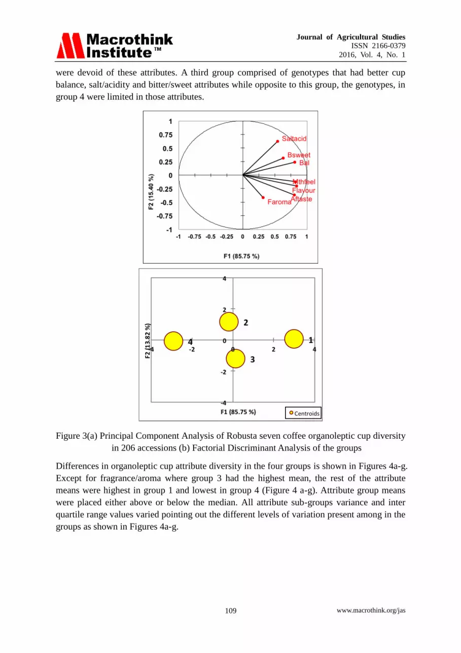
Journal of Agricultural Studies
ISSN 2166-0379
2016, Vol. 4, No. 1
www.macrothink.org/jas 109
were devoid of these attributes. A third group comprised of genotypes that had better cup
balance, salt/acidity and bitter/sweet attributes while opposite to this group, the genotypes, in
group 4 were limited in those attributes.
Figure 3(a) Principal Component Analysis of Robusta seven coffee organoleptic cup diversity
in 206 accessions (b) Factorial Discriminant Analysis of the groups
Differences in organoleptic cup attribute diversity in the four groups is shown in Figures 4a-g.
Except for fragrance/aroma where group 3 had the highest mean, the rest of the attribute
means were highest in group 1 and lowest in group 4 (Figure 4 a-g). Attribute group means
were placed either above or below the median. All attribute sub-groups variance and inter
quartile range values varied pointing out the different levels of variation present among in the
groups as shown in Figures 4a-g.

Journal of Agricultural Studies
ISSN 2166-0379
2016, Vol. 4, No. 1
www.macrothink.org/jas 110
a b c d
e f g
e f g
Figures 4 (a-g). Description of organoleptic cup attribute diversity groups
All Mahalanobis distances were greater than 3, implying that the groups were different
populations (Table 5). Equally, all the Fisher distances were significantly different, implying
that the formed groups had different organoleptic cup attributes. The Fisher as well as the
Mahalanobis data indicated that the longest distances was between group 1 and 4 while the
shortest was between group 2 and 3. The distance between group 1 and 2 was greater than
that between group 1 and 3.
Table 5. Mahalanobis and Fisher distances for organoleptic cup attribute groups
Fisher distances
Gp 1 2 3 4 1 2 3 4
1 0 0
2 11.81 0 46.18* 0
3 9.80 5.76 0 36.35* 22.31* 0
4 35.73 9.10 11.14 0 117.04* 30.97* 36.20* 0
Fisher‟s distances marked * were significant at p<(0.0001)
Figures 5 (a and b), further confirms the results of Figures 3 (a and b) and those in Table 6. In
Table 5 (a), factor 1 of the PCA, contributed 38.85% variance while factor 2 contributed
12.52% variance when altitude and age were also considered alongside accessions. Age and
altitude accounted for the organoleptic attributes variance in all accessions. Group 1
comprised of genotypes that were superior in all organoleptic cup attributes (Figure 5 a, b).
Group 2 had more acidity, sweet mouth feel while group 3 genotypes had better fragrance and
aroma, aftertaste, balance and flavour (Figure 5 a, b). Genotypes that were inferior in all

Journal of Agricultural Studies
ISSN 2166-0379
2016, Vol. 4, No. 1
www.macrothink.org/jas 111
organoleptic cup attributes were placed in group 4 (Figure 5 a, b). Although fragrance and
aroma increased with altitude, very high elevations and old trees had reduced organoleptic
quality. The longest distance was between group 1 to 4 while group 2 and 3 distances were in
between 1 and 4 groups.
Figure 5 (a). Organoleptic cup attribute relationships with altitude and tree age as shown by
the Principal Component Analyses (b) Organoleptic cup attribute groups from a factorial step
discriminant analysis
Table 6 also confirms that all the groups were correctly placed. Correct group placement
ranged from 88.10-96.23% with an average of 92.79% (Table 6).
Table 6. Estimated correct genotype group placement and pair wise distance comparison for
farm Robusta organoleptic cup attributes using confusion matrix
from \ to 1 2 3 4 Total % correct
1 50 2 2 0 54 92.59 %
2 1 54 4 0 59 93.22 %
3 0 1 52 0 53 96.23 %
4 0 1 0 41 42 88.10 %
Total 51 58 58 41 208 92.79 %
All the organoleptic attributes measured had more or less the same mean abundance that
ranged from 0.35 for cup balance to 0.47 for aftertaste (Table 7). But cup balance had a
cumulative percentage variance of 100 % meaning that the groups were distinctly different
for this trait and less so for aftertaste (Table 7).

Journal of Agricultural Studies
ISSN 2166-0379
2016, Vol. 4, No. 1
www.macrothink.org/jas 112
Table 7. Pooled contribution of variance for Robusta coffee organoleptic cup attributes and
mean group content derived from Bray-Curtis distance measure
Variance Mean group abundance
Variable Contribution Cumulative % 1 2 3 4
Aftaste 0.47 16.49 7.76 7.16 7.47 6.97
Mthfeel 0.43 31.43 7.66 7.22 7.36 6.91
Flavour 0.43 46.33 7.77 7.31 7.49 7.02
Faroma 0.42 60.95 7.45 7.18 7.48 7.16
Salt/acid 0.39 74.53 7.05 6.93 6.6 6.55
B/sweet 0.37 87.63 7.34 7.14 7.01 6.79
Cup Balance 0.35 100 7.72 7.45 7.37 7.09
4. Discussion
The protocol used to evaluate farm Robusta coffee organoleptic cup attributes was able to
detect, differentiate and segment organoleptic cup differences using their technical experience
(Tables 1; 2; 3). The significant differences found in evaluator organoleptic cup scores reflect
the subjective individual preference enriched by past experience. Individual cup taste
perception and preference for varietal specific characters such as acidity, body, aroma, flavour
and taste that constituted the nature and scoring of the brew implied that markets too vary and
are specific. Coffee drink preference is personal and consumers have a specific taste
according to their nationality, which makes it further difficult to define organoleptic cup
quality (Leroy et al., 2006). Furthermore, cup flavour in roasted coffee is reported to
constitute of over 800 multiple aromatic compounds and individuals perceive them
differently (Wintgens, 2004). Other factors that might also have contributed to liquor
differences among the accessions but were not measured in this study include, date of
harvesting, processing and storage.
Organoleptic cup characteristics were variable as shown in Table 2. Overall salt/acidity had
the least cup grading, an attribute that confers a low grade rating for Robusta coffee (Prakash
et al., 2005), despite some cultivars being achieving premium grade in all other attributes. Of
the 206 genotypes, 81% had average liquor salt/acidity of the usual good quality while 19%
were of very good premium grade.
Most of the assessed attributes were positively significantly correlated to each other as
shown by Table 4, meaning that there is opportunity to improve most of the desirable
organoleptic characters simultaneously. The overall cup quality was highly positively
significantly correlated with cup balance (r=0.75), mouth feel (r=0.73) and flavour (r=0.72)
than with aroma (r=0.32) and salt/acidity (r=0.41). However, cup acidity had positive
significant correlation coefficients with a sweet cup (r=0.31), good mouth feel (r=0.31), cup
balance (r=0.51) and overall cup (r=0.41 (Table 4) implying that acidity is an important
determining factor by consumers. Cup balance accounted for most to the total variance

Journal of Agricultural Studies
ISSN 2166-0379
2016, Vol. 4, No. 1
www.macrothink.org/jas 113
(Figure 1) making it, a major organoleptic trait in Robusta coffee and a priority in quality
improvement. This fact is further supported by the results in the PCA analysis (Figures 3a, b;
4 a-g and 5 a, b) and by the non-Euclidean dissimilarity cumulative variance shown in Table
7. Cup balance stands out as one trait that could be targeted for improvement as it
consistently demonstrated larger variance and diversity than the rest of the attributes.
Aroma/fragrance on the other hand was a lesser variable organoleptic trait. Aroma was not at
all correlated with acidity or sweetness in this study, though Moschetto et al., (1996) reported
linear correlation coefficients between preference and acidity and aroma in Robusta coffee
hybrids and in commercial clones. In this study, cup balance and aftertaste were at the highest
levels at altitudes between 1301-1400 metres above sea level whereas acidity was on the
decline (Figure 2 b). At higher altitudes of 1500 metres above sea level and above, cup
balance and acidity levels decreased but aftertaste levels were on the increase (Figure 2 b).
Decazy et al., (2003) also supported the idea that high sensory quality is associated with
altitude, which can be a criterion for selecting genotypes with high levels of salt/acidity
(Leroy et al., 2006b).
The „nganda‟ and „erecta‟ landraces had significantly more acidity and were more
bitter/sweeter than the research elite commercial and hybrid types (Figure 2). As suggested by
(Bertrand et al., 2006; Dessalegn et al., 2008), selection for vigour and larger seeds in the
hybrids and in the commercial types may have led to reduced variability for acidity and
sweetness.
The four categories of organoleptic cup attributes obtained from the PCA in Figures 3 and 5 a,
b) reflected the combined effect of genotype and genotype x environment variances. Group 1
(Figures 5, a, b) regarded as having the best brew had the highest ratings for fragrance/aroma,
flavour, aftertaste, acidity, sweetness, mouth-feel and cup balance. Group 1 was also
influenced by altitude whereas group 2 which was defined by mouthfeel, acidity and
bitter/sweetness was also mostly influenced by age. All the variances in groups 3 and 4 were
entirely due to altitude and age. Table 7 confirmed that indeed group 1 was the most superior
in organoleptic qualities and group 4, the least. The Malanobis and Fisher distances in Table 5,
show that the differences between group 1 and 4 that translate to genetic distances, again
implied that these two groups of genotypes are distantly related. The fact that four groups
comprised of genotypes from different locations that were far apart with varying ecologies
and crop husbandry practices, suggest that organoleptic variability was not restricted to any
site or location (Figures, 3,4 5; Table 4) but was influenced by both genotype and the
environment (Leroy et al., 2006b). The diverse organoleptic cup characteristics (Table 2)
coupled with a wide geographical distribution (Table 4; Figures 2; 3) provide immense
variability among Ugandan grown landraces of coffee that can not only be traded to diverse
markets but that can be selected for quality and other desirable agronomic traits.
5. Conclusion
Ugandan Robusta coffee was characterized into four distinct organoleptic cup groups using
the principle component and factorial step discriminant analyses. Organoleptic cup
differences based on Robusta coffee types were detected. About 84% of Robusta coffee

Journal of Agricultural Studies
ISSN 2166-0379
2016, Vol. 4, No. 1
www.macrothink.org/jas 114
produced in Uganda was of the premium grade while 13% was of the average grade and 3%
of the fine grade. Genotypes with low caffeine, high acidity and superior organoleptic cup
attributes exist among „nganda‟ and „erecta‟ land races and can be identified. Cup balance
was the most important organoleptic trait in determining overall cup.
Acknowledgement
We thank NARO for granting Pauline Aluka study leave to do this work and also
acknowledge financial support from USDA. We thank the Ugandan Robusta coffee farmers
for providing the ripe beans used in this study, field extension officers for identifying sample
farms and the evaluators, for their expertise on coffee cupping. We also thank Mr. Brian
Isabirye for his help in data analysis.
References
Aluka, P., Musoli, P., Curbry, P., Davrieux, F., Ribeyre, F., Guyot, B., De Bellis, F., Pinard, F.,
Kyetere, D., Ogwang, J., Dufour, M., & Leroy, T. (2006). Proceedings of the 21st
International Conference on Coffee Science, Montpellier, France, 93.
Bertrand, B., Vaast, P., Alpizar, E., Etienne, H., Davrieux, F., & Charmetant, P. (2006).
Comparison of bean biochemical composition and beverage quality of Arabica hybrids
involving Sudanese-Ethiopian origins with traditional varieties at various elevations in
Central America. Tree Physiology, 26(9), 1239-48.
Campa, C., Noirot, M., Bourgeois, M., Pervent, M., Ky, C. L., Chrestin, H., Hamon S., & De
Kochko, A. (2003). Genetic mapping of a caffeoyl-coenzyme A 3-0-methltransferase gene in
coffee trees: Impact on chlorogenic acid content. Theor. Appl. Genet., 107, 751-756.
Cannell, M. G. R. (1985). Physiology of the coffee crop. In N.M. Clifford & K.C. Willson
(Eds), Coffee: Botany, Biochemistry and Production of Beans and Beverage (pp 108-134).
London, Croom Helm.
Clifford, M. N. (1985). Chemical and physical aspects of green coffee and coffee products, In
M.N. Clifford, & K. C. Willson (Eds), Coffee: botany, biochemistry and production of beans
and beverage, ( pp 305-374), Connecticut, USA, Westport , Avi Publishing Company.
Decazy, F., Avelino, J., Guyot, B., Perriot, J. J., Pineda, C., & Cilas, C. (2003). Quality of
different Honduran coffees in relation to several environments. Journal of Food Science, 68,
2356-2361.
Dessalegn, Y., Labuschagne, M. T., Osthoff, G., & Herselman, L. (2008). Genetic diversity
and correlation of bean caffeine content with cup quality and green bean physical
characteristics in coffee (Coffea Arabica L.). Journal of the Science of Food and Agriculture,
88(10), 1726-1730.
International Coffee Organization, (ICO). (1991). Sensory evaluation of coffee: Technical Unit
Quality Series, ICO No 9, 209-243.

Journal of Agricultural Studies
ISSN 2166-0379
2016, Vol. 4, No. 1
www.macrothink.org/jas 115
Ky, C. L., Louarn, J., Dussert, S., Guyot, B., Hamon, S., & Noirot, M. (2001a). Caffeine,
trigonelline, chlorogenic acids and sucrose diversity in wild Coffea arabica L. and C.
canephora P. accessions. Food Chemistry, 75, 223-230.
Ky, C. L., Guyot, B., Louarn, J., Hamon, S., & Noirot, M. (2001b). Trigonelline inheritance in
the interspecific Coffea pseudozanguebariae x C. liberica var. dewevrei cross. Theor Appl.
Genet., 102, 630-634.
Ky, C. L., Louarn, J., Guyot, B., Charrier, A., Hamon, S., & Noirot, M. (1999). Relations
between and inheritance of chlorogenic acid contents in an interspecific cross between Coffea
pseudozanguebariae and Coffea liberica var 'dewevrei'. Theor. Appl. Genet., 98, 628-637.
Leroy, T., Ribeyre, F., Bertrand, B., Charmetant, P., Dufour, M., Montagnon, C., Marraccini,
P., & Pot, D. (2006a). Genetics of coffee quality. Braz. J. Plant Physiol., 18(1), 229-242.
Leroy, T., Curbry, P., Durand, N., Dufour, M., De Bellis, F., Jourdan, I., Vieira, L.G., Musoli,
P., Aluka, P., Marraccini, P., & Pot, D. (2006b). Coffea spp. and Coffea canephora diversity
evaluated with microsatellites and Single Nucleotide Polymorphism, Lessons from
comparative analysis, 21st International Conference on Coffee Science, Montpellier, France,
53.
Leroy, T., De Bellis, F., Legnate, H., Kananura, E., Gonzales, G., Luiz Felipe Pereira, L.F.,
Andrade, A. C., Charmetant, P., Montagnon, C., Cubry, P., Marraccini, P., Pot, D., & De
Kochko, A. (2011). Improving the quality of African robustas: QTLs for yield and quality
related traits in Coffea canephora. Tree Genetics & Genomes, 1-18.
http://dx.doi.org/10.1007/s11295-011-0374-6.
Mohammadi, S. A., & Prasanna, B. M. (2003). Analysis of Genetic Diversity in Crop Plants;
Salient Statistical Tools and Considerations. Crop Science, 43, 1235–1248.
Montagnon, C., Guyot, B., Cilas, C., & Leroy, T. (1998). Genetic parameters of several
biochemical compounds from green coffee. Coffea canephora, Plant Breed., 117, 576-578.
Moschetto, D., Montagnon, C., Guyot, B., Perriot , J. J, Leroy, T., & Eskes, A. B. (1996).
Studies on the effect of genotype on cup quality of Coffea canephora, Tropical Science, 36,
18-31.
Prakash, N.S., Combes, M.C., Dussert, S., Naveen, S., & Lashermes, P. (2005). Analysis of
genetic diversity in Indian Robusta coffee genepool (Coffea canephora) in comparison with a
representative core collection using SSRs and AFLPs. Genetic Resources and Crop Evolution,
52, 333-342.
Uganda Coffee Trade Federation, Coffee Year Book. (2009).
Wintgens, J. N. (Ed) (2004). Coffee: growing, processing, sustainable production. A
guidebook for growers, processors, traders, and researchers, Weinheim, WILEY-VCH Veriag
GmbH & Co. KGaA, ISBN: 3-527-30731-1.
Yapo, A., Louarn, J., & Montagnon, C. (2003). Genetic gains for yield after two back crosses
of the interspecific hybrid Libusta (Coffea canephora P x C. liberica Bull. Ex Hiern) to C.
canephora. P. Plant Breed., 122, 288-290.

Journal of Agricultural Studies
ISSN 2166-0379
2016, Vol. 4, No. 1
www.macrothink.org/jas 116
Copyright Disclaimer
Copyright for this article is retained by the author(s), with first publication rights granted to
the journal.
This is an open-access article distributed under the terms and conditions of the Creative
Commons Attribution license (http://creativecommons.org/licenses/by/3.0/).

Journal of Agricultural Studies
ISSN 2166-0379
2016, Vol. 4, No. 1
www.macrothink.org/jas 117
Resource-Use Efficiency of Honey Production in
Kachia Local Government Area, Kaduna-State, Nigeria
Ahmad,* Olohungbebe, S (Corresponding Author)
Department of Agricultural Economics and Extension, Faculty of Agriculture,
University of Abuja, PMB 117, Gwagwalada, Abuja, [email protected]
Alabi, Olugbenga. O (PhD)
Department of Agricultural Economics and Extension, Faculty of Agriculture,
University of Abuja, PMB 117, Gwagwalada, Abuja, Nigeria.
Daniel, P. O.
Department of Agricultural Economics and Extension, Faculty of Agriculture,
University of Abuja, PMB 117, Gwagwalada, Abuja, Nigeria.
Received: December 4, 2015 Accepted: December 24, 2015 Published: December 28, 2015
doi:10.5296/jas.v4i1.8790 URL: http://dx.doi.org/10.5296/jas.v4i1.8790
Abstract
This study examined resource-use efficiency of honey production in Kachia Local
Government Area, Kaduna, Nigeria. The primary data used for the investigation were
obtained using structured questionnaires administered to 50 producers. The data were
analysed using descriptive statistics, farm budget techniques, multiple regression analysis and
resource-use efficiency. Multiple regression analysis used to examine factors influencing
output of honey in the study area revealed that the coefficient of multiple determinations (R2)
of 0.59 which implies that 59% of the dependent variable in the model was explained by the
independent variables included in the model. Number of bee hives was significant at (p<
0.01).Estimated resource use efficiency revealed that number of bee hives and family labours
were underutilized. This study concluded that the bee farmers in the study area should be
given adequate training on rudiments of beekeeping.
Keywords: Resource-Use Efficiency, Honey Production, Kaduna State, Nigeria.
1. Introduction
In recent years, the production of honey through beekeeping is becoming popular among the
small scale farmers. This is due to the fact that the farmers have resorted to the need for

Journal of Agricultural Studies
ISSN 2166-0379
2016, Vol. 4, No. 1
www.macrothink.org/jas 118
income in diverse ways; thereby reducing the risk involved in depending on conventional
crop and animal production as the only source of income (Olarinde et al, 2008). Apiculture is
an aspect of the agricultural sector that has not been given much attention particularly at the
commercial level in the country (ICTA, 2004). Modern beekeeping is undertaken because it
serves as a source of food, employment and income (Olagunju and Adejumobi, 2003).
Beekeeping for honey production has been identified as one of the most lucrative enterprise
in many parts of the World. In United States of America, about 109,799,366.60 Kg of honey
worth $24, 200, 00.00 is produced each year; the same goes to the former USSR. Australia
produces 18,375,00051 Kg of honey and exports 5,898,313.08 Kg of it worth 900,000 pounds,
and Tanzania about 750,000 pounds worth of honey produce annually (Canadian Statistics,
2003). Presently in Nigeria, honey production is still at its developmental stage, though its
awareness was created for back early 1950s. This could be attributed to inefficient and
inadequate information on the enterprise and the belief that swarms of bees are a taboo and
signifies that a terrible mayhem is about to befall the individual whom it visits (Oyekuru,
2004). Generally, honey production enterprise attracts the attention of a greater percentage of
the populace these days because of its profitability and it is a visible complementary activity
for rural people and requires very little investments and in addition, produces quick returns
(Onyekuru, 2004).The demand for bee honey in Nigeria is on the increase, but organized
beekeeping as an enterprise is low (Eluagu and Nwani, 1999). ). In most parts of Africa it is
used for brewing honey beer and to a much lesser degree, as medicine; honey provides a
valuable food when it is consumed in its unprocessed state, i.e. liquid, crystallized or in the
comb. In these forms it is taken as medicine, eaten as food or incorporated as an ingredient in
various food recipes (Olstrom, 1983). Also, in addition to the thousands of "home-made"
recipes in each cultural tradition, honey is largely used on a small scale, as well as, at an
industrial level in baked products, confectionary, candy, marmalades, jams, spreads, breakfast
cereals, beverages, milk products and many preserved products (Olstrom, 1983). The broad
objective of the study is to evaluate the resource-use efficiencies of honey production in
Kachia Local Government Area, Kaduna State, Nigeria. The specific objectives are to:(i)
examine the socio-economic characteristics of honey producers in the study area, (ii) estimate
the costs and returns of honey production in the study area, (iii) evaluate resource-use
efficiency of honey production in the study area.
2. Methodology
2.1 The Study Area
The study was undertaken in Kaduna metropolis. Kaduna State is located in the mid-central
portion of the Northern parts of Nigeria, approximately between Latitudes 10020 N and
Longitudes 70 45’ E and covers an area of 45, 71.2 Square Kilometres. It has a population of
6,113503 (2006 census figures) and a population density of 130 people per Square Kilometre.
It accounts for 4.3% of Nigeria’s total population. The mean annual rainfall in the southern
part (in places like Kafanchan and Kagoro) is 1,1016mm. The State experiences a tropical
continental climate with two distinct seasonal climates, dry and rainy seasons. The wet
season (May to October) is heavier in the southern part of the state than the northern part.
Agriculture constitutes the largest occupation of the people with many citizens participating

Journal of Agricultural Studies
ISSN 2166-0379
2016, Vol. 4, No. 1
www.macrothink.org/jas 119
in small scale farming. The State is a major region of animal husbandry. Major foods and
cash crops produced in the State includes, cotton, groundnut, guinea corn, millet, ginger,
tobacco, beans etc. (www.google.com).
2.2 Sampling Technique and Sample Size
For the purpose of this study, two communities were visited in Kachia Local Government Area
in Kaduna State, specifically Katari and Azara Areas of the State. Simple random sampling
technique was used for this study. Twenty-five (25) respondents were randomly selected from
each of the villages giving a total sample size of fifty (50) respondents.
2.3 Method of Data Collection
The data used for this study consist mainly of primary data. Data were obtained through the use
of questionnaire. The questionnaire was used to collect information on the socio-economic
variable of the beekeepers, their management practices, the cost incurred, their income,
revenue, efficiency and production data. The interview was carried out during their group
meeting. The survey was carried out in 2014 production season. The production cycle as stated
by the beekeepers take place within a year (9-12 months).
2.4 Methods of Data Analysis
The analytical tools that were used in this study to achieve stated objectives include the
following:
(i) Descriptive Statistics
(ii) Farm Budgeting Technique
(iii) Multiple Regression Analysis
(iv) Resource-Use Efficiency
2.4.1 Descriptive Statistics
This analytical tool was used to examine the socio-economic characteristics of honey
producers which include; their gender, marital status, household size, age, level of education
etc. Statistical package for Social Science (SPSS) was used. Descriptive statistics involve the
use of mean, frequency distribution tables, percentages etc. This was used to achieve objective
one (1).
2.4.2 Farm Budgeting Technique
Costs incurred and returns in honey and beeswax production were estimated based on
prevailing market price. Costs of production include; raw materials such as bucket, container;
expenses on land (rent or lease); labour (wages) etc.
The Net Farm Income (NFI) is calculated thus:
NFI=TR-TC
Where, NFI = Net Farm Income (N)

Journal of Agricultural Studies
ISSN 2166-0379
2016, Vol. 4, No. 1
www.macrothink.org/jas 120
TR = Total Revenue from Honey and other Hive Products
TC = TFC + TVC
TR = P.Q
Where, P = Price of honey produced in Naira per Litre.
Q = Output of honey produced in Litre
This was be used to achieve specific objective two.
2.4.3 Multiple Regression Analysis
The model is implicitly stated as:
Y = f(X1, X2, X3, X4, Ui)
Where,
Y =Output of Honey Produced (Litres)
X1 = Number of Hives set by the Beekeeper (Units)
X2 = Hired Labor (Mandays)
X3 =Family Labour (Mandays)
X4 = Cost of Bating Materials (Naira)
Ui = Random Error Term/Disturbance Error Term.
Explicitly, the functions are stated as:
Y = a + bX1 + CX2 + dX3 + eX4 + Ui (Linear)
Log Y = a + b LogX1 + cLogX2 + dLogX3 + eLogX4 + Ui (Double-Log)
Y = a + bLog X1 + cLogX2 + dLogX3 + eLogX4 + Ui (Semi-Log).
This was used to achieve objective two (2).
2.4.4 Resource-Use Efficiency
Resource-Use Efficiency of honey production was estimated using the formula,
MVP = r
MFC
Where,
MVP = Marginal Value Product
MFC = Marginal Factor Costs (N)
r= Resource-Use Efficiency of Honey Production.
If r = 1, it indicates that the resource-use efficiency of honey production is utilized.
Journal of Agricultural Studies
ISSN 2166-0379
2016, Vol. 4, No. 1
www.macrothink.org/jas 121
If r > 1, it indicates that the resource-use honey production is underutilized.
If r < 1, it indicates that the resource-use efficiency of honey production is over
utilized.
MVP = MPP x Pq
Where,
MPP = Marginal Physical Product
Pq = Price of Unit Output (N)
This was used to achieve objective three (3).
3. Results and Discussion
Table 1 show that ninety (90) percent of honey producers in the study area were male, thus
confirming the notion that bee keeping is a hazardous occupation, and about ten (10) percent of
the beekeepers were women (Babatunde et al, 2007). Furthermore, seventy-eight (78) percent
of honey producers were married. Most of the respondents were educated (Lawal, 2002).
Sixteen (16) percent of honey producers were single, four (4) percent were widow and only two
(2) percent were widower. About ninety (90) percent of honey producers had less than10
members as household. This is in line with finding of Mbah (2012) who opined that beekeepers
rely so much on household labour for beekeeping activities. However, under subsistence
agriculture, much reliance is often placed on the strength of household to supply the much need
farm labour in the absence of mechanized equipment. Thus, the larger the household size, the
higher the supply of household labour. Also, about ten (10) percent had between 11-20
members of household size who worked on the farm of honey. Honey producers in the study
area are middle-aged. About eighty-eight (88) percent of honey producers were less than fifty
(50) years of age, which means they are still in their active productive age, which signifies
increase in the output of honey as also observed by Mbah (2012). The study also revealed that
twelve (12) percent of honey producers are between fifty-one (51) and seventy (70) years of
age. The results further showed that majority (42 percent) of honey producers in the study area
are into farming, and sixteen (16) percent are civil servants. This corroborates with the views of
Folayan et al (2013) that the both (farmers and civil servants) diversify into honey production
to ensure optimum and continuous flow of income. This study further shows that students (10
percent) are among honey producers in the study area. Furthermore almost all the beekeepers in
the study area are literate. About ninety –eight (98) percent of honey producers had formal
education. This implies that beekeeping is practiced mostly by educated people and therefore,
adoption of modern beekeeping techniques would not be a problem. Studies have shown that
education is positively related to adoption of innovation (Balogun, 2000). Nevertheless, only
two (2) percent of the honey producers had non-formal education. Also, about ninety (90)
percent of honey producers had less than 20 years of experience in honey production. This is in
line with finding of Tijani et al (2011) who observed that the higher the numbers of years spend
in farming by a farmer, the more he becomes aware of new production techniques, thereby
increasing the level of productivity. The results of the farm budgeting analysis are presented in

Journal of Agricultural Studies
ISSN 2166-0379
2016, Vol. 4, No. 1
www.macrothink.org/jas 122
Table 2. Costs incurred on various resources used and profits obtained from the sale of the
produce were estimated based on the market price at the period under consideration 2014
family season. The gross income was calculated by multiplying the total quantity of honey
produced by the price of output sold. The gross income of the honey producers was N363, 672.
The total cost was put into consideration by adding the total variable costs which was
N50071.49 and the total fixed cost was N153259.73 which gave the total cost of N6, 953,820.
The total variable costs include: cost of land cleaning, cost of bating materials, cost of chemical,
cost of hired labour, and cost of family labour to mention a few. Also, total fixed cost include:
cost of uniform, cost of boot, cost of container etc. The net income was estimated to be N
17,980,268.78. The factors influencing output of honey produced were expressed in the
econometric multiple regression analysis Table 3. The variables examined in the model include;
number of hives (colony) X1; hired labour (mandays) X2; family labour (mandays) X3; and cost
of bating materials (N) X4. Double-log functional form was selected as the lead equation. In the
lead equation, numbers of hives X1 were significant at 1% probability level. The coefficient of
multiple determinations (R2) is 0.529. This implies that 52.95 of variations in the dependent
variable were explained by variations in the explanatory variables included in the model. An
estimate obtained from the double-log functional form is direct elastics. For instance, the
estimated coefficient for number of hives was 0.895. This implies that if numbers of hives are
increased by 1% holding other variable constant, the output of honey produced will increase by
0.895. Estimated resource use efficiency shows that number of bee hives(X1) and family labour
(X4) are underutilized (Table 4).
Table 1. Socio-Economic Characteristics of Honey Producers in Kachia Local Government
Area, Kaduna State.
Variable Frequency Percentage (%)
Sex
Male 45 90.00
Female 05 10.00
Marital Status
Married 39 78.00
Single 08 16.00
Widow 02 04.00
Widower 01 02.00
Household Size
1-10 45 90.00
11-20 05 10.00
Age (Years)
21-30 09 18.00
31-40 15 30.00
41-50 20 40.00
51-60 04 08.00

Journal of Agricultural Studies
ISSN 2166-0379
2016, Vol. 4, No. 1
www.macrothink.org/jas 123
61-70 02 04.00
Major Occupation
Farming 21 42.00
Civil servant 08 16.00
Business 03 06.00
Caterpillar mechanic 01 02.00
Honey producers & Business 04 08.00
Farming and business 01 02.00
Honey producers & Farming 03 06.00
Clergy 01 02.00
Mason 01 02.00
Student 05 10.00
Student and Business 01 02.00
Honey producer 01 02.00
Mode of Honey Production
Full - Time 33 66.00
Part - Time 17 34.00
Education Level
Primary 09 18.00
Secondary 19 38.00
Tertiary 21 42.00
Non- Formal 01 02.00
Experience of Honey Production (Years)
1-10 25 50.00
11-20 20 40.00
21-30 03 06.00
31-40 02 04.00
Total 50 100.00
Source:-Field Survey, 2014.
Farm Budget Technique
Table 2. Costs and Returns Analysis of Honey Production in the Study Area.
Items Mean value (N)
A Variable Cost
(i) Cost of Land Clearing 15,636,36.00
(ii) Cost of Bating Material 2,654.00
(iii) Cost of Chemical (Additive) 410.00
(iv) Cost of Labour (Hired) 3,525.00

Journal of Agricultural Studies
ISSN 2166-0379
2016, Vol. 4, No. 1
www.macrothink.org/jas 124
(v) Labour Cost of Children 2,519.05
(vi) Labour Cost of Women 2,645.83
(vii) Rentage Cost of Land 22,681.25
(B) Total Variable Cost 50,071.49
(C) Fixed Cost
(i) Cost of Hive 30,491.53
(ii) Cost of Uniform 14,157.14
(iii) Cost of Boot 7,418.75
(iv) Cost of Machete 4,296.88
(v) Cost of Basin 13,903.45
(vi) Cost of Wheelbarrow/Motorbike 36,903.45
(vii) Cost of Container 27,501.00
(viii) Cost of Bucket 8,503.19
(ix) Cost of Plastic Bowl 20,060.71
(D) Total Fixed Cost 153, 259.73
Total Cost (B + D) 203, 333. 22
Gross Income 363,672.00
Net Income 17, 980, 268. 78
Source: - Field Survey, 2014.
Multiple Regressions Analysis
Table 3. Multiple Regressions Analysis (Double Equation as Lead Equation)
Variables Regression Coefficient
Standard Error
t-value
Constant 3.279 0.928 3.532
X1(Number of Bee Hives)
0.895 0.130 6.867***
X2(Hired Labour) -0.257 0.201 -1.277 X3(Family Labour) 0.053 0.229 0.232 X4 (Cost of Bating Material)
-0.014 0.120 -1.116
R2
Value 0.529 Adjusted R
2 Value 0.487
F – Value 12.615***
Source- Field Survey, 2014.

Journal of Agricultural Studies
ISSN 2166-0379
2016, Vol. 4, No. 1
www.macrothink.org/jas 125
Table 4. Estimated Resource- Use Efficiency of Honey Production in the Study Area.
Resource MPP MVP MFC Allocative
Efficiency (r)
Number of Bee Hives (X1) 15.59 11310.55 725.5 15.59
Hired Labour (X2) -118.9
8
-86319.04 725.5 -118.98
Family Labour (X3) 135.27 98138.39 725.5 135.27
Cost of Bating Material (X4) -0.009 -6.66 725.5 -0.009
Source: Field Survey, 2014
4. Conclusion and Recommendations
The study revealed that the honey production in the study area is a viable and profitable
enterprise. Based on the results, the following recommendations are made: the farmers in the
study area should be given adequate training on rudiments of beekeeping. This will ensure
proper understanding of modern equipment and adopt technology capable of increasing not
only the profitability of the enterprise but also make efficient use of bee resources.
Establishment of bee farmers’ cooperation association for annexing financial aids, marketing
information and inputs from government and non-government organisations .Creating a
market channel that will take care of commensurate price for product of new beekeeping
enterprise .Government at all levels should endeavour to stimulate farmers to boost honey
production by providing and subsidise if need be, necessary infrastructures and enabling
environment which provide impetus that will ease people transition from traditional to
modern beekeeping easy.
References
Babatunde, R. O., Olorunsanya, E. O., Omotesho, O. A., & Alao, B. I. (2007). Economic of
Honey Production in Nigeria: Implications for Poverty Reduction and Rural Development,
Global Approaches to Extension Practice (GAEP), 3(2).
Balogun, A. L. (2000). Adoption of Alley Farming Among the Farmers in Osun State, Nigeria.
Unpublished Ph.D Thesis, Obafemi Awolowo University, Ile-Ife, Nigeria, 291.
Canadian Statistics (2003). Honey production, (2003). Canadian Bee Journal, 35(4), 61-72.
Eluagu, L. S., & Nwani, L. N. (1999). An Economic Appraisal of an Improved Method of
Beekeeping in Nigeria. A case study of Apiculture unit, Federal College of Agriculture,
Umudike. The Nigerian Agricultural Journal, 6(2), 90-105.
ERLS (1995).Bee keeping Technologies for Nigerian Farmers. Extension Bulletin. Ahmadu
Bello Univeristy, Zaria. Nigeria.

Journal of Agricultural Studies
ISSN 2166-0379
2016, Vol. 4, No. 1
www.macrothink.org/jas 126
Folayan, J. A., & Bifarin, J. O. (2013). Profitability Analysis of Honey Production in Edo
North Local Government of Area of Edo State, Nigeria. Journal ofAgricultural Economics and
Development, 2(2), 60-64.
ICTA (2004). The Prospect of Beekeeping in the Modern World. Paper Delivered at Training
The Trainers State Organized Workshop for Officials of L.G. As, held between 11th
-14th
March,
2003, at the Federal College of Forestry Mechanization, Afaka, Kaduna, P4. International
Centre for Tropical Apiculture, 2004.
Lawal, W. L., & Ibebulem, U. O., & Ajani, O. I. (2002). Resource-Use Efficiency in
Apiculture in Umuahia-North Local Government, Abia State, Nigeria.
Mbah, S. O. (2012). Profitability of Honey Production Enterprise in Umuahia Agricultural
Zone of Abia State, Nigeria Int’l Journal of Agric and Rural Development.
Olagunju, F. I., & Ajetumobi, J. O. (2003). Profitability of Honey Production under Improved
Method of Beekeeping in Oyo State, Nigeria. International Journal of Economics and
Development, 3(1), 148-151.
Olarinde, L., Ajao, O., & Okunola, S. O. (2008): Determinants of Technical Efficiency in
Beekeeping Farms in Oyo State, Nigeria: A Stochastic Production Frontier Approach.
Research Journal of Agriculture and Biological Sciences, INSI Net Publication.
Olstrom, J. M. (1983). Dried honey. Am. Bee J. 123, 656-659.
Onyekuru, N. A. (2004). “ Economics Analysis of Honey Production in Nsukka, L. G. A. of
Enugu State. Unpublished B.Sc. Degree Thesis , Department of Agricultural Economics
University, Nsukka.
Tijani B. A., Ala, A. L. Maikasuwa, M. A., & Ganawa, N. (2011) Economic Analysis of
Beekeeping in Chibok Local Government Area of Borno State, Nigeria. Nigeria Journal of
Basic and Applied Science (2011) ISS 079498.www.google.com [accessed 23/07/2014].
Copyright Disclaimer
Copyright for this article is retained by the author(s), with first publication rights granted to
the journal.
This is an open-access article distributed under the terms and conditions of the Creative
Commons Attribution license (http://creativecommons.org/licenses/by/3.0/).

Journal of Agricultural Studies
ISSN 2166-0379
2016, Vol. 4, No. 1
www.macrothink.org/jas 127
Improving Seed Potato Leaf Area Index, Stomatal
Conductance and Chlorophyll Accumulation Efficiency
through Irrigation Water, Nitrogen and Phosphorus
Nutrient Management
Gathungu Geofrey Kingori
Department of Plant Sciences, Chuka University, P. O. Box 109 – 60400, Chuka, Kenya.
Aguyoh Joseph Nyamori
School of Agriculture, Natural Resources & Environmental Studies, Rongo University
College, P.O. Box 103-40404, Rongo, Kenya.
Isutsa Dorcas Khasungu
Chuka University, P. O. Box 109 – 60400, Chuka, Kenya and Department of Crops,
Horticulture and Soils, Egerton University, P. O. Box 536-20115, EGERTON, Njoro, Kenya.
Received: December 17, 2015 Accepted: January 4, 2016 Published: January 19, 2016
doi:10.5296/jas.v4i1. 8908 URL: http://dx.doi.org/10.5296/jas.v4i1.8908
Abstract
A study was conducted in a Rainshelter (RTrial) at Horticultural Research and Teaching Farm,
Egerton University to determine the effect of integration of irrigation water, nitrogen (N) and
phosphorus (P) application on seed potato leaf area index (LAI), stomatal conductance and
chlorophyll content. The treatments arranged in a split-split plot layout in a completely
randomised block design, consisted of three irrigation water rates (40%, 65% and 100% field
capacity), four N rates (0, 75, 112.5 and 150 kg N/ha) supplied as urea (46% N), and four P
rates (0, 50.6, 75.9, 101.2 kg P/ha) supplied as triple superphosphate, replicated three times
and repeated once. During the growth leaf area, stomatal conductance, and chlorophyll
content were measured. Data collected were subjected to analysis of variance and
significantly different means separated using Tukey’s Studentized Range Test at P≤0.05. Leaf
area index was greater with high irrigation water at 100%, N at 150 kg N/ha and P at 101.2 kg
P/ha, which was 2.6 and 1.3 at 51 days after planting (DAP) and 3.5 and 3.1 at 64 DAP.
Furthermore, low irrigation water rate at 40% together with low N and P rates of 0 kg N/ha
and 0 kg P/ha had the least LAI, which was 0.28 and 0.19 at 51 DAP and 0.28 and 0.24 at 64
DAP both in RTrials I and II, respectively. Subjecting potato to 100% compared to 40%

Journal of Agricultural Studies
ISSN 2166-0379
2016, Vol. 4, No. 1
www.macrothink.org/jas 128
irrigation rate increased stomatal conductance at 87 days after planting (DAP) by 32.82 and
31.99 mmolm⁻²s⁻¹, leaf chlorophyll content index by 16.2 and 16.5, 19.8 and 19.6, and 15
and 20.3, when integrated with high compared with low N and P application rates at 59, 73
and 87 DAP, in RTrials I and II respectively. Irrespective of N and P rates LAI, stomatal
conductance and chlorophyll content were significantly greater with high irrigation water at
100% followed by 65% and was lowest with 40% irrigation water rate.
Keywords: Potato, Irrigation, Nitrogen, Phosphorus, Leaf, Conductance, Chlorophyll
1. Introduction
Plant growth and development and consequently yields are influenced by many stress factors,
such as low or high temperatures, water deficit, excessive radiation within the
photosynthetically active range, mechanical injuries, gaseous contamination, phytotoxins,
herbicides applied, or intensive fertilization (Sawicka et al., 2015). Although potato is the
most widely distributed crop in tropical and subtropical zones of the world (Burhan et al.,
2007), its productivity and quality are inadequate due to disjointed investigation of the many
factors that hinder them. These factors include poor seed potato tuber quality, irrigation
management, mineral fertilization, insect pest and disease forecasting, as well as poor
planting dates and storage conditions (Walingo et al., 2004). Potato growth depends on a
supply of plant nutrients, such as nitrogen (N), phosphorus (P) and potassium (K), each with
a specific function for plant growth and lack of them results in retarded growth processes and
reduced yields (van der Zaag, 1981).
In Kenya, low application of N and P under continuous cultivation is a major constraint that
leads to poor potato growth and productivity. Mineral nutrients are essential for healthy plant
growth, optimum yield, and better economic returns. Potato plants have a high demand on
soil nutrients and their proper management is one of the most important factors required to
obtain maximum tuber yield (Braun et al., 2015).Therefore, it is important to maintain high
soil fertility through balanced nutrient supply (ICIPE, 2006). Optimum use of mineral
fertilisers by crops is essential for sustainable agriculture and nutrient use efficiency
comprises both uptake efficiency and utilisation efficiency (Hawkesford, 2012). The aim of
fertiliser application is to feed the soil, which in return feeds the plant. Another factor that has
limited seed potato production in many parts of Kenya is unreliable rainfall. Potato is
sensitive to soil water deficit (Bowen, 2003; Kiziloglu et al., 2006) and is often considered as
a drought sensitive crop and its sustainable production is threatened due to frequent drought
episodes (Obidiegwu et al., 2015). Plant needs for water and nutrients are interdependent, as
a good water supply improves the nutritional status of crops, and adequate nutrient supply
saves water (Roy et al., 2006).
Effective management and proper coordination of N, P and irrigation water can increase
potato productivity through their efficient use. Most work on seed potato tuber quality has
focused on effect of diseases and little attention has been given to the effect of nutrient and
water management in different genotypes. Irrigation has been increasingly employed to
curtail effects of drought (Thompson et al., 2007) in other countries, but in Kenya potato
farmers rarely use this practice due to cost and lack of knowledge, among other factors.
Farmers in the informal seed production sector are inconsistently and inappropriately

Journal of Agricultural Studies
ISSN 2166-0379
2016, Vol. 4, No. 1
www.macrothink.org/jas 129
applying N and P fertilisers due to lack of information on their combined effects on potato
growth and development for high quantity and quality seed potato tuber production. In the
long-term misapplication influences potato leaf area expansion, stomatal conductance,
chlorophyll content, seed potato yield and quality, as well as market and consumer values.
Conductance of the diffusion and the transport of CO2 play a major role in determining
CO2:O2 ratio (Biman et al., 2014) which is crucial in determining photosynthetic rates. The
lower stomatal conductance inhibits water losses, thus helping the plants to cope with the
drought in better way (Naveed et al., 2012) although it inhibits the CO2 fixation, resulting in
lower productivity (Cornic 2000; Chaves et al., 2002). Nitrogen is an important nutrient since
it has a positive effect on chlorophyll concentration, photosynthetic rate, plant height and dry
matter accumulation and higher potato tuber yields (Sinfield et al., 2010; Tremblay et al.,
2011). Chlorophyll is one of the most photochemically active compounds in photosynthesis
and its determination provides useful information concerning the photosynthetic status
(Yadav et al., 2010)
Where fertilization is done, farmers do not supply irrigation water to the crop to enable it
utilize the nutrients efficiently and realize better returns. As the need for food production
increases with increasing population growth, it is important that strategies are developed to
enhance the nutrient uptake and utilization efficiencies (Liu et al., 2012). This can be
achieved through combined investigation of N, P and irrigation water effects. Furthermore, in
the face of increased fertilizer and irrigation water cost and stringent environmental
regulation, there is a critical need to improve N, P and water use efficiency to ensure seed
potato production remains sustainable. Excess water can be a cause of nutrient losses, and
insufficient water at a critical stage can limit growth and yield, and timing of water
application influences nutrient use efficiency (Roy et al., 2006). Therefore, water
management and/or rainfall are among the most important factors determining yield and
quality of potatoes (DAFF, 2013).
There is therefore need to evaluate, document and disseminate comprehensive management
packages and knowledge on leaf expansion capacities, stomatal conductance and chlorophyll
content in environments characterized by varied rainfall and nutrient amounts. The ability
of leaves to expand, stomatal conductance and the chlorophyll concentration determined by
water and nutrient supply forms critical determinants of leaf photosynthetic capacities which
influences the photoassimilates available for plant growth and consequent yield. Study of
tolerance of seed potato to varying irrigation water and mineral nutrient supply rates will
assist producers in predicting expected potato growth and tuber yields under their prevailing
agro-ecological conditions.
2. Materials and Methods
2.1 Potato Growth in the Field
Potatoes were planted in a rainshelter at the Horticultural Research and Teaching Farm of
Egerton University, Njoro between 19th
August and 19th
December 2011 (RTrial I) and the
trial was repeated between 5th
April and 6th
August 2012 (RTrial II). Potatoes were planted to
determine the effect of irrigation water, nitrogen (N) and phosphorus (P) application rates on
leaf area index, stomatal conductance, and chlorophyll content of seed potato. The three

Journal of Agricultural Studies
ISSN 2166-0379
2016, Vol. 4, No. 1
www.macrothink.org/jas 130
factors were tested in a split-split plot design with the irrigation water rate assigned to main
plots, N to subplots and P to sub-subplots. The treatments were replicated three times. The
treatments consisted of three irrigation water (W) rates (40%, 65% and 100% field capacity
[FC]), applied throughout the potato growth period through drip tube lines. Water was
supplied through irrigating only the root zone, leaving the inter-row spaces dry. A
WaterScout (Model SM 100 Sensor) connected to 2475 Plant Growth Station (Watch Dog
Model, Spectrum Technologies, Plainfield, IL 60585, USA), which is applicable between 0%
to saturation was used to indicate the need for irrigation.
Nitrogen (N) was supplied as urea (46% N) at four rates (0, 75, 112.5 and 150 kg N/ha), each
in two splits, with the first half at planting and the second at 5 weeks after planting.
Phosphorus (P) was supplied at planting time as triple superphosphate (46% P2O5) at four
rates (0, 50.6, 75.9, 101.2 kg P/ha). Each plot measured 1.8 m x 2.25 m. Each
experimental unit consisted of seven rows each with seven tubers planted. Routine field
maintenance practices such as weeding and spraying against diseases and insect pests using
appropriate fungicides and insecticides was done when necessary. Weeding or physical
uprooting of weeds was done any time weeds were visible. Recommended fungicides for
control of early and late blight such as Ridomil® were used. Insect pests mainly aphids,
thrips, and white flies were controlled using Metasystox® and mites using miticides. Earthing
up was done during weeding. The haulm was not cut off before harvesting for purposes of
shoot growth determination at harvest.
2.2 Leaf area index (LAI)
Three plants per treatment were pegged and the leaf area measured using the graphical
method in both RTrials I and II. The total leaf area per plant was estimated using a graph
paper whereby leaves within a plant were randomly selected and divided into four growth
categories namely smallest, small, medium and large. The leaves within these categories were
removed from a potato plant and placed on a graph paper and their approximate area
determined by counting the number of 1 cm2 grids on the graph paper occupied by the
individual leaf. The individual leaf area for the smallest, small, medium and large was 7 cm2,
18 cm2, 34 cm
2, and 42.5 cm
2, respectively. When the individual leaf area of these four
categories of leaves within the potato was determined, leaves within the plant similar to the
smallest, small, medium and large were counted separately. The total leaf area per category
was obtained by multiplying the number of leaves counted per category by the respective
individual leaf area i.e. multiplying the leaf area per active haulm by the number of active
haulms per plant. The total leaf area of the plant was obtained by adding the total leaf area of
smallest, small, medium and large leaf categories. The total leaf area was determined at 51
and 64 DAP a period characterised by tuber set and initiation of tuber bulking within the
potato plant. The resulting total leaf area was used to calculate LAI using the formula: LAI
= Total leaf area (cm2)/ground area (cm
2) (Beedle, 1987).
2.3 Leaf stomatal conductance
The stomatal conductance was measured on fresh tissues of one randomly selected leaf of
medium growth on three middle randomly pegged plants per treatment at 59, 73 and 87 days

Journal of Agricultural Studies
ISSN 2166-0379
2016, Vol. 4, No. 1
www.macrothink.org/jas 131
after planting (DAP) in both RTrials I and II using a leaf porometer (SC-1; Decagon
Devices, Pullman, WA). Stomatal regulation of gas exchange by leaves is of great importance
to photosynthesis and stomatal movements can be affected by various environmental factors,
including plant water status, CO2 concentration and light (Raschke, 1975; Kim et al., 2004).
2.4 Leaf chlorophyll content index
Leaf chlorophyll content was measured at 59, 73 and 87 DAP using chlorophyll content
meter (CCM-200 plus; Opti-Sciences, Tyngsboro, MA) on fresh tissues of lower, middle and
uppermost fully expanded leaves on the three randomly pegged plants per plot. The
measurements were taken halfway from the leaf base to the tip and halfway from the midrib
to the leaf margin. Chlorophyll content meter assists in rapid, non-destructive, determination
of chlorophyll content in intact leaf samples. A non-destructive estimation of leaf Chlorophyll
and Chlorophyll Concentration Index (CCI) value that is proportional to the amount of
chlorophyll in the sample is the units of measurements. Leaf chlorophyll content provides
valuable information about physiological status of plants (Gitelson et al., 2003).
2.5. Data Analysis
Data collected was subjected to analysis of variance using the SAS system for windows V8
1999-2001 by SAS Institute Inc., Cary, NC, USA (SAS, 2011) and significantly different
means separated using Tukey’s Studentized Range Test at P 0.05.
3. Results
3.1. Leaf area index (LAI)
Leaf area index significantly differed among the treatments at 51 and 64 DAP. Potatoes that
received high irrigation water, N and P rates had significantly higher LAI than those that
received lower rates. Leaf area index significantly increased between 51 and 64 DAP with
integrated application of high irrigation water, N and P rates in both RTrials. Leaf area index
was greater with high irrigation water at 100%, N at 150 kg N/ha and P at 101.2 kg P/ha,
which was 2.6 and 1.3 at 51 DAP and 3.5 and 3.1 at 64 DAP. Furthermore, low irrigation
water rate at 40 % together with low N and P rates of 0 kg N/ha and 0 kg P/ha had the least
LAI, which was 0.28 and 0.19 at 51 DAP and 0.28 and 0.24 at 64 DAP both in RTrials I and
II, respectively.
Irrespective of N and P rates LAI was significantly greater with high irrigation water at 100%
followed by 65% and was lowest with 40% irrigation water rate. High compared to low
irrigation water together with high N and P application rates increased the LAI by 1.54 and
0.61 at 51 DAP and by 2.06 and 1.78 at 64 DAP both in RTrials I and II, respectively.
Similarly LAI significantly increased from low to high rates of N and P at all irrigation water
rates. However, slight but significant differences were observed when 40% and 65%
irrigation water rates was supplied together with high N and P rates of 150 kg N/ha and either
75.9 kg P/ha or 101.2 kg P/ha (Table 1).
3.2. Leaf stomatal conductance (mmolm⁻²s⁻¹)
Leaf stomatal conductance was significantly affected by all the treatments at the various

Journal of Agricultural Studies
ISSN 2166-0379
2016, Vol. 4, No. 1
www.macrothink.org/jas 132
stages of potato growth. Integration of irrigation water, N and P application rates did not
affect leaf stomatal conductance. However, effects of integration of N and P on leaf stomatal
conductance were observed at all growth stages. Leaf stomatal conductance increased with
irrigation water, N and P application rates. While high irrigation water rate increased the leaf
stomatal conductance, low irrigation water rate reduced the leaf stomatal conductance (Table
2). Therefore water stress resulted in decrease in the net leaf stomatal conductance
Furthermore, leaf stomatal conductance increased from 59 DAP and was highest at 73 DAP
after which it reduced regardless of irrigation water application rate later in the growth season.
Average leaf stomatal conductance at 87 DAP decreased by 24.1 and 35 mmolm⁻²s⁻¹ with
high compared to 21 and 33.9 mmolm⁻²s⁻¹ observed with low irrigation water rate in RTrials
I and II, respectively. Therefore although decreases in leaf stomatal conductance were also
observed with high irrigation water rate greater reduction resulted from low irrigation water
application rate at the later growth stages. Therefore, higher irrigation water application
rates maintained higher leaf conductance compared to lower application rates in both RTrials
(Table 2).
Similarly leaf stomatal conductance increased with N and P application rate. High rates of N
and P application increased leaf stomatal conductance from 59 to 79 DAP after which there
were declines regardless of their application rate (Table 3).
Table 1. Effect of irrigation water, N and P application rate treatments on potato LAI
RTrial I LAI at 56 DAP LAI at 64 DAP
P rate (kg P/ha) P rate (kg P/ha)
kg N/ha 0 50.6 75.9 101.2 0 50.6 75.9 101.2
Irri
gat
ion
wat
er r
ate
(% F
C)
100%
0 0.78d* 0.85d 1.46c 1.58d 1.05d 1.14d 1.95c 2.12d
75 0.92c 1.02c 1.45c 1.76c 1.23c 1.37c 1.95c 2.37c
112.5 1.34b 1.22b 1.76b 2.14b 1.63b 1.8b 2.35b 2.87b
150 1.37a 1.8a 2.36a 2.64a 1.84a 2.46a 3.17a 3.54a
65%
0 0.44d 0.65d 1.02d 1.11d 0.59d 0.87d 1.37d 1.48d
75 0.65c 0.73c 1.1c 1.32c 0.87c 0.98c 1.48c 1.75c
112.5 0.93b 1.05b 1.3b 1.4b 1.24b 1.4b 1.74b 1.88b
150 0.97a 1.13a 1.34a 1.51a 1.29a 1.54a 1.79a 2.03a
40
%
0 0.21d 0.35d 0.53d 0.69d 0.28d 0.47d 0.71d 0.93d
75 0.37c 0.48c 0.82c 0.91c 0.49c 0.64c 1.1c 1.22c
112.5 0.5b 0.60b 0.88b 1.07b 0.67b 0.8b 1.18b 1.44b
150 0.62a 0.64a 0.93a 1.1a 0.83a 0.85a 1.25a 1.48a
MSD 0.02(N) 0.02 (P) 0.02 (W) 0.03 (P) 0.03 (N) 0.02 (W)
CV (%) 5.80 6.05
RTrial II
Irri
gat
ion
wat
er
rate
(%
FC
) 100 %
0 0.59d* 0.64d 0.76d 0.82d 0.91d 0.98d 1.63d 1.83d
75 0.69c 0.75c 0.78c 0.91c 1.06c 1.18c 1.67c 2.04c
112.5 0.76b 0.81b 0.88b 1.03b 1.41b 1.55b 2.03b 2.45b
150 0.85a 1.11a 1.16a 1.29a 1.59a 2.08a 2.73a 3.05a
65
%
0 0.38d 0.55d 0.59d 0.64c 0.51d 0.75d 1.18d 1.28d

Journal of Agricultural Studies
ISSN 2166-0379
2016, Vol. 4, No. 1
www.macrothink.org/jas 133
75 0.55c 0.62c 0.65c 0.76b 0.75c 0.84c 1.27c 1.53c
112.5 0.6b 0.68b 0.71b 0.78b 1.07b 1.21b 1.49b 1.62b
150 0.63a 0.73a 0.75a 0.84a 1.12a 1.31a 1.55a 1.75a
40
%
0 0.2d 0.31d 0.39d 0.45d 0.24d 0.41d 0.61d 0.8c
75 0.35c 0.45c 0.54c 0.59c 0.42c 0.55c 0.95c 1.05b
112.5 0.42b 0.48b 0.56b 0.66b 0.58b 0.69b 1.01b 1.24a
150 0.51a 0.52a 0.59a 0.68a 0.71a 0.73a 1.08a 1.27a
MSD 0.02 (N) 0.02 (P) 0.02 (W) 0.04 (N) 0.04 (P) 0.03 (W)
CV
(%)
8.23 8.83
Means followed by the same letter(s) along the column for different irrigation water rate with
N by P rates are not significantly different at P≤0.05 according to Tukey’s Studentized Range
Test. FC = Field Capacity, DAP = Days after Planting, MSD = Minimum Significant
Difference. Mean separation was done within each season.
High compared to low P application rate increased the leaf stomatal conductance by 22.8 and
27.2 mmol m⁻²s⁻¹ while high N application increased the same by 24.6 and 24.2 mmol m⁻²
s⁻¹ at 87 DAP in RTrials I and II, respectively (Table 3).
Generally potato leaf stomatal conductance significantly increased with irrigation, N and P
application rates. Significant difference in the leaf stomatal conductance was observed among
the treatments throughout the growth period in both RTrials I and II (P ≤ 0.05).
Table 2. Effect of irrigation water rates on potato leaf stomatal conductance
59 DAP 73 DAP 87 DAP
Irrigation rate (% FC) Irrigation rate (% FC) Irrigation rate (% FC)
RTrial I 100 65 40 100 65 40 100 65 40
Mean 131.7a* 112.7b 98.7c 148.2a 125.7b 112.2c 124.1a 102.3b 91.2c
MSD 4.8 (N) 3.8 (W) 5.7 (N) 4.5 (W) 5.2 (N) 4.1 (W)
CV (%) 11.9 12.6 14
RTrial II
Mean 138.9a 123.7b 104c 150a 132.3b 117.3c 115.4a 108.9b 83.4c
MSD 5.3 (N) 4.2 (W) 5.8 (N) 4.6 (W) 4.3 (N) 3.4 (W)
CV (%) 12.4 12.3 12.0
*Means followed by the same letter (s) along the row at the same DAP are not significantly
different at P≤0.05 according to Tukey’s Studentized Range Test. FC = Field Capacity, DAP
= Days after Planting, MSD = Minimum Significant Difference. Mean separation was done
within each season.
3.2 Leaf chlorophyll content index (CCI)
The average leaf chlorophyll content index of potato increased significantly over the growth
period with irrigation water, N and P application rates (Table 4). Interactions between
irrigation water, N and P rates resulted to significant differences in leaf chlorophyll content
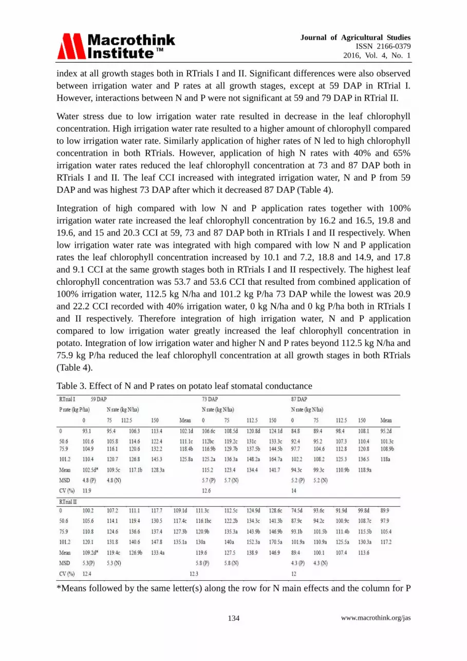
Journal of Agricultural Studies
ISSN 2166-0379
2016, Vol. 4, No. 1
www.macrothink.org/jas 134
index at all growth stages both in RTrials I and II. Significant differences were also observed
between irrigation water and P rates at all growth stages, except at 59 DAP in RTrial I.
However, interactions between N and P were not significant at 59 and 79 DAP in RTrial II.
Water stress due to low irrigation water rate resulted in decrease in the leaf chlorophyll
concentration. High irrigation water rate resulted to a higher amount of chlorophyll compared
to low irrigation water rate. Similarly application of higher rates of N led to high chlorophyll
concentration in both RTrials. However, application of high N rates with 40% and 65%
irrigation water rates reduced the leaf chlorophyll concentration at 73 and 87 DAP both in
RTrials I and II. The leaf CCI increased with integrated irrigation water, N and P from 59
DAP and was highest 73 DAP after which it decreased 87 DAP (Table 4).
Integration of high compared with low N and P application rates together with 100%
irrigation water rate increased the leaf chlorophyll concentration by 16.2 and 16.5, 19.8 and
19.6, and 15 and 20.3 CCI at 59, 73 and 87 DAP both in RTrials I and II respectively. When
low irrigation water rate was integrated with high compared with low N and P application
rates the leaf chlorophyll concentration increased by 10.1 and 7.2, 18.8 and 14.9, and 17.8
and 9.1 CCI at the same growth stages both in RTrials I and II respectively. The highest leaf
chlorophyll concentration was 53.7 and 53.6 CCI that resulted from combined application of
100% irrigation water, 112.5 kg N/ha and 101.2 kg P/ha 73 DAP while the lowest was 20.9
and 22.2 CCI recorded with 40% irrigation water, 0 kg N/ha and 0 kg P/ha both in RTrials I
and II respectively. Therefore integration of high irrigation water, N and P application
compared to low irrigation water greatly increased the leaf chlorophyll concentration in
potato. Integration of low irrigation water and higher N and P rates beyond 112.5 kg N/ha and
75.9 kg P/ha reduced the leaf chlorophyll concentration at all growth stages in both RTrials
(Table 4).
Table 3. Effect of N and P rates on potato leaf stomatal conductance
*Means followed by the same letter(s) along the row for N main effects and the column for P

Journal of Agricultural Studies
ISSN 2166-0379
2016, Vol. 4, No. 1
www.macrothink.org/jas 135
rates are not significantly different at P≤0.05 according to Tukey’s Studentized Range Test.
Some interactions were not significant. DAP = Days after Planting, MSD = Minimum
Significant Difference. Mean separation was done within each season.
Table 4. Effect of irrigation water, N and P rates on potato leaf chlorophyll content index
RTrial I CCI at 59 DAP CCI at 73 DAP CCI at 87 DAP
P rate (kg P/ha) P rate (kg P/ha) P rate (kg P/ha)
kg N/ha 0 50.6 75.9 101.2 0 50.6 75.9 101.2 0 50.6 75.9 101.2
Irri
gat
ion
wat
er r
ate
(%
FC
)
10
0%
0 26.6d* 33.6c 35.9b 38.2a 33d 39.8c 42.2b 46.8a 22.6c 28.6b 29.7b 32.7a
75 30.3c 35.2b 36.2b 38.9a 37.1d 42.1c 45.2b 49.3a 26.5c 29.6b 29.8b 33.8a
112.5 33.1d 36.6c 39.2b 43.2a 40.5d 46.6c 51.4b 53.7a 29.5c 30.3c 32.2b 36.4a
150 35.3d 38.6c 40.5b 42.8a 41.4d 44.5c 49.2b 52.8a 27.5d 30.6c 35.2b 37.6a
65%
0 27.4d 29.5c 32.2b 34.8a 30.1c 35.3b 36.2b 41.9a 23.1c 23.6c 26.1b 30.1a
75 29.4d 31.7c 33.8b 36.4a 34c 38.9b 40.2b 45.4a 23.2c 27.4b 28.6b 31.4a
112.5 31d 33.7c 39.4b 42.7a 35.5c 42.4b 48.9a 48.8a 26.1c 31b 34.6a 34.4a
150 31.8d 35.9c 41.4a 38.6b 37d 42.2c 48.3a 45.7b 26.1d 29.3c 35.6a 32.9b
40%
0 23.6d 28.8c 30.4b 33.6a 29.2c 30.9b 35.7a 36.8a 20.9c 22.7b 26.3a 26.3a
75 27.3c 30.4b 33.4a 33.9a 30.9c 36.6b 40.2a 39.7a 22.7c 24.3b 27.9a 28.3a
112.5 28.9c 30.4b 33.2a 33.2a 36.1c 39.9b 47.1a 48a 25.5c 26.5c 38.7a 36.7b
150 27.8c 32.5b 36.9a 33.7a 37.2d 41.6c 47.7a 40.3b 25.5c 27.3b 31a 27.5b
MSD 1.1 (N,P) 0.9 (W) 1.5 (N,P) 1.2 (W) 1.1(N,P) 0.8 (W)
CV (%) 16.2 18.1 18.2
RTrial II
Irri
gat
ion
wat
er r
ate
(% F
C)
10
0%
0 29.4d 35.1c 37.5b 39.5a 32.9c 41.7b 42.7b 47.8a 25.7c 28.8b 29.7b 34.1a
75 32d 36.6c 38.1b 39.9a 36.9d 44.6c 47.4b 51.4a 29.2c 31.3b 32.1b 35.7a
112.5 32.6d 36.9c 39.7b 42.5a 42.8c 49.2b 49.9b 53.6a 31c 32.6b 33.5b 35a
150 36.5d 39c 41.6b 45.9a 43.9d 48c 51.1a 52.5a 29.5d 32.6c 39.7b 46a
65%
0 28.6d 31.2c 32.5b 36.2a 31.8d 37.6c 44b 45.9a 23.7c 25.8b 28.8a 29.5a
75 29.9d 33.6c 34.7b 38.7a 35.4d 38.5c 46.2b 47.9a 24.9d 28.1c 29.9b 31.5a
112.5 33.6d 36.1c 37.6b 39.6a 41.8c 44.4b 45.7b 48.5a 27.9d 31.4c 32.6a 33.3a
150 28.8d 32c 38.2b 40.3a 37.9d 45.8c 47.6b 50.6a 25.3d 28.8c 36.7a 32.9b
40%
0 27.9c 30.9b 31.7b 33.7a 30b 31.5b 38.2a 37.70 22.2d 23.9c 29.1a 27.8b
75 28.7c 31.5b 35.6a 35.7a 31.7c 37b 40.3a 41.6a 24.6d 26.7c 30.7a 28.1b
112.5 29.9d 31.7c 35.7a 34.1b 35.7d 38.9c 41.8b 44.9a 24.5c 26.1b 31.3a 30.5a
150 28.9d 32.6c 38.3a 35.1b 39.3b 43.8a 43.7a 42.7a 26.5c 28.8b 30.2a 28.2b
MSD 1.1 (N,P) 0.9 (W) 1.6 (N,P) 1.3(W) 1.1(N,P) 0.8(W)
CV (%) 15.5 18.9 17.5
*Means followed by the same letter(s) along the row at the same DAP and irrigation water
and N rate are not significantly different at P≤0.05 according to Tukey’s Studentized Range
Test. FC = Field Capacity, DAP = Days after Planting, MSD = Minimum Significant
Difference. Mean separation was done within each season.

Journal of Agricultural Studies
ISSN 2166-0379
2016, Vol. 4, No. 1
www.macrothink.org/jas 136
4. Discussion
In Kenya, farmers grow seed potato during the rainy season using fertilizer rates of
commercial potato production. In this study, 100% irrigation water rate represented a normal
rainy season, and fertilizer rates were varied from zero to recommended commercial potato
production rates. In the present study, potato plants supplied with high irrigation water, N and
P rates had larger LAI, higher leaf stomatal conductance and chlorophyll content index.
Potatoes supplied with 100% irrigation water had better growth and development compared
to those supplied with 65%, which had intermediate and those supplied with 40% rate had the
least.
It is possible that low irrigation water led to droughty conditions and water stress within the
potato plant, which possibly resulted in low LAI, stomatal conductance and chlorophyll
content index and consequently reduced photosynthetic activity. Plants under water stress
have been reported to show a decrease in leaf conductance (Obidiegwu et al., 2015), total
area of leaves (Albiski et al., 2012), reduced plant chlorophyll content (Anithakumari et al.,
2012), and the photosynthesis rate (Li et al., 2015).
Loggini et al. (1999), and Apel and Hirt (2004) reported that drought inhibits or slows down
photosynthetic carbon fixation mainly through limiting the entry of CO2 into the leaf or
directly inhibiting metabolism. Probably potato supplied with high compared to low irrigation
water experienced higher rates of leaf stomatal conductance, which lead to high metabolism
and consequently greater chlorophyll content index. Chlorophyll is the key pigment involved
in the primary reactions of photosynthesis which is the global biological process that provides
primary biomass and energy for almost all living beings (Shpilyov et al., 2013). High
chlorophyll content index might have led to higher photosynthetic activity within the potato
supplied with high irrigation water. Van der Zaag (1992) reported that insufficient water
supply reduces foliage growth and efficiency in use of intercepted light by reducing the rate
of photosynthesis, and consequently stimulating maturity through death of the leaves. This
possibly explains why potato plants supplied with low irrigation water, N and P mineral
nutrients attained lower stomatal conductance, chlorophyll content and consequently reduced
total dry matter (biomass) accumulation as indicated by the least LAI.
Nitrogen and phosphorus are crucial elements required for different roles in potato plant
growth and development. Low N and P probably impaired potato plant growth and
development, leading to low leaf stomatal conductance and chlorophyll accumulation.
Chlorophyll traps light and transfers energy for driving photochemical reactions (Yadav et al.,
2010) and photosynthetic activity is related to the content of the photosynthetic pigment,
chlorophyll (Maclntyre et al., 2002; Huang et al., 2014). Therefore, amount of irrigation
water, N and P applied was an important factor in determining the rate of growth and
development of potato plant. It was observed that the key to potato plant growth and
development depended on establishment of a large LAI that is durable through the
reproductive phase. This was achieved through high irrigation water, N and P rates. Early
foliage development due to high irrigation water, N and P rates indicated by high LAI
possibly lead to a high interception of solar radiation and radiation use efficiency (RUE),

Journal of Agricultural Studies
ISSN 2166-0379
2016, Vol. 4, No. 1
www.macrothink.org/jas 137
mainly due to the greater photosynthetic surface area of the resultant potato crop.
Stalham and Allison (2012) reported that RUE was increased by irrigating and that this was
also associated with significant increase in total dry matter and tuber yield compared with
non-irrigated plots. Therefore, LAI could be a significant feature in determining
photosynthetic activity. Kara and Mujdeci (2010) reported that LAI is a key structural
characteristic of plants due to the role green leaves play in controlling many biological and
physical processes in plant canopies. The increased LAI due to high irrigation water, N and P
rates could have resulted in increased photosynthetic capacity and supply of assimilates
necessary for high growth and development. Elsewhere, N has also been reported to increase
the total chlorophyll content, meristematic cells and growth, leading to the formation of
branches in addition to leaf expansion (Tabassum et al., 2013). The low stomatal
conductance and chlorophyll content observed in potato plants that received low irrigation
water, N and P rates could have lead to low LAI and consequently to low interception of solar
radiation and hence low photosynthetic capacity to support potato plant growth.
Photosynthesis in plants has been reported to be as a result of interaction among different
factors like carbon dioxide concentration, ambient temperature, chlorophyll content, and
water and nutrient supply, which influence LAI (Tabassum et al., 2013).
Overall greater LAI was observed with high irrigation water, N and P rates. However,
treatments which received high irrigation water together with low N and P rates and
vice-versa did not record greater LAI. This suggests that the effect of irrigation water, N or P
was closely related to the ability of potato plant to utilize them from the soil. Waraich et al.
(2011) reported that when water inside the plant declines below a threshold level, stomata
close and decrease transpiration rate resulting in reduction in water transport through the
plant, consequently affecting roots ability to absorb water and nutrients as effectively as
supposed to be done under normal transpiration. Therefore, it is possible that normal
transpiration required certain amounts of irrigation water below which the high N or P rates
cannot lead to greater potato growth and development. It therefore seems there is a
synergistic relationship between the irrigation water, N and P rates towards potato growth and
development. Probably, availability of N and P to the potato crop depends on the amount of
irrigation water supplied. Furthermore, the utilization of the applied irrigation water by the
potato crop depends on the amount of N or P applied.
Segal et al. (2000) reported that high irrigation amounts and frequency provide desirable
conditions for water movement in soil and uptake by roots. However, it is possible that under
moisture stress conditions resulting from low irrigation water rate, mobility of N and P was
interfered with and therefore curtailing the benefits of these mineral nutrients. Najm et al.
(2010) reported that increased N fertilizer can increase N uptake for a positive effect on
chlorophyll content, photosynthetic rates, leaf expansion, total number of leaves and dry
matter accumulation. Similarly, in this study, high irrigation water, N and P rates could have
increased water, N and P uptake by the potato plant which led to a positive effect on leaf
stomatal conductance, chlorophyll content, LAI, and total biomass accumulation. Kumar et al.
(2013) reported that the increased dry matter production when inorganic and organic minerals
are applied is attributable to higher photosynthetic activity and translocation of
Journal of Agricultural Studies
ISSN 2166-0379
2016, Vol. 4, No. 1
www.macrothink.org/jas 138
photosynthates. This probably explains why low potato growth and development was
observed where low irrigation water together with high N or P rates were applied.
5. Conclusion and Recommendations
The overall combination of irrigation water, N and P rates affects soil moisture and nutrient
content during the potato growing period. This result influences the physiological status of
the potato plants, including leaf expansion capacities, stomatal conductance and chlorophyll
content. Integration of high irrigation water at 100%, N and P rates at 150 kg N/ha and
101.2 kg P/ha increases potato physiological activities that enhances greater growth and
development rates. It is recommended to avoid low irrigation water rates at 40% FC and low
N and P rates at 0 kg N/ha and 0 kg P/ha due to their potential negative effects on seed potato
growth and development.
Acknowledgements
The authors acknowledge the support given by National Commission for Science,
Technology and Innovation in funding this study, Egerton University for logistical support,
Joseph Muya Githaiga for maintaining the trial and Julia Muthoni Ndegwa of USA for
unconditionally assisting in procurement of the Plant Growth Station.
References
Anithakumari, A. M., Nataraja, K. N., Visser, R. G. F., & Van Der Linden, C. G. (2012).
Genetic dissection of drought tolerance and recovery potential by quantitative trait locus
mapping of a diploid potato population. Mol. Breed, 30, 1413–1429.
HTTP://DX.DOI.ORG/10.1007/s11032 -012-9728-5
Albiski, F., Najla, S., Sanoubar, R., Alkabani, N., & Murshed, R. (2012). In vitro screening of
potato lines for drought tolerance. Physiol. Mol. Bio. Plants, 18, 315–321. http://dx.doi.org/
10.1007/s12298-012-0127-5
Apel, K. & H. Hirt. (2004). Reactive oxygen species: Metabolism, oxidative stress, and signal
transduction. Annual Review of Plant Biology, 55, 373-399. http://dx.doi.org/
10.1146/annurev.arplant.55.031903.141701
Beedle, C. L. (1987). Plant growth analysis techniques of bioproductivity and photosynthesis.
2nd ed. J. Coombs, D. Hall., S. Lang and Sucrlock, J. (eds.). Pergamon Press, Oxford, 21-23.
http://dx.doi.org/10.1016/B978-0-08-031999-5.50011-X
Biman, D., Mayukh, G., Banani, D., & Bimal, D. (2014). Stomatal Conductance of Potato
Grown under Sub-tropical Conditions. International Journal of Bio-resource and Stress
Management, 5(1), 007-011. http://dx.doi.org/10.5958/j.0976-4038.5.1.002.
Bowen, W. T. (2003). Water productivity and potato cultivation, p. 229-238. In: J.W. Kijne, R.
Barker, & Molden, D. (eds.). Water Productivity in Agriculture: Limits and Opportunities for
Improvement. CAB International, Wallingford, UK.
Braun, H., de Castro Silva, M. C., Fontes, P. C. R., Coelho, F. S., & Cecon, P. R. (2015).
Top-dressing nitrogen management decision in potato using the “UFV-80” color chart and
SPAD readings. African Journal of Agricultural Research, 10(35), 3494-3501.
http://dx.doi.org/ 10.5897/ajar2015.9813
Burhan, M., Aslam, K., Irfanullah, M., Ishfaq, M., & Ehsan, J. M. (2007). Comparison of

Journal of Agricultural Studies
ISSN 2166-0379
2016, Vol. 4, No. 1
www.macrothink.org/jas 139
seed potato produced from different rapid multiplication sources against PVX, PVY and PVS
through ELISA. Journal of Agricultural Research, 45(1):67-73.
Chaves, M. M., Pereira, J. S., Maroco, J., Rodrigues, M. L., Ricardo, C. P. P., Osório, M. L.,
Carvalho, I., Faria, T., & Pinheiro, C. (2002). How plants cope with stress in the field:
photosynthesis and growth. Ann Bot 89, 907–916. http://dx.doi.org/10.1093/aob/mcf105.
Cornic, G. (2000). Drought stress inhibits photosynthesis by decreasing stomatal aperture –
not by affecting ATP synthesis. Trends Plant Sci, 5, 183–221.
http://dx.doi.org/ 10.1016/s1360-1385(00)01625-3
Department of Agriculture, Forestry and Fisheries (DAFF). (2013). Directorate Plant
Production Division: Vegetables, Pretoria, Republic of South Africa. 52.
Gitelson, A. A., Gritz, Y., & Merzlyak, M. N. (2003). Relationships between leaf chlorophyll
content and spectral reflectance and algorithms for non-destructive chlorophyll assessment in
higher plant leaves. Journal of Plant Physiology, 160, 271–282.
Hawkesford, M. J. (2012). Improving Nutrient Use Efficiency in Crops. In: John Wiley &
Sons Ltd, Chichester. http://dx.doi.org/ 10.1002/9780470015902.a0023734.
Huang, W. D., Lin, K. H., Hsu, M. H., Huang, M.Y., Yang, Z.W., Chao, P. Y., & Yang, C. M.,
(2014). Eliminating interference by anthocyanin in chlorophyll estimation of sweet potato
(Ipomoea batatas L.) leaves. Botanical Studies.
International Centre for Insect Physiology and Ecology (ICIPE). (2006). The organic farmer.
The magazine for sustainable agriculture in Kenya. ICIPE. Nairobi. Kenya. No. 14 June 2006.
8 pp.
Kara, B., & Mujdeci, M. (2010). Influence of late-season nitrogen application on chlorophyll
content and leaf area index in wheat. Science Research Essays, 5(16), 299-2303.
Kim, H. H., Goins, G. D., Wheeler, R. M., & Sager, J. C. (2004). Stomatal conductance of
lettuce grown under or exposed to different light qualities. Annals of Botany, 94, 691–697.
http://dx.doi.org/ 10.1093/aob/mch192
Kiziloglu, F. M., Sahin, U., Tune, T., & Diler, S. (2006). The effect of deficit irrigation on
potato evapotranspiration and tuber yield under cool season and semiarid climatic conditions.
Journal of Agronomy, 5, 284-288. http://dx.doi.org/ 10.3923/ja.2006.284.288
Kumar, C. V., Prakash, S. S., Prashantha, G. M., Kumar, M. B. M., Lohith, S., &
Chikkaramappa, T. (2013). Dry matter production and yield of potato as influenced by
different sources and time of fertilizer application and soil chemical properties under rainfed
conditions. Research Journal of Agricultural Science, 4(2), 155-159.
Li, J., Cang, Z., Jiao, F., Bai, X., Zhang, D., & Zhai, R. (2015). Influence of drought stress on
photosynthetic characteristics and protective enzymes of potato at seedling stage. Journal of
the Saudi Society of Agricultural Sciences, http://dx.doi.org/10.1016/j.jssas.2015.03.001
Liu, G., Li, Y., Alva, A. K., Porterfield, D. M., & Dunlop, J. (2012). Enhancing nitrogen use
efficiency of potato and cereal crops by optimizing temperature, moisture, balanced Nutrients
and oxygen bioavailability. Journal of Plant Nutrition, 35, 428–441. http://dx.doi.org/
10.1080/01904167.2012.639922
Loggini, B., Scartazza, A., Brugnoli, E., & Navari-Izzo, F. (1999). Antioxidative defence

Journal of Agricultural Studies
ISSN 2166-0379
2016, Vol. 4, No. 1
www.macrothink.org/jas 140
system, pigment composition, photosynthetic efficiency in two wheat cultivars subjected to
drought. Plant Physiology, 119, 1091-1099.
Maclntyre, H. L., Kana, T. M., Anning, T., & Geider, R. J. (2002). Photoacclimation of
photosynthesis irradiance response curves and photosynthetic pigments in microalgae and
cyanobacteria. J. Phycology, 38(1), 17-38.
http://dx.doi.org/10.1046/j.1529-8817.2002.00094.x
Najm, A., Haj Seyed Hadi, M. R., Fazeli, F., Taghi Darzi, M., & Shamorady, R. (2010). Effect
of utilization of organic and inorganic nitrogen source on the potato shoots dry matter, leaf
area index and plant height, during middle stage of growth. World Academy of Science,
Engineering and Technology, 47, 900-903.
Naveed, A., Asif, A., Khan, A. A., & Rau, S. (2012). The Potential of Breeding Okra
( Abelmoschus esculentus L.) for Water Stress Tolerance. In: Ashraf, M., Öztürk, M.,
Ahmad, M.S.A and A. Aksoy. Crop Production for Agricultural Improvement. Springer,
Dordrecht Heidelberg, New York, London, 796.
http://dx.doi.org/ 10.1007/978-94-007-4116-4_8
Obidiegwu, J. E., Bryan, G. J., Jones, H.G., & Prashar, A. (2015). Coping with drought: stress
and adaptive responses in potato and perspectives for improvement. front. plant sci. 6:542.
http://dx.doi.org/ 10.3389/fpls.2015.00542
Raschke, K. (1975). Stomatal action. Annual review of plant physiology, 26: 309–340.
http://dx.doi.org/ 10.1146/annurev.pp.26.060175.001521
Roy, R. N., Finck, A., Blair, G. J., & Tandon, H. L. S. (2006). Plant nutrition for food security:
A guide for integrated nutrient management. Food and Agriculture Organisation of the United
Nations, Fertiliser and Nutrition Bulletin. Rome, Italy, 348.
SAS Institute Inc. (2011). The SAS system for Windows. SAS Institute Inc., Cary, NC, USA
Sawicka, B., Michalek, W. And P. Pszczolkowski. (2015). The relationship of potato tubers
chemical composition with selected physiological indicators. Zemdirbyste Agriculture, 102
(1), 41-50. http://dx.doi.org/10.13080/z-a.2015.102.005
Segal, E., Ben-Gal, A., and U.Shani. (2000). Water availability and yield response to
high-frequency micro-irrigation in sunflowers. In: Proceedings of the Sixth International
Micro-irrigation Congress on ‘Micro-irrigation Technology for Developing Agriculture’,
Conference Papers, 22–27 October, South Africa.
Shpilyov, A. V., Vladislav, V. Z., Bernhard, G., & Lokstein, H. (2013). Chlorophyll a
phytylation is required for the stability of photosystems I and II in the cyanobacterium
Synechocystis PCC 6803. The Plant J. 73:336-346. http://dx.doi.org/10.1111/tpj.12044.
Sinfield, J. V., Fagerman, D., & Colic, O. (2010). Evaluation of sensing technologies for on
the go detection of macro-nutrients in cultivated soils. Computers and Electronics in
Agriculture, 70, 1-18. http://dx.doi.org/10.1016/j.compag.2009.09.017
Stalham, M. A., & Allison, M. F. (2012). Improving water use efficiency through
understanding soil and plant water balance. Final Report, Reporting Period: 2008-2011, Ref:
R406. Report No: 2012/2. Potato Council, Agriculture & Horticulture Development Board,
Steleigh Park, Kenilworth, Warwickshire, UK, 155.

Journal of Agricultural Studies
ISSN 2166-0379
2016, Vol. 4, No. 1
www.macrothink.org/jas 141
Tabassum, D., Akhtar, A., & Inam, A. (2013). Effect of waste water irrigation on growth,
physiology, and yield of mustard. International Journal of Botany and Research, 3(1):27-34.
Thompson, A. J., King, J. A., Smith, K. A., & Don, H. T. (2007). Opportunities for reducing
water use in agriculture. Defra Research Project Final Report for WU0101.
Tremblay, N., Fallon, E., & Ziadi, N. (2011). Sensing of crop nitrogen status: Opportunities,
tools, limitations, and supporting information requirements. Hortic. Technol. 21:274-281.
http://horttech.ashspublications.org/content/21/3/274.full.pdf+html
Van Der Zaag, D. E. (1992). Potatoes and Their Cultivation in the Netherlands. Directorate
for Agricultural Research, NIVAA (Netherlands Potato Consultative Institute), Wageningen,
The Netherlands.
Van Der Zaag, P. (1981). Soil fertility requirements for potato production. Technical
information bulletin, No. 14. CIP, Lima, Peru.20.
Walingo, A. M., Lung’aho, C., Ng’ang’a, N., Kinyae, P. M., & Kabira, J. N. (2004). Potato
marketing, storage, processing and utilization in Kenya. In: Hanafi, A. (Ed.). Proceeding of
Sixth Triennial Congress of the African Potato Association held at Agadir Morocco from 5-10
April 2004.
Waraich, E. A., Amad, R., Ashraf, M. Y., Saifullah, M., & Ahmad, M. (2011). Improving
agricultural water use efficiency by nutrient management. Acta Agriculture Scandi – Soil &
Plant Science, 61(4), 291-304. http://dx.doi.orG/10.1080/09064710.2010.491954.
Yadav, S. P., Ibaraki, Y., & Gupta, S. D. (2010). Estimation of the chlorophyll content of
micropropagated potato plants using RGb based image analysis. Plant cell tiss. organ cult.
100:183-188. http://dx.doi.org/ 10.1007/s11240-009-9635-6.
Copyright Disclaimer
Copyright for this article is retained by the author(s), with first publication rights granted to
the journal.
This is an open-access article distributed under the terms and conditions of the Creative
Commons Attribution license (http://creativecommons.org/licenses/by/3.0/).

Journal of Agricultural Studies
ISSN 2166-0379
2016, Vol. 4, No. 1
www.macrothink.org/jas 142
Analyzing the Linkage between Agricultural Exports
and Agriculture’s Share
of Gross Domestic Products in South Africa
Mushoni B. Bulagi (Corresponding author)
Senior Researcher, Centre for Science, Technology and Innovation Indicators, Human
Science Research Council
Jan J. Hlongwane
Senior Lecturer, Department of Agricultural Economics and Animal Production, University
of Limpopo
Abenet Belete
Professor, Senior Lecturer: Department of Agricultural Economics and Animal Production,
University of Limpopo
Received: December 22, 2015 Accepted: January 6, 2016 Published: January 23, 2016
doi:10.5296/jas.v4i1.8918 URL: http://dx.doi.org/10.5296/jas.v4i1.8918
Abstract
The paper analyses the link between avocado, apple, mango and orange exports and
agriculture’s share of Gross Domestic Product in South Africa. The study used secondary
time series data that covered a sample size of 20 years (1994 - 2014) of avocado, apple,
mango and orange exports in South Africa. Two Stages Least Square models were used for
data analysis. Empirical results for agricultural exports equation revealed that agricultural
economic growth in South Africa was significant with a positive coefficient. Also a negative
relationship between the Net Factor Income (NFI) and the agricultural exports in South
Africa was noticed. Real Capital Investments had a significant positive coefficient.
Consequently, results from agricultural economic growth equation revealed that agricultural
exports were significant with a positive correlation. A relationship between NFI and
agricultural GDP was also witnessed. Like other variables, Real Capital Investment was
significant but negatively correlated.
Keywords: agricultural exports, agricultural GDP, exports policy, agricultural trade, South
African agriculture

Journal of Agricultural Studies
ISSN 2166-0379
2016, Vol. 4, No. 1
www.macrothink.org/jas 143
1. Introduction
1.1 Background
South Africa’s agricultural sector is dualistic: a developed commercial farming sector
co-exists with a large number of small-scale farms. South African agriculture is increasingly
export-oriented with approximately one third of total production exported. Although reforms
of agricultural policies has also been initiated, changes in South African agriculture policies
in the past decade have been shaped by substantial macroeconomic and social reforms
implemented during the mid-1900s to date. According to (Organisation for Economic
Co-operation and Development, 2006) such policies included the deregulation of the
marketing of agricultural products, abolishing certain tax concessions favoring the sector,
reductions in budgetary expenditure on the sector, land reform, and trade policy reform. The
opening of the agricultural sector after 1996 placed South Africa among the world’s exporters
of agro-food products such as wine, fresh fruit and sugar. South Africa is also an important
trader of agricultural exports in Africa. In the global market, Europe is by far the largest
destination, absorbing almost one half of the South African agricultural exports. Imports were
also growing but less rapidly than exports (DAFF, 2012).
The South African Gross Domestic Product (GDP) increased from 2.9% to 3.1% while
agriculture contributes less than 3% to the share of GDP (DAFF, 2012). Wine and fruit
production has seen the most dynamic development in the past ten years with a large share of
total output exported, mainly to Europe. Agricultural products, particularly those with export
potential, have been viewed by many underdeveloped nations around the globe as playing a
vital role in economic development. The debate on the relationship between agricultural
export and agricultural GDP has exhibited considerable interest in the field of development
economics. Several empirical studies (Xu, 1996; Tyler, 1981; Shirazi and Manap, 2004;
Faridi, 2012) were conducted to assess the role of exports towards the economic growth of
developing countries from various aspects. While the true measure of these nations’
development needs to be expressed through improvements in the standard of living of the
people, their economic growth plays a significant part in this process by providing increased
per capita income, increased revenue for government sponsored social services and leading to
export led-growth. Relatively recent studies [Tiffin and Irz (2006); Memon et al., (2008);
Shombe (2008); Sanjuan-Lopez and Dawson (2010); Raza et al., (2012); Faridi (2012)], have
their main emphasis on causality between export growth and economic growth. This has been
adopted in a number of recent studies designed to assess whether or not individual countries
exhibit evidence for export-led growth hypothesis using time series data. The major
disadvantage of these causality test results is that the Granger or Sims tests used in these
studies are only valid if the original time series are co-integrated.
The opportunity to expand exports is a key determinant of the prospects for economic growth
in developing countries. Regardless of whether or not exports drive economic growth, one of
the primary aims of any country’s economic policy includes trade, industry policy and
internationally competitive sectors which contribute to job creation. It is within this
framework that the linkage between avocado, apple, mango and orange exports and
agriculture’s share of GDP needs to be studied and also its roles in economic development in
South Africa need to be assessed. Literature [Katircioglu (2006); Shombe (2008), Khalafalla

Journal of Agricultural Studies
ISSN 2166-0379
2016, Vol. 4, No. 1
www.macrothink.org/jas 144
and Webb (2001)] on economic development and growth discusses the relationship between
exports and economic growth. This group of studies found correlation between these two
variables and better support an export led-growth hypothesis.
The role of agricultural exports to agriculture’s share of Gross Domestic Product (GDP) in
South Africa is of extreme importance and exhibit strong interest from all parts of the
economy. Many believe that agriculture can salvage the declining economic growth under
such global economic conditions. The decision to diversify and expand exports of these
produce will improve the unstable South African economy. This is a result of the effect of
agricultural export diversity and it’s expectation to provide economic development and
sustainable finances needed. It is necessary for the study to focus on an individual in order to
account for all the factors that are truly unique to a nation’s economy. Therefore, the study
will help to shift the focus of avocado, apple, mango and orange growers to export more due
to the international market demand for such produce.
1.2 Purpose and objectives of the study
The purpose of the study was to analyse the link between agricultural exports and
agriculture’s share of gross domestic products in South Africa. The specific objectives of the
study were to :
(i) determine the correlation between avocado, apple, mango and orange exports and the
agriculture’s share of Gross Domestic Product in South Africa and
(ii) investigate the contribution of avocado, apple, mango and orange exports to agriculture’s
share of Gross Domestic Product in South Africa.
1.3 Hypotheses of the study
(i) there is no correlation between avocado, apple, mango and orange exports and the
agriculture’s share of Gross Domestic Product in South Africa and
(ii) there is no contribution of avocado, apple, mango and orange exports to agriculture’s
share of Gross Domestic Product in South Africa.
2. Avocado, apple, mango and orange exports in South Africa
In the past five years tonnes of avocado, apple, mango and orange have been exported to
different destinations, and these exports face competition in the markets.

Journal of Agricultural Studies
ISSN 2166-0379
2016, Vol. 4, No. 1
www.macrothink.org/jas 145
Figure 1. Avocado, apple, mango and orange exports in tonnes from 2007 to 2011
Source : DAFF (2012)
Figure 1 shows flactuating exported tonnes over the past five years and does not have room
for mango exports due to low export volumes, with the highest tonnes reached in 2007. It is
worthwhile to note that should the share of other exports increasing with lower volumes,
avocado exports rise with very big volume due to favourable climatimacal conditions and its
market share.
3. Data and Methodology
3.1 Study area and sampling technique
The study of the impact analysis of the linkage between avocado, apple, mango and orange
exports to agriculture’s share of Gross Domestic Products was conducted in South Africa.
The study used the secondary time series data that were obtained from Department of
Agriculture, Fishery and Forestry Statistical Directorate and Statistics South Africa. The
study used a sample size of 20 years (1994 – 2014) of avocado, apple, mango and orange
exports in South Africa. Data was broken into four sub sectors i.e. Agricultural exports,
Agricultural Economic Growth, Net Factor Income and Real Capital Income. Agricultural
exports covered avocado, apple, mango and orange exports. These exports were expressed
physically in monetary value and tonnes. Agriculture GDP, NFI and INV were expressed in
percentage. The data were lagged at two, to avoid stationary using the Augmented
Dickey-Fuller test. This test was run independently from the models used to analyse data in
order to show the ability of secondary time series data to address objectives of the study.
3.2 Analytical technique
The study used the Two-stage Least Square (2SLS) model to determine the relationship
between avocado, apple, mango and orange exports and agriculture’s share of Gross

Journal of Agricultural Studies
ISSN 2166-0379
2016, Vol. 4, No. 1
www.macrothink.org/jas 146
Domestic Products in South Africa from 1994 to 2014. The Statistical Package for Social
Sciences (SPSS) 22.0 was used to analyse. The 2SLS model assumes that agricultural
economic growth is simultaneously determined along with avocado, apple, mango and orange
exports. As proposed by Davidson and McKinnon (1981), the J-test was used in the process
of model selection, and only statistically significant variables were included in the two stage
least square system equation. This assures that the model is specifically tailored to suit the
South African agricultural economic growth. The two stage least squares systems approach
was used to estimate the equations in this study in order to avoid simultaneity bias. The
selected model for this study has a system of two simultaneous equations determining
agricultural economic growth and avocado, apple, mango and orange exports of South Africa.
General models
Avocado, apple, mango and orange exports equation:
log (Xa) t = β
1 log (β
1)
t + β
2 log (β
2)t-1
+ β3 log (β
3)t-2
+ U ……………………..1
Agricultural economic growth equation:
log (AGE) t = β
1 log (β
1)
t + β
2 log (β
2)t-1
+ β3
log (β3)t-2
+ U ………………...............2
Specific models
Avocado, apple, mango and orange exports equation:
log (Xa) t-1
= 0 + AGE log(AGE)t +NFI log(NFI)
t-1 +INV log(INV)
t-2 + U…................3
Agricultural economic growth equation:
log (AGE) t-2
= 0 + Xa log(Xa)t-2
+NFI log(NFI)t-2
+ INV log(INV)t-2
+ U ……………4
Xa represents avocado, apple, mango and orange exports; AGE represents agricultural
economic growth; NFI and INV represents Net Factor Income and Real Capital Investments
which are all coefficients; t is the time factor and U is the disturbance term.
4. Empirical Results and Discussion
Table 1. Correlation matrixes of agricultural GDP and agricultural exports
Variables Correlation Co-efficient Significance(2-tailed) Avocado - 0.558** 0.001 GDP 1.000 1.000 Apple - 0.399** 0.023 GDP 1.000 1.000 Mango 0.452* 0.010 GDP 1.000 1.000 Orange - 0.739*** 0.000
*, **, *** Correlation is significant at 1%, 5% and 10% levels (2-tailed)
In table 1 above the direction of association that exists between avocado and agriculture’s

Journal of Agricultural Studies
ISSN 2166-0379
2016, Vol. 4, No. 1
www.macrothink.org/jas 147
share of GDP was significant at 10%. This implies a linear correlation between these
variables such that when avocado exports increase the agricultural GDP will also increase or
decrease thus supporting the export-led growth hypothesis. Avocado exports have a negative
coefficient which implies that the avocado exports of the above produce have a negative
influence on the agricultural GDP of South Africa. Due to higher volumes of apple exports
across the borders, the share of apple exports towards agricultural GDP differs with the
avocado’s contribution. This is because of a significant correlation between apple exports and
the agriculture’s share of GDP; hence the export-led growth notion still holds true. These
variables were significant at 5%, which implied that when apple exports increase a decrease
in agriculture’s share of GDP is witnessed.
A very low quantity of mango exports goes over South African borders as a result mango
exports make a limited contribution to the GDP. Table 1 above shows the direction of
association that exists between mango exports and agriculture’s share of GDP which was
significant at 10%. An increase in the mango exports will trigger an increase in agricultural
GDP and this goes to support the export-led growth hypothesis. Orange exports attract most
markets in international trade. In a season, higher volumes of oranges are exported across the
borders; the share of orange exports towards agricultural GDP contribution was positive. This
is because of a significant correlation between orange exports and the agriculture’s share of
GDP like other three produce. This supports the export-led growth hypothesis. Orange
exports were significant at 10%, which implies that when orange exports increase the
agriculture’s share of GDP will decrease.
Table 2. Empirical results of agricultural GDP equation
Variables Co-efficient Standard Error
Wald statistics
Significance
Xa 0.463** 0.422 1.095 0.040 NFI 0.742 0.633 1.172 0.266 INV -0.032*** 0.745 -0.043 0.007 Constant -0.038 0.190 0.199 0.846 - 2 Log likelihood 12.39 Pseudo R square 35% % cases correctly predicted 95.0% Chi – square 20.50
*, **, *** represent significance at 1%, 5% and 10% respectively
Table 2 above shows that agricultural exports are significant at 5% level, this denotes that
when the exports increase the agricultural GDP will also increase hence supporting the
export-led growth hypothesis. Agricultural exports have a positive coefficient which implies
that the exports of the above produce have a positive influence on the agricultural GDP of
South Africa. In most recent studies agricultural export was found to be a factor that matters
most to the agricultural GDP all over the world. There is a positive relationship between the
net factor income and the agricultural GDP of South Africa. Table 1 shows that this variable
does not appear to be significant at any level. The implication of an increase in net factor
income is that there will be an increase in the exports of mangoes from South Africa which
also leads to an increase in the agricultural GDP.

Journal of Agricultural Studies
ISSN 2166-0379
2016, Vol. 4, No. 1
www.macrothink.org/jas 148
Apple, avocado, mango and orange farmers desire results that earn them much needed
foreign currency and to the economist, on the other hand, it would be the law of demand.
Conversely; when the farmer is not exposed to international trade, which heightens exports,
the possibilities of farming for exports and international trade are very slim. Real Captical
Investment as a variable was significant at 10% and has a negative coefficient which means
that money invested by farmers for exporting apple, avocado, mango and orange in South
Africa has a negative influence on the agricultural GDP. This is a result of lack of other funds
which can be used to export more products in the future and also a result of different
investment decisions that may be taken.
Table 3. Empirical results of agricultural exports equation
Variables Co-efficient Standard Error
Wald statistics
Significance
AGE 0.215** 0.191 1.124 0.030 NFI -0.002 0.276 -0.006 0.995 INV 0.237*** 0.266 0.890 0.000 Constant 0.771 0.787 0.980 0.346 - 2 Log likelihood 18.46 Pseudo R square 41.6% % cases correctly predicted 51.4% Chi – square 6.62
*, **, *** represent significance at 1%, 5% and 10% respectively
Increasing GDP is one of the major targets of almost every economy (Shombe, 2008). There
are many ways which can be used to achieve economic growth, and to mention one, exports
have received a notable attention in recent studies. Table 3 shows that the agricultural GDP
of South Africa is significant at five percent level. This implies that an increase in the
agricultural GDP results from an increase of agricultural exports in South Africa hence
leading to the export-led growth hypothesis. The agricultural GDP of South Africa has a
positive coefficient and it means that the country’s agricultural GDP can somewhat benefit
from the exports of avocados, apples, mangoes and oranges.
There is a negative relationship between the net factor income and the apple, avocado, mango
and orange exports in South Africa. Table 3 above shows that this variable does not appear to
be significant at any level. This implies that if the net factor income increases there will be a
decrease in the exports of mangoes in South Africa hence a decline in the agricultural GDP.
This will be a result of excessive spending of farmers that export apple, avocado, mangoes
and orange in respect to other international markets which leads to a negative balance of
payments hence a negative GDP. Most authors who found a positive relationship between
exports instability and economic growth argue that if we assume risk-averse behaviour,
uncertainty about export earnings can lead to a reduction in consumption and in turn, an
increase in saving and investment and thus economic growth (Sinha, 1999). Furthermore,
table 3 above shows that this variable is significant at ten percent and has a positive
coefficient which means that money invested by farmers exporting mangoes in South Africa
have a positive influence on the agricultural GDP. This will be a result of much needed
interest and other benefits that are earned from other investments (physical and monetary

Journal of Agricultural Studies
ISSN 2166-0379
2016, Vol. 4, No. 1
www.macrothink.org/jas 149
from these exports).
The relationship between agricultural GDP and apple, avocado, mango and orange exports in
South Africa was demonstrated by the estimated parameter for the independent agricultural
exports variable in the GDP equation and by the estimated parameter for GDP growth in the
agricultural exports. In the Two-Staged Least Square System Approach which estimated the
agricultural GDP, it was found that agricultural export was positive and statistically
significant at a level of five percent. According to this model, a five percent increase in
agricultural exports would ultimately result in examined in a variety of ways. In this quest the
agricultural exports equation was drawn into the study. This equation helped to analyse the
link between agricultural exports and agriculture’s share of GDP in South Africa. The
estimation of two among all three variables was positive and significant at one and five
percent while the other variable was negative and not significant at any level. The positive
estimates for the agricultural GDP and the Real Capital Investments which were significant at
ten percent and one percent and positive coefficients respectively.
The consistent positive relation suggests that the positive externalities generated by avocado,
apple, mango and orange exports on the agricultural GDP increase when the share of avocado,
apple, mango and orange exports increases also helped in not rejecting these two hypotheses.
The NFI was negative and not consistent with prior expectations; however the coefficients
were very small, implying that an increase in income remittance on agricultural GDP as a
result of agricultural exports being negative will result in a direct role that was determined in
the agricultural GDP equation. These outcomes draw serious conclusion. In responding to the
last two hypotheses, it was found that agricultural exports in South Africa were influenced by
other factors over the past 20 years. With the possible factor been higher rate of interest
which makes it difficult for farmers to loan money to improve their exports.
The information of this nature is important for the analysis of agricultural economic
development strategies in South Africa. The timing of this information is critical as South
African policy makers now face major economic reforms in a quest for a more export
oriented and stable agricultural economic development. As the South African government is
under pressure to alter the UK Citrus ban, historical land claims and agricultural policies,
understanding the impact of agricultural export for few quantities or exports on GDP growth
will provide important information for policy analysis.
5. Conclusions and Recommendation
The results of this study show that the amount of avocado, apple, mango and orange exports
was positively related to agricultural economic growth. Another point of interest in this study
was that while avocado, apple, mango and orange exports are positive and significantly
related, the magnitude of its coefficient is smaller than the coefficients of Real Capital
Investments. This implies that the agricultural economic growth benefits more from an
exports structure which is rich due to direct investments. It is in this framework that a
positive correlation exists between agriculture economic growth and avocado, apple, mango
and orange exports. It is recommended that investments opportunity in the agricultural sector
need to be investigated because knowledge on such issue is very limited. There are reasons

Journal of Agricultural Studies
ISSN 2166-0379
2016, Vol. 4, No. 1
www.macrothink.org/jas 150
related to this notion which this study did not investigate, but this could be one of the
important issues to investigate. The department of Agriculture, Forestry and Fishery and the
private sector need to join hands and forge a mutual relationship to aid in developing an
agricultural economy atmosphere which can be able to encourage and open doors for more
exports than imports. This can also be done by subsidising farmers with capital to endure
other cost.
References
Davidson, R., & Mackinnon, J. G. (1981). Several Tests for Model Specification in the
Presence of Alternative Hypotheses, Econometrica, Econometric Society, 49, 781 – 793.
DEPARTMENT OF AGRICULTURE, FISHERY AND FORESTRY (DAFF), (2012).
Economic Review of the South African Agriculture. South Africa. Available at
http://www.daff.gov.za/docs/statsinfo/EconReview2012.pdf [accessed :27/10/2015]
Faridi, M. Z. (2012). Contribution of Agricultural Exports to Economic Growth in Pakistan,
Pakistan Journal of Commercial and Social Sciences, 6, 133 – 146.
Katircioglu, S. T. (2006). Causality between Agriculture and Economic Growth in a small
nation under Political isolation: A case from North Cyprus. International Journal of Social
Economics, 33, 331 – 343.
Khalafalla, K.Y., & Webb, A. J. (2001). Export-led Growth and Structural Change: Evidence
from Malaysia, Applied Economics, 33, 1703 – 1715.
Memon, M.H.,Baig, W. S., & Ali, M. (2008). Causal Relationship between Exports and
Agricultural GDP in Pakistan: Applied Economic Research Center, University of Karachi,
paper No 11845.
ORGANISATION FOR ECONOMIC CO-OPERATIVE AND DEVELOPMENT (OECD),
(2006). OECD Review of Agricultural Policies: South Africa, ISNB 92-64-03679-2.
http://www.fanrpan.org/documents/d00456/OECD_review_agricultural_policies_SA.pdf
[accessed: 27/10/2015]
Sanjuan-Lopez, A. I., & Dawson, P. J. (2010). Agricultural Exports and Economic Growth in
Developing Countries: A Panel Cointegration Approach. Journal of Agricultural Economics,
61, 565 – 583.
Shirazi, N.S., & Manap, T. A. A. (2004). Export and Economic Growth Nexus: The case of
Pakistan, Pakistan Development Review, 43, 563 – 581.
Shombe, N. H. (2008). Causality Relationships between Total Exports with Agricultural and
Manufacturing GDP in Tanzania, Institute of Developing Economies, Discussion Paper
No.136.
Sinha, D. (1999). Exports Instability, Investment and Economic growth in Asian Countries: A
Time Series Analysis, Economic Growth Center, Yale University. Center Discussion Paper
No. 799.
Tiffin, R., & Irz, X. (2006). Is Agriculture the engine of Growth, Agricultural Economics,
International Association of Agricultural Economists, 35, 79-89.
Tyler, W.G. (1981). Growth and Export Expansion in Developing Countries: some Empirical

Journal of Agricultural Studies
ISSN 2166-0379
2016, Vol. 4, No. 1
www.macrothink.org/jas 151
evidence. Journal of Development Economics, 9, 121 – 130.
Raza, S. A., Ali, Y., & Mehboob, F. (2012). Role of Agriculture in Economic Growth of
Pakistan. International Research Journal of Finance and economics, 83, 1450 - 2887.
Xu, Z. (1996). On the causality between export growth and GDP growth: An empirical
investigation. The Review of International Economics, 4, 172-184.
Copyright Disclaimer
Copyright for this article is retained by the author(s), with first publication rights granted to
the journal.
This is an open-access article distributed under the terms and conditions of the Creative
Commons Attribution license (http://creativecommons.org/licenses/by/3.0/).

Journal of Agricultural Studies
ISSN 2166-0379
2016, Vol. 4, No. 1
www.macrothink.org/jas 152
Effects of Plant Pattern and Nitrogen Fertilizer on Yield
and Yield Components of Silage Corn Cultivars
Mohammad Hossein Haddadi
Scientific member of Agronomic and Horticulture Crops Research Department, Mazandaran
Agricultural and Natural Resources Research and Education Center, AREEO, Sari,
Iran.Box:48175-556
Masoud Mohseni
Scientific member of Agronomic and Horticulture Crops Research Department, Mazandaran
Agricultural and Natural Resources Research and Education Center, AREEO, Sari, Iran
Received: January 18, 2016 Accepted: January 23, 2016 Published: February 14, 2016
doi:10.5296/jas.v4i1.8883 URL: http://dx.doi.org/10.5296/jas.v4i1.8883
Abstract
To study effect of sowing pattern and nitrogen on maize silage yield and its dependents
components a trial was done at split-split plot design in completely randomized block at four
replications in Qrakheil (Qaemshahr) agricultural research station in 2015 in Iran. Row
spacing was chosen as main plots including: 65cm, 75cm and 85cm.Two cultivars (Sc704 and
Sc770) in sub plots and three levels of N (250, 350 and 450 kg ha1) in sub-sub plots were laid
out. Silage forage yield, ear and dry ear yield, leaf and dry leaf yield, plant dry weight and
stem and dry stem weight, plant height, ear height, kernel number in ear row and row number
in ear were measured. The results indicated that row spacing, were not affected on
investigated traits. While nitrogen effected on silage yield, ear and dry ear yield, leaf and dry
leaf yield, plant dry weight and stem and dry stem weight, plant height and ear height and
showed significant difference. Sc704 had significant difference on plant silage weight, dry
and wet stem weight with Sc770. Amount of 350kg/ha nitrogen was caused the most silage
yield (36.74t/ha) and plant dry weight (16.64 t/ha) that had not significant difference with
usage of 450kg/ha nitrogen(16.46 t/ha). Amount of 450kg/ha nitrogen was caused the most
silage yield (37.30t/ha) that had not significant difference with usage of 350kg/ha nitrogen
(36.74 t/ha). The most silage yield (38.21t/ha) obtained from Sc704 that was better than
Sc770 (34.22 t/ha). The most plant dry weight (16.54) obtained from Sc704 that had not
significant difference with Sc770 (15.92 t/ha).
Keywords: Corn, nitrogen and potassium fertilizer, row spacing.

Journal of Agricultural Studies
ISSN 2166-0379
2016, Vol. 4, No. 1
www.macrothink.org/jas 153
1. Introduction
Maize (Zea maize L. ) is importance grain-forage plant in Iran (Hashemi, et al 2005).
The mean kernel yield of maize is greater than eight t/ha and produce increase each years. New
hybrids for each location can increase maize yield (Allard, 1960 ). maize have importance role
in the live of the people of Americas (Kiniry et al., 1992).
Maize requires three main element nitrogen ( N ) potassium ( K ) and phosphorus (P and on
most soils, the amount of nitrogen is very much needed and provide sufficient nitrogen in
various stages of growth for having a good performance(Tad,2004). according to the study
conducted by subedi et al (2006 ), nitrogen consumption increased corn silage yield. Amount
of corn nitrogen necessary depends on the silage yield when no restrictions have on the other
elements( Pampolino et al 2007 ).nitrogen application have significant effect on qualitative and
quantitative maize yield( sanjeev and Bangawa ,1997).Application of nitrogen is appropriate
method for increasing the yield of corn (Norwood, 2000).Study have shown that the best
response of maize to nitrogen was 250 and 300 kg per hectare net nitrogen (Di paolo and
Rinaldi, 2008). Nitrogen is a importance factor for corn growth (Adediran and Banjoko,
1995,.Tollenaar and Aguilera. 1992).Protein and nucleic acids have nitrogen and when
Nitrogen is no sufficient; produce is reduced (Haque et al., 2001).For suitable corn growth it is
necessary that nitrogen must be enough,throut the growing period. Nitrogen is a necessary
element for many other essential compounds for plant growth processes such as chlorophyll
and many enzymes. It is also necessary for using of phosphorus, potassium and other elements
in plants (Brady, 1984). Therefore, deficiency or excess of nitrogen were caused reduces of
corn produce. Sowing pattern is a main factor that determines the produce of corn (Cardwell,
1982). Sowing method affects germination, water requirements of crop, growth and
development of roots and exploitation of moisture from soil layers. If plants have a suitable
pattern, water and nutrients is better utilized (Ali et al ,1998). Efficiency of radiation use is
influenced by Sowing pattern. Sowing of corn in narrow rows results increasing light using for
each plant. Therefore, narrow rows increase photosynthetic activity and yield (Tollenaar and
Aguilera, 1992).Suitable plant density was caused increasing. Maize have low tolerance to
high plant density. Maize yield was negatively correlated to radiation interception at time of
pollination with the wider spacing (Andrade et al., 2002 ). Higher yields were obtained for
maize in narrow rows vs. wide rows regardless of hybrids and plant density in Indiana and
Michigan (Widdcombe and Thelen, 2002).
Narrower row spacing with higher plant density results in a more equidistant planting pattern,
is expected to delay initiation of intra specific competition (Duncan , 1984) .Early crop growth
is increased with narrow row spacing(Bullock et al 1988). Optimum row spacing differs among
plant genotype; yields will generally be maximized by sowing in rows an equidistant spacing
among plants (Saseendranet al, 2005). Narrow-row has been advocated in recent years to
increase grain yield (Kucharik. 2008). These differences in yield associated with row spacing
appear to be emphasize for corn grown at more northerly location within the U.S. Corn Belt
(Saseendran et al, 2005).Positive response was showed in yield of corn in narrower rows
( Ottman and Welch,1989). An 11% lower yield for corn grown in 0.19- m rows vs. 0.38- and
0.76-m rows in Wisconsin was shoewd (Pedersen and Lauer, 2003). Farnham (2001) showed a

Journal of Agricultural Studies
ISSN 2166-0379
2016, Vol. 4, No. 1
www.macrothink.org/jas 154
2% decreasing yield for maize grown in 0.38-m rows vs. 0.76-m rows in Iowa.
2. Material and Methods
The study was done at the Agricultural Research station of Mazandran in Qaemshahr (31°28' N,
52°35' E, and an altitude of 14. 7 meters above of sea level) in Iran. The soil type was clay loam.
To determine the effect of plant pattern, nitrogen on forage yield and its dependents
components on corn (Zea mays L. SC704 and SC770), an experiment was done as split-split
plot with a randomized complete block design in Qrakheil (Qaemshahr) agricultural research
station in 2015in Iran. Main plot is row space (P1=65cm, P2=75cm,P3=85cm),sub plot is
cultivar V1=SC704andV2=SC770,sub-sub plot is nitrogen (N1=250kg/ha, N2=350kg/ha ,
N3=450 kg/ha Urea manure).Plant at each treatment were planted at four rows an four
replications.
Weeds control was done with hand. Irrigation was done with a sprinkler system. Plants in each
treatment harvested separately. Plants were cut done at the two middle rows in the plots (Area
of 9 m2). In harvest time, plants in each plot were weighted then dry and wet ear, stem, leaves
and silage yield were measured. Number of kernel in ear row, number of row in ear, ear height
(cm) and plant height (cm) also were measured. Data was analyzed by MSTAT-C
procedure .The DMRT procedure was used to make tests of simple and interaction effects. All
differences are significant at P< 0.05 unless otherwise stated.
3. Result and Discussion
3.1 Plant height
The highest plant height was in related to SC770 with 251.7 cm. There was 235.9 cm and
162.8 cm plant height for SC704.
Row spacing had not significant effect on plant height. Lowest plant height was in related to
row spacing of 65cm (241.3cm). Row spacing of 85cm (245.7 plant/ha) and 75cm (244.4
plant/ha) have highest plant height (Table 2).Nitrogen had significant effect on dry silage
yield. The highest plant height was obtained from 450 kg/ha N (246.8cm). The lowest plant
height was obtained from 250 kg/ha N (240.0cm) (Table 2).
3.2 Ear height
SC704 had highest ear hight(116. 4cm).SC770 (115.56 cm) had less ear hight than SC704but
no significant difference had between cultivars. There is not significant difference between
row spacing .Row spacing of 85cm and 65cm had higher ear height with 117.9 cm and 116.5
cm respectively. Nitrogen had significant effect on ear hight . The highest ear hight was
obtained from 450 kg/ha N (118.7cm). The lowest ear height was obtained from 250 kg/ha N
(113.4cm) (Table 2).
3.3 Kernel Row Number
Cultivars were nearly similar in point of kernel row number and had not significant difference.
SC770 and SC704 had 15.44and 15.61 kernel row number respectively.Row spacing had not
significant difference at this trait. Row spacing of 65cm had the highest kernel row
number(15.58n) (Table 2).Nitrogen had not significant difference on this trait.450 kg/haN had
the highest kernel row number(36.54n) (Table 2).
3.4 Kernel number in ear row

Journal of Agricultural Studies
ISSN 2166-0379
2016, Vol. 4, No. 1
www.macrothink.org/jas 155
There was no difference effect between cultivars on kernel number in ear row .SC704 had the
highest kernel number in ear row with 36.14n.SC770 had 35.94n) .The highest kernel row in
ear row with 30.33n was optained from 75000p/ha.Row spacing had not significant different
effect on this trait.Row spacing of 65cm, 75cm and 85cm, had 36.50, 35.79 and 35.83 n
kernel row in ear row respectively (Table 2).
Table 1. Variance analysis of experimental traits
Plant
height(cm)
Plant height(cm) Row
number
Kernel number in
row
df Source of variation
1155.61* 41.57ns 0.65ns 67.09ns 3 Replication
120.68ns 115.26ns 0.06ns 3.79ns 2 Row spacing
159.18 61.26 5.32 22.31 6 Error(a)
4449.39* 15.13ns 0.500ns 0.67ns 1 Cultivar(b)
270.01ns 51.54ns 1.17ns 1.68ns 2 Row spacingx
Cultivar
250.73 175.99 1.09 44.16 9 Error( b)
284.26ns 168.43ns 1.72ns 4.54ns 2 N(c)
69.41ns 73.18ns 2.72ns 53.08* 4 Row spacingxN
78.43ns 41.63ns 1.50ns 30.85ns 2 CultivarxN
233.37ns 76.79ns 0.17ns 86.97** 4 Row
spacingxCultivarxN
206.93 75.39 1.43 18.66 36 Error( c)
5.90 7.49 7.69 11.98 3 %CV
*,** and ns significant at the 5% , 1% and non-significant respectively.
Table 2. Mean comparison of different treatments for the studied agronomic characteristics in corn
Plant height(cm) Ear height(cm) Row number Kernel number in row Treatments
Row spacing
241.3a 116.5a 15.58a 36.50a 65cm
244.4a 113.6a 15.50a 35.79a 75cm
245.7a 117.9a 15.50a 35.83a 85cm
Cultivar
235.9b 116.4a 15.44a 36.14a Sc704
251.7a 115.5a 15.61a 35.94a Sc770
N
240.0c 113.4c 35.75a 15.42a Kg 250
244.6b 115.8b 35.83a 15.83a Kg 350
246.8a 118.7a 36.54a 15.33a Kg 450
Means followed by the same letters in each column and factor are not significantly different
by Duncan’s test at 5% probability level.

Journal of Agricultural Studies
ISSN 2166-0379
2016, Vol. 4, No. 1
www.macrothink.org/jas 156
3.5 Silage yield
Variance analysis and means comparision of traites was shown in tables 3 and 4. Row spacing
had not a significant effect on silage yield (Table 4). The highest silage yield was produced in
65cm row spacing with 66.54and 36.30 t/ha.The lowest silage yield(34.21) was produced in
250kg/ha nitrogen(Urea manure) with 34.21t/ha. Amount of 250kg/ha and 350 kg/ha nitrogen
produced highest silage yield with 36.74 and 37.30t/ha respectively. There is no significant
difference between 350kg/ha and 450kg/ha nitrogen on silage yield.SC704 produced the
highest silage yield with 38.21t/ha .The lowest silage yield(34.22 t/ha) were produced in
related to SC770(Table4). Light interception was not affected by corn row spacing. No yield
advantage was showed in narrow (spacing of 0.38 m) rows vs. conventional (spacing of 0.76 m)
rows in maize at two growing seasons in Minnesota (Westgate et al.,1997).
Nitrogen is the main element in increasing productivity and the increase of agricultural food
production worldwide over the past four decades (Rahimizadeh, 2010), but large amount of
fertilizer N was caused a serious environmental problem such as groundwater ontamination. In
investigation of comparing liquid swine manure with chemical N and P fertilizer sources,
maize yield and N and P uptake was similar for both N sources (Asghar et al , 2010).
3.6 Dry and wet leaf weight
Cultivars were nearly same in point of dry and wet leaf weight,SC770 had the higher and
lower dry and wet leaf weight with 2.13t/ha and 6.56 t/ha than SC704 with 2.11t/ha and 6.60
t/ha(Table 4and Table 6).The lowest wet leaf weight was in related to 250 kg/ha with
5.87t/ha.350kg/haN (6.99 t/ha)and 450kg/ha N (6.89t/ha) effects had not significant
difference on this trait . There was no difference effect between row spacings on dry and wet
leaf weight(Table 4and Table 6).The highest and lowest wet leaf weight was obtained from
75cm (7.09t/ha)and 65cm (6.02t/ha)respectively. Nitrogen had not significant effect on dry
leaf weight. The lowest dry leaf weight was in related to 250 kg/ha with 2.10 t/ha(Table 6).
3.7 Dry and wet stem weight
SC704 had the highest dry and wet stem weight with 7.77t/ha and 18.47t/ha in compare of
SC770 with 6.53 t/ha and 14.82t/ha respectively. Row spacings had not significant difference
on dry and wet stem weight (Table 4and Table 6).Nitrogen had significant effect on dry and
wet stem weight. The lowest wet stem weight was obtained from 250kg/ha N with 15.8t/ha .
350kg/ha N with16.65t/ha and 450kg/ha Nwith17.07t/ha wet stem weight had not significant
difference on wet stem weight. The lowest dry stem weight was obtained from 250kg/ha N
with 6.82t/ha. 350kg/ha N with7.48 t/ha and 450kg/ha Nwith7.17t/ha dry stem weight had not
significant difference on dry stem weight (Table 6).
3.9 Dry and wet ear weight
Row spacings had not significant difference on dry and wet ear weight .65cm row spacing
had highest dry and wet stem weight with 13.10 t/ha and 7.52 t/ha respectively.SC704 had
higher wet ear weight (13.14t/ha) than SC770(12.84t/ha). SC770 had higher dry ear weight
(7.26t/ha) than SC704(6.66t/ha).The lowest dry and wet ear weight were obtained from

Journal of Agricultural Studies
ISSN 2166-0379
2016, Vol. 4, No. 1
www.macrothink.org/jas 157
250kg/ha N with 6.60t/ha and 15.80 t/ha respectively.There is no significant difference
between 350kg/ha N and 450 kg/ha N on dry and wet ear weight (Table 4and Table 6).
Table 3. Variance analysis of experimental traits
Ear weight (t/ha) stem weight(t/ha) Leaf weight (t/ha) Silage yeild(t/ha) df
Source of variation
6.62* 6.55ns 9.44ns 36.35ns 3 Replication
0.45ns 5.54ns 6.95ns 0.14ns 2 Row spacing
4.05 6.53 2.71 17.66 6 Error(a)
1.60* 239.88* 0.03ns 286.88* 1 Cultivar(b)
2.09ns 5.52ns 3.38ns 29.92ns 2 Row spacingx Cultivar
9.84 6.97 4.72 25.59 9 Error( b)
5.71ns 7.69ns 9.12ns 4.18ns 2 N(c)
9.34ns 17.39ns 1.87ns 62.45* 4 Row spacingxN
1.85ns 7.89ns 13.15ns 6.88ns 2 CultivarxN
3.57ns 3.54ns 5.29ns 17.99** 4 Row spacingxCultivarxN
3.88 4.03 2.69 15.37 36 Error( c)
15.17 12.06 19.93 10.83 %CV
*,** and ns significant at the 5% , 1% and non significant respectively.
Table 4.-Mean comparison of different treatments for the studied agronomic characteristics in corn
Ear weight (t/ha) stem weight(t/ha) Leaf weight (t/ha) Silage yield(t/ha) Treatments
Row spacing
13.10a 17.18a 6.02a 36.30a 65cm
12.83a 16.27a 7.09a 36.19a 75cm
13.04a 16.47a 6.64a 36.15a 85cm
Cultivar
13.14a 18.47a 6.60a 38.21a Sc704
12.84b 14.82b 6.56a 34.22b Sc770
N
12.54b 15.80b 5.87b 34.21b Kg 250
13.10a 16.65a 6.99a 36.74a Kg 350
13.34a 17.07a 6.89a 37.30a Kg 450
Means followed by the same letters in each column and factor are not significantly different
by Duncan’s test at 5% probability level.
3.8 Dry silage yield
SC704 (16.54 t/ha) and SC770 (15.92t/ha) were nearly similar for dry silage yield and had

Journal of Agricultural Studies
ISSN 2166-0379
2016, Vol. 4, No. 1
www.macrothink.org/jas 158
not significant effect on dry silage yield at 0.05 probability levels (Tables 6). The highest dry
silage yield were produced in 350 kg/haN (16.64 t/ha) and 450kg/haN (16.46 t/ha) plant/ha
and the lowest dry silage yield (15.52 t/ha) were produced in 250kg/haN. Row spacing had
not significant difference on dry silage yield. 65cm row spacing with 16.92t/ha had highest
dry silage yield, 75cm row spacing had 15.83t/ha and 85 cm row spacing had 15.91t/ha dry
silage yield (Table 6).
Table 5. Variance analysis of experimental traits
Dry stem
weight(t/ha)
Dry ear weight
(t/ha)
Dry leaf weight
(t/ha)
Dry silage
yield(t/ha)
df
Source of variation
5.61ns 2.89* 0.28ns 19.63ns 3 Replication
2.70ns 2.01ns 0.15ns 8.36ns 2 Row spacing
4.35 10.84 0.29 29.63 6 Error(a)
27.44* 6.51* 0.01ns 6.89ns 1 Cultivar(b)
2.29ns 0.47ns 0.04ns 4.79ns 2 Row spacingx
Cultivar
3.87 7.16 0.34 19.37 9 Error( b)
1.27ns 0.70ns 0.07ns 0.55ns 2 N(c)
9.14ns 7.00ns 0.51ns 31.93* 4 Row spacingxN
7.74ns 3.53ns 0.01ns 17.99ns 2 CultivarxN
5.04ns 10.64ns 0.60ns 37.35** 4 Row
spacingxCultivarxN
3.12 5.19 0.21 13.53 36 Error( c)
16.69 19.74 15.55 18.66 %CV
*,** and ns significant at the 5% , 1% and non significant respectively.
Table 6. Mean comparison of different treatments for the studied agronomic characteristics in corn
Dry stem weight(t/ha) Dry ear yield(t/ha)
Dry leaf yield(t/ha)
Plant dry weight(t/ha)
Treatments
Row spacing
7.52a 7.29a 2.11a 16.92a 65cm
7.07a 6.75a 2.01a 15.83a 75cm
6.86a 6.84a 2.21a 15.91a 85cm
Cultivar
7.77a 6.66b 2.11a 16.54a Sc704
6.53b 7.26a 2.13a 15.92a Sc770
N
6.82b 6.60b 2.10a 15.52b Kg 250
7.48a 7.03a 2.13a 16.64a Kg 350
7.17a 7.24a 2.15a 16.46a Kg 450
Means followed by the same letters in each column and factor are not significantly different
by Duncan’s test at 5% probability level.

Journal of Agricultural Studies
ISSN 2166-0379
2016, Vol. 4, No. 1
www.macrothink.org/jas 159
Means followed by the same letters in each column and factor are not significantly different
by Duncan’s test at 5% probability level.
Knowledgement
This project was supported financially by the Agricultural and Natural Resources Research
Center of Mazandaran, highly appreciated.
References
Adediran, J. A., & Banjoko, V. A. (1995). Response of Maize to Nitrogen, Phosphorus and
Potassium fertilizers in the savanna zone of Nigeria. Commun Soil Science. Plant Anal., 26,
593-606.
Ali, M., Khalil., S. Ayaz., K. S., & Marwat, M. I. ( 1998). Phenological stages, flag leaf area,
plant height and leaves per plant of corn as influenced by phosphorus levels and plant spacing.
Jornal of Agriculture, 14, 515- 522.
Allard, R.W. ( 1960). Principles of plant breeding. John Wiley and Sons Inc . NewYork, 485.
Andrade, F. H., Calvino, P., Cirilo, A., & Barbieri, P. (2002). Yield responses to narrow rows
depend on increased radiation interception. Argonomy Journal, 94, 975-980.
Asghar, A., Ali., W. Syed, H., Asif, M., Khaliq, T., & Abid, A. A. (2010). Growth and yield of
maize (Zea mays L.)cultivars affected by N.P.K application in different proportion. Pakistan
Journal of Science, 62(4).
Brady, N. C. (1984). The nature and properties of Soils. Macmillan Publishing Company,
New York, 152-158.
Bullock D. G, Nielsen RL, Nyquist W. E. ( 1988). A growth analysis comparison of corn
grown in conventional and equidistant plant spacing. Crop Sci. 28, 254–258.
Cardwell, V. B. ( 1982). Fifty Years of Minnesota: Corn Production Sources of yield increases.
Argonomy Journal, 74(6), 984-990.
Rajendran, C. R., & Buresh, R. J. (2007). Environmental impact and economic benefits of
sitespecific nutrient management(SSNM) in irrigated rice systems. Agriculture System, 93,
124.
Dipaolo, E., & M. Rinaldi.(2008). Yield response of corn to irrigation and nitrogen
fertilization in a Mediterranean environment. Field Crops Research, 105, 202-210.
Duncan WG. 1984. A theory to explain the relationship between corn population and grain
yield. Crop Science, 24, 1141-1145.
Farnham, D. E. (2001). Row spacing, plant density, and hybrid effects on corn grain yield and
moisture. Argonomy Journal, 93, 1049–1053.
Hashemi, M. H., Herbert, S. J., & Putnam, D. H. ( 2005).Yield response of corn to crowding
stress. American Society of Agronomy, 97, 839-846. http ://dx. doi. org/ 10.2134 / jeq
2014.12.0540.
Haque, M. M., Hamid, A., & Bhuiyan, N. I. (2001). “Nutrient uptake and productivity as

Journal of Agricultural Studies
ISSN 2166-0379
2016, Vol. 4, No. 1
www.macrothink.org/jas 160
affected by nitrogen and potassium application levels n maize/sweet potato intercropping
system”.Korean J. Crop Science, 46(1), 1-5. http ://dx. doi. org/10.2135/ cropsci
2014.01.0025.
Kiniry, J. R., Tischler, C., Rosenthal, W. D., & Gerik, T. J. (1992). Non structural
carbohydrate utilization by sorghum and maize shaded during growth. Crop Science., 32,
131-137. http ://dx. doi. org/10.2135/ cropsci 2014.01.0025.
Kucharik, C. J. ( 2008).Contribution of planting date trends to increased maize yield in the
central United States. Argonomy Journal.100:328-336.
Ottman M., & Welch, L. (1989). Planting patterns and radiation interception, plant nutrient
concentration, and yield in corn. Argonomy Journal, 81,167–174.
Pampolino. M.F.,I .J . Manguit.S. Ramanathan. H.C. Cines, P.S. Tan,T.T.N. Sanjeev, K.and
A.S.Bangarwa.(1997). Yield and yield components of writer maize (Zea mays L). as
inluenced byplant density and nitrogen levels. Agriculture Science. Digest (Karnal), 17, 181-
184.
Pedersen, P., & Lauer, J. G. ( 2003). Corn and soybean responses to rotation sequence, row
spacing, and tillage system. Argonomy Journal, 95, 965–971.
Rahimizadeh M. (2010). Nitrogen use efficiency of wheat as affected by preceding crop,
application rate of nitrogen and crop residues. Australian Journal of Crop Science, 3, 89-93.
http ://dx. doi. org/ 10.1.1.322.8551.
Saseendran.S.A., L.Ma, D.C.Nielsen, M.F.vigil and .R.Ahuja, (2005). Simulating planting
date effects on corn production using RZWQM and CERES maize models. Argonomy
Journal, 97, 58-71.
Shanti, K. V. P., Rao, M. R., Reddy, M. S., & Sarma, R. S. (1997). Response of maize (Zea
mays) hybrid and composite to different levels of nitrogen. Indian Journal of Agricultural
science, 67, 424-425.
Subedi, K. D., Ma, B. L., & Smith, D. L. (2006). Response of a leafy and nonleafy maize
hybrid to population densities and fertilizer nitrogen Levels. Crop Science. 46:1860-1869.
http ://dx. doi. org/10.2135/ cropsci 2014.01.0025.
Tad, W. P. (2004). Thermody mamice of the cornethanol biofuel cycle. Critical Reviews in
Plant Sciences, 23(6), 519-567.
Tollenaar M., & Aguilera, A. (1992) .Radiation use efficiency of an old and new maize hybrid.
Argonomy Journal, 84, 536-541.
Westage, M. E, Forcella F, Riecosky D. C., & Somsen, J. (1997). Rapid canopy closure for
maize production in thenorthern US corn belt: Radiation use efficiency and grain yield. Field
Crops Research, 49, 249–258.
Widdicombe, W. D., & Thelen, K. D. (2002). Row width and plant density effects on corn
grain production in the northern Corn Belt. Argonomy Journal, 94, 1020–1023.
Norwood, C. A. ( 2000). Water use and yield of limited irrigated and dryland corn.Soil
Science Society of American Journal, 64, 365-370.

Journal of Agricultural Studies
ISSN 2166-0379
2016, Vol. 4, No. 1
www.macrothink.org/jas 161
Copyright Disclaimer
Copyright for this article is retained by the author(s), with first publication rights granted to
the journal.
This is an open-access article distributed under the terms and conditions of the Creative
Commons Attribution license (http://creativecommons.org/licenses/by/3.0/).

Journal of Agricultural Studies
ISSN 2166-0379
2016, Vol. 4, No. 1
www.macrothink.org/jas 162
Managing Data Acquisition, Cleansing and
Transformation in an Agriculture Data Warehouse
Ahsan Abdullah (Corresponding author)
Department of Information Technology, King Abdulaziz University
Jeddah, Kingdom of Saudi Arabia
Fuad Bajaber
Department of Information Technology, King Abdulaziz University
Jeddah, Kingdom of Saudi Arabia
Received: November 19, 2015 Accepted: December 3, 2015 Published: February 17, 2016
doi:10.5296/jas.v4i1.8583 URL: http://dx.doi.org/10.5296/jas.v4i1.8583
Abstract
Pakistan is the world‟s fourth largest cotton producer (Anonymous, 2015). The country relies
heavily on cotton yield to sustain and enhance its export and economic growth. Several state
run organizations have been monitoring the cotton crop for decades through pest-scouting,
agriculture and meteorological data-gathering processes. This non-digitized and
non-standardized dirty data is of little use for strategic analysis and decision support. This
paper is based on the data collection and cleansing issues of that cotton pest-scouting data
consisting of approximately 15,000 sheets from 20 cotton-growing districts of Punjab
province. Various real-life agriculture data management and data quality problems are
discussed and explained in this paper using several real examples.
Keywords: Agriculture, Pest Scouting, Pesticides, Data warehouse, Data Quality, Data
Cleansing
1. Introduction
For decades, different government departments have been monitoring dynamic agricultural
conditions all over the Punjab province i.e. the breadbasket of Pakistan (Davidson et al. 2000).
Subsequently, hundreds and thousands of digital and non-digital i.e. conventional files are
created from hundreds of pest-scouting, yield surveys, meteorological data recordings and
other similar undertakings. The multivariate data collected from different sources is
heterogeneous and dirty, which is difficult to integrate. The lack of data standardization,

Journal of Agricultural Studies
ISSN 2166-0379
2016, Vol. 4, No. 1
www.macrothink.org/jas 163
cleansing and integration contributes to an under-utilization of this valuable and expensive
asset. This results in a limited capability and utility of this data to provide decision support,
analysis, research and development (Abdullah et al. 2006). Data quality in agriculture has
different facets too, such as field sensor data which is typically noisy [ifti15]. For such data, the
popular data cleansing methods based on prediction, moving averages or classification are not
suitable.
ADSS (Agriculture Decision Support System) aims at using agro-met data for analysis,
decision support, research, development, education and ultimately, to solve agro-related
problems. Conventionally agricultural analysis and decision making process is based on expert
opinion. ADSS employs in-house cutting-edge IT tools and techniques and offers decision
makers an advantage over traditional way of analyzing data. To achieve the objectives, data
inscribed on pest-scouting sheets has been collected, digitized, cleansed and used in the
agriculture Data Warehouse. This wealth of agricultural data is then presented to, and analyzed
by ADSS users for their strategic analysis and decision support. ADSS has the analysis
capability of using decades old pest-scouting data, but in this paper we will discuss the data for
six years i.e. from 2001 to 2006 covering approximately 15,000 sheets with 244,000 records.
This paper is divided into five sections. Section 2 gives the background information and
definitions to familiarize readers with relevant terminologies used in this paper. Related work
is in Section 3. Section 4 discusses the data extraction and transformation along with data
cleansing. The paper concludes with conclusions in section-5.
2. Background
2.1 Data Warehouse and Decision Support Systems (DSS)
A decision is a choice among alternatives which are centered on estimates of alternative values.
Decisions are based on qualitative or quantitative approaches or their combination. This may
also require using past experience and knowledge of the current situation. Figure-1 shows the
decision making process (Heinemann, 2010). Decision Support Systems (DSS) are meant to
make the corporate historical data available for decision makers in the course of strategic
planning and analysis. DSS relies on a Data Warehouse for keeping summarized records and
making the data available as a single source of truth. Supporting a subsequent decision means
people work alone or in a group and gather necessary intelligence, generate alternatives and
finally make choice(s). Supporting the choice-making process involves supporting the
approximation, the evaluation and/or the assessment of alternatives (Daniel, 2001). However,
agriculture decision making is a complex problem, as this requires extensive and hard number
crunching.

Journal of Agricultural Studies
ISSN 2166-0379
2016, Vol. 4, No. 1
www.macrothink.org/jas 164
Figure-1: The decision making process (Heinemann, 2010)
To address the complexities of large volume of historical data with low selectivity, a data
warehouse is used. A Data Warehouse is the main repository, in fact, a corporate memory, of
an organization‟s historical data. Data Warehouse contains the processed, integrated and clean
data used by management for decision support. A data analyst can run complex queries and
elaborate analysis using the Data. A Data Warehouse can be viewed as a data-driven approach
for running complex queries with low selectivity. Prompt availability of information is vital for
strategic analysis as well as for decision making. Online Analytical Processing (OLAP) is used
as a supporting application to obtain high performance analysis running ad-hoc “queries” using
the Data Warehouse.
2.2 Data Quality
Data is the raw material on which a data warehouse runs. If we consider the analogy of water,
tap water is suitable for bathing and washing clothes, but is not suitable for drinking or cooking.
Similarly, the bottled water is suitable for drinking, but not for intravenous injection. Similarly,
data of right quality and quantity is required for desirable results that are motivated by suitable
decision support. Figure-2 shows the six main dimensions of data quality (Hichhorn, 2015).
Very briefly, validity deals with compliance with requirements such as, application of
definitions, consistency over time and consistency with others. Accuracy means is the data
accurate enough for intend purposes and use, such as, is there balance between use, cost and
effort and how closely the data is to the point of activity and that the accuracy compromises are
clear. Timeliness influences decision i.e. how quickly the data was captured after the event and
how quickly it is available and how frequently enough. Completeness is matching quality to
meet data needs which includes missing data, invalid data and incomplete data.

Journal of Agricultural Studies
ISSN 2166-0379
2016, Vol. 4, No. 1
www.macrothink.org/jas 165
Figure-2: Data Quality Dimensions (Hichhorn, 2015)
2.3 The Need for ADSS
The agriculture decision-making environment is complex. As per Tarrant (1974), there are
three possible methods to the theoretic approaches to agriculture: the first supposes that the
physical environment controls agricultural decision-making; the second assumes that uniform
producers react in a uniform and rational manner in response to economic circumstances this is
called as economic determinism; and the third assumption recognizes that there are additional
set of stimuli and effects on agriculture which are neither based on economic nor on
physical-environmental factors.
Information Technology (IT) facilitates the smooth running of systems and processes. It is not
merely a theoretical discipline but a system for solving problems by using tried and tested
techniques. Agro-Informatics i.e. Agriculture + IT is a hybrid of different knowledge-based
systems and disciplines that include (but not limited to), agri-sciences, computer sciences,
statistics, remote sensing and GIS. IT can enable not only experts and policy makers but also
the farmers to utilize the intellectual resources and find the solution of agro-related problems.
With the ever-increasing complexity of farming operations both in nature and scope resulting
in data generation, the need for prompt and swift flow of information has become important.
3. Related Work
The initial concept of ADSS was presented in (Abdullah et al., 2006). The paper presents a
comprehensive discussion of a complete life-cycle implementation of a Pilot Agriculture
Extension Data Warehouse. This was followed by query-based data analysis. Some interesting
conclusions have been drawn through data mining, using an indigenous clustering technique.
Actual cotton pest-scouting data of only 1,500 farmers consisting of about 4,000 data records
for 2001-02 of District Multan was processed and used in the pilot project with few forecasted
values of weather parameters. The ADSS discussed in the current paper is a full-scale system
unlike the pilot project.

Journal of Agricultural Studies
ISSN 2166-0379
2016, Vol. 4, No. 1
www.macrothink.org/jas 166
NASS (National Agricultural Statistics Service), USDA (U.S. Department of Agriculture) has
developed a user-friendly Data Warehouse System that integrates prior survey and census data,
and makes the data readily accessible to all NASS employees (Nealon, 2008). Users of the
integrated and generalized Data Warehouse are required to navigate only seven tables in a star
scheme. The schema consists of the central fact table containing all the survey and census data,
and six dimension tables that provide all the necessary metadata to readily access the data. The
ADSS developed is different from the NASS Data Warehouse because it uses pest-scouting
and Metrological data. In addition to this, ADSS not only provides useful information to the
researchers but has also been designed for decision makers and farmers, so that they can get
timely information and make suitable decisions based on analysis of historical data.
A NATP (National Agriculture Technology Project) called Integrated National Agricultural
Resources Information System (INARIS) was undertaken at IASRI (Indian Agricultural
Statistical Research Institute) India. In this project, Central Data Warehouse (CDW) was
developed. CDW provided systematic and periodic information to research scientists, planners,
decision makers and development agencies in the form of an Online Analytical Processing
(OLAP) decision support system (Rai 2007). The ADSS is different from INARIS as the
system provides detailed analysis to decision makers and farmers using OLAP as well as
query-based applications that provide analysis at District, Tehsil and Markaz Level based on
monthly and weekly grain of data.
The National Electronics and Computer Technology Center (NECTEC) in collaboration with
the Ministry of Agriculture in Thailand launched an "Agriculture Information Network (AIN)"
in response to the information requirements of the agricultural sector (Paiboonrat, 2002).
Farmers can get access to the contents through the Internet by themselves or from groups of
professionals called "Information Brokers". Although the ultimate beneficiaries of both ADSS
and AIN are farmers, but the scope of ADSS is comparatively smaller.
4. Data Extraction and Transformation
ADSS provides decision support by virtue of performance reporting, chart generation, farmer
demographic analysis, pest and pesticide analysis, predator and cotton-yield analysis etc.
Analysis is performed using historical and latest-recorded data from which projected and
derived outcomes are ascertained. Using ADSS processes, the utility of the extracted data is
increased by transforming the outcomes into derived attributes and projected results. The major
steps of the ADSS workflow are shown in Figure-3.
1. Data Collection: The scouts of the Directorate General of Pest Warning
(http://www.pestwarning.agripunjab.gov.pk/) visit the target area i.e. South Punjab
including District Multan. After interviewing the local farmers, the scouts fill the
corresponding information in pest-scouting sheets. The summaries generated from these
sheets serve the purpose of informing policy makers where pest hot spots for a particular
pest have developed.

Journal of Agricultural Studies
ISSN 2166-0379
2016, Vol. 4, No. 1
www.macrothink.org/jas 167
Figure-3. ADSS Work Flow
2. Archiving of Data Files: Manually-filled pest scouting sheets are put in files and stored in
rooms in different cities of Punjab. This has been the practice for several decades.
3. Folder Preparation Process: The sheets at the Directorate of Pest warning are copied and
shifted to ADSS premises where these sheets are assigned unique IDs, sorted and separated
according to their IDs and subsequently organized into properly labeled folders.
4. Folder Maintenance: The folders are maintained in the folder bank for easy retrieval by
following a spatial indexing procedure for locating the folder of interest. The folder bank is
accessible to data entry personnel who need the pest-scouting sheets for the purpose of
scanning, data-entry and error reconciliation.
5. Scanning of Sheets: Every pest scouting sheet is scanned and saved as an image in the
database. A scanning plan and storage is hierarchy is created prior to the actual scanning.
The objective is to ensure that all scanned sheets are just as accessible (actually more) as
compared to the original pest-scouting sheets in hard-copy format.
6. Data Digitization: A team of Data-entry Operators transform the manually filled data
sheets into digitized form i.e. transcribed in a staging database as text/numbers. The
process is completed using an indigenous data-entry tool.

Journal of Agricultural Studies
ISSN 2166-0379
2016, Vol. 4, No. 1
www.macrothink.org/jas 168
7. Data Cleansing and Transformation: Digitized data is then analyzed using data profiling
tools and necessary transformation performed and then loaded in the data warehouse.
4.1 Data Collection
This section describes in detail the data collection procedure. The process includes: data
collection, folder preparation, scanning, data-entry process, data cleansing and data validation.
Pest-Scouting data is collected periodically in the Province of Punjab by the Directorate
General of Pest Warning and Quality Control of Pesticides (DGPWQCP) and is recorded on
pest-scouting sheets. The scouts from the Directorate General of Pest Warning and Quality
Control of Pesticides weekly sample 50 points in each Tehsil of the cotton- growing districts of
Punjab. Historically, 3,000 sample points in 60 tehsils of Punjab province are sampled with
roughly 150 of these points are from District Multan. It is estimated that until now cotton
pest-scouting has resulted in about 3 million records.
The pest-scouting data is recorded on hand-held pads in the field by field scouts, which is
subsequently typed or handwritten on pest scouting sheets. Photocopied pest-scouting sheets
were acquired from DGPWQCP over a period of several weeks. The data sheet has 27
attributes, such as farmer‟s name, date of scout visit, variety of cotton sown, land owned (in
acres), date of sowing, plant population, bollworm infestation, incidence of sucking pests,
incidence of Cotton Leaf Curl Virus (CLCV), pesticide spray date, etc.
Other than statistical tests of data quality, such as p-value, t-test and ANOVA, a rigorous
field-based procedure was adopted for validation of the data recorded on the pest scouting
sheets. ADSS team conducted field visits of District Multan. This was meant to learn and
observe the data acquisition techniques in the field conditions and to meet the randomly
selected farmers in person whose data is used in this study. The ADSS team verified the
pest-scouting information after interviewing farmers at different cotton farms. For this purpose,
modified pest-scouting sheets similar to the DGPWQCP sheets were used, but with some
additional information recorded (farmer demographics etc.). The ADSS team recorded
additional data about farmers, such as farmer education, area owned, mobility/transport (car or
motor bike), accessibility to TV, radio, computer, internet etc. A total of 36 farmers were
visited by the ADSS team in four Tehsils. Furthermore, separate meetings were held with
different officers of the Directorate General of Pest Warning and Quality Control of Pesticides
(DGPWQCP) in which data collection and data quality processes were discussed.
4.1.1 Process of Folder Preparation
The pest-scouting sheets obtained from DGPWQCP from Multan and Lahore cities were
photocopied, labeled with lead pencil and sent back to ADSS premises in the form of packets.
This procedure was adopted to ensure that pest-scouting sheets obtained by the ADSS team
were in the same order as those of DGPWQCP. The packets were opened and the pest-scouting
sheets were punched and organized in folders. The average number of sheets per folder was
350. The folders were prepared methodically so as to make the sheets uniquely identifiable. By

Journal of Agricultural Studies
ISSN 2166-0379
2016, Vol. 4, No. 1
www.macrothink.org/jas 169
way of this process duplicate sheets were eliminated and redundant data was not entered into
the database.
Figure-4 illustrates the whole process of the preparation of folder and their storage in the
folder/data bank for easy retrieval in the future data-entry purposes. One folder requires
approximately 22 man-hours of work to make the folder useable for data-entry into the
database.
Figure-4: Folder Preparation Process
Description of the components of the ADSS sheet ID used is given in Table-1. After folder
coding, the folder is cross-checked for any possible mistake made in the code-allocation
process.
Table-1: ADSS Scouting Sheet ID Coding
4.1.2 Data Sheet Archiving
Following folder preparation, the pest-scouting sheets are scanned and saved in the computer.
The purpose of this exercise is to keep a digital record of all the data sheets at the ADSS
premises to ensure safety against loss due to moisture, termites, fire etc. ADSS used multiple
scanners with vertical document feeder allowing fast scanning.

Journal of Agricultural Studies
ISSN 2166-0379
2016, Vol. 4, No. 1
www.macrothink.org/jas 170
4.1.3 Sheet Scanning
Each ADSS data collection agent scans the sheets from one folder at a time. The sheets from
one folder are neither assigned to more than one person, nor are the folders split. This
restriction is to ensure that sheets from various folders do not become mixed and that they
remain in their original order in the folder undisturbed. Each scanned sheet is then saved as
a .jpg file.
4.1.4 Saving the File
The soft folder is named according to the name of the folder in hard form. Tags or separator
dates (from the hard copy) are used to create more folders in the parent folder along with one
for the summary, which is compiled during the folder preparation. Each of these has a folder
name according to the districts scouted during that date (separator). The scanned pest-scouting
sheets are saved in the district files. Each image is saved according to the unique ID which has
been stamped on the sheet. The division of sheets according to each district ensures that the
risks of image mixing in a file are eliminated. Once saved on the hard drive, they are
additionally copied on a writable DVD as a backup.
4.1.5 Image Quality
The scanned images are in .jpg format. Pictures in this format take less space as compared to
bitmaps of the similar quality. The images are scanned using resolution settings of „200dpi‟ and
paper size is set to „Legal‟. This translates into size of 1.5 to 1.7 Mb per sheet image.
4.2 Process of Data-entry
ADSS uses SET-C (Scouting Entry Tool for Cotton) for digitizing data recorded in the
pest-scouting sheets. Benefits of this tool are as follows:
a. SET-C contains a First, Second and Third time data-entry process which assures the
quality of data by identifying mismatches found in one record after a second-time entry.
The highlighted mismatches are resolved in the reconciliation (third-time entry) stage.
b. Built-in checks prohibit the entry of duplicate records and sheets.
c. Performance, mismatch, reconciliation and summary reports can be generated on daily,
weekly and monthly basis.
d. Data is directly stored in the database server.
e. New varieties and pesticides can be added easily.
f. The search option is available in SET-C which makes it possible to search any sheet or
record promptly.
After scanning, sheets from different folders are issued to Data-Entry Operators (DEO‟s)
according to the targeted districts. The following Data-Entry process is followed:
1. Determining which district‟s data is to be entered and for which year. Information related to
the target district is copied from summaries prepared at folder preparation time (see section
4.1.1) and initially kept in an „Excel‟ file as shown in Figure-5. This also includes the initial
plan of assigning sheets to different data-entry operators.

Journal of Agricultural Studies
ISSN 2166-0379
2016, Vol. 4, No. 1
www.macrothink.org/jas 171
Figure-5: Multan sheets selected from folder summaries to be entered into the database
2. A list is prepared in „Excel‟ file (which is later loaded into an SQL database) with the
information containing District, Tehsil, Markaz, Union Council, Mouza and Farmer‟s
Name as shown in Figure-6:
Figure-6: Demographics list of Multan sheets that are uploaded into the database
3. The purpose of this list is to maintain consistency regarding farmers‟ names and their
demographics. Once the list is prepared, it is entered into the SET-Cotton system tables by
the DBA. The Data-Entry Operators can now select the appropriate entry from a
drop-down menu. One person prepares the list by looking at the pest-scouting sheets. This
method is time consuming to implement, but the cost is effectively amortized across all
entries made.
4. The DEO Team Lead adds pest-scouting sheets one by one in SET-C for Data-entry. The
„Excel‟ file prepared in Step 1 greatly reduces the time required for this process as all
required sheets and their relevant information is available at one location.
5. After adding sheets in SET-C, the DEO Lead assigns these sheets to Data-entry Operators
for first-time data-entry. The assignment of sheets is done according to the list prepared
during Step 1.
6. Data-Entry Operators use the form containing pest-scouting sheet details for data-entry.
The demographics data is entered from a drop down menu using the list created in Step 3.
7. After the first-time data-entry, the DEO Lead receives that particular sheet and assigns the
sheet to another DEO for second-time data-entry. The same process is repeated when the
second-time data-entry is performed and is ready for reconciliation. Only the records of a
sheet are visible to the third DEO (to whom the sheet was assigned) which do not match for

Journal of Agricultural Studies
ISSN 2166-0379
2016, Vol. 4, No. 1
www.macrothink.org/jas 172
first and second time data-entry, these mismatches are checked and corrected at the time of
reconciliation. The reconciliation process is the final step in data-entry. The DEO lead
finalizes the reconciled data sheets in SET-C. After reconciliation the data is ready to be
cleansed.
4.3 Data Quality Management
The process of data quality management adopted in ADSS is as per Figure-7. Here SME is the
subject matter expert. Note that the self-explanatory process is iterative and the more the
number of iterations, the higher will be the data quality. But one must keep in mind the
cost-quality trade-off i.e. unless one is careful, in the extreme case the cost of achieving high
data quality will increase exponentially with little increase in actual data quality.
Figure-: Data Quality Methodology (DeLua, 2009)
The pest-scouting sheets contain non-standardized as well as erroneous data recorded by pest
scouts during surveys. Moreover, errors could have been made during the data-entry process
due to the poor quality of photocopied pest-scouting sheets. The end result is a dataset which is
dirty and not ready for scientific analysis. Data standardization and cleansing procedures are
performed to address these problems.
Problems encountered during the discovery of errors and their resolutions are of many types.
To avoid confusion and maintain timely delivery of quality data, the entire process is divided
into well-defined parts which are performed sequentially (For data transformation details see
section 4.4). The procedures used to cleanse and standardize the data are described in the
following sections.
The indigenous prototype Data Profiling Tool identifies the business rule violations, trends in
data, null values and duplication. These features are utilized to assess data quality and help
cleanse the pest-scouting data. The most commonly used features of this tool are „detailed
profiling‟ and „summarized profiling‟ which show unique value distribution, null values and
prevalent trends.

Journal of Agricultural Studies
ISSN 2166-0379
2016, Vol. 4, No. 1
www.macrothink.org/jas 173
Other features of this tool include „House Holding‟ (to identify duplication), Cleansing
(loading standard values against non-standard data) and Data Quality Assessment (shows a
graph to describe quality of data).
The selected columns are checked by the profiling tool for unique value distributions (for
standardization as well as quality assessment purposes) and trends. A unique number of
instances, listed in alphabetical order are especially useful in determining misspellings in virus
incidence, pesticides, units and location columns. The trends and errors are highlighted and
recorded in the quality assessment report. This report contains quality assessment graphs for
selected columns, along with general comments and trends in data.
4.3.1 Data Standardization
Erroneous names and misspellings are particular problems for the Pesticide Names‟, Tehsil and
Markaz names, Variety names and Units‟ columns. The profiling tool and SQL queries are
used to find errors in these columns. These problems and their solutions are documented after
consultation with agriculture expert.
Example-1
This example shows data standardization for pesticide names. A sample of standard pesticide
names is given in Figure-7. It can be seen that the pesticide „Abamechin‟ contains six
abbreviations and is misspelled on the pest-scouting sheets. These values were converted to
one standard name with the help of the data profiling tool by creating a column with the correct
value.
Figure-7: Standard names for pesticides
The same procedure is used for other columns where multiple values of the same name may
exist. The same procedure is followed for Variety column. For example the variety NIAB 111
is also commonly written as N-111in the pest scouting sheets.
4.3.2 Data Cleansing
Validation checks on SET-C restrain certain types of data to be entered during the data-entry
process. This is necessary to decrease errors at the time of data entry. These errors are recorded
in the Data quality document (excluding location columns). Once standardization has been
performed, further errors (if any) are removed using the data profiling tool. All these errors
(and their resolution in later stages) are recorded in the „Quality Assessment Report‟ for future
reference and resolution of errors.

Journal of Agricultural Studies
ISSN 2166-0379
2016, Vol. 4, No. 1
www.macrothink.org/jas 174
4.3.2.1 Dose Unit Errors
No unit has been assigned to the dose of pesticide used i.e. ml or gm. This problem arises when
the unit is not given with the pesticide name on the pest-scouting sheet. The problem is solved
by using an update query which assigns a unit value where the dose column is not null. Entries
in the Data quality document also point out unusual figures, for example numerical values like
1 or 2 are occasionally found in pesticide dose columns due to errors made during data-entry.
The entries are shown to the agriculture specialist who provides the solution. Here, entries must
be inscribed and corrected manually in the database.
Example-2
This example shows a query that is used for mass updation in instances where units are
missing.
Update combined set spray1unit = 'gm'
where spray1pesticide IN ('Actra', 'Buprofizen', 'Crown', 'Getred', 'Imidacloprid',
'Lanate', 'Larvan', 'Pride', 'Thiodicarb', 'Imicon', 'Pestidor')
AND spray1dosage is not null
4.3.2.2 Wrong Location Name
This situation occurs when one markaz has erroneously been assigned to more than one district
(Markaz is a sub-region in a District). These mistakes are due to ambiguous entries on the
pest-scouting sheets. This data quality problem is handled during standardization.
Example-3
This example explains how incorrect location names are corrected in the database. Figure-8
shows a problem in the pest-scouting data of the year 2001 for Tehsil Shujabad. Hafizwala is
shown as one of the Markaz in this Tehsil, where in reality only one Markaz (Shujabad) is
located. If the errors are minor, they are corrected manually; otherwise, SQL queries are used.
Figure-8: Incorrect geographic entry in the database
4.3.2.3 Variety Names
Improper variety names are sometimes seen on the pest-scouting sheets. This is usually due to
hasty entries made by scouts or illegible handwriting.
Example-4
This example shows how incorrect crop variety names are corrected during the cleansing phase.
These entries are almost always corrected at the time of data-entry with the consultation of the
agriculture specialist. Unresolved errors at the time of data-entry are resolved in the cleansing
phase. SET-C uses a drop-down list for the variety column and any variety name not found in
that list is dealt with as per the method described. Figure-9 shows an example of this problem
and its solution in the Data quality document. An incorrect entry of IRFH-901 was entered
correctly as FH-901.

Journal of Agricultural Studies
ISSN 2166-0379
2016, Vol. 4, No. 1
www.macrothink.org/jas 175
Figure-9: Solution for incorrect variety name entry
4.3.2.4 Issues of wrong dates
This is one of the most common problems encountered in pest-scouting data. Cross checking is
required with the original pest-scouting sheets in order to fix these problems. Some of these
problems have to be solved at entry time and recorded in the Data quality document.
Example-5
This example explains issues related to date columns and their resolution. Figure-10 shows an
entry that was confusing as two dates were used for one pesticide. As the later date was not
possible (due to the given visit date), only the first date was used. This issue was solved at the
time of data-entry.
Figure-10: Solution for wrong date issues
4.3.3 Data Cleansing Using Business Rules
Business rules (total 22 business rules) have been developed as part of ADSS for all attributes
of the pest-scouting sheets to find errors or unusual entries. Some of these rules are described
as follows:
Rule-1: Plant Population: Cannot be zero. If so then these might have been left out by scouts.
Values can be from 20,000 to 75,000.
Rule-2: Whitefly Adult: 1 to 10 (ETL = 5)
Rule -3: Pesticide Spray Date: Must be later then sowing date and earlier the visit date.
Rule-4: Area: Cannot be zero
Rule-5: Variety: Cannot be zero. Must have a prefix (variety type) before number
Rule-6: CLCV Incidence: Cannot be greater then 100.
Rule-7: Predators: Can be up to 50.
Note that here ETL (Economic Threshold Level) is the pest population beyond which it is
economical to use pesticides. The errors found by implementing these rules must be cleansed
by manually cross-checking with the original pest-scouting sheets. The record of any changes
made is written in the Quality Assessment Report.

Journal of Agricultural Studies
ISSN 2166-0379
2016, Vol. 4, No. 1
www.macrothink.org/jas 176
4.4 Data Transformation
The data is received by the Data Quality Assurance Manager in an „MS Access‟ database in a
denormalized, flat-file form. The main reasons for this is that the prototype profiler works only
on MS Access and cleansing process becomes much easier when dealing with data in flat file
form. During the data transformation phase, different non-standard column values are
converted into a standardized format. Some important conversions which take place are as
follows:
4.4.1 Transforming Farmer Demographics Column
Data-entry for farmer demographics is done through a list prepared before actual data-entry
begins. The farmer demographics details are entered in the SET-C database to ensure that
spelling mistakes are kept to a minimum and to decrease data-entry time. Data in this form has
to be divided into separate columns. Transformation of the farmer demographics list, as entered
by DEO‟s takes place, and one column is converted into 6 distinct columns (Figure-11 and
Figure-12) i.e. 1:M transformation.
Figure-11: Actual form of data as entered by DEOs in the SQL server
Figure-12: Transformed form of the data as corrected by the DBA
4.4.2 Plant Height Problems
Cm and Inch values are used for recording plant height on the pest-scouting sheets. All inch
values are converted to cm by multiplying the value by 2.5 and thereby replacing inches with
cm. This is done by an update SQL query. (The use of a distinct query or data profiling tool is
necessary to find which kinds of units are being used for one column) i.e. 1:1 transformation.
update Combined set plantheight = plantheight*2.5 , plantheightunit = 'cm'
where plantheightunit = 'inch';

Journal of Agricultural Studies
ISSN 2166-0379
2016, Vol. 4, No. 1
www.macrothink.org/jas 177
4.4.3 Separation of other pests
The pest-scouting sheets contain only one column for „Other Pests‟ and might contain more
than one pest. Original entries are divided into separate columns, with standard pest names.
Figure-13 shows an example of such a step in the database.
Figure-13: Transforming ambiguous entries to clearly readable names
5. Conclusions
Although DSS have been around for a while, and financial or telecommunication data
warehouses are not something new, however, an agriculture data warehouse is relatively a new
entrant in the domain of DSS. In the absence of an MIS system for agriculture data, managing
the corresponding data is a challenge. Therefore, processes and procedures are presented in this
paper demonstrating how to manage the pest scouting data. Data quality or the lack of it is an
important and time consuming issue in traditional data warehouses, and for number of reasons,
this being of higher complexity for an agriculture data warehouse. For agriculture pest scouting
data, quality is a hard problem for a number of reasons, such as absence of an online transaction
processing system, variability and diversity in the pesticide names, pests, plant viruses and
crop varieties. In this paper, we have discussed the data management and data quality problems
associated with agriculture pest scouting data, and also given the processes and techniques to
fix or reduce the impact of these problems.
References
Abdullah, A., & Hussain, A. (2006). Data mining a new pilot agriculture extension data
warehouse. Journal of Research and Practice in Information Technology, 38(3), 229-250.
Anonymoushttp://www.statista.com/statistics/263055/cotton-production-worldwide-by-top-c
ountries/ (14 Nov. 2015)
Davidson, A. P. (2000). Soil salinity, a major constraint to irrigated agriculture in the Punjab
region of Pakistan: Contributing factors and strategies for amelioration. American journal of
alternative agriculture, 15(04), 154-159.
Davidson, A. P., Ahmad, M., & Ali, T. (2001). Dilemmas of agricultural extension in Pakistan:
Food for thought. Overseas development institute (ODI). Agricultural research & extension
network (AgREN).
Gadi Hichhorn, 3 Reasons Why Data Quality Should Be Your Top Priority This Year (2014),
http://www.realisedatasystems.com/3-reasons-why-data-quality-should-be-your-top-priority-t
his-year/ (14 Nov. 2015)
Heinemann, P. H. (2010). Decision support system for food and agriculture. System analysis
and modelling in food and agriculture, Encyclopedia of life support system (EOLSS).
Iftikhar, N., Liu, X., & Nordbjerg, F. E. (2015). Relational-Based Sensor Data Cleansing.

Journal of Agricultural Studies
ISSN 2166-0379
2016, Vol. 4, No. 1
www.macrothink.org/jas 178
In New Trends in Databases and Information Systems (pp. 108-118). Springer International
Publishing.
Julianna DeLua, Data quality can put your organization on the defense or offense depending
on how well you manage it (2009),
https://tdwi.org/Articles/2009/01/28/Data-Quality-Management-Getting-More-from-Your-BI-
Investment.aspx?Page=1 (14 Nov. 2015)
Nealon, J., &Yost, M. (2008): Easy and fast data access for everyone. National Agricultural
Statistics Services, U.S. Department of Agriculture.
Paiboonrat, P. (2002). IT for Rural Agriculture and Rural Development. Socialist GIS and
Spatial Database Section. National Electronics and Computer Technology Center (NECTEC),
Bangkok, Thailand.
Power, D. J. (2001, June). Supporting decision-makers: An expanded framework.
In e-Proceedings Informing Science Conference, Krakow, Poland(pp. 431-436).
Rai, A. (2009). Data warehouse and its Applications in Agriculture. Indian Agricultural
Statistics Research Institute Library Avenue, New Delhi, 175-183.
Tarrant, J. R. (1974). Agricultural geography, 78-82.
Copyright Disclaimer
Copyright for this article is retained by the author(s), with first publication rights granted to
the journal.
This is an open-access article distributed under the terms and conditions of the Creative
Commons Attribution license (http://creativecommons.org/licenses/by/3.0/).

Journal of Agricultural Studies
ISSN 2166-0379
2016, Vol. 4, No. 1
http://jas.macrothink.org 179
Reviewer Acknowledgements
Journal of Agricultural Studies would like to acknowledge the following reviewers for their assistance with peer
review of manuscripts for this issue. Many authors, regardless of whether JAS publishes their work, appreciate
the helpful feedback provided by the reviewers. Their comments and suggestions were of great help to the
authors in improving the quality of their papers. Each of the reviewers listed below returned at least one review
for this issue
Reviewers for Volume 4, Number 1
Ashit Kumar Paul
BOUMAHDI MERAD
ZOUBEIDA
Carlos Alberto Zúniga González
Chenlin Hu
Eliana Mariela Werbin
Ewa Moliszewska
Ferdaous Mani
Gajanan T Behere
Gerardo Ojeda
Gulzar Ahmad Nayik
Hojjat Hasheminasab
Hui Guo
Idin Zibaee
Idress Hamad Attitalla
Ivo Vaz Oliveira
Luisa Pozzo
Martin Ernesto Quadro
Ming-Chi Wei
Mohamed EL Sayed Megahed
Mohammad Reza Alizadeh
Moses Olotu
Muhammed Yuceer
Pramod Kumar Mishra
Rasha Mousa Ahmed
Reham Ibrahim Abo-Shnaf
Richard Uwiera
Sahar Bahmani
Sait Engindeniz
Syed Rizwan Abbas
Tran Dang Khanh
Zakaria Fouad Abdallah
Zhao Chen
Zoi M. Parissi
Richard Williams
Editor
Journal of Agricultural Studies
-------------------------------------------
Macrothink Institute
5348 Vegas Dr.#825
Las Vegas, Nevada 89108
United States
Phone: 1-702-953-1852 ext.521
Fax: 1-702-420-2900
Email: [email protected]
URL: http://jas.macrothink.org

The journal is peer-reviewedThe journal is open-access to the full textThe journal is included in:
CrossrefGale's Academic DatabasesGoogle ScholarJ-GateJournalTOCsLOCKSSPKP Open Archives HarvesterPKP Open Archives HarvesterProQuestPubgetSherpa/RomeoStandard Periodical DirectoryWorldCat
Journal of Agricultural Studies Quarterly
PublisherAddressTelephone
FaxE-mailWebsite
Macrothink Institute5348 Vegas Dr.#825, Las Vegas, Nevada 89108, United States1-702-953-18521-702-420-2900jas@macrothink.orgwww.macrothink.org/jas