is there a rationale for rebating environmental levies?

Is There a Rationale for Rebating Environmental Levies?

Alain Bernard, Carolyn Fischer, and Marc Vielle

October 2001 • Discussion Paper 01–31

Resources for the Future 1616 P Street, NW Washington, D.C. 20036 Telephone: 202–328–5000 Fax: 202–939–3460 Internet: http://www.rff.org

© 2001 Resources for the Future. All rights reserved. No portion of this paper may be reproduced without permission of the authors.

Discussion papers are research materials circulated by their authors for purposes of information and discussion. They have not necessarily undergone formal peer review or editorial treatment.


Alain L. Bernard, Carolyn Fischer, and Marc Vielle

Abstract Political pressure often exists for rebating environmental levies, particularly when incomplete

regulatory coverage allegedly creates an “unlevel playing field” with other, unregulated firms or industries. This paper assesses the conditions under which rebating environmental levies is justified for the regulated sector. It combines a theoretical approach based on second-best modeling with numerical simulations aimed at determining the most sensitive parameters. We find that if an adequate tax on production can be levied in the unregulated sector, no rebate is justified for the regulated sector. Moreover, even in the case of constrained taxation in the unregulated sector, a tax rebate or a subsidy in the regulated sector is not necessarily a welfare-increasing policy. The exception occurs when the goods of the competing sectors are close substitutes. We find that these kinds of policy contraints can be quite costly in terms of welfare.

Key Words: Environmental levy; tax rebate; fiscal distortions

JEL Classification Numbers: Q2, Q43, H2, D61

1


Alain L. Bernard, Carolyn Fischer, and Marc Vielle∗

Introduction

Environmental taxes, like many tax policies with a narrow focus, have long been tied to related expenditures. For example, France has used effluent fees to subsidize investments in abatement equipment, and the United States has earmarked a “feedstock tax” on petroleum and chemical industries for financing Superfund cleanup operations.1 Such environmental taxes have primarily been the source of funds for environmental improvement policies; today, emission taxes are more often becoming the environmental policies themselves. When price mechanisms, such as taxes or tradable permits, are levied on emissions to create sufficient incentives for environmental protection, the question arises of how to distribute the accompanying revenues or rents.

Political pressure exists for environmental regulators to design self-contained, revenue-neutral policies.2 Owners of sunk capital argue for grandfathered emissions permits or other lump-sum transfers as compensation for lost investments or forgone profits. Those concerned about pre-existing distortions in the economy argue for using the revenues to reduce income and other taxes.3 Apart from the affected sectors, others, including the environmental community, worry about the incomplete coverage of environmental regulation. They argue that to maintain a

∗ Alain L. Bernard is at the Ministry of Transportation and Housing, Tour Pascal B, 92055 Paris La Défense Cedex 04, France, [email protected]; Carolyn Fischer is a Fellow at Resources for the Future, 1616 P St., NW, Washington, DC 20036-1400, [email protected] (corresponding author); Marc Vielle is a researcher at the Atomic Energy Agency and IDEI at the University of Toulouse, Place Anatole France, 31042 Toulouse, France, [email protected]. 1 OECD 1993. 2 Such revenue earmarking has been a focus in political economy, where earmarking can be shown to offer an enforcement mechanism for compromise among different interest groups (Wagner 1991). However, we abstract from the distributional issues behind these motivations. 3 A considerable literature exists on the so-called double dividend. See, e.g., Bovenberg and Goulder (1996).

Resources for the Future Bernard, Fischer, and Vielle

2

level competitive playing field and to prevent leakage to unregulated producers, the revenues should be used to subsidize the production of regulated sectors.

In the case of climate policy, energy-intensive industries argue that without output subsidies, a policy of emissions prices alone will distort the playing field with their competitors in nonparticipating countries. Distortions also can arise in domestic environmental policy when costly environmental regulations are unevenly applied due to technical, administrative, or other concerns. For example, firms or industries whose emissions can be easily measured can be made subject to environmental regulation, while those whose emissions cannot be monitored cost-effectively would escape those regulatory costs. Policymakers have proposed earmarking mechanisms aimed at alleviating or canceling the distortionary effect of pollution taxation vis-à-vis unregulated competitors.

In particular, output-based rebating has emerged as a popular mechanism for integrating an offsetting subsidy into an environmental policy that raises production costs. Output-based rebating can take several forms: tradable performance standards, emissions taxes with rebates according to output shares, and output-allocated emissions permits. Although these policies are not typically considered together, they are in fact similar forms of the same scheme: they each simultaneously impose a marginal cost on emissions and offer a subsidy to production. Furthermore, the marginal value of that subsidy is often not fixed but rather tied to the average value of inframarginal emissions to the affected industry.

Tradable performance standards require (allow) firms to buy (sell) permits for their output to the extent their emissions rates are above (below) the standard; the U.S. Environmental Protection Agency (EPA) used tradable performance standards to phase out lead in gasoline. The tax-rebate scheme is exemplified by the Swedish program to reduce NOx emissions: producers pay a tax on actual emissions and at the end of the period are rebated the program revenues according to their output shares. Output-based allocation has surfaced as a proposed rule to distribute emissions permits for multiple pollutants, including NOx, in the U.S., as well as for CO2 in many countries’ discussions of setting up emissions trading systems to comply with the Kyoto Protocol targets for greenhouse gas emissions.


3

Some initial studies of rebating policies have been made, typically focusing on a specific type.4 Although some researchers have compared the distributional effects of rebating to traditional tax or permit policies, the issue of optimal second-best subsidies has not been studied. Fischer (2001) compares the efficiency effects of output-based rebating instruments as a class in a partial equilibrium framework but does not address pre-existing distortions or general equilibrium effects.

The purpose of this paper is to assess, on theoretical grounds and through numerical simulations, the desirability of such measures for correcting the distortion between the regulated and unregulated sectors. Various corrective measures are considered, including output-based rebating, but also commodity taxes and subsidies more generally, in conjunction with constrained environmental regulation. If an emissions tax can be imposed on one sector but not another, the next recourse is a system of commodity taxation on all goods. One might expect that a positive rate of taxation on the good produced by the unregulated sector, coupled with a negative tax (a rebate) in the regulated sector, would prove desirable. Analysis developed in section 2 shows that only part of this intuition is true: it is (second-best) optimal to tax the unregulated sector, but not generally to rebate in the regulated sector.

It also may be that the unregulated sector is untaxable, for various reasons. The rationale for a rebate in the regulated sector then appears stronger. However, as will be shown in section 3, this result is not guaranteed, and it is possible to show examples in which it is desirable that the regulated sector, though facing competition from an unregulated and nontaxable sector, be positively taxed. Different examples to this effect are presented using a numerical model developed in section 4.

Other scenarios with additional restrictions are assessed in section 5. These constraints include a single-sector pollution tax without rebating, mandatory full rebating of the pollution tax in the regulated sector, and full rebating in both sectors when pollution taxes are available for both. The welfare calculations reveal that policy constraints are costly, with possibly half of the gains of optimal environmental policy foregone when one sector’s emissions cannot be taxed directly.

4 Kerr and Maré (1996) perform empirical analysis of the lead phasedown; Sterner and Höglund (1998) focus on the Swedish NOx program; Jensen and Rasmussen (1998) look at permit trading with output-based allocation for CO2.


4

Section 1: Model and First-Best Benchmark

In this section, we introduce the basic model that will be used to assess the consequences of the various fiscal and earmarking constraints on environmental policy. We begin by presenting the benchmark scenario, based on Pigouvian taxation and Pareto efficiency.

A. The Model

The “minimal” representation of the economy necessary to cope with the issues at hand involves a model with two sectors (regulated and unregulated), two goods, and two factors of production (labor and emissions). Labor is usually considered in optimal taxation and second-best methodology as the third good, entering as an argument in production and utility functions. As there is a degree of liberty in setting the two price systems (consumption prices and production prices), labor is usually (without loss of generality) taken as the numéraire and untaxed good (with its price set to unity). When second-best constraints apply, the model is then of the Boiteux type, as opposed to the Diamond and Mirrlees type.5 Notations and relations of the model are given below.

Notation:

Q1 = Production in the regulated sector

Q2 = Production in the unregulated sector

L1 = Labor demand in the regulated sector

L2 = Labor demand in the unregulated sector

L = Labor supply

C1 = Demand for good produced in the regulated sector

C2 = Demand for good produced in the unregulated sector

E1 = Emissions of pollutant in the regulated sector

E2 = Emissions of pollutant in the unregulated sector

5 See Bernard 1999.


5

Specifications:

The household sector comprises a representative consumer, allowing us to avoid consideration of equity in the analysis. Utility is a function of consumption of both goods and leisure:

)1,,( 21 LCCUU −= .

Households also suffer disutility as a function of total emissions:6

)( 21 EED += δ .

The welfare function, then, is the difference between consumption utility and emissions disutility, which we have assumed to be separable:7

).()1,,( 2121 EELCCUDUW

+−−=−=

δ

Production in each sector (i = 1, 2) is a function of labor and emissions:

),( iiii ELfQ = .

Equivalently, labor in each sector can be specified as a function of output and emissions:

),( iiii EQLL = .

Note that there is no link between the two sectors through intermediate consumption. This link will be considered below in a special case but not generally in the model, because intermediate consumption is not a major aspect of the issue.

B. The First-Best Case

The optimal fiscal and environmental policy is obtained when welfare is maximized only under physical constraints, production functions, and market-clearing relations. Primal and dual (Kuhn-Tucker) conditions for optimality are given below.

6 An alternative—and equivalent—formalization would be to impose a limit to total damages; the shadow price of the constraint then represents the value of the marginal damage. Simulations would then compare results given an emissions target, such as with a cap-and-trade policy, rather than given an emissions tax that equalizes marginal costs and benefits. 7 Separable preferences ensure that in the standard case of second-best taxation with a revenue requirement, optimal emissions taxes are Pigouvian while commodity taxes are set according to optimal tax principles (Cremer and Gahvari 2001).


6

Unconstrained Policy Problem

The social planner maximizes

),()1,,( 2121 EELCCU +−− δ

subject to the constraints that demand equal supply for each good and for labor (presented with their shadow values):

.0),(),()(0)(

0)(

222111

222

111

=−+=−

=−

LEQLEQLQCQC

ωππ

The conditions for optimality are

2

22

1

11

2

222

1

111

22

2

11

1

)(

)(

)(

)(

)(

)(

)(

ELE

EL

E

QLQ

QLQ

LUL

CUC

CUC

∂∂

=−

∂∂

=−

∂∂

=

∂∂

=

−=∂∂

=∂∂

=∂∂

ωδ

ωδ

ωπ

ωπ

ω

π

π

Interpretation in Terms of Market Prices

Dual variables ωππ and,, 21 are classically defined as “social marginal utilities” of the

corresponding goods—that is, the increase in welfare brought by the availability of an additional unit of the related good. Results of the optimization process can be interpreted through a comparison with market prices, defined in the consumption sphere by the marginal utility of goods, and in the production sphere by the marginal productivity. To this end, we introduce the


7

following additional notation:

p1 = Consumer prices in the regulated sector

p2 = Consumer prices in the unregulated sector

q1 = Producer prices in the regulated sector

q2 = Producer prices in the unregulated sector

w = Labor wage

τ1 = Tax on emissions in the regulated sector

τ 2 = Tax on emissions in the unregulated sector

T = Refund of tax revenues (Lump-sum transfer)

Consumer Problem

Taking pollution externalities as given, the representative household maximizes utility with respect to consumption and leisure,

)1,,( 21 LCCU −

subject to a budget constraint:

.0)( 2211 =−−+ TwLQpQpλ

From the consumer problem, we obtain

.)(

;)(

;)(

22

2

11

1

wLUL

pCUC

pCUC

λ

λ

λ

−=∂∂

=∂∂

=∂∂

Producer Problems

The representative firm in each sector i chooses output and emissions to maximize profits:

iiiiiii EEQwLQq τ−− ),( ,


8

from which we obtain

.)(

;)(

wEL

E

QL

wqQ

i

i

ii

i

iii

τ−=

∂∂

∂∂

=

Equilibrium

Substituting these expressions into the first-order conditions from the planner’s problem, we recover the classic result that the consumer prices (relative to the wage) are equal to the social values:

ωπωπ

22

11

=

=

wpwp

and the producer prices are equal to them as well:

.22

11

ωπωπ

=

=

wqwq

The combination implies that

22

11

qpqp

==

As for the externality, the condition for optimality implies

.21 ωδττ w==

Thus, when pollution can be taxed in each sector, the optimal policy is to do so at the marginal social cost of pollution, while leaving goods untaxed (and unsubsidized).

So far, we have obtained classical Pigouvian results. The question at hand is what happens when sector 2 cannot be regulated to control pollution. The reasons may be

• technical, as when firm-level monitoring of emissions is infeasible or prohibitively costly (for example, a sector with a great number of small actors, like the transportation industry);


9

• jurisdictional, as is the case when some polluters operate outside the regulator’s reach, such as outside the particular controlled industry (like electricity) or across state or national boundaries; or

• “political,” as when the sector is considered vulnerable or is otherwise influential (for example, steel producers or farmers).

Two polar cases will be considered:

• the output of the unregulated sector can be taxed (or subsidized), as can that of the regulated sector; and

• the unregulated sector must also remain untaxed, while the regulated sector can be taxed or subsidized as well as regulated.

These issues of policy constraints are dealt with in the two following sections, using different mathematical tools. Additional constraints will subsequently be evaluated numerically.

Section 2: The Case of an Unregulated but Taxable Sector (Second Best 1)

By definition, the unregulated sector receives no direct price signal for emitting pollution; consequently, it sets its emissions at a level such that the marginal productivity is always zero. However, this level is logically limited, whatever the expected production (else emissions would be infinite), and we have to represent this property in the specification of the production function. More precisely, the production function must be such that when the marginal productivity of emitted pollution is set to zero, labor and emitted pollution become simple functions of the level of production:

)()(

22

22

QEQL

ψϕ

==

A. Second Best 1

When sector 2 cannot be regulated, Pareto efficiency is no longer attainable, and one must resort to a second-best approach. However, in the present case, the mathematical structure of the problem is fairly simple and does not require the more complicated apparatus of second-best models that will be needed for the next scenario.


10

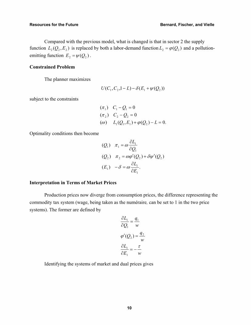
Compared with the previous model, what is changed is that in sector 2 the supply function ),( 222 EQL is replaced by both a labor-demand function )( 22 QL ϕ= and a pollution-emitting function )( 22 QE ψ= .

Constrained Problem

The planner maximizes

))(()1,,( 2121 QELCCU ψδ +−−

subject to the constraints

.0)(),()(0)(

0)(

2111

222

111

=−+=−

=−

LQEQLQCQC

ϕωππ

Optimality conditions then become

.)(

)()()(

)(

1

11

2222

1

111

ELE

QQQQLQ

∂∂

=−

′+′=∂∂

=

ωδ

ψδϕωπ

ωπ

Interpretation in Terms of Market Prices

Production prices now diverge from consumption prices, the difference representing the commodity tax system (wage, being taken as the numéraire, can be set to 1 in the two price systems). The former are defined by

wEL

wq

Q

wq

QL

τ

ϕ

−=∂∂

=′

=∂∂

1

1

22

1

1

1

)(

Identifying the systems of market and dual prices gives


11

).( 222

11

Qqpqp

w

ψτ

ωδτ

′+==

=

These results are particularly simple:

• emissions in sector 1 are taxed according to marginal damages;

• there is neither tax nor rebate for commodity 1; and

• commodity 2 is taxed according to the marginal damages of the associated emissions.

The tax rate on sector 2 equals the pollution tax applied in sector 1 multiplied by the marginal propensity to emit. When ψ is the identity function, the optimal commodity tax is

exactly equal to the pollution tax τ , and receipts of the commodity tax are then equal to the receipts that would accrue from a pollution tax (given the zero marginal product constraint on emissions). However, the level of emitted pollution is not the same as in the first-best case because the incentive effect is not at work. Then the optimized unregulated equilibrium exhibits a welfare loss, which can be measured and will be calculated in numerical simulations.

Zero commodity taxation (more precisely, no rebate and no subsidy) in the first sector is a result that raises questions about the underlying assumptions. In fact, an important assumption in the model is that the two sectors are independent in production and not linked to each other, such as through intermediate consumption. Considering the case in which each sector uses the good produced by the other sector as a factor of production changes the picture. There now may be reasons to tax good 1 in order to give a price signal—however small—to the other sector.

B. Unregulated Sector with Intermediate Consumption

Let us introduce Leontieff coefficients representing intermediate consumption. A unit of production in sector 1 requires 1γ units of good 2, while producing a unit of good 2 requires 2γ

units of good 1. The necessary change in the above model regards the market-clearing relations, which become

.0)(0)(

11222

22111

=+−=+−

QQCQQC

γπγπ

While the condition for the optimal emissions tax in sector 1 remains the same, the new optimality conditions for production are


12

).()(

)(

)(

22

2

2

2

21222

1

12111

QQQE

QLQ

QLQ

ψδϕω

δωπγπ

ωπγπ

′+′=∂∂

+∂∂

=−

∂∂

=−

Substituting in the market price relations from the consumer problem, as well as the optimal tax relation, and rewriting gives

.)()( 212

22

21

1

1

1

wQ

wp

wpQ

wp

wp

QL

ψτγϕ

γ

′−−=′

−=∂∂

Representing the producer problem relations in terms of market prices:

wq

wq

Q

wq

wq

QL

12

22

21

1

1

1

)( γϕ

γ

−=′

−=∂∂

and solving with the former yields

ψτγγ

ψτγγ

γ

′−

+=

′−

+=

2122

21

111

11

1

qp

qp

Sector 2 is still taxed according to the emissions embodied in its production, inflated somewhat by the interaction of the goods through intermediate consumption.8 Meanwhile, sector 1 in this case is taxed in proportion to the quantity of goods used in the second sector as intermediate consumption. If the Leontieff coefficients can reasonably be considered small, we

8 An additional unit of consumer good 2 requires 2γ units of good 1, which requires 21γγ of 2 which requires

221γγ of 1 and 2

22

1 γγ of 2, and so on. Thus, another consumer good 2 involves emissions from

210 21 1

1)(γγ

γγ−

=∑∞ i units of good 2.


13

find again that good 1 is (approximately) untaxed and commodity 2 is (approximately) taxed at a level equal to the pollution tax applied in sector 1.

Section 3: Unregulated and Untaxable Sector (Second Best 2)

When sector 2 is unregulated, we have seen that its emissions adjust so that the marginal product is always zero. A planner then cannot influence emissions directly, but rather indirectly through the output choice, of which emissions are then a straightforward function. When sector 2 cannot be taxed, the planner can no longer affect the output choice directly either. Output in sector 2 then becomes a function of the general equilibrium of the system.

Taking into account direct constraints—or indirect, such as budget constraints—on the price system requires resorting to the classic second-best apparatus. This method was first set out by Boiteux in his seminal paper of 1953 and afterward implemented by several economists addressing optimal taxation, including Diamond and Mirrlees (1971), Atkinson and Stiglitz (1972), Guesnerie (1995), Sandmo (1975), and Bradford and Rosen (1975), among others. It is based on supply and demand functions (instead of utility and production functions) and indirect utility functions.9

A. Second Best 1, Revisited

Using the new framework, let us present again the previous problem of an unregulated but taxable sector 2. The critical variables are now not quantities but prices: the production prices, the pollution tax, the consumption prices (and then implicitly the commodity taxes), and the household’s income R. Labor is chosen as the numéraire and the untaxed good (without loss of generality), with its price is set to 1. The second-best problem can now be written in the following form.

Second Best 1(b)

The planner maximizes

[ ]),(),,(),,( 221121 wqEwqERppU +− τδ

9 However, it is possible to set out second-best models in the primal language of production and utility functions (see Bernard 1977) and the equivalence with dual language easily checked (see Bernard 1990)


14

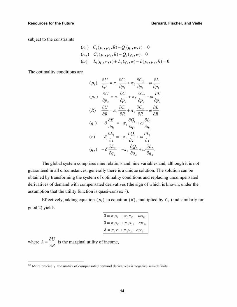
subject to the constraints

.0),,(),(),,()(0),(),,()(0),,(),,()(

212211

222122

112111

=−+=−=−

RppLwqLwqLwqQRppC

wqQRppC

τωπ

τπ

The optimality conditions are

.)(

)(

)(

)(

)(

)(

2

2

2

22

2

22

111

1

1

1

1

11

1

11

22

11

22

22

2

11

22

11

22

1

11

11

qL

qQ

qEq

LQEqL

qQ

qEq

RL

RC

RC

RUR

pL

pC

pC

pUp

pL

pC

pC

pUp

∂∂

+∂∂

−=∂∂

−

∂∂

+∂∂

−=∂∂

−

∂∂

+∂∂

−=∂∂

−

∂∂

−∂

∂+

∂∂

=∂∂

∂∂

−∂∂

+∂∂

=∂∂

∂∂

−∂∂

+∂∂

=∂∂

ωπδ

τω

τπ

τδτ

ωπδ

ωππ

ωππ

ωππ

The global system comprises nine relations and nine variables and, although it is not guaranteed in all circumstances, generally there is a unique solution. The solution can be obtained by transforming the system of optimality conditions and replacing uncompensated derivatives of demand with compensated derivatives (the sign of which is known, under the assumption that the utility function is quasi-convex10).

Effectively, adding equation )( 1p to equation )(R , multiplied by 1C (and similarly for

good 2) yields

L

L

L

vvvssssss

ωππλωππωππ

−+=−+=−+=

2211

2222121

1122111

00

where RU

∂∂

=λ is the marginal utility of income,

10 More precisely, the matrix of compensated demand derivatives is negative semidefinite.


15

RC

CpC

s ij

j

iij ∂

∂+

∂∂

= is the compensated derivative of demand in commodity i, and

RC

v ii ∂

∂= is the derivative of demand in commodity i with respect to income.

The above system is identically verified for wpp === ωππ ;; 2211 . Assuming

uniqueness of the solution then shows that the social values of goods are equal to the consumption prices.

The same reasoning applied to sector 1 shows that the production prices are equal to the social values of goods, and then that 11 qp = , meaning that no commodity taxation is warranted in

sector 1. As for sector 2, the dual relation is as presented before. Commodity 2 is (optimally) taxed at a rate equal to the pollution tax (as applying to sector 1) times the marginal associated emissions.

B. Second Best 2: Constraint on Commodity Taxation in Sector 2

Suppose now that unregulated sector 2 cannot be taxed at all. A unilateral tax on sector 1’s emissions would then raise the relative price of good 1. To alleviate the distortion to competition, it may be desirable to subsidize sector 1—that is, impose a negative commodity tax. Such a result is not assured, however; it depends, as is always the case in second-best analysis, on the substitutability or complementarity between the three goods—commodities 1 and 2 and leisure.

Imposing a zero tax in sector 2 (i.e., the condition that 22 pq = ) modifies the

optimization problem and the optimality conditions in the following way:

• p2 replaces q2 in the target function and in the constraints (π2) and (ω);

• correspondingly, optimality conditions (p2) and (q2) are gathered into a single constraint:

2

2

2

22

22

22

2

11

2

2

22 )(

pL

pQ

pL

pC

pC

pE

pUp

∂∂

+∂∂

−∂∂

−∂∂

+∂∂

=∂∂

−∂∂ ωπωππδ

The global system (primal and dual) consists now of eight relations and eight variables, reflecting the limitation to two of the policy instruments (the pollution tax and the commodity tax, both of which apply to sector 1). The above formula clearly shows that the social values of goods no longer coincide with the consumption prices.


16

As a consequence, the optimal tax on commodity 1 is no longer equal to zero. A negative value (i.e., a tax rebate or a subsidy) could normally be expected to alleviate the distortion between the two sectors vis-à-vis pollution abatement. However, as is usual in second-best models, no general intuitive or qualitative result can be exhibited, though in some circumstances “rules of thumb” may emerge (Bernard 1990). A thorough understanding of the general equilibrium workings of the system can come only from numerical simulations, showing how the main parameters affect results.

Section 4: Numerical Model

Though it is not the most general specification, a convenient one for the subsequent numerical analysis is the two-level nested CES utility function. For three goods, X1, X2, and X3, its formulation is

[ ] µµµ1

3)1(−−− −+= XuuZU

with

[ ] ννν1

21 )1(−−− −+= XvvXZ

This function is homogenous of degree one and separable; although it is not the most general specification, it allows us to capture various possible relations of substitutability and complementarity between good 1, good 2, and leisure. The choice of the values of the elasticity

of substitution is µ+

=1

11s in the global function and

ν+=

11

2s in the nest. The various

possible combinations of nesting (the two goods together, or one good and leisure) yield a broad range of situations.

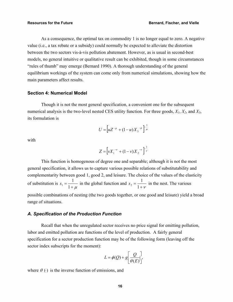
A. Specification of the Production Function

Recall that when the unregulated sector receives no price signal for emitting pollution, labor and emitted pollution are functions of the level of production. A fairly general specification for a sector production function may be of the following form (leaving off the sector index subscripts for the moment):

,)(

)(

+=

EQgQL

θφ

where )(⋅θ is the inverse function of emissions, and


17

−−= −1

1)( nn x

nnxxg β .

We assume that φ , g, and θ are monotonic increasing functions.

Effectively, the condition that marginal productivity of pollution equals zero implies that additional emissions would have no impact on output or thereby on labor:

.02 =′′

=∂∂

θθgQ

EL

Since )(Eθ is monotonic and strictly increasing, it must be that 0)( 21 =−=′ −− nn nxnxxg , the solution of which is 1=x , implying QE =)(θ . Then, in the case of no emissions tax, the factor

functions for sector 2 reduce to

.1

)(

),(

222

22

−−=

=

nQL

QEβ

φ

ψ

In numerical simulations, we will retain

3)()()( 2

====

nQQEEQQ

ψθ

αφ

The production function for each sector i can then be written in extensive form as

ii

i

i

iiiii c

EQ

EQ

QL +

−

+=

232

23βα ,

which in cases of a zero emissions price reduces to 222

222 5. cQL +−= βα . (That L is not equal

to zero when Q is zero is not a problem, since we consider the working of the production function only for sufficiently high values of output).

The marginal labor requirement (the inverse of the marginal product of labor) in this specification is

−+=

∂∂

QmmQ

QL

3

132 βα ,

where QEm /= is the emissions rate (sector indices are not noted but implicit). The parameter

α2 represents the slope of direct marginal production costs (in terms of labor units needed),


18

while β shifts those marginal costs upward, essentially to the extent that the emissions rate falls

below 1, the zero-marginal-product rate of emissions.

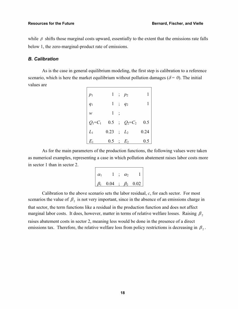
B. Calibration

As is the case in general equilibrium modeling, the first step is calibration to a reference scenario, which is here the market equilibrium without pollution damages (δ = 0). The initial values are

p1 1 ; p2 1

q1 1 ; q2 1

w 1 ;

Q1=C1 0.5 ; Q2=C2 0.5

L1 0.23 ; L2 0.24

E1 0.5 ; E2 0.5

As for the main parameters of the production functions, the following values were taken as numerical examples, representing a case in which pollution abatement raises labor costs more in sector 1 than in sector 2.

α1 1 ; α2 1

β1 0.04 ; β2 0.02

Calibration to the above scenario sets the labor residual, c, for each sector. For most scenarios the value of 2β is not very important, since in the absence of an emissions charge in

that sector, the term functions like a residual in the production function and does not affect marginal labor costs. It does, however, matter in terms of relative welfare losses. Raising 2β

raises abatement costs in sector 2, meaning less would be done in the presence of a direct emissions tax. Therefore, the relative welfare loss from policy restrictions is decreasing in 2β .


19

In sum, we consider a general scenario involving products with similar production and emissions profiles, the latter being identical and equal to output in the absence of regulation. The key parameters for optimal tax values are the elasticities of substitution between the goods.11

a) Specification I: Nesting of Commodities 1 and 2

For the utility function, we first nest the two commodities, varying the values of the elasticity of substitution within the nest and between the nest and leisure in the global utility function. With this specification, we investigate two main scenarios:

• commodities 1 and 2 are complements: values of the elasticity of substitution are, respectively, 0.75 (in the function) and 0.25 (in the nest); and

• commodities 1 and 2 are substitutes: values of the elasticity of substitution are, respectively, 0.25 and 0.75.

The results show that the magnitude of tax and welfare differences as the externality cost δ varies from 0 to 0.4, compared with first-best and Second Best 1.12 They clearly demonstrate the importance of the substitutability between the two commodities.

The rate of compensatory rebate in sector 1 is the ratio of tax rebates or subsidies to pollution taxes raised in that sector. 13 In the case of a high level of complementarity, the optimal rebate rate in the regulated sector is very small, and it can even be negative (i.e., positive taxation) for lower levels of marginal damage. When the two commodities are instead substitutes, the compensating rebate is high, with a rate close to 100% (a little less for low damages, a little more for high damages). Figure 1 contrasts these cases. Of course, the numerical results depend on the precise values of the two elasticities of substitution, but the general picture is that compensation is unjustified when the two goods are complements, and justified when they are close substitutes.

11 As seen in Section 3, emissions intensity in the unregulated sector is important for determining the second-best commodity tax; naturally, it will also affect the degree of optimal rebating, given the substitutability of the commodities. In the extreme case where sector 2 is nonpolluting, the optimal commodity tax is zero; since not being able to tax the output of sector 2 is then not actually a constraint, no rebate would be warranted. In general, since the effect of emissions intensity is primarily proportional, it is not a focus of the modelling effort. 12 The underlying assumptions regarding the use of emissions in each production function are also important. 13 Stated mathematically, the rebate rate is 111 / ECt τ− .


20

Figure 1: Rebate Rate in Sector 1

Substitutes

-20%

0%

20%

40%

60%

80%

100%

120%

140%

0 0.05 0.1 0.15 0.2 0.25 0.3 0.35 0.4

Second Best 1 Second Best 2100% Rebate

Complements

-20%

0%

20%

40%

60%

80%

100%

120%

0 0.05 0.1 0.15 0.2 0.25 0.3 0.35 0.4

Second Best 1 Second Best 2100% Rebate

These results can be explained by the nature of the substitution between the three goods, commodities 1 and 2 and leisure. When the two commodities are complements (less substitutable between each other than between both of them and leisure), a price differential between them is not efficient for pollution abatement because it does not significantly change their relative demand. Efficient pollution abatement is easily reached (i.e., at not too great a cost) by substituting leisure for consumption goods, and the shift occurs. As shown in Table 1 (appended due to its size), the prices of commodities increase with pollution abatement, which means that the purchasing power of labor decreases, and correspondingly so does labor supply by households, leaving more room for leisure.

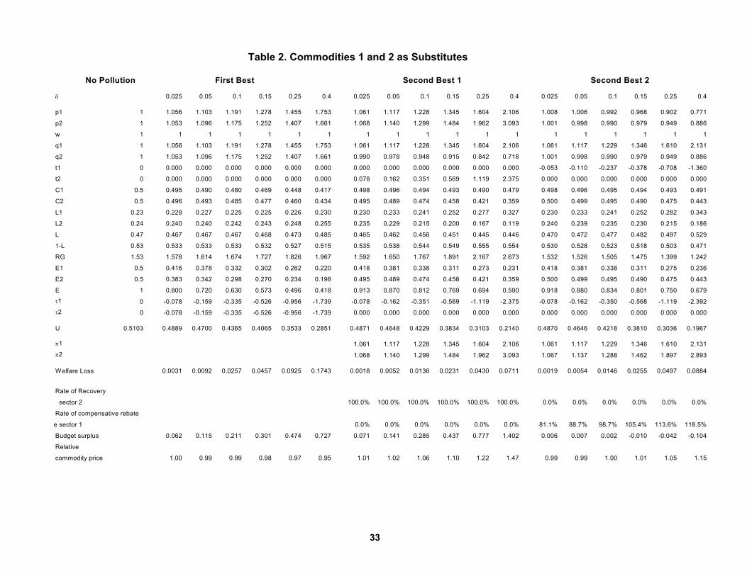
On the other hand, when the two consumption goods are substitutes (again relative to leisure), substitution works mainly between the goods, and less between both of them and leisure. Table 2 (also appended) shows that, in contrast to the previous case, the prices of the commodities remain rather low in spite of taxation, while the labor supply remains rather high. Obviously, when compensation is advocated for the regulated sector, the assumption is that the sector faces stiff competition from an unregulated, untaxed sector.

Regarding the actual level of taxation, it is important to note that in all of the cases thus far, the constrained optimal emission tax rate is higher than in the first-best case. When sector 2 cannot be properly regulated, emissions are higher and their damages more costly in marginal welfare terms. Sector 1 then has to do more of the work of emissions reduction. However, other policy constraints may cause the equilibrium emission tax rate to fall below that of the first-best scenario. (These cases will be shown in Figures 3 and 4 in the next section.)


21

b) Specification II: Nesting of Commodity 1 and Leisure

Nesting commodity 1 and leisure in the utility function gives somewhat comparable results. The main difference is that complementarity between commodities 1 and 2 requires a low elasticity of substitution both in the nest and in the utility function. As a result, complementarity between the goods also requires complementarity with leisure.

Simulations were performed with s1=0.85 and s2=0.15, and with s1=0.15 and s2=0.85. The first set of parameters corresponds to a higher degree of substitutability between the two commodities than the second set. Effectively, the optimal rate of compensatory rebate is always higher than 100% in the first case and smaller than 30% in the second case, as shown in the following table. However, we never obtain a “negative” compensation (i.e., a positive tax).

Rebate Rate with Specification II

δ 0.025 0.05 0.1 0.15 0.25 0.4

s1=0.85 and s2=0.15 125.2% 134.4% 143.9% 148.0% 148.5% 141.1%

s1=0.15 and s2=0.85 11.8% 13.2% 15.4% 17.3% 21.1% 27.6%

Section 5: Comparing Constraints on Taxation

To place these results in a policy context, we would like to evaluate the effects of policy constraints on optimal tax rates and on welfare. In addition to the first-best policy and the two second-best policies analyzed in sections 2 and 3, we identify several more and compare the results in Table 3. These other second-best configurations are easily considered in the given framework.

To give a baseline for comparison of the welfare gains from each policy, we calculate the welfare achieved when no environmental policy is implemented (“No Taxation” scenario). As another potential benchmark, we offer the scenario of nothing but a pollution tax in sector 1 (Second Best 3), representing when rebates and commodity taxation are both unavailable.

Next, even though we have demonstrated it is not usually optimal, since it is frequently advocated we consider two cases of a mandatory 100% rebate of the pollution tax in sector 1. One imposes it when commodity taxation is unavailable for sector 2 (Second Best 4), and the other imposes full rebating when the commodity tax is available (Second Best 5). In the latter


22

case, the requirement affects not only the optimal pollution tax rate in sector 1, but also the commodity tax on good 2. Comparison with Second Best 1 and 2 gives a measure of the additional welfare loss generated by such policies and the impact on the choice of tax rate.

Similarly, we present the case where complete rebating of environmental revenues is mandated, although direct pollution taxes are available in both sectors (Second Best 6); the constraint that all revenue be given back in output subsidies to the producing sectors creates a distortion compared to lump-sum rebating.14

Table 3. Comparison of Scenarios

Pollution Tax in

Sector 1 Pollution Tax in

Sector 2 CommodityTax

in Sector 1 CommodityTax

in Sector 2

Pareto Yes Yes Yes (Opt.= 0) Yes (Opt.= 0)

No Taxation No No No No

Second Best 1: 2 Exempt from Pollution Tax Yes No Yes Yes

Second Best 2: 2 Exempt From All Yes No Yes No

Second Best 3: Pollution tax in 1 Alone Yes No No No

Second Best 4: Full Rebating in Sector 1 Yes No 100% Rebate No

Second Best 5: Full Rebating in Sector 1 Yes No 100% Rebate Yes

Second Best 6: Pareto Tax with Full Rebate Yes Yes 100% Rebate Overall

A. Effects of Policy Constraints on Tax Rates

The rate of recovery is defined as the percent of emissions that are implicitly taxed at the rate faced by sector 1.15 In sector 2, the recovery rate is by definition 100% in Second Best 1,

14 An important assumption here is that no distorting taxes, like a labor tax, already exist. This extension will be discussed in the conclusion. 15 Otherwise stated, the rate of recovery in sector 2 is the ratio of the receipts accruing from the commodity taxation to the receipts that would accrue from a pollution tax, or )/( 222 ECt τ .


23

since all embodied emissions are taxed, and zero in Second Best 2, since no tax is allowed. However, when 100% rebating is mandated in sector 1, the rate of recovery in sector 2 will vary according to the degree of substitutability.

Figure 2 compares second-best scenario 5 with scenario 1, with respect to the rate of recovery in sector 2. In the case of complements, a full rebate in sector 1 is too high; to compensate, more than 100% of the pollution implicit in the production of section 2 is taxed. In a sense, the tax on 2 is serving to tax the inefficiently subsidized complement. In the case of substitutes, the rebate rate is closer to that in Second Best 2, causing the optimal rate of recovery to be lower. In other words, the subsidy is inefficiently diverting consumption toward Sector 1, and taxing in full the pollution implicit in the substitute output would exacerbate this effect.

Figure 2: Rate of Recovery in Sector 2

Substitutes

0.0

0.2

0.4

0.6

0.8

1.0

1.2

0 0.05 0.1 0.15 0.2 0.25 0.3 0.35 0.4

Second Best 1

Second Best 5

Complements

0.0

0.2

0.4

0.6

0.8

1.0

1.2

1.4

1.6

0 0.05 0.1 0.15 0.2 0.25 0.3 0.35 0.4

Second Best 1

Second Best 5

We noted before that for second-best scenarios 1 and 2, the constrained optimal emission tax rate is always higher than in the first-best case, regardless of whether the goods are complements or substitutes. For other policy constraints, however, the degree of substitutability matters in determining where the equilibrium emission tax rate falls compared to the first-best and other scenarios. Figure 3 shows emission tax rates for the complements case; Figure 4 shows them for substitutes.

For example, compare taxing pollution in only one of the polluting sectors (Second Best 3) to Second Best 2, which adds the rebating option. In the case of complements, we see that the tax rate is generally somewhat higher for 3, as it does all the work for encouraging emissions reduction in sector 1 and its complement in sector 2. Correspondingly, overall emissions are


24

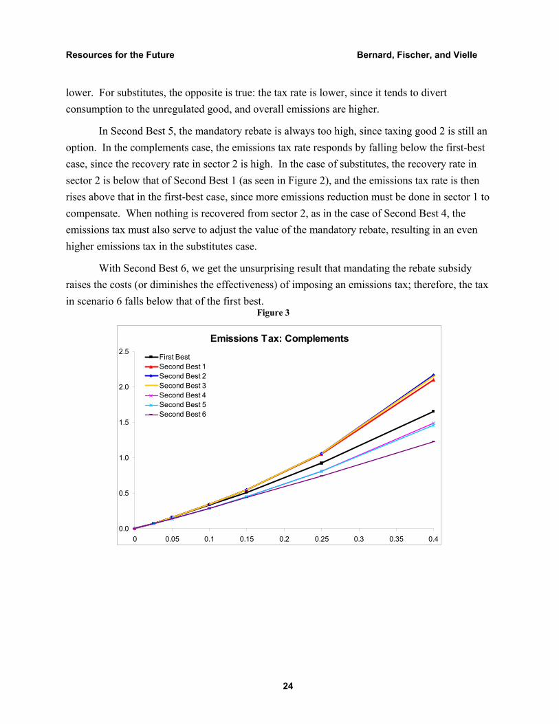
lower. For substitutes, the opposite is true: the tax rate is lower, since it tends to divert consumption to the unregulated good, and overall emissions are higher.

In Second Best 5, the mandatory rebate is always too high, since taxing good 2 is still an option. In the complements case, the emissions tax rate responds by falling below the first-best case, since the recovery rate in sector 2 is high. In the case of substitutes, the recovery rate in sector 2 is below that of Second Best 1 (as seen in Figure 2), and the emissions tax rate is then rises above that in the first-best case, since more emissions reduction must be done in sector 1 to compensate. When nothing is recovered from sector 2, as in the case of Second Best 4, the emissions tax must also serve to adjust the value of the mandatory rebate, resulting in an even higher emissions tax in the substitutes case.

With Second Best 6, we get the unsurprising result that mandating the rebate subsidy raises the costs (or diminishes the effectiveness) of imposing an emissions tax; therefore, the tax in scenario 6 falls below that of the first best.

Figure 3

Emissions Tax: Complements

0.0

0.5

1.0

1.5

2.0

2.5

0 0.05 0.1 0.15 0.2 0.25 0.3 0.35 0.4

First BestSecond Best 1Second Best 2Second Best 3Second Best 4Second Best 5Second Best 6


25

Figure 4

Emissions Tax: Substitutes

0.0

0.5

1.0

1.5

2.0

2.5

3.0

3.5

0 0.05 0.1 0.15 0.2 0.25 0.3 0.35 0.4

First BestSecond Best 1Second Best 2Second Best 3Second Best 4Second Best 5Second Best 6

B. Effects of Policy Constraints on Welfare

We have presented how different constraints on policymaking affect optimal tax and rebate rates. The ultimate question is how the constraints, given these optimal responses to them, affect welfare. The following Figures depict the welfare losses of each scenario, compared to optimal Pigouvian policy, for the two polar cases of complementarity and substitutability (as defined with specification I of the utility function).

Clearly, inaction is very costly in terms of welfare. Overall, we see that welfare costs increase with the stringency of the restrictions.

For the unregulated sector, we showed that the optimal second-best policy is a commodity tax at a level equal to the pollution tax in the regulated sector times the implicit emissions, without any rebate for the regulated sector. Notably, looking at Second Best 1 in the Figures, we see that with this single restriction of no pollution regulation for one sector, even with the option of commodity taxation, roughly half the welfare gains from environmental policy are foregone.

In the case of an unregulated and untaxable sector, the rationale for rebating pollution taxes in the regulated sector depends primarily on whether they are really in close competition. The closer the substitutes, the more justification there is for rebating. As such, the substitutes


26

case is probably the context that advocates of rebating usually have in mind. But our main conclusion is that built-in compensatory measures, such as rebating pollution taxes in the regulated sector, may in other contexts do more harm than good. In any case, taxing polluting sectors, through commodity taxation if taxing pollution directly is impossible, is always preferable.

Examples can be seen in Figures 5 and 6, portraying the relative welfare losses of the different scenarios. In general, welfare losses grow with the increasing restrictiveness of the policy constraints. Second Best 2, 3 and 5 are all worse than 1 and Second Best 4 is worse than 2 and 4, by design. Interestingly, Second Best 5 always outperforms Second Best 2 in our scenarios: that means the option to tax the emissions embodied in sector 2’s output is more important than flexibility in setting the rebate rate, even for complements. However, whether mandatory rebating is better than no rebating depends on the degree of substitutability between the commodities.

Taxing pollution in only one of the polluting sectors without any compensatory rebate or commodity taxation in the other sector (Second Best 3) achieves the least welfare gain of any of the policies considered when the goods are substitutes. In this case, the tax diverts more consumption toward the unregulated sector and it becomes a weaker instrument for reducing emissions. On the other hand, in the case of complements, when little or no rebate was justified anyway, the welfare loss is very similar to Second Best 2. Meanwhile, mandatory rebating in sector 1 without commodity taxation in 2 (Second Best 4) implies an even greater welfare loss than no rebating at all in this complements case.

Second Best 6 models the case where the emissions of each sector can be taxed directly, but the revenues must be refunded by subsidies to output in both industries, rather than in lump-sum form to consumers. The resulting distortion to the leisure-consumption decision creates a welfare loss; however, since the emissions of both industries are taxed, the loss is less severe than when one industry cannot be regulated.


27

Figure 5

Welfare Loss: Complements

0.0

0.1

0 0.05 0.1 0.15 0.2 0.25 0.3 0.35 0.4

No TaxationSecond Best 1Second Best 2Second Best 3Second Best 4Second Best 5Second Best 6

Figure 6

Welfare Loss: Substitutes

0.0

0.1

0 0.05 0.1 0.15 0.2 0.25 0.3 0.35 0.4

No TaxationSecond Best 1Second Best 2Second Best 3Second Best 4Second Best 5Second Best 6

Conclusion

We have considered the arguments for allocating environmental revenues in the form of output subsidies to affected industries. The desirability of such a policy depends on the


28

circumstances of the constraint on policy making and on whether the goods of the regulated industry are substitutes or complements with those of the unregulated industry.

As usual, the first-best policy is always to have a full set of policy tools. Then the emissions of each industry are taxed directly, and the revenues are refunded in a non-distorting manner to consumers.

However, if for some reason the emissions of one of the polluting sectors cannot be regulated directly, the next-best response is to tax those emissions indirectly. A tax should be levied on the output of the unregulated sector, reflecting the extent to which emissions are incorporated in its production. Meanwhile, a direct tax on the regulated sector’s emissions remains in place, and the revenues are again refunded in lump sum; no rebate is justified.

If taxing the unregulated sector’s output is not possible either, then an output-based rebate to the regulated sector is justified, but only to the extent that (i) the goods are close substitutes and (ii) the unregulated sector is polluting. Any surplus (or shortfall) in revenue is transferred in lump sum to (from) consumers.

Imposing a 100% rebate for the regulated sector represents an additional policy constraint and thus reduces welfare compared to the previous scenario. Obviously, such a requirement is least costly in situations when the optimal rebate rate is close to one, such as if both the goods and their emissions profiles are similar. In a complements situation, a mandatory full rebate is worse than no rebate at all. In any case, the loss in terms of flexibility for setting the rebate can be more than made up for if a tax can also be levied on the output of the unregulated sector.

Policy constraints can be quite costly, and a general-equilibrium framework is important for understanding the extent of those costs. The effectiveness of the remaining policy tools depends critically on the elasticities of substitution between the polluting goods and with leisure. For complements, taxes or subsidies on commodities are weak tools since they have similar effects on the untaxed sector. Meanwhile, the emissions tax then also has the spillover effect of reducing output in the unregulated sector. For substitutes, on the other hand, cost increases in the regulated sector have the extra effect of shifting output toward the unregulated sector. As a result, an emissions tax in one sector alone is a weaker tool for reducing emissions, while output taxes and subsidies offer a more powerful remedy.

In a final note, almost all of the second-best configurations considered here involve lump-sum transfers from government to households—lump-sum grants when the total amount of fiscal receipts is positive, lump-sum levies when negative. The exception is Second Best 6, in which emissions in both sectors are taxed, but the revenues are rebated back to both industries; this


29

100% overall rebating requirement is essentially a balanced-budget constraint. Not only is the feasibility of lump-sum transfers debatable, but environmental taxes normally operate in a world with pre-existing taxes. These taxes, notably on labor and consumption goods, leave leisure as an untaxed good. Thus, distortions to behavior are pre-existing when the environmental tax is levied and the use of the revenue has important impacts. In subsequent work, we will assess the effect of adding a constraint of a balanced budget (i.e., that the sum of all receipts from taxation, both pollution taxes and commodity taxes, be equal to a revenue requirement) when leisure remains an untaxed good. In this case rebating, which tends to function like a labor tax reduction, can be welfare improving over lump-sum redistribution.


30

References

Atkinson, A.B., and J.E. Stiglitz. 1972. The Structure of Indirect Taxation and Economic Efficiency. Journal of Public Economics 1:97–119

Bernard, A.L. 1977. Optimal Taxation and Public Production with Budget Constraints. In The Economics of Public Services, edited by M.S. Feldstein and R.P. Inman. MacMillan.

Bernard, A.L. 1990. Rules of Thumb for Optimal Tolls. In Essays in Honor of Edmond Malinvaud, edited by P. Champsaur et al. Cambridge, MA: MIT Press.

Bernard, A.L. 1999. The Pure Economics of Tradable Pollution Permits. Communication presented at the Joint Meeting of the International Energy Agency, the Energy Modeling Forum, and the International Energy Workshop, 16–18 June, Paris.

Boiteux, M. 1956. Sur la Gestion des Monopoles Publics Astreints à l’Equilibre Budgétaire. Econometrica 24:22–40.

Bradford, D.F., and H.S. Rosen. 1975. The Optimal Taxation of Commodities and Income. U.S. Treasury Department, OTA Paper 8, December. (A condensed version appears in American Economic Review, May 1976.)

Bovenberg, A.L., and L.H. Goulder. 1996. Optimal Environmental Taxation in the Presence of Other Taxes: General Equilibrium Analyses. American Economic Review 86:985–1000.

Cremer, H., and F. Gahvari. 2001. Second-best taxation of emissions and polluting goods. Journal of Public Economics 80:169–97.

Diamond, P.A.., and J. Mirrlees. 1971. Optimal Taxation and Public Production. American Economic Review 61:8–27, 261–78.

Fischer, C. 2001. Rebating Environmental Policy Revenues: Output Based Allocations and Tradable Performance Standards. RFF Discussion Paper 01-22. Washington, DC: Resources for the Future.

Guesnerie, R. 1995. A Contribution to the Pure Theory of Taxation. Econometric Society Monographs. Cambridge University Press.

Jensen, J., and T.N. Rasmussen. 1998. Allocation of CO2 Emission Permits: A General Equilibrium Analysis of Policy Instruments. Copenhagen: Danish Ministry of Business and Industry.


31

Kerr, S.C., and D. Maré. 1996. Efficient Regulation through Tradeable Permit Markets: The United States Lead Phasedown. Department of Agricultural and Resource Economics, University of Maryland at College Park, working paper 96-06.

Organization for Economics Cooperation and Development. 1993. Taxation and the Environment: Complementary Policies. Paris: OECD.

Sandmo, A. 1975. Optimal Taxation in the Presence of Externalities. Economic Journal 37:47–61.

Sterner, T., and L. Högland. 1999. Output Based Refunding of Emission Payments: Theory, Distribution of Costs and International Experience. Manuscript. Goteborg University, Sweden.

Wagner, R.E., ed. 1991. Charging for Government: User Charges and Earmarked Taxes in Principle and Practice. London and New York: Routledge.

1

Table 1. Commodities 1 and 2 as Complements

No Pollution First Best Second Best 1 Second Best 2

δ 0.025 0.05 0.1 0.15 0.25 0.4 0.025 0.05 0.1 0.15 0.25 0.4 0.025 0.05 0.1 0.15 0.25 0.4

p1 1 1.049 1.091 1.169 1.245 1.403 1.668 1.051 1.095 1.181 1.268 1.461 1.840 1.052 1.098 1.187 1.278 1.481 1.874

p2 1 1.045 1.081 1.147 1.212 1.344 1.563 1.061 1.125 1.270 1.436 1.853 2.777 0.998 0.996 0.990 0.983 0.966 0.932

w 1 1 1 1 1 1 1 1 1 1 1 1 1 1 1 1 1 1 1

q1 1 1.049 1.091 1.169 1.245 1.403 1.668 1.051 1.095 1.181 1.268 1.461 1.840 1.051 1.096 1.183 1.273 1.477 1.893

q2 1 1.045 1.081 1.147 1.212 1.344 1.563 0.983 0.965 0.927 0.887 0.804 0.672 0.998 0.996 0.990 0.983 0.966 0.932

t1 0 0.000 0.000 0.000 0.000 0.000 0.000 0.000 0.000 0.000 0.000 0.000 0.000 0.001 0.002 0.004 0.005 0.003 -0.019

t2 0 0.000 0.000 0.000 0.000 0.000 0.000 0.078 0.161 0.343 0.549 1.049 2.105 0.000 0.000 0.000 0.000 0.000 0.000

C1 0.5 0.492 0.484 0.469 0.455 0.427 0.387 0.493 0.486 0.472 0.458 0.427 0.372 0.493 0.486 0.473 0.460 0.434 0.391

C2 0.5 0.492 0.485 0.472 0.458 0.432 0.393 0.492 0.482 0.463 0.444 0.402 0.336 0.499 0.498 0.495 0.491 0.483 0.466

L1 0.23 0.224 0.221 0.215 0.211 0.204 0.197 0.225 0.222 0.218 0.215 0.209 0.201 0.225 0.223 0.219 0.217 0.217 0.222

L2 0.24 0.236 0.233 0.228 0.225 0.218 0.211 0.232 0.223 0.205 0.187 0.152 0.103 0.239 0.238 0.235 0.232 0.223 0.207

L 0.47 0.460 0.453 0.443 0.435 0.422 0.408 0.457 0.445 0.423 0.402 0.361 0.304 0.464 0.461 0.454 0.449 0.440 0.429

1-L 0.53 0.540 0.547 0.557 0.565 0.578 0.592 0.543 0.555 0.577 0.598 0.639 0.696 0.536 0.539 0.546 0.551 0.560 0.571

RG 1.53 1.570 1.599 1.646 1.687 1.758 1.852 1.582 1.630 1.723 1.816 2.008 2.314 1.552 1.569 1.597 1.622 1.670 1.739

E1 0.5 0.414 0.374 0.327 0.296 0.253 0.210 0.414 0.374 0.326 0.294 0.247 0.194 0.414 0.375 0.327 0.296 0.251 0.201

E2 0.5 0.381 0.338 0.292 0.263 0.224 0.185 0.492 0.482 0.463 0.444 0.402 0.336 0.499 0.498 0.495 0.491 0.483 0.466

E 1 0.795 0.712 0.619 0.559 0.477 0.394 0.906 0.857 0.790 0.738 0.649 0.530 0.913 0.873 0.822 0.787 0.734 0.667τ1 0 -0.077 -0.158 -0.330 -0.515 -0.925 -1.651 -0.078 -0.161 -0.343 -0.549 -1.049 -2.105 -0.078 -0.160 -0.343 -0.549 -1.055 -2.166τ2 0 -0.077 -0.158 -0.330 -0.515 -0.925 -1.651 0.000 0.000 0.000 0.000 0.000 0.000 0.000 0.000 0.000 0.000 0.000 0.000

U 0.5103 0.4884 0.4697 0.4366 0.4073 0.3557 0.2907 0.4866 0.4646 0.4236 0.3854 0.3162 0.2279 0.4865 0.4643 0.4220 0.3818 0.3059 0.2011

π1 1.051 1.095 1.181 1.268 1.461 1.840 1.051 1.096 1.183 1.273 1.477 1.893π2 1.061 1.125 1.270 1.436 1.853 2.777 1.059 1.121 1.257 1.411 1.789 2.620

Welfare Loss 0.0032 0.0094 0.0264 0.0470 0.0955 0.1805 0.0018 0.0050 0.0130 0.0218 0.0396 0.0629 0.0019 0.0054 0.0146 0.0255 0.0498 0.0896

Rate of Recovery

sector 2 100.0% 100.0% 100.0% 100.0% 100.0% 100.0% 0.0% 0.0% 0.0% 0.0% 0.0% 0.0%

Rate of compensative rebate

sector 1 0.0% 0.0% 0.0% 0.0% 0.0% 0.0% -1.6% -1.7% -1.6% -1.3% -0.5% 1.7%

Budget surplus 0.061 0.113 0.204 0.288 0.442 0.651 0.070 0.138 0.271 0.405 0.681 1.115 0.033 0.061 0.114 0.164 0.266 0.427

Relative

commodity price 1.00 0.99 0.98 0.97 0.96 0.94 1.01 1.03 1.08 1.13 1.27 1.51 0.95 0.91 0.83 0.77 0.65 0.50

33

Table 2. Commodities 1 and 2 as Substitutes

No Pollution First Best Second Best 1 Second Best 2

δ 0.025 0.05 0.1 0.15 0.25 0.4 0.025 0.05 0.1 0.15 0.25 0.4 0.025 0.05 0.1 0.15 0.25 0.4

p1 1 1.056 1.103 1.191 1.278 1.455 1.753 1.061 1.117 1.228 1.345 1.604 2.106 1.008 1.006 0.992 0.968 0.902 0.771

p2 1 1.053 1.096 1.175 1.252 1.407 1.661 1.068 1.140 1.299 1.484 1.962 3.093 1.001 0.998 0.990 0.979 0.949 0.886

w 1 1 1 1 1 1 1 1 1 1 1 1 1 1 1 1 1 1 1

q1 1 1.056 1.103 1.191 1.278 1.455 1.753 1.061 1.117 1.228 1.345 1.604 2.106 1.061 1.117 1.229 1.346 1.610 2.131

q2 1 1.053 1.096 1.175 1.252 1.407 1.661 0.990 0.978 0.948 0.915 0.842 0.718 1.001 0.998 0.990 0.979 0.949 0.886

t1 0 0.000 0.000 0.000 0.000 0.000 0.000 0.000 0.000 0.000 0.000 0.000 0.000 -0.053 -0.110 -0.237 -0.378 -0.708 -1.360

t2 0 0.000 0.000 0.000 0.000 0.000 0.000 0.078 0.162 0.351 0.569 1.119 2.375 0.000 0.000 0.000 0.000 0.000 0.000

C1 0.5 0.495 0.490 0.480 0.469 0.448 0.417 0.498 0.496 0.494 0.493 0.490 0.479 0.498 0.496 0.495 0.494 0.493 0.491

C2 0.5 0.496 0.493 0.485 0.477 0.460 0.434 0.495 0.489 0.474 0.458 0.421 0.359 0.500 0.499 0.495 0.490 0.475 0.443

L1 0.23 0.228 0.227 0.225 0.225 0.226 0.230 0.230 0.233 0.241 0.252 0.277 0.327 0.230 0.233 0.241 0.252 0.282 0.343

L2 0.24 0.240 0.240 0.242 0.243 0.248 0.255 0.235 0.229 0.215 0.200 0.167 0.119 0.240 0.239 0.235 0.230 0.215 0.186

L 0.47 0.467 0.467 0.467 0.468 0.473 0.485 0.465 0.462 0.456 0.451 0.445 0.446 0.470 0.472 0.477 0.482 0.497 0.529

1-L 0.53 0.533 0.533 0.533 0.532 0.527 0.515 0.535 0.538 0.544 0.549 0.555 0.554 0.530 0.528 0.523 0.518 0.503 0.471

RG 1.53 1.578 1.614 1.674 1.727 1.826 1.967 1.592 1.650 1.767 1.891 2.167 2.673 1.532 1.526 1.505 1.475 1.399 1.242

E1 0.5 0.416 0.378 0.332 0.302 0.262 0.220 0.418 0.381 0.338 0.311 0.273 0.231 0.418 0.381 0.338 0.311 0.275 0.236

E2 0.5 0.383 0.342 0.298 0.270 0.234 0.198 0.495 0.489 0.474 0.458 0.421 0.359 0.500 0.499 0.495 0.490 0.475 0.443

E 1 0.800 0.720 0.630 0.573 0.496 0.418 0.913 0.870 0.812 0.769 0.694 0.590 0.918 0.880 0.834 0.801 0.750 0.679τ1 0 -0.078 -0.159 -0.335 -0.526 -0.956 -1.739 -0.078 -0.162 -0.351 -0.569 -1.119 -2.375 -0.078 -0.162 -0.350 -0.568 -1.119 -2.392τ2 0 -0.078 -0.159 -0.335 -0.526 -0.956 -1.739 0.000 0.000 0.000 0.000 0.000 0.000 0.000 0.000 0.000 0.000 0.000 0.000

U 0.5103 0.4889 0.4700 0.4365 0.4065 0.3533 0.2851 0.4871 0.4648 0.4229 0.3834 0.3103 0.2140 0.4870 0.4646 0.4218 0.3810 0.3036 0.1967

π1 1.061 1.117 1.228 1.345 1.604 2.106 1.061 1.117 1.229 1.346 1.610 2.131π2 1.068 1.140 1.299 1.484 1.962 3.093 1.067 1.137 1.288 1.462 1.897 2.893

Welfare Loss 0.0031 0.0092 0.0257 0.0457 0.0925 0.1743 0.0018 0.0052 0.0136 0.0231 0.0430 0.0711 0.0019 0.0054 0.0146 0.0255 0.0497 0.0884

Rate of Recovery

sector 2 100.0% 100.0% 100.0% 100.0% 100.0% 100.0% 0.0% 0.0% 0.0% 0.0% 0.0% 0.0%

Rate of compensative rebate

e sector 1 0.0% 0.0% 0.0% 0.0% 0.0% 0.0% 81.1% 88.7% 98.7% 105.4% 113.6% 118.5%

Budget surplus 0.062 0.115 0.211 0.301 0.474 0.727 0.071 0.141 0.285 0.437 0.777 1.402 0.006 0.007 0.002 -0.010 -0.042 -0.104

Relative

commodity price 1.00 0.99 0.99 0.98 0.97 0.95 1.01 1.02 1.06 1.10 1.22 1.47 0.99 0.99 1.00 1.01 1.05 1.15

is there a rationale for rebating environmental levies?

Documents