is there an environmental benefit to being an exporter? evidence from firm-level data

ORI GIN AL PA PER

Is there an environmental benefit to being an exporter?Evidence from firm-level data

Svetlana Batrakova • Ronald B. Davies

Published online: 13 March 2012

� Kiel Institute 2012

Abstract One concern over globalisation is its impact on the environment. We

analyse the consequences of becoming an exporter on a firm’s energy consumption.

We show theoretically and empirically with firm-level data that the increase in

energy use when exporting is negatively correlated with energy intensity. This is

because, although energy use rises with exporting due to greater production and

transportation, it can be offset by adopting more energy-efficient technology. This

second effect is strongest for high energy intensity firms. As such, analysis of

average effects, as in other studies, conceals important connections between the

trade and the environment.

Keywords Exporting � Energy � Heterogeneity � Matching � Quantiles

JEL Classification F18 � L23 � Q56 � C21

This paper uses confidential micro data set of the Central Statistics Office Ireland (CSO). The restricted

and controlled access to the data was provided in accordance with the Statistics Act, 1993. We are very

grateful to Kevin Phelan, Dan Lawlor and Jane O’Brien for the provided assistance. We thank Stefanie

Haller, Paul Devereux, Fergal McCann, participants at the 2010 Spring Midwest International Trade

Meeting, at the ESRI Research Seminar, Xth RIEF Meeting, at the 24th Irish Economic Association

Conference and the editor and one anonymous referee for helpful comments and suggestions. Funding

from the Irish Research Council for the Humanities and Social Sciences (IRCHSS) and the Irish

Research Council for Science, Engineering and Technology (IRCSET) is gratefully acknowledged. This

paper is produced as part of the project ‘‘Globalization, Investment and Services Trade (GIST) Marie

Curie Initial Training Network (ITN)’’ funded by the European Commission under its Seventh

Framework Programme—Contract No. FP7-PEOPLE-ITN-2008-211429.

S. Batrakova (&) � R. B. Davies

School of Economics, University College Dublin, Dublin, Ireland

e-mail: [email protected]

123

Rev World Econ (2012) 148:449–474

DOI 10.1007/s10290-012-0125-2

1 Introduction

With international trade now comprising half of world GDP [World Bank (2010)],

the impact of international trade on the environment is a subject of growing concern

by economists, environmentalists, and policy makers. The pollution haven

hypothesis is now a cornerstone of the debate on globalisation and the environment.

As formulated by Pethig (1976) and McGuire (1982) this hypothesis postulates that

opening up to trade allows pollution-intensive industries to move to countries with

weaker environmental regulations. This results in a race to the bottom in overall

environmental standards and increased pollution levels. With this in mind, most of

the attention has concentrated on foreign direct investment (FDI), plant location,

and multinationals’ impact on the overall level of environmental standards and

pollution. However, more recent theoretic work finds the effect is not as

straightforward when environmental policy is endogenised (Copeland and Taylor

1994, 1995), pollution is local (Markusen et al. 1995), factor endowments are taken

into consideration (Copeland and Taylor 1997; Antweiler et al. 2001), or when

governments have other strategic considerations (Barrett 1994). The empirical

evidence has been inconclusive on the pollution haven hypothesis. Studies using

aggregate data, such as Dean and Lovely (2010), Javorcik and Wei (2004),

Ederington et al. (2004) and Antweiler et al. (2001), generally fail to find support

for increased FDI leading to increased pollution. An overview of an early literature

by Jaffe et al. (1995) draws the same conclusion. In addition, recent firm-level

studies including Albornoz et al. (2009), Cole et al. (2006, 2008), and Kaiser and

Schulze (2003) have uncovered a positive effect of foreign ownership on the

environmental performance of firms in the host country. This should not be taken to

imply that there is no evidence for a shift in activities as a result of differences in

environmental standards, since Levinson and Taylor (2008), Ederington et al.

(2005), List et al. (2003) and Keller and Levinson (2002) find evidence of imports

and FDI responding to environmental regulations. Rather, as discussed by Levinson

(2009), these effects, at least for the US, are quantitatively small compared to other

factors such as the effect of advances in technology.

This paper contributes to the debate by considering the impact of exporting status

on energy use by firms. Since energy use is correlated with pollution, this is our

measure of environmental performance.1 We begin with a theoretical model

borrowing from the heterogeneous firms literature popularised by Melitz (2003).2

When a firm begins exporting, its output will tend to rise, increasing its demand for

energy and the pollution it is responsible for. However, this greater scale increases

the return from investment in energy-efficiency enhancing technologies which

would reduce energy use. This latter effect is likely to be particularly large for big

1 This is similar to the aggregate data studies by Eskeland and Harrison (2003) and Cole et al. (2008).

The existing firm-level studies of Galdeano-Gomez (2010), Girma et al. (2008) and Kaiser and Schulze

(2003) consider the impact of exporting status on, respectively, a firm’s environmental productivity

performance, adoption of pollution abatement technology and environmental expenses as alternative

measures of environmental performance. In contrast, we examine the impact of exporting on actual

energy use.2 For an overview of the empirical findings see Wagner (2007).

450 S. Batrakova, R. B. Davies

123

firms (i.e. more productive firms) and those that are energy intensive. The link

between productivity and technology adoption is similar to the theoretical result

found by Bustos (2011) following trade liberalization.3 Therefore the net effect of

exporting on energy use is ambiguous and varies across different firms, with low

energy intensity firms increasing energy use when exporting and high energy

intensity firms reducing energy use when exporting.

We then test this using firm-level data on Irish manufacturing firms from 1991 to

2007. Looking at just the mean effect of exporting on a firm’s use of energy hides

differences between low and high energy intensity firms, resulting in an overall

neutral effect.4 Distinguishing between different energy intensities, we find that

exporting status is associated with an increase in energy use for low energy intensity

firms and with a decrease in energy use for high energy intensity firms.5 Thus, mean

effects mask important variation in the data since such analysis restricts both low

energy intensity firms (those for whom the increased output effect dominates) and

high energy intensity firms (those most likely to adopt more energy efficient

technologies) to have the same estimated coefficients. Our results therefore

complement those of Bustos (2011) by considering how the effect of exporting

differs depending on factor intensity.

We further establish that these differences arise after firms begin exporting, not

before. By employing matching and difference-in-differences estimations we show

that low energy intensity firms increase their energy use as a result of output

expansion due to exporting.6 Likewise, high energy intensity firms decrease their

energy use following the commencement of exporting, in line with our model’s

prediction. In addition, we find that for low energy intensity firms that cease

exporting, there is no difference between them and comparable non-exporters

immediately following the cessation of exporting. For high energy intensity firms,

there is a lasting reduction in energy usage even after exporting stops. If the scale

effect disappears immediately but newly adopted technology remains when

exporting stops, this is exactly the pattern one would expect to see. Thus, as

highlighted by Levinson (2009), there is an important interplay between global-

isation, technology adoption, and the environment.

Looking at the role of exporters is a relatively new terrain with only a few studies

examining the issue. Galdeano-Gomez (2010) finds higher export orientation to be

positively associated with an environmental performance component of a firm’s

total productivity. Galdeano-Gomez (2010) also shows that a firm’s environmental

performance measure positively affects a firm’s export performance. Kaiser and

3 Unlike our model the general equilibrium model of Bustos (2011) only has one factor of production and

therefore does not consider the impact of factor intensity.4 When using a pooled sample, comparable to other studies, we find no significant effect of exporting on

energy intensity. These results are available on request.5 Here we rely on quantile regression technique as used before in some trade literature, such as Yasar

et al. (2006) and Girma and Gorg (2005).6 Matching in combination with difference in differences has been widely used. Amongst the studies used

to analyse an effect of exporting on productivity using matching and difference in differences are Girma

et al. (2004) and Wagner (2002).

Is there an environmental benefit to being an exporter? 451

123

Schulze (2003) find that among Indonesian manufacturing plants those engaging in

export activities are significantly more likely to report spending on environmental

protection, with magnitudes at least on a par with spending by the non-exporting

plants. Girma et al. (2008) analyse environmental performance of firms in a

heterogeneous setting. Extending the Melitz (2003) model, they show that compared

to non-exporters, more productive exporting firms will adopt newer and, therefore,

more advanced and more environmentally-efficient technologies because they can

afford them. Further, using the UK survey data Girma et al. (2008) empirically

confirm their theoretical prediction by showing that exporters are more likely to

report their innovations to be more environmentally- and energy-efficient. Our paper

complements these by looking at energy use, rather than just the adoption of

environmentally friendly technologies. Since exporting has a pollution-generating

scale effect even for firms that do adopt new technologies, examining energy use is

critical to understanding the link between exporting and the environment. In

particular, it raises the possibility that targeting export promotion policies towards

high energy intensity firms may be much more successful in persuading them to

adopt greener technologies than when such policies are adopted at their low energy

intensity counterparts.

The remainder of the paper is structured as follows. Section 2 outlines a simple

theoretical model designed to illustrate the competing scale and technology

adoption effects of exporting status with a particular eye for how these vary across

energy intensities. Section 3 describes the data and provides some descriptive

statistics. Section 4 presents our empirical methodology and findings for the

exporter effects on environmental performance. Section 5 distinguishes between

pre- and post-exporting dynamics of energy use, outlining both the empirical

methodology and key findings. Section 6 gives a brief summary of some robustness

checks. Section 7 concludes.

2 Theory

In this section, we present a simple theory of the decision to export and

environmentally-friendly technology adoption. The purpose of this is to illustrate

how technology adoption, and thus energy usage, can depend on both the firm’s

productivity, the firm’s intensity of energy usage, and market size (in which access

to foreign markets is a crucial component). Our basis begins with the well-known

Melitz (2003) model of heterogeneous firms. Since our intent is to formulate some

intuitive predictions regarding this relationship for use in our estimation rather than

to provide a full and detailed model of technology adoption, the simple theory here

omits issues such as the timing of technology adoption.

Since our data is at the firm level, we focus on a partial equilibrium analysis to focus

our discussion. There exists a continuum of firms, indexed by i, which, as in Melitz

(2003), are distinguished by a productivity parameter b(i), which we assume is

increasing in i. Unlike Melitz (2003), firms use two factors of production, labour

(l) and energy (e). The price of labour is given by w while the price of energy is r. Each

firm’s production function is Cobb–Douglas in these two inputs, where the exponent


123

on energy (a(i)) varies with i.7 Note that we do not assume a particular relationship

between the distributions of b(•) and a(•). In addition, the firm chooses a level of

technology tj = tH, tL where tH [ tL. This technology choice augments the effective-

ness of energy usage, i.e. higher technology for a given amount of energy increases the

efficiency units of energy in production. Combining these elements yields the

production function for firm i : bðiÞl1�aiðtjeÞai . Taking the firms technology and factor

prices as given, the cost minimising unit production cost function for firm i is:

cði; tjÞ ¼ t�aij bðiÞ�1a�ai

i ð1� aiÞai�1rai wð1�aiÞ: ð1Þ

This unit production cost is lower for a firm with high technology and/or a greater

productivity parameter.

In addition to these production costs, the firm must purchase s units of energy in

order to get exports to the overseas country.8 Note that since unit production costs

are the same for both domestic and foreign destined output, this makes exports

energy intensive relative to domestic output. Finally, the firm faces three types of

fixed costs. First, should it choose to produce at all, it incurs F.9 Second, it faces

beachhead costs FX if it chooses to serve the foreign market in addition to the home

market.10 The firm’s final fixed cost is c(tj), which is the cost of its technology

choice. We assume that FX [ F and c(tH) [ c(tL).

The continuum of firms compete monopolistically competitively, with each

facing a domestic inverse demand function of

qðiÞ ¼ pðiÞ�rPðr�1ÞI ð2Þ

and

q�ðiÞ ¼ p�ðiÞ�rP�ðr�1ÞI� ð3Þ

where r is the elasticity of substitution, p(i) (p*(i)) is the domestic (foreign) price of

firm i, P (P*) is the home (foreign) price index (a weighted average of firm prices),

and I is the amount of income spent on the differentiated product industry. These

latter two terms are endogenous in general equilibrium (see Melitz 2003), however

individual firms treat them as given under monopolistic competition. Since our goal

is to describe individual firm behaviour to motivate our regressions, we will also

treat them as parameters. Under profit maximization, prices will be constant

markups over unit costs. Thus the domestic and foreign prices for firm i with

technology tj will be:

7 This is akin to the multi-factor model of Bernard et al. (2007). In practice, we would expect the largest

differences in a(i)’s to be found across sectors, with some industries more energy-intensive than others.

This does not negate, however, the potential for firms within an industry to vary according to energy

intensity as some firms, through design or happenstance, may utilize different production methods than

others in the same industry.8 This is akin to the iceberg transport costs common to these models.9 In addition, it is common to assume a cost to learning one’s b(i) and a(i). Since this does not affect

relative payoffs from the different choices, we ignore it here.10 In line with the heterogeneous firms literature, we assume that parameters are such that any exporting

firm also chooses to serve the domestic market. Assuming positive transport costs and/or that FX [ F are

sufficient for this.


123

pði; tÞ ¼ rr� 1

cði; tÞ ð4Þ

and

p�ðiÞ ¼ rr� 1

ðcði; tÞ þ rsÞ ð5Þ

which yield quantities of

qðiÞ ¼ rðr� 1Þ cði; tÞ� ��r

Pðr�1ÞI ð6Þ

and

q�ðiÞ ¼ rðr� 1Þ ðcði; tÞ þ rsÞ� ��r

P�ðr�1ÞI�: ð7Þ

This leaves firms with five choices each associated with a particular profit. The

profit for firm i if it only serves the domestic market with low technology is:

pDði; tLÞ ¼ Xcði; tLÞ1�rPðr�1ÞI � F � cðtLÞ ð8Þ

where X ¼ ðr� 1Þ�r�1r�r.

Compare this to the profits of a firm that only serves the domestic market but uses

the high technology:

pDði; tHÞ ¼ Xcði; tLÞ1�rPðr�1ÞI � F � cðtHÞ: ð9ÞThe difference between these is that while a high technology firm has higher

profits due to its lower production costs, it has a greater fixed cost as well. An

exporter with low technology will earn:

pEXði; tLÞ ¼ Xðcði; tLÞ1�rPðr�1ÞI þ ðcði; tLÞ þ rsÞ1�rP�ðr�1ÞI�Þ � F � FX � cðtLÞð10Þ

which, compared to a comparable low technology non-exporter has greater revenues

(even after netting out the added shipping costs) but also greater fixed costs due to

FX. An exporter with high technology will earn:

pEXði; tHÞ ¼ Xðcði; tHÞ1�rPðr�1ÞI þ ðcði; tHÞ þ rsÞ1�rP�ðr�1ÞI�Þ � F � FX � cðtHÞ:ð11Þ

which has lower production costs than a low technology exporter but greater fixed

costs as well. If the maximum of these four is negative, a firm can simply decide not

to enter at all and earn zero profits.

In order to most easily compare these four profit levels, consider Fig. 1 which

illustrates the profit level as it varies across a(i). Values for the various parameters

are found in Table 7 in the ‘‘Appendix’’. Three main results can be seen. First, there

is a link between energy intensity (a(i)) and technology adoption. For low levels of

a, low technology choices dominate high technology choices for a given export

status (i.e. domestic only or exporting). Since these firms use relatively little energy


123

in production, the increased productivity of energy use is outweighed by the added

cost of installing this technology. For the highest values of a, the reverse is true.

Second, there is a link between energy intensity and exporting. Firms that have

extreme values of a benefit more from exporting. This is because under the Cobb–

Douglas production technology, unit production costs are greatest when a = 0.5, all

else equal.11 Thus firms with mid-range a have the highest cost and generate the

least profits overseas. Therefore these firms will not choose to export.

Third, and most important for the current study, there is a link between exporting

status and technology adoption. This can be seen for firms with moderately high

values of a(i). When they do not export, the low technology is the profit maximizing

choice. When exporting, however, the reverse is true. This is because the rate of

return from installing the high technology is rising in output and firms that export

produce more than firms that do not (all else equal). As such, for these firms, the

more energy-efficient technology is only worth the added cost when they are serving

a larger (international) market. For further insight, consider Fig. 2, which repeats

this set of simulations but imposes a 25% reduction in trade costs s. Two key

differences are seen by comparing the figures. First, more firms choose to export.

Second, the set of exporters that choose to install the high technology grows. This is

because with reduced trade costs, exporters increase overseas sales and therefore

benefit more from the reduction in marginal costs which results from the high

technology. Thus there is a positive correlation between exporting status and

Fig. 1 Profits across entry modes

11 Similar figures are found if we alter the production function to be bðiÞa�aii ð1� aiÞai�1l1�ai ðtjf Þai , a

production function in which the cost function depends on a only in the exponents on wages and energy

prices. When these prices are equal, this alternative production function yields profits that are linear in a.

However, the relative ranking of technology choices remains the same, i.e. high a firms are more likely to

use the high technology than low a firms regardless of export status, and exporters are more likely to

adopt the high technology than non-exporters for a given a.


123

technology adoption. Figure 3 reverts to the original trade cost, but increases

productivity by 50%. Again, we see that more firms export (and under this

productivity rise, all firms do so) and that more firms choose the high technology.

Thus not only do we see the Melitz (2003) result that more productive firms are

more apt to export, be we also find that more productive firms are more likely to

adopt the energy-efficient technology.12

Fig. 2 Profits across entry modes with reduced trade costs

Fig. 3 Profits across entry modes with higher productivity

12 This provides a potential benefit to the environment from trade since highly productive exporters drive

out low productivity domestic firms. If this results in a greater percentage of firms using a more

environmentally friendly technology, this could lead to a positive correlation between international trade

and the environment. We leave a thorough treatment of this issue to future research.


123

What then of total energy expenditures? Energy use for a firm i with technology jis:

re ¼ ðqþ q�ÞbðiÞ�1t�aij

ð1� aiÞraiw

� �ai�1

þ rsq� ð12Þ

which is increasing in domestic production, exports, and lower for a high tech-

nology firm for given production levels (and therefore given sales). As discussed

above, when a firm begins to export, two changes occur. First, since domestic sales

do not change, total energy use rises. Furthermore, since exports require additional

transportation, there is actually an increase in the energy intensity of output. Ceterisparibus, this will increase energy use. It also increases energy expenditures relative

to sales (our dependent variable in the data) since:

o repqþp�q�

oq�¼ rðr� 1Þ

� ��1

cði; tÞ qþ q�ð Þ þ rsq�ð Þ�2rscði; tÞð1� aiÞq [ 0 ð13Þ

Second, for high energy intensity firms, the firm will adopt a more efficient tech-

nology. For a given level of output, this reduces energy usage relative to sales:

d repqþp�q�

dt¼ � aiðqþ q�Þðpqþ p�q�Þ aið1� aiÞ�ð1�aiÞa�ai

i bðiÞ�1rai wð1�aiÞt�ai�1\0 ð14Þ

Given the discussion above, we expect that when a low energy intensity firm

begins exporting, only this first effect will be present, i.e. there will be a positive

correlation between exporting status and energy expenditures relative to sales. For

high energy intensity firms, however, both effects are present. Thus, for these firms

we expect either a smaller positive correlation or possibly even a negative

correlation between exporting status and relative energy expenditures. This is the

main prediction we will test. One item to keep in mind is the converse of this story.

When a firm stops exporting, its scale declines as does its energy use. If technology

is partially irreversible, or at least does not immediately depreciate, however, the

effect of choosing the high technology will persist even after exporting ceases.

Thus, we expect that low energy intensity firms that stop exporting see their energy

intensity revert to that of comparable firms that never exported while high energy

intensity firms that stop exporting will still use less energy than their counterparts

because of the technology they adopted while exporting. This is a second prediction

which will be tested.

3 Data, descriptive statistics

3.1 Data

The panel of firm level data used in this study comes from the Irish Census of

Industrial Production (CIP), an annual census of manufacturing, mining and

utilities. The Census is conducted by the Central Statistics Office (CSO) at both

enterprise and plant level. The CIP covers all enterprises or plants with three or


123

more employees. The CIP data covers the period 1991–2007. Industries covered by

the CIP are in classes 10–41 of the NACE Revision 1.1 (European Statistical

Classification System). In this paper we concentrate solely on manufacturing

(NACE classes 15–36).13 This leaves us with an unbalanced panel of 10,785 unique

firms.14

Our dependent variable is energy intensity, i.e. energy use divided by sales (total

turnover), which is a measure of environmental performance. We use this because

there are no data available on pollution at the firm level. This approach is similar to

Eskeland and Harrison (2003) and Cole et al. (2008). As the questions on total fuel

and power (energy) used were asked on the enterprise rather than plant level, we use

the enterprise data set of the CIP. Most enterprises (more than 90%) in the Census

are single-plant firms. Energy purchases include purchases of solid fuels, petroleum

products, natural and derived gas, renewable energy sources, heat, and electricity. In

addition, in our robustness checks, we add relative freight charges, i.e. firm

expenditures on shipping, to energy intensity (relative energy use). This is to

account for the likelihood that firms that ship overseas may be outsourcing their

transportation, and hence a portion of their energy use. However, since the data do

not breakdown these outsourced freight expenditures into those on energy and those

on other costs, we do not use them in our main results.

Our main variable of interest is a dummy variable ‘‘Exporter‘‘ which is equal to

one if a firm exports in year t and is zero otherwise. We expect this to be greater for

firms that have low energy intensity as compared to firms with high energy

intensities (for whom the coefficient may well be negative). Again, as discussed in

the theory section, it is important to control for exports as well as sales since the

latter will not equal output (the true scale effect) in the presence of transportation

costs. In our data, 57% of all firms export at some point during the sample.

Since the theory suggests that more productive firms produce more and are more

likely to install energy-efficient technologies, we include labour productivity

(measured as turnover per employee). To control for other aspects of a firm’s

technology, we include the firm’s capital stock and skill level, with the idea that

firms using a good deal of capital may require more energy while those with more

white-collar workers may use less. In addition, we control for out-of-house R&D

expenses which may be particularly important when focusing on technology

changes. Earlier studies suggest that foreign ownership increases a firm’s

environmental performance, as might be the case if the parent provides the

subsidiary with better technology. With this in mind, we include an ownership

variable equal to one if a firm is foreign owned. Since our dependent variable is

13 The list of industries is given in Table 8 in the ‘‘Appendix’’.14 To prepare the data prior to analysis, we were required to clean the data. In a few instances, the CIP

data reported negative or missing values of energy and/or export share and/or zero values of employment,

earnings and/or turnover. When possible, these were replaced using values from adjacent years. When

this was not possible, the observation was dropped. For instances of export shares bigger than 100 their

values were replaced using values from previous and later years. Export share values that could not have

been replaced were treated as follows. Firms which did not have an export share equal to 100 in any other

years were dropped from the sample. If a firm had at least one occurrence of export share equal to 100 in

other years the value of export share larger than 100 was set to 100.


123

energy use relative to sales, this should control for scale effects assuming constant

returns to scale. Nevertheless, as a safeguard against non-constant returns, we

include both the size (measured as total earnings) and size squared of a firm.

Finally, we include 3-digit industry classification dummies and year dummies. It

is important to recognise that year dummies control for variations in the price of

energy over time. Table 9 in the ‘‘Appendix’’ presents a list of variables used and

their definitions for the purpose of this analysis. Table 10 in the ‘‘Appendix’’

provides summary statistics for the main variables used in the subsequent analysis.15

3.2 Descriptive statistics

Table 1 provides a brief overview of the distribution of exporters in manufacturing.

Exporters comprise 57% of firms. The average share of exports in sales for all

exporters is 45%. Amongst the exporters, 86% are domestic firms and 14% are

foreign owned. Almost all (97%) of the non-exporters are domestic firms.

Table 2 shows how the mean of energy intensity compares between exporters

and non-exporters alongside the means of other firm characteristics.

Similar to what has been found in previous research, exporting firms are larger,

more productive and capital-intensive, employ more people in general and more

skilled people in particular.16 Their energy use, however, is almost indistinguishable

from that of non-exporters. An important caveat to these comparisons is that they

use unconditional means and do not account for other important characteristics of a

firm, however, in unreported results pooling all firms there is no significant

difference between exporters and non-exporters. Nevertheless, as we show in the

next section the mean values in Table 2 mask important heterogeneity in the effect

of exporting on a firm’s energy use.

Table 1 Exporting status and ownership

% Total % Foreign-owned % Domestic

Exporter 57 14 86

Non-exporter 43 3 97

Table 2 Exporters versus non-exporters

Exporter Energy per

turnover

Productivity Total

earnings

Employment % High-

skilled

Capital

Yes 0.0153 185.41 2,017.08 72.29 26.88 24.49

No 0.0151 106.12 495.72 20.89 22.66 14.37

Reported are mean values over the period of 1991–2007. All monetary values are in thousands of euros

15 Monetary values are deflated using Industrial Producer Price Indices with year 2000 as a base,

provided by the CSO. Energy variables are deflated using the CSO Wholesale Price Indices for Energy

Products with year 1995 as a base.16 Although not reported here, exporters are also on average more R&D intensive.


123

4 Exporting and energy use

This section estimates the effect exporting has on energy use in manufacturing. As

suggested in Sect. 2 it is important to concentrate on a firm’s energy intensity, which

we hereby measure as a firm’s energy use relative to its total turnover.17

To check whether the exporter effect varies along the distribution of relative

energy consumption we employ quantile regressions as they allow us to study the

impact of exporting at different points (conditional quantiles) of energy intensity

distribution and not just the conditional mean. Quantile regression method as first

introduced by Koenker and Bassett (1978) estimates conditional quantile functions:

models in which quantiles of the dependent variable are conditioned on the observed

covariates (Koenker and Hallock 2001). The advantage of using quantile regression

is that it provides a more complete picture about the effect of the control variables

(X) on the dependent variables (Y) as it allows us to study the impact of X along the

full conditional distribution, or at different points (quantiles), of Y. When the impact

of a control variable varies across the range of the dependent variable, this can give

a much better picture of the underlying data than when looking at just the

conditional mean. Since we expect the dynamics of the relationship between

exporting and energy intensity to vary with energy intensity, quantile regression is

an optimal technique for our study. In particular, we expect the coefficient on

exporting to be greater for low quantiles of energy intensity than for high quantiles.

The quantile regression model can be written as:

QuantilehðEnergyitjXitÞ ¼ X0itbh ð15Þ

where Quantileh(Energyit|Xit) denotes a conditional quantile of energy intensity and

Xit represent control covariates.

Koenker and Bassett (1978) show that the hth regression quantile, where

0 \ h\ 1, can be computed by:

minb

Xi;t:Energy [ X0bh

hjEnergyit � X0itbhj þX

i;t:Energy\X0bh

ð1� hÞjEnergyit � X0itbhj" #

ð16Þ

where b will be estimated differently at different quantiles h, with h and 1 - h used

as weights and X are the set of variables as discussed in Sect. 3.

The results of estimations in (16) are presented in Table 3.18 Indeed, as predicted

by the theory, there is a heterogeneity in the effect of exporting on energy use. The

results in Table 3 show that as one moves from low energy intensity towards high

energy intensity, the coefficient on exporting declines.

Looking to our other controls, labour productivity is significantly negative in all

cases. As the theory indicates, more productive firms are more apt to invest in

energy-efficiency enhancing technologies, therefore this too is in line with our

17 The same results are obtained when using energy relative to total costs or absolute energy usage as

alternative measures of a firm’s energy intensity.18 Results for 0.10th quantile are not reported to save space but the exporter effect is positive in line with

theoretical predictions.


123

priors. Also in line with our priors, we find that firms with more capital and less skill

use more energy relative to sales. Firms that spend more on out-of-house R&D also

use more energy.19 Looking at the size variables, we find that increased size seems

to reduce energy intensity for small firms, but that the effect is reduced for large

ones. Finally, we find heterogeneity across quantiles for the ownership variable.

Unlike the exporter variable, this is negative for low energy intensity firms,

suggesting that in the lower quantiles foreign ownership reduces energy intensity.

For higher quantiles, however, the reverse is true and the effect grows as one moves

towards the most energy intensive firms.

5 Pre- and post-exporter dynamics

As a next step of the analysis we would like to see whether the exporter effect

observed above can be attributed to pre- or post-exporter differences in energy

intensity. It is reasonable to expect that similar to the observations that most

productive firms self-select into exporting, firms may adopt newer, more energy-

Table 3 Quantile estimations of exporter effects on energy intensity

0.20 0.50 0.70 0.80 0.90 0.95

Exporter 0.05087***

(0.00213)

0.04550***

(0.00236)

0.01804***

(0.00392)

-0.00099

(0.00573)

-0.02722***

(0.01046)

-0.06952***

(0.01899)

Ownership -0.01649***

(0.00339)

-0.00192

(0.00368)

0.02697***

(0.00608)

0.06698***

(0.00886)

0.10622***

(0.01603)

0.11870***

(0.02903)

Labour

productivity

-0.04861***

(0.00082)

-0.05459***

(0.00122)

-0.05292***

(0.00254)

-0.05894***

(0.00423)

-0.06852***

(0.00906)

-0.07333***

(0.01977)

Size -0.00198

(0.00176)

-0.01521***

(0.00186)

-0.02233***

(0.00301)

-0.03102***

(0.00439)

-0.05687***

(0.00829)

-0.07305***

(0.01578)

Size2 0.00019

(0.00131)

0.01084***

(0.00174)

0.01267***

(0.00257)

0.01584***

(0.00363)

0.02867***

(0.00543)

0.03615***

(0.00877)

Capital 0.00839***

(0.00167)

0.01285***

(0.00138)

0.02153***

(0.00186)

0.02839***

(0.00245)

0.04570***

(0.00346)

0.05957***

(0.00468)

Skill -0.02631***

(0.00118)

-0.02718***

(0.00125)

-0.02882***

(0.00210)

-0.03281***

(0.00312)

-0.02361***

(0.00580)

-0.01671

(0.01088)

R&D 0.00816***

(0.00099)

0.01412***

(0.00107)

0.01270***

(0.00191)

0.01425***

(0.00249)

0.01729***

(0.00451)

0.00617

(0.00708)

Constant -0.38265***

(0.00672)

-0.03708***

(0.00737)

0.31409***

(0.01218)

0.59334***

(0.01784)

1.22525***

(0.03235)

2.33197***

(0.05902)

Observations 74,257 74,257 74,257 74,257 74,257 74,257

Pseudo R2 0.11 0.17 0.19 0.20 0.22 0.24

Standard errors in parentheses *** p \ 0.01, ** p \ 0.05, * p \ 0.1

Dependent variable: total fuel and power purchase per turnover, all coefficients are standardised

The model includes year and 3-digit industry dummies, which are not reported

19 Statistical significance of this result generally disappears when removing outliers from the data set.


123

efficient technologies before becoming exporters. Alternatively, as Sect. 2 suggests,

upon becoming exporters more energy-intensive firms may find it more profitable to

adopt a higher level of technology. In order to disentangle these two effect, we

employ a matching and difference-in-differences technique as suggested by

Heckman et al. (1997) and Blundell and Dias (2000) to establish a causal effect

of becoming an exporter on a firm’s energy consumption. Propensity score matching

and difference-in-differences techniques allow us to deal with selection bias and any

differences in time-invariant unobserved characteristics of firms that matching alone

was unable to control for.

5.1 Empirical strategy

According to Blundell and Dias (2000), matching is a way of re-creating the

conditions of a natural experiment where none is realistically available. Matching

uses non-experimental data by assuming that selection into treatment, in our case

exporting, is completely determined by observed variables and, conditional on these

observed variables, the assignment to treatment is random. This is known as

conditional independence assumption (CIA) and can be written as:

ðY1; Y0Þ ?? DjX ð17Þ

where ?? denotes independence, D the treatment (=1) or control (=0) group, (Y1, Y0)

are the outcomes and X the observed covariates.

Conditioning on a large number of covariates X, however, can present a serious

dimensionality problem. The solution to this was proposed by Rosenbaum and

Rubin (1983) who suggested to use propensity score which measures the probability

of receiving a treatment given the observed variables. Propensity scoring therefore

allows us to match the treated and the control on one number rather than across a

whole range of covariates. Here we select a number of variables that predict the

probability of becoming an exporter and calculate propensity scores based on those

observable variables.

We do this by running probit estimations predicting the probability of becoming

an exporter to see what characteristics make a firm more likely to start exporting

(based on Wooldridge 2002, p. 482):

PðYit ¼ 1jXit�1Þ ¼ GðXit�1bÞ ð18Þ

where Y equals 1 for an exporting firm and 0 otherwise and X is a set of 1 year

lagged covariates used to predict a probability of becoming an exporter at a year

t. We additionally control for industry (at NACE 3-digit) and year effects.20 The

probit estimations are also used to calculate propensity scores for matching.

We then match firms from the treatment group (exporters) with firms from the

control group (non-exporters) based on their respective propensity scores. As it is

impossible to match the scores exactly, the Nearest Neighbor Matching (NNM)

20 We cannot include firm-level fixed effects in a probit estimation as it leads to inconsistent estimates,

see Wooldridge (2002, p. 484).


123

method with one neighbour and with replacement is used. Nearest Neighbor

Matching chooses a firm from the control group of non-exporters that is closest in

terms of propensity score to a firm in the treatment group of exporters.

Common support is also imposed to ensure there are no regions where the

support of X does not overlap for the D = 1 and D = 0 (Smith and Todd 2005), in

other words we exclude those firms for whom a match could not be found or whose

propensity scores are too far apart from each other.

When performing matching a careful balance needs to be established between the

CIA and the common support. Selecting a large number of covariates might

introduce a bias due to the weakness of the common support, while adhering to a

minimal number of explanatory variable will ensure the common support is not a

problem but the plausibility of the CIA becomes questionable.21 In Sect. 5.2 we try

and strike a balance between both common support and the CIA to ensure a good

quality of matching.

The conditional independence assumption, however, is quite strong and it is

possible some unobserved, time-invariant characteristics may influence the selection

into treatment (e.g. geographic location, among other things). We therefore use a

difference-in-differences estimator to remove such temporally-invariant compo-

nents of bias (Heckman et al. 1997).

Therefore (based on Angrist and Pischke 2009),

EðY1t � Y0tjX;D ¼ exportersÞ � EðY1t � Y0tjX;D ¼ non� exportersÞ ¼ d ð19Þ

is the causal effect of interest, or difference-in-differences estimator where Y is the

outcome of a firm’s energy intensity among exporters and non-exporters. Y0t rep-

resents energy intensity 1 year before a firm switches to exporting. Y1t represents the

outcomes of energy intensity after the switch to exporting. We utilise three speci-

fications for this latter variable: at the first year a firm exports, at the second year of

exporting and at the third year of exporting.

To establish how exporting matters for energy intensity we need to single out

firms that change their exporting status from non-exporter to exporter to be able to

see the causal effect of that change on their energy use. We therefore leave out all

firms that always export during the sample since we do not have any pre-export

information on their energy use. We also need those firms that switch to exporting

to stay exporters for some time if we are to examine effects of a long-term decision

to export that ‘‘phase in’’ over time. We thus require that firms to stay exporters for

at least 3 years to be classified as such. To eliminate firms that switch more than

once in our sample we require firms not to export for at least 3 years before they

switch to exporting. Therefore, we focus on those firms that do not export 3 years

prior to switching to exporting and then export for at least 3 years (years t to

t ? 2). We contrast these firms with those that have never exported (our control

group).

The procedure is then to first match firms on a number of characteristics that

make them likely to become exporter in a year t, select firms that have the most

similar characteristics in a year t - 1 from exporter and non-exporter groups and

21 See Caliendo and Kopeinig (2005) for further details on the quality of matching.


123

then examine how the energy intensity of firms that become exporters diverges from

those that stay non-exporters.22

5.2 Results

To establish a pre-exporter effect on energy intensity we run a probit estimation that

measures the probability that a firm exports in year t based on its characteristics in

t - 1, as in (18). Table 4, column (1) presents these results.23 We find no evidence

that more energy-efficient firms self-select into becoming exporters. We do find that

firms with more capital are more likely to become exporters. Additionally, given the

range of values for size, the probability of exporting is decreasing as size increases.

Table 4 Selection into

exporting

Probit estimations. Standard

errors in parentheses ***

p \ 0.01, ** p \ 0.05, * p \ 0.1

Energy intensity: low—up to

median quantile of energy

intensity; high—from 0.6th

upwards

The models include year and

3-digit industry dummies and an

intercept, which are not reported

The reported coefficients are

standardised. Matching is

performed on non-standardised

values

All firms Low energy

intensity

firms

High energy

intensity

firms

(1) (2) (3)

Energy intensityt-1 -0.0394

(0.0387)

-0.0488

(0.0701)

-0.0022

(0.0759)

Labour productivityt-1 0.0213

(0.0400)

0.0241

(0.1602)

-0.0047

(0.1983)

Sizet-1 0.1283**

(0.0604)

0.8298***

(0.1921)

0.7667*

(0.4203)

Sizet-12 -0.2226***

(0.0730)

-1.6535***

(0.5232)

-3.2195*

(1.8305)

Ownershipt-1 0.1908

(0.2554)

0.8026*

(0.4635)

Capitalt-1 0.2104***

(0.0665)

0.1819

(0.1386)

0.8735

(0.5470)

Skillt-1 0.0311

(0.0323)

0.0744

(0.0726)

-0.1595

(0.0985)

R&Dt-1 0.2306

(0.3815)

Observations 5,275 1,853 1,511

Chi2 282.10 136.84 77.17

Prob. [ Chi2 0.0000 0.0000 0.0000

Pseudo R2 0.10 0.23 0.15

22 A caveat should be mentioned here that although matching with difference in difference allows us to

control for both observable firm level characteristics and time-invariant unobservables, it is possible that

subject to data limitations some time-varying firm characteristics might be omitted.23 The choice of variables used is a combination of their significance and quality of matching. Tables 11,

12 and 13 in the ‘‘Appendix’’ assess the quality of matching by reporting t-tests that indicate that there are

no statistically significant differences in the means of variables used to calculate the propensity scores.


123

Similar to McCann (2009) and International Study Group on Exports and

Productivity (2008) who also use Irish firm-level data, we do not find that

more productive firms self-select into exporting. This is in contrast to studies

such as Bernard and Jensen (1999) who find that more productive firms self-

select into exporting. As such, this may represent an unusual feature of the Irish

data.

To establish what happens after a firm begins exporting, we compare the

subsequent energy intensity of matched exporters and non-exporters as defined in

(19) in the upper part of Table 5. The pattern afterwards is mixed and shows no

significant differences in relative energy consumption of exporters compared to

non-exporters.

However, as shown in Sect. 2, the patterns of energy expenditures of

exporters may vary depending on an energy intensity of a firm. To test this, we

divide the sample into two groups, based on their energy intensity. This division

is based on unconditional quantiles of energy intensity. We cannot directly apply

Table 5 Comparing energy intensity of firms that start exporting and non-exporters: difference-in-

differences results on the matched sample

1 year before

exporting

1st year of

exporting

2nd year of

exporting

3rd year of

exporting

All firms

Treated 0.0155 0.0137 0.0141 0.0135

Control 0.0161 0.0154 0.0137 0.0132

DiD -0.0011

(0.0010)

0.0009

(0.0011)

0.0008

(0.0013)

No. of matched pairs 375 375 375 375

Low energy intensity firms

Treated 0.0052 0.0054 0.0052 0.0050

Control 0.0056 0.0047 0.0046 0.0042

DiD 0.0011***

(0.0003)

?20%

0.0010**

(0.0005)

?19%

0.0012**

(0.0005)

?22%


High energy intensity firms

Treated 0.0325 0.0259 0.0259 0.0254

Control 0.0324 0.0343 0.0329 0.0283

DiD -0.0085***

(0.0029)

-26%

-0.0071**

(0.0034)

-22%

-0.0031

(0.0034)



Energy intensity: low-up to median quantile of energy intensity; high-from 0.6th upwards

% indicates change relative to the average level of energy intensity before exporting


123

any insights from the quantile regressions since they give conditional quantile

functions that do not directly translate into unconditional quantiles. We therefore

try out several divisions, starting with the one at the median. After splitting the

sample, we find that there is a clear difference in the pattern of energy

consumption of exporters based on their initial energy intensity. This difference

is most plainly seen when we contrast two groups: firms up to (and including)

the median quantile of energy intensity, which we refer to as low energy

intensity firms, and firms from the 0.6th quantile of energy intensity onward,

whom we refer to as high energy intensity firms. We then go on to repeat the

same matching and difference-in-differences estimations for these low and high

energy intensity firms. The results for the propensity to export are found in

columns 2 and 3 of Table 4 while the changes in subsequent energy intensity are

in the lower two panels of Table 5.24

While there are not any big variations between the two groups in their pre-

exporting patterns, their post-exporting behaviour is clearly different, as shown in

Table 5. Low energy intensity firms that start exporting increase their energy

intensity relative to comparable non-exporters and this difference persists across

time. This would be expected if their energy use rises due to increased production.

On average, we observe an increase in energy intensity of about 20% compared to

the pre-exporting year.

For high energy intensity firms that start to export we observe a decrease in

energy intensity compared to comparable non-exporters, which is statistically

significant in the first and the second year of exporting and of slightly higher

magnitude than the increase in energy consumption of low energy intensity

firms. This difference, however, becomes insignificant in the third year after

exporting. This would be consistent with a setting in which high energy intensity

exporting firms experience a scale effect increasing energy use but also choose

to adopt greener technology, resulting in a net negative effect. If this technology

either depreciates or becomes cheaper over time, in which case even non-

exporters adopt it, this difference would gradually disappear. This is consistent

with the observed dynamics of energy intensity of high energy intensity non-

exporters.

An additional way of testing whether the observed outcome differences can

indeed be attributed to, respectively, output and technology effects, we invert the

focus and examine what happens when firms stop exporting as compared to firms

that have never exported. Our theoretical predictions would suggest that scale effect

would cease immediately when a firm stops exporting. Technology adoption,

however, would have a longer lasting effect since once the fixed cost of adoption is

paid a firm would continue to utilise it. By replicating the estimations used to derive

the results of the last two rows of Table 5 for firms that stop rather than start

exporting, as shown in Table 6, this is exactly what we find.

24 It is important to note here that these results are not derived from matching firms on the extreme ends

of the distribution. Rather, results for the low energy intensity are derived from firms at slightly above the

0.20 percentile of energy intensity, while results for the high energy intensity firms are for those firms

clustered at around the 0.90 percentile.


123

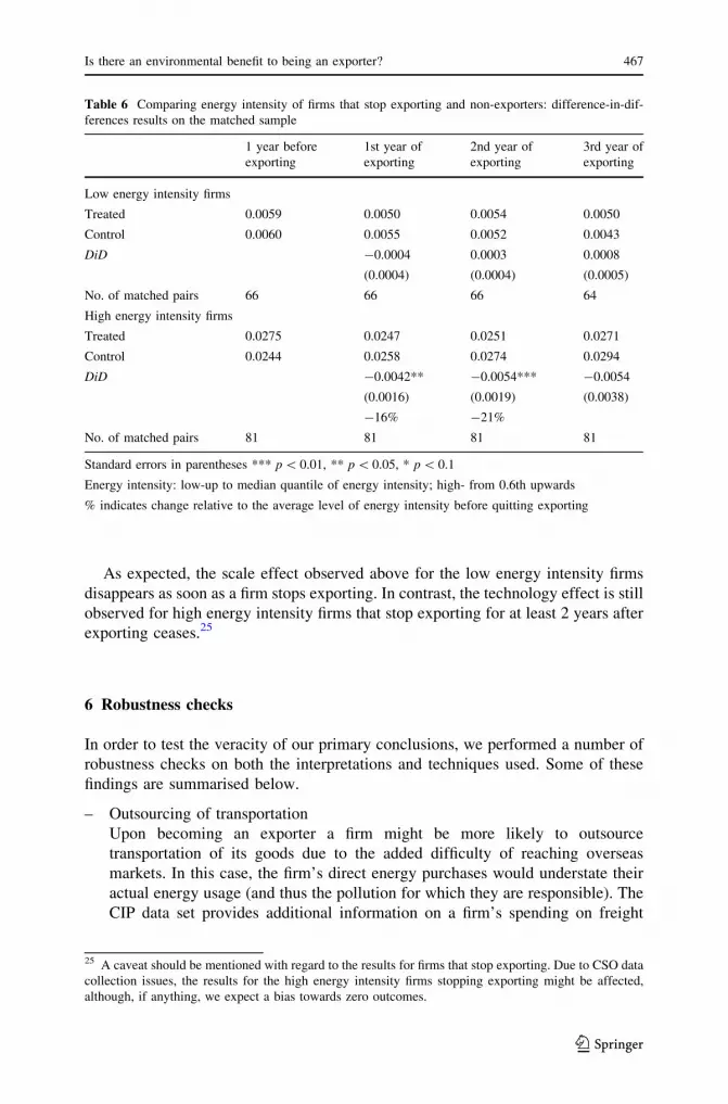
As expected, the scale effect observed above for the low energy intensity firms

disappears as soon as a firm stops exporting. In contrast, the technology effect is still

observed for high energy intensity firms that stop exporting for at least 2 years after

exporting ceases.25

6 Robustness checks

In order to test the veracity of our primary conclusions, we performed a number of

robustness checks on both the interpretations and techniques used. Some of these

findings are summarised below.

– Outsourcing of transportation

Upon becoming an exporter a firm might be more likely to outsource

transportation of its goods due to the added difficulty of reaching overseas

markets. In this case, the firm’s direct energy purchases would understate their

actual energy usage (and thus the pollution for which they are responsible). The

CIP data set provides additional information on a firm’s spending on freight

Table 6 Comparing energy intensity of firms that stop exporting and non-exporters: difference-in-dif-

ferences results on the matched sample

1 year before

exporting

1st year of

exporting

2nd year of

exporting

3rd year of

exporting

Low energy intensity firms

Treated 0.0059 0.0050 0.0054 0.0050

Control 0.0060 0.0055 0.0052 0.0043

DiD -0.0004

(0.0004)

0.0003

(0.0004)

0.0008

(0.0005)


High energy intensity firms

Treated 0.0275 0.0247 0.0251 0.0271

Control 0.0244 0.0258 0.0274 0.0294

DiD -0.0042**

(0.0016)

-16%

-0.0054***

(0.0019)

-21%

-0.0054

(0.0038)



Energy intensity: low-up to median quantile of energy intensity; high- from 0.6th upwards

% indicates change relative to the average level of energy intensity before quitting exporting

25 A caveat should be mentioned with regard to the results for firms that stop exporting. Due to CSO data

collection issues, the results for the high energy intensity firms stopping exporting might be affected,

although, if anything, we expect a bias towards zero outcomes.


123

charges which we used to check the importance of transportation outsourcing.

Both low and high energy intensity firms outsource transportation significantly

more after starting to export. The difference between the two groups, however,

is small and not high enough to suggest that it affects one group significantly

more than the other. As a next step we added outsourced freight charges to the

expenses on energy to account for any potential outsourcing influence. Using

this alternative measure of environmental performance, we find that the results

are qualitatively unchanged for the low energy intensity firms with a higher

magnitude of the output effects but the negative dynamics of exporters’ energy

use becomes insignificant for the high energy intensity firms.26 Thus, although

we do not find the reductions for high energy intensity firms we find that, unlike

low energy intensity firms, they do not increase expenditures on energy and

shipping when they begin exporting. Since the theory only implies that the rise

in total expenditures should fall as energy intensity rises, not that it be negative,

this is again consistent with our model.

– Increased import of inputs

Another alternative explanation of the technology effect might be the increasing

reliance of exporters on imported inputs which would lead to a lower energy

use. It is possible that firms develop international ties after starting to export and

begin importing more of their inputs and this might bring their relative energy

use down significantly. This increase in import intensity would then have to be

much stronger for high energy intensity firms than for low energy intensity ones

for it to substitute for a technology effect. The former group might be more

prone to import inputs given that energy constitutes a large share of their costs.

However, we find this not to be the case. First, the import intensity of low

energy intensity firms is on a higher level than that of high energy intensity

firms. Moreover, the observed growth of inputs importing is of the same

magnitude for both low and high energy intensity firms when averaged over 3

years exporting time and the dynamics of the changes year on year is very

similar. Second, and more important, we observe import intensity to rise quite

notably in a second year of exporting while the significant changes in relative

energy use are already observed in the first year for both types of firms. This

suggests that technology effects cannot be attributed to an increased import of

inputs.

– Kernel matching

To test the robustness of Nearest Neighbor Matching with one neighbour we

double check the results with kernel matching since Caliendo and Kopeinig

(2005) suggest using it where the number of comparable control observations is

large, as is the case in our sample. Qualitatively, the kernel matching results are

unchanged with the magnitudes of the effects somewhat smaller overall.

– Alternative exporter definitions

An alternative definition of exporters is also tried out where export starters are

defined as firms that do not export for 2 years and then export for two

26 Note that here firms are divided into lower and upper quantiles of the sum of energy and freight costs

relative to turnover rather than energy costs alone.


123

consecutive years. Such an abridged definition might introduce volatility since

some firms change their exporting status more than once and one might expect

that it is longer term exporting plans that would have a stronger and more

pronounced effect. The main results, however, stay unchanged.

– Absolute energy use

In the above analysis, we use energy use relative to sales as our dependent

variable. As an alternative, we repeated our estimation using absolute, rather

than relative, energy use. When doing so, we found comparable results: i.e.

exporting increases energy use for firms that use small amounts of energy,

reduces it for firms using large quantities of energy, and that these changes are

largely driven by changes while exporting. The only distinction is that we

observe a self-selection effect of more energy-efficient firms into exporting

among big energy users.

– Outlying observations

To make sure extreme control variable values are not driving the results, we

have removed the top and bottom 0.1% of observations and all negative values

of capital, some of which are so by construction of this variable. Our main

findings are mainly unaffected, although matching estimation outcomes lose

some of their statistical significance though retaining the observed signs.

– Capital intensity

To account for capital intensity of a firm which may more likely be a

determinant of energy intensity than total capital, we re-ran all estimations using

the capital/labour ratio instead of total capital. Quantile estimations produce

very similar outcomes. Matching findings lose their significance although

retaining their signs. Since capital intensity might be strongly correlated with the

industry a firm is in, when we repeat the matching estimations taking out

controls at NACE 3-digit level, matching results return to the previous levels of

significance.

7 Conclusions

One of the greatest concerns over globalisation and trade openness is the impact on

the environment. This paper contributes to this debate by examining the relationship

between a firm’s decision to export and its energy use. Our theoretical model

predicts a positive correlation between exporting and energy expenditures for low

energy intensity firms and a smaller or even a negative correlation for high energy

intensity firms. This is because for low energy intensity firms exporting creates only

a scale effect through which increased production increases energy use. For high

energy intensity firms, this is at least partially offset by the adoption of greener

technology made profitable because of the increased market size. We confirm this

empirically using a panel firm-level data set on Irish manufacturing firms for

1991–2007. This suggests that studies using aggregated data or firm level data with

a focus entirely on mean effects may miss important links between globalisation,

energy use, and the environment.


123

Although neither our model nor our estimates speak directly to policy

implications, our results suggest that the energy use implications of trade

liberalization are likely to be complex. If trade barriers are lowered in energy

intensive industries, our estimates suggest that the associated change in energy

consumption is likely to be lower than when barriers are removed in a less

energy-intensive industry. Similarly, the mix of energy-intensities within an

industry would affect the net change in usage because of differing technology

adoption rates within a sector. Furthermore, although if energy use rises on net

pollution too will rise (as shown by correlation between the two in Eskeland and

Harrison 2003; Cole et al. 2008), trade liberalisation can induce improved

pollution abatement, expansion in renewable energy, and other changes which

would mitigate the environmental impact. Although such analysis is beyond the

scope of this paper, we hope that our estimates provide a useful framework for the

continuing debate.

Appendix

See Tables 7, 8, 9, 10, 11, 12, and 13.

Table 7 Baseline values for

simulationsVariable Interpretation Baseline

value

F Fixed cost of a domestic plant 0

Fx Fixed cost of exporting 10

P Domestic price index 2

I Domestic income 15

P* Foreign price index 4

I* Foreign income 30

r Elasticity of substitution 3.8

s Energy use for exporting 1

b(i) Productivity parameter 1

r Cost of fuel 1

w Wage rate 1

tH High technology parameter 1.08

tL Low technology parameter 1

c(tH) High technology cost 2.1

c(tL) Low technology cost 0


123

Table 8 List of NACE 2-digit industries in the census of industrial production (CIP)

NACE code Description

15 Manufacture of food products and beverages

16 Manufacture of tobacco products

17 Manufacture of textiles

18 Manufacture of wearing apparel; dressing and dyeing of fur

19 Tanning and dressing of leather; manufacture of luggage,

handbags, saddlery, harness and footwear

20 Manufacture of wood and of products of wood and cork,

except furniture; manufacture of articles of straw and plaiting materials

21 Manufacture of pulp, paper and paper products

22 Publishing, printing and reproduction of recorded media

23 Manufacture of coke, refined petroleum products and nuclear fuel

24 Manufacture of chemicals and chemical products

25 Manufacture of rubber and plastic products

26 Manufacture of other non-metallic mineral products

27 Manufacture of basic metals

28 Manufacture of fabricated metal products, except machinery and equipment

29 Manufacture of machinery and equipment n.e.c.

30 Manufacture of office machinery and computers

31 Manufacture of electrical machinery and apparatus n.e.c.

32 Manufacture of radio, television and communication equipment and apparatus

33 Manufacture of medical, precision and optical instruments, watches and clocks

34 Manufacture of motor vehicles, trailers and semi-trailers

35 Manufacture of other transport equipment

36 Manufacture of furniture; manufacturing n.e.c.

Table 9 Definition of variables

Variable Description

Relative energy

use

Total fuel and power purchase as declared by firms in the CIP, scaled down by total

turnover.

Exporter Dummy variable equal to 1 if a firm exports in any given year and 0 otherwise. For

matching estimations exporters are defined as firms that switch to and stay

exporting: firms that do not export 3 years prior to switching to exporting and then

export for at least 3 years.

Ownership Dummy variable equal to 1 if a firms is foreign-owned and 0 if it is a domestic firm.

Labour

productivity

Total turnover divided by the number of employees.

Size Total earnings (in constant thousand of euros).

Skill % of managerial/technical and clerical personnel in total employment.

R&D Research and development services supplied to the enterprise.

Freight costs Freight charges for transport of the firm’s products.

Capital Firm’s capital additions built over the whole period minus sales of capitals assets,

assuming 10% yearly depreciation rate overall.


123

t-tests for Sect. 5.2 comparing sample means of the treated and control groups to

assess the quality of propensity score matching performed. Both tables indicate that

there is no statistically significant difference in the means of variables used to

calculate the propensity score.

Table 10 Summary statistics, manufacturing

Variable Mean SD Min Max

Total energy use 120.72 853.57 0 66,043.99

Energy per turnover 0.015 0.021 0 1.356

Export share 25.86 36.48 0 100

Total turnover 18,240.99 203,343.73 0 12,670,647

Size 1,370.54 5,144.87 0 257,530.28

Total employed 50.42 143.66 0 4,554

Labour productivity 151.71 373.58 0 16,062.42

% High-skilled 25.09 18.87 0 100

Capital 2,726.69 38,761.71 -93,586.49 4,326,626.5

R&D 384.16 12,639.16 0 1,386,157

Energy and freight charges 330.84 2,087.33 0 195,178.77

Energy and freight per turnover 0.033 0.037 0 1.935

All monetary values are in thousands of euros

Table 11 All manufacturing

firms, t-testTreated Control t-test

Energy intensityt-1 0.01553 0.01611 -0.52

Labour productivityt-1 101.73 101.42 0.03

Sizet-1 611.55 710.87 -0.94

Sizet-12 1.9e?06 3.2e?06 -1.01

Capitalt-1 672.92 865.16 -0.80

Ownershipt-1 0.01867 0.02133 -0.26

Skillt-1 25.215 24.827 0.30

Table 12 Low energy intensity

firms, t-test

Low energy intensity firms—

firms in up to and including

median quantile of energy

intensity

Treated Control t-test

Energy intensityt-1 0.00521 0.00558 -0.81

Labour productivityt-1 113.06 123.32 -0.57

Sizet-1 694.89 541.81 1.04

Sizet-12 1.2e?06 8.4e?05 0.64

Capitalt-1 404.76 514.23 -0.65

Ownershipt-1 0.05 0.08333 -0.73

Skillt-1 30.646 33.572 -0.65


123

References

Albornoz, F., Cole, M. A., Elliott, R. J. R., & Ercolani, M. G. (2009). In search of environmental

spillovers. The World Economy, 32(1), 136–163.

Angrist, J. D., & Pischke, J.-S. (2009). Mostly harmless econometrics: An empiricist’s companion.

Princeton: Princeton University Press.

Antweiler, W., Copeland, B. R., & Taylor, M. S. (2001). Is free trade good for the environment? TheAmerican Economic Review, 91(4), 877–908.

Barrett, S. (1994). Strategic environmental policy and international trade. Journal of Public Economics,54(3), 325–338.

Bernard, A. B., & Jensen, J. B. (1999). Exceptional exporter performance: Cause, effect, or both? Journalof International Economics, 47(1), 1–25.

Bernard, A. B., Redding, S. J., & Schott, P. K. (2007). Comparative advantage and heterogeneous firms.

Review of Economic Studies, 74(1), 31–66.

Blundell, R., & Dias, M. C. (2000). Evaluation methods for non-experimental data. Fiscal Studies, 21(4),

427–468.

Bustos, P. (2011). Trade liberalization, exports, and technology upgrading: Evidence on the impact of

MERCOSUR on Argentinian firms. American Economic Review, 101(1), 304–340.

Caliendo, M., & Kopeinig, S. (2005). Some practical guidance for the implementation of propensity scorematching (IZA Discussion Paper No. 1588). Bonn: Institute for the Study of Labor.

Cole, M. A., Elliott, R. J. R., & Strobl, E. (2008). The environmental performance of firms: The role of

foreign ownership, training, and experience. Ecological Economics, 65(3), 538–546.

Cole, M. A., Elliott, R. J. R., & Shimamoto, K. (2006). Globalization, firm-level characteristics and

environmental management: A study of Japan. Ecological Economics, 59(3), 312–323.

Copeland, B. R., & Taylor, M. S. (1994). North-south trade and the environment. The Quarterly Journalof Economics, 109(3), 755–787.

Copeland, B. R., & Taylor, M. S. (1995). Trade and transboundary pollution. The American EconomicReview, 85(4), 716–737.

Copeland, B. R., & Taylor, M. S. (1997). A simple model of trade, capital mobility, and the environment(NBER Working Paper No. 5898). Cambridge, MA: National Bureau of Economic Research.

Dean, J. M., & Lovely, M. E. (2010). Trade growth, production fragmentation, and China’s environment.

In: R. Feenstra, & S.-J. Wei (Eds.), China’s growing role in world trade, (chapter 11 pp. 429–474).

Chicago: University of Chicago Press.

Ederington, J., Levinson, A., & Minier, J. (2004). Trade Liberalization and pollution havens. Advances inEconomic Analysis & Policy, 4(2), Article 6.

Ederington, J., Levinson, A., & Minier, J. (2005). Footloose and pollution-free. The Review of Economicsand Statistics, 87(1), 92–99.

Eskeland, G. S., & Harrison, A. E. (2003). Moving to greener pastures? Multinationals and the pollution

haven hypothesis. Journal of Development Economics, 70(1), 1–23.

Galdeano-Gomez, E. (2010). Exporting and environmental performance: A firm-level productivity

analysis. The World Economy, 33(1), 60–88.

Table 13 High energy intensity

firms, t-test

High energy intensity firms—

firms from 0.6th quantile of

energy intensity upwards

Treated Control t-test

Energy intensityt-1 0.03249 0.03235 0.03

Sizet-1 444.58 414.22 0.34

Sizet-12 4.4e?05 3.8e?05 0.34

Capitalt-1 506.4 416.7 0.40

Labour productivityt-1 73.171 82.007 -0.72

Skillt-1 18.27 17.32 0.46

R&Dt-1 2.1859 0.56206 1.43


123

Girma, S., & Gorg, H. (2005). Foreign direct investment, spillovers and absorptive capacity: Evidencefrom quantile regressions (Kiel Working Paper No. 1248). Kiel: Kiel Institute for the World

Economy.

Girma, S., Hanley, A., & Tintelnot, F. (2008). Exporting and the environment: A new look with micro-data (Kiel Working Paper No. 1423). Kiel: Kiel Institute for the World Economy.

Girma, S., Greenaway, D., & Kneller, R. (2004). Does Exporting increase productivity? A microeco-

nometric analysis of matched firms. Review of International Economics, 12(5), 855–866.

Heckman, J. J., Ichimura, H., & Todd, P. E. (1997). Matching as an econometric evaluation estimator:

Evidence from evaluating a job training programme. The Review of Economic Studies, 64(4),

605–654.

International Study Group on Exports and Productivity (2008). Understanding cross-country differences

in exporter premia: Comparable evidence for 14 countries. Review of World Economics/Weltwirtschaftliches Archiv, 144(4), 596–635.

Jaffe, A. B., Peterson, S. R., Portney, P. R., & Stavins, R. N. (1995). Environmental regulation and the

competitiveness of U.S. manufacturing: What does the evidence tell us? Journal of EconomicLiterature, 33(1), 132–163.

Javorcik, B. S., & Wei, S.-J. (2004). Pollution havens and foreign direct investment: Dirty secret or

popular myth? Contributions to Economic Analysis & Policy, 3(2), Article 8.

Kaiser, K., & Schulze, G. G. (2003). International competition and environmental expenditures:Empirical evidence from Indonesian manufacturing plants (HWWA Discussion Paper 222).

Hamburg: Hamburg Institute of International Economics.

Keller, W., & Levinson, A. (2002) Pollution abatement costs and foreign direct investment inflows to

U.S. States. Review of Economics and Statistics, 84(4), 691–703.

Koenker, R., & Bassett, G. Jr. (1978). Regression quantiles. Econometrica, 46(1), 33–50.

Koenker, R., & Hallock, K. F. (2001). Quantile regression. The Journal of Economic Perspectives, 15(4),

143–156.

Levinson, A. (2009). Technology, international trade, and pollution from US manufacturing. AmericanEconomic Review, 99(5), 2177–2192.

Levinson, A., & Taylor, M. S. (2008). Unmasking the pollution haven effect. International EconomicReview, 49(1), 223–254.

List, J. A., Millimet, D. L., Fredriksson, P. G., & McHone, W. W. (2003). Effects of environmental

regulations on manufacturing plant births: Evidence from a propensity score matching estimator.

Review of Economics and Statistics, 85(4), 944–952.

Markusen, J. R., Morey, E. R., & Olewiler, N. (1995). Competition in regional environmental policies

when plant locations are endogenous. Journal of Public Economics, 56(1), 55–77.

McCann, F. (2009). Importing, exporting and productivity in Irish manufacturing (UCD Centre for

Economic Research Working Paper WP09/22). University College Dublin.

McGuire, M. C. (1982). Regulation, factor rewards, and international trade. Journal of Public Economics,17(3), 335–354.

Melitz, M. J. (2003). The impact of trade on intra-industry reallocations and aggregate industry

productivity. Econometrica, 71(6), 1695–1725.

Pethig, R. (1976). Pollution, welfare, and environmental policy in the theory of comparative advantage.

Journal of Environmental Economics and Management, 2(3), 160–169.

Rosenbaum, P. R., & Rubin, D. B. (1983). The central role of the propensity score in observational

studies for causal effects. Biometrika, 70(1), 41–55.

Smith, J. A., & Todd, P. E. (2005). Does matching overcome LaLondes critique of nonexperimental

estimators? Journal of Econometrics, 125(1–2), 305–353.

Wagner, J. (2002). The causal effects of exports on firm size and labour productivity: First evidence from

a matching approach. Economics Letters, 77, 287–292.

Wagner, J. (2007). Exports and productivity: A survey of the evidence from firm-level data. The WorldEconomy, 30(1), 60–82.

Wooldridge, J. M. (2002). Econometric analysis of cross section and panel data. Cambridge, MA,

Washington, DC: MIT Press.

World Bank (2010). World Development Indicators. Washington, DC.

Yasar, M., Nelson, C. H., & Rejesus, R. (2006). Productivity and exporting status of manufacturing firms:

Evidence from quantile regressions. Review of World Economics/Weltwirtschaftliches Archiv,142(4), 675–694.


123

is there an environmental benefit to being an exporter? evidence from firm-level data

Documents