Graduate Theses, Dissertations, and Problem Reports

2016

Investigation of Combustion Phenomena in a Single-Cylinder Investigation of Combustion Phenomena in a Single-Cylinder

Spark-Ignited Natural Gas Engine with Optical Access Spark-Ignited Natural Gas Engine with Optical Access

Vishnu Padmanaban

Follow this and additional works at: https://researchrepository.wvu.edu/etd

Recommended Citation Recommended Citation Padmanaban, Vishnu, "Investigation of Combustion Phenomena in a Single-Cylinder Spark-Ignited Natural Gas Engine with Optical Access" (2016). Graduate Theses, Dissertations, and Problem Reports. 6367. https://researchrepository.wvu.edu/etd/6367

This Thesis is protected by copyright and/or related rights. It has been brought to you by the The Research Repository @ WVU with permission from the rights-holder(s). You are free to use this Thesis in any way that is permitted by the copyright and related rights legislation that applies to your use. For other uses you must obtain permission from the rights-holder(s) directly, unless additional rights are indicated by a Creative Commons license in the record and/ or on the work itself. This Thesis has been accepted for inclusion in WVU Graduate Theses, Dissertations, and Problem Reports collection by an authorized administrator of The Research Repository @ WVU. For more information, please contact researchrepository@mail.wvu.edu.

Investigation of Combustion Phenomena in a Single-Cylinder Spark-Ignited Natural Gas Engine with Optical Access

Vishnu Padmanaban

Thesis submitted to the Benjamin M. Statler College of Engineering and Mineral Resources

at West Virginia University

in partial fulfillment of the requirements for the degree of

Master of Science in

Mechanical Engineering

Cosmin Dumitrescu, Ph.D., Chair

Arvind Thiruvengadam, Ph.D. V’yacheslav Akkerman, Ph.D.

Department of Mechanical and Aerospace Engineering

West Virginia University

Morgantown, West Virginia July 2016

Keywords: IC engine, natural gas, spark ignition, optical engine, flame visualization

Copyright 2016 Vishnu Padmanaban

ABSTRACT

Investigation of Combustion Phenomena in a Single-Cylinder Spark- Ignited Natural Gas Engine with Optical Access

Vishnu Padmanaban

More demanding efficiency and emissions standards for internal combustion (IC) engines require

novel combustion strategies, alternative fuels, and improved after-treatment systems. However, their

development depends on improved understanding of in-cylinder processes. For example, the lower

efficiency of conventional spark-ignited (SI) natural-gas (NG) engines reduces their utilization in the

transportation sector. Single-cylinder optical-access research engines allow the use of non-intrusive

visualization techniques that study in-cylinder flow, fuel-oxidizer mixing, and combustion and emissions

phenomena under conditions representative of production engines. These visualization techniques can

provide qualitative and quantitative answers to fundamental combustion-phenomena questions such as the

effects of engine design, operating conditions, fuel composition, fuel delivery strategy, and ignition

techniques.

The thesis is divided in two main parts. The first part focuses on the setup of a single-cylinder research

engine with optical access including the design of its control system and the acquisition of in-cylinder

pressure data and high-speed combustion images. The second part focuses on measurements of the turbulent

flame speed using the high-speed combustion images. Crank-angle-resolved images of methane combustion

were taken with a high-speed CMOS camera at a rate of 15,000 Hz. The optical engine was operated in a

skip-firing mode (one fired cycle followed by 5 motored cycles) at 900 RPM and a load of 5.93 bar IMEP.

The images show that flow turbulence and flame stretch resulted in flame velocities several order of

magnitude higher compared to the laminar flame velocity. In addition, both in-cylinder pressure and optical

data were used to determine the cycle-to cycle variability of the combustion phenomena.

iii

Dedication

This thesis is dedicated to my beloved parents, Dr.Padmanaban, and Beena Padmanaban

iv

Acknowledgements First and foremost, I would like to thank my research advisor Dr. Cosmin Dumitrescu for his support,

knowledge and all the friendship he shared with me right from the beginning. Everything he taught me

both, in academics and building me as a person will surely stay with me and help me progress in my future

career. His perseverance in work have always strongly motivated me to put in a lot of efforts and set an

example to my colleagues in the laboratory. I am very grateful to him for teaching me the difference

between a scientific and an engineering work, helping me start transforming into a good researcher. On a

lighter note, I am very thankful to him for having funded me three long semesters in my master’s study.

I would like to express my gratitude to Dan Carder for having initially hired me to the CAFEE, and help

me settle down to work with optical engines research project. My heartfelt thanks are due to my committee

member Dr. Arvind Thiruvengadam for having been a good friend and a wonderful source of inspiration.

With his stature and knowledge, nobody I could think of to have been this modest, helpful and supportive

to anybody who approaches him. I thank Dr. Slava Akkerman for having been so kind during my Teaching

Assistantship days, and also for his time in reviewing my thesis – a very generous committee member,

indeed.

Dr. Ross Ryskamp and Dr. Marc Besch – I thank you affectionately for having taught me immensely at the

lab. My special thanks to Jesse Griffins, for developing the engine’s skip-firing controller. Dozens of other

CAFEE members helped me to successfully finish up my thesis, and I am thankful to each and every one

of them. Extraordinary engineers, inspiring senior students, and my dear graduate student colleagues, I

thank you all very much.

Madhuri Vemulapalli, a best friend for my lifetime – I would like to thank her from the bottom of my heart

for all the emotional support, comradery, motivation and care she has been providing me with. It was the

strong bonding in the friendship that we shared, helped me face difficult times in the US. Nobody could

replace your friendship and sisterhood, I believe. Sushmita, Aliya and Charan- these loving friends were

like a second family to me. I still fondly cherish the time we spent at Twin Campus. Thanks for sharing all

my happiest and troubled moments. My buddies –Satya and Shiva, without you guys the fun would not

have been continuing so long. I thank the entire Indian student community and other new friends I made

here at WVU for having provided a great companionship.

Last but certainly not least, I would like to thank my family – Padmanaban, Ramesh Vijayrangan, Beena,

Madhusudhan, AR Vijayrangan and Vathsala. Without their unconditioned love, warmth and selfless

sacrifice, I would not have been enjoying a life like this. More like a father, Ramesh uncle has been beside

me throughout my endeavors.

v

TABLE OF CONTENTS

CHAPTER 1 INTRODUCTION ...................................................................................................... 1

1.1 BACKGROUND ............................................................................................................................................... 3

1.2 MOTIVATION ................................................................................................................................................. 4

1.3 OPTICAL DIAGNOSTIC TECHNIQUES IN COMBUSTION ............................................................................ 5

1.4 OBJECTIVE ...................................................................................................................................................... 7

CHAPTER 2 REVIEW OF LITERATURE ..................................................................................... 8

2.1 NATURAL GAS COMBUSTION IN LARGE BORE ENGINES ......................................................................... 8

2.2 FUEL COMPOSITION EFFECTS ..................................................................................................................... 9

2.3 CYCLE TO CYCLE VARIATIONS IN SI ENGINE ............................................................................................. 11

2.4 OPTICAL ACCESS ENGINE FOR COMBUSTION STUDY ..................................................................... 15

CHAPTER 3 EXPERIMENTAL SETUP ...................................................................................... 20

3.1 THE RESEARCH ENGINE .............................................................................................................................. 20

3.1.1 Base engine ....................................................................................................................... 21

3.1.2 Optical experiment test procedure .................................................................................... 24

3.1.3 Dynamometer .................................................................................................................... 25

3.1.4 Engine control unit ........................................................................................................... 26

3.1.5 Intake air system ............................................................................................................... 26

3.1.6 Engine cooling and lubrication system ............................................................................. 27

3.2 DATA ACQUISITION ........................................................................................................................ 28

3.2.1 In-cylinder data ................................................................................................................. 29

3.2.2 Other engine parameters .................................................................................................. 29

3.3 IMAGE ACQUISITION .................................................................................................................................. 30

3.3.1 Optical measurement system............................................................................................. 30

3.3.2 Image acquisition software ............................................................................................... 32

3.4 ENGINE MANAGEMENT SYSTEM .............................................................................................................. 32

3.5 FUEL INJECTOR ............................................................................................................................................ 33

3.6 SKIP FIRING CONTROLLER .............................................................................................................. 36

vi

3.7 EXHAUST GAS ANALYSIS ................................................................................................................ 37

3.7.1 Emissions sampling manifold ........................................................................................... 38

3.7.2 CO and CO2 emissions analyzer ....................................................................................... 38

3.7.3 THC emissions analyzer ................................................................................................... 39

3.1.2 NOx emissions analyzer .................................................................................................... 40

CHAPTER 4 RESULTS ................................................................................................................... 45

4.1 IN-CYLINDER PRESSURE ANALYSIS ................................................................................................. 45

4.1.1 Correlation of combustion with optical data .................................................................... 57

4.2 IMAGE PROCESSING ....................................................................................................................... 59 4.2.1 Flame radius ..................................................................................................................... 61

4.3 FLAME PROPAGATION ................................................................................................................... 64 4.3.1 Flame speed calculation ................................................................................................... 64

4.4 INTAKE FLOW MEASUREMENT ...................................................................................................... 66

4.5 EMISSION CHARACTERISTICS ......................................................................................................... 67

CHAPTER 5 CONCLUSIONS ....................................................................................................... 69

5.1 FUTURE WORK ............................................................................................................................................ 70

CHAPTER 6 BIBLIOGRAPHY...................................................................................................... 71

vii

LIST OF FIGURES

FIGURE 1.1 CONSUMPTION OF NATURAL GAS IN THE US .................................................................................... 1 FIGURE 1.2 ESTIMATED CONSUMPTION OF ALTERNATIVE FUEL BY AFVS IN THE U.S. ........................................ 2 FIGURE 1.3 TYPICAL (A) OPTICAL ENGINE CONFIGURATION, (B) STANDARD METAL ENGINE CONFIGURATION

(SINGLE CYLINDER GDI ENGINE), AND (C) A 3D-CAD VIEW OF AN ELONGATED PISTON WITH

OPTICAL ACCESS ............................................................................................................................... 4 FIGURE 1.4 ENDOSCOPE INSERTION IN THE CYLINDER HEAD OF A DIESEL ENGINE ............................................. 7 FIGURE 2.1 SCHEMATIC DIAGRAM OF BOWDITCH’S SLOTTED, EXTENDED PISTON DESIGN .............................. 16 FIGURE 2.2 HIGH-SPEED OPTICAL ENGINE DEVELOPED BY LOTUS ENGINEERING LIMITED AND

LOUGHBOROUGH UNIVERSITY ........................................................................................................ 19 FIGURE 3.1 SCHEMATIC ARRAGEMENT OF THE ENGINE TEST SETUP ................................................................. 22 FIGURE 3.2 DIFFERENT VIEWS OF THE TESTING FACILITY .................................................................................. 23 FIGURE 3.3 EXPERIMENTAL PROTOCOL ............................................................................................................ 25 FIGURE 3.4 SKETCH OF REAR PANEL OF THE HIGH SPEED CAMERA ................................................................... 31 FIGURE 3.5 SCHEMATIC SHOWING THE OPTICAL MEASUREMENT SYSTEM ...................................................... 31 FIGURE 3.6 MANUFACTURER CALIBRATION FLOW CURVES FOR THE INJECTOR IG7 WITH 4 SEATS WORKING . 33 FIGURE 3.7 INJECTOR FLOW CURVE PLOTTED FROM BENCH TESTING AT LAB .................................................. 34 FIGURE 3.8 SCHEMATIC WAVEFORM OF INJECTOR EVENTS PER CYCLE BASIS ................................................... 34 FIGURE 3.9 LINEARITY REGION IN THE FLOW CALIBRATED INJECTOR PERFORMANCE

CURVES ............................................................................................................................................ 35 FIGURE 3.10 SCHEMATIC OF THE SKIP FIRING CONTROLLER LOGIC ..................................................................... 36 FIGURE 3.11 TRIGGERING SCHEMATIC FOR CAMERA .......................................................................................... 37 FIGURE 3.12 SCHEMATIC ILLUSTRATION OF NDIR OPERATING PRINCIPLE .......................................................... 38 FIGURE 3.13 SCHEMATIC ILLUSTRATION OF FID OPERATING PRINCIPLE ............................................................. 39 FIGURE 3.14 SCHEMATIC ILLUSTRATION OF CLD OPERATING PRINCIPLE ............................................................ 40 FIGURE 3.15 FLOW SCHEMATIC FOR CO2 ANALYZER BOX .................................................................................... 41 FIGURE 3.16 FLOW SCHEMATIC FOR THC ANALYZER BOX ................................................................................... 42 FIGURE 3.17 FLOW SCHEMATIC FOR NOX ANALYZER BOX ................................................................................... 43 FIGURE 4.1 MOTORING TRACE AFTER PEGGING FOR COMPRESSION RATIO CALCULATION ............................. 45 FIGURE 4.2 EXAMPLE OF A COMBUSTION PRESSURE TRACE FOR A FIRED CYCLE .............................................. 46 FIGURE 4.3 IN-CYLINDER PRESSURE RAW DATA (WITHOUT FILTER) FOR COMBUSTION TRACE OF 97 CYCLES .. 46 FIGURE 4.4 ZERO PHASE DIGITAL FILTER FOR COMBUSTION TRACES OF 97 CYCLES .......................................... 47 FIGURE 4.5 BUTTERWORTH FILTER FOR COMBUSTION TRACES OF 97 CYCLES ................................................. 47 FIGURE 4.6 P-V DIAGRAM OF AN ENGINE CYCLE ................................................................................................ 49 FIGURE 4.7 IN-CYLINDER CUT OFF VIEW OF A TYPICAL SINGLE CYLINDER OPTICALLY ACCESIBLE ENGINE ........ 49 FIGURE 4.8 LOG P VS LOG V, PLOT OF A COMBUSTION CYCLE ........................................................................... 50 FIGURE 4.9 THE NET HEAT RELEASE RATE FOR A REPRESENTATIVE COMBUSTING CYCLE ................................. 51 FIGURE 4.10 MASS FRACTION BURNED FROM -5 DEG TO 50 DEG COMBUSTION DURATION OF A

REPRESENTATIVE CYCLE .................................................................................................................. 52 FIGURE 4.11 MASS FRACTION BURNED PROFILE BASED ON RASSWIELER & WITHROW METHOD FOR A

REPRESENTATIVE CYCLE .................................................................................................................. 53 FIGURE 4.12 IMEP OF COMBUSTING CYCLES ....................................................................................................... 54 FIGURE 4.13 ENGINE LOAD PROFILE FOR ONE SET OF SKIP FIRED OPERATION .................................................... 55

viii

FIGURE 4.14 IMAGED REGION RELATIVE TO THE TOTAL CYLINDER HEAD AREA, SPARK LOCATION AND ENGINE

VALVES ............................................................................................................................................ 56 FIGURE 4.15 RAW FLAME IMAGES REPRESENTATIVE OF COMBUSTION EVENTS FROM CAD -10 TO CAD 50 ....... 57 FIGURE 4.16 IMAGE PROCESSING STEPS .............................................................................................................. 58 FIGURE 4.17 CHARACTERISTIC PLOT OF WRINKLING RATIO WITH THE FLAME GROWTH .................................... 60 FIGURE 4.18 EXAMPLE OF FLAME IMAGES USED TO DETERMINE BURN RATE PARAMETERS .............................. 61 FIGURE 4.19 THE FLAME RADIUS INCREASE WITH CAD FOR A REPRESENTATIVE COMBUSTING CYCLE ............... 62 FIGURE 4.20 EVOLUTION OF FLAME GROWTH STUDIED EXPERIMENTALLY USING PLIF BY [105] ........................ 62 FIGURE 4.21 FLAME VELOCITY FOR A REPRESENTATIVE FLAME IMAGES SET ...................................................... 64 FIGURE 4.22 CYCLIC VARIABILITY IN FLAME SPEED VS CAD .................................................................................. 65 FIGURE 4.23 EFFECT OF SURGE TANK ON INTAKE FLOW FLUCTUATIONS WITH 0.01” ORIFICE SNUBBERS .......... 65 FIGURE 4.24 MEASURED EMISSION LEVEL FROM NDIR GAS ANALYZER FOR ONE SET OF SKIP FIRED OPERATION

........................................................................................................................................................ 66 FIGURE 4.25 MEASURED EMISSIONS LEVEL FROM FID GAS ANALYZER FOR ONE SET OF SKIP FIRED OPERATION

........................................................................................................................................................ 67

ix

LIST OF TABLES

TABLE 1.1 ANALYSIS TECHNIQUES IN TRANSPARENT RESEARCH ENGINES AND STANDARD ENGINES .............. 5 TABLE 1.2 LASER BASED IN-CYLINDER ANALYSIS TEHNIQUES ............................................................................ 6 TABLE 3.1 ENGINE SPECIFICATIONS IN THE PHOTOGRAPHIC BUILD ................................................................ 21 TABLE 3.2 COMPOSITION SPECIFICATION OF CHEMICALLY-PURE-GRADE METHANE ..................................... 28 TABLE 3.3 TECHNICAL SPECIFICATIONS OF THE SENSORS USED FOR DATA ACQUISITON ................................ 30 TABLE 3.5 TECHNICAL SPECIFICATIONS OF THE IG7 NAVAJO CNG INJECTOR .................................................. 33 TABLE 4.1 ENGINE OPERATING PARAMETERS ................................................................................................. 55

x

LIST OF ABBREVIATIONS ATDC – After Top Dead Center BDC - Bottom Dead Center CAD – Crank Angle Degree CAFEE – Center for Alternative Fuels, Engines and Emissions CCD – Charge Coupled Device CCV – Cycle to Cycle Variation CFD – Computational Fluid Dynamics CLD – Chemiluminiscence Detector CMOS – Complementary Metal-Oxide Semiconductor CNG – Compressed Natural Gas CO – Carbon Monoxide CO2 – Carbon di-oxide COV – Coefficient of Variance CP – Chemically Pure CR – Compression Ratio DAQ – Data Acquisition DC – Direct Current DI – Direct Injection DOE – Department of Energy ECU – Engine Control Unit EGR – Exhaust Gas Recirculation EOC- End of Combustion FID – Flame Ionization Detector FPS – Frames per Second GDI – Gasoline Direct Injection GGE – Gasoline Gallon Equivalent GHG – Green House Gas HC – Hydrocarbon HCCI – Homogenous Charge Compression Ignition HDV – Heavy Duty Vehicle HRR – Heat Release Rate HV – Heating Value IC – Integrated Chip IDI- Indirect Injection IMEP – indicated Mean Effective Pressure LDA – Laser Doppler Anemometry LFE – Laminar Flow Element LIF – Laser Induced Fluorescence LII – Laser Induced Incandescence LPG – Liquefied Petroleum Gas MAP – Manifold Absolute Pressure MFB – Mass Fraction Burned MN- Methane Number MON – Motor Octane Number

xi

NDIR – Non Dispersive Infrared NGV – Natural Gas Vehicle NMHC – Non-Methane Hydro Carbon NOx – Oxides of Nitrogen OC – Oxidation Catalyst PAH – Polycyclic Aromatic Hydrocarbons PFI – Port Fuel Injection PIV – Particle Image Velocimetry PLIF – Planar Laser Induced Fluorescence PM – Particulate Matter RON – Research Octane Number RPM – Revolutions Per Minute SCFM – Standard Cubic Foot per Minute SI – Spark Ignition SOC – Start of Combustion SOI – Start of Ignition SSR – Solid State Relay TD – Turbo Diesel TDC – Top Dead Center THC – Total Hydrocarbon TTL – Transistor – Transistor Logic TWC – Three Way Catalyst UHC – Unburnt Hydrocarbon WN – Wobbe Number

1

Chapter 1

Introduction

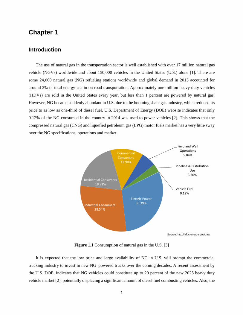
The use of natural gas in the transportation sector is well established with over 17 million natural gas

vehicle (NGVs) worldwide and about 150,000 vehicles in the United States (U.S.) alone [1]. There are

some 24,000 natural gas (NG) refueling stations worldwide and global demand in 2013 accounted for

around 2% of total energy use in on-road transportation. Approximately one million heavy-duty vehicles

(HDVs) are sold in the United States every year, but less than 1 percent are powered by natural gas.

However, NG became suddenly abundant in U.S. due to the booming shale gas industry, which reduced its

price to as low as one-third of diesel fuel. U.S. Department of Energy (DOE) website indicates that only

0.12% of the NG consumed in the country in 2014 was used to power vehicles [2]. This shows that the

compressed natural gas (CNG) and liquefied petroleum gas (LPG) motor fuels market has a very little sway

over the NG specifications, operations and market.

Figure 1.1 Consumption of natural gas in the U.S. [3]

It is expected that the low price and large availability of NG in U.S. will prompt the commercial

trucking industry to invest in new NG–powered trucks over the coming decades. A recent assessment by

the U.S. DOE. indicates that NG vehicles could constitute up to 20 percent of the new 2025 heavy duty

vehicle market [2], potentially displacing a significant amount of diesel fuel combusting vehicles. Also, the

Electric Power30.39%Industrial Consumers

28.54%

Residential Consumers18.91%

Commercial Consumers

12.90%

Field and Well Operations

5.84%

Pipeline & Distribution Use

3.30%

Vehicle Fuel0.12%

Source: http://afdc.energy.gov/data

2

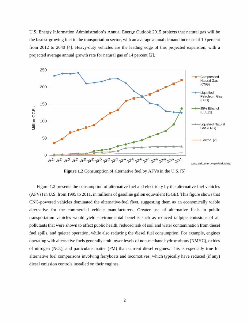
U.S. Energy Information Administration’s Annual Energy Outlook 2015 projects that natural gas will be

the fastest-growing fuel in the transportation sector, with an average annual demand increase of 10 percent

from 2012 to 2040 [4]. Heavy-duty vehicles are the leading edge of this projected expansion, with a

projected average annual growth rate for natural gas of 14 percent [2].

Figure 1.2 Consumption of alternative fuel by AFVs in the U.S. [5]

Figure 1.2 presents the consumption of alternative fuel and electricity by the alternative fuel vehicles

(AFVs) in U.S. from 1995 to 2011, in millions of gasoline gallon equivalent (GGE). This figure shows that

CNG-powered vehicles dominated the alternative-fuel fleet, suggesting them as an economically viable

alternative for the commercial vehicle manufacturers. Greater use of alternative fuels in public

transportation vehicles would yield environmental benefits such as reduced tailpipe emissions of air

pollutants that were shown to affect public health, reduced risk of soil and water contamination from diesel

fuel spills, and quieter operation, while also reducing the diesel fuel consumption. For example, engines

operating with alternative fuels generally emit lower levels of non-methane hydrocarbons (NMHC), oxides

of nitrogen (NOx), and particulate matter (PM) than current diesel engines. This is especially true for

alternative fuel comparisons involving ferryboats and locomotives, which typically have reduced (if any)

diesel emission controls installed on their engines.

0

50

100

150

200

250

Milli

on G

GEs

CompressedNatural Gas(CNG)

LiquefiedPetroleum Gas(LPG)

85% Ethanol(E85)[1]

Liquefied NaturalGas (LNG)

Electric [2]

www.afdc.energy.gov/afdc/data/

3

1.1 Background

More stringent IC engine emissions regulations, the depletion of fossil-fuel reserves and climate-effects

considerations continue to stimulate the spark engine development. These stringent efficiency and emission

regulations require novel combustion strategies and improved after treatment systems. Single cylinder

optically-accessible engines can help the development of such novel strategies by improving the

fundamental understanding of in-cylinder processes. Such engines allow the use of non-intrusive

visualization techniques that study in-cylinder flow, fuel-oxidizer mixing, and combustion and emissions

phenomena under conditions representative of production engines. The experimental data obtained from

engines with extended optical access (“optical engines”) is used for both the validation of engine

computational models that accelerate engine development and the development of new combustion

strategies as they provide a detailed insight into the physical processes occurring inside the combustion

chamber. However, the operation of optical engines presents numerous challenges as compared to

production (metal) engines. In addition, there are a few design differences between an optical engine and a

production engine. First, optical research engines have simplified chamber geometries to facilitate optical

access while minimizing image distortion issues. Further, the optical components (i.e., glass windows)

cannot resist the thermal stress accumulated during continuous engine operation. As a result, optical engines

can run only for a few minutes and usually in a skip-firing mode (one fired engine cycle followed by n

motored cycles, where n ≥ 1). Furthermore, the location of the piston ring pack on an optical engine usually

differs from that on an all-metal engine, due to the use of dry lubrication methods in the extended portion

of the optical piston. In addition to these design aspects, the use of materials such as quartz, sapphire and

titanium in optical engines has a significant impact on engine combustion characteristics. The reason for

this is that the thermal conductivity of the aforementioned materials is significantly lower than the thermal

conductivity of steel or aluminum. Therefore, it is very important that an adequate control of intake

temperature, fueling and ignition systems is established in the test setup to ensure the longevity of optical

and metal components, repeatable experimental results, and also that the optical engine experiments are

representative of the metal engine and hence could provide us with deep a meaningful insight on a physical

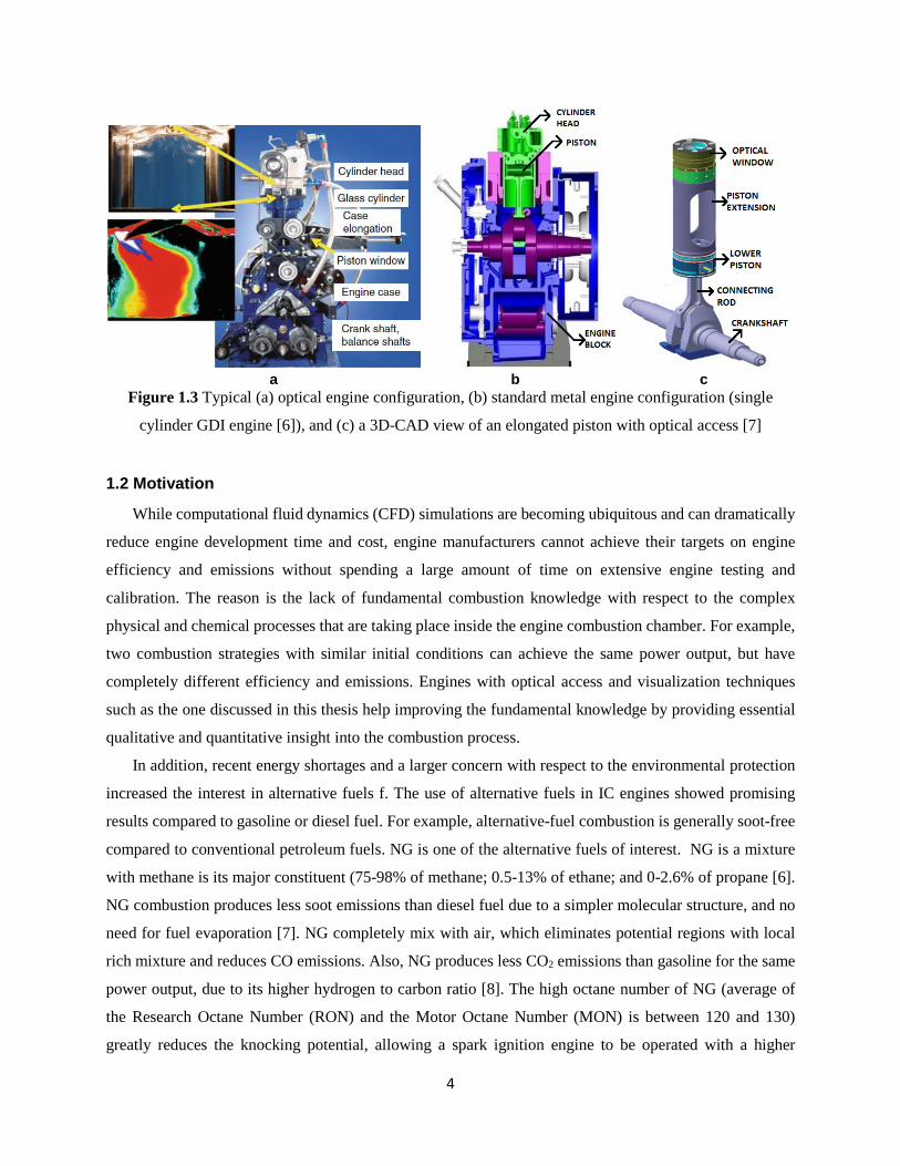
phenomenon taking place inside the combustion chamber. Figure 1.3 shows the difference between an

optical (Figure 1.3a) and standard metal configuration of the same type of engine (Figure 1.3b) to give the

readers an idea about the major differences in build and component types in either of the configurations.

4

a b c

Figure 1.3 Typical (a) optical engine configuration, (b) standard metal engine configuration (single

cylinder GDI engine [6]), and (c) a 3D-CAD view of an elongated piston with optical access [7]

1.2 Motivation

While computational fluid dynamics (CFD) simulations are becoming ubiquitous and can dramatically

reduce engine development time and cost, engine manufacturers cannot achieve their targets on engine

efficiency and emissions without spending a large amount of time on extensive engine testing and

calibration. The reason is the lack of fundamental combustion knowledge with respect to the complex

physical and chemical processes that are taking place inside the engine combustion chamber. For example,

two combustion strategies with similar initial conditions can achieve the same power output, but have

completely different efficiency and emissions. Engines with optical access and visualization techniques

such as the one discussed in this thesis help improving the fundamental knowledge by providing essential

qualitative and quantitative insight into the combustion process.

In addition, recent energy shortages and a larger concern with respect to the environmental protection

increased the interest in alternative fuels f. The use of alternative fuels in IC engines showed promising

results compared to gasoline or diesel fuel. For example, alternative-fuel combustion is generally soot-free

compared to conventional petroleum fuels. NG is one of the alternative fuels of interest. NG is a mixture

with methane is its major constituent (75-98% of methane; 0.5-13% of ethane; and 0-2.6% of propane [6].

NG combustion produces less soot emissions than diesel fuel due to a simpler molecular structure, and no

need for fuel evaporation [7]. NG completely mix with air, which eliminates potential regions with local

rich mixture and reduces CO emissions. Also, NG produces less CO2 emissions than gasoline for the same

power output, due to its higher hydrogen to carbon ratio [8]. The high octane number of NG (average of

the Research Octane Number (RON) and the Motor Octane Number (MON) is between 120 and 130)

greatly reduces the knocking potential, allowing a spark ignition engine to be operated with a higher

5

compression ratio than an equivalent gasoline engine. This increases engine thermal efficiency and lowers

fuel consumption. The RON for a particular fuel composition is determined from laboratory tests performed

with a special research engine with a variable compression ratio. Motor Octane Number (MON) also uses

a similar test engine, but with a preheated fuel mixture, a higher engine speed and variable ignition timing.

Additionally, NG has a lower lean limit than gasoline, which can further reduce CO and HC emissions and

increase the thermal efficiency. However, the number of fundamental studies in the literature that explain

these observation and can be used to predict engine efficiency and emissions is limited compared to those

dedicated to gasoline or diesel fuel. This motivates the present study of investigating the combustion

phenomena occurring inside a spark-ignition NG engine with extended optical access.

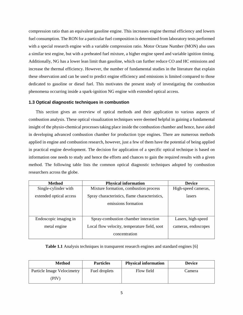
1.3 Optical diagnostic techniques in combustion

This section gives an overview of optical methods and their application to various aspects of

combustion analysis. These optical visualization techniques were deemed helpful in gaining a fundamental

insight of the physio-chemical processes taking place inside the combustion chamber and hence, have aided

in developing advanced combustion chamber for production type engines. There are numerous methods

applied in engine and combustion research, however, just a few of them have the potential of being applied

in practical engine development. The decision for application of a specific optical technique is based on

information one needs to study and hence the efforts and chances to gain the required results with a given

method. The following table lists the common optical diagnostic techniques adopted by combustion

researchers across the globe.

Method Physical information Device Single-cylinder with

extended optical access

Mixture formation, combustion process

Spray characteristics, flame characteristics,

emissions formation

High-speed cameras,

lasers

Endoscopic imaging in

metal engine

Spray-combustion chamber interaction

Local flow velocity, temperature field, soot

concentration

Lasers, high-speed

cameras, endoscopes

Table 1.1 Analysis techniques in transparent research engines and standard engines [6]

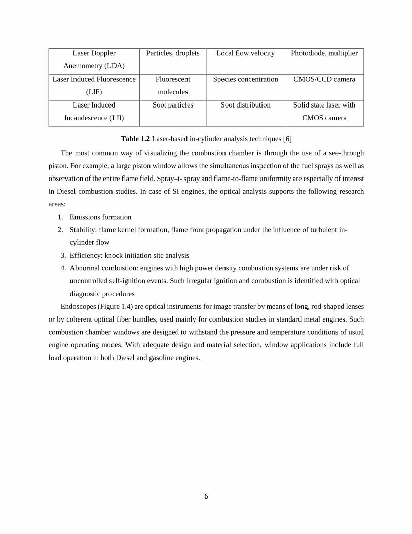
Method Particles Physical information Device

Particle Image Velocimetry

(PIV)

Fuel droplets Flow field Camera

6

Laser Doppler

Anemometry (LDA)

Particles, droplets Local flow velocity Photodiode, multiplier

Laser Induced Fluorescence

(LIF)

Fluorescent

molecules

Species concentration CMOS/CCD camera

Laser Induced

Incandescence (LII)

Soot particles Soot distribution Solid state laser with

CMOS camera

Table 1.2 Laser-based in-cylinder analysis techniques [6]

The most common way of visualizing the combustion chamber is through the use of a see-through

piston. For example, a large piston window allows the simultaneous inspection of the fuel sprays as well as

observation of the entire flame field. Spray–t- spray and flame-to-flame uniformity are especially of interest

in Diesel combustion studies. In case of SI engines, the optical analysis supports the following research

areas:

1. Emissions formation

2. Stability: flame kernel formation, flame front propagation under the influence of turbulent in-

cylinder flow

3. Efficiency: knock initiation site analysis

4. Abnormal combustion: engines with high power density combustion systems are under risk of

uncontrolled self-ignition events. Such irregular ignition and combustion is identified with optical

diagnostic procedures

Endoscopes (Figure 1.4) are optical instruments for image transfer by means of long, rod-shaped lenses

or by coherent optical fiber bundles, used mainly for combustion studies in standard metal engines. Such

combustion chamber windows are designed to withstand the pressure and temperature conditions of usual

engine operating modes. With adequate design and material selection, window applications include full

load operation in both Diesel and gasoline engines.

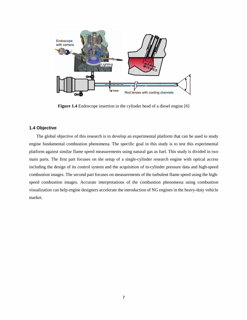
7

Figure 1.4 Endoscope insertion in the cylinder head of a diesel engine [6]

1.4 Objective

The global objective of this research is to develop an experimental platform that can be used to study

engine fundamental combustion phenomena. The specific goal in this study is to test this experimental

platform against similar flame speed measurements using natural gas as fuel. This study is divided in two

main parts. The first part focuses on the setup of a single-cylinder research engine with optical access

including the design of its control system and the acquisition of in-cylinder pressure data and high-speed

combustion images. The second part focuses on measurements of the turbulent flame speed using the high-

speed combustion images. Accurate interpretations of the combustion phenomena using combustion

visualization can help engine designers accelerate the introduction of NG engines in the heavy-duty vehicle

market.

8

Chapter 2

Review of Literature

2.1 Natural gas combustion in large bore engines

Natural gas consumption is forecasted to be doubled between 2001 and 2025, with the most robust

growth in demand expected among the developing nations [9]. Similarly, natural gas vehicles (NGVs) have

been implemented in a variety of applications as part of efforts to improve urban air quality in the United

States, particularly within California [10-12]. Two technologies have been widely being used for NG heavy

duty engines, namely lean-burn combustion and stoichiometric combustion. Older technology NGVs are

equipped with lean-burn engines and oxidation catalysts to effectively control CO and formaldehyde

emissions. Current heavy-duty NGVs are equipped with spark-ignited stoichiometric combustion engines,

with water cooled exhaust gas recirculation (EGR) technology, and three-way catalysts (TWC) in order to

meet the more stringent 2010 NOx emission standards from the US Environmental Protection Agency

(USEPA). Stoichiometric combustion engines with TWC are superior to lean-burn combustion engines

with oxidation catalysts for reducing NOx emissions [13, 14]. However, stoichiometric engines with TWCs

produce higher CO emissions than lean-burn engines [14]. Particulate Matter (PM) emissions from both

stoichiometric and lean-burn combustion NG engines are very low due to the almost homogeneous

combustion of the air–gas mixture, and the absence of large hydrocarbon chains and aromatics in the fuel

[15]. For NGVs, one issue that has been shown to be important with respect to emissions is the effect of

changing the composition of the fuel. This is part of a broader range of issues which are classified under

the term interchangeability, which is the ability to substitute one gaseous fuel for another in a combustion

application without materially changing operational safety, efficiency, performance or materially increasing

air pollutant emissions. Changes in the NG composition used in NGVs can affect the reliability, efficiency,

and exhaust emissions. Studies conducted with small stationary source engines, heavy-duty

engines/vehicles, and light-duty vehicles have shown that NG composition can have an impact on emissions

[16-19]. Karavalakis et al. [20] showed higher NOx emissions when they tested a 2002 lean-burn NG waste

hauler on lower methane number/higher Wobbe number fuels. Hajbabaei et al. [21] reported NOx and non-

methane hydrocarbon (NMHC) emission increases for fuels with low methane contents when they tested

two transit buses equipped with lean-burn NG engines. However, they did not find any fuel effect on NOx

emissions when they tested a bus with a stoichiometric combustion engine and a TWC. The effect of NG

9

composition on exhaust emissions was also confirmed by Feist et al. [22] where they found NOx and total

hydrocarbon (THC) emissions increases with higher Wobbe number fuels under lean-burn engine

combustion, while the stoichiometric engines showed no clear trends for NOx and THC emissions with

different fuels [23,24].

2.2 Fuel composition effects

Natural gas is considered to be a promising alternative fuel for passenger cars, truck transportation and

stationary engines providing positive effects both on the environment and energy security. The US

government is continually pushing the use of natural gas engines in order to reduce foreign oil dependence

and achieve lower greenhouse gas (GHG) emissions. The most important GHGs are carbon dioxide (CO2),

methane (CH4), and nitrous oxide (N2O), with the transportation sector being the main contributor of the

overall GHG emissions in the US [25]. Therefore, the introduction of natural gas as a potential alternative

to conventional liquid fuels in the heavy-duty vehicle segment (viz., vehicles with gross vehicle weight

ratings ranging from 3.9 to 15 tons and over), which consumes a large amount of fuel, is a fast growing

market. Currently, California supplies 85–90% of its needs with NG imported domestically from the

Rockies, from southwest states, such as Texas, and from Canada [26]. Natural gas is a mixture of various

hydrocarbon molecules such as methane (CH4), ethane (C2H6), propane (C3H8), and butane (C4H10), and

inert diluents such as molecular nitrogen (N2) and carbon dioxide (CO2). Several parameters affect the

natural gas composition such as demographic location, season, and treatments applied during production or

transportation [26-30]. Moreover, additional mixing of different gases occurs during pipeline transmission

[31, 32]. Therefore, its thermodynamic properties are dependent on the composition of the gas [33]. To

obtain the thermodynamics properties accurately, the effect of the gas compositions must be also

considered. Many researchers working on the natural gas engines demonstrated that natural gas composition

significantly affects engine performance and emissions. It was also reported that the heating value (HV),

thermal efficiency, and concentration of un-burnt hydrocarbon (UHC) and other emission particles would

highly depend on the source of supply of natural gas as the main fuel [34, 35]. The most important

compositional parameters that affect the quality of natural gas include methane number (MN) and Wobbe

number (WN). A 100% methane composition is given 100 as MN and as the higher hydrocarbons

percentage increases, the MN decreases. Methane is a dominant component in the natural gas and hence is

an important parameter for consideration. The MN of the mixture is defined as the percentage of methane

in a methane hydrogen mixture. The WN is a measure of the fuel energy flow rate through a fixed orifice

under given inlet conditions. It is calculated as the ratio of the heating value divided by the square root of

the specific gravity. Generally, the WN is a good criterion for natural gas because it correlates well with

the ability of an internal combustion engine to use a particular gas. [36-38]. The earliest research on

10

implication of natural gas composition in SI engines should be traced back to the middle of 1980s, when

natural gas was employed as the secondary fuel in gasoline engine. Elder et al. [39] carried out experimental

and theoretical investigations at the University of Auckland to determine the effects of varying fuel

compositions on vehicle fuel consumption, power output and pollutant emissions. King [40] analyzed the

impact of natural gas fuel composition on fuel metering and engine operational characteristics. He

developed a fuel metering model to analyze the impact of fuel composition on carbureted, premixed, and

direct-injected engine configurations. The change in physical properties of the fuel was found to have a

profound effect on fuel metering characteristics. He found that fuel composition affects fuel metering

configurations. However, these variations were minor compared to the fuel property effects. Moreover, he

reported that fuel composition also affects the lean- flammability-limit of the mixture which, when

combined with fuel metering variations, can cause a lean-burn engine to misfire. Also, fuel temperature

variations affected fuel metering and must also be considered. The results indicated that closed-loop mixture

control is essential for stoichiometric engines and very beneficial for lean-burn engines. Thiagarajan et al.

[41] experimentally investigated effect of varying gas composition on the performance and emissions of a

SI engine. The pipeline natural gas composition was varied by adding volumes of propane (up to 20%) or

nitrogen (up to 15%). They found that brake power, fuel conversion efficiency and before catalyst emissions

of CO, NOx and hydrocarbons were not affected by propane addition as long as stoichiometric combustion

was maintained. In addition, nitrogen addition at the stoichiometric condition significantly reduced before

catalyst NOx emissions and increased after catalyst CO emissions. Limited information is available on the

unregulated emissions from NGVs, including gaseous toxic pollutants and PAHs (polycyclic aromatic

hydrocarbons). Kado et al. [42] found that the carbonyl emissions from CNG (compressed natural gas)

buses were primarily formaldehyde. Formaldehyde emissions from these buses were much greater than

those of diesel buses fitted with OCs, and CRTs (continuously regenerating traps). Ayala et al. [43] also

found that formaldehyde emissions were reduced by OCs on CNG buses by over 95% over the CBD

(Central Business District) cycle. Okamoto et al. [44] and Kado et al. [42] performed mutagenic tests on

the exhaust from transit buses operating on CNG. They both reported lower mutagenic activity for CNG

buses equipped with OCs, compared to buses without OCs. Kado et al. [42] also found that mutagenic

activity using the TA98NR test strain decreased, indicating the possible presence of nitro-PAH in the PM

emissions. Turrio-Baldassarri et al. [45] showed that a spark ignition heavy-duty urban bus NG engine with

a TWC produced 20 times lower formaldehyde, more than 30 times lower PM emissions, and 50 times

lower PAH emissions, compared to a diesel engine without after treatment.

11

2.3 Cycle to cycle variations in SI engine

Today, engine designers are seeking every kind of solution aimed at the reduction of fuel consumption

and emission levels. The cycle to cycle variation (CCV) in combustion significantly influences the

performance of spark-ignition engines. The process variables such as pressure and heat release in an

internal combustion engine undergo cycle-to-cycle variations. SI engines superficially operating under

steady-state conditions do not maintain perfectly stable operation i.e. a comparison between one cycle and

another reveals random variations in. In general, combustion in spark-ignition engines varies considerably

from cycle to cycle. Many studies have been carried out in order to find the main causes of this effect. These

variations are associated with considerable variations in flame speed and combustion duration. Very early

in the combustion event taking place within the cylinder, cyclic variation in peak cylinder pressure, the rate

of pressure rise and the work done by the gas are observed by the researchers [46]. The CCV may become

severe under lean-burn conditions, and for highly dilute mixtures with exhaust gas recirculation [47]. Cycle-

to-cycle variations have been observed in spark ignition, compression ignition, and HCCI engines. The

CCV may reduce the power output of the engine, lead to operational instabilities, and result in undesirable

engine vibrations and noise. Cyclic variation of automobile engine combustion is a fundamental

characteristic of the power plant that is the primary means of transportation in this country. The extremes

of this variation reduce drivability and gas mileage, and can be responsible for significant air pollutant

emissions from the engine. There have been many studies of cyclic variation from various perspectives.

Several sources of CCV in a spark ignition engine have been identified. They include (a) turbulence

intensity of the flow field in the cylinder, (b) variations in the fuel air ratio, (c) amount of residual or

recirculated exhaust gases in the cylinder, (d) spatial inhomogeneity of the mixture composition especially

near the spark plug, and (e) spark discharge characteristics and flame kernel development. It has been

estimated that elimination of the CCV may lead to about 10% increase in power output for the same fuel

consumption in a gasoline engine [48]. There have been many studies on the analysis of CCV in internal

combustion engines. Some of these studies have revealed that any process that increases the burning

velocity of the combustible mixture will result in a reduction of the CCV. Stone et al. [49] highlight that

total elimination of cyclic variation is not desirable for engine management systems that retard the ignition

when incipient knock is detected. If there were no cyclic variation, there would be no foresight for the

engine management system to detect when the onset of knock will occur. Galloni [50] studied the different

parameters that could affect the cyclic variation in a SI engine. The engine under consideration used three

different shapes of combustion chamber, featuring four cylinders with two vertical valves per cylinder. The

fuel was introduced upstream the inlet valves by means of plate four hole injectors capable of producing

droplets with a Sauter mean-diameter of about 130 nm. The author proposed that laminar flame speed,

turbulence intensity and velocity magnitude have been considered among the factors that affect the extent

12

of the engine cyclic variation. The influence of these parameters was investigated. Correlating these features

of the charge with the measured coefficient of variation in the indicated mean effective pressure, a

mathematical relationship was obtained by means of a multiple regression, by the author [50]. Further Reyes

et al. [51] evaluated the relative influence of the equivalence fuel/air ratio and the engine rotational speed

on the cycle-to-cycle variations produced in a single-cylinder spark ignition engine fueled with natural gas,

through a thermodynamic combustion diagnostic model that includes genetic algorithms for parameter

adjusting. The single cylinder air cooled engine under study had a flat piston bowl arrangement. A

traditional estimator of the cycle-to-cycle variation is the Coefficient of Variation in Indicated Mean

Pressure, COVIMEP. In this paper, the authors propose complementary considering the variation of the mass

fraction burning rate of each individual cycle to characterize cyclic variation, The authors propose that

standard deviation of mass fraction burned could be used as an indicator of cyclic dispersion of combustion

events [51]. Kaleli et al. [52] used the approach controlling spark timing for consecutive cycles to reduce

the cyclic variations of SI engines. A stochastic model was performed between spark timing and in cylinder

maximum pressure by using the system identification techniques. The combustion process begins before

the end of the compression stroke with spark event. Then, this process continues through the early part of

the expansion stroke and, ends after the point in the cycle at which the peak cylinder pressure occurs. If the

choice of ignition point versus crank angle is too late, then although the work done by the piston during the

compression stroke is reduced, so is the work done on the piston during the expansion stroke, since all

pressures during the cycles will be reduced. If the spark timing is controlled for consecutive cycles instead

of the open loop system by predicting the pressure related parameters of the one step ahead cycle, it will be

possible to reduce the cyclic variations. For the faster cycles, the ignition timing should be retarded and it

should be advanced for slower cycles. The experiments for this study were performed on a FORD MVH-

418 spark ignition engine with electronically controlled fuel injectors [52]. Finally Ji et al. [53] studied the

cyclic variation of large-bore multi point injection engine fueled by natural gas with different types of

injection systems. The studied engine was a 12-cylinder natural gas engine mainly used for power

generation. The quality of mixture formation was correlated closely with cycle-to-cycle combustion

variation (COV), so COV was used to evaluate the influence of the shape and location of the injection

nozzle as well as end of ignition (EOI) timing on mixture formation. According to the structural

characteristics of the studied engine, four types of injection system with different shapes and locations were

proposed to measure and analyze cylinder pressure in the same working conditions. The influence of the

shape and location of the injection nozzle as well as EOI timing on mixture formation and combustion

process was studied in the research. Experimental results showed that the mixture formation quality of high

power gas engine which has weak airflow in the cylinder could be improved by optimizing the shape and

13

position of the nozzle as well as EOI timing. Improvement of mixture formation can promote combustion

process finally.

Methane which is the main composition of natural gas has unique tetrahedral molecular structure with

larger C–H bond energies, thus demonstrates some unique combustion characteristics such as high ignition

temperature and low flame propagation speed, leading to the poor lean-burn ability and slow burning

velocity. These may lead to the incomplete combustion, high misfire ratio and large cycle-by-cycle

variations when utilizing natural gas in the spark ignition engine especially under lean mixture operating

condition. One effective way to solve this problem is to mix the natural gas with a fuel that possesses the

high burning velocity. Hydrogen is an excellent additive to improve the combustion of natural gas due to

its low ignition energy and high burning velocity. Ma et al. conducted a work in a turbocharged lean burn

natural gas S.I. engine with hydrogen enrichment, to investigate the effects of hydrogen addition on the

combustion behavior and cycle by-cycle variations in a turbocharged lean burn natural gas spark ignition

engine. They found that hydrogen addition contributes to reducing the duration of flame development,

which has highly positive effects on reducing cycle-by-cycle variations [54]. Wang et al. studied the effect

of hydrogen addition on cycle-by-cycle variations of the natural gas engine. Their results showed that the

peak cylinder pressure, the maximum rate of pressure rise and the indicated mean effective pressure

increased and their corresponding cycle-by-cycle variations decreased with the increase of hydrogen

fraction at lean mixture operation [55]. Huang et al. [56] analyzed the cycle-by-cycle variations in a spark

ignition engine fueled with natural gas hydrogen blends combined with EGR. The authors show that the

cylinder peak pressure, the maximum rate of pressure rise and the indicated mean effective pressure

decrease and cycle-by-cycle variations increase with the increase of EGR ratio. Interdependency between

the above parameters and their corresponding crank angles of cylinder peak pressure is decreased with the

increase of EGR ratio. For a given EGR ratio, combustion stability is promoted and cycle-by-cycle

variations are decreased with the increase of hydrogen fraction in the fuel blends. Recently, Reyes et al.

[51] characterized mixtures of natural gas and hydrogen (in different propositions) in a single-cylinder spark

ignition engine by means of a zero dimensional thermodynamic model. A thermodynamic combustion

diagnostic model based on genetic algorithms is used to evaluate the combustion chamber pressure data

experimentally obtained in the mentioned engine. The model is used to make the pressure diagnosis of

series of 830 consecutive engine cycles automatically, with a high grade of objectivity of the combustion

analysis, since the relevant adjustment parameters (i.e. pressure offset, effective compression ratio, top dead

center angular position, heat transfer coefficients) are calculated by the genetic algorithm. Results indicate

that the combustion process is dominated by the turbulence inside the combustion chamber (generated

during intake and compression), showing little dependency of combustion variation on the mixture

14

composition. This becomes more evident when relevant combustion variables are plotted versus the mass

fraction burned (MFB) of each mixture.

The formation of the flame kernel and the following flame growth through a laminar like phase depend

on: the local air fuel ratio, the mixture motion and the exhaust gas concentrations in the spark-plug gap at

the time of ignition and in the spark-plug region immediately after ignition. Cyclic variations occur because

the bulk flow, turbulence, residual amounts and gasoline supplied to each cylinder vary from cycle to cycle.

Moreover, within the cylinder, the mixing of air fuel and exhaust gas residuals is not complete, therefore

the mixture is not homogeneous at the spark time. The turbulent nature of the flow in the cylinder causes

random spatial and time-dependent fluctuations in the variables characterizing the mixture and its flow

field. These fluctuations cause a random value of the mixture concentration in the spark-plug region, a

random convection of the spark kernel away from the electrodes, a random heat transfer from the burning

kernel, etc. [57-59]. In particular, the random displacement of the flame kernel during the early stages of

combustion seems to play a major role in the origination of cycle variation in combustion.

Ozdor et.al. commented that despite many years of experimentation and research a full understanding

of cyclic variation was still lacking, back then. They also mentioned previous studies which have shown

that it may be possible to achieve a 10% increase in power for the same fuel consumption if cyclic variations

could be eliminated. However, the elimination of cyclic variation may not be truly desirable even if it were

possible, which still remains true till date [60]. According to Ozdor [61], Matekunas [62] and Heywood

[47], the cyclic variations can be characterized by the parameters in four main categories; pressure related

parameters, combustion related parameters, flame front related parameters and exhaust gas related

parameters. Pressure related parameters are the in-cylinder maximum pressure (Pmax), the crank angle at

which the in-cylinder maximum pressure occurs (qPmax), the maximum rate of pressure rise (dP/dq) max,

the crank angle at which the maximum rate of pressure rise occurs q(dP/dq) max, indicated mean effective

pressure (IMEP) of individual cycles. Combustion related parameters are about the heat release, burnt mass

fraction and combustion duration characteristics. Flame front related parameters are about the formation,

progression and the speed of the flame. The last category is on the subject of the concentration of exhaust

gases in the exhaust. Moreover, even if many factors do not cause cyclic variation, they determine the

sensitivity of the engine to the factors which give origin to the phenomenon. For example, the overall

weakness of the mixture [63], the spark-plug and the spark-timing and the in cylinder mixture motion do

not cause cyclic dispersion in combustion themselves but affect the extent of cyclic variation caused by

other factors [64-66]. The conclusion seems to be that anything that tends to slow down the flame

propagation process, especially in its development stage, tends to increase the cyclic dispersion in

combustion. In a completely different perspective, Pischinger and Heywoood investigated how heat losses

to the spark plug electrodes affect the flame kernel development in an SI engine [67]. A conventional spark

15

plug and a spark plug with smaller electrodes were studied in M.I.T.'s transparent square piston engine. The

purpose was to learn more about how the electrode geometry affects the heat losses to the electrodes and

the electrical performance of the ignition system, and how this affects the flame development process in an

engine. The spark plug with the smaller electrodes was shown to reduce the heat losses to the electrodes,

and thereby extend the stable operating regime of the engine. At conditions close to the stable operating

limit, cycle-by-cycle variations in heat losses cause significant cyclic variations in flame development.

Cyclic variations in heat loss are due to cyclic variations in the contact area between flame and electrodes.

The contact area is largely controlled by the local flow field in the spark plug vicinity: cycles in which the

flame is convected away from the electrodes have a smaller contact area than cycles in which the flame

remains centered in the spark gap.

The cyclic variations are due to the variations in combustion process. Although the engine runs under

steady state conditions, there are variations in the pressure traces during the combustion process especially

due to the variations in the rate of flame development and the combustion duration for consecutive cycles.

While the combustion for some cycles occurs at optimum conditions, it may occur faster for some cycles

and slower for others. The faster combustion cycles have higher in cylinder maximum pressure values (Pmax)

than slower cycles, and the crank angle at which the in cylinder peak pressure qPmax occurs closer to TDC.

Conversely, as the rate of combustion decreases, the Pmax decreases and the qPmax increases.

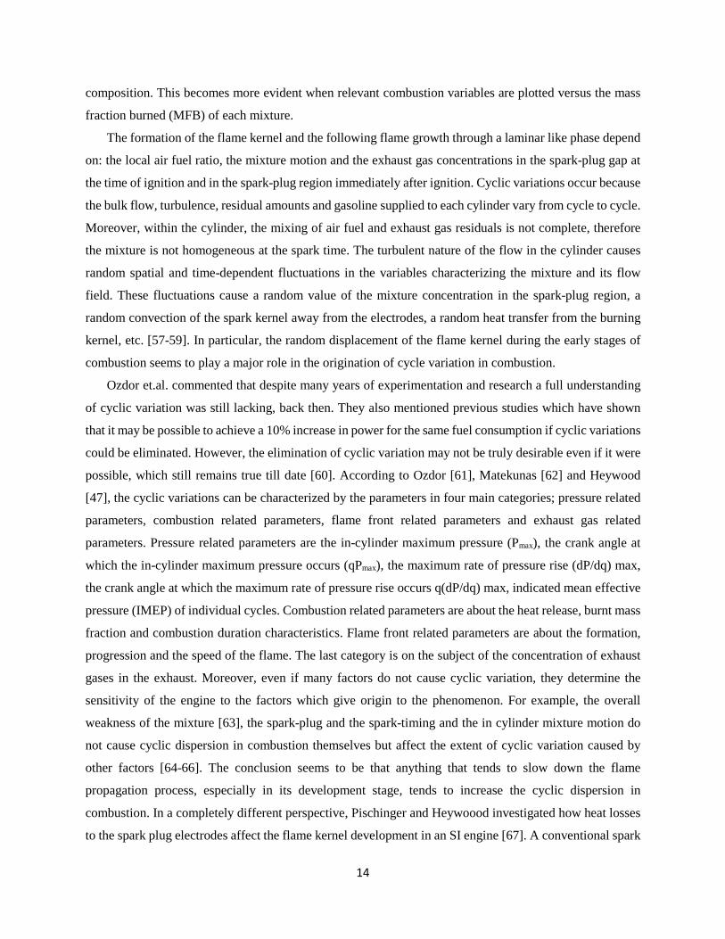
2.4 Optical-access engines for combustion studies

The visualization of in-cylinder mixing processes and combustion characterization remain a challenge

from the very beginning of the IC engine. A particular interest is in the evolution of the combustion process

of alternative fuels used pure or in blends with fossil fuels, in engines adopting more or less conventional

configurations or new ignition systems, which could help to make possible further steps in the development

of systems characterized by ever-lower emissions and fuel consumption levels. Visualization studies today

still serve this purpose – after over a century of application, studies in optically accessible engines continue

to provide new perspectives in engine research [68].

16

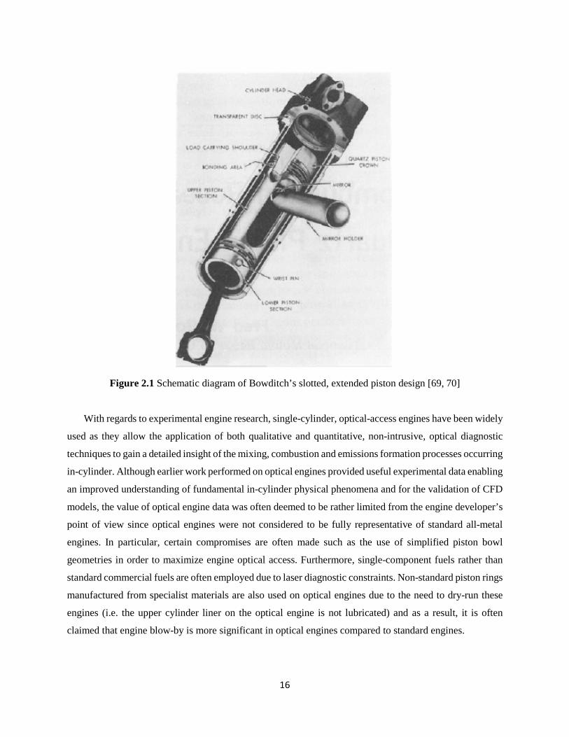
Figure 2.1 Schematic diagram of Bowditch’s slotted, extended piston design [69, 70]

With regards to experimental engine research, single-cylinder, optical-access engines have been widely

used as they allow the application of both qualitative and quantitative, non-intrusive, optical diagnostic

techniques to gain a detailed insight of the mixing, combustion and emissions formation processes occurring

in-cylinder. Although earlier work performed on optical engines provided useful experimental data enabling

an improved understanding of fundamental in-cylinder physical phenomena and for the validation of CFD

models, the value of optical engine data was often deemed to be rather limited from the engine developer’s

point of view since optical engines were not considered to be fully representative of standard all-metal

engines. In particular, certain compromises are often made such as the use of simplified piston bowl

geometries in order to maximize engine optical access. Furthermore, single-component fuels rather than

standard commercial fuels are often employed due to laser diagnostic constraints. Non-standard piston rings

manufactured from specialist materials are also used on optical engines due to the need to dry-run these

engines (i.e. the upper cylinder liner on the optical engine is not lubricated) and as a result, it is often

claimed that engine blow-by is more significant in optical engines compared to standard engines.

17

In this section of the review of optically accessible engines, the unique characteristics of these special

research engines and how these characteristics evolved to enable measurement of the desired quantities in

a SI engine will be discussed. The basic architecture of the modern day optical accessible piston assembly

was designed in 1958 by F.W. Bowditch of the General Motor Corporation, shown in Figure. Bowditch’s

essential innovation involved slotting the piston extension to allow the combustion chamber to be viewed

from below via a 45° mirror and a quartz piston top. In this way, a large degree of optical access could be

obtained in overhead valve designs without significant modifications to the combustion chamber geometry.

Bowditch reports successfully operating this engine at compression ratio up to 10.7:1 at engine speeds of

1200 rpm. In developing this engine, Bowditch addressed many of the design challenges that optical

designer will struggle with today. The shape and size of the quartz piston top, was selected considering

mechanical, thermal and optical stress requirements. The operational difficulties that Bowditch encountered

with this engine are likewise familiar to modern researchers. Excessive oil leakage past the valve guides

was found to eventually foul the mirror, a problem that was resolved with special valve stem seals.

Likewise, oil coming up from the crankcase was problematic, and required a special ring pack to resolve.

Post 1945 work on SI engines, an engine design incorporating a large quartz head window similar to

that used by Rassweiler and Withrow [71] was employed by Nakanishi, et.al [72]. Few decades later,

researchers from MIT’s Sloan Automotive Laboratory [73] studied the combustion process in SI engine

using flame photographs. In a SI engine, the combustion is initiated with the assistance of spark discharge

and propagating a turbulent flame through a premixed air-fuel mixture. The researchers believed that the

details of the flame propagation process influence the efficiency of energy conversion and engine

performance, as well as pollutant formation. They studied the structure of flame development and its

propagation, with the use of a square cross section engine [74] where two of the cylinder walls were quartz

windows to permit full optical access to the cylinder volume throughout the entire engine cycle. The engine

had a CR of 4.8:1, was run at a speed of 1380 rpm and was fired in short bursts of approximately 16 cycles.

After approximately 3 fired cycles, the combustion was reasonably stable. Similar ‘burst’ firing strategies

to obtain stable operation or desired surface temperatures in optical engines have been subsequently

employed by others [75-77]. From the study, it was summarized that, from the set of photographs

illustrating important aspects of flame development in a SI engine, both bulk gas motion and smaller scale

turbulence were seen to have an influence on the flame kernel within a few degrees after ignition. The flame

kernel can be convected away from the spark gap, the direction and extent of motion varying cycle by cycle.

Around the same year, Richman and Reynolds developed the transparent cylinder research engine having

a compression ratio which could be varied from 6.25 to 11, and a speed up to 3000 rpm. The innovative

features of this engine were the use of electro hydraulic valve actuators and thin walled transparent cylinder

fabricated from single crystal sapphire. Further after, due largely to the expense of full transparent liners, a

18

number of researchers chose instead to employ a transparent ring of limited height for the upper portion of

the liner. In parallel the drawback to the transparent liner designs with the lack of optical access into the

combustion chamber of pent roof design, was rectified by placing optical windows in to the gables of engine

head.

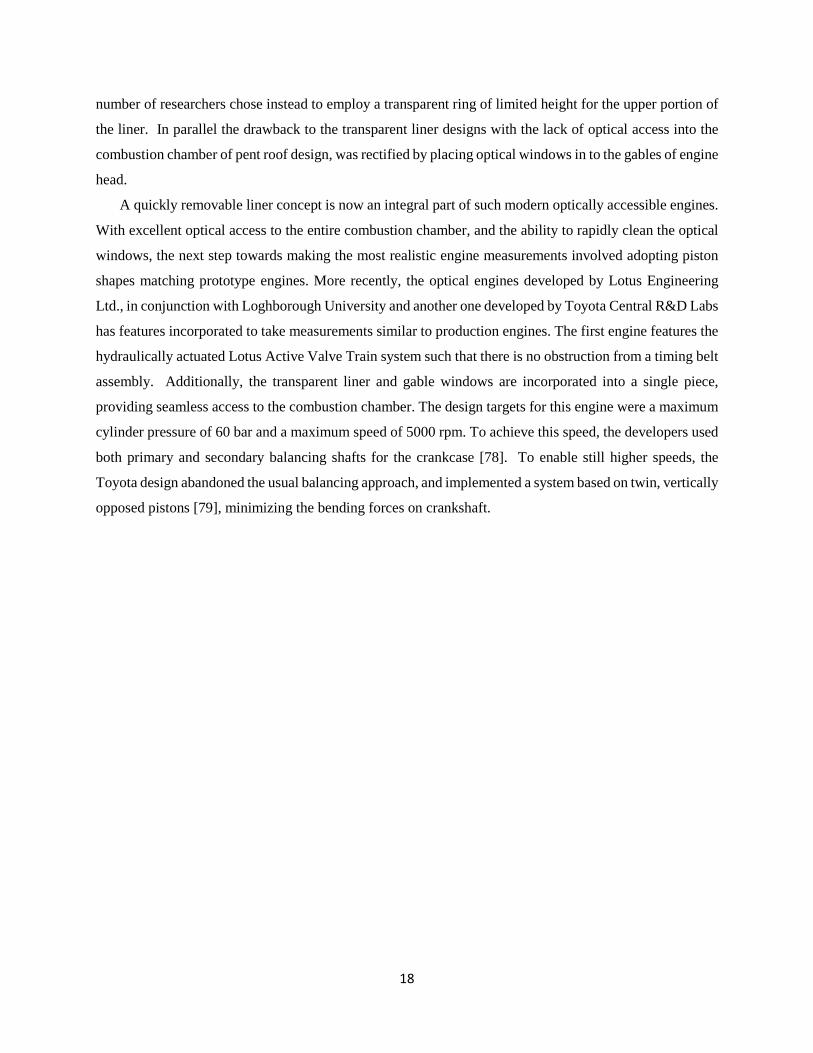
A quickly removable liner concept is now an integral part of such modern optically accessible engines.

With excellent optical access to the entire combustion chamber, and the ability to rapidly clean the optical

windows, the next step towards making the most realistic engine measurements involved adopting piston

shapes matching prototype engines. More recently, the optical engines developed by Lotus Engineering

Ltd., in conjunction with Loghborough University and another one developed by Toyota Central R&D Labs

has features incorporated to take measurements similar to production engines. The first engine features the

hydraulically actuated Lotus Active Valve Train system such that there is no obstruction from a timing belt

assembly. Additionally, the transparent liner and gable windows are incorporated into a single piece,

providing seamless access to the combustion chamber. The design targets for this engine were a maximum

cylinder pressure of 60 bar and a maximum speed of 5000 rpm. To achieve this speed, the developers used

both primary and secondary balancing shafts for the crankcase [78]. To enable still higher speeds, the

Toyota design abandoned the usual balancing approach, and implemented a system based on twin, vertically

opposed pistons [79], minimizing the bending forces on crankshaft.

19

Figure 2.2 High-speed optical engine developed by Lotus Engineering Limited and Loughborough

University ([79])

20

Chapter 3

Experimental Setup

This chapter describes the engine setup and explains the testing procedure. This study was performed

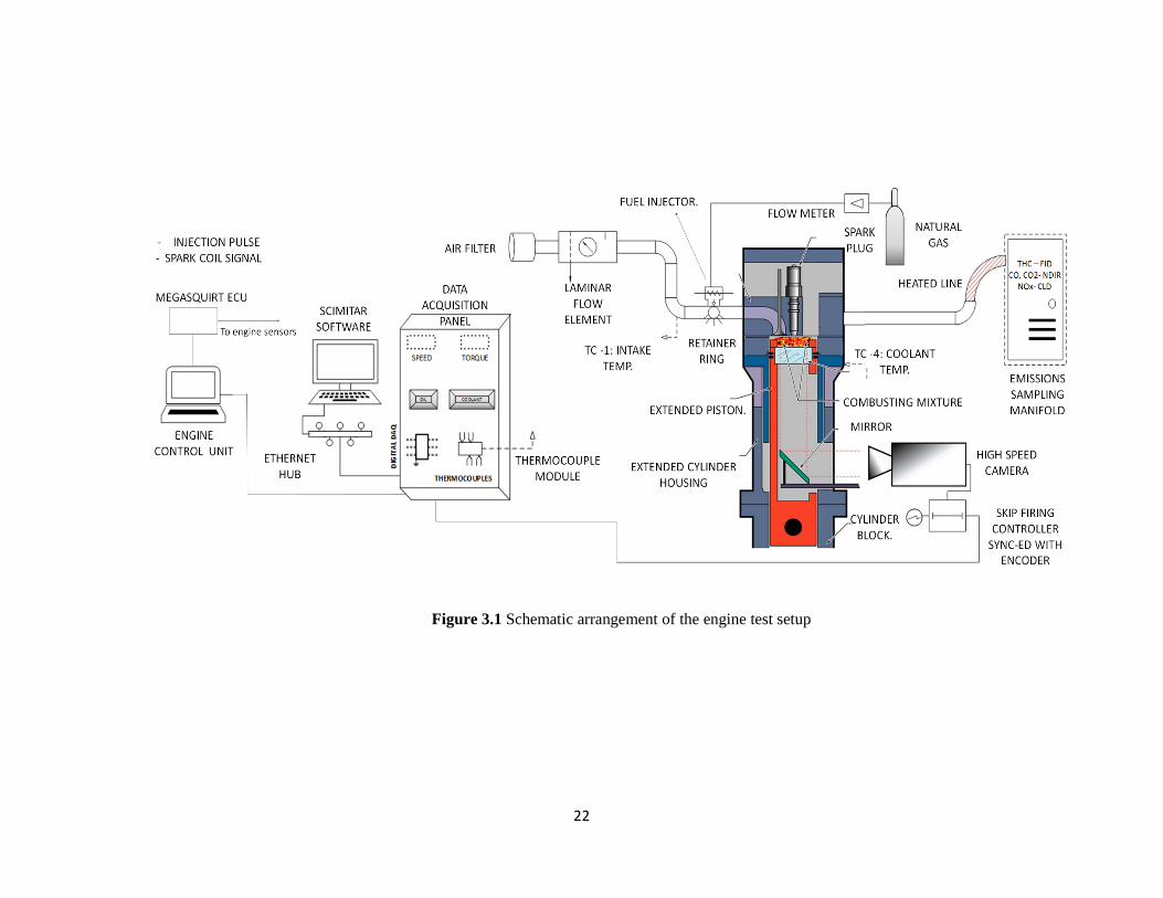
in one of the engine laboratories in the WVU Evansdale campus. Figure 3.1 shows a schematic of the

experimental setup, which consists of a single-cylinder research engine, dynamometer, control and

instrumentation hardware for measuring and modifying the operational conditions of the engine.

A 75-kW dynamometer (McClure 4999 Trunnion type) maintains a constant engine speed regardless

of the engine load. The test setup includes an air flow measurement device, temperature measurement

devices, fuel delivery equipment, different engine sensors (for e.g., cam sensor, crank sensor, etc.), and a

central engine controller unit. A laminar flow element (LFE) measures intake flow rate, K-type

thermocouples measure the temperatures of engine coolant, engine oil, intake air, and exhaust gas. A 100-

kg load cell with a strain gauge arrangement (TEDEA-Huntleigh 104H Coated) measures the engine torque.

Further, an emissions bench with different types of gas analyzers for measuring the constituent species

concentration in the exhaust gas is present. An aftermarket engine management system (Megasquirt Model

3X), containing the pre-programed engine maps with desired operating parameters, is synced with all the

essential engine sensors to monitor/control the engine operation.

An in-house build skip firing controller (based on Arduino Nano prototyping platform) receives input

from the engine encoder and the engine management system to allow the fuel injector to skip certain number

of engine cycles. Additionally the skip firing controller provides burst of signals for triggering the camera

for image acquisition during the fired engine cycles. These controls are vital for experiments conducted in

an optical engine.

3.1 The research engine The single cylinder research engine (Ricardo/Cussons, Model Proteus) was built to meet the need for a

robust single cylinder machine in the 100-150 mm bore and 120-165 mm stroke range. Such an engine

enables a wide variety of research areas to be investigated and in particular to replicate commercial multi-

cylinder engines without incurring the problems and costs of adapting a multi cylinder engine for research

purposes. The engine, which is based on a Volvo TD 120 engine, has a classic toroidal bowl in piston

combustion chamber in conjunction with a helical swirl. In addition, the same engine could be adapted for

21

both DI/IDI operations as well as photographic build for in cylinder flame observations. The engine is

mounted on an integral base frame with separate oil and cooling modules. The control instrumentation is

provided in a remote console. The original diesel configuration was modified to a high-compression spark

ignition (SI) engine. As a result, the original diesel pump and injector were removed from the engine and

the intake system has been modified to accommodate a port fuel injector. In addition, the original diesel

injector mount was modified to fit a NG spark plug.

3.1.1 Base engine

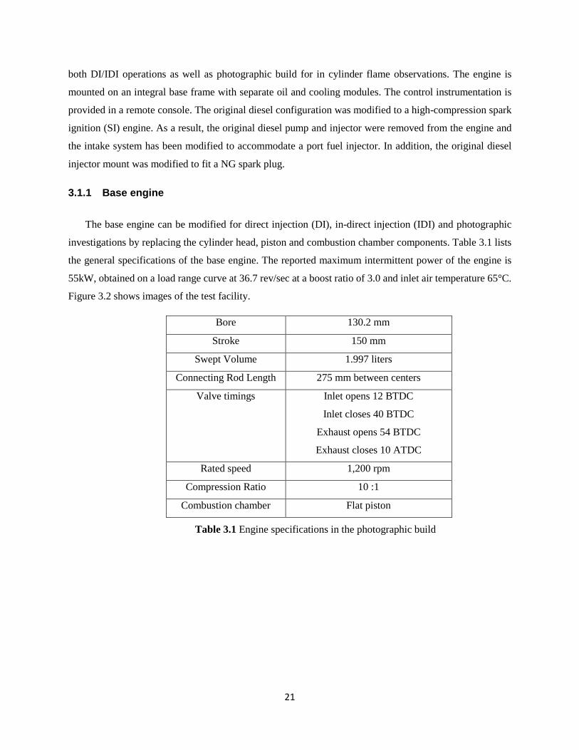
The base engine can be modified for direct injection (DI), in-direct injection (IDI) and photographic

investigations by replacing the cylinder head, piston and combustion chamber components. Table 3.1 lists

the general specifications of the base engine. The reported maximum intermittent power of the engine is

55kW, obtained on a load range curve at 36.7 rev/sec at a boost ratio of 3.0 and inlet air temperature 65°C.

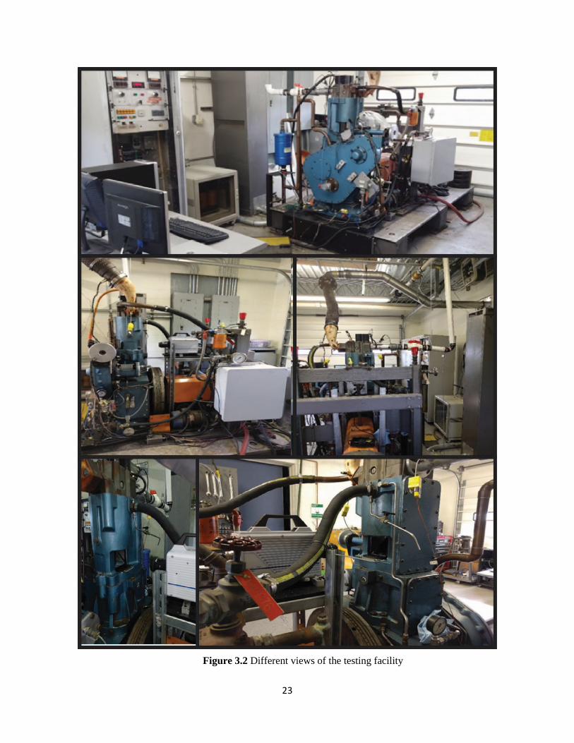
Figure 3.2 shows images of the test facility.

Bore 130.2 mm

Stroke 150 mm

Swept Volume 1.997 liters

Connecting Rod Length 275 mm between centers

Valve timings Inlet opens 12 BTDC

Inlet closes 40 BTDC

Exhaust opens 54 BTDC

Exhaust closes 10 ATDC

Rated speed 1,200 rpm

Compression Ratio 10 :1

Combustion chamber Flat piston

Table 3.1 Engine specifications in the photographic build

22

Figure 3.1 Schematic arrangement of the engine test setup

23

Figure 3.2 Different views of the testing facility

24

3.1.2 Optical experiment test procedure

A Bowditch extended piston mounted inside a special engine extension “sandwiched” between the

crankcase base and the cylinder head provides the optical access to the engine combustion chamber from

below. However, this special arrangement of photographic piston and its corresponding liner does not

contain the regular oil-feed channels. Hence, it is recommended by the manufacturer that the photographic

engine build be run for just the minimum time necessary to obtain the conditions required for combustion

imaging. The only method of lubrication for the extended piston assembly is the application of a small

amount of molybdenum disulphide anti-scuffing paste to the walls of the upper liner. This provides enough

lubrication for a few minutes of operation and hence need to be re-applied every run of the engine. However,

this also means that the cylinder head needs to be removed any time a new application of anti-scuffing paste

is needed. In addition, the application of a larger volume of the lubricating paste would lead to fouling of

the optical windows and hence would distort the quality of the images recorded with the high speed camera.

There are significant differences between the optical engine configuration and the DI/IDI engine

configurations. These differences mainly arise from the design of the Bowditch piston. The Bowditch piston

produces a lower compression ratio than the conventional piston; 10:1 compared to 13.3:1. In addition, the

flat quartz piston creates a cylindrical bowl, compared to the original toroidal bowl. Further, the thermal

conductivity of quartz is much lower than the one of the original aluminum piston, which can promote the

formation of hot spots. Finally, the optical liner used with the Bowditch piston has a greater clearance than

the stock thermodynamic liner, which results in greater blow-by. The Bowditch piston uses two of the three

stock (thermodynamic) piston rings, which necessitate manual lubrication of the liner and piston rings at

very frequent intervals during testing. Because of these numerous differences between the optical and

thermodynamic engine configurations, a different operating protocol is required when performing optical

engine measurements. To keep the quartz window from over-heating, the engine must be operated in a skip-

fired mode, where a fired cycle is followed by n motored cycles (with n ≥ 1) to reduce the heat transferred

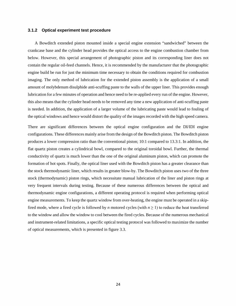
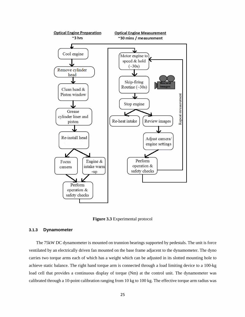
to the window and allow the window to cool between the fired cycles. Because of the numerous mechanical

and instrument-related limitations, a specific optical testing protocol was followed to maximize the number

of optical measurements, which is presented in figure 3.3.

25

Figure 3.3 Experimental protocol

3.1.3 Dynamometer

The 75kW DC dynamometer is mounted on trunnion bearings supported by pedestals. The unit is force

ventilated by an electrically driven fan mounted on the base frame adjacent to the dynamometer. The dyno

carries two torque arms each of which has a weight which can be adjusted in its slotted mounting hole to

achieve static balance. The right hand torque arm is connected through a load limiting device to a 100-kg

load cell that provides a continuous display of torque (Nm) at the control unit. The dynamometer was

calibrated through a 10-point calibration ranging from 10 kg to 100 kg. The effective torque arm radius was

26

fixed at 407.8mm during the calibration. An arrangement of thyristor bank (KTK Model PS4O) powers up

and drives the dynamometer, so that it can act as DC motor to drive the engine while it is motoring, or as a

DC generator when the engine is fired (the DC power from the dynamometer is converted to 3 phase A.C.

mode by the converter unit and fed back into the mains supply). A tach generator mounted on the

dynamometer shaft provides a speed signal to the closed loop speed control system so that the speed selected

at the control console is maintained by automatic adjustments to the motoring or loading torque.

3.1.4 Engine control unit

The engine control unit is a racked panel consisting of three main sub systems: the safety shutdown

unit (SSU), the dynamometer control unit and the speed/torque control unit.

SSU is a safety trip system designed to protect the equipment based on the feedback of a certain fault

conditions, such as dyno fault, under speed, over speed, oil pressure, or coolant temperature. In the event

of any of these conditions being unsatisfactory, the appropriate warning light will start pulsing.

The dynamometer control unit consists of start/auto, absorb and motor controls to facilitate the dyno

operation. In the start/auto mode, the dynamometer automatically changes from motor to load and vice

versa to maintain speed setting. In absorb mode, the dynamometer absorbs the power generated by the

engine. The set speed is not maintained if engine power is below pumping and friction losses. Further, in

the motor mode, dynamometer motors only. To start the dynamometer the SSU must be reset and coolant

pump should be kept on.

The torque-and-speed rack consists of digital and analogue displays reading the engine load (Nm) and

speed (rev/sec).The signal received from the engine is conditioned and amplified through a dedicated signal

conditioning system, whose detailed functionality is listed in the operating manual [80].

3.1.5 Intake air system

The engine is naturally aspirated through a 2”-diameter pipe system. A 2”-diameter laminar flow

element (LFE; Meriam, Model 50MC2-2) ensures high accuracy, fast response time, and good repeatability

of the intake air flow measurements (max 100 SCFM at a differential pressure of 5 inches of water). The

intake air is filtered before passing through the LFE. As higher intake flow pulsations are expected from a

single cylinder engine, pressure snubbers and orifices are placed downstream the LFE to dampen the

pulsation effects produced by the intake valve motion. The LFE operation is detailed next. In addition to

multiple internal flow straighteners to eliminate any turbulent flow, the LFE consists of an absolute pressure

transducer positioned before and differential pressure transducer positioned across the flow straightening

mechanism to calculate the volume flow of air flowing through. Included with the LFE is a NIST traceable

calibration curve that provides the volumetric flow rate of air as function of the measured pressure. The

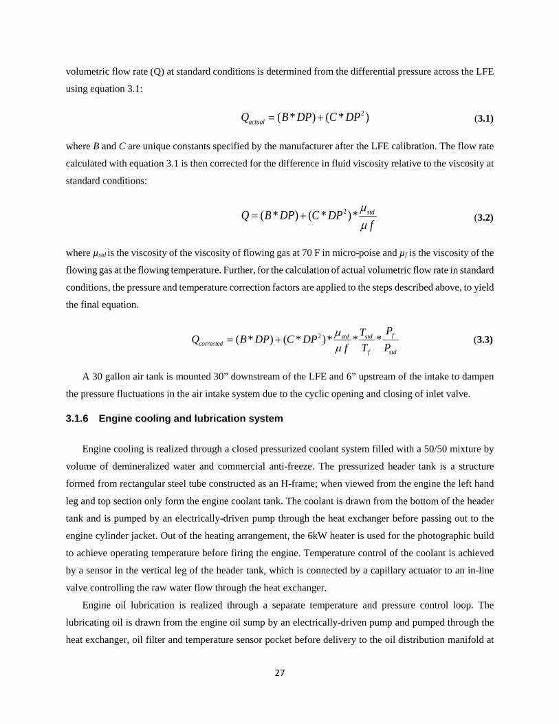
27

volumetric flow rate (Q) at standard conditions is determined from the differential pressure across the LFE

using equation 3.1:

2( * ) ( * )actualQ B DP C DP= + (3.1)

where B and C are unique constants specified by the manufacturer after the LFE calibration. The flow rate

calculated with equation 3.1 is then corrected for the difference in fluid viscosity relative to the viscosity at

standard conditions:

2( * ) ( * )* stdQ B DP C DP

fµµ

= + (3.2)

where µstd is the viscosity of the viscosity of flowing gas at 70 F in micro-poise and µf is the viscosity of the

flowing gas at the flowing temperature. Further, for the calculation of actual volumetric flow rate in standard

conditions, the pressure and temperature correction factors are applied to the steps described above, to yield

the final equation.

2( * ) ( * )* * * fstd stdcorrected

f std

PTQ B DP C DPf T P

µµ

= + (3.3)

A 30 gallon air tank is mounted 30” downstream of the LFE and 6” upstream of the intake to dampen

the pressure fluctuations in the air intake system due to the cyclic opening and closing of inlet valve.

3.1.6 Engine cooling and lubrication system

Engine cooling is realized through a closed pressurized coolant system filled with a 50/50 mixture by

volume of demineralized water and commercial anti-freeze. The pressurized header tank is a structure

formed from rectangular steel tube constructed as an H-frame; when viewed from the engine the left hand

leg and top section only form the engine coolant tank. The coolant is drawn from the bottom of the header

tank and is pumped by an electrically-driven pump through the heat exchanger before passing out to the

engine cylinder jacket. Out of the heating arrangement, the 6kW heater is used for the photographic build

to achieve operating temperature before firing the engine. Temperature control of the coolant is achieved

by a sensor in the vertical leg of the header tank, which is connected by a capillary actuator to an in-line

valve controlling the raw water flow through the heat exchanger.

Engine oil lubrication is realized through a separate temperature and pressure control loop. The

lubricating oil is drawn from the engine oil sump by an electrically-driven pump and pumped through the

heat exchanger, oil filter and temperature sensor pocket before delivery to the oil distribution manifold at

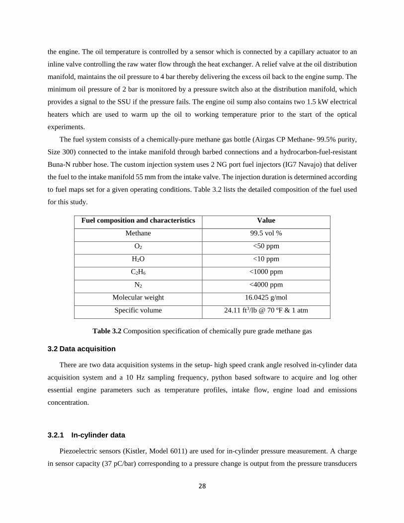
28

the engine. The oil temperature is controlled by a sensor which is connected by a capillary actuator to an

inline valve controlling the raw water flow through the heat exchanger. A relief valve at the oil distribution

manifold, maintains the oil pressure to 4 bar thereby delivering the excess oil back to the engine sump. The

minimum oil pressure of 2 bar is monitored by a pressure switch also at the distribution manifold, which

provides a signal to the SSU if the pressure fails. The engine oil sump also contains two 1.5 kW electrical

heaters which are used to warm up the oil to working temperature prior to the start of the optical

experiments.

The fuel system consists of a chemically-pure methane gas bottle (Airgas CP Methane- 99.5% purity,

Size 300) connected to the intake manifold through barbed connections and a hydrocarbon-fuel-resistant

Buna-N rubber hose. The custom injection system uses 2 NG port fuel injectors (IG7 Navajo) that deliver

the fuel to the intake manifold 55 mm from the intake valve. The injection duration is determined according

to fuel maps set for a given operating conditions. Table 3.2 lists the detailed composition of the fuel used

for this study.

Fuel composition and characteristics Value

Methane 99.5 vol %

O2 <50 ppm

H2O <10 ppm

C2H6 <1000 ppm

N2 <4000 ppm

Molecular weight 16.0425 g/mol

Specific volume 24.11 ft3/lb @ 70 ºF & 1 atm

Table 3.2 Composition specification of chemically pure grade methane gas

3.2 Data acquisition There are two data acquisition systems in the setup- high speed crank angle resolved in-cylinder data

acquisition system and a 10 Hz sampling frequency, python based software to acquire and log other

essential engine parameters such as temperature profiles, intake flow, engine load and emissions

concentration.

3.2.1 In-cylinder data

Piezoelectric sensors (Kistler, Model 6011) are used for in-cylinder pressure measurement. A charge

in sensor capacity (37 pC/bar) corresponding to a pressure change is output from the pressure transducers

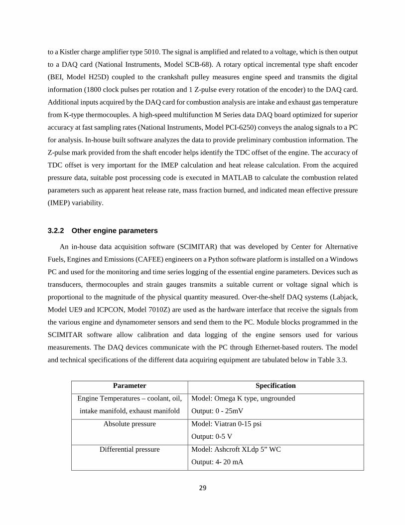
29

to a Kistler charge amplifier type 5010. The signal is amplified and related to a voltage, which is then output

to a DAQ card (National Instruments, Model SCB-68). A rotary optical incremental type shaft encoder

(BEI, Model H25D) coupled to the crankshaft pulley measures engine speed and transmits the digital

information (1800 clock pulses per rotation and 1 Z-pulse every rotation of the encoder) to the DAQ card.

Additional inputs acquired by the DAQ card for combustion analysis are intake and exhaust gas temperature

from K-type thermocouples. A high-speed multifunction M Series data DAQ board optimized for superior

accuracy at fast sampling rates (National Instruments, Model PCI-6250) conveys the analog signals to a PC

for analysis. In-house built software analyzes the data to provide preliminary combustion information. The

Z-pulse mark provided from the shaft encoder helps identify the TDC offset of the engine. The accuracy of

TDC offset is very important for the IMEP calculation and heat release calculation. From the acquired

pressure data, suitable post processing code is executed in MATLAB to calculate the combustion related

parameters such as apparent heat release rate, mass fraction burned, and indicated mean effective pressure

(IMEP) variability.

3.2.2 Other engine parameters An in-house data acquisition software (SCIMITAR) that was developed by Center for Alternative

Fuels, Engines and Emissions (CAFEE) engineers on a Python software platform is installed on a Windows

PC and used for the monitoring and time series logging of the essential engine parameters. Devices such as

transducers, thermocouples and strain gauges transmits a suitable current or voltage signal which is

proportional to the magnitude of the physical quantity measured. Over-the-shelf DAQ systems (Labjack,

Model UE9 and ICPCON, Model 7010Z) are used as the hardware interface that receive the signals from

the various engine and dynamometer sensors and send them to the PC. Module blocks programmed in the

SCIMITAR software allow calibration and data logging of the engine sensors used for various

measurements. The DAQ devices communicate with the PC through Ethernet-based routers. The model

and technical specifications of the different data acquiring equipment are tabulated below in Table 3.3.

Parameter Specification

Engine Temperatures – coolant, oil,

intake manifold, exhaust manifold

Model: Omega K type, ungrounded

Output: 0 - 25mV

Absolute pressure Model: Viatran 0-15 psi

Output: 0-5 V

Differential pressure Model: Ashcroft XLdp 5” WC

Output: 4- 20 mA

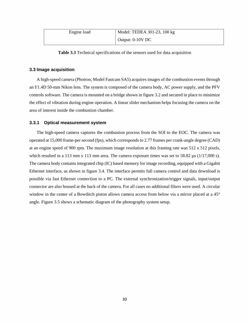
30

Engine load Model: TEDEA 301-23, 100 kg

Output: 0-10V DC

Table 3.3 Technical specifications of the sensors used for data acquisition

3.3 Image acquisition

A high-speed camera (Photron, Model Fastcam SA5) acquires images of the combustion events through

an f/1.4D 50-mm Nikon lens. The system is composed of the camera body, AC power supply, and the PFV

controls software. The camera is mounted on a bridge shown in figure 3.2 and secured in place to minimize

the effect of vibration during engine operation. A linear slider mechanism helps focusing the camera on the

area of interest inside the combustion chamber.

3.3.1 Optical measurement system

The high-speed camera captures the combustion process from the SOI to the EOC. The camera was

operated at 15,000 frame-per second (fps), which corresponds to 2.77 frames per crank-angle degree (CAD)

at an engine speed of 900 rpm. The maximum image resolution at this framing rate was 512 x 512 pixels,

which resulted in a 113 mm x 113 mm area. The camera exposure times was set to 58.82 µs (1/17,000 s).

The camera body contains integrated chip (IC) based memory for image recording, equipped with a Gigabit

Ethernet interface, as shown in figure 3.4. The interface permits full camera control and data download is

possible via fast Ethernet connection to a PC. The external synchronization/trigger signals, input/output

connector are also housed at the back of the camera. For all cases no additional filters were used. A circular

window in the center of a Bowditch piston allows camera access from below via a mirror placed at a 45°

angle. Figure 3.5 shows a schematic diagram of the photography system setup.

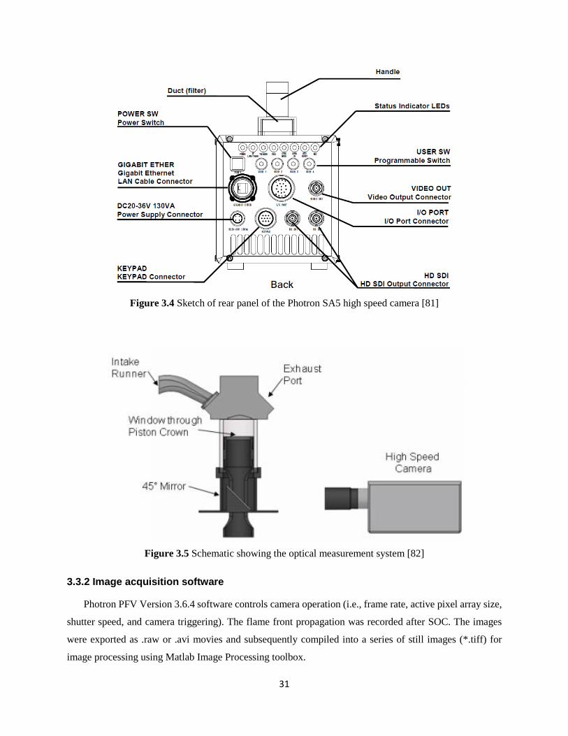
31

Figure 3.4 Sketch of rear panel of the Photron SA5 high speed camera [81]

Figure 3.5 Schematic showing the optical measurement system [82]

3.3.2 Image acquisition software

Photron PFV Version 3.6.4 software controls camera operation (i.e., frame rate, active pixel array size,

shutter speed, and camera triggering). The flame front propagation was recorded after SOC. The images

were exported as .raw or .avi movies and subsequently compiled into a series of still images (*.tiff) for

image processing using Matlab Image Processing toolbox.

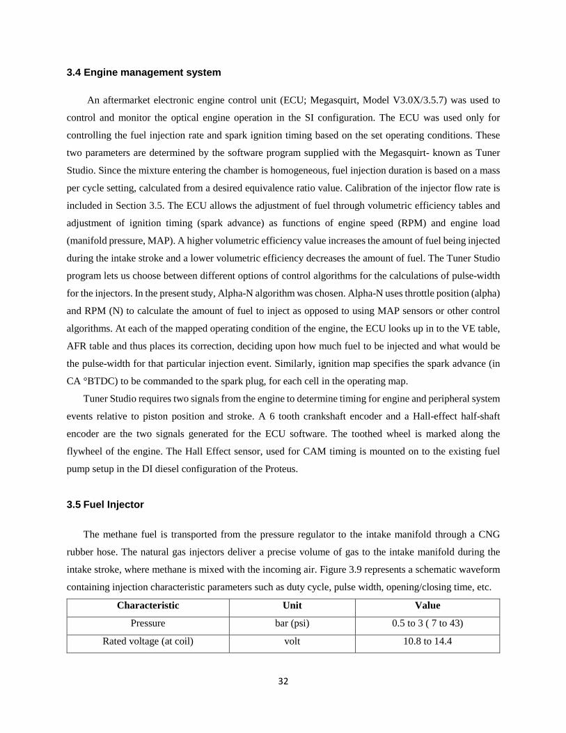
32

3.4 Engine management system

An aftermarket electronic engine control unit (ECU; Megasquirt, Model V3.0X/3.5.7) was used to

control and monitor the optical engine operation in the SI configuration. The ECU was used only for

controlling the fuel injection rate and spark ignition timing based on the set operating conditions. These

two parameters are determined by the software program supplied with the Megasquirt- known as Tuner

Studio. Since the mixture entering the chamber is homogeneous, fuel injection duration is based on a mass

per cycle setting, calculated from a desired equivalence ratio value. Calibration of the injector flow rate is

included in Section 3.5. The ECU allows the adjustment of fuel through volumetric efficiency tables and

adjustment of ignition timing (spark advance) as functions of engine speed (RPM) and engine load

(manifold pressure, MAP). A higher volumetric efficiency value increases the amount of fuel being injected

during the intake stroke and a lower volumetric efficiency decreases the amount of fuel. The Tuner Studio

program lets us choose between different options of control algorithms for the calculations of pulse-width

for the injectors. In the present study, Alpha-N algorithm was chosen. Alpha-N uses throttle position (alpha)

and RPM (N) to calculate the amount of fuel to inject as opposed to using MAP sensors or other control

algorithms. At each of the mapped operating condition of the engine, the ECU looks up in to the VE table,

AFR table and thus places its correction, deciding upon how much fuel to be injected and what would be

the pulse-width for that particular injection event. Similarly, ignition map specifies the spark advance (in

CA °BTDC) to be commanded to the spark plug, for each cell in the operating map.

Tuner Studio requires two signals from the engine to determine timing for engine and peripheral system

events relative to piston position and stroke. A 6 tooth crankshaft encoder and a Hall-effect half-shaft

encoder are the two signals generated for the ECU software. The toothed wheel is marked along the

flywheel of the engine. The Hall Effect sensor, used for CAM timing is mounted on to the existing fuel

pump setup in the DI diesel configuration of the Proteus.

3.5 Fuel Injector

The methane fuel is transported from the pressure regulator to the intake manifold through a CNG

rubber hose. The natural gas injectors deliver a precise volume of gas to the intake manifold during the

intake stroke, where methane is mixed with the incoming air. Figure 3.9 represents a schematic waveform

containing injection characteristic parameters such as duty cycle, pulse width, opening/closing time, etc.

Characteristic Unit Value

Pressure bar (psi) 0.5 to 3 ( 7 to 43)

Rated voltage (at coil) volt 10.8 to 14.4

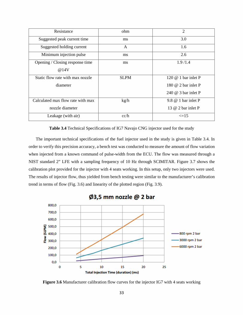
33

Resistance ohm 2

Suggested peak current time ms 3.0

Suggested holding current A 1.6

Minimum injection pulse ms 2.6

Opening / Closing response time

@14V

ms 1.9 /1.4

Static flow rate with max nozzle

diameter

SLPM 120 @ 1 bar inlet P

180 @ 2 bar inlet P

240 @ 3 bar inlet P

Calculated max flow rate with max

nozzle diameter

kg/h 9.8 @ 1 bar inlet P

13 @ 2 bar inlet P

Leakage (with air) cc/h <=15

Table 3.4 Technical Specifications of IG7 Navajo CNG injector used for the study

The important technical specifications of the fuel injector used in the study is given in Table 3.4. In

order to verify this precision accuracy, a bench test was conducted to measure the amount of flow variation

when injected from a known command of pulse-width from the ECU. The flow was measured through a

NIST standard 2” LFE with a sampling frequency of 10 Hz through SCIMITAR. Figure 3.7 shows the

calibration plot provided for the injector with 4 seats working. In this setup, only two injectors were used.

The results of injector flow, thus yielded from bench testing were similar to the manufacturer’s calibration

trend in terms of flow (Fig. 3.6) and linearity of the plotted region (Fig. 3.9).

Figure 3.6 Manufacturer calibration flow curves for the injector IG7 with 4 seats working

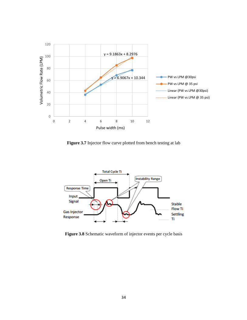
34

Figure 3.7 Injector flow curve plotted from bench testing at lab

Figure 3.8 Schematic waveform of injector events per cycle basis

y = 6.9067x + 10.344

y = 9.1863x + 8.2976

0

20

40

60

80

100

120

0 2 4 6 8 10 12

Volu

met

ric F

low

Rat

e (L

PM)

Pulse width (ms)

PW vs LPM @30psi

PW vs LPM @ 35 psi

Linear (PW vs LPM @30psi)

Linear (PW vs LPM @ 35 psi)

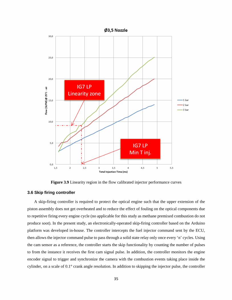
35

Figure 3.9 Linearity region in the flow calibrated injector performance curves

3.6 Skip firing controller

A skip-firing controller is required to protect the optical engine such that the upper extension of the

piston assembly does not get overheated and to reduce the effect of fouling on the optical components due

to repetitive firing every engine cycle (no applicable for this study as methane premixed combustion do not

produce soot). In the present study, an electronically-operated skip-firing controller based on the Arduino

platform was developed in-house. The controller intercepts the fuel injector command sent by the ECU,

then allows the injector command pulse to pass through a solid state relay only once every ‘n’ cycles. Using

the cam sensor as a reference, the controller starts the skip functionality by counting the number of pulses

to from the instance it receives the first cam signal pulse. In addition, the controller monitors the engine

encoder signal to trigger and synchronize the camera with the combustion events taking place inside the

cylinder, on a scale of 0.1° crank angle resolution. In addition to skipping the injector pulse, the controller

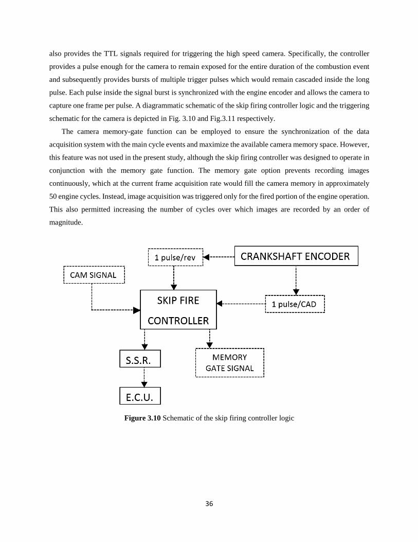
36

also provides the TTL signals required for triggering the high speed camera. Specifically, the controller

provides a pulse enough for the camera to remain exposed for the entire duration of the combustion event

and subsequently provides bursts of multiple trigger pulses which would remain cascaded inside the long

pulse. Each pulse inside the signal burst is synchronized with the engine encoder and allows the camera to

capture one frame per pulse. A diagrammatic schematic of the skip firing controller logic and the triggering

schematic for the camera is depicted in Fig. 3.10 and Fig.3.11 respectively.

The camera memory-gate function can be employed to ensure the synchronization of the data

acquisition system with the main cycle events and maximize the available camera memory space. However,

this feature was not used in the present study, although the skip firing controller was designed to operate in

conjunction with the memory gate function. The memory gate option prevents recording images

continuously, which at the current frame acquisition rate would fill the camera memory in approximately

50 engine cycles. Instead, image acquisition was triggered only for the fired portion of the engine operation.

This also permitted increasing the number of cycles over which images are recorded by an order of

magnitude.

Figure 3.10 Schematic of the skip firing controller logic

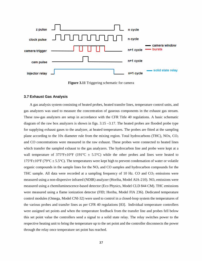
37

Figure 3.11 Triggering schematic for camera

3.7 Exhaust Gas Analysis

A gas analysis system consisting of heated probes, heated transfer lines, temperature control units, and

gas analyzers was used to measure the concentration of gaseous components in the exhaust gas stream.

These raw-gas analyzers are setup in accordance with the CFR Title 40 regulations. A basic schematic

diagram of the raw box analyzers is shown in figs. 3.15 –3.17. The heated probes are flooded probe type

for supplying exhaust gases to the analyzer, at heated temperatures. The probes are fitted at the sampling

plane according to the 10x diameter rule from the mixing region. Total hydrocarbons (THC), NOx, CO2

and CO concentrations were measured in the raw exhaust. These probes were connected to heated lines

which transfer the sampled exhaust to the gas analyzers. The hydrocarbon line and probe were kept at a

wall temperature of 375°F±10°F (191°C ± 5.5°C) while the other probes and lines were heated to

175°F±10°F (79°C ± 5.5°C). The temperatures were kept high to prevent condensation of water or volatile

organic compounds in the sample lines for the NOx and CO samples and hydrocarbon compounds for the

THC sample. All data were recorded at a sampling frequency of 10 Hz. CO and CO2 emissions were

measured using a non-dispersive infrared (NDIR) analyzer (Horiba, Model AIA-210). NOx emissions were

measured using a chemiluminescence-based detector (Eco Physics, Model CLD 844 CM). THC emissions

were measured using a flame ionization detector (FID; Horiba, Model FIA 236). Dedicated temperature

control modules (Omega, Model CNI-32) were used to control in a closed-loop system the temperatures of

the various probes and transfer lines as per CFR 40 regulations [83]. Individual temperature controllers

were assigned set points and when the temperature feedback from the transfer line and probes fell below

this set point value the controllers send a signal to a solid state relay. The relay switches power to the

respective heating unit to bring the temperature up to the set point and the controller disconnects the power

through the relay once temperature set point has reached.

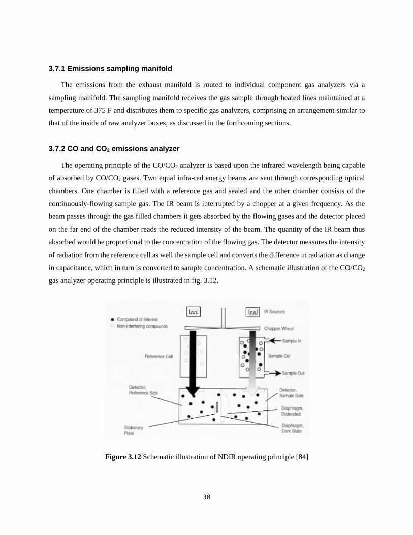
38

3.7.1 Emissions sampling manifold

The emissions from the exhaust manifold is routed to individual component gas analyzers via a

sampling manifold. The sampling manifold receives the gas sample through heated lines maintained at a

temperature of 375 F and distributes them to specific gas analyzers, comprising an arrangement similar to

that of the inside of raw analyzer boxes, as discussed in the forthcoming sections.

3.7.2 CO and CO2 emissions analyzer

The operating principle of the CO/CO2 analyzer is based upon the infrared wavelength being capable

of absorbed by CO/CO2 gases. Two equal infra-red energy beams are sent through corresponding optical

chambers. One chamber is filled with a reference gas and sealed and the other chamber consists of the

continuously-flowing sample gas. The IR beam is interrupted by a chopper at a given frequency. As the

beam passes through the gas filled chambers it gets absorbed by the flowing gases and the detector placed

on the far end of the chamber reads the reduced intensity of the beam. The quantity of the IR beam thus

absorbed would be proportional to the concentration of the flowing gas. The detector measures the intensity

of radiation from the reference cell as well the sample cell and converts the difference in radiation as change

in capacitance, which in turn is converted to sample concentration. A schematic illustration of the CO/CO2

gas analyzer operating principle is illustrated in fig. 3.12.

Figure 3.12 Schematic illustration of NDIR operating principle [84]

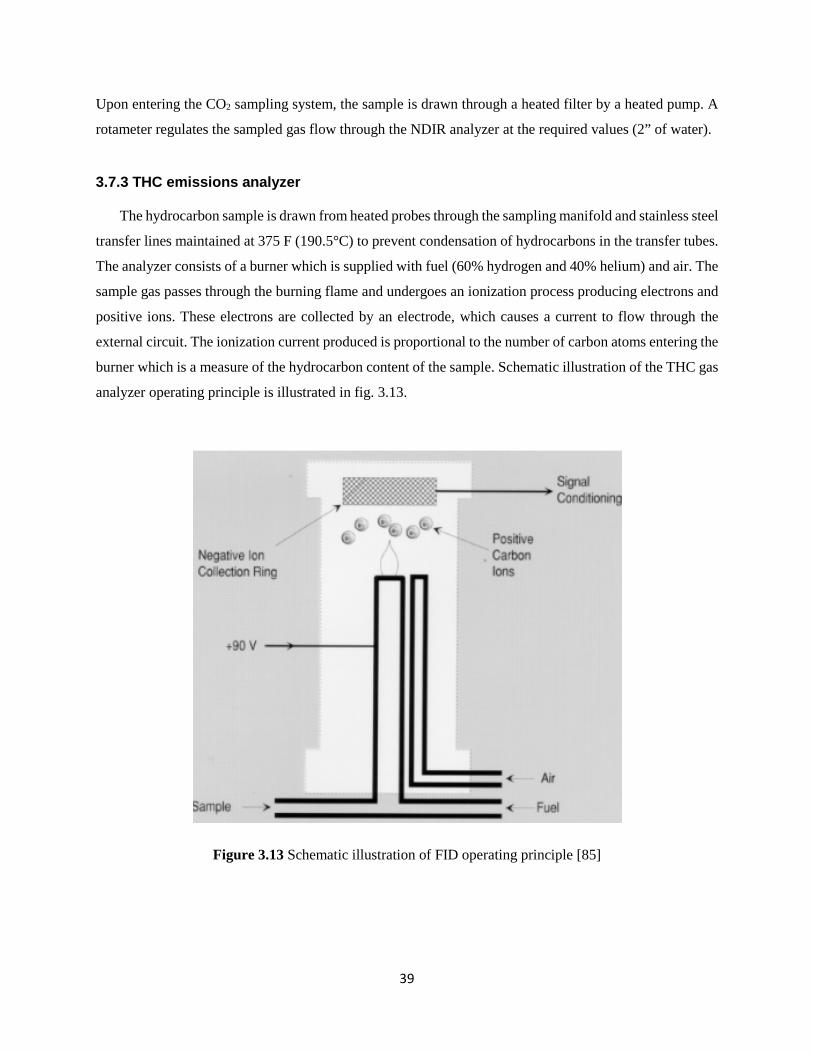
39

Upon entering the CO2 sampling system, the sample is drawn through a heated filter by a heated pump. A

rotameter regulates the sampled gas flow through the NDIR analyzer at the required values (2” of water).

3.7.3 THC emissions analyzer

The hydrocarbon sample is drawn from heated probes through the sampling manifold and stainless steel

transfer lines maintained at 375 F (190.5°C) to prevent condensation of hydrocarbons in the transfer tubes.

The analyzer consists of a burner which is supplied with fuel (60% hydrogen and 40% helium) and air. The

sample gas passes through the burning flame and undergoes an ionization process producing electrons and

positive ions. These electrons are collected by an electrode, which causes a current to flow through the

external circuit. The ionization current produced is proportional to the number of carbon atoms entering the

burner which is a measure of the hydrocarbon content of the sample. Schematic illustration of the THC gas

analyzer operating principle is illustrated in fig. 3.13.

Figure 3.13 Schematic illustration of FID operating principle [85]

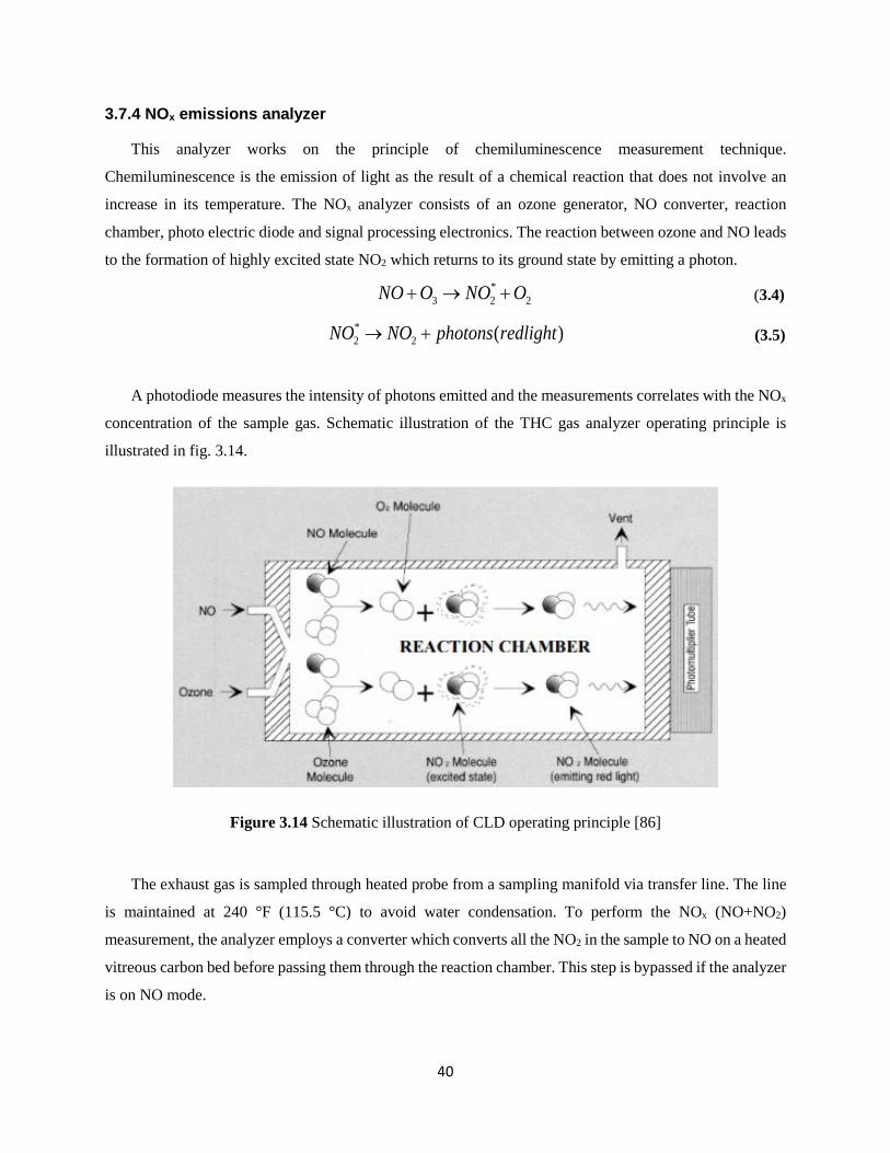
40

3.7.4 NOx emissions analyzer

This analyzer works on the principle of chemiluminescence measurement technique.

Chemiluminescence is the emission of light as the result of a chemical reaction that does not involve an

increase in its temperature. The NOx analyzer consists of an ozone generator, NO converter, reaction

chamber, photo electric diode and signal processing electronics. The reaction between ozone and NO leads

to the formation of highly excited state NO2 which returns to its ground state by emitting a photon.

*3 2 2NO O NO O+ → + (3.4)

*2 2 ( )NO NO photons redlight→ + (3.5)

A photodiode measures the intensity of photons emitted and the measurements correlates with the NOx

concentration of the sample gas. Schematic illustration of the THC gas analyzer operating principle is

illustrated in fig. 3.14.

Figure 3.14 Schematic illustration of CLD operating principle [86]

The exhaust gas is sampled through heated probe from a sampling manifold via transfer line. The line

is maintained at 240 °F (115.5 °C) to avoid water condensation. To perform the NOx (NO+NO2)

measurement, the analyzer employs a converter which converts all the NO2 in the sample to NO on a heated

vitreous carbon bed before passing them through the reaction chamber. This step is bypassed if the analyzer

is on NO mode.

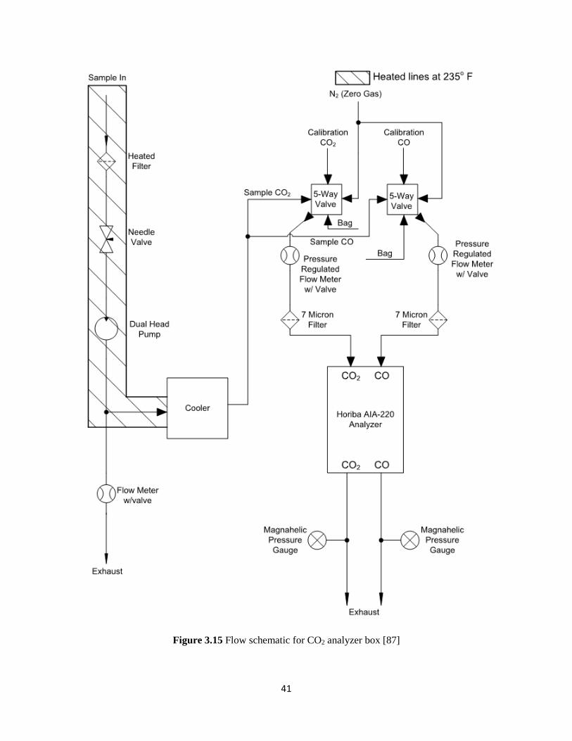
41

Figure 3.15 Flow schematic for CO2 analyzer box [87]

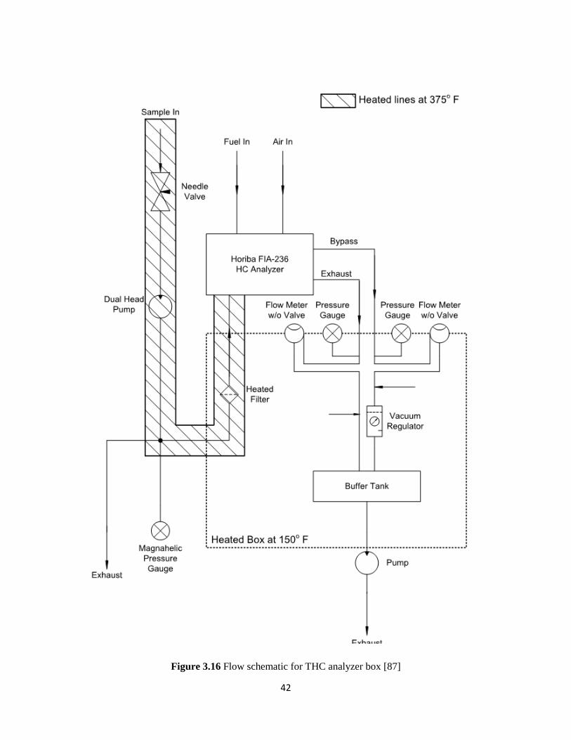
42

Figure 3.16 Flow schematic for THC analyzer box [87]

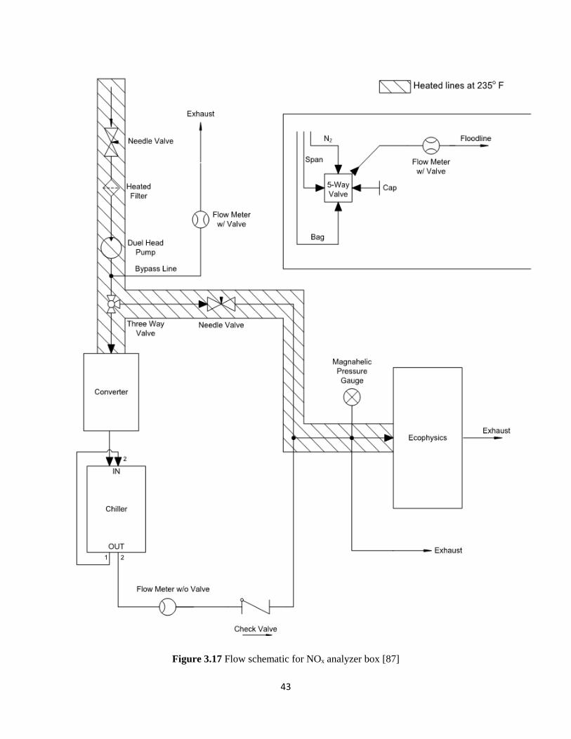
43

Figure 3.17 Flow schematic for NOx analyzer box [87]

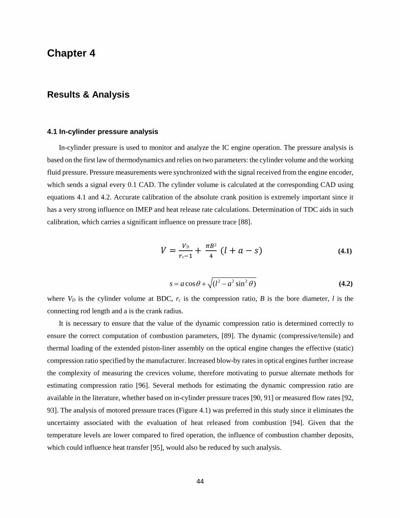
44

Chapter 4

Results & Analysis

4.1 In-cylinder pressure analysis

In-cylinder pressure is used to monitor and analyze the IC engine operation. The pressure analysis is

based on the first law of thermodynamics and relies on two parameters: the cylinder volume and the working

fluid pressure. Pressure measurements were synchronized with the signal received from the engine encoder,

which sends a signal every 0.1 CAD. The cylinder volume is calculated at the corresponding CAD using

equations 4.1 and 4.2. Accurate calibration of the absolute crank position is extremely important since it

has a very strong influence on IMEP and heat release rate calculations. Determination of TDC aids in such

calibration, which carries a significant influence on pressure trace [88].

𝑉𝑉 = 𝑉𝑉D

𝑟𝑟c−1+ 𝜋𝜋𝜋𝜋

2

4 (𝑙𝑙 + 𝑎𝑎 − 𝑠𝑠) (4.1)

2 2 2cos ( sin )s a l aθ θ= + − (4.2)

where VD is the cylinder volume at BDC, rc is the compression ratio, B is the bore diameter, l is the

connecting rod length and a is the crank radius.

It is necessary to ensure that the value of the dynamic compression ratio is determined correctly to

ensure the correct computation of combustion parameters, [89]. The dynamic (compressive/tensile) and

thermal loading of the extended piston-liner assembly on the optical engine changes the effective (static)

compression ratio specified by the manufacturer. Increased blow-by rates in optical engines further increase

the complexity of measuring the crevices volume, therefore motivating to pursue alternate methods for

estimating compression ratio [96]. Several methods for estimating the dynamic compression ratio are

available in the literature, whether based on in-cylinder pressure traces [90, 91] or measured flow rates [92,

93]. The analysis of motored pressure traces (Figure 4.1) was preferred in this study since it eliminates the

uncertainty associated with the evaluation of heat released from combustion [94]. Given that the

temperature levels are lower compared to fired operation, the influence of combustion chamber deposits,

which could influence heat transfer [95], would also be reduced by such analysis.

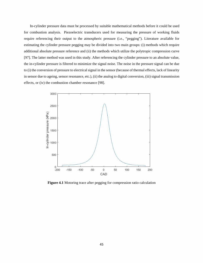
45

In-cylinder pressure data must be processed by suitable mathematical methods before it could be used

for combustion analysis. Piezoelectric transducers used for measuring the pressure of working fluids

require referencing their output to the atmospheric pressure (i.e., “pegging”). Literature available for

estimating the cylinder pressure pegging may be divided into two main groups: (i) methods which require

additional absolute pressure reference and (ii) the methods which utilize the polytropic compression curve

[97]. The latter method was used in this study. After referencing the cylinder pressure to an absolute value,

the in-cylinder pressure is filtered to minimize the signal noise. The noise in the pressure signal can be due

to (i) the conversion of pressure to electrical signal in the sensor (because of thermal effects, lack of linearity

in sensor due to ageing, sensor resonance, etc.), (ii) the analog to digital conversion, (iii) signal transmission

effects, or (iv) the combustion chamber resonance [98].

Figure 4.1 Motoring trace after pegging for compression ratio calculation

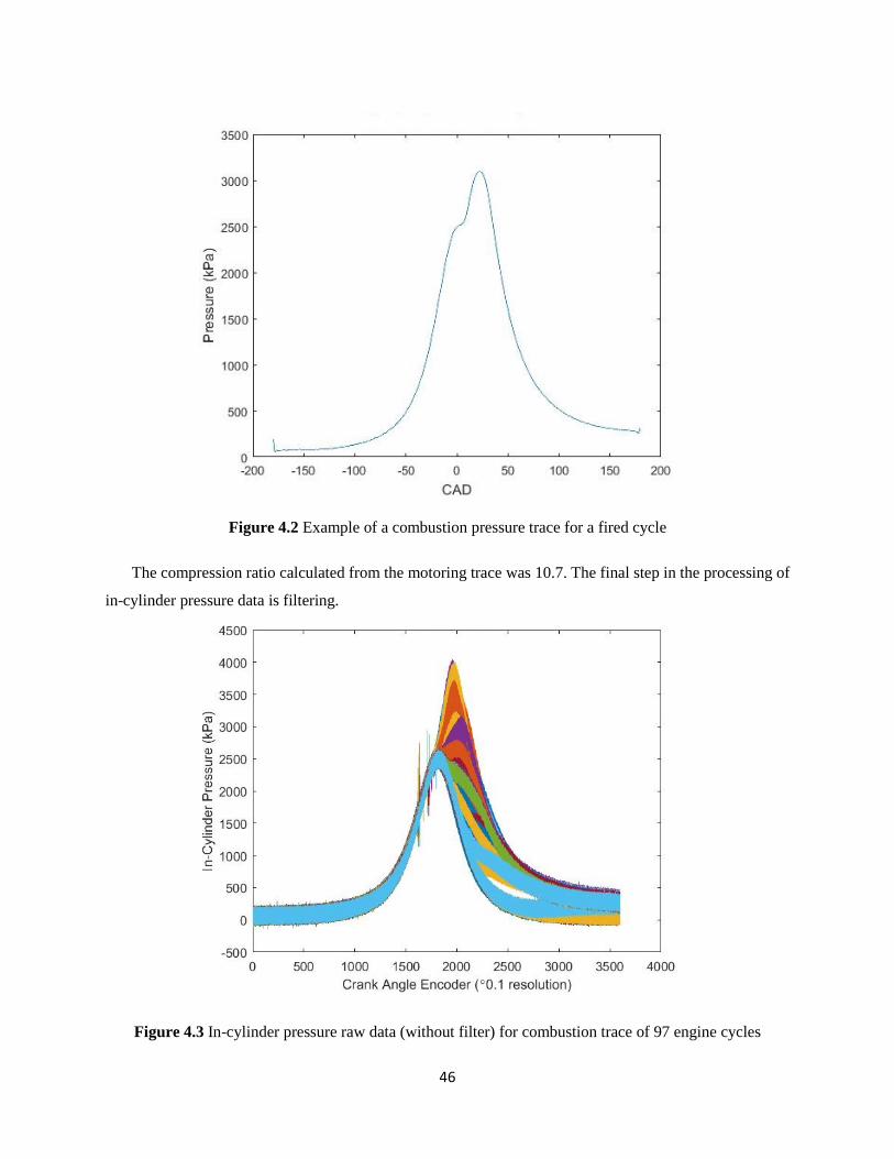
46

Figure 4.2 Example of a combustion pressure trace for a fired cycle

The compression ratio calculated from the motoring trace was 10.7. The final step in the processing of

in-cylinder pressure data is filtering.

Figure 4.3 In-cylinder pressure raw data (without filter) for combustion trace of 97 engine cycles

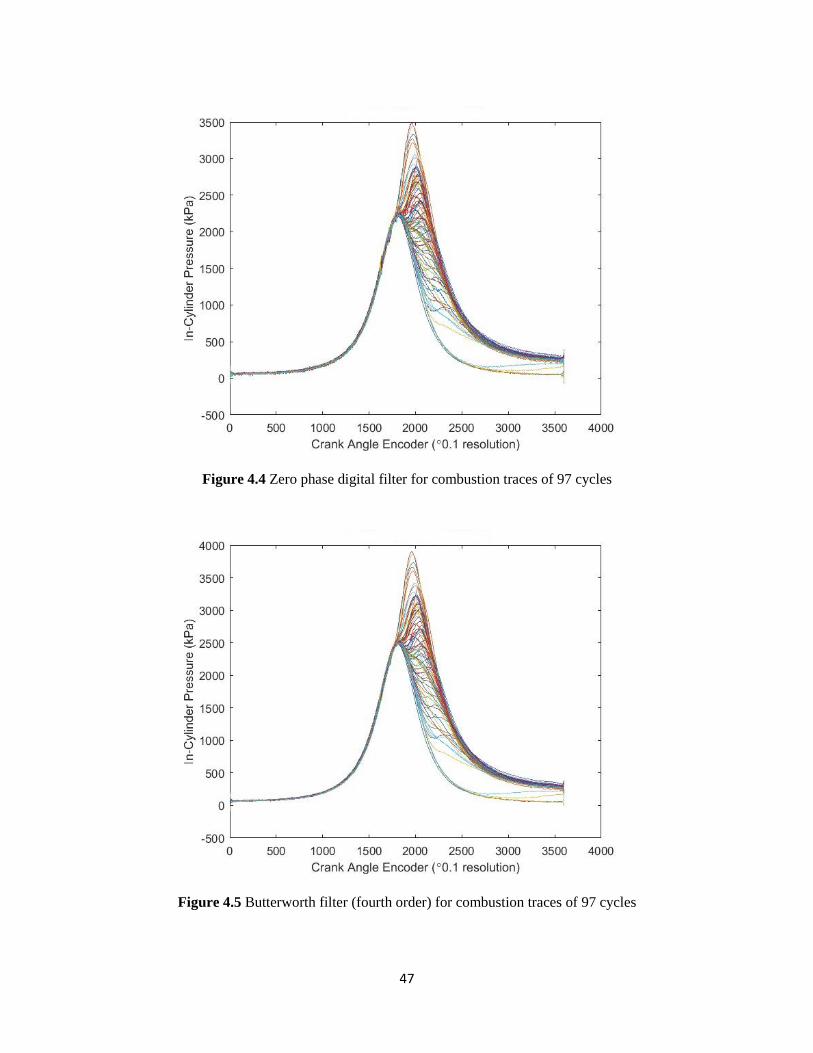
47

Figure 4.4 Zero phase digital filter for combustion traces of 97 cycles

Figure 4.5 Butterworth filter (fourth order) for combustion traces of 97 cycles

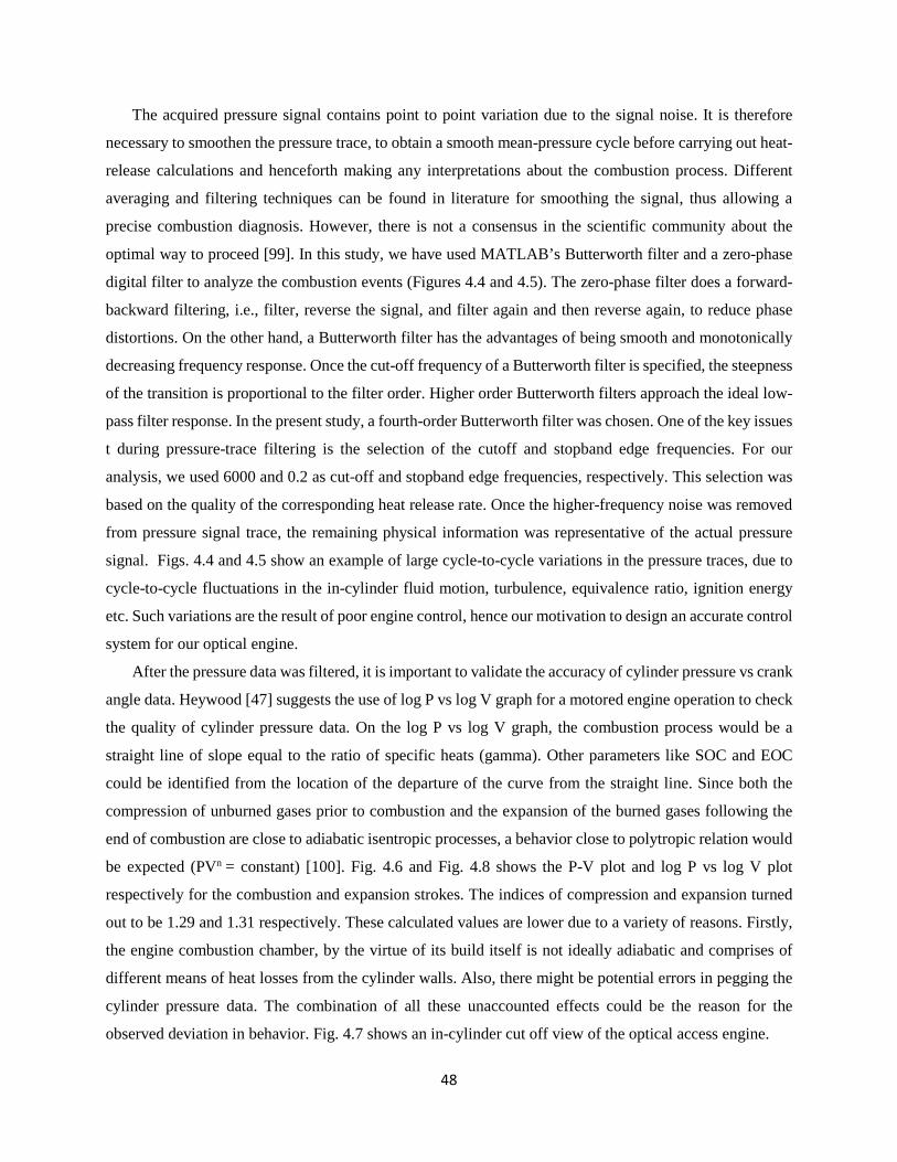
48

The acquired pressure signal contains point to point variation due to the signal noise. It is therefore

necessary to smoothen the pressure trace, to obtain a smooth mean-pressure cycle before carrying out heat-

release calculations and henceforth making any interpretations about the combustion process. Different

averaging and filtering techniques can be found in literature for smoothing the signal, thus allowing a

precise combustion diagnosis. However, there is not a consensus in the scientific community about the

optimal way to proceed [99]. In this study, we have used MATLAB’s Butterworth filter and a zero-phase

digital filter to analyze the combustion events (Figures 4.4 and 4.5). The zero-phase filter does a forward-

backward filtering, i.e., filter, reverse the signal, and filter again and then reverse again, to reduce phase

distortions. On the other hand, a Butterworth filter has the advantages of being smooth and monotonically

decreasing frequency response. Once the cut-off frequency of a Butterworth filter is specified, the steepness

of the transition is proportional to the filter order. Higher order Butterworth filters approach the ideal low-

pass filter response. In the present study, a fourth-order Butterworth filter was chosen. One of the key issues

t during pressure-trace filtering is the selection of the cutoff and stopband edge frequencies. For our

analysis, we used 6000 and 0.2 as cut-off and stopband edge frequencies, respectively. This selection was

based on the quality of the corresponding heat release rate. Once the higher-frequency noise was removed

from pressure signal trace, the remaining physical information was representative of the actual pressure

signal. Figs. 4.4 and 4.5 show an example of large cycle-to-cycle variations in the pressure traces, due to

cycle-to-cycle fluctuations in the in-cylinder fluid motion, turbulence, equivalence ratio, ignition energy

etc. Such variations are the result of poor engine control, hence our motivation to design an accurate control

system for our optical engine.

After the pressure data was filtered, it is important to validate the accuracy of cylinder pressure vs crank

angle data. Heywood [47] suggests the use of log P vs log V graph for a motored engine operation to check

the quality of cylinder pressure data. On the log P vs log V graph, the combustion process would be a

straight line of slope equal to the ratio of specific heats (gamma). Other parameters like SOC and EOC

could be identified from the location of the departure of the curve from the straight line. Since both the

compression of unburned gases prior to combustion and the expansion of the burned gases following the

end of combustion are close to adiabatic isentropic processes, a behavior close to polytropic relation would

be expected (PVn = constant) [100]. Fig. 4.6 and Fig. 4.8 shows the P-V plot and log P vs log V plot

respectively for the combustion and expansion strokes. The indices of compression and expansion turned

out to be 1.29 and 1.31 respectively. These calculated values are lower due to a variety of reasons. Firstly,

the engine combustion chamber, by the virtue of its build itself is not ideally adiabatic and comprises of

different means of heat losses from the cylinder walls. Also, there might be potential errors in pegging the

cylinder pressure data. The combination of all these unaccounted effects could be the reason for the

observed deviation in behavior. Fig. 4.7 shows an in-cylinder cut off view of the optical access engine.

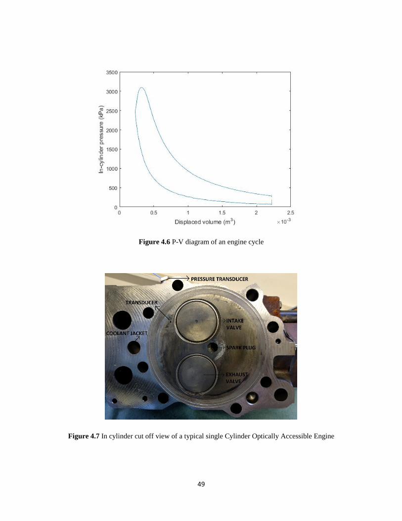
49

Figure 4.6 P-V diagram of an engine cycle

Figure 4.7 In cylinder cut off view of a typical single Cylinder Optically Accessible Engine

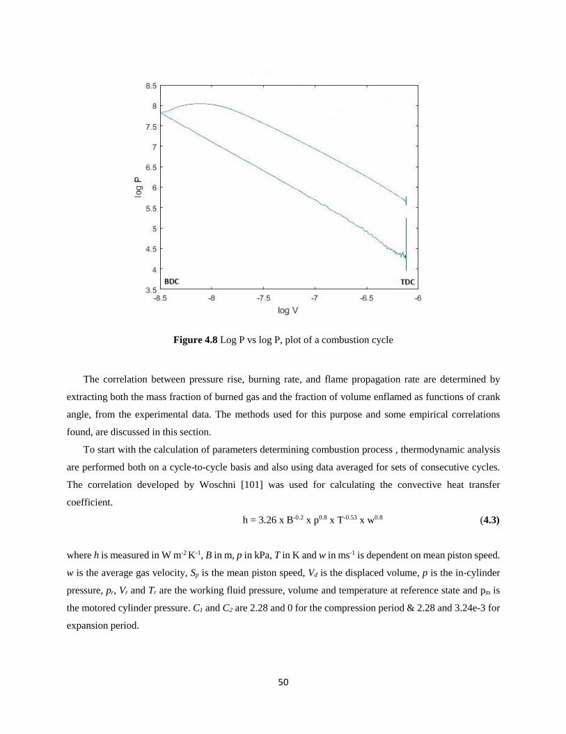
50

Figure 4.8 Log P vs log P, plot of a combustion cycle

The correlation between pressure rise, burning rate, and flame propagation rate are determined by

extracting both the mass fraction of burned gas and the fraction of volume enflamed as functions of crank

angle, from the experimental data. The methods used for this purpose and some empirical correlations

found, are discussed in this section.

To start with the calculation of parameters determining combustion process , thermodynamic analysis

are performed both on a cycle-to-cycle basis and also using data averaged for sets of consecutive cycles.

The correlation developed by Woschni [101] was used for calculating the convective heat transfer

coefficient.

h = 3.26 x B-0.2 x p0.8 x T-0.53 x w0.8 (4.3)

where h is measured in W m-2 K-1, B in m, p in kPa, T in K and w in ms-1 is dependent on mean piston speed.

w is the average gas velocity, Sp is the mean piston speed, Vd is the displaced volume, p is the in-cylinder

pressure, pr, Vr and Tr are the working fluid pressure, volume and temperature at reference state and pm is

the motored cylinder pressure. C1 and C2 are 2.28 and 0 for the compression period & 2.28 and 3.24e-3 for

expansion period.

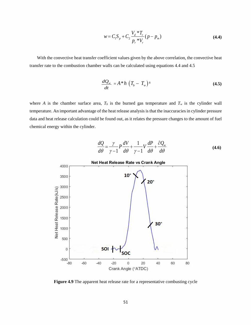
51

1 2* ( )*

d rp m

r r

V Tw C S C p pp V

= + − (4.4)

With the convective heat transfer coefficient values given by the above correlation, the convective heat

transfer rate to the combustion chamber walls can be calculated using equations 4.4 and 4.5

wdQdt

= ( )* – b wA h T T 8 (4.5)

where A is the chamber surface area, Tb is the burned gas temperature and Tw is the cylinder wall

temperature. An important advantage of the heat release analysis is that the inaccuracies in cylinder pressure

data and heat release calculation could be found out, as it relates the pressure changes to the amount of fuel

chemical energy within the cylinder.

1

1 1wQdQ dV dPP V

d d d dγ

θ γ θ γ θ θ∂

= + +− −

(4.6)

Figure 4.9 The apparent heat release rate for a representative combusting cycle

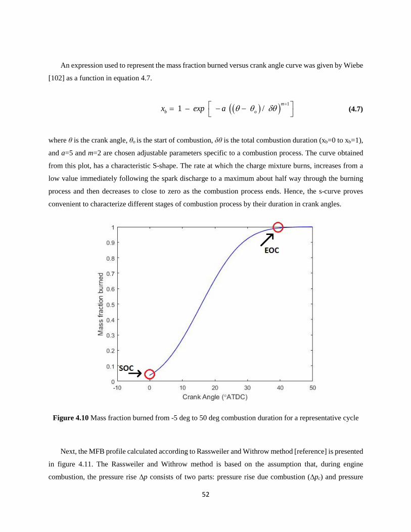
52

An expression used to represent the mass fraction burned versus crank angle curve was given by Wiebe

[102] as a function in equation 4.7.

( )( ) 1 1 – /

mb ox exp a θ θ δθ

+= − −

(4.7)

where θ is the crank angle, θo is the start of combustion, δθ is the total combustion duration (xb=0 to xb=1),

and a=5 and m=2 are chosen adjustable parameters specific to a combustion process. The curve obtained

from this plot, has a characteristic S-shape. The rate at which the charge mixture burns, increases from a

low value immediately following the spark discharge to a maximum about half way through the burning

process and then decreases to close to zero as the combustion process ends. Hence, the s-curve proves

convenient to characterize different stages of combustion process by their duration in crank angles.

Figure 4.10 Mass fraction burned from -5 deg to 50 deg combustion duration for a representative cycle

Next, the MFB profile calculated according to Rassweiler and Withrow method [reference] is presented

in figure 4.11. The Rassweiler and Withrow method is based on the assumption that, during engine

combustion, the pressure rise ∆p consists of two parts: pressure rise due combustion (∆pc) and pressure

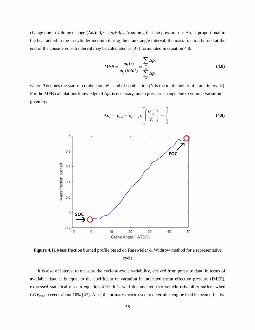
53

change due to volume change (∆pv): Δp= Δpc+Δpv. Assuming that the pressure rise ∆pc is proportional to

the heat added to the in-cylinder medium during the crank angle interval, the mass fraction burned at the

end of the considered i-th interval may be calculated as [47] formulated in equation 4.8:

0

0

( )( )

b

i

cb

N

c

pm iMFB

m total p

∆= =

∆

∑

∑ (4.8)

where 0 denotes the start of combustion, N – end of combustion (N is the total number of crank intervals).

For the MFB calculations knowledge of ∆pc is necessary, and a pressure change due to volume variation is

given by:

11 1

n

iv i i i

i

Vp p p pV+

+

∆ = − = −

(4.9)

Figure 4.11 Mass fraction burned profile based on Rasswieler & Withrow method for a representative

cycle

It is also of interest to measure the cycle-to-cycle variability, derived from pressure data. In terms of

available data, it is equal to the coefficient of variation in indicated mean effective pressure (IMEP),

expressed statistically as in equation 4.10. It is well documented that vehicle drivability suffers when

COVimep exceeds about 10% [47]. Also, the primary metric used to determine engine load is mean effective

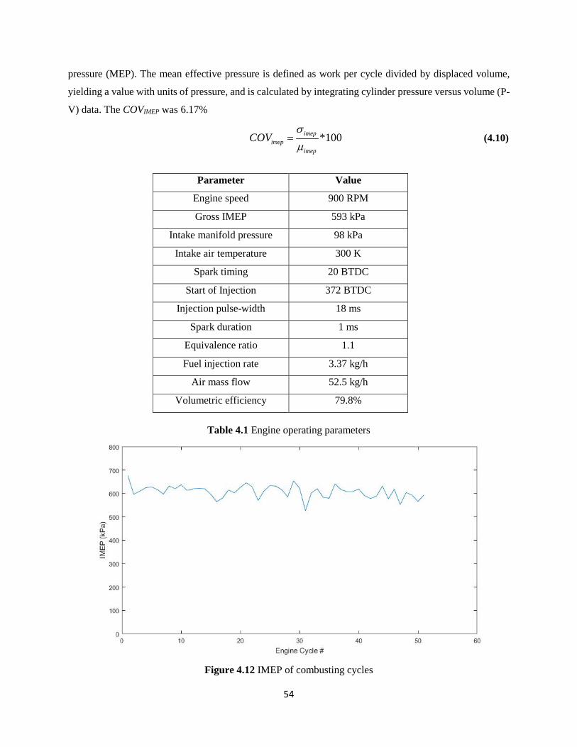
54

pressure (MEP). The mean effective pressure is defined as work per cycle divided by displaced volume,

yielding a value with units of pressure, and is calculated by integrating cylinder pressure versus volume (P-

V) data. The COVIMEP was 6.17%

*100imepimep

imep

COVσµ

= (4.10)

Parameter Value

Engine speed 900 RPM

Gross IMEP 593 kPa

Intake manifold pressure 98 kPa

Intake air temperature 300 K

Spark timing 20 BTDC

Start of Injection 372 BTDC

Injection pulse-width 18 ms

Spark duration 1 ms

Equivalence ratio 1.1

Fuel injection rate 3.37 kg/h

Air mass flow 52.5 kg/h

Volumetric efficiency 79.8%

Table 4.1 Engine operating parameters

Figure 4.12 IMEP of combusting cycles

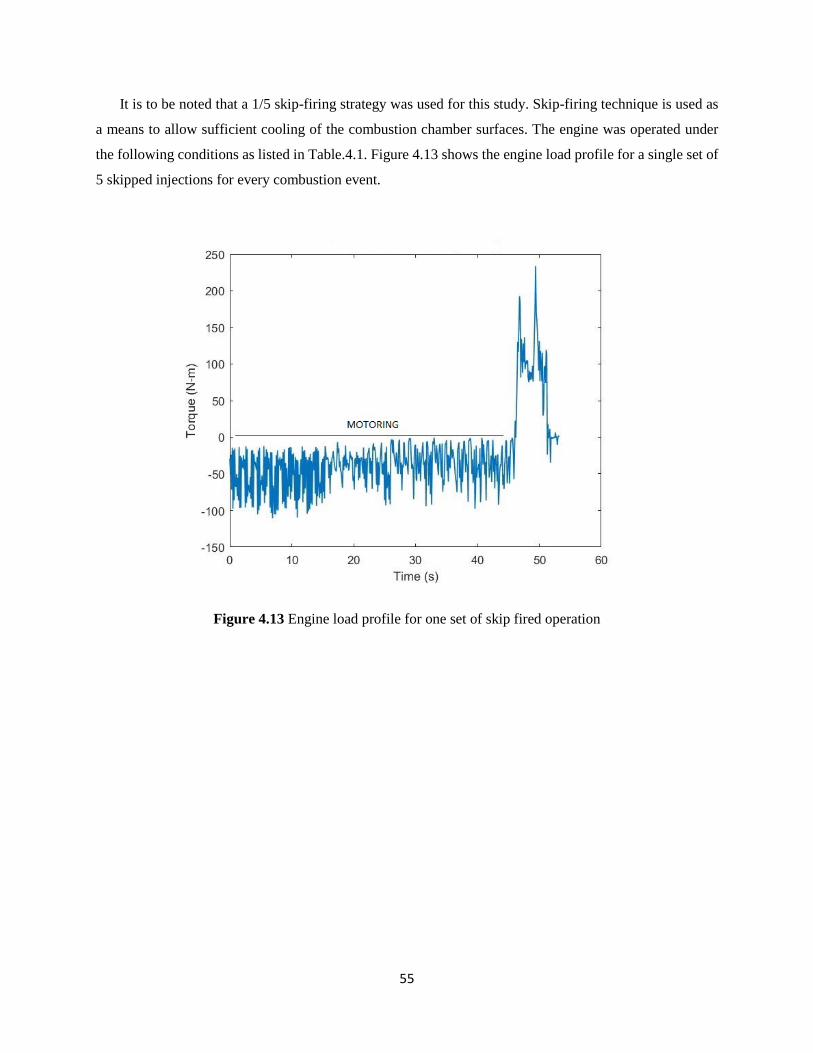
55

It is to be noted that a 1/5 skip-firing strategy was used for this study. Skip-firing technique is used as

a means to allow sufficient cooling of the combustion chamber surfaces. The engine was operated under

the following conditions as listed in Table.4.1. Figure 4.13 shows the engine load profile for a single set of

5 skipped injections for every combustion event.

Figure 4.13 Engine load profile for one set of skip fired operation

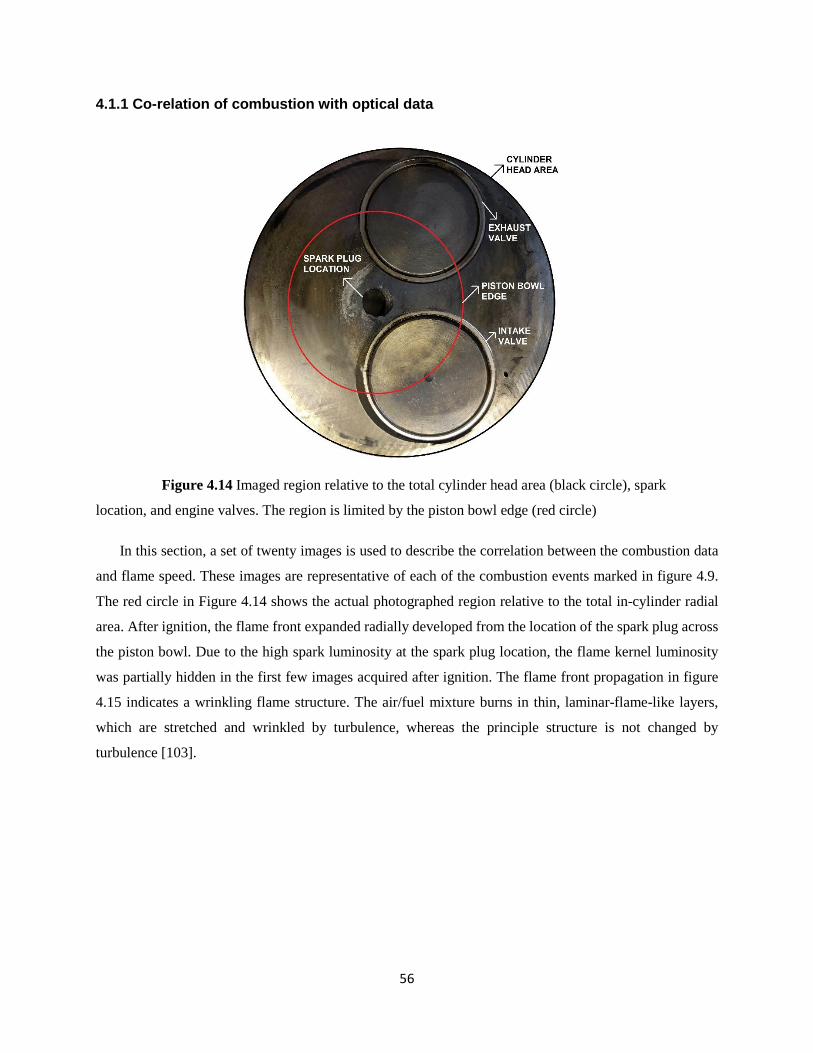
56

4.1.1 Co-relation of combustion with optical data

Figure 4.14 Imaged region relative to the total cylinder head area (black circle), spark

location, and engine valves. The region is limited by the piston bowl edge (red circle)

In this section, a set of twenty images is used to describe the correlation between the combustion data

and flame speed. These images are representative of each of the combustion events marked in figure 4.9.

The red circle in Figure 4.14 shows the actual photographed region relative to the total in-cylinder radial

area. After ignition, the flame front expanded radially developed from the location of the spark plug across

the piston bowl. Due to the high spark luminosity at the spark plug location, the flame kernel luminosity

was partially hidden in the first few images acquired after ignition. The flame front propagation in figure

4.15 indicates a wrinkling flame structure. The air/fuel mixture burns in thin, laminar-flame-like layers,

which are stretched and wrinkled by turbulence, whereas the principle structure is not changed by

turbulence [103].

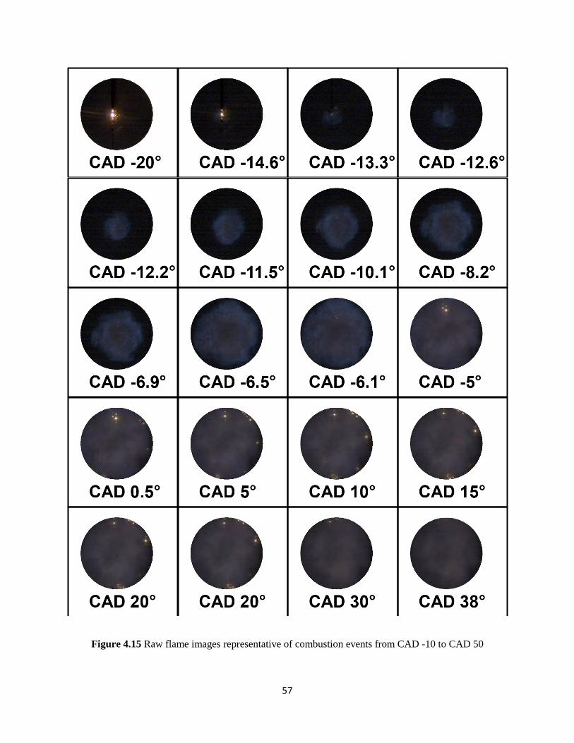
57

Figure 4.15 Raw flame images representative of combustion events from CAD -10 to CAD 50

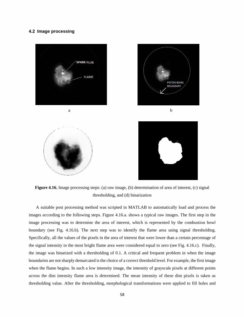
58

4.2 Image processing

a b

Figure 4.16. Image processing steps: (a) raw image, (b) determination of area of interest, (c) signal

thresholding, and (d) binarization

A suitable post processing method was scripted in MATLAB to automatically load and process the

images according to the following steps. Figure 4.16.a. shows a typical raw images. The first step in the

image processing was to determine the area of interest, which is represented by the combustion bowl

boundary (see Fig. 4.16.b). The next step was to identify the flame area using signal thresholding.

Specifically, all the values of the pixels in the area of interest that were lower than a certain percentage of

the signal intensity in the most bright flame area were considered equal to zero (see Fig. 4.16.c). Finally,

the image was binarized with a thresholding of 0.1. A critical and frequent problem in when the image

boundaries are not sharply demarcated is the choice of a correct threshold level. For example, the first image

when the flame begins. In such a low intensity image, the intensity of grayscale pixels at different points

across the dim intensity flame area is determined. The mean intensity of these dim pixels is taken as

thresholding value. After the thresholding, morphological transformations were applied to fill holes and

59

remove small border objects. In order to decrease noise and smooth the contour, a low pass filter was

applied. Further these steps, a circle of dimensions equal to that of the piston bowl edge is masked onto the

binarized image. Now, the matrix of masked image is multiplied with the image matrix of the binary image.

In doing so, all the white pixels (binary-1) inside the masked circle will be retained and those outside the

region of interest will be turned black (binary-0). From the obtained flame images, geometric properties

such as area and perimeter are computed using inbuilt MATLAB image processing functions. The above

described procedure is iterated in a loop for all the images and thereafter written into a destination folder,

after applying the processing steps.

The burning rate can be extracted from the flame area. Assuming a spherical flame, the radii of the

burnt gas area and the perimeter, Rs and Rp respectively, were determined using equation 4.11:

2

s

p

AR

PR

π

π

=

= (4.11)

where A and P are the flame area and perimeter, respectively, deduced from the monochromatic combustion

images. The wrinkling ratio W as defined by Renou and Boukhalfa [104] is also calculated according to

equation 4.12:

2

2p

s

RW

R= (4.12)

Fig. 4.17 shows a plot of the computed wrinkling ratio growth with CAD, for a combustion cycle. A

flame propagation (turbulent) speed is then derived from Rs:

sRs

dRSdt

= (4.13)

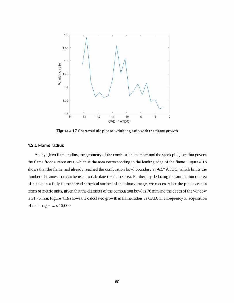
60

Figure 4.17 Characteristic plot of wrinkling ratio with the flame growth

4.2.1 Flame radius

At any given flame radius, the geometry of the combustion chamber and the spark plug location govern

the flame front surface area, which is the area corresponding to the leading edge of the flame. Figure 4.18

shows that the flame had already reached the combustion bowl boundary at -6.5º ATDC, which limits the

number of frames that can be used to calculate the flame area. Further, by deducing the summation of area

of pixels, in a fully flame spread spherical surface of the binary image, we can co-relate the pixels area in

terms of metric units, given that the diameter of the combustion bowl is 76 mm and the depth of the window

is 31.75 mm. Figure 4.19 shows the calculated growth in flame radius vs CAD. The frequency of acquisition

of the images was 15,000.

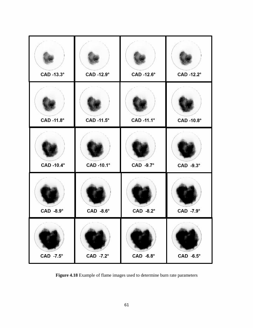
61

Figure 4.18 Example of flame images used to determine burn rate parameters

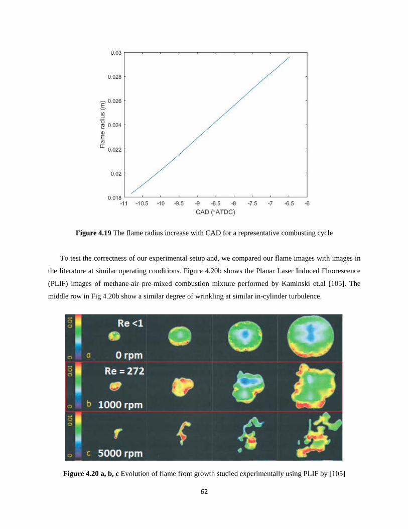
62

Figure 4.19 The flame radius increase with CAD for a representative combusting cycle

To test the correctness of our experimental setup and, we compared our flame images with images in

the literature at similar operating conditions. Figure 4.20b shows the Planar Laser Induced Fluorescence

(PLIF) images of methane-air pre-mixed combustion mixture performed by Kaminski et.al [105]. The

middle row in Fig 4.20b show a similar degree of wrinkling at similar in-cylinder turbulence.

Figure 4.20 a, b, c Evolution of flame front growth studied experimentally using PLIF by [105]

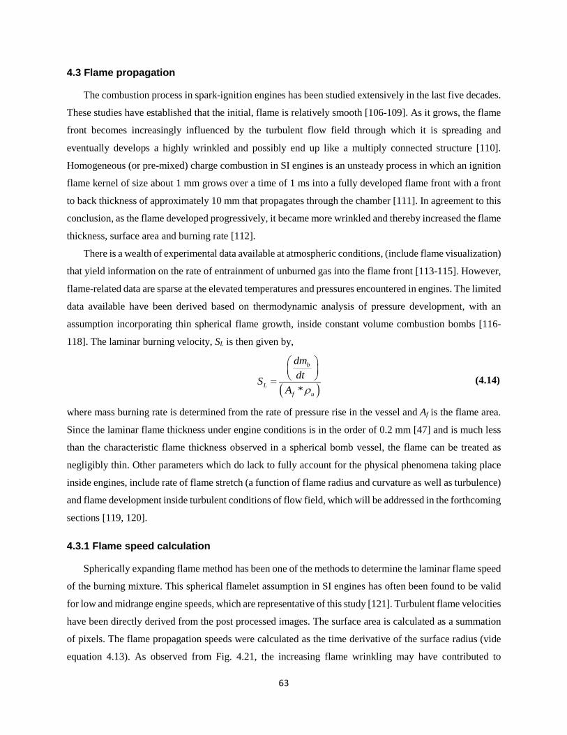
63

4.3 Flame propagation

The combustion process in spark-ignition engines has been studied extensively in the last five decades.

These studies have established that the initial, flame is relatively smooth [106-109]. As it grows, the flame

front becomes increasingly influenced by the turbulent flow field through which it is spreading and

eventually develops a highly wrinkled and possibly end up like a multiply connected structure [110].

Homogeneous (or pre-mixed) charge combustion in SI engines is an unsteady process in which an ignition

flame kernel of size about 1 mm grows over a time of 1 ms into a fully developed flame front with a front

to back thickness of approximately 10 mm that propagates through the chamber [111]. In agreement to this

conclusion, as the flame developed progressively, it became more wrinkled and thereby increased the flame

thickness, surface area and burning rate [112].

There is a wealth of experimental data available at atmospheric conditions, (include flame visualization)

that yield information on the rate of entrainment of unburned gas into the flame front [113-115]. However,

flame-related data are sparse at the elevated temperatures and pressures encountered in engines. The limited

data available have been derived based on thermodynamic analysis of pressure development, with an

assumption incorporating thin spherical flame growth, inside constant volume combustion bombs [116-

118]. The laminar burning velocity, SL is then given by,

( )

*

b

Lf u

dmdtS

A ρ

= (4.14)

where mass burning rate is determined from the rate of pressure rise in the vessel and Af is the flame area.

Since the laminar flame thickness under engine conditions is in the order of 0.2 mm [47] and is much less

than the characteristic flame thickness observed in a spherical bomb vessel, the flame can be treated as

negligibly thin. Other parameters which do lack to fully account for the physical phenomena taking place

inside engines, include rate of flame stretch (a function of flame radius and curvature as well as turbulence)

and flame development inside turbulent conditions of flow field, which will be addressed in the forthcoming

sections [119, 120].

4.3.1 Flame speed calculation

Spherically expanding flame method has been one of the methods to determine the laminar flame speed

of the burning mixture. This spherical flamelet assumption in SI engines has often been found to be valid

for low and midrange engine speeds, which are representative of this study [121]. Turbulent flame velocities

have been directly derived from the post processed images. The surface area is calculated as a summation

of pixels. The flame propagation speeds were calculated as the time derivative of the surface radius (vide

equation 4.13). As observed from Fig. 4.21, the increasing flame wrinkling may have contributed to

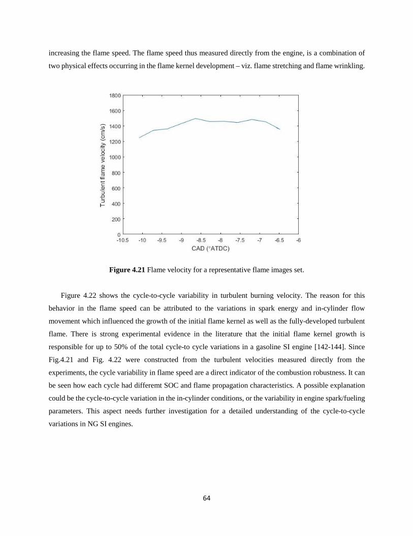
64

increasing the flame speed. The flame speed thus measured directly from the engine, is a combination of

two physical effects occurring in the flame kernel development – viz. flame stretching and flame wrinkling.

Figure 4.21 Flame velocity for a representative flame images set.

Figure 4.22 shows the cycle-to-cycle variability in turbulent burning velocity. The reason for this

behavior in the flame speed can be attributed to the variations in spark energy and in-cylinder flow

movement which influenced the growth of the initial flame kernel as well as the fully-developed turbulent

flame. There is strong experimental evidence in the literature that the initial flame kernel growth is

responsible for up to 50% of the total cycle-to cycle variations in a gasoline SI engine [142-144]. Since

Fig.4.21 and Fig. 4.22 were constructed from the turbulent velocities measured directly from the

experiments, the cycle variability in flame speed are a direct indicator of the combustion robustness. It can

be seen how each cycle had differemt SOC and flame propagation characteristics. A possible explanation

could be the cycle-to-cycle variation in the in-cylinder conditions, or the variability in engine spark/fueling

parameters. This aspect needs further investigation for a detailed understanding of the cycle-to-cycle

variations in NG SI engines.

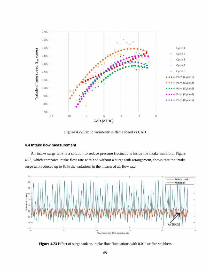
65

Figure 4.22 Cyclic variability in flame speed vs CAD

4.4 Intake flow measurement

An intake surge tank is a solution to reduce pressure fluctuations inside the intake manifold. Figure

4.23, which compares intake flow rate with and without a surge tank arrangement, shows that the intake

surge tank reduced up to 83% the variations in the measured air flow rate.

Figure 4.23 Effect of surge tank on intake flow fluctuations with 0.01” orifice snubbers

700

800

900

1000

1100

1200

1300

1400

1500

1600

1700

-12 -10 -8 -6 -4 -2 0

Turb

ulen

t fla

me

spee

d, S

Rs

(cm

/s)

CAD (ATDC)

Cycle 1

Cycle 2

Cycle 3

Cycle 4

Cycle 5

Poly. (Cycle 1)

Poly. (Cycle 2)

Poly. (Cycle 3)

Poly. (Cycle 4)

Poly. (Cycle 5)

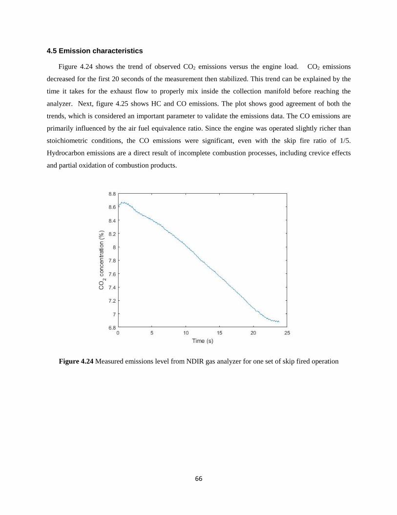
66

4.5 Emission characteristics

Figure 4.24 shows the trend of observed CO2 emissions versus the engine load. CO2 emissions

decreased for the first 20 seconds of the measurement then stabilized. This trend can be explained by the

time it takes for the exhaust flow to properly mix inside the collection manifold before reaching the

analyzer. Next, figure 4.25 shows HC and CO emissions. The plot shows good agreement of both the

trends, which is considered an important parameter to validate the emissions data. The CO emissions are

primarily influenced by the air fuel equivalence ratio. Since the engine was operated slightly richer than

stoichiometric conditions, the CO emissions were significant, even with the skip fire ratio of 1/5.

Hydrocarbon emissions are a direct result of incomplete combustion processes, including crevice effects

and partial oxidation of combustion products.

Figure 4.24 Measured emissions level from NDIR gas analyzer for one set of skip fired operation

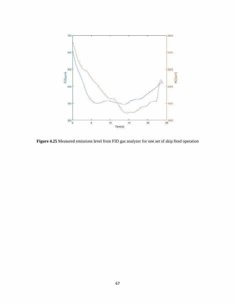
67

Figure 4.25 Measured emissions level from FID gas analyzer for one set of skip fired operation

68

Chapter 5

Conclusions

The goal of this study was to develop an experimental platform for optical investigations of engine

combustion phenomena based on a single-cylinder heavy-duty spark-ignited engine. The Ricardo Proteus

research engine uses a Bowditch piston to provide optical access to the combustion chamber. This optical

engine was used for a preliminary investigation of the flame speed in NG combustion. The first part focuses

on the setup of a single-cylinder research engine with optical access including the design of its control

system and the acquisition of in-cylinder pressure data and high-speed combustion images. The second part

focuses on measurements of the turbulent flame speed using the high-speed combustion images.

The optical engine control system can acquire operating parameters (engine speed and torque, air and

fuel mass flows, engine fluids temperature), in-cylinder pressure data, combustion images, and engine

emissions. The LFE used for intake flow measurements showed large variations in before the installation

of pressure snubbers and a surge air tank close to the intake valve.

Two different methods of digital signal processing, i.e., zero phase digital filter and fourth order

butterworth filter, eliminated signal artefacts and smoothened the in-cylinder pressure signal for combustion

analysis. The Butterworth filter showed superior performance compared to the zero-phase digital filter,

indicating it as a method of choice for pressure analysis.

Combustion natural luminosity was used for fundamental combustion analysis in the second part of the

study. This visualization technique used a high-speed CMOS camera to acquire time resolved in-cylinder

flame images of the burning mixture at 900 rpm, at close to stoichiometric conditions. A post processing

technique based on the increase of flame area per unit time was developed in MATLAB and use to

determine the flame speed. The flame front radius were calculated and reported as a function of the CAD

during the first stages of the combustion process (i.e., up to the moment the flame reaches the piston bowl

edge), for each of the engine cycle recorded. The turbulent burning velocity was derived from the growth

radius. Subsequently, the processing was applied for several engine cycles to discuss the cycle-to-cycle

variability with reference to the SOI and SOC.

The following conclusions were drawn from the analysis of the acquired in-cylinder images:

- Image analysis is a helpful tool to explain the results obtained from thermodynamic analysis.

69

- The flame edge at the operating conditions investigated in this study was irregular, but roughly

spherical, supporting the flamelet assumptions.

- Flame stretch and the turbulent in-cylinder flow strongly affected the calculated flame speed.

5.1 Future work

It is recommended that the experiments could be repeated with different blends of natural gas with

varying composition and thereby study the effect of fuel compositional changes on flame properties. The

study could be extended for investigation of the effect of the equivalence ratio on the turbulent burning

velocity of the flame. Flame stretching and curvature as well as Lewis number effects could also be studied

over a wide parametric range.

The current framework of skip firing controller based on Arduino are very sensitive to external RF

interferences and hence requires proper insulation of the controller from the strong electric fields nearby,

such as those coming from the dyno. There is a need for a more robust technique to synchronize both the

image acquisition, data acquisition, fueling, and emissions systems simultaneously. One feasible approach

could be to tap in to the PCI card for the digital signals of z pulse (1 pulse/ rev) and clock pulse (1 pulse/

0.1 CAD) from the rotary shaft encoder. These signals could be processed and suitably to output TTL

signals for camera trigger and digital outputs to open the solid state relay for the injection circuit. Also, this

type of master-slave synchronization technique would allow us to corelate the emissions data with the

acquired images, to gain an insight in to the formation of pollutants, from an in-cylinder perspective.

The optical portion of the engine limits us in taking experiments for more than a few minutes. The dry

lubrication paste and coolant jackets are the only means of reducing the effect of thermal stress. In order to

ensure, uniform cooling of the cylinder wall to get accurate representative data, it is recommended to modify

the coolant system to allow precise control of raw water supply, during the course of bringing the engine

to steady state operating condition.

70

Chapter 6

Bibliography

1. C.L.Fevre, The prospects for natural gas as a transport fuel in Europe, Oxford Institute for

Energy Studies (2014).

2. U.S. Energy Information Administration, Annual Energy Outlook 2016 with projections to

2040, DOE/EIA-0383 (2016). U.S. Energy Information Administration, 2016.

3. Alternative Fuels Data Center, U.S. Natural gas consumption by different end uses in 2014,

Retrieved from http://www.afdc.energy.gov/afdc/data/, U.S.Energy Information

Administration, 2015.

4. Degaldo, O and Munciref, R. Assessment of heavy duty natural gas vehicle emissions:

Implications and policy recommendations. ICCT White paper, 2015.

5. Alternative Fuels Data Center, Trends of alternative fuels consumption in AFVs by fuel type

from 1992-2011, Retrieved from http://www.afdc.energy.gov/afdc/data/, U.S.Energy

Information Administration, 2014.

6. Merker,G.P., Schwarz,C., Teichmann,R., Combustion Engines Development: Mixture

Formation, Combustion. Emissions and Simulation. Springer Publication; 2009

7. Naber JD, Siebers DL, Di.Julio SS, Westbrook CK. Effects of natural gas composition on

ignition delay under diesel conditions. Combustion and Flame Vol 99 (1994): 192-200.

8. El-Sherif AS. Effects of natural gas composition on the nitrogen oxide, flame structure and

burning velocity under laminar premixed flame conditions. Fuel Vol.77 (1998): 1539-47

9. Rosen J. Running on methane. Mech Eng.Vol.112 (1990): 66-71

10. IEO. Natural gas trends. ⟨http://www.eia.doe/iea/overview.html⟩, May 2003.

11. Hesterberg TW, Lapin CA, Bunn WB. A comparison of emissions from vehicles fueled with

diesel or compressed natural gas. Environ Sci Technol Vol.42 (2008): 6437–45.

12. Fontaras G, Martini G, Manfredi U, Marotta A, Krasenbrink A, Maffioletti F, et al.

Assessment of on-road emissions of four Euro V diesel and CNG waste collection trucks for

supporting air-quality improvement initiatives in the City of Milan. Sci Total Environ (2012):

65–72.

13. Walkowicz K, Proc K, Wayne S, Nine R, Campbell K, Wiedemeier G. Chassis dynamometer

emission measurements from refuse trucks using dual-fuel natural gas engines. SAE

Technical Paper 2003-01-3366; 2003.

71

14. Einewall P, Tunestål P, Johansson B. Lean burn natural gas operation vs. stoichiometric

operation with EGR and a three way catalyst. SAE Technical Paper 2005-01-0250; 2005.

15. Yoon S, Collins J, Thiruvengadam A, Gautam M, Herner J, Ayala A. Criteria pollutant and

greenhouse gas emissions from CNG transit buses equipped with three-way catalysts

compared to lean-burn engines and oxidation catalyst technologies. J Air Waste Manage

Assoc Vol.63 (2013): 926–33.

16. McTaggart-Cowan GP, Reynolds CCO, Bushe WK. Natural gas fuelling for heavy-duty on-

road use: current trends and future direction. Int J Environ Stud Vol. 63 (2006): 421–40.

17. Gutierrez JH, Saldivar AR, Mora JR. LNG research study – phase 1. Testing of a natural gas

compressor engine. Report by the Southern California gas Company, October 2003.

18. Karavalakis G, Durbin TD, Villela M, Miller JW. Air pollutant emissions of light duty

vehicles operating on various natural gas compositions. J Nat Gas Sci Eng Vol 4 (2012): 8–

16.

19. Graboski MS, McCormick RL, Newlin AW, Dunnuck DL, Kamel MM, Ingle WD. Effect of

fuel composition and altitude on regulated emissions from a leanburn, closed loop controlled

natural gas engine. SAE Technical Paper 971707; 1997.

20. McTaggart-Cowan GP, Rogak SN, Munshi SR, Hill PG, Bushe WK. The influence of fuel

composition on a heavy-duty, natural-gas direct-injection engine. Fuel Vol.89 (2010):752–9.

21. Karavalakis G, Hajbabaei M, Durbin TD, Johnson KC, Zheng Z, Miller WJ. The effect of

natural gas composition on the regulated emissions, gaseous toxic pollutants, and ultrafine

particle number emissions from a refuse hauler vehicle. Energy Vol.50 (2013): 280–91.

22. Hajbabaei M, Karavalakis G, Johnson KC, Lee L, Durbin TD. Impact of natural gas fuel

composition on criteria, toxic, and particle emissions from transit buses equipped with lean

burn and stoichiometric engines. Energy Vol.62 (2013): 425–34.

23. Feist MD, Landau M, Harte E. The effect of fuel composition on performance and emissions

of a variety of natural gas engines. SAE Technical Paper 2010- 01-1476; 2010.

24. G.Karavalakis, et.al. Regulated, greenhouse gas, and particulate emissions from lean burn and

stoichiometric natural gas heavy duty vehicles on different fuel compositions. J.Fuel Vol.175

(2016): 146-156

25. A.Kakaee, A.Paykani, M.Ghajar, “The influence of fuel composition on the combustion and

emission characteristics of natural gas fueled engines”, Renewable and Sustainable Energy

Reviews, Vol.38 (2014): 64-78.

72

26. United States Climate Action Report 2014. First biennial report of the United States of

America, sixth national communication of the United States of America, under the united

nations framework convention on climate change; 2014.

27. Feist MD. Fuel Composition Testing using Cummins, John Deere, and Detroit Diesel natural

gas engines. Final report prepared by Southwest Research Institute for the Southern

California Gas Company, Report No. 03.13721, April 2009.

28. Hajbabaeia M, Karavalakisa G, Johnsona K, Lee L, Durbina T. Impact of natural gas fuel

composition on criteria, toxic, and particle emissions from transit buses equipped with lean

burn and stoichiometric engines. Energy Vol.62 (2013): 425-34.

29. Karavalakisa G, Hajbabaeia M, Durbina T, Johnsona K, Zheng Zh, Miller W. The effect of

natural gas composition on the regulated emissions, gaseous toxic pollutants, and ultrafine

particle number emissions from a refuse hauler vehicle. Energy Vol.50 (2013): 28-91.

30. McTaggart-Cowan, G.P., Rogak, S.N., Munshi, S.R., Hill, P.G., Reynolds, Bushe, W.K., The

influence of fuel composition on a heavy-duty, natural-gas directinjection engine. Fuel

Vol.89 (2010): 752-759.

31. Economides, M.J., Wood, D.A. The state of natural gas. J. Nat. Gas. Sci. Eng. Vol.1 (2009):

1-13.

32. Korakianitis, T., Namasivayam, A.M., Crookes, R.J. Natural-gas fueled spark ignition (SI)

and compression-ignition (CI) engine performance and emissions. Prog. Energy Combust.

Sci. Vol.37 (2011): 89-112.

33. Farzaneh-Gord M, Rahbari HR, Nikofard H. The effect of important parameters on the

natural gas vehicles driving range. Pol J Chem Technol Vol.14 (2012): 61–8.

34. Farzaneh-Gord M, Rahbari HR, Bajelan M, Pilehvari L. Investigation of hydrate formation in

natural gas flow through underground transmission pipeline. J Nat Gas Sci Eng Vol.15 (2013)

:27–37

35. Jahanian, O., Jazayeri, S.A. A comprehensive numerical study on effects of natural gas

composition on the operation of an HCCI engine. Oil Gas Sci. Tech. Vol. 67 (2012): 503-

515.

36. Kakaee, A.H., Paykani, A., Ghajar, M. The influence of fuel composition on the combustion

and emission characteristics of natural gas fueled engines. Renew. Sust. Energy Rev. Vol. 38

(2014): 64-78.

37. Malenshek, M., Olsen, D.B. Methane number testing of alternative gaseous fuels. Fuel

Vol.88 (2009), 650-56

73

38. Kim, K., Kim, H., Kim, B., Lee, K., Lee, K. Effect of natural gas composition on the

performance of a CNG engine. Oil Gas Sci. Tech. Vol.64 (2009): 199-206.

39. Elder ST, Jones K, Taine RR. Effects of varying fuel composition on the performance of

CNG and LPG fueled vehicles. Trans Inst Prof Eng N Z: Electr/Mech/Chem Eng Sect Vol.12

(1985):161–72.

40. King S. The impact of natural gas composition on fuel metering and engine operational

characteristics. SAE Technical 920593; 1992.

41. Thiagarajan S, Midkiff KC, Bell SR, Green MN. Investigation of fuel composition effects on

a natural gas fueled spark-ignited engine. In: Proceedings of the ASME internal combustion

engine division spring meeting; Marietta, OH, USA; 1995

42. Kado N, Okomoto RA, Kuzmicky P, Kobayashi R, Ayala A. Emissions of toxic pollutants

from compressed natural gas and low sulfur diesel-fueled heavyduty transit buses tested over

multiple driving cycles. Environ Sci Technol Vol.29 (2005) :7638-49

43. Ayala A, Gebel ME, Okamoto RA, Rieger PL, Kado NY, Cotter C, et al. Oxidation catalyst

effect on CNG transit bus emissions. SAE Technical Paper 2003-01-1900; 2003.

44. Okomoto RA, Kado N, Kuzmicky P, Ayala A. Unregulated emissions from compressed

natural gas (CNG) transit buses configured with and without oxidation catalyst. Environ Sci

Technol Vol.40 (2006): 332-341.

45. Turrio-Baldassarri L, Battistelli C, Conti L, Crebelli R, De Berardis B, Iamiceli A, et al.

Evaluation of emission toxicity of urban bus engines: compressed natural gas and comparison

with liquid fuels. Sci Total Environ Vol.355 (2006): 64e-77.

46. M.Sjeric, et.al., Modelling of early flame kernel growth towards a better understanding of

cyclic combustion variability in SI engines, Energy conversion and Management, Vol. 103

(2015) :895-909

47. Heywood, J.B. Internal Combustion Engine Fundamentals. McGraw Hill. New York, USA,

1988.

48. N. Ozdor, M. Dulger, E. Sher, Cyclic variability in spark ignition engines: a literature survey.

SAE Technical Paper No. 940987; 1994.

49. C.R. Stone, A.G. Brown, P. Beckwith, Cycle-by-cycle variations in spark ignition engine

combustion – Part II: Modelling of flame kernel displacements as a cause of cycle-by-cycle

variations, SAE Paper no. 960613; 1996.

50. Galloni, Enzo. Analyses about parameters that affect cyclic variation in a spark ignition

engine. J.Applied Thermal Engineering. Vol.29 (2009): 1131-1137.

74

51. Reyes M, Tinaut FV, Gimenez B, Perez A. Characterization of cycle-to-cycle variations in a

natural gas spark ignition engine, 2015.

52. Kaleli Aliriza, et.al. Controlling spark timing for consecutive cycles to reduce the cyclic

variations of SI engines. J.Applied Thermal Engineering, Vol.87 (2015): 624-632.

53. Ji Shaobo., et.al. Cyclic variation of large-bore multi point injection engine fuelled by natural

gas with different types of injection systems. J. Applied Thermal Engineering Vol.102 (2016)

:1241-1249.

54. Ma F, Ding S, Wang Y, Wang Y, Wang J, Zhao S. Study on combustion behaviors and cycle-

by-cycle variations in a turbocharged lean burn natural gas S.I. engine with hydrogen

enrichment. Int J Hydrogen Energy, 2008.

55. Wang J, Chen H, Liu B, Huang Z. Study of cycle-by-cycle variations of a spark ignition

engine fueled with natural gas hydrogen blends. Int J Hydrogen Energy Vol. 33 (2008): 4876-

83.

56. Huang B, Hu E, Huang Z, Zheng J, Liu B, Jiang D. Cycle-by cycle variations in a spark

ignition engine fueled with natural gas hydrogen blends combined with EGR. Int J Hydrogen

Energy, 2009

57. B. Johansson, Cycle to cycle variations in SI engines – the effects of fluid flow and gas

composition in the vicinity of the spark plug on early combustion, SAE Paper no. 962084;

1996.

58. N. Ozdor, M. Dulger, E. Sher, Cyclic variability in spark ignition engines. a literature survey,

SAE Paper no. 940987; 1994.

59. T.A. Baritaud, Optical and numerical diagnostic for SI engine combustion studies,

Proceedings of International Symposium COMODIA, 1994.

60. N. Ozdor, M. Dulger, E. Sher, Cyclic Variability in Spark Ignition Engines a Literature

Survey, SAE Technical Paper, 1994

61. F. Matekunas, Modes and Measures of Cyclic Combustion Variability, 1983

62. B. Johansson, Cycle to cycle variations in SI engines – the effects of fluid flow and gas

composition in the vicinity of the spark plug on early combustion, SAE Paper no. 962084;

1996.

63. P.G. Hill, Cyclic variation and turbulence structure in spark-ignition engines, Combustion

and Flame Vol. 72 (1988) :73–89

64. M.B. Young, Cyclic dispersion in the homogeneous-charge spark-ignition – a literature

survey, SAE Paper no. 810020; 1981.

75

65. N. Nedunchezhian, S. Dhandapani, Experimental investigation of cyclic variation and

combustion phases in a lean-burn, two-stroke SI engine, SAE Paper no. 2001-28-0059; 2001.

66. K. Kampanis, C. Arcoumanis, R. Kato, S. Kometani, Flow, combustion and emissions in a

five-valve research engine, SAE Paper no. 2001-01-3556; 2001.,

67. Pischinger.S and Heywood, J.B. How Heat Losses to the Spark Plug Electrodes Affect Flame

Kernel Development in an SI-Engine. SAE Publication J.Engines; 1990.

68. Miles, C.Paul .The history and evolution of optically accessible research engines and their

impact on our understanding of engine combustion. Proceedings of the ASME 2014 IC

Engine Division Fall Technical Conference, (2014) IN, USA.

69. Bowditch, F.W. Cylinder and Piston Assembly.US Patent App 2,919,688.

70. Bowditch F.W. A New Tool for Combustion Research a Quartz Piston Engine. SAE

Technical paper 610002; 1961.

71. Withrow, L. and Rassweiler,G.M., Absorption Spectra of Gaseous Charges in a Gasoline

Engine. Industrial and Engineering Chemistry Vol.23 (7): 923-931.

72. Nakanishi,K, et.al. The effects of charge dilution on combustion and its improvement- flame

photograph study. SAE Technical paper 750054; 1975.

73. Heywood, J.B. and Gatokowski, J.A. Flame Photographs in a Spark Ignition Engine.

Combustion and Flame, Vol 56 (1984): 71-81.

74. Namazian.M., Hansen.S., Lyford-Oike,E., Sanchez-Barsse,J., Heywood,J., and Rifle, J. SAE

Transation Paper 800044 , Vol 89 (1980).

75. Miles, P.C., Green, R.M., and Witze, P.O. In-cylinder gas velocity measurements comparing

crankcase and blower scavenging in a fired two-stroke cycle engine. SAE Technical Paper

940401; 1994.

76. Steeper, R.R. and Stevens, E.J. Characterization of Combustion, Piston Temperature, Fuel

Sprays and Fuel Air Mixing in a DISI optical engine. SAE Technical paper 2000-01-2900;

2000.

77. Bates, S.C. A Transparent Engine for Flow and Combustion Visualization Studies. SAE

Technical paper 880520; 1988.

78. Allen, J., Simms, A., et.al. An advanced optically accessed single cylinder research and

development engine for fuel/air mixing and combustion diagnostics. Proceedings of the 15th

Internal Combustion Engine Smposium, No.9936102 (1999): 595-600.

79. Fuyoto,T., Matsumoto, T., et.al. A new generation of optically accessible single cylinder

engines for high speed and high load combustion analysis. SAE Int. J.Fuels Lubricants Vol.5

(2011): 307-315.

76

80. Proteus single cylinder research engine No.102. Instruction and Operating Manual. 1986.

81. Photron Fastcam SA5, Hardware Manual, Revision 1.00E (US/EU), Photron Limited. May

2009

82. Justham,T. Cyclic variation in the flow field behavior within a direct injection spark ignition

engine: a high speed digital particle image velocimetry study. Doctoral thesis, Loghborough

University (2010).

83. U.S.E.PA. Electronic Code of Federal Regulations Title 40 Part 1065. Retrieved from

http://www.ecfr.gov/cgi-bin/text-idx?tpl=/ecfrbrowse/Title40/40cfr1065_main_02.tpl

[Accessed on July 10, 2016].

84. Non-dispersive Infrared analyzer (NDIR) module, Horiba Limited, 1999.

85. FID Hydrocarbon analyzer module, Rosemount Analytical. 2006

86. CLD NO/NOx analyzer module, Rosemount Analytical, 2006.

87. Center for Alternative Fuels, Engines and Emissions (2010). Raw emissions analyzer box

plumbing schematic, West Virginia University, Morgantown.

88. E. Pipitone and A.Beccari. Determination of TDC in internal combustion engines by a newly

developed thermodynamic approach. Appl. Therm. Eng. 30 (2010): 1914-1926.

89. M.Klein and L.Eriksson. Methods for cylinder pressure based compression ratio estimation.

SAE Tech Paper 2006-01-0185; 2006.

90. M.Klein, L.Eriksson, J.Aslund. Compression ratio estimation based on cylinder pressure data.

Control Eng. Pract Vol.14 (2006): 197-211.

91. V.T.Lamaris and D.T.Hountalas. Validation of a diagnostic method for estimating the

compression condition of direct injection diesel engines. Proc. Inst. Mech. Eng. A.J. Power

Energy Vol.224 (2010).

92. K.Sticker, L.Koecher, D.Vanalstine, G.M. Shaver. Estimation of effective compression ratio

for engine utilizing flexible intake valve actuation”, Proc. Inst. Mech. Eng. D.J. Automob

Eng. Vol.226 (2012).

93. K.Sticker, L.Kocher, E.Koeberlein, D.Vanalstine, G.M. Shaver. Input observer convergence

and robustnesss: application to compression ratio estimation. Control Eng. Pract. Vol.21

(2012) :565-582

94. A.Irimescu, C.Tornatore, L.Marchitto and S.Merola. Compression ratio and blow by rates

estimation based on motored pressure trace analysis for an optical spark ignition engine.

Appl.Therm. Eng. Vol.61 (2013): 101-109.

95. M.Cerit and H.S. Soyhan. Thermal analysis of a combustion chamber surrounded by deposits

in an HCCI engine. Appl. Therm. Eng. Vol.50 (2013): 81-88.

77

96. K. Lee, M. Yoon, M. Sunwoo. A study on pegging methods for noisy cylinder pressure

signal, Control Engineering Practice Vol.16 (2008): 922–929.

97. F. Payri, A. Broatch, B. Tormos, V. Marant. New methodology for in-cylinder pressure

analysis in direct injection diesel engines—application to combustion noise, Measurement

Science and Technology Vol.16 (2005): 540–547.

98. F. Payri, J.M. Lujan, J. Martin, A. Abbad. Digital signal processing of in-cylinder pressure

for combustion diagnosis of internal combustion engines, Mechanical Systems and Signal

Processing Vol.24 (2010): 1767–1784.

99. R.K.Maurya, D.D.Pal and A.K.Agarwal. Digital signal processing of cylinder pressure data

for combustion diagnostics of HCCI engine, Mechanical Systems and Signal Processing

Vol.36 (2013): 95-109.

100. T.Thurnheer and P.Soltic. The polytropic volume method to detect engine events based on

the measured cylinder pressure. Control Eng. Pract Vol.20 (2012): 293-99.

101. G.Woschini. A universally applicable equation for the instantaneous heat transfer co-

efficient in the internal combustion engine” SAE Tech Paper 670931 ;1967.

102. Heywood,J.B., Higgins,J.M., Watts, P.A., and Tabaczynski, R.J. Development and use of a

cycle simulation to predict SI engine efficiency and NOx emissions. SAE paper 710159

;1979.

103. Dreizler,A., Lindenmaeir,S., Maas,U., Hult,J., et.al. Characterisation of a spark ignition

system by planar laser-induced fluorescence of OH at high repitition rates and comparison

with chemical kinetics calculations. Vol. 70 (2000) :287-294.

104. B. Renou and A. Boukhalfa. An experimental study of freely propagating premixed flames

at various Lewis numbers, Combust. Sci. Technol. Vol. 162 (2001) :347–370.

105. Kaminski, F.C., Hult, J., Alden,M., et.al. Spark ignition of turbulent methane/air mixtures

revealed by time resolved planar laser-induced fluorescence and direct numerical

simulations. Proceedings of the Combustion Institute. Vol.28 (2000) :399-405.

106. Gautam.T.Khalgatgi. Early Flame Development in a Spark Ignition Engine, Combustion and

Flame Vol.60 (1985) :299-308.

107. Curry, S. A three dimensional study of flame propagation in spark ignition engine. SAE

Transactions Vol. 71(1963) :628-650.

108. Harrow, G. A., Orman, P. L., and Toft, G. B., J. Inst. Petroleum (1975) :49-204.

109. Lancaster, D. R., Krieger, R. B., Sorenson, S. C., and Hull, W. L., SAE Paper No. 760160;

1976.

78

110. De Soete, G. C. Propagation behavior of spark ignited flames in the early stages. Proc. Int.

Conf. Combustion and Engineering, I. Mech. E. 1983.

111. Abraham,J., Forman,A. and Bracco, F.V. A discussion of turbulent flame structure in Pre-

mixed charges. SAE Paper No. 850354; 1985.

112. L.Gillespie, et.al. Aspects of Laminar and Turbulent Burning Velocity Relevant to SI

Engines. SAE Technical Paper 2000-01-0192; 2000.

113. Bradley, D., Hicks, R.A., Lawes, M., Sheppard, C.G.W. and Woolley, R. The measurement

of laminar burning velocities and Markstein numbers for isooctane-air and iso-octane-n-

heptane-air mixtures at elevated temperatures and pressures in an explosion bomb.

Combustion and Flame. Vol.115 (1998): 126-144.

114. Kwon, S., Tseng, L.-K, and Faeth, G.M. Laminar burning velocities and transition to

unstable flames in H2/O2/N2 and C3H8/O2/N2 mixtures. Combustion and Flame. Vol.90

(1992): 230-246.

115. Palm-Leis, A. and Strehlow, R.A. On the propagation of turbulent flames, Combustion and

Flame, Vol.13 (1969): 111-129.

116. Metghalchi, M. and Keck, J.C. Laminar burning velocity of propane-air mixtures at high

temperature and pressure. Combustion and Flame Vol.38 (1980): 143-154.

117. Lewis, B. and Von Elbe, G. Combustion, flames and explosions of gases, 3rd Ed. Academic

Press Inc. London, 1984.

118. Karpov, V.P. and Severin, E.S. Combustion Explosion & Shock Waves, (1980): 16-41.

119. Lancaster, D.R., Krieger, R.B., Sorenson, S.C. and Hull, W.L. Effects of turbulence on spark

ignition engine combustion, SAE paper 760160 ;1976.

120. Lipatnikov, A. and Chomiak, J. Effects of turbulence length scale on flame speed: a

modelling study, Engineering Turbulence Modelling and Experiments 4th Ed. Elsevier, 1999.

121. Becker, H., Arnold, A., Suntz, R., Monkhouse, P.,Wolfrum, J., Maly, R., and Pfister, W.,

Appl. Phys. B Vol.50 (1990): 473-78.

122. C.Xiouris, T.Ye, J.Jayachandran, F.N.Egolfopoulos. Laminar flame speeds under engine-

relevant conditions: Uncertainity quantification and minimization in spherically expanding

flame experiments. Combustion and Flame Vol. 163 (2016): 270-283.

123. Bradley D, Lau AKC, Lawes M. Flame stretch rate as a determinant of turbulent burning

velocity. Philosophical Transactions R. Soc. Lond. A: Physical Sciences and Engineering.

Vol. 338 (1992): 359-387.

79

124. J. Vancoillie, J. Demuynck , L. Sileghem , M. Van De Ginste , S. Verhelst , L. Brabant et al.

The potential of methanol as a fuel for flex-fuel and dedicated spark-ignition engines. Appl.

Energy Vol.102 (2013): 140–149.

125. X. Wu , Q. Li , J. Fu , C. Tang , Z. Huang , R. Daniel , et al. Laminar burning characteristics

of 2,5-dimethylfuran and iso-octane blend at elevated temperatures and pressures. J.Fuel

Vol.95 (2012): 234–240.

126. X. Wu , Z. Huang , X. Wang , C. Jin , C. Tang , L. Wei , et al. Laminar burning velocities

and flame instabilities of 2,5-dimethylfurane–air mixtures at elevated pressures. Combustion

and Flame Vol.158 (2011): 539–546.

127. P. Brequigny, G. Dayma, F. Halter , C. Mounaïm-Rousselle , T. Dubois , P. Dagaut.

Laminar burning velocities of premixed nitromethane/air flames: an experimental and

kinetic modeling study, Proc. Combust. Inst. Vol.35 (2014): 703–710.

128. P. Brequigny, F.Halter, et.al. Fuel performances in Spark Ignition (SI) engines: Impact of

flame stretch, J. Combustion and Flame Vol.166 (2016): 98-112.

129. S.M. Candel, T.J. Poinsot. Flame stretch and the balance equation for the flame area,

Combust. Sci. Technol. Vol.70 (1990): 1–15.

130. Aung, K. T., Tseng, L.K., Ismail, M.A. and Faeth G.M. Response to Comment by S. C.

Taylor and D.B. Smith on Laminar Burning Velocities and Markstein Numbers of

Hydrocarbon/Air Flames. Combustion & Flame, Vol.109 (1995): 526-530.

131. F.A. Williams. A review of some theoretical considerations of turbulent flame structure,

Agard Conference Procedings Vol.164 (1975).

132. B. Karlovitz , D.W. Denniston , D.H. Knapschaefer , F.E. Wells. Studies on turbulent

flames, Symp. (Int.) Combust. Vol.4 (1953): 613–620.

133. G.H. Markstein. Non-steady flame propagation, Pergamon Press, 1964.

134. A.Bilgili (2015). Acceleration of Non-Equidiffusive Flames in Channels: Computational

Simulations and Analytical Studies, West Virginia University, Morgantown, USA.

135. Akkerman and V. Bychkov, Turbulent flame and Darrieus-Landau instability in a three

dimensional flow. Combust. Theory Modeling, 7 (2003): 767-794.

136. Davis, S.G., Quinard, J. and Searby, G. Combustion and Flame, Vol.130 (2002): 123–136.

137. V.Akkerman and V.Bychkov. Velocity of weakly turbulent flames of finite thickness,

Combustion Theory and Modelling. Vol.9 (2005): 323-351.

138. Bradley, D., Gaskell, P.H. and Gu, X.J. Burning velocities, Markstein lengths and flame

quenching for spherical methane-air flames: a computational study. Combustion and Flame

Vol. 104 (1996): 176-198.

80

139. Rallis, C.J. and Garforth, A.M. The determination of laminar burning velocity’, Proc.

Energy Combust. Sci. Vol.6 (1980): 303-329.

140. Clavin, P. Dynamic Behaviour of Premixed Flame Fronts in Laminar and Turbulent Flows.

Progress in Energy & Combustion Science Vol. 11 (1985): 1-59.

141. Bradley, D. and Harper, C.M. The development of instabilities in laminar explosion flames’,

Combustion and. Flame Vol.99 (1994): 562-572.

142. Holmström K, Denbratt I. Cyclic variation in an SI engine due to the random motion of

flame kernel. SAE technical paper 961152; 1996.

143. Stone CR, Brown AG, Beckwith P. Cycle-by-cycle variations in spark ignition engine

combustion – Part II: modeling of flame kernel displacements as a cause of cycle-by-cycle

variations. SAE technical paper 960613; 1996.

144. Chen H, Xu M, Hung DLS, Zhuang H. Cycle-to-cycle variation analysis of early flame

propagation in engine cylinder using proper orthogonal decomposition. Exp Thermal Fluid

Sci Vol. 58(2014) :48–55.