Combustion & Fuels Chemistry & Kinetics William H. Green

MIT Dept. of Chemical Engineering 2017 Princeton-CEFRC Summer School On Combustion

Course Length: 15 hrs June 2017 Copyright ©2017 by William H. Green This material is not to be sold, reproduced or distributed without prior written permission of the owner, William H. Green.

1

Combustion & Fuels Chemistry & Kinetics

William H. Green Combustion Summer School

June 2017

2

Acknowledgements

• Thanks to the following people for allowing me to show some of their figures or slides:

• Mike Pilling, Leeds University • Hai Wang, Stanford University • Tim Wallington, Ford Motor Company • Charlie Westbrook (formerly of LLNL) • Stephen J. Klippenstein (Argonne) • Tianfeng Lu (Univ. Connecticut) • Branko Ruscic (Argonne) …and many of my hard-working students and postdocs from MIT

3

Lesson 1: Basics of Fuels & Kinetics

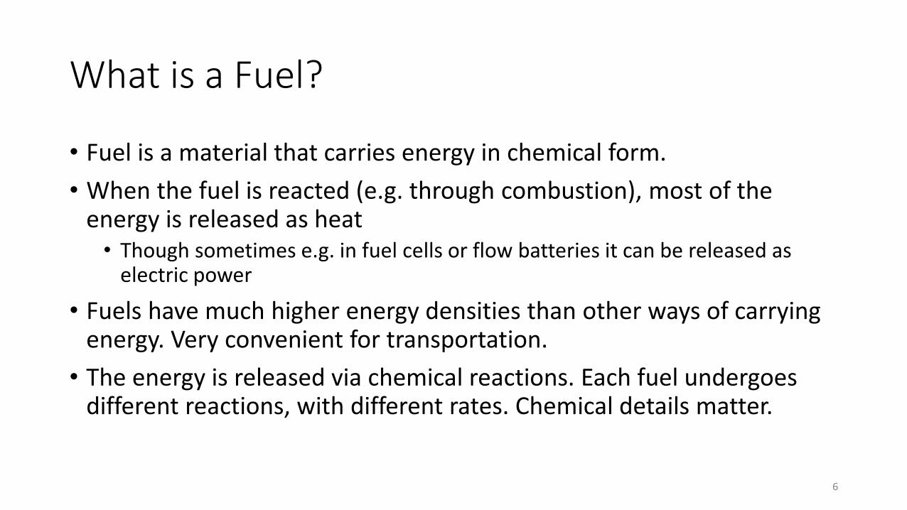
What is a Fuel?

• Fuel is a material that carries energy in chemical form. • When the fuel is reacted (e.g. through combustion), most of the

energy is released as heat • Though sometimes e.g. in fuel cells or flow batteries it can be released as

electric power

• Fuels have much higher energy densities than other ways of carrying energy. Very convenient for transportation.

• The energy is released via chemical reactions. Each fuel undergoes different reactions, with different rates. Chemical details matter.

6

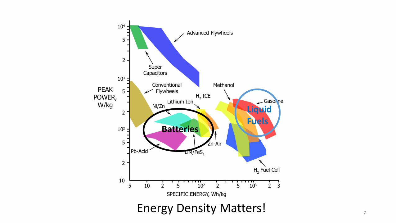
Energy Density Matters!

Batteries

Liquid Fuels

7

8 of 42

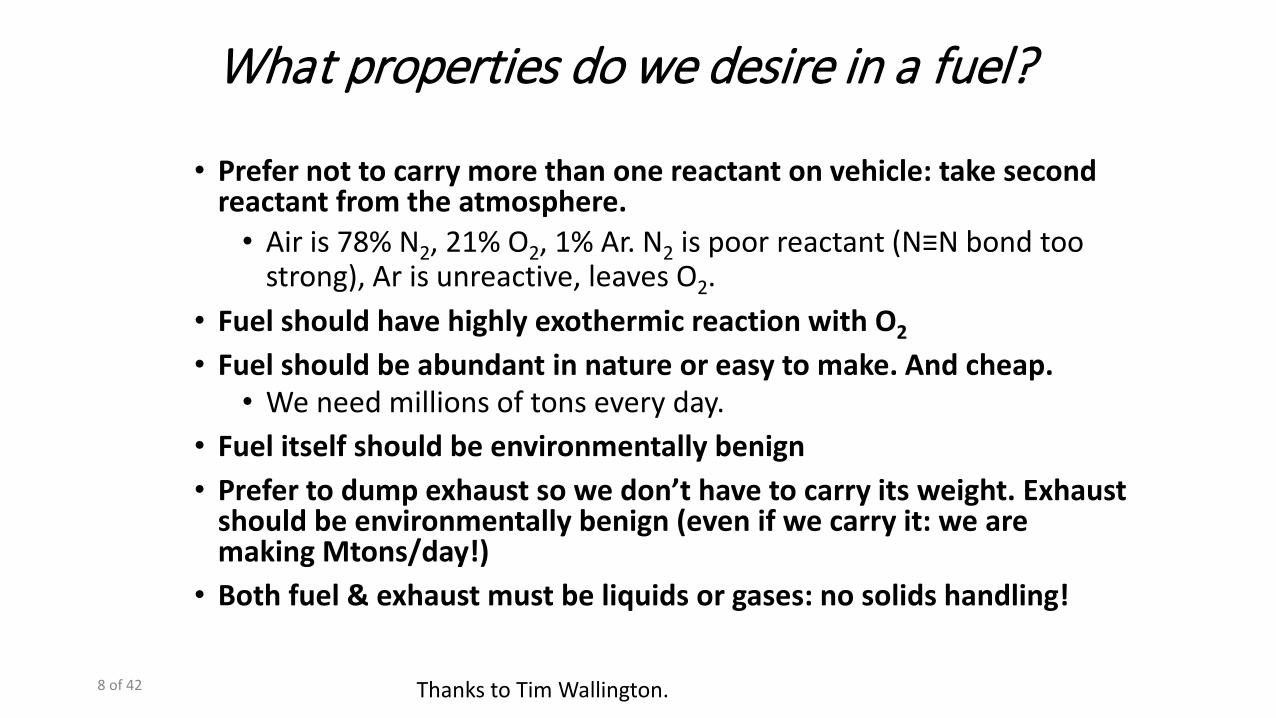
What properties do we desire in a fuel?

• Prefer not to carry more than one reactant on vehicle: take second reactant from the atmosphere. • Air is 78% N2, 21% O2, 1% Ar. N2 is poor reactant (N≡N bond too

strong), Ar is unreactive, leaves O2. • Fuel should have highly exothermic reaction with O2 • Fuel should be abundant in nature or easy to make. And cheap.

• We need millions of tons every day. • Fuel itself should be environmentally benign • Prefer to dump exhaust so we don’t have to carry its weight. Exhaust

should be environmentally benign (even if we carry it: we are making Mtons/day!)

• Both fuel & exhaust must be liquids or gases: no solids handling!

Thanks to Tim Wallington.

9 of 42

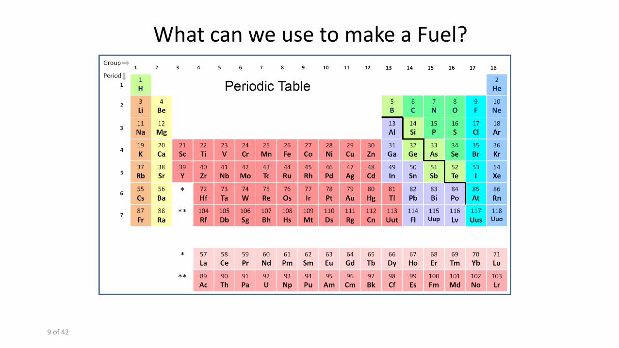
What can we use to make a Fuel?

10 of 42

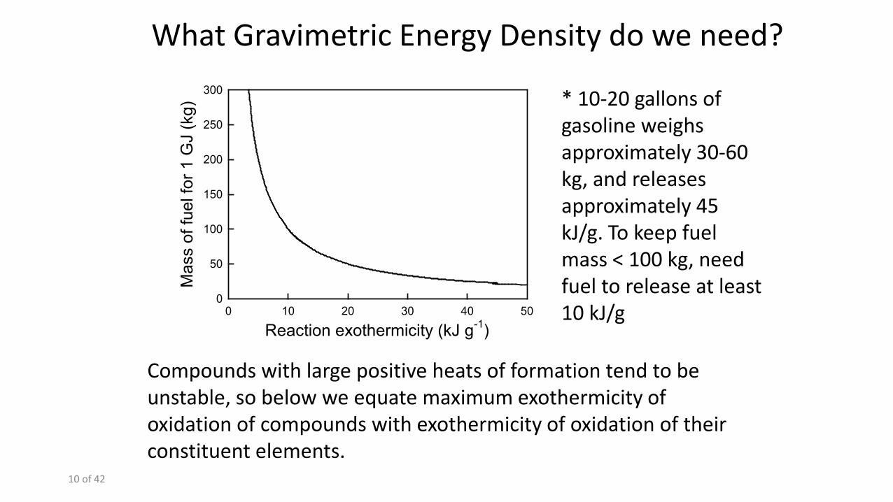
Compounds with large positive heats of formation tend to be unstable, so below we equate maximum exothermicity of oxidation of compounds with exothermicity of oxidation of their constituent elements.

* 10-20 gallons of gasoline weighs approximately 30-60 kg, and releases approximately 45 kJ/g. To keep fuel mass < 100 kg, need fuel to release at least 10 kJ/g

What Gravimetric Energy Density do we need?

Reaction exothermicity (kJ g-1)0 10 20 30 40 50

Mas

s of

fuel

for 1

GJ

(kg)

0

50

100

150

200

250

300

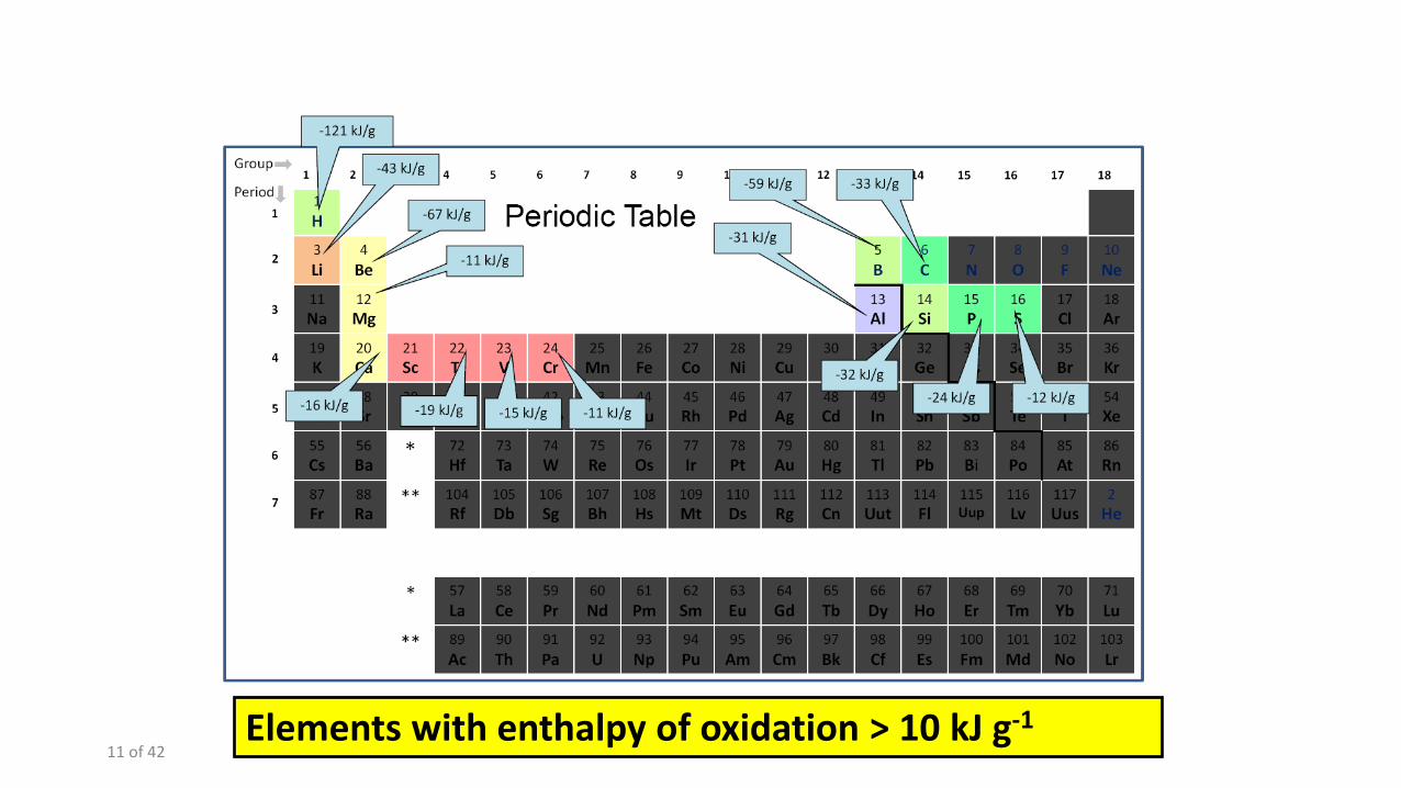
11 of 42 Elements with enthalpy of oxidation > 10 kJ g-1

12 of 42

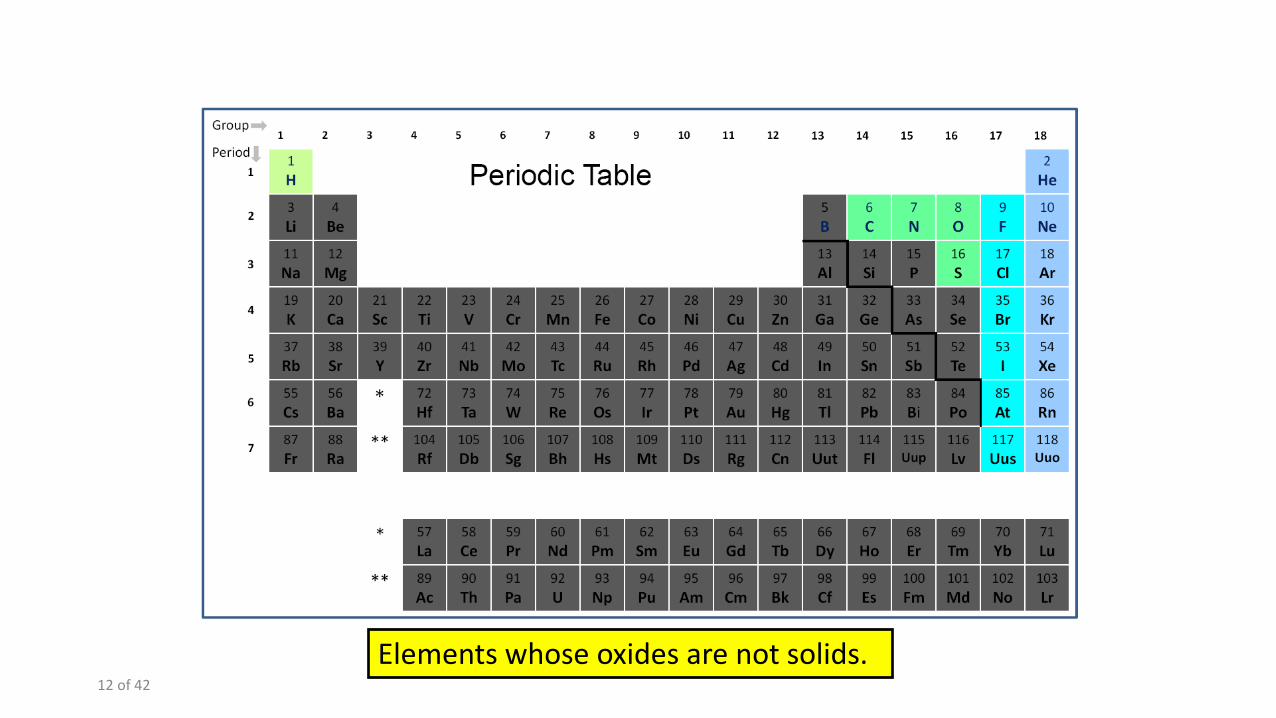
Elements whose oxides are not solids.

13 of 42

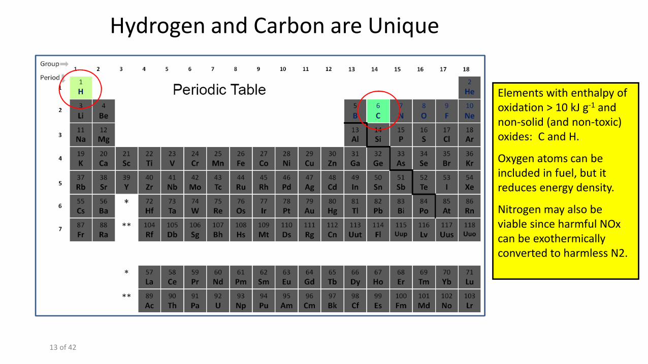
Elements with enthalpy of oxidation > 10 kJ g-1 and non-solid (and non-toxic) oxides: C and H.

Oxygen atoms can be included in fuel, but it reduces energy density.

Nitrogen may also be viable since harmful NOx can be exothermically converted to harmless N2.

Hydrogen and Carbon are Unique

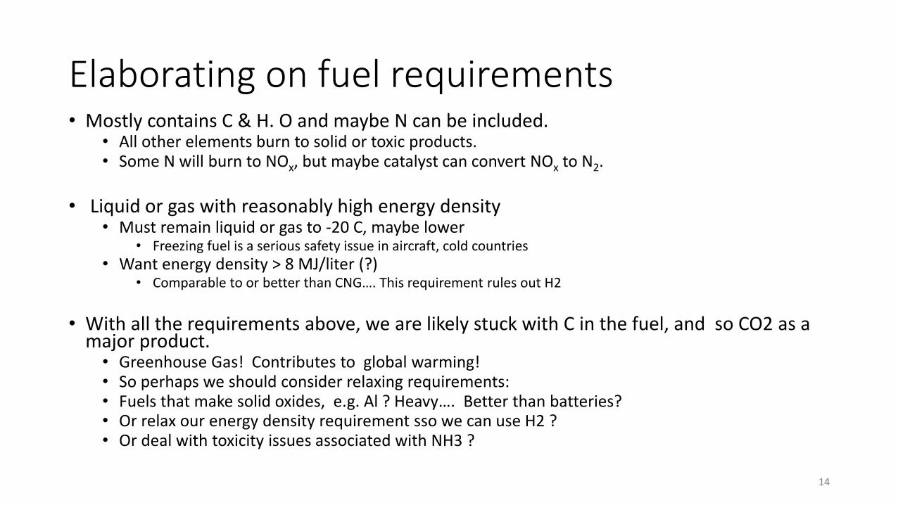
Elaborating on fuel requirements • Mostly contains C & H. O and maybe N can be included.

• All other elements burn to solid or toxic products. • Some N will burn to NOx, but maybe catalyst can convert NOx to N2.

• Liquid or gas with reasonably high energy density

• Must remain liquid or gas to -20 C, maybe lower • Freezing fuel is a serious safety issue in aircraft, cold countries

• Want energy density > 8 MJ/liter (?) • Comparable to or better than CNG…. This requirement rules out H2

• With all the requirements above, we are likely stuck with C in the fuel, and so CO2 as a major product. • Greenhouse Gas! Contributes to global warming! • So perhaps we should consider relaxing requirements: • Fuels that make solid oxides, e.g. Al ? Heavy…. Better than batteries? • Or relax our energy density requirement sso we can use H2 ? • Or deal with toxicity issues associated with NH3 ?

14

Quiz Question #1

We want a fuel that: 1) reacts with O2 2) major oxidation product is a non-toxic gas or liquid 3) have energy density at least 10 kJ/g and 8 MJ/liter 4) Fuel is liquid or gas for T > -20 C 5) Major oxidation product is not a greenhouse gas It appears no fuel meets all these requirements. Which of these requirements do you think we should relax? Why?

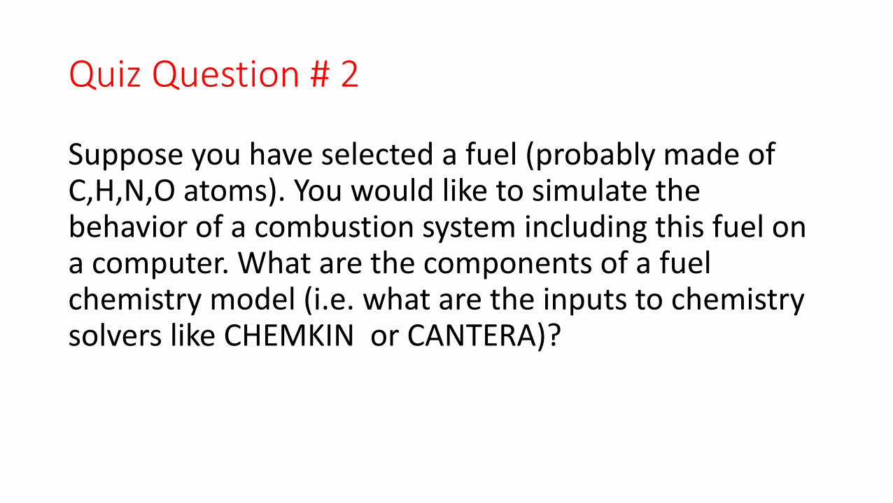
Quiz Question # 2

Suppose you have selected a fuel (probably made of C,H,N,O atoms). You would like to simulate the behavior of a combustion system including this fuel on a computer. What are the components of a fuel chemistry model (i.e. what are the inputs to chemistry solvers like CHEMKIN or CANTERA)?

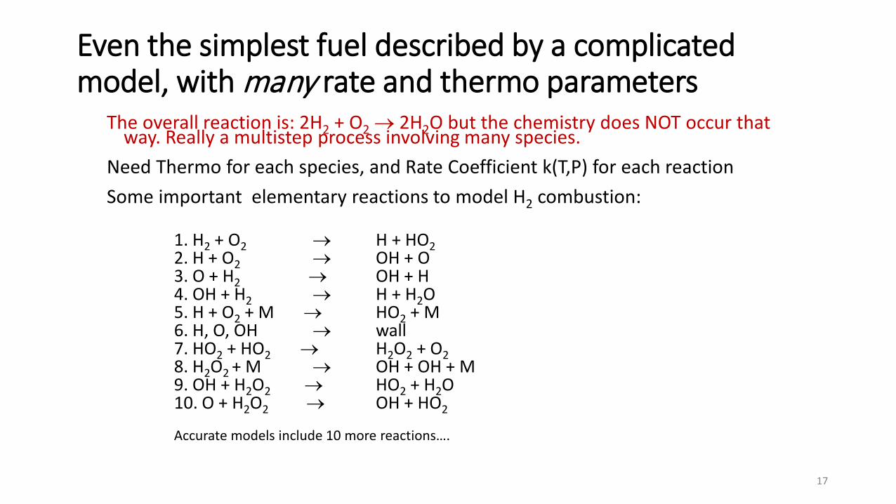
Even the simplest fuel described by a complicated model, with many rate and thermo parameters

The overall reaction is: 2H2 + O2 → 2H2O but the chemistry does NOT occur that way. Really a multistep process involving many species.

Need Thermo for each species, and Rate Coefficient k(T,P) for each reaction Some important elementary reactions to model H2 combustion:

1. H2 + O2 → H + HO2 2. H + O2 → OH + O 3. O + H2 → OH + H 4. OH + H2 → H + H2O 5. H + O2 + M → HO2 + M 6. H, O, OH → wall 7. HO2 + HO2 → H2O2 + O2 8. H2O2 + M → OH + OH + M 9. OH + H2O2 → HO2 + H2O 10. O + H2O2 → OH + HO2 Accurate models include 10 more reactions….

17

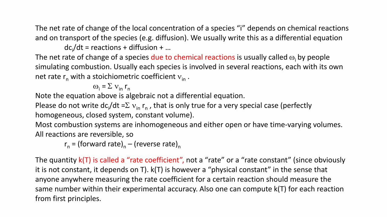
The net rate of change of the local concentration of a species “i” depends on chemical reactions and on transport of the species (e.g. diffusion). We usually write this as a differential equation dci/dt = reactions + diffusion + … The net rate of change of a species due to chemical reactions is usually called ωi by people simulating combustion. Usually each species is involved in several reactions, each with its own net rate rn with a stoichiometric coefficient νin . ωi = Σ νin rn Note the equation above is algebraic not a differential equation. Please do not write dci/dt =Σ νin rn , that is only true for a very special case (perfectly homogeneous, closed system, constant volume). Most combustion systems are inhomogeneous and either open or have time-varying volumes. All reactions are reversible, so rn = (forward rate)n – (reverse rate)n The quantity k(T) is called a “rate coefficient”, not a “rate” or a “rate constant” (since obviously it is not constant, it depends on T). k(T) is however a “physical constant” in the sense that anyone anywhere measuring the rate coefficient for a certain reaction should measure the same number within their experimental accuracy. Also one can compute k(T) for each reaction from first principles.

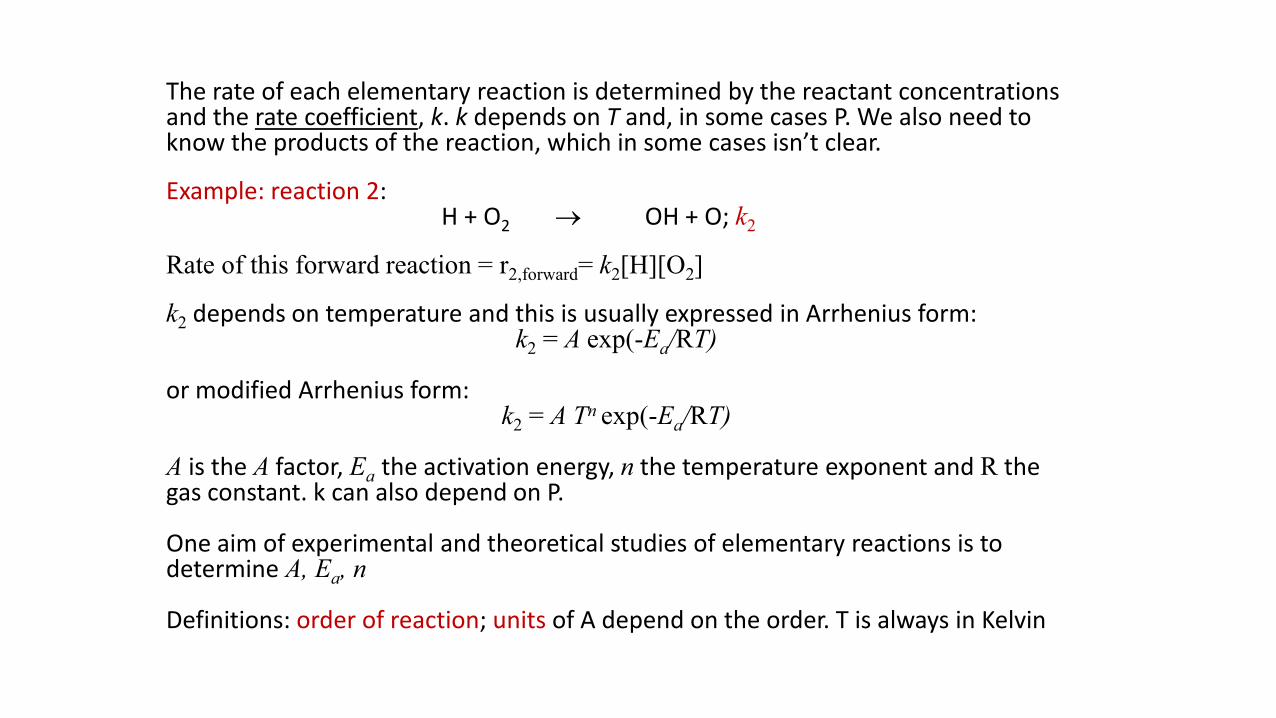
The rate of each elementary reaction is determined by the reactant concentrations and the rate coefficient, k. k depends on T and, in some cases P. We also need to know the products of the reaction, which in some cases isn’t clear. Example: reaction 2: H + O2 → OH + O; k2 Rate of this forward reaction = r2,forward= k2[H][O2] k2 depends on temperature and this is usually expressed in Arrhenius form:

k2 = A exp(-Ea/RT)

or modified Arrhenius form: k2 = A Tn exp(-Ea/RT)

A is the A factor, Ea the activation energy, n the temperature exponent and R the gas constant. k can also depend on P. One aim of experimental and theoretical studies of elementary reactions is to determine A, Ea, n Definitions: order of reaction; units of A depend on the order. T is always in Kelvin

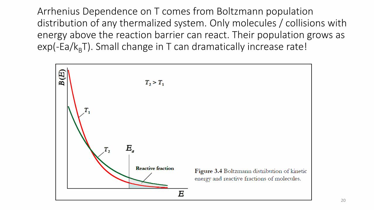
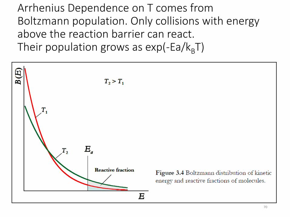
Arrhenius Dependence on T comes from Boltzmann population distribution of any thermalized system. Only molecules / collisions with energy above the reaction barrier can react. Their population grows as exp(-Ea/kBT). Small change in T can dramatically increase rate!

20

Quiz Question #3 All kinetic models are approximate: they neglect some minor species and minor reactions (perhaps because the author of the model is unaware of the minor species chemistry). Sometimes we do this on purpose, intentionally making the chemistry model smaller and so further from the truth. Why would someone do that?

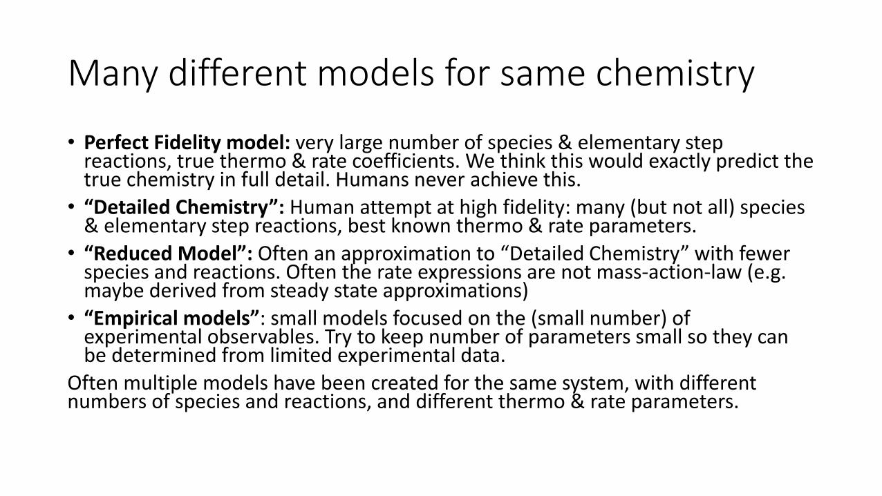
Many different models for same chemistry

• Perfect Fidelity model: very large number of species & elementary step reactions, true thermo & rate coefficients. We think this would exactly predict the true chemistry in full detail. Humans never achieve this.

• “Detailed Chemistry”: Human attempt at high fidelity: many (but not all) species & elementary step reactions, best known thermo & rate parameters.

• “Reduced Model”: Often an approximation to “Detailed Chemistry” with fewer species and reactions. Often the rate expressions are not mass-action-law (e.g. maybe derived from steady state approximations)

• “Empirical models”: small models focused on the (small number) of experimental observables. Try to keep number of parameters small so they can be determined from limited experimental data.

Often multiple models have been created for the same system, with different numbers of species and reactions, and different thermo & rate parameters.

Quiz Question #4

In all chemistry models, the main variables we are computing are concentrations or mass fractions of “chemical species”. What is a chemical species?

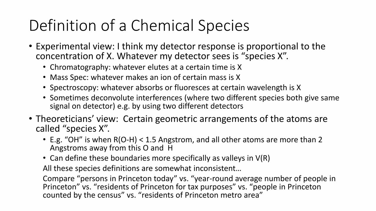
Definition of a Chemical Species • Experimental view: I think my detector response is proportional to the

concentration of X. Whatever my detector sees is “species X”. • Chromatography: whatever elutes at a certain time is X • Mass Spec: whatever makes an ion of certain mass is X • Spectroscopy: whatever absorbs or fluoresces at certain wavelength is X • Sometimes deconvolute interferences (where two different species both give same

signal on detector) e.g. by using two different detectors • Theoreticians’ view: Certain geometric arrangements of the atoms are

called “species X”. • E.g. “OH” is when R(O-H) < 1.5 Angstrom, and all other atoms are more than 2

Angstroms away from this O and H • Can define these boundaries more specifically as valleys in V(R) All these species definitions are somewhat inconsistent… Compare “persons in Princeton today” vs. “year-round average number of people in Princeton” vs. “residents of Princeton for tax purposes” vs. “people in Princeton counted by the census” vs. “residents of Princeton metro area”

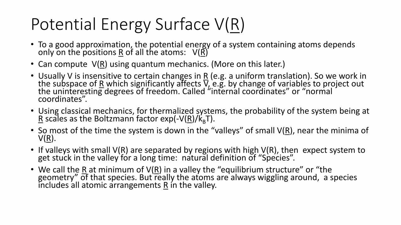
Potential Energy Surface V(R) • To a good approximation, the potential energy of a system containing atoms depends

only on the positions R of all the atoms: V(R) • Can compute V(R) using quantum mechanics. (More on this later.) • Usually V is insensitive to certain changes in R (e.g. a uniform translation). So we work in

the subspace of R which significantly affects V, e.g. by change of variables to project out the uninteresting degrees of freedom. Called “internal coordinates” or “normal coordinates”.

• Using classical mechanics, for thermalized systems, the probability of the system being at R scales as the Boltzmann factor exp(-V(R)/kBT).

• So most of the time the system is down in the “valleys” of small V(R), near the minima of V(R).

• If valleys with small V(R) are separated by regions with high V(R), then expect system to get stuck in the valley for a long time: natural definition of “Species”.

• We call the R at minimum of V(R) in a valley the “equilibrium structure” or “the geometry” of that species. But really the atoms are always wiggling around, a species includes all atomic arrangements R in the valley.

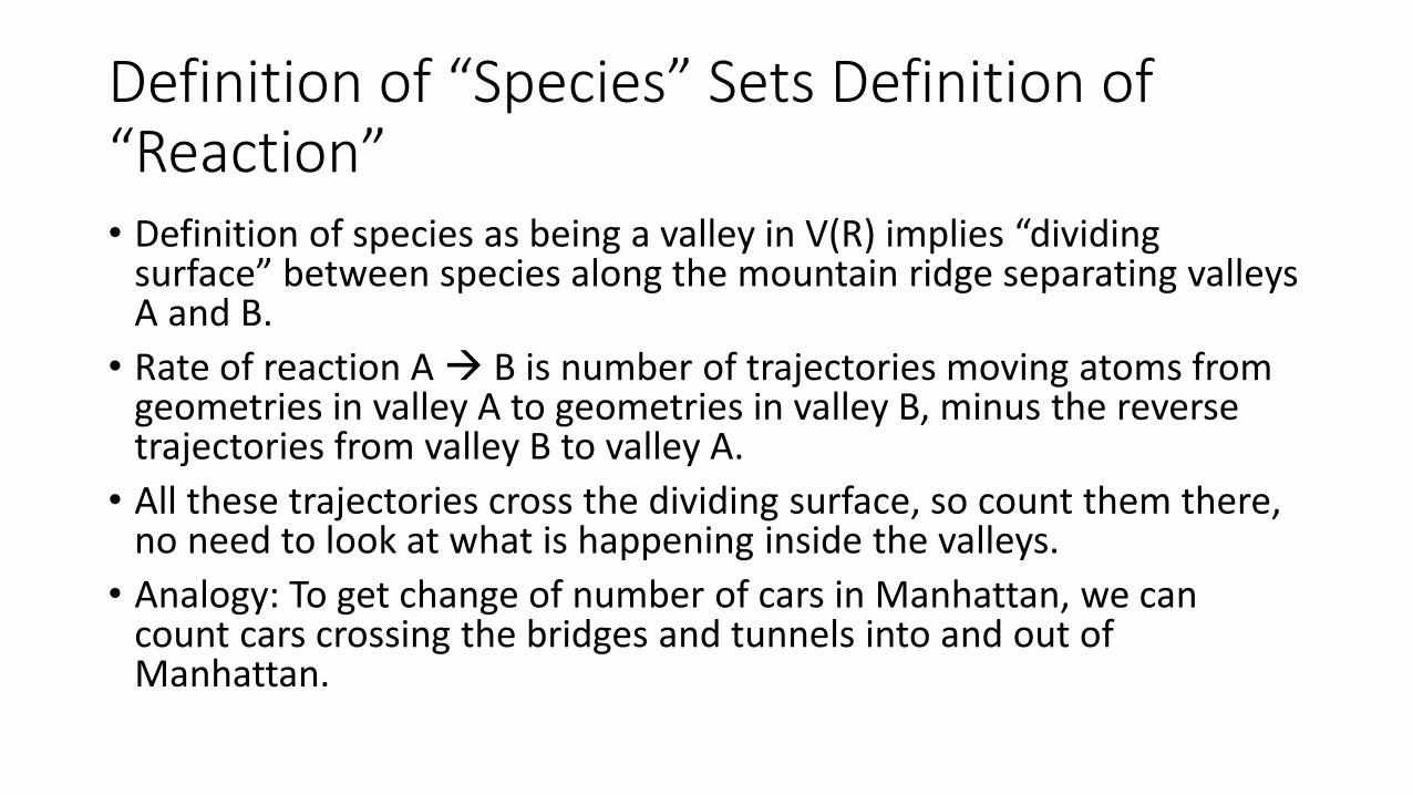
Definition of “Species” Sets Definition of “Reaction” • Definition of species as being a valley in V(R) implies “dividing

surface” between species along the mountain ridge separating valleys A and B.

• Rate of reaction A B is number of trajectories moving atoms from geometries in valley A to geometries in valley B, minus the reverse trajectories from valley B to valley A.

• All these trajectories cross the dividing surface, so count them there, no need to look at what is happening inside the valleys.

• Analogy: To get change of number of cars in Manhattan, we can count cars crossing the bridges and tunnels into and out of Manhattan.

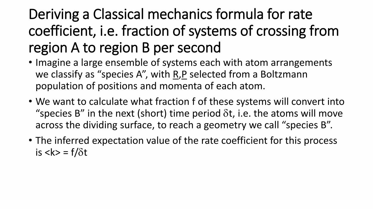
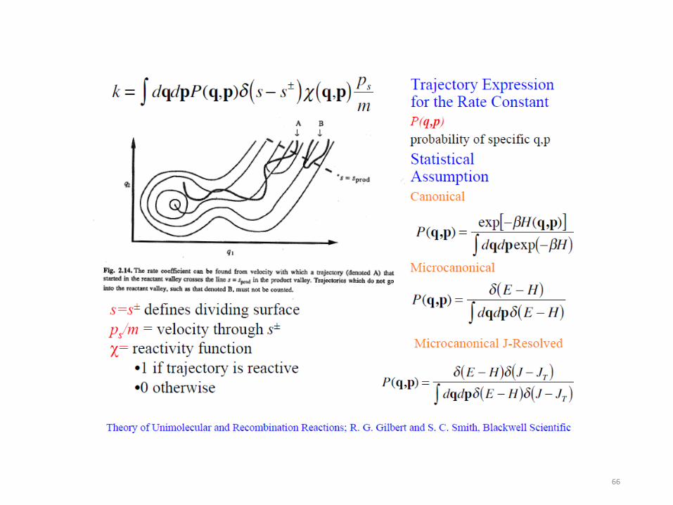
Deriving a Classical mechanics formula for rate coefficient, i.e. fraction of systems of crossing from region A to region B per second • Imagine a large ensemble of systems each with atom arrangements

we classify as “species A”, with R,P selected from a Boltzmann population of positions and momenta of each atom.

• We want to calculate what fraction f of these systems will convert into “species B” in the next (short) time period δt, i.e. the atoms will move across the dividing surface, to reach a geometry we call “species B”.

• The inferred expectation value of the rate coefficient for this process is <k> = f/δt

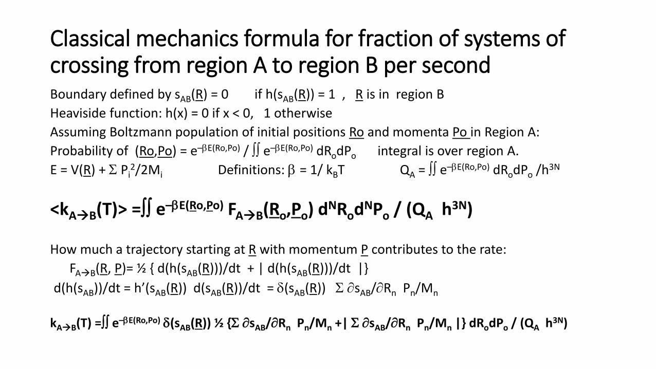
Classical mechanics formula for fraction of systems of crossing from region A to region B per second Boundary defined by sAB(R) = 0 if h(sAB(R)) = 1 , R is in region B Heaviside function: h(x) = 0 if x < 0, 1 otherwise Assuming Boltzmann population of initial positions Ro and momenta Po in Region A: Probability of (Ro,Po) = e–βE(Ro,Po) / ∫∫ e–βE(Ro,Po) dRodPo integral is over region A. E = V(R) + Σ Pi

2/2Mi Definitions: β = 1/ kBT QA = ∫∫ e–βE(Ro,Po) dRodPo /h3N <kAB(T)> =∫∫ e–βE(Ro,Po) FAB(Ro,Po) dNRodNPo / (QA h3N) How much a trajectory starting at R with momentum P contributes to the rate: FAB(R, P)= ½ { d(h(sAB(R)))/dt + | d(h(sAB(R)))/dt |} d(h(sAB))/dt = h’(sAB(R)) d(sAB(R))/dt = δ(sAB(R)) Σ ∂sAB/∂Rn Pn/Mn

kAB(T) =∫∫ e–βE(Ro,Po) δ(sAB(R)) ½ {Σ ∂sAB/∂Rn Pn/Mn +| Σ ∂sAB/∂Rn Pn/Mn |} dRodPo / (QA h3N)

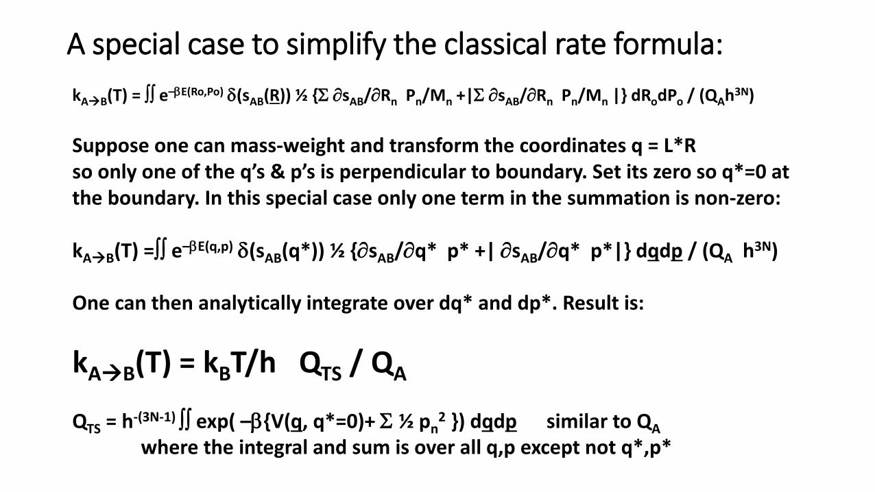
A special case to simplify the classical rate formula: kAB(T) = ∫∫ e–βE(Ro,Po) δ(sAB(R)) ½ {Σ ∂sAB/∂Rn Pn/Mn +|Σ ∂sAB/∂Rn Pn/Mn |} dRodPo / (QAh3N) Suppose one can mass-weight and transform the coordinates q = L*R so only one of the q’s & p’s is perpendicular to boundary. Set its zero so q*=0 at the boundary. In this special case only one term in the summation is non-zero: kAB(T) =∫∫ e–βE(q,p) δ(sAB(q*)) ½ {∂sAB/∂q* p* +| ∂sAB/∂q* p*|} dqdp / (QA h3N) One can then analytically integrate over dq* and dp*. Result is:

kAB(T) = kBT/h QTS / QA QTS = h-(3N-1) ∫∫ exp( –β{V(q, q*=0)+ Σ ½ pn

2 }) dqdp similar to QA where the integral and sum is over all q,p except not q*,p*

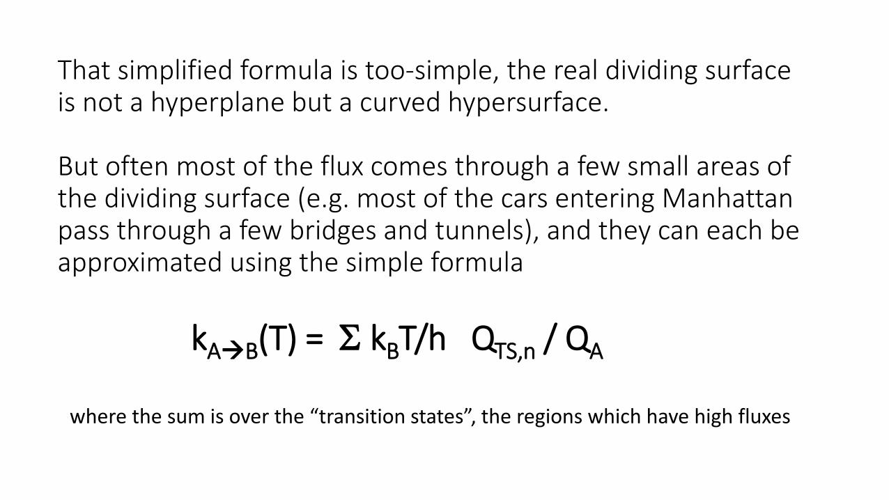
That simplified formula is too-simple, the real dividing surface is not a hyperplane but a curved hypersurface. But often most of the flux comes through a few small areas of the dividing surface (e.g. most of the cars entering Manhattan pass through a few bridges and tunnels), and they can each be approximated using the simple formula kAB(T) = Σ kBT/h QTS,n / QA

where the sum is over the “transition states”, the regions which have high fluxes

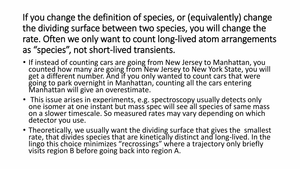
If you change the definition of species, or (equivalently) change the dividing surface between two species, you will change the rate. Often we only want to count long-lived atom arrangements as “species”, not short-lived transients. • If instead of counting cars are going from New Jersey to Manhattan, you

counted how many are going from New Jersey to New York State, you will get a different number. And if you only wanted to count cars that were going to park overnight in Manhattan, counting all the cars entering Manhattan will give an overestimate.

• This issue arises in experiments, e.g. spectroscopy usually detects only one isomer at one instant but mass spec will see all species of same mass on a slower timescale. So measured rates may vary depending on which detector you use.

• Theoretically, we usually want the dividing surface that gives the smallest rate, that divides species that are kinetically distinct and long-lived. In the lingo this choice minimizes “recrossings” where a trajectory only briefly visits region B before going back into region A.

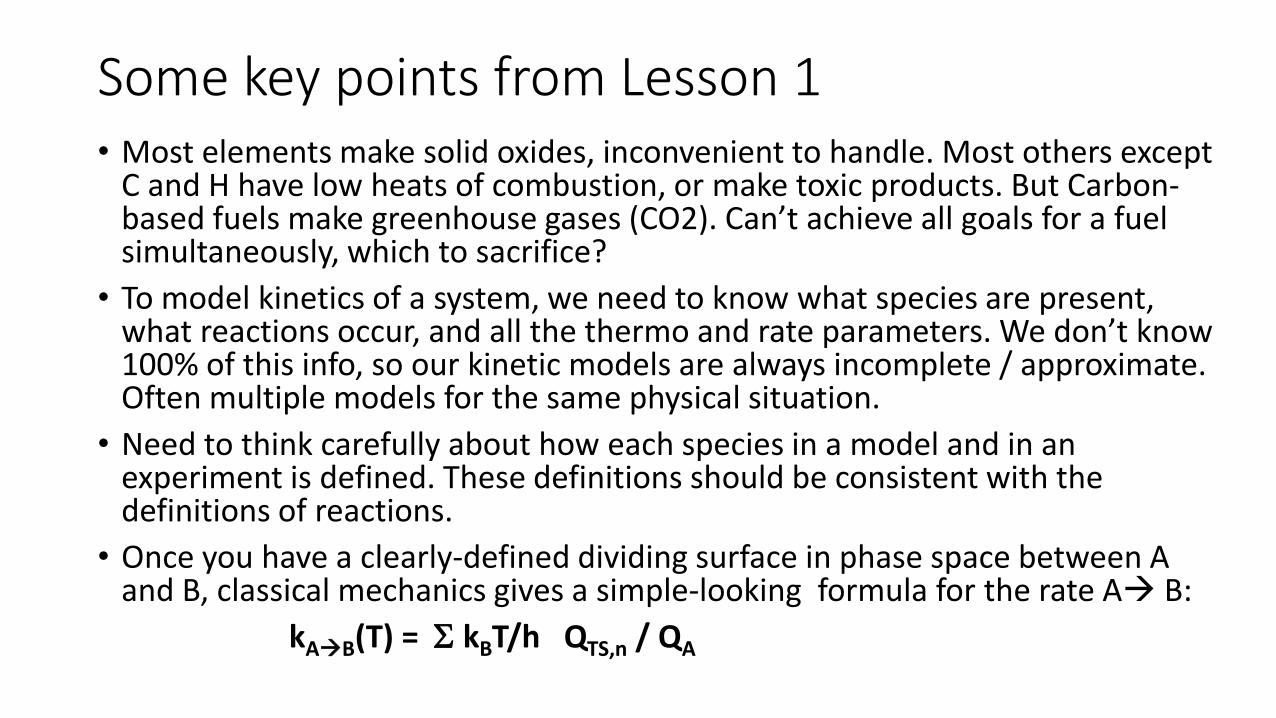
Some key points from Lesson 1 • Most elements make solid oxides, inconvenient to handle. Most others except

C and H have low heats of combustion, or make toxic products. But Carbon-based fuels make greenhouse gases (CO2). Can’t achieve all goals for a fuel simultaneously, which to sacrifice?

• To model kinetics of a system, we need to know what species are present, what reactions occur, and all the thermo and rate parameters. We don’t know 100% of this info, so our kinetic models are always incomplete / approximate. Often multiple models for the same physical situation.

• Need to think carefully about how each species in a model and in an experiment is defined. These definitions should be consistent with the definitions of reactions.

• Once you have a clearly-defined dividing surface in phase space between A and B, classical mechanics gives a simple-looking formula for the rate A B:

kAB(T) = Σ kBT/h QTS,n / QA

End of Lesson 1

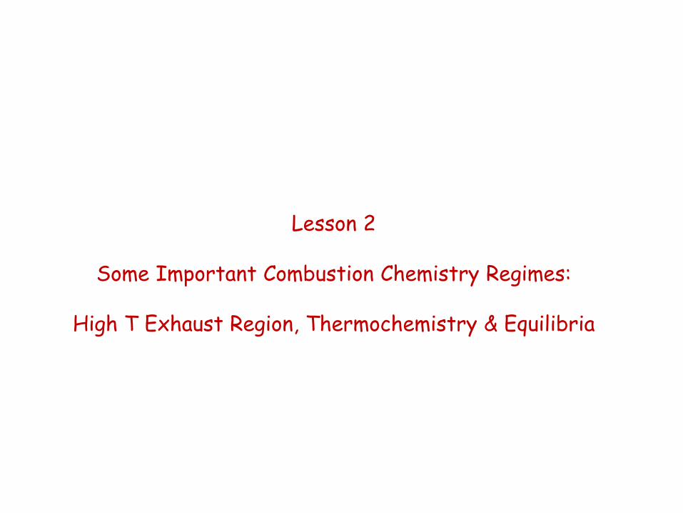
Lesson 2

Some Important Combustion Chemistry Regimes:

High T Exhaust Region, Thermochemistry & Equilibria

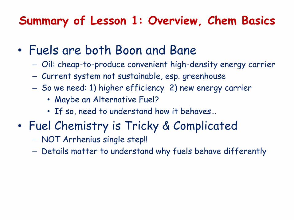
Summary of Lesson 1: Overview, Chem Basics

• Fuels are both Boon and Bane – Oil: cheap-to-produce convenient high-density energy carrier – Current system not sustainable, esp. greenhouse – So we need: 1) higher efficiency 2) new energy carrier

• Maybe an Alternative Fuel? • If so, need to understand how it behaves…

• Fuel Chemistry is Tricky & Complicated – NOT Arrhenius single step!! – Details matter to understand why fuels behave differently

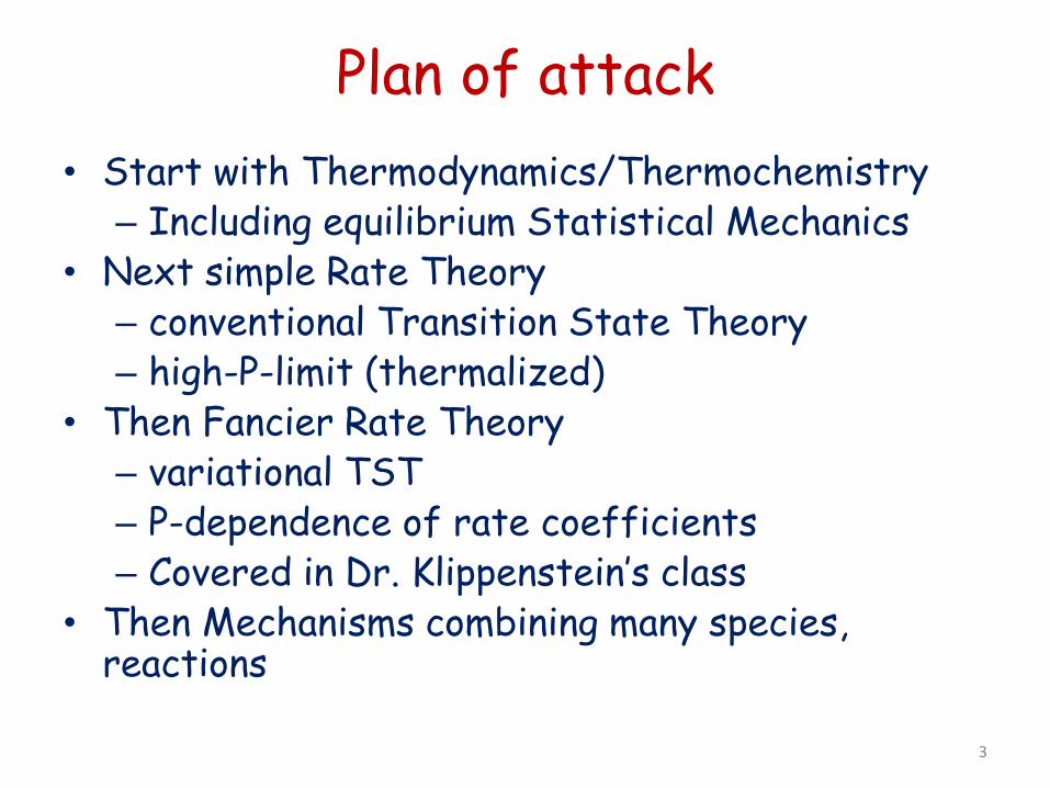
Plan of attack • Start with Thermodynamics/Thermochemistry

– Including equilibrium Statistical Mechanics • Next simple Rate Theory

– conventional Transition State Theory – high-P-limit (thermalized)

• Then Fancier Rate Theory – variational TST – P-dependence of rate coefficients – Covered in Dr. Klippenstein’s class

• Then Mechanisms combining many species, reactions

3

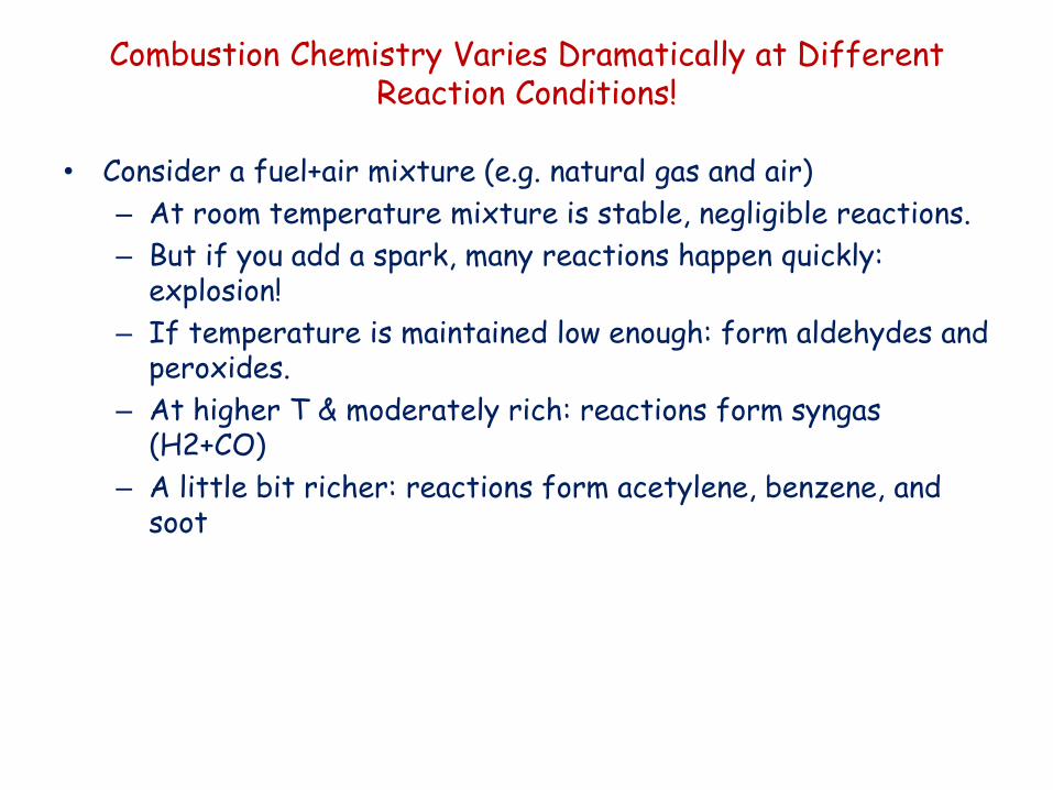
Combustion Chemistry Varies Dramatically at Different Reaction Conditions!

• Consider a fuel+air mixture (e.g. natural gas and air) – At room temperature mixture is stable, negligible reactions. – But if you add a spark, many reactions happen quickly:

explosion! – If temperature is maintained low enough: form aldehydes and

peroxides. – At higher T & moderately rich: reactions form syngas

(H2+CO) – A little bit richer: reactions form acetylene, benzene, and

soot

Most combustion systems are extremely inhomogeneous. Chemistry and transport/mixing both important.

5

Structure of a Premixed laminar methane/air flame. In less than one millimeter variation of 1500 K, and more than 2 order of magnitude changes in most species concentrations

Because of the inhomogeneity, the rates of reactions vary by many orders of magnitude . So we will consider what is going in different regions separately.

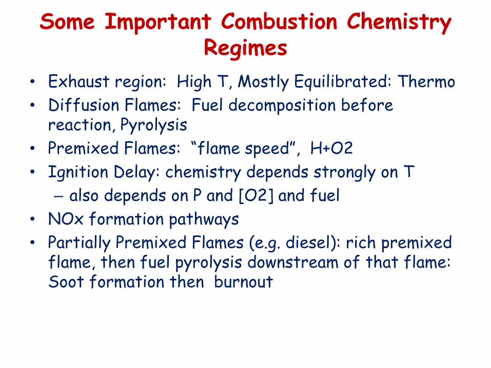
Some Important Combustion Chemistry Regimes

• Exhaust region: High T, Mostly Equilibrated: Thermo • Diffusion Flames: Fuel decomposition before

reaction, Pyrolysis • Premixed Flames: “flame speed”, H+O2 • Ignition Delay: chemistry depends strongly on T

– also depends on P and [O2] and fuel • NOx formation pathways • Partially Premixed Flames (e.g. diesel): rich premixed

flame, then fuel pyrolysis downstream of that flame: Soot formation then burnout

EXHAUST REGION: HIGH T, MOSTLY EQUILIBRATED, THERMO IS KEY

7

Thermodynamics/Thermochemistry

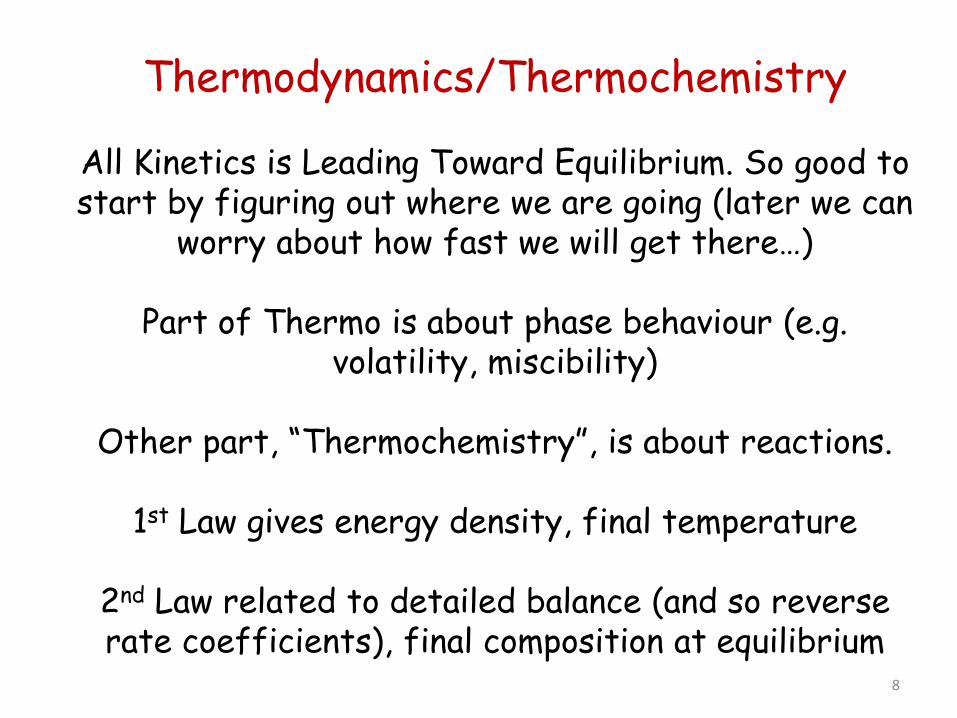
All Kinetics is Leading Toward Equilibrium. So good to start by figuring out where we are going (later we can

worry about how fast we will get there…)

Part of Thermo is about phase behaviour (e.g. volatility, miscibility)

Other part, “Thermochemistry”, is about reactions.

1st Law gives energy density, final temperature

2nd Law related to detailed balance (and so reverse rate coefficients), final composition at equilibrium

8

LHV is computed easily from enthalpies

9

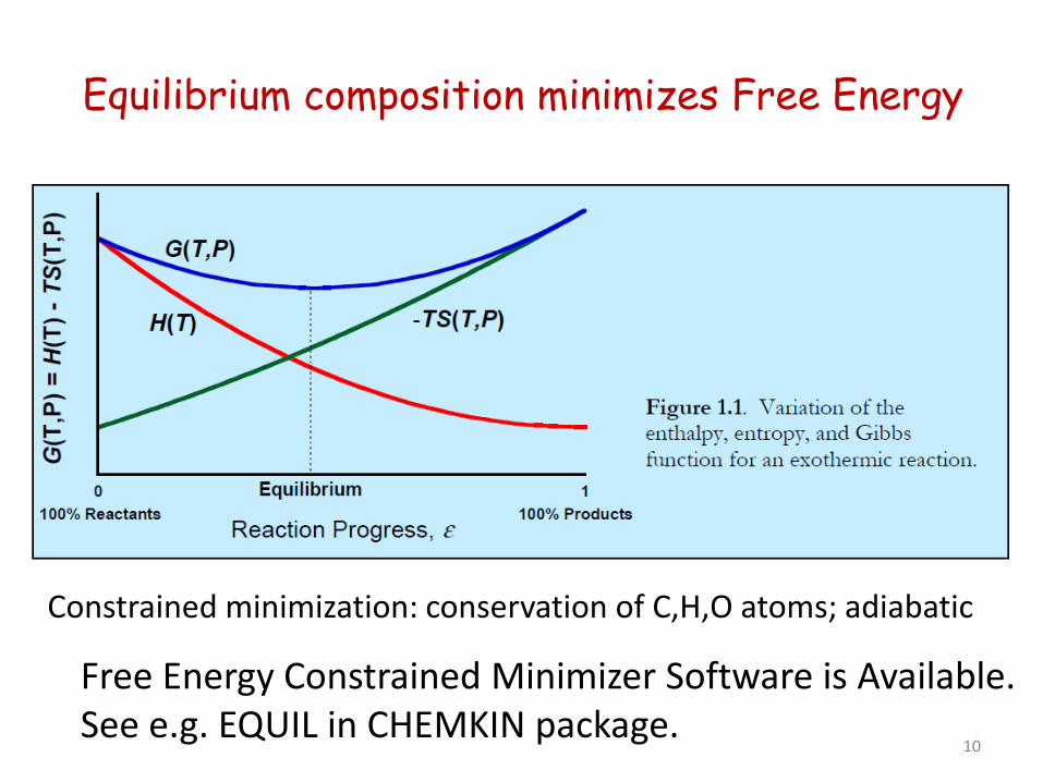
Equilibrium composition minimizes Free Energy

Free Energy Constrained Minimizer Software is Available. See e.g. EQUIL in CHEMKIN package.

10

Constrained minimization: conservation of C,H,O atoms; adiabatic

How do programs like EQUIL work to compute equilibrium concentrations?

• Take as input the initial composition and Temperature • Take as input a database of molecules with thermochemical data

(usually in form of NASA polynomials). • Assume ideal gas, ideal mixture, adiabatic so Gtotal = Σ ni Gi(T) Htotal = Σ ni Hi(T) = constant (adiabatic) the conservation of atom equations look like this for each element: S ni Ci = constant where Ci is the number of carbon atoms in species “i”. • Program finds the vector (n,T) that minimizes Gtotal(n,T) subject

to the constraint equations. • Note that the program only knows about the existence of the

molecules in the database. If benzene is not listed in the database, the program will not predict formation of benzene.

11

Thermochemistry

• We need thermodynamic data to: – Compute equilibrium compositions – Determine the heat release in a combustion process – Calculate the equilibrium constant for a reaction – this allows

us to relate the rate coefficients for forward and reverse reactions

• This lecture considers: – Classical thermodynamics and statistical mechanics –

relationships for thermodynamic quantities – Sources of thermodynamic data – Measurement of enthalpies of formation for radicals – Active Thermochemical Tables – Representation of thermodynamic data for combustion

models 14

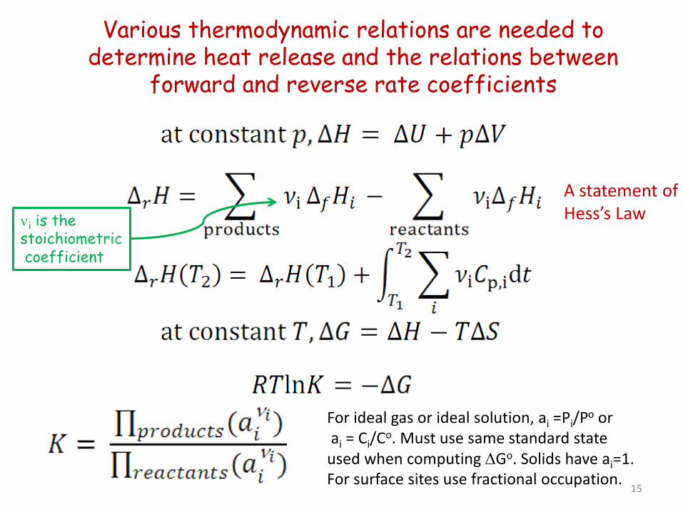
Various thermodynamic relations are needed to determine heat release and the relations between

forward and reverse rate coefficients

A statement of Hess’s Law νi is the

stoichiometric coefficient

For ideal gas or ideal solution, ai =Pi/Po or ai = Ci/Co. Must use same standard state used when computing ∆Go. Solids have ai=1. For surface sites use fractional occupation.

15

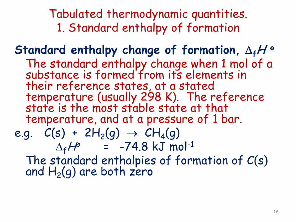
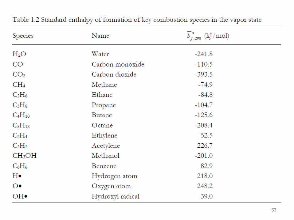
Tabulated thermodynamic quantities. 1. Standard enthalpy of formation

Standard enthalpy change of formation, ∆fH o The standard enthalpy change when 1 mol of a

substance is formed from its elements in their reference states, at a stated temperature (usually 298 K). The reference state is the most stable state at that temperature, and at a pressure of 1 bar.

e.g. C(s) + 2H2(g) → CH4(g) ∆fHo = -74.8 kJ mol-1 The standard enthalpies of formation of C(s)

and H2(g) are both zero

16

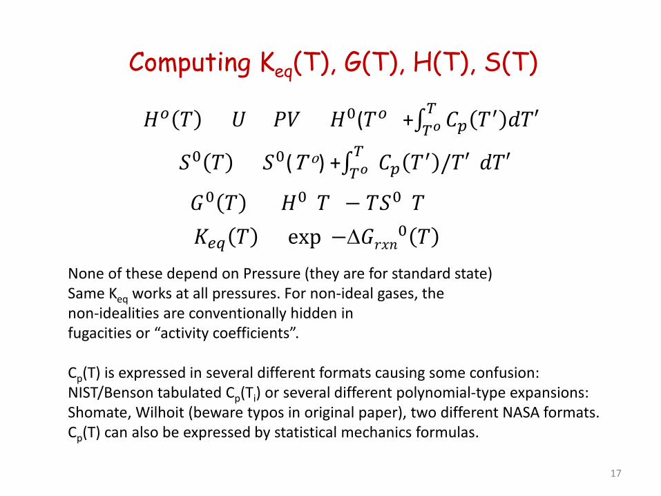
Computing Keq(T), G(T), H(T), S(T)

𝐻𝐻𝑜𝑜 𝑇𝑇 = 𝑈𝑈 + 𝑃𝑃𝑃𝑃 = 𝐻𝐻0(𝑇𝑇𝑜𝑜) +∫ 𝐶𝐶𝑝𝑝 𝑇𝑇′ 𝑑𝑑𝑇𝑇𝑑𝑇𝑇𝑇𝑇𝑜𝑜

𝑆𝑆0 𝑇𝑇 = 𝑆𝑆0(T o) +∫ (𝐶𝐶𝑝𝑝 𝑇𝑇′ /𝑇𝑇𝑑)𝑑𝑑𝑇𝑇𝑑𝑇𝑇𝑇𝑇𝑜𝑜

𝐺𝐺0 𝑇𝑇 = 𝐻𝐻0(𝑇𝑇) − 𝑇𝑇𝑆𝑆0(𝑇𝑇) 𝐾𝐾𝑒𝑒𝑒𝑒 𝑇𝑇 = exp (−∆𝐺𝐺𝑟𝑟𝑟𝑟𝑟𝑟0 𝑇𝑇 )

None of these depend on Pressure (they are for standard state) Same Keq works at all pressures. For non-ideal gases, the non-idealities are conventionally hidden in fugacities or “activity coefficients”. Cp(T) is expressed in several different formats causing some confusion: NIST/Benson tabulated Cp(Ti) or several different polynomial-type expansions: Shomate, Wilhoit (beware typos in original paper), two different NASA formats. Cp(T) can also be expressed by statistical mechanics formulas.

17

18

Now maintained by Elke Goos.

19

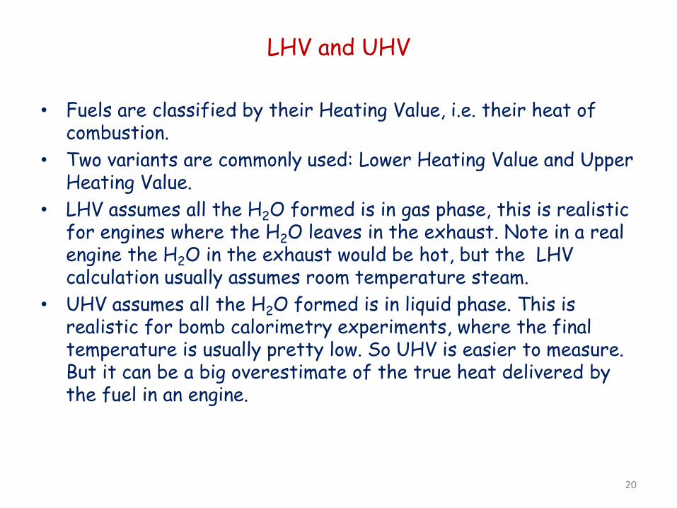
LHV and UHV

• Fuels are classified by their Heating Value, i.e. their heat of combustion.

• Two variants are commonly used: Lower Heating Value and Upper Heating Value.

• LHV assumes all the H2O formed is in gas phase, this is realistic for engines where the H2O leaves in the exhaust. Note in a real engine the H2O in the exhaust would be hot, but the LHV calculation usually assumes room temperature steam.

• UHV assumes all the H2O formed is in liquid phase. This is realistic for bomb calorimetry experiments, where the final temperature is usually pretty low. So UHV is easier to measure. But it can be a big overestimate of the true heat delivered by the fuel in an engine.

20

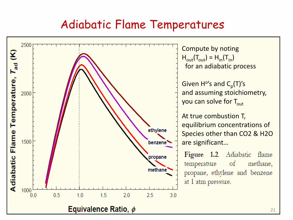
Adiabatic Flame Temperatures

Compute by noting Hout(Tout) = Hin(Tin) for an adiabatic process Given Ho’s and Cp(T)’s and assuming stoichiometry, you can solve for Tout At true combustion T, equilibrium concentrations of Species other than CO2 & H2O are significant…

21

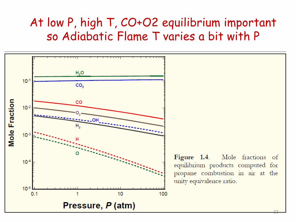
At low P, high T, CO+O2 equilibrium important so Adiabatic Flame T varies a bit with P

22

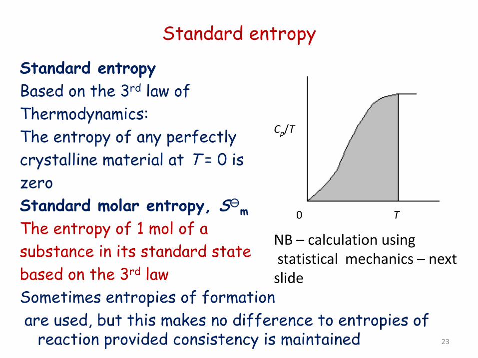
Standard entropy

Standard entropy Based on the 3rd law of Thermodynamics: The entropy of any perfectly crystalline material at T = 0 is zero Standard molar entropy, Sm The entropy of 1 mol of a substance in its standard state based on the 3rd law Sometimes entropies of formation are used, but this makes no difference to entropies of

reaction provided consistency is maintained

Cp/T

0 T

NB – calculation using statistical mechanics – next slide

23

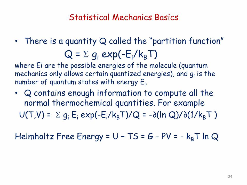
Statistical Mechanics Basics

• There is a quantity Q called the “partition function” Q = Σ gi exp(-Ei/kBT) where Ei are the possible energies of the molecule (quantum mechanics only allows certain quantized energies), and gi is the number of quantum states with energy Ei. • Q contains enough information to compute all the

normal thermochemical quantities. For example U(T,V) = Σ gi Ei exp(-Ei/kBT)/Q = -∂(ln Q)/∂(1/kBT ) Helmholtz Free Energy = U – TS = G - PV = - kBT ln Q

24

HOW DO WE COMPUTE THE ALLOWED ENERGIES {Ei} FOR A MOLECULE?

25

First we need V(R) for our molecule

• Not practical to directly measure V(R), we need to compute it. • The forces between the atoms are electrostatic, but the

electrons are so light that quantum mechanics effects dominate, so we need to solve the Schroedinger equation. This is an eigenvalue equation; the lowest eigenvalue is the value of V(R).

• Unfortunately,the Schroedinger equation is a pde in 3Nelectrons dimensions, with tricky physicality constraints called the Pauli conditions: too hard to solve exactly.

• So we solve it approximately by expanding the solution wavefunction in a finite basis set, and making many other approximations. This is the field of “quantum chemistry”.

• The quantum chemists have developed efficient software for some of these approximate ways of computing V(R). Some of the famous commercial software packages are GAUSSIAN and MOLPRO.

26

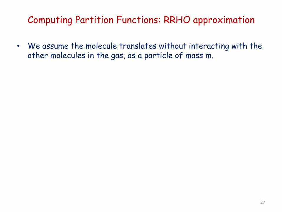
Computing Partition Functions: RRHO approximation

• We assume the molecule translates without interacting with the other molecules in the gas, as a particle of mass m.

27

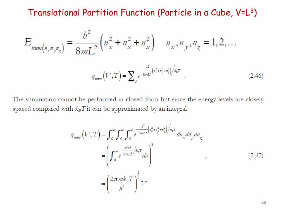
Translational Partition Function (Particle in a Cube, V=L3)

28

Computing Partition Functions: RRHO approximation

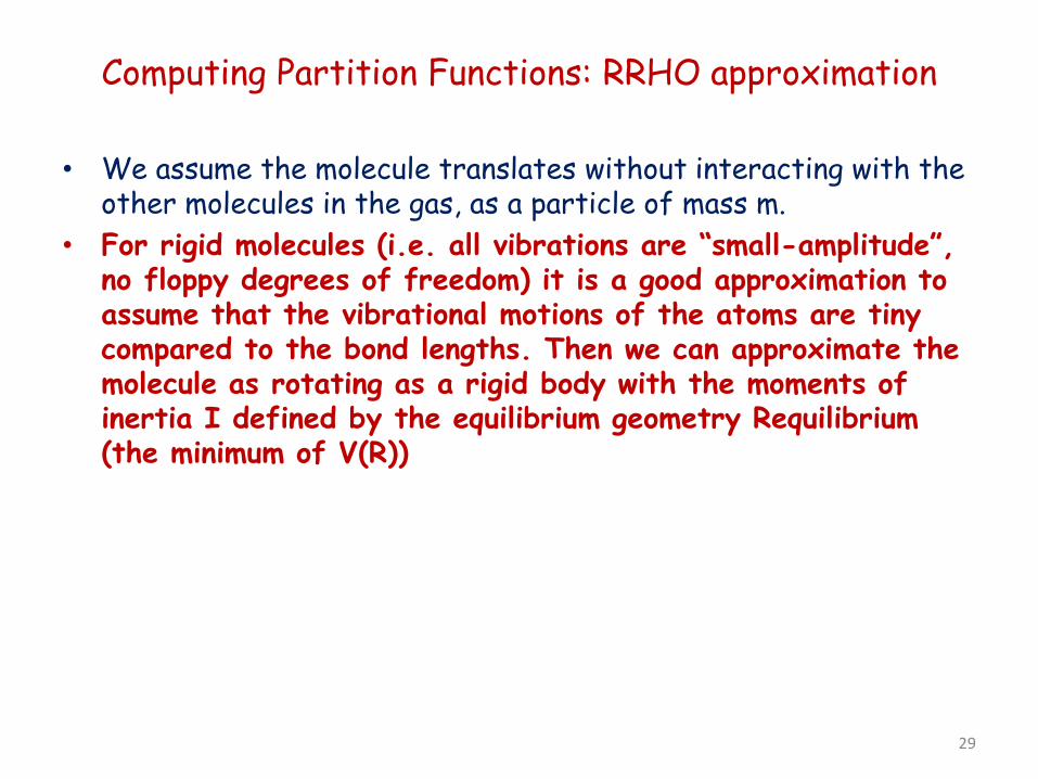
• We assume the molecule translates without interacting with the other molecules in the gas, as a particle of mass m.

• For rigid molecules (i.e. all vibrations are “small-amplitude”, no floppy degrees of freedom) it is a good approximation to assume that the vibrational motions of the atoms are tiny compared to the bond lengths. Then we can approximate the molecule as rotating as a rigid body with the moments of inertia I defined by the equilibrium geometry Requilibrium (the minimum of V(R))

29

Rotational Partition Functions

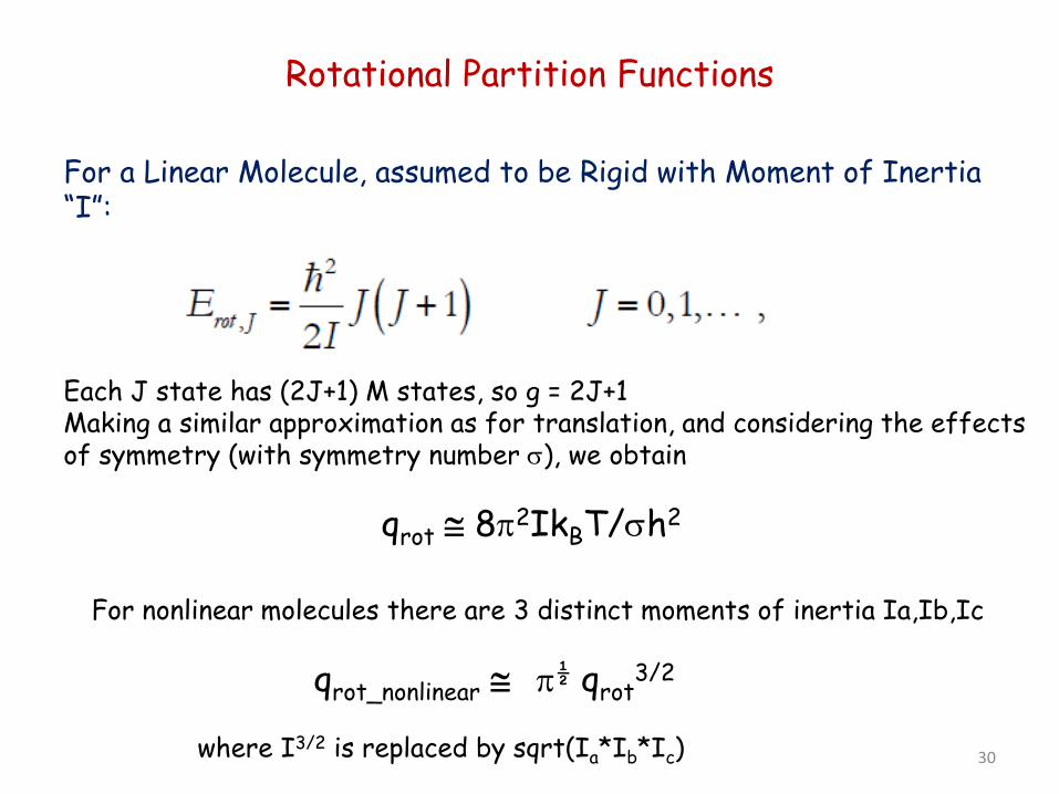
For a Linear Molecule, assumed to be Rigid with Moment of Inertia “I”:

Each J state has (2J+1) M states, so g = 2J+1 Making a similar approximation as for translation, and considering the effects of symmetry (with symmetry number σ), we obtain qrot ≅ 8π2IkBT/σh2

For nonlinear molecules there are 3 distinct moments of inertia Ia,Ib,Ic qrot_nonlinear ≅ π½ qrot

3/2

where I3/2 is replaced by sqrt(Ia*Ib*Ic) 30

Computing Partition Functions: RRHO approximation

• We assume the molecule translates without interacting with the other molecules in the gas, as a particle of mass m.

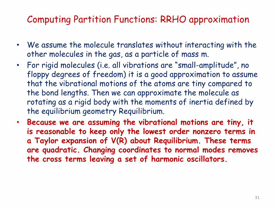
• For rigid molecules (i.e. all vibrations are “small-amplitude”, no floppy degrees of freedom) it is a good approximation to assume that the vibrational motions of the atoms are tiny compared to the bond lengths. Then we can approximate the molecule as rotating as a rigid body with the moments of inertia defined by the equilibrium geometry Requilibrium.

• Because we are assuming the vibrational motions are tiny, it is reasonable to keep only the lowest order nonzero terms in a Taylor expansion of V(R) about Requilibrium. These terms are quadratic. Changing coordinates to normal modes removes the cross terms leaving a set of harmonic oscillators.

31

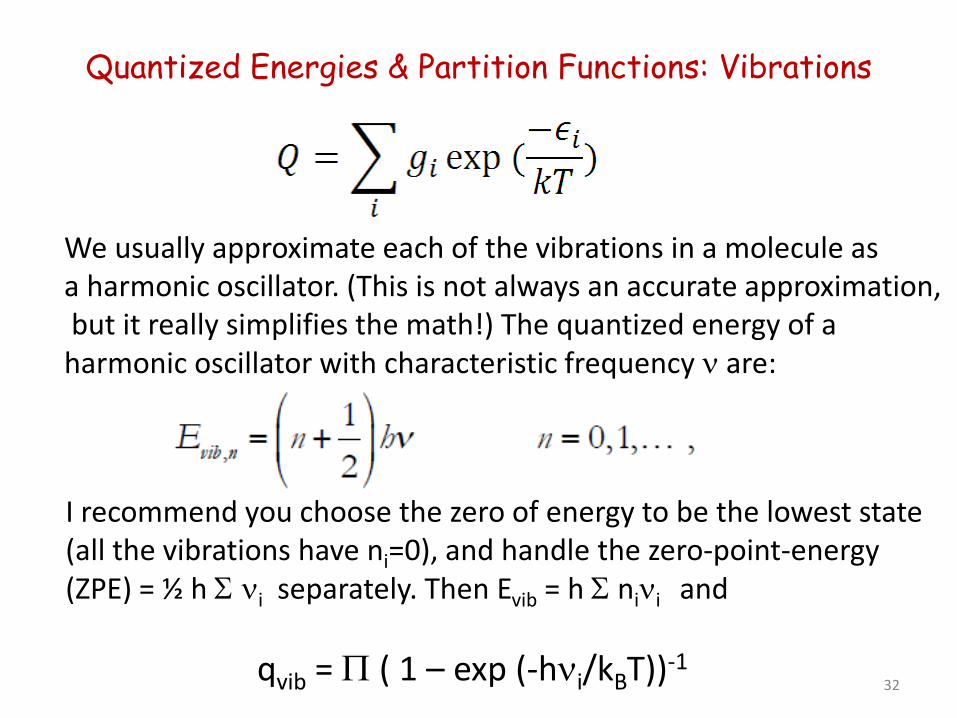
Quantized Energies & Partition Functions: Vibrations

We usually approximate each of the vibrations in a molecule as a harmonic oscillator. (This is not always an accurate approximation, but it really simplifies the math!) The quantized energy of a harmonic oscillator with characteristic frequency ν are:

I recommend you choose the zero of energy to be the lowest state (all the vibrations have ni=0), and handle the zero-point-energy (ZPE) = ½ h Σ νi separately. Then Evib = h Σ niνi and qvib = Π ( 1 – exp (-hνi/kBT))-1

32

Where do we get the vibrational frequencies {νi}?

• For some small molecules: experiment (from IR spectroscopy) • More commonly, only a few or zero of the vibrational

frequencies have been measured. Need to calculate: – Functional groups have some characteristic frequencies, but

not all frequencies can be predicted. – For stable closed-shell organic molecules, there are pretty

good force fields which can be used. – For small molecules, you can use high-level quantum

chemistry, e.g. CCSD. Very accurate & very CPU-intensive… – Most common approach in combustion chemistry is to do a

DFT calculation, e.g. B3LYP or M06-2X. Quantum chemistry programs are set up to do this calculation automatically for you, and DFT is not CPU-intensive.

33

Density Functional Theory (DFT)

• Schroedinger gave equation for E[Ψ], we vary Ψ to try to minimize E. Ψ is a function of 3*Nelectrons variables (the positions of all the electrons). So for benzene, we have to find the best possible function of 126 variables: difficult!

• Hohenberg & Kohn proved that E[ρ] existed, where ρ(x,y,z) is the electron density. Just an existence proof, E[ρ] is unknown.

• Kohn & Sham showed a good way to proceed, based on varying orbitals ψ(x,y,z), one for each electron. ρ = Σ |ψn(x,y,z)|2

• Easier to expand functions of 3 variables in a basis set. Much easier than handling a function of 126 variables all coupled!

• In the 1980’s the first accurate approximate functionals E[ρ], actually E[{ψ}], were discovered. Since then many more. Names like “B3LYP”, “PBE” and “M06-2X”. Give convenient & fairly accurate way to compute E=V(R) for not much CPU time.

34

DFT for geometry (Requilibrium)

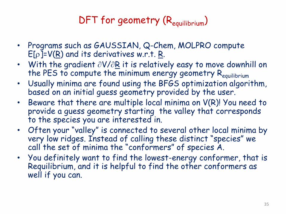
• Programs such as GAUSSIAN, Q-Chem, MOLPRO compute E[ρ]=V(R) and its derivatives w.r.t. R.

• With the gradient ∂V/∂R it is relatively easy to move downhill on the PES to compute the minimum energy geometry Requilibrium

• Usually minima are found using the BFGS optimization algorithm, based on an initial guess geometry provided by the user.

• Beware that there are multiple local minima on V(R)! You need to provide a guess geometry starting the valley that corresponds to the species you are interested in.

• Often your “valley” is connected to several other local minima by very low ridges. Instead of calling these distinct “species” we call the set of minima the “conformers” of species A.

• You definitely want to find the lowest-energy conformer, that is Requilibrium, and it is helpful to find the other conformers as well if you can.

35

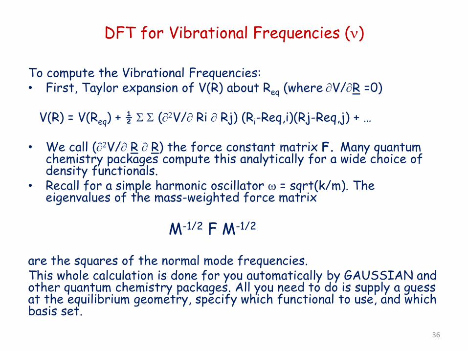
DFT for Vibrational Frequencies (ν)

To compute the Vibrational Frequencies: • First, Taylor expansion of V(R) about Req (where ∂V/∂R =0) V(R) = V(Req) + ½ Σ Σ (∂2V/∂ Ri ∂ Rj) (Ri-Req,i)(Rj-Req,j) + … • We call (∂2V/∂ R ∂ R) the force constant matrix F. Many quantum

chemistry packages compute this analytically for a wide choice of density functionals.

• Recall for a simple harmonic oscillator ω = sqrt(k/m). The eigenvalues of the mass-weighted force matrix

M-1/2 F M-1/2

are the squares of the normal mode frequencies. This whole calculation is done for you automatically by GAUSSIAN and other quantum chemistry packages. All you need to do is supply a guess at the equilibrium geometry, specify which functional to use, and which basis set.

36

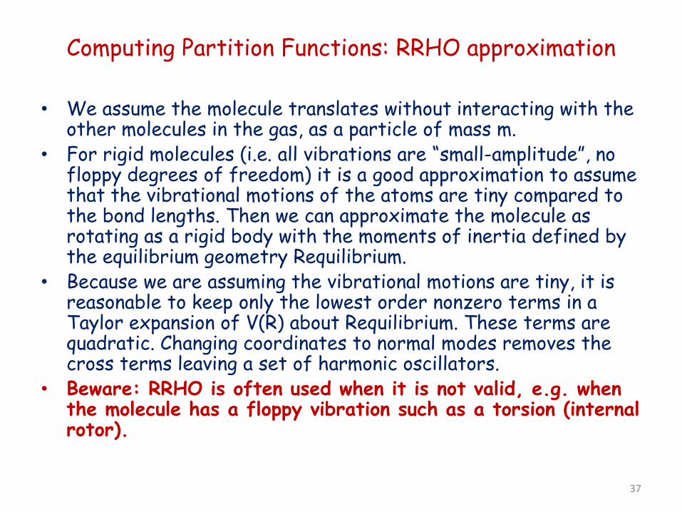
Computing Partition Functions: RRHO approximation

• We assume the molecule translates without interacting with the other molecules in the gas, as a particle of mass m.

• For rigid molecules (i.e. all vibrations are “small-amplitude”, no floppy degrees of freedom) it is a good approximation to assume that the vibrational motions of the atoms are tiny compared to the bond lengths. Then we can approximate the molecule as rotating as a rigid body with the moments of inertia defined by the equilibrium geometry Requilibrium.

• Because we are assuming the vibrational motions are tiny, it is reasonable to keep only the lowest order nonzero terms in a Taylor expansion of V(R) about Requilibrium. These terms are quadratic. Changing coordinates to normal modes removes the cross terms leaving a set of harmonic oscillators.

• Beware: RRHO is often used when it is not valid, e.g. when the molecule has a floppy vibration such as a torsion (internal rotor).

37

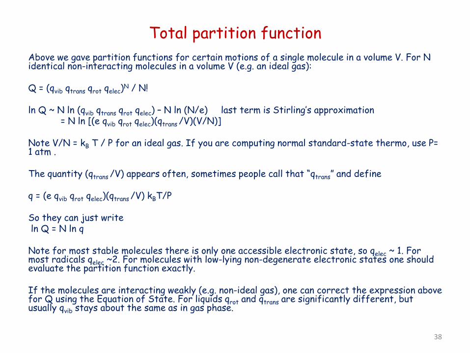
Total partition function Above we gave partition functions for certain motions of a single molecule in a volume V. For N identical non-interacting molecules in a volume V (e.g. an ideal gas):

Q = (qvib qtrans qrot qelec)N / N! ln Q ~ N ln (qvib qtrans qrot qelec) – N ln (N/e) last term is Stirling’s approximation = N ln [(e qvib qrot qelec)(qtrans /V)(V/N)] Note V/N = kB T / P for an ideal gas. If you are computing normal standard-state thermo, use P= 1 atm . The quantity (qtrans /V) appears often, sometimes people call that “qtrans” and define q = (e qvib qrot qelec)(qtrans /V) kBT/P So they can just write ln Q = N ln q Note for most stable molecules there is only one accessible electronic state, so qelec ~ 1. For most radicals qelec ~2. For molecules with low-lying non-degenerate electronic states one should evaluate the partition function exactly. If the molecules are interacting weakly (e.g. non-ideal gas), one can correct the expression above for Q using the Equation of State. For liquids qrot and qtrans are significantly different, but usually qvib stays about the same as in gas phase.

38

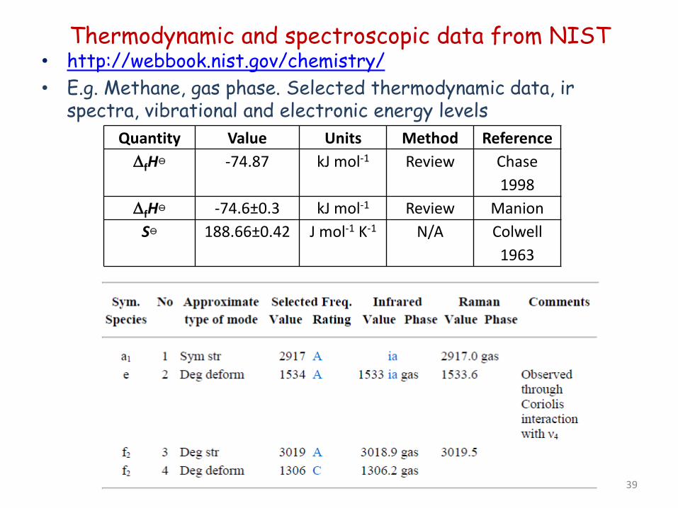
Thermodynamic and spectroscopic data from NIST • http://webbook.nist.gov/chemistry/ • E.g. Methane, gas phase. Selected thermodynamic data, ir

spectra, vibrational and electronic energy levels Quantity Value Units Method Reference

∆fH -74.87 kJ mol-1 Review Chase 1998

∆fH -74.6±0.3 kJ mol-1 Review Manion S 188.66±0.42 J mol-1 K-1 N/A Colwell

1963

39

Beware Internal Rotors & Floppy Motions!

• The normal vibrational partition function formulas are for harmonic oscillators.

• Some types of vibrational motions (torsions/internal rotations, umbrella vibrations, pseudorotations) are NOT harmonic. – E.g. rotations about C-C bonds – Puckering of 5-membered rings like cyclopentane

• Many of the entropy values in standard tables are derived using approximate formulas to account for internal rotation. Who knows what formulas they used to estimate other floppy motions. They can be significantly in error!

• If you care about the numbers, read the footnotes in the tables to see how the numbers were computed. Just because it is in a table does not mean it is Truth.

• Always read the error bars!!!

40

Often impossible to measure all the vibrational frequencies… so use quantum chemistry to fill in the gaps

• For many quantum chemistry methods, people have implemented software that efficiently computes the second derivatives of the potential energy surface

∂2V/ ∂xm∂yn

• From the second derivatives, one can do normal-mode analysis to compute all the small-amplitude-limit vibrational frequencies νi

• It is hard (essentially impossible) to compute V exactly for multi-electron molecules. However, there are many good approximate methods: e.g. B3LYP, CCSD, CAS-PT2, MRCI, HF – After the slash is the name of the basis set used when

expanding the molecular orbitals: e.g. 6-31G*, TZ2P, etc. • Currently, most people use Density Functional Theory

approximations to compute the second derivatives of V, e.g. M08, M06, B3LYP, …

41

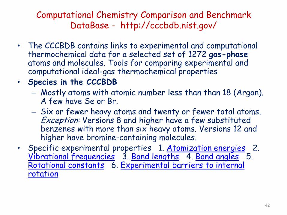
Computational Chemistry Comparison and Benchmark DataBase - http://cccbdb.nist.gov/

• The CCCBDB contains links to experimental and computational thermochemical data for a selected set of 1272 gas-phase atoms and molecules. Tools for comparing experimental and computational ideal-gas thermochemical properties

• Species in the CCCBDB – Mostly atoms with atomic number less than than 18 (Argon).

A few have Se or Br. – Six or fewer heavy atoms and twenty or fewer total atoms.

Exception: Versions 8 and higher have a few substituted benzenes with more than six heavy atoms. Versions 12 and higher have bromine-containing molecules.

• Specific experimental properties 1. Atomization energies 2. Vibrational frequencies 3. Bond lengths 4. Bond angles 5. Rotational constants 6. Experimental barriers to internal rotation

42

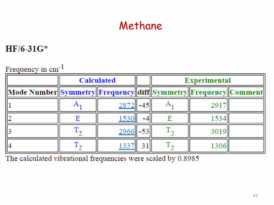
Methane

43

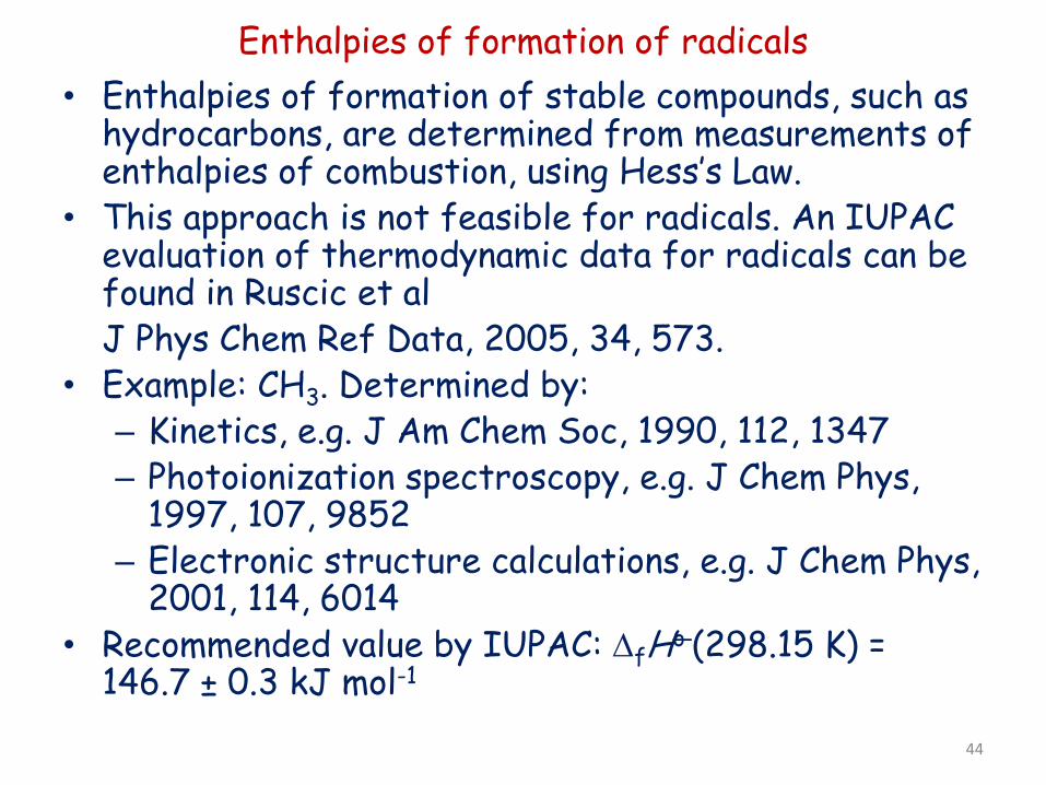
Enthalpies of formation of radicals • Enthalpies of formation of stable compounds, such as

hydrocarbons, are determined from measurements of enthalpies of combustion, using Hess’s Law.

• This approach is not feasible for radicals. An IUPAC evaluation of thermodynamic data for radicals can be found in Ruscic et al

J Phys Chem Ref Data, 2005, 34, 573. • Example: CH3. Determined by:

– Kinetics, e.g. J Am Chem Soc, 1990, 112, 1347 – Photoionization spectroscopy, e.g. J Chem Phys,

1997, 107, 9852 – Electronic structure calculations, e.g. J Chem Phys,

2001, 114, 6014 • Recommended value by IUPAC: ∆fHo (298.15 K) =

146.7 ± 0.3 kJ mol-1

44

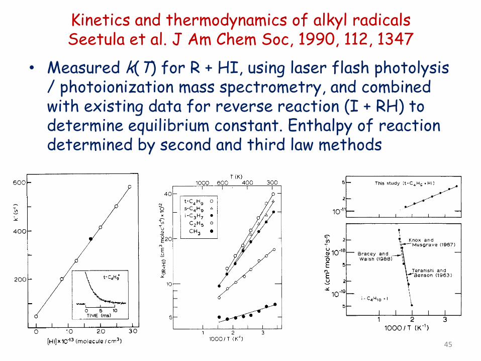
Kinetics and thermodynamics of alkyl radicals Seetula et al. J Am Chem Soc, 1990, 112, 1347

• Measured k(T) for R + HI, using laser flash photolysis / photoionization mass spectrometry, and combined with existing data for reverse reaction (I + RH) to determine equilibrium constant. Enthalpy of reaction determined by second and third law methods

45

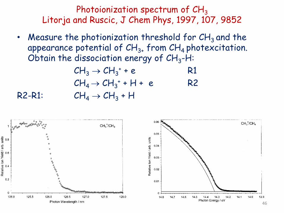
Photoionization spectrum of CH3 Litorja and Ruscic, J Chem Phys, 1997, 107, 9852

• Measure the photionization threshold for CH3 and the

appearance potential of CH3+ from CH4 photexcitation. Obtain the dissociation energy of CH3-H:

CH3 → CH3+ + e R1

CH4 → CH3+ + H + e R2

R2-R1: CH4 → CH3 + H

46

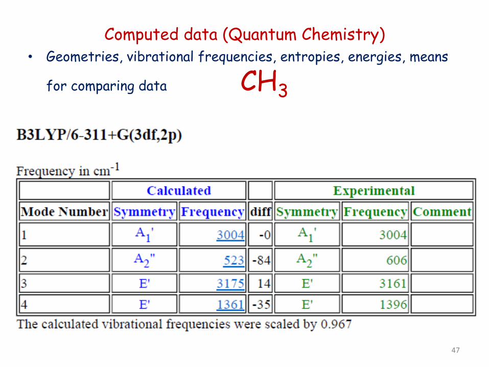
Computed data (Quantum Chemistry) • Geometries, vibrational frequencies, entropies, energies, means

for comparing data CH3

47

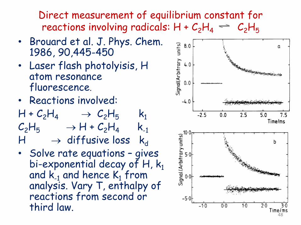
Direct measurement of equilibrium constant for reactions involving radicals: H + C2H4 C2H5

• Brouard et al. J. Phys. Chem. 1986, 90,445-450

• Laser flash photolyisis, H atom resonance fluorescence.

• Reactions involved: H + C2H4 → C2H5 k1 C2H5 → H + C2H4 k-1 H → diffusive loss kd • Solve rate equations – gives

bi-exponential decay of H, k1 and k-1 and hence K1 from analysis. Vary T, enthalpy of reactions from second or third law.

48

R-H bond energies: Extensive tabulation and review Berkowitz et al. 1994, 98, 2744

• The bond enthalpy change at 298 K is the enthalpy change for the reaction R-H → R + H:

• The bond energy (change) or dissociation energy at zero K is:

• Bond energies can be converted to bond enthalpy changes using the relation U = H + pV = H +RT, so that, for R-H → R + H,

∆U = ∆H +RT. At zero K, the dissociation energy is equal to the bond enthalpy change.

• Berkowitz et al provide an extensive dataset for R-H bond energies

using radical kinetics, gas-phase acidity cycles, and photoionization mass spectrometry

49

Thermodynamic databases

• Active, internally consistent thermodynamic databases: – ATcT Active thermochemical tables. Uses

and network approach. Ruscic et al. J. Phys. Chem. A 2004, 108, 9979-9997.

– NEAT . Network of atom based thermochemistry. Csaszar and Furtenbacher: Chemistry – A european journal, 2010,16, 4826 50

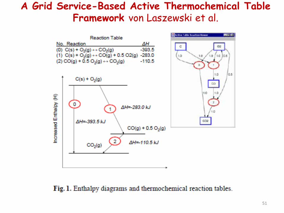
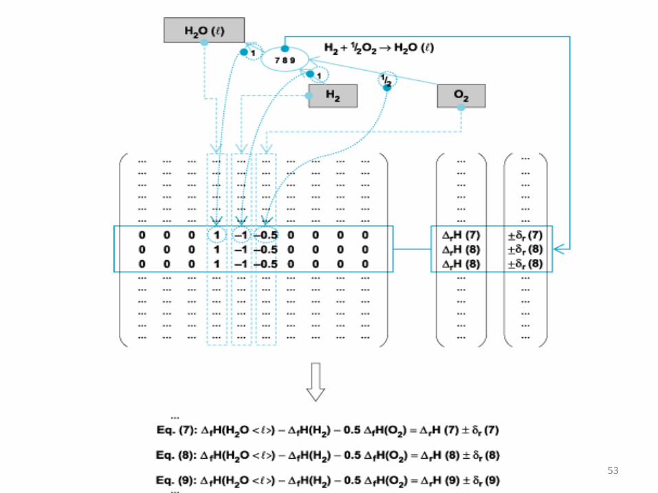
A Grid Service-Based Active Thermochemical Table Framework von Laszewski et al.

51

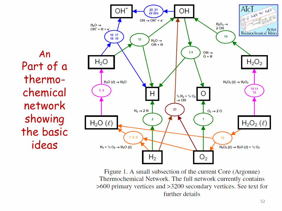
An Part of a thermo-chemical network showing

the basic ideas

52

53

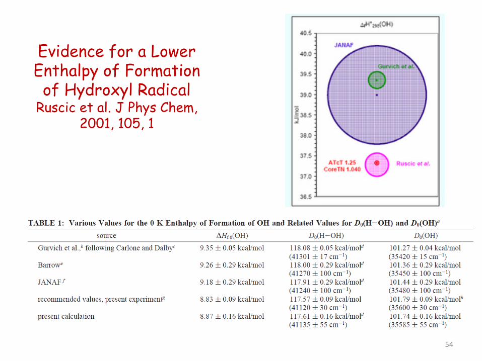
Evidence for a Lower Enthalpy of Formation of Hydroxyl Radical

Ruscic et al. J Phys Chem, 2001, 105, 1

54

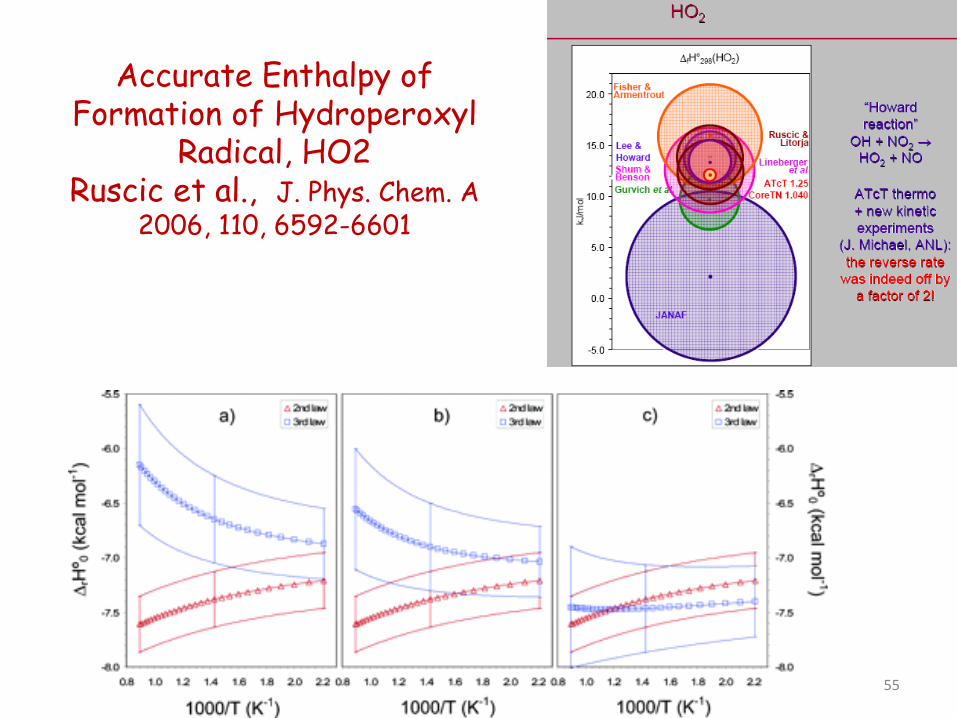
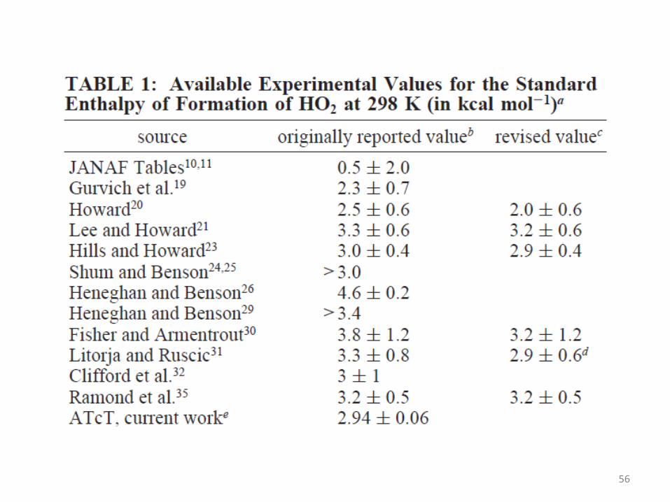
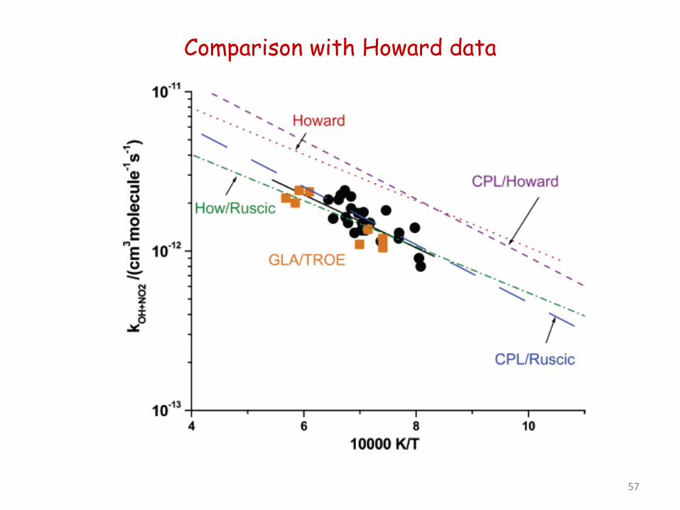
Accurate Enthalpy of Formation of Hydroperoxyl

Radical, HO2 Ruscic et al., J. Phys. Chem. A

2006, 110, 6592-6601

55

56

Comparison with Howard data

57

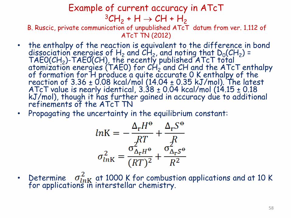
Example of current accuracy in ATcT 3CH2 + H → CH + H2

B. Ruscic, private communication of unpublished ATcT datum from ver. 1.112 of ATcT TN (2012)

• the enthalpy of the reaction is equivalent to the difference in bond dissociation energies of H2 and CH2, and noting that D0(CH2) = TAE0(CH2)-TAE0(CH), the recently published ATcT total atomization energies (TAE0) for CH2 and CH and the ATcT enthalpy of formation for H produce a quite accurate 0 K enthalpy of the reaction of 3.36 ± 0.08 kcal/mol (14.04 ± 0.35 kJ/mol). The latest ATcT value is nearly identical, 3.38 ± 0.04 kcal/mol (14.15 ± 0.18 kJ/mol), though it has further gained in accuracy due to additional refinements of the ATcT TN

• Propagating the uncertainty in the equilibrium constant:

• Determine at 1000 K for combustion applications and at 10 K for applications in interstellar chemistry.

58

From a Network of Computed Reaction Enthalpies to Atom-Based Thermochemistry (NEAT)

A. G. Csaszar and T. Furtenbacher, Chemistry – A european journal, 2010,16, 4826

Abstract: A simple and fast, weighted, linear least-squares refinement protocol and code is presented for inverting the information contained in a network of quantum chemically computed 0 K reaction enthalpies. This inversion yields internally consistent 0 K enthalpies of formation for the species of the network.

59

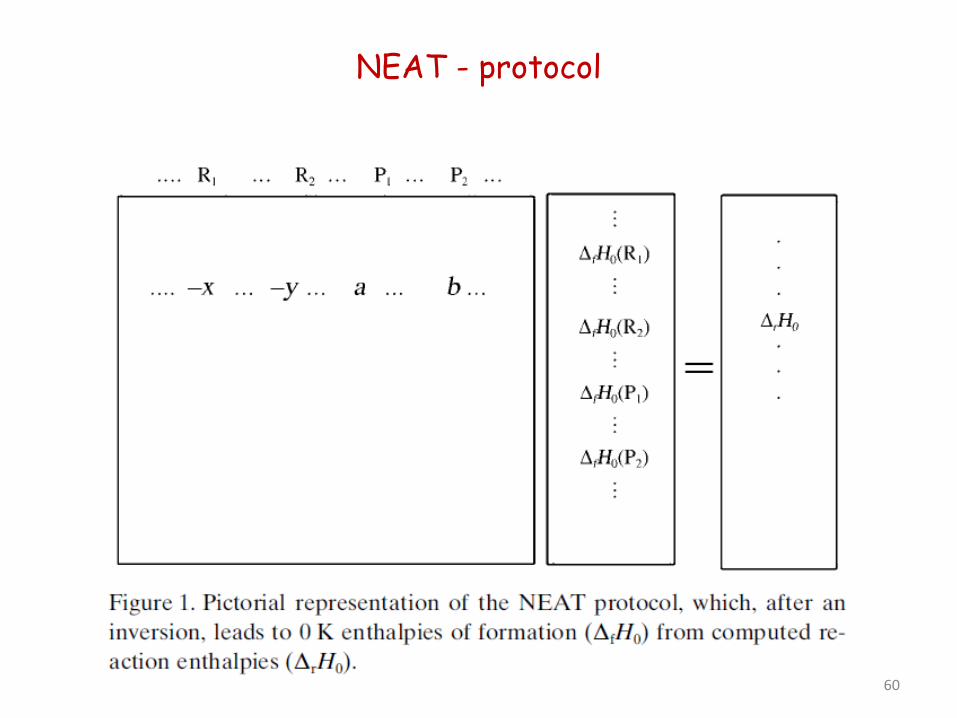
NEAT - protocol

60

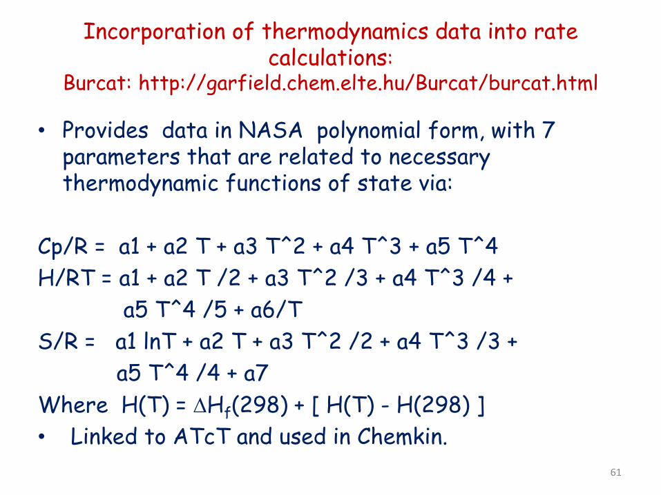
Incorporation of thermodynamics data into rate calculations:

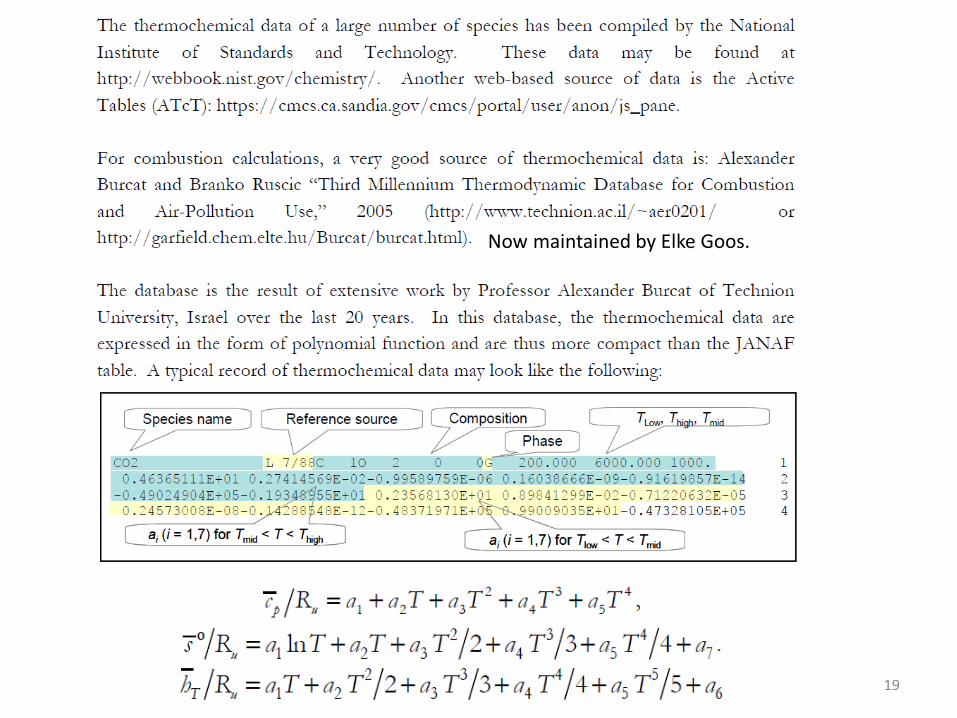
Burcat: http://garfield.chem.elte.hu/Burcat/burcat.html

• Provides data in NASA polynomial form, with 7 parameters that are related to necessary thermodynamic functions of state via:

Cp/R = a1 + a2 T + a3 T^2 + a4 T^3 + a5 T^4 H/RT = a1 + a2 T /2 + a3 T^2 /3 + a4 T^3 /4 + a5 T^4 /5 + a6/T S/R = a1 lnT + a2 T + a3 T^2 /2 + a4 T^3 /3 + a5 T^4 /4 + a7 Where H(T) = ∆Hf(298) + [ H(T) - H(298) ] • Linked to ATcT and used in Chemkin.

61

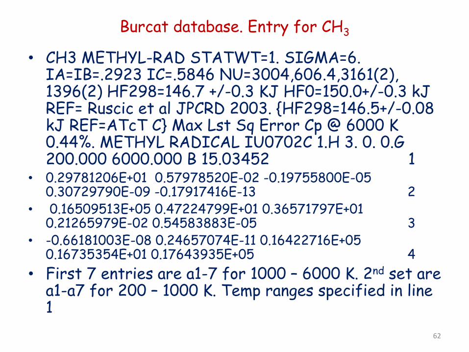
Burcat database. Entry for CH3

• CH3 METHYL-RAD STATWT=1. SIGMA=6. IA=IB=.2923 IC=.5846 NU=3004,606.4,3161(2), 1396(2) HF298=146.7 +/-0.3 KJ HF0=150.0+/-0.3 kJ REF= Ruscic et al JPCRD 2003. {HF298=146.5+/-0.08 kJ REF=ATcT C} Max Lst Sq Error Cp @ 6000 K 0.44%. METHYL RADICAL IU0702C 1.H 3. 0. 0.G 200.000 6000.000 B 15.03452 1

• 0.29781206E+01 0.57978520E-02 -0.19755800E-05 0.30729790E-09 -0.17917416E-13 2

• 0.16509513E+05 0.47224799E+01 0.36571797E+01 0.21265979E-02 0.54583883E-05 3

• -0.66181003E-08 0.24657074E-11 0.16422716E+05 0.16735354E+01 0.17643935E+05 4

• First 7 entries are a1-7 for 1000 – 6000 K. 2nd set are a1-a7 for 200 – 1000 K. Temp ranges specified in line 1

62

63

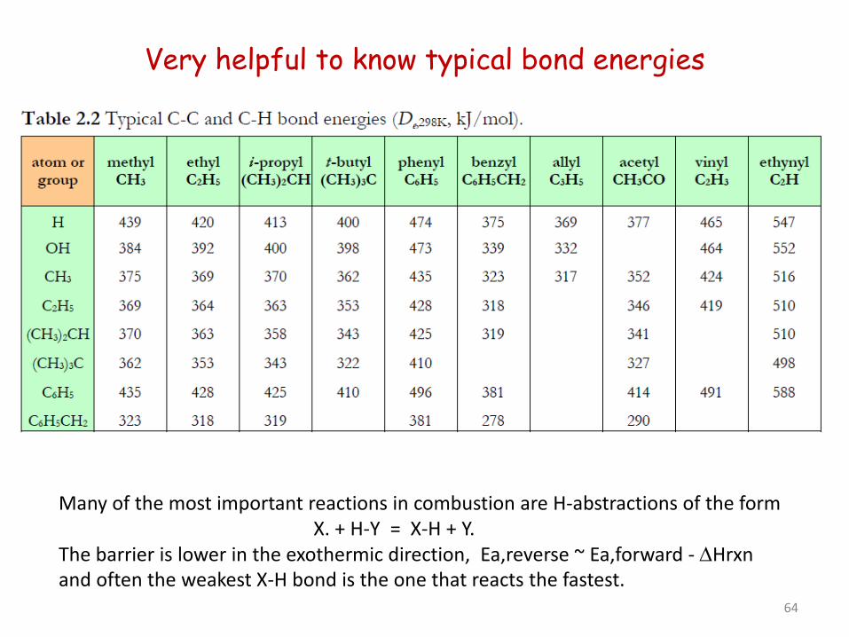
Very helpful to know typical bond energies

Many of the most important reactions in combustion are H-abstractions of the form X. + H-Y = X-H + Y. The barrier is lower in the exothermic direction, Ea,reverse ~ Ea,forward - ∆Hrxn and often the weakest X-H bond is the one that reacts the fastest.

64

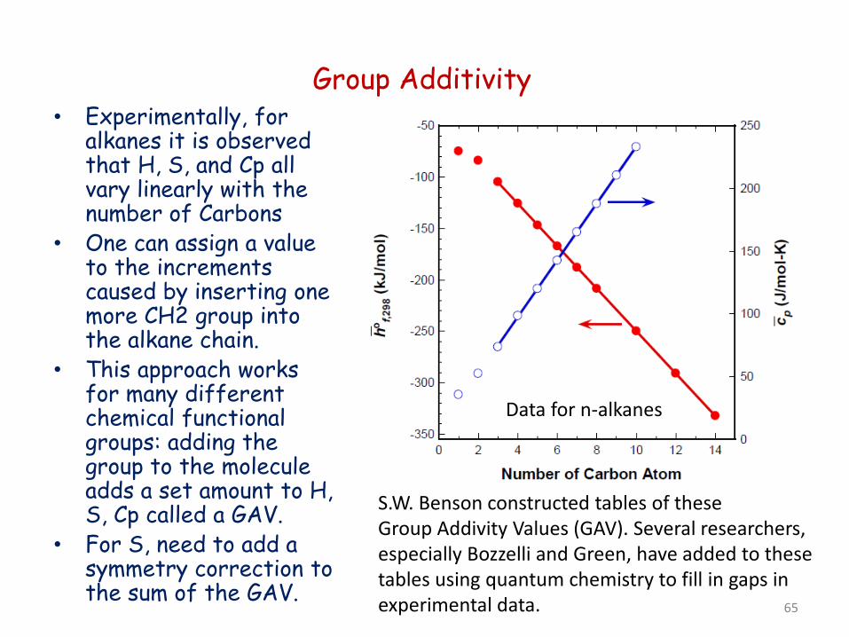
Group Additivity • Experimentally, for

alkanes it is observed that H, S, and Cp all vary linearly with the number of Carbons

• One can assign a value to the increments caused by inserting one more CH2 group into the alkane chain.

• This approach works for many different chemical functional groups: adding the group to the molecule adds a set amount to H, S, Cp called a GAV.

• For S, need to add a symmetry correction to the sum of the GAV.

S.W. Benson constructed tables of these Group Addivity Values (GAV). Several researchers, especially Bozzelli and Green, have added to these tables using quantum chemistry to fill in gaps in experimental data.

Data for n-alkanes

65

Programs to estimate thermo with Group Additivity

• http://webbook.nist.gov/chemistry/grp-add/ • THERGAS (Nancy group) • THERM (Bozzelli) • RMG (Green group, MIT) • Several others... All of these programs are based on Benson’s methods described in his textbook “Thermochemical Kinetics” and in several papers by Benson. See also several improvements to Benson’s method by Bozzelli. Group additivity is related to the “functional group” concept of organic chemistry, and to “Linear Free Energy Relationships” (LFER) and “Linear Structure-Activity Relationships” (LSAR).

66

Problems with Group Additivity

• While the group additivity method is intuitively simple, it has its drawbacks stemming from the need to consider higher-order correction terms for a large number of molecules. Take cyclopentane as an example, the addition of group contributions yields Ho = –103 kJ/mol, yet the experimental value is –76 kJ/mol. The difference is caused by the ring strain, which is not accounted for in the group value of C–(C2,H2) obtained from unstrained, straight-chain alkane molecules.

• Cyclics are the biggest problem for group additivity, but some other species also do not work well, e.g. some halogenated compounds, and some highly branched compounds. Very small molecules are often unique (e.g. CO, OH), so group additivity does not help with those.

• Species with different resonance forms can also cause problems, e.g. propargyl CH2CCH can be written with a triple bond or two double bonds, which should be used when determining the groups?

67

Summary of this section

• Species concentrations in the Hot Exhaust Zone of a combustor are nearly in equilibrium due to the high Temperature & high radical concentrations. – Whatever system you are studying, it is good to know what the

equilibrium is, that is where the kinetics are heading! • Can compute Equilibrium composition using EQUIL and similar

programs, but need thermochemical parameters for each species. • Thermochemical parameters also allow us to infer reverse rate

coefficients from forward rate coefficients • These parameters are obtained in a variety of ways, many of them

not quite accurate enough for quantitative modeling. – Most convenient are group contribution methods, which are very

fast. • Recent Active Thermochemical Tables approach and high level

quantum chemistry methods achieve excellent accuracy, so far mostly for smaller molecules.

68

Lesson 3

Combustion Chemistry Regimes: Diffusion Flames

Fuel Pyrolysis, and Rate Coefficients

Non-Premixed Diffusion Flames: Pyrolysis

• In Diffusion Flames, the fuel and the oxidizer are separate. Flame lies between them.

• Burning Rate controlled by diffusion of fuel and O2 into the flame.

• In flame zone, very high T and radical concentrations: drives most processes to equilibrium (e.g. CO2 + H2O) very quickly – Relatively small chemistry effects inside the flame: “Mixed is Burnt”

• Fast thermal NOx formation (O+N2 NO + N) in hottest zone • Relatively little chemistry occurring on air side • Lots of Pyrolysis Chemistry occurring on fuel side!

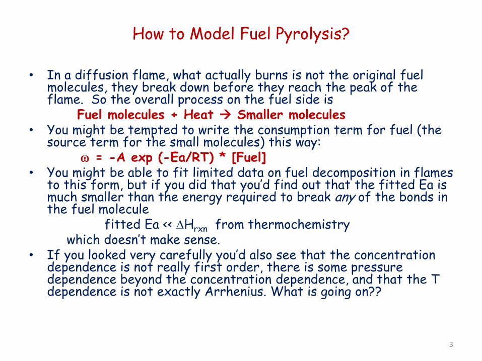
How to Model Fuel Pyrolysis?

• In a diffusion flame, what actually burns is not the original fuel molecules, they break down before they reach the peak of the flame. So the overall process on the fuel side is

Fuel molecules + Heat Smaller molecules • You might be tempted to write the consumption term for fuel (the

source term for the small molecules) this way: ω = -A exp (-Ea/RT) * [Fuel] • You might be able to fit limited data on fuel decomposition in flames

to this form, but if you did that you’d find out that the fitted Ea is much smaller than the energy required to break any of the bonds in the fuel molecule

fitted Ea << ∆Hrxn from thermochemistry which doesn’t make sense. • If you looked very carefully you’d also see that the concentration

dependence is not really first order, there is some pressure dependence beyond the concentration dependence, and that the T dependence is not exactly Arrhenius. What is going on??

3

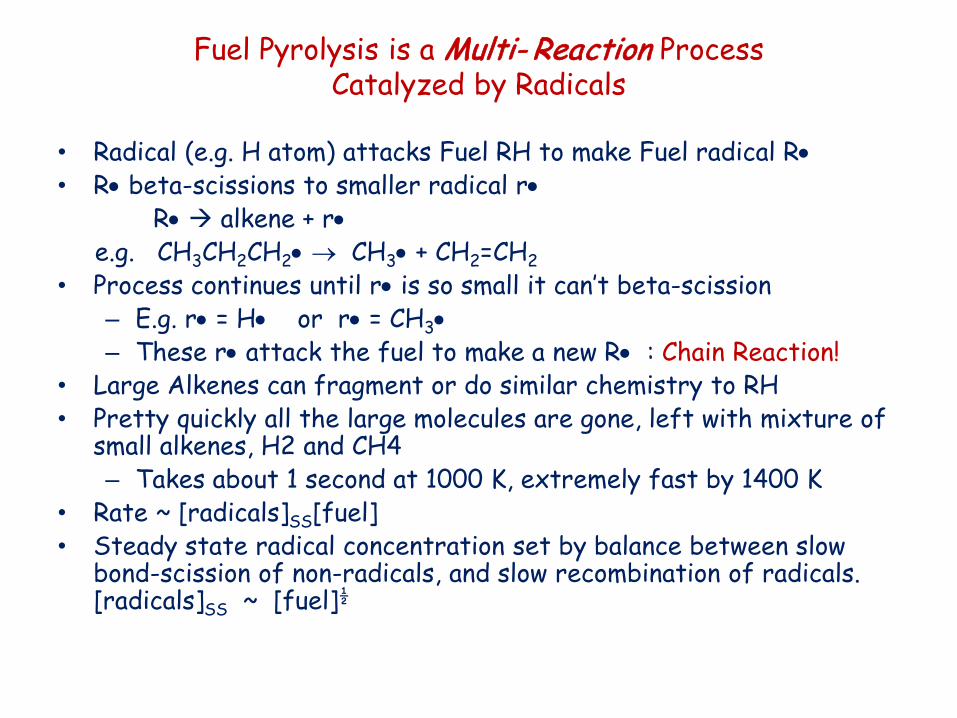
Fuel Pyrolysis is a Multi- Reaction Process Catalyzed by Radicals

• Radical (e.g. H atom) attacks Fuel RH to make Fuel radical R• • R• beta-scissions to smaller radical r• R• alkene + r• e.g. CH3CH2CH2• → CH3• + CH2=CH2 • Process continues until r• is so small it can’t beta-scission

– E.g. r• = H• or r• = CH3• – These r• attack the fuel to make a new R• : Chain Reaction!

• Large Alkenes can fragment or do similar chemistry to RH • Pretty quickly all the large molecules are gone, left with mixture of

small alkenes, H2 and CH4 – Takes about 1 second at 1000 K, extremely fast by 1400 K

• Rate ~ [radicals]SS[fuel] • Steady state radical concentration set by balance between slow

bond-scission of non-radicals, and slow recombination of radicals. [radicals]SS ~ [fuel]½

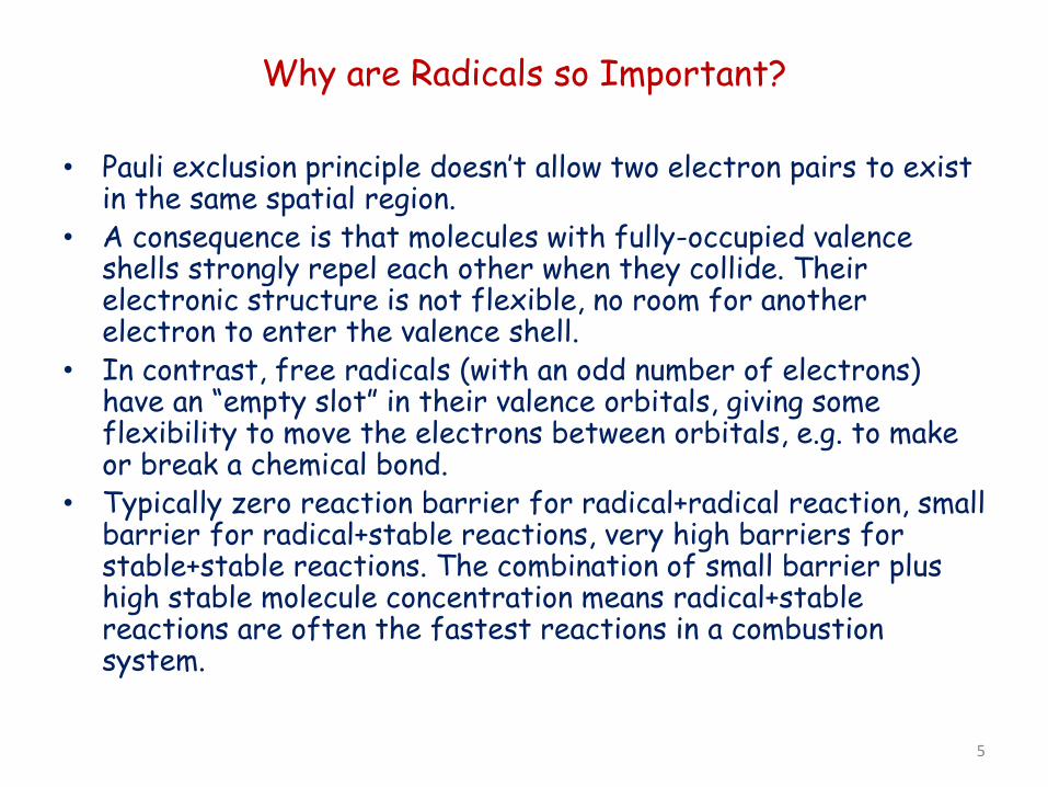
Why are Radicals so Important?

• Pauli exclusion principle doesn’t allow two electron pairs to exist in the same spatial region.

• A consequence is that molecules with fully-occupied valence shells strongly repel each other when they collide. Their electronic structure is not flexible, no room for another electron to enter the valence shell.

• In contrast, free radicals (with an odd number of electrons) have an “empty slot” in their valence orbitals, giving some flexibility to move the electrons between orbitals, e.g. to make or break a chemical bond.

• Typically zero reaction barrier for radical+radical reaction, small barrier for radical+stable reactions, very high barriers for stable+stable reactions. The combination of small barrier plus high stable molecule concentration means radical+stable reactions are often the fastest reactions in a combustion system.

5

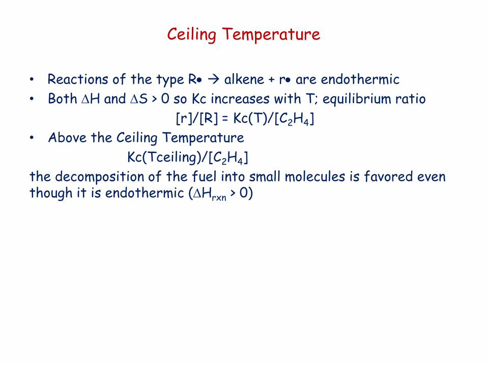
Ceiling Temperature

• Reactions of the type R• alkene + r• are endothermic • Both ∆H and ∆S > 0 so Kc increases with T; equilibrium ratio [r]/[R] = Kc(T)/[C2H4] • Above the Ceiling Temperature Kc(Tceiling)/[C2H4] the decomposition of the fuel into small molecules is favored even though it is endothermic (∆Hrxn > 0)

What do the small alkene products do?

• Main alkene is usually ethene (C2H4). In absence of O2 it is gradually converted to acetylene (C2H2).

• Second most important alkene is propene. It converts to resonance-stabilized radical allyl C3H5 (resistant to O2 reaction), and then gradually to resonance stabilized radical propargyl C3H3.

• Propargyl + Propargyl and various addition reactions of acetylene can lead to aromatics and to Soot Formation.

• So one idea for clean combustion is to get the ethene and propene into the flame where they can react with O2, before they have time to cook further to form soot!

• In the flame, the key reaction is C2H3 + O2 H2CO + HCO

Different Fuels make different mix of alkenes, high fidelity multi-step models can predict this accurately

• At high T, this is the main difference between fuels: how much ethene and H2 (reactive with O2) vs. how much propene and methane (relatively unreactive)

• One can extend this to understand very complicated fuels e.g. real jet fuels: if you can measure the ratio of alkenes formed from the fuel, you can understand the high T chemistry pretty well. – E.g. see the HyChem project

• Alkene Mix directly important in petrochemical industry: naphtha steam-cracking – Biggest part of chemical industry, very heavily studied,

strong demand for kinetic models. But where do we get all the rate coefficients needed to construct a high-fidelity model for fuel pyrolysis?

Where do we get all the rate coefficients k(T)?

• We can look them up: – Try http://kinetics.nist.gov – Beware: raw data, not evaluated!

• We can measure them: – Experimental Kinetics

• We can calculate them from first principles: – Computational Kinetics

• We can estimate them: – by analogy to known reactions with

similar functional groups 9

Experimental Kinetics

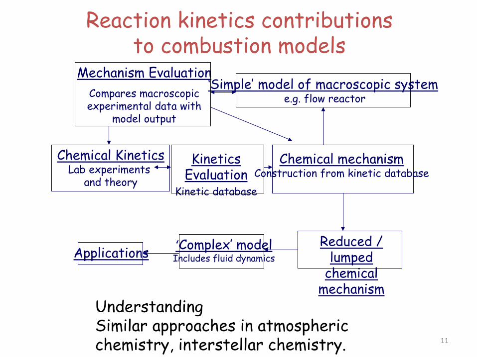
Reaction kinetics contributions to combustion models

Chemical Kinetics Lab experiments

and theory

Kinetics Evaluation

Kinetic database

Chemical mechanism Construction from kinetic database

Mechanism Evaluation Compares macroscopic experimental data with

model output

‘Simple’ model of macroscopic system e.g. flow reactor

Reduced / lumped

chemical mechanism

‘Complex’ model Includes fluid dynamics Applications

Understanding Similar approaches in atmospheric chemistry, interstellar chemistry. 11

Measurement of rates of elementary

reactions

• Ideally, isolate the individual reaction and study it at the appropriate combustion conditions.

• Not always possible: – May have to model the system to extract k of

interest. Problems in other parts of the model can contaminate inferred value of k

– May need to extrapolate to appropriate T, p. At high T reactant may disappear faster than you can make it.

– Ideally extrapolate with the help of theory, but extrapolation always introduces uncertainties.

12

Measurement Techniques

• Pulsed laser photolysis (laser flash photolysis) • Shock tubes • Flow tubes for elementary reactions and whole

systems • Static studies of whole systems

For Radical + Stable reactions, you have several challenges: 1) How to make the specific radical you want 2) How to achieve a high enough radical

concentration that you can measure it. 3) High radical concentrations rapidly diminish

due to fast radical + radical reactions

13

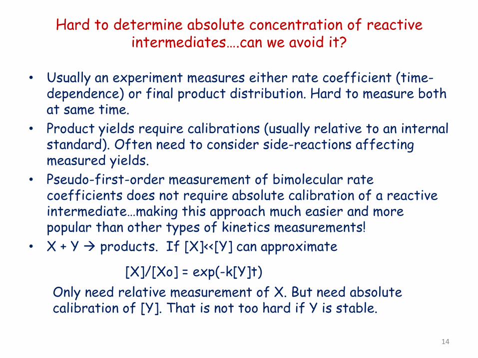
Hard to determine absolute concentration of reactive intermediates….can we avoid it?

• Usually an experiment measures either rate coefficient (time-dependence) or final product distribution. Hard to measure both at same time.

• Product yields require calibrations (usually relative to an internal standard). Often need to consider side-reactions affecting measured yields.

• Pseudo-first-order measurement of bimolecular rate coefficients does not require absolute calibration of a reactive intermediate…making this approach much easier and more popular than other types of kinetics measurements!

• X + Y products. If [X]<<[Y] can approximate

[X]/[Xo] = exp(-k[Y]t) Only need relative measurement of X. But need absolute calibration of [Y]. That is not too hard if Y is stable.

14

Pulsed laser photolysis

15

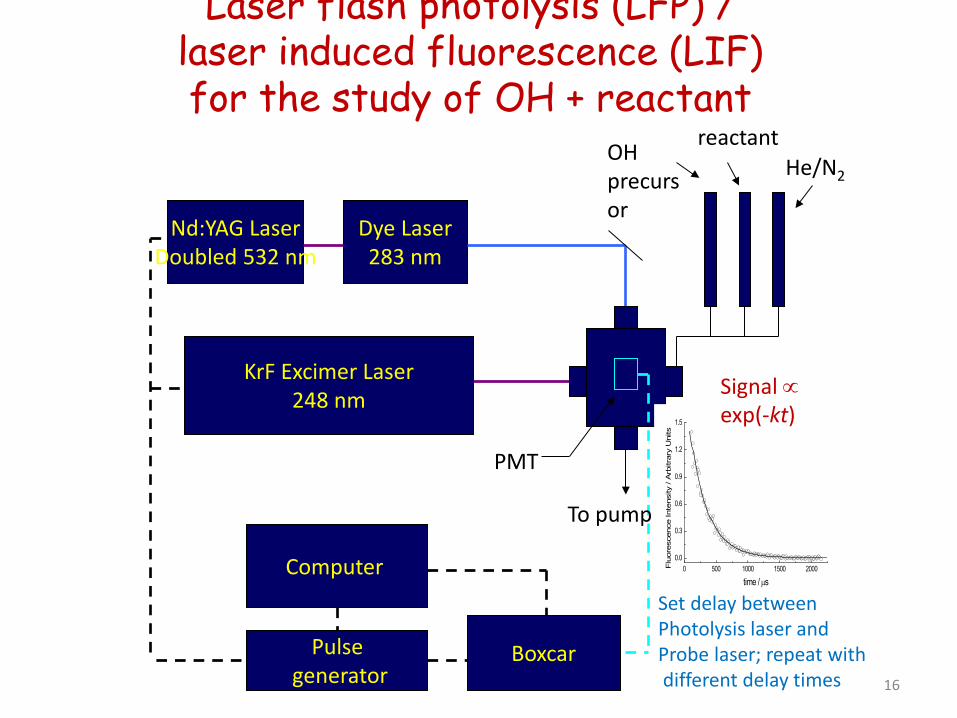
Laser flash photolysis (LFP) / laser induced fluorescence (LIF) for the study of OH + reactant

Nd:YAG Laser Doubled 532 nm

Dye Laser 283 nm

KrF Excimer Laser 248 nm

Computer

Boxcar

PMT

OH precursor

reactant He/N2

To pump

Pulse generator

0 500 1000 1500 20000.0

0.3

0.6

0.9

1.2

1.5

Flu

ores

cenc

e In

tens

ity / A

rbitr

ary

Uni

ts

time / µs

Set delay between Photolysis laser and Probe laser; repeat with different delay times

Signal ∝ exp(-kt)

16

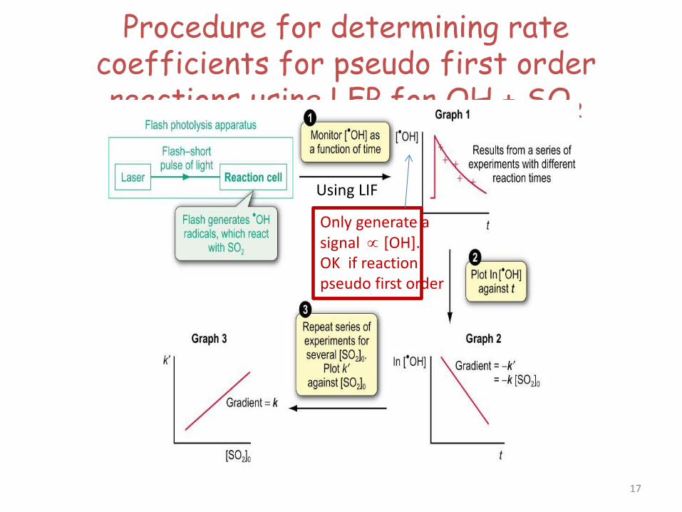
Procedure for determining rate coefficients for pseudo first order reactions using LFP for OH + SO2

Using LIF

Only generate a signal ∝ [OH]. OK if reaction pseudo first order

17

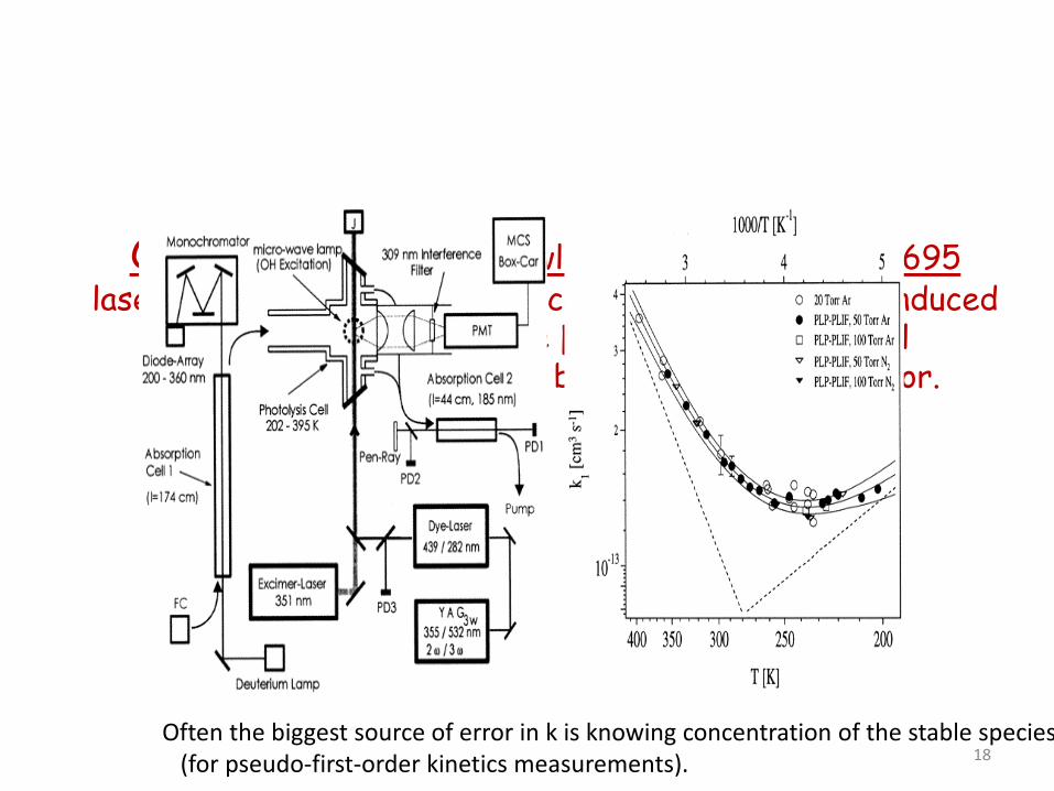
OH + acetone, J N Crowley, JPCA, 2000, 104,2695 laser flash photolysis, resonance fluorescence/laser induced

fluorescence to measure [OH] (relative). Optical measurement of [acetone] before and after reactor.

Often the biggest source of error in k is knowing concentration of the stable species (for pseudo-first-order kinetics measurements). 18

G3

G2

G1

Turbo Pump 300 l/s

VUV-Photoionisation

Pump 28 l/h Diffusion Pump 3000 l/h

Flight Tube ∼5*10-6 Torr

Gas Flow

in

Metal/ Quartz Flow Reactor

Main Vacuum Chamber 10-3-10-4 Torr

Quartz window

248 nm Excimer Laser Beam

ToFMS

d= 1.27 cm, l = 70 cm

1 mm

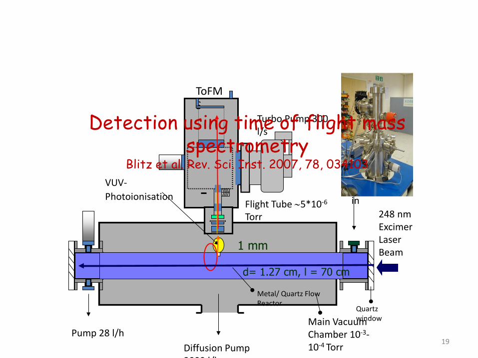
Time of flight mass spectrometer / laser flash photolysis

Detection using time of flight mass spectrometry

Blitz et al. Rev. Sci. Inst. 2007, 78, 034103

19

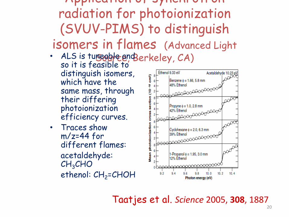
Application of synchrotron radiation for photoionization (SVUV-PIMS) to distinguish

isomers in flames (Advanced Light Source, Berkeley, CA) • ALS is tuneable and

so it is feasible to distinguish isomers, which have the same mass, through their differing photoionization efficiency curves.

• Traces show m/z=44 for different flames:

acetaldehyde: CH3CHO

ethenol: CH2=CHOH

Taatjes et al. Science 2005, 308, 1887 20

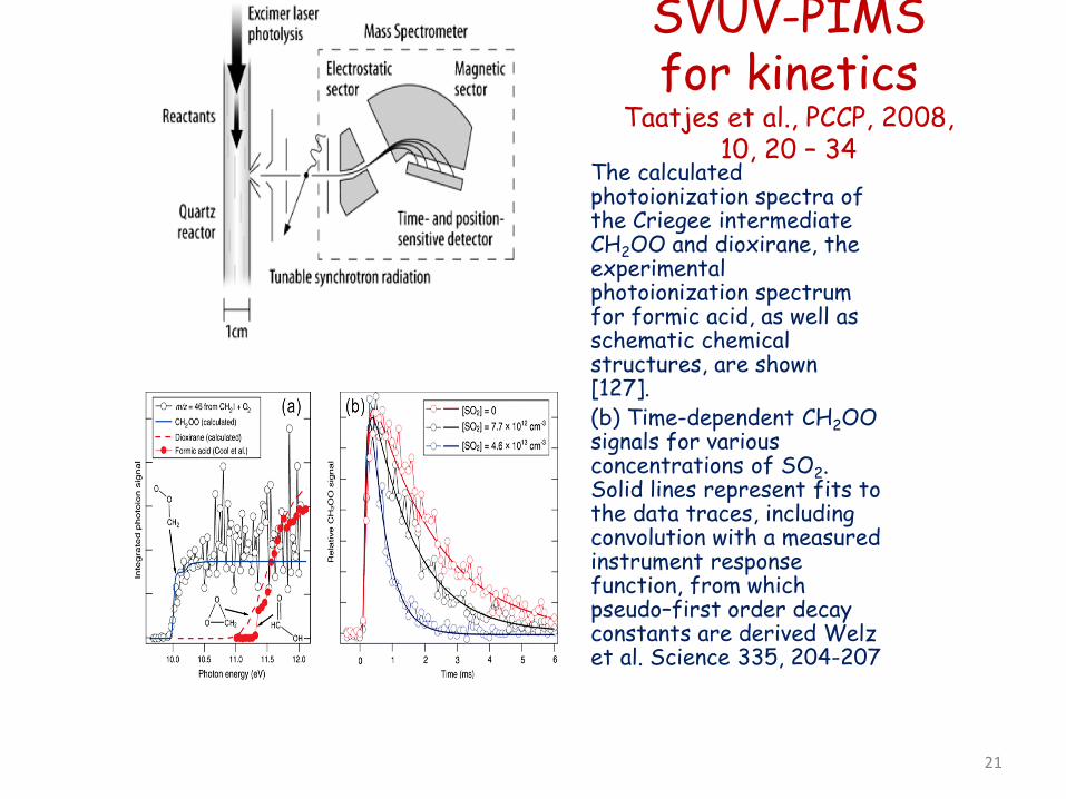
SVUV-PIMS for kinetics

Taatjes et al., PCCP, 2008, 10, 20 – 34

The calculated photoionization spectra of the Criegee intermediate CH2OO and dioxirane, the experimental photoionization spectrum for formic acid, as well as schematic chemical structures, are shown [127].

• (b) Time-dependent CH2OO signals for various concentrations of SO2. Solid lines represent fits to the data traces, including convolution with a measured instrument response function, from which pseudo–first order decay constants are derived Welz et al. Science 335, 204-207

21

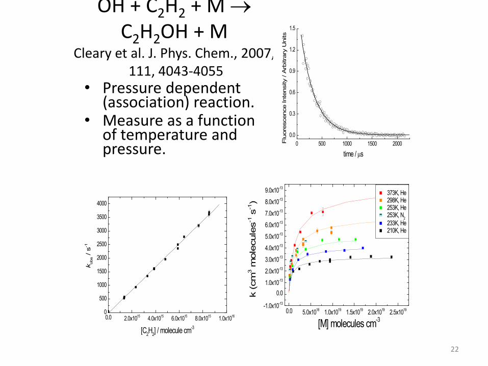
OH + C2H2 + M → C2H2OH + M

Cleary et al. J. Phys. Chem., 2007, 111, 4043-4055

• Pressure dependent (association) reaction.

• Measure as a function of temperature and pressure.

0 500 1000 1500 20000.0

0.3

0.6

0.9

1.2

1.5

Flu

ores

cenc

e In

tens

ity / A

rbitr

ary

Uni

ts

time / µs

0.0 2.0x1015 4.0x1015 6.0x1015 8.0x1015 1.0x10160

500

1000

1500

2000

2500

3000

3500

4000

k obs / s-1

[C2H2] / molecule cm-3

0.0 5.0x1018 1.0x1019 1.5x1019 2.0x1019 2.5x1019-1.0x10-13

0.01.0x10-13

2.0x10-13

3.0x10-13

4.0x10-13

5.0x10-13

6.0x10-13

7.0x10-13

8.0x10-13

9.0x10-13

k (c

m3 m

olec

ules

-1 s

-1)

[M] molecules cm-3

373K, He 298K, He 253K, He 253K, N2 233K, He 210K, He

22

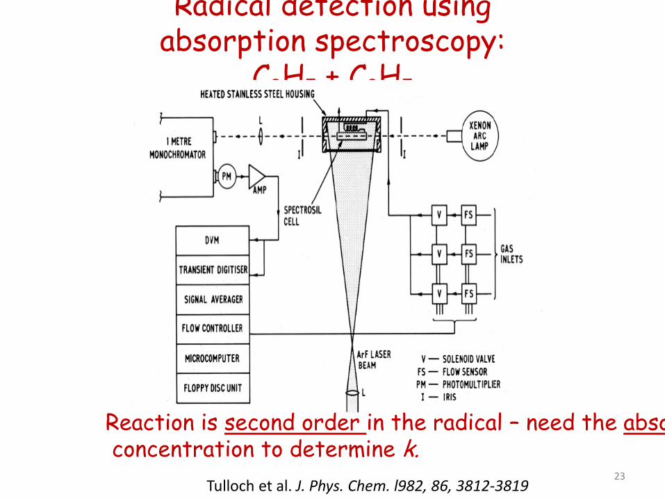
Radical detection using absorption spectroscopy:

C3H5 + C3H5

Tulloch et al. J. Phys. Chem. l982, 86, 3812-3819

Reaction is second order in the radical – need the abso concentration to determine k.

23

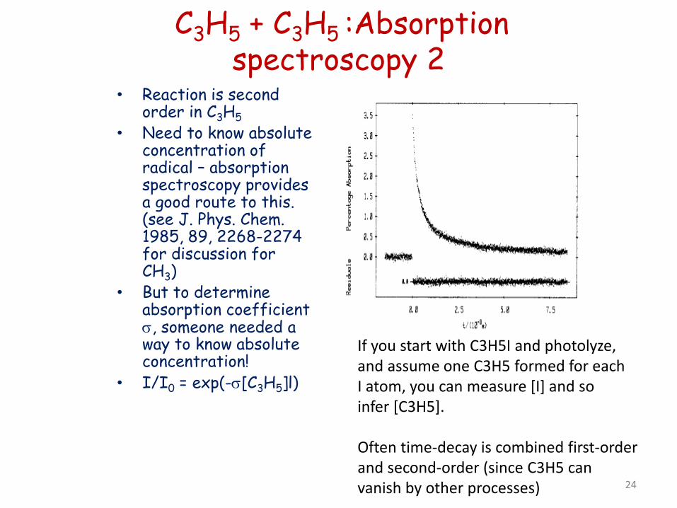
C3H5 + C3H5 :Absorption spectroscopy 2

• Reaction is second order in C3H5

• Need to know absolute concentration of radical – absorption spectroscopy provides a good route to this. (see J. Phys. Chem. 1985, 89, 2268-2274 for discussion for CH3)

• But to determine absorption coefficient σ, someone needed a way to know absolute concentration!

• I/I0 = exp(-σ[C3H5]l)

If you start with C3H5I and photolyze, and assume one C3H5 formed for each I atom, you can measure [I] and so infer [C3H5]. Often time-decay is combined first-order and second-order (since C3H5 can vanish by other processes) 24

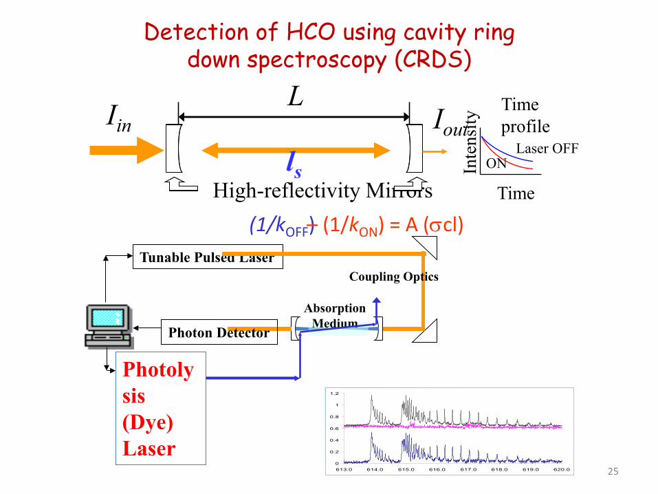
Iin

High-reflectivity Mirrors

L Iout

ls

Time profile

Time

Inte

nsity

ON Laser OFF

(1/kOFF) – (1/kON) = A (σcl) Tunable Pulsed Laser

Photon Detector

Coupling Optics

Absorption Medium

Photolysis (Dye) Laser

Detection of HCO using cavity ring down spectroscopy (CRDS)

0

0.2

0.4

0.6

0.8

1

1.2

613.0 614.0 615.0 616.0 617.0 618.0 619.0 620.0 25

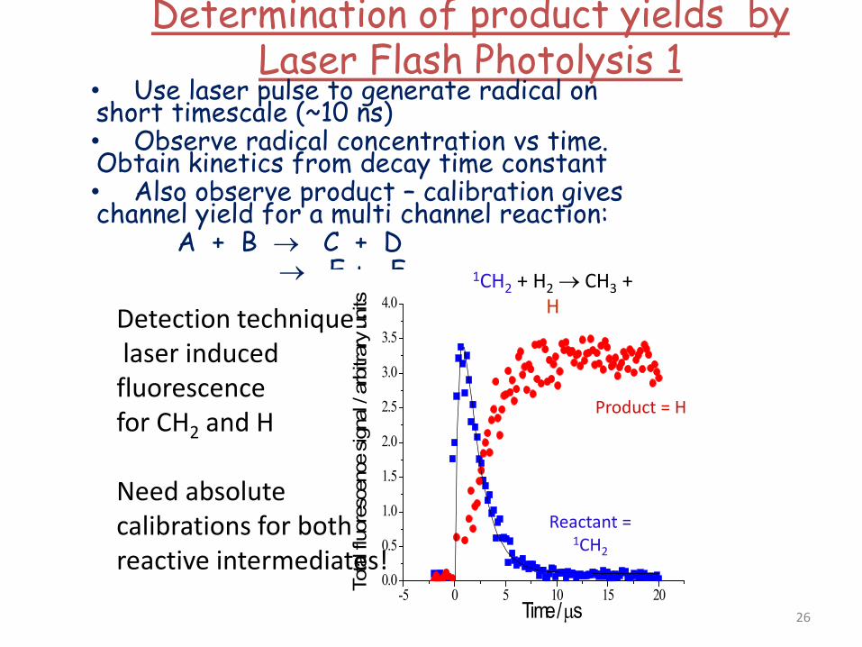
Determination of product yields by Laser Flash Photolysis 1

• Use laser pulse to generate radical on short timescale (~10 ns) • Observe radical concentration vs time. Obtain kinetics from decay time constant • Also observe product – calibration gives channel yield for a multi channel reaction: A + B → C + D → E + F

-5 0 5 10 15 200.0

0.5

1.0

1.5

2.0

2.5

3.0

3.5

4.0

Tota

l fluo

resc

ence

sign

al / a

rbitr

ary u

nits

Time / µs

Reactant = 1CH2

Product = H

Taatjes, J. Phys. Chem. A 2006, 110 4299

1CH2 + H2 → CH3 + H

Detection technique : laser induced fluorescence for CH2 and H Need absolute calibrations for both reactive intermediates!

26

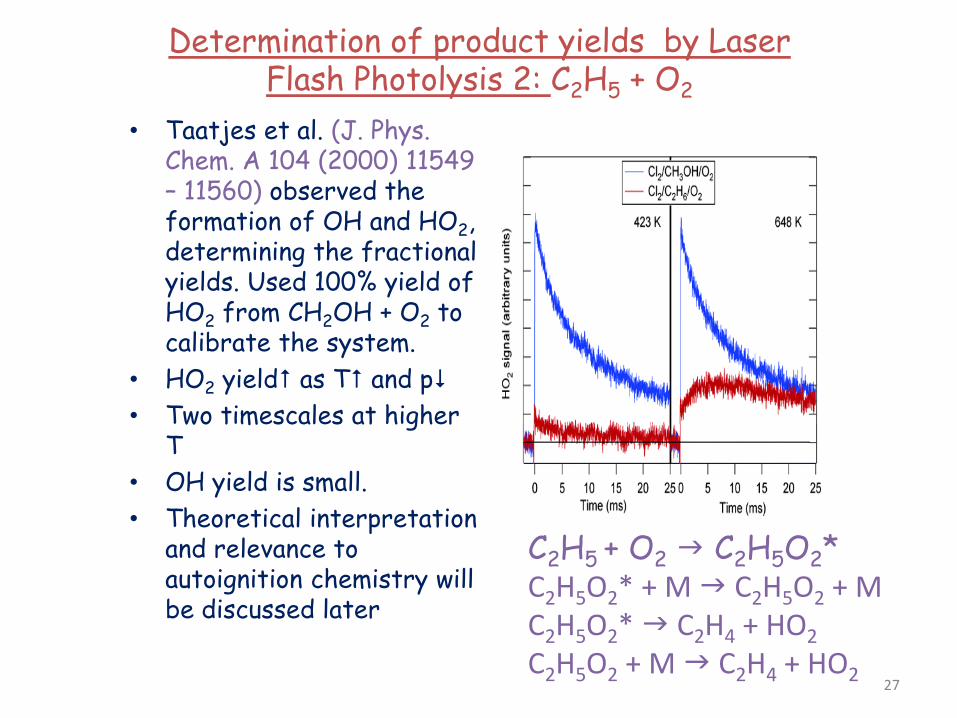
Determination of product yields by Laser Flash Photolysis 2: C2H5 + O2

• Taatjes et al. (J. Phys. Chem. A 104 (2000) 11549 – 11560) observed the formation of OH and HO2, determining the fractional yields. Used 100% yield of HO2 from CH2OH + O2 to calibrate the system.

• HO2 yield as T and p • Two timescales at higher

T • OH yield is small. • Theoretical interpretation

and relevance to autoignition chemistry will be discussed later

C2H5 + O2 C2H5O2* C2H5O2* + M C2H5O2 + M C2H5O2* C2H4 + HO2 C2H5O2 + M C2H4 + HO2

27

Shock tubes

28

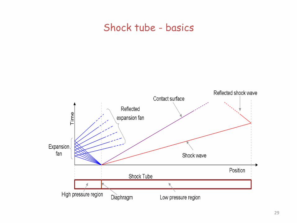
Shock tube - basics

29

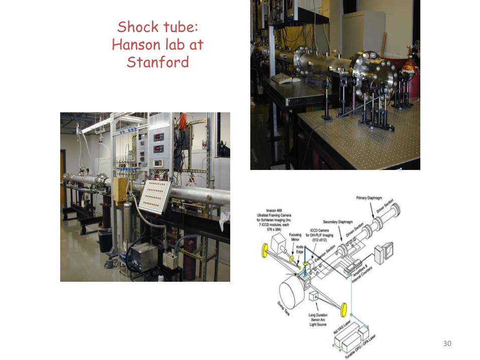
Shock tube: Hanson lab at

Stanford

30

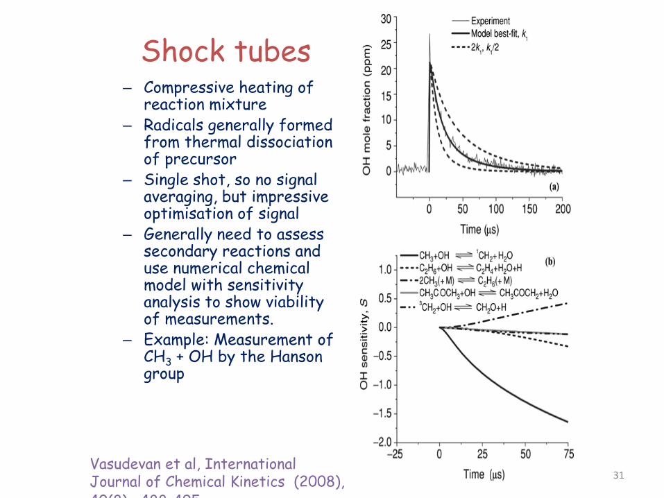
Shock tubes – Compressive heating of

reaction mixture – Radicals generally formed

from thermal dissociation of precursor

– Single shot, so no signal averaging, but impressive optimisation of signal

– Generally need to assess secondary reactions and use numerical chemical model with sensitivity analysis to show viability of measurements.

– Example: Measurement of CH3 + OH by the Hanson group

Vasudevan et al, International Journal of Chemical Kinetics (2008), 40(8) 488 495

31

OH + HCHO, 934 K to 1670 K, 1.6 atm Int J Chem Kinet 37: 98–109, 2005

• Behind reflected shock waves. OH radicals formed by shock-heating tert-butyl hydroperoxide

• OH concentration time-histories were inferred from laser absorption using the R1(5) line of the OH A-X (0, 0) band near 306.7 nm.

• Other reactions contribute to the OH time profile, especially CH3 + OH.

• Rate coefficient determined by fitting to detailed model (GRI-Mech – see Wednesday), with addition of acetone chemistry, deriving from dissociation of OH precursor (t-butylhydroperoxide). Detailed uncertainty analysis

32

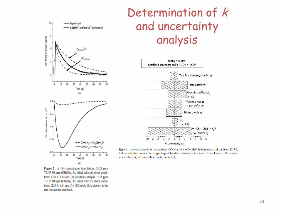
Determination of k and uncertainty

analysis

33

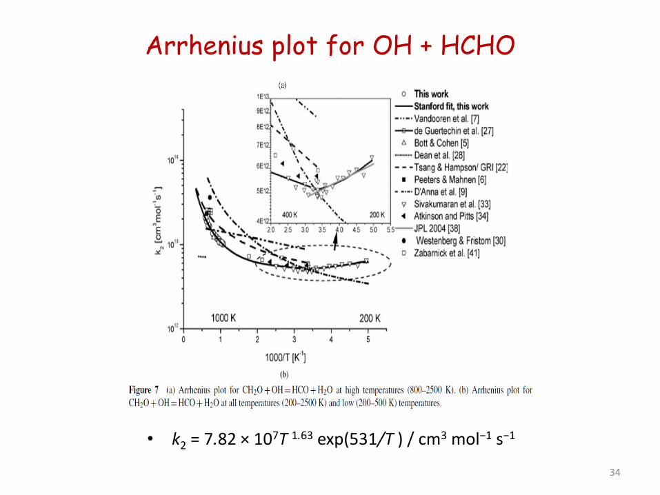
Arrhenius plot for OH + HCHO

• k2 = 7.82 × 107T 1.63 exp(531/T ) / cm3 mol−1 s−1

34

Flow tubes for elementary reactions and whole systems

35

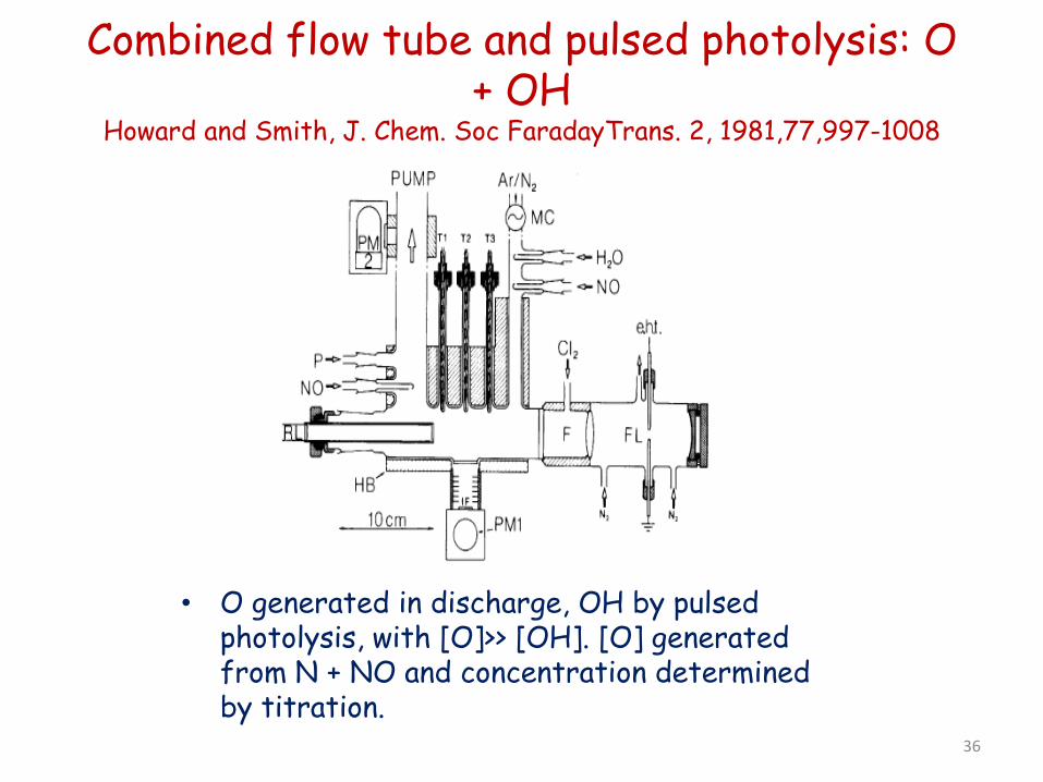
Combined flow tube and pulsed photolysis: O + OH

Howard and Smith, J. Chem. Soc FaradayTrans. 2, 1981,77,997-1008

• O generated in discharge, OH by pulsed photolysis, with [O]>> [OH]. [O] generated from N + NO and concentration determined by titration.

36

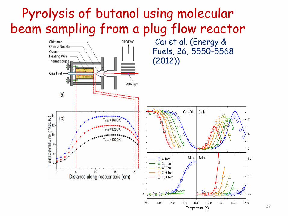
Pyrolysis of butanol using molecular beam sampling from a plug flow reactor

Cai et al. (Energy & Fuels, 26, 5550-5568 (2012))

37

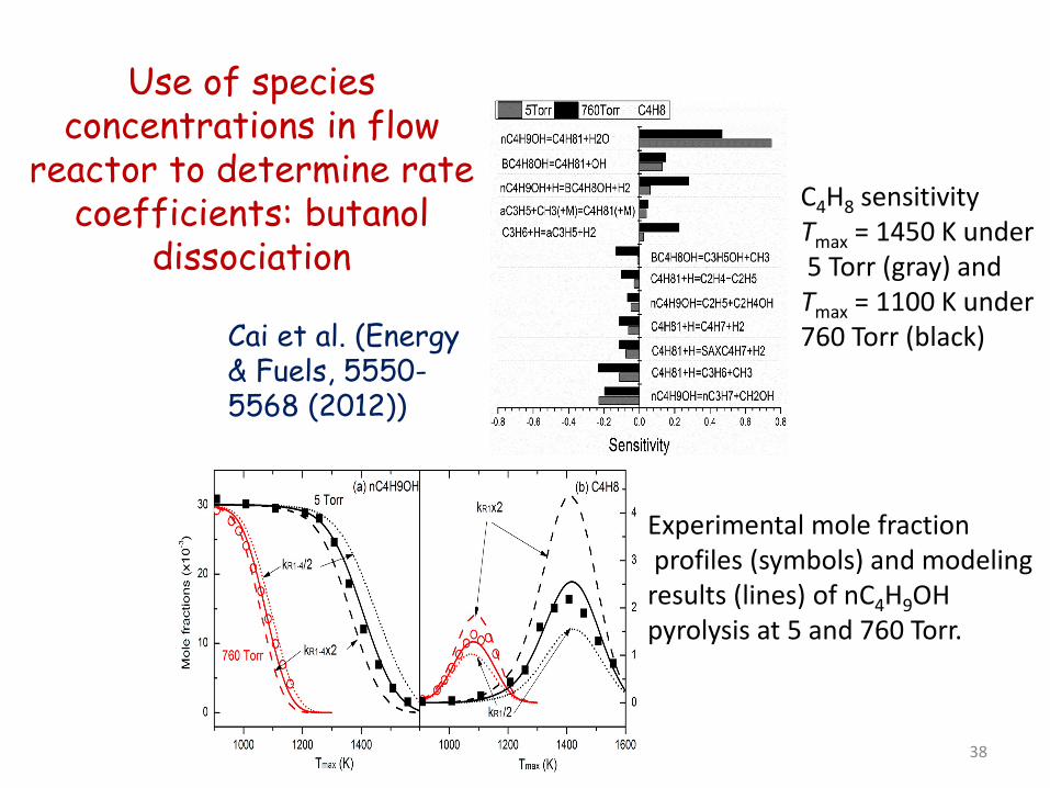
Use of species concentrations in flow

reactor to determine rate coefficients: butanol

dissociation

Cai et al. (Energy & Fuels, 5550-5568 (2012))

C4H8 sensitivity Tmax = 1450 K under 5 Torr (gray) and Tmax = 1100 K under 760 Torr (black)

Experimental mole fraction profiles (symbols) and modeling results (lines) of nC4H9OH pyrolysis at 5 and 760 Torr.

38

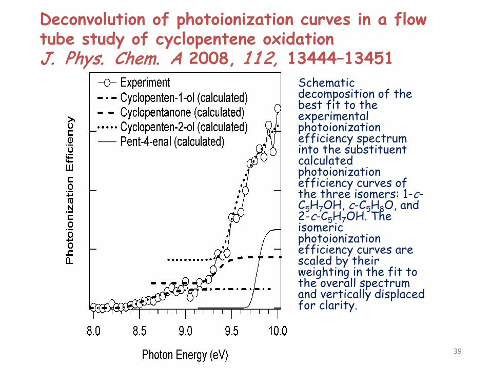
Deconvolution of photoionization curves in a flow tube study of cyclopentene oxidation J. Phys. Chem. A 2008, 1 1 2, 13444–13451

Schematic decomposition of the best fit to the experimental photoionization efficiency spectrum into the substituent calculated photoionization efficiency curves of the three isomers: 1-c-C5H7OH, c-C5H8O, and 2-c-C5H7OH. The isomeric photoionization efficiency curves are scaled by their weighting in the fit to the overall spectrum and vertically displaced for clarity.

39

Static reactors: Studies of alkane oxidation kinetics and mechanism by

Baldwin, Walker and co-workers • The techniques rely on end product analysis using gas

chromatography. Three techniques were used: – Addition of small amounts of alkane, RH, to a slowly reacting

H2 + OH mixture at ~ 750 K allowed measurements of, e.g. OH, H, HO2 + RH. H2 + O2 provides a well-controlled environment containing the radicals. (JCS Faraday Trans 1., 1975, 71, 736)

– Oxidation of aldehydes (550 – 800 K). Aldehydes act as a source of alkyl radicals, e.g. 2-C3H7 from 2-C3H7CHO (JCS Faraday Trans 2., 1987, 83, 1509)

– Decomposition of tetramethylbutane (TMB) in the prsence of O2. System acts as a source of HO2. (JCS Faraday Trans 1., 1986, 82, 89)

40

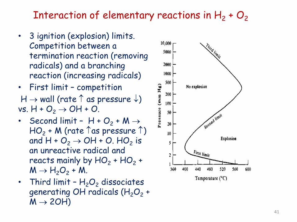
Interaction of elementary reactions in H2 + O2

• 3 ignition (explosion) limits. Competition between a termination reaction (removing radicals) and a branching reaction (increasing radicals)

• First limit – competition H → wall (rate ↑ as pressure ↓) vs. H + O2 → OH + O. • Second limit – H + O2 + M →

HO2 + M (rate ↑as pressure ↑) and H + O2 → OH + O. HO2 is an unreactive radical and reacts mainly by HO2 + HO2 + M → H2O2 + M.

• Third limit – H2O2 dissociates generating OH radicals (H2O2 + M → 2OH)

41

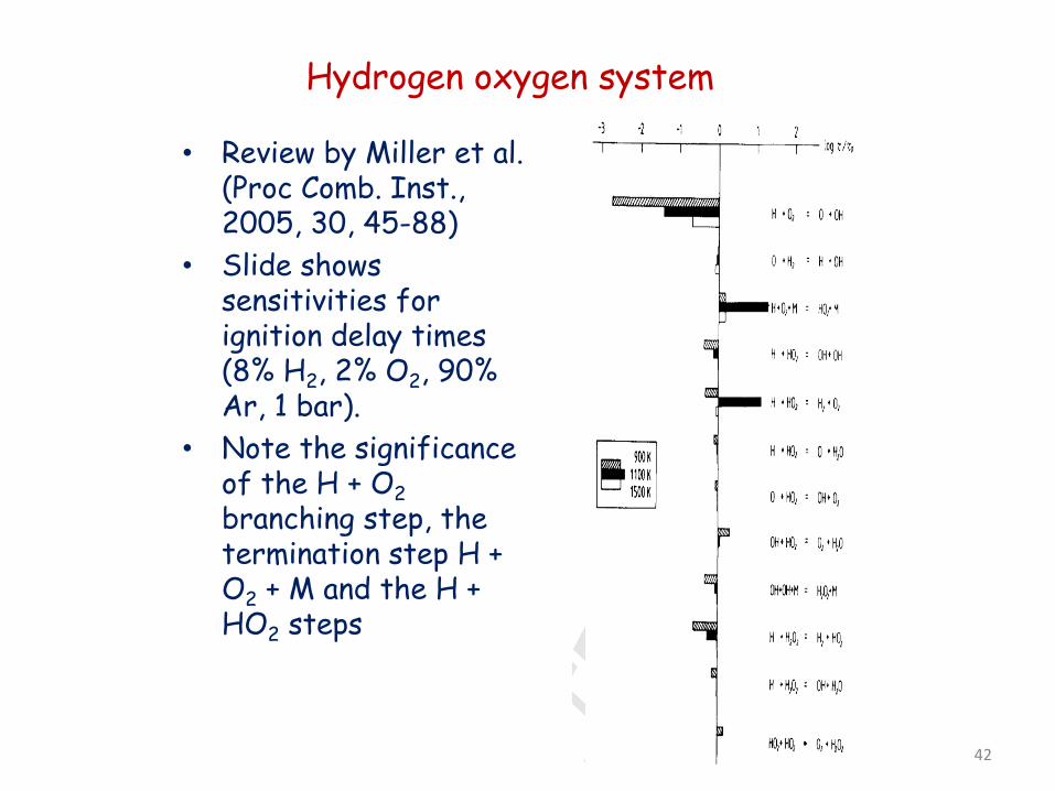
Hydrogen oxygen system

• Review by Miller et al. (Proc Comb. Inst., 2005, 30, 45-88)

• Slide shows sensitivities for ignition delay times (8% H2, 2% O2, 90% Ar, 1 bar).

• Note the significance of the H + O2 branching step, the termination step H + O2 + M and the H + HO2 steps

42

H + O2 OH + O is the most important combustion reaction

• Once the temperature gets high enough (~1000 K), this reaction often becomes the main source of new radicals.

• Since many of the new radicals beta-scission to release H atoms, this process has strong positive feedback, rapidly amplifies the radical concentration several orders of magnitude.

H+O2 OH + O O + fuel OH + R 2*( OH + fuel H2O + R) (+ heat) 3*( R x H (+ alkenes + CH3) ) if x > 1/3 this sequence exponentially amplifies [H] • In premixed flames, the heat and the H atoms diffuse into the

unburned fuel+air mixture. There a small number of H atoms gets amplified, advancing the flame front: “flame speed”

43

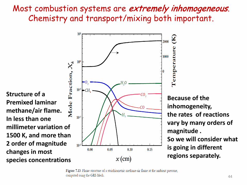
Most combustion systems are extremely inhomogeneous. Chemistry and transport/mixing both important.

44

Structure of a Premixed laminar methane/air flame. In less than one millimeter variation of 1500 K, and more than 2 order of magnitude changes in most species concentrations

Because of the inhomogeneity, the rates of reactions vary by many orders of magnitude . So we will consider what is going in different regions separately.

Combustion Chemistry: Pre-Mixed Flames • Rate of Combustion is a combination of chemical rates (create large

T and [H] gradients), thermal diffusion, and H atom diffusion into unburned fuel+air mixture – Simplest analysis says flame speed scales as sqrt(reaction

rate)*sqrt(Diffusivity) • Most fuels have similar flame speeds (see review by C.K. Law)

– Similar adiabatic flame temperatures and similar thermal diffusivities give similar heat fluxes into fuel+air mixture

– Some compensation that makes flame speeds similar: e.g. diffusional losses of H, T increase with reaction rate.

– Note that many times people assume Le=1 for flame speed analysis, but many important cases have different Le, see papers by Law and by Egolfopoulos

• A few odd cases: H2, C2H2 – H2 makes much higher [H] than other fuels – Also, H2 diffusion is fast, so it diffuses forward into flame – C2H2 has much high reactivity with O atom than other fuels

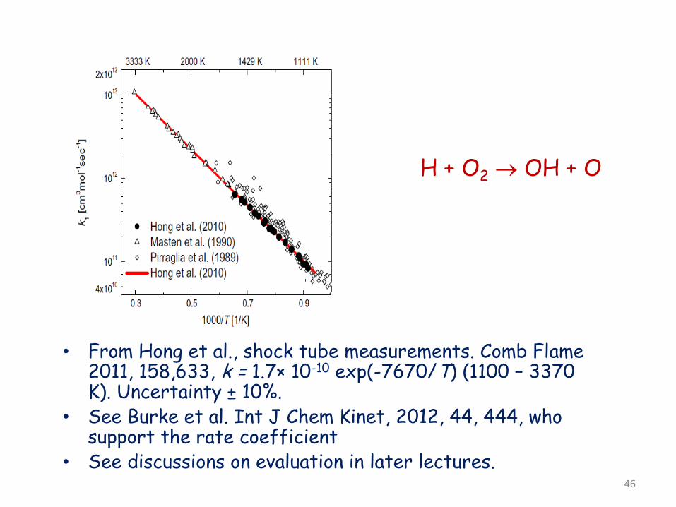
H + O2 → OH + O

• From Hong et al., shock tube measurements. Comb Flame 2011, 158,633, k = 1.7× 10-10 exp(-7670/T) (1100 – 3370 K). Uncertainty ± 10%.

• See Burke et al. Int J Chem Kinet, 2012, 44, 444, who support the rate coefficient

• See discussions on evaluation in later lectures.

46

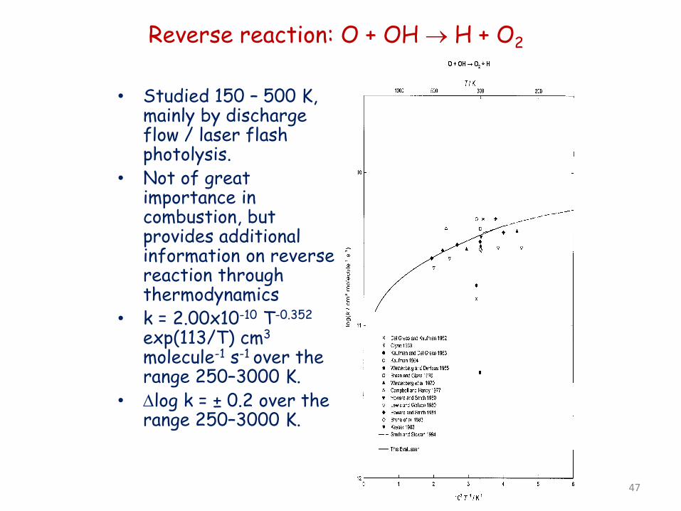
Reverse reaction: O + OH → H + O2

• Studied 150 – 500 K, mainly by discharge flow / laser flash photolysis.

• Not of great importance in combustion, but provides additional information on reverse reaction through thermodynamics

• k = 2.00x10-10 T-0.352

exp(113/T) cm3 molecule-1 s-1 over the range 250–3000 K.

• ∆log k = ± 0.2 over the range 250–3000 K.

47

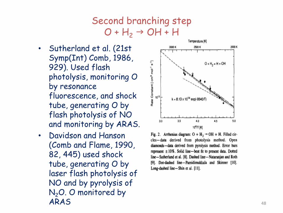
Second branching step O + H2 OH + H

• Sutherland et al. (21st Symp(Int) Comb, 1986, 929). Used flash photolysis, monitoring O by resonance fluorescence, and shock tube, generating O by flash photolysis of NO and monitoring by ARAS.

• Davidson and Hanson (Comb and Flame, 1990, 82, 445) used shock tube, generating O by laser flash photolysis of NO and by pyrolysis of N2O. O monitored by ARAS 48

H + O2 + M HO2 + M

• Termination step at lower T, converting reactive H into less reactive HO2. Acts as a route to branching through formation of H2O2 through HO2 + HO2 (and HO2 + RH in hydrocarbon combustion)

• Reaction is at the third order limit except at higher pressures. • Michael et al. J. Phys. Chem. A 2002, 106, 5297-5313 used flash

photolysis at room T for a wide range of third bodies, and a shock tube at higher T for Ar,. O2 and N2. Showed that H2O is an unusually effective third body.

• Detailed analysis of collision frequencies and energy transfer parameters.

49

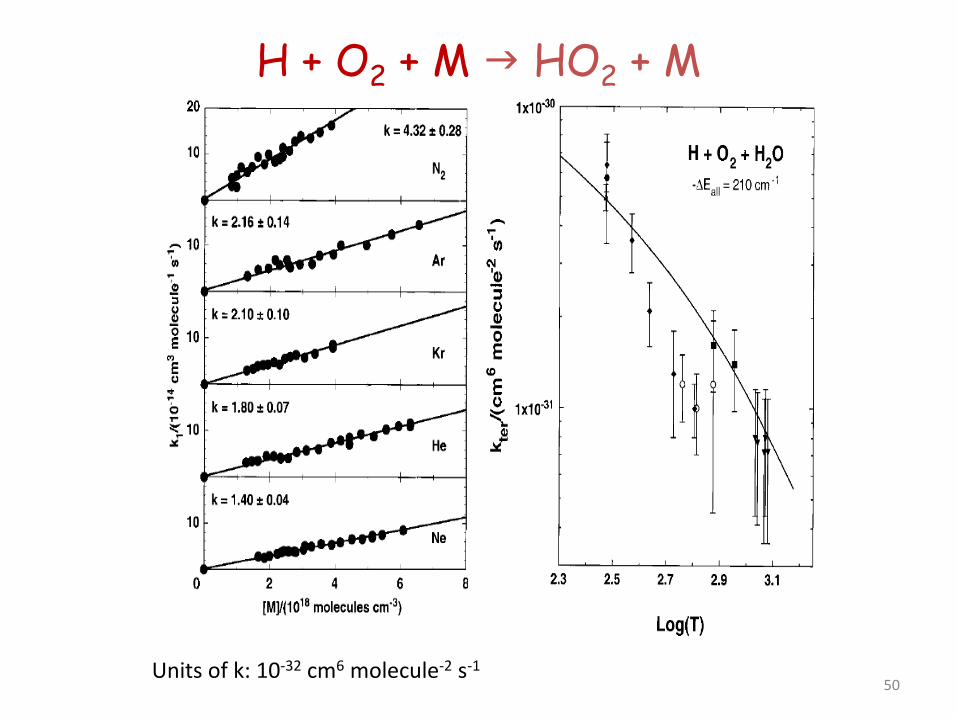
H + O2 + M HO2 + M

Units of k: 10-32 cm6 molecule-2 s-1 50

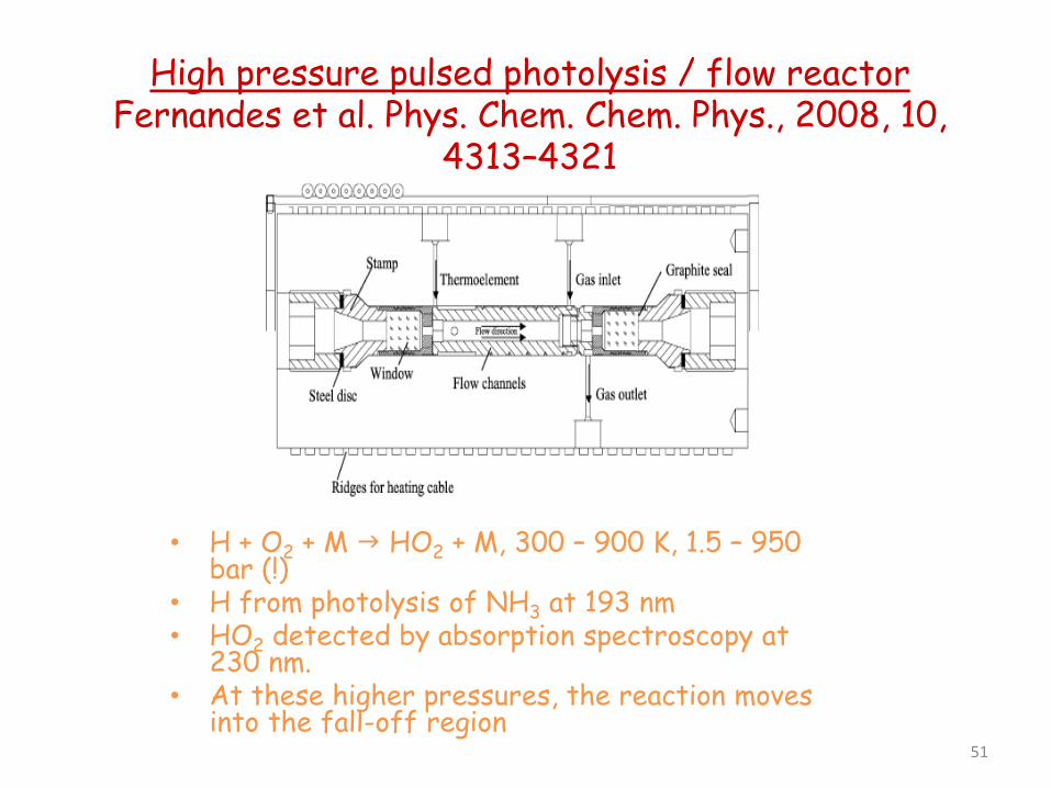
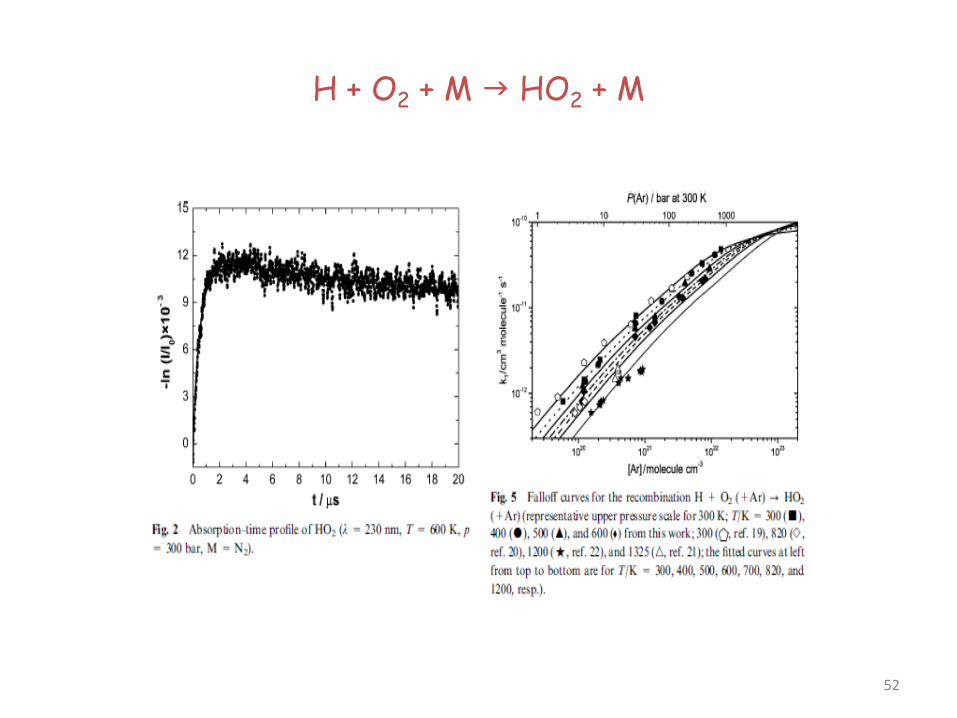
High pressure pulsed photolysis / flow reactor Fernandes et al. Phys. Chem. Chem. Phys., 2008, 10,

4313–4321

• H + O2 + M HO2 + M, 300 – 900 K, 1.5 – 950 bar (!)

• H from photolysis of NH3 at 193 nm • HO2 detected by absorption spectroscopy at

230 nm. • At these higher pressures, the reaction moves

into the fall-off region 51

H + O2 + M HO2 + M

52

H + O2 + M HO2 + M

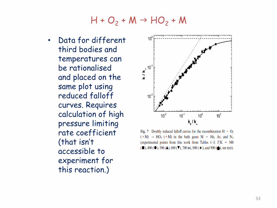
• Data for different third bodies and temperatures can be rationalised and placed on the same plot using reduced falloff curves. Requires calculation of high pressure limiting rate coefficient (that isn’t accessible to experiment for this reaction.)

53

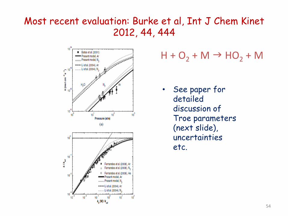
Most recent evaluation: Burke et al, Int J Chem Kinet 2012, 44, 444

• See paper for detailed discussion of Troe parameters (next slide), uncertainties etc.

54

H + O2 + M HO2 + M

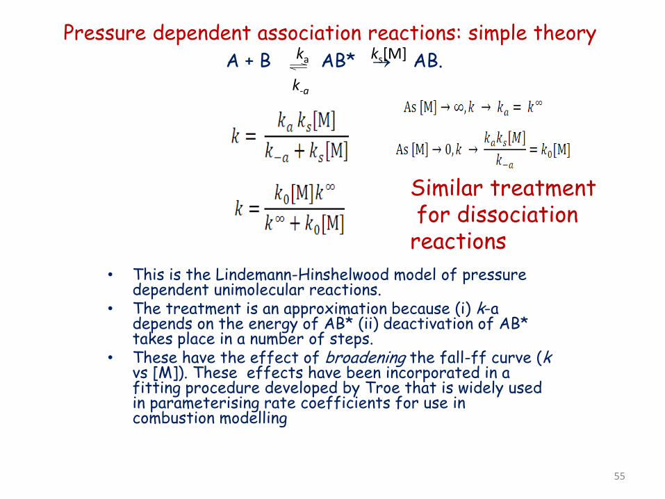
Pressure dependent association reactions: simple theory A + B AB* → AB.

• This is the Lindemann-Hinshelwood model of pressure dependent unimolecular reactions.

• The treatment is an approximation because (i) k-a depends on the energy of AB* (ii) deactivation of AB* takes place in a number of steps.

• These have the effect of broadening the fall-ff curve (k vs [M]). These effects have been incorporated in a fitting procedure developed by Troe that is widely used in parameterising rate coefficients for use in combustion modelling

ka

k-a

ks[M]

Similar treatment for dissociation reactions

55

56

HO2 + HO2 → H2O2 + O2

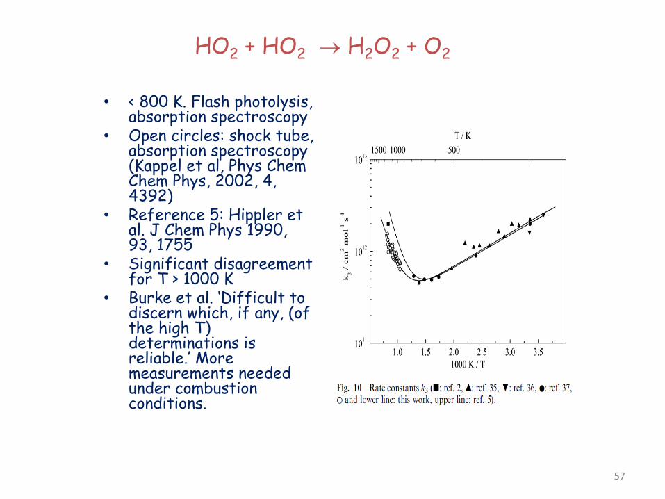
• < 800 K. Flash photolysis, absorption spectroscopy

• Open circles: shock tube, absorption spectroscopy (Kappel et al, Phys Chem Chem Phys, 2002, 4, 4392)

• Reference 5: Hippler et al. J Chem Phys 1990, 93, 1755

• Significant disagreement for T > 1000 K

• Burke et al. ‘Difficult to discern which, if any, (of the high T) determinations is reliable.’ More measurements needed under combustion conditions.

57

H2O2 + M → 2OH + M

• Troe, Combustion and Flame 2011, 158, 594–601 The thermal dissociation/recombination reaction of hydrogen peroxide H2O2=2OH Analysis and representation of the temperature and pressure dependence over wide ranges.

• Reaction is far from the high pressure limit. To obtain a representation of k(T,p), Troe used the statistical adiabatic channel model to calculate k∞, using an ab initio surface (Phys. Chem. Chem. Phys. 10 (2008) 3915; J. Chem. Phys. 111 (1999) 2565.)

• An important aspect of this work was the use of thermodynamics to relate forward and reverse reactions, using the revised enthalpy of formation of OH – see lecture on thermodynamics

58

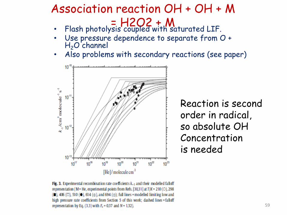
Association reaction OH + OH + M = H2O2 + M

• Flash photolysis coupled with saturated LIF. • Use pressure dependence to separate from O +

H2O channel • Also problems with secondary reactions (see paper)

Reaction is second order in radical, so absolute OH Concentration is needed

59

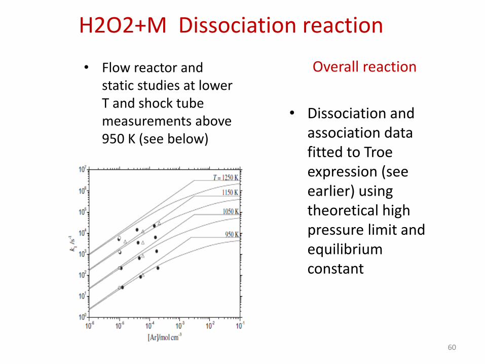
H2O2+M Dissociation reaction

• Flow reactor and static studies at lower T and shock tube measurements above 950 K (see below)

Overall reaction

• Dissociation and association data fitted to Troe expression (see earlier) using theoretical high pressure limit and equilibrium constant

60

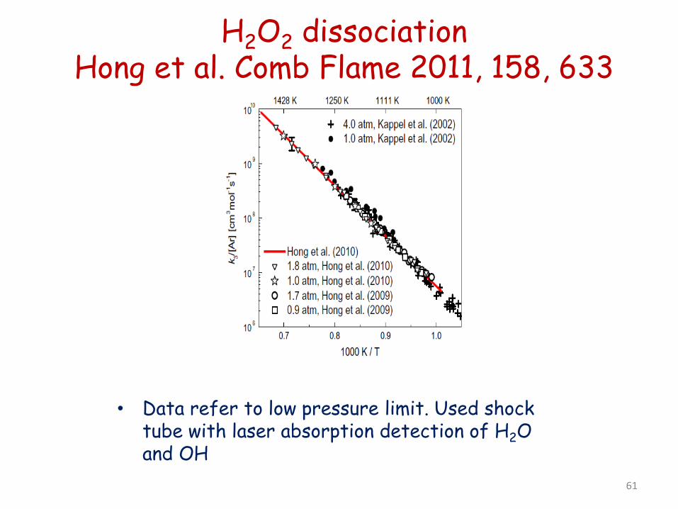
H2O2 dissociation Hong et al. Comb Flame 2011, 158, 633

• Data refer to low pressure limit. Used shock tube with laser absorption detection of H2O and OH 61

Computational Kinetics

Rate Theory

62

63

Start with Born-Oppenheimer approximation • Electrons are light and have high kinetic energies, so they move very fast

compared to the nuclei. So expect nuclei to feel time-averaged force exerted by swarm of electrons.

• Electrons are very quantum mechanical (wave-like, Pauli-exclusion principle). Described by Schroedinger’s Wave Equation.

• Atoms/Nuclei are much heavier, move slowly, act like classical particles (mostly). Treat them with classical mechanics with some corrections.

• So solve the electron-motion problem first, assuming the nuclei are stationary at different geometries R, yielding a potential field V(R) that the nuclei are moving in. • Done with programs such as GAUSSIAN or MOLPRO • Hard problem, so we use basis set expansions & approximations like CCSD(T) or

DFT • How can we use computed V(R) to compute rate coefficients k(T)?

64

Recall how one computes a rate coefficient using classical mechanics First, assume ergodicity, i.e. all phase space (q,p) is equally likely to be sampled, biased only by Boltzmann weighting and conservation laws. Divide phase space into “reactant” and “product” regions by specifying dividing surface s±(q)=0. Sample from “reactant” phase space, and find the probability a trajectory moves from reactant to product in short time dt. The fraction that changes from reactant to product is related to the rate coefficient.

65

66

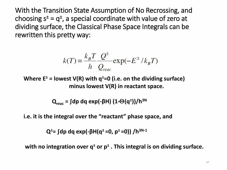
With the Transition State Assumption of No Recrossing, and choosing s± = q±, a special coordinate with value of zero at dividing surface, the Classical Phase Space Integrals can be rewritten this pretty way:

Where E± = lowest V(R) with q±=0 (i.e. on the dividing surface) minus lowest V(R) in reactant space. Qreac = ∫dp dq exp(-βH) (1-Θ(q±))/h3N i.e. it is the integral over the “reactant” phase space, and Q±= ∫dp dq exp(-βH(q± =0, p± =0)) /h3N-1 with no integration over q± or p± . This integral is on dividing surface.

67

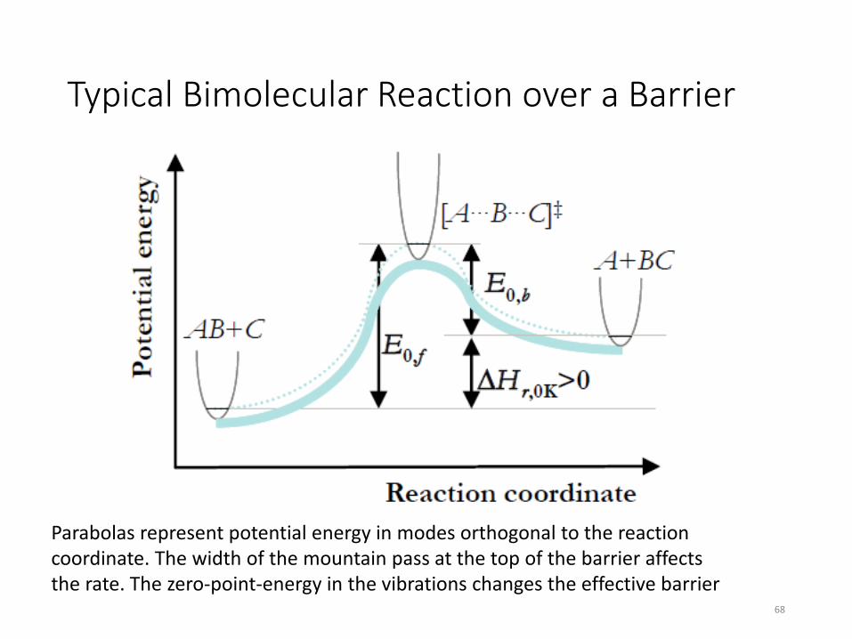
Typical Bimolecular Reaction over a Barrier

68

Parabolas represent potential energy in modes orthogonal to the reaction coordinate. The width of the mountain pass at the top of the barrier affects the rate. The zero-point-energy in the vibrations changes the effective barrier

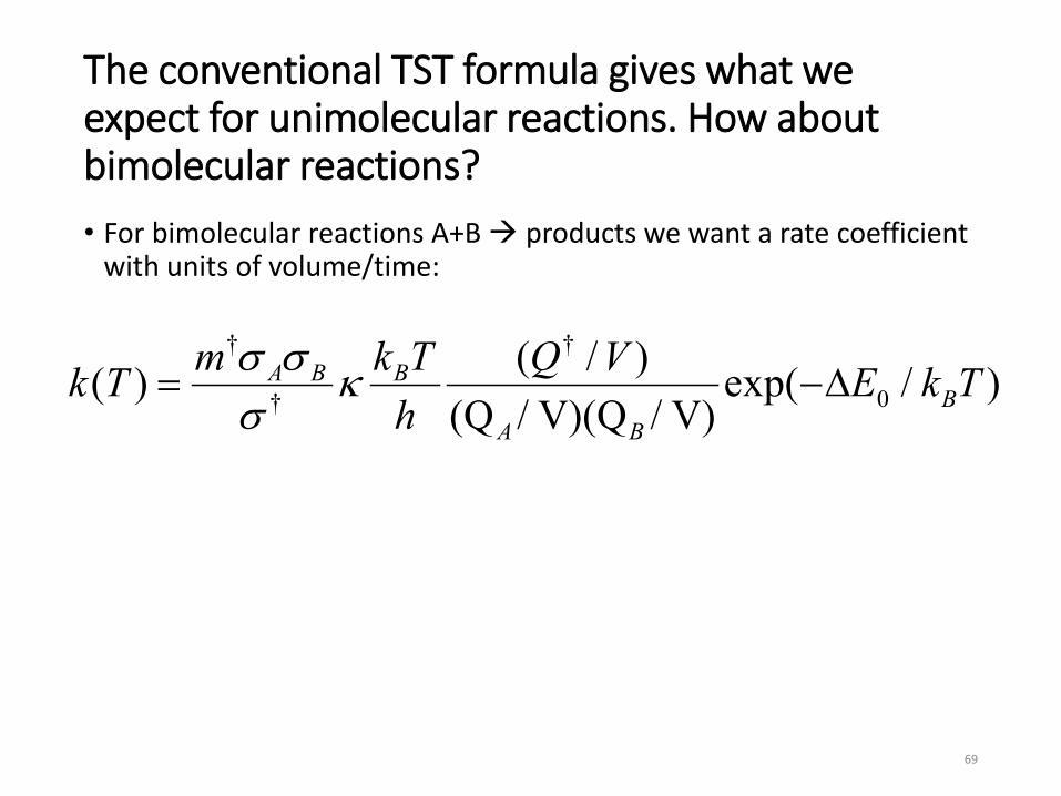
The conventional TST formula gives what we expect for unimolecular reactions. How about bimolecular reactions? • For bimolecular reactions A+B products we want a rate coefficient

with units of volume/time:

69

† †

0†( / )( ) exp( / )

(Q / V)(Q / V)A B B

BA B

m k T Q Vk T E k Th

σ σ κσ

= −∆

Arrhenius Dependence on T comes from Boltzmann population. Only collisions with energy above the reaction barrier can react. Their population grows as exp(-Ea/kBT)

70

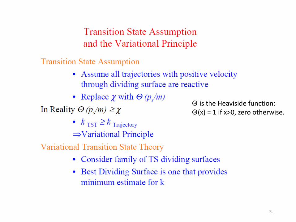
Θ is the Heaviside function: Θ(x) = 1 if x>0, zero otherwise.

71

Why use Transition State Theory?

72

However, we cannot completely ignore quantum mechanics for atomic motions… • There is an exact quantum mechanical operator corresponding to the

classical phase space integrals, with and without the transition state assumption, see W.H. Miller papers. • Exact version is expensive, biggest case done so far is CH4 + H, by Manthe. • Several different approximations to the exact formula have been proposed,

no consensus yet on best way to proceed. • Some people just ignore the quantum mechanics, and do classical

calculations, either phase space integrals or molecular dynamics. But neglecting zero-point-energy of vibrations is a big approximation, and there are also issues about rare-event sampling.

• Several patches to molecular dynamics try to include zero point energy approximately. You may be interested in the RPMD method (see RPMDRate program) which avoids some of the TS approximations.

• If you are willing to make the TS approximations and some other approximations, you get a cheap and convenient recipe for computing rates…

73

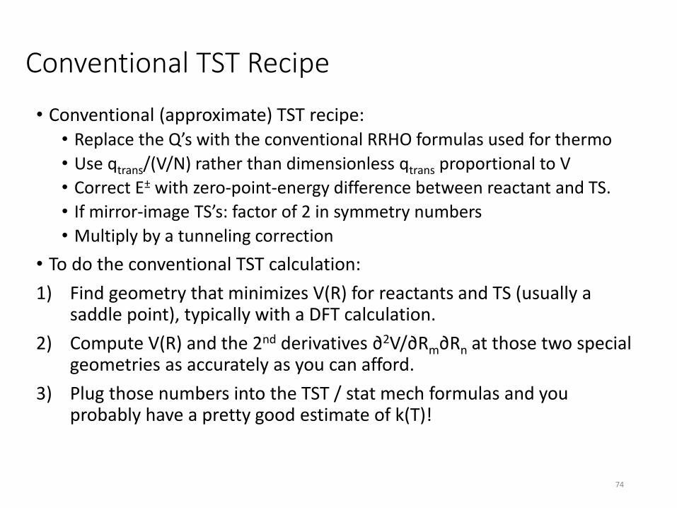
Conventional TST Recipe

• Conventional (approximate) TST recipe: • Replace the Q’s with the conventional RRHO formulas used for thermo • Use qtrans/(V/N) rather than dimensionless qtrans proportional to V • Correct E± with zero-point-energy difference between reactant and TS. • If mirror-image TS’s: factor of 2 in symmetry numbers • Multiply by a tunneling correction

• To do the conventional TST calculation: 1) Find geometry that minimizes V(R) for reactants and TS (usually a

saddle point), typically with a DFT calculation. 2) Compute V(R) and the 2nd derivatives ∂2V/∂Rm∂Rn at those two special

geometries as accurately as you can afford. 3) Plug those numbers into the TST / stat mech formulas and you

probably have a pretty good estimate of k(T)!

74

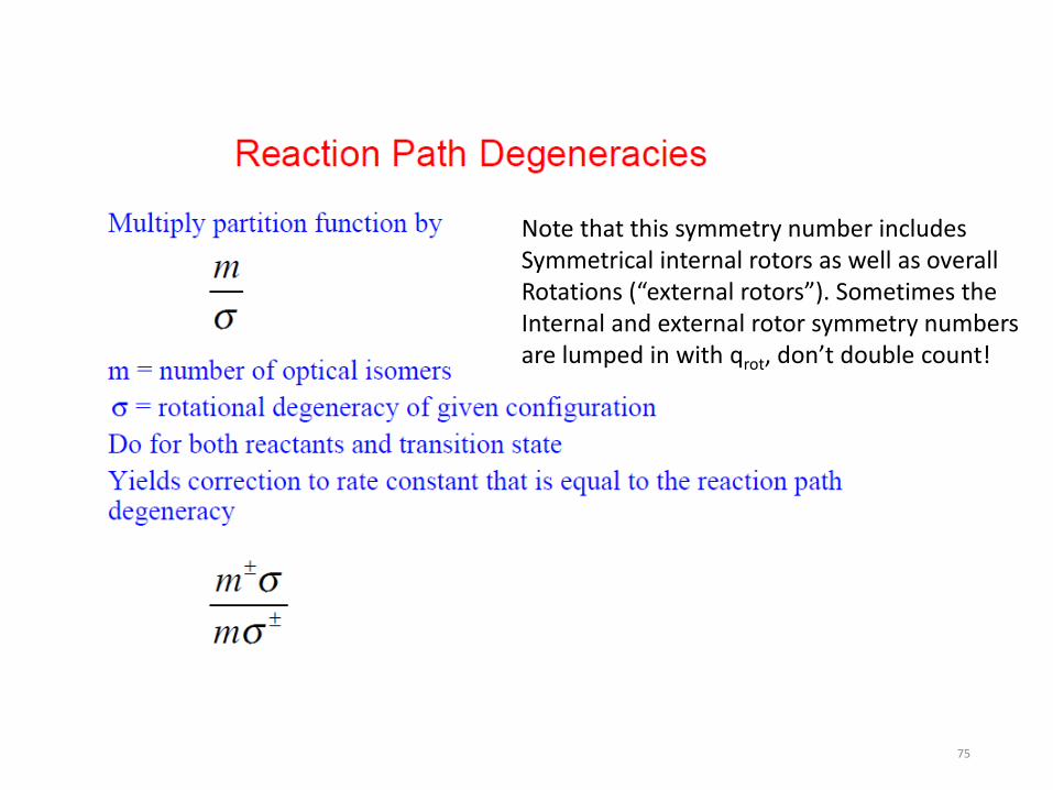
Note that this symmetry number includes Symmetrical internal rotors as well as overall Rotations (“external rotors”). Sometimes the Internal and external rotor symmetry numbers are lumped in with qrot, don’t double count!

75

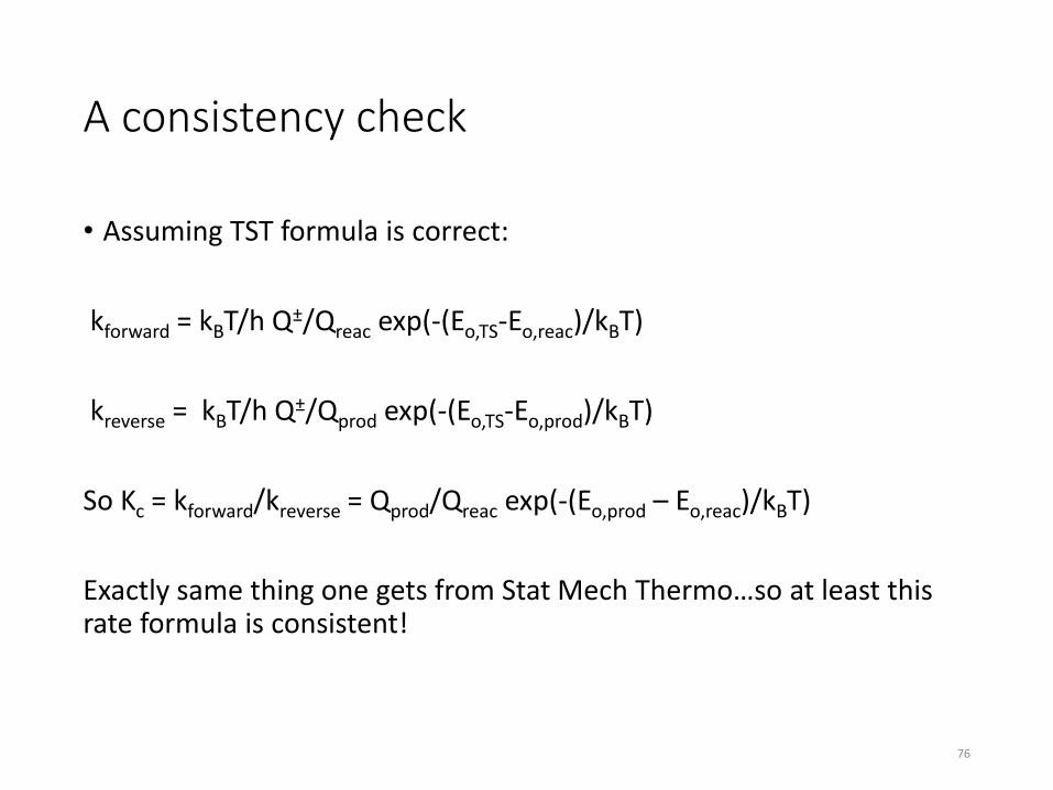
A consistency check

• Assuming TST formula is correct: kforward = kBT/h Q±/Qreac exp(-(Eo,TS-Eo,reac)/kBT) kreverse = kBT/h Q±/Qprod exp(-(Eo,TS-Eo,prod)/kBT) So Kc = kforward/kreverse = Qprod/Qreac exp(-(Eo,prod – Eo,reac)/kBT) Exactly same thing one gets from Stat Mech Thermo…so at least this rate formula is consistent!

76

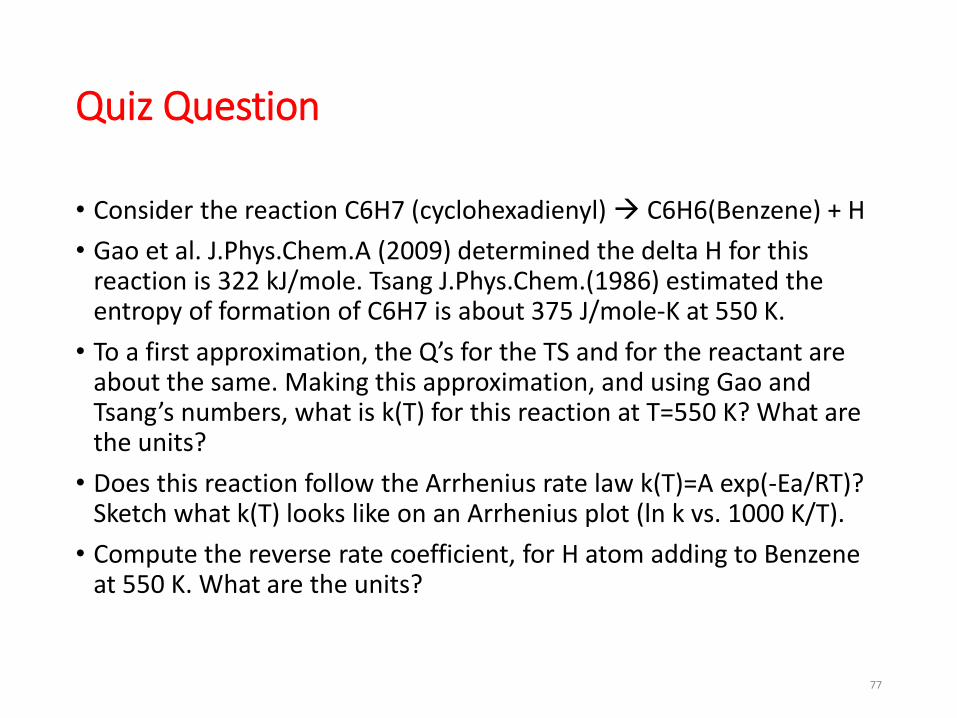
Quiz Question

• Consider the reaction C6H7 (cyclohexadienyl) C6H6(Benzene) + H • Gao et al. J.Phys.Chem.A (2009) determined the delta H for this

reaction is 322 kJ/mole. Tsang J.Phys.Chem.(1986) estimated the entropy of formation of C6H7 is about 375 J/mole-K at 550 K.

• To a first approximation, the Q’s for the TS and for the reactant are about the same. Making this approximation, and using Gao and Tsang’s numbers, what is k(T) for this reaction at T=550 K? What are the units?

• Does this reaction follow the Arrhenius rate law k(T)=A exp(-Ea/RT)? Sketch what k(T) looks like on an Arrhenius plot (ln k vs. 1000 K/T).

• Compute the reverse rate coefficient, for H atom adding to Benzene at 550 K. What are the units?

77

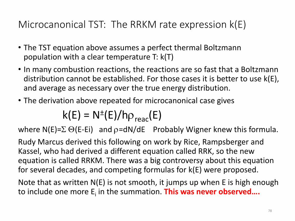
Microcanonical TST: The RRKM rate expression k(E)

• The TST equation above assumes a perfect thermal Boltzmann population with a clear temperature T: k(T)

• In many combustion reactions, the reactions are so fast that a Boltzmann distribution cannot be established. For those cases it is better to use k(E), and average as necessary over the true energy distribution.

• The derivation above repeated for microcanonical case gives

k(E) = N±(E)/hρreac(E) where N(E)=Σ Θ(E-Ei) and ρ=dN/dE Probably Wigner knew this formula. Rudy Marcus derived this following on work by Rice, Rampsberger and Kassel, who had derived a different equation called RRK, so the new equation is called RRKM. There was a big controversy about this equation for several decades, and competing formulas for k(E) were proposed. Note that as written N(E) is not smooth, it jumps up when E is high enough to include one more Ei in the summation. This was never observed….

78

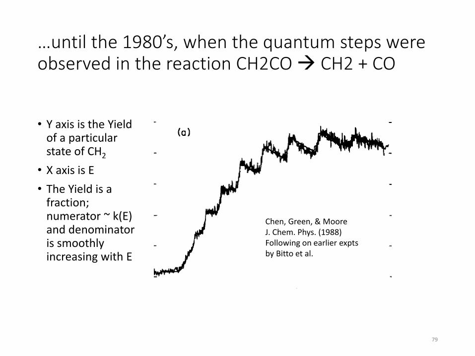
…until the 1980’s, when the quantum steps were observed in the reaction CH2CO CH2 + CO

• Y axis is the Yield of a particular state of CH2

• X axis is E • The Yield is a

fraction; numerator ~ k(E) and denominator is smoothly increasing with E

Chen, Green, & Moore J. Chem. Phys. (1988) Following on earlier expts by Bitto et al.

79

Now everyone believes k(E) = N±(E)/hρreac(E)

• W.H. Miller has derived the exact quantum mechanical operator for N, including tunneling etc. and shown it gives k(E). The exact N gives steps rounded off a bit by tunneling.

• A Boltzmann average of k(E) gives k(T) as expected k(T) = 1/Qreac ∫ρreac(E)k(E) exp(-E/kBT)dE = 1/hQreac ∫N±(E)exp(-E/kBT)dE integrate by parts = kBT/hQreac ∫ρTS(E)exp(-E/kBT)dE = kBT/h Q±/Qreac exp(-β∆E) • Microcanonical detailed balance: ρreac(E)kforward(E) = ρprod(E)kreverse(E) (= N(E)/h )

80

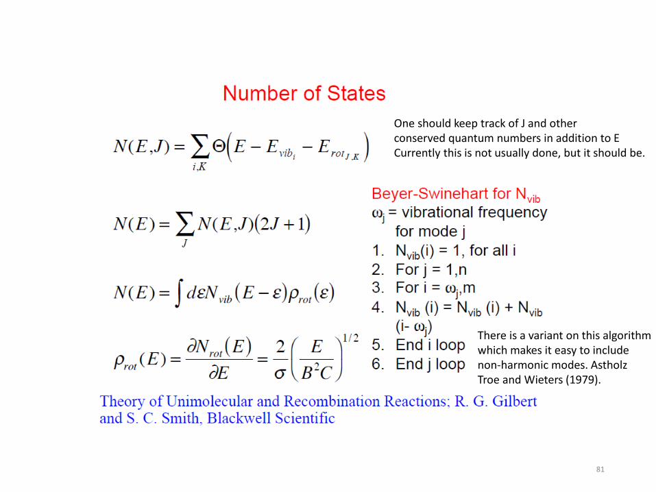
One should keep track of J and other conserved quantum numbers in addition to E Currently this is not usually done, but it should be.

There is a variant on this algorithm which makes it easy to include non-harmonic modes. Astholz Troe and Wieters (1979).

81

82

See also recent papers by Truhlar on a way to handle coupled torsions. This problem is not completely resolved

83

84

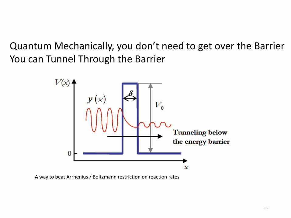
Quantum Mechanically, you don’t need to get over the Barrier You can Tunnel Through the Barrier

A way to beat Arrhenius / Boltzmann restriction on reaction rates

85

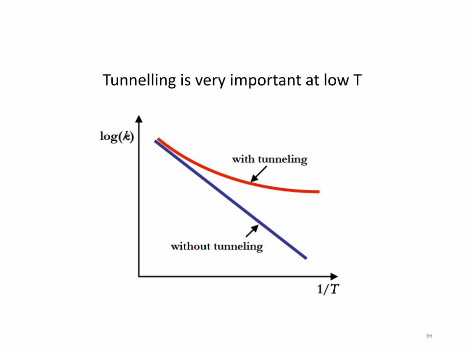
Tunnelling is very important at low T

86

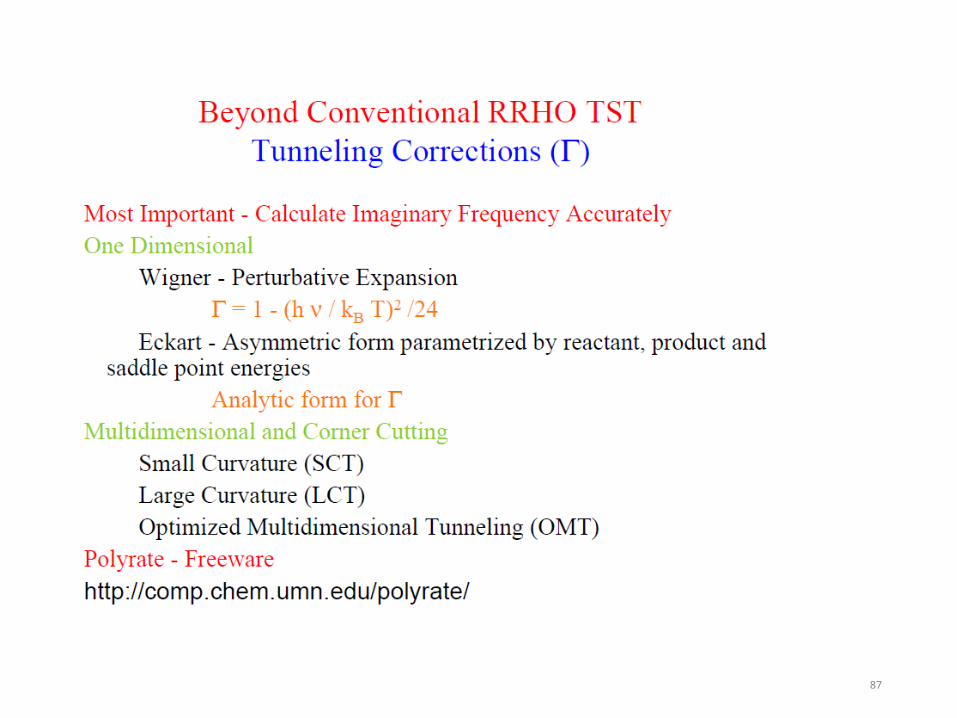
87

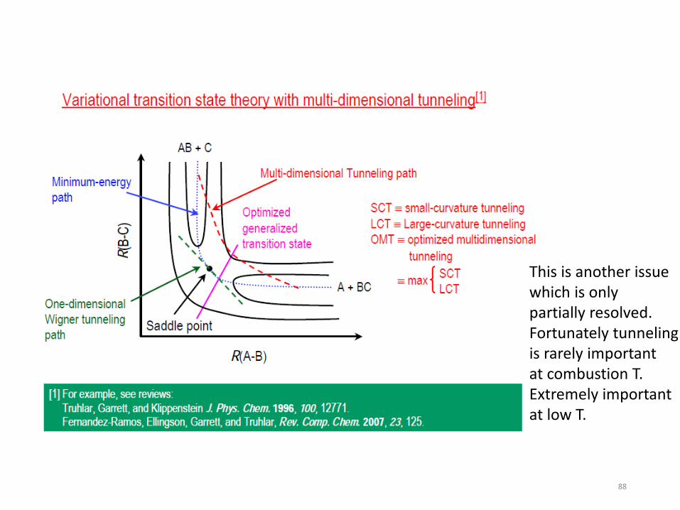
This is another issue which is only partially resolved. Fortunately tunneling is rarely important at combustion T. Extremely important at low T.

88

Summary of Rate Theory • Almost all methods start from Born-Oppenheimer V(R)

• Crucially depend on accuracy of the (approximate) V(R) • Errors in V(R) directly lead to errors in Ea, can give big errors. • Modern methods can achieve pretty accurate reaction barriers (but

not always) • Classical Mechanics Rate Theory can be transformed into Quantum

Mechanics, but exact quantum mechanics usually too hard to solve • Some simple approximations convert Classical Mechanics into

Conventional Transition State Theory, which is much less expensive to compute. Requires V(R) at only two points. • With reasonable V(R) almost always gives k(T) within order of

magnitude of true value. Sometimes better than factor of 2. • Several of the simple approximations in Conventional Transition State

Theory are not quite good enough, give small but significant errors. Improved approximations are under development.

89

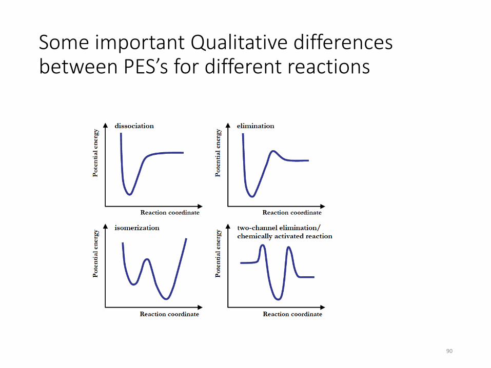
Some important Qualitative differences between PES’s for different reactions

90

Lesson 4: Ignition

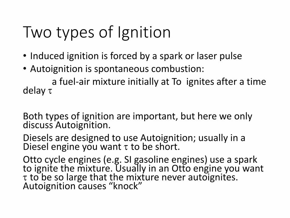
Two types of Ignition • Induced ignition is forced by a spark or laser pulse • Autoignition is spontaneous combustion: a fuel-air mixture initially at To ignites after a time delay τ Both types of ignition are important, but here we only discuss Autoignition. Diesels are designed to use Autoignition; usually in a Diesel engine you want τ to be short. Otto cycle engines (e.g. SI gasoline engines) use a spark to ignite the mixture. Usually in an Otto engine you want τ to be so large that the mixture never autoignites. Autoignition causes “knock”

Several different reasons to care about Low-T Combustion Chemistry

• Spark-Ignited Engine power & efficiency strongly constrained by knock (i.e. unwanted autoignition).

• Diesel ignition delay about 50% due to chemistry • So civilian Diesel fuel has a cetane spec • Many of the challenges in Military diesels are because JP-8 does

not have a tight cetane spec, & has high fuel variability • “LTC” engine concepts very sensitive to fuel ignition, add a

control element to adjust (e.g. duel fuel or EGR) • Provide large increase in efficiency at ~constant power density:

huge potential value to society (and to military) • Viability of Alternative Fuels for civilian ground transport • Jet engines: We think ignition & re-light sensitive to LTC

but note a spark is involved. Unwanted autoignition at high T3.

W.H. Green, MIT

Because it is so important, Combustion Chemistry in general, including Low-T Ignition, has been well-studied.

Many reviews of low-T combustion chemistry, e.g.: • S.W. Benson, PECS (1981) • C.K. Westbrook, PECS (1984) & PECS (2000) • Walker & Morley, Comp. Chem. Kinet. (1997) • F. Battin-Leclerc, PECS (2008) • Zador, Taatjes, & Fernandes, PECS (2011) Community has achieved very detailed quantitative understanding of several simple fuels, with demonstrated accuracy for large number of observables. But still some aspects of these models are incomplete, and many of the numbers have significant uncertainties. This talk is just my perspective on what is important, not the full story by any means…

W.H. Green, MIT

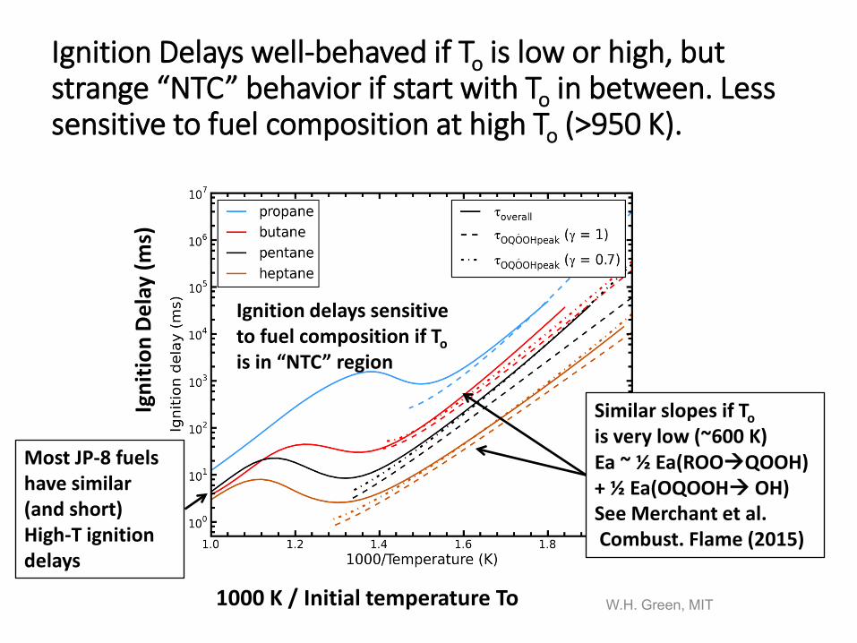
Ignition Delays well-behaved if To is low or high, but strange “NTC” behavior if start with To in between. Less sensitive to fuel composition at high To (>950 K).

Similar slopes if To is very low (~600 K) Ea ~ ½ Ea(ROOQOOH) + ½ Ea(OQOOH OH) See Merchant et al. Combust. Flame (2015)

1000 K / Initial temperature To

Igni

tion

Dela

y (m

s)

Most JP-8 fuels have similar (and short) High-T ignition delays

Ignition delays sensitive to fuel composition if To is in “NTC” region

W.H. Green, MIT

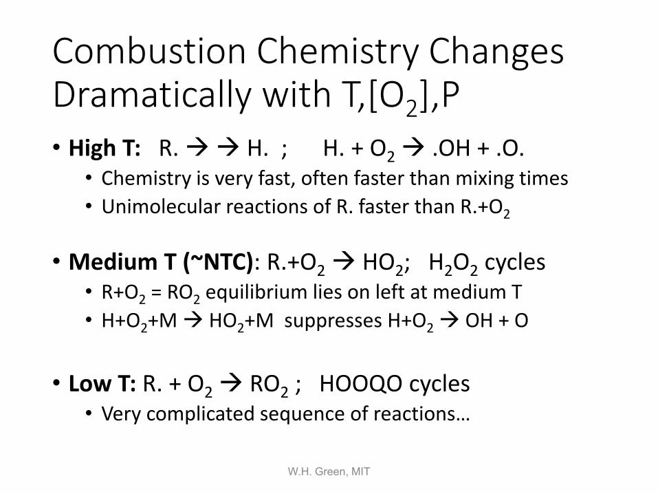
Combustion Chemistry Changes Dramatically with T,[O2],P • High T: R. H. ; H. + O2 .OH + .O.

• Chemistry is very fast, often faster than mixing times • Unimolecular reactions of R. faster than R.+O2

• Medium T (~NTC): R.+O2 HO2; H2O2 cycles • R+O2 = RO2 equilibrium lies on left at medium T • H+O2+M HO2+M suppresses H+O2 OH + O

• Low T: R. + O2 RO2 ; HOOQO cycles • Very complicated sequence of reactions…

W.H. Green, MIT

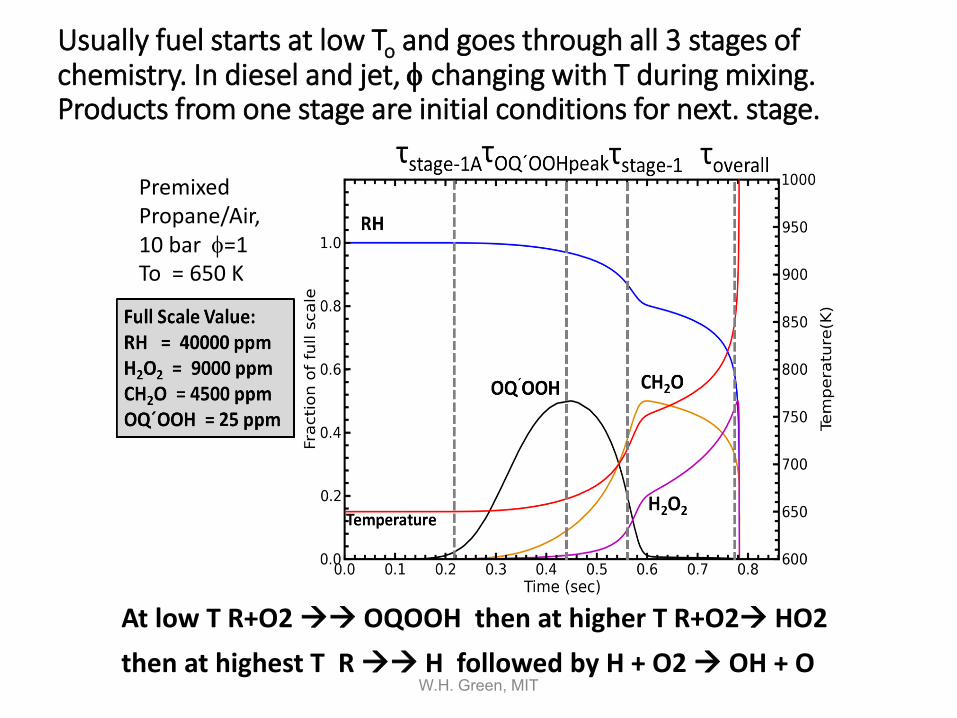
Usually fuel starts at low To and goes through all 3 stages of chemistry. In diesel and jet, φ changing with T during mixing. Products from one stage are initial conditions for next. stage.

At low T R+O2 OQOOH then at higher T R+O2 HO2 then at highest T R H followed by H + O2 OH + O

Premixed Propane/Air, 10 bar φ=1 To = 650 K

W.H. Green, MIT

High T (>1000 K) ignition pretty well understood… • High T Ignition delays can be predicted

quantitatively with detailed models. • Significant challenge is handling complexity of real

fuels…but fortunately fuel decomposition nicely separates from the small-molecule chemistry (e.g. see work by Stanford team)

• Main challenges at high T not ignition, but accurately modeling/predicting soot formation, & correctly handling chemistry-flow (turbulence) interactions.

W.H. Green, MIT

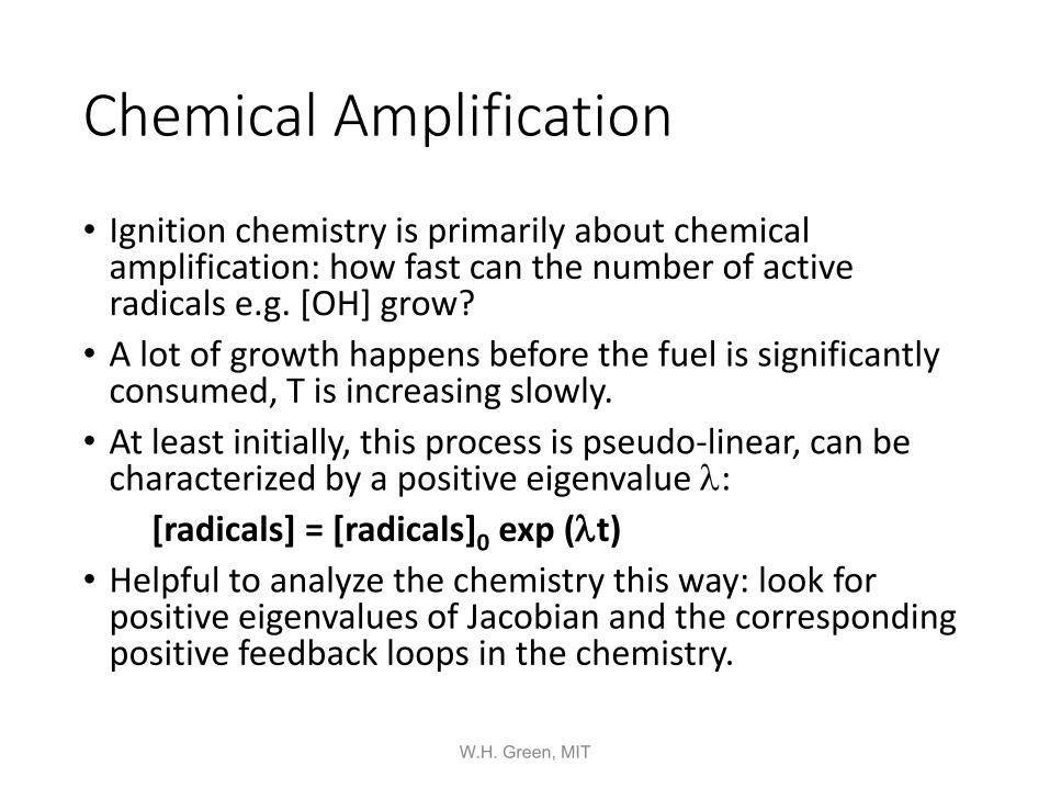
Chemical Amplification

• Ignition chemistry is primarily about chemical amplification: how fast can the number of active radicals e.g. [OH] grow?

• A lot of growth happens before the fuel is significantly consumed, T is increasing slowly.

• At least initially, this process is pseudo-linear, can be characterized by a positive eigenvalue λ:

[radicals] = [radicals]0 exp (λt) • Helpful to analyze the chemistry this way: look for

positive eigenvalues of Jacobian and the corresponding positive feedback loops in the chemistry.

W.H. Green, MIT

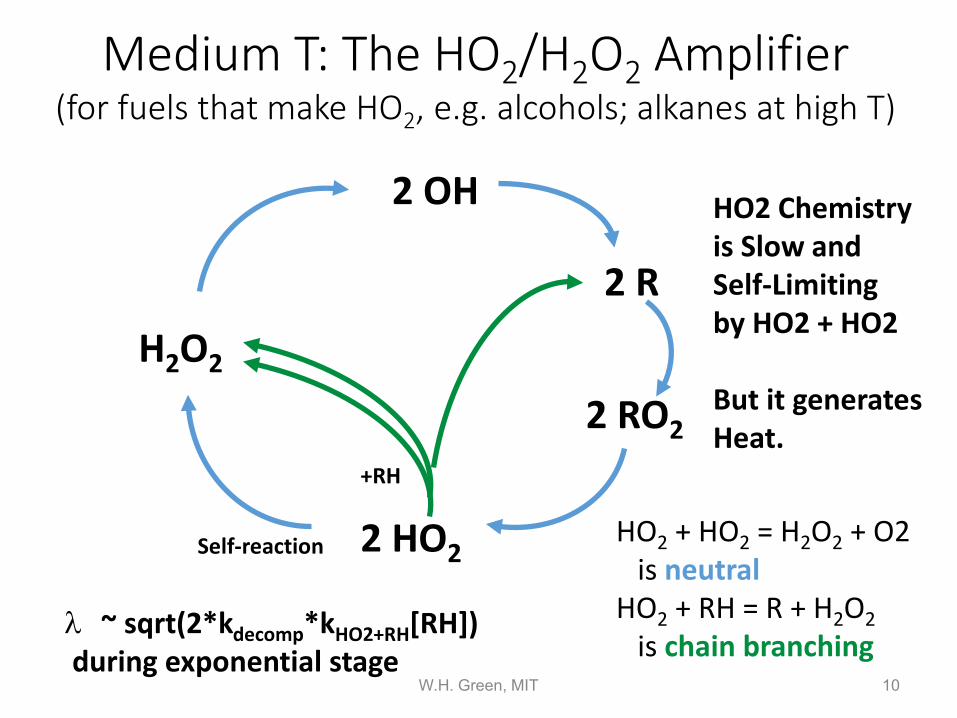
Medium T: The HO2/H2O2 Amplifier (for fuels that make HO2, e.g. alcohols; alkanes at high T)

H2O2

2 OH

2 R

2 HO2 HO2 + HO2 = H2O2 + O2 is neutral HO2 + RH = R + H2O2 is chain branching

λ ~ sqrt(2*kdecomp*kHO2+RH[RH]) during exponential stage

2 RO2

10 W.H. Green, MIT

+RH

Self-reaction

HO2 Chemistry is Slow and Self-Limiting by HO2 + HO2 But it generates Heat.

Medium T (~750-1000 K) ignition chemistry is understood moderately well. Sensitive to fuel, T(t), φ(t), P(t), heat losses. • We think we know most/all the important reactions.

• HO2 reacts in several ways, some rates not conclusively nailed down, e.g.

• HO2 + R RH + O2 versus HO2 + R RO + OH • Sensitive to HO2 + RH but OH + RH is main fuel consumer

• Ignition delays sensitive to transitions from low-T to medium-T, and medium-T to high-T mechanisms; carry-over of reactive species formed by the earlier chemistry. T(t), [RH], [O2], P(t) all matter.

• Significant low-T chemistry occurs as fuel is raised to reaction temperature (e.g. in RCM or flow tube).

• hard to know what discrepancies between model and experiment are due to medium-T vs. low-T chemistry.

W.H. Green, MIT

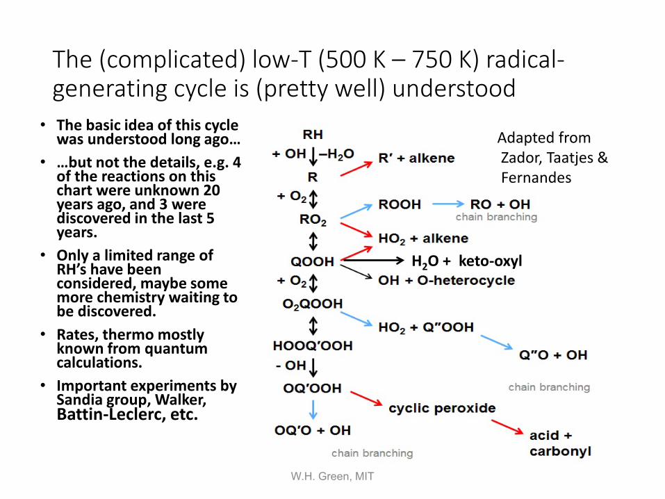
The (complicated) low-T (500 K – 750 K) radical-generating cycle is (pretty well) understood

• The basic idea of this cycle was understood long ago…

• …but not the details, e.g. 4 of the reactions on this chart were unknown 20 years ago, and 3 were discovered in the last 5 years.

• Only a limited range of RH’s have been considered, maybe some more chemistry waiting to be discovered.

• Rates, thermo mostly known from quantum calculations.

• Important experiments by Sandia group, Walker, Battin-Leclerc, etc.

H2O + keto-oxyl

Adapted from Zador, Taatjes & Fernandes

W.H. Green, MIT

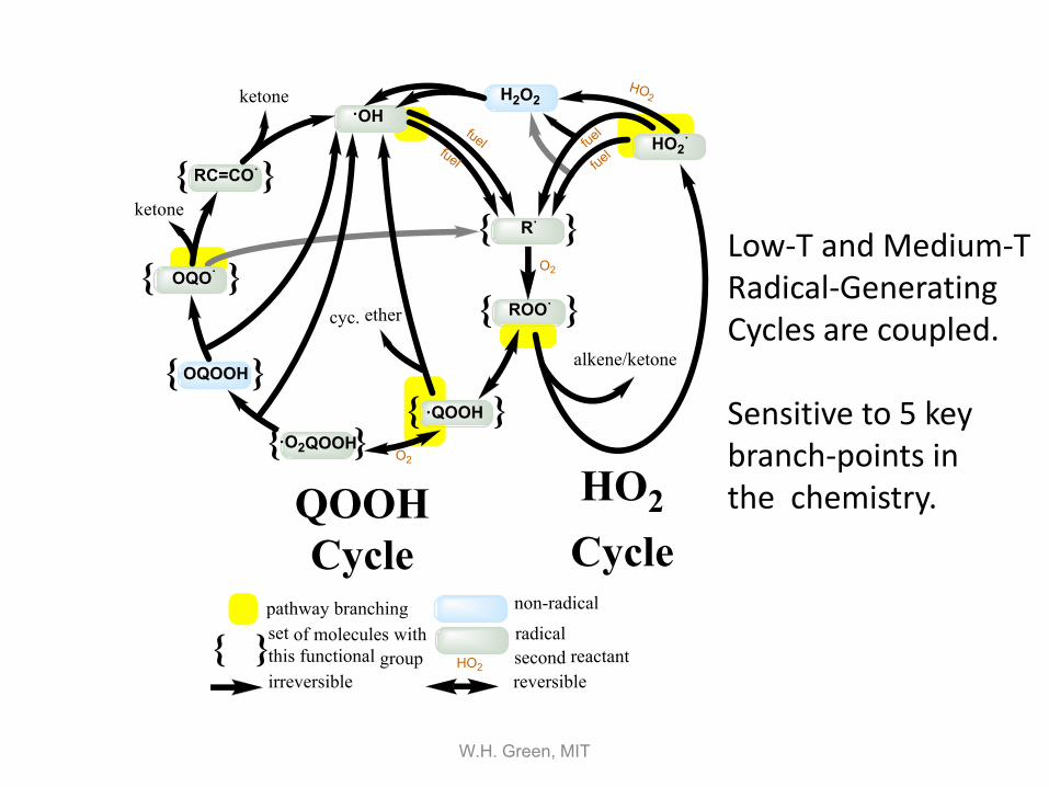
HO2 Cycle

QOOH Cycle

·OHHO2

·

R·{ }

ROO·{ }

·QOOH{ }·O2QOOH{ }

OQOOH{ }

OQO·{ }

RC=CO·{ }

cyc. ether

alkene/ketone

H2O2HO2

fuel

O2

O2

fuel

fuelfuel

ketone

ketone

QOOH Cycle

HO2 Cycle

{ }pathway branchingset of molecules withthis functional group

non-radical

radicalHO2

second reactantirreversible reversible

Low-T and Medium-T Radical-Generating Cycles are coupled. Sensitive to 5 key branch-points in the chemistry.

W.H. Green, MIT

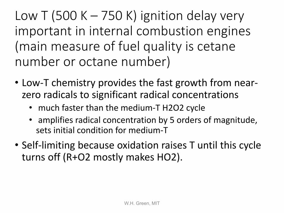
Low T (500 K – 750 K) ignition delay very important in internal combustion engines (main measure of fuel quality is cetane number or octane number) • Low-T chemistry provides the fast growth from near-

zero radicals to significant radical concentrations • much faster than the medium-T H2O2 cycle • amplifies radical concentration by 5 orders of magnitude,

sets initial condition for medium-T

• Self-limiting because oxidation raises T until this cycle turns off (R+O2 mostly makes HO2).

W.H. Green, MIT

Low T ignition not as well understood as high and medium T chemistry • Empirical approaches e.g. “blending octane” and “IQT

derived cetane number” have limited applicability • Only for specific tested conditions • Limited ability to predict effect of changing fuel blend.

• Many distinct reactive intermediates. Still discovering that additional reactions and species are important, at least in some cases.

• Peroxy chemistry challenging for both experimentalists and quantum chemists, so rate and thermo parameters not as well known as for hydrocarbon chemistry.

W.H. Green, MIT

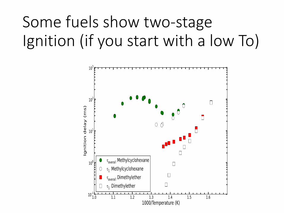
Some fuels show two-stage Ignition (if you start with a low To)

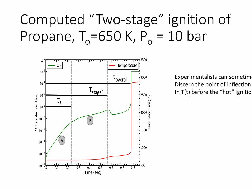
Computed “Two-stage” ignition of Propane, To=650 K, Po = 10 bar

Experimentalists can sometime Discern the point of inflection In T(t) before the “hot” ignition

Good news: Low-T is not quite as bad as one might fear • Clear stages dominated by different physics

• Natural simplifications • One stage usually controls the ignition delay

• Only a few reactive intermediates matter • Drastically reduces number of rate coefficients required • Fuel ignition characterized by just a few parameters

18 W.H. Green, MIT

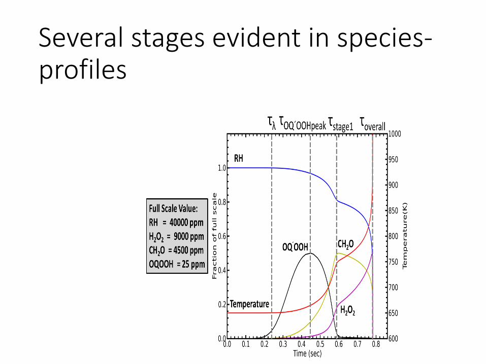
Several stages evident in species-profiles

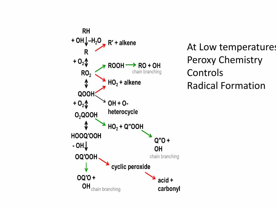
At Low temperatures Peroxy Chemistry Controls Radical Formation

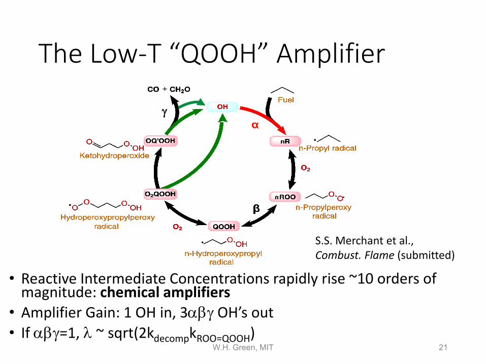
The Low-T “QOOH” Amplifier

• Reactive Intermediate Concentrations rapidly rise ~10 orders of magnitude: chemical amplifiers

• Amplifier Gain: 1 OH in, 3αβγ OH’s out • If αβγ=1, λ ~ sqrt(2kdecompkROO=QOOH)

γ

21 W.H. Green, MIT

S.S. Merchant et al., Combust. Flame (submitted)

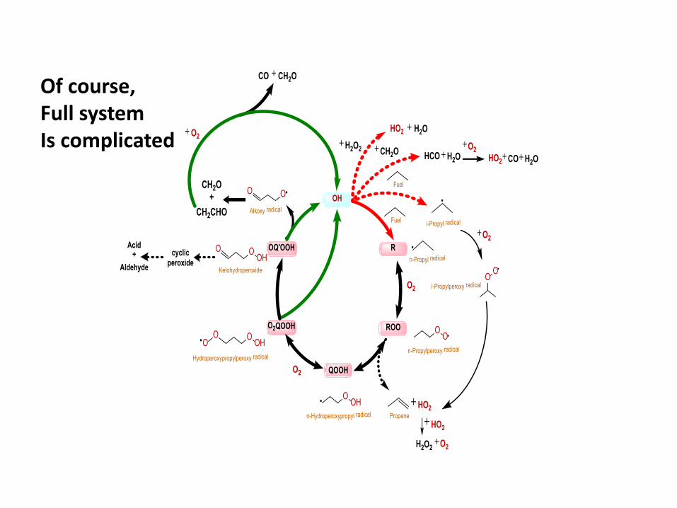
OH

ROO

QOOH

O2QOOH

OQ'OOH R

Fuel

Propene

n-Propyl radical

n-Propylperoxy radical

n-Hydroperoxypropyl radical

Ketohydroperoxide

Alkoxy radical

Hydroperoxypropylperoxy radical

HO2

CH2O +

CH2CHOi-Propyl radical

O O

O O

O OH

O OHO

O

O OHO

OOFuel

CH2O HCO HO2 COH2O2

HO2 H2O

i-Propylperoxy radical

H2O2

O2

O2

+

H2O+ H2O

cyclicperoxide

Acid +

Aldehyde

+

+ ++ + O2+

O2+

O2+

CO CH2O+

O2+HO2+

Of course, Full system Is complicated

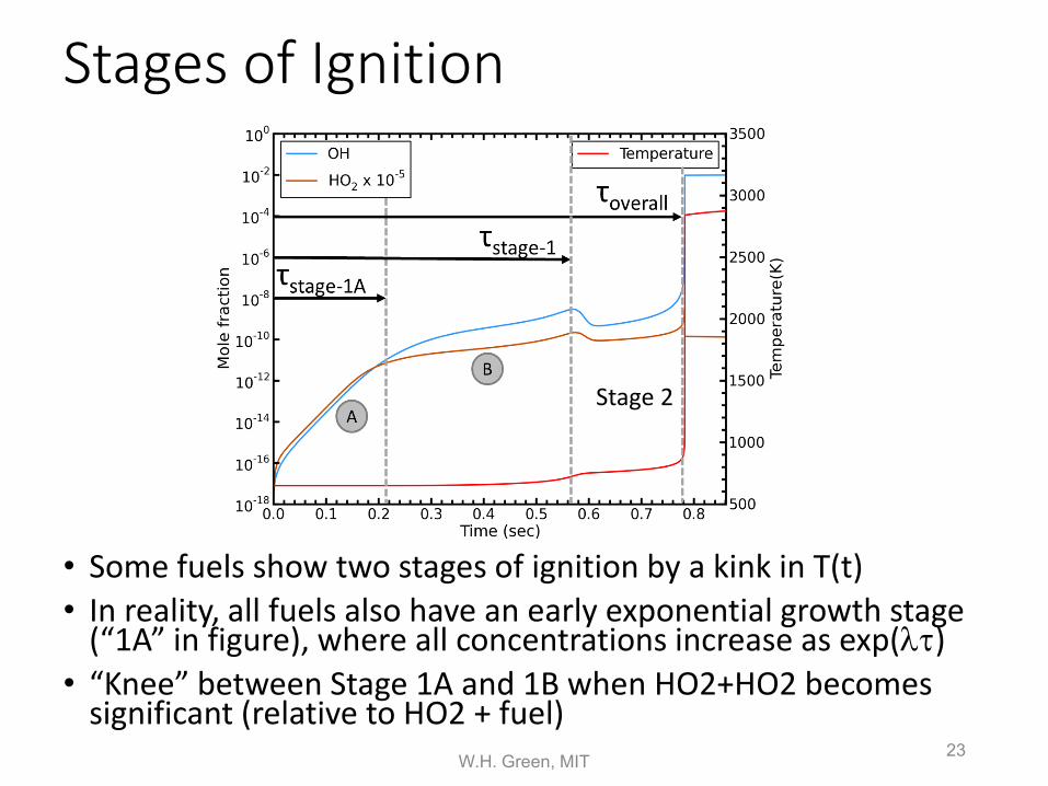
• Some fuels show two stages of ignition by a kink in T(t) • In reality, all fuels also have an early exponential growth stage

(“1A” in figure), where all concentrations increase as exp(λτ) • “Knee” between Stage 1A and 1B when HO2+HO2 becomes

significant (relative to HO2 + fuel)

Stages of Ignition

Stage 2

23 W.H. Green, MIT

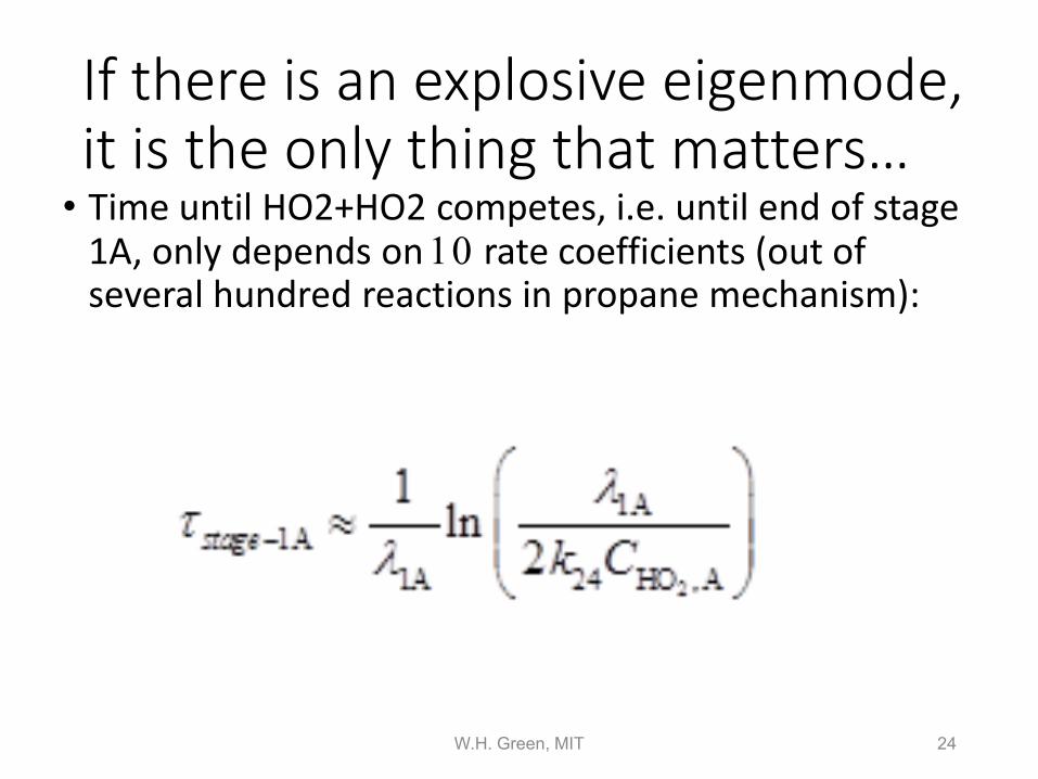
If there is an explosive eigenmode, it is the only thing that matters…

• Time until HO2+HO2 competes, i.e. until end of stage 1A, only depends on 10 rate coefficients (out of several hundred reactions in propane mechanism):

24 W.H. Green, MIT

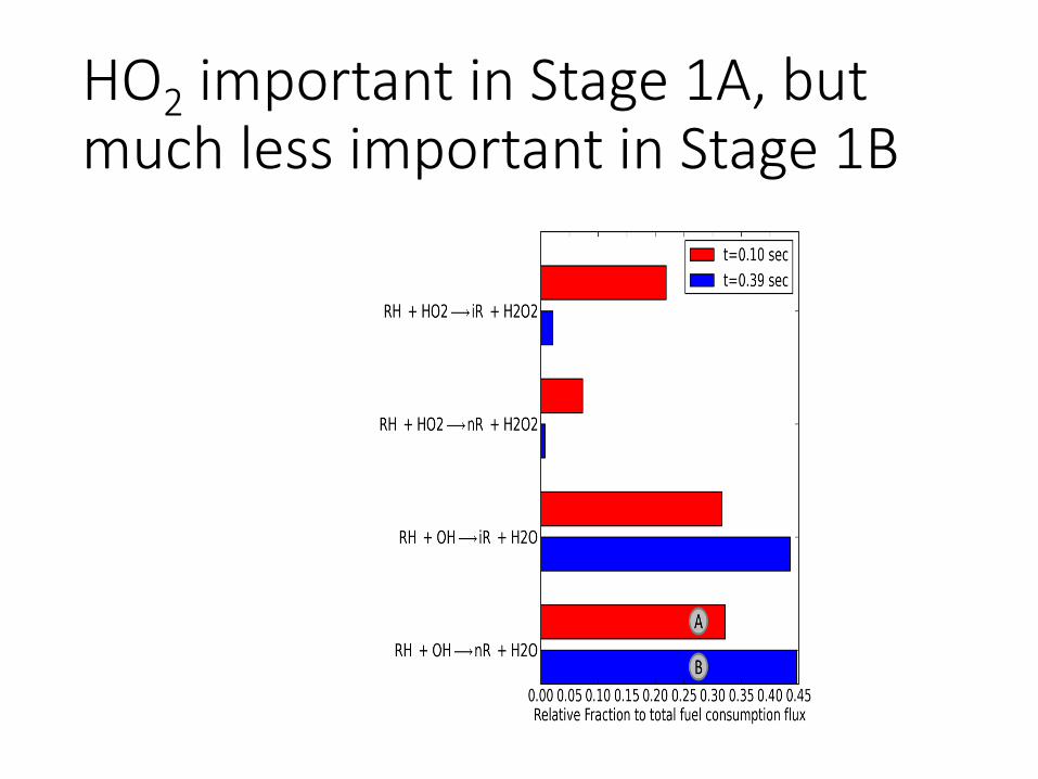
HO2 important in Stage 1A, but much less important in Stage 1B

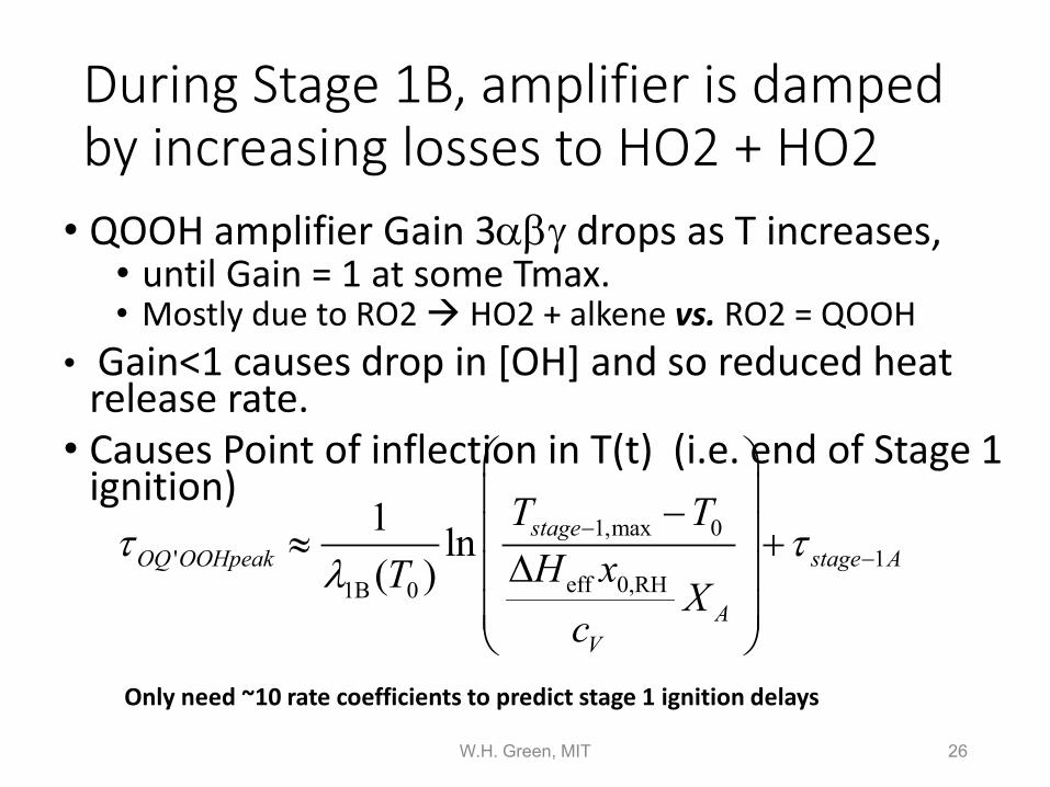
During Stage 1B, amplifier is damped by increasing losses to HO2 + HO2

• QOOH amplifier Gain 3αβγ drops as T increases, • until Gain = 1 at some Tmax. • Mostly due to RO2 HO2 + alkene vs. RO2 = QOOH

• Gain<1 causes drop in [OH] and so reduced heat release rate.

• Causes Point of inflection in T(t) (i.e. end of Stage 1 ignition)

1,max 0' 1

eff 0,RH1B 0

1 ln( )

stageOQ OOHpeak stage A

AV

T TH xT X

c

τ τλ

−−

− ≈ +

∆

Only need ~10 rate coefficients to predict stage 1 ignition delays

26 W.H. Green, MIT

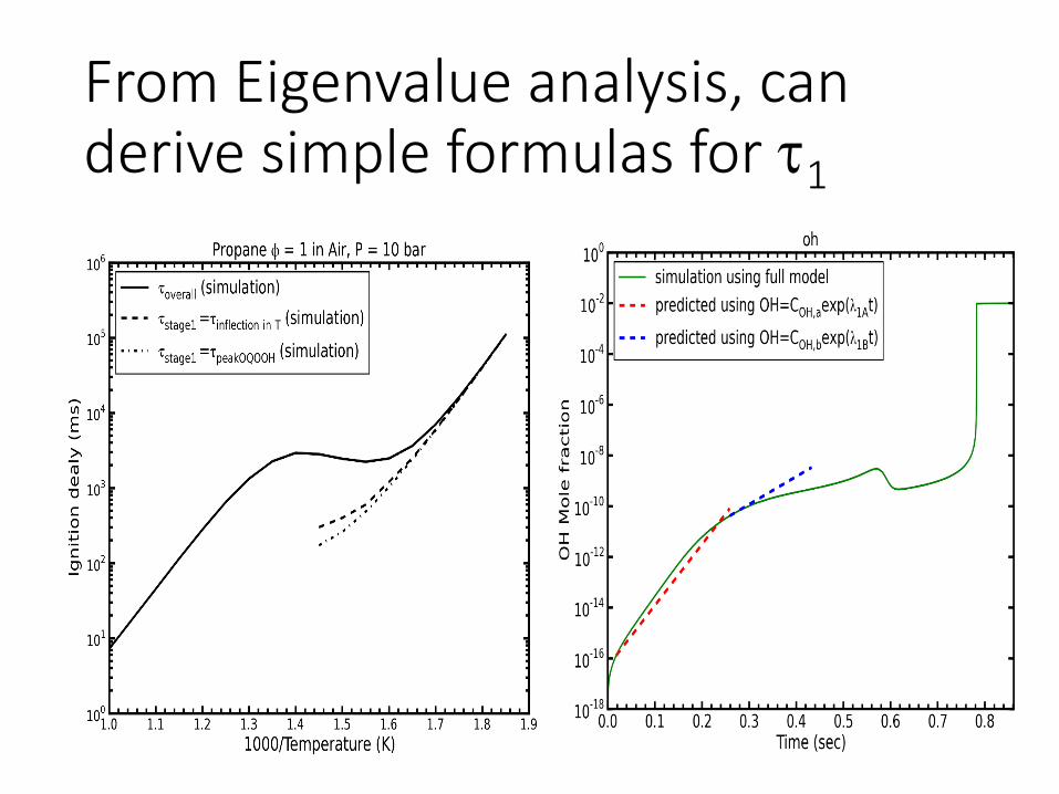
From Eigenvalue analysis, can derive simple formulas for τ1

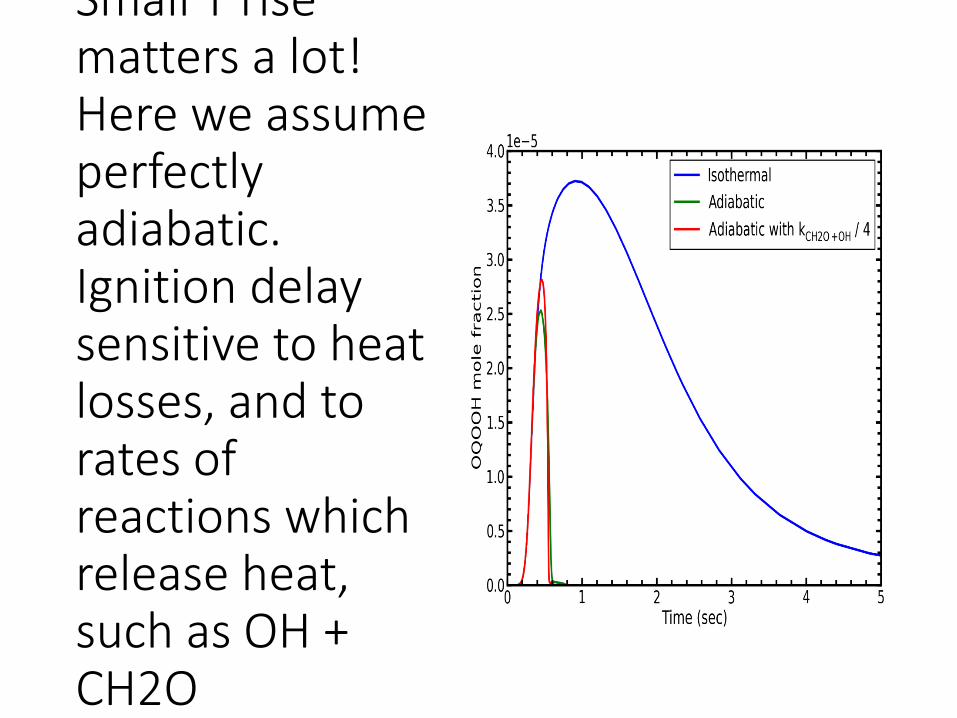
Small T rise matters a lot! Here we assume perfectly adiabatic. Ignition delay sensitive to heat losses, and to rates of reactions which release heat, such as OH + CH2O

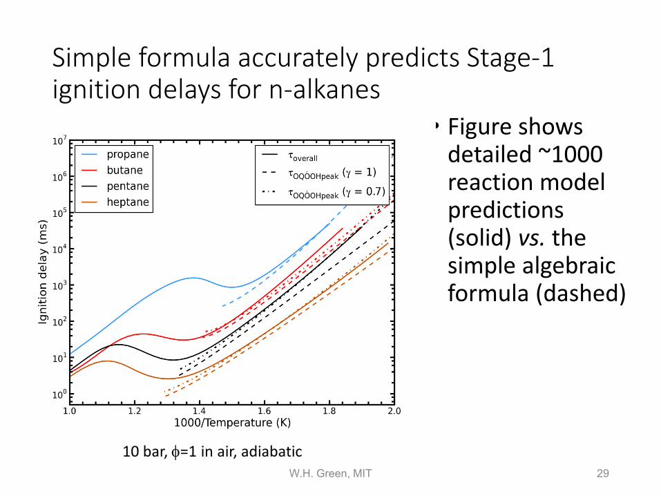
Simple formula accurately predicts Stage-1 ignition delays for n-alkanes

• Figure shows detailed ~1000 reaction model predictions (solid) vs. the simple algebraic formula (dashed)

10 bar, φ=1 in air, adiabatic 29 W.H. Green, MIT

Low T ignition formula was based on analysis of QOOH amplifier. What about fuels which cannot make QOOH?

• Small hydrocarbons (methane, C2’s) • Aromatics (with no long side chains) • Small alcohols • …for example, Methanol CH3OH • Note: alcohols make a lot of HO2 via HOR. + O2

HO2 + carbonyl, so we analyzed the H2O2 amplifier

30 W.H. Green, MIT

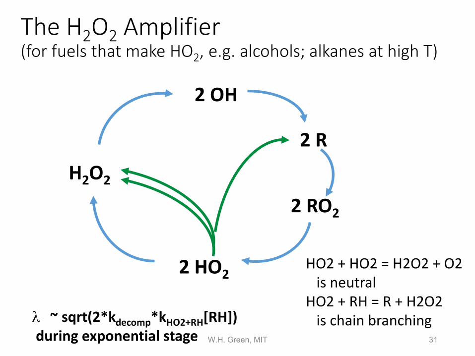
The H2O2 Amplifier (for fuels that make HO2, e.g. alcohols; alkanes at high T)

H2O2

2 OH

2 R

2 HO2 HO2 + HO2 = H2O2 + O2 is neutral HO2 + RH = R + H2O2 is chain branching λ ~ sqrt(2*kdecomp*kHO2+RH[RH])

during exponential stage

2 RO2

31 W.H. Green, MIT

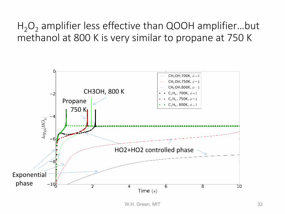
H2O2 amplifier less effective than QOOH amplifier…but methanol at 800 K is very similar to propane at 750 K

CH3OH, 800 K Propane 750 K

Exponential phase

HO2+HO2 controlled phase

32 W.H. Green, MIT

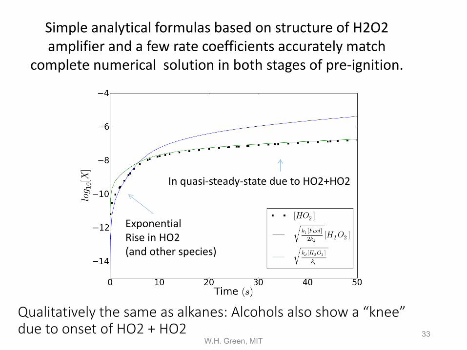
Qualitatively the same as alkanes: Alcohols also show a “knee” due to onset of HO2 + HO2

Exponential Rise in HO2 (and other species)

In quasi-steady-state due to HO2+HO2

33

Simple analytical formulas based on structure of H2O2 amplifier and a few rate coefficients accurately match

complete numerical solution in both stages of pre-ignition.

W.H. Green, MIT

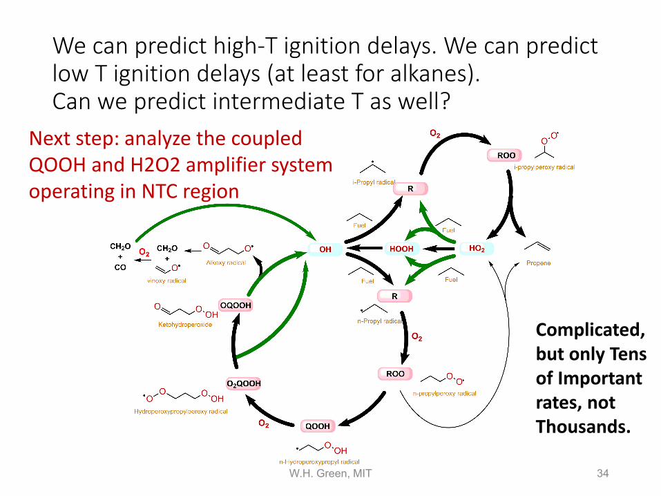
We can predict high-T ignition delays. We can predict low T ignition delays (at least for alkanes). Can we predict intermediate T as well?

Next step: analyze the coupled QOOH and H2O2 amplifier system operating in NTC region

Complicated, but only Tens of Important rates, not Thousands.

34 W.H. Green, MIT

How to model complicated Low-T chemistry? Often too many QOOH etc species to measure each one experimentally. Here are two alternative approaches: 1) Calculate all the QOOH etc isomers from first principles

using tools like KINBOT and RMG. - Accuracy of first-principles approach has been demonstrated.

- Detailed model, predicts all observables. - Need model reduction for CFD. - Will require supercomputers, cost increases with size of molecules.

2) Find a way to lump QOOH’s etc. together. Calibrate lumped model with experiments.

- Won’t be able to predict as many observables as detailed model. - Accuracy not yet demonstrated in a convincing way - Might work even if fuel composition not perfectly known.

W.H. Green, MIT

The complexity is real • If you want to predict all the chemistry details, the

model has to be detailed (i.e. very complicated) • There is an ongoing long-term project to be able to

predict fuel chemistry in detail • So far good success with a simple light fuels (e.g.

methane, heptane, butanols). Good prospect for predicting all of gasoline chemistry in detail by 2025.

• Full-detail chemistry scales poorly with molecular size:

• difficult-to-completely-impractical for jet fuel • not at all promising for diesel or heavier fuels.

W.H. Green, MIT 36

If we really need to know every detail about our fuels and their chemistry, things are not looking good…

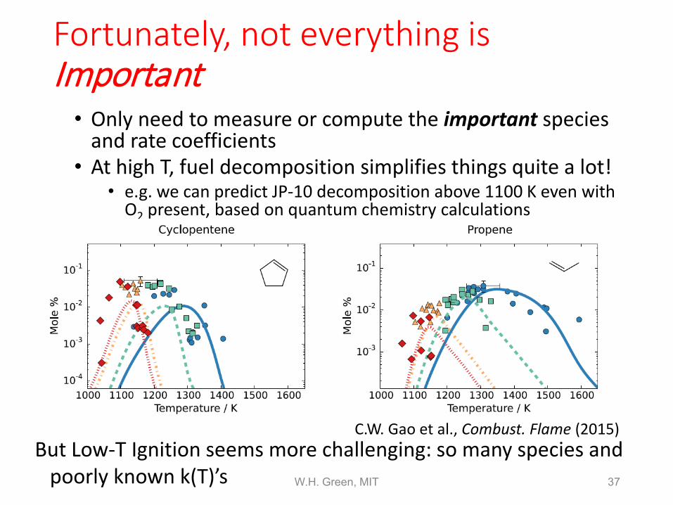
Fortunately, not everything is Important • Only need to measure or compute the important species

and rate coefficients • At high T, fuel decomposition simplifies things quite a lot!

• e.g. we can predict JP-10 decomposition above 1100 K even with O2 present, based on quantum chemistry calculations

37

But Low-T Ignition seems more challenging: so many species and poorly known k(T)’s W.H. Green, MIT

C.W. Gao et al., Combust. Flame (2015)

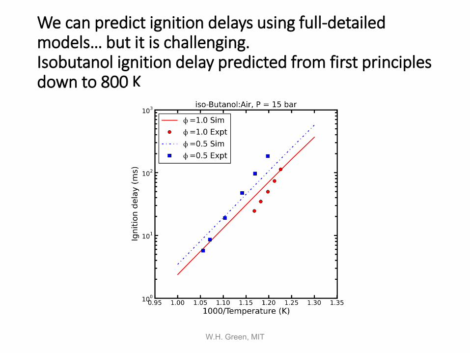
We can predict ignition delays using full-detailed models… but it is challenging. Isobutanol ignition delay predicted from first principles down to 800 K

W.H. Green, MIT

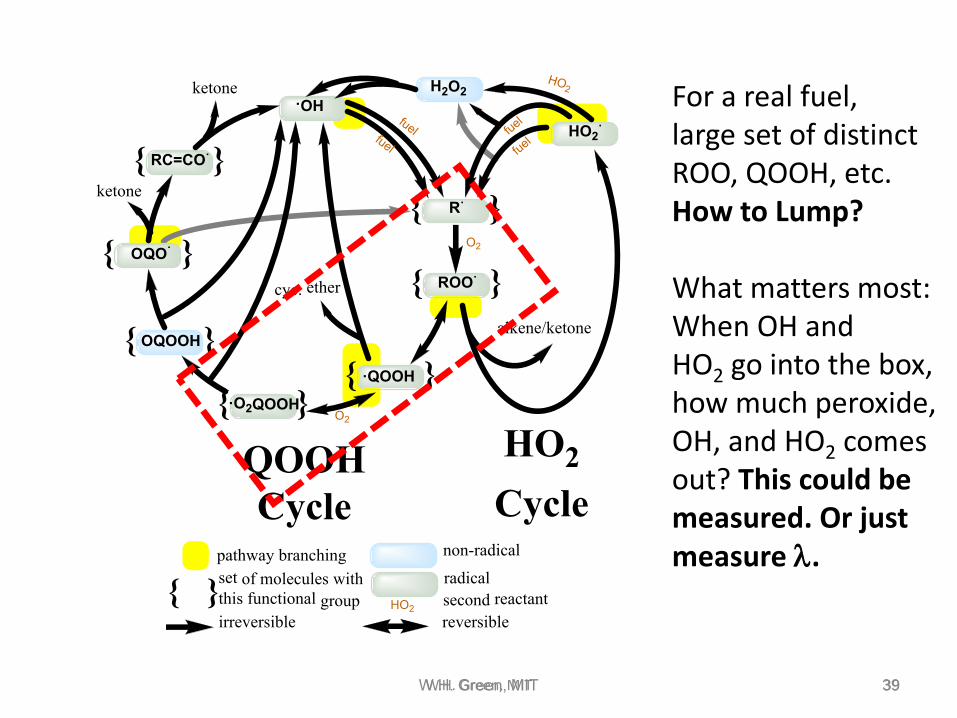
W.H. Green, MIT 39 W.H. Green, MIT 39

HO2 Cycle

QOOH Cycle

·OHHO2

·

R·{ }

ROO·{ }

·QOOH{ }·O2QOOH{ }

OQOOH{ }

OQO·{ }

RC=CO·{ }

cyc. ether

alkene/ketone

H2O2HO2

fuel

O2

O2

fuel

fuelfuel

ketone

ketone

QOOH Cycle

HO2 Cycle

{ }pathway branchingset of molecules withthis functional group

non-radical

radicalHO2

second reactantirreversible reversible

For a real fuel, large set of distinct ROO, QOOH, etc. How to Lump? What matters most: When OH and HO2 go into the box, how much peroxide, OH, and HO2 comes out? This could be measured. Or just measure λ.

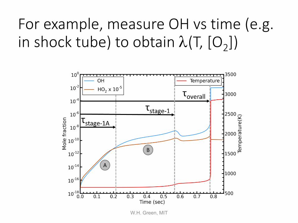
For example, measure OH vs time (e.g. in shock tube) to obtain λ(T, [O2])

W.H. Green, MIT

Summary • Focusing on the important physics in each stage drastically

simplifies low-T chemistry • Simple analytical formula from eigenvalue analysis

accurately predicts QOOH-controlled first-stage ignition delay for the n-alkanes

• This is approximately equal to total ignition delay below NTC region • From the two easy-to-compute high-T and low-T curves of ignition

delay vs. T one might be able to estimate ignition delay in NTC region

• Similar analysis also works for systems where H2O2 amplifier is controlling ignition (e.g. small alcohols).

• Ignition controlled by tens, not hundreds or thousands of rate coefficients!

• How best to determine those tens of rate coefficients? How to optimally combine theory and experiment?

41 W.H. Green, MIT

Future Directions • Do similar analysis to cover stage 2 and NTC region, and other fuel types

(e.g. aromatics, methane). • Write a simple, accurate, fundamentally-based expression for ignition

delay at any condition! • Complete analysis for any fuel of known composition (e.g. surrogates)

looks practical. • The important parameters can come from quantum chemistry and/or

experiment. • Models likely to be simple enough to be included in CFD

• but the implementation requires some thought. • Perhaps there is a way to measure the key fuel parameters (e.g. the T-

dependent Gain 3αβγ) directly even if one does not know the fuel composition?

• This would be more fundamental than cetane & octane numbers, and might be easier and more accurate than doing the difficult analytical chemistry to determine the fuel composition.

42 W.H. Green, MIT

Acknowledgments • Shamel Merchant, C. Franklin Goldsmith, Michael

Burke, and Stephen Klippenstein collaborated in the QOOH amplifier analysis for alkanes.

• Nathan Yee, Mark Goldman, Shamel Merchant, Samah Mohammed and Mani Sarathy collaborated in aspects of the alcohol/H2O2 amplifier analysis.

• Several others have made advances in this line of research previously (and ongoing), notably Norbert Peters and his collaborators. Recently Tianfeng Lu and Ed Law have emphasized eigenvalue analysis for explosive modes.

43 W.H. Green, MIT

Kinetic Modeling of Autoignition: Engine Knock, HCCI and fuel economy

Charles K. Westbrook Lawrence Livermore National Laboratory

CEFRC

June 2010

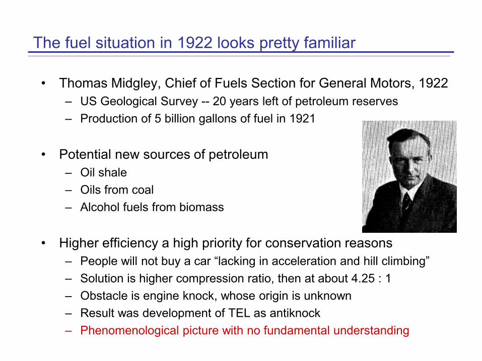
The fuel situation in 1922 looks pretty familiar

• Thomas Midgley, Chief of Fuels Section for General Motors, 1922 – US Geological Survey -- 20 years left of petroleum reserves – Production of 5 billion gallons of fuel in 1921

• Potential new sources of petroleum

– Oil shale – Oils from coal – Alcohol fuels from biomass

• Higher efficiency a high priority for conservation reasons

– People will not buy a car “lacking in acceleration and hill climbing” – Solution is higher compression ratio, then at about 4.25 : 1 – Obstacle is engine knock, whose origin is unknown – Result was development of TEL as antiknock – Phenomenological picture with no fundamental understanding

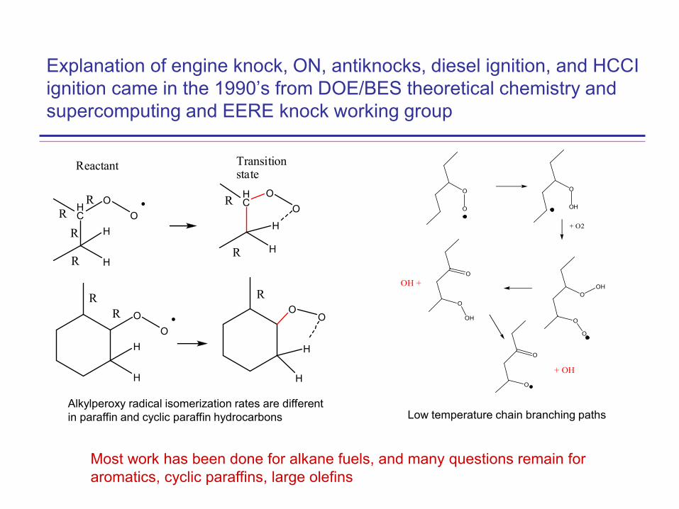
Explanation of engine knock, ON, antiknocks, diesel ignition, and HCCI ignition came in the 1990’s from DOE/BES theoretical chemistry and supercomputing and EERE knock working group

OO

H

H

OO

H

H

R

Reactant Transitionstate

HC

OO

H

H

R

R

HC

OO

H

H

R R

RR

RR

Most work has been done for alkane fuels, and many questions remain for aromatics, cyclic paraffins, large olefins

+ O2

OH +

+ OH

O

O

O

OH

OOH

O

O

O

O

OH

O

O

Low temperature chain branching paths Alkylperoxy radical isomerization rates are different in paraffin and cyclic paraffin hydrocarbons

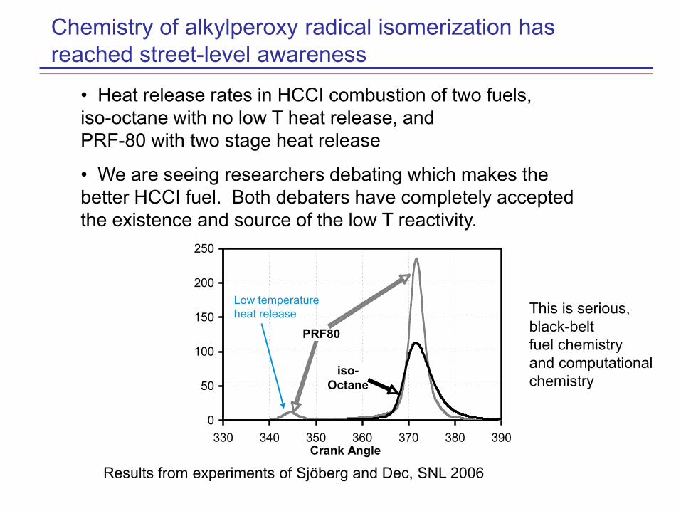
0

50

100

150

200

250

330 340 350 360 370 380 390Crank Angle

iso-Octane

PRF80

• Heat release rates in HCCI combustion of two fuels, iso-octane with no low T heat release, and PRF-80 with two stage heat release

Results from experiments of Sjöberg and Dec, SNL 2006

• We are seeing researchers debating which makes the better HCCI fuel. Both debaters have completely accepted the existence and source of the low T reactivity.

Chemistry of alkylperoxy radical isomerization has reached street-level awareness

This is serious, black-belt fuel chemistry and computational chemistry

Low temperature heat release

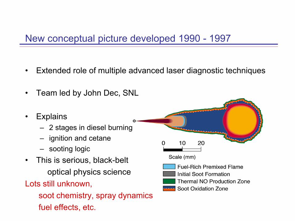
New conceptual picture developed 1990 - 1997

• Extended role of multiple advanced laser diagnostic techniques

• Team led by John Dec, SNL

• Explains – 2 stages in diesel burning – ignition and cetane – sooting logic

• This is serious, black-belt optical physics science Lots still unknown, soot chemistry, spray dynamics fuel effects, etc.

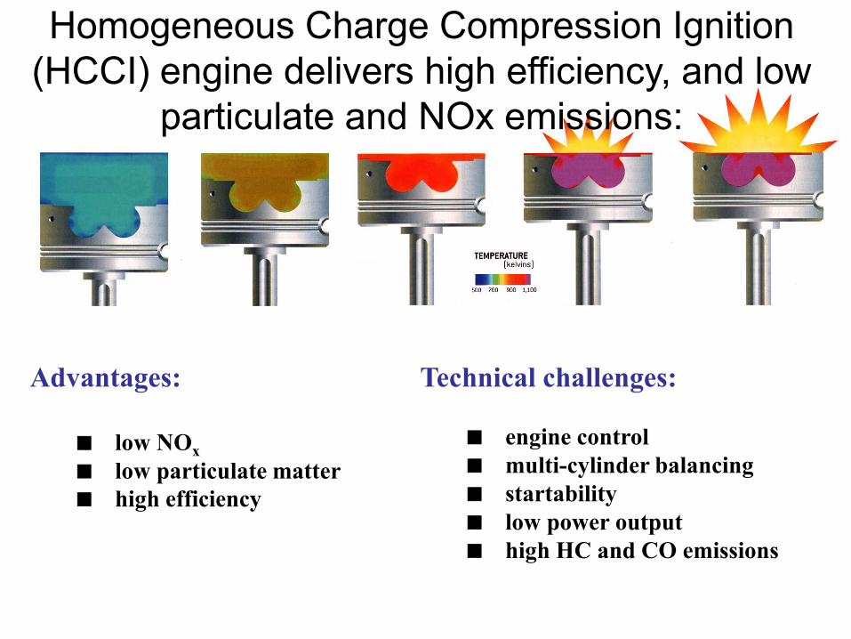
Homogeneous Charge Compression Ignition (HCCI) engine delivers high efficiency, and low

particulate and NOx emissions:

Technical challenges: engine control multi-cylinder balancing startability low power output high HC and CO emissions

Advantages: low NOx low particulate matter high efficiency

Have we have come a long way since 1922?

• We still are looking to oil shale, oil sands and biomass for the future

• However, our understanding of knocking, antiknocks and low T chemistry has grown enormously e.g., Current engine designers debate how much low T heat release is

best, and take its sources for granted • Conceptual model for diesel combustion has led to breakthroughs

e.g., Understanding of anti-sooting action of oxygenates • Entirely new concept engine (HCCI) is being developed Great majority of this progress is due to basic science

understanding, e.g., optical diagnostics, quantum chemistry and electronic structure theory, high performance computing, etc.

We have used basic science advances to make big jumps in understanding, but we are back to trial and error in many cases

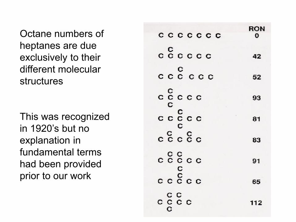
Octane numbers of heptanes are due exclusively to their different molecular structures This was recognized in 1920’s but no explanation in fundamental terms had been provided prior to our work

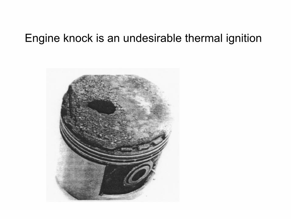
Engine knock is an undesirable thermal ignition

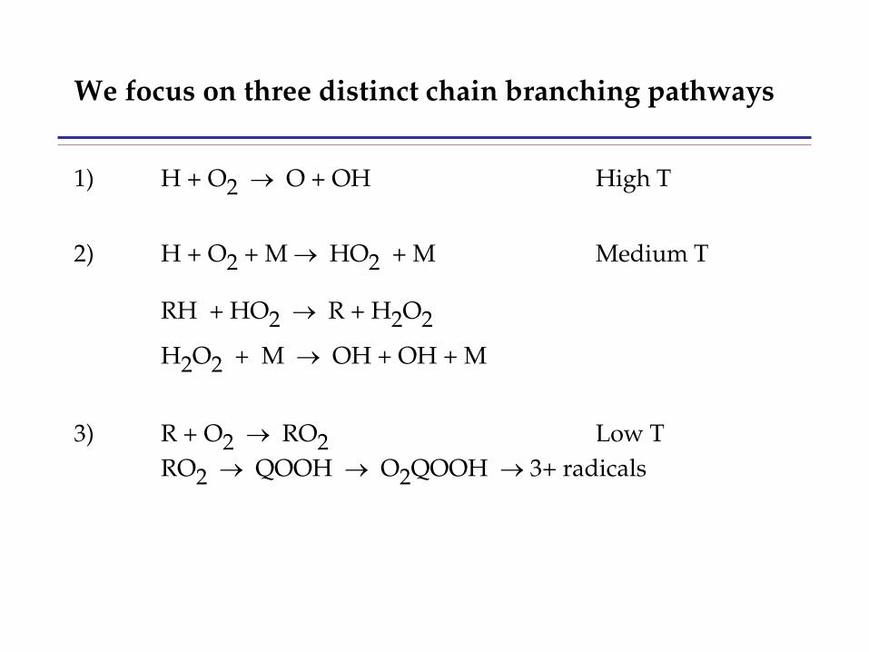
We focus on three distinct chain branching pathways

1) H + O2 → O + OH High T

2) H + O2 + M → HO2 + M Medium T

RH + HO2 → R + H2O2 H2O2 + M → OH + OH + M

3) R + O2 → RO2 Low T RO2 → QOOH → O2QOOH → 3+ radicals

0

200

400

600

800

1,000

1,200

1,400

1,600

0.00E+00 2.00E-01 4.00E-01 6.00E-01 8.00E-01 1.00E+00 1.20E+00

Tem

pera

ture

Time

n-hexane ignition

Heat release rate

Temperature

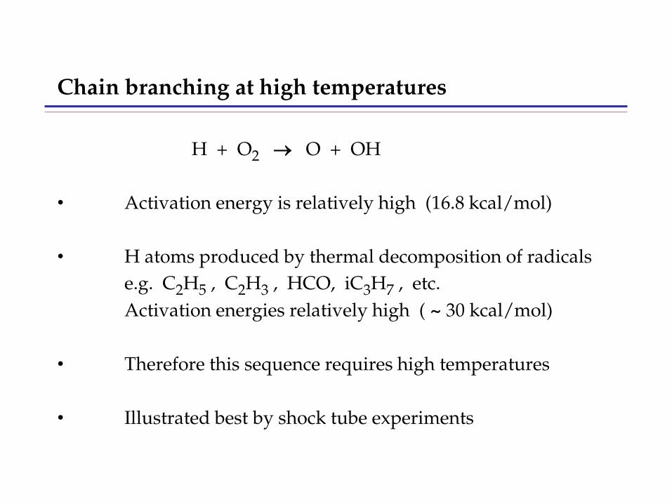
Chain branching at high temperatures

H + O2 → O + OH • Activation energy is relatively high (16.8 kcal/mol) • H atoms produced by thermal decomposition of radicals e.g. C2H5 , C2H3 , HCO, iC3H7 , etc. Activation energies relatively high ( ~ 30 kcal/mol) • Therefore this sequence requires high temperatures • Illustrated best by shock tube experiments

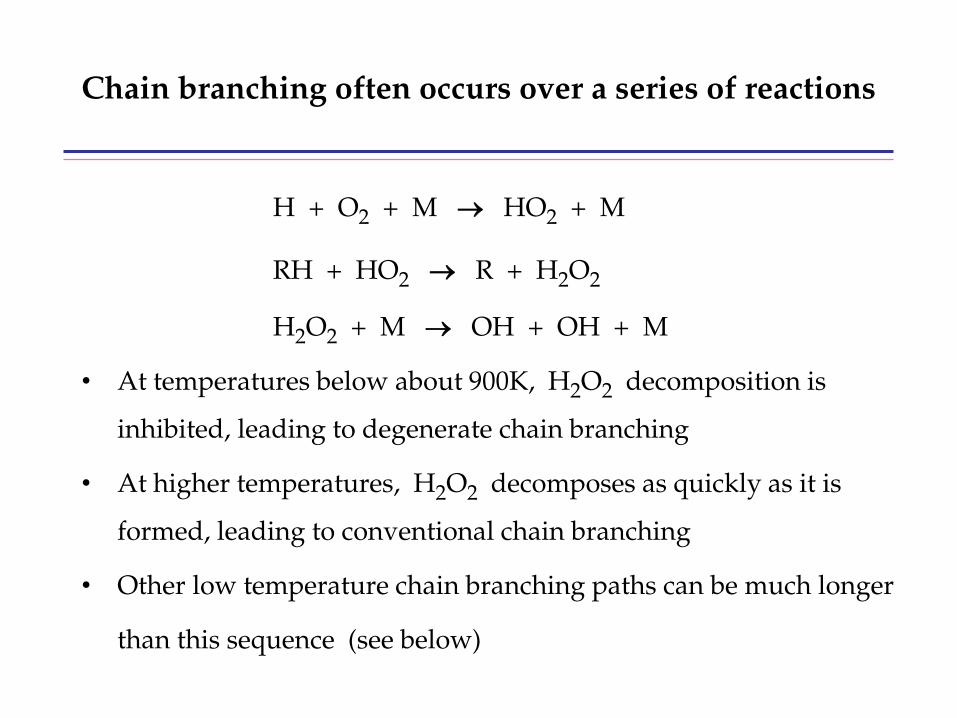
Chain branching often occurs over a series of reactions

H + O2 + M → HO2 + M

RH + HO2 → R + H2O2

H2O2 + M → OH + OH + M

• At temperatures below about 900K, H2O2 decomposition is

inhibited, leading to degenerate chain branching

• At higher temperatures, H2O2 decomposes as quickly as it is

formed, leading to conventional chain branching

• Other low temperature chain branching paths can be much longer

than this sequence (see below)

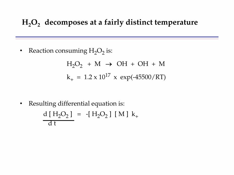
H2O2 decomposes at a fairly distinct temperature

• Reaction consuming H2O2 is:

H2O2 + M → OH + OH + M

k+ = 1.2 x 1017 x exp(-45500/RT)

• Resulting differential equation is:

d [ H2O2 ] = -[ H2O2 ] [ M ] k+ d t

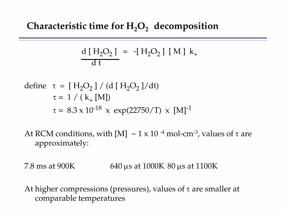
Characteristic time for H2O2 decomposition

d [ H2O2 ] = -[ H2O2 ] [ M ] k+ d t define τ = [ H2O2 ] / (d [ H2O2 ]/dt) τ = 1 / ( k+ [M])

τ = 8.3 x 10-18 x exp(22750/T) x [M]-1 At RCM conditions, with [M] ~ 1 x 10 -4 mol-cm-3, values of τ are

approximately: 7.8 ms at 900K 640 µs at 1000K 80 µs at 1100K At higher compressions (pressures), values of τ are smaller at

comparable temperatures

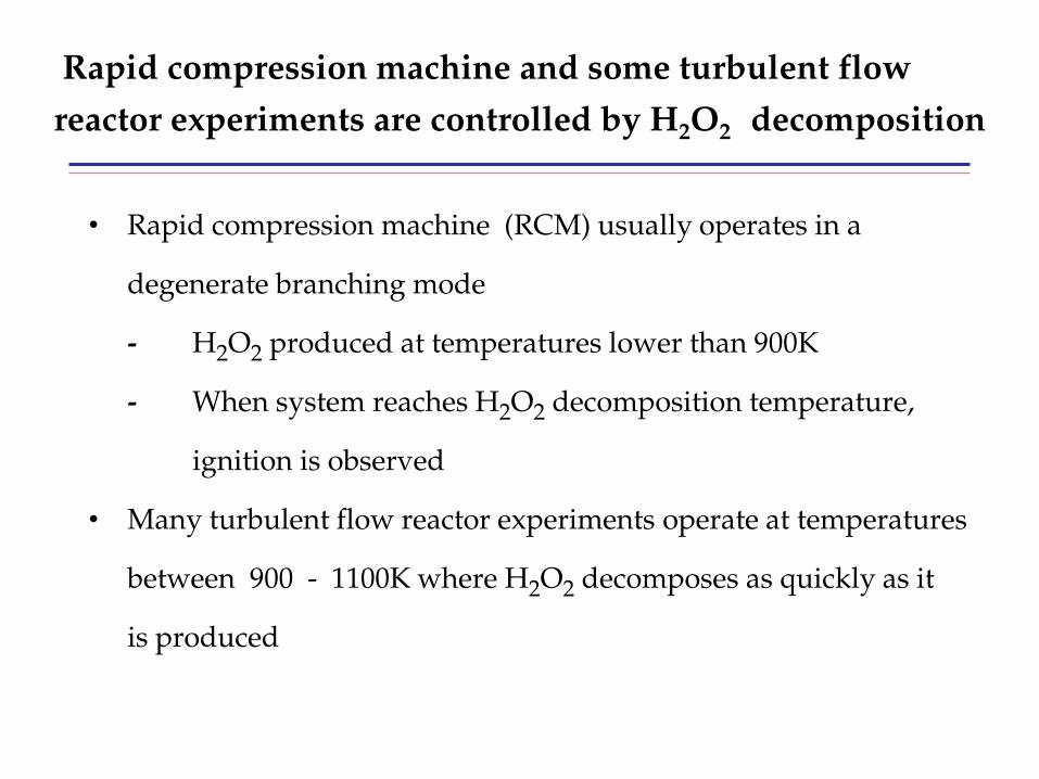
Rapid compression machine and some turbulent flow

reactor experiments are controlled by H2O2 decomposition

• Rapid compression machine (RCM) usually operates in a

degenerate branching mode

- H2O2 produced at temperatures lower than 900K

- When system reaches H2O2 decomposition temperature,

ignition is observed

• Many turbulent flow reactor experiments operate at temperatures

between 900 - 1100K where H2O2 decomposes as quickly as it

is produced

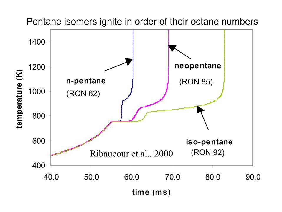
400

600

800

1000

1200

1400

40.0 50.0 60.0 70.0 80.0 90.0

time (ms)

tem

pera

ture

(K) neopentane

iso-pentane

n-pentane

Pentane isomers ignite in order of their octane numbers

(RON 62)

(RON 92)

(RON 85)

Ribaucour et al., 2000

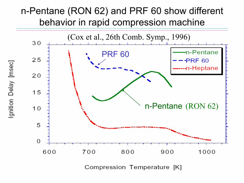
n-Pentane (RON 62) and PRF 60 show different behavior in rapid compression machine

n-Pentane

PRF 60

(RON 62)

(Cox et al., 26th Comb. Symp., 1996)

Role of H2O2 decomposition is very general

• RCM ignition

• Engine knock

• HCCI ignition

• Diesel ignition

• Each system follows a unique pathway in the relevant phase space to arrive at this ignition temperature where H2O2 decomposes

Kinetic features of engine knock

• History of octane numbers and empirical observations

• End gas self-ignition prior to flame arrival

• Actual ignition driven by H2O2 decomposition at ~ 900K

• Kinetic influence of molecular size and structure

• Effects of additives, both promoters and inhibitors

• Reduced models must retain H2O2 decomposition reaction to

describe ignition

• Issue of real SI engine fuel being complex mixture of components

• Lots of kinetics research still needed (aromatics, cyclics, etc.)

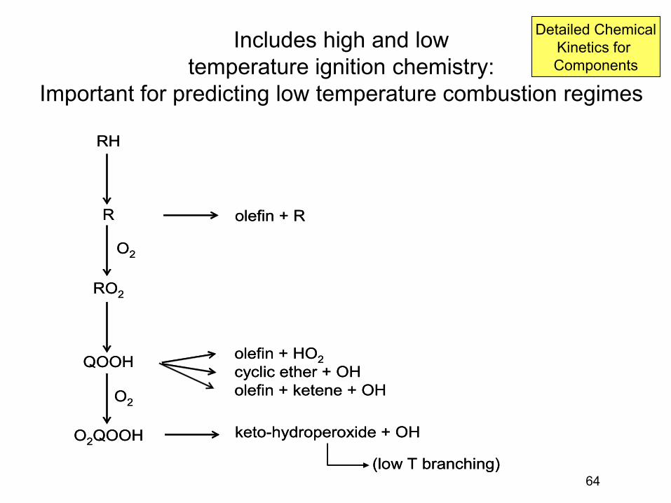
64

Includes high and low temperature ignition chemistry:

Important for predicting low temperature combustion regimes

Detailed Chemical Kinetics for Components

RH

R

RO2

QOOH

O2QOOH

olefin + HO2cyclic ether + OHolefin + ketene + OH

keto-hydroperoxide + OH

O2

O2

olefin + R

(low T branching)

RH

R

RO2

QOOH

O2QOOH

olefin + HO2cyclic ether + OHolefin + ketene + OH

keto-hydroperoxide + OH

O2

O2

olefin + R

(low T branching)

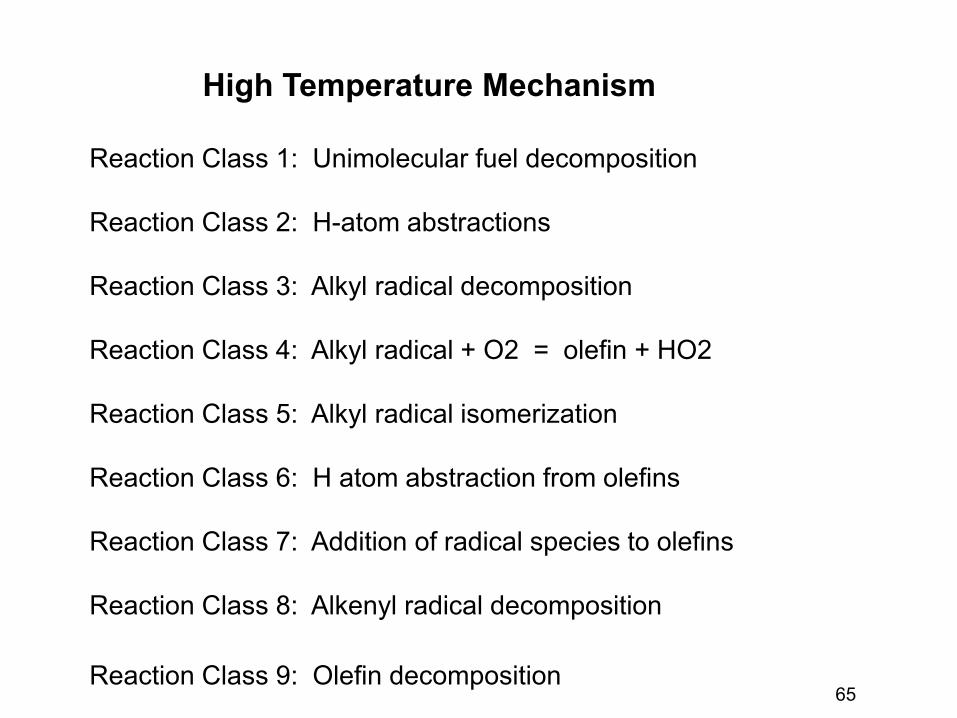
65

High Temperature Mechanism

Reaction Class 1: Unimolecular fuel decomposition Reaction Class 2: H-atom abstractions Reaction Class 3: Alkyl radical decomposition Reaction Class 4: Alkyl radical + O2 = olefin + HO2 Reaction Class 5: Alkyl radical isomerization Reaction Class 6: H atom abstraction from olefins Reaction Class 7: Addition of radical species to olefins Reaction Class 8: Alkenyl radical decomposition Reaction Class 9: Olefin decomposition

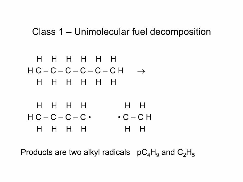
Class 1 – Unimolecular fuel decomposition

H H H H H H H C – C – C – C – C – C H → H H H H H H H H H H H H H C – C – C – C • • C – C H H H H H H H Products are two alkyl radicals pC4H9 and C2H5

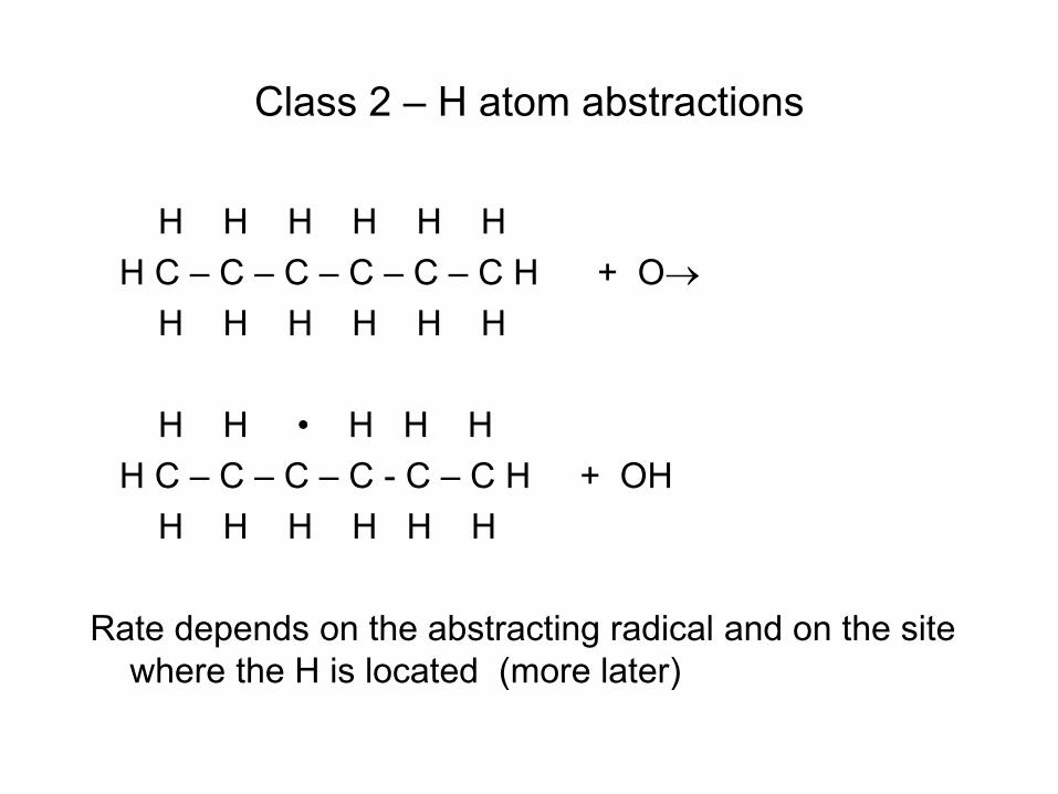
Class 2 – H atom abstractions

H H H H H H H C – C – C – C – C – C H + O→ H H H H H H H H • H H H H C – C – C – C - C – C H + OH H H H H H H Rate depends on the abstracting radical and on the site

where the H is located (more later)

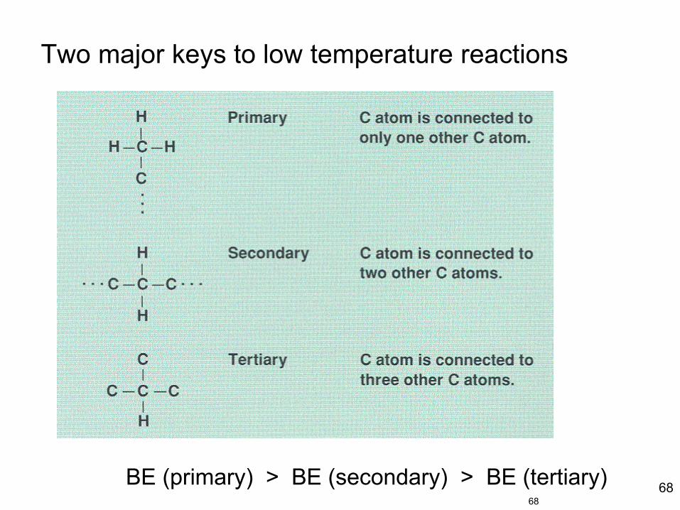
68

Two major keys to low temperature reactions

68

BE (primary) > BE (secondary) > BE (tertiary)

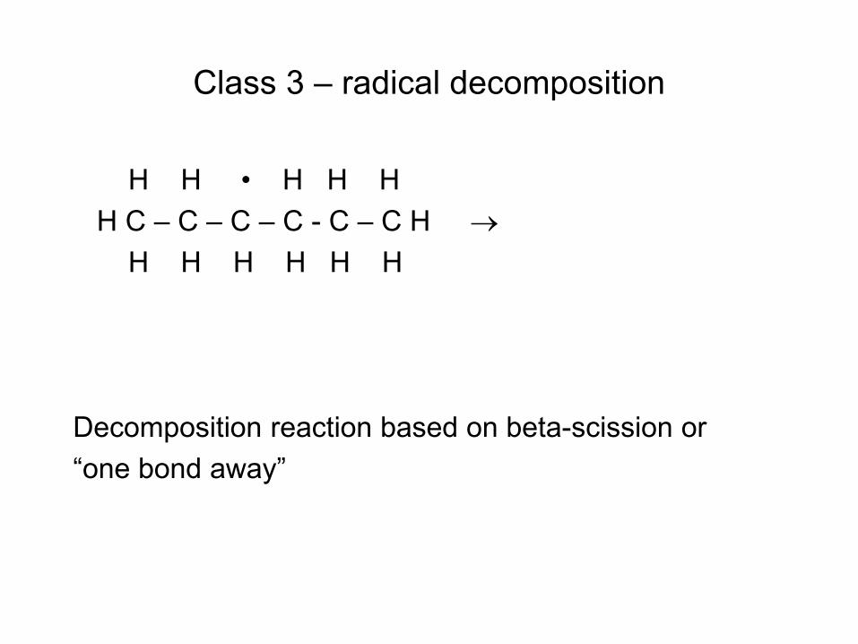
Class 3 – radical decomposition

H H • H H H H C – C – C – C - C – C H → H H H H H H Decomposition reaction based on beta-scission or “one bond away”

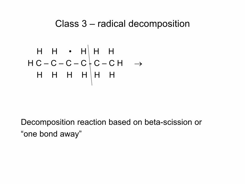
Class 3 – radical decomposition

H H • H H H H C – C – C – C - C – C H → H H H H H H Decomposition reaction based on beta-scission or “one bond away”

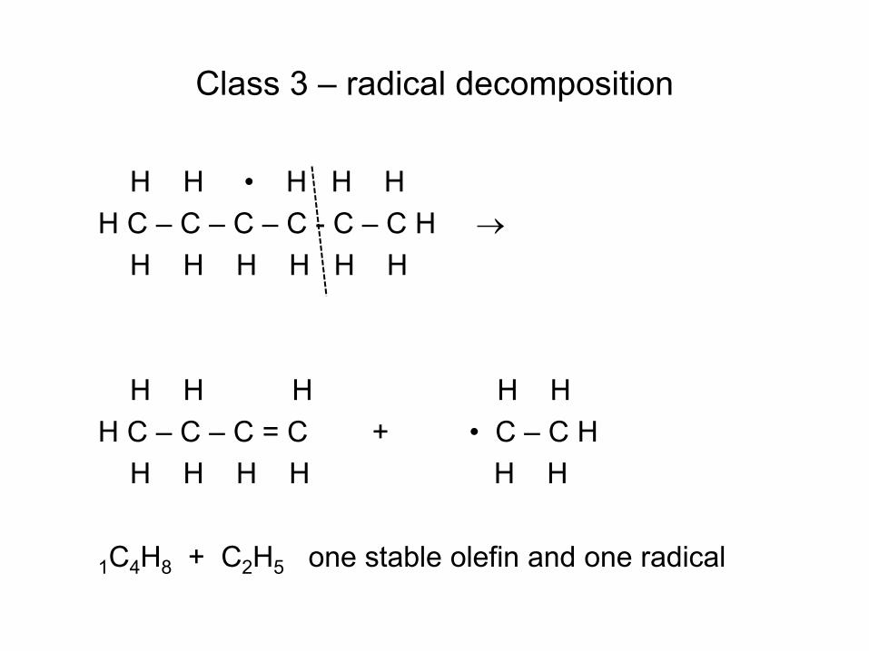
Class 3 – radical decomposition

H H • H H H H C – C – C – C - C – C H → H H H H H H H H H H H H C – C – C = C + • C – C H H H H H H H 1C4H8 + C2H5 one stable olefin and one radical

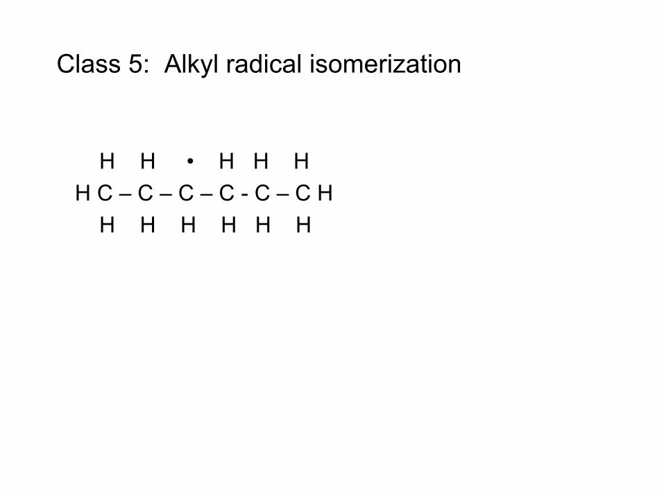
Class 5: Alkyl radical isomerization

H H • H H H H C – C – C – C - C – C H H H H H H H

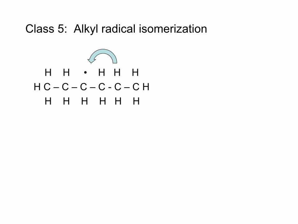
Class 5: Alkyl radical isomerization

H H • H H H H C – C – C – C - C – C H H H H H H H

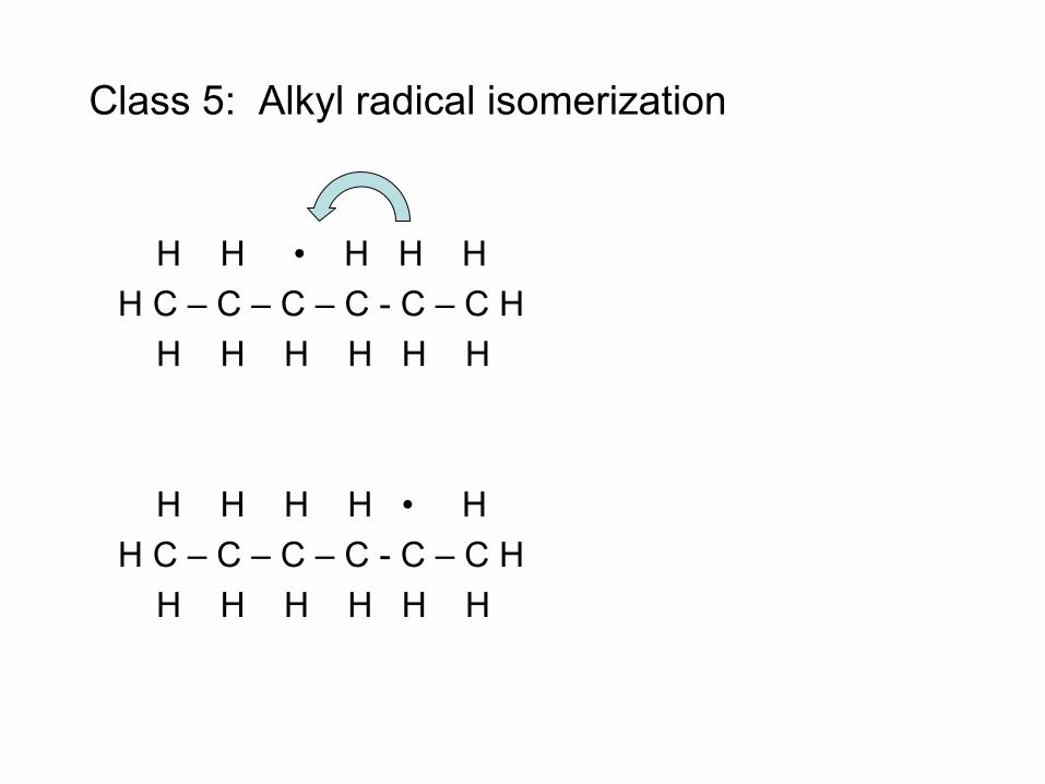
Class 5: Alkyl radical isomerization

H H • H H H H C – C – C – C - C – C H H H H H H H H H H H • H H C – C – C – C - C – C H H H H H H H

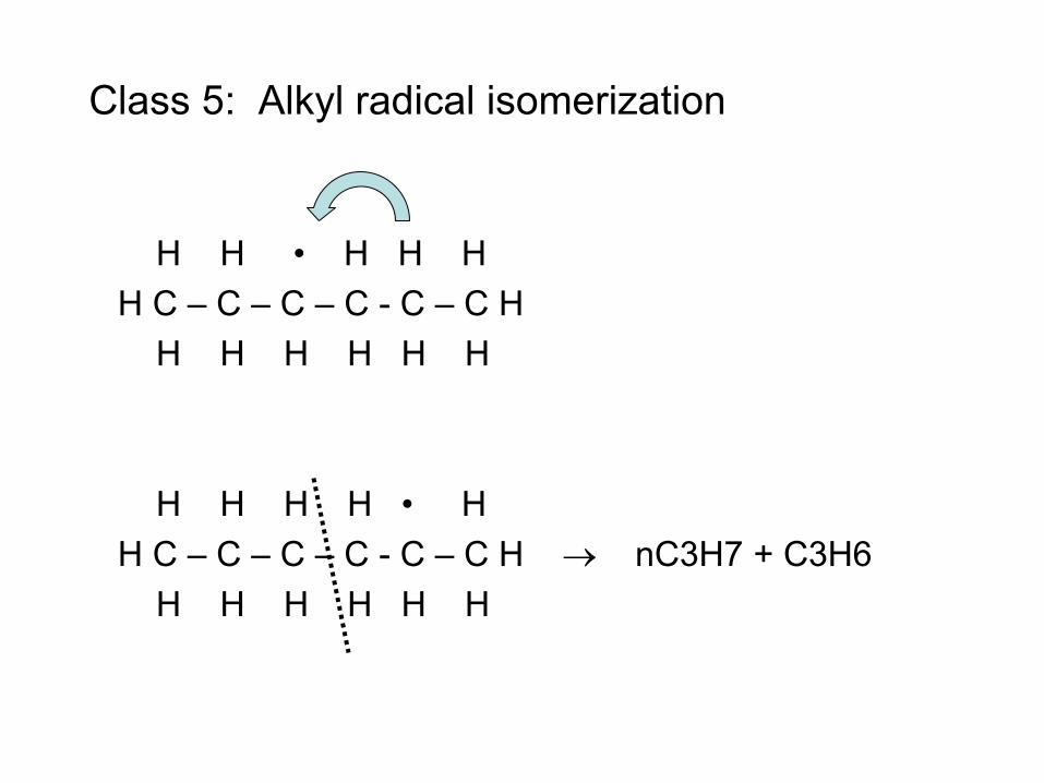
Class 5: Alkyl radical isomerization

H H • H H H H C – C – C – C - C – C H H H H H H H H H H H • H H C – C – C – C - C – C H → nC3H7 + C3H6 H H H H H H

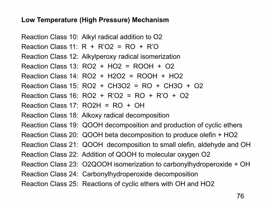
76

Low Temperature (High Pressure) Mechanism Reaction Class 10: Alkyl radical addition to O2 Reaction Class 11: R + R’O2 = RO + R’O Reaction Class 12: Alkylperoxy radical isomerization Reaction Class 13: RO2 + HO2 = ROOH + O2 Reaction Class 14: RO2 + H2O2 = ROOH + HO2 Reaction Class 15: RO2 + CH3O2 = RO + CH3O + O2 Reaction Class 16: RO2 + R’O2 = RO + R’O + O2 Reaction Class 17: RO2H = RO + OH Reaction Class 18: Alkoxy radical decomposition Reaction Class 19: QOOH decomposition and production of cyclic ethers Reaction Class 20: QOOH beta decomposition to produce olefin + HO2 Reaction Class 21: QOOH decomposition to small olefin, aldehyde and OH Reaction Class 22: Addition of QOOH to molecular oxygen O2 Reaction Class 23: O2QOOH isomerization to carbonylhydroperoxide + OH Reaction Class 24: Carbonylhydroperoxide decomposition Reaction Class 25: Reactions of cyclic ethers with OH and HO2

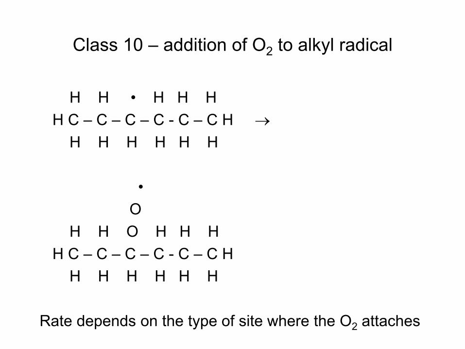
Class 10 – addition of O2 to alkyl radical

H H • H H H H C – C – C – C - C – C H → H H H H H H • O H H O H H H H C – C – C – C - C – C H H H H H H H Rate depends on the type of site where the O2 attaches

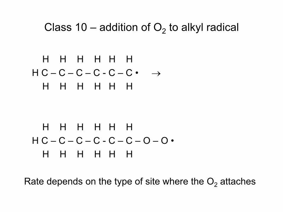
Class 10 – addition of O2 to alkyl radical

H H H H H H H C – C – C – C - C – C • → H H H H H H H H H H H H H C – C – C – C - C – C – O – O • H H H H H H Rate depends on the type of site where the O2 attaches

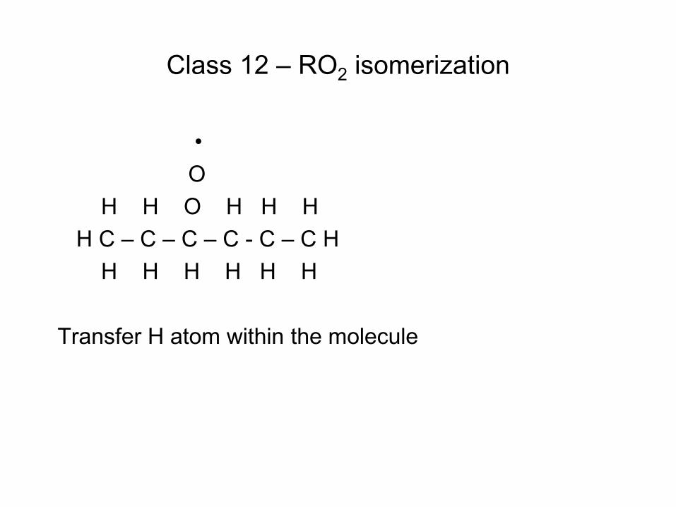
Class 12 – RO2 isomerization

• O H H O H H H H C – C – C – C - C – C H H H H H H H Transfer H atom within the molecule

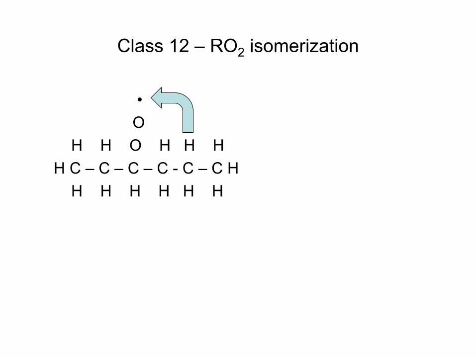
Class 12 – RO2 isomerization

• O H H O H H H H C – C – C – C - C – C H H H H H H H

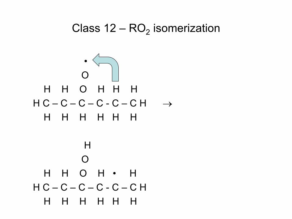
Class 12 – RO2 isomerization

• O H H O H H H H C – C – C – C - C – C H → H H H H H H H O H H O H • H H C – C – C – C - C – C H H H H H H H

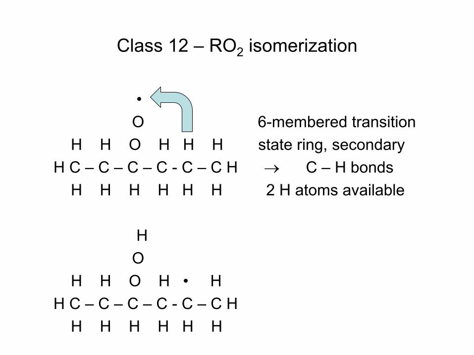
Class 12 – RO2 isomerization

• O 6-membered transition H H O H H H state ring, secondary H C – C – C – C - C – C H → C – H bonds H H H H H H 2 H atoms available H O H H O H • H H C – C – C – C - C – C H H H H H H H

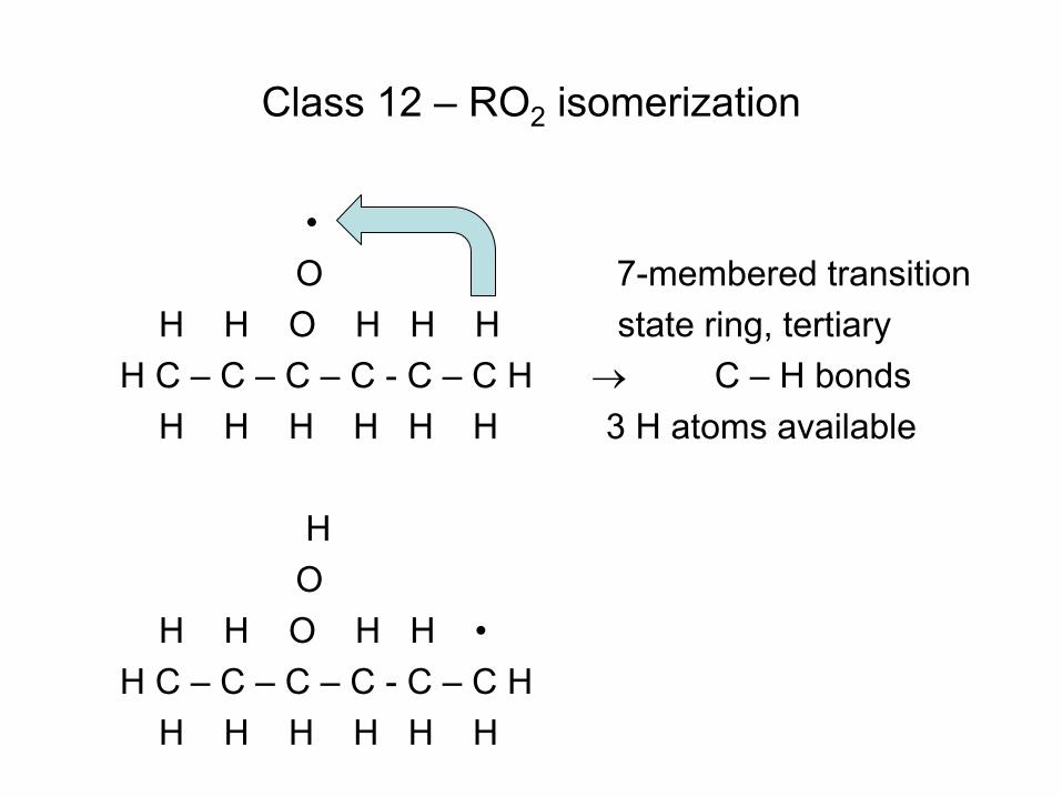
Class 12 – RO2 isomerization

• O 7-membered transition H H O H H H state ring, tertiary H C – C – C – C - C – C H → C – H bonds H H H H H H 3 H atoms available H O H H O H H • H C – C – C – C - C – C H H H H H H H

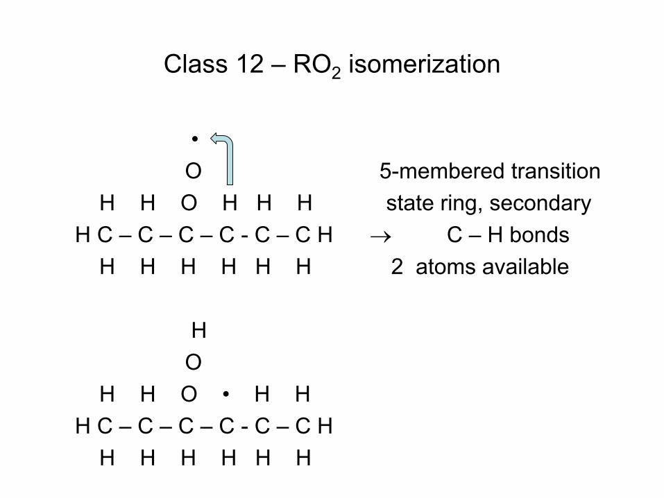
Class 12 – RO2 isomerization

• O 5-membered transition H H O H H H state ring, secondary H C – C – C – C - C – C H → C – H bonds H H H H H H 2 atoms available H O H H O • H H H C – C – C – C - C – C H H H H H H H

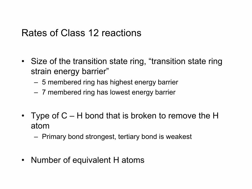
Rates of Class 12 reactions

• Size of the transition state ring, “transition state ring strain energy barrier” – 5 membered ring has highest energy barrier – 7 membered ring has lowest energy barrier

• Type of C – H bond that is broken to remove the H

atom – Primary bond strongest, tertiary bond is weakest

• Number of equivalent H atoms

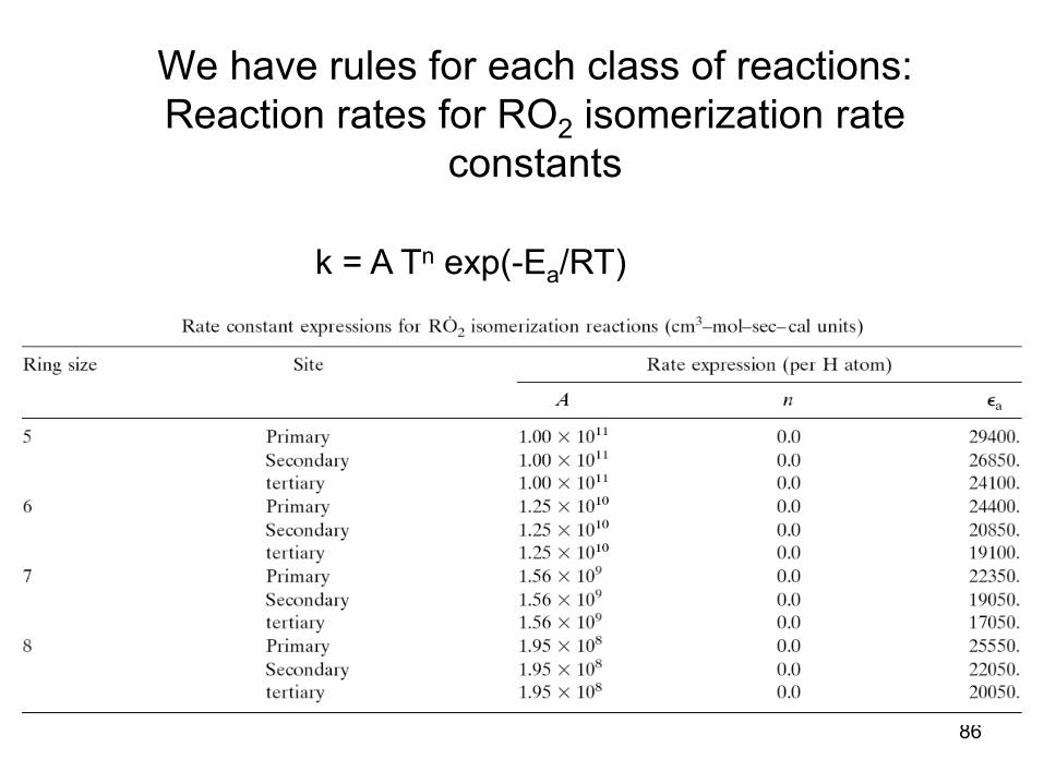
86

We have rules for each class of reactions: Reaction rates for RO2 isomerization rate

constants

k = A Tn exp(-Ea/RT)

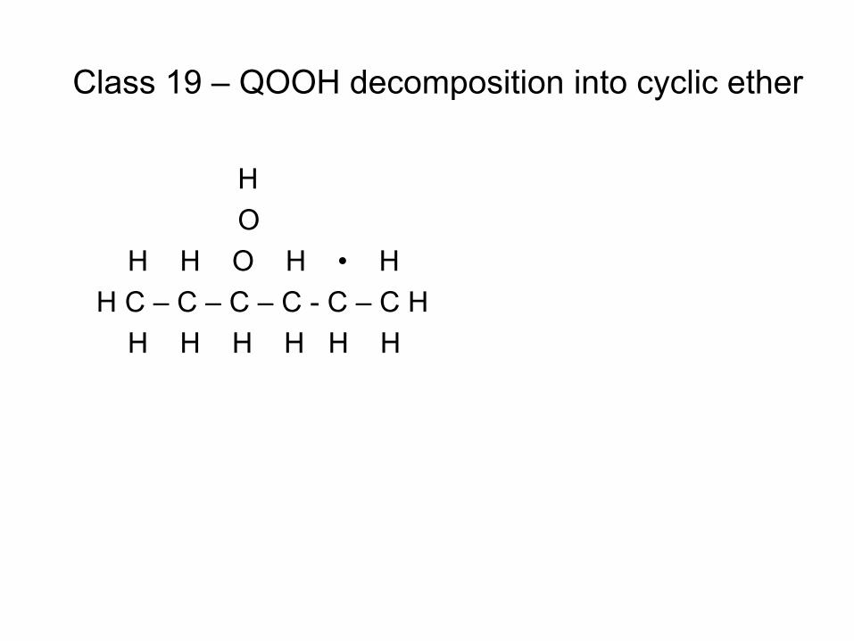
Class 19 – QOOH decomposition into cyclic ether

H O H H O H • H H C – C – C – C - C – C H H H H H H H

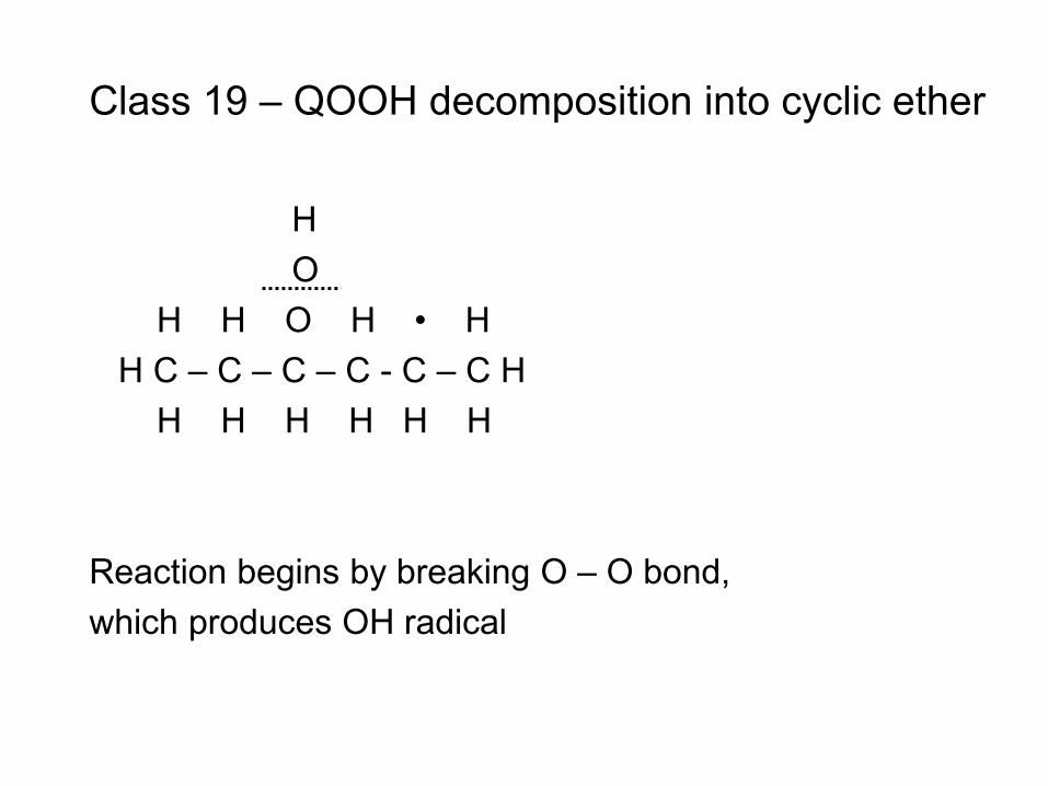
Class 19 – QOOH decomposition into cyclic ether

H O H H O H • H H C – C – C – C - C – C H H H H H H H Reaction begins by breaking O – O bond, which produces OH radical

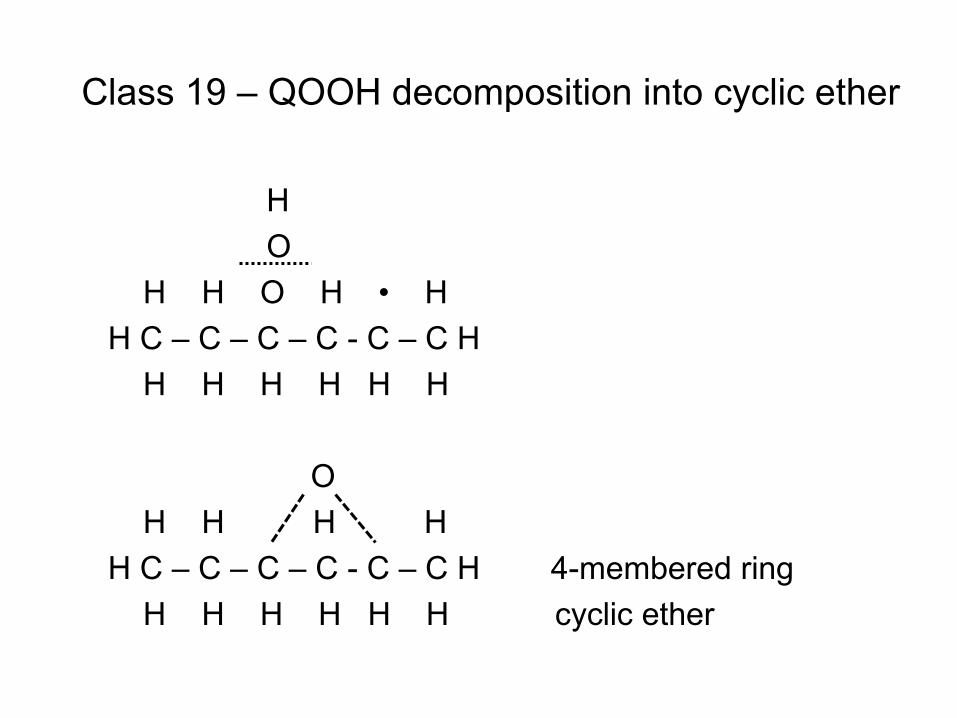
Class 19 – QOOH decomposition into cyclic ether

H O H H O H • H H C – C – C – C - C – C H H H H H H H O H H H H H C – C – C – C - C – C H 4-membered ring H H H H H H cyclic ether

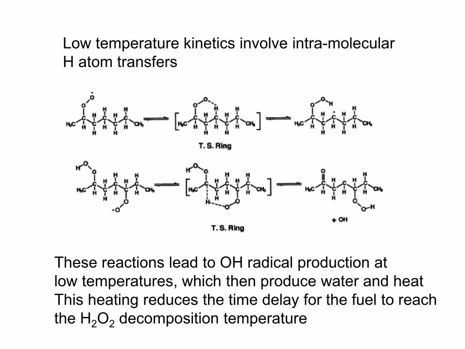
Low temperature kinetics involve intra-molecular H atom transfers

These reactions lead to OH radical production at low temperatures, which then produce water and heat This heating reduces the time delay for the fuel to reach the H2O2 decomposition temperature

91

Two major keys to low temperature reactions

91

BE (primary) > BE (secondary) > BE (tertiary)

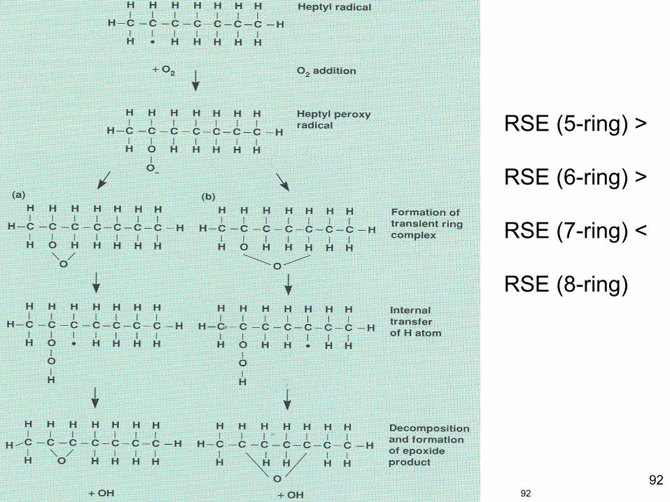
92 92

RSE (5-ring) > RSE (6-ring) > RSE (7-ring) < RSE (8-ring)

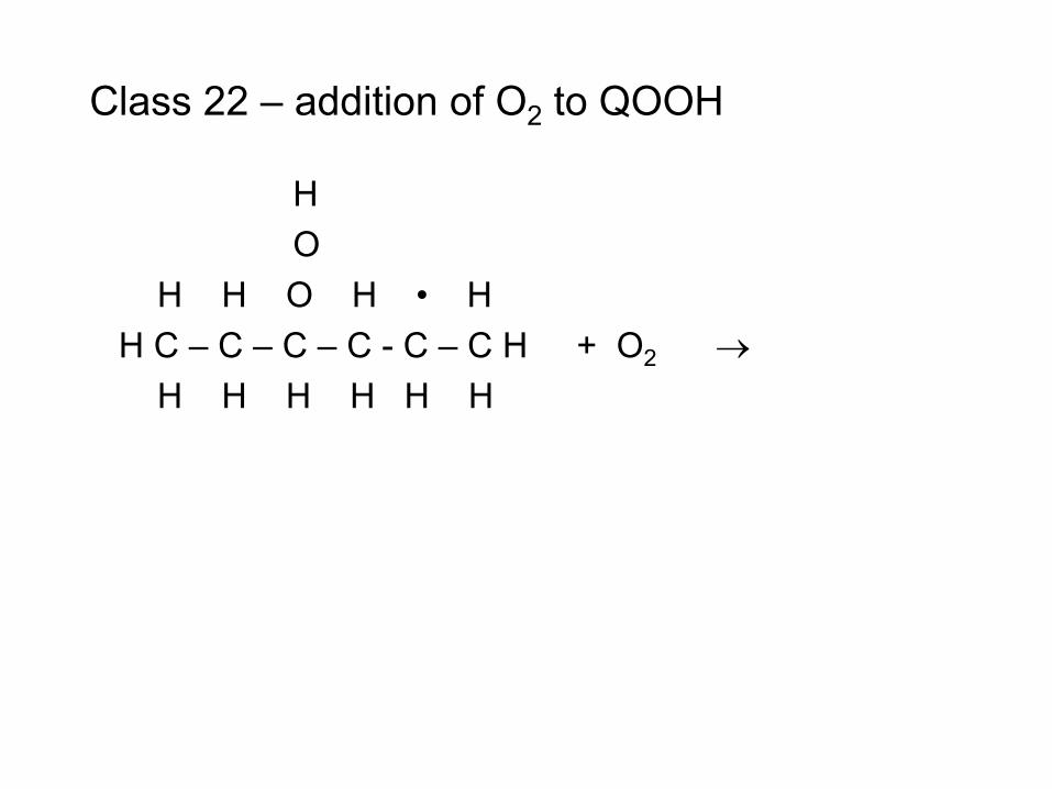
Class 22 – addition of O2 to QOOH

H O H H O H • H H C – C – C – C - C – C H + O2 →

H H H H H H

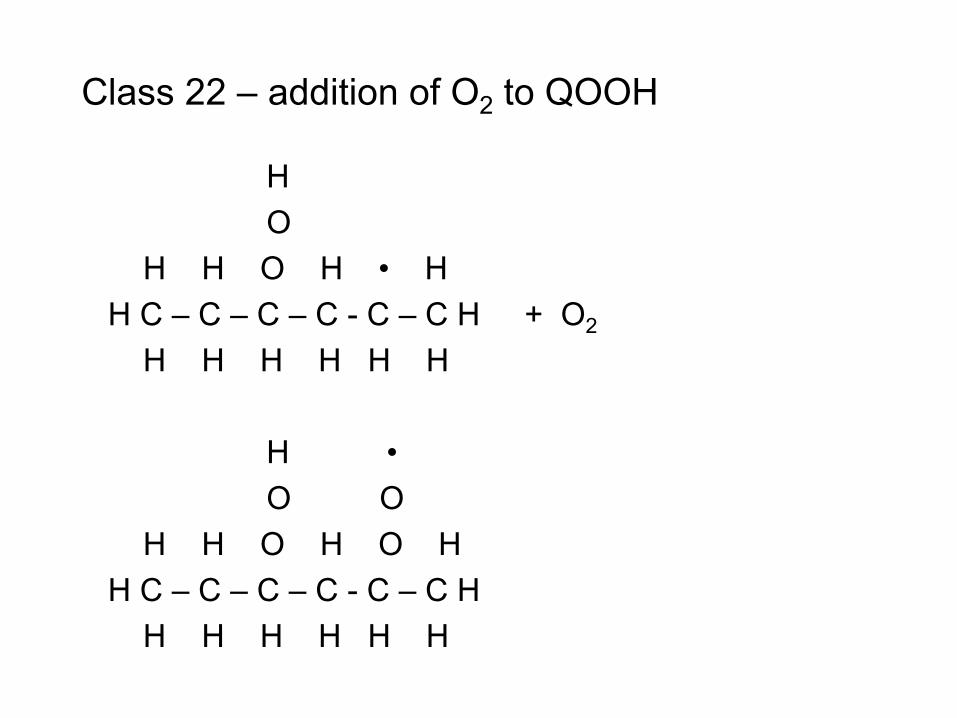
Class 22 – addition of O2 to QOOH

H O H H O H • H H C – C – C – C - C – C H + O2

H H H H H H H • O O H H O H O H H C – C – C – C - C – C H H H H H H H

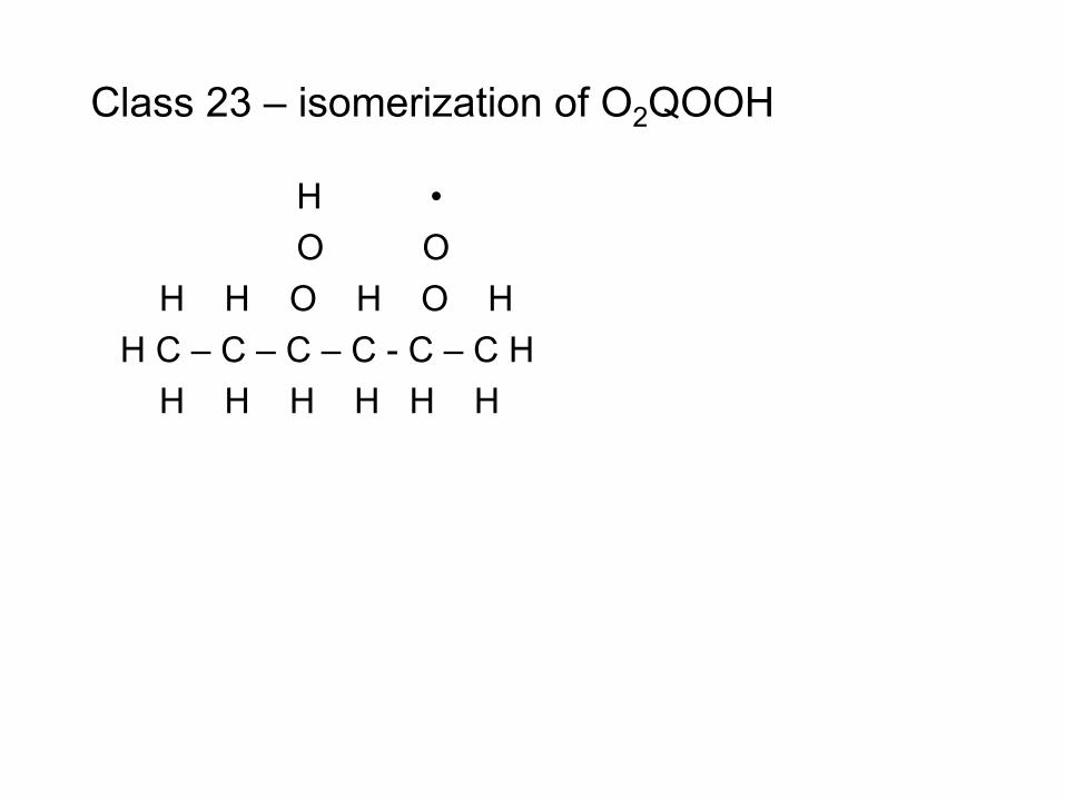
Class 23 – isomerization of O2QOOH

H • O O H H O H O H H C – C – C – C - C – C H H H H H H H

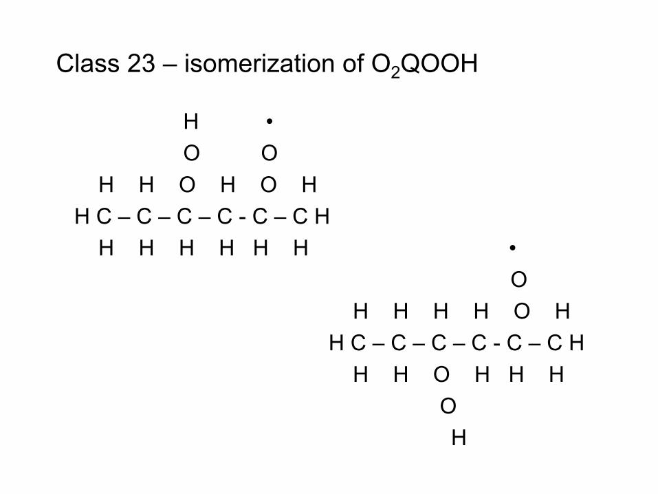
Class 23 – isomerization of O2QOOH

H • O O H H O H O H H C – C – C – C - C – C H H H H H H H • O H H H H O H H C – C – C – C - C – C H H H O H H H O H

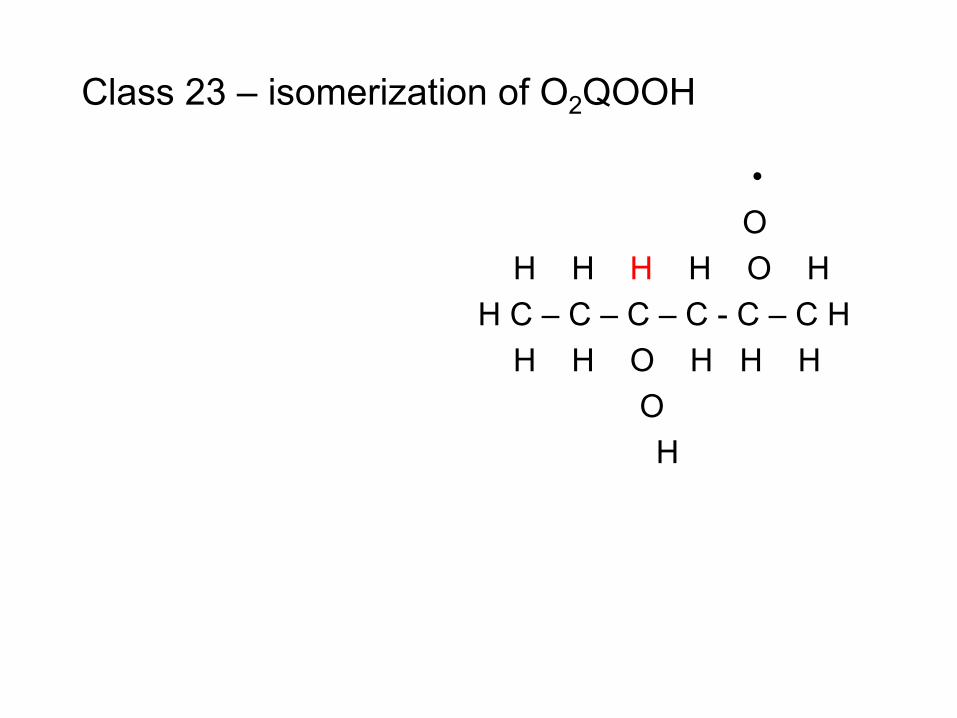
Class 23 – isomerization of O2QOOH

• O H H H H O H H C – C – C – C - C – C H H H O H H H O H

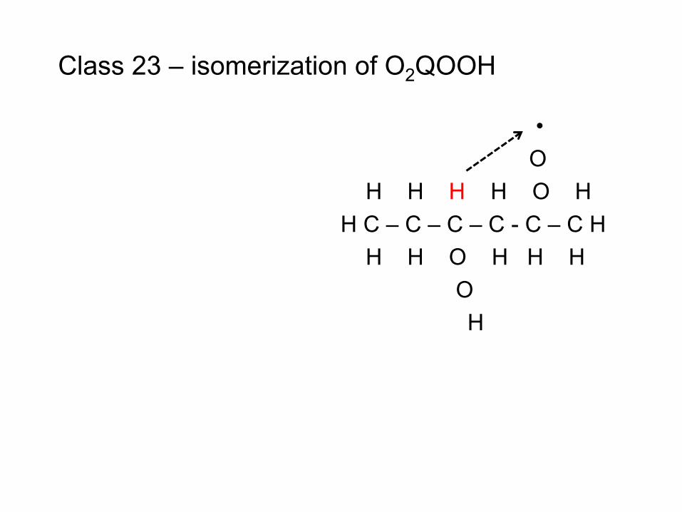
Class 23 – isomerization of O2QOOH

• O H H H H O H H C – C – C – C - C – C H H H O H H H O H

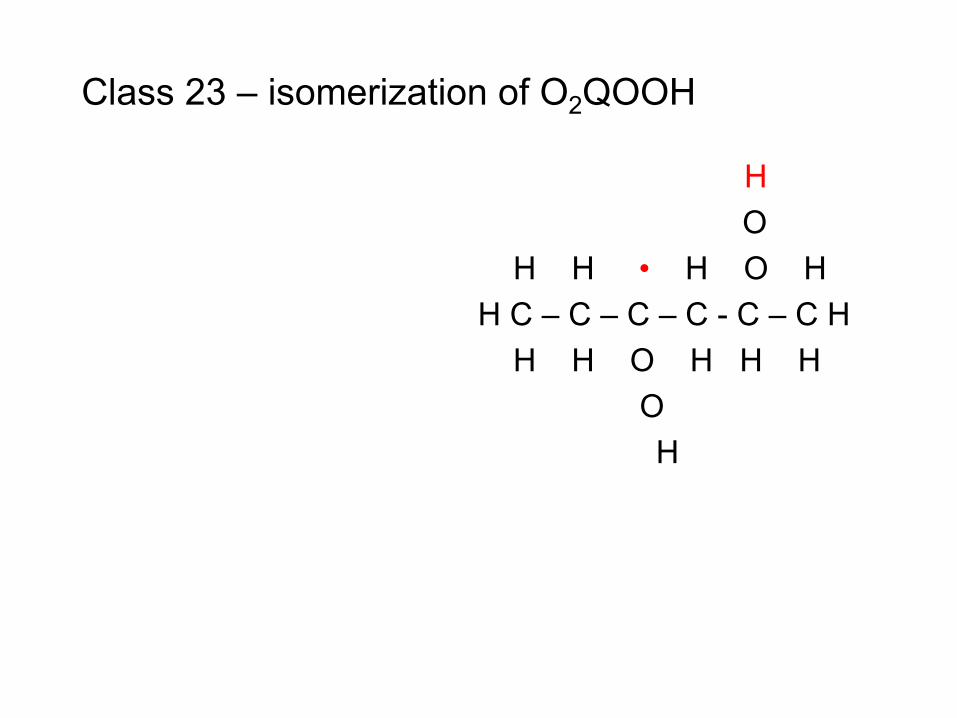
Class 23 – isomerization of O2QOOH

H O H H • H O H H C – C – C – C - C – C H H H O H H H O H

Class 23 – isomerization of O2QOOH

H O H H • H O H H C – C – C – C - C – C H H H O H H H O H

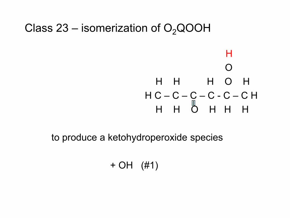
Class 23 – isomerization of O2QOOH

H O H H H O H H C – C – C – C - C – C H H H O H H H to produce a ketohydroperoxide species + OH (#1)

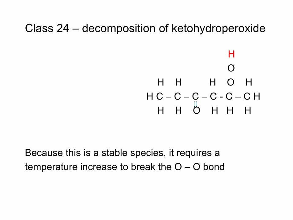
Class 24 – decomposition of ketohydroperoxide

H O H H H O H H C – C – C – C - C – C H H H O H H H Because this is a stable species, it requires a temperature increase to break the O – O bond

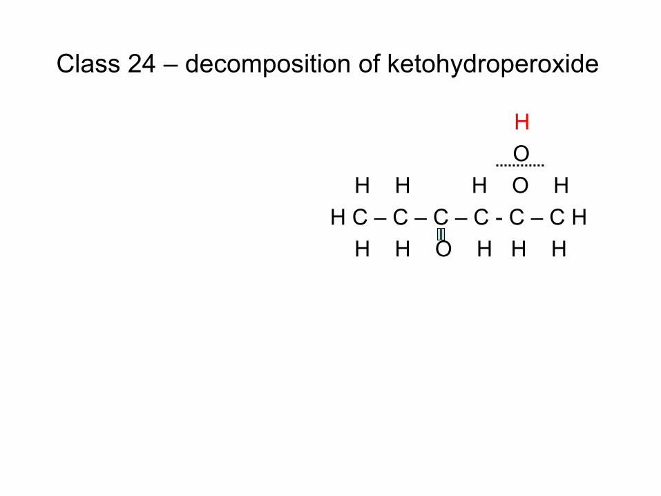
Class 24 – decomposition of ketohydroperoxide

H O H H H O H H C – C – C – C - C – C H H H O H H H

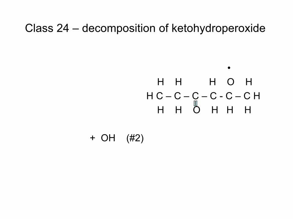
Class 24 – decomposition of ketohydroperoxide

• H H H O H H C – C – C – C - C – C H H H O H H H + OH (#2)

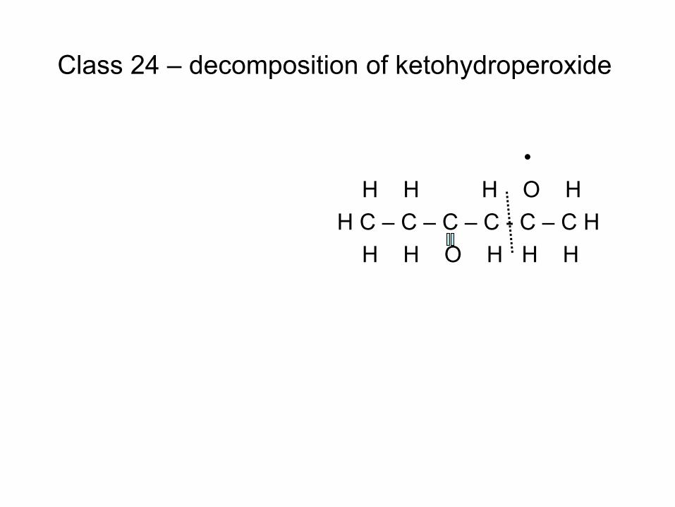
Class 24 – decomposition of ketohydroperoxide

• H H H O H H C – C – C – C - C – C H H H O H H H

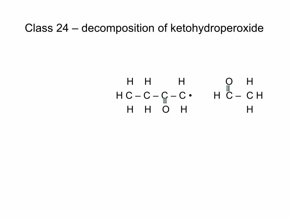
Class 24 – decomposition of ketohydroperoxide

H H H O H H C – C – C – C • H C – C H H H O H H

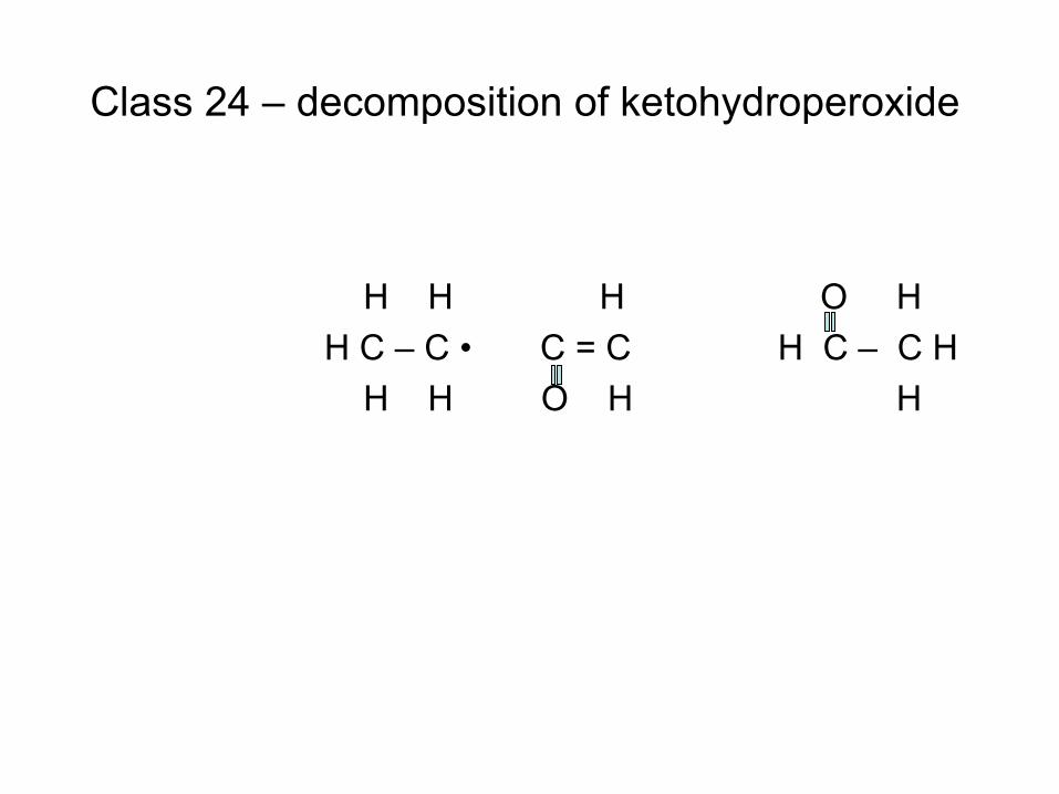
Class 24 – decomposition of ketohydroperoxide

H H H O H H C – C • C = C H C – C H H H O H H

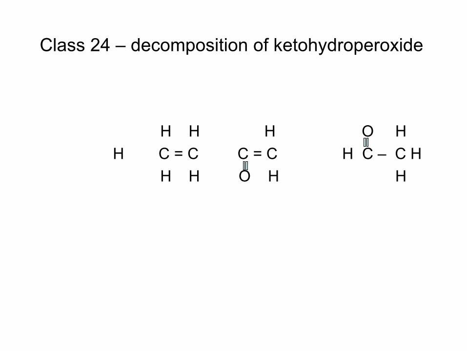
Class 24 – decomposition of ketohydroperoxide

H H H O H H C = C C = C H C – C H H H O H H

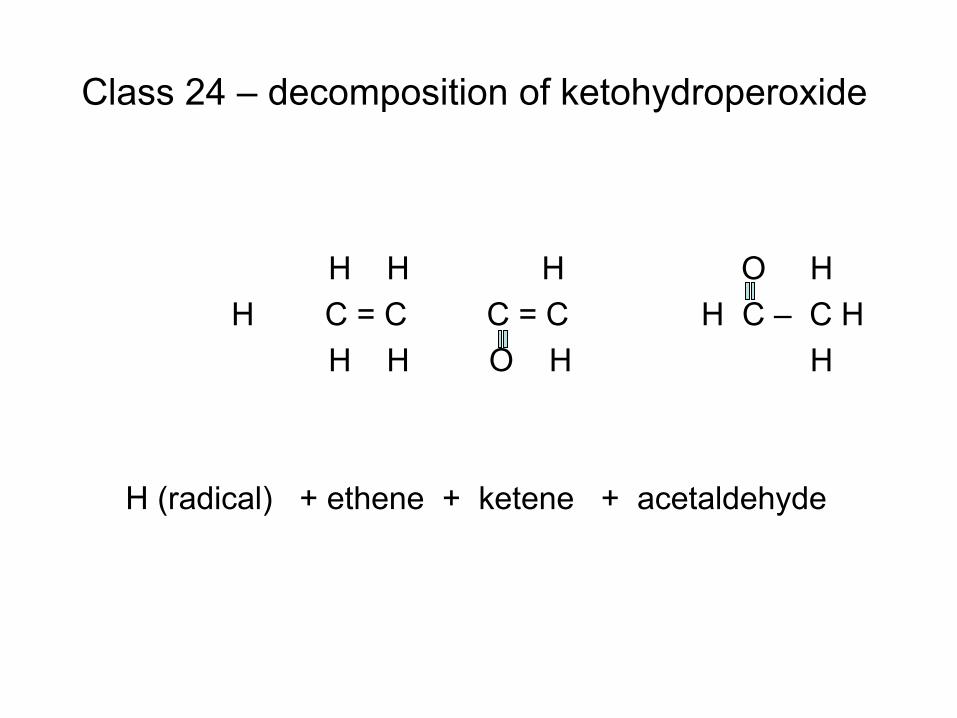
Class 24 – decomposition of ketohydroperoxide

H H H O H H C = C C = C H C – C H H H O H H H (radical) + ethene + ketene + acetaldehyde

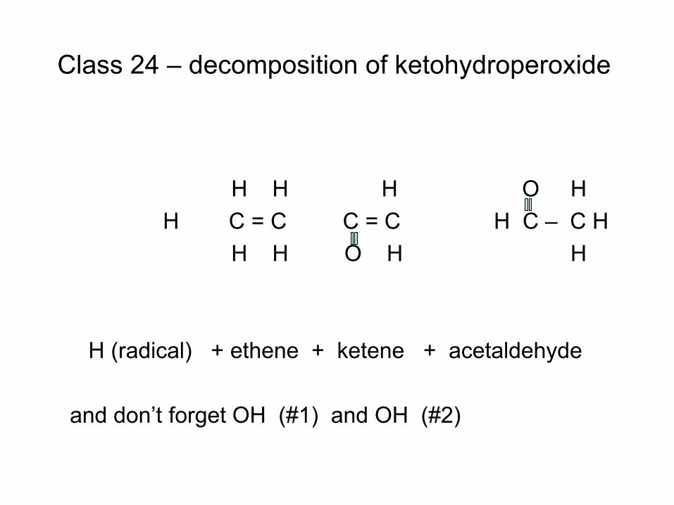
Class 24 – decomposition of ketohydroperoxide

H H H O H H C = C C = C H C – C H H H O H H H (radical) + ethene + ketene + acetaldehyde and don’t forget OH (#1) and OH (#2)

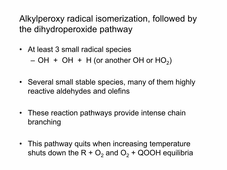
Alkylperoxy radical isomerization, followed by the dihydroperoxide pathway

• At least 3 small radical species – OH + OH + H (or another OH or HO2)

• Several small stable species, many of them highly

reactive aldehydes and olefins

• These reaction pathways provide intense chain branching

• This pathway quits when increasing temperature shuts down the R + O2 and O2 + QOOH equilibria

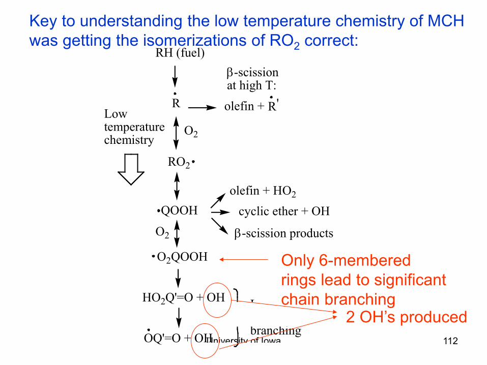
University of Iowa 112

Key to understanding the low temperature chemistry of MCH was getting the isomerizations of RO2 correct:

RH (fuel)

R

β-scissionat high T:

olefin + HO2

O2

QOOH

olefin +R '

cyclic ether + OH

β-scission products

O2QOOH

HO2Q'=O + OH

OQ'=O + OH

Low temperaturebranching

Low temperaturechemistry

O2

RO2

2 OH’s produced

Only 6-membered rings lead to significant chain branching

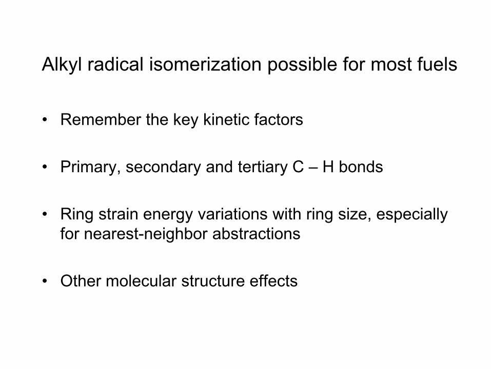
Alkyl radical isomerization possible for most fuels

• Remember the key kinetic factors

• Primary, secondary and tertiary C – H bonds

• Ring strain energy variations with ring size, especially for nearest-neighbor abstractions

• Other molecular structure effects

Octane numbers of heptanes are due exclusively to their different molecular structures Low octane fuels have lots of secondary C-H bonds and high octane fuels have lots of primary C-H bonds and lots of tight, 5-membered TS rings

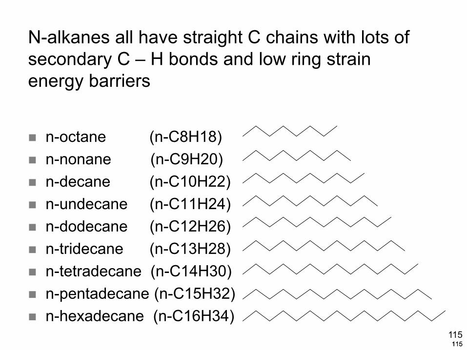
115 115 115

N-alkanes all have straight C chains with lots of secondary C – H bonds and low ring strain energy barriers

n-octane (n-C8H18) n-nonane (n-C9H20) n-decane (n-C10H22) n-undecane (n-C11H24) n-dodecane (n-C12H26) n-tridecane (n-C13H28) n-tetradecane (n-C14H30) n-pentadecane (n-C15H32) n-hexadecane (n-C16H34)

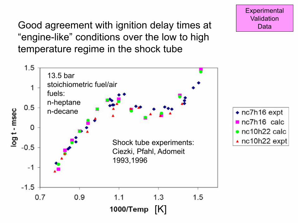
116

Good agreement with ignition delay times at “engine-like” conditions over the low to high temperature regime in the shock tube

[K]

Shock tube experiments: Ciezki, Pfahl, Adomeit 1993,1996

13.5 bar stoichiometric fuel/air fuels: n-heptane n-decane

Experimental Validation

Data

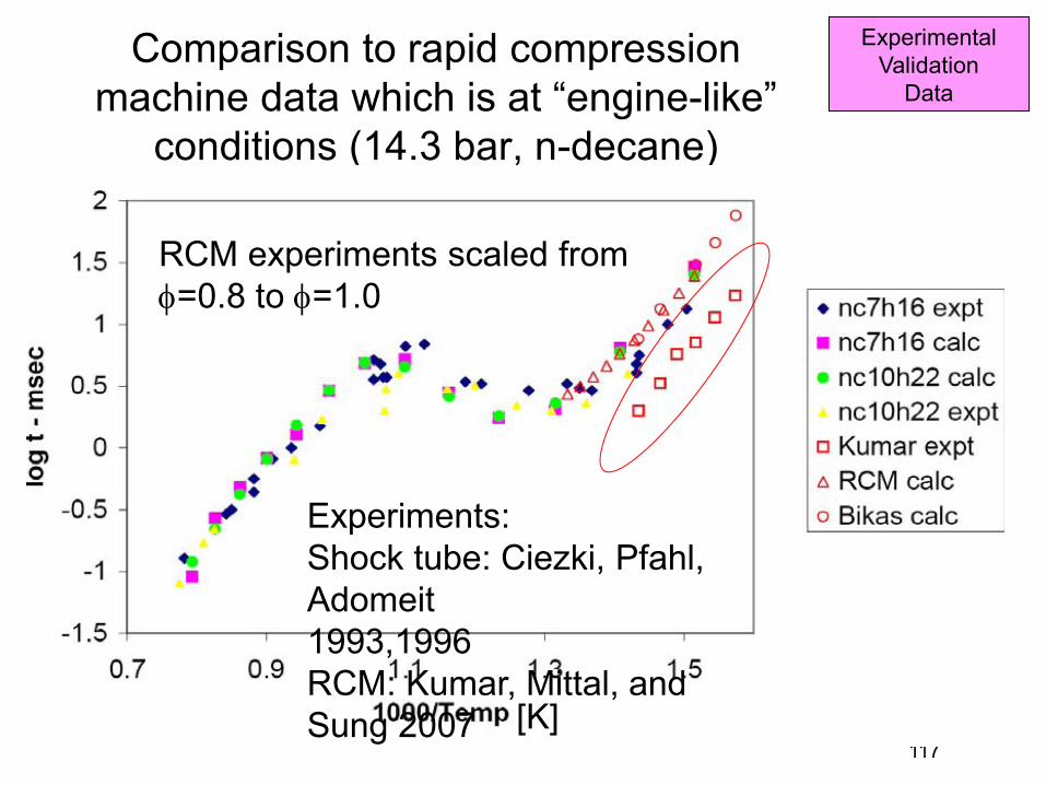
117

Comparison to rapid compression machine data which is at “engine-like”

conditions (14.3 bar, n-decane)

[K]

Experiments: Shock tube: Ciezki, Pfahl, Adomeit 1993,1996 RCM: Kumar, Mittal, and Sung 2007

RCM experiments scaled from φ=0.8 to φ=1.0

Experimental Validation

Data

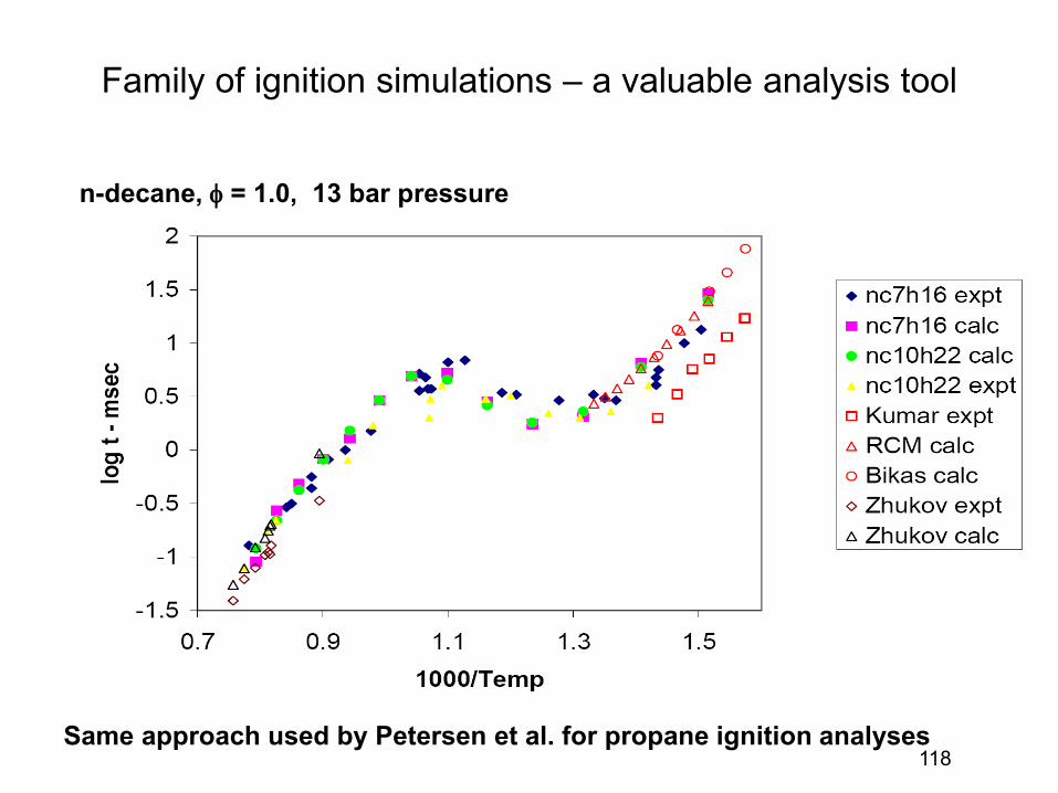
118

Family of ignition simulations – a valuable analysis tool

n-decane, φ = 1.0, 13 bar pressure

Same approach used by Petersen et al. for propane ignition analyses

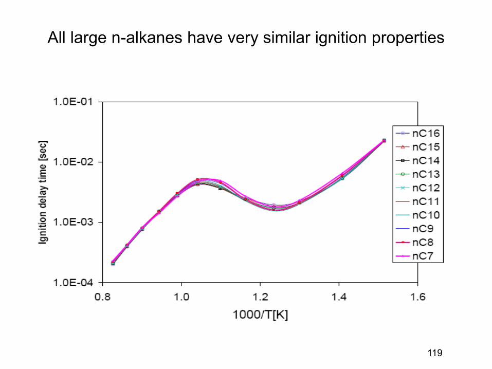
119

All large n-alkanes have very similar ignition properties

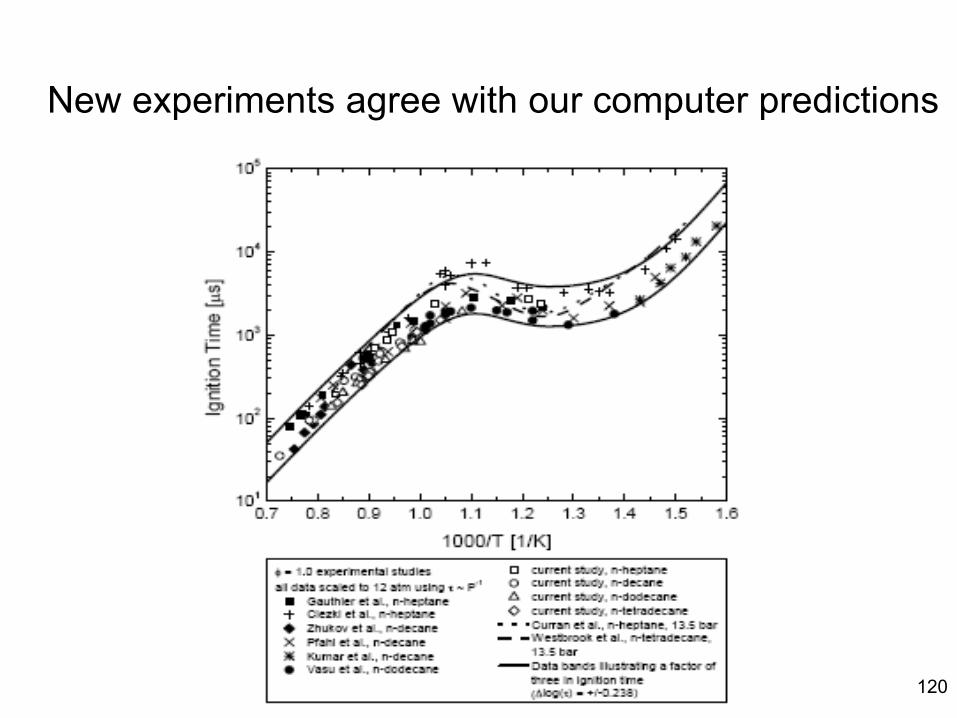
120

New experiments agree with our computer predictions

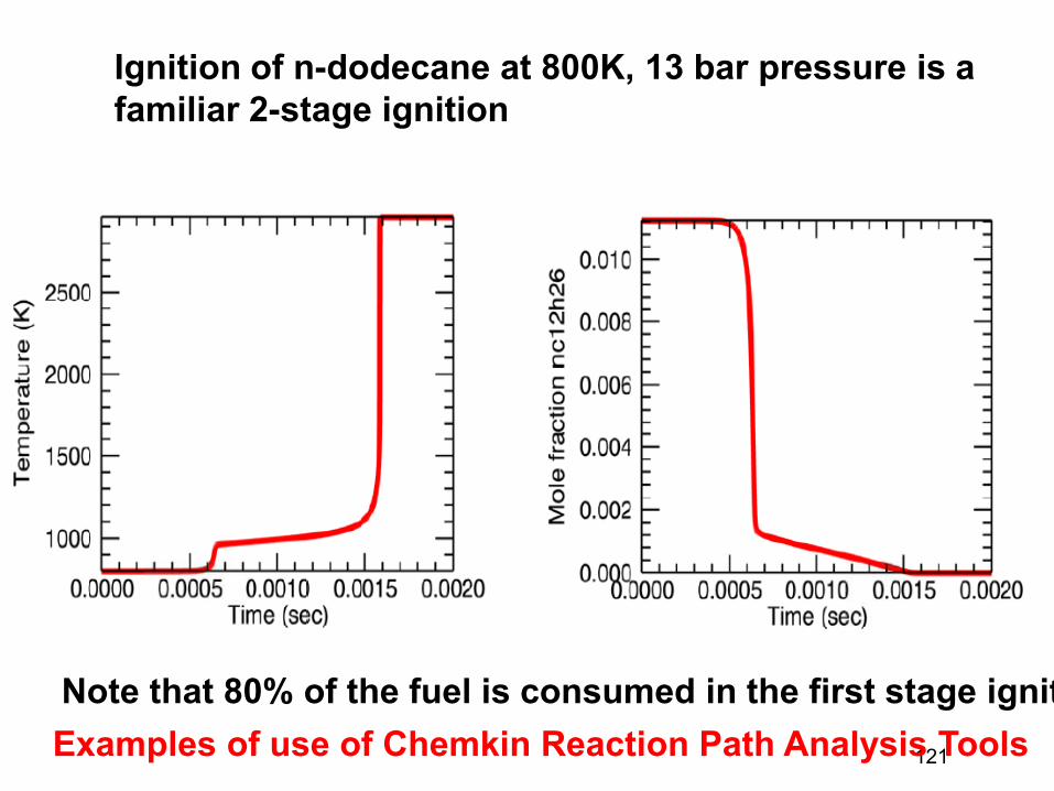
121

Ignition of n-dodecane at 800K, 13 bar pressure is a familiar 2-stage ignition

Note that 80% of the fuel is consumed in the first stage ignit Examples of use of Chemkin Reaction Path Analysis Tools

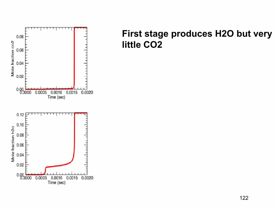
122

First stage produces H2O but very little CO2

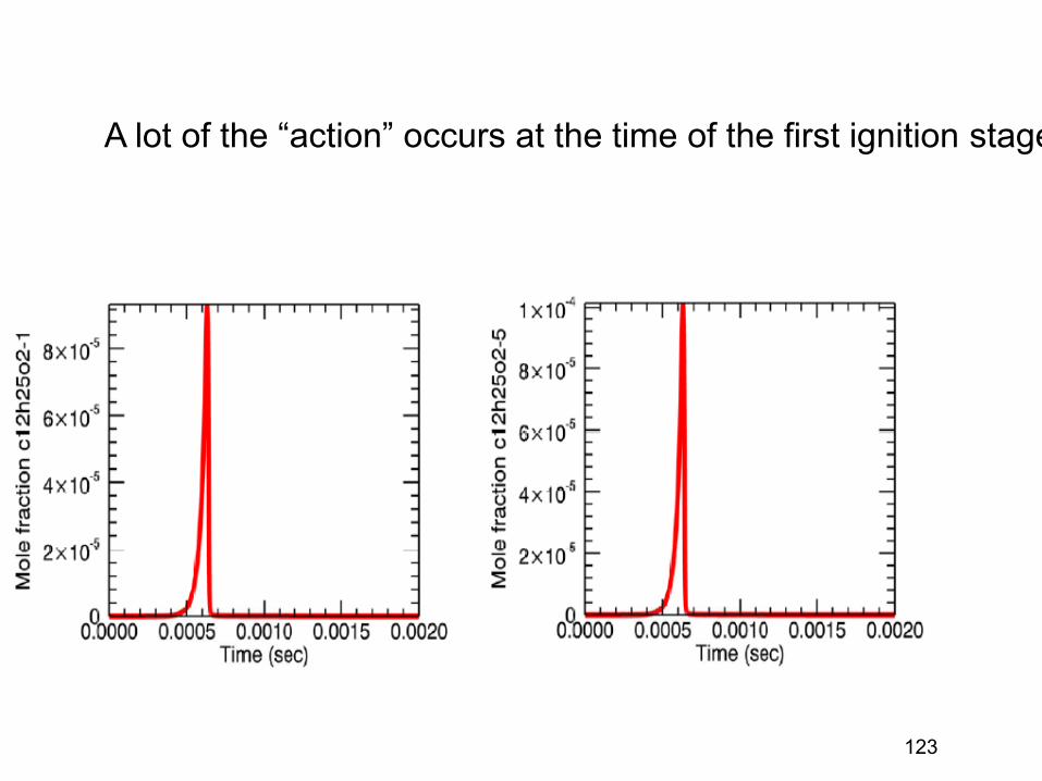
123

A lot of the “action” occurs at the time of the first ignition stage

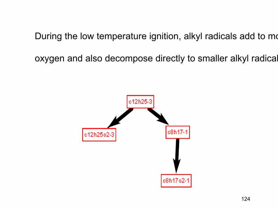
124

During the low temperature ignition, alkyl radicals add to mo oxygen and also decompose directly to smaller alkyl radical

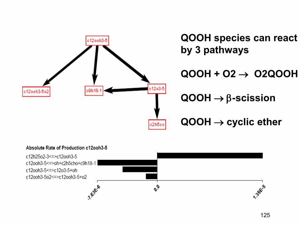
125

QOOH species can react by 3 pathways QOOH + O2 → O2QOOH QOOH → β-scission QOOH → cyclic ether

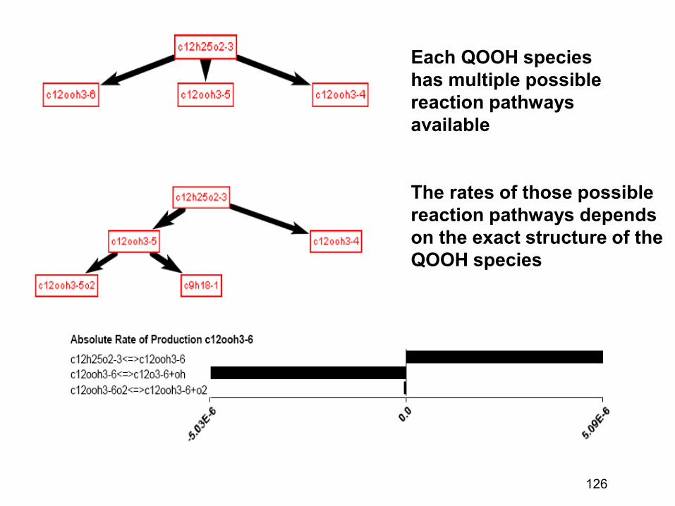
126

Each QOOH species has multiple possible reaction pathways available

The rates of those possible reaction pathways depends on the exact structure of the QOOH species

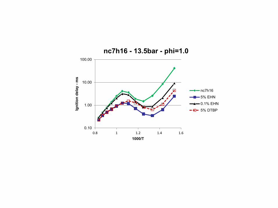
0.10

1.00

10.00

100.00

0.8 1 1.2 1.4 1.6

Igni

tion

dela

y - m

s

1000/T

nc7h16 - 13.5bar - phi=1.0

nc7h16

5% EHN

0.1% EHN

5% DTBP

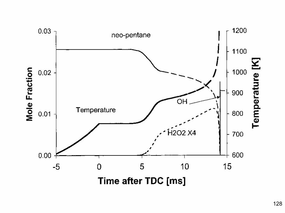
128

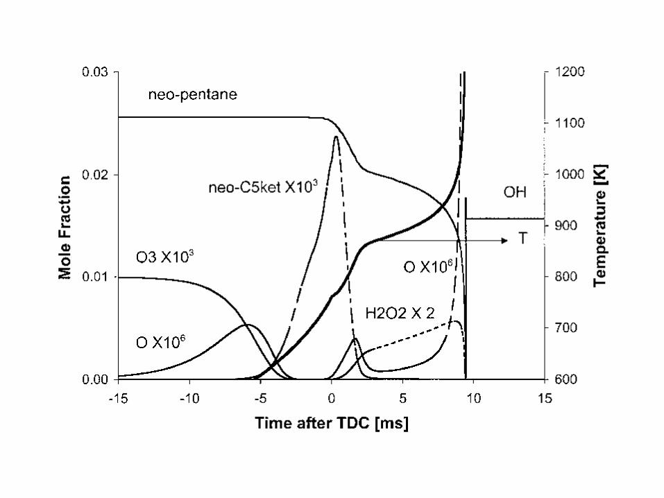
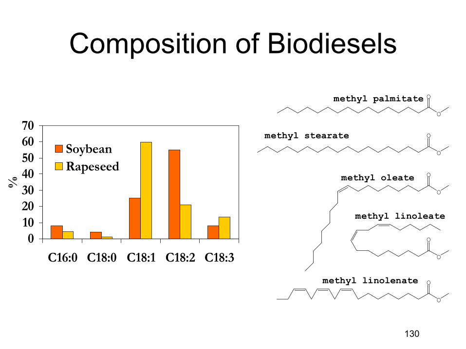
130

Composition of Biodiesels O

O

O

O

O

O

O

O

O

O

methyl palmitate

methyl stearate

methyl oleate

methyl linoleate

methyl linolenate

010203040506070

C16:0 C18:0 C18:1 C18:2 C18:3

%

SoybeanRapeseed

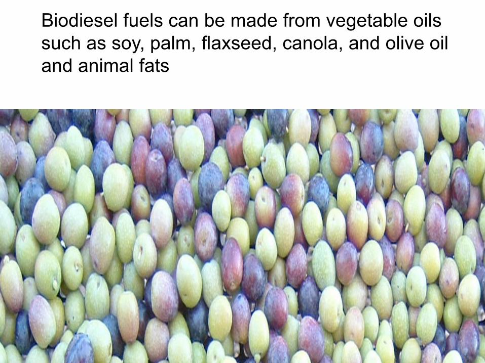
Biodiesel fuels can be made from vegetable oils such as soy, palm, flaxseed, canola, and olive oil and animal fats

QuickTime™ and aTIFF (LZW) decompressor

are needed to see this picture.

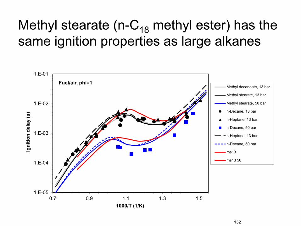
Methyl stearate (n-C18 methyl ester) has the same ignition properties as large alkanes

132

1.E-05

1.E-04

1.E-03

1.E-02

1.E-01

0.7 0.9 1.1 1.3 1.5

Igni

tion

dela

y (s

)

1000/T (1/K)

Fuel/air, phi=1 Methyl decanoate, 13 bar

Methyl stearate, 13 bar

Methyl stearate, 50 bar

n-Decane, 13 bar

n-Heptane, 13 bar

n-Decane, 50 bar

n-Heptane, 13 bar

n-Decane, 50 bar

ms13

ms13 50

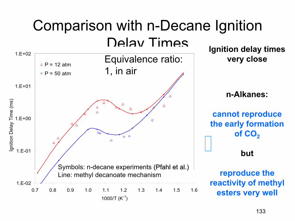
133

Comparison with n-Decane Ignition Delay Times

1.E-02

1.E-01

1.E+00

1.E+01

1.E+02

0.7 0.8 0.9 1.0 1.1 1.2 1.3 1.4 1.5 1.6

1000/T (K-1)

Igni

tion

Del

ay T

ime

(ms)

P = 12 atm

P = 50 atm

Symbols: n-decane experiments (Pfahl et al.) Line: methyl decanoate mechanism

Ignition delay times very close

n-Alkanes:

cannot reproduce the early formation

of CO2

but

reproduce the reactivity of methyl

esters very well

Equivalence ratio: 1, in air

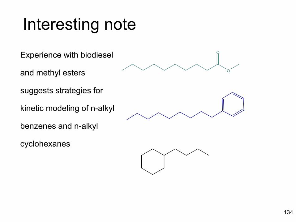
134

Interesting note

Experience with biodiesel

and methyl esters

suggests strategies for

kinetic modeling of n-alkyl

benzenes and n-alkyl

cyclohexanes

O

O

135

Branched hydrocarbons are different

Both octane and cetane rating systems have a straight-chain reference fuel that is easy to ignite and a branched reference fuel that is hard to ignite

iso-octane and 2,2,4,4,6,8,8-heptamethyl nonane

n-heptane and n-hexadecane

Are all branched hydrocarbons as similar to each other as the straight-chain hydrocarbons?

Very few laboratory experiments available for mechanism validation of HMN

Base a reaction mechanism on previous sets of reaction classes

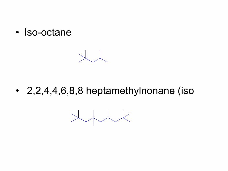
• Iso-octane

• 2,2,4,4,6,8,8 heptamethylnonane (iso

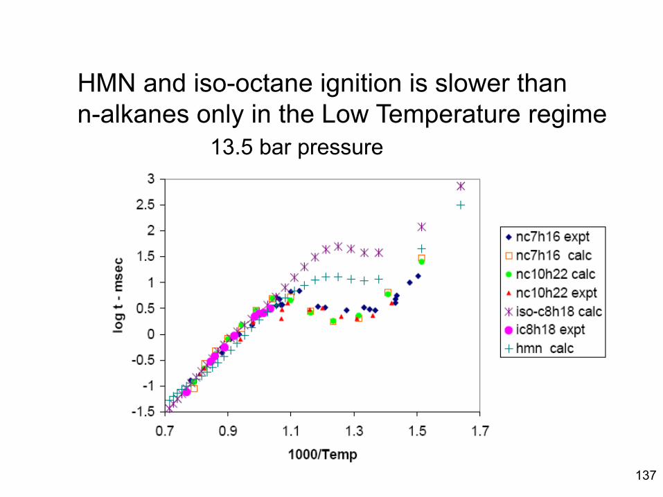
137

HMN and iso-octane ignition is slower than n-alkanes only in the Low Temperature regime

13.5 bar pressure

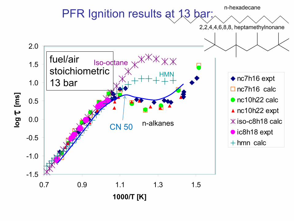
PFR Ignition results at 13 bar:

-1.5

-1.0

-0.5

0.0

0.5

1.0

1.5

2.0

0.7 0.9 1.1 1.3 1.5

1000/T [K]

log

τ [m

s]

nc7h16 exptnc7h16 calcnc10h22 calcnc10h22 exptiso-c8h18 calcic8h18 expthmn calc

Iso-octane

n-alkanes

HMN

fuel/air stoichiometric 13 bar

CN 50

n-hexadecane

2,2,4,4,6,8,8, heptamethylnonane

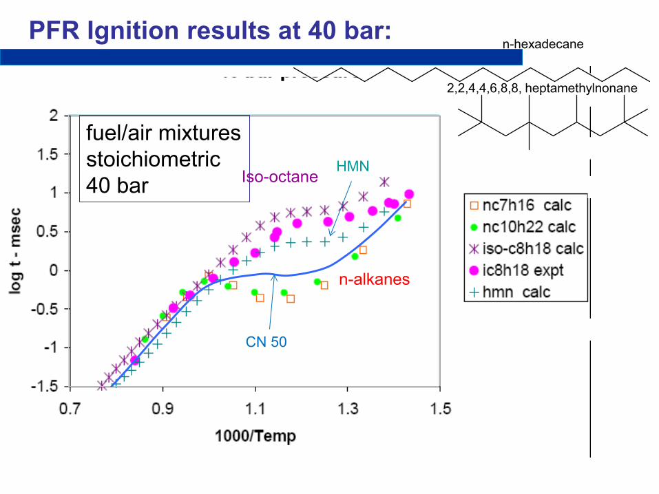
fuel/air mixtures stoichiometric 40 bar Iso-octane

n-alkanes

HMN

PFR Ignition results at 40 bar: n-hexadecane

2,2,4,4,6,8,8, heptamethylnonane

CN 50

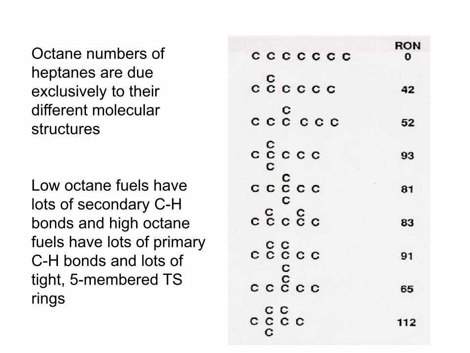
Octane numbers of heptanes are due exclusively to their different molecular structures Low octane fuels have lots of secondary C-H bonds and high octane fuels have lots of primary C-H bonds and lots of tight, 5-membered TS rings

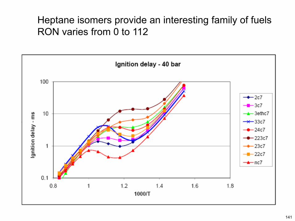
141

Heptane isomers provide an interesting family of fuels RON varies from 0 to 112

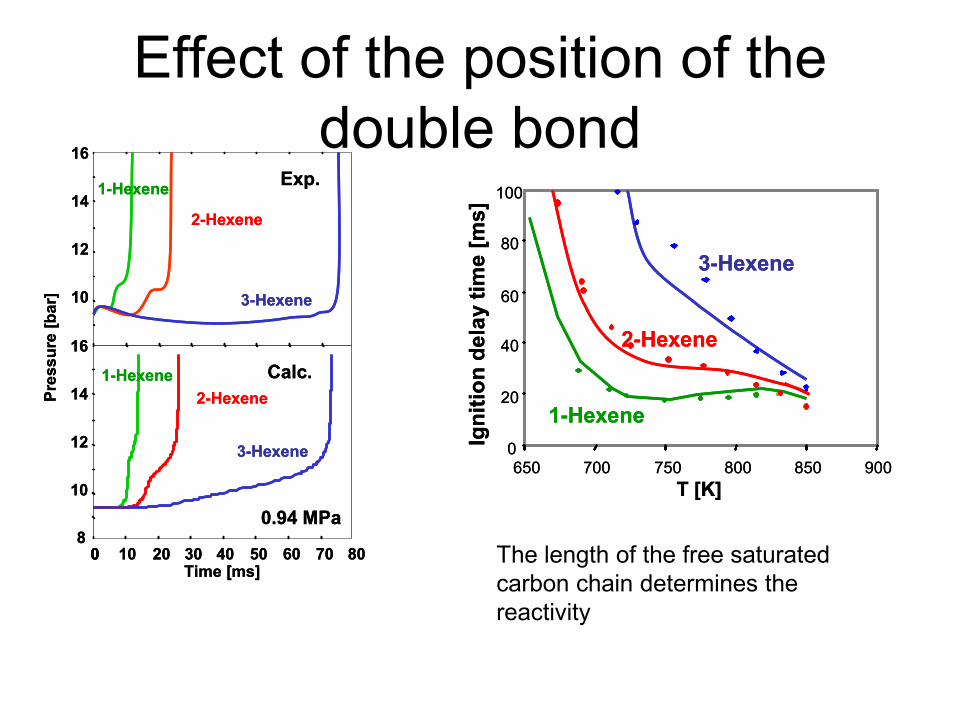
Effect of the position of the double bond

Time [ms]

8

10

12

14

16

0 10 20 30 40 50 60 70 800

Pres

sure

[bar

]

2-Hexene

3-Hexene

1-Hexene

10

12

14

16

1-Hexene

2-Hexene

3-Hexene

Exp.

Calc.

0.94 MPa

Time [ms]

8

10

12

14

16

0 10 20 30 40 50 60 70 800

Pres

sure

[bar

]

2-Hexene

3-Hexene

1-Hexene

10

12

14

16

1-Hexene

2-Hexene

3-Hexene

Exp.

Calc.

0.94 MPa

3-Hexene

2-Hexene

1-Hexene0

20

40

60

80

100

650 700 750 800 850 900T [K]

Igni

tion

dela

y tim

e [m

s]

3-Hexene

2-Hexene

1-Hexene0

20

40

60

80

100

650 700 750 800 850 900T [K]

Igni

tion

dela

y tim

e [m

s]

The length of the free saturated carbon chain determines the reactivity

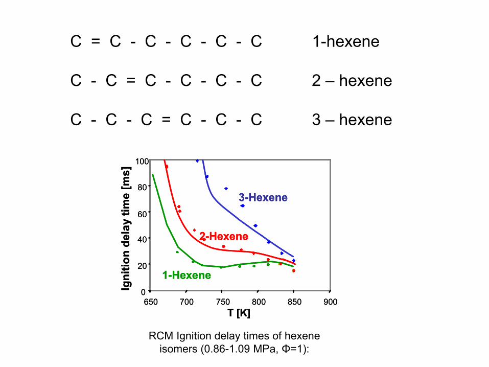
3-Hexene

2-Hexene

1-Hexene0

20

40

60

80

100

650 700 750 800 850 900T [K]

Igni

tion

dela

y tim

e [m

s]

3-Hexene

2-Hexene

1-Hexene0

20

40

60

80

100

650 700 750 800 850 900T [K]

Igni

tion

dela

y tim

e [m

s]

RCM Ignition delay times of hexene isomers (0.86-1.09 MPa, Φ=1):

C = C - C - C - C - C 1-hexene C - C = C - C - C - C 2 – hexene C - C - C = C - C - C 3 – hexene

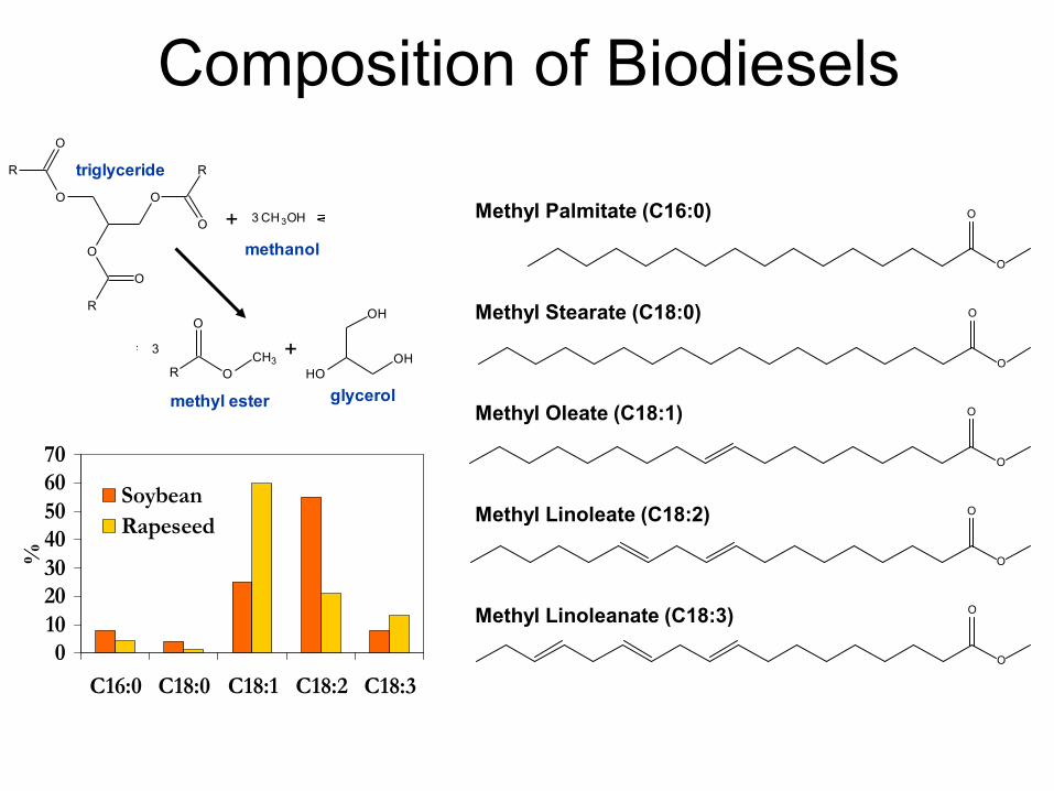
Composition of Biodiesels

010203040506070

C16:0 C18:0 C18:1 C18:2 C18:3

%

SoybeanRapeseed

O

O

O

O

O

O

O

O

O

O

Methyl Palmitate (C16:0)

Methyl Stearate (C18:0)

Methyl Oleate (C18:1)

Methyl Linoleate (C18:2)

Methyl Linoleanate (C18:3)

triglyceride

methanol

OO

O

O

O

O

R

R R

+ 3 CH 3OH

methyl ester glycerol

OH

OH

OH

CH3O

O

R

3 +

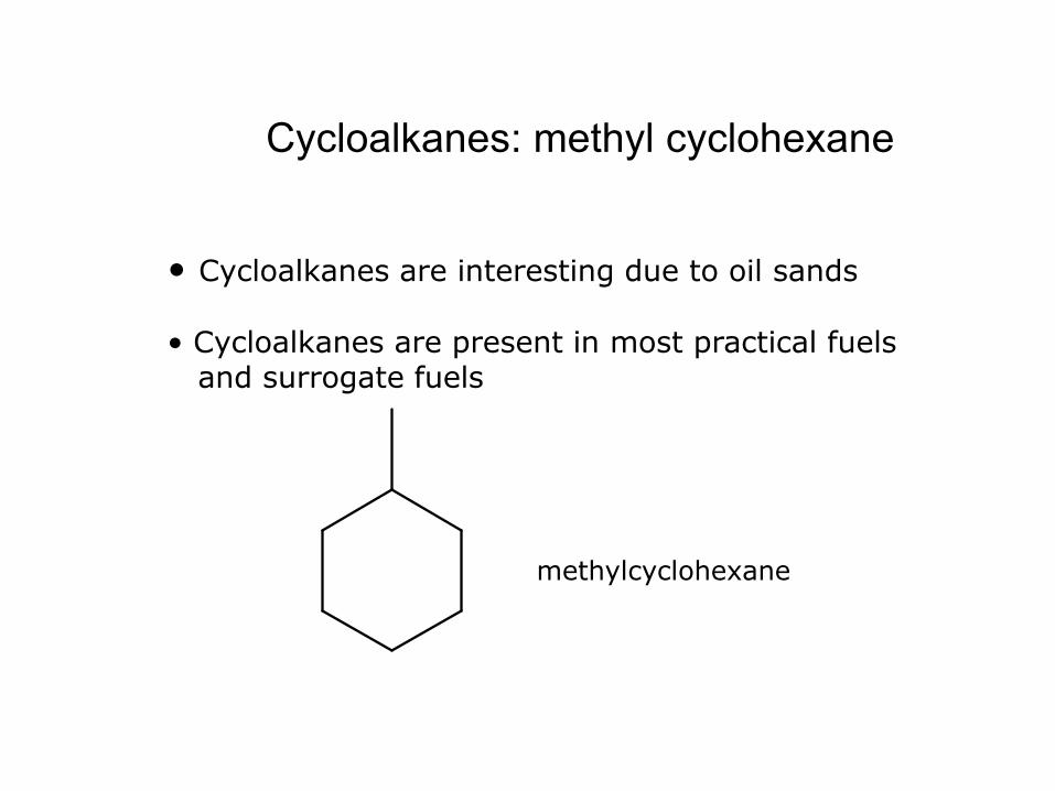
Cycloalkanes: methyl cyclohexane

• Cycloalkanes are interesting due to oil sands • Cycloalkanes are present in most practical fuels and surrogate fuels

methylcyclohexane

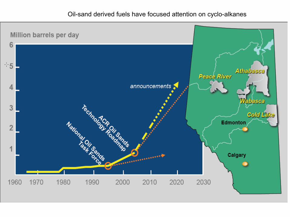
Slide courtesy Phil Smith, University of Utah

Oil-sand derived fuels have focused attention on cyclo-alkanes

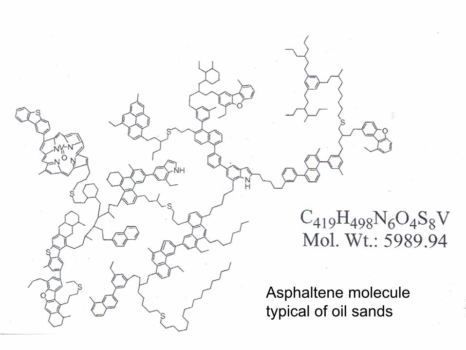
Asphaltene molecule typical of oil sands

University of Iowa 148

Experiments: Rapid compression machine (RCM) at NUI Galway

• Opposed piston RCM originally used by Shell – => fast compression times of about 16 ms

• Large crevice on perimeter of piston to contain wall boundary layer – =>uniform temperatures across combustion chamber

• Use N2 and Ar as diluents to attain range of compressed gas temperatures

• Stoichiometric mixtures of MCH/O2/Ar/N2 • 10,15 and 20 atm pressure at the end of

compression.

University of Iowa 149

0.001

0.010

0.100

1.000

650 750 850 950 1050 1150

Temperature at the end of compression [K]

Igni

tion

dela

y tim

e [s

]

Experimental data NUI Galway

Experimental data at 10 atm shows distinct NTC region:

University of Iowa 150

N-alkane based RO2 isomerization rates gave too slow ignition delay times in rapid compression machine at low temperatures:

0.001

0.010

0.100

1.000

650 750 850 950 1050 1150

Temperature at the end of compression [K]

Igni

tion

dela

y tim

e [s

]

Experimental data NUI Galway

MCH mechanism result

Predictions show complete absence of a negative temperature coefficient region

Rates of important isomerization reactions were estimated by comparison with known reactions for alkanes

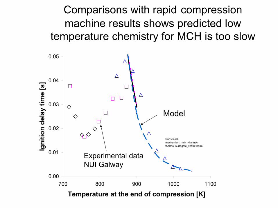
Comparisons with rapid compression machine results shows predicted low

temperature chemistry for MCH is too slow

0.00

0.01

0.02

0.03

0.04

0.05

700 800 900 1000 1100

Temperature at the end of compression [K]

Igni

tion

dela

y tim

e [s

]

Runs 5-23mechanism: mch_v1a.mechthermo: surrogate_ver8b.therm

Model

Experimental dataNUI Galway

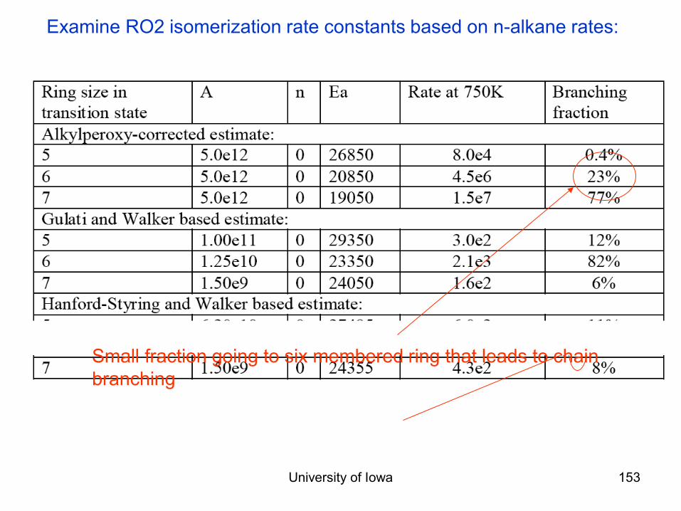
University of Iowa 153

Examine RO2 isomerization rate constants based on n-alkane rates:

Small fraction going to six membered ring that leads to chain branching

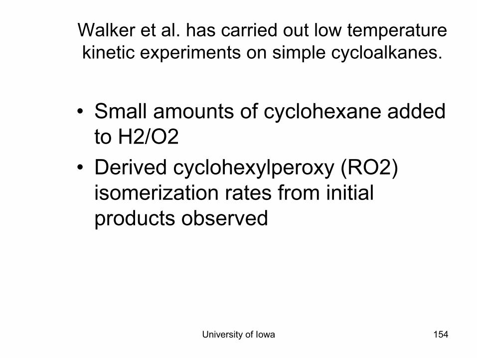
University of Iowa 154

Walker et al. has carried out low temperature kinetic experiments on simple cycloalkanes.

• Small amounts of cyclohexane added to H2/O2

• Derived cyclohexylperoxy (RO2) isomerization rates from initial products observed

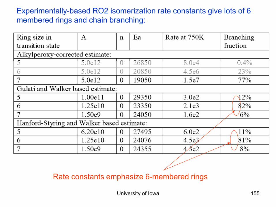
University of Iowa 155

Experimentally-based RO2 isomerization rate constants give lots of 6 membered rings and chain branching:

Rate constants emphasize 6-membered rings

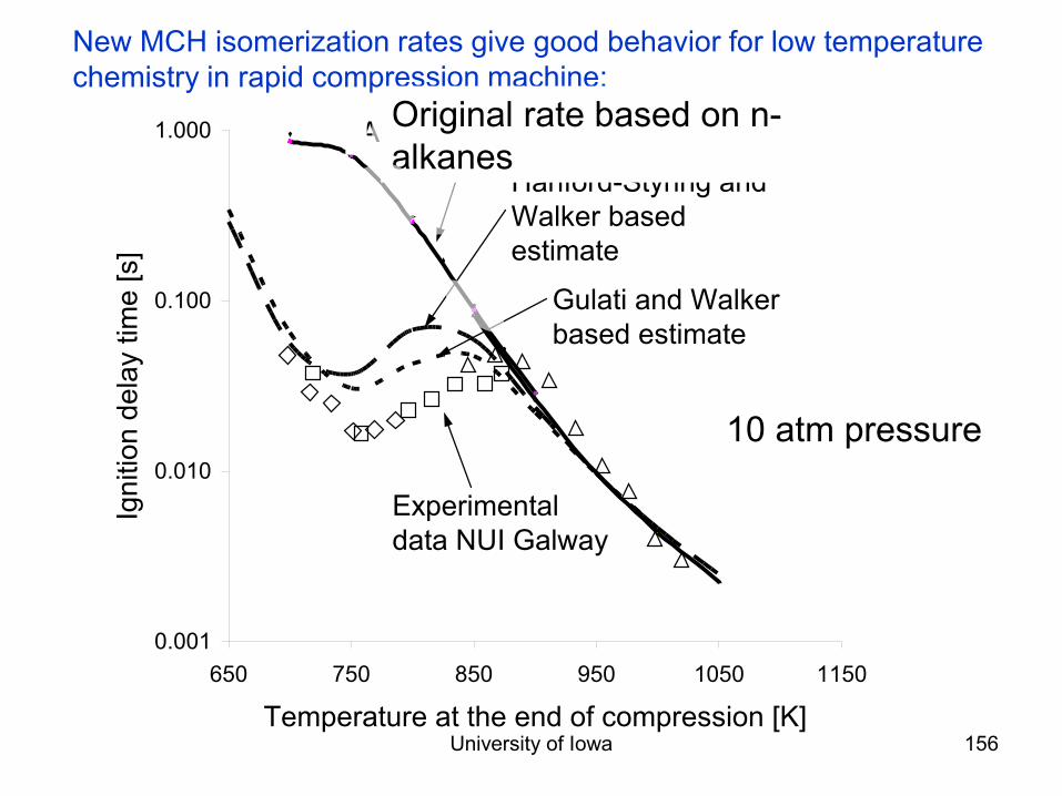
University of Iowa 156

0.001

0.010

0.100

1.000

650 750 850 950 1050 1150

Temperature at the end of compression [K]

Igni

tion

dela

y tim

e [s

]

Gulati and Walker based estimate

Alkylperoxy corrected estimate

Experimental data NUI Galway

Hanford-Styring and Walker based estimate

New MCH isomerization rates give good behavior for low temperature chemistry in rapid compression machine:

10 atm pressure

Original rate based on n-alkanes

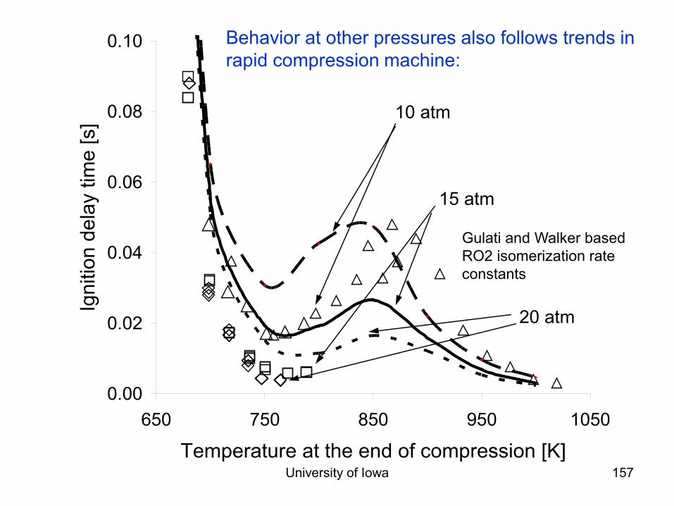
University of Iowa 157

0.00

0.02

0.04

0.06

0.08

0.10

650 750 850 950 1050

Temperature at the end of compression [K]

Igni

tion

dela

y tim

e [s

] 10 atm

15 atm

20 atm

Behavior at other pressures also follows trends in rapid compression machine:

Gulati and Walker based RO2 isomerization rate constants

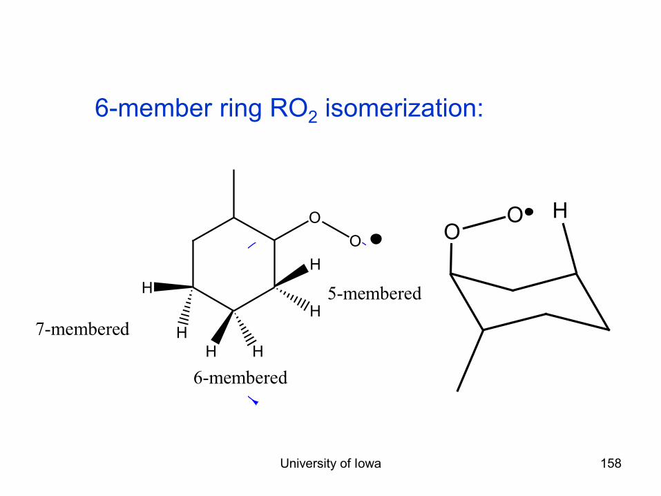
University of Iowa 158

OO

H

H

HH

H

H

5-membered

6-membered

7-membered

6-member ring RO2 isomerization:

OO H

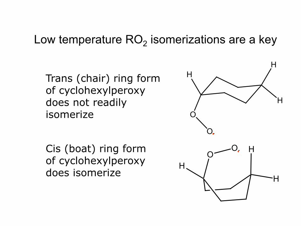
Low temperature RO2 isomerizations are a key

H

H

O

H

O.

Trans (chair) ring form of cyclohexylperoxy does not readily isomerize

H

H

OH

O.Cis (boat) ring form of cyclohexylperoxy does isomerize

.

.

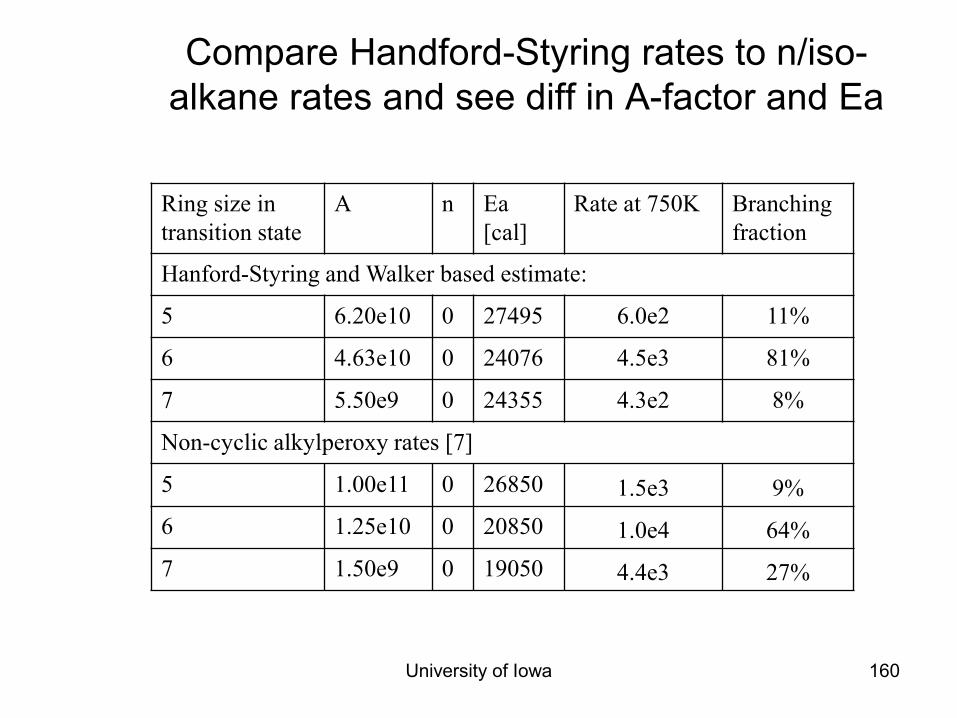
University of Iowa 160

Compare Handford-Styring rates to n/iso-alkane rates and see diff in A-factor and Ea

Ring size in transition state

A n Ea [cal]

Rate at 750K Branching fraction

Hanford-Styring and Walker based estimate:

5 6.20e10 0 27495 6.0e2 11%

6 4.63e10 0 24076 4.5e3 81%

7 5.50e9 0 24355 4.3e2 8%

Non-cyclic alkylperoxy rates [7]

5 1.00e11 0 26850 1.5e3 9% 6 1.25e10 0 20850 1.0e4 64% 7 1.50e9 0 19050 4.4e3 27%

Explanation of engine knock, ON, antiknocks, diesel ignition, and HCCI ignition came in the 1990’s from DOE/BES theoretical chemistry and supercomputing and EERE knock working group

OO

H

H

OO

H

H

R

Reactant Transitionstate

HC

OO

H

H

R

R

HC

OO

H

H

R R

RR

RR

Most work has been done for alkane fuels, and many questions remain for aromatics, cyclic paraffins, large olefins

+ O2

OH +

+ OH

O

O

O

OH

OOH

O

O

O

O

OH

O

O

Low temperature chain branching paths Alkylperoxy radical isomerization rates are different in paraffin and cyclic paraffin hydrocarbons

There are many poorly understood phenomena

• All of our intuition, experience and theory of flame properties is based on flames at atmospheric and lower pressures

• In engines, at high pressures due to compression, unburned gas temperatures are also quite high

• Characteristic times to autoignition can be much shorter than characteristic times for flame propagation

• Assumptions built into our picture of flame propagation break down at high pressures, and it is not clear how to define limiting conditions

• Extrapolation of flame data to 100 bar not appropriate; great need for high pressure “flame” data of all kinds

• We don’t know very much about combustion at high pressures • We simply extrapolate phenomena from atmospheric pressure

to high pressure, but they probably are no longer valid • We don’t even know if “flames” still exist

Lesson 5: RMG

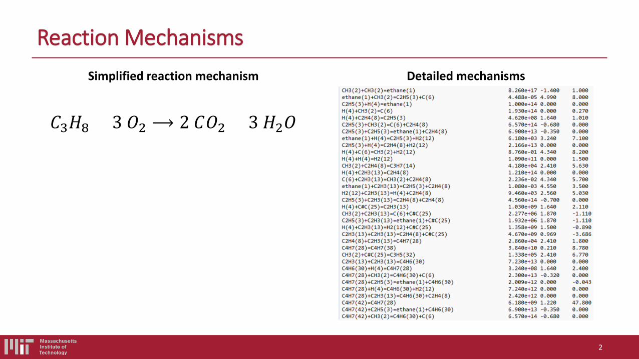
Reaction Mechanisms Simplified reaction mechanism

𝐶𝐶3𝐻𝐻8 + 3 𝑂𝑂2 ⟶ 2 𝐶𝐶𝑂𝑂2 + 3 𝐻𝐻2𝑂𝑂

Detailed mechanisms

2

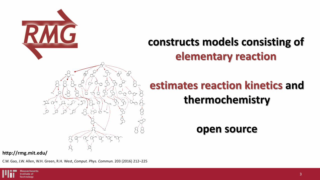
http://rmg.mit.edu/ C.W. Gao, J.W. Allen, W.H. Green, R.H. West, Comput. Phys. Commun. 203 (2016) 212–225

open source

estimates reaction kinetics and thermochemistry

constructs models consisting of elementary reaction

3

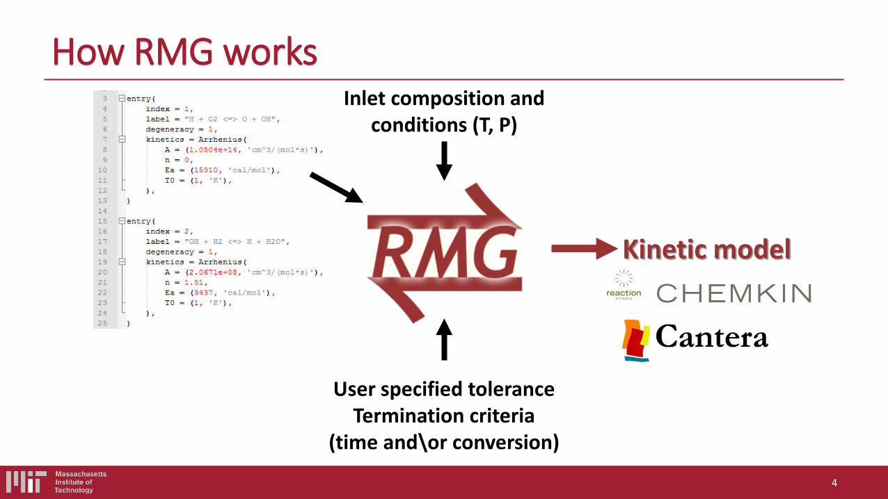
User specified tolerance Termination criteria

(time and\or conversion)

Kinetic and Thermodynamic

libraries (optional, recommended

for small species) Kinetic model

Inlet composition and conditions (T, P)

How RMG works

4

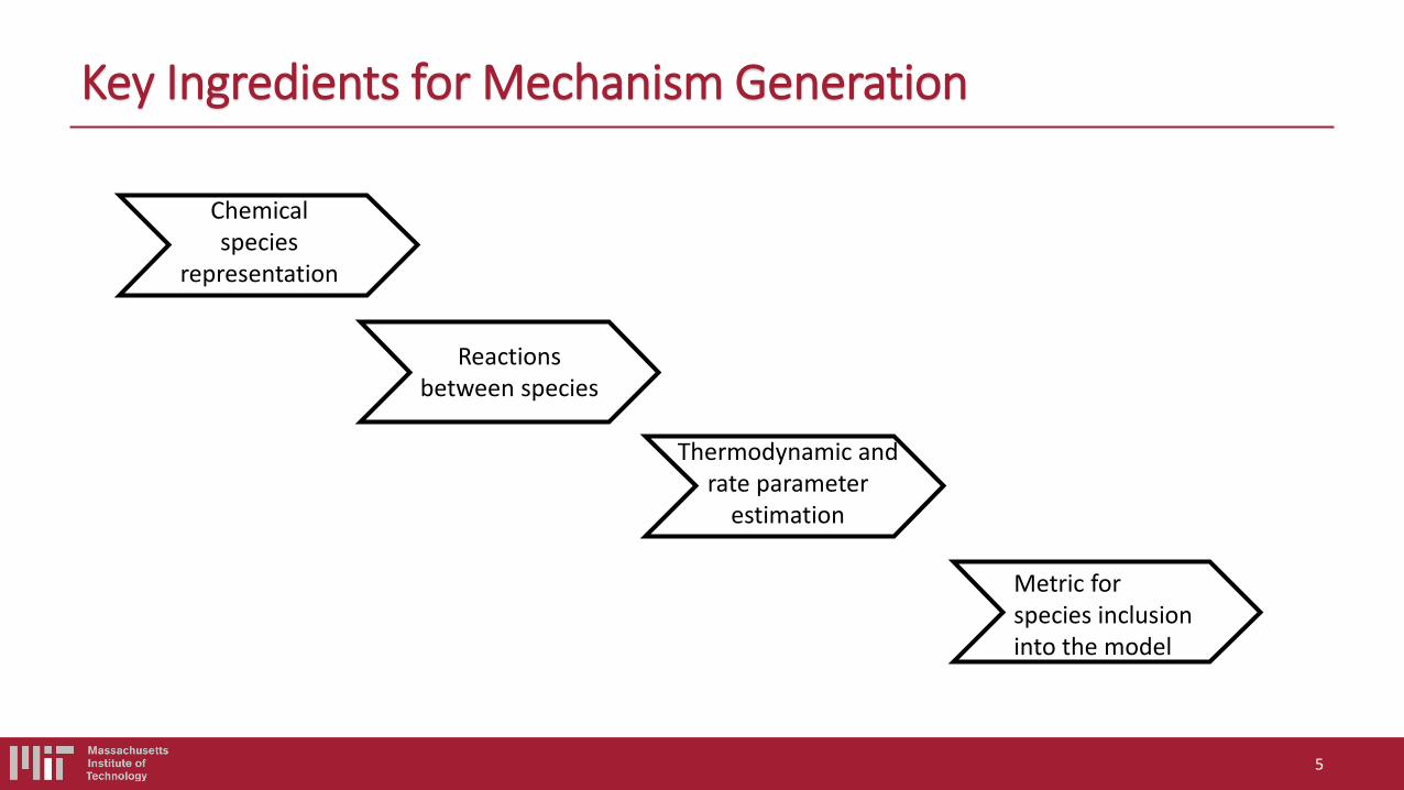
Key Ingredients for Mechanism Generation

5

Chemical species

representation

Reactions between species

Thermodynamic and rate parameter

estimation

Metric for species inclusion into the model

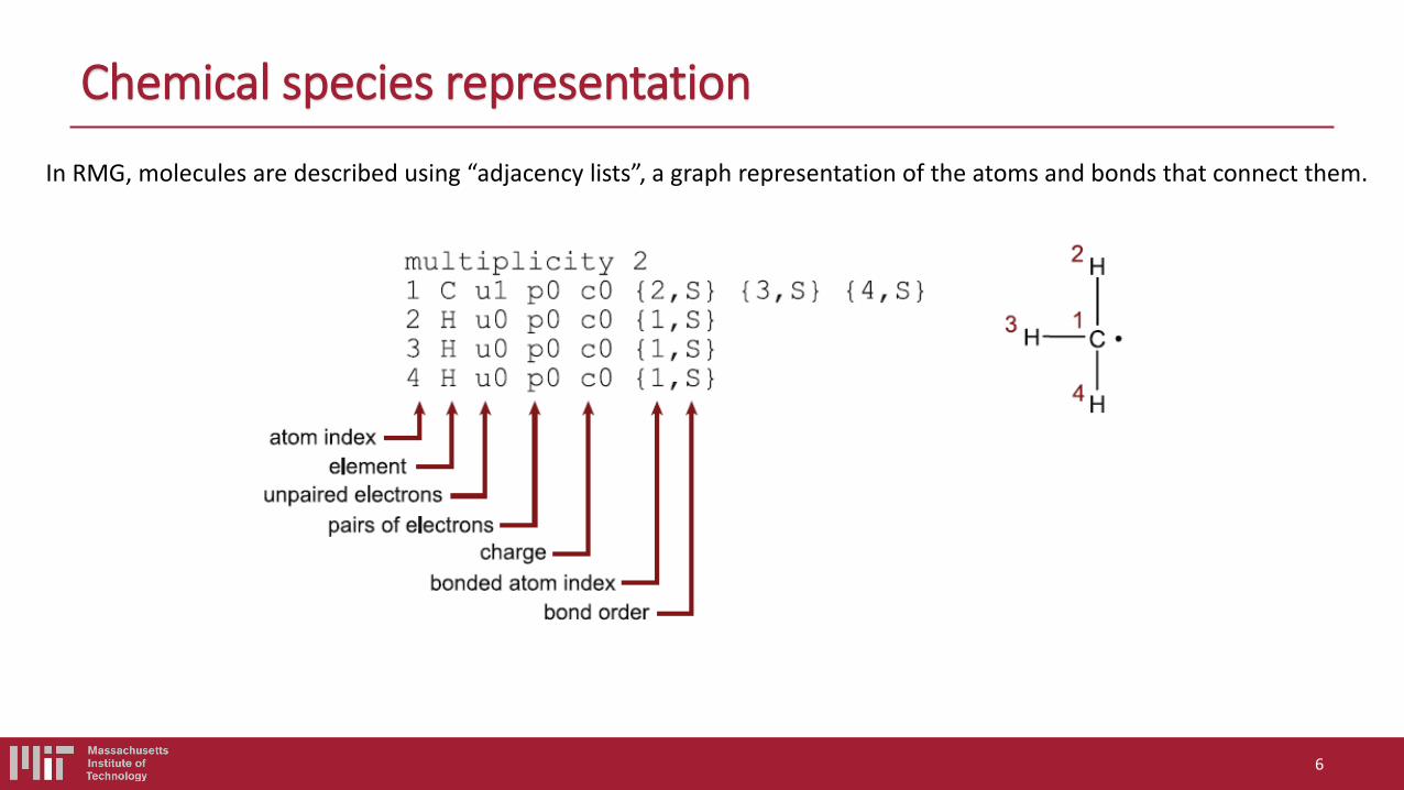
Chemical species representation

6

In RMG, molecules are described using “adjacency lists”, a graph representation of the atoms and bonds that connect them.

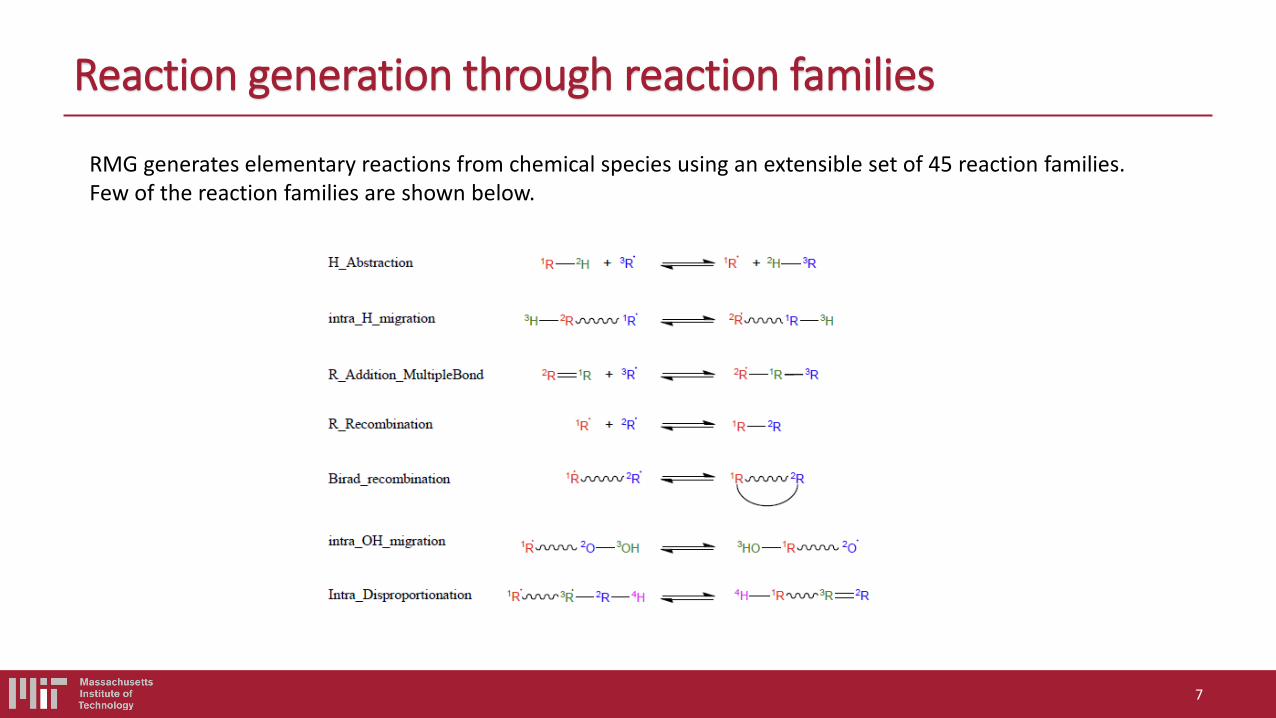
Reaction generation through reaction families

7

RMG generates elementary reactions from chemical species using an extensible set of 45 reaction families. Few of the reaction families are shown below.

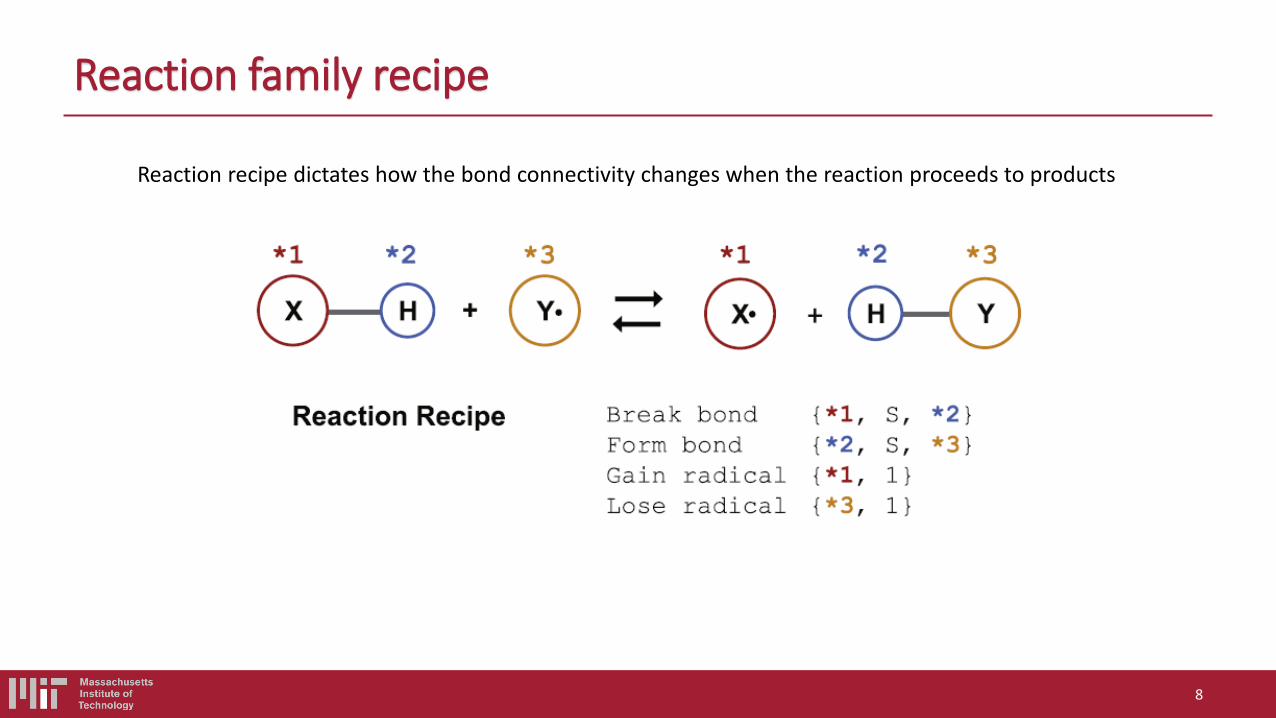
Reaction family recipe

8

Reaction recipe dictates how the bond connectivity changes when the reaction proceeds to products

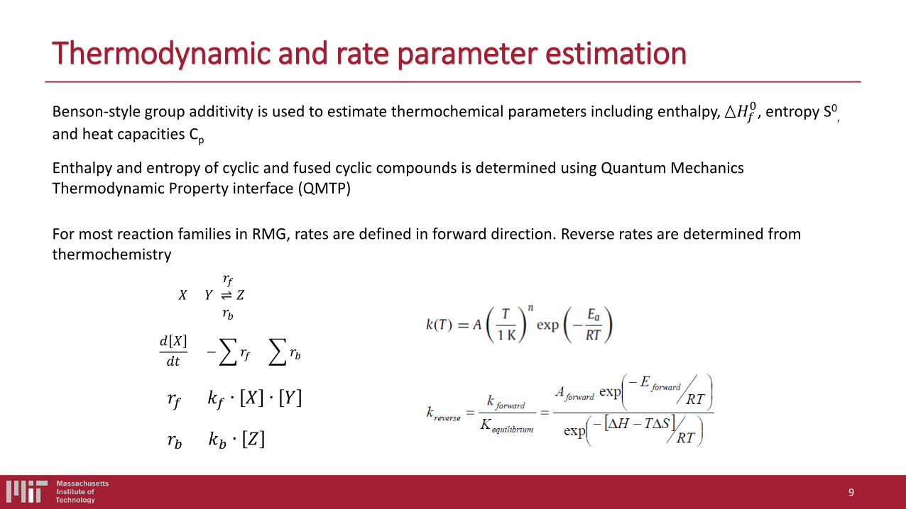
9

Thermodynamic and rate parameter estimation

Benson-style group additivity is used to estimate thermochemical parameters including enthalpy, 𝐻𝐻𝑓𝑓0, entropy S0,

and heat capacities Cp Enthalpy and entropy of cyclic and fused cyclic compounds is determined using Quantum Mechanics Thermodynamic Property interface (QMTP)

For most reaction families in RMG, rates are defined in forward direction. Reverse rates are determined from thermochemistry

𝑋𝑋 + 𝑌𝑌 ⇌ 𝑍𝑍 𝑟𝑟𝑓𝑓

𝑟𝑟𝑏𝑏

𝑑𝑑 𝑋𝑋𝑑𝑑𝑑𝑑

= −�𝑟𝑟𝑓𝑓 + �𝑟𝑟𝑏𝑏

𝑟𝑟𝑓𝑓 = 𝑘𝑘𝑓𝑓 ∙ 𝑋𝑋 ∙ 𝑌𝑌

𝑟𝑟𝑏𝑏 = 𝑘𝑘𝑏𝑏 ∙ 𝑍𝑍

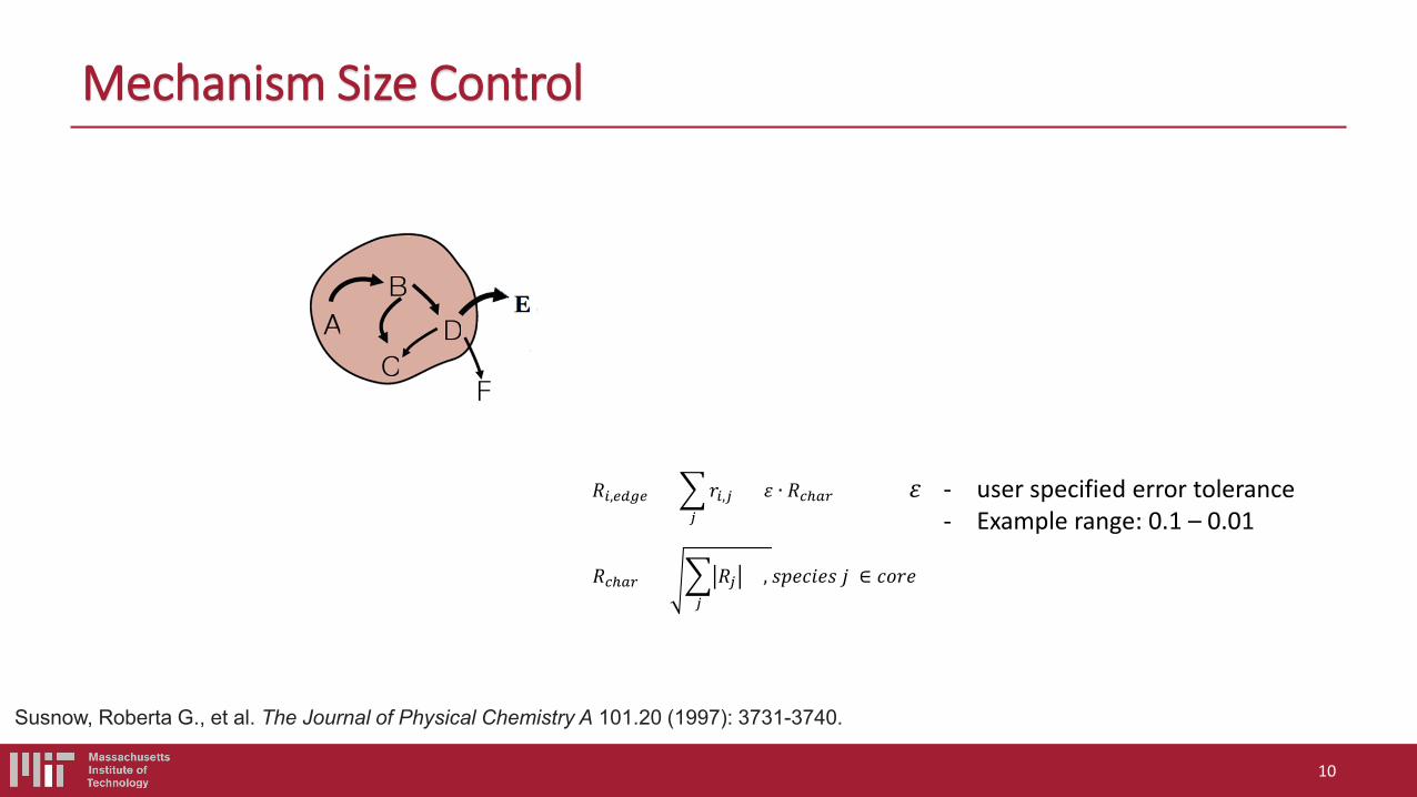
Mechanism Size Control

10

𝑅𝑅𝑖𝑖,𝑒𝑒𝑒𝑒𝑒𝑒𝑒𝑒 = �𝑟𝑟𝑖𝑖,𝑗𝑗𝑗𝑗

> 𝜀𝜀 ∙ 𝑅𝑅𝑐𝑐𝑐𝑐𝑐𝑐𝑐

𝑅𝑅𝑐𝑐𝑐𝑐𝑐𝑐𝑐 = � 𝑅𝑅𝑗𝑗 ²𝑗𝑗

, 𝑠𝑠𝑠𝑠𝑠𝑠𝑠𝑠𝑠𝑠𝑠𝑠𝑠𝑠 𝑗𝑗 ∈ 𝑠𝑠𝑐𝑐𝑟𝑟𝑠𝑠

Susnow, Roberta G., et al. The Journal of Physical Chemistry A 101.20 (1997): 3731-3740.

𝜀𝜀 - user specified error tolerance - Example range: 0.1 – 0.01

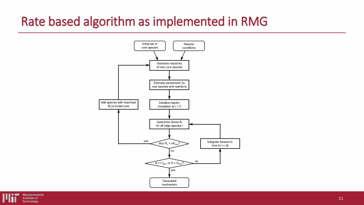
11

Rate based algorithm as implemented in RMG

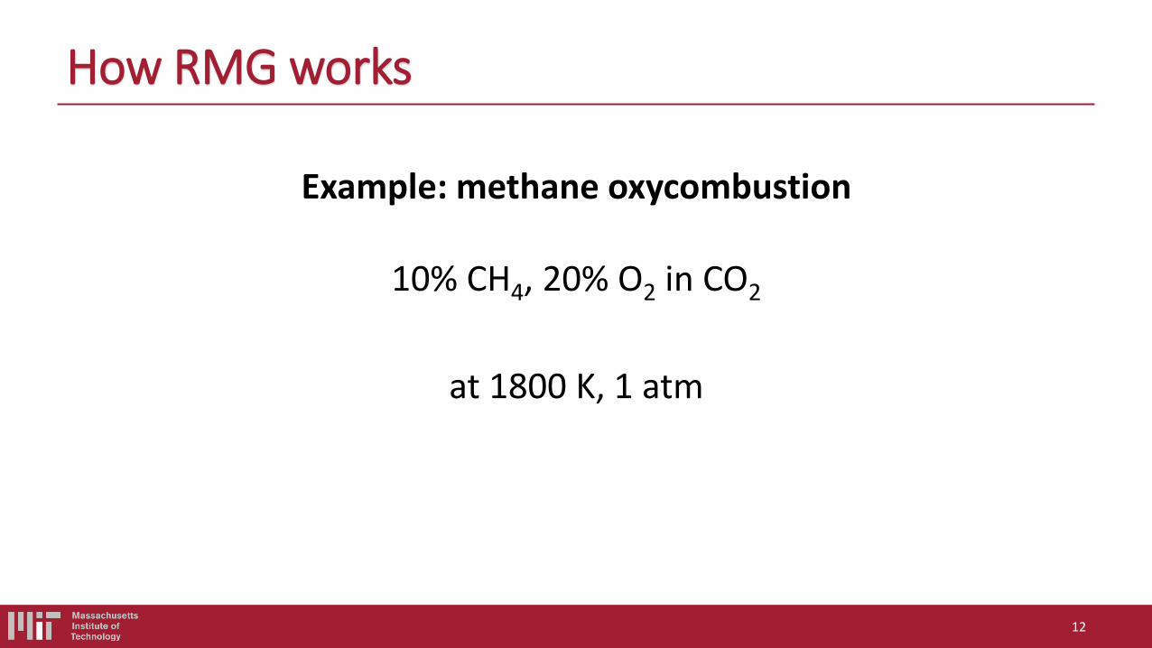
How RMG works

Example: methane oxycombustion

10% CH4, 20% O2 in CO2

at 1800 K, 1 atm

12

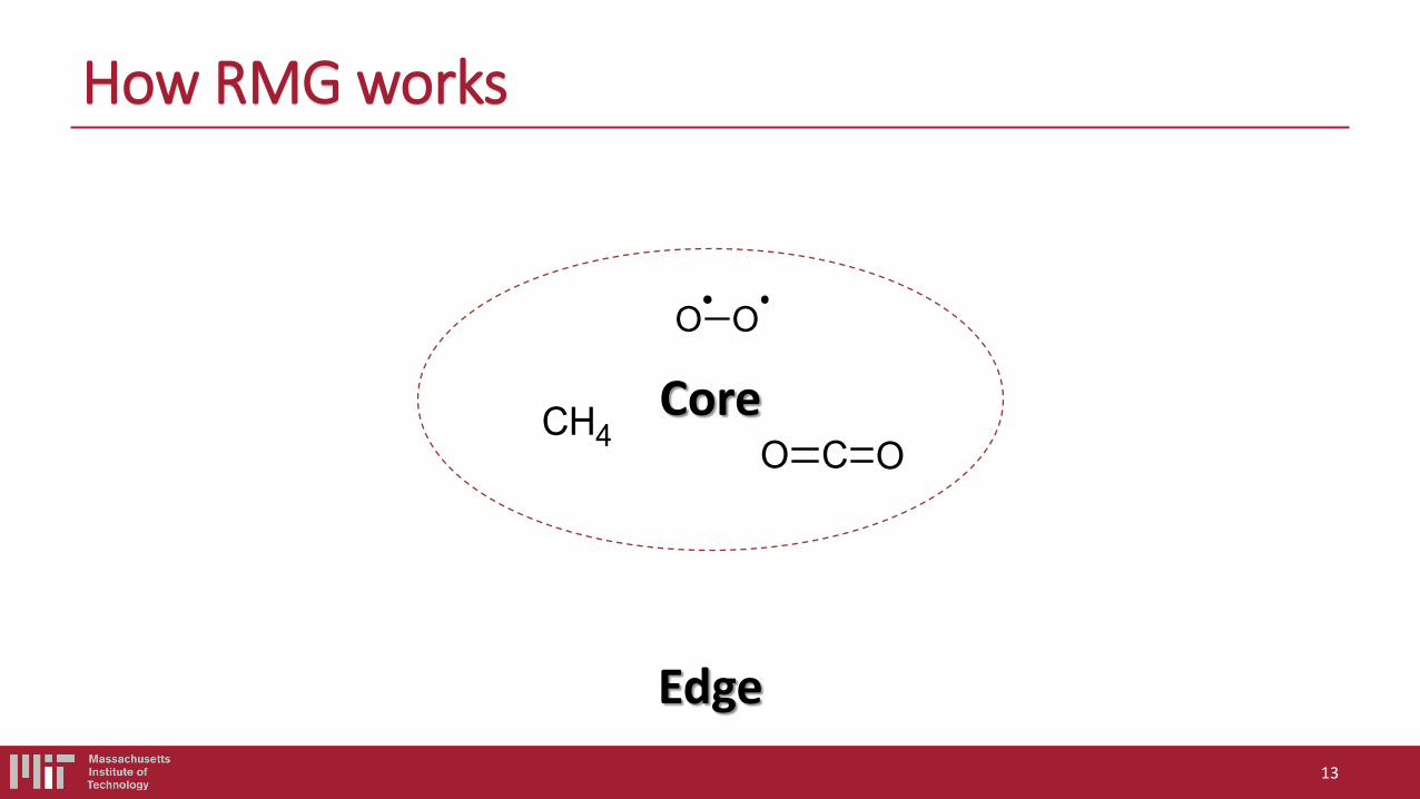
Core

Edge

CH4

O O

O C O

How RMG works

13

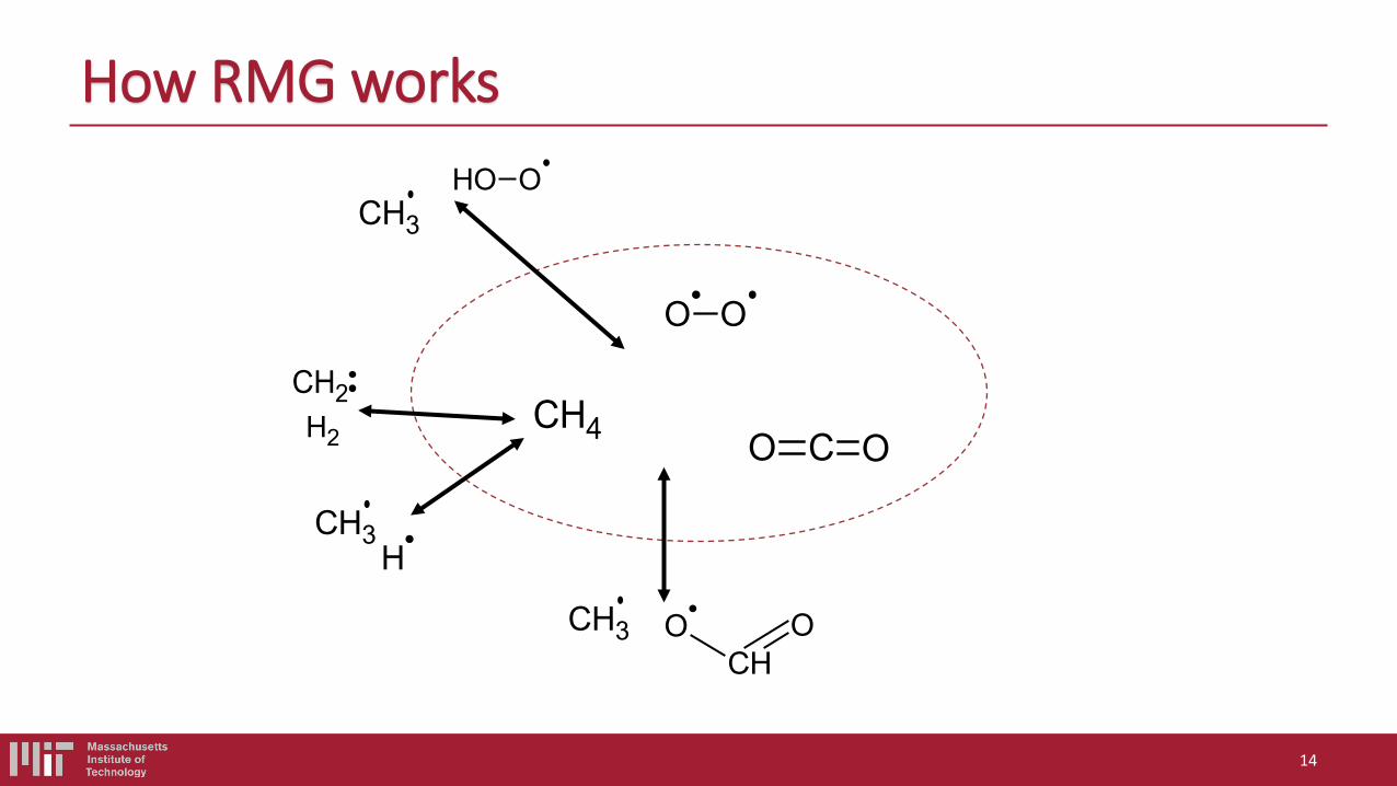
CH4

O O

O C O

CH3H

H2

CH2

CH3

OH O

CH3CH

OO

How RMG works

14

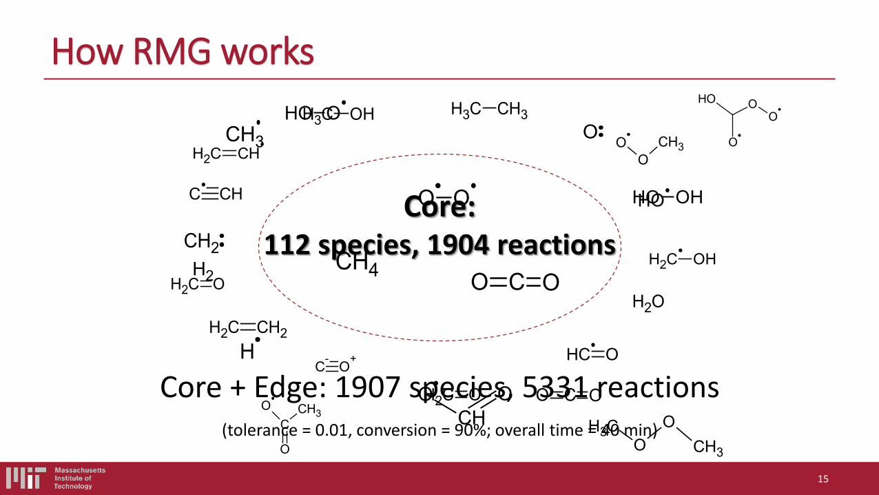
CH4

O O

O C O

H

H2

CH2

CH3

OH O

CHOO

CH3 CH3O

OH

OH2

CH O

CH2 O

CH2 CH2

C-

O+

CH2 CH

CH3 OH

CH2 OH

O C O

OO

CH3

C

O

O CH3

OH

O

OO

CH3O

OCH3

OH OHC CH

CH2 O

Core: 112 species, 1904 reactions

Core + Edge: 1907 species, 5331 reactions (tolerance = 0.01, conversion = 90%; overall time = 40 min)

How RMG works

15

Sections in an input file

16

Detailed description regarding sections in input file at http://reactionmechanismgenerator.github.io/RMG-Py/users/rmg/examples.html#commented-input-file

Mechanism files are in chemkin folder in the directory: chem.inp chem_annotated.inp species_dictionary.txt tran.dat

The RMG output

17

Download the example’s input file from here: shoutkey.com/up • Can you tell what are the inlet composition and conditions? • What termination criterion is used? • Which PDep interpolation method in used? • What is the tolerance? • How many Heavy Atoms are allowed?

Run this example (or your version of it) and let us know: – How long did it take RMG to run it? – How many species and reactions were added to the core? – How many S & R were explored by RMG overall?

Example 2: Methane Combustion

18

Scripts Using RMG’s scripts you could: • Merge models • Compare models • Generate a flux diagram • Run Sensitivity Analysis • Standardize species names • Estimate thermo data • Generate reactions • Create an RMG library • … and much more!

19

RMG Website Tools

See http://rmg.mit.edu/

20

Troubleshooting on GitHub

See https://github.com/ReactionMechanismGenerator/RMG-Py/issues

21

Chemkin

22

Selected past & present RMG projects • 2003 – Methane • 2007 – Neopentyl Radical • 2011 – JP10 • 2013 – BuOH • 2014 – Diisopropyl ketone • 2015 – Alkyl sulfide • 2015 – Propane • 2016 – DME • 2016 – Ethylamine

23

Acknowledgments • Prof. William H. Green

• Prof. Richard West

• RMG Developer Team

• Dr. Nick M. Vandewiele

24

rmg.mit.edu

25

Mechanism Construction, Valid Ranges of Chemistry Models,

& Solving big kinetic models: Reduction

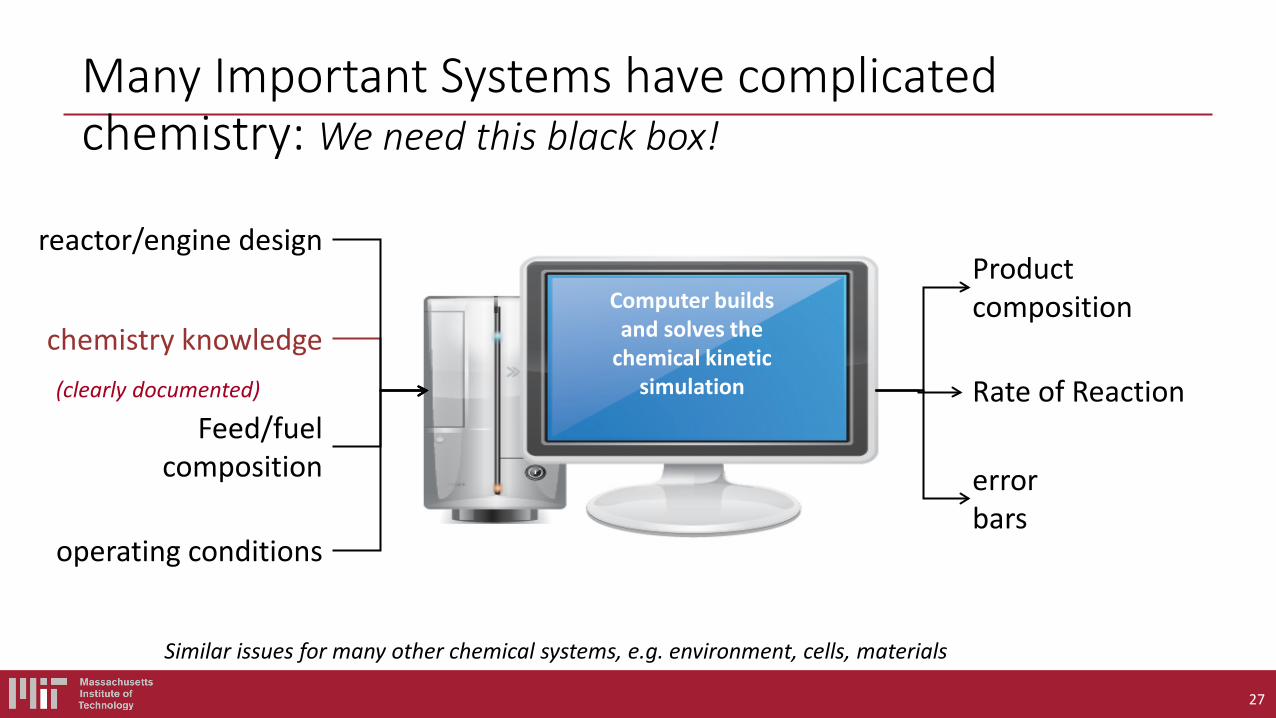
Many Important Systems have complicated chemistry: We need this black box!

27

Feed/fuel composition

operating conditions

reactor/engine design

chemistry knowledge

Product composition

Rate of Reaction

error bars

(clearly documented)

Computer builds and solves the

chemical kinetic simulation

Similar issues for many other chemical systems, e.g. environment, cells, materials

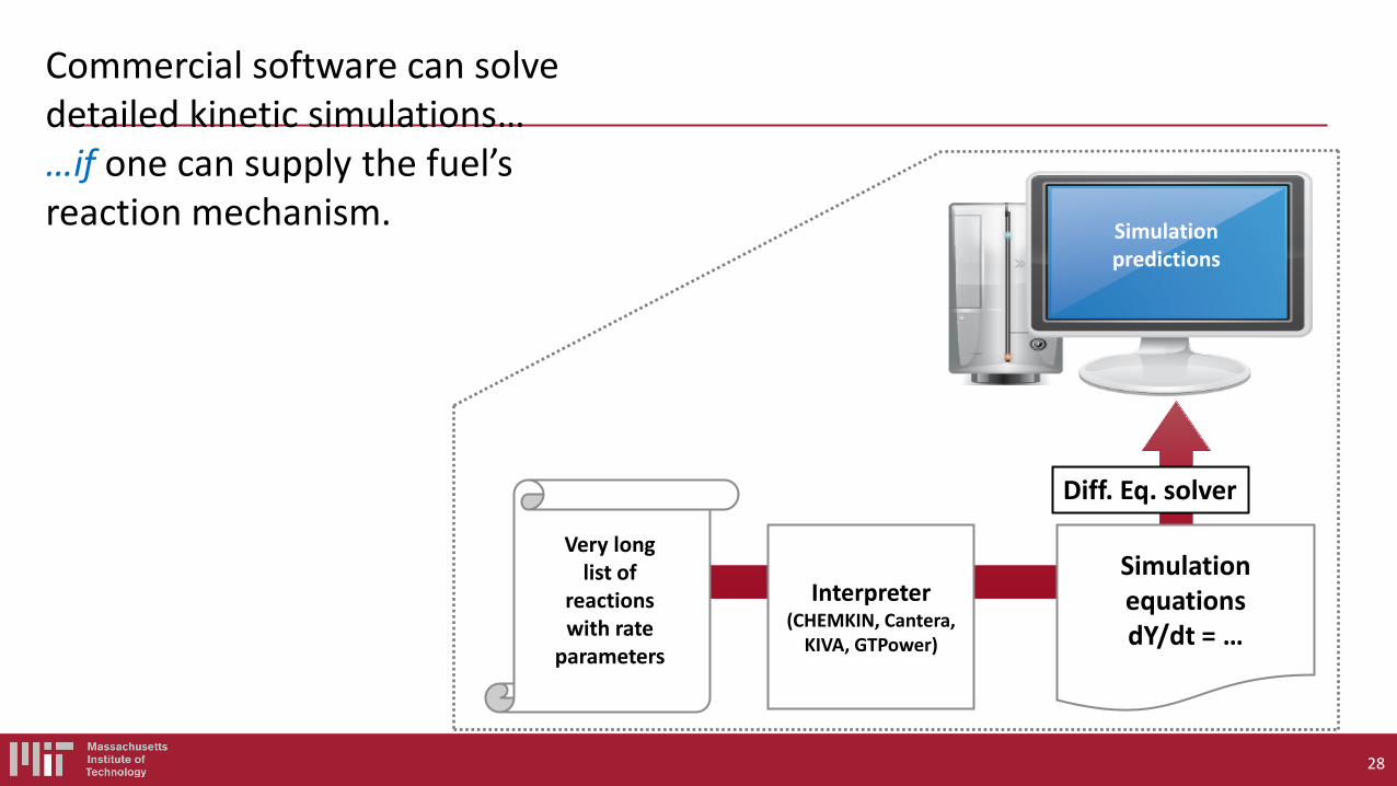
28

Simulation equations dY/dt = …

Interpreter (CHEMKIN, Cantera,

KIVA, GTPower)

Very long list of

reactions with rate

parameters

Simulation predictions

Commercial software can solve detailed kinetic simulations… …if one can supply the fuel’s reaction mechanism.

Diff. Eq. solver

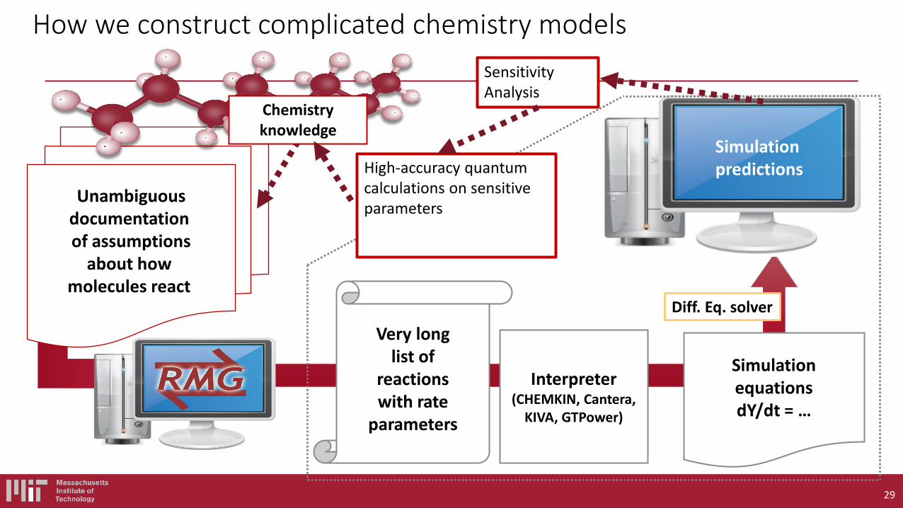
How we construct complicated chemistry models

29

Simulation equations dY/dt = …

Interpreter (CHEMKIN, Cantera,

KIVA, GTPower)

Very long list of

reactions with rate

parameters

Simulation predictions

Unambiguous documentation of assumptions

about how molecules react

Chemistry knowledge

Diff. Eq. solver

High-accuracy quantum calculations on sensitive parameters

Sensitivity Analysis

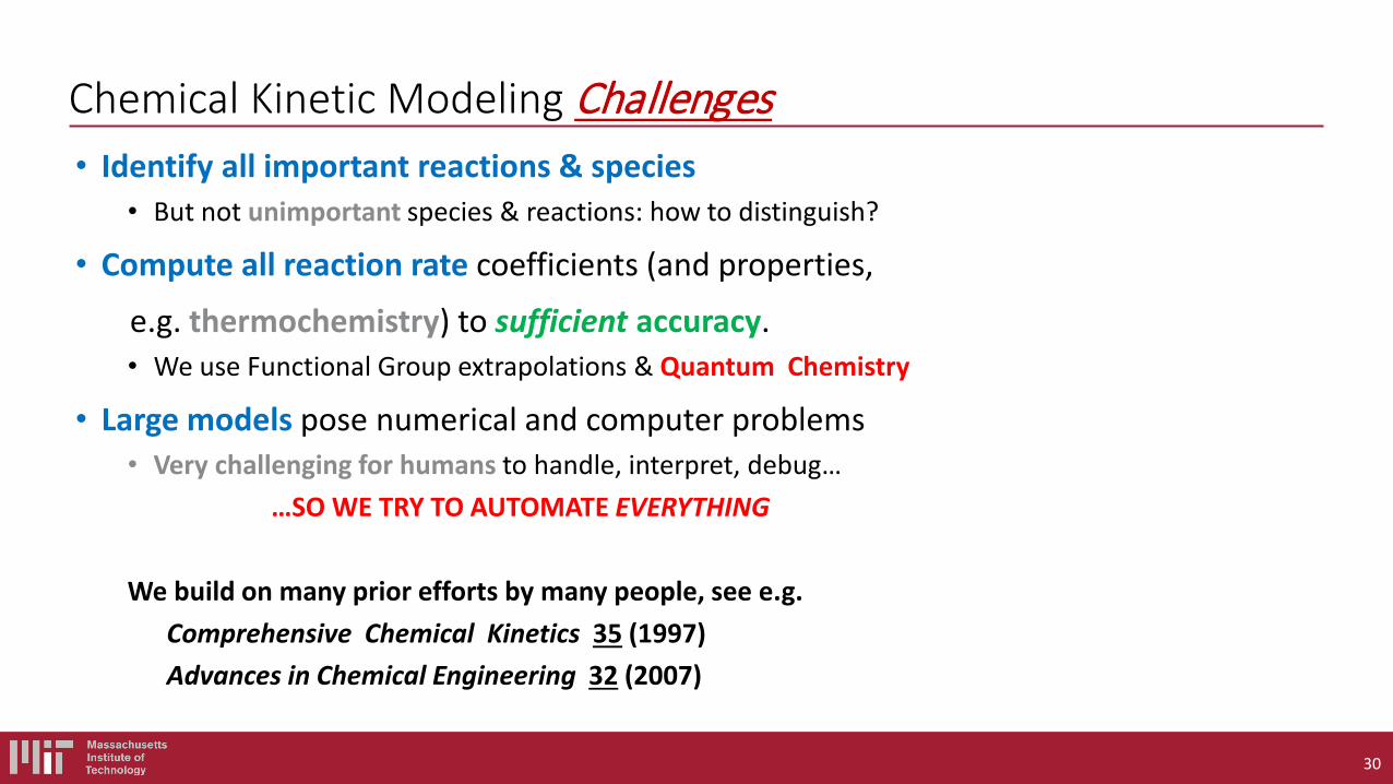
Chemical Kinetic Modeling Challenges • Identify all important reactions & species

• But not unimportant species & reactions: how to distinguish?

• Compute all reaction rate coefficients (and properties,

e.g. thermochemistry) to sufficient accuracy. • We use Functional Group extrapolations & Quantum Chemistry

• Large models pose numerical and computer problems • Very challenging for humans to handle, interpret, debug… …SO WE TRY TO AUTOMATE EVERYTHING We build on many prior efforts by many people, see e.g.

Comprehensive Chemical Kinetics 35 (1997) Advances in Chemical Engineering 32 (2007)

30

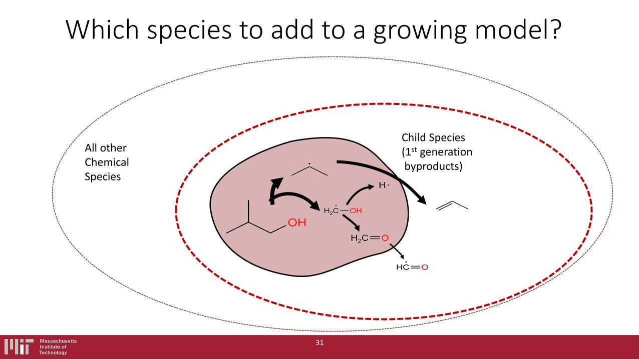
Which species to add to a growing model?

31

Child Species (1st generation byproducts)

All other Chemical Species

Several alternatives for how to construct network

• Human selection: add the reactions and additional species you think are important.

• Generational growth: at each iteration add all the child molecules which can be formed in a single elementary step from species currently in the model.

• Directed growth: for certain types of species, only allow them to do certain types of reactions. For example, big radicals only allowed to unimolecularly decompose into smaller radicals.

• Rate-based algorithm is like directed growth or human selection, but uses a numerical test of importance to decide which species to add to the model, rather than a pre-set rule or human intuition.

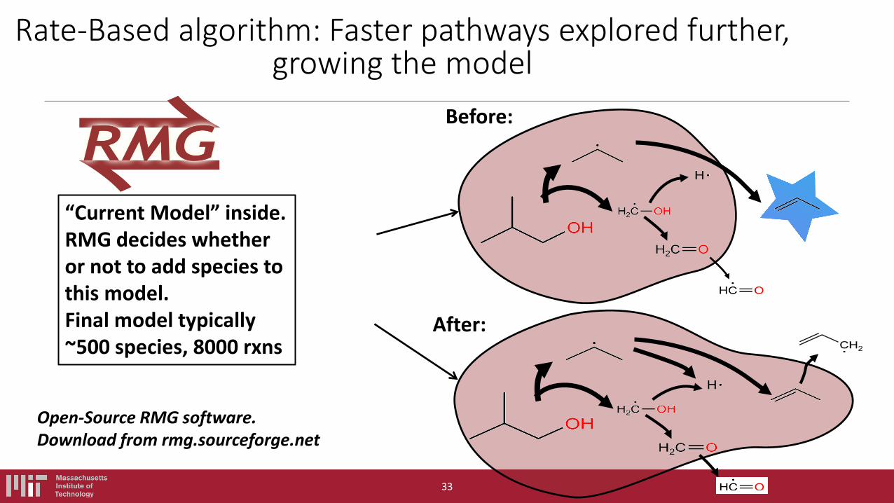
Rate-Based algorithm: Faster pathways explored further, growing the model

Open-Source RMG software. Download from rmg.sourceforge.net

“Current Model” inside. RMG decides whether or not to add species to this model. Final model typically ~500 species, 8000 rxns

After:

Before:

33

Issues with Rate-Based Selection • If you have an error in a rate estimate, it will change which model is

constructed. • Worst rate estimates are for the reactions humans think are least

important; sometimes they are estimated too high and get included in model

• Rate is important, but it is not the same as sensitivity: some low-rate reactions are important, must be included in the model.

• There is a proof that for a very tight tolerance rate-based algorithm converges, but in practice we often cannot achieve a tight enough tolerance because of computer/programming limitations.

Valid Range of a model • Chemistry changes a lot with composition and reaction conditions

(especially temperature). • Models are always a truncated expression of reality, leave out some

reactions. • If you change composition or temperature enough, some reaction left

out of the model will become important. • Jing Song’s valid range analysis defines how far the conditions could

change before an additional species would need to be added.

How to install RMG on your computer? See: http://rmg.mit.edu/ > Documentation > User’s Guide > Installation

36

Progress towards Accurate Predictive Gas Kinetics

William H. Green

MIT Dept. of Chemical Engineering

24th Intl. Symposium on Gas Kinetics York, July 19, 2016

37

Long-term project: making Gas Kinetics into a Quantitative Predictive Science • Historically: Kinetics has been more Postdictive than Predictive

– Do the experiment first, then build a model to interpret/rationalize the known results

• Instead: make quantitative predictions first, then do experiments to falsify the predictions

• If predictions were this good, they would be very helpful in designing the most informative experiments.

• Valuable for public policy decision-making e.g. air pollution • Accurate predictions the key to efficient rational design

– Rapidly engineer improved reactive systems

38

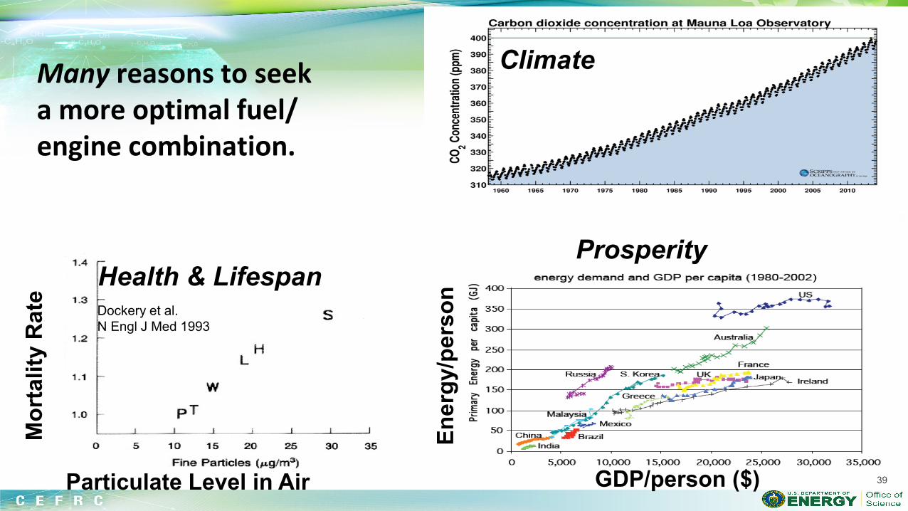
Many reasons to seek a more optimal fuel/ engine combination.

39 GDP/person ($) En

ergy

/per

son

Mor

talit

y R

ate

Dockery et al. N Engl J Med 1993

Particulate Level in Air

Climate

Prosperity Health & Lifespan

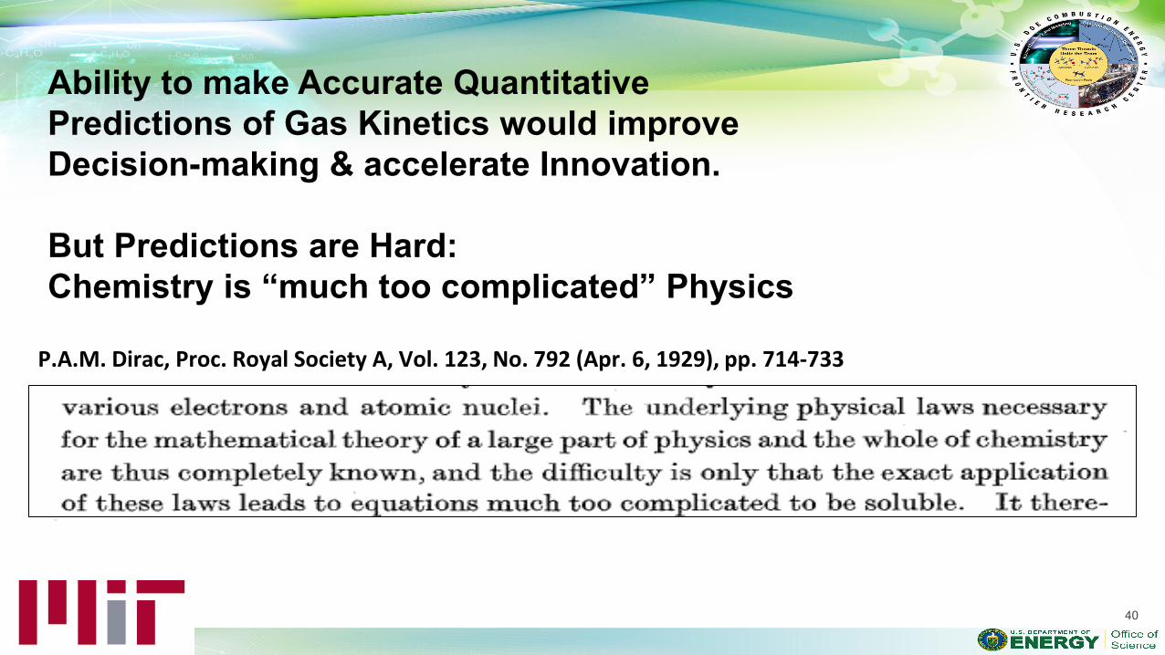
P.A.M. Dirac, Proc. Royal Society A, Vol. 123, No. 792 (Apr. 6, 1929), pp. 714-733

40

Ability to make Accurate Quantitative Predictions of Gas Kinetics would improve Decision-making & accelerate Innovation. But Predictions are Hard: Chemistry is “much too complicated” Physics

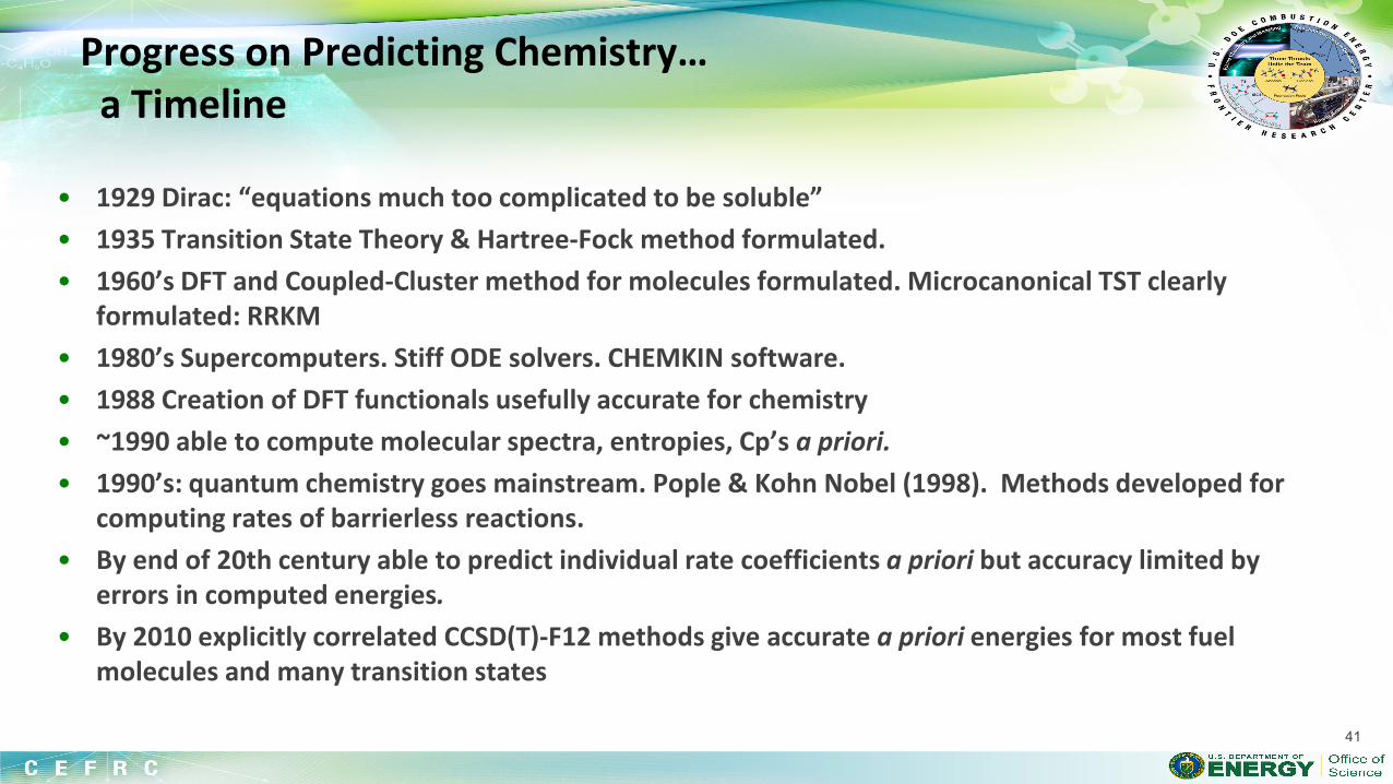
Progress on Predicting Chemistry… a Timeline

• 1929 Dirac: “equations much too complicated to be soluble” • 1935 Transition State Theory & Hartree-Fock method formulated. • 1960’s DFT and Coupled-Cluster method for molecules formulated. Microcanonical TST clearly

formulated: RRKM • 1980’s Supercomputers. Stiff ODE solvers. CHEMKIN software. • 1988 Creation of DFT functionals usefully accurate for chemistry • ~1990 able to compute molecular spectra, entropies, Cp’s a priori. • 1990’s: quantum chemistry goes mainstream. Pople & Kohn Nobel (1998). Methods developed for

computing rates of barrierless reactions. • By end of 20th century able to predict individual rate coefficients a priori but accuracy limited by

errors in computed energies. • By 2010 explicitly correlated CCSD(T)-F12 methods give accurate a priori energies for most fuel

molecules and many transition states

41

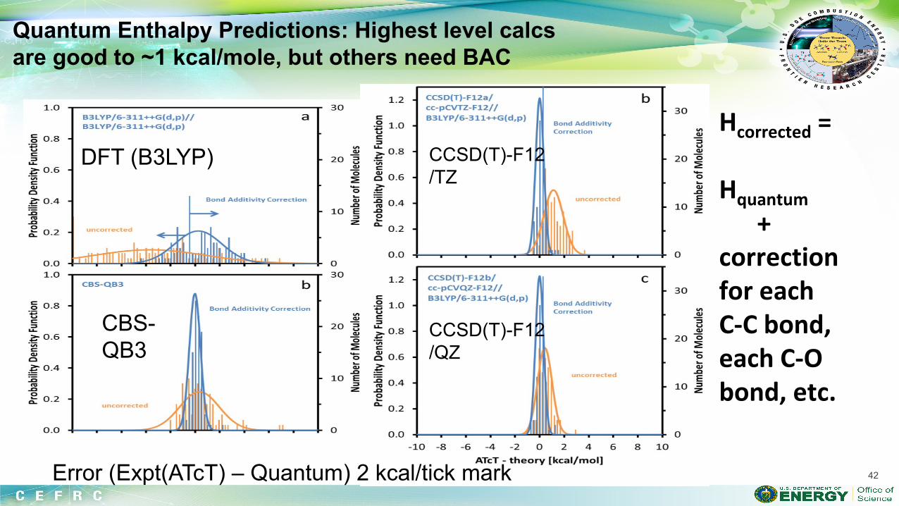
Hcorrected = Hquantum + correction for each C-C bond, each C-O bond, etc.

DFT (B3LYP)

CBS- QB3

CCSD(T)-F12 /TZ

CCSD(T)-F12 /QZ

Error (Expt(ATcT) – Quantum) 2 kcal/tick mark

Quantum Enthalpy Predictions: Highest level calcs are good to ~1 kcal/mole, but others need BAC

42

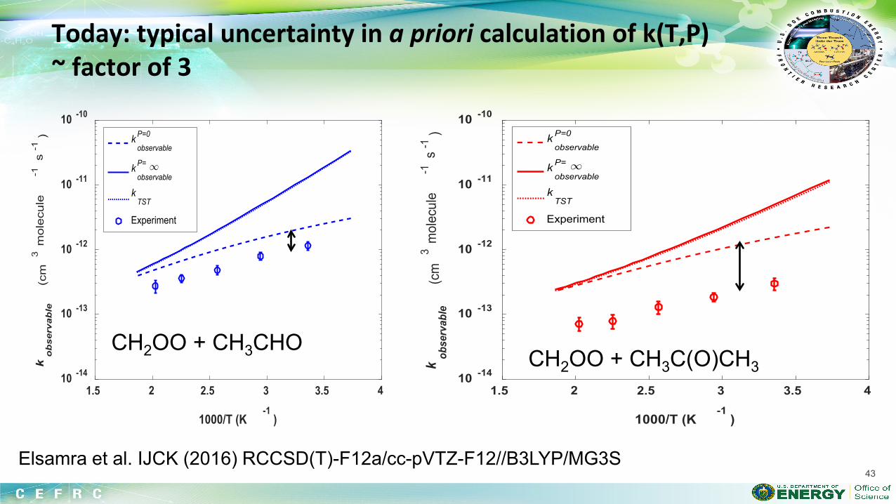
Today: typical uncertainty in a priori calculation of k(T,P) ~ factor of 3

43

1.5 2 2.5 3 3.5 4

1000/T (K-1

)

10 -14

10 -13

10 -12

10 -11

10 -10

kob

serv

able

(cm

3 m

olec

ule

-1 s

-1) k

observable

P=0

kobservable

P=

kTST

Experiment

1.5 2 2.5 3 3.5 4

1000/T (K-1

)

10 -14

10 -13

10 -12

10 -11

10 -10

ko

bse

rvab

le(c

m3

mol

ecul

e-1

s-1

) kobservable

P=0

kobservable

P=

kTST

Experiment

CH2OO + CH3CHO CH2OO + CH3C(O)CH3

Elsamra et al. IJCK (2016) RCCSD(T)-F12a/cc-pVTZ-F12//B3LYP/MG3S

Can we predict time-evolution of whole reacting systems? Many Issues… • Often O(103) important molecules, and O(104) important reactions; must

select from a much larger list of candidate species and reactions. – Humans are not good at making or checking models this complicated. Use

computer to list the reactions – Requires very large number of quantum chemistry calculations. Need

supercomputer resources. – Need good Benson-type estimates to identify which reactions are worth

computing quantum mechanically – Experiments only test some predictions of the model, often cannot

determine any of the parameters. – All the numbers in model have uncertainties: UQ

44

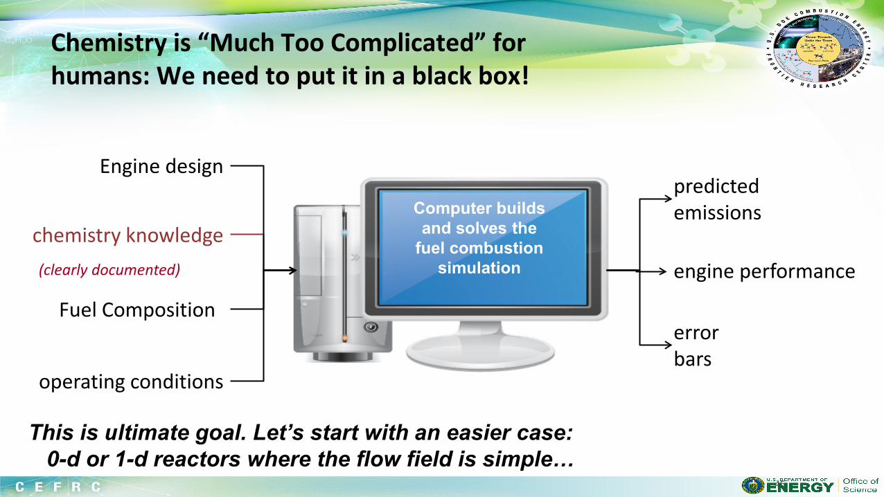
Chemistry is “Much Too Complicated” for humans: We need to put it in a black box!

45

Fuel Composition

operating conditions

Engine design

chemistry knowledge

predicted emissions

engine performance

error bars

(clearly documented)

Computer builds and solves the

fuel combustion simulation

This is ultimate goal. Let’s start with an easier case: 0-d or 1-d reactors where the flow field is simple…

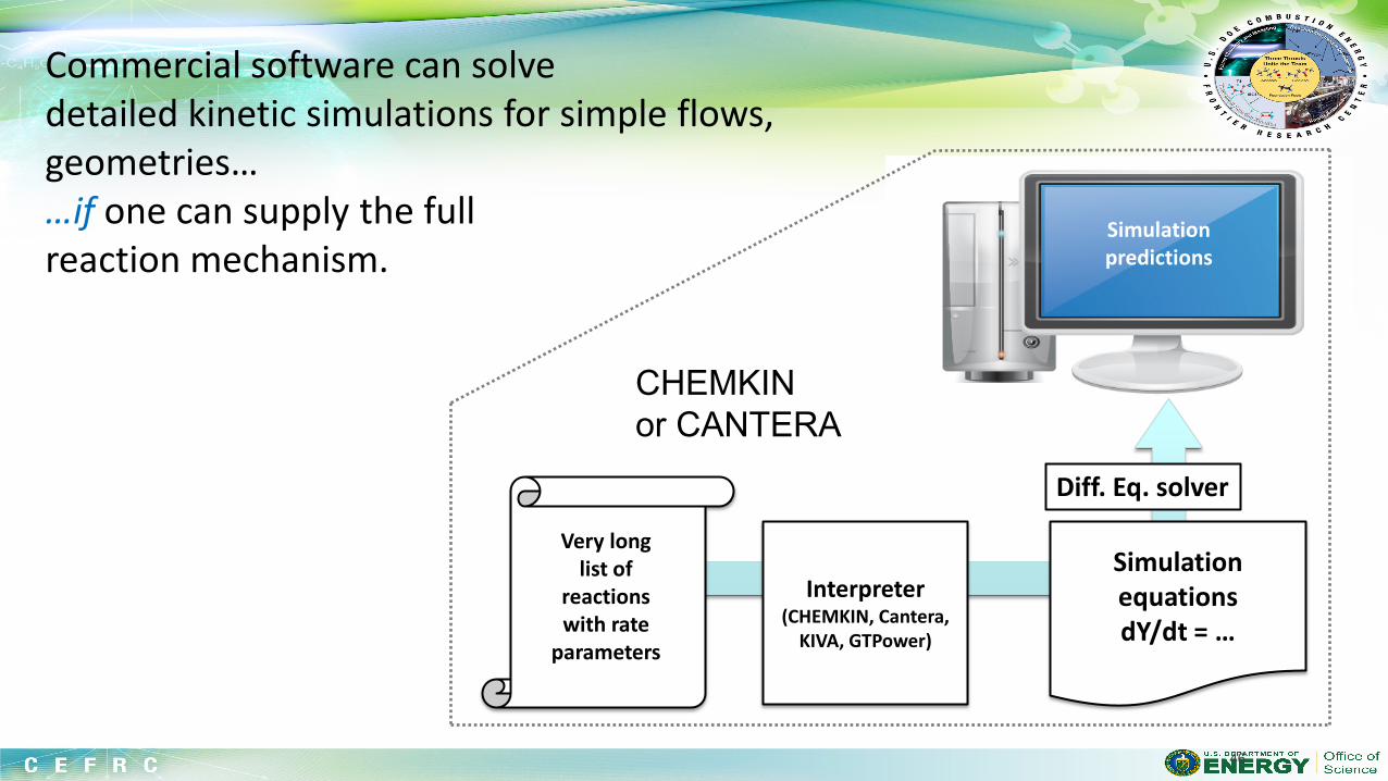
46

Simulation equations dY/dt = …

Interpreter (CHEMKIN, Cantera,

KIVA, GTPower)

Very long list of

reactions with rate

parameters

Simulation predictions

Commercial software can solve detailed kinetic simulations for simple flows, geometries… …if one can supply the full reaction mechanism.

Diff. Eq. solver

CHEMKIN or CANTERA

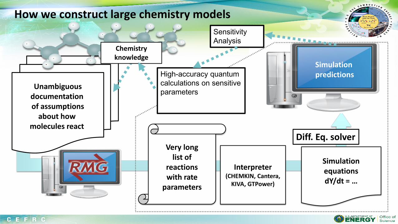
How we construct large chemistry models

47

Simulation equations dY/dt = …

Interpreter (CHEMKIN, Cantera,

KIVA, GTPower)

Very long list of

reactions with rate

parameters

Simulation predictions

Unambiguous documentation of assumptions

about how molecules react

Chemistry knowledge

Diff. Eq. solver

High-accuracy quantum calculations on sensitive parameters

Sensitivity Analysis

RMG algorithm: Faster pathways explored further, growing the model

Open-Source RMG software. Download from reactionmechanismgenerator.github.io

“Current Model” inside. RMG decides whether or not to add species to this model. Final model typically ~500 species, 8000 rxns

After:

Before:

48

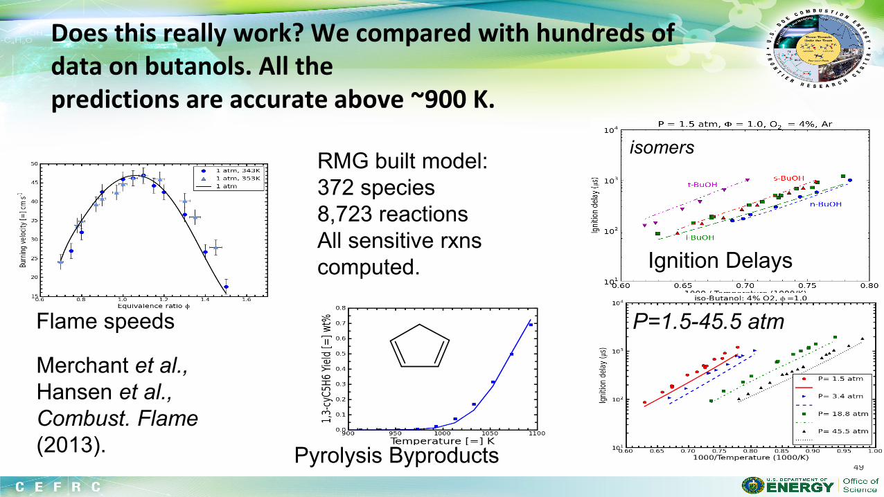
Does this really work? We compared with hundreds of data on butanols. All the predictions are accurate above ~900 K.

49

Flame speeds

Ignition Delays

Pyrolysis Byproducts

Merchant et al., Hansen et al., Combust. Flame (2013).

RMG built model: 372 species 8,723 reactions All sensitive rxns computed.

isomers

P=1.5-45.5 atm

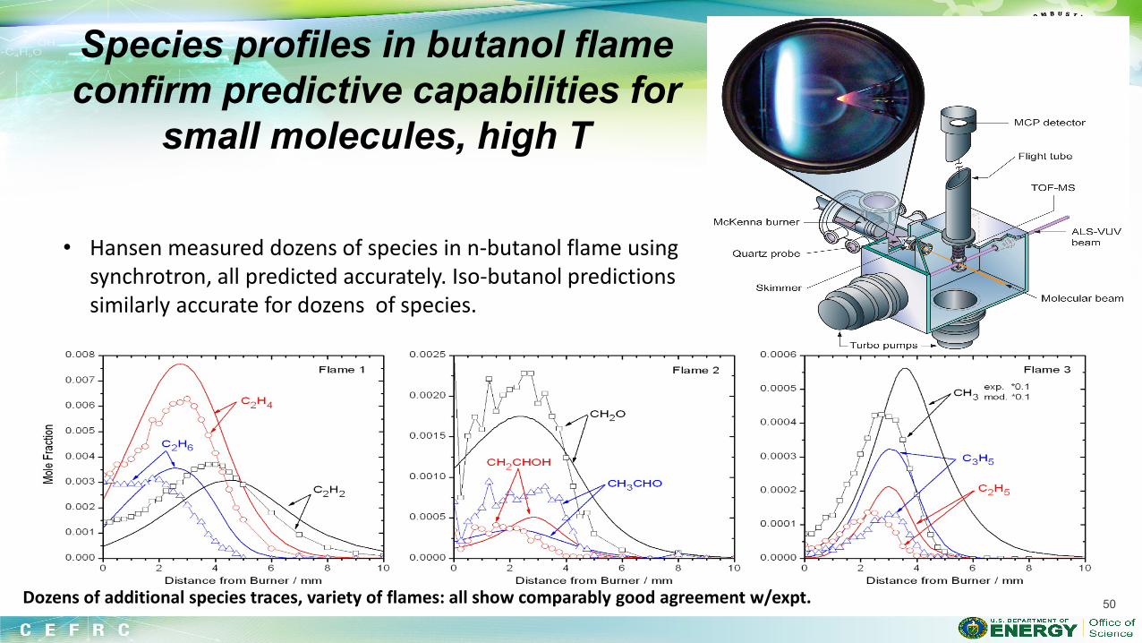
• Hansen measured dozens of species in n-butanol flame using synchrotron, all predicted accurately. Iso-butanol predictions similarly accurate for dozens of species.

Dozens of additional species traces, variety of flames: all show comparably good agreement w/expt.

Species profiles in butanol flame confirm predictive capabilities for

small molecules, high T

50

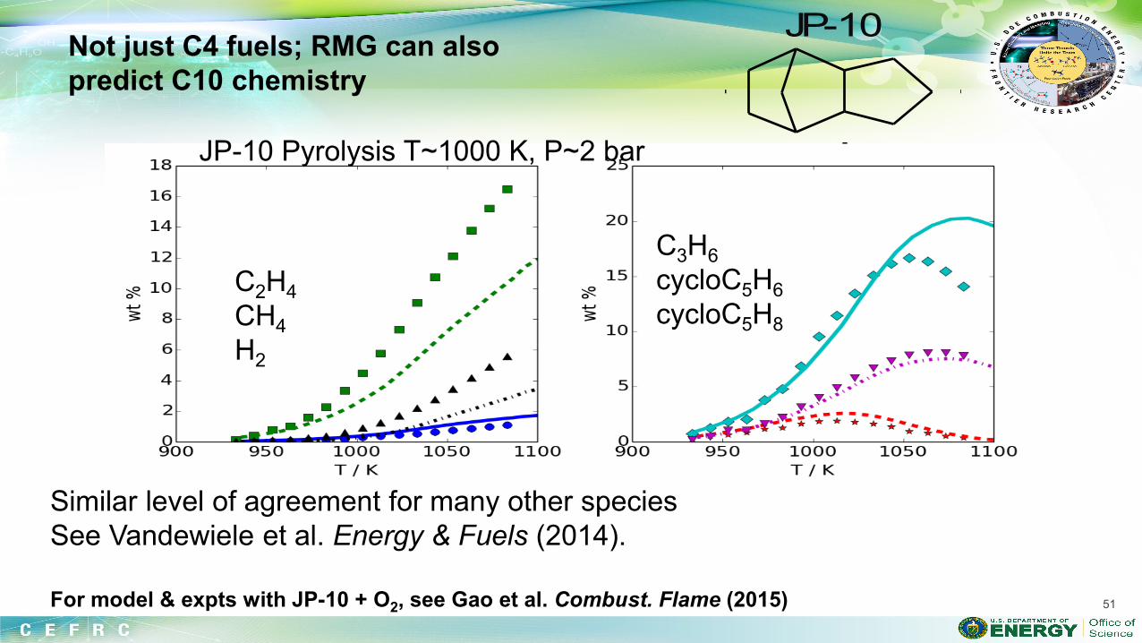
C2H4 CH4 H2

C3H6 cycloC5H6 cycloC5H8

Similar level of agreement for many other species See Vandewiele et al. Energy & Fuels (2014). For model & expts with JP-10 + O2, see Gao et al. Combust. Flame (2015)

JP-10 Pyrolysis T~1000 K, P~2 bar

51

JP-10

Not just C4 fuels; RMG can also predict C10 chemistry

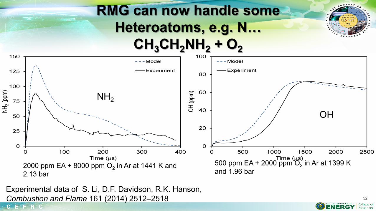
52

RMG can now handle some Heteroatoms, e.g. N…

CH3CH2NH2 + O2

2000 ppm EA + 8000 ppm O2 in Ar at 1441 K and 2.13 bar

Experimental data of S. Li, D.F. Davidson, R.K. Hanson, Combustion and Flame 161 (2014) 2512–2518

500 ppm EA + 2000 ppm O2 in Ar at 1399 K and 1.96 bar

NH2

OH

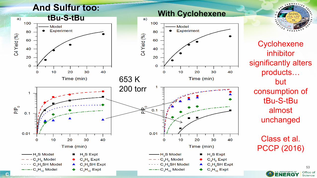
53

And Sulfur too: tBu-S-tBu With Cyclohexene

Cyclohexene inhibitor

significantly alters products…

but consumption of

tBu-S-tBu almost

unchanged

Class et al. PCCP (2016)

653 K 200 torr

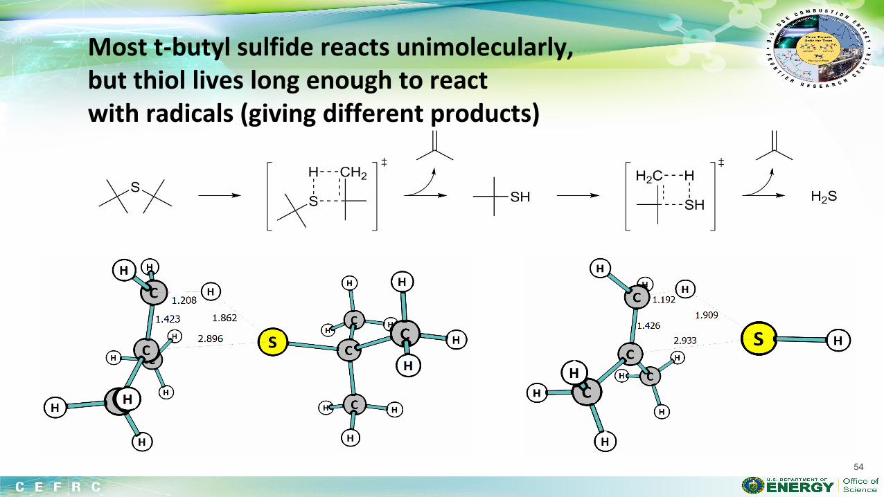
54

Most t-butyl sulfide reacts unimolecularly, but thiol lives long enough to react with radicals (giving different products)

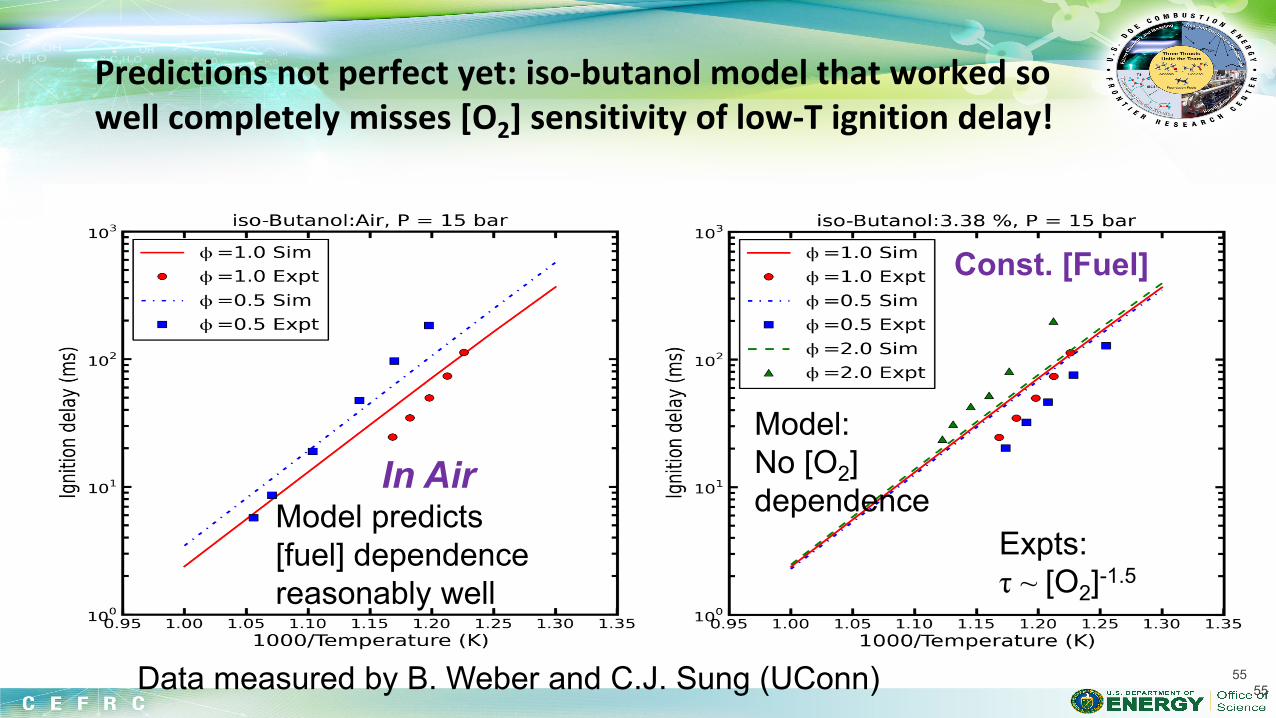
55

Expts: τ ~ [O2]-1.5

Predictions not perfect yet: iso-butanol model that worked so well completely misses [O2] sensitivity of low-T ignition delay!

In Air Model predicts [fuel] dependence reasonably well

Model: No [O2] dependence

Const. [Fuel]

Data measured by B. Weber and C.J. Sung (UConn) 55

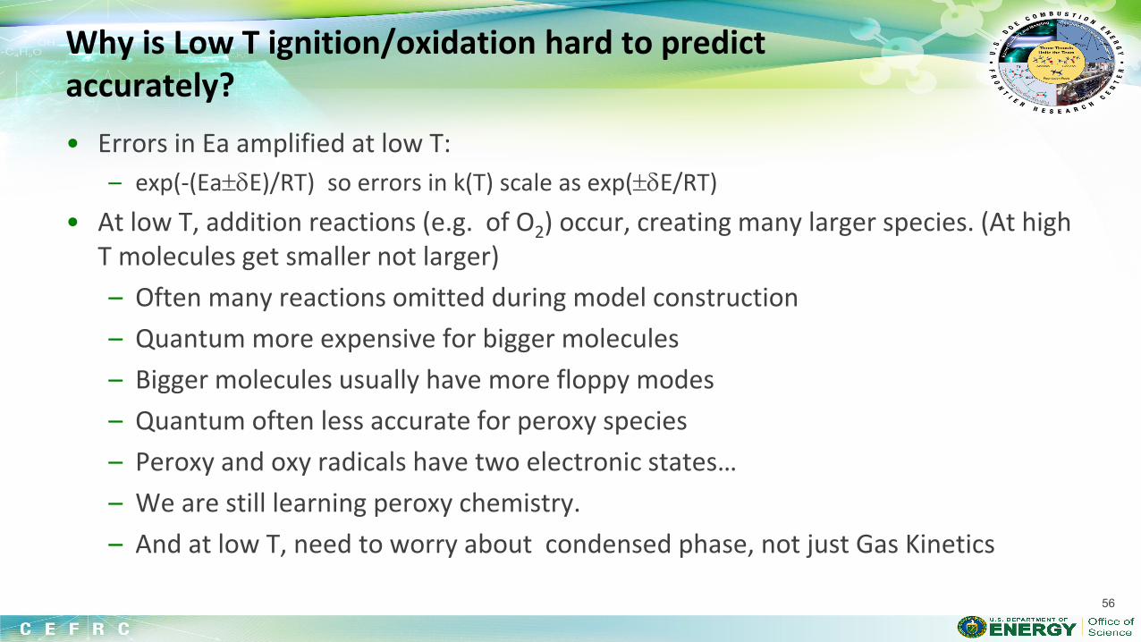
Why is Low T ignition/oxidation hard to predict accurately? • Errors in Ea amplified at low T:

– exp(-(Ea±δE)/RT) so errors in k(T) scale as exp(±δE/RT) • At low T, addition reactions (e.g. of O2) occur, creating many larger species. (At high

T molecules get smaller not larger) – Often many reactions omitted during model construction – Quantum more expensive for bigger molecules – Bigger molecules usually have more floppy modes – Quantum often less accurate for peroxy species – Peroxy and oxy radicals have two electronic states… – We are still learning peroxy chemistry. – And at low T, need to worry about condensed phase, not just Gas Kinetics

56

57

Summary • Predictive Gas Kinetics would help address the world’s energy/environment

problems. • Now practical to make fairly accurate predictions of thermo & kinetic parameters (~1

kcal/mole, factor of 3). • We can automatically build predictive kinetic models for CHNOS species up to about

C10…guided by Benson methods. – Sensitive numbers refined using quantum chemistry.

• Often the model predictions are quantitative at high T. – Real Predictions and Experimental Tests, not fits to a training set, needed to quantify

errors of the prediction methodology – many accurate quantum calculations will be needed to extend to new chemistry,

lower temperatures • Predictive Chemistry looks a lot more promising now than it did in 1929…

57

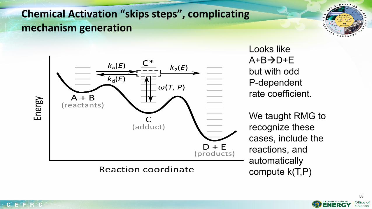
Chemical Activation “skips steps”, complicating mechanism generation

58

Looks like A+BD+E but with odd P-dependent rate coefficient. We taught RMG to recognize these cases, include the reactions, and automatically compute k(T,P)

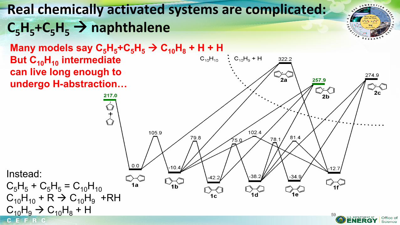
Real chemically activated systems are complicated: C5H5+C5H5 naphthalene Many models say C5H5+C5H5 C10H8 + H + H But C10H10 intermediate can live long enough to undergo H-abstraction…

Instead: C5H5 + C5H5 = C10H10 C10H10 + R C10H9 +RH C10H9 C10H8 + H

59

Lesson 5: Introduction to Mechanism Reduction

Tianfeng Lu

University of Connecticut Email: tianfeng.lu@uconn.edu

2017 Princeton-Combustion Institute

Summer School on Combustion June 25-30, 2017

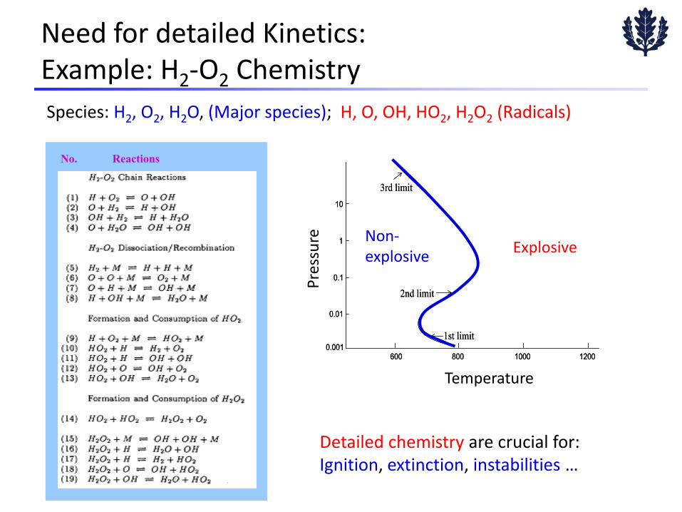
Need for detailed Kinetics: Example: H2-O2 Chemistry Species: H2, O2, H2O, (Major species); H, O, OH, HO2, H2O2 (Radicals)

No. Reactions

Detailed chemistry are crucial for: Ignition, extinction, instabilities …

p, a

tm

T, K

1st limit

2nd limit

3rd limit

Extended 2nd limit;

Weak chain branching

H+O2+M → HO2+M

HO2+H2 → H2O2+H

H2O2+M → OH+OH+M

Chain “termination”

H+O2+M → HO2+M

Strong chain branching

H+O2 → O+OH

O+H2 → H+OH

OH+H2 → H2O+H

k9

k1

Crossover temperature

k2

k3

k9

k17

k15

600 800 1000 12000.001

0.01

0.1

1

10

p, a

tm

T, K

1st limit

2nd limit

3rd limit

Extended 2nd limit;

Weak chain branching

H+O2+M → HO2+M

HO2+H2 → H2O2+H

H2O2+M → OH+OH+M

Chain “termination”

H+O2+M → HO2+M

Strong chain branching

H+O2 → O+OH

O+H2 → H+OH

OH+H2 → H2O+H

k9

k1

Crossover temperature

k2

k3

k9

k17

k15

600 800 1000 12000.001

0.01

0.1

1

10

Non-explosive Explosive

Temperature

Pres

sure

Need of Realistic Chemistry

– Fuel chemistry substantially affects flame dynamics – Accurate chemical kinetics needed to predict flame behaviors

Ex1: Negative Temperature Coefficients (NTC)

0.0001

0.001

0.01

0.1

1

10

100

0.5 1 1.5 2

with low-T chemistry

without low-T chemistry

n-Heptane-Air

p = 1 atmφ = 1

1000/T (1/K)

Igni

tion

dela

y (s

ec)

10-8 10-6 10-4 10-2 100 102500

1000

1500

2000

2500

Tem

pera

ture

, K

Residence time, s

Hydrogen

Methyl Decanoate

Propane p = 30 atmT0 = 700Kφ = 1

Perfectly Stirred Reactor

Ex2: Combustion “S”-curves

Computers and Numerical Combustion

ENIAC, 1946

Sunway TaihuLight, >10 million cores, 125 PetaFLOPS (Peak)

1990 2000 2010 2020109

1012

1015

1018

TaihuLightTitan

FLO

PSYear

CM-5Num. Wind Tunnel

SR2201CP-PCAS

ASCI Red ASCI Red

ASCI WhiteEarthe Sim.

Columbia

SX-8 ASCI PurpleBlue Gene/L

MDGrape 3Roadrunner Jaguar XT-5

Tianhe-1A K Computer

Source: Top500

Tianhe-2

https://www.top500.org/news/china-tops-supercomputer-rankings-with-new-93-petaflop-machine/

https://en.wikipedia.org/wiki/ENIAC

Scaling of Detailed Chemistry • Detailed mechanisms are

large

• Transportation fuels: ~103 species ~104 reactions

• Flame simulations with detailed chemistry are time-consuming or unaffordable

• The excessive output data renders it difficult to identify the controlling physicochemical processes

(Lu & Law, PECS 2009)

101 102 103 104

102

103

104

JetSURF 2.0

Ranzi mechanismcomlete, ver 1201

methyl palmitate (CNRS)

Gasoline (Raj et al)

2-methyl alkanes (LLNL)

Biodiesel (LLNL)

before 2000 2000-2004 2005-2009 since 2010

iso-octane (LLNL)iso-octane (ENSIC-CNRS)

n-butane (LLNL)

CH4 (Konnov)

neo-pentane (LLNL)

C2H4 (San Diego)CH4 (Leeds)

MD (LLNL)C16 (LLNL)

C14 (LLNL)C12 (LLNL)

C10 (LLNL)

USC C1-C4USC C2H4

PRF (LLNL)

n-heptane (LLNL)

skeletal iso-octane (Lu & Law)skeletal n-heptane (Lu & Law)

1,3-ButadieneDME (Curran)C1-C3 (Qin et al)

GRI3.0

Num

ber o

f rea

ctio

ns, I

Number of species, K

GRI1.2

I = 5K

The Law of Mass Action • For a reaction in general form

ν1’M1 + ν2’M2 + … + νK’MK -> ν1”M1 + ν2”M2 + … + νK”MK

• The reaction rate of the reaction is given by

• For example: – 2A + B -> products – A + B C + D

• Calculation of reverse rate

∏=

=K

iiff

icTk1

')( νω

BAff ccTk 2)(=ω

BAff ccTk )(=ω DCrr ccTk )(=ω

)()(

)(TkTk

TKr

fC =

∏=

=K

iirr

icTk1

")( νω

Reaction Rates of Multi-Reaction Systems

• For a system with the following reactions νi,1’M1 + νi,2’M2 + … + νi,K’MK ⇔ νi,1”M1 + νi,2”M2 + … + νi,K”MK i=1,…I

• The rate for the ith reaction is:

• In matrix form:

∏∏==

−=−=K

kiir

K

kiifirifi

kiki cTkcTk1

"

1

' ,, )()( ννωωω

...+⋅= ωScdtd

=×

K

K

c

cc

...2

1

1c

∆∆∆

∆∆∆∆∆∆

=×

KIKK

I

I

IK

,,2,1

2,2,22,1

1,1,21,1

.........

...

...

ννν

νννννν

S

=×

I

I

ω

ωω

...2

1

1ω

Identification of Important Pathways • Reaction rates are determined by temperature and species

concentrations (T, C), i.e. local reaction states • Different reaction pathways are controlling at different reaction

states • Any mechanism reduction is specific to a target set of reaction

states – Important reactions cannot be identified without concentration

information, i.e. only using the rate parameters or potential surface information

– Reaction state sampling from representative reactors is required for reduction

• Reactors for reaction state sampling – Auto-ignition – Perfectly stirred reactors (PSR) – 1-D laminar flames – Turbulent flames?

10-6

10-4

10-2

100

500

1000

1500

2000

2500

3000

3500

Residence time, s

Tem

pera

ture

, K

Sampling from Auto-ignition

Methane-air, φ = 1.0, p = 1 atm Methane-air, φ = 1.0, p = 1 atm, T0 = 1200K

0 10 20 30 40 50 601000

1500

2000

2500

10-9

10-7

10-5

10-3

Tem

pera

ture

, K

Time, ms

Mas

s fra

ctio

n of

H

• Auto-ignition typically involves radical explosion and thermal runaway stages • The radical explosion is slow (in milliseconds), and typically dominates ignition delay time • Thermal runaway is typically much faster (in microseconds) • Radical explosion stage can be bypassed in (laminar and turbulent) flames for fast burning • Sample reaction states from auto-ignition are representative for ignition chemistry,

important for compression ignition engines, detonation waves etc.

Sampling from PSR

1000

1500

2000

2500

3000

1E-6 1E-5 1E-4 1E-3 1E-2 1E-1 1E+0

Tem

pera

ture

, K

Residence Time, sec

CH4-airp = 1 atmφ = 1T0 = 1200K

Ignition point

extinction point

S-curve response of PSR

• PSR and other continuous flow reactors feature S-curve responses • The turning points are corresponding to extinction and ignition states • The extinction state is determined by how fast chemistry can be • The states from the upper and middle branches are representative to flame

chemistry, important for spark ignition engines, jet engines, flame holding etc.

Reaction States in Different Flames

Ka = 1000

1D premixed flame

PSR

auto-ignition

Ka = 100

1D premixed flame

PSR

auto-ignition

n-dodecane/air 𝑃𝑃 = 30𝑎𝑎𝑎𝑎𝑎𝑎, 𝜙𝜙 = 0.7,𝑇𝑇0 = 700𝐾𝐾

DNS of premixed C12/air flame by Alexei Poludnenko

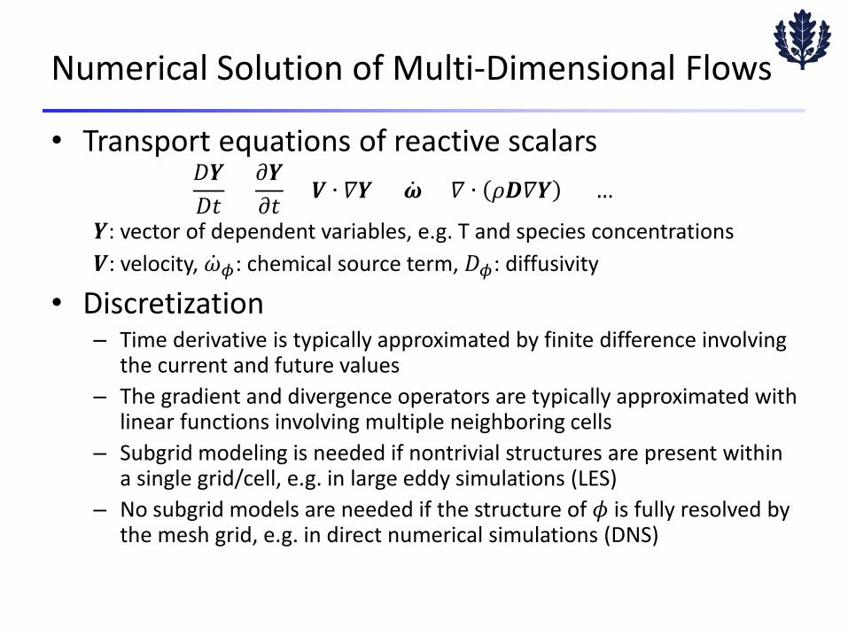
Numerical Solution of Multi-Dimensional Flows

• Transport equations of reactive scalars 𝐷𝐷𝒀𝒀𝐷𝐷𝑎𝑎

=𝜕𝜕𝒀𝒀𝜕𝜕𝑎𝑎

+ 𝑽𝑽 ∙ 𝛻𝛻𝒀𝒀 = �̇�𝝎 + 𝛻𝛻 ∙ 𝜌𝜌𝑫𝑫𝛻𝛻𝒀𝒀 + …

𝒀𝒀: vector of dependent variables, e.g. T and species concentrations 𝑽𝑽: velocity, �̇�𝜔𝜙𝜙: chemical source term, 𝐷𝐷𝜙𝜙: diffusivity

• Discretization – Time derivative is typically approximated by finite difference involving

the current and future values – The gradient and divergence operators are typically approximated with

linear functions involving multiple neighboring cells – Subgrid modeling is needed if nontrivial structures are present within

a single grid/cell, e.g. in large eddy simulations (LES) – No subgrid models are needed if the structure of 𝜙𝜙 is fully resolved by

the mesh grid, e.g. in direct numerical simulations (DNS)

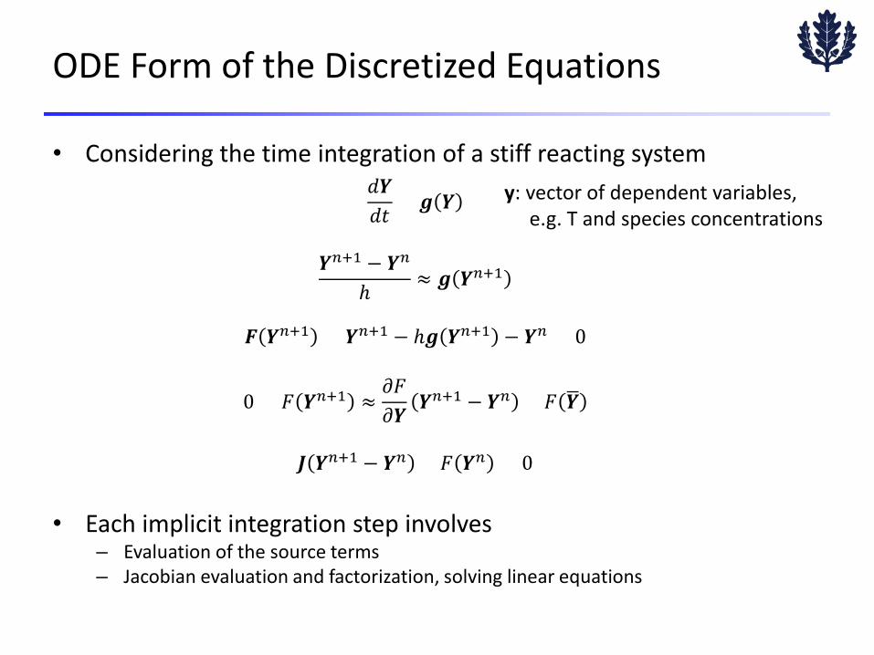
ODE Form of the Discretized Equations

• Considering the time integration of a stiff reacting system 𝑑𝑑𝒀𝒀𝑑𝑑𝑎𝑎

= 𝒈𝒈 𝒀𝒀

𝒀𝒀𝑛𝑛+1 − 𝒀𝒀𝑛𝑛

ℎ≈ 𝒈𝒈 𝒀𝒀𝑛𝑛+1

𝑭𝑭 𝒀𝒀𝑛𝑛+1 = 𝒀𝒀𝑛𝑛+1 − ℎ𝒈𝒈 𝒀𝒀𝑛𝑛+1 − 𝒀𝒀𝑛𝑛 = 0

0 = 𝐹𝐹 𝒀𝒀𝑛𝑛+1 ≈𝜕𝜕𝐹𝐹𝜕𝜕𝒀𝒀

𝒀𝒀𝑛𝑛+1 − 𝒀𝒀𝑛𝑛 + 𝐹𝐹 𝒀𝒀�

𝑱𝑱 𝒀𝒀𝑛𝑛+1 − 𝒀𝒀𝑛𝑛 + 𝐹𝐹 𝒀𝒀𝑛𝑛 = 0

• Each implicit integration step involves

– Evaluation of the source terms – Jacobian evaluation and factorization, solving linear equations

y: vector of dependent variables, e.g. T and species concentrations

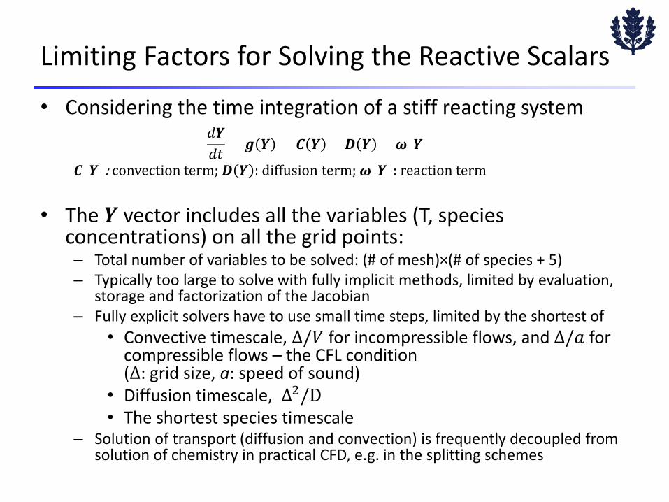
Limiting Factors for Solving the Reactive Scalars

• Considering the time integration of a stiff reacting system 𝑑𝑑𝒀𝒀𝑑𝑑𝑎𝑎

= 𝒈𝒈 𝒀𝒀 = 𝑪𝑪 𝒀𝒀 + 𝑫𝑫 𝒀𝒀 + 𝝎𝝎(𝒀𝒀)

𝑪𝑪(𝒀𝒀): convection term; 𝑫𝑫 𝒀𝒀 : diffusion term; 𝝎𝝎(𝒀𝒀): reaction term

• The 𝒀𝒀 vector includes all the variables (T, species concentrations) on all the grid points: – Total number of variables to be solved: (# of mesh)×(# of species + 5) – Typically too large to solve with fully implicit methods, limited by evaluation,

storage and factorization of the Jacobian – Fully explicit solvers have to use small time steps, limited by the shortest of

• Convective timescale, Δ/𝑉𝑉 for incompressible flows, and Δ/𝑎𝑎 for compressible flows – the CFL condition (Δ: grid size, a: speed of sound)

• Diffusion timescale, Δ2/D • The shortest species timescale

– Solution of transport (diffusion and convection) is frequently decoupled from solution of chemistry in practical CFD, e.g. in the splitting schemes

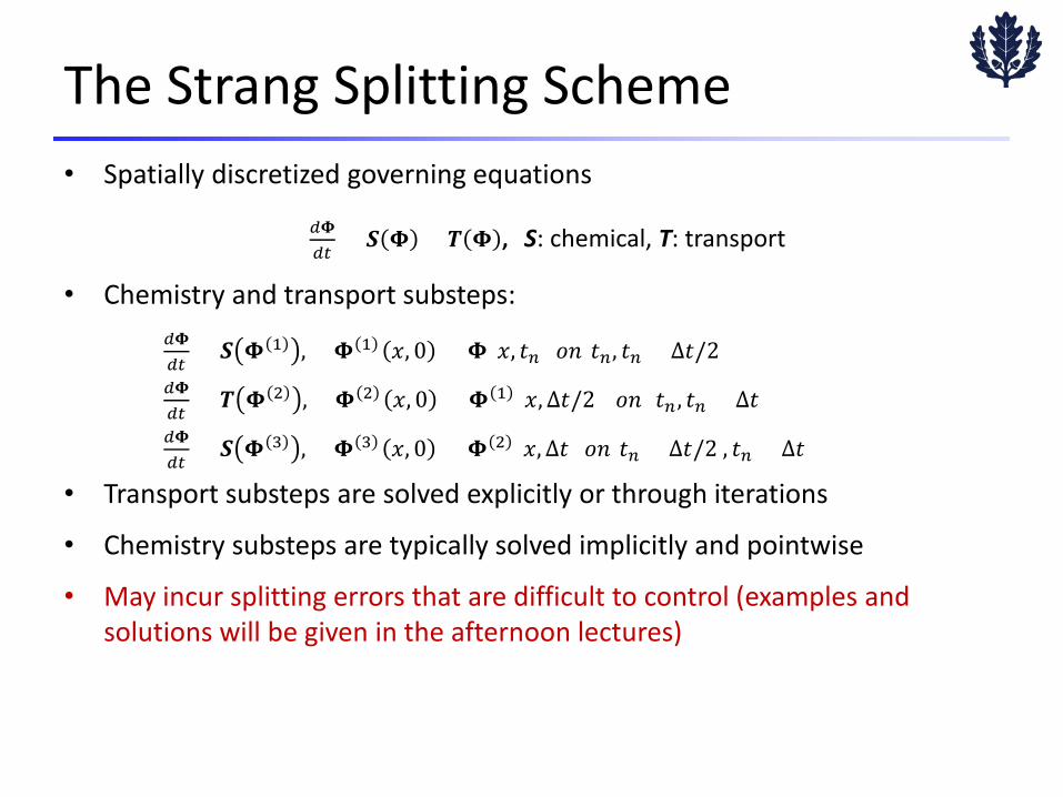
The Strang Splitting Scheme • Spatially discretized governing equations

𝑑𝑑𝑑𝑑𝑑𝑑𝑑𝑑

= 𝑺𝑺 𝑑𝑑 + 𝑻𝑻 𝑑𝑑 , S: chemical, T: transport

• Chemistry and transport substeps: 𝑑𝑑𝑑𝑑𝑑𝑑𝑑𝑑

= 𝑺𝑺 𝑑𝑑 1 , 𝑑𝑑 1 𝑥𝑥, 0 = 𝑑𝑑(𝑥𝑥, 𝑎𝑎𝑛𝑛) 𝑜𝑜𝑜𝑜[𝑎𝑎𝑛𝑛, 𝑎𝑎𝑛𝑛 + Δ𝑎𝑎/2 ] 𝑑𝑑𝑑𝑑𝑑𝑑𝑑𝑑

= 𝑻𝑻 𝑑𝑑 2 , 𝑑𝑑 2 𝑥𝑥, 0 = 𝑑𝑑 1 (𝑥𝑥,Δ𝑎𝑎/2 ) 𝑜𝑜𝑜𝑜 [𝑎𝑎𝑛𝑛 , 𝑎𝑎𝑛𝑛 + Δ𝑎𝑎] 𝑑𝑑𝑑𝑑𝑑𝑑𝑑𝑑

= 𝑺𝑺 𝑑𝑑 3 , 𝑑𝑑 3 𝑥𝑥, 0 = 𝑑𝑑 2 (𝑥𝑥,Δ𝑎𝑎) 𝑜𝑜𝑜𝑜[𝑎𝑎𝑛𝑛 + Δ𝑎𝑎/2 , 𝑎𝑎𝑛𝑛 + Δ𝑎𝑎 ] • Transport substeps are solved explicitly or through iterations

• Chemistry substeps are typically solved implicitly and pointwise

• May incur splitting errors that are difficult to control (examples and solutions will be given in the afternoon lectures)

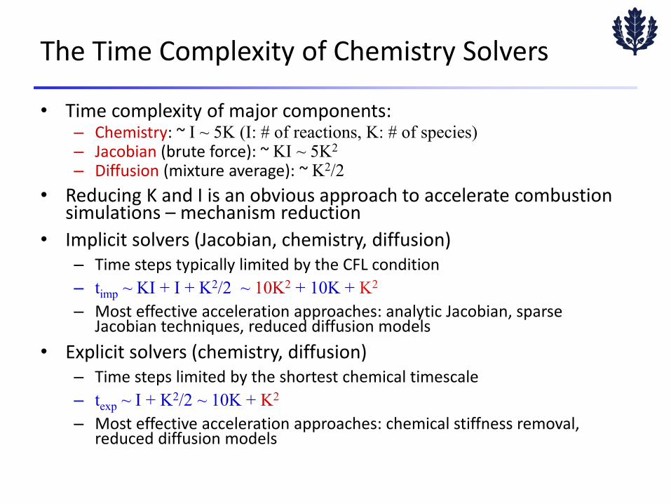
The Time Complexity of Chemistry Solvers

• Time complexity of major components: – Chemistry: ~ I ~ 5K (I: # of reactions, K: # of species) – Jacobian (brute force): ~ KI ~ 5K2 – Diffusion (mixture average): ~ K2/2

• Reducing K and I is an obvious approach to accelerate combustion simulations – mechanism reduction

• Implicit solvers (Jacobian, chemistry, diffusion) – Time steps typically limited by the CFL condition – timp ~ KI + I + K2/2 ~ 10K2 + 10K + K2

– Most effective acceleration approaches: analytic Jacobian, sparse Jacobian techniques, reduced diffusion models

• Explicit solvers (chemistry, diffusion) – Time steps limited by the shortest chemical timescale – texp ~ I + K2/2 ~ 10K + K2

– Most effective acceleration approaches: chemical stiffness removal, reduced diffusion models

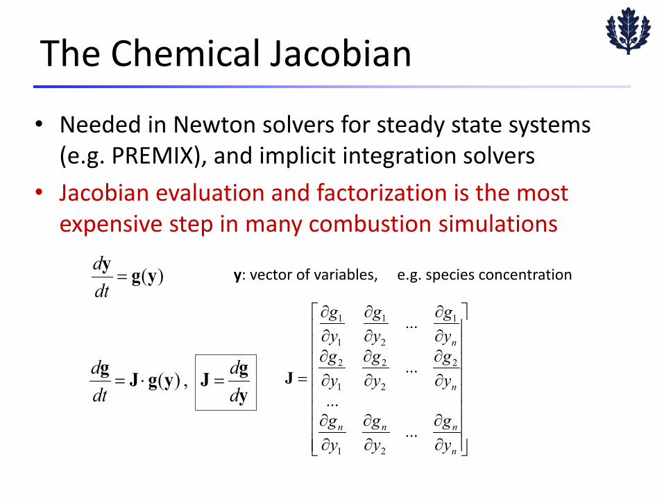
• Needed in Newton solvers for steady state systems (e.g. PREMIX), and implicit integration solvers

• Jacobian evaluation and factorization is the most expensive step in many combustion simulations

The Chemical Jacobian

∂∂

∂∂

∂∂

∂∂

∂∂

∂∂

∂∂

∂∂

∂∂

=

n

nnn

n

n

yg

yg

yg

yg

yg

yg

yg

yg

yg

...

...

...

...

21

2

2

2

1

2

1

2

1

1

1

J

)(ygy=

dtd

, )(ygJygJg

dd

dtd

=⋅=

y: vector of variables, e.g. species concentration

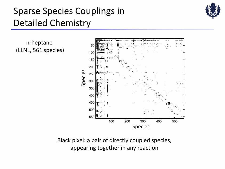
Sparse Species Couplings in Detailed Chemistry

Black pixel: a pair of directly coupled species, appearing together in any reaction

100 200 300 400 500

50

100

150

200

250

300

350

400

450

500

550

Species

Spec

ies

n-heptane (LLNL, 561 species)

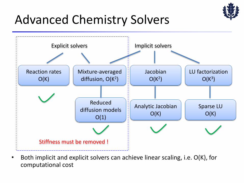
Reduced diffusion models

O(1)

Advanced Chemistry Solvers

Explicit solvers Implicit solvers

Reaction rates O(K)

Mixture-averaged diffusion, O(K2)

Jacobian O(K2)

LU factorization O(K3)

Stiffness must be removed !

Analytic Jacobian O(K)

Sparse LU O(K)

• Both implicit and explicit solvers can achieve linear scaling, i.e. O(K), for computational cost

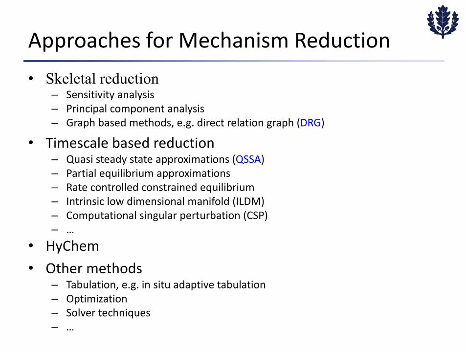
Approaches for Mechanism Reduction • Skeletal reduction

– Sensitivity analysis – Principal component analysis – Graph based methods, e.g. direct relation graph (DRG)

• Timescale based reduction – Quasi steady state approximations (QSSA) – Partial equilibrium approximations – Rate controlled constrained equilibrium – Intrinsic low dimensional manifold (ILDM) – Computational singular perturbation (CSP) – …

• HyChem • Other methods

– Tabulation, e.g. in situ adaptive tabulation – Optimization – Solver techniques – …

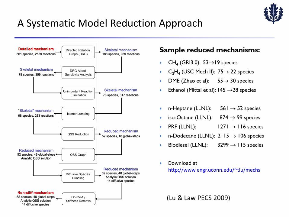
A Systematic Model Reduction Approach

Directed Relation

Graph (DRG)Detailed mechanismDetailed mechanism

561 species, 2539 reactions561 species, 2539 reactions

DRG Aided Sensitivity Analysis

Reduced mechanismReduced mechanism52 species, 48 global52 species, 48 global--stepssteps

Analytic QSS solutionAnalytic QSS solution

Unimportant ReactionElimination

Isomer Lumping

Skeletal mechanismSkeletal mechanism78 species, 359 reactions78 species, 359 reactions

Skeletal mechanismSkeletal mechanism188 species, 939 reactions188 species, 939 reactions

Skeletal mechanismSkeletal mechanism78 species, 317 reactions78 species, 317 reactions

““SkeletalSkeletal”” mechanismmechanism68 species, 283 reactions68 species, 283 reactions

QSS ReductionReduced mechanismReduced mechanism

52 species, 48 global52 species, 48 global--stepssteps

QSS Graph

Diffusive Species Bundling

Reduced mechanismReduced mechanism52 species, 48 global52 species, 48 global--stepssteps

Analytic QSS solutionAnalytic QSS solution14 diffusive species14 diffusive species

On-the-fly Stiffness Removal

NonNon--stiff mechanismstiff mechanism52 species, 48 global52 species, 48 global--stepssteps

Analytic QSS solutionAnalytic QSS solution14 diffusive species14 diffusive species

Directed Relation Graph (DRG)

Detailed mechanismDetailed mechanism561 species, 2539 reactions561 species, 2539 reactions

DRG Aided Sensitivity Analysis

Reduced mechanismReduced mechanism52 species, 48 global52 species, 48 global--stepssteps

Analytic QSS solutionAnalytic QSS solution

Unimportant ReactionElimination

Isomer Lumping

Skeletal mechanismSkeletal mechanism78 species, 359 reactions78 species, 359 reactions

Skeletal mechanismSkeletal mechanism188 species, 939 reactions188 species, 939 reactions

Skeletal mechanismSkeletal mechanism78 species, 317 reactions78 species, 317 reactions

““SkeletalSkeletal”” mechanismmechanism68 species, 283 reactions68 species, 283 reactions

QSS ReductionReduced mechanismReduced mechanism

52 species, 48 global52 species, 48 global--stepssteps

QSS Graph

Diffusive Species Bundling

Reduced mechanismReduced mechanism52 species, 48 global52 species, 48 global--stepssteps

Analytic QSS solutionAnalytic QSS solution14 diffusive species14 diffusive species

On-the-fly Stiffness Removal

NonNon--stiff mechanismstiff mechanism52 species, 48 global52 species, 48 global--stepssteps

Analytic QSS solutionAnalytic QSS solution14 diffusive species14 diffusive species

Sample reduced mechanisms:

CH4 (GRI3.0): 53→19 species

C2H4 (USC Mech II): 75→ 22 species

DME (Zhao et al): 55→ 30 species

Ethanol (Mittal et al): 145 →28 species

n-Heptane (LLNL): 561 → 52 species

iso-Octane (LLNL): 874 → 99 species

PRF (LLNL): 1271 → 116 species

n-Dodecane (LLNL): 2115 → 106 species

Biodiesel (LLNL): 3299 → 115 species

Download at http://www.engr.uconn.edu/~tlu/mechs

(Lu & Law PECS 2009)

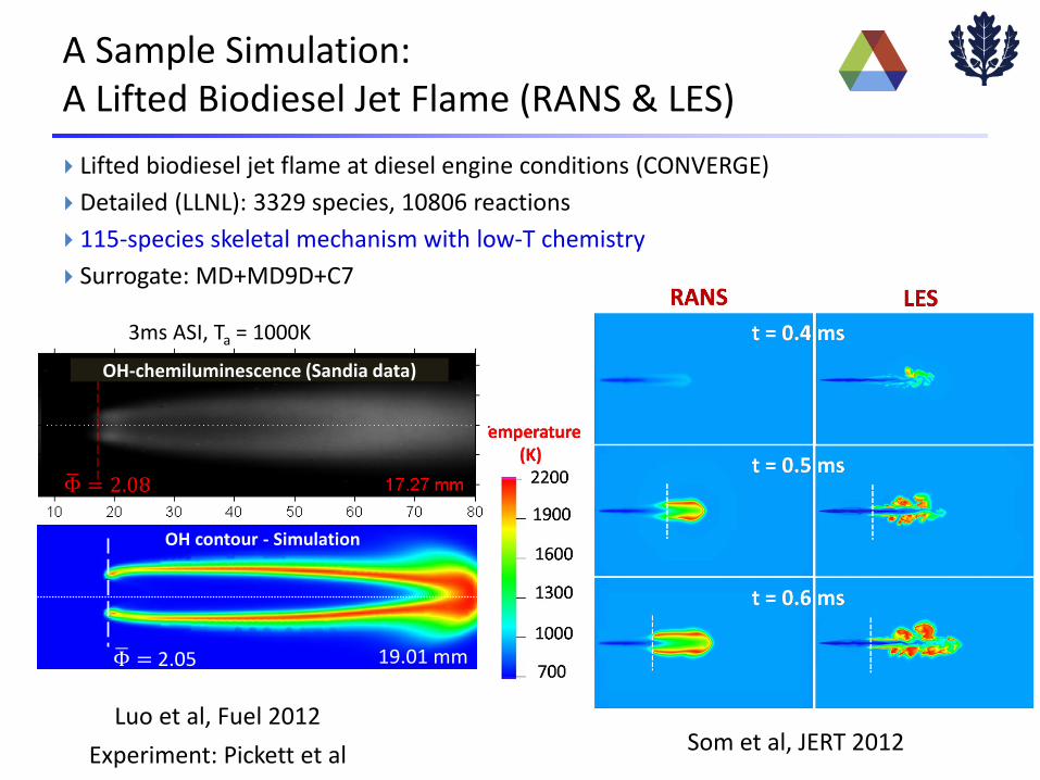
A Sample Simulation: A Lifted Biodiesel Jet Flame (RANS & LES) Lifted biodiesel jet flame at diesel engine conditions (CONVERGE) Detailed (LLNL): 3329 species, 10806 reactions 115-species skeletal mechanism with low-T chemistry Surrogate: MD+MD9D+C7

Experiment: Pickett et al

3ms ASI, Ta = 1000K

Som et al, JERT 2012 Luo et al, Fuel 2012

OH-chemiluminescence

2.05 19.01 mm

OH contour - Simulation

OH-chemiluminescence (Sandia data)

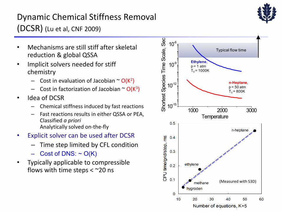
(Measured with S3D)

Dynamic Chemical Stiffness Removal (DCSR) (Lu et al, CNF 2009)

• Mechanisms are still stiff after skeletal reduction & global QSSA

• Implicit solvers needed for stiff chemistry

– Cost in evaluation of Jacobian ~ O(K2) – Cost in factorization of Jacobian ~ O(K3)

• Idea of DCSR – Chemical stiffness induced by fast reactions – Fast reactions results in either QSSA or PEA,

Classified a priori Analytically solved on-the-fly

• Explicit solver can be used after DCSR – Time step limited by CFL condition – Cost of DNS: ~ O(K)

• Typically applicable to compressible flows with time steps < ~20 ns

1000 2000 300010-15

10-12

10-9

10-6

Shor

test

Spe

cies

Tim

e Sc

ale,

Sec

Temperature

Ethylene,p = 1 atmT0 = 1000K

n-Heptane, p = 50 atmT0 = 800K

Typical flow time

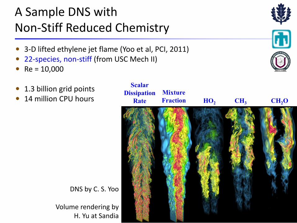
A Sample DNS with Non-Stiff Reduced Chemistry 3-D lifted ethylene jet flame (Yoo et al, PCI, 2011) 22-species, non-stiff (from USC Mech II) Re = 10,000

1.3 billion grid points 14 million CPU hours

DNS by C. S. Yoo

Volume rendering by H. Yu at Sandia

Scalar Dissipation

Rate Mixture Fraction HO2 CH3 CH2O

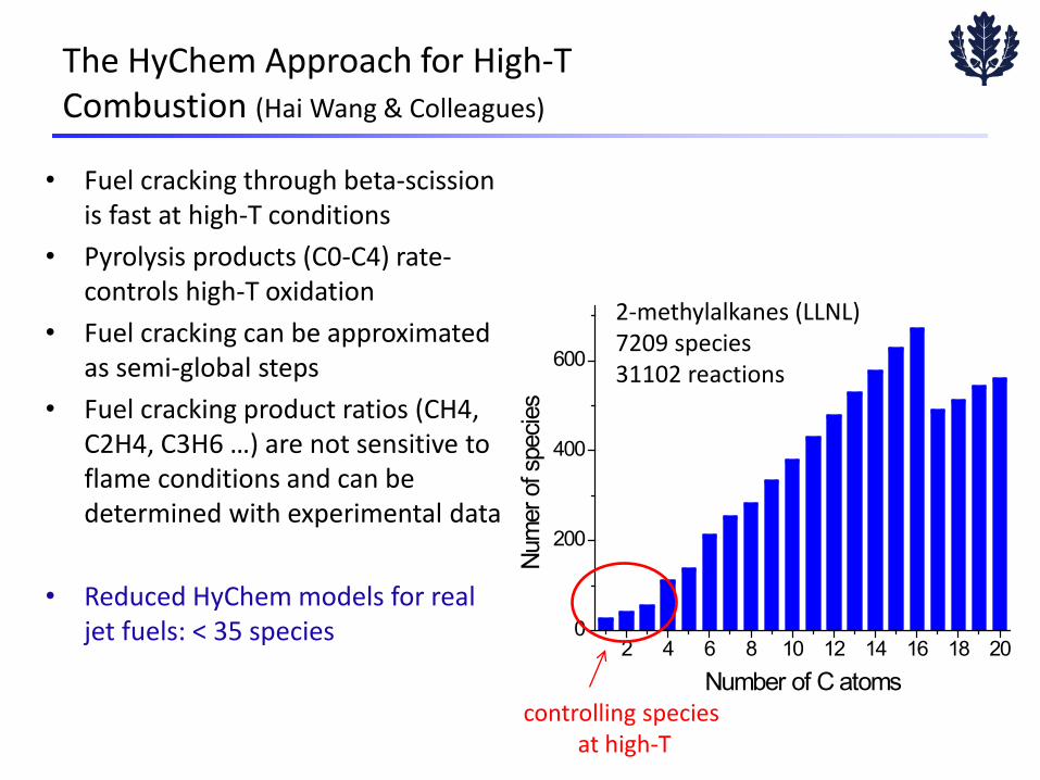
The HyChem Approach for High-T Combustion (Hai Wang & Colleagues)

• Fuel cracking through beta-scission is fast at high-T conditions

• Pyrolysis products (C0-C4) rate-controls high-T oxidation

• Fuel cracking can be approximated as semi-global steps

• Fuel cracking product ratios (CH4, C2H4, C3H6 …) are not sensitive to flame conditions and can be determined with experimental data

• Reduced HyChem models for real jet fuels: < 35 species

2 4 6 8 10 12 14 16 18 200

200

400

600

Num

er o

f spe

cies

Number of C atoms

2-methylalkanes (LLNL) 7209 species 31102 reactions

controlling species at high-T

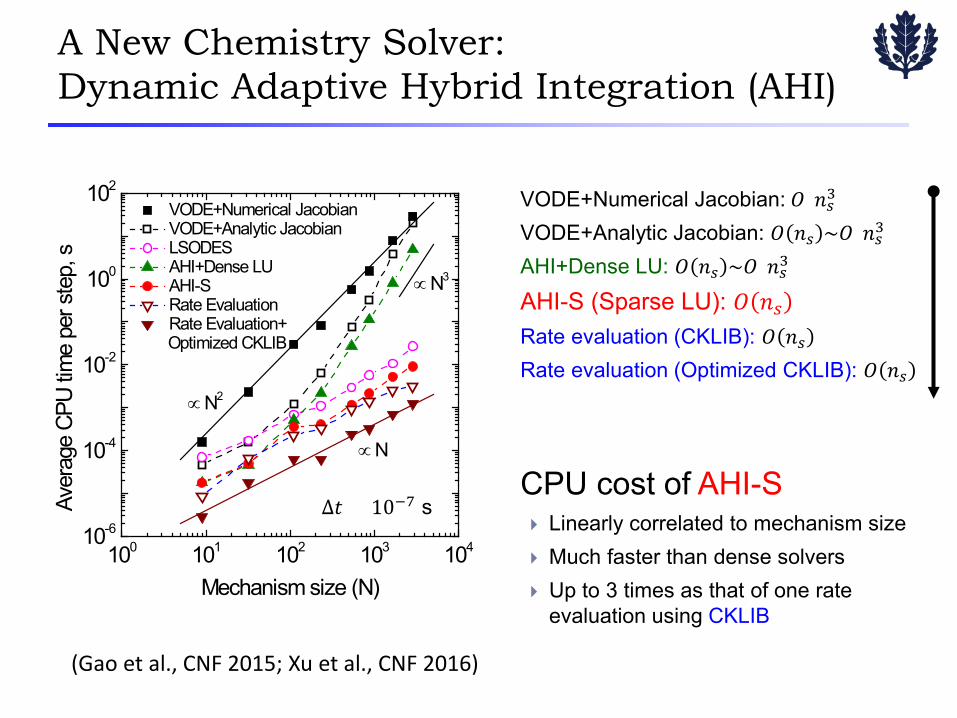
A New Chemistry Solver: Dynamic Adaptive Hybrid Integration (AHI)

VODE+Numerical Jacobian: 𝑂𝑂(𝑜𝑜𝑠𝑠3) VODE+Analytic Jacobian: 𝑂𝑂 𝑜𝑜𝑠𝑠 ~𝑂𝑂(𝑜𝑜𝑠𝑠3) AHI+Dense LU: 𝑂𝑂 𝑜𝑜𝑠𝑠 ~𝑂𝑂(𝑜𝑜𝑠𝑠3)

AHI-S (Sparse LU): 𝑂𝑂 𝑜𝑜𝑠𝑠 Rate evaluation (CKLIB): 𝑂𝑂 𝑜𝑜𝑠𝑠 Rate evaluation (Optimized CKLIB): 𝑂𝑂 𝑜𝑜𝑠𝑠

CPU cost of AHI-S Linearly correlated to mechanism size Much faster than dense solvers Up to 3 times as that of one rate

evaluation using CKLIB

100 101 102 103 10410-6

10-4

10-2

100

102

∝ N3

Aver

age

CPU

time

per s

tep,

s

Mechanism size (N)

VODE+Numerical Jacobian VODE+Analytic Jacobian LSODES AHI+Dense LU AHI-S Rate Evaluation Rate Evaluation+

Optimized CKLIB

∝ N2

∝ N

Δ𝑎𝑎 = 10−7 s

(Gao et al., CNF 2015; Xu et al., CNF 2016)

Formation of Nascent Soot and Other Condensed‐Phase Materials in Flames

Hai WangUniversity of Southern California

Work supported by NSF, SERDP and DOE (CEFRC)

Lesson 7

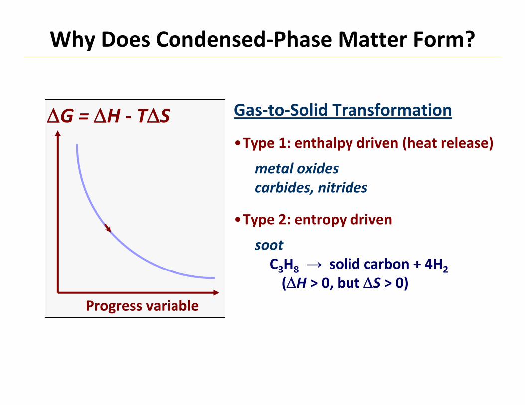
Why Does Condensed‐Phase Matter Form?

G = H ‐ TS

Progress variable

Gas‐to‐Solid Transformation

•Type 1: enthalpy driven (heat release)

metal oxidescarbides, nitrides

•Type 2: entropy driven

sootC3H8 → solid carbon + 4H2

(H > 0, but S > 0)

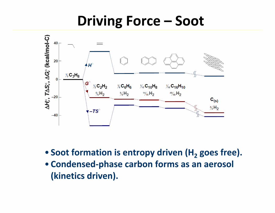
Driving Force – Soot

S○,

G○

(kca

l/mol

-C)

rrS○,

G○

(kca

l/mol

-C)

rrS○,

G○

(kca

l/mol

-C)

rrS○,

G○

(kca

l/mol

-C)

rr

H○ ,

TS○

, G

○(k

cal/m

ol-C

)r

rr

H○ ,

TS○

, G

○(k

cal/m

ol-C

)r

rr

H○ ,

TS○

, G

○(k

cal/m

ol-C

)r

rr

H○ ,

TS○

, G

○(k

cal/m

ol-C

)r

rr

• Soot formation is entropy driven (H2 goes free).•Condensed‐phase carbon forms as an aerosol (kinetics driven).

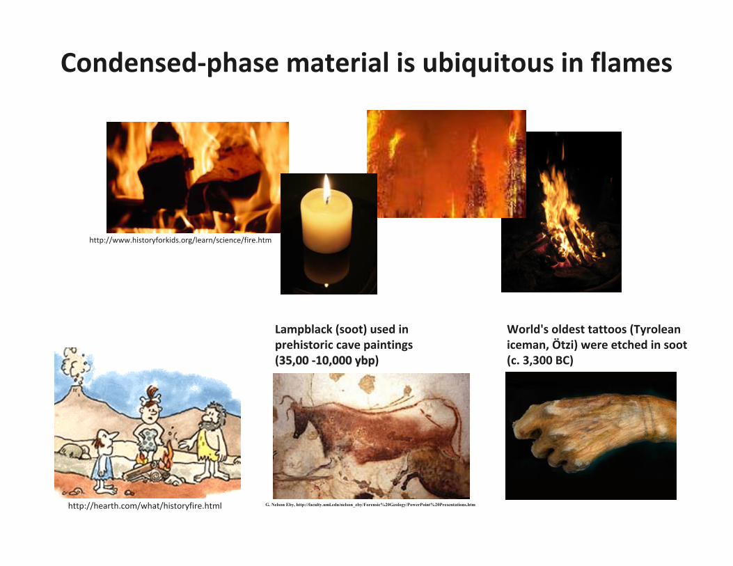
Condensed‐phase material is ubiquitous in flames

http://www.historyforkids.org/learn/science/fire.htm

http://hearth.com/what/historyfire.html

World's oldest tattoos (Tyrolean iceman, Ötzi) were etched in soot(c. 3,300 BC) 

Lampblack (soot) used in prehistoric cave paintings (35,00 35,00 ‐‐10,000 10,000 ybpybp)

G. Nelson Eby, http://faculty.uml.edu/nelson_eby/Forensic%20Geology/PowerPoint%20Presentations.htm

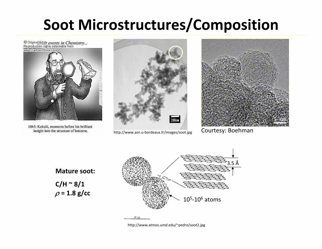
Soot Microstructures/Composition

http://www.atmos.umd.edu/~pedro/soot2.jpg

3.5 Å

105‐106 atoms

http://www.asn.u‐bordeaux.fr/images/soot.jpg Courtesy: Boehman

Mature soot:

C/H ~ 8/1 = 1.8 g/cc

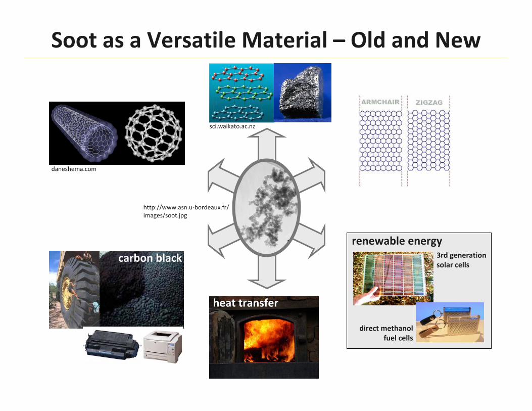
Soot as a Versatile Material – Old and New

daneshema.com

sci.waikato.ac.nz

carbon black 3rd generation solar cells

direct methanolfuel cells

renewable energy

heat transfer

http://www.asn.u‐bordeaux.fr/images/soot.jpg

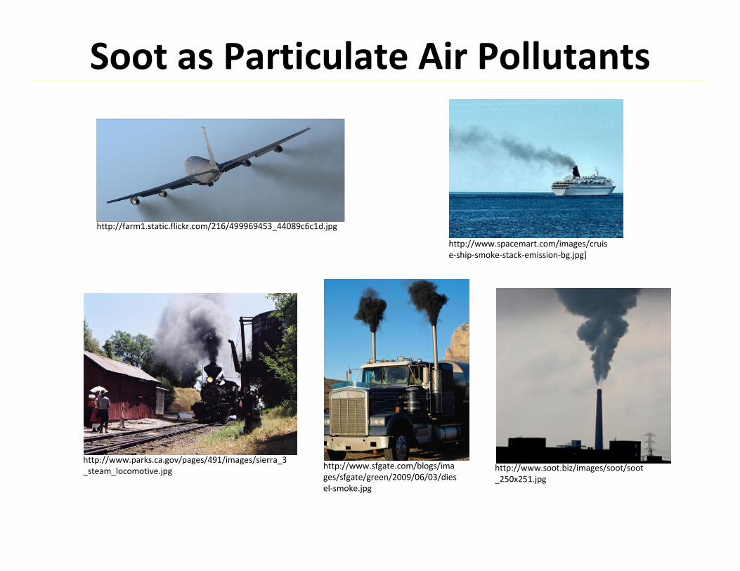
Soot as Particulate Air Pollutants

http://www.spacemart.com/images/cruise‐ship‐smoke‐stack‐emission‐bg.jpg]

http://www.sfgate.com/blogs/images/sfgate/green/2009/06/03/diesel‐smoke.jpg

http://www.soot.biz/images/soot/soot_250x251.jpg

http://farm1.static.flickr.com/216/499969453_44089c6c1d.jpg

http://www.parks.ca.gov/pages/491/images/sierra_3_steam_locomotive.jpg

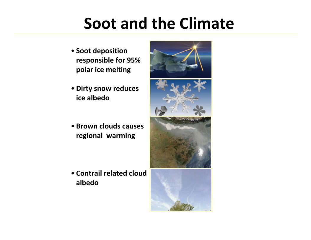
Soot and the Climate • Soot deposition responsible for 95% polar ice melting

•Dirty snow reduces ice albedo

• Brown clouds causes regional  warming

• Contrail related cloud albedo

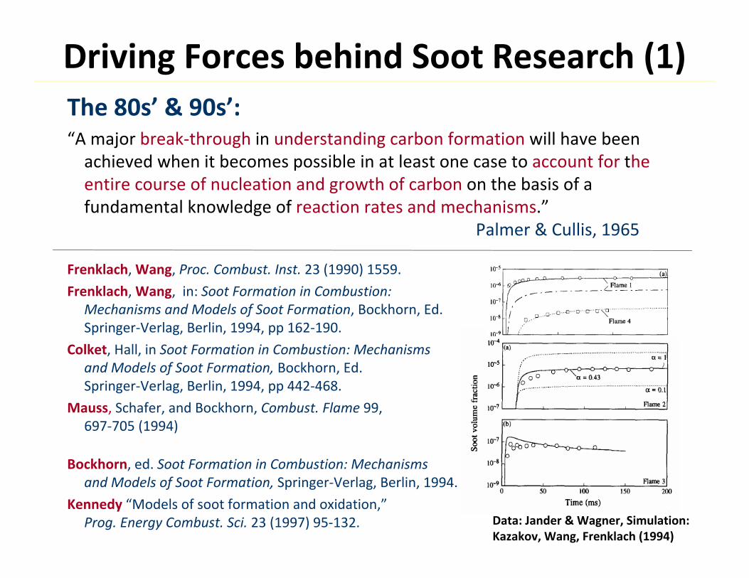
Driving Forces behind Soot Research (1)The 80s’ & 90s’:“A major break‐through in understanding carbon formation will have been achieved when it becomes possible in at least one case to account for the entire course of nucleation and growth of carbon on the basis of a fundamental knowledge of reaction rates and mechanisms.”

Palmer & Cullis, 1965

Frenklach, Wang, Proc. Combust. Inst. 23 (1990) 1559.

Frenklach, Wang,  in: Soot Formation in Combustion: Mechanisms and Models of Soot Formation, Bockhorn, Ed.Springer‐Verlag, Berlin, 1994, pp 162‐190.

Colket, Hall, in Soot Formation in Combustion: Mechanisms and Models of Soot Formation, Bockhorn, Ed.Springer‐Verlag, Berlin, 1994, pp 442‐468.

Mauss, Schafer, and Bockhorn, Combust. Flame 99, 697‐705 (1994)

Bockhorn, ed. Soot Formation in Combustion: Mechanisms and Models of Soot Formation, Springer‐Verlag, Berlin, 1994.

Kennedy “Models of soot formation and oxidation,”Prog. Energy Combust. Sci. 23 (1997) 95‐132. Data: Jander & Wagner, Simulation: 

Kazakov, Wang, Frenklach (1994)

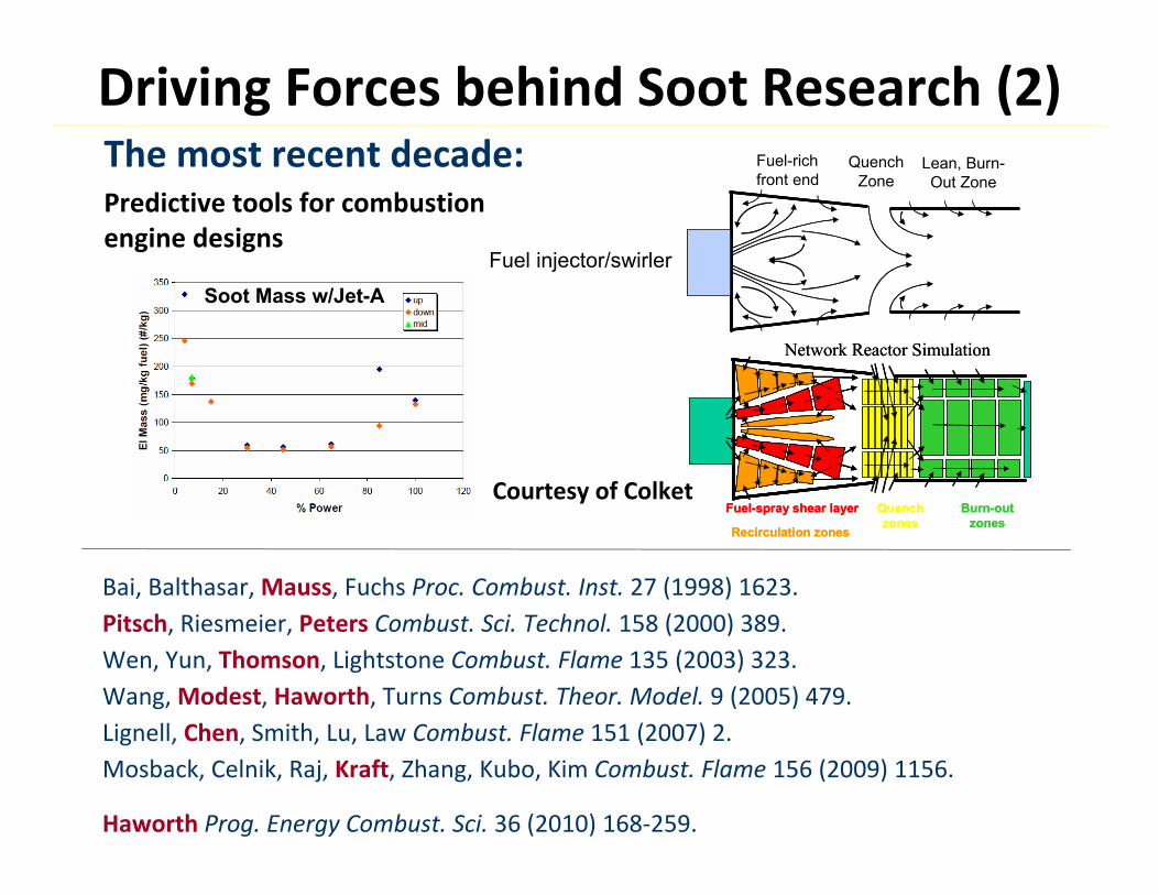
Driving Forces behind Soot Research (2)The most recent decade:Predictive tools for combustion engine designs

Network Reactor Simulation

Fuel-spray shear layer

Recirculation zones

Quench zones

Burn-out zones

Network Reactor Simulation

Fuel-spray shear layer

Recirculation zones

Quench zones

Burn-out zones

Fuel injector/swirler

Fuel-rich front end

Quench Zone

Lean, Burn-Out Zone

Soot Mass w/Jet-A

Courtesy of Colket

Bai, Balthasar, Mauss, Fuchs Proc. Combust. Inst. 27 (1998) 1623.Pitsch, Riesmeier, Peters Combust. Sci. Technol. 158 (2000) 389.Wen, Yun, Thomson, Lightstone Combust. Flame 135 (2003) 323.Wang, Modest, Haworth, Turns Combust. Theor. Model. 9 (2005) 479.Lignell, Chen, Smith, Lu, Law Combust. Flame 151 (2007) 2.Mosback, Celnik, Raj, Kraft, Zhang, Kubo, Kim Combust. Flame 156 (2009) 1156.

Haworth Prog. Energy Combust. Sci. 36 (2010) 168‐259.

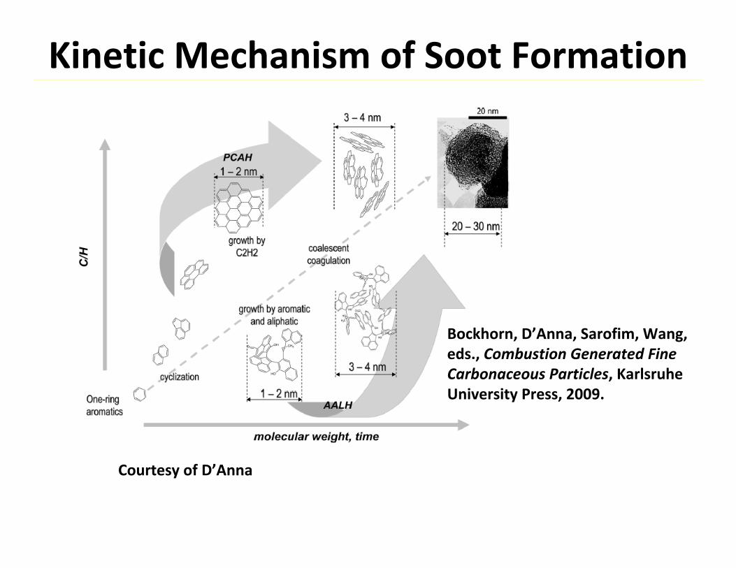
Kinetic Mechanism of Soot Formation

Courtesy of D’Anna

Bockhorn, D’Anna, Sarofim, Wang, eds., Combustion Generated Fine Carbonaceous Particles, KarlsruheUniversity Press, 2009.

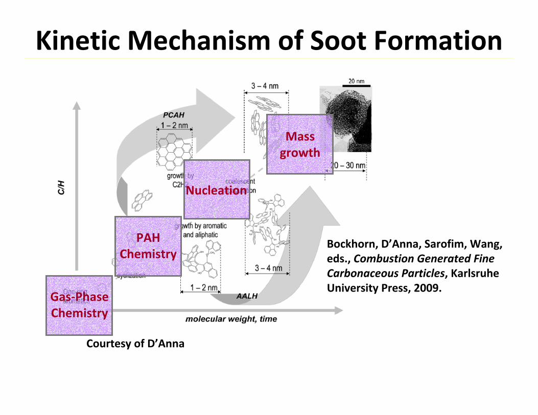
Kinetic Mechanism of Soot Formation

Courtesy of D’Anna

Bockhorn, D’Anna, Sarofim, Wang, eds., Combustion Generated Fine Carbonaceous Particles, KarlsruheUniversity Press, 2009.

Gas‐PhaseChemistry

PAHChemistry

Nucleation

Massgrowth

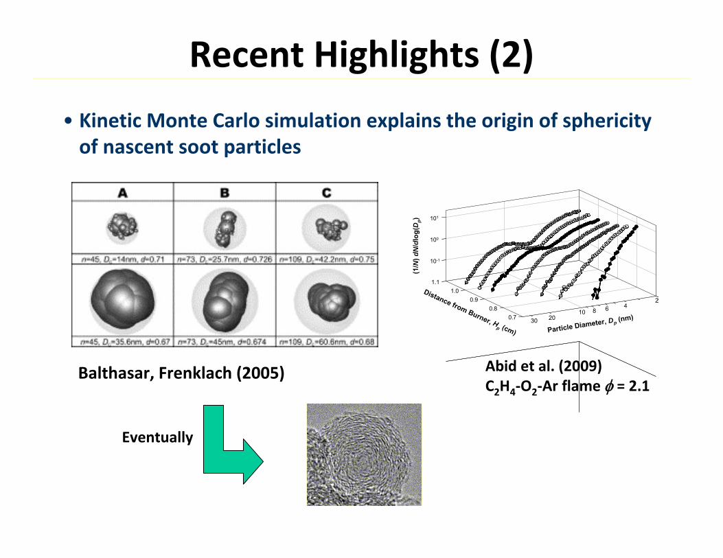
Recent Highlights (2)

Balthasar, Frenklach (2005)

• Kinetic Monte Carlo simulation explains the origin of sphericityof nascent soot particles

10-1

100

101

0.70.8

0.91.0

1.1

(1/N

) dN

/dlo

g(D

p)

Particle Diameter, Dp (nm)

Distance from Burner, Hp (cm)

246810

2030

10-1

100

101

0.70.8

0.91.0

1.1

(1/N

) dN

/dlo

g(D

p)

Particle Diameter, Dp (nm)

Distance from Burner, Hp (cm)

246810

2030

Abid et al. (2009)C2H4‐O2‐Ar flame  = 2.1

Eventually

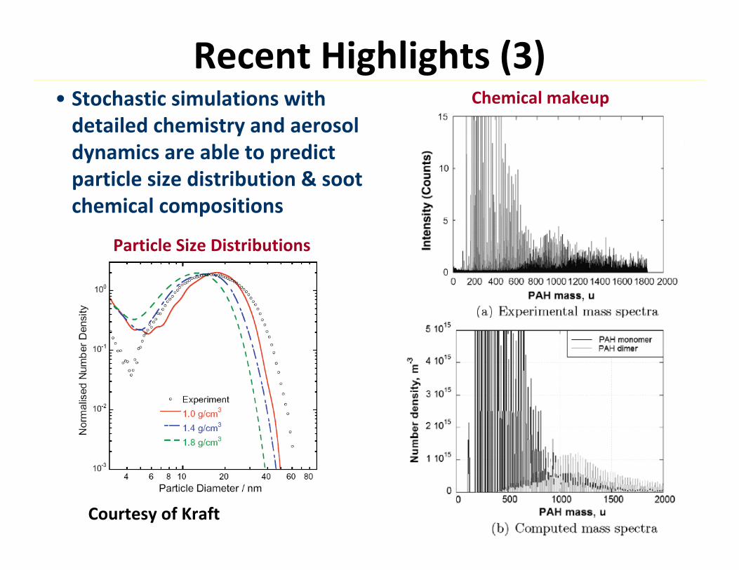
Recent Highlights (3)

Particle Size Distributions

Chemical makeup

Courtesy of Kraft

• Stochastic simulations with detailed chemistry and aerosol dynamics are able to predict particle size distribution & soot chemical compositions

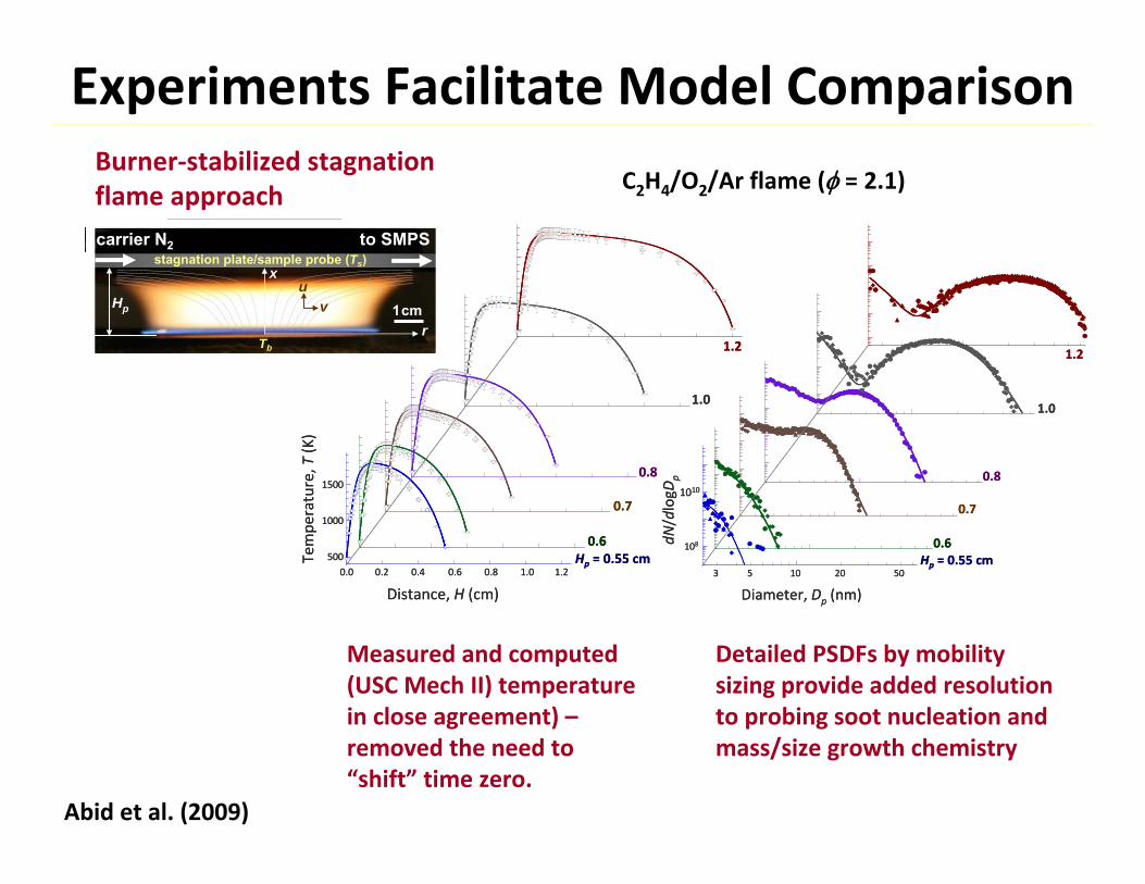
Experiments Facilitate Model Comparison

Measured and computed (USC Mech II) temperature in close agreement) –removed the need to “shift” time zero.

Burner‐stabilized stagnation flame approach C2H4/O2/Ar flame ( = 2.1)

Abid et al. (2009)

Distance, H (cm)1.2

5001.00.80.60.40.20.0

1000

1500

Tempe

rature, T

(K)

1.2

Hp = 0.55 cm0.6

0.7

0.8

1.0

Distance, H (cm)1.2

5001.00.80.60.40.20.0

1000

1500

Tempe

rature, T

(K)

1.2

Hp = 0.55 cm0.6

0.7

0.8

1.0

1.2

0.6

0.7

0.8

1.0

Diameter, Dp (nm)3 5 10 20 50

108

1010

dN/dlogD

p

Hp = 0.55 cm

1.2

0.6

0.7

0.8

1.0

Diameter, Dp (nm)3 5 10 20 50

108

1010

dN/dlogD

p

Hp = 0.55 cm

cooling assembly

1cmHp

stagnation plate/sample probe (Ts)

Tb

r

xu

v

to SMPScarrier N2

Detailed PSDFs by mobility sizing provide added resolution to probing soot nucleation and mass/size growth chemistry

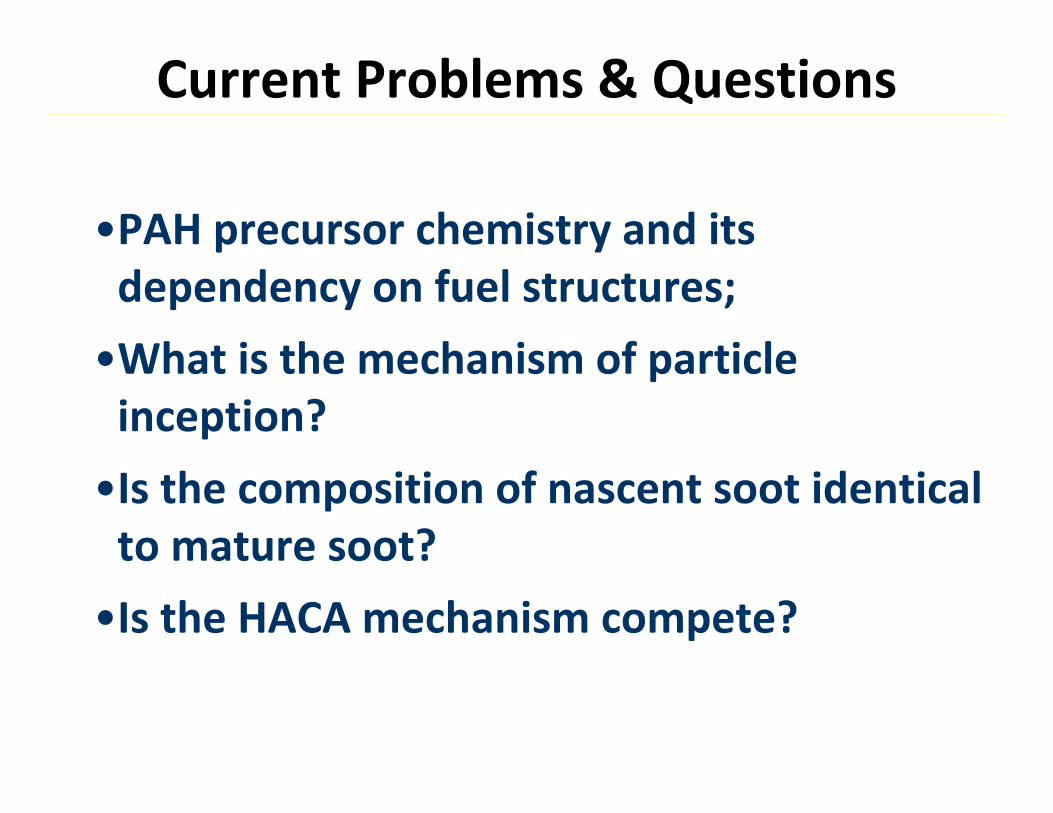
Current Problems & Questions

•PAH precursor chemistry and its dependency on fuel structures;

•What is the mechanism of particle inception?

•Is the composition of nascent soot identical to mature soot?

•Is the HACA mechanism compete?

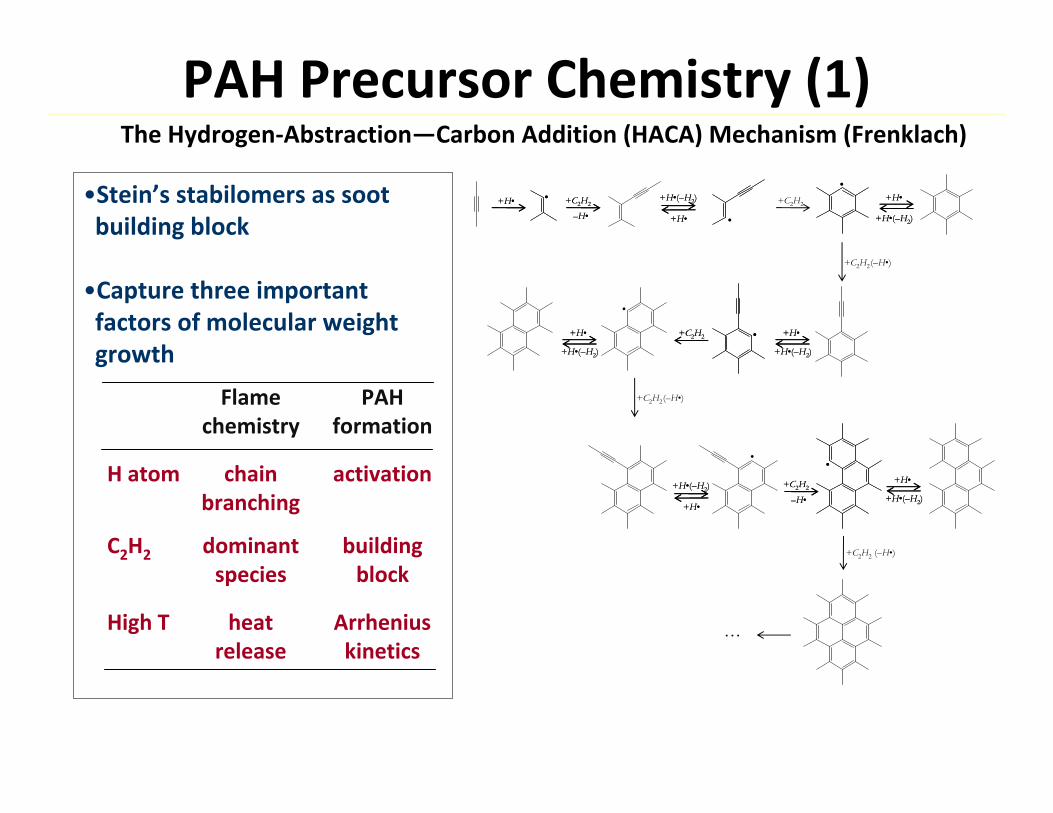
PAH Precursor Chemistry (1)

+H•+H• ••

••

+C2H2

••

(–H•)

••

+C2H2

–H•

+C2H2

–H•

+C2H2

+H•(–H2)

+H•

+H•(–H2)

+H•

+H•(–H2)

+H•

+H•(–H2)

+H•

+H•(–H2)

+H•

+H•(–H2)

+H•

+C2H2+C2H2

•

+H•(–H2)

+H•

+H•(–H2)

+H•

+C2H2(–H•)

+H•(–H2)

+H•

+H•(–H2)

+H•

•

+C2H2

–H•

+C2H2

–H• +H•(–H2)

+H•

+H•(–H2)

+H•

+C2H2 (–H•)

…

••

The Hydrogen‐Abstraction—Carbon Addition (HACA) Mechanism (Frenklach)

•Stein’s stabilomers as soot building block

•Capture three important factors of molecular weight growth

Flame PAHchemistry formation

H atom chain activationbranching

C2H2 dominant buildingspecies block

High T heat Arrheniusrelease kinetics

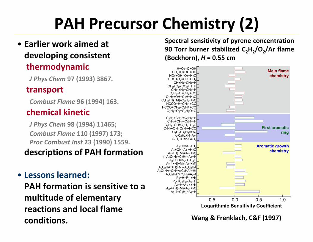
PAH Precursor Chemistry (2)• Earlier work aimed at developing consistent   thermodynamicJ Phys Chem 97 (1993) 3867.

transportCombust Flame 96 (1994) 163.

chemical kineticJ Phys Chem 98 (1994) 11465; Combust Flame 110 (1997) 173; Proc Combust Inst 23 (1990) 1559.

descriptions of PAH formation

• Lessons learned:PAH formation is sensitive to a multitude of elementary reactions and local flame conditions.

-0.5 0.0 0.5 1.0

H+O2=O+OHHO2+H=OH+OH

HO2+OH=O2+H2OHCO+O2=CO+HO2

CH+H2=CH2+HCH2+O2=CO2+H+H

CH2*+H2=CH3+HC2H2+O=CH2+CO

C2H2+OH=C2H+H2OC2H2+H(+M)=C2H3(+M)

HCCO+H=CH2*+COHCCO+CH3=C2H4+CO

C2H3+O2=C2H3O+O

C2H2+CH2*=C3H3+HC2H2+CH2=C3H3+H

C3H3+OH=C3H2+H2OC3H3+OH=C2H3+HCO

C3H3+C3H3=>A1c-C6H4+H=A1-

C4H2+H=n-C4H3

A1+H=A1-+H2A1+OH=A1-+H2O

A1-+H(+M)=A1(+M)n-A1C2H2+C2H2=A2+H

A2+OH=A2-1+H2OA2-1+H(+M)=A2(+M)

A2C2HA*+H(+M)=A2C2HAA2C2HA+OH=A2C2HA*+H2

A2C2HA*+C2H2=A3-4P2+H=P2-+H2

P2-+C2H2=A3+HA3+H=A3-4+H2

A3-4+H(+M)=A3(+M)A3-4+C2H2=A4+H

Logarithmic Sensitivity Coefficient

Main flamechemistry

First aromaticring

Aromatic growthchemistry

Spectral sensitivity of pyrene concentration 90 Torr burner stabilized C2H2/O2/Ar flame (Bockhorn), H = 0.55 cm

Wang & Frenklach, C&F (1997)

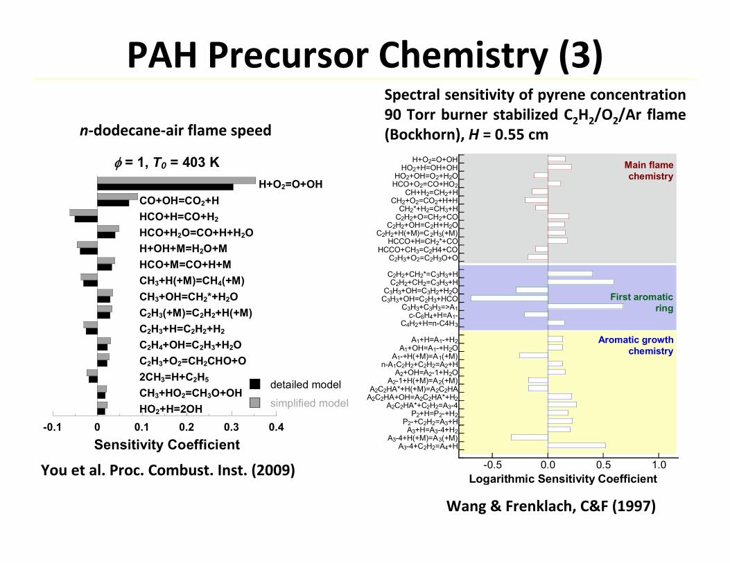
PAH Precursor Chemistry (3)

-0.5 0.0 0.5 1.0

H+O2=O+OHHO2+H=OH+OH

HO2+OH=O2+H2OHCO+O2=CO+HO2

CH+H2=CH2+HCH2+O2=CO2+H+H

CH2*+H2=CH3+HC2H2+O=CH2+CO

C2H2+OH=C2H+H2OC2H2+H(+M)=C2H3(+M)

HCCO+H=CH2*+COHCCO+CH3=C2H4+CO

C2H3+O2=C2H3O+O

C2H2+CH2*=C3H3+HC2H2+CH2=C3H3+H

C3H3+OH=C3H2+H2OC3H3+OH=C2H3+HCO

C3H3+C3H3=>A1c-C6H4+H=A1-

C4H2+H=n-C4H3

A1+H=A1-+H2A1+OH=A1-+H2O

A1-+H(+M)=A1(+M)n-A1C2H2+C2H2=A2+H

A2+OH=A2-1+H2OA2-1+H(+M)=A2(+M)

A2C2HA*+H(+M)=A2C2HAA2C2HA+OH=A2C2HA*+H2

A2C2HA*+C2H2=A3-4P2+H=P2-+H2

P2-+C2H2=A3+HA3+H=A3-4+H2

A3-4+H(+M)=A3(+M)A3-4+C2H2=A4+H

Logarithmic Sensitivity Coefficient

Main flamechemistry

First aromaticring

Aromatic growthchemistry

Spectral sensitivity of pyrene concentration 90 Torr burner stabilized C2H2/O2/Ar flame (Bockhorn), H = 0.55 cm

Wang & Frenklach, C&F (1997)

-0.1 0 0.1 0.2 0.3 0.4HO2+H=2OHCH3+HO2=CH3O+OH2CH3=H+C2H5

C2H3+O2=CH2CHO+OC2H4+OH=C2H3+H2OC2H3+H=C2H2+H2

C2H3(+M)=C2H2+H(+M)CH3+OH=CH2*+H2OCH3+H(+M)=CH4(+M)HCO+M=CO+H+MH+OH+M=H2O+MHCO+H2O=CO+H+H2OHCO+H=CO+H2

CO+OH=CO2+HH+O2=O+OH

= 1, T0 = 403 K

detailed model

simplified model

Sensitivity Coefficient

You et al. Proc. Combust. Inst. (2009)

n‐dodecane‐air flame speed

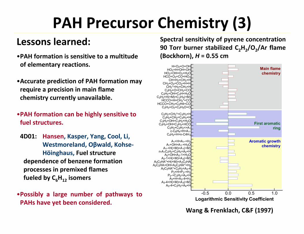
PAH Precursor Chemistry (3)

-0.5 0.0 0.5 1.0

H+O2=O+OHHO2+H=OH+OH

HO2+OH=O2+H2OHCO+O2=CO+HO2

CH+H2=CH2+HCH2+O2=CO2+H+H

CH2*+H2=CH3+HC2H2+O=CH2+CO

C2H2+OH=C2H+H2OC2H2+H(+M)=C2H3(+M)

HCCO+H=CH2*+COHCCO+CH3=C2H4+CO

C2H3+O2=C2H3O+O

C2H2+CH2*=C3H3+HC2H2+CH2=C3H3+H

C3H3+OH=C3H2+H2OC3H3+OH=C2H3+HCO

C3H3+C3H3=>A1c-C6H4+H=A1-

C4H2+H=n-C4H3

A1+H=A1-+H2A1+OH=A1-+H2O

A1-+H(+M)=A1(+M)n-A1C2H2+C2H2=A2+H

A2+OH=A2-1+H2OA2-1+H(+M)=A2(+M)

A2C2HA*+H(+M)=A2C2HAA2C2HA+OH=A2C2HA*+H2

A2C2HA*+C2H2=A3-4P2+H=P2-+H2

P2-+C2H2=A3+HA3+H=A3-4+H2

A3-4+H(+M)=A3(+M)A3-4+C2H2=A4+H

Logarithmic Sensitivity Coefficient

Main flamechemistry

First aromaticring

Aromatic growthchemistry

Spectral sensitivity of pyrene concentration 90 Torr burner stabilized C2H2/O2/Ar flame (Bockhorn), H = 0.55 cm

Wang & Frenklach, C&F (1997)

Lessons learned:•PAH formation is sensitive to a multitude of elementary reactions.

•Accurate prediction of PAH formation may require a precision in main flame chemistry currently unavailable.

•PAH formation can be highly sensitive to fuel structures.

4D01: Hansen, Kasper, Yang, Cool, Li, Westmoreland, Oβwald, Kohse‐Höinghaus, Fuel structure

dependence of benzene formationprocesses in premixed flames fueled by C6H12 isomers

•Possibly  a  large  number  of  pathways  to PAHs have yet been considered.

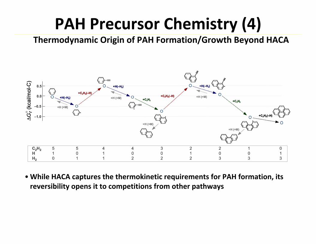
PAH Precursor Chemistry (4)Thermodynamic Origin of PAH Formation/Growth Beyond HACA

C2H2 5 5 4 4 3 2 2 1 0H 1 0 1 0 0 1 0 0 1H2 0 1 1 2 2 2 3 3 3

0.0

0.5

–0.5

–1.0G○

(kca

l/mol

-C)

r

+C2H2(–H)+H(–H2)

+H(–H2)

+C2H2

+C2H2(–H)

+H(–H2)

+C2H2

+C2H2(–H)

+H (+M)

+H (+M)

+H (+M) +H (+M)

••

•

•

•+H (+M)

C2H2 5 5 4 4 3 2 2 1 0H 1 0 1 0 0 1 0 0 1H2 0 1 1 2 2 2 3 3 3

0.0

0.5

–0.5

–1.0G○

(kca

l/mol

-C)

r

+C2H2(–H)+H(–H2)

+H(–H2)

+C2H2

+C2H2(–H)

+H(–H2)

+C2H2

+C2H2(–H)

+H (+M)

+H (+M)

+H (+M) +H (+M)

•••

••

••

••+H (+M)

•While HACA captures the thermokinetic requirements for PAH formation, its reversibility opens it to competitions from other pathways

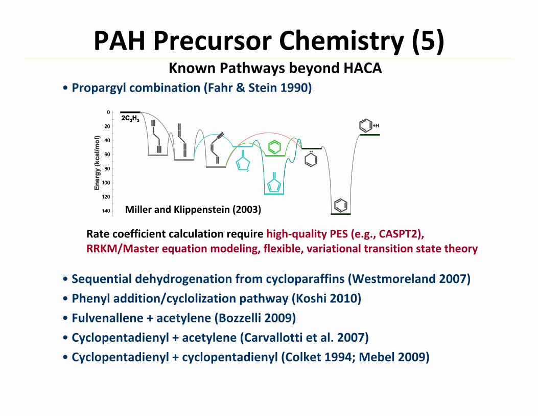
PAH Precursor Chemistry (5)Known Pathways beyond HACA

0

20

40

60

80

100

120

140

2C3H3

••

••

+H

Ener

gy (k

cal/m

ol)

0

20

40

60

80

100

120

140

2C3H3

••

••••

+H

Ener

gy (k

cal/m

ol)

• Propargyl combination (Fahr & Stein 1990)

Rate coefficient calculation require high‐quality PES (e.g., CASPT2), RRKM/Master equation modeling, flexible, variational transition state theory

• Sequential dehydrogenation from cycloparaffins (Westmoreland 2007)

• Phenyl addition/cyclolization pathway (Koshi 2010)

• Fulvenallene + acetylene (Bozzelli 2009)

• Cyclopentadienyl + acetylene (Carvallotti et al. 2007)

• Cyclopentadienyl + cyclopentadienyl (Colket 1994; Mebel 2009)

Miller and Klippenstein (2003)

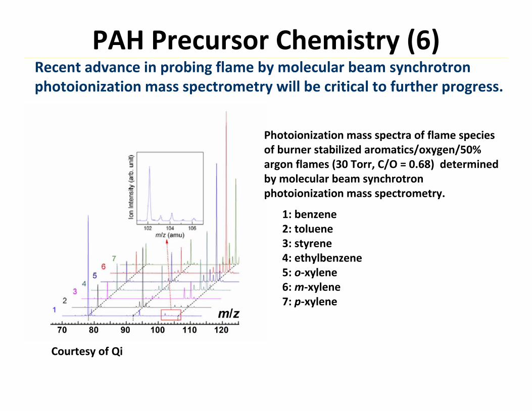
PAH Precursor Chemistry (6)Recent advance in probing flame by molecular beam synchrotron photoionization mass spectrometry will be critical to further progress.

Courtesy of Qi

Photoionization mass spectra of flame species of burner stabilized aromatics/oxygen/50% argon flames (30 Torr, C/O = 0.68)  determined by molecular beam synchrotron photoionization mass spectrometry.  

1: benzene2: toluene3: styrene4: ethylbenzene5: o‐xylene6: m‐xylene7: p‐xylene 

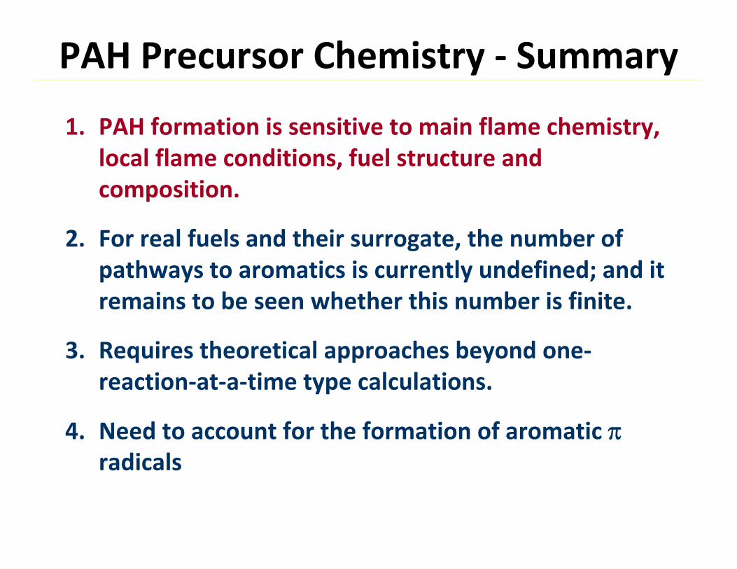
PAH Precursor Chemistry ‐ Summary

1. PAH formation is sensitive to main flame chemistry, local flame conditions, fuel structure and composition.

2. For real fuels and their surrogate, the number of pathways to aromatics is currently undefined; and it remains to be seen whether this number is finite.

3. Requires theoretical approaches beyond one‐reaction‐at‐a‐time type calculations.

4. Need to account for the formation of aromatic radicals

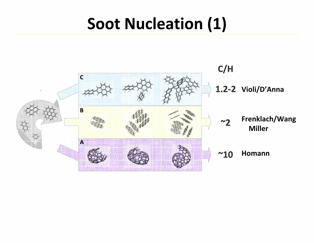
Soot Nucleation (1)

C/H

1.2‐2

~2

~10

C

B

A

C/H

1.2‐2

~2

~10

C

B

A

Violi/D’Anna

Frenklach/WangMiller

Homann

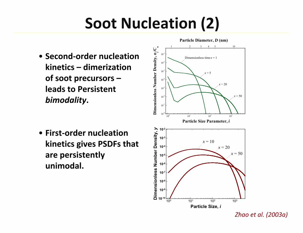
Soot Nucleation (2)

• Second‐order nucleation kinetics – dimerization of soot precursors –leads to Persistent bimodality.

• First‐order nucleation kinetics gives PSDFs that are persistently unimodal.

10-8

10-7

10-6

10-5

10-4

10-3

10-2

10-1

100 101 102 103Dim

ensi

onle

ss N

umbe

r D

ensi

ty, n

i/Co

Particle Size Parameter, i

1 2 3 4 5 10

Particle Diameter, D (nm)

Dimensionless time x = 1

x = 5

x = 20

x = 50

Zhao et al. (2003a)

10-10

10-9

10-8

10-7

10-6

10-5

10-4

10-3

10-2

100 101 102 103Dim

ensi

onle

ss N

umbe

r Den

sity

, y

Particle Size, i

x = 10x = 20

x = 50

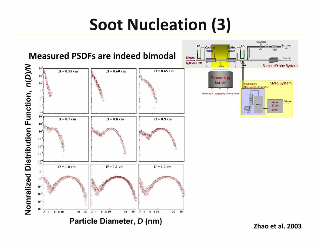
Soot Nucleation (3)

Zhao et al. 2003

Porous plug burner

Porous plug burner

Shielding Ar C2H4/O2/Ar Cooling water

Kr85

NDMA

P

Model 3080Electrostatic Classifier

Model 3025A

UCPC

Exhaust

SMPS System

Secondary air

P1

Diluent

N2 at 29.5 lpm

P2

Exhaust

Flow meter

Filter

orifice

Cooling water

Cooling water

Sample Probe System

Kr85

NDMA

P

Model 3080Electrostatic Classifier

Model 3025A

UCPC

Exhaust

SMPS System

Kr85

NDMA

P

Model 3080Electrostatic Classifier

Model 3025A

UCPC

Exhaust

SMPS System

Secondary air

P1

Diluent

N2 at 29.5 lpm

P2

Exhaust

Flow meter

Filter

orifice

Cooling water

Cooling water

Sample Probe System

10-4

10-3

10-2

10-1

100

101

102

H = 0.55 cm H = 0.60 cm H = 0.65 cm

10-4

10-3

10-2

10-1

100

101

102

H = 0.7 cm H = 0.8 cm H = 0.9 cm

Nom

raliz

ed D

istr

ibut

ion

Func

tion,

n(D

)/N

10-4

10-3

10-2

10-1

100

101

102

4 6 8 10 30 503

H = 1.0 cm

4 6 8 10 30 503

H = 1.1 cm

4 6 8 10 30 503

H = 1.2 cm

Particle Diameter, D (nm)

Measured PSDFs are indeed bimodal

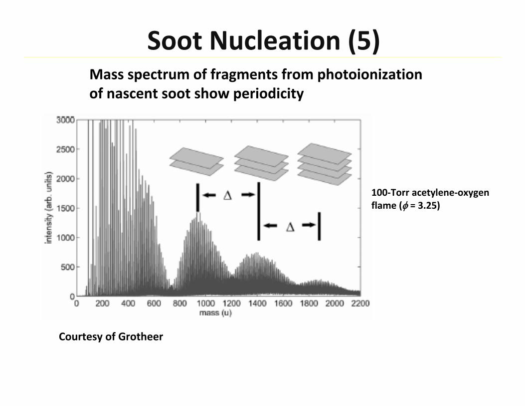
Soot Nucleation (5)Mass spectrum of fragments from photoionization of nascent soot show periodicity

100‐Torr acetylene‐oxygenflame ( = 3.25) 

Courtesy of Grotheer 

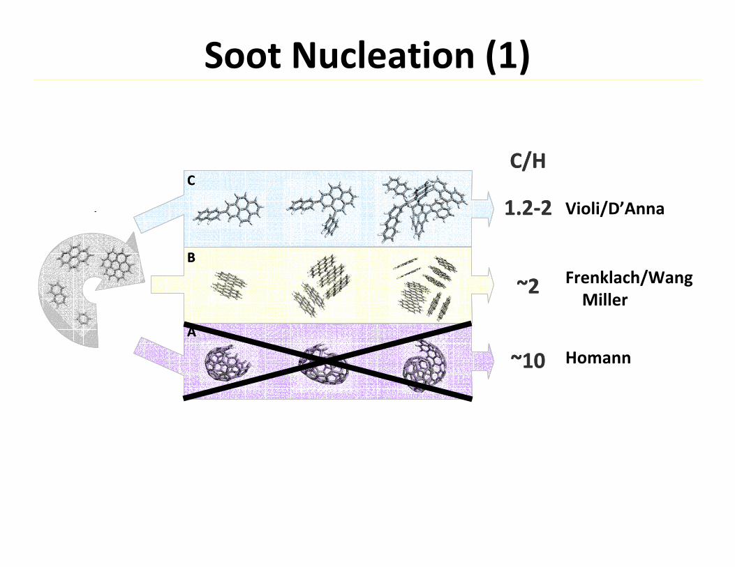
Soot Nucleation (1)

C/H

1.2‐2

~2

~10

C

B

A

C/H

1.2‐2

~2

~10

C

B

A

Violi/D’Anna

Frenklach/WangMiller

Homann

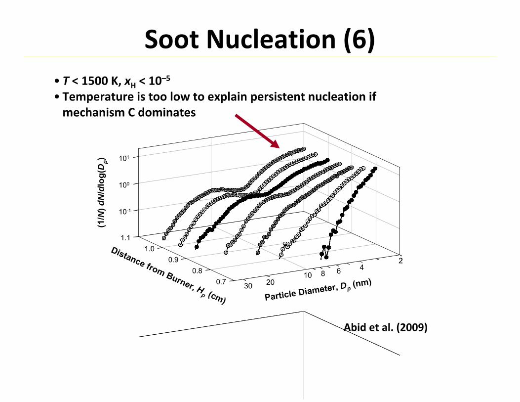
Soot Nucleation (6)

10-1

100

101

0.70.8

0.91.0

1.1

(1/N

) dN

/dlo

g(D

p)

Particle Diameter, Dp (nm)

Distance from Burner, Hp (cm)

246810

2030

10-1

100

101

0.70.8

0.91.0

1.1

(1/N

) dN

/dlo

g(D

p)

Particle Diameter, Dp (nm)

Distance from Burner, Hp (cm)

246810

2030

Abid et al. (2009)

• T < 1500 K, xH < 10–5

• Temperature is too low to explain persistent nucleation if mechanism C dominates  

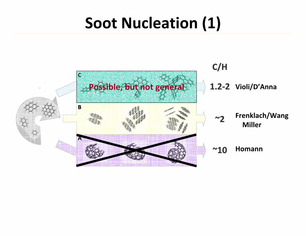
Soot Nucleation (1)

C/H

1.2‐2

~2

~10

C

B

A

C/H

1.2‐2

~2

~10

C

B

A

Possible, but not general Violi/D’Anna

Frenklach/WangMiller

Homann

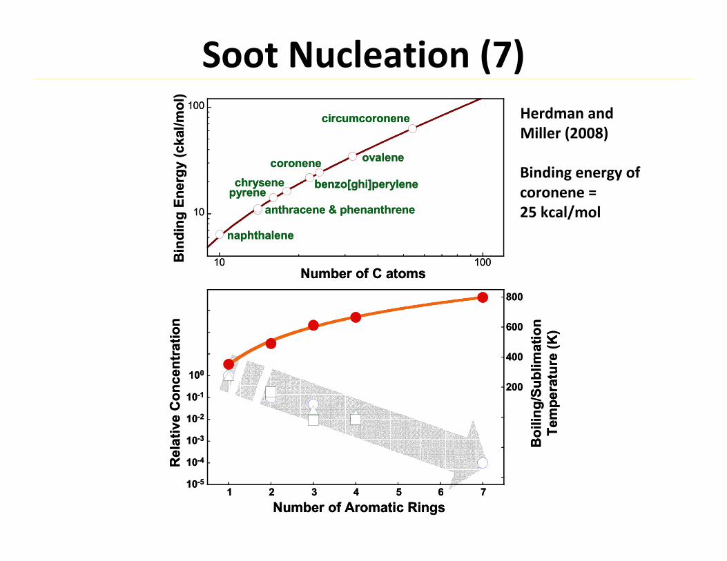
Soot Nucleation (7)

10

100

10 100

coroneneB

indi

ng E

nerg

y (c

kal/m

ol)

Number of C atoms

ovalene

circumcoronene

chrysene benzo[ghi]perylenepyrene

anthracene & phenanthrene

naphthalene

10-5

10-4

10-3

10-2

10-1

100

200

400

600

800

1 2 3 4 5 6 7

Rel

ativ

e C

once

ntra

tion

Number of Aromatic Rings

Boi

ling/

Subl

imat

ion

Tem

pera

ture

(K)

10

100

10 100

coroneneB

indi

ng E

nerg

y (c

kal/m

ol)

Number of C atoms

ovalene

circumcoronene

chrysene benzo[ghi]perylenepyrene

anthracene & phenanthrene

naphthalene

10-5

10-4

10-3

10-2

10-1

100

200

400

600

800

1 2 3 4 5 6 7

Rel

ativ

e C

once

ntra

tion

Number of Aromatic Rings

Boi

ling/

Subl

imat

ion

Tem

pera

ture

(K)

Herdman and Miller (2008) 

Binding energy of coronene = 25 kcal/mol

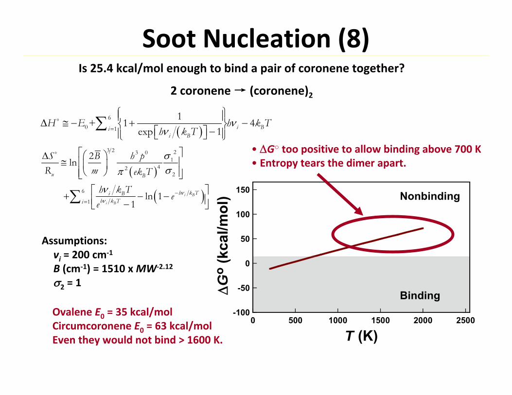
Soot Nucleation (8)

6

0 1

1+ 1 4exp 1 i Bi

i B

H E h k Th k T

3 2 23 01

422

6

1

2ln

ln 11

i B

i B

u B

h k Ti Bh k Ti

h pS BR m ek T

h k T ee

Is 25.4 kcal/mol enough to bind a pair of coronene together?

2 coronene → (coronene)2

Assumptions:vi = 200 cm‐1

B (cm‐1) = 1510 x MW‐2.12

2 = 1

-100

-50

0

50

100

150

0 500 1000 1500 2000 2500

G

o (k

cal/m

ol)

T (K)

Binding

Nonbinding

• G○ too positive to allow binding above 700 K• Entropy tears the dimer apart.

Ovalene E0 = 35 kcal/molCircumcoronene E0 = 63 kcal/molEven they would not bind > 1600 K.

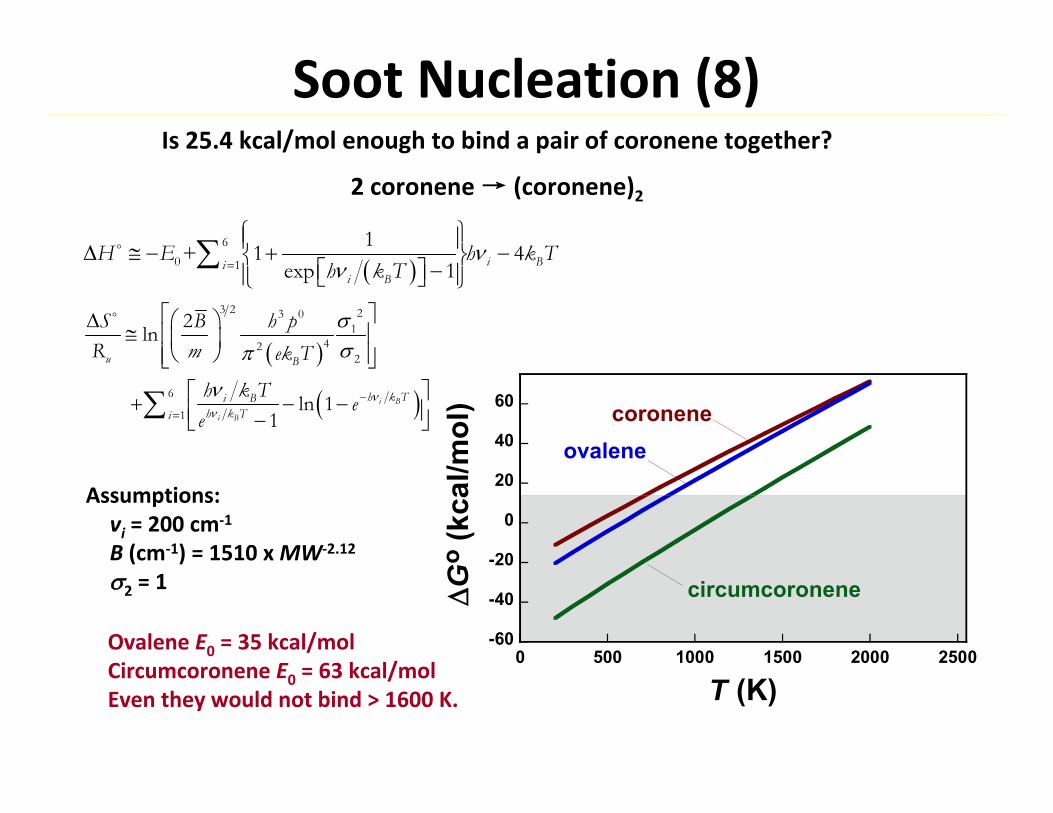
-60

-40

-20

0

20

40

60

0 500 1000 1500 2000 2500

G

o (k

cal/m

ol)

T (K)

coroneneovalene

circumcoronene

Soot Nucleation (8)

6

0 1

1+ 1 4exp 1 i Bi

i B

H E h k Th k T

3 2 23 01

422

6

1

2ln

ln 11

i B

i B

u B

h k Ti Bh k Ti

h pS BR m ek T

h k T ee

Is 25.4 kcal/mol enough to bind a pair of coronene together?

2 coronene → (coronene)2

Assumptions:vi = 200 cm‐1

B (cm‐1) = 1510 x MW‐2.12

2 = 1

Ovalene E0 = 35 kcal/molCircumcoronene E0 = 63 kcal/molEven they would not bind > 1600 K.

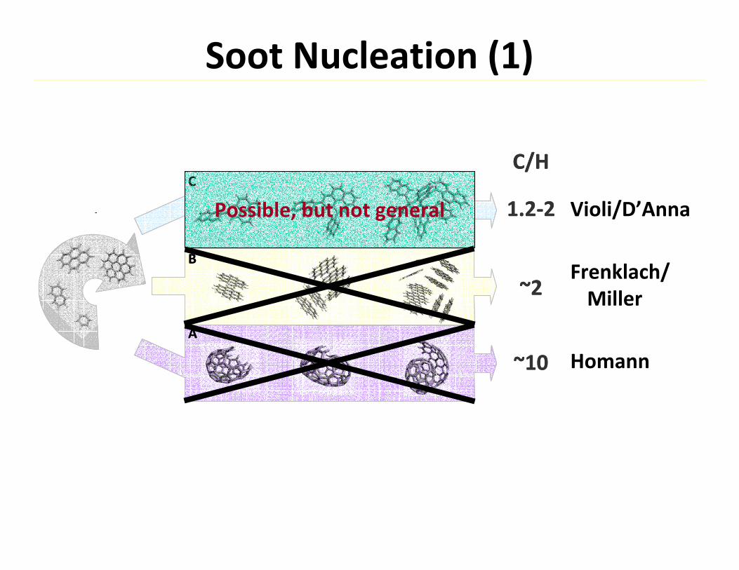
Soot Nucleation (1)

C/H

1.2‐2

~2

~10

C

B

A

C/H

1.2‐2

~2

~10

C

B

A

Violi/D’Anna

Frenklach/Miller

Homann

Possible, but not general

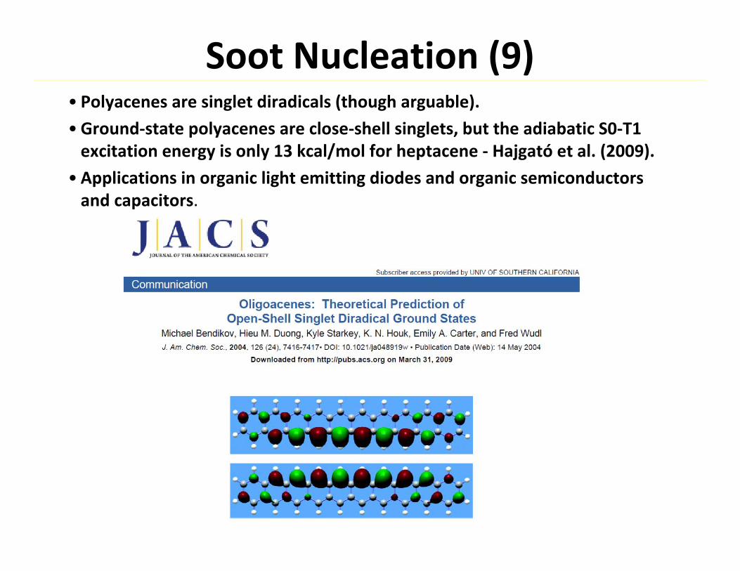
Soot Nucleation (9)• Polyacenes are singlet diradicals (though arguable).

•Ground‐state polyacenes are close‐shell singlets, but the adiabatic S0‐T1 excitation energy is only 13 kcal/mol for heptacene ‐ Hajgató et al. (2009).

•Applications in organic light emitting diodes and organic semiconductors and capacitors.

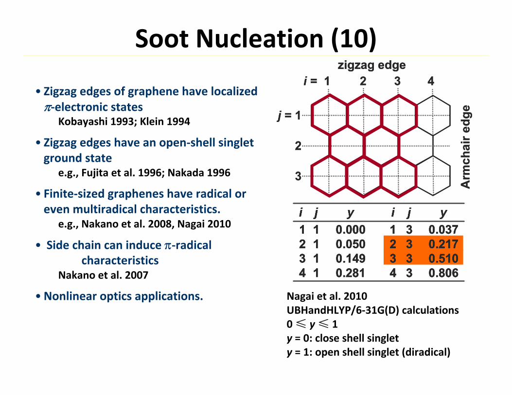
Soot Nucleation (10)

• Zigzag edges of graphene have localized ‐electronic states 

Kobayashi 1993; Klein 1994

• Zigzag edges have an open‐shell singlet ground state 

e.g., Fujita et al. 1996; Nakada 1996

• Finite‐sized graphenes have radical or even multiradical characteristics.

e.g., Nakano et al. 2008, Nagai 2010

• Side chain can induce ‐radical characteristics 

Nakano et al. 2007

•Nonlinear optics applications.

i = 1 2 3 4

j = 1

2

3

i j y i j y1 1 0.000 1 3 0.0372 1 0.050 2 3 0.2173 1 0.149 3 3 0.5104 1 0.281 4 3 0.806

zigzag edge

Arm

chai

r edg

e

i = 1 2 3 4

j = 1

2

3

i j y i j y1 1 0.000 1 3 0.0372 1 0.050 2 3 0.2173 1 0.149 3 3 0.5104 1 0.281 4 3 0.806

i j y i j y1 1 0.000 1 3 0.0372 1 0.050 2 3 0.2173 1 0.149 3 3 0.5104 1 0.281 4 3 0.806

zigzag edge

Arm

chai

r edg

e

Nagai et al. 2010UBHandHLYP/6‐31G(D) calculations 0 ≤ y≤ 1y = 0: close shell singlety = 1: open shell singlet (diradical)

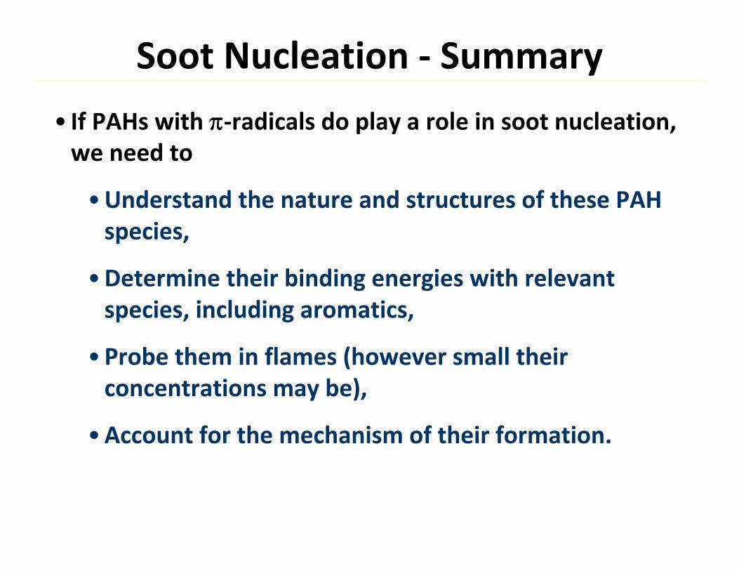
Soot Nucleation ‐ Summary

• If PAHs with ‐radicals do play a role in soot nucleation, we need to 

•Understand the nature and structures of these PAHspecies,

•Determine their binding energies with relevant species, including aromatics,

•Probe them in flames (however small their concentrations may be),

•Account for the mechanism of their formation.

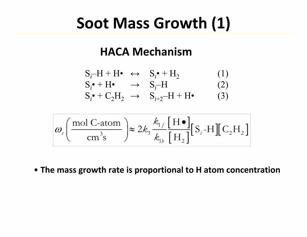
Soot Mass Growth (1)

Si–H + H• ↔ Si• + H2 (1)Si• + H• → Si–H (2)Si• + C2H2 → Si+2–H + H• (3)

13 2 23

1 2

Hmol C-atom 2 S -H C Hcm s H

fs i

b

kkk

• The mass growth rate is proportional to H atom concentration

HACA Mechanism

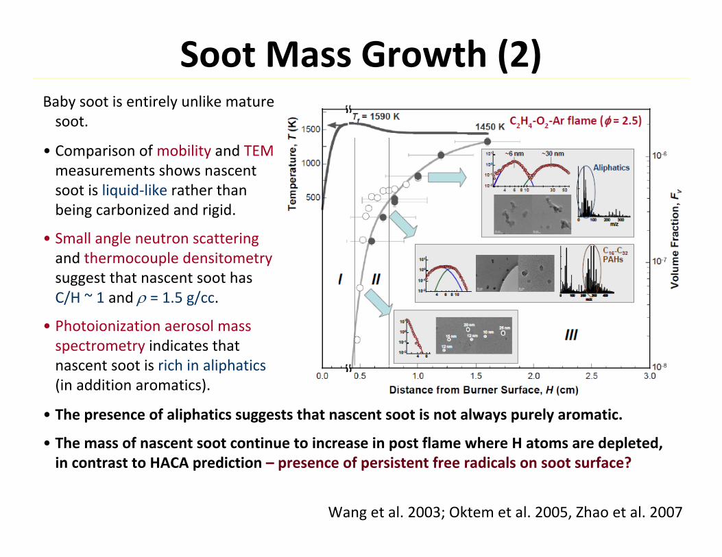
Soot Mass Growth (2)Baby soot is entirely unlike mature soot.

• Comparison of mobility and TEMmeasurements shows nascent soot is liquid‐like rather than being carbonized and rigid.

• Small angle neutron scatteringand thermocouple densitometrysuggest that nascent soot has C/H ~ 1 and  = 1.5 g/cc. 

• Photoionization aerosol mass spectrometry indicates that nascent soot is rich in aliphatics(in addition aromatics).

• The presence of aliphatics suggests that nascent soot is not always purely aromatic.

• The mass of nascent soot continue to increase in post flame where H atoms are depleted, in contrast to HACA prediction – presence of persistent free radicals on soot surface?

Wang et al. 2003; Oktem et al. 2005, Zhao et al. 2007

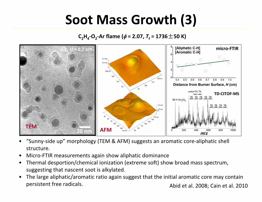
Soot Mass Growth (3)C2H4‐O2‐Ar flame ( = 2.07, Tf = 1736±50 K) 

• “Sunny‐side up” morphology (TEM & AFM) suggests an aromatic core‐aliphatic shell structure.

• Micro‐FTIR measurements again show aliphatic dominance • Thermal desportion/chemical ionization (extreme soft) show broad mass spectrum, 

suggesting that nascent soot is alkylated.• The large aliphatic/aromatic ratio again suggest that the initial aromatic core may contain 

persistent free radicals. Abid et al. 2008; Cain et al. 2010

Soot Mass Growth (4)Evidence supporting persistent free radicals

• Electron Spin Resonance spectra of anthracite, a coal containing little to no oxygenated compounds, show a measurable concentration of free radicals (Retcofsky, Stark & Friedel 1968).

• Soot volume fraction observed towards the stagnation surface can be predicted only if soot surface persists its radical nature (Wang et al 1996).

• Soot from pyrolysis of C2H4, C2H2 and jet fuel surrogates has appreciable amounts of free radicals of aromatic  nature.  The spin concentrations is ~1021 per gram (1 in 50 every C atoms) (Eddings, Sarofim &  Pugmire 2005).

• Soot, an otherwise hydrophobic material, has the ability to uptake water (Popovicheva 2003). 

• Binding energy between CH3 and H2O is 1.5 kcal/mol (Crespo‐Otero et al. 2008), increases to 2–4 kcal/mol for C2‐C4 alkyl radicals (Li et al. 2009).

Soot Mass Growth ‐ Summary•Nascent soot has aromatic core/aliphatic shell structure.

• Soot mass growth without the presence of H atom.

• Immediate questions and hypothesis: Is HACA mechanism complete?Do persistent free radicals exist on nascent soot surfaces?

Resonantly stabilized free radicals of semiquinone and phenoxyl origins (Dellinger 2001).

Radicals due to strain energy in hexaphenylethane and acenaphthene derivatives (Dames et al. 2010).

Soot Mass Growth ‐ SummaryRadicals due to strain energy in hexaphenylethane and acenaphthene derivatives (Dames, Sirjean, Wang 2010).

0

10

20

30

40

50

60

70

0 2 4 6 8

M06-2X/6-31+G(d,p) electronic energy*M06-2X/6-31+G(d,p) Isodesmicexpt60

ONIOM62

Cen

tral

BD

E (k

cal/m

ol)

7

9

11

13

1

4

5

Soot Mass Growth ‐ Summary•Nascent soot has aromatic core/aliphatic shell structure.

• Soot mass growth without the presence of H atom.

• Immediate questions and hypothesis: Is HACA mechanism complete?Do persistent free radicals exist on nascent soot surfaces.

Resonantly stabilized free radicals of semiquinone and phenoxyl origins (Dellinger 2001).

Radicals due to strain energy in hexaphenylethane and acenaphthene derivatives (Dames et al. 2010).

Delocalized aromatic  radicals on zigzag edges propagated into soot structures (Cain et al. 2010 – 3D02).

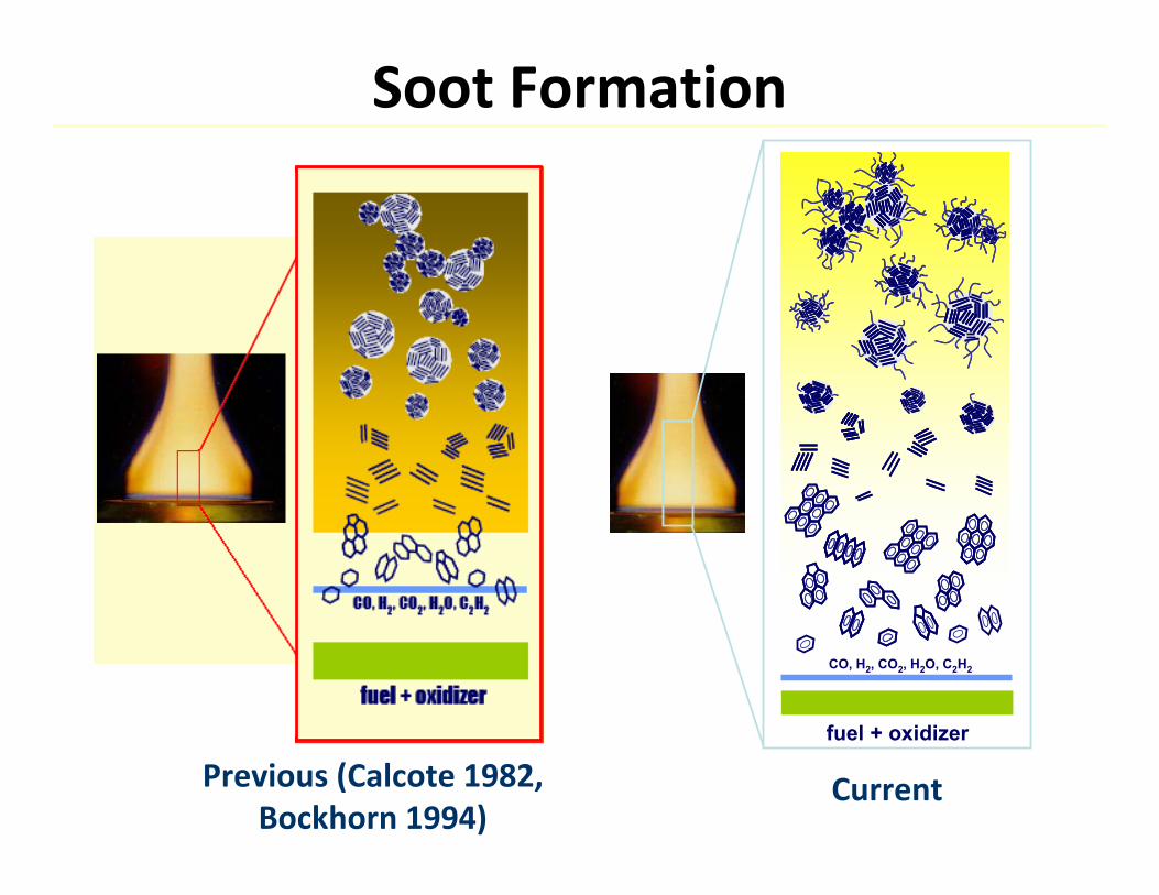
Soot Formation

CurrentPrevious (Calcote 1982, Bockhorn 1994)

fuel + oxidizer

CO, H2, CO2, H2O, C2H2

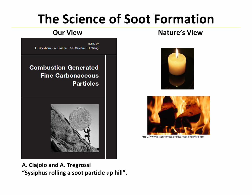
The Science of Soot Formation

A. Ciajolo and A. Tregrossi“Sysiphus rolling a soot particle up hill”.

Our View Nature’s View

http://www.historyforkids.org/learn/science/fire.htm

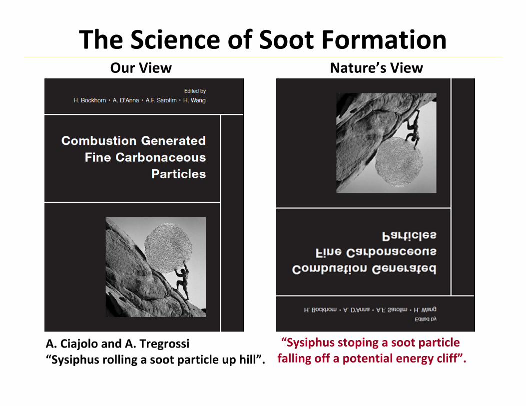
The Science of Soot Formation

A. Ciajolo and A. Tregrossi“Sysiphus rolling a soot particle up hill”.

Our View Nature’s View

“Sysiphus stoping a soot particle falling off a potential energy cliff”.

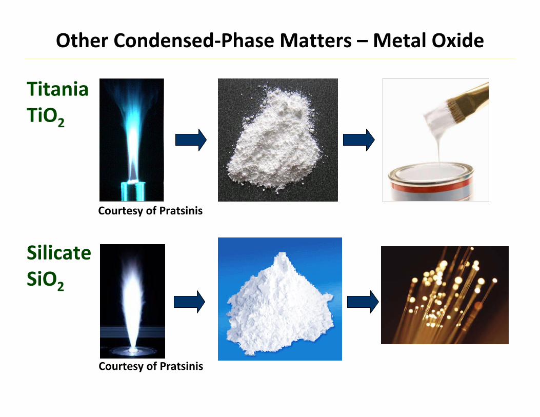
TitaniaTiO2

SilicateSiO2

Courtesy of Pratsinis

Courtesy of Pratsinis

Other Condensed‐Phase Matters – Metal Oxide

Lesson 8:

1

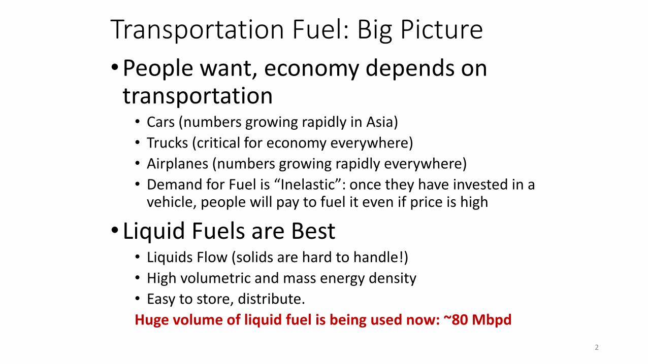
Transportation Fuel: Big Picture •People want, economy depends on

transportation • Cars (numbers growing rapidly in Asia) • Trucks (critical for economy everywhere) • Airplanes (numbers growing rapidly everywhere) • Demand for Fuel is “Inelastic”: once they have invested in a

vehicle, people will pay to fuel it even if price is high

•Liquid Fuels are Best • Liquids Flow (solids are hard to handle!) • High volumetric and mass energy density • Easy to store, distribute. Huge volume of liquid fuel is being used now: ~80 Mbpd

2

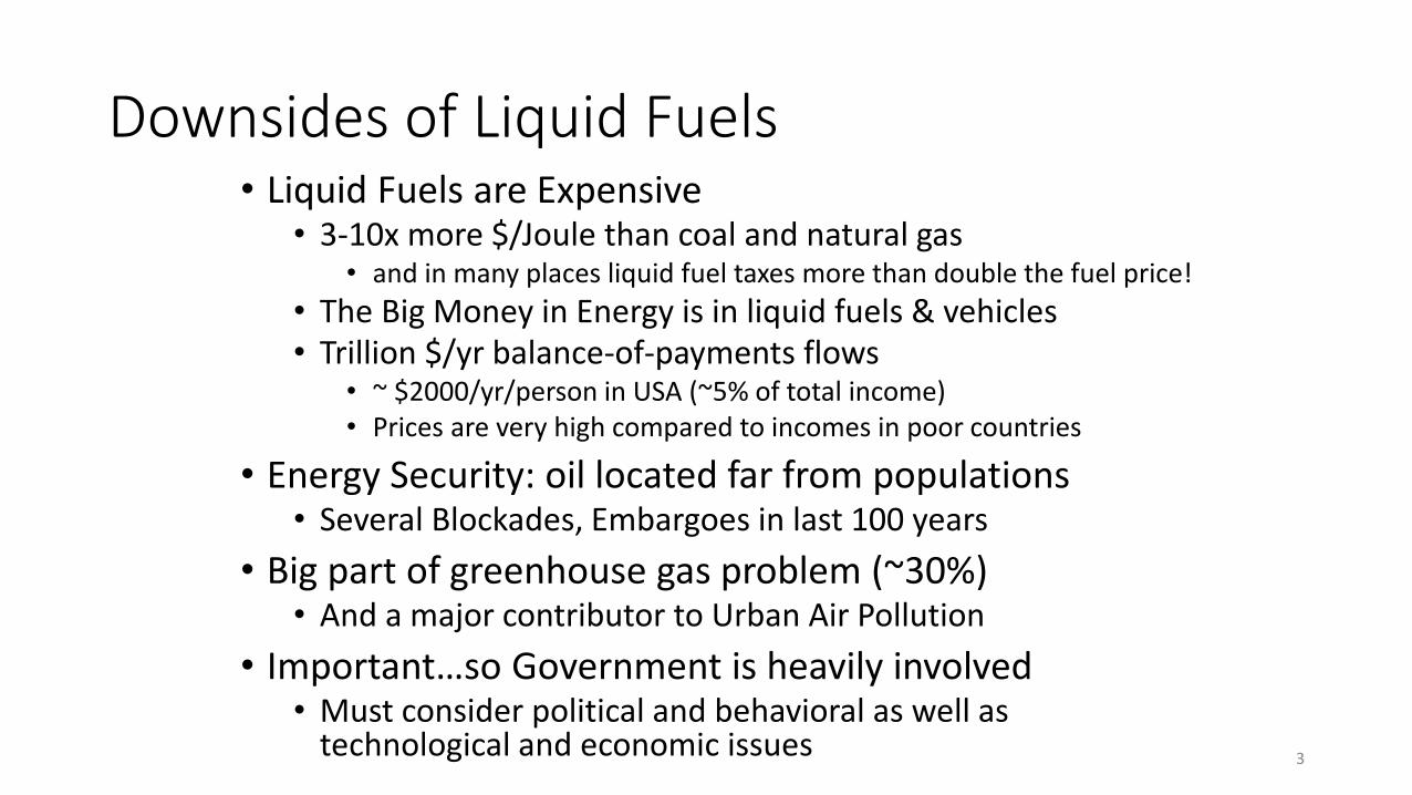
Downsides of Liquid Fuels • Liquid Fuels are Expensive

• 3-10x more $/Joule than coal and natural gas • and in many places liquid fuel taxes more than double the fuel price!

• The Big Money in Energy is in liquid fuels & vehicles • Trillion $/yr balance-of-payments flows

• ~ $2000/yr/person in USA (~5% of total income) • Prices are very high compared to incomes in poor countries

• Energy Security: oil located far from populations • Several Blockades, Embargoes in last 100 years

• Big part of greenhouse gas problem (~30%) • And a major contributor to Urban Air Pollution

• Important…so Government is heavily involved • Must consider political and behavioral as well as

technological and economic issues

3

Quiz Question #1

Diesel engines are significantly more efficient than Otto cycle (SI) engines, but also more expensive to manufacture. Why does it make sense for Europeans to use diesel cars, but the case for diesels is not so compelling to Americans?

4

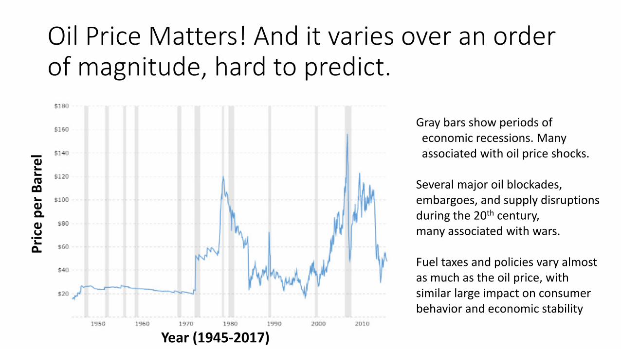
Oil Price Matters! And it varies over an order of magnitude, hard to predict.

Year (1945-2017)

Pric

e pe

r Bar

rel

Gray bars show periods of economic recessions. Many associated with oil price shocks. Several major oil blockades, embargoes, and supply disruptions during the 20th century, many associated with wars. Fuel taxes and policies vary almost as much as the oil price, with similar large impact on consumer behavior and economic stability

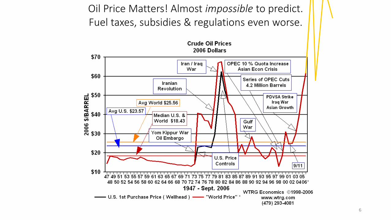
Oil Price Matters! Almost impossible to predict. Fuel taxes, subsidies & regulations even worse.

6

Quiz Question #2

• Fuel Price started rising dramatically ~2000, and has remained very high ever since (except for a brief drop during the economic crash of 2008). In part because of the high price, gasoline consumption has been dropping in USA and Western Europe. The oil price has been much higher than the cost of producing oil through this whole period.

Why do you think the price rose and is staying high during this time period even though world oil production is increasing?

7

Fuel Price Fluctuations are a Big Problem • Very high fuel prices help drive the world economy

into recession (1974, 1980, 2008) • Adds Large Risk to Alternative Fuel projects

• Many dramatic business failures in late 1980’s • Price fluctuation often larger than technological & political

uncertainties, biggest investment risk • Possibility that OPEC will intentionally drop oil price to

drive competitors into bankruptcy. • Investors demand high rate of return because of risk; less

lucrative processes are never built.

8

Why & Why Not use Fossil Fuels? • Finite but Very Large Amount of Fossil Fuel

– We are definitely going to run out of fossil fuel energy… in a century or two: Long Term issue

– Fossil fuels are available now in huge scale (unlike most other energy sources) - Although oil price is high at the moment, cost of production is

low. (Coal price is low everywhere. Natural Gas prices varies.)

• Greenhouse Effect on Climate Change is the Medium-Term issue

– We’ll “run out of atmosphere” to hold the CO2 before we run out of fossil fuel.

– Might run out of capacity to store CO2 underground or in ocean...

9

Conventional Oil is Expensive (at the moment) (Maybe) Running Out Not Secure A Greenhouse Gas Problem So we might want to use alternative fuels…with different combustion chemistry 10

Quiz Question #2

• Shell has invested in Gas-to-Liquids to make liquid diesel fuel in Qatar. US truck companies are investing to develop trucks that burn Compressed Natural Gas. Can they both be right?

11

What do you want in a fuel?

And what constraints does any new fuel need to satisfy?

12

13 of 42

Not desirable from a gravimetric and volumetric energy density standpoint, but… Oxygenated fuels tend to have lower emissions of carbon monoxide, soot, and unburned hydrocarbons. N containing fuels have higher NOx emissions, but can reduce to N2 with catalyst and CO or urea. A little bit of N is good for cleaning fuel injectors. Hydrogen bonding in liquid fuels containing O and N results in enhanced evaporative cooling + decreases the likelihood of autoignition; increases fuel octane + increases amount of air in cylinder, and so power density Biomass feedstocks (and some fossil fuels) contain a lot of O (glucose = C6H12O6, cellulose = glucose polymer = (C6H10O5)n). Also some N. Perhaps it is not necessary to remove all the O and N from biofuels?

Oxygen and Nitrogen

Requirements, Continued

• Not Corrosive • “Corrosive” depends on materials used in engine • “Backwards Compatible”: want new fuel to work in old vehicles • Known issues with acids (in biofuels), high concentrations of alcohols

• Suitable Volatility • Must match fuel injection system • Want liquid to quickly evaporate to flammable gas. • Some molecules (e.g. sugars) pyrolyze to solids before they evaporate – not

good transportation fuels.

14

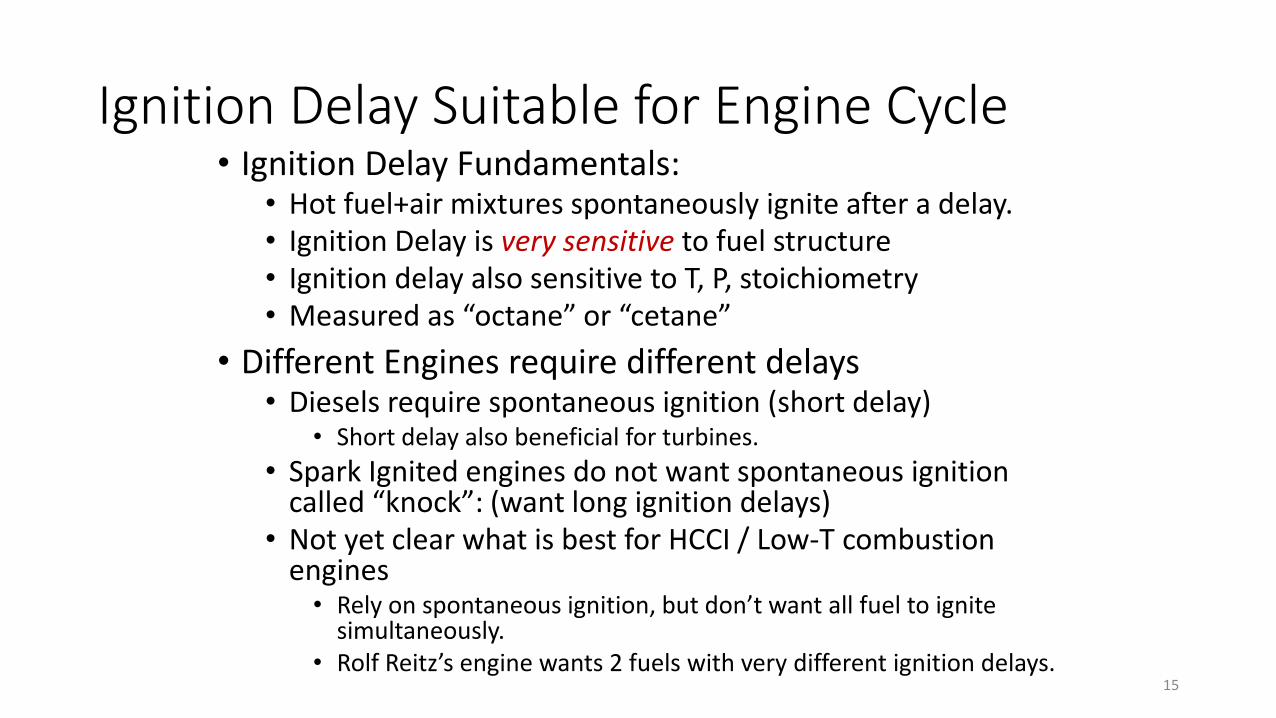
Ignition Delay Suitable for Engine Cycle • Ignition Delay Fundamentals:

• Hot fuel+air mixtures spontaneously ignite after a delay. • Ignition Delay is very sensitive to fuel structure • Ignition delay also sensitive to T, P, stoichiometry • Measured as “octane” or “cetane”

• Different Engines require different delays • Diesels require spontaneous ignition (short delay)

• Short delay also beneficial for turbines. • Spark Ignited engines do not want spontaneous ignition

called “knock”: (want long ignition delays) • Not yet clear what is best for HCCI / Low-T combustion

engines • Rely on spontaneous ignition, but don’t want all fuel to ignite

simultaneously. • Rolf Reitz’s engine wants 2 fuels with very different ignition delays.

15

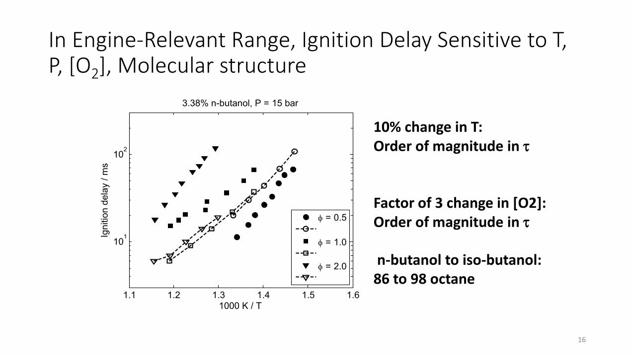
In Engine-Relevant Range, Ignition Delay Sensitive to T, P, [O2], Molecular structure

1.1 1.2 1.3 1.4 1.5 1.6

101

102

1000 K / T

Igni

tion

dela

y / m

s3.38% n-butanol, P = 15 bar

φ = 0.5

φ = 1.0

φ = 2.0

10% change in T: Order of magnitude in τ Factor of 3 change in [O2]: Order of magnitude in τ n-butanol to iso-butanol: 86 to 98 octane

16

Sufficient Flame Speed

• Sensitive to T, P, stoichiometry, dilution • Many fuels have very similar flame speeds

• H2, acetylene have unusually high flame speeds

• Flame speed very important in turbines running near lean limit, or in high speed flows • Flame can “blow out”

• Helpful in Spark-Ignited Engines

17

New Fuel Must be Cheap, Plentiful!

• New Fuel will be competing with petroleum. • Subsidies or regulations favoring new fuel will not last forever!

• It takes work to verify new fuel will not cause problems. • It takes capital to build fuel production facilities. • This work will not be done, and investors will not provide the

capital, unless fuel looks economically viable and likely to be available in huge volumes ( ~ million barrels per day).

18

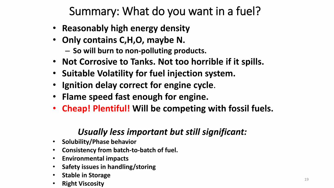
Summary: What do you want in a fuel? • Reasonably high energy density • Only contains C,H,O, maybe N.

– So will burn to non-polluting products. • Not Corrosive to Tanks. Not too horrible if it spills. • Suitable Volatility for fuel injection system. • Ignition delay correct for engine cycle. • Flame speed fast enough for engine. • Cheap! Plentiful! Will be competing with fossil fuels.

Usually less important but still significant: • Solubility/Phase behavior • Consistency from batch-to-batch of fuel. • Environmental impacts • Safety issues in handling/storing • Stable in Storage • Right Viscosity

19

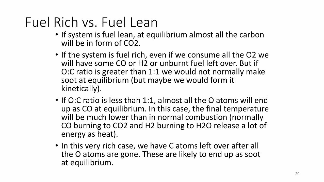
Fuel Rich vs. Fuel Lean • If system is fuel lean, at equilibrium almost all the carbon

will be in form of CO2. • If the system is fuel rich, even if we consume all the O2 we

will have some CO or H2 or unburnt fuel left over. But if O:C ratio is greater than 1:1 we would not normally make soot at equilibrium (but maybe we would form it kinetically).

• If O:C ratio is less than 1:1, almost all the O atoms will end up as CO at equilibrium. In this case, the final temperature will be much lower than in normal combustion (normally CO burning to CO2 and H2 burning to H2O release a lot of energy as heat).

• In this very rich case, we have C atoms left over after all the O atoms are gone. These are likely to end up as soot at equilibrium.

20

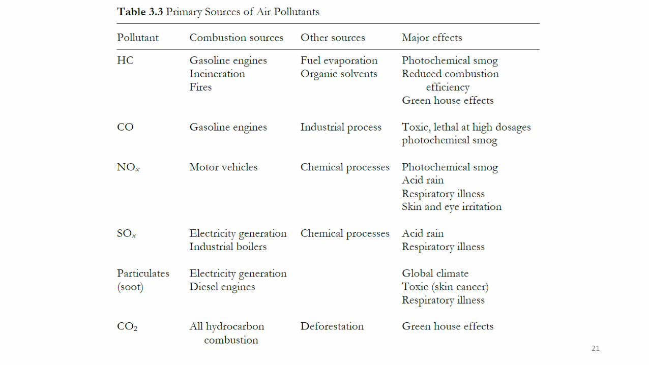
21

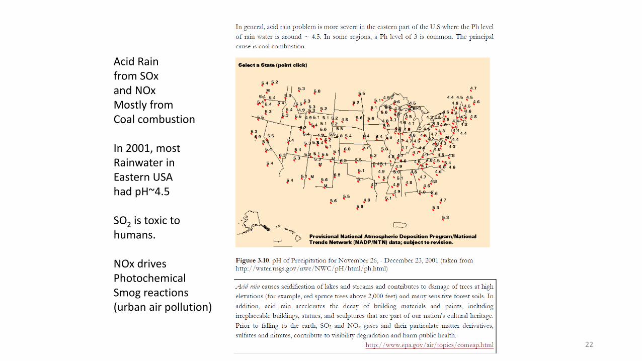
22

Acid Rain from SOx and NOx Mostly from Coal combustion In 2001, most Rainwater in Eastern USA had pH~4.5 SO2 is toxic to humans. NOx drives Photochemical Smog reactions (urban air pollution)

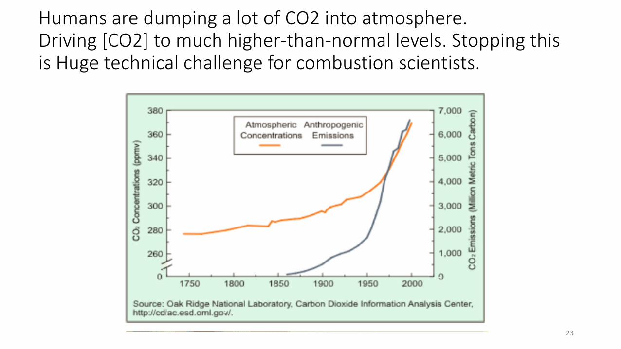
Humans are dumping a lot of CO2 into atmosphere. Driving [CO2] to much higher-than-normal levels. Stopping this is Huge technical challenge for combustion scientists.

23

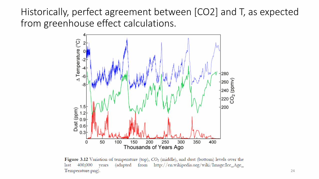
Historically, perfect agreement between [CO2] and T, as expected from greenhouse effect calculations.

24

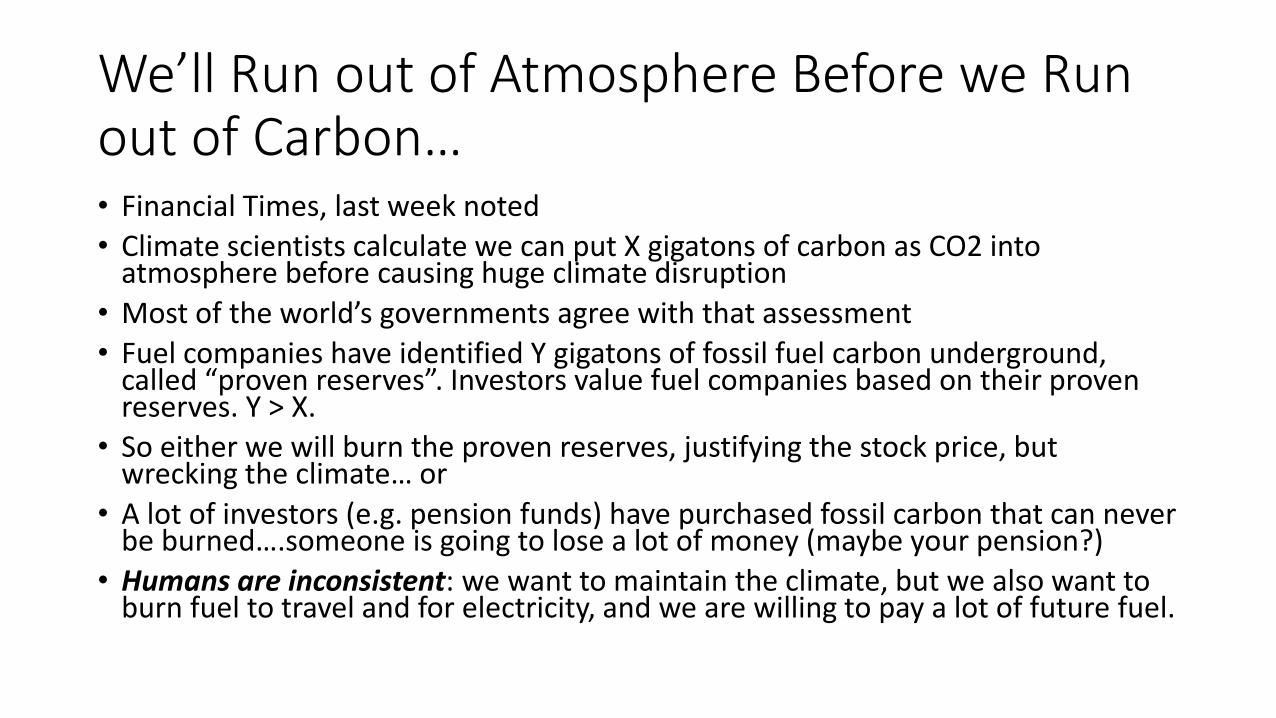
We’ll Run out of Atmosphere Before we Run out of Carbon… • Financial Times, last week noted • Climate scientists calculate we can put X gigatons of carbon as CO2 into

atmosphere before causing huge climate disruption • Most of the world’s governments agree with that assessment • Fuel companies have identified Y gigatons of fossil fuel carbon underground,

called “proven reserves”. Investors value fuel companies based on their proven reserves. Y > X.

• So either we will burn the proven reserves, justifying the stock price, but wrecking the climate… or

• A lot of investors (e.g. pension funds) have purchased fossil carbon that can never be burned….someone is going to lose a lot of money (maybe your pension?)

• Humans are inconsistent: we want to maintain the climate, but we also want to burn fuel to travel and for electricity, and we are willing to pay a lot of future fuel.

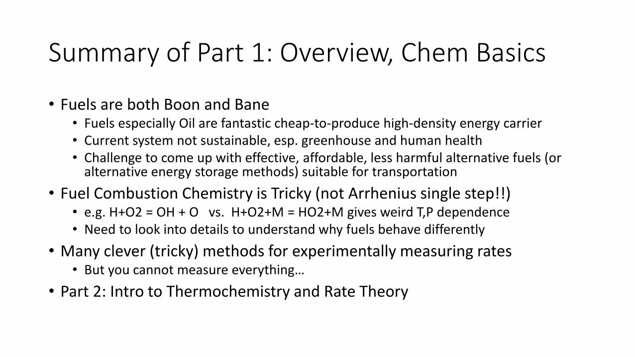
Summary of Part 1: Overview, Chem Basics

• Fuels are both Boon and Bane • Fuels especially Oil are fantastic cheap-to-produce high-density energy carrier • Current system not sustainable, esp. greenhouse and human health • Challenge to come up with effective, affordable, less harmful alternative fuels (or

alternative energy storage methods) suitable for transportation • Fuel Combustion Chemistry is Tricky (not Arrhenius single step!!)

• e.g. H+O2 = OH + O vs. H+O2+M = HO2+M gives weird T,P dependence • Need to look into details to understand why fuels behave differently

• Many clever (tricky) methods for experimentally measuring rates • But you cannot measure everything…

• Part 2: Intro to Thermochemistry and Rate Theory