internet of things based real-time water quality
TRANSCRIPT

INTERNET OF THINGS BASED REAL-TIME WATER QUALITY
MONITORING SYSTEM FOR WATER STORAGE TANK
TAN SHIN YIN
A project report submitted in partial fulfilment of the
requirements for the award of Bachelor of Engineering
(Honours) Mechatronics Engineering
Lee Kong Chian Faculty of Engineering and Science
Universiti Tunku Abdul Rahman
May 2021

i
DECLARATION
I hereby declare that this project report is based on my original work except
for citations and quotations which have been duly acknowledged. I also
declare that it has not been previously and concurrently submitted for any
other degree or award at UTAR or other institutions.
Signature :
Name : TAN SHIN YIN
ID No. : 16UEB03662
Date : 19/4/2021

ii
APPROVAL FOR SUBMISSION
I certify that this project report entitled “INTERNET OF THINGS BASED
REAL-TIME WATER QUALITY MONITORING SYSTEM FOR
WATER STORAGE TANK” was prepared by TAN SHIN YIN has met the
required standard for submission in partial fulfilment of the requirements for
the award of Bachelor of Engineering (Honours) Mechatronics Engineering at
Universiti Tunku Abdul Rahman.
Approved by,
Signature :
Supervisor : DR. KWAN BAN HOE
Date :
Signature :
Co-Supervisor : IR. DANNY NG WEE KIAT
Date :

iii
The copyright of this report belongs to the author under the terms of
the copyright Act 1987 as qualified by Intellectual Property Policy of
Universiti Tunku Abdul Rahman. Due acknowledgement shall always be made
of the use of any material contained in, or derived from, this report.
© 2021, Tan Shin Yin. All right reserved.

iv
ABSTRACT
Water leaving the treatment plant should be safe and of good quality, but
contamination could easily happen along the distribution pipelines. This is due
to factors like rusty pipes that cause heavy metals to leach and dissolve in
water, damaged or broken pipes that let soil and other contaminants or sewage
enter the water. Sediments, scale and algae could also build up on water
storage tanks over time. In order to keep track of water quality, this study is
aimed to develop a real-time water quality monitoring system in water storage
tanks that can be implemented in society, residential areas and restaurant and
food service industry by utilizing Internet of Things (IoT) technology. This
system employs sensors to collect water quality parameters (pH, temperature,
TDS and turbidity), transmits the data wirelessly and uploads it to cloud so
users can monitor remotely. The intelligent system can alert users at real-time
in case of failing water quality.

v
TABLE OF CONTENTS
DECLARATION i
APPROVAL FOR SUBMISSION ii
ABSTRACT iv
TABLE OF CONTENTS v
LIST OF TABLES ix
LIST OF FIGURES x
LIST OF SYMBOLS / ABBREVIATIONS xiii
LIST OF APPENDICES xv
CHAPTER
1 INTRODUCTION 1
1.1 General Introduction 1
1.2 Importance of the Study 3
1.3 Problem Statement 4
1.4 Aim and Objectives 6
1.5 Scope and Limitation of the Study 6
1.6 Contribution of the Study 7
1.7 Outline of the Report 7
2 LITERATURE REVIEW 8
2.1 Introduction 8
2.2 Hardware 10
2.2.1 Embedded Board 10
2.2.2 Multiparameter sensor 12
2.2.3 Temperature sensor 12
2.2.4 Turbidity sensor 13
2.2.5 pH sensor 14
2.2.6 EC sensor 15
2.3 Software 16

vi
2.3.1 Data transmission protocol with the respective gateway
module (hardware) used 16
2.4 Summary of Literature Review of Internet of Things
Based Water Quality Monitoring System from Different Author
(s) 19
3 METHODOLOGY AND WORK PLAN 24
3.1 Project Planning and Milestones 24
3.2 System Architecture Block Diagram 26
3.3 Solution Selection 27
3.3.1 Arduino Nano 27
3.3.2 pH Sensor 28
3.3.3 TDS Sensor 28
3.3.4 Turbidity Sensor 29
3.3.5 Temperature Sensor 30
3.3.5 Voltage Sensor 30
3.3.6 Arduino Mega 2560 31
3.3.7 Arduino Ethernet Shield 31
3.3.8 Radio-Frequency Transceiver Module 32
3.4 Solution Selection (Software) 33
3.4.1 Arduino IDE 33
3.4.2 Proteus 33
3.4.3 Eagle 34
3.4.4 Solidworks 34
3.4.5 Ubidots Cloud Server 35
3.4.6 Ubidots Android Mobile App 35
3.5 Hardware design 36
3.5.1 Circuit Diagram and Pin Connection 36
3.5.2 PCB Design 40
3.5.3 Float design 41
3.6 Software Development 44
3.6.1 Overall Program Flow Chart 44
3.6.2 Sensor Subsystem 46
3.6.3 Receiver Subsystem 51
3.7 Prototype Costing 58

vii
3.8 Safe Water Quality Parameters for Drinking Based on
WHO Standards 59
3.9 Summary 60
4 RESULTS AND DISCUSSION 61
4.1 Sensor Calibration and Benchmark Test 61
4.1.1 pH Sensor Calibration and Benchmark Test61
4.1.2 Turbidity Sensor Calibration 63
4.1.3 Temperature Sensor Benchmark Test 65
4.1.4 TDS Sensor Calibration and Benchmark Test
67
4.2 Project prototype developed 68
4.2.1 Sensor subsystem prototype 68
4.2.2 Receiver Subsystem Prototype 70
4.3 Prototype Performance 71
4.3.1 Data Upload and Monitoring On Ubidots
Cloud 71
4.3.2 User Request to Log Real-Time Data or
Change Time Interval 73
4.3.3 Ubidots Mobile Application 73
4.3.4 Data Storage in SD Card and Reupload to
Ubidots cloud 74
4.3.5 Real Time Notification 75
4.4 Problem Encountered and Improvement During and
After Data Collection 76
4.5 Data Analysis 77
4.5.1 pH 77
4.5.2 Temperature 78
4.5.3 TDS 79
4.5.4 Turbidity 80
4.5.5 Battery voltage 80
4.6 Summary 80
5 CONCLUSIONS AND RECOMMENDATIONS 81
5.1 Conclusion 81
5.2 Limitation of the prototype 82

viii
5.3 Recommendation for Future Work 82
REFERENCES 83
APPENDICES 89

ix
LIST OF TABLES
Table 1.1: Water Resources in Malaysia 3
Table 2.1: Advantage (s) and Disadvantage(s) Between Embedded Board
11
Table 2.2: Advantage (s) and Disadvantage (s) of Reviewed Temperature
Sensor 13
Table 2.3: Advantage (s) and Disadvantage (s) of Reviewed Turbidity
Sensor 14
Table 2.4: Advantage (s) and Disadvantage (s) of Reviewed pH Sensor 15
Table 2.5: Advantage (s) and Disadvantage (s) of Reviewed EC Sensor 16
Table 2.6: Comparison of System Architectures for Water Quality
Monitoring Systems 19
Table 3.1: Gantt Chart of FYP1 25
Table 3.2: Gantt Chart of FYP2 25
Table 3.3: Pin Connections between Arduino Boards and Modules 36
Table 3.4: Operating Voltage and Current of Each Sensor Module and Its
Powering Method 37
Table 3.5: Prototype Costing 57

x
LIST OF FIGURES
Figure 1.1: Schematic Diagram of a Public Water Supply System 2
Figure 1.2: Malaysia: River water quality Trend, 2008-2017 4
Figure 1.3: Dirty water storage tank due to deposits and sedimentation 5
Figure 2.1: Hierarchy of general IoT water quality monitoring system 9
Figure 2.2: Summary of some relevant IoT communication protocols 9
Figure 3.1: Block Diagram of Water Quality Monitoring System 25
Figure 3.2: Arduino Nano 27
Figure 3.3: pH sensor (Model: PH Sensor Module V1.1) 27
Figure 3.4: TDS sensor (Model: SKU:SEN0244) 28
Figure 3.5: Turbidity sensor (Model name: SKU: SEN0189) 29
Figure 3.6: Temperature sensor (Model: DS18B20) 29
Figure 3.7: Voltage sensor (Model: DS18B20) 29
Figure 3.8: Arduino Mega 30
Figure 3.9: Arduino Ethernet Shield 31
Figure 3.10: RF transceiver module 31
Figure 3.11: Snapshot of Arduino IDE 32
Figure 3.12: Snapshot of Proteus 32
Figure 3.13: Snapshot of Eagle 33
Figure 3.14: Snapshot of Solidworks 33
Figure 3.15: Snapshot of Ubidots Cloud Server 34
Figure 3.16: Snapshot of Ubidots Dashboard in Mobile App 35
Figure 3.17: Schematic of Sensor Subsystem of IoT Water Quality
Monitoring System 38
Figure 3.18: Schematic of Receiver Subsystem of IoT Water Quality
Monitoring System 38
Figure 3.19: PCB Layout of Sensor Subsystem 39
Figure 3.20: PCB Top View (Left) and Bottom View (Right) 39
Figure 3.21: PCB with components soldered 40
Figure 3.22: PVC Pipe Float Design 41
Figure 3.23: Sensor Subsystem Design 42
Figure 3.24: Free Body Diagram of Sensor Subsystem 43
Figure 3.25: Water quality monitoring system flowchart 44
Figure 3.26: Arduino Nano main program flowcharts 45

xi
Figure 3.27: User Request from Receiver flowchart 47
Figure 3.28: Sensor flowcharts 48
Figure 3.29: Arduino Mega main program flowcharts 50
Figure 3.30: Ethernet start up and obtain current current date and time
flowcharts 52
Figure 3.31: Upload data to cloud flowcharts 53
Figure 3.32: Data storing in SD card flowcharts 53
Figure 3.33: Uploading of SD card data to cloud flowcharts 54
Figure 3.34: User request log data and change time interval flowcharts 55
Figure 3.35: Email notifications by Ubidots flowchart 56
Figure 3.36: TDS reference chart 58
Figure 3.37: Turbidity levels (Smith, 2010) 59
Figure 4.1: Calibration and benchmark test of pH sensor at pH 6.86
standard solution 61
Figure 4.2: Calibration and benchmark test of pH sensor at pH 4.01
standard solution 61
Figure 4.3: Calibration and benchmark test of pH sensor at pH 9.18
standard solution 62
Figure 4.4: Trimmer potentiometer on Turbidity Sensor 62
Figure 4.5: Graph of Turbidity versus Voltage 63
Figure 4.6: Calibration of Turbidity Sensor in Clear water (0 NTU) 64
Figure 4.7: Verification using Milo solution (3000 NTU) 64
Figure 4.8: Benchmark test of temperature sensor in ice 65
Figure 4.9: Benchmark test of temperature sensor in clear water at room
temperature 65
Figure 4.10: Standard buffer solution of EC 1413 us/cm or 707 ppm 66
Figure 4.11: Serial monitor for Calibration of TDS sensor 67
Figure 4.12: Electronic hardware system in junction box 67
Figure 4.13: Sensor Subsystem Prototype Front View 68
Figure 4.14: Sensor Subsystem Prototype Side View 69
Figure 4.15: Sensor Subsystem Prototype Top View 69
Figure 4.16: Receiver Subsystem Prototype 69
Figure 4.17: Ubidots cloud database 70
Figure 4.18: Snapshot of dashboard for displaying real-time (latest) data 71

xii
Figure 4.19: Snapshot of dashboard for displaying historical data 71
Figure 4.20: Snapshot of dashboard for user input to request to log real-time
data or change time interval 72
Figure 4.21: Snapshot of dashboard accessed through Ubidots mobile
application 72
Figure 4.22: Data stored in text file of SD card 73
Figure 4.23: Backup data in table format available in historical data
dashboard of Ubidots 73
Figure 4.24: Notification email to alert user on pH parameter 74
Figure 4.25: Notification email to alert user on TDS parameter 74
Figure 4.26: Notification email to alert user on turbidity parameter 74
Figure 4.27: MOSFET changed to relay module 75
Figure 4.28: pH value still fluctuating despite changing MOSFET to relay
module 75
Figure 4.29: pH of 7.57 captured by sensor 76
Figure 4.30: pH of 7.58 captured by pH meter 76
Figure 4.31: pH of 4.40 captured by sensor (with impurities) 77
Figure 4.32: pH of 4.33 captured by pH meter 77
Figure 4.33: Temperature of 28.94 ºC captured by sensor 77
Figure 4.34: Temperature of 30.3 ºC captured by thermometer 77
Figure 4.35: Temperature of 28.75 ºC captured by sensor(with impurities)78
Figure 4.36: Temperature of 30.3 ºC captured by thermometer 78
Figure 4.37: TDS of 31.78 ppm captured by sensor 78
Figure 4.38: TDS of 32 ppm captured by TDS meter 78
Figure 4.39: TDS of 58.44 ppm captured by sensor (with impurities) 78
Figure 4.40: TDS of 54 ppm captured by TDS meter 78
Figure 4.41: Turbidity of 161.22 NTU captured by sensor(with impurities)79

xiii
LIST OF SYMBOLS / ABBREVIATIONS
% percentage
± plus-minus
µ micro
A ampere
degree Celsius
G giga
Hz Hertz
K kilo
KB kilobyte
km kilometre
ppm parts per million
m milli
mg/L milligram per liter
V voltage
density, kg/m3
2G second-generation cellular network
3G third generation
4G fourth generation
5G 5th generation mobile network
AC Alternating current
ADC Analog to Digital Converter
BNC Bayonet Neill-Concelman
CSS Cascading Style Sheets
DO Dissolved Oxygen
EC Electrical Conductivity
GPRS General Packet Radio Services
GUI Graphic User Interface
HTTP Hypertext Transfer Protocol
I/O Input/Output
I2C inter-integrated circuits
IDE Integrated Development Environment

xiv
IoT Internet of Things
IP Internet Protocol
LAN Local Area Network
LoRa Long range
LoRaWAN Long Range Wide Area Network
MQTT Message Queuing Telemetry Transport
NTU Nephelometric Turbidity Unit
NTP Network Time Protocol
PCB Printed Circuit Board
pH potential of Hydrogen
PHP Hypertext Pre-processor
RF Radio frequency
RTC Real-Time Clock
Rx Receive
S/m Siemens per meter
SD Secure Digital
SG Specific Gravity
SPI Serial Peripheral Interface
TCP/IP Transmission Control Protocol/Internet Protocol
TDS Total Dissolved Solids
Tx Transmit
UART Universal Asynchronous Receiver-Transmitter
UDP User Datagram Protocol
WHO World Health Organizations
WSN Wireless sensor network

xv
LIST OF APPENDICES
APPENDIX A: Datasheet 89
APPENDIX B: Prototype Built 90
APPENDIX C: Graphs 91
APPENDIX D: Coding of Sensor Subsystem 98
APPENDIX E: Coding of Receiver Subsystem 104

1
CHAPTER 1
1 INTRODUCTION
1.1 General Introduction
Malaysia is facing water scarcity and its water resources are expected to reduce by
20-30% between 2025 and 2030 (Soong, 2019). Malaysia is considered rich in water
resources due to its abundant annual rainfall with about 97% of raw water supply
derived from surface water sources which is mainly from its 189 river basins (WWF,
2020). However, factors like rapid population growth and, development of
metropolitan areas, industrialization alongside with increment of irrigated agriculture
contribute to rising water pollution and water demand which induce deterioration in
water quality (Food and Agriculture Organization, 2007). Moreover, with greater
social development and better education, the expectations of people in general have
boosted in terms of water quality as they are well aware that the rising economic
development will negatively affect the environment which in turn impact their health
and living standards.
Water quality parameters like pH, temperature, turbidity, dissolved oxygen
(DO), Total Dissolved Solids (TDS), conductivity and nutrients (nitrogen and
phosphorus) can be tested and monitored to determine the quality of public water
supply. Water from public water supply system and sampling stations in Malaysia is
safe as it complies with the World Health Organizations (WHO) standard (Is Kuala
Lumpur tap water safe to drink, n.d.). As water from rivers and dams enters water
treatment plant will undergo multiple stages of treatment from coagulation and
flocculation, sedimentation, filtration to disinfection, water leaving the treatment
plant should be safe and of good quality, but contamination could easily happen
along the distribution pipelines. This contamination in the pipes is due to factors like
rusty pipes that cause heavy metals to leach and dissolve in water, damaged or
broken pipes let soil and other contaminants or sewage enter the water as well as
stagnant water in pipes that could act as a breeding place for bacteria. Furthermore,
when there is a water disruption in the distribution system, for example during pipe
repair where the supply is opened up, the loose deposits in the pipe is stirred and
flowed along the pipe and discharged as discoloured tap water. On top of that, water

2
stored in the storage tank could have sediments and dirt deposited onto walls and
inner structure bars. After a prolonged period of time, the turbidity and taste of water
could be affected.
Figure 1.1: Schematic Diagram of a Public Water Supply System (Mohd Talha, 2019)
IoT is a thriving trend as the technology of internet is expanding
exponentially especially with the recently developed 5G network which promises
greater speed. In recent years, there have been many researches on developing IoT
water quality monitoring systems in various fields, from aquaculture to rivers and
sampled drinking waters. IoT is different from conventional monitoring systems
because the sensors take measurements automatically without the need of human
intervention and it also has the capability to store and upload the data to a cloud
server in which users could access and interact with at anytime and anywhere with
internet access.
This project is to design and develop a system that is able to conduct real-
time water quality monitoring system, upload the data to cloud platform, display the
result data to users in graphical format and make relative deductive reasoning to
determine the water quality based on measured data. With the implementation of this
IoT water quality monitoring system, the public including society residents and
eateries could easily keep an eye on the water they consume daily as well as detect
any undesirable conditions with the water promptly. This hardware system would

3
apply a microcontroller as the heart of the embedded system, five sensors (pH,
turbidity, TDS, temperature and voltage) and an RF module for transmission of data
signals. A software application would be developed as a cloud platform for users to
view and control the data.
1.2 Importance of the Study
Rivers and streams contribute to 98% of total water usage in Malaysia, which makes
river quality monitoring crucial. Table 1.1 shows the water resources in Malayisa
with its contributions in volume. Urbanization and rapid development have caused
severe pollution to rivers including domestic and industrial sewage, effluents from
livestock farms, oil spills as well as sedimentation due to housing development. The
Department of Environement (DOE) has performed river water quality monitoring in
477 rivers based on three parameters: Biochemical Oxygen Demand (BOD),
Suspended Solids (SS) and Ammoniacal Nitrogen (NH3-N). Based on Figure 1.2
below, 11% of the rivers are polluted in 2017, while the percentage of clean rivers
has reached an all-time low of 46% in 10 years (Department of Environment, 2018).
Table 1.1: Water resources in Malaysia (Food and Agriculture Organization, 2007)
Annual rainfall 990 billion m3
Surface runoff 566 billion m3
Evapo-transpiration 360 billion m3
Groundwater recharge 64 billion m3
Surface artificial storage (dams) 25 billion m3
Groundwater storage (aquifers) 5,000 billion m3

4
Figure 1.2: Malaysia: River water quality Trend, 2008-2017 (Department of
Environment, 2018)
It is obvious that the more polluted the river water, the worse the water
quality will become despite government’s efforts in enhancing water treatment to
remove the increasing organic pollutants and sewage from domestic, industrial and
commercial activities. Moreover, water that travels hundreds of miles through the
distribution pipes are easily contaminated primarily due to damaged or rusty pipes
and water disruption as discussed earlier. To act as an additional safety measure for
housing society and food service industry, this monitoring system can be
implemented with the help of advanced IoT technology to provide real-time
monitoring and can replace the conventional monitoring system that requires the
hassle of collecting water samples and sending to laboratories.
1.3 Problem Statement
Water quality monitoring is important as there is a growing concern that the drinking
water quality is deteriorating due to contamination of water bodies from industrial
waste, sewage, wastewater, chemical pesticides and fertilizers. Although public
water systems install water purifying treatments and monitoring systems, water
coming out from the treatment plants could be safe but water is easily contaminated
along distribution network due to household plumbing and service lines.

5
Malaysia’s water supply does not contain E.coli bacteria anymore and is safe
for drinking (Malaymail, 2018). However, most Malaysians do not drink directly
from tap water as the water sometimes contain bad smell, taste and is even brown
which is caused by rusty pipelines. Therefore, the locals usually install water filters
and often boil water before drinking. However, filtering and boiling water do not
completely eliminate all bacteria as substances like lead, nitrates, and pesticides are not
affected (WebMD, 2020). Sediments could also accumulate and microorganisms would
grow in water in storage tanks as shown in Figure 1.3 below. This results in stagnation of
water. Stagnation is a slow process in which the deposits and bacteria cause water to be
separated into layers. Stagnant water further attracts insects and crustaceans (Henderson,
2015). There are also rare and usually uncontrollable contaminations due to dead
animals or even dead bodies but could have been detected earlier if there were water
monitoring systems installed. A dead body was discovered in a water tank which
served some 200 condominium residents in Kuala Lumpur. They drank and bathed
with the water for five days until the body was found (Baker, 2015).
Figure 1.3: Dirty water storage tank due to deposits and sedimentation
(Starawaterhygiene, 2020)
The conventional water quality monitoring is carried out by collecting water
samples and sending them to laboratories for testing. This process is slow, expensive
and wastes manpower. To cope with the problems stated above, a real-time water
quality monitoring system is implemented to check the water quality using various
sensors.

6
1.4 Aim and Objectives
In this project, the aim is to develop a real-time water quality monitoring system in
water storage tanks that can be implemented in society, residential areas and
restaurant and food service industry by utilizing Internet of Things technology. The
objectives of the project are:
1. Design and develop an embedded system architecture to perform real-time
water quality monitoring based on parameters such as pH, turbidity,
temperature and Total Dissolved Solids (TDS).
2. Integrating IoT into real-time water quality monitoring system to allow users
to observe water quality remotely and alerts users through electronic devices
such as smartphones or laptops, when water quality is poor.
3. Develop GUI to display the water quality in a graphical format for greater
visual interactions.
1.5 Scope and Limitation of the Study
The scope of this study is to develop an embedded system that is able to perform
real-time water quality in water storage tanks with the integration of IoT. This
project is separated into two parts in which the first part is on developing the
hardware of the system and the second part is implementing IoT into the system by
creating a GUI for users to view data and control particular sensors.
The limitation of this project is the cost of sensors. This is because there are
many other parameters such as free chlorine and oxidation reduction potential (ORP)
that need to be tested for water quality. Due to budget constraint, the sensors are
decided to be pH, turbidity, TDS and temperature.
The second limitation of this project is on the smooth data transmission
between two RF modules. Since most water storage tanks are located on rooftops of
residential buildings, physical barriers like the storage tank itself and concrete walls
will block the signal and reduce the communication range.

7
1.6 Contribution of the Study
The contribution of the study is to enable residential and restaurant owners to
monitor the water quality of water storage tanks remotely through Internet of Things
(IoT) technology and modify the system settings when necessary.
1.7 Outline of the Report
This report provides the introduction, problem statement, aim and objectives of the
project in Chapter 1, followed by literature review of research papers of the similar
topic in Chapter 2. Chapter 3 describes the methodology applied in the
implementation of IoT water quality monitoring system while Chapter 4 is about
analysis or results obtained. Finally, Chapter 5 illustratates the conclusion of the
project and recommendations for future work.

8
CHAPTER 2
2 LITERATURE REVIEW
2.1 Introduction
The blooming of IoT technology and the growing concerns over deteriorating water
quality have sparked many researches on developing IoT based monitoring system.
The working principle and function of the developed IoT water quality monitoring
system are somewhat similar but there are distinct differences in the system
architecture, parameters and sensors used, cloud platform, data transmission protocol
and Graphical User Interface (GUI) used. To design a good quality model, many
researches were reviewed.
A general water quality monitoring system has been summarized to a
hierarchy diagram in Figure 2.1 after reviewing various research papers. Firstly, the
quality of water is measured by sensors and the parameters will depend on the
application but the common parameters used are temperature, turbidity, pH,
dissolved oxygen and conductivity. The time of sensing depends on the program of
microcontroller that the sensors are connected to. Typical microcontrollers used are
Arduino based ATmega328 chip (Sabari et al, 2018) and Raspberry Pi 3
(Gopavanitha and Nagaraju, 2017) that has built-in Wi-Fi capability. The
microcontrollers will feed the data to cloud server via gateway. A gateway is a
networking hardware for telecommunications networks to enable data flow between
one network and the other. The gateway used depends on the wireless
communication protocol such as GSM, Wi-Fi, Bluetooth, Zigbee, LoRa and LTE.
Das and Jain (2017) used ESP8266 to connect to Wi-Fi, Liu et al (2018) applied
LoRa gateway to connect to LoRaWAN while Sujay et al (2018) connected to 2G
and 3G internet data using GPRS module (SIM 800L). The cloud server will store
the data and display to end users via GUI or application. The selection of hardware is
based on factors like cost, power consumption and coverage range of communication
protocol.

9
Figure 2.1: Hierarchy of general IoT water quality monitoring system
Figure 2.2: Summary of some relevant IoT communication protocols (Cheng and
Han, 2018)

10
2.2 Hardware
2.2.1 Embedded Board
Sabari et al (2020) employed Arduino ATmega 328 as the core controller. The
Arduino Uno development board communicates with ESP8266 module as the Wi-Fi
module to upload data to cloud. Arduino Uno was used because it could output 5 V
which is the input voltage needed by the sensors (Temperature-DS18B20, Flow
sensor-YF-S201, Turbidity sensor-TSW-20M), so no external voltage regulators
were needed. Moreover, Arduino is open source and has many libraries available
online with wide range of useful example codes that could greatly reduce
development time. On the other hand, Liu et al (2018) used Arduino Pro Mini which
has a smaller form factor than Uno and has only 3.3 V regulator on board. They
implemented LoRaWAN communication protocol using LoRa module that is best
suited for long range transmission and battery operated applications with very low
power consumption.
Next, Ajith et al (2020) used NodeMCU development board as the
microcontroller that has built in Wi-Fi chip of ESP8266 to send data obtained from
sensors (temperature, pH, humidity, CO2, dissolved oxygen and soil moisture) to
Firebase cloud. NodeMCU supports TCP/IP protocol and can be programmed and
developed using ESPlorer IDE (Lua language) and Arduino IDE (C/C++ language).
The difference between NodeMCU and Arduino is that NodeMCU can be used as the
main embedded board (data processing center) as well as a gateway module to
connect to the cloud unlike Arduino that requires Arduino Ethernet Shield or
ESP8266 module.
Apart from that, Memon et al (2020) used WeMos D1 Mini development
board that uses ESP8266EX as the microcontroller. It has two clock speeds available
that are 80 MHz or 160 MHz which means it can execute up to 80 or 160 million
instructions per second. Arduino only runs at 16MHz but it has eight analog input
pins while WeMos only has one. This means that more than one WeMos boards are
required if more than one analogue water quality parameters are needed.
Besides this, Gopavanitha and Nagaraju (2017) applied Raspberry Pi 3 B as
the core controller of their system. It was used because it has plenty of GPIO pins
(26pins) to interface with five sensors and a motor for controlling flow of water

11
using solenoid valve. Raspberry Pi is a powerful device that can function as a
computer with onboard Wi-Fi and Bluetooth so it can be setup as a gateway to
directly forward and analyse the sensed data to the server. It is also programmable
using C++, C, Python, Java, and Ruby. However, since it is designed to run operating
systems unlike Arduino, it takes longer time to startup and has higher power
consumption.
Table 2.1: Advantage (s) and disadvantage(s) between embedded boards
Embedded Board Advantage (s) Disadvantage (s)
Arduino board
(Uno, Pro Mini)
- Plenty of libraries and
examples available
- Wide operating voltage
(3.3 V and 5 V)
- Affordable cost ($22)
- Requires external
gateway connect to the
internet
NodeMCU ESP8266
- Built-in Wi-Fi module
- Easy to code
- Low cost ($8)
- Less libraries available
- Only 3.3 V operating
voltage
WeMos D1 Mini
- Combination of Arduino
and NodeMCU
- Easy to code
- Built-in Wi-Fi module
- Low cost ($6)
- Only 1 analog input pin
Raspberry Pi 3
- Built-in Wi-Fi module
and Bluetooth
- Supports multiple
languages
- Supports complex tasks
and multitasking
- High cost ($35)
- Slow startup time
-High power consumption

12
2.2.2 Multiparameter sensor
There are various multiparameter sonde sensors in the market that can sample and
measure multiple water quality parameters within one instrument probe. These
sondes are extremely expensive that are applied in industry levels for long-term
deployment and requires large data storage. Chen and Han (2018) applied Aqua
TROLL 600 multiparameter probe that can measure dissolved oxygen (DO),
temperature, turbidity, pH and oxidation reduction potential (ORP) and log the data
into the internal SD card or upload the data to Wi-Fi server via Rs485 serial port
Modbus protocol. Therefore, this system does not require external development
board. Budiarti et al (2019) deployed YSI 600R sensor that is capable of measuring
temperature, conductivity, TDS, salinity, DO saturation, DO, and pH. They used
Raspberry Pi 3 to process and transmit data collected into MQTT database using
SQLite and MQTT protocols.
2.2.3 Temperature sensor
Madhavireddy and Koteswarrao (2018) used LM35 to detect the surrounding
temperature as it is not waterproof and cannot be immersed in water. It produces an
output voltage that is linearly proportional to temperature (ºC) so it does not need
calibration like other linear temperature sensors that measures temperature in Kelvin.
It has wide measuring range of 55 ºC to 150 ºC with about ±1 ºC (National
Semiconductor, 2000).
Memon et al (2020) applied DS18B20 to measure temperature of water. It is
a waterproof and direct-to-digital sensor with temperature range of 55 ºC to 125 ºC
and accuracy of ±0.5ºC (Maxim Integrated, 2002). Most importantly, its
programmable capability with 9-bit to12-bit resolution makes it ideal for IoT remote
water quality monitoring system.
Pande, Warhade and Komati (2017) deployed DHT22 sensor that could
measure surrounding temperature and humidity with internal chip to perform analog-
to-digital conversion. It is made of two parts, a capacitive humidity sensor and a
thermistor.

13
Table 2.2: Advantage (s) and Disadvantage (s) of Reviewed Temperature Sensor
Temperature sensor Advantage (s) Disadvantage (s)
LM35
- Calibrated directly in
ºCelsius
- Low current drain
- Low cost
- Not waterproof
- Require signal
conditioning circuit
DS18B20
- Waterproof
- Wide temperature range
- Digital (one wire) interface
- Require microcontroller
with ADC capability
DHT22
- Low power consumption
- Wide temperature range
- High accuracy
- Not waterproof
- Capacitive humidity
sensing has limited long
term stability
2.2.4 Turbidity sensor
Dandekar et al (2018) tested turbidity of water using TSD-10. Turbidity is a
quantifiable reading of relative clarity of a solution optically in nephelometric
turbidity units (NTU) (Turbidity and Water, n.d.). TSD-10 are typically applied in
wash water of washing machines and dishwashers, so it is suitable for this research
that targets residential society. It measures the amount of transmitted light and
scattered light when it meets suspended particles to determine turbidity. It has a
testing range of 0 NTU to 4000 NTU and wide operating temperature from 10 ºC to
90 ºC (Amphenol, 2019).
Osman et al (2018) applied SEN0189 turbidity sensor by DFRobot. It has the
same operating principle as that of TSD-10, except that it can be configured in
analog or digital mode. Water turbidity data can be continuously logged when in
analog mode. Its analog output is from 0-4.5 V and a formula is provided to convert
the output to NTU unit (0-3000 NTU). It consumes more current (max 40 mA) and
operates within temperatures of 5 to 90 (DFRobot, n.d.).

14
Table 2.3: Advantage (s) and Disadvantage (s) of Reviewed Turbidity Sensor
Turbidity sensor Advantage (s) Disadvantage (s)
TSD-10
- Cheap
- Wide operating temperature
range
- Wide measuring range of
NTU
- Unable to submerge in
water
SEN0189
- Can be configured into
analog/ digital mode
- Readily available in market
- Unable to submerge in
water
2.2.5 pH sensor
pH is a quantifiable reading of amount of free hydrogen and hydroxyl ions in a
liquid. It is important as water that has pH lower than 7 (acidic) is likely to be
contaminated and may be unsafe to drink (Cirino, 2018). Osman et al (2018) utilized
PH-4502C analog pH sensor from DIYMORE. A full pH range from 0 to 14 is
measurable by the sensor and it operates at temperature of 0 to 60 ºC. Its probe is a
hydrogen ion sensitive glass bulb and the output in mV will depend on the changes in
the relative hydrogen ion concentration between internal and external of the glass
bulb (Omega, n.d.). Its breakout board has a port for the BNC connection with the
probe as well as a port specifically for connection of temperature sensor, DS18B20
to log the temperature (DIYMore, 2020).
Memon et al (2020) used SEN0161 analog pH meter by DFRobot that is
specially designed for Arduino controllers. Powered by 5 V, it also has a measuring
range of 0 to 14 pH with accuracy of ±0.1 pH and measuring temperature of 0-60 ºC.
It also has BNC connector and needs to be re-calibrated in buffer solution during
each use (DFRobot, n.d.).

15
Table 2.4: Advantage (s) and Disadvantage (s) of Reviewed pH Sensor
pH sensor Advantage (s) Disadvantage (s)
PH-4502C
- Low cost
- Has port on breakout board
to connect to DS18B20
(Temperature sensor)
- Low cost ($17.99)
- Fast response time (≤ 5 s)
-
SEN0161
- High accuracy (± 0.1 pH)
- Medium cost ($29.50)
- Slower response time
(≤ 60 s)
2.2.6 EC sensor
Pure water is not a good conductor of electricity. Electrical Conductivity (EC) is the
measure of water’s capability to carry an electric current measured in Siemens per
meter [S/m] (Lenntech, n.d.). Since salts and heavy metals have high conductivity,
water with high EC indicates that the water contains high concentrations of harmful
substances. Total Dissolved Solids (TDS) counts the sum of ions in the liquid and its
relation with EC is by TDS (ppm) = 1000EC (mS/cm) (Lenntech, n.d.).
Osman et al (2018) deployed Atlas Scientific EZO conductivity circuit that in
known for its accurate scientific-grade conductivity measurements of EC, TDS,
Specific Gravity (SG) and salinity of water. The EC was read in unit of µS/cm and
TDS in ppm. It has accurate reading range of 0.07-500,000+ µS/cm with ± 2%
accuracy and fast response time of 1 reading per sec. The resolution will
automatically scale up such that it will only output first 4 digits, for example,
resolution is 1.0µS/cm for EC of 1000-9000 µS/cm. The data protocol used is UART
and I2C and it is compatible with Arduino and Raspberry Pi (AtlasScientific, n.d.).
Chen and Han (2018) applied Aqua TROLL 600 multiparameter probe that
has EC sensor with measuring range of 0 to 350,000 µS/cm. The sonde will perform
relevant calculations to determine TDS and salinity values from the EC value

16
measured (In-Situ, 2018). Then it will log the data into the internal SD card or
directly send it to Wi-Fi Server using Modbus Protocol.
EC is essential for water quality parameters, but due to budget constraints not
many researches applied EC nor TDS. When EC is used by the few researchers, they
tend to select sophisticated, high end mutiparameter sensors to save time and
improve accuracy of the readings. An EC sensor by DFRobot without any controller
costs $69.90 which is more expensive than the Atlas Scientific EZO conductivity
circuit (DFRobot, n.d.).
Table 2.5: Advantage (s) and Disadvantage (s) of Reviewed EC Sensor
EC sensor Advantage (s) Disadvantage (s)
Atlas Scientific EZO
conductivity circuit
- Affordable price ($59.99)
-Wide accurate reading range
(0.07 – 500,000+ µS/cm)
- High resolution (0.1 µS/cm)
- Resolution will
change according to
output value
Aqua TROLL 600
multiparameter probe
-Wide accurate reading range
(0 – 350,000+ µS/cm)
- High resolution (0.1 µS/cm)
- Extremely high cost
($1195.00)
- Industry standard, not
feasible for small
researches
2.3 Software
The software involved in the monitoring system includes the data transmission
protocol with the respective gateway module used and cloud service provider.
2.3.1 Data transmission protocol with the respective gateway module
(hardware) used
A communication protocol is a system of rules that enable two or more units (node)
in a network to transmit information or data for communications purpose. There are
various types of wireless communication protocols for IoT devices such as Zigbee,

17
Z-Wave, Bluetooth Low Energy (BLE), LoRa, Sigfox, Thread that are of low power
as well as Wi-Fi and 3G/4G cellular that are of high power.
Dandekar et al (2018) employed 2G/3G communication to send the data to
WWW web page written using PHP and Java SQL to display the water quality
parameters. The GPRS module or gateway used was SIM800L that provides the
communication has a data rate of 56kb/s – 114kb/s and can support SMS messaging
and broadcasting, internet application for smart devices wirelessly and point-to-point
(P2P) service.
Pasika and Gandla (2019) applied Wi-Fi using ESP8266 module that has
contains Wi-Fi chip with TCP/IP stack and a microcontroller chip. It uses Rx and Tx
serial transceiver pins to receive data from Arduino Mega (core controller) and send
data over Wi-Fi to the IoT application via SPI and UART.
Faustine et al (2014) used WSN RF transceiver based on Zigbee
communication because it is low cost consumes little power at data rate of 250kbps
at 2.4 GHz. A wireless connection between WSN sensor nodes and WSN gateway
node is achievable by applying XBee Pro Series 2 module from Digi. The operation
mode is in a point to multipoint topology due to its low latency between remote
WSN sensor nodes and gateway node.
Liu et al (2018) used LoRa module to send data packets from end node
sensors to the gateway wirelessly, then gateway undergoes LoRaWAN
communication layer to the central server over a backbone IP-based network. LoRa
is suitable for outdoor IoT applications that requires long range communications and
low power.
2.3.2 Cloud Server
Pasika and Gandla (2019) used ThingSpeak server that collects data from end node
sensors via ESP8266 and display them over the application. It enables the data to be
reviewed for analysing historical data in software environment and interpreted with
MATLAB code.
Budiatri et al (2019) built a Python-based MQTT2DB application to allow the
data to be sent to this database using MQTT protocols. A web-based UI was created
using PHP and HighChart Javascript to display graphs of live sensor data.

18
Liu et al (2018) used MQTT Broker as the protocol to send data from
gateway to MongodB cloud database. The backend network is Node.js and the cloud
database design was written using HTML, JavaScript, CSS and Bootstrap.

19
2.4 Summary of Literature Review of Internet of Things Based Water Quality Monitoring System from Different Author (s)
Table 2.6: Comparison of system architectures for water quality monitoring systems
Authors Parameters MCU and
wireless module
Power Supply Data logging
interval
Potential
Application
Scenario
Special
features
Liu et al (2018) Temperature,
turbidity, pH,
conductivity
Arduino Pro
Mini, LoRa
module
Solar 30 minutes Fresh water sources
such as rivers,
streams, lakes
Sleep-Awake
mode
Jerom,
Manimegalai
and Ilayaraja
(2020)
DO, temperature,
humidity, pH,
CO2, soil
moisture
NodeMCU
ESP8266
Battery 1 hour Surface water
(rivers, streams,
lakes)
-Sleep-Awake
mode
-Deep learning
algorithm to
process and
send only
significant
change in data
to database
Budiarti et al
(2019)
YSI 600R
multiparameter
(Turbidity,
Raspberry Pi 3
Model B
Adapter Input 5
Volt and 12
Volt.
24 hours River water source
(At the intake are
on the water gate)
-Web Scraping
technique to
obtain passive

20
chlorine, TSS, pH,
DO)
WTW IQ
SensorNet 2020
XT (passive
sensor)
sensor data
Dandekar et al
(2018)
Turbidity, pH,
temperature,
conductivity
ARM 7
LPC2148,
SIM800L(GPRS)
Solar, Backup
battery
Unknown Residential
Society, Hospitals,
Chemical
Laboratories and
Agricultural
Purposes
Unknown
Chowdury et al
(2019)
pH, turbidity,
temperature,
conductivity, flow
Arduino Mega,
ESP8266
Unknown Unknown River water and
reservoir at remote
places
Artificial neural
networks for
the prediction
of water quality
parameters
Memon et al
(2020)
pH, turbidity,
temperature,
ultrasonic
WeMos D1 with
built-in Wi-Fi
Micro USB
5VDC
5 minutes to 1
hour (Depending
on different
sensors)
Drinking water
(industry, home,
shopping mall,
campus and
Unknown

21
laboratory)
Das and Jain
(2017)
pH, conductivity,
temperature
LPC2148,
ESP8266
Power supply
adapter
Unknown River water Unknown
Kawarkhe and
Agrawal (2019)
Temperature, pH
and flow
GSM Battery Unknown Residential water
tanks
SMS to alert
when values
not within
specified range
Pasika and
Gandla (2019)
Turbidity, pH,
temperature,
ultrasonic
Arduino Mega,
NodeMCU
ESP8266
Adapter 10 seconds Residential water
storage tank
Unknown
Madhavireddy
and
Koteswarrao
pH, water level,
CO2, temperature
ESP8266 Adapter 1 minute Drinking water Unknown
Jia et al (2017) oxidation
reduction,
temperature,
conductivity, pH
and light and
oxygen
myRIO ship
controller,
TOOM wireless
communicatiob
12V battery 24 hours Surface water
(rivers, streams,
lakes)
Smart
unmanned ship
with GPS and
video
surveillance to
cruise along the
lake

22
Chen and Han
(2018)
Multiparameter
(Temperature, pH,
DO, salinity,
ORP, turbidity)
None (using
multiparameter
sonde), USB
serial to Wi-Fi
Server
50W solar
panel, 2 internal
D-cell alkaline
battery
15 minutes Surface water in
smart city
Video
surveillance
and smart probe
without
external
microcontroller
Sabari et al
(2020)
Turbidity, pH,
temperature, flow
Arduino Mega,
ESP8266
Power supply Unknown Pollution control
and agriculture.
Pande,
Warhade and
Komati (2017)
Turbidity, pH,
temperature, water
level
WeMos D1 with
built-in Wi-Fi
Unknown Unknown Smart cities, big
housing societies
and water storage
tanks at the top of
building
Has motor to
refill water tank
when water
level is below
threshold
Osman et al
(2018)
pH, turbidity,
conductivity,
temperature
Arduino UNO,
Serial
communication
(UART) to
computer
Power supply 11 hours Unknown Buzzer
notification
whenever the
value of a water
quality
parameter
exceeds the
safe ranges

23
Faustine et al
(2014)
pH, DO, EC,
temperature
Arduino Mega,
XBee, SIM900
3.7 V 6 AH
rechargeable
polymer lithium
ion battery, 10
W solar panel
20 minutes Surface water
(rivers, streams,
lakes)
Sleep mode

24
CHAPTER 3
3 METHODOLOGY AND WORK PLAN
3.1 Project Planning and Milestones
Final year project is divided into two stages in which Part 1 is on background
research, prototype design and preliminary data carried out in May 2020 trimester
whereas Part 2 is on development of fully functional prototype with completed
software, cloud server platform and mobile app (GUI) carried out in Jan 2021
trimester.
In FYP1, problem statement and objectives were defined based on the project
title. A complete background research was executed to identify problem statement
and objectives. Then, literature review was carried out for seven weeks to gather
information on the methodologies used by other researchers to monitor water quality
and allow the data to be uploaded to Internet and be visible to other users remotely.
A first stage prototype was developed to be used for preliminary testing and data
gathering. The data was analysed and problems encountered during the process were
evaluated and solutions were suggested to resolve them.
In FYP2, the hardware devices, programming language, cloud server
platform and GUI to view the logged data were finalized before proceeding to build a
fully functional prototype. Since there were changes in the system architecture, the
new circuit was designed and the hardware devices were connected using jumper
wires and breadboard. The hardware was tested with the relevant code while the code
was continuously being modified. The data uploading and user request functions
were later combined with the code and tested numerous times to ensure they work
properly as desired. Then, the finalized circuit design was designed using Eagle
software, followed by design of Printed Circuit Board (PCB). Due to Movement
Control Order, the PCB was fabricated from home and the hardware components
were soldered onto the PCB. Tests and debugging process were carried out and after
ensuring the hardware and software design work as preferred, the float where all the
hardware components are placed were designed using Solidworks.

25
When the final prototype is completed, calibration of sensors will be
performed and the prototype will be placed onto the water storage tank for testing.
The sensor data collected will be compared with that of the benchmark meters and if
there are errors in reading or any problems faced, they are resolved first before
proceeding to official data collection. The collection of data would be performed for
several days for further analysis.
Table 3.1 shows the Gantt chart for FYP1 while Table 3.2 shows the Gantt
chart of FYP2.
Table 3.1: Gantt chart of FYP1
Table 3.2: Gantt chart of FYP2

26
3.2 System Architecture Block Diagram
Figure 3.1: Block Diagram of Water Quality Monitoring System
Based on Figure 3.1, the system consists of two subsystems in which each subsystem
is controlled by its own microcontroller, Arduino Nano and Arduino Uno
respectively. This is because the subsystem that is responsible for measuring water
quality parameters will be placed in water storage tank that is typically placed on
rooftop of building or remote area where wired connection to the Internet is not
possible. This subsystem is called the sensor subsystem in which it is responsible for
collecting water quality parameters using sensor and then communicate and send the
collected data to the other subsystem (receiver) via wireless radio frequency. The
receiver side subsystem would be placed indoor close to a router in which the
Arduino Ethernet shield would function as a gateway to upload the received data to a
cloud server platform.
The sensor subsystem uses Arduino Nano as the microcontroller and there
will be four sensors: pH sensor, temperature sensor, TDS sensor, turbidity sensors to
log the water quality parameters and a voltage sensor will be added to monitor the
voltage level of the batteries used to power the subsystem. Two 3.7V lithium ion
rechargeable batteries arranged in parallel connection are used to power this
subsystem. A boost converter is applied to step up the battery voltage to 5V as 5V is
the operating voltage of Arduino Nano and other sensors. After logging all five data,
nRF24L01 (RF) module will transmit the data to the receiver subsystem. Then, it will
enter listening mode to wait for any user requests from receiver subsystem and return

27
to writing mode when the next log cycle is reached. The process will be repeated as
long as the subsystem is powered.
In the receiver subsystem, the microcontroller used is Arduino Mega and it is
connected to a gateway module which is Arduino Ethernet shield. This shield is
connected to the router via an RJ45 cable. This subsystem is always listening to data
from sensor subsystem and if there is data, it will upload the data to the cloud
platform. Ubidots cloud server is used as it provides simple and secure connection
during real-time transmission and receiving data from the cloud. An SD card is used
to store the logged data temporarily in case of interrupted internet connection and the
microcontroller will upload the stored data when internet connection is available.
Whenever user requests to log real time data or change time interval to log the data,
user may make these requests on the Ubidots App using mobile devices or Ubidots
website. The receiver subsystem will constantly check the cloud for these user
requests and send them to sensor subsystem via RF module. This subsystem is
powered by 5V power supply using an adapter.
3.3 Solution Selection
3.3.1 Arduino Nano
The microcontroller used in sensor subsystem is Arduino Nano as shown in Figure
3.2 which has ATmega 328 as the core controller. Arduino Nano is selected because
it is much smaller (18 x 45 mm) but has similar functions as compared to an Arduino
Uno. Arduino Nano has 14 digital I/O pins and 8 analog pins which can meet the I/O
requirements (4 analog, 1 digital) of this project. It outputs 5V, so all four sensors
used to collect water quality parameters could be directly powered by it without any
external power source. It runs at 16 MHz clock speed and has a flash memory of 32
KB that is enough for the program code of the subsystem. The maximum DC current
per I/O pin is 40 mA. The Arduino Nano works with a Mini-B USB cable instead of
a standard one. The reason for selecting Arduino Nano is due to its small size, and
since Arduino is an open source platform, it has many libraries available online for
sensors like TDS sensor and temperature sensor that could greatly reduce
development time. Arduino Nano also supports wide range of communication
protocols such as UART, SPI and I2C.

28
Figure 3.2: Arduino Nano (Elektorstore, n.d.)
3.3.2 pH Sensor
Figure 3.3 shows the pH sensor used with model name of pH Sensor Module V1.1.
This sensor has an operating voltage of 5V and response time of less than 1 minute.
The accuracy is ± 0.1 pH at 25 ºC which makes it ideal for this project as the pH of
water is critical and any change will affect the water quality. The measuring
temperature ranges from 0 to 60 ºC. Its laboratory-grade probe is made up of a pH
glass electrode and a silver chloride silver reference electrode that can be used to
measure the pH value of aqueous solution from 0 to 14. When the probe is immersed
into water, hydrogen ions in the water exchange for other positively charged ions on
the glass bulb and thus an electrochemical potential is created across the bulb. The
electronic amplifier in the breakout board detects the difference in electrical potential
between the two electrodes generated and amplify the output analog signal, so the
pin needs to be connected to the analog pin of microcontroller for analog to digital
conversion. A formula is applied to convert the digital millivolt to pH units.
Figure 3.3: pH sensor (Model: PH Sensor Module V1.1) (Banggood, n.d.)
3.3.3 TDS Sensor
Figure 3.4 shows the Total Dissolved Solids (TDS) sensor used in the project with
the model name of SKU:SEN0244 from DFRobot. It measures the total
concentration of dissolved content including inorganic and organic substances in

29
water. This sensor is applicable in domestic water, hydroponics and other fields
where cleanliness of water in concerned. TDS is an important water parameter as
high concentration of dissolved solids could mean there are harmful contaminants
from human activities like iron, manganese, bromide, arsenic and sulphate. This
sensor can operate from 3.3 V to 5.5 V and has an analog voltage output of 0 to 2.3
V. The AC signal avoids the probe from polarization and therefore could ensure long
lasting of the probe and stability of output. It has a measuring range of 0 to 1000 ppm
with an accuracy of ± 10% full scale reading at liquid temperature of 25 .
Figure 3.4: TDS sensor (Model: SKU:SEN0244) (DFRobot, 2020b)
3.3.4 Turbidity Sensor
Figure 3.5 shows the turbidity sensor used in this project with model name of SKU:
SEN0189 from DFRobot. Turbidity is the optical characteristic or measurement of a
liquid’s Total Suspended Solids (TSS). This sensor can be configured to display
measurement in analog output (0 - 4.5 V) or in digital output (high or low level
signal). In this project, analog output is used so a conversion to digital signal is
required. The operating voltage is 5 V with response time of less than 550 ms. The
sensor works by projecting a light and measuring the amount of light transmittance
and scattering rate. The units of turbidity is in Nephelomotric Turbidity Units (NTU).
A low light transmittance indicates that the water is very cloudy and the output
voltage would be low. Formula is provided by the manufacturer to convert the
measured output voltage into units of NTU. This sensor can operate in water
temperature from 5 to 90. The top of the probe is not waterproof so only the
bottom part of probe is submerged in the water.

30
Figure 3.5: Turbidity sensor (Model name: SKU: SEN0189) (DFRobot, 2020d)
3.3.5 Temperature Sensor
Figure 3.6 shows the temperature sensor used with the model name of DS18B20
from Maxim Integrated. It is used due to its ability to be submerged fully in water at
long hours coupled with its programmable capability with 9-bit to12-bit resolution
that makes it ideal for IoT system without requiring external components. It is a
direct-to-digital sensor with temperature range of 55 ºC to 125 ºC and accuracy of ±
0.5 ºC.
Figure 3.6: Temperature sensor (Model: DS18B20) (Ebay, 2021)
3.3.5 Voltage Sensor
Figure 3.7 shows the voltage sensor used for measuring the voltage of batteries used
in the system. This sensor works based on voltage divider circuit that consists of two
resistors of resistances 30 kΩ and 7.5 kΩ respectively. The sensor’s interface with
Arduino is through analog pin.
Figure 3.7: Voltage sensor (Osoyoo, 2018)

31
3.3.6 Arduino Mega 2560
Figure 3.8 shows the microcontroller used in the receiver subsystem. The Arduino
Mega is based on the ATmega2560. This board has 54 digital I/O pins, 16 analog
inputs and 4 UART ports. It operates at 5V, and can have an input voltage of 6-20V.
Arduino Mega can be powered up by direct connection to USB cable (computer or
AC-to-DC adapter), DC power jack or via Vin power pin from batteries. The
maximum DC current per I/O pin is 20mA. The reason for selecting this device
instead of Arduino Uno is because of its 256KB flash memory that is sufficient to
store the program code for the receiver subsystem. It is also compatible with the
Arduino Ethernet shield. The Arduino Mega has 4 KB EEPROM, 8 KB SRAM and
runs at a clock speed of 16 MHz.
Figure 3.8: Arduino Mega (Arduino store, n.d.)
3.3.7 Arduino Ethernet Shield
This shield as shown in Figure 3.9 is used as the gateway module for Arduino Mega
to connect to the Internet. An RJ45 network cable is used to connect the shield to the
router to provide Local Area Network (LAN) access. This is called Ethernet
connection where data transmission is through network cable, unlike Wi-Fi that is
wireless which allows Internet access while users could move freely around a space.
Ethernet is selected in this project because the receiver subsystem responsible for
data uploading to the cloud is designed to be placed indoor and therefore it is not
necessary to move the subsystem around the indoor area to connect to the Wi-Fi. On
top of that, Ethernet offers greater speed with faster data transfer and more secured
connection with less interference.
The shield operates in 5 V and is based on the Wiznet W5100 ethernet chip
with internal 16K buffer that is capable of providing TCP and UDP. It has a

32
connection speed of 10 or 100Mb and the communication protocol with Arduino
Uno is SPI. Another advantage of this shield is that it has an onboard micro-SD card
slot which eliminates the need for external SD shield like other development boards
like ESP32. The SD library is also available and since the SD card shares the SPI bus
with Arduino Mega, only one could be active at the same time.
Figure 3.9: Arduino Ethernet Shield (Distrelec, n.d.)
3.3.8 Radio-Frequency Transceiver Module
Figure 3.10 shows the nRF24L01 RF transceiver module used for the wireless
communication between the sensor subsystem and the receiver subsystem. This
module operates in free license 2.4G ISM band (2400MHz ~ 2524MHz), and can be
configured into point to point application (125 different independent channels at one
place) or star network (6 networks at a time). The operating voltage ranges from 2.7
V to 3.6 V and the operating current ranges from 7.0 mA to 12.3 mA depending on
the RF output power. This variation of the nRF24L01 module has a duck antenna and
an RFX2401C chip that has PA (Power Amplifier) and LNA (Low-Noise
Amplifier). The amplification of the RF signal has allowed much better transmission
range of up to 1000 meters in open space.
Figure 3.10: RF transceiver module (Elecrow, 2020)

33
3.4 Solution Selection (Software)
3.4.1 Arduino IDE
Figure 3.11 shows the snapshot of Arduino Integrated Development Environment
(IDE). It is an open source cross-platform application for operating systems like
Windows, Linux or MAC that allows code to be written in C or C++ programming.
The IDE allows code to be edited, compiled and uploaded to the microcontroller. The
main code (sketch) when compiled, will generate a Hex file which contains all
instructions that are understood by the microcontroller. Two separate sketches
(sensor subsystem and receiver subsystem) are to be written and uploaded to each
subsystem.
Figure 3.11: Snapshot of Arduino IDE
3.4.2 Proteus
Figure 3.12 shows the snapshot of Proteus. It is a software that can perform circuit
schematic, simulation and Printed Circuit Board (PCB) designing. It will be used in
to design the schematic for the receiver subsystem.
Figure 3.12: Snapshot of Proteus

34
3.4.3 Eagle
Figure 3.13 shows the snapshot of Eagle software. Eagle is a software that lets PCB
designers connect schematic diagrams, component placement, PCB routing, and
comprehensive library content. It will be used in designing the schematic and PCB of
the sensor subsystem.
Figure 3.13: Snapshot of Eagle
3.4.4 Solidworks
Figure 3.14 shows the snapshot of Solidworks software. Solidworks is used to design
the float platform and the base for the casing of hardware devices for sensor
subsystem. Before designing, calculations are computed to determine the size of the
float platform.
Figure 3.14: Snapshot of Solidworks

35
3.4.5 Ubidots Cloud Server
Figure 3.15 shows the snapshot of data displayed on the Ubidots cloud server. This
cloud platform is chosen because it supports HTTP/MQTT/TCP/UDP protocols and
provides simple, secured data sending and uploading as well as interactive
visualisations (widgets). Furtherrmore, the capacity for free version (4000 dots per
day for data ingestion and 50,000 dots per day for data extraction) is sufficient for
the water quality monitoring system to work as required. This cloud provides two
types of data representation, i.e. static dashboard and dynamic dashboard. Static
dashboards display the data obtained from predetermined devices and variables,
whereas dynamic dashboard is used for Human Machine Interface (HMI) where
users can input control or modify paramters of the system remotely via the cloud
without physically interfering with the system. Ubidots cloud also has alert features
like SMS, email, voice call or Telegram notifications that will be triggered when the
event conditions predefind are met.
Figure 3.15: Snapshot of Ubidots Cloud Server
3.4.6 Ubidots Android Mobile App
Figure 3.16 shows the snapshot of Ubidots mobile application. Ubidots Android
Mobile App is a GUI that allows users to remotely view the system data in graphical
format as well as input to control and modify the settings of system provided that
internet connection is available.

36
Figure 3.16: Snapshot of Ubidots Dashboard in Mobile App
3.5 Hardware design
3.5.1 Circuit Diagram and Pin Connection
Table 3.3 shows the pin connections for both sensor and receiver subsystems while
Tablw 3.4 shows how each sensor module is powered based on its operating voltage
and current. For sensor subsystem, Arduino Nano, pH, temperature, TDS and
turbidity are required to be powered by 5 V, while the nRFL01 is powered by 3.3 V.
The operating voltages and currents by each sensor module is tabulated in Table 3.4.
Arduino Nano is powered by two 3.7 V 18650 lithium ion batteries arranged in
parallel via a 5 V USB boost converter. This boost converter can output a stable 5 V
to Arduino Nano with a maximum output current of 600 mA to ensure the board
functions properly. The parallel connection of batteries are used to increase the amp-
hour capacity so the system could be powered longer. For receiver subsystem,
Arduino Mega is powered by a 5 V adapter through the USB mini-B port.
To save battery and reduce power consumption, all sensors are not turned on
the whole time so they are not directly connected to 5V pins. They will only be
turned on when taking reading of the water quality. Turbidity and pH sensors are
powered by IRF520N MOSFETs. This is because their operating currents are higher
than what the Arduino Nano digital output pins could provide (40mA maximum), so
they cannot be powered by digital I/O pins directly. Based on the datasheet of
IRF520N, only 2V is required at the gate (VGS) to fully turn on the MOSFET.
According to Appendices Figure A-1, the graph shows that with 5V gate voltage, it is
able to deliver about 4A which is enough to turn on the sensors. Resistors of 100 Ω

37
are placed in series with the gate pins of both MOSFETs to limit the current to the
gate since Arduino digital I/O pins can only source a maximum of 40 mA to the gate.
On the other hand, temperature and TDS sensors consume less currents and
can be powered by the digital I/O pins (D2 and D4) of Arduino Nano respectively.
This not only saves space to achieve small solution, but also saves costs as
MOSFETs are not needed. Next, two 100µF decoupling capacitors are used across
the power supply line (VCC and GND) of nRF24L01 modules for both subsystems
to smoothen and eliminate power supply noises as RF signals are very sensitive to
these noises. Figure 3.17 shows the schematic diagram of sensor subsystem while
Figure 3.18 illustrates the schematic diagram of receiver subsystem. The schematic
for sensor subsystem is drawn using Eagle software because PCB will be designed
from the schematic. Eagle has all the necessary libraries for the components used.
However, the receiver subsystem does not require fabrication of PCB so its
schematic is drawn using Proteus for better illustration as compared to that of Eagle.
The connection between the Arduino Ethernet shield and Arduino Mega is not shown
in the schematic as they are compatible such that the Ethernet shield can be plugged
onto the Mega board directly.
Table 3.3: Pin connections between Arduino boards and modules
Module Module Pins Arduino Pins
pH sensor Power pin
Data pin
GND pin
5V (Nano)
A0
Drain (MOSFET)
Temperature sensor Power pin
Data pin
GND pin
D2 (Nano)
D3 (Nano)
GND (Nano)
TDS sensor Power pin
Data pin
GND pin
D4 (Nano)
A1 (Nano)
GND (Nano)
Turbidity sensor Power pin
Data pin
GND pin
5V (Nano)
A2 (Nano)
Drain (MOSFET)

38
Voltage sensor Analog Pin
GND pin
A3 (Nano)
GND (Nano)
nRF24L01 Power pin
GND pin
CE pin
CSN pin
SCK pin
MOSI pin
MISO pin
3.3V
GND
D7
D8
D13(Nano)/D52(Mega)
D11(Nano)/D51(Mega)
D12(Nano)/D50(Mega)
Table 3.4: Operating voltage and current of each sensor module and its powering
method
Module Operating
Voltage (DC)
Operating
Current
Powered by
(Output voltage, Max current)
pH sensor 5V 8.88mA (rms) 5V pin
(5V, 200mA)
Temperature
sensor
3 - 5V 0.54mA Digital Pin
(5V, 40mA)
TDS sensor 3.3 – 5.5V 3 – 6mA Digital Pin
(5V, 40mA)
Turbidity sensor 5V 40mA (max) 5V pin
(5V, 200mA)
nRF24L01 3.3VDC 30mA 3.3V Pin
(3.3V, 50mA)

39
Figure 3.17: Schematic of sensor subsystem of IoT Water Quality Monitoring
System
Figure 3.18: Schematic of receiver subsystem of IoT Water Quality Monitoring
System

40
3.5.2 PCB Design
Figure 3.19 shows the PCB layout of the sensor subsystem. The size of the PCB is
10cm by 6 cm. The red route represents the top layer routing while the blue route
represents the bottom routing. This view shows placement of each component and
connections with the Arduino Nano. Next, Figure 3.20 shows the top layer and
bottom layer of the fabricated PCB. The smeared dirt marks on the surface are due to
remaining ink from laser printer after performing the heat transfer method instead of
the chemical method used in the laboratory. Figure 3.21 shows the PCB with
components soldered on it.
Figure 3.19: PCB Layout of Sensor subsystem
Figure 3.20: PCB Top View (Left) and Bottom View (Right)

41
Figure 3.21: PCB with components soldered
3.5.3 Float design
A float where all the hardware components are placed above it so that the whole
prototype could float on the water surface of the water storage tank is designed using
Solidworks as shown in Figure 3.22. The float will be made from PVC pipes of
diameter 5 cm. An acrylic sheet of dimension 29.7 cm by 42 cm will be placed above
the float to support the junction box (IP65 rating: Water resistant) of dimension 16 x
13.5 x 7.7 cm that stores all electronic components. The 3D CAD model of the entire
sensor subsystem is shown in Figure 3.23. To ensure that the designed float can
indeed float perfectly on the water surface, calculations are performed based on the
Archimedes’ principle to determine if the planned dimensions of the PVC pipe can
generate enough buoyant force. The calculations are shown in the following page.
Figure 3.22: PVC Pipe Float Design

42
Figure 3.23: Sensor Subsystem Design
acrylic sheet = 1.18g/cm3
PVC = 1.38g/cm3
water = 1g/cm3
acrylic = 1.18g/cm3
air @ 30ºC = 0.0011644g/cm3
Length of PVC float = 47cm
Width of PVC float = 35cm
Inner diameter of PVC pipe = 5cm
Outer diameter of PVC pipe = 6.03cm
Acrylic sheet (A3 size) (L×W×H) = 42cm×29.7cm×0.4cm
Assuming the entire PVC float is made up of 4 cylindrical pipes (2 long and 2 short)
and ignoring the 90º PVC elbow in calculation, and since the PVC pipe is hollow,
Vfloat = 2(𝜋router 2hlength 𝜋rinner
2hlength) + 2(𝜋router 2hwidth 𝜋rinner
2hwidth)
= 2 [𝜋hlength(router 2 rinner
2)] + 2 [𝜋hwidth(router 2 rinner
2)]
= 2[(𝜋×47) (3.0152 2.52)] + 2[(𝜋×22.94) (3.0152 2.52)]
= 1248.13cm3
Volume of air contained in PVC pipe
= 2 [𝜋hlengthrinner2] + 2 [𝜋hwidthrinner
2]
= 2[(𝜋×47) (2.52)] + 2[(𝜋×22.94) (2.52)]
= 2746.54cm3

43
Mass of acrylic sheet = acrylicVacrylic
= 1.18(29.7×42×0.4)
= 588.77g
Measured mass of junction box (with electronic components) = 650g
Total mass of load = 588.77g+650g
= 1238.77g
= 1.24kg
Figure 3.24: Free Body Diagram of Sensor Subsystem
Figure 3.24 above shows the free body diagram of the the sensor subsystem and the
maximum mass of load that can be supported by the designed float platform is
calculation based on the equilibrium of forces as shown below.
ΣF = 0
FB Wfloat Wair WLoad = 0
Just before the PVC float is fully submerged, volume of water displaced = VPVC+Vair
FB Wfloat Wair = WLoad
FB/g mfloat mair = mLoad
water × (Vfloat + Vair) PVCVfloat air Vair = mLoad
mLoad = 1(1248.13+2746.54) 1.38(1248.13) 0.0011644 (2746.54)
= 2269.05g ≈ 2.27kg

44
The mass of load that can be sustained without sinking is 2.27kg, but the
actual measured mass of load is 1.24kg. Therefore, the designed PVC float is more
than enough to sustain the weight of load without submerging.
3.6 Software Development
3.6.1 Overall Program Flow Chart
Figure 3.25: Water quality monitoring system flowchart

45
Figure 3.25 shows the logic flow of the water quality monitoring system for water
storage tank. The left side of the flowchart represents that of sensor subsystem while
the right side of the flowchart represents that of receiver subsystem. Both subsystems
would begin with setting up when the microcontrollers are powered up such as
initialization of sensor power and pins, initialization of RF modules, Ethernet,
Ubidots cloud and SD card.
The sensor subsystem would then begin polling where the microcontroller
would check if 20 minutes is reached using counter. If so, it would turn on the
sensors one by one and take reading. When all five sensors have taken the reading,
the RF module would enter writing mode and transmits all data to the receiver
system. Once all data has been transmitted, the RF module would return to listening
mode where it would wait for any signals from receiver system to update user
requests like log real time data or change time interval to log data. If there is a
change in time interval, the 20 minutes counter would be replaced with the new time
interval. The program would continue polling from the beginning.
On the other hand, the receiver subsystem also begin polling where the RF
module would listen for any data transmitted from sensor subsystem. If so, the
microcontroller would check if Ethernet connection is available. If it is available, it
would upload the data the Ubidots cloud. If not, it would store the data into SD card.
Then, the microcontroller would return to the loop and check the cloud if user has
requested to log real time data. This operation would be repeated every 90 seconds.
Next, there would be a counter to count for every 15 minutes to check for user
request to change time interval. Lastly, if 1 hour has reached, the microcontroller
would check if there is any data stored in the SD card. If so, it would read the SD
card and upload the data to Ubidots cloud provided there is Ethernet connection.

46
3.6.2 Sensor Subsystem
Figure 3.26: Arduino Nano main program flowcharts
Figure 3.26 shows the flowchart of main program for Arduino Nano that includes
setup() and loop(). The main program begins with including libraries needed to
execute the code like RF24, OneWire and DallasTemperature (for DS18B20
temperature sensor). A header file named GravityTDS.h is included for TDS sensor.
After that, all I/O and digital power pins for sensors are defined followed by
declaration of global variables to store the sensor values and counters. The
microcontroller will then execute setup() function. The setup() function is to set up
all sensor modules interface settings with the microcontroller at the beginning and to
define I/O pins configuration. Temperature and TDS sensors are powered by digital
output pins while pH and turbidity sensors are powered by MOSFETs, so there will
be four digital output pins defined as output pins to output 5V. The sensors.begin()
function is to start up the library for temperature sensor. Next, tds_initialise() is used
to set the reference voltage and resolution of ADC. The RF module is set to listening
mode initially to listen for any signals from receiver subsystem. An equation is used
to define the counter to count interval of 20 minutes and is shown below:
interval_clock = time_interval_to_take_reading × 1200 (3.1)

47
where,
interval_clock = counter
time_interval_to_take_reading = 20 (default)
Once setup() is completed, the loop() function will run continuously as long
as the microcontroller is being powered and reset button is not pressed. The
microcontroller will listen to RF signals from receiver subsystem. If so, it will call
the function user_request_from_receiver(). If no RF signals are received, the
microcontroller will check if 18 minutes and 30 seconds is reached and the receiver
subsystem is not busy checking on cloud. If so, it will send an alert to receiver so that
it can standby for incoming data and not perform other operations or the data sent
might not be received properly. The counter of 20 minutes is achieved by
multiplying the time interval (20 mintes by default) by a constant 1200. Here the
constant represents 1 minute because the whole loop is paused by 50 ms (delay(ms))
and 1200 mulitplied by 50 ms is 60000 or 60 seconds. In other words, counter will
increment by 1 for each loop run and 20 minutes will be reached when the loop runs
for 1200 times. By that time, the microcontroller will call the function take_reading()
to take reading from the sensors, then send the values using RF to receiver subsystem.
The counter would be cleared and the program loop will run repeatedly again.

48
Figure 3.27: User Request from Receiver flowchart
Figure 3.27 shows the flowchart of the function user_request_from_receiver().
This function will run when the RF is in listening mode and the microcontroller is
not performing logging data operations. The microcontroller will execute different
operations depending on the values received by RF module. If the value received is
within the range of 2000 to 3000, it means that user has requested to change time
interval and the new interval is found by subtracting the value by 2000. The
microcontroller will update this value to the global variable
time_interval_to_take_reading. If the data received is equal to 11, it means that user
has turned on the switch on Ubidots cloud to request to log real time data. The
microcontroller will now call the function take_reading() to take reading from the

49
sensors and then send these data to the receiver subsystem. The counter will be reset
to 0. If the data received is equal to 777, the microcontroller will not execute the
take_reading() function and only listen to signals from receiver subsystem. To
rephrase it, the microcontroller is locked from reading data from sensors. Lastly, if
the data received is equal to 888, the microcontroller is unlocked and can resume the
take_reading function. This prevents the sensor subsystem from missing signals from
receiver subsystem while it is performing take_reading() function.
Figure 3.28: Sensor flowcharts
Figure 3.28 above shorws the flowcharts of the function take_reading() and
its subfunctions. Every time each subfunction is called, the digital output power pin
associated with the sensor will be set to high to turn on the sensor and will be set low
at the end of each subfunction. When take_reading() is running, it will first execute
the getpH() function. 10 sample readings are taken to improve the accuracy. The
averaged analog value is converted to millivolt by the 10-bit internal ADC and
amplified before adding an offset value to compensate for the difference between
actual pH value and the measured pH value. Secondly, the getTemp() function will

50
perform first read while allowing the voltage at the power pin to stabilize. The first
value is wrong, so a second read is necessary and at this time, 10 digital samples will
be taken and the values are averaged to get a better accuracy. No calculation is
required to convert the raw data because the Dallas Temperature library is utilized.
Thirdly, getTDS is executed similarly, two reads are performed whereby the first
read outputs an incorrect value. Since TDS is affected by temperature, the
temperature value obtained earlier is included in the function as a compensation to
read the TDS value. The function to read TDS analog value is accomplished using
the predefined function from the GravityTDS header file. Again, the second read is
repeated 10 times to get the average value. Next, getTurbidity() is run and 15 analog
samples are taken. An equation is provided to convert the measured output voltage
value into the related turbidity value in units of NTU. The detailed explanation of
conversion of analog values will be discussed in the section of calibration of sensor
in Chapter 4. Lastly, getVoltage() will be called to obtain the analog value sensed
and this value will be converted to voltage that corresponds to voltage across the 7.5
kΩ resistor. A simple voltage divider equation will be applied to calculate the voltage
of batteries used.

51
3.6.3 Receiver Subsystem
Figure 3.29: Arduino Mega main program flowcharts
Figure 3.29 shows the flowchart of main program for Arduino Mega that includes
setup() and loop(). The main program begins with including libraries needed to
execute the code like RF24, SPI (for communicating with Ethernet shield), Ethernet,
Ubidots Ethernet, SD and TimeLib. After that, the token to access Ubidots

52
Application Programming Interface (API) and the API label for variables are defined.
The MAC address of Ethernet shield is defined, followed by declaration of global
variables to store the sensor values and counters. The microcontroller will then
execute setup() function. The setup() function is to disable the SD card first and then
start up the Ethernet connection. This is because the WIZnet W5100 Ethernet chip
and micro SD card socket share the same SPI bus and having both devices enabled at
the same time will cause data being sent to the other device unintentionally which
results in data corruption. Once the Ethernet UDP library has been initialized with
proper network connection, it is time to call the function setSyncProvider(getTime)
to get the current date and time from NTP server. The last operation in the setup() is
to initialize the RF module to listening mode to listen for any incoming data from
sensor subsystem.
Once setup() is completed, the loop() function will run continuously as long
as the microcontroller is being powered and reset button is not pressed. The
microcontroller will first listen to RF signals from sensor subsystem. If all sensor
data has been received and the microcontroller is not performing other operations
such as checking on the Ubidots cloud for user request, it will upload the data to
cloud. If no RF signals are received, the microcontroller will check if 90 seconds is
reached. If so, it will go to cloud to check for the on-off switch state to find out if
user has requested to log real time data. Since the microcontroller is set to check for
user request to change time interval every 15 minutes, it will send an alert to sensor
subsystem during the 14th minute so that it can standby for incoming signals and not
perform other operations or the new time interval sent might not be received properly.
When 15 minutes is reached, the microcontroller will execute the function
user_request_chg_int(). Finally, if 1 hour is reached, the microcontroller will enable
SD card to check if any content is stored in the card and upload the backup data to
cloud. All of the counters (90 seconds, 14 minutes, 15 minutes and 1 hour) are
achieved by using the similar method used by sensor subsystem as mentioned earlier.

53
Figure 3.30: Ethernet start up and obtain current current date and time flowcharts
Figure 3.30 shows the two flowcharts under setup(). The startup_ethernet()
function is called every time the Ethernet shield requires Ethernet connection (to get
current date and time from NTP server and to upload data or check Ubidots cloud). If
there is proper Ethernet connection, the microcontroller will get the current date and
time from the NTP time server. The NTP time server will return a timestamp (48
bytes long) which is the number of seconds elapsed since the NTP epoch (01 January
1900). This function is only required to run once during the beginning of setup() to
keep track of the current date and time and the microrontrolller will automatically
subtract the seconds elapsed since the NTP epoch from the timestamp in the packet
received. Hence, when Ethernet is suddenly disconnected during the uploading of
data to cloud, the microcontroller will store the data to the SD card along with the
current date and time so that when Ethernet becomes available for back up data to be
uploaded to cloud, user can still monitor the back up data with the corresponding
date and time.

54
Figure 3.31: Upload data to cloud flowcharts
Figure 3.31 shows the flowcharts of the code that will run when sensor data is
received by Arduino Mega and ready to be uploaded to cloud. In the function
upload_data_to_cloud(), the microcontroller will first run startup_ethernet() to check
if Ethernet is available. If Ethernet_state is equal to 1, the subfunction
ubidot_sendValue() is called to send or post data to the cloud. If Ethernet_state is 0
(Ethernet unavailable), the microcontroller will execute the function
print_realtime_and_save_data_to_sd_card() which will be discussed in the following
paragraph.
Figure 3.32: Data storing in SD card flowcharts

55
Figure 3.32 shows the flowcharts of storing back up data into SD card. In the
function print_realtime_and_save_data_to_sd_card(), the microcontroller will first
enable the the SD card. If the current date and time has been updated based on the
NTP epoch, it will call the subfunction print_realtime_and_data(). Since the updated
time is Coordinated Universal Time (UTC), a conversion is needed to convert it to
Malaysia time. Then, a text file is opened and the time and sensor data are printed
according to the format:
\n"%"day/month/year"%"hour:minute"%pH%temp%tds%turbidity%volt*%. After
that, the text file is closed and SD card is disabled.
Figure 3.33: Uploading of SD card data to cloud flowcharts
Figure 3.33 shows the flowcharts of uploading back up data in SD card to
Ubidots cloud. The first function, read_SD_to_upload_backup_data() will be
executed every 1 hour. This is to ensure all back up data stored in SD card be sent to
cloud and cleared every 1 hour so that user can examine if there has been any
unusual water quality in the past 1 hour. The microcontroller will first check if
Ethernet connection is available and if so, it will proceed to read the data in SD card
by calling the function read_SD_card(). In this subfunction, SD card is first enabled

56
and the text file is opened. If the text file is not empty, the microcontroller will read
the data and store each data as an array such that the first and second array are date
and time while the following arrays belong to back up pH, back up temperature, back
up TDS and back up turbidity respectively. A character ‘*’ added to the end of every
row of data during print_realtime_and_data() acts as an indication of end of line, so
when the microcontroller reads the data until ‘*’, it will go to the next line and
continue reading the data. If all data has been read and stored into arrays, the text file
is closed, all content is removed and the SD card is disabled. Then, the subfunction
upload_back_up_data_to_cloud() is called. The back up data is sent or posted to the
cloud one by one.
Figure 3.34: User request log data and change time interval flowcharts
Figure 3.34 shows the flowcharts to check user request to log real time data
or change time interval using the widgets in the cloud. The first function,

57
user_request_log_data() is executed every 90 seconds and starts off with checking if
Ethernet connection is available. If so, the microcontroller will get the switch state
from cloud and if switch is turned on, it will send an alert using RF signals to sensor
subsystem to log real time data. The second function, user_request_chg_int() is run
every 15 minutes and will also start off by checking the availability of Ethernet. If
yes, it will get the value of time interval from the cloud compare it with 20. If the
value is not equal to 20 (default), it will send an alert using RF signals to sensor
subsystem so that it could update the new time interval to log data.
Figure 3.35: Email notifications by Ubidots flowchart
Figure 3.35 shows the flowchart of email notifications that will be sent when
Ubidots detects that the new sensor data uploaded does not meet the standard for safe
water quality parameters. If any of the parameters is out of the defined range,
Ubidots server will send email to the user so that the user can manually inspect the
water tank as soon as possible.

58
3.7 Prototype Costing
Table 3.5 below shows the individual costs of each component and the quantity used
in the prototype. The total cost of the finished prototype would cost RM 484.80.
Table 3.5: Prototype Costing
Component Unit Price
Quantity Total Cost
(RM) (RM)
Arduino Mega Board 42.50 1 42.50
Arduino Nano Boad 16.90 1 16.90
W5100 Ethernet Shield 22.80 1 22.80
nRF24L01 14.90 2 29.80
pH Sensor Module v1.1 86.99 1 86.99
DS18B20 Temperature Sensor 12.90 1 12.90
DFR3067 TDS Sensor 69.50 1 69.50
DFR3044 Turbidity Sensor 51.90 1 51.90
IRF520n Power Mosfet 5.00 2 10.00
Switch 0.90 1 0.90
18650 Double Two Slot Battery Holder 1.80 1 1.80
18650 3.7V 38000mAh Battery 6.89 1 6.89
5V Output USB Boost Regulator 3.40 1 3.40
IP65 Junction Box 34.69 1 34.69
Acrylic Sheet A3 Size 24.50 1 24.50
PVC Pipe 13.20 1 13.20
PVC Elbow 2.20 4 8.80
5V Output USB Boost Regulator 3.40 1 3.40
MicroSD card 11.80 1 11.80
5V Adapter 13.90 1 13.90
Cable Tie 0.085 6 0.51
Jumper Wires 2.30 1 2.30
Pin Headers 1.00 1 1.00
Hot Glue Stick 1.50 1 1.50
L Shaped Bracket 0.43 4 1.72
Screw and Nut 1.80 4 7.20
Mini Breadboard 1.80 1 1.80
PCB Stand 0.40 4 1.60
100Ω Resistor 0.10 2 0.20
Capacitor 100μF 0.20 2 0.40
Total (RM) 484.80

59
3.8 Safe Water Quality Parameters for Drinking Based on WHO Standards
To determine if a water body is safe for consumption, the World Heath
Organizations have set several international standards as a guideline for the safety of
consumers. The designed system in this project will be triggered to alert users when
the water quality does not meet the standards as mentioned below.
Firstly, pH is the measurement of hydrogen ion concentration to identify the
corrosivity of water. The direct health effects from ingesting excessive acidic water
are not perceivable, but an acidic water could affect the degree of corrosion of metals
especially in plumbing or piping systems that would increase consumption of metals.
The optimum pH is often in the range of 6.5 to 9.5 (World Health Organization,
2007).
Secondly, World Health Organization (2003) stated that the presence of
inorganic salts and organic matter might affect the taste of water. Although there is
no recent data on health effects caused by ingestion of excessive TDS, there have
been associations between health impacts due to hardness of water such as cancer,
coronary heart disease, cardiovascular disease and arteriosclerotic heart disease.
Water that is hard contains high concentration of calcium and magnesium. Figure
3.16 shows the reference chart of water in different TDS values. There are four
categories for the determination of palatability of drinking water:
(i) Excellent: less than 300 ppm
(ii) Fair: between 600 and 900 ppm
(iii) Poor: between 900 and 1200 ppm
(iv) Unacceptable: greater than 1200 ppm
Figure 3.36: TDS reference chart (Basilla, 2021)

60
Thirdly, high turbidity due to suspended chemical and biological particles
could indicate unsafe and displeasing of water supplies. Water supplies in
households and storage are targeted to ideally score less than 1 NTU. Higher
disinfection doses should be imposed if turbidity goes above 1 NTU because
between 1 to 100 NTU, free chlorine residuals could be produced that may affect the
activation of bacterial indicators and cause rising diarrhoeal cases (World Health
Organization, 2017). Figure 3.37 shows the appearance of water at different turbifity
levels.
Figure 3.37: Turbidity levels (Smith, 2010)
Lastly, water temperature is not of a great concern compared to other water
parameters, except that increasing temperature above 16 ºC will lead to increase in
growth of micro fungi on the internal walls of piping systems that could affect the
taste of the water. According to Canadian standards, the ideal temperature is 16 ºC
but this is not achievable in Malaysia due to the weather (Safe drinking water
foundation, 2016).
3.9 Summary
To summarize Chapter 3, the Gantt chart of FYP1 and FYP2 had been planned out
beforehand and the progress of project development was followed accordingly. The
hardware devices and software platform were selected for building the prototype.
PCB was designed and fabricated and a PVC float platform was built. For software
development, the flowcharts of both sensor and receiver subsystems were outlined.

61
CHAPTER 4
4 RESULTS AND DISCUSSION
4.1 Sensor Calibration and Benchmark Test
In this project, three sensors required calibration to minimise any measurement
uncertainty to ensure the accuracy of the readings obtained. These sensors were pH
sensor, TDS sensor and turbidity sensor. Benchmark tests were carried out
simultaneously with the calibration to verify the readings taken by the sensor.
Calibration was not required for temperature sensor, only the benchmark test was
carried out.
4.1.1 pH Sensor Calibration and Benchmark Test
Buffer powder to make standard solutions of pH 4.01, 6.86 and 9.18 was purchased.
The buffer powder was each dissolved in 250 ml distilled water to achieve the
standard pH. The benchmark test was performed simultaneously with the calibration
of pH sensor by applying a pH meter that was also capable of measuring a pH range
of 0 – 14.
Firstly, the pH sensor was connected to Arduino Nano and the sample code
for the sensor was uploaded to the board. Secondly, the probes of the pH sensor and
the pH meter were washed with distilled water and wiped with absorbent paper
before immersing them into the pH 6.86 solution. The “CAL” button on the pH
meter was pressed and held until the display reading of 6.86 flickered and then a
value close to 6.86 was displayed. During the test, the solution measured by the pH
meter was pH 6.78 as shown in Figure 4.1. The value obtained by the pH sensor was
observed from the Serial monitor of the Arduino IDE. The difference between the
value from the sensor and the value from the meter was noted as “Offset”. During the
test, the offset value was 0.37. This value was changed in the code from the initial
0.00 value to 0.37. Then, the microcontroller will now add this offset value to the
formula below when reading the analog signal from the pH electrode:
pHValue = 3.5*Voltage+Offset (4.1)

62
Figure 4.1: Calibration and benchmark test of pH sensor at pH 6.86 standard solution
The probes of pH sensor and pH meter were washed, then immersed into the
pH 4.01 solution. Here the pH meter after calibrated returned a value of 4.01 as
shown in Figure 4.2. The pH value obtained by the pH sensor was observed and
when the values stabilize, the potentiometer on the breakout board of the pH sensor
was adjusted until the value stabilized at around 4.01. The acidic calibration has
completed.
Figure 4.2: Calibration and benchmark test of pH sensor at pH 4.01 standard solution
Finally, the process as mentioned previously was repeated for pH 9.18. The
pH value obtained by pH meter was 9.18 as shown in Figure 4.3. Thus, the
potentiometer was adjusted until the pH value meausred by the pH sensor stabalized
at around 9.18. The calibration and benchmark test for pH sensor was completed.

63
Figure 4.3: Calibration and benchmark test of pH sensor at pH 9.18 standard solution
4.1.2 Turbidity Sensor Calibration
The turbidity sensor was calibrated by adjusting the trimmer potentiometer of the
sensor as shown in Figure 4.4 below. The resistance will decrease or increase when
turning the potentiometer clockwise or anticlockwise respectively. The resistance is
used to limit the analog signal captured by the light detector.
Figure 4.4: Trimmer potentiometer on Turbidity Sensor
Since this sensor was configured to output analog signals, the signals
captured by the sensor will undergo ADC conversion by the Arduino Nano to ouput
a voltage value. The ADC conversion equation is shown below:
𝑉𝐼𝑁 = 𝑉𝑅𝐸𝐹×𝐴𝐷𝐶
1023 (4.2)

64
where,
VIN = Input Voltage, V
VREF = Reference Voltage, V
ADC = Converted Input Voltage
VIN is the converted voltage from the turbidity sensor and the turbidity value
in unit of NTU can be conputed from the equation below:
NTU = 1120.4 (𝑉𝐼𝑁)2 + 5742.3(𝑉𝐼𝑁) 4352.9 (4.3)
where,
VIN = Input Voltage, V
NTU = Nephelometric Turbidity Unit, NTU
Equation 4.3 is obtained from the curve of graph of relationship between
turbidity and voltage as provided by the manufacturer of the turbidity sensor, DF
Robot. The graph is shown in Figure 4.5 below.
Figure 4.5: Graph of Turbidity versus Voltage
A cup of clear filtered water (0 NTU) was used and the turbidity sensor was
submerged into it. The output voltage obtained was observed through the Serial
monitor of Arduino IDE after uploading the sample code to the Arduino Nano. The
trimmer potentiometer was adjusted until the output voltage was 4.2 V which
corresponds to 0 NTU as shown in Figure 4.6. Any voltage larger than 4.2 will be 0
NTU as well. The maximum value of NTU that can be measured by the sensor is

65
3000 NTU, so any voltage velow 2.5 will correspond to 3000 NTU according to the
graph.
Figure 4.6: Calibration of Turbidity Sensor in Clear water (0 NTU)
Due to budget constraint of the project, turbidity meter was not able to be
purchased as a single meter costs around RM 400 – RM 600. To verify the reading
measured by the turbidity sensor, a solution mixed with Milo powder was used. The
measured voltage was 0.45 V which corresponds to 3000 NTU as shown in Figure
4.7 below.
Figure 4.7: Verification using Milo solution (3000 NTU)
4.1.3 Temperature Sensor Benchmark Test
Calibration was not required for DS18B20 temperature sensor, but benchmark test
was carried out using a digital thermometer with waterproof probe. Since the
thermometer has a lower accuracy of ±1 than that of the sensor (±0.5 ), when

66
immersing both probes into ice as shown in Figure 4.8, the sensor outputs 0.5
while the thermometer outputs 1 . This showed that the sensor is more accurate
than the benchmark thermometer as ice (freezing point) should be 0 . On the other
hand, when testing with clear water at room temperature, the temperature measured
was 29 while the thermometer measured 30.3 as shown in Figure 4.9. The
difference in temperature was 1.3 which gave a percentage error of 4.3 %.
Figure 4.8: Benchmark test of temperature sensor in ice
Figure 4.9: Benchmark test of temperature sensor in clear water at room temperature
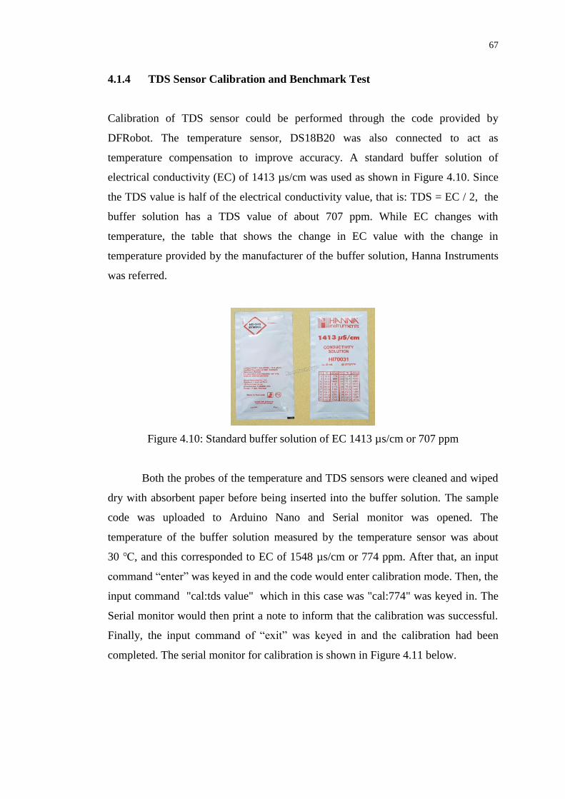
67
4.1.4 TDS Sensor Calibration and Benchmark Test
Calibration of TDS sensor could be performed through the code provided by
DFRobot. The temperature sensor, DS18B20 was also connected to act as
temperature compensation to improve accuracy. A standard buffer solution of
electrical conductivity (EC) of 1413 µs/cm was used as shown in Figure 4.10. Since
the TDS value is half of the electrical conductivity value, that is: TDS = EC / 2, the
buffer solution has a TDS value of about 707 ppm. While EC changes with
temperature, the table that shows the change in EC value with the change in
temperature provided by the manufacturer of the buffer solution, Hanna Instruments
was referred.
Figure 4.10: Standard buffer solution of EC 1413 µs/cm or 707 ppm
Both the probes of the temperature and TDS sensors were cleaned and wiped
dry with absorbent paper before being inserted into the buffer solution. The sample
code was uploaded to Arduino Nano and Serial monitor was opened. The
temperature of the buffer solution measured by the temperature sensor was about
30 , and this corresponded to EC of 1548 µs/cm or 774 ppm. After that, an input
command “enter” was keyed in and the code would enter calibration mode. Then, the
input command "cal:tds value" which in this case was "cal:774" was keyed in. The
Serial monitor would then print a note to inform that the calibration was successful.
Finally, the input command of “exit” was keyed in and the calibration had been
completed. The serial monitor for calibration is shown in Figure 4.11 below.
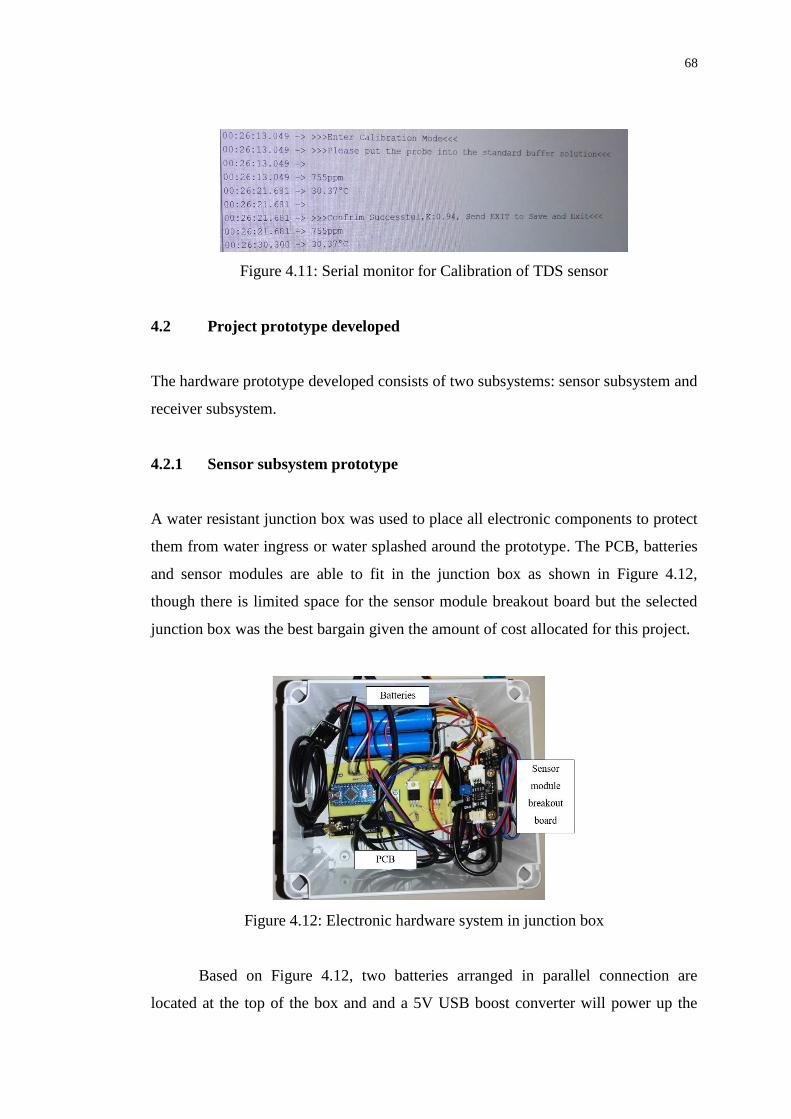
68
Figure 4.11: Serial monitor for Calibration of TDS sensor
4.2 Project prototype developed
The hardware prototype developed consists of two subsystems: sensor subsystem and
receiver subsystem.
4.2.1 Sensor subsystem prototype
A water resistant junction box was used to place all electronic components to protect
them from water ingress or water splashed around the prototype. The PCB, batteries
and sensor modules are able to fit in the junction box as shown in Figure 4.12,
though there is limited space for the sensor module breakout board but the selected
junction box was the best bargain given the amount of cost allocated for this project.
Figure 4.12: Electronic hardware system in junction box
Based on Figure 4.12, two batteries arranged in parallel connection are
located at the top of the box and and a 5V USB boost converter will power up the

69
PCB from the Arduino Nano located at the centre of the box. The right side of the
box is where the sensor module breakout boards are placed. Six holes of different
sizes were drilled to allow the four sensor probes and antenna of nRF24L01 to pass
through the junction box as well as to place the main switch for the electronic system.
The size of holes depend on the diameter of the probes and wires and the holes were
later sealed with silicone sealant and hot glue to prevent water from entering into the
box.
In order to place the box on the float with even weight distribution, the box
was adjusted to be placed in the middle and above an acrylic sheet. Four L-brackets
were used to fasten the junction box and acrylic sheet. The L-brackets were directly
screwed and fixed in place using electric screwdriver. Next, six nylon cable ties were
used to fasten the acrylic sheet to the PVC float. As for the float, PVC pipe was cut
into four segments based on the dimensions calculated and joined by 90º PVC
elbows glued using PVC solvent cement. After that, four holes of different sizes were
drilled on the acrylic sheet to allow the pH, temperature, TDS and turbidity probes to
pass through and immerse in water. The probes were then fixed and glued especially
the turbidity sensor as its top is not waterproof. The final prototype of the sensor
subsystem is shown in front, top and side views in Figures 4.13 to 4.15 below.
Figure 4.13: Sensor Subsystem Prototype Front View

70
Figure 4.14: Sensor Subsystem Prototype Side View
Figure 4.15: Sensor Subsystem Prototype Top View
4.2.2 Receiver Subsystem Prototype
The receiver subsystem is placed indoor next to the router which consists of Arduino
Ethernet shield with Arduino Mega powered by 5 V adapter as shown in Figure 4.16.
The two-way communication is through the RF module and data received by this
subsystem will be uploaded to the cloud via the Ethernet connection from the RJ45
Ethernet cable.
Figure 4.16: Receiver Subsystem Prototype

71
4.3 Prototype Performance
4.3.1 Data Upload and Monitoring On Ubidots Cloud
The receiver subsystem is designed to work such that when data from sensor
subsystem is received and internet connection is available, it would upload the data
to Ubidots cloud. The data will be stored in Ubidots database and is displayed via the
graphical user interface (GUI) or dashboard and can be accessed through the Ubidots
website or its mobile application. The number of variables created for this project in
the cloud are 12 in which five variables (purple colured) are real-time sensor data
and the other five variables are for backup sensor data (green coloured) whilst the
remaining two are log real-time data state (yellow coloured) and time interval (red
coloured). Figure 4.17 below shows the variables created in the cloud, where each
variable is issued a unique API key so that the sensor data will be stored to the
correct variable. The time and date at the time of upload will be captured.
Figure 4.17: Ubidots cloud database
The dashboard is where the data will be visible to users and displayed in
graphical format where the duration range of data is modifiable. Figure 4.18 shows
the snapshot of dashboard for displaying real-time or latest set of data while Figure
4.19 is for displaying historical data. These static dashboard views are from the
Ubidots website viewed from laptop.

72
Figure 4.18: Snapshot of dashboard for displaying real-time (latest) data
Figure 4.19: Snapshot of dashboard for displaying historical data
Link to view real-time data:
https://stem.ubidots.com/app/dashboards/public/dashboard/uxpVWc33_Jrq6XjBgb7c
YPU-qJvHfUL9Jsy4BNX9hZ8?datePicker=true
Link to view historical data:
https://stem.ubidots.com/app/dashboards/public/dashboard/2FutOe6Zb196JXU4-
1Nq4zKUH3bbaGusp8nTC6vGmEw?datePicker=true

73
4.3.2 User Request to Log Real-Time Data or Change Time Interval
There is also dynamic dashboard designed for user interface where user could
modify the system settings by either request to log real-time data or change the time
interval to log data. The default setting is that the log data switch is not turned on and
the slider for time interval is set to 20 minutes as shown in Figure 4.20. User can
slide the slider as desired to change the time from 0 minute to 60 minutes.
Figure 4.20: Snapshot of dashboard for user input to request to log real-time data or
change time interval
Link to view user request:
https://stem.ubidots.com/app/dashboards/public/dashboard/4D4Vn5UqJUs325cq3W
9y06St3Suy9ZWasI50-zmR-uI?datePicker=true
4.3.3 Ubidots Mobile Application
User may also perform the similar operations earlier (view graphical data or modify
user request) by accessing the Ubidots mobile application from mobile phone.
Figure 4.21 below shows the snapshot of dashboard in mobile application view.
Figure 4.21: Snapshot of dashboard accessed through Ubidots mobile application

74
4.3.4 Data Storage in SD Card and Reupload to Ubidots cloud
When internet connection is not available upon receiving sensor data, the receiver
subsystem will automatically save the data to the micro SD card attached to the
Ethernet shield. The communication interface with the card is in the SPI protocol
and the SD library is needed for coding in Arduino. The micro SD card used has a
storage capacity of 8 gigabytes. The data will be stored in text file in a specified
format as shown in Figure 4.22 below. The microcontroller will check the content of
SD card every 1 hour and if there is backup data found while internet connection is
back, it will upload the data to the five backup variables in the cloud as shown in
Figure 4.23. These data will be available in the historical data of dashboard and
displayed in table format. The content in the text file will be erased after successful
upload of backup data.
Figure 4.22: Data stored in text file of SD card
Figure 4.23: Backup data in table format available in historical data dashboard of
Ubidots

75
4.3.5 Real Time Notification
An alert notification sent via email will be triggered whenever any of the value of
water quality parameters is out of the predefined safe range. Figures 4.24 to 4.26
below show the snapshot of emails received when the water in the tank was
deliberately mixed with apple cider vinegar, soil and acid pH buffer powder to
decrease the pH and increase the turbidity and TDS values. These three parameters
fell out of the range and therefore three emails were sent to alert user to inspect the
water.
Figure 4.24: Notification email to alert user on pH parameter
Figure 4.25: Notification email to alert user on TDS parameter
Figure 4.26: Notification email to alert user on turbidity parameter

76
4.4 Problem Encountered and Improvement During and After Data
Collection
The official data collection was carried out from 22nd March 2021 to 25th March
2021. On 21st March 2021 when the sensor subsystem prototype was first placed into
a large storage container filled with water to simulate the environment for real water
storage tank, there was a problem encountered and it was solved before being
deployed for official data collection.
The problem faced was that the pH sensor could not return the correct value
due to ground loop. When placed in standard buffer solution for calibration and also
tested in cup water, the pH sensor could function well as intended. However, there
was error in reading when placed in the water tank. This was because the pH sensor
was connected to a different point of ground (Drain pin of MOSFET). A voltage
proportional to the current and the electrode resistance develops across the drain pin
to the source pin of MOSFET. The currents created by ground loops were unstable,
so pH readings kept fluctuating around 5 instead of around 7. After determining the
problem was due to MOSFET, the MOSFET was changed to a relay module to turn
on and off the pH sensor but the problem still existed as shown in Figure 4.27 and
4.28. Therefore, it was solved by turning on the pH sensor for 24 hours. However,
this has led to large drain in battery current that caused the batteries intended to last
for five days to drop to only three hours.
Figure 4.27: MOSFET changed to Figure 4.28: pH value still fluctuating
relay module despite changing MOSFET to relay module

77
4.5 Data Analysis
During the data collection period, a total of four water quality parameters were being
monitored which were pH, temperature, TDS and turbidity. Battery voltage was
being monitored only on the first day because 5 V adapter was used to power the
subsystem after that to reduce the hassle of having the recharge the batteries every
three hours. The water was changed partially every day at 6pm to simulate the water
flow in and out of the water storage tank. The interval to log data was set to 20
minutes on 22nd March 2021, changed to 25 minutes on 23rd March 2021 and then to
40 minutes on 24th March 2021. All of the graphs could be found in Appendix C of
this report. Towards the end of data collection, the water was intentionally polluted
by adding apple cider vinegar, acid pH buffer powder and a few spoonfuls of soil to
simulate the environment where water is polluted and is not safe for consumption.
4.5.1 pH
Since the water used was directly from the tap, it was logic to obtain values around 7
to 8. This indicated that the pH of water was safe as the optimum pH is in the range
of 6.5 to 9.5 according to the World Health Organization (WHO). The pH of water
was observed to have dropped every time when the water was being changed every
day around 6pm. Besides this, the pH also change slightly with time. This was due
to the surrounding air that contains carbon dioxide (CO2) and when given the chance
to be absorbed by water (H2O), a weak acid known as carbonic acid (H2CO3) will be
produced. Benchmark test was carried out to verify the pH value obtained and is
shown in Figures 4.29 and 4.30 below. When the tank was added with impurities as
mentioned earlier, the pH dropped as shown in Figures 4.31 and 4.32.
Figure 4.29: pH of 7.57 captured by sensor Figure 4.30: pH of 7.58
captured by pH meter

78
Figure 4.31: pH of 4.40 captured by sensor Figure 4.32: pH of 4.33
(with impurities) captured by pH meter
4.5.2 Temperature
The temperature generally remained constant throughout the day and only varied due
to relocation of the water storage tank and change of surrounding temperature. On
the 22nd March 2021, the tank was placed in the bathroom for data collection so
temperature was the lowest at 28.88 ºC. At around 6pm on the same day, the water
tank was relocated to the living room near the window. At the same time, water was
changed. Temperature went up to 29.00 ºC and was slowly increasing to peak at
30.12 ºC on the next day afternoon. This was because of heat trapped in the wall of
building that had slowly dissipated through and affected the surrounding temperature
as well as the water temperature. It then rained from afternoon till night time on the
24th March 2021 and the water temperature decreased gradually due to drop in
surrounding temperature. The water temperature then remained constant in the
evening from 7 pm to 11 pm. Benchmark test was carried out to verify the
temperature value obtained and is shown in Figures 4.33 and 4.34 below. The
benchmark test for addition of impurities is shown in Figures 4.35 and 4.36 below.
Since the impurities were obtained at room temperature upon being added, the
temperature of water remain unchanged.
Figure 4.33: Temperature of 28.94 ºC Figure 4.34: Temperature of 30.3 ºC
captured by sensor captured by thermometer

79
Figure 4.35: Temperature of 28.75 ºC Figure 4.36: Temperature of 30.3 ºC
captured by sensor (with impurities) captured by thermometer
4.5.3 TDS
The TDS of water generally fell within the range of 26 to 35 ppm during data
collection. These values are well within the range of safe water quality (less than 300
ppm) based on WHO standards. The slight fluctuation in TDS values were due to
temperature change and evaporation which could cause concentration and mobility
of ions to vary. Benchmark test was carried out to verify the TDS value obtained and
is shown in Figures 4.37 and 4.38 below. The TDS rose to 58.44 ppm when water
was added with impurities and the results are shown in Figures 4.39 and 4.40 below.
The increase of TDS value was due to the high content of dissolved calcium and
magnesium in apple cider vinegar.
Figure 4.37: TDS of 31.78 ppm captured Figure 4.38: TDS of 32 ppm
by sensor captured by TDS meter
Figure 4.39: TDS of 58.44 ppm captured Figure 4.40: TDS of 54 ppm
by sensor (with impurities) captured by TDS meter

80
4.5.4 Turbidity
The turbidity of water according to WHO standards should ideally score less than 1
NTU for water supplies in households and storage. Therefore, the turbidity of water
remained at 0 NTU throughout the entire data collection. This proved that the water
was safe. However when impurities were added, the turbidity level climbed to about
161.22 NTU as shown in Figure 4.41 as the water had become very murky.
Figure 4.41: Turbidity of 161.22 NTU captured by sensor (with impurities)
4.5.5 Battery voltage
Battery voltage was monitored when batteries were used to power the subsystem.
Since the batteries were tested before deploying for official data collection, the
duration they could last had been known as about 3 hours. Thus, batteries were
replaced for recharge every 2 and a half hours and thus the battery voltage never
dropped to critical value of 3.5 V and stayed at minimum of 4.02 V only.
4.6 Summary
To summarize Chapter 4, sensor calibration was performed to ensure the sensor data
was accurate and the performance of prototype and IoT cloud platform developed
were evaluated. All the system features were tested and they could work properly as
intended. A problem related to pH sensor was found and it was solved before
deploying the system for data collection. The data collection that lasted for five days
was successful with the results being verified by benchmark meters.

81
CHAPTER 5
5 CONCLUSIONS AND RECOMMENDATIONS
5.1 Conclusion
In conclusion, this project has successfully developed an Internet of Things water
quality monitoring system in water storage tank that can monitor four water quality
parameters, i.e. pH, temperature, TDS and turbidity. This system is able to capture
the data of these parameters at real-time and allow user to monitor at any time while
being remotely away from the water storage tank. The two-way communication
between the sensor subsystem placed in the tank and the receiver subsystem placed
indoor is made possible by using RF modules with maximum transmission range of 1
km in open space. The sensor subsystem uses Arduino Nano as the microcontroller
due to its compact size and lightweight while also being able to support the software
development of the sensors used. On the other hand, the receiver subsystem uses
Arduino Mega with Etherney shield to receive sensor data and upload to cloud server.
The IoT platform used in this project is Ubidots because it supports 4,000
dots per day that is more than enough for the normal operation of the developed
system. The system will log five sensor data (four water quality parameters and
battery voltage data) every 20 minutes by default. Additional features such as real-
time notification in the case of failing water quality, preview of historical data in
graphical format and user request to control the data logging as well as request to
change time interval have also been implemented successfully. The monitoring and
controlling of system could also be made via Ubidots mobile application accessed
from mobile phone.
A problem related to the pH sensor was encountered when deploying the
prototype for data collection. This problem was solved and discussed in Chapter 4.
To sum up, all objectives in this project have been achieved successfully. The
developed system is able to perform real-time water quality monitoring, alert user
when water quality fails, its system settings can be modified by users and the
historical data can be tracked and monitored via cloud platform and mobile
application.

82
5.2 Limitation of the prototype
There are several limitations to this project. Firstly, since the sensor subsystem is
battery-powered, the system have been initially designed to sustain for about five
days. However after facing ground loop issue with the pH sensor, the sensor had to
be turned on the whole time which caused the overall power consumption to increase
drastically and the batteries could only last about three hours. As mentioned earlier,
the junction box could fit the electronic components just right so it could not hold
more batteries to increase the capacity.
Secondly, the system is unable to predict future water quality based on the
water quality parameter data collected such as pH, temperature, TDS and turbidity.
This is because Artificial Intelligence or machine learning algorithm are not
implemented to forecast when the water storage tank will get dirty due to
sedimentation of scales. Users have to decide when they should wash the tanks on
their own by observing the change in data collected.
Next, due to cost constraint, only four water quality parameters are being
monitored. However, there are plenty other water parameters that are essential to be
monitored to determine the safety of water consumed. Examples of these parameters
are ammonia, chlorine and dissolved oxygen.
5.3 Recommendation for Future Work
In future, there could be some improvements to enhance the functionality and
performance of this IoT water quality monitoring system. The first recommendation
is to install solar panel outside of the water storage tank to allow for self-
sustainability.
Secondly, the implementation of machine learning algorithm is recommended
for predictive analysis of data so that it could automatically alert users as to when
they should inspect and deep clean their water storage tanks.
Thirdly, more sensors could be added to the system such as ammonia sensor,
chlorine sensor and dissolved oxygen sensor as they are also equally important in
determining the safety of water in water storage tanks.

83
REFERENCES
Arduino Store. n.d. Arduino Mega 2560 REV3 [online] Available at:
<https://store.arduino.cc/usa/mega-2560-r3> [Accessed 5 August 2020].
Atlas Scientific. 2020. EZO™ Conductivity Circuit [online] Available at:
<https://atlas-scientific.com/circuits/ezo-conductivity-circuit/> [Accessed 5 August
2020].
Banggood. n.d. PH Sensor Module V1.1 + PH Probe for AVR 51 PH Shield with
MSP430 Test Code Sensor [online] Available at: <https://my.banggood.com/PH-
Sensor-Module-V1_1-+-PH-Probe-For-AVR-51-PH-Shield-with-MSP430-Test-
Code-Sensor-p-1460488.html?cur_warehouse=CN> [Accessed 5 August 2020].
Basilla, A.A. 2021. TDS in Tap Water: Its Potential Health Risks and How to
Reduce It [online] Available at: <https://www.aquaoxwaterfilters.com/everything-
you-need-to-know-about-interpreting-your-water-quality-reports/> [Accessed 5
August 2020].
Budiarti, R. P. N., Tjahjono, A., Hariadi, M. and Purnomo, M. H., 2019.
Development of IoT for Automated Water Quality Monitoring System. In: 2019
International Conference on Computer Science, Information Technology, and
Electrical Engineering (ICOMITEE). 2019 International Conference on Computer
Science, Information Technology, and Electrical Engineering (ICOMITEE). Jember,
Indonesia, 16/10/2019 - 17/10/2019: IEEE, pp. 211–216.
Chalchisa, D., Megersa, M. and Beyene, A., 2018. Assessment of the quality of
drinking water in storage tanks and its implication on the safety of urban water
supply in developing countries. Environmental Systems Research, [e-journal] 6(1).
http://dx.doi.org/10.1186/s40068-017-0089-2.
Chen, Y. and Han, D., 2018. Water quality monitoring in smart city: A pilot project.
Automation in Construction, [e-journal] 89, pp. 307–316.
<http://dx.doi.org/10.1016/j.autcon.2018.02.008> [Accessed 5 August 2020].
Chowdury, M. S. U., Emran, T. B., Ghosh, S., Pathak, A., Alam, M. M., Absar, N.,
Andersson, K. and Hossain, M. S., 2019. IoT Based Real-time River Water Quality
Monitoring System. Procedia Computer Science, [e-journal] 155, pp. 161–168.
http://dx.doi.org/10.1016/j.procs.2019.08.025.
Conserve Energy Future, 2013. Sources and Causes of Water Pollution That Affect
Our Environment - Conserve Energy Future [online] Available at:
<https://www.conserve-energy-future.com/sources-and-causes-of-water-
pollution.php> [Accessed 11 September 2020].
Dandekar, S., Kadam, S. S., Choudhary, R. N., Vaidya, S. S. and Rajderkar, V. S.,
2018 - 2018. IOT based Real Time Water Grade Tracking System using Solar
Energy. In: 2018 3rd International Conference on Communication and Electronics
Systems (ICCES). 2018 3rd International Conference on Communication and

84
Electronics Systems (ICCES). Coimbatore, India, 15/10/2018 - 16/10/2018: IEEE,
pp. 773–775.
Das, B. and Jain, P.C. 2017. Real-Time Water Quality Monitoring System using
Internet of Things. In: 2017 International Conference on Computer, Communications
and Electronics (Comptelix). Manipal University Jaipur, Malaviya National Institute
of Technology Jaipur & IRISWORLD, July 01-02, 2017. Piscataway, NJ. 1/7/2017 –
2/7/2017: IEEE, pp. 78–82.
<http://ieeexplore.ieee.org/servlet/opac?punumber=8000236> [Accessed 5 August
2020].
Distrelec. n.d. Shield Model Ethernet – Arduino Ethernet shield R3 [online]
Available at: <https://www.distrelec.biz/en/arduino-ethernet-shield-r3-arduino-
shield-model-ethernet/p/11038923> [Accessed 5 August 2020].
Department of Environment. 2018. River Water Quality. [online] Malaysia:
Department of Environment. Available through:
<https://www.doe.gov.my/portalv1/wp-content/uploads/2018/09/Kualiti-Air-
Sungai.pdf> [Accessed 1 August 2020].
DFRobot. 2020a. Gravity: Analog Electrical Conductivity Sensor /Meter V2 (K=1)
[online] Available at: <https://www.dfrobot.com/product-1123.html> [Accessed 5
August 2020].
DFRobot. 2020b. Gravity Analog TDS Sensor Meter For Arduino SKU SEN0244
[online] Available at:
<https://wiki.dfrobot.com/Gravity__Analog_TDS_Sensor___Meter_For_Arduino_S
KU__SEN0244> [Accessed 5 August 2020].
DFRobot. 2020c. PH_meter_SKU__SEN0161_- [online] Available at:
<https://wiki.dfrobot.com/PH_meter_SKU__SEN0161_> [Accessed 5 August 2020].
DFRobot. 2020d. Turbidity_sensor_SKU__SEN0189 [online] Available at:
<https://wiki.dfrobot.com/Turbidity_sensor_SKU__SEN0189> [Accessed 5 August
2020].
Ebay. 2021. DS18B20 Stainless Steel Probe Waterproof Temperature Sensor 1M
Cable + PCB kit [online] Available at < https://www.ebay.co.uk/itm/264054673584>
[Accessed 5 August 2020].
Elecrow. 2020. NRF24L01+PA+LNA Wireless Module – 1100 Meters [online]
Available at: <https://www.elecrow.com/nrf24l01palna-wireless-module-1100-
meters-p-556.html> [Accessed 5 August 2020].
Elektorstore. n.d. Arduino Nano [online] Available at:
<https://www.elektor.com/arduino-nano> [Accessed 5 August 2020].

85
Electronics Hub. 2018. Interfacing Voltage Sensor with Arduino – Measure up to 25
V using Arduino [online] Retrieved from
https://www.electronicshub.org/interfacing-voltage-sensor-with-arduino/ [Assessed 5
March 2020].
Faustine, A., Mvuma, A. N., Mongi, H. J., Gabriel, M. C., Tenge, A. J. and Kucel, S.
B., 2014. Wireless Sensor Networks for Water Quality Monitoring and Control
within Lake Victoria Basin: Prototype Development. Wireless Sensor Network, [e-
journal] 06(12), pp. 281–290. <http://dx.doi.org/10.4236/wsn.2014.612027>
[Accessed 5 August 2020].
Food and Agriculture Organization. 2007. MALAYSIA’S WATER VISION: THE
WAY FORWARD - The Malaysian Water Partnership. [online] Available at:
<http://www.fao.org/3/ab776e/ab776e02.htm> [Accessed 5 August 2020].
General Electric Company. 2013. TSD-10 Turbidity Sensor.
<http://www.farnell.com/datasheets/1770074.pdf> [Accessed 9 December 2020].
In-Situ. 2018. AquaTROLL500-spec-sheet [online] <https://in-
situ.com/pub/media/support/documents/AquaTROLL500-spec-sheet.pdf> [Accessed
9 December 2020].
Henderson, E. 2015. Preventing contamination in water storage tanks [online]
Available at: <https://esemag.com/water/water-storage-tanks-
contamination/#:~:text=Stagnant%20water%20lures%20potential%20hosts,less%20
dense%2C%20warmer%20surface%20water. > [Accessed 5 August 2020].
International Rectifier, 2003. IRF520NPbF [online]. Available at:
<https://www.infineon.com/dgdl/irf520npbf.pdf?fileId=5546d462533600a4015355e
340711985> [Accessed 5 March 2021]
Is Kuala Lumpur Tap Water Safe to Drink?. n.d. [online] Available at:
<https://www.canyoudrinktapwaterin.com/kuala-lumpur-tap-water/> [Accessed 11
September 2020].
JALELAH ABU BAKER, 2015. Body found in KL condo water tank; 200 residents
affected. [online] Available at: <https://www.straitstimes.com/asia/body-found-in-kl-
condo-water-tank-200-residents-affected> [Accessed 5 August 2020].
Jerom B., A. and Manimegalai, R., 2020 - 2020. An IoT Based Smart Water Quality
Monitoring System using Cloud. In: 2020 International Conference on Emerging
Trends in Information Technology and Engineering (ic-ETITE). 2020 International
Conference on Emerging Trends in Information Technology and Engineering (ic-
ETITE). Vellore, India, 24/2/2020 - 25/2/2020: IEEE, pp. 1–7.
Jia Shuo, Zhang Yonghui, Ran Wen and Tong Kebin, 2017. 2017 International
Conference on Computer Systems, Electronics and Control (ICCSEC): 25-27 Dec.
2017. [e-book]. Piscataway, NJ: IEEE.
<http://ieeexplore.ieee.org/servlet/opac?punumber=8429892> [Accessed 5 August
2020]..

86
Kawarkhe, M.B. and Agrawal, S. 2019. Smart Water Monitoring System Using IOT
at Home. IOSR Journal of Computer Engineering (IOSR-JCE), [e-journal] 21(1), pp.
12-19. <http://www.iosrjournals.org/> [Accessed 5 August 2020].
Lenntech. n.d. Water conductivity [online] Available at:
<https://www.lenntech.com/applications/ultrapure/conductivity/water-
conductivity.htm> [Accessed 5 August 2020].
Liu, Y.-T., Lin, B.-Y., Yue, X.-F., Cai, Z.-X., Yang, Z.-X., Liu, W.-H., Huang, S.-Y.,
Lu, J.-L., Peng, J.-W. and Chen, J.-Y., 2018 - 2018. A solar powered long range real-
time water quality monitoring system by LoRaWAN. In: 2018 27th Wireless and
Optical Communication Conference (WOCC). 2018 27th Wireless and Optical
Communication Conference (WOCC). Hualien, 30/4/2018 - 1/5/2018: IEEE, pp. 1–2.
M, S., P, A., T, K. and C, B. k., 2020 - 2020. Water Quality Monitoring System
Based On IoT. In: 2020 5th International Conference on Devices, Circuits and
Systems (ICDCS). 2020 5th International Conference on Devices, Circuits and
Systems (ICDCS). Coimbatore, India, 5/3/2020 - 6/3/2020: IEEE, pp. 279–282.
Madhavireddy, V. and Koteswarrao, B., 2018. Smart Water Quality Monitoring
System Using Iot Technology. International Journal of Engineering & Technology,
[e-journal] 7(4.36), p. 636–636. http://dx.doi.org/10.14419/ijet.v7i4.36.24214.
[Accessed 5 August 2020].
Malay Mail. 2020. Malaysia’s water safe to drink straight from tap, says SPAN.
[online] Available at:
<https://www.malaymail.com/news/malaysia/2018/10/20/malaysias-water-safe-to-
drink-straight-from-tap-says-span/1684932> [Accessed 5 August 2020].
Maxim Integrated. n.d. DS18B20: Programmable Resolution 1-Wire Digital
Thermometer [online] Available at:
<https://datasheets.maximintegrated.com/en/ds/DS18B20.pdf> [Accessed 9
December 2020].
Memon, A. R., Kulsoom Memon, S., Memon, A. A. and Din Memon, T., 2020 -
2020. IoT Based Water Quality Monitoring System for Safe Drinking Water in
Pakistan. In: 2020 3rd International Conference on Computing, Mathematics and
Engineering Technologies (iCoMET). 2020 3rd International Conference on
Computing, Mathematics and Engineering Technologies (iCoMET). Sukkur,
Pakistan, 29/1/2020 - 30/1/2020: IEEE, pp. 1–7.
Mohd Talha. 2019. River Pollution and Health Risk [online].
<https://www.span.gov.my/document/upload/CaZC6EQKwXtn7bGFUyOklLwDNU
zAVfpR.pdf> [Accessed 9 December 2020].
Osoyoo. 2018. Arduino lesso – Voltage Sensor Module [online] Available at
<https://osoyoo.com/2018/11/06/arduino-lesson-voltage-sensor-module/> [Accessed
5 August 2020].

87
Pasika, S. and Gandla, S. T., 2020. Smart water quality monitoring system with cost-
effective using IoT. Heliyon, [e-journal] 6(7), e04096.
http://dx.doi.org/10.1016/j.heliyon.2020.e04096.
Pule, M., Yahya, A. and Chuma, J., 2017. Wireless sensor networks: A survey on
monitoring water quality. Journal of Applied Research and Technology, [e-journal]
15(6), pp. 562–570. http://dx.doi.org/10.1016/j.jart.2017.07.004.
Safe Drinking Water Foundation. 2016. Water Temperature [online] 28 Nov.
Available at: <https://www.safewater.org/fact-sheets-1/2018/8/15/water-temperature-
fact-sheet> [Accessed 5 August 2020].
Smith, M. 2010. RSBOJC Water Quality Program [online] Available at:
<http://www.svid.org/rsbojc_water_quality_program.htm> [Accessed 12 September
2020].
Soong, K. K., 2019. Water crisis – the price of populism [online] 28 Jul. Available
at: <https://www.thestar.com.my/news/nation/2019/07/28/water-crisis--the-price-of-
populism/> [Accessed 5 August 2020].
Stara Water Hygiene Manchester, 2020. Water Tank Cleaning Chlorination and
Disinfection Manchester. [online] Available at:
<http://starawaterhygiene.co.uk/service-list/tank-cleaning-and-disinfection/>
[Accessed 5 August 2020].
Texas Instruments. 2017. LM35 Precision Centigrade Temperature Sensors datasheet
(Rev. H). <https://www.ti.com/lit/ds/symlink/lm35.pdf> [Accessed 9 December
2020].
Turbidity and Water. 2020 [online] Available at: <https://www.usgs.gov/special-
topic/water-science-school/science/turbidity-and-water?qt-
science_center_objects=0#qt-science_center_objects> [Accessed 5 August 2020].
WebMD, 2020. What Do You Know About Your Drinking Water? [online]
Available at: <https://www.webmd.com/women/safe-drinking-water#3> [Accessed 5
August 2020].
What is a pH meter? 2020. Introduction to digital pH meters [online] Available at:
<https://www.omega.co.uk/prodinfo/pH-meter.html> [Accessed 5 August 2020].
WWF Malaysia. 2020. Freshwater [online] Available at:
<https://www.wwf.org.my/about_wwf/what_we_do/freshwater_main/> [Accessed 5
August 2020].
World Health Organization. 2003. Total dissolved solids in Drinking-water. In:
World Health Organization, ed. 1996. Guidelines for drinking-water quality. Geneva:
World Health Organization. pp 1-3. [online] Available at:
<https://www.who.int/water_sanitation_health/dwq/chemicals/tds.pdf> [Accessed 5
August 2020].

88
World Health Organization. 2007. pH in Drinking-water [online] Available at:
<https://www.who.int/water_sanitation_health/dwq/chemicals/ph_revised_2007_clea
n_version.pdf> [Accessed 5 August 2020].
World Health Organization. 2017. WATER QUALITY AND HEALTH - REVIEW
OF TURBIDITY: Information for regulators and water suppliers [online] Available
at:
<https://www.who.int/water_sanitation_health/publications/turbidity-information-
200217.pdf> [Accessed 5 August 2020].
Yousif, A. F., Ahmed, S. Y. M. and Elhag, N. A. A., eds., 2018. 2018 International
Conference on Computer, Control, Electrical, and Electronics Engineering
(ICCCEEE): 12th-14th August- 2018, Corinthia Hotel, Khartoum, Sudan.
Piscataway, NJ: IEEE. Available at: Yousif, Alaelddin Fuad (HerausgeberIn) Ahmed,
Sulafa Y. M. (HerausgeberIn) Elhag, Nihad A. A. (HerausgeberIn).
<http://ieeexplore.ieee.org/servlet/opac?punumber=8501351> [Accessed 5 August
2020].

89
APPENDICES
APPENDIX A: Datasheet
Figure A-1: IRF520N VGS versus IDS Characteristics

90
APPENDIX B: Prototype Built
Figure B-1: Prototype placed in water storage tank for data collection
Figure B-2: Prototype placed in water storage tank containing polluted water

91
APPENDIX C: Graphs
Figure C-1-1: pH Graph from 22-03-2021 to 25-03-2021
Figure C-1-2: Temperature Graph from 22-03-2021 to 25-03-2021
Figure C-1-3: TDS Graph from 22-03-2021 to 25-03-2021

92
Figure C-1-4: Turbidity Graph from 22-03-2021 to 25-03-2021
Figure C-1-5: Battery Voltage Graph from 20-03-2021 to 21-03-2021
Figure C-2-1: pH Graph on 22-03-2021

93
Figure C-2-2: Temperature Graph on 22-03-2021
Figure C-2-3: TDS Graph on 22-03-2021
Figure C-2-4: Turbidity Graph on 22-03-2021

94
Figure C-3-1: pH Graph on 23-03-2021
Figure C-3-2: Temperature Graph on 23-03-2021
Figure C-3-3: TDS Graph on 23-03-2021

95
Figure C-3-4: Turbidity Graph on 23-03-2021
Figure C-4-1: pH Graph on 24-03-2021
Figure C-4-2: Temperature Graph on 24-03-2021

96
Figure C-4-3: TDS Graph on 24-03-2021
Figure C-4-4: Turbidity Graph on 24-03-2021
Figure C-5-1: pH Graph on 25-03-2021

97
Figure C-5-2: Temperature Graph on 25-03-2021
Figure C-5-3: TDS Graph on 25-03-2021
Figure C-5-4: Turbidity Graph on 25-03-2021

98
APPENDIX D: Coding of Sensor Subsystem
Figure D-1-1: Arduino Nano Main Program (1)

99
Figure D-1-2: Arduino Nano Main Program (2)
Figure D-2: Sensors and RF Module Initialization

100
Figure D-3-1: Take Sensors Reading Program
Figure D-3-2: Take pH Reading Program
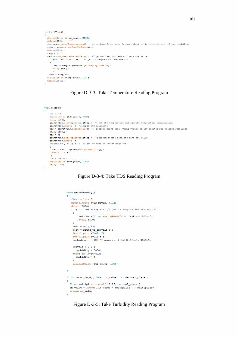
101
Figure D-3-3: Take Temperature Reading Program
Figure D-3-4: Take TDS Reading Program
Figure D-3-5: Take Turbidity Reading Program

102
Figure D-3-6: Take Voltage Reading Program
Figure D-4: RF Send Data Program

103
Figure D-5: User Request Program

104
APPENDIX E: Coding of Receiver Subsystem
Figure E-1-1: Arduino Mega Main Program (1)

105
Figure E-1-2: Arduino Mega Main Program (2)
Figure E-1-3: Arduino Mega Main Program (3)

106
Figure E-1-4: Arduino Mega Main Program (4)
Figure E-2: RF Initialization Program

107
Figure E-3: Ethernet Connection Program

108
Figure E-4: RF Receive Sensor Data Program

109
Figure E-5: Upload Data to Ubidots Cloud Program
Figure E-6: Clear Current Sensor Data Program

110
Figure E-7-1: User Request Program (1)
Figure E-7-2: User Request Program (2)

111
Figure E-8: RF Alert Sensor Subsystem to Standby Program
Figure E-9-1: SD Card Program (1)

112
Figure E-9-2: SD Card Program (2)
Figure E-9-3: SD Card Program (3)

113
Figure E-9-4: SD Card Program (4)

114
Figure E-10: Get Time from NTP Server Program

115
Figure E-11-1: Upload Backup Data Program (1)
Figure E-11-2: Upload Backup Data Program (2)