integration of mussel in fish farm: mathematical model and analysis

Nonlinear Analysis: Hybrid Systems 3 (2009) 74–86

Contents lists available at ScienceDirect

Nonlinear Analysis: Hybrid Systems

journal homepage: www.elsevier.com/locate/nahs

Integration of mussel in fish farm: Mathematical model and analysisNurul Huda Gazi a,∗, Safiur Rahaman Khan b, Charu Gopal Chakrabarti ba St. Xavier’s College, 30, Mother Teresa Sarani, Kolkata - 700 016, Indiab Department of Applied Mathematics, University of Calcutta, 92, Acharya Prafulla Chandra Road, Kolkata - 700 009, India

a r t i c l e i n f o

Article history:Received 23 July 2008Accepted 31 October 2008

Keywords:Fish farmNonlinear differential equation modelEutrophicationStabilityTime delayOscillationHopf-bifurcation

a b s t r a c t

The paper deals with the dynamical behavior of fish and mussel population in a fish farmwhere external food is supplied. The ecosystem of the fish farm is represented by a set ofnonlinear differential equations involving the nutrient (food), fish and mussels. We havestudied the boundedness, local stability and global stability of the model system. We haveincorporated the discrete type gestational delay of fish and analyze effect of the delay on thedynamical behavior of the model system. The delay parameter complicates the dynamicsdepending on the external food from changing the stable state to unstable damped periodictrajectories leading to a limit cycle oscillation. We have studied the Hopf-bifurcation of themodel system in the neighborhood of the coexisting equilibrium point considering delayas a variable bifurcation parameter. We have performed numerical simulation to verifythe analytical results. The entire study reveals that the external food supply controls thedynamics of the system.

© 2008 Elsevier Ltd. All rights reserved.

1. Introduction

There is a necessity for sustainable development in aquaculture for both individual livelihoods and the economy.Most of the European countries have taken some strategy towards the development of aquaculture. There are severalconstraints, one, themost important, being the environmental concern linked to the location of the fish farm and the impactof their effluents on the surrounding environment. Nutrient pollution from aquacultural waste exceeds the assimilationcapacity of receiving water deteriorating water quality [1]. Past studies show several types of impact of fish farming inthe Mediterranean region. [2–5] and the references cited therein. Karakassis et al. [6] studied the potential impact of fishfarming on nutrient content and concluded that fish farmwaste can cause 1% on nutrient concentration in contrast to otheranthropogenic activities. There is a greater impact of detritivorous fish on the estuarian ecosystem [7]. Samanta et al. [8]investigated how themaximumamount of economically important species can be harvested from a fishery. Bandyopadhyayet al. [9] investigated the dynamics of an ecological system where the nutrient has a very important role in controlling thebehavior of the system.Lakes Erie, Michigan, Huron, Superior, and Ontario are well known important sources of fresh water and are home to

many species of wildlife. However, with the belief thatwater could dilute any substance, the lakes have become destinationsof dumping grounds for many different types of pollutants. With so many different sources of pollutants, ranging fromindustrial waste, pesticide and fertilizer runoff, and fecal matter, it is not surprising the extent to which these contaminantshave affected the wildlife and ecosystem surrounding the Great Lakes. As seen in the biomass of Lake Huron trout, pollutiondirectly influences the wildlife and environment surrounding the lakes. Such influences include promoting the abundance

∗ Corresponding author. Tel.: +91 33 3296 7065; fax: +91 33 2287 9966.E-mail addresses: [email protected] (N. Huda Gazi), [email protected] (S. Rahaman Khan), [email protected] (C. Gopal Chakrabarti).

1751-570X/$ – see front matter© 2008 Elsevier Ltd. All rights reserved.doi:10.1016/j.nahs.2008.10.008

http://www.elsevier.com/locate/nahs

http://www.elsevier.com/locate/nahs

mailto:[email protected]



http://dx.doi.org/10.1016/j.nahs.2008.10.008

N. Huda Gazi et al. / Nonlinear Analysis: Hybrid Systems 3 (2009) 74–86 75

of diseases that occur in both animals and humans, as well as disrupting the natural balance of nutrients. So, aquacultureneeds to pay more attention to study and analysis.There are different categories of fish farming. The brackish water ponds depend on tidal water flow. Several ponds are

connected in a series to allow the fish to move from one pond to other for natural food. In a fresh water fish farm severalspecies of fish are cultured. The main foods of such a system are agricultural by-products and commercial feeds. In freshwater pens or cages, the species are dependent on natural food. In open coastal water, seaweed, oysters and mussels arecultivated. The culturedmacroalgae are present in this system. External food is sometimes a threat to the fish farm. The heavyorganic load causes depletion of dissolved oxygen in the water column. The water current speed is sometimes decreasedfor the uncontrolled proliferation of milkfish cages which causes the depletion of dissolved oxygen in the water columnwith organic loading from fish waste and excess feeds [10]. The optimum level of oxygen is 5 mg/l. The red tide caused byharmful algal bloom (pyrodinium bahamense) [11] in the open coastal water impact severely on aquaculture. The use ofreservoirs with ‘green water’, probiotics, sedimentation ponds with biofilters, recirculation water systems, the preventionof virulent bacterial outbreaks are the possibleways to increase the level of dissolved oxygen inwater column. Probiotics arebacteria capable of repressing the growth of pathogenic organisms either through the production of inhibitory substancesby competition [12]. The shellfish, seaweeds and oyster are used as biofilters (clean-up agents). The rafts are used for oystersto reduce siltation and pollution in the ecosystem.If the fish are less densely populated there is less competition for same food and space, which can cause faster growth

rates for individual fish. Artificial external food can cause a rapid increase of fish population and at the same time it mayhave a negative effect if the farm is overfed leading to a low oxygen condition. The shellfish plays an important role incontrolling such a negative impact on the fish population. An important characteristic of the shellfish is that they are filterfeeders, feeding on bacteria and nutrients found in the water column. Barnacles, mussels and other shellfish are used in aninnovative way so that they can behave like biofiltering systems to clean up fish farms. The shellfish are usually regardedby sailors as a nuisance as they form thick growths on the hulls of ships and impede speed and fuel efficiency. The shellfishwould be useful in disposing of debris such as feed waste and fish excreta produced at fish farms. Nutrients from the debris,mainly carbon, nitrogen and phosphorus, can cause significant marine pollution. Analysis shows that 68% of nutrients comefromphytoplankton, 28% from trash fish, and 4% from excrement [13]. Mussels can solve the pollution problem in twoways:mussels can digest particles of feed waste and fish excreta and also consume phytoplankton which thrives on inorganicnutrients such as phosphorus and nitrogen.Withmore nutrients, phytoplankton can form algal bloom or ‘red tides’, some ofwhich can become toxic. Another study of the integration of open-water mussel and Atlantic salmon cultures in Tasmaniashows that the growth ofmussels culturedwithin the fish farmwas not enhanced due to several contributing factors: (i) solidwastes from the farm do not significantly increase particulate food concentrations above ambient levels, (ii) phytoplanktonproduction within the farm is not enhanced [14]. Our study will be confined in developing a mathematical model of fishfarm where mussels have been integrated as a biofilter (clean up agent). We will study the effect of excessive external food(nutrient) on the fish farm when the mussel species is being cultured in the farm and the dynamics of the other populationpresent in the system.It is often that time delays are incorporated in themathematicalmodel of population biology. It is evident that in presence

of a timedelay, the dynamics of any natural systembecomes complicated. A delay has been incorporated in biologicalmodelsby many authors, namely, [15,16,18,19,21], and the references cited therein. It has been established that time delays havethe ability to drive a stable system into an unstable one. So, time delays are responsible for population oscillations in aconstant environment.We organize the paper as follows: In Section 2, we describe the model equation of the three components, namely,

nutrient, fish andmussel which are nonlinear differential equations. In Section 3, we analyze themodel system for boundedsolution, local asymptotic stability criteria and global asymptotic stability. In Section 4, we analyze the stability andbifurcation of the delay model system. In the last conclusion section (Section 5) we make a critical analysis of the analyticaland numerical results.

2. Model description

An aquatic environment includes brackish estuaries, the tidal zone, open sea, lakes and ponds. Lake eutrophication,strictly speaking, means an increase in chemical nutrients – typically compounds containing nitrogen or phosphorus – inan ecosystem. It may occur on land or in water. The term is, however, often used to mean the resultant increase in theecosystem’s primary productivity – in otherwords excessive plant growth and decay – and even further impacts, including alack of oxygen and severe reductions inwater quality and in fish and other animal populations. Some algal blooms, otherwisecalled ‘nuisance algae’ or ‘harmful algal blooms’, are toxic to plants and animals. The toxic compounds they produce canmaketheir way up the food chain, resulting in animal mortality. Freshwater algal blooms can pose a threat to livestock. When thealgae die or are eaten, neuro- and hepatotoxins are released which can kill animals and may pose a threat to humans. Anexample of algal toxins working their way into humans is the case of shellfish poisoning. Biotoxins created during algalblooms are taken up by shellfish (mussels and oysters), leading to these human foods acquiring the toxicity and poisoninghumans. Examples include paralytic, neurotoxic, and diarrhoetic shellfish poisoning. Other marine animals can be vectorsfor such toxins, as in the case of ciguatera, where it is typically a predator fish that accumulates the toxin and then poisonshumans. Nitrogen can also cause toxic effects directly. Nutrient poor water columns is oligotrophic.

76 N. Huda Gazi et al. / Nonlinear Analysis: Hybrid Systems 3 (2009) 74–86

The dynamics of the phosphorus (nutrient) may be expressed [22] by the following differential equation

dxdt= φ − µx+ r

xp

mp + xp. (2.1)

Here x is the density of nutrient, φ, µ, r , m are all positive constants representing respectively the constant externalinput of nutrient, the outflow or sedimentation and absorption by consumers and plants, maximum recycling rate and theconcentration of nutrient atwhich recycle is half of itsmaximum rate. p is the steepness of the sigmoid function xp/(mp+xp).The lake may be eutrophic or oligotrophic depending on the external input ‘φ’ of the nutrient. If the input of the nutrient islow, the lake is oligotrophic, and eutrophic state occurs when the input of the nutrient is high. A balancemay bemaintainedby adjusting different parameters in Eq. (2.1) which leads to several equilibria.We now consider the following model system giving the dynamical behavior of a lake ecosystem with two components

consisting food (x) and fish (y)

dxdt= φ − (µ+ αy)x,

dydt= −(δ + γ y− βx)y. (2.2)

Here φ, µ, α, represent the external food, outflow or sedimentation rate of nutrient, nutrient uptake rate of the fishpopulation respectively. δ, γ and β are respectively the death rate, the intra-specific competition, and the proportion ofnutrients contributing to the biomass of fish. For a higher level of external food (φ), the fish population can not assimilate it,the excess of the foodmakes the fish farm eutrophic. It has a great impact on how the ecosystem functions. The degradationof organic matter uses oxygen depleting it below the life-sustaining level. Depletion also releases nutrients contributing tophytoplankton bloom. Thus the lack of oxygen affects the fish farm in several ways severely. At this stage, another speciesfeeding on the by-product in the fish farm could balance the ecosystem where both the species co-exist. The inclusion ofmussel species is a traditional way to control eutrophication. It can feed on the organic substances available in the watercolumn maximizing oxygen into the ecosystem. The growth equation of the mussel population (z) may be taken as

dzdt= −(ρ − ηx)z (2.3)

where ρ and η are the death rate and the conversion efficiency of the mussel population. Thus the external feed are notassimilated into the fish biomass and could reach themussels in the form of particulate organicmatter. Anotherway that theextra feed indirectly reachesmussel population is via phytoplankton. An ideal ecosystem for a fish farm is a wide area with ahighwater exchange for the exchange of oxygenwhereas themussel can grow rapidly in a lowwater exchange farmwith anabundance of feed. Thus the fish andmusselmariculture regains different environments.When integrated these two speciesinto a single farm, it helps to keep the water conditions sustainable for the growth of different populations. So, we considerthe following set of differential equations representing the fish farm with three components: nutrient, fish and mussel

dxdt= φ − (µ+ αy+ ζ z)x,

dydt= −(δ + γ y− βx)y,

dzdt= −(ρ − ηx)z (2.4)

where ζ is the maximum nutrient uptake rate of the mussel. Here x(t), y(t) and z(t) are the densities of nutrient, fish andmussel population biomass at time ‘t ’. The dynamics of the nutrient density are slightly different than those in (2.1).We haveneglected the recycling of the nutrient. The model system is different from the classical Lotka–Volterra model. The modelsystem (2.4) without the third equation (growth equation of mussel population) is studied by [23]. Their study reveals thatthe excess supply of external food leads the system into becoming an unstable one. The role of pollution on this model hasbeen studied. With our model system (2.4), we will study the dynamical behavior of the fish and mussel populations fordifferent levels of external food.

3. Stability analysis of the model

This section includes the study of the stability behavior of the model system (2.4). Model system (2.2) represents the fishfarm with food and fish populations. The system has two equilibria, around one of which the system is always stable. Theother equilibrium is stable if the external food precedes some critical level (φ < µδ/β). Our study involves in studying thesystem (2.4) when the external food supply exceeds the critical level (φ > µδ/β). Thus, for a higher level of external food,the system (2.2) is unstable. So, we recall the following model system

dxdt= φ − (µ+ αy+ ζ z)x,

dydt= −(δ + γ y− βx)y,

dzdt= −(ρ − ηx)z (3.1)

with initial densities x(0) > 0, y(0) > 0 z(0) > 0. x(t), y(t) and z(t) are the densities of the food, fish andmussel populationsat some time ‘t ’. Here all the parameters are positive and β < α, η < ζ and also φ > µδ/β . The several equilibria are:

1. S1 (x1, 0, 0), x1 =φ

µ.

2. S2 (x2, y2, 0), x2 =γ

2αβ

[−(µ− αδ

γ)+

√(µ− αδ

γ)2 + 4φ αβ

γ

], y2 = 1

γ[βx2 − δ].


3. S3 (x3, 0, z3), x3 =ρ

η, z3 = 1

ζ

(φ

x3− µ

).

4. S4 (x4, y4, z4), x4 =ρ

η, y4 = 1

γ(βx4 − δ), z4 = 1

ζ

(φ

x4− µ− αy4

).

Let

φ1 = µδ

β, φ2 = µ

ρ

η, φ3 = φ2

[1+

αδ

γµ

(φ2

φ1− 1

)](3.2)

then S1 is always feasible (biologically), S2 is feasible if φ > φ1, S3 is feasible if φ > φ2 and S4 is feasible if φ2 > φ1 andφ > φ3. Thus for a set of parameters of model system (3.1), different equilibria exist for different levels of the externalinput of nutrient (food). Before studying the stability of the model system we show that the solutions of the model systemis bounded in a finite region initiating at (x(0), y(0), z(0)).

Theorem 3.1. All the solutions of system (3.1) with the positive initial condition are uniformly bounded within the region B,where B = (x, y, z) ∈ R3

+: 0 ≤ x+ y+ z ≤ φ/ν + ε, for any ε > 0.

Proof. We assume that the right hand sides of system of Eqs. (3.1) are smooth functions of (x(t), y(t), z(t)) of t (t ∈ R+). Letx(t), y(t) and z(t) be any solution with positive initial condition (x(0), y(0), z(0)). We consider a time dependent functionW (t) = x(t)+ y(t)+ z(t). The time derivative ofW (t) along the solution of model system (3.1) is

dWdt= φ − (µ+ αy+ ζ z)x− (δ + γ y− βx)y− (ρ − ηx)z.

Since β < α and η < ζ , the above expression reduces to

dWdt

< φ − (µx+ δy+ ρz) < φ − νW

where ν = minµ, δ, ρ. Thus

dWdt+ νW ≤ φ.

Applying a theorem in differential inequalities [24] we obtain

0 ≤ W (x, y, z) ≤φ

ν+W (x(0), y(0), z(0))e−νt (3.3)

and for t → +∞, 0 ≤ W (x, y, z) ≤ φ

ν. Therefore, all solutions of system (3.1) initiated at (x(0), y(0), z(0)) enter into the

region B = (x, y, z) ∈ R3+: 0 < x + y + z ≤ φ/ν + ε, for any ε > 0. Thus all solutions of system (3.1) is uniformly

bounded initiated at (x(0), y(0) z(0)). This completes the proof.

3.1. Local behavior

Now we study the stability of model system (3.1) around several equilibria. We want to study the behavior of themodel system in the neighborhood of the equilibria. We linearize model equations about the equilibria and determinethe associated variational matrix U . If all roots of the characteristic equation of the variational matrix U about a pointS∗(x∗, y∗, z∗) have a negative real part, then the model system is stable around the equilibrium point S∗. We employRouth–Hurwitz [25,26] criteria to determine the conditions for negativity of the real part of the roots of the characteristicequation. Here

U(S∗(x∗, y∗, z∗)) =

(−(µ+ αy∗ + ζ z∗) −αx∗ −ζ x∗

βy∗ −(δ + 2γ y∗ − βx∗) 0ηz∗ 0 −(ρ − ηx∗)

). (3.4)

The characteristic equation in λ of the variational matrix U(S∗(x∗, y∗, z∗)) is

det(U(x∗, y∗, z∗)− λI3) = 0 (3.5)

where I3 is the third order identity matrix. We will determine the negativity criteria of the roots of the characteristicequations corresponding to its variational matrix at different equilibria.Thus the variational matrix of the linearized system of (3.1) about S1(x1, 0, 0) is

U(S1(x1, 0, 0)) =

(−µ −αx1 −ζ x10 −(δ − βx1) 00 0 −(ρ − ηx1)

)(3.6)

and the real parts of the roots of the characteristic equation

det(U(x1, 0, 0)− λI3) = 0


are negative if φ < µδ/β = φ1 and φ < µρ/η = φ2. Similarly, the variational matrix of the linearized system aboutS2 (x2, y2, 0) is

U(S2(x2, y2, 0)) =

−φ

x2−αx2 −ζ x2

βy2 −γ y2 00 0 −(ρ − ηx2)

(3.7)

and real parts of the roots of the characteristic equationdet(U(x2, y2, 0)− λI3) = 0

are negative if φ <ρ

η

[µ+ α

γ

(βρ

η− δ

)]= φ3. And similarly, the variational matrix of the linearized system about

S3 (x3, 0, z3) is

U(S3(x3, 0, z3)) =

−φ

x3−αx3 −ζ x3

0 −(δ − βx3) 0ηz3 0 0

(3.8)

and real parts of the roots of the characteristic equationdet(U(x3, 0, z3)− λI3) = 0

are negative if ρ/η < δ/β , that is, φ2 < φ1. The variational matrix associated with the linearized system of (3.1) aboutS4(x4, y4, z4) is

U(S4(x4, y4, z4)) =

−φ

x4−αx4 −ζ x4

βy4 −γ y4 0ηz4 0 0

. (3.9)

The characteristic equation corresponding to above matrix (3.9) is

∆(λ, τ ) ≡ λ3 +

(φ

x4+ γ y4

)λ2 +

(φγ y4x4+ ηζ x4z4 + αβx4y4

)λ+ γ ζηx4y4z4 = 0. (3.10)

The real parts of the roots of the Eq. (3.10) are negative if it satisfy the Routh–Hurwitz criteria. Applying the criteria weobtain that the roots are always negative.We summarize the feasibility conditions and stability conditions of several equilibria in the following table:

Equilibriumpoint

Feasibilityconditions

Negative rootcriteria

S1 (x1, 0, 0) Always φ < φ1, φ < φ2S2 (x2, y2, 0) φ > φ1 φ < φ3S3 (x3, 0, z3) φ > φ2 φ2 < φ1S4 (x4, y4, z4) φ2 > φ1, φ > φ3 Always

Mathematically, for a set of parameter values, we see that the equilibrium S1 is always unstable as the external food(nutrient) supply exceeds the critical level φ1. The model system about equilibrium S2 will be stable when the external foodsupply lies between two levelsφ1 andφ3(φ1 < φ3). Themodel system cannot be stable around S3 as the feasibility conditionand the stability conditions do not hold simultaneously. The model system (3.1) is stable around the coexisting equilibriumS4 if the external food supply exceeds the level φ3 with φ1 < φ2. Thus the stability of model system (3.1) (for a particularset of parameter values) depends on the different levels of the external food supply.We verify the above results numerically using MATLAB 7.0. We take a particular data set µ = 3, α = 20, ζ = 9, δ = 12,

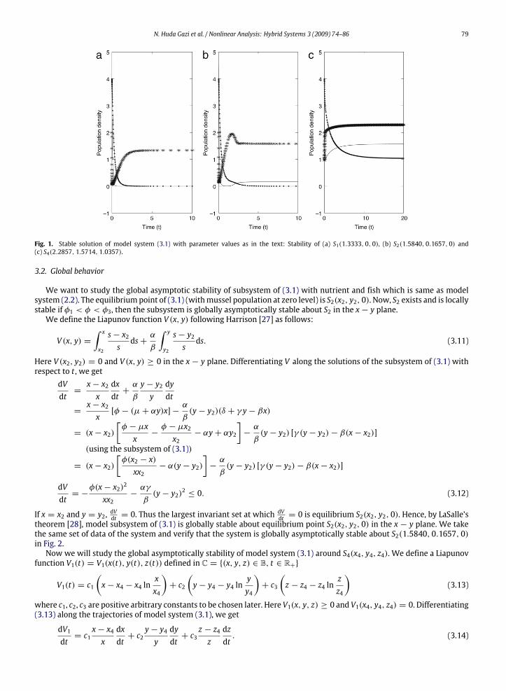
γ = 4, β = 8, ρ = 4 and η = 1.75. If we provide the external food input φ = 4.0, then the model system (3.1) is stableabout S1(1.3333, 0, 0) (see Fig. 1(a)). In this case, φ1 = 4.5, φ2 = 6.8571, both are less than φ. If we supply external foodφ = 10.0, then S1 becomes unstable and themodel system converges to S2(1.5840, 0.1657, 0) (Fig. 1(b)). Hereφ ∈ (φ1, φ3),φ3 = 78.6939. We take now the external food input φ = 100, then the model system is unstable about S2 and it becomesstable about S4(2.2857, 1.5714, 1.0357) (see Fig. 1(c)). Here φ > φ3.Thus different levels of external food input in the fish farm changes the system into different stable equilibrium states.

As the external food input is increased the mussel density is increased. The extra food which is not assimilated by the fishalways deteriorate the water quality leading to eutrophication of the farm. The excess food can help in the rapid increase ofthe fish population, but, at the same time it has negative effect on the fish population. The excess food not assimilated in thefarm will help in reducing the dissolved oxygen in the water column. As the mussel population is increased, the extra foodpresent as particulate organic matter in the water column of fish farm not assimilated by the fish population is consumed.Consequently, the water is cleared by the available mussel population, as a mussel behaves like a biofiltering system. Themussel integration can therefore help in making a balance in the aquaculture for sustaining the fish population and keepingthe ecosystem healthy.


Fig. 1. Stable solution of model system (3.1) with parameter values as in the text: Stability of (a) S1(1.3333, 0, 0), (b) S2(1.5840, 0.1657, 0) and(c) S4(2.2857, 1.5714, 1.0357).

3.2. Global behavior

We want to study the global asymptotic stability of subsystem of (3.1) with nutrient and fish which is same as modelsystem (2.2). The equilibriumpoint of (3.1) (withmussel population at zero level) is S2(x2, y2, 0). Now, S2 exists and is locallystable if φ1 < φ < φ3, then the subsystem is globally asymptotically stable about S2 in the x− y plane.We define the Liapunov function V (x, y) following Harrison [27] as follows:

V (x, y) =∫ x

x2

s− x2sds+

α

β

∫ y

y2

s− y2sds. (3.11)

Here V (x2, y2) = 0 and V (x, y) ≥ 0 in the x − y plane. Differentiating V along the solutions of the subsystem of (3.1) withrespect to t , we get

dVdt=x− x2xdxdt+α

β

y− y2y

dydt

=x− x2x

[φ − (µ+ αy)x]−α

β(y− y2)(δ + γ y− βx)

= (x− x2)[φ − µxx−φ − µx2x2

− αy+ αy2

]−α

β(y− y2) [γ (y− y2)− β(x− x2)]

(using the subsystem of (3.1))

= (x− x2)[φ(x2 − x)xx2

− α(y− y2)]−α

β(y− y2) [γ (y− y2)− β(x− x2)]

dVdt= −

φ(x− x2)2

xx2−αγ

β(y− y2)2 ≤ 0. (3.12)

If x = x2 and y = y2, dVdt = 0. Thus the largest invariant set at whichdVdt = 0 is equilibrium S2(x2, y2, 0). Hence, by LaSalle’s

theorem [28], model subsystem of (3.1) is globally stable about equilibrium point S2(x2, y2, 0) in the x − y plane. We takethe same set of data of the system and verify that the system is globally asymptotically stable about S2(1.5840, 0.1657, 0)in Fig. 2.Now we will study the global asymptotically stability of model system (3.1) around S4(x4, y4, z4). We define a Liapunov

function V1(t) = V1(x(t), y(t), z(t)) defined in C = (x, y, z) ∈ B, t ∈ R+

V1(t) = c1

(x− x4 − x4 ln

xx4

)+ c2

(y− y4 − y4 ln

yy4

)+ c3

(z − z4 − z4 ln

zz4

)(3.13)

where c1, c2, c3 are positive arbitrary constants to be chosen later. Here V1(x, y, z) ≥ 0 and V1(x4, y4, z4) = 0. Differentiating(3.13) along the trajectories of model system (3.1), we get

dV1dt= c1

x− x4xdxdt+ c2

y− y4y

dydt+ c3

z − z4zdzdt. (3.14)


Fig. 2. Global stability of model subsystem comprising food and fish of (3.1) about S2(1.5840, 0.1657, 0).

Fig. 3. Global stability of model system (3.1) at S4(2.2857, 1.5714, 1.0357).

Using (3.1) in the above expression, we getdV1dt= c1

x− x4x[φ − (µ+ αy+ ζ z)x] − c2(y− y4)(δ + γ y− βx)− c3(z − z4)(ζ − ηx).

Since S4 (x4, y4, z4) is an equilibrium point, the above expression reduces to

= c1(x− x4)[φ − µxx−φ − µx4x4

− (αy+ ζ z)+ (αy4 + ζ z4)]

− c2(y− y4) [δ + γ y− βx− (δ + γ y4 − βx4)]− c3(z − z4) [ζ − ηx− (ζ − ηx4)]

= c1(x− x4)[φ(x4 − x)xx4

− α(y− y4)− ζ (z − z4)]

−c2(y− y4) [γ (y− y4)− β(x− x4)]− c3(z − z4) [−η(x− x4)]

= −c1φ(x− x4)2

xx4− c2γ (y− y4)2 + (−αc1 + βc2)(x− x4)(y− y4)+ (−ζ c1 + ηc3)(z − z4)(x− x4).

Now, we choose c1 = 1, c2 = αβand c3 =

ζ

η, then

dV1dt= −

φ(x− x4)2

xx4−α

βγ (y− y4)2 ≤ 0. (3.15)

At S4(x4, y4, z4),dV1dt = 0. Thus the largest invariant subset at which

dV1dt = 0 is the equilibrium S4(x4, y4, z4). Hence,

by LaSalle’s theorem [28], the model system (3.1) is globally asymptotically stable about the coexisting equilibriumS4(x4, y4, z4). We use the same data set to verify the analytical result obtained here. Fig. 3 shows that model system (3.1) isglobally asymptotically stable about a point S4(2.2857, 1.5714, 1.0357).

4. Analysis of delay model

In this section we want to analyze the effect of a discrete time delay on the dynamics of model system (3.1) representingthree component in a fish farm around the coexisting equilibrium S4 (x4, y4, z4). In any biological system, ecology, in


particular, several species coexist depending on one another. The growth of a species on consumption of the other is abiochemical process that cannot occur instantaneously. It takes some amount of time for any type of such biochemicalprocess. In a realistic situation this type of time delay always occurs. So we take into account gestation delay of the fishpopulation for consumption on the food (nutrient). There are many literatures onmodeling delay differential equations [15,17–20]. In our study of model system (3.1), we incorporate delay due to gestation of the fish populations for consumptionof the food present in the fish farm.

4.1. Criteria for preservation of delay-induced stability

Many studies reveal that the delay has effect on stability of the equilibrium of a system and the model system becomesunstable exhibiting periodic oscillations. We take τ as a discrete type gestation delay of fish for consumption of the nutrientin the fish farm. Then model system (3.1) takes the following form

dxdt= φ − [µ+ αy+ ζ z]x,

dydt= −[δ + γ y− βx(t − τ)]y,

dzdt= −[ρ − ηx]z (4.1)

with initial densities x(θ) = ξ(θ) for −τ ≤ θ ≤ 0 where ξ(θ) ∈ C([−τ , 0],R+) and ξ(θ) ≥ 0, ξ(0) ≥ 0, y(0) > 0 andz(0) > 0. In a similar way as in Section 3, we derive the characteristic equation of the variational matrix associated with thelinearized system of (4.1) about S4(x4, y4, z4) as under

∆(λ, τ ) ≡ λ3 + pλ2 + q1λ+ q2λe−λτ + r = 0 (4.2)

where p = φ/x4 + γ y4, q1 = φγ y4/x4 + ηζ x4z4, q2 = αβx4y4 and r = γ ζηx4y4z4. At this stage, we want to analyzethe effect of discrete delay on the dynamics of the model system. Now we can find the condition for nonexistence of delayinduced instability by using the following theorem as a similar one in [17].

Theorem 4.1. A set of necessary and sufficient conditions for S4 to be locally asymptotically stable in presence of time delay, τ if

(i) The real parts of all the roots of ∆(λ, 0) = 0 are negative,(ii) For all real ω and any τ > 0,∆(iω, τ) 6= 0, where i =

√−1.

Proof. (i) First, we consider the case when τ = 0. Then from (4.2) we get characteristic Eq. (3.10) for non-delay modelsystem (3.1). We have obtained criteria that the roots of the equation are negative, that is, φ1 < φ2 and φ > φ3.(ii) Let τ 6= 0, then from (4.2), putting λ = iω, ω is any real number, we get

∆(iω, τ) = −pω2 + q2ω sinωτ + r + i(−ω3 + q1ω + q2ω cosωτ) (4.3)

If ω = 0, then∆(0, τ ) = r = γ ζηx4y4z4 > 0. Thus∆(0, τ ) 6= 0.Again if ω 6= 0, then, if possible, we suppose that iω satisfies the characteristic equation (4.2), that is,

∆(iω, τ) = −pω2 + q2ω sinωτ + r + i(−ω3 + q1ω + q2ω cosωτ) = 0. (4.4)

Separating real and imaginary parts we get

− pω2 + q2ω sinωτ + r = 0, −ω3 + q1ω + q2 cosωτ = 0 (4.5)

which when we square and add, gives

ω6 + (p2 − 2q1)ω4 + (q21 − 2pr − q22)ω

2+ r2 = 0 (4.6)

The equivalent cubic equation of (4.6) is

χ3 + (p2 − 2q1)χ2 + (q21 − 2pr − q22)χ + r

2= 0. (4.7)

The roots of Eq. (4.7) are the square of the roots of Eq. (4.6) and therefore are positive. Now, by Descartes’ rule of sign, for anequation with real coefficients, the non-existence of a positive root of Eq. (4.7) is that the coefficients are positive, that is,

p2 > 2q1 and q21 > 2pr + q22.

Combining this two inequalities we arrive at

p4 > 4(2pr + q22)

which is the condition that Eq. (4.6) does not have a positive ω2. So, iω is not a root of ∆(λ, τ ) = 0 and consequently∆(iω, τ) 6= 0 for any real ω and τ 6= 0 satisfying Eq. (4.5). Thus the nonexistence of delay induced instability of modelsystem (4.1) is given by

p4 > 4(2pr + q22).


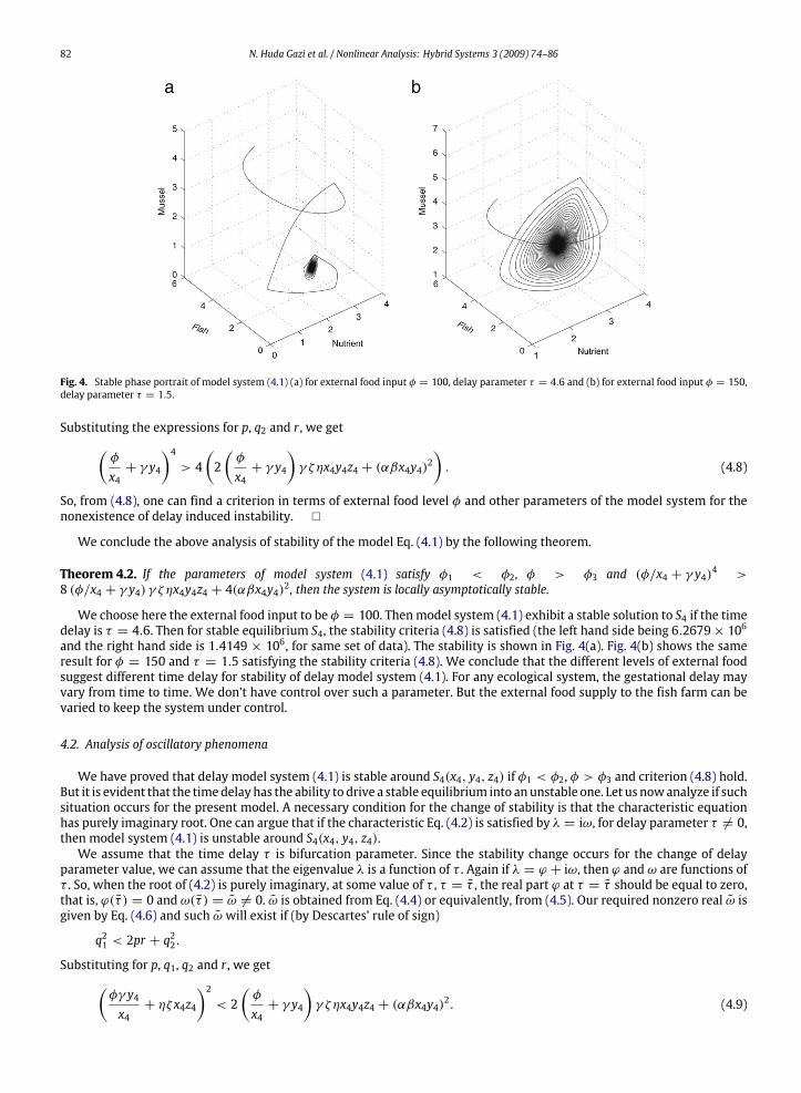
Fig. 4. Stable phase portrait of model system (4.1) (a) for external food input φ = 100, delay parameter τ = 4.6 and (b) for external food input φ = 150,delay parameter τ = 1.5.

Substituting the expressions for p, q2 and r , we get(φ

x4+ γ y4

)4> 4

(2(φ

x4+ γ y4

)γ ζηx4y4z4 + (αβx4y4)2

). (4.8)

So, from (4.8), one can find a criterion in terms of external food level φ and other parameters of the model system for thenonexistence of delay induced instability.

We conclude the above analysis of stability of the model Eq. (4.1) by the following theorem.

Theorem 4.2. If the parameters of model system (4.1) satisfy φ1 < φ2, φ > φ3 and (φ/x4 + γ y4)4 >8 (φ/x4 + γ y4) γ ζηx4y4z4 + 4(αβx4y4)2, then the system is locally asymptotically stable.

We choose here the external food input to be φ = 100. Thenmodel system (4.1) exhibit a stable solution to S4 if the timedelay is τ = 4.6. Then for stable equilibrium S4, the stability criteria (4.8) is satisfied (the left hand side being 6.2679× 106and the right hand side is 1.4149 × 106, for same set of data). The stability is shown in Fig. 4(a). Fig. 4(b) shows the sameresult for φ = 150 and τ = 1.5 satisfying the stability criteria (4.8). We conclude that the different levels of external foodsuggest different time delay for stability of delay model system (4.1). For any ecological system, the gestational delay mayvary from time to time. We don’t have control over such a parameter. But the external food supply to the fish farm can bevaried to keep the system under control.

4.2. Analysis of oscillatory phenomena

We have proved that delay model system (4.1) is stable around S4(x4, y4, z4) if φ1 < φ2, φ > φ3 and criterion (4.8) hold.But it is evident that the timedelay has the ability to drive a stable equilibrium into anunstable one. Let us nowanalyze if suchsituation occurs for the present model. A necessary condition for the change of stability is that the characteristic equationhas purely imaginary root. One can argue that if the characteristic Eq. (4.2) is satisfied by λ = iω, for delay parameter τ 6= 0,then model system (4.1) is unstable around S4(x4, y4, z4).We assume that the time delay τ is bifurcation parameter. Since the stability change occurs for the change of delay

parameter value, we can assume that the eigenvalue λ is a function of τ . Again if λ = ϕ + iω, then ϕ and ω are functions ofτ . So, when the root of (4.2) is purely imaginary, at some value of τ , τ = τ , the real part ϕ at τ = τ should be equal to zero,that is, ϕ(τ ) = 0 and ω(τ ) = ω 6= 0. ω is obtained from Eq. (4.4) or equivalently, from (4.5). Our required nonzero real ω isgiven by Eq. (4.6) and such ω will exist if (by Descartes’ rule of sign)

q21 < 2pr + q22.

Substituting for p, q1, q2 and r , we get(φγ y4x4+ ηζ x4z4

)2< 2

(φ

x4+ γ y4

)γ ζηx4y4z4 + (αβx4y4)2. (4.9)


Consequently, τ is given by (from (4.5))

τ =1ωarctan

[pω2 − rω3 − q1ω

]+jπω, j = 0, 1, 2, . . . . (4.10)

So, j = 0 in (4.10) gives

τ0 =1ωarctan

[pω2 − rω3 − q1ω

](4.11)

which is the smallest time delay for which ϕ(τ ) = 0 and ω(τ ) = ω 6= 0.Thus we have a pair (iω, τ ) for which the stable state of model system (4.1) around S4(x4, y4, z4) changes into unstable

one. We will analyze if it is a Hopf-bifurcation [29,30] at that point. Truly, we want to see when τ passes through τ = τ ,how the Reλ changes which is zero at (iω, τ ). So, we are to verify transversality condition d

dτ Re λ|(iω,τ ) 6= 0. Since we

need only the sign of ddτ Re λ|(iω,τ ), which is same as the sign of Re[ dλdτ

]−1|(iω,τ ), so, for the sake of simplicity, we calculate

Re[ dλdτ

]−1|(iω,τ ). Differentiating left hand side of (4.2) and then rearranging in the form of

[ dλdτ

]−1, we get,[

dλdτ

]−1=3λ2 + 2pλ+ q1

q2λ2eλτ +

1− λτλ2

. (4.12)

Now, after rearranging

Re[dλdτ

]−1∣∣∣∣∣(iω,τ )

=(−3ω2 + q1) cos ωτ − 2pω sin ωτ

−q2ω2−1ω2.

Nowmaking use of (4.5) and rearranging, we get,

Re[dλdτ

]−1∣∣∣∣∣(iω,τ )

=1q2ω2

[3ω4 + 2(p2 − 2q1)ω2 + q21 − 2pr − q

22

]. (4.13)

In Eq. (4.6), denoting the left hand side byΩ and taking ω2 = s, we get,

Ω = s3 + (p2 − 2q1)s2 + (q21 − 2pr − q22)s+ r

2

which after differentiation at s = ω2 gives the right hand side of (4.13). Therefore, from (4.13), we get

Re[dλdτ

]−1∣∣∣∣∣(iω,τ )

=1q2ω2

dΩds

∣∣∣∣s=ω2

. (4.14)

The sign of (4.14) is either positive or negative but nonzero ( 6= 0) as the characteristic Eq. (4.2) cannot have a multipleimaginary roots.Thus the transversality condition is satisfied and therefore, the point (iω, τ ) is a Hopf type bifurcation point. Therefore,

model system (4.1) has a periodic oscillation around S4(x4, y4, z4) if the condition (4.9) is satisfied. Thus for certain levels ofthe external food φ to be deduced from (4.9) and for τ ≥ τ (smallest τ being τ0), the stable solution of the model systemoscillates and exhibit a periodic oscillation around the equilibrium S4(x4, y4, z4). We summarize the above analysis by thefollowing theorem.

Theorem 4.3. (i) If φ1 < φ2, φ > φ3 and (φ/x4 + γ y4)4 > 8 (φ/x4 + γ y4) γ ζηx4y4z4 + 4(αβx4y4)2, then the equilibriumS4 is asymptotically stable for all τ ≥ 0. If the above is satisfied then S4 is locally asymptotically stable for τ ∈ [0, τ0). (ii) Ifφ1 < φ2, φ > φ3 and (φγ y4/x4 + ηζ x4z4)2 < 2 (φ/x4 + γ y4) γ ζηx4y4z4 + (αβx4y4)2, then model system (4.1) is unstablefor τ ≥ τ0. Hopf-bifurcation occurs at τ = τ0. Thus the periodic solution bifurcates from S4 as τ passes through τ0.

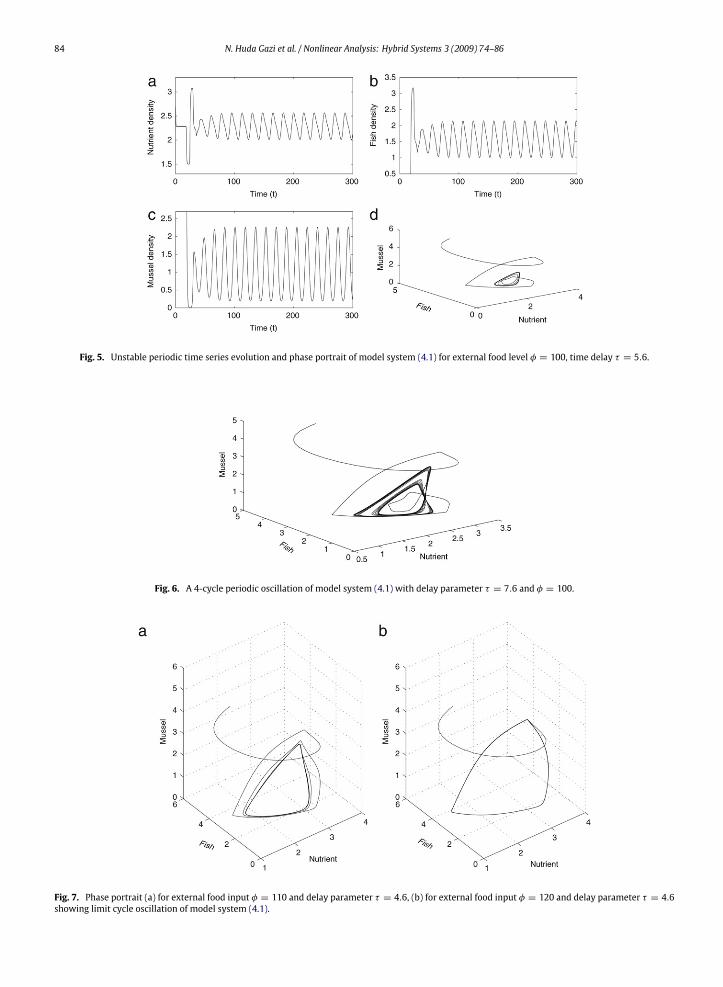
Thus from the above discussionwe conclude thatmodel (4.1) system is stable for some φ satisfying (4.8) and 0 ≤ τ < τ0.If τ ≥ τ0 and the external food input satisfies (4.9), then the delay model system becomes unstable. We verify theabove analytical results numerically for the same data set. We have seen that when φ = 100 and τ = 4.6, the systemexhibits the stable solution (Fig. 4(a)). If τ is increased to τ = 4.8, the external food level being φ = 100 satisfying (4.9)(LHS = 9.7522× 104 and RHS = 3.5373× 105), then equilibrium S4 loses stability and bifurcates into 2-cycle [31] periodicoscillation. Thus τ0 lies between 4.6 and 4.8. If we go on increasing the time delay value, the amplitude of the periodicoscillation is increased leading to a stable limit cycle of the system around S4 when φ = 100, τ = 5.6 (see Fig. 5). If weincrease the delay value, the 2-cycle stable limit cycle loses stability exhibiting a 4-cycle periodic oscillation (see Fig. 6).If the external food level is increased keeping the timedelay value fixed,we see that as the external food level is increasing

the stable trajectories of the model system becomes unstable (see Fig. 4(a) and Fig. 7).We conclude that time delay can drive the stable system into unstable periodic oscillation. Keeping the delay value fixed,

the different external food levels can make a unstable oscillation into a stable system. Thus the external food supply is avery important instrument for the stability of a fish farm.


Fig. 5. Unstable periodic time series evolution and phase portrait of model system (4.1) for external food level φ = 100, time delay τ = 5.6.

Fig. 6. A 4-cycle periodic oscillation of model system (4.1) with delay parameter τ = 7.6 and φ = 100.

Fig. 7. Phase portrait (a) for external food input φ = 110 and delay parameter τ = 4.6, (b) for external food input φ = 120 and delay parameter τ = 4.6showing limit cycle oscillation of model system (4.1).


5. Conclusion

In this paper we have considered the deterministic model of a fish farm with three interacting components: food(nutrient), fish and mussel population. We have stated and proved several results giving criteria for the existence of severalequilibriumpoints, stability and bifurcations for themodel system in presence of discrete type time delay. Themajor, aswellas, important results we have obtained for stability (local and global) of the differential equations and the delay differentialequation model system in order to study the effect of gestational delay on various dynamic behaviors with different levelsof external food input. Time delays have the ability to drive a stable equilibrium point to an unstable one and it is alsoresponsible for the oscillations of various trophic levels. Here we have seen that the external food supply also drive thedelayed system into an unstable oscillation.In Section 3, we have seen that the all the solutions of model system representing food, fish and mussel population of a

fish farm are uniformly bounded in a finite region. Since the region is defined by B = (x, y, z) ∈ R3+: 0 ≤ x + y + z ≤

φ/ν + ε, for any ε > 0, finite region is dependent on the external food input. The increased external food input widensthe region and the populations assume more densities. Then, we have seen that four equilibria are feasible depending onthe density level of the external food input. The 3-dimensional model (3.1) is an extension of the model system (2.2) [23].The model system has an equilibrium ( φ

µ, 0) which is unstable for a greater nutrient (food) level φ > φ1 which leads to

eutrophication of the fish farm. In the present study (with model system (3.1)), the level of the nutrient (φ > φ1) drivesthe model system into an unstable one around the similar [23] equilibrium point S1(x1, 0, 0). Our model system is stablearound S2(x2, y2, 0)when the nutrient level exceeds φ1, but does not exceed a higher level φ3, (φ1 < φ3). The study showsthat (mathematically) only nutrient and mussel population cannot coexist. The equilibrium S4(x4, y4, z4) where the threecomponents (nutrient, fish, mussel) coexist when external input of nutrient exceeds the critical level φ3. Also the ratio ofthe death rate of fish to it’s conversion efficiency of food precedes that of mussel population. Thus, different levels of foodsuggest the coexistence of different populations and the stability (local) of the coexistence.For a particular set of parameter values the model system is asymptotically stable at S1(1.3333, 0, 0) when φ = 4.0 <

φ1(= 4.5) and φ = 4.0 < φ2(= 6.8571). When the external food input increased to φ = 10.0, the equilibrium S1becomes unstable and the system converges to S2(1.5840, 0.1657, 0), the external food input being limited inφ1(= 4.5) andφ3(= 78.6939). The increased level of external food input leads the equilibrium S2 into an unstable state when it exceedsφ3(= 78.6939), the interior equilibrium S4 becomes stable at S4(2.2857, 1.5714, 1.0357), φ = 100 (Fig. 1(a), (b), (c)). Thusdifferent levels of external food input determine the stability of the coexistence of different populations. The increasedfood input which is not assimilated by the fish always deteriorate the water quality. As the mussel population is increased,consuming extra food present in the water column can help in increasing the oxygen level indirectly. Thus the effect ofoxygen depletion in the water column is reduced in this way sustaining a balance in the fish farm.We have proved that the subsystem is globally stable in the x− y plane when φ1 < φ < φ3 by constructing a Liapunov

function. We have constructed a Liapunov function V1(t) to study the global stability of model system (3.1) around S4.We have shown that the model system in globally asymptotically stable about S4 when φ1 < φ2 and φ > φ3. We havetaken the same set of data for parameters of the system and verified that the system is globally asymptotically stable aboutS2(1.5840, 0.1657, 0) (Fig. 2). We have used the same data set to verify the analytical result obtained. Fig. 3 shows thatmodel system (3.1) is globally asymptotically stable about a point S4(2.2857, 1.5714, 1.0357). For any initial density of thedifferent populations, the subsystem of (3.1) with food and fish population and the system (3.1) are globally asymptoticallystable at S2 and S4 respectively.Delay model system (4.1) analysis shows more complicated behavior than its non-delayed counterpart. The stability of

the system about S4 suggests some value of the delay parameter given by the equations in (4.10) and the smallest valueof τ being τ0 given in (4.11). For a particular data set used earlier, the system remains stable at external food input levelφ = 100 when τ = 4.6 satisfying the conditions φ1 < φ2, φ > φ3 and p4 > 4(2pr + q22). The stability is shown in Fig. 4(a).Fig. 4(b) also shows the same result for φ = 150 and τ = 1.5 satisfying p4 > 4(2pr + q22). The system bifurcates into2-cycle periodic oscillation when τ ≥ τ0, τ0 ∈ (4.6, 4.8). As the delay parameter value or the level of external food inputis increased, the amplitude of the oscillation is increased. With φ = 100 and τ = 7.6, the 2-cycle periodic oscillation losesstability and becomes a 4-cycle periodic oscillation (Fig. 6). Increasing the external food level (delay parameter value fixed)annihilates stable trajectories of the model system and the system exhibits periodic oscillation ultimately leading to limitcycle oscillation (see Fig. 7). From this analysis we conclude that the delay parameter value and the external food inputdriving the system from stable state to unstable one can control the system. The delay parameter is not in our control. Incontrast, the external food input level can be controlled. Therefore, the external food can control the system frompopulationoscillation. Thus external food input has a very important role in shaping the dynamics of the system of the fish farm.

References

[1] R.L. Naylor, R.J. Goldburg, J.H. Primavera, N. Kautsky, M.C.M. Beveridge, J. Clay, C. Folke, J. Lubchenco, H. Mooney, M. Troell, Effect of aquaculture onworld fish supplies, Nature 405 (2000) 117–124.

[2] P. Pitta, I. Karakassis, M. Tsapakis, S. Zivanovic, Natural vs mariculture induced variability in nutrients and plankton in the Eastern Mediterranean,Hydrobiologia 391 (1999) 181–194.

[3] I. Karakassis, M. Tsapakis, E. Hatziyanni, P. Pitta, Diel variation of nutrients and chlorophill in sea beam and sea bass cages in the Mediterranean,Fresenius Environment Bulletin 10 (2001) 278–283.


[4] O. Delgado, J. Ruiz, M. Perez, J. Romero, E. Ballestreros, Effects of fish farming on seagrass (Posidonia Oceanica) in a Mediterranean bay: sea grassdecline after loading cessation, Oceanol. Acta. 22 (1999) 109–117.

[5] J.M. Ruiz, M. Perez, J. Romero, Effect of fish farm loading on seagrass (Posidonia Oceania) distribution, growth and photosynthsi, Marine PollutionBulletin 42 (2001) 749–760.

[6] I. Karakassis, P. Pitta, M.D. Krom, Contribution of fish farming to the nutrient loading of the Mediterranean, Scientia Marina 69 (2) (2005) 313–321.[7] S. Ray, M. Strakraba, The impact of detritivorous fishes on the mangrove estuarine system, Ecological Modelling 140 (2001) 207–218.[8] G.P. Samanta, D. Manna, A. Maiti, Bioeconomic modelling of a three-species fishery with switching effect, The Korean Journal of Computational &Applied Mathematics 12 (1–2) (2003) 219–231.

[9] M. Bandyopadhyay, R. Bhattacharyya, B.Mukhopadhyay, Dynamics of an autotroph herbivore ecosystemwith nutrient recycling, EcologicalModelling176 (2004) 201–209.

[10] G.S. Jacinto, Fish cage farming in coastal waters—environmental, biological, social and governance issues, pp. 48–56, in: B.V.L. Querijero, C.R. Pagdilaoand S.V. Ilagan (Eds.), Guidelines in the Establishment of Fish Cages and Other Structures in Lakes and Coastal Waters. PCAMRD Book Series No.36/2006, Los Baõs, Laguna, Philippines, 2006, p. 174.

[11] H. Iwasaki, Recent progress of red tide studies in Japan: An overview, in: T. Okaichi (Ed.), Red Tides, Biology, Environmental Science and Toxicology,Elsevier, Amsterdam, 1989, p. 3.

[12] D.J.W. Moriarty, Control of luminous vibrio species in penaeid aquaculture ponds, Aquaculture 164 (1998) 351–358.[13] K.S.P. Shin, Shellfish used as fish farm biofilter, Research Frontier 10 (2005).[14] B.W. Cheshuk, G.J. Purser, R. Quintana, Integrated open-water mussel (Mytilus planulatus) and Atlantic salmon (Salmo salar) culture in Tasmania,

Australia, Aquaculture 218 (1–4) (2003) 357–378.[15] J.M. Cushing, Integro–differential equations and delay model in population dynamics, Springer-Verlag, Heidelberg, 1977.[16] K. Gopalsamy, Harmless delay in model systems, Bulletin of Mathematical Biology 45 (1983) 295–309.[17] K. Gopalsamy, Stability and Oscillation in Delay Differential Equations of Population Dynamics, Kluwer Academic Publisher, The Netherlands, 1992.[18] Y. Kuang, Delay Differential Equations with Application in Population Dynamics, Acadermic Press, New York, 1993.[19] R.M. May, Time delay versus stability in population models with two and three tropic levels, Ecology 4 (1973) 315–325.[20] S. Ruan, Absolute stability, conditional stability and bifurcation in Kolmogorov-type predator–prey systemswith discrete delays, Quarterly of Applied

Mathematics 59 (1) (2001) 159–173.[21] E. Beretta, Y. Kuang, Convergence results in a well-known delayed prey–predator system, Journal of Mathematical Analysis and Applications 204

(1996).[22] S.R. Carpenter, D. Ludwig, W.A. Brock, Management of eutrophication for lakes subject to potentially reversible change, Ecological Applications 9

(1999) 751–771.[23] A. Ardito, S. De Gregorio, L. Lamberti, P. Ricciardi, Dynamics of a lake ecosystem, in: L.M. Ricciardi (Ed.), Biomathematics and Related Computational

Problems, 1988, pp. 111–119.[24] G. Birkhoff, G.C. Rota, Ordinary Differential Equation, Ginn. and Co., 1982.[25] R.M. May, Stability and Complexity in Model Ecosystems, Princeton University Press, New Jersey, 2001.[26] J.D. Murray, Mathematical Biology, Springer, 2002.[27] G.W. Harrison, Global stability of predator–prey interaction, Journal of Mathematical Biology 8 (1979) 159–171.[28] J. LaSalle, S. Lefschetz, Stability by Liapunov’s Direct Moethod, Academic Press, New York, 1961.[29] B.D. Hassard, N.D. Kazarinoff, Y.H. Wan, Theory and Applications of Hopf-bifurcation, Cambridge University Press, Cambridge, 1981.[30] J.E. Marsden, M. Ma Krachen, Hopf-bifurcation and its Application, Springer, New York, 1974.[31] M. Kot, Elements of Mathematical Ecology, Cambridge University Press, Cambridge, 2001.

integration of mussel in fish farm: mathematical model and analysis

Documents