1

FACTORS AFFECTING VARIABILITY IN FARM AND OFF-FARM INCOME

Kenneth Poon

(poonk@uoguelph.ca)

and

Alfons Weersink

(aweersin@uoguelph.ca)

The authors are a research associate and a professor, Dept of Food, Agricultural and Resource Economics (FARE),

University of Guelph, Guelph Ontario N1G 2W1.

Cahier de recherche/Working paper #2011-3

2

Factors Affecting Variability in Farm and Off-farm Income

Abstract The purpose of this paper is to examine the factors affecting the relative variability in farm and off-farm income for Canadian farm operators. Previous attempts have been limited by the lack of available data combining both farm and off-farm income levels for farm operations over time. Statistic Canada’s Farm Micro-Longtidinal Dataset of 17,000 farm operators from 2001 to 2006 allowed such an analysis. The coefficient of variation (CV) in farm income is significantly greater than that for off-farm income but both measures are inversely related to the permanence of the income source to the operation. The greater the reliance on farm income and the greater the labour demand within the farm, the lower (greater) the relative variability in farm (off-farm) income. Larger commercial operations tend to experience larger farm income volatility either because they are less risk averse and/or have the ability to manage more risk. Diversification and off-farm employment appear to be substitute for risk management strategies for commercial operations. Pension and lifestyle farms have lower coefficient of variation for both farm and off-farm income compared to business-focused farms since they are possibly more risk averse and benefit from a permanent stream of off-farm revenue. Government payments have mixed effects on the relative variability of both income sources, which may be due the lag between the time of the income reduction and the time at which the aid is received. Résumé Cet article examine les facteurs qui influent sur la variabilité relative des revenus agricoles et hors ferme des exploitants agricoles canadiens. Les tentatives précédentes ont été limitées par le manque de données chronologiques combinant les revenus agricoles aux revenus hors ferme des exploitations agricoles. Notre analyse utilise de la banque de données de Statistiques Canada Farm Micro-Longtidinal Dataset qui compile de l’information sur 17000 exploitants agricoles de 2001 à 2006. Le coefficient de variation (CV) du revenu agricole est nettement supérieur à celui du revenu hors ferme, mais les deux mesures sont inversement proportionnelles à la permanence de la source du revenu considéré. Plus grande est la dépendance à l'égard du revenu agricole et plus grande la demande de travail au sein de la ferme, plus faible (grande) sera la variabilité du revenu agricole par rapport au revenu hors ferme. Les grandes exploitations commerciales ont tendance à afficher une plus grande volatilité du revenu agricole, soit parce qu'elles sont moins sensibles au risque et/ou ont une capacité accrue de gestion des risques. La diversification et un emploi hors ferme semblent être des substituts pour des stratégies de gestion des risques pour les fermes commerciales. Les fermes appartenant à un retraité et les fermes d'agrément ont un plus faible coefficient de variation pour les revenus agricoles et non agricoles par rapport aux fermes commerciales possiblement parce que les opérateurs sont plus riscophobes et bénéficient d'un flux permanent de revenus hors ferme. Les paiements gouvernementaux ont des effets mixtes sur la variabilité relative des deux sources de revenu, probablement à cause du décalage temporel entre la réduction des revenus et l'envoi de l’aide. The authors wish to acknowledge the helpful comments provided by Alessandro Alessia, Ray Bollman, and an anonymous SPAA reviewer. Financial support was provided by the Ontario Ministry of Agriculture, Food and Rural Affairs (OMAFRA), Statistics Canada and by the Structure and Performance of Agriculture and Agri-products Indusry (SPAA) research network which is part of Agriculture and Agrifood Canada’s Enabling Research for a Competitive Agriculture (ERCA) program. Weersink also wishes to acknowledge the support of the Business Economics Group, Wageningen University.

3

Factors Affecting Variability in Farm and Off-farm Income

Introduction

Economic well-being is affected not only by the level of income but also its fluctuations.

The financial hardship caused by unexpected income losses are the basis for a range of public

policy programs that provide a safety-net in times of need. In the agricultural sector, income

stabilization is a major objective of government programs, such as Canadian Agricultural Income

Stabilization (CAIS) and AgriStability, which compensate farm operators when they experience

a decline in income or production margin. The payouts from these programs have risen from

$2.56 billion in 2002 to a peak of $3.97 million in 2005 and have since fallen back down to

$2.83 million in 2008. However, payments received per operator have risen from $3,500 in 1995

to approximately $11,500 for crop operations and $20,900 for livestock operations in 2008

(calculations from CANSIM, 2010). The potential for greater market volatility in the future

(FAO, 2010) implies potentially greater demands on these programs and greater scrutiny

surrounding which types of farms require support. In addition to knowing how the levels of

government funds may flow to alternative farm types, it is important to know whether these

funds do stabilize farm income as opposed to encouraging greater risk-taking behavior on the

part of farms.

Income stabilization for farms no longer means income stabilization for farm families as

approximately half of Canadian and American farm operators have off-farm employment

(Niekamp 2009, O’Donoghue et. al. 2009). Thus, understanding the financial well-being of farm

families requires assessing the variability of off-farm income as well as farm income variation.

Depending on the type of farms, the pursuit of off-farm income opportunities may be construed

4

as a self-insurance mechanism complementing government programs to stabilize household

income or it could be motivated by changes in labour market conditions that impose significant

hardship on low-equity families relying more on off-farm income than revenue from the farm to

pay for household expenditures.

While income variation remains a focus of public policy programs, the factors affecting

its variability are not well-understood. Schurle and Tholstrup (1989) found income variability

for Kansas farms to be influenced by factors affecting business risk such as enterprise mix,

returns and size. Using an updated sample of the same Kansas farms, Purdy, Langemeier and

Featherstone (1997) found specialization and business risk position increased the variance of

returns on equity. Barry, Escalante and Bard (2001) also found that diversification reduced farm

income variability by using a panel of Illinois farms as opposed to a single cross-section. The

majority of studies on off-farm income have examined the factors affecting the decision to

participate in off-farm employment (Huffman 1980). A few recent studies have extended this

analysis to consider the dynamics of the participation decision and more specifically the duration

of the participation (e.g., Ahituv and Kimhi 2002; Phimister et al. 2002; Corsi and Findeis 2000).

The role of off-farm income on the adoption of risk-mitigating strategies has been analyzed by

Valendia et al. (2009). None of these studies have examined the variability in off-farm income

nor have studies examined the variance in both sources of income.

The purpose of this paper is to examine the factors affecting the variability in farm and

off-farm income for Canadian farm operators. The paper begins with a conceptual framework

about labour allocation among alternative farm enterprises and off-farm employment. We use

labour allocations to compute the variances in farm and off-farm income. We then identify and

measure the impact of factors conditioning these variances. . The next section presents summary

5

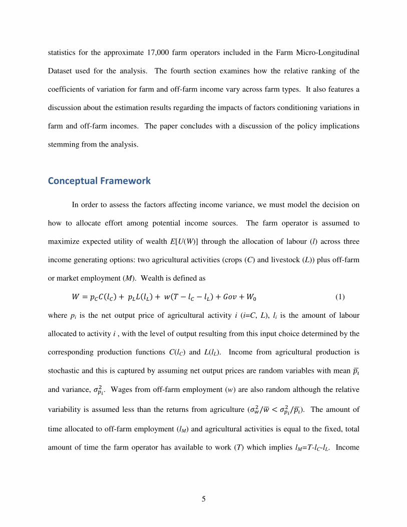
statistics for the approximate 17,000 farm operators included in the Farm Micro-Longitudinal

Dataset used for the analysis. The fourth section examines how the relative ranking of the

coefficients of variation for farm and off-farm income vary across farm types. It also features a

discussion about the estimation results regarding the impacts of factors conditioning variations in

farm and off-farm incomes. The paper concludes with a discussion of the policy implications

stemming from the analysis.

Conceptual Framework

In order to assess the factors affecting income variance, we must model the decision on

how to allocate effort among potential income sources. The farm operator is assumed to

maximize expected utility of wealth E[U(W)] through the allocation of labour (l) across three

income generating options: two agricultural activities (crops (C) and livestock (L)) plus off-farm

or market employment (M). Wealth is defined as

� = ������� + ������� + �� − �� − ��� + ��� + �� (1)

where pi is the net output price of agricultural activity i (i=C, L), li is the amount of labour

allocated to activity i , with the level of output resulting from this input choice determined by the

corresponding production functions C(lC) and L(lL). Income from agricultural production is

stochastic and this is captured by assuming net output prices are random variables with mean ���

and variance, ���

� . Wages from off-farm employment (w) are also random although the relative

variability is assumed less than the returns from agriculture (��� / � < ���

� /��� ). The amount of

time allocated to off-farm employment (lM) and agricultural activities is equal to the fixed, total

amount of time the farm operator has available to work (T) which implies lM=T-lC-lL. Income

6

can also be earned from two additional sources: government payments related to agricultural

production (Gov) and initial or exogenous wealth (W0).

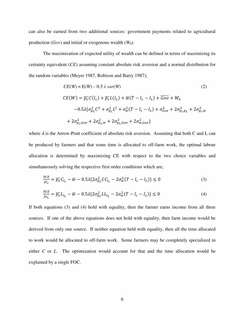
The maximization of expected utility of wealth can be defined in terms of maximizing its

certainty equivalent (CE) assuming constant absolute risk aversion and a normal distribution for

the random variables (Meyer 1987, Robison and Barry 1987);

CE(W) = E(W) – 0.5 λ var(W) (2)

����� = ���������� + ���������� + ��� − �� − ��� + �������� + ��

−0.5#{��%

� �� + ��&

� �� + ��� �� − �� − ��� + �'()

� + 2��+,�&

� + 2��+,��

+ 2��+,'()� + 2��&,�

� + 2��&,'()� + 2��,'()

� }

where λ is the Arrow-Pratt coefficient of absolute risk aversion. Assuming that both C and L can

be produced by farmers and that some time is allocated to off-farm work, the optimal labour

allocation is determined by maximizing CE with respect to the two choice variables and

simultaneously solving the respective first order conditions which are;

.�/

.0+= ������0+

− � − 0.5#{2��%

� ��0+− 2��

� �� − �� − ���} ≤ 0 (3)

.�/

.0&= ������0&

− � − 0.5#{2��&

� ��0&− 2��

� �� − �� − ���} ≤ 0 (4)

If both equations (3) and (4) hold with equality, then the farmer earns income from all three

sources. If one of the above equations does not hold with equality, then farm income would be

derived from only one source. If neither equation held with equality, then all the time allocated

to work would be allocated to off-farm work. Some farmers may be completely specialized in

either C or L. The optimization would account for that and the time allocation would be

explained by a single FOC.

7

Whether a farmer decides to seek off-farm employment depends on comparing the

marginal returns to farm employment (pi �0�) to the wage rate with all labour allocated to farm

work. If the reservation wage is less than the market wage, then the operator will work off the

farm until the FOCs are satisfied (Huffman 1980). Note that the optimal labour allocation (l*)

depends on the marginal productivity of labour in the alternative activities, the variability in

those efforts, the covariance, and risk aversion. Substituting the optimal labour choices

determines the expected returns among the three income sources along with the variability in

those returns.

The variance in income sources will thus depend on the factors influencing the optimal

effort across these sources. One variable will be farm type. In terms of farm income variability,

price and production uncertainty will vary across sectors. Production uncertainty tends to be

lower for livestock productions than for crop productions because the former are less impacted

by weather conditions which are inherently volatile. Price levels will be higher and variability

lower for supply managed sectors due to the nature of the mandated policies.

Farm type influences off-farm income variability in several ways. Sectors with lower

relative returns, and thus a lower reservation wage, will be more inclined to work off the farm

and this could either reduce or increase off-farm income variance. Farmers on such operations

might be employed full-time in stable off-farm work which would lower off-farm income

variance. On the other hand, these farmers might be in and out of the off-farm labour market,

getting into off-farm activities that do not require a substantial time commitment, and this would

be associated high higher off-farm income variance. In addition, some sectors are more likely to

have surplus labour at some points during the year and are more conducive to off-farm

employment than more labour-demanding sectors such as dairy (Alasia et al. 2009). Finally,

8

given the diversification effects of off-farm employment, it is expected that farm types with

greater income volatility will increase the likelihood of off-farm employment for farms in those

sectors and subsequently increase the variance in off-farm income ((Jetté-Nantel et al. 2010);

Mishra and Goodwin 1997).

Farm size, regardless of farm type, will also affect the variability in farm and off-farm

income. Increases in size can increase relative income due to production and pecuniary

economies of size. Larger farms may also be more adept at coping with risk either due to greater

management ability or to greater access to risk-management strategies ranging from credit

reserves to hedging (Valendia et al. 2009, Goddard et al. 1993). However, this ability to cope

with risk may induce larger farms to handle greater farm income variance and several studies

have estimated a positive relationship between size and net farm income volatility (Dunn and

Williams 2000; Schurle and Tholstrup 1987; and Pope and Prescott 1980). However, Barry,

Escalante and Bard (2000) and Purdy, Langemeier and Featherstone (1997) found that farm size

had no effect on the risk/return tradeoff.

The effect of farm size on the variance of off-farm income is also likely indeterminate.

While the likelihood of off-employment decreases with farm size (Alasia et al. 2009), the

variance may increase. Small farms are more likely to use off-farm employment as a permanent

income source while larger farms are more likely to seek outside income in times of financial

pressures within the agricultural sector. The self-insurance use of outside work for commercial

producers suggests that the variance in off-farm income is likely to increase with farm size.

Specialization increases risk and therefore variability according to portfolio theory

(O’Donoghue, Roberts, and Key 2009). Shurle and Tholstrup (1989) found that both

specialization and variance in returns correlates with average net farm income implying

9

movement along the tradeoff curve between mean returns and business risk. However, the

empirical evidence on the effect of diversification on farm income variance is mixed. Purdy,

Langemeier, and Featherstone (1997) found that specialization increased volatility for crop

operations, but not for livestock farms suggesting that there are differences in risk management

strategies across farm types. The effect of diversification may not only depend on farm type but

also location. Barry, Escalante and Bard (2000) found that diversification is only significantly

related to reduction in volatility in areas with a low concentration of highly specialized farms.

Location will also affect the variability in farm returns in other manners. While it may

not have as large an impact on the livestock sector, it is assumed that variability in crop returns

will be higher in the Prairie provinces where greater fluctuations in weather patterns are

observed. Regions will also vary in terms of the vibrancy and stability of the labour market and

this will have effects on the variability in off-farm income (Alasia et al. 2009). The volatility in

off-farm income is assumed to be directly correlated with the volatility in local employment

conditions.

The theoretical model provides no testable hypotheses on the effect of age. Purdy,

Langemeier, and Featherstone (1997) suggest using the operator’s age as a proxy of experience,

and more experienced operators are able to manage risk better leading to lower volatility. Rather

than risk management ability, the inverse relationship between age and farm income variance

may have been due to the length of planning horizon. Less risk-taking activities are likely to

used the shorter the planning horizon. Schurle and Tholstrup (1989) find age to be positively

related to the variance of net farm income and propose the result could be due to older operators

being less flexible in adjusting to unusual circumstances and/or less risk averse due to higher

wealth. Barry, Escalante, and Bard (2001) combine the two possibilities and find a quadratic

10

relationship between age and volatility implying experience reduces volatility up to a certain

point in the operator’s life cycle. The same non-linear relationship for age has also been found in

many other empirical studies on off-farm labour supply. The relative returns to market

employment are expected to increase with age but then decline suggesting that it will likely have

a similar effect on the variance in off-farm income.

Government payments are intended to supplement farm income in times of need. The

negative covariance effect thus suggests that these support payments reduce the volatility of farm

income and several studies have estimated an inverse relationship (Jetté-Nantel et al. 2010;

Purdy, Langemeier, and Featherstone 1997; and Schurle and Tholstrup 1989). However, several

other studies have found that the reduction in risk associated with government payments may

actually increase overall volatility by inducing risk averse producers to use higher levels of risk-

increasing inputs (Serra et al. 2005; Hennessy 1998). This wealth effect of government policy

suggests the impact of a support program on farm income volatility is indeterminate. The

theoretical model suggests the wealth effect of higher government funds will decrease the

likelihood of off-farm work and thus the variability in off-farm income. However, sectors with

higher government payments may also be the ones requiring additional measures of risk

mitigation such as off-farm employment, suggesting that government payments could be

positively related to the variation in off-farm income.

Methods

We use a two-step approach to measure the impact of the factors affecting the variance of

farm and off-farm income. The first step consists of ranking all farmers by the value of their

coefficient of variation for each income source. Quintiles are established for each ranking. The

11

quintile cutoffs are based on the weighted sample so that each quintile will not necessarily have

the same number of observations (20%) as would unweighted quintiles.

The quintiles are plotted for the whole data set, by production types and by the

Agriculture and Agri-Food Canada (AAFC) farm typology that categorizes farms into seven

types on the basis of farm revenue and household characteristics. The quintiles of income

variation are determined and then the percentage of farm operators of a particular group, such as

production type, within each quintile are examined. The resulting bivariate distribution reveals

the ‘spread’ of volatility and illustrates whether operators in a specific farm typology category

are concentrated into one volatility quintile or evenly spread between quintiles. Since an

operator in one category can be placed in different quintiles depending on the volatility measure

and income source, these graphs can also show the volatility relationships across groupings and

income types.

The second step entails regressing the coefficient of variation for farm and off-farm

income against a set of explanatory variables defined in the next section. Two sets of regression

analysis were done: a 1-period OLS regression model and a 4-period panel regression model.

For the 1-period model, each of the variables with 6 years of data is condensed to a single

measure (this is described in the data section below). For example, the 6-year volatility for farm

and off-farm income were measured by single CV observations, which are then regressed against

independent variables that are also condensed into single observations. The second set of

regressions condenses the 6-year longitudinal sample into four 3-year periods, and a fixed effects

panel regression is applied. This maximizes the length of the panel given that 6 years are

available and that each CV is computed with three years of data. The time trend in the panel

regression is used to account for inter-temporal patterns common to all farms in the sample but

12

not captured by the explanatory variables. These patterns include price fluctuations, weather

patterns, and other exogenous factors and conditions that change over time but cannot be

effectively captured in the model.

Data

Data Source

The analysis uses the Farm Micro-Longitudinal Dataset, which contains the income tax

files of approximately 38,000 Canadian farm operators or shareholders between the years of

2001 to 2006. However, only individuals associated with unincorporated farms plus their family

members are included in the sample since the study requires information on the operator’s off-

farm income as well as farm income. Individuals involved with incorporated farms (31% of the

records) were excluded from the analysis for two reasons: (1) it is impossible to distinguish

between the operator’s farm earnings and the operator’s off-farm earnings as the incorporated

farm flows earnings to its shareholders as wages or as dividends, and (2) there is no information

on the operator’s family income. Tax files with average gross farm revenue less than $10,000

(7% of unincorporated farms), as well as operators of farms with a non-farm label for any one-

year (29% of unincorporated farms) were also excluded from the dataset.

Only one operator from each farm and each family is kept, so inferences can be made at

the one-operator-per-farm-per-family level. Matching the Family Identification Number (FIN)

and gross farm revenue of the tax records identifies operators in the same farm and family. For

multiple operators with matching FIN and gross farm revenue, only the eldest operator with the

largest share was kept in the sample. For ‘duplicate’ operators with the same age and farm share,

one operator was picked and kept randomly. Duplicates represented 9% of unincorporated farms

13

in the sample. This leaves a final sample size of approximately 17,000 operators representing a

population of 175,000 farms across Canada. This subset follows a contingent group of

unincorporated, non-hobby farms within the longitudinal sample who have been active in

agricultural production for all six years in sample.

Variable Definition

Dependent Variables

Farm income is calculated as gross farm operating revenues minus gross farm operating

expenses. This is calculated before depreciation and it also includes government payments.

Only records with positive average farming income over the six year period are included

although negative net farm income in given sample years are possible. Off-farm income is non-

negative and is defined as the sum of wages and salaries plus net unincorporated self-

employment income from operating a non-farm enterprise. Off-farm income can also include

investment income, pension income, and social transfers. Both income sources, along with all

other monetary values, were adjusted to real 2001 dollars using the Consumer Price Index.

The volatility for each of the two income sources is measured in relative terms by the

coefficient of variation (CV). A single CV measure is calculated for each income type over the

six year period. The CV for each grouping of 3 successive time periods was also calculated, but

the results did not differ significantly from the ones reported below. The CV measures are log-

transformed in both sets of regressions in order to reduce heteroscedasticity issues in the

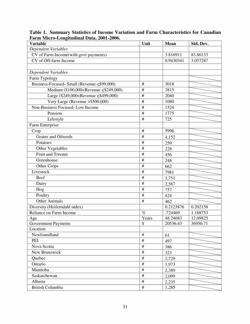
regression analysis. The summary statistics for the CV measures are reported in Table 1 along

with those for the explanatory variables below.

Explanatory Variables

14

Farm type and size are hypothesized to be major determinants of relative income

variability. These variables are proxied in this study by the farm typologies developed by AAFC

(2009). These typologies are used for aggregating farm level data to reveal patterns related to

different types of operations for sector and policy analysis. Based on a combination of operator

demographics and revenue classes, farms are sorted into seven mutually exclusive groups: four

business-focused farms (small, medium, large and very large), and three non-business focused

farms (pension farms, lifestyle farms, and low income farms).

The four business-focused categories are exclusively based on gross revenue as indicated

in Table 1. The gross revenues used to classify the business-focus farms is the average between

2001 and 2006. Criteria for non-business-focused farm typologies are based on gross farm

revenue as well as characteristics of the operator or the operator’s family. Pension farms

represent farmers approaching retirement and are downsizing their farms or in the process of

exiting the industry. Operators of lifestyle farms rely on off-farm employment as their main

source of income, and have a net farm income of less than $50,000. Low-income farms have a

gross farm revenue of less than $250,000 and a family income below the poverty line. The

poverty cut-off is Statistic’s Canada’s Low Income Measure (LIM), which is calculated as half

of the median adjusted before-tax family income, with adjustments based on the number of

adults and children in a household. For this analysis, we compare the 2001 family income to the

2001 LIM of $19,473 for a family of four in a rural area. Hobby farms (those with less than

$10,000 in average gross farm revenue between 2001 and 2006) are excluded from the analysis

due to limited data availability. Typologies are defined by in the OLS regression using 6-year

averages of gross farm income and family income. For the panel regression, 3-year averages for

each of the 4 periods are used. The 2001 observations for age and pension were used to

15

determine whether the farm is a pension farm or not. Dummy variables were defined for each

typology, except the medium sized business-focused farm which defines our benchmark.

Farm operations are also distinguished by the major enterprise of focus. The initial two

groupings are crops and livestock, but each are further sub-divided (grains and oilseeds, potatoes,

other vegetables, fruit and treenut, greenhouses, and other crops for crop farms; beef, dairy, hog,

poultry, and other animals for livestock farms). Farm types are identified as a specific farm type

if one of the enterprises generates over 50% of the farm’s gross revenue, and is predetermined in

the dataset by Statistics Canada. Farm types also define dummy variables. The grain and oilseed

sector defines our benchmark because it is the commodity group with the largest number of

operators. For the OLS regression, farm type is determined by the farm type identified in 2001.

For the panel regression, farm type is determined by the type identified in the first year of each

period.

The degree of specialization across these enterprise types is calculated using the

Herfindahl Index which is based on gross revenue generated from each enterprise (sum of

squares of the share of the revenue generated by the enterprise over gross, S=∑[(Reventerprise /

Revgross )2]). The lower the value of the Herfindahl Index, the greater the diversification on the

farm. We expect the degree of specialization to be directly related to the variability in farm

income but its expected sign on off-farm income variability is ambiguous. The Herfindahl Index

for the OLS regression is calculated using enterprise and gross revenue for all 6 years. For the

panel regression, it is calculated using 3-year averages for enterprise and gross revenue. An

alternative diversification measure is the family’s reliance on farm income, which is calculated

as the operator’s average family income between 2001 and 2006, divided by the average farm

16

income over the same period. For the panel regression, reliance measures are based on 3-year

average income divided by the average farming income over the same period.

Location effects are accounted for through identifying the province in which the farm

operation is based. Dummy variables were created for each province, and Quebec, the province

with the highest number of farms, was used for our benchmark. Farm locations are identified by

their address reported in 2001 for the OLS regression model, and were determined by the address

reported at the start of each 3-year period for the panel regression.

Age is measured as the age of the operator in 2001 in the OLS regression, and is

measured at the beginning of each 3-year period for the panel regression. The square of the age

variable is also included in both sets of regressions to capture any non-linear effects that age

might have on income volatility due to life-cycle changes in management ability and planning

horizon.

The final variable is government payments. It is measured as the amount of payment

received through all government support programs, including crop insurance. Although some of

the support payments are received a year after taxes are filed (e.g., the CAIS program requires

tax data to calculate payment), others, such as crop insurance, are paid out in the year of need.

Both types of payments are reported in the same tax year and combined into one variable in the

longitudinal database. Because crop insurance are commodity-specific, the level of payment will

be different between different types of operations. For the OLS regression, the 6-year average of

the net program payment are used, and for the panel regression, 3-year averages of the net

program payments are used. The government payment variable is logged transformed as well, as

the magnitude of this variable is very large compared to the dummy variable.

17

Results Graphical Quintile Analysis

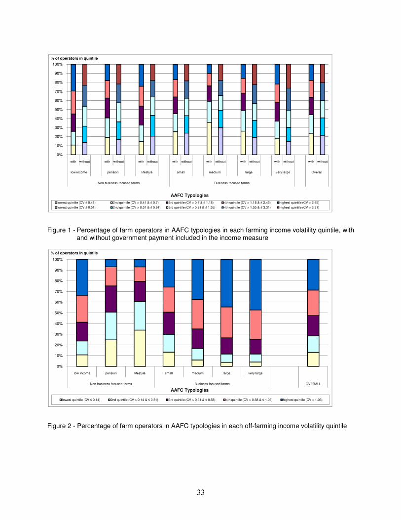
The distribution of farm operators between the quintiles of farm income volatility for

each of the seven AAFC farm typologies is illustrated in Figure 1. A CV of 0.51 delineates the

20% of the represented population (22% of operators in sample) with the lowest CV of farm

income without government payments included while those in the highest quintile have a CV of

3.31 or higher. If government payments are included in farm income, the respective CV

measures are 0.41 for the lowest quintile and 2.45 for the highest quintile. Government

payments, thus, appear to lower the variability in farm income as desired.

When government payments are taken into account in farm income, approximately 20%

of the small and very large commercial farmers fall into the lowest CV quintile while 35% of the

medium sized commercial farmers are in the least volatile quintile. Similarly, approximately

20% of the smallest and very large commercial farmers are in the highest quintile with the

highest volatility (CV>2.46) while only 10% of medium sized commercial farmers are in this

quintile. One reason for the apparent lower farm income volatility experienced by operators of

medium sized farms is that a relatively high proportion of farms in supply management fit in the

medium sized farm category as will be discussed further below. In addition, the result conforms

with previous studies that found larger farm operators tend to be less risk averse and take on

more risky investments.

Operators in the three non-business focused farm types experience higher relative income

variability than operators in the four business-focused farm types. For example, only 10% of the

low-income and lifestyle farmers are in the lowest quintile of farm income variability while

18

approximately 30% of these types of farmers are in the highest volatility quintile. Pension

farmers appear to have volatility measures that compare more to commercial farms than the other

two non-business focused farm types.

Removal of government payments as part of revenue increased the relative volatility of

farm income for commercial farmers as compared to non-business focused farmers. The effect

of government support on stabilizing farm income was particularly notable for the large

commercial farmers. For example, the percentage of the very large farms in the upper two

volatility quintiles increased from approximately 42% with government payments included to

over 50% without these stabilization funds. In contrast, the percentage of low-income and

lifestyle farmers in the highest quintile categories fell if government payments were not included.

Such farm operators are likely to receive few dollars from government programs and,

subsequently would have little effect on farm income volatility.

The volatility of off-farm income for operators of the seven farm typologies, as well as

for the overall sample, is illustrated in Figure 2. The CV of off-farm income is significantly

lower than the CV for farm income. For example, the CV measure at the least (most) volatile

quintile is 0.14 (1.03) for off-farm income and is 0.41 (2.45) for farm income with government

payments. In contrast to the volatility of farm income, operators of business-focused farms tend

to have a higher proportion of farms with relatively volatile off-farm income than non-business

focused farm operators, and this proportion increases with farm size.

Approximately 50% of large and very large farms are in the most volatile off-farm

income quintile (CV > 1.03) while less than 5% are in the lowest quintile. The result may be due

to the lower level of off-farm earnings for larger operations (Chaplina et al. 2004). Bigger farms

are unlikely to have surplus labour and tend to have a higher opportunity cost of spending labour

19

hours outside the farm operation. It may also suggest that off-farm income may be used to

supplement family income during periods of low farm income. Off-farm employment may be a

self-insurance mechanism for commercial farms.

In contrast to commercial farmers, pension and lifestyle operators tend to have higher and

more stable off-farm income through either stable off-farm work or pension payments.

Consequently, the proportion number of these farms in the low quintile bracket is higher than

commercial farms. The operators of low-income farms have high farm income volatility as well

as high off-farm income volatility. Because of the low revenues these farms generate, they

receive lower amounts of stabilization payments as compared to farms with higher sales. These

farms also suffer relatively high off-farm income volatility suggesting these operations are

particularly vulnerable and may require special focus from rural policy programs.

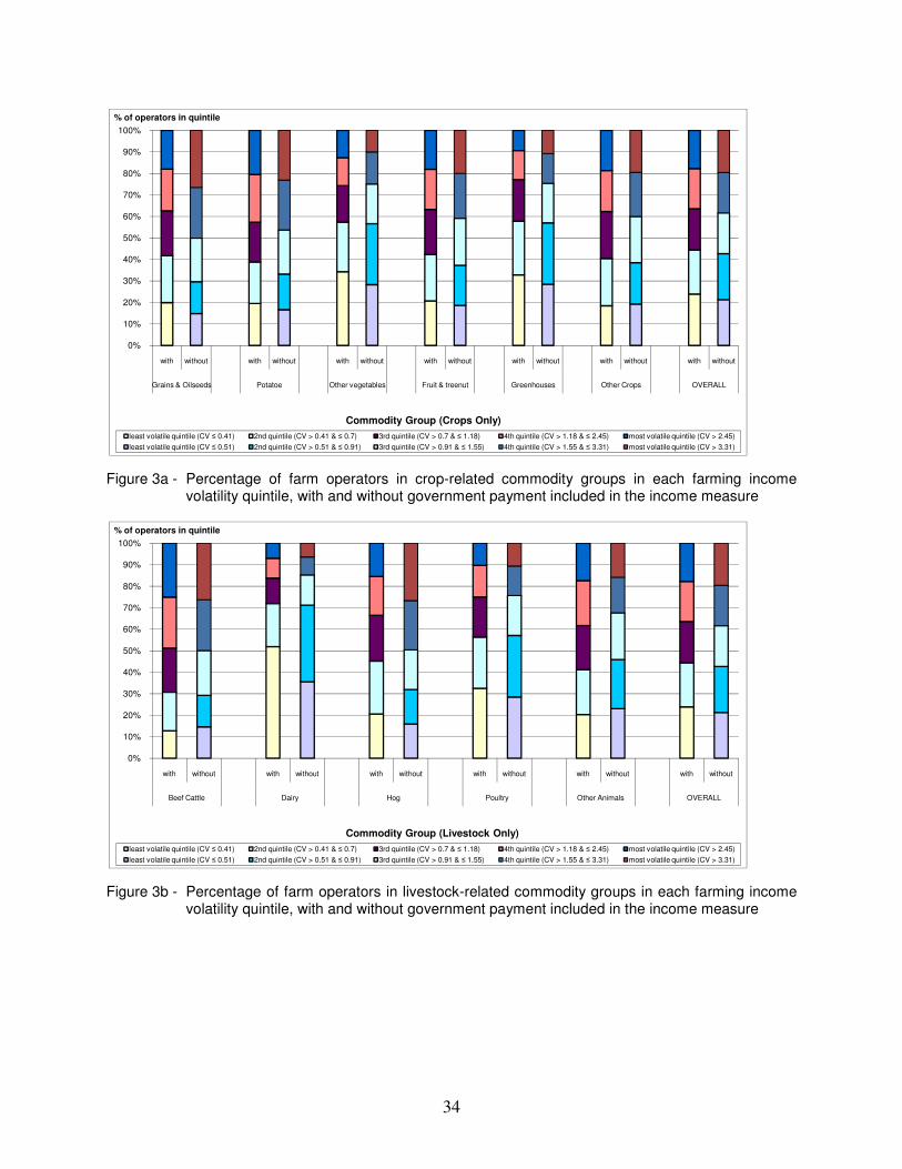
Relative income volatility between commodity groups is illustrated in Figure 3a for the

crop sectors and in Figure 3b for the livestock sectors. Note that the CV measures differentiating

income volatility quintiles are the same as in Figure 1. Farm income variability is measured as

before, but farms are categorized by commodity rather than by AAFC’s farm typology.

The sector with the most stable farm income is dairy with over 50% of dairy operators in

the least volatile farm income quintile. The result was expected because the mandate of supply

management is to ensure stable and fair returns for its producers. The poultry sector is also

under a quota system, but its operators do not benefit from the same level of farm income

stability. Approximately one-third of its farmers are in the lowest quintile and its volatility

distribution is very similar to the vegetables and the greenhouse sectors. The most volatile sector

in terms of farm income is beef. Approximately half of beef operators are in the highest two

quintiles of farm income volatility. The result reflects the price cycles normally faced by the

20

sector which were accentuated due to factors such as the BSE outbreak that closed export

markets during this time period. The distribution of farm operators across the quintiles of farm

income volatility is very similar for several commodity groups. The percentage of farmers in

each quintile is approximately equally distributed for the following sectors: grains and oilseeds,

potatoes, fruit, hogs, and other animals.

Excluding government payments from farm revenue increases income volatility (CV

measures of the quintile groups increases). This is most noticeable for operators in the grains

and oilseeds sector and the hog sector. Operators in these two sectors experience the biggest

stability gain (in terms of the decrease in the proportion of operators in the highest quintiles)

from government payments. Approximately one-third of farmers in these sectors were in the two

most volatile quintiles of farm income when government payments are included but this

percentage increased to 50% of farmers when government payment were not taken into account.

The result reflects the relatively large amount of stabilization funds flowing to these two sectors

either in the form of crop insurance and/or ad hoc income support.

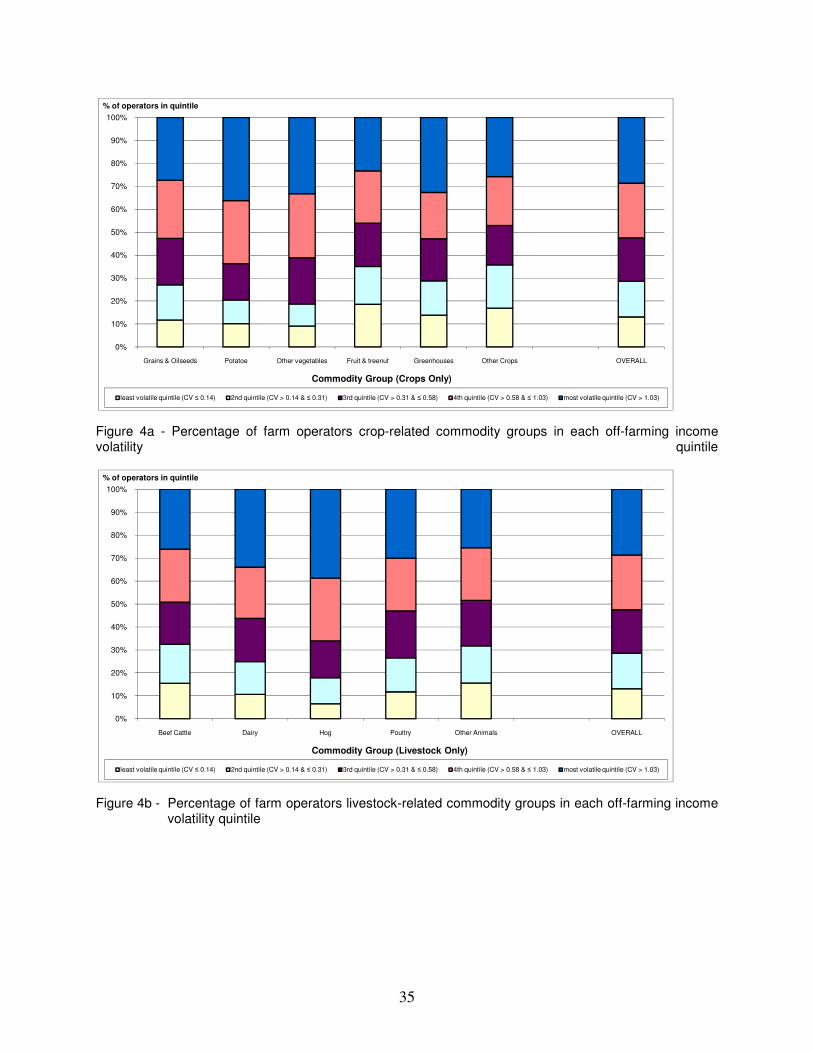
The relative volatility of off-farm income across commodity groups, as illustrated in

Figures 4a and 4b, depends on the likelihood of off-farm employment as it did across farm

typologies as illustrated in Figure 2. The sectors with the largest relative variation in operator’s

off-farm income are potato and vegetable in the crop sectors and dairy and hogs in the livestock

sectors. Approximately 60% of operators in these four sectors are categorized into the two most

volatile quintiles. Operations specialized in these commodities are more labour-intensive

throughout the year than other commodity groups; less surplus labour provides operators fewer

opportunities for off-farm employment.

21

Commodity groups displaying less relative volatility in off-farm income tend to be either

ones with a greater likelihood of surplus labour available for outside work and/or have faced

significant financial pressures. Fruit and other crop farms may have time periods during the year

that are suitable for off-farm employment. Given the part-time nature of many beef operations,

this may also be a factor explaining the relatively stable levels of off-farm income for operators

in this commodity group. Over 30% of beef farm operators are categorized into the two least

volatile quintiles and this could also be due to these farmers seeking means to supplement their

unstable and low farming income.

The distribution of operator’s family income volatility for crop-related and livestock-

related commodity groups is illustrated in Figures 4a and 4b respectively. The sectors with the

most unstable operator’s family income are the potato and hog sectors. Operators in both sectors

had relatively high farm and off-farm volatility and the result is that over 55% of operators from

these two sectors are in the two most volatile quintiles. Farms with relatively low variation in

operator’s family income tend to have either stable farm income (supply managed and

greenhouse sectors) and/or stable off-farm earnings (fruit and other crops). Approximately 20%

of greenhouse and dairy farm operators are categorized into the two most volatile quintiles.

Although off-farm earnings were relatively unstable for dairy farmers, the level and stability of

their farm earnings more than compensate. As a result, dairy operators have stable family

income.

Government payments did little to stabilize operator’s family income of most commodity

groups. Government payments were most effective for the grain and oilseed sector and the hog

sector. Operators in these sectors received a relatively large share of stabilization funds over this

time period and tend to rely more on farm income for the operator’s family income. In contrast,

22

the inclusion of government payment increased the relative volatility of operator’s family income

for the supply-managed sectors (dairy and poultry). Since government payments have a

stabilizing effect on other commodity groups (i.e. grains and hogs) and the supply-managed

farms receive relatively few dollars directly from government, the absolute volatility in family

income for the dairy and poultry sectors does not change with the inclusion of government

payments but in relative terms, a higher percentage of operators end up categorized into the most

volatile quintile.

Regression Analysis

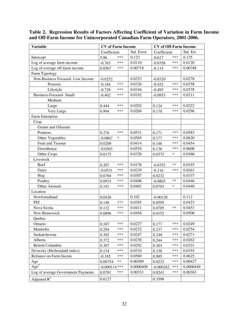
The OLS regression results over the six-year average are reported in Table 2. The results

for both income variance equations have a relatively high explanatory power given the cross-

sectional nature of the data with an R2 of 0.61 for the coefficient of variation of farm income and

0.36 for coefficient of variation of off-farm income. In addition, the majority of the explanatory

variables are statistically significant and the signs are consistent with expectations.

The volatility in farm income increases with decreases in average farm income and

decreases in off-farm income. The result suggests that more efficient operators (i.e. those with a

higher margin) are better at managing their volatility. Schurle and Thostrup (1989) found

variance to increase with average farm income but the movement along the implied EV frontier

was due to increases in specialization. The negative coefficient on average farm income

estimated here suggests that the higher average is partially due to avoiding income falls which

translates into lower farm income volatility. The positive effect on farm income variance

estimated from average off-farm income suggests that the relative variability is greatest for non-

business focused farm operations, which is consistent with the earlier descriptive analysis.

23

In terms of farm typologies, pension, lifestyle, and small business-focused operations all

have significantly lower farm income volatility than medium-sized commercial farms. This

result is opposite to the results from the descriptive analysis, which indicated that medium farms

have the lowest relative farm income variance. The regression analysis controls for other factors

and so the finding confirms our suspicion that the low income volatility of medium size farms

found in the descriptive analysis is mainly attributed to the high proportion of dairy operations in

this group. Large and very large farms, on the other hands, tend to have higher farm income

volatility. This result supports the hypothesis that larger operations take on higher risk to

generate a higher level of net farm income. The result is consistent with the findings of Dunn

and Williams (2000) and Schurle and Tholstrup (1987) who conjecture that larger farms are less

risk averse and/or have greater ability to manage higher volatility.

Farm income volatility for most crops is not significantly different than for the grain and

oilseed sector. In contrast, the majority of livestock operations have significantly higher farm

income volatility compared to grain and oilseed operations, with the exception of dairy

operations. While random weather events may have a larger relative impact on crop farms,

livestock farms, especially beef and hogs, may face even more uncertainty because of the length

of the period separating production from marketing decisions (Larue, Gervais and Lapan, 2004).

The results suggest that it is market rather than production volatility that is primarily causing the

fluctuations in farm income over this period. The significantly higher variance of farm income

for beef and potato producers reflect border closures that affected both farm types in the early

2000s. As expected, dairy operations have a significantly lower farm income volatility

compared to grains and oilseeds farms when all other factors are held constant due to the

stabilizing effect of supply management. However, poultry, which is also a supply-managed

24

sector, was found to have a significantly higher level of relative farm income variance than grain

and oilseed farmers. The result may reflect the greater amount of labour time that poultry

operations have in comparison to dairy which can be allocated to other farming activities that are

more risky than the returns from their supply-managed enterprise, or it could also reflect the cost

of production formula used for pricing which transmits feed cost volatility.

Relative farm income variance is lower in Quebec than all other provinces, which may

reflect higher levels of government support for agriculture in addition to the actual payments

received and the high relative concentration of supply-managed farms. The difference is greatest

between Quebec and the Prairies, as Western Canada tends to have greater weather variability

and be specialized in agricultural sectors more sensitive to world market shocks.

Farm enterprise diversity did not lower farm income volatility as expected which

suggests that encouraging a wider mix of enterprises is not an effective strategy to reduce

fluctuations in farm income. Diversity was also found to have mixed effects on farm income

variance in previous studies, with the expected reduction in volatility occurring only in certain

locations with high concentrations of certain farm types (Barry, Escalante and Bard 2000; Purdy,

Langemier, and Featherstone 1987). Consistent with the finding on average off-farm income, an

increase in the reliance on farm income reduces the coefficient of variation in farm income. It

was expected that increases in age or management experience would lower the relative

variability in farm income up to a certain point and then it would increase due to changes in

abilities and planning horizon. The estimated coefficients on the two age variables suggest that

the coefficient of variation on farm income declines until the mid-30s and then increases.

Finally, level of government payment increases farm income volatility, even though the

effect is small. The result could suggest that government support encourage farmers to engage in

25

more risky activities (Serra et al. 2006, and Hennesy 1998). However, our result can also be due

to the lag between the drop in farm income that triggers the program and the reception of the

payment several months later.

The coefficient of variation in off-farm income was found to be inversely related to

average farm and average off-farm income. Holding farm type constant, the negative effect of

farm income suggests that increases in average farm returns reduce the need for supplemental

revenue and thus the movement in and out of off-farm employment. The larger effect, and

consistent with prior expectations, is from an increase in average off-farm income. The greater

these revenue sources from either pension, investment returns or off-farm employment, the

greater the likelihood that these income flows will be permanent and the lower their relative

variability.

The relative permanence of off-farm income can also explain the signs on the farm

typologies. Relative to medium-sized, commercial farms, the coefficient of variation of off-farm

income is less for non-business-focused farms and greater for larger, business-focused farms.

Off-farm income for low-income, pension, life-style, and small commercial farms is more likely

to be relatively constant since it is the main source of total family income. In contrast, farm

income is the main income generating activity for larger commercial operations and off-farm

employment is more likely to be a temporary income supplement. The increase in the variability

with the size of the operation suggests off-farm work is a self-insurance mechanism for

commercial farms.

The ability to seek off-farm employment as a means to either counter changes in farm

income or to supplement total family income will be greater for crop than livestock farms due to

the greater likelihood of excess labour. The larger coefficient of variation of off-farm income

26

for crop producers compared to grain and oilseed producers, all other things being equal,

suggests that these farms have greater opportunity to move in and out of off-farm employment.

In contrast, the labour demands are greater for livestock farms compared to grain and oilseed

operations and thus are expected to be less involved in off-farm work.

Producers located in provinces west of Quebec have significantly higher levels of off-

farm income volatility. The result could be due to the lower level of farm income volatility

noted for producers in Quebec and thus less of a need to supplement their family income with

non-farm revenue. It may also be due to the reliance on dairy farming, which provides less

surplus labour for off-farm employment. It could also be due to more opportunities for off-farm

employment west of Quebec and thus the greater chance that farm family members are moving

in an out of off-farm employment depending on their family income needs.

Farm enterprise diversity and reliance on farm income have a statistically significant

positive effect on the off-farm income volatility. The result suggests that diversification is a

substitute to off-farm employment as a risk-management strategy for total household income. It

could also be due to having less time for off-farm employment as the increase in farming

activities will reduce an operation’s available surplus labour. Both reasons could lead to more

diversified farms being less likely to seek off-farm employment and thus experience greater

variations in its level. Similarly, as an operation’s reliance on farm income increases, the

likelihood of a stable, off-farm job decreases and the covariance of off-farm increases.

The increase in the covariance of off-farm income with age until approximately 50 years

and then a decrease suggests that perhaps there is more movement in and out of off-farm

employment when the operator is younger. This could be due to the greater need to supplement

27

the income of the farm business during certain period or due to the increase in investment or

pension income as the operator gets older.

Finally, government payments increase the covariance of off-farm income. As with farm

diversification, the need for alternative risk management options such as off-farm employment if

government payments serve to reduce total family income fluctuations. Thus, the increases in

government payments decrease the likelihood of full-time off-farm work and thus increase the

variability in off-farm income.

Conclusion

The stabilization of farm income and family income is a major objective of agricultural

and public policy. The purpose of this research was to examine the factors affecting the

variability of the sources of income to the farm and the farm family. Little research has been

done on the variability in either income source and attempts to look at both within the same

framework have been limited by the lack of available data combining both farm and off-farm

income levels for farm operations over time. Statistic Canada’s Farm Micro-Longtidinal Dataset

of 17,000 farm operators from 2001 to 2006 allowed such an analysis.

The coefficient of variation (CV) in farm income is significantly greater than that for off-

farm income but both measures are inversely related to the permanence of the income source to

the operation. The greater the reliance on farm income and the labour demands within the farm,

the lower (greater) the relative variability in farm (off-farm) income. However, there are notable

variations within the farm typologies. Larger commercial operations tend to experience larger

farm income volatility either because they are less risk averse and/or have the ability to manage

more risk. More profitable farms also have lower income variability since the average is higher

28

due to the avoidance of income drops. These larger farms also tend to have greater variability in

off-farm income sources since it is not a permanent income source but rather a self-insurance

mechanism against temporary reductions in farm income. Diversification and off-farm

employment appear to be substitute risk management strategies for commercial operations.

Pension and lifestyle farms have lower covariances for both farm and off-farm income compared

to business-focused farms since these farms will be likely be more risk averse and have a

permanent stream of off-farm revenue.

The results on relative variation in the two income sources across farm types raises

questions about whether government programs should target specific farm types. Indeed some

provincial programs such as Quebec’s ASRA have put a cap on the number of productive units

that are covered under the price support program, which is now based on the cost for the 75%

most efficient producers. Although the CV measures in the descriptive analysis decline with the

inclusion of government payments, there is a small positive effect in the regression results

implying that government support leads farmers to take on more risky activities. Government

payments also were found to increase the covariance of off-farm income suggesting that the need

for alternative risk management options such as off-farm employment (or diversification)

decrease if government payments serve to reduce total family income fluctuations. However, the

results could also be due to the lag between the time of the income reduction and the time in

which the aid is received. Further research is necessary to decipher the effects of government

support on farm decisions and subsequently the distribution of farm and off-farm income.

29

References

ALASIA, A., WEERSINK, A., BOLLMAN, R. D. and CRANFIELD, J. 2009. Off-farm labour decision of Canadian farm operators: Urbanization effects and rural labour market linkages. Journal of Rural Studies, 25, 12-24.

AHITUV, A. and KIMHI, A. 2002. Off-farm work and capital accumulation decisions of farmers over the life cycle: The role of heterogeneity and state dependence. Journal of

Development Economics. 68, 329-343.

BARRY, P. J., ESCALANTE, C. L. and BARD, S. K. 2001. Economic risk and the structural characteristics of farm businesses. Agricultural Finance Review, 61, 74-86.

CHAPLINA, H., DAVIDOVAA, S. and GORTONB, M. 2004. Agricultural adjustment and the diversification of farm households and corporate farms in Central Europe. Journal of

Rural Studies, 20, 17.

CORSI, A. and FINDEIS, J.L. 2000. True state dependence and heterogeneity in off-farm labor participation. European Review of Agricultural Economics. 27, 127-151.

DUNN, J. W. and WILLIAMS, J. R. 2000. Farm Characteristics that Influence Net Farm Income Variability and Losses. Western Agricultural Economics Association Annual Meetings. Vancouver, BC.

GODDARD, E., WEERSINK, A., CHEN, K. and TURVEY, C. G. 1993. Economics of Structural Change in Agriculture. Canadian Journal of Agricultural Economics, 41, 475-489.

HENNESSY, D. A. 1998. The Production Effects of Agricultural Income Support Policies under Uncertainty. American Journal of Agricultural Economics, 80, 46-57.

HUFFMAN, W. E. 1980. Farm and Off-Farm Work Decisions: The Role of Human Capital. The

Review of Economics and Statistics, 62, 14-23.

JETTÉ-NANTEL, S., FRESHWATER, D., BEAULIEU, M. and KATCHOVA, A. 2010. Income Variability and Off-Farm Diversification in Canadian Agriculture. Southern

Agricultural Economics Association Annual Meeting. Orlando, FL.

KENYON, D., KLING, K., JORDAN, J., SEALE, W. and MCCABE, N. 1987. Factors affecting agricultural futures price variance. Journal of Futures Markets, 7, 73-91.

LARUE, B., GERVAIS, J. and LAPAN, H. E. 2004. Low-price low-capacity traps and government interventions in agricultural markets. Canadian Journal of Agricultural

Economics, 52, 237-256.

MISHRA, A. K. and GOODWIN, B. K. 1997. Farm Income Variability and the Supply of Off-Farm Labor. American Journal of Agricultural Economics, 79, 880-887.

MEYER, J. 1987. Two-moment Decision Models and Expected Utility Maximization. American

Economic Review, 77, 421-30.

30

NIEKAMP, D. 2009. Financial Situation and Performance of Canadian Farms. Agriculture and

Agri-Food Canada.

O’DONOGHUE, E.J., HOPPE, R.A., BANKER, D.E., and KORB, P. 2009. Exploring

Alternative Farm Definitions: Implications for Agricultural Statistics and Program

Eligibility. EIB-49, U.S. Dept. of Agriculture, Econ. Res. Serv. March.

OECD, FOOD AND AGRICULTURE ORGANIZATION OF THE UNITED NATIONS. 2010. OECD-FAO Agricultural Outlook 2010, Paris: OECD Publishing

PHIMISTER, E., VERA-TOSCANO, E., and WEERSINK, A. 2002. Female labour participation and labour market attachment in rural Canada. American Journal of Agricultural

Economics. 84, 210-221.

POPE, R. D. and PRESCOTT, R. 1980. Diversification in Relation to Farm Size and Other Socioeconomic Characteristics. American Journal of Agricultural Economics, 62, 6.

PURDY, B. M., LANGEMEIER, M. R. and FEATHERSTONE, A. M. 1997. Financial Performance, Risk, And Specialization. Journal of Agricultural and Applied Economics, 29, 149-161.

ROBISON, L. and BARRY, P. 1987. The Competitive Firm’s Response to Risk, New York, Macmillan.

SERRA, T., GOODWIN, B. K. and HYVONEN, K. 2005. Replacement of Agricultural Price

Supports By Area Payments in the European Union and the Effects on Pesticide Use. American Journal of Agricultural Economics, 87, 870-884.

VELANDIA, M., REJESUS, R. M, KNIGHT, T. O. and SHERRICK, B. J. 2009. Factors

Affecting Farmers' Utilization of Agricultural Risk Management Tools: The Case of Crop Insurance, Forward Contracting, and Spreading Sales. Journal of Agricultural and

Applied Economics, 4, 107-123.

31

Table 1. Summary Statistics of Income Variation and Farm Characteristics for Canadian

Farm Micro-Longitudinal Data, 2001-2006. Variable Unit Mean Std. Dev. Dependent Variables

CV of Farm Income(with govt payments) 3.816911 83.86133 CV of Off-farm Income 0.9430341 3.057287 Dependent Variables Farm Typology Business-Focused- Small (Revenue <$99,000) # 3018 Medium ($100,000<Revenue <$249,000) # 3815 Large ($249,000<Revenue <$499,000) # 2040 Very Large (Revenue >$500,000) # 1080 Non-Business Focused- Low Income # 1524 Pension # 1775 Lifestyle # 725 Farm Enterprise Crop # 5996 Grains and Oilseeds # 4,152 Potatoes # 250 Other Vegetables # 228 Fruit and Treenut # 456 Greenhouse # 248 Other Crops # 662 Livestock # 7981 Beef # 3,751 Dairy # 2,587 Hog # 757 Poultry # 424 Other Animals # 462 Diversity (Heiferndahl index) 0.2123876 0.202158 Reliance on Farm Income % .724469 1.188753 Age Years 48.24683 12.09825 Government Payments $ 20536.43 36950.71 Location Newfoundland # 61 PEI # 497 Nova Scotia # 386 New Brunswick # 323 Quebec # 2,729 Ontario # 1,973 Manitoba # 2,389 Saskatchewan # 2,099 Alberta # 2,235 British Columbia # 1,285

32

Table 2. Regression Results of Factors Affecting Coefficient of Variation in Farm Income

and Off-Farm Income for Unincorporated Canadian Farm Operators, 2001-2006. Variable CV of Farm Income CV of Off-Farm Income

Coefficient Std. Error Coefficient Std. Err. Intercept 5.86 *** 0.123 -0.617 *** 0.135 Log of average farm income -0.763 *** 0.0110 -0.0356 *** 0.0120 Log of average off-farm income 0.0567 *** 0.00718 -0.114 *** 0.00788 Farm Typology Non-Business Focused- Low Income -0.0252 0.0253 -0.0320 0.0278 Pension -0.184 *** 0.0326 -0.452 *** 0.0358 Lifestyle -0.729 *** 0.0344 -0.495 *** 0.0378 Business-Focused- Small -0.402 *** 0.0192 -0.0953 *** 0.0211 Medium

Large 0.444 *** 0.0202 0.124 *** 0.0222 Very Large 0.994 *** 0.0269 0.170 *** 0.0296 Farm Enterprise Crop Grains and Oilseeds

Potatoes 0.276 *** 0.0531 0.171 *** 0.0583 Other Vegetables -0.0867 * 0.0565 0.177 *** 0.0620 Fruit and Treenut 0.0209 0.0414 0.146 *** 0.0454 Greenhouse -0.0303 0.0554 0.136 *** 0.0608 Other Crops 0.0175 0.0328 0.0575 * 0.0360 Livestock Beef 0.207 *** 0.0176 -0.0352 ** 0.0193 Dairy -0.0531 *** 0.0239 -0.116 *** 0.0263 Hog 0.0764 *** 0.0307 0.0232 0.0337 Poultry 0.0933 *** 0.0406 -0.0803 ** 0.0446 Other Animals 0.191 *** 0.0401 0.0703 * 0.0440 Location Newfoundland 0.0426 0.102 -0.00120 0.112 PEI 0.146 *** 0.0385 0.0595 0.0423 Nova Scotia 0.132 *** 0.0411 0.0705 ** 0.0451 New Brunswick 0.0896 *** 0.0456 0.0152 0.0500 Quebec

Ontario 0.107 *** 0.0227 0.177 *** 0.0249 Manitoba 0.294 *** 0.0232 0.237 *** 0.0254 Saskatchewan 0.302 *** 0.0247 0.240 *** 0.0271 Alberta 0.372 *** 0.0238 0.244 *** 0.0262 British Columbia 0.307 *** 0.0292 0.303 *** 0.0321 Diversity (Heiferndahl index) 0.134 *** 0.0324 0.330 *** 0.0355 Reliance on Farm Incom -0.185 *** 0.0569 0.985 *** 0.0625 Age 0.00754 ** 0.00389 0.0232 *** 0.00427 Age2

-0.000114 *** 0.0000409 -0.000262 *** 0.0000449

Log of average Government Payments 0.0781 *** 0.00331 0.0243 *** 0.00363 Adjusted R2 0.6127

0.3598

33

Figure 1 - Percentage of farm operators in AAFC typologies in each farming income volatility quintile, with and without government payment included in the income measure

Figure 2 - Percentage of farm operators in AAFC typologies in each off-farming income volatility quintile

0%

10%

20%

30%

40%

50%

60%

70%

80%

90%

100%

with without with without with without with without with without with without with without with without

low income pension lifestyle small medium large very large Overall

Non-business-focused farms Business-focused farms

% of operators in quintile

AAFC Typologies

lowest quintile (CV ≤ 0.41) 2nd quintile (CV > 0.41 & ≤ 0.7) 3rd quintile (CV > 0.7 & ≤ 1.18) 4th quintile (CV > 1.18 & ≤ 2.45) highest quintile (CV > 2.45)

lowest quintile (CV ≤ 0.51) 2nd quintile (CV > 0.51 & ≤ 0.91) 3rd quintile (CV > 0.91 & ≤ 1.55) 4th quintile (CV > 1.55 & ≤ 3.31) highest quintile (CV > 3.31)

0%

10%

20%

30%

40%

50%

60%

70%

80%

90%

100%

low income pension lifestyle small medium large very large

Non-business-focused farms Business-focused farms OVERALL

% of operators in quintile

AAFC Typologies

lowest quintile (CV ≤ 0.14) 2nd quintile (CV > 0.14 & ≤ 0.31) 3rd quintile (CV > 0.31 & ≤ 0.58) 4th quintile (CV > 0.58 & ≤ 1.03) highest quintile (CV > 1.03)

34

Figure 3a - Percentage of farm operators in crop-related commodity groups in each farming income volatility quintile, with and without government payment included in the income measure

Figure 3b - Percentage of farm operators in livestock-related commodity groups in each farming income volatility quintile, with and without government payment included in the income measure

0%

10%

20%

30%

40%

50%

60%

70%

80%

90%

100%

with without with without with without with without with without with without with without

Grains & Oilseeds Potatoe Other vegetables Fruit & treenut Greenhouses Other Crops OVERALL

% of operators in quintile

Commodity Group (Crops Only)

least volatile quintile (CV ≤ 0.41) 2nd quintile (CV > 0.41 & ≤ 0.7) 3rd quintile (CV > 0.7 & ≤ 1.18) 4th quintile (CV > 1.18 & ≤ 2.45) most volatile quintile (CV > 2.45)

least volatile quintile (CV ≤ 0.51) 2nd quintile (CV > 0.51 & ≤ 0.91) 3rd quintile (CV > 0.91 & ≤ 1.55) 4th quintile (CV > 1.55 & ≤ 3.31) most volatile quintile (CV > 3.31)

0%

10%

20%

30%

40%

50%

60%

70%

80%

90%

100%

with without with without with without with without with without with without

Beef Cattle Dairy Hog Poultry Other Animals OVERALL

% of operators in quintile

Commodity Group (Livestock Only)

least volatile quintile (CV ≤ 0.41) 2nd quintile (CV > 0.41 & ≤ 0.7) 3rd quintile (CV > 0.7 & ≤ 1.18) 4th quintile (CV > 1.18 & ≤ 2.45) most volatile quintile (CV > 2.45)

least volatile quintile (CV ≤ 0.51) 2nd quintile (CV > 0.51 & ≤ 0.91) 3rd quintile (CV > 0.91 & ≤ 1.55) 4th quintile (CV > 1.55 & ≤ 3.31) most volatile quintile (CV > 3.31)

35

Figure 4a - Percentage of farm operators crop-related commodity groups in each off-farming income volatility quintile

Figure 4b - Percentage of farm operators livestock-related commodity groups in each off-farming income volatility quintile

0%

10%

20%

30%

40%

50%

60%

70%

80%

90%

100%

Grains & Oilseeds Potatoe Other vegetables Fruit & treenut Greenhouses Other Crops OVERALL

% of operators in quintile

Commodity Group (Crops Only)

least volatile quintile (CV ≤ 0.14) 2nd quintile (CV > 0.14 & ≤ 0.31) 3rd quintile (CV > 0.31 & ≤ 0.58) 4th quintile (CV > 0.58 & ≤ 1.03) most volatile quintile (CV > 1.03)

0%

10%

20%

30%

40%

50%

60%

70%

80%

90%

100%

Beef Cattle Dairy Hog Poultry Other Animals OVERALL

% of operators in quintile

Commodity Group (Livestock Only)

least volatile quintile (CV ≤ 0.14) 2nd quintile (CV > 0.14 & ≤ 0.31) 3rd quintile (CV > 0.31 & ≤ 0.58) 4th quintile (CV > 0.58 & ≤ 1.03) most volatile quintile (CV > 1.03)