int. journ clim. 2014 cioffi

INTERNATIONAL JOURNAL OF CLIMATOLOGYInt. J. Climatol. (2014)Published online in Wiley Online Library(wileyonlinelibrary.com) DOI: 10.1002/joc.4116

Space-time structure of extreme precipitation in Europeover the last century

Francesco Cioffi,a* Upmanu Lall,b Ester Rusc and Chandra Kiran B. Krishnamurthyd

a Department of Civil, Structural and Environmental Engineering, University of Rome ‘La Sapienza’, Italyb Department of Earth and Environmental Engineering, Columbia University, New York, NY, USA

c Thames Water Innovation Centre, Reading, UKd Center for Environmental and Resources Economics and Department of Economics, Umea University, Sweden

ABSTRACT: We investigate the space-time structure of extreme precipitation in Europe over the last century, using dailyrainfall data from the European Climate Assessment & Dataset (ECA&D) archive. The database includes 267 stations withrecords longer than 100 years. In the winter season (October to March), for each station, two classes of daily rainfall amountvalues are selected that, respectively, exceed the 90th and 95th percentile of daily rainfall amount over all the 100 years. Foreach class, and at each location, an annual time series of the frequency of exceedance and of the total precipitation, definedrespectively as the number of days the rainfall threshold (90th and 95th percentiles) is exceeded and total precipitation on dayswhen the percentile is exceeded, are developed. Space-time structure of the frequency and total precipitation time series atthe different locations are then pursued using multivariate time and frequency domain methods. The identified key trends andorganized spectral modes are linked to well-known climate indices, as North Atlantic Oscillation (NAO) and El Nino SouthernOscillation (ENSO). The spectra of the leading principal component of frequency of exceedance and of total precipitation havea peak with a 5-year period that is significant at the 5% level. These are also significantly correlated with ENSO series with thisperiod. The spectrum of total rainfall is significant at the 10% level with a period of ∼8 years. This appears to be significantlycorrelated to the NAO index at this period. Thus, a decomposition of both secular trends and quasi-periodic behaviour inextreme daily rainfall is provided.

KEY WORDS extreme precipitation; hydrology; frequency analysis; atmospheric teleconnections

Received 24 December 2013; Revised 25 June 2014; Accepted 27 June 2014

1. Introduction

In Europe, floods occurring in autumn and winter arethe most common natural disaster (Hajat et al., 2005).Extreme river floods have had devastating effects in cen-tral Europe during the last decade (Mudelsee et al., 2004).Using a combined database of 2580 flood and land-slide events in Italy, Guzzetti et al. (2005) showed thatfloods with human consequences are mainly caused byhigh-intensity as well as prolonged rainfall.

Characterizing variations in and predicting the frequencyand intensity of extreme precipitation are crucial to car-rying out a proper evaluation of the type, location anddimension of civil infrastructure in Europe (Frei et al.,2000; Zolina et al., 2004; Hajat et al., 2005; Lehner et al.,2006; Marchi et al., 2010; Christensen et al., 2012). Inrecent years, a number of papers have discussed thepossibility of an increase in the frequency of occur-rence of extreme rainfall in response to the increase ofglobal temperature (Yonetani and Gordon, 2001; Palmerand Rälsänen, 2002; Kharin et al., 2007; Bengtsson et al.

* Correspondence to: F. Cioffi, Department of Civil, Structural andEnvironmental Engineering, University of Rome ‘La Sapienza’, Rome,Italy. E-mail: [email protected]

2009; Kundzewicz et al., 2013). Experiments with cou-pled ocean–atmosphere climate models have shown anincrease in the occurrence of extreme precipitation eventsin mid-latitudes (Hennessy et al., 1997; Cubasch et al.,2001). Frei et al. (2006) suggested that an increase ofatmospheric greenhouse gas concentrations could increasethe frequency of heavy precipitation in many regions of theglobe. They found that during the winter months, precipi-tation extremes tend to increase north of about 45∘N, whilethere is a non-significant change or a decrease to the south.However, these projections often differ significantly acrossmodels leading to high uncertainty in the projections.

The trends found in extreme precipitation in Europe dif-fer, depending on the regions, datasets and methodologyused. (New et al., 2002; González Hidalgo et al., 2003;Mudelsee et al., 2003; Wijngaard et al., 2003; Mobergand Jones, 2005; Nastos and Zerefos, 2007; Costa andSolares, 2009; Karagiannidis et al., 2012; Zolina et al.,2012). Most studies show secular trends in European pre-cipitation. Karagiannidis et al. (2012) studied the trends inextreme precipitation for the period of 1958–2000, find-ing decreasing trends in southern Europe and increasingtrends on continental Europe as a whole from Septem-ber to February. Klein Tank and Könen (2003) foundindices of wet extremes increasing during the 1946–1999

© 2014 Royal Meteorological Society

F. CIOFFI et al.

period, although the spatial coherence of the trends waslow. Moberg and Jones (2005) also found a significantincrease in precipitation intensity over the 20th centuryduring the winter. However, a unified analysis is lack-ing due to the inhomogeneity of the data. Indeed, moststudies on extreme precipitation have focused on an anal-ysis of trends for a single station time series or for agroup of stations belonging to a single country, or forgridded data. Furthermore, studies have also shown thatorography affects the characteristics and intensity of pre-cipitation (Sevruk, 1997; Frei and Schär, 2001). Thedifferences in the length of data, resolution and meth-ods applied in its processing have made it challengingto build a picture of the trends for the European con-tinent. (Klein Tank et al., 2002; Klok and Klein Tank,2009)

Here, we use the recently updated ECA dataset whichmay provide the most comprehensive readily accessiblecoverage of station data for Europe. The database includes267 stations with records longer than 100 years.

In the winter season (October to March), for each stationtwo classes of daily rainfall amount values are selectedthat exceed the 90th and 95th percentile of daily rainfallamount, respectively, over all the 100 years. For eachclass an annual time series is developed at each locationof the frequency, and of the total precipitation, definedas the total precipitation on days when the percentile isexceeded.

Monotonic trends in the derived frequency and totalprecipitation for each station are identified using theMann–Kendall (MK) test. In order to estimate the signifi-cance of the test statistic, taking into account the possibilityof existence of serial correlations in data, the Block Boot-strap (BBS) method is applied.

Further, considering that low frequency climate variabil-ity due to natural sources may be present in the data, weexplore frequency domain methods combined with spa-tial analysis techniques to assess whether there are coher-ent space-time climate variations that are detectable inthe dataset, and whether these may have a relation tothe well-known modes of climate variability such as theEl Nino Southern Oscillation (ENSO) and North AtlanticOscillation (NAO).

According to Yiou and Nogaj (2004), heavy precipita-tion is associated with the positive NAO phase regime overNorthern Europe, especially during the winter months.Southern Europe is believed to experience more extremerainfall events during the negative NAO phase (Yiou andNogaj, 2004; Hidalgo-Muñoz et al., 2011). The period1995–2004 was dominated by a positive NAO phase (Yiouand Nogaj, 2004) that could have generated more frequentextreme precipitation over Northern Europe. Given thatthis is towards the end of the time series, a simple trendanalysis could be influenced by this persistent segment.The impact of the ENSO index on European precipitationis not as well established as that of the NAO. However,a number of existing studies conjecture that ENSO canextend its influence to the remote North Atlantic-Europeansector (Fraedrich and Larnder, 1993; Pozo-Vazquez et al.,

2005; Brönnimann, 2007; Brönnimann et al., 2007).Since the existence of a possible link between the NorthAtlantic-European climate and ENSO has importantimplications for seasonal forecasting in that region, theidentification of such an influence from observations isalso pursued.

Principal component analysis (PCA), multiple-tapermethod-singular value decomposition (MTM-SVD)and wavelet analysis are applied to investigate on thespatio-temporal structure of frequency and total pre-cipitation extremes. The influence of NAO and ENSOis examined through the significance of the frequencyspectra of the associated climate indices and the leadingprincipal components (PCs) of each derived rainfall seriesanalysed. Finally, the casual relations between ENSO andNAO climate indices and the leading PCs of extreme pre-cipitation are explored by using a bivariate linear Grangercausality test.

2. Data and methods

2.1. Data

Klein Tank et al. (2002) assembled long time seriesof daily temperature and precipitation data from Euro-pean stations as part of the ECA dataset. This datasethas been updated and extended (Klok and Klein Tank,2009) and now contains a total of 267 stations that havequality-controlled daily precipitation data from 1901 to2006.

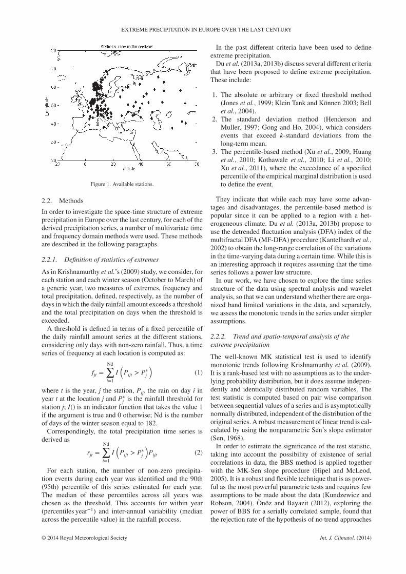
Figure 1 shows the locations of stations used in the anal-ysis. All stations were tested for homogeneity (Wijngaardet al., 2003), and the results from this test show that 180stations (70%) are considered to have consistent data;26 (10%) are doubtful and 55 (20%) are suspect (i.e.did not pass the test). Having a large number of stationswith homogeneous data makes the analysis proposedhere more reliable. Unfortunately, most of stations arelocated in central Europe and Scandinavia, thus theresults are dominated by characteristics related to thoseregions. Nonetheless, since large-scale meteorologicalsystems determine extreme winter rainfall, some generalconsiderations for all of Europe may be drawn.

The climate indices considered are the NAO, ENSO(Nino3.4), East Atlantic/Western Russia (EAWR), PacificNorth America (PNA) and global surface temperature gra-dients, Equator to Pole gradient (EPG) and Ocean LandContrast (OLC). The data used for the EPG and OLC cal-culations are monthly Northern Hemisphere data from thevariance adjusted version of the Hadley Centre ClimaticResearch Unit temperature anomaly (HadCRUT), and areprocessed as described by Karamperidou et al. (2012).The NAO index was obtained from the Centers for Envi-ronmental Prediction–National Center for AtmosphericResearch (NCEP–NCAR) reanalysis data (Kalnay et al.,1996). The Nino-3.4 index was obtained from Kaplan et al.(1998) and Reynolds et al. (2002). The Nino3, EAWR,NAO and PNA monthly indices were downloaded from theKNMI Climate Explorer (http://climexp.knmi.nl).

© 2014 Royal Meteorological Society Int. J. Climatol. (2014)

EXTREME PRECIPITATION IN EUROPE OVER THE LAST CENTURY

Figure 1. Available stations.

2.2. Methods

In order to investigate the space-time structure of extremeprecipitation in Europe over the last century, for each of thederived precipitation series, a number of multivariate timeand frequency domain methods were used. These methodsare described in the following paragraphs.

2.2.1. Definition of statistics of extremes

As in Krishnamurthy et al.’s (2009) study, we consider, foreach station and each winter season (October to March) ofa generic year, two measures of extremes, frequency andtotal precipitation, defined, respectively, as the number ofdays in which the daily rainfall amount exceeds a thresholdand the total precipitation on days when the threshold isexceeded.

A threshold is defined in terms of a fixed percentile ofthe daily rainfall amount series at the different stations,considering only days with non-zero rainfall. Thus, a timeseries of frequency at each location is computed as:

fjt =Nd∑i=1

I(

Pijt > P∗j

)(1)

where t is the year, j the station, Pijt the rain on day i inyear t at the location j and P∗

j is the rainfall threshold forstation j; I() is an indicator function that takes the value 1if the argument is true and 0 otherwise; Nd is the numberof days of the winter season equal to 182.

Correspondingly, the total precipitation time series isderived as

rjt =Nd∑i=1

I(

Pijt > P∗j

)Pijt (2)

For each station, the number of non-zero precipita-tion events during each year was identified and the 90th(95th) percentile of this series estimated for each year.The median of these percentiles across all years waschosen as the threshold. This accounts for within year(percentiles year−1) and inter-annual variability (medianacross the percentile value) in the rainfall process.

In the past different criteria have been used to defineextreme precipitation.

Du et al. (2013a, 2013b) discuss several different criteriathat have been proposed to define extreme precipitation.These include:

1. The absolute or arbitrary or fixed threshold method(Jones et al., 1999; Klein Tank and Können 2003; Bellet al., 2004).

2. The standard deviation method (Henderson andMuller, 1997; Gong and Ho, 2004), which considersevents that exceed k-standard deviations from thelong-term mean.

3. The percentile-based method (Xu et al., 2009; Huanget al., 2010; Kothawale et al., 2010; Li et al., 2010;Xu et al., 2011), where the exceedance of a specifiedpercentile of the empirical marginal distribution is usedto define the event.

They indicate that while each may have some advan-tages and disadvantages, the percentile-based method ispopular since it can be applied to a region with a het-erogeneous climate. Du et al. (2013a, 2013b) propose touse the detrended fluctuation analysis (DFA) index of themultifractal DFA (MF-DFA) procedure (Kantelhardt et al.,2002) to obtain the long-range correlation of the variationsin the time-varying data during a certain time. While this isan interesting approach it requires assuming that the timeseries follows a power law structure.

In our work, we have chosen to explore the time seriesstructure of the data using spectral analysis and waveletanalysis, so that we can understand whether there are orga-nized band limited variations in the data, and separately,we assess the monotonic trends in the series under simplerassumptions.

2.2.2. Trend and spatio-temporal analysis of theextreme precipitation

The well-known MK statistical test is used to identifymonotonic trends following Krishnamurthy et al. (2009).It is a rank-based test with no assumptions as to the under-lying probability distribution, but it does assume indepen-dently and identically distributed random variables. Thetest statistic is computed based on pair wise comparisonbetween sequential values of a series and is asymptoticallynormally distributed, independent of the distribution of theoriginal series. A robust measurement of linear trend is cal-culated by using the nonparametric Sen’s slope estimator(Sen, 1968).

In order to estimate the significance of the test statistic,taking into account the possibility of existence of serialcorrelations in data, the BBS method is applied togetherwith the MK-Sen slope procedure (Hipel and McLeod,2005). It is a robust and flexible technique that is as power-ful as the most powerful parametric tests and requires fewassumptions to be made about the data (Kundzewicz andRobson, 2004). Önöz and Bayazit (2012), exploring thepower of BBS for a serially correlated sample, found thatthe rejection rate of the hypothesis of no trend approaches


F. CIOFFI et al.

the nominal significance level if the block length of boot-strap samples is chosen properly. Here, we experimentedwith differented block lengths, ensuring that the blocklengths are larger than the characteristic periods of vari-ability of interest (corresponding to the large scale oscilla-tion climate indices such as NAO and ENSO).

The spatial coherence of the detected trends and of com-mon (spatio-temporal) modes of variability is explorednext. Three separate approaches are used: (1) analysis ofspatial correlation through the PCs of each field (90th and95th frequency and corresponding total precipitation);(2) application of the frequency domain multiple-tapermethod-singular value decomposition (MTD-SVD)method and (3) application of wavelet analysis to theleading PCs of each field.

The frequency domain MTM-SVD approach(Rajagopalan et al., 1998) is applied to assess the exis-tence of low-frequency modes of large scale climate. TheMTM method of spectral analysis (Thomson, 1982) relieson the assumption that climate modes are narrow band andevolve in a noise background that varies smoothly acrossfrequency. The discrete Fourier spectrum of the timeseries at each individual station at a given frequency isfirst estimated and smoothed using K orthogonal Slepiantapers. An SVD analysis is then conducted at each Fourierfrequency of a matrix with the columns representing thecomplex coefficients of the MTM spectrum for each of Ktapers, and the rows representing each of the sites on whichthe MTM spectrum is computed. The resulting localizedfractional variance (LFV) spectrum provides a measure ofthe distribution of variance across the orthogonal tapersby frequency. In this paper we used three 2𝜋 tapers forthe analysis. If the spatial coherence is high across sites ata given frequency, the associated leading singular valueexplains a large fraction of the variance across sites. Thesignificance levels for the null hypothesis that the size ofthe leading singular value is consistent with what may beexpected by chance are computed by using a bootstrapmethod as suggested by Mann and Park (1999). In orderto confirm the findings obtained by MTM-SVD, waveletanalysis on the leading components from the PCA of eachfield is also carried out.

MTM coherence and cross wavelet analysis are also usedto verify the possible influence of well-established climateindices such as NAO, ENSO, EAWR, PNA and globaltemperature gradients, EPG and OLC.

Finally a bivariate linear Granger causality test (Granger,1969) is applied to explore the strength of the causal rela-tions between the climate indices found to be connected tothe leading PCs of extreme precipitation from the previousanalyses.

3. Results

3.1. Trend analysis

Figure 2 shows the results of application of MK test to theannual series of frequency and total precipitation at eachstation location, for each of the time series. To check the

significance levels of the calculated trends we carried outBBS with BBS of length of 5 and 10 years respectivelywith 1000 bootstrap samples. No appreciable differencesin results were observed in the two cases. Thus, a BBSof length 5 years seems to cover any significant memorydue to the influence of large scale climate modes such asNAO and/or ENSO. In evaluating the significance level ofthe trends for each field of data, we consider a two-tailedtest for a hypothesis of no trend with a 95% interval fromthe BBS.

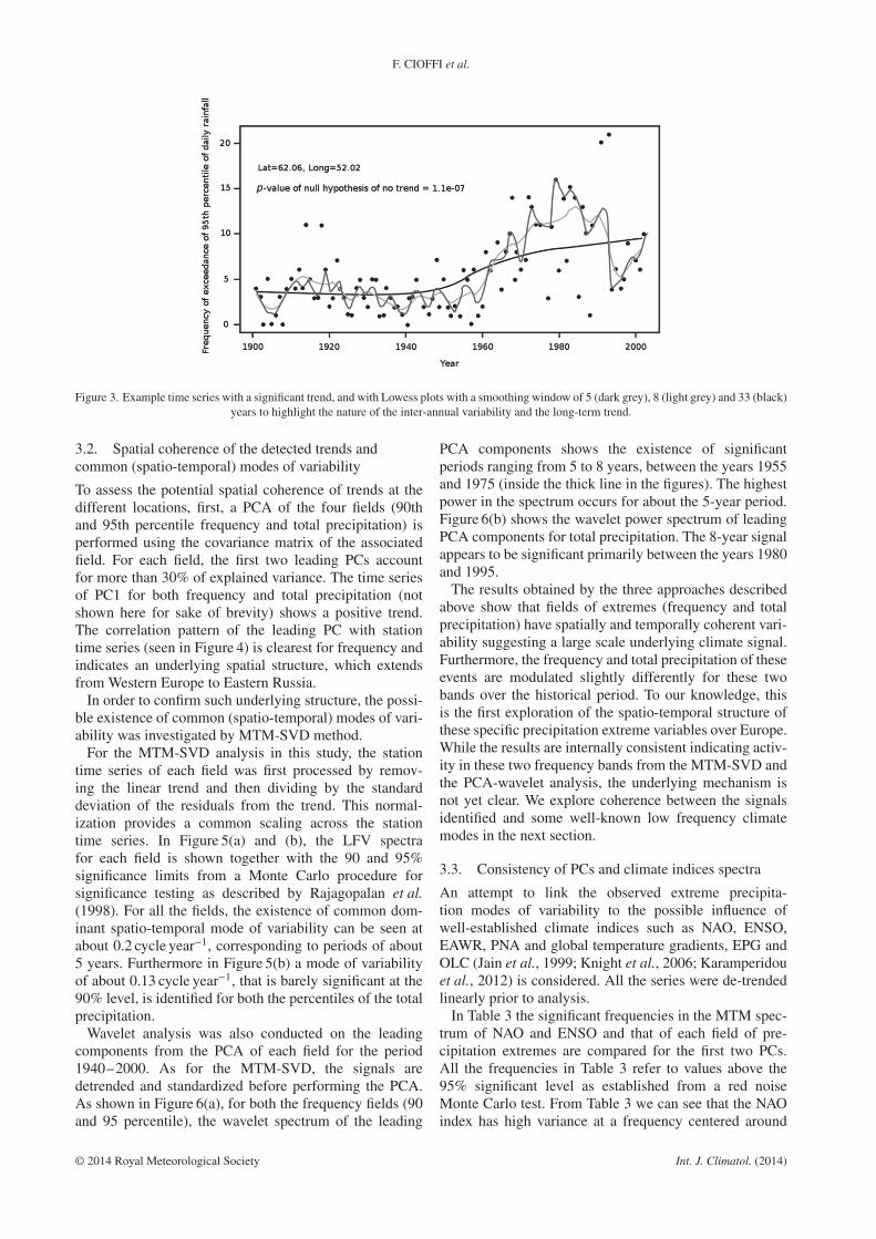
In Figure 2, a plot of stations with significant positive(black circle) and negative (grey circle) trends is provided.Stations with no significant trend are indicated with a whitecircle. Table 1 shows that for the frequency of exceedance,at either the 90th or the 95th percentile thresholds, thenumber of stations with positive trends far exceeds thosewith negative trends. The results are similar for total pre-cipitation. Positive trends in both frequency and amountoccur mainly above 45∘N and extend from Western Europeto Russia. At lower latitudes, for the few stations avail-able in the dataset, significant negative trends for bothtotal precipitation and frequency exceedance are evident.In Figure 3, an example time series with a significant trendis shown. In such figure the plots with a smoothing win-dow of 5 (dark grey), 8 (light grey) and 33 (black) years tohighlight the nature of the inter-annual variability and thelong-term trend are shown.

It is important to understand whether the increase inthe last century, at a large number of locations, of totalprecipitation is due to the increasing trends in the fre-quency, the rainfall intensity of extreme events or both.In Table 2, for each percentile, the number of significantand non-significant trends of rainfall intensity is shown asa function of the number of significant and non-significanttrends of frequency and total precipitation. Here, intensityis defined as the ratio between the total annual precipitationexceeding the threshold and the number of such events.The same MK-BBS analysis is used for the intensity vari-able.

From Table 2, the primary conclusion is that if the totalprecipitation trend is significant, it is very likely in all casesthat the frequency trend is also significant, and a muchsmaller likelihood that the intensity trend is significant.Correspondingly, if the frequency trend is significant, theintensity trend is significant for a modest number of cases.Thus, we note that the trend in the total precipitationfrom extreme events appears to be predominantly relatedto changes in the frequency of extreme events exceedingthe two thresholds and modestly due to changes in theaverage intensity of such events. The detailed results areas follows.

For the 90th percentile, we have 224 cases of which112 are significant for frequency and total precipitationbut only 46 for intensity. If the trend in frequency isnot significant then only 8/112 of the intensity trends aresignificant, while if frequency is significant then in 38/112cases the intensity trend is also significant. Essentially, ifthe frequency trend is not significant, so is the intensitytrend. Thus, both frequency and intensity trends can be



(a) (b)

(d)(c)

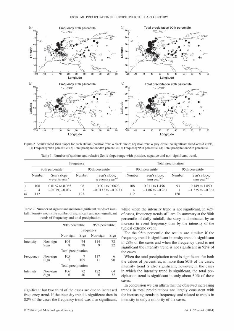
Figure 2. Secular trend (Sen slope) for each station (positive trend= black circle; negative trend= grey circle; no significant trend= void circle).(a) Frequency 90th percentile; (b) Total precipitation 90th percentile; (c) Frequency 95th percentile; (d) Total precipitation 95th percentile.

Table 1. Number of stations and relative Sen’s slope range with positive, negative and non-significant trend.

Frequency Total precipitation

90th percentile 95th percentile 90th percentile 95th percentile

Number Sen’s slope,n events year−1

Number Sen’s slope,n events year−1

Number Sen’s slope,mm year−1

Number Sen’s slope,mm year−1

+ 108 0.0167 to 0.085 98 0.001 to 0.0623 108 0.211 to 1.456 93 0.149 to 1.850− 4 −0.019, −0.037 3 −0.0137 to −0.0233 4 −1.86 to −0.267 3 −1.375 to −0.367ns 112 – 123 – 112 – 128 –

Table 2. Number of significant and non-significant trends of rain-fall intensity versus the number of significant and non-significant

trends of frequency and total precipitation.

90th percentile 95th percentile

Frequency

Non-sign Sign Non-sign Sign

Intensity Non-sign 104 74 114 72Sign 8 38 9 22

Total precipitation

Frequency Non-sign 105 7 117 6Sign 7 105 11 90

Total precipitation

Intensity Non-sign 106 72 122 64Sign 6 40 6 32

significant but two third of the cases are due to increasedfrequency trend. If the intensity trend is significant then in82% of the cases the frequency trend was also significant,

while when the intensity trend is not significant, in 42%of cases, frequency trends still are. In summary at the 90thpercentile of daily rainfall, the story is dominated by anincrease in event frequency than by the intensity of thetypical extreme event.

For the 95th percentile the results are similar: if thefrequency trend is significant intensity trend is significantin 28% of the cases and when the frequency trend is notsignificant the intensity trend is not significant in 92% ofthe cases.

When the total precipitation trend is significant, for boththe values of percentiles, in more than 80% of the cases,intensity trend is also significant; however, in the casesin which the intensity trend is significant, the total pre-cipitation trend is significant in only about 30% of thesecases.

In conclusion we can affirm that the observed increasingtrends in total precipitations are largely consistent withthe increasing trends in frequency, and related to trends inintensity in only a minority of the cases.


F. CIOFFI et al.

Figure 3. Example time series with a significant trend, and with Lowess plots with a smoothing window of 5 (dark grey), 8 (light grey) and 33 (black)years to highlight the nature of the inter-annual variability and the long-term trend.

3.2. Spatial coherence of the detected trends andcommon (spatio-temporal) modes of variability

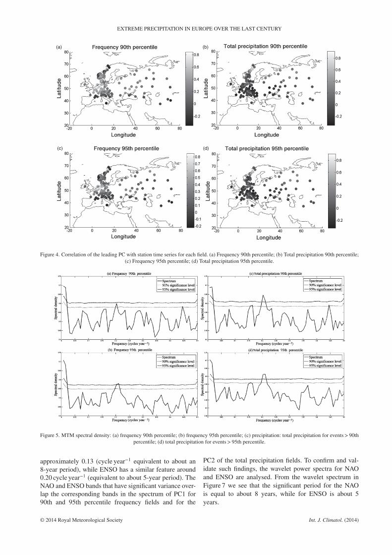
To assess the potential spatial coherence of trends at thedifferent locations, first, a PCA of the four fields (90thand 95th percentile frequency and total precipitation) isperformed using the covariance matrix of the associatedfield. For each field, the first two leading PCs accountfor more than 30% of explained variance. The time seriesof PC1 for both frequency and total precipitation (notshown here for sake of brevity) shows a positive trend.The correlation pattern of the leading PC with stationtime series (seen in Figure 4) is clearest for frequency andindicates an underlying spatial structure, which extendsfrom Western Europe to Eastern Russia.

In order to confirm such underlying structure, the possi-ble existence of common (spatio-temporal) modes of vari-ability was investigated by MTM-SVD method.

For the MTM-SVD analysis in this study, the stationtime series of each field was first processed by remov-ing the linear trend and then dividing by the standarddeviation of the residuals from the trend. This normal-ization provides a common scaling across the stationtime series. In Figure 5(a) and (b), the LFV spectrafor each field is shown together with the 90 and 95%significance limits from a Monte Carlo procedure forsignificance testing as described by Rajagopalan et al.(1998). For all the fields, the existence of common dom-inant spatio-temporal mode of variability can be seen atabout 0.2 cycle year−1, corresponding to periods of about5 years. Furthermore in Figure 5(b) a mode of variabilityof about 0.13 cycle year−1, that is barely significant at the90% level, is identified for both the percentiles of the totalprecipitation.

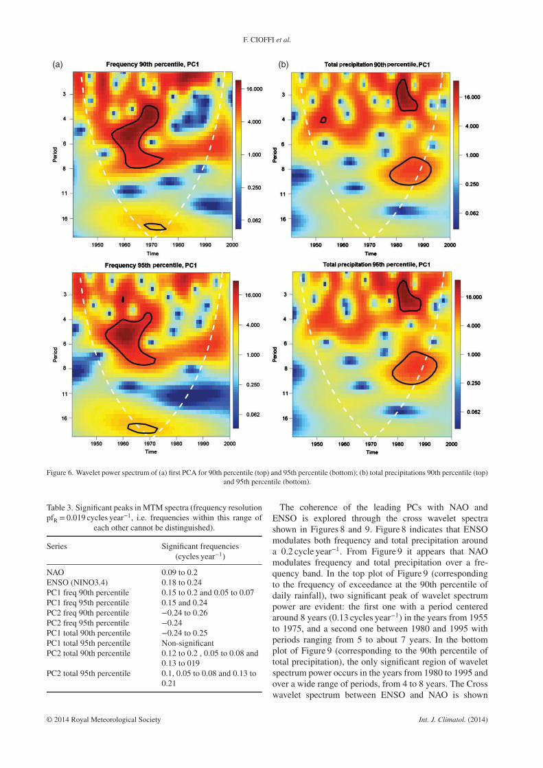
Wavelet analysis was also conducted on the leadingcomponents from the PCA of each field for the period1940–2000. As for the MTM-SVD, the signals aredetrended and standardized before performing the PCA.As shown in Figure 6(a), for both the frequency fields (90and 95 percentile), the wavelet spectrum of the leading

PCA components shows the existence of significantperiods ranging from 5 to 8 years, between the years 1955and 1975 (inside the thick line in the figures). The highestpower in the spectrum occurs for about the 5-year period.Figure 6(b) shows the wavelet power spectrum of leadingPCA components for total precipitation. The 8-year signalappears to be significant primarily between the years 1980and 1995.

The results obtained by the three approaches describedabove show that fields of extremes (frequency and totalprecipitation) have spatially and temporally coherent vari-ability suggesting a large scale underlying climate signal.Furthermore, the frequency and total precipitation of theseevents are modulated slightly differently for these twobands over the historical period. To our knowledge, thisis the first exploration of the spatio-temporal structure ofthese specific precipitation extreme variables over Europe.While the results are internally consistent indicating activ-ity in these two frequency bands from the MTM-SVD andthe PCA-wavelet analysis, the underlying mechanism isnot yet clear. We explore coherence between the signalsidentified and some well-known low frequency climatemodes in the next section.

3.3. Consistency of PCs and climate indices spectra

An attempt to link the observed extreme precipita-tion modes of variability to the possible influence ofwell-established climate indices such as NAO, ENSO,EAWR, PNA and global temperature gradients, EPG andOLC (Jain et al., 1999; Knight et al., 2006; Karamperidouet al., 2012) is considered. All the series were de-trendedlinearly prior to analysis.

In Table 3 the significant frequencies in the MTM spec-trum of NAO and ENSO and that of each field of pre-cipitation extremes are compared for the first two PCs.All the frequencies in Table 3 refer to values above the95% significant level as established from a red noiseMonte Carlo test. From Table 3 we can see that the NAOindex has high variance at a frequency centered around



(a) (b)

(d)(c)

Figure 4. Correlation of the leading PC with station time series for each field. (a) Frequency 90th percentile; (b) Total precipitation 90th percentile;(c) Frequency 95th percentile; (d) Total precipitation 95th percentile.

Figure 5. MTM spectral density: (a) frequency 90th percentile; (b) frequency 95th percentile; (c) precipitation: total precipitation for events> 90thpercentile; (d) total precipitation for events> 95th percentile.

approximately 0.13 (cycle year−1 equivalent to about an8-year period), while ENSO has a similar feature around0.20 cycle year−1 (equivalent to about 5-year period). TheNAO and ENSO bands that have significant variance over-lap the corresponding bands in the spectrum of PC1 for90th and 95th percentile frequency fields and for the

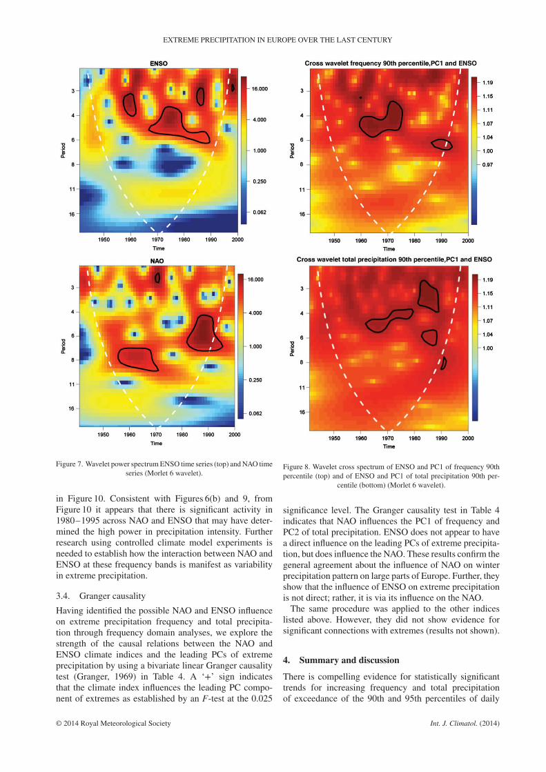
PC2 of the total precipitation fields. To confirm and val-idate such findings, the wavelet power spectra for NAOand ENSO are analysed. From the wavelet spectrum inFigure 7 we see that the significant period for the NAOis equal to about 8 years, while for ENSO is about 5years.


F. CIOFFI et al.

(a) (b)

Figure 6. Wavelet power spectrum of (a) first PCA for 90th percentile (top) and 95th percentile (bottom); (b) total precipitations 90th percentile (top)and 95th percentile (bottom).

Table 3. Significant peaks in MTM spectra (frequency resolutionpfR = 0.019 cycles year−1, i.e. frequencies within this range of

each other cannot be distinguished).

Series Significant frequencies(cycles year−1)

NAO 0.09 to 0.2ENSO (NINO3.4) 0.18 to 0.24PC1 freq 90th percentile 0.15 to 0.2 and 0.05 to 0.07PC1 freq 95th percentile 0.15 and 0.24PC2 freq 90th percentile −0.24 to 0.26PC2 freq 95th percentile −0.24PC1 total 90th percentile −0.24 to 0.25PC1 total 95th percentile Non-significantPC2 total 90th percentile 0.12 to 0.2 , 0.05 to 0.08 and

0.13 to 019PC2 total 95th percentile 0.1, 0.05 to 0.08 and 0.13 to

0.21

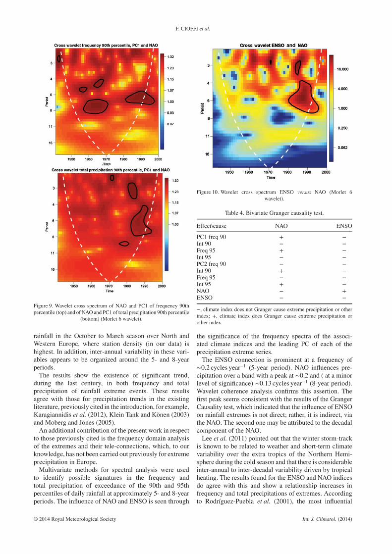
The coherence of the leading PCs with NAO andENSO is explored through the cross wavelet spectrashown in Figures 8 and 9. Figure 8 indicates that ENSOmodulates both frequency and total precipitation arounda 0.2 cycle year−1. From Figure 9 it appears that NAOmodulates frequency and total precipitation over a fre-quency band. In the top plot of Figure 9 (correspondingto the frequency of exceedance at the 90th percentile ofdaily rainfall), two significant peak of wavelet spectrumpower are evident: the first one with a period centeredaround 8 years (0.13 cycles year−1) in the years from 1955to 1975, and a second one between 1980 and 1995 withperiods ranging from 5 to about 7 years. In the bottomplot of Figure 9 (corresponding to the 90th percentile oftotal precipitation), the only significant region of waveletspectrum power occurs in the years from 1980 to 1995 andover a wide range of periods, from 4 to 8 years. The Crosswavelet spectrum between ENSO and NAO is shown



Figure 7. Wavelet power spectrum ENSO time series (top) and NAO timeseries (Morlet 6 wavelet).

in Figure 10. Consistent with Figures 6(b) and 9, fromFigure 10 it appears that there is significant activity in1980–1995 across NAO and ENSO that may have deter-mined the high power in precipitation intensity. Furtherresearch using controlled climate model experiments isneeded to establish how the interaction between NAO andENSO at these frequency bands is manifest as variabilityin extreme precipitation.

3.4. Granger causality

Having identified the possible NAO and ENSO influenceon extreme precipitation frequency and total precipita-tion through frequency domain analyses, we explore thestrength of the causal relations between the NAO andENSO climate indices and the leading PCs of extremeprecipitation by using a bivariate linear Granger causalitytest (Granger, 1969) in Table 4. A ‘+’ sign indicatesthat the climate index influences the leading PC compo-nent of extremes as established by an F-test at the 0.025

Figure 8. Wavelet cross spectrum of ENSO and PC1 of frequency 90thpercentile (top) and of ENSO and PC1 of total precipitation 90th per-

centile (bottom) (Morlet 6 wavelet).

significance level. The Granger causality test in Table 4indicates that NAO influences the PC1 of frequency andPC2 of total precipitation. ENSO does not appear to havea direct influence on the leading PCs of extreme precipita-tion, but does influence the NAO. These results confirm thegeneral agreement about the influence of NAO on winterprecipitation pattern on large parts of Europe. Further, theyshow that the influence of ENSO on extreme precipitationis not direct; rather, it is via its influence on the NAO.

The same procedure was applied to the other indiceslisted above. However, they did not show evidence forsignificant connections with extremes (results not shown).

4. Summary and discussion

There is compelling evidence for statistically significanttrends for increasing frequency and total precipitationof exceedance of the 90th and 95th percentiles of daily


F. CIOFFI et al.

Figure 9. Wavelet cross spectrum of NAO and PC1 of frequency 90thpercentile (top) and of NAO and PC1 of total precipitation 90th percentile

(bottom) (Morlet 6 wavelet).

rainfall in the October to March season over North andWestern Europe, where station density (in our data) ishighest. In addition, inter-annual variability in these vari-ables appears to be organized around the 5- and 8-yearperiods.

The results show the existence of significant trend,during the last century, in both frequency and totalprecipitation of rainfall extreme events. These resultsagree with those for precipitation trends in the existingliterature, previously cited in the introduction, for example,Karagiannidis et al. (2012), Klein Tank and Könen (2003)and Moberg and Jones (2005).

An additional contribution of the present work in respectto those previously cited is the frequency domain analysisof the extremes and their tele-connections, which, to ourknowledge, has not been carried out previously for extremeprecipitation in Europe.

Multivariate methods for spectral analysis were usedto identify possible signatures in the frequency andtotal precipitation of exceedance of the 90th and 95thpercentiles of daily rainfall at approximately 5- and 8-yearperiods. The influence of NAO and ENSO is seen through

Figure 10. Wavelet cross spectrum ENSO versus NAO (Morlet 6wavelet).

Table 4. Bivariate Granger causality test.

Effect\cause NAO ENSO

PC1 freq 90 + −Int 90 − −Freq 95 + −Int 95 − −PC2 freq 90 − −Int 90 + −Freq 95 − −Int 95 + −NAO − +ENSO − −

−, climate index does not Granger cause extreme precipitation or otherindex; +, climate index does Granger cause extreme precipitation orother index.

the significance of the frequency spectra of the associ-ated climate indices and the leading PC of each of theprecipitation extreme series.

The ENSO connection is prominent at a frequency of∼0.2 cycles year−1 (5-year period). NAO influences pre-cipitation over a band with a peak at ∼0.2 and ( at a minorlevel of significance) ∼0.13 cycles year−1 (8-year period).Wavelet coherence analysis confirms this assertion. Thefirst peak seems consistent with the results of the GrangerCausality test, which indicated that the influence of ENSOon rainfall extremes is not direct; rather, it is indirect, viathe NAO. The second one may be attributed to the decadalcomponent of the NAO.

Lee et al. (2011) pointed out that the winter storm-trackis known to be related to weather and short-term climatevariability over the extra tropics of the Northern Hemi-sphere during the cold season and that there is considerableinter-annual to inter-decadal variability driven by tropicalheating. The results found for the ENSO and NAO indicesdo agree with this and show a relationship increases infrequency and total precipitations of extremes. Accordingto Rodríguez-Puebla et al. (2001), the most influential



indices for winter precipitation were the NAO and theEAWR pattern, with coherent oscillations at about 8 yearsbetween precipitation and the NAO. Haylock and Good-ess (2004) found that extreme rainfall is generally not asspatially coherent as mean rainfall and suggested that theobserved trend in the NAO has strongly contributed tothe observed trends, but not EAWR. From the Grangercausality test, as well as from the wavelet cross-spectrawe see a hint that the ENSO influence on precipitationextremes over Europe may be manifest through its mod-ulation of the NAO effects. Essentially, these relate to themodulation of the winter jet stream and the associatededdies. Consequently, we recommend that analyses ofGCM-based projections of future changes in precipitationextremes consider at least the following performancemetrics:

1. the ability of the model to reproduce the historicalfrequency and intensity of ENSO and NAO, and oftheir modulation of the jet stream location and strength,as well as eddy coupling;

2. the relationship between the persistence and inten-sity of extreme precipitation in Northern Europe, andregional atmospheric circulation patterns in the model;

3. the projected changes in ENSO, NAO and jet streamdynamics, and their implication for changes in thenature of extreme precipitation;

4. The historical trends in the frequency and inten-sity of the extreme daily rainfall, including theirspatio-temporal structure in the models relative to therecord.

The severity of extreme floods is related to the frequencyand intensity of extreme daily rainfall events. Planning fornon-stationary conditions and for climate change adapta-tion is crucial to develop a good financial risk portfoliomanagement, and it needs to incorporate both secular vari-ations and quasi-periodic or regime-like variations, espe-cially when they can be identified by observable climateindicators.

Acknowledgements

The analysis presented here is part of a Global Flood Ini-tiative (http://water.columbia.edu/research-projects/the-columbia-global-flood-initiative/) that aims to linkclimate, floods, impacts and risk management as partof research towards a climate adaptation and risk mit-igation strategy. The support of the H2CU programfor the research agreement between Columbia Univer-sity and University of Roma, La Sapienza is gratefullyacknowledged.

References

Bell JL, Sloan LC, Snyder M. 2004. Regional changes in extremeclimatic events: a future climate scenario. J. Clim. 17(1): 81–87, DOI:10.1175/1520-0442(2004)017.

Bengtsson L, Hodges K, Keenlyside N. 2009. Will extratropical stormsintensify in a warmer climate? J. Clim. 22: 2276–2301, DOI:10.1029/2011GL049599.

Brönnimann S. 2007. Impact of El Niño–southern oscillationon European climate. Rev. Geophys. 45(3): RG3003, DOI:10.1029/2006RG000199.

Brönnimann S, Xoplaki E, Casty C, Pauling A, Luterbacher J. 2007.ENSO influence on Europe during the last centuries. Clim. Dyn.28(2–3): 181–197, DOI: 10.1007/s00382-006-0175-z.

Christensen OB, Goodess CM, Ciscar J. 2012. Methodologicalframework of the PESETA project on the impacts of cli-mate change in Europe. Clim. Change 112(1): 7–28, DOI:10.1007/s10584-011-0337-9.

Costa AC, Solares A. 2009. Trends in extreme precipitation indicesderived from a daily rainfall database for the South of Portugal. Int.J. Climatol. 29: 1956–1975, DOI: 10.1002/joc.1834.

Cubasch U, Meehl GA, Boer GJ, Stouffer RJ, Dix M, Noda A, SeniorCA, Raper S, Yap KS. 2001. Projections of future climate change.In Climate Change 2001: The Scientific Basis, Contribution of Work-ing Group I to the Third Assessment Report of the IntergovernmentalPanel on Climate Change, Houghton JT, Ding Y, Griggs DJ, NoguerM, Van der Linden PJ, Dai X, Maskell K, Johnson CA (eds). Cam-bridge University Press: New York, NY, 525–585.

Du H, Wu Z, Li M, Jin Y, Zong S, Meng X. 2013a. Characteristics ofextreme daily minimum and maximum temperature over NortheastChina: 1961–2009. J. Theor. Appl. Climatol. 111(1–2): 161–171,DOI: 10.1007/s00704-012-0649-3.

Du H, Wu Z, Zong S, Meng X, Wang L. 2013b. Assessing the charac-teristics of extreme precipitation over northeast China using the mul-tifractal detrended fluctuation analysis. J. Geophys. Res. Atmos. 118:6165–6174, DOI: 10.1002/jgrd.50487.

Fraedrich K, Larnder C. 1993. Scaling regimes of composite rainfall timeseries. Tellus Ser. A: Dyn. Meteorol. Oceanogr. 45: 289–298.

Frei C, Schär C. 2001. Detection probability of trends in rare events:theory and application to heavy precipitation in the Alpine region.J. Clim. 14: 1568–1584, DOI: 10.1007/s00704-012-0649-3.

Frei C, Davies HC, Gurtz J, Schär C. 2000. Climate dynamics andextreme precipitation and flood events in Central Europe. Integr.Assess. 1(4): 281–300, DOI: 10.1023/A:1018983226334.

Frei C, Schöll R, Fukutome S, Schmidli J, Vidale PL. 2006. Futurechange of precipitation extremes in Europe: intercomparison of sce-narios from regional climate models. J. Geophys. Res. 111: D06105,DOI: 10.1029/2005JD005965.

Gong DY, Ho CH. 2004. Intra-seasonal variability of wintertime tem-perature over East Asia. Int. J. Climatol. 24(2): 131–144, DOI:10.1002/joc.1006.

González Hidalgo JC, De Luís M, Raventós J, Sánchez JR. 2003. Dailyrainfall trend in the Valencia Region of Spain. Theor. Appl. Climatol.75: 117–130, DOI: 10.1007/s00704-002-0718-0.

Granger CWJ. 1969. Investigating causal relations by economet-ric models and cross-spectral methods. Econometrica 37(3):424–438.

Guzzetti F, Stark CP, Salvati P. 2005. Evaluation of flood and landsliderisk to the population of Italy. Environ. Manage. 36(1): 15–36, DOI:10.1007/s00267-003-0257-1.

Hajat S, Ebi KL, Kovats RS, Menne B, Edwards S, Haines A.2005. The human health consequences of flooding in Europe: areview. In Extreme Weather Events and Public Health Responses.Springer-Verlag: Berlin and Heidelberg, Germany.

Haylock MR, Goodess CM. 2004. Interannual variability of Europeanextreme winter rainfall and links with mean large-scale circulation.Int. J. Climatol. 24: 759–776, DOI: 10.1002/joc.1033.

Henderson KG, Muller RA. 1997. Extreme temperature days inthe South-Central United States. Clim. Res. 8(2): 151–162, DOI:10.3354/cr0008151.

Hennessy KJ, Gregory JM, Mitchell JFB. 1997. Changes in daily pre-cipitation under enhanced greenhouse conditions. Clim. Dyn. 13:667–680.

Hidalgo-Muñoz JM, Argüeso D, Gámiz-Fortis SR, Esteban-Parra MJ,Castro-Díez Y. 2011. Trends of extreme precipitation and associatedsynoptic patterns over the southern Iberian Peninsula. J. Hydrol. 409:497–511, DOI: 10.1016/j.jhydrol.2011.08.049.

Hipel KW, McLeod AI. 2005. Time Series Modelling of WaterResources and Environmental Systems. Electronic reprint of ourbook originally published in 1994, Retrieved July 14, 2014.http://www.stats.uwo.ca/faculty/aim/1994Book/.

Huang DQ, Qian YF, Zhu J. 2010. Trends of temperature extremes inChina and their relationship with global temperature anomalies. Adv.Atmos. Sci. 27(4): 937–946, DOI: 10.1007/s00376-009-9085-4.


F. CIOFFI et al.

Jain S, Lall U, Mann M. 1999. Seasonality and interannual variationsof Northern Hemisphere temperature: equator-to-pole gradient andocean-land contrast. J. Clim. 12: 1086–1100.

Jones PD, Horton EB, Folland CK, Hulme M, Parker DE, Basnett TA.1999. The use of indices to identify changes in climatic extremes.Clim. Change 42(1): 131–149, DOI: 10.1023/a:1005468316392.

Kalnay E, Kanamitsu M, Kistler R, Collins W, Deaven D, Gandin L,Iredell M, Saha S, White G, Woollen J, Zhu Y, Chelliah M, EbisuzakiW, Higgins W, Janowiak J, Mo KC, Ropelewski C, Wang J, LeetmaaA, Reynolds R, Jenne R, Joseph D. 1996. The NCEP/NCAR 40-YearReanalysis Project. Bull. Am. Meteorol. Soc. 77: 437–471, DOI:10.1175/1520,0477(1996)077<0437:TNYRP>2.0.CO;2.

Kantelhardt JW, Zschiegner SA, Koscielny-Bunde E, Havlin S, BundeA, Stanley HE. 2002. Multifractal detrended fluctuation analysisof nonstationary time series. Physica A 316(1): 87–114, DOI:10.1016/s0378-4371(02)01383-3.

Kaplan A, Cane M, Kushnir Y, Clement A, Blumenthal M, RajagopalanB. 1998. Analyses of global sea surface temperature 1856–1991. J.Geophys. Res. 103(18): 567–589.

Karagiannidis AF, Karacostas T, Maheras P, Makrogiannis T. 2012.Climatological aspects of extreme precipitation in Europe, related tomid-latitude cyclonic systems. Theor. Appl. Climatol. 107: 165–174.

Karamperidou C, Cioffi F, Lall U. 2012. Surface temperature gradientsas diagnostic indicators of midlatitude circulation dynamics. J. Clim.25(12): 4154–4171, DOI: 10.1175/JCLI-D-11-00067.1.

Kharin VV, Zwiers FW, Zhang X, Hegerl GC. 2007. Changes intemperature and precipitation extremes in the IPCC ensemble ofglobal coupled model simulations. J. Clim. 20(8): 1419–1444, DOI:10.1175/JCLI4066.1.

Klein Tank AMG, Können GP. 2003. Trends in indices of daily tem-perature and precipitation extremes in europe, 1946–99. J. Clim. 16:3665–3680, DOI: 10.1175/1520-0442(2003)016<3665:TIIODT>2.0.CO;2.

Klein Tank AMG, Wijngaard JB, Können GP, Böhm R, Demarée G,Gocheva A, Mileta M, Pashiardis S, Hejkrlik L, Kern-Hansen C, HeinoR, Bessemoulin P, Müller-Westermeier G, Tzanakou M, Szalai S,Pálsdóttir T, Fitzgerald D, Rubin S, Capaldo M, Maugeri M, LeitassA, Bukantis A, Aberfeld R, van Engelen AFV, Forland E, MietusM, Coelho F, Mares C, Razuvaev V, Nieplova E, Cegnar T, AntonioLJ, Dahlström B, Moberg A, Kirchhofer W, Ceylan A, Pachaliuk O,Alexander LV, Petrovic P. 2002. Daily dataset of 20th-century surfaceair temperature and precipitation series for the European ClimateAssessment. Int. J. Climatol. 22: 1441–1453, DOI: 10.1002/joc.

Klok EJ, Klein Tank AMG. 2009. Updated and extended Europeandataset of daily climate observations. J. Clim. 29: 1182–1191, DOI:10.1002/joc.1779.

Knight JR, Folland CK, Scaife AA. 2006. Climate impacts of theAtlantic Multidecadal Oscillation. Geophys. Res. Lett. 33: L17706,DOI: 10.1029/2006GL026242.

Kothawale DR, Revadekar JV, Rupa Kumar K. 2010. Recent trends inpre-monsoon daily temperature extremes over India. J. Earth. Syst. Sci119(1): 51–65, DOI: 10.1007/s12040-010-0008-7.

Krishnamurthy CKB, Lall U, Kwon HH. 2009. Changing frequency andintensity of rainfall extremes over India from 1951 to 2003. J. Clim.22: 4737–4746, DOI: 10.1175/2009JCLI2896.1.

Kundzewicz ZW, Robson AJ. 2004. Change detection in hydrologi-cal records – a review of the methodology. Hydrol. Sci. J. 49(1):7–19.

Kundzewicz ZW, Kanae S, Seneviratne SI, Handmer J, Nicholls N,Peduzzi P, Mechler R, Bouwer LM, Arnell N, Mach K, Muir-WoodR, Brakenridge GR, Kron W, Benito G, Honda Y, TakahashiK, Sherstyukov B. 2013. Flood risk and climate change: globaland regional perspectives. Hydrol. Sci. J. 59(1): 1–28, DOI:10.1080/02626667.2013.857411.

Lee SS, Lee JY, Wang B, Ha K, Heo K, Ha KJ, Jin F, Straus DM,Shukla J. 2011. Interdecadal changes in the storm track activity overthe North Pacific and North Atlantic. Clim. Dyn. 39: 313–327, DOI:10.1007/s00382-011-1188-9.

Lehner B, Döll P, Alcamo J, Henrichs T, Kaspar F. 2006. Estimatingthe impact if global change on flood and drought risks in Europe:a continental, integrated analysis. Clim. Change 75: 273–299, DOI:10.1007/s10584-006-6338-4.

Li Z, Zheng FL, Liu WZ, Flanagan DC. 2010. Spatial distribution andtemporal trends of extreme temperature and precipitation events on

the Loess Plateau of China during 1961–2007. Quat. Int. 226(1–2):92–100, DOI: 10.1016/j.quaint.2010.03.003.

Mann ME, Park J. 1999. Oscillatory spatiotemporal signal detection inclimate studies: a multi-taper spectral domain approach. Adv. Geo-phys. 41: 1–131.

Marchi L, Borga M, Preciso E, Gaume E. 2010. Characterizationof selected extreme flash floods in Europe and implications forflood risk Management. J. Geophys. Res. 391: 118–133, DOI:10.1016/j.jhydrol.2010.07.017.

Moberg A, Jones PD. 2005. Trends in indices for extremes in daily tem-perature and precipitation in central and western Europe, 1901–99.Int. J. Climatol. 25: 1149–1171, DOI: 10.1002/joc.1163.

Mudelsee M, Börngen M, Tetzlaff G, Grünewald U. 2003. No upwardtrends in the occurrence of extreme floods in central Europe. Nature425: 166–169.

Mudelsee M, Börngen M, Tetzlaff G, Grünewald U. 2004. Extremefloods in central Europe over the past 500 years: role of cyclonepathway “Zugstrasse Vb”. J. Geophys. Res. 109: D23101, DOI:10.1029/2004JD005034.

Nastos PT, Zerefos CS. 2007. On extreme daily precipitation totals atAthens, Greece. Adv. Geosci. 10: 59–66.

New M, Todd M, Hulme M, Jones P. 2002. Precipitation measurementsand trends in the twentieth century. Int. J. Climatol. 21: 1889–1922,DOI: 10.1002/joc.680.

Önöz B, Bayazit M. 2012. Block bootstrap for Mann–Kendall trend testof serially dependent data. Hydrol. Processes 26: 3552–3560, DOI:10.1002/hyp.8438.

Palmer TN, Rälsänen J. 2002. Quantifying the risk of extreme sea-sonal precipitation events in a changing climate. Nature 415:512–514.

Pozo-Vazquez D, Gamiz-Fortis SR, Tovar-Pescador J, Esteban-ParraMJ, Castro-Deiz Y. 2005. El Niño–Southern Oscillation events andassociated European winter precipitation anomalies. Int. J. Climatol.25: 17–31, DOI: 10.1002/joc.1097.

Rajagopalan B, Mann ME, Lall U. 1998. A multivariatefrequency-domain approach to long-lead climatic forecasting.Weather Forecast. 13(1): 58–74.

Reynolds RW, Rayner NA, Smith TM, Stokes DC, Wang W. 2002. Animproved in situ and satellite SST analysis for climate. J. Clim. 15:1609–1625.

Rodríguez-Puebla C, Encinas AH, Sáenz J. 2001. Winter precipitationover the Iberian Peninsula and its relationship to circulation indices.Hydrol. Earth Syst. Sci. 5(2): 233–244.

Sen PK. 1968. Estimates of regression coefficient based on Kendall’s tau.J. Am. Stat. Assoc. 1: 1379–1389.

Sevruk B. 1997. Regional dependency of precipitation-altitude relation-ship in the Swiss Alps. Clim. Change 36: 355–569.

Thomson DJ. 1982. Spectrum estimation and harmonic analysis. Proc.IEEE 70: 1055–1096.

Wijngaard JB, Klein Tank AMG, Können GP. 2003. Homogeneity of20th century European daily temperature and precipitation series. Int.J. Climatol. 23: 679–692, DOI: 10.1002/joc.906.

Xu Y, Xu CH, Gao XJ, Luo Y. 2009. Projected changes in tem-perature and precipitation extremes over the Yangtze River Basinof China in the 21st century. Quat. Int. 208(1–2): 44–52, DOI:10.1016/j.quaint.2008.12.020.

Xu X, Du YG, Tang JP, Wang Y. 2011. Variations of temperature andprecipitation extremes in recent two decades over China. Atmos. Res.101(1–2): 143–154, DOI: 10.1016/j.atmosres.2011.02.003.

Yiou P, Nogaj M. 2004. Extreme climatic events and weather regimesover the North Atlantic: when and where? Geophys. Res. Lett. 31:L07202, DOI: 10.1029/2003GL019119.

Yonetani T, Gordon HP. 2001. Simulated changes in the frequency ofextremes and regional features of seasonal/annual temperature andprecipitation when CO2 is doubled. J. Clim. 14: 1765–1779, DOI:10.1175/1520-0442(2001)014<1765:SCITFO>2.0.CO;2.

Zolina O, Kapala A, Simmer C, Gulev SK. 2004. Analysis ofextreme precipitation over Europe from different reanalyses: acomparative assessment. Glob. Planet. Sci. 44: 129–161, DOI:10.1016/j.gloplacha.2004.06.009.

Zolina O, Simmer C, Brelyaev K, Gulev SK, Koltermann P. 2012.Changes in the duration of European wet and dry spells during thelast 60 years. J. Clim. 26: 2022–2047, DOI: 10.1175/JCLI-D-11-00498.1.


int. journ clim. 2014 cioffi

Documents