Electronic copy available at: http://ssrn.com/abstract=1154989

D S E Working Paper

Information Sharing Networks in Oligopoly

Sergio CurrariniFrancesco Feri

Dipartimento Scienze Economiche

Department of Economics

Ca’ Foscari University ofVenice

ISSN: 1827/336X

No. 16/WP/2008

Electronic copy available at: http://ssrn.com/abstract=1154989

W o r k i n g P a p e r s D e p a r t m e n t o f E c o n o m i c s

C a ’ F o s c a r i U n i v e r s i t y o f V e n i c e N o . 1 6 / W P / 2 0 0 8

ISSN 1827-3580

The Working Paper Series is availble only on line

(www.dse.unive.it/pubblicazioni) For editorial correspondence, please contact:

wp.dse@unive.it

Department of Economics Ca’ Foscari University of Venice Cannaregio 873, Fondamenta San Giobbe 30121 Venice Italy Fax: ++39 041 2349210

Information Sharing Networks in Oligopoly

Sergio Currarini Università di Venezia

Francesco Feri

Università di Innsbruck

First Draft: June 2008

Abstract We study the incentives of oligopolistic firms to share private information on demand parameters. Differently from previous studies, we consider bilateral sharing agreements, by which firms commit at the ex-ante stage to truthfully share information. We show that if signals are i.i.d., then pairwise stable networks of sharing agreements are either empty or made of fully connected components of increasing size. When linking is costly, non complete components may emerge, and components with larger size are less densly connected than components with smaller size. When signals have different variances, incomplete and irregular network can be stable, with firms observing high variance signals acting as "critical nodes". Finally, when signals are correlated, the empty network may not be pairwise stable when the number of firms and/or correlation are large enough. Keywords Information sharing, oligopoly, networks, Bayesian equilibrium JEL Codes D43, D82, D85, L13

Address for correspondence: Sergio Currarini

Department of Economics Ca’ Foscari University of Venice

Cannaregio 873, Fondamenta S.Giobbe 30121 Venezia - Italy

Phone: (++39) 041 2349133 Fax: (++39) 041 2349176

e-mail: s.currarini@unive.it

This Working Paper is published under the auspices of the Department of Economics of the Ca’ Foscari University of Venice. Opinions expressed herein are those of the authors and not those of the Department. The Working Paper series is designed to divulge preliminary or incomplete work, circulated to favour discussion and comments. Citation of this paper should consider its provisional character.

Electronic copy available at: http://ssrn.com/abstract=1154989

1 Introduction

The incentives of oligopolistic firms to share private information about a random demand

intercept have been studied by vast literature, pioneered by the works of Novshek and Son-

nenschein (1982), Clarke (1983), Vives (1985), Li (1985) and Gal-or (1985). All works in this

literature has modeled the transmission of information by assuming that firms disclose their

private information to a central agency (e.g., a Trade Association), which aggregates all the

received information and delivers it back to firms. While in most papers it is assumed that

firms receive the aggregated information independently of their disclosure decision, some au-

thors have studied a quid pro quo exchange mechanism, in which firms receive the aggregated

information if and only if they have disclosed their own (see Clark (1983), Kirby (1988),

Raith (1996)).

In the case of quid pro quo exchange, most results have compared firms’ expected profits

in a scenario of complete absence of information with profits in a scenario in which all firms

share their own information. Kirby (1988) has studied the Nash Equilibrium of a game in

which each firm decides its disclosure behaviour in a quid pro quo exchange,game.

In this paper we contribute to this literature by exploring the equilibrium sharing be-

haviour of firms when contracts are bilateral. In our model, firms meet in pairs, and decide

whether to share their own private information by means of an quid pro quo contract. What

we have in mind is therefore not a central device of information transmission, such as a

Trade Association, but rather a series of private and bilateral contacts, by which firms share

information in a targeted way, without necessarily disclosing it to all firms in the system.

The structure of bilateral sharing agreement is well represented by a non directed network,

in which nodes represent firms, and links represent agreements.

In this new context we address old and new questions in a simple Cournot game with

homogeneous goods and no production costs. Do we observe information sharing in equi-

librium? Can we characterize the equilibrium architectures agreements? Can we trace the

sharing behaviour of firms to their position in the network and vice versa? And what is the

role of asymmetry and correlation of private signals in determining equilibrium networks?

We employ the model of Gal-Or (1985), in which a set of Cournot oligopolists each

observes a piece of the demand intercept. In this framework, the signals observed by firms

can be independently distributed, thus allowing for a benchmark model in which the model

remains tractable. For the case of i.i.d signals, we are able to fully characterize the set

2

pairwise stable sharing networks.1 In this simple case, the incentives of two firms to share

information turn out to only depend on their relative degrees in the network (that is, on

the number of firms that observe their signals). In particular, the incentive of firm i to

share information with firm j increase with the degree of i and decrease with the degree of j.

Information sharing presents here clear aspects of congestion, with signals observed by many

firms having less informational value than signals viewed by few. One way of explaining

this result is the following. Expected profits are strictly related to the variability of firms

equilibrium strategies in the Cournot game. The acquisition of new information has the effect

of adding one source of variability (the new observed signal) and to reduce the variability

of the signals already observed (by sharing it with another firm). The variability added by

the acquisition of the new signal decreases with the number of firms observing that signal

(because of the larger correlation of firms’ equilibrium strategies), while the loss in variability

due to the disclosure of one’s own signal decreases with the number of firms that already

observe that signal.

This simple structure of incentives originate a large set of pairwise stable networks with,

nonetheless, neat qualitative features. First, the empty network (with no information shar-

ing) is always stable, a result that echoes previous literature. Indeed, two isolated firms

have no incentives to share information, just like two duopolist in the traditional approach.

Second, there exist many other pairwise stable networks in which positive information is

shared, all made of completely connected components with strictly increasing size. Firms are

therefore organized in ”Information Sharing Groups”, each informationally equivalent to a

centralized transmission device. For this benchmark model, we also look at the effect of an

exogenous linking cost. Somewhat surprisingly, a small cost lead to qualitative differences

in the incentives to share and in equilibrium information structures. In particular, non com-

plete components are now possible as part of a stable network. Moreover, the ”density” of a

component (measure as the ratio between its average degree and its size) decreases with its

size. In other words, small groups of firms share information more tightly that large groups.

We then study extensions of this benchmark model. We first allow independent signals

to have heterogeneous variances. The incentives to form a link depend now on the relative

degrees of firms and on the relative variance of their private signals. In general, the incentive

1The well known concept of pairwise stability, first used in Jackson and Wolinsky (1996)), requires that

no link is either added or severed from the network. Adding a link requires mutual consent, while severing

requires the conent of one firm only.

3

of firm i to form a link with firm j are decreasing in the variance of the signal observed

by i, and increasing in the variance of j’s signal. Intuitively, a large variance signal has a

large informational value, since it allows equilibrium strategies to acquire more variability.

Although the empty network remains an equilibrium, new and informationally incomplete

architecture are now possible. In particular, we show that non regular networks, usually

referred to as ”core-periphery”, are stable, in which high variance firms have high degree and

act as ”connectors”, indirectly linking low variance firms.

We finally turn to the richer and more complex case of correlated signals. We first show

that the empty network is not be pairwise stable for high enough levels of correlation. In

such cases, some positive amount of information sharing is present in all pairwise stable

networks - a result to be contrasted with the traditional view that information sharing is

incompatible with equilibrium in Cournot games with homogeneous goods. Intuitively, the

additional incentives of two firms to share information come from the improved inference

over the signals observed by the remaining firms; this better inference comes without any

additional disclosure of information to the remaining firms and is, in this sense, at no cost.

After showing that the complete network is always stable, we fully work out the case of four

firms, for which we characterize the set of stable network for different ranges of the correlation

parameter. It is of some interest to analyze the effect of correlation on the incentives to share.

In particular, as correlation grows we pass from a stable structure in which one isolated firm

refuses to join the information sharing group formed by the other firms, to one in which the

same firm is excluded from the group. Intuitively, for low levels of correlation, the isolated

firm finds it profitable to exploit the full variance of its own signal; as correlation increases,

the profitability for the isolated firm of observing another signal increases, simply because

of the increased inference power of such signal. However, the high level of correlation allows

the sharing group to have a good enough inference on the isolated firm, which is therefore

excluded.

We start by presenting the basic model, the information sharing mechanism and the

Cournot game played by firms. In section 3 we study the set of pairwise stable networks

when signals are independently distributed. Section 4 studies the case of correlated signals.

Section 5 concludes the paper.

4

2 The Model

2.1 Set-up

We consider a n-firms oligopolistic market with linear demand and no costs. The size of the

market, given by the intercept of the demand function, is the sum of n random variables

(a1, a2, ..., an) plus a deterministic part A:

p(Q) = A+ a− bQ (1)

where Q ≡n∑

i=1qi is the aggregate produced level in the market, and where a ≡ a1+a2+...+an.

Each variable ai is private information of firm i.

The vector of random variables (a1, a2, ..., an) is jointly normally distributed with zero

mean and matrix of variances and covariances:

Ω =

σ11 σ12 ... σ1n

... σ22 ... σ2n

... ... ... ...

... ... ... σnn

.

2.2 Information Sharing

Before observing the realization of private signals, firms can engage in bilateral information

sharing agreements. By signing such an agreement, firms i and j commit to truthfully

exchange the private information they receive, so that firm i gets to observe the realization

of the random variable aj and viceversa.

Bilateral agreements need not be transitive: the agreements ij and jk need not imply the

existence of an agreement between firms i and k. This is the main difference between the

present approach and the previous literature, in which the transmission of a firm’s private

signals has a universal nature, as it is immediately and non exclusively received by all other

firms.

Bilateral sharing agreements generate an information structure that can be usefully de-

scribed as a non directed network. Given a set N , a non directed network g is defined as any

subset of the set of all (unordered) pairs of elements in N :

g ⊆ ij : i ∈ N and j ∈ N, i = j .

5

The elements of N are called nodes, and a pair ij ∈ g is called a ”link”. We denote by

Ngi = j ∈ N : ij ∈ g∪i the neighbourhood of i in g, with cardinality ngi (this cardinality

is called ”degree” of i). We will denote by g − ij the network obtained from g by deleting

the link ij ∈ g and by g + ij the network obtained from g by adding the link ij /∈ g.

The network g is connected if for all pairs i and j in N there exists a connecting path

P (i, j), that is, a set i1, i2, ..., ik such that i = i1, j = ik, and ipip+1 ∈ g for all p = 1, ..., k−1.

Given the network g, the network h with set of nodes M ⊆ N is a subnetwork of g if h ⊆ g.

The subnetwork h of g is a component of g if it is connected and if for all i ∈M and j /∈M

we have ij /∈ g. A component h is regular if all i ∈ h have the same degree. With some abuse

of terminology, we will say that the network g is regular when all its components are regular.

The size of a component h, denoted by n(h), is the cardinality of the set M . A component

is completely connected is it is regular and its size coincides with its degree.

We derive the incentives of firms to form and sever links by associating with each possible

network g the expected profits of each firm i, denoted by E [πi(g)]. These expectations are

taken ex-ante, as decisions to sign sharing agreements are made before the realization of

private signals.2 In more detail, once private signals are realized, firms play the Cournot

game with incomplete information Γg, in which the information available to firm i is given by

the vector agi = aj : j ∈ Ngi . We will denote by E [· |agi ] the expectation conditional on the

information agi , and by Egi [·] the expectation taken over all possible realization of the signals

agi . Finally, we denote by qi(g) the quantity set by firm i in the Bayesian Nash Equilibrium

of the game Γg. We have the following standard result (see proposition 1 in Kirby (1988)).

Lemma 1 Ex-ante expected profits of firm i in the game Γg are given by:

E [πi(g)] = Egi

[bqi(g)

2]

Following Jackson and Wolinsky (1996), we use the concept of pairwise stable networks

as a solution concept for the network formation stage. The network g is pairwise stable if no

link is either formed or severed.

Definition 1 The network g is pairwise stable iff:

2In this we follow most of the existing literature. A study of link formation at the interim stage is of

great interest, and involves strategic consideration and technical difficulties that are not present in the ex-ante

approach. This is left for future research.

6

i) E [πi(g)]−E [πi(g − ij)] ≥ 0 and E [πj(g)]−E [πj(g − ij)] ≥ 0 for all ij ∈ g;

ii) if E [πi(g + ij)]−E [πi(g)] > 0 then E [πi(g + ij)]−E [πj(g)] < 0, for all ij /∈ g.

2.3 Bayesian Cournot Equilibrium for a Given Network of Agreements

Before turning to the analysis of pairwise stable networks in the next sections, we study the

structure of Bayesian Nash Equilibrium of the game Γg in more detail. A pure strategy for

firm i is a function si : Rngi+ → R+ setting a quantity level for each possible vector of signal

observed by i. A Bayesian Nash equilibrium of this game is a profile of strategies (si)i=1,...,n

such that for all i, for all qi and for all agi :

Ei

A+ a− b

si (agi ) +∑

j =i

sj(agj

)

si (agi )

∣∣∣∣∣∣agi

≥

≥ Ei

A+ a− b

qi +∑

j =i

sj(agj

)

qi

∣∣∣∣∣∣agi

(2)

The first order conditions (one for each i ∈ N) that characterize a Bayesian Nash equilibrium

for the game Γg is given by

qi =

A+∑

j∈Ngi

aj +Ei

∑

j /∈Ngi

aj

∣∣∣∣∣∣agi

− bEi

∑

j =i

sj(agj

)∣∣∣∣∣∣agi

2b(3)

Applying standard results on linear Cournot games with incomplete information (see

Radner (1962)), we can work with equilibrium strategies that are affine in signals. Let αi

be the constant term of the equilibrium strategy of firm i, and βij be the coefficient applied

by firm i to each element aj of the vector agi . To identify the equilibrium parameters, we

substitute in (3) the affine expression of the strategies of players other than i:

qi =

A+∑

j∈Ngi

aj +∑

j /∈Ngi

Egi [aj]− b

∑

j =i

αj +∑

j =i

∑

k∈Ngj \N

gi

βjkEi [ak |agi ] +

∑

k∈Ngj ∩N

gi

βjkak

2b.

(4)

We can explicitly derive the expectation of firm i over firm j’s signal (for j /∈ Ngi ) by

applying standard Bayesian updating formulae:

Ei [aj |agi ] = ΣgijΣ

−1i a

gi =

∑

h∈Ngi

λihj(g)ah, (5)

7

where Σgij is the (1× ngi ) vector of covariances between the signals in agi and signal aj , Σi is

the (ngi × ngi ) matrix of variances-covariances of the signals in agi and λ

ihj(g) is the updating

coefficient applied by agent i to signal ah to infer signal aj in network g (we discuss the

expression of λ coefficients in some detail in section 4).

Using (3) and (5) we obtain an expression of qi in terms only of the signals observed by

firm i, that we can use to identify the parameters of i’s linear equilibrium strategy:

qi =

A+∑

j∈Ngi

aj +∑

k/∈Ngi

∑

j∈Ngi

λijk(g)aj

2b−

b

∑

h =i

αh +∑

h =i

∑

k∈Ngh\Ng

i

βhk∑

j∈Ngi

λijk(g)aj +∑

j∈Ngh∩Ng

i

βhjaj

2b.

Rearranging terms we obtain an expression for the equilibrium parameters of i’s strategy:

βij =

1 +∑

k/∈Ngi

λijk(g)− b

∑

h =i

∑

k∈Ngh\Ng

i

βhkλijk(g) +

∑

h∈Ngj \i

βhj

2b, ∀j ∈ Ng

i ; (6)

αi =A− b

∑h=i αh

2b. (7)

We first note that the α parameters are defined by an independent set of equations, and

that they do not depend on the network g. Since the expected values of all signal is zero,

this implies that the expected aggregate quantity is the same in each network.

We then observe that the expression for the terms β has intuitive interpretations that

highlight the role of the network in shaping equilibrium behaviour. The term βij (measuring

the reaction of firm i to the observed signal aj) is determined by the use that firm i makes

of signal aj to estimate the intercept (the term 1 +∑

k/∈Ngi

λijk(g)), minus the two terms in

the squared brackets. The first measures the use that firm i makes of signal aj in order to

estimate the reaction of the other firms to signals that i does not observe. If signals are

positively correlated, the larger the terms λijk(g) (more correlated signals), the less firm i

should react to signal aj . This is due to the facts that aj predicts the behaviour of the other

firms and that strategies are substitutes. The second term has a different, though related,

interpretation. Firm i reacts less to signal aj the more numerous are the firms that observe

8

aj and base their decisions on it. Intuitively, the information provided by signal aj is more

valuable the less it is observed by other firms - a clear congestion effect.

3 Pairwise Stable Networks with Independently Distributed

Signals

If signals are independently distributed, the matrix Ω has all zeros outside the main diagonal.

For this case, the equilibrium parameters of firm i are (see (6)-(7)):

βij =

1− b∑

h∈Ngj \i

βhj

2b, ∀j ∈ Ng

i ; (8)

αi =

A− b∑

h =i

αh

2b. (9)

From (8) we note that for each j, the equilibrium coefficients applied to signal aj by the

firms in Ngj are determined by an independent set of identical equations, so that βij = βhj

for all i and h in Ngj . Also, from (9) we note that the coefficients αi are constant with respect

to the network g, and that αi = αh for all i and h.

3.1 Identically Distributed Signals

This section presents the benchmark model of i.i.d. signals, for which all terms on the main

diagonal of matrix Ω are equal, that is σii = σjj = σ for all i, j ∈ N .. For this case we

are able to fully characterize the set of pairwise stable networks by exploiting the extremely

simple structure of incentives. We start by expressing necessary and sufficient conditions for

a network to be pairwise stable.

Proposition 1 A network g is pairwise stable if and only both of the following conditions

are verified.

For all ij ∈ g:

1

(ngj + 1)2+

1

(ngi + 1)2≥

1

(ngi )2; (10)

1

(ngj + 1)2+

1

(ngi + 1)2≥

1

(ngj )2. (11)

9

For all ij /∈ g:

1

(2 + ngi )2+

1

(2 + ngj )2>

1

(1 + ngi )2

(12)

implies1

(2 + ngi )2+

1

(2 + ngj )2<

1

(1 + ngj )2. (13)

The proof this and all other results of the paper can be found in the appendix.

Condition (10) requires that no link in a stable network is severed: on the LHS is the

gain in terms of i’s equilibrium quantity’s variance due to the maintenance of link ij, which

has to be greater then the cost of maintaining the link. Condition (11) requires the same for

j. Conditions (12-13) requires that no link is added to a stable network. If the net gain for

firm i of forming the link ij exceeds the cost c, then the reverse must hold for firm j.

The incentives to form or sever a link ij only depend on the degree of the nodes i and j

in the network. This is a direct implication of the separability in signals of the equilibrium

coefficients β: the formation or severance of the link ij does not affect the way in which

firms react to all signals other than ai and aj . The β coefficients determine the variability of

equilibrium strategies and, as shown in the proof of proposition 1, the level of expected profits

(note here that by the assumption of independent signals, the total variance of equilibrium

quantities is separable across signals). So, although total expected profits will typically vary

in different networks, the difference in expected profits induced by the formation of the link

ij in the network g will be the same as in the network g′ as long as ngi = ng′

i and ngj = ng′

j .

Note that the effect of degrees on incentives described in proposition 1 are similar to those

at work in the coauthor model studied by Jackson and Wolinsky (1996). As in that model,

here the incentives of a firm i to link with another firm j decrease with the j’s degree and

increase with i’s degree.

We are therefore able to identify thresholds in the degree of a node j, below which a node

i of a given degree would be willing to form (or not to sever) the link ij.

Definition 2 For any ngi , the threshold F (ngi ) has the property that firm i does not sever a

link with firm j (condition 10 is satisfied) if and only if ngj ≤ F (ngi ).

Definition 3 For any ngi , the threshold f(ngi ) has the property that firm i wishes to form a

link with firm j (condition 12 is satisfied) if and only if ngj < f(ngi ).

10

It can be easily shown that F (n) and f(n) exist for all n. In particular we have:

F (n) =

√n2(1 + n)2

1 + 2n− 1; (14)

f(n) =

√(n+ 1)2 (2 + n)2

2n+ 3− 2. (15)

We start the analysis of stable pairwise networks by recording properties of the threshold

functions F and f , that will be exploited in the propositions to follow.

Lemma 2 i) F (n) > F (m) if n > m.

ii) f(n) > f(m) if n > m;

iii) F (n)− 1 = f(n− 1).

iv) F (n)− F (n− 1) > 1.

v) n ≤ f(n) if and only if n ≥ 2 and n ≤ F (n) if and only if n ≥ 3.

vi) F (n) < f(n) for all n ≥ 2.

Properties i) and ii) establish monotonicity of F and f : the larger the degree of a node

i, the larger the maximal degree of the nodes that i is willing to stay linked to and to form

a new link with. Property iii) simply says that if a node with degree n is not severing a link

with a node with degree m, then a node with degree n − 1 is willing to form a link with a

node of degree m− 1. Property iv) is purely technical. Property v) says that isolated nodes

have no incentives to link; in all other cases, nodes with equal degree have an incentive to

stay linked. Finally, property vi) implies that if a node of degree n is linked with a node of

degree m, then it has an incentive to link with all other nodes of degree m in the network.

The next proposition characterizes the set of pairwise stable networks for the case of i.i.d.

signals.

Proposition 2 Let n ≥ 3. The set of pairwise stable networks is characterized by the fol-

lowing properties.

i) Every pairwise consists of p ≥ 1 completely connected components, with size either 1

(isolated nodes) or at least 3.

ii) Both p = 1 (complete) and p = n (empty) are always equilibrium architectures.

iii) All components with size of at least 3 are strictly ordered according to size. In par-

ticular, for all S ⊂ N , all architectures in which all nodes in S appear has singleton and

11

in which the set of nodes in N\S is organized in p completely connected components of size

n1, n2, ..., np such that ni > f(ni+1) for all i = 1, ..., p− 1, are stable architectures.

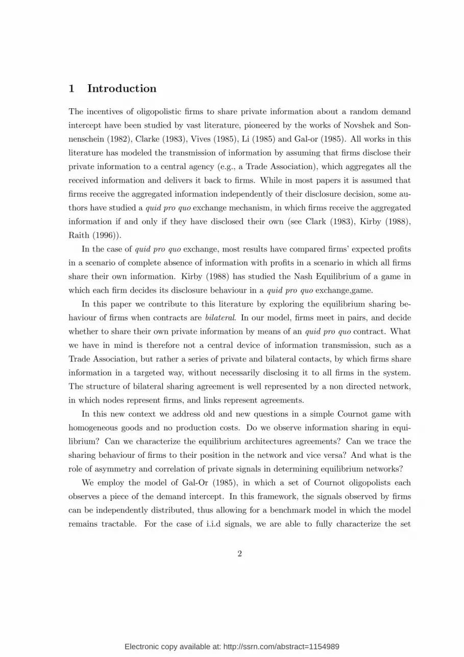
The set of pairwise stable networks characterized in Proposition 2 is very large. However,

we obtain two precise qualitative predictions on stable networks. First, information sharing

is organized in groups (the fully connected components), within which the transmission of

information is equivalent to one in firms publicly discloses its observed signal to all other

firms in the group. Second, information sharing groups must be of different size, to make

sure that firms in different groups do not form links (remember that by point (v) in lemma 2,

firms with similar degree link together). For convenience, we will refer to such fully connected

components as ”Information Sharing Groups” (ISG), and to the architectures made only of

such components as ISG networks.

Figure 1. A Pairwise Stable ISG Network

We remark that the empty network is always a stable architecture, confirming the tra-

ditional results of absence of information sharing in Cournot Oligopoly with demand un-

certainty. The stability of other regular structures is a result of the incentives to share

information of non isolated firms with equal degree. Here we see the effect of the bilateral

structure of contracts, and the implication of adopting a link-based concept of stability: the

incentives of two oligopolists to share information crucially depend on their location in the

network.

12

3.2 Signals with Heterogeneous Variances

In this section we relax the assumption that signals are identically distributed, and allow

the variances of firms’ signals - the terms on the main diagonal of Ω - to differ. In this

new context we are able to address new and interesting issues, relating the architecture of

stable networks, and the position of various firms in such architectures, to the distribution

of variances.

For simplicity we focus on the case of no linking costs. Steps at all similar to those

employed in the proof of proposition 1 lead to the following necessary and sufficient conditions

for a network g to be pairwise stable:

For all ij ∈ g:

σjj(ngj + 1)2

+σii

(ngi + 1)2≥

σii(ngi )

2; (16)

σjj(ngj + 1)2

+σii

(ngi + 1)2≥

σjj(ngj )

2. (17)

For all ij /∈ g:

σii(2 + ngi )

2+

σjj(2 + ngj )

2>

σii(1 + ngi )

2(18)

impliesσii

(2 + ngi )2+

σjj(2 + ngj )

2<

σjj(1 + ngj )

2. (19)

Condition (16)-(19) tell us that, given the degrees ngi and ngj , the incentive of i to sever

the link ij increases with the ratio of variancesσiiσjj

. Conversely, the incentive of i to form the

link ij decreases withσiiσjj

. This can be understood in terms of the additional variability of

i’s equilibrium quantity due to the link ij. The higher the term σjj , the higher the additional

variability of i’s quantity due to ij, and the higher the informational ”value” of j’s signal for

firm i. Similarly, the higher the term σii, the lower the incentive of firm i to form the link ij;

this because it is costly to share a signal with high variance with one additional firm. Again,

a high value of σii reflects therefore a high informational value of i’s signal. The effect of

firms’ degrees on the incentive to form a link are therefore enriched by the effect of signals’

variances, so that a firm with low degree may now find it profitable to form a link with a

firm with high degree if the latter has a relatively high variance.

We start by looking at two architectures, the empty and the complete, that were shown

to be always stable in the case of i.i.d. signals without costs: the empty and the complete

13

networks. We first show that the empty network is still a pairwise stable architecture, and

that this results holds true even if the firm with lower variance were allowed to make ex-ante

transfers to convince a potential partner to sign a sharing agreement.

Proposition 3 The empty network is pairwise stable for all distributions of variances. More-

over, the empty network remains pairwise stable even if firms are allowed to make side pay-

ments at the ex-ante stage..

Differently from the symmetric case, the complete network fails to be stable when vari-

ances differ substantially. This comes as a result of the weak incentives of firms with high

variance to link with firms with low variance (see conditions (16)-(17) and the subsequent

discussion).

Example 1 Consider the complete network g with three nodes. Node 1 has variance σ1 = 1,

while node 2 has variance σ2 =710 . Condition (16) is not satisfied for node 1 who severs link

12.

In the example, link 12 is severed due to the large difference in the variances of firm 1’s

and 2’s signals. From (16), the condition for firm i to maintain the link ij in the complete

network g is:

σiiσjj

≤n2

1 + 2n. (20)

Although this condition is violated in example 1, we note that the RHS of (20) grows

without bound with n, implying that (20) would be satisfied for n large enough. This implies

the following proposition.

Proposition 4 For any distribution of the variances, there exists a finite number of firms n

such that for all n ≥ n the complete network is pairwise stable.

We now turn to the effect of heterogeneity on the set of pairwise stable ISG networks

other than the empty and complete ones. We first note that components with equal size

may, in principle, be consistent with stability. In such structures, stability would require

firms in different components to have different variances, in order not to face incentives to

”bridge” components. This intuitive argument is made clear in the next proposition. Let

(σ11, σ22, ..., σnn) be the variances of the n firms, with the convention that σii < σjj for all

14

i = 1, ..., n − 1 and j = i + 1. We say that the network g is consecutive if components can

be ordered as (h1, h2, ..., hp) with the following property. Let σ−(h) and σ+(h) be the lowest

and highest variances of firms in component h. Then if i ∈ hk+1 we have σii > σ+(h) for all

k = 1, ..., p− 1.

Proposition 5 Let g be a pairwise stable network in which all components are fully connected

and of the same size. Then g is consecutive.

The next is an example of such stable structures.

Example 2 Consider a network with 9 nodes, made of three fully connected components of

size 3, with set of nodes h1 = 12, 23, 13, h2 = 45, 56, 46, h3 = 78, 89, 79. Variances are

constant within components: σ1 = σ2 = σ3 = 1; σ4 = σ5 = σ6 =12 ; σ7 = σ8 = σ9 =

14 . For

any link across components not to form we need the firm with larger variance y not to wish

to form the link with the firm with lower variance x (see condition (19)):

x

25+y

25<y

16→ x ≤

225

400.

The ratio x = 12y in the example satisfies this constraint for all components.

We finally turn to the analysis of pairwise stable networks which are not ISG networks.

As for the case of i.i.d signals, we find that regular incomplete architecture are never pairwise

stable.

Proposition 6 There exists no distribution of variances under which a pairwise stable net-

work can include regular and incomplete components.

The result of Proposition 6 can be understood as follows. From the stability conditions

derived in section 3.1, two firms with same degree and variance always have an incentive

to form a link. We have also noted that if two firms have the same degree, then the firm

with a higher variance has less incentive to form the link (see condition (18)). Proposition 6

shows that although we may eliminate the incentives of any two firms in a regular network to

form a link by choosing the appropriate distribution of variances, by doing so we necessarily

introduce incentives to sever links from the network. As a result, no incomplete and regular

architecture is pairwise stable.

15

Differently from the i.i.d. case, when firms have heterogeneous variance non regular

architectures may be stable. Intuitively, this is due to the fact that firms with large variance

and large degree need not have an incentive to sever a link, and, at the same time, can still be

”attractive” for firms with lower variance and degree, acting therefore as ”connectors” in the

network. We show that such architectures, usually referred to as ”core-periphery networks”

can be pairwise stable for suitable distributions of variances. In more detail, core periphery

networks present a dense set of interconnected nodes - the core - each linked with all nodes

in the network, and sets of peripheral nodes which are internally connected and are linked

with the core nodes (see figure 2). Formally, a core-periphery network g consists of a set

g1, g2, ....gH of fully connected subnetworks, such that i ∈ gk and j ∈ gm implies that ij /∈ g

for all k = m such that k = 2, 3, ..., H and m = 2, 3, ..., H, and such that i ∈ g1 and j ∈ gk

implies ij ∈ g for all k = 1, 2, 3, ..., H. We call the subnetwork g1 core, and the subnetworks

g2, ....gH peripheral planets. A symmetric core-periphery network is such that all peripheral

planets contain the same number of nodes np ≥ 1, and in which all nodes in the same planet

have the same variance. The number of nodes in the core is denoted by nc. We also have

H =n− ncH

.

Proposition 7 A symmetric core-periphery network is pairwise stable for some distribution

of variances only if the following condition holds:

((nc + np + 1)2

2nc + 2np + 3

)H−1≤

n2 (nc + np)2

(2n+ 1) (2nc + 2np + 1). (21)

A direct consequence of condition (21) is that the ”star” network (in which np = nc = 1)

is never pairwise stable. The next is an example of a stable core-periphery architecture.

Example 3 Consider a network with 5 nodes: node 1 is the ”core” node, while the two

peripheral components are 23 and 45. Variances are σ1 = 1, σ2 = σ3 =15 , σ4 = σ5 =

12 .

Relevant stability conditions (16)-(19) (for links 12, 15 and 34, respectively) are satisfied:

1

36+

1

5

1

16≥

1

25;

1

36+

1

2

1

16≥

1

25;

(1

2+

1

5

)1

25≤

1

5

1

36.

16

2

3

4

5

1

Figure 2. A core-periphery network

3.3 The Effect of a Linking Cost

Before turning to the more complex and richer case of correlated signals in section 4, we briefly

study the effect of an exogenous cost of forming links on the architecture of stable networks.

The cost c represents all monetary expenditures that a firm bears in order to arrange and

execute an information sharing agreement. For instance, when such arrangements are viewed

by the regulator as a signal of collusion, the cost c may refer to the expected fine. For

simplicity, and in order to isolate the pure effect of costs, we return here to the benchmark

model of i.i.d. signals.

Interestingly, the addition of a linking cost has qualitative effects on the condition for

pairwise stability, with a new role played by market conditions (the slope b of the demand

function) and by the magnitude of the variance σ. The following stability conditions are

obtained by a minor modification of the proof of proposition 1:

For all ij ∈ g:

1

(ngj + 1)2+

1

(ngi + 1)2−

1

(ngi )2≥

b2c

σ;

1

(ngj + 1)2+

1

(ngi + 1)2−

1

(ngj )2≥

b2c

σ. (22)

17

For all ij /∈ g:

1

(2 + ngi )2+

1

(2 + ngj )2−

1

(1 + ngi )2>

b2c

σ(23)

implies1

(2 + ngi )2+

1

(2 + ngj )2−

1

(1 + ngj )2<

b2c

σ. (24)

Notice the role played by the parameter b: a more elastic demand (small b) provides

higher incentives to maintain (and to form) links, while a rigid demand (large b) provides

higher incentives to sever a link. From now on we will refer to the gross cost parameter

C =b2c

σ, and refer to the single elements of C only when needed.

In the next proposition we study the effect of the new stability conditions on the set of

pairwise stable networks. In order to compare the stable networks given a cost c with those

characterized in proposition 2 in the absence of costs, we restrict the analysis to the set of

regular networks,

Proposition 8 Let c > 0. There exist size levels m1(C) ≤ 4 ≤ m2(C) such that all regular

pairwise stable networks satisfy the following properties:

a) no component of size 2 ≤ n(h) < m1(C) exists.

b) all components h of size m1(C) ≤ n(h) ≤ m2(C) are fully connected;

c) all components h of size n(h) ≥ m2(C) have degree equal to m2(C);

We can better understand the effect of a linking cost c on equilibrium architectures by

first looking at stable ISG networks. Point b) imposes a lower bound and an upper bound on

the size of a stable ISG (that is, of a stable fully connected component). These bounds can

be understood as follows. The presence of a linking cost c increases the incentives to sever

links. This disrupts the stability of those components whose members have lower incentives

to maintain their links (as these are expressed by the LHS of conditions (22)-(22)). As

explained in the proof of Proposition 8, these incentives are non monotonic in the size m of a

component, increasing until m = 4 and decrease thereafter. It follows that as the gross cost

parameter C increases, the largest and smallest ISGs are the first to drop out of the set of

stable ISG. Interestingly, market conditions play a role for the size of ISGs. In particular,

to more elastic demand curves correspond lower values of C, allowing for the emergence of

large ISGs.

18

The second effect of the cost c is to decrease the incentives to form new links. This allows

ISGs with similar size in a stable network, since links bridging components are harder to

form.

Point b) of Proposition 8 considers the possibility that a pairwise stable network include

non complete components. While the emergence of such structures is a natural consequence

of a positive (large enough) cost c, proposition 8 provides information on the relation between

the density of a component (measured here as the ration between average degree and size)

and its size. In a stable configuration, larger groups partially share information (organizing

in a non complete component), while smaller groups (with size smaller than m2(C)) share

information more intensely (see figure 3).

Figure 3. The relation between size and degree of stable components

4 Stable Networks with Correlated Signals

We finally turn to the case of correlated signal. For simplicity, we assume that signals are

identically distributed. In this case the matrix Ω has a constant term σ on the main diagonal,

and a constant term ρ ∈ [0, σ] elsewhere. The expression of the updating coefficients λ

introduced in condition (5) is as follows:

λihj(g) = λgi =

δ

1 + δ(ngi − 1), ∀h ∈ Ng

i , ∀j /∈ Ngi ,

19

where δ ≡ρ

σis a correlation coefficient. We can now rewrite (6)-(7) as:

βij =

1 + (n− ngi )λgi − b

λgi∑

h =i

∑

k∈Ng

h\Ng

i

βhk +∑

h∈Ngj \i

βhj

2b, ∀j ∈ Ng

i ; (25)

αi =A− b

∑h =i αh

2b. (26)

Direct computations using (25)-(26) show that each firm prefers the empty network to

the complete network for all possible values of the correlation parameter δ. This is just a

special case of proposition 4.4 in Raith (1996). However, the next proposition shows that

empty network is not pairwise stable if correlation is larger that a given threshold.

Proposition 9 Let n 4 and δ ∈ [0, 1]. There exists a threshold δ (n) such that for all δ

δ (n) the empty network is not pairwise stable.

The intuition behind Proposition 9 is very simple. Compared to the case of independent

signals (in which the empty network is always stable), correlation brings in new incentives to

form a link starting from the empty network. Such incentives come from the better inference

that linking firms expect to make on the signals and the behaviour of other firms. This

better inference comes at no additional cost in terms of revealing one’s own signal, and is

not present when signals are independent. In order for such new incentives to undermine the

stability of the empty network, both the number of firms and the correlation parameter must

be large enough. This is intuitive, since they both measure how effective the new inference

is, in terms of precision and in terms of number of signals to be inferred. This result makes

clear how bilateral sharing agreement may be profitable even in a Cournot oligopoly with

homogeneous goods - a conclusion in contrast with the traditional view, well summarized

by proposition 4.4 in Raith (1996). The difference in results is mainly due to the difference

in the transmission mechanism and in the adopted equilibrium concept. Bilateral contracts

allow two firms to reach a sharing agreement without necessarily share their signal with

all firms in the market. The pairwise stability concept allow two firms to coordinate their

action, possibility that was missing in the early analysis of quid pro quo contracts by Kirby

(1988), who looks at the Nash Equilibria of the sharing game, who suffer, in the presence of

correlation, of coordination failures.

20

The next proposition shows that the instability of the empty network does not come from

a general existence problem.

Proposition 10 The complete network is stable for all δ ∈ [0, 1]

Characterizing all pairwise stable networks for this case of correlation is a very hard task.

It is actually very difficult to simply understand the effect of correlation of the equilibrium

coefficients (and thus on the incentives to form links) in a generic network g, as these are

expressed in conditions (25)-(26). In order to get some understanding on the effect of cor-

relation, we fully work out the case of four firms, the minimal number that allows for non

trivial equilibrium structures.

4.1 Pairwise Stable Network with 4 Firms

With four firms, there are eleven architectures to be considered.

g1 g2 g3 g4

g5 g6 g7 g8

g9 g10 g11

Figure 4. Possible architectures with 4 firms

We identify pairwise stable architectures for various ranges of the correlation parameter

δ.

1. When δ is low (δ ≤ 0.619), the set of stable networks has the same qualitative features

as in the case of independent signals: empty and complete networks are stable, plus an

ISG network, in particular network ”g6” in figure ??.

21

2. For an intermediate range of δ (0.619 ≤ δ ≤ 0.710), network ”g6” ceases to be stable.

In this range, a link between a firm i in the completely connected component and the

isolated firm j is formed. It is interesting to note that firm i wishes to form the link

for δ ≤ 0.710, while firm j wishes to form it for 0.619 ≥ δ. This highlights the effect of

correlation: if correlation is low, then firm i has not a good enough inference on firm

j’s signal, and wishes to form the link ij; if correlation is high, firm j wishes to form

the link, in order to have a good inference on the remaining firms. Note that firm j has

a low degree, and would never accept to form the link ij in the absence of correlation.

3. As δ grows (0.710 ≤ δ ≤ 0.747), network ”g6” becomes stable again, since firm i has a

good enough inference on firm j due to i’s high degree and the high level of correlation.

4. Finally, if δ grows even more, the empty network ceases to be a stable architecture, as

was proved for the general case in proposition 9.

Interestingly, the stability of the network ”g6” in the ranges of values δ ≤ 0.619 and

0.710 ≤ δ results from different incentives of firms. When δ is low, each of the three firms

sharing information would like to link to the isolated firm, whose signal has a large infor-

mational value due to the low degree. In this case, the isolated firm decides not to join the

group. When δ is high, the three firms sharing information are excluding the fourth firm,

which would like to join if allowed.

g1

g6

g11

g1 g1

g11 g11 g11

g6 g6

Figure 5. Pairwise stable networks for various ranges of δ

22

5 Conclusions

We have studied the incentives of oligopolistic firms to share information on a random demand

intercept by means of bilateral contracts. We have first studied the benchmark model of i.i.d.

signals, for which we have shown that pairwise stable networks are made of fully connected

components of increasing size. When linking has a cost, then non complete components can

be stable, and in this case density is inversely related to size. We have then shown that

when variances of signals are heterogeneous, non regular components of the core-periphery

architecture may arise in equilibrium, with high variance firms acting as connectors. Finally,

correlated signals introduce new and interesting aspects of analysis, and group formation and

exclusion seem to be typical features of this case.

Although we believe that the novelty of our approach brings new and interesting insights

in the theory of information sharing, there are several aspects of the present analysis that

deserve discussion and improvement. First, the notion of pairwise stability is somewhat

specific, and one may wish to study solution concepts that allow multiple links to be formed

or severed at the same time. Also, the assumption that information sharing occurs at the

ex-ante stage could be removed, so to explore the rich strategic structure of an interim model

of information sharing. Finally, the assumption that all firms reveal truthfully their signal is

quite strong (although common to all this stream of literature), and the incentives to report

false information could be dealt with in an interim model. Finally, a full characterization

of stable network in the case of correlated signals is certainly desirable, although technically

quite difficult. We leave all of these issues for future research.

References

[1] Clarke, R., Collusion and the Incentives for Information Sharing, Bell J. Econ. 14 (1983),

383-394.

[2] Gal-Or, E., Information Sharing in Oligopoly, Econometrica 53 (1985), 329-343.

[3] Kirby, A. J., Trade Associations as Information Exchange Mechanisms, Rand J. Econom.

19 (1988), 138-146.

23

[4] Jackson, M. O., and A. Wolinsky, A strategic model of social and economic networks, J.

Econ. Theory 71 (1996), 44-74.

[5] Li, L., Cournot oligopoly with information sharing, Rand J. Econom. 16 (1985), 521-536

[6] Novshek, W. and H. Sonnenschein, Fulfilled expectations Cournot duopoly with informa-

tion acquisition and release, Bell J. Econ. 13 (1982), 214-218.

[7] Radner, R., Team decision problems, Annals Math. Statist. 33 (1962), 857-81.

[8] Raith, M., A General Model of Information Sharing in Oligopoly, J. Econ. Theory 71

(1996), 260-288.

[9] Vives, X., Duopoly information equilibrium: Cournot and Bertrand, J. Econ. Theory 34

(1985), 71-94.

24

6 Appendix

Proof of Lemma 1. To explicitly derive the term E [πi(g)], consider the best response

condition for firm i in the game Γg:

qi =

A+∑

j∈Ngi

aj +Ei

∑

j /∈Ngi

aj

∣∣∣∣∣∣agi

− bEi

∑

j =i

sj(agj

)∣∣∣∣∣∣agi

2b(27)

which can be rewritten as:

qi =

Ei

A+∑

j∈N

aj − b∑

j∈N

sj(agj )

∣∣∣∣∣∣agi

b=Ei [P (a, g) |a

gi ]

b, (28)

where P (a, g) is the market price given realization a in network g. Given a and g, firm i´s

equilibrium profits can be expressed as:

πi(a, g) =P (a, g)Ei [P (a, g) |agi ]

b. (29)

The (interim) expected value of πi(a, g) evaluated by firm i in g is:

Ei

[P (a, g)Ei [P (a, g)|agi ]

b

∣∣∣∣agi

]=Ei [P (a, g) |agi ]

2

b= bqi

2. (30)

Ex-ante expected profits E [πi(g)] of firm i in g are now obtained as follows:

E [πi(g)] = Egi

[bqi(g)

2]. (31)

Proof of proposition 1.

From (31), ex-ante profits are given by Ei[bqii(g)

2]. Using standard results, we write for

a generic variable x3:

E [x]2 = E[x2]− var(x) (32)

3This relation is derived as follows:

E[x2]− var(x) = E

[x2]− E

[(x2 +E [x]2 − 2xE [x]

)]=

2E [xE [x]]− E [x]2 = E [x]2 .

25

We can therefore write:

E [πi(g)] = Ei[bqi(g)

2]= bEi

[qi(g)

2]= b

(Ei [qi(g)]

2 + var(qi(g))). (33)

Since from (30) Ei [qi(g)] =A

b(n+1) irrespective of the graph structure, we conclude that the

difference between the profits of firm i in graphs g and g′ = g−ij (for ij ∈ g) is the difference

in the two variances of equilibrium quantities:

E [πi(g)]−E[πi(g

′)]= b

[var(qi(g))− var(qi(g

′))]. (34)

We can write down explicit expressions for the equilibrium parameters as follows:To obtain

an expression for this difference, let us explicitly derive the equilibrium coefficients βij and

αi for this case. Solving conditions (8)-(9) we obtain:

βij =1

b(ngj + 1

) , ∀i ∈ Ngj and ∀j ∈ N ;

αi =A

b (n+ 1)∀i ∈ N. (35)

It is clear from (35) that the coefficient applied to signal j only depends on the degree

of node j, and is independent of all other topological properties of the network. Also, the

ex-ante expected equilibrium quantity in the aggregate game Γg is αi. Using (35)-35), the

equilibrium quantity of firm i in game Γg is given by:

qi(g) =A

b(n+ 1)+∑

k∈Ngi

ak(ngk + 1)b

, (36)

with variance (using the fact that covariance are zero across ai’s and that all variances are

equal to σ):

var(qi(g)) =∑

k∈Ngi

σ

(ngk + 1)2b2. (37)

For Γg′we obtain:

qi(g′) =

A

b(n+ 1)+∑

k∈Ng′

i

ak

(ng′

k + 1)b(38)

26

with variance:

var(qi(g′)) =

∑

k∈Ng′

i

σ

(ng′

k + 1)2b2. (39)

The only two terms that are different in the sums of the above expressions of variances are

those that concern signals j and i. Using the fact that ng′

i = ngi − 1 we obtain that:

var(qi(g))− var(qi(g′)) = σ

[1

(ngj + 1)2b2+

1

(ngi + 1)2b2−

1

(ngi )2b2

]

. (40)

The conditions for the link ij not to be severed from g are therefore the following:

1

(ngj + 1)2+

1

(ngi + 1)2−

1

(ngi )2≥ 0;

1

(ngi + 1)2+

1

(ngj + 1)2−

1

(ngj )2≥ 0. (41)

We now turn to the condition for the link ij /∈ g not to be formed. Firm i has an incentive

to form ij inducing the network g′ = g + ij if

var(qi(g′))− var(qi(g)) > 0 (42)

where qi and q′i are the equilibrium quantities in g and g′, respectively. Stability requires

that if (42) holds then:

var(qj(g′))− var(qj(g)) < 0. (43)

Using again the expression for variances and the fact that ng′

i = ngi +1 we obtain the following

condition:

if

1

(ngj + 2)2+

1

(ngi + 2)2−

1

(ngi + 1)2> 0 (44)

then(

1

(ngi + 2)2+

1

(ngj + 2)2−

1

(ngj + 1)2

)

< 0. (45)

27

Proof of Lemma 2: Point i) is implied by the fact that the RHS of (14) is increasing

in n: it is always positive for all n. Point ii) is proved along the same lines of point i). To

prove point iii), consider the equations defining F (n) and f(m), respectively:

1

n2−

1

(1 + n)2=

1

(1 + F (n))2. (46)

1

(1 +m)2−

1

(2 +m)2=

1

(2 + f(m))2. (47)

The LHS of (46) and of (47) coincide for all m−1. It follows that also the RHS must coincide

for such values, and this happens when f(n− 1) = F (n)− 1.

iv) By definition:

F (n) =

√n2(1 + n)2

(1 + n)2 − n2− 1.

For n = 2 we obtain:

F (n)− F (n− 1) =

√36

5−

√4

3> 1.

We then compute the derivative ddn [F (n)− F (n− 1)], that it is positive for all value n > 2.

v) Simple algebraic manipulation of conditions (14)-(15).

vi) Directly from iii) and iv).

Proof of Proposition 2. i) We first show that only regular networks can be pairwise

stable. Let g be pairwise stable, and let h be a non regular component of g. Then there exist

nodes i and j such that ni > nj and ij ∈ h. This means that there exists some node k = j

such that ik ∈ h and jk /∈ h. Pairwise stability of g imposes the following requirements on

the degrees of nodes i, j and k:

nk ≤ F (ni) and ni ≤ F (nk);

nj ≤ F (ni) and ni ≤ F (nj). (48)

Note now that since ni > nj, then ni − 1 ≥ nj (remember that degrees are integers).

This, together with (48), implies

nj ≤ F (nk)− 1. (49)

28

Point iii) in lemma 2 together with (49) imply:

nj ≤ f(nk − 1). (50)

We finally use point (ii) in lemma 2 to conclude that:

nj < f(nk). (51)

For g to be stable, link jk should not form. This, together with (51), requires that:

nk > f(nj). (52)

Suppose now that nk ≤ nj . In this case, condition (48) plus point (iv) in lemma 2 would

imply that ni ≤ f(nj), implying, together with (51), that nj > ni, a contradiction. We have

therefore concluded that nk > ni.

This result implies that there exists some node w such that wk ∈ h, wi /∈ h and nw > nk.

To these three nodes i, k and w we can now apply similar arguments as above to conclude

that there exists some neighbour w′ of w such that w′k /∈ h and nw′ > nw. Reiterating these

steps, and given that the number of nodes n is finite, we obtain a contradiction.

Consider now a regular component of degree m. Since m ≤ f(m) for all m, we conclude

that each component of g is fully connected. Components of size 2 are not stable because

F (2) < 2 by point v) of lemma (2).

ii) The complete network and the empty network are both stable since F (m) ≥ m for

m ≥ 3 and f(1) < 1 by point v) of lemma 2. This last inequality also implies that isolated

firms do not wish to form a link with firms in a component of size m ≥ 2. .

iii) Two components of the same size m ≥ 2 are not consistent with stability, since

f(m) ≥ m by point v) of lemma 2. To complete the proof of point iii), note that any pair of

components of sizes m1 < m2 such that m1 ≥ 3, m2 ≥ 3 and m2 > f(m1) are such that no

link is severed within components nor formed across components.

Proof of Proposition 3:. The change in aggregate profits of isolated firms i and j when

they form a link is:

2(σjj

9+σii9

)−σjj4−σii4

which is always negative for all values of σjj.and σii

Proof of Proposition 5: Consider components hk and hk+1, both of the same size q.

Let j be the firm with highest variance in hk (σ+(hk) = σjj) and let l be the firm with lowest

29

variance in hk (σ−(hk) = σll). Stability conditions for component h require that firm j does

not sever the link jl, where l is the firm with lower variance in h, that is, σ−(h) = σll:

σjjm2

≤σjj + σll

(m+ 1)2. (53)

Suppose now that there exists firm i ∈ hk+1 such that σii < σ+(hk). In order for the network

g to be stable, firms j must not have an incentive to form a link with firm i:

σjj

(m+ 1)2>σjj + σii

(m+ 2)2. (54)

Conditions (53)-(54) imply:

(m+ 1)2 (m+ 1)2

(m+ 2)2m2<

(σjj + σll)

(σjj + σii).

If σii ≥ σll we have that(m+ 1)2 (m+ 1)2

(m+ 2)2m2≤ 1

which is never satisfied. Suppose now that σii < σll and that there exists some firm m such

that σii > σll (if such firm does not exist the consecutiveness of g is not violated). In this

case, the same steps used above can be followed by replacing firm j with firm m and firm l

with firm j.

Proof of Proposition 6: We proceed as follows. We first show in step 1 that if g contains

a minimal cycle of length at least 4, then g cannot be pairwise stable for any configuration

of variances. We then show that if g is regular and incomplete with degree at least 3, then g

contains a minimal cycle of length at least 4.

Step 1.. Let g = gc be a connected regular network of degree k, with k ≥ 2. Let

P = 1, 2, ....x, 1 be a minimal cycle of length x ≥ 4. For simplicity, in this proof we denote

by σi the variance σii. Necessary condition for link i(i+2) not to form is the following for all

i ∈ 1, 2, ...x:

σi+2 > σi(1 +m)2

2m+ 3. (55)

Necessary condition for link i(i+ 1) not to be severed is the following for all i ∈ 1, 2, ...x:

σi+1 < σim2

2m+ 1. (56)

30

Given that m2

2m+1 <(1+m)2

2m+3 , a necessary condition is that σi be strictly increasing on

1, 2, ...x, from which:

σx > σ1(1 +m)2

2m+ 3. (57)

However, necessary condition for link ix not to be severed is the following:

σx < σ1m2

2m+ 1. (58)

It can be easily checked that (57) and (56) are not compatible.

Step 2. Let g be a regular incomplete connected network of degree k, with k ≥ 3.

Consider three nodes i, j, and l such that ij /∈ g, il ∈ g and jl ∈ g (such three nodes must

exist since g is not complete and connected). Since ngl = ngj = k, there must exist j1 = l such

that j1 = i, j1 ∈ Ngj and j1 /∈ N

gl . If j1 ∈ N

gi , then we obtain the 4-minimal cycle i, l, j, j1, i

(see figure 6). If, instead, j1 /∈ Ngi , consider the set Ng

j1. Again, since j1 /∈ N

gl while j ∈ Ng

l ,

and since ngj1 = ngj = k, there must exist a node j2 ∈ N

gj1

such that j2 /∈ Ngj (and, therefore,

j2 = l). If j2 ∈ Ngl , then we obtain the 4-minimal cycle l, j, j1, j2, l. If j2 /∈ N

gl but j2 ∈ N

gi ,

then we obtain the 5-minimal cycle i, l, j, j1, j2, i. If, instead, j2 /∈ Ngl and j2 /∈ N

gi , then

consider the set Ngj2. Since j2 /∈ N

gj and j1 ∈ N

gj , and since in a k-regular network each node

has the same degree k, there must exist a node j3 ∈ Ngj2

such that j3 /∈ Ngj1

(and, therefore,

j3 = j). Note also that j3 = l, j3 = i by the previous arguments. It follows that if j3 ∈ Ngi

we obtain a 6-minimal cycle; a 5-minimal cycle is obtained if j3 ∈ Ngl ; a 4-minimal cycle

is obtained if j3 ∈ Ngj . If none of these is true, then we consider Ngj3 and repeat the same

arguments as above.

31

i

l j

j1

j2

j3

jm-1

jm

Figure 6

In general, for any jm obtained along this process, there must exist a node jm+1 ∈ Ngjm

such

that jm+1 /∈ Ngjm−1

. So, if jm+1 ∈ Ngjm−2

, we obtain a 4-minimal cycle; if jm+1 ∈ Ngjm−2

but

jm+1 ∈ Ngjm−3

, we have a 5-minimal cyle, and so on until we check whether jm+1 ∈ Ngi . If

none of these inclusions is verified, we can identify a node jm+2 ∈ Ngjm+1

such that jm+2 /∈ Ngjm

and such that jm+2 = jm−i for all i = 0, 1, 2, ...,m− 1. Since the number of nodes is finite,

the process must stop and a minimal cycle of size at least 4 must be found.

Proof of Proposition 7. Denote by i ∈ g1 and j ∈ ∪Hk=2gk. From proposition 1, we

know that the following two conditions are necessary and sufficient for the link ij ∈ g not to

be severed:

σiin2−

σii(n+ 1)2

≤σjj

(nc + np + 1)2(59)

σjj(nc + np)2

−σjj

(nc + np + 1)2≤

σii(1 + n)2

. (60)

These conditions can be rewritten as follows:

σjj ≥ σii(2n+ 1)(nc + np + 1)2

(1 + n)2n2(61)

σjj ≥ σii(nc + np)

2(nc + np + 1)2

(2nc + 2np + 1) (n+ 1)2(62)

It follows that a link between agents i ∈ g1 and agent j ∈ ∪hk=2gk is stable only if:

σjj ∈

[

σii(2n+ 1)(nc + np + 1)2

(1 + n)2n2, σii

(nc + np)2(nc + np + 1)2

(2nc + 2np + 1) (n+ 1)2

]

. (63)

32

This condition indirectly imposes an upper bound rmax on the ratio between the larger and

the smaller variance of agents in the set ∪hk=2gk:

rmax =n2 (nc + np)

2

(2n+ 1) (2nc + 2np + 1). (64)

We now turn to the conditions ensuring that no link between agents i ∈ gk and j ∈ gm

is formed. Note first that since all peripheral components have the same degree, a necessary

condition for ij not to form is that σii = σjj . Moreover, from proposition 1 we know that,

given that i and j have the same degree, the node with smaller variance has an incentive to

form the link; we then need to require that the node with larger variance has no incentive to

do so. Without loss of generality, suppose σ2i > σ2j . The link ij does not form if:

σii

(nc + np + 1)2−

σii

(nc + np + 2)2>

σjj

(nc + np + 2)2, (65)

yielding:

σii >(nc + np + 1)2

2nc + 2np + 3σj . (66)

Therefore, a necessary and sufficient condition for the link ij not to form is the following:

σiiσjj>

(nc + np + 1)2

2nc + 2np + 3. (67)

Under this condition, the minimum ratio between the larger and the smaller possible vari-

ance of peripheral agents is: rmin =((nc+np+1)

2

2nc+2np+3

)H−1, where H is the number of peripheral

planets. Then, a necessary and sufficient condition for the network g to be pairwise stable is

that rmin ≤ rmax, that is condition (21).

Proof of Proposition 8. We first prove that for each C there exist integers m1(C) ≤ 4

and m2(C) ≥ 4 such that two firms with equal degree m have an incentives to maintain their

link if and only if m1(C) ≤ m ≤ m2(C). Also, for all m in this range, two firms with degree

m− 1 have an incentive to form a link. To see this, note that the stability condition ?? can

be rearranged as follows when ngi = m:

(2

(m+ 1)2−

1

(m)2

)≥ C. (68)

33

The LHS of expression (68), when defined on the set of integers, reaches a maximum at

m = 4, and is increasing for m ≤ 3 and decreasing for m ≥ 4. The values m1(C) and m2(C)

are the first integers above and below the smaller and larger solutions of (68) taken with

equality, respectively.

a) Suppose component h is such that m1(C) ≤ n(h) ≤ m2(C) and is not completely

connected. Then, its degree m is strictly less than m2(C). If m < m1(C) then by lemma ??

there exist a firm with an incentive to sever one of its links. If m ≥ m1(C), then by lemma

?? we conclude that there exist two firms with an incentive to form a link. This because

m+ 1 ≤ m2(C).

b) Suppose that n(h) ≥ m2(C) and the degree of h is strictly smaller thanm2(C). Lemma

?? implies again that there exist two firms with an incentive to form a link. Suppose the

degree of h is strictly larger than m2(C). In this case lemma ?? implies that there are

incentives to sever a link.

Proof of Proposition 9. Consider the empty network. Applying (25) and (26) we obtain

α = Ab(n+1) and βii =

1+δ(n−1)b[2+δ(n−1)] where qi = α + βiiai ∀i. The payoff is πi = β

2σ for all i.

Now consider two firms, i and j, forming a link. Applying (25) and (26) we obtain α = Ab(n+1)

for all i and βii = βjj = βji = βij =2+δ(2n−3)−δ2(n−1)b[6+3δ(n−1)−δ2(n+1)]

where q′i = q′j = α + βii (ai + aj).

Expected profits of firms i and j are π′i = π′j = 2 · β2ii (σ + ρ). Now we consider a variable

D = πi − π′i; when D is positive the empty network is stable, otherwise it is not. By direct

computation we get: D = σ(1+δ(n−1)

b

)2 [6+3δ(n−1)−δ2(n+1)]2−2(δ−2)2(δ+1)[2+δ(n−1)]2[2+δ(n−1)]2[6+3δ(n−1)−δ2(n+1)]2

. The sign

of D is the same as the sign of the numerator in the second term. We find that D has only

one root in δ satisfying D = 0 for all n 4 and D is strictly positive for δ = 0.

Proof of Proposition 10. Consider the complete network. Applying (25) we ob-

tain α = Ab(n+1) and βii =

1b(n+1) where qi = α + βii

∑

j∈Naj ∀i. The payoff for each firm

i is πi = β2 [n · σ + n · (n− 1) ρ]. Now consider two firms, i and j, severing a link. Ap-

plying (25) we obtain α = Ab(n+1) for all i and βii = βjj = 1+δ(n−1)

b[n+δ(n−1)2], βih = βjh =

n[1+δ(n−1)]

b(n+1)[n+δ(n−1)2]for all h = i, j, where q′i = α + βiiai + βih

∑

h∈N/i,j

ah. The payoff of agent

i id π′i =[β2ii + (n− 2)β2ih

]σ +

[2 (n− 2)βiiβih + (n− 2) (n− 3)β2ih

]ρ. Now we consider a

variable D = πi − π′i; when D is positive the complete network is stable, otherwise it is not.

By direct computation we get: D = σ (1−δ)[1+δ(n−1)]n[n−2+(n−3)(n−1)δ]−1b2(n+1)2[n+(n−1)2δ]

2 , which is strictly

positive for all δ ∈ [0, 1).

34