oligopoly and strategic interactions
TRANSCRIPT

Oligopoly and Strategic Interactions
Dr. Sanja Samirana PattnayakIIMT

Oligopoly
In market structures considered so far –monopolies and perfect competition- optimal strategies do not depend on the actions of the others.
Characteristics of these markets include:
Few firms High barriers to entryAbove normal profit (not necessarily though)Product differentiation may or may not exist
2

Herfindahl-Hirschman Index (HHI)
An oligopoly is a market in which a few firms(usually more than 2 and less than 10) havemarket power- the power to control the price.
Economists use concentration ratios to measurethe degree to which a market or industry isoligopolistic.
The more concentrated the market/industry, theless competitive it is.
3

Herfindahl-Hirschman Index (HHI)
An important measure of market concentration is the Herfindahl-Hirschman Index (HHI).
It is calculated by squaring the market share of each firm in the market and then summing the resulting numbers.
Example, consider a market with 2 firms, one with 60% market share and second with 40% share. The HHI for the market is 5200.
4
Herfindahl-Hirschman Index (HHI)
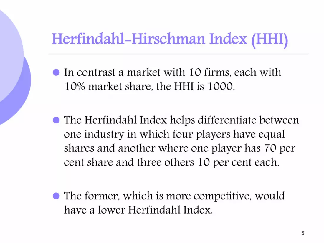
In contrast a market with 10 firms, each with 10% market share, the HHI is 1000.
The Herfindahl Index helps differentiate between one industry in which four players have equal shares and another where one player has 70 per cent share and three others 10 per cent each.
The former, which is more competitive, would have a lower Herfindahl Index.
5

Herfindahl-Hirschman Index (HHI)
In an extremely competitive market, say, withten players having 10 per cent share each, theindex would be 1,000.
A 1,000-2,000 value generally indicates intensecompetition. In India, values less than 2,000 isseen in the consumer electronics market.
6

Oligopoly
Examples of Oligopoly markets include:Automobiles, steel, petrochemicals, electricalequipment, computers etc.
Management challenges: Strategic actions andRival behavior.
Within the managerial decision makingframework, the key trait of oligopolies isinterdependence of market players. Managerscontrol their actions, but not directly those ofothers. 7

Oligopoly
A prudent manager would take actions to affect rivals’ actions to her advantage.
Example: What are the possible rival responses to a 10% price cut by Maruti, or supplying twice of oil barrels by Iraq?
What can you do to let your rivals behave to your favour?
8

Oligopoly
In oligopolistic markets, many behavioural assumptions are feasible; hence several solutions exist, with each solution based on different behavioural assumptions.
Differentiated products or notStrategic variable varyOrder of movementInformation structureCompetition one shot or repeated
9

Cournot’s Quantity Competition
What would happen if firms compete by quantity?
The behavioural assumption is that manager of each firm maximizes his/her profits based on the belief that the quantity produced by her rival is invariant (fixed) with respect to his/her own quantity decisions.
Clearly, this is an interactive strategy game – now played out in strategies of plant capacity or in quantities.
10
The Model
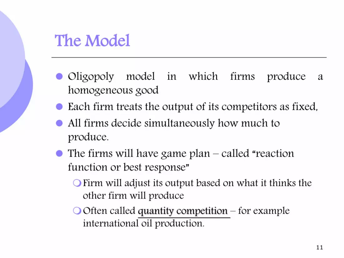
Oligopoly model in which firms produce ahomogeneous good
Each firm treats the output of its competitors as fixed, All firms decide simultaneously how much to
produce. The firms will have game plan – called “reaction
function or best response”Firm will adjust its output based on what it thinks the
other firm will produceOften called quantity competition – for example
international oil production.
11

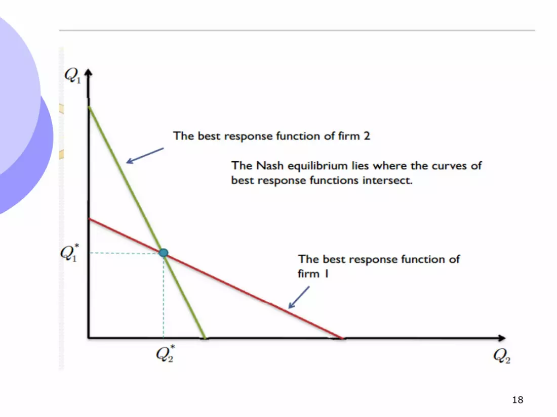
Equilibrium Concept –Nash equilibrium
Equilibrium concept: “Nash Equilibrium” . Each firm is doing the best it can given its belief on what its competitors are doing. (Details later part of the lecture on Game Theory)
Firms do the best they can and have no incentive to change their output or price, assuming all firms are taking rivals’ decisions into account.
12

13

14

15

16

17
18

19

20

21

22
23
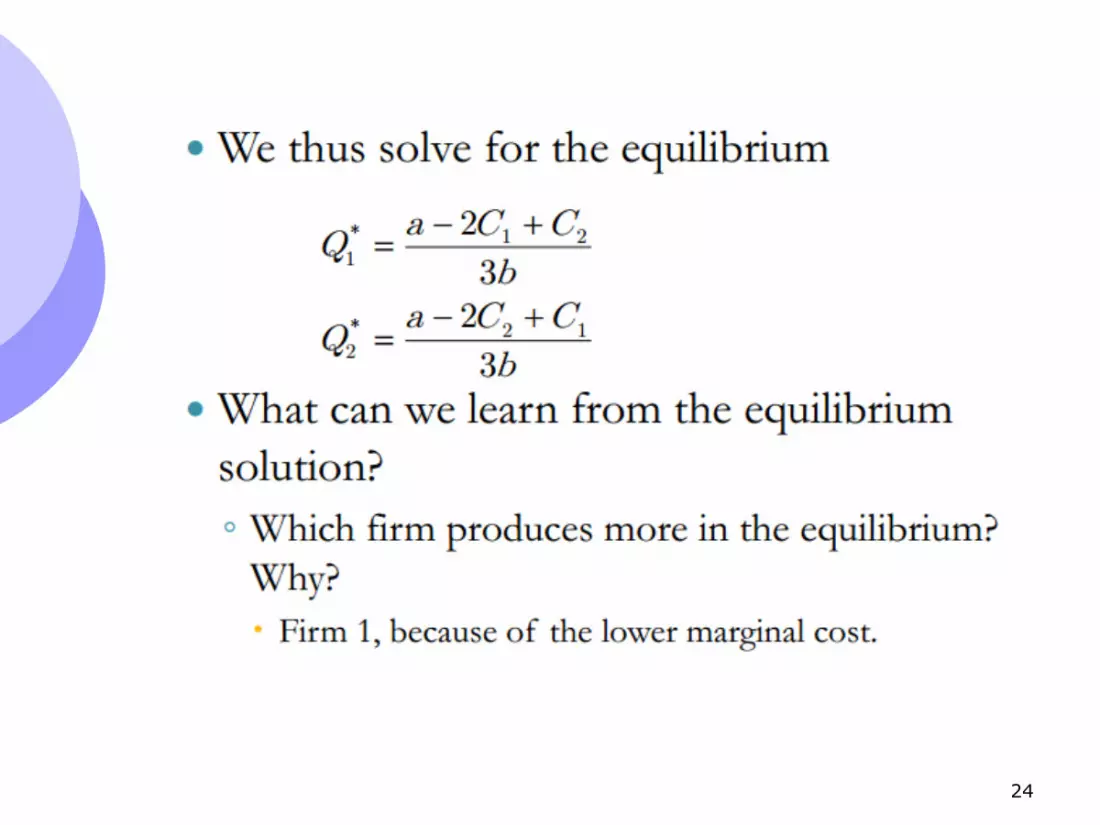
24

25
Cournot model: Example
An Example of the Cournot EquilibriumTwo firms face linear market demand curve
Market demand is P = 30 - Q Q is total production of both firms: Q = Q1 + Q2 Both firms have MC1 = MC2 = 0
Each Firm’s action is to choose a level of production
Firm i’s profit is
QQQQQ ijijii 30,

26
Duopoly Example
We want to calculate what each firm’s profit maximizing output level, i.e. Their best response, to the other firms output decision.
This is called the firm’s reaction function
Firm 1’s Reaction Curve MR(Q2)=MC

27
Duopoly Example
Calculating the reaction functions
215
CurveReaction s2' Firm
215
CurveReaction s1' Firm
0
230
12
21
11
21111
MCMR
QQQRMR

28
Duopoly Example
In a Nash equilibrium Q1 and Q2 are best responses to each other.
each $100 are profits ,1030
20
102
1515*
215* and
215*
*
2
*
21
*
12
*
21
1
*1
QP
QQQ
Q
Q

29
Duopoly ExampleQ1
Q2
Firm 2’s
Reaction Curve
30
15
Firm 1’s
Reaction Curve
15
30
10
10
Cournot Equilibrium
The demand curve is P = 30 - Q and
both firms have 0 marginal cost.
Comparing Oligopoly Models
Assume we have no anti-trust laws, so rival firms can talk to one another.
If managers recognize their mutual interdependence, they should agree to act in unison to maximize their joint payoff behaving as a single entity.
30

Comparing Oligopoly Models
Let the market demand curve is given by the inverse demand function; P=1,000-Q
The associated MR = 1,000-2Q; this MR function assumes that firms act as a single profit maximizing firm, which what collusion all about.
The cost function of each firm is identical and given by Ci(Qi)=4Qi, so MC of each firm is 4.
31

Comparing Oligopoly Models We will now see how outputs, prices and profits vary according
to the type of the oligopolistic interdependence that exists in the market.
Cournot: Q1=Q2=332. Total output Q=Q1+Q2=664 and price is $336 and profits of $110,224
Bertrand: use price equal to MC. Therefore, with the given inverse demand function and cost function, P=$4and profits are zero for each firm. Total market output is 996 units. Given the symmetric firms, each firm gets half of the market.
Collusion: Q=498, P=$502 and each firm earns a profit of $124,002
32

Comparing Oligopoly Models
Rankings of the market output: Bertrand>Cournot>Collusive
Ranking of total profit: Collusive>Cournot>Bertrand
Ranking of Price: Collusive>Cournot>Bertrand Exercise: Find Stackelberg optimal strategy and
compare with the above model If you become a manger in an oligopolistic market, it is
important to recognize that your optimal decisions and profits will vary depending on the type of oligopolistic interactions that exists in the market.
33

34
Price Competition-Bertrand Model
You might object to the Cournot model on the grounds that ‘in reality firms’ chose prices rather than quantities
So competition in an oligopolistic industry may occur with price instead of output.
The Bertrand Model : Firms produce a homogeneous good, each firm treats the price of its competitors as fixed, and all firms decide simultaneously what price to charge?

35
Price Competition – Bertrand Model
Assumptions
Homogenous goodMarket demand is P = 30 - Q where Q = Q1 + Q2MC1 = MC2 = $3
Can show the Cournot equilibrium if Q1 = Q2 = 9 and market price is $12 giving each firm a profits of $81.
36
Price Competition – Bertrand Model
Assume here that the firms compete with price, not quantity.
Since good is homogeneous, consumers will buy from lowest price seller.
If firms charge different prices, consumers buy from lowest priced firm only.
If firms charge same price, consumers are indifferent who they buy from.
37
Price Competition – Bertrand Model
Nash equilibrium is competitive output since firms have incentive to cut prices
Both firms set price equal to MCP = MC; P1 = P2 = $3Q = 27; Q1 & Q2 = 13.5
Both firms earn zero profit Why not charge a different price?

38
Price Competition – Differentiated Products
Market shares are now determined not just by prices, but by differences in the design, performance, and durability of each firm’s product.
In these markets, more likely to compete using price instead of quantity

39
Price Competition – Differentiated Products
ExampleDuopoly with costs of $20 Firms face the following demand curves
Firm 1’s demand: Q1 = 12 - 2P1 + P2 Firm 2’s demand: Q2 = 12 - 2P + P1
Quantity that each firm can sell decreases when it raises its own price but increases when its competitor charges a higher price
2

40
Price Competition – Differentiated Products
Firms set prices at the same time
202-12
20)212(
20$ :1 Firm
21
2
11
211
111
PPPP
PPP
QP

41
Price Competition – Differentiated Products
12 is firmeach for Profits
4,4, is mEquilibriuNash
413
curvereaction s2' Firm
413
curvereaction s1' Firm
0412
price maximizingprofit s'1 Firm
*
2
*
1
12
21
2111
PP
PP
PP
PPP

42
Competition Versus Collusion: The Prisoners’ Dilemma
Nash equilibrium is a non-cooperativeequilibrium: each firm makes decision that gives greatest profit, given actions of competitors
Although collusion is illegal, why don’t firms cooperate without explicitly colluding?Why not set profit maximizing collusion price
and hope others follow?
43
Competition Versus Collusion: The Prisoners’ Dilemma
Competitor is not likely to follow
Competitor can do better by choosing a lower price, even if they know you will set the collusive level price.
We can use example from before to better understand the firms’ choices
44
Competition Versus Collusion: The Prisoners’ Dilemma
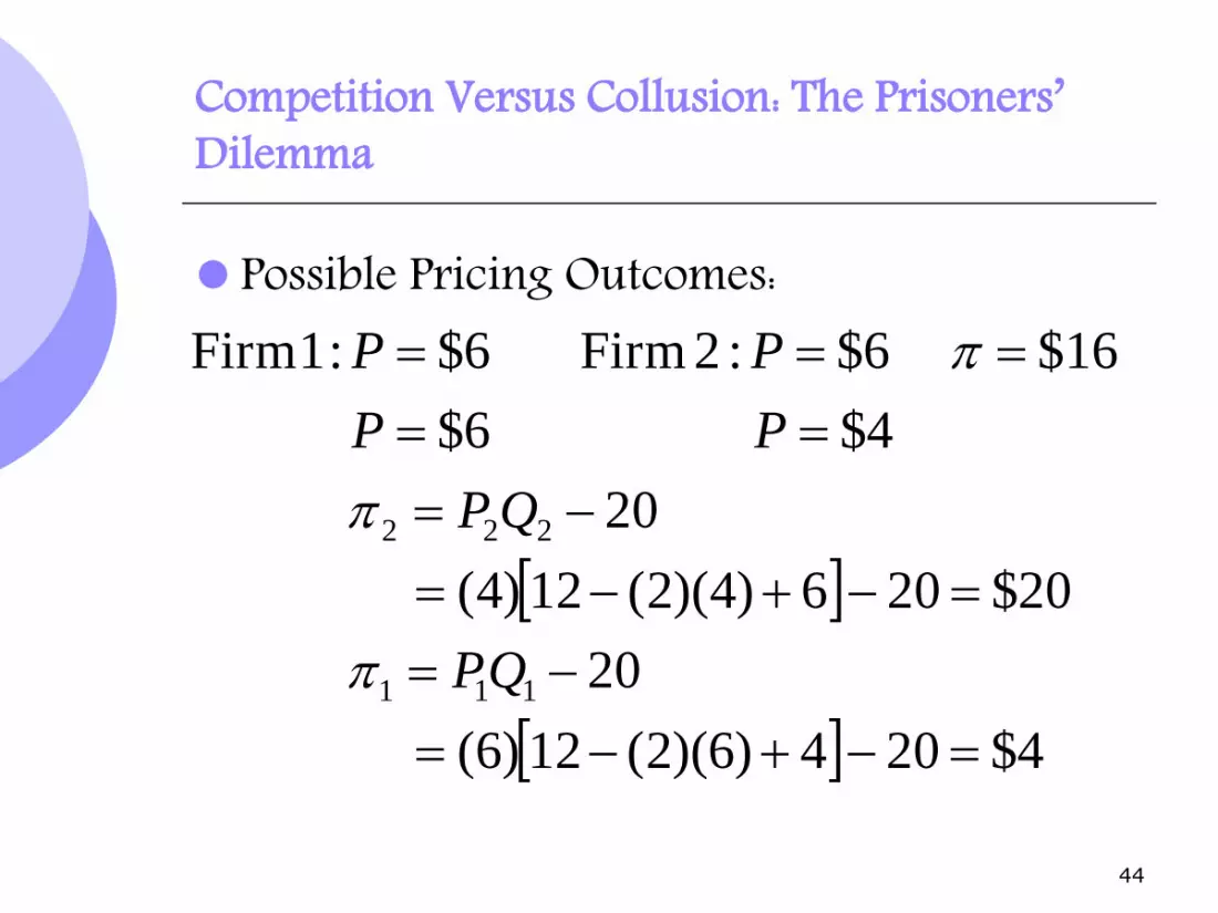
Possible Pricing Outcomes:
4$204)6)(2(12)6(
20
20$206)4)(2(12)4(
20
4$ 6$
$16 6$ :2 Firm 6$ :1 Firm
111
222
QP
QP
PP
PP

45
Payoff Matrix for Pricing GameFirm 2
Firm 1
Charge $4 Charge $6
Charge $4
Charge $6
$12, $12 $20, $4
$16, $16$4, $20

46
Competition Versus Collusion:The Prisoners’ Dilemma
We can now answer the question of why firm does not choose cooperative price.
Cooperating means both firms charging $6 instead of $4 and earning $16 instead of $12
Each firm always makes more money by charging $4, no matter what its competitor does
Unless enforceable agreement to charge $6, will be better off charging $4

Quantity Leadership: Stackelberg Model
Suppose there are two firms in the market (duopoly)
One firm (Firm1) choose a level of output before the other firm (Firm 2)
After observing the decision of Firm 1, Firm 2 decides a level of output
This model is used to describe industries in which there is a dominant firm or natural leader called the Stackelberg leader
47

Quantity Leadership: Stackelberg Model
Suppose firm 1 is the leader and that it chooses to produce a quantity Q1
Firm 2 responds by choosing quantity Q2
Each firm knows that the equilibrium price in the market depends on the total output produced
What output should the leader choose to maximize its profits?
48

Quantity Leadership: Stackelberg Model The answer depends on how the leader thinks
that the follower will react to its choice.
The leader should expect that the follower will attempt to maximize profits as well, given a choice made by the Him (leader)
Therefore, the leader should consider the follower’s profit-maximization problem in order to make a sensible decision about its own production.
49

Quantity Leadership: Stackelberg Model
Start by the end of the game (backward): evaluate the follower’s maximization problem, taking as predetermined level of output chosen by the leader:
The follower chooses Q2 such that Π2 (Q1, Q2) is maximized
You will find Q2 = f(Q1), the reaction function for the follower
50

Quantity Leadership: Stackelberg Model Solve the leader’s optimization problem, subject to
the reaction of the follower
The leader chooses Q1 such Π1 (Q1, Q2) is maximized subject to Q2 = f(Q1), i.e., max Π1 (Q1, f(Q1))
51

Quantity Leadership: Stackelberg Model
Cournot and Stackelberg models are alternative representations of oligopolistic behavior.
Which model is more appropriate depends on the industry.
For an industry roughly comprising of similar firms (none having strong operating advantage or leadership position), the Cournot model is the most appropriate one.
52

Quantity Leadership: Stackelberg Model
On the other hand, industry dominated by a large firm that usually takes the lead in introducing new product or setting price.
The mainframe computer market is an example, with IBM the leader.
Then the Stackelberg model may be more realistic.
53