incorporating reliability performance measures in operations and planning modeling tools:...
TRANSCRIPT
20
14Incorporating Reliability Perform
ance Measures into O
perations and Planning Modeling Tools
65+ pages; Perfect Bind with SPINE COPY or 0–64 pages; Saddlewire (NO SPINE COPY)
Accelerating solutions for highway safety, renewal, reliability, and capacity
Incorporating Reliability Performance Measures into Operations and Planning Modeling Tools
RepoRt S2-L04-RR-1

TRANSPORTATION RESEARCH BOARD 2014 EXECUTIVE COMMITTEE*
OFFICERS
Chair: Kirk T. Steudle, Director, Michigan Department of Transportation, LansingViCe Chair: Daniel Sperling, Professor of Civil Engineering and Environmental Science and Policy; Director, Institute of Transportation Studies,
University of California, DavisexeCutiVe DireCtor: Robert E. Skinner, Jr., Transportation Research Board
MEMBERS
Victoria A. Arroyo, Executive Director, Georgetown Climate Center, and Visiting Professor, Georgetown University Law Center, Washington, D.C.Scott E. Bennett, Director, Arkansas State Highway and Transportation Department, Little RockDeborah H. Butler, Executive Vice President, Planning, and CIO, Norfolk Southern Corporation, Norfolk, Virginia (Past Chair, 2013)James M. Crites, Executive Vice President of Operations, Dallas–Fort Worth International Airport, TexasMalcolm Dougherty, Director, California Department of Transportation, SacramentoA. Stewart Fotheringham, Professor and Director, Centre for Geoinformatics, School of Geography and Geosciences, University of St. Andrews,
Fife, United KingdomJohn S. Halikowski, Director, Arizona Department of Transportation, PhoenixMichael W. Hancock, Secretary, Kentucky Transportation Cabinet, FrankfortSusan Hanson, Distinguished University Professor Emerita, School of Geography, Clark University, Worcester, Massachusetts Steve Heminger, Executive Director, Metropolitan Transportation Commission, Oakland, CaliforniaChris T. Hendrickson, Duquesne Light Professor of Engineering, Carnegie Mellon University, Pittsburgh, PennsylvaniaJeffrey D. Holt, Managing Director, Bank of Montreal Capital Markets, and Chairman, Utah Transportation Commission, Huntsville, UtahGary P. LaGrange, President and CEO, Port of New Orleans, LouisianaMichael P. Lewis, Director, Rhode Island Department of Transportation, ProvidenceJoan McDonald, Commissioner, New York State Department of Transportation, AlbanyAbbas Mohaddes, President and CEO, Iteris, Inc., Santa Ana, CaliforniaDonald A. Osterberg, Senior Vice President, Safety and Security, Schneider National, Inc., Green Bay, WisconsinSteven W. Palmer, Vice President of Transportation, Lowe’s Companies, Inc., Mooresville, North CarolinaSandra Rosenbloom, Professor, University of Texas, Austin (Past Chair, 2012)Henry G. (Gerry) Schwartz, Jr., Chairman (retired), Jacobs/Sverdrup Civil, Inc., St. Louis, MissouriKumares C. Sinha, Olson Distinguished Professor of Civil Engineering, Purdue University, West Lafayette, IndianaGary C. Thomas, President and Executive Director, Dallas Area Rapid Transit, Dallas, TexasPaul Trombino III, Director, Iowa Department of Transportation, AmesPhillip A. Washington, General Manager, Regional Transportation District, Denver, Colorado
EX OFFICIO MEMBERS
Thomas P. Bostick, (Lt. General, U.S. Army), Chief of Engineers and Commanding General, U.S. Army Corps of Engineers, Washington, D.C.Alison J. Conway, Assistant Professor, Department of Civil Engineering, City College of New York, New York, and Chair, TRB Young
Members CouncilAnne S. Ferro, Administrator, Federal Motor Carrier Safety Administration, U.S. Department of TransportationDavid J. Friedman, Acting Administrator, National Highway Traffic Safety Administration, U.S. Department of TransportationLeRoy Gishi, Chief, Division of Transportation, Bureau of Indian Affairs, U.S. Department of the Interior, Washington, D.C.John T. Gray II, Senior Vice President, Policy and Economics, Association of American Railroads, Washington, D.C.Michael P. Huerta, Administrator, Federal Aviation Administration, U.S. Department of TransportationPaul N. Jaenichen, Sr., Acting Administrator, Maritime Administration, U.S. Department of TransportationTherese W. McMillan, Acting Administrator, Federal Transit AdministrationMichael P. Melaniphy, President and CEO, American Public Transportation Association, Washington, D.C.Gregory Nadeau, Acting Administrator, Federal Highway Administration, U.S. Department of TransportationCynthia L. Quarterman, Administrator, Pipeline and Hazardous Materials Safety Administration, U.S. Department of TransportationPeter M. Rogoff, Under Secretary for Policy, U.S. Department of TransportationCraig A. Rutland, U.S. Air Force Pavement Engineer, Air Force Civil Engineer Center, Tyndall Air Force Base, FloridaJoseph C. Szabo, Administrator, Federal Railroad Administration, U.S. Department of TransportationBarry R. Wallerstein, Executive Officer, South Coast Air Quality Management District, Diamond Bar, CaliforniaGregory D. Winfree, Assistant Secretary for Research and Technology, Office of the Secretary, U.S. Department of TransportationFrederick G. (Bud) Wright, Executive Director, American Association of State Highway and Transportation Officials, Washington, D.C.Paul F. Zukunft, Adm., U.S. Coast Guard, Commandant, U.S. Coast Guard, U.S. Department of Homeland Security.
* Membership as of July 2014.
TRANSPORTATION RESEARCH BOARDWASHINGTON, D.C.
2014www.TRB.org
The SecondS T R A T E G I C H I G H W A Y R E S E A R C H P R O G R A M
RepoRt S2-L04-RR-1
Incorporating Reliability Performance Measures into Operations and Planning Modeling Tools
Hani S. MaHMaSSani, Jiwon KiM, and Ying CHen
Northwestern University
YanniS StogioS and andY BriJMoHan
Delcan Corporation
Peter VoVSHa
Parsons Brinckerhoff

Subscriber Categories
HighwaysOperations and Traffic ManagementPlanning and Forecasting
SHRP 2 Reports
Available by subscription and through the TRB online bookstore:
www.TRB.org/bookstore
Contact the TRB Business Office:202-334-3213
More information about SHRP 2:
www.TRB.org/SHRP2
The Second Strategic Highway Research Program
America’s highway system is critical to meeting the mobility and economic needs of local communities, regions, and the nation. Developments in research and technology—such as advanced materials, communications technology, new data collection technologies, and human factors science—offer a new oppor-tunity to improve the safety and reliability of this important national resource. Breakthrough resolution of significant trans-portation problems, however, requires concentrated resources over a short time frame. Reflecting this need, the second Strategic Highway Research Program (SHRP 2) has an intense, large-scale focus, integrates multiple fields of research and technology, and is fundamentally different from the broad, mission-oriented, discipline-based research programs that have been the mainstay of the highway research industry for half a century.
The need for SHRP 2 was identified in TRB Special Report 260: Strategic Highway Research: Saving Lives, Reducing Conges-tion, Improving Quality of Life, published in 2001 and based on a study sponsored by Congress through the Transportation Equity Act for the 21st Century (TEA-21). SHRP 2, modeled after the first Strategic Highway Research Program, is a focused, time-constrained, management-driven program designed to comple-ment existing highway research programs. SHRP 2 focuses on applied research in four areas: Safety, to prevent or reduce the severity of highway crashes by understanding driver behavior; Renewal, to address the aging infrastructure through rapid design and construction methods that cause minimal disruptions and produce lasting facilities; Reliability, to reduce congestion through incident reduction, management, response, and miti-gation; and Capacity, to integrate mobility, economic, environ-mental, and community needs in the planning and designing of new transportation capacity.
SHRP 2 was authorized in August 2005 as part of the Safe, Accountable, Flexible, Efficient Transportation Equity Act: A Legacy for Users (SAFETEA-LU). The program is managed by the Transportation Research Board (TRB) on behalf of the National Research Council (NRC). SHRP 2 is conducted under a memo-randum of understanding among the American Association of State Highway and Transportation Officials (AASHTO), the Federal Highway Administration (FHWA), and the National Academy of Sciences, parent organization of TRB and NRC. The program provides for competitive, merit-based selection of research contractors; independent research project oversight; and dissemination of research results.
SHRP 2 Report S2-L04-RR-1
ISBN: 978-0-309-27377-0
Library of Congress Control Number: 2014946504
© 2014 National Academy of Sciences. All rights reserved.
Copyright InformationAuthors herein are responsible for the authenticity of their materials and for obtaining written permissions from publishers or persons who own the copy-right to any previously published or copyrighted material used herein.
The second Strategic Highway Research Program grants permission to repro-duce material in this publication for classroom and not-for-profit purposes. Permission is given with the understanding that none of the material will be used to imply TRB, AASHTO, or FHWA endorsement of a particular product, method, or practice. It is expected that those reproducing material in this document for educational and not-for-profit purposes will give appropriate acknowledgment of the source of any reprinted or reproduced material. For other uses of the material, request permission from SHRP 2.
Note: SHRP 2 report numbers convey the program, focus area, project number, and publication format. Report numbers ending in “w” are published as web documents only.
NoticeThe project that is the subject of this report was a part of the second Strategic Highway Research Program, conducted by the Transportation Research Board with the approval of the Governing Board of the National Research Council.
The members of the technical committee selected to monitor this project and to review this report were chosen for their special competencies and with regard for appropriate balance. The report was reviewed by the technical committee and accepted for publication according to procedures established and overseen by the Transportation Research Board and approved by the Governing Board of the National Research Council.
The opinions and conclusions expressed or implied in this report are those of the researchers who performed the research and are not necessarily those of the Transportation Research Board, the National Research Council, or the program sponsors.
The Transportation Research Board of the National Academies, the National Research Council, and the sponsors of the second Strategic Highway Research Program do not endorse products or manufacturers. Trade or manufacturers’ names appear herein solely because they are considered essential to the object of the report.
The National Academy of Sciences is a private, nonprofit, self-perpetuating society of distinguished scholars engaged in scientific and engineering research, dedicated to the furtherance of science and technology and to their use for the general welfare. On the authority of the charter granted to it by Congress in 1863, the Academy has a mandate that requires it to advise the federal government on scientific and technical matters. Dr. Ralph J. Cicerone is president of the National Academy of Sciences.
The National Academy of Engineering was established in 1964, under the charter of the National Academy of Sciences, as a parallel organization of outstanding engineers. It is autonomous in its administration and in the selection of its members, sharing with the National Academy of Sciences the responsibility for advising the federal government. The National Academy of Engineering also sponsors engineering programs aimed at meeting national needs, encourages education and research, and recognizes the superior achieve-ments of engineers. Dr. C. D. (Dan) Mote, Jr., is president of the National Academy of Engineering.
The Institute of Medicine was established in 1970 by the National Academy of Sciences to secure the services of eminent members of appropriate professions in the examination of policy matters pertaining to the health of the public. The Institute acts under the responsibility given to the National Academy of Sciences by its congressional charter to be an adviser to the federal government and, on its own initiative, to identify issues of medical care, research, and education. Dr. Victor J. Dzau is president of the Institute of Medicine.
The National Research Council was organized by the National Academy of Sciences in 1916 to associate the broad community of science and technology with the Academy’s purposes of furthering knowledge and advising the federal government. Functioning in accordance with general policies determined by the Academy, the Council has become the principal operating agency of both the National Academy of Sciences and the National Academy of Engineering in providing services to the government, the public, and the scientific and engineering communities. The Council is administered jointly by both Academies and the Institute of Medicine. Dr. Ralph J. Cicerone and Dr. C. D. (Dan) Mote, Jr., are chair and vice chair, respectively, of the National Research Council.
The Transportation Research Board is one of six major divisions of the National Research Council. The mission of the Transportation Research Board is to provide leadership in transportation innovation and progress through research and information exchange, conducted within a setting that is objective, interdisci-plinary, and multimodal. The Board’s varied activities annually engage about 7,000 engineers, scientists, and other transportation researchers and practitioners from the public and private sectors and academia, all of whom contribute their expertise in the public interest. The program is supported by state transportation departments, federal agencies including the component administrations of the U.S. Department of Transporta-tion, and other organizations and individuals interested in the development of transportation. www.TRB.org
www.national-academies.org

ACKNOWLEDGMENTS
This work was sponsored by the Federal Highway Administration in cooperation with the American Association of State Highway and Transportation Officials. It was conducted in the second Strategic Highway Research Program, which is administered by the Transportation Research Board of the National Academies. The project was managed by William Hyman, SHRP 2 Senior Program Officer, Reliability.
SHRP 2 STAFF
Ann M. Brach, DirectorStephen J. Andrle, Deputy DirectorNeil J. Pedersen, Deputy Director, Implementation and CommunicationsCynthia Allen, EditorKenneth Campbell, Chief Program Officer, SafetyJoAnn Coleman, Senior Program Assistant, Capacity and ReliabilityEduardo Cusicanqui, Financial OfficerRichard Deering, Special Consultant, Safety Data Phase 1 PlanningShantia Douglas, Senior Financial AssistantCharles Fay, Senior Program Officer, SafetyCarol Ford, Senior Program Assistant, Renewal and SafetyJo Allen Gause, Senior Program Officer, CapacityJames Hedlund, Special Consultant, Safety CoordinationAlyssa Hernandez, Reports CoordinatorRalph Hessian, Special Consultant, Capacity and ReliabilityAndy Horosko, Special Consultant, Safety Field Data CollectionWilliam Hyman, Senior Program Officer, ReliabilityLinda Mason, Communications OfficerReena Mathews, Senior Program Officer, Capacity and ReliabilityMatthew Miller, Program Officer, Capacity and ReliabilityMichael Miller, Senior Program Assistant, Capacity and ReliabilityDavid Plazak, Senior Program Officer, Capacity and ReliabilityRachel Taylor, Senior Editorial AssistantDean Trackman, Managing EditorConnie Woldu, Administrative Coordinator
F o r e w o r dWilliam Hyman, SHRP 2 Senior Program Officer, Reliability
The Incorporating Reliability Performance Measures into Operations and Planning Mod-eling Tools project explored how to address reliability using micro- and mesosimulation models. In addition, it provided guidance on how to address reliability in other modeling systems, namely in traditional demand forecasting models and with activity-based models coupled with dynamic traffic assignment models. Substantial advances were made in this project, both conceptually and in terms of practical products produced.
This research should be of interest to those concerned with modeling travel time reliability and using the results for transportation system management and operations. The audience for the reports and products resulting from this research includes researchers, planners, traffic engineers, vendors of simulation models, consultants who work hand in hand with transportation agencies, and decision makers concerned with highway operations.
Early in the project the researchers set out a framework for incorporating reliability into plan-ning and operation models that distinguishes between the demand and supply side. Travel demand may be static, as in typical planning models; dynamic for planning and operational models; or activity-based. Supply—in other words, the capacity of each part of the network—may be fixed, stochastic, or systematically varying.
The SHRP 2 Reliability focus area identified seven sources of nonrecurring congestion: incidents, weather, work zones, special events, traffic control devices not working properly, unusual fluctuations in demand, and bottlenecks that can exacerbate these sources of unre-liability. These nonrecurring sources of congestion can affect supply, demand, or both; for example, work zones affect supply; special events, demand; and incidents and weather, both. These supply and demand factors influence the travel time for origin–destination (O-D) pairs across the network and, in turn, the distribution of travel time from which various reliability measures can be derived.
To explain how to address reliability when using micro- and mesosimulation models, the framework was extended to distinguish between sources of nonrecurring congestion exter-nal (exogenous) to a simulation model and internal (endogenous) to it. Exogenous factors include incidents, weather, and work zones, whereas endogenous factors include heteroge-neity of driver behavior and vehicle type on the demand side and breakdown of flow, traffic control, and differences in car-following behavior on the supply side.
Microsimulation models are widely used in the transportation field to understand how vehicles behave in detailed settings, such as a series of traffic signals along an arterial street, freeway onramps, or a small network of roads. Mesosimulation models are suitable for higher-resolution analysis and can be applied to networks of varying sizes, including an entire region. Both micro- and mesosimulation models are based on some form of traffic physics, in contrast to a standard four-step demand model.
This project focused considerable attention on how micro- and mesosimulation models could address travel time reliability. The essence of the approach is to sandwich a simulation model between a pre- and post-processor such that together, all three components can portray travel time reliability on a network or part of it.
The researchers developed two software prototypes that were tested with both a widely used mesosimulation model and a widely used microsimulation model. The first software prototype, the Scenario Manager, consisted of the pre-processor for either type of simula-tion model. The Scenario Manager produces random scenarios involving various sources of nonrecurring congestion such as traffic incidents, weather, and work zones. It can also address scenarios based on historical data or scenarios previously constructed for planning purposes. The other software prototype is the Trajectory Processor. This post-processor determines the distribution of travel time for every O-D pair on a network. Nearly all the travel time reliability metrics, including standard deviation and the Planning Time Index, can be derived from the travel time distribution. For information about how to use the two prototypes, see their user guides. This report provides more information about the Scenario Manager and the Trajectory Processor, as well as the research.
The research also produced SHRP 2 Report S2-L04-RR-1: Incorporating Reliability Perfor-mance Measures into Operations and Planning Modeling Tools: Application Guidelines, about a micro- or mesosimulation model with pre- and post-processors. Private sector software vendors may wish to closely examine the prototype software to determine the merits of incorporating similar capability into the products they have on the market. The application guidelines and user guides should help private vendors make informed decisions.
It is worth noting that a similar scenario manager and procedures for compiling the dis-tribution of travel time were also developed and applied in the SHRP 2 L02 project, Incor-poration of Travel Time Reliability into the Highway Capacity Manual. The Transportation Research Board Committee on Highway Capacity and Quality of Service approved a motion to incorporate this new approach into the Highway Capacity Manual.
The SHRP 2 L04 project also drew on earlier work performed in the SHRP 2 Capacity focus area under a project titled Improving our Understanding of How Highway Congestion and Pricing Affect Travel Demand (SHRP 2 C02). Reliability was introduced into succes-sively richer utility functions, beginning with the traditional variables of out-of-pocket costs and travel time, and progressively adding other variables including travel time reliability. The researchers describe how to place a value on travel time reliability given other relevant terms in the utility function and emphasize that the value of reliability is not a constant; rather, it varies with such factors as vehicle occupancy and household income. This project on incorporating reliability into planning and operation models absorbed important aspects of the earlier research performed within the SHRP 2 Capacity focus area.
Finally, a substantial effort was undertaken within this project to provide guidance on how to integrate reliability into a modeling system that uses activity-based models on the demand side and a fine-grained, time-sensitive model on the supply side (e.g., a mesosimulation model). This guidance appears in the project’s reference material report (SHRP 2 Report S2-L04-RR-1: Incorporating Reliability Performance Measures into Operations and Planning Modeling Tools: Reference Material).
C O N T E N T S
1 Executive Summary
4 CHAPTER 1 Introduction 4 Objectives 4 Approach 4 Report Organization
7 PART 1 RESEARch BAckgRouNd
8 CHAPTER 2 Fundamental Issues of Incorporating Travel Time Reliability into Modeling Tools
8 Introduction 10 Incorporating Reliability into Planning and Operation Models 18 Systematic and Random Fluctuations in Travel Demand and Network Supply:
Impact on Recurrent and Nonrecurrent Congestion 20 Approaches to Incorporating Travel Time Variability into Network
Simulation Tools
22 CHAPTER 3 Integrating Travel Time Reliability into Planning Models
22 Specifics of ABM-DTA Equilibration Versus Aggregate Models 23 ABM-DTA Integration Principles 29 Approaches to Quantifying Reliability and Its Impacts 31 Incorporating Reliability into Demand Model 35 Incorporating Reliability into Network Simulation 36 Single-Run Versus Multiple-Run Approach 42 Technical Aspects of Scenario Formation 45 Recommendations for Future Research
47 CHAPTER 4 Functional Requirements of Stochastic Network Simulation Models
47 Introduction 47 Framework 49 Functional Requirements 51 Quantifying Travel Time Variability 52 Constructing Travel Time Distributions 54 Trajectories: A Unifying Framework 58 Model Variability and Its Sources in Traffic Simulation Tools
61 PART 2 FRAMEwoRk ANd ToolS FoR TRAvEl TIME RElIABIlITy ANAlySIS
62 CHAPTER 5 Model and data Requirements 62 Scenario Manager 63 Trajectory Processor 63 Data Requirements
66 CHAPTER 6 Scenario Manager 66 Introduction 68 Methodology for Scenario-Based Reliability Analysis Using Simulation Tools 72 Implementation of Scenario Manager
82 CHAPTER 7 Trajectory Processor 82 Introduction 83 Software Description 83 Integration with Selected Models (DYNASMART and Aimsun) 90 Travel Time Reliability Indices
93 PART 3 APPlIcATIoNS
94 CHAPTER 8 Analysis Process: Mesoscopic Models 94 Defining Scenarios 94 Generating Scenarios Using the Scenario Manager 96 Simulating Scenarios Using DYNASMART-P 96 Obtaining Reliability Statistics Using the Trajectory Processor
114 CHAPTER 9 Analysis Process: Microscopic Models 114 Study Area Description 114 Microsimulation Approach and Objective 114 Scenario Description 114 Microsimulation Travel Time Reliability Results
128 CHAPTER 10 Study Findings and conclusions 130 Implementation Steps 131 Agency Adoption 131 Developers 131 Success Factors 131 Recommendations for Further Research
133 References
1
The broader goals of the Reliability focus area within the second Strategic Highway Research Program (SHRP 2) are to address unexpected traffic congestion and improve travel time reli-ability. To this end, SHRP 2 research projects have brought forward numerous technical measures and policies for further consideration and development. In parallel with these proj-ects, the L04 project, Incorporating Reliability Performance Measures into Operations and Planning Modeling Tools, is aimed at improving planning and operations models to create suitable tools for the evaluation of projects and policies that are expected to improve reliability.
The L04 project addressed the need for a comprehensive framework and conceptually coher-ent set of methodologies to (1) better characterize reliability, and the manner in which the vari-ous sources of variability operate individually and in interaction with each other in determining overall reliability performance of a network; (2) assess the impact of reliability on users and the system; and (3) determine the effectiveness and value of proposed counter measures. In doing so, this project has closed an important gap in the underlying conceptual foundations of travel modeling and traffic simulation, and provided practical means of generating realistic reliability measures using network simulation models in a variety of application contexts. A principal accomplishment of the project is a unifying framework for reliability analysis using essentially any particle-based microsimulation or mesosimulation model that produces vehicle travel trajectories.
The framework developed in this study is built on a taxonomy that recognizes demand- versus supply-side, exogenous versus endogenous, and systematic versus random variability. The framework features three components:
1. A Scenario Manager, which captures exogenous sources of unreliability, such as special events, adverse weather, work zones, and travel demand variation;
2. Reliability-integrated simulation models that model sources of unreliability endogenously, including user heterogeneity, flow breakdown, and collisions; and
3. A vehicle Trajectory Processor, which extracts reliability information from the simulation output, namely, vehicle trajectories.
The primary role of the Scenario Manager is to prepare input scenarios for the traffic simula-tion models; these scenarios represent mutually consistent combinations of demand- and supply-side random factors and are intended to capture exogenous sources of variation. Endogenous variation sources are captured in the traffic simulation model, depending on the modeling capability of the selected platform and the intended purpose of the analysis. The framework may be used with any “particle-based” simulation model, namely, microscopic and mesoscopic
Executive Summary
2
simulation models that produce individual vehicle (or particle) trajectories. These trajectories enable construction of any level of travel time distributions of interest (e.g., networkwide, origin–destination pair, path, and link) and subsequent extraction of any desired reliability met-ric. These tasks are performed by the Trajectory Processor, which produces the scenario-specific travel time distribution from each simulation run and constructs the overall travel time distribu-tion aggregated over multiple scenarios.
The Scenario Manager allows generation of hypothetical scenarios for analysis and design purposes, while the scenario management functionality allows retrieval of historically occurring scenarios or of scenarios previously constructed as part of a planning exercise (e.g., in conjunc-tion with emergency preparedness planning). Furthermore, the Scenario Manager/Generator facilitates direct execution of the simulation model for a particular scenario by creating the necessary inputs that reflect the scenario assumptions. When exercised in the latter manner (i.e., in random generation mode), the Scenario Manager becomes the primary platform for conduct-ing reliability analyses, as experiments are conducted to replicate certain field conditions, under both actual and hypothetical (proposed) network and control scenarios. In particular, the Sce-nario Generator enables execution of experimental designs that entail simulation over multiple days, thus reflecting daily fluctuations in demand, both systematic and random. Two main approaches may be used to assess the travel time reliability for a given project assessment or application: (1) the Monte Carlo approach and (2) the mix-and-match (or user-defined) approach. In addition to the framework and tool itself, the project also developed the method-ological aspects of conducting scenario-based reliability analysis, including mechanisms for gen-erating scenarios recognizing logical, temporal, and statistical interdependencies among different sources of variability modeled through the scenario approach.
The vehicle Trajectory Processor produces and helps visualize reliability performance measures (travel time distributions and indicators) from observed or simulated trajectories. The travel time distributions and associated indicators are derived from individual vehicle trajectories, defined as sequences of geographic positions (nodes) and associated passage times. These trajectories are obtained as output from particle-based microscopic or mesoscopic simulation models. Such trajectories may alternatively be obtained directly through measurement [e.g., probe vehicles equipped with global positioning systems (GPSs)], thus enabling validation of travel time reliability metrics generated on the basis of output from simulation tools.
Prototypes of a Scenario Manager and a Trajectory Processor have been developed as project-specific deliverables of this research. The tools are conceptually generic and (simulation) software-neutral. The prototypes were demonstrated for the microsimulation modeling platform Aimsun and the mesosimulation dynamic traffic assignment (DTA) platform DYNASMART-P, both of which are representative of other available options in their respective categories to enable rapid cross-platform adaptation.
The prototypes and the overall reliability-analysis framework were demonstrated by applying these microsimulation and mesosimulation models to networks extracted from the New York City regional network. Detailed calibration and validation steps were described using available data sources in addition to a specially acquired sample of actual vehicle trajectories based on GPS traces—highlighting and demonstrating the role and potential of such vehicle trajectories in traffic simulation model development and application, especially for reliability-oriented analysis purposes.
In addition to the development and application of this general framework, the study made specific contributions in several related areas, namely: (1) development and validation of a robust relationship between the standard deviation of the trip time per unit distance and the mean of the trip time per unit distance, using both simulated and observed trajectories; (2) a detailed proposal of an approach for incorporating reliability considerations into planning
3
models and practices, using different levels of representational detail and associated computa-tional requirements; and (3) initial development of a new approach to microscopic modeling of driver behavior that can capture endogenously more of the sources of variability than currently available models.
In summary, this project developed and demonstrated a unified approach with broad applicability to various planning and operations analysis problems, which allows agencies to incorporate reliability as an essential evaluation criterion. The approach as such is indepen-dent of specific analysis software tools so that it can enable and promote wide adoption by agencies and modeling software developers. The project also developed specific software tools intended to serve as prototypes of the key concepts—namely, a Scenario Manager and a Trajectory Processor—and demonstrated them with two commonly used network modeling software platforms.
4
SHRP 2 L04, Incorporating Reliability Performance Mea-sures into Operations and Planning Modeling Tools, is a cen-tral project within the second Strategic Highway Research Program (SHRP 2) Reliability focus area. The goal of this focus area is to reduce unexpected congestion and improve travel time reliability. Numerous technical measures and policies are under consideration within SHRP 2 research projects to confront the problems of traffic congestion and devise means to improve reliability. The motivation for this L04 project is the recognition that it is essential to improve planning and operations models in parallel with these devel-opments to have suitable evaluation tools for the projects and policies that are expected to improve reliability. What is lacking is a comprehensive framework and conceptually coherent set of methodologies to (1) better characterize reli-ability, and the manner in which the various sources of vari-ability operate individually and in interaction with each other in determining overall reliability performance of a net-work; (2) assess the impacts of reliability on users and the system; and (3) determine the effectiveness and value of proposed counter measures. Therefore, this model develop-ment project has a significant and practical role to play in future project investment evaluations that will use reliabil-ity improvement estimates.
objectives
The primary objective of this project is to develop the capability of producing measures of reliability performance as output in traffic simulation models and planning models. A secondary objective is to then examine how travel demand forecasting models can use reliability measures to produce revised esti-mates of travel patterns. The intent of this project is therefore to close this gap in the underlying conceptual foundations of travel modeling and traffic simulation, and provide practical means of generating realistic reliability measures using network simulation models.
Approach
The research team’s approach centers on providing a unify-ing framework for reliability analysis, using essentially any particle-based microsimulation or mesosimulation model that produces trajectories. To address the challenges associ-ated with this task, the framework proposes to capture the sources of unreliability in network traffic performance through a combination of endogenous mechanisms (i.e., capture directly the phenomena that cause delay, such as flow break-down) and exogenous events with given probabilities. Previ-ous technical reports, particularly the Task 7 Report, Simulation Model Adaptation and Development [part of the SHRP 2 L04 Project Reference Material Report (Stogios et al. 2014)], the team elaborated on the conceptual and method-ological frameworks developed as an outcome of this project. They also presented the specific methodologies and procedures devised to incorporate reliability performance measures in supply-side (network operations) models used on their own or in conjunction with integrated demand-supply model systems for both strategic and operational planning applications.
This final report is intended to provide an application-focused description of the methodology and tools developed under the L04 project to address the study objectives of assess-ing the reliability performance of a network and evaluate the effectiveness of different projects and measures to improve reliability.
report organization
The report is organized into three principal parts. The first part focuses on the underlying conceptual and methodologi-cal foundations of the work. The second part describes the specific framework and tools devised to perform the reliabil-ity analysis. The final part concludes with study findings and conclusions that are preceded by the application of the frame-work and tools on a real-world test network.
C h A p t e r 1
Introduction
5
different levels of resolution (path, origin–destination, net-work), from the set(s) of simulated trajectories obtained for a particular scenario simulation, or from actual vehicle tra-jectories obtained through real world observations and data sources.
The third part, Part 3: Applications, consists of three chap-ters. Chapter 8 describes the application of the overall meth-odology in connection with a state-of-the-art mesoscopic traffic network simulator and dynamic assignment tool to the New York City regional network. Chapter 9 presents similar information using the selected microscopic simulation tool, applied in a subset of the New York City network for which the needed data were available. The applications provide vali-dation by comparing the simulated outputs with those observed as part of a sample of GPS-equipped vehicles. Chapter 10 concludes the report with a summary of the key findings, along with directions for further research necessary to advance the state of the art as well as the state of the practice in this important area.
Overall, this project has succeeded in meeting the main points articulated in the functional requirements and has shown considerable potential for general applicability to large-scale networks under realistic scenario assumptions. The approach was able to produce reasonable reliability metrics when compared with the observed trajectory data.
The first part, Part 1: Research Background, consists of three chapters. Chapter 2 describes the challenges associated with incorporating reliability measures into operational and plan-ning models and provides a synthesis of existing approaches, thus placing the developments in this project against the back-drop of existing contributions. Chapter 3 focuses on incorpo-rating reliability into strategic planning tools; it is based on a report developed as the outcome of Task 11, which is now part of the SHRP 2 L04 Project Reference Material Report (Stogios et al. 2014). Chapter 4 articulates the functional requirements that have guided the development of the framework and the methods presented in the second part of the report.
The second part, Part 2: Framework and Tools for Travel Time Reliability Analysis, consists of three chapters. Chapter 5 describes the data requirements and model selected for the application of the tools used in the application. Chapters 6 and 7 present the principal general-purpose tools developed as part of this project. In particular, Chapter 6 describes the scenario-based approach devised in this study to capture exogenous sources of travel time variability in a network. It is a major contribution of this study, which may be used in connection with both planning and operations models, as described in Chapter 6. Chapter 7 describes the general pur-pose Trajectory Processor designed to extract reliability per-formance indicators, including travel time distributions at

7
RESEARCH BACKGROUND
The chapters in this part of the report discuss the fundamental issues of incorporating travel time reliability into modeling tools, investigate the feasibility of incorporating such into plan-ning models, and identify the functional requirements for incorporating travel time reliability into simulation models.
p A r t 1
8
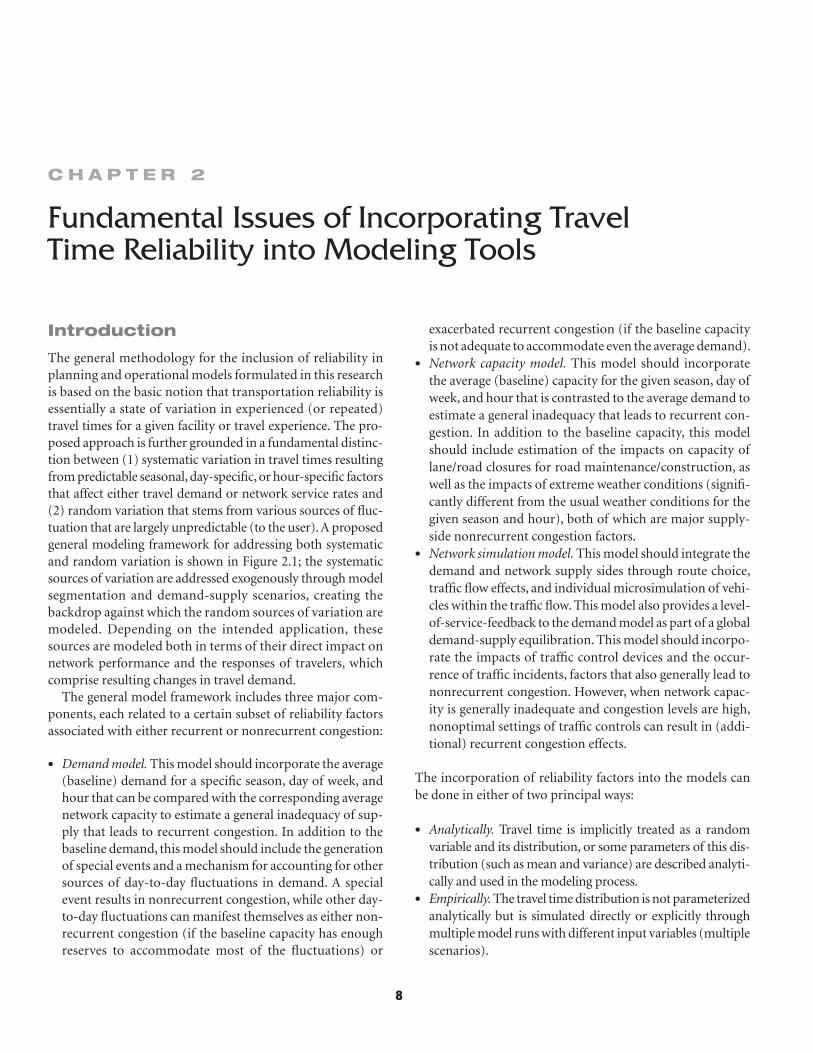
exacerbated recurrent congestion (if the baseline capacity is not adequate to accommodate even the average demand).
• Network capacity model. This model should incorporate the average (baseline) capacity for the given season, day of week, and hour that is contrasted to the average demand to estimate a general inadequacy that leads to recurrent con-gestion. In addition to the baseline capacity, this model should include estimation of the impacts on capacity of lane/road closures for road maintenance/construction, as well as the impacts of extreme weather conditions (signifi-cantly different from the usual weather conditions for the given season and hour), both of which are major supply-side nonrecurrent congestion factors.
• Network simulation model. This model should integrate the demand and network supply sides through route choice, traffic flow effects, and individual microsimulation of vehi-cles within the traffic flow. This model also provides a level-of-service-feedback to the demand model as part of a global demand-supply equilibration. This model should incorpo-rate the impacts of traffic control devices and the occur-rence of traffic incidents, factors that also generally lead to nonrecurrent congestion. However, when network capac-ity is generally inadequate and congestion levels are high, nonoptimal settings of traffic controls can result in (addi-tional) recurrent congestion effects.
The incorporation of reliability factors into the models can be done in either of two principal ways:
• Analytically. Travel time is implicitly treated as a random variable and its distribution, or some parameters of this dis-tribution (such as mean and variance) are described analyti-cally and used in the modeling process.
• Empirically. The travel time distribution is not parameterized analytically but is simulated directly or explicitly through multiple model runs with different input variables (multiple scenarios).
Fundamental Issues of Incorporating Travel Time Reliability into Modeling Tools
C h A p t e r 2
Introduction
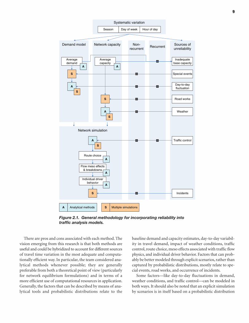
The general methodology for the inclusion of reliability in planning and operational models formulated in this research is based on the basic notion that transportation reliability is essentially a state of variation in experienced (or repeated) travel times for a given facility or travel experience. The pro-posed approach is further grounded in a fundamental distinc-tion between (1) systematic variation in travel times resulting from predictable seasonal, day-specific, or hour-specific factors that affect either travel demand or network service rates and (2) random variation that stems from various sources of fluc-tuation that are largely unpredictable (to the user). A proposed general modeling framework for addressing both systematic and random variation is shown in Figure 2.1; the systematic sources of variation are addressed exogenously through model segmentation and demand-supply scenarios, creating the backdrop against which the random sources of variation are modeled. Depending on the intended application, these sources are modeled both in terms of their direct impact on network performance and the responses of travelers, which comprise resulting changes in travel demand.
The general model framework includes three major com-ponents, each related to a certain subset of reliability factors associated with either recurrent or nonrecurrent congestion:
• Demand model. This model should incorporate the average (baseline) demand for a specific season, day of week, and hour that can be compared with the corresponding average network capacity to estimate a general inadequacy of sup-ply that leads to recurrent congestion. In addition to the baseline demand, this model should include the generation of special events and a mechanism for accounting for other sources of day-to-day fluctuations in demand. A special event results in nonrecurrent congestion, while other day-to-day fluctuations can manifest themselves as either non-recurrent congestion (if the baseline capacity has enough reserves to accommodate most of the fluctuations) or
9
There are pros and cons associated with each method. The vision emerging from this research is that both methods are useful and could be hybridized to account for different sources of travel time variation in the most adequate and computa-tionally efficient way. In particular, the team considered ana-lytical methods whenever possible; they are generally preferable from both a theoretical point of view (particularly for network equilibrium formulations) and in terms of a more efficient use of computational resources in application. Generally, the factors that can be described by means of ana-lytical tools and probabilistic distributions relate to the
baseline demand and capacity estimates, day-to-day variabil-ity in travel demand, impact of weather conditions, traffic control, route choice, meso effects associated with traffic flow physics, and individual driver behavior. Factors that can prob-ably be better modeled through explicit scenarios, rather than captured by probabilistic distributions, mostly relate to spe-cial events, road works, and occurrence of incidents.
Some factors—like day-to-day fluctuations in demand, weather conditions, and traffic control—can be modeled in both ways. It should also be noted that an explicit simulation by scenarios is in itself based on a probabilistic distribution
Demand model Network capacity
Network simulation
A Analytical methods S Multiple simulations
Sources of unreliability
RecurrentNon-
recurrent
Road works
Weather
Traffic control
Special events
Day-to-day fluctuation
Incidents
Inadequate base capacity
Season Day of week Hour of day
Systematic variation
Average demand
Average capacity
A
S
S
S
A
S
A A
A
S
S
Route choice
Flow meso effects & breakdowns
Individual driver behavior
A
A
A
Figure 2.1. General methodology for incorporating reliability into traffic analysis models.
10
of input parameters (such as parameterized probability of occurrence of a certain event). However, the principal differ-ence is that the resulting variation in travel times is generated through multiple simulations, rather than derived analyti-cally from the distribution of input variables in a one-time network simulation.
The following sections discuss each of the reliability factors in detail, survey existing approaches to their modeling, and propose specific approaches for the current project.
Incorporating reliability into planning and operation Models
Reliability as an Objective Network Performance Dimension
Characterization of Reliability Through Variability of Travel Times
In a very practical and constructive way, reliability is character-ized by the lack of variability of travel times. This approach is largely adopted for the current project, as well as for the entire set of SHRP 2 projects. It should be noted, however, that if a more general view of highway system performance is adopted that includes such additional dimensions as variable cost (e.g., as a result of real-time dynamic pricing) and safety, then the highway reliability definition should be extended accordingly. Another salient point specifically discussed in Institute for Transportation Studies (2008) is that reliability also can include the ideas of trustworthiness and reliance, which can be affected by information available to highway users.
Travel time variability can be measured and analyzed in many different ways and at different levels of disaggregation; this is both important to and a complicating factor for this research. To constructively measure variability of travel times, a specific time unit must be chosen in terms of interval dur-ing the day (e.g., an hour between 7:00 a.m. and 8:00 a.m.), day of week (e.g., Monday), and season (e.g., fall). This is nec-essary to set aside differences in travel time that occur between hours of the day, between days of the week, and between sea-sons; such differences are considered systematic variations because they are predictable, at least for most highway users familiar with the travel conditions in the area. The remaining variability of travel times across different days for the same unit (hour, day of week, and season) can then be used as the basic measure of travel reliability.
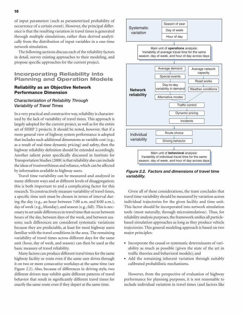
Many factors can produce different travel times for the same highway facility or route even if the same user drives through it on two or more consecutive workdays at the same time (see Figure 2.2). Also, because of differences in driving style, two different drivers may exhibit quite different patterns of travel behavior that result in significantly different travel times for exactly the same route even if they depart at the same time.
Given all of these considerations, the team concludes that travel time variability should be measured by variation across individual trajectories for the given facility and time unit. This factor should be incorporated into network simulation tools (most naturally, through microsimulation). Thus, for reliability analysis purposes, the framework unifies all particle-based simulation approaches as long as they produce vehicle trajectories. This general modeling approach is based on two major principles:
• Incorporate the causal or systematic determinants of vari-ability as much as possible (given the state of the art in traffic theories and behavioral models); and
• Add the remaining inherent variation through suitably calibrated probabilistic mechanisms.
However, from the perspective of evaluation of highway performance for planning purposes, it is not reasonable to include individual variation in travel times (and factors like
Systematicvariation
Networkreliability
Individualvariability
Season of year
Day of week
Hour of day
Main unit of operations analysis: Variability of average travel time for the same
season, day of week, and hour of day across days
Day-to-day variability in demand
Alternative modes
Traffic control
Road works
Weather conditions
Special events
Main unit of behavioral analysis: Variability of individual travel time for the same
season, day of week, and hour of day across days
Average demand Average network capacity
Dynamic pricing
Incidents
Route choice
Driving behavior
Figure 2.2. Factors and dimensions of travel time variability.
11
driving style) as a reliability component. Thus, for measuring reliability from the operations perspective, travel time vari-ability should be averaged within the chosen time unit. For the current project, the team adopted the following definition for reliability as a highway performance measure:
Reliability as a highway performance measure is characterized by variability of travel times for the same chosen time unit (hour, day of week, season) observed for different days and averaged across individual travel times observed within the unit for the same day.
By virtue of this definition, the corresponding network simu-lations incorporating reliability should be implemented with the same level of temporal resolution in terms of demand and supply, that is, hour/day/season-specific trip tables and hourly static traffic assignments (STA) or dynamic traffic assignments (DTA) covering several successive hours.
For individual behavioral analysis, additional sources of vari-ation, such as different routes and different driving styles across individuals, are important. Thus, the team arrived at a different definition for individual behavioral analysis and microscopic modeling:
Reliability as a LOS measure for individual behavior is char-acterized by variability of travel time for the same chosen unit (hour, day of week, season) across individual travel times observed within the unit.
This duality of reliability has a direct implication for the modeling approaches considered for the current project. Approaches that are based on macro modeling paradigms (i.e., operate with aggregate traffic flows) can only incorporate reli-ability in the aggregate sense (first definition). Approaches that are based on individual microsimulation (i.e., operate with individual particles like persons on the demand side and vehi-cles on the network supply side) can address both types of reli-ability. Because several meso modeling paradigms capture characteristics of individual particles, the lines are increasingly blurred between micro and meso approaches—thus the refer-ence to particle-based approaches as a basis for the approach developed in this study.
Approaches to Quantification of Travel Time Variability
Many quantitative measures have been proposed for travel time variability in different contexts, but most frequently for one of two distinct purposes: either for overall assessment of the highway facility performance, or for explaining individ-ual preferences for a route, trip departure time, or mode for a particular trip. All such measures can be derived from the travel time distribution and none of them can be claimed to
be particularly right or exhaustive. Each of them makes sense in its particular context.
From the perspective of highway operations, decisions about highway capacity expansion and traffic management reliability of travel times on a certain facility are naturally the focus of the analysis. Most of the actual data on travel time variability have been collected at the facility level. These data sources are valu-able for building analytical functions that relate reliability mea-sures to the traffic volume and facility characteristics (number of lanes, length, cross-sectional design, access, traffic signals). For example, robust statistical dependencies have been estab-lished between almost all reliability measures, including stan-dard deviation; 80th, 90th, and 95th percentile; buffer time and index; and average traffic volumes at the facility level. The SHRP 2 L03 project, Analytical Procedures for Determining the Impacts of Reliability Mitigation Strategies, specifically focused on this particular issue (Cambridge Systematics, Inc. et al. 2013). The specific measures of reliability that were proposed by the L03 team and which have largely been accepted in the majority of SHRP 2 projects are discussed in the next section.
Having these functions in place, however, does not yet provide an immediate basis for network simulation and travel demand models. Highway facilities represent elemental links in the high-way network. The crux of the modeling challenge is that reli-ability measures have to be generated at the trip route level, since that is the unit for which travel choices are essentially modeled. Construction of route-level reliability measures from facility-level reliability measures is a nontrivial problem since almost all reasonable reliability measures (e.g., travel time stan-dard deviation) are not additive by links, and those that might be additive under certain conditions (e.g., travel time variances if assumed independent by links or buffer time) cannot be assumed independent in a general case.
User’s Perspective
Reliability as Travelers’ Subjective Perception and Determinant of Travel Behavior
Travel demand models and network simulation tools are based on the mathematical representation of choices made by the travelers with respect to network routes, departure times, modes, destinations, and frequencies for each trip type. Specifi-cally, in the new generation travel demand models—called activity-based models (ABM)—and microscopic network sim-ulation tools, the individual nature of these choices has been made explicit. These models have been developed and esti-mated not only to replicate the observed aggregate traffic flows but also to replicate individual-level choices with the maximum degree of behavioral realism so as to provide reasonable predic-tions of responses to future scenarios and policies.
12
Obtaining behavioral realism in individual choices requires taking into account travelers’ subjective perceptions of reliabil-ity, as well as the entire set of highway LOS attributes. Subjective perceptions of travel attributes can be quite different from their objective measurements. This phenomenon is well known to transportation modelers and has been long taken into account in some manner within the framework of conventional models. For example, in transit assignment and mode choice, compo-nents of out-of-vehicle transit travel time such as wait and walk time are applied with perceived weights relative to in-vehicle time that are significant (in the range of 1.5 to 4.0). It is also not unusual for transit in-vehicle time to be differentiated by mode to reflect that rail modes are generally perceived as more conve-nient and comfortable than conventional bus.
On the highway side, most of the travel models and network assignment procedures operate with a generic physical time variable regardless of the facility type, level of congestion, and associated reliability characteristics. There is compelling statis-tical evidence from behavioral studies that travelers place a very significant value on reliability and other highway time attri-butes, such as the level of congestion and driving conditions. Thus the concept of value of reliability (VOR) was introduced to complement value of time (VOT). See Concas and Kolpakov (2009) for a good survey of research and practical works in which VOT and VOR were estimated.
The highway operations perspective primarily relates the quantification of reliability to the comprehensive monitoring and measurement of the actual physical traffic times and speeds observed in the traffic flow. In contrast, the user’s perspective cannot be directly measured with roadside observations; it can only be quantified by relating user choices with respect to net-work routes, trip departure times, modes, and so on to actual travel times and reliability measures. For each of these travel choices, the corresponding behavioral parameters like VOT and VOR are established by statistical estimation of the correspond-ing choice models. The SHRP 2 C04 project, Improving Our Understanding of How Highway Congestion and Pricing Affect Travel Demand, is specifically devoted to this issue and provides behavioral models of route choice, trip departure time choice, and mode choice incorporating reliability measures for the L04 project (Parsons Brinckerhoff et al. 2013).
In summary, the following two important aspects of the problem need to be taken into account when the user’s perspec-tive on reliability (and performance in general) is compared with the highway operations perspective:
• The user perspective can include many perceived compo-nents and weights compared with the physical measures of average travel time and reliability in the highway operations perspective. The measure that looks the best and most sta-tistically significant from the highway operations perspec-tive might not be the best choice for modeling user responses.
For example, the 95th percentile of travel time is favored in highway operations because it singles out the most critical cases of nonrecurrent congestion, mostly those associated with traffic incidents, road works, special events, and extreme weather (see Cambridge Systematics, Inc. 2005; Cambridge Systematics, Inc. et al. 2013). The current experience with models of individual behavior in the context of route choice, however, indicates that the decision-making point at which users evaluate reliability lies somewhere between the 80th and 90th percentile thus mixing recurrent and nonrecur-rent congestion (see Concas and Kolpakov 2009; Parsons Brinckerhoff et al. 2013).
• The user perspective is inherently an entire-trip perspec-tive. Thus, the reliability measures for travel models and network simulation tools have to be synthesized at the O–D-route level, while the bulk of statistical evidence on highway operations is collected at the facility/link level. This synthesis is not a trivial task because practically all sensible reliability measures are inherently nonadditive (Institute for Transportation Studies 2008).
Although reliability measures adopted for a travel model are different from reliability measures adopted for the analysis of highway operations, this fact does not mean that the opera-tional simulation tools cannot be used to generate the reliabil-ity measures needed for highway performance evaluation as an aggregate output. Eventually, the modeling tools designed in the current research will be able to generate the entire distribu-tion of travel times for each network link, which would suffice for constructing virtually any reliability measure.
Reliability as a Decision-Making Factor in Transportation Operations and Scheduling
In addition to the general highway systems performance per-spective and the individual driver’s perspective which consti-tute the focus for this research project, there are several other important highway users, each with its own perspective on reliability. The other types of highway users and their per-spectives include the following:
• Freight companies and truck operators. In certain regions, trucks constitute a significant share of traffic, and it is a nor-mal practice to single them out as a separate vehicle class in traffic assignment (sometimes subdivided into heavy trucks, light trucks, and/or commercial vehicles), as well as have a separate demand model for them. Trucks are treated as a separate vehicle class because of their different speed and delay functions, possible network prohibitions, different toll rates, and VOT. With respect to reliability, trucks have an especially strong impact on traffic conditions and rep-resent a risk factor in traffic. In general, all else being equal,
13
the higher the share of trucks in the traffic, the higher the variability of travel times. A related issue that has not yet been fully explored is the associated willingness to pay for travel time savings and reliability improvements. The behavioral mechanism associated with freight movements under the condition of uncertain travel time is different from the con-sideration of reliability by private car drivers, although there may be some commonalities (such as the consideration of buffer times for on-time arrival at the destination). Some trucking companies, such as FedEx or UPS, might be signifi-cantly more willing to pay for improvement in travel time reliability than an average trucker because those companies specialize in real-time deliveries. It should be recognized, however, that modeling truckers’ responses to reliability improvements is fundamentally different from modeling private car users’ responses in that, frequently, the truckers are not the actual decision makers; thus the whole (compli-cated) aspect of dispatching and scheduling comes into play.
• Logistics companies. This category is another (sometimes invisible) player on the field. Logistics companies essentially generate the demand for truck movements and affect all choices on the truckers’ side with respect to travel time and reliability improvements. Unfortunately, most transporta-tion models attempt to model truck movements directly and ignore the logistics component since it is very complicated. It is unrealistic to tackle this issue in the framework of the current project.
• Bus companies. Transit service reliability is an issue that is equally as important as highway reliability for the improve-ment of modeling tools. Travelers perceive transit schedule adherence as one of the important attributes of a transit service (Institute for Transportation Studies 2008). Cars, trucks, and buses share the same road space in a mixed-traffic case, thus highway reliability directly affects bus ser-vices. It is generally agreed that due to their high occupancy levels, buses have very high underlying VOT and VOR per vehicle. This could be a very significant component in the evaluation of user benefits stemming from reliability improvements associated with special bus lanes as well as high-occupancy vehicle (HOV) and high-occupancy toll (HOT) lanes shared with buses.
• Taxi cab companies. In some urban areas taxis constitute a significant share of the traffic. For example, the share of taxis in internal traffic in Manhattan is almost 40%. This is, however, a rare case; taxis represent a negligible compo-nent in traffic in most metropolitan regions in the United States. Consequently, for modeling purposes taxis are fre-quently mixed with high-occupancy vehicles in terms of VOT, VOR, and other behavioral attributes that govern their route choice, departure time choice, and other related choices. To be exact, the full-day movement of taxis is rarely modeled, and the modeling system includes only the
portion of their itinerary associated with the passenger trips they serve. The validity of these modeling assump-tions has not been explored, and research relating to cab drivers’ behavior is practically nonexistent.
These specific markets are not the focus of the current project and are left for future research.
Reliability as a Result of Travel Decisions
The inclusion of travel time reliability in operational models that are based on individual microsimulation implies a two-way linkage between the demand and network supply sides. In the direction from the network to the demand model, travel decisions (e.g., route choice) are obviously affected by reliabil-ity, with drivers strongly preferring routes that are more reli-able and predictable in terms of travel time. However, a model that includes only this linkage (i.e., feedback from the network supply model to the demand model that includes both average travel times and reliability measures) would not be complete without feedback to the network simulation.
This aspect of modeling reliability is important and actually less explored: the generation of reliability measures as a result of travel decisions made by multiple participants in the traffic flow. The most common way to establish this linkage (with methods largely inherited from the equilibrium techniques developed for conventional network assignment tools) is to model link-level reliability measures as an aggregate statistical function of the average traffic volume (or average travel time), which is itself a function of average traffic volume (Watling 2006; Institute for Transportation Studies 2008). This is one possible approach, probably the most straightforward, and will be discussed in detail in the subsequent sections.
A traffic microsimulation platform in combination with a microsimulation demand model offers additional ways to gen-erate travel time distributions for quantifying reliability, beyond the type of analytical functions of volume-delay-reliability that are built using aggregate statistical analysis (i.e., without explicit modeling of the particular mechanisms that lead to travel time variation). In particular, such phenomena as flow breakdown or the genesis of traffic collisions can be effectively and efficiently simulated explicitly at the micro- or meso-level. The same approach can be applied to special events on the demand side. This leads to the concept of an approach with multiple simulations (scenarios) that would produce travel time distributions (and any reliability measure derived from them) in a nonanalytically explicit way. This avenue of research is also discussed in detail in the subsequent sections.
The ultimate outcome of the current project is a complete model that includes both analytical and empirical (multiple-simulation) features to produce a reasonable, stable demand-supply equilibrium solution accounting for travel time
14
reliability in both directions of the modeling: from supply to demand (impact of reliability on travel choices) and from demand to supply (generation of reliability measures as a result of travel decisions).
Implication for Planning and Operation Models
Improving Reliability as a Policy Objective
Tackling traffic congestion and improving reliability has been recognized as one of the most important strategic goals of the highway transportation industry. Numerous technical mea-sures and policies related to these issues have been considered in the SHRP 2 program. However, the genesis of this research project is the recognition that it is essential to improve plan-ning models in parallel with these developments to have suit-able evaluation tools for projects and policies that improve reliability.
From this perspective, when considering different possible approaches to the modeling of reliability, approaches that have the prospect of giving rise to a fully operational and com-plete regional travel model are taken the most seriously. For these, the following modeling principles should be met:
• Measures of reliability should be incorporated into travel demand models, specifically in mode choice and time-of-day choice, and (through these choices or in a different way) incorporated into the other travel choices, such as destina-tion choice and trip frequency choice. This research direc-tion is characterized by the largest body of work and proposed approaches. However, most of the results reported so far have been based on stated preference (SP) exercises; only a few based on revealed preference (RP) cases have ever been published.
• The reliability measures should be incorporated into net-work simulation models in such a way that they can be effec-tively generated within the network simulation procedure, as well as affect the route choice embedded in it. This research direction is characterized by a relatively scarce subset of pub-lished works and suggested approaches. Most of the attempts resulted in path-based route choice models with complicated path utilities that cannot be directly incorporated into real-world network simulations.
• The travel demand models and network simulation models that incorporate reliability measures should be combined in a certain equilibrium framework. It is probably unrealis-tic to expect that a closed-form equilibrium formulation with reliability measures will ever be found. It is more real-istic to construct a so-called loosely coupled demand-supply model with at least some level of consistency between the reliability measures generated by the network simulation
and those used in the route choice and demand models. The existence and uniqueness of the equilibrium (stationary) solution in this case becomes largely an empirical issue. This area has been demonstrated as part of the SHRP 2 C04 project with a restricted set of travel decisions in the equilibration loop (Jiang et al. 2011).
• The travel demand models and network simulation mod-els that incorporate reliability measures must be opera-tional in large networks. This is especially challenging for the network supply side, since most of the proposed for-mulations inherently require path-based assignment.
Incorporating Reliability as a Way of Improving Modeling Tools
The incorporation of travel time reliability is generally recog-nized as one of the main strategic directions for improving modeling tools on both the demand and the network-supply sides. It relates equally to the reliability of highway and transit times, although only highway reliability is the subject of the current research. Current practice and the existing culture of travel modeling are almost exclusively based on modeling with average travel times, ignoring actual travel time variability. There is generally no difference in this regard between 4-step and advanced activity-based models on the demand side, or between static and dynamic traffic assignments on the network simulation side, in current practice. As the result of excluding reliability, many of the travel phenomena associated with reli-ability cannot be modeled properly; consequently, the models are required to incorporate a large number of nonbehavioral and nonparameterized constants that are calibrated to repli-cate the base year data. The following common examples can be specifically mentioned in this respect:
• Large mode-specific biases in mode choice, specifically for rail transit services to areas associated with a high level of congestion (e.g., metropolitan cores).
• Positive toll road biases that capture all factors beyond average travel time and cost trade-offs, but primarily reli-ability (though there are some other factors that can con-tribute to this bias such as toll-averse behavior in a region where toll roads have not been used before).
These nonbehavioral and nonparametric components, how-ever, can only help to shape the model to look good for the base year. They are not helpful for modeling new projects and policies that are intended to change reliability. For example, modeling a dynamic real time pricing facility that is designed to maintain a guaranteed LOS on the managed lanes repre-sents a new challenge to travel modeling that cannot be fully addressed with existing models even excluding an explicit modeling of reliability.
15
Respective Roles of Planning and Operation Models in Addressing Reliability
It is unrealistic to expect that it will be possible to establish one particular set of reliability measures associated with one par-ticular method of incorporating reliability into demand and network simulation tools—that is, “one size fits all.” First, as existing practice shows, there are different modeling tasks asso-ciated with highway planning and operations analysis that lead to different modeling frameworks and scales. Second, the team has distinguished between state-of-the-art, which reflects the best and theoretically consistent solutions available regardless of their complexity, and state-of-the-practice, which reflects numerous current constraints associated with the network size, reasonable runtime, data availability, and complexity for model use and analysis of results in a practical setting. The cur-rent research project aims to cover and provide guidance for all four possible combinations of the following modeling tasks and frameworks:
• Complete regional-scale model for planning applications (e.g., traffic impacts of a new or significantly improved highway facility), including demand side and network simulation with consideration of equilibrium—a state-of-the-art ver-sion based on an advanced activity-based microsimulation demand model that provides a way to link the demand and supply sides at the individual level.
• Complete regional-scale model for planning applications, including demand side and network simulation with con-sideration of equilibrium—a state-of-the-practice version based on an aggregate demand model.
• Corridor-specific model for highway operations analysis, including demand side and network simulation—a state-of-the-art version based on microsimulation of demand with a mode choice component.
• Corridor-specific model for highway operations analysis, including demand side and network simulation—a state-of-the-practice version based on aggregate demand without a mode choice component.
The Crux of Reliability Modeling
Significant progress has been made in recent years in research on reliability, in a number of different directions that include qualitative characterization of reliability and congestion [see Cambridge Systematics, Inc. (2005) for a good overview], quan-titative methods to measure reliability and VOR [see Concas and Kolpakov (2009) for a good synthesis], and mathematical models of reliability [see Institute for Transportation Studies (2008) for an extensive survey]. These research streams, however, have not yet been constructively combined into a single theoretical framework that would produce a complete
operational travel model addressing reliability in both the demand and network simulation sides.
The crux of the problem seems to be in the inevitable com-plexity that arises from any attempt to reconcile the following logical requirements for the model structure:
1. The model system should operate with some specific quan-titative measures of reliability—that is, travel time variabil-ity (standard deviation, buffer time, etc.)—in addition to average travel times and cost that are modeled in current practice.
2. The model system should integrate the demand and net-work simulation sides in a reasonable way. Ideally it should be an equilibrium formulation. In practical terms, some logical structure of feedback with an empirical proof of convergence obtained within a reasonable number of iter-ations would suffice.
3. The demand side of the model (specifically, mode choice and time-of-day choice, as well as other travel dimensions depending on the model structure) should be sensitive to the reliability measures. Since these models are inherently O–D-trip-level models, these reliability measures should be fed to them at the entire-route level.
4. The network side of the model (specifically, the functional or simulated dependences of link travel time distributions and derived reliability measures on link traffic volumes) should be based on the observed data from highway oper-ations. The physics of traffic flow occurs and is observed at the link level. From this point of view, the model should be well calibrated to replicate the observed link-time vari-ability patterns as functions of link (average) volumes.
5. The route choice model that is embedded in the network simulation model (assignment) should be sensitive to link reliability measures and also be able to produce O–D-level reliability skims for the demand model.
So far, all attempts to formulate such a model have resulted in computationally overly demanding path-based constructs, because of the inherently non-additive-by-link structure of all conceivable reliability measures. These formulations also required some very specific and simplifying assumptions about the link-level distributions (e.g., independence) that fail to account for such essential features as the correlation between the adjacent links because of mutually shared traffic flow. For this reason, it is very difficult to reconcile requirements 2, 3, and 4 in a behaviorally reasonable and computationally effi-cient route-choice framework.
In light of these considerations, the main objective of the current L04 research project is to find a solution to this prob-lem by means of certain empirically justified simplifications and arrive at a practical solution that can be applied at the regional scale.
16
Specific Impacts of Congestion and Travel Time Reliability on Individual Travel Behavior
Travel time reliability has been generally recognized as an important missing component in the previous generation of travel demand models and network simulation tools. However, as important as it is, reliability is not the only additional issue or variable that needs to be incorporated into existing travel models to better address and account for congestion. To cap-ture the impact of reliability effectively and correctly in demand models, a behavioral framework that captures the various dimensions in which congestion and its manifestations affect travel choices is needed. The L04 team believes that a deeper understanding of congestion impacts on travel behavior should include several additional aspects that directly or indirectly interact with the perception and effect of reliability, as discussed in this section of the report.
Unreliable Travel Times
This is the most commonly recognized aspect of conges-tion that gives rise to the notion of reliability. As previously explained, the attempt to quantify this factor leads to dif-ferent measures of travel time variability.
Perception of Highway Travel Time by Congestion Levels and Correlation with Reliability
The practice of using differential weights for different travel time components was introduced long ago and has been uni-versally accepted for transit modeling. Transit in-vehicle time, walk time, and wait time are perceived differently by riders; the corresponding estimated utility function coefficients (weights) normally range between 1.0 and 4.0, with the highest weights associated with waiting time under uncertain conditions. There has not been, however, a parallel effort to estimate per-ceived highway time as a function of highway level of service. Perceived highway time has always been implicitly assumed to be a totally generic variable in both route choice and mode choice models, as well as in the use of mode choice “logsums” or “generalized cost” in the trip distribution and upper-level models (in a hierarchical choice structure). However, a behav-ioral analogue—between an uncertain waiting time for an unreliable transit service and an uncertain waiting time for being stuck in a car in a traffic jam—is appealing. The team believes that the idea of a perceived highway time structure (e.g., by travel speed categories) might be very beneficial from both a theoretical and a practical modeling perspective. Either as a simple operational proxy for reliability or as a complemen-tary model parameter, perceived highway travel time under different conditions might be useful, especially in the context of applied operational models. The reason that this is relevant for this project is because unreliability manifests itself and
affects demand in several complementary ways that are weighted differently by travelers.
Different Patterns of Highway User Behavior in Presence of Unpredictable Travel Times
A major assumption underlying conventional modeling approaches that becomes unrealistic under congested condi-tions is that travelers (and specifically highway users) possess full information about all possible routes and modes and make rational decisions. In behavioral terms, congestion and associated unpredictability of travel times lead travelers to make seemingly irrational decisions based on intuition and past experience that may or may not be relevant for the cur-rent situation. In modeling terms, we might expect the associ-ated choice models to have relatively smaller coefficients for travel time and cost (more random behavior and regardless of VOT) compared with models estimated for uncongested areas where travel time is predictable.
As a result, in a route choice framework we might expect large deviations from the calculated shortest path. This general pattern will be affected by the travel information system, and more so as congestion creates demand for real-time informa-tion. Travel information is especially essential for highway users who are not familiar with the area and do not implement trips along this route regularly; thus, this aspect requires some non-traditional segmentation of the driving population. Specific inclusion of reliability information in addition to prevailing travel times could significantly affect this behavior (Dong and Mahmassani 2009).
Disequilibrium (Lagged Feedback) between Travel Demand and Network Performance
Another interesting and less investigated aspect of modeling reliability relates to the equilibrium formulation. It is gener-ally recognized that travel models should reach a perfect (simultaneous) equilibrium between the demand and supply sides; a corresponding theory and effective algorithms are well established for aggregate 4-step models. While the con-cept of equilibration is more ad hoc with the new generation of activity-based microsimulation models, the intention is still to reach a perfect equilibrium. Equilibrating with reliability as a demand factor has only recently been reported in the con-text of a dynamic corridor analysis (Zhou et al. 2008). It is interesting to note that integrated land-use and transporta-tion models have never used the concept of static equilib-rium, since the land-use and transportation responses belong to different time scales. Most integrated land-use and trans-portation models incorporate the concept of lagged equilib-rium. In reality, there are also numerous and very different time scales within a travel demand model itself. In the
17
presence of congestion that makes travel time unstable, the process of traveler learning and adaptation associated with reaching equilibrium becomes longer and fuzzier. Integrating demand and supply models, with explicit consideration of reliability, has been addressed in the course of the current project, as well as part of the SHRP 2 C04 project.
Different Time Scales for Traveler Responses
Another important and related aspect is the identification of the time scales for each travel dimension and model compo-nent that are behaviorally appropriate and which can also result in operational model structures. This issue is also the focus of the SHRP 2 C04 project, Improving Our Understand-ing of How Highway Congestion and Pricing Affect Travel Demand (Parsons Brinckerhoff et al. 2013). The range of travel choices with very different time scales for traveler responses that are affected by travel time reliability is wide. Short-term responses include such travel dimensions as network route choice (including any portion of the route when new travelers’ information becomes available), route type choice (toll versus nontoll and/or managed lanes versus general-purpose lanes), trip departure times, and possibly mode choice (if a transit option is competitive). Since the perception of travel time reli-ability generally stems from observed variability over time, it requires a certain learning curve and experience from travelers to perceive it and respond to changes (though an advance information system that provides reliability estimates along with the shortest and/or average travel times can change this drastically). Models that are based on the distribution of travel times imply that the travelers have a good idea about this dis-tribution; in practical terms that probably means at least five to 10 recent trips along the route at the same time of day. Researchers have yet to explore how the modeling assump-tions about travelers’ knowledge and information match the reality, but this is largely the same problem with the conven-tional models that operate with average travel time. The assumptions about drivers’ perfect knowledge and immediate response to changes in average travel times are seen to be essen-tial for making the models analytically simple and operational, but they might be quite far from reality.
Classification of Sources of Travel Time Variability
Survey of the State of the Art and State of the Practice
This is a well-explored area, at least on the qualitative side. There have been several comprehensive surveys reported in literature, reflecting some consensus regarding the major sources of travel time variability and corresponding mechanisms that affect travel time (Cambridge Systematics, Inc. 2005).
Traffic delay factors. As stated in the request for proposal and according to previous research, seven major factors account for approximately half of all traffic delay and, there-fore, a great deal of the uncertainty associated with travel time: (1) traffic incidents, (2) work zones, (3) weather, (4) special events, (5) traffic control devices, (6) fluctuations in demand, and (7) inadequate base capacity. These factors are well described and analyzed in Anatomy of Congestion (Cambridge Systematics, Inc. 2005, Figure 2.3). They do not always affect travel time reliability separately. They often interact, which increases the challenge of reducing the uncertainty of travel time that drivers experience.
While the L04 team accepts this classification as a very good and constructive starting point, this project incorpo-rates certain details in the research that are important for operationalizing the simulation models that would address these factors. In particular, this research distinguishes between the systematic and random variation factors (loosely corre-sponding to recurrent and nonrecurrent congestion) as well as between demand and supply (network) sides.
Systematic and random fluctuations in demand and network supply. It is important to distinguish between systematic and random variations in both travel demand and network sup-ply. Speaking rigorously, reliability should only relate to the random variations (recurrent and nonrecurrent), while pre-dictable systematic variations should not be included. On the demand side, that means year-to-year trends (associated with population growth, land-use development, and transporta-tion network changes), seasonality, day-of-week fluctuations, and even certain large-scale one-time events planned in advance should not be considered as unreliability manifesta-tions, but rather modeled explicitly. For example, Olympic Games or large conventions should not be directly counted in the travel time variation measures. The systematic demand variations essentially affect the basic equilibrium point from which unreliability effects are measured. Factor 7, inadequate base capacity, also relates to the basic equilibrium point.
In the same vein, systematic seasonal variations in the driv-ing conditions in certain regions due to extreme but predict-able weather (e.g., winter/icy periods in northern regions, rainy periods in tropical regions) should be included in the basic equilibrium conditions and not mixed together with the other seasons when the travel reliability measures are calculated.
What follows is a suggested list of true random variation fac-tors that should be included in the reliability calculation. The factors are broken into demand-side and supply-side groups.
On the demand side the following factors can be referred to as demand spikes:
• Special events such as sport events, large conventions, exhi-bitions (Factor 4). This factor relates to nonrecurrent congestion.

18
• Day-to-day fluctuations due to an inherent randomness of individual behavior (people do not repeat the same trips exactly every day), as well as to variations on the activity supply side, for example, not the same business meeting in the office every day (Factor 6). This factor relates to recur-rent congestion since it is always present in the travel demand generation process.
• Nonresident populations such as visitors staying in hotels and making trips in the area along with the modeled popu-lation of residents. If the number of visitors is significant and there is a clear seasonal pattern in their arrival, a spe-cial visitors’ model should be developed along with the core demand model. In any case, this demand component is normally characterized by a higher level of variation compared with the resident household behavior. This fac-tor relates to recurrent congestion since it is always present in the travel demand generation process.
• Temporary closure or significant change in frequency of alternative modes (rail, bus, or other services). This factor relates to nonrecurrent congestion.
On the supply side, the following factors can be referred to as drops in throughput:
• Incidents (Factor 1). This factor relates to nonrecurrent congestion.
• Work zones (Factor 2). Again, incidental traffic changes for road maintenance should be distinguished from planned large-scale road construction. This factor relates to non-recurrent congestion.
• Weather/visibility beyond predictable seasonal fluctuations (Factor 3). This factor relates to nonrecurrent congestion.
• Impact of traffic control devices (Factor 5). This factor generally relates to nonrecurrent congestion.
• Randomness of individual driver behavior. For example, an HOV lane can be blocked by a single slow driver, just as one slow heavy truck can create a bottleneck on a two-lane road. This factor generally relates to recurrent congestion since it is always present in the traffic flow.
Quantification of factors producing travel time variation. The team explored a method for modeling each type of factor of travel time variation. In general, a Monte Carlo variation of random numbers involved in the microsimulation process is only one of the approaches. Many of the seven factors fall into the area in which the randomness can be parameterized and probabilities can be assigned based on the known param-eters of the demand and/or supply.
Quantification and integration of these factors in the demand-supply equilibrium is needed to produce the travel time distributions by link, segment, and trip (O–Ds) needed for modeling reliability. It is also necessary to produce the
reliability performance measures for the entire system that will serve as the important output of the model for compari-son of different network alternatives, policy, and operation scenarios. The travel time distribution in general will reflect the combination of recurring and nonrecurring congestion as found in real networks.
Systematic and random Fluctuations in travel demand and Network Supply: Impact on recurrent and Nonrecurrent Congestion
The key question to address from a modeling standpoint, which goes to the heart of the functional requirements as reported in Chapter 4, has to do with the degree of determin-ism with which an inherently stochastic phenomenon can be represented. While this may seem like a contradiction in terms, it is not. The variability in system performance at the center of interest in this project has both systematic causes, which can be modeled and predicted, and causes that can only be modeled as random variables and which occur according to some probabilistic mechanism. There is, how-ever, a continuum between what may be captured as system-atic and what is viewed as a random process with partially or fully known characteristics. In particular, the following aspects have to be taken into account:
• It is still necessary to model the physics of the vehicular traffic dynamics when such exogenous events occur. For example, if there is a lane blockage, or bad weather is simu-lated, we still need to be able to model how traffic reacts and maneuvers in this situation. In other words, we need the rules, or logic for vehicular flow under these events.
• The statistical distributions need to be calibrated on a location-specific basis, and there is no guarantee that they would be stationary (time-invariant), resulting in considerable burden for practical application.
• Because they are exogenously specified, the model would provide no sensitivity to factors that may affect these occur-rences and so would not be responsive to changes in supply and/or demand that are aimed at improving reliability.
• Ideally, researchers should capture within the model itself the phenomena that cause the variability experienced in network travel times. It is at this level that differences will be manifested between different simulation approaches, includ-ing micro versus meso versus macro, as well as between the different behavioral rules that may be embedded in a given simulation model.
As part of the conceptual framework developed in this study, several sources of variability need to be distinguished,
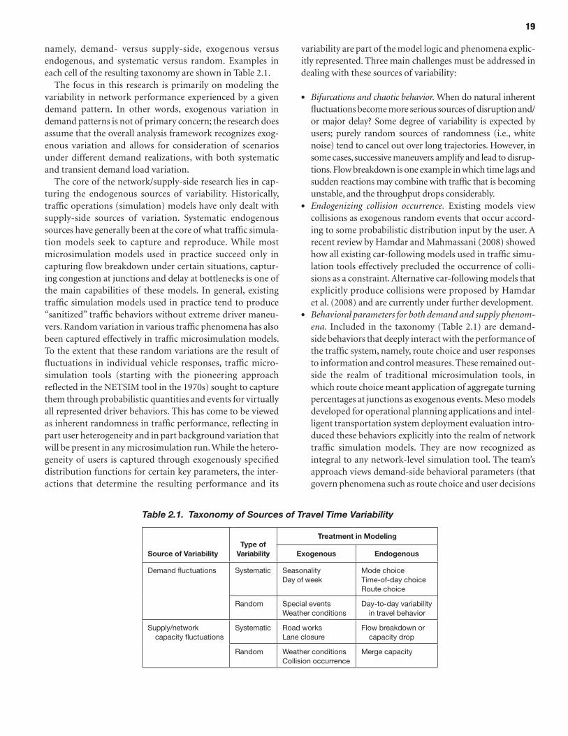
19
namely, demand- versus supply-side, exogenous versus endogenous, and systematic versus random. Examples in each cell of the resulting taxonomy are shown in Table 2.1.
The focus in this research is primarily on modeling the variability in network performance experienced by a given demand pattern. In other words, exogenous variation in demand patterns is not of primary concern; the research does assume that the overall analysis framework recognizes exog-enous variation and allows for consideration of scenarios under different demand realizations, with both systematic and transient demand load variation.
The core of the network/supply-side research lies in cap-turing the endogenous sources of variability. Historically, traffic operations (simulation) models have only dealt with supply-side sources of variation. Systematic endogenous sources have generally been at the core of what traffic simula-tion models seek to capture and reproduce. While most microsimulation models used in practice succeed only in capturing flow breakdown under certain situations, captur-ing congestion at junctions and delay at bottlenecks is one of the main capabilities of these models. In general, existing traffic simulation models used in practice tend to produce “sanitized” traffic behaviors without extreme driver maneu-vers. Random variation in various traffic phenomena has also been captured effectively in traffic microsimulation models. To the extent that these random variations are the result of fluctuations in individual vehicle responses, traffic micro-simulation tools (starting with the pioneering approach reflected in the NETSIM tool in the 1970s) sought to capture them through probabilistic quantities and events for virtually all represented driver behaviors. This has come to be viewed as inherent randomness in traffic performance, reflecting in part user heterogeneity and in part background variation that will be present in any microsimulation run. While the hetero-geneity of users is captured through exogenously specified distribution functions for certain key parameters, the inter-actions that determine the resulting performance and its
variability are part of the model logic and phenomena explic-itly represented. Three main challenges must be addressed in dealing with these sources of variability:
• Bifurcations and chaotic behavior. When do natural inherent fluctuations become more serious sources of disruption and/or major delay? Some degree of variability is expected by users; purely random sources of randomness (i.e., white noise) tend to cancel out over long trajectories. However, in some cases, successive maneuvers amplify and lead to disrup-tions. Flow breakdown is one example in which time lags and sudden reactions may combine with traffic that is becoming unstable, and the throughput drops considerably.
• Endogenizing collision occurrence. Existing models view collisions as exogenous random events that occur accord-ing to some probabilistic distribution input by the user. A recent review by Hamdar and Mahmassani (2008) showed how all existing car-following models used in traffic simu-lation tools effectively precluded the occurrence of colli-sions as a constraint. Alternative car-following models that explicitly produce collisions were proposed by Hamdar et al. (2008) and are currently under further development.
• Behavioral parameters for both demand and supply phenom-ena. Included in the taxonomy (Table 2.1) are demand-side behaviors that deeply interact with the performance of the traffic system, namely, route choice and user responses to information and control measures. These remained out-side the realm of traditional microsimulation tools, in which route choice meant application of aggregate turning percentages at junctions as exogenous events. Meso models developed for operational planning applications and intel-ligent transportation system deployment evaluation intro-duced these behaviors explicitly into the realm of network traffic simulation models. They are now recognized as integral to any network-level simulation tool. The team’s approach views demand-side behavioral parameters (that govern phenomena such as route choice and user decisions
Table 2.1. Taxonomy of Sources of Travel Time Variability
Source of Variabilitytype of
Variability
treatment in Modeling
exogenous endogenous
demand fluctuations Systematic Seasonalityday of week
Mode choiceTime-of-day choiceRoute choice
Random Special eventsweather conditions
day-to-day variability in travel behavior
Supply/network capacity fluctuations
Systematic Road workslane closure
Flow breakdown or capacity drop
Random weather conditionscollision occurrence
Merge capacity
20
in response to information) as part of the range of behav-ioral parameters that determine supply-side relations (such as gap acceptance and lane changing in micro- simulation models). These parameters can be viewed as randomly distributed across the population of drivers in a given application that can be calibrated and specified externally, though they play a key role in determining var-ious aspects of network performance through the rules included in the simulation logic.
The functional requirements presented in Chapter 4 are intended to identify phenomena and behaviors that account for the observed variability in network traffic performance and to determine the most effective approach for modeling these phenomena at both microscopic and mesoscopic levels. As noted, for reliability analysis purposes, the framework uni-fies all particle-based simulation approaches so long as they produce vehicle trajectories. The general approach to model-ing these phenomena is to incorporate as much as possible, and as may be supported by existing or in-progress theories and behavioral models, the causal or systematic determinants of variability; the remaining inherent variation is then added to the representation through suitably calibrated probabilistic mechanisms. To increase the framework’s usefulness and responsiveness to various reliability-improving measures, the team’s philosophy is to push as much as possible the portion of the total variation from the unexplained (noise) side of the equation to the systematic observable side. This approach can be implemented for both micro- and mesosimulation levels, both of which are addressed in this project.
Notwithstanding the desire for explanation, the portion of variability that must be viewed as inherent, or random, is likely to remain substantial. This has important implications for how the models are used to produce reliability estimates, and how these measures are interpreted and in turn used operationally.
Approaches to Incorporating travel time Variability into Network Simulation tools
While significant progress has been made in understanding how different travel time reliability measures can affect such dimensions of travel demand as time-of-day (trip departure time) choice and route choice, the so-called supply-side of reliability that consists of network simulation of travel time variability measures remains largely an unexplored area. A significant breakthrough is needed to create a consistent methodology and computationally efficient network simula-tion tool that can incorporate distributed travel times. Several principally different ways can be outlined, and while it is too early to decide which of them is the most promising in all respects, some pros and cons are becoming clear. In
particular, the following main dimensions and characteristics can be identified:
• An analytical approach in which travel time is represented by a random variable (“implicit”) can be contrasted to an approach in which multiple simulation runs are imple-mented (“explicit”). An analytical approach has such advantages as closer relation to theoretical equilibrium formulations. It is tempting to tackle this issue as an exten-sion of the stochastic user equilibrium (SUE) model, though there is a principal difference between accounting for mean of the random travel time that is additive-by-link and any reliability measure. Additionally, a single simula-tion run (though with some implications for analytical complexity) seems more efficient computationally than a multiple-run strategy. Explicit multiple simulations do not directly correspond to any existing equilibrium theory. However, from a practical as well as behavioral perspective, this analytical approach is quite appealing. As shown below, this approach allows for a natural incorporation of such phenomena as special events (on the demand side) as well as flow breakdowns and incidents (on the supply side). An approach that assumes analytical integration with the demand model (assuming that some demand-supply equi-librium can be formulated, existence and uniqueness of the solution can be proved, and practical methods for finding this solution can be developed) can be contrasted to a loose coupling with the demand model by means of iterative application with feedback [referred to as a shell approach in Institute for Transportation Studies (2008)]. While the analytical integration approach has an obvious advantage, it currently looks unrealistic to achieve because of the complexity and frequent nonconvexity of both network-related cost and demand functions. Additional argument in favor of the loose coupling is that any individual micro-simulation, by introducing discreteness, inevitably devi-ates from the perfect analytical equilibrium that is based on continuous traffic flows and demand variables.
• An approach in which the route choice is assumed to be affected by reliability (i.e., is inherently probabilistic) can be contrasted to a simpler approach in which route choice is assumed to be made deterministically based on the per-fect knowledge of the traffic conditions for each particular trip (by using advance information system, for example). In both cases, the route choice model can be either deter-ministic or probabilistic, reflecting the limited knowledge of the modeler. Accounting for reliability in the route choice, combined with a consistent generation of travel time reliability at the link and O–D-path levels, represents a complicated problem for which an effective and efficient solution has not yet been proposed. Route choice based on average travel times is a simpler solution that can be natu-rally combined with the explicit multiple-run approach
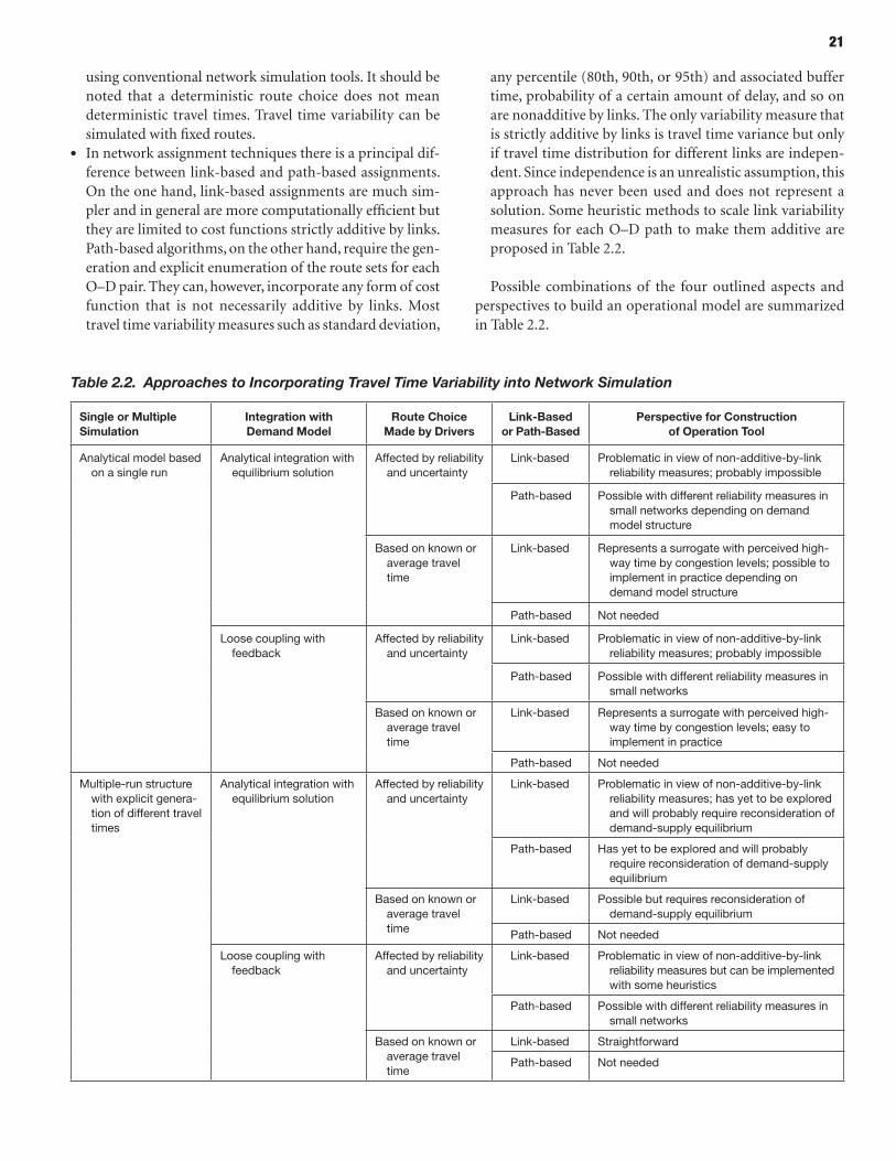
21
using conventional network simulation tools. It should be noted that a deterministic route choice does not mean deterministic travel times. Travel time variability can be simulated with fixed routes.
• In network assignment techniques there is a principal dif-ference between link-based and path-based assignments. On the one hand, link-based assignments are much sim-pler and in general are more computationally efficient but they are limited to cost functions strictly additive by links. Path-based algorithms, on the other hand, require the gen-eration and explicit enumeration of the route sets for each O–D pair. They can, however, incorporate any form of cost function that is not necessarily additive by links. Most travel time variability measures such as standard deviation,
any percentile (80th, 90th, or 95th) and associated buffer time, probability of a certain amount of delay, and so on are nonadditive by links. The only variability measure that is strictly additive by links is travel time variance but only if travel time distribution for different links are indepen-dent. Since independence is an unrealistic assumption, this approach has never been used and does not represent a solution. Some heuristic methods to scale link variability measures for each O–D path to make them additive are proposed in Table 2.2.
Possible combinations of the four outlined aspects and perspectives to build an operational model are summarized in Table 2.2.
Table 2.2. Approaches to Incorporating Travel Time Variability into Network Simulation
Single or Multiple Simulation
Integration with Demand Model
Route Choice Made by Drivers
Link-Based or path-Based
perspective for Construction of operation tool
Analytical model based on a single run
Analytical integration with equilibrium solution
Affected by reliability and uncertainty
link-based Problematic in view of non-additive-by-link reliability measures; probably impossible
Path-based Possible with different reliability measures in small networks depending on demand model structure
Based on known or average travel time
link-based Represents a surrogate with perceived high-way time by congestion levels; possible to implement in practice depending on demand model structure
Path-based Not needed
loose coupling with feedback
Affected by reliability and uncertainty
link-based Problematic in view of non-additive-by-link reliability measures; probably impossible
Path-based Possible with different reliability measures in small networks
Based on known or average travel time
link-based Represents a surrogate with perceived high-way time by congestion levels; easy to implement in practice
Path-based Not needed
Multiple-run structure with explicit genera-tion of different travel times
Analytical integration with equilibrium solution
Affected by reliability and uncertainty
link-based Problematic in view of non-additive-by-link reliability measures; has yet to be explored and will probably require reconsideration of demand-supply equilibrium
Path-based has yet to be explored and will probably require reconsideration of demand-supply equilibrium
Based on known or average travel time
link-based Possible but requires reconsideration of demand-supply equilibrium
Path-based Not needed
loose coupling with feedback
Affected by reliability and uncertainty
link-based Problematic in view of non-additive-by-link reliability measures but can be implemented with some heuristics
Path-based Possible with different reliability measures in small networks
Based on known or average travel time
link-based Straightforward
Path-based Not needed
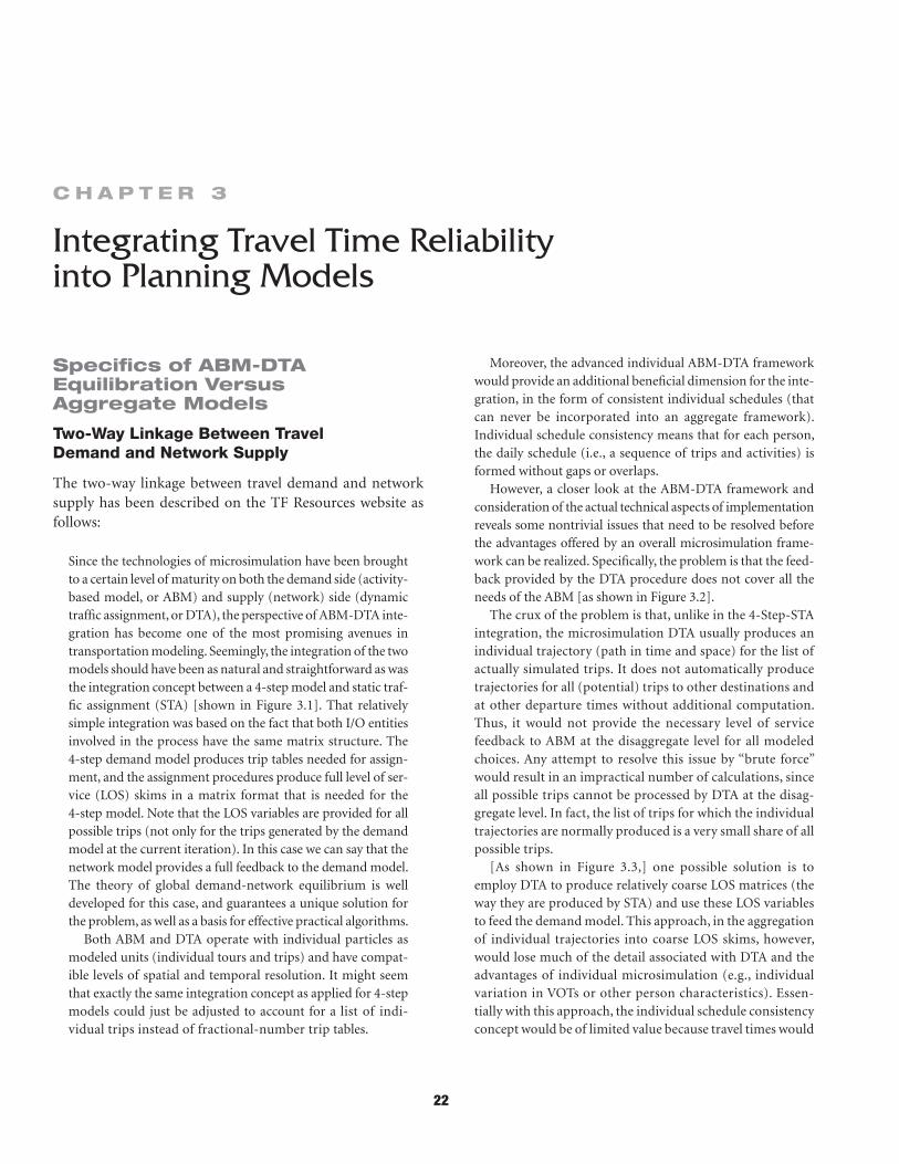
22
Specifics of ABM-dtA equilibration Versus Aggregate Models
Two-Way Linkage Between Travel Demand and Network Supply
The two-way linkage between travel demand and network supply has been described on the TF Resources website as follows:
Since the technologies of microsimulation have been brought to a certain level of maturity on both the demand side (activity-based model, or ABM) and supply (network) side (dynamic traffic assignment, or DTA), the perspective of ABM-DTA inte-gration has become one of the most promising avenues in transportation modeling. Seemingly, the integration of the two models should have been as natural and straightforward as was the integration concept between a 4-step model and static traf-fic assignment (STA) [shown in Figure 3.1]. That relatively simple integration was based on the fact that both I/O entities involved in the process have the same matrix structure. The 4-step demand model produces trip tables needed for assign-ment, and the assignment procedures produce full level of ser-vice (LOS) skims in a matrix format that is needed for the 4-step model. Note that the LOS variables are provided for all possible trips (not only for the trips generated by the demand model at the current iteration). In this case we can say that the network model provides a full feedback to the demand model. The theory of global demand-network equilibrium is well developed for this case, and guarantees a unique solution for the problem, as well as a basis for effective practical algorithms.
Both ABM and DTA operate with individual particles as modeled units (individual tours and trips) and have compat-ible levels of spatial and temporal resolution. It might seem that exactly the same integration concept as applied for 4-step models could just be adjusted to account for a list of indi-vidual trips instead of fractional-number trip tables.
Moreover, the advanced individual ABM-DTA framework would provide an additional beneficial dimension for the inte-gration, in the form of consistent individual schedules (that can never be incorporated into an aggregate framework). Individual schedule consistency means that for each person, the daily schedule (i.e., a sequence of trips and activities) is formed without gaps or overlaps.
However, a closer look at the ABM-DTA framework and consideration of the actual technical aspects of implementation reveals some nontrivial issues that need to be resolved before the advantages offered by an overall microsimulation frame-work can be realized. Specifically, the problem is that the feed-back provided by the DTA procedure does not cover all the needs of the ABM [as shown in Figure 3.2].
The crux of the problem is that, unlike in the 4-Step-STA integration, the microsimulation DTA usually produces an individual trajectory (path in time and space) for the list of actually simulated trips. It does not automatically produce trajectories for all (potential) trips to other destinations and at other departure times without additional computation. Thus, it would not provide the necessary level of service feedback to ABM at the disaggregate level for all modeled choices. Any attempt to resolve this issue by “brute force” would result in an impractical number of calculations, since all possible trips cannot be processed by DTA at the disag-gregate level. In fact, the list of trips for which the individual trajectories are normally produced is a very small share of all possible trips.
[As shown in Figure 3.3,] one possible solution is to employ DTA to produce relatively coarse LOS matrices (the way they are produced by STA) and use these LOS variables to feed the demand model. This approach, in the aggregation of individual trajectories into coarse LOS skims, however, would lose much of the detail associated with DTA and the advantages of individual microsimulation (e.g., individual variation in VOTs or other person characteristics). Essen-tially with this approach, the individual schedule consistency concept would be of limited value because travel times would
C h A p t e r 3
Integrating Travel Time Reliability into Planning Models
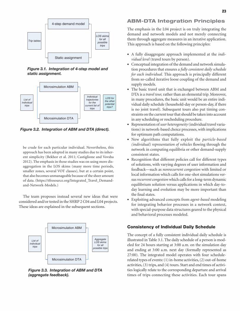
23
ABM-dtA Integration principles
The emphasis in the L04 project is on truly integrating the demand and network models and not merely connecting them through aggregate measures in an iterative application. This approach is based on the following principles:
• A fully disaggregate approach implemented at the indi-vidual level (travel tours by person).
• Conceptual integration of the demand and network simula-tion procedures that ensures a fully consistent daily schedule for each individual. This approach is principally different from so-called iterative loose coupling of the demand and supply models.
• The basic travel unit that is exchanged between ABM and DTA is a travel tour, rather than an elemental trip. Moreover, in many procedures, the basic unit would be an entire indi-vidual daily schedule (household-day or person-day, if there is no joint travel). Subsequent tours also put timing con-straints on the current tour that should be taken into account in any scheduling or rescheduling procedure.
• Representation of user heterogeneity (individual travel varia-tions) in network-based choice processes, with implications for optimum path computations.
• New algorithms that fully exploit the particle-based (individual) representation of vehicles flowing through the network in computing equilibria or other demand-supply consistent states.
• Recognition that different policies call for different types of solutions, with varying degrees of user information and feedback—such as nonrecurrent congestion with limited or local information which calls for one-shot simulations ver-sus recurrent congestion which calls for a long-term dynamic equilibrium solution versus applications in which day-to-day learning and evolution may be more important than the final states.
• Exploiting advanced concepts from agent-based modeling for integrating behavior processes in a network context, with special-purpose data structures geared to the physical and behavioral processes modeled.
Consistency of Individual Daily Schedule
The concept of a fully consistent individual daily schedule is illustrated in Table 3.1. The daily schedule of a person is mod-eled for 24 hours starting at 3:00 a.m. on the simulation day and ending at 3:00 a.m. next day (formally represented as 27:00). The integrated model operates with four schedule-related types of events: (1) in-home activities, (2) out-of-home activities, (3) trips, and (4) tours. Start and end times of activi-ties logically relate to the corresponding departure and arrival times of trips connecting these activities. Each tour spans
Figure 3.1. Integration of 4-step model and static assignment.
4-step demand model
Static assignment
Trip tables
LOS skimsfor all
possibletrips
Figure 3.2. Integration of ABM and DTA (direct).
Microsimulation ABM
Microsimulation DTA
List ofindividual
trips
Individualtrajectories
for thecurrent list of
trips
LOS forthe otherpotential
trips?
Figure 3.3. Integration of ABM and DTA (aggregate feedback).
Microsimulation ABM
Microsimulation DTA
List ofindividual
trips
AggregateLOS skims
for allpossible trips
be crude for each particular individual. Nevertheless, this approach has been adopted in many studies due to its inher-ent simplicity (Bekhor et al. 2011; Castiglione and Vovsha 2012). The emphasis in those studies was on using more dis-aggregation in the LOS skims (many more time periods, smaller zones, several VOT classes), but at a certain point, that also becomes unmanageable because of the sheer amount of data. (https://tfresource.org/Integrated_Travel_Demand-and-Network-Models.)
The team proposes instead several new ideas that were considered and/or tested in the SHRP 2 C04 and L04 projects. These ideas are explained in the subsequent sections.
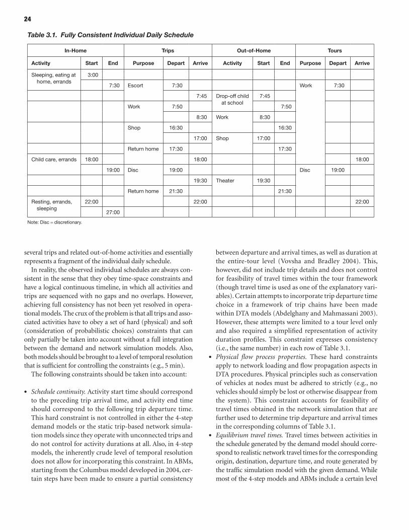
24
several trips and related out-of-home activities and essentially represents a fragment of the individual daily schedule.
In reality, the observed individual schedules are always con-sistent in the sense that they obey time-space constraints and have a logical continuous timeline, in which all activities and trips are sequenced with no gaps and no overlaps. However, achieving full consistency has not been yet resolved in opera-tional models. The crux of the problem is that all trips and asso-ciated activities have to obey a set of hard (physical) and soft (consideration of probabilistic choices) constraints that can only partially be taken into account without a full integration between the demand and network simulation models. Also, both models should be brought to a level of temporal resolution that is sufficient for controlling the constraints (e.g., 5 min).
The following constraints should be taken into account:
• Schedule continuity. Activity start time should correspond to the preceding trip arrival time, and activity end time should correspond to the following trip departure time. This hard constraint is not controlled in either the 4-step demand models or the static trip-based network simula-tion models since they operate with unconnected trips and do not control for activity durations at all. Also, in 4-step models, the inherently crude level of temporal resolution does not allow for incorporating this constraint. In ABMs, starting from the Columbus model developed in 2004, cer-tain steps have been made to ensure a partial consistency
between departure and arrival times, as well as duration at the entire-tour level (Vovsha and Bradley 2004). This, however, did not include trip details and does not control for feasibility of travel times within the tour framework (though travel time is used as one of the explanatory vari-ables). Certain attempts to incorporate trip departure time choice in a framework of trip chains have been made within DTA models (Abdelghany and Mahmassani 2003). However, these attempts were limited to a tour level only and also required a simplified representation of activity duration profiles. This constraint expresses consistency (i.e., the same number) in each row of Table 3.1.
• Physical flow process properties. These hard constraints apply to network loading and flow propagation aspects in DTA procedures. Physical principles such as conservation of vehicles at nodes must be adhered to strictly (e.g., no vehicles should simply be lost or otherwise disappear from the system). This constraint accounts for feasibility of travel times obtained in the network simulation that are further used to determine trip departure and arrival times in the corresponding columns of Table 3.1.
• Equilibrium travel times. Travel times between activities in the schedule generated by the demand model should corre-spond to realistic network travel times for the corresponding origin, destination, departure time, and route generated by the traffic simulation model with the given demand. While most of the 4-step models and ABMs include a certain level
Table 3.1. Fully Consistent Individual Daily Schedule
In-Home trips out-of-Home tours
Activity Start end purpose Depart Arrive Activity Start end purpose Depart Arrive
Sleeping, eating at home, errands
3:00
7:30 Escort 7:30 work 7:30
7:45 drop-off child at school
7:45
work 7:50 7:50
8:30 work 8:30
Shop 16:30 16:30
17:00 Shop 17:00
Return home 17:30 17:30
child care, errands 18:00 18:00 18:00
19:00 disc 19:00 disc 19:00
19:30 Theater 19:30
Return home 21:30 21:30
Resting, errands, sleeping
22:00 22:00 22:00
27:00
Note: disc = discretionary.
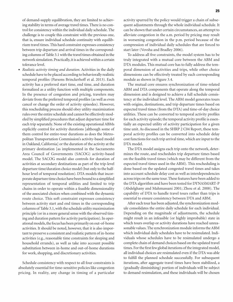
25
of demand-supply equilibration, they are limited to achiev-ing stability in terms of average travel times. There is no con-trol for consistency within the individual daily schedule. The challenge is to couple this constraint with the previous one, that is, ensure individual schedule continuity with equilib-rium travel times. This hard constraint expresses consistency between trip departure and arrival times in the correspond-ing columns of Table 3.1 with the travel times obtained in the network simulation. Practically, it is achieved within a certain tolerance level.
• Realistic activity timing and duration. Activities in the daily schedule have to be placed according to behaviorally realistic temporal profiles (Parsons Brinckerhoff et al. 2013). Each activity has a preferred start time, end time, and duration formalized as a utility function with multiple components. In the presence of congestion and pricing, travelers may deviate from the preferred temporal profiles (as well as even cancel or change the order of activity episodes). However, this rescheduling process should obey utility-maximization rules over the entire schedule and cannot be effectively mod-eled by simplified procedures that adjust departure time for each trip separately. None of the existing operational ABMs explicitly control for activity durations [although some of them control for entire-tour durations as does the Metro-politan Transportation Commission’s activity-based model in Oakland, California] or the duration of the activity at the primary destination [as implemented in the Sacramento Area Council of Governments (SACOG) activity-based model. The SACOG model also controls for duration of activities at secondary destinations as part of the trip-level departure time/duration choice model (but only to the half-hour level of temporal resolution). DTA models that incor-porate departure time choice have been bound to a simplified representation of temporal utilities and limited to trip chains in order to operate within a feasible dimensionality of the associated choices when combined with the dynamic route choice. This soft constraint expresses consistency between activity start and end times in the corresponding columns of Table 3.1, with the schedule utility maximization principle (or in a more general sense with the observed tim-ing and duration pattern for activity participation). In oper-ational models, the focus has been primarily on out-of-home activities. It should be noted, however, that it is also impor-tant to preserve a consistent and realistic pattern of in-home activities (e.g., reasonable time constraints for sleeping and household errands), as well as take into account possible substitution between in-home and out-of-home durations for work, shopping, and discretionary activities.
Schedule consistency with respect to all four constraints is absolutely essential for time-sensitive policies like congestion pricing. In reality, any change in timing of a particular
activity spurred by the policy would trigger a chain of subse-quent adjustments through the whole individual schedule. It can be shown that under certain circumstances, an attempt to alleviate congestion in the a.m. period by pricing may result in worsening congestion in the p.m. period because of the compression of individual daily schedules that are forced to start later (Vovsha and Bradley 2006).
To address all five constraints, the model system has to be truly integrated with a mutual core between the ABM and DTA modules. This mutual core has to fully address the tem-poral dimension of activities and trips, while other choice dimensions can be effectively treated by each corresponding module as shown in Figure 3.4.
The mutual core ensures synchronization of time-related ABM and DTA components that operate along the temporal dimension and is designed to achieve a full schedule consis-tency at the individual level. The ABM model generates tours with origins, destinations, and trip departure times based on expected travel times (from the DTA) and time-of-day choice utilities. These can be converted to temporal activity profiles for each activity episode; the temporal activity profile is essen-tially an expected utility of activity participation for a given time unit. As discussed in the SHRP 2 C04 Report, these tem-poral activity profiles can be converted into schedule delay cost functions for each trip arrival time, which are input to the DTA model.
The DTA model assigns each trip onto the network, deter-mines the route, and reschedules trip departure times based on the feasible travel times (which may be different from the expected travel times used in the ABM). This rescheduling is done based on the updated congested travel times and takes into account schedule delay cost as well as interdependencies across trips on the same tour. These features have been added to the DTA algorithm and have been tested for DYNASMART-P (Abdelghany and Mahmassani 2001; Zhou et al. 2008). The capability of DTA to handle travel tours rather than trips is essential to ensure consistency between DTA and ABM.
After each tour has been adjusted, the synchronization mod-ule consolidates the entire daily schedule for each individual. Depending on the magnitude of adjustments, the schedule might result in an infeasible (or highly improbable) state in which tours overlap or activity durations have reached unrea-sonable values. The synchronization module informs the ABM which individual daily schedules have to be resimulated. Indi-viduals whose schedules have to be resimulated undergo a complete chain of demand choices based on the updated travel times. For the first few global iterations of the integrated model, all individual choices are resimulated even if the DTA was able to fulfill the planned schedule successfully. For subsequent iterations, after aggregate travel times have been stabilized, a (gradually diminishing) portion of individuals will be subject to demand resimulation, and these individuals will be chosen
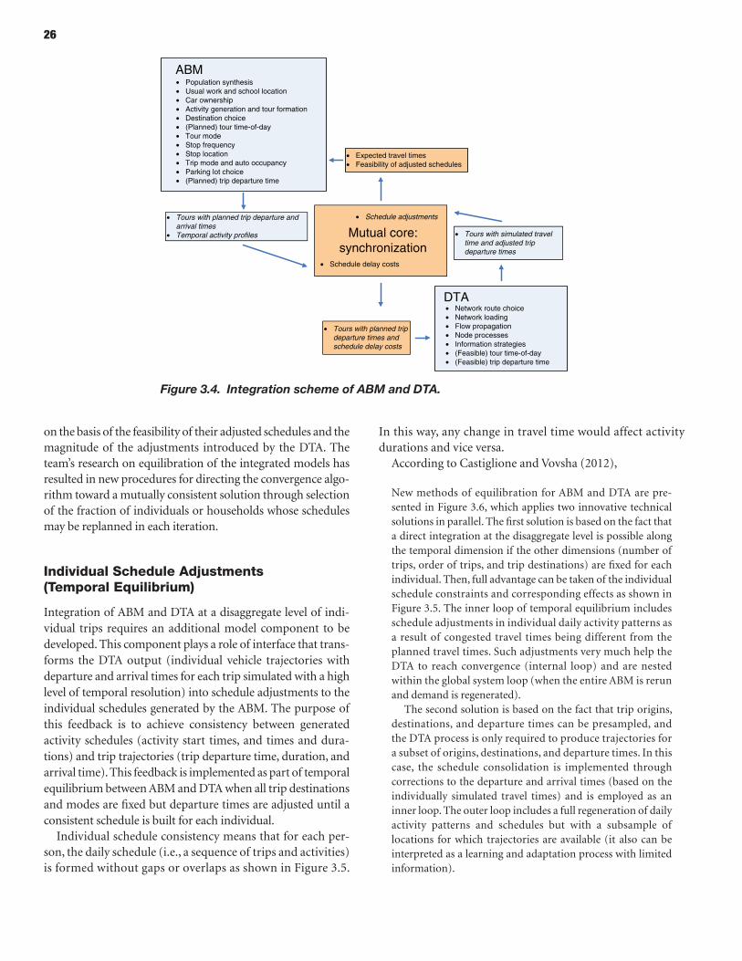
26
on the basis of the feasibility of their adjusted schedules and the magnitude of the adjustments introduced by the DTA. The team’s research on equilibration of the integrated models has resulted in new procedures for directing the convergence algo-rithm toward a mutually consistent solution through selection of the fraction of individuals or households whose schedules may be replanned in each iteration.
Individual Schedule Adjustments (Temporal Equilibrium)
Integration of ABM and DTA at a disaggregate level of indi-vidual trips requires an additional model component to be developed. This component plays a role of interface that trans-forms the DTA output (individual vehicle trajectories with departure and arrival times for each trip simulated with a high level of temporal resolution) into schedule adjustments to the individual schedules generated by the ABM. The purpose of this feedback is to achieve consistency between generated activity schedules (activity start times, and times and dura-tions) and trip trajectories (trip departure time, duration, and arrival time). This feedback is implemented as part of temporal equilibrium between ABM and DTA when all trip destinations and modes are fixed but departure times are adjusted until a consistent schedule is built for each individual.
Individual schedule consistency means that for each per-son, the daily schedule (i.e., a sequence of trips and activities) is formed without gaps or overlaps as shown in Figure 3.5.
In this way, any change in travel time would affect activity durations and vice versa.
According to Castiglione and Vovsha (2012),
New methods of equilibration for ABM and DTA are pre-sented in Figure 3.6, which applies two innovative technical solutions in parallel. The first solution is based on the fact that a direct integration at the disaggregate level is possible along the temporal dimension if the other dimensions (number of trips, order of trips, and trip destinations) are fixed for each individual. Then, full advantage can be taken of the individual schedule constraints and corresponding effects as shown in Figure 3.5. The inner loop of temporal equilibrium includes schedule adjustments in individual daily activity patterns as a result of congested travel times being different from the planned travel times. Such adjustments very much help the DTA to reach convergence (internal loop) and are nested within the global system loop (when the entire ABM is rerun and demand is regenerated).
The second solution is based on the fact that trip origins, destinations, and departure times can be presampled, and the DTA process is only required to produce trajectories for a subset of origins, destinations, and departure times. In this case, the schedule consolidation is implemented through corrections to the departure and arrival times (based on the individually simulated travel times) and is employed as an inner loop. The outer loop includes a full regeneration of daily activity patterns and schedules but with a subsample of locations for which trajectories are available (it also can be interpreted as a learning and adaptation process with limited information).
Figure 3.4. Integration scheme of ABM and DTA.
ABM
DTA
Population synthesisUsual work and school locationCar ownershipActivity generation and tour formationDestination choice(Planned) tour time-of-dayTour modeStop frequencyStop locationTrip mode and auto occupancyParking lot choice(Planned
•••••••••••• ) trip departure time
Network route choiceNetwork loadingFlow propagationNode processesInformation strategies(Feasible) tour time-of-day(Feasible
••••••• ) trip departure time
Mutual core:synchronization
Schedule delay costs
Schedule
•
• adjustmentsTours with planned trip departure andarrival timesTemporal
•
• activity profiles
Expected travel timesFeasibilit
•• y of adjusted schedules
Tours• with planned tripdeparture times andschedule delay costs
Tours• with simulated traveltime and adjusted tripdeparture times
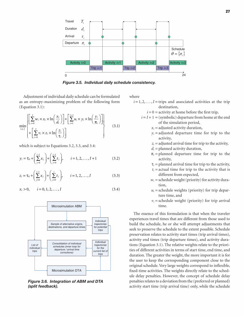
27
Adjustment of individual daily schedule can be formulated as an entropy-maximizing problem of the following form (Equation 3.1):
min
ln ln
ln
(3.1)0 1
1
0
w xx
du y
y
v zzx
i
i
I
ii
ii i
i
ii
I
i ii
ii
Ii
∑ ∑
∑
× ×
+ × ×π
+ × ×τ
{ }
= =
+
=
which is subject to Equations 3.2, 3.3, and 3.4:
, 1, 2, . . . , 1 (3.2)0
0
1
0
1
y x t i Ii j
j
i
j
j
i
∑ ∑= τ +
+
= +=
−
=
−
, 1, 2, . . . , (3.3)0
0
1
0
z x t i Ii j
j
i
j
j
i
∑ ∑= τ +
+
==
−
=
0, 0, 1, 2, . . . , (3.4)x i Ii > =
wherei = 1, 2, . . . , I = trips and associated activities at the trip
destination, i = 0 = activity at home before the first trip, i = I + 1 = (symbolic) departure from home at the end
of the simulation period, xi = adjusted activity duration, yi = adjusted departure time for trip to the
activity, zi = adjusted arrival time for trip to the activity, di = planned activity duration, pi = planned departure time for trip to the
activity, ti = planned arrival time for trip to the activity, ti = actual time for trip to the activity that is
different from expected, wi = schedule weight (priority) for activity dura-
tion, ui = schedule weights (priority) for trip depar-
ture time, and vi = schedule weight (priority) for trip arrival
time.
The essence of this formulation is that when the traveler experiences travel times that are different from those used to build the schedule, he or she will attempt adjustments that seek to preserve the schedule to the extent possible. Schedule preservation relates to activity start times (trip arrival times), activity end times (trip departure times), and activity dura-tions (Equation 3.1). The relative weights relate to the priori-ties of different activities in terms of start time, end time, and duration. The greater the weight, the more important it is for the user to keep the corresponding component close to the original schedule. Very large weights correspond to inflexible, fixed-time activities. The weights directly relate to the sched-ule delay penalties. However, the concept of schedule delay penalties relates to a deviation from the (preferred or planned) activity start time (trip arrival time) only, while the schedule
Figure 3.5. Individual daily schedule consistency.
0 24
Activity i=0 Activity i=1 Activity i=2
Trip i=1 Trip i=2 Trip i=3
Activity i=3
Departure
Arrival
Duration
Travel
id
iT
i
i
Schedule
i
Figure 3.6. Integration of ABM and DTA (split feedback).
Microsimulation ABM
Microsimulation DTA
List ofindividual
trips
Individualtrajectories
for thecurrent list of
trips
Consolidation of individualschedules (inner loop fordeparture / arrival time
corrections)
Sample of alternative origins,destinations, and departure times
Individualtrajectoriesfor potential
trips
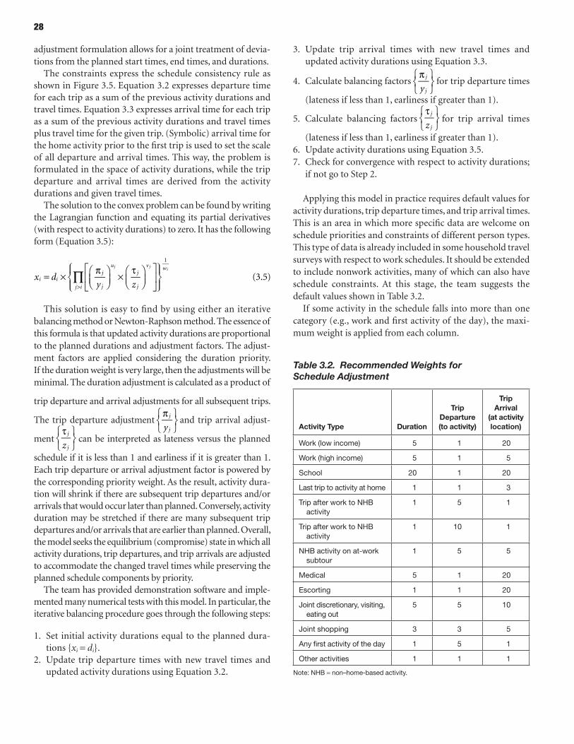
28
adjustment formulation allows for a joint treatment of devia-tions from the planned start times, end times, and durations.
The constraints express the schedule consistency rule as shown in Figure 3.5. Equation 3.2 expresses departure time for each trip as a sum of the previous activity durations and travel times. Equation 3.3 expresses arrival time for each trip as a sum of the previous activity durations and travel times plus travel time for the given trip. (Symbolic) arrival time for the home activity prior to the first trip is used to set the scale of all departure and arrival times. This way, the problem is formulated in the space of activity durations, while the trip departure and arrival times are derived from the activity durations and given travel times.
The solution to the convex problem can be found by writing the Lagrangian function and equating its partial derivatives (with respect to activity durations) to zero. It has the following form (Equation 3.5):
(3.5)
1
∏= × π
× τ
>x d
y zi i
j
j
uj
j
v
j i
wj ji
This solution is easy to find by using either an iterative balancing method or Newton-Raphson method. The essence of this formula is that updated activity durations are proportional to the planned durations and adjustment factors. The adjust-ment factors are applied considering the duration priority. If the duration weight is very large, then the adjustments will be minimal. The duration adjustment is calculated as a product of
trip departure and arrival adjustments for all subsequent trips.
The trip departure adjustmenty
j
j
π
and trip arrival adjust-
mentz
j
j
τ
can be interpreted as lateness versus the planned
schedule if it is less than 1 and earliness if it is greater than 1. Each trip departure or arrival adjustment factor is powered by the corresponding priority weight. As the result, activity dura-tion will shrink if there are subsequent trip departures and/or arrivals that would occur later than planned. Conversely, activity duration may be stretched if there are many subsequent trip departures and/or arrivals that are earlier than planned. Overall, the model seeks the equilibrium (compromise) state in which all activity durations, trip departures, and trip arrivals are adjusted to accommodate the changed travel times while preserving the planned schedule components by priority.
The team has provided demonstration software and imple-mented many numerical tests with this model. In particular, the iterative balancing procedure goes through the following steps:
1. Set initial activity durations equal to the planned dura-tions {xi = di}.
2. Update trip departure times with new travel times and updated activity durations using Equation 3.2.
3. Update trip arrival times with new travel times and updated activity durations using Equation 3.3.
4. Calculate balancing factorsy
j
j
π
for trip departure times
(lateness if less than 1, earliness if greater than 1).
5. Calculate balancing factorsz
j
j
τ
for trip arrival times
(lateness if less than 1, earliness if greater than 1).6. Update activity durations using Equation 3.5.7. Check for convergence with respect to activity durations;
if not go to Step 2.
Applying this model in practice requires default values for activity durations, trip departure times, and trip arrival times. This is an area in which more specific data are welcome on schedule priorities and constraints of different person types. This type of data is already included in some household travel surveys with respect to work schedules. It should be extended to include nonwork activities, many of which can also have schedule constraints. At this stage, the team suggests the default values shown in Table 3.2.
If some activity in the schedule falls into more than one category (e.g., work and first activity of the day), the maxi-mum weight is applied from each column.
Table 3.2. Recommended Weights for Schedule Adjustment
Activity type Duration
trip Departure (to activity)
trip Arrival
(at activity location)
work (low income) 5 1 20
work (high income) 5 1 5
School 20 1 20
last trip to activity at home 1 1 3
Trip after work to NhB activity
1 5 1
Trip after work to NhB activity
1 10 1
NhB activity on at-work subtour
1 5 5
Medical 5 1 20
Escorting 1 1 20
Joint discretionary, visiting, eating out
5 5 10
Joint shopping 3 3 5
Any first activity of the day 1 5 1
other activities 1 1 1
Note: NhB = non–home-based activity.
29
Approaches to Quantifying reliability and Its Impacts
Construction of User-Centric Network Reliability Measures
In summary, the following two important aspects of the problem need to be taken into account when the user’s per-spective on reliability (and performance in general) is com-pared with the highway operations perspective:
• The user perspective can be different and include many per-ceived components and weights compared with the physical measures of average travel time and reliability. The measure that looks the best and most statistically significant from the highway operations perspective might not be best when model-ing user responses. For example, the 95th percentile of travel time is favored in highway operations since it singles out the most critical cases of nonrecurrent congestion (mostly asso-ciated with traffic collisions, road works, special events, and extreme weather); see Cambridge Systematics, Inc. (2005) and Cambridge Systematics, Inc. et al. (2013). The current experience with models of individual behavior in the route choice context, however, indicates that the decision-making point at which users evaluate reliability lies rather some-where between the 80th and 90th percentile, that is, mixes of recurrent and nonrecurrent congestion; see Concas and Kolpakov (2009) and Parsons Brinckerhoff et al. (2013).
• The user perspective is inherently an entire-trip perspective. Thus, the reliability measures for travel models and network simulation tools have to be synthesized at the O–D-route level, while the bulk of statistical evidence on highway operations is naturally collected at the facility/link level. This synthesis is not a trivial task, because practically all sensible reliability measures are inherently nonadditive (Institute for Trans-portation Studies 2008). This aspect is discussed in detail in the subsequent sections and constitutes one of the major challenges for the current project.
Suggested Approaches to Quantifying Reliability Impacts on Highway Users
In general, there are four possible methodological approaches to quantifying reliability either suggested in the research litera-ture or already applied in operational models:
• Indirect measure: Perceived highway time by congestion levels. This concept is based on statistical evidence that in conges-tion conditions, travelers perceive each minute with a certain weight (Small et al. 1999; Axhausen et al. 2007; Levinson et al. 2004; MRC and PB 2008). Perceived highway time is not a direct measure of reliability since only the average travel time is considered (although it is segmented by congestion levels).
It can serve, however, as a good instrumental proxy for reli-ability since the perceived weight of each minute spent in congestion is partially a consequence of associated unreli-ability. This is the simplest measure that can be readily incor-porated into both demand models and network simulation tools and equilibrated between them.
• First direct measure: Time variability (distribution) measures. This is considered the most practical direct approach and has received considerable attention in recent years. This approach assumes that several independent measurements of travel time are known that allow for forming the travel time distribution and calculation of derived measures, such as variance, standard deviation, or buffer time (Small et al. 2005; Brownstone and Small 2005; Bogers et al. 2008). One of the important technical details with respect to the genera-tion of travel time distributions is that even if the link-level time variations are known, it is a nontrivial task to synthe-size the O–D-level time distribution (reliability “skims”) because of the dependence of travel times across adjacent links due to a mutual traffic flow. This implementation chal-lenge posed by issue is specifically addressed in the course of the project. This is a more complicated measure—primarily on the network simulation side. The network model has to incorporate travel time distribution measures (like variance or standard deviation) in the route choice and also generate the O–D reliability skims. This can be achieved only by using path-based assignment algorithms since the reliability measures are (in general) not additive by links. Recommen-dations are made how an equilibrium framework with these measures could be implemented.
• Second direct measure: Schedule delay cost. This approach has been adopted in many research works on individual behavior in academia (Small 1982; Small et al. 1999). According to this concept, the direct impact of travel time unreliability is measured through cost functions (penalties expressed in monetary terms) of being late (or early) compared with the planned schedule of the activity. This approach assumes that the desired schedule is known for each person and activity in the course of the modeled period. This assumption, however, is difficult to meet in a practical model setting. This is a more sophisticated approach that is more difficult to implement. However, certain directions are outlined, including incorpo-ration of schedule delay penalties into the combined trip route and departure time cost. It was shown that under cer-tain assumptions on the shape of the earliness and lateness penalties, this approach can be reduced to the mean-variance approach (Fosgerau and Karlstrom 2007; Fosgerau 2008).
• Third direct measure: Loss of activity participation utility. This method can be thought of as a generalization of the schedule delay concept. It is assumed that each activity has a certain temporal utility profile and individuals plan their schedules to achieve maximum total utility over the modeled period
30
(e.g., the entire day), taking into account expected (average) travel times. Then, any deviation from the expected travel time due to unreliability can be associated with a loss of participation in the corresponding activity (or gain if travel time proved to be shorter) (Supernak 1992; Kitamura and Supernak 1997; Tseng and Verhoef 2008). This approach recently was adopted in several research works on DTA for-mulation integrated with activity scheduling analysis (Kim et al. 2006; Lam and Yin 2001). It was shown that under spe-cific assumptions about the shape of temporal utility profiles of two consecutive activities, the expected generalized cost function that includes travel time variation impact can be reduced to the mean-variance approach (Engelson 2011). Similar to the schedule delay concept, however, this approach suffers from the data requirements that are difficult to meet in practice. The added complexity of estimation and calibration of all temporal utility profiles for all possible activities and all person types is significant. This makes it unrealistic to adopt this approach as the main concept for the current project. This approach, however, can be considered in future research efforts. Early research indicates that this approach may be the most promising theoretical avenue for a fully integrated ABM-DTA model formulation that can eliminate the need to equilibrate two separate models. Unfortunately, these meth-ods are currently applicable only in very small networks.
A summary of the main features of the proposed approaches to quantifying reliability impacts on travel choices is presented in Table 3.3.
Some clarification is needed regarding preferred arrival time (PAT) and its relation to time-of-day (TOD) choice. Travel demand (TOD choice) models in general predict the preferred departure time (PDT) for each trip, since this is the choice dimension that is controlled by the traveler. Arrival time in general is not controlled, and a PAT is not directly generated by travel demand procedures in a conventional ABM.
If travel time is considered deterministic, PAT can always be derived from PDT by adding the travel time; thus TOD choice with deterministic travel times can be thought of as a (simplis-tic) simultaneous model for predicting PDT and PAT. How-ever, travel time reliability is ignored in this case. Also, even if times are deterministic within each time of day, as long as con-gestion causes average travel times to vary across times of day, some people may shift their travel away from their most pre-ferred time to avoid driving in congested conditions (even if it is perfectly predictable congestion).
If travel time is considered probabilistic, PAT has to be either defined exogenously (assuming fixed scheduling constraints) or generated by the demand model before modeling PDT. If we assume that PDT is optimized by the traveler, conditional on the predetermined PAT with a full knowledge of travel time distribution, this leads to a model equivalent to the mean-variance approach in terms of the form of the generalized cost function. It is also possible to assume that PDT is optimized by the user based on the PAT and mean travel time only (e.g., by subtracting mean travel time from PAT). This would mean, however, that travel time reliability is ignored at least at the TOD-choice stage. The concept of temporal activity
Table 3.3. Methods to Quantify Reliability Impacts on Travel
MethodRepresentation of
travel timeImpact on travel Choices through
Generalized Cost FunctionSpecial Features
Needed
Perceived highway time by congestion levels
Segmented by congestion levels
Travel time is weighted by congestion levels.
Mean-variance (travel time distribution measures)
Mean (or mode), variance [or Sd(T ) or buffer time]
Mean (or mode) and variance [or Sd(T ) or buffer time] are linearly included in generalized cost as loS components.
Schedule delay distribution Expected schedule delay cost over travel time distribution is linearly included in generalized cost along with the mean travel time.
Preferred arrival time (PAT) has to be defined externally or generated by the demand model.
Temporal activity profiles distribution Expected loss in activity participation over travel time distribution is linearly included in gener-alized cost along with the mean travel time.
Requirements for network simulation model with any of the methods above
Travel time characteristics above have to be generated by network simulation model.
generalized cost function above has to be incorporated into route choice.
Requirements for travel demand model with any of the methods above
generalized cost function above has to be incorporated into mode, time-of-day, destina-tion, and other choices.
Note: Sd(T) = standard deviation of travel time.
31
profiles is a way to endogenize PAT within the demand model-ing (scheduling) framework.
Incorporating reliability into demand Model
The proposed methods of quantification of reliability should be incorporated into the demand model (ABM) with respect to subchoices such as tour and trip mode choice, destination choice, and TOD choice. In the typical ABM structure, a gen-eralized cost function with the reliability terms can be directly included in the utility function for highway modes. Further on, it will have an impact on destination and TOD choice through mode choice logsums. In the same vein, it has an impact on upper-level choice models of car ownership and activity-travel patterns through accessibility measures that represent simplified destination choice logsums. The demand side of travel time reliability has been explored in detail in the recently completed SHRP 2 C04 project. The relevant model structures and techniques are described in the Task 11 Report (Stogios et al. 2014). This section presents a concise overview of each method and its applicability in an operational travel demand model.
Perceived Highway Time in Demand Model
This method is easy to implement without a significant restruc-turing of the demand model. Essentially, the generic highway travel time variable in mode choice should be replaced with segmented travel time by congestion levels with the recom-mended weights shown in Table 3.4. For each level of conges-tion, the table provides approximate volume to capacity (V/C) ratios that can be used to classify highway network links after the traffic simulation.
The weights applied have to be consistent between traffic assignment and mode choice. The table provides pivot points that can be interpolated between them linearly using V/C ratio or flow density parameter. However, perceived travel time is not a direct measure of travel time reliability. It can be used as
a surrogate when more advanced methods are not available, but it is less appealing behaviorally and is not the main focus of the current research.
Mean-Variance in Demand Model
This method is easy to implement and does not require a significant restructuring of the demand model. Essentially, it requires an inclusion of an additional reliability term in the mode choice utility for highway modes. The following form of generalized cost component in the mode utility function (Equation 3.6) can be recommended as the first step for incor-poration into operational models. There are many additional modifications and nonlinear transformations analyzed in the SHRP 2 C04 project and described in the Task 11 Report (Stogios et al. 2014).
( )= × + × + × SD (3.6)U a T b C c T
where T = mean travel time, C = travel cost, SD(T) = standard deviation of travel time, a = coefficient for travel time, b = coefficient for travel cost, c = coefficient for standard deviation of travel time, a/b = value of time (VOT), c/b = value of reliability (VOR), and c/a = reliability ratio (r = VOT/VOR).
A summary of recommended values for the parameters is presented in Table 3.5. The parameters are segmented by travel purpose, household income, car occupancy, and travel distance. More details and the actual values for all coefficients can be found in (Parsons Brinckerhoff et al. 2013).
Schedule Delay Cost in Demand Model
There are multiple estimated models with schedule delay cost, as described in the Task 11 Report (Stogios et al. 2014). The majority of them were estimated using different stated pre-ference (SP) settings in which either route or departure time served as the underlying travel choice dimension. The techni-cal details for the inclusion of this method in an operational travel demand model have not yet been fully explored. The team outlines two possible approaches that differ in how and where the schedule delay cost component is calculated; see Figure 3.7.
In both approaches, the travel demand model (its time-of-day choice or activity scheduling submodel) produces pre-ferred departure time (PDT) and preferred arrival time (PAT) for each trip based on the expected travel times (and known
Table 3.4. Recommended Highway Time Weight by Congestion Level
travel time Conditions Weight LoS V/C
Free flow 1.00 A, B under 0.5
Busy 1.05 c 0.5–0.7
light congestion 1.10 d 0.7–0.8
heavy congestion 1.20 E 0.8–1.0
Stop start 1.40 F 1.0–1.2
gridlock 1.80 F 1.2+
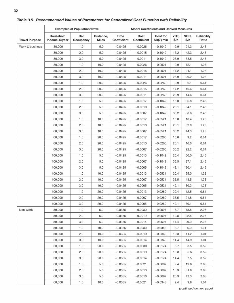
32
Table 3.5. Recommended Values of Parameters for Generalized Cost Function with Reliability
travel purpose
examples of population/travel Model Coefficients and Derived Measures
Household Income, $/year
Car occupancy
Distance, Miles
time Coefficient
Cost Coefficient
Cost for SD(T) min
Vot, $/h
VoR, $/h
Reliability Ratio
work & business 30,000 1.0 5.0 -0.0425 -0.0026 -0.1042 9.9 24.3 2.45
30,000 2.0 5.0 -0.0425 -0.0015 -0.1042 17.2 42.3 2.45
30,000 3.0 5.0 -0.0425 -0.0011 -0.1042 23.9 58.5 2.45
30,000 1.0 10.0 -0.0425 -0.0026 -0.0521 9.9 12.1 1.23
30,000 2.0 10.0 -0.0425 -0.0015 -0.0521 17.2 21.1 1.23
30,000 3.0 10.0 -0.0425 -0.0011 -0.0521 23.9 29.2 1.23
30,000 1.0 20.0 -0.0425 -0.0026 -0.0260 9.9 6.1 0.61
30,000 2.0 20.0 -0.0425 -0.0015 -0.0260 17.2 10.6 0.61
30,000 3.0 20.0 -0.0425 -0.0011 -0.0260 23.9 14.6 0.61
60,000 1.0 5.0 -0.0425 -0.0017 -0.1042 15.0 36.8 2.45
60,000 2.0 5.0 -0.0425 -0.0010 -0.1042 26.1 64.1 2.45
60,000 3.0 5.0 -0.0425 -0.0007 -0.1042 36.2 88.6 2.45
60,000 1.0 10.0 -0.0425 -0.0017 -0.0521 15.0 18.4 1.23
60,000 2.0 10.0 -0.0425 -0.0010 -0.0521 26.1 32.0 1.23
60,000 3.0 10.0 -0.0425 -0.0007 -0.0521 36.2 44.3 1.23
60,000 1.0 20.0 -0.0425 -0.0017 -0.0260 15.0 9.2 0.61
60,000 2.0 20.0 -0.0425 -0.0010 -0.0260 26.1 16.0 0.61
60,000 3.0 20.0 -0.0425 -0.0007 -0.0260 36.2 22.2 0.61
100,000 1.0 5.0 -0.0425 -0.0013 -0.1042 20.4 50.0 2.45
100,000 2.0 5.0 -0.0425 -0.0007 -0.1042 35.5 87.1 2.45
100,000 3.0 5.0 -0.0425 -0.0005 -0.1042 49.1 120.4 2.45
100,000 1.0 10.0 -0.0425 -0.0013 -0.0521 20.4 25.0 1.23
100,000 2.0 10.0 -0.0425 -0.0007 -0.0521 35.5 43.5 1.23
100,000 3.0 10.0 -0.0425 -0.0005 -0.0521 49.1 60.2 1.23
100,000 1.0 20.0 -0.0425 -0.0013 -0.0260 20.4 12.5 0.61
100,000 2.0 20.0 -0.0425 -0.0007 -0.0260 35.5 21.8 0.61
100,000 3.0 20.0 -0.0425 -0.0005 -0.0260 49.1 30.1 0.61
Non-work 30,000 1.0 5.0 -0.0335 -0.0030 -0.0697 6.7 13.8 2.08
30,000 2.0 5.0 -0.0335 -0.0019 -0.0697 10.8 22.5 2.08
30,000 3.0 5.0 -0.0335 -0.0014 -0.0697 14.4 29.9 2.08
30,000 1.0 10.0 -0.0335 -0.0030 -0.0348 6.7 6.9 1.04
30,000 2.0 10.0 -0.0335 -0.0019 -0.0348 10.8 11.2 1.04
30,000 3.0 10.0 -0.0335 -0.0014 -0.0348 14.4 14.9 1.04
30,000 1.0 20.0 -0.0335 -0.0030 -0.0174 6.7 3.5 0.52
30,000 2.0 20.0 -0.0335 -0.0019 -0.0174 10.8 5.6 0.52
30,000 3.0 20.0 -0.0335 -0.0014 -0.0174 14.4 7.5 0.52
60,000 1.0 5.0 -0.0335 -0.0021 -0.0697 9.4 19.6 2.08
60,000 2.0 5.0 -0.0335 -0.0013 -0.0697 15.3 31.8 2.08
60,000 3.0 5.0 -0.0335 -0.0010 -0.0697 20.3 42.3 2.08
60,000 1.0 10.0 -0.0335 -0.0021 -0.0348 9.4 9.8 1.04
(continued on next page)
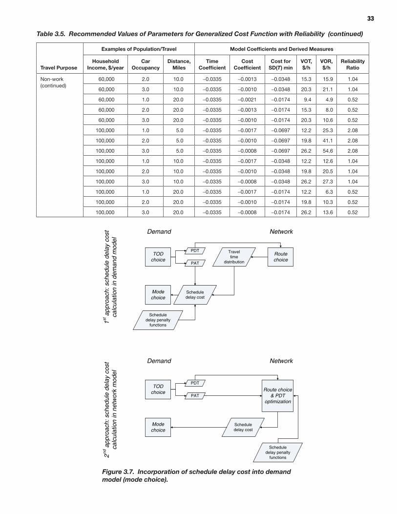
33
(continued)Table 3.5. Recommended Values of Parameters for Generalized Cost Function with Reliability
travel purpose
examples of population/travel Model Coefficients and Derived Measures
Household Income, $/year
Car occupancy
Distance, Miles
time Coefficient
Cost Coefficient
Cost for SD(T) min
Vot, $/h
VoR, $/h
Reliability Ratio
Non-work (continued)
60,000 2.0 10.0 -0.0335 -0.0013 -0.0348 15.3 15.9 1.04
60,000 3.0 10.0 -0.0335 -0.0010 -0.0348 20.3 21.1 1.04
60,000 1.0 20.0 -0.0335 -0.0021 -0.0174 9.4 4.9 0.52
60,000 2.0 20.0 -0.0335 -0.0013 -0.0174 15.3 8.0 0.52
60,000 3.0 20.0 -0.0335 -0.0010 -0.0174 20.3 10.6 0.52
100,000 1.0 5.0 -0.0335 -0.0017 -0.0697 12.2 25.3 2.08
100,000 2.0 5.0 -0.0335 -0.0010 -0.0697 19.8 41.1 2.08
100,000 3.0 5.0 -0.0335 -0.0008 -0.0697 26.2 54.6 2.08
100,000 1.0 10.0 -0.0335 -0.0017 -0.0348 12.2 12.6 1.04
100,000 2.0 10.0 -0.0335 -0.0010 -0.0348 19.8 20.5 1.04
100,000 3.0 10.0 -0.0335 -0.0008 -0.0348 26.2 27.3 1.04
100,000 1.0 20.0 -0.0335 -0.0017 -0.0174 12.2 6.3 0.52
100,000 2.0 20.0 -0.0335 -0.0010 -0.0174 19.8 10.3 0.52
100,000 3.0 20.0 -0.0335 -0.0008 -0.0174 26.2 13.6 0.52
Demand Network
TOD choice
Mode choice
Route choice
PDT
PAT
Travel time
distribution
Schedule delay cost
Schedule delay penalty
functions
TOD choice
Mode choice
Route choice & PDT
optimization
PDT
PAT
Schedule delay cost
Schedule delay penalty
functions
Demand Network
1stap
proa
ch: s
ched
ule
dela
y co
st
calc
ulat
ion
in d
eman
d m
odel
2nd
appr
oach
: sch
edul
e de
lay
cost
ca
lcul
atio
n in
net
wor
k m
odel
Figure 3.7. Incorporation of schedule delay cost into demand model (mode choice).
34
variations if used in the scheduling procedure and departure time optimization). In both approaches, schedule delay pen-alty functions are assumed known for each trip. The principal difference is in how the demand model interacts with the net-work simulation model to produce the expected schedule delay cost for each trip.
In the first approach, schedule delay cost is calculated in the demand model as part of the mode utility calculation for high-way modes. The network simulation model assigns trips based on PDT without a consideration of PAT. The role of the net-work simulation model is to produce travel time distributions for each trip (through a single equilibrium run or multiple runs). Subsequently, schedule delay cost is integrated over the travel time distribution in the demand model. This scheme has not been tested yet. The most realistic implementation approach for this scheme is a multiple-run framework.
In the second approach, the calculation of schedule delay cost is incorporated into the network model and is fed into the demand model. Perhaps, the most behaviorally appealing aspect of this implementation approach is when the network simulation model is allowed to optimize PDT based on the PAT and specified schedule delay penalties. This means that the route choice component is replaced with a joint route and departure time choice. This type of model can be imple-mented in a single-run framework, and some testing of this approach has been already reported (Zhou et al. 2008).
In both cases, the main (technical) obstacle for practical implementation of the schedule delay approach is the neces-sity to generate PAT for each trip against which the schedule delay cost is calculated as a consequence of unreliable travel time. It is currently unrealistic to prepare PAT as an input to travel demand models, although for some trips with inher-ently fixed schedules (work with a fixed schedule, appoint-ments, ticket shows) this might be ultimately the right approach. Some approaches to endogenously calculated PAT within the scheduling model as a latent variable were sug-gested (Ben-Akiva and Abou-Zeid 2007). Further research is needed to operationalize this approach within the framework of a regional travel model.
Temporal Utility Profiles in Demand Model
This is the most theoretically advanced approach. Its opera-tionalization on the demand side requires that temporal util-ity profiles be defined for each activity. The attractive part of this approach is that these profiles are indeed implicitly defined in the time-of-day choice model embedded in any ABM. However, conversion of the time-of-day choice model output into the utility profiles with the necessary level of temporal resolution is not a trivial procedure and has yet to be developed and explored. The crux of the problem is that a
time-of-day choice model produces probabilities for each activity to be undertaken at a certain time in a form of joint start (arrival) and end (departure) time probability over all feasible combinations P(ta, td) as in Equation 3.7:
, 1 (3.7)0
P t ta d
t t
T
t
T
d aa
∑∑ ( ) ===
These probabilities are defined for each activity, and they are not directly comparable across different activities. To con-vert the time-of-day choice probabilities into temporal utility profiles, an overall scale Uk for each activity k has to be defined. Then the utility profile could be calculated as in Equation 3.8:
, , (3.8)u t t U P t tk a d k a d( ) ( )= ×
The overall scale reflects the importance of (a unit duration of) each activity versus generalized travel cost. General travel cost Cad is a part of the time-of-day choice utility Vk(ta, td) used to calculate the probability P(ta, td). Thus the following esti-mate of Uk can be suggested that is essentially the coefficient for travel cost in the time-of-day choice utility, assuming that this is a single coefficient not differentiated by departure or arrival time (Equation 3.9):
,(3.9)U
V t t
Ck
k a d
ad
( )= ∂∂
However, these techniques are yet to be explored and fur-ther research is needed to unify time-of-day choice and tem-poral utility profiles. Also, even if the temporal utility profiles are available for each activity, their incorporation into an operational travel demand model is not straightforward. In a certain sense, two approaches similar to the approaches out-lined in Figure 3.7 for the schedule delay method can be adjusted to the temporal profiles framework.
The first approach would employ the network simulation model to produce travel time distributions for each trip departure time bin (30 min). Then, the demand model (mode choice) would convert these distributions to estimates of activity participation loss using temporal activity profiles. This approach has never been applied and its details have yet to be explored. The second approach would include temporal profiles in the network simulation that would require a simultaneous choice of network routes and departure times for the entire daily schedule (or each travel tour to make this model more realistic). Theoretical constructs of this type and corresponding experiments in small networks have been reported (Kim et al. 2006; Lam and Yin 2001). However, at the current time, the second approach cannot be recommended for implementation in real-size networks.
35
Incorporating reliability into Network Simulation
This section presents a concise overview of each method of quantification of travel time reliability from the perspective of its inclusion in an operational network simulation model. This means that the reliability measure of interest has to be incorporated into the route choice and generated at the O–D level to feed into the demand model.
Perceived Highway Time in Network Simulation
This method is easy to implement without a significant restructuring of the network assignment model, whether a user equilibrium static assignment or advanced DTA. Essen-tially, the generic highway travel time variable in route choice is replaced with segmented travel time by congestion levels, with the recommended weights shown in Table 3.4. The high-way LOS skims for the demand model have to be segmented accordingly.
However, in the same way as mentioned for a demand model, perceived travel time is not a direct measure of travel time reliability for network simulation. It can be used as a sur-rogate when more advanced methods are not available, but it is less appealing behaviorally and is not the main focus of the current research.
Mean-Variance in Network Simulation
This method requires an inclusion of an additional reliability term (standard deviation, variance, or buffer time) in the route choice generalized cost along with the mean travel time and cost as shown in Equation 3.9. Further on, the correspondent O–D skims for the reliability measure have to be generated to feed to the demand model (mode choice and other choice through mode choice logsums). However, implementation of this method on the network simulation side proved to be more complicated than its incorporation into a demand model.
Any demand model, whether 4-step or ABM, inherently operates with entire-trip O–D performance measures. Conse-quently, adding one more measure does not affect the model structure. However, network simulation models that are effi-cient in large networks operate with link-based shortest-path algorithms for route choice. This results in the necessity to construct entire-route O–D performance measures from link performance measures. While mean travel time and cost are additive by link, the reliability measures are not in a general case. This represents a significant complication that has to be resolved.
Even if an explicit route enumeration is applied, which means that several entire O–D routes are explicitly considered in route
choice, it is not trivial to incorporate a reliability measure like standard deviation, variance, or buffer time. In a single-run framework, this measure has to be generated based on the traf-fic flow versus capacity characteristics that require nonstandard statistical dependences to be involved. In a multiple-run frame-work, this measure can be summarized from multiple simula-tions. However, the whole framework of multiple runs has to be defined in a consistent way across demand, network supply, and equilibration parameters.
The next section is specifically devoted to an analysis of these issues and a substantiation of the team’s recommended methods. Single-run and multiple-run equilibration frame-works are discussed in subsequent chapters.
Schedule Delay Cost in Network Simulation
The previous section outlined two possible approaches that differ in how and where the schedule delay cost component is calculated (see Figure 3.7). With the first approach, schedule delay cost is calculated in the demand model as part of the mode utility calculation for highway modes. The network sim-ulation model assigns trips based on PDT without a consider-ation of PAT. The role of the network simulation model is to produce travel time distributions for each trip (through a sin-gle equilibrium run or multiple runs). Subsequently, schedule delay cost is integrated over the travel time distribution in the demand model. The most realistic implementation approach with this scheme is a multiple-run framework.
In the second approach, the schedule delay cost calculation is incorporated into the network model and is fed to the demand model. Perhaps the most behaviorally appealing implementation of this approach is when the network simu-lation model is allowed to optimize departure time based on the PAT and specified schedule delay penalties. This type of model can be implemented in a single-run framework, and some testing of this approach has been already reported (Zhou et al. 2008).
In both cases, the main (technical) obstacle for practical implementation of the schedule delay approach is the necessity to generate PAT (externally or endogenously in the demand model scheduling procedure) for each trip against which the schedule delay cost is calculated as a consequence of unreliable travel time. Further research is needed to operationalize this approach in the framework of a regional travel model.
Temporal Utility Profiles in Network Simulation
Two approaches similar to the approaches outlined for the schedule delay method can be adjusted within a temporal pro-files framework.
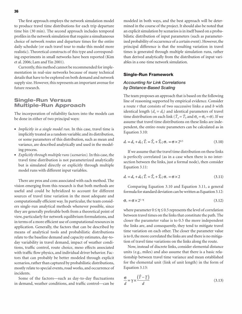
36
The first approach employs the network simulation model to produce travel time distributions for each trip departure time bin (30 min). The second approach includes temporal profiles in the network simulation that require a simultaneous choice of network routes and departure times for the entire daily schedule (or each travel tour to make this model more realistic). Theoretical constructs of this type and correspond-ing experiments in small networks have been reported (Kim et al. 2006; Lam and Yin 2001).
Currently, this method cannot be recommended for imple-mentation in real-size networks because of many technical details that have to be explored on both demand and network supply size. However, this represents an important avenue for future research.
Single-run Versus Multiple-run Approach
The incorporation of reliability factors into the models can be done in either of two principal ways:
• Implicitly in a single model run. In this case, travel time is implicitly treated as a random variable; and its distribution, or some parameters of this distribution, such as mean and variance, are described analytically and used in the model-ing process.
• Explicitly through multiple runs (scenarios). In this case, the travel time distribution is not parameterized analytically but is simulated directly or explicitly through multiple model runs with different input variables.
There are pros and cons associated with each method. The vision emerging from this research is that both methods are useful and could be hybridized to account for different sources of travel time variation in the most adequate and computationally efficient way. In particular, the team consid-ers single-run analytical methods whenever possible, since they are generally preferable both from a theoretical point of view, particularly for network equilibrium formulations, and in terms of a more efficient use of computational resources in application. Generally, the factors that can be described by means of analytical tools and probabilistic distributions relate to the baseline demand and capacity estimates, day-to-day variability in travel demand, impact of weather condi-tions, traffic control, route choice, meso effects associated with traffic flow physics, and individual driver behavior. Fac-tors that can probably be better modeled through explicit scenarios, rather than captured by probabilistic distributions, mostly relate to special events, road works, and occurrence of incidents.
Some of the factors—such as day-to-day fluctuations in demand, weather conditions, and traffic control—can be
modeled in both ways, and the best approach will be deter-mined in the course of the project. It should also be noted that an explicit simulation by scenarios is in itself based on a proba-bilistic distribution of input parameters (such as parameter-ized probability of occurrence of a certain event). However, the principal difference is that the resulting variation in travel times is generated through multiple simulation runs, rather than derived analytically from the distribution of input vari-ables in a one-time network simulation.
Single-Run Framework
Accounting for Link Correlations by Distance-Based Scaling
The team proposes an approach that is based on the following line of reasoning supported by empirical evidence. Consider a route r that consists of two successive links a and b with identical length (da = db) and identical parameters of travel time distribution on each link (T̃a = T̃b and sa = sb = s). If we assume that travel time distributions on these links are inde-pendent, the entire-route parameters can be calculated as in Equation 3.10:
; ; 2 (3.10)0.5d d d T T Tr a b r a b r� � �= + = + σ = σ ×
If we assume that the travel time distribution on these links is perfectly correlated (as in a case when there is no inter-section between the links, just a formal node), then consider Equation 3.11:
; ; 2 (3.11)d d d T T Tr a b r a b r� � �= + = + σ = σ ×
Comparing Equation 3.10 and Equation 3.11, a general formula for standard deviation can be written as Equation 3.12:
2 (3.12)1rσ = σ × −η
where parameter 0 ≤ h ≤ 0.5 represents the level of correlation between travel times on the links that constitute the path. The closer the parameter value is to 0.5 the more independent the links are, and consequently, they tend to mitigate travel time variation on each other. The closer the parameter value is to 0, the more correlated the links are and there is no mitiga-tion of travel time variations on the links along the route.
Now, instead of discrete links, consider elemental distance units (e.g., miles) and also assume that there is a basic rela-tionship between travel time variance and mean established for the elemental unit (link of unit length) in the form of Equation 3.13:
(3.13)d
T T
d
�( )σ = γ ×−
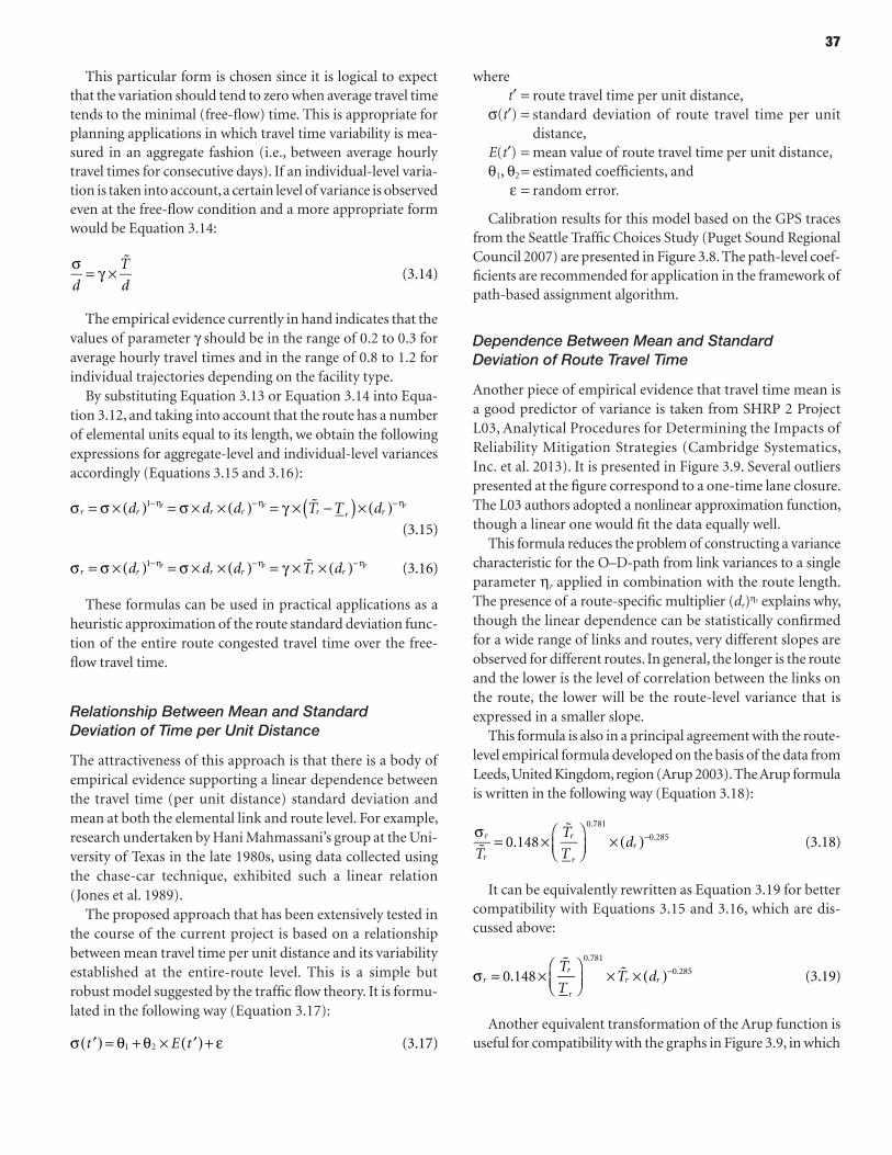
37
This particular form is chosen since it is logical to expect that the variation should tend to zero when average travel time tends to the minimal (free-flow) time. This is appropriate for planning applications in which travel time variability is mea-sured in an aggregate fashion (i.e., between average hourly travel times for consecutive days). If an individual-level varia-tion is taken into account, a certain level of variance is observed even at the free-flow condition and a more appropriate form would be Equation 3.14:
(3.14)d
T
d
�σ = γ ×
The empirical evidence currently in hand indicates that the values of parameter g should be in the range of 0.2 to 0.3 for average hourly travel times and in the range of 0.8 to 1.2 for individual trajectories depending on the facility type.
By substituting Equation 3.13 or Equation 3.14 into Equa-tion 3.12, and taking into account that the route has a number of elemental units equal to its length, we obtain the following expressions for aggregate-level and individual-level variances accordingly (Equations 3.15 and 3.16):
(3.15)
1d d d T T dr r r r r r rr r r�( )( ) ( ) ( )σ = σ × = σ × × = γ × − ×−η −η −η
(3.16)1d d d T dr r r r r rr r r�( ) ( ) ( )σ = σ × = σ × × = γ × ×−η −η −η
These formulas can be used in practical applications as a heuristic approximation of the route standard deviation func-tion of the entire route congested travel time over the free-flow travel time.
Relationship Between Mean and Standard Deviation of Time per Unit Distance
The attractiveness of this approach is that there is a body of empirical evidence supporting a linear dependence between the travel time (per unit distance) standard deviation and mean at both the elemental link and route level. For example, research undertaken by Hani Mahmassani’s group at the Uni-versity of Texas in the late 1980s, using data collected using the chase-car technique, exhibited such a linear relation (Jones et al. 1989).
The proposed approach that has been extensively tested in the course of the current project is based on a relationship between mean travel time per unit distance and its variability established at the entire-route level. This is a simple but robust model suggested by the traffic flow theory. It is formu-lated in the following way (Equation 3.17):
(3.17)1 2t E t( ) ( )σ ′ = θ + θ × ′ + ε
where t′ = route travel time per unit distance,s(t′) = standard deviation of route travel time per unit
distance, E(t′) = mean value of route travel time per unit distance,q1, q2 = estimated coefficients, and e = random error.
Calibration results for this model based on the GPS traces from the Seattle Traffic Choices Study (Puget Sound Regional Council 2007) are presented in Figure 3.8. The path-level coef-ficients are recommended for application in the framework of path-based assignment algorithm.
Dependence Between Mean and Standard Deviation of Route Travel Time
Another piece of empirical evidence that travel time mean is a good predictor of variance is taken from SHRP 2 Project L03, Analytical Procedures for Determining the Impacts of Reliability Mitigation Strategies (Cambridge Systematics, Inc. et al. 2013). It is presented in Figure 3.9. Several outliers presented at the figure correspond to a one-time lane closure. The L03 authors adopted a nonlinear approximation function, though a linear one would fit the data equally well.
This formula reduces the problem of constructing a variance characteristic for the O–D-path from link variances to a single parameter hr applied in combination with the route length. The presence of a route-specific multiplier (dr)hr explains why, though the linear dependence can be statistically confirmed for a wide range of links and routes, very different slopes are observed for different routes. In general, the longer is the route and the lower is the level of correlation between the links on the route, the lower will be the route-level variance that is expressed in a smaller slope.
This formula is also in a principal agreement with the route-level empirical formula developed on the basis of the data from Leeds, United Kingdom, region (Arup 2003). The Arup formula is written in the following way (Equation 3.18):
0.148 (3.18)0.781
0.285
T
T
Td
r
r
r
r
r��
( )σ = ×
× −
It can be equivalently rewritten as Equation 3.19 for better compatibility with Equations 3.15 and 3.16, which are dis-cussed above:
0.148 (3.19)0.781
0.285T
TT dr
r
r
r r
�� ( )σ = ×
× × −
Another equivalent transformation of the Arup function is useful for compatibility with the graphs in Figure 3.9, in which
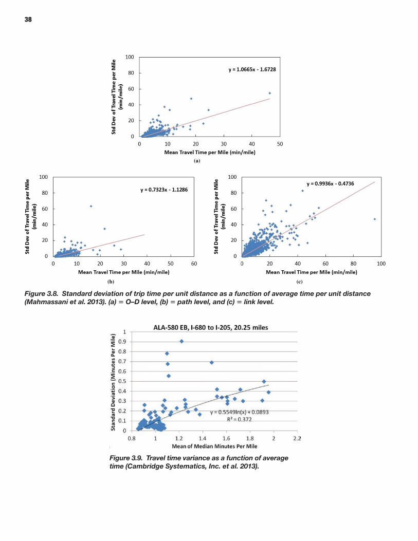
38
(a)
(b) (c)
Figure 3.8. Standard deviation of trip time per unit distance as a function of average time per unit distance (Mahmassani et al. 2013). (a) O–D level, (b) path level, and (c) link level.
Figure 3.9. Travel time variance as a function of average time (Cambridge Systematics, Inc. et al. 2013).
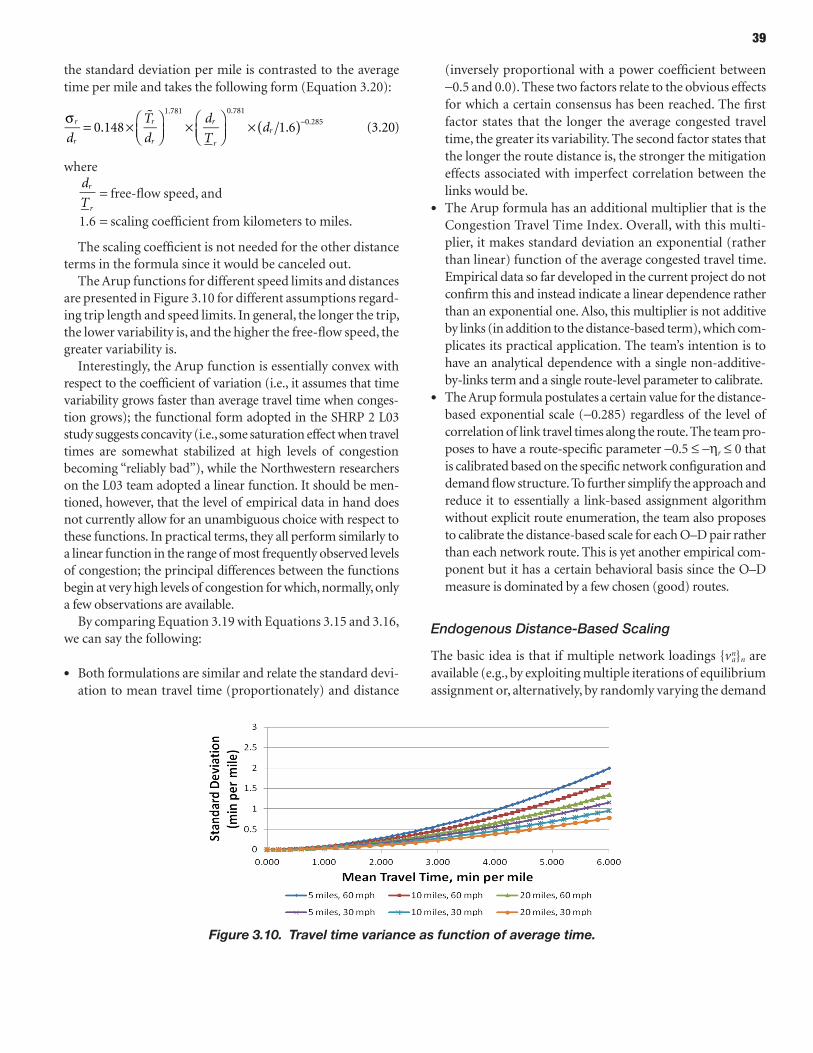
39
the standard deviation per mile is contrasted to the average time per mile and takes the following form (Equation 3.20):
0.148 1.6 (3.20)1.781 0.781
0.285�
( )σ = ×
×
× −
d
T
d
d
Td
r
r
r
r
r
r
r
where
d
Tr
r
= free-flow speed, and
1.6 = scaling coefficient from kilometers to miles.
The scaling coefficient is not needed for the other distance terms in the formula since it would be canceled out.
The Arup functions for different speed limits and distances are presented in Figure 3.10 for different assumptions regard-ing trip length and speed limits. In general, the longer the trip, the lower variability is, and the higher the free-flow speed, the greater variability is.
Interestingly, the Arup function is essentially convex with respect to the coefficient of variation (i.e., it assumes that time variability grows faster than average travel time when conges-tion grows); the functional form adopted in the SHRP 2 L03 study suggests concavity (i.e., some saturation effect when travel times are somewhat stabilized at high levels of congestion becoming “reliably bad”), while the Northwestern researchers on the L03 team adopted a linear function. It should be men-tioned, however, that the level of empirical data in hand does not currently allow for an unambiguous choice with respect to these functions. In practical terms, they all perform similarly to a linear function in the range of most frequently observed levels of congestion; the principal differences between the functions begin at very high levels of congestion for which, normally, only a few observations are available.
By comparing Equation 3.19 with Equations 3.15 and 3.16, we can say the following:
• Both formulations are similar and relate the standard devi-ation to mean travel time (proportionately) and distance
(inversely proportional with a power coefficient between -0.5 and 0.0). These two factors relate to the obvious effects for which a certain consensus has been reached. The first factor states that the longer the average congested travel time, the greater its variability. The second factor states that the longer the route distance is, the stronger the mitigation effects associated with imperfect correlation between the links would be.
• The Arup formula has an additional multiplier that is the Congestion Travel Time Index. Overall, with this multi-plier, it makes standard deviation an exponential (rather than linear) function of the average congested travel time. Empirical data so far developed in the current project do not confirm this and instead indicate a linear dependence rather than an exponential one. Also, this multiplier is not additive by links (in addition to the distance-based term), which com-plicates its practical application. The team’s intention is to have an analytical dependence with a single non-additive- by-links term and a single route-level parameter to calibrate.
• The Arup formula postulates a certain value for the distance-based exponential scale (-0.285) regardless of the level of correlation of link travel times along the route. The team pro-poses to have a route-specific parameter -0.5 ≤ -hr ≤ 0 that is calibrated based on the specific network configuration and demand flow structure. To further simplify the approach and reduce it to essentially a link-based assignment algorithm without explicit route enumeration, the team also proposes to calibrate the distance-based scale for each O–D pair rather than each network route. This is yet another empirical com-ponent but it has a certain behavioral basis since the O–D measure is dominated by a few chosen (good) routes.
Endogenous Distance-Based Scaling
The basic idea is that if multiple network loadings {vna}n are
available (e.g., by exploiting multiple iterations of equilibrium assignment or, alternatively, by randomly varying the demand
Figure 3.10. Travel time variance as function of average time.
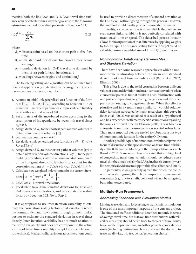
40
matrix), both the link-level and O–D-level travel time vari-ances can be calculated in a way that gives rise to the following estimation method for scaling parameter (Equation 3.21):
(3.21)1
dijij
a
a A
ij
ij
∑( ) = σ
σ−η
∈
where dij = distance skim based on the shortest path at free-flow
time,sa = link standard deviations for travel times across
loadings,sij = standard deviation for O–D travel time skimmed by
the shortest path for each iteration, and Aij = loadings between origin i and destination j.
The following setting and algorithm can be outlined for a practical application (i.e., iterative traffic assignment), where n now denotes the iteration number:
1. Assume an initial link generalized cost function of the form ca = T̃a(va) + l × sa[T̃a(va)] according to Equation 3.13 or Equation 3.14, where parameter l represents a reliability ratio with a normal value of 0.8.
2. Set a matrix of distance-based scales according to the assumption of independence between link travel times hij = 0.5.
3. Assign demand Wij to the shortest paths at zero volumes to obtain zero iteration volumes {va
0}.4. Set iteration counter n = n + 1.5. Recalculate link generalized cost functions ca
n+1 = T̃a(van) +
l × sa[T̃a(van)].
6. Assign demand Wij to the shortest paths at volumes {van} to
obtain next iteration volume directions {wan+1}. In the path
building procedure, scale the variance-related component of the link generalized cost functions to account for the correlation pattern ca
n+1 = T̃a(van) + l × sa[T̃a(va
n)] ⁄ (dij)1-hij.7. Calculate new weighted link volumes for the current itera-
tions1 1
1 1 1vn
wn
nva
nan
an{ }= + −+ + + .
8. Calculate O–D travel time skims.9. Recalculate travel time standard deviations for links and
O–D pairs across iterations, and recalculate the scaling factors by Equation 3.21. Go to Step 4.
It is appropriate to use inter-iteration variability to esti-mate the correlation scaling factors (that essentially reflect the common demand flows going through different links) but not to estimate the standard deviation in travel times directly. Inter-iteration variability has not much relation to real world variability and does not correspond to the actual sources of travel time variability (except for some relation to route choice). Mechanically, variation across iterations could
be used to provide a direct measure of standard deviation at the O–D level, without going through this process. However, that method would hardly produce reasonable estimates.
In reality, some congestion is more reliable than others; so even across links, variability is not perfectly correlated with mean travel time or speed. The described process broadly allows for incorporation of that difference by applying weights by facility type. The distance scaling factors in Step 9 could be calculated using a weighted sum of link SD(T)s in this case.
Nonmonotonic Relationship Between Mean and Standard Deviation
There have been some research approaches in which a non-monotonic relationship between the mean and standard deviation of travel time was advocated (Bates et al. 2002; Eliasson 2006).
This effect is due to the serial correlation between different values of standard deviation and mean across observations taken at successive points in time. It results in a two-fold function with one part corresponding to growing congestion and the other part corresponding to congestion release. While this effect is plausible and in a certain sense similar to two-fold volume-delay functions advocated by many researchers, this curve in Bates et al. (2002) was obtained as a result of a hypothetical one-link experiment with many specific assumptions regarding the sources of travel time. In Eliasson (2006) it was based on automatic travel time measurements on selected urban links. Thus, more empirical data are needed to substantiate this type of nonmonotonic function for the entire O–D route.
Another possible type of nonmonotonic relationship was the focus of discussion at the special session on travel time reliabil-ity at the 89th Annual Meeting of the Transportation Research Board in 2010. Some researchers advocated that at a high level of congestion, travel time variation should be reduced since travel time becomes “reliably bad.” Again, there is currently very little empirical evidence to support this effect (Brennand 2011).
In particular, it was generally agreed that when the recur-rent congestion grows, the relative impact of nonrecurrent congestion (e.g., due to a traffic collision) will not be mitigated, but rather exacerbated.
Multiple-Run Framework
Addressing Feedback with Simulation Models
Linking travel demand forecasting to traffic microsimulation is one of the most important aspects of the current project. The simulated traffic conditions (described not only in terms of average travel time, but as travel time distributions with reli-ability measures) should be fed back to choices of travel route, travel mode, departure time, and other possible choice dimen-sions (including destination choice and even the decision to travel at all—i.e., trip frequency/generation choice).
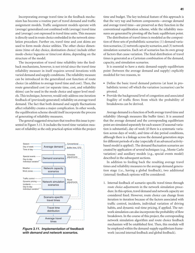
41
Incorporating average travel time in the feedback mecha-nism has become a routine part of travel demand and traffic assignment models. Traffic assignment models operate with (average) generalized cost combined with (average) travel time and (average) cost expressed in travel time units. This measure is directly used in route choice embedded in the network simu-lation procedure. Further on, travel time and cost skims are used to form mode choice utilities. The other choice dimen-sions (time-of-day choice, destination choice) include either mode-choice logsums or time/cost skims, depending on the structure of the model.
The incorporation of travel time reliability into the feed-back mechanisms, however, is not trivial since the travel time reliability measure in itself requires several iterations with varied demand and supply conditions. The reliability measure can be introduced in the generalized cost function of route choice (in addition to average travel time and cost). Then, the route generalized cost (or separate time, cost, and reliability skims) can be used in the mode choice and upper level mod-els. This technique, however, would only address one iteration feedback of (previously generated) reliability on average travel demand. The fact that both demand and supply fluctuations affect reliability creates a major complication. In other words, the equilibration scheme should itself incorporate the process of generating of reliability measures.
The general suggested structure that resolves this issue is pre-sented in Figure 3.11. It includes the travel time variation mea-sure of reliability as the only practical option within the project
time and budget. The key technical feature of this approach is that the very top and bottom components—average demand and average travel time—are preserved as they function in the conventional equilibration scheme, while the reliability mea-sures are generated by pivoting off the basic equilibrium point.
The distribution of travel times is modeled as the composi-tion of three sets of probabilistic scenarios: (1) demand varia-tion scenarios, (2) network capacity scenarios, and (3) network simulation scenarios. Each set of scenarios has its own group of factors that cause variation. The final distribution of travel times is generated as a Cartesian combination of the demand, capacity, and simulation scenarios.
It is essential to have a static demand-supply equilibrium point (between the average demand and supply) explicitly modeled for two reasons, to
• Define the basic travel demand patterns (at least in pro-babilistic terms) off which the variation (scenarios) can be pivoted.
• Provide the background level of congestion and associated fragility of traffic flows from which the probability of breakdowns can be derived.
Average demand is a function of both average travel time and reliability (through measures like buffer time). It is assumed that the average demand and the corresponding equilibrium point are simulated separately for each season (if seasonal varia-tion is substantial), day-of-week (if there is a systematic varia-tion across days of week), and time-of-day period conditions, although there is a linkage across the demand generation steps for different periods of a day (especially if an advanced activity-based model is applied). The demand fluctuation scenarios are created by application of several techniques (e.g., Monte Carlo variation) and auxiliary models (e.g., special events model) described in the subsequent sections.
In addition to feeding back the resulting average travel times and reliability measures to the average demand genera-tion stage (i.e., having a global feedback), two additional (internal) feedback options will be considered:
1. Internal feedback of scenario-specific travel times through route choice adjustments in the network simulation proce-dure. In this option, travel demand and network capacity are considered fixed. However, route choice can change from iteration to iteration because of the factors associated with traffic control, incidents, individual variation of driving habits, and dynamic real-time pricing, if applied. The net-work simulation can also incorporate the probability of flow breakdown. In the course of this project, the corresponding network simulation algorithm and route choice feedback mechanism will be established first. Then, this module will be employed within the demand-supply equilibrium frame-work (second internal feedback and global feedback).
Average demand
Demand scenarios
Network capacityscenarios
Season
Day of week
Time of day
Special events
Day-to-dayindividual variation
Weather
Work zones
Network simulationscenarios
Traffic control
Dynamic pricing
IncidentsDay-to-dayindividual variation
Scenario-specifictravel times
Travel timedistribution
Average traveltimes
Conventional
Buffer time, STD
Scheduleadjustments
Routeadjustments
Figure 3.11. Implementation of feedback with demand and network scenarios.
42
2. Internal feedback of travel time distributions (and any derived measure of reliability) to the demand scenario through schedule adjustments of trip departure times. In this option, the demand scenario (in terms of trip genera-tion, distribution, and mode choice) is considered fixed, while the trip departure time can change from iteration to iteration as the result of travel time fluctuations modeled by the network capacity and network simulation scenar-ios. The purpose of this feedback is to stabilize trip depar-ture times for each demand scenario. This feedback is applied within the global equilibrium loop.
The details of the demand generation process and its sensi-tivity to reliability measures depend on the type of travel demand model. The team plans to address both traditional (4-step) trip-based travel demand models and advanced activity-based models. The activity-based modeling frame-work represents a more promising counterpart to microscopic and mesoscopic network simulation models because of their more compatible temporal resolution. Advanced activity-based models in practice already operate with 30–60-minute demand slices, while traditional 4-step models typically oper-ate with broad 3–4-hour periods.
For a 4-step travel demand model, the following dimension and components of travel demand can be included in the equilibrium framework and incorporate reliability measures:
• Mode choice, in which utility functions for highway modes (drive alone, shared ride) can include buffer time or any other reliability measure;
• Trip distribution, in which the travel impedance function can include mode choice logsum or directly include reli-ability measures;
• Trip time-of-day choice, specifically for highway modes, in which the peak (and other period-specific) factors can include period-specific reliability measures; and
• Trip generation, which can be made sensitive to accessibility measures (destination choice logsums) that can include reli-ability measures along with average travel time and cost.
It should be noted that it may not be easy to incorporate all of these features into 4-step models. This has been part of the motivation for development and adoption of activity-based models by planning agencies over the past two decades.
For an activity-based travel demand model, the following dimension and components of travel demand can be included in the equilibrium framework and incorporate reliability measures:
• Mode choice, in which utility functions for highway modes (drive alone, shared ride) can include buffer time or any other reliability measure;
• Primary destination choice, in which the travel impedance function can include mode choice logsum or directly include reliability measures;
• Stop frequency and location choices for chained tours that are also based on travel impedance functions with reliabil-ity measures;
• Tour generation models (daily activity-travel pattern), which can be made sensitive to accessibility measures (des-tination choice logsums) that can include reliability mea-sures along with average travel time and cost; and
• Tour time-of-day models (daily schedule), which can be made sensitive to time-specific reliability measures.
It should be mentioned that despite certain similarities between the 4-step and activity-based models in their approaches to incorporating reliability feedback, there are some important principal differences. In particular, 4-step models operate with aggregate zonal flows, so that any demand response to reliability will be identical for all trips within the same segment. In contrast, activity-based models are based on individual microsimulation, which opens the way to imple-ment the feedback on the individual level, at which point additional individual variation can be taken into account. Also, the utility coefficients in activity-based microsimulation models can be effectively randomized, taking into account individual variation of value of time and value of reliability.
technical Aspects of Scenario Formation
Practical implementation of the equilibrium mechanism shown in Figure 3.11 requires the establishment of certain rules for scenario formation, as well as specific technical aspects for the combination of different sources of travel time variability. The team envisions the following general imple-mentation scheme:
• All three types of scenarios are defined as discrete cases with a predetermined number of states. These discrete states are randomly generated at each global iteration; however, the number of states and the core probabilistic distributions are prepared in advance. It should be men-tioned that even with a small number of states generated in each dimension, the Cartesian combination of them can easily reach a number that would result in unrealistic run-times for simulations (especially in large urban networks). Thus, generally, two to three random scenarios for each factor would be enough. A fractional factorial design can be effectively employed to reduce random variation.
• Scenarios associated with travel demand and network capacity are simulated first since they are assumed indepen-dent. Then they are combined in a Cartesian way. Travel
43
demand scenarios in turn are combined with scenarios for special events and day-to-day variation scenarios that are also assumed independent. Network simulation scenarios are combined with scenarios for weather conditions and scenarios for work zones that are also assumed indepen-dent. For example, assume that for each of the four dimen-sions we generate two scenarios. This would already result in 2 × 2 × 2 × 2 = 16 combined basic scenarios. Taking into account that day-to-day variation in travel demand con-tributes 60% to 70% of the observed variability in travel times, we may generate more scenarios (three or four) for this particular factor. This would make the total number of possible combined scenarios 24 or 32. A fractional factorial might also be adequate here, allowing for more scenarios for each dimension while keeping the total number of com-binations realistic. The goal is to come up with a realistic distribution of travel times across a wide range of combina-tions of conditions—not to test every combination.
• Each of the 16 basic scenarios is simulated, taking into account several possible network simulation scenarios. Each network simulation scenario is essentially a full run of net-work simulation with certain randomly drawn parameters that relate to traffic control, dynamic pricing algorithm, incidence occurrence, and individual route choice and driv-ing style. On top of these randomized factors, a flow break-down probability will be applied. If we implement three runs for each scenario, it would result in 3 × 16 = 48 simula-tions. This would supply travel time distribution for each O–D pair with the necessary degree of details. Essentially, any of the applied reliability measures (standard deviation; 80th, 85th, 90th, or 95th percentile) can be derived from this distribution. Parallel processing can be effectively employed for multiple simulation runs. Since the core 16 scenarios for travel demand and network capacity have been defined, the simulation runs can be implemented independently.
• Trip tables associated with special events will be pre-calculated for each venue and randomly chosen from the list based on the frequency (as described in the next subsection). These tables will be added to the core trip table generated by the demand model.
• The core trip table will be randomized as described in the next subsection to account for day-to-day individual variation.
• The weather condition scenarios will be randomly chosen from the frequency table that will contain two to three weather-related states that are significantly different from the travel condition point of view. Dependent on the chosen region for simulation, the states will be classified as normal, rainy, and/or snowy/icy. For each of the weather condi-tions different from the normal, network capacities and/or volume-delay functions will be adjusted to account for the additional difficulty of driving.
• The scenarios associated with work zones will be con-structed based on the observed/planned frequency of link/lane closures by road type for the time-of-day periods of the simulation. Based on the defined frequencies, some network links/lanes will be disabled in the traffic simulation process.
The methodological and implementation details associated with scenario formation are described in Chapter 6. They are described again in connection with the applications presented in Part 3 of this report.
Travel Demand Scenarios
Individual travel behavior is inherently stochastic from the perspective of the modeler. Except for work and school com-muting, most of the trips are not implemented on a daily basis. Even for commuting trips that are the most stable demand component of travel, there is an average weekday attendance factor (trips per workplace) of around 0.8 because of vaca-tions, sickness, days off, work in other locations, and so on. This means that a 5% spike in traffic flow can be just a com-bination of random individual trip frequencies. It can be said that the random variation in individual travel behavior is a consequence of small special events unknown to the modeler. There are probably some opportunities to move some of the uncertainty attributed to random individual behavior into the systematic variation category. For example, one can speculate that there might be a seasonal effect in workplace attendance. However, in general, randomness of individual behavior cannot be eliminated from the travel forecasting process, and it should be explicitly incorporated into the new generation of travel models. The team suggests two possible and different approaches to incorporating this factor.
Approach 1. One of the natural options is embedded in the demand microsimulation structure of activity-based models. These models operate with parameterized probabilities that are converted into travel choices by using Monte Carlo (or sometimes more elaborate discretizing method); see Vovsha et al. (2008) for technical details. Thus, a certain level of vari-ability can be effectively modeled by changing random num-ber seeds in the microsimulation process (so-called Monte Carlo variability). This option is comparatively simple to imple-ment, and it will be fully explored in the current project for both travel choices and route choice in the traffic simulation. This approach is difficult to operationalize for a 4-step model that operates with aggregate flows. The conceptual limita-tions of this approach have to be understood nonetheless since Monte Carlo variability does not have a systematic rela-tionship to real world variability.
Approach 2. Another possible approach that is equally appli-cable to 4-step and activity-based models is estimating variation
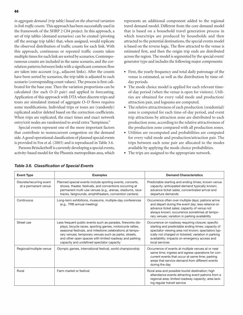
44
in aggregate demand (trip table) based on the observed variation in link traffic counts. This approach has been successfully used in the framework of the SHRP 2 C04 project. In this approach, a set of trip tables (demand scenarios) can be created (pivoting off the average trip table) that, when assigned, would replicate the observed distribution of traffic counts for each link. With this approach, continuous or repeated traffic counts taken multiple times for each link are sorted by scenarios. Contempo-raneous counts are included in the same scenario, and the cor-relation patterns between links with a significant common flow are taken into account (e.g., adjacent links). After the counts have been sorted by scenarios, the trip table is adjusted to each scenario (corresponding count values). The process is first cali-brated for the base year. Then the variation proportions can be calculated (for each O–D pair) and applied in forecasting. Application of this approach with DTA when discrete trips and tours are simulated instead of aggregate O–D flows requires some modifications. Individual trips or tours are (randomly) replicated and/or deleted based on the correction coefficients. When trips are replicated, the exact times and exact network entry/exit nodes are randomized to avoid extra “lumpiness.”
Special events represent one of the more important factors that contribute to nonrecurrent congestion on the demand side. A good operational classification of planned special events is provided in Fox et al. (2003) and is reproduced in Table 3.6.
Parsons Brinckerhoff is currently developing a special events, activity-based model for the Phoenix metropolitan area, which
represents an additional component added to the regional travel demand model. Different from the core demand model that is based on a household travel generation process in which tours/trips are produced by households and then attracted to the potential destinations, the special events model is based on the reverse logic. The flow attracted to the venue is estimated first, and then the origin trip ends are distributed across the region. The model is segmented by the special event/generator type and includes the following major components:
• First, the yearly frequency and total daily patronage of the venue is estimated, as well as the distribution by time-of-day periods.
• The mode choice model is applied for each relevant time-of-day period (when the venue is open for visitors). Utili-ties are obtained for every valid mode and production/attraction pair, and logsums are computed.
• The relative attractiveness of each production (residential) zone is computed for each time-of-day period, and event trip attractions by attraction zone are distributed to each production zone, according to the relative attractiveness of the production zone compared with all production zones.
• Utilities are recomputed and probabilities are computed for every valid mode and production/attraction pair. The trips between each zone pair are allocated to the modes available by applying the mode choice probabilities.
• The trips are assigned to the appropriate network.
Table 3.6. Classification of Special Events
event type examples Demand Characteristics
discrete/recurring event at a permanent venue
Planned special events include sporting events, concerts, shows, theater, festivals, and conventions occurring at permanent multi-use venues (e.g., arenas, stadiums, race-tracks, fairgrounds, amphitheaters, convention centers)
Predictable starting and ending times; known venue capacity; anticipated demand typically known; advance ticket sales; concentrated arrival and departure demands
continuous long-term exhibitions, museums, multiple-day conferences (e.g., TRB annual meeting)
occurrence often over multiple days; patrons arrive and depart during the event day; less reliance on advance ticket sales; capacity of venue not always known; occurrence sometimes at tempo-rary venues; variation in parking availability
Street use less frequent public events such as parades, fireworks dis-plays, bicycle races, sporting games, motorcycle rallies, seasonal festivals, and milestone celebrations at tempo-rary venues; temporary venues such as parks, streets, and other open spaces with limited roadway and parking capacity and undefined spectator capacity
occurrence on roadway requiring closure; specific starting and predictable ending times; capacity of spectator viewing area not known; spectators typ-ically not charged or ticketed; variation in parking availability; impacts on emergency access and local services
Regional/multiple-venue olympic games, international festival, world championship occurrence of events at multiple venues at or near same time; ingress and egress operations for con-current events that occur at same time; parking areas that service demand from different events during the day
Rural Farm market or festival Rural area and possible tourist destination; high attendance events attracting event patrons from a regional area; limited roadway capacity; area lack-ing regular transit service
45
A model of this type naturally lends itself to a traffic simu-lation incorporating reliability. The probability of the event occurring during the simulation run is estimated based on the frequency for each venue. In each generated demand sce-nario, some of the randomly selected special events will be included. To better control for variability across different demand scenarios, the random selection process can be orga-nized with “no replacement” rules.
Network Capacity Scenarios
Network capacity can be significantly affected by the weather conditions and road works that require closure of some lanes or entire road segments for some period of time. The impacts of weather conditions on road capacity can also be explicitly taken into account in the network simulation through param-eters of car following. To include these factors in the network simulation, the following technical steps will be implemented:
• Weather conditions. A categorization of possible weather conditions will be implemented for the given season and hour with probability for each particular condition to occur. Then for each condition that is different from nor-mal, network capacities and speed functions will be adjusted accordingly.
• Work zones. The probability of lane/road segment closure for maintenance or other purpose will be calculated for all facil-ity types. According to this probability, in the network simu-lation, some network links are fully or partially disabled. If special events are associated with some predetermined road closures (in addition to the demand spike associated with the event), this factor can be combined with road works in the network scenario formation.
Details that relate to these factors are discussed in the pilot applications.
Network Simulation Scenarios
For a given combined demand and network capacity sce-nario, there are two major factors that can significantly affect travel time reliability (and specifically relate to nonrecurrent congestion): incidences and traffic flow breakdowns. Ways to parameterize the probability of these factors occurring, and the associated practical techniques to incorporate them into network simulations, have been discussed in detail in the Task 7 Report (Stogios et al. 2014). In the framework of mul-tiple simulation runs (implicitly associated with different days), these factors form scenarios of network simulation. It should be stressed that due to these factors, different simulation runs can produce very different travel times even though the demand and network capacity are fixed.
Drivers’ response to changing network conditions is subject to different time scales. This has to be taken into account when forming the equilibration strategies. For example, route choice can change in response to a collision or work zone. However, this is not a long-term equilibrium state for the network.
Varying time scales affect equilibration (fixed versus equilibrated versus one-pass) in the context of recurrent and nonrecurrent congestion. This section explains the differences between equilibrium in different time scales. This is of special relevance for modeling nonrecurrent congestion that cannot be considered as a state of equilibrium but is rather a one-pass event. Recurrent congestion in general is recognized as an example of a well-equilibrated state in which multiple highway users tried different routes (presumably on different days) and eventually reached a certain level of convergence (average day). Recommendations are made on how an equilibration time scale can be properly accounted for.
A wide range of travel choices with very different time scales for traveler responses are affected by travel time reli-ability. Short-term responses include travel dimensions such as network route choice (including any portion of the route when new travelers’ information becomes available), route type choice (toll versus nontoll and/or managed lanes versus general-purpose lanes), trip departure times, and possibly mode choice (if a transit option is competitive). Because the perception of travel time reliability generally stems from observed variability over time, it requires a certain learning curve and experience from travelers to perceive it and respond to changes in it, although an advance information system that would provide reliability estimates along with the shortest and/or average travel times can change this drastically. Mod-els that are based on the distribution of travel times imply that the travelers have a good idea about this distribution, which probably means in practical terms at least 5–10 recent trips along the route at the same time of day. It is yet to be explored how the modeling assumptions about travelers’ knowledge and information match the reality, but this is largely the same problem with the conventional models that operate with average travel time. The assumptions about drivers’ per-fect knowledge and immediate response to changes in average travel times are seen to be essential for making the models analytically simple and operational, but they might be quite far from reality.
recommendations for Future research
Several important research directions have become clear in the course of the current project. Many of them relate to more advanced methods of incorporation of travel time reli-ability, specifically schedule delay cost and temporal activity
46
profiles. However, improving travel demand models and net-work simulation tools in this direction is closely intertwined with a general improvement of individual microsimulation models. The following specific recommendations for future research are made:
• Continue research on advanced methods for incorporation of travel time reliability into demand models and network simulations tools, including the schedule delay cost approach and temporal utility profile (loss of activity participation) approach. As part of such research, continue research and development of path-based assignment algorithms that incorporate travel time reliability and can generate a trip travel time distribution in addition to mean travel time.
• Continue research on schemes for the integration of advanced ABM and DTA that can ensure a full consistency of daily activity patterns and schedules at the individual level and behavioral realism of traveler responses. In this regard, enhancement of time-of-day choice, trip departure time choice, and activity scheduling components are essential to address. This relates to the conceptual structure of these
models and their implementation with respect to temporal resolution.
• Encourage additional data collection on the supply side of activities and on scheduling constraints, including the dis-tribution of jobs and workers by schedule flexibility, clas-sification of maintenance and discretionary activities by schedule flexibility, as well as developing approaches to forecast related trends.
• Continue research and application of multiple-run model approaches and associated scenario formations, for both the demand and network supply sides. The team’s synthe-sis and research have shown that a conventional single-run framework is inherently too limited to incorporate some important reliability-related phenomena such as nonre-current congestion due to a traffic incident, special event, or extreme weather condition.
• Incorporate travel time reliability in project evaluation and user benefit calculations. Restructure the output of travel models to support project evaluation and user benefit cal-culations with consideration of the impact of improved travel time reliability.
47
C h A p t e r 4
Introduction
This chapter describes the framework and the functional requirements for the inclusion of travel time reliability esti-mates in transportation network modeling tools, with par-ticular focus on stochastic traffic simulation models. The framework identifies phenomena and behaviors that account for the observed variability in network traffic performance, and unifies all particle-based simulations at the microscopic and mesoscopic levels. Recognizing that the requirements development process is focused on the uses of traffic opera-tional models in agencies at the local, metropolitan, regional, and state levels, the functional requirements are developed for different resolutions and scales. In addition, a repeatable framework is proposed to model travel time variability induced by incidents and random events, recognizing the difference between so-called recurring and nonrecurring congestion due to various sources.
Incorporating travel time reliability into stochastic traffic simulation models has the primary objective of enabling the off-line evaluation of traffic network performance, including assessment of management interventions, policies and geo-metric configuration, and so forth, as well as both short-term and long-run impacts of policies aimed at improving travel time and service reliability.
Longer-term impact evaluation entails integrating reliabil-ity considerations in equilibrium planning models. An ideal integration would bring together reliability-sensitive network simulation models with micro-level activity-based demand models. However, practical approaches consistent with the current state of the practice can also be formulated.
In addition to off-line applications, reliability-sensitive simulation models can support the design and implementa-tion of real-time operational decisions. The design of online traffic information and management strategies calls for sto-chastic simulation tools that are capable of modeling recur-rent and nonrecurrent congestion and generating reliability measures in real time.
Framework
Traffic operations and planning models generally require both demand and supply inputs. Travel demand could be static (for planning models), dynamic (for planning and operational models), or in the form of activity schedules (for activity-based models). In virtually all applications, actual travel demand cannot be perfectly forecast and is subject to a variety of dis-turbances, including special events, day-to-day variation in individual behavior, (unfamiliar) visitor traffic, and diversion from temporary unavailability of alternative modes. On the supply side, the operational capacity of network elements could be assumed as fixed, stochastic, or systematically vary-ing with traffic conditions through actuated signal controls, ramp metering, dynamic tolls, and so on. Unreliability sources that affect supply-side attributes consist of incidents, work zones, weather, traffic control, dynamic pricing, and varia-tion in individual driving behavior. These variations in demand and supply affect the movement of vehicles and the propagation of traffic flow, resulting in different travel times for drivers traveling on the same link or path or between a given origin–destination (O–D) pair. Therefore, travel time variability, at the individual or aggregated levels, could be quantified based on the simulation results, in particular, vehicle trajectories. Commonly used reliability measures include the probability of arriving on time, the Travel Time Index (ratio of the mean experienced travel time to the free mean travel time), the variance (or standard deviation) of experienced travel times, and various descriptive statistics that can be derived from the distribution of travel times, which is the most general and complete way of character-izing travel time variability across a population of drivers in a network.
Figure 4.1 presents a general framework for incorporating reliability aspects into modeling tools used to support traffic operations and planning applications. The framework recog-nizes the different sources of unreliability and their interac-tion with the key components of network simulation models.
Functional Requirements of Stochastic Network Simulation Models
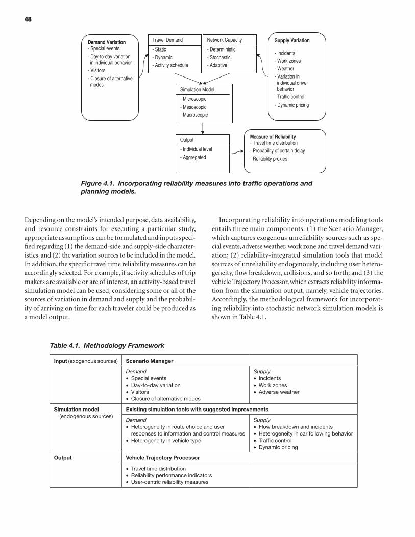
48
Depending on the model’s intended purpose, data availability, and resource constraints for executing a particular study, appropriate assumptions can be formulated and inputs speci-fied regarding (1) the demand-side and supply-side character-istics, and (2) the variation sources to be included in the model. In addition, the specific travel time reliability measures can be accordingly selected. For example, if activity schedules of trip makers are available or are of interest, an activity-based travel simulation model can be used, considering some or all of the sources of variation in demand and supply and the probabil-ity of arriving on time for each traveler could be produced as a model output.
Incorporating reliability into operations modeling tools entails three main components: (1) the Scenario Manager, which captures exogenous unreliability sources such as spe-cial events, adverse weather, work zone and travel demand vari-ation; (2) reliability-integrated simulation tools that model sources of unreliability endogenously, including user hetero-geneity, flow breakdown, collisions, and so forth; and (3) the vehicle Trajectory Processor, which extracts reliability informa-tion from the simulation output, namely, vehicle trajectories. Accordingly, the methodological framework for incorporat-ing reliability into stochastic network simulation models is shown in Table 4.1.
Figure 4.1. Incorporating reliability measures into traffic operations and planning models.
Travel Demand
- Static - Dynamic
- Activity schedule
Network Capacity
- Deterministic - Stochastic
- Adaptive
Simulation Model
- Microscopic - Mesoscopic
- Macroscopic
Output
- Individual level - Aggregated
Demand Variation - Special events - Day-to-day variation in individual behavior
- Visitors - Closure of alternative modes
Supply Variation - Incidents - Work zones - Weather - Variation in individual driver behavior
- Traffic control
- Dynamic pricing
Measure of Reliability - Travel time distribution - Probability of certain delay - Reliability proxies
Table 4.1. Methodology Framework
Input (exogenous sources) Scenario Manager
Demand• Special events• day-to-day variation• visitors• closure of alternative modes
Supply• Incidents• work zones• Adverse weather
Simulation model (endogenous sources)
existing simulation tools with suggested improvements
Demand• heterogeneity in route choice and user
responses to information and control measures• heterogeneity in vehicle type
Supply• Flow breakdown and incidents• heterogeneity in car following behavior• Traffic control• dynamic pricing
output Vehicle trajectory processor
• Travel time distribution• Reliability performance indicators• user-centric reliability measures
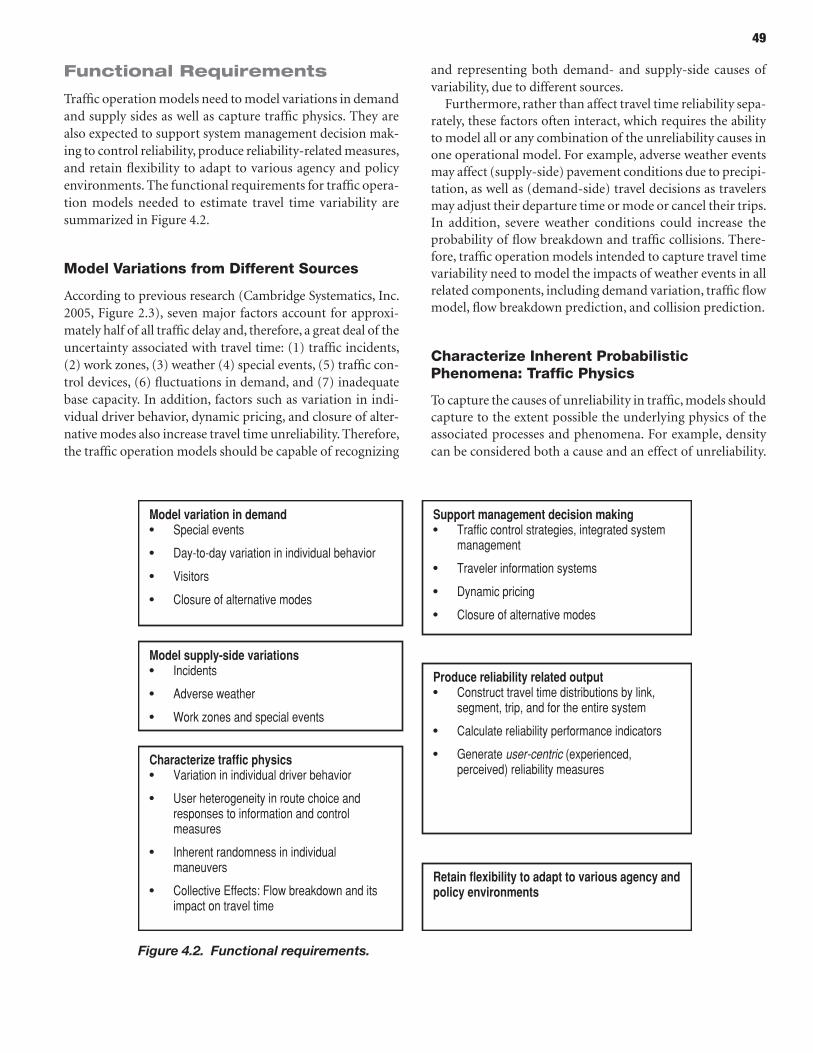
49
Functional requirements
Traffic operation models need to model variations in demand and supply sides as well as capture traffic physics. They are also expected to support system management decision mak-ing to control reliability, produce reliability-related measures, and retain flexibility to adapt to various agency and policy environments. The functional requirements for traffic opera-tion models needed to estimate travel time variability are summarized in Figure 4.2.
Model Variations from Different Sources
According to previous research (Cambridge Systematics, Inc. 2005, Figure 2.3), seven major factors account for approxi-mately half of all traffic delay and, therefore, a great deal of the uncertainty associated with travel time: (1) traffic incidents, (2) work zones, (3) weather (4) special events, (5) traffic con-trol devices, (6) fluctuations in demand, and (7) inadequate base capacity. In addition, factors such as variation in indi-vidual driver behavior, dynamic pricing, and closure of alter-native modes also increase travel time unreliability. Therefore, the traffic operation models should be capable of recognizing
and representing both demand- and supply-side causes of variability, due to different sources.
Furthermore, rather than affect travel time reliability sepa-rately, these factors often interact, which requires the ability to model all or any combination of the unreliability causes in one operational model. For example, adverse weather events may affect (supply-side) pavement conditions due to precipi-tation, as well as (demand-side) travel decisions as travelers may adjust their departure time or mode or cancel their trips. In addition, severe weather conditions could increase the probability of flow breakdown and traffic collisions. There-fore, traffic operation models intended to capture travel time variability need to model the impacts of weather events in all related components, including demand variation, traffic flow model, flow breakdown prediction, and collision prediction.
Characterize Inherent Probabilistic Phenomena: Traffic Physics
To capture the causes of unreliability in traffic, models should capture to the extent possible the underlying physics of the associated processes and phenomena. For example, density can be considered both a cause and an effect of unreliability.
Figure 4.2. Functional requirements.
Model variation in demand • Special events
• Day-to-day variation in individual behavior
• Visitors
• Closure of alternative modes
Model supply-side variations • Incidents
• Adverse weather
• Work zones and special events
Characterize traffic physics • Variation in individual driver behavior
• User heterogeneity in route choice and responses to information and control measures
• Inherent randomness in individual maneuvers
• Collective Effects: Flow breakdown and its impact on travel time
Support management decision making• Traffic control strategies, integrated system
management
• Traveler information systems
• Dynamic pricing
• Closure of alternative modes
Produce reliability related output • Construct travel time distributions by link,
segment, trip, and for the entire system
• Calculate reliability performance indicators
• Generate user-centric (experienced, perceived) reliability measures
Retain flexibility to adapt to various agency and policy environments
50
When density goes above a threshold, the vehicle-to-vehicle interactions become a dominant factor. While density can be considered a result of these other variables, at a certain thresh-old, density might itself be an independent random variable contributing to instability, such as flow breakdown.
In particular, both systematic variations in individual driver behavior and inherent randomness in individual maneuvers—including driver’s choice of speed, gap acceptance, and lane changing—account for considerable observed variability in traffic speeds and resulting travel times. Interdriver behav-ioral differences are essential for capturing certain congestion dynamics. For instance, the presence of aggressive drivers and conservative drivers in the traffic stream gives rise to traffic dis-turbances that may increase in intensity (creating congestion and even traffic breakdowns) or dampen with time (Daganzo 1999). Most critically, these models should capture the col-lective effects that arise from the inherent randomness in driving behavior, namely, flow breakdown and its impact on travel time.
In addition, behavioral models that may be embedded in traffic simulation models need to account for user hetero-geneity in route choice and responses to information and control measures. For example, when provided with travel time information, users could choose whether to react to such information and decide how to evaluate the reliability aspect in choosing their paths.
Support System Management Decision Making
As explained earlier, traffic controls and dynamic pricing affect travel decisions, flow distribution, and thus experienced travel times. Therefore, operations/traffic control strategies and trav-eler information systems need to be incorporated into the modeling process intended to quantify travel time variability. In particular, traffic control strategies can be either explicitly modeled in a microsimulation setting or included implicitly through intersection capacity. In both cases, adaptation/ optimization algorithms can be applied. Alternatively, infor-mation systems could be incorporated into the traffic simula-tion models by emulating the real-time information process and its resulting effect on the route (and possibly departure time in the case of pretrip information) choices of highway users both pretrip and at intermediate points along the trip.
Moreover, traffic management actions, including control strategies, integrated system management, traveler information systems, dynamic pricing, and closure of alternative modes, are essential supply-side actions to alleviate congestion and possi-bly improve travel time reliability. As such, it is essential that traffic operation models be able to represent such actions and capture their impact on system performance.
Produce Reliability-Related Output
The main intended functionality of reliability-sensitive traffic operation models requires the generation of an array of per-formance indicators and figures of merit that allow model users to characterize the existing variability and interpret its impact from the standpoint of the quality of traffic service experienced by users. A general approach to characterizing variability is examining the travel time distribution, which reflects the net result of the combination of recurring and nonrecurring congestion as found in real networks. It is there-fore desirable for the traffic simulation models to produce travel time distributions by link, path, and trip (O–Ds). In addition, these models are expected to produce reliability-related performance measures. In particular, from the sys-tem operator’s perspective, reliability performance indicators for the entire system should allow comparison of different network alternatives and policy and operational scenarios. This could facilitate decision making in regard to actions intended to control reliability and evaluation of system per-formance. In addition, it is essential to reflect the user’s point of view, by producing user-centric reliability measures, which describe user experienced or perceived travel time reliability. The reliability-related output processing is realized through the vehicle Trajectory Processor, which is discussed in detail in Chapter 7.
Retain Flexibility to Adapt to Various Agency and Policy Environments
As the ultimate goal of this project is to develop practical operational tools that could be eventually applied by metro-politan planning organizations (MPOs), departments of transportation (DOTs), and other agencies for testing pro-posed projects and policies, the developed approaches need to be designed in a flexible way to adapt to various agency and policy environments. This means application to a range of problems in terms of geographic scope, time frame, stage in the development process, and target impact. As such, incor-porating reliability is of interest for both planning and opera-tions applications, as well as for operational planning activities. As noted previously, this means having sensitivity to an array of policy interventions and operational measures, including various highway pricing options such as real-time adaptive pricing. Real-time adaptive pricing is considered a particularly promising strategy to regulate travel demand and improve reliability of the highway system. In addition, the operations models need to recognize the primary applications for which reliability information may be required, calibration require-ments, and ability/needs of typical agencies to leverage such capabilities.
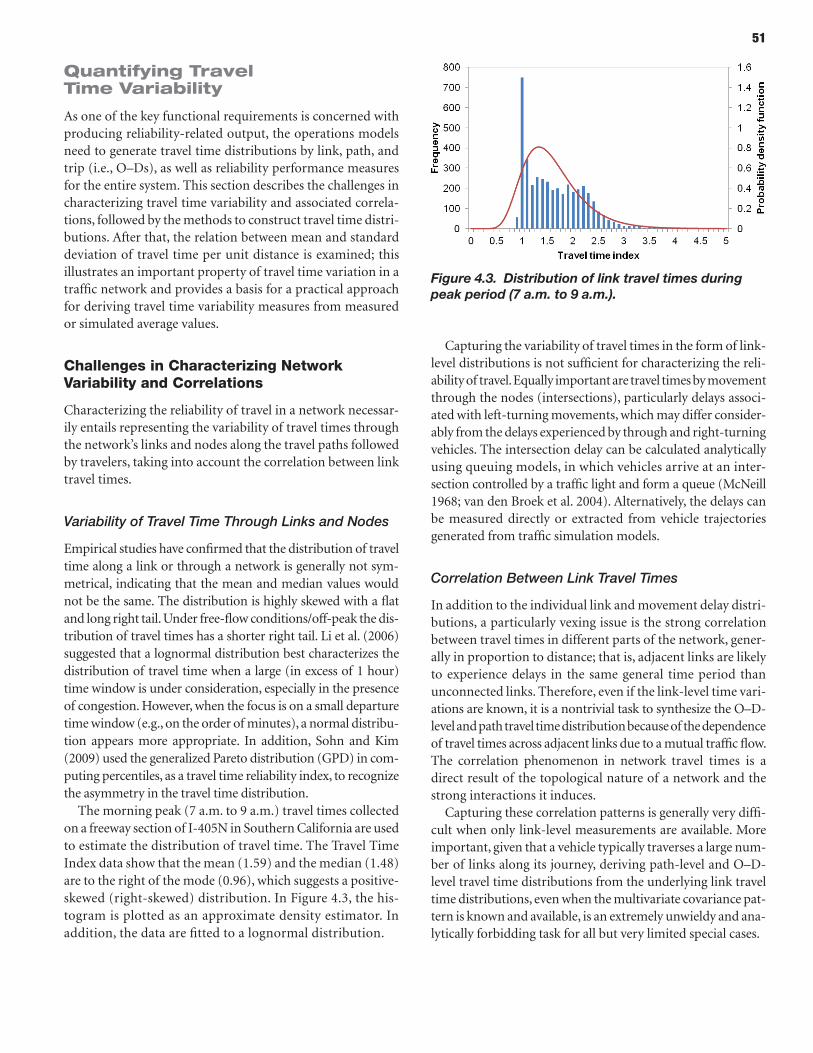
51
Quantifying Travel Time Variability
As one of the key functional requirements is concerned with producing reliability-related output, the operations models need to generate travel time distributions by link, path, and trip (i.e., O–Ds), as well as reliability performance measures for the entire system. This section describes the challenges in characterizing travel time variability and associated correla-tions, followed by the methods to construct travel time distri-butions. After that, the relation between mean and standard deviation of travel time per unit distance is examined; this illustrates an important property of travel time variation in a traffic network and provides a basis for a practical approach for deriving travel time variability measures from measured or simulated average values.
Challenges in Characterizing Network Variability and Correlations
Characterizing the reliability of travel in a network necessar-ily entails representing the variability of travel times through the network’s links and nodes along the travel paths followed by travelers, taking into account the correlation between link travel times.
Variability of Travel Time Through Links and Nodes
Empirical studies have confirmed that the distribution of travel time along a link or through a network is generally not sym-metrical, indicating that the mean and median values would not be the same. The distribution is highly skewed with a flat and long right tail. Under free-flow conditions/off-peak the dis-tribution of travel times has a shorter right tail. Li et al. (2006) suggested that a lognormal distribution best characterizes the distribution of travel time when a large (in excess of 1 hour) time window is under consideration, especially in the presence of congestion. However, when the focus is on a small departure time window (e.g., on the order of minutes), a normal distribu-tion appears more appropriate. In addition, Sohn and Kim (2009) used the generalized Pareto distribution (GPD) in com-puting percentiles, as a travel time reliability index, to recognize the asymmetry in the travel time distribution.
The morning peak (7 a.m. to 9 a.m.) travel times collected on a freeway section of I-405N in Southern California are used to estimate the distribution of travel time. The Travel Time Index data show that the mean (1.59) and the median (1.48) are to the right of the mode (0.96), which suggests a positive-skewed (right-skewed) distribution. In Figure 4.3, the his-togram is plotted as an approximate density estimator. In addition, the data are fitted to a lognormal distribution.
Capturing the variability of travel times in the form of link-level distributions is not sufficient for characterizing the reli-ability of travel. Equally important are travel times by movement through the nodes (intersections), particularly delays associ-ated with left-turning movements, which may differ consider-ably from the delays experienced by through and right-turning vehicles. The intersection delay can be calculated analytically using queuing models, in which vehicles arrive at an inter-section controlled by a traffic light and form a queue (McNeill 1968; van den Broek et al. 2004). Alternatively, the delays can be measured directly or extracted from vehicle trajectories generated from traffic simulation models.
Correlation Between Link Travel Times
In addition to the individual link and movement delay distri-butions, a particularly vexing issue is the strong correlation between travel times in different parts of the network, gener-ally in proportion to distance; that is, adjacent links are likely to experience delays in the same general time period than unconnected links. Therefore, even if the link-level time vari-ations are known, it is a nontrivial task to synthesize the O–D-level and path travel time distribution because of the dependence of travel times across adjacent links due to a mutual traffic flow. The correlation phenomenon in network travel times is a direct result of the topological nature of a network and the strong interactions it induces.
Capturing these correlation patterns is generally very diffi-cult when only link-level measurements are available. More important, given that a vehicle typically traverses a large num-ber of links along its journey, deriving path-level and O–D-level travel time distributions from the underlying link travel time distributions, even when the multivariate covariance pat-tern is known and available, is an extremely unwieldy and ana-lytically forbidding task for all but very limited special cases.
Figure 4.3. Distribution of link travel times during peak period (7 a.m. to 9 a.m.).
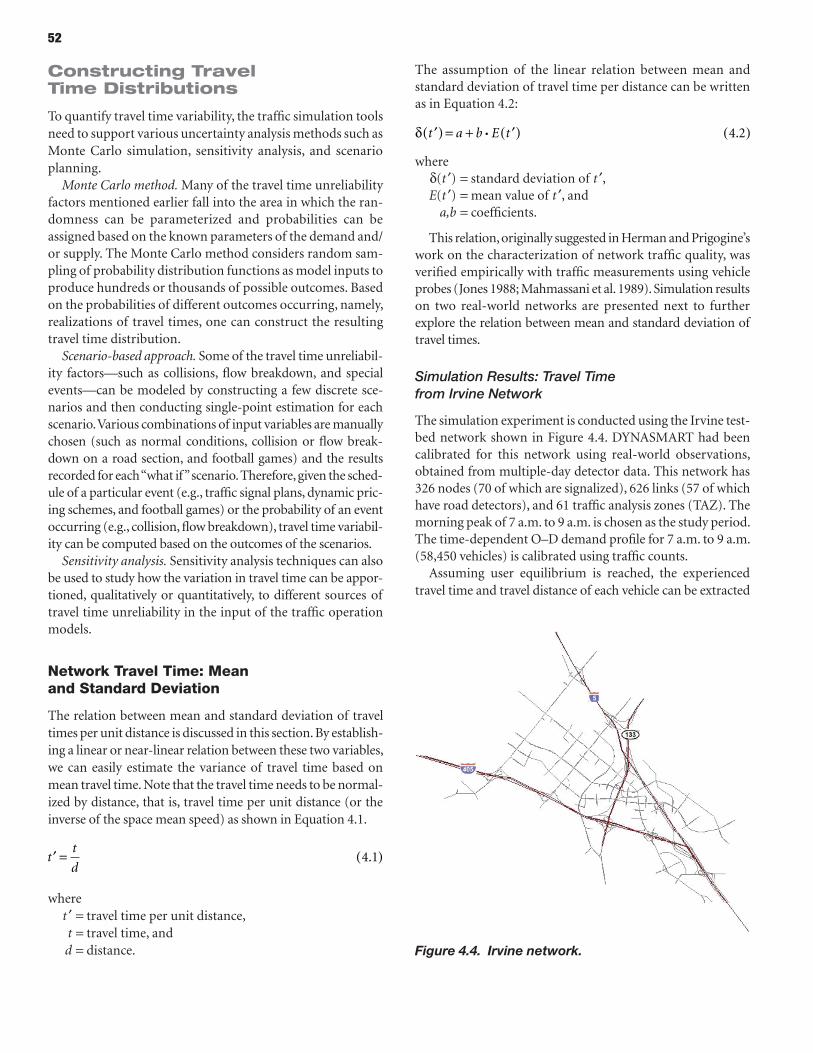
52
Constructing Travel Time Distributions
To quantify travel time variability, the traffic simulation tools need to support various uncertainty analysis methods such as Monte Carlo simulation, sensitivity analysis, and scenario planning.
Monte Carlo method. Many of the travel time unreliability factors mentioned earlier fall into the area in which the ran-domness can be parameterized and probabilities can be assigned based on the known parameters of the demand and/or supply. The Monte Carlo method considers random sam-pling of probability distribution functions as model inputs to produce hundreds or thousands of possible outcomes. Based on the probabilities of different outcomes occurring, namely, realizations of travel times, one can construct the resulting travel time distribution.
Scenario-based approach. Some of the travel time unreliabil-ity factors—such as collisions, flow breakdown, and special events—can be modeled by constructing a few discrete sce-narios and then conducting single-point estimation for each scenario. Various combinations of input variables are manually chosen (such as normal conditions, collision or flow break-down on a road section, and football games) and the results recorded for each “what if” scenario. Therefore, given the sched-ule of a particular event (e.g., traffic signal plans, dynamic pric-ing schemes, and football games) or the probability of an event occurring (e.g., collision, flow breakdown), travel time variabil-ity can be computed based on the outcomes of the scenarios.
Sensitivity analysis. Sensitivity analysis techniques can also be used to study how the variation in travel time can be appor-tioned, qualitatively or quantitatively, to different sources of travel time unreliability in the input of the traffic operation models.
Network Travel Time: Mean and Standard Deviation
The relation between mean and standard deviation of travel times per unit distance is discussed in this section. By establish-ing a linear or near-linear relation between these two variables, we can easily estimate the variance of travel time based on mean travel time. Note that the travel time needs to be normal-ized by distance, that is, travel time per unit distance (or the inverse of the space mean speed) as shown in Equation 4.1.
4.1tt
d( )′ =
where t ′ = travel time per unit distance, t = travel time, and d = distance.
The assumption of the linear relation between mean and standard deviation of travel time per distance can be written as in Equation 4.2:
( ) ( ) ( )δ ′ = + ′ 4.2t a b E ti
where d(t ′) = standard deviation of t ′, E(t ′) = mean value of t ′, and a,b = coefficients.
This relation, originally suggested in Herman and Prigogine’s work on the characterization of network traffic quality, was verified empirically with traffic measurements using vehicle probes (Jones 1988; Mahmassani et al. 1989). Simulation results on two real-world networks are presented next to further explore the relation between mean and standard deviation of travel times.
Simulation Results: Travel Time from Irvine Network
The simulation experiment is conducted using the Irvine test-bed network shown in Figure 4.4. DYNASMART had been calibrated for this network using real-world observations, obtained from multiple-day detector data. This network has 326 nodes (70 of which are signalized), 626 links (57 of which have road detectors), and 61 traffic analysis zones (TAZ). The morning peak of 7 a.m. to 9 a.m. is chosen as the study period. The time-dependent O–D demand profile for 7 a.m. to 9 a.m. (58,450 vehicles) is calibrated using traffic counts.
Assuming user equilibrium is reached, the experienced travel time and travel distance of each vehicle can be extracted
Figure 4.4. Irvine network.
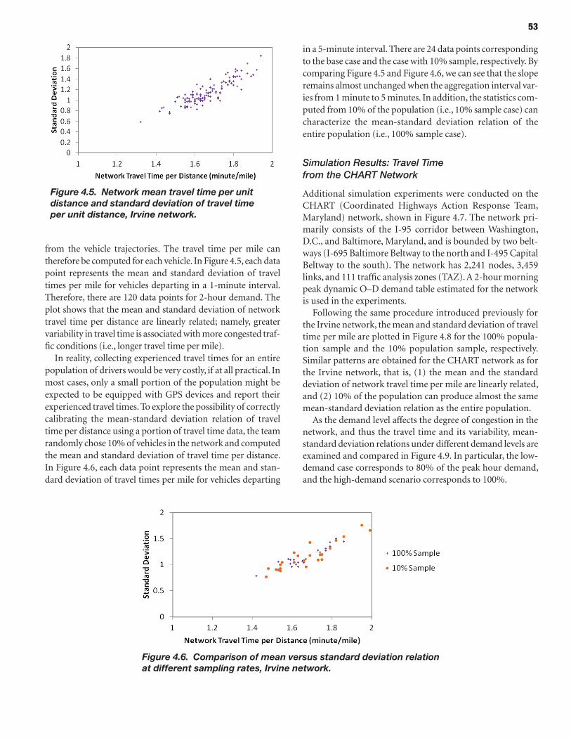
53
from the vehicle trajectories. The travel time per mile can therefore be computed for each vehicle. In Figure 4.5, each data point represents the mean and standard deviation of travel times per mile for vehicles departing in a 1-minute interval. Therefore, there are 120 data points for 2-hour demand. The plot shows that the mean and standard deviation of network travel time per distance are linearly related; namely, greater variability in travel time is associated with more congested traf-fic conditions (i.e., longer travel time per mile).
In reality, collecting experienced travel times for an entire population of drivers would be very costly, if at all practical. In most cases, only a small portion of the population might be expected to be equipped with GPS devices and report their experienced travel times. To explore the possibility of correctly calibrating the mean-standard deviation relation of travel time per distance using a portion of travel time data, the team randomly chose 10% of vehicles in the network and computed the mean and standard deviation of travel time per distance. In Figure 4.6, each data point represents the mean and stan-dard deviation of travel times per mile for vehicles departing
in a 5-minute interval. There are 24 data points corresponding to the base case and the case with 10% sample, respectively. By comparing Figure 4.5 and Figure 4.6, we can see that the slope remains almost unchanged when the aggregation interval var-ies from 1 minute to 5 minutes. In addition, the statistics com-puted from 10% of the population (i.e., 10% sample case) can characterize the mean-standard deviation relation of the entire population (i.e., 100% sample case).
Simulation Results: Travel Time from the CHART Network
Additional simulation experiments were conducted on the CHART (Coordinated Highways Action Response Team, Maryland) network, shown in Figure 4.7. The network pri-marily consists of the I-95 corridor between Washington, D.C., and Baltimore, Maryland, and is bounded by two belt-ways (I-695 Baltimore Beltway to the north and I-495 Capital Beltway to the south). The network has 2,241 nodes, 3,459 links, and 111 traffic analysis zones (TAZ). A 2-hour morning peak dynamic O–D demand table estimated for the network is used in the experiments.
Following the same procedure introduced previously for the Irvine network, the mean and standard deviation of travel time per mile are plotted in Figure 4.8 for the 100% popula-tion sample and the 10% population sample, respectively. Similar patterns are obtained for the CHART network as for the Irvine network, that is, (1) the mean and the standard deviation of network travel time per mile are linearly related, and (2) 10% of the population can produce almost the same mean-standard deviation relation as the entire population.
As the demand level affects the degree of congestion in the network, and thus the travel time and its variability, mean-standard deviation relations under different demand levels are examined and compared in Figure 4.9. In particular, the low-demand case corresponds to 80% of the peak hour demand, and the high-demand scenario corresponds to 100%.
Figure 4.5. Network mean travel time per unit distance and standard deviation of travel time per unit distance, Irvine network.
Figure 4.6. Comparison of mean versus standard deviation relation at different sampling rates, Irvine network.
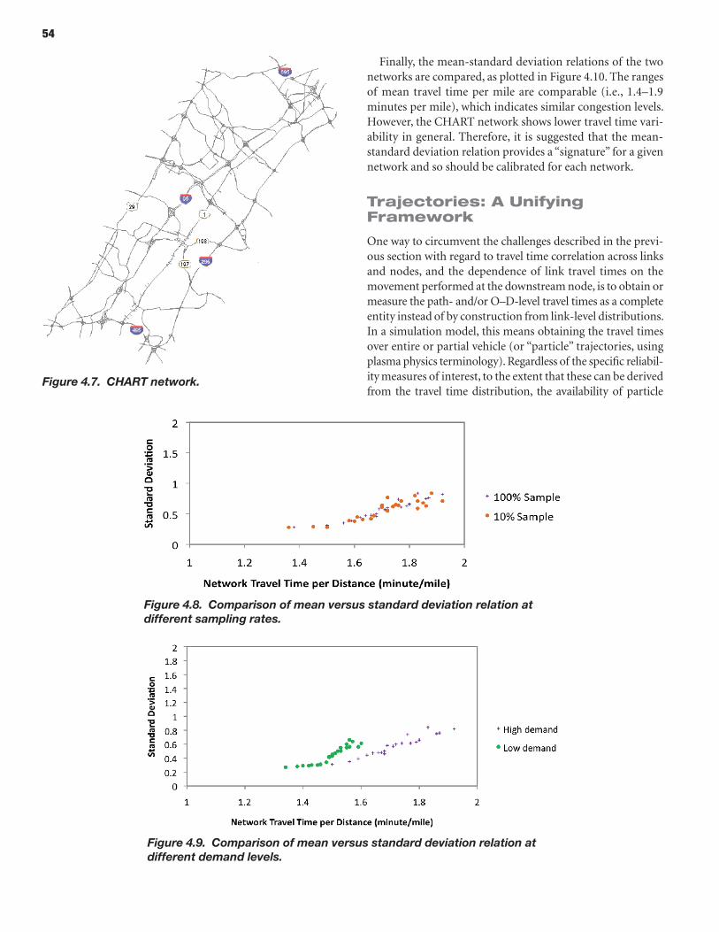
54
Figure 4.7. CHART network.
Figure 4.8. Comparison of mean versus standard deviation relation at different sampling rates.
Figure 4.9. Comparison of mean versus standard deviation relation at different demand levels.
Finally, the mean-standard deviation relations of the two networks are compared, as plotted in Figure 4.10. The ranges of mean travel time per mile are comparable (i.e., 1.4–1.9 minutes per mile), which indicates similar congestion levels. However, the CHART network shows lower travel time vari-ability in general. Therefore, it is suggested that the mean-standard deviation relation provides a “signature” for a given network and so should be calibrated for each network.
Trajectories: A Unifying Framework
One way to circumvent the challenges described in the previ-ous section with regard to travel time correlation across links and nodes, and the dependence of link travel times on the movement performed at the downstream node, is to obtain or measure the path- and/or O–D-level travel times as a complete entity instead of by construction from link-level distributions. In a simulation model, this means obtaining the travel times over entire or partial vehicle (or “particle” trajectories, using plasma physics terminology). Regardless of the specific reliabil-ity measures of interest, to the extent that these can be derived from the travel time distribution, the availability of particle
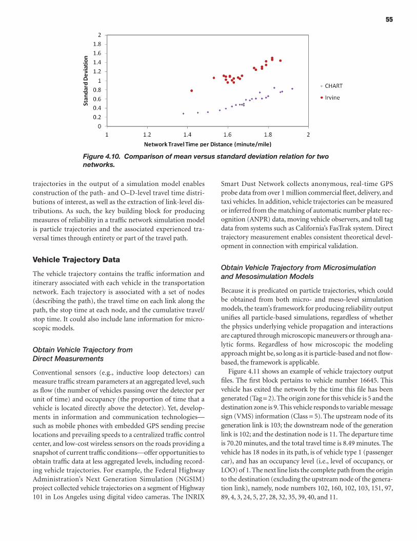
55
trajectories in the output of a simulation model enables construction of the path- and O–D-level travel time distri-butions of interest, as well as the extraction of link-level dis-tributions. As such, the key building block for producing measures of reliability in a traffic network simulation model is particle trajectories and the associated experienced tra-versal times through entirety or part of the travel path.
Vehicle Trajectory Data
The vehicle trajectory contains the traffic information and itinerary associated with each vehicle in the transportation network. Each trajectory is associated with a set of nodes (describing the path), the travel time on each link along the path, the stop time at each node, and the cumulative travel/stop time. It could also include lane information for micro-scopic models.
Obtain Vehicle Trajectory from Direct Measurements
Conventional sensors (e.g., inductive loop detectors) can measure traffic stream parameters at an aggregated level, such as flow (the number of vehicles passing over the detector per unit of time) and occupancy (the proportion of time that a vehicle is located directly above the detector). Yet, develop-ments in information and communication technologies—such as mobile phones with embedded GPS sending precise locations and prevailing speeds to a centralized traffic control center, and low-cost wireless sensors on the roads providing a snapshot of current traffic conditions—offer opportunities to obtain traffic data at less aggregated levels, including record-ing vehicle trajectories. For example, the Federal Highway Administration’s Next Generation Simulation (NGSIM) project collected vehicle trajectories on a segment of Highway 101 in Los Angeles using digital video cameras. The INRIX
Smart Dust Network collects anonymous, real-time GPS probe data from over 1 million commercial fleet, delivery, and taxi vehicles. In addition, vehicle trajectories can be measured or inferred from the matching of automatic number plate rec-ognition (ANPR) data, moving vehicle observers, and toll tag data from systems such as California’s FasTrak system. Direct trajectory measurement enables consistent theoretical devel-opment in connection with empirical validation.
Obtain Vehicle Trajectory from Microsimulation and Mesosimulation Models
Because it is predicated on particle trajectories, which could be obtained from both micro- and meso-level simulation models, the team’s framework for producing reliability output unifies all particle-based simulations, regardless of whether the physics underlying vehicle propagation and interactions are captured through microscopic maneuvers or through ana-lytic forms. Regardless of how microscopic the modeling approach might be, so long as it is particle-based and not flow-based, the framework is applicable.
Figure 4.11 shows an example of vehicle trajectory output files. The first block pertains to vehicle number 16645. This vehicle has exited the network by the time this file has been generated (Tag = 2). The origin zone for this vehicle is 5 and the destination zone is 9. This vehicle responds to variable message sign (VMS) information (Class = 5). The upstream node of its generation link is 103; the downstream node of the generation link is 102; and the destination node is 11. The departure time is 70.20 minutes, and the total travel time is 8.49 minutes. The vehicle has 18 nodes in its path, is of vehicle type 1 (passenger car), and has an occupancy level (i.e., level of occupancy, or LOO) of 1. The next line lists the complete path from the origin to the destination (excluding the upstream node of the genera-tion link), namely, node numbers 102, 160, 102, 103, 151, 97, 89, 4, 3, 24, 5, 27, 28, 32, 35, 39, 40, and 11.
Figure 4.10. Comparison of mean versus standard deviation relation for two networks.
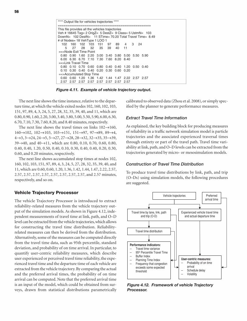
56
The next line shows the time instance, relative to the depar-ture time, at which the vehicle exited nodes 102, 160, 102, 103, 151, 97, 89, 4, 3, 24, 5, 27, 28, 32, 35, 39, 40, and 11, which are 0.80, 0.90, 1.60, 2.20, 3.00, 3.40, 3.80, 5.00, 5.50, 5.90, 6.00, 6.30, 6.70, 7.10, 7.30, 7.60, 8.20, and 8.40 minutes, respectively.
The next line shows the travel times on links 102→160, 160→102, 102→103, 103→151, 151→97, 97→89, 89→4, 4→3, 3→24, 24→5, 5→27, 27→28, 28→32, 32→35, 35→39, 39→40, and 40→11, which are 0.80, 0.10, 0.70, 0.60, 0.80, 0.40, 0.40, 1.20, 0.50, 0.40, 0.10, 0.30, 0.40, 0.40, 0.20, 0.30, 0.60, and 0.20 minutes, respectively.
The next line shows accumulated stop times at nodes 102, 160, 102, 103, 151, 97, 89, 4, 3, 24, 5, 27, 28, 32, 35, 39, 40, and 11, which are 0.60, 0.60, 1.20, 1.36, 1.42, 1.44, 1.47, 2.22, 2.57, 2.57, 2.57, 2.57, 2.57, 2.57, 2.57, 2.57, 2.57, and 2.57 minutes, respectively, and so on.
Vehicle Trajectory Processor
The vehicle Trajectory Processor is introduced to extract reliability-related measures from the vehicle trajectory out-put of the simulation models. As shown in Figure 4.12, inde-pendent measurements of travel time at link, path, and O–D level can be extracted from the vehicle trajectories, which allows for constructing the travel time distribution. Reliability-related measures can then be derived from the distribution. Alternatively, some of the measures can be computed directly from the travel time data, such as 95th percentile, standard deviation, and probability of on time arrival. In particular, to quantify user-centric reliability measures, which describe user experienced or perceived travel time reliability, the expe-rienced travel time and the departure time of each vehicle are extracted from the vehicle trajectory. By comparing the actual and the preferred arrival times, the probability of on time arrival can be computed. Note that the preferred arrival time is an input of the model, which could be obtained from sur-veys, drawn from statistical distributions parametrically
calibrated to observed data (Zhou et al. 2008), or simply spec-ified by the planner to generate performance measures.
Extract Travel Time Information
As explained, the key building block for producing measures of reliability in a traffic network simulation model is particle trajectories and the associated experienced traversal times through entirety or part of the travel path. Travel time vari-ability at link, path, and O–D levels can be extracted from the trajectories generated by micro- or mesosimulation models.
Construction of Travel Time Distribution
To produce travel time distributions by link, path, and trip (O–Ds) using simulation models, the following procedures are suggested.
Figure 4.11. Example of vehicle trajectory output.
**** Output file for vehicles trajectories **** ================================================= This file provides all the vehicles trajectories Veh # 16645 Tag= 2 OrigZ= 5 DestZ= 9 Class= 5 UstmN= 103 DownN= 102 DestN= 11 STime= 70.20 Total Travel Time= 8.49 # of Nodes= 18 VehType 1 LOO 1 102 160 102 103 151 97 89 4 3 24 5 27 28 32 35 39 40 11 ==>Node Exit Time Point 0.80 0.90 1.60 2.20 3.00 3.40 3.80 5.00 5.50 5.90 6.00 6.30 6.70 7.10 7.30 7.60 8.20 8.40 ==>Link Travel Time 0.80 0.10 0.70 0.60 0.80 0.40 0.40 1.20 0.50 0.40 0.10 0.30 0.40 0.40 0.20 0.30 0.60 0.20 ==>Accumulated Stop Time 0.60 0.60 1.20 1.36 1.42 1.44 1.47 2.22 2.57 2.57 2.57 2.57 2.57 2.57 2.57 2.57 2.57 2.57
Figure 4.12. Framework of vehicle Trajectory Processor.
Travel time distribution
Performance indicators:– Travel time variance – 95th Percentile Travel Time – Buffer Index – Planning Time Index – Frequency that congestion
exceeds some expected threshold
Vehicle trajectories
Travel time by lane, link, path and trip (O-D)
User-centric measures: – Probability of on time
arrival– Schedule delay – Volatility
Experienced vehicle travel time and actual departure time
Preferred arrival time
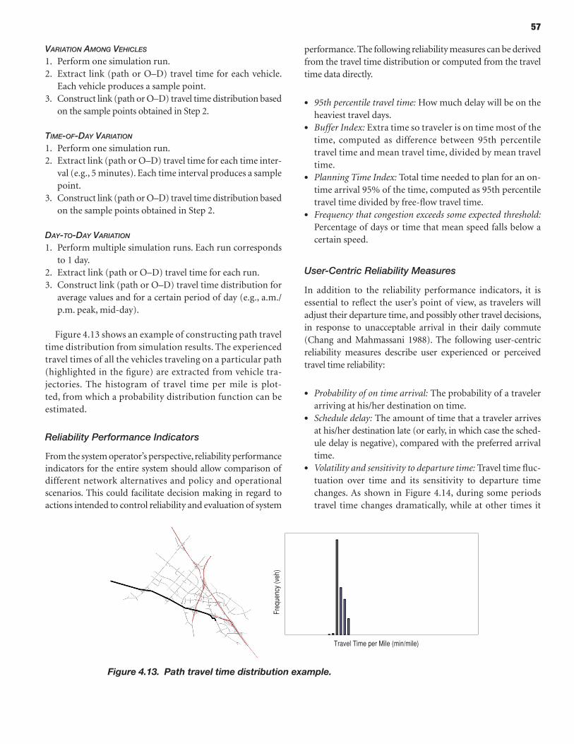
57
Variation among Vehicles
1. Perform one simulation run.2. Extract link (path or O–D) travel time for each vehicle.
Each vehicle produces a sample point.3. Construct link (path or O–D) travel time distribution based
on the sample points obtained in Step 2.
time-of-Day Variation
1. Perform one simulation run.2. Extract link (path or O–D) travel time for each time inter-
val (e.g., 5 minutes). Each time interval produces a sample point.
3. Construct link (path or O–D) travel time distribution based on the sample points obtained in Step 2.
Day-to-Day Variation
1. Perform multiple simulation runs. Each run corresponds to 1 day.
2. Extract link (path or O–D) travel time for each run.3. Construct link (path or O–D) travel time distribution for
average values and for a certain period of day (e.g., a.m./p.m. peak, mid-day).
Figure 4.13 shows an example of constructing path travel time distribution from simulation results. The experienced travel times of all the vehicles traveling on a particular path (highlighted in the figure) are extracted from vehicle tra-jectories. The histogram of travel time per mile is plot-ted, from which a probability distribution function can be estimated.
Reliability Performance Indicators
From the system operator’s perspective, reliability performance indicators for the entire system should allow comparison of different network alternatives and policy and operational scenarios. This could facilitate decision making in regard to actions intended to control reliability and evaluation of system
performance. The following reliability measures can be derived from the travel time distribution or computed from the travel time data directly.
• 95th percentile travel time: How much delay will be on the heaviest travel days.
• Buffer Index: Extra time so traveler is on time most of the time, computed as difference between 95th percentile travel time and mean travel time, divided by mean travel time.
• Planning Time Index: Total time needed to plan for an on-time arrival 95% of the time, computed as 95th percentile travel time divided by free-flow travel time.
• Frequency that congestion exceeds some expected threshold: Percentage of days or time that mean speed falls below a certain speed.
User-Centric Reliability Measures
In addition to the reliability performance indicators, it is essential to reflect the user’s point of view, as travelers will adjust their departure time, and possibly other travel decisions, in response to unacceptable arrival in their daily commute (Chang and Mahmassani 1988). The following user-centric reliability measures describe user experienced or perceived travel time reliability:
• Probability of on time arrival: The probability of a traveler arriving at his/her destination on time.
• Schedule delay: The amount of time that a traveler arrives at his/her destination late (or early, in which case the sched-ule delay is negative), compared with the preferred arrival time.
• Volatility and sensitivity to departure time: Travel time fluc-tuation over time and its sensitivity to departure time changes. As shown in Figure 4.14, during some periods travel time changes dramatically, while at other times it
Figure 4.13. Path travel time distribution example.
Freq
uenc
y (v
eh)
Travel Time per Mile (min/mile)
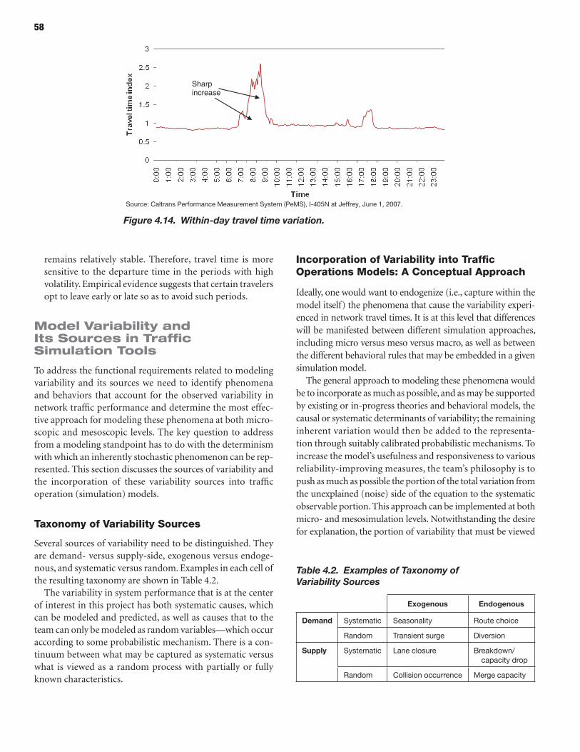
58
remains relatively stable. Therefore, travel time is more sensitive to the departure time in the periods with high volatility. Empirical evidence suggests that certain travelers opt to leave early or late so as to avoid such periods.
Model Variability and Its Sources in traffic Simulation tools
To address the functional requirements related to modeling variability and its sources we need to identify phenomena and behaviors that account for the observed variability in network traffic performance and determine the most effec-tive approach for modeling these phenomena at both micro-scopic and mesoscopic levels. The key question to address from a modeling standpoint has to do with the determinism with which an inherently stochastic phenomenon can be rep-resented. This section discusses the sources of variability and the incorporation of these variability sources into traffic operation (simulation) models.
Taxonomy of Variability Sources
Several sources of variability need to be distinguished. They are demand- versus supply-side, exogenous versus endoge-nous, and systematic versus random. Examples in each cell of the resulting taxonomy are shown in Table 4.2.
The variability in system performance that is at the center of interest in this project has both systematic causes, which can be modeled and predicted, as well as causes that to the team can only be modeled as random variables—which occur according to some probabilistic mechanism. There is a con-tinuum between what may be captured as systematic versus what is viewed as a random process with partially or fully known characteristics.
Incorporation of Variability into Traffic Operations Models: A Conceptual Approach
Ideally, one would want to endogenize (i.e., capture within the model itself) the phenomena that cause the variability experi-enced in network travel times. It is at this level that differences will be manifested between different simulation approaches, including micro versus meso versus macro, as well as between the different behavioral rules that may be embedded in a given simulation model.
The general approach to modeling these phenomena would be to incorporate as much as possible, and as may be supported by existing or in-progress theories and behavioral models, the causal or systematic determinants of variability; the remaining inherent variation would then be added to the representa-tion through suitably calibrated probabilistic mechanisms. To increase the model’s usefulness and responsiveness to various reliability-improving measures, the team’s philosophy is to push as much as possible the portion of the total variation from the unexplained (noise) side of the equation to the systematic observable portion. This approach can be implemented at both micro- and mesosimulation levels. Notwithstanding the desire for explanation, the portion of variability that must be viewed
Table 4.2. Examples of Taxonomy of Variability Sources
exogenous endogenous
Demand Systematic Seasonality Route choice
Random Transient surge diversion
Supply Systematic lane closure Breakdown/ capacity drop
Random collision occurrence Merge capacity
Figure 4.14. Within-day travel time variation.
Sharp increase
Source: Caltrans Performance Measurement System (PeMS), I-405N at Jeffrey, June 1, 2007.
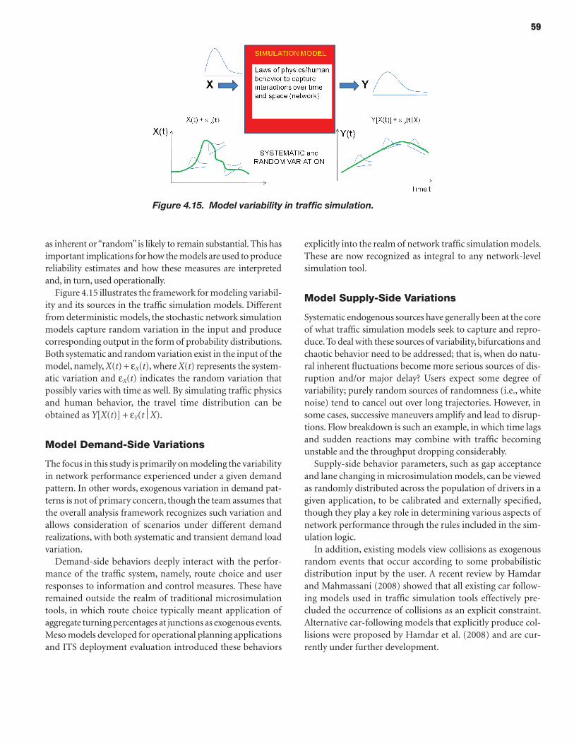
59
as inherent or “random” is likely to remain substantial. This has important implications for how the models are used to produce reliability estimates and how these measures are interpreted and, in turn, used operationally.
Figure 4.15 illustrates the framework for modeling variabil-ity and its sources in the traffic simulation models. Different from deterministic models, the stochastic network simulation models capture random variation in the input and produce corresponding output in the form of probability distributions. Both systematic and random variation exist in the input of the model, namely, X(t) + eX(t), where X(t) represents the system-atic variation and eX(t) indicates the random variation that possibly varies with time as well. By simulating traffic physics and human behavior, the travel time distribution can be obtained as Y[X(t)] + eY(tX).
Model Demand-Side Variations
The focus in this study is primarily on modeling the variability in network performance experienced under a given demand pattern. In other words, exogenous variation in demand pat-terns is not of primary concern, though the team assumes that the overall analysis framework recognizes such variation and allows consideration of scenarios under different demand realizations, with both systematic and transient demand load variation.
Demand-side behaviors deeply interact with the perfor-mance of the traffic system, namely, route choice and user responses to information and control measures. These have remained outside the realm of traditional microsimulation tools, in which route choice typically meant application of aggregate turning percentages at junctions as exogenous events. Meso models developed for operational planning applications and ITS deployment evaluation introduced these behaviors
explicitly into the realm of network traffic simulation models. These are now recognized as integral to any network-level simulation tool.
Model Supply-Side Variations
Systematic endogenous sources have generally been at the core of what traffic simulation models seek to capture and repro-duce. To deal with these sources of variability, bifurcations and chaotic behavior need to be addressed; that is, when do natu-ral inherent fluctuations become more serious sources of dis-ruption and/or major delay? Users expect some degree of variability; purely random sources of randomness (i.e., white noise) tend to cancel out over long trajectories. However, in some cases, successive maneuvers amplify and lead to disrup-tions. Flow breakdown is such an example, in which time lags and sudden reactions may combine with traffic becoming unstable and the throughput dropping considerably.
Supply-side behavior parameters, such as gap acceptance and lane changing in microsimulation models, can be viewed as randomly distributed across the population of drivers in a given application, to be calibrated and externally specified, though they play a key role in determining various aspects of network performance through the rules included in the sim-ulation logic.
In addition, existing models view collisions as exogenous random events that occur according to some probabilistic distribution input by the user. A recent review by Hamdar and Mahmassani (2008) showed that all existing car follow-ing models used in traffic simulation tools effectively pre-cluded the occurrence of collisions as an explicit constraint. Alternative car-following models that explicitly produce col-lisions were proposed by Hamdar et al. (2008) and are cur-rently under further development.
Figure 4.15. Model variability in traffic simulation.
61
FRAMEWORK AND TOOLS FOR TRAVEL TIME RELIABILITY ANALYSIS
This part of the report describes the modeling tools and the general methodology/process of how to use the tools and interpret the results.
p A r t 2
62
Scenario Manager
The Scenario Manager is essentially a preprocessor of simula-tion input files for capturing exogenous sources of travel time variation. Recognizing the importance of the scenario defini-tion and the complexity of identifying relevant exogenous sources, the Scenario Manager provides the ability to construct scenarios that entail any mutually consistent combination of external events. These may be both demand- and supply-related events, including different traffic control plans that may be deployed under certain conditions. Accordingly, it captures parameters that define external sources of unreliability (such as special events, adverse weather, and work zones) and enables users either to specify scenarios with particular historical sig-nificance or policy interest, or to generate them randomly given the underlying stochastic processes with specific characteristics (parameters) following a particular experimental design.
The built-in Monte Carlo sampling functionality allows the Scenario Manager to generate hypothetical scenarios for analy-sis and design purposes. When exercised in the latter manner (i.e., in random generation mode), the Scenario Manager becomes the primary platform for conducting reliability analy-ses: experiments are conducted to replicate certain field condi-tions, under both actual and hypothetical (proposed) network and control scenarios. In particular, the Scenario Manager enables execution of experimental designs that entail simula-tion over multiple days, thus reflecting daily fluctuations in demand, both systematic and random.
The Scenario Manager also allows users to manage the conduct of reliability analyses by providing an environment for storage and retrieval of previously generated scenarios, through a scenario library approach. The scenario manage-ment functionality allows retrieval of historically occurring scenarios or of previously constructed scenarios as part of a planning exercise (e.g., in conjunction with emergency pre-paredness planning). Given a particular scenario, the Scenario Manager’s main function then is to prepare input files for
The travel time reliability analysis framework incorporates two essential tools that provide the capability to produce reli-ability performance measures as output from operational planning and simulation models. The Scenario Manager, an integral component of the overall analytical framework, cap-tures external unreliability sources such as special events, adverse weather, and work zones, and generates appropriate files as input into simulation models. The other key analysis tool is a vehicle Trajectory Processor that calculates and visu-alizes travel time distributions and associated reliability indi-cators (such as 95th percentile travel time, Buffer Time Index, Planning Time Index, frequency that congestion exceeds some threshold) at link, path, O–D, and network levels.
The travel time distributions and associated indicators are derived from individual vehicle trajectories, defined as sequence of geographic positions (nodes) and associated passage times. These trajectories are obtained as output from particle-based microscopic or mesoscopic simulation tools. Such trajectories may alternatively be obtained directly through measurement (e.g., GPS-equipped probe vehicles), thereby also enabling vali-dation of travel time reliability metrics generated on the basis of output from simulation tools.
It should be noted that both the Scenario Manager and the Trajectory Processor have been developed at a prototype level of detail and functionality for project team use only and are shared with the developer and user community on an “as is” basis. For this reason, they may not meet all requirements of an implementing agency without further development.
A prerequisite for the use of these analysis tools is the avail-ability of a particle-based traffic simulation model, capable of producing vehicle trajectory output. It is further assumed that the simulation model is fully calibrated to reasonably simulate traffic flows. For demonstration purposes, the Sce-nario Manager and Trajectory Processor prototypes incorpo-rate interfaces to the Aimsun and DYNASMART-P simulation platforms, as examples of microscopic and mesoscopic tools, respectively.
Model and Data Requirements
C h A p t e r 5
63
quantify user-centric reliability measures, the experienced travel time and the departure time of each vehicle are extracted from the vehicle trajectory. By comparing the actual and the preferred arrival time, the probability of on-time arrival can be computed.
data requirements
This section provides a brief discussion of the types of data needed to implement the proposed reliability analysis frame-work. This discussion assumes that a base simulation model is already developed and properly validated, and focuses on (a) data required for the development of scenarios for reliability analysis, and (b) data required to refine/adapt the simulation model and/or to perform travel time reliability analysis based on observed congestion conditions.
As indicated, numerous external factors can affect varia-tions in travel time. To consider these factors in the compre-hensive methodology, extensive background data are required. These includes collision data, weather data, and event data encompassing lane closures, work zones, and other incidents affecting normal traffic flow. In addition, historical vehicle traffic volumes and background travel demand for other sce-narios are important in being able to simulate events that may cause changes in travel patterns or the overall level of traffic demand. Desirable data also include trajectory data from GPS or other probe vehicle sources. These data can be processed to provide valuable information regarding actual trip travel times (portions of trips) through the study area, thus allowing comparisons to simulated data.
Data for Scenario-Based Analysis
The reliability analysis framework addresses a number of sources of travel time variability under both recurring and nonrecurring congestion conditions, whether these affect the demand or supply side of the transportation system, in a ran-dom or systematic manner, endogenously or exogenously to the involved modeling tools.
In general, data are needed to parameterize factors that will be captured endogenously in the model(s), whether on the demand or supply side of the system. For example, speed, flow, and occupancy data can be used to describe character-istics relevant to flow breakdown conditions (jam density, and so forth); locations, time, and pricing applicable by vehi-cle class and type (truck, bus, high-occupancy vehicle/single-occupancy vehicle) would be needed to incorporate dynamic pricing schemes; event logs and observed or estimated com-pliance rates may also be needed to capture user responses to information and control measures.
For the proposed scenario-based analysis in particular, data are needed to generate scenarios for factors causing travel time
mesoscopic/microscopic simulation models. In addition, the Scenario Manager can facilitate direct execution of the simulation software for a particular scenario, by creating the necessary inputs that reflect the scenario assumptions.
An especially important and interesting feature of a well-configured Scenario Manager is that it can be tied into an area’s traffic and weather monitoring system(s). As such, particular scenario occurrences could be stored when they materialize, with all applicable elements that define that scenario, especially demand characteristics and traffic control plans triggered for that scenario. For example, if Houston experiences major rain-fall with extensive flood-like conditions, that scenario could be stored in terms of the events and exogenous parameter values as such. With a properly configured Scenario Manager inter-faced with the data warehousing system at a given traffic man-agement center, it would then be possible to extract the relative occurrence probabilities and distribution functions, which would then allow calibration of these external event scenarios to actual observations. Considerable sophistication and func-tionality could be introduced in such a process over time, as the historical data records increase in quantity, quality, and com-pleteness and allow robust estimation of occurrence probabili-ties of otherwise infrequent events.
trajectory processor
The vehicle Trajectory Processor is introduced to extract reliability-related measures from the vehicle trajectory out-put of the simulation models. It produces and helps visualize reliability performance measures (travel time distributions, indicators) from observed or simulated trajectories. Indepen-dent measurements of travel time at link, path, and O–D level can be extracted from the vehicle trajectories, which allow for constructing the travel time distribution.
From the system operator’s perspective, reliability perfor-mance indicators for the entire system allow comparison of different network alternatives and policy and operational scenarios. This could facilitate decision making in regard to actions intended to control reliability and evaluation of sys-tem performance. Reliability measures (such as 95th percen-tile travel time, Buffer Index, Planning Time Index, frequency that congestion exceeds some expected threshold) can be derived from the travel time distribution or, alternatively, computed directly from the travel time data.
In addition to the reliability performance indicators, it is essential to reflect the user’s point of view, as travelers will adjust their departure time, and possibly other travel deci-sions, in response to unacceptable travel times and delays in their daily commutes. User-centric reliability measures describe user-experienced or perceived travel time reliability, such as probability of on time arrival, schedule delay, and vol-atility and sensitivity to departure time. In particular, to
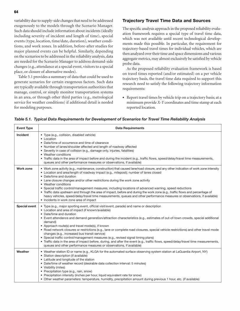
64
Trajectory Travel Time Data and Sources
The specific analysis approach in the proposed reliability evalu-ation framework requires a special type of travel time data, which was not available until recent technological develop-ments made this possible. In particular, the requirement for trajectory-based travel times for individual vehicles, which are then analyzed over their time and space dimensions and various aggregate metrics, may almost exclusively be satisfied by vehicle probe data.
As the proposed reliability evaluation framework is based on travel times reported (and/or estimated) on a per vehicle trajectory basis, the travel time data required to support this research need to satisfy the following trajectory information requirements:
• Report travel times by vehicle trip on a trajectory basis; at a minimum provide X-Y coordinates and time stamp at each reported location.
variability due to supply-side changes that need to be addressed exogenously to the models through the Scenario Manager. Such data should include information about incidents (ideally including severity of incident and length of time), special events (type, location, time/date, duration), weather condi-tions, and work zones. In addition, before-after studies for major planned events can be helpful. Similarly, depending on the scenarios to be addressed in the reliability analysis, data are needed for the Scenario Manager to address demand-side changes (e.g., attendance at a special event, visitors to a special place, or closure of alternative modes).
Table 5.1 provides a summary of data that could be used to generate scenarios for certain exogenous factors. Such data are typically available through transportation authorities that manage, control, or simply monitor transportation systems in an area, or through other third parties (e.g., metrological service for weather conditions) if additional detail is needed for modeling purposes.
Table 5.1. Typical Data Requirements for Development of Scenarios for Travel Time Reliability Analysis
event type Data Requirements
Incident • Type (e.g., collision, disabled vehicle)• location• date/time of occurrence and time of clearance• Number of lanes/shoulder affected and length of roadway affected• Severity in case of collision (e.g., damage only, injuries, fatalities)• weather conditions• Traffic data in the area of impact before and during the incident (e.g., traffic flows, speed/delay/travel time measurements,
queues and other performance measures or observations, if available)
Work zone • work zone activity (e.g., maintenance, construction) that caused lane/road closure, and any other indication of work zone intensity• location and area/length of roadway impact (e.g., milepost); number of lanes closed• date/time and duration• lane closure changes and/or other restrictions during the work zone activity• weather conditions• Special traffic control/management measures, including locations of advanced warning, speed reductions• Traffic data upstream and through the area of impact, before and during the work zone (e.g., traffic flows and percentage of
heavy vehicles, speed/delay/travel time measurements, queues and other performance measures or observations, if available)• Incidents in work zone area of impact
Special event • Type (e.g., major sporting event, official visit/event, parade) and name or description• location and area of impact (if known/available)• date/time and duration• Event attendance and demand generation/attraction characteristics (e.g., estimates of out-of-town crowds, special additional
demand)• Approach route(s) and travel mode(s), if known• Road network closures or restrictions (e.g., lane or complete road closures, special vehicle restrictions) and other travel mode
changes (e.g., increased bus transit service)• Special traffic control/management measures (e.g., revised signal timing plans)• Traffic data in the area of impact before, during, and after the event (e.g., traffic flows, speed/delay/travel time measurements,
queues and other performance measures or observations, if available)
Weather • weather station Id or name (e.g., klgA for the automated surface observing system station at laguardia Airport, Ny)• Station description (if available)• latitude and longitude of the station• date/time of weather record (desirable data collection interval: 5 minutes)• visibility (miles)• Precipitation type (e.g., rain, snow)• Precipitation intensity (inches per hour, liquid equivalent rate for snow)• other weather parameters: temperature, humidity, precipitation amount during previous 1 hour, etc. (if available)
65
• Provide travel time at disaggregated levels (e.g., vehicle travel time) and at fine time intervals (e.g., link/path travel time for every 5 minutes), in addition to average travel times, to capture time-of-day variation and vehicle-to-vehicle variation.
• Provide sufficient information on components, causes, and other characteristics of congestion, so that appropriate parameterization can be established for simulation testing purposes.
The emergence of probe data over the past few years has opened the opportunity to capture all necessary information for this type of analysis, since such data can be available all the time for all major roads in the network including major arteri-als. Probe-based trajectory data represent a significant increase in the quality and quantity of relevant information. The detail in such data makes it possible to analyze travel time data according to network and route components (e.g., on a link and path basis) as well as according to geographic aggrega-tions (e.g., on an O–D zone basis).
• Capture both recurring and nonrecurring congestion on a range of road facilities (from freeways to arterial roads and possibly managed lanes).
• Represent sufficient sampling and time-series to allow statistically meaningful analysis.
• Provide the ability to tie travel time data to other ancillary data for time variability sources (to allow parameterization for simulation testing purposes as discussed earlier).
Furthermore, the trajectory data should ideally possess the following general characteristics for travel time reliability analysis:
• Capture both types of congestion (recurring and nonrecurring).
• Cover the range of road facilities that may be included in the subject area analysis from freeways to arterial roads and (possibly) managed lanes.
• Allow statistically meaningful analysis of data through availability for a relatively long period of time (e.g., a time frame long enough to cover seasonal variation).
66
Introduction
Purpose and Objectives
Distinguishing exogenous sources of variation both on the demand and the supply sides from endogenous sources of variation lie at the foundation of this conceptualization and approach. It should be recognized, however, that unlike regimes, which are typically mutually exclusive states with distinct properties of a physical system, these sources of vari-ation can operate simultaneously and often will. In other words, incidents may well occur during times of otherwise recurring congestion, precipitation may act in concert with a surge in demand or special event, and so on. Therefore, from a modeling standpoint, it is desirable to retain the ability to apply any source of variation that may be applicable in a scenario of interest.
Recognizing the importance of the scenario definition and the complexity of identifying relevant exogenous sources, the study adopts the concept of a Scenario Manager, which pro-vides the ability to construct scenarios that entail any mutually consistent combination of external events, both demand as well as supply related, including different traffic control plans that may be deployed under certain conditions. The Scenario Generator also acts in a scenario management role, which allows retrieval of historically occurring scenarios or of previ-ously constructed scenarios as part of a planning exercise (e.g., in conjunction with emergency preparedness planning). It also allows generation, through Monte Carlo sampling, of hypothetical scenarios for analysis and design purposes. Of course, the Scenario Manager/Generator facilitates direct exe-cution of the simulation software for a particular scenario, by creating the necessary inputs that reflect the scenario assump-tions. When exercised in the latter manner (i.e., in random generation mode), the Scenario Manager becomes the pri-mary platform for conducting reliability analyses, as experi-ments are conducted to replicate certain field conditions, under both actual and hypothetical (proposed) network and
control scenarios. In particular, the Scenario Generator enables execution of experimental designs that entail simula-tion over multiple days, thus reflecting daily fluctuations in demand, both systematic and random.
An especially important and interesting feature of a well-configured Scenario Manager is that it can be tied into an area’s traffic and weather monitoring system(s). As such, particular scenario occurrences can be stored when they materialize, with all applicable elements that define that scenario, especially demand characteristics and traffic control plans triggered for that scenario. For example, if Houston experienced major rain-fall with extensive flood-like conditions, that scenario could be stored in terms of the events and exogenous parameter values as such. With a properly configured Scenario Manager inter-faced with the data warehousing system at a given traffic man-agement center, it would be possible to extract the relative occurrence probabilities and distribution functions and to calibrate these external events to actual observations. Consid-erable sophistication and functionality could be introduced in such a process over time, as the historical data records increase in quantity, quality, and completeness and allow robust estima-tion of occurrence probabilities of otherwise infrequent events.
Concept of Operations
The methodological framework recognizes the different sources of uncertainty that affect the reliability of travel time in the roadway environment. As discussed in Chapter 4, a previous study (Cambridge Systematics, Inc. 2005) identified seven major root causes of travel time variability: (1) traf-fic incidents, (2) work zones, (3) weather, (4) special events, (5) traffic control devices, (6) fluctuations in demand, and (7) inadequate base capacity. Many existing simulation tools view and model these factors as exogenous events using user-specified scenarios (Mahmassani et al. 2009). Distinct from these exogenous factors, there are also endogenous sources of variation that are inherently reproduced, to varying degrees, by
C h A p t e r 6
Scenario Manager
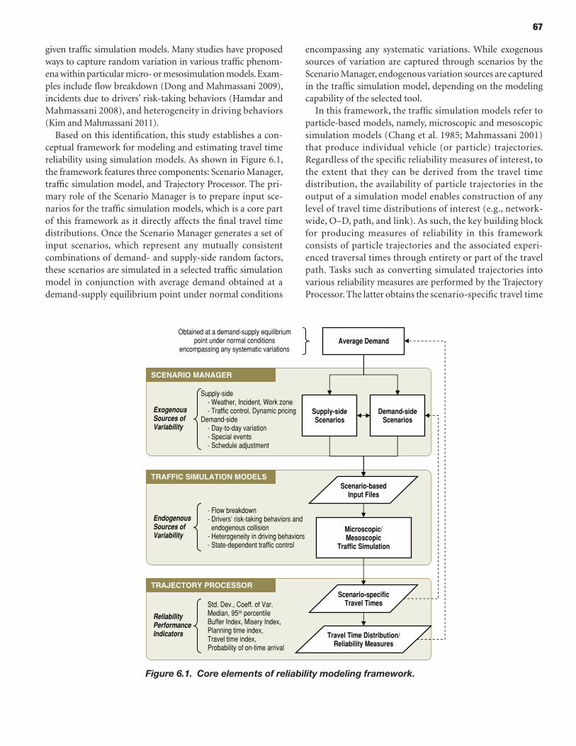
67
encompassing any systematic variations. While exogenous sources of variation are captured through scenarios by the Scenario Manager, endogenous variation sources are captured in the traffic simulation model, depending on the modeling capability of the selected tool.
In this framework, the traffic simulation models refer to particle-based models, namely, microscopic and mesoscopic simulation models (Chang et al. 1985; Mahmassani 2001) that produce individual vehicle (or particle) trajectories. Regardless of the specific reliability measures of interest, to the extent that they can be derived from the travel time distribution, the availability of particle trajectories in the output of a simulation model enables construction of any level of travel time distributions of interest (e.g., network-wide, O–D, path, and link). As such, the key building block for producing measures of reliability in this framework consists of particle trajectories and the associated experi-enced traversal times through entirety or part of the travel path. Tasks such as converting simulated trajectories into various reliability measures are performed by the Trajectory Processor. The latter obtains the scenario-specific travel time
given traffic simulation models. Many studies have proposed ways to capture random variation in various traffic phenom-ena within particular micro- or mesosimulation models. Exam-ples include flow breakdown (Dong and Mahmassani 2009), incidents due to drivers’ risk-taking behaviors (Hamdar and Mahmassani 2008), and heterogeneity in driving behaviors (Kim and Mahmassani 2011).
Based on this identification, this study establishes a con-ceptual framework for modeling and estimating travel time reliability using simulation models. As shown in Figure 6.1, the framework features three components: Scenario Manager, traffic simulation model, and Trajectory Processor. The pri-mary role of the Scenario Manager is to prepare input sce-narios for the traffic simulation models, which is a core part of this framework as it directly affects the final travel time distributions. Once the Scenario Manager generates a set of input scenarios, which represent any mutually consistent combinations of demand- and supply-side random factors, these scenarios are simulated in a selected traffic simulation model in conjunction with average demand obtained at a demand-supply equilibrium point under normal conditions
Supply-side - Weather, Incident, Work zone - Traffic control, Dynamic pricing
Demand-side - Day-to-day variation - Special events - Schedule adjustment
Exogenous Sources of Variability
SCENARIO MANAGER
TRAJECTORY PROCESSOR
TRAFFIC SIMULATION MODELS
Demand-side Scenarios
Supply-side Scenarios
Average Demand
Scenario-based Input Files
Microscopic/ Mesoscopic
Traffic Simulation
Scenario-specific Travel Times
Travel Time Distribution/ Reliability Measures
- Flow breakdown- Drivers’ risk-taking behaviors and
endogenous collision - Heterogeneity in driving behaviors - State-dependent traffic control
Endogenous Sources of Variability
Std. Dev., Coeff. of Var. Median, 95th percentile Buffer Index, Misery Index, Planning time index, Travel time index, Probability of on-time arrival
Reliability Performance Indicators
Obtained at a demand-supply equilibrium point under normal conditions
encompassing any systematic variations
Figure 6.1. Core elements of reliability modeling framework.
68
distribution from each simulation run and constructs the overall travel time distribution aggregated over multiple scenarios.
While chaining these three modules completes the neces-sary procedures for performing a scenario-based reliability analysis, there are two feedback loops worth mentioning to further incorporate behavioral aspects of travelers into the reliability modeling framework. The inner loop in Figure 6.1 suggests that information from scenario-specific travel times might be used to make scenario-conditional demand adjust-ments (e.g., departure time change under severe weather condition). The outer loop indicates that the overall system uncertainty might affect the average demand by shifting the equilibrium point (i.e., reliability-sensitive network equilib-rium) based on travel demand forecasting models that pre-dict the impact of reliability measures on travel patterns (e.g., Zhou et al. 2008; Jiang et al. 2011).
Methodology for Scenario-Based reliability Analysis Using Simulation tools
Scenario-Based Reliability Analysis
This section elaborates on the basic idea of the scenario-based reliability analysis within the aforementioned frame-work. Conceptually, the traffic simulation models can be viewed as an input-output function, in which inputs are sce-narios that represent exogenous sources of roadway disrup-tions and outputs are travel time distributions experienced by travelers under such disruptions. The objective of the sce-nario-based reliability analysis is to investigate variability in the output travel time distribution by controlling the input scenario (i.e., input scenarios can be generated completely at random or in a more directed manner based on a particular experimental design). In this equation, endogenous sources of random variations are not part of control variables as those are considered as part of the traffic simulation model logic. To enhance understanding and conceptualization of pro-cesses, the mathematical representation of the basic concept of this analysis is presented.
Let X denote a vector of exogenous sources of random variation (e.g., weather, incident, day-to-day demand varia-tion) that is selected as scenario components to characterize input scenario and let Xj represent the jth element of X. Each scenario component itself is also a vector of several attri-butes describing temporal (e.g., start-time and duration), spatial (e.g., event location), and state (i.e., intensity or con-dition) aspects of a given demand- and supply-side factor. Let Si denote the ith input scenario, which is the ith realiza-tion of the set of scenario components X, that is, Si = X(i) = {X1
(i), X2(i), . . . , XJ
(i)}.
Consider we have N input scenarios S1, S2, . . . , SN drawn from a joint distribution of X. Then the output travel time distribution for each scenario is obtained by Equation 6.1:
, 1, . . . , 6.1T H S i Ni i( ) ( )= =
where Ti represents a collection of travel time t for a given O–D/path/link of interest under the ith scenario Si, and H(z) denotes a black-box representation of a traffic simulation model. Let fi(t) denote the probability density function of scenario-specific travel times under Si such that {t ∈Ti: t ~ fi(t)}. Then the main goal of the analysis is to obtain the probability density function of overall travel times f(t) based on the scenario-specific travel time distributions fi(t). By knowing the probability of each scenario occurring, f(t) can be calculated by the weighted sum (i.e., convex combi-nation) of scenario-specific travel time distribution fi(t) as follows in Equation 6.2:
6.21
f t w f ti ii
N
∑( ) ( ) ( )==
where wi denotes the weight of the ith scenario with Σni =1wi = 1,
which is typically obtained from the scenario probability wi = P(Si). Figure 6.2 presents a schematic diagram to illus-trate the procedure of constructing the overall travel time distribution based on this concept.
Approaches to Assessing Reliability
Travel time reliability is a relative concept in that it depends on the temporal and spatial boundaries for which travel times are observed. For example, the travel time reliability for week-days is different from that for weekends on the same road network. Therefore, defining time and space domains needs to precede assessing reliability. In general, the time domain is specified by a date range of the overall time period (e.g., 6/1/2012–8/31/2012), day of week (e.g., Monday–Friday), and time of day (6 a.m.–10 a.m.). Or the time domain could be a specific season or day of each year (e.g., Thanksgiving Day). The space domain defines at which level travel times are collected and the reliability measures are calculated (e.g., network-level, O–D-level, path-level, and link-level). Two dif-ferent approaches are explored to assess the travel time reli-ability for given time and space domains: (1) Monte Carlo approach and (2) mix-and-match approach. The former tries to generate all possible scenarios that could occur during the given temporal and spatial boundaries to introduce realistic variations in the resulting travel time distribution; the latter constructs scenarios by manually choosing various combina-tions of scenario components. These approaches are dis-cussed in more detail.
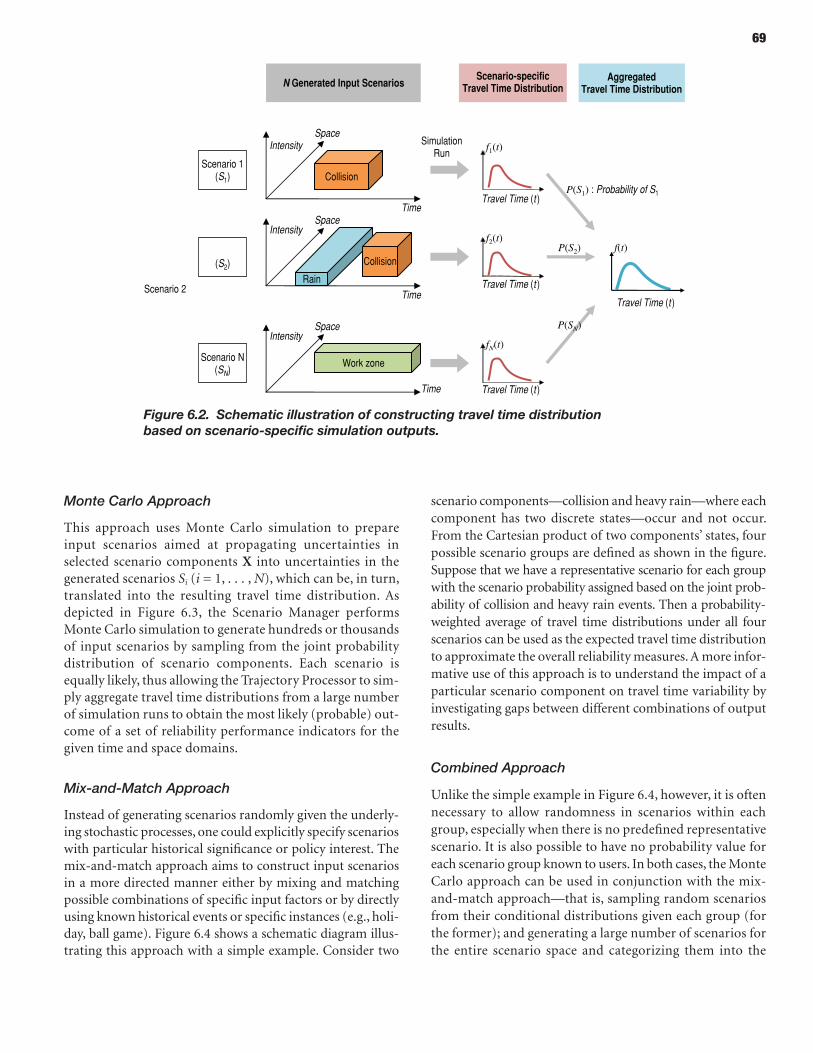
69
Monte Carlo Approach
This approach uses Monte Carlo simulation to prepare input scenarios aimed at propagating uncertainties in selected scenario components X into uncertainties in the generated scenarios Si (i = 1, . . . , N), which can be, in turn, translated into the resulting travel time distribution. As depicted in Figure 6.3, the Scenario Manager performs Monte Carlo simulation to generate hundreds or thousands of input scenarios by sampling from the joint probability distribution of scenario components. Each scenario is equally likely, thus allowing the Trajectory Processor to sim-ply aggregate travel time distributions from a large number of simulation runs to obtain the most likely (probable) out-come of a set of reliability performance indicators for the given time and space domains.
Mix-and-Match Approach
Instead of generating scenarios randomly given the underly-ing stochastic processes, one could explicitly specify scenarios with particular historical significance or policy interest. The mix-and-match approach aims to construct input scenarios in a more directed manner either by mixing and matching possible combinations of specific input factors or by directly using known historical events or specific instances (e.g., holi-day, ball game). Figure 6.4 shows a schematic diagram illus-trating this approach with a simple example. Consider two
scenario components—collision and heavy rain—where each component has two discrete states—occur and not occur. From the Cartesian product of two components’ states, four possible scenario groups are defined as shown in the figure. Suppose that we have a representative scenario for each group with the scenario probability assigned based on the joint prob-ability of collision and heavy rain events. Then a probability-weighted average of travel time distributions under all four scenarios can be used as the expected travel time distribution to approximate the overall reliability measures. A more infor-mative use of this approach is to understand the impact of a particular scenario component on travel time variability by investigating gaps between different combinations of output results.
Combined Approach
Unlike the simple example in Figure 6.4, however, it is often necessary to allow randomness in scenarios within each group, especially when there is no predefined representative scenario. It is also possible to have no probability value for each scenario group known to users. In both cases, the Monte Carlo approach can be used in conjunction with the mix-and-match approach—that is, sampling random scenarios from their conditional distributions given each group (for the former); and generating a large number of scenarios for the entire scenario space and categorizing them into the
Rain
Collision
Time
Intensity Space
Scenario 1 (S1)
Simulation Run
Travel Time (t )
Scenario-specific Travel Time Distribution
Travel Time (t )
P(S1) : Probability of S1
P(S2)
P(SN)
Aggregated Travel Time Distribution
Collision
Work zone
Scenario 2
(S2)
Scenario N (SN)
N Generated Input Scenarios
f1(t)
f2(t)f(t)
fN(t)
Intensity
Intensity
Space
Space
Time
Time
Travel Time (t )
Travel Time (t )
Figure 6.2. Schematic illustration of constructing travel time distribution based on scenario-specific simulation outputs.
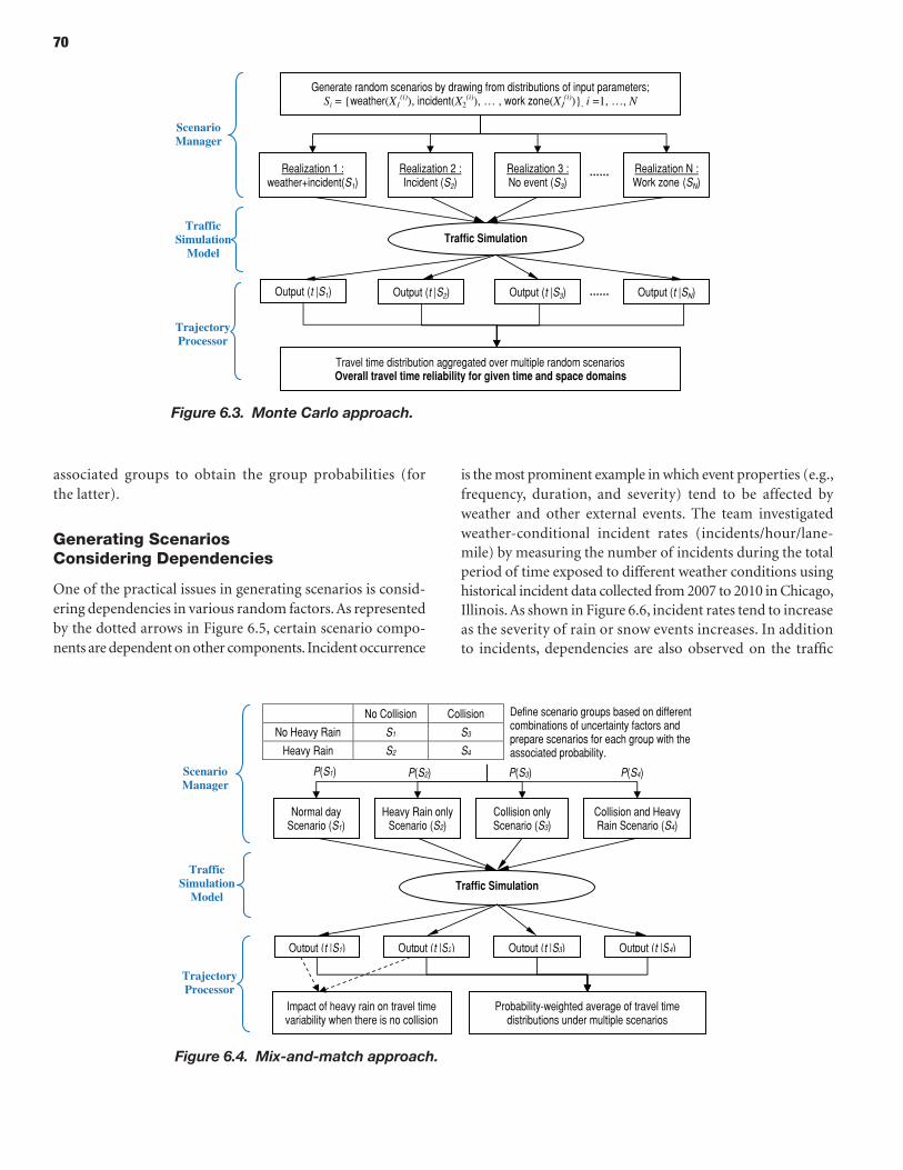
70
Realization N : Work zone (SN)
Realization 3 : No event (S3)
Realization 2 : Incident (S2)
Realization 1 : weather+incident(S1)
……
Traffic Simulation
Output (t |S2) Output (t |S3) Output (t |SN) Output (t |S1) ……
Generate random scenarios by drawing from distributions of input parameters; Si = {weather(X1
(i)), incident(X2(i)), … , work zone(XJ
(i))}, i =1, …, N
Travel time distribution aggregated over multiple random scenarios Overall travel time reliability for given time and space domains
Trajectory Processor
Traffic Simulation
Model
Scenario Manager
Figure 6.3. Monte Carlo approach.
Traffic Simulation
Output (t |S2) Output (t |S1)
Impact of heavy rain on travel time variability when there is no collision
P(S2) P(S1)
Normal day Scenario (S1)
Heavy Rain only Scenario (S2)
Collision only Scenario (S3)
Collision and Heavy Rain Scenario (S4)
Output (t |S3) Output (t |S4)
P(S4)
Trajectory Processor
Traffic Simulation
Model
Scenario Manager
No Collision Collision Define scenario groups based on different combinations of uncertainty factors and prepare scenarios for each group with the associated probability.
No Heavy Rain S1 S3
Heavy Rain S2 S4
P(S3)
Probability-weighted average of travel time distributions under multiple scenarios
Figure 6.4. Mix-and-match approach.
associated groups to obtain the group probabilities (for the latter).
Generating Scenarios Considering Dependencies
One of the practical issues in generating scenarios is consid-ering dependencies in various random factors. As represented by the dotted arrows in Figure 6.5, certain scenario compo-nents are dependent on other components. Incident occurrence
is the most prominent example in which event properties (e.g., frequency, duration, and severity) tend to be affected by weather and other external events. The team investigated weather-conditional incident rates (incidents/hour/lane-mile) by measuring the number of incidents during the total period of time exposed to different weather conditions using historical incident data collected from 2007 to 2010 in Chicago, Illinois. As shown in Figure 6.6, incident rates tend to increase as the severity of rain or snow events increases. In addition to incidents, dependencies are also observed on the traffic
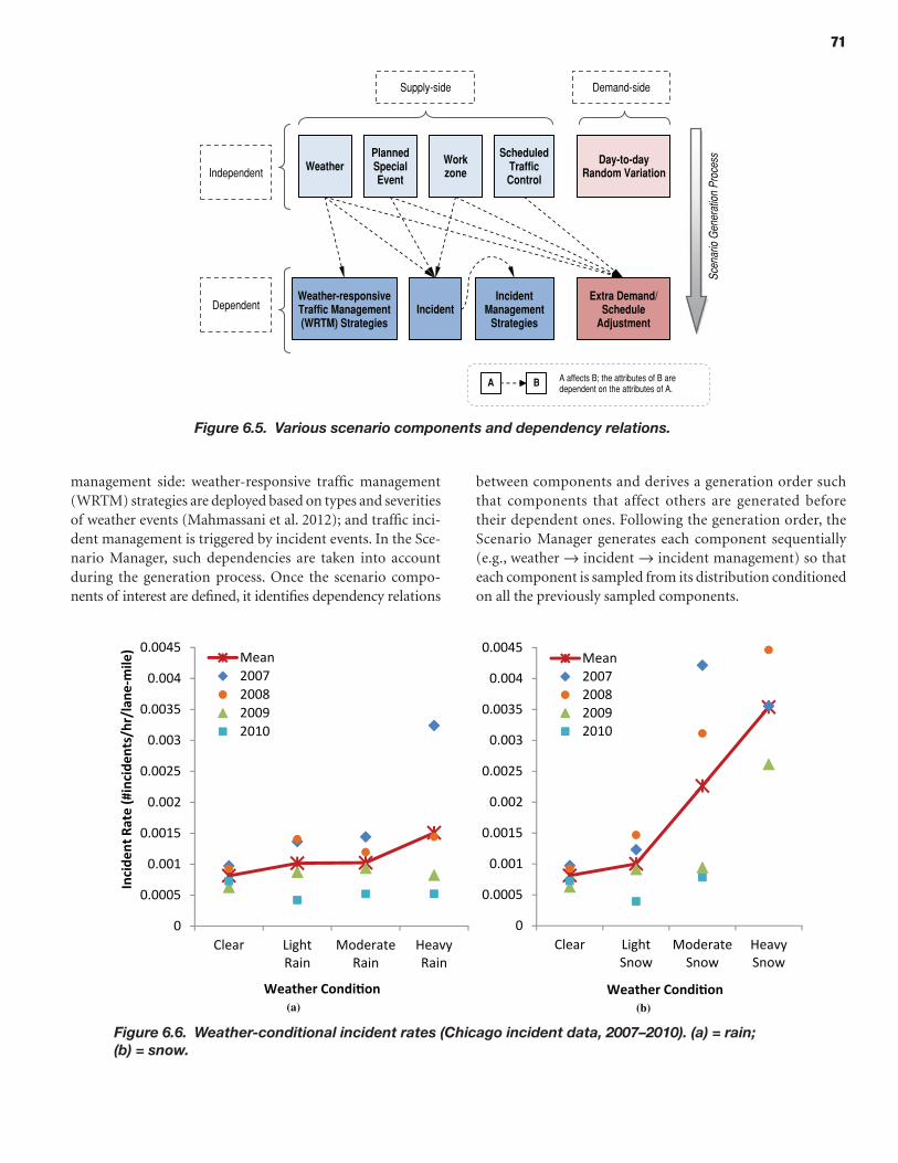
71
Independent Weather Planned Special Event
Scheduled Traffic Control
Incident
Workzone
Incident Management
Strategies
Weather-responsive Traffic Management (WRTM) Strategies
Extra Demand/ Schedule
Adjustment
Day-to-day Random Variation
Scen
ario
Gen
erat
ion
Proc
ess
A affects B; the attributes of B are dependent on the attributes of A.
A B
Supply-side Demand-side
Dependent
Figure 6.5. Various scenario components and dependency relations.
0
0.0005
0.001
0.0015
0.002
0.0025
0.003
0.0035
0.004
0.0045
Clear LightRain
ModerateRain
HeavyRain
Inci
dent
Rate
(#in
cide
nts/
hr/l
ane
mile
)
Weather Condition
Mean2007200820092010
(a) (b)
0
0.0005
0.001
0.0015
0.002
0.0025
0.003
0.0035
0.004
0.0045
Clear LightSnow
ModerateSnow
HeavySnow
Weather Condition
Mean2007200820092010
Figure 6.6. Weather-conditional incident rates (Chicago incident data, 2007–2010). (a) = rain; (b) = snow.
management side: weather-responsive traffic management (WRTM) strategies are deployed based on types and severities of weather events (Mahmassani et al. 2012); and traffic inci-dent management is triggered by incident events. In the Sce-nario Manager, such dependencies are taken into account during the generation process. Once the scenario compo-nents of interest are defined, it identifies dependency relations
between components and derives a generation order such that components that affect others are generated before their dependent ones. Following the generation order, the Scenario Manager generates each component sequentially (e.g., weather → incident → incident management) so that each component is sampled from its distribution conditioned on all the previously sampled components.
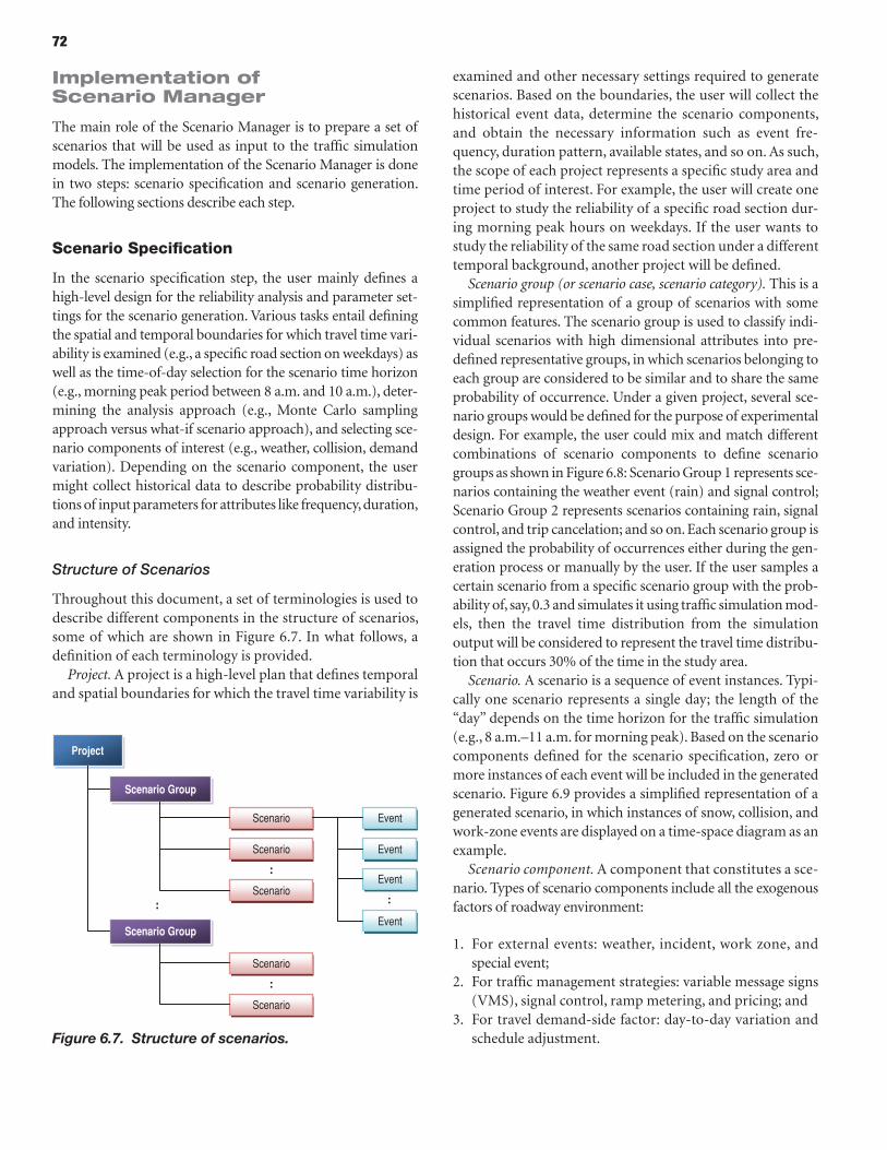
72
Implementation of Scenario Manager
The main role of the Scenario Manager is to prepare a set of scenarios that will be used as input to the traffic simulation models. The implementation of the Scenario Manager is done in two steps: scenario specification and scenario generation. The following sections describe each step.
Scenario Specification
In the scenario specification step, the user mainly defines a high-level design for the reliability analysis and parameter set-tings for the scenario generation. Various tasks entail defining the spatial and temporal boundaries for which travel time vari-ability is examined (e.g., a specific road section on weekdays) as well as the time-of-day selection for the scenario time horizon (e.g., morning peak period between 8 a.m. and 10 a.m.), deter-mining the analysis approach (e.g., Monte Carlo sampling approach versus what-if scenario approach), and selecting sce-nario components of interest (e.g., weather, collision, demand variation). Depending on the scenario component, the user might collect historical data to describe probability distribu-tions of input parameters for attributes like frequency, duration, and intensity.
Structure of Scenarios
Throughout this document, a set of terminologies is used to describe different components in the structure of scenarios, some of which are shown in Figure 6.7. In what follows, a definition of each terminology is provided.
Project. A project is a high-level plan that defines temporal and spatial boundaries for which the travel time variability is
examined and other necessary settings required to generate scenarios. Based on the boundaries, the user will collect the historical event data, determine the scenario components, and obtain the necessary information such as event fre-quency, duration pattern, available states, and so on. As such, the scope of each project represents a specific study area and time period of interest. For example, the user will create one project to study the reliability of a specific road section dur-ing morning peak hours on weekdays. If the user wants to study the reliability of the same road section under a different temporal background, another project will be defined.
Scenario group (or scenario case, scenario category). This is a simplified representation of a group of scenarios with some common features. The scenario group is used to classify indi-vidual scenarios with high dimensional attributes into pre-defined representative groups, in which scenarios belonging to each group are considered to be similar and to share the same probability of occurrence. Under a given project, several sce-nario groups would be defined for the purpose of experimental design. For example, the user could mix and match different combinations of scenario components to define scenario groups as shown in Figure 6.8: Scenario Group 1 represents sce-narios containing the weather event (rain) and signal control; Scenario Group 2 represents scenarios containing rain, signal control, and trip cancelation; and so on. Each scenario group is assigned the probability of occurrences either during the gen-eration process or manually by the user. If the user samples a certain scenario from a specific scenario group with the prob-ability of, say, 0.3 and simulates it using traffic simulation mod-els, then the travel time distribution from the simulation output will be considered to represent the travel time distribu-tion that occurs 30% of the time in the study area.
Scenario. A scenario is a sequence of event instances. Typi-cally one scenario represents a single day; the length of the “day” depends on the time horizon for the traffic simulation (e.g., 8 a.m.–11 a.m. for morning peak). Based on the scenario components defined for the scenario specification, zero or more instances of each event will be included in the generated scenario. Figure 6.9 provides a simplified representation of a generated scenario, in which instances of snow, collision, and work-zone events are displayed on a time-space diagram as an example.
Scenario component. A component that constitutes a sce-nario. Types of scenario components include all the exogenous factors of roadway environment:
1. For external events: weather, incident, work zone, and special event;
2. For traffic management strategies: variable message signs (VMS), signal control, ramp metering, and pricing; and
3. For travel demand-side factor: day-to-day variation and schedule adjustment.
Project
Scenario Group
Scenario Group
Scenario
Scenario
:Scenario
:
Scenario
Scenario
:
Event
Event
Event
:
Event
Figure 6.7. Structure of scenarios.
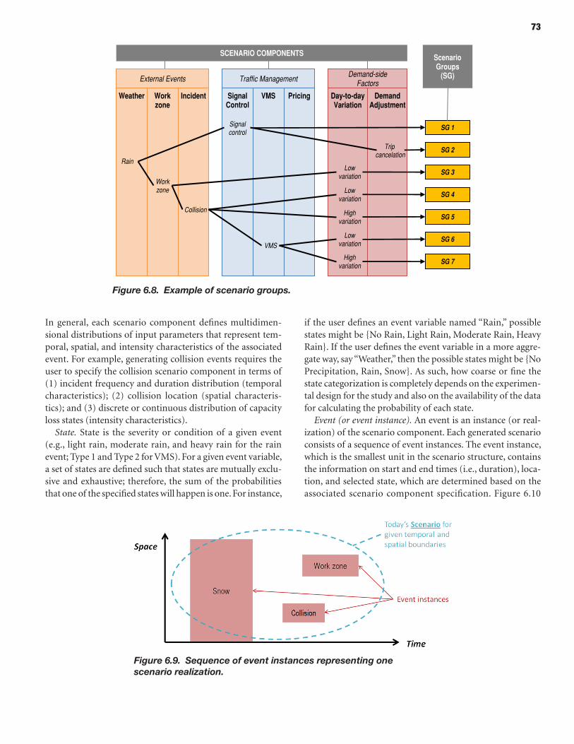
73
SG 1
External Events
Scenario Groups
(SG) Traffic Management Demand-side
Factors
Rain
Collision
VMS
SCENARIO COMPONENTS
Weather Workzone
Incident Signal Control
VMS
Pricing
Day-to-day Variation
Demand Adjustment
Signal control
Low variation
Low variation
Workzone
Trip cancelation
Low variation
High variation
High variation
SG 2
SG 3
SG 4
SG 5
SG 6
SG 7
Figure 6.8. Example of scenario groups.
Figure 6.9. Sequence of event instances representing one scenario realization.
In general, each scenario component defines multidimen-sional distributions of input parameters that represent tem-poral, spatial, and intensity characteristics of the associated event. For example, generating collision events requires the user to specify the collision scenario component in terms of (1) incident frequency and duration distribution (temporal characteristics); (2) collision location (spatial characteris-tics); and (3) discrete or continuous distribution of capacity loss states (intensity characteristics).
State. State is the severity or condition of a given event (e.g., light rain, moderate rain, and heavy rain for the rain event; Type 1 and Type 2 for VMS). For a given event variable, a set of states are defined such that states are mutually exclu-sive and exhaustive; therefore, the sum of the probabilities that one of the specified states will happen is one. For instance,
if the user defines an event variable named “Rain,” possible states might be {No Rain, Light Rain, Moderate Rain, Heavy Rain}. If the user defines the event variable in a more aggre-gate way, say “Weather,” then the possible states might be {No Precipitation, Rain, Snow}. As such, how coarse or fine the state categorization is completely depends on the experimen-tal design for the study and also on the availability of the data for calculating the probability of each state.
Event (or event instance). An event is an instance (or real-ization) of the scenario component. Each generated scenario consists of a sequence of event instances. The event instance, which is the smallest unit in the scenario structure, contains the information on start and end times (i.e., duration), loca-tion, and selected state, which are determined based on the associated scenario component specification. Figure 6.10
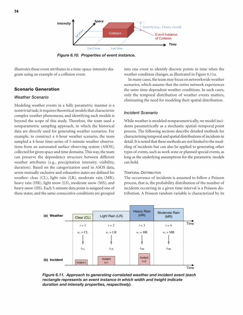
74
illustrates these event attributes in a time-space-intensity dia-gram using an example of a collision event.
Scenario Generation
Weather Scenario
Modeling weather events in a fully parametric manner is a nontrivial task; it requires theoretical models that characterize complex weather phenomena, and identifying such models is beyond the scope of this study. Therefore, the team used a nonparametric sampling approach, in which the historical data are directly used for generating weather scenarios. For example, to construct a 4-hour weather scenario, the team sampled a 4-hour time-series of 5-minute weather observa-tions from an automated surface observing system (ASOS), collected for given space and time domains. This way, the team can preserve the dependency structure between different weather attributes (e.g., precipitation intensity, visibility, duration). Based on the categorization used in ASOS data, seven mutually exclusive and exhaustive states are defined for weather: clear (CL), light rain (LR), moderate rain (MR), heavy rain (HR), light snow (LS), moderate snow (MS), and heavy snow (HS). Each 5-minute data point is assigned one of these states, and the same consecutive conditions are grouped
into one event to identify discrete points in time when the weather condition changes, as illustrated in Figure 6.11a.
In many cases, the team may focus on networkwide weather scenarios, which assume that the entire network experiences the same time-dependent weather conditions. In such cases, only the temporal distribution of weather events matters, eliminating the need for modeling their spatial distribution.
Incident Scenario
While weather is modeled nonparametrically, we model inci-dents parametrically as a stochastic spatial–temporal point process. The following sections describe detailed methods for characterizing temporal and spatial distributions of incidents in detail. It is noted that these methods are not limited to the mod-eling of incidents but can also be applied to generating other types of events, such as work zone or planned special events, as long as the underlying assumptions for the parametric models can hold.
Temporal DisTribuTion
The occurrence of incidents is assumed to follow a Poisson process, that is, the probability distribution of the number of incidents occurring in a given time interval is a Poisson dis-tribution. A Poisson random variable is characterized by its
Figure 6.10. Properties of event instance.
Clear (CL) Light Rain (LR) Heavy Rain
(HR) Moderate Rain
(MR)
Time
(a) Weather
Time
Incident n Incident
n+1
Incident n+2
i = 1
wi = CL
CL
i = 2
wi = LR
LR
i = 3
wi = HR
HR
i = 4
wi = MR
MR
(b) Incident
Figure 6.11. Approach to generating correlated weather and incident event (each rectangle represents an event instance in which width and height indicate duration and intensity properties, respectively).
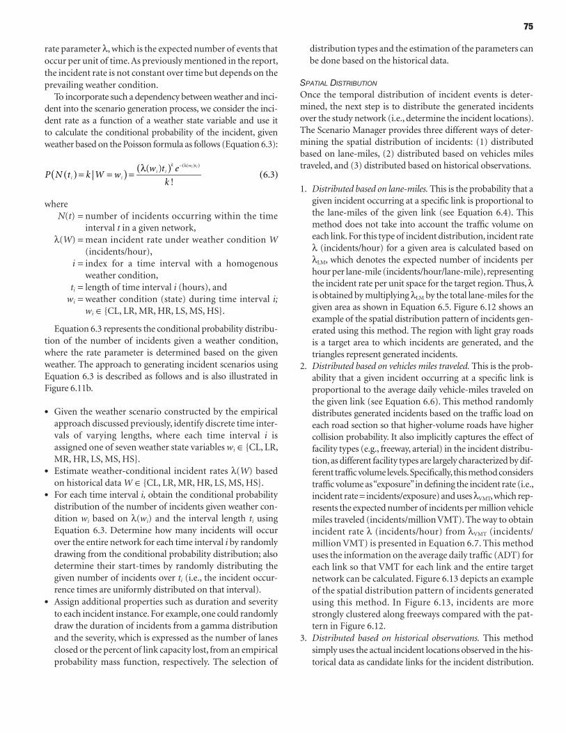
75
rate parameter l, which is the expected number of events that occur per unit of time. As previously mentioned in the report, the incident rate is not constant over time but depends on the prevailing weather condition.
To incorporate such a dependency between weather and inci-dent into the scenario generation process, we consider the inci-dent rate as a function of a weather state variable and use it to calculate the conditional probability of the incident, given weather based on the Poisson formula as follows (Equation 6.3):
P N t k W ww t e
ki i
i i
k w ti i
( ) ( )( ) ( )= = = λ ( )( )− λ
|( )
!6.3
where N(t) = number of incidents occurring within the time
interval t in a given network,l(W) = mean incident rate under weather condition W
(incidents/hour), i = index for a time interval with a homogenous
weather condition, ti = length of time interval i (hours), and wi = weather condition (state) during time interval i;
wi ∈{CL, LR, MR, HR, LS, MS, HS}.
Equation 6.3 represents the conditional probability distribu-tion of the number of incidents given a weather condition, where the rate parameter is determined based on the given weather. The approach to generating incident scenarios using Equation 6.3 is described as follows and is also illustrated in Figure 6.11b.
• Given the weather scenario constructed by the empirical approach discussed previously, identify discrete time inter-vals of varying lengths, where each time interval i is assigned one of seven weather state variables wi ∈{CL, LR, MR, HR, LS, MS, HS}.
• Estimate weather-conditional incident rates l(W) based on historical data W ∈{CL, LR, MR, HR, LS, MS, HS}.
• For each time interval i, obtain the conditional probability distribution of the number of incidents given weather con-dition wi based on l(wi) and the interval length ti using Equation 6.3. Determine how many incidents will occur over the entire network for each time interval i by randomly drawing from the conditional probability distribution; also determine their start-times by randomly distributing the given number of incidents over ti (i.e., the incident occur-rence times are uniformly distributed on that interval).
• Assign additional properties such as duration and severity to each incident instance. For example, one could randomly draw the duration of incidents from a gamma distribution and the severity, which is expressed as the number of lanes closed or the percent of link capacity lost, from an empirical probability mass function, respectively. The selection of
distribution types and the estimation of the parameters can be done based on the historical data.
spaTial DisTribuTion
Once the temporal distribution of incident events is deter-mined, the next step is to distribute the generated incidents over the study network (i.e., determine the incident locations). The Scenario Manager provides three different ways of deter-mining the spatial distribution of incidents: (1) distributed based on lane-miles, (2) distributed based on vehicles miles traveled, and (3) distributed based on historical observations.
1. Distributed based on lane-miles. This is the probability that a given incident occurring at a specific link is proportional to the lane-miles of the given link (see Equation 6.4). This method does not take into account the traffic volume on each link. For this type of incident distribution, incident rate l (incidents/hour) for a given area is calculated based on lLM, which denotes the expected number of incidents per hour per lane-mile (incidents/hour/lane-mile), representing the incident rate per unit space for the target region. Thus, l is obtained by multiplying lLM by the total lane-miles for the given area as shown in Equation 6.5. Figure 6.12 shows an example of the spatial distribution pattern of incidents gen-erated using this method. The region with light gray roads is a target area to which incidents are generated, and the triangles represent generated incidents.
2. Distributed based on vehicles miles traveled. This is the prob-ability that a given incident occurring at a specific link is proportional to the average daily vehicle-miles traveled on the given link (see Equation 6.6). This method randomly distributes generated incidents based on the traffic load on each road section so that higher-volume roads have higher collision probability. It also implicitly captures the effect of facility types (e.g., freeway, arterial) in the incident distribu-tion, as different facility types are largely characterized by dif-ferent traffic volume levels. Specifically, this method considers traffic volume as “exposure” in defining the incident rate (i.e., incident rate = incidents/exposure) and uses lVMT, which rep-resents the expected number of incidents per million vehicle miles traveled (incidents/million VMT). The way to obtain incident rate l (incidents/hour) from lVMT (incidents/million VMT) is presented in Equation 6.7. This method uses the information on the average daily traffic (ADT) for each link so that VMT for each link and the entire target network can be calculated. Figure 6.13 depicts an example of the spatial distribution pattern of incidents generated using this method. In Figure 6.13, incidents are more strongly clustered along freeways compared with the pat-tern in Figure 6.12.
3. Distributed based on historical observations. This method simply uses the actual incident locations observed in the his-torical data as candidate links for the incident distribution.
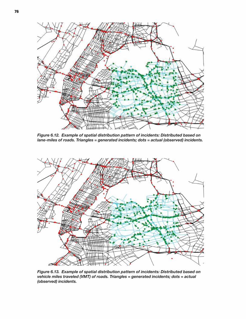
76
Figure 6.12. Example of spatial distribution pattern of incidents: Distributed based on lane-miles of roads. Triangles = generated incidents; dots = actual (observed) incidents.
Figure 6.13. Example of spatial distribution pattern of incidents: Distributed based on vehicle miles traveled (VMT) of roads. Triangles = generated incidents; dots = actual (observed) incidents.
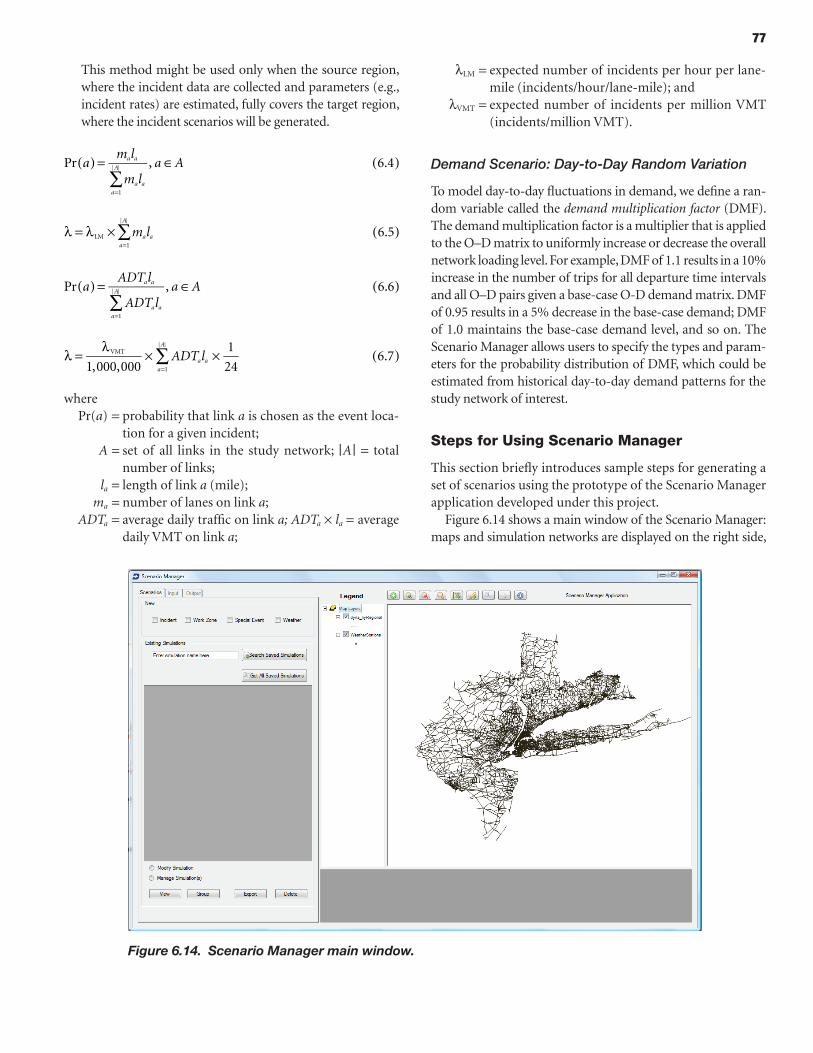
77
This method might be used only when the source region, where the incident data are collected and parameters (e.g., incident rates) are estimated, fully covers the target region, where the incident scenarios will be generated.
am l
m la Aa a
a aa
A
∑( ) ( )= ∈
=
Pr , 6.4
1
m la aa
A
∑ ( )λ = λ ×=
6.5LM1
aADT l
ADT la Aa a
a aa
A
∑( ) ( )= ∈
=
Pr , 6.6
1
ADT la aa
A
∑ ( )λ = λ × ×=1,000,000
1
246.7VMT
1
where Pr(a) = probability that link a is chosen as the event loca-
tion for a given incident; A = set of all links in the study network; |A | = total
number of links; la = length of link a (mile); ma = number of lanes on link a; ADTa = average daily traffic on link a; ADTa × la =average
daily VMT on link a;
lLM = expected number of incidents per hour per lane-mile (incidents/hour/lane-mile); and
lVMT = expected number of incidents per million VMT (incidents/million VMT).
Demand Scenario: Day-to-Day Random Variation
To model day-to-day fluctuations in demand, we define a ran-dom variable called the demand multiplication factor (DMF). The demand multiplication factor is a multiplier that is applied to the O–D matrix to uniformly increase or decrease the overall network loading level. For example, DMF of 1.1 results in a 10% increase in the number of trips for all departure time intervals and all O–D pairs given a base-case O-D demand matrix. DMF of 0.95 results in a 5% decrease in the base-case demand; DMF of 1.0 maintains the base-case demand level, and so on. The Scenario Manager allows users to specify the types and param-eters for the probability distribution of DMF, which could be estimated from historical day-to-day demand patterns for the study network of interest.
Steps for Using Scenario Manager
This section briefly introduces sample steps for generating a set of scenarios using the prototype of the Scenario Manager application developed under this project.
Figure 6.14 shows a main window of the Scenario Manager: maps and simulation networks are displayed on the right side,
Figure 6.14. Scenario Manager main window.
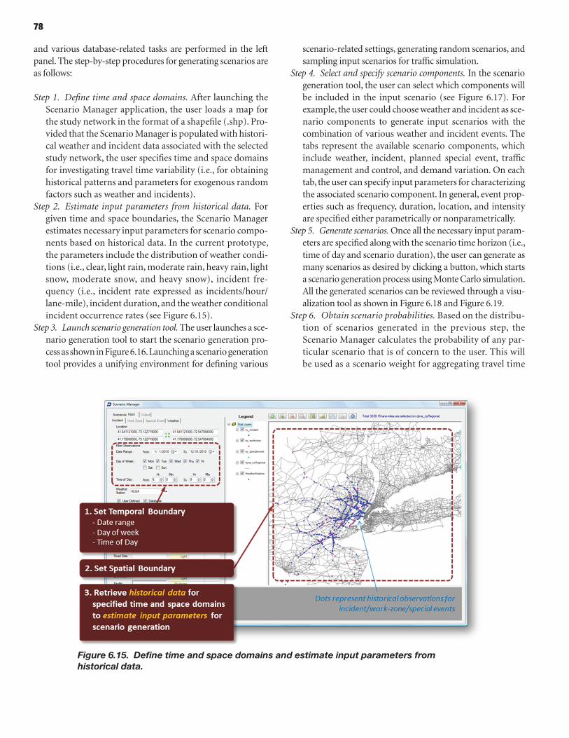
78
and various database-related tasks are performed in the left panel. The step-by-step procedures for generating scenarios are as follows:
Step 1. Define time and space domains. After launching the Scenario Manager application, the user loads a map for the study network in the format of a shapefile (.shp). Pro-vided that the Scenario Manager is populated with histori-cal weather and incident data associated with the selected study network, the user specifies time and space domains for investigating travel time variability (i.e., for obtaining historical patterns and parameters for exogenous random factors such as weather and incidents).
Step 2. Estimate input parameters from historical data. For given time and space boundaries, the Scenario Manager estimates necessary input parameters for scenario compo-nents based on historical data. In the current prototype, the parameters include the distribution of weather condi-tions (i.e., clear, light rain, moderate rain, heavy rain, light snow, moderate snow, and heavy snow), incident fre-quency (i.e., incident rate expressed as incidents/hour/lane-mile), incident duration, and the weather conditional incident occurrence rates (see Figure 6.15).
Step 3. Launch scenario generation tool. The user launches a sce-nario generation tool to start the scenario generation pro-cess as shown in Figure 6.16. Launching a scenario generation tool provides a unifying environment for defining various
scenario-related settings, generating random scenarios, and sampling input scenarios for traffic simulation.
Step 4. Select and specify scenario components. In the scenario generation tool, the user can select which components will be included in the input scenario (see Figure 6.17). For example, the user could choose weather and incident as sce-nario components to generate input scenarios with the combination of various weather and incident events. The tabs represent the available scenario components, which include weather, incident, planned special event, traffic management and control, and demand variation. On each tab, the user can specify input parameters for characterizing the associated scenario component. In general, event prop-erties such as frequency, duration, location, and intensity are specified either parametrically or nonparametrically.
Step 5. Generate scenarios. Once all the necessary input param-eters are specified along with the scenario time horizon (i.e., time of day and scenario duration), the user can generate as many scenarios as desired by clicking a button, which starts a scenario generation process using Monte Carlo simulation. All the generated scenarios can be reviewed through a visu-alization tool as shown in Figure 6.18 and Figure 6.19.
Step 6. Obtain scenario probabilities. Based on the distribu-tion of scenarios generated in the previous step, the Scenario Manager calculates the probability of any par-ticular scenario that is of concern to the user. This will be used as a scenario weight for aggregating travel time
Figure 6.15. Define time and space domains and estimate input parameters from historical data.
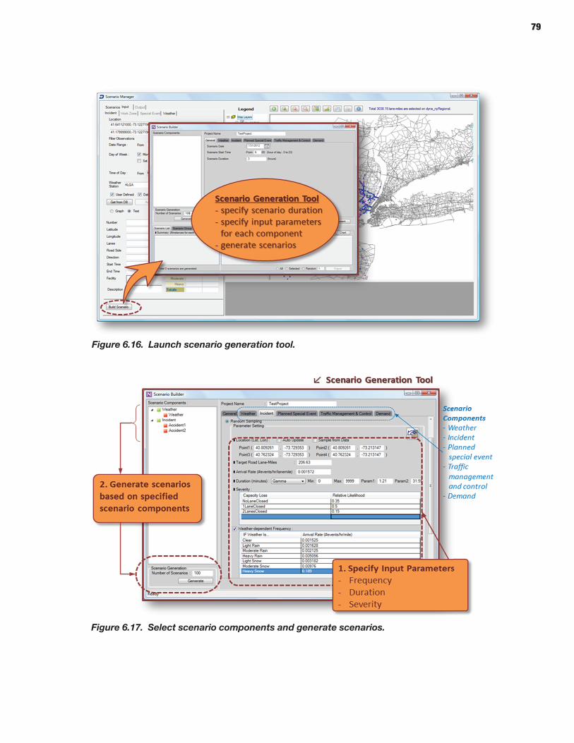
79
Figure 6.16. Launch scenario generation tool.
Figure 6.17. Select scenario components and generate scenarios.
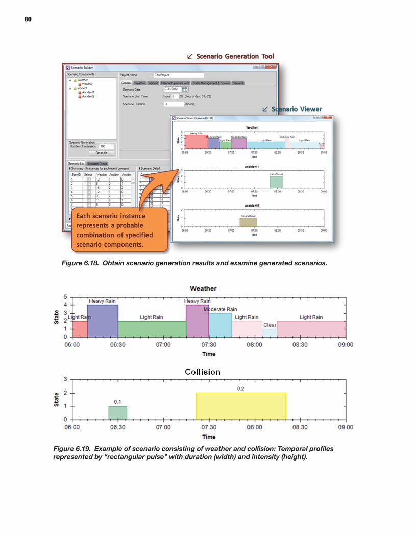
80
Figure 6.18. Obtain scenario generation results and examine generated scenarios.
Figure 6.19. Example of scenario consisting of weather and collision: Temporal profiles represented by “rectangular pulse” with duration (width) and intensity (height).
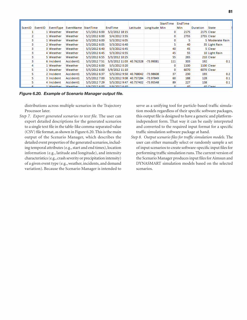
81
distributions across multiple scenarios in the Trajectory Processor later.
Step 7. Export generated scenarios to text file. The user can export detailed descriptions for the generated scenarios to a single text file in the table-like comma-separated value (CSV) file format, as shown in Figure 6.20. This is the main output of the Scenario Manager, which describes the detailed event properties of the generated scenarios, includ-ing temporal attributes (e.g., start and end times), location information (e.g., latitude and longitude), and intensity characteristics (e.g., crash severity or precipitation intensity) of a given event type (e.g., weather, incidents, and demand variation). Because the Scenario Manager is intended to
serve as a unifying tool for particle-based traffic simula-tion models regardless of their specific software packages, this output file is designed to have a generic and platform-independent form. That way it can be easily interpreted and converted to the required input format for a specific traffic simulation software package at hand.
Step 8. Output scenario files for traffic simulation models. The user can either manually select or randomly sample a set of input scenarios to create software-specific input files for performing traffic simulation runs. The current version of the Scenario Manager produces input files for Aimsun and DYNASMART simulation models based on the selected scenarios.
Figure 6.20. Example of Scenario Manager output file.
82
C h A p t e r 7
Introduction
To promote the use of end-to-end travel time reliability mea-sures in the professional community for regionwide transpor-tation operations planning, it is important and critically necessary to develop a flexible visualization platform for ana-lyzing microscopic and mesoscopic dynamic simulation results, particularly in tracking vehicular movement, path, and time-dependent trip-related statistics. As a generic visualiza-tion platform for travel time reliability, the vehicle Trajectory Processor designed in this project aims to apply new methods of communication between transportation practitioners, decision makers, and the public. This software package aims to help stakeholders from DOTs and MPOs effectively apply data processing and visualization tools to (1) understand advanced but sophisticated model structures and reliability-related output and (2) use higher fidelity transportation simu-lation and measurement results to estimate and calibrate underlying transportation system processes under different traffic conditions.
Purpose and Objectives
The objective of the vehicle Trajectory Processor is to provide a visualization platform for tracking and analyzing traffic assignment simulation results with a special focus on system-level travel time reliability. The vehicle Trajectory Processor is designed to perform the following tasks:
• Read vehicle trajectory files for each scenario, including an interface that directly imports simulation outputs from DYNASMART and other software packages, such as Aimsun.
• Read GPS vehicle trajectory data.• Publish scenario-specific travel time reliability measures
and display on the network/Google maps (e.g., most unre-liable O–D, link, path).
• Display the aggregate travel time distribution over multiple scenarios by considering the probability of each scenario.
• Compare observed and simulated travel time reliability measures.
Concept of Operations
To meet the design goals, the vehicle Trajectory Processor con-sists of the following basic functioning modules.
Map Matching and Vehicle Data Preprocessor
Internally, simulated vehicle trajectories (from DTA or micro-simulation) may not contain longitude and latitude infor-mation. In addition, although the GPS trajectories data are recorded in a longitude and latitude coordinate system, this information may not match to the real-world network. Thus, to correctly display the vehicle trajectories on the real-world network, the raw data must be preprocessed by the map matching module to correct geographic location information. As the vehicle trajectory data can come from various sources, including geographically distributed (clouded-based) data-bases, a vehicle data preprocessor must be able to access the data, locally or remotely, and convert various sources of data into a universal data representation for easier processing for the vehicle Trajectory Processor.
Vehicle Trajectory Processor
The vehicle Trajectory Processor module is the core data fusion component of the software application developed in this research. The inputs to this module include a set of simu-lated vehicle trajectories, generated using different scenarios in traffic simulation software, and GPS vehicle trajectories (both data sources are already preprocessed and converted into a universal format by the vehicle data preprocessed mod-ule). Based on the predefined measure of effectiveness (MOE)
Trajectory Processor
83
settings, this module will generate individual scenario-specific O–D travel time statistics (scenario-specific average O–D travel time and standard deviation) and aggregated O–D travel time statistics (aggregated average O–D travel time and stan-dard deviation). It also produces both O–D-level and path-level travel time statistics.
Besides these statistics, the vehicle Trajectory Processor module also prepares data for various internal visualization tools to present the results.
Statistics Result Presenting and Analysis Module
This module provides three styles of user interfaces (UI) to present statistics results to better analyze either O–D-level or path-level travel time.
a. Table-based statistic presentation UI. Both O–D-level and path-level travel time statistics (average and standard devia-tion of travel time) are presented in tables. Scenario-specific travel time statistics are listed side-by-side for straight-forward comparisons so that the critical O–D pairs or most unreliable O–D pairs can be easily identified.
b. Chart-based statistic presentation UI. The O–D-level travel time distribution is visualized with different graphs: scenario-specific or aggregated probability distribution function (PDF) graph, cumulative distribution function (CDF) graph, and so on. This UI can also display addi-tional travel time reliability indices, for example, Planning Time Index or buffer time.
c. Google Earth-based path presentation UI. To view and compare paths, this UI is able to display any possible paths between any O–D pair on Google Earth. With this capabil-ity, it is much easier to identify whether a path is a normal path or a detour.
The overall system architecture is illustrated in Figure 7.1.
Software description
The major software components developed in this research can be described by the universal vehicle data representation used to describe the vehicle trajectory data and by the data flow diagrams, which identify system components and their interactions.
Universal Vehicle Data Representation
The input data for the vehicle Trajectory Processor are simu-lated vehicle trajectory files from traffic assignment and simu-lation software packages, for example, DYNASMART and Aimsun. GPS vehicle trajectory data are another important source of input data. The simulated vehicle trajectory files from
these software packages and the GPS vehicle trajectory data have their own unique formats to represent the movements of the vehicles in the network. For the vehicle Trajectory Proces-sor to load and analyze these various sources and formats of vehicle trajectory files, it is important to design a universal data structure internally to represent these various input data. After thoroughly investigating the formats of the vehicle files from the DYNASMART and Aimsun software packages and GPS vehicle trajectory data, this universal vehicle representation (data structure) is designed to encompass necessary informa-tion to identify the vehicle movement and allow derivation of the travel time information between origin and destination zones. Table 7.1 lists the necessary information recorded by this universal vehicle data structure.
Data Flow
The overall vehicle trajectory processing procedure can be divided into three subprocedures: preprocessing, vehicle trajectory processing, and result presentation. Figure 7.2 illus-trates the input and output data for each subprocedure.
During the preprocessing, the map-matching engine converts the vehicle movements in a transportation planning network into real-network representation. These converted vehicle trajectory data are then output in a universal format.
The universally formatted vehicle trajectory data are input for the vehicle trajectory processing procedure, along with MOE settings. The standard output from this procedure is O–D-level or path-level, scenario-specific or aggregated travel time statistics (average and standard deviation of travel time). Based on specified MOE settings, other MOEs can be gener-ated as well.
The result presentation procedure takes the statistics gen-erated in the vehicle trajectory processing procedure and pre-pares data for display in various UIs. Based on the UI control selected by the user, the corresponding UI is activated to present the statistic results.
Integration with Selected Models (dYNASMArt and Aimsun)
Procedure
1. Import trajectory for multiple scenarios:a. DTA simulation results (e.g., DYNASMART);b. GPS vehicle location records (e.g., from TomTom);c. Simulated vehicle records (e.g., from VisSim, Aimsun).
2. Read user defined MOE (critical O–Ds, paths).3. Extract trajectory set for selected spatial element (O–D,
path).
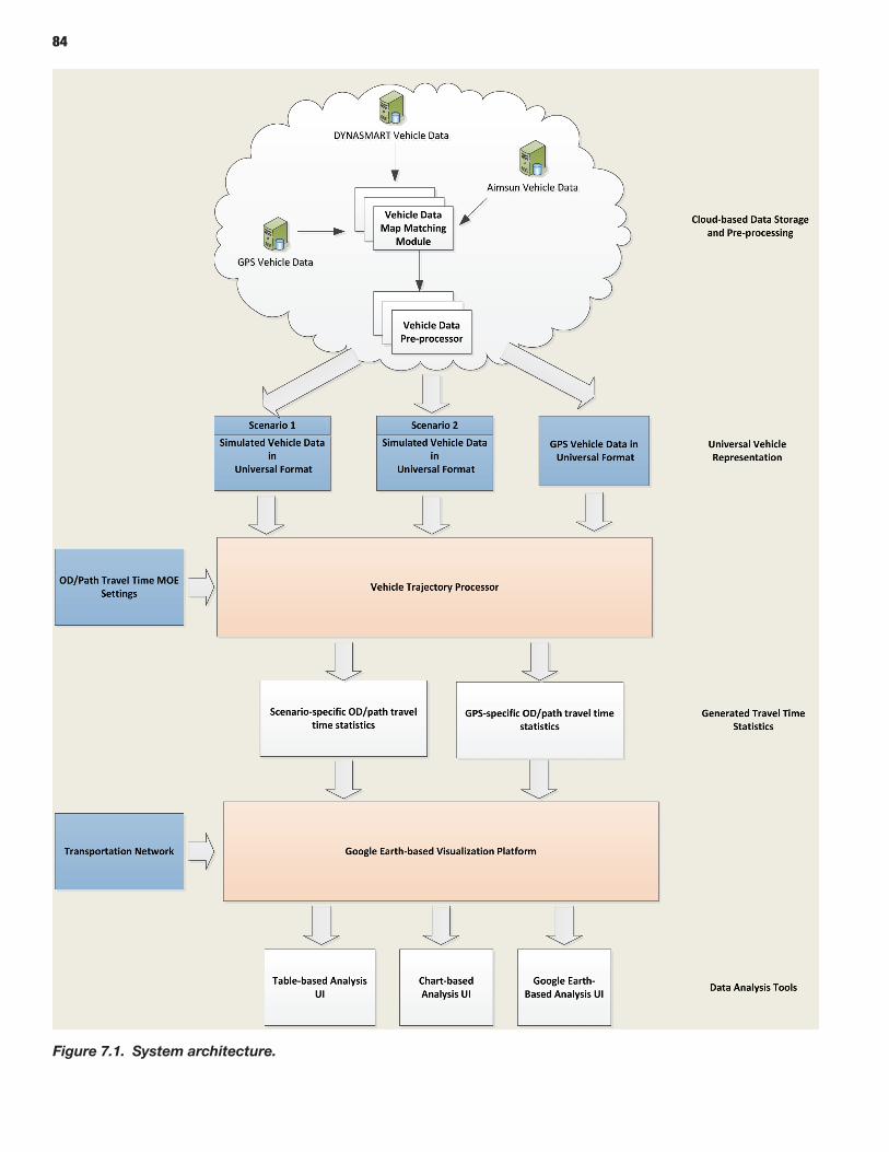
84
Figure 7.1. System architecture.
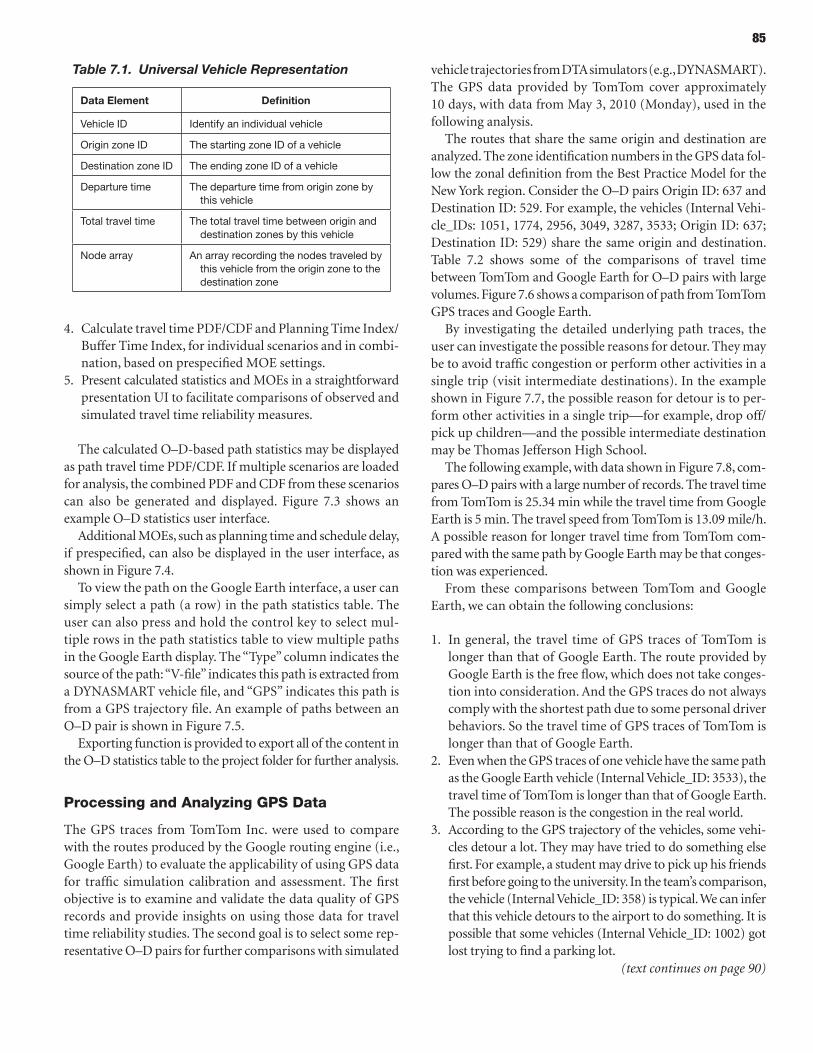
85
4. Calculate travel time PDF/CDF and Planning Time Index/Buffer Time Index, for individual scenarios and in combi-nation, based on prespecified MOE settings.
5. Present calculated statistics and MOEs in a straight forward presentation UI to facilitate comparisons of observed and simulated travel time reliability measures.
The calculated O–D-based path statistics may be displayed as path travel time PDF/CDF. If multiple scenarios are loaded for analysis, the combined PDF and CDF from these scenarios can also be generated and displayed. Figure 7.3 shows an example O–D statistics user interface.
Additional MOEs, such as planning time and schedule delay, if prespecified, can also be displayed in the user interface, as shown in Figure 7.4.
To view the path on the Google Earth interface, a user can simply select a path (a row) in the path statistics table. The user can also press and hold the control key to select mul-tiple rows in the path statistics table to view multiple paths in the Google Earth display. The “Type” column indicates the source of the path: “V-file” indicates this path is extracted from a DYNASMART vehicle file, and “GPS” indicates this path is from a GPS trajectory file. An example of paths between an O–D pair is shown in Figure 7.5.
Exporting function is provided to export all of the content in the O–D statistics table to the project folder for further analysis.
Processing and Analyzing GPS Data
The GPS traces from TomTom Inc. were used to compare with the routes produced by the Google routing engine (i.e., Google Earth) to evaluate the applicability of using GPS data for traffic simulation calibration and assessment. The first objective is to examine and validate the data quality of GPS records and provide insights on using those data for travel time reliability studies. The second goal is to select some rep-resentative O–D pairs for further comparisons with simulated
vehicle trajectories from DTA simulators (e.g., DYNASMART). The GPS data provided by TomTom cover approximately 10 days, with data from May 3, 2010 (Monday), used in the following analysis.
The routes that share the same origin and destination are analyzed. The zone identification numbers in the GPS data fol-low the zonal definition from the Best Practice Model for the New York region. Consider the O–D pairs Origin ID: 637 and Destination ID: 529. For example, the vehicles (Internal Vehi-cle_IDs: 1051, 1774, 2956, 3049, 3287, 3533; Origin ID: 637; Destination ID: 529) share the same origin and destination. Table 7.2 shows some of the comparisons of travel time between TomTom and Google Earth for O–D pairs with large volumes. Figure 7.6 shows a comparison of path from TomTom GPS traces and Google Earth.
By investigating the detailed underlying path traces, the user can investigate the possible reasons for detour. They may be to avoid traffic congestion or perform other activities in a single trip (visit intermediate destinations). In the example shown in Figure 7.7, the possible reason for detour is to per-form other activities in a single trip—for example, drop off/pick up children—and the possible intermediate destination may be Thomas Jefferson High School.
The following example, with data shown in Figure 7.8, com-pares O–D pairs with a large number of records. The travel time from TomTom is 25.34 min while the travel time from Google Earth is 5 min. The travel speed from TomTom is 13.09 mile/h. A possible reason for longer travel time from TomTom com-pared with the same path by Google Earth may be that conges-tion was experienced.
From these comparisons between TomTom and Google Earth, we can obtain the following conclusions:
1. In general, the travel time of GPS traces of TomTom is longer than that of Google Earth. The route provided by Google Earth is the free flow, which does not take conges-tion into consideration. And the GPS traces do not always comply with the shortest path due to some personal driver behaviors. So the travel time of GPS traces of TomTom is longer than that of Google Earth.
2. Even when the GPS traces of one vehicle have the same path as the Google Earth vehicle (Internal Vehicle_ID: 3533), the travel time of TomTom is longer than that of Google Earth. The possible reason is the congestion in the real world.
3. According to the GPS trajectory of the vehicles, some vehi-cles detour a lot. They may have tried to do something else first. For example, a student may drive to pick up his friends first before going to the university. In the team’s comparison, the vehicle (Internal Vehicle_ID: 358) is typical. We can infer that this vehicle detours to the airport to do something. It is possible that some vehicles (Internal Vehicle_ID: 1002) got lost trying to find a parking lot.
Table 7.1. Universal Vehicle Representation
Data element Definition
vehicle Id Identify an individual vehicle
origin zone Id The starting zone Id of a vehicle
destination zone Id The ending zone Id of a vehicle
departure time The departure time from origin zone by this vehicle
Total travel time The total travel time between origin and destination zones by this vehicle
Node array An array recording the nodes traveled by this vehicle from the origin zone to the destination zone
(text continues on page 90)
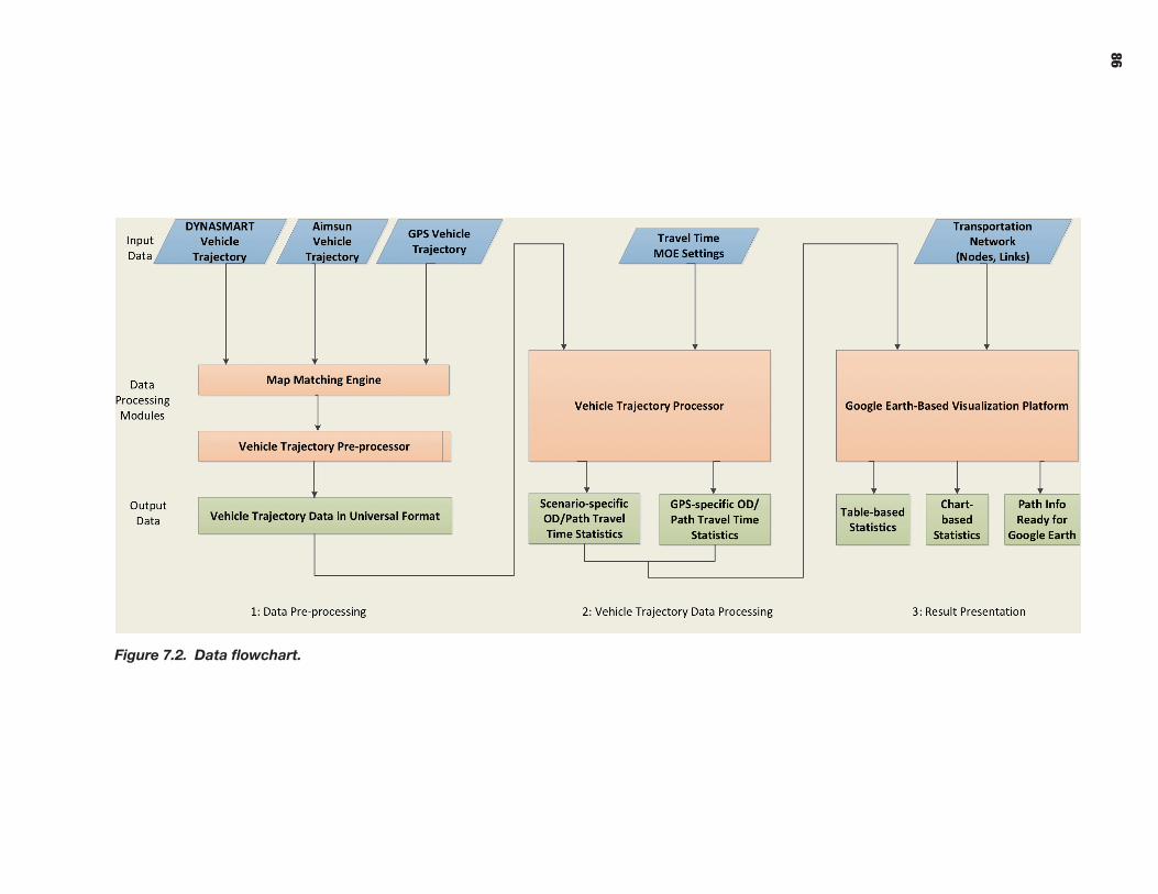
86
Figure 7.2. Data flowchart.
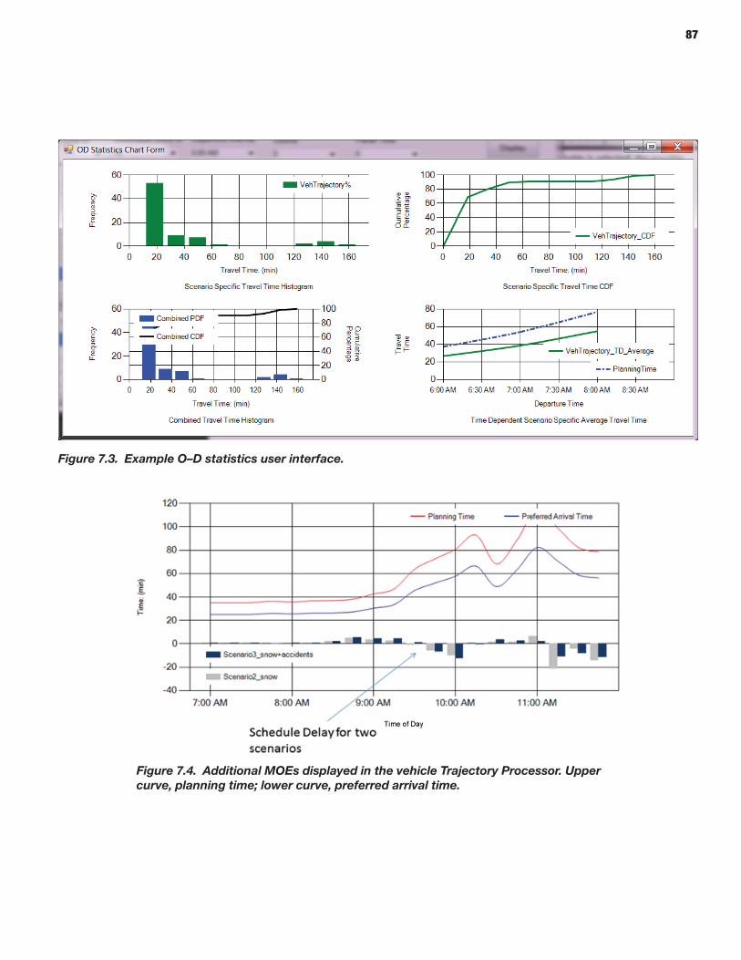
87
Figure 7.3. Example O–D statistics user interface.
Figure 7.4. Additional MOEs displayed in the vehicle Trajectory Processor. Upper curve, planning time; lower curve, preferred arrival time.
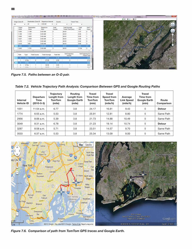
88
Table 7.2. Vehicle Trajectory Path Analysis: Comparison Between GPS and Google Routing Paths
Internal Vehicle ID
Departure Time
(2010-5-3)
Trajectory Length from
TomTom (mile)
Routing Length from Google Earth
(mile)
Travel Time from TomTom
(min)
Travel Speed from
TomTom (mile/h)
Average Link Speed
(mile/h)
Travel Time from
Google Earth (min)
Route Comparison
1051 11:54 a.m. 6.77 3.8 24.17 16.81 9.43 5 Detour
1774 6:55 a.m. 5.53 3.8 25.91 12.81 8.80 5 Same Path
2956 8:06 a.m. 5.39 3.8 21.73 14.88 10.49 5 Same Path
3049 8:31 a.m. 6.78 3.8 21.23 19.14 10.74 5 Detour
3287 8:58 a.m. 5.71 3.8 23.51 14.57 9.70 5 Same Path
3533 6:37 a.m. 5.53 3.8 25.34 13.09 9.00 5 Same Path
Figure 7.5. Paths between an O–D pair.
Figure 7.6. Comparison of path from TomTom GPS traces and Google Earth.
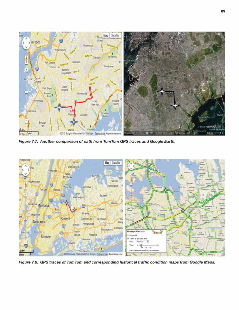
89
Figure 7.7. Another comparison of path from TomTom GPS traces and Google Earth.
Figure 7.8. GPS traces of TomTom and corresponding historical traffic condition maps from Google Maps.
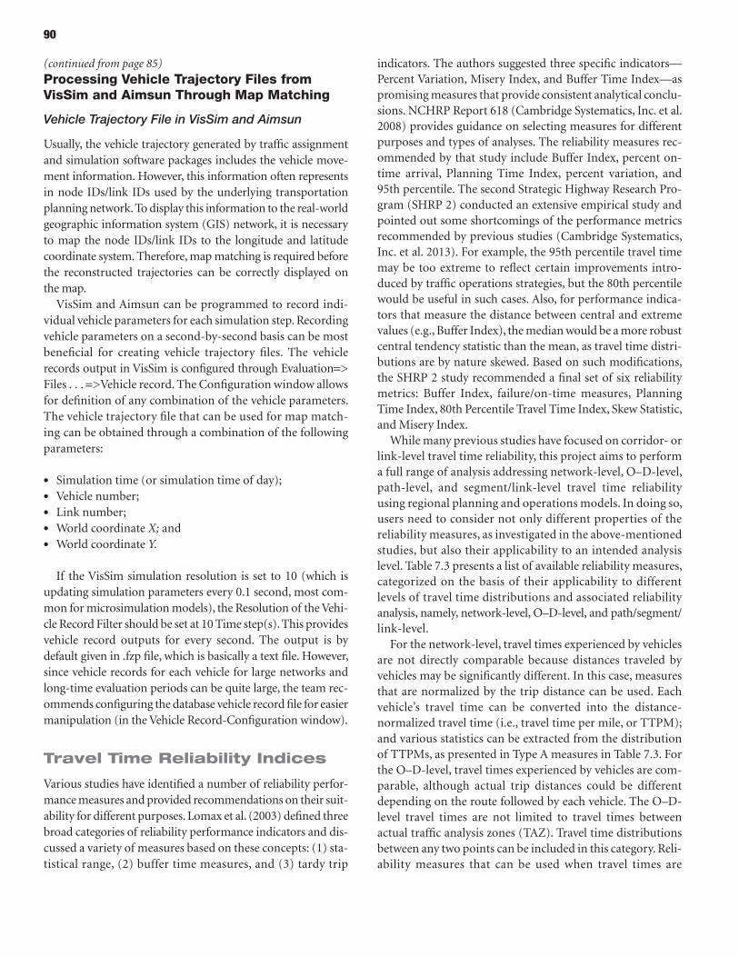
90
Processing Vehicle Trajectory Files from VisSim and Aimsun Through Map Matching
Vehicle Trajectory File in VisSim and Aimsun
Usually, the vehicle trajectory generated by traffic assignment and simulation software packages includes the vehicle move-ment information. However, this information often represents in node IDs/link IDs used by the underlying transportation planning network. To display this information to the real-world geographic information system (GIS) network, it is necessary to map the node IDs/link IDs to the longitude and latitude coordinate system. Therefore, map matching is required before the reconstructed trajectories can be correctly displayed on the map.
VisSim and Aimsun can be programmed to record indi-vidual vehicle parameters for each simulation step. Recording vehicle parameters on a second-by-second basis can be most beneficial for creating vehicle trajectory files. The vehicle records output in VisSim is configured through Evaluation=> Files . . . =>Vehicle record. The Configuration window allows for definition of any combination of the vehicle parameters. The vehicle trajectory file that can be used for map match-ing can be obtained through a combination of the following parameters:
• Simulation time (or simulation time of day);• Vehicle number;• Link number;• World coordinate X; and• World coordinate Y.
If the VisSim simulation resolution is set to 10 (which is updating simulation parameters every 0.1 second, most com-mon for microsimulation models), the Resolution of the Vehi-cle Record Filter should be set at 10 Time step(s). This provides vehicle record outputs for every second. The output is by default given in .fzp file, which is basically a text file. However, since vehicle records for each vehicle for large networks and long-time evaluation periods can be quite large, the team rec-ommends configuring the database vehicle record file for easier manipulation (in the Vehicle Record-Configuration window).
travel time reliability Indices
Various studies have identified a number of reliability perfor-mance measures and provided recommendations on their suit-ability for different purposes. Lomax et al. (2003) defined three broad categories of reliability performance indicators and dis-cussed a variety of measures based on these concepts: (1) sta-tistical range, (2) buffer time measures, and (3) tardy trip
indicators. The authors suggested three specific indicators—Percent Variation, Misery Index, and Buffer Time Index—as promising measures that provide consistent analytical conclu-sions. NCHRP Report 618 (Cambridge Systematics, Inc. et al. 2008) provides guidance on selecting measures for different purposes and types of analyses. The reliability measures rec-ommended by that study include Buffer Index, percent on-time arrival, Planning Time Index, percent variation, and 95th percentile. The second Strategic Highway Research Pro-gram (SHRP 2) conducted an extensive empirical study and pointed out some shortcomings of the performance metrics recommended by previous studies (Cambridge Systematics, Inc. et al. 2013). For example, the 95th percentile travel time may be too extreme to reflect certain improvements intro-duced by traffic operations strategies, but the 80th percentile would be useful in such cases. Also, for performance indica-tors that measure the distance between central and extreme values (e.g., Buffer Index), the median would be a more robust central tendency statistic than the mean, as travel time distri-butions are by nature skewed. Based on such modifications, the SHRP 2 study recommended a final set of six reliability metrics: Buffer Index, failure/on-time measures, Planning Time Index, 80th Percentile Travel Time Index, Skew Statistic, and Misery Index.
While many previous studies have focused on corridor- or link-level travel time reliability, this project aims to perform a full range of analysis addressing network-level, O–D-level, path-level, and segment/link-level travel time reliability using regional planning and operations models. In doing so, users need to consider not only different properties of the reliability measures, as investigated in the above-mentioned studies, but also their applicability to an intended analysis level. Table 7.3 presents a list of available reliability measures, categorized on the basis of their applicability to different levels of travel time distributions and associated reliability analysis, namely, network-level, O–D-level, and path/segment/link-level.
For the network-level, travel times experienced by vehicles are not directly comparable because distances traveled by vehicles may be significantly different. In this case, measures that are normalized by the trip distance can be used. Each vehicle’s travel time can be converted into the distance-normalized travel time (i.e., travel time per mile, or TTPM); and various statistics can be extracted from the distribution of TTPMs, as presented in Type A measures in Table 7.3. For the O–D-level, travel times experienced by vehicles are com-parable, although actual trip distances could be different depending on the route followed by each vehicle. The O–D-level travel times are not limited to travel times between actual traffic analysis zones (TAZ). Travel time distributions between any two points can be included in this category. Reli-ability measures that can be used when travel times are
(continued from page 85)
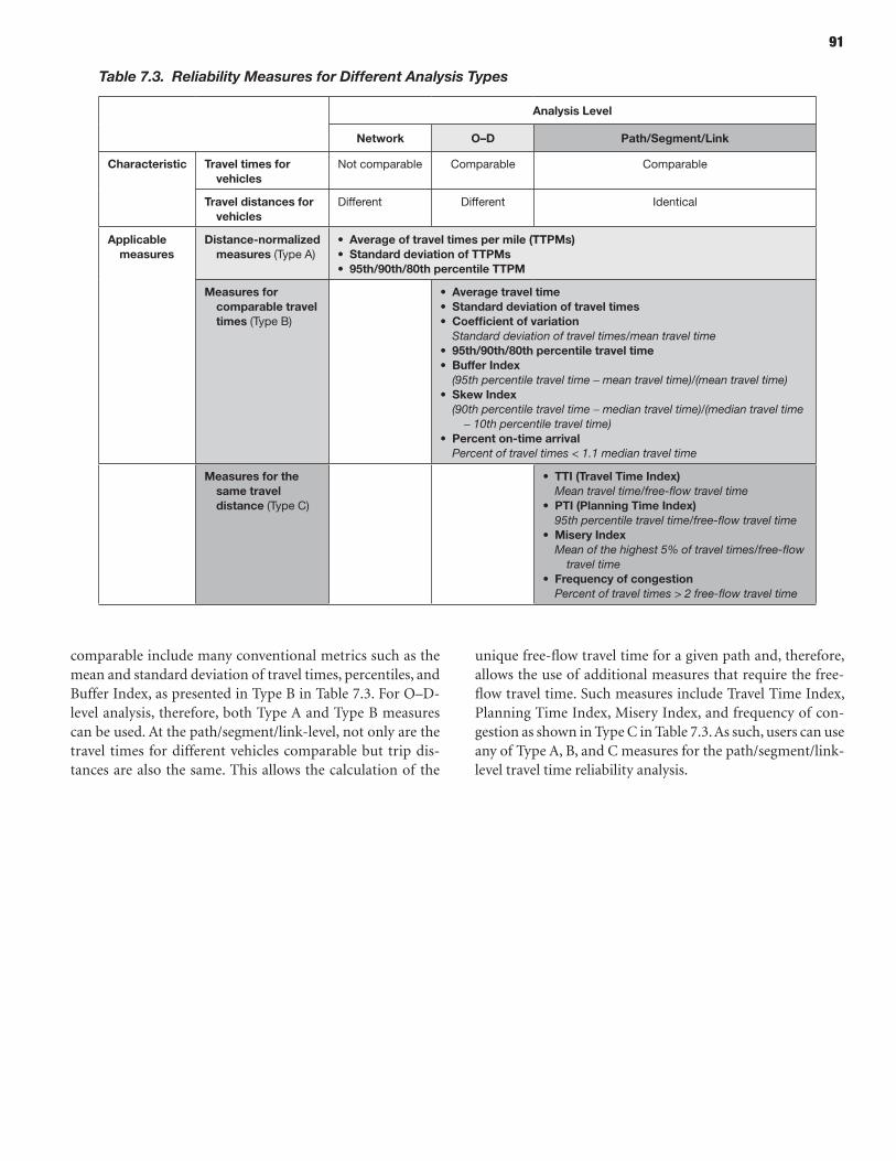
91
comparable include many conventional metrics such as the mean and standard deviation of travel times, percentiles, and Buffer Index, as presented in Type B in Table 7.3. For O–D-level analysis, therefore, both Type A and Type B measures can be used. At the path/segment/link-level, not only are the travel times for different vehicles comparable but trip dis-tances are also the same. This allows the calculation of the
Table 7.3. Reliability Measures for Different Analysis Types
Analysis Level
Network o–D path/Segment/Link
Characteristic travel times for vehicles
Not comparable comparable comparable
travel distances for vehicles
different different Identical
Applicable measures
Distance- normalized measures (Type A)
• Average of travel times per mile (ttpMs)• Standard deviation of ttpMs• 95th/90th/80th percentile ttpM
Measures for comparable travel times (Type B)
• Average travel time• Standard deviation of travel times• Coefficient of variation
Standard deviation of travel times/mean travel time• 95th/90th/80th percentile travel time• Buffer Index
(95th percentile travel time - mean travel time)/(mean travel time)• Skew Index
(90th percentile travel time - median travel time)/(median travel time - 10th percentile travel time)
• percent on-time arrivalPercent of travel times < 1.1 median travel time
Measures for the same travel distance (Type c)
• ttI (travel time Index)Mean travel time/free-flow travel time
• ptI (planning time Index)95th percentile travel time/free-flow travel time
• Misery IndexMean of the highest 5% of travel times/free-flow
travel time• Frequency of congestion
Percent of travel times > 2 free-flow travel time
unique free-flow travel time for a given path and, therefore, allows the use of additional measures that require the free-flow travel time. Such measures include Travel Time Index, Planning Time Index, Misery Index, and frequency of con-gestion as shown in Type C in Table 7.3. As such, users can use any of Type A, B, and C measures for the path/segment/link-level travel time reliability analysis.

93
p A r t 3
This part of the report describes two case studies incorporating travel time reliability into microscopic and mesoscopic models and summarizes the findings and conclusions of this research project.
APPLICATIONS
94
deterministic scenarios from existing historical sources. This case study uses the former approach: a set of random scenarios are constructed using Monte Carlo sampling for each category. The factors that are considered as scenario components are weather, incident, and day-to-day demand random variation as shown in Table 8.1. A detailed description for each scenario component is presented in the following subsections.
Scenario Specification
Weather
While considering incident and demand variations as random factors, we control the weather factor in constructing scenar-ios in this case study. In other words, we create a specific rain scenario and use it for all weather cases (i.e., WD-RA and WE-RA). The rain scenario is based on historical observations as discussed in the Chapter 6 section, Implementation of Sce-nario Manager, subsection Weather Scenario. The Scenario Manager allows users to supply specific weather time-series data to generate a fixed weather scenario. We used the weather data collected on May 3, 2010, at the ASOS weather station located at the LaGuardia Airport. Figure 8.2 shows the 5-hour weather scenario prepared for this case study.
Incidents
Incident properties are characterized using parametric mod-els as discussed in the Chapter 6 section, Implementation of Scenario Manager, subsection Incident Scenario. For fre-quency, we use a Poisson distribution to model the number of incidents for a given time period. To capture the dependency between weather and incident frequency, we use weather- conditional incident rates. Table 8.1 presents the estimated rate parameters. For incident duration, we specified a gamma distribution based on model-fitting results and estimated two input parameters: shape = 1.210 and scale = 31.553. Incident intensity is expressed as the percentage capacity loss (the
The purpose of this chapter is to demonstrate application of the overall methodology for performing reliability analyses using the framework and tools developed under this project in connection with a mesoscopic traffic simulation model, in this case DYNASMART-P (Mahmassani and Sbayti 2009). The following sections describe the entire procedure for per-forming the analysis in sequential order: defining, generating, and simulating scenarios; analyzing simulation outputs and extracting reliability statistics; and comparing simulation-based analysis results with observed data.
defining Scenarios
Defining Spatial and Temporal Boundaries for Evaluating Travel Time Reliability
The spatial domain of interest selected for this application is an area in the New York City region. Figure 8.1 shows the sim-ulation network prepared for the analysis, which covers most of New York City and part of New Jersey. The time domain of interest is the morning time period from 6 a.m. until 11 a.m. between May 2, 2010, and May 17, 2010.
Formulating Study Objectives and Defining Scenario Cases
The objective of the case study is to examine the effect of weather on travel time reliability for weekday and weekend traffic. Specifically, we obtain reliability performance measures for the following four scenario cases: Weekdays under Rain (WD-RA), Weekends under Rain (WE-RA), Weekdays under No Rain (WD-NR), and Weekends under No Rain (WE-NR).
Generating Scenarios Using the Scenario Manager
Specific scenarios under each of the four cases may be obtained either by generating random scenarios using the Scenario Manager’s Monte Carlo sampling capability or by using
Analysis Process: Mesoscopic Models
C h A p t e r 8
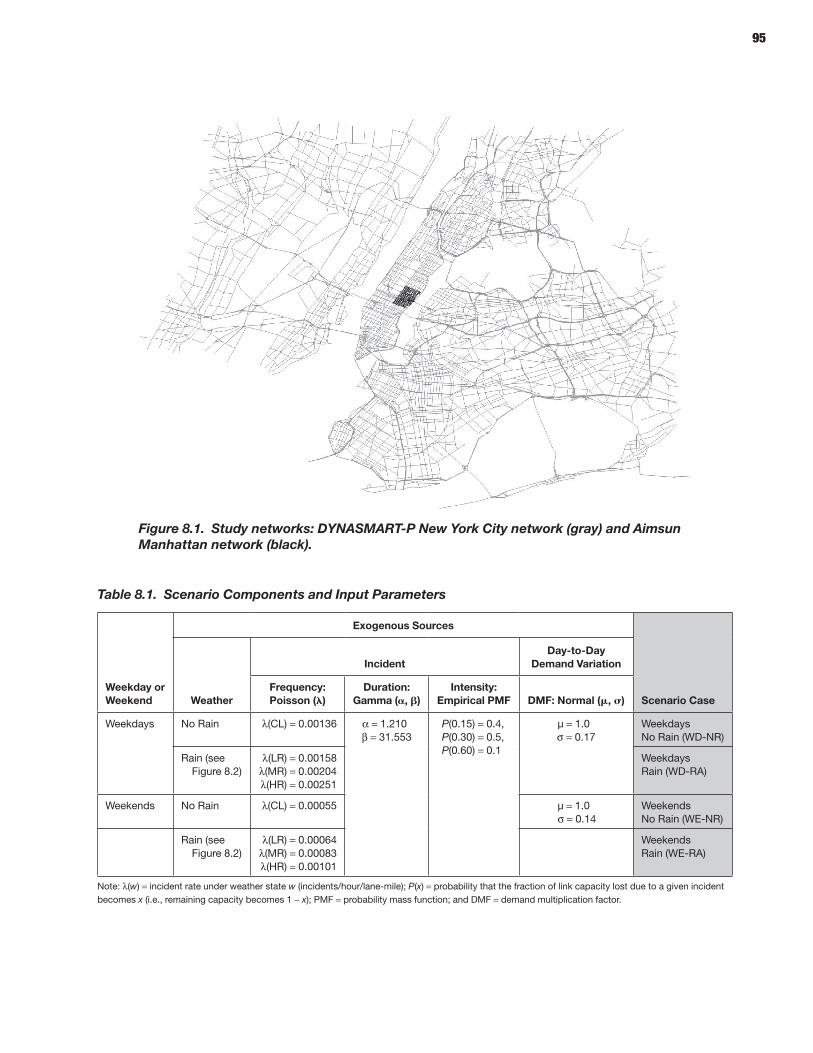
95
Table 8.1. Scenario Components and Input Parameters
Weekday or Weekend
exogenous Sources
Scenario CaseWeather
IncidentDay-to-Day
Demand Variation
Frequency: poisson ()
Duration: Gamma (, )
Intensity: empirical pMF DMF: Normal (, )
weekdays No Rain l(cl) = 0.00136 a = 1.210b = 31.553
P(0.15) = 0.4,P(0.30) = 0.5,P(0.60) = 0.1
µ = 1.0s = 0.17
weekdaysNo Rain (wd-NR)
Rain (see Figure 8.2)
l(lR) = 0.00158l(MR) = 0.00204l(hR) = 0.00251
weekdaysRain (wd-RA)
weekends No Rain l(cl) = 0.00055 µ = 1.0s = 0.14
weekendsNo Rain (wE-NR)
Rain (see Figure 8.2)
l(lR) = 0.00064l(MR) = 0.00083l(hR) = 0.00101
weekendsRain (wE-RA)
Note: l(w) = incident rate under weather state w (incidents/hour/lane-mile); P(x) = probability that the fraction of link capacity lost due to a given incident becomes x (i.e., remaining capacity becomes 1 - x); PMF = probability mass function; and dMF = demand multiplication factor.
Figure 8.1. Study networks: DYNASMART-P New York City network (gray) and Aimsun Manhattan network (black).
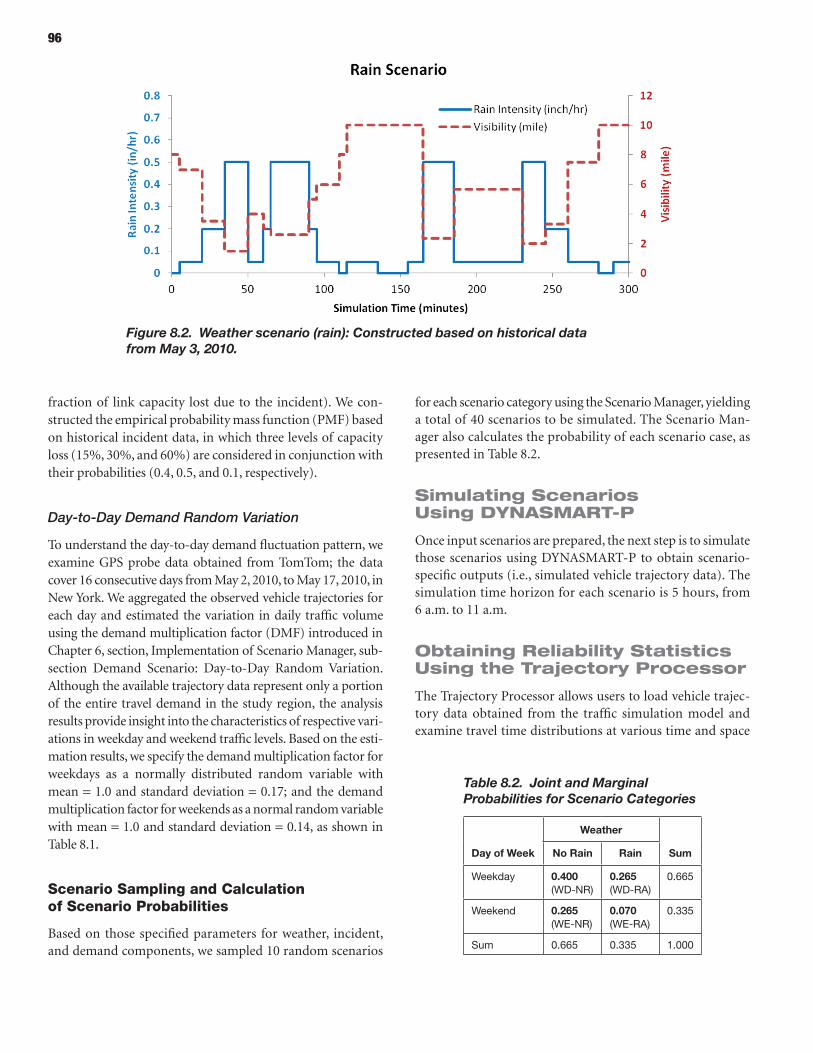
96
fraction of link capacity lost due to the incident). We con-structed the empirical probability mass function (PMF) based on historical incident data, in which three levels of capacity loss (15%, 30%, and 60%) are considered in conjunction with their probabilities (0.4, 0.5, and 0.1, respectively).
Day-to-Day Demand Random Variation
To understand the day-to-day demand fluctuation pattern, we examine GPS probe data obtained from TomTom; the data cover 16 consecutive days from May 2, 2010, to May 17, 2010, in New York. We aggregated the observed vehicle trajectories for each day and estimated the variation in daily traffic volume using the demand multiplication factor (DMF) introduced in Chapter 6, section, Implementation of Scenario Manager, sub-section Demand Scenario: Day-to-Day Random Variation. Although the available trajectory data represent only a portion of the entire travel demand in the study region, the analysis results provide insight into the characteristics of respective vari-ations in weekday and weekend traffic levels. Based on the esti-mation results, we specify the demand multiplication factor for weekdays as a normally distributed random variable with mean = 1.0 and standard deviation = 0.17; and the demand multiplication factor for weekends as a normal random variable with mean = 1.0 and standard deviation = 0.14, as shown in Table 8.1.
Scenario Sampling and Calculation of Scenario Probabilities
Based on those specified parameters for weather, incident, and demand components, we sampled 10 random scenarios
for each scenario category using the Scenario Manager, yielding a total of 40 scenarios to be simulated. The Scenario Man-ager also calculates the probability of each scenario case, as presented in Table 8.2.
Simulating Scenarios Using dYNASMArt-p
Once input scenarios are prepared, the next step is to simulate those scenarios using DYNASMART-P to obtain scenario-specific outputs (i.e., simulated vehicle trajectory data). The simulation time horizon for each scenario is 5 hours, from 6 a.m. to 11 a.m.
obtaining reliability Statistics Using the trajectory processor
The Trajectory Processor allows users to load vehicle trajec-tory data obtained from the traffic simulation model and examine travel time distributions at various time and space
Table 8.2. Joint and Marginal Probabilities for Scenario Categories
Day of Week
Weather
SumNo Rain Rain
weekday 0.400(wd-NR)
0.265(wd-RA)
0.665
weekend 0.265(wE-NR)
0.070(wE-RA)
0.335
Sum 0.665 0.335 1.000
Figure 8.2. Weather scenario (rain): Constructed based on historical data from May 3, 2010.
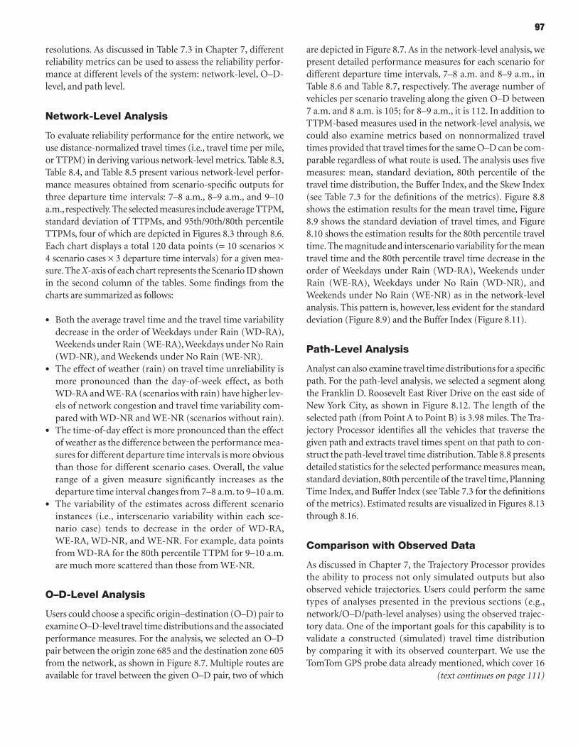
97
resolutions. As discussed in Table 7.3 in Chapter 7, different reliability metrics can be used to assess the reliability perfor-mance at different levels of the system: network-level, O–D-level, and path level.
Network-Level Analysis
To evaluate reliability performance for the entire network, we use distance-normalized travel times (i.e., travel time per mile, or TTPM) in deriving various network-level metrics. Table 8.3, Table 8.4, and Table 8.5 present various network-level perfor-mance measures obtained from scenario-specific outputs for three departure time intervals: 7–8 a.m., 8–9 a.m., and 9–10 a.m., respectively. The selected measures include average TTPM, standard deviation of TTPMs, and 95th/90th/80th percentile TTPMs, four of which are depicted in Figures 8.3 through 8.6. Each chart displays a total 120 data points (= 10 scenarios × 4 scenario cases × 3 departure time intervals) for a given mea-sure. The X-axis of each chart represents the Scenario ID shown in the second column of the tables. Some findings from the charts are summarized as follows:
• Both the average travel time and the travel time variability decrease in the order of Weekdays under Rain (WD-RA), Weekends under Rain (WE-RA), Weekdays under No Rain (WD-NR), and Weekends under No Rain (WE-NR).
• The effect of weather (rain) on travel time unreliability is more pronounced than the day-of-week effect, as both WD-RA and WE-RA (scenarios with rain) have higher lev-els of network congestion and travel time variability com-pared with WD-NR and WE-NR (scenarios without rain).
• The time-of-day effect is more pronounced than the effect of weather as the difference between the performance mea-sures for different departure time intervals is more obvious than those for different scenario cases. Overall, the value range of a given measure significantly increases as the departure time interval changes from 7–8 a.m. to 9–10 a.m.
• The variability of the estimates across different scenario instances (i.e., interscenario variability within each sce-nario case) tends to decrease in the order of WD-RA, WE-RA, WD-NR, and WE-NR. For example, data points from WD-RA for the 80th percentile TTPM for 9–10 a.m. are much more scattered than those from WE-NR.
O–D-Level Analysis
Users could choose a specific origin–destination (O–D) pair to examine O–D-level travel time distributions and the associated performance measures. For the analysis, we selected an O–D pair between the origin zone 685 and the destination zone 605 from the network, as shown in Figure 8.7. Multiple routes are available for travel between the given O–D pair, two of which
are depicted in Figure 8.7. As in the network-level analysis, we present detailed performance measures for each scenario for different departure time intervals, 7–8 a.m. and 8–9 a.m., in Table 8.6 and Table 8.7, respectively. The average number of vehicles per scenario traveling along the given O–D between 7 a.m. and 8 a.m. is 105; for 8–9 a.m., it is 112. In addition to TTPM-based measures used in the network-level analysis, we could also examine metrics based on nonnormalized travel times provided that travel times for the same O–D can be com-parable regardless of what route is used. The analysis uses five measures: mean, standard deviation, 80th percentile of the travel time distribution, the Buffer Index, and the Skew Index (see Table 7.3 for the definitions of the metrics). Figure 8.8 shows the estimation results for the mean travel time, Figure 8.9 shows the standard deviation of travel times, and Figure 8.10 shows the estimation results for the 80th percentile travel time. The magnitude and interscenario variability for the mean travel time and the 80th percentile travel time decrease in the order of Weekdays under Rain (WD-RA), Weekends under Rain (WE-RA), Weekdays under No Rain (WD-NR), and Weekends under No Rain (WE-NR) as in the network-level analysis. This pattern is, however, less evident for the standard deviation (Figure 8.9) and the Buffer Index (Figure 8.11).
Path-Level Analysis
Analyst can also examine travel time distributions for a specific path. For the path-level analysis, we selected a segment along the Franklin D. Roosevelt East River Drive on the east side of New York City, as shown in Figure 8.12. The length of the selected path (from Point A to Point B) is 3.98 miles. The Tra-jectory Processor identifies all the vehicles that traverse the given path and extracts travel times spent on that path to con-struct the path-level travel time distribution. Table 8.8 presents detailed statistics for the selected performance measures mean, standard deviation, 80th percentile of the travel time, Planning Time Index, and Buffer Index (see Table 7.3 for the definitions of the metrics). Estimated results are visualized in Figures 8.13 through 8.16.
Comparison with Observed Data
As discussed in Chapter 7, the Trajectory Processor provides the ability to process not only simulated outputs but also observed vehicle trajectories. Users could perform the same types of analyses presented in the previous sections (e.g., network/O–D/path-level analyses) using the observed trajec-tory data. One of the important goals for this capability is to validate a constructed (simulated) travel time distribution by comparing it with its observed counterpart. We use the TomTom GPS probe data already mentioned, which cover 16
(text continues on page 111)
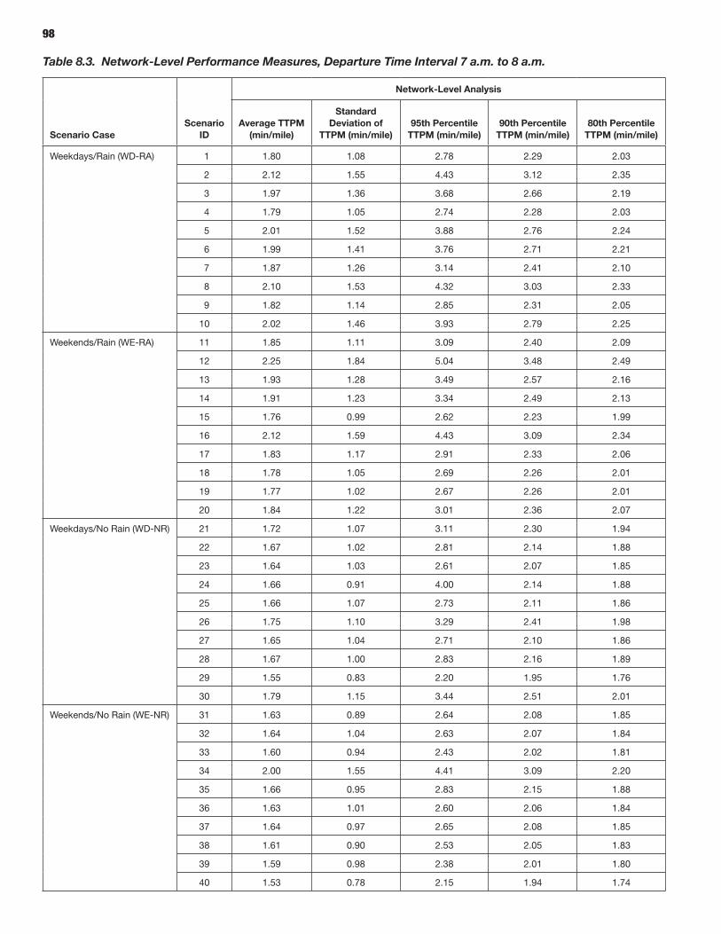
98
Table 8.3. Network-Level Performance Measures, Departure Time Interval 7 a.m. to 8 a.m.
Scenario CaseScenario
ID
Network-Level Analysis
Average ttpM (min/mile)
Standard Deviation of
ttpM (min/mile)95th percentile
ttpM (min/mile)90th percentile
ttpM (min/mile)80th percentile
ttpM (min/mile)
weekdays/Rain (wd-RA) 1 1.80 1.08 2.78 2.29 2.03
2 2.12 1.55 4.43 3.12 2.35
3 1.97 1.36 3.68 2.66 2.19
4 1.79 1.05 2.74 2.28 2.03
5 2.01 1.52 3.88 2.76 2.24
6 1.99 1.41 3.76 2.71 2.21
7 1.87 1.26 3.14 2.41 2.10
8 2.10 1.53 4.32 3.03 2.33
9 1.82 1.14 2.85 2.31 2.05
10 2.02 1.46 3.93 2.79 2.25
weekends/Rain (wE-RA) 11 1.85 1.11 3.09 2.40 2.09
12 2.25 1.84 5.04 3.48 2.49
13 1.93 1.28 3.49 2.57 2.16
14 1.91 1.23 3.34 2.49 2.13
15 1.76 0.99 2.62 2.23 1.99
16 2.12 1.59 4.43 3.09 2.34
17 1.83 1.17 2.91 2.33 2.06
18 1.78 1.05 2.69 2.26 2.01
19 1.77 1.02 2.67 2.26 2.01
20 1.84 1.22 3.01 2.36 2.07
weekdays/No Rain (wd-NR) 21 1.72 1.07 3.11 2.30 1.94
22 1.67 1.02 2.81 2.14 1.88
23 1.64 1.03 2.61 2.07 1.85
24 1.66 0.91 4.00 2.14 1.88
25 1.66 1.07 2.73 2.11 1.86
26 1.75 1.10 3.29 2.41 1.98
27 1.65 1.04 2.71 2.10 1.86
28 1.67 1.00 2.83 2.16 1.89
29 1.55 0.83 2.20 1.95 1.76
30 1.79 1.15 3.44 2.51 2.01
weekends/No Rain (wE-NR) 31 1.63 0.89 2.64 2.08 1.85
32 1.64 1.04 2.63 2.07 1.84
33 1.60 0.94 2.43 2.02 1.81
34 2.00 1.55 4.41 3.09 2.20
35 1.66 0.95 2.83 2.15 1.88
36 1.63 1.01 2.60 2.06 1.84
37 1.64 0.97 2.65 2.08 1.85
38 1.61 0.90 2.53 2.05 1.83
39 1.59 0.98 2.38 2.01 1.80
40 1.53 0.78 2.15 1.94 1.74
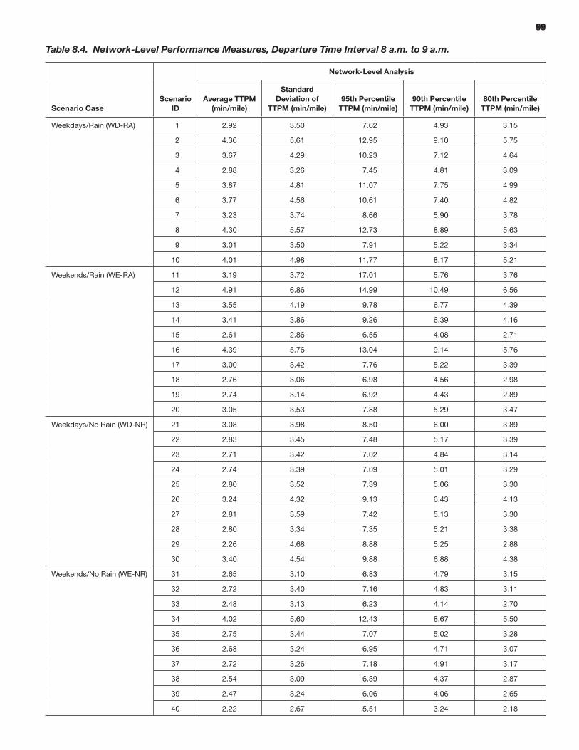
99
Table 8.4. Network-Level Performance Measures, Departure Time Interval 8 a.m. to 9 a.m.
Scenario CaseScenario
ID
Network-Level Analysis
Average ttpM (min/mile)
Standard Deviation of
ttpM (min/mile)95th percentile
ttpM (min/mile)90th percentile
ttpM (min/mile)80th percentile
ttpM (min/mile)
weekdays/Rain (wd-RA) 1 2.92 3.50 7.62 4.93 3.15
2 4.36 5.61 12.95 9.10 5.75
3 3.67 4.29 10.23 7.12 4.64
4 2.88 3.26 7.45 4.81 3.09
5 3.87 4.81 11.07 7.75 4.99
6 3.77 4.56 10.61 7.40 4.82
7 3.23 3.74 8.66 5.90 3.78
8 4.30 5.57 12.73 8.89 5.63
9 3.01 3.50 7.91 5.22 3.34
10 4.01 4.98 11.77 8.17 5.21
weekends/Rain (wE-RA) 11 3.19 3.72 17.01 5.76 3.76
12 4.91 6.86 14.99 10.49 6.56
13 3.55 4.19 9.78 6.77 4.39
14 3.41 3.86 9.26 6.39 4.16
15 2.61 2.86 6.55 4.08 2.71
16 4.39 5.76 13.04 9.14 5.76
17 3.00 3.42 7.76 5.22 3.39
18 2.76 3.06 6.98 4.56 2.98
19 2.74 3.14 6.92 4.43 2.89
20 3.05 3.53 7.88 5.29 3.47
weekdays/No Rain (wd-NR) 21 3.08 3.98 8.50 6.00 3.89
22 2.83 3.45 7.48 5.17 3.39
23 2.71 3.42 7.02 4.84 3.14
24 2.74 3.39 7.09 5.01 3.29
25 2.80 3.52 7.39 5.06 3.30
26 3.24 4.32 9.13 6.43 4.13
27 2.81 3.59 7.42 5.13 3.30
28 2.80 3.34 7.35 5.21 3.38
29 2.26 4.68 8.88 5.25 2.88
30 3.40 4.54 9.88 6.88 4.38
weekends/No Rain (wE-NR) 31 2.65 3.10 6.83 4.79 3.15
32 2.72 3.40 7.16 4.83 3.11
33 2.48 3.13 6.23 4.14 2.70
34 4.02 5.60 12.43 8.67 5.50
35 2.75 3.44 7.07 5.02 3.28
36 2.68 3.24 6.95 4.71 3.07
37 2.72 3.26 7.18 4.91 3.17
38 2.54 3.09 6.39 4.37 2.87
39 2.47 3.24 6.06 4.06 2.65
40 2.22 2.67 5.51 3.24 2.18
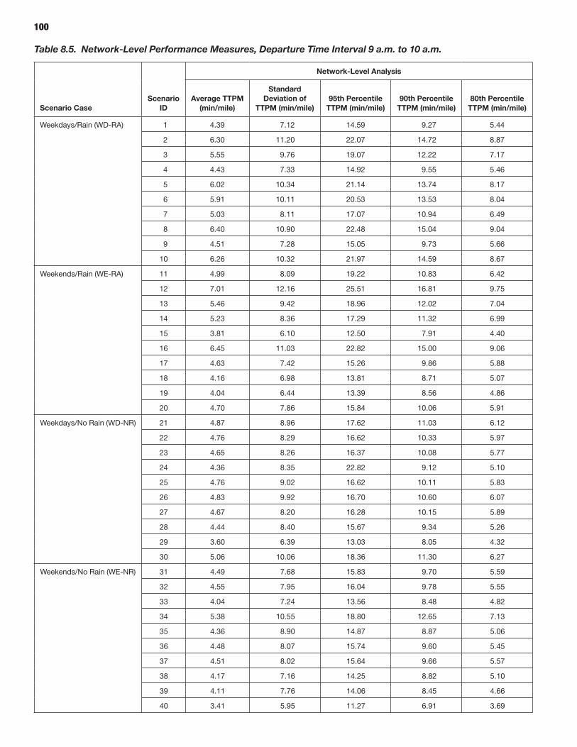
100
Table 8.5. Network-Level Performance Measures, Departure Time Interval 9 a.m. to 10 a.m.
Scenario CaseScenario
ID
Network-Level Analysis
Average ttpM (min/mile)
Standard Deviation of
ttpM (min/mile)95th percentile
ttpM (min/mile)90th percentile
ttpM (min/mile)80th percentile
ttpM (min/mile)
weekdays/Rain (wd-RA) 1 4.39 7.12 14.59 9.27 5.44
2 6.30 11.20 22.07 14.72 8.87
3 5.55 9.76 19.07 12.22 7.17
4 4.43 7.33 14.92 9.55 5.46
5 6.02 10.34 21.14 13.74 8.17
6 5.91 10.11 20.53 13.53 8.04
7 5.03 8.11 17.07 10.94 6.49
8 6.40 10.90 22.48 15.04 9.04
9 4.51 7.28 15.05 9.73 5.66
10 6.26 10.32 21.97 14.59 8.67
weekends/Rain (wE-RA) 11 4.99 8.09 19.22 10.83 6.42
12 7.01 12.16 25.51 16.81 9.75
13 5.46 9.42 18.96 12.02 7.04
14 5.23 8.36 17.29 11.32 6.99
15 3.81 6.10 12.50 7.91 4.40
16 6.45 11.03 22.82 15.00 9.06
17 4.63 7.42 15.26 9.86 5.88
18 4.16 6.98 13.81 8.71 5.07
19 4.04 6.44 13.39 8.56 4.86
20 4.70 7.86 15.84 10.06 5.91
weekdays/No Rain (wd-NR) 21 4.87 8.96 17.62 11.03 6.12
22 4.76 8.29 16.62 10.33 5.97
23 4.65 8.26 16.37 10.08 5.77
24 4.36 8.35 22.82 9.12 5.10
25 4.76 9.02 16.62 10.11 5.83
26 4.83 9.92 16.70 10.60 6.07
27 4.67 8.20 16.28 10.15 5.89
28 4.44 8.40 15.67 9.34 5.26
29 3.60 6.39 13.03 8.05 4.32
30 5.06 10.06 18.36 11.30 6.27
weekends/No Rain (wE-NR) 31 4.49 7.68 15.83 9.70 5.59
32 4.55 7.95 16.04 9.78 5.55
33 4.04 7.24 13.56 8.48 4.82
34 5.38 10.55 18.80 12.65 7.13
35 4.36 8.90 14.87 8.87 5.06
36 4.48 8.07 15.74 9.60 5.45
37 4.51 8.02 15.64 9.66 5.57
38 4.17 7.16 14.25 8.82 5.10
39 4.11 7.76 14.06 8.45 4.66
40 3.41 5.95 11.27 6.91 3.69
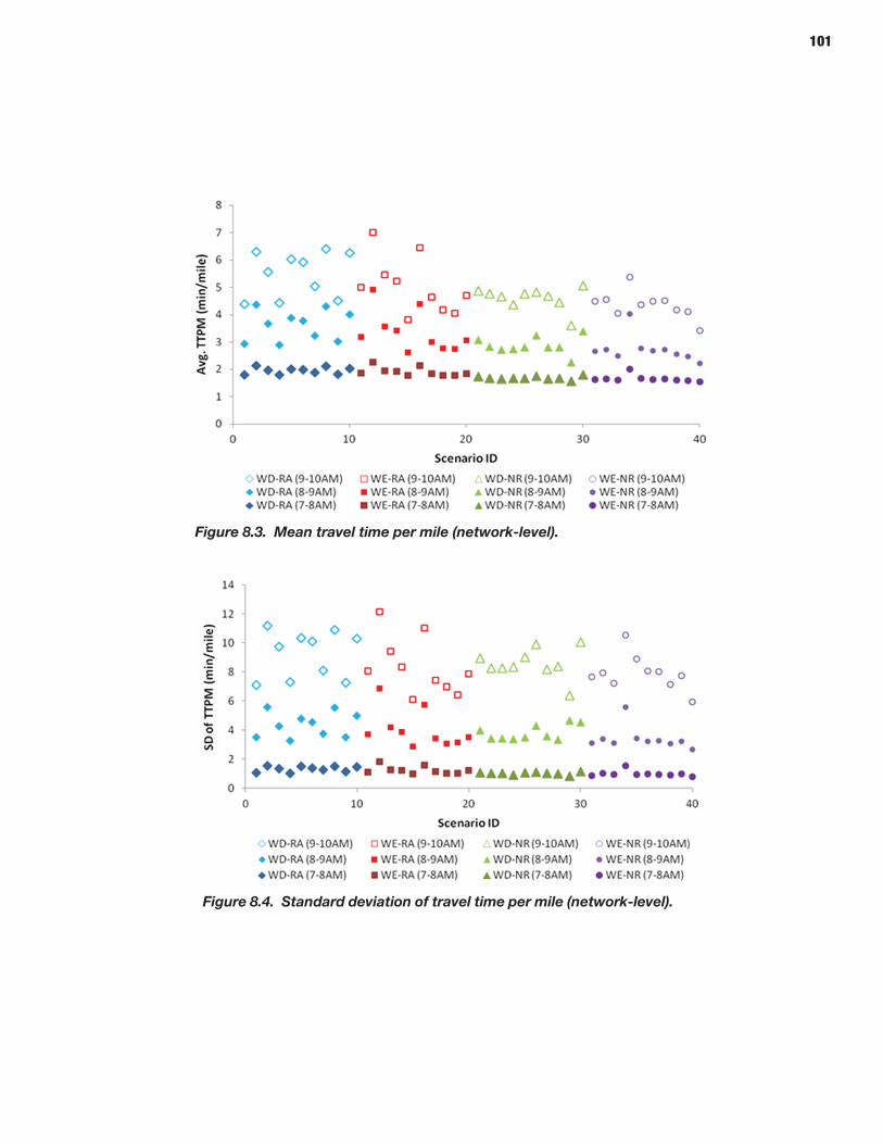
101
Figure 8.3. Mean travel time per mile (network-level).
Figure 8.4. Standard deviation of travel time per mile (network-level).
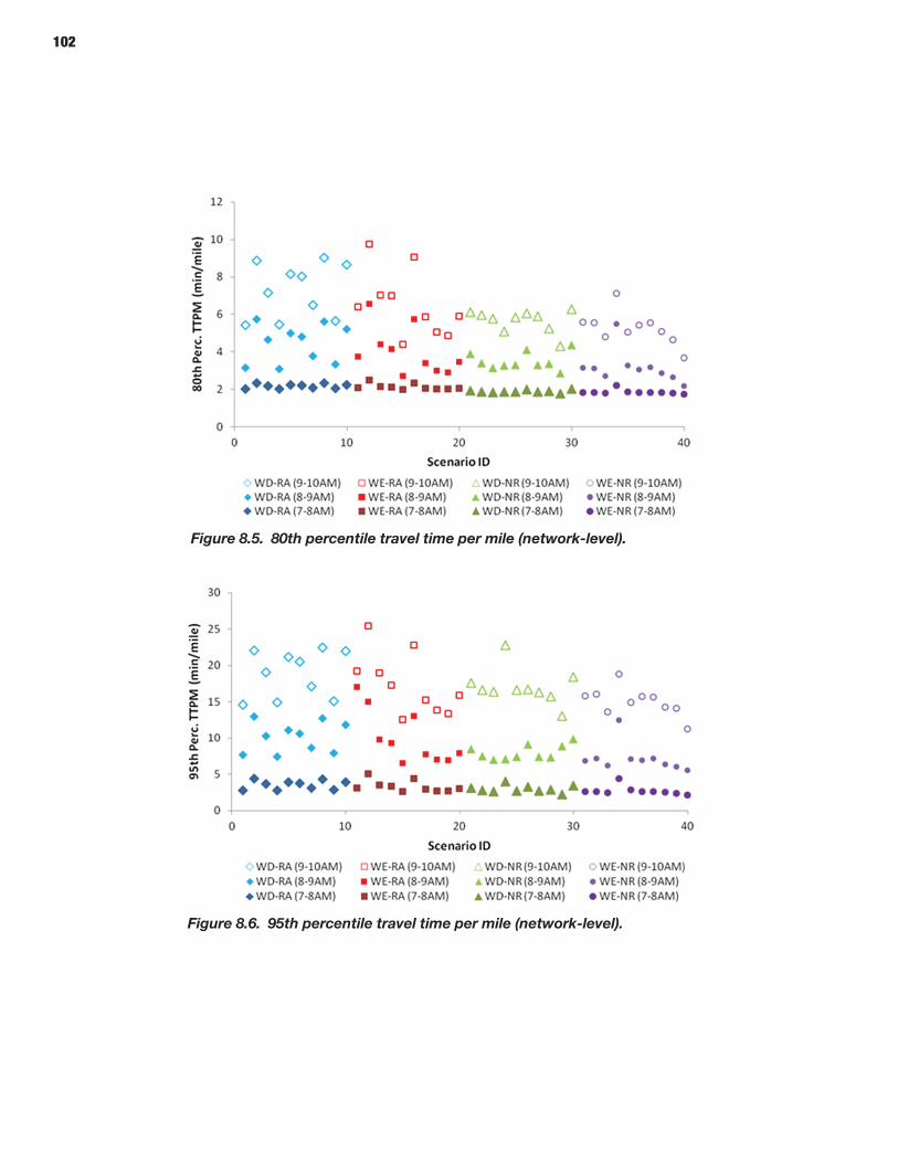
102
Figure 8.5. 80th percentile travel time per mile (network-level).
Figure 8.6. 95th percentile travel time per mile (network-level).
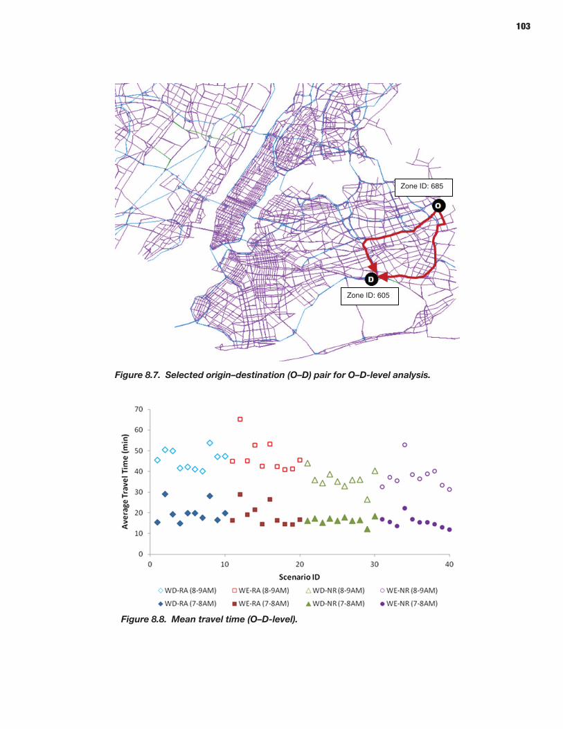
103
Zone ID: 685
Zone ID: 605
Figure 8.7. Selected origin–destination (O–D) pair for O–D-level analysis.
Figure 8.8. Mean travel time (O–D-level).
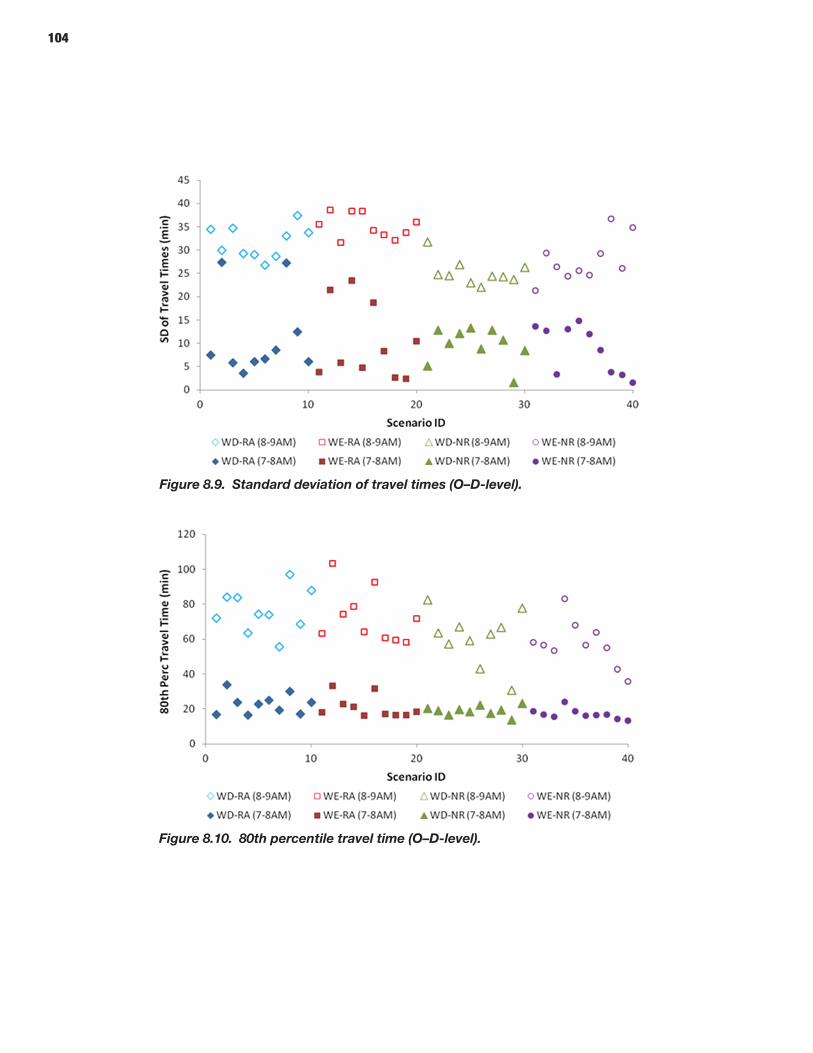
104
Figure 8.9. Standard deviation of travel times (O–D-level).
Figure 8.10. 80th percentile travel time (O–D-level).
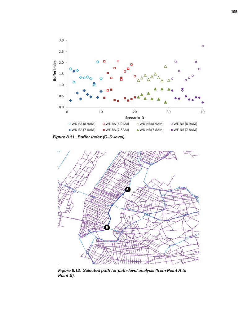
105
Figure 8.11. Buffer Index (O–D-level).
Figure 8.12. Selected path for path-level analysis (from Point A to Point B).
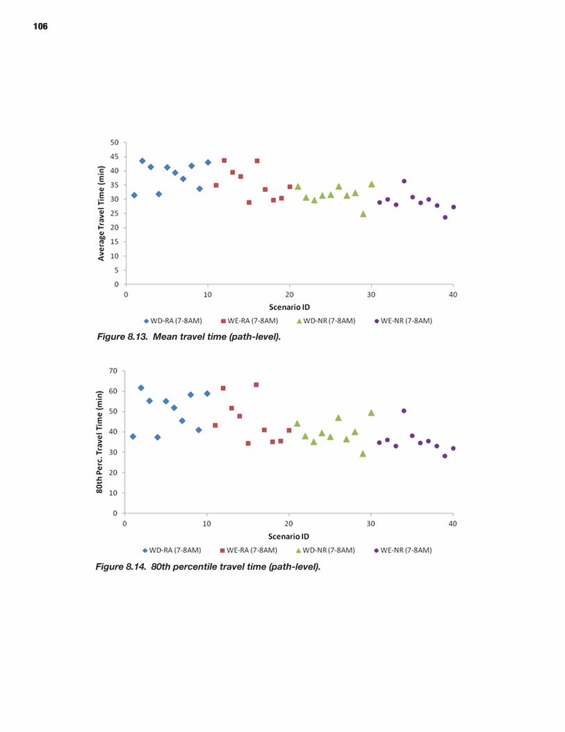
106
Figure 8.13. Mean travel time (path-level).
Figure 8.14. 80th percentile travel time (path-level).
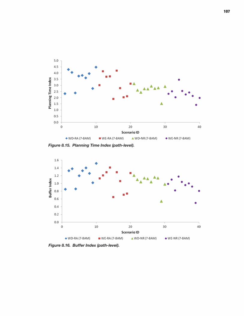
107
Figure 8.15. Planning Time Index (path-level).
Figure 8.16. Buffer Index (path-level).
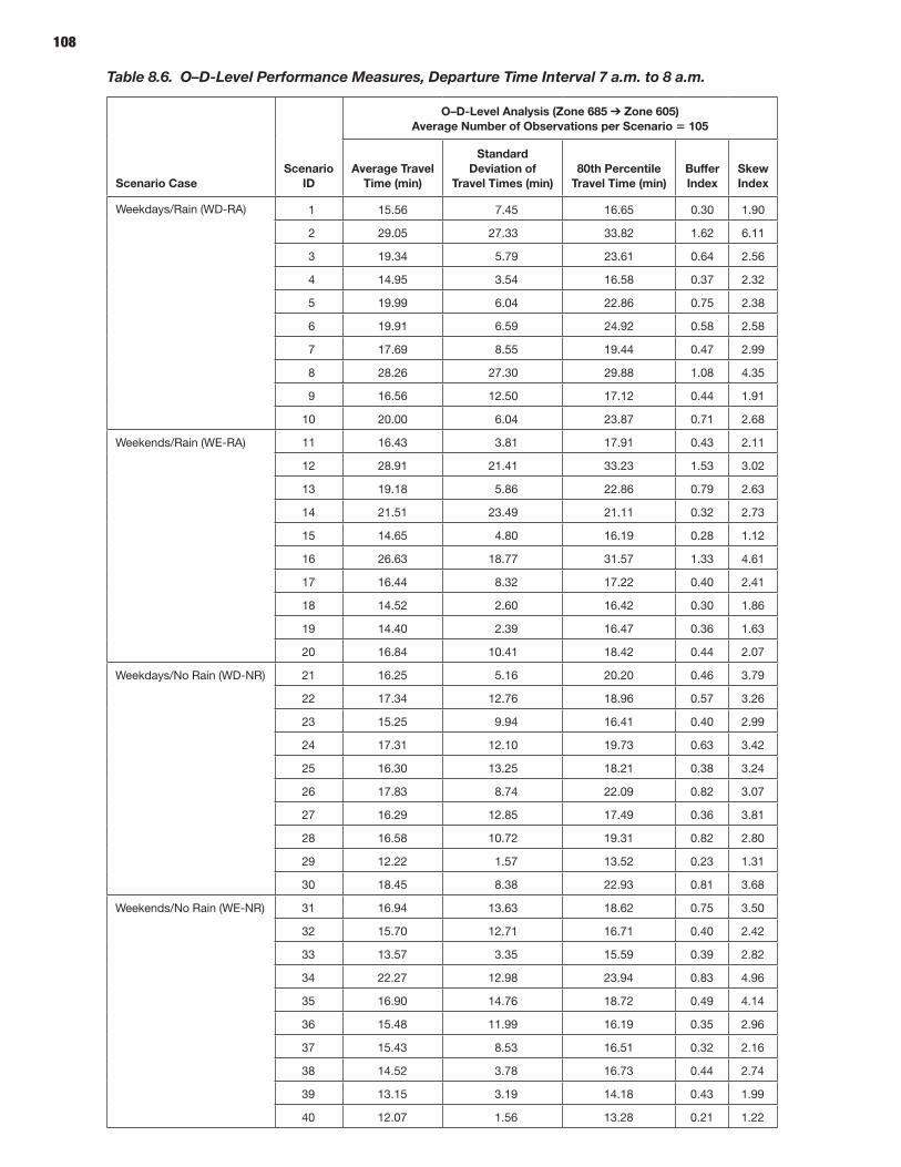
108
Table 8.6. O–D-Level Performance Measures, Departure Time Interval 7 a.m. to 8 a.m.
Scenario CaseScenario
ID
o–D-Level Analysis (Zone 685 ➔ Zone 605) Average Number of observations per Scenario 105
Average travel time (min)
Standard Deviation of
travel times (min)80th percentile
travel time (min)Buffer Index
Skew Index
weekdays/Rain (wd-RA) 1 15.56 7.45 16.65 0.30 1.90
2 29.05 27.33 33.82 1.62 6.11
3 19.34 5.79 23.61 0.64 2.56
4 14.95 3.54 16.58 0.37 2.32
5 19.99 6.04 22.86 0.75 2.38
6 19.91 6.59 24.92 0.58 2.58
7 17.69 8.55 19.44 0.47 2.99
8 28.26 27.30 29.88 1.08 4.35
9 16.56 12.50 17.12 0.44 1.91
10 20.00 6.04 23.87 0.71 2.68
weekends/Rain (wE-RA) 11 16.43 3.81 17.91 0.43 2.11
12 28.91 21.41 33.23 1.53 3.02
13 19.18 5.86 22.86 0.79 2.63
14 21.51 23.49 21.11 0.32 2.73
15 14.65 4.80 16.19 0.28 1.12
16 26.63 18.77 31.57 1.33 4.61
17 16.44 8.32 17.22 0.40 2.41
18 14.52 2.60 16.42 0.30 1.86
19 14.40 2.39 16.47 0.36 1.63
20 16.84 10.41 18.42 0.44 2.07
weekdays/No Rain (wd-NR) 21 16.25 5.16 20.20 0.46 3.79
22 17.34 12.76 18.96 0.57 3.26
23 15.25 9.94 16.41 0.40 2.99
24 17.31 12.10 19.73 0.63 3.42
25 16.30 13.25 18.21 0.38 3.24
26 17.83 8.74 22.09 0.82 3.07
27 16.29 12.85 17.49 0.36 3.81
28 16.58 10.72 19.31 0.82 2.80
29 12.22 1.57 13.52 0.23 1.31
30 18.45 8.38 22.93 0.81 3.68
weekends/No Rain (wE-NR) 31 16.94 13.63 18.62 0.75 3.50
32 15.70 12.71 16.71 0.40 2.42
33 13.57 3.35 15.59 0.39 2.82
34 22.27 12.98 23.94 0.83 4.96
35 16.90 14.76 18.72 0.49 4.14
36 15.48 11.99 16.19 0.35 2.96
37 15.43 8.53 16.51 0.32 2.16
38 14.52 3.78 16.73 0.44 2.74
39 13.15 3.19 14.18 0.43 1.99
40 12.07 1.56 13.28 0.21 1.22
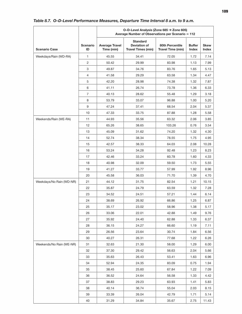
109
Table 8.7. O–D-Level Performance Measures, Departure Time Interval 8 a.m. to 9 a.m.
Scenario CaseScenario
ID
o–D-Level Analysis (Zone 685 ➔ Zone 605) Average Number of observations per Scenario 112
Average travel time (min)
Standard Deviation of
travel times (min)80th percentile
travel time (min)Buffer Index
Skew Index
weekdays/Rain (wd-RA) 1 45.55 34.41 72.05 1.72 7.14
2 50.42 29.99 83.98 1.13 7.99
3 49.87 34.76 83.76 1.65 5.13
4 41.58 29.29 63.58 1.34 4.47
5 42.20 28.98 74.38 1.32 7.87
6 41.11 26.74 73.78 1.36 6.33
7 40.13 28.62 55.48 1.29 3.18
8 53.79 33.07 96.88 1.00 5.20
9 47.24 37.41 68.54 2.04 5.37
10 47.33 33.75 87.88 1.28 5.58
weekends/Rain (wE-RA) 11 44.93 35.56 63.32 2.06 3.85
12 65.26 38.65 103.26 0.76 3.54
13 45.09 31.62 74.20 1.32 4.30
14 52.74 38.34 78.55 1.75 4.95
15 42.57 38.33 64.03 2.08 10.28
16 53.24 34.28 92.48 1.23 8.23
17 42.46 33.24 60.78 1.60 4.33
18 40.98 32.09 59.50 1.73 5.55
19 41.27 33.77 57.99 1.92 8.96
20 45.58 36.03 71.70 1.39 4.70
weekdays/No Rain (wd-NR) 21 44.12 31.75 82.54 1.21 10.15
22 35.87 24.79 63.59 1.32 7.28
23 34.52 24.51 57.21 1.44 6.14
24 38.69 26.92 66.86 1.25 6.87
25 35.17 23.02 58.96 1.38 5.17
26 33.06 22.01 42.88 1.49 9.76
27 35.92 24.40 62.88 1.33 6.37
28 36.15 24.27 66.60 1.19 7.11
29 26.56 23.64 30.74 1.84 6.56
30 40.27 26.31 77.68 1.22 6.26
weekends/No Rain (wE-NR) 31 32.63 21.30 58.00 1.29 6.00
32 37.30 29.42 56.63 2.04 5.66
33 35.63 26.43 53.41 1.63 6.96
34 52.94 24.35 83.09 0.75 1.94
35 38.45 25.60 67.84 1.22 7.09
36 36.52 24.64 56.58 1.33 4.42
37 38.83 29.23 63.93 1.41 5.83
38 40.14 36.74 55.04 2.03 8.15
39 33.39 26.04 42.79 1.71 5.14
40 31.29 34.84 35.67 2.75 11.43
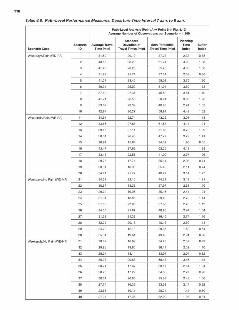
110
Table 8.8. Path-Level Performance Measures, Departure Time Interval 7 a.m. to 8 a.m.
Scenario CaseScenario
ID
path-Level Analysis (point A ➔ point B in Fig. 8.12) Average Number of observations per Scenario 1,199
Average travel time (min)
Standard Deviation of
travel times (min)80th percentile
travel time (min)
planning time Index
Buffer Index
weekdays/Rain (wd-RA) 1 31.50 20.10 37.73 2.33 0.85
2 43.56 28.20 61.74 4.29 1.33
3 41.45 28.25 55.28 4.05 1.38
4 31.88 21.71 37.34 2.38 0.86
5 41.27 28.45 55.03 3.75 1.20
6 39.31 25.92 51.91 3.80 1.33
7 37.19 27.31 45.52 3.61 1.40
8 41.74 26.55 58.24 3.95 1.26
9 33.69 23.39 40.96 2.74 1.02
10 42.94 30.27 58.91 4.48 1.52
weekends/Rain (wE-RA) 11 34.91 22.74 43.22 3.01 1.13
12 43.65 27.81 61.53 4.14 1.21
13 39.46 27.11 51.65 3.70 1.29
14 38.01 26.43 47.77 3.72 1.41
15 28.91 15.94 34.32 1.90 0.65
16 43.47 27.69 63.25 4.19 1.29
17 33.48 22.55 41.00 2.77 1.06
18 29.73 17.74 35.14 2.03 0.71
19 30.31 18.35 35.46 2.11 0.74
20 34.41 25.72 40.72 3.14 1.27
weekdays/No Rain (wd-NR) 21 34.59 22.15 44.23 3.13 1.21
22 30.67 18.23 37.97 2.61 1.10
23 29.72 19.95 35.16 2.44 1.04
24 31.34 18.86 39.40 2.72 1.14
25 31.56 22.88 37.63 2.70 1.12
26 34.50 21.67 46.95 2.94 1.04
27 31.33 24.28 36.46 2.74 1.16
28 32.22 20.18 40.13 2.80 1.14
29 24.79 12.13 29.35 1.52 0.54
30 35.34 19.64 49.40 2.91 0.98
weekends/No Rain (wE-NR) 31 28.82 16.69 34.70 2.32 0.99
32 29.95 19.65 36.11 2.52 1.10
33 28.04 18.14 33.07 2.04 0.82
34 36.38 20.88 50.47 3.46 1.18
35 30.74 17.67 38.17 2.54 1.04
36 28.78 17.29 34.55 2.27 0.96
37 30.01 20.60 35.63 2.43 1.00
38 27.74 16.29 33.02 2.14 0.92
39 23.66 10.11 28.24 1.42 0.50
40 27.27 17.36 32.00 1.98 0.81
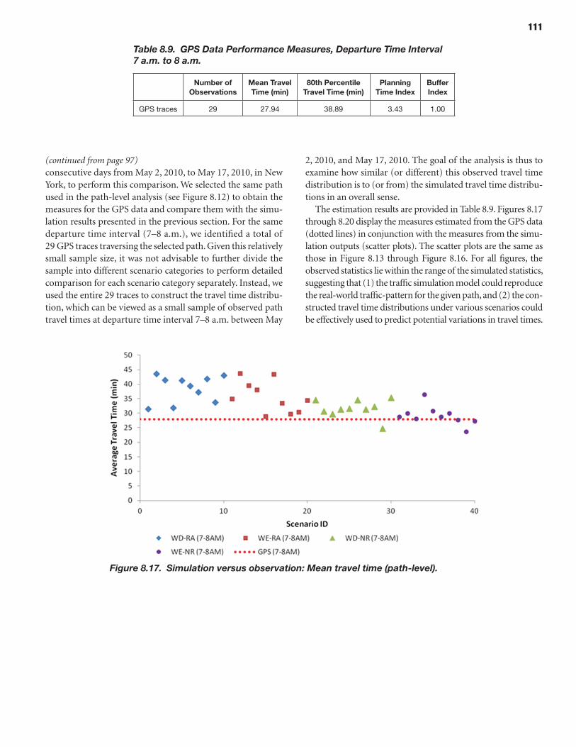
111
consecutive days from May 2, 2010, to May 17, 2010, in New York, to perform this comparison. We selected the same path used in the path-level analysis (see Figure 8.12) to obtain the measures for the GPS data and compare them with the simu-lation results presented in the previous section. For the same departure time interval (7–8 a.m.), we identified a total of 29 GPS traces traversing the selected path. Given this relatively small sample size, it was not advisable to further divide the sample into different scenario categories to perform detailed comparison for each scenario category separately. Instead, we used the entire 29 traces to construct the travel time distribu-tion, which can be viewed as a small sample of observed path travel times at departure time interval 7–8 a.m. between May
2, 2010, and May 17, 2010. The goal of the analysis is thus to examine how similar (or different) this observed travel time distribution is to (or from) the simulated travel time distribu-tions in an overall sense.
The estimation results are provided in Table 8.9. Figures 8.17 through 8.20 display the measures estimated from the GPS data (dotted lines) in conjunction with the measures from the simu-lation outputs (scatter plots). The scatter plots are the same as those in Figure 8.13 through Figure 8.16. For all figures, the observed statistics lie within the range of the simulated statistics, suggesting that (1) the traffic simulation model could reproduce the real-world traffic-pattern for the given path, and (2) the con-structed travel time distributions under various scenarios could be effectively used to predict potential variations in travel times.
Table 8.9. GPS Data Performance Measures, Departure Time Interval 7 a.m. to 8 a.m.
Number of observations
Mean travel time (min)
80th percentile travel time (min)
planning time Index
Buffer Index
gPS traces 29 27.94 38.89 3.43 1.00
(continued from page 97)
Figure 8.17. Simulation versus observation: Mean travel time (path-level).
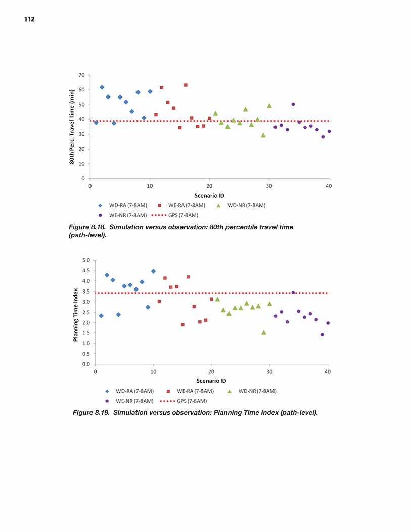
112
Figure 8.18. Simulation versus observation: 80th percentile travel time (path-level).
Figure 8.19. Simulation versus observation: Planning Time Index (path-level).
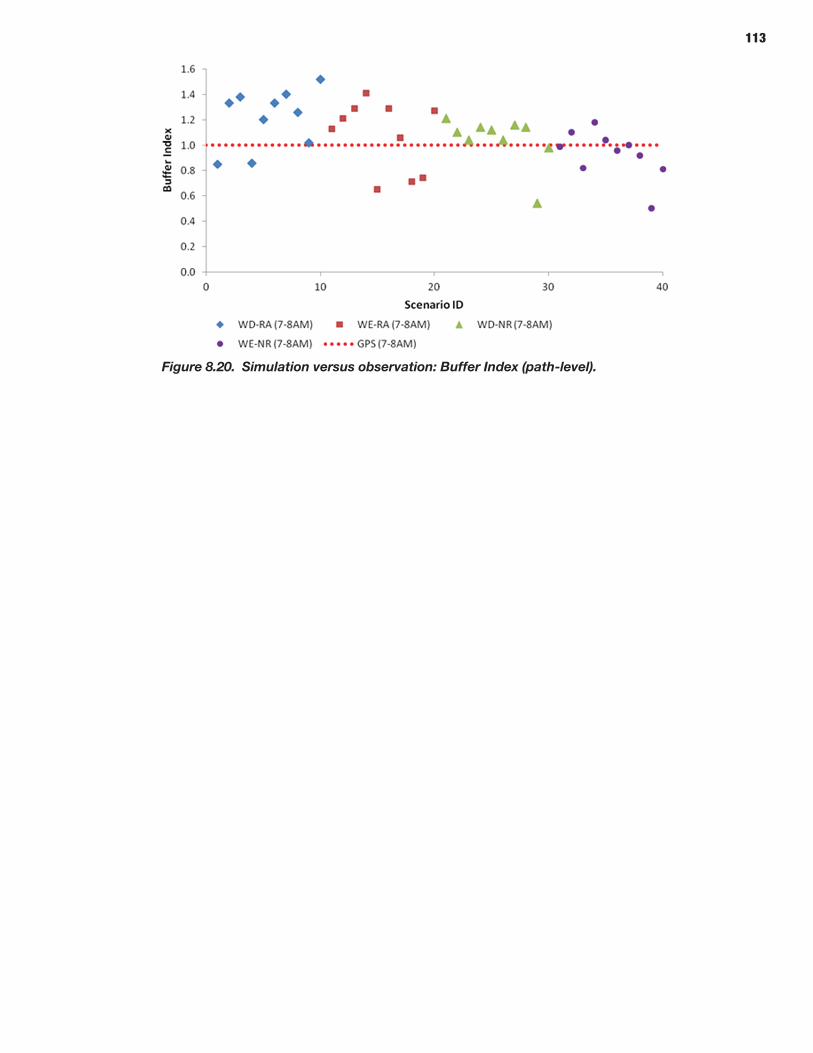
113
Figure 8.20. Simulation versus observation: Buffer Index (path-level).
114
C h A p t e r 9
The purpose of this chapter is to demonstrate how micro-simulation tools can be used in performing reliability analy-ses using the framework and tools developed under this project. The Aimsun simulation software was used to per-form the microsimulation task.
Study Area description
For the micro-model scenario the study area was a section of the wider meso-model study area and was located in the East Manhattan area bounded by 74th Street to the north, 48th Street to the south, 5th Avenue to the west, and York Avenue to the east. Figure 9.1 shows the extent of the study area con-sidered for microsimulation purposes.
The micro-model covers an area that includes 178 lane kilo-meters and 217 signalized intersections. A total of 147 centroids were connected to the network to generate origin–destination trips, including 44 gate and 103 internal centroids.
Two base models were constructed representing peak a.m. weekday and weekend conditions. The weekday a.m. peak period model consisted of a total demand of around 155,000 vehicles over a 5-hour period from 6 a.m. to 11 a.m. The weekend peak period model consisted of a total demand of around 80,000 vehicles over a period of 3 hours from 2 p.m. to 5 p.m.
Microsimulation Approach and objective
The general objective of the microsimulation tests was to determine a range of reliability measures that is characteristic of the study area for weekday and weekend traffic. The week-day and weekend scenarios were subjected to incident and demand variation events that are typical of the study area. Due to limitations with the modeling platform, the imple-mentation of variable weather conditions was not possible as part of the microsimulation study. It was assumed that
constant fair weather conditions prevailed across all the sce-narios tested for weekday and weekend.
Scenario description
The same methodology that was used to generate scenarios for the meso-model using the Scenario Manager was applied for the micro-model. The approach that was taken was to generate all the scenarios in one operational step using the Scenario Manager for the wider study area. Additional details of that procedure can be found in the Chapter 8 section, Gen-erating Scenarios Using the Scenario Manager.
The scenarios relevant for the microsimulation study area were then selected based on incidents that were located within the boundaries. Fifteen of the generated weekday scenarios and four of the weekend scenarios contained incidents within the microsimulation study area. Figure 9.2 and Figure 9.3 show the incident locations used for the study.
Microsimulation travel time reliability results
The input scenarios were prepared and imported into the Aimsun weekday and weekend models. The trajectories out-put for each vehicle completing trips were obtained for each scenario run and processed through the Trajectory Processor to obtain the reliability metrics.
Network-Level Results
The reliability performance across the entire network was measured using distance normalized travel times (i.e., aver-age travel time per mile, or TTPM) across 3 hours for the weekday and weekend peak periods. The weekday peak was for the a.m. period with time intervals spanning 7–8 a.m., 8–9 a.m. and 9–10 a.m. (Tables 9.1, 9.2, and 9.3). For the weekend, peak hourly intervals were reported between 2 p.m.
Analysis Process: Microscopic Models
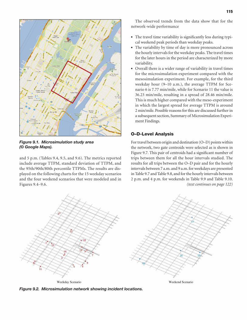
115
and 5 p.m. (Tables 9.4, 9.5, and 9.6). The metrics reported include average TTPM, standard deviation of TTPM, and the 95th/90th/80th percentile TTPMs. The results are dis-played on the following charts for the 15 weekday scenarios and the four weekend scenarios that were modeled and in Figures 9.4–9.6.
The observed trends from the data show that for the network-wide performance
• The travel time variability is significantly less during typi-cal weekend peak periods than weekday peaks.
• The variability by time of day is more pronounced across the hourly intervals for the weekday peaks. The travel times for the later hours in the period are characterized by more variability.
• Overall there is a wider range of variability in travel times for the microsimulation experiment compared with the mesosimulation experiment. For example, for the third weekday hour (9–10 a.m.), the average TTPM for Sce-nario 6 is 7.77 min/mile, while for Scenario 11 the value is 36.23 min/mile, resulting in a spread of 28.46 min/mile. This is much higher compared with the meso-experiment in which the largest spread for average TTPM is around 2 min/mile. Possible reasons for this are discussed further in a subsequent section, Summary of Microsimulation Experi-ment Findings.
O–D-Level Analysis
For travel between origin and destination (O–D) points within the network, two gate centroids were selected as is shown in Figure 9.7. This pair of centroids had a significant number of trips between them for all the hour intervals studied. The results for all trips between the O–D pair and for the hourly intervals between 7 a.m. and 9 a.m. for weekdays are presented in Table 9.7 and Table 9.8, and for the hourly intervals between 2 p.m. and 4 p.m. for weekends in Table 9.9 and Table 9.10.
Figure 9.1. Microsimulation study area (© Google Maps).
Weekday Scenario Weekend Scenario
Figure 9.2. Microsimulation network showing incident locations.
(text continues on page 122)
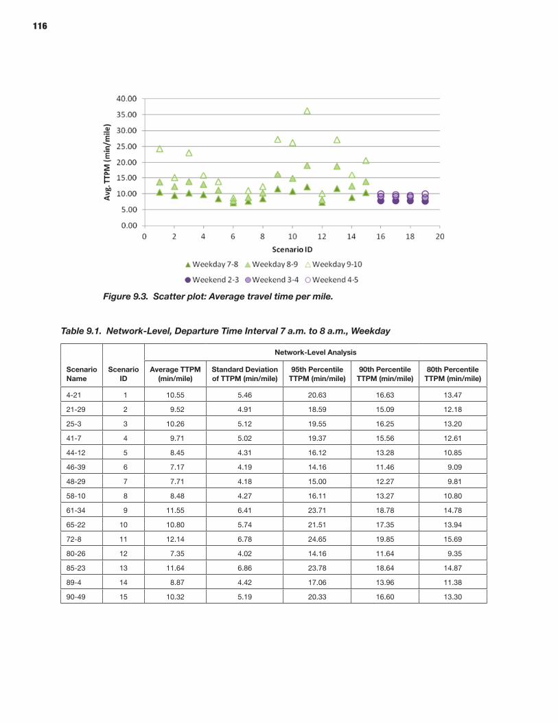
116
Table 9.1. Network-Level, Departure Time Interval 7 a.m. to 8 a.m., Weekday
Scenario Name
Scenario ID
Network-Level Analysis
Average ttpM (min/mile)
Standard Deviation of ttpM (min/mile)
95th percentile ttpM (min/mile)
90th percentile ttpM (min/mile)
80th percentile ttpM (min/mile)
4-21 1 10.55 5.46 20.63 16.63 13.47
21-29 2 9.52 4.91 18.59 15.09 12.18
25-3 3 10.26 5.12 19.55 16.25 13.20
41-7 4 9.71 5.02 19.37 15.56 12.61
44-12 5 8.45 4.31 16.12 13.28 10.85
46-39 6 7.17 4.19 14.16 11.46 9.09
48-29 7 7.71 4.18 15.00 12.27 9.81
58-10 8 8.48 4.27 16.11 13.27 10.80
61-34 9 11.55 6.41 23.71 18.78 14.78
65-22 10 10.80 5.74 21.51 17.35 13.94
72-8 11 12.14 6.78 24.65 19.85 15.69
80-26 12 7.35 4.02 14.16 11.64 9.35
85-23 13 11.64 6.86 23.78 18.64 14.87
89-4 14 8.87 4.42 17.06 13.96 11.38
90-49 15 10.32 5.19 20.33 16.60 13.30
Figure 9.3. Scatter plot: Average travel time per mile.
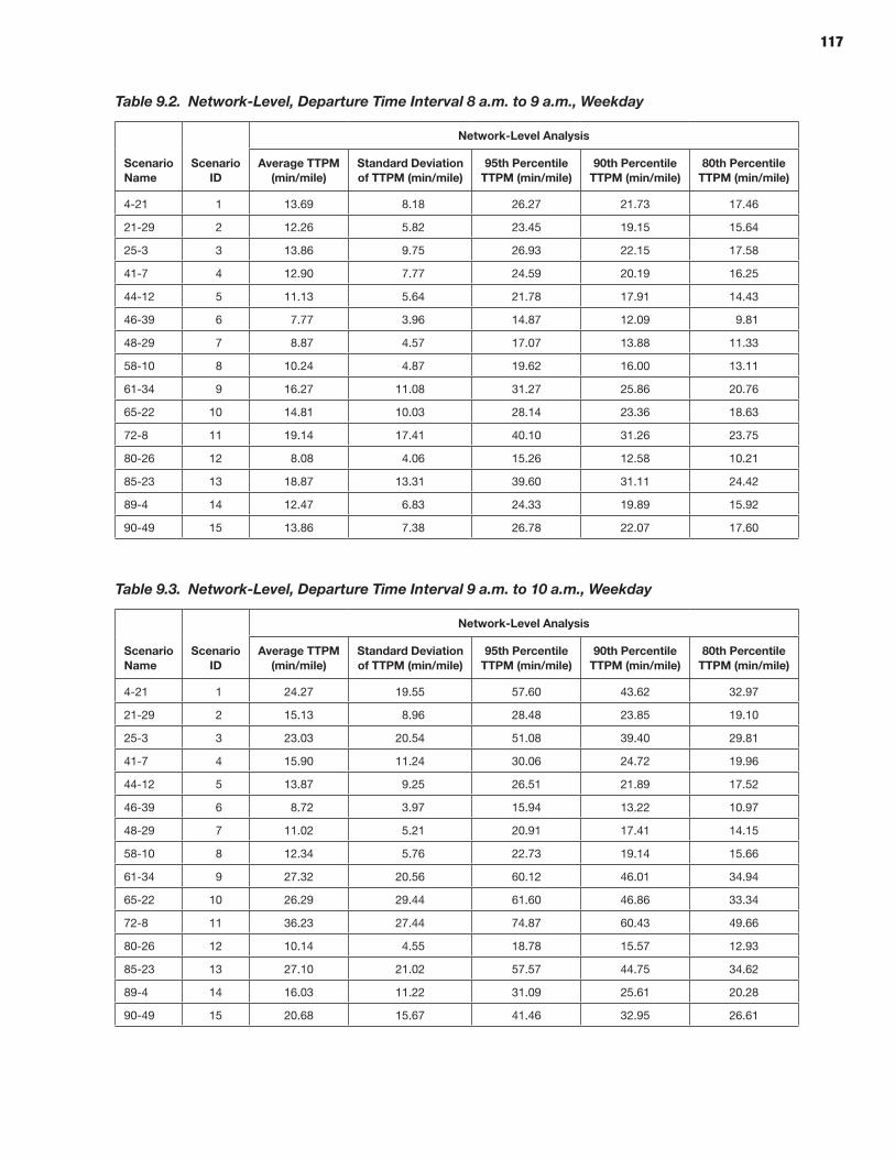
117
Table 9.2. Network-Level, Departure Time Interval 8 a.m. to 9 a.m., Weekday
Scenario Name
Scenario ID
Network-Level Analysis
Average ttpM (min/mile)
Standard Deviation of ttpM (min/mile)
95th percentile ttpM (min/mile)
90th percentile ttpM (min/mile)
80th percentile ttpM (min/mile)
4-21 1 13.69 8.18 26.27 21.73 17.46
21-29 2 12.26 5.82 23.45 19.15 15.64
25-3 3 13.86 9.75 26.93 22.15 17.58
41-7 4 12.90 7.77 24.59 20.19 16.25
44-12 5 11.13 5.64 21.78 17.91 14.43
46-39 6 7.77 3.96 14.87 12.09 9.81
48-29 7 8.87 4.57 17.07 13.88 11.33
58-10 8 10.24 4.87 19.62 16.00 13.11
61-34 9 16.27 11.08 31.27 25.86 20.76
65-22 10 14.81 10.03 28.14 23.36 18.63
72-8 11 19.14 17.41 40.10 31.26 23.75
80-26 12 8.08 4.06 15.26 12.58 10.21
85-23 13 18.87 13.31 39.60 31.11 24.42
89-4 14 12.47 6.83 24.33 19.89 15.92
90-49 15 13.86 7.38 26.78 22.07 17.60
Table 9.3. Network-Level, Departure Time Interval 9 a.m. to 10 a.m., Weekday
Scenario Name
Scenario ID
Network-Level Analysis
Average ttpM (min/mile)
Standard Deviation of ttpM (min/mile)
95th percentile ttpM (min/mile)
90th percentile ttpM (min/mile)
80th percentile ttpM (min/mile)
4-21 1 24.27 19.55 57.60 43.62 32.97
21-29 2 15.13 8.96 28.48 23.85 19.10
25-3 3 23.03 20.54 51.08 39.40 29.81
41-7 4 15.90 11.24 30.06 24.72 19.96
44-12 5 13.87 9.25 26.51 21.89 17.52
46-39 6 8.72 3.97 15.94 13.22 10.97
48-29 7 11.02 5.21 20.91 17.41 14.15
58-10 8 12.34 5.76 22.73 19.14 15.66
61-34 9 27.32 20.56 60.12 46.01 34.94
65-22 10 26.29 29.44 61.60 46.86 33.34
72-8 11 36.23 27.44 74.87 60.43 49.66
80-26 12 10.14 4.55 18.78 15.57 12.93
85-23 13 27.10 21.02 57.57 44.75 34.62
89-4 14 16.03 11.22 31.09 25.61 20.28
90-49 15 20.68 15.67 41.46 32.95 26.61
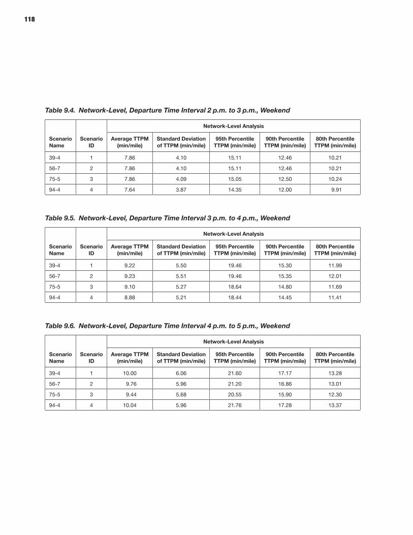
118
Table 9.4. Network-Level, Departure Time Interval 2 p.m. to 3 p.m., Weekend
Scenario Name
Scenario ID
Network-Level Analysis
Average ttpM (min/mile)
Standard Deviation of ttpM (min/mile)
95th percentile ttpM (min/mile)
90th percentile ttpM (min/mile)
80th percentile ttpM (min/mile)
39-4 1 7.86 4.10 15.11 12.46 10.21
56-7 2 7.86 4.10 15.11 12.46 10.21
75-5 3 7.86 4.09 15.05 12.50 10.24
94-4 4 7.64 3.87 14.35 12.00 9.91
Table 9.5. Network-Level, Departure Time Interval 3 p.m. to 4 p.m., Weekend
Scenario Name
Scenario ID
Network-Level Analysis
Average ttpM (min/mile)
Standard Deviation of ttpM (min/mile)
95th percentile ttpM (min/mile)
90th percentile ttpM (min/mile)
80th percentile ttpM (min/mile)
39-4 1 9.22 5.50 19.46 15.30 11.99
56-7 2 9.23 5.51 19.46 15.35 12.01
75-5 3 9.10 5.27 18.64 14.80 11.69
94-4 4 8.88 5.21 18.44 14.45 11.41
Table 9.6. Network-Level, Departure Time Interval 4 p.m. to 5 p.m., Weekend
Scenario Name
Scenario ID
Network-Level Analysis
Average ttpM (min/mile)
Standard Deviation of ttpM (min/mile)
95th percentile ttpM (min/mile)
90th percentile ttpM (min/mile)
80th percentile ttpM (min/mile)
39-4 1 10.00 6.06 21.60 17.17 13.28
56-7 2 9.76 5.96 21.20 16.86 13.01
75-5 3 9.44 5.68 20.55 15.90 12.30
94-4 4 10.04 5.96 21.76 17.28 13.37
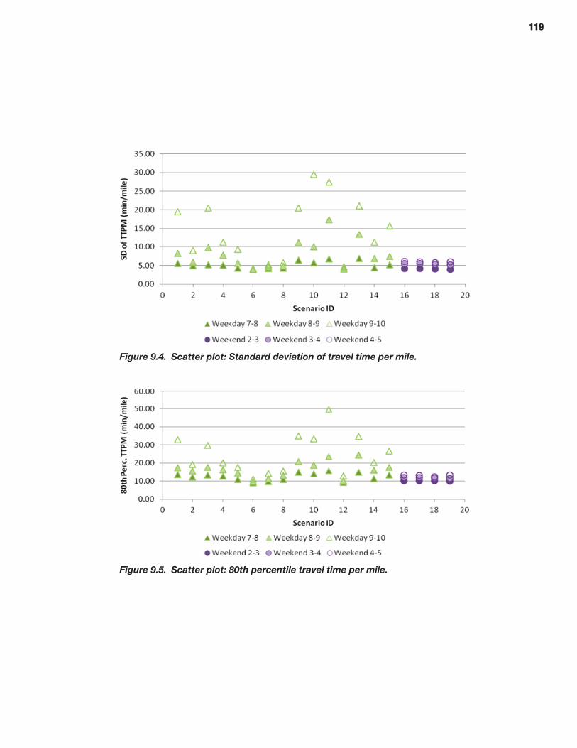
119
Figure 9.4. Scatter plot: Standard deviation of travel time per mile.
Figure 9.5. Scatter plot: 80th percentile travel time per mile.
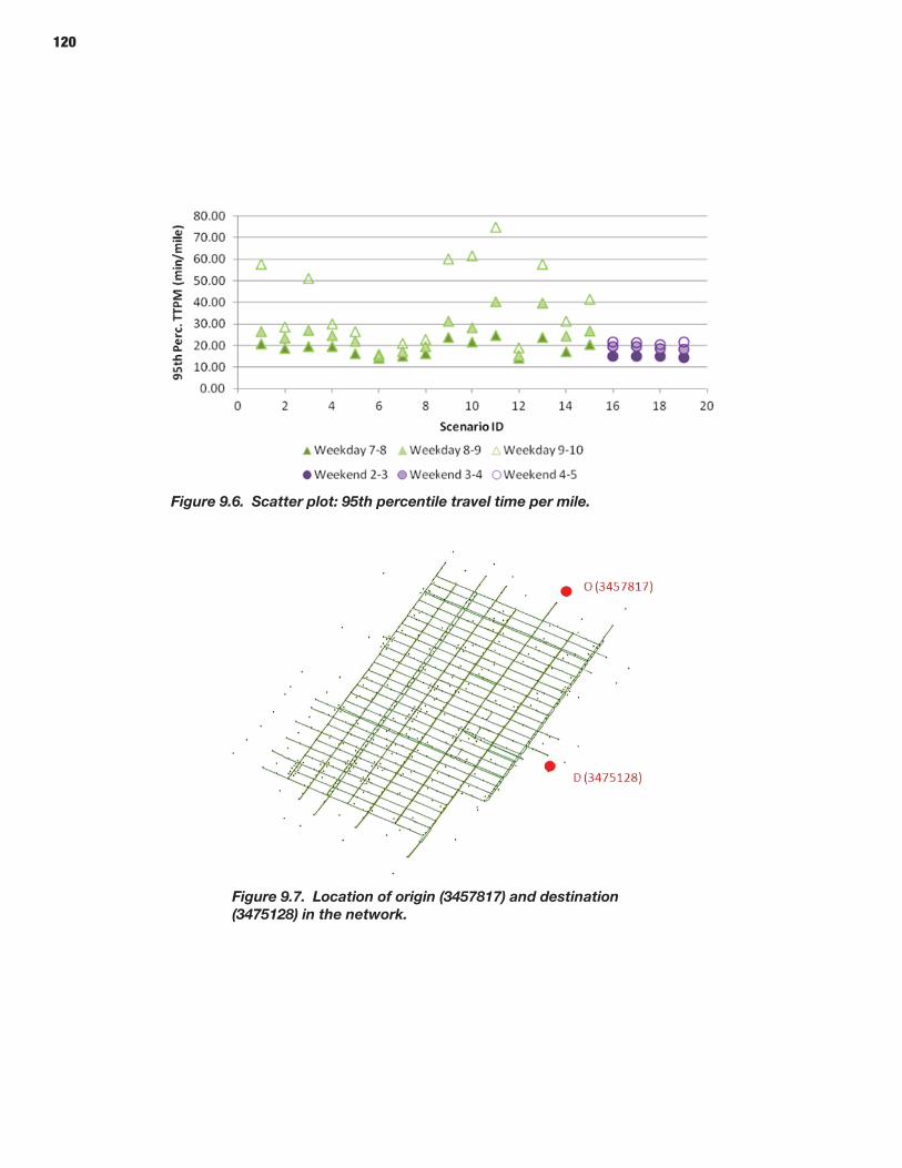
120
Figure 9.6. Scatter plot: 95th percentile travel time per mile.
Figure 9.7. Location of origin (3457817) and destination (3475128) in the network.
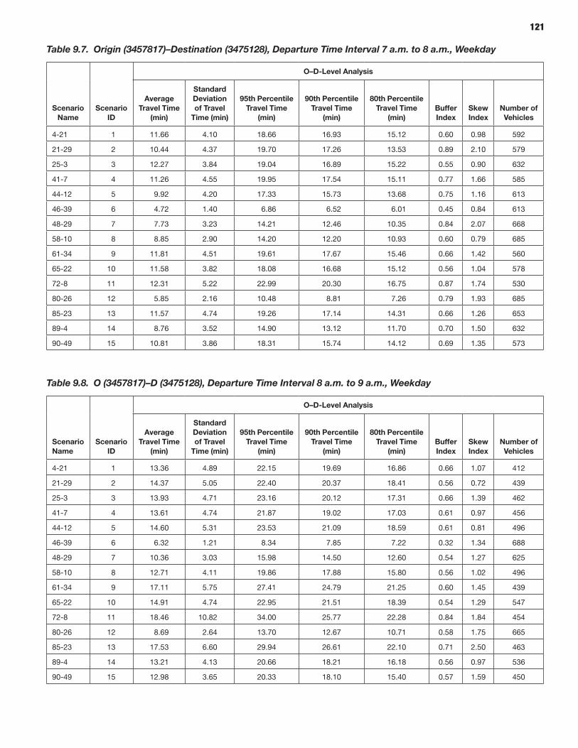
121
Table 9.7. Origin (3457817)–Destination (3475128), Departure Time Interval 7 a.m. to 8 a.m., Weekday
Scenario Name
Scenario ID
o–D-Level Analysis
Average travel time
(min)
Standard Deviation of travel
time (min)
95th percentile travel time
(min)
90th percentile travel time
(min)
80th percentile travel time
(min)Buffer Index
Skew Index
Number of Vehicles
4-21 1 11.66 4.10 18.66 16.93 15.12 0.60 0.98 592
21-29 2 10.44 4.37 19.70 17.26 13.53 0.89 2.10 579
25-3 3 12.27 3.84 19.04 16.89 15.22 0.55 0.90 632
41-7 4 11.26 4.55 19.95 17.54 15.11 0.77 1.66 585
44-12 5 9.92 4.20 17.33 15.73 13.68 0.75 1.16 613
46-39 6 4.72 1.40 6.86 6.52 6.01 0.45 0.84 613
48-29 7 7.73 3.23 14.21 12.46 10.35 0.84 2.07 668
58-10 8 8.85 2.90 14.20 12.20 10.93 0.60 0.79 685
61-34 9 11.81 4.51 19.61 17.67 15.46 0.66 1.42 560
65-22 10 11.58 3.82 18.08 16.68 15.12 0.56 1.04 578
72-8 11 12.31 5.22 22.99 20.30 16.75 0.87 1.74 530
80-26 12 5.85 2.16 10.48 8.81 7.26 0.79 1.93 685
85-23 13 11.57 4.74 19.26 17.14 14.31 0.66 1.26 653
89-4 14 8.76 3.52 14.90 13.12 11.70 0.70 1.50 632
90-49 15 10.81 3.86 18.31 15.74 14.12 0.69 1.35 573
Table 9.8. O (3457817)–D (3475128), Departure Time Interval 8 a.m. to 9 a.m., Weekday
Scenario Name
Scenario ID
o–D-Level Analysis
Average travel time
(min)
Standard Deviation of travel
time (min)
95th percentile travel time
(min)
90th percentile travel time
(min)
80th percentile travel time
(min)Buffer Index
Skew Index
Number of Vehicles
4-21 1 13.36 4.89 22.15 19.69 16.86 0.66 1.07 412
21-29 2 14.37 5.05 22.40 20.37 18.41 0.56 0.72 439
25-3 3 13.93 4.71 23.16 20.12 17.31 0.66 1.39 462
41-7 4 13.61 4.74 21.87 19.02 17.03 0.61 0.97 456
44-12 5 14.60 5.31 23.53 21.09 18.59 0.61 0.81 496
46-39 6 6.32 1.21 8.34 7.85 7.22 0.32 1.34 688
48-29 7 10.36 3.03 15.98 14.50 12.60 0.54 1.27 625
58-10 8 12.71 4.11 19.86 17.88 15.80 0.56 1.02 496
61-34 9 17.11 5.75 27.41 24.79 21.25 0.60 1.45 439
65-22 10 14.91 4.74 22.95 21.51 18.39 0.54 1.29 547
72-8 11 18.46 10.82 34.00 25.77 22.28 0.84 1.84 454
80-26 12 8.69 2.64 13.70 12.67 10.71 0.58 1.75 665
85-23 13 17.53 6.60 29.94 26.61 22.10 0.71 2.50 463
89-4 14 13.21 4.13 20.66 18.21 16.18 0.56 0.97 536
90-49 15 12.98 3.65 20.33 18.10 15.40 0.57 1.59 450
122
Table 9.9. O (3457817)–D (3475128), Departure Time Interval 2 p.m. to 3 p.m., Weekend
Scenario Name
Scenario ID
o–D-Level Analysis
Average travel time
(min)
Standard Deviation of travel
time (min)
95th percentile travel time
(min)
90th percentile travel time
(min)
80th percentile travel time
(min)Buffer Index
Skew Index
Number of Vehicles
39-4 1 6.47 2.28 10.22 8.26 7.53 0.58 1.39 547
56-7 2 6.47 2.28 10.22 8.26 7.53 0.58 1.39 547
75-5 3 6.52 2.31 10.54 8.80 7.61 0.62 1.71 547
94-4 4 6.14 1.36 8.29 7.85 7.25 0.35 1.18 563
Table 9.10. O (3457817)–D (3475128), Departure Time Interval 3 p.m. to 4 p.m., Weekend
Scenario Name
Scenario ID
o–D-Level Analysis
Average travel time
(min)
Standard Deviation of travel
time (min)
95th percentile travel time
(min)
90th percentile travel time
(min)
80th percentile travel time
(min)Buffer Index
Skew Index
Number of Vehicles
39-4 1 10.60 4.80 19.51 17.22 14.05 0.84 1.70 576
56-7 2 10.66 4.80 19.39 17.28 14.26 0.82 1.65 576
75-5 3 8.92 3.42 15.67 12.63 10.94 0.76 1.51 575
94-4 4 9.50 4.46 18.08 15.71 12.48 0.90 2.10 586
The results are reported based on average nonnormalized travel times for all trips across all routes between the O–D pair. Five metrics were reported: the average travel time, standard deviation of travel time, 95th/90th/80th percentile travel times, Buffer Index, and Skew Index.
Figures 9.8 to 9.11 display the results that show that the inter scenario variability is more significant for weekdays com-pared with weekends. Compared with the meso-model results, the results for the micro experiment show a much wider range of variation.
Path-Level Analysis
Analysis of travel time reliability can also be done at a path level for trips following a route between two points in the network. The length of the path chosen for this experiment is around 1.2 miles and is shown in Figure 9.12. The weekday peak was for the 7–8 a.m. time interval (Table 9.11), and the weekend peak was for the 2–3 p.m. interval (Table 9.12). The performance measures reported for the path analysis are average travel time, standard deviation, 95th/90th/80th per-centile, Planning Time Index, and Buffer Index. The results are displayed in Figures 9.13 to 9.16 and indicate that the
travel time distribution at a path level is significantly more variable between scenarios for the weekday peak versus sce-narios for the weekend peak.
Summary of Microsimulation Experiment Findings
In summary, the findings of the microsimulation experi-ments across all levels of detail are characterized by the following:
• Weekday peak period travel times are more variable than weekend peak periods.
• Variability in travel time increases as the demand increases during the simulation period.
• Compared with the meso-model the microsimulation travel times are much more variable for the same period of analysis. This can be attributed to:44 Study area size. The much smaller study area of the micro-model does not allow for much contribution to the mean travel time by trips that are not affected by incidents. The impact of incidents is more significant in this small microsimulation context because the majority of the trips in the model are affected. Across a wider
(continued from page 115)
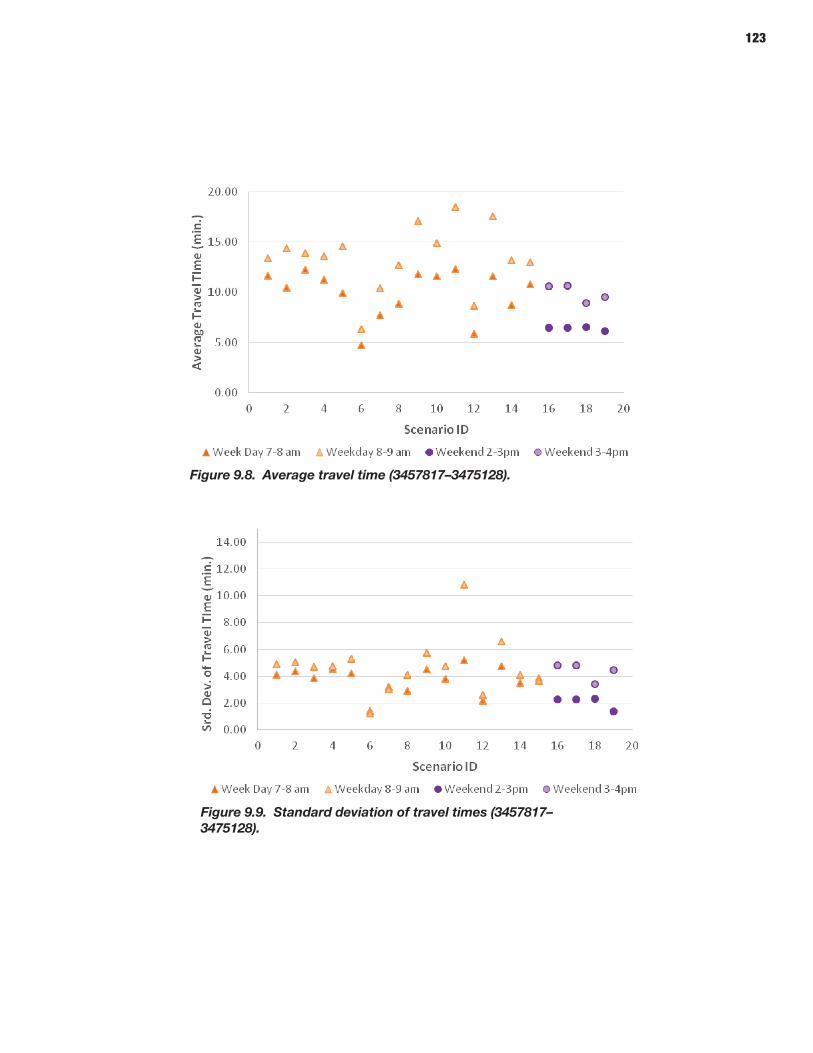
123
Figure 9.8. Average travel time (3457817–3475128).
Figure 9.9. Standard deviation of travel times (3457817–3475128).
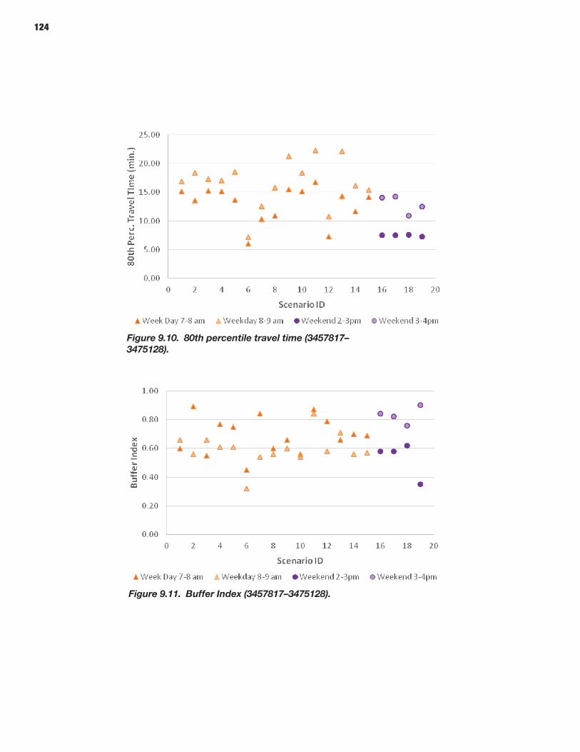
124
Figure 9.10. 80th percentile travel time (3457817–3475128).
Figure 9.11. Buffer Index (3457817–3475128).
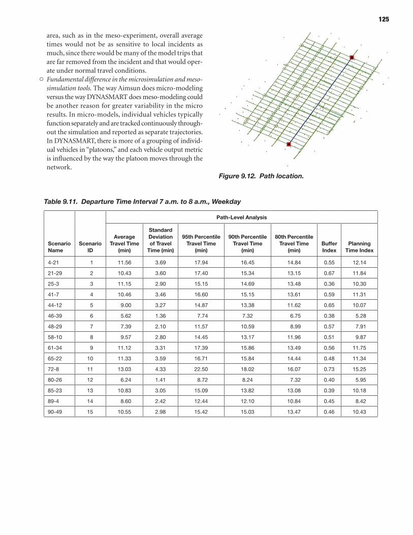
125
area, such as in the meso-experiment, overall average times would not be as sensitive to local incidents as much, since there would be many of the model trips that are far removed from the incident and that would oper-ate under normal travel conditions.
44 Fundamental difference in the microsimulation and meso-simulation tools. The way Aimsun does micro-modeling versus the way DYNASMART does meso-modeling could be another reason for greater variability in the micro results. In micro-models, individual vehicles typically function separately and are tracked continuously through-out the simulation and reported as separate trajectories. In DYNASMART, there is more of a grouping of individ-ual vehicles in “platoons,” and each vehicle output metric is influenced by the way the platoon moves through the network.
Figure 9.12. Path location.
Table 9.11. Departure Time Interval 7 a.m. to 8 a.m., Weekday
Scenario Name
Scenario ID
path-Level Analysis
Average travel time
(min)
Standard Deviation of travel
time (min)
95th percentile travel time
(min)
90th percentile travel time
(min)
80th percentile travel time
(min)Buffer Index
planning time Index
4-21 1 11.56 3.69 17.94 16.45 14.84 0.55 12.14
21-29 2 10.43 3.60 17.40 15.34 13.15 0.67 11.84
25-3 3 11.15 2.90 15.15 14.69 13.48 0.36 10.30
41-7 4 10.46 3.46 16.60 15.15 13.61 0.59 11.31
44-12 5 9.00 3.27 14.87 13.38 11.62 0.65 10.07
46-39 6 5.62 1.36 7.74 7.32 6.75 0.38 5.28
48-29 7 7.39 2.10 11.57 10.59 8.99 0.57 7.91
58-10 8 9.57 2.80 14.45 13.17 11.96 0.51 9.87
61-34 9 11.12 3.31 17.39 15.86 13.49 0.56 11.75
65-22 10 11.33 3.59 16.71 15.84 14.44 0.48 11.34
72-8 11 13.03 4.33 22.50 18.02 16.07 0.73 15.25
80-26 12 6.24 1.41 8.72 8.24 7.32 0.40 5.95
85-23 13 10.83 3.05 15.09 13.82 13.08 0.39 10.18
89-4 14 8.60 2.42 12.44 12.10 10.84 0.45 8.42
90-49 15 10.55 2.98 15.42 15.03 13.47 0.46 10.43
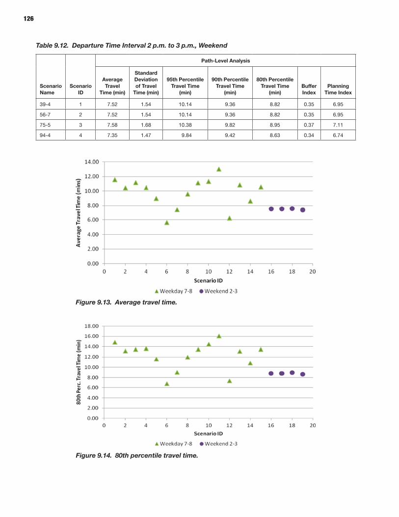
126
Table 9.12. Departure Time Interval 2 p.m. to 3 p.m., Weekend
Scenario Name
Scenario ID
path-Level Analysis
Average travel
time (min)
Standard Deviation of travel
time (min)
95th percentile travel time
(min)
90th percentile travel time
(min)
80th percentile travel time
(min)Buffer Index
planning time Index
39-4 1 7.52 1.54 10.14 9.36 8.82 0.35 6.95
56-7 2 7.52 1.54 10.14 9.36 8.82 0.35 6.95
75-5 3 7.58 1.68 10.38 9.82 8.95 0.37 7.11
94-4 4 7.35 1.47 9.84 9.42 8.63 0.34 6.74
Figure 9.13. Average travel time.
Figure 9.14. 80th percentile travel time.
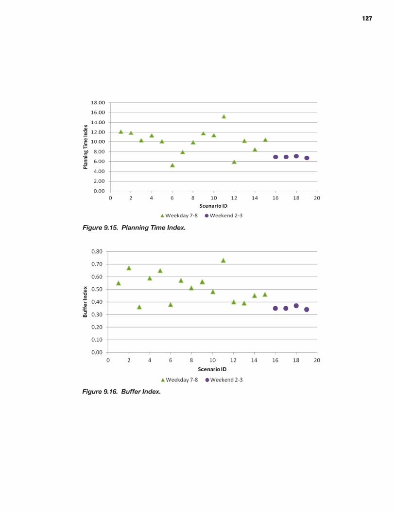
127
Figure 9.15. Planning Time Index.
Figure 9.16. Buffer Index.
128
C h A p t e r 1 0
The SHRP 2 L04 research project has addressed the need for a comprehensive framework and a conceptually coherent set of methodologies to (1) better characterize travel time reliability and the manner in which the various sources of variability operate individually and in interaction with each other in determining the overall reliability performance of a network, (2) assess its impacts on users and the system, and (3) deter-mine the effectiveness and value of proposed counter mea-sures. In doing so, this project has closed an important gap in the underlying conceptual foundations of travel modeling and traffic simulation, and provided practical means of generating realistic reliability measures using network simulation models in a variety of application contexts.
The general methodology for the inclusion of reliability in planning and operational models is based on the notion that transportation reliability is intrinsically related to the varia-tion in experienced (or repeated) travel times for a given facility or travel experience. Thus, integrating reliability in traffic models is about capturing and representing the effect of the various sources of variation on the performance of the transportation system. The proposed approach is grounded in a fundamental distinction between (1) systematic variation in travel times resulting from predictable seasonal, day-specific, or hour-specific factors that affect either travel demand or net-work service rates, and (2) random variation that stems from various sources of largely unpredictable (to the user) fluctua-tion. The former are addressed exogenously through model segmentation and demand/supply scenarios, creating the back-drop against which the random sources of variation are mod-eled. These sources are modeled both in terms of their direct impact on network performance and in terms of travelers’ responses which result in changes in travel demand.
In this study, several sources of variability have been dis-tinguished in a taxonomy that recognizes demand- versus supply-side, exogenous versus endogenous, and systematic versus random variability. The variability in system perfor-mance has both systematic causes, which can be modeled
and predicted, and causes that can only be modeled as random variables and which occur according to some probabilistic mechanism. The general approach to modeling phenomena and sources of variability incorporates as much as possible the causal or systematic determinants of variability, while the remaining inherent variation is then added to the representa-tion through suitably calibrated probabilistic mechanisms. This approach can be implemented for both micro- and mesosimulation levels, as demonstrated in this project. Not-withstanding the desire for explanation, the portion of vari-ability that must be viewed as inherent, or random, is likely to remain substantial.
The incorporation of reliability factors into the models can be done in either of two principal ways: (1) analytically, in which case travel time is implicitly treated as a random vari-able and its distribution, or some parameters of this distribu-tion, such as mean and variance, are described analytically and used in the modeling process or; (2) empirically, through multi ple scenarios, in which case the travel time distribution is not parameterized analytically but is simulated directly or explicitly through multiple model runs with different input variables. The conclusion emerging from this research is that both methods are useful and could be hybridized to account for different sources of travel time variation in the most effec-tive and computationally efficient way.
Travel time variability can be measured and analyzed in a variety of ways and at different levels of disaggregation. To constructively measure variability of travel times, a specific time unit must be chosen in terms of interval during the day (e.g., an hour between 7:00 a.m. and 8:00 a.m.), day of week (e.g., Monday), and season (e.g., fall). This is necessary to control for systematic (e.g., seasonal) differences in travel time that occur between hours of the day, between days of the week, and between seasons. The remaining variability of travel times across different days for the same unit (hour, day of week, and season) can then be used as the basic mea-sure of travel reliability.
Study Findings and Conclusions
129
By necessity, the quantification of travel time variability (that characterizes the reliability of travel in a network) entails representing the variability of travel times through the network’s links and nodes along the travel paths followed by travelers, and taking into account the correlation between link travel times. Capturing these correlation patterns is gen-erally very difficult when only link-level measurements are available. More important, given that a vehicle typically tra-verses a large number of links along its journey, deriving path-level and O–D-level travel time distributions from the underlying link travel time distributions is an extremely unwieldy and analytically forbidding task.
A way around these challenges with regard to travel time correlation across links and nodes is to obtain or measure the path- and/or O–D-level travel times as a complete entity and not by constructing it from link-level distributions. In a sim-ulation model, this means obtaining the travel times over entire or partial vehicle trajectories. Regardless of the specific reliability measures of interest, the availability of vehicle tra-jectories in the output of a simulation model enables con-struction of the path- and O–D-level travel time distributions of interest, as well as the extraction of link-level distributions. As such, the key building block for producing measures of reliability in a network simulation model is vehicle trajecto-ries and the associated experienced traversal times through the entirety or part of the travel path. The vehicle trajectory contains the traffic information and itinerary associated with each vehicle in the transportation network.
An important conclusion and contribution of the study is that travel time variability is best measured by variation across individual trajectories for the given facility and time unit. Thus, for reliability analysis purposes, the proposed framework unifies all particle-based simulation approaches so long as they produce vehicle trajectories; this methodological approach is further supported with the detailed discussion in Chapter 4 and the development of functional requirements for such simulation models.
In addition, many existing simulation tools view and model various sources of travel time variability (e.g., traffic incidents, work zones, weather, special events, other fluctua-tions in demand) as exogenous events using user-specified scenarios. Distinct from these exogenous factors, there are also endogenous sources of variation that are inherently reproduced, to varying degrees, by given traffic simulation models. Many studies have proposed ways to capture random variation in various traffic phenomena within particular micro- or mesosimulation models. Examples include flow breakdown, incidents due to drivers’ risk-taking behaviors, and heterogeneity in driving behaviors. All these have impor-tant implications for how the models are used to produce reliability estimates, and how these measures are interpreted and in turn used operationally.
The proposed methodological approach for modeling and estimating travel time reliability using simulation models fea-tures three components:
1. The Scenario Manager, which captures exogenous unre-liability sources such as special events, adverse weather, work zones, and travel demand variation;
2. Reliability-integrated simulation tools that model sources of unreliability endogenously, including user heterogene-ity, flow breakdown, and collisions; and
3. The Vehicle Trajectory Processor, which extracts reliability information from the simulation output, namely, vehicle trajectories.
The primary role of the Scenario Manager is to prepare input scenarios for the traffic simulation models; this a core part of the framework as it directly affects the final travel time distributions. The Scenario Manager is essentially a preproces-sor of simulation input files for capturing exogenous sources of travel time variation, such as external events, traffic control and management strategies, and travel demand-side factors. Recognizing the importance of the scenario definition and the complexity of identifying relevant exogenous sources, the Scenario Manager provides the ability to construct scenarios that entail any mutually consistent combinations of external events. It captures parameters that define external sources of unreliability (such as special events, adverse weather, and work zones) and enables users either to specify scenarios with par-ticular historical significance or policy interest, or to generate them randomly given the underlying stochastic processes of the associated events.
Using these generated scenarios in conjunction with the his-torical average demand as inputs, the traffic simulation models produce the vehicle trajectory outputs. During the simulation, the traffic simulation models capture the endogenous sources of travel time variability, such as endogenous flow breakdown, heterogeneous driving behaviors, and so forth. In general, traf-fic operation models need to model variations from different sources in both demand and supply sides; they also need to cap-ture traffic physics that characterize inherent probabilistic phe-nomena, including the collective effects that arise from the inherent randomness in driving behavior, namely, flow break-down and its impact on travel time. In general, traffic operation models should be capable of recognizing and representing both demand- and supply-side causes of variability, due to different sources. Importantly, rather than affecting travel time reliability separately, these factors often interact, which requires the ability to model all or any combination of causes of variability in one operational model. Most critically, such operational models should be particle-based (whether microscopic or mesoscopic simulation models) and capable of producing reliability-related output in the form of vehicle travel trajectories.
130
The vehicle Trajectory Processor is then introduced to extract reliability-related measures from the vehicle trajectory output of the simulation models. It produces and helps visual-ize reliability performance measures (travel time distributions, indicators) from observed or simulated trajectories. Observed trajectories may be obtained directly through measurement (e.g., GPS-equipped probe vehicles), thus enabling validation of travel time reliability metrics generated on the basis of out-put from simulation tools.
While chaining the three modules of the reliability analysis framework (Scenario Manager, Simulation Model, and Trajec-tory Processor) completes the necessary procedures for per-forming a scenario-based reliability analysis, there are two feedback loops worth mentioning to further incorporate behavioral aspects of travelers into the reliability modeling framework. One of these feedback loops could potentially use scenario-specific travel times to make scenario-conditional demand adjustment (e.g., departure time change under severe weather condition). The other loop suggests that the overall system uncertainty might affect the average demand by shift-ing the equilibrium point (i.e., reliability-sensitive network equilibrium), and such feedback could be used in travel demand forecasting models that predict the impact of reliabil-ity measures on travel patterns. These are key considerations for future research and development as identified further in the subsequent section, Recommendations for Future Research.
The reliability analysis framework and associated proto-type tools developed in this project enable a full range of analysis to address network-level, O–D-level, path-level, and segment/link-level travel time reliability using regional plan-ning and operations models. In doing so, users need to con-sider not only different properties of the reliability measures but also their applicability at an intended analysis level. A number of reliability performance measures have been iden-tified and categorized on the basis of their applicability to different levels of travel time distributions and associated reliability analysis, namely, network-level, O–D-level, and path/segment/link-level. It is essential in the reliability per-formance analysis to consider the user’s point of view, as trav-elers will adjust their departure time, and possibly other travel decisions, in response to unacceptable travel times and delays in their daily commutes. User-centric reliability mea-sures describe user-experienced or perceived travel time reli-ability, such as probability of on time arrival, schedule delay, and volatility, and sensitivity to departure time. The majority of these measures can be readily generated through the pro-totype Trajectory Processor that was developed as part of this project, while others could be incorporated into future devel-opment and enhancement of the Trajectory Processor.
The potential linking of travel demand forecasting models to traffic microsimulation provides the opportunity for more accurate representation of traffic conditions to be fed back to
choices about travel time, travel route, travel mode, or the decision to travel at all. This project highlighted the impor-tance of a feedback mechanism that could incorporate travel time reliability into traditional trip-based travel demand models, emerging activity-based models, and route choice models. In the context of this project, incorporation of reli-ability was primarily considered in the overall framework of demand-network equilibrium, with the demand side repre-sented by an advanced activity-based model (ABM) and the network simulation side represented by an advanced dynamic traffic assignment (DTA). Several important aspects of ABM-DTA integration and associated feedback mechanisms are essential and need to be addressed even before incorporation of travel time reliability measures. The incorporation of reli-ability into a network simulation model requires innovative approaches to generate the reliability measures that are fed into the demand model, to make route choice sensitive to reli-ability measures, and to ensure that a realistic correlation pat-tern is taken into account when route-level measures of reliability are constructed from link-level measures.
Incorporating travel time reliability into stochastic traffic simulation models enables the off-line evaluation of traffic network performance, including assessment of management interventions, policies, and geometric configuration, as well as both short-term and long-run impacts of policies aimed at improving travel time and service reliability. The reliability analysis tools developed in this project (namely, the Scenario Manager and Trajectory Processor), even in their current pro-totype state of development, can be readily used to perform essential elements of such evaluations. A prerequisite for the use of the analysis tools is the availability of a particle-based traffic simulation model, capable of producing vehicle trajec-tory output. For demonstration purposes, the Scenario Man-ager and Trajectory Processor prototypes incorporate interfaces to the Aimsun and DYNASMART-P simulation platforms, as examples of microscopic and mesoscopic models, respectively. It is noted that both the Scenario Manager and the Trajectory Processor have been developed at a prototype level of detail and functionality for project team use only, and are shared with the developer and user community on an “as is” basis. For this reason, they may not meet all requirements of an implement-ing agency without further development.
Implementation Steps
This project has developed and demonstrated a unified approach with broad applicability to various planning and operations analysis problems, which allows agencies to incor-porate reliability as an essential evaluation criterion. The approach is independent of specific analysis software tools to enable and promote wide adoption by agencies and developers. The project has also developed specific software tools intended
131
to prototype the key concepts—namely, those of a Scenario Manager and a Trajectory Processor—and demonstrated them with two commonly used network modeling software platforms.
Agency Adoption
Throughout this study, it has become clear that reliability as an evaluation and decision factor is here to stay. It is therefore essential for agencies and consultants that support them to provide the inputs required to consider reliability in design-ing and evaluating future programs, projects, and policies. Agency hesitation to adopt new approaches is rooted in two factors: (1) the institutional cost of doing something differ-ent, and (2) lack of trust and experience in the new genera-tion of tools available to address this need. The present project provides the approaches and tools to address the second fac-tor. Furthermore, it addresses the first factor by developing an approach that is essentially software neutral and can be read-ily adapted with the agencies’ existing modeling tools.
Nonetheless, unless developers of commercial software provide the necessary utilities and linkages to fully enable reliability-based analysis approaches, agencies will not totally come on board. The SHRP 2 program has taken important steps to create further awareness of the importance of reli-ability as a decision factor and to create further awareness of the availability of these new approaches and tools.
To further promote agency adoption, it is important to identify and facilitate early adopters—that is, those agencies that will show the way and that others can point to as success-ful examples to be emulated. Program funding for demonstra-tion projects with full agency engagement and commitment is therefore an essential ingredient to achieve greater agency adoption.
developers
Developers of commercial software application tools for both planning and operations applications play a critical role in the dissemination of new knowledge and advances in meth-odology developed under projects such as this one. The proj-ect team members are themselves actively engaged in the application and further development of the tools and their application; however, the transportation field is a vast one that requires a large number of players to work toward similar technical goals.
The approaches and tools developed in this project are readily applicable with most software tools for microscopic and mesoscopic network simulation, albeit to varying degrees of completeness. The steps required by developers are rela-tively minor given the templates and code developed for this
project. Naturally, commercial developers would all like to somehow add unique value to their offerings, for competitive market reasons. However, they will only do so if they believe there is market demand for the capability. This is where hav-ing a few early agency adopters will start the cycle of agency demand and developer supply. The present project has removed the technical risk for the developers, who need only invest in programming time to customize to their software’s unique features.
Success Factors
Key success factors for the results of this project include the following:
• Creating greater awareness of the importance of reliability analysis for major planning and operations projects, as well as of the attainability of such analysis capabilities;
• Adopting scenario-based approaches to project evalua-tion as the primary, default approach for conducting such evaluations;
• Promoting greater appreciation and recognition of the entire distribution of travel time, rather than simply mean values; and
• Making utilities available for use in connection with most network simulation software both to manage the creation and generation of scenarios and to analyze the output of such scenario runs to obtain travel time distributions and reliability descriptors.
recommendations for Further research
Longer-term impact evaluation entails integrating reliability considerations in equilibrium planning models. An ideal inte-gration would bring together reliability-sensitive network sim-ulation models with micro-level activity-based demand models. To this end, several important research directions have become clear in the course of this project. Many of them relate to more advanced methods of incorporation of travel time reliability, specifically schedule delay cost and temporal activity profiles. However, improving travel demand models and network simulation tools in this direction is closely intertwined with a general improvement of individual mesosimulation and micro-simulation models. The team makes the following specific recommendations for future research:
• Continue research on advanced methods for incorporating travel time reliability into demand models and network sim-ulations tools, including the schedule delay cost approach and temporal utility profile approach. For demand models,
132
reliability should be included in mode choice and time- of-day choice and (through these choices or in a different way) also be incorporated into the other travel choices such as destination choice and trip frequency choice.
• For network simulation models, in particular, reliability measures should be incorporated in such a way that they could be effectively generated within the network simula-tion procedure, as well as affect the route choice embedded in it. Most of the attempts to date have resulted in path-based route choice models with complicated path utilities that cannot be directly incorporated into real-world net-work simulations.
• Travel demand and network simulation models that incor-porate reliability measures must be operational in large net-works. This is especially challenging for the network supply side, since most of the proposed formulations inherently require path-based assignment. Accordingly, and as part of the recommendations above, continue research and devel-opment of path-based assignment algorithms that incor-porate travel time reliability and can generate a trip travel time distribution in addition to mean travel time.
• Continue research on schemes for the integration of advanced ABM and DTA that can ensure a full consistency of daily activity patterns and schedules at the individual level and behavioral realism of traveler responses. In this regard, addressing enhancement of time-of-day choice, trip departure time choice, and activity scheduling components is essential. This point relates to the conceptual structure of these models and their implementation with respect to temporal resolution.
• The travel demand models and network simulation models that incorporate reliability measures should be combined in a certain equilibrium framework. It is probably unrealistic to expect that a closed-form equilibrium formulation with reliability measures would ever be found. It is more realistic to construct a so-called loosely coupled demand-supply model with at least some level of consistency between the reliability measures generated by the network simulation and those used in the route choice and demand models. The existence and uniqueness of the equilibrium (stationary) solution in this case becomes largely an empirical issue.
• Encourage additional data collection on the supply side of activities and on scheduling constraints—including the distribution of jobs and workers by schedule flexibility, classification of maintenance and discretionary activities by schedule flexibility—and develop approaches to forecast related trends.
• Continue research and application of multiple-run model approaches and associated scenario formations, for both the demand and network supply sides. This project’s syn-thesis and research have shown that a conventional single-run framework is inherently too limited to incorporate some important reliability-related phenomena such as non-recurrent congestion due to a traffic incident, special event, or extreme weather condition.
• Incorporate travel time reliability in project evaluation and user benefit calculations. Restructure the output of travel models to support project evaluation and user benefit calcu-lations with consideration of the impact of improved travel time reliability.
133
Abdelghany, K., and H. Mahmassani. 2001. Dynamic Trip Assignment-Simulation Model for Intermodal Transportation Networks. In Transportation Research Record: Journal of the Transportation Research Board, No. 1771, Transportation Research Board, National Research Council, Washington, D.C., pp. 52–60.
Abdelghany, A. F., and H. S. Mahmassani. 2003. Temporal Spatial Microassignment and Sequencing of Travel Demand with Activity Trip Chains. In Transportation Research Record: Journal of the Trans-portation Research Board, No. 1831, Transportation Research Board of the National Academies, Washington, D.C., pp. 89–97.
Arup. 2003. Frameworks for Modeling the Variability of Journey Times on the Highway Network. Arup, London.
Axhausen, K., S. Hess, A. Konig, G. Abay, J. Bates, and M. Bierlaire. 2007. State of the Art Estimates of the Swiss Value of Travel Time Savings. Presented at the 86th Annual Meeting of the Transportation Research Board, Washington, D.C. (CD-ROM)
Bates, J., I. Black, J. Fearon, C. Gilliam, and S. Porter. 2002. Supply Models for Use in Modeling the Variability of Journey Times on the Highway Network. AET: Proceedings of the European Transport Conference. Association for European Transport (AET), Cambridge, UK.
Bekhor, S., D. Christoph, and K. W. Axhausen. 2011. Integration of Activity-Based and Agent-Based Models: Case of Tel Aviv, Israel. Presented at the 90th Annual Meeting of Transportation Research Board, Washington, D.C.
Ben-Akiva, M., and M. Abou-Zeid. 2007. Methodological Issues in Modeling Time-of-Travel Preferences. In: 11th World Conference on Transport Research, Berkeley, CA.
Bogers, E. A. I., H. W. C. van Lint, and H. J. van Zuylen. 2008. Reliability of Travel Time: Effective Measures from Behavioral Point of View. Transportation Research Record: Journal of the Transportation Research Board, No. 2082. Transportation Research Board of the National Academies, Washington, D.C., pp. 27–34.
Brennand, A. W. 2011. Incorporating Travel Time Reliability in the Estimation of Assignment Models. New Zealand Transport Agency Research Report 464.
Brownstone, D., A. Chosh, T. F. Golob, C. Kazimi, and D. Van Amelsfort. 2003. Drivers’ Willingness-to-Pay to Reduce Travel Time: Evidence from the San-Diego I-15 Congestion Pricing Project, Transportation Research, 37A(4), pp. 373–388.
Brownstone, D., and K. A. Small. 2005. Valuing Time and Reliability: Assessing the Evidence from Road Pricing Demonstrations, Trans-portation Research A, 39A, pp. 279–293.
Cambridge Systematics, Inc. 2005. Traffic Congestion and Reliability: Trends and Advanced Strategies for Congestion Mitigation. Final Report.
Prepared for Federal Highway Administration by Cambridge System-atics, Inc., with Texas Transportation Institute.
Cambridge Systematics, Inc., Dowling Associates, Inc., System Metrics Group, Inc., and Texas A&M Transportation Institute. 2008. NCHRP Report 618: Cost-Effective Performance Measures for Travel Time Delay, Variation, and Reliability. Transportation Research Board of the National Academies, Washington, D.C.
Cambridge Systematics, Inc., Texas A&M Transportation Institute, University of Washington, Dowling Associates, Street Smarts, H. Levinson, and H. Rakha. 2013. SHRP 2 Report S2-L03-RR-1: Analytical Procedures for Determining the Impacts of Reliability Mitigation Strategies. Transportation Research Board of the National Academies, Washington, D.C.
Castiglione, J., and P. Vovsha. August 2012. Activity-Based Modeling, Session 11: Network Integration. TMIP Webinar Series presentation. See http://media.tmiponline.org/webinars/2012/TMIP_ABM_Webinars/Session_11/Webinar11_Network%20Integration_Slides-With-Notes2.pdf.
Castiglione, J., B. Grady, M. Outwater, and S. Lawe. 2012. Sensitivity Test-ing and Assessment of an Integrated Regional Travel Demand and Traffic Micro-simulation Model. To be presented at the 91st Annual Meeting of the Transportation Research Board, Washington, D.C.
Chang, G. L., H. Mahmassani, and R. Herman. 1985. A Macroparticle Traffic Simulation Model to Investigate Peak-Period Commuter Decision Dynamics. In Transportation Research Record: Journal of the Transportation Research Board, No. 1005, Transportation Research Board, National Research Council, Washington, D.C., pp. 107–120.
Chang, G. L., and H. S. Mahmassani. 1988. Travel time prediction and departure time adjustment behavior dynamics in a congested traf-fic system. Transportation Research Part B: Methodological 22(3), pp. 217–232.
Concas, S., and A. Kolpakov. 2009. Synthesis of Research on Value of Time and Value of Reliability. Final Report. Prepared by the Center for Urban Transportation Research and the National Center for Transit Research of University of South Florida for the Florida Department of Transportation.
Daganzo, C. F. 1999. A Behavioral Theory of Multi-Lane Traffic Flow, Part I: Long. Homogeneous Freeway Sections. Institute of Transporta-tion Studies, University of California, Berkeley.
Dehghani, Y., T. Adler, T. Doherty, and R. Fox. 2003. Development of a New Toll Mode Choice Modeling System for Florida’s Turnpike Enterprise, In Transportation Research Record: Journal of the Trans-portation Research Board, No. 1858, Transportation Research Board of the National Academies, Washington, D.C., pp. 9–17.
References
134
Dong, J., and H. S. Mahmassani. 2009. Flow Breakdown and Travel Time Reliability. In Transportation Research Record: Journal of the Transportation Research Board, No. 2124, Transportation Research Board of the National Academies, Washington, D.C., pp. 203–212.
Eliasson, J. 2006. The Relationship Between Travel Time Variability and Road Congestion. Proceedings of the 2007 World Conference of Trans-port Research, Berkeley, Calif.
Engelson, L. 2011. Properties of Expected Travel Cost Function with Uncertain Travel Time. Transportation Research Board Annual Meeting 2011, Paper #11-2709.
Fosgerau, M. 2008. Congestion costs in bottleneck equilibrium with stochastic capacity and demand. Proceedings of the European Transport Conference 2008. Association for European Transport, London.
Fosgerau, M., and N. B. Karlstrom. 2007. The Value of Reliability and the Distribution of Random Durations. Proceedings of the Euro-pean Transport Conference, Noordwijk, The Netherlands, Octo-ber 2007.
Fox, J., A. Daly, and H. Gunn. 2003. Review of RAND Europe’s Transport demand Model Systems. RAND Europe.
Hamdar, S. H., and H. S. Mahmassani. 2008. From Existing Accident-Free Car-Following Models to Colliding Vehicles: Exploration and Assessment. In Transportation Research Record: Journal of the Trans-portation Research Board, No. 2088, Transportation Research Board of the National Academies, Washington, D.C., pp. 45–56.
Hamdar, S. H., M. Treiber, H. S. Mahmassani, and A. Kesting. 2008. Modeling Driver Behavior as a Sequential Risk Taking Task. Transpor-tation Research Record: Journal of the Transportation Research Board, No. 2088, Washington, D.C., pp. 208–217.
Hensher, D. A., and P. Goodwin. 2003. Using Values of Travel Time Sav-ings for Toll Roads: Avoiding Some Common Errors. Transport Policy, 11, pp. 171–181.
Institute for Transportation Studies. 2008. Multimodal Travel Time Vari-ability. Final report for Department for Transport. Institute for Trans-portation Studies, University of Leeds, Imperial College London, John Bates Services.
Jiang, L., H. Mahmassani, and K. Zhang. 2011. Congestion Pricing, Heterogeneous Users, and Travel Time Reliability. In Transporta-tion Research Record: Journal of the Transportation Research Board, No. 2254, Transportation Research Board of the National Acade-mies, Washington, D.C., pp. 58–67.
Jones, E. G. 1988. The Variability of Travel Times in a Commuting Cor-ridor During the Evening Peak Period. MS Thesis, Department of Civil Engineering, University of Texas at Austin.
Jones, E. G., H. Mahmassani, R. Herman, and C. M. Walton. 1989. Travel Time Variability in a Commuting Corridor: Implications for Electronic Route Guidance. Proc., First International Conference on Applications of Advanced Technologies in Transportation Engineering, San Diego, Calif., pp. 27–32.
Kim, J., and H. Mahmassani. 2011. Correlated Parameters in Driving Behavior Models. In Transportation Research Record: Journal of the Transportation Research Board, No. 2049, Transportation Research Board of the National Academies, Washington, D.C., pp. 62–77.
Kim, H., J.-S. Oh, and R. Jayakrishnan. 2006. Activity Chaining Model Incorporating Time Use Problem and Its Application to Network Demand Analysis. Presented at the 85th Annual Meeting of the Transportation Research Board, Washington, D.C. (CD-ROM)
Kitamura, R., and J. Supernak. 1997. Temporal Utility Profiles of Activ-ities and Travel: Some Empirical Evidence. In Stopher, P., and M. Lee-Gosselin (Eds.), Understanding Travel Behavior in Era of Change. Elsevier, pp. 339–350.
Lam, W., and Y. Yin. 2001. An Activity-Based Time-Dependent Traffic Assignment Model, Transportation Research B, 35B, pp. 549–574.
Levinson, D., K. Harder, J. Bloomfield, and K. Winiarczyk. 2004. Weighting Waiting: Evaluating Perception of In-Vehicle Travel Time under Mov-ing and Stopped Conditions. Transportation Research Record: Journal of the Transportation Research Board, 1898, Transportation Research Board of the National Academies, Washington, D.C., pp. 61–68.
Li, R., G. Rose, and M. Sarvi. 2006. Using Automatic Vehicle Identifica-tion Data to Gain Insight into Travel Time Variability and Its Causes. In Transportation Research Record: Journal of the Transportation Research Board, No. 1945, Transportation Research Board of the National Academies, Washington, D.C., pp. 24–32.
Lomax, T., D. Schrank, S. Turner, and R. Margiotta. 2003. Selecting Travel Reliability Measures. Texas Transportation Institute and Cambridge Systematics, Inc.
Lyman, K., and R. L. Bertini. 2008. Using Travel Time Reliability Mea-sures to Improve Regional Transportation Planning and Operations. In Transportation Research Record: Journal of the Transportation Research Board, No. 2046, Transportation Research Board of the National Academies, Washington, D.C., pp. 1–10.
Mahmassani, H. S. 2001. Dynamic Network Traffic Assignment and Simu-lation Methodology for Advanced System Management Applications. Networks and Spatial Economics, 1(3–4), pp. 267–292.
Mahmassani, H. S., J. Dong, J. Kim, R. B. Chen, and B. Park. 2009. Incor-porating Weather Impacts in Traffic Estimation and Prediction Sys-tems. Publication No. FHWA-JPO-09-065. FHWA, U.S. Department of Transportation, Washington, D.C.
Mahmassani, H. S., T. Hou, and J. Dong. 2013. Characterizing Travel Time Variability in Vehicular Traffic Networks: Deriving a Robust Relation for Reliability Analysis. In Transportation Research Record: Journal of the Transportation Research Board, No. 2315, Transporta-tion Research Board of the National Academies, Washington, D.C., pp. 141–152.
Mahmassani, H. S., E. Jones, R. Herman, and C. M. Walton. 1989. Travel Time Variability in a Commuting Corridor: Implications for Elec-tronic Route Guidance. Proceedings of the First International Confer-ence on Application of Advanced Technologies in Transportation Engineering, American Society of Civil Engineers, San Diego, Calif.
Mahmassani, H. S., J. Kim, T. Hou, A. Zockaie, M. Saberi, L. Jiang, O. Verbas, S. Cheng, Y. Chen, and R. Haas. 2012. Implementation and Evaluation of Weather Responsive Traffic Estimation and Prediction System. Final Report, Publication No. FHWA-JPO-12-055, FHWA, U.S. Department of Transportation, Washington, D.C.
Mahmassani, H. S., and H. Sbayti. 2009. DYNASMART-P Version 1.6 User’s Guide. Northwestern University, Evanston, Ill.
Mastako, K. A. 2003. Choice Set as an Indicator for Choice Behavior When Lanes Are Managed with Value Pricing. PhD dissertation. Texas A&M University. College Station.
McNeill, D. R. 1968. A Solution to the Fixed-Cycle Traffic Light Problem for Compound Poisson Arrivals. Journal of Applied Probability, 5, pp. 624–635.
Ministry of Transportation. 2003. Travel Demand Model Development for Traffic and Revenue Studies for Public-Private Partnership Highway Projects in the Montreal Region. Prepared by PB Consult, Inc., for the Ministry of Transportation of Quebec.
MRC and PB. 2008. Technical Report. McCormick Rankin Corporation and Parsons Brinckerhoff. Ottawa TRANS Model Redevelopment, Technical Report.
New Jersey DOT. 2005. Evaluation Study of Port Authority of New York and New Jersey’s Time of Day Pricing Initiative. Final Report. New Jersey Department of Transportation, Trenton.
Palmquist, R., D. Phaneuf, and K. Smith. 2007. Measuring the Value of Time. NBER Working Paper Series, National Bureau of Economic Research, Cambridge, Mass.
135
Parsons Brinckerhoff, Northwestern University, Mark Bradley Research & Consulting, University of California at Irvine, Resource System Group, University of Texas at Austin, F. Koppelman, and GeoStats. 2013. SHRP 2 Report S2-C04-RW-1: Improving Our Understanding of How Highway Congestion and Pricing Affect Travel Demand. Transportation Research Board of the National Academies, Wash-ington, D.C.
Puget Sound Regional Council. 2007. Traffic Choice Study. Available at http://psrc.org/transportation/traffic.
Small, K. A. 1982. The Scheduling of Consumer Activities: Work Trips. American Economic Review, Vol. 72, No. 3, pp. 467–479.
Small, K. A., R. Noland, X. Chu, and D. Lewis. 1999. Valuation of Travel-Time Savings and Predictability in congested Conditions for Highway User-cost Estimation. NCHRP Report 431. Transportation Research Board, Washington, D.C.
Small, K. A., C. Winston, and J. Yan. 2005. Uncovering the Distribution of Motorists’ Preferences for Travel Time and Reliability. Econometrica 73(4), pp. 1367–1382.
Sohn, K., and D. Kim. 2009. Statistical Model for Forecasting Link Travel Time Variability. Journal of Transportation Engineering, 135(7), pp. 440–453.
Spear, B. D. 2005. A Summary of the Current State of the Practice in Modeling Road Pricing. Resource paper presented at Expert Forum on Road Pricing and Travel Demand Modeling, U.S. Department of Transportation, Alexandria, Va.
Stefan, K., J. McMillan, C. Blaschuk, and J. Hunt. 2007. Estimation of a Weekend Location Choice Model for Calgary. Presented at 11th Transportation Planning Application Conference, Transportation Research Board, Daytona Beach, Fla.
Stockton, W., P. Hughes, M. Hickman, D. Puckett, Q. Brown, A. Miranda, and S. Woong. 2000. An Evaluation of the Katy Freeway HOV Lane Pricing Project, TTI Report E 205001, Texas A&M Transportation Institute, College Station.
Stockton, W., R. Benz, L. Rilett, D. Skowronek, S. Vadali, and G. Daniels. 2000. Investigation of General Feasibility of High Occupancy/Toll Lanes in Texas, TTI Report 4915-1, Texas A&M Transportation Institute, College Station.
Stogios, Y. C., H. Mahmassani, and P. Vovsha. 2014. SHRP 2 Report: Incorporating Reliability Performance Measure into Operations and Planning Modeling Tools—Reference Material. Transportation Research Board of the National Academies, Washington, D.C.
Supernak, J. 1992. Temporal Utility Profiles of Activities and Travel: Uncertainty and Decision Making. Transportation Research B, 26(B), pp. 549–574.
Tseng, Y., and E. T. Verhoef. 2008. Value of Time by Time of Day: A Stated Preference Study. Transportation Research Part B, 42B (7–8), pp. 607–618.
Tseng, Y. Y., B. Ubbels, and E. Verhoef. 2005. Value of Time, Schedule Delay, and Reliability—Estimation Results of a Stated Choice Experi-ment Among Dutch Commuters Facing Congestion, Paper presented at the 45th Congress of European Regional Science Association.
van den Broek, M. S., J. S. H. van Leeuwaarden, I. J. B. F. Adan, and O. J. Boxma. 2004. Bounds and Approximations for the Fixed-Cycle Traffic-Light Queue. SPOR Report.
Vovsha, P., and M. Bradley. 2004. A Hybrid Discrete Choice Departure Time and Duration Model for Scheduling Travel Tours, In Transpor-tation Research Record: Journal of the Transportation Research Board, No. 1894, Transportation Research Board of the National Acade-mies, Washington, D.C., pp. 46–56.
Vovsha, P., and M. Bradley. 2006. Advanced Activity-Based Models in Con-text of Planning Decisions. In Transportation Research Record: Journal of the Transportation Research Board, 1981, Transportation Research Board of the National Academies, Washington, D.C., pp. 34–41.
Vovsha, P., and E. Petersen. 2005. Escorting Children to School: Statisti-cal Analysis and Applied Modeling Approach. In Transportation Research Record: Journal of the Transportation Research Board, No. 1921, Transportation Research Board of the National Acade-mies, Washington, D.C., pp. 131–140.
Vovsha, P., M. Bradley, and J. Bowman. 2005. Activity-Based Travel Forecasting Models in the United States: Progress Since 1995 and Prospects for the Future. In Progress in Activity-Based Analysis (H. Timmermans, ed.), Elsevier, Waltham, Mass., pp. 389–414.
Vovsha, P., W. Davidson, and R. Donnelly. 2005. Making the State of the Art the State of the Practice: Advanced Modeling Techniques for Road Pricing. Resource paper presented at Expert Forum on Road Pricing and Travel Demand Modeling, U.S. Department of Trans-portation, Alexandria, Va.
Vovsha, P., R. Donnelly, and S. Gupta. 2008. Network Equilibrium with Activity-Based Microsimulation Models: The New York Experi-ence. In Transportation Research Record: Journal of the Transporta-tion Research Board, No. 1005, Transportation Research Board, Washington, D.C., pp. 102–109.
Vovsha, P., E. Petersen, and R. M. Donnelly. 2003. Explicit Modeling of Joint Travel by Household Members: Statistical Evidence and Applied Approach. In Transportation Research Record: Journal of the Transportation Research Board, No. 1831, Transportation Research Board of the National Academies, Washington, D.C., pp. 1–10.
Watling, D. P. 2006. User Equilibrium Traffic Network Assignment with Stochastic Travel Times and Late Arrival Penalty. European Journal of Operational Research, 175(3), pp. 1539–1556.
Zhou, X., H. S. Mahmassani, and K. Zhang. 2008. Dynamic Micro-Assignment Modeling Approach for Integrated Multimodal Urban Corridor Management. Transportation Research Part C, 16, pp. 167–186.

TRB OVERSIgHT COMMITTEE fOR THE STRATEgIC HIgHwAy RESEARCH PROgRAM 2*
Chair: Kirk T. Steudle, Director, Michigan Department of Transportation
MEMBERSH. Norman Abramson, Executive Vice President (retired), Southwest Research InstituteAlan C. Clark, MPO Director, Houston–Galveston Area CouncilFrank L. Danchetz, Vice President, ARCADIS-US, Inc.Malcolm Dougherty, Director, California Department of TransportationStanley Gee, Executive Deputy Commissioner, New York State Department of TransportationMary L. Klein, President and CEO, NatureServeMichael P. Lewis, Director, Rhode Island Department of TransportationJohn R. Njord, Executive Director (retired), Utah Department of TransportationCharles F. Potts, Chief Executive Officer, Heritage Construction and MaterialsAnanth K. Prasad, Secretary, Florida Department of TransportationGerald M. Ross, Chief Engineer (retired), Georgia Department of TransportationGeorge E. Schoener, Executive Director, I-95 Corridor CoalitionKumares C. Sinha, Olson Distinguished Professor of Civil Engineering, Purdue UniversityPaul Trombino III, Director, Iowa Department of Transportation
EX OFFICIO MEMBERSVictor M. Mendez, Administrator, Federal Highway AdministrationDavid L. Strickland, Administrator, National Highway Transportation Safety AdministrationFrederick “Bud” Wright, Executive Director, American Association of State Highway and Transportation Officials
LIAISONSKen Jacoby, Communications and Outreach Team Director, Office of Corporate Research, Technology, and Innovation Management, Federal Highway AdministrationTony Kane, Director, Engineering and Technical Services, American Association of State Highway and Transportation OfficialsJeffrey F. Paniati, Executive Director, Federal Highway AdministrationJohn Pearson, Program Director, Council of Deputy Ministers Responsible for Transportation and Highway Safety, CanadaMichael F. Trentacoste, Associate Administrator, Research, Development, and Technology, Federal Highway Administration
RELIABILITy TECHNICAL COORDINATINg COMMITTEE*
Chair: Carlos Braceras, Deputy Director and Chief Engineer, Utah Department of TransportationViCe Chair: John Corbin, Director, Bureau of Traffic Operations, Wisconsin Department of TransportationViCe Chair: Mark F. Muriello, Assistant Director, Tunnels, Bridges, and Terminals, The Port Authority of New York and New Jersey
MEMBERSMalcolm E. Baird, ConsultantMike Bousliman, Chief Information Officer, Information Services Division, Montana Department of TransportationKevin W. Burch, President, Jet Express, Inc.Leslie S. Fowler, ITS Program Manager, Intelligent Transportation Systems, Bureau of Transportation Safety and Technology, Kansas Department of Transportation Steven Gayle, Consultant, Gayle Consult, LLCBruce R. Hellinga, Professor, Department of Civil and Environmental Engineering, University of Waterloo, Ontario, Canada Sarath C. Joshua, ITS and Safety Program Manager, Maricopa Association of GovernmentsSandra Q. Larson, Systems Operations Bureau Director, Iowa Department of TransportationDennis Motiani, Executive Director, Transportation Systems Management, New Jersey Department of TransportationRichard J. Nelson, Nevada Department of TransportationRichard Phillips, Director (retired), Administrative Services, Washington State Department of TransportationMark Plass, District Traffic Operations Engineer, Florida Department of TransportationConstance S. Sorrell, Chief of Systems Operations, Virginia Department of TransportationWilliam Steffens, Vice President and Regional Manager, McMahon AssociatesJan van der Waard, Program Manager, Mobility and Accessibility, Netherlands Institute for Transport Policy AnalysisJohn P. Wolf, Assistant Division Chief, Traffic Operations, California Department of Transportation (Caltrans)
FHWA LIAISONSRobert Arnold, Director, Transportation Management, Office of Operations, Federal Highway AdministrationJoe Conway, SHRP 2 Implementation Director, National Highway InstituteJeffrey A. Lindley, Associate Administrator for Operations, Federal Highway Administration
U.S. DEPARTMENT OF TRANSPORTATION LIAISONPatricia S. Hu, Director, Bureau of Transportation Statistics, U.S. Department of Transportation
AASHTO LIAISONGummada Murthy, Associate Program Director, Operations
CANADA LIAISONAndrew Beal, Manager, Traffic Office, Highway Standards Branch, Ontario Ministry of Transportation
* Membership as of July 2014.
Dynamic, Integrated Model System: Jacksonville-Area Application (C10A)Transferability of Activity-Based Model Parameters (C10A)Dynamic, Integrated Model System: Sacramento-Area Application,
Volume 1—Summary Report (C10B)Dynamic, Integrated Model System: Sacramento-Area Application,
Volume 2—Network Report (C10B)Improving Our Understanding of How Highway Congestion and Pricing
Affect Travel Demand (C04)Understanding the Contributions of Operations, Technology, and Design
to Meeting Highway Capacity Needs (C05)Incorporating Travel Time Reliability into the Highway Capacity Manual (L08)Value of Travel Time Reliability in Transportation Decision Making:
Proof of Concept—Portland, Oregon, Metro (L35A)Value of Travel Time Reliability in Transportation Decision Making:
Proof of Concept—Maryland (L35B)Strategic Approaches at the Corridor and Network Level to Minimize
Disruption from the Renewal Process (R11)