in recent solvency ii considerations much effort has been put

RECURSIVE CREDIBILITY FORMULA FOR CHAIN LADDER FACTORSAND THE CLAIMS DEVELOPMENT RESULT

BY

HANS BÜHLMANN, MASSIMO DE FELICE, ALOIS GISLER,FRANCO MORICONI AND MARIO V. WÜTHRICH

ABSTRACT

In recent Solvency II considerations much effort has been put into the develop-ment of appropriate models for the study of the one-year loss reserving uncer-tainty in non-life insurance. In this article we derive formulas for the conditionalmean square error of prediction of the one-year claims development result inthe context of the Bayes chain ladder model studied in Gisler-Wüthrich [9].The key to these formulas is a recursive representation for the results obtainedin Gisler-Wüthrich [9].

KEYWORDS

Claims reserving, chain ladder method, credibility chain ladder method, claimsdevelopment result, year end expectation, loss experience prior accident years,liability at maturity, solvency, mean square error of prediction.

1. INTRODUCTION

In the classical chain ladder model the parameters are assumed to be determin-istic. In general, these model parameters are not known and need to be estimatedfrom the data, see Mack [12] for the distribution-free chain ladder approachand its chain ladder factor estimators. In Gisler-Wüthrich [9] we have presenteda Bayesian approach assuming that the unknown model parameters follow aprior distribution. This prior distribution indicates our uncertainty about thetrue parameters and allows for determining these parameters using Bayesianinference methods. One of the advantages of this Bayesian approach is that itleads to a natural and unified way for the consideration of the prediction uncer-tainty, that is, also the parameter estimation uncertainty is contained withinthe model in a natural way (see also the discussion in Section 3.2.3 in Wüthrich-Merz [6]). In the present manuscript we revisit the Bayesian approach presentedin Gisler-Wüthrich [9] by giving a recursive algorithm for the calculation ofthe Bayesian estimators. This recursive approach allows for the study of the

Astin Bulletin 39(1), 275-306. doi: 10.2143/AST.39.1.2038065 © 2009 by Astin Bulletin. All rights reserved.

one-year claims development result in the chain ladder method which is ofcentral interest in profit & loss statements under Solvency II, a discussion isgiven in Section 3 below and in Merz-Wüthrich [13].

1.1. Notation and Model Assumptions

For the notation we closely follow Gisler-Wüthrich [9]. Assume that cumula-tive claims are denoted by Ci, j > 0, where i ! {0, …, I} denotes the accident yearand j ! {0, …, J} the development year (I $ J ). At time I we have observa-tions in the upper trapezoid

DI = {Ci, j : i + j # I}, (1.1)

and we need to predict the future claims in the lower triangle {Ci, j, i + j > I,i # I}. The individual development factors are defined by

,,

,i j

i j

i j 1=

+Y CC

(1.2)

for j ! {0, …, J – 1}.

We now define the Bayes chain ladder model considered in Gisler-Wüthrich [9],that is, we assume that the underlying (unknown) chain ladder factors aredescribed by random variables F0, …, FJ–1, and, given these variables Fj , weassume that the cumulative claims Ci, j satisfy the distribution-free chain laddermodel.

Model Assumptions 1.1 (Bayes Chain Ladder Model)

B1 Conditionally, given F = (F0, …, FJ –1)�, the random variables Ci, j belongingto different accident years i ! {0, …, I } are independent.

B2 Conditionally, given F and {Ci,0, Ci,1, …, Ci, j}, the conditional distribution ofYi, j only depends on Fj and Ci, j , and it holds that

j, , , ..., ,E F, , , ,i j i i i j0 1 =Y C C C F8 B

jj, , , ..., .Var F

s, , , ,

,i j i i i j

i j0 1

2

=Y C C C CF_ i

8 B

B3 The random variables F0, F1, …, FJ –1 are independent.

We give brief model interpretations here, for an extended discussion we referto Section 3 in Gisler-Wüthrich [9].

276 H. BUHLMANN, M. DE FELICE, A. GISLER, F. MORICONI AND M.V. WUTHRICH

Remarks.

• The true (unknown) chain ladder factors are modelled stochastically by thechoice of a prior distribution for Fj. This prior distribution can have differentmeanings: (i) If the prior distribution is chosen by a pure expert choicethen the prior distribution simply reflects the expert’s uncertainty about thetrue underlying chain ladder factors. (ii) If we have claims data sets of sim-ilar individual portfolios we collect them into a collective portfolio. Typical sit-uations are: within a company we have the same line of business in differentgeographic regions (see Example 5.1 below), or different companies run thesame line of business and the prior distribution then reflects market infor-mation, e.g., specified by the regulator (see Example 5.3 below). For themodelling of different individual portfolios under (ii), one typically assumesthat the generic risk parameters are a priori i.i.d. On the other hand businessvolume may freely vary (Model Assumptions 1.1 are only stated for a singleportfolio). (iii) If there is no prior knowledge on the chain ladder factors onechooses uninformative priors for Fj (see Section 4.3 below).

• In Gisler-Wüthrich [9] we have seen that the Bayesian chain ladder frameworkleads to a natural approach for the estimation of the prediction uncertainty.For uninformative priors one obtains an estimate of the conditional meansquare error of prediction for the classical chain ladder algorithm. The result-ing formula is different but similar to the Mack [12] formula.

• Note that the conditional variance sj2(Fj ) in Model Assumptions 1.1 B2 is

a function of Fj .

Under Model Assumptions 1.1 we can calculate the Bayesian estimator for Fj,given the observations DI (using the posterior distribution). This can be doneanalytically in closed form in the so-called ‘‘exponential family and conjugatepriors’’ case (exact credibility case), see Section 6 in Gisler-Wüthrich [9], how-ever in most other cases this can not be done. In such other situations onecan either apply numerical methods like Markov chain Monte Carlo methods(see Asmussen-Glynn [2] and Gilks et al. [8]) or one can restrict the class ofestimators to credibility estimators (for details we refer to Section 4 in Gisler-Wüthrich [9]). Here, we consider such credibility estimators. We note that thecredibility estimators coincide with the Bayesian estimators from the exactcredibility case (see Section 6 in Gisler-Wüthrich [9]).

Definition 1.2.

The credibility based chain ladder predictor for the cumulative claim Ci,k, k >I – i, at time I is given by (see Definition 4.1 in Gisler-Wüthrich [9])

j ,, ,

( )

i k i I i

I

j I i

k 1

= -= -

-( )I

C C F%%% %% (1.3)

RECURSIVE CREDIBILITY FORMULA FOR CHAIN LADDER FACTORS 277

where the credibility estimate j

( )I

F%%

at time I for Fj is given by (see Theorem 4.3in Gisler-Wüthrich [9])

j jj j ,a a1)

( ) ( ) ( )I I Ij= + -

( I

F F f%% %` j (1.4)

where Sj[k] = ,i ji

k0=C! and

jj

j 1+,

S

S

,

,

,

,,I j

I j

i ji

I ji ji

I j

k jk

I ji j

i

I j

i j1

1

0

110

1

0

10

1

= = =- -

- -

=

- -

+=

- -

=

- -=

- -( )I

C

C

C

CYF

!!

!!%

5

5

?

?

(1.5)

jj jj

j

/,a

S

S

s t( )I

I j

I j

1 2 2

1

=+

- -

- -

5

5

?

?

(1.6)

and the structural parameters are given by

fj = E [Fj ], sj2 = E [sj

2(Fj )] and tj2 = Var(Fj ). (1.7)

Thus, the credibility estimator j

( )I

F%%

is a weighted average between the classicalchain ladder estimator j

( )IF% (based on the information DI) and a prior value

fj . Moreover, it is the optimal estimator among all estimators that are linearin the observations Yi, j (relative to the quadratic loss function). For more onthis topic we refer to Bühlmann-Gisler [4]. The conditional mean square errorof prediction (MSEP) of the credibility estimator for the chain ladder factorsis given in formula (4.10) in Gisler-Wüthrich [9] which reads as

j jj j jj

j j

j

,a aQ ES

stB 1( )

( )( ) ( ) ( )I

II I

I jI

2

1

22

= - = = -- -

F F%%J

L

KK `

N

P

OO j

R

T

SSS

5

V

X

WWW

?(1.8)

with

j I : .k jB ( ),

Ii k ! #= C D# - (1.9)

Bj(I ) denotes that first j + 1 columns of the observed claims development trape-

zoid DI . These observations serve as a volume measure in the posterior esti-mation of Fj . Note also that the random variable Fj is independent of Bj

(I). Thisindependence is no longer true for B (I )

j+1, that is


dP (Fj |B j(I )) = dP(Fj ) and dP (Fj |B (I )

j+1) ! dP(Fj ), (1.10)

where we write dP (Fj | ·) for the conditional distributions of Fj .

Remark 1.3 (Exponential Family and Conjugate Priors, Exact Credibility)

We define

Fj(I ) = E [Fj |DI ] = E [Fj |B (I )

j+1]. (1.11)

Fj(I ) denotes the Bayesian estimator for Fj given the observations DI. Note

that in general Fj(I ) is different from j

( )I

F%%

, but in the case of the exponentialfamily and conjugate priors (exact credibility case) they coincide, i.e. Fj

(I ) =

j

( )I

F%%

, see Theorem 6.4 in Gisler-Wüthrich [9] and Bühlmann-Gisler [4].

1.2. Prediction Uncertainty

We measure the prediction uncertainty with the help of the conditional meansquare error of prediction. In general assume that at time I we have informationDI and we need to predict the random variable X. The conditional mean squareerror of prediction of a DI-measurable predictor X (I ) for X is defined by

I .X XE Xmsep ( ) ( )X

I I 2= -

ID D` `j j: D (1.12)

Applying this measure of uncertainty to the credibility based chain ladder pre-dictor we obtain (see Theorem 4.4 and Corollary 4.5 in Gisler-Wüthrich [9]).

Result 1.4 (Conditional MSEP, ultimate claim) For i > I – J we have

I i I i- -

( )I,i I i-I

,

E C Cmsep

msep

G D, , , ,( )

,

( )

C i J i J i J i I iI

C i J

I

2

2,

,

i J

i J

.= - +

=

-

( ) ( )I I

.def

I

I

D

D

C C C

C

D%% %%

% %%

J

L

KK

J

L

KK

J

L

KK

N

P

OO

N

P

OO

N

P

OO

R

T

SSS

V

X

WWW

where


I i- k ,QsG ( )( ) ( )

( )Im

I

n

I

nI

n k

J

m I i

k

k I i

J2

2

1

111

= += +

-

= -

-

= -

-

F F%%! %% %%J

L

KK

J

L

KKK

N

P

OO

N

P

OOO

* 4 (1.13)

I i-

( )Ij jj .QD

( )( )

( )II

I

j I i

J

j I i

J2 2

11

= + -= -

-

= -

-

F F%! %% %%J

L

KK

J

L

KKK

J

L

KK

N

P

OO

N

P

OOO

N

P

OO

(1.14)

For aggregated accident years we have

I i-

( )I

I

.

Emsep

msep

msep

D2

,

( )

, ,

, , ,

( )

,

C i J

I

i I J

I

i Ji I J

I

i Ji I J

I

C i Ji I J

I

i I i k I i

I

k i

I

i I J

I

C i Ji I J

I

D

1 1 1

2

1 11

1

,

,

,

i Ji I J

I

i J

i J Ii I J

I

1

1

.

= -

+

=

= - + = - + = - +

= - +- -

= += - +

= - +

= - +

= - +

( )

( )

( )

I

I

I.def

I

I

D

D

C C C

C C C

C

D! ! !

! !!

!

!

!

%% %%

%% %%

% %%

J

L

KK

J

L

KK

J

L

KK

J

L

KK

N

P

OO

N

P

OO

N

P

OO

N

P

OO

R

T

SSS

V

X

WWW

(1.15)


In the exact credibility case the Bayesian estimator coincides with the credibilityestimator (see (1.11)) and we have

j j

j

j j j j

j

j I

I .

F FQ E E E

E Var

B B

B

( ) ( ) ( ) ( ) ( )

( )

I I I I I

I

2 2= - = -

=

D

D

F F

F

a a

_

k k

i

; ;;

8

E E E

B

(1.16)

With (1.8) we therefore obtain

j j jj

j j

jI .a aE

SVar

stB 1( ) ( ) ( )I I

I jI

1

22

= = -- -

DF_ `i j85

B?

(1.17)

Therefore in many cases Var(Fj |DI) is approximated/predicted either by aj(I )sj

2 /Sj

[I – j –1] or (1 – aj(I )) tj

2. This approximation takes an additional average overB j

(I ) and is exact in the normal-normal case. This justifies approximationsmsep%

Ci,J |DIand msep%

!Ii =I – J +1Ci,J |DI

in Result 1.4. In other cases (e.g. in the gamma-gamma model) one can explicitly calculate Var(Fj |DI) which then also leadsto an exact formula for the conditional MSEP, see Section 9.2.6 in Wüthrich-Merz [16].


2. RECURSIVE CREDIBILITY FORMULA

For solvency considerations one needs to study the updating process from time Ito I + 1, i.e. the change in the predictors by the increase of information DI 7

DI+1, that is, when we add a new diagonal to our observations. Therefore, itseems natural to understand the updating and estimation procedure recur-sively. Early versions of recursive credibility estimation go back to Gerber-Jones [7], Sundt [15] and Kremer [11].

Theorem 2.1 (Recursive Credibility Formula) For I > j we have

j j j jj j j

jj j

,

,Q Q

b b b

b

1

1

( ),

( )( )

( ),

( ) ( ) ( )

II j j

II

II j j

I I I

1

1

1

1

= + - = + -

= -

- -

-

- -

-

( ) ( ) ( )I I I1 1- -

Y YF F F F%% %% %% %%J

L

KK`

`

N

P

OOj

j

where j

( )I

F%%

= fj , Qj( j ) = tj

2 and for I > j

jj

j/.

Qb

s( )

,( )

,I

I j jI

I j j

12 11

=+- -

-

- -

C

C(2.1)

Proof. We prove the claim by induction. Assume I = j + 1, then aj(I ) = bj

(I )

and Fj(I ) = Y0, j which implies that the claim is true for I = j + 1.

Induction step: Assume that the claim holds true for I – 1 $ j + 1. We provethat it holds also true for I. From (1.6) and (1.8) we obtain

j j

j

jj

/.Q

S s t

s( )I

I j 1 2 2

2

=+

- -5 ?

This implies

j jjj

j

/.

Q

Q

S s t1( )

( ),

I

I

I jI j j

1 1 2 2

1= -

+- - -

- -C5 ?

Thus, there remains to show that the right-hand side is equal to 1 – bj(I) in order

to prove the recursive statement for Qj(I ). Note that

j j jjj/ / ,Q Ss s t,( )

I j jI I j

12 1 1 2 2

+ = +- -- - -C 5 ?

which implies

jj j jjj/ /

.Q S

bs s t

( )

,( )

, ,I

I j jI

I j jI j

I j j

12 11

1 2 2

1=

+=

+- --

- -

- -

- -

C

C C5 ?


Moreover, using the induction assumption for the credibility chain ladder factor

j

j

j j

j

j

j

j

j j

j jj j j

j jj

j jj

j j j jj j

j j j

j

j j

j

j j

j

1

1

+

+

/

/ /

/ /

.

a a

a

a

a a

S

S S

S

S S

S

b b

s tb

s tb

s t

s t s tb

b

1

1 1

1 1

1 1

1 1

( ),

( )( )

, ( ) ( ) ( ) ( )

, ( ) ( )

, ( ) ( )

( ) ( ) ( ) ( )

II j j

II

I jI j j I I I I

I jI j j I

I j

I j

I

I jI j j

I j

I j

I I

I I I I

1

1

1 2 2

1 1 1 1 1

1 2 2

1 12 2 2

2

1

1 2 2

1 11 2 2

2

1

1

+ -

=+

+ - + -

=+

+ -+

+ -

=+

++

+ - -

= + - - =

- -

-

- -

- - + --

-

- -

- - +

- -

- -

-

- -

- - +

- -

- -

-

-( )I

C

C

C

Y F

F

F F

f

f

f

f

%%

%

% %%

J

L

KKK

`

` `d

` `

` `

` `

N

P

OOO

j

j j n

j j

j j

j j

5

5 5

5

5 5

5

?

? ?

?

? ?

?

This proves the claim of the theorem.¡

Corollary 2.2 We have seen that

jj jj /

,S

bs t

( ) ,II j

I j j12 2

=+

+

-

-C5 ?

and bj(I+1) is DI -measurable.

Remarks 2.3

• Note that the proof of the theorem is somehow solving the problem by“brute force”. It is well-known in credibility theory (see, for example, Sundt[15] or Theorem 9.6 and the successive remark in Bühlmann-Gisler [4]) thatwe could also give a credibility argument saying that we look for the opti-mal bj

(I ) that minimizes

(2.2)j j

j j j

j

j j j j

jj

j

j

j ,

Q E

E E

Q

b b

bs

b

B

B B1

1

( )( )

( )

( ),

( ) ( )( )

( )

( )

,

( ) ( )

II

I

II j j

I II

I

I

I j j

I I

2

2

12 2

1 2

2

1

22 1

= -

= - + - -

= + -

- -

-

- -

-

C

Y

F F

F F F

%%

%%

J

L

KK

J

L

KK` _ `

` `

N

P

OO

N

P

OOj i j

j j

R

T

SSS

R

T

SSS

:

V

X

WWW

V

X

WWW

D


where the second equality holds due to the independence of different acci-dent years and unbiasedness. This minimization then leads exactly to theresult given in Theorem 2.1 since we consider credibility estimators that arelinear in the observations Yi, j.

• With Theorem 2.1 we have found a second way to calculate the credibilityestimator for the chain ladder factors as well as the ingredients for Result 1.4which gives the credibility based conditional MSEP estimation for the fulldevelopment period. The recursive algorithm allows however to get more.It is the key for the derivation of estimates for the one-year claims develop-ment result which takes into consideration the updating procedure of infor-mation DI 7 DI +1. This is discussed in the next section.

• Note that bj(I ) given in (2.1) is sometimes not so convenient since one needs

first to calculate Qj(I –1). Corollary 2.2 gives a second more straightforward

representation.

3. ONE-YEAR CLAIMS DEVELOPMENT RESULT

In the Solvency II framework the time period under consideration is one year.Henceforth, insurance companies need to study possible shortfalls in theirprofit & loss statement and in their balance sheet on a one-year time horizon.For claims reserving, this means that the companies need to study possiblechanges in their claims reserves predictions when updating the informationfrom DI 7 DI +1. Hence, we assume that we consider “best estimate” predictorsfor the ultimate claim Ci,J, both at time I and with updated information attime I + 1. The credibility based chain ladder predictors are then given by

j ,, ,i J i I ij I i

J 1

= -= -

-( ) ( )I I

C C F%%% %% (3.1)

j j ., , , ,i J ij I i

J

i I i i I ij I i

J

1

1

1

1

= == - +

-

- -= - +

-( ) ( ) ( )I I I1 1 1+ + +

I i 1- +C C CF FY% %%% %% %% (3.2)

These two predictors of the ultimate claim Ci,J yield the claims reserves esti-mates Ri

(I ) and Ri(I +1) at times I and I + 1, when we subtract the latest observed

cumulative payments at times I and I + 1, respectively. The claims reserves Ri(I)

are often called the opening reserves for accounting year I + 1 and Ri(I +1) the

closing reserves at the end of this accounting year (see, e.g., Ohlsson-Lauzeningks[14]). The one-year claims development result for accident year i at time I + 1 analyzes possible changes in this update of predictions of ultimate claims. Itis given by (see Merz-Wüthrich [13], formula (2.19))

.ICDR 1 , ,

( )

i J i J

I 1

+ = -+( )I

C Ci% %% %%

] g (3.3)


This is a random variable viewed from time I and it is known at time I + 1.In the one-year solvency view we need to study its volatility in order to deter-mine the uncertainty in the annual profit & loss statement position ‘‘loss expe-rience prior accident years’’ (see Table 1 for an example).


TABLE 1

EXAMPLE OF A PROFIT & LOSS STATEMENT INCOME

budget values P&L statement (predictions at time I ) (observations at time I + 1)

a) premiums earned 4’000’000 4’020’000

b) claims incurred current accident year –3’200’000 –3’250’000

c) loss experience prior accident years 0 –40’000

d) underwriting and other expenses –1’000’000 –990’000

e) investment income 600’000 610’000

Income before taxes 400’000 350’000

That is, positition c) in Table 1 is predicted by 0 at time I (see Proposition 3.1and (3.4), below) and we have an observed claims development result of –40’000at time I + 1 which reflects the information update at time I + 1 (for a moreextended discussion we refer to Merz-Wüthrich [13] and Ohlsson-Lauzeningks[14]).

This one-year solvency view is in contrast to the classical claims reservingview, where one studies the uncertainties in the claims reserves over the wholerunoff period of the liabilities. Therefore, this Solvency II one-year view hasmotivated several contributions in the actuarial literature. An early paper waswritten by De Felice-Moriconi [5]. In De Felice-Moriconi [5] the “year-endobligations” of the insurer (i.e. claims paid plus best estimate reserves at timeI + 1 of the ultimate loss) were considered and their predictive distribution wasderived using the over-dispersed Poisson (ODP) model. The approach was referredto as “year-end expectation” (YEE) point of view, as opposed to the “liability-at-maturity” (LM) approach, which corresponds to the traditional long-termview in loss reserving. The YEE approach with the ODP model has also beenused by ISVAP [10] in a field study where solvency capital requirements on alarge sample of Italian MTPL companies have been derived. De Felice-Mori-coni [6] also applied the YEE approach to the distribution-free chain laddermodel. The same formulas were derived independently in Wüthrich et al. [17]for the MSEP of the one-year claims development result and a field study byAISAM-ACME [1] analyzed the numerical results of these one-year claimsdevelopment result formulas.

Proposition 3.1 (Expected One-Year Claims Development Result) We have fori > I – J

jI i-j j jj

I

,F F

E ICDR

b

1

( )( ) ( ) ( )

i I i

I

j I i

JI I I

j I i

J11

1

1

+

= - + --= -

-+

= - +

- ( ) ( )I I

,C

D

F F F

i

% %

%

%% %% %%J

L

KK

J

L

KKK

]

N

P

OO

N

P

OOO

g9 C

* 4

where an empty product is equal to 1.

Proposition 3.1 says that the conditionally expected one-year claims developmentresult is, in general, not equal to 0, i.e. the Bayesian estimator Fj

(I ) may differ

from the credibility estimator j

( )IF%%

. Therefore, one may question the termi-nology “best estimate” reserves (and also the prediction 0 at time I for posi-tition c) in Table 1). However, in most practical situations this is the best onecan do, due to the lack of information that would allow to find Fj

(I ), j = 0, …,J – 1.


In the exact credibility case j

( )I

F%%

= Fj(I ) we obtain that the expected one-year

claims development result is equal to zero, that is,

I .E ICDR 1 0+ =Di%

] g9 C (3.4)

This exactly justifies the prediction 0 of the one-year claims development resultin the budget statement.

Proof of Proposition 3.1. The proof is essentially similar to the martingaleproperty of successive conditional expectations (tower (iterativity) property ofconditional expectations). Using Theorem 2.1 we find

j j

j j jj

I

I

I .

E I

E

E

CDR

b

1

( ),

i I ij I i

J

i I ij I i

J

i I ij I i

J

i I iI

I j jj I i

J

1

1

1

11

1

1

+

= -

= - + -

-= -

-

-= - +

-

-= -

-

-+

-= - +

-

( ) ( )

( ) ( ) ( )

I I

I I I

1+

, ,

, ,

C

C

D

D

D

F F

F F F

Y

Y Y

i

% %

% %

%

%% %%

%% %% %%

J

L

KKK

J

L

KK

J

L

KKK

]

N

P

OOO

N

P

OO

N

P

OOO

g

R

T

SSS

R

T

SSS

:

V

X

WWW

V

X

WWW

D

* 4


Hence, we need to calculate the last term of the equality above. Note that bj(I+1)

is DI -measurable. We have using the conditional independence of differentaccident years

j j

j j

j j j

j

j

j

I

I I I

I

, ,

.

E

E E E

E

F F

b

b

b

( ),

( ),

( )

i I iI

I j jj I i

J

i I iI

I j jj I i

J

I iI

j I i

J

1

1

1

1

1

1

1

1

1

+ -

= + -

= + -

-+

-= - +

-

-+

-= - +

-

-+

= - +

-

( ) ( )

( ) ( )

( ) ( )

I I

I I

I I

,

,

D

D D D

D

F F

F F

F F F

Y Y

Y Y

F

%

%

%

%% %%

%% %%

%% %%

J

L

KK

J

L

KK

J

L

KK

N

P

OO

N

P

OO

N

P

OO

R

T

SSS

R

T

SSS

R

T

SSSR

T

SSS

7

V

X

WWW

V

X

WWW

V

X

WWW

V

X

WWW

A

*

*

4

4

Next, we use Theorem 3.2 of Gisler-Wüthrich [9] which says that Fj have inde-pendent posterior distributions, given DI. Hence the above expression is equal to

i-I

j j j

j j

j

j j

I I

.F F

E Eb

b

( )

( ) ( ) ( )

I iI

j I i

J

I I I

j I i

J

1

1

1

1

1

1

= + -

= + -

-+

= - +

-

+

= - +

-

( ) ( )

( ) ( )

I I

I I

D DF F F

F F

F %

%

%% %%

%% %%

J

L

KK

J

L

KK

N

P

OO

N

P

OO

6 8@ B*

*

4

4

This completes the proof.¡

4. MSEP OF THE CLAIMS DEVELOPMENT RESULT

For the estimation of the conditional MSEP of the crediblity based ultimate

claim predictor ,

( )

i J

I

C%%

only the three quantities j

( )I

F%%

, sj2 and Qj

(I ) play a rolein G(I )

I–i and D(I )I–i (see (1.13) and (1.14)). If we want to study the volatility in the

one-year claims development I " I + 1 instead of the full development we needto replace Qj

(I ), given in (1.8), by

j jj j .D E B( )( )

( )II

I

2

= -( )I 1+

F F%% %%J

L

KK

N

P

OO

R

T

SSSS

V

X

WWWW

(4.1)

This, we are going to explain. We start the analysis for a single accident year i >I – J, and in a second stage we derive the estimators for aggregated accident years.


4.1. Single Accident Years

For the time being we concentrate on a single accident year i > I – J. Our goalis to study the conditional MSEP of the one-year claims development result,that is,

I

I

I

I.

E I

E

msep CDR

msep

0 1 0

, , ,

( )

I

i J i J i J

I

CDR

D

1

2

2

,i J

= + -

= - =

+

( ) ( )I I 1( )I 1

++

D

C C C

D

D C

ii

%

%% %% %%

%

%%J

L

KK

J

L

KK

] ] ]a

N

P

OO

N

P

OO

g g g k

R

T

SSSS

<

V

X

WWWW

F

(4.2)

Formula (4.2) says that we predict the position one-year claims developmentresult in the budget statement at time I by 0 (see position c) in Table 1) andwe want to measure how much the realization of the one-year claims devel-opment result ICDR 1+i

%] g at time I + 1 fluctuates around this prediction.

Formula (4.2) also explains the difference in terminology used in earlier pub-lications by De Felice-Moriconi [6], where the expression “year end expecta-tion” (YEE) is used instead of claims development result (CDR).

Note that in the exact credibility case j

( )I

F%%

= Fj(I ) formula (4.2) gives the

posterior variance of the one-year claims development result ICDR 1+i%

] g,given DI. Hence, in analogy to Gisler-Wüthrich [9], formula (4.15), we assume

that the credibility estimator j

( )I

F%%

is a good approximation to the Bayesianestimator Fj

(I ), which provides the following estimator for the conditional meansquare error of prediction.

Result 4.1 The conditional MSEP of the one-year claims development result fora single accident year i $ I – J + 1 is estimated by

I i I i- -

( )D I,i I i-

I

,Cmsep G D0 ,( )

Ii I i

D I

CDR 1

2= +

+-

DC

i

%%

]]

gg

with

I i- jjI i-I i- ,Ds bG 1( ) ( ) ( )D I I I

j I i

J2 1

2

1

1

= + ++

= - +

- ( )I

F% %%J

L

KK

J

L

KKK

`

N

P

OO

N

P

OOO

j

i- jj jI ,DD ( )( )

( )( )

D II

I

j I i

J I

j I i

J2

12

1

= + -= -

-

= -

-

F F% %%% %%J

L

KK

J

L

KKK

J

L

KK

N

P

OO

N

P

OOO

N

P

OO

where bj(I +1) is given in Corollary 2.2, Qj

(I ) is given in (1.8) and Dj(I) in Lemma 4.3.


Remarks 4.2

• Note that the two terms GI – iD(I ) and DI – i

D(I ) look very similar to the terms G(I )I – i

and D(I )I – i given in (1.13)-(1.14). GI – i

D(I ) only contains the first summand ofG(I)

I – i corresponding to the one-year development. However, in the G-term weobtain an additional factor which is given by

I i I i

I i I i

- -

- -

I i-

I i

I i

-

-

/

/.

S

Sb

s t

s t1 ( ) ,I

ii I i

i1

2 2

2 2

+ =+

+ ++ -C5

5

?

?

(4.3)

• Often one uses the terminology Ci,I – i GI – iD(I) as process variance term and Ci,I – i

DI – iD(I) as parameter estimation error term. This terminology comes from a fre-

quentist’s perspective. In a Bayesian setup this is debatable because thereare also other natural splits. Moreover, the intuition of process uncertaintyand parameter uncertainty gets even more lost in the one-year claims develop-ment view. In the one-year view the process variance components also influ-ence parameter estimation error terms (one period later). Observe that in thederivation of Result 4.1 we are shifting terms between variance components.Therefore one should probably drop this frequentist’s terminology. For thetime-being we keep it because it may help to give interpretations to thedifferent terms.

In the remainder of this subsection we derive the estimator given in Result 4.1.We start with auxiliary results. The fast reader (not interested into the techni-cal details of the derivation of Result 4.1) can directly jump to Result 4.7 foraggregated accident years.

Lemma 4.3. We have for (4.1)

jj j jj j j j .D Q Q Q Qb

sb( ) ( )

,

( ) ( ) ( ) ( ) ( )I I

I j j

I I I I I1 22

1 1= + = = -

+

-

+ +

C

J

L

KKK

`

N

P

OOO

j

Proof. By definition of bj(I ) (see (2.1)) we have

jj j j .Q Qb

s( )

,

( ) ( )I

I j j

I I12

+ =+

-C

J

L

KKK

N

P

OOO

Using Theorem 2.1 we have

jj j j .D Eb B( ) ( ),

( )I II j j

I1 22

= -+

-

( )I

FY %%J

L

KK`

N

P

OOj

R

T

SSSS

V

X

WWWW


As YI – j, j and j

( )I

F%%

belong to distinct accident years, we get

jj j jj j j j .D Q Q Q Qb

sb( ) ( )

,

( ) ( ) ( ) ( ) ( )I I

I j j

I I I I I1 22

1 1= + = = -

+

-

+ +

C

J

L

KKK

`

N

P

OOO

j

This completes the proof of the lemma.¡

Corollary 4.4 We have the following useful identities

I i I i

I i

- -

-

I i I i

I i I i I i

- -

- - -

I i

I i I i I i

-

- - -

,

.

Q D

Q D Q D Q

s sb

bs

1,

( ) ( )

,

( )

( )

,

( ) ( ) ( ) ( ) ( )

i I i

I I

i I i

I

I

i I i

I I I I I

2 21

12

1

+ - = +

+ - = - =

- -

+

+

-

+

C C

C

J

L

KK

`

N

P

OO

j

Proof. By definitions (1.8) and (2.1) we have

j jj j

jj .aQ

S

sb

s( ) ( ) ( )

,

I II j

I

I j j1

2

1

2

= =- -

- -C5 ?

Using the result from Lemma 4.3 we obtain

I i I i I i- - -

I i I i- -I i I i- - ,Q D Qs s s

b1,

( ) ( )

,

( )

,

( )

i I i

I I

i I i

I

i I i

I2 2

12

1+ - = + = +

- -

+

-

+

C C C ` j

and similarly for the last statement. This completes the proof of the corollary.¡

Lemma 4.5 We have the following approximation

I i J1 1- + -

j

j

jI i-

I I

I i-

, , ...,

.

E F F

Q D

Var

s

,

( )

,

( ) ( )( )

i I i

I

j I i

J

i I i

I II

j I i

J

1

1

1

2 2

1

1

. + +

-

+

= - +

-

- = - +

-

( ) ( )I I1 1+ +

C

D DF

F

Y %

%

%% %% %%

%%

J

L

KK

J

L

KK

J

L

KK

J

L

KKK

N

P

OO

N

P

OO

N

P

OO

N

P

OOO

R

T

SSS

V

X

WWW

Proof. We have the following equality


I i J

I i J

1 1

1 1

- + -

- + -

j

j

I I

I I

, , ...,

, , ..., .

E F F

E F F

Var

Var

,

( )

,

i I ij I i

J

I

i I ij I i

J

1

1

1 2

1

1

=

-= - +

-

+

-= - +

-

( ) ( ) ( )

( ) ( )

I I I

I I

1 1 1

1 1

+ + +

+ +

D D

D D

F

F

Y

Y

%

%

%% %% %%

%% %% %%

J

L

KK

J

L

KK

J

L

KK

N

P

OO

N

P

OO

N

P

OO

R

T

SSS

R

T

SSSS

V

X

WWW

V

X

WWWW

For j = I – i + 1, …, J – 1 we have (see Theorem 2.1)

j j jj .b ( ),

( )I

I j j

I1

= + -+

-

( ) ( )I I1+

YF F F%% %% %%J

L

KK

N

P

OO

Since j

( )I

F%%

and bj(I +1) are DI-measurable, the random variable j

( )I 1+

F%%

onlydepends on YI – j, j , given DI. This implies that


I i J1 1- + -I I

I

, , ..., , ,...,

,

F FVar Var

Var

, , , ,

,

i I i i I i i I i I J J

i I i

1 1 1 1=

=

- - - - + - + -

-

( ) ( )I I1 1+ +

D D

D

Y Y Y Y

Y

%% %%J

L

KK _

_

N

P

OO i

i

where the last equality follows from the fact that accident years are condi-tionally independent, given F, and because the posterior of FI – i does not dependon the observations Yi – 1, I – i + 1, …, YI – J + 1, J – 1 (different development periods,see also Theorem 3.2 in Gisler-Wüthrich [9]). This immediately implies

I i J1 1- + -j

j

I I

I I

, , ...,

.

E F F

E

Var

Var

,

( )

,

( )

i I i

I

j I i

J

i I i

I

j I i

J

1

1

1

1 2

1

1

=

-

+

= - +

-

-

+

= - +

-

( ) ( )I I1 1+ +

D D

D D

F

F

Y

Y

%

%

%% %% %%

%%

J

L

KK

J

L

KK_

N

P

OO

N

P

OOi

R

T

SSS

R

T

SSSS

V

X

WWW

V

X

WWWW

So we need to estimate these two factors. For the first factor we obtain theapproximation

I i-

I i-

I I I I I

I I

I i- ,

, ,E E

E

Q

Var Var Var

Var

F F

s

s

, , ,

,

,

( )

i I i i I i i I i

i I i

I iI i

i I i

I

2

2

.

= +

= +

+

- - -

-

--

-

C

C

D D D D D

D DF

F

Y Y Y_ _ _

^^

i i i

hh

R

T

SSS

8 7

V

X

WWW

B A

(4.4)

where in the last step we have used the approximation similar to the onedescribed after (1.16)-(1.17). The second factor is approximated as follows(note that different accident years are conditionally independent, given F)

j j

j

j

I I I

I I

I ,

,

,

E E E

E E

E

F

F

( ) ( )

( )

( )

I

j I i

J

j I i

J I

j I i

J I

j I i

J I

1 2

1

1

1

1 1 2

1

1 1 2

1

1 1 2

=

=

=

+

= - +

-

= - +

- +

= - +

- +

= - +

- +

D D D

D D

D

F F

F

F

% %

%

%

%% %%

%%

%%

J

L

KK

J

L

KK

J

L

KK

J

L

KK

N

P

OO

N

P

OO

N

P

OO

N

P

OO

R

T

SSSS

R

T

SSSS

R

T

SSSS

R

T

SSSS

R

T

SSSSR

T

SSSS

V

X

WWWW

V

X

WWWW

V

X

WWWW

V

X

WWWW

V

X

WWWW

V

X

WWWW

where the second step follows from the fact that the product runs only over pair-wise different development factors Fj and the posterior distributions of Fj givenDI are independent (see Theorem 3.2 in Gisler-Wüthrich [9]). Similar to thederivations in Gisler-Wüthrich [9] this last term is now approximated by

j jjI .E D( )

( )( )

j I i

J I

j I i

JI

I

1

1 1 2

1

12

. += - +

- +

= - +

-

DF F% %%% %%J

L

KK

J

L

KK

J

L

KKK

N

P

OO

N

P

OO

N

P

OOO

R

T

SSSS

V

X

WWWW

This completes the proof.¡

Lemma 4.6 We have the following approximation

I i J

I i

1 1- + -

-

j

j jj

I I, , ...,

.

E F F

F D

Var ,

( )

( )( ) ( )

i I i

I

j I i

J

j I i

JI

I

j I i

J I

1

1

1

2

1

12

1

12

. + -

-

+

= - +

-

= - +

-

= - +

-

( ) ( )

( )

I I

I

1 1+ +

D DF

F F

Y %

% %

%% %% %%

%% %% %%

J

L

KKK

J

L

KK

J

L

KK

J

L

KKK

J

L

KK

N

P

OOO

N

P

OO

N

P

OO

N

P

OOO

N

P

OO

R

T

SSS

V

X

WWW

* 4

Proof. As in Lemma 4.5 above we find

I i J1 1- + -j

j

I I

I I

, , ...,E F F

E

Var

Var

,

( )

,

( )

i I i

I

j I i

J

i I i

I

j I i

J

1

1

1

21

1

1

=

-

+

= - +

-

-

+

= - +

-

( ) ( )I I1 1+ +

D D

D D

F

F

Y

Y

%

%

%% %% %%

%%

J

L

KKK

J

L

KK

N

P

OOO

N

P

OO

R

T

SSS

7

V

X

WWW

A


j jI I I .E E E,

( ) ( )

i I ij I i

J I I

j I i

J2

1

1 1 2 1

1

12

= --= - +

- + +

= - +

-

D D DF FY % %%% %%J

L

KK

J

L

KKK

N

P

OO

N

P

OOO

R

T

SSSS

R

T

SSS

7

V

X

WWWW

V

X

WWW

A

But then the claim follows using the same arguments and approximations asin the derivations of Lemma 4.5.

¡

Derivation of Result 4.1. Under the exact credibility approximation j

( )IF%%

. Fj(I )

we approximate

j,i I i-

I I

I

I

.

I

C

msep Var CDR Var

Var

0 1 ,

( )

,

( )

I i J

I

i I ij I i

J I

CDR 1

1

2

1

1 1

. + =

=

+

+

-= - +

- +

D CD D

DY F

ii

%

% %%

%%

%

J

L

KK

J

L

KK

] ] ]a

N

P

OO

N

P

OO

g g g k

(4.5)

There remains to estimate this last term to get an estimation.

I i J

I i J

1 1

1 1

- + -

- + -

j

j

j

I

I I

I I

, , ...,

, , ..., .

E F F

E F F

Var

Var

Var

,

( )

,

( )

,

( )

i I i

I

j I i

J

i I i

I

j I i

J

i I i

I

j I i

J

1

1

1

1

1

1

1

1

1

=

+

-

+

= - +

-

-

+

= - +

-

-

+

= - +

-

( ) ( )

( ) ( )

I I

I I

1 1

1 1

+ +

+ +

D

D D

D D

F

F

F

Y

Y

Y

%

%

%

%%

%% %% %%

%% %% %%

J

L

KK

J

L

KK

J

L

KKK

N

P

OO

N

P

OO

N

P

OOO

R

T

SSS

R

T

SSS

V

X

WWW

V

X

WWW

Using Lemmas 4.5 and 4.6 imply that we find the following approximation

I i-

j

j

j j

j

j

I i-

I

I i-Q D

F D

Var

s

,

( )

,

( ) ( )( )

( )( ) ( )

i I i

I

j I i

J

i I i

I

j I i

JI

I

j I i

JI

I

j I i

J I

1

1

1

2

1

12

2

1

12

1

12

. + +

+ + -

-

+

= - +

-

- = - +

-

= - +

-

= - +

-( )I

C

DF

F

F F

Y %

%

% %

%%

%%

%% %% %%

J

L

KK

J

L

KK

J

L

KK

J

L

KKK

J

L

KK

J

L

KK

J

L

KKK

J

L

KK

N

P

OO

N

P

OO

N

P

OO

N

P

OOO

N

P

OO

N

P

OO

N

P

OOO

N

P

OO* 4


j

j j

j

j

I i-

I i I i- -

.

Q D D

D

s

,

( ) ( ) ( )( )

( )( ) ( )

i I i

I I

j I i

JI

I

j I i

JI

I

j I i

J I

2

1

12

12

12

= + - +

+ + -

- = - +

-

= -

-

= -

-

C F

F F

%

% %

%%

%% %%

J

L

KK

J

L

KK

J

L

KKK

J

L

KK

J

L

KKK

J

L

KK

N

P

OO

N

P

OO

N

P

OOO

N

P

OO

N

P

OOO

N

P

OO

Finally, we apply Lemma 4.3 and Corollary 4.4 which provide the estimatorin Result 4.1.

¡

4.2. Aggregated Accident Years

Our goal is to study the conditional MSEP of aggregated accident years given by

I

I

I I, ,

E Imsep CDR

msep

Var

Var Cov

0 1 0

2

,

( )

,

( )

,

( )

<,

( )

,

( )

Ii I J

I

i J

I

i I J

I

i J

I

i I J

I

i J

I

i I J

I

I J i k Ii J

I

k J

I

CDR 11

2

1

1

1

1

1 1

1 1

,

( )

i I J

I

i J

I

i I J

I

1

1

1

.

= + -

=

= +# #

+= - +

= - +

+

= - +

+

= - + - +

+ +

= - +

+

= - +

I

I

D

D C

C

C C C

D

D

D D

C

ii!

!

!

! !

!

!

%

%%

%%

%% %% %%

%

%%J

L

KK

J

L

KK

J

L

KK

J

L

KK

] ] ]e

N

P

OO

N

P

OO

N

P

OO

N

P

OO

g g g o

R

T

SSS

V

X

WWW

(4.6)

where we have used the same approximation as in (4.5). Hence, in addition tothe variance terms we need to estimate the covariance terms between differentaccident years. We choose i < k. Similar to the derivations above we find theapproximation

(4.7)

j j j

I

I

,

, .

Cov

Cov

, ,

, ,

( )

,

( ) ( )

i J k J

i I i k I kj I k

I i I

i I ij I i

J I

j I i

J I1

1

1 1 1 1

. - -= -

- -

-= - +

- +

= -

- +

( ) ( )I I1 1+ +

C C

C C

D

DF F FY% % %

%% %%

%% %% %%

J

L

KK

J

L

KK

N

P

OO

N

P

OO

Note that the only difference in the derivation now is that Var (Yi, I – i |DI) needsto be replaced by (see also (4.4))


I i-

I i-I II i I i- - I i-, .F DCov Varb b

s,

( ),

( )

,

( )i I i

Ii I i

I

i I i

I1 12

.= +-+

-+

-

( )I 1+

CD DY Y%%J

L

KK _

N

P

OO i

(4.8)

Accounting for D(I )I – i in DD(I )

I – i we obtain in complete analogy to the single acci-dent year case the following estimator:

Result 4.7 The conditional MSEP of the one-year claims development result ofaggregated accident years is estimated by

( )ID DI i I i- - ,

msep msep

D F

0 0

2 , ,<

( ) ( )

I Ii I J

I

i I i k I iI J i k I

I I

CDR CDR1 11

1

i I J

I

1

=

+ +# #

++= - +

- -- +

= - +I

ID D

C C

ii

!

!

!% %

%%

%%]

]]

]

`

gg

gg

j

with

j jI i-

I i-DI i- ,Db

sF ( ) ( )

,

( )I I

i I i j I i

JI1

2

1

12

= ++

- = - +

- ( )I

C F% %%J

L

KK

J

L

KKK

N

P

OO

N

P

OOO

where bj(I+1) is given in Corollary 2.2, Qj

(I) is given in (1.8) and Dj(I) in Lemma 4.3.

Remark 4.8

• We obtain an additional term FD(I )I – i when aggregating accident years. This

difference to the conditional MSEP for the ultimate claim (compare with for-mula (1.15)) comes from the fact that the process variance in the nextaccounting year has also an effect on the fluctuation of the chain ladderfactor estimates one period later. This again indicates that for the one-yearclaims development result there is no canonical split into process varianceand parameter estimation uncertainty as it is done in the frequentist’sapproach for the total runoff uncertainty (see also Remark 4.2).

4.3. Claims Development Result in the Asymptotic Credibility Based ChainLadder Model and the Classical Chain Ladder Model

In the classical chain ladder model (see Mack [12]) the chain ladder factors fj

are supposed to be deterministic parameters and they are estimated by the chain

ladder factor estimates j( )IF% (frequentist’s approach). This gives the classical

chain ladder predictor


,, ,

( )

i J

CL

i I ik I i

J

k

I1

= -= -

-

C C F%% % (4.9)

for the ultimate claim Ci,J at time I. From the credibility based chain ladder

predictor ,i J

( )I

C%%

we asymptotically obtain the same estimator if we send tj2" 3

because in that case aj(I )" 1 and j

( )I

F%%

" j

( )IF% , see formulas (1.3) and (1.4).

The predictor ,i J

( )I

C%%

for finite tj2 < 3 is called credibility based chain ladder

predictor. The asymptotic predictor for tj2 = 3 is called asymptotic credibility

based chain ladder predictor and it gives the same best estimate reserves as the

classical chain ladder predictor ,i JCL

C% .

For the conditional MSEP of the asymptotic credibility based chain ladderpredictor we simply use Results 4.1 and 4.7 with

aj(I ) = 1 and bj

(I+1) =j

,S

,I jI j j

-

-C5 ?

(4.10)

hence

Qj(I ) =

j

jS

sI j 1

2

- -5 ?and Dj

(I ) =j

j j

.S S

s,I jI j j

I j 1

2

-

-

- -

C5 5? ?

(4.11)

Summarizing we obtain the following result.

Result 4.9 (CDR for the Asymptotic Credibility Based CL Predictor)

(i) Single accident years i ! {I – J + 1, …, I}:

I i I i- -,i I i-I

* ,Cmsep G D0 ,I

i I iCDR 1

2= +

+-

*

DC

i

%%

]]

gg

with

I i

I i

-

-

j

j j*

j

j

j j

j j

I iI i

-

-

,

.

S S S

S S

ss

s

G

D

1 , ( ) ,

( ) , ( )

ii I i

j I i

J I

I jI j j

I j

j I i

J I

I jI j j

I jj I i

J I

2

1

1 2

1

2

1 2

1

21 2

= + +

= + -

-

= - +

-

-

-

- -

= -

-

-

-

- -= -

-

*C C

C

F

F F

%

% %

%

% %

J

L

KK

J

L

KKK

J

L

KKK

d

d d

N

P

OO

N

P

OOO

N

P

OOO

n

n n

5 5 5

5 5

? ? ?

? ?

(ii) Aggregated accident years:


( )I

I i I i- - ,

msep msep

D F

0 0

2 , ,<

I Ii I J

I


CDR CDR1 11

1

i I J

I

1

=

+ +# #

++= - +

- -- +

= - +

* *

II

D D

C C

ii

!

!

!% %

%%

%%]

]]

]

`

gg

gg

j

with

j

j

j j

I i-

I i-

I i- .S S S

s sF

( ) ,i

j I i

J I

I jI j j

I j

2

1

1 2

1

2

= += - +

-

-

-

- -

*C

F% %J

L

KKKd

N

P

OOO

n5 5 5? ? ?

The conditional MSEP estimators in Result 4.9 are higher than the condi-tional MSEP estimators for the claims development result in the classical chainladder model presented in Results 3.2 and 3.3 in Merz-Wüthrich [13]. Oneobtains equality only if one linearizes Result 4.9.

For the linearization we assume

jj

I i-% ,

S

s ( )

I j

I2 2

-F%d n

5 ?(4.12)

which allows for a first order approximation for Gj*, D*

j and F*j (this is similar

to the approximations used in Merz-Wüthrich [13]). Property (4.12) is in manypractical example satisfied. G*

I– i and F*I– i are approximated by

I i- jI iI i

-

-

,GS

s 1 , ( )

ii I i

j I i

J I2

1

1 2

= +-

= - +

-* C

F% %J

L

KK

d

N

P

OO

n5 ?

(4.13)

I i- jI i-

I i-

* .FS

s ( )

ij I i

J I2

1

1 2

== - +

-

F% %d n

5 ?(4.14)

For the approximation of D*j we use that for aj positive constants with 1 & aj

we have

,1 1jj

J

jj

J

1 1

.+ -= =

a a% !_ i (4.15)

where the right-hand side is a lower bound for the left-hand side (see also (A.1)in Merz-Wüthrich [13]). Then D*

I– i is approximated by


I i- j

jj

j j

*/

.DS S

s( ) ,

( )

j I i

J I

I jI j j

j I i

J

I j

I

1 2 1

1

22

== -

-

-

-

= -

-

- -

CF

F% !%

%

d

d

n

n

5 5? ?(4.16)

This then gives the following linearized version of the conditional MSEP esti-mator in the asymptotic credibility based chain ladder method:

Result 4.10 (Asymptotic Cred. Based CL Method, Linear Approximation)

(i) Single accident years i ! {I – J + 1, …, I }:

I i I i- -*

,i I i-I,G DCmsep 0 ,I i I iCDR 1

2= ++ -D

*Ci

%] ]g g (4.17)

(ii) Aggregated accident years:

(4.18)

CL

I

I i I i- - .D F

msep msep0 0

2 , ,<

I Ii I J

I


CDR CDR1 11

1

i I J

I

1

=

+ +# #

+ += - +

- -- +

= - +

* *

DID

C C

i i!

!

!

%

% %] ] ] ]

a

g g g g

k

Remark 4.11

As already mentioned in Remarks 4.2 and 4.8 one should interpret the sumsrather than the single components on the right-hand side of (4.17) and (4.18).Doing so we obtain


”

”

”

””

”

jj

j j

I i I i- -

I i-

I

/ / /,C

S S S

msep

s s s

0

,,

( ) ( )

,

( )

I

i J

CL

i I i

I i

I

i

I i

I

I jI j j

j I i

J

I j

I

CDR 1

22

2

1

22

1

1

1

22

= + +

+

-

-

-

-

-

-

= - +

-

- -

D

CCF F F

i

!%% % %

%] ]

d

d d d

g g

n

n n n

R

T

SSSSS

5 5 5

V

X

WWWWW

? ? ?

and for the right-hand side of (4.18) we obtain

jj

j j

I i-

I i-

I

/ /.C C

S S S

msep msep

s s

0 0

2<

, ,

( )

,

( )

I Ii I J

I

I J i k Ii J

CL

k J

CL

i

I i

I

I jI j j

j I i

J

I j

I

CDR CDR1 11

11

22

1

1

1

22

i I J

I

1

=

+ +# #

+ += - +

- +-

-

-

-

= - +

-

- -

= - +

DID

CF F

i i!

! !

!

% %% %

% %] ] ] ]

d d

g g g g

n n

R

T

SSSSS

5 5 5

V

X

WWWWW

? ? ?

(4.20)

(4.19)

Formulas (4.19) and (4.20) are now directly comparable to the Mack [12] for-mulas in the classical chain ladder model (see also Estimators 3.12 and 3.16in Wüthrich-Merz [16]). Formulas (4.19) and (4.20) show that the linearlyapproximated conditional MSEP of the one-year claims development risk islower than the conditional MSEP of the total runoff risk for the ultimate claimcalculated by the classical Mack [12] formulas. From the process variance termin the Mack [12] formula one only considers the first term of the sum forthe uncertainty in the one-year claims development result. For the parameterestimation error term (4.19) contains the full first term from the Mack [12]formula whereas all the remaining terms are scaled down by CI–j, j /Sj

[I – j ] # 1.

4.4. Important Inequalities

For the reason of completeness we provide various inequalities that apply toour estimators:

(1) In the credibility based chain ladder approach, i.e. tj2 < 3 (see Results 1.4

and 4.7), we have

.msep msep0 ,

( )

I C i J

I

i I J

I

CDR 11

,i I J

I

i Ji I J

I

1 1

#+

= - += - + = - +I ID D C

i!! !

% % %%%

J

L

KK]

]

N

P

OOg

g (4.21)

This observation requires some calculation and says that the uncertainty ofthe one-year claims development result is bounded from above by the totalrunoff uncertainty of the ultimate claims predictors. The formal proof for (4.21)is provided in the Appendix.

(2) Of course (4.21) also applies to the asymptotic credibility based chainladder case, i.e. for tj

2" 3, which says that the estimator for the MSEP of the

one-year claims development result from Result 4.9 is bounded by the MSEPof the total runoff provided by Corollary 5.3 in Gisler-Wüthrich [9], i.e. fortj

2" 3 we obtain

,Cmsep msep0 ,I C i J

CL

i I J

I

CDR 11

,i I J

I

i Ji I J

I

1 1

#+

= - += - + = - +I ID Di

!! !% % %

%]

] eg

g o (4.22)

where the left-hand side now corresponds to the asymptotic credibility basedchain ladder claims development result from Result 4.9.

(3) The linear approximation (4.20) for the asymptotic credibility based chainladder case satisfies

,Cmsep msep0 ,I C

Mack

i J

CL

i I J

I

CDR D D11,i I

i I J

I

i J Ii I J

I

11

#+= - += - +

= - +

!! !

% %%] ] eg g o (4.23)


”

where the right-hand side is the conditional MSEP provided by the classicalMack method [12], the proof is provided in Remark 4.11.

(4) In the asymptotic credibility based chain ladder case, i.e. for tj2" 3, we

find that the linear approximations are lower bounds.

,

.C C

msep msep

msep msep

0 0

, ,

I I

C

Mack

i J

CL

i I J

I

C i J

CL

i I J

I

CDR CDRD

D D

1 1

1 1, ,

i Ii I J

I

i I J

I

i J Ii I J

I

i J Ii I J

I

1 1

1 1

#

#

+ +

= - + = - +

= - + = - +

= - + = - +

IDi

! !

! !

! !

%

% % % %

% %] ]

]]

e e

g gg

g

o o

(4.24)

This follows directly from the derivations.We illustrate these inequalities in the next section.

5. EXAMPLES

We study three examples.

Example 5.1 (Gisler-Wüthrich [9] revisited)

We revisit the example given in Gisler-Wüthrich [9] with the same parameterchoices. The example in Gisler-Wüthrich [9] considers the line of business“building engineering” in different geographic zones in Switzerland, that is,we assume that all these portfolios have a similar behaviour so that prior toany observations we may assume that they satisfy Model Assumptions 1.1 withthe same priors.

For the sj we choose the estimators that are taken over the whole portfolio,see Gisler-Wüthrich [9]. The results are illustrated in Table 2.

The case aj(I) < 1 corresponds to the credibility based chain ladder predictors

with an appropriate choice for tj2. The case tj

2 = 3 (aj(I ) = 1) gives the MSEP

estimate for the asymptotic credibility based chain ladder predictors, see Gisler-Wüthrich [9] and Subsection 4.3 (Result 4.9, above). Columns (C4), (C6) and(C8) exactly correspond to inequality (4.21) that compares the total runoffrisk to the one-year risk in the crediblity based chain ladder case, i.e. for tj

2 <3.Columns (C3), (C5) and (C7) correspond to inequality (4.22) that does thesame consideration in the asymptotic credibility based chain ladder case, i.e. fortj

2" 3. We see that the one-year claims development uncertainty makes almost

80% of the entire claims development uncertainty.

Example 5.2 (Merz-Wüthrich [13] revisited)

We revisit the example given in Merz-Wüthrich [13]. There, we have derived esti-mates for the conditional MSEP of the one-year claims development result in


”

the classical CL model which are equal to linearized formulas (4.19)-(4.20),above. We now compare that result with the one obtained from the asymptoticcredibility based CL method (non linearized version, see formulas (4.17)-(4.18)).This example also highlights the appropriateness of the linear approximationsused in Subsection 4.3. The results are presented in Table 3.


TABLE 2

EXAMPLE [9], REVISITED: CLAIMS RESERVES FROM THE ASYMPTOTIC CREDIBILITY BASED CHAIN LADDER

METHOD AND THE CREDIBILITY BASED METHOD, msep1/2 OVER THE ENTIRE CLAIMS DEVELOPMENT

(FULL RUNOFF RISK) AND FOR THE ONE-YEAR CDR.

TABLE 3

EXAMPLE [13], REVISITED: CLAIMS RESERVES FROM THE ASYMPTOTIC CREDIBILITY BASED CHAIN LADDER

METHOD, THE msep1/2 OVER THE ENTIRE CLAIMS DEVELOPMENT AND FOR THE ONE-YEAR CDR(RESULT 4.10 AND RESULT 4.9).

Columns (C2), (C4) and (C5) correspond to inequality (4.22), that is, in thisexample the one-year claims development result makes about 75% of the totalrunoff risk measured in terms of the conditional MSEP.

Finally, Columns (C3) and (C4) correspond to inequality (4.24) saying that(4.19)-(4.20) (and the method in Merz-Wüthrich [13] for the classical chain lad-der model, respectively) give a linear lower bound to Result 4.9. This comes fromthe fact that in Result 4.9 also higher order terms in the parameter uncertainty areconsidered. However, the difference in the higher order terms is negligible (as formany real data sets). This is in line with the findings in Buchwalder et al. [3].

Example 5.3 (Italian MTPL Market)

This example has immediate practical importance in the context of Solvency IIwhere national development factors will be used for companies that are new inthe business. Then as they gain data, their own estimates might be credibilityweighted with the nation-wide factors. Of course, from a theoretical point ofview there is no reason to treat new companies differently from established ones.For branches like Motor Third Party Liability (MTPL) insurance the credi-bility approach should be used for all companies. As our example will illustratebig companies will automatically have high credibility weights for their ownobservations.

The example describes a field study on paid losses data of the MTPL market.Complete data of 37 companies was available. That is, these companies haveprovided 12 ≈ 12 sufficiently regular runoff triangles of observations whichhas allowed for doing our credibility based chain ladder analysis (the data pro-vided was as of end 2006). These 12 ≈ 12 triangles were considered to besufficiently developed in order to do our analysis, moreover we have neglectedany possible tail development factor.

For anonymity reasons we have coded the companies according to theirbusiness volume. For further protection the business volume of the largest fourcompanies was set equal to their average volume and their ranking is random.The results are given in Table 4. We have used the following abbrevations:

reserves credibility factors j

( )I

F%%

, aj(I ) < 1

%D reserves = – 1, (5.1)reserves CL factors j

( )IF% , aj

(I ) = 1,

overall asymptotic credibility msep1/2, aj(I ) = 1

%msep 1 = , (5.2)reserves CL factors,

overall credibility msep1/2, aj(I ) < 1

%msep 1 = , (5.3)reserves CL factors


CDR asymptotic credibility msep1/2, aj(I ) = 1

%msep CDR 1 = , (5.4)reserves CL factors,

credibility CDR msep1/2, aj(I ) < 1

%msep CDR 1 = . (5.5)reserves CL factors.


TABLE 4

EXAMPLE ITALIAN MTPL, THE CAPTION IS GIVEN IN FORMULAS (5.1)-(5.5).


Findings.

• Especially for smaller companies there is a material difference between thecredibility based chain ladder reserves and the chain ladder reserves (column %Dreserves). This comes from the fact that only small credibility weight isattributed to their own observations Fj so that their reserves heavily rely onthe market parameters fj, see (1.4). For the large companies the credibilityfactors aj

(I ) were around 94%, whereas for small companies they were in therange of 16%.

• The %msep’s are increasing for decreasing volume. This comes from morediversification and better estimators in larger portfolios. Heuristically, thisis a reasonable feature that is also reflected in our observations.

• The %msep’s coming from aj(I ) < 1 are smaller than the ones from aj

(I ) = 1.This empirical finding comes from the fact that the prior distribution takesfor aj

(I ) < 1 some part of the parameter uncertainty.

• The ratios between the uncertainty of the one-year claims development resultcompared to the total uncertainty of the ultimate claim is around 80%. Thiscorresponds to (4.21)-(4.22). These numerical findings are in line with thefield study presented in AISAM-ACME [1].

APPENDIX

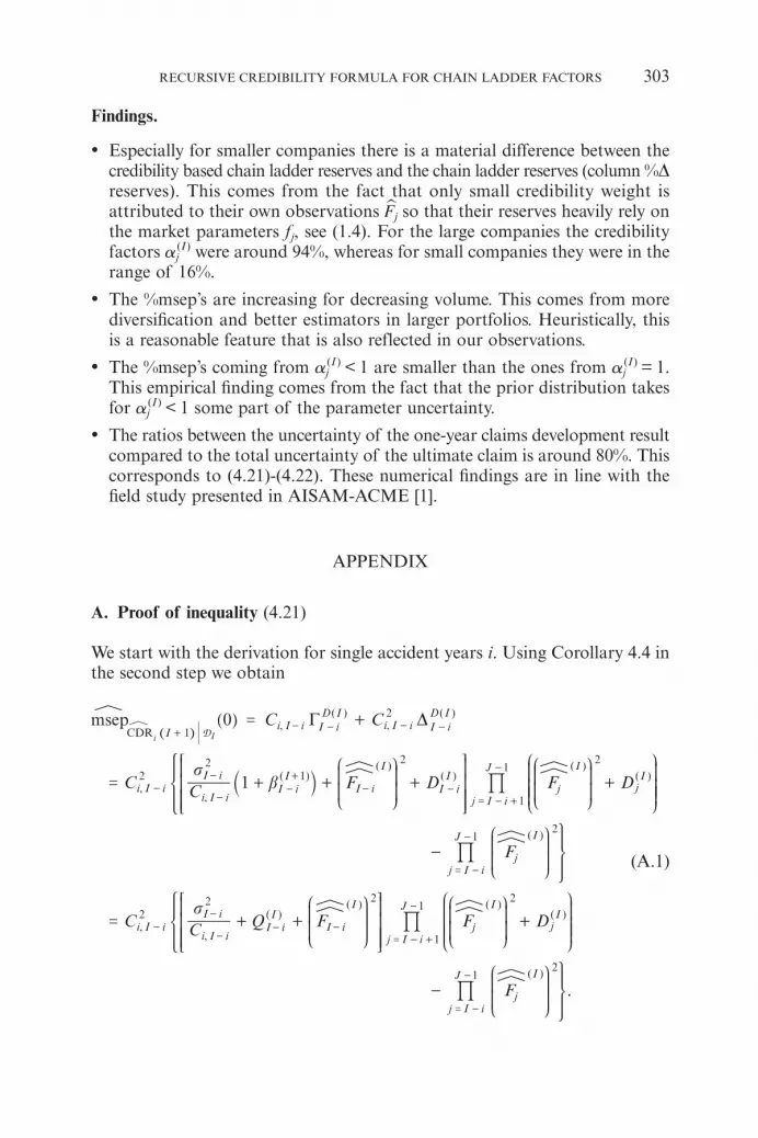
A. Proof of inequality (4.21)

We start with the derivation for single accident years i. Using Corollary 4.4 inthe second step we obtain

I i I i- -

j

j

j

j

j

j

,

,

,

i I i

i I iI i

i I iI i

-

--

--

I i I i

I i

- -

-

I

.

C

C D D

C Q D

msep

sb

s

G D0

1

,( ) ( )

,

( ) ( ) ( )

,

( ) ( )

Ii I i

D I D I

i I i

II i

I

j I i

JI

j I i

J

i I i

II i

j I i

JI

j I i

J

CDR 1

2

22

12

1

12

21

22 2

1

12

21

= +

= + + + +

-

= + + +

-

+-

-

+-

= - +

-

= -

-

--

= - +

-

= -

-

( ) ( )

( )

( ) ( )

( )

I I

I

I I

I

DC

C

C

F F

F

F F

F

i

%

%

%

%

%

%% %%

%%

%% %%

%%

%

J

L

KK

J

L

KK

J

L

KKK

J

L

KK

J

L

KK

J

L

KK

J

L

KKK

J

L

KK

]]

a

N

P

OO

N

P

OO

N

P

OOO

N

P

OO

N

P

OO

N

P

OO

N

P

OOO

N

P

OO

gg

k

R

T

SSSS

R

T

SSSS

V

X

WWWW

V

X

WWWW

*

*

4

4

(A.1)

In the next step we use that

Dj(I ) = bj

(I+1)Qj(I ) # Qj

(I ), (A.2)

which implies

I i I i

I i

I i I i

- -

-

- -

j

j

j

j

j

,

,

,

,

i I i

i I iI i

I i i I i

i I i

-

--

- -

-

I i-

I

I,

C

C Q Q

Q C

C C

msep

msep

s

s

G D

D

G D

0 ,( ) ( )

,

( ) ( )

,( ) ( )

,( ) ( )

,

( )

Ii I i

D I D I

i I i

II i

j I i

JI

j I i

J

i I ij I i

JI I

i I iI I

C i J

I

CDR 1

2

22 2

1

12

21

2

1

12

2

2

,i J

#

#

= +

+ + +

-

= + +

+ =

+-

--

= - +

-

= -

-

-= - +

-

-

( ) ( )

( )

( )

I I

I

I

D

D

C

C

C

C

F F

F

F

i

%

%

%

%

%% %%

%%

%%

% %%

%

J

L

KK

J

L

KK

J

L

KKK

J

L

KK

J

L

KK

J

L

KKK

J

L

KK

]]

N

P

OO

N

P

OO

N

P

OOO

N

P

OO

N

P

OO

N

P

OOO

N

P

OO

gg

R

T

SSSS

V

X

WWWW

*

4 (A.3)

where in the last step we have used that we only need to consider the first termof the sum in G (I )

I–i .Note that we obtain a strict inequality if sj

2 > 0 for some j > I – i and allchain ladder factor estimators are strictly positive.

For aggregated accident years we need to consider in addition the covari-ance terms. For i < k this implies using Corollary 4.4.


I i I i

I i

- -

-

j j

j j

j j

I i-j

j

j

I i- I i

I i

-

-

.

D D

Q D

Q

bs

D F

D

( ) ( )

( )

,

( ) ( )

( ) ( )

( ) ( )

D I D I

I

i I iI i

I

j I i

JI

j I i

J

I iI

j I i

JI

j I i

J

j I i

JI

j I i

JI

12 2

1

12

12

2

1

12

12

12

12

#

+

= + + + -

= + + -

+ - =

+

--

= - +

-

= -

-

-= - +

-

= -

-

= -

-

= -

-

( ) ( ) ( )

( ) ( ) ( )

( ) ( )

I I I

I I I

I I

C F F F

F F F

F F

% %

% %

% %

%% %% %%

%% %% %%

%% %%

J

L

KK

J

L

KK

J

L

KKK

J

L

KK

J

L

KK

J

L

KK

J

L

KKK

J

L

KK

J

L

KK

J

L

KKK

J

L

KK

N

P

OO

N

P

OO

N

P

OOO

N

P

OO

N

P

OO

N

P

OO

N

P

OOO

N

P

OO

N

P

OO

N

P

OOO

N

P

OO

R

T

SSSS

R

T

SSSS

V

X

WWWW

V

X

WWWW (A.4)

This completes the proof of inequality (4.21).

REFERENCES

[1] AISAM-ACME (2007) AISAM-ACME study on non-life long tail liabilities. Reserve risk andrisk margin assessment under Solvency II. October 17, 2007.

[2] ASMUSSEN, S. and GLYNN, P.W. (2007) Stochastic Simulation. Springer.[3] BUCHWALDER, M., BÜHLMANN H., MERZ, M. and WÜTHRICH, M.V. (2006) The mean square

error of prediction in the chain ladder reserving method (Mack and Murphy revisited).ASTIN Bulletin 36(2), 521-542.

[4] BÜHLMANN, H. and GISLER, A. (2005) A Course in Credibility Theory and its Applications.Springer, Berlin.

[5] DE FELICE, M. and MORICONI, F. (2003) Risk based capital in P&C loss reserving or stressingthe triangle. Research Group on “Insurance Companies and Pension Funds”, Working Papern. 1, Rome, December 2003.

[6] DE FELICE, M. and MORICONI, F. (2006) Process error and estimation error of year-endreserve estimation in the distribution free chain-ladder model. Alef Working Paper, Rome,November 2006.

[7] GERBER, H.U. and JONES, D.A. (1975) Credibility formulas of the updating type. In P.M. Kahn(ed.), Credibility: Theory and Applications. Academic Press.

[8] GILKS, W.R., RICHARDSON, S. and SPIEGELHALTER, D.J. (1996) Markov Chain Monte Carloin Practice. Chapman & Hall, London.

[9] GISLER, A. and WÜTHRICH, M.V. (2008) Credibility for the chain ladder reserving method.ASTIN Bulletin 38(2), 565-600.

[10] ISVAP (2006) Reserve requirements and capital requirements in non-life insurance. An analysisof the Italian MTPL insurance market by stochastic claims reserving models. Report preparedby De Felice M., Moriconi F., Matarazzo L., Cavastracci S. and Pasqualini S., Rome, Octo-ber 2006.

[11] KREMER, E. (1982) Credibility for some evolutionary models. Scand. Act. Journal 1982(3-4),129-142.

[12] MACK, T. (1993) Distribution-free calculation of the standard error of chain ladder reserveestimates. ASTIN Bulletin 23(2), 213-225.

[13] MERZ, M. and WÜTHRICH, M.V. (2008) Modelling the claims development result for solvencypurposes. CAS E-Forum, Fall 2008, 542-568.

[14] OHLSSON, E. and LAUZENINGKS, J. (2008) The one-year non-life insurance risk. ConferencePaper, ASTIN Colloquium 2008, Manchester.

[15] SUNDT, B. (1981) Recursive credibility estimation. Scand. Act. Journal 1981(1), 3-21.[16] WÜTHRICH, M.V. and MERZ, M. (2008) Stochastic Claims Reserving Methods in Insurance.

Wiley.[17] WÜTHRICH, M.V., MERZ, M. and LYSENKO, N. (2008) Uncertainty in the claims development

result in the chain ladder method. Accepted for publication in Scand. Act. J.

HANS BÜHLMANN

Department of MathematicsETH Zurich8092 Zurich, SwitzerlandE-Mail: [email protected]

MASSIMO DE FELICE

Dipartimento di Studi Sociali, Economici,Aattuariali e FinanziariViale Regina Elena, 295 00161 Roma, ItalyE-Mail: [email protected]


ALOIS GISLER

AXA Winterthur Insurance CompanyP.O. Box 3578401 Winterthur, SwitzerlandE-Mail: [email protected]

FRANCO MORICONI

Dipartimento di Economia, Finanza e StatisticaUniversità di PerugiaVia A. Pascoli, 106100 Perugia, ItalyE-Mail: [email protected]

MARIO V. WÜTHRICH

Department of MathematicsETH Zurich8092 Zurich, SwitzerlandE-Mail: [email protected]


in recent solvency ii considerations much effort has been put

Documents