risks

Article

Revisiting Calibration of the Solvency II StandardFormula for Mortality Risk: Does the StandardStress Scenario Provide an AdequateApproximation of Value-at-Risk?

Rokas Gylys and Jonas Šiaulys *

Institute of Mathematics, Vilnius University, Naugarduko 24, LT-03225 Vilnius, Lithuania; rokas.gylys@mif.vu.lt* Correspondence: jonas.siaulys@mif.vu.lt; Tel.: +370-5-219-3085

Received: 18 April 2019; Accepted: 13 May 2019; Published: 19 May 2019�����������������

Abstract: The primary objective of this work is to analyze model based Value-at-Risk associatedwith mortality risk arising from issued term life assurance contracts and to compare the resultswith the capital requirements for mortality risk as determined using Solvency II Standard Formula.In particular, two approaches to calculate Value-at-Risk are analyzed: one-year VaR and run-offVaR. The calculations of Value-at-Risk are performed using stochastic mortality rates which arecalibrated using the Lee-Carter model fitted using mortality data of selected European countries.Results indicate that, depending on the approach taken to calculate Value-at-Risk, the key factorsdriving its relative size are: sensitivity of technical provisions to the latest mortality experience,volatility of mortality rates in a country, policy term and benefit formula. Overall, we found thatSolvency II Standard Formula on average delivers an adequate capital requirement, however, we alsohighlight particular situations where it could understate or overstate portfolio specific model basedValue-at-Risk for mortality risk.

Keywords: mortality risk; Value-at-Risk; Solvency II; Lee-Carter; standard formula; solvencycapital requirement

MSC: 91B30; 91G10; 91G70

1. Introduction

Solvency II was a major driver for European insurers to upgrade their quantitative risk assessmentmodels both for the purposes of the assessment of the regulatory solvency position and internal riskmanagement needs. Major European insurance groups have developed and implemented full orpartial internal models, which value risks from the perspective of a company specific risk profile.However, as demonstrated in Table 1, majority of the European insurers, predominantly small andmedium sized firms, calculate the regulatory solvency capital requirement using the standard methodsand stress scenarios prescribed by the legislation (Standard Formula). First, according to the StandardFormula, an insurer’s regulatory Solvency Capital Requirement (SCR) is estimated on individual riskmodule/sub-module level. Secondly, the individual risk assessments at risk module and sub-modulelevel are aggregated to the total SCR by taking into account the diversification between the risks.For example, SCR for mortality risk sub-module is assessed by calculating the amount of loss ofinsurer’s available Solvency II regulatory capital (Basic Own Funds) resulting from an immediate andpermanent 15% increase in mortality probabilities used for calculation of the Solvency II technicalprovisions. SCR for mortality risk is aggregated with SCR’s for other life underwriting risks such as

Risks 2019, 7, 58; doi:10.3390/risks7020058 www.mdpi.com/journal/risks

Risks 2019, 7, 58 2 of 24

lapse risk, longevity risk, expense risk and life CAT risk to derive SCR for the life underwriting riskmodule, which is used as an input for calculations of the overall SCR.

Table 1. Number of Solvency II submissions (solo undertakings) in 2017 by the method used forcalculation of the Solvency Capital Requirement (SCR). Data source: EIOPA.

Type of Insurer Internal Model Partial Internal Model Standard Formula Total

Life insurance companies 21 29 545 595Non-life insurance companies 37 42 1519 1598

Reinsurance companies 15 4 253 272Composite insurance companies 8 30 368 406

Total 81 105 2685 2871

In practice, the use of the Standard Formula goes beyond the calculation of statutory solvencyposition. Insurers often treat the outcome of the Standard Formula risk assessments as the key riskindicators, which are embedded in their enterprise risk management systems. Insurers which aresubject to Solvency II regulatory regime at least annually perform Own Risk and Solvency Assessment(ORSA), which includes qualitative and quantitative assessment of risks as well as analysis on how wellthe Standard Formula fits the company’s specific risk profile. Both insurers and regulators aim to ensurethat such an assessment includes sufficient quantitative analysis of risks. Therefore, for StandardFormula users it is important to understand what is behind the calibration of Standard Formulastandard stress scenarios and the key deviations of their risk profiles form the risk profile on which theStandard Formula calibration is based.

In its essence, the Standard Formula is designed to suit the risk profile of the “average” Europeaninsurer. However, insurers in the European Union (EU) are highly heterogeneous and the “average”insurer is difficult to define. For example, life insurers may be exposed to different levels of mortalityrisk due to the differences in products offered, distribution channels used, maturity of insuranceportfolios, prevailing policy terms and conditions, volatility of mortality in a country where insureroperates and a number of other factors.

The topic of modelling solvency capital for the risk of variation of mortality rates in the literaturewas addressed mainly with the focus to longevity risk. Solvency II Directive requires that SCR iscalibrated to the VaR of the basic own funds subject to a confidence level of 99.5% over a one-yearperiod. However, as argued by Richards et al. (2013):

. . . some risk do not fit naturally into one year VaR framework and it would be excessively dogmaticto insist that longevity trend risk only be measured over a one year horizon.

It seems that this approach is shared by the European Insurance and Occupational PensionsAuthority (EIOPA), who used run-off approach for the calibration of the uniform mortality shocks formortality and longevity risks during the review of the Standard Formula (EIOPA 2018).

Several models have been proposed to model mortality/longevity risk using one-year VaRapproach, where the key challenge is how to model the risk of variation of technical provisions inone year’s time after the valuation date. Börger et al. (2014) and Plat (2011) developed models whichexplicitly model the mortality trend risk which is used as the proxy to capture the risk of variation oftechnical provisions. Richards et al. (2013) took into account the risk of changes in technical provisionsby simulating one year’s portfolio mortality and subsequently refitting stochastic mortality model foreach simulation scenario based on the results of the first year simulations. A similar approach wasused by Jarner and Møller (2015) who proposed a model designed specifically for the Danish systemof reserving for longevity risks. Olivieri and Pitacco (2009) developed a model, which included aBayesian procedure for updating the parameters of projected distributions of deaths and formulatedconditions for few alternative definitions of solvency capital rules, however, their model did notnecessarily strictly follow a one-year VaR approach.

Risks 2019, 7, 58 3 of 24

Calculation of mortality VaR usually requires the simulations from a stochastic mortality modelas an input. A model proposed by Lee and Carter (1992) started a new generation of the extrapolativemortality projection methods, and in its original or modified form is widely used both in academicresearch and in practice. A number of improvements of Lee-Carter model have been proposed, bothfrom the point of view of model specification and statistical estimation of parameters, for example,see Lee and Miller (2001), Booth et al. (2002); Brouhns et al. (2002); Renshaw and Haberman (2003).In parallel, several alternative extrapolative stochastic mortality models have been developed (seecomparative study by Cairns et al. (2009), some of which explicitly model the cohort effect on mortalityrates. The simulations of mortality rates may be performed using simple approaches based onrandomly generated i.i.d. residuals or using more complex strategies with application of bootstrap orBayesian methods. Different simulation approaches are discussed by Renshaw and Haberman (2008)and Li (2014).

The purpose of this paper is to analyse how closely SCR for mortality risk, calculated usingStandard Formula, approximates the portfolio specific mortality VaR, and to identify factors whichmay affect the adequacy of this approximation. We performed the analysis for four selected Europeancountries: Lithuania, Sweden, Poland and the Netherlands, which have substantially different mortalityexperience. In calculations we follow the approach similar to EIOPA (2018) with the followingkey modifications:

• EIOPA follows run-off VaR approach and we examine the results using both run-off VaR andone-year VaR approaches.

• EIOPA assumes random walk with drift (RWD) as the default model for forecasting of the timevarying parameter, which is driving the projected mortality improvements. We perform formalstatistical testing for the purpose of confirming the hypothesis that RWD does not contradict thehistoric data.

• EIOPA fits the stochastic mortality model using the mortality data for ages 40–120 years (the sameas for longevity risk). We fit the stochastic mortality model for ages 25–75 years. We assume, thatfor most of life assurance protection products the highest exposure to mortality risk is associatedwith mid-aged assured lives. Therefore, the model fitted using the experience from the targetpopulation range can provide the most relevant parametrisation for the forecast.

• EIOPA calibrates VaR using temporary life expectancies, thus implicitly assuming that the benefitpayable under life assurance policy decreases with time. Decreasing benefits are common in lifeassurance products linked to mortgages or other credit instruments. In addition, mortality sumat risk is decreasing with policy duration for some risk and savings products (e.g., traditionalendowment insurance) where the total benefit payable on death is fixed and insurer is able torecoup part of the losses by reversing the accumulated savings amount. However, a significantpart of life assurance products have fixed sums assured. In this paper we examine the effect onVaR of both benefit formulas: level (fixed) sum assured and sum assured which is decreasinglinearly with time.

The rest of this paper is organized as follows: Section 2 discusses overall approach to VaRcalculations and provides the results. Section 3 discusses the results. Section 4 provides the details ofthe statistical fitting of Lee-Carter model. Section 5 describes in detail our VaR calculation methodology.

2. Results

According to McNeil et al. (2005) (see page 38) given certain confidence level α ∈ (0, 1) VaR canbe defined as:

VaRα(L) = inf{l ∈ R : P(L > l) 6 1− α}, (1)

where L is a random variable of a loss. Throughout the paper, consistently with the Solvency IIlegislation, we calculated VaR using 99.5% confidence level, that is, set α = 0.005.

Risks 2019, 7, 58 4 of 24

As we show in Section 5, in the context of mortality risk in the Solvency II framework,L is a loss/gain of the Solvency II capital (Basic Own Funds) due to variation of mortality rates.Thus, VaR 0.005 (L) defines extra capital needed to cover the unreserved mortality losses arising fromthe increase in the future mortality rates.

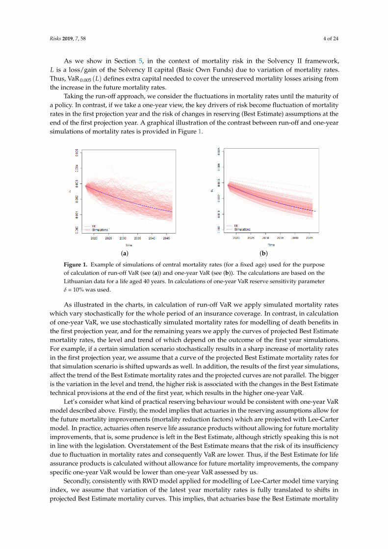
Taking the run-off approach, we consider the fluctuations in mortality rates until the maturity ofa policy. In contrast, if we take a one-year view, the key drivers of risk become fluctuation of mortalityrates in the first projection year and the risk of changes in reserving (Best Estimate) assumptions at theend of the first projection year. A graphical illustration of the contrast between run-off and one-yearsimulations of mortality rates is provided in Figure 1.

(a) (b)

Figure 1. Example of simulations of central mortality rates (for a fixed age) used for the purposeof calculation of run-off VaR (see (a)) and one-year VaR (see (b)). The calculations are based on theLithuanian data for a life aged 40 years. In calculations of one-year VaR reserve sensitivity parameterδ = 10% was used.

As illustrated in the charts, in calculation of run-off VaR we apply simulated mortality rateswhich vary stochastically for the whole period of an insurance coverage. In contrast, in calculationof one-year VaR, we use stochastically simulated mortality rates for modelling of death benefits inthe first projection year, and for the remaining years we apply the curves of projected Best Estimatemortality rates, the level and trend of which depend on the outcome of the first year simulations.For example, if a certain simulation scenario stochastically results in a sharp increase of mortality ratesin the first projection year, we assume that a curve of the projected Best Estimate mortality rates forthat simulation scenario is shifted upwards as well. In addition, the results of the first year simulations,affect the trend of the Best Estimate mortality rates and the projected curves are not parallel. The biggeris the variation in the level and trend, the higher risk is associated with the changes in the Best Estimatetechnical provisions at the end of the first year, which results in the higher one-year VaR.

Let’s consider what kind of practical reserving behaviour would be consistent with one-year VaRmodel described above. Firstly, the model implies that actuaries in the reserving assumptions allow forthe future mortality improvements (mortality reduction factors) which are projected with Lee-Cartermodel. In practice, actuaries often reserve life assurance products without allowing for future mortalityimprovements, that is, some prudence is left in the Best Estimate, although strictly speaking this is notin line with the legislation. Overstatement of the Best Estimate means that the risk of its insufficiencydue to fluctuation in mortality rates and consequently VaR are lower. Thus, if the Best Estimate for lifeassurance products is calculated without allowance for future mortality improvements, the companyspecific one-year VaR would be lower than one-year VaR assessed by us.

Secondly, consistently with RWD model applied for modelling of Lee-Carter model time varyingindex, we assume that variation of the latest year mortality rates is fully translated to shifts inprojected Best Estimate mortality curves. This implies, that actuaries base the Best Estimate mortality

Risks 2019, 7, 58 5 of 24

assumptions on the mortality level implied by the last year’s experience. In practice, actuaries oftenuse various smoothing, averaging and similar methods, as a results of which the variation driven bythe mortality level of the last observed year may be taken into account only partially. Application ofsuch techniques may result in lower risk of changes in Best Estimate and lower VaR.

Finally, even if the reserving methodology allows for mortality improvements, the sensitivity ofthe mortality reduction factors (trend risk) to the last year’s mortality experience may vary from insurerto insurer. In our calculations we use two levels of credibility factor δ (5% and 10%), which representsvariation in reserve risk due to differences in actuarial methodologies applied. The credibilityparameter may be interpreted as the proportion of evidence related to the last year’s experienceaccounted for in setting the assumed mortality reduction factors. Thus, in case of δ = 10% mortalityreduction factors are more sensitive to the last year’s experience than in case of δ = 5%, and themodelled trend risk increases with the growth of δ. See Section 5.2 for more detailed discussion of thetrend risk modelling.

Overall, the above considerations imply that our approach results in rather conservative estimateof one-year VaR for two levels of selected trend risk parameters.

For the purpose of comparability of our results with the Standard Formula mortality stressparameter we have converted the calculated VaR’s to equivalent VaR rates. We define VaR rate as gwhich satisfy the following condition

BEt + VaR 0.005(L) =n

∑i=1

CF(g)t+i .

Here L is random variable of a loss in basic own funds, BEt is the initial Best Estimate, t isthe valuation year, n is projection term and CF(g)

t+i , i ∈ {1, 2, . . . , n}, are projected mortality benefitscalculated according to the applicable benefit formula by applying the following m year stressedmortality probabilities

mq(g)x (t) = 1−

m−1

∏s=0

(1− (1 + g)qx+s(t + s)

),

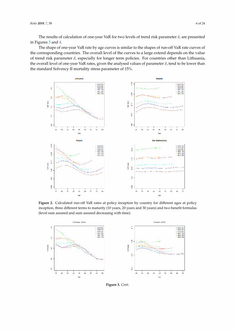
where x denotes age at time t, qx(t) are the Best Estimates of one year mortality probabilities andm ∈ {1, 2, . . . , n}. In such a way, we search for rate g, which makes the stressed Best Estimate equal to theinitial Best Estimate plus VaR. The results of calculation of run-off VaR rates are presented in Figure 2.

The results obtained indicate that run-off VaR rates tend to increase with policy term. Uncertaintyabout the future mortality rates grows with time, which leads to wider confidence intervals of mortalityrates for long term projections.

Similarly, for the policies with decreasing sum assured, higher sums assured are paid in earlypolicy years when the mortality uncertainty is lower than in later policy years, which implies thatrun-off VaR rates are generally lower for policies with decreasing sum assured than for equivalentpolicies with fixed sum assured.

The shape of VaR rate by age curves is related to the shape of Lee-Carter parameter βx

(see Section 4) which determines the sensitivity of projected age specific mortality rates to the changesin the time varying parameter, and drives the relative level of age specific projected volatility ofmortality rates. As demonstrated in Section 4, Sweden and the Netherlands have relatively stableparameter βx over the modelled ages. Consequently, for those countries run-off VaR rate curves areflat as well. For Lithuania and Poland, higher volatility of mortality rates at younger ages increase therun-off VaR rates for policies issued to younger policyholders.

Comparing the results with the standard Solvency II stress level of 15%, the calculated VaR ratesare significantly higher for Lithuania, however, for other countries the results are close to the value ofthe standard parameter. As discussed in Section 4, Lithuanian mortality improvement trend is not sosettled as in other countries, which resulted in high standard error of time varying index and wideconfidence intervals of projected mortality rates.

Risks 2019, 7, 58 6 of 24

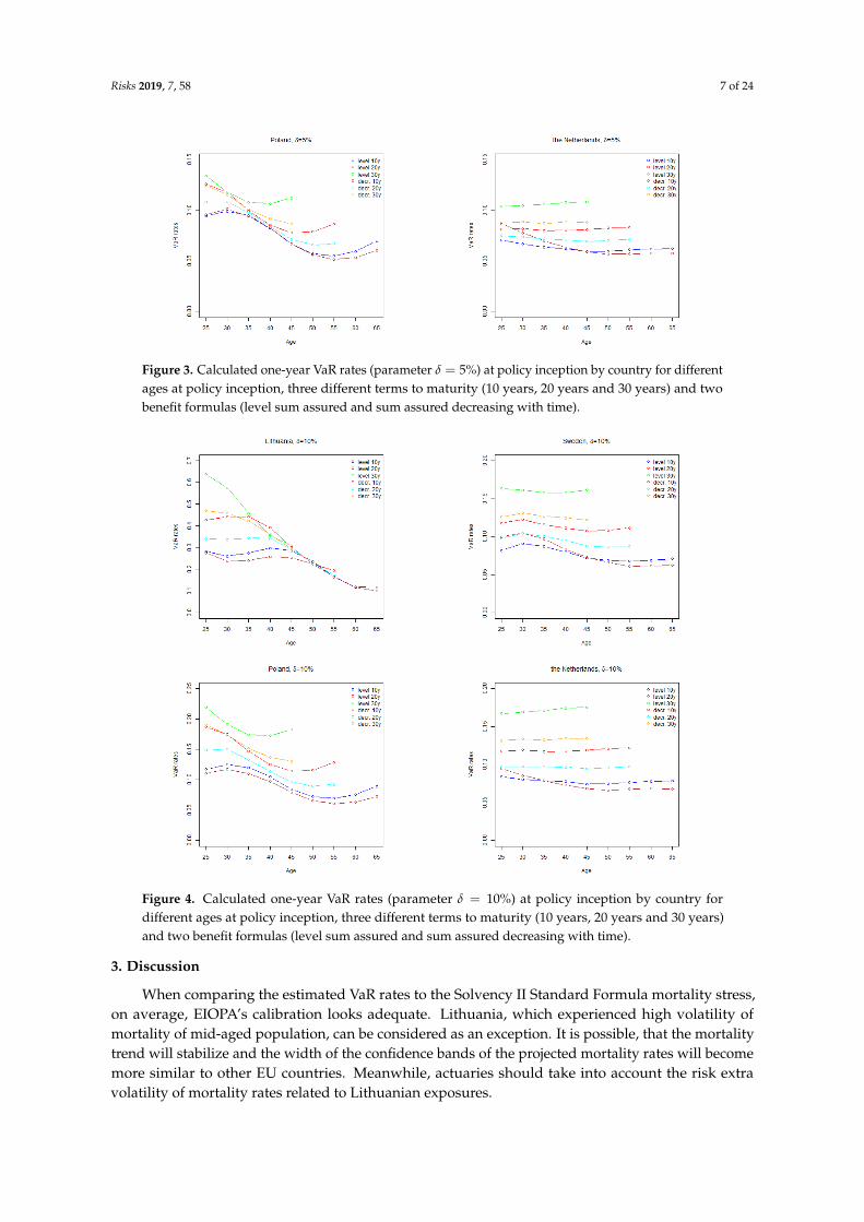
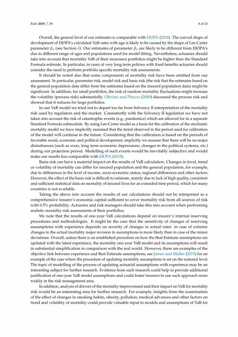
The results of calculation of one-year VaR for two levels of trend risk parameter δ, are presentedin Figures 3 and 4.

The shape of one-year VaR rate by age curves is similar to the shapes of run-off VaR rate curves ofthe corresponding countries. The overall level of the curves to a large extend depends on the valueof trend risk parameter δ, especially for longer term policies. For countries other than Lithuania,the overall level of one-year VaR rates, given the analysed values of parameter δ, tend to be lower thanthe standard Solvency II mortality stress parameter of 15%.

Figure 2. Calculated run-off VaR rates at policy inception by country for different ages at policyinception, three different terms to maturity (10 years, 20 years and 30 years) and two benefit formulas(level sum assured and sum assured decreasing with time).

Figure 3. Cont.

Risks 2019, 7, 58 7 of 24

Figure 3. Calculated one-year VaR rates (parameter δ = 5%) at policy inception by country for differentages at policy inception, three different terms to maturity (10 years, 20 years and 30 years) and twobenefit formulas (level sum assured and sum assured decreasing with time).

Figure 4. Calculated one-year VaR rates (parameter δ = 10%) at policy inception by country fordifferent ages at policy inception, three different terms to maturity (10 years, 20 years and 30 years)and two benefit formulas (level sum assured and sum assured decreasing with time).

3. Discussion

When comparing the estimated VaR rates to the Solvency II Standard Formula mortality stress,on average, EIOPA’s calibration looks adequate. Lithuania, which experienced high volatility ofmortality of mid-aged population, can be considered as an exception. It is possible, that the mortalitytrend will stabilize and the width of the confidence bands of the projected mortality rates will becomemore similar to other EU countries. Meanwhile, actuaries should take into account the risk extravolatility of mortality rates related to Lithuanian exposures.

Risks 2019, 7, 58 8 of 24

Overall, the general level of our estimates is comparable with EIOPA (2018). The curved shape ofdevelopment of EIOPA’s calculated VaR rates with age is likely to be caused by the shape of Lee-Carterparameter βx (see Section 4). Our estimates of parameter βx are likely to be different from EIOPA’sdue to different range of ages and populations used for model fitting. Nevertheless, actuaries shouldtake into account that mortality VaR of their insurance portfolios might be higher than the StandardFormula estimate. In particular, in cases of very long term policies with fixed benefits actuaries shouldconsider the need to perform portfolio specific mortality risk assessments.

It should be noted also that some components of mortality risk have been omitted from ourassessment. In particular, parameter risk, model risk and basis risk (the risk that the estimates based onthe general population data differ from the estimates based on the insured population data) might besignificant. In addition, for small portfolios, the risk of random mortality fluctuations might increasethe volatility (process risk) substantially. Olivieri and Pitacco (2009) discussed the process risk andshowed that it reduces for large portfolios.

In our VaR model we tried not to depart too far from Solvency II interpretation of the mortalityrisk used by regulators and the market. Consistently with the Solvency II legislation we have nottaken into account the risk of catastrophic events (e.g., pandemics) which are allowed for in a separateStandard Formula submodule. By using Lee-Carter model as a basis for the calibration of the stochasticmortality model we have implicitly assumed that the trend observed in the period used for calibrationof the model will continue in the future. Considering that the calibration is based on the periods offavorable social, economic and political development, implicitly we assume that there will be no majordisturbances (such as wars, long term economic depressions, changes in the political systems, etc.)during our projection period. Modelling of such events would be inevitably subjective and wouldmake our results less comparable with EIOPA (2018).

Basis risk can have a material impact on the results of VaR calculation. Changes in level, trendor volatility of mortality can differ for insured population and the general population, for example,due to differences in the level of income, socio-economic status, regional differences and other factors.However, the effect of the basis risk is difficult to estimate, mainly due to lack of high quality, consistentand sufficient statistical data on mortality of insured lives for an extended time period, which for manycountries is not available.

Taking the above into account the results of our calculations should not be interpreted as acomprehensive insurer’s economic capital sufficient to cover mortality risk from all sources of riskwith 0.5% probability. Actuaries and risk managers should take this into account when performingrealistic mortality risk assessments of their portfolios.

We note that the results of one-year VaR calculations depend on insurer’s internal reservingprocedures and methodologies. It might be the case that the sensitivity of changes of reservingassumptions with experience depends on severity of changes in actual rates: in case of extremechanges in the actual mortality major revision in assumptions is more likely than in case of the minordeviations. Overall, unless there is an established procedure on how the Best Estimate assumptions areupdated with the latest experience, the mortality one-year VaR model and its assumptions will resultin substantial simplification in comparison with the real world. However, there are examples of theobjective link between experience and Best Estimate assumptions, see Jarner and Møller (2015) for anexample of the case where the procedure of updating mortality assumptions is set on the national level.The topic of modelling of the process of updating actuarial assumptions with experience may be aninteresting subject for further research. Evidence from such research could help to provide additionaljustification of one-year VaR model assumptions and could foster insurers to use such approach morewidely in the risk management area.

In addition, analysis of drivers of the mortality improvement and their impact on VaR for mortalityrisk would be an interesting area for further research. For example, insights from the examinationof the effect of changes in smoking habits, obesity, pollution, medical advances and other factors ontrend and volatility of mortality could provide valuable input to models and assumptions of VaR for

Risks 2019, 7, 58 9 of 24

mortality risk. On the other hand, the credibility of such analysis is often compromised by the lack ofcredible data and complex interdependencies between the mortality data and the underlying driversof mortality improvement.

In conclusion, based on the analysis performed for the selected countries, we found the overallcalibration of the Standard Formula for mortality risk adequate, given the current definition andinterpretation of the mortality risk in Solvency II. However, there are insurance portfolio or countryspecific differences which can result in portfolio specific VaR higher or lower than the capitalrequirement produced by the Standard Formula.

4. Stochastic Mortality Model

4.1. Overview of the Data

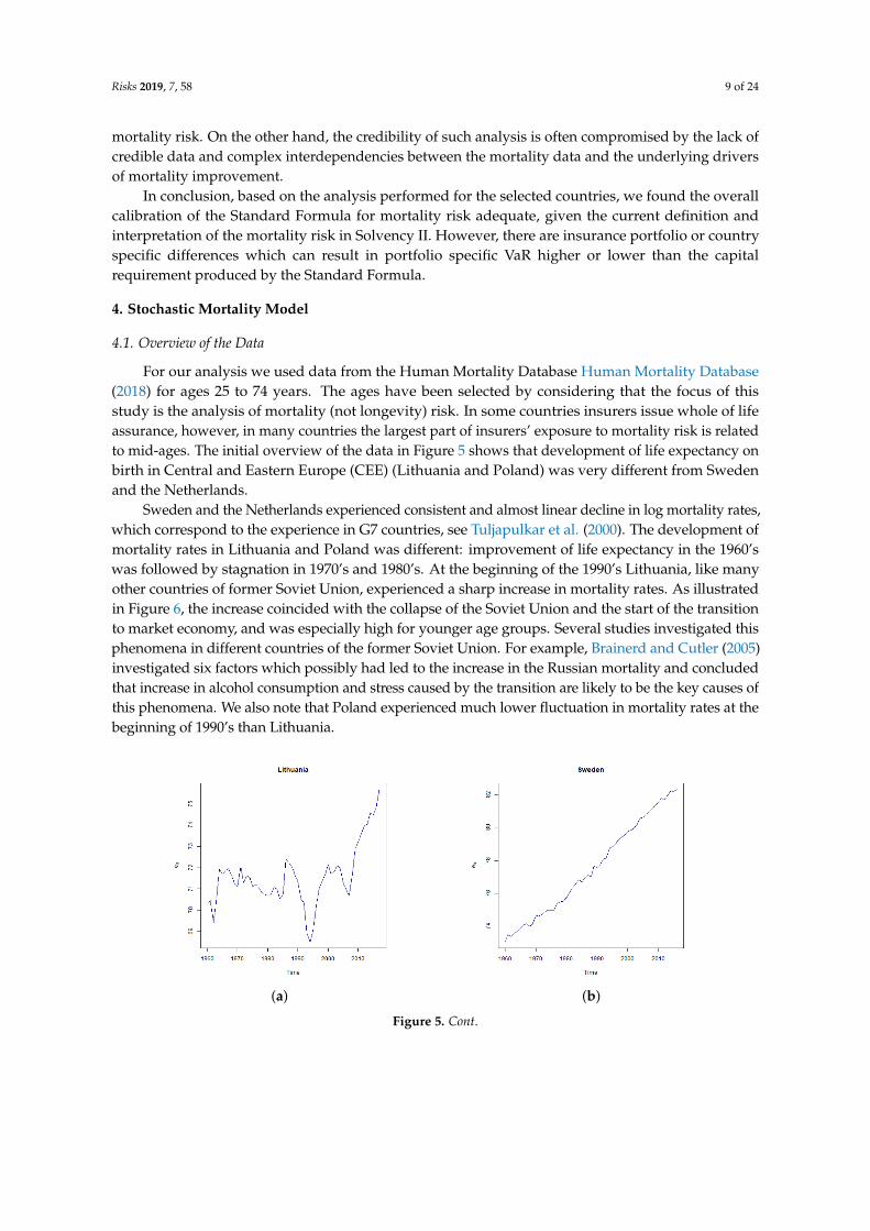
For our analysis we used data from the Human Mortality Database Human Mortality Database(2018) for ages 25 to 74 years. The ages have been selected by considering that the focus of thisstudy is the analysis of mortality (not longevity) risk. In some countries insurers issue whole of lifeassurance, however, in many countries the largest part of insurers’ exposure to mortality risk is relatedto mid-ages. The initial overview of the data in Figure 5 shows that development of life expectancy onbirth in Central and Eastern Europe (CEE) (Lithuania and Poland) was very different from Swedenand the Netherlands.

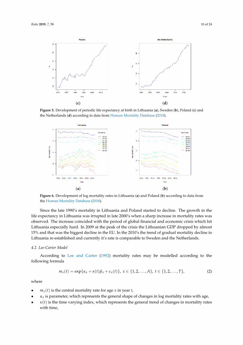
Sweden and the Netherlands experienced consistent and almost linear decline in log mortality rates,which correspond to the experience in G7 countries, see Tuljapulkar et al. (2000). The development ofmortality rates in Lithuania and Poland was different: improvement of life expectancy in the 1960’swas followed by stagnation in 1970’s and 1980’s. At the beginning of the 1990’s Lithuania, like manyother countries of former Soviet Union, experienced a sharp increase in mortality rates. As illustratedin Figure 6, the increase coincided with the collapse of the Soviet Union and the start of the transitionto market economy, and was especially high for younger age groups. Several studies investigated thisphenomena in different countries of the former Soviet Union. For example, Brainerd and Cutler (2005)investigated six factors which possibly had led to the increase in the Russian mortality and concludedthat increase in alcohol consumption and stress caused by the transition are likely to be the key causes ofthis phenomena. We also note that Poland experienced much lower fluctuation in mortality rates at thebeginning of 1990’s than Lithuania.

(a) (b)

Figure 5. Cont.

Risks 2019, 7, 58 10 of 24

(c) (d)

Figure 5. Development of periodic life expectancy at birth in Lithuania (a), Sweden (b), Poland (c) andthe Netherlands (d) according to data from Human Mortality Database (2018).

(a) (b)

Figure 6. Development of log mortality rates in Lithuania (a) and Poland (b) according to data fromthe Human Mortality Database (2018).

Since the late 1990’s mortality in Lithuania and Poland started to decline. The growth in thelife expectancy in Lithuania was irrupted in late 2000’s when a sharp increase in mortality rates wasobserved. The increase coincided with the period of global financial and economic crisis which hitLithuania especially hard. In 2009 at the peak of the crisis the Lithuanian GDP dropped by almost15% and that was the biggest decline in the EU. In the 2010’s the trend of gradual mortality decline inLithuania re-established and currently it’s rate is comparable to Sweden and the Netherlands.

4.2. Lee-Carter Model

According to Lee and Carter (1992) mortality rates may be modelled according to thefollowing formula

mx(t) = exp{αx + κ(t)βx + εx(t)}, x ∈ {1, 2, . . . , A}, t ∈ {1, 2, . . . , T}, (2)

where

• mx(t) is the central mortality rate for age x in year t,• αx is parameter, which represents the general shape of changes in log mortality rates with age,• κ(t) is the time varying index, which represents the general trend of changes in mortality rates

with time,

Risks 2019, 7, 58 11 of 24

• βx is parameter, which determines the impact of the time varying index on age specific logmortality rates,

• εx(t) are residuals, it is supposed that εx(t) are independent and identically distributed randomvariables with zero mean and finite variance.

According to the original model fitting procedure, parameters are estimated using two stageprocedure. Firstly, κ(t) and βx are estimated using singular value decomposition (SVD) of a matrixof log mortality rates minus age specific constant αx. Age specific constant may be estimated as anaverage of log mortality rate for each age group. To ensure that the model is determined, the followingtwo constrains are introduced

T

∑t=1

κ(t) = 0,A

∑x=1

βx = 1. (3)

As the second step, after fixing αx and βx, κ(t) are re-estimated to ensure that the actual historictotal number of deaths in a year equals to the fitted number of death.

Brouhns et al. (2002) developed a method of fitting the Lee-Carter model as Poisson regression:

D{x,t} ∼ Poisson(E{x,t}µx(t)

)with µx(t) = exp{αx + κ(t)βx}, (4)

where D{x,t} and E{x,t} are the number of deaths and the number of exposed to risk respectively,at age x and time t. The motivation for fitting the model with Poisson regression is to avoid theSVD assumption that errors are distributed homoskedastically. The model is overparametrized as theoriginal Lee-Carter model, therefore, the identifiability constrains (3) are used in this model settingas well.

As noted by McCullag and Nelder (1989), in practice, when modelling data with Poissonregression it is not uncommon that the variance of the response variable Y exceeds the varianceimplied by the model according to which var(Y) = E(Y). This phenomenon is called overdispersionand may occur due to a number of reasons, one of which is heterogeneity of the modelled populationdue to features other than factors explicitly taken into account by the model. For example, mortalityof same age population may further vary with income level, urban/rural living location, and soforth. Li et al. (2009) allowed for overdispersion in mortality data by expressing Lee-Carter model asNegative Binomial regression. Such approach allows to estimate different overdispersion parametersfor each age group. We will take a simpler approach and will estimate only the total overdispersionparameter. The overdispersion parameter will be used for the purpose of assessment of model fit andwhere appropriate will be taken into account in simulation of random realisations from model (4).

The Lee-Carter model projections are derived using the same basic model structure defined byFormula (2). In the original paper Lee and Carter (1992) assumed that αx and βx are fixed and changesin the mortality rates are driven by innovations of time varying index κ(t). In later applications,several methods were developed (see Renshaw and Haberman (2008) and Li (2014) for overview)to take into account uncertainty in other model parameters, however, in majority of applications ofLee-Carter model κ(t) has remained the key source of uncertainty. As a simplification, in this paperwe will assume that αx and βx parameters are equal to the estimated values and do not change overthe projection period.

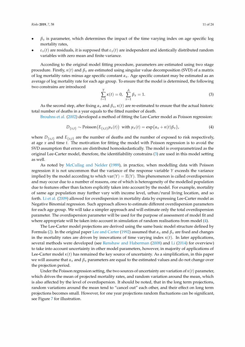
Under the Poisson regression setting, the two sources of uncertainty are variation of κ(t) parameter,which drives the mean of projected mortality rates, and random variation around the mean, whichis also affected by the level of overdispersion. It should be noted, that in the long term projections,random variations around the mean tend to “cancel out” each other, and their effect on long termprojections becomes small. However, for one year projections random fluctuations can be significant,see Figure 7 for illustration.

Risks 2019, 7, 58 12 of 24

(a) (b)

Figure 7. Confidence intervals for 30-year projection (a) and 1-year projection (b) of mortality rateswith and without taking into account the additional volatility from random fluctuation around themodelled mean mortality rates. The calculations were performed for Lithuanian data by assumingGaussian approximation of Poisson distribution and by allowing for overdisperion.

Further in our analysis as a simplification we will not allow for additional volatility randomdue to variation of mortality rates around the projected mean in run-off VaR calculation, which ismainly driven by the long term projections of mortality rates. However, we will allow for additionalvolatility in one-year VaR calculations, which proportionally is more influenced by the results of thefirst year projections.

4.3. Estimation of Parameters

Firstly, we considered which time periods should be used for estimation of the parameters.Mortality data for Poland and Lithuania was provided from the end of 1950’s. Due to unevendevelopment of mortality until 1990’s our initial fits of the models for these countries using fulldata sets were poor. The key reason of the inadequate fit was inconsistent and unstable changes inmortality rates for different age groups. For example, in the early 1990’s Lithuanian mortality of midage population increased sharply. Meanwhile, mortality of higher age population stayed constant.This trend changed in early 2010’s when the mortality in mid age groups started to decline rapidly.

One possibility to improve the fit is to include in the model the second term of SVD decompositionor additional set of time varying parameters in the Poisson regression. This modification, for example,was applied by Renshaw and Haberman (2003) when modelling the UK data and Booth et al. (2002) inthe model fitted to the Australian data. The inclusion of higher order terms improves the fit, however,in most of the cases higher order parameters proved to be less predictable than the main trend ofmortality decline with time, which makes the forecasting problematic. For the Lithuanian data similaradjustment was implemented by Ignataviciute et al. (2012) who applied original Lee-Carter modelto the Lithuanian data for the time period 1970 to 2005. The adjustment resulted only in marginalimprovement of the prediction accuracy of the model and the second order trend parameter wasvolatile and difficult to predict. Therefore, we will not include higher order terms to improve the fit ofour model.

Another simple adjustment to improve the fit as applied by Lee and Miller (2001);Booth et al. (2002) and Tuljapulkar et al. (2000) is to calibrate the Lee-Carter model using only thelatest and the most relevant mortality experience. In the Lithuanian case we have refitted the modelusing the mortality data for 1995–2017. The starting year was chosen by considering that by 1995 allmajor reforms of transition from Soviet system have already been implemented and by performingthe graphical inspection of the mortality trends. In Polish case the fitting period was selected to be1990–2016 as the reforms of transition to market economy in Poland were implemented earlier and the

Risks 2019, 7, 58 13 of 24

mortality shock due to transition was lower. For Sweden and the Netherlands the data for 1960–2016was used.

We have performed the estimation of the model parameters using both the original Lee-Cartermodel and the Poisson regression approach. When fitting the data with Poisson regression we usedthe gnm function fromR package gnm. The identifiability constrains (4) were imposed as describedby Currie (2016). The estimates of βx parameters lacked smoothness (see Figure A1 in Appendix A,and therefore were smoothed with cubic splines with 11 knots and penalty parameter of 0.3. In order toensure the internal consistency of parameters, we have refitted the Poisson regression and re-estimatedparameter κ(t) using the constraint that αx and βx parameters equal to originally estimated αx andsmoothed βx values. After the refitting we checked that due to smoothing there was no major decreasein the log-likelihood. Table 2 provides a summary statistics on the fit of the models.

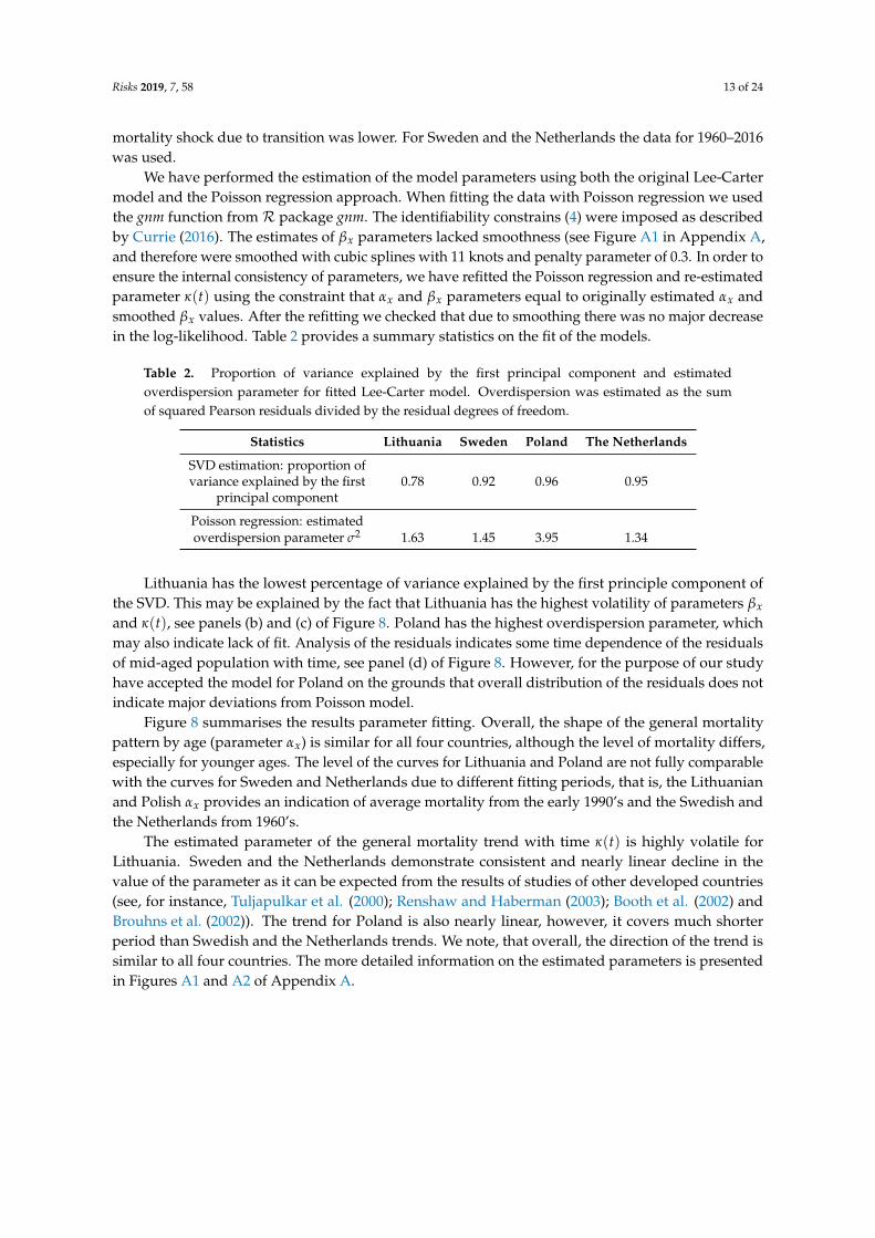
Table 2. Proportion of variance explained by the first principal component and estimatedoverdispersion parameter for fitted Lee-Carter model. Overdispersion was estimated as the sumof squared Pearson residuals divided by the residual degrees of freedom.

Statistics Lithuania Sweden Poland The Netherlands

SVD estimation: proportion ofvariance explained by the first 0.78 0.92 0.96 0.95

principal component

Poisson regression: estimatedoverdispersion parameter σ2 1.63 1.45 3.95 1.34

Lithuania has the lowest percentage of variance explained by the first principle component ofthe SVD. This may be explained by the fact that Lithuania has the highest volatility of parameters βx

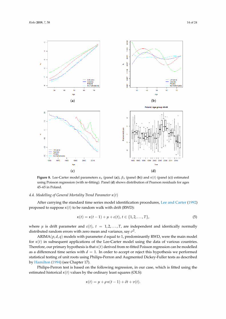
and κ(t), see panels (b) and (c) of Figure 8. Poland has the highest overdispersion parameter, whichmay also indicate lack of fit. Analysis of the residuals indicates some time dependence of the residualsof mid-aged population with time, see panel (d) of Figure 8. However, for the purpose of our studyhave accepted the model for Poland on the grounds that overall distribution of the residuals does notindicate major deviations from Poisson model.

Figure 8 summarises the results parameter fitting. Overall, the shape of the general mortalitypattern by age (parameter αx) is similar for all four countries, although the level of mortality differs,especially for younger ages. The level of the curves for Lithuania and Poland are not fully comparablewith the curves for Sweden and Netherlands due to different fitting periods, that is, the Lithuanianand Polish αx provides an indication of average mortality from the early 1990’s and the Swedish andthe Netherlands from 1960’s.

The estimated parameter of the general mortality trend with time κ(t) is highly volatile forLithuania. Sweden and the Netherlands demonstrate consistent and nearly linear decline in thevalue of the parameter as it can be expected from the results of studies of other developed countries(see, for instance, Tuljapulkar et al. (2000); Renshaw and Haberman (2003); Booth et al. (2002) andBrouhns et al. (2002)). The trend for Poland is also nearly linear, however, it covers much shorterperiod than Swedish and the Netherlands trends. We note, that overall, the direction of the trend issimilar to all four countries. The more detailed information on the estimated parameters is presentedin Figures A1 and A2 of Appendix A.

Risks 2019, 7, 58 14 of 24

(a) (b)

(c) (d)

Figure 8. Lee-Carter model parameters αx (panel (a)), βx (panel (b)) and κ(t) (panel (c)) estimatedusing Poisson regression (with re-fitting). Panel (d) shows distribution of Pearson residuals for ages45–65 in Poland.

4.4. Modelling of General Mortality Trend Parameter κ(t)

After carrying the standard time series model identification procedures, Lee and Carter (1992)proposed to suppose κ(t) to be random walk with drift (RWD):

κ(t) = κ(t− 1) + µ + ε(t), t ∈ {1, 2, . . . , T}, (5)

where µ is drift parameter and ε(t), t = 1, 2, . . . , T, are independent and identically normallydistributed random errors with zero mean and variance, say σ2.

ARIMA(p, d, q) models with parameter d equal to 1, predominantly RWD, were the main modelfor κ(t) in subsequent applications of the Lee-Carter model using the data of various countries.Therefore, our primary hypothesis is that κ(t) derived from re-fitted Poisson regression can be modelledas a differenced time series with d = 1. In order to accept or reject this hypothesis we performedstatistical testing of unit roots using Philips-Perron and Augmented Dickey-Fuller tests as describedby Hamilton (1994) (see Chapter 17).

Philips-Perron test is based on the following regression, in our case, which is fitted using theestimated historical κ(t) values by the ordinary least squares (OLS):

κ(t) = µ + ρ κ(t− 1) + δt + v(t).

Risks 2019, 7, 58 15 of 24

In the equation above, v(t), t ∈ {1, 2, . . . , T} are zero mean residuals, which may beheterogeneously distributed or serially correlated, and µ, ρ, δ are estimated parameters. To testthe hypothesis of the presence of unit root the following two statistics are calculated:

Z(ρ) = T(ρ− 1)−T2σ2

ρ

2s2 (λ2 − γ0)

Z(t) =

√γ0

λ2ρ− 1

σρ−

Tσρ

2sλ(λ2 − γ0),

where and in the sequel γm (m = 0, 1, . . . , q) is sample auto covariance with m-th lag, q is the maximumlag considered in the test, σρ is OLS standard error of ρ, s is the standard error of v(t), and the quantityλ2 is calculated using the following formula

λ2 = γ0 + 2q

∑j=1

(1− j

q + 1

)γj.

The Augmented Dickey-Fuller test is based on the following regression using OLS:

κ(t) = µ + ρκ(t− 1) + δt +p−1

∑i=1

ζi(κ(t− i)− κ(t− i + 1)

)+ ε(t),

where p is number of lags considered in the test, ε(t), t ∈ {1, 2, . . . , T}, are i.i.d. random residuals withzero mean and finite fourth moments, and µ, ρ, δ, ζ1, . . . , ζp−1 are the model parameters. To test tohypothesis on the presence of unit root the following two statistics are used:

ZDF(ρ) = T(ρ− 1)/(1− ζ1 − ζ2 − . . .− ζp−1),

ZZD = (ρ− 1)/σ2ρ ,

where σ2ρ is OLS standard error of ρ and ρ, ζ1, . . . , ζp−1 denote estimations of corresponding parameters.

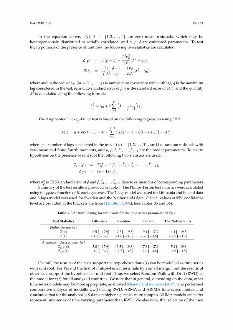
Summary of the test results is provided in Table 3. The Philips-Perron test statistics were calculatedusing the pp.test function ofR package tseries. The 2-lags model was used for Lithuania and Poland dataand 3-lags model was used for Sweden and the Netherlands data. Critical values at 95% confidencelevel are provided in the brackets are from Hamilton (1994), (see Tables B5 and B6).

Table 3. Statistical testing for unit-roots for the time series parameter of κ(t).

Test Statistics Lithuania Sweden Poland The Netherlands

Philips-Perron testZ(ρ) −6.5 [−17.9] −2.7 [−19.8] −19.1 [−17.9] −4.1 [−19.8]Z(t) −1.7 [−3.6] −1.6 [−3.5] −3.6 [−3.6] −2.2 [−3.5]

Augmented Dickey-Fuller testZDF(ρ) −5.8 [−17.9] −3.5 [−19.8] −17.8 [−17.9] −5.4 [−19.8]ZDF(t) −1.1 [−3.6] −2.7 [−3.5] −2.3 [−3.6] −1.9 [−3.5]

Overall, the results of the tests support the hypotheses that κ(t) can be modelled as time serieswith unit root. For Poland the first of Philips-Perron tests fails by a small margin, but the results ofother tests support the hypothesis of unit root. Thus we select Random Walk with Drift (RWD) asthe model for κ(t) for all analyzed countries. We note that in general, depending on the data, othertime series models may be more appropriate, as showed Kleinov and Richards (2017) who performedcomparative analysis of modelling κ(t) using RWD, ARMA and ARIMA time series models andconcluded that for the analyzed UK data on higher age males more complex ARIMA models can betterrepresent time series of time varying parameter than RWD. We also note, that selection of the time

Risks 2019, 7, 58 16 of 24

series model might have major implications on the width of the confidence intervals of projected κ(t)and, subsequently, calculated VaR. The estimated parameters of time series models (5) for κ(t) areprovided in Table 4.

Table 4. Estimated Random Walk with Drift (RWD) parameters of time series κ(t) derived from there-fitted Poisson regression.

Parameter Lithuania Sweden Poland The Netherlands

µ −1.25 −0.79 −1.05 −0.63σ2 6.62 0.65 1.14 0.78

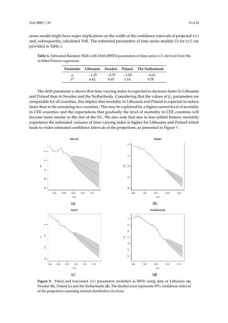
The drift parameter µ shows that time varying index is expected to decrease faster in Lithuaniaand Poland than in Sweden and the Netherlands. Considering that the values of βx parameters arecomparable for all countries, this implies that mortality in Lithuania and Poland is expected to reducefaster than in the remaining two countries. This may be explained by a higher current level of mortalityin CEE countries and the expectations that gradually the level of mortality in CEE countries willbecome more similar to the rest of the EU. We also note that due to less settled historic mortalityexperience the estimated variance of time varying index is higher for Lithuania and Poland whichleads to wider estimated confidence intervals of the projections, as presented in Figure 9.

(a) (b)

(c) (d)

Figure 9. Fitted and forecasted κ(t) parameters modelled as RWD using data of Lithuania (a),Sweden (b), Poland (c) and the Netherlands (d). The shaded error represents 95% confidence intervalof the projections assuming normal distribution of errors.

Risks 2019, 7, 58 17 of 24

5. Methodology of VaR Calculations

5.1. Run-off VaR Methodology

We used the following formula for calculation of run-off VaR:

VaR0.005

( n

∑i=1

CFt+i

)= inf

{l ∈ R : P

( n

∑i=1

CFt+i − BEt > l)6 0.995

}. (6)

The formula implies that run-off VaR is simply the quantile of the distribution of the deviation ofthe sum of total estimated losses till maturity in n years minus the Best Estimate at the end of yeart which is calculated as the expected value of future mortality cash flows derived using the centralprojection of the mortality probabilities

BEt = E( n

∑i=1

CFt+i

).

The distribution of future cash flows is assessed by performing for each projection year 104

simulations of random errors ε distributed according Normal law N(0, σ2) with standard errorestimated in fitting RWD model for κ(t). The simulations are used to derive the simulated paths of theLee-Carter model parameter κ(t) for time moments t + 1, t + 2, . . . , t + n. Keeping the parameters αx

and βx be fixed we derive the simulated mortality probabilities, which are converted to cash flowsusing the formulas described in Section 5.3.

5.2. One-Year VaR Methodology

In deriving one-year VaR we use the basic Solvency II principle, which requires calibration ofSCR to VaR of the (loss of) Basic Own Funds subject to a confidence level of 99.5% over a one-yearperiod. Basic Own Fund BOFt at the end of year t, is defined as the difference between insurer’s assetsAt and liabilities Lt, valued according to the Solvency II requirements, plus subordinated liabilities,which we will ignore in our analysis as a simplification. Liabilities Lt may be disaggregated intotechnical provisions, consisting of Best Estimate BEt and Risk Margin RMt, and other liabilities OLt.Therefore we suppose that

BOFt = At − BEt − RMt −OLt

for each year t.In practice, there are many factors which could contribute to the change in the Basic Own Funds

over the year. Considering that our focus is on the mortality risk, the analysis was performed fora simplified portfolio of a single premium (payable in advance) fixed term life assurance policies.We assumed that there are no lapses, no expenses, no new business, no changes in other liabilities andthat claims are paid immediately after they occur. We also assumed that there are no cash flows to orfrom a shareholder, such as dividends, capital injections, and that the investment return on assets andthe discount rate used for calculation of technical provisions both are zero. Depending in the size ofa discount rate, discounting would have a similar effect as a reduction of benefits with time, that is,based on the results presented in Section 2 would generally reduce VaR. Finally, we assumed that RiskMargin is also fixed. In practice, changes in Best Estimate and Risk Margin are likely to be positivelydependent and Risk Margin is likely to affect VaR. However, we have accepted this simplification,considering that due to its relative size, Risk Margin is likely to have significantly smaller effect onVaR than the Best Estimate.

Risks 2019, 7, 58 18 of 24

Under the above assumptions a change in assets during year t+ 1 is caused only by a cash outflowCFt+1 due to payment of death claims. Therefore, the random variable of a change in Basic Own Fundsduring the year t + 1 can be expressed as follows:

∆BOFt+1 = At+1 − At − (BEt+1 − BEt) = BEt − CFt+1 − BEt+1. (7)

Best Estimate for valuation date at the end of the year t + 1, assessed using the information Ft

available at the end of year t is

E(

BEt+1 |Ft))=

n

∑i=2

E(CFt+i | Ft

).

Inserting this into Equation (7), and assuming that we assess ∆BOFt+1 using information availableat the end of year t we obtain the following expression

∆BOFt+1 = BEt −(

CFt+1 +E(

BEt+1 | Ft))

. (8)

Thus, random variable of the change in the Basic Own Funds during the next valuation year isequal to the difference between the initial Best Estimate and the sum random variables of the claimscash flow during the year t + 1 and the Best Estimate at the end of year t + 1.

Substituting the result (8) into Formula (1), we get the VaR formula for the loss of the BasicOwn Funds over one year (one-year VaR), with the confidence level of 99.5%, as assessed using theinformation available at time t:

VAR0.005(∆BOFt+1

)= inf

{l ∈ R : P

(BEt −

(CFt+1 +E

(BEt+1 | Ft

))> l)6 0.995

}. (9)

Thus, SCR is the capital required to cover the excess of the total of claims payments during thefirst projection year and the Best Estimate at the end of the first projection year over the initial BestEstimate with 99.5% probability. We note that random variables CFt+1 and E

(BEt+1 | Ft

)are not

independent. Actuaries usually reconsider the assumptions used to calculate Best Estimate basedon the recent actual mortality experience. For example, significantly higher than expected incurredmortality losses are likely to lead to upwards revision of the Best Estimate mortality assumptions.Therefore, we can presume positive dependence between CFt+1 and E

(BEt+1 | Ft

)and our modelling

challenge is to estimate conditional expectation

E( n

∑i=2

CFt+i |CFt+1

).

There are several ideas how to model this relationship. For example, Richards et al. (2013) foreach simulation run added the simulated mortality experience in year t + 1 to the already availablehistoric data and used the total data set to refit the stochastic mortality model, which enabled toquantify variation in mortality trend parameter. Similarly, Börger et al. (2014) used simulated mortalityexperience for each stochastic run to re-estimate the mortality trend parameter at t + 1. We applieda similar approach, and for each run used simulated time varying index κ(t + 1) of the Lee-Cartermodel to adjust the RWD drift parameter:

µ(t + 1) = µ + δ(κ(t + 1)− κ(t)− µ

),

where δ is chosen credibility factor and µ, κ(t) are parameters estimated during the initial Lee-Cartermodel fitting (see Section 4.4).

Our approach requires setting explicit credibility factor δ, which is avoided in the methodsmentioned above. However, the above methods also rely on certain additional model parameters

Risks 2019, 7, 58 19 of 24

which control the level of trend risk produced by the simulation. Börger et al. (2014) for the purpose ofintroducing variability in the slope of the linear trend, re-estimates with weighted least squares thetrend using a new stochastic realisation of mortality trend parameter. In this model trend sensitivity isdependent on the choice of the length of the fitting period and the weights used. Similarly, using theapproach of Richards et al. (2013), if applied together with Lee-Carter model, trend sensitivity woulddepend on the selected length of the fitting period. For the purpose of our analysis considering thatfitting periods for CEE and non CEE countries differ, we found it more convenient to set an explicitparameter controlling the level of trend risk.

Using the above we firstly take 104 simulations of Lee-Carter parameter κ(t + 1) generated inrun-off VaR calculations. They are used to calculate a vector of simulated trend parameters µ(t + 1)which, together with κ(t + 1) which set the level of forecasted mortality, and are used to derive thecurves of forecasted time varying index starting from year t + 2.

The simulated mortality probabilities are derived as for run-off VaR, except for the allowance forthe additional volatility from the mean, as noted in Section 4.2.

5.3. Modelling Different Mortality Benefit Formulas

5.3.1. Level Benefits

Since we assume that there is no discounting, lapses, future premiums and the death benefitdoes not change during the policy term, we can ignore the timing of death benefits during the periodcovered by an insurance policy. Therefore, for a policy with sum assured of 1 monetary unit we cancalculate the sum of expected cash outflows (death benefits) as the estimated mortality probabilityover the remaining policy term n:

n

∑i=1

CFt+i = nqx(t),

where nqx(t) is n year death probability assuming that a life aged x is alive at the end of year t,and which can be calculated using the following formulas:

nqx(t) = 1− n px(t),

n px(t) =n−1

∏s=0

px+s(t + s) =n−1

∏s=0

(1− qx+s(t + s)

).

In case of run-off VaR, inserting this into Formula (6) and noting the Best Estimate of termassurance policy with level benefits as BE(L)

t , we get that

Var(L)0.005

( n

∑i=1

CFt+i

)= inf

{l ∈ R : P

(BE(L)

t − nqx(t) > l)6 0.995

}.

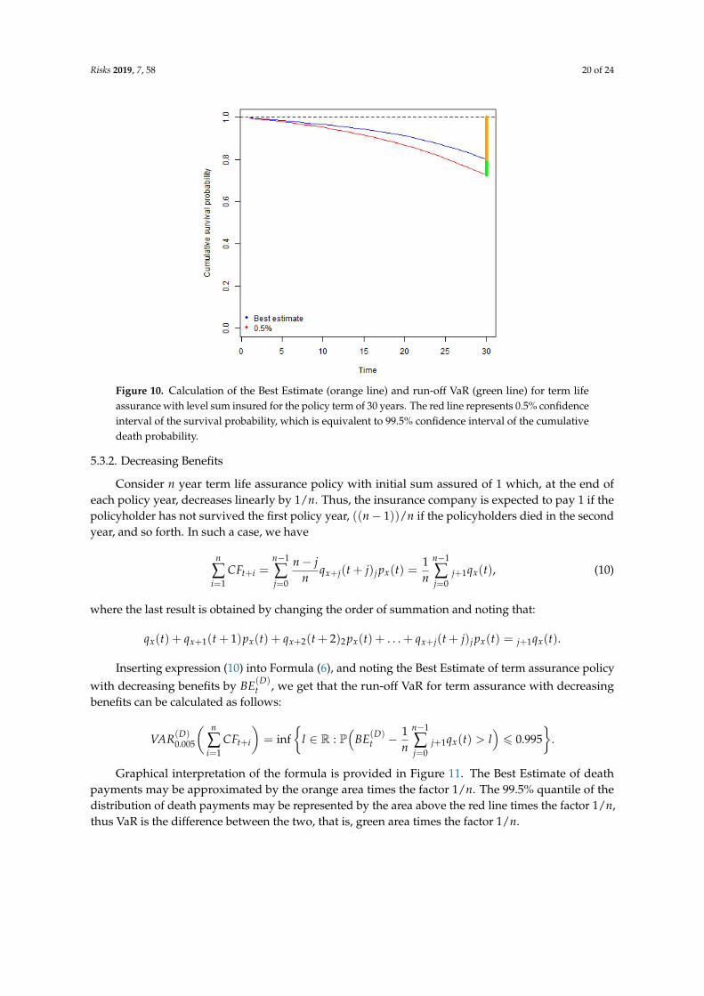
Graphical interpretation of the formula is provided in Figure 10. The Best Estimate of the deathpayout is equal to the expected death probability over the total policy term (represented by the orangeline). Run-off VaR (green line) is the difference between 99.5% quantile of the distribution of the deathprobability over the total policy term minus the Best Estimate.

In case of one-year VaR, in addition to the first year’s death benefits we calculate the projectedbenefits starting from year t + 2, multiplied by the probability of survival in the first year. Inserting toFormula (9), one-year VaR for term life assurance with level benefits can be calculated as follows:

VAR(L)0.005

(∆BOFt+1

)= inf

{l ∈ R : P

(BE(L)

t − qx(t)− px(t)E(

n−1qx+1(t + 1) | Ft)> l)6 0.995

}.

Risks 2019, 7, 58 20 of 24

Figure 10. Calculation of the Best Estimate (orange line) and run-off VaR (green line) for term lifeassurance with level sum insured for the policy term of 30 years. The red line represents 0.5% confidenceinterval of the survival probability, which is equivalent to 99.5% confidence interval of the cumulativedeath probability.

5.3.2. Decreasing Benefits

Consider n year term life assurance policy with initial sum assured of 1 which, at the end ofeach policy year, decreases linearly by 1/n. Thus, the insurance company is expected to pay 1 if thepolicyholder has not survived the first policy year, ((n− 1))/n if the policyholders died in the secondyear, and so forth. In such a case, we have

n

∑i=1

CFt+i =n−1

∑j=0

n− jn

qx+j(t + j)j px(t) =1n

n−1

∑j=0

j+1qx(t), (10)

where the last result is obtained by changing the order of summation and noting that:

qx(t) + qx+1(t + 1)px(t) + qx+2(t + 2)2 px(t) + . . . + qx+j(t + j)j px(t) = j+1qx(t).

Inserting expression (10) into Formula (6), and noting the Best Estimate of term assurance policywith decreasing benefits by BE(D)

t , we get that the run-off VaR for term assurance with decreasingbenefits can be calculated as follows:

VAR(D)0.005

( n

∑i=1

CFt+i

)= inf

{l ∈ R : P

(BE(D)

t − 1n

n−1

∑j=0

j+1qx(t) > l)6 0.995

}.

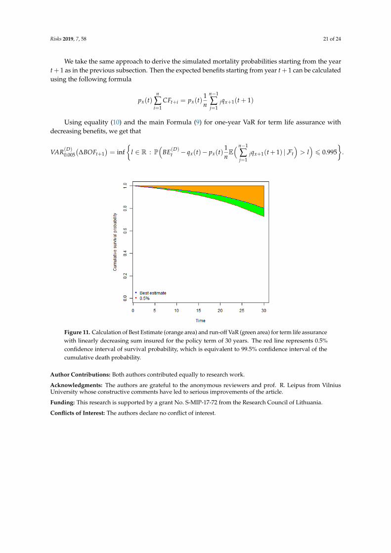
Graphical interpretation of the formula is provided in Figure 11. The Best Estimate of deathpayments may be approximated by the orange area times the factor 1/n. The 99.5% quantile of thedistribution of death payments may be represented by the area above the red line times the factor 1/n,thus VaR is the difference between the two, that is, green area times the factor 1/n.

Risks 2019, 7, 58 21 of 24

We take the same approach to derive the simulated mortality probabilities starting from the yeart+ 1 as in the previous subsection. Then the expected benefits starting from year t+ 1 can be calculatedusing the following formula

px(t)n

∑i=1

CFt+i = px(t)1n

n−1

∑j=1

jqx+1(t + 1)

Using equality (10) and the main Formula (9) for one-year VaR for term life assurance withdecreasing benefits, we get that

VAR(D)0.005

(∆BOFt+1

)= inf

{l ∈ R : P

(BE(D)

t − qx(t)− px(t)1nE( n−1

∑j=1

jqx+1(t+ 1) | Ft

)> l)6 0.995

}.

Figure 11. Calculation of Best Estimate (orange area) and run-off VaR (green area) for term life assurancewith linearly decreasing sum insured for the policy term of 30 years. The red line represents 0.5%confidence interval of survival probability, which is equivalent to 99.5% confidence interval of thecumulative death probability.

Author Contributions: Both authors contributed equally to research work.

Acknowledgments: The authors are grateful to the anonymous reviewers and prof. R. Leipus from VilniusUniversity whose constructive comments have led to serious improvements of the article.

Funding: This research is supported by a grant No. S-MIP-17-72 from the Research Council of Lithuania.

Conflicts of Interest: The authors declare no conflict of interest.

Risks 2019, 7, 58 22 of 24

Appendix A

(a) (b)

(c) (d)

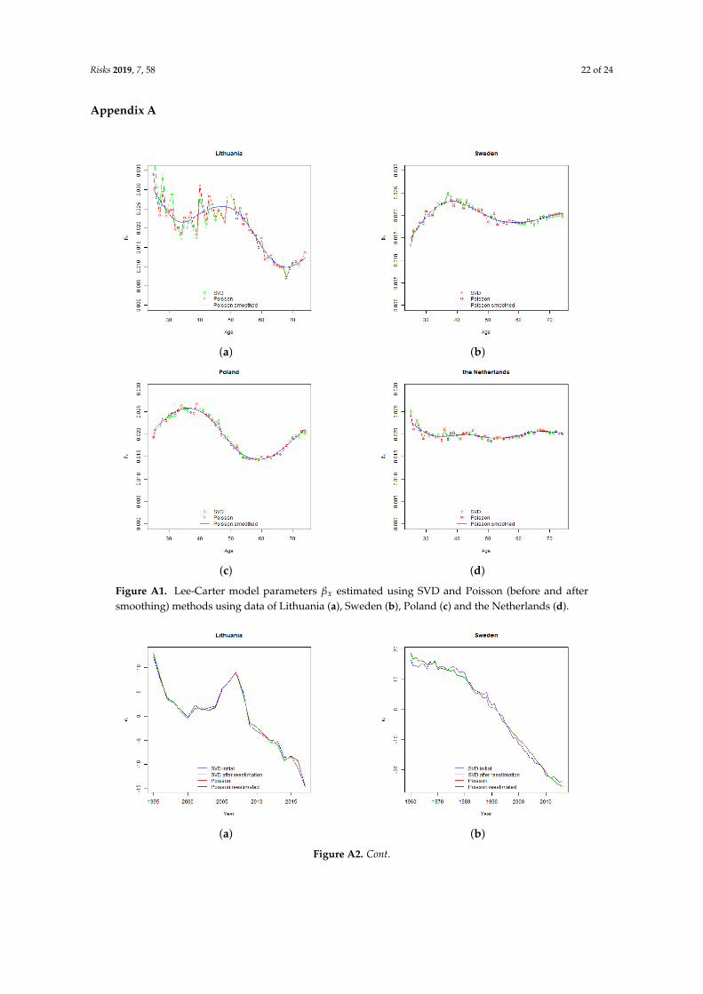
Figure A1. Lee-Carter model parameters βx estimated using SVD and Poisson (before and aftersmoothing) methods using data of Lithuania (a), Sweden (b), Poland (c) and the Netherlands (d).

(a) (b)

Figure A2. Cont.

Risks 2019, 7, 58 23 of 24

(c) (d)

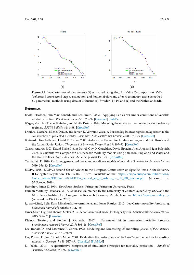
Figure A2. Lee-Carter model parameters κ(t) estimated using Singular Value Decomposition (SVD)(before and after second step re-estimation) and Poisson (before and after re-estimation using smoothedβx parameters) methods using data of Lithuania (a), Sweden (b), Poland (c) and the Netherlands (d).

References

Booth, Heather, John Maindonald, and Len Smith. 2002. Applying Lee-Carter under conditions of variablemortality decline. Population Studies 56: 325–36. [CrossRef] [PubMed]

Börger, Matthias, Daniel Fleischer, and Nikita Kuksin. 2014. Modeling the mortality trend under modern solvencyregimes. ASTIN Bulletin 44: 1–38. [CrossRef]

Brouhns, Natacha, Michel Denuit, and Jeroen K. Vermunt. 2002. A Poisson log-bilinear regression approach to theconstruction of projected lifetables. Insurance: Mathematics and Economics 31: 373–93. [CrossRef]

Brainerd, Elizabbeth, and David M. Cutler. 2005. Autopsy on the empire: Understanding mortality in Russia andthe former Soviet Union. The Journal of Economic Perspectives 19: 107–30. [CrossRef]

Cairns, Andrew J. G., David Blake, Kevin Dowd, Guy D. Coughlan, David Epstein, Alen Ang, and Igor Balevich.2009. A Quantitative Comparison of stochastic mortality models using data from England and Wales andthe United States. North American Actuarial Journal 13: 1–35. [CrossRef]

Currie, Iain D. 2016. On fitting generalized linear and non-linear models of mortality. Scandinavian Actuarial Journal2016: 356–83. [CrossRef]

EIOPA. 2018. EIOPA’s Second Set of Advice to the European Commission on Specific Items in the SolvencyII Delegated Regulation. EIOPA-BoS-18/075. Available online: https://eiopa.europa.eu/Publications/Consultations/EIOPA-18-075-EIOPA_Second_set_of_Advice_on_SII_DR_Review.pdf (accessed on30 October 2018).

Hamilton, James D. 1994. Time Series Analysis. Princeton: Princeton University Press.Human Mortality Database. 2018. Database Maintained by the University of California, Berkeley, USA, and the

Max Planck Institute for Demographic Research, Germany. Available online: https://www.mortality.org(accessed on 15 October 2018).

Ignataviciute, Egle, Rasa Mikalauskaite-Arminiene, and Jonas Šiaulys. 2012. Lee-Carter mortality forecasting.Lithuanian Journal of Statistics 51: 22–35.

Jarner, Søren Fiig, and Thomas Møller. 2015. A partial internal model for longevity risk. Scandinavian Actuarial Journal2015: 352–82. [CrossRef]

Kleinov, Torsten, and Stephen J. Richards. 2017. Parameter risk in time-series mortality forecasts.Scandinavian Actuarial Journal 2017: 804–28. [CrossRef]

Lee, Ronald D., and Lawrence R. Carter. 1992. Modeling and forecasting US mortality. Journal of the AmericanStatistical Association 87: 659–71.

Lee, Ronald D., and Timothy Miller. 2001. Evaluating the performance of the Lee-Carter method for forecastingmortality. Demography 38: 537–49. [CrossRef] [PubMed]

Li, Jackie. 2014. A quantitative comparison of simulation strategies for mortality projection. Annals ofActuarial Sciences 8: 281–97. [CrossRef]

Risks 2019, 7, 58 24 of 24

Li, Johny Siu-Hang, Mary R. Hardy, and Ken Seng Tan. 2009. Uncertainty in mortality forecasting: An extensionto the classical Lee-Carter approach. ASTIN Bulletin 39: 137–64. [CrossRef]

McCullag, Peter, and John A. Nelder. 1989. Generalized Linear Models, 2nd ed. London: Chapman & Hall.Mcneil, Alexander J., Rüdiger Frey, and Paul Embrechts. 2005. Quantitative Risk Management: Concepts, Techniques

and Tools. Princeton: Princeton University Press.Olivieri, Annamaria, and Ermanno Pitacco. 2009. Stochastic mortality: The impact on target capital. ASTIN Bulletin

39: 541–63. [CrossRef]Plat, Richard. 2011. One-year Value-at-Risk for longevity and mortality. Insurance: Mathematics and Economics 49:

462–70. [CrossRef]Renshaw, Arthur E., and Steven Haberman. 2003. Lee-Carter mortality forecasting with age-specific enhancement.

Insurance: Mathematics and Economics 33: 255–72. [CrossRef]Renshaw, Arthur E., and Steven Haberman. 2008. On simulation-based approaches to risk measurement in

mortality with specific reference to Poisson Lee-Carter modelling. Insurance: Mathematics and Economics 42:797–816. [CrossRef]

Richards, Stephen J., Ian D. Currie, and Gavin P. Ritchie. 2013. A Value-at-Risk framework for longevity trendrisk. British Actuarial Journal 19: 116–39. [CrossRef]

Tuljapulkar, Shripad, Nan Li, and Carl Boe. 2000. A universal pattern of mortality decline in the G7 countries.Nature 405: 789–92. [CrossRef] [PubMed]

c© 2019 by the authors. Licensee MDPI, Basel, Switzerland. This article is an open accessarticle distributed under the terms and conditions of the Creative Commons Attribution(CC BY) license (http://creativecommons.org/licenses/by/4.0/).