portfolio optimization under solvency constraints: a dynamical approach

PORTFOLIO OPTIMIZATION UNDER SOLVENCY CONSTRAINTS: A DYNAMICAL APPROACH

Sujith Asanga1

Alexandru V. Asimit2

Alexandru M. Badescu3

Steven Haberman4

Abstract

We propose portfolio optimization problems for non-life insurance companies for finding the

minimum capital required, which simultaneously satisfy solvency and portfolio performance

constraints. Motivated by standard insurance regulations, we consider solvency capital re-

quirements based on three criteria: Ruin Probability (RP ), Conditional Value at Risk (CV aR)

and Expected Policyholder Deficit (EPD) ratio. We introduce a novel semiparametric for-

mulation for each problem and we explore the advantages of implementing this methodology

over other potential approaches. Using different expected Return on Capital (ROC) target

levels, we construct efficient frontiers when portfolio assets are modelled with multivariate

GARCH models and losses are assumed to have a Lognormal distribution. The out-of-sample

performance of our methods is empirically tested for both, the solvency requirement and the

portfolio performance, through an extensive double rolling window estimation exercise.

Keywords and phrases: Optimal allocation; solvency constraint; ruin probability; Value at

Risk; Conditional Value at Risk; Expected Policyholder Deficit; Return on Capital; rolling

window; Sharpe ratio; multivariate GARCH models.

1Department of Mathematics and Statistics, University of Calgary, Calgary, Alberta T2N 1N4, Canada.

E-mail: [email protected] Business School, City University, London EC1Y 8TZ, United Kingdom. E-mail: [email protected] author: Department of Mathematics and Statistics, University of Calgary, Calgary, Alberta T2N 1N4,

Canada. E-mail: [email protected]. Phone: 1-403-2203963.4Cass Business School, City University, London EC1Y 8TZ, United Kingdom. E-mail: [email protected].

1

1 Introduction

The rest of the paper is organized as follows. In the next section, we introduce the optimization problems

based on the solvency and expected ROC constraints and we illustrate the semiparametric approach for

solving them. Models for both assets and liabilities and discussions on the convexity of the proposed

methods are provided in Section 3. An extensive empirical analysis is performed in Section 4. We

conclude the paper in Section 5.

2 Preliminaries and solvency constrained optimization

We consider a discrete-time framework with the set of trading dates indexed by T = {0, 1, . . . , T}. The

market consists of a portfolio of n assets with the gross return5 process over the period [t, t+1] defined by

Rt+1 = (R1,t+1, . . . , Rn,t+1)T . We denote by Ft, the historical information on the asset return evolution

up to time t, so that Ft = σ(R1, . . . ,Rt). For convenience, we use the following notations for conditional

probabilities, expectations and variances: Pr(·|Ft) = Prt(·), E[·|Ft] = Et[·] and V ar[·|Ft] = V art[·].

Moreover, we use majuscules for random variables (except for cases when un upper script associated to a

random variable may be interpreted as a realization of that r.v.) and non-capital letters for deterministic

quantities.

In this section we introduce three optimization problems based on different solvency criteria for a non-

life insurance company within a one-period setting, [t, t + τ ], where τ is the solvency horizon satisfying

τ ≤ T − t. First, we denote by pt the aggregate premium available for investment at time t. In addition,

we assume that shareholders provide a regulatory initial capital of size ct. Without the loss of generality,

no other premiums are collected and no capital is issued or retired between t and t + τ , so the total

invested amount is pt + ct. Let xt = (x1,t, . . . , xn,t)T be the portfolio weights whose components satisfy

the standard budget constraint,n∑i=1

xi,t = 1 and the no short sales constraint, xi,t ≥ 0, i = 1, . . . , n. Since

our problem is designed as a single-period optimization, no rebalancing is allowed during the solvency

period.

5The gross return process is defined here as the ratio between the terminal and initial asset prices, and thus is non-

negative.

2

To fully describe the setup we let the insurer’s liability be modelled by a univariate random variable

Yt+τ . This represents the aggregate claim amount incurred over the solvency horizon which is assumed to

be paid at time t+ τ . At this point, no particular assumptions regarding the conditional distributions of

Rt+τ and Yt+τ , are made and no premium calculation principle is assigned for pt. We define the insurer’s

net loss as the difference between the liability and the portfolio value over the solvency horizon:

Lt,t+τ = Yt+τ − (pt + ct)RTt+τxt. (2.1)

Since both the capital requirement and the portfolio allocations are decision variables in our joint opti-

mization problems, we can view the net loss r.v. as a function of these quantities (i.e. Lt,t+τ := L(ct,xt)).

For convenience, we assume there are no other sources of risk other than the ones modelled through Y

and R, and there are no transaction or other friction costs.

Each optimization problem proposed in the following subsections is characterized by the same objective

function and it is based on minimizing the capital requirement ct, subject to two key constraints. The

first constraint consists of the solvency capital requirement imposed by insurance regulators, and it is

based on one of the following criteria: Ruin Probability (RP ), Conditional Value-at-Risk (CV aR) and

Expected Policyholder Deficit (EPD). Next, we define the gross Return on Capital (ROC) over the

investment period:

ROCt,t+τ = −Lt,t+τct

. (2.2)

Since shareholders typically require a rate of return on the capital provided, the second constraint is

introduced as a portfolio performance measure based on a target level for shareholder’s expected return.

For each type of solvency, we provide a novel a semiparametric approach which allows us to reformulate

the constraints and to further implement the optimization without costly computational effort.

2.1 Optimization with Ruin Probability (RP ) constraint

The use of the ruin probability constraint is motivated by the Solvency II concept for EU based insurance

companies, and consist of identifying the capital required to maintain a target level for the ruin probability

3

over a specified period of time. Thus, we define the RP -constrained problem as follows:

minct,xt

ct

s.t. Et[1{Lt,t+τ>0}

]≤ 1− α,

Et[ROCt,t+τ

]≥ ROCα,

1Txt = 1, xt ≥ 0, ct ≥ 0.

(2.3)

Here, α represents the specified solvency level, 1{·} is the indicator function and ROCα is the lower bound

for the shareholders’ expected return on capital, which also depends α. We notice that the solvency chance

constraint in (2.3) can be reformulate as a Value-at-Risk constraint, where the V aR of a loss random

variable Z at a confidence level α is defined by:

V aRα(Z) := inf{z ∈ < : Pr(Z ≤ z) ≥ α},

Indeed, it follows immediately that:

Et[1{Lt,t+τ >0}

]≤ 1− α⇔ Prt

(Lt,t+τ > 0

)≤ 1− α⇔ V aRαt (Lt,t+τ ) ≤ 0,

where V aRαt is the value at risk conditional on the historical asset return evolution up to time t. The

main difficulty in dealing with this type of problems is the convexity of the chance constraint. Closed

form expressions for the ruin probability only exist in very few special cases. For example, if we assume

that Lt,t+τ has a multivariate Gaussian distribution, then (2.3) can be re-written as a Second Order

Cone optimization, which can be efficiently implemented with appropriate solvers. Asimit et al. (2012)

found a closed form expression for such a problem in the absence of the short-sales and ROC constraints.

However, when Yt+τ and Rt+τ do not belong to the same family of distributions, we may not be able to

even identify the distribution of Lt,t+τ .

A standard approach in the chance constrained programming literature is to use a fully non-parametric

method for approximating the conditional expectation in (2.3). This can be done using a Monte-Carlo

estimator by generating scenarios for both assets and liabilities. The solvency condition can be thus

reformulated as:

1

m

m∑j=1

1{Yt+τ (j)−(pt+ct)RTt+τ

(j)xt>0} ≤ 1− α.

Here, m is the number of Monte-Carlo simulations and Yt+τ (j) and Rt+τ (j) represent the jth generated

path for liabilities and assets conditional on Ft. Due to the presence of the indicator function, the

4

optimization problem is still non-convex. As already mentioned in the introduction, several approaches

such as convex approximations or non-convex Mixed Integer Programming (MIP) representations have

been recently proposed in the literature to handle the non-parametric constraint. In general, their

implementation becomes less efficient when m is large, which is generally required for a better accuracy

of the Monte-Carlo estimator. Another alternative is to find optimal values for m in order to obtain an

equivalent chance constraint based on a different confidence level (which also has to be found); however,

this depends on the data used and requires a calibration procedure. In order to avoid such issues, we use

a conditional version of the semiparametric approach proposed in Asimit et al. (2012). This methodology

is based on a pre-specified parametric conditional liability distribution and scenario-based asset returns.

Using the notation, E[· |Ft

⋃{Rt+τ = Rt+τ (j)}

]= E

(j)t

[·], and using the double expectation rule, we

reformulate the initial problem:

minct,xt

ct

s.t. 1m

m∑j=1

E(j)t

[1{Yt+τ−(pt+ct)RT

t+τ(j)xt>0}

]≤ 1− α,

Et[ROCt,t+τ

]≥ ROCα,

1Txt = 1, xt ≥ 0, ct ≥ 0.

(2.4)

The expectation in the solvency constraint is taken with respect to the r.v. Y . A sufficient condition

for (2.4) to be a convex problem is that E(j)t

[1{Yt+τ−(pt+ct)RT

t+τ(j)xt>0}

]is convex in (ct, xt), for any

j = 1, . . . ,m. This is equivalent to having a conditionally convex survival function for the liability Yt+τ .

Most of the survival functions used for modelling claim data posses this property (some not on their

entire domain) and all our empirical results in Section 4 will be based on such a distribution.

2.2 Optimization with Conditional Value at Risk (CV aR) constraint

The CV aR was introduced by Rockafellar and Uryasev (2000) as an alternative coherent risk measure to

V aR, which quantifies the loss severity in the case of default. For general random variables, the CV aR

is defined as a weighted average of the corresponding V aR and conditional expected losses which strictly

exceed V aR. When losses have a continuous distribution function, CV aR coincides with the Expected

Shortfall (ES) or Tail Value-at-Risk (TV aR), which constitute the basis for quantifying the target capital

according to the Swiss Solvency Test (EIOPA, 2011).

5

Following a similar approach as in the V aR-constrained case, we define the following optimization

problem with a CV aR solvency constraint:

minct,xt

ct

s.t. CV aRβt(Lt,t+τ

)≤ 0,

Et[ROCt,t+τ

]≥ ROCβ ,

1Txt = 1, xt ≥ 0, ct ≥ 0.

(2.5)

Here, β is the confidence level for CV aR and ROCβ is the associated lower bound for our performance

measure. CV aR is a more conservative measure of risk than V aR given the same confidence level. In

the empirical analysis in Section 4, we shall relate the confidence levels for each of the risk measures

by, β = 1 − 2(1 − α). This is also satisfied by the values used in the Solvency II and SST directives

(α = 99.5% and β = 99%).

There are various ways of formulating CV aR in the literature. The most appropriate representation

for our context is the one provided by Pflug (2000) and Rockafellar and Uryasev (2000), who define

CV aR as the solution of an optimization problem. For a general loss r.v. Z we have:

CV aRβ(Z) = infs∈<

{s+

1

1− βE[(Z − s)+

]}, (2.6)

where (Z − s)+ = max(Z − s, 0). Using the above definition, the optimization (2.5) becomes:

mins,ct,xt

ct

s.t. s+ 11−βEt

[(Lt,t+τ − s)+

]≤ 0,

Et[ROCt,t+τ

]≥ ROCβ ,

1Txt = 1, xt ≥ 0, ct ≥ 0.

(2.7)

There are different potential strategies for reformulating the solvency constraint. The traditional method

used in the literature is based on approximating the above conditional expectation with a Monte-Carlo

type estimator and transforming (2.7) into a Linear Programming (LP) problem. Indeed, under a fully

non-parametric prescription, the CV aR constraint can be re-written as:

s+1

m(1− β)

m∑j=1

(Yt+τ (j)− (pt + ct)R

Tt+τ (j)xt − s

)+≤ 0,

6

https://www.researchgate.net/publication/228609755_Optimization_of_Conditional_Value-At-Risk?el=1_x_8&enrichId=rgreq-3e06d84c-19aa-4510-be8f-d99e7138acfc&enrichSource=Y292ZXJQYWdlOzI1NjA1MDA5NjtBUzoxNjA0NDAwMjU4ODY3MjFAMTQxNTI2MzI5MTc4Mw==

which can be further reformulated as a system of linear inequalities by introducing m additional decision

variables (e.g. see Rockafellar and Uryasev (2000)). Despite the attractiveness of having the LP repre-

sentation, the implementation of (2.7) with standard solvers becomes less efficient when the number of

Monte-Carlo paths is large, since the dimension of the problem increases with m. Therefore, other al-

ternative convex approximations for the conditional expectation should be investigated to accommodate

such scenarios. For example, Alexander et al. (2006) use a continuously differentiable piecewise quadratic

approximation. As in the RP -constrained optimization case, we propose here a semiparametric approach

which reformulates (2.7) as:

mins,ct,xt

ct

s.t. s+ 1m(1−β)

m∑j=1

E(j)t

[(Yt+τ − (pt + ct)R

Tt+τ (j)xt − s)+

]≤ 0,

Et[ROCt,t+τ

]≥ ROCβ ,

1Txt = 1, xt ≥ 0, ct ≥ 0.

(2.8)

A sufficient condition which ensures the convexity of (2.8) is that E(j)t


Tt+τ (j)xt− s

)+

]is a convex function in s, ct and xt. This issue is discussed in Section 4, once the liability r.v. is fully

specified.

2.3 Optimization with Expected Policyholder Deficit (EPD) constraint

The Expected Policyholder Deficit (EPD) concept was introduced by Bustic (1994) as an alternative

method to the ruin probability for measuring insolvency risk, and it constitutes a useful tool in establishing

the US Risk Based Capital system. EPD is defined as the expected loss in the event of insolvency, and

thus it is similar to the ES concept (e.g. see Cummins and Phillips (2009) for a detailed discussion).

Translating this definition into our setting, we write:

EPD(Lt,t+τ ) = Et[(Yt+τ − (pt + ct)R

Tt+τxt)+

]. (2.9)

The solvency constraint based on this measure can be constructed by imposing a maximum allowance

level for EPD. However, since an a priori choice of such a threshold is not straightforward and it depends

on the insurer expected liability, we introduce a solvency criteria based on a target level of a deficit ratio.

7

https://www.researchgate.net/publication/228609755_Optimization_of_Conditional_Value-At-Risk?el=1_x_8&enrichId=rgreq-3e06d84c-19aa-4510-be8f-d99e7138acfc&enrichSource=Y292ZXJQYWdlOzI1NjA1MDA5NjtBUzoxNjA0NDAwMjU4ODY3MjFAMTQxNTI2MzI5MTc4Mw==

Consequently, the EPD constraint is defined as:

EPD(Lt,t+τ

)Et[Yt+τ

] ≤ f.

Here, f is the maximum level for the EPD ratio with 0 ≤ f < 1. Since (2.9) contains a similar expectation

term as in the CV aR definition, the whole discussion on dealing with CV aR-constrained problems applies

here as well. For consistency, we only give the semiparametric representation for our EPD-constrained

optimization problem:

minct,xt

ct

s.t. 1m

m∑j=1

E(j)t


Tt+τ (j)xt)+

]≤ fEt

[Yt+τ

],

Et[ROCt,t+τ

]≥ ROCf ,

1Txt = 1, xt ≥ 0, ct ≥ 0.

(2.10)

The convexity of the solvency constraint in (2.10) will be discussed in the same manner as in the CV aR

case.

3 Modelling assets and liabilities

Multivariate GARCH (MV-GARCH) processes are probably the most popular tools for modelling the

variances and covariances of different assets in discrete time. Depending of the conditional covariance

matrix structure, a large number of MV-GARCH models have been proposed in the literature. For recent

surveys on MV-GARCH models we refer to Bauwens et al. (2006) and Silvennoinen and Terasvirta (2009).

In this paper we consider the class of Dynamic Conditional Correlation (DCC) GARCH models of Engle

(2002), for modelling the multivariate dynamic of the log-return process. Due to their relative simple

estimation procedure, the DCC framework is also convenient for large scale risk management problems.

We assume the vector of asset log-returns are observed at a higher frequency than solvency is observed.

In particular, we sample returns on a daily basis:

log Rt+1 = mt+1 + εt+1, εt+1|Ft ∼MVN(0, Ht+1). (3.1)

Here mt+1 is the n-dimensional Ft-measurable conditional mean log-return vector and εt+1 = (ε1,t, . . . , εn,t)T

has a conditionally multivariate Gaussian distribution with mean 0 and covariance matrix Ht+1.

8

One of the main features of the DCC structure is that it allows for separate dynamics for the individual

conditional variances and the time-varying conditional correlation matrix. In the following, we briefly

illustrate Engle’s (2002) formulation:

Ht+1 = D1/2t+1Σt+1D

1/2t+1, (3.2)

Dt+1 = diag(h1,t+1, . . . , hn,t+1), (3.3)

Σt+1 = diag(q−1/211,t+1, . . . , q

−1/2nn,t+1)Qt+1diag(q

−1/211,t+1, . . . , q

−1/2nn,t+1), (3.4)

Qt+1 = (1− θ1 − θ2)Q+ θ1utuTt + θ2Qt. (3.5)

Here, Dt+1 is the n × n diagonal matrix formed with the univariate conditional variances which are

assumed to follow a standard GARCH(1,1) process as below:

hi,t = ωi + αiε2t−1 + βihi,t−1, i = 1, . . . , n (3.6)

The time-varying conditional correlation matrix of Rt+1 is denoted by Σt+1 and its elements ρij,t+1 are

of the form ρij,t+1 = qij,t+1q−1/2ii,t+1q

−1/2jj,t+1, for any 1 ≤ i, j ≤ n. qij,t+1 are the elements of Qt+1 and are

assumed to follow another GARCH(1,1) dynamic given in (3.5). The process ut represents the n × 1

vector of devolatilized, but correlated, innovations (i.e. ui,t = h−1/2i,t εi,t ) and Q is the unconditional

covariance matrix of ut. We assume that all univariate GARCH parameters in (3.6) (ωi, αi and βi) and

the DCC parameters in (3.5) (θ1, θ2) satisfy the conditions required for covariance stationarity and the

positive definiteness of Ht+1, for any t.

In order to investigate the effect of the time-varying conditional correlations between the portfolio’s

assets, we shall also look at two other models, which can be viewed as particular cases of the DCC-

GARCH. The first one is the Conditional Constant Correlation (CCC) model of Bollerslev (1990) which

can be obtained by replacing the time-varying correlation matrix by a symmetric positive definite matrix

with constant elements (i.e. Σt = Σ). The second alternative analyzed assumes the assets are uncorre-

lated, and this is immediately obtained by letting Σt = In in (3.5), where In is the n×n identity matrix.

The estimation results are illustrated in the next section.

Historical data for modelling loss payments is commonly fitted using one-component parametric distri-

butions such as, Pareto, Lognormal, Gamma, Weibull etc., or more recently using composite distributions

9

(see for example Scollnik and Sun (2012) and the references therein for Pareto composite models). Since

the objective of the paper is not to investigate goodness-of-fit of different alternatives, we restrict our

attention only to a one parametric family. In particular, we consider that claims are modelled with a Log-

normal distribution. Since our semiparametric method requires the computations of various conditional

expectations given historical information on the asset evolutions, we further assume in our numerical

examples that Yt+τ is independent of the enlarged filtration Ft⋃σ(Rt+τ ), for any time t and a given

solvency horizon τ . Although this allows us for a more convenient implementation, the optimization

problems can be solved under more general dependence structures between assets and liabilities, as long

as the resulting constraints are convex. Therefore, we let:

Yt+τ ∼ LGN(µt+τ , σt+τ ). (3.7)

The model parameters are assumed to be time-dependent as they will be re-estimated using a dou-

ble rolling-window exercise. In the remainder of this section we discuss the convexity of the solvency

constraints under the lognormality assumption from (3.7).

First, we let zt = (pt + ct)xt in all three optimization problems (2.4), (2.8) and (2.10). With this

notational change, the new decision variables are ct and zt, and the budget constraint becomes 1T zt =

pt + ct with zt ≥ 0. Under the above assumption, the solvency constraint for the EPD problem can be

rewritten as:

1

m

m∑j=1

E[(Yt+τ −RT

t+τ (j)zt)+]≤ fE

[Yt+τ

].

A sufficient condition for convexity is that E[(Yt+τ −RT

t+τ (j)zt)+]

is convex for any j = 1, . . . ,m. We

notice that the quantity under the expectation represents the payoff of a European Call option written on

Yt+τ . Under the lognormality assumption of Yt+τ , we can write the above expectation as the present value

at maturity of a Black-Scholes Call price, erTBS(S,K, T, σ, r), with the following parameter matching:

S = 1, K = RTt+τ (j)zt, T = 1, σ = σt+τ , r = µt+τ +

σ2t+τ

2.

Thus, the solvency constraint can be reformulated as:

m∑j=1

ïeµt+τ+

σ2t+τ2 Φ

(− log RTt+τ (j)zt + µt+τ + σ2

t+τ

σt+τ

)−RT

t+τ (j)ztΦ(− log RT

t+τ (j)zt + µt+τ

σt+τ

)ò≤ b (3.8)

10

Here, b = fmeµt+τ+σ2t+τ2 and Φ(·) is the cumulative distribution function of a standard Gaussian random

variable. The convexity of (3.8) follows now from the convexity property of the European Call price with

respect to the strike price, which is itself an affine function of zt.

Using a similar prescription, we can show the convexity of the CV aR optimization problem (2.8)

based on the Black-Scholes formula. The only difference consists of having a different strike price K =

RTt+τ (j)zt + s, which is a linear function of the decision variables s and zt.

We now turn our attention to the RP problem (2.4). The solvency constraint is equivalent to:

1

m

m∑j=1

Φ(− log RT

t+τ (j)zt + µt+τ

σt+τ

)≤ 1− α. (3.9)

Since the standard Gaussian c.d.f. is convex only on its negative domain, a sufficient condition for

convexity is the following:

min1≤j≤m

RTt+τ (j)zt > eµt+τ . (3.10)

Thus, according to condition (3.10), convexity of (2.4) is satisfied when the terminal value of the total

assets investment in the worst case scenario is greater than the median of the liability distribution.

Although this requirement cannot be verified analytically as in the previous two cases, our extensive

numerical experiments from the next section indicate that (3.10), is never violated.

4 Empirical Analysis

In this section we investigate the empirical performance of three MV-GARCH models for all optimization

problem considered. We provide two main numerical experiments: first, for a specified solvency target,

we construct efficient frontiers for (2.4), (2.8) and (2.10) by varying the expected ROC; the out-of-sample

performance analysis is next carried out through a detailed double rolling window estimation exercise.

4.1 Data Description

We consider a 3-asset portfolio formed with two types of financial instruments: one ”risk-free” asset

represented by three month US T-Bills and two risky assets consisting of the NASDAQ and NYSE

Composite indices. Both index series were observed on a daily basis from January 3, 2005 to July 29,

11

2011 for a total of l = 1, 656 observations. Descriptive statistics for NASDAQ and NYSE log-returns

are provided in Table 4.1.1. We notice that there are not significant differences between the two series

Index Min Max Mean Std Skewness Kurtosis

NASDAQ -0.0959 0.1116 0.0001 0.0149 -0.1670 10.2725

NYSE -0.1023 0.1153 0.0001 0.0150 -0.3480 12.7329

Table 4.1.1: Descriptive statistics for NASDAQ and NYSE log-returns from January 3, 2005 - July 29,

2011 for a total of 1,656 observations.

in terms of the first two moments. However, the NYSE log-returns have a more pronounced negative

skewness and a higher kurtosis than the NASDAQ counterpart. The data set is divided into two samples:

Sample A consists of lA = 1, 259 daily observations for a 5-year period from January 3, 2005 through

December 32, 2009, and it is used for the in-sample estimation and analysis of the efficient frontiers.

Sample B, which covers the period from January 1, 2010 through July 29, 2011 with lB = 397 daily

points, is used for testing the out-of-sample performance in the rolling window exercise. The evolution

of both indices over the entire period is depicted in Figure 4.1. The most significant part of the financial

crisis period is included into Sample A. Figure 4.1 also indicates a strong correlation between the two

risky assets, with similar volatility clustering shapes.

For liabilities, we use a data set on property insurance losses provided by a Romanian insurance

company for the period same period used in the assets case. However, the main difference is that the

sampling frequency is different from the one used for assets. There are 79 observations representing

aggregate monthly claim amounts, which are divided into two samples according to a similar prescription

(i.e. Sample A′ consist of lA′ = 60 monthly observations and Sample B′ has lB′ = 19 data points which

are used for the out-of-sample comparison). The main characteristics of the entire sample are illustrated

in Table 4.1.2.

12

2005 2006 2007 2008 2009 2010 2011−0.1

−0.05

0

0.05

0.1

(a) NASDAQ

2005 2006 2007 2008 2009 2010 2011−0.12

−0.07

−0.02

0.03

0.08

(b) NYSE

Figure 4.1.1: Time series of log-returns for NASDAQ and NYSE over the period January 3, 2005 - July 29, 2011

for a total of 1656 observations.

13

Min Max Mean StDev Skewness Kurtosis

8.2465 2049.2119 603.2802 375.1311 1.2434 5.5068

Table 4.1.2: Descriptive statistics for monthly claim amounts from January 3, 2005 - July 29, 2011 for a

total of 79 observations (figures are in thousands €).

4.2 Estimation results

We first estimate the parameters for the asset returns. There are various ways one can specify the condi-

tional mean vector in the MV-GARCH log-return equation (3.1). For example, Stentoft and Rombouts

(2011) use a multivariate risk premium specification for mt when pricing options under a DCC-GARCH

model, while Hlouskova et al. (2009) consider an autoregressive structure for deriving multistep predic-

tions with applications in risk management. Since our objective is to analyze the conditional correlation

effect to the optimal capital and its allocation, we perform our estimation ignoring the mean effect.

The estimation procedure follows the two-stage Maximum Likelihood Estimator (MLE) algorithm

proposed by Engle and Sheppard (2001). In the first stage the univariate GARCH parameters are

estimated by replacing the conditional correlation matrix of Rk, Σk, with the identity matrix in the

log-likelihood function below:

logL = −1

2

l∑k=1

(log(|Hk|) + ε′kH

−1k εk

),

where l represents the number of observations in the dataset. Given the parameters estimated at the

first stage, the DCC and CCC parameters are estimated based on the correct log-likelihood specification

with Σk and Σ, respectively. Thus, at the second stage only θ1 and θ2 for DCC and ρ for CCC are

estimated. The results are reported in Table 4.2. According to all three selection criteria, the DCC

specification is preferred to the CCC one. The parameter estimates for the DCC-GARCH are in the

same range with the values obtained in other previous studies. Each univariate series is characterized by

a high degree of persistence (i.e. α1 + β1 = 0.988 for NASDAQ and α2 + β2 = 0.992 for NYSE). Similar

persistence can be observed in the conditional correlation dynamic since θ1 + θ2 = 0.984. The value

of ρ = 0.91 in the CCC case suggests a high degree of positive correlation over the period considered.

The implied univariate GARCH conditional variances and the conditional correlation between the two

14

Estimation Stage Model parameters Selection criteria

Index ωi αi βi

NASDAQ 2.0E-06 0.0736 0.9146

1 (5.06E-13) (1.35E-04) (1.40E-04)

NYSE 1.4E-06 0.0856 0.9061

(3.99E-13) (1.46E-04) (1.41E-04)

Covariance model

DCC θ1 θ2 logL AIC BIC

0.0432 0.9409 11,630 -23,245 -23,201

2 (5.58E-05) (9.28E-05)

CCC ρ logL AIC BIC

0.9061 11,574 -23,134 -23,096

(1.64E-05)

Table 4.2.1: Parameter estimates (with corresponding asymptotic variances reported the brackets) using log-

returns for NASDAQ and NYSE during January 3, 2005 - July 29, 2011 for a total of 1656 observations. AIC

and BIC are the Akaike and Bayesian Information Criteria.

assets are illustrated in Figure 4.2.1. We notice the conditional correlation implied by the DCC-GARCH

structure has a minimum value of around 0.7 ( reached at the beginning of 2007), while its maximum is

approximately 0.95 (reached at the beginning of 2009).

Next, we use the MLE to fit a Lognormal distribution on the monthly claim amounts for the same

period. The results are reported in Table 4.2.2. The Kolmogorov-Smirnov test indicates that a Lognormal

distribution cannot be rejected at 5% significance level.

µ σ Log L KStest

6.160460 0.829457 584.00 0.1297

(0.0087) (0.0044) (0.1279)

Table 4.2.2: Parameter estimates (with corresponding asymptotic variances reported the brackets) for Lognormal

distribution using monthly claim amounts for property insurance during January 3, 2005 - July 29, 2011 for a

total of 79 observations. KStest is the Kolmogorov-Smirnov test and the p-value is reported in the bracket.

4.3 Implementation of solvency constrained optimization

All three optimization problems (2.4), (2.8) and (2.10), combined with the convex reformulations for

the solvency constraints from Section 3, are implemented using Matlab’s non-linear optimization routine

15

2005 2006 2007 2008 2009 2010 20110

0.5

1

1.5

2

2.5x 10

−3

(a) Conditional variance for NASDAQ

2005 2006 2007 2008 2009 2010 20110

0.5

1

1.5

2

2.5

3

x 10−3

(b) Conditional variance for NYSE

2005 2006 2007 2008 2009 2010 20110.65

0.7

0.75

0.8

0.85

0.9

0.95

1

(c) Conditional correlation

Figure 4.2.1: Conditional variances and correlations for the DCC-GARCH models based on the MLE estimates

over the period January 3, 2005 - July 29, 2011 for a total of 1656 observations.

16

fmincon based on interior-point algorithms. The solvency targets are fixed as follows: α = 99.5% for

the RP -constrained problem, β = 99% for the CV aR-constrained problem and f = 0.25% for the EPD-

constrained problem. Since losses are sampled on a monthly basis, we let the solvency horizon τ = 21

days. Given al the information up to time t, each optimization is implemented according to the following

algorithm:

1. Estimate the asset and liability parameters according to the methodology described in Section 4.2.

2. Compute the insurance premiums using the expected premium principle, so pt = (1 + η)E[Yt+τ ],

where η is the relative security loading factor fixed at 0.1.

3. Generate m = 10, 000 Monte-Carlo paths, Rt+τ (j), j = 1, . . . ,m, for the asset returns, according

to the corresponding covariance structure from equations (3.1)-(3.5). For the For the T-Bill rate

we use the three month rate corresponding to the period [t, t+ τ ].

4. Solve each optimization problem and find the optimal capital required c∗t , and the optimal portfolio

allocation (x∗i,t, i = 1, . . . , 3).

Our analysis is based on three covariance models: DCC-GARCH, CCC-GARCH and UNI-GARCH (which

is the no-correlation model and is obtained from the CCC specification by letting ρ = 0).

4.3.1 Efficient Frontier Analysis

Efficient frontiers are constructed by running the above algorithm for different expected return on capital

targets. The minimum levels for the expected ROC are obtained by solving the unconstrained version

of each optimization (i.e. we discard the performance measure constraint). All parameters are estimated

from data in Sample A.

The behaviour of (c∗t ) and (x∗i,t, i = 1, . . . , 3) is analyzed for all three covariance specifications. First,

we plot the efficient frontiers in Figure 4.3.1. We notice that all efficient frontiers are smooth for all three

optimizations. Moreover, the same pattern can be observed for each of the covariance model considered.

The DCC-GARCH, which captures the best the correlation dynamic, is the most conservative model in

the sense that it requires the highest minimum optimal capital, for the same level of expected ROC.

17

1873 1875 1877 1879 1881 1883 1885 1887 1889 18911.034

1.035

1.036

1.037

1.038

1.039

1.04

Optimal Capital

Expecte

d R

etu

rn o

n C

apital

DCC GARCH

CCC GARCH

UNI GARCH

(a) RP -constrained optimization

2074 2076 2078 2080 2082 2084 2086 2088 2090 2092 20941.031

1.032

1.033

1.034

1.035

1.036

1.037

Optimal Capital

Expecte

d R

etu

rn o

n C

apital

DCC GARCH

CCC GARCH

UNI GARCH

(b) CV aR-constrained optimization

2274 2276 2278 2280 2282 2284 2286 2288 2290 2292 22941.028

1.029

1.03

1.031

1.032

1.033

1.034

Optimal Capital

Expecte

d R

etu

rn o

n C

apital

DCC GARCH

CCC GARCH

UNI GARCH

(c) EPD-constrained optimization

Figure 4.3.1: Efficient frontiers for DCC, CCC and UNI-GARCH models under the RP , CV aR and EPF -

constrained problems. Solvency constraints are approximated based on 10,000 Monte-Carlo paths and scenarios

are generated based on Sample A estimates.

On the other hand, c∗t has the smallest values for UNI-GARCH, as this model totally ignores the strong

positive correlation between the two risky assets. The correlation dynamic seems to have a strong impact

on the structure of the optimal portfolio. This is depicted in Figure 4.3.2. The optimal allocation into

NASDAQ increases with the expected ROC level for all three models and for all problems considered,

while the optimal allocation in T-Bills decreases in a similar fashion. Interestingly, the optimal allocation

in NYSE is almost zero for the DCC-GARCH, while for the other two dynamics it first increases until a

maximum is reached, and after that decreases to zero as well.

4.3.2 Out-of-Sample Performance

In this section we carry out an out-of-sample analysis for the optimal portfolios based on RP , CV aR

and EPD constraints. Our approach is similar to the standard rolling window methodology proposed in

the portfolio optimization literature (e.g. see De Miguel et al. (2009)). However, since we have two main

sources of risk, we further propose and analyze the effect of a double rolling window estimation on our

optimal solutions.

We set the length of the rolling window lA = 1, 259 for asset return estimation and lA′ = 60 observa-

18

1873 1875 1877 1879 1881 1883 1885 1887 1889 18910.1

0.2

0.3

0.4

0.5

0.6

0.7

0.8

0.9

1

Optimal Capital

Optim

al A

sset

Allocation −

Nasdaq

DCC GARCH

CCC GARCH

UNI GARCH

(a) RP -constrained optimization

2074 2076 2078 2080 2082 2084 2086 2088 2090 2092 20940.1

0.2

0.3

0.4

0.5

0.6

0.7

0.8

0.9

1

Optimal CapitalO

ptim

al A

sset

Allocation −

Nasdaq

DCC GARCH

CCC GARCH

UNI GARCH

(b) CV aR-constrained optimization

2274 2276 2278 2280 2282 2284 2286 2288 2290 2292 22940.1

0.2

0.3

0.4

0.5

0.6

0.7

0.8

0.9

1

Optimal Capital

Optim

al A

sset

Allocation −

Nasdaq

DCC GARCH

CCC GARCH

UNI GARCH

(c) EPD-constrained optimization

1873 1875 1877 1879 1881 1883 1885 1887 1889 18910

0.1

0.2

0.3

0.4

0.5

Optimal Capital

Optim

al A

sset A

llocation −

NY

SE

DCC GARCH

CCC GARCH

UNI GARCH

(d) RP -constrained optimization

2074 2076 2078 2080 2082 2084 2086 2088 2090 2092 20940

0.1

0.2

0.3

0.4

0.5

Optimal Capital

Optim

al A

sset A

llocation −

NY

SE

DCC GARCH

CCC GARCH

UNI GARCH

(e) CV aR-constrained optimization

2274 2276 2278 2280 2282 2284 2286 2288 2290 2292 22940

0.1

0.2

0.3

0.4

0.5

Optimal Capital

Optim

al A

sset A

llocation −

NY

SE

DCC GARCH

CCC GARCH

UNI GARCH

(f) EPD-constrained optimization

1873 1875 1877 1879 1881 1883 1885 1887 1889 18910

0.1

0.2

0.3

0.4

0.5

0.6

0.7

0.8

0.9

Optimal Capital

Optim

al A

sset A

llocation T

−B

ill

DCC GARCH

CCC GARCH

UNI GARCH

(g) RP -constrained optimization

2074 2076 2078 2080 2082 2084 2086 2088 2090 2092 20940

0.1

0.2

0.3

0.4

0.5

0.6

0.7

0.8

0.9

Optimal Capital

Optim

al A

sset A

llocation T

−B

ill

DCC GARCH

CCC GARCH

UNI GARCH

(h) CV aR-constrained optimization

2274 2276 2278 2280 2282 2284 2286 2288 2290 2292 22940

0.1

0.2

0.3

0.4

0.5

0.6

0.7

0.8

0.9

Optimal Capital

Optim

al A

sset A

llocation T

−B

ill

DCC GARCH

CCC GARCH

UNI GARCH

(i) EPD-constrained optimization

Figure 4.3.2: Optimal asset allocation for different levels of expected ROC for DCC, CCC and UNI-GARCH

models under the RP , CV aR and EPF -constrained problems. Solvency constraints are approximated based on

10,000 Monte-Carlo paths and scenarios are generated based on Sample A estimates.

19

tions for liability estimation. First, we compute the optimal solutions (c∗t ,x∗t ) for period [t, t + τ ] using

data from Samples A and A′. Next, we construct a new sample for assets by dropping the first τ = 21

observations from Sample A and adding the same number of data points from Sample B. This corresponds

to a monthly portfolio rebalancing. Similarly, we construct the new sample for liabilities by discarding the

first observation from Sample A′ and adding the first observation from Sample B′. With this new data

set, we recompute the next period optimal solutions (c∗t+τ ,x∗t+τ ) using Step 1 - Step 4. We repeat this

sampling procedure and the corresponding optimization steps until the end of Sample B/Sample B′ is

reached. In other words, we have computed (c∗t+(k−1)τ ,x∗t+(k−1)τ ), with k = 1, . . . , lB′ , optimal solutions

for each solvency constrained problem and MV-GARCH model. The effect of the liability estimates is

investigated by comparing the optimal solutions obtained under the double rolling window experiment

with the ones calculated from a single rolling window exercise (i.e. when only asset return re-estimation

is allowed). In the latter case, all optimizations are solved based on liability parameters obtained from

Sample A′. In order to avoid potential feasibility issues created by the expected return on capital con-

straint under liability re-estimation, all optimization problems are implemented without a lower bound

for the expected ROC. The results illustrated in Figures 4.3.3-4.3.5.

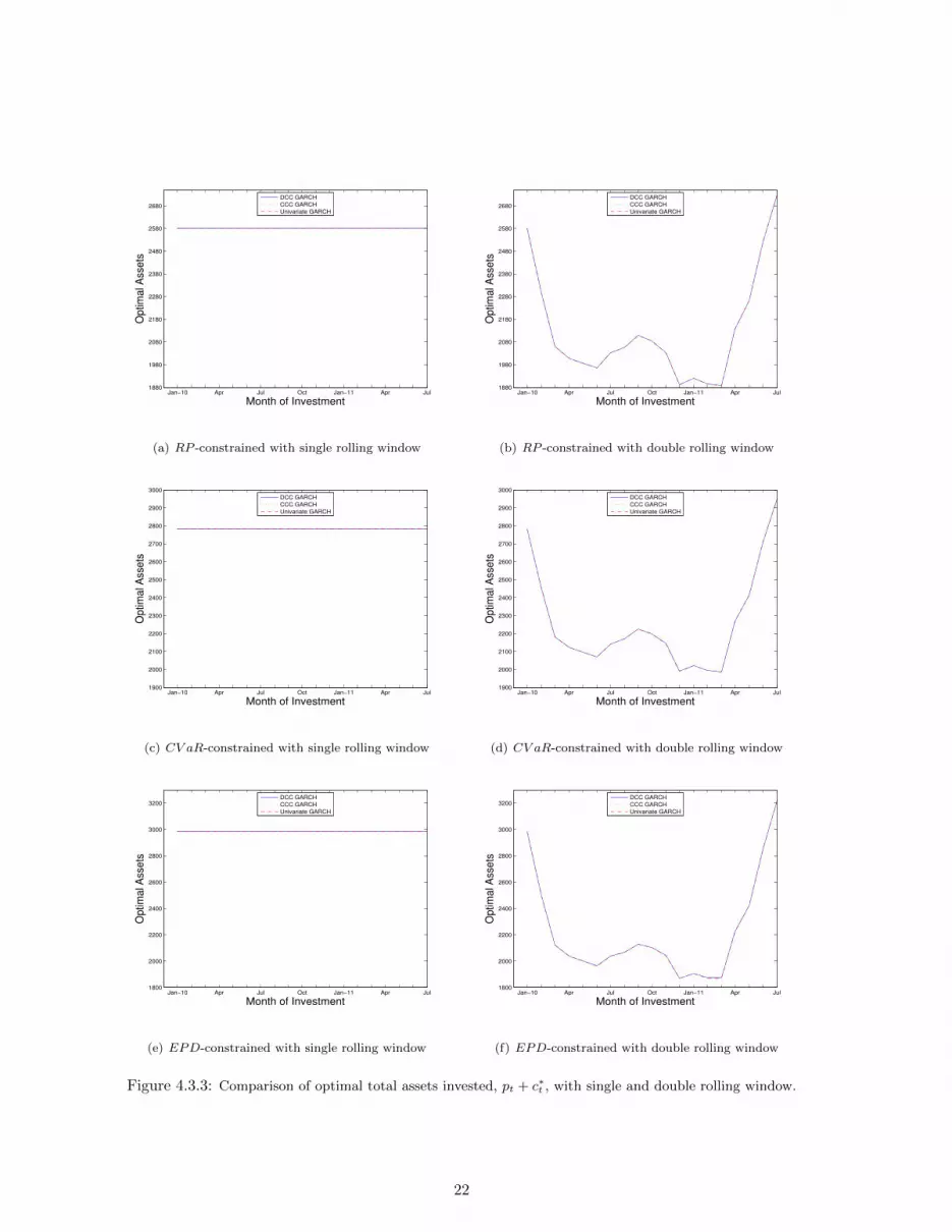
Figure 4.3.3 plots the evolution of the total optimal assets invested (pt+c∗t ) into the optimal portfolio

under the two exercises. A comparison only between optimal capital requirements would be misleading,

since insurance premiums change at each step under the double rolling window (they are linear functions

of expected severity), and this may also cause changes in c∗t . First, we notice that there are no significant

differences among the covariance models. Under the single rolling window scenario, the optimal capital

required is almost unchanged for all three solvency constrained problems. This is no longer the case when

we allow re-estimation for Yt. The variation in total assets invested is quite large, ranging from 1,887

to 2,728 for RP , 1,986 to 2,949 for CV aR and 1,868 to 3,222 for EPD; thus, the EPD problem has

the largest fluctuation, while RP is the smallest. Figures 4.3.4-4.3.5 suggest that the differences between

the optimal portfolio allocations with and without liability re-estimation are much less pronounced. The

portfolio structure also depends on the choice of the MV-GARCH model. For example, for the RP

and CV aR problems the variation in optimal allocations for NASDAQ and NYSE are smaller for the

UNI-GARCH when compared to the DCC and CCC counterparts. Although the double rolling window

20

exercise indicates that the optimal investment is very sensitive to the liability parameters, the sample

size used for estimation is based on only 60 observations.

In the remainder of this section, we compute a variety of out-of-sample indicators and we provide a

comparison between the covariance models relative to the solvency and portfolio performances. In order

to measure the solvency requirement performance of the optimal solutions, we consider three metrics: the

average assets invested, the average solvency value and the maximum solvency value. All averages are

computed over the rolling window period, with and without re-estimation. Depending on the solvency

constraint, the average solvency values are computed based on the following expressions:

RP =1

lB′

lB′∑k=1

Φ(dt+kτ

),

CV aR =1

lB′

lB′∑k=1

(E[Yt+kτ ]

1− βΦ(σt+kτ − Φ−1(β)

)−RT

t+kτz∗t+(k−1)τ

),

EPD =1

lB′

lB′∑k=1

ïE[Yt+kτ ]Φ

(dt+kτ + σ2

t+kτ

)−RT

t+kτz∗t+(k−1)τΦ

(dt+kτ

)ò.

Here,

z∗t+(k−1)τ = (pt+(k−1)τ + c∗t+(k−1)τ )x∗t+(k−1)τ ,

dt+kτ =− log RT

t+kτz∗t+(k−1)τ + µt+kτ

σt+kτ,

where (c∗t+(k−1)τ ,x∗t+(k−1)τ ) and Rt+kτ represents the optimal solution and the gross return vector,

respectively, over the period [t + (k − 1)τ, t + kτ ], for any k = 1, . . . , lB′ . The average assets invested

are calculated by taking the averages of all pt+(k−1)τ + c∗t+(k−1)τ over the rolling period. The results are

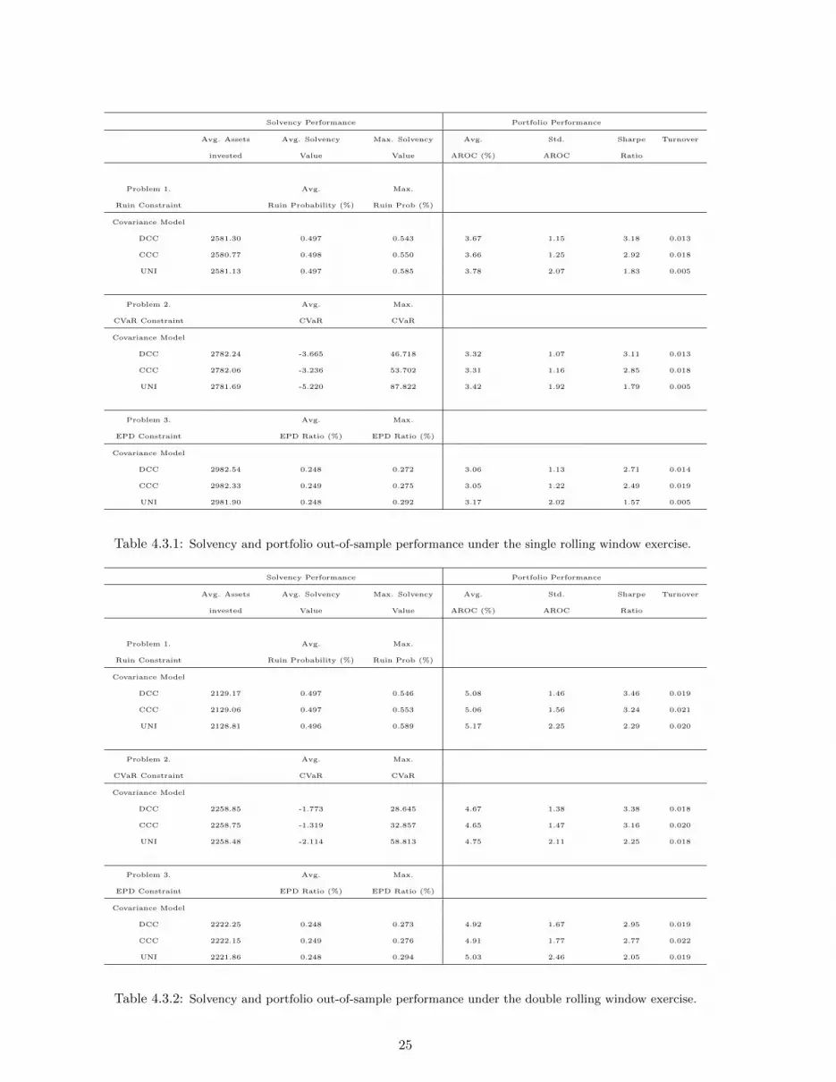
reported in the first panel of Tables 4.3.1 and Table 4.3.2.

For all models and for both rolling window exercises the average total investment is almost the

same across each covariance model. We notice that the CV aR optimization at 99% requires a higher

a higher initial optimal capital than the corresponding V aR at 99.5% problem. The EPD-constrained

optimization based on a ratio f = 0.25 is the most conservative method. The average out-of-sample

ruin probability is around 0.497 for both experiments. However, we observe scenarios under which the

ruin solvency constraint is violated. Although not reported in the tables, the number of violations is

the same across all models and typically corresponds to a negative monthly rate of return for both

21

Jan−10 Apr Jul Oct Jan−11 Apr Jul1880

1980

2080

2180

2280

2380

2480

2580

2680

Month of Investment

Optim

al A

ssets

DCC GARCH

CCC GARCH

Univariate GARCH

(a) RP -constrained with single rolling window


1980

2080

2180

2280

2380

2480

2580

2680

Month of Investment

Optim

al A

ssets

DCC GARCH

CCC GARCH

Univariate GARCH

(b) RP -constrained with double rolling window


2000

2100

2200

2300

2400

2500

2600

2700

2800

2900

3000

Month of Investment

Optim

al A

ssets

DCC GARCH

CCC GARCH

Univariate GARCH

(c) CV aR-constrained with single rolling window


2000

2100

2200

2300

2400

2500

2600

2700

2800

2900

3000

Month of Investment

Optim

al A

ssets

DCC GARCH

CCC GARCH

Univariate GARCH

(d) CV aR-constrained with double rolling window


2000

2200

2400

2600

2800

3000

3200

Month of Investment

Optim

al A

ssets

DCC GARCH

CCC GARCH

Univariate GARCH

(e) EPD-constrained with single rolling window


2000

2200

2400

2600

2800

3000

3200

Month of Investment

Optim

al A

ssets

DCC GARCH

CCC GARCH

Univariate GARCH

(f) EPD-constrained with double rolling window

Figure 4.3.3: Comparison of optimal total assets invested, pt + c∗t , with single and double rolling window.

22

Jan−10 Apr Jul Oct Jan−11 Apr Jul0.06

0.08

0.1

0.12

0.14

0.16

0.18

0.2

Month of Investment

Optim

al A

sset

Allo

catio

n −

Nasd

aq

DCC GARCH

CCC GARCH

Univariate GARCH



0.08

0.1

0.12

0.14

0.16

0.18

0.2

Month of Investment

Optim

al A

sset

Allo

catio

n −

Nasd

aq

DCC GARCH

CCC GARCH

Univariate GARCH



0.08

0.1

0.12

0.14

0.16

0.18

0.2

Month of Investment

Optim

al A

sset A

lloca

tion −

Nasd

aq

DCC GARCH

CCC GARCH

Univariate GARCH



0.08

0.1

0.12

0.14

0.16

0.18

0.2

Month of Investment

Optim

al A

sset A

lloca

tion −

Nasd

aq

DCC GARCH

CCC GARCH

Univariate GARCH



0.08

0.1

0.12

0.14

0.16

0.18

0.2

Month of Investment

Optim

al A

sset A

lloca

tion −

Nasd

aq

DCC GARCH

CCC GARCH

Univariate GARCH



0.08

0.1

0.12

0.14

0.16

0.18

0.2

Month of Investment

Optim

al A

sset A

lloca

tion −

Nasd

aq

DCC GARCH

CCC GARCH

Univariate GARCH


Figure 4.3.4: Comparison of optimal portfolio allocation in NASDAQ, with single and double rolling window.

23


0.02

0.04

0.06

0.08

0.1

0.12

0.14

Month of Investment

Optim

al A

sset A

lloca

tion −

NY

SE

DCC GARCH

CCC GARCH

Univariate GARCH



0.02

0.04

0.06

0.08

0.1

0.12

0.14

Month of Investment

Optim

al A

sset A

lloca

tion −

NY

SE

DCC GARCH

CCC GARCH

Univariate GARCH



0.02

0.04

0.06

0.08

0.1

0.12

0.14

Month of Investment

Optim

al A

sset A

lloca

tion −

NY

SE

DCC GARCH

CCC GARCH

Univariate GARCH



0.02

0.04

0.06

0.08

0.1

0.12

0.14

Month of Investment

Optim

al A

sset A

lloca

tion −

NY

SE

DCC GARCH

CCC GARCH

Univariate GARCH



0.02

0.04

0.06

0.08

0.1

0.12

0.14

Month of Investment

Optim

al A

sset A

lloca

tion −

NY

SE

DCC GARCH

CCC GARCH

Univariate GARCH



0.02

0.04

0.06

0.08

0.1

0.12

0.14

Month of Investment

Optim

al A

sset A

lloca

tion −

NY

SE

DCC GARCH

CCC GARCH

Univariate GARCH


Figure 4.3.5: Comparison of optimal portfolio allocation in NYSE, with single and double rolling window.

24

Solvency Performance Portfolio Performance

Avg. Assets Avg. Solvency Max. Solvency Avg. Std. Sharpe Turnover

invested Value Value AROC (%) AROC Ratio

Problem 1. Avg. Max.

Ruin Constraint Ruin Probability (%) Ruin Prob (%)

Covariance Model

DCC 2581.30 0.497 0.543 3.67 1.15 3.18 0.013

CCC 2580.77 0.498 0.550 3.66 1.25 2.92 0.018

UNI 2581.13 0.497 0.585 3.78 2.07 1.83 0.005


CVaR Constraint CVaR CVaR

Covariance Model

DCC 2782.24 -3.665 46.718 3.32 1.07 3.11 0.013

CCC 2782.06 -3.236 53.702 3.31 1.16 2.85 0.018

UNI 2781.69 -5.220 87.822 3.42 1.92 1.79 0.005


EPD Constraint EPD Ratio (%) EPD Ratio (%)

Covariance Model

DCC 2982.54 0.248 0.272 3.06 1.13 2.71 0.014

CCC 2982.33 0.249 0.275 3.05 1.22 2.49 0.019

UNI 2981.90 0.248 0.292 3.17 2.02 1.57 0.005

Table 4.3.1: Solvency and portfolio out-of-sample performance under the single rolling window exercise.

Solvency Performance Portfolio Performance

Avg. Assets Avg. Solvency Max. Solvency Avg. Std. Sharpe Turnover

invested Value Value AROC (%) AROC Ratio


Ruin Constraint Ruin Probability (%) Ruin Prob (%)

Covariance Model

DCC 2129.17 0.497 0.546 5.08 1.46 3.46 0.019

CCC 2129.06 0.497 0.553 5.06 1.56 3.24 0.021

UNI 2128.81 0.496 0.589 5.17 2.25 2.29 0.020


CVaR Constraint CVaR CVaR

Covariance Model

DCC 2258.85 -1.773 28.645 4.67 1.38 3.38 0.018

CCC 2258.75 -1.319 32.857 4.65 1.47 3.16 0.020

UNI 2258.48 -2.114 58.813 4.75 2.11 2.25 0.018


EPD Constraint EPD Ratio (%) EPD Ratio (%)

Covariance Model

DCC 2222.25 0.248 0.273 4.92 1.67 2.95 0.019

CCC 2222.15 0.249 0.276 4.91 1.77 2.77 0.022

UNI 2221.86 0.248 0.294 5.03 2.46 2.05 0.019

Table 4.3.2: Solvency and portfolio out-of-sample performance under the double rolling window exercise.

25

risky assets. More precisely, the maximum values for the ruin probabilities are attained when the asset

rate of returns are −11% and −12%, respectively. Potential improvements for reducing the number

of constraint violations could be obtained by using of a more sophisticated conditional mean return

(e.g. an autoregressive structure) and estimating the model parameters based on lower frequency data

(e.g. weekly or monthly). The latter reduces the number of simulation steps and thus improves the

GARCH forecasting. The DCC-GARCH model is the best in the sense that it gives the lowest maximum

solvency level of 0.543% (0.546% for liability re-estimation) as opposed to 0.585% (0.589% for liability

re-estimation) ruin probability observed for the no-correlation case. A similar pattern can be observed

for the maximum levels of CV aR and EPD ratio. For example, the CV aR under the UNI-GARCH case

is almost twice as large as the DCC-GARCH counterpart.

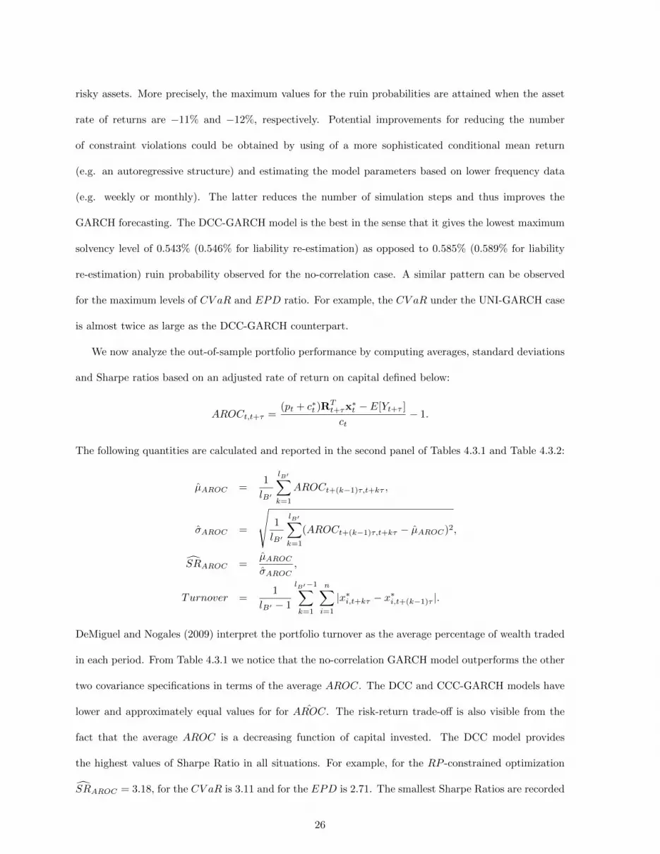
We now analyze the out-of-sample portfolio performance by computing averages, standard deviations

and Sharpe ratios based on an adjusted rate of return on capital defined below:

AROCt,t+τ =(pt + c∗t )R

Tt+τx

∗t − E[Yt+τ ]

ct− 1.

The following quantities are calculated and reported in the second panel of Tables 4.3.1 and Table 4.3.2:

µAROC =1

lB′

lB′∑k=1

AROCt+(k−1)τ,t+kτ ,

σAROC =

Ã1

lB′

lB′∑k=1

(AROCt+(k−1)τ,t+kτ − µAROC)2,”SRAROC =µAROCσAROC

,

Turnover =1

lB′ − 1

lB′−1∑k=1

n∑i=1

|x∗i,t+kτ − x∗i,t+(k−1)τ |.

DeMiguel and Nogales (2009) interpret the portfolio turnover as the average percentage of wealth traded

in each period. From Table 4.3.1 we notice that the no-correlation GARCH model outperforms the other

two covariance specifications in terms of the average AROC. The DCC and CCC-GARCH models have

lower and approximately equal values for for ˆAROC. The risk-return trade-off is also visible from the

fact that the average AROC is a decreasing function of capital invested. The DCC model provides

the highest values of Sharpe Ratio in all situations. For example, for the RP -constrained optimization”SRAROC = 3.18, for the CV aR is 3.11 and for the EPD is 2.71. The smallest Sharpe Ratios are recorded

26

by the no-correlation dynamic with 1.83, 1.79 and 1.57. Thus, we can conclude that the incorporation of

a dynamic correlation increases the portfolio performance as measured by the Sharpe Ratio. However,

the UNI-GARCH model provides the smallest portfolio turnover value. Similar patterns can be observed

by examining the results from Table 4.3.2. Under the double rolling window exercise, the average values

for the AROC increase across all models and optimization problems. This is a direct consequence of the

fact that the optimal asset invested decreases due to changes in the liability parameters. The Sharpe

Ratio values indicate that DCC-GARCH is the best model for all three problems, the highest value being

obtained for the RP constrained optimization (3.46) and the lowest for the EPD. Unlike in the single

rolling exercise, the turnover ratios have now similar values for the DCC and no-correlation models. We

further notice that the turnovers are higher when we re-estimate loss parameters.

5 Conclusions

In this paper we proposed and analyze three problems to jointly solve for the optimal capital requirement

and its optimal portfolio allocation. Each problem is constructed based on two types of constraints. The

first set of constraints are dictated by standard solvency insurance requirements such as the Value-at-

Risk, Conditional Value-at-Risk and Expected Policyholder Deficit calculated for a specified horizon and

for a given confidence level. The second constraint is performance measure constraint based on a lower

bound for the shareholders’ expected Return-on-Capital. We provide a novel semiparametric approach for

solving these problems based on a parametric distribution of the liability and on the empirical distribution

for asset returns. In particular, we assume losses have a Lognormal distribution and the portfolio’s asset

returns are generated according to a Dynamical Conditional Correlation multivariate GARCH model. We

provide sufficient conditions such that each solvency constraint admits a convex representation which are

further implemented using the non-linear optimization Matlab solver based on interior-point algorithms.

We examine optimal solutions for a 3-asset portfolios (two indices and one risk-free asset) through two

numerical experiments. In the first numerical example, we construct efficient frontiers for the optimal

capital based on different levels of expected ROC. The efficient frontiers have the same pattern for all

constraints and covariance models considered. The correlation between the two risky plays an important

27

role in the behaviour of the optimal capital required and the portfolio structure. For the same level

of expected ROC the minimum value of c∗t is obtained for the no-correlation model, while the DCC-

GARCH gives the highest value. Furthermore, the portfolio weights behaves differently; for example, the

DCC-GARCH allocates nothing to in NYSE index, while the optimal weights are non-zero for the other

covariance specifications. The out-of-sample performance of our portfolio is tested in a second detailed

numerical example using a double rolling window estimation for both assets and liabilities. We compute

two types of indicators for assessing the solvency and return on capital performances. Our results suggest

that the DCC model outperforms the other candidates under both scenarios. More specifically, the

DCC-GARCH has the smallest value of the maximum RP , CV aR and EPD and provides the highest

out-of-sample Sharpe Ratio. Several extensions to our models can be further investigated by including

more complex models for assets and liabilities, as well as by extending this work to allow for multiple

business lines, friction costs and possibly a multiperiod setting.

28

References

[1] Alexander, S., Coleman, T., and Li, Y. (2006). Minimizing CVaR and VaR for a Portfolio of Deriva-

tives. Journal of Banking and Finance, 30, 583-605.

[2] Acerbi, C. and Tasche, D. (2002). On the Coherence of Expected Shortfall. Journal of Banking and

Finance, 26(7), 1487-1503.

[3] Artzner, P., Delbaen, F., Eber, J. M., and Heath, D. (1999). Coherent measure of risk. Mathematical

Finance, 9(3), 203-228.

[4] Barth, M. (2000). A Comparison of Risk-Based Capital Standards under the Expected Policyholder

Deficit and the Probability of Ruin Approaches. Journal of Risk and Insurance. 67(3), 397-413.

[5] Bustic, R.P. (1994). Solvency Measurement for Property-Liability Risk-Based Capital Applications.

Journal of Risk and Insurance, 61, 656-690.

[6] Bogentoft E., Romeijn H.E., and S. Uryasev. (2001). Asset/Liability Management for Pension Funds

Using CVaR Constraints. The Journal of Risk Finance, 3(1), 57-71.

[7] Charnes, A., and Cooper, W.W. (1959). Chance-Constrained Programming. Management Science,

6, 73-79.

[8] Cummins, J.D., and Nye, D.J. (1981). Portfolio Optimization Models for Property Liability Insurance

Companies: An Analysis and some Extensions. Management Science, 27, 414-430.

[9] Cummins, D. and Phillips, R.D. (2009) Capital adequacy and insurance risk-based capital systems,

Journal of Insurance Regulation, 28(1), 2572.

[10] Dhaene J., Vanduffel S., Goovaerts M., Kaas R., Tang Q., and Vyncke D. (2006). Risk measures and

comonotonicity: A review. Stochastic models, 22(4), 573 - 606.

[11] Djehiche, B., and Horfelt, P. (2004). Standard Approaches to Asset & Liability Risk, Scandinavian

Actuarial Journal, 5, 377 - 400.

29

[12] Eling, M., Schmeiser, H., and Schmit, J.T. (2007). The Solvency II process: Overview and critical

analysis, Risk Management and Insurance Review, 10(1), 69-85.

[13] Ferrari, J.R. (1967). A Theoretical Portfolio Selection Approach for Insurance Property and Liability

Lines. Proceedings of the Casual Actuarial Society, LIV, 33-69.

[14] FOPI. (2004). Federal Office of Private Insurance, Whitepaper on Swiss Solvency Test.

[15] Gaivoronski, A., and Pflug, G. (2004). Value at Risk in Portfolio Optimization: Properties and

Computational Approach. Journal of Risk, 7(2), 1-31.

[16] Hurliman, W. (2003). Conditional Value-at-Risk Bounds for Poisson Risks and a Normal Approxi-

mation. Journal of Applied Mathematics, 3, 141-153.

[17] Krokhmal. P., Palmquist, J., and S. Uryasev. (2002). Portfolio Optimization with Conditional Value-

At-Risk Objective and Constraints. The Journal of Risk, 4(2), 11-27.

[18] Larsen, N. Mausser, H. and Uryasev, S. (2002). Algorithms for optimization of value-at-risk. In

P. Pardalos and V.K. Tsitsiringos, editors, Financial Engineering, e-Commerce and Supply Chain,

129157. Kluwer Academic Publishers.

[19] Luedtke, J., and Ahmed, S. (2008). A sample approximation approach for optimization with proba-

bilistic constraints. SIAM Journal on Optimization, 19, 674-699.

[20] Mankai, S., and Bruneau, C. (2012). Optimal Investment and Capital Management decisions for a

Non-Life Insurance Company, Bankers, Markets & Investors, 119.

[21] Nemirovski, A., and Shapiro, A. (2005). Scenario Approximations of Chance Constraints. in Proba-

bilistic and Randomized Methods for Design under Uncertainty, G. Calafiore and F. Dabbene, eds.,

Spreinger-Verlag, London.

[22] Nemirovski, A., and Shapiro, A. (2006). Convex Approximations of Chance Constrained Programs.

SIAM Journal of Optimization, 17(4), 969-996.

[23] Rockafellar, R.T. and Uryasev, S. (2000). Optimization of Conditional Value-at-Risk. Journal of

Risk, Number 2, 21-41.

30

[24] Rockafellar, R.T. and Uryasev, S. (2002). Conditional Value-at-Risk for General Loss Distributions.

Journal of Banking and Finance, 26(7), 1443-1471.

[25] Sandstrom, A. (2006). Solvency: Models, Assessment and Regulation. Chapman & Hall/CRC, Boca

Raton.

[26] Tian R., Cox, S.H., Lin, Y, and Zuluaga, L.F. (2010). Portfolio Risk Management with CVaR-like

Constraints. North American Actuarial Journal, 14(1), 86-106.

[27] Wozabal, D., Hochreiter, R., Pflug, G. (2008). A d.c. Formulation of Value-at-Risk Constrained Opti-

mization. Tech. Rep. TR2008-01, Department of Statistics and Decision Support Systems, University

of Vienna, Vienna.

31

portfolio optimization under solvency constraints: a dynamical approach

Documents