in part'ial fulfillment of the - mspace

PRESSUREHETER CREEP TESTTI{6 IN LABORÅTORY ICE

BRUCE H. KJARTANSON

A Thesi s

Presented to the University of Manitoba

in Part'ial Fulfillment of the

Requirements for the Degree of

Doctor of Ph'i I osophy i n Ci vi I Engi neeri ns

þli nni peg, l.lani toba

;¿ HÅY" t9B6

By

Permission has been grantedto the Nat ional- L ibrarY ofCanada to microfilm thisthesis and to lend or seIlcopies of the film.

The author (coPYright owner)has reserved otherpublication rights' andne ither the t.hes is norextensive extract.s from itmay be Print.ed or otherwisereproduced without his/herwritten Permission.

Lr autorisation a -eté accordéeà Ia Bibliothèque nationaledu Canada de microfilmercette thèse et de Prêter oude vendre des exemPlaires duf ilm.

Lrauteur ( titulaire du droitd'auteur) se réserve lesautres droits de Publication;n i I a thèse ni de long sextraits de celle-ci nedoivent être imPrimés ouautrement reProduits sans sonautorisation écrit.e.

rsBN Ø_3L5_34 Ø2Ø_7

PRESSUREMETER CREEP TESTING IN LABORATORY ICE

BRUCE H. KJARTANSON

A tllesis sr¡b¡nitted to tlrc Facult¡, ol- Craduate Studies oftlte U¡tiversity of Manitoba in partial [ulfillnle¡rt of the requirernerrts

of the degree of

DOCTOR OF PI-IILOSOPHY

o t986

Permissio¡r has bee¡t granted to the LIBRARY OF THE UNIVER-

SITY OF MANITOBA to le¡rd or sell copies of this thesis. to

the NATIONAL LIBRARY OF CANADA to microfilnr this

thesis and to lend or sell copies of the film, and UNIVERSITY

MICROFILMS to publish an abstract of this thesis.

The author reserves ofher publicatio¡r rights, and neither the

thesis nor extensive extracts from it may be printed or other-

wise reproduced without the author's written permissiolt.

BY

TO ffiY FAHILY

ABSTRACÏ

Si ng'l e stage and mul ti stage pressuremeter creep tests

have been conducted i n 'large , I aboratory-prepared samp'les of

polycrystal I ine ice at temperatures of -2"C. One purpose of the

experimenta'l program was to investigate the validity and applicability

of two creep theories, the wide'ly used simple power I aw theory

(strain-hardening formulation) and the recent'ly proposed modified

second-order fluid model. Another purpose was to investigate the

relationshjp between single stage and multistage pressuremeter creep

tests, in the same stress range, and thus to deduce the effect of

loading history on the creep parameters.

For both models, the creep information obtained from the

mul ti stage pressuremeter tests was found to compare very wel I wi th

the information derived from singìe stage pressuremeter creep tests'

both in terms of creep parameters and predicted'long-term behaviour.

The modified second-order fluid model, however, produced less scatter

in the stress exponent n derived from the multistage tests than the

simple power law model. This was attributed to the creep parameter

optimi zati on procedure used i n the anal ysi s for the modi fi ed

second-order fluÍd model.

Through analysis of the multistage tests, it appears that

the past history of app'lied stresses in a pressuremeter creep test

has little effect on the nature of the creep; rather, the amount

of accumulated strain appears to be the controì1ing factor.

For pressuremeter testing in ice or ice-rich frozen soils,

it should be assumed that a steady-state creep condition will eventualìy

(i )

prevail with continued straìning. Each stress increment in a

pressuremeter creep test shoul d be appl ied unti I at I east the

steady-state condition Ís approached, as evidenced by a b (time

exponent) of at least 0.90 or an exponentialìy increasing cavity radius

w'ith time. In order to aüain the steady-state condition in a reasonable

amount of time, a fjeld multistage pressuremeter creep test may be

started at any stress level; for exampìe, a multìstage test may be

started at a pressure of 1.50 MPa and have 0.25 MPa pressure increments.

H'ith careful'ly run cal i brations both before and after

each test, the 0Y0 Elastmeter-100 pressuremeter performed exceedingly

wel I in thi s experimentaì program. Thi s pressuremeter, or a

pressuremeter sim'ilar to this, with an electronjc rad'ius measuring

device is recommended for testing frozen soils olice. Ana'lysis of

the results, for the time being, should be conducted in terms of the

simple power law creep theory in its steady-state form. Because it

can represent both prìmary and secondary creep j n the same motion

equation and is valid for large strains, the modified second-order

fluid model is preferable to the sìmpìe power law model. Solutjons

to selected boundary-value prob'ìems, however, must be solved before

it can be used in practìce.

(ii)

ACKNOWLEDGEMEHTS

Thisstudylt,ascarriedoutunderthedirectsupervision

of Dr. D.H. Shields, Department of Cìvil Engineering' University of

Man.itoba. The author wishes to express his sjncere gratitude to Dr'

Shieldsforsuggestingth.istopicofresearch,andforhiscontjnuedquidance' encouragement and support throughout the investigation'

Theauthora]sowishestothankDr.L.Domaschuk,Dr.E.T.

Lajtai and Dr. G. Bauer who, aS members of the author's thesis examininq

committee, provìded useful ideas and constructive criticism' Durinq

h.is stay in canada, Dr. F. Baguelin provided many helpful comments

whi ch were greatl Y aPPrec'i ated '

Special thanks are due to Dr' C-S' Man who introduced

the author to the field of continuum mechan'ics and who contributed

s.ignifìcant'ly to the analytical components of this study in its early

stages.Inaddition,Mr.Q.-X.Sun.isacknow.ledgedforhisdevelopment

of the modified second-order fluid numerical analysis and many helpful

discussions with the author'

The author i s very grateful to Messrs. M. Lemieux, R'

Kenyon, R. Kwok, B. Turnbull and K. Leung for providing assistance

during the 'laboratory experimental proqram' The excel lent work of

J. Clark and s. Meyerhof .in the civil Engineering Machjne shop is

a'l so gratef ul I Y acknowl edqed '

Thefinanc.ialsupportprov.idedbytheNatura]Scierìces

and tng.ineerìng Research Counci ] , Canada Hortgaoe and Housinq

Corporation and the C'ivil Enqinee¡ing Department' through postoraduate

teaching assistantships are deepìy appreciated'

(.iii)

' Gratitude 'is extended to Inqrid Trestrail for her efficient

and error-free typing of the manuscript.

F'inaììy, last but not least, the author wishes to thank

his wife Cathy who persevered through the trials and tribulations

of the past four and a hal f years. Her support and encouraqement

made completìon of this thesis possible.

(iv)

TABLE OF COHTENTS

ABSTRACT

TABLE

LIST

LIST

LIST

OF TABLES

CTIAPTER 2 iiE Ë-Ëts['*Ëlli:*o'

2.12.2

44

67I

10

162.3

'-.Lc z - -Eouations "":z: 2".L i"

- st tonda rY creeP

- :u*7'.V'.1"ã Pt'ituty creep La',

2.2.2 l'lultiu*iui'iätË ót tttttt: Constitu-L'c'É

tive rquations '1" "';:'

ii:r'i,:i"i'i:îii':i:iit!;ii,;::::1l II,i,1, ^-2.3.I Derivatìon äï-tt't Strain-Hardening Power

uaw creej"Eiuuiiãn ior the Pressuremeter

Ëi:il:i' o;' ;i' P; ; ;;ä;iå;' ö'ååP

Þarameters " ':"""'Review of Publ i

'r'åå-t¡9 :':::T::'[^1i:'o

16

2T2.3.2

2.3.3 Revlew or ruu' ''iiË-niãh Frot.n Soi 1 sTest Resul ts 'in Ice-Kt uIr r I wrç"

and Ice2330

3;?;ir .:iTå'{.r ååiåå' iillåtïv å i ü' - p'"obr ems

Ëri' düilhïlii"i.:;'iîh:iit.,: : :

2,4.2 Ci rcu t ar-î,;i;i^ i:tll:l'i'ï:iå:l'Êì,.i : : : : : : : : : : : : : :

ACKT{OHLEDGEHENTS

0F c0t{TEnils

OF FIGURES

OF PHOTOGRAPHIC PLATES

CHAPTER 1 IF¡TRODUCTIOI{

1. 1 ScoPe of Thesi s

IäT.fäits-Tr'nl'?[Introducti on '.' ' ' 'å;iiiHlltlil .i

it,i?:å i,'iî,:::: o

ii ri :1 : : i r i'

ICE.RICH FROZEI{

Paqe

(i )

1i i i )

(v)

(ì x)

(xxi )

(xxl l U

3131323333

2.4

(v)

Paqe

352.4.5 SurnmarY

2.5 Background toÌ.1odel

2.6 Modified Second-Order

the llodified Second-0rder Fl uid

Fluid Model: Theoreti cal35

37

50

5052

5255

58

60636566

Consi derati ons

CHAPTER 3 TEST EQUIPI-{EhIT AND TEST PR0CEDURES

3.13.2

Introducti onTest Equ'iPment3.2.L Pressuremåü; Test'ing Tanks' Including

the SamPle Freezj!9-SYstem3.2.? óVo rl aitmeter 100- Pres-suremeters

3.2.2.L öãiiuration of the Cal Íper Arm

- I VnT Svstem- LVDT System3.2.2.2 Cal i brati on f or Membrane

S.+.t Single Stage Testsg.4.2 Multistage Tests

CHAPTER 4 PRESSUREI{ETER CREEP TEST RESULTS

4.1 Introduction4.2 ExPerimental

Pressuremeter4.3 ExPerimental

Thi ckness3.2.2.3 Membrane Resi stance Correcti on

Pressure

Ice SamPle PreParat'ionTest Procedures

Results of theCreeP Tests

Results of the

Single Stage

Mul ti stage

3.2.3 Data Acquisitìon SYstem

á'.r-.4 Temperature l'4easurement .

Z.Z.S Pressure Transducers and

Regu'lators3.2.6 Otíl l'ing and Samp'ling Equipment

CreepPower

Terms

676870747478

99

99

99

102102

104

106

127

r27

-t27

127

130131133

3.33.4

Creep TestsTest Resu'lts

and Pressuremeter Test SamPle

Homogenei tY4.6 Pressuremeter Test

Test RePeatabiìitY

CI{APTER5ANALYSIS0FTHEPRESSuREI,IETERCREEPTESTS

5. 1 Introduct'ioná'., ÀnalYsis of Pressuremeter

oi t'fl. Strai n-Hardeni ng 'TheorY5.2.L5.2.2

P;;å;;i;;-iñ. Pressuremeter creep restsÀ;;i;;ìs ót *,. Muttistage Pressuremeter'i;;'p-i;.is

Usi ns Strai n-Hardeni ns 'Power Law CreeP Theory ' :':''s".'à".'z.i- nnuivlii ói iaultistage rest # 10

s'.r'.r'.ã Ânãlvtii ót Multistase Test # 11

Pressuremeter4.4 Dìscussion of4.5 Ice ProPerties

Samp'le ReproducibiljtY and

Tests inLaw CreeP

(vi )

5.2.2.3 Analysi s of Mul t'istage Test # 12

5.2.2.4 Analysis of Muitistage Test # 13

5.2.3 Ana]ysis of the single stage PressuremeterCreep Tests Using Strain-Hardening'Power Law CreeP Model

5.2.4 Comparison of Èxperimental and PredictedPressuremeter Creep Curves Using theStrajn-Hardening, Power Law Creep Model

5.3 Analysis of Pressuremeler Creep Tgt.tt.in Terms

oi t-ft. Modified Second-Order Fluid Model

5.3.1 Processing the Pressuremeter Creep

Paqe

134135

136

140

143

143

143

148

148

150

151

t52

5.3.3.2

5.3.3.3

5.3.3.4

DISCUSSION OF RESULTS

TESTIT{G PROGRA}I II{ ICE

5.3.4 Comparison of Experimental Sing'le llugt,Presiuremeter Creep Curves and PredictedCreep Curves Using the Modified Second-

0rder Fluid Model

5.4 RelationshÍp Between the Strain-Harden'ing'power Law Ci:eep Model and the Modified second-

0rder Fluid Model

Tests5.3.2 AnalYs'is of the Single

meter Tests Using the

#10

Order Fluìd Model5.3.3 Ánalysis of the Multistage Pressuremeter

Creeþ Tests Usìng the Modified Second-

Order Fluid Model5.3.3.1 Analysi s of Mul ti stage Test

Stage Pressure-Modified Second-

Anal ysi s of Multistage Test#11Anal ysi s of Mult'istage Test#L2Anal ysi s of Hul t'i stage Test#13

OF THE PRESSURE}IETER CREEPCHAPTER 6

L52

154

259

259

260

6. 1 Rel ati onshi p Between Mul t'i stage and Si ng'l e

Stage Pressuremeter CreeP-TestsO.tlt Strain-Hardening, Power Law Creep

Model ; Rel ati oñshi p Between l'lul ti stageand Single Stage Creep ]t:!t..'.':""'

6.1.2 Modifieã Second-0rder Fluid Model;Relationship Between Multistage and

Single Stage CreeP Tests 265?676.1.3 SummarY

6.2

6.3

Compari son of the Creep Parametersio.y t.. Derived in This StudY WithReported in the LiteratureReäommended Pressuremeter Testi ng

and AnalYsis in Ice and lce-Rich6.3.1 Dri I 1 ing and SamPl ing

for Labora-Those

Techni ques

:::"'soiIs

268

27L271

(vii)

Paqe

6.3.2 RecommendedTechnì ques

Pressuremeter CreeP'in ice and Ice-Rich

Testi ngFrozen

Soi I6.3.3 AnalYsì s

Resul ts

C}IAPTER 7 CONCLUDING REI4ARKS

of Pressuremeter CreeP Test272

275

28r

7.I Pressuremeter Testing Equipment

7.2 AnaìYsis of Test Resultsi'.a Cäcommenoed Pressuremeter Creep Testing^. .

Techniques and Ana'lysis in Ice and lce-KlcnFrozen So'il s

7.4 Recornmendat'ions for Further Research

PRESSURE},IETER CREEP TEST DATA PLOTS

CAVITY EXPANSIOIiI RATE

FOR THE PRESSUREI'{ETER

/ RADIUS VERSUS TIHE PLOTS

CREEP TESTS

APPEAIDIX C COHPUTER PROGRAITS

i10Y0PL1OYORATEl-ADFoS1I-ADPLPRDPLS

QSUfl

281282

284286

288

293REFEREilCES

APPENDIX A

ÃPPENDIX B 340

373374379391395398400

(viii)

Fi qure

?_.r

LIST CIF FIGURES

Constant stress creep test;(a) creep curve variations(b) basjc creep curve(c) strain rate versus time

Linearized creep curves

Log-'log plot of the secondary creep 'law

Primary creep curves

Primary creep curves at discontinuous

Notation for interpretation of stage

Paqe

42

2.2

2.3

2.4

2.5

2.6

2.7

2.8

2.9

2.r0

2.TI

2.12

2.t3

2.14

3.1

3.2

3.3

3.4

49

49

82

83

84

85

stress change

I oaded

43

43

44

44

45

45

46

46

47

pressuremeter test

Determination of creep parameters from the resultsof a stage loaded pressusremeter test

Determination of creep parameters for a multistagetest in a varved silt-clay frozen soil

Single stage creep test in a varved silt-cìayfrozen soil

Stage loaded pressusremeter Test 214, with 15minutes per stage: creep parameter determination

Stage loaded pressuremeter Test 216, with 60minutes per s

Long-term pre

tage: creep parameter determination

ssuremeter creep tests

Fifteen minute creep curves in a 'log-log pìot andthe determination of creep parameters, Test 14

Long-term creep curves for Tests 7, 18 and 20

Schematic ìayout of pressuremeter testing system

0Y0 Elastmete

Geometry of c

r-100 ca'liper arm system

aliper arm-rod system

Membrane cross-sectional area calibration test,

47

48

S.S. Test 9

(ix)

Fi qure

3.5

3.6

3.7

3.8

3.9

3. 10

4.1

4.2

4.3

4.4

4.5

4.6

4.7

4.8

4.9

4.10

4.11

4.L2

5.1

5.2

Cavi tyStage 3

Cavi tyStage 4

Cavi tyStage 5

Change in membrane thickness with time calibra-tion Test, S.

Procedure forcreep tests

S. Test 9

data processing 0Y0 Elastmeter-100

l'lembrane reaction curves

Thermistor I inearizing circuit

Thermocouple and thermistor layout, S.S. Test 2

Temperature-depth-time plots for freezing ofsample for S.S. Test 2

Compiled pìot of cavity radius versus time curvesfor the sing'le stage tests

Cavi ty pressure vari at'ion wi th time; S. S. Test 4

Sample temperature variation with time; S.S. Test 4

Cavity expansion rate versus time; S.S. Test 4

Cav'ity pressure variation with time; MS Test 10

Sampìe temperature variation with time; MS Test 10

Cavity expans'ion rate versus time; MS Test 10'Stage 1

Cavi tyStage 2

expansion rate versus time; MS Test 10'

expansíon rate versus t'ime; MS Test 10'


expansion rate. versus time; HS Test 10'

Cavity radius versus timeand S.S. Test 4;2.00 MPa

curves for S.S. Test 3

fromtest

(:)

Paqe

86

87

88

89

90

91

113

114

115

116

TL7

118

119

L20

LzL

122

L23

.L24

175

176

Creep parameter determinationmul ti stage pressuremeter creeP

Circumferential strain and ln

a simulated

MS Test 10; alì data

(x)

ri versus time,

Fi qure

5.3

5.4

5.5

5.6

5.7

5.8

5.9

5. 10

5. 11

5.L2

5.13

5. 14

5. 15

5. 16

5.L7

5. 18

5. 19

5.20

Test 10;

rn (fr)

Paqe

177

178

179

180

181

r82

183

184

185

186

187

188

189

190

191

t92

193

194

F and b versus pressure, MS

Circumferential strain andMS Test 10; Stage 1 omitted

F and b versus pressure, MS Test 10; Stage 1

al I data

versus time,

Circumferential strainMS Test 11; all data


Circumferential strain andMS Test 11, Stage 1 omitted


and ln {fr) versus time,

Test 11; all

ln (ft) u.rsrs

omi tted

omi tted

omi tted

data

time,

Test l1; Stage 1

Circumferential strainMS Test IZ; a1l data


CÍrcumferential strain andMS Test 12; Stage I omitted


and ln tfr) versus time,

Test

ln (L'ri

Test

12; a1l data

) versus time,

L2' Stage I

Ci rcumferenllS Test 13;

F and b ver

Ci rcumferenMS Test 13;

F and b verand 3 omitt

Ci rcumferenMS Test 13;

F and b ver6 omitted

tial strainal I data

Circumferential strain and lnsingle stage tests; all data

and ln tfi-) versus time,

Test 13; all data

ln (*) versus time,3 '1 omitted

Test 13; Stages 1, 2

ti al strai n and I n (l) versus time,Stages 1 to 6 rl omitted

sus pressure, l4S Test 13; Stages I to

(ft) uettus time,

sus pressure, MS

tial strain andStages L, 2 and

sus pressure, MS

ed

(xi )

Fi gure

5.2r

5.22

5.23

5.24

5.25

5.26

5.27

5.28

5.29

5. 30

5. 31

5.32

5. 33

5. 34

5. 3s

5. 36

5.37

F anddata

b versus pressure, single stage tests; all

Pa qe

195

196

197

versus time1,440 and

14,400 minutes used

F and b versus pressure, sing'le stage tests; databetween L,440 and 14,400 minutes used

time,and

1.25 MPa

F and b versus pressure, single stage tests; omittests at 1.00 and 1.25 MPa

Predicted versus experimental creep curves, strain-hardening power law creep model; 2.50 MPa

Predicted versus experimental creep curves, strain-hardening power law creep model; 2.25 l4Pa

Predicted versus experimental creep curves, strain'hardening power law creep model; 2.00 MPa

Predicted versus experimental creep curves, strain-hardening power ìaw creep model ', 1.7 5 MPa

Predicted versus experimental creep curves, strain-hardenÍng power law creep model; 1.50 MPa

Predicted versus experimental creep curves, strain-hardening power 'law creep model; 1.25 MPa

Predicted versus experimental creep curves, strain-hardening power ìaw creep model; 1.00 MPa

Circumferential strain and ln (*)sing'le stage tests; data betweehr

Ci rcumferenti al strai n and I n (*) versussi ng'le stage tests , omi t tests ' I at 1 .00

ln P versus t, ?, single stage testsro

S'imp'lified flow chart for program QSUN

198

199

200

20r

202

203

204

205

206

207

208

209

2r0

?IL

Best fit creep curve, modified second-order fluidmodel; S.S. Test 2

Best fit creep curve, modified second-order fluidmodel; S.S. Test 6 ..

Best fit creep curve, modified second-order fluidmodel; S.S. Test 3 ..

(xii)

Fi qure

5. 38

5. 39

5.40

5.41

5.42

5.43

5.44

Ã ¿.8

5.46

5 .47

5. 48

5.49

5. 50

5. 51

5.52

5. 53

Best fit creep curve, modjfied second-order fluidmodel; S.S. Test 4



Best fit creep curve, mod'ified second-order fluidmodel; S.S. Test 9

Best fit creep curve, mod'ified second-order fluidmodel; S.S. Test 8

Pa qe

2t2

213

214

215

2r6

Cavi tyation ote sts

expansion rate / radius versus time;f f irst 1,440 minutes of the s'ingle

compi 1 -stage

ln þ versus ln þ"'ro 2

7 20 minutes , si ng'le

ln b versus ln þ"'ro 2

Best fit creepmodel; MS Test

ln þ versusro


ln þ versusro


laln " versusF9

for times ofstage tests

, MS Test 10

120, 360 and

curve, modified second-order fluid10

?17

2t8

219

220

22t

222

223

224

225

226

l. ? , MS Test 11

curve, mod'ified second order fluid11

tr ?, MS Test 12

curvg, modified second order fluidL2

lr ? , MS Test 13

Best fit creep curve, modified second order fluidmodel; MS Test 13

Predicted versus experimental creep curves'modified second-order fluid model ' 2.50 l4Pa;

MS Test 1.0 parameters used for prediction

(xiii)

227

Fi qure

5. 54

5. 55

5. 56

5.57

5. 58

5. 59

5.60

5.61

5.62

5. 63

5. 64

5.65

Predicted versus experimental creep curves,modified second-order fluid model, 2.50 MPa;MS Test 11 parameters used for prediction

Predicted versus experimental creep curves,modified second-order fluid model, 2.50 MPa;MS Test 12 parameters used for prediction

Predicted versus experimental creep curves,modjfied second-order fluid model, 2.50 MPa;

l4S Test 1.3 parameters used for prediction

Predicted versus experimental creep curves,modified second-order fluid model , 2.25 l4Pa;MS Test 10 parameters used for prediction

Predicted versus experimental creep curves,modified second-order fluid model , 2.25 l(Pa;MS Test 11 parameters used for prediction

Predicted versus experimental creep curves,modified second-order fluid model , 2.25 l{Pa;MS Test 1.2 parameters used for prediction

Predicted versus experimental creep curves,modified second-order fluid model , 2.25 l'ïPa;MS Test 13 parameters used for prediction

Predicted versus experimental creep curves,modified second-order fluid model, 2.00 MPa (Test3); MS Test 10 parameters used for prediction

Predicted versus experimental creep curves,modified second-order fluid model, 2.00 MPa (Test3); mS Test 11 parameters used for pred'iction

Predicted versus experimental creep curves,modified second-order fluid model, 2.00 MPa (Test3); MS Test 12 parameters used for prediction

Predicted versus experimental creep curves,modified second-order fluid model, 2.00 MPa (Test3); mS Test 13 parameters used for prediction

Predicted versus experimental creep curves,modified second-order fluid model, 2.00 MPa (Testa); NS Test 10 parameters used for prediction

Predicted versus experimental creep curves,modified second-order fluid model, 2.00 MPa (Testa); MS Test 11 parameters used for prediction

Pa qe

228

229

230

23t

232

233

234

235

236

237

238

239

5.66

(xiv)

240

Fi qure

5.67

5.68

5. 69

5.70

5.7 7

5.7 2

5.7 3

5.7 4

5.7 5

5.7 6

5.77

5.78

Predicted versus experimental creep curves'modified second-order flu'id model, 2.00 MPa (Test4); MS Test 12 parameters used for pred'iction

Predicted versus experimental creep curves'modified second-order fluid model, 2.00 MPa (Test4); NS Test 12 parameters used for prediction

Predicted versus experimental creep curves'modified second-order fluid model, 1.75 MPa; MS

Test 10 parameters used for prediction

Predicted versus experimental creep curves'modjfied second-order fluid model , L.7 5 MPa; MS




Predicted versus experimental creep curves'modified second-order fluid model ,1.75 l4Pa; llSTest 13 parameters used for prediction







Predicted versus experimental creep curves'modified second-order fluid model, 1.50 IlPa; MS


Predicted versus experimental creep curves'modified second-order fluid model , 1.25 l''lPa; MS


Predicted versus experimental creep curves'mod'ified second-order fluid model , L-25 MPa; MS


Predicted versus experimental creep curves'modified second-order fluid model , L.25 MPa; MS


Paqe

24r

242

243

244

245

246

247

2ß

249

250

25r

252

5.79

(xv)

253

Fi qure

5.80

Paqe

254

?.55

256

257

258

279

280

294

295

296

297

298

299

300

30i

302

303

304

5.8 i

5.82

5.83

5.84

6.1

6.2

4.1

4.2

4.3

4.4

A.5

A.6

4.7

4.8

4.9

A.10

4.11

Predi ctemod'i f i edTest 12

Pred'icted versus experimental creep curves,modified second-order fluid model , 1.25 MPa; MS


Predicted versus experimental creep curves,modified second-order fluid model, 1.00 MPa; MS

Test 10 parameters used for pred'iction

Predicted versus experimental creep curves,modifíed second-order fluid model, 1.00 MPa; MS


Predicted versus experimental creep curves,modified second-order fluid model, 1.00 t4Pa; MS


Comparison of predictions, strain-hardening powerlaw creep model ; 2.00 MPa

Comparison of predictions,'law creep model; 1.25 MPa

strai n-hardeni ng power

Cavity pressure variation with time; S.S. Test 2

Samp'le temperature variation with time: S.S.Test 2

Cavi ty

Cavi ty

Sampl eTest 6

Cavi ty

Cavi ty

Sampì eTest 3

Cavi ty

Cavi ty

Sampì eTest 7

d versus experimentaì creep curves,second-order fluid model, 1.00 MPa; MS

parameters used for prediction

expansion rate versus time; S.S. Test 2

pressure variation with time; S.S. Test 6

temperature variation with time: S.S.

expansion rate versus t'ime; S.S. Test 6

pressure variation wÍth time; S.S. Test 3

temperature variation with time: S.S.

expansion rate versus time; S.S. Test 3

pressure variation wÍth time; S.S. Test 7

temperature variation with time: S.S.'

(xvi )

Fi gu re

A.I2 Cavity expansion rate versus time; S.S. Test 7

4.13 Cavity pressure variation wÍth time; S.S. Test 5

4.14 Sample temperature variation wjth time: S.S.Test 5

4.15 Cavity e

4.16 Cavity p

A.L7 Sampl e tTest 9

4.18 Cavi ty e

A. 19 Cav'i ty p

4.20 Sample tTest I

Pa qe

305

306

307

xpansion rate versus time; S.S. Test 5

ressure variation with time; S.S. Test 9

emperature variation with time: S.S.

xpansion rate versus time; S.S. Test 9

ressure variation with time; S.S. Test 8

emperature variation with time: S.S.

308

309

310

311

3t2

3i3

A.zL Cavity expansion rate versus time; S.S. Test 8 314

A.22 Cav'ity pressure variation with time; MS Test 11 315

A.23 Sample temperature variation with time: MS

Test 11

4.24 Cavity exStage 1

4.25 Cavity exStage 2

pansion rate versus time; MS Test 11,


A.26 Cavity expansion rate versus time; MS Test 11,Stage 3

4.27 Cav'ity exStage 4


4.28 Cavity expansion rate versus time; MS Test 11,Stage 5

A.29 Cavity pressure variation with time; MS Test 12 322

4.30 Sampìe temperature variation with time; l4S Test 12 323

A.3i Cavity expansion rate versus time; ltlS Test 12,

316

317

318

319

320

32L

Stage I

(xvi i )

324

Fi gure

4.32

A. 33

A. 34

A. 35

A. 36

4.37

A. 38

A. 39

A.40

A. 41

4.42

A. 43

A. 44

A. 45

A. 46

8.1

8.2

8.3

Cavi tyStage

Cavity expansion rate versus t'ime; MS Test 12'Stage 2

Cavity expansion rate versus time; MS Test 12'Stage 3

Cavity expansion rate versus tjme; MS Test 12'Stage 4

Cavity pressure variation with time; t'îS Test 13

Sample temperature variation with tìme; MS Test 13

Cavìty expansion rate versus time; MS Test 13'Stage 1


Cavi tyStage 3




Cavity expansion rate versus time; I'lS Test 13'Stage 6

Cavìty expansion rate versus time; MS Test 13'Stage 7



expansion rate versus time; MS Test 13,

328

329

Pa oe

325

326

327

330

331

332

333

334

335

336

337

338

339

341

342

343

10

Cavity expansion rate / radius versus time; S.S.Test 2

Cavity expansion rate / radius versus time; S.S.Test 6

Cavìty expansion rate / radius versus time; S.S.Test 4

(xv]'r'r J

Fi qure

8.4

8.5

8.6

8.7

8.8

8.9

B. 10

B. i1

B.t2

B. 13

8.14

8.15

B. 16

B.L7

B. 18

8.19

B. 20

Cavi tyTest 3

Cavi tyTest 7

Cavi tyTest 5

Cavi tyTest 9

Cavi tyTest 8

expansion rate / radius versus tjme; S.S.

expanst'on rate / radius versus time; S.S.

expansion rate / radius versus time; S.S.



Paqe

344

345

346

347

348

349

350

351

352

353

354

355

356

357

358

359

360

Cavity expansionTest 10, Stage I

Cavity expansionTest 10, Stage 2




Cav'ity expansionTest 11, Stage 1




Cavity expansÍonTest 11, Stage 5

Cavi'ty expansi onTest 12, Stage I

Cavity expansÍonTest 12, Stage 2

rate / radius versus time; MS




rate / radius versus time; l4S

rate / radius versus time; þlS

rate / radius versus time; HS






(xix)

Fi qure

B.2T

8.22

8.23

B.?.4

8.25

8.26

8.27

8.28

8.29

B. 30

B. 31

8.32



Cavíty expansionTest 13, Stage 1.







Cavity expansionTest 13, Stage ICavity expansionTest 13, Stage 9

Cav'i ty expansi onTest 13, Stage 10


rale / radius versus time; I'lS

rate / radius versus tÍme; MS




rate / radius versus time; l'1S






Paqe

361

362

363

364

36s

366

367

368

369

370

37r

372

(xx)

Table

2.r

2.2

3.1

3.2

4.1

4.2

4.3

4.4

4.5

4.6

5.1

5.2

5.3

5.4

5.5

5.6

LIST OF TABLES

Results of Pressuremeter Creep Tests, Inuvik, 1978

Results of Pressuremeter Creep Tests in Sea Ice

Chemical Properties of City of l,linnipeg Tap l'laterand ArctÍc lce Co. L

Results of Change inMultistage Test 10

td. Ice Crystals

l4embrane Thickness Test for

Paqe

40

4t

80

81

107

108

109

110

111

712

158

159

160

161

162

t64

165

Sunrmary of Pressuremeter

SuÍrnary of Pressuremeter

Creep Tests

Calibration Constants forSingìe Stage Tests

Sunrnary of Pressuremeter Calibration Constants forMul ti stage Tests

Minimum Cavity Expansion Rates for the Síng'le Stageand the Multistage Pressuremeter Creep Tests

Degree of Cracking in Pressuremeter Test lceSpec i men s

Density of lce Core Samp'les

Creep Parameter Determination, Strain-HardeningPower Law Creep l4odel; Multistage Test 10

Creep Parameter Determination, StraÍn-HardeningPower Law Creep Hodel; Multistage Test 11 ......Creep Parameter Determination, Strain-HardeningPower Law Creep Model; Multistage Test 12

Creep Parameter Determ'ination, Strain-HardeningPower Law Creep Model ; Mul ti stage Test 13

Creep Parameter Determination, Strain-HardeningPower Law Creep l-lodel; Single Stage Tests

Best Fit Creep Parameters .for the Multistage TestsUs'ing the Strain-Hardening Power Law CreepHodel

l4inimum þ ,0" the Sing'le Stage Testsl"6

(xxi )

5.7

Tabl e

5.8

5.9

5. 10

5. 11

5.12

t67

168

Second-

Pa qe

166Creep Parameter Determination, Modified0rder Fluid Model; Single Stage Tests

and 720 l4inutes for the Sìng'leI at 120. 360ro stage Íests

I'li nimum 3 Vul ues for Each Stage of Mul ti stageroTest 10

Mi nimum

Test 11

Minimum

Test 12

Minimum

Test 13

rot?

rot:

rota

Values for Each Stage of Multistage



169

170

T7T

172

173

174

278

5. 13

5. 14

5. 15

Best Fit Creep Parameters for the Multistage TestsUsing the Modified Second-Order Fluid Model

Maximum Error Between Predicted Creep Curves Usingthe Modified Second-Order Fluid Model and txperi-mental Singìe Stage Creep Curves

Compari son of Creep Exponents; Strain-Hardening,Power Law Creep Model and Modified Second-Order

5. 16

6.1

Fl uid Model

Total Accumulated StrainStage of the Hultistage

-rln -ri at the

TestsEnd of Each

(xxi i )

Pl ate

3.1

3.2

3.3

3.4

3.5

3.6

3.7

3.8

3.9

3. 10

3. 11

3.r2

3. 13

4.1

4.2

4.3

LIST OF PHOTOGRÂPHIC PLATES

Condenser for sampìe freezing

0Y0 Elastmeter-100 pressuremeter components

Calibrating the caìiper arm - LVDT system

Pa qe

92

98

r25

L25

L26

92

93

93Pressuremeter cal ibration tubes

Inflating the pressuremeter inmembrane thickness cal ibration

tube#2fora

barrel; 104 mm diameter

barrel ; 77 nn diameter

with the 104 rnm diameter

th thebarrel

104 mm diameter

nrning equipment

and ice crystal tamper for

94

94Compressed dry nitrogen supply and pressureregulators for the

Modified CRREL core

Modified CRREL core

pressuremeters

modi fCoring Íce samplesmodified CRREL corCRREL core barrel

95

95

96

96

97

97

Ice sample cored wimodified CRREL core

Ice core sample triPorewater reservoirice sample making

Insul ationduring a p

Surface of

View intoTest # 7

of the steel tankresssuremeter test

and pressuremeter

the sample for Test # 7

the deformed pressuremeter cavity of

Radial crack development in Test # 10

(xx'r'r 1 ,l

CHAPTER 1-

THTRODUCTIOH

Major projects i n arcti c Canada and Al aska , pri nci paì I y

associated with the expìoration and production of energy resources,

have required that geotechnical eng'ineers des'iqn and construct larqe

structures on sites underlain by permafrost. In addition, man.y offshore

structures either bear on or are affected by sea ice and some structures

are actually made of ice.

Much of the permafrost in the north is ice-rjch (i.e. frozen

soils in which a siqnificant port'ion of the soil particles are

completely separated from each other by ice). Nixon (1978), Morgenstern

et al. (1980) and t,{eaver and Morqenstern (1981a), among others, have

concluded that the creep behaviour of ice constitutes an upper bound

to the creep of ice-rich frozen soil; that is to say that ice-rich

frozen soil , li ke ice, wil I creep continuously under load. This

sim'ilarÍty between ice-rich frozen soil and ice, pìus the lack of

a suffi cj ent data base, I ed Sego ( 1980 ) to carry out an extensi ve

testing program on warm ice (temperatures hiqher than '2"C) under

'low app'lied pressures (less than 1 Npa).

Sego, recognizinq the need to develop in situ test techniques

for frozen soils, conducted a series of laboratory punch indentat'ion

experiments in sampìes of polycrystal I ine ice. He was able to

successfu'lìy predict the penetratìon of the punch (commonly referred

to as a stati c cone i n geotechni ca'l practi ce ) , usi ng spheri cal cavi t.y

expansion theory. The deformation properties of permafrost may be

tested in situ using the pressuremeter as wel I ; in th'i s case

2

cylindrical cavity expansion theory would apply.

Ladanyi may be credited as having introduced pressuremeter

testing to ice and permafrost. Some advantages of conductinq

pressuremeter tests in situ aS compared to, SâY, testing sampìes in

the laboratory are as follows:

1) The problems associated wjth obta'ining and transportino

thermally and mechan'ica1ìy undisturbed samples to the lab'

for creep testing, are avoided.

Z) A large volume of material is tested in situ. This is

important in ice-rich frozen soils with segregated ice or

discrete ice veins or in sea ice, which usual ìy has very

large crystaì sizes.

3) The frozen so'il or ice is tested in its natural environment'

under the prevailing in situ stresses.

4) Data is collected and analyzed, ât least ín a preliminary

sense, right at the site. Therefore, the geotechnical engineer

can assess whether or not he has sufficient data for desiqn

before'leaving the site. The need to return to the site

to augment the originaì investiqation is greatly reduced.

This thesis represents an extension to our knowledqe of

the use of the pressuremeter to determine the creep properties of

warm ice or ice-rich frozen soils.

1.1 SCOPE OF THESIS

Thi s thesi s rePresents an

the va1 i d'i ty of two theori es whi ch

creep deformation of ice and ice-rich

experimentaì i nvesti gat'ion i nto

have been proposed to model the

frozen soils.

3

The methodo'logy which has been adopted is to carry out

mul ti stage pressuremeter tests, determi ne the appropri ate creep

parameters from these tests, and then see 'if these parameters can

be used to predict the behaviour of sing'le stage pressuremeter tests.

Us'ing this methodology, an attempt is made to deduce the effect of

loading history on creep parameters. As well, the sinqle stage

pressuremeter tests can be considered to represent simp'le foundation

unjts (such as footings or piles) which carry a qiven (constant) 'load;

here the idea is to see how well multistage pressuremeter test results

will predict the longer term (up to 7L, weeks) behaviour of

'foundatjons'. Thirdly, it is of interest to learn if it is feasible

to carry out very long (multi-week) pressuremeter tests with to-day's

(commercial'ly avai I able) equipment.

Ladanyi appears to have been the first to attempt to interpret

pressuremeter creep tests, in Ladanyi's case using a simp'le power

law creep theory (Ladany'i and Johnston ' 1973). Doubts concerning

the theoretical soundness of the simple power law creep theory, and

prob'lems associated with data reduction using this theory, led Han

to deve'lop a new model, the modÍfied second-order fluid model (l4an

et al., 1985).

This thesis includes a discussion of the val idity and

appìicability of both models to engÍneering anal.ysis and design in

fce and ice-rich soil conditions

THE T{EASUREHEI{T OF

Å¡{0

CTIAPTER 2

CREEP PROPERTIES OF ICE.RICH FROZEH SOILS

ICE WITH T}IE PRESSUREHETER

2.I INTRODUCTIOI{

In this chapter, the essentials of the simple power law

creep theory, for both secondary and primary creep, are presented.

The appì Ícatjon of this theory to the pressuremeter, using a

strain-hardening formulation of the simp'le power law creep theory

is then developed. A review of published pressuremeter creep studies

in ice-rich frozen soil and ice is then made. Next, the use of the

pressuremeter test to give creep parameters which may be used to predict

creep settl ements of a number of di fferent foundati on types i sillustrated. Fina'l'ly, the essentials of the modifjed second-order

fiuid model are presented.

2.2 BACKGROUND TO THE POHER UIH CREEP THEORY

As stated by Ladanyi (L972), two approaches may be taken

to the analysis of time-dependent creep probìems: micromechanjstic

and macroanalytìcal. In the micromechanistic approach, the observed

phenomena of creep are described in terms of establ ished concepts

of physics. Thermodynamic energy concepts and motion mechanisms on

the atomic scale, such as rate process theory, di slocation theory

and grain boundary sliding are utilized. In the macroanalytical

approach , empi ri cal I aws are used to descri be thg time-dependent

deformations of engineering structures. These laws basical'ly represent

5

an extension of the theory of plasticity to include time and temperature

effects. The ideal case would be to develop a macroanalytical '

engineering creep theory whjch satisfied the laws of physics'

Todate,nosuchjdea]theoryexists.Moreover,thesolution

of boundary vaìue problems, such as the penetrat'ion of a deeply imbedded

circular punch (end bearìng pi'le) or a 1ateral1y loaded pi'le' in terms

of a theory of this type, would be extremely d.ifficult indeed. This

led Ladany.i (1g72) to the conclusion that a macroanalytica'1, engineerìng

theory of creep of frozen soils should be deveìoped for solvìnq spec'ific

sojl mechanics probìems, such as the calculation of a tÍme-dependent

stress or dispìacement field in a foundatjon medium' The theory should

have re'latjvely simpl e mathemati cal expressions with a smal I number

of experimenta'l parameters, and should be able to be applied to

multiaxial states of stress easìly. Moreover, the parameters should

be able to be derived from'laboratory and/or field tests and utilized

in the specific boundary value problem. such a theory, called the

power 'law theory (Norton, LgZg) has been used successfully to describe

the creep of high temperature metals'

Ladanyi (Ig72) has taken the power law theory, as developed

in Hult (1966) and odqvist (1966), and presented a macroanalytical

engineerìng creep theory to be used for frozen soils' Thjs theory'

besides being extended to the pressuremeter problem (Ladanyi and

Johnston, 1973), has been used to model' for example:

1) the cone penetrat'ion test in f rozen so'il s (Ladanyi ' 1976;

LadanYi , 1982a; Ladany'i ' 1985a)

grouted rod anchors (Johnston and Ladanyi , 1972)

deep end bearing piìes and plate anchors in frozen so'iIs2)

3)

6

(Ladanyi and Johnston, L974; Ladanyi and Paquin, 1978)

4) strip footings in frozen soils (Ladany'i' 1975)'

The theory is still w.idely used today. Before actua'l1y describing

the solut.ion for the pressuremeter problem, the power law theory itself

i s di scussed.

As a startìng poìnt, the constitut'ive equations are first

presented for a uni axi al state of stress. General'izat'ion to a

mul ti axi al state of stress fol I ows '

2.2.L Uniaxial state of stress: constitutive Equations

Most of the early work in the creep of metals was done with

uniaxjal tests, either in tension or compression' The first laws'

therefore, were formulated in terms of unÍax'ial loading conditions.

The type of creep curve shown in Fig. 2.Ib, obtained by

step loading under uniaxjal stress conditions and at a constant

temperature, is common to many materials, includ'ing frozen soils and

.ice. The corresponding creep rates åt"ot Ë, versus time are shown 'in

Fig. 2.Lc. Three periods of time are observed, during whìch the creep

rate is decreas'ing (l), remaining essent'iaì1y constant (II) and then

increasing (lII). These are common'ly called perìods of primary'

secondary and tertiary creep respect'iveìy. If the designer is majnly

i nterested i n the 'long-term creep behavi our , and not So 'i nterested

in the shorter term, primary creep portion, then a "secondary creep"

type of anaìysis may be undertaken. 0n the other hand, if one is

interested in the shorter term, primary creep part of the deformatjon

w.ith the notion of extrapolating to ìonger time periods (for instance,

extrapo'l at.i nq short-term pressuremeter test resul ts ) , then primary

creep constitutive relations may be

both of these conditions and they are

7

used. Hul t ( 1966) has outl i ned

presented as fo'l I ows .

2.2.1.1 Secondary CreeP Law

Figure 2.2 shows a set of creep curves obtained from a series

of tests at the same temperature, but I oaded to a di fferent

unÍaxial stress level 01 1 oZ ( o3 ( o4. In these creep curves, the

amount of strain developed during the secondary creep period'is large

compared with the straìn developed during the primary period' Hult

(1966) has proposed that these creep curves be approximated by straight

lines, and that the creep law should describe these straight lines

rather than the actual creep curves. Thi s approximation seems

acceptabìe for most practical long-term problems. In this method'

the strain in the secondary period is given by:

e = e('i) +,(c)

where: e =total strain

.(i) = pseudo-instantaneous strain (see Fig. 2.2)

. (c ) = creep stra'in .

The pseudo-instantaneous strain i s generaì ìy thought to

be composed of an elastic and a plastic part (Hu1t,1966):

,(i) = ,(ie) + r(iP) ,

wheret ,(i.) = gTf) where E(T) is a fictitious temperature

dependent Young's modul us

,(in)=.rt*fulk(T)in which ok pìays the role

of a temperature dependent deformation

modul us and e k i s an arbi trari 1y smal I

(2.1)

I

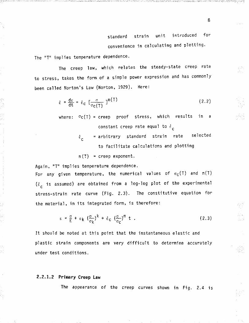
standard stra'in uni t i ntroduced for

conveni ence i n cal cul ati ng and p'l otti ng '

The "T" implies temperature dependence'

The creep 1aw, whjch relates the steady-state creep rate

to stress, takes the form of a simp'le power expression and has commonly

been cal led Norton's Law (Norton , 1929) ' Here:

,-dr-. ¡ o rn(T) Q.Z)E = ãî - ec Loc(T) r

where: oc (T) = creep proof stress , whi ch resul ts 'in a

constant creep rate equal to óa

Ë^ = arb.itrary standard strain rate selectedc

to faci I itate cal cul ations and p1 otti ng

n (T) = creep exponent.

Again, "T" impl'ies temperature dependence.

For any given temperature, the numerical values of oç(T) and n(T)

(Ëc is assumed) are obta'ined from a log-'log plot of the experimental

stress-stra'in rate curve (Fig. 2.3). The constitut'ive equation for

the material, in 'its integrated form, is therefore:

, =Ë*,r (ä)¡aËc (f;)n t. (2.3)

It should be noted at this point that the instantaneous elastic and

plastic strain components are very difficult to determine accurate'ly

under test conditions.

2.2.1.2 Primary Creep l-aw

The appearance of the creep curves shown in Fig. 2.4 is

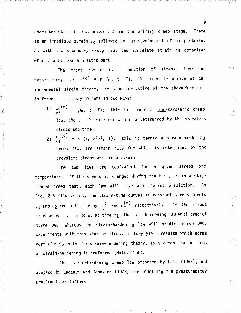
characteri sti c of most materi al s

is an irnmedjate straìn eq followed

As with the secondary creep 1aw,

of an elastic and a Plastic Part.

Ijn the primary creep stage. There

by the development of creep strain.

the jmmediate strain is comprìsed

termed a time-hardening creeP

i s determi ned bY the Preva'lent

The creep strain j s a function of stress, time and

temperature; i.e. ,(c) = f (o, t, T). In order to arrive at an

incremental strain theory, the time derjvatjve of the abovefunct'ion

is formed. Th'is may be done in two ways:

1) *i,t, = e(o, t, T); this is1aw, the strain rate for which

stress and t'ime

z\ q:(t) - h (o, .(c), T); this is termed a strajn-hardenÍngLt dt

creep law, the strain rate for which is determined by the

preva'lent stress and creep strain.

The two I aws are equi va] ent for a qi ven stress and

temperature. If the stress Ís changed during the test, as in a staqe

loaded creep test, each law wil I give a different prediction. As

Fig. 2.5 jllustrates, the strain-time curves at constant stress levels

o1 and 02 are indicated O, .[t) unA .tt) respectively. If the stress

ìs changed from o1 to o2 at time t1, the time-hardening law will predict

curve 0AB, whereas the strain-hardening law will predict curve OAc.

Experiments with this kind of stress history yield results whjch agree

very close'ly with the strain-hardening theory, so a creep law in terms

of strain-hardening is preferred (Hult, 1966).

The strain-hardening creep law proposed by Hult (1966), and

adopted by Ladanyi and Johnston (1973) for mode'l'ling the pressuremeter

probìem is as follows:

10

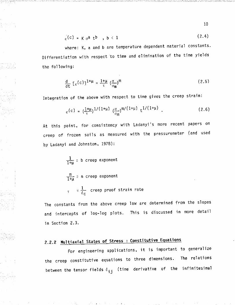
,(c)=4oâ¿b,b(l (2'4)

where: K, a and b are temperature dependent material constants'

Differentiation with respect to time and el'imjnation of the time yields

the fol 'lowi ng:

l¡ r'(c)11+s = +Integration of the above with

.(c) = t$l17(1+u)

t A rllìt-,o¡

respect to time gives

t9-tn/ (l+u) ,1/(1+u)'om'

(2.5)

the creep strain:

(2.6)

At this point, for consistency w'ith Ladanyi's more recent papers on

creep of frozen soils as measured wjth the pressuremeter (and used

by Ladanyi and Johnston, 1978):

creep exPonent

tr= n creeP exPonent

r = f,- creeP Proof strain rate

The constants f rom the above creep I aw are determ'ined f rom the s'lopes

and intercepts of loq-log plots. This is discussed in more detail

in Section 2.3.

2.2.?

For engineering applications, jt is important to generalize

the creep const'itutive equations to three dimensions' The relations

between the tensor fields êr, (time derivatjve of the infinitesjmal

fr=u

l4ultiaxial States of Stress : Constitut

11

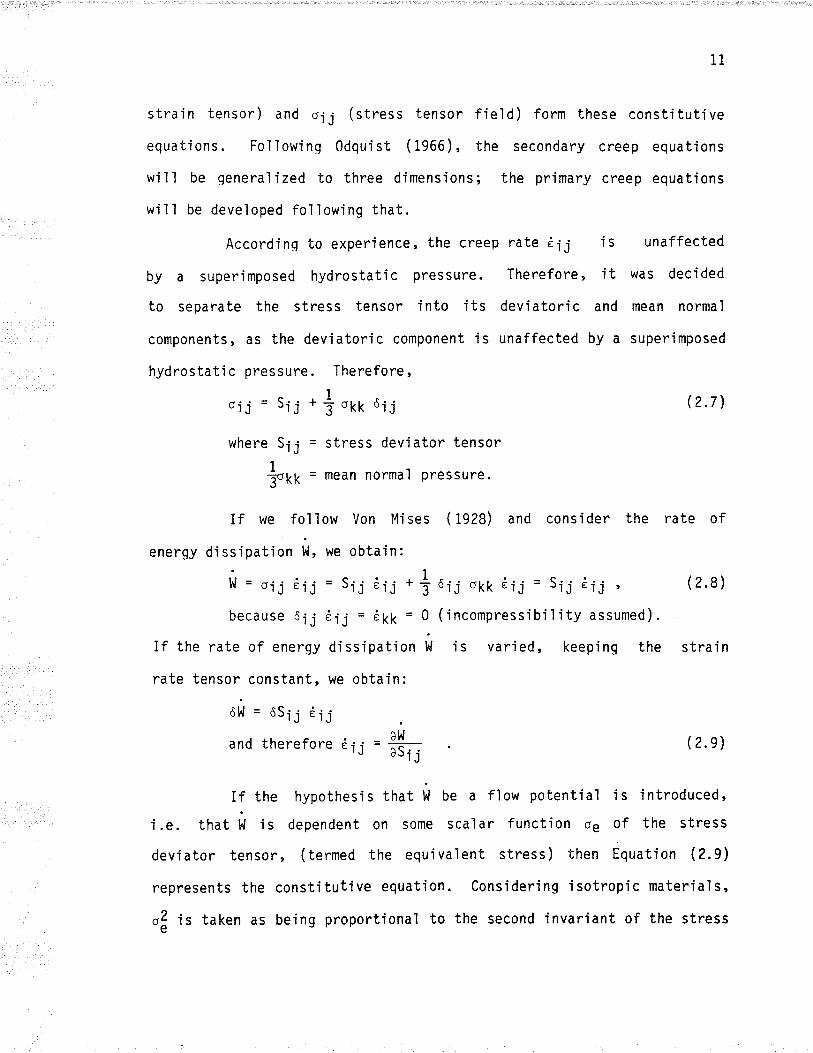
strain tensor) and o.ij (stress tensor field) form these constitutive

equations. Fol'lowjng 0dquist (1966), the secondary creep equations

wjll be qeneraìized to three dimensions; the primary creep equations

wi I I be devel oped fo'l ì owi ng that.

According to experience, the creep rate Ëi¡ is unaffected

by a superimposed hydrostatic pressure. Therefore, it was decided

to separate the stress tensor into its deviatoric and mean normal

components, as the deviatoric component is unaffected by a superimposed

hydrostatic pressure. Therefore,Ioij = S.ij +åotf ôij

where S.ij = stress devi ator tensor

1

t"ft = mean normal pressure.

(2.7 )

( 1928) and consider the rate ofIf we fol low Von Mi ses

energy dissipation ù, *. obtain:

:.. = c, -:.. . 1W = oij rij = Sij å.¡j *T

because ôij Ëij = êkk = 0

If the rate of energy dissipation hJ

rate tensor constant, we obtain:

où = osrj Ëij

and therefore Ëi¡

6ij okk Ëij = Sij Ëtj ,

( i ncompres s i bi 'l 'i ty a s sumed ) .

i s vari ed , keepi ng the

(2.8)

strain

(2.e)

If the hypothesìs that W be a flow potential is introduced,

i.e. that ù 'is dependent on some scalar function os of the stress

deviator tensor, (termed the equivalent stress) then Equation (2.g)

represents the constitutive equat'ion. Considering isotropic materials,

o! is taken as be'ing proportional to the second invariant of the stress

= âl'laSij

T?

deviator tensor. (The influence of the third invariant of the stress

deviator tensor on the creep rate has been found to be neg'ligible

i n most cases (Odqvi st, i966 ) ) . Add'ing the requ'i rement that og shal I

reduce to o1 jn the uniaxial case' we have:

^Z = 3 c.. ç.. (2.10)oe-Z 'lJ -lJ

= 3,rl =2,2 . =]t(oroz)2+ (o2-o3)z+ (o3-o1)21uZ 2 'oct 2

where Jl = second invariant of stress devjator tensor

toct = octahedral shear stress

o!,oZ,o3 = princiPaì stresses.

Carrying out the d'ifferentiation in Equation (2.9):

Ëij =åä"fo=:åå*=å{hT (z.io)

The unjaxial stress case yields:

Sll = 3 "rr, SZZ= S33 = - å ort

From fruati on ( 2. i0 ) :

oe = o11 (2.12)

The requirement that Equation (2.10) w'ill reduce to Norton's Law,

tquation (2.2) (i.e.the uniaxial case) then yields:

. 3dl{ 2oIl . .o11,rìå11 = Ë ¿% å ,i = u. Fa:ì" (2.13\

Therefore:

( 2. 11)

dl,l . "oe'n-

= ^ t-t

doe "c Locl t (2.14)

Thus, subst'ituting Equation (2.L4) into Equation (2.10) yields the

constitutive equation for secondary creep:

i.. = å^ rog.rn I fu- e.r6)tll - 'c \oc, Z oe

Thi s consti tuti ve equati on , therefore , i s founded on the

fol lowing hypotheses:

1) The constitutive equatìon for the uniaxial state of stress

should result when the multiaxial state of stress degenerates

into a uniax'ial one ('i .e. should retain Equati on ?'2) '

2) The equations should express the incompressible nature of

the material, which is a consequence of the plast'ic nature

of creep.

The creep rate is independent of superimposed hydrostatic

pressure.

For an i sotrop'i c medi um, the pri nci paì di rectj ons of the

strain rate and stress tensors coincjde (i'e'a flow potentìaì

exi sts ) .

3)

4)

withù=Ëc(h)t-"Jn*t

An al ternati ve form of Eq uat'ion (2 ' 16 ) ' i n

the equi val ent strai n ) i s favoured by some

Here:

13

(2.15)

terms of rÁt )

(e.9. Ladanyi,

(2.r7 )

[(r1-, z)2 * (ez'es)Z * 1.3-'1)21

( termed

Le7 2) .

(c)ze¿ =

(c) (c)tij 'ij

rr - 1 2Lz - 21'oct2

9

23

43

T4

where Ii = second invariant of the strain deviator tensor

Yoct = octahedral shear strain

E!'e2,83 = PrinciPal strains.

From Equations (2.10) " (2.76) and (2.t7)l

;!c)z = å ru. (ä)'åF, r;. (ä)''åF, ,

Therefore:

;(c)Z ="e

Subst'i tuti ng Equati on (2. 10 ) :

29.)3 4 'c

?úE3;2-e

3.?= z',

roer2n sijsijt%'

-{

;(c)2-e

This reduces to:

(+)2nuc

Therefore:

;(c) = ; fStn"e "C '06'

For primary creep, the same hypotheses stated

hold. Hult (1966) presents the generalizat'ion of the

ìaw (Equation 2.5) to a multiaxÍal state of stress as:

¡(c)2 =-e (ä,";2"c

Aga i n , an a'l ternati ve form of Equati on (Z.tg ) i s

of r[c) and og. First, integrate Equation (2.19)

(2. te)

above shoul d

primary creep

(2.re)

derived in terms

with respect to

15

time and substitute'into tquation (2.17):

.(c)2 = !u Ë.)2(ä)zn(l+u) t,[c) ]-2t'(+)2 s:¿siil t2 Q.z0)

Now substitute Equation (2.10) into Equation (2.20):

2

,[c)z = !u ¿.)2 (ä)"(1+u) t,[c)]-2u (å)' tât q, u (z.zt)

Cance'l ì'ing terms and reduci ng yi el ds :

.[c)z = (Ëclz tfrlzn(t+¡) t.Á., TZv tz Q.zz)

Taking the square root of tquation (2.22) gives:

.Á.) = Ë. (ä)t(l+u) t,jc)l-u t (?.23)

Now, taking the time derjvat'ive of Equation (2.23) yields:

o.Át) =. roern(l+u) [.(c)l-H (2.24)-ar- - ec \om/ t.[c)1-u

Now, considering:

ar[c)(1+u) ' (c)___¡T_ = (1+g) G Á.llu 'åT , and substitutins Equatìon

(2.24) y'iel ds :

(2.25)

Now, integrating Equation Q.25) with respect to time y'ields:

,!c) = [(1+u) Ëc]1/(i+H) tält ¿1l(1+u) 12.26)

i6

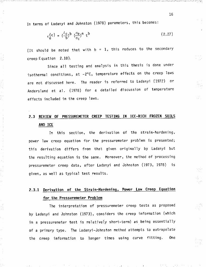
In terms of Ladanyi and Johnston ( 1978) parameters, thi s becomes:

.(c)"e(2.27 )

(lt should be noted that with þ = 1, this reduces to the secondary

creep E quation 2.18).

since all testing and analysis'in this thesis is done under

isothermal condit'ions, at -2"C, temperature effects on the creep laws

are not discussed here. The reader is referred to Ladanyi (I972) or

Andersland et al. (i978) for a detailed discussion of temperature

effects included in the creep laws.

2.3 REVIEH OF PRESSURE}IETER CREEP TESTII{G IH ICE-RICH FROZEil SOILS

AND ICE

In thj s section, the deri vation of the strai n-hardeni ng,

power law creep equation for the pressuremeter probìem is presented;

this derÍvatjon differs from that given orig'inally by LadanyÍ but

the resulting equat'ion is the same. Moreover, the method of processing

pressuremeter creep data, after Ladanyi and Johnston (1973, 1978) is

given, as welì as typicaì test results.

2.3.L tÞriva'!þn of the Strain-Hardening" Powr

for the Pressurereter Problem

The interpretation of pressuremeter creep tests as proposed

by Ladanyi and Johnston (1973), considers the creep information (which

in a pressuremeter test is relativeìy short-term) as. being essent'ial'ly

of a primary type. The Ladanyi-Johnston method attempts to extrapolate

the creep i nformation to I onger times usi ng curvè fittì ng. One

= tïlo (9)n tbuc

t7

important assumption which Ladanyi and Johnston (1973) made is that

the creep is essentiaììy of a stationary type; i.e. that all stress

redistribution from the ínitial elastic state to the limiting statìonary

state has aìready occurred. This assumptìon implies that the elastic

ana'logue method of analysis may be used.

Using the elastic analogue, a prob'lem of nonlinear creep

may be ana'lyzed as a prob'lem in nonl inear elastic'ity by making the

creep strain rate correspond to the elastic strain. l.l'ithout this,

the solution of the nonl inear creep problem would be extremeìy

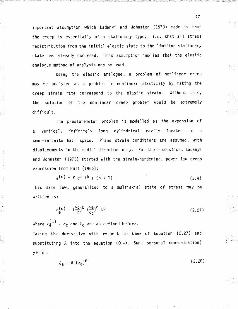
di ffi cul t.The pressuremeter problem is modelled as the expansion of

a vertical, infiniteìy ìong cy'lindrÍcaì cavity located in a

semi-infinite half space. Plane strain conditions are assumed, wìth

disp'lacements Ín the radial direction on'ly. For their solution, Ladanyi

and Johnston (1973) started with the strajn-hardenÍng, power law creep

expression from Hult (1966):

,(c) = K oa tb ; (b < t) (2.4)

This same law, genera'lized to a multiaxial state of stress may be

written as:

.[c) - tïto (fln tu

*n.r. ,[t) , oç ônd Ëç are as defined before.

Taking the derivative with respect to time

substituting A into the equation (Q.-X. Sun,

yields:

(2.27 )

of Equation (2.27) and

personal communi cati on )

Ëe = A (os)n (2.28)

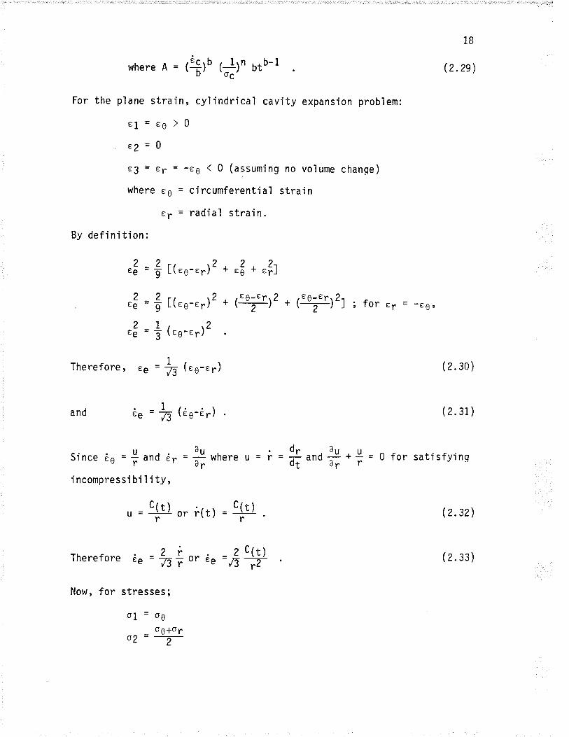
where u = (T)o ftålt utb-l

For the pìane strain, cylindrica'l cavity expansion prob.lem:

e1 = ee ) 0

e2=0

e3 = er = -ee < 0 (assuming no volume chanqe)

where eg = circumferential strain

e, = radiaì strain.

By definition:

,'" = Ê [(rs-r¡)' * râ + r?]

e3 = Ê [(16-.¡)2 * ,eø--er¡z * (er")z); for e¡ = -esr

? L, ,2re = T (eg-e¡)

Therefore, Ee = fu tr6-.¡)

and ¿.=å(;u-;r)

Therefore ¿" = 13i or^ ;. =åryNow, for stresses;

o1=o0_ og*o¡

o2 - -z-

. u au dr ,âuSince Ëe = ïand ð" = fr where u = i = fr and ãi -+ = 0 for satisfyinq

i ncompressi b'i I i ty,

,=Pori(r)='lr). (2.s2)

1B

(2.2e)

(2.30)

( 2. 31)

(2.33)

19

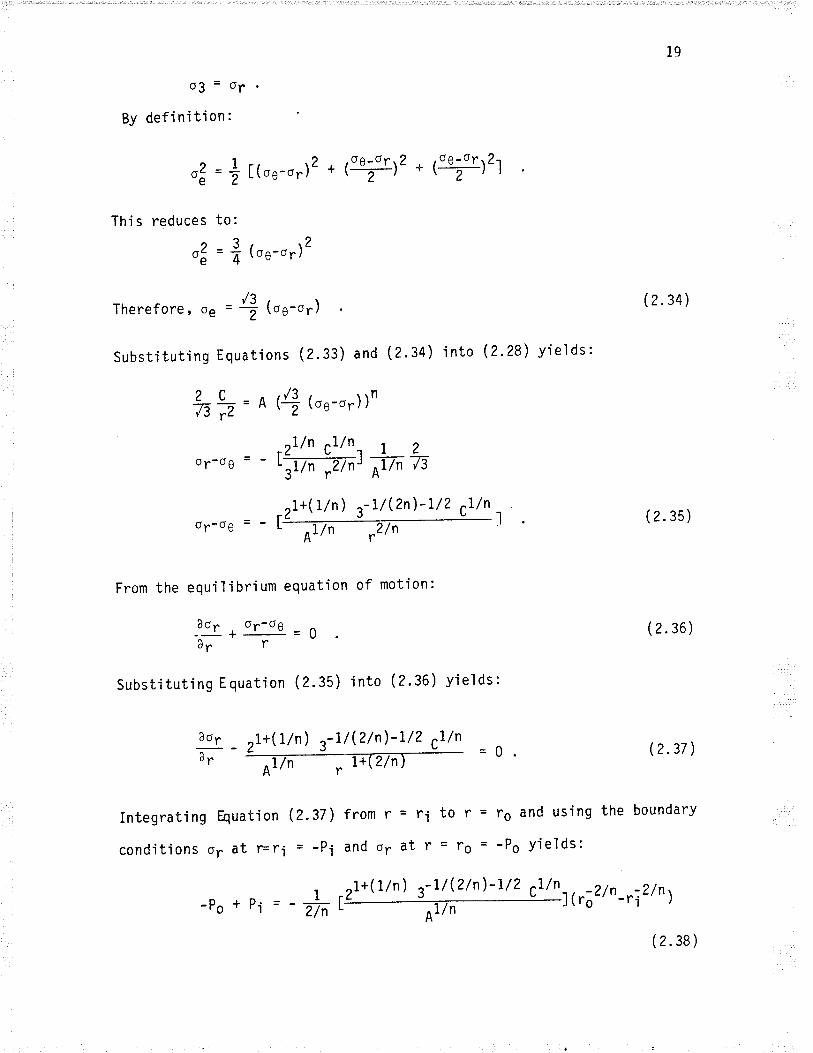
"r"=+[(os-o¡)z o ('-zo')z o ('io')2]

This reduces to:

4 = + (os-o')2

Therefore, oe = $Gu-or)

Substitutìng Equations (2.33) and (2'34) into (2'28) yields:

%þ= o (+ (os-o¡))n

.ZL/n Clln. I zor-oo = - tTnTntpn

_ ,rL+(L/n) ,-t/(2n)-t/2 ,r/n a (2. gs)of-og=-L '

From the equ'i I i bri um equati on of moti on :

o3=or'

By defìnition:

-aa*or-oo=oar r

Substitut'ing Equation (2.35) into (2.36) vields:

(2.34)

(2.36)

âor 2I+(I/n) 3-1l(2/n)-L/2 "l/na. ---Fn

, =0' (2'37)

IntegratÍng Equation (Z.Sl) from r = ri to r = re and using the boundary

condit'ions o¡ at r=ri - -P1 and o¡ at r = Fo = -Po yieìds:

-po+Pi =-+ )ft-o2/n-,:2/n¡

(2.38)

20

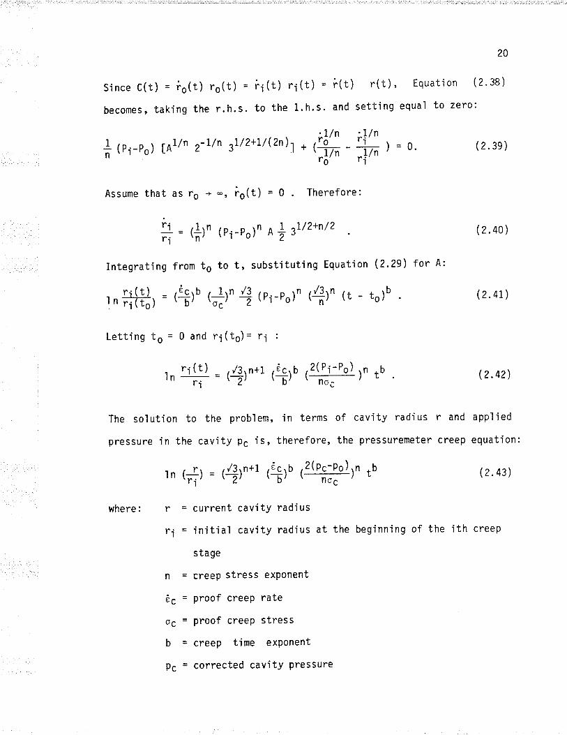
since c(t) = io(t) rs(t) = ii(t) ri(t) = i(t) r(t), Equation (2'38)

becomeso taking the r.h.s. to the 1.h's' and settjng equaì to zero:

f rni-eor [n1ln ,-L/n 3L/2+r/(2n)r * ,# #) = 0. ( z.3s)

Assume that as fo * -, io(t) = 0 Therefore:

*=tlln(Pi-Po)n a!{/z+ntz (2'40)ri

integrating from to to t, substituting Equation (2.29) for A:

l. ii{*) = tflo ,rå,n 5 ,r,-Po)n tfl' 1t - to)b . ( 2'4r)

Lett'ing to = 0 and ri(ts)= ri :

r,' + = rSln*t t*tu 12(ij:Po) )n tb . (2.42)

The solution to the problem, in terms of cavìty radius r and applied

pressure in the cavity pc is, therefore, the pressuremeter creep equation:

ln (+) = ($)n*t tïlo,3Q;,|o)-)n tb (2.4s)

where: r = current cav'ity radius

r.i = jnitial cavity radius at the beginning of the ith creep

stage

n = creep stress exPonent

Ëç = Proof creeP rate

oç = proof creep stress

b = creep time exPonent

Ps = corrected cavitY Pressure

2T

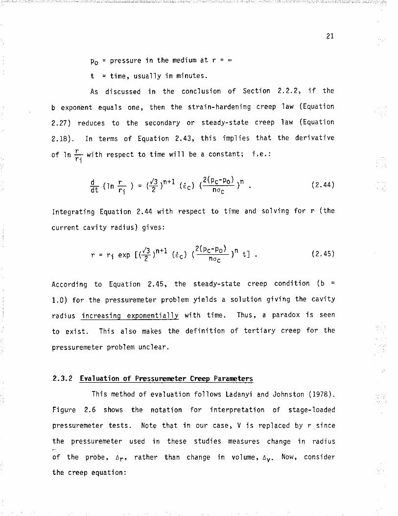
Po = Pressure in the medium at r = -t = time, usually in mínutes.

As díscussed in the concl usion of Section 2.2-2, if the

b exponent equals one, then the stra'in-hardening creep'law (Equation

2.27) reduces to the secondary or steady-state creep law (Equation

2.L8). In terms of Equat'ion 2.43, this implies that the derivative

of ln rri with respect to time will be a constant; i.e.:

Integrat'ing Equati on 2.44 with respect to time and so'l vi ng

current cavíty radius) gives:

r = ri exp [{f )n*i {e.) ,t!# )n t]

dUT

(2.44)

for r ( the

(2.4s)

According to Equation 2.45, the steady-state creep conditÍon (b =

1.0) for the pressuremeter problem y'ields a solution giving the cavity

radius increasinq exponentially with time. Thus, a paradox is seen

to exist. ThÍs also makes the definition of tertiary creep for the

pressuremeter problem unclear.

2.3.2 Evaluation of Pressurereter Creep Parar¡eters

ThÍs method of evaluation folìows Ladanyi and Johnston (1978).

Figure 2.6 shows the notation for interpretation of stage-loaded

pressuremeter tests. Note that in our case, V js replaced by r since

the pressuremeter used in these studies measures change in radius

of the probe, a' rather than change in volume, av. Now, consider

the creep equation:

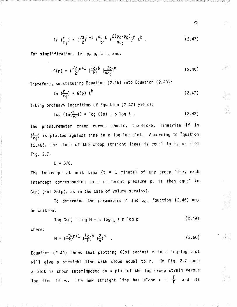
ln (fr) =

For simp'lification,

r4tno' tTlo (+#d)n tb

let p.-po = p, and:

22

(2.43)

(2.46)

(2.47 )

12. so)

I og- ì og p'lot

Fig. 2.7 such

strain versustr

È and its

G(p) = tþtn*'tTlo (r*)'

Therefore, substitut'ing Equation (2.46) into Equation (2.43):

ln (:) = G(p) tb'ri

Taking ordinary logarithms of Equation (2.47) yields:

log (tn(f¡)) = los G(p) + u'los t (2.48)

The pressuremeter creep curves shoul d, therefore , I'i neari ze i f I n

(ä) i s pìotted against time in a 1og-'log p1ot. According to Equation

(2.48), the s'lope of the creep straiqht I ínes is equa'l to b, or from

Fig. 2.7,

b = D/C.

The intercept at unìt time (t = 1 minute) of any creep l'ine, each

i ntercept correspondi ng to a d'i fferent pressure P , ì s then equaì to

e(p) (not 2G(p), as in the case of volume strains).

To determine the parameters n and oc, Equation (2.46) may

be wri tten:

log G(p) = log l'l - n logo. + n log P

where:

, = ($)n*t tïlo tåln

Equation (2.49) shows that p'lotting e(p) aqainst p in a

will give a straight line with sìope equal to n. In

a p'lot is shown superimposed on a pìot of the log creep

log time lines. The new straìght line has s'lope rì =

(2.4e)

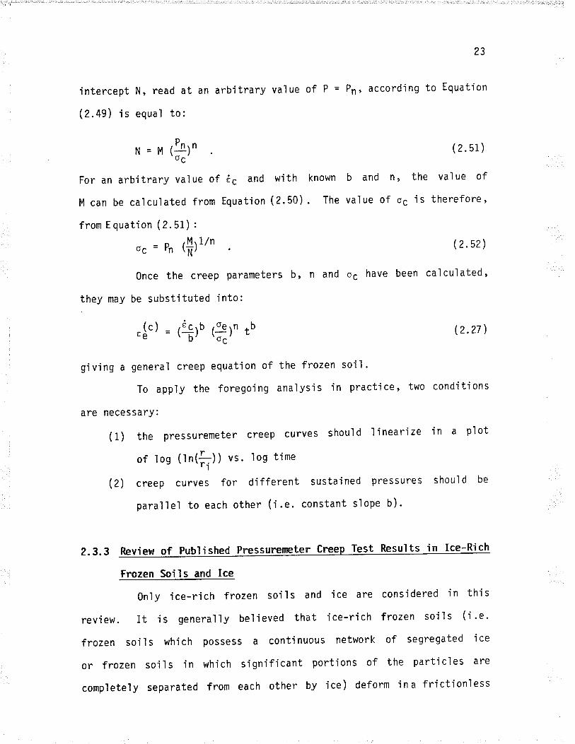
intercept N, read at an arbitrary value of P =

(2.49) is equal to:

23

P¡, ôccording to tquation

N = M tbln (2.5i)'oç'

For an arbítrary value of Ëc and with known b and n, the value of

M can be calculated from Equation (2.50). The value of os is therefore'

from E quati on (2.51) :

oc = Pn (frltun

Once the creep Parameters b, n and oç

they may be substituted into:

.!') = tïlo tffln tb

(2.52)

have been cal cul ated,

(2.27 )

g'iving a general creep equation of the frozen soil'

To apply the foregoing analysis in pract'ice, two conditions

are necessary:

( 1) the pressuremeter creep curves should I inearize in a pìot

of los (rn(fi)) vs. los time

(Z) creep curves for di fferent sustaj ned pressures shoul d be

paral'leì to each other (i .e. constant slope b)'

2-3.3 Review of Pubìished Pressureneter Test Results in lce-Rich

Frozen Soils and lce

0nìy ice-rich frozen soi I s and ice are considered in thi s

review. It is generaì'ly believed that ice-rich frozen soils (i.e.

frozen soi I s whj ch possess a conti nuous network of segregated i ce

or frozen so'ils in which significant port'ions of the particìes are

completely separated from each other by ice) deform ina frictionless

24

manner and display marked secondary creep (e.g. Andersland et â1.'

1978; Morgenstern et âl . , 1980; þ{eaver and Morgenstern , 198ia ) .

Moreover, the creep (flow) law for ice'is considered to form an upper

limit to the 'long-term creep of ice-rich frozen soils. Ice-poor frozen

soi'ls, on the other hand, such as frozen sands, would deform in a

frictional manner and woul d normal 1y not di sp1 ay secondary creep,

unless under extremeìy high loads. In addition, the assumption of

no volume change would be more nearly satisfied in ice-rich frozen

soi I s than ice-poor frozen soi I s (assuming that consol idation of

unfrozen water is not significant). Therefore, it is felt that the

hypotheses of vol ume constancy and no effect of a superimposed

hydrostatic stress on the creep rate (i.e. frictionless behaviour)

Ín deriving the creep laws are more close'ly satisfied for ice-rich

frozen soÍls and ice than ice-poor granu'lar soils such as frozen sands.

(For a review of the creep properties of frozen sand as measured by

the pressuremeter, the reader is referred to Fensury, 1985.)

Ladanyi and Johnston (1973) carried out pressuremeter creep

tests in ice-rich frozen soil at Thompson, Manitoba. Ladany'i (1982b)

presents results of pressuremeter creep tests in ice-rich frozen soil

near Inuvik, N.tl.T. Ladanyi and Saint-Pierre (1978) and Ladanyi et

al. (I979) present results of pressuremeter creep tests in an Arctic

Sea ice cover and laboratory, fresh water ice. Important fìndings

and results from these papers are sulnmarized below.

Ladanyi and Johnston (1973) is believed to be the firstpaper pub'lished on the measurement of creep properties of frozen soil

using the pressuremeter. Their study was conducted in ice-rich frozen

cl ay and si I t at Thompson , l,lani toba. Both mul ti stage pressuremeter

25

creep tests, with 15 minutes per stage, and single stage creep tests'

'lastíng s1ìghtly over 300 minutes in duration, were carried out with

a Menard pressuremeter. Permafrost temperatures were quite warm'

rang'ing f rom -0. 10'C to -0. 30'C.

Figure 2.8' presents the results of a multistage test, while

Fig. Z.g presents a single stage test. Note that volume strains are

used and the creep parameters are evaluated in terms of Hult (1966)

parameters.

Ladany'i and Johnston report that the creep I ines (as in

Fig. 2.8) for the multistage tests were neither straight nor paralleì.

i'Nevertheless, they appeared to linearize better in one-stage tests

than in multistage tests and showed a tendency to become paralle'l

after 15 minutes. " They therefore consÍdered the creep curves in

the multistage tests as being paraìle'l after 15 minutes, and fjt a

line wÍth an average sìope b to each pressure interval. These creep

línes were proiected back to L minute, where the intercept values

were p'lotted against pressure to obtain n and os. In the tests

performed in the ice-rich varved silt, it was found that the value

of b ranged from 0.4 to 0.67 while m varied from 2 to 4, givìng a

poss'ib'le range in n from

and analysi s, i t woul d

per stage Yield results

much judgement.

L.3 to 2.7. From this initial testing program

appear that multistage tests of 15 minutes

which are difficult to interpret, requ'iring

Ladany.i (1982b) presents the results of pressuremeter creep

tests carried out in ice-rich sil ts and cl ays near Inuv'i k, N 'l.l'T'

Permafrost temperatures varjed from -1.5'C (at 1.5 m depth) to -2'40"C

(at 2.26 m depth). These creep tests were performed with conventional

26

F4enard pressuremeter equipment.

A total of 11 borehole creep tests þrere carried out. Three

hrere mul ti stage w'ith 15 mi nutes per stage , one was mul ti stage wi th

60 minutes per stage while the remaining seven tests were medium-

and'long-term single stage creep tests with creep periods of up to,

and over, ?4 hours. Table 2.L presents a review of data obtained

in these tests. The plotted creep information from some typical tests

carried out at the s'ite is presented in Figs. ?.10 to 2.I2. The

procedures used for determining the creep parameters b, n and oç are

the same as discussed previousìY.

0f interest is the fact that, in all of the multistage creep

tests, the exponent b showed an increase with increasing pressure

from about 0.38 to 1.00. For the purposes of determining values of

n and oc, Ladanyì adopted an average value of b. As shown in Table

2.!, these average values vary between, approximately, 0.7 and 0.8.

Ladanyi has proposed two solutions to this problem of b being

stress dependent:

1) make the b parameter stress dependent through an equation

2) use separate b va'lues for each pressure range, SâY, low,

medium and high; the ones corresponding to the stress range

in the particular problem being considered may then be used.

Using average b values, the n exponent is found to range

from 2.37 to 2.84 and oç from 0.446 to 0.731 MPa (using éç = 19'57min).

0f interest in the determination of the n exponent is the curvature

in the low stress range of the log 2F (pi - po) versus log (pi - po)

p'lots on Figs. 2.10 and 2.IL (pl = Pc'in Equation 2.43). Ladany'i

has ignored the first few stages in determining the n value' Th'is

27

is particularly interesting since the b s'lopes have already been

"fi tted" , usi ng judgement.

The ìong-term, sing'le stage tests (Fig. 2.L2) are reìati vely

para'l'leì and have less scatter in their average b value than the

multistage tests (except for the test at the lowest stress). If the

intercepts of these tests were plotted against pi - Po to determine

rì, the lowest stress test would most ìike'ly be anomolous, as is the

case with the lowest stress increments of the multistage tests.

Therefore , three apparent di ffi cul ti es i n the processi ng

of pressuremeter creep data seem to arise in this paper:

1) tne cr-eep lines are not straight, but curve w1th time

2) the b exponent appears to be stress dependent

3) the plot of log 2F (pi - po) versus log (pi - po) (the slope

of which gives the n exponent) appears to be curved in the

low stress region.

Ladanyi and Sa'int-Pierre ( tgZA) present the results of

pressuremeter creep tests conducted in a seasonal Arctic sea ice cover

at Igloolik, N.lll.T. The cover, which was about 1.5 m thick' was

comprised of columnar-grained ice of type S2; i.e. the optical c

axis of the crystaìs was horizontal. The ice also had a high content

of air bubbles in the top 20 cm. The ice temperature at the level

of most of the tests (about 50 cm below the ice surface) was about

-4oC. A Henard pressuremeter was used to conduct the creep tests'

In this study, a total of 10 creep tests were performed;

6 were short-term, multistage and 4 were single stage, long-term creep

tests. The results of analysis of these tests are presented in Table

2.2. In addition, the last stage of short-term, mu'ltistage tests

28

3,5and?2washe]dforupto20minutes.Theinformationfromthislastcreepstageisa]sopresentedinTable2.2.Thedurationofeach stage 'ln the multistage tests was 15 minutes, except for test

no.l3,whjchhad30mìnutesperstage.Thecreeptimeinthesing.le

stage tests varied from 75 to 720 mìnutes'

The creep parameters shown in Table 2.2 were determjned

in the standard way (Ëc = 1g-S¡min). It is seen that, within the

creep test pressure range of L to 3 MPa, the exponent b showed an

increase from 0.?2 to 1.0, which means that a condition of steady-state

creep was approached at higher pressures. For determìning the values

of n and oc, an average value of b, taken at 15 minutes for the high

stress range, had to be adopted. A general average value of b = 0'822

was determined.

Fi gures 2.13 and 2.I4 present pl ots of an examp'le of a

multistage creep test (test no. 14) and the singìe stage tests' The

standard method of derivation of the creep parameters is shown. Figure

2.13.illustrates again that the creep lines in the 15 minute stages

are not particu'larly "well behaved" (accord'ing to the model ) and

some interpretation i s needed in drawing the "para1 ìel " b I ines '

Moreover, the plot of log 2G (pc -po) versus log (pc - po) is again

curved in the low stress region. 0f the most reliable tests (in the

opinion of Ladanyi and Saint-Pierre), n varied from 2.05 to 2'18 with

an average of z.IL and oç varjed from 0.184 to 0.634 MPa, wjth an

average of 0.394 MPa. The'long-term tests p'lotted in F'ig. 2.74 show

that there is a tendency for b to decrease with time.

Ladanyi and saint-P'ierre claim that the n values are probably

low because the b exponents were determjned at a creep time of only

?9

15 minutes, meaning that the ice was stjll in primary creep. They

would have anticipated values closer to 3 'if the b values had been

determined at a longer time. An n value of 3 is generally thought

to represent the steady-state creep of ice (e.g. Morgenstern et ä1.,

1980; Sego, 1980 ) .

Ladanyi et al. (1979) present the results of di'latometer

relaxation testing in laboratory prepared samples of fresh water ice'

Accord'ing to Ladanyi et â1., the creep parameterS b, n and oç may

be determined from relaxation test data by approximate techniques.

These results are presented here because they are the on'ly known results

of any kind of pressuremeter or dilatometer testing jn fresh water

i ce.

The results are interesting for a number of reasons' First'

Ladanyi et al . note that radial cracking deve'loped very ear'ly on in

the tests, which were conducted in unconfined ice cyìinders' Moreover'

total failure was reported to have occurred at ln (fr, = SZ. Therefore,

these tests could not be run to ìarge strajns without cracks developìng

or comp'lete failure. Secondly, the creep parameters b, n and os seem

quìte dependent on the amount of strain the ice sample has undergone'

For example:

1) in the low strain region, ln (ï^ ) < 2'48%;YO

b = 0.14, n = 1.10, oc = 63'4 MPa at ðç = 10-5/min

2) in the medium strain range,2.¿18 ( jn tfl < 3'63%;'Vg'

b = 0.28, n = 1.75, oc = 7.49 MPa at Ëç = 10-57m'in

3) in the high strain range, f n (fr) > 3'63%;

b = 0.42, n = 2.40, oc = 2'60 MPa at ê. = 10-5/tin'

30

2"3.4 Sumnary

To date, therefore, there is no long-term ('i.e. greater

than about 24 hours) creep data which supports the use of the

strai n-hardeni ng, power I aw creep theory i n the anal ys'i s of

pressuremeter creep tests in ice-rich frozen soils and ice. Moreover'

the results presented in the last subsection indicate that a degree

of judgement is required ín processing the pressuremeter creep resuìts;

i.e. the creep lines are often not linear, and therefore a tangent

at 15 minutes is used, and the b exponent ìs found to be stress level

dependent. In fact, Ladanyi et al. (1984) address these very problems.

Using a finite element simulation of the borehole creep

test, Ladanyi et al. (1984) performed a parametric study to evaluate

the minimum time under a g'iven load to actually approach a condìtion

of stationary creep. (Recal I that the derivat'ion of the

strajn-hardening creep 1aw, using the elastic analogue, has assumed

that a cond'ition of stationary creep already exists.) Usìng the test

results for sea ice from Ladany'i and Saint-Pierre (tgZg) as a basis,

they show that about 4 to 5 hours, and up to 7 hours are required

for the stresses to approach the stat'ionary state for appl ied pressures

in the range I to 2.5 MPa. This study indicates, therefore, that

times much longer than 15 or 30 minutes are required to proper'ly

determjne the creep parameters of ice with the pressuremeter. The

data presented in thìs thesis will, therefore, attempt to fil I in

the void in the long-term pressuremeter creep data'in ice and answer

some of the questÍons which Ladanyi'et al. (1984), with their finite

element anaìysis, have posed.

Now that the pressuremeter test itself has been reviewed,

31

the next section díscusses the use of the pressuremeter test to give

creep parameters which may be used to predict creep settlements of

foundations resting on ice-rich frozen soil or ice.

2"4 SOLUTIO}IS TO SELECTED Bü'NDÂRY-VALUE-PROBLEÞIS APPLIED TO ICE OR

ICE-RICH FROZEN SOILS

As has already been discussed, Ladanyi (I972) adopted the

power law theory to describe the creep of frozen soils because it

was a relatively simpìe mathematical expression which al lowed the

solution of relatively complex boundary-va'lue-problems to be found.

ñormal design procedures involvíng structures founded on ice or ice-rich

frozen soil involve an estimate of the creep settlement. In order

to estimate creep settlements, values for the creep parameters appearing

in the solution for the boundary-value problem must be determined.

Intu'it'ive1y, and as indicated by Sego (1980), an accurate assessment

of the parameters governing creep in the field can be gained only

through in situ testìng as compared to ìaboratory testing. The

pressuremeter test, as was first indicated by Ladany'i, is a promising

in situ procedure. The sol utions to a number of typical

boundary-val ue-prob'l ems i nvol vi ng creep are presented . From thj s

presentat'ion it will be Seen which creep parameters are required,

and which of these parameters are the most important.

2.4.L Grouted Rod Anchors in Permafrost (Johnston and Ladanyi, 1972)

The anchor rod sol uti on has al so been appl ì ed to the

steady-state creep of friction pi'les embedded in ice or. ice-rich frozen

soils (bV Nixon and McRoberts, I976; Morgenstern et ô1., 1980 and

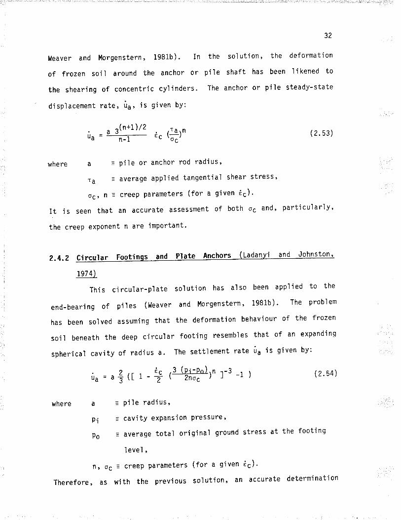
Heaver and Morgenstern, 1981b). In

of frozen soi I around the anchor or

the sheari ng of concentri c cy'l i nders .

di spl acement rate, ùu , i s g'i ven bY:

the sol uti on ,

p'ile shaft has

The anchor or

32

the deformation

been likened to

pi le steady-state

. a t(n+l )/2tl =ua n-1

T¿

¿. (ä)n

= pile or anchor rod radius'

= average applied tangential shear stress'

- Ëc ,3 (pi-pn))n l-3 _t )t-7 1 Znoc

(2.53)

(2.54)

êc)'

accurate determìnation

oç: Iì = creep parameters (for a given Ës)'

It is seen that an accurate assessment of both oç and, particularly'

the creep exponent n are important'

2-4.2 Circular Footi and PIate Ãnchors Ladan and Johnston,

Le7 4)

Thi s ci rcul ar-pì ate sol uti on has al so been app'l 'ied to the

end-bearing of piles (l,leaver and Morgenstern, 198ib) ' The problem

has been solved assuming that the deformat'ion behaviour of the frozen

sojl beneath the deep circular footing resembles that of an expanding

spherical cavity of radius a. The settlement rate ùu is given by:

where a

lì, OC

Therefore, as

ùa=â

where a

pí

po

å rr

= pi ìe rad'ius,

= cavity exPansion Pressure'

=averagetotaloriqjnalgroundstressatthefootinglevel,

= creep parameters

with the previous

(for a g'iven

solution, an

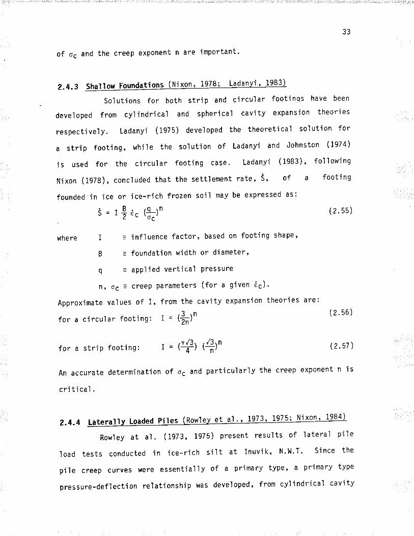
33

of os and the creep exponent n are important'

2.4.3 Shallow Foundations (Njxon, 1978' Ladanvi' 1983)

Solutions for both strip and circular footinqs have been

deveìoped from cyì indrica] and spherica'l cavity expans'ion theories

respectively. Ladanyi (1975) developed the theoretical solution for

a strip footing, while the solution of Ladanyi and Johnston (1974)

is used for the circular footing case. Ladanyi (1983)' following

Nixon (lg7$), concluded that the settlement rate, S, of a foot'ing

founded'in ice or ice-rich frozen sojl may be expressed as:

S = ,9, ,. (f;)n (2.55)

where I = i nf 'l uence factor,

B = foundat'ion width

q = applied vertical

tì, oc = creep parameters

Approximate values of I, from the cavity expansion theories are:

for a circular footing: I = (*)n

based on footing shaPe'

or diameter,

pressure

(for a gìven Ës).

(2.56)

for a strip footing: r = (+) tfl' (2.57 )

An accurate determination of oç and partìcularly the creep exponent n is

critical.

2.4.4

Rowley at al. ( 1973, 1975) present results of lateral pi'le

load tests conducted in ice-rjch silt at Inuvik, N.l'l.T. Since the

pile creep curves were essentialìy of a prìmary type, a primary type

pressure-deflection relationship was developed, from cyìindrical cav'ity

Laterallv l-oaded Piles (Rowley et al" 1973' 1975; Nixon' 1984

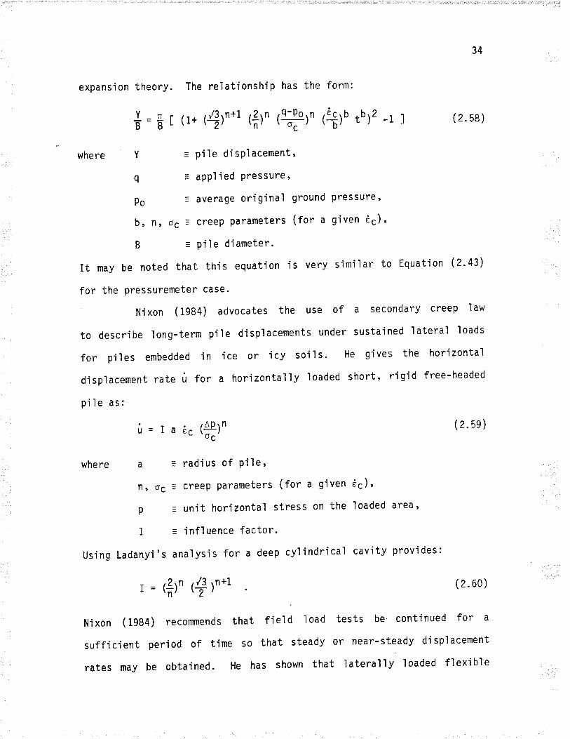
34

expansion theory. The relationship has the form:

(r* (4)n*1 t*t' tl3l' tb)Z -t:ì (z.sa)rïroY-rrE'-EL

where Y

q

po

b, fl,

B

= p'i 1e di sPl acement '

= appl i ed pres sure '

= average origina'l ground pressure'

oc = creep parameters (for a given Ës),

= piìe diameter.

It may be noted that this equation is

for the pressuremeter case.

very simjlar to Equation (?.43)

Nixon ( 1984) advocates the use of a secondary creep law

to describe long-term p'ile disp]acements under sustained lateral loads

for piles embedded'in ice or icy soils. He gives the horizontal

dispìacement rate ù for a ho¡izontalìy loaded short, rigid free-headed

pile as:

ú=ra;c(fl)n (2.5e)

where a

lì¡ OC

p

I

Usi ng Ladanyi 's cavìty provides:

r = (å)n tf ln*t (2.60)

N.ixon (1984) reconrmends that field load tests be continued for a

suff.icient period of time so that steady or near-steady disp'lacement

rates may be obtained. He has shown that lateral'ly'loaded flexible

= radius of pi1e,

= creep parameters (for a given

= unit horizontal stress on the

= influence factor.

anal ysi s for a deeP cY'l i ndri cal

e6J r

loaded area,

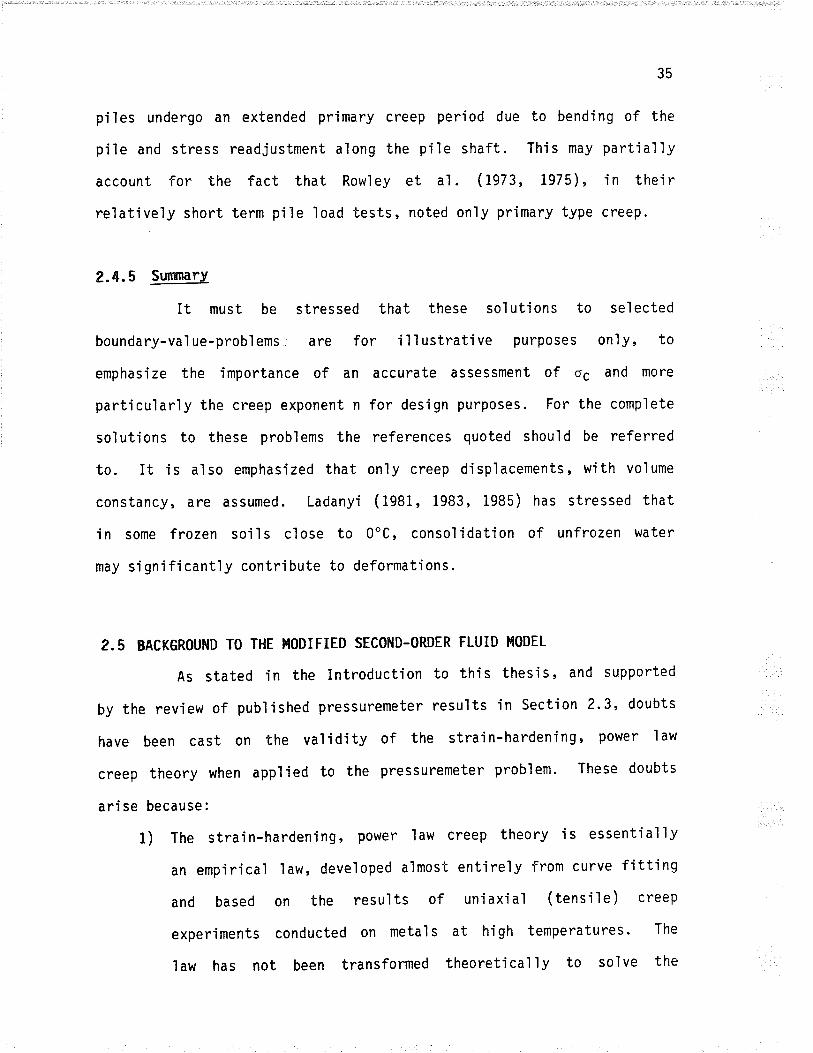
35

pÍles undergo an extended primary creep period due to bending of the

pi'le and stress readjustment aìong the pile shaft. This may partial'ly

account for the fact that Rowìey et al. (1973, 1975), in their

relatively short term pile load tests, noted only primary type creep.

2.e,.5 St¡rrnary

It must be stressed that these solutions to selected

boundary-vaìue-problems, are for illustrative purposes on'ly, to

emphasize the importance of an accurate assessment of oç and more

particularly the creep exponent n for design purposes. For the complete

solutions to these probìems the references quoted should be referred

to. It is also emphasized that only creep d'isp'lacements, with volume

constancy, are assumed. LadanyÍ (198i, 1983, 1985) has stressed that

in some frozen soils close to 0oC, consolidation of unfrozen water

may significantly contribute to deformations.

2.5 BACKGROUND TO THE I'IODIFIED SECOND-ORDER FLUID HODEL

As stated in the Introduction to this thesis, and supported

by the review of published pressuremeter results in Section 2-3, doubts

have been cast on the validity of the strain-hardening, power law

creep theory when app'l i ed to the pressuremeter prob'l em. These doubts

arise because:

l) The strain-hardening, power law creep theory is essentiaì'ly

an empirical law, developed almost entire'ly from curve fitting

and based on the results of uniaxial (tens'i1e) creep

experiments conducted on metals at high temperatures. The

'law has not been transformed theoreticaì ly to solve the

36

three-dimensional (multiaxial) case; rather, âr equiva'lent

stress and an equiValent strain (oe and .e) were s'imply

substituted into the one-dirnensional model.

2) The model incorporates the infinitesimal strain tensor, which

shoul d only be used for smal I di spl acements. Creep

díspìacements are often large.

3) As the last sections have indicated, evaluatÍon of the creep

parameters for this model is often ambiguous, with the main

prob'lem being the variation of b with both time and pressure.

The select'ion of b Ís critical, since b is not onìy the

exponent of the time in the creep equation, but also enters

into the determination of n and oç. The use of a stress

dependent b, as in Ladanyi and Eckardt (1983) and Fensury

(1985), is an attempt to solve at least part of this probìem,

but the necessary conditions for the vaìid'ity of the model

(i.e., linear, parallel creep lines) have been violated.

4) The model cannot represent both primary and secondary creep

at once . If b < 1 , then the primary, or attenuat'ing port'i on

of the creep curve may be represented. If extrapolated to

longer times and larger strains, however, the use of b less

than 1 may be in serious error. If b - 1, then secondary

creep may be representêd, but the primary part of the creep

curve must be accounted for separately'

llith these thoughts in mind, Man et al. (1985) set out to

theoretica'lly develop, from continuum mechanics principles' a reasonabìy

simp]e creep model which could represent both prima¡y and secondary

creep, as well as capture the nonlinear dependence of the secondary

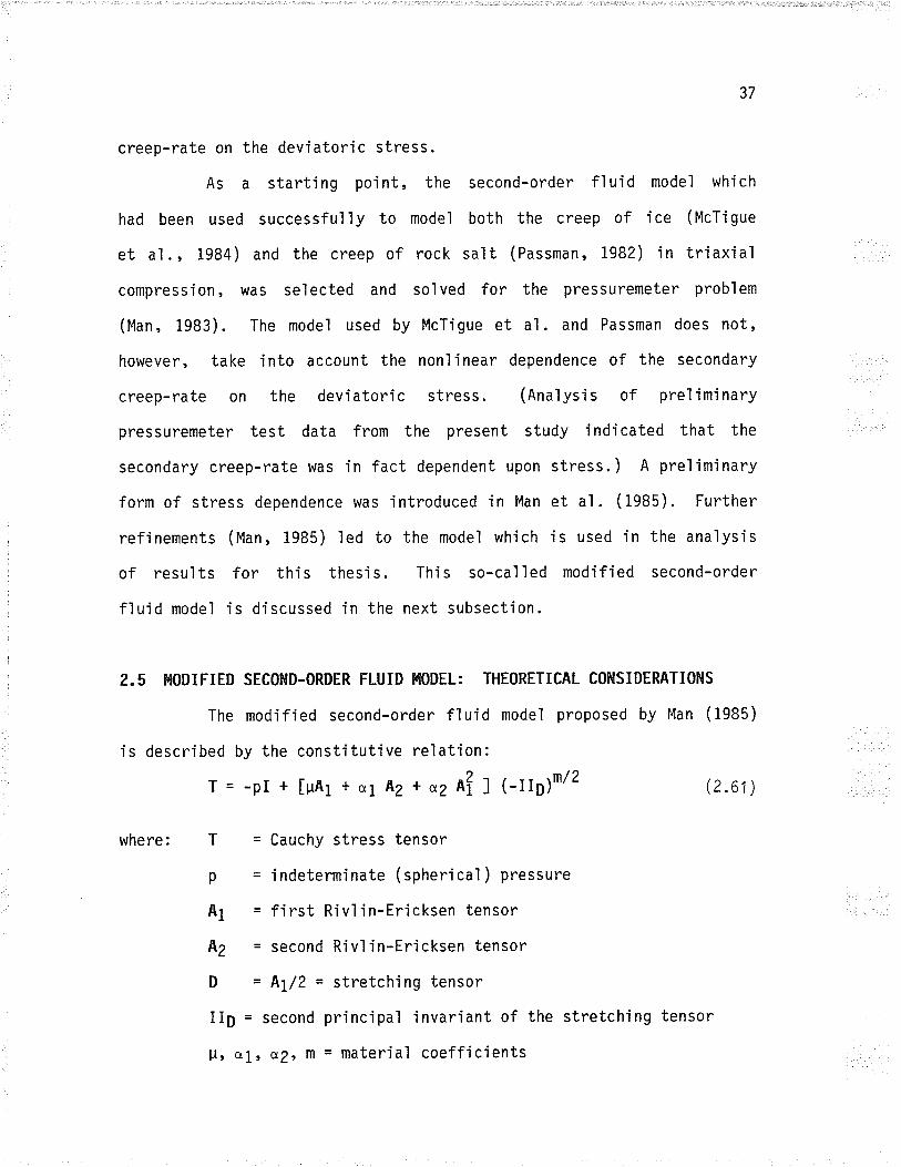
37

creep-rate on the deviatoric stress.

As a starting point, the second-order fluid model whjch

had been used successfu'l1y to model both the creep of jce (McTigue

et â1., i984) and the creep of rock salt (Passman, 1982) in triaxial

compression, was selected and solved for the pressuremeter probìem

(l'1an , 1983) . The model used by McT'igue et al . and Passman does not,

however, take into account the nonlínear dependence of the secondary

creep-rate on the devi atori c stress. (Analysi s of prel imi nary

pressuremeter test data from the present study indicated that the

secondary creep-rate was in fact dependent upon stress.) A preliminary

form of stress dependence was introduced in Man et al. (1985). Further

refinements (Man, 1985) led to the model which is used in the analysis

of results for this thesis. This so-called modified second-order

fluid model is discussed in the next subsection.

2"5 HODIFIED SECOND-0RDER FLUID HODEL: THE0RETICAL CO$ISIDERATI0NS

The modified second-order fluid model proposed by l4an (1985)

is described by the constitutive relation:

T = -pr + [unr + ur Az + a2 A! ] (-Iro)*/2 (2.61)

where: T = Cauchy stress tensor

p = indeterminate (sphericaì) pressure

A1 = first Rivlin-Ericksen tensor

A2 = second Rivlin-Ericksen tensor

D = A1/2 = stretching tensor

IID = second principal invariant of the stretching tensor

H, al , aZ, m = material coefficients

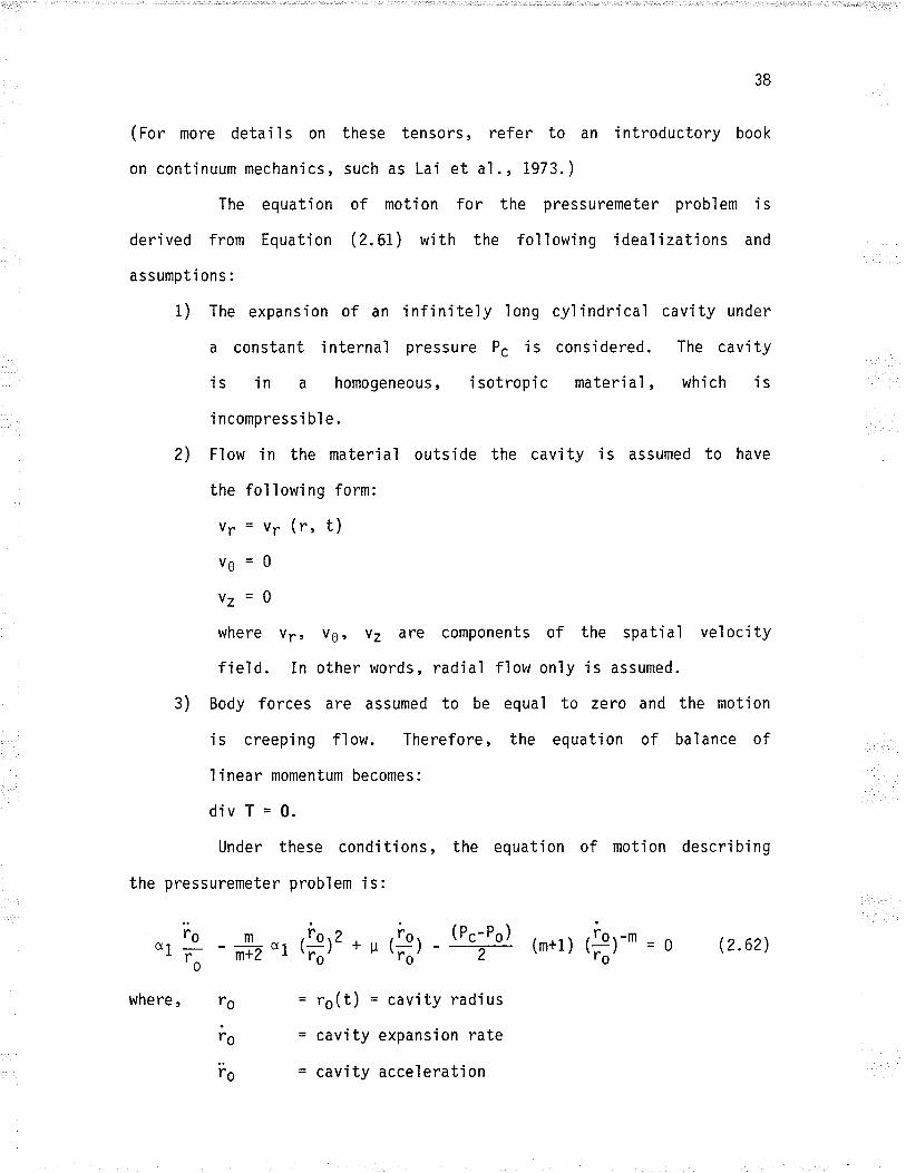
38

(For more details on these tensors, refer to an introductory book

on continuum mechanics, such as Lai et al., 1973.)

The equation of motion for the pressuremeter probì em i s

deri ved from Equatì on (2.6L ) wj th the foì 'lowi ng i deal i zat'ions and

assumpti ons :

1) The expansion of an infin'itely long cylindricaì cavity under

a constant Ínternal pressure Pc is considered. The cav'ity

is in a homogeneous, isotropic material, which isincompressíble.

2) Flow ín the material outside the cavity is assumed to have

the folìowing form:

vr = vr (r, t)Vo=o

vz=0

where Vr, v0, v7 are components of the spatial veìocity

field. In other words, radial flow only is assumed.

3) Body forces are assumed to be equa'l to zero and the motion

is creeping flow. Therefore, the equation of balance of

linear momentum becomes:

divT=0.Under these conditions, the equation of motion describing

the pressuremeter problem is:

"r * - nb "r ,*,'* u (*, - (Pc:Po) (m+1) tfit-* = o (2.62)

'0

where, fo = ro(t) = cavity radius

io = cavity expansion rate

io = cavity acceleration

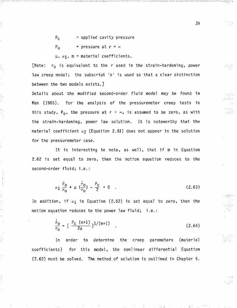
39

Pc

Po

= applied cavity pressure

= pressurê ât r = -[, 01, rr = materia] coefficients.

[Note: ro is equivalent to the r used in the strain-harden'ing, power

1aw creep model; the subscript 'o' is used so that a clear distinction

between the two models exists.]

Details about the modified second-order fluid model may be found in

Man ( 1985) . For the analysi s of the pressuremeter creep tests inthis study, Po, the pressure at r = -, is assumed to be ze?o, as wÍth

the strain-hardening, power law solution. It is noteworthy that the

material coefficient o2 (Equation 2.6I) does not appear in the solution

for the pressuremeter case.

It is interesting to note, as well, that if m in Equation

2.62 is set equal to zero, then the motion equation reduces to the

second-order fluid; i.e. :

In addition, if o1 in Equation (2.62) is set

motion equation reduces to the power law fluid;

'1 * * u (*&) -+ = o

io _ . p. (m+i) r1l(m+1)r, - L--T-)

(2. 63 )

equal to zero, then the

i.e.:

In order to determine the creep

coefficients) for thi s model , the nonl inear

(2.62) must be solved. The method of solution is

pa rameters

di fferenti al

outl ined in

(2.64)

(material

Equati on

Chapter 5.

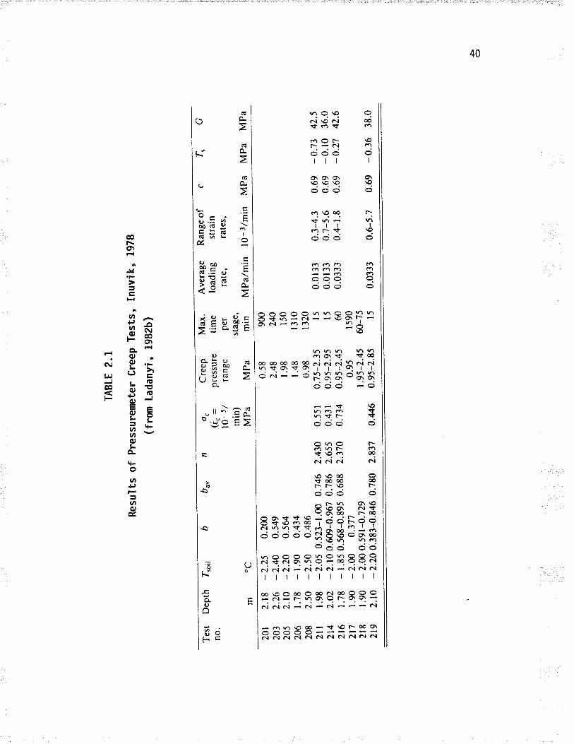
Tes

t D

epth

Tio

irno

.

TA

BLE

2.I

Res

ults

of

Pre

ssur

emet

er C

reep

Tes

ts"

Inuv

ik'

1978

(fro

m L

adan

yi,

1982

b)

201

2.18

-2.

25 0

.2m

203

2.26

-2.

40 0

.549

205

2.10

- 2

.20

0.56

420

6 r.

78 -

1.9

0 0.

434

208

2.50

- 2

.50

0.48

62l

l 1.

98 -

2.05

0.5

23-1

.00

2t4

2.02

- 2

.10

0.60

9-0.

967

2t6

r.78

- 1

.85

0.56

8-0.

895

2t7

1.90

- 2

.00

0.37

721

8 1.

90 -

2.0

0 0.

591-

0;t2

9zt

g 2.

10 -

2.20

0.3

83-0

.846

oc

b^,

oc

(É.

=lo

-s/

min

)M

Pa

Cre

eppr

essu

rera

nge

MP

a

0.74

6 2.

430

0.55

1

0.78

6 2.

655

0.43

1

0.68

8 2.

370

0.73

4

0.78

0 2.

837

0.44

6

Max

.tim

epe

rst

age,

min

0.58

2.48

r.98

1.48

0.98

0.75

-2.3

50.

95-2

.95

0.95

-2.4

50.

95r.

95-2

.45

0.95

-2.8

5

Ave

rage

load

ing

rate

,

900

240

150

l3l0

I 32

0 l5 l5 60I 59

0û-

75 l5

MP

a/m

in l0

-3/m

in M

Pa

MP

a M

Pa

Ran

ge o

fst

rain

rate

s,

0.01

330.

0r 3

3

0.03

33

0.03

33

r,G

0.3-

4.3

0.?-

5.6

0.4-

I .8

0.ó-

5.7

0.69

- 0

.73

42.5

0.69

- 0

.10

36.0

0.ó9

- 0

.27

42.6

0.69

- 0

.36

38.0

Þ o

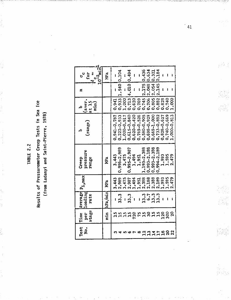
TA

BLE

2.2

Res

ults

of

Pre

ssur

enet

er C

reep

Tes

ts in

Sea

Ice

(fro

m L

adan

yi a

nd S

aint

-Pie

rre'

197

8)

Tes

tN

ooT

ime

Per

stag

e

f,ver

?'g€

Ioad

in6

rate

3 4 5 6 ? I 12 13 14 1? 18 20 22

ntl.n

Pirr

"*

l5 1s 1s I5 720

'15

15 30 1s 1s 120

300 20

kPa/

rnir

Cre

eppr

eSsu

rera

nge

33,3

33"3

13.3 6.7

13.3

t:.t

MP

a

3.44

32.

989

3"4?

52.

987

1.49

41"

951

2"38

82.

188

2"38

82,

189

I.993

1" 5

952.

479

3.44

30.

996-

2.98

93.

475

0.99

5-2.

98?

I,494

1.95

r1.

193-

2.38

80.

993-

2.18

80.

993-

2.38

80.

994-

2"18

91.

993

I.595

2.47

9

MP

a

b

(ran

ge)

b(a

ver.

at 1

5m

in)

0.94

1-0.

?97

o.22

2-0.

933

I.000

-0,9

I70.

615-

0.84

0o.

620-

0"42

00"

?69-

0.52

60.

580-

0.90

50.

698-

0.92

90.

669-

I,000

0.?3

3-0.

882

0.82

8-0.

627

0.74

0-0.

669

1.00

0-0.

9I3

noc for

{ec-

o-5¡

nin-

0.94

Lo"

933

1.00

00.

?I3

0"62

00"

769

o.?4

50.

?06

0.90

5o.

882

o.82

80"

740

I.000

I

1. s

40

4"O

10

z.lts

2.04

82.

O54

2.].4

5

IlPa

-L

0"10

4

o"49

4

o.ig

o0.

634

0.32

t0"

Ì84

I I

Þ lJ

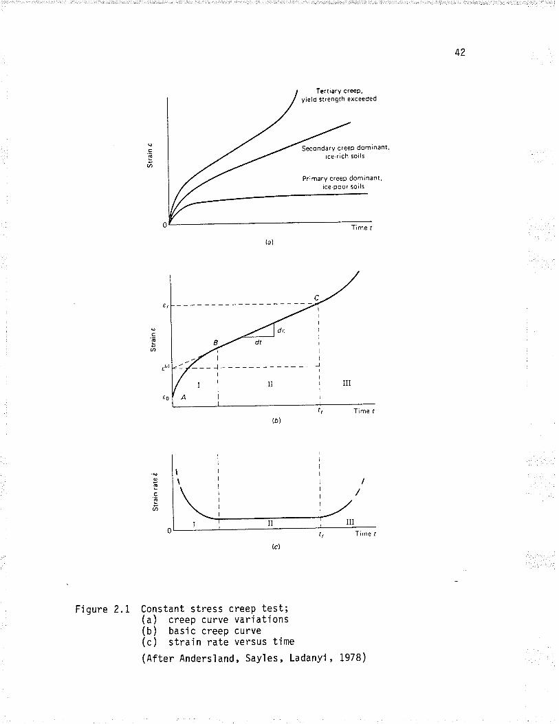
42

'õ

(h

Tertiary creeP,yield strength exceeded

Secondary creeP dominant.ice rich soils

Primary creep dominanl,rce'poor soils

'õ

U'

o€

'õ

tn

Constant stress creep test;(a) creep curve variations(b) basic creep curve(c) strain rate versus time

(After Andersland, Sayles, Ladanyi, 1978)

Figure 2.1

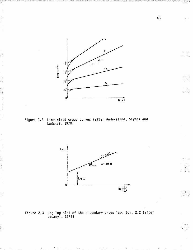
43

-{i Ièa

'!'

,t'

,l',r

0

Figure 2.2 Linearized creep curves (after Andersland, Sayles andLadanyi, 1978)

o

o)Þ

Figure 2.3 Log-ìogLadanyi

p'lot of, 1972)

Time t

the secondary creep 'law, Eqn . 2.2 (after

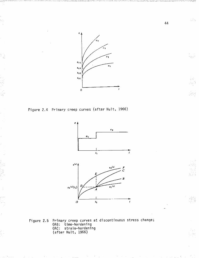
44

tigure 2.4 Primary creep curves (after Hult, 1966)

ét (c)(rl)

Figure 2.5 PrimarY creep curves at0AB: time-hardeningOAC: strai n-hardeni ng(after Hult,1966)

di scont'inuous stress chanqe;

45

29z

o

o

¡z.f

cuMUtATtvt lrMt. I I

Figure 2.6 Notation fortest (after

interpretation of staqe loadedLadanyi and Johnston, 1973)

p re s s uremete r

Ëq(]

ì'oo1

:o

õ

Trme f, mrn

Presgre r¡- MP¡

Figure 2.7 Determjnation of creep parameterg lrom the results of a

staqe loaded pressuremeter test (after Ladanyi andJohnston, 1978)

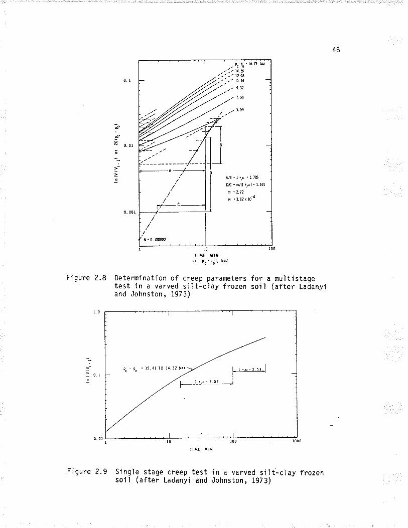
46

I0.0t

0.00t

IO

TIME. ÀIINor {Pc - pol. b¡r

Figure 2.8 DeterminatÍon of creep parameters fortest i n a varved si I t-c'lay f rozen soi Iand Johnston, 1973)

a mul ti stage(after Ladanyi

l.0

Þc 9o 15.41 T0 14. 32 bãr

t l.u'2.02I o.tc

ftÀrt. Mlr

Figure 2.9 single stage creep test in a varved silt-cìay frozensoil (after Ladanyi and Johnston, l973)

Aß'l +/, '1.785

DÆ . m/(t ?l 'l.5Uln -272

r¡ . 3. t? x l0-4

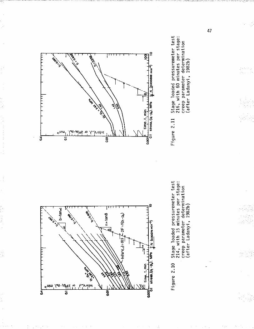
,/ /4 N 7--

---

:l l-z

F.

Fiq

ure

2.10

Sta

qe l

oade

d pr

essu

rem

eter

tes

t2I

4, w

lth 1

5 m

inut

es p

er s

tage

:cr

eep

para

met

er d

eter

mjn

atio

n(a

fter

Lada

nyi,

1982

b)

.d .l .if lr 'ô¡

.ô .iI c

<I

time.

l. m

in

I

Fì gu

re 2

. I

1S

tage

load

ed p

ress

urem

eter

tes

t21

6, w

jth 6

0 m

inut

es p

er s

tage

:cr

eep

para

met

er d

eter

min

atio

n(a

fter

Lada

nyi,

1982

b)

Þ \¡

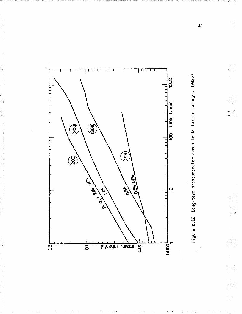
1 È .ç É ¡n

ool

Fjq

ure

2.12

Lon

g-te

rm p

ress

urem

eter

cre

ep t

ests

(af

ter

Lada

nyi,

1982

b)

100

time.

t. m

in

Þ æ

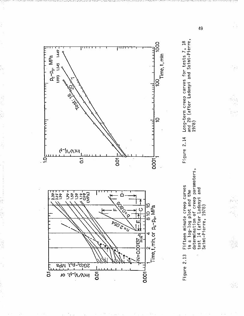
N=

0Or0

132-

u

.\Ê A/

cv'/

a/ Q/

t

1 2

4 81

0 15

Tim

e, t

,mln

, or

pc-

po,

MP

a

Fiq

ure

2.13

Fift

een

min

ute

cree

p cu

rves

in a

log-

'log

pìot

and

the

dete

rmin

atìo

n of

cre

ep p

aram

eter

s,'

test

14

(afte

r La

dany

i and

Sai

nt-P

ierr

e, 1

978)ff-

,icl

J

Pç-

Ps,

MP

a

1.99

3 1.

545

\449

Fig

ure

2.14

Lon

g-te

rm c

reep

cur

ves

for

test

s 7,

18

and

20 (

afte

r La

dany

i and

Sai

nt-P

ierr

e,1e

78 )

100

1000

Tim

e, t

, m

ln

Þ rg

50

CHAPTER 3

TEST EQUIPHEHT A¡{D TEST PROCEDURES

3. I IruTRODUCTIOru

In hjs 1982 paper on."Borehole creep and relaxation tests

in ice-rich permafrost", Ladanyi concludes:

"Nevertheless, it is felt that a definite answer as to thevalidity and relative merit of such borehole expansion testscan onìy be obtained if they are performed underwell-controlled ìaboratory conditions in thick cylindersof frozen soi l . "

Pressuremeter testing in the laboratory assures:' 1) tne production of artificial samples which are reproducibìe

and homogeneous.

2) temperature control, so that conditions are uniform and

isothermal.

recording by data acquisition system.

'longer creep durations than are logistically possible in

the field.

Ice was chosen to be the test material for the foìlowing

reasons:

1) Ice i s general ly thought to deform in an incompressible,

frictionless manner (e.g. Sego and Horgenstern, 1983, 1985;

Ladanyi and Saint-Pierre, 1979); therefore, two conditions

critical to the use of the strain-hardening, power law creep

model are believed to be satisfied. Moreover, Sego and

Morgenstern ( 1985) demonstrated that the power law creep

model, generalized to multiaxial states of stress, can be

used to model the indentation of a circular punch into ice.

3)

4)

51

They modelled the deformation of the ice beneath the punch

with sphericaì cavity expansion theory; the pressuremeter

represents a case of cyìindrical cavity expansion.

2) It is re'latively easy to make homogeneous, isotropìc,

reproducibìe samp'les of ice using the seed crysta'l technique

discussed in Sectjon 3.3. Eckardt (1981), on the other hand,

testi ng samp'les of f rozen sand, attri butes 'large scatter

in the pressuremeter creep data to variability in the sand

density.

3) There is a growing interest in the creep of ice:

. i) ice is generaì1y thought to form an approximate upper

bound to the creep of ice-rich frozen soil.

ii ) stress measurements in icebergs (Shields et â1., 1986)

must consider creep.

iii ) the practicaì use of artificial, sprayed ice islands

in the American Arctic Ocean (Hughes, 1985) wil'l depend

on creep performance.

iv) the bearing capacity of and pressures exerted by sea

ice covers (Ladanyi and Saint-Pierre,1978) are creep

dependent.

The purpose of the testing program in this thesis, therefore,

was to investigate, under controlled laboratory conditions:

1) the validity of the strain-hardeninq power law creep theory

and the modified second-order fl uid model in mode'l Ìing

'long-term pressuremeter creep tests in ice;2) the validity of stage-loaded creep tests, as opposed to single

stage tests conducted at equi va'l ent stresses , i n determi ni ng

the stress dependence of the creep law; i.e. does the material

52

possess "fading memory", ds the power law creep theory assumes?

(Hult, i966)

The next three subsections present the test equipment, ice

sampìe preparation, and pressuremeter creep test procedures.

3.2 ïEST EQUIPI4ENï

The schemati c ì ayout of the pressuremeter testi ng system

used in this study is illustrated jn Fig. 3.1. In the schematjc

diagram, only one pressuremeter system and one testing tank are shown.

In fact, three comp'lete pressuremeter testing systems were used

concurrentìy to reduce the total time required to carry out the test

program. Each of the components in the system, as well as the driììing

and sampl i ng equi pment whj ch was used i s descrì bed i n the foì 1 owi ng

secti ons.

3-2.I Pressurreneter Testing Tanks, Including the Sample Freezing

System

One of the most important aspects of the testing program

was to decÍde on the sample boundary condjtions. A number of options

were available:

1) completely unconfined cy]inder of ice (Ladanyj et al., 1979);

2) frozen sampìe in a thin-walled tank with no top constraint

(Snields et al., 1984; Fensury, 1985);

3) pressurized lateral boundary (pressure appì ied througl'r a

membrane) with top and bottom semi-rigid constraints (Eckardt,

1981);

4) semi-rigìd bottom and I ateral boundari es wi th free toP

53

bounda ry.

0ption no. l is impractica'l due to the size of the samp'les

that would be required and the problem of removing them from the mould

(even for thjs study, with a semj-rigid cylindrical boundary, samples

weighing approximate'ly 475 kg were used). 0ption no. 2" which has

boundary conditions very sim'ilar to no. 1, is attractive from a

theoretical po'int of view (i.e. may use thick-wal 1ed cyl inder solutions)

but not from a practical point of view. Serious iniury almost resulted

when several samples literally exploded while being tested in thjn

wal led tanks with the pressuremeter at the University of Manitoba

(R. Kenyon, pers. commun.). Moreover, deformation in thin-walled

tanks or with the ice unconfined is believed to result in radial

cracking at an early stage; this js contrary to the assumption of

creeping flow, which the creep theories are based upon. For example,

Ladanyi et âl . , (1979) whì'le test'ing unconfined cyl inders of fresh

water ice, noted cracking at a very earìy stage in the test, with

complete failure of the cyìinders at rather low strains. 0ption no.

3 is again attractive from a theoretical point of view, with forced

pìane strain condjtions, but again sampìe cracking Ís believed to

occur wi th thi s test set-up ( Eckardt, 1981 i Ladanyi and Eckardt,

1983). In addition, with the top lid in p1ace, the sampìe cannot be

moni tored vi suaì ìy duri ng the test for the devel opment of cracks.

Therefore, all things being considered, option no.4, with

both the bottom and the lateral boundaries semi-rigid, was believed

to offer the best compromise. 0ption 4 would reduce the tendency

for fa'ilure of the sampìe through cracking, and would force the ice

to flow in a visco-plastic manner. Elastic anaìysis of the ice-steel

54

tank system which was chosen showed the radial stress distribution

in the sample to be very close to the stress distribution wh'ich would

prevail in the field case, with the "external radius" go'ing to infinity.

Moreover, the radial stress at the ice-steel tank boundary is less

than one percent of the appì ied stress in the cavity. Therefore,

the results can be analyzed us'ing "field" equations (Ladanyi and

Johnston, 1978). As discussed by Briaud and Shields (1981), however,

the proxim'ity of the free upper surface of the sample to the

pressuremeter membrane may have an influence on the nature of the

deformation. Numerjcal analysis would be necessary to proper'ly assess

thi s condition.

The tanks themselves are composed of sections of steel pipe

(890 mm inside diameter by 11.7 mm wall thickness) with a 9.5 mm thick

steel pìate welded onto the base. A 76 mm wide ìip was welded around

the top of the tank to enable a steel lid to be fastened to the tank

i f requi red, and for transporti ng the tanks. In the col d room, the

tanks were pìaced on top of two (100 mm square by 6.4 rnm wall thickness)

hol low structural members. These structural members were I ocated

beneath the centroid of each semi-circular half of the tank. This

confi gurat'i on al I owed for ai r ci rcul atj on beneath the tanks , thus

promotìng uniform temperature conditions withjn the sampìe.

A heat exchange (freezing) coil was installed in the bottom

of each tank to freeze the samp'les from the bottom upr thus considerably

reducing thermal stresses and strains in the sampìe (Sego, 1980). -In

order to minimÍze heat flow through the base and lateral boundary

of the tank, the heat exchange coil was pìaced on top of a 50 mm thick

disk of rig'id styrofoam insulation. Finally, saturated sand was packed

55

around the coil to enhance heat exchange capabilities in the vic'inity

of the coi I (dense, saturated frozen sand has a hi gher thermal

conduct'ivity than ice) and to provide a working base for formìng the

samp'l e. Thi s sand was fi rst frozen sol j d before i ce maki ng was

attempted, so that no mixing of the sand and the superincumbent jce

occurred.

The heat exchange coil in the base of all three tanks was

connected to a Tecumseh condens'ing unit. Th'is half-horsepower unit,

which is air cooled and powered at 115 volts, has a rated heat flow

capacity of 344 watts at an evaporator (coil) temperature of -40'C

and 996 watts at an evaporator temperature of 0oC. As P late 3.1

i I I ustrates, the condensi ng uni t can be swi tched to any one of the

tanks by opening and cìos'ing the appropriate shut-off valves. More

details on sample preparation and freezing are given in Sectjon 3.3.

3.2.2 0Y0 EIasùrcter 100 Pressureneters

In order to carry out long-term pressuremeter tests (lastjng

for weeks) in wh'ich volume change of the measuring cell is used to

represent deformation, a 'leak-proof hydraul ic pressuremeter would

be needed. Since a pressuremeter meet'ing these requirements could

not be bought and it was doubtful if one could be constructed, it

was decided to use a pressuremeter which measures radius change

directly, through a caìiper arm - LVDT system. The 0Y0 Elastmeter

100, used successfu'l'ly by Fensury (1985), is such a pressuremeter.

Moreover, the LVDT system of measuring change in radius lends itself

to automatic data acquisition. The pressuremeter components are

illustrated in Plate 3.2.

56

As the maximum appl'ied pressure in this study was only 2.5

14Pa, the thin rubber membrane developed for soft ground by the 0Y0

Corporation, Japan, was used (Onya, 1982). Thi s membrane, in the

unstressed condi tj on , has an outsj de dÍ ameter of 70 rnm and a wal I

th.ickness of 4 nrm. When instal led on the pressuremeter, the membrane

has an effective ìength of 390 rnm, giving a length to djameter ratio

(L/D) of 5.6. Accord'ing to Bagueìin et â1., (1978), the minimum

accepted L/D for this type of pressuremeter is four.

In order to determine r and ri in Equation (2.43) (the current

and initial cavity radius, respectively), the movement of the caliper

arms, which are connected to the core of an LVDT (see Fig. 3.2), must

be correlated to the inner radius of the membrane (since the spring

I oaded cal i per arms are al ways j n contact wi th the i nsi de surface

of the membrane). In addition, the thjckness of the membrane must

be accounted for to calculate the outside radius of the membrane (which

i s assumed equa'l to the cavi ty radi us ) .

The movement of the caì iper arms ' in uni son ' causes the

core of the LVDT to move within the differential transformer. As

the term LVDT Ímplies (linear vo'ltage differential transformer) the

rel a ti onshi p between the d'ispì acement of the core and the vo'l tage

output from the dífferential transformer js linear. Therefore, what

is needed is a relationship between X (the rod displacement) and Ri,

the radius being measured by the caliper arms (Fig. 3.3). From geometry

(Fig. 3.3):

X = 25 sine mm

or sine = X/25"

where o = angle of rotatíon of the caliper arm.

(3.1)

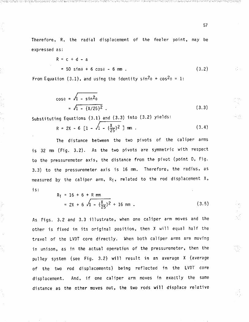
Therefore , R, the rad'ial di spì acement of the

expressed as:

R=c+d-a=50sino+6coso-6mm

From Equation (¡. t), and using the identity sinZe + 66529 = 1'

tffiSubstituting Equations (S.tLann3.3) into (3'2) vields:

R = 2x - 6 I - /t - tä12 I * .

+Rmm

Fq + 16mm

57

feel er poi nt, rnây be

(3.2)

cose =

The di stance between the two pi vots of the ca] i per arms

is gZ mn (Fig. 3.2). As the two pivots are symmetrìc wjth respect

to the pressuremeter axis, the distance from the pivot (point 0, Fig'

3.3) to the pressuremeter axi s i s 16 rrl'rì. Therefore, the radíus, as

measured by the caìiper arm' Ri, related to the rod displacement X,

is:

(3.3)

(3.4)

(3.5)

R1=16+6

=2X+6

As Fi gs. 3.2 and 3.3 i I I ustrate, when one cal i per arm moves and the

other is fjxed in its original position, then X wilì equaì half the

travel of the LVDT core directly. When both caliper arms are movìng

in unjson, aS in the actual operation of the pressuremeter, then the

pulley system (see Fjg. 3.2) w'ill result in an average X (average

of the two rod di spl acements ) bei ng refl ected i n the LVDT core

disp'lacement. And, if one caliper arm moves in exactìy the same

djstance as the other moves out, the two rods will dispìace relatjve

sin2e

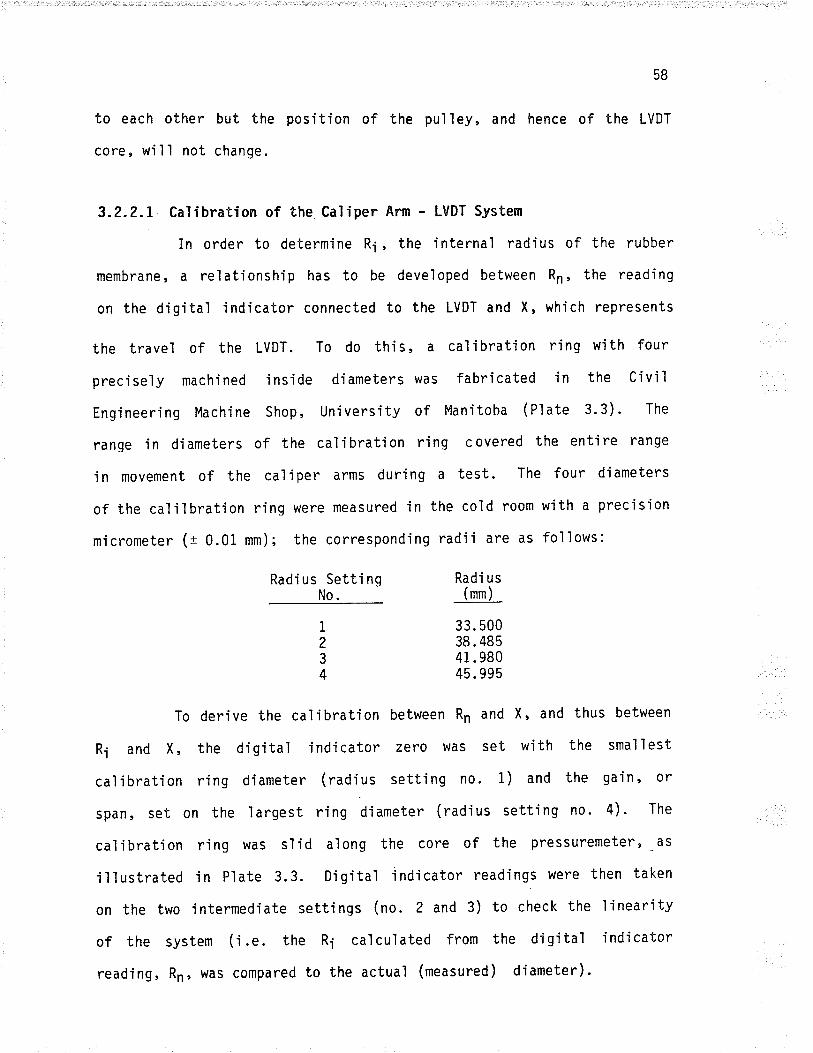
58

to each other but the position of the pulley, and hence of the LVDT

core, wi I I not change.

3.2.2.1 CaTibration of the Caliper Arm - LVDT System

In order to determine Ri, the internal radius of the rubber

membrane, a relatjonshjp has to be developed between Rn, the reading

on the dig'itaì indicator connected to the LVDT and X, which represents

the travel of the LVDT. To do this, a caljbration ring with four

preciseìy mach'ined inside diameters was fabricated in the Civil

Eng'ineerìng Machine Shop, University of l4anitoba (Plate 3.3). The

range in diameters of the cal'ibration ring covered the entire range

in movement of the cafiper arms during a test. The four diameters

of the caljlbration ring were measured in the cold room with a precision

micrometer (r 0.01 mm); the correspondìng radìi are as follows:

Radj us Setti ngNo.

Radi us

33.50038.48541 .98045.995

To derive the cal'ibration between Rn and X, and thus between

Ri and X , the di gi ta'l i ndi cator zero was set wj th the smal I est

caljbration ring diameter (radius setting no. 1) and the gain, or

span, set on the ìargest ring diameter (radius settìng no. 4). The

calibration rìng waS slid aìong the core of the pressuremeter, -as

illustrated in Plate 3.3. Digital indicator read'ings were then taken

on the two intermedÍate settings (no. 2 and 3) to check the ìinearity

of the system (i.e. the Ri calculated from the d'igital indicator

reading, Rn, was compared to the actual (measured) diameter).

1

234

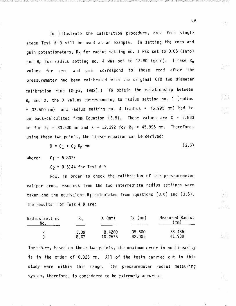
59

To illustrate the calibration procedure, data from síngle

stage Test # 9 will be used as an example. In setting the zero and

gain potentiometers, Rn for radius setting no. 1 was set to 0.05 (zero)

and Rn for radius sett'ing no. 4 was set to 12.80 (gain). (These Rn

val ues for zero and gai n correspond to those read after the

pressuremeter had been cal'ibrated with the original 0Y0 two diameter

calibration ¡ing (0hya,1982).) To obtajn the relationsh'ip between

Rn and X, the X values corresponding to radius setting no' 1 (rad'ius

= 33.500 mm) and radjus setting no. 4 (radius = 45.995 mm) had to

be back-calculated from Equation (3.5). These values are X - 5.833

mm for Ri = 33.500 mm and X - 12.392 for Ri = 45.995 rm. Therefore'

using these two points, the linear equat'ion can be derived:

X=C1+C2Rnmm (3.6)

where: Cl = 5.8077

CZ = 0.5144 for Test # 9

Now, in order to check the calibration of the pressuremeter

caliper arms, readings from the two intermediate rad'ius settings were

taken and the equivalent Ri calculated from Equations (S.O¡ and (3.5).

The resul ts from Test # 9 are:

Rn X (mm) Ri (mm)Radi us Setti ngNo.

2

3

5.098. 67

8.4260L0 .267 5

38. 50042.005

Measured Radi us(mm)

38.48541.980

Therefore, based on these two points, the maximum error in nonlinearity

is in the order of 0.025 mm. All of the tests carried out in this

study were wi thi n thj s range . The pressuremeter radi us measuri ng

system, therefore, is considered to be extremely accurate.

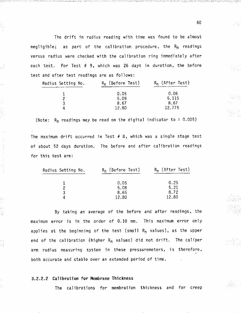
60

The drift in radìus reading with time t,/as found to be almost

negligible; as part of the calibration procedure, the Rn readings

versus radius were checked with the calibration ring immediately after

each test. For Test # g" which was 26 days in duration, the before

test and after test read'ings are as follows:

Radius Setting No. Rn (Before Test) Rn (After Test)

1

z3

4

(Note: Rn readings may be read on the dig'ita1 indicator to t 0.005)

0. 055. 098.67

12.80

0.065.1158.67

12.775

The maximum drift occurred

of about 52 days duration.

for this test are:

in Test # 8, which was

The before and after

a sinqle stage test

cal i brati on readi ngs

Radius Sett'ing No. Rn (Before Test) Rn (After Test)

1

234

0. 055.088. 65

12.80

0.255.2I8.7 2

12.80

By taking an average of the before and after readings, the

maximum error is in the order of 0.10 mm. This maximum error only

applies at the beginninq of the test (small Rn values), as the upper

end of the calibration (higher Rn values) did not drift. The caìiper

arm radjus measuring system in these pressuremeters, iS therefore,

both accurate and stable over an extended period of time.

3.2.2.2 Calibration for kmbrane Thickness

The cal ibrations for membration thickness and for creep

61

of the membrane with time during a creep test were carried out'in

five thick-walled steel tubes, wjth inside rad'iì ranging from 37'84

to 47.58 mm (Plate 3.4). The tubes were honed to a tolerance jn the

inside djameter of t 0.01 mm. The diameters were again measured jn

the cold room using the precision micrometer, accurate to t 0'01 mm'

The inside radii of the five tubes were determined to be:

Tube No. Ro (mm) (lnside Radius)

37 .8439. 63541.34544.40547. 58

The calibrations for membrane thickness and change in membrane

thjckness with time were carried out separately. To obtain the membrane

thickness versus Rn correction (without membrane compression ) , the

pressuremeter was placed inside each of the five steel tubes (Plate

3.5); the membrane was brought into contact with the steel tube by

increasing the pressure Ín 35 kPa increments, held for 1 minute. l'lhen

contact of the membrane with the steel tube was first made, (w'ithout

compression of the membrane), the corresponding Rn reading was noted.

The Rn reading was converted to an inside radjus (R1) wìth Equat'ions

(S.S¡ and (3.6). Since the ínside radius of the membrane was now

known, and the outside radius was equaì to the inside radius of the

steel tube, Rq, then:

1

2

3

45

s = n tt&-rorlz - tfulzl cmz ,

s/tr = ttfulz - t$¡lzl cnlor

(3.7)

6Z

vJhere S = cross sectional area of the membrane'

(Note: the cross sectional area was calculated jn cm2 to be consjstent

with 0y0 Corporatìon's instruction manual and the paper by Ohya,1982)'

The cross sectional area of the membrane d'ivided by pi (S/¡) was then

cal cul ated for each steel tube, before and after the pressuremeter

test. l{hen S/r versus R¡ was plotted, a linear relat'ionship was found

(ris. 3.4):

S/¡ = C5 + C6 Rn cn?

where: C5 = 2.283

(3.8)

C6 = 0.0102 for Test # 9

The change in membrane thickness with time calibration test

involves two steps. The pressuremeter was first of all inflated under

a small pressure in steel tube # 2 so that contact of the outside

of the membrane with the inside of the steel tube was made. This

Rn reading, assuming that no compress'ion of the membrane had taken

p1ace, represented the zero reading for the calibration test. Next,

the pressure was then immedjately increased to the test pressure,

and changes in Rn readings were taken with time. The change in membrane

thickness with time, Pg, showed a strong correlatjon with the natural

logarithm of time, in minutes:

Pg = C3 + Cq ln(t) mm (3.e)

For Test # 9, the change in membrane thickness test was carried out

overnight in steel tube No. 2 to a total tjme of 910 minutes. _The

curve was plotted as Fig. 3.5, and the coefficients were determined

to be: C3 = 0.0485 and C4 = 0.0054.

If the change'in membrane thickness with time was found

to be neg'l i gi b'l e after about the f i rst 5 mi nutes , the tì me-dependent

R, = (Ri - Pg)/10.0 cm

where R5 = coFrected inside radius.

Then, the outside radjus is calculated:

63

term in Equation (3.9) was droppe¿ (i.e.C4 set equal to zero).

In order to calculate the outside rad'ius of the membrane,

Ro, during a pressuremeter creep test, the two membrane corrections

(Equat.ions 3.8 and 3.9) are appìied separate'ly. First, the membrane

thickness correct'ion is app'l'ied:

(3.10)

Ro=(Ç- -?)10.0 nrn (3.11)

As Equation (3.11) illustrates, the R! term dominates the determination

of Ro. Since the maximum error in determining Rs from all the tests

was on the order of t 0.10 ffiffi, it is believed that the maximum error

ìn Ro for all the tests was within t 0.10 nml.

As a summary, a flow chart (fig. 3.6) illustrates all the

equations and calibrations which are necessary to convert a dig'ita1

indjcator reading, Rn, to the outside rad'ius of the membrane (or cavity

rad'ius ) Ro.

3.2.2.3 hmbrane Resistance Comection

In order to calculate the true pressure being app'lied to

the cavity wall, the resistance of the membrane, as it expands, must

be determined and subtracted from the applied pressure. To determine

thj s correction, the membrane was inflated in ai r to its maximum

expansion with 20 kPa increments, each increment held for 60 minutes.

These tests were conducted in the cold room at -2"C. Plots of the

60 min readings of Rn versus applied pressure for Tests # I and #

9 (both before and inrnediately after the test) are shown on Fig. 3.7.

64

It may be noted that the "before test" resi stance i s

approxìmateìy 20 to 30 kPa higher than the "after test" resistance

at the same expans'ion. Therefore, the membrane has lost some of its

stiffness, particuìarìy in the lower end of the deformation range.

Since Tests # I and # 9 were the two longests tests (5? days and 26

days in durat'ion, respectiveìy) these "after test" curves represent

the maximum loss of stiffness. The before and after curves for all

the other tests fal I between these two I jmits, wi th "before test"

curves usualìy beìng very close to the "before test" curves for Tests

# 8 and # 9 shown. In order to compensate for this loss of stiffness

duri ng the test, a composi te curve was drawn ( Fi g. 3.7 ) . Thi s curve

refl ects the membrane resi stance of the "before test" curves earl y

in the test, and then reflects the less stiff "after teSt" curVes

near the end of the test, as the membrane expands to'its maximum radjus.

For comparison, the recomnended curve from Ohya (tggZ) ts presented.

His tests were conducted in steel tubes at room temperature. As is

illustrated, this curve c'losely follows the "before test" curves,

ind'icat'ing that the change to cold temperature has not affected the

membrane resistance to any great degree.

All tests in thjs study (both singìe stage and multistage)

were carried out under the assumption that the membrane resistance

is dependent only on the curren't membrane radius usìng the composite

curve. Moreover, the internal pressure'in the probe was adiusted

during the test

order to gi ve

Therefore:

account for the current membrane res'istance, in

constant appìied pressure on the cavity wall.

to

a

Pa = Pcav + Rg/1000.0 MPa (3.12)

ryhere Pu

Pcuv

Rg

Thi s correction was

notjceable change ìn

65

= applìed pressure MPa

= pressure applied to the cavity wall MPa

= membrane resistance correction

= 51.28 + 30.18 ln Rn kPa.

used for al I of the tests, ôs there was no

resistance from membrane to membrane.

3.2.3 Data Acquisition System

In order to avoi d bei ng unabl e to obtai n test data ,

particu'larly overnight, the pressuremeter pressure transducers and

iemperature sensing device sìgnal conditioners were all connected

to a data acqu'isjtion system. Comp'lete creep-tjme curves were obtained'

whìch is particularly important for the numerjcal process'ing procedures

as discussed in Chapter 5.

The data acqu'i s i t'ion system used i n thi s study was a 32

channel Neff 620S multiplexer, with a L2 bit anaìog to d'igital

converter, connected to a Hewlett-Packard 9825 A desk top computer.

Calibration factors for each device were entered into the computer

memory, So that output from the device was read in units of

dìsp'lacement, temperature or stress directly. A real time clock waS

connected to the computer so that all the channels could be scanned

automatical ly at preset time interval s. The data was recorded on

to a cassette tape as scann'ing proceeded. The scann'ing i nterval s

most common'ly used in this testing program are as follows:

start of test to 20 m'inutes

20 m'inutes to 30 minutes

30 minutes to 120 minutes

I minute interval s

2 minute intervals

5 minute intervals

66

120 minutes to 300 m'inutes t0 minute intervals

300 mi nutes on - 20 minute or 30 minute intervals'

Inthelongers.ingìestagetests,thescanninqinterval

wasincreasedtolto2hoursafterafewdays.Inconclus.ion,the

Nef f 12 bi t anal og to d'i g.i ta1 converter aì ways gave a measurement

resolution which was w'ithin the determined accuracy range of that

part'icul ar devi ce.

3.2.4 Temperature kasurerPnt

Twotypesoftemperaturesensingdeviceswereusedinthis

study; thermi stors and thermocoupìes. The thermi stors were 0mega

Engineering I inear response probes, l4odel 0L-701. The therm'i stor

sensor, actual I y composed of two el ements , and the accompany'i ng

ì.inearizing cìrcuit are shown in Fig. 3.8. The vo'ltage drop measured

across Ri is linearly related to the temperature of the sensor in

the range 50"c to -30"c. Type T thermocouples (copper-constantan),

withthemeasur.ingjunct.ionsweldedjnmercury'wereusedextens.ively

i n th j s study. They were connected to a Kaye Instruments 'ice po'int

reference, as'indicated in Fig' 3'1'

Formaximumaccuracy,eachtherm.istorandthermocoupìewas

cal j brated in the temperature ranqe -10'c to 0oc in a temperature

bath. Therefore, rather than using the manufacturer's general equat'ion'

each therm'istor and thermocoup'le had its own calibration factor

Calibrat'ions were done twice; once at the beginning and

agai n at about the mj ddl e of the testì ng program' The fj rst

calibrations were done using a Rosemount p'latinum resjstance temperature

standard,readwithaMuellerBridge.Theaccuracyofthissystem

67

is rated to be within t 0.01'C. The thermistors and thermocouples

were calibrated the second time with a Brooklyn Calorimeter Thermometer,

with a rated accuracy of t 0.02"C. In summary, the results of both

calibrations showed that the thermistors could be considered accurate

to t 0.10"C and the thermocoupìes to t 0.15'C. These accuracy figures

includes dev'iat'ion from linearity, instability and drÍft with time.

3.2.5 Pressure Transducers and Pressure Regulators

The pressure transducers used in thi s study were Dyn'i sco

Model PT370 DHF, with a pressure range from 0 to 7 MPa. The compensated

temperature range ís -18'C to 65'C. Tero drjft and nonl inearity,

therefore, are not a problem at the testing temperature of -2"C.

As w'ith the temperature sensìng dev'ices, the pressure

transducers were calibrated twjce; once at the begìnning and again

at about the middle of the testing program. The cal'ibrations were

done with a dead load tester in the cold room at a temperature of

-2"C. The accuracy of these pressure transducers , i nc1 udi ng

nonlinearity, hysteres'is and repeatability is within t 10 kPa.

The compressed dry nitrogen gas used to inflate the

pressuremeter membrane was regu'lated with Tescom 44-1100 series

reguì ators. They are sel f-contaj ned, di rect-acting and pressure

reducing with an adjustabìe vent valve. As well as having excellent

setting sensitiv'ity, these reguìators, when set on a test pressure

did not allow a pressure drjft of more than I 10 kPa over pe.'iãCs

as ìong as 12 hours. The regulators and nitrogen tank are illustrated

in Plate 3.6.

68

3.?.6 Dri I I ing and Sampl ing Equipnent

As the pressuremeters used i n thi s study are not of the

sel f boring type, a proper'ly sized, smooth, thermal ly undi sturbed

pilot hole had to be drilled in the centre of the ice sample for the

pressuremeter. In addition, core samp'les of the ice had to be obtajned

for visual classification and ice density determinations. The ideal

would have been to combine the pressuremeter pilot hole driììing process

and the sampling process into one operation. The modified CRREL core

barrel , used successfully by Roggensack (I977 ) and Savigny ( 1980)

for sampling ice-rich permafrost, showed promise in this regard.

Two different sized modified CRREL type core barrels were

fabricated in the Civil Engineering Machine Shop at the Un'iversity

of Man j toba. One was des'igned to dri I I a 104 rrm di ameter hol e and

yie1d core of 69 mm diameter (Plate 3.7), while the other was des'igned

to drill a 77 mm diameter hole and g'ive core 43 mm in diameter (Plate

3.8). The smaller barrel was des'igned to drill the pressuremeter

pilot hole, while the larger barrel was designed for taking larger

core samples, perhaps for triaxial test'ing. Both of these core barrels

were turned with a high capacity e'lectric drill. The rate of rotation

was approximately 300 rpm (Plate 3.9).

As with any new testing program, it usua'l1y takes a few

tests to "iron the wrinkles out" and develop a systematic methodology

of testing. In this study, it was found that the 77 nn diameter c_ore

barrel drilled a very high qualìty hoìe, but cored poor quaìity samples.

(Problems with coring mass'ive ice and obtaining undisturbed samples

with thjs type of core barrel were, in fact, reported by Roggensack'

!977,1979; and Savigny, 1980.) After Tests # 2, # 3 and # 4, jt

69

was dec j ded to abandon samp'l i ng duri ng the pì l ot hol e dri 'l ì i ng and

take l arger di ameter sampl es wi th the 'larger core barrel , as requ'i red ,

after the particular test. A hole was drjlled wjth the 104 rnm djameter

core barrel about midway between the pressuremeter cavìty and the

wall of the tank (P1ate 3.9). The hole was drilled typicaì'ly to a

depth of about 600 rlìm, so that four samples approximateìy 100 to i30

mm jn'ìength after trimming could be obtajned. The qualìty of these

core samples i s i I I ustrated in Plate 3.10. No si gns of di sturbance

from expansion of the cavíty durìng the pressuremeter test were detected

in any of the samples. The equ'ipment used to trim the ends of the

core samples ìs illustrated in Plate 3.11. Results of the'ice density

measurements are gìven in Chapter 4.

As with the sampling, the pilot hole drilling technìque

was perfected as testing progressed' At first, a short core barrel

(about 250 mm long) was used 'in conjunction with a drilìing stand

which was mounted on top of the tank. The pilot hole, typically drilled

to a depth of about 750 lrìm, had to be drj I led in three runs. Thi s

procedure, although it produced a high quaìity hole, took a lot of

time. A much better method proved to be using the longer core barrel

(P'late 3.8), which could drill the entjre pi'lot hole in one run.

Vertical alignment was checked before and during the driìlìng process

with a carpenter's level. The'long barrel method took about 5 minutes

to drill the hole, versus about 45 minutes for the short barrel method.

In all cases, no me'lting of the ice took pìace during driì'lìng. The

cuttings came up as "snow" and tiny ice ch'ips (Pìate 3.9).

The ratio of the diameter of the undisturbed test cavity

to the diameter of the unínflated pressuremeter probe (often used

70

as a measure of the quality or calibration of the test cavity) in

this testing program was invariably about 1.10. According to Briaud

and Gambin (1983), a well calibrated hole should have a ratjo which

falls between 1.03 and L.20. Therefore, it may be concluded that

the p'ilot holes drilled in th'is test'ing program were well caljbrated

and the surroundjng Íce was not disturbed thermalìy.

3.3 ICE SAHPLE PREPARATIOH

In order to make reproduci b'l e , homogeneous and i sotropi c

samples of ice in the laboratory, the method used by Sego ( 1980),

and here termed the seed ice crystaì technique, was adopted. Because

of the re'latÍve'ly large size of the sampìes used Ín this study (890

mm diameter by 800 mm deep) the Sego technique could not be followed

precìsely, and some improvizations had to be made. It is believed,

however, that the improvizations d'id not seriousìy affect the

reproducib'iìity, homogene'ity or isotropy of the samp'les.

Briefly, the seed ice crysta'l technique 'invol ves pack'ing

a samp'le mould with sieved ice crystals (of un jform grain s'ize), pìacing

a vacuum pump on the mould and packed crystals to reduce the quantity

of entrapped a'ir in the sample, flooding the mould from the bottom

up with chilled, de-ajred deionized water and then freezing the sampìe

from the base upward by placing the mould on a cooling plate maintajned

at -30'C (Sego and Morgenstern, l983). The seed ice crystaìs act

as nucleation po'ints and cause a random orientation of the c-axis

of the individual ice crystals in the bulk sample. Moreover, thermal

strajns due to freezing are reduced and relieved by using the prepacked

seed ice crystals (which did not undergo a phase change) and by a'llowing

71

the sampie to expand vertjca'l1y at the top. Prior to sampìe making,

the sides of the mould had been greased with petroleum ielly to prevent

the samp'le from freezing to the mould.

The ice making procedure used in th'is study is outlined

below, step by step. The procedure is subd'ivided into two sections;

i) preparations for ice making and 2) making and freezing the ice

samp'le.

I Preparations for lce Makjng

1. The cold room thermostat was set to give an average temperature

close to 0"C. This temperature was checked by pìac'ing pails of

. water in the cold room and monitoring them. The temperature was

judged to be set correctly when thin layers of ice began to form

on the surface.

2. The water reservoir (Plate 3.i2) was filled with enough cold tap

water to fl ood the sampl e. Each sampl e requÍ red approximate'ly

0.17 m3 of porewater.

3. The porewater was chjlled to 0oC. This usuaì'ly took two to three

days.

4. 0n the morning of sample making, the sjdes of the tank were cleaned

and coated with a thin layer of petro'leum jeì ly. As wel I , the

Tecumseh condensing unit was turned on to freeze the sand around

the coils and to depress the temperature of the base of the tank.

5. The thermocouples mounted on the thermocouple stick were checked

to make sure they were still fastened proper'ly and workìng.

6. Fourteen, S0 kg bags of fine grained party ice were purchased

f rom Arcti c Ice Co. Ltd. of l,li nni peg. Th j s 'ice , whi ch was used

aS the seed ice crystals, was made from filtered tap water. All

II.

1.

72

of the crystals, which were sub-angular to angu'lar in shape' were

passed through a half inch sieve and were retained on a quarter

inch sieve. Therefore, all of the ice crystals were between 13

and 6.5 mm in size. The chemical propertiesof the tap water and

the seed ice crystals are given in Table 3.1.

Makinq and Freezinq the Sample

The hose from the porewater reservoir waS pìaced jn the bottom

of the tank and the tap control'ling the flow was opened.

Immedìately, two bags of ice were poured into the tank and compacted

i00 times with the specjally constructed tamper (Plate 3.12).

The thermocoupìe string was then pushed into the compacted ice,

and into contact with the base of the tank. Figure 3.1 illustrates

the standard location of the thermocoupìe string.

The ice crystals were then poured 'into the tank and compacted,

bag by bag. Each bag formed a loose lift of ice crysta'ls about

50 to 75 mm thick. Each lift of ice crystals were tamped 100

ti mes w'ith the speci a1 tamPer.

The level of the compacted ice crysta'ls was brought to within

about 25 to 50 mm of the topof the tank. When the porewater had

just flooded the top crystals, the tap was shut off and the hose

removed. Due to the long tjme required to de-air a sample of

this size (on the order of days), a vacuum pump was not used.

0f the 12 sampìes 'in this testing program, the average ratio of

the volume of porewater added to the volume of seed ice solids

('i .e. void ratio) was 0.533 (assuming 100% saturat'ion). The maximum

void ratio was 0.659 wh'ile the minimum ratio was 0.429.

The ice samp'le temperature and room temperature were monitored

2.

3.

4.

5.

73

c'l oseì y unti I the sampl e was compl etel y frozen . The room

temperature waS mai ntai ned as cl ose to 0oC as poss'i b'le , So that

neither significant freezing nor thawing occurred on the sample

sides and top. The top of the sampìe was usual'ly maintained as

slushy ice, easy to poke a finger into. As the freezìng front

progressed from the base to the top of the sample,300 mm wide

strips of 50 mm thick duct insulation were placed around the outside

of the tank to retard heat flow into the part of the sample already

frozen.

The freezÍng of sample # 2 can serve as an illustration of the' effectiveness of the freezing techniques. Two strings of

thermocoupl es , as wel I as two thermi stors , were pì aced i n thi s

samp'le to check for progression of the freezing front and

temperature distribution in the sampìe during freezing (layout

shown in Fig. 3.9). As may be seen in Fig. 3.10, the freezing

front came up very uniformly.

0f the LZ samples which were prepared, the average freez'ing tjme

was 180 hours (7.5 days), wjth a variation from 139 to 238 hours

( 5.8 to 9.9 days ) .

6. When freezing was complete, the Tecumseh condensing unit was either

turned off or swjtched over to another tank to make another samp'le.

If another samp'le was to be made inrnediately, the f j rst samp'le

was packed with 150 mm thick "pilìows" of fibreg'lass insulation

to retard heat flow. The depressed temperature condjtfons

inrnediateìy after freezing (see Fig. 3.10) and the extra insulation

prevented thawing of the first samp'le from occurring whjle the

second sample was being frozen.

74

The sampì es produced i n thi s way were reproduci bl e and

homogeneous as the test results and ice density measurements presented

in Chapter 4 indicate. Moreover, examination of thin sections of

ice core under p'lane poìarized ì ight ind jcated random'ly oriented ice

crysta'ls (whjch suogests that the ice was isotropic). The ice crystals,

however, were not uniform in size. The crystaìs whjch formed in pore

spaces were genera'l 'ly smal I er than the seed crystal s . Ti ny bubbl es ,

about 1 nm in size, were noted around the grain boundaríes of the

seed ice crystals. The ice was genera'lly, however, quite clear.

It may be concl uded , that i n spi te of the fact that tap

water and not distilled water was used to form the ice, the porewater

was not deaired, and the ice crystaìs making up the sampìe were of

non-uni form si ze , the sampì es were neverthel ess reproduci b'l e,

homogeneous, and i sotropÍc.

3.4 TEST PROCEDURES

The procedures used to prepare for and carry out both si'ng'le

stage and multistage pressuremeter creep tests are discussed in thjs

subsection. The procedures used for single stage tests are discussed

first, while the subsection on the multistage tests mainìy focuses

on the d'ifferences between singìe stage and multistage tests.

3.4.1 Single Stage Tests

0nce the samp'le was completeìy frozen and ready to test'

the thermostat for the cold room was adjusted so that the temperature

in the sampìe stabilized as close to -2"C as possible. Fans were

pìaced in the corners of the cold room to enhance air cjrculation

75

and thus promote uniform temperature conditions. The tìme taken for

the sample to come to thermal equiìibrium (i.e. from the condition

indicated in Fjg.3.10 at the end of freezing, to a uniform samp'le

temperature of -2"c) usual]y ranged from two to four days.

As the temperature was stab'i'lizing jn the samp'le, the

pressuremeter cal i brati ons were undertaken . The step by step

cal i brati on procedure was as fol'lows:

i) Three days before the proposed start of the test, the zero and

gain were set on the pressuremeter signaì conditjoner box using

the calibratjon ring. The ring was left to compress the caìiper

arms of the probe for two days (to the morning before the test

day) to check the cal i per arm-LVDT-si gnaì condi t'i oner system

for drift and repeatability. The ring was periodically shjfted

to all four radius settings du¡ing th'is period. Typ'icaìly, the

settings did not drift by more than 0.01 Rn units (equjvalent

to about 0.01 mm)

2) 0n the morning of the day before the start of the test, the

pressuremeter membrane calibrations were started. Fjrst, final

readi ngs for al I four rad'i i of the cal i I brat j on ri ng lvere noted

and the ri ng was removed . Next , the membrane was carefu'l 1 y

assembled onto the pressuremeter core wìth the speciaì wrenches

( Pl ate 3.2) .

3) Next, the pressuremeter was pìaced in the hoìding stand and-the

membrane resistance test (as per Section 3.2) was car¡ied out'

4) Inrmediately after the membrane resi stance test was completed,

the membrane cross sectional area test (as per Section 3.2) was

carried out to determine the S/r versus R¡ relationship'

76

5) Hhen this test was finished, the membrane was inflated in Tube

# 2 to the test pressure and left overnight. Readings of Rn

versus time were taken to develop the membrane change in thickness

correlation. In additjon, any leaks in the membrane could be

detected at th'is time.

6) 0n the morning of the start of the test, sample temperatures

were checked for uniformity, the excitation vo'ltages for the

s'ignal cond'itioners were checked and the dri'l1ing equìpment was

moved into the cold room. After the dri'l1ing equipment had cooled

down to below zero, so that it would not induce any melting when

in contact with the ice, the pilot hole was drilled as described

i n Secti on 3.2.6. Two thermi stors were p1 aced i n the cav'ity

(one at the top and one at the bottom) and the cavity was sealed

wi th a smal I pl asti c bag ful I of fi bregì ass i nsul ati on. The

temperature of these thermi stors v.Jas conti nuousì y mon'itored to

check for thermal equì'l i bri um j n the cav'ity. The cavi ty reached

thermal equiìibrium (i.e. the sample temperature) usually within

aboutltoZhours.

WhiIe the cavity was approaching thermal equi'librium, another

membrane cross-sectional area test was performed. The results

sometimes deviated s'lightly from the first test. If they did'

the results of the latter test were used in the calibration.

If the test was to last longer than about 2 to 3 days, a specia_lly

prepared rigid styrofoam lid was placed on the top of the tank

and we'ighted down. This lid effectiveìy sealed the top of the

samp'le and prevented subl imati on 'in the 'long term tests. In

the shorter term tests, the lid was left off so that any crack

7)

8)

77

formation could be observed (some cracking was noted in a few

of the hi gh pressure tests , whi ch were al so the shortest i n

durati on ) .

9) When the cavity reached thermal equi'librium, the thermistors

were removed and mounted on the pressuremeter with electrjcal

tape. The pressuremeter was then placed in the cavity. The

annular space at the top of the cavity was plugged with a pìastic

bag and the top of the pressuremeter was wrapped with duct

insulation (P'late 3.13). This effectìvely prevented deviations

i n the room temperature from bei ng transmi tted through the

pressuremeter to the cavity.

10) At an appropriate tìme, the test was started. The membrane was

first seated on the walIs of the cavity under an app'lied pressure

of about 150 kPa. This took approximately 30 seconds. After

the membrane was properìy seated, the applied pressure was adjusted

to the test pressure as qui ck'l y as possi bl e. It usuaì ly took

about 1 minute to set the regu'lator to the proper app'l'ied pressure

(Pa = Pcav. + Rn/1000.0 MPa) ( s. tz)

11) During the test, readings of Rn, cavÍty pressure and temperature

were recorded according to the schedule presented in Section

3.2.3. The temperatures were measured by the three thermocoupìes

closest to the cavity (Fig. 3.1) and one of the thermistors mounted

on the pressuremeter. 0ften, addi tional thermocoupl es or

thermistors were pìaced in the samp'le to check how uniform _the

ice temperature was. In all of the tests, the temperatures did

not deviate from -2.0oC by more than I 0.2"C. Temperature versus

time records for all of the tests are given in Appendix A.

78

12) After the test was comp'leted, the pressuremeter was removed from

the cavity and all of the calibrations were repeated immediately.

(In the latter tests, the membrane resjstance calibration was

not repeated as the Composite Curve had already been developed.)

As well, the cavity was examjned for any cracks' The ìarge

di ameter core samp'l es were then taken; they were i nspected

v'isually and had their densities determined.

3.4.2 h¡ltistage Tests

As discussed in the introductory remarks in thjs subsection,

on'ly the d'ifferences between the procedures for a single stage and

mul ti stage test are i I I ustrated here.

For a pressuremeter creep test with the 0Y0 tlastmeter 100'

the cross sectional area and the membrane resistance corrections are

assumed to be a function of Rn only (Equations 3.8 and 3.12), and

not dependent on the hì story of appl ied stress app'l ications.

caljbratjons, therefore, were done in the same manner for mult'istage

tests as they were for single stage tests. The change in membrane

thicknesscorrectÍon,however,doesdependuponthehistoryofstress.

The general procedure for conducting change in membrane

thickness tests fol lowed the sing'le stage test procedures except

pressure increments, which corresponded to the proposed increments

in the test, were used. The first pressure increment, if ']*schedu'ling allowed, was agaÍn left on overnight and changes in the

digital indicator reading, Rn, were recorded. Each of the remaining

pressure increments was then held constant for a maximum time of only

l5 minutes because it was found that the change in membrane thickness

79

for the second and remaining pressure increments was almost negììgibìe

compared to the first increment (see Table 3.2). It appears therefore

that most of the membrane creep takes p'lace in the ear'ly stages of

the first increment. The membrane thickness correction for a multistage

test, therefore, is:

Pn = MTI(K) + MT2(K) x ln(t) mm (3'13)

where: MT1(K) and MT2(K) are the coefficients for the Kth

stage (K = I to N, where N, is the number of stages)

t = time in minutes

In the multistage tests, the correction for the first pressure increment

ivas usually found to be a function of time, whereas in the second

to final pressure increments MT2(K) could usual'ly be set to zero' A

typ'ical set of correction coefficients (for Test # 10) is given in

Table 3.2.

The other difference in test procedures between a sing]e

stage and a mul t'i stage test i s that the pressure must be 'increased

in a mul tì stage test at predetermined times during the test' The

f.inal reading for the preced'ing stage became the zero t'ime reading

for the next stage. The pressure adjustment was usualìy completed

withinaminute,soalmìnutereadingforthenextstagecouldbeobtai ned.

No attempt has been made in thi s study to measure the

instantaneous response (elastic and plastic) of the ice (Seg0,1980)

and on'ly creep deformations are cons'idered in thi s thesi s. Creep

strains are assumed to cornrnence after L minute, as Ladanyi and Eckardt

( 1983) assumed.

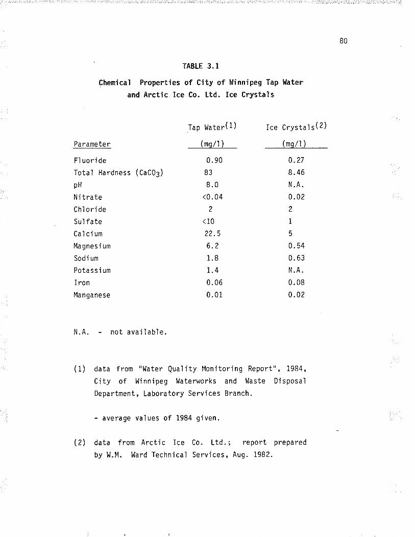
80

TABLE 3.X

Chemica'l Properties of CÍty ofand Arctic. Ice Co" Ltd.

Winnipeg Tap Haten

Ice Crystal s

Tap tlater(1)

(mq/l )

0. 90

83

8.0

<0.04

2

<10

22.5

6.2

1.8

1.4

0.06

0.01

Parameter

Fl uori de

Total Hardness (CaC03)

pH

Ni trateChl ori de

Sul fateCalcium

Magnes i um

Sodi um

Potassi um

I ron

Man gane se

Ice Crystals(2)

(mqll )

4.27

8. 46

N.A.

0.02

2

1

5

0. 54

0. 63

N.A.

0. 08

0.02

N. A. not available.

(1) data from "l.later Qual íty l,lonitoring Report", 1984,

Ci ty of l,Ji nn'ipeg ï,laterworks and l,laste DÍ sposaì

Department, Laboratory Services Branch.

- average values of 1984 given.

(2) data from Arctjc Ice Co. Ltd. ; report prepared

by tll.M. Ward Technical Services, Aug. 1982.

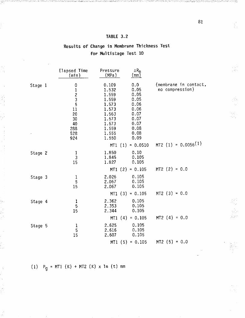
81

TABLE 3.2

Results of Change in kmbrane Thickness Test

for &4ultistage Test 10

Stage 1

Stage 2

Stage 3

Stage 4

Stage 5

E1 apsed Time(mjn)

01

23

5

11203040

2885?8924

Pressure(MPa)

0. 1091.5321.5591.5591.5731.5731. 5631.5731.5731.5591. 555i.550

r4T1 ( 1)

1 .8501 .8457.827

MT1 (2)

2.0262.0672.067

MTl (3)

?..3622.3532.344

MT1 (4)

2.6252.6162.607

MTl (5)

ÀRn(mm)

0.00.050.050.050.060.060.070. 070.070.080.080.09

= 0.0510

0. i00. i050. 105

= 0. 105

0. 1050. 1050. 105

= 0.105

0. 1050. 1050. 105

= 0.105

0. 1050. 1050. 105

= 0.105

1

3

15

1

5

15

1

5

15

1

5

15

(membrane in contact,no compression)

MTz (1) = 0.s656(1)

F,lTz (2) = 0.0

MTZ (3) = 0.0

MTz (4) = 0.0

MTZ (5) = 0.0

(1) Pg = MTl (K) + HTz (K) x ln (t) mm

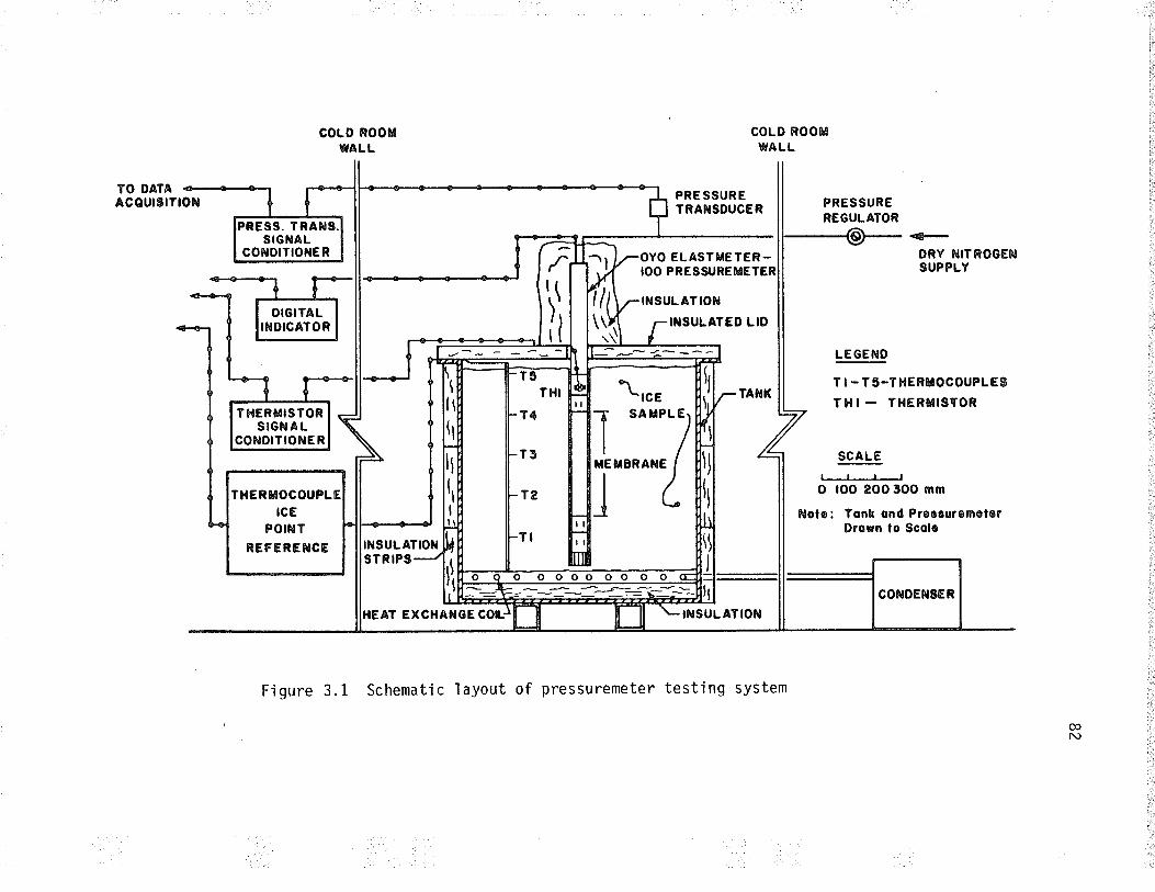
TO DATAACOUrSrltON

coLD ROOWWALL

ESs. TRANg.SIG¡{AL

CONOITIONER

THERIIISTORSIGNA L

CONOITIONER

THERgOCOUPLtcE

POINT

REFERES{CE

PRE SSUR ETRAf{SDUCER

COLD ROOMWALL

OYO ELASfIIETER.IOO PRESSIJREUETER

INSULATION

THI

T¿T

T3

T?

TI

INSULATION

Figure 3.1 Schematic la.yout of pressuremeter testing system

HEAT EXCHANGE

INSULATED LID

lHE

l

ORY NITROOENSUPPLY

LEGENO

TI-T5-THERMOCOUPLE9THI - THERMIgYOR

SCALE

llll

O IOO ?OO 3OO mm

Nole: Tonk ond Pressur@m616rDrown to Scol6

rr{suLATloN

oof\)

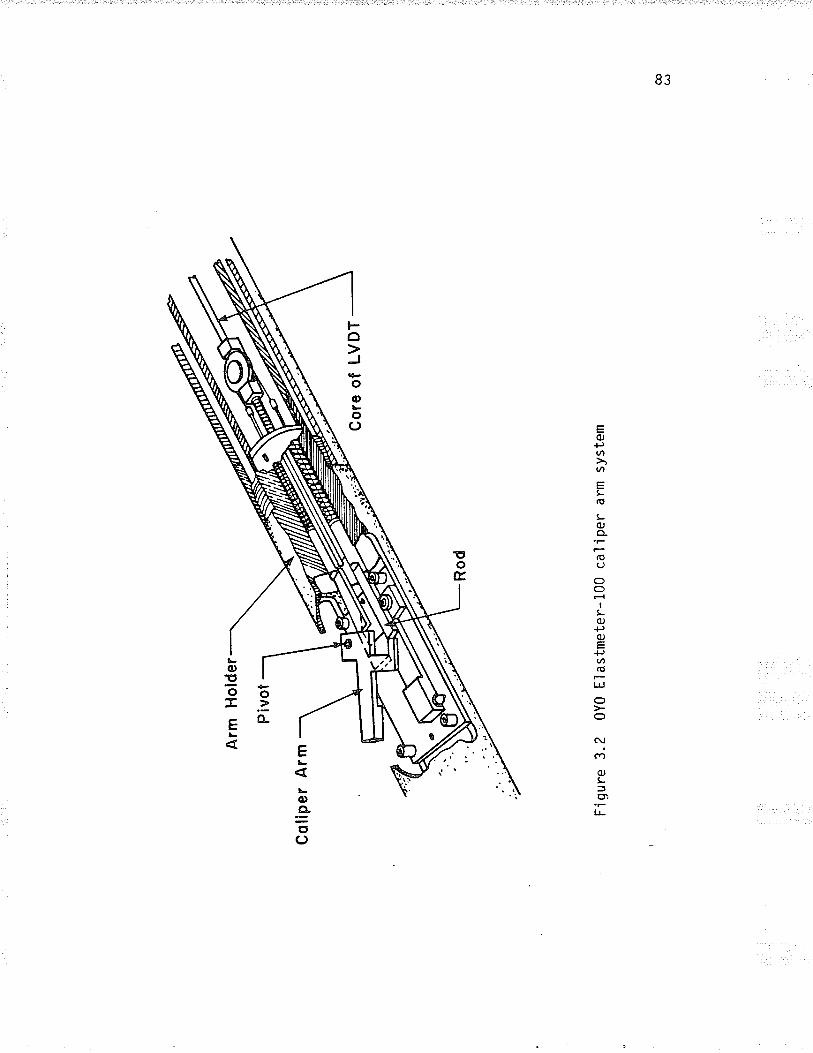
Col

lper

Arm

Arm

Hol

der

Piv

ot

F'ig

ure

3.2

0Y0

Ela

stm

eter

-100

cal

ìper

arm

sys

tem

Rod

Cor

e of

LV

DT

æ G,

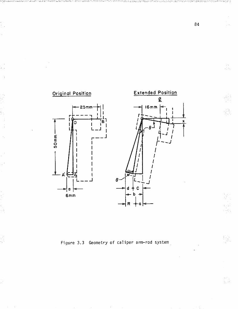
84

Originol Position Extended Position

l6 mm

Fiqure 3.3 Geometry of caliper arm-rod system

g.

l*l

e

,1-

IIIII

II

J

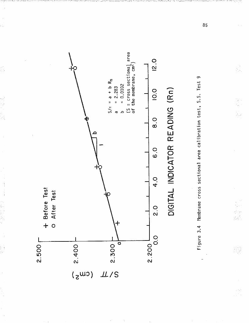
2.50

0

ñú

F c)

?.40

r'j^

+ o

h (Í)

Bef

ore

Tes

t

Afte

r T

est

2 .3

00o

2.?O

Oo.

o2.

O

4.O

6.

0

DIG

ITA

L IN

DIC

AT

OR

Fig

ure

3.4

llem

bran

e cr

oss

sect

iona

l

S/n

=a+

bRn

a =

2.2

83b

= 0

.010

2(S

= c

ross

sec

tiona

l are

aof

the

mem

bran

e, c

m2)

8. O

lO

.O

RE

AD

ING

(R

n)

area

cal

i br

ati o

n te

st ,

S. S

. T

est

9

r2.o

o (¡

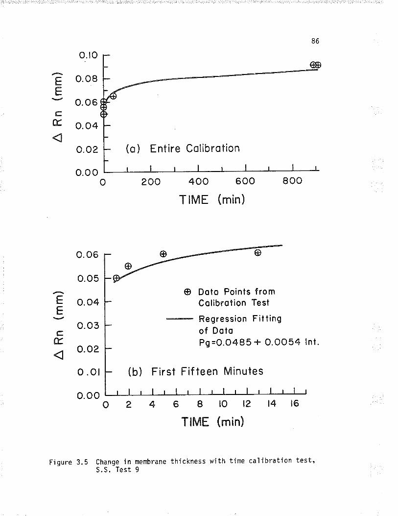
o. ro

o. oB

o. 06

o. o4

o. o2

o.o o

o. 06

o. o5

o. 04

o. o3

o. o2

o.ot

o. oo

86

@

?"5cÍr

o

(o ) Entire Colibrotion

200 800

@ Doto Points f ro m

Colibrotion Test

" Regression Fittingof DotoPg =O.O485 + O.OO54 lnt.

(b) First Fifteen Minutes

68lO12TltulE (min)

400 600

T ¡ME (min)

Ë

5C

æ.

l6l4

Change in membraneS.S. Test 9

Fi gure 3. 5 thÍckness with time calibratjon test'

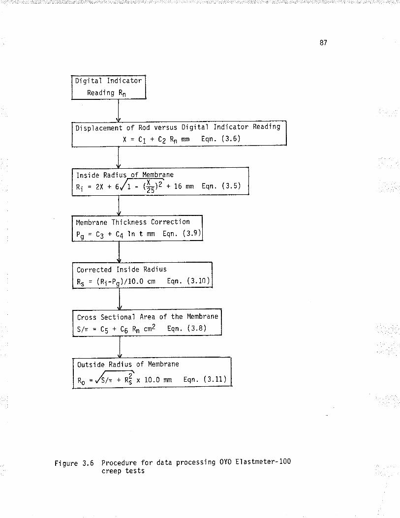
87

Di gì taì Indi catorReading Rn

Dispìacement of Rod versus Digìtaì Indicator Reading

X = C1 + C2 Rn mm Eqn. (3.6)

inside Radius of Membrane

Ri = zx + urîæ + 16 mm Eqn. (3.5)

l4embrane Thi ckness Correction

Pq = C3 + C4 ln t mm Eqn' (3'9)

Corrected Ins'ide Radi us

Rs = (Ri-Po)/tO.O cm tqn. (3.10)

Cross Sectional Area of the Membrane

S/r = C5 + C6 Rn cm2 Eqn. (S.a¡

of Membrane

x 10.0 mm Eqn. ( 3.11 )

Outs i de Rad'i us

no =/s/n * n!

Figure 3.6 Procedure for datacreep tests

processing 0Y0 Elastmeter-i00

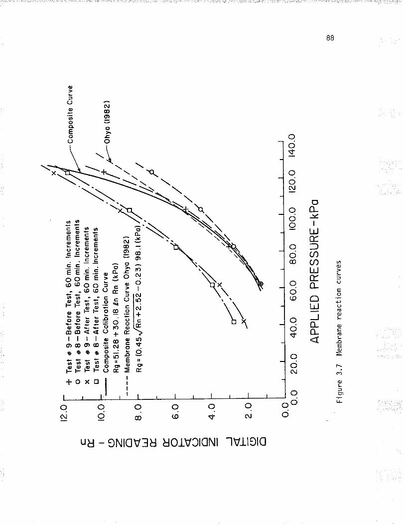
C æ.

I (9 z. o UJ É.

E. o k ç2 o 4 J F o o

t2.o

+ o X

_tr

ro.o

Tes

t *

9 -

Bef

ore

Tes

t, 60

min

. ln

crem

enls

Tes

t *

I -

Bef

ore

Tes

t, 6O

min

. ln

crem

ents

Tes

t *

9- A

fter

Tes

l, 60

min

. ln

crem

enls

Tes

l * 8

-Afte

r T

esl,

60 m

in.

lncr

emen

ls

8.O

Com

posi

te C

olib

rolio

n C

urve

Rg=

51.2

8 +

30.

18 é

n R

n (k

Po)

Mem

bron

e R

eocl

ion

Cur

ve O

hYo

Rs

= (o

.4sf

fi.-o

.zs)

6.O

4.O

2.O

Jii';

,., /'

o.o

/

o.o

AP

PLI

ED

PR

ES

SU

RE

- kP

o

Fi g

ure

3.7

f'lem

bran

e re

acti

on c

urve

s

I

20.o

40.

o 60

.0

r,

Com

posi

le C

urve

þonr

o(re

e2)

,/,

/,/

/

80.o

loo.

o 12

0. o

t40.

o

co co

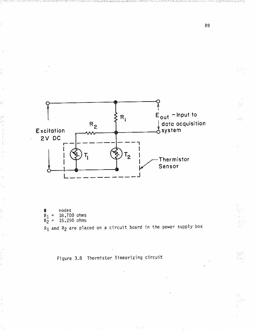
89

E out - lnput to

doto ocquisitionsystemE xcitotion

2V DC

Ther rn is torSen sor

@ nodesRl = 18,700 ohmsRZ = 35,250 ohms

R1 and R2 are pìaced on a circuit board in the power supply box

Figure 3.8 Thermistor 1 inearizing c'ircujt

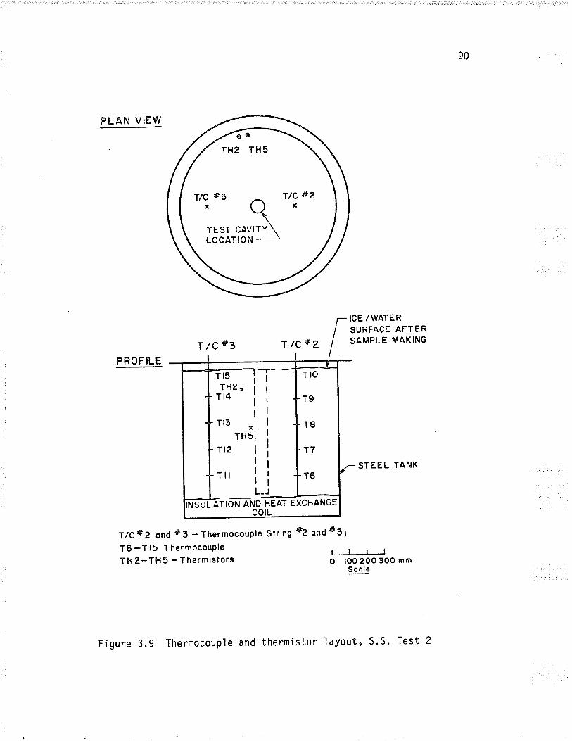
90

PLAh' VIEW

ICE /WATERSURFACE AFTERSAMPLE MAKING

PROFILE

T/ce 2 ond a*3 - ThermocouPle

T6 -T 15 T hermocouPle

TH2-TH5 - Thermislors

STEEL TANK

Slring #2 ond 63;

llllO IOO 2OO 3OO mm

Scols

T lCeZ T /C#z7

T15fïzx

T14

Tr3 xTH5

112

Tll

Tro

T9

T8

17

T6

iñi6ùil-uarrotl aND HEAr EXcHANGEcotL

Figure 3.9 Thermocoupìe and thermistor layout, S'S' Test 2

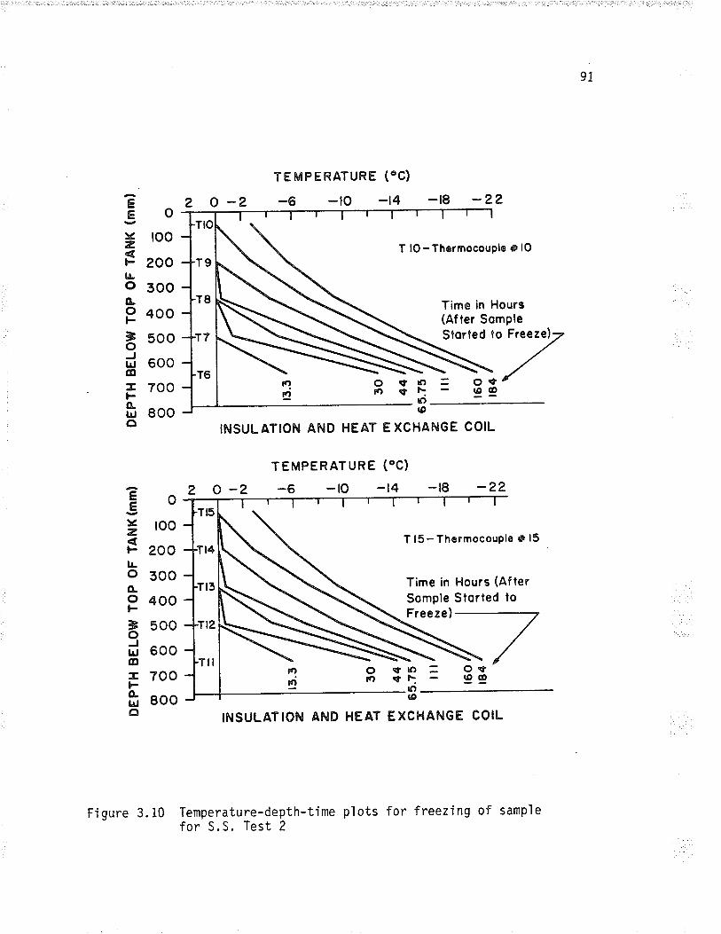
9I

tE

æ,4ÞtÀoo.ot'-Bol¡Jot.Þo.t¡Jo

E.E!Ét

Þlloo.oÞ9oJt¡¡@Eû-o.trlo

? o-2TEMPERATURE (OC)

-6 -lo -t4 -18 -??

T lO - Thørmocouplø @ lO

Time in Hours(After Somple

o

roo

200

300

400

500

600

700

800

o

roo

200

300

400

500

600

700

800

úl\ú)(o

\tqf

oÉ,

2 0-2TEMPERATURE (OC)

-6 -ro -14 - t8 -2?

T l5 - ThermocouPle * l5

Time in Hours (Af terSomple Storted toFreeze)

Figure 3.i0 Temperature-depth-time plots for freezing of samplefor S.S. Test 2

= o<t99

()\K'(e

oçÉ, <r

INSULATION AND HEAT EXCHAF{GE COIL

INSULATIOt{ AND HEAT EXCHAÞ*IGE COIL

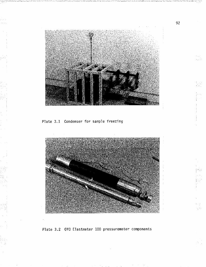
92

l¡:'

'.:ir.tl

:,:,:::.:1.

'.))

Plate 3.1 Condenser for samp'le freezing

Plate 3.2 0Y0 Elastmeter 100 pressuremeter components

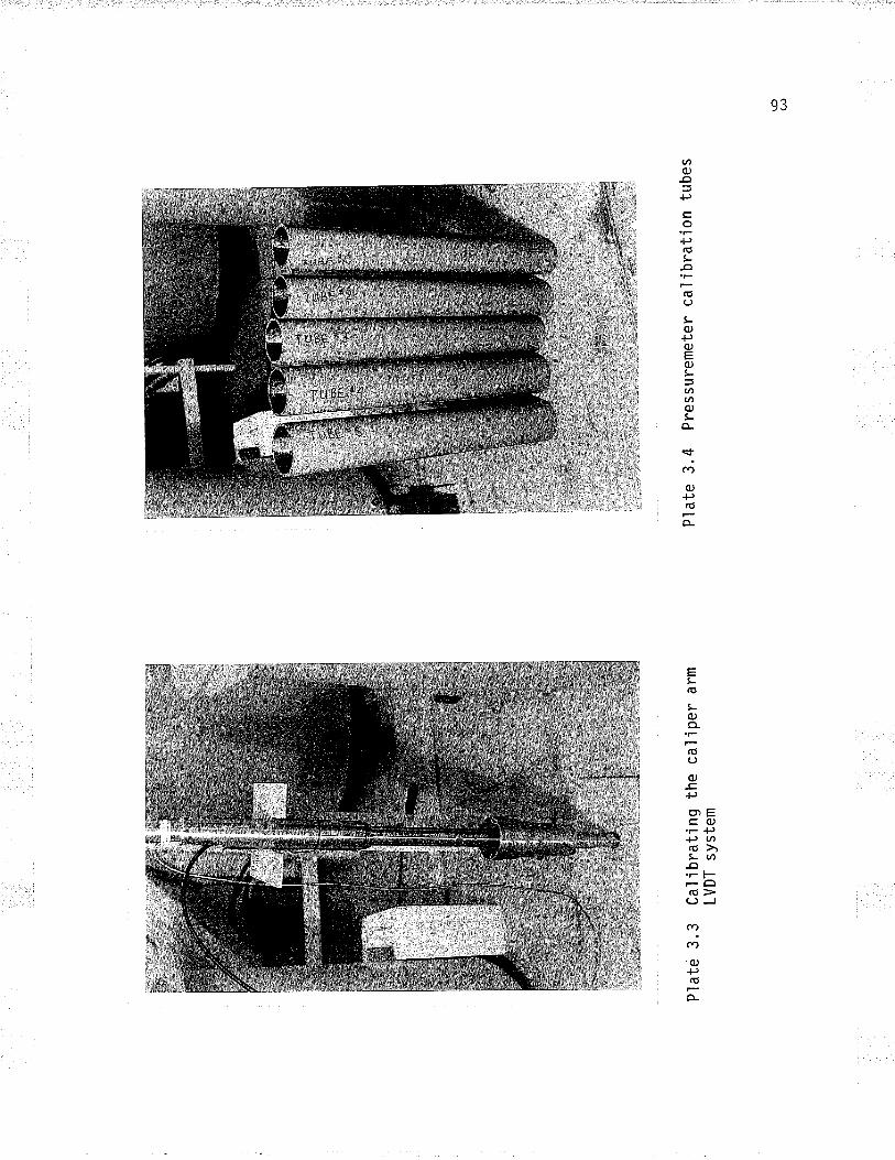
Pla

te 3

.3 C

alib

ratin

g th

e ca

liper

arm

LVD

T s

yste

mP

late

3.4

Pre

ssur

emet

er c

alib

ratio

n tu

bes

\o (,

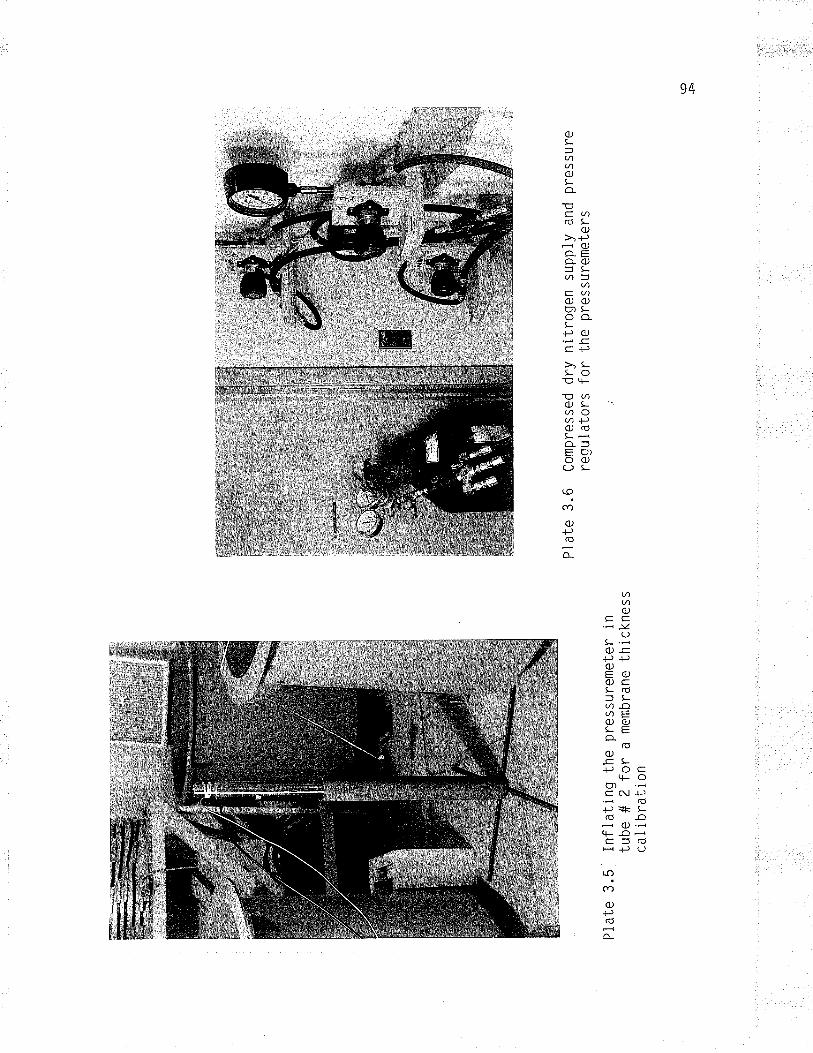
Pla

te 3

.5 In

flatin

g th

etu

be#2

fora

cal i

brat

ion

pres

sure

met

er in

mem

bran

e th

ickn

ess

Pla

te 3

.6C

ompr

esse

d dr

yre

gula

tors

for

nitr

ogen

sup

ply

and

pres

sure

the

pres

sure

met

ers

\.o Þ

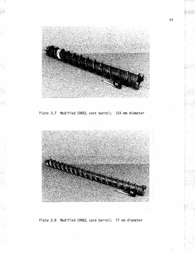
95

Plate 3.7 Modified CRREL core barrel; 104 mm diameter

Plate 3.8 Modified CRREL core barrel; 77 nn d'iameter

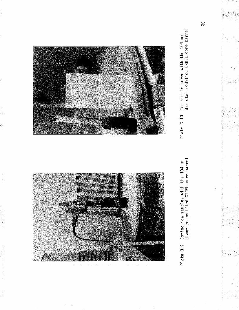
PI a

te 3

.9 C

orin

g ic

e sa

mpl

esdi

amet

er m

odifi

edw

ith t

he 1

04 m

m

CR

RE

L co

re b

arre

lP

l ate

3.

10Ic

e sa

mpl

e co

red

with

the

104

mm

diam

eter

mod

ified

CR

RE

L co

re b

arre

l

(O Ol

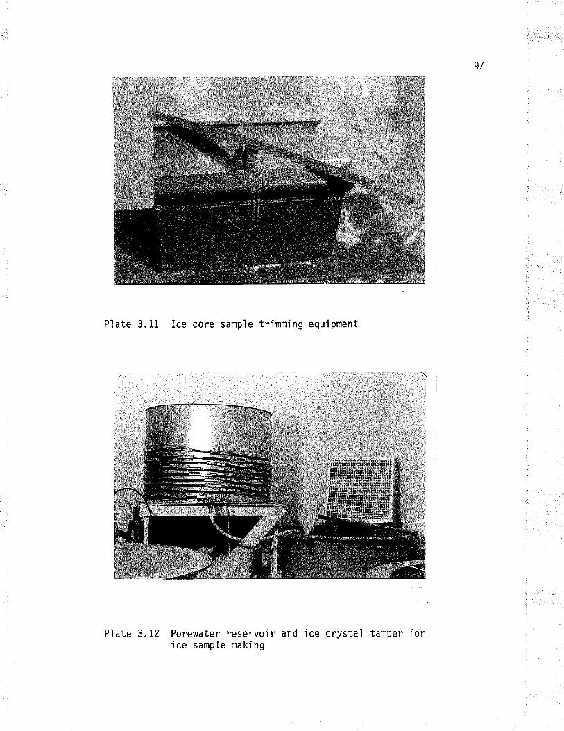
97

Plate 3.11 lce core sample trimming equipment

Plate 3.12 Porewaterice sample

reservoir and ice crysta'l tamper formaking

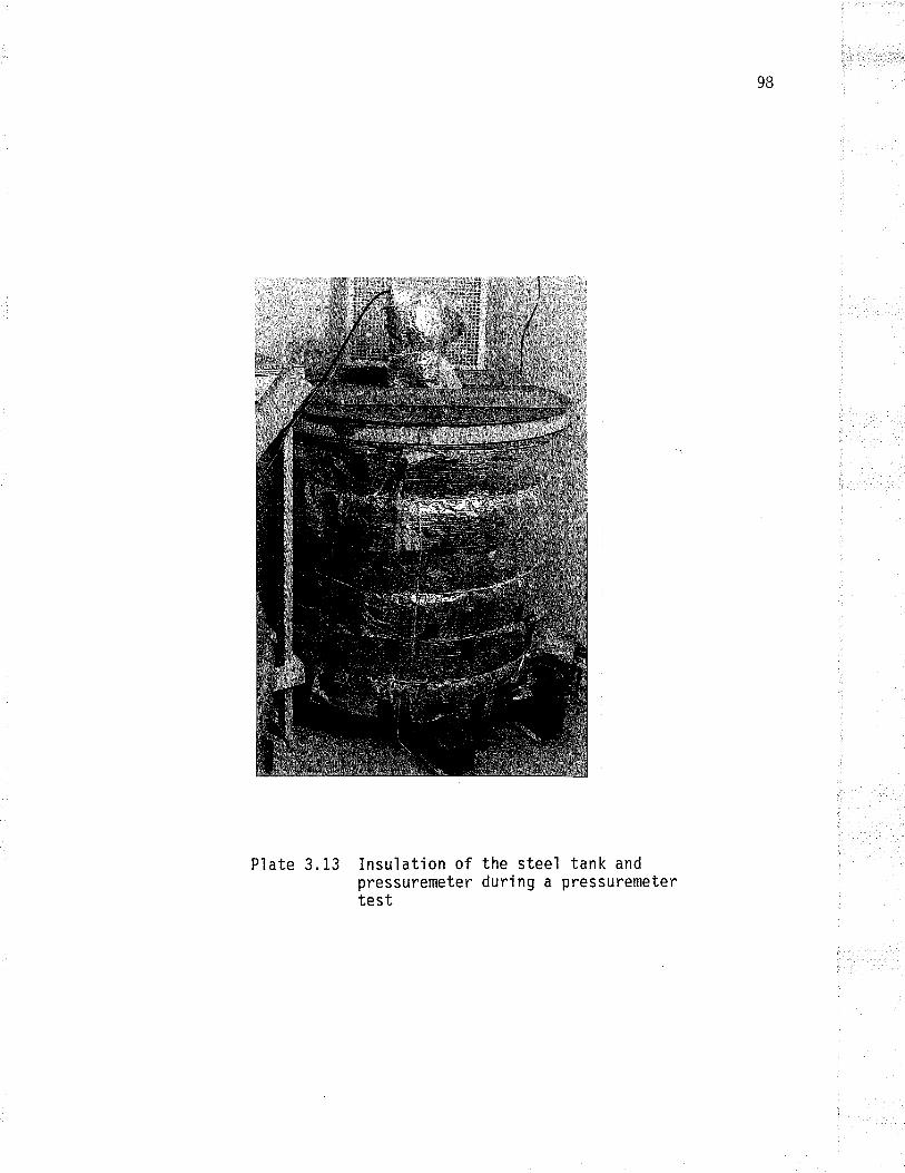
98

Plate 3.13 Insulation ofpressuremetertest

the steel tank andduring a pressuremeter

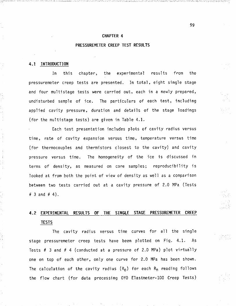
99

CH¡TPÏER 4

PRESSUREMETER CREEP TEST RESU!-TS

4" 1 I${TRODUCTIOH

In thi s chapter, the experimental resul ts from the

pressuremeter creep tests are presented. In total, eight sing'le stage

and four multistage tests were carried out, each in a newly prepared,

undisturbed samp'le of ice. The particulars of each test, includìng

appl ied cavity pressure, duration and detai I s of the stage 'loadings

(for the multistage tests) are given in Table 4.1.

. Each test presentation includes plots of cavity radius versus

time, rate of cavity expans'ion versus time, temperature versus time

(for thermocouples and thermistors closest to the cavity) and cavity

pressure versus time. The homogeneìty of the ice is discussed jn

terms of densi ty, as measured on core sampl es; reproduci bi ì i ty j s

looked at from both the point of vjew of density as we'll as a comparison

between two tests carried out at a cavity pressure of 2.0 MPa (Tests

# 3 and # 4).

4.2 EXPERII.IENTAL RESULTS OF THE SINGLE STAGE PRESSUREI{ETER CREEP

TESTS

The cavity radius versus time curves for all the s'ing1e

stage pressuremeter creep tests have been plotted on Fig. 4.1. As

Tests # 3 and # 4 (conducted at a pressure of 2.0 MPa) plot virtually

one on top of each other, only one curve for 2.0 MPa has been shown.

The calculation of the cavity radius (Ro) for each Rn reading follows

the flow chart (for data processing 0Y0 Elastmeter-100 Creep Tests)

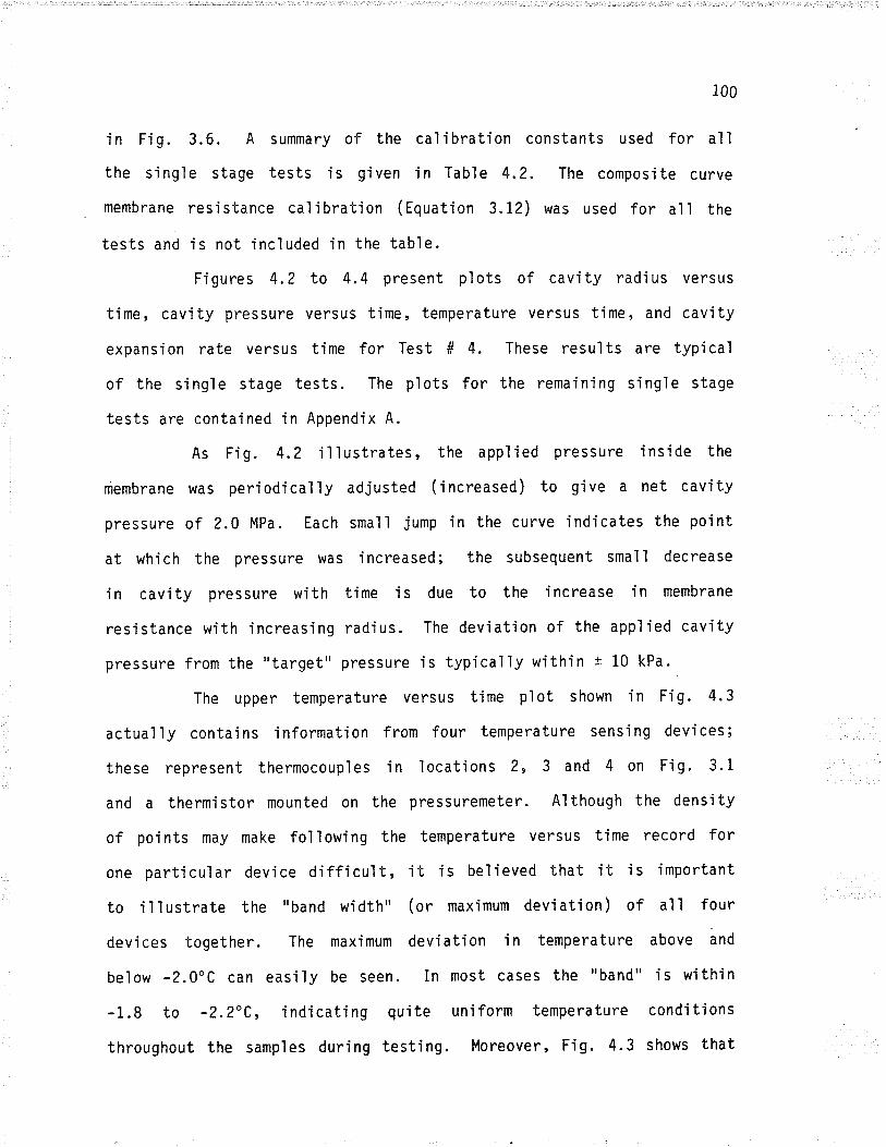
100

in Fig. 3.6. A summary of the calibration constants used for all

the singìe stage tests js given in Table 4.2. The composite curve

membrane resjstance calibration (Equation 3.LZ) was used for all the

tests and is not included in the table.

Figures 4.2 to 4.4 present p'lots of cavity radius versus

time, cavity pressure versus time, temperature versus time, and cavity

expansion rate versus time for Test # 4. These results are typicaì

of the singìe stage tests. The plots for the remaining single stage

tests are contained in Appendix A.

As Fig. 4.2 illustrates, the app'l'ied pressure inside the

membrane was periodically adiusted ('increased) to give a net cavity

pressure of 2.0 MPa. Each small jump in the curve indicates the poìnt

at whi ch the pressure was 'i ncreased; the subsequent smal I decrease

in cavity pressure with time is due to the increase in membrane

resistance with increasing radius. The deviation of the applied cavity

pressure from the "target" pressure is typicalìy within t 10 kPa.

The upper temperature versus time pìot shown in F'ig.4.3

actually contains information from four temperature sensing devices;

these represent thermocouples in locatjons 2, 3 and 4 on Fig. 3.1

and a thermistor mounted on the pressuremeter. Although the density

of points may make fo'lìowing the temperature versus time record for

one part'icular device difficult, it js beljeved that it is important

to illustrate the "band width" (or maxjmum devjation) of all four

devices together. The maximum deviation in temperature above and

below -2.0"C can easi'ly be seen. In most cases the "band" is within

-1.8 to -2.2"C, indicating quite uniform temperature conditjons

throughout the samples during testing. I'loreover, Fig. 4.3 shows that

101

the average temperature in the sampìe remaÍned very close to -2.0"C

during the test.

The pressuremeter creep data has been reduced and plotted

using two computer programs, which are listed in Append'ix C. The

fi rst program, cal I ed M0Y0PLl , cal cul ates the cavi ty radi us versus

tÍme, using the flow chart illustrated in Fig. 3.6, and produces plots

as shown in Figs. 4.2 and 4.3. The second program, called 0Y0RATE,

calculates and plots the cavity expansion rate versus time, as shown

i n Fi g. 4.4.

To calculate the cavity expans'ion rate, OYORATE incorporates

a moving point, second order polynomÍaì least squares regression curve

fìtting analysis. The length of fitted segment is typicaììy 9 points

in the early stages of the test. After the curve has essentially become

flat, the length of segment is increased to 3i or 4l points. The

first derivative of the polynomial express'ion which represents each

segment is calculated for each experímental point in the segment.

0n1y the value at the midpoint is plotted, as jn Fig. 4.4. The segment

is shifted aìong the experimental curve by one to as many as 30 points,

depending upon the density of data points and degree of curvature.

The quality of fit of each segment was assessed by calculating the

sum of the squared residuals of the experimental cavity radius versus

the cavity radius calculated from the po'lynomial expression. In most

cases the qua'lity of fit was good; i.e. the radius calculated from

the fitted poìynomial expression was typica'lìy wÍthin 0.02 mm of lh.

experimental radius at the midpoints of the segments.

t02

4.3 EXPERI&{E¡{TAL RESULTS OF THE T4ULTISÏA6E PRESSUREI{ETER CREEP TESTS

Figures 4.5 and 4.6 present plots of cavity radius versus

time, cavity pressure versus time, and temperature versus time for

Test # 10. Fígures 4.7 to 4.11 present plots of cavity expansion

rate versus ti'me for each stage. The plots for the remajning mult'istage

tests are contained in Appendix A.

As with the sing'le stage tests, the data processing flow

chart illustrated in Fig. 3.6 was used to calculate the cavity radius

(Ro) for each Rn reading for all of the multistage tests. A summary

of the cal i bration constants used for al I the mul ti stage tests i s

!iven in Table 4.3. The composite curve membrane resistance calibration

(Equation 3.12) was used for all the multistage tests and is not

included in the Table.

As Fig. 4.5 i I I ustrates, deviations in the appl ied cavity

pressure were small and changes in pressure from one Íncrement to

the next lvere carried out within about one minute. Moreover, as with

the sing'le stage tests, temperature uniform'ity throughout the samples

used for the multistage tests was good (as Fig. 4.6 iììustrates).

The cavity expansion rate versus time curves for each stage,

shown Ín Figs. 4.7 to 4.11, were calculated and p'lotted using the

program OY0RATE. A segment ìength of 9 po'ints was used for all stages

of all of the multistage tests.

4.4 DISCUSSIOH OF TEST RESULTS

As the cavity radius and

curves for the singìe stage tests

rapid decrease in deformation rate

cavi ty expans'ion rate versus time

illustrate, there is typicaìly a

to a minimum (i.e. relatively short

103

prjmary creep period), with a gradual increase in rate thereafter.

The time to the minimum rate ranges from about 330 mÍnutes at a pressure

of 2.5 MPa to about 6,000 minutes at a pressure of 1.0 MPa. The

increase in deformat'ion rate after the minimum is much more pronounced

at higher pressures than at lower pressures (e.g. Figures 4.3 and

4.6, for 2.5 and 2.25 MPa respect'ively as compared to Figures 4.18

and 4.21, for 1.25 and 1.0 MPa respectively). As discussed in Chapter

2, steady-state creep for the pressuremeter case, 'in terms of the

power I aw creep model , i s represented by an exponent'iaì 'ly i ncreasi ng

cavity radius with time. It appears, therefore, according to this

definition, that steady-state creep dominates after the initial ,

relativeìy short primary creep period. As the form of response for

tertiary creep in the pressuremeter problem has never been discussed,

it is difficult to cornment on whether the creep is going into a tertiary

mode or not.

Examination of the cavìty radius and cavity expansion rate

versus time curves for each stage of the multistage tests indicates

a wel'l developed primary period in only the first stage of each test.

The second and subsequent stages show some i ni tj al fl uctuati on i n

the rate with time and then generally level off. Sìight increases

in rate may be noted near the ends of the higher pressure increments.

Also evident in the cavity radius versus time curves for the multistage

tests (for example, see Figure 4.5) is the small magnitude of the

time independent deformation (i.e. elastic and p'lastic strain) developed

when the pressure is increased from one stage to the next.

The minimum cavity expansion rates for the single stage

tests and each stage of the multistage tests are compi'led in Table

4.4.

104

review of this data indicates that:

The minimum cavity expansion rates for the sing'le stage tests

generally agree quìte well with the mjnimum cavity expansion

rates for the multistage test increments at the same pressures.

The multistage rates are, however, typically slight'ly higher.

The minjmum rates from mul ti stage Test 12 genera'l 1y show

the best agreement w'ith the single stage results, while the

rates from multistage Test 11 show the largest deviation

from the single stage results.

4.5 ICE PROPERTIES AI{D PRESSUREI{ETER TEST SAHPLE HOþÐGEI{EITY

As d.i scussed 'in chapter 3, test tanks wi th a semi -ri g'id

lateral boundary were chosen for this program to inhibit radial crack

development and eliminate complete failure of the ice cylinder at

low strains. Even with this boundary conditjon, however, some crackìng

of the ice did develop. Table 4.5 gìves a surnmary of any cracking

which was observed.

A major radial crack, which went from the cavìty wall to

the sample boundary, deveìoped in on'ly one test (Test # 6). A m'inor

crack, extending into the sample about 180 nm from the cavity wall,

occurred in another test (Test # 10) while traces of cracks (penetrating

to a maximum of about 10 nrm) were found jn three other tests (Tests

# 2, # 3 and # 4). A thorough examinat'ion of the other seven samples

revealed no visible cracking whatsoever. Plates 4.I and 4.2 tho*

the sample for Test # 7, with no visible cracks, while Plate 4.3 shows

the crack which developed during Test # 10.

When stud'ied in detail after the testsn all of the cracks

A

i)

2)

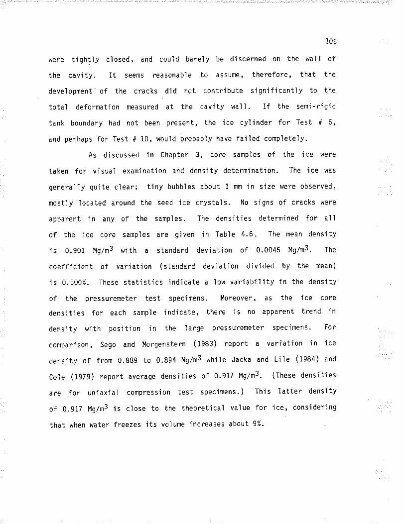
105

were tightly closed, and could barely be discerned on the wall of

the cavi ty. It seems reasonabl e to assume , therefore , that the

development of the cracks djd not contribute signifÍcantly to the

total deformati on measured at the cavi ty wal I . If the semi -ri gi d

tank boundary had not been present, the ice cylinder for Test # 6,

and perhaps for Test # 10, would probably have failed completely.

As di scussed i n Chapter 3, core samp'l es of the i ce were

taken for visual examination and density determination. The ice was

generaì1y quite clear; tiny bubbles about 1 mm in size were observed,

mostly located around the seed ice crystaìs. No signs of cracks were

apparent in any of the sampìes. The densities determined for all

of the ice core sampìes are gìven in Table 4.6. The mean density

i s 0.901 Mg/m3 wi th a standard devi ati on of 0.0045 Mg/m3. The

coefficient of variation (standard deviation divided by the mean)

is 0.500%. These statistics indicate a low variability in the densÍty

of the pressuremeter test specimens. Moreover, as the ice core

densi ti es for each sampl e i ndi cate , there i s no apparent trend i n

density with position in the 'large pressuremeter specimens. For

comparison, Sego and Morgenstern (i983) report a variation in ice

density of from 0.889 to 0.894 Mg/m3 while Jacka and Lile (1984) and

Cole (i979) report average densities of 0.917 Mg/m3. (These densities

are for uniaxial compression test specimens. ) This latter densìty

of 0.917 Mg/tn¡ is close to the theoretical value for ice, consjdering

that when water freezes its volume increases about 9%.

106

4.6 PRESSUREHETER TEST SAffiPLE REPRODUCIBILITY AND TEST REPEATABILITY

As Table 4.6 indicates, the variabi I ity 'in ice densities

for the pressuremeter test specimens is quite small. In fact, on'ly

two of the 37 ice core sample densities determ'ined fall outside of

I two standard devjations from the mean; two standard deviations

from the mean represents an error of about I% from the mean. These

resul ts i ndj cate , therefore , that as far as densi ty i s concerned ,

the sampìes were very reproducible.

As discussed in the Introduction to this chapter, two single

stage tests were conducted at an applied cavity pressure of 2.0 MPa

to check for both sample reproducibility and test repeatabjìity. Figure

4.12 shows the two cavity rad'ius versus time curves superimposed one

upon the other. Thi s Fi gure 'i ndi cates that the sampl es were

reproducible and the test is repeatable.

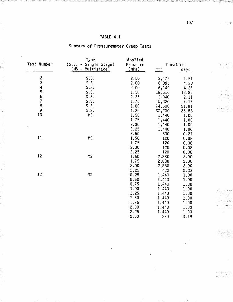
Test Number

TABLE 4. T.

Sunønary of Pressurereter

Type(S.S. - Sí ng'le Stage )

S. S.S.S.S. S.s. s.S. S.s. s.S. S.S. S.

MS

Creep Tests

Appl i edPressure

lmna)

2.502.002. 001. 502.25I.7 5

1.00r.251. 507.7 52.002.252.501. 50t.7 5

2.002.251. 50r.7 5

2.002.250.250. 500.751.007.251. 50r.7 5

2.00?.252.50

mln

2,r7 5

6,0956, 140

18,5i03,040

i0,32074,60037 ,200

1 ,4401 ,440r,4401 ,440

300r20720t20r20

2 ,8802,8802 ,880

4801 ,440I ,4401 ,4401 ,4401 ,4401 ,4401 ,4401 ,4401 ,440

270

Durati on

L07

days

1.514.234.26

12.852.7r7.r7

51.8125.83

1. 001. 001.001. 000.270. 080. 080. 080. 082.002.002. 000. 331.001. 001. 001. 001. 001. 001.001. 001.000. 19

2

345

67

I9

10

MS

MS

MS

11

I2

13

MS - Multistage)

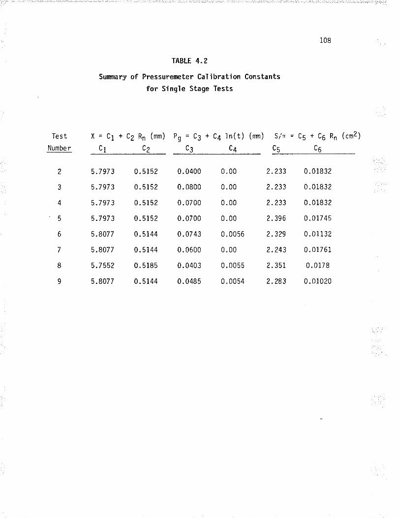
108

Test

Number

TABLE 4"2

Sunrnary of Pressuremeter Cal ibration Constants

for Single Stage Tests

= C1 + C2 Rn (mm) Pg = C3 + C4 ln(t) (rnm) Si''

C1 C2 C3 C4 C5

= c5 + c6 Rn (cm2)

C6

2

3

4

5

6

7

I9

5.7973

5.7973

5.7973

5.7973

5.8077

5.8077

5 .7 552

5.8077

0. 5152

0 . 5152

0. 5152

0.5152

0.5i44

0 . 5144

0 . 5185

0. 5 144

0.0400

0.0800

0.0700

0.0700

0.0743

0.0600

0.0403

0.0485

0.00

0.00

0.00

0.00

0.0056

0.00

0.0055

0.0054

2.233

2.233

2.233

2.396

2.329

2.243

2.35r

2.283

0.01832

0.0i832

0.01832

0.0i745

0.01132

0.01761

0.0i78

0.01020

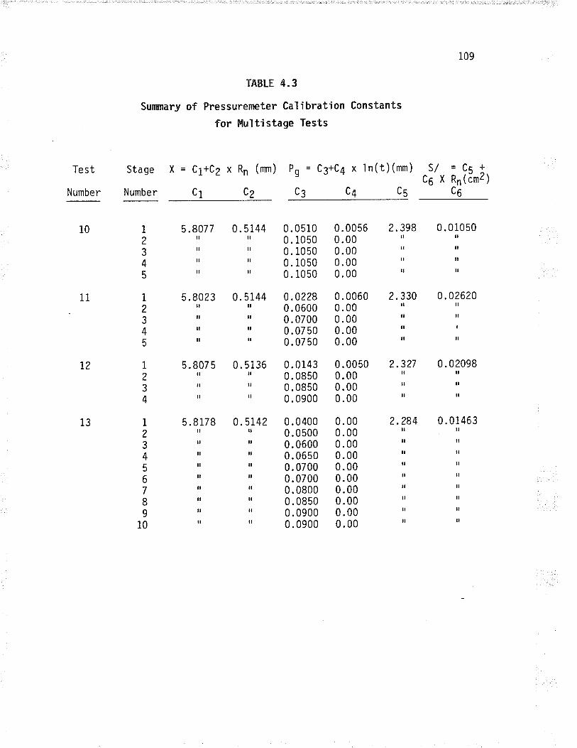
109

TABLE 4.3

Sunø'nary of Pressurereter Calibration Constants

for Hultistage Tests

Test

Number

Stage X=C1+C2¡ftn(nrm)

Number C1 C2

Pn = c3+c4 x ln(t)(mm) ,l/, 0.11,nälC4 c5 c6C3

10

11

t2

13

1

2345

1

23

45

1

234

5.8077il

il

lt

il

5.8023ll

ll

il

il

5.807 5tl

ll

ll

5.8178lt

il

il

il

ll

il

il

il

il

0 . 5144il

lt

ll

il

0 . 5144il

il

il

il

0 . 5136ll

il

tl

0.5142il

lt

il

il

il

il

il

il

lt

0.05100. 10500. 10500. 10500. 1050

0.02280.06000.07000.07 500. 07 50

0.01430.08500.08500.0900

0.04000.05000.06000.06500.07000.07000.08000.08500.09000.0900

0.00560.000.000.000.00

0.00600.000.000.000.00

0.00500.000.000.00

0.000.000.000.000.000.000.000.000.000.00

2. 398il

il

il

u

2. 330¡l

ll

il

il

2.327il

il

il

2.284il

ll

il

il

il

ll

il

lt

ll

0.01050ll

il

il

il

0.02620il

il

I

il

0.02098il

ll

il

0.0i463¡t

il

il

il

il

lt

il

il

lt

I23

45

67I9

10

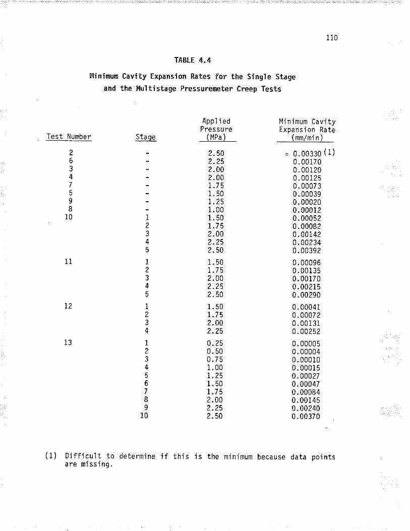
TABLE 4"4

Hinimum Cavity Expansion Rates for the Single Stage

and the Hultistage Pressurereter Creep Tests

App'l ì edPressure

110

Minimum CavityExpansion Rate

(mm/mi n )Test Number Sta ge

Difficult to determineare missing.

(MPa)

263475

98

10

:

:

1

2345

1

2345

1

234

1

234567

I9

10

?.502.252.002.00r.75i. 501.251.001.501.7 52.002.252.50

1.501.752.002.252.50

1.501.7 5

2.002.25

0. 250. 500.7 51 .00t.251.501.7 52.002.252. 50

= 0.00330 (1)0.00i700.001200.001250.000730.000390.000200.000120.000520.000820.00i420.002340.00392

0.000960.001350.001700.002150.00290

0.000410.000720.00i310.00252

0.0000s0.000040.000100. 000i 5

0.000270.000470.000840.001450.002400.00370

11

L2

13

(i) if this is the minimum because data points

111

TABLE 4"5

lÞgree of Cracking in Pressurereter Test lce SpecinNens

Degree ofTest Number Cracking Nature of Cracks

2 Trace 3 radial cracks spaced at about120' at the top of the cav'ity -penetrate = 5 to 10 mm into the icespecimen.

3 Trace 3 radial hairline cracks spaced atabout 120"; only vìsible at the topof the cav'ity.

4 Trace 2 radial hairline cracks; on'ly visibleat the top of the cav'ity.

5 No cracking visible

6 Major 2 radial cracks; one extends from thecavity to the steel tank while theother extends about 300 mm from thecavÍ ty.



9 No cracking visìble

10 llinor One radial crack extends about 180mm from the cavity wall.




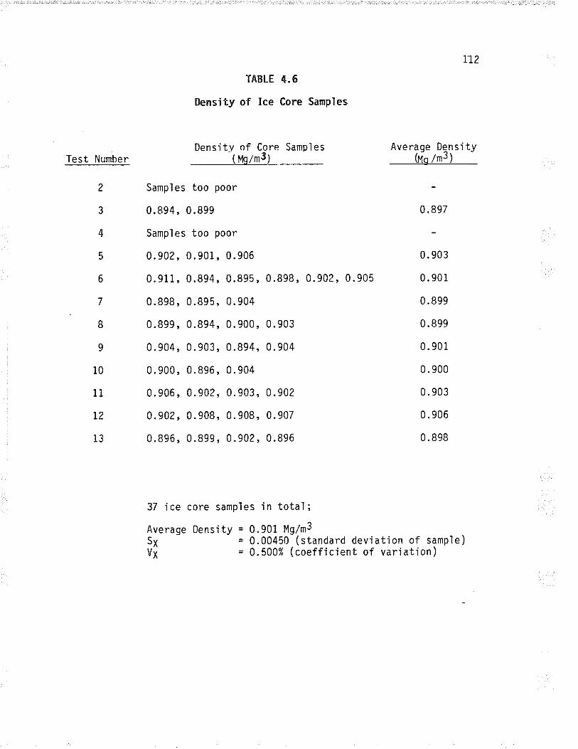
I't2

TABLE 4.6

flensity of lce Core Samples

Test Number

2

3

4

5

6

7

8

9

10

11

L2

13

Sampl es

0.894,

Sampl es

0.902,

0.911 ,

0.998,

0.899 ,

0.904,

0.900,

0.906 ,

0.90?.,

0.896 ,

too poor

0.899

too poor

0.901,0.906

0.894, 0.895,

0.895,0.904

0.894,0.900,

0.903,0.894,

0.896,0.904

0.902, 0.903,

0.908,0.908,

0.899,0.902,

Densit.v of Core Samples(¡'h/m3)

Average Dens'ityhs /mr )

0.897

0.898,

0.903

0.904

0.902

0. 907

0.896

0.903

0.902,0.905 0.901

0.899

0.899

0.901

0.900

0.903

0.906

0.898

37 i ce core sampl es 'in total ;

Average Density = 0.901 Mg/m3S¡ = 0.00450 (standard deviation of sampìe)Vi = 0.500% (coefficient of variation)

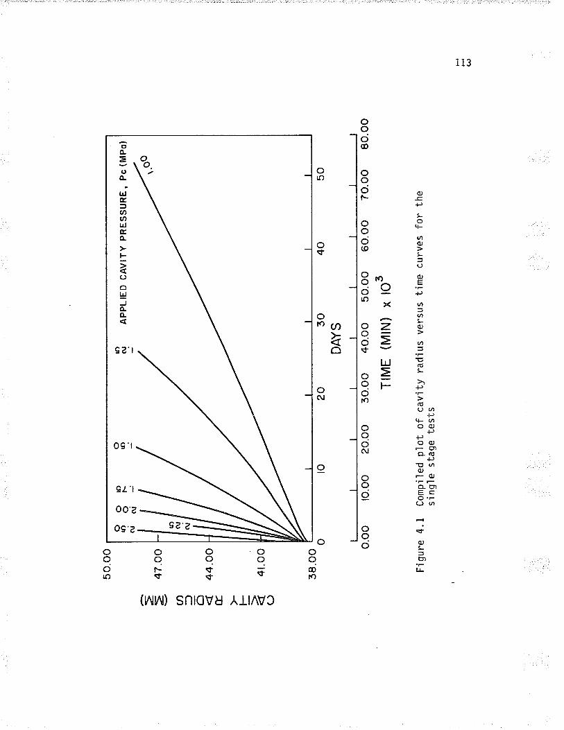
50.o

o

s ë (n :) õ É.

t-- ã C)

47.O

O

oorr

lrr

? O

¡-

(\,

Gj

:

44.O

O

ro ry a,

o rO

4l.o

o

38.O

O

rf,, ol

o

AP

PLI

ED

CA

VIT

Y P

RE

SS

UR

E,

Pc

(MP

o)

o.oo

Fig

ure

4.1

Com

pile

d pl

ot o

f ca

v'ity

rad

ius

vers

us t

ime

curv

es f

or th

esi

ngle

sta

ge te

sts

to

ro.o

o20

.oo

20

I

30.o

o 40

.oo

50.o

o

TIM

E (

MlN

) x

lO3

30D

AY

SI

r.oo

40 60.o

o

50

70.o

o80

.oo

H lJ (,

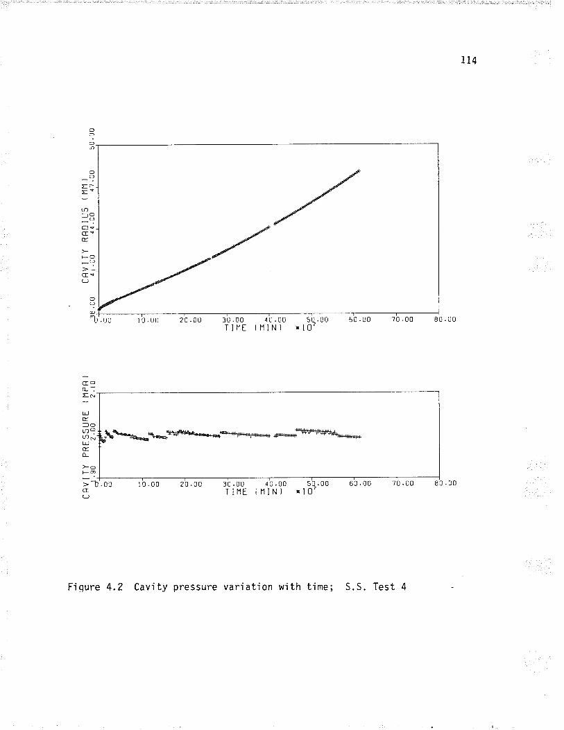
114

O?O

OO

tÈ

='tn_O'oCleG<É.

FO_?cIe(-J

.uu

OO

@_

n I{J . uu 20 .0u 60 . fJ030 .00T INE

¿0 .00 50 .00( ll lN ì x 102

/0 .00 80 .0u

Goo-:5*LLJÉ=oØ=cDNtrlÉ.o_

)-sFO

Ct)

>-b.oo 10.00 20.00 3.0.0tJ 40.00 ÞQ.oo 60'00 70.00 80.00l-lNE tlllN) *102

Fiqure 4.2 Cavìty pressure varjation with tjme; S.S. Test 4

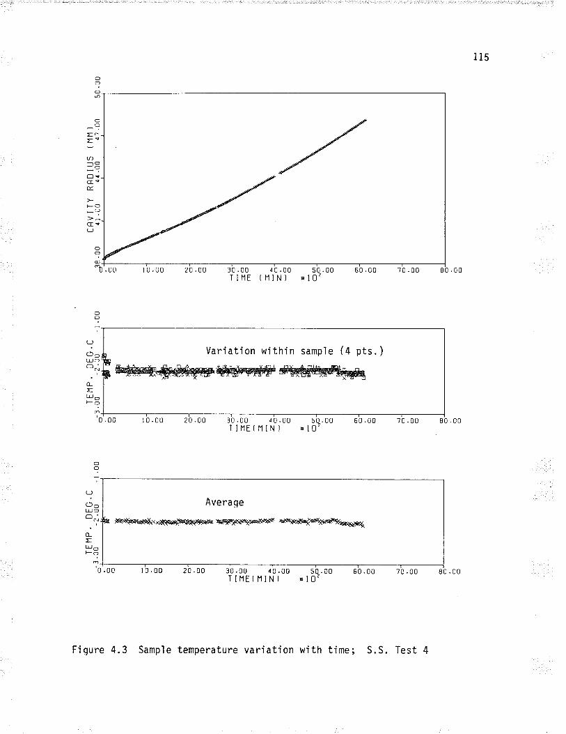
115

ooOô

OO

='U)-o_O

C)ecr<É

F()

-?ce(J

?c)oLLJ oo"i

ùELrJ o*?

3C .00T INE

.u0

oo@_

"b

O?

O]or

"".

O?

0

oO

?Òt!O

rELL,l-

'70 .00 80 .00

Variation within

@ffiÉWffi

1 0 .00 20 .00 30 .00 ¿ 0 .00 50 .00TIIlE{11lNt '10'

70 .0u 80 . û0.00

r0.00 20 .00

r0.00

40.00 50.00( M IN I ' l0'

tì0 .00

60 .00I

70 .00 80 .00

60 .00

Averaqe

@¡xrcffiæ wÈftr]M wë#effielðõÈe

'0 .00 20 .00 30 .00 40 .00TIIlE(HIN)

50 .00u l0t

Fiqure 4.3 Sampìe temperature vari ati on wi th ti me ; S . S . Test 4

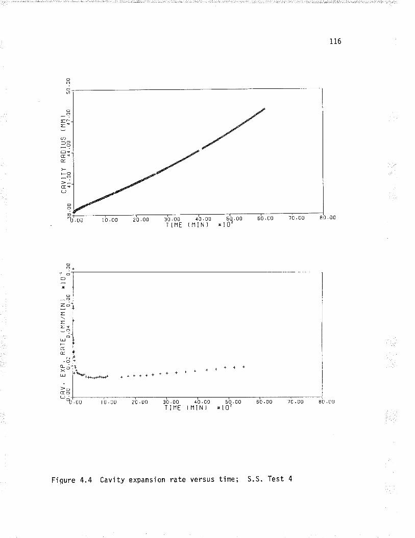
116

O?Oû

OO

E-

="U)

-OOçGTÉ.

FO

-?(IrLJ

o?o

r 0 .00 20 .00 ¡b . oo 4'o . oo st¿. ooTlllE tNIN) xl0'"b'. oo 60 .00 7û .00

++

'* { +r.¡++!+* ++++++**++

I0 .00 ?0.oo 30.00 40.00 50.00TINE (l'llN) xl02

?0 .00 80 . Lì0

80 .00

.00

æo

:O

:x

@_O

1O

;TEç-?.

Ot!GÉ.

a,J.O

o-c'><tLJ

>OLJ_-I 60 .00

Fiqure 4.4 Cavity expans'ion rate versus time; S.S. Test 4

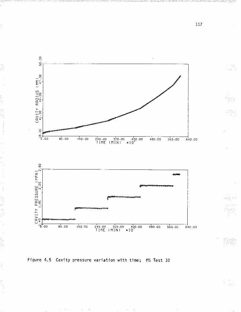
It7

o?oû

O

E-

='(n-O

cr;G9

l- cf_?Ge(J

240.00T IHE

4 00 .00rl0' d 80 .00 560 .00 640.00

80 .00 t60.00 240.00 320.00 áq0.00 ¿80.00 s'oo.oo sio.ooTINE (NlN) '10'

.00

cf(¡

_NCEo_E

ON

LLI '-ÈN

=U)U)LrJøSo_ .-

|-

CO(J.

-b

l 60 .00 320 .00ININ)

Fiqure 4.5 Cavity pressure variation with time; tls Test 10

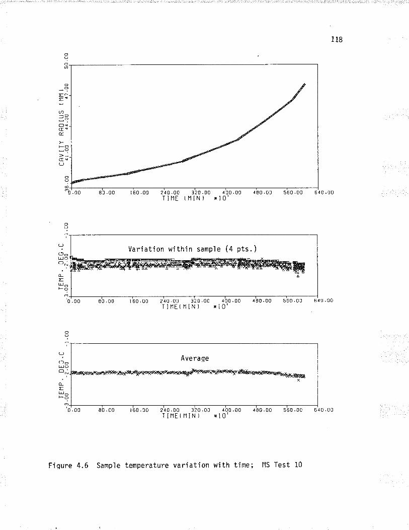
118

oo

=-='<n-O_O

OçcEqÉ

l-o

-?c<(J

?(JoL¡J OON

o_EL¡J o*?

240.00T IIlE

¿ 80 .00320 .00rrllN)

¿ 00 .00xl0l

640.00

q

=Ir*

-l:l0.

OO

?(-)trJÕ

LEL¡JF

240.00 320.00TIIlE(11IN)

¿ 0 .00r 60 .00 560 .00 640.00xl0

Average

0 .00 80 .00 r 60 .00 240.00 320.00 400.00TINE(NIN) *10'

480.00 560.00 640.00

560 .00

Variation within sample (4 pts.)

Fiqure 4.6 Sample temperature variation with time; l{S Test 10

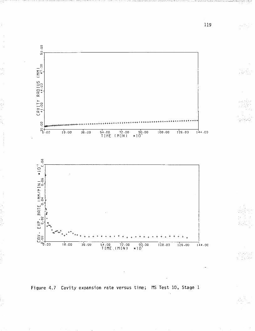
119

O?Oa

OO

E-

==tî)_O-oOçG<É.

tso-.?G9Lj

++++++++++++++++++ ++++++++++++++++++++++++++++++++ +++++

t26.00 t4a.99.00

O?Ð_

n 36 .00 I 08 .0054.00 1?.OO 90.00TINE (11lN) xl0'

f

++s+

+. *a+. .+ r +4 -+ +' *..+ '- * + + + + + + + + + + + + + + + + + + + + + + + + +

l I .00 36 .00 54 .00 12 .OO 90 .00TINE (11lN) xl0'

rtt108.00 126.00 l4a.g¡

llS Test 10, Stage

.00

@O

'O

=x@

_oZQ

EEEv_o

OL¡J

CEÉ.

N.oo-o-XUJ

>OGO-.b

Fi qure 4.7 Cavity expansjon rate versus time;

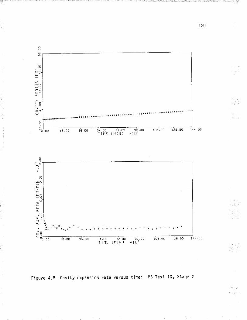
r20

O?Orn

oO

E.-

='(n

---oClqG9E

l-o-?ce(J

.00

@

?O.O

clx

@

-(fZO

ELts-?

OUJÞGE.

N

o-¿

OO

R

+ +++ +++ + ++ ++ + + + + + + + + + + + + + +++ { ++ + + + + + + ++ + + + + + + ++ + ++ + + + +

Oo;l"b.oo lB.oo

¡

36 .00

I 8.00 36 .00

90 .00XIOI

l 08 .00 126.00 laa.¡¡54.00 12.QOTINE (IlIN)

o_XUJ

G(J

**r.*A***. *****+++î++*+++*++++++++++***++*++++*

54 .00 '72 .OO 90 .00TIIlE (11lNl xl0'

r 08 .00 r 25 .00 I 4 4 .00

Fiqure 4.8 CavitY expansion rate versus tjrne; l4S Test 10, Staqe 2

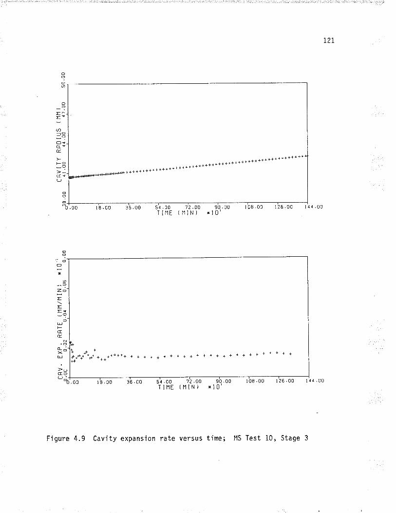
T2T

o?On

OO

Er

:'(n-o_O

OçcrrÈ

FO

-9cfe(J

++++++++++++++++++++++++++

+++++ t++++++++++++r

51 .00 1?.ao 90.00TlllE (NIN) rl0l

126.00 l4a.¡g.00

O?@_a

tJ

@

?O

r8.00 36 .00 I 08 .00

Ox

@

-?Z.otE=q_(]

CfL¡Jl-CEÉ.

N.C)o-jXt¡J

>oGOg-

I.oo lB.oo 36.00 51.00 108.00 126.00 144.00I

72 .OO(NIN)

90 .00xl0'T IIlE

+*.++r'**j*** *++ ******** + + + + + + + + + + + + + + ++++++***++

Figure 4.9 Cavity expansion rate versus time; llS Test 10, Stage 3

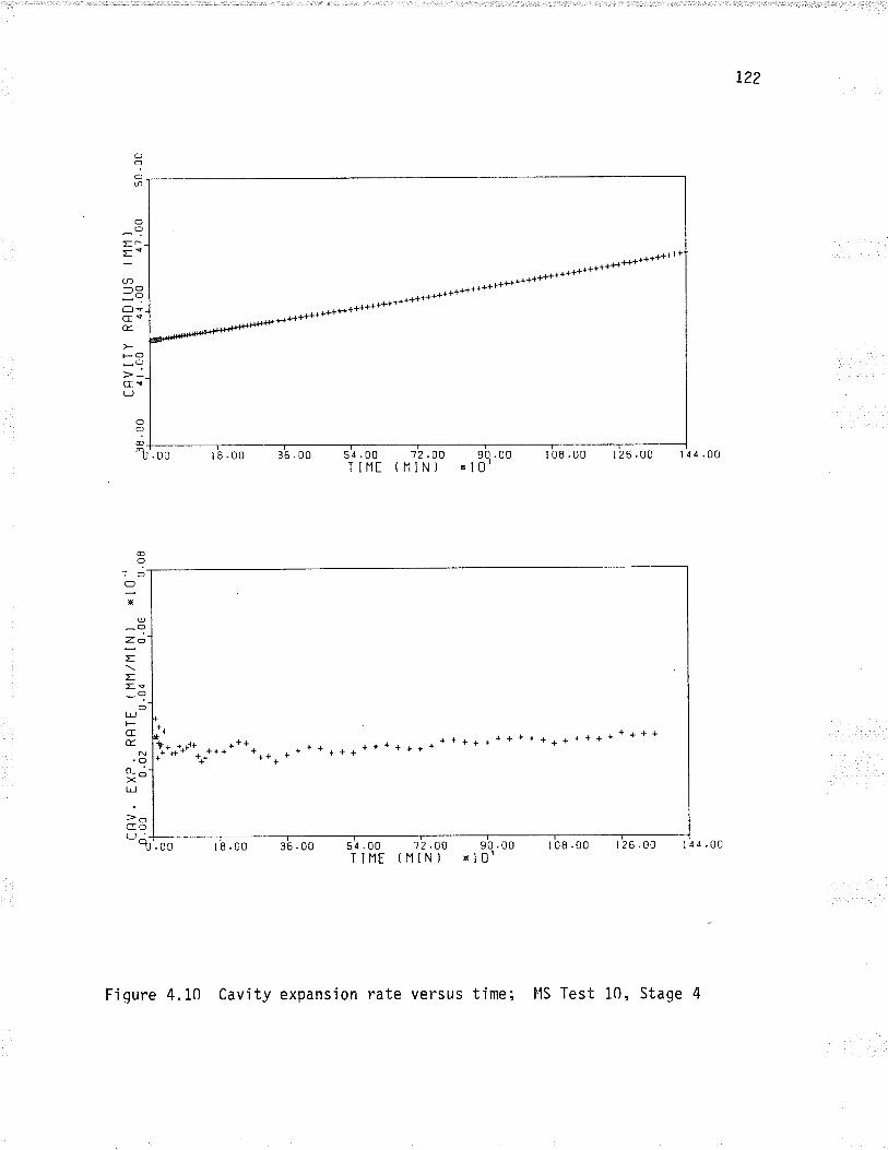
122

O?o'Ð

OO

Er

="U)-O-oOeGeÉ.

l-o

-?cEv(.J

.00

O?@-

"b ¡8.00 36 .00 r 08 .0051.00 '12.00 90.00TINE (11lN) rl0'

126.00 l4¿.00

*r++++*+**+++++++

i. *..r* +*+ + a ¿ + * ¡ . - + * { * + +

]*,Jf''*t*** **** * + { * * * * * * * + + + +

r 8 .00 36 .00 54 .00 17 .OO 90 .00TINE (lllNl xl0l

t08.00 126.00 l4¿'00.00

@

?-; J'

Ox

@

-OZO

;EEç-?

OlrJl-GÉ.

.Oo-oo_><t¡J

G(J

OO

l]

Fiqure 4.10 Cavity expansion rate versus time; llS Test 10, Stage

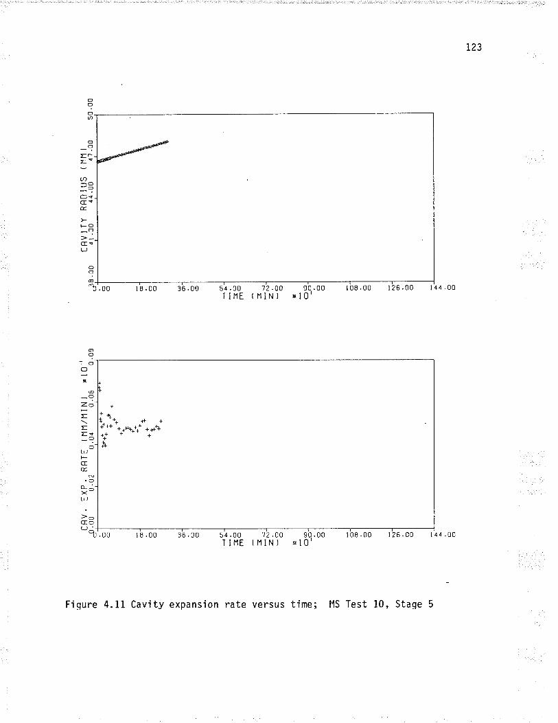
123

o?Oa

oO

Er

='U)-o"ÒOv(reÉ.

FO_?cre(J

.00

o

;_"b

@O

,Ool

I

18.00 36 .00

18.00

51 .00 12 .00 90 .00TItlE tNIN) ol0l

r 08 .00 126.00 111.00

.00

@

-OzåEE.Eç-?_

OLLJt-crÉ,

N.Oo- o-XLLJ

>OCo(.J'-

R 36 .00 54 .00T I I1I

?2.00(NiN)

90.00 108.00 126.00 laa.¡6xl0'

*¡,+ ++

+*++ '+,+++*+++

+++

å,++

+++'+a+t+

Fi qure 4. 11 Cavi ty expans'ion rate versus time; llS Test 10, Stase 5

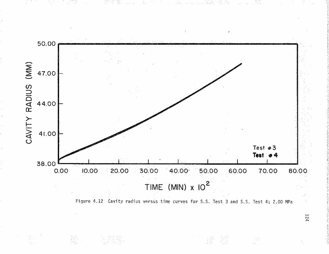
so. oo

së

CN:)õ

E

t()

47.OO

44.OO

4r.oo

38.OOo.oo ro.oo

Fjqure 4.12 Cavjtv radius versus time curves for S.S. Test 3 and S.S. Test 4;2.00 t{Pa

20.oo 30.oo 40.oG so.oo

T|¡V1E (MlN) x lOz

60.oo

Test * 3To¡t o 4

70. oo BO.OO

t\Þ

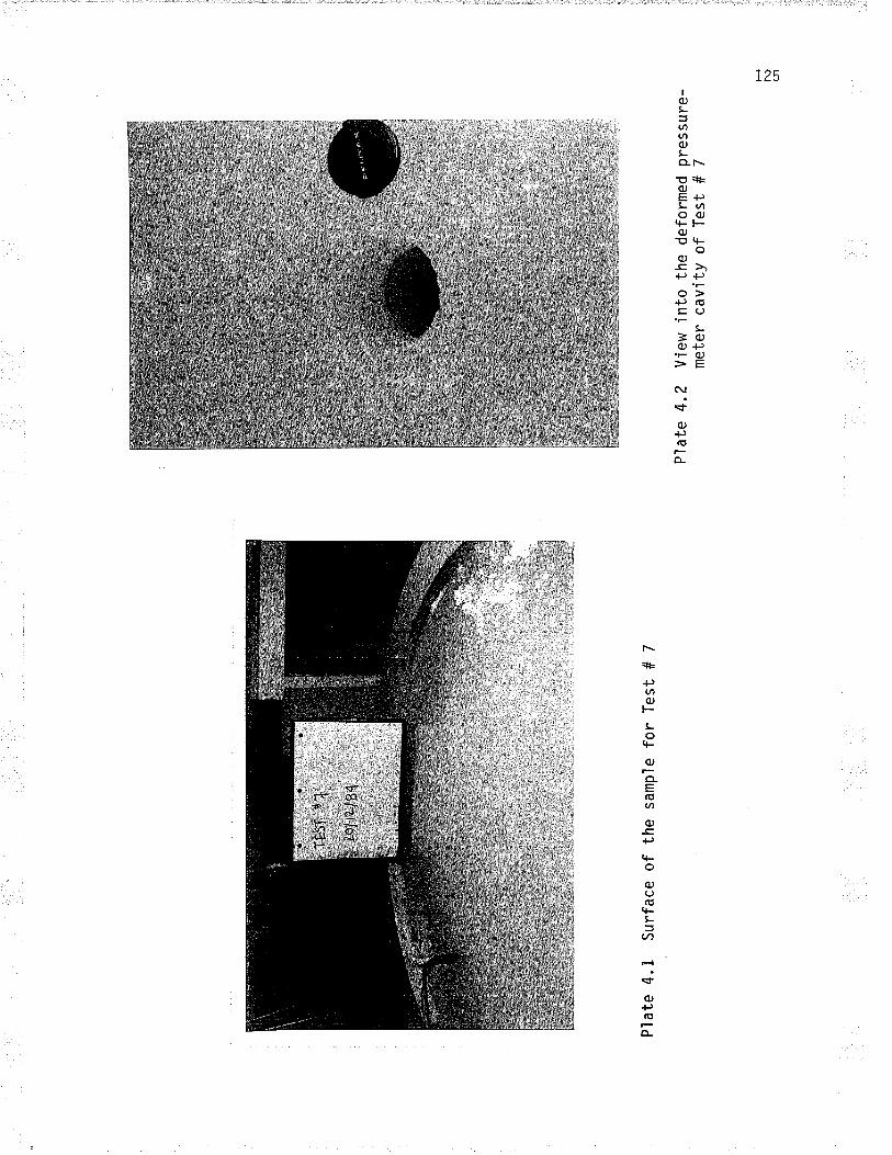
Pla

te 4

.1 S

urfa

ce o

f th

e sa

mpl

e fo

r T

est

# 7

Pla

te 4

.2V

iew

into

the

met

er c

avity

defo

rmed

of T

est

#

pres

sur

e-7

l-r N)

(-'r

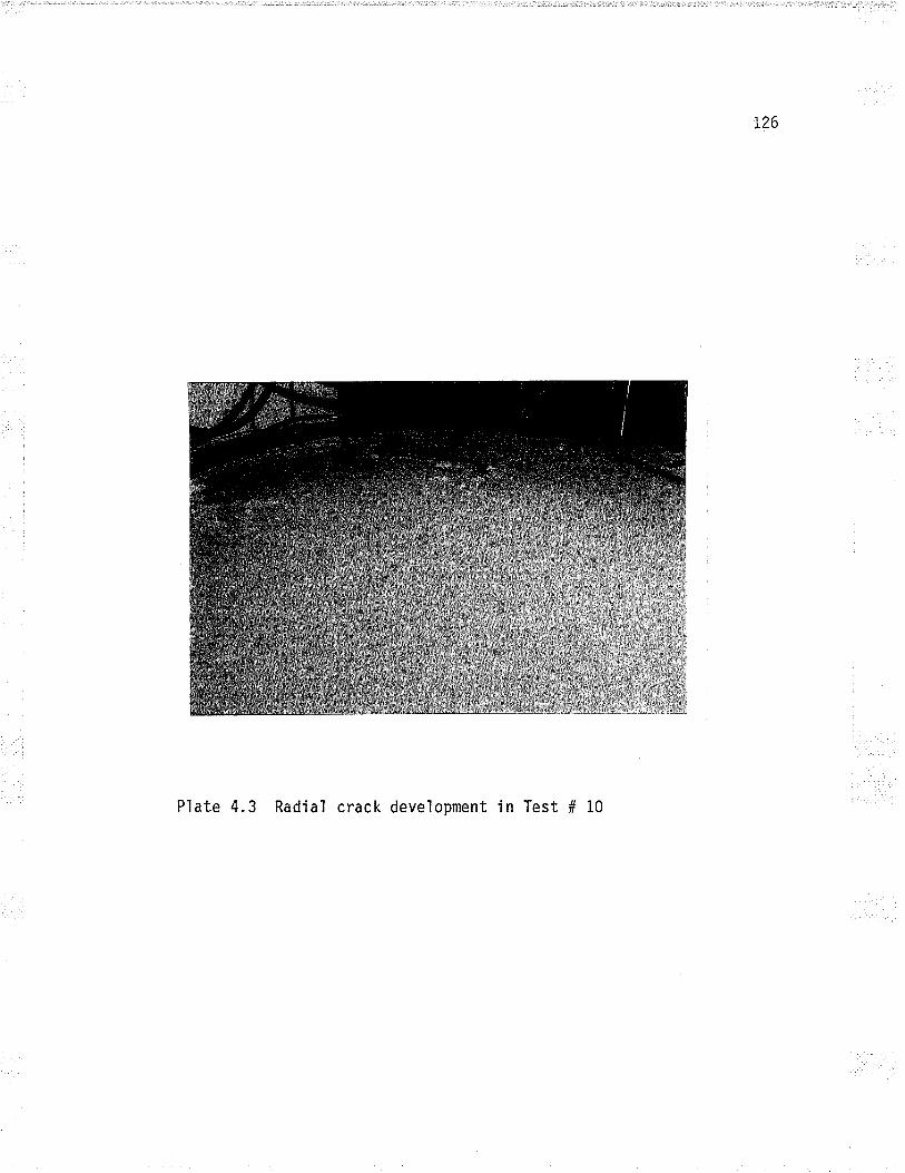
t26

Plate 4.3 Radial crack development in Test # 10

127

CHAPTER 5

ANALYSIS OF THE PRESSUREHETER CREEP TESTS

5.1 IWTRODUCTIOH

The pressuremeter creep test resul ts presented in Chapter

4 are analyzed in this chapter in terms of the two rheologjcal rnodels

presented in Chapter 2:

1) the strain-hardening, power law creep model used extensivel.y

by Ladanyi;

2) the modified second order flujd model.

. Creep parameters for the two model s have been determined

from both the sinqle stage and multistage tests. The predictive

capabiìity of both models is assessed by generat'ino pressuremeter

creep curves, based on creep parameters determined from the multistage

tests, and comparing these qenerated curves to the experjmental single

stage creep curves.

5.2 ANALYSIS OF PRESSUREþTETER CREEP TESTS IN TER}IS

STRAIfl-HARDENIIIG, POHER LAH CREEP THEORY

5.2.1 Processing the Pressuremeter Creep Tests

OF THE

As stated at the end of Chapter 3, no attempt has been made

in thj s study to measure the instantaneous response (el asti c and

pìastic) of the ice. 0nly creep strains are considered. Fol'lowing

Ladanyi and Eckardt (1983), creep strain'inq Ís assumed to commence

one minute after the applicatÍon of the pressure; all creep strains

are therefore referenced to the cavity radius (r) at one mjnute.

Because of the large number of data points for each test

r28

(e.g. 1,040 data points for Test # 13), the results were processed

and plotted using the University of Manitoba's ma'inframe computer.

To faci I i tate data proces si nq wi th the computer , the pres suremeter

creep equations have been redefined in the following v\,ay (after Ladanyi

and G'ill, 1981; Fensury, 1985).

The creep equation:

rn (li) = rtf*' rïlo (+P)n tb , (2. qs)

becomes:

tn(f;)=Ftb

where: F=H(Pt;To)n

N = (# )n*1 tf; lb tfl'

log (rn fr) =

!,lhen Ir tfrl is ptotted

loqF+bìogt (5.4)

against time in a log-log plot (as the simulated

t

and

(5.t¡

(5.2)

(5.3)

All the variables are as defined before, except ri is now defined

aS the cavity radius at a time of one minute for each stage. Also,

for these tests, ps, the radial pressure in the medium at F = - has

been set equal to zero. (Elastic stress analysis of the 'ice-tank

system has shown that the radial stress at the 'ice-tank boundary is

less than one percent of the app'lied cavity pressure. Moreover, no

residual stress in the ice, due to the freezing process r wâs âssumed

to exjst in the ice sampìe.)

Followinq Fensury (1985), the values of the creep parameters

b, n and oç may be found from two log-log plots. First, takìng the

ìogarithm of both sides of Equation (S.t¡ yields:

129

mult'istage test in Fig. 5.1 illustrates), the creep curves should

linearize with a s'lope equaì to b. The intercept at unit tjme (tor

this case 1 minute) of any creep line is then equa'l to F, for each

app'lied pressure P..

The values of n and oç may then be found by taking the

ìogarithms of both sjdes of Equation (5.2):

'logF=logM+nìogP.-nlogoc, (5.5)

and plottinq log F (the intercepts in the upper figure of Fig. 5.1)

versus log Pc (as in the lower figure of Fig. 5.1). The best fit

line will have a slope equa'l to n. The intercept of this ljne at

unjt pressure (1.0 MPa) yìe'lds F1. According to Equation (5.5), F1

is equal to:

where

Since Equation (5.3) may be solved to find

oc may be calculated from Equation (5.6),

N = {f )n*1 rf tb tft'

Fl = Mn ; or,o6"

- ,M tl/noc - \F1,

log Fl = log M - nìog o¿ , (s'o¡

(5.3)

M (assuming Ë = 10-5 min-1),

i.e.:

(5.7)

For data processing, the program LADF0Sl was used to read

the test data and calculate log (ln :) and the log (time) for al I' ri'of the creep curves. This data set was subsequently read and processed

by the program LADPL. The program LADPL, as well as produc'ino plots

similar to the ones shown in Fig.5.1, calculated the b and F values

for each creep line and determined n and Fl for each test by regression

130

analyses. Curve fitting is done by least squares linear regression,

so that if some data is deemed to be unsuitable from visual inspection

of the LADPL plots (for exampìe one point does not follow the trend

of the rest of the data) it must be removed from the data set before

processing. Some of the final plots, therefore, will not show all

of the data. The position taken in this thesis is that as much data

as possibìe is used for anaìysis, as long as the results conform to

the model. The programs LADF0SI and LADPL, modifjed after Fensury

(l98S), are listed in Append'ix C. More details about these programs

may be found in FensurY (i985).

. As the strain-hardening, power law creep model has been

used historicalìy to analyze multistage tests, they are presented

first. Analysis of the singìe stage tests follows.

5.2.2 Analysis of the tilultistage Pressureneter Creep Tests Using

Strain-Hardening, Power Law Creep Theory

in the following, each of the 4 multistage tests is analyzed.

The first trjal analysis includes all of the data from that particular

test, while further trials delete part of the data to achieve a "better

fit", accord'ing to the model. The creep parameters from alI of the

runs for a part'icular test are surnmarized in tables. The injtial

plots whjch include all the test data and the best fit p'lots are placed

at the end of this chapter.

It must be noted that circumferential strain for this model

is defined in terms of the infinitesimal strain tensor. Therefore,

c'ircumferential strain is equal to $ where ^r = change in cavityr'l

radjus (i.e. r-ri) and ri = initial cavity radius.

131

5.2.2.L AnaÏysis of ffiultistage Test # 10

l4ultistage Test # 10 was carríed out with cavity pressures

of 1.50, 1.75, 2.00 and 2.25 MPa, with each pressure being appl'ied

for a duration of 1,440 minutes (1 day). The last stage, with a cavity

pressure of 2.50 MPa, was held onìy for 300 minutes, since the

pressuremeter reached its maximum allowable expansion after that length

of time.

The resul ts of the fi rst tri al , usi ng al I the data from

all five stages, are presented in Figs. 5.2 and 5.3 and Table 5.1;

Fig. 5.2 presents pìots of circumferential strain at the cavity wall

yersustimeandlog(ln*) versus log time, whÍle Fig. 5.3 presentsrlpìots of log F versus log pressure and b value versus pressure. The

creep parameters are summarized in Table 5.1. tt|hat is immediate'ly

evident from Figs. 5.2 and 5.3 is that:

1) the creep line for the first pressure stage of 1.50 MPa has

a b which is much lower and an F intercept which is much

higher than the other stages (note: the term "creep I ine"

in thís thesis refers to the linear regression lÍnes on the

log (tn f;) versus los (time) plot).

2) the ear'ly data i n the creep pl ots i s qui te

approximately 90 minutes). (Note: "creep

data pì ots" in thi s thesi s refers to the

.the los (.|. fil versus log (time) plot. )

scattered (before

p'lots" or "creep

data pl otted on

Inclusion of the first stage resulted Ín an n value of'1.37, which

does not conform to the model; i.e. n cannot be negative.

In order to obtain results which conform to the model,

therefore, the data of the first stage had to be excluded from the

r32

analysis. Findings similar to this, that is to sây, where the first,and sometimes second stage could not be used in data reduction, can

be noted in Eckardt ( 198i) and Fensury ( 1985) . The reason for thi s

behavjour is unclear. It may be due to "delayed" elastic/pìastic com-

pression. Another reason may be that the first stage had not approached

steady-state or secondary creep, while the remaining stages had.

The second trial was run with the first stage'information

omitted, while the third trial was run with both the first stage omitted

as well as the data for the first 90 minutes of the remaining staqes.

Although Trial # 2 gives reasonable results (Table 5.1), Trial # 3

yields:

1) correlation coefficients for the creep regress'ion lines greater

than 0.999, which are higher than for Trial # 2,

2) less variation in the b values than in Trial # 2, indicating

better parallelism of the creep lines,

3) less scatter in the p'lot of log F versus ìog pressure than

is the case with Trial # 2.

Trial # 3 is considered to best sat'isfy the necessary

conditions for the model; í.e.:

1) creep curves should linearize in a ìog-'log p'lot,

?) creep curves for dífferent sustained pressures shoul d be

paralleì to each other.

The plots for Trial # 3 are presented in Figs. 5.4 and 5.5. It is

interesting to note that the creep deformation is very close to a

steady-state condition in the last four stages of the test (i.e. b

values are very close to one). Moreover, as there appears to be no

definite relationship between b and pressure, âfl áverage value of

133

b is used for the test. Ladanyi and Eckardt (1983) and Fensury (1985),

on the other hand, found that b increased with pressure according

to a power function.

5.2.2.2 Analysis of Multistage Test # 11

MultÍstage Test # 11 was carried out with cavity pressures

of 1.50, 7.75,2.00, 2.25 and 2.50 l4Pa, each pressure be'ing held for

720 minutes. The results of the first trial, using a'll of the data

points, are presented in Figs. 5.6 and 5.7 and Table 5.2. As with

Test # 10, the first stage at a cavity pressure of 1.50 MPa has a

much higher F value and a much lower b than the other stages. Aga'in,

as with Test # 10, a negative n s'lope (which does not conform to the

model) has resulted. It is clear, however (see Fig. 5.7) that ifthe data from the first stage is omitted, while all the rest of the

data is kept, a negative n slope will again result. It is evident

from Fig. 5.6 that the first 60 minutes of data points in the last

four stages have caused the creep I ines to become non-para'l ìeì and

intersect each other.

The second trial was carried out with the data from the

first stage and the first 60 minutes of data of the remaining stages

deleted. As Figs.5.8 and 5.9 illustrate, the creep lines are now

quite paralìe'l and a good fit is obtained on the log F versus ìog

pressure pìot (Fig. 5.8); reasonable results have been obtained (Tabìe

5.2). The b values of 0.85 to 0.91 indicate that steady-state creep

conditions are being approached in the last four stages. Again, as

wjth Test # 10, there does not appear to be a clear relationship between

b and pressure (Fig. 5.9), so an average value of b = 0.90 is adopted.

134

5"2"2"3 ÅnaTysis of MuTtistage Test # 12

Mul ti stage Test # 12 vlas carr j ed out w'ith cav'ity pressures

of 1.50, L.75 and 2.00 MPa held for a duratíon of 2,880 minutes (Z

days). The final stage, with a cavity pressure of 2.25 MPa, on'ly

lasted 480 minutes as the pressuremeter reached its maximum allowable

expansion at the end of thjs time period.

The results of the first trial, using alì of the data points'

are presented in F'igs. 5.10 and 5.11 and Table 5.3. As with Tests

# 10 and 11, the results are unreasonable (negative n value)'largely

due to the lack of conformity of the first stage at a cavity pressure

of 1.50 MPa (Figs. 5.10 and 5.11). Al1 subsequent trials, therefore'

have the data from stage I deleted. In addition, as with Test # 10'

the data pojnts in the first 90 minutes of the last three stages have

also been om'itted as they appear to be causing intersection of the

creep lines (Fig. 5.10).

Trial s # 2 and 3 (Table 5.3) give an indicatÍon of how

sensitive the determination of the n parameter is to the choice of

data. Trial # 2 uses only data at times between 90 and 2,880 minutes

for the last three stages of Test # 12, whiìe Trial # 3 uses data

between 90 and 1,440 minutes for these stages (to allow eventual

comparison with Test # 10). The correlation coefficients (rZ values)

for the creep lines in both trials are in excess of 0.999, indicating

excellent ìinearity of the creep data. The range in b is also small

(Table 5.3), with the average b values being essentially equal in

both cases (0.97 compared to 0.96). Because of the s'light'ly steeper

sìopes in the creep lines for 1.75 and 2.00 MPa fqr Trial # 2 as

compared to Trial # 3, the F values for Trial # 2 are s'lightly lower,

135

leading to an increase in the slope n in the log F versus 1og pressure

plot (see Figs. 5.L2 and 5.13, Trial # 3). Th'is slight'ly steeper

s'lope of the creep lines in Trial # 2 compared with Trial # 3 caused

a change in n from 4.14 to 4.53.

For comparison purposes (with both Test # 10 and Test #

13, which follows) the Trjal # 3 parameters, derived between times

of 90 and 1,440 mjnutes, are used to represent Test # 12. Plots of

the creep curves and creep parameters determined from Trial # 3 are

g'iven on Fi gs. 5.LZ and 5. 13 respecti vely. As wi th Tests # 10 and

11, the b values close to unity indicate that a condition of

steady-state creep was approached. Figure 5.13 indicates no clear

dependence of the b values on pressure, so an average value of 0.96

has been adopted for this test.

5.2.2.4 Analysis of Hultistage Test # 13

Multistage Test # 13 was carried out with cavity pressures

rangìng from 0.25 to 2.25 MPa, applied in increments of 0.25 MPa,

with each increment held for 1,440 minutes (1 day). The final stage,

at a pressure of 2.50 MPa, lasted for only 270 minutes since the

pressuremeter reached its maximum allowable expansion after this time.

The results of the first trial, using aìl of the data points'

are presented in Figs. 5.14 and 5.15 and Table 5.4. As Figs. 5.14

and 5.15 indicate, the first three stages at 0.25,0.50 and 0.75 MPa

do not conform to the model and result in an n value of -0.60. In

addition to deìeting the data from these three stages, as was done

with Tests # 10 and L2, the first 90 m'inutes of data is deleted from

the remaining stages in subsequent trials.

136

Figures 5.16 and 5.17 illustrate pìots of the creep curves

and creep parameters for Trial # 2. It is interesting to note (Fjg.

S.17) that the p'lot of log F versus log pressure is curved marked'ly

with n increasing with increasing pressure. Thj s is probably due

to the fact that the creep in the lower pressure stages (1.0 to 1.5

MPa) did not approach a steady-state condition; i.e. the b values

for these stages range from 0.83 to 0.90. If these stages had been

of a longer durat'ion, b woul d undoubted'ly have increased and reached

values closer to unity; F would have decreased, causing the log F

versus 'log pressure plot to become more linear. Although the necessary

conditions for the strain-hardening, power law creep, model (i.e.

l'inear, parallel creep Iines) are for alI intents and purposes satisfied

for cavity pressures in excess of 0.75 MPa, the omission of the data

from an additional three stages (with pressures of 1.00, 1.25 and

1.50 MPa) wil'l produce less scatter in the b values and gìve a better'

i.e. more linear, correlatÍon of log F versus log pressure.

Trial # 3 was carried out using only the stages wÍth cavity

pressures rang'ing from I.75 to 2. 50 tlPa . The resul ts are presented

in Figs. 5.18 and 5.19 and Table 5.4. These results, wjth an n value

of 2.63 and an average b va'lue of 0.97 are deemed to best represent

Test # 13.

5.2.3 AnaTysis of the SinqTe Stage Pressur€n€ter CÌ'€ep Tests Usinq

Strain-Hardeninqo Pouner Law Creep Theory

The results of the first trial, using all. of the data from

the seven tests in the pressure range 1.00 to 2.50 MPa (Test # 3 is

used to represent 2.OO MPa), are presented in Figs. 5.20 and 5.2I

137

and Table 5.5. The creep data plots shown in Fig.5.20 are concave

upward, with the result that b increases with time. The Jinear

regression fits to the creep data, which are reasonably paral ìel ,

represent an "average" b value for the tests. The creep parameters

derived from these fits, (n = 3.26 and oç = 1.00 Mpa) are reasonable

(e. g. Morgenstern et âl . , 1980; Sego, 1980; Sego and l4orgenstern ,

1983). A major prob'lem, however, I f es in the variation of b with

time. if an average value of b of 0.7I is adopted, then the creep

curves predicted from Equation (5.1) will show attenuat'ion with time.

Figure 5.20 indicates that just the opposite is true; the creep curves

show accelerat'ing behaviour even at the lowest cavity pressure of

1 .00 MPa.

If the creep data plots shown in Fig. s.zo are examined

carefully' it may be noted that the curves are para'llel at approximately

the same strain (tn fr) rather than at the same time. Furthermore,

when a condÍtion of steady-state creep is reached, (for these tests,

at ln fr values between about 0.0s and 0.10) the creep lines become

essentially paral'leì and remain that way to the maximum strain. Itis postulated that the creep lines will never be para'lìel in a given

interval of time unless a condition of steady-state creep (u = 1)

has been approached in each pressure stage. It al so seems that a

minjmum deformation (1. frl of about 5% is needed for the steady-state

condition to be developed. The remaining triaì analyses for the sing'le

stage tests examine how the creep parameters vary with both time and

strain (ln L).' ri'Trial # 2 (Table 5.5) was carried out in order to compare

i38

the creep parameters determined for the single stage tests, between

times of 90 and 1.,440 minutes, wìth the creep parameters determined

from the multistage tests in the same time'intervals and at the same

stress levels. As the results in Table 5.5 indjcate, an average b

value of 0.73 and an n value of 0.99 are not even close to the

multistage parameters (Tables 5.1 to 5.4).

Trial # 3 was carried out using the time interval from 1,440

to 14,400 mi nutes. The resul ts , wh'ich 'incl ude al I the pressure stages ,

are illustrated in F'igs. 5.2? and 5.23 and under Trial # 3a in Table

5.5. As can be seen in Figs. 5.22 and 5.23, the creep l'ines for'pressures of 1.00 and 1.25 MPa result in considerable scatter in the

log F versus log pressure p'lot. If these two pressures are deleted

from the anaìysis (Trial # 3b, Table 5.5), then the more realistic

value n = 3.45 is obtained. It is noted that in this case, the average

b value is exactly 1.0, indìcatìng the exjstence of a steady-state

creep conditjon in the tests at higher pressure.

Trial # 4 was carried out to determjne, approximately, the

minimum time (less than 1,440 minutes) tnat steady-state creep

conditions are approached in the pressure stages ana'lyzed in Trial

# 3b (i.e. 1.50 to 2.50 MPa). From Fig. 5.20, it may be noted that

scatter has largeìy disappeared by about 600 minutes. Thjs time was

chosen in a trial to see if steady-state rea'l ìy i s approached. The

results of this trial are presented in Figs. 5.24 and 5.25 and in

Table 5 (Triaì # 4). The differences between this trial and Trial

# 3b are a slightìy lower n value (3.37 as compar'ed to 3.45) and a

slightìy lower average b va'lue (0.95 as compared to 1.00). It may

be concl uded, therefore, that steady-state conditions are being

139

approached at about 600 minutes for these pressures.

Trial # 5 was carried out to determine the creep parameters

for times greater than 1i,000 minutes even though only 3 tests ran

for longer than thi s time period and the resul ts are inconcl usi ve.

The tests at pressures of 1.25 and 1.50 MPa had paral'le1 creep lines

with a b value of 1.09; the log F versus log pressure p'lot yieìded

an n exponent of 4.01. The creep line for the test at 1.0 MPa had

a slightly lower b value (0.95), but thìs was enough to cause scatter

in the 1og F versus log pressure pìot, resulting in a neqatjve n.

Trials # 6 to 9 (see Table 5.5) were carried out to examine

the effect of strain magnitude (ln l) on the determination of theri'creep parameters. As is indicated in the Table, all of the tests,

from cav'ity pressures of 1.00 to 2.50 MPa, were used in each of the

trials. The results indicate that there is in fact better paraìlelism

of the creep lines at given strajn levels in the tests rather than

at equaì time intervals. This paraìlelism gives a high deqree of

linearity in the log F versus ìog pressure plot even in the low stress

range. This is not true for the equaì time'intervals where the low

stress data results in much scatter. It may be noted that the average

b values increase with increasing strain level, from 0.69 at ln :rifrom 0.01 to 0.03, to a b of 1.06 at ,t t greater than 0.10. The

steady-state condition (b = 1) is deve'loped at ìn I values of aboutri0.05 to 0.10. From these trials, there does not seem to be an apparent

trend in the value of n with straÍn; n varies between 3.4 and 4.0.

The lack of an apparent trend in the exponent n may in fact be due

to the difficu'lty in determining n precisely. The determination of

the exponent n requires two sets of curve fitting, and error is

introduced at each stage; i.e.

considerable scatter in the log

140

s'light variation in b can cause

versus I og pressure pl ot.

5.2.4 Comparison of Experirental and Predicted Pressuremeter Creep

Curves Usinq the Strain-Hardening, Pov¿er Law Creep Hodel

As an Índependent method of assessing the predictive

capability of the strain-hardening, power'law creep model, pressuremeter

creep curves have been generated using the best fit creep parameters

from the multistage tests. These predicted curves are compared to

the experimentaì single stage pressuremeter creep curves at equivalent

pressures. The best fit creep parameters determined from the four

multistage tests are given in Table 5.6.

In order to predi ct ci rcumferenti al strai ns from the

pressuremeter creep data, it is assumed that ee = * = ln l = F tbri ri(EquatÍon 5.8). This assumption was used by Fensury (1985) tor his

comparisons. Moreover, the maximum difference betweeñ e0 and ln L,

at the maximum circumferential strai n of 26% is onl V 3% (i...* .qrutTri26% while ln å gives 23%). Considering the fact that we are usingrithe infinitesimal strain tensor in this creep analysis to represent

what are reaì'ly large strains, this difference is considered to be

unimportant.

Now, considering the creep parameters given in Table 5.6 and

using the Fensury assumption:

a

F

.o =fr= F tb = Fl (p.)n tb

s'l nce,

Fl = M tält from Equation (5.6)

(s.e)

141

and,

F = tvl ,ä,t from Equation (s.Z).

Based on values of F1, n and b from Table 5.6, fictitious constant

stress pressuremeter creep curves for any appl ied cav'ity pressure

Pc may be generated usinq Equation (5.9). (A computer program called

PRDFg1 (modified after Fensury, 1985) which generates the fjctitious

curves may be found listed ìn Appendix C.) Both fìctitious and real

experimenta'l curves can be pì otted usi ng the program PRDPLS ( al so

after Fensury,1985 and l'isted in Appendìx C as well). PRDPLS curves

are illustrated in Figs. 5.26 to 5.32.

The main findings from these comparisons are as follows:

1) All of the predicted, i.e. fictitious, curves have a strain

rate that is nearly constant wjth time (i.e. they reach a

steady-state condi ti on ) . Thi s i s due to the fact that b

= l.2) The maximum difference between the predicted curves and the

corresponding experimentaì curves occurs at 1.00 MPa. Th'is

difference is on the order of 15% when calculated in terms

of circumferential strain. The four predicted curves generaìly

fit the experimental results better at higher cavity pressures.

3) [verall, the creep parameters from Test # 10 give the closest

predì cti ons over the enti re stress range. Thj s i s not

surprising, since these parameters are Closest to the

parameters considered to be the best fit for the sing'le staqe

tests (Trial # 4; b average = 0.95, n = 3'37 and Fl

0 . 00000s 34 ) .

r42

4) In the lower pressure range (1.00, !.25, 1.50 MPa) Fl dominates

the predìcted curves, and the exponent n is less important

(i.e. F1 (P.)n tb = Fl tb for Pc close to unìty). At these

3 pressures, PRD 13 (i.e. the predict'ion using Test # 13

parameters) overestimates the experimental curves while PRD

12 underestimates the experimentaì curves. At the hiqhest

pressure (2.50 MPa) n becomes more important than F1. The

highest exponent n = 4.I4 (Test # LZ) yields the predicted

curve with the highest strains, wh'ile the lowest exponent

n = 2.63 (Test # 13) yields the predicted curve with the

lowest strains (Fig. 5.26).

The pred'i cted curves , therefore , usi ng the assumpti on i n

Equati on (5.9 ) are i n reasonab'le agreement wi th the experÍmental si ng'le

stage curves over the time period in question. It is readily apparent,

however, by examination of Figures 5.26 to 5.32 that Equation (5.9)

does not model the strain rate accurately. Equat'ion (5.9) will predict

either a decreasing strain rate with time if b < 1.0, or a constant

strain rate w'ith time, if b = 1.0. The experimental curves, after

an initial decreasing strain rate period, show an increasing strain

rate with time, with the increase becoming more pronounced near the

end of the creep curve. The assumption of e0 = ìn f, then, couldrl

result in significant divergence of the experimentaì and predicted

creep curves when extrapo'lati ng to 'longer perì ods of time. Another

method of predi cti on , whi ch tends to model the strai n rate more

accurately, is given in Chapter 6.

5.3 AHALYSIS OF PRESSUREHETER CREEP TESTS Iru TERþ{S OF

SECOND-ORDER FLUID WDEL

5.3"1. Processing the Pressurer¡eter Creep Tests

As the motion equation,

143

ÏHE ruDIFIED

(2.62)roro

m

mal ,l,t-urf,r -f (m+1) ,*l-'=o

'is a complicated nonlinear differential equation of order two, a closed

form solution is unlikely. Instead, a numerical solution was deveìoped

by Q.-X.Sun (1985). (The details of the solution and computer program

form part of Mr. Sun's ongoing Ph.D. work.) First it is necessary

to calculate an approximate value of the exponent m, and then, using

a computer program cal'led QSUN, it is necessary to optimize the

numerical solution of Equation (2.62) using the experimental test

results. The numerical solution of Equation (2.62) uses a fifth order

Runge-Kutta technique (see, for example, James et al., 1985). A lìsting

of QSUN is included in Appendix C. In order to illustrate the method

of solution, the single stage tests are analyzed first.

5.3.2 Analysis of the Single Stage Pressurereter Tests Using the

Þtodified Second-0rder Fluid Fbdel

nt 3 , the cavity expansion rate divided by the currentro

cav'ity radius, is a varjable Ín three of the four terms of Equat'ion

(2.62), its variation wjth time was examined for each of the sing'le

state tests (see Figs. 8.1 to 8.8, Appendix B). As is readily apparent

from these tiSure.s, f, approaches a minimum value qu'ite rapidly,

which means that P approaches zero rapid'ly. With this in mind, anFg

assumption was made that the first two terms of Equati on (2.62) became

negligibìe compared to the last two wnen f approached zero

wnen fr approached a minimum). Under th'is assumption, Equatìon

reduces to:

t44

(i.e.

(2.62)

(5.10)

It may be noted that Equat'ion (5.10) is exactìy the power-law fluid'

Equation (2.64). Rewriting Equation (5'10) vields:

io _ 'p.(m+t)

11/(m+1) 1 ?.64)%-' 2]t J

Now, taking ìogarithms of both sides of Equation (2.64) g'ives:

rn tP) =#(rn+)-#trn$) (5'11)'Fg

It.is readi'ly apparent that it ln io is plotted against lt ? r Iro

strai ght I i ne shoul d resul t w.ith st one fr. Thus , the creep exponent

m may be determined.

For the single stage tests, a minimum value rt I v,Jas chosen

for each test (note: the minimum of P versus time corresponds toro

þ.oual to zero). In the lower pressure tests, choosing an absolutero Fg

minjmum is difficult because the increase tn * with time after the

minimum.is very slight.. These results are presented in Table 5'7'

A pìot of ln fi u..ru, lt + is presented in Fig' 5'33' As

the minimum ft value for Test # 2 at 2.50 MPa is in doubt because

of m.issì'ng data po'ints, it i s left out of the regression analyses '

A linear regression analysis of the rema'ining 6 data points yie'lds

b nu, been taken for 2'00 MPa):(an average ln ¡o

145

r - s.qsl " 12 = o.ggigmTT -

Therefore, rTt = -0.709.

Because of apparent curvature in the lower StreSs range '

a second regression ana'lysis has been conducted with both the Tests

# 2 and I data points removed. These results are:

1= = 3.731 , rz = o.9g7om+1

Therefore , tTr = -0 .7 32.

For now, the regression analysis oìving an m exponent of

-0.709 will be used, as there is not a significant djfference between

the correlation coefficients of the two fits.

in order to determjne the creep parameters alr g and m which

best fit an experimental creep curve, QSUN is run. As the simp'lified

flow chart in Fig. 5.34 indicates, the necessary input information

are: (1) the experimenta'l cav'ity radius versus time data, (2) the

cavity pressure(s) and (3) the appropriate rrmrr exponent. Initial

o1 and ¡ parameters are calculated from the input m value and the

experimentaì data. These creep parameters are then optím'ized using

the data points from a segment of the experimental curve. The optimized

creep parameters cl, ¡r and m are then substituted into the numerical

solution of the motion equation, which is based on a fifth order

Runge-Kutta technique. The predicted (tictitious) cavity radius versus

time curve is then calculated for the same experimentaì time nodes.

To assess the quality of fit, the error between the experimental curve

and the predicted curve is calculated as:

trD1=ro(t)-rp(t)L¡\¿ ro(t) - ri(5.12)

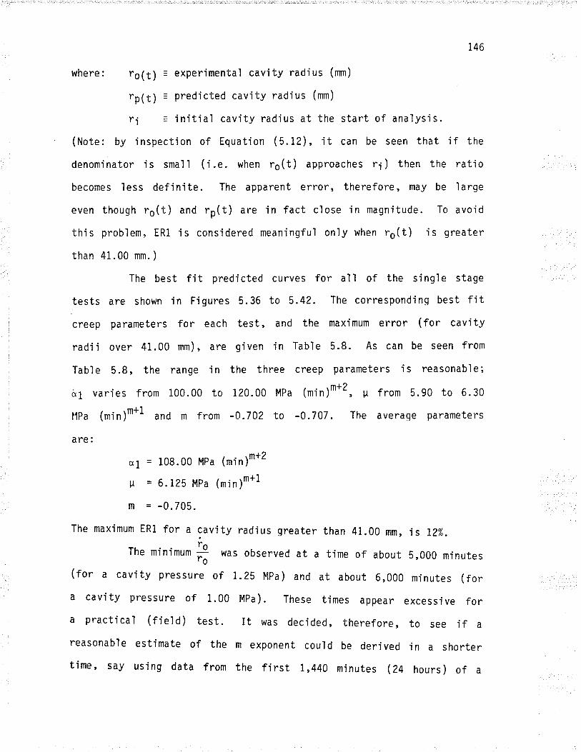
146

where: Fo(t) = experimentaì cavìty radius (n¡m)

rp(t) = predicted cavity radìus (mm)

ri = initial cavity radius at the start of analys'is.

(Note: by inspection of Equation ( 5.12), it can be seen that if the

denominator is small (i.e. when ro(t) approaches ri) then the rat'io

becomes less definite. The apparent error, therefore, may be large

even though re(t) and rp(t) are in fact close in magnitude. To avojd

thjs probìem, ER1 is considered meaningful onìy when rs(t)

than 41.00 mm. )

i s greater

The best fit predicted curves for all of the sing'le stage

tests are shown in Figures 5.36 to 5.42. The correspond'ing best fit

creep parameters for each test, and the max'imum error (for cavity

rad'iì over 41.00 mm), are given in Table 5.8. As can be seen from

Tabl e 5.8, the range i n the three creep parameters i s reasonabl e;

s1 varies from 100.00 to i20.00 l4Pa (min)m+2, 1¡ from 5.90 to 6.30

llPa (mi n )m+1 and m f rom -0.702 to -0.707. The averaqe parameters

are:

c1 = 108.00 MPa (min)m+2

u = 6. 125 Mpa (min )m+1

m = -0.705.

The maximum ERl for a cavity radius greater than 41.00 mm,

The mi F6 Inrmum ro was observed at a tfme of about

(for a cavity pressure of t.25 Mpa) and at about 6,000

a cavi ty pressure of 1.00 Mpa ) . These times appear

a practical (field) test. It was decided, therefore,

reasonable estimate of the m exponent could be derived

time, say using data from the first 1,440 minutes (Zq

is 72%.

5,000 minutes

mÍnutes (tor

excessi ve for

to see if a

in a shorter

hours ) of a

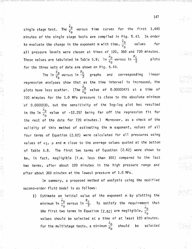
t47

single stage test. fne p versus time curves for the first 1,440ro

m'inutes of the sì ng'le stage tests are compi I ed i n li g. 5. 43. In order

to evaluate the change in the exponent m with time, ff values for

all pressure levels were chosen at times of.120, 360 and 720 ninutes.

These values are tabulated in Table 5.9i ln 3 u.rrrr tn 3 plots-ro¿for the three sets of data are shown on Fig. 5.44.

The ln 3 u..rm ln 3 graphs and corresponding l'inearro¿regression analyses show that .as the t'ime interval is increased, the

rplots have less scatter. (fne f value of 0.00000475 at a time of

o

720 minutes for the 1.0 MPa pressure is close to the absolute minimum

of 0.00000.30, but the sensitivity of the log-ìog p'lot has resulted

in the ln 3 value of -L2.?57 be'ing far off the regression fit forro

the rest of the data for 720 minutes.) Moreover, as a check of the

va'l 'idi ty of thi s method of estimati ng the m exponent , val ues of al I

four terms of Equat'ion (2.62) were calculated for all pressures using

values of o1, Lr and m close to the average values quoted at the bottom

of Table 5.8. The first two terms of Equation Q.62) were shown to

be, in fact, negl igÍbìe ('i.e. less than L0%) compared to the last

two terms, after about L20 minutes in the high pressure range and

after about 360 minutes at the lowest pressure of 1.0 HPa.

In summary, a proposed method of analysis using the modifjed

second-order fluid model is as follows:

1) Estimate an. initial value of the exponent m by p'lotting the

minimum ln 3 versus ln 1. To satisfy the requ'irement thatrsrîothe first two terms 'in Equation (2.62) are negligible'

,^o

values should be selected at a time of at least 120 minutes.

For the multistage tests, a mín'imum p should be selecteclro

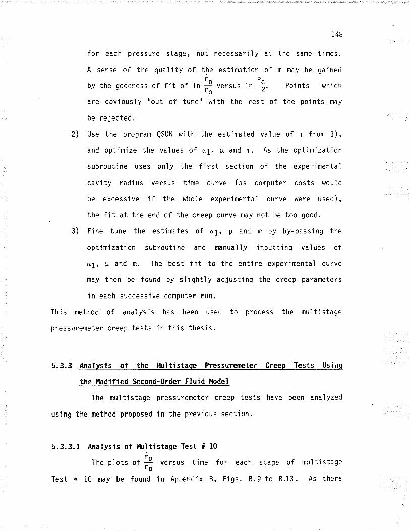
148

for each pressure stage, not necessarily at the same t'imes.

A sense of the qua'lity of t!'e est'imation of m may be ga'inedrP^

by the goodness of fit of ln I o.rsus ln T. Points whichro¿. are obviously "out of tune" w'ith the rest of the points may

be rejected.

2) Use the program QSUN with the estimated value of m from 1),

and optimize the values of o1, u and m. As the optimization

subroutine uses only the first section of the experimental

cavì ty radi us versus time curve ( as computer costs woul d

be excessjve if the whole experimenta'l curve were used),

the fit at the end of the creep curve may not be too good.

3) Fine tune the estimates of q1, g and m by by-passing the

optimization subroutjne and manua'lìy inputting values of

a1, U and m. The best fit to the entire experimental curve

may then be found by slightly adjusting the creep parameters

in each successive computer run.

Thi s method of ana'lysi s has been used to process the mul ti stage

pressuremeter creep tests in this thesis.

5.3.3 Analysfs of the K¡Itistage Fressure¡reter Creep Tests Usinq

the Hodified Second-Order FIuid hbdel

The multistage pressuremeter creep tests have been ana'lyzed

using the method proposed 'in the previous sectjon.

5.3.3.1 Analysis of Hultistage Test #

The pìots ot p versus timero

Test # 10 may be found in Appendix

l0

for each stage of mul ti stage

B, Figs. 8.9 to 8.13. As there

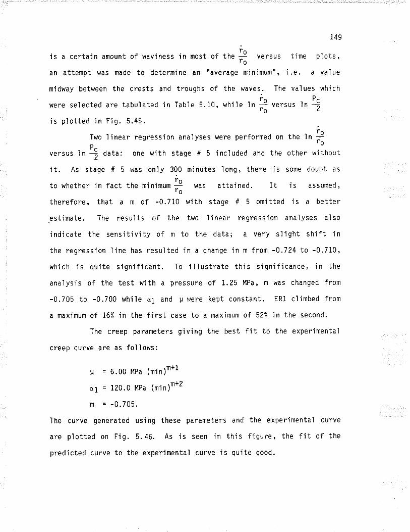
149

iis a certain amount of waviness in most of the ¡f versus time p'lots,

o

an attempt was made to determine an "average minimum", i.e. a value

m'idway between the crests and troughs of the waves.. The values whjch

were selected are tabulated in Table 5.10, while ln ff u.rrr, lt +is plotted in Fig. 5.45.

Two linear regression analyses were performed on the ln PD

--r - ro

versus ln j data: one with stage # 5 included and the other without¿

it. As stage # 5 was only 390 minutes ìong, there is some doubt as

to whether in fact the mjnimum 3 was attained. It is assumed,ro

therefore, that a m of -0.710 with stage # 5 omitted is a better

estimate. The results of the two linear regression anaìyses also

indicate the sensitivity of m to the data; a very sìight shift in

the regression line has resulted in a change in m from -0.724 to -0.710,

which is qu'ite significant. To illustrate this significance, in the

anaìysis of the test with a pressure of I.25 MPa, m was changed from

-0.705 to -0.700 while c1 and U were kept constant. ER1 climbed from

a maximum of 16% in the first case to a maximum of 52% in the second.

The creep parameters giving the best fit to the experimenta'l

creep curve are as follows:

u = 6. o0 MPa (mi n )m+1

a1 = 120.0 MPa (min)m+2

m = -0.705.

The curve generated using these parameters and the experimental curve

are plotted on Fig. 5.46. As is seen in this figure, the fit of the

predicted curve to the experìmentaì curve is quite good.

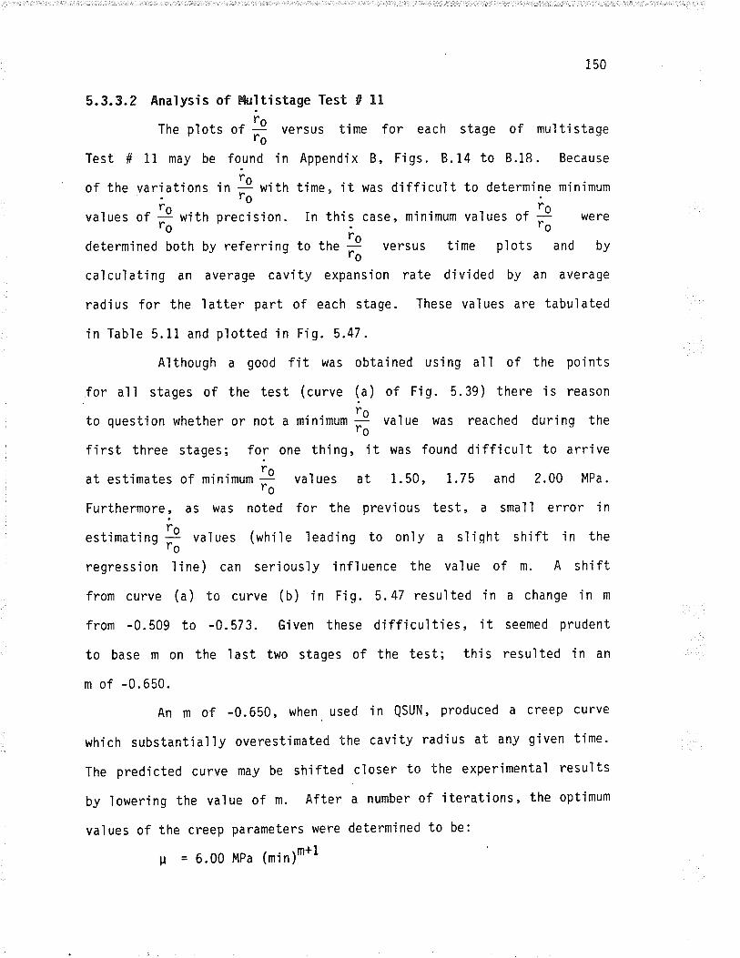
150

5"3.3.2 AnaTysis of Wultistage Test # 3.1

The plots of p versus time for each stage of multistagero

Test # Il may be found in Append'ix B, Figs. 8.14 to 8.18. Because

of the variat'ions in ff *ith time, it was diffjcult to determine minimum

rn ':. . -iovalues of - with precision. In this case, minimum values of;= werero ro

determjned both by referring to tne p versus tíme pìots and byro

calculating an average cavìty expansion rate djvided by an average

radjus for the latter part of each stage. These values are tabulated

in Table 5.11 and plotted in Fig. 5.47.

Aìthough a good fit was obtained using al I of the poìnts

for al I stages of the test ( curve (u ) of Fi g. 5. 39 ) there i s reason

to question whether or not a minimum p value was reached during theFg

first three stages; for one thing,'it was found difficult to arrive

at estimates of minimum 3 values at 1.50, L.75 and 2.00 MPa.ro

Furthermore, as was noted for the previous test, a small error inFg

estimat'ing;Y values (wh'iìe leading to only a sljqht shift in thero

regression line) can serious'ly influence the value of m. A shift

from curve (a) to curve (b) in Fig. 5.47 resulted in a change in m

from -0.509 to -0.573. Gjven these difficulties, it seemed prudent

to base m on the last two stages of the test; this resulted in an

m of -0.650.

An m of -0.650, when. used in QSUN' produced a creep curve

whì ch substant j aì'ly overestimated the cavi ty radi us at any g'iven time.

The predícted curve may be shifted closer to the experímental results

by lowering the value of m. After a number of iterations, the optimum

values of the creep parameters were determined to be:

u = 6.00 l'lPa (mi n )m+1

151

cl = 120.00 MPa (min)m+Z

m = -0.695.

The fictitìous creep curve, generated using the above creep parameters,

and the experimentaì creep curve for Test # 11 are compared l'n Fig.

5.48.

5.3.3.3 AnaTysis of t4ultistage Test # 12

Plots of 3 versus t'ime for each stage of multistage Testro

# L?. may .be found in Appendix B, Figs. 8.19 to 8.22. The minjmum

values of 3 for the first three stages, âS Figs. 8.19 to B.2IF6

.illustrate, are well defined without the dispersion found in the

previous two multistage tests.. Since the fourth stage is only about

480 minutes 'long, the minimum p value for thjs stage may be in doubt.. ,o io

The minimum & vatues are listed in Table 5.L2, whíle minimum ,n iro P-

values are p'lotted against ln j in Fig. 5.49.

As Fig.5.49 illustrates, good fits to the data were obtained

both with and without stage # 4. As is becoming apparent, however,

the determinatjon of m is extreme'ly sensitive to the selection of

the data points. Movement of the data points up or down sìightìy'

or excludÍng one or more data points changes m by severaì hundredths'

The iterative process built into QSUN is, therefore, critjcal to the

success of the modified second-order fluid model; QSUN checks the

in'itial creep parameters against the actual experimental data and

the parameters are refined as necessary. This iterative step is missing

in the strain-hardening, power ìaw creep model analysis.

The best fit creep parameters determined by QSUN were:

u = 5. 9o MPa (mi n )m+1

cl =

m=

120.00 MPa (min)m+2

-0.7 10.

t52

of multistage Test

8.32. The minimum

5.13; minimum ln t'o

ro

ln b versus l. P'ro ta.

The creep curve generated using the above creep parameters, and the

experimenta'l curve are compared in Fig. 5.50.

5.3.3.4 Anaìysis of.Multistage Test # 13

Plots of 3 versus time for each stagero

{ 13 may be found in Appendix B, Figs. 8.23 toFgi values for alì 10 stages are compiled in Tablero

P^values are ploted against 'ln j Ín Fig. 5.51 .

As Fjg.5.51 illustrates, the graph of

becomes markedìy curved in the lower stress region, particularly for

stages # l, 2 and 3, at 0.25, 0.50 and 0.75 MPa respectively. These

resul ts , therefore , have been left out of the I i near regressi on

anaìysis. The ana'lysis performed with the remaining stages, # 4,

to 10, gives a very good fit to the data and an m of -0.697.

According to QSUN, the best fit creep parameters were:

u = 6.oo MPa (min)m+l

a1 = 12o.oo MPa (min)m+2

m = -0.704.

The creep curve generated using the above creep parameters,

and the experimental creep curve are compared in F'ig. 5.52.

5.3.4 Comparison of Experimental Single Stage Pressurereter Creep

Curves and Predicted Creep Curves Using the fudified Second-0rder

FluÍd Mdel

In order to assess the predictive capabi'lity of the modified

153

second-order fluid model, fictitious pressuremeter creep curves have

been generated using the best-fit creep parameters from the multistage

tests (Tab'l e 5. 14) . These fi cti ti ous curves are compared to the

experìmental si ng'l e stage pressuremeter creep curves at equ'i val ent

pressures. The predi cted and experimenta'l curves are compared i n

terms of cavity rad'ius versus time, rather than strain versus time

as with the strain-harden'ing, power law curves. The predicted curves

have been generated usìng QSUN.

The predi cted versus experimentaì curves are i I I ustrated

in Figs. 5.53 to 5.84. The maximum difference between the predicted

and the experimentaì curves, in terms of ERi (Equation 5.12) for cav'ity

radii greater than 41.00 fiffi, are given in Table 5.15. The major

findings from these comparisons are:

1) The creep parameters derived from Tests # 10,11 and 13

typical'ly overestimate the real deformation wh'ile those f rom

Test # 12 typical'ly underestimate the real deformation.

2) Except at I.25 and 1. 5 ?,lPa , the di f ference between the

experimentaì and predicted curves (in terms of tRl), using

the creep parameters from Tests # 10, 12 and 13 to generate

the predicted curves, is less than 25%.

3) SÍnce al i s constant for al I four sets of parameters and

¡l varies on'ly for Test # 12, it may be assumed that m

primarily controls the predicted creep curves. As is seen

from Table 5.15, the highest m (-0.695) gives the greatest

overestimation whj le the lowest m (-0.710) gives a sì ìght

underestÍmation. The other two m va'lues, -0.705 and -0.704,

give predictions between these two timits. Goìng strictìy

754

on the relatÍonship between the ER1 values and m, an m value

between -0.705 and -0.710 would probabìy give the best overall

fit to all of the experimenta'l curves.

As was the case with the strain-hardening, power law creep

comparisons, the predicted creep curves using the modified second-order

fluid model are in reasonable agreement with the experimentaì singìe

stage curves over the time period 'in question. The creep parameters

derived from Tests # 10 and 13 predict the deformation rates throughout

the comparison time period rather well. The creep parameters from

Test # 11 and 12, predict deformation rates at the end of the comparison

period rather poorly. The prediction of deformation rate is an

important consideration when using pressuremeter creep data to

extrapolate creep curves to longer time periods.

5.4 RELATIOI{SHIP BETHEEN THE STRAIhI-HARDENING, POWER LAH CREEP M)DEL

AND THE !'{0DIFIED SEC0ND-0RDER FLUID ruDEL

As d'iscussed previousìy, the strain-hardening power law

creep model, defined bY;

ln (f;) = r tb ,(5.1)

may represent either primary creep if b < L or secondary or steady-state

creep if b = l. It may not represent both primary and secondary creep

at the same time.

If Equation (S.f¡ is differentiated w'ith respect to time

the fol lowìng resul ts:

d¡T llnr-)=Fbtb-1' ri'

(5. i3)

The left-hand-side of Equation (5'13) may be re-written as:

å, rr. s)l = fÐ ,h,*r (r(t)) = *fÌTherefore;

i(t) = i = r u tb-l and substjtutinq for F yields:TTt) = r

i = ¡/=3 ,,n+1 rilb tSln ¡ tb-1 15.15)

I-'2 ' \b' 'nrc

For steady-state creep, b = 1 and Equation (5'15) becomes:

i-,/3,,n+1 . r2Pcrn (5.16)F= \-T) 'c \ñ*t '

Integrating Equation (5.16) qives;

+ = (+)n*1 Ë. tftln ot;

rn titsl = (+)n*1 Ë. tz.ftr't '

r(t) = r(0) exp [{f )n*1 ;. tzfrlt tt (5'i7)

Thus, the cavity radius will increase exponentia'lly w'ith tìme under

steady,state conditions, s jnce +ft) increases w'ith increasing time'

The creep curves illustrated in Fig. 4.1 show this exponent'ia'l increase

in r to be the case for the single stage tests in the entire pressure

range from 1.0 to 2.5 MPa.

Aswaspoìntedoutear].ier,whenthefjrsttwotermsof

Equation(2.62¡becomenegligible,themodjf.iedsecond.orderflujd

modelreducesessentiallytothepower-lawfluidmodel;i'e':

155

( 5. 14)

io . P. (m+1).,,r/(m+1) (2.64)

156

of theNow comParing thi s to the

stra'in-harden'ing power law creep

î = t/3 ìr+1 å. tzlq lni - \ 2 ' ' lìoc'

it is 'ins'nediately evident that

right-hand-sjde are equaì and that:

steadY- state

model; i.e.:

ì...p f orm

the two expressions

(5.16)

on the

1n=m (s.ta)

Thus, the creep exponents for both models may be compared when a

condition of secondary or steady-state creep exists or nearìy ex'ists;

i.e. þ = 1 for the simp]e power law model and the first two terms

of Equation (2.62) become neqliqible. In order to compare the deqree

of variation in the creep exponents determined for the two models

from the multìstage tests, the m values from the modified second-order

fl ui d model have been converted to an "equi val ent" n val ue (Tabl e

5.16). Analyses have shown that the creep rate Io approaches a constantF9

value in the multjstage tests w'ithin about 300 minutes' so secondary

creep dominates beyond this time. These n values thus represent the

dependence of the secondary or steady-state creep rate on the appl'ied

stress. From Table 5.16 'it may be seen that there 'is much less

variation in the equivalent n values using the modified second-order

fl ui d model ana'l ysi s than the n val ues determi ned usi ng the

stra.in-harden'ing, power law creep analysis. The sign'ificance of thjs

is discussed in the next chaPter'

In suffrnary, Creep curves which fit the experìmentaì sìng'ìe

stage test curves reasonab'ly well have been generated by both the

stra.in-hardening, power law creep model and the mod'ified second-order

r57

I

fluid model, using the best fit creep parameters derived from the

multistage tests. However, there is much more variation in the

relationship between secondary creep rate and stress (represented

by n) us'ing the strain-hardening power law ana'lysis than using the

modifÍed second-order fluid model. As the solution of most

boundary-value problems in ice and ice-rjch frozen soils using a power

law creep formulation are strongly dependent on the value of n, this

variation can be important. The importance of n is discussed in detajl

in the next chapter. In addition, the relationship between the

multistage tests and singìe stage tests wi I I be exp'lored further.

Final ly, recommendatÍons wi I I be proposed concern'ing both the

pressuremeter testing technique and the method of analysis.

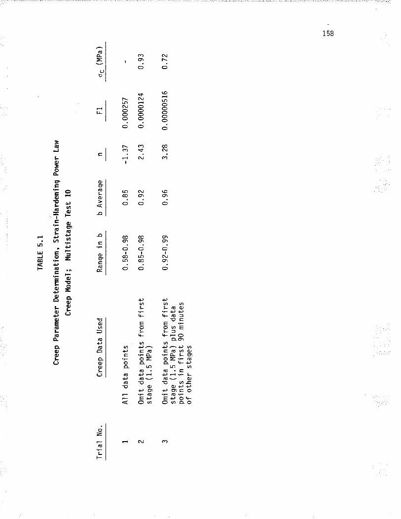
Trì

al N

o.

TA

BLE

5.1

Cre

ep P

aram

eter

Det

erm

inat

ion,

Str

ain-

Har

deni

ng P

o¡ve

r La

w

Cre

ep F

lode

l; H

u'lti

stag

e T

est

l0

Al I

data

poi

nts

Om

it da

ta p

oint

sst

ase

( 1.

5 M

Pa

)

Om

it da

ta p

oint

sst

aqe

( 1.

5 M

Pa

)po

i nts

'in

f i r

stof

oth

er s

taqe

s

Cre

ep D

ata

Use

d

from

firs

t

from

firs

tp1

us

data

90 m

inut

es

Ran

ge in

b

0. 5

8-0.

98

0.85

-0.

98

0.92

-0.

99

b A

vera

ge

0.85

0.92

0. 9

6

-t.3

7

2.43

3.28

F1

0. 0

0025

7

0. 0

0001

24

0 . 00

0005

16

o. (N

Ra

)

0.93

0.72

(¡ co

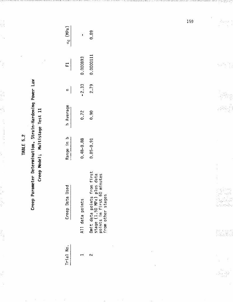
Tria

l No.

TA

BLE

5.2

Cre

ep P

aram

eter

Det

er¡n

inat

ion"

Str

ain-

Har

deni

nq P

orer

Cre

ep $

bdel

; l{u

ltist

age

Tes

t ll

Cre

ep D

ata

Use

d

Al I

dat

a po

'ints

Om

it da

ta p

oint

s fr

om fi

rst

stag

e (1

.50

MP

a) p

lus

data

poin

ts in

firs

t 60

min

utes

from

oth

er s

tage

s

Ran

qe in

b

0.48

-0.8

8

0.85

-0.9

1

b A

vera

ge

Law

0.72

0.90

-2.3

3

2.7

9

F1

0.00

0893

0.00

001

I 1

oc (M

Pa)

0.89

(tl (o

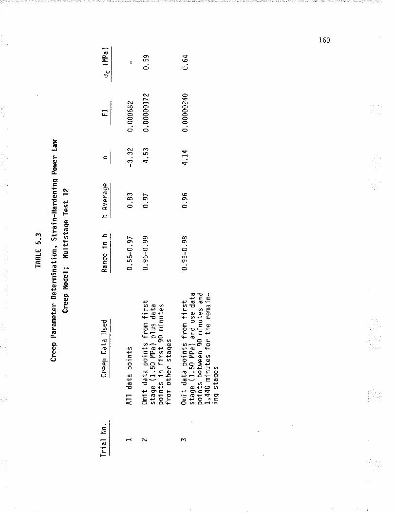
Tri

a'l N

o.

TA

BLE

5.3

Cre

ep P

aram

eter

Det

erm

inat

ion,

Str

ain-

Har

deni

ng P

ower

Law

Cre

ep &

lode

l; M

ultis

taqe

Tes

t 12

All

data

poi

nts

Om

it da

ta p

oint

s fr

om fi

rst

stag

e (1

.50

MP

a) p

lus

data

poin

ts in

firs

t 90

min

utes

from

.oth

er s

taqe

s

Om

it da

ta p

oint

s fr

om fi

rst

stag

e ( 1.

50 M

Pa )

and

use

data

po'in

ts b

etw

een

90 m

inut

es a

nd1,

440

min

utes

for

the

rem

ain-

inq

stag

esCre

ep D

ata

Use

dR

ange

in b

0. 5

6-0

. 97

0. 9

6-0.

99

b A

vera

ge

0. 9

5-0.

98

0.83

0. 9

7

-3.3

2

4.53

0. 9

6

F1

0.00

0682

0. 0

0000

172

4.14

0.

0000

0240

o. (m

Pa

)

0.59

0. 6

4

¡J Oì

O

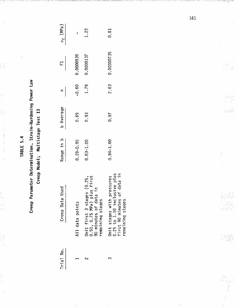
Tria

l No.

TA

BLE

5.4

Cre

ep P

aram

eter

lþte

rmin

atio

n, S

trai

n-H

arde

ning

Cre

ep l{

odel

; i{u

ïtist

age

Tes

t 13

All

data

poi

nts

Om

it fir

st 3

sta

ges

(0.2

5,0.

50,0

.75

MP

a) p

lus

first

90 m

inut

es o

f da

ta in

rem

aini

nq s

taqe

s

Om

it st

aqes

with

pre

ssur

es0.

25 to

1.5

0 in

clus

ive

plus

first

90

m'in

utes

of

data

inre

mai

ning

sta

ges

Cre

ep D

ata

Use

dR

anqe

in b

0.29

-0.9

5

0.83

- 1.

00

Pow

er L

aw

b A

vera

qe

0.94

-1.0

0

0. 6

9

0.93

-0.6

0

r.79

0.97

F1

0.00

0093

9

0.00

0013

7

2.63

0.

0000

0735

oc (M

Pa)

1.22

0.81

l-¡ Oì

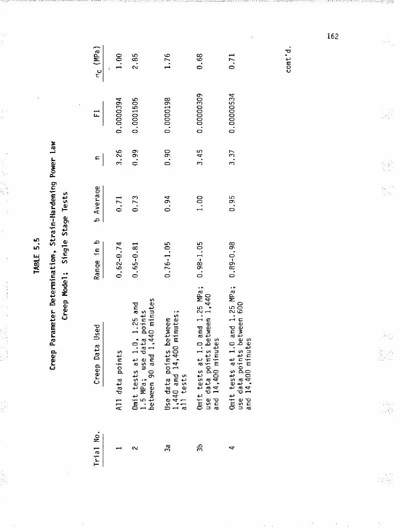
Tria

l No.

TA

BLE

5.5

Cre

ep P

aran

rete

r D

eter

min

atio

n" S

trai

n-H

arde

ning

Pow

er L

aw

Cre

ep $

lode

l; S

ingl

e S

tage

Tes

ts

I 2

All

data

poi

nts

Om

it te

sts

at 1

.0,

1.25

and

1 . 5

MP

a ;

use

data

poi

nts

betw

een

90 a

nd 1

,440

min

utes

Use

dat

a po

ints

bet

wee

n1,

440

and

14,4

00 m

inut

es;

al I

test

s

Om

it te

sts

at 1

.0 a

nd 1

.25

MP

a;us

e da

ta p

oint

s be

twee

n I"

440

and

14,4

00 m

inut

es

0mit

test

s at

1.0

and

1.2

5 Ì'l

Pa;

use

data

poi

nts

betw

een

600

and

14,4

00 m

inut

es

Cre

ep D

ata

Use

d

3a 3b

Ran

ge in

b

0.62

-0.7

4

0.65

-0.8

1

b A

vera

qe

0.76

- 1

.05

0. 7

1

0.73

0. 9

8- 1

.05

1 . 00

3.

4s

0. 0

0000

309

3.26

0.99

0.89

-0 .

98

0. 9

4

F1

0.00

0039

4

0.00

01s0

5

0.90

0.

0000

198

"._

(MP

a)

1.00

2.85

0.9s

3.37

0.

0000

0534

r.7

6

0. 6

8

0.71

cont

'd.

Oì

N)

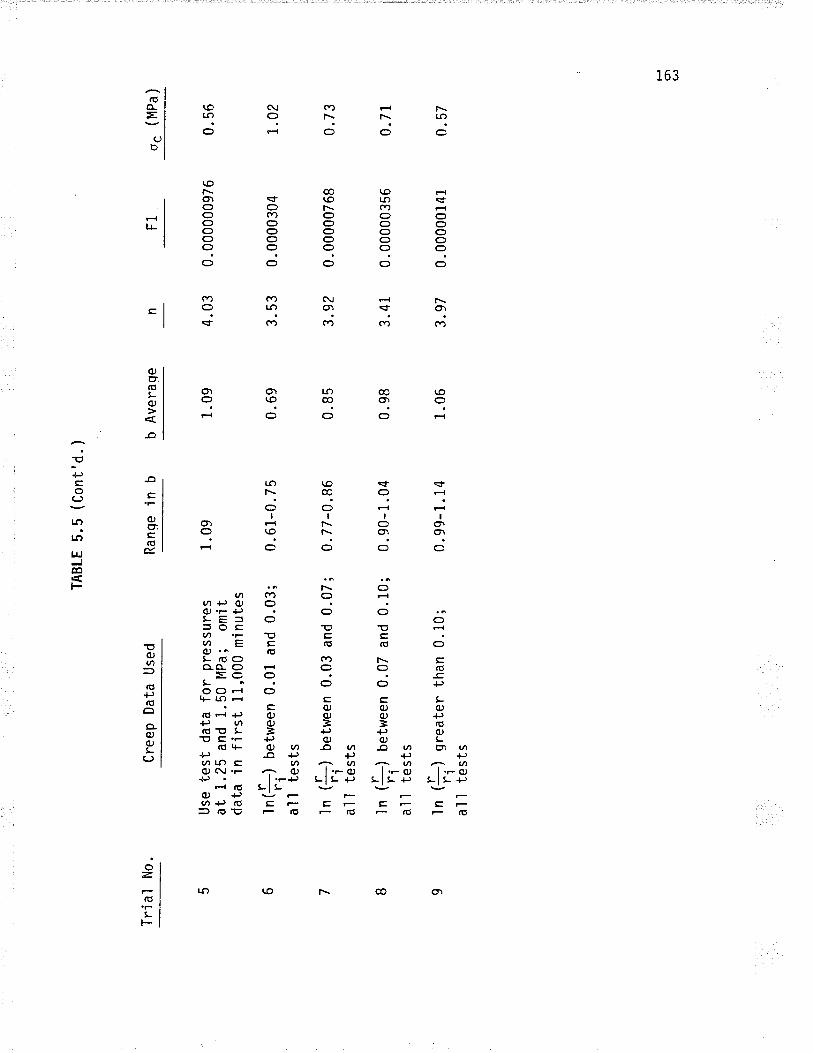
ïria

l N

o.

6

Cre

ep D

ata

Use

d

Use

test

dat

a fo

r pr

essu

res

at 1

.25

and

1.50

l.lP

a; o

mi t

data

in fi

rst

11,0

00 m

inut

es

tntft

) be

twee

n 0.

01 a

nd 0

.03;

al I

test

s

I n

({;)

U.t*

een

0.03

and

0.0

7 ;

al I

test

s

t n

(f;)

bet

wee

n o.

o7

and

o. 1

o;

al I

test

s

I n

(f¡)

s".

uter

tha

n 0.

10;

al I

test

s

I

TA

BLE

5.5

(C

ont'd

. )

Ran

qe in

b

1 .0

9

b A

vera

ge

1.09

0.61

-0.7

5

0.77

-0.8

6

0.90

- 1.

04

0.99

-1.1

4

0. 6

9

0.85

0.98

1 .0

6

4.03

0.0

0000

0976

F1

3. 5

3

3.92

3. 4

1

3.97

oc (M

Pa)

0. 5

6

0.00

0030

4

0.00

0007

68

0.00

0003

56

0.00

0001

41

7.02

0.73

0.71

0. 5

7

P Ot

(^,

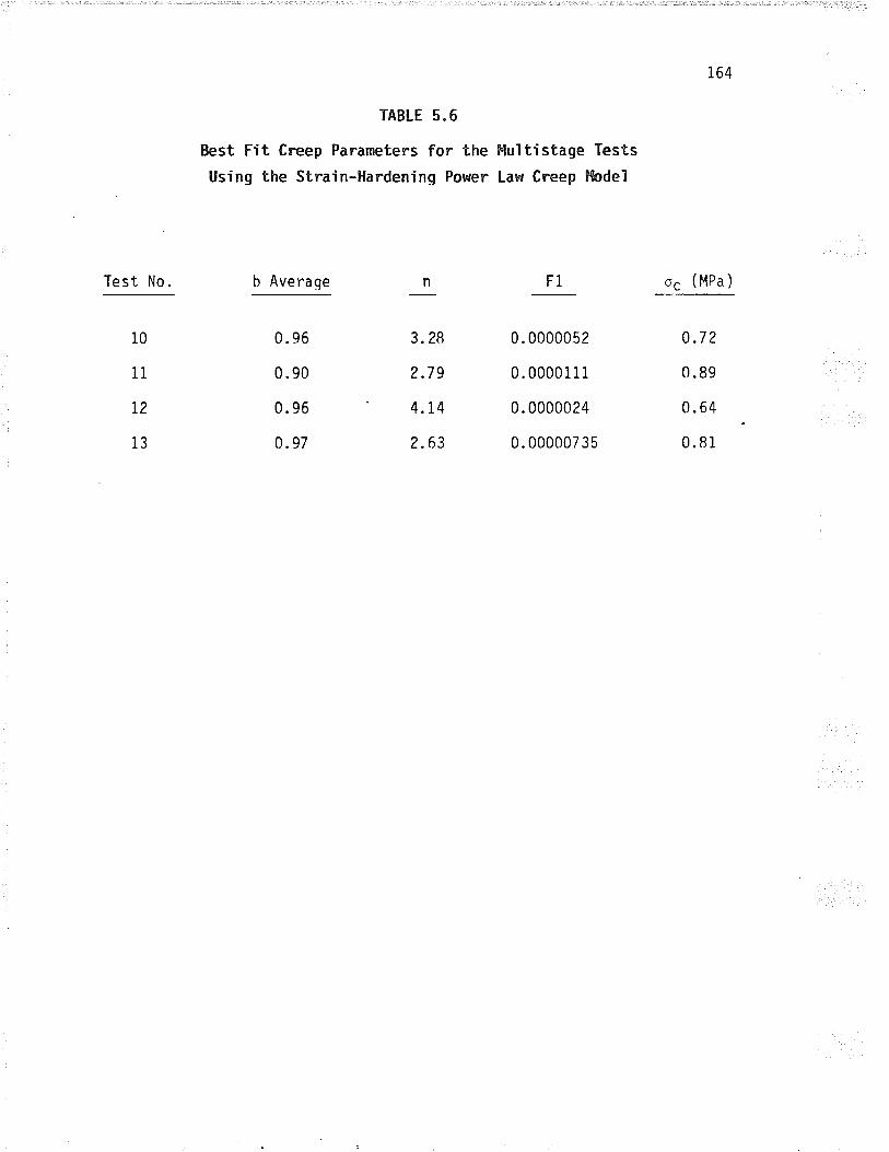
TABLE 5.6

Best Fit Creep Parareters for the

Using the Strain-Hardening Power

F4uT ti stage Tests

Law Creep þdeì

164

oç (MPa )Test No. b Averaqe F1

10

11

T2

13

0. 96

0.90

0. 96

0.97

3.28

?.7 9

4.14

2.63

0.72

0.89

0. 64

0.81

0.0000052

0.0000111

0. 0000024

0.00000735

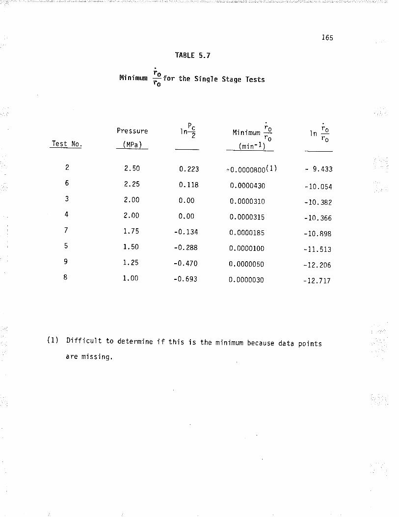
ro-- îorro

TABLE 5"7

the SinqIe Stage TestsMinfnm¡

PressureD

t 'C,n-Test No.

2

6

3

4

7

5

9

I

0.223

0. 118

0. 00

0. 00

-0. 134

-0. 288

-0.470

-0. 693

f'linimum þro

(min-i)

=9.6696969( 1 )

0.0000430

0. 0000310

0. 0000315

0.0000185

0. 0000100

0. 0000050

0. 0000030

(1)

(MPa)

?.50

2.25

2.00

2.00

1.7 5

1. 50

L.25

i. 00

Difficult to determine

are missing.

i f this is the minimum because data points

i65

rn iero

- 9. 433

- 10.054

- 10. 382

- 10. 366

- 10.898

-11.s13

-72.206

-72.717

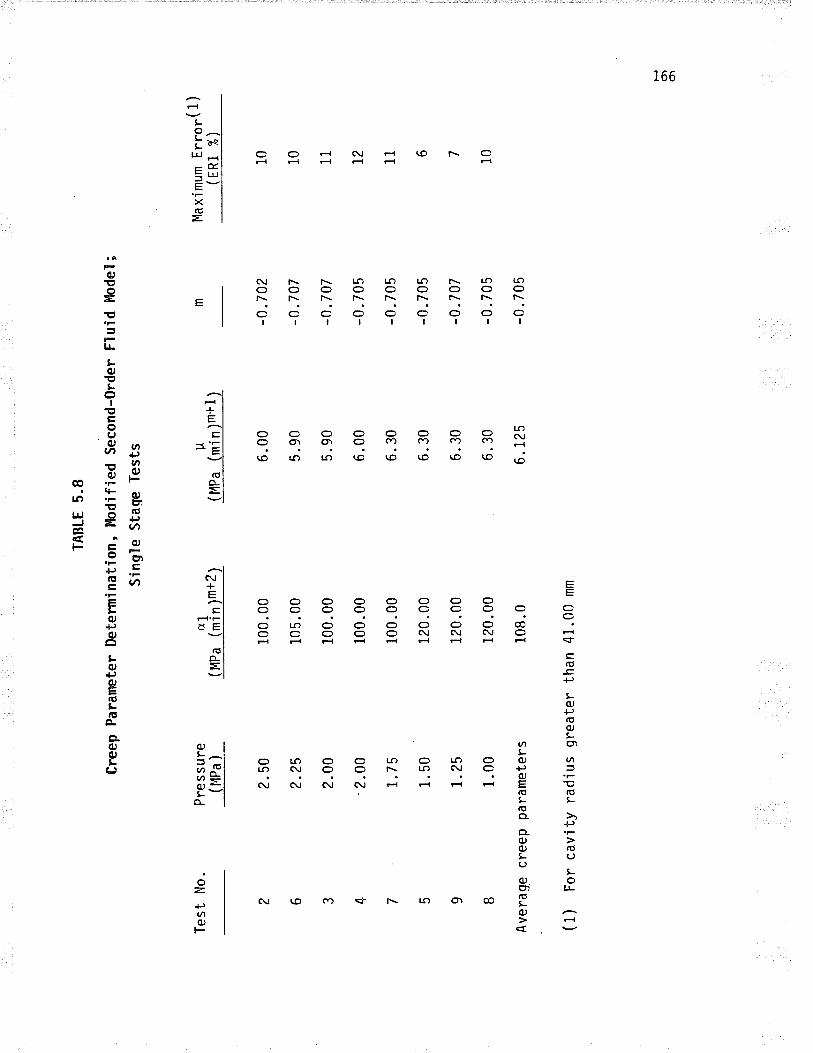
Tes

t N

o.

TA

BLE

5.8

Cre

ep P

aram

eter

Det

erm

inat

ion,

hdi

fied

Sec

ond-

0rde

r F

luid

lfud

et;

Sin

gle

Sta

ge T

ests

Pre

ssur

e(

Ìapa

)

2.s0

2.25

2.00

'2.0

0

1.75

1. 5

0

t.25

1.00

pa ra

met

ers

4 7

( M

Pa

1fi|n

¡m

+z

1

9 IA

vera

ge c

reep

100.

00

105.

00

100.

00

100.

00

100.

00

120.

00

120.

00

120.

00

108.

0

(1)

For

cav

ity r

adiu

s gr

eate

r th

an 4

1.00

mm

u( tlP

a (m

i n )

m+

1 ¡

6.00

5.90

5.90

6.00

6. 3

0

6. 3

0

6. 3

0

6. 3

0

6.L2

5

-0.7

02

-0.7

07

-0.7

07

-0.7

05

-0.7

05

-0.7

05

-0.7

07

-0.7

05

-0.7

05

Max

imum

Err

or(

1)(E

R1

%)

10 10 1l t2 11 10

lJ Or

Oì

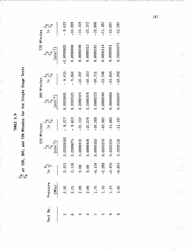
Tes

t N

o.

ro ro

TA

BLE

5.9

at 1

20,

360"

and

720

Ffin

utes

for

2 6 3 4 7 5 9 I

Pre

s s

ure

(MP

a)

2. 5

0

2.25

2.00

2. 0

0

1.75

1.50

r.25

1 .0

0

.Pc

,nz

0.22

3

0. 1

18

0.00

0 .0

0

-0.1

34

-0.

288

-0.

470

-0.6

93

io ro

120

Min

utes ln

(mi n

- 1)

0.00

0093

50

0 .0

0006

7 5

0.00

0041

0

0.00

0042

0

0.00

0035

0

0.00

0017

0

0.00

001s

4

0.00

0011

8

thê

Sin

gle

Sta

ge T

ests

io ro

- 9.

277

- 9.

603

- 10

. 10

2

- 10

.079

- 10

.260

- 10

.982

- 1 1.

081

-11.

347

ro ro

360

Min

utes ln

(mi n

- 1)

0.00

0080

0

0.00

0052

0

0.00

0032

4

0.00

0037

8

0.00

0022

3

0 .0

0001

44

0.00

0008

6

0.00

0004

7

ro ro

- 9.

433

- 9.

864

- 10

. 33

7

- 10

. 18

3

- 10

.711

-11.

148

-11.

664

-t2.

268

720

Min

utes

rotn

ro(m

'¡n-1

)

=0.

0000

800

0.00

0045

0

0.00

0033

0

0.00

0031

3

0.00

0019

1

0 .0

0001

14

0.00

0006

1

0 . 00

0004

7 5

io ro

- 9.

433

- 10

.009

- 10

. 31

9

-r0

.37

2

- 10

.866

-11.

382

-r?.

007

-72.

257

or --¡

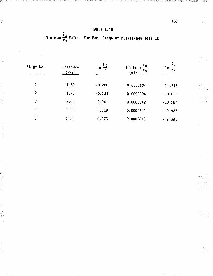
168

ffiinimun þro

TABLE 5.10

VaIues f-or Each Stage of P{ultistage Test l0

Stage No. Pre s sureP^1nì Mi nimum

(mi n- 1

.ioro

-i1.218

- 10.802

- 10. 284

- 9.827

- 9.385

ioIo)

1

2

3

4

5

(MPa )

1. 50

L.7 5

2.00

2.25

2.50

-0.288

-0.134

0.00

0. 118

0.223

0 . 00001 34

0.0000204

0.0000342

0.0000540

0.0000840

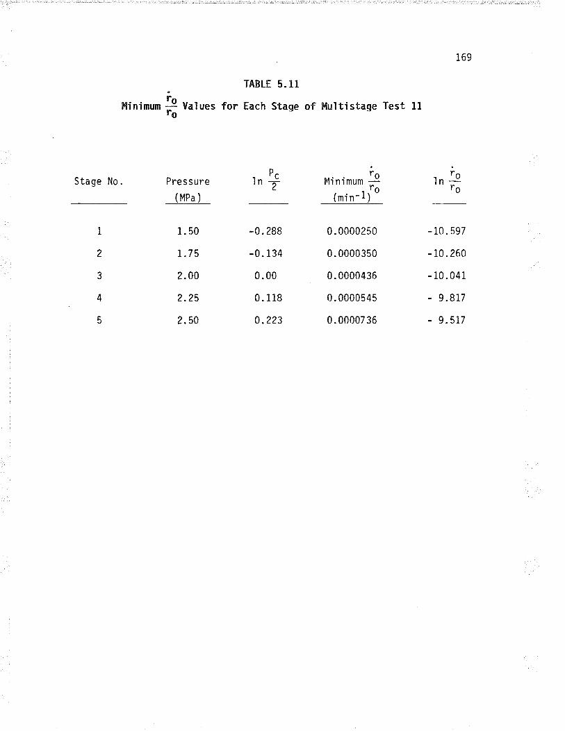
169

Hinimunrono

TABLE 5" 1.1

Val ues for Each Stage of Hultistage Test L1

Stage No.

1

2

3

4

5

Pre s sure

(MPa)

1.50

r.75

2.00

2.25

2. 50

D, rctnz Fli n i mum

(mi n- 1

ln þFg

roro)

-0. 288

-0. 134

0.00

0. 118

0.223

0.0000250

0.0000350

0.0000436

0.000054s

0 . 00007 36

- 10. 597

- 10. 260

- 10.041

- 9.817

- 9.5r7

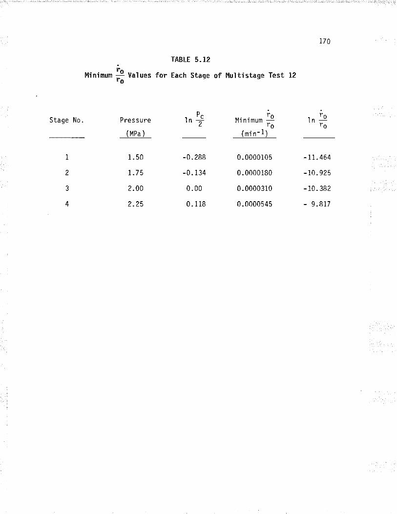
Stage No. Pre s s ure

(Npa)

1.50

1.75

2.00

2.25

Ninimum bro(mi n- 1)

0.000010s

0 . 0000 180

0.0000310

0.0000545

170

.ioln -ro

-1r.464

-70.925

- i0. 382

- 9.817

Hinimumroro

TABLE 5. 12

VaIues for Each Stage of t{ultistage Test L2

DlnT

-0. 288

-0. 134

0.00

0. 118

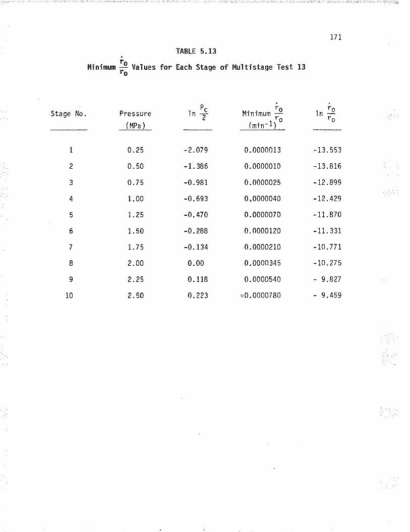
T7I

ffiinimwnioro

TABLE 5"13

Vaïues for Each Stage of ffiultistage Test n3

Stage No.

3

4

5

6

7

8

9

10

Pre s sure

(MPa)

0.25

0. 50

0.75

1 .00

1.25

1.50

7.75

2.00

2.?.5

2.50

¡,tinimum þ-ro

(mi n- 1)

Dr 'Ctnz .ioIn

-ro

1

2

-2.079

- 1. 386

-0.981

-0.693

-0. 470

-0. 288

-0.134

0.00

0.118

0.223

0.0000013

0.0000010

0.0000025

0 ,0000040

0.0000070

0. 0000120

0.0000210

0.0000345

0.0000540

=0.0000780

-13.553

-13.816

-r2.899

-r2.429

-11.870

-11.331

-r0 .77 r

-to .27 5

- 9.827

,9.459

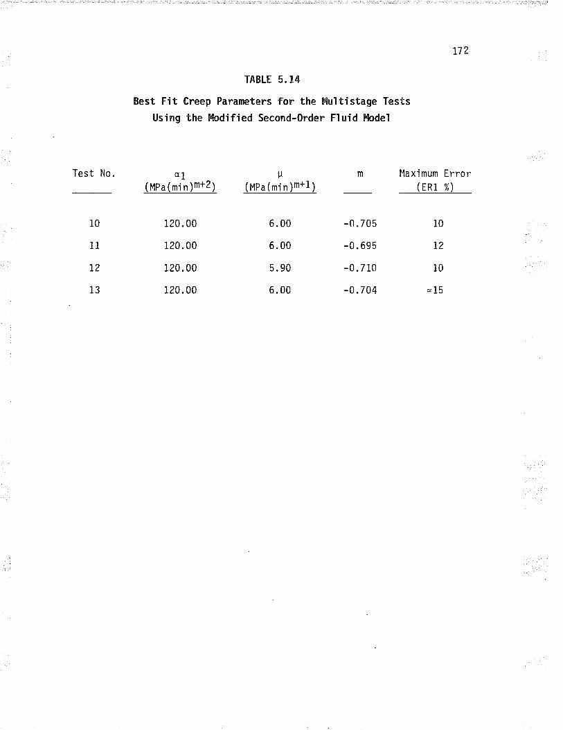
TABLE 5. 14

Best Fit Creep Paranete¡'s fon the ffiultistage Tests

Using the tudified Second-0rder Fluid þdeï

172

m l'laximum ErrorTest No. al tl(MPa (m'i n )m+2 ) (MPa (mi n )m+1 I

120. 00

120.00

120.00

120. 00

(ERi %)

6.00 -0.705 10

6.00 -0.695 72

5.90 -0.7 i0 10

6.00 -0.704 =15

10

11

T2

13

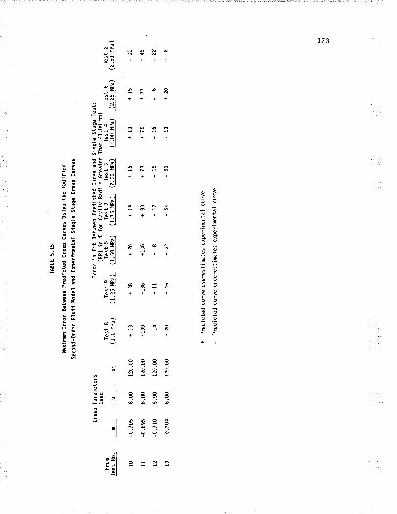
Fro

mT

est

No.

l0 lt t2 l3

Cre

ep P

aram

eter

sU

sed

mu

TA

BLE

5.1

5

Hax

im¡m

Err

or B

etw

en P

redi

cted

Cre

ep C

urve

s U

slnq

the

lbdl

fied

Sec

ond-

0rde

r F

luld

Þbd

el a

nd E

xper

lnen

tal

Sln

gle

Sta

ge C

reep

Cur

ves

-0.7

05

6.00

-0.6

95

6.00

-0.7

l0

5.90

-0.7

04

6.00

dl

120.

00

120.

00

120.

00

120.

00

Tes

t I

( 1.

0 llP

a )

+ 1

3

+10

9

-14

+20

Err

or in

Fit

Bet

wee

n P

redi

cted

Cur

ve a

nd S

ingl

e S

taqe

Tes

ts(E

Rl i

n Í

for

Cav

ity R

adlu

s G

reat

er T

han

41.0

0 n¡

n)T

est 9

Tes

t 5

Tes

t 7

Tes

t 3

Tes

t 4

Tes

t 6

Tes

t 2

(1.2

5t'lP

a) (

]_.!g

_Ife

l (1

.7sl

'lPa)

(2.

00M

Pa)

(2.

00r'l

Pa)

(2.

25M

Pa)

(2.5

0MP

a)

+38

+l

36

+ ll

+46

Pre

dict

ed c

urve

ove

rest

imat

es

expe

rimen

tal

curv

e

Pre

dict

ed c

urve

und

eres

timat

es e

xper

irent

al c

urve

+?6

+10

6

-8 +32

+19

+90 -t2

+24

+16

+78 -16

+21

+ 1

3

+ 7

5

-16

+18

+15 +77 -6 +20

-10

+45 -2?

+6

! CÐ

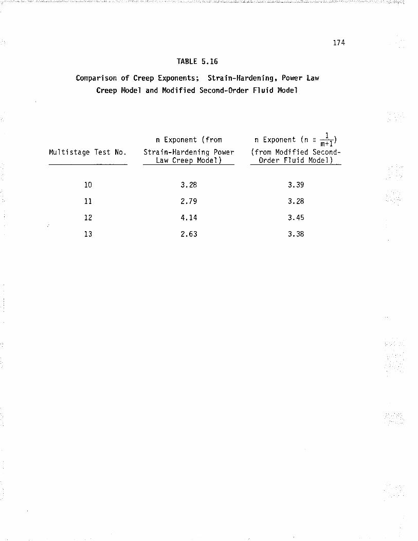
L74

TABLE 5.16

Comparison of Creep Exponents; Strain-Hardening, Poær l-aw

Creep fudel and Hodified Second-Order Fluid &bdel

n Exponent (from n Exponent (n = #)Murtistase Test No' Strali-!il:;.ü:3.Ti''" (tä:i.T'Élll:'-:::ii'-

10

i1

72

13

3.28

2.79

4. t4

2.63

??o

3.28

3. 45

3. 38

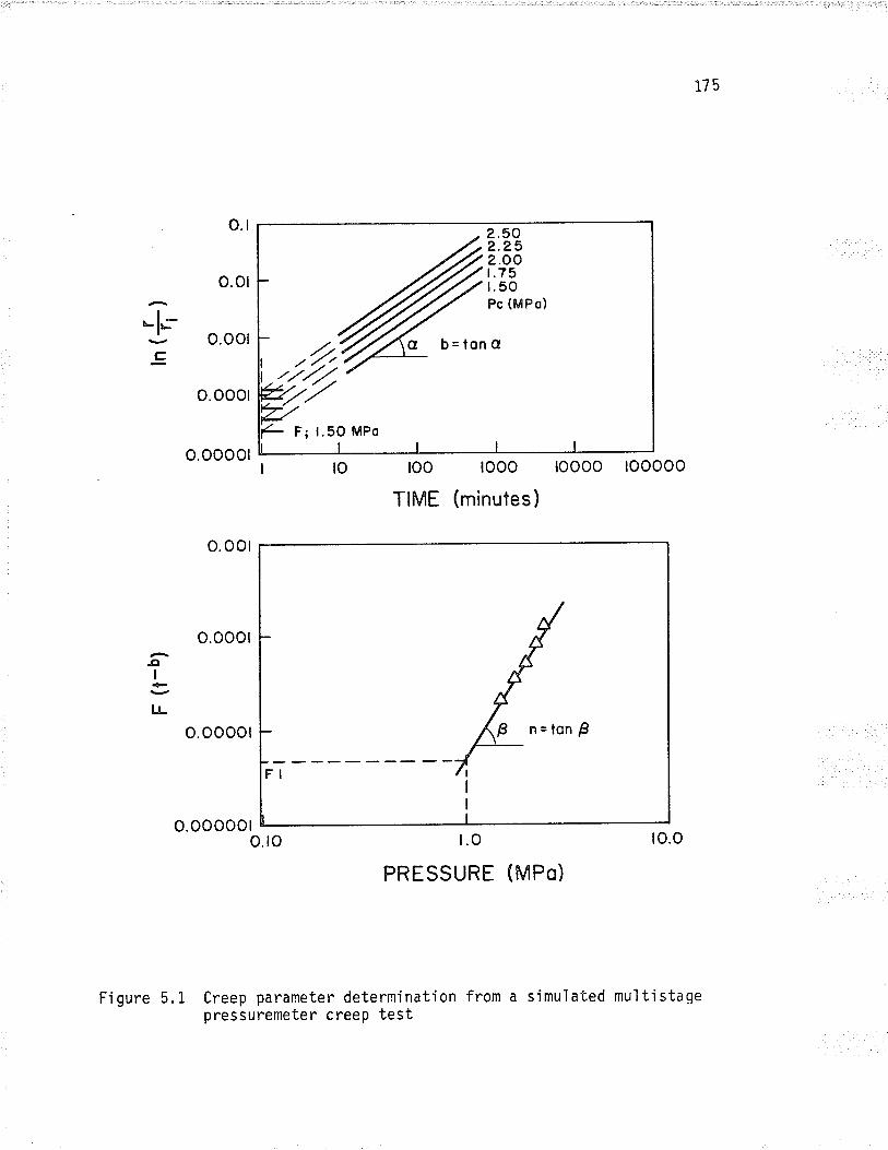
L75

fc

o.t

o.or

o.oot

o.ooot

o.ooool

o.oot

o.ooot

o.oooor

o.ooooot

roo rooo loooo looooo

TIME (minutes )

n=ton Ê

FI

to

Í¡I

u-

o.ro

Figure 5.1 Creep pararneter determinationpressuremeter creep test

r.o

PRESSURE (MPo)

ro.o

2.502.252.OO1.75t.50Pc (MPo)

'zb=tono

F¡ l.50 MPo

from a simulated multistaqe

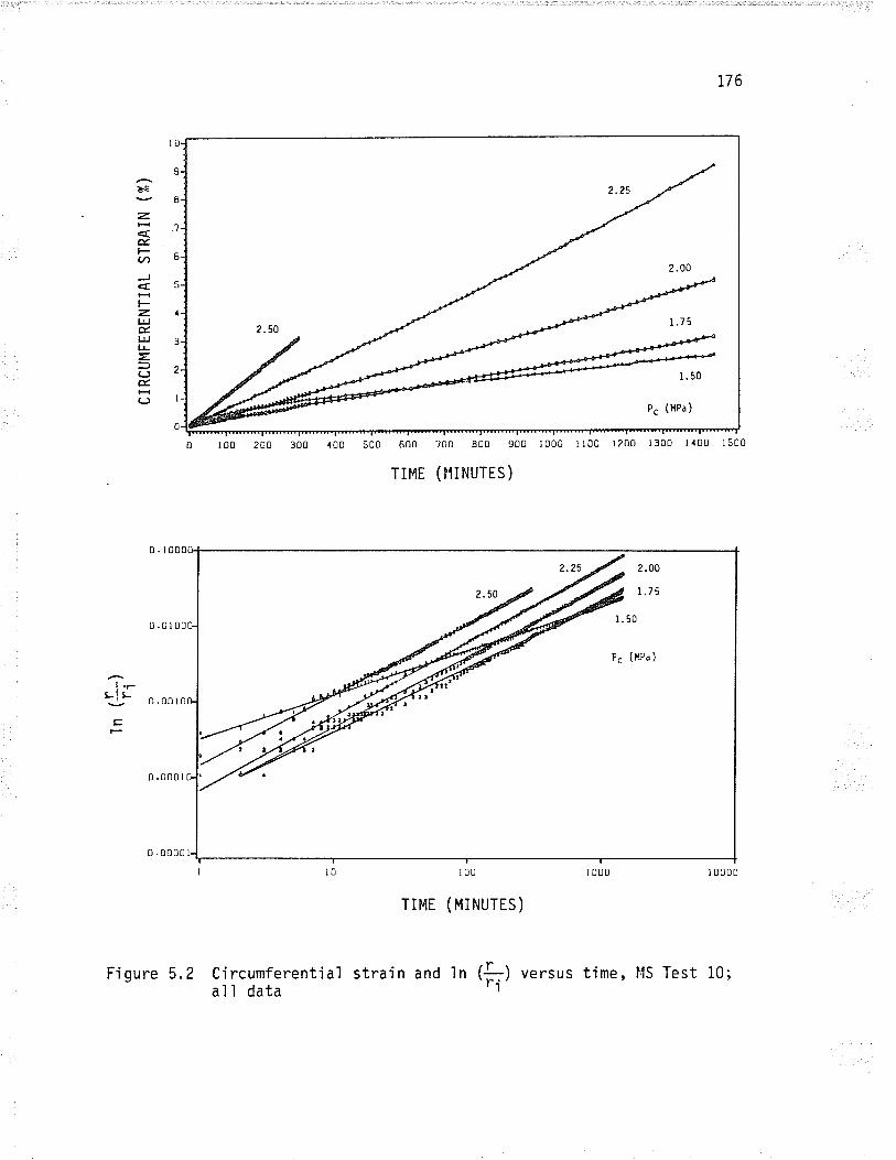
be

zú.t-(./,

J

t-t¿ldUJt!=.JQÉc)

176

r 00 200 300 100 500 600

TIME

2.00

1.75

1.50

'" (l{Pa)

t.-LIL

g

0.0100

0.00r

0 .0000

TIME (MINUTES)

I 000 l 0000

5.2 Circumferentialal I data

strain and tn (ft) versus time, l.1S Test 10;

?00 800 900 ¡ 000 r I 00 I 200 I 300 I 100

( Hr NUTES )

Fi gure

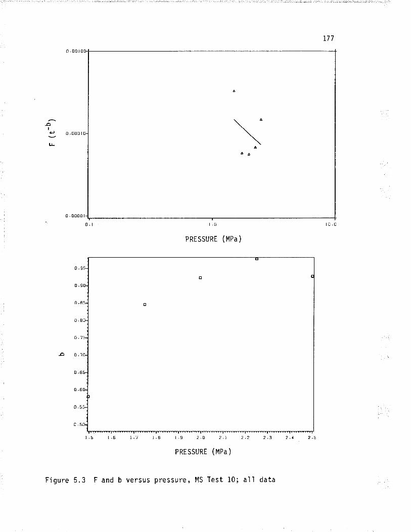
177

-oI{J

LL

PRTSSURE (MPa)

PRESSURE (MPa )

Fi gure 5. 3 F and b versus pressure , F'lS Test 10; al I data

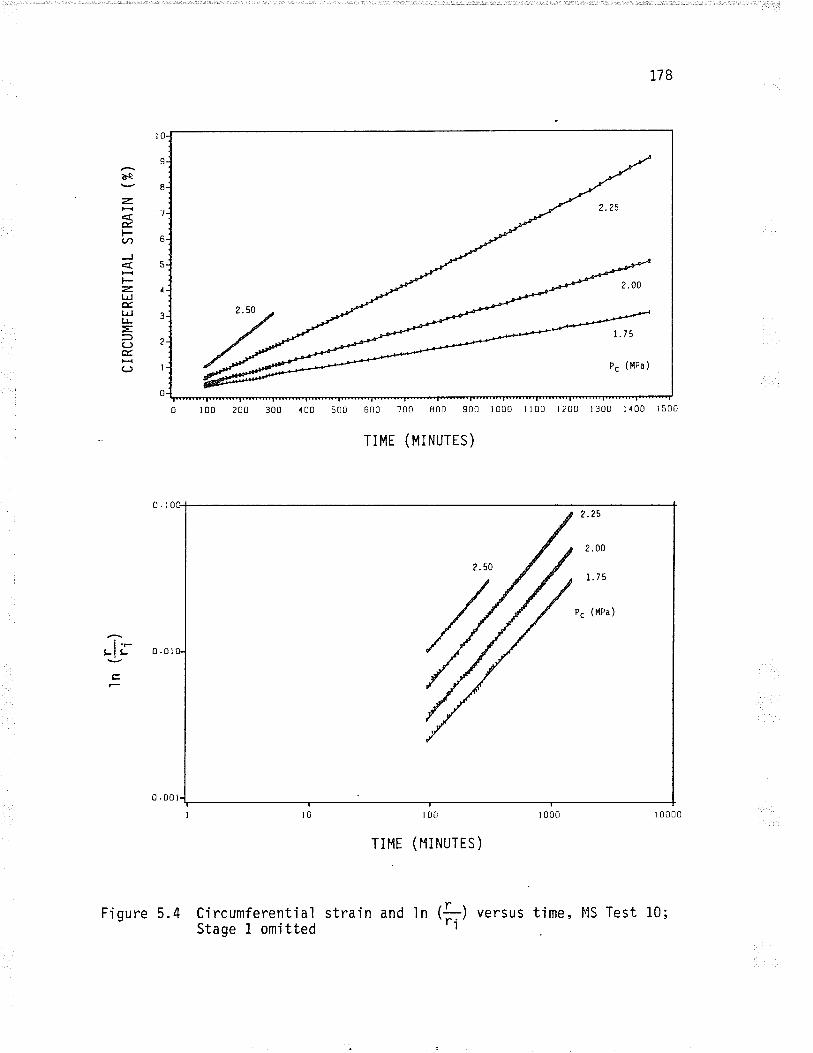
Iba

Iz.

1

ÉFu1 b

J

F-z1UJd.t¿l ru-==(-)¿É.(Jl

0

178

t 0000

600 ?00 tì00 900 r000 rr00 1200 1300 1400 I500

TIME (MINUTES)

2.50

?.2s

2.00

1.7 5

r. (HPa)

s00,r 00200t00

t.-LIL

E

0 .00

Figure 5.4 CircumferentialStage I omi tted

r00

TrMr (¡{rNUTES )

strain and ln (fr) ve"sus time, þ1S Test 10;

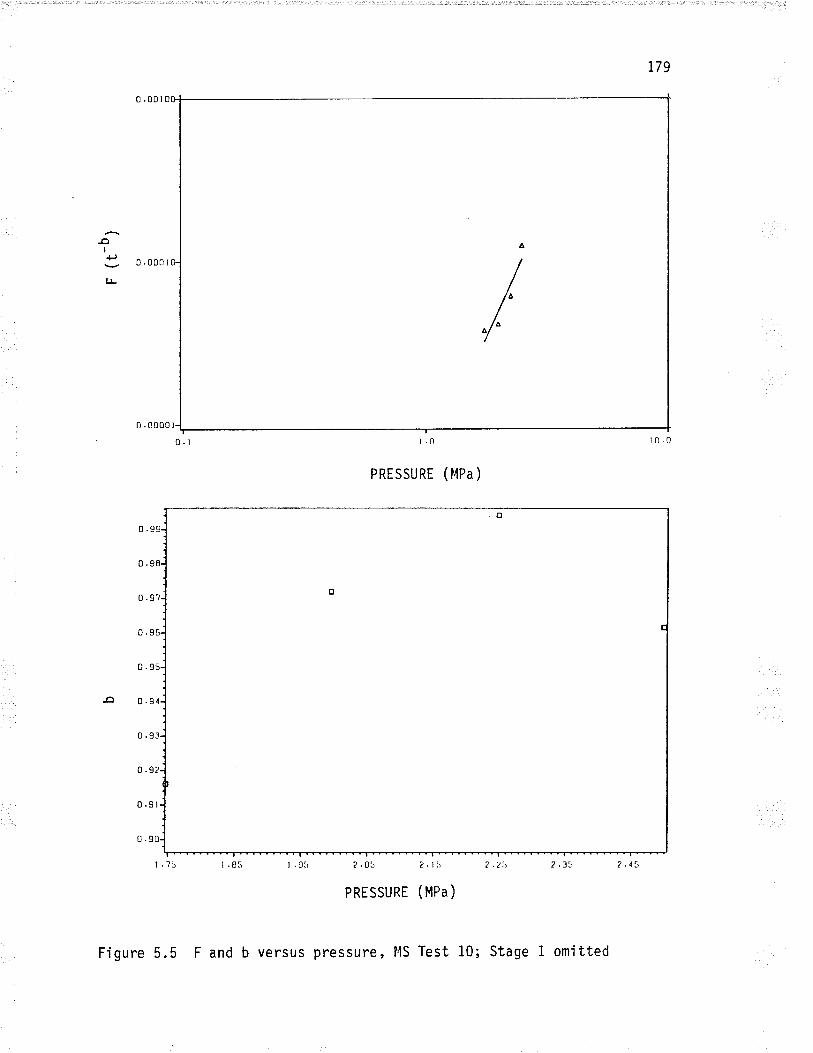
179

-oI+)

u-

ì.0

PRESSURE (MPa)

PRESSURE (MPa)

Figure 5.5 F and b versus pressure, llS Test Stage I omj tted

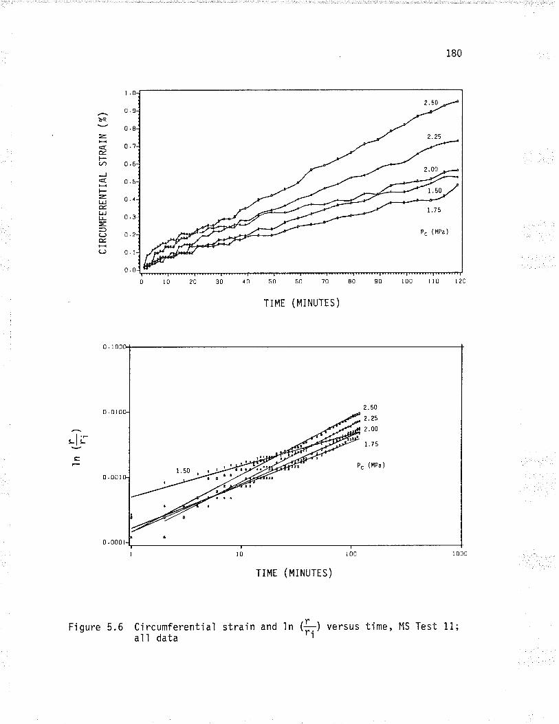
bs

z.

Ét--t¿l

J

t-z.tJJÉUJu-EJc)É.(J

180

2.50

2.25

2 .00

1.75

P. (tlPa )

l.r!lL

E

0.00r

5.6 Ci rcumferenti alal I data

TrMr (MTNUTTS)

60 ?0 80 90 r00 ll0

( Mr NUTES )

Fi gure strai n and I n (fr) u.rtus time, MS Test 11;

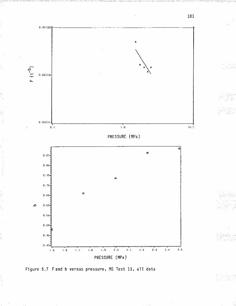
18i

-a¡+J

l!

1.8 t.9

PRESSURE

pressure, l,ls

PRESSURE (NPa )

?.o 2.t

( I'lPa )

Test 11,

?.?

Figure 5.7 F and b versus al I data

2.5

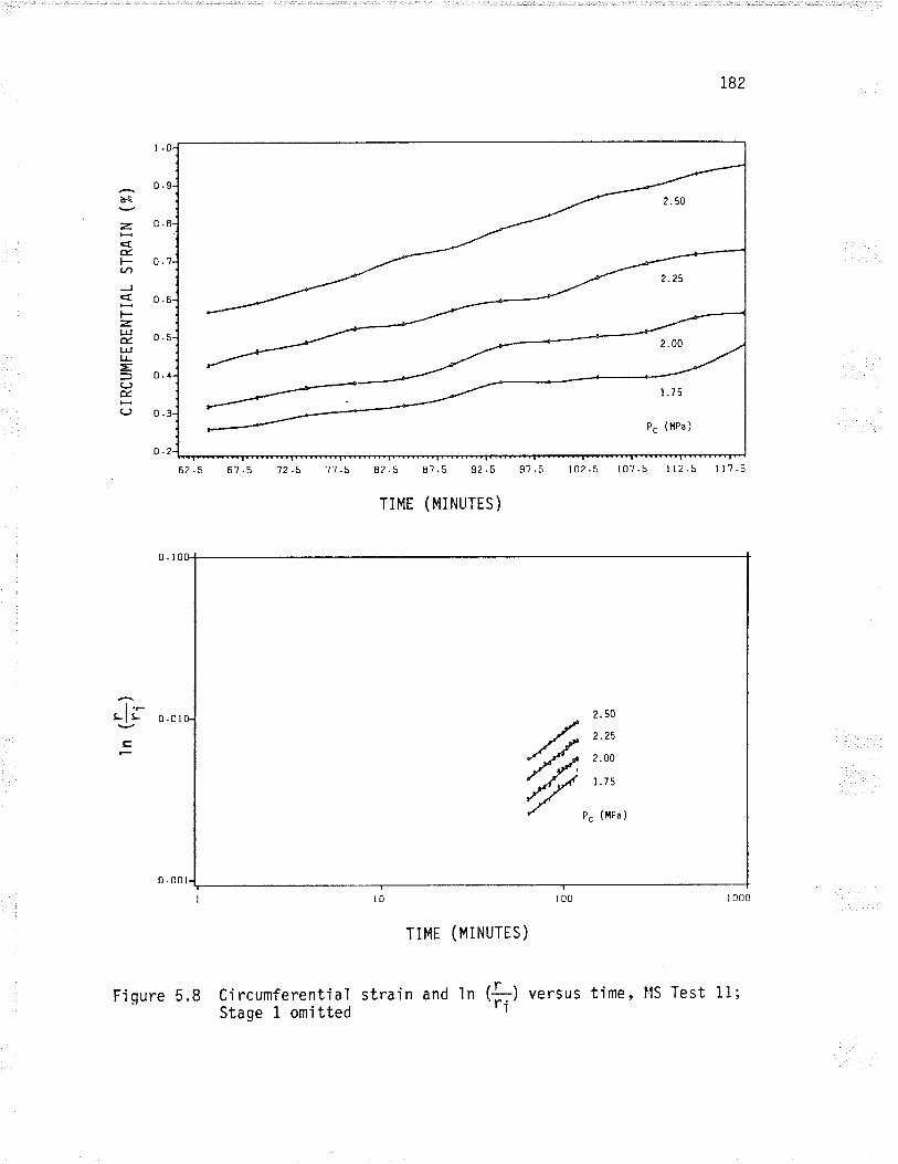
182

be

z.

É.FVIJ

l-þJÉ.UJl!Jc)Éc)

t.-tlr

E

6? .5 't2 .5 't1 .5 8? .5

TIMT

TIME (MINUTES)

Fi gure 5 .8 Ci rcumferenti al strai n and 'l n

Stage 1 omjtted

8?.5 92.5 97.5 102.5 r0?.S 112.5 ll?.5

( MI NUTES )

2. 50

2.25

2. 00

1.75

P. ( l{Pa )#

(f;) o.tsus time, l{S Test 11;

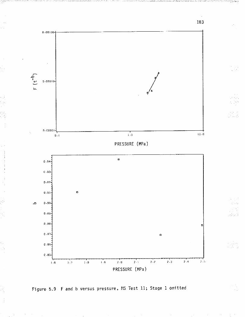
183

0 .0010

-oIP

l-L

10 .0

PRESSURE (l'lPa )

¿.1 ¿.¿

(¡tpa )

Figure 5.9 F and b versus pressure, l,1S Test 11; Staqe l omitted

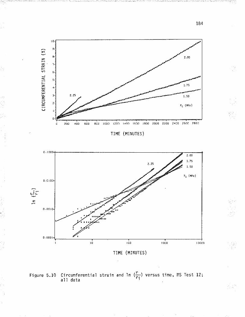
be

zÉFv,J

F--ztJJÉ.Ldll-=c)ÉL)

t0

I

I

"t

i84

2.00

1.75

2.25 1.50

P. ( l{Pa )

1

3

2

I

600100 800 r 000 r 200 l I 00 r 600 l 800 2000 2200 21 00 2600 2800

TIME (HINUTES)

100

TIME (MINUTIS)

t.-LIL

c

Fi qure 5. 10 Ci rcumferenti alal I data

strain and ln (ft) versus time, tlS Test i2;

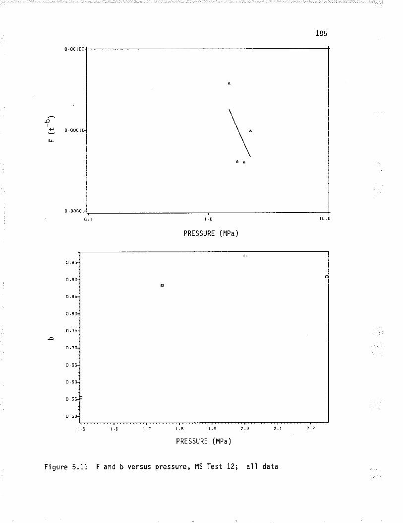
185

-oIP

l!

PRESSURE ( l,lPa )

I.1 t.8 t.9 ?.O

PRESSURE (MPa)

versus pressure, l4S Test 12; allF'i gure 5. 11 F and b data

{

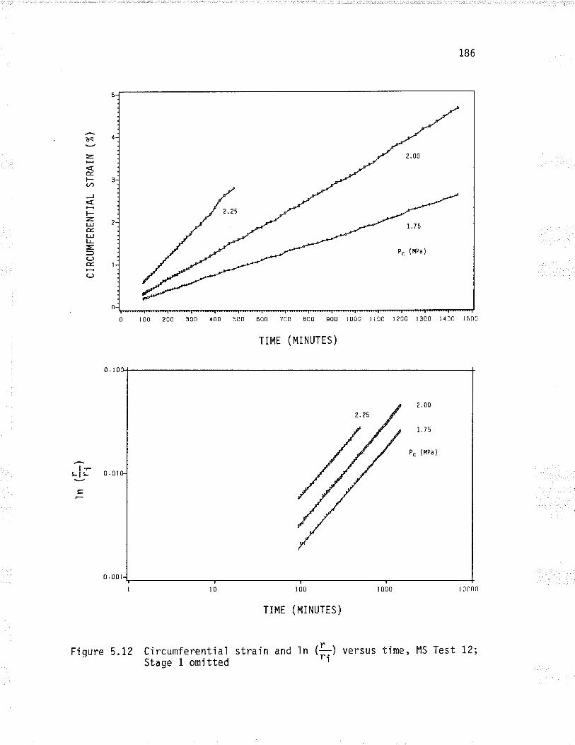
3

2

I

be

z.

É1-tJ',

J

t'--z.lrJÉl¿JU-

¿c)É.CJ

c 100 200 300 {00 500 600 ?00 800 900 1000 I 100 1200 1300 1100 1500

TIME (MINUTES)

2.002.?5

1.7 5

P. ( l{Pa )

186

10000

l.-LIL o.ol

g

TIFIE ( MINUTES )

Fiqure 5.12 Circumferential strain and tn (fr) versus time, l'''lS Test 12;Stage 1 omitted

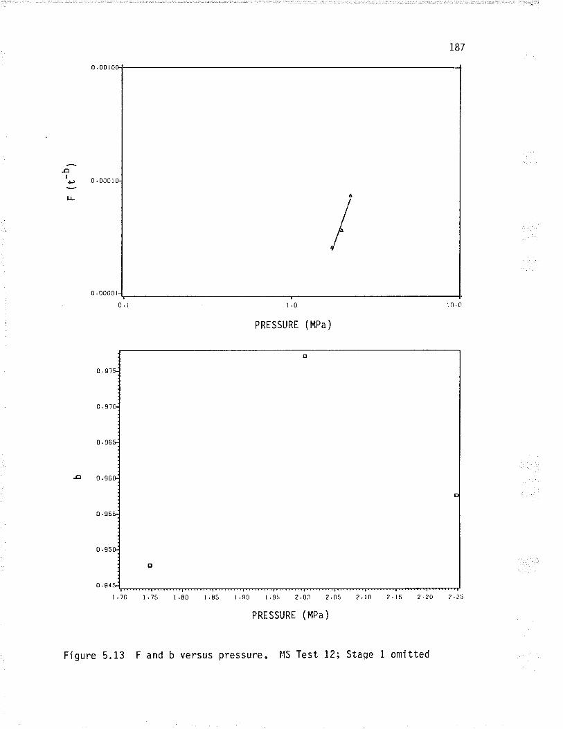
187

-o!+)

l¿

0 .001

0 .0000 r

PRESSURE (MPa)

I .90 I .95

PRESSURE

/

2.00 ?.05 2.to 2.r5 ?.20

(MPa)

Figure 5.13 F and b versus pressure, l.{S Test 12; Staqe 1 omitted

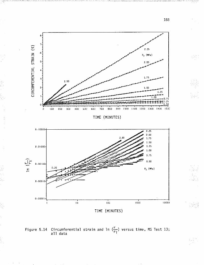
ba

z.

É.F-aJ1

J

FztJJÉ.lJJLJ(-)É(-)

2. 50

188

))<

P. (HPa )

2.00

0.750 .25

.50

600 700 800 900 r 000 r r 00 I 200 I 300 I 100 1500

TIME (MINUTES)

TrME (FTTNUTES)

t.-LIL

5. 14 Ci rcumferenti alal I data

strain and ln (fr) u.rtrt

? .25

2.OO

1.75

1.50

1.25

1.00

0. 75

0. 50

P. (llPa )

Fi gure time, FIS Test 13;

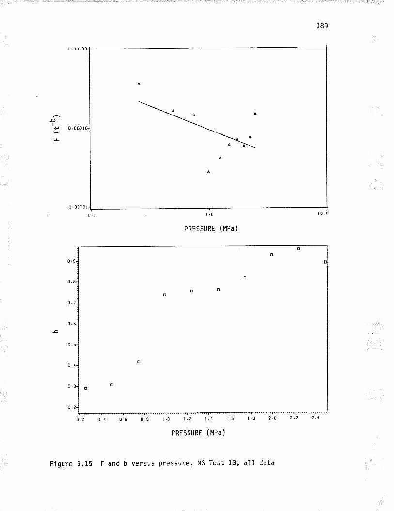
189

-oI+J

¡r

r0.0

PRESSURE (MPA)

1.0 1.2 1.4 1.6

PRESSURE (MPa)

Figure 5.15 F and b versus pressure, 1'lS Test 13; all data

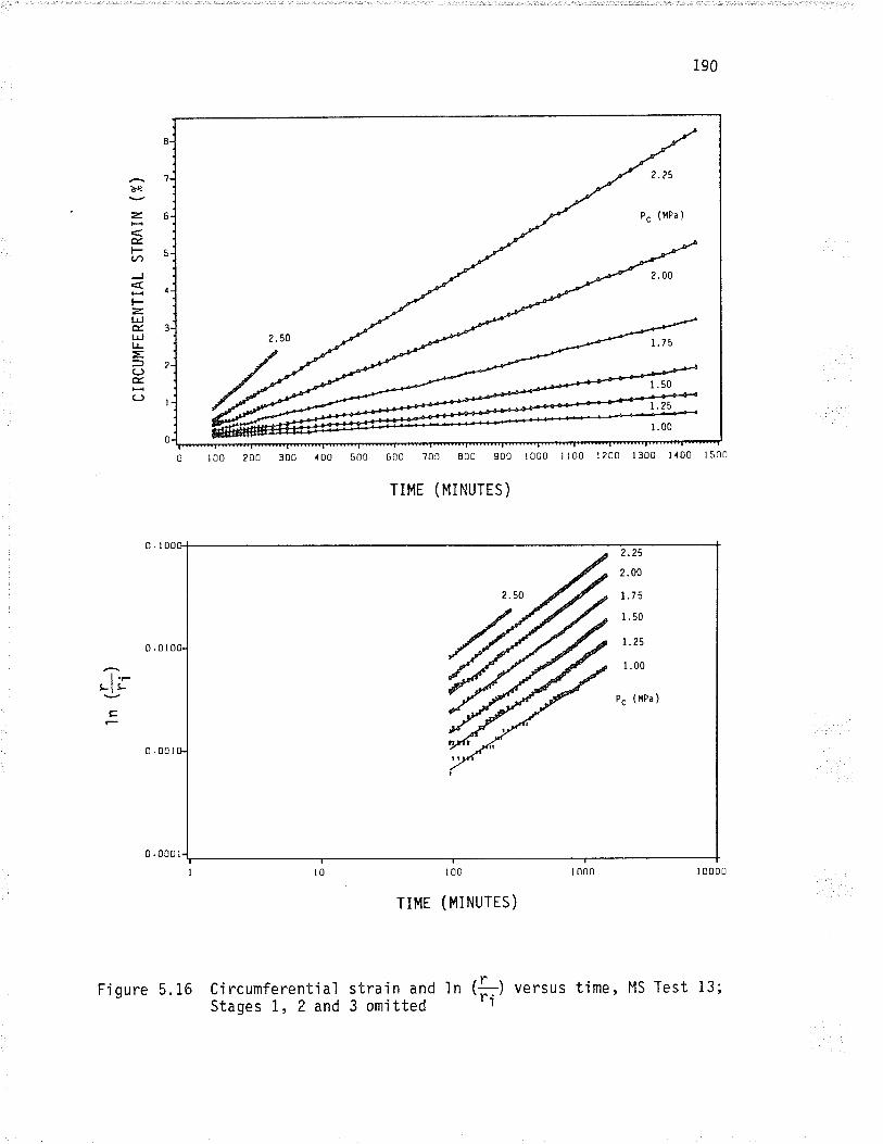
be

zH

ÉFU)

J

Fz.llJÉl!u-=J(JÉc)

i90

500 600 ?00 800 900 1000 ll00 1200 1300 1100 1500

TIHE (MINUTES)

{00

t.-LIL

E

0 .000 l

TIME (MINUTES)

I 0000r 000

Ci rcumferenti alStages L, 2 and

strain and ln3 omitted

(|) versus time,'ri '

P. (HPa )

2.

,á,

2.25

2.00

1.75

1.50

1.25

I .00

P. ( l{Pa )

Fìgure 5.16 MS Test 13;

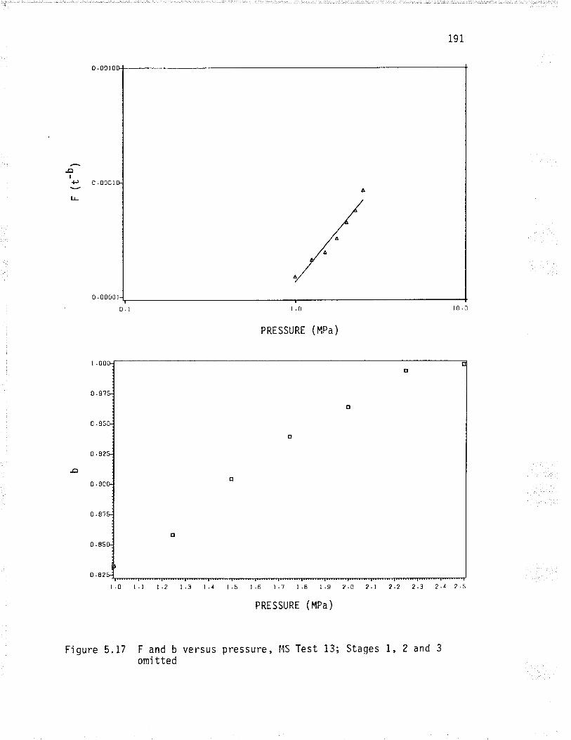
191

-oI+)

l¿-

0 .0000 r

PRESSURE (MPa)

r.6 r.7 r.8 1.9 2.O 2.1

PRESSURE (HPa)

?.3 2.1 2.5

Figure 5.17 F and b versus pressure, l4S Test 13; Stages 1,2 and 3

omi tted

2.?

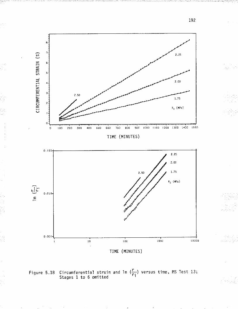
è.e

zÉt-U'J

t--zL¡Jæl+lL:EL)Éc)

t92

r00 200 300 100 500 600 ?00 800 900 1000 tl00 1200 1300 1100 ls00

TIME (MINUTES)

t.-LIL

ç

2.2s

2 .00

I.75

P. (llPa)

t 000

0 .001

TIME (MINUTES)

I 0000

(r ) versus'ri '5. 18 Ci rcumferenti al strai n and I nStageslto6omitted

Fi gure ti me , l4S Test 13;

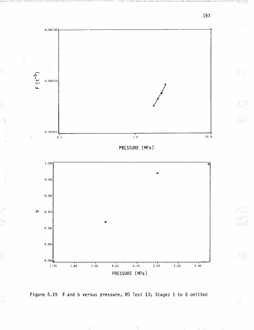
193

-oI+)

¡J-

0 .0000 I

PRESSURE (MPa)

0.

0 .91

t.?5 2.05 2.r5 2.25

PRESSURE lMNa)

/

Figure 5.19 F and b versus pressure,14S Test 13; Stages 1 to 6 omitted

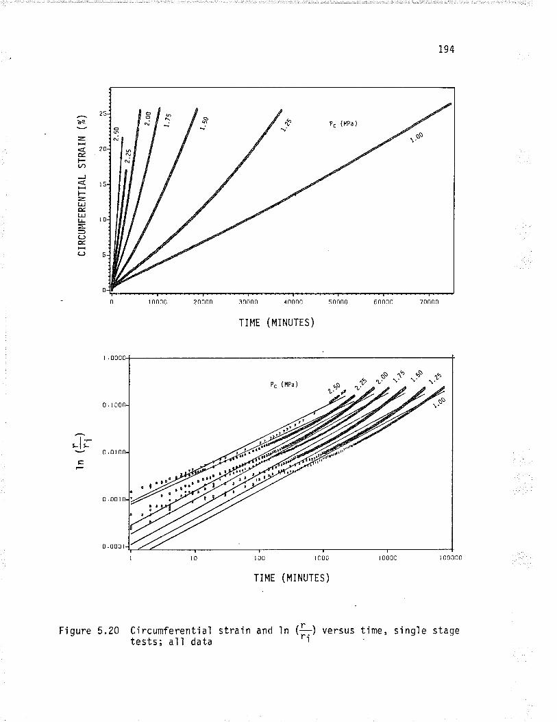
be

z.

Ét-t¡,J

F=LrJÉt-tJu-=J(-)É.HL)

20000

5.20 Circumferentialtests; all data

30000 4 0000

TIl-lE (MINUTES)

194

I 00000

time, single stage

50000

t.-¡'l ¡-

TIME (IitINUTES)

strain ancl tn (f;) versus'l

ooñ o

P. (HPa)a

NnO

N

Pç ( l{Pa )

" C'-Ðgl

¡l-

Fi gure

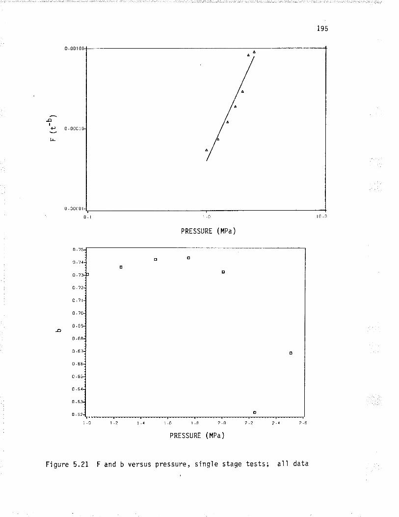
-oI+)

u-

0.00t

0 .0000 r

195

t0.01.0

PRESSURE (MPa )

0.

o.1

o.7

0.

0.?t

0.

0.6

0.6

0.6

0.

0.

0.6

0.6

0.6

1.6 r.8 ?.O

PRESSURE (MPa )

F and b versus pressure,Figure 5.21 si nql e stage tests; al I data

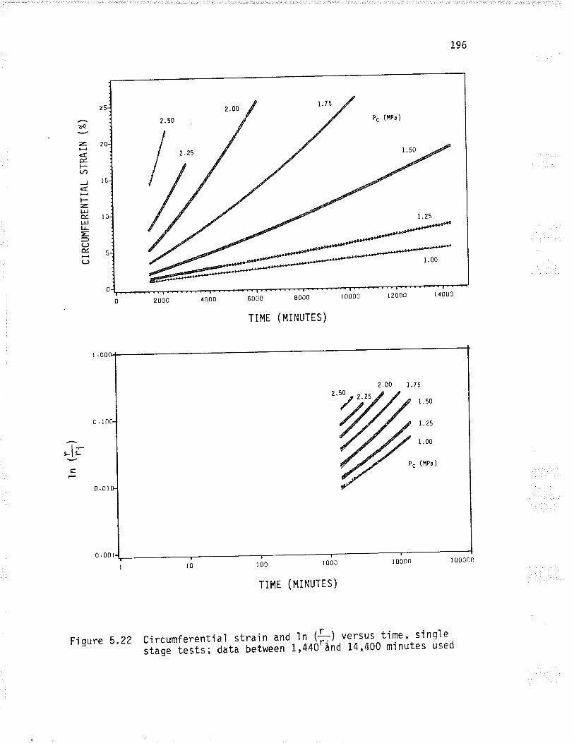
be

zÉt-a.r,

J

t-zt!Él!LtJ(-)ÉHrJ

196

P. (HPa )

f-;il-' ' '

4000 6000 8000 10000 12000 11000

TIME (MINUTES)

2.00 I .7 5

1.50

t.zs

I .00

P. (HPa)

l 000 l 0000 I 00000

TIME (MINUTES)

0.

l.-!l!

=0l0.

00r100

F.igure 5.22 Circumferential strajn and-ll.!å) ,versus t'ime, singlestuõ."tãtii; ãutã bàtween 1,440Iånd 14,400 minutes used

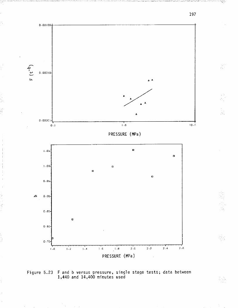
-oI{J

l-L

797

ÂA

0 .0000 I

5.23 F andI ,440

PRESSURE (HPa)

b versus pressure, sing'le stage tests; data betweenand 14,400 minutes used

JRE (l'lPa )

Fi gure

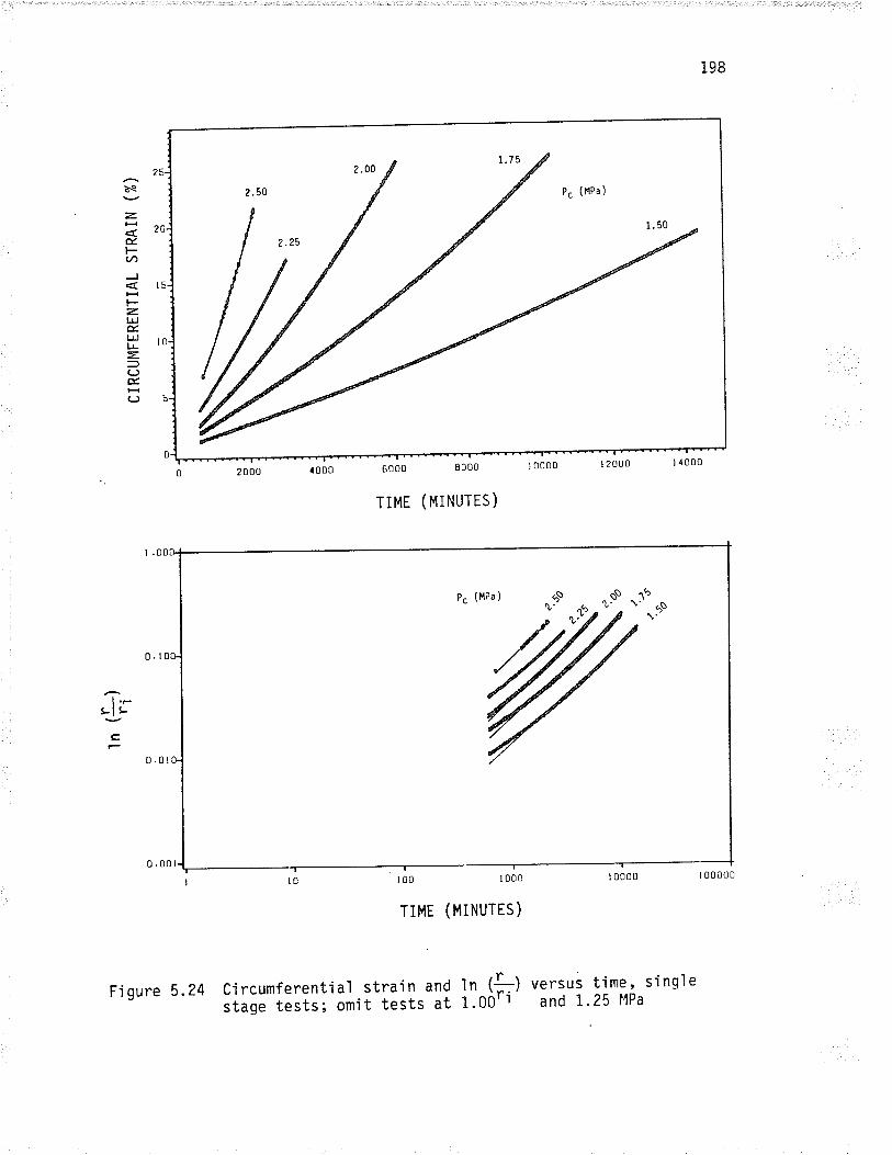
be

Ét--t/)JHt--zUJÉtrJI-LE)L)Éc)

198

P. (HPa )

20

I

I

0

l.-LIL

E

f-C;--';;å; soåo 8000 10000 12000 r{000

TIME (MINUTES)

Pc (HPa )

I 00 I 000 I 0000 I 00000

TIMT (MINUTES)

00t0.

Fi gure 5.24 Ci rcumferenti al stra'in and f n (!) versus time , si ngl e

staõã tãsts; omit tests at 1.00'1 and 1.25 l4Pa

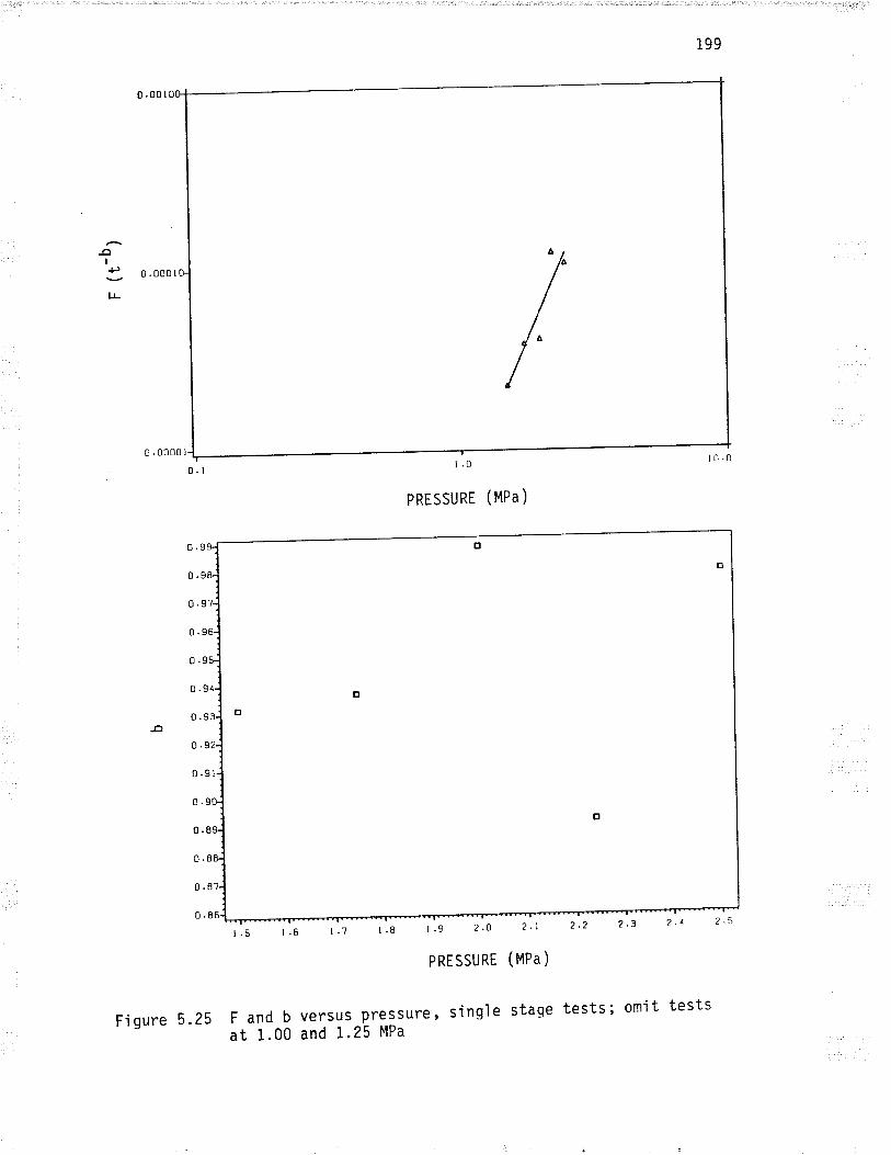
-oIP

l!

0 .000 I

0 .0000 I

199

I '0

pRESSURE (Mpa)

t.9 2.t 2.1

PRESSURE lNea)

versus pressure, s'in91e staqe tests; omjt tests

and 1.25 MPa

10.0

0.

0.9

o.

0.

0.9

0.9

0.9

0 .91

0.

0.

0.

0 .8?

0.8

F'i gure 5.25 F and b

at 1 .00

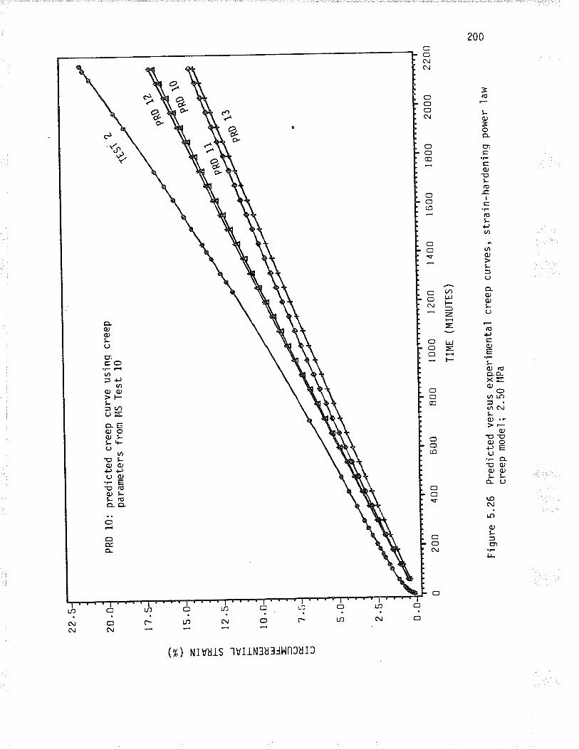
22.

20.

Èc z. ú t--

aJ1 J F. z L¡J

É.

LI u- = ¿ (J É H (J

t'l .

15.

t2.

10.

PR

D 1

0: p

redi

cted

cre

epP

aram

eter

s fr

om

7.5

curv

e us

inq

cree

pl4

S T

est

10

5 2 0

.0 .5 .0

200

Fig

ure

5.26

Pre

dict

ed v

ersu

s ex

perim

enta

l cre

ep c

urve

s'cr

eep

mod

el;

2.50

IlP

a

400

.L1t

5'

600

800

9Rs.

I 00

0 12

00

TIM

E (

MIN

UT

ES

)

1400

l 600

stra

j n-

hard

en'in

q P

ower

ì aw

I B

ÛO

2000

22tO

f\) a O

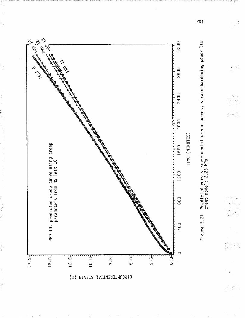
15.0

èe z H ú F l,r', J H l-- z. L¡J

É.

LlJ L = =q) É (-)

t2.

PR

D 1

0:

t0.

pred

i ct

edpa

ram

eter

scr

eep

curv

e us

lng

cree

pfr

orn

llS T

est

10

400

Fiq

ure

5.27

Pre

dict

ed v

ersu

s ex

perim

enta

l cr

eep

curv

es,

stra

in-h

arde

ning

pow

er 'la

w

cree

p m

odel

; 2.

25 l[

Pa

800

r 20

0 I 60

0 20

00

TIM

T (

MIN

UT

ES

)

2 40

028

0032

00

f\) ()

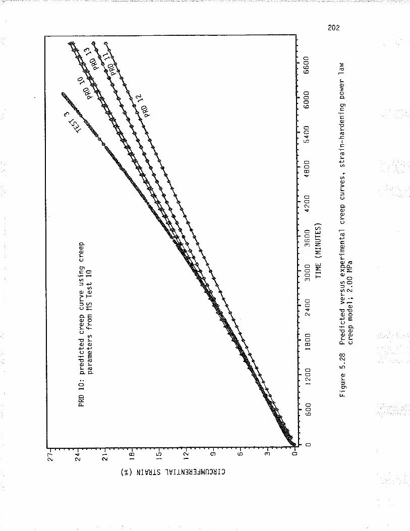
be z. É.

l-- t!1 J l-- z. UJ É lrJ lJ- = = L) É (-)

PR

D 1

0: p

redi

cted

cre

eppa

ram

eter

s fr

omcu

rve

usin

g cr

eep

llS T

est

10

600

I 20

0

*+:

Fig

ure

5.28

Pre

dict

ed v

ersu

s ex

perim

enta

l cr

eep

curv

es,

stra

in-h

arde

ning

pov

rer

1aw

cree

p m

odel

; 2.

00 l4

Pa

l 800

1R$

2400

1O

1s$

3000

36

00

4200

TIM

E (

MIN

UT

ES

)

lss

\j

$

1\

4 80

054

0060

0066

00

l\) O f\)

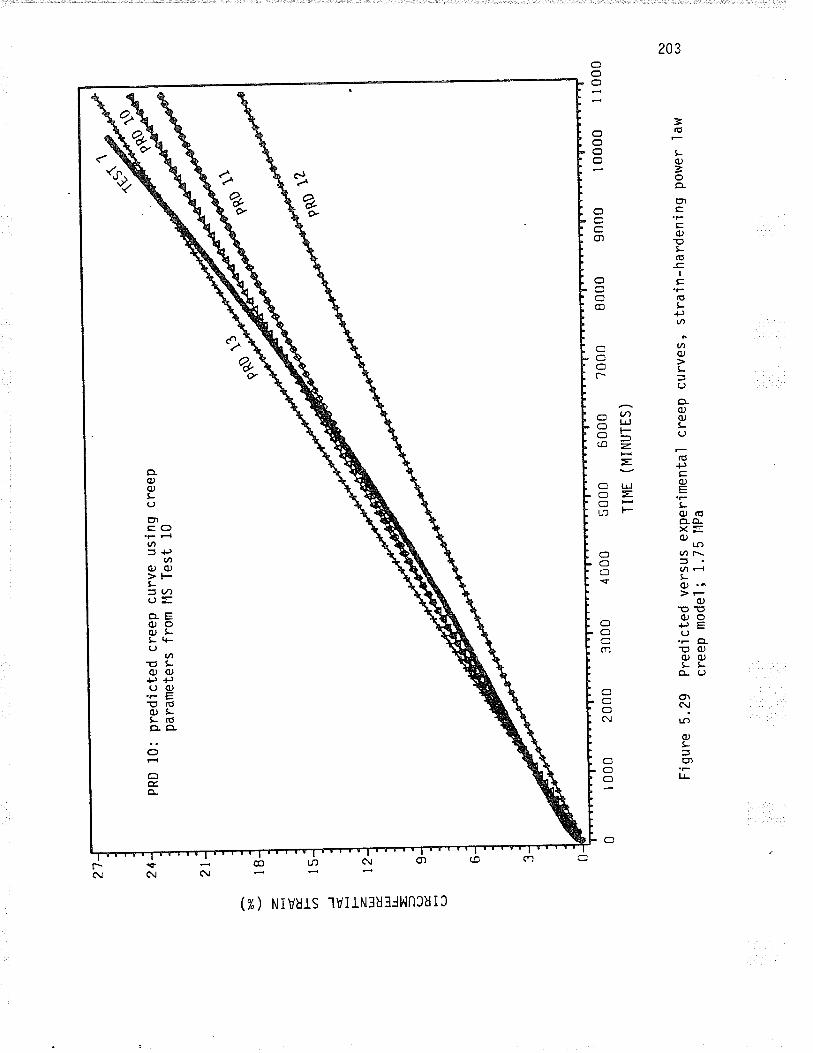
be z É t- U'' J F-- z UJ É l¡J lJ- = L) d. (J

PR

D 1

0: p

redi

cted

cre

ePpa

ram

eter

s fr

omcu

rve

usin

g cr

eep

l'lS

Tes

t 10

I 00

0

1$$

\j

2000

Fig

ure

5.29

Pre

djct

ed v

ersu

s ex

perim

enta

lcr

eep

mod

el ;

7-7

5 Î:î

Pa

"-;

3000

qq!

1S

lRs

4 00

0

\\

5000

60

00

TIM

E (

MIN

UT

ES

)

?RD

\?-

7 00

0

cree

p cu

rves

, st

rain

-har

deni

ng p

ower

1aw

8000

9000

l 000

011

000

N) o (¡)

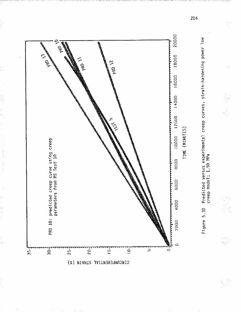
ùs z É. F tt1 J F- z. L¡J É tlJ lr E = c) É L)

25

PR

D 1

0: p

redi

cted

cre

ep c

urve

usi

ng c

reep

para

met

ers

from

llS

Tes

t 10

20

2000

40

00

6000

Fjq

ure

5.30

Pre

dict

ed v

ersu

s ex

perim

enta

l cr

eep

curv

es'

cree

p m

odel

; 1.

50 l4

Pa

B 0

00

TIM

E

I 00

00 I

200

0

( M

r N

UT

Es

)

I 40

00 I

600

0 I 80

00 2

0000

stra

in-h

arde

njnq

pow

er 1

aw

N) o Þ

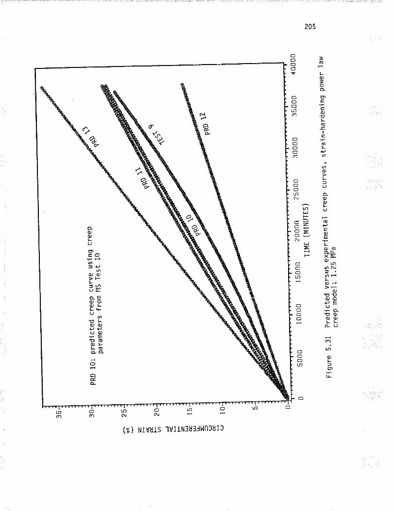
ùa d. l- Lt'l J F z. trl É IJ t-L = J (J æ.

(J

PR

D 1

0: P

redi

cted

cre

ePP

aram

eter

s fr

om

25 20

curv

e us

'ing

cree

pl.1

S T

est

10

5000

oooo

ç

F'iq

ure

5.31

Pre

dict

ed v

ersu

s-ex

perim

enta

l cr

eep

curv

es '

cree

p m

odel

; 1'

25

l4P

a

es$-

*

ïq$

1S

I 00

00

l.g 1ç,1

I 50

û0

2000

0 25

000

TIM

t (M

INU

TE

S)

n*o

tt

3000

0

stra

in-h

arde

ning

Pow

er la

w

3500

040

000

¡\)

O (tr

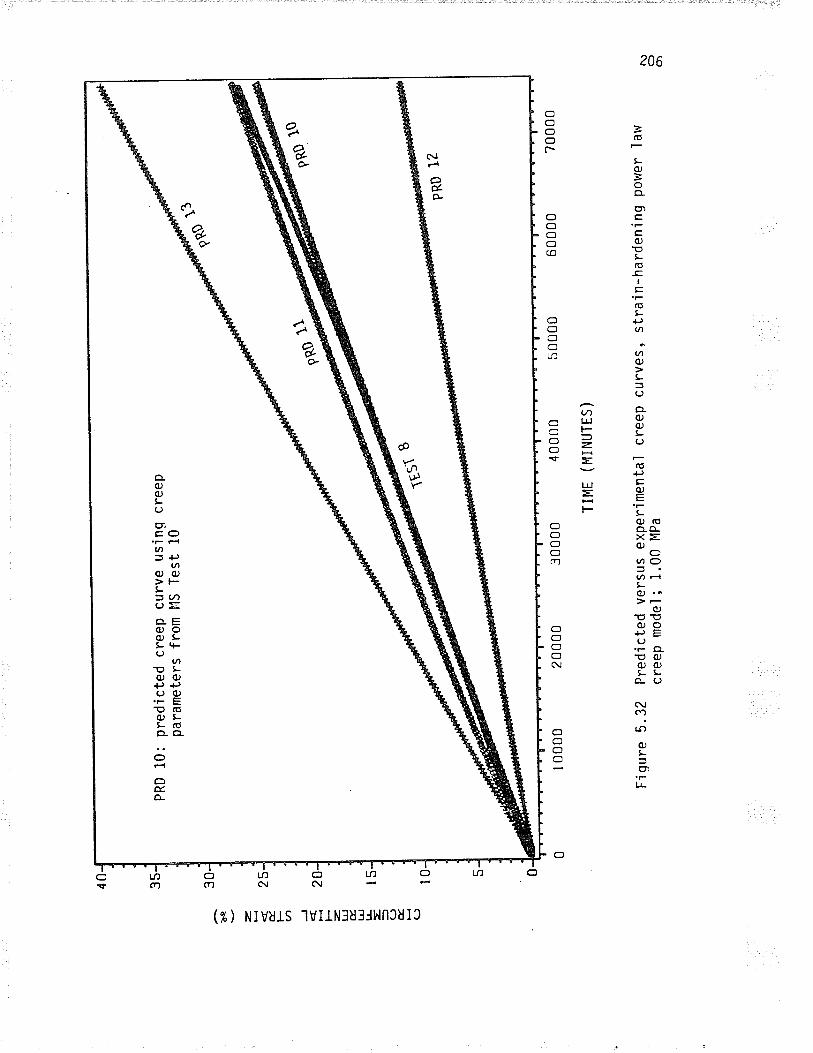
bs z æ F-

Lr1 J t-- z, UJ É.

LrJ u- =(.) É c)

PR

D 1

0: p

redi

cted

cre

ePpa

ram

eter

s fr

om

20

curv

e us

lng

cree

pItl

S T

est

10

I 00

00

Fig

ure

5.32

Pre

dict

ed v

ersu

s ex

perim

enta

l cr

eep

curv

es,

stra

in-h

arde

ning

pow

er la

wcr

eep

mod

el;

1.00

MP

a

2000

0

PR

S *

dn' r

iQ

$s'

3000

0 40

000

TIM

E (

MIN

UT

ES

)

5000

0

PR

D 1

2

6000

070

000

t\) O Oì

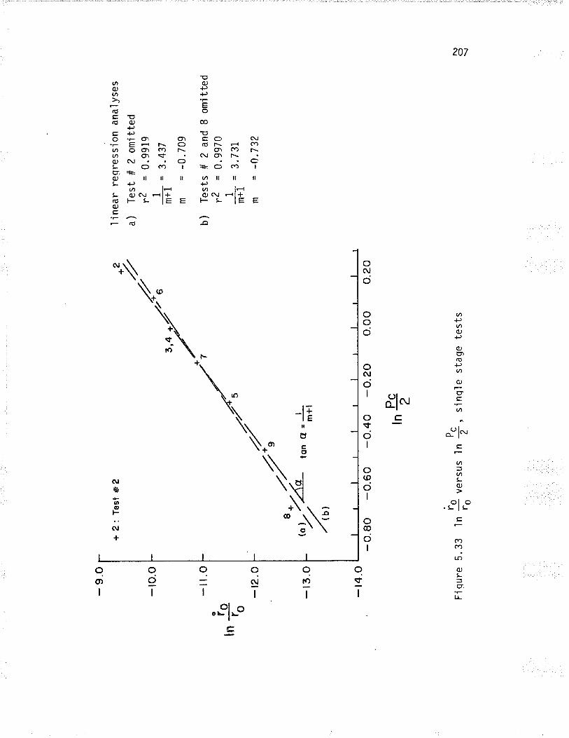
- 9.

O

-to.

o

-11.

oo

In# to

-12.

o

+ 2

: T

est *2

- r3

.o

,r/

,//u

z + I

-r4.

o

.2 z/ '/' 6

- o.

80 -

0.60

-o.

40 -

o.20

,nä

ton

C =

I m+

l

F'iq

ure

5.33

ln 3

ver

sus

ln 3

, sj

nsle

sta

ge te

sts

ro¿

I in

ear

regr

essi

on a

naly

ses

a) T

est#

2om

itted

rZ =

0.9

919

'l -l- =

3.4

37m

+l

m =

-0.

709

b) T

ests

#2an

dSom

itted

rZ =

0.9

970

1, =

3.7

3I

m+

r

m =

-0.7

32

o.oo

o.20

f\, a \

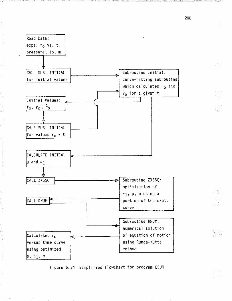
208

Read Data:

xpt. Fg vS. trressure, to, m

CALL SUB. INITIAL

for Ínitial values

Subroutine Initial:curve-fitting subroutine

which calculates rs and

ro for a g1 ven IIni ti al Val ues :

t6, l"9 r Fg

CALL SUB. INITIAL

for values i9 = Q

CALCULATE INITIAL

g and o1

Subrout'ine ZXSSQ:

optimization ofa1, [, m using a

portion of the expt.

curve

CALL ZXSSQ

CALL RNUM

Subrouti ne RNUI4:

numenical sol ut'ion

of equation of motion

us'inq Runge-Kutta

method

alculated rsversus time curve

using optimized

U, 01, m

Fiqure 5.34 Simplified flowchart for proqram QSUN

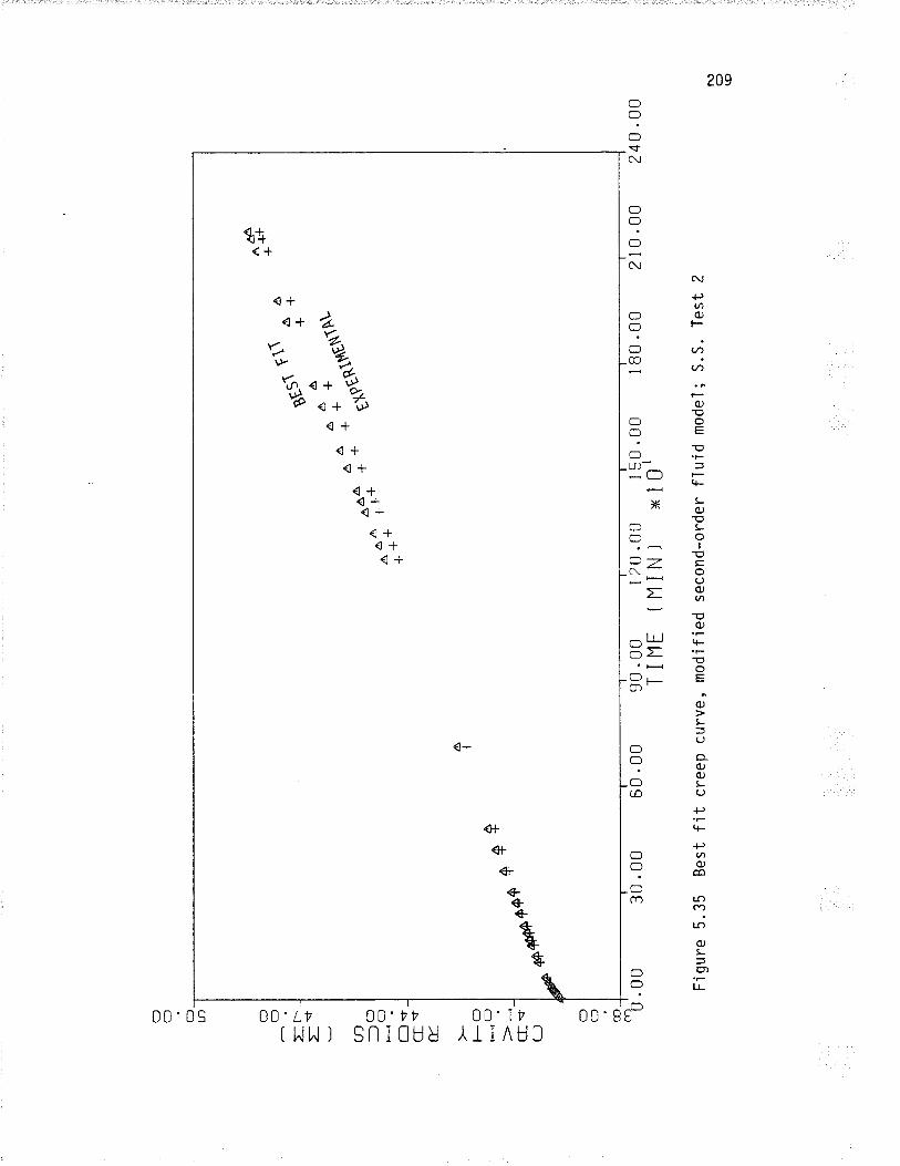
î#r1

1 a

ug$

t' f

+

Â

î î i

*oiu

r,nt

**

240.

00

l\) a (.o

îîî

+

210

.00

îîî

I 8U

.00

F.ig

ure

5.35

Bes

t fit

cr

eep

curv

e, m

odifj

ed s

econ

d-or

der flu

id m

odel

; S

.S.

Tes

t 2

150

.00

x10'

1 20

.00

n1 IN

i

(:l ? cl tn

/\ +

90 .0

ûT

I H

I

O O

Jr-

=*

^1¿

L+-|

-

a -C)

to f-ì

.<-

cf <

'E

.

F(]

HO ct <

"(-

J

60 .

00

4Þ4$

++

++ 30

.00

O ? co_

an0

.00

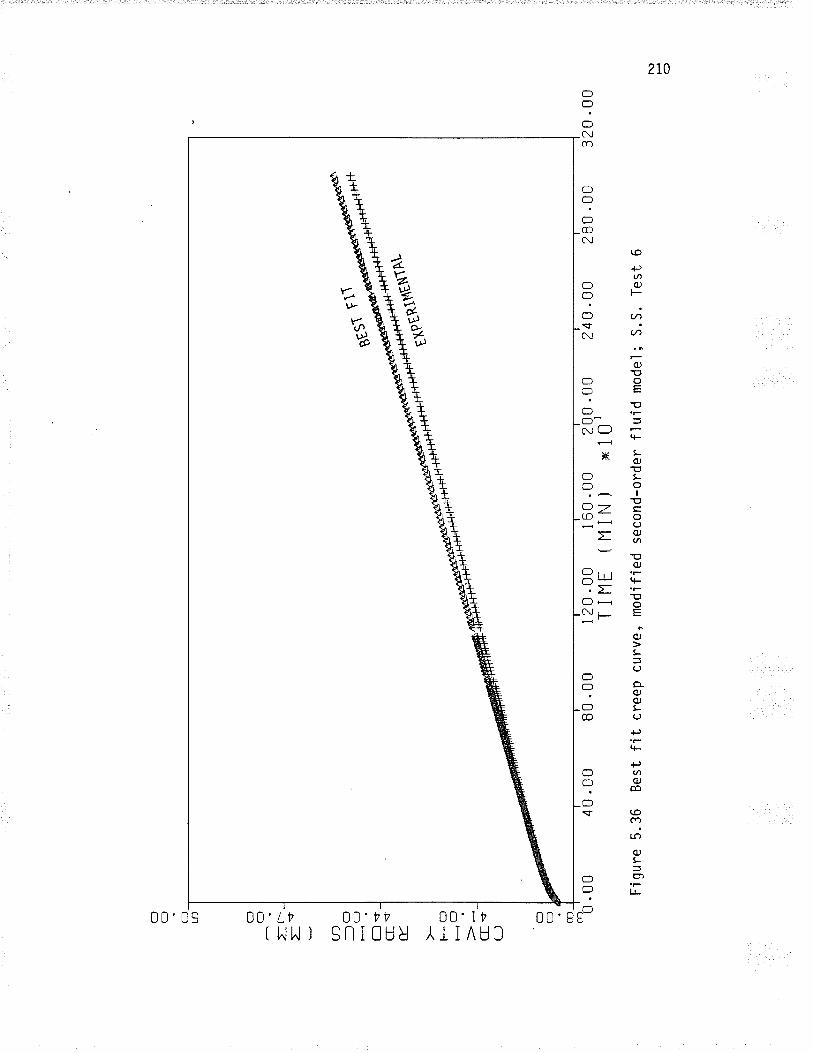
O ? O LN O O

rr-

TS a --l o

-O f-l s

CI'+

É_ l-- c

lH

O cr <

-(J

O C]

c0_

rrì '0

.00 Fìg

ure

5.36

Bes

t fit

cr

eep

curv

e, m

odjfi

ed s

econ

d-or

der flu

id m

odel

; S

.S.

Tes

t 6

40.0

0B

0 .0

012

0 .0

0 1 60

.00

20u

. rju

24

0 .0

û 28

0 .0

0T

IIlE

(11

lN)

xlO

l

*ç-s

ç]l

,Ë*t

*tot

320

.00

N) o

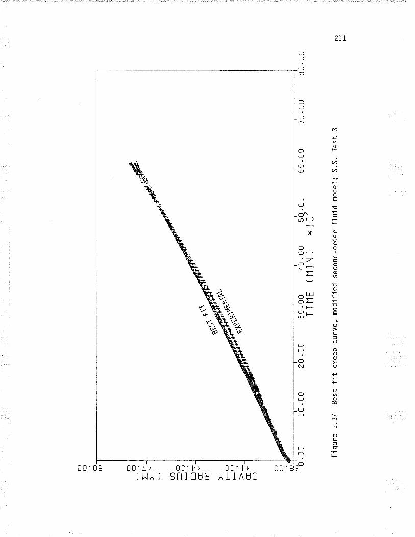
c) ? O tr) O C:]

Ir-

t=t

(t)

--l o

_O f-l

.<-

cf<

É.

l-- o

H

C:J

cf 'ú

(-J

O OI

co_

ar) 0

.00

,ffi

Fjq

ure

5.37

Bes

t fjt

cr

eep

curv

e, m

odifi

ed s

econ

d-or

der flu

'id m

odel

; S

.S.

Tes

t 3

10.0

0

#-d

20 .

003û

.00

T I

I1E

4U.0

0(t

l IN

)50

.0u

x 10

260

.00

70 .

0080

.00

N)

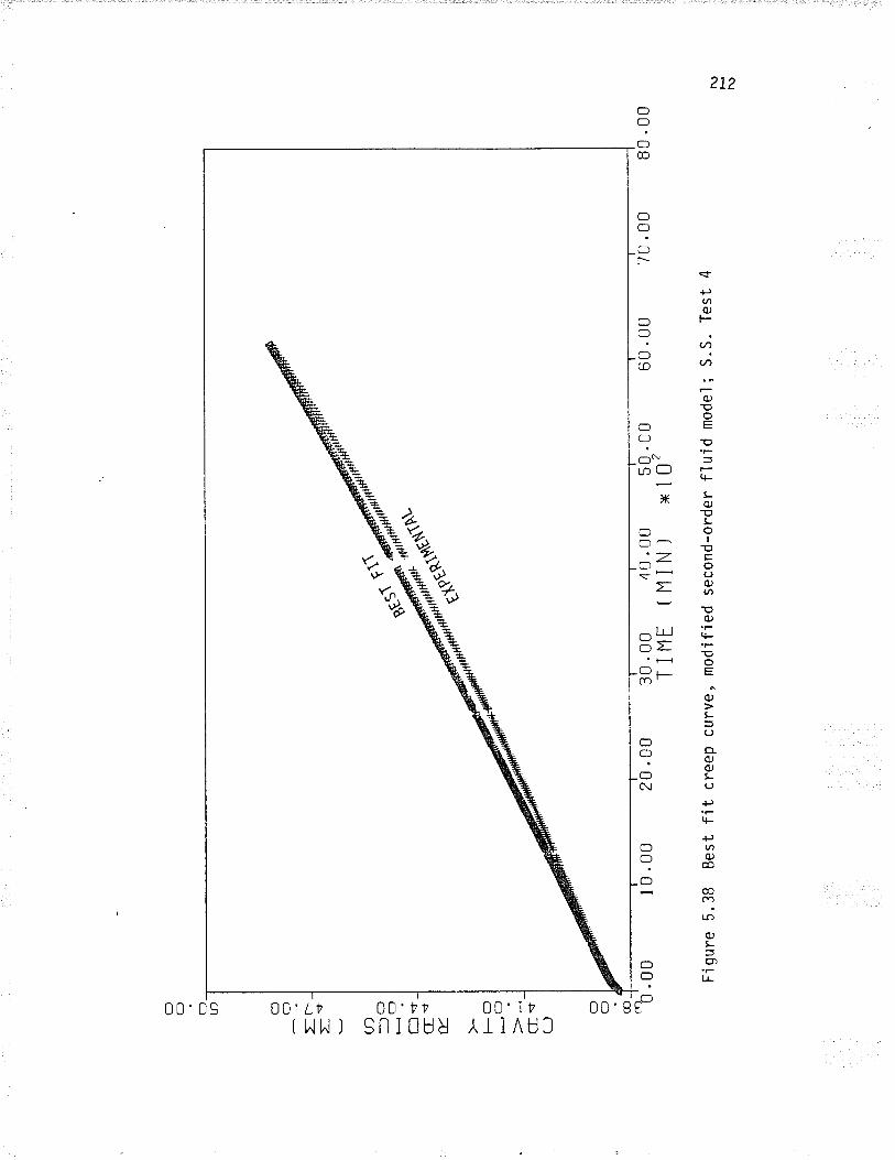
O ? O U) O C:]

=r-

=*

u-)

---ì

o-ç

¡f-

l v

C-+

v_ FO

HO cts

(-J

O O cD_

rn0

.00 F'ig

ure

5.38

Bes

t fit

cr

eep

curv

e, m

odjfi

ed s

econ

d-or

der flu

id m

odel

; S

.S.

Tes

t 4

10.0

020

.û0

30 .

00T

I H

E40

.0u

Î1 IN

I50

.0t1

x 10

260

.00

70 .

00B

0 .0

0

¡\)

l\)

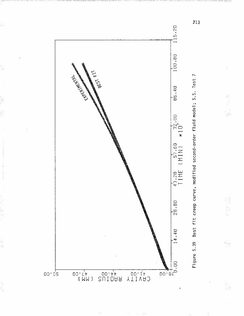
O ? (:l tn O cl

Er-

=*

U)

-- c

ltc

)

l--l s

Cs

É.

FO

HO Cf \t

(J

'(f ? CD -o

'. oo Fig

ure

5.39

Bes

t fit

cr

eep

curv

e, m

odifi

ed s

econ

d-or

der flu

id m

odel

; S

.S.

Tes

t 7

14.4

028

.80

,*-'s

43.2

0T

I I1

E

{-

c{st

st

57.6

0(l1

INI

1?.O

Ox

102

86.4

01 00

.80

1i5.

20

l\) H (,

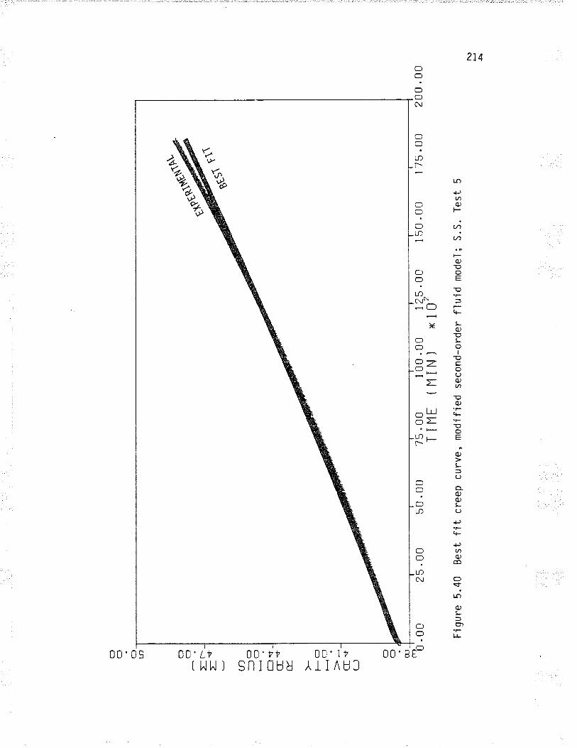
O ? O LD O (]E

r--

=*

(t) --lo

_O fl .q

(J s

t

É.

FO

-O cs (-J

C] ? æ rl.ll 0

.00 Fìg

ure

5.40

Bes

t fit

cr

eep

curv

e, m

odifi

ed s

econ

d-or

der flu

id m

odel

; S

.S.

Tes

t 5

25 .

0050

.00

75 .0

0T

i I1

EI 00

.00

I 25

.00

11 I

N )

x 10

'I 50

.00

I 75

.00

200

.00

f\) H Ã

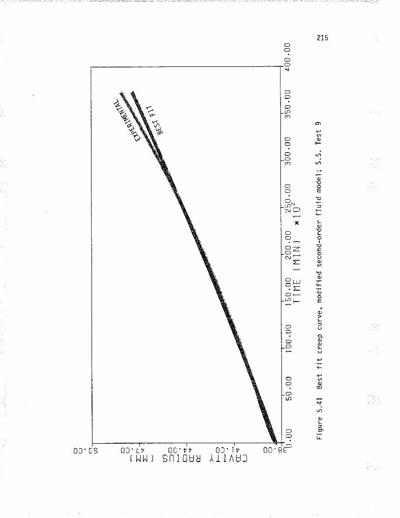
O ? O tf) O O

rr-

=*

(.t) --l c

l_O f-

t ç

C.ú

É.

l-- o

HO cfs

C-J

O C]

cr]

añ0

.00

Fìg

ure

5.41

Bes

t fjt

cr

eep

curv

e, m

odjfi

ed s

econ

d-or

der flu

jd m

odel

; S

.S.

Tes

t 9

50 .

00I 00

.00

*r'.N

1 50

.00

T I

IlE

4çf

stS

r

200.

0û

250.

00

300.

00

3s0.

00(

11 I

N )

x 10

'40

0.00

f\) H (tl

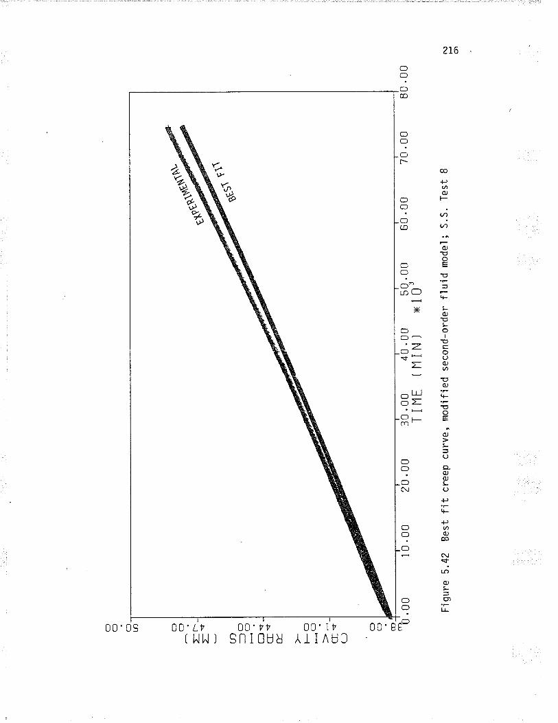
O ? C]

tn O O

Jr-

=*

(n -O -c)

Cl -

tG

$É

.

F-

Cl

>'+

cf .

r(-

J

O ? CD rrl 0

.00

F'ig

ure

5.42

Bes

t fit

cr

eep

curv

e, m

odifi

ed s

econ

d-or

der flu

id m

odel

; S

.S.

Tes

t I

10.0

020

.00

$,f-

q

30 .0

0 40

.0û

TIIl

E t

IlIN

]50

.00

x 10

360

.00

70 .

00B

0 .0

0

l\) Oì

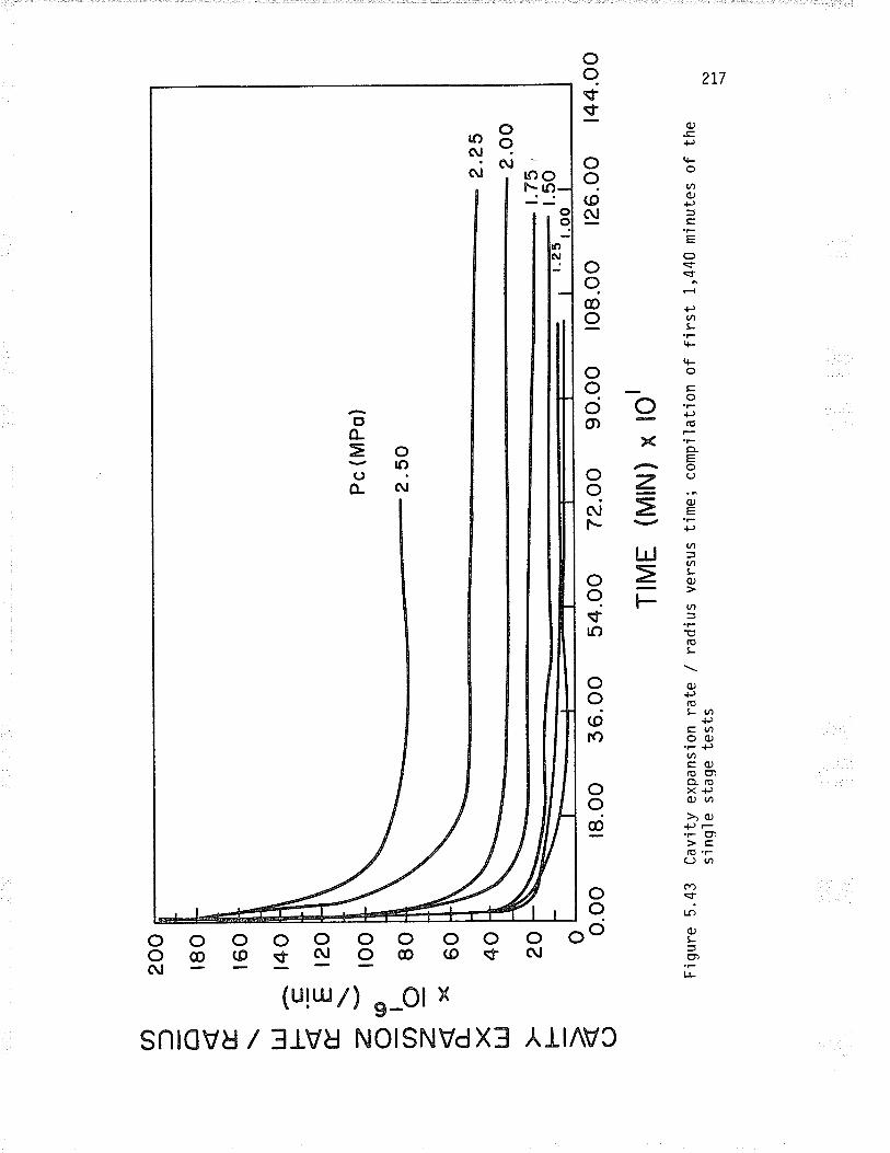
(n 3 õ fr lrj t- fr z. I Ø z. fL >< bJ L à ()

200

rBo

r60

t40

t20

roo

BO 60 40 20

o

.E E

(o I O =

o.oo

18

. oo

3

6. O

O

Fi g

ure

5.43

Cav

ity e

xpan

sion

rat

es'

ing1

e st

aqe

test

s

Pc

(MP

o)

2 .5

0

54.O

O 7

2.O

O 9

0.O

O lO

8.O

O

TIM

E (t

ul|N

) x

lol

/ ra

dius

ver

sus

time;

com

pila

tion

of fi

rst

1,44

0

2.?5

1.75

rr .5

0

2.O

O

t26.

OO

l44.

OO

min

utes

of

the

l\) P -_J

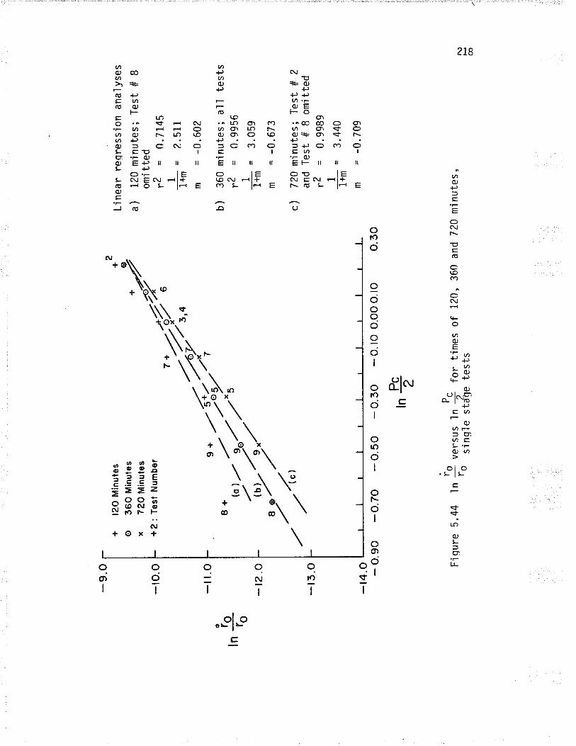
-9.O

-to.

o

,r*

+

l2O

Min

ules

+

'o

360

Min

ute "

*y'

x T

Í:lM

inut

es

y+

2: T

est N

umbe

r -4

tl'.¿

l 6

I

9-8+

)il?

'-il

.o

- r2

.o

o -,

o ,.-

t"

^/

l,-4:

/"r

/ ,/

/ -1

,-r

3.o

-r4.

o - o.

90-o

.70

- o.

50

roF

i our

e 5.

44 I

n -

'ro

Line

ar r

eqre

ssio

n an

alys

es

a) 1

20 m

inut

es;

Tes

t #

8om

i tte

drZ

= 0

.714

5'l ,l

- ?.

511

r+m m =

-0.

602

b) 3

60 m

inut

es; al

l tes

tsrZ

= 0

.995

6

- 1

= 3

.059

Irm m

= -

0.67

3

- o.

30 -

o. ro

o.o

o o.

ro

ln

vers

u s

si n

ql e

Pc ?

ln ?

for

tim

esst

fge

test

s

c)72

0an

d

Y2 1

lJm

m

o.30

of 1

20,

min

utes

; T

est

# 2

Tes

t #

I om

itted

= 0

.998

9

= 3

.440

= -

0.70

9

360

and

720

ninu

tes,

l\) F¡

c)c

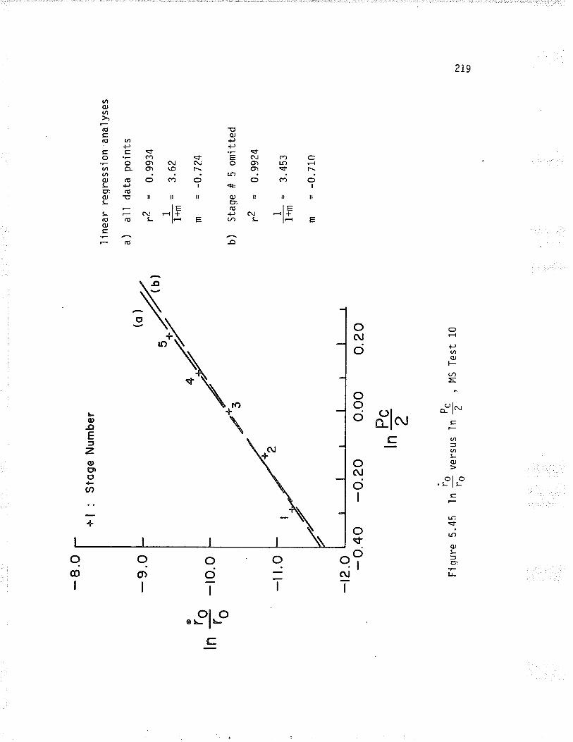
- B

.O

-9.O

ln

+l :

Sto

ge N

umbe

r

ÍO ro-t

o.o

-t t.

o

-r2

.o - o.

40 -

o.20

l'ine

ar r

eqre

ss'io

n an

aìys

es

a )

al I

data

poi

nts

rZ =

0.9

934

1 -i =

3.6

2r+

m m =

-0.

724

b) S

tase

#5om

itted

12 =

0.9

924

-1 =

3.4

53t+

m

m

= -

0.71

0

Fiq

ure

5.45

ln 3

ver

sus

ln å

qro

¿

o.oo

lnP

c 2

o.20

l'1S

Tes

t 10

l\) \o

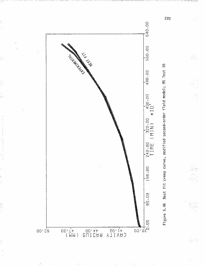
(:) ? O LN O O

=r-

=*

(t) --lo

-O f-'ì.

+cf

sÉ

. l--o

HO G$

LJ

cl ? CO -o

'. oo Fig

ure

5.46

Bes

t fit

cr

eep

curv

e, m

odifi

ed s

econ

d-or

der flu

'id m

odel

; l'1

S T

est

10

80.0

0I 60

.00

z40.

oo

320.

00

400.

00T

Illt

(tliN

l x1

0'48

0 .0

056

0 .0

064

0 .0

0

l\) f\) O

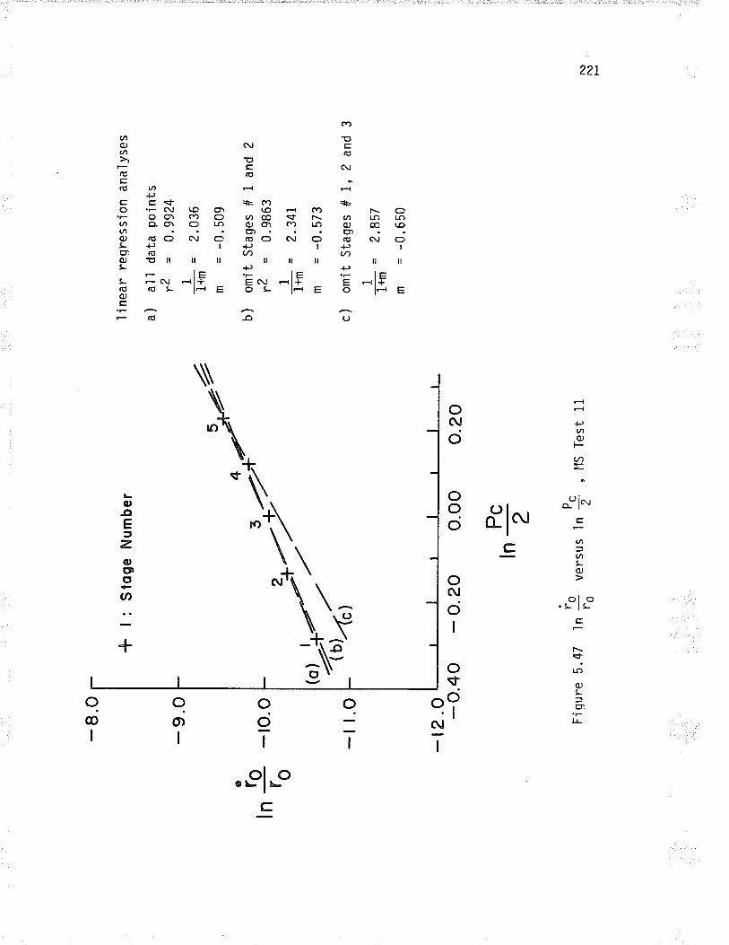
- B

.O

@

ln {q

-ro

. o

to

- 9.

O

,Ën

'4:d

7

S to

ge h

lum

ber

-t t.

o

-r2.

o - o.

40 -

o. 2

0 0.

oo

o.20

.pc

'n2

I in

ear

regr

essi

on a

naly

ses

a)

all

data

poi

nts

12 =

0.9

924

- 1

= 2

.036

r+m m =

-0.

509

U)

omit

Sta

ges

# 1

and

2

rZ =

0.9

863

1 ' i

= 2

.34I

l+m m =

-0.

573

c) o

mit

Sta

ges

# 1,

2 a

nd 3

1 ft =

2.8

57

m =

-0.

650

Fiq

ure

5.47

ln P

ve

rsus

ln k

, [

tS T

est

1tro

¿f\) f\)

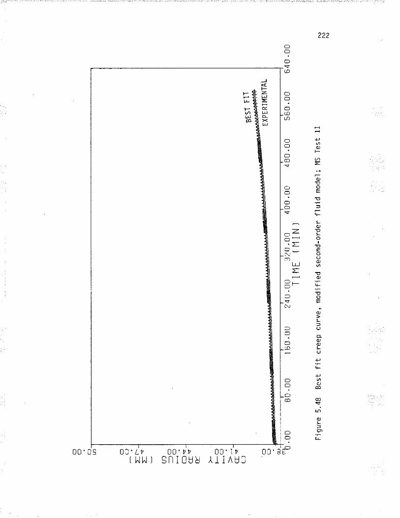
O ? O Lr)

C]

O

Er-

a -lo -cl

O'+

CJS

E-

l-- o

HO (rtÛ

(J

O ? @_

rrì o

.00 Fig

ure

5.48

Bes

t fit

cr

eep

curv

e, m

odifj

ed s

econ

d-or

der flu

id m

odel

; M

S T

est

11

B0

.00

I 60

.00

240

.00

320

.00

400

.00

T I tlt

nl l

N )

480.

00

BE

ST

FlT

EX

PE

RIM

EN

TA

L

560

.00

640.

00

f\) N)

t\)

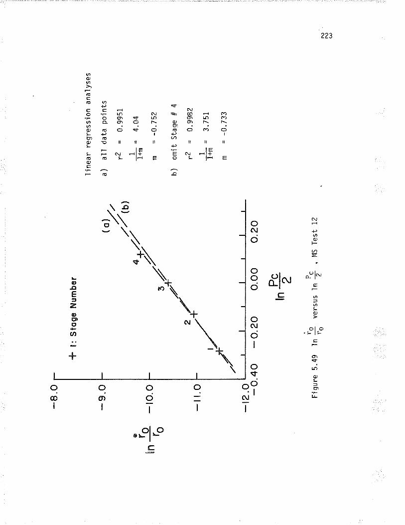
-8.O

-9.O

@ ro roIn

+

-ro.

o

Sto

ge N

umbe

r

-il.o

-r2.

o - o.

40 -

o.2

0

ln

Fiq

ure

5.49

ln P

ve

rsus

ro

I in

ear

regr

essi

on a

naly

ses

a) a

ll da

ta p

oint

s

r? =

0.9

951

1 =l-

- 4.

04l+

m m =

-0.

752

b) o

mit

Sta

ge #

4

rZ =

0.9

982

1 =i

= 3

.751

Irm m

= -

0.73

3

o.oo Pc 2 D

tnä

o.20

,1r1

S T

est

12N

)f\) (^

)

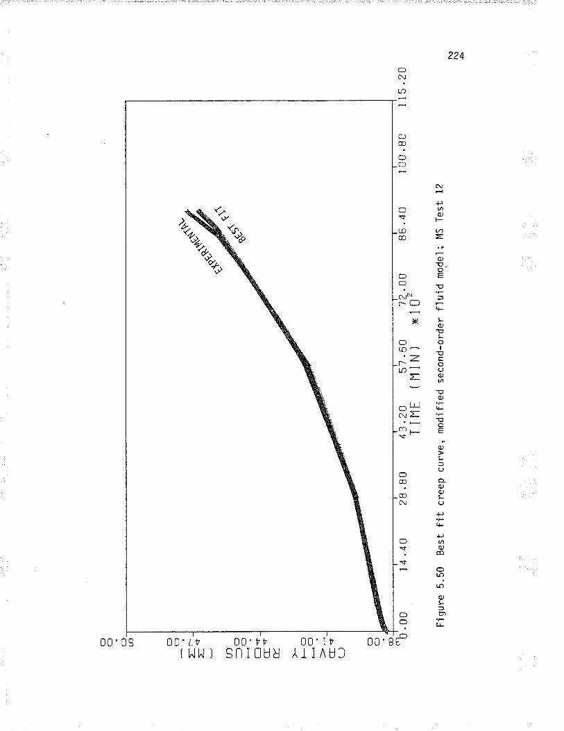
cl ? O a cf (]

=r-

-- -í

-

a ---t

(:l

_(]

f--ì

-+

al- s

É.

l--- o -

>*

cts

(-J

O C]

@_

arì '0

.00

Fig

ure

5.50

Bes

t fit

cr

eep

curv

e, m

odifj

ed s

econ

d-or

der flu

id m

odel

; M

S T

est

12

l4 .4

02B

.80

M

43.2

0 57

.60

T I

I1E

( 11

I N

]12

.OO

x 10

286

.40

I 00

.80

1 15

.20

fu l\) À

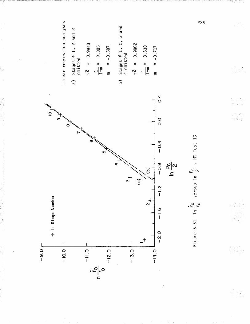
, -l

l.o

ln iq to

-t2.

o

*l:S

toge

Num

ber

-?.o

Fjq

ure

5.51

ln P

ve

rsus

ln 3

, M

S T

est

13F

6¿

-1.2

Line

ar r

egre

ssio

n an

a'ly

ses

a) S

tage

s #

I" 2

and

3om

i tte

d

rZ =

0.9

940

- I

= 3

.305

r+m m =

-0.

697

,nä

o.o

b) S

taqe

s #

L" 2

, 3

and

4 om

itted

rZ =

0.9

982

-1 =

3.5

30r+

m

m

= -0

.717

o.4

l\) N)

(n

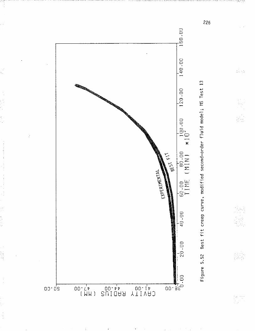
O ? O tf) Cf

O

rr-'

=* a -lo -o l--l -

tC

I <

t

É_

È-

c)

-o cts

(-J

cf ? OJ

rn0

.00

F'ig

ure

5.52

Bes

t fit

cr

eep

curv

e, m

odifi

ed s

econ

d-or

der flu

jd m

odel

; llS

Tes

t 13

2U .0

040

.00

60 .

00T

I I1

E80

.00

(HiN

]1 00

.00

x 10

tI 20

.00

140.

00I 60

.00

f\) ^)O)

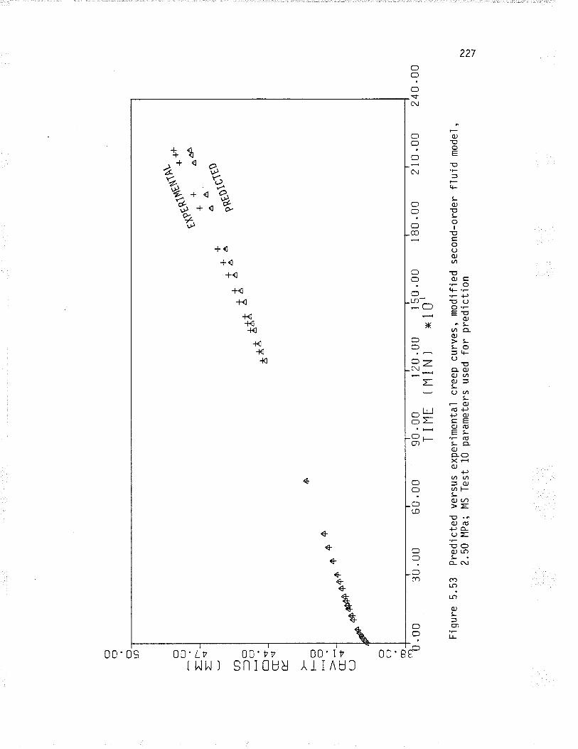
O ? O LN O O

Ir--

I.f U)

-OtÇ) l-1

.*cr

$É

.

FO c-

-)

>-

cf$

(-J

a¡4$

++

++

O ? co_

rrì 0

444

.00

Fìq

ure

5.53

Pre

dict

ed v

ersu

s ex

perim

enta

l cre

ep c

urve

s, m

odifi

ed2.

50 l4

Pa;

1'1S

Tes

t 10

par

amet

ers

used

for

pred

'ictio

n

ê

30 .

00

^À åå

f

60 .

00

+.*

a,+

Ä

aÃ

a

,*"-

tlts*

:i+

A'

þtot

o

90.

TI

00 11E

I 20

.00

11 IN

I xl

1l 00

.00

I B

0 .0

0

seco

nd-o

rder

flui

d m

odel

210.

0024

0 .0

0

N)

t\) !

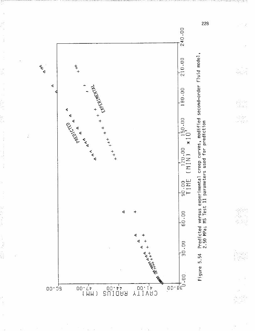
O ? O LD O O

tt- =*

U) -lo -cl

f-ls cts

É. l--o

HC

]

ct \

rL)

s#îîî

O ? CD

ÂA

Î.+

rrì 0

.00

30 .0

0 60

.00

QsÊ

$qt$

^

^^^

aÂ

F.ig

ure

5.54

Pre

dict

ed v

ersu

s ex

perim

enta

l cre

ep c

urve

s, m

odifi

ed s

econ

d-or

der flu

jd m

odel

,-

2.50

MP

a; l

"lS T

est

11 p

aram

eter

s us

ed fo

r pr

ed'ic

tjon

A**

+*

t*t

Lt

++

'

¿ê

A

-++

r -*

r1È

L

ÉJ'

lÉS

ltttv

'''

90 .0

0 I 20

.00

I 5.

0 .0

0itr

r (H

iN)

xto'

++

+

1 80

.00

21 0

.00

240.

00

f\) l\) æ

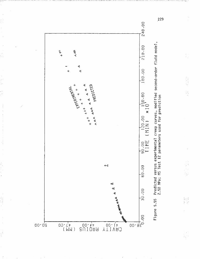
O ? O a C] O

Ir-

=*

U) --ro

-o l-l -

tC

sfu_ È

-oH

O af$

(J4S

4¡+

+åa

a

O ? O-

"b

*ÅÅ

.00

30 .

00

F'ig

ure

5. 5

5 P

redí

cte

d2.

50

l4P

a ;

+ ô

'*o*

t'n:Y

t.+

+r+

++

^^^

**'

Â Â

l^^

^^^

pRÉ

Dlg

lED

60.0

0

vers

us e

xper

imen

tal

cree

p cu

rves

, mod

ified

l'lS

Tes

t 12

par

amet

ers

used

for

pred

ictio

n

90 .0

0 l 2

0 .0

0 I 50

.00

TIIl

E (

11lN

l x1

0r

++

+

a4

^Á

180.

00

210.

00

seco

nd-o

rder

fluj

d m

odel

,

z40.

oo

l\) l\) \o

O ? O a O (]rr

-IS <n --l o

-"O

l--l -

tC

ISE

. l- c)

HO Gs

(J*d

***

C] ? co_ -o

++

+

.00 Fìg

ure

5.56

Pre

dict

ed v

ersu

s ex

perim

enta

l cr

eep

curv

es, m

odifi

ed s

econ

d-or

der flu

id m

odel

2.50

MP

a; M

S T

est

13 p

aram

eter

s us

ed fo

r pr

edìc

tion

+

30.0

060

.00

¿a

ÁÂ

Å

,*"*

t*tl;

À å

sord

Éo

90 .

00T

I I1

EI

2U .0

0 1 50

.00

11 IN

I xl

O'

I 80

.00

2i0.

0024

0 .0

0 1\)

(¡)

O

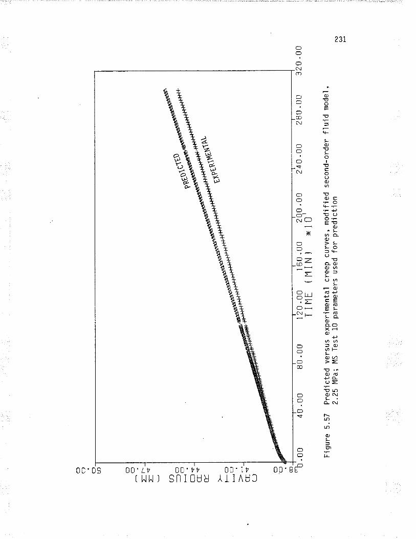
cf ? O U]

O O

tr-

=*

a ---lo

- çt

Os

ct <

"

E.

FO

HO Þ*

cf .û

(J

O ? @

.00 Fig

ure

5.57

Pre

dict

ed v

ersu

s ex

perim

enta

l cr

eep

curv

es,

mod

ifjed

sec

ond-

orde

r flu

id m

odeJ

,2.

25 lf

iPa;

MS

Tes

t 10

par

amet

ers

used

for

pred

ictjo

n

40.0

080

.00

I 20

.00

1 60

.00

TIIl

E (

IlIN

]

PR

ÉS

}*}

,Ë*t

*tot

200

x10r

.00

240.

00

280.

00

320.

00

1\) (,

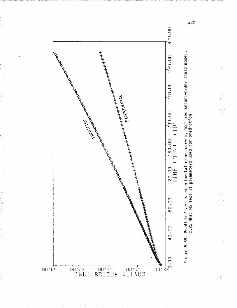
C:] ? C)

LN (:) O

=r-

=s

U)

-- c

l-o l-l

sC

tE

. l--o

H(] cfs

(J

O cf cD_

-o.0

0

Fig

ure

5.58

Pre

dict

ed v

ersu

s ex

perì

men

tal

cree

p cu

rves

, mod

'ifie

d2.

25 l(

Pa;

MS

Tes

t 11

par

amet

ers

used

for

pred

ictio

n

40.0

0

-ç$

est$

:d

80 .

0020

.00

I I

I1E

t.Ë**

t*

60.0

0IN

]20

0x1

0'.0

0 24

0 .0

0

seco

nd-o

rder

flui

d m

odel

"

280

.00

320

.0u

f\) (, N)

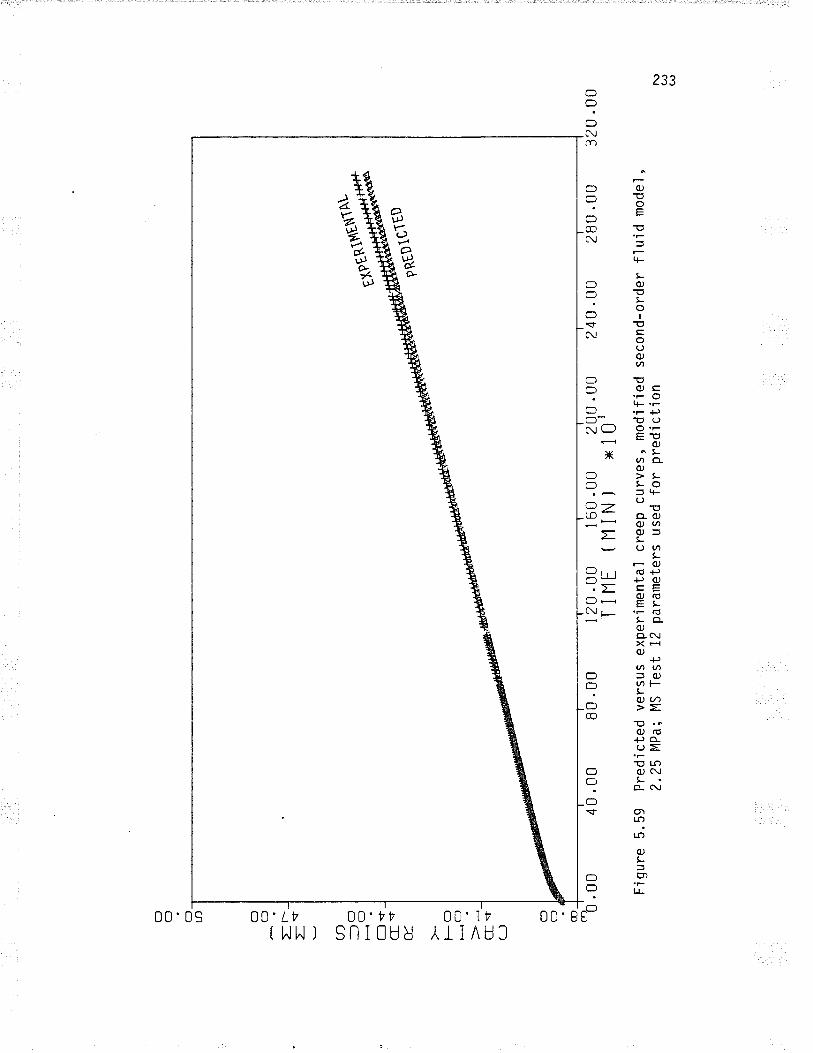
cl ? O LC)

C]

(f

rr-

I$ r_n -

c:l

to r-l$

Cs

É_ FO

H c

:)

CI9

LJ

cf ? @ rr) 0

.00

40 .0

0 80

.00

Fì gu

re 5

.59

Pre

di c

ted

vers

us2.

?5 l4

Pa;

l4S

Tes

t

I 20

.00

I 60

.00

z0û

.00

TIIl

E (

11lN

) x1

0'ex

perim

enta

ì cr

eep

curv

es, m

odifi

ed12

par

amet

ers

used

for

pred

ictio

n

ErP

ÉR

lI:)I

[;

ñtot

ttto

240

.00

280

.00

seco

nd-o

rder

flui

d m

odel

,

320

.00

l'\)

(¡)

(¡)

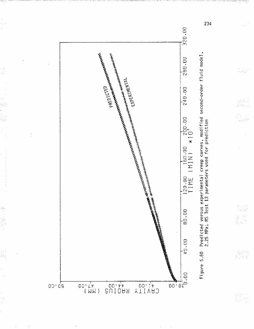
O ? (:l to O O

tr-

=*

a -- c:

f-ç

)f-

l st

cf s

t

É.

FO

HC

]

crs

L)

(f ? CD -o

'. oo Fìg

ure

5.60

Pre

dict

ed v

ersu

s ex

perim

enta

l cre

ep c

urve

s, m

odjfi

ed2.

25 l{

Pa;

MS

Tes

t 13

par

amet

ers

used

for

pred

ictio

n

40.0

080

.00

1 20

.00

I 60

.00

T I

NE

I 11

I N

)

PR

É01

*

,Ë**

*

200

xi0'

.00

240.

00

seco

nd-o

rder

flui

d m

odel

,

280

.00

320

.00

l\) (^, Þ

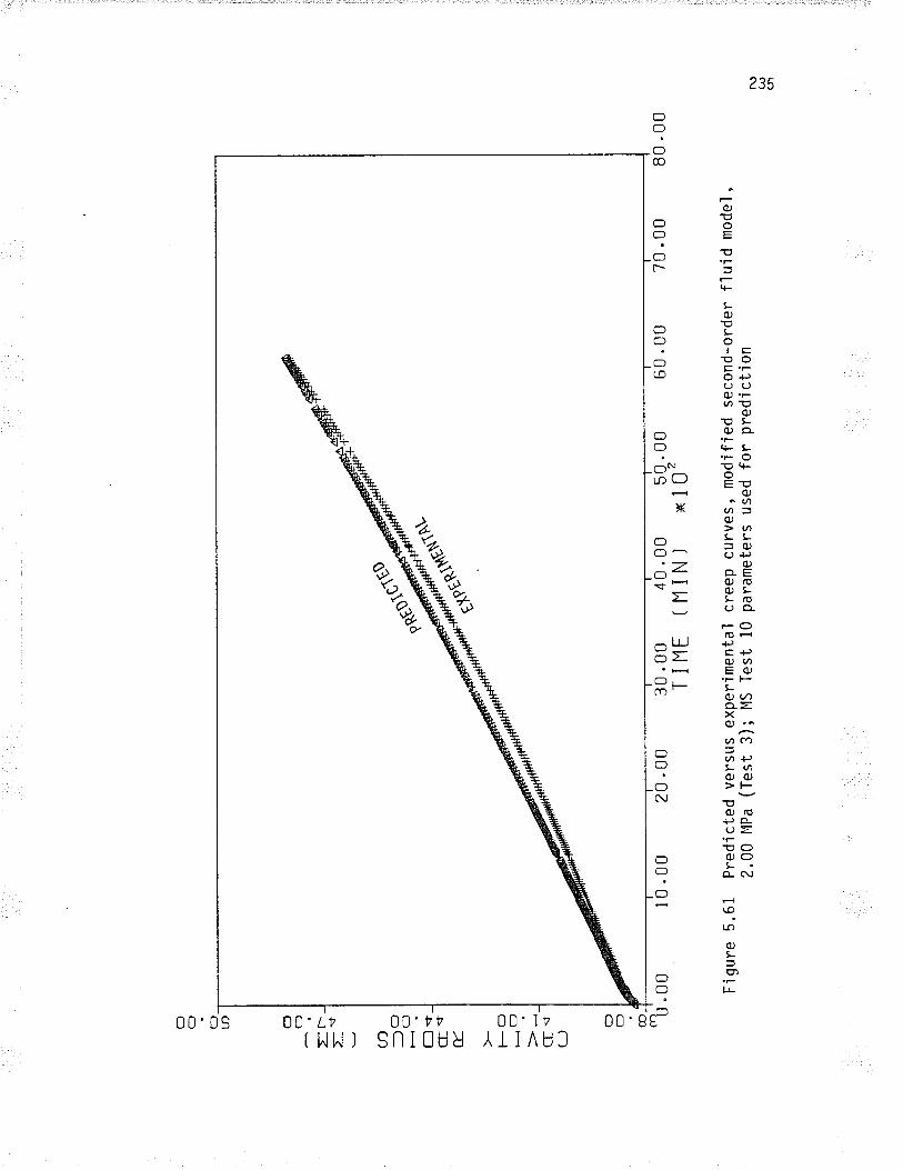
O ? O TJ) O O

ur-

I.+ (t)

-'--ì

c:)

-c)

Cl'+

CI

<+

É_ l--o

Hcl

CI-

$(J

cl ? co -o'.

oo Fig

ure

5.61

Pre

dict

ed v

ersu

s ex

perim

enta

l cr

eep

curv

es, m

odifi

ed s

econ

d-or

der flu

id m

odel

,2.

00 Ì'

lPa

(Tes

t 3)

; ta

S T

est l0

par

amet

ers

used

for

pred

ictjo

n

W

l0 .0

0

d-d

20.0

030

.00

T I

I1E

40.0

0$1

IN)

50 .

00t 0'

60.0

û10

.00

80.0

0

f\) (, c.¡r

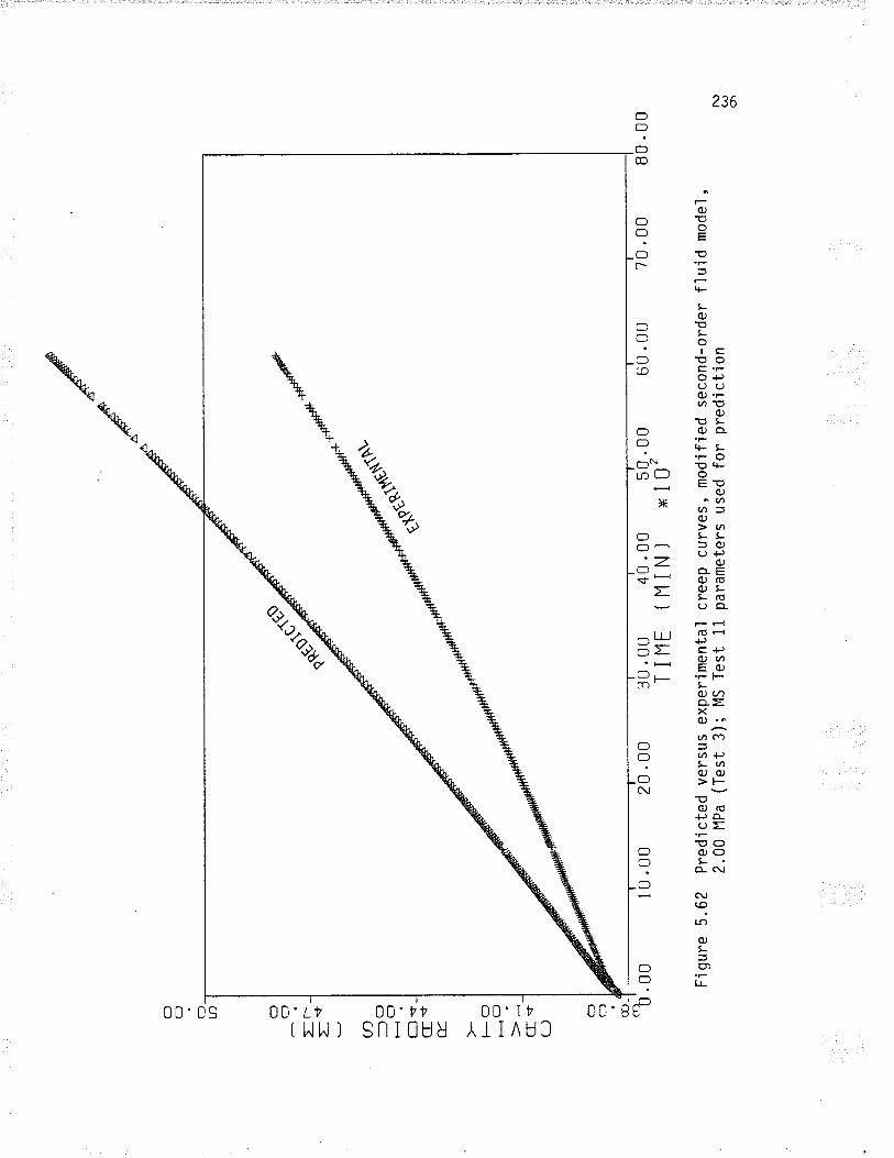
O ? C]

Lfl cl O

Jr-

t.f U)

--t o

-O -.q rild.

É_ FC

IH

O cf -

r(-

J

O ? c0

.00

Fig

ure

5.62

Pre

dict

ed v

ersu

s ex

perim

enta

l cr

eep

curv

es, m

odifi

ed s

econ

d-or

der flu

id m

odel

,2.

00 l*

lPa

(Tes

t 3)

; la

S T

est

11 p

aram

eter

s us

ed fo

r pr

edìc

tion

l0 .0

0

ø-$

s"g\

qt'

*ddo

*-s

20 .

0030

.00

T I

I1E

40.0

0(N

IN]

50 .

0010

'60

.00

10.0

0.0

0

N)

G,

Oì

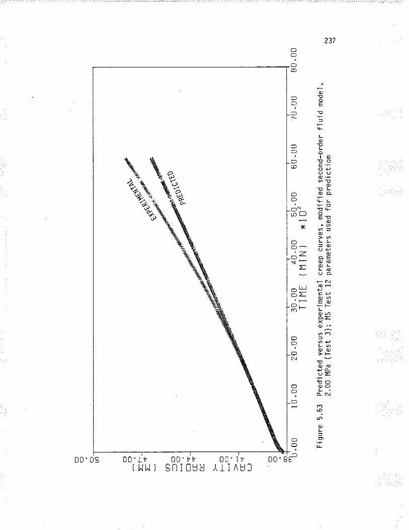
Cf ? O tn O O

rt-

L U)

--ro

-c)

f-l .

qcf

sÉ

_ FO r-

--ì

>"{

Ct'r

t(J .O

? CD

.00 Fìg

ure

5.63

Pre

djct

ed v

ersu

s ex

perim

enta

l cr

eep

curv

es,

mod

ified

sec

ond-

orde

r flu

id m

odel

,2.

00 M

Pa

(Tes

t 3)

; t.t

S T

est

12 p

aram

eter

s us

ed fo

r pr

edíc

tion

10.0

0

#-$Ë

20 .

0030

.00

T I

I1E

40.0

0î1

IN

I50

.00

10'

60 .

0070

.00

80.0

0

t\) (, {

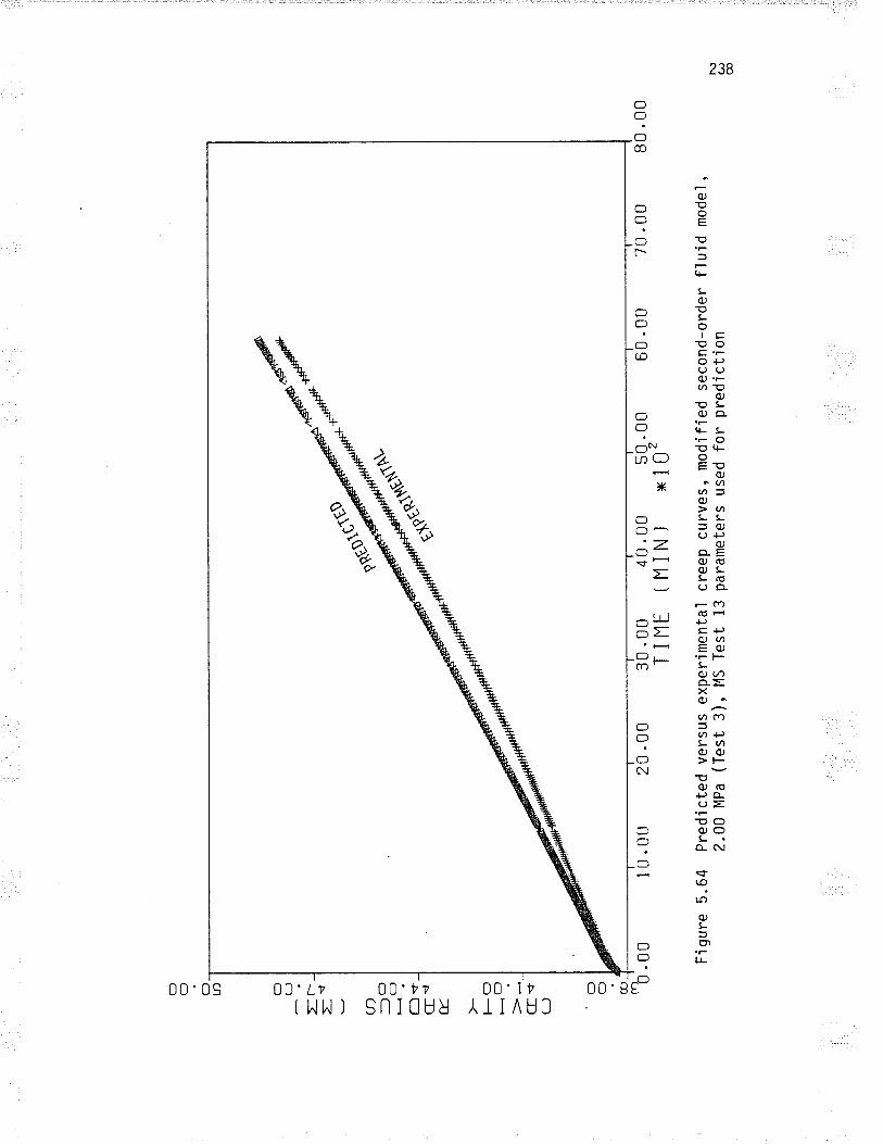
O ? O Lll

O O

Ir-

=Ú

U)

-O -()

f-l s Is E.

FO

HO CI

-1(J

O O cD-

cr) IJ

.00 Fìg

ure

5.64

Pre

dict

ed v

ersu

s ex

perjm

enta

l cr

eep

curv

es, m

odjfi

ed s

econ

d-or

der flu

id m

odel

,2.

00 M

Pa

(Tes

t 3)

, l4

S T

est

13 p

aram

eter

s us

ed fo

r pr

edìc

tion

-.1t

$es

r$:d

10.0

0

w*

#

20 .

00

s

30 .

00T

I I1

E40

.00

(MIN

)50

.00

10,

60 .

0070

.00

80.0

0

l\) G)

@

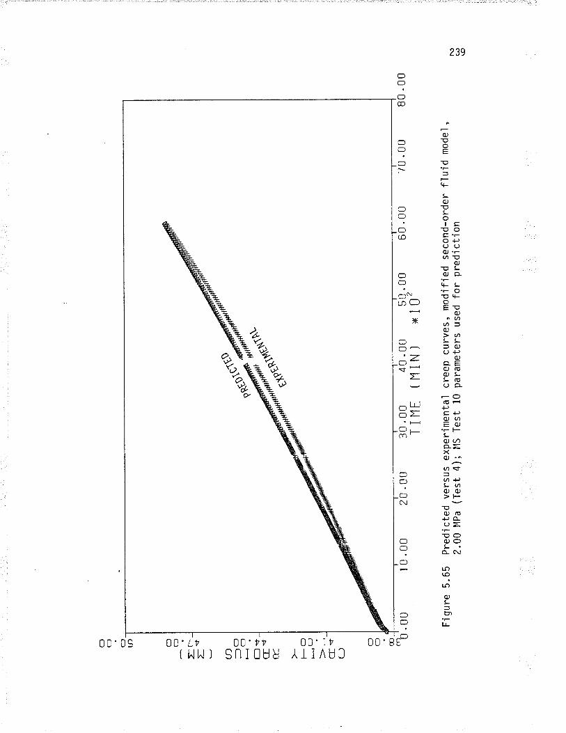
O ? O LD O cl

rr-

=* a -lo -OH O'+

CI

Sf

E.

F_

Cf

HO crs

(J

cf C:) æ_

cr),

- U.0

0

Fì gu

re 5

.65

Pre

di c

ted

vers

us e

xper

imen

tal

2.00

l4P

a (T

est 4)

; Ì4

S T

est

10

10.0

020

.00

30 .0

0T

I I1

E40

.00

11 IN

)

cree

p cu

rves

, mod

ified

sec

ond-

orde

r flu

id m

odel

,pa

ram

eter

s us

ed fo

r pr

edic

tion

50 .

00x

102

60.0

070

.00

BO

.00

N) (, (O

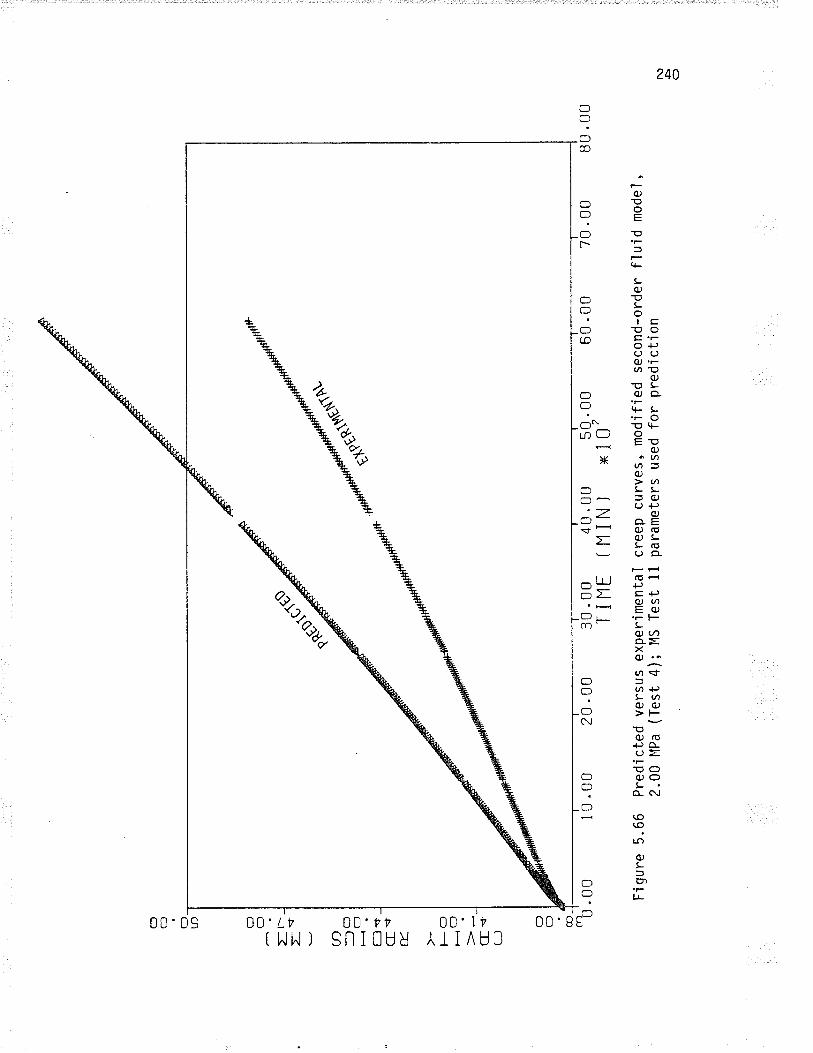
O ? O tn O (]Ir

-

=- a -(]

t() n-f

Cs

É_ FO

HO

Cfs

(-J

c) C)

I@

_rr

ì tJ

.-rs

.00

Fig

ure

5.66

Pre

dict

ed v

ersu

s ex

perim

enta

l cr

eep

curv

es,

mod

ified

sec

ond-

orde

r flu

id m

odel

,2.

00 M

Pa

(Tes

t 4)

; N

S T

est

11 p

aram

eter

s us

ed fo

r pr

edic

t'ion

10 .0

0

ñ*

20.û

030

.00

T i

I1E

40.0

0(t

1 IN

I50

.00

x 10

260

.00

70 .

00B

0 .0

0

t\) Þ o

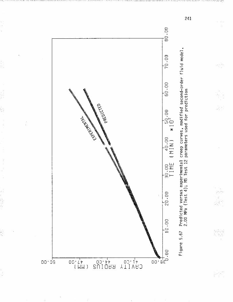
O ? O LN O O

rt-

=*

(.t-

) -ìo

-()

O-t

CI

-Û

E-

FO

HO

[$ (-J

O ? CD -o

.00

I 0 .0

0 20

.00

30 .0

0T

I I1

E

Fìg

ure

5.67

Pre

dict

ed v

ersu

s ex

perim

enta

l2.

00 M

Pa

(Tes

t 4)

; l.1

S T

est

12

t-rt

s:ìq 6f

*'..1

Ç$

PR

tSr"

40 .0

0 50

.00

60 .

00(

11 I

N I

x 10

'cr

eep

curv

es, m

odifi

ed s

econ

d-or

der

para

met

ers

used

for

pred

'ictio

n

70 .0

0

fl ui

d m

odeJ

,

80.0

0

l\) Þ Þ

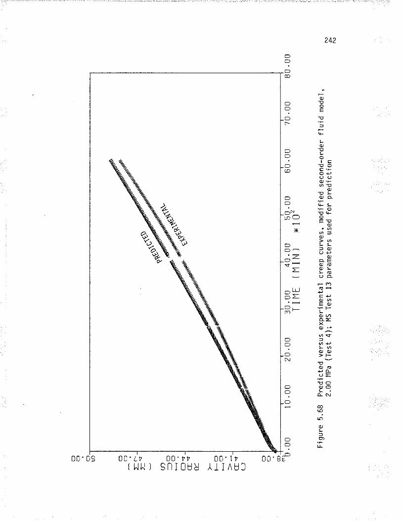
C:] ? (:l

LD c) (]tr

r-_.

úL a --

-\ c

:f-(

)l--

-ì v

CJ$

v. FO

HO (rv

(J

C]

OI

O_

at-l 0

.00 Fig

ure

5.68

Pre

dict

ed v

ersu

s ex

perim

enta

l cr

eep

curv

es, m

odifi

ed s

econ

d-or

der flu

id m

odel

,2.

00 l{

Pa

(Tes

t 4)

; M

S T

est

13 p

aram

eter

s us

ed fo

r pr

edic

tion

t0.0

020

.00

30 .0

0T

I I1

E40

.00

(l1 iN

)50

.00

X 1

0260

.00

70 .0

080

.00

N) è t\

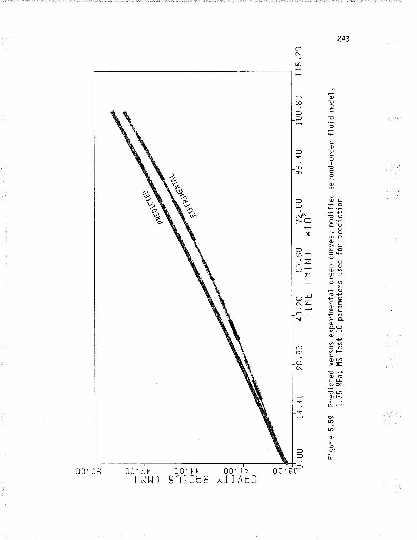
O ? O tn O C:]

tr-

IS (n --)

cl-c

lf-

.ì -t

CI

ST

E.

F_

C3

r--)

>*

c-+

C-)

'cl O co_

crl U

.00

Fig

ure

5.69

Pre

dict

ed v

ersu

s ex

perim

enta

l cr

eep

curv

es,

mod

ified

1.75

MP

a; M

S T

est

10 p

aram

eter

s us

ed fo

r pr

edic

tjon

l4 .4

0

-.'{s

2B .8

0

'SË

o-"

43.2

0T

i I1

E57

.60

n1 IN

)12

.OO

x 10

286

.40

seco

nd-o

rder

flui

d m

odel

.80

t5.2

û

N) Þ (^)

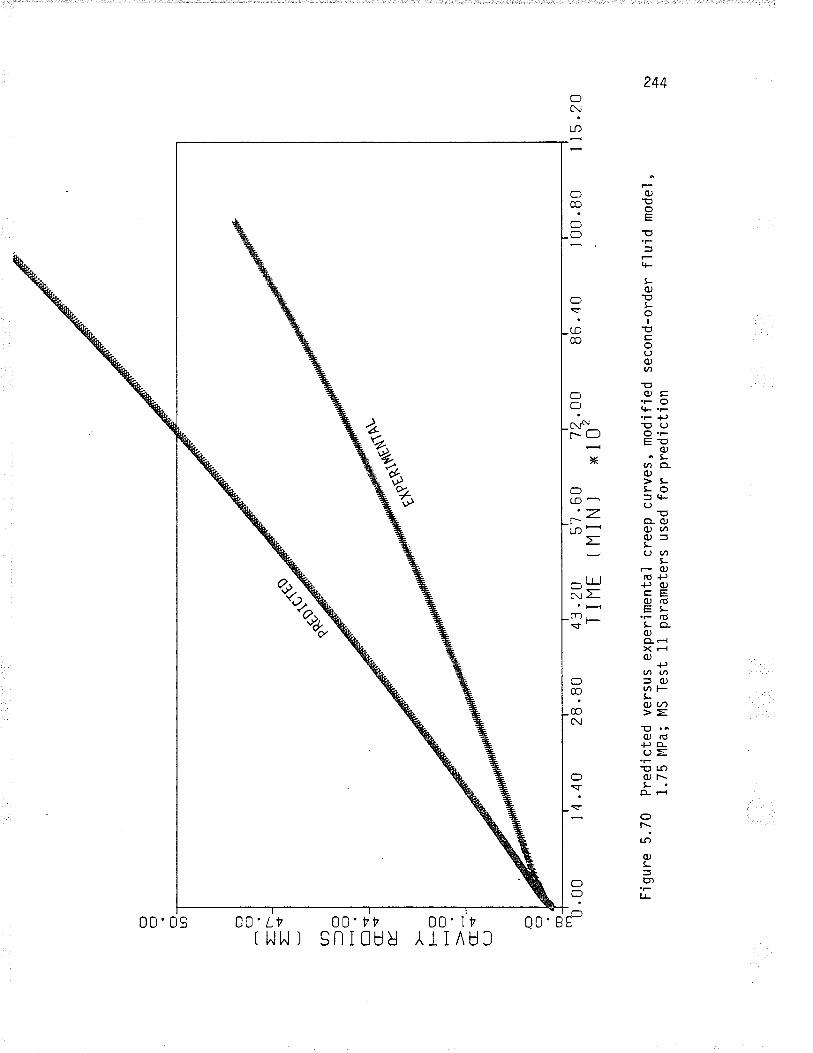
O ? O an O O

Ir-

=*

U)

----

ìo-o f--1

.<-

crs

E.

F-O

HO cts

CJ

.O ? CO ctl

I

0 .0

0 Fig

ure

5.70

Pre

dict

ed v

ersu

s ex

perim

enta

l cr

eep

1.75

l4P

a; M

S T

est

11 p

aram

eter

s us

ed

14 .4

02B

.BO

S**

-"

curv

es, m

odi f

ied

for

pred

ictjo

n

86.4

0

seco

nd-o

rder

flui

d m

odel

,

1 00

.80

ll5.z

0

f\) Þ Þ

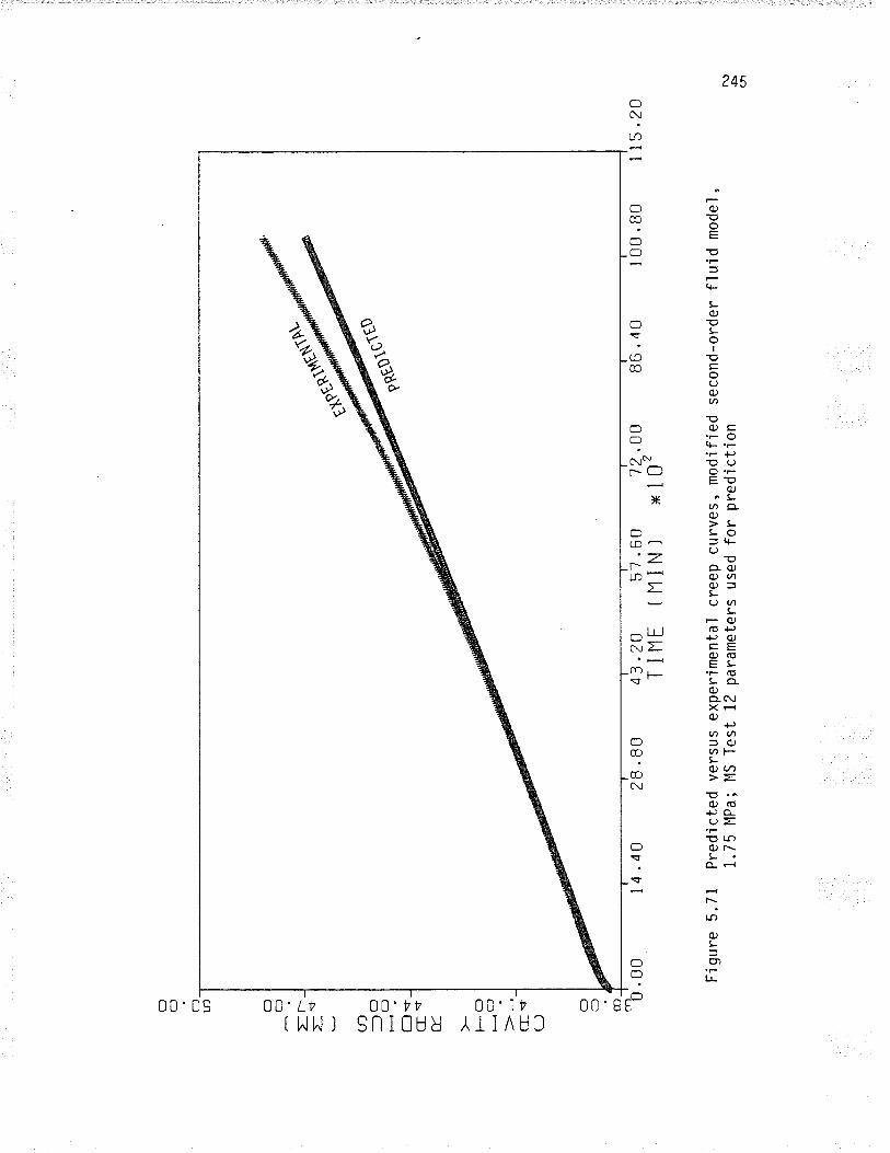
O ? O a O cl

=r-

--+¿

_ U)

--r

cl-c

)H fls C

sV

-

FO >-

CT

ST

-)

O Cf

co_

afì '0

.00

Fìg

ure

5.71

Pre

dict

ed v

ersu

s ex

perim

enta

l cr

eep

curv

es,

mod

ified

1.75

MP

a; M

S T

est

12 p

aram

eter

s us

ed fo

r pr

edic

tion

14.4

02B

.80

*r's

q

43.?

BT

i I1

E

o6to

to

57 .

60il1

IN)

1?.O

Ox

102

86.4

0

seco

nd-o

rder

flui

d m

odel

I 00

.80

I l5

.20

l\) Þ ctr

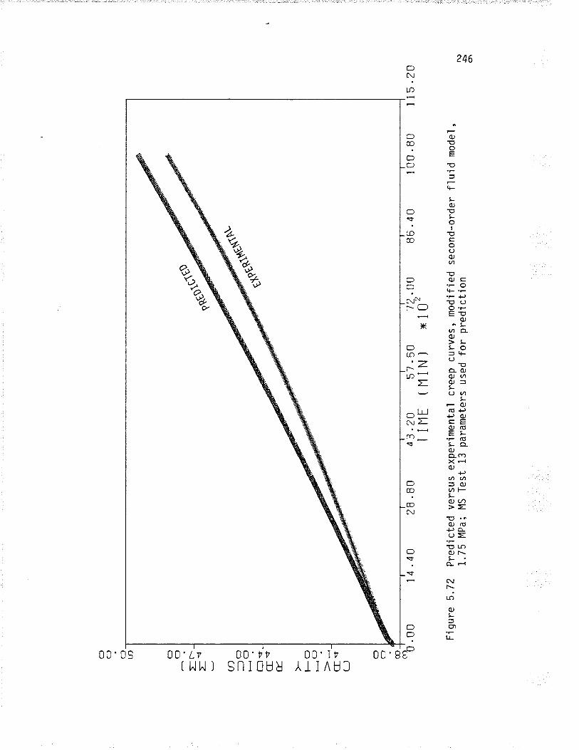
O ? O U) O (]

Ir-

=* a --ìo

-o H. f-lç

CI'S t l-o HO

CT

S(-

J

Cf ? C

D -o.0

0

Fìg

ure

5.72

Pre

dict

ed v

ersu

s ex

perim

enta

l cre

ep c

urve

s, m

odifi

ed s

econ

d-or

der flu

id m

odel

,1.

75 M

Pa;

MS

Tes

t 13

par

amet

ers

used

for

pred

ictio

n

l4 .4

8

^ag$

e$ç%

2B.B

O

,*{Ë

**-"

43.2

0T

I I1

T57

.60

(l1 IN

)12

.OO

x 10

286

.40

1 00

.8û

I l5

.20

l\) Þ Ol

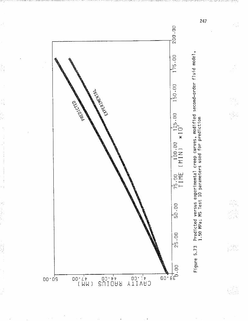
cl ? O LO C:] O

=r-

=*

(n --l o

_O H. -$ 6s É. l--o

-o Þ- cts

(J

O ? Cf] -o

'. oo Fig

ure

5.73

pre

dict

ed v

ersu

s ex

perim

enta

l cre

ep c

urve

s, m

odifi

ed s

econ

d-or

der flu

jd m

odel

,-

1.50

MP

a; M

S T

est

10 p

aram

eter

s us

ed fo

r pr

edic

tion

25 .

00

-"'s

50 .

00

'Ñ*-

"

75 .

00T

I IlE

I 00

.00

I 25

.00

( M

I N

J

x 10

,I 50

.00

l 75

.00

200

.00

f\) å \.1

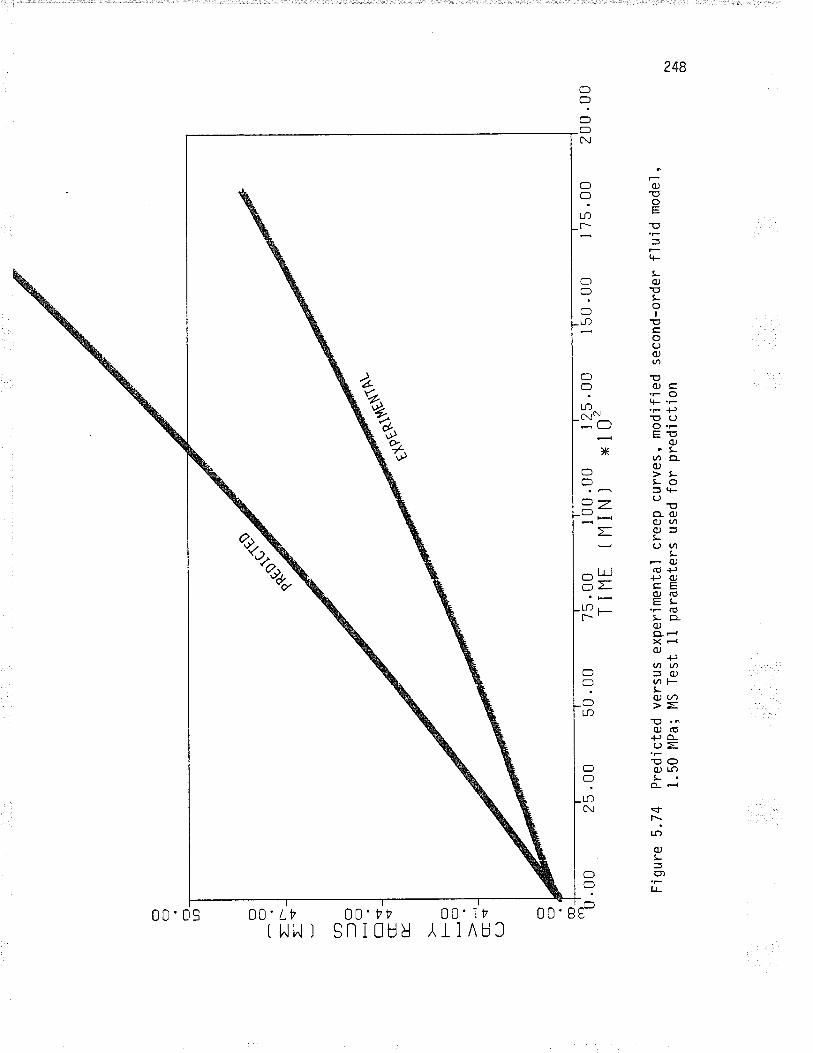
O ? O L.tf-

)

O O

=r-

-

=*

u-) -lo _O f-

-'ì .

í-

Ctt

É-

FO

HC

]

cf<

(J

(:l ? C

O -o'.

oo Fìg

ure

5.74

Pre

dict

ed v

ersu

s ex

perim

enta

l cr

eep

curv

es, m

odifj

ed s

econ

d-or

der flu

id m

odel

,1.

50 M

Pa;

l4S

Tes

t 11

par

amet

ers

used

for

pred

ictio

n

25.0

050

.00

,Ñ*-

'

75.0

0 I0

0.u0

I2

5.00

TIIl

E (

11lN

) x1

0'I 50

.00

I 75

.00

200

.00

l\) å æ

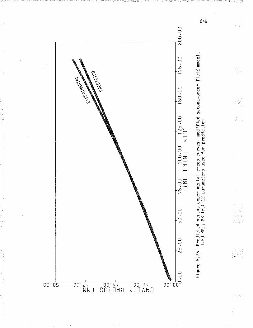
O ? O LD O O

Ir- rs U)

-ì c

:l-ç

)flq Is É

_ FO

HO Is (-J

O O cD-

cr| 0

.00

Fiq

ure

5.75

Pre

dict

ed v

ersu

s ex

perim

enta

l cr

eep

curv

es, m

odifi

ed1.

50 M

Pa;

MS

Tes

t 12

par

amet

ers

used

for

pred

'ictio

n

25 .0

050

.00

*rts

75 .

00T

I I1

E

o6to

to

I 00

.00

I 25

.00

( tl

I N

I x

10'

I 50

.00

seco

nd-o

rder

flui

d m

odel

I 75

.00

200

.00

l\) Þ \o

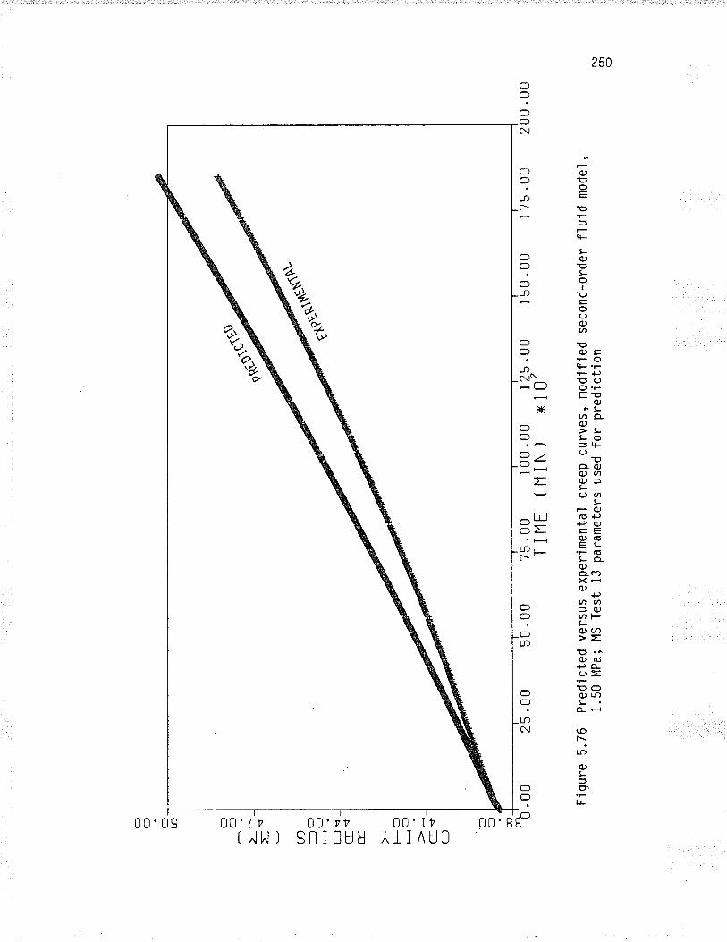
cl ? O tr) cl cl

Er-

-IS Lr

)-l

cl_O l-l

.q

q.f,

E. l--o

-o ct$

(-J

'O O cD_

-o.0

0

Fig

ure

5.76

Pre

dict

ed v

ersu

s ex

perim

enta

l cr

eep

curv

es, m

odifi

ed s

econ

d-or

der flu

id m

odeJ

1.50

MP

a; M

S T

est

13 p

aram

eter

s us

ed fo

r pr

edic

tjon

25 .

0050

.00

,Ñ*-

'

75 .

00T

I IlE

I 00

.00

I 25

.00

( 11

I N

I x

10'

I 50

.00

1 75

.0û

200

.00

f\) (.¡l o

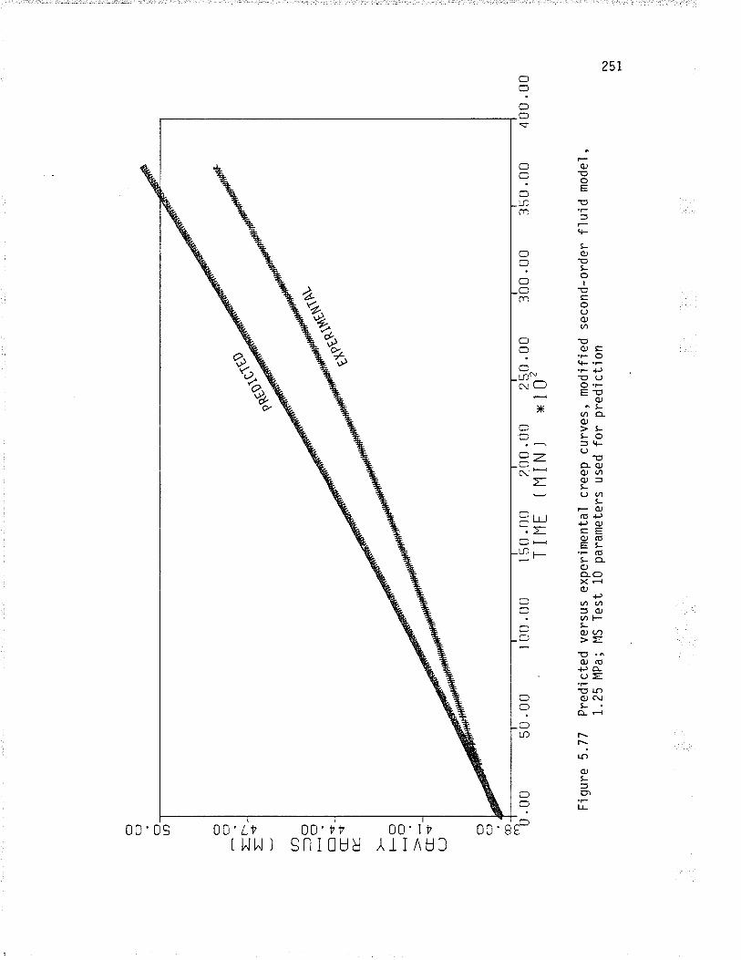
cl ? (:l a O O

Jr-

=*

U)

---lo

-OH n-r

Cs

V.

FO

HO cr<

(J

O ? @ -o'.

oo Fig

ure

5.77

Pre

dict

ed v

ersu

s ex

perim

enta

l cr

eep

curv

es, m

odifi

ed s

econ

cl-o

rder

flu

id m

odel

,1.

25 M

Pa;

l,1

S T

est

10 p

aram

eter

s us

ed fo

r pr

edic

tjon

50 .

00

-ç$

qrc$

I 00

.00

,*#*

-"

150.

00

200.

00

250.

00T

IIlE

(11

iN)

xlO

'30

0 .0

035

0 .0

04

00 .

00

N)

(tl

H

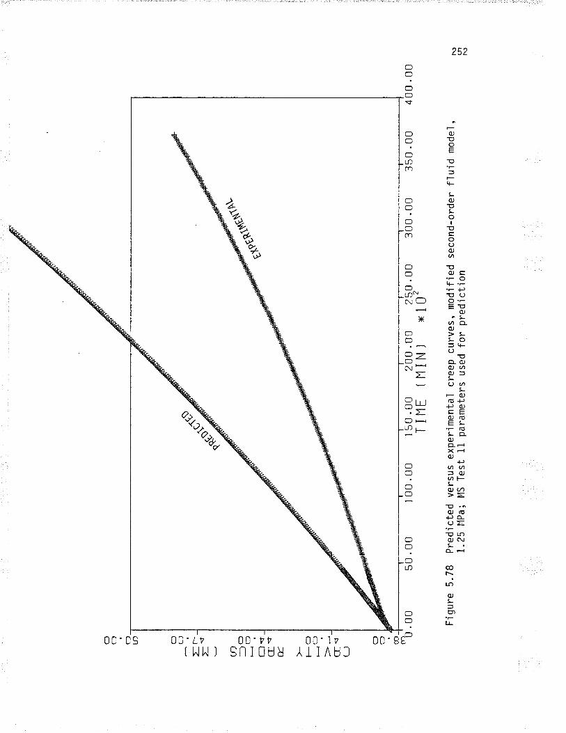
O ? cl Lrl

O O

=r-

E<

-

a -O -o H f-l

ç(r

\r.

É.

FO

-o Cf

rú(J

O O cD_

-o.0

0 Fig

ure

5.78

Pre

djct

ed v

ersu

s ex

perjm

enta

J cr

eep

curv

es, m

odifi

ed1.

25 I

'lPa;

l',lS

Tes

t 11

par

amet

ers

used

for

pred

ictio

n

50 .

00I 00

.00

Sñ-

'

50 .

00T

I I1

E20

0.00

25

0.00

30

0.00

11 I

N )

x 10

'

seco

nd-o

rder

f 'l

uid

mod

el ,

350

.00

400

.00

t\) (tl t\)

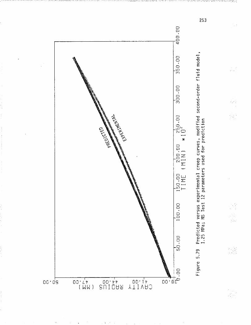
O ? (:l ln (:l

O

tr-

I9 U) --ìo

- çt

f--l

-tC

.r-

É FC

IH

O c$ (-J

C] ? co -o'.

oo Fig

ure

5.79

Pre

dict

ed v

ersu

s ex

perim

enta

'l cr

eep

curv

es, m

odjfi

ed s

econ

d-or

der flu

jd m

odel

1.25

l'lP

a; I

'lS T

est l2

par

amet

ers

used

for

pred

ictio

n

50 .

00

. "1

tseR

rDk

1 û0

.00

ffi'*

-"

I 50

.00

200

.00

250

.00

300

.00

350

.00

400

. Û

0

TIIl

E (

11lN

l x1

0'

1\) (, (,

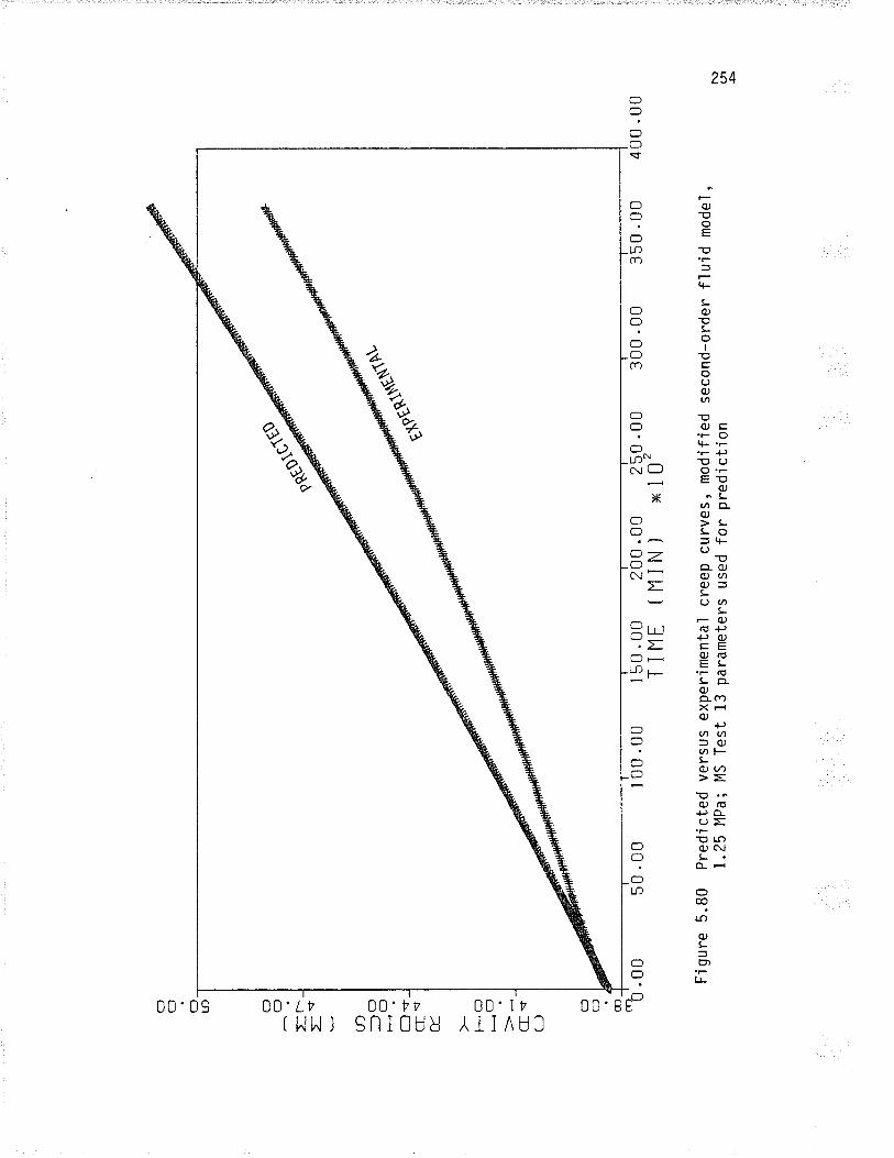
O ? (] rf) O (:l

rr-

TS a --)

c:)

_O H. l--l.q

(r s

tE

. l--o

HO ct<

(-J

C:) ? @

.00

Fig

ure

5.80

Pre

dict

ed v

ersu

s ex

perim

enta

l cr

eep

curv

es,

mod

ified

sec

ond-

orde

r flu

jd m

odel

,1.

25 l

lPa;

MS

Tes

t 13

par

amet

ers

used

for

pred

ictio

n

50.û

0

-."s

:

I 0Û

.00

*ø{t

onrv

t.\Îf'

sr' '

50 .

00T

i I'l

E20

0.00

25

0.00

30

0.00

35

0.00

11 I

N )

x 10

'40

0 .0

0

f\) (tr

.Þ

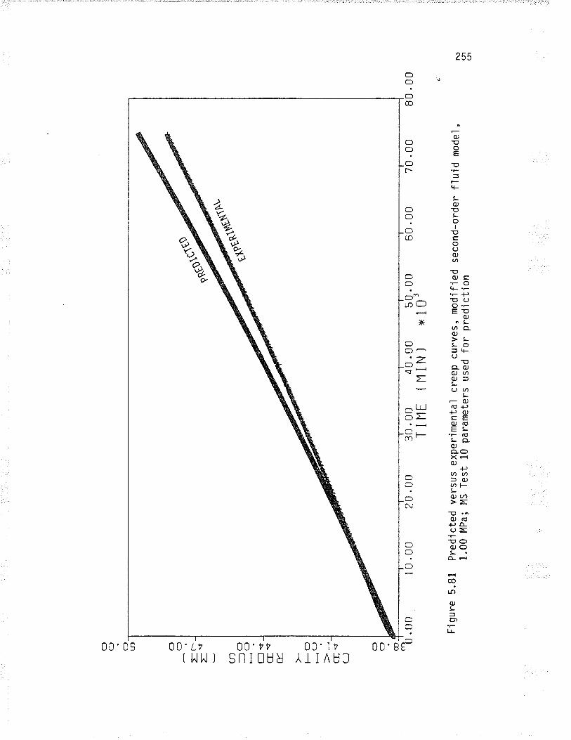
O ? O a O C]

r[-

=s

(n -OO

f-'ì

sct

<E

.

FO >-

ct -ú

(-) O O co

lar

) 0.u

0

Fìg

ure

5.81

Pre

dict

ed v

ersu

s ex

perim

enta

l cre

ep c

urve

s, m

odifi

ed1.

00 M

Pa;

MS

Tes

t 10

par

amet

ers

used

for

pred

ictio

n

l0 .0

020

.00

,*"s ñ*

0"

30.

TI00 11

E

40.0

0il1

IN)

50 .

00x

103

60.0

0

seco

nd-o

rder

flui

d m

odel

,

70.0

080

.00 a.

N)

(tr

ctr

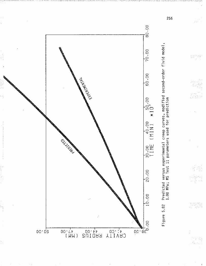
O ? O a O (:l

tt--

r-f

u-)

---)

cl

_O H. O.q crs

É.

FC

IH

(] Þ*

cts

(J

C]

O co

.00

Fig

ure

5.82

Pre

dict

ed v

ersu

s ex

perim

enta

l cre

ep c

urve

s, m

odifi

ed1.

00 M

Pa;

MS

Tes

t 11

par

amet

ers

used

for

pred

'ictio

n

10.0

020

.00

'Ñ*-

"

30 .0

0T

I I1

E40

.00

Î1 IN

)50

.00

x 10

360

.00

seco

nd-o

rder

fluj

d m

odeJ

,

70 .

00B

0 .0

0

l\) (t'r

Oì

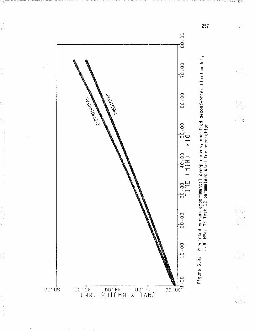
(f ? cl a O O

tr-

r-+

(n -l cl

_O []s (r'Û

É.

l-- (

fH

O cts

(-J

O O col

rrì 0

.00

Fig

ure

5.83

Pre

dict

ed v

ersu

s ex

perim

enta

l cr

eep

curv

es,

mod

ified

1.00

MP

a; M

S T

est

12 p

aram

eter

s us

ed fo

r pr

ed.ic

tion

20 .

00

*-r{

s

30 .0

0T

I I1

E

o6t*

to

40.0

0n1

iNl

50.0

0x

103

60 .

00

seco

nd-o

rder

flui

d m

odel

,

70 .

0080

.00

l\) (tr \¡

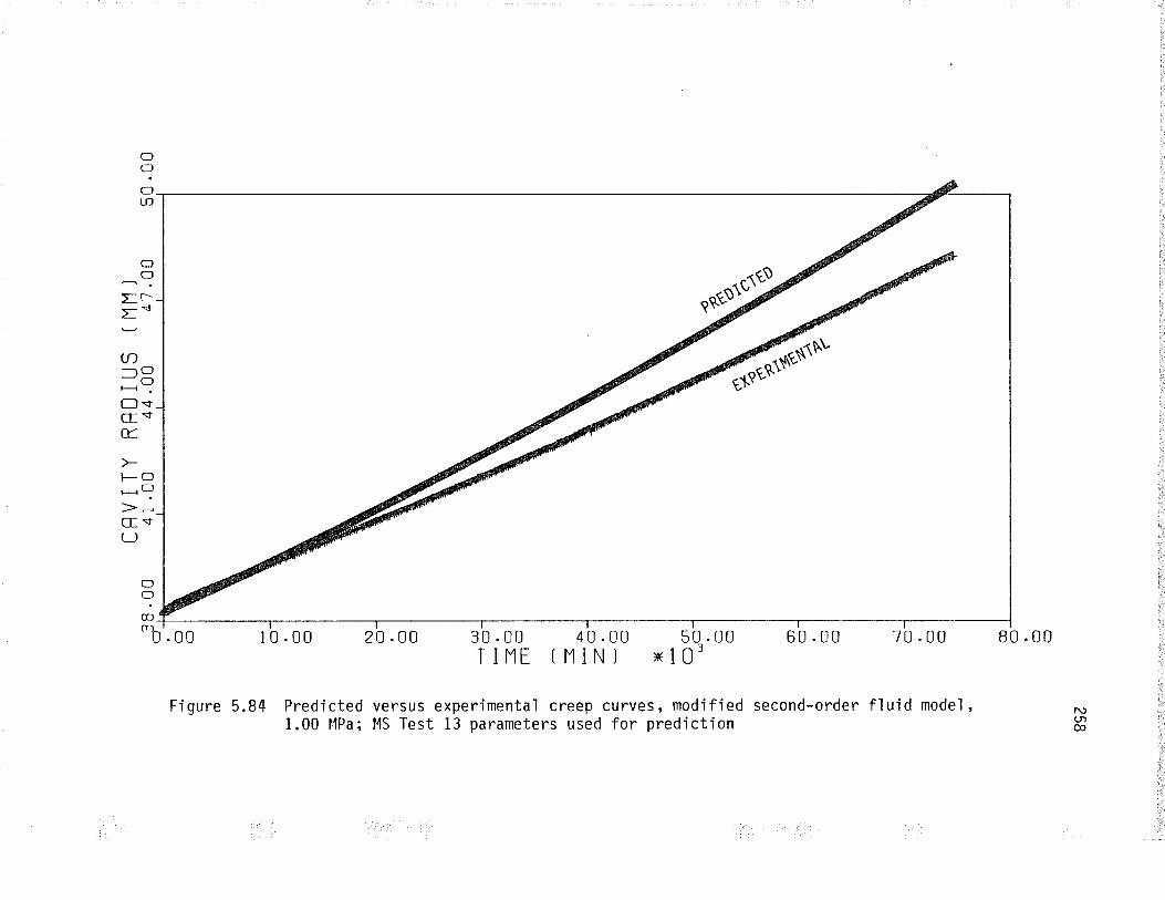
C]

?Oa

OO

Jr-

=*<J)---l cf_O

l--ì sCJ'TIrFO

a---)

>-Cf st(J

O?co-o'. oo

Fìgure 5.84 Predjcted versus experimental creep curves, modifjed1.00 l.lPa; MS Test 13 parameters used for pred jction

10.00 20 .00 30 .00T I I1T

40.00n1 iN)

50 .00x 103

60.00

second-order flujd model,

70 .00 80 .0u

l\)CN@

259

CHAPTER 6

DISCUSSION OF RESULTS OF THE PRESSUREMETER CREEP TESTIruG

PROGRAH Iru ICE

In this chapter, the relationship between the multistaqe

and sinqle staqe pressuremeter creep tests'is explored. The princ'ipaì

question that 'is asked is: Are the creep parameters derived from

relatìve'ly short term multistage pressuremeter tests the same as the

parameters derived from lonq term sinqle stage tests? In other words,

can long term creep under constant loacl be predicted from short term,

nult'i-stress level testinq? This question is examined in terms of

both the strain-hardeninq, power law creep model and the modifjed

second-order fl ui d model . Si nce the pressuremeter test specimens

can be considered to be homogeneous and reproducible, and the test

repeatab'le ( Secti on 4.6 ) ' these factors shoul d not 'inf I uence the

comparìson between the multistage and sinqle stage tests.

As a further check on the vaìidìty of the work, the creep

parameters derived for laboratory ice in this study, usjnq pressuremeter

testing, are compared with creep parameters for laboratory ice reported

in the literature using other test techniques. Finally, the results

of this study are evaluated in terms of enqÍneerinq practice, both

w'ith regards to pressuremeter creep testinq techniques and analysis,

as well as usinq the results for foundation desiqn.

6.I RELATIONSHIP BETWEEN $IULTISTAGE AND SINGLE STAGE PRESSUREÞIETER

CREEP TESTS

As one of the main purposes of this study was to investiqate

260

the validity of the strain-hardening, power ìaw creep theory as applied

to the multistage pressuremeter creep test in warm ice, the relationship

between mul ti stage and s i ng1 e stage tests i s i nvesti gated fi rstl y

in terms of this model.

6.1.1 Strain-Hardeninq, Pouær Law Creep F$odel ; Relationship Betv*een

${ultistage and Single Stage Creep Tests

Ladanyi et al . ( 1984) proposed that the nonl inearity of

the creep I ines on 1og {tn fr) versus log (time) pìots i s due main'ly

to stress redistribution w'ith'in the thick-walled cyl indricaì sample;

i.e. a certain time is required for the stresses to redistribute from

their initial elastic state to the stat'ionary state. Under stationary

state conditions the creep-rate should, theoretically, be independent

of t'ime, in this case, independent of the transformed time r = ¡b.

If stress redistribution within the specimen is really the maior factor

to influence b over time, then the results of the sing'le stage tests

(from pressures of 1.75 to 2.5 MPa) between 90 and 1,440 minutes (Trial

# 2, Iable 5.5) should compare favourably with the results of multistase

Test # 10 (Trial # 3, Table 5.1) and multistaqe Test # 13 (Trial #

3, Table 5.4). In other words, for the same stresses in the same

time intervals, the b values should be comparab'le. This, however,

is not the case. in this 1,350 minute time Ínterval, the sìngle stage

tests have a range in b of from 0.65 to 0.81, with a correspondÍng

n exponent of 0.99, while mult'istaqe Tests # 10 and 13 have b ranqes

of 0.92 to 0.99 and 0.94 to 1.00 corresponding to n values of 3.28

and 2.63 respectiveìy. The penu'lt'imate stages of the multistage tests

approached a steady-state condition after on'ly 90 minutes (i.e. a

261

condítion of þ = 1), whereas it took the single stage tests, at the

same stress levels, at least 600 minutes (Trial # 4" Table 5.5) to

even get close to approaching a steady-state condition. Stress

redistrjbutíon as a function of time does not, then, appear to be

the factor control'ling the onset of steady-state creep; if it were,

then both the single stage and multistage tests, at the same stresses,

would approach steady-state at the same elapsed time. In fact, eiapsed

time does not seem to be the key to the relationsh'ip between the sing'le

stage and multistage tests.

The key appears to be the total amount of strain, represented

by ln å, which the ice specimen has undergone. Examination of the" ri-results of Trials # 6 to 9, Table 5.5, for the single stage tests

appears to support this statement. It seems that an amount of strain

on the order of ln ! = 0.05 to 0.07, was necessary for the steady-statericondìt'ion to be developed in the single staqe tests. It is postulated,

based on the resul ts of thi s study, that i f i n a mul ti stage

pressuremeter creep test an equivaìent minimum amount of total stra'in

is achieved by the end of the first, second or even thìrd staqe, then

the fo'lìowing stages will approach the steady-state condition rapidly,

usua'l'ly within about 90 minutes. Table 6.1 gives the total accumulated

strai n , def i ned by I n l, at the end of each stage of the four- ri-mul ti stage tests.

From Table 6.1, it may be noted that for Tests # 10 and

12, ìn I is in the ranqe of 0.02 to 0.04 at the end of the first-ristaqe, while Test # 11 on'ly approaches this range at the end of the

fifth stage. This range of strain is not approached in Test # 13

until about the fifth stage. All of the ana'lyses on all of the

262

multistage tests have indicated that a steady-state condition (U =

1) is not approached until a mínimum strain equivalent to ln .I- =ri0.03 has occurred. After this strain has occurred, steady-state creep

(U = 1) is approached rapidly in each stage. Moreover, if the creep

data pìot for the first stage of Test # 12 is examined c'losely (flg.

5.10)' it fs noted that the first stage results become paraììeì at

the end to the creep data p'lots for the other three stages.

In other words, the creep data p'lot at the end of the firststage of Test # !2, with ln I = 0.036, approaches a steady-state-ricondition with b close to unity. Test # ll, on the other hand, onìy

begins to approach a steady-state condjtion (U = 1) at the end of

the last stage, with ln l = 0.03.riIn summary, 'it is postuìated that steady-state creep will

start once the ice has strained a sufficiently large amount regardless

of the number or duration of ìoad app'lications that have gone on before.

A corollary statement would be that the lines on a loq strain versus

log time plot of a multistage pressuremeter test w'ill be straight

and paral 1e'l provided a steady-state condition has been reached in

each increment, i.e. all lines will have the slope b = 1.

Prior to the steady-state condition beinq reached, i.e. when

b is less than sây,0.9, the log strain versus log time pìots can

be nearly strai ght and para'l ì e1 prov'ided that the strai n i ncrements

for each stage are the same. (For multistage Test # 11, the total

strain is so small that each stage may be considered to have undergone

approximately the same degree of stra'in. This may in fact be why

these creep lines are reasonab'ly para'llel . )

It may be, in ice at least, that the slopes of the creep

263

lines will not tend to unity if the appìied cavity pressure is very

low, i.e. lower than the stress levels used in this research. Sego

and l4orgenstern (1983), however, have shown that secondary and tert'iary

creep conditions develop in uniaxial compression test samples at

stresses as low as 0.2 MPa. Nevertheless the low stress reg'ion must

be investigated for pressuremeter creep testing in ice. in addition,

the stress redi stri bution hypothesi s must be revi ewed i n the ì i ght

of the data presented in this thesis.

Comparison of the creep curves generated using the multistage

test creep parameters with the curves of the experimental singìe stage.tests, ât equivaìent pressures, indicates that the creep parameters

derived from multistage tests reasonabìy predict the creep response

under a single step cavity pressure in the range from 1.0 to 2.5 l4pa.

As was discussed in Chapter 5, however, the Fensury assumption of

Ee = * = F ¡b = Fl (P.)n 1b (tquation 5.9) has led to unreasonable' ripredictions of the strain rate, particularly near the end of the

comparison period. A better approach would be to take exponentials

of both sides of Equation (5.1); i.e.:ln (ä) = F tb ,

ä=.*o(Ftb),

(s.t)

(6.1)

and to substitute this into an expression for c'ircumferential strain;

i.e.:

^rEo = -" ri =

F-firi =ä-1=exp(Ftb)-1 (6.2)

Now, substi tuti ng for F yi e'l ds :

es = exp (Fl (p.)n tb) -t (6.3)

264

Circumferential strain versus tÍme curves for pressures of 2.0 and

1.25 l'{Pa, using Mul ti stage Test # 10 creep parameters and Equation

(6.3) have been calculated and plotted on Figures 6.1 and 6.2. For

comparison, the corresponding singìe stage test and predicted curve

using Equation (5.9) have been added. It is apparent from Figures

6.1 and 6.2 that:

1) At 2.0 MPa (Figure

better than the fitfi t of the data and

peri od .

6.1), the fit using Equation (6.3) is

using Equation ( 5.9) , both in terms of

strain rate at the end of the comparison

2) At 1.25 MPa (Figure 6.2), the fit of the data is worse usìng

Equation (6.3) , but the predicted strain rate at the end

of the comparison period is better.

Therefore, ôs these two cases illustrate, Equation (6.3) will not

always fit the data better than Equation (5.9), but it will g'ive a

better prediction of the strain rate, which is Ímportant for

extrapolating to longer time intervals.

As discussed previously, the power law creep model represents

primary creep (strain-hardening formulation) when b < 1.0 and secondary

or steady-state creep when þ = 1.0. There are no provi sions for

tertiary creep. Nevertheless, near the end of some of the sing'le

stage tests, the creep exponent b was greater than 1.0, see for examp'le

Trial No. 9 of Table 5.5 when ln | > 0.10. This imp'lìes that theseriparticular tests reached tertiary creep. This accounts for the

deviations in the strain rates at the ends of the predicted versus

experimental curves, still evident even when Equat'ion (6.3) is used

(see Figures 6.1 and 6.2). In other words, the model is predictìng

265

a steady-state response (b = 1.0) whi le the experimental curve i s

actual'ly going into tertiary creep near the end, with associated higher

strain rates. This question requires further study.

6.I.2 t4odified Second-0rder Fluid hdel; Relationship Between

Hultistage and Single Stage Creep Tests

The anaìysìs of both the single stage and multistaqe

pressuremeter creep tests usinq the modified second-order fluid model

has shown that:

1) multistage tests yie'ld essentia'l'ly the same creep parameters

. as singìe stage tests, over the same stress range'

2) mul ti stage tests may be started at any stress level , for

example, a multìstage test may be started at a pressure of

1.50 MPa and have 0.25 I'lPa pressure increments.

In reference to 1) above, the range in the creep exponent

m from the multistage tests is -0.695 to -0.710 (Table 5.14) while

the average m for the single stage tests was determined to be -0.705.

(The equivalent range in n, for the multistage tests under steady-state

conditjons, is 3.28 to 3.45, while the average equivalent n for the

single stage tests is 3.39). In fact, multistage Tests # 10 and 13

virtually gave the single stage m value; m for Test # 11 was a l'ittle

higher while m for Test # 12 was a l'ittle lower. This variation in

the creep exponent m may in fact be directly related to the strain

levels in the various stases of the tests (as was discussed previously).

Usinq ln ! as an indicator of the level of stra'in (Table 6.1), Test"ri# 11 underwent the least amount of strain (jn the ranqe of 1.50 to

2.00 tlPa) while Test # L2 underwent the most. Tests # 10 and 13

266

strained approximately the same amount, an amount in between Tests

# 11 and 12. It may be postulated, therefore, that the Test # lIparameters represent smal I strain deformation whi le the Test # 12

parameters represent ì arge strai ns , i n the pressure range 1. 50 to

2.00 MPa. The other creep parameters g and a1 from the multistage

tests are also very close to the average for the sing'le stage tests;

i.e. u values of 5.90 and 6.00 versus 6.125 MPa (mìn)m+1 for the singìe

stage tests, and al of 120.0 versus 108.0 MPa (mjn)m+2 for the singìe

stage tests.

In reference to point 2) above, Test # 10 was begun at an

applied pressure of 1.50 MPa and Test # 13 was begun at an app'lied

pressure of 0.25 MPa; both tests used pressure increments of 0.25 MPa.

As the results in Table 5.14 indicate, Tests # 10 and 13 yielded almost

exactìy the same creep parameters. It is postulated, therefore, based

on this result, that it is not necessary to beqin a multistage

pressuremeter creep test at zero pressure. In fact, the init'ial

increments of Test # 13 would have had to be left on much longer than

1,440 minutes to be of any use in the analysis.

Hhereas the strain-hardeninq, power law creep model could

take the creep parameters derived from multistage Test # 11 and

reasonabìy predict the experimentaì singìe stage test results at all

pressures, the second-order fluid model could not. This 'impì'ies

perhaps, that even though a good fit to the Test # 11 experimentaì

creep curve was obtained usÍng creep parameters a1 = 120.00 MPa

(min)m+2, u = 6.00 MPa (min)m+1 and m = -0.695, these parameters may

onìy be valid for the small strain range of deformation and should

not be used for extrapoìation to ìarge strains (i.e. they are valid

267

when ln ! < 0.03 or r ( 39.5 mm).ri

6. 1. 3 Sunsnary

In surnmary, the 'informatjon obtained from multistage

pressuremeter creep tests compares very weìl with the creep information

derived from single stage pressuremeter creep tests, in the same stress

and strain range. The modified second-order fluid ana'lysis produces

reìatively little scatter in the values of the creep exponent m (or

equivalent n) derived from the multistage tests, and the m values

compare well with the average m derived from the single stage tests.

It further appears that the past history of app'lied stresses in a

creep test has little effect on the nature of the creep; rather,

the amount of total strain appears to be the control I ing factor.

Therefore, creep parameters derived in a certan range of strain should

only be app'lied in practice to that same level of strain. Both Seqo

and Morgenstern (1983) and Ladanyi et al. (I979) have indicated the

dependence of creep parameters on the level of strain in ice. The

role of stress redistribution in a thick walled cylindrical specimen

is as yet unclear. The anaìysis of the results presented in this

thesis seem to suggest that it is unimportant.

For pressuremeter testing in ice or ice-rich frozen soils,

it should be assumed that a steady'state creep cond'ition will eventually

prevail w1th continued straining. To support this hypothesis' }rleaver

and Florgenstern (1981a), present data from simpìe shear creep tests

wh'ich show that secondary creep conditjons prevail for ice and ice'rjch

frozen soils at applied shear stresses of as low as 0.01 MPa. There

seems no reason , therfore , to use the strai n-hardeni ng , power I aw

?68

creep theory with an exponent b less than about 0.9 sjnce thjs will

predíct a damped creep response (which for ice and ice-rich frozen

soi I could be seriously in error). Each stress increment 'in a

pressuremeter creep test should be appl ied unti I at least the

steady-state condition is approached, as evjdenced by a b of at least

0. 90.

The creep parameters derived from this study will now be

compared to those found in the literature.

6.2 COI'IPARISON OF THE CREEP PARATIETERS FOR LABORATORY ICE DERIVED

. IN THIS STUDY HITH THOSE REPORTED IN THE LITERATURE

As has aìready been pointed out in Chapter 2, there are

no ìong-term (i.e. greater than 24 hour) pressuremeter creep test

results in ice pubìished in the literature. Comparisons will be drawn,

therefore , wi th the resul ts from 'l aboratory creep tests ( such as

unjaxial compression tests) conducted on po'lycrystalline ice.

Before comparing creep data for poìycrystal I ine ice, the

factors which most influence creep should be enumerated. Sego (1980),

in rev'iewing the literature, listed several factors which have a major

influence on the flow of poìycrystalline ice:

1 ) temperature,

2) crystal si ze ,

3) crystal orientation,

4 ) type of stress app'l i cati on ,

5) density of specimen.

From his own experimental work, Sego (1980) has discovered'it was

not only crystaì size that was important but what he called the "grain

269

size ratio". This ratio Ís defined as the crystal size divided by

the size of the specimen. Moreover, he has verified the claim by

Glen ( 1975) tnat the amount of straining undergone by the ice al so

great'ly influences flow. Therefore, "grain size ratio" and stra'in

should be added to the list above.

For the ice tested in this study, no account has been taken

of the grain size ratio. Moreover, the specimens tested in this program

have to be considered as having undergone large strains, except perhaps

the specimen for multistage Test # 11. And in the case of this work,

al I specimens were maintained at the same constant temperature of

-2"C. Therefore, comparì sons with other work must be made at a

temperature of -2"C.

l{ost of the creep data presented i n the I i terature 'i s based

on a simpìe power law of the form,

u(c) = ¿. (å)n (2.2)

Equation (2.2) is used to represent the dependence of the secondary

creep rate on deviatorÍc stress. Sego (1980) and Sego and Morgenstern

(1983) indicated that while the qrain size ratio onìy effects the

creep proof stress oc, it does not effect the creep exponent n.

Therefore, since the grain size ratio of the ice which was tested

both in this and most other testing programs is unknown, only the

creep exponent n wi I I be compared between these and other tests.

In reviewing the literature, much of the published data

on the creep of'laboratory ice is for test temperatures of -5oc or

colder (e.g. Mellor and Cole,1981; Hellor and Cole, lgBZ; Cole,1983; Cole, 1984). In order to extrapolate this data to a temperature

270

of -2"C, for our purposes, a temperature versus creep-rate relationship

would have to have been established. This was not done in any of

the studies, at -5oC or lower, so extrapolations to -Z"C are not

possi bì e.

Sego (1980), in his ljterature review, did report the work

of steinemann (1958) which was conducted at a temperature of -1.9"c.

uniaxial, constant stress compression tests þrere carried out by

Steinemann to ìarge strains. The best fit flow law for this large

strain data, using the simp'le power 1aw creep model, gives an exponent

n equal to 3.45, which compares very well w'ith the creep exponents

determined'in the present study. By means of constant rate of stra'in

triaxial tests, sego and Morgenstern (1983) defined the flow law of

samples subjected to I0% axial strain at -2"C by a creep exponent

n of 3.18. This value of n also compares well with the results of

this study. Even though grain size ratios have not been accounted

for, these compari sons are encouraging and support the resul ts of

the tests performed for this study.

For design purposes, Sego and Morgenstern (1993) recommended

using an exponent n of 3.0 for both small and large strain conditions.

Thi s postuì ate i s corroborated by the earl ier work of 1'lorgenstern

et al. (1980), who found that ìong-term creep of friction pi'les inice and ice-rich soils may be predicted quite accurateìy usÍng the

simple power law formulation with an n exponent of 3.0.

body for

the field.

To accurately assess the creep properties of a natural ice

design, sego (1980) recommended that tests must be done in

He stated:

natural ice body it would be difficult to determine" In a

271

the gra'in size ratio and the strain that it has al readyundergone in the field. Therefore, to determine theappropriate flow ìaw for design, one must use field methodsbecause many factors influence the flow law determíned inthe laboratory for it to be used for design."

Hence the recommendation to use field based creep parameters.

6" 3 RECOI'I¡{EHDED PRESSUREHETER TESTING TECHNIQUES AND ANALYSIS IN

ICE AND ICE-RICH FROZEN SOILS

Th'is section is subdivided into three parts:

1) drilling and sampfing,

2) pressuremeter creep test techniques,

3) analysi s of resul ts.

6.3.1 Drilling and Sampling

Dri 1 1 ing and sampì ing operations are an ìntegral part of

any s'i te i nvesti gatì on , whether Í n frozen or unfrozen ground .

Pressuremeter testing i s normal ìy conducted as part of an overal I

dri'l'ling and sampling program; decisions as to where in the

strati graphy to conduct the pressuremeter tests are normaì 'l y made

on si te , as the dri I ì i ng progresses .

If site and frozen soil conditions allow, dry augering with

an auger core barrel , such as the CRREL type core barrel , 'i s the

preferred method of driììing and sampìing. Disturbance of the frozen

sojl is usuaì1y kept to a minimum and high qua'lity samp'les may be

retrieved. If dense sand and grave'l layers or til'l with cobbles and

boulders must be penetrated, wet rotary drilling techniques are normaì'ly

reverted to. The dri'l ì ing mud must be maintained at temperatures

below zero by a refrigeration plant to minimize thermal disturbance.

272

Freezing point depression of the drilling mud is usual'ly accomplished

by adding KCL. This may result in some corrosion of the frozen soil,

however. Samp'ling may be conducted using core barrels and wire line

equipment. Driììing and samp'l'ing techniques in permafrost so'ils are

discussed in greater detail by Roggensack (7979) and Sav'igny (1980).

When the proposed location for a pressuremeter test is

reached, the core barrel whjch is used must be capable of drillìng

a proper'ly calibrated pressuremeter pilot hole (refer to Section 3.2.6).

After the pì 'lot hol e has been dri I I ed , a thermi stor or thermocoup'le

should be lowered into the test cavity to check its thermal equilibrjum.

The samp'les recovered from the core barrel should be logged and packed

jn an insulated constant temperature container for future'laboratory

i ndex tests .

6.3.2 Recormended Pressuremeter Creep Testing Techniques in lce and

Ice-Rich Frozen Soil

The 0Y0 Elastmeter-100, or a pressuremeter s'imilar to this,

with an electronic radius measuring device is recommended for testing

frozen soils or ice. With the radÍus being measured electronically,

the membrane can be inflated with a gas such as compressed nitrogen.

There is no need for mixing an antifreeze solution such as ethelyne

g'lycol and water nor for saturating the probe in sub-zero temperatures

as is required with pressuremeters of the l4enard type which require

the probe volume to be measured. .Correcting for the hydrauìic head

is also not requ'ired. Moreover, the probìems associated with testing

in a dry hole deeper than about 10 m with a hydrau'lic pressuremeter

(Baguelin et a1.,1978) are avoided.

273

The pressuremeter may be calÍbrated folìowìng the procedures

outlined in Chapter 3. During the calibration, the zero and gain

controls on the digita'l indicator should fírst be set using the smallest

and I argest cal i brati on ri ngs. The two i ntermedi ate cal i brati on ri ngs

should then be used to check the ìinearity of the radius measuring

system. This step in the calibration process must be done carefuì1y,

otherwise all of the cavity radius measurements will be in error,

no matter how much care is taken in the other steps. To save time

(with no great ìoss in accuracy), a composite membrane reactíon curve

of the type shown in Fig. 3.7 may be deve'loped by runn'ing res'istance

cal ibrations in the laboratory. The change in membrane thickness

test may be carried out with 5 minute increments, and the membrane

cross-sectional area correction may be deve'loped using onìy two steel

tubes si nce al I of the cal i brati ons wi th the 0Y0 pressuremeter to

data have shown that the pìot of S/r versus digita'l indicator reading

is very close to linear.

0nce the pressuremeter has been cal ibrated and the hole

has reached thermal equilibrium (i.e. the temperature is not changing

significantly), the pressuremeter should be lowered down into the

test cavity. If the outside air temperature is significantly different

from the temperature of the frozen ground, the calibrations may have

to be carri ed out i n a healed tank or a van ( for col der ai r

temperatures), or in an ice or refrigerated bath (for warmer air

temperatures). An ideal way to regulate the temperature of the probe

would be to place a heat exchange coiì in the probe itself. The rubber

membrane could be maintained at the desired temperature whi le the

calibrations are being performed by looseìy wrappíng insuìat'ion around

274

the probe or p'lacing the probe in an insulated container. The heat

exchange coi I method woul d provi de conti nuous temperature control

and thus eliminate possible heat flow up or down the metal rods during

the pressuremeter test. As a minimum, a 'heat break' shoul d be

installed in the rods (tnis will be a coup'lÍng made of low heat

conducti ve p'last'ic such as nyl on ) or the top of the rods shoul d be

kept from sticking up out of the hole.

The recommended mul ti stage test procedure i s to set the

first pressure increment to about 1.5 MPa, and then let the cavìty

creep until a condition of steady-state creep prevails. ThÍs typically

occured when ìn I approached about 0.03 to 0.05 in this testing't

program. This means that the test data must be plotted in real time

as the test is running. Once a condition of steady-state creep has

been reached, the pressure may be increased in 0.25 MPa increments.

The second and fo'lìowing increments need be app'lied onìy long enough

to obtain a clear measure of the steady-state creep-rate for that

particular pressure increment. A condition of steady-state creep

is indicated most c'lear'ly when b approaches unity (in the

strain-hardening, power ìaw theory). The steady-state creep condition

i s al so i ndi cated when the cav'ity radi us versus time curve exh'i bi ts

an exponential increase in radius with time. If the first increment,

using a pressure of 1.5 MPa, takes too long, a starting pressure of

1-.75 or 2.0 MPa may be used in subsequent tests. It should be

remembered, however, that pressures of even I MPa are much higher

than the bearing stress generated by most structures founded on or

in contact with permafrost. There ís advantage, then, in using a

low pressure for the first increment, particular'ly if steady-state

275

conditions develop rapidly.

In order to determine the creep parameters accurately, the

multistage test should have at least four to five increments. Aìthough

one test may end up taking one, to as many as two days, this ìength

of time is consÍdered to be necessary if high quality results are

to be obtained. One way to get around this prob'lem of time is to

drill two or more holes at the same time, and using two or more

pressuremeters, to run tests concurrentìy. Another way would be to

bui I d a pressuremeter stri ng, wi th say ? or 3 or possi b]y 10

pressuremeters mounted on the string at intervals of, say, 1 metre.

'Tests could therefore be run concurrentìy in the same hole. It must

be remembered, however, that the in situ horizontal stress will normal'ly

not be zero, as was assumed for the ana'lysis of results for this thesis.

6.3.3 Analysis of Pressuremeter Creep Test Results

Both the single stage and multistage tests analyzed for

thís study, in the pressure range 1.0 to 2.5 MPa, conform to a power

law creep formulation; i.e. the secondary creep-rate is related tothe deviatoric stress through a power law. A considerable body of

analysis and field observations supports the concept that ice and

ice-rich frozen soils will tend to reach a steady-state or secondary

creep condition under sustained load. It is therefore postulated

that the strain-hardening, power law creep theory, with b < 1, should

not be used to extrapo'late creep test information to longer time

periods. The steady-state form with b = 1, should be used instead.

If one wishes to estimate creep deformatjons for, Sôy, piìes

or footings, using a power law creep formulation, then the creep

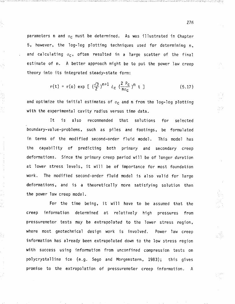
276

parameters n and oc must be determined. As was illustrated in Chapter

5, however, the log-ìog plotting techniques used for determ'in'ing n,

and cal cul ati ng oc, often resul ted in a ì arge scatter of the final

estjmate of n. A better approach mìght be to put the power 1aw creep

theory Ínto its integrated steady-state form:

r(t¡ = r(o) exp (5.17 )

and optìmize the initial estimates of oç and n from the'log-1og plotting

with the experimentaì cavity radius versus time data.

It i s al so recommended that sol uti ons for sel ected

boundary-va'l ue-probl ems , such as pi I es and footi ngs , be formul ated

in terms of the modified second-order fluid model. This model has

the capabi ì i ty of predi cti ng both primary and secondary creep

deformations. Since the primary creep period will be of 'longer duration

at lower stress levels, it will be of importance for most foundation

work. The modified second-order fluid model is also valid for large

deformations, and is a theoreticaììy more satisfying solution than

the power 'law creep model .

For the time being, it will have to be assumed that the

creep information determined at reìativeìy high pressures from

pressuremeter tests may be extrapolated to the lower stress region,

where most geotechnical design work is involved. Power law creep

information has already been extrapolated down to the low stress region

with success usíng information from unconfined compression tests on

polycrystalline ice (e.g.Sego and Morgenstern,1983); this g'ives

promise to the extrapo'lation of pressuremeter creep information. A

t(+ )n*1 Ë. (i"T )n t l

in the

277

lowpressuremeter

stress region

testing program in

(less than 1.0 MPa)

ice should be

to verify this

underta ken

promi se.

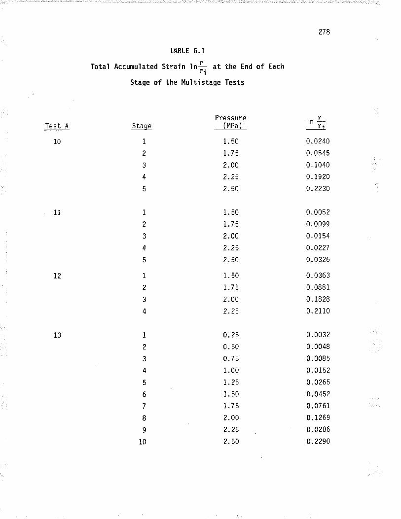
TABLE 6.1

TotaÏ Accumulated Strain lnl at the End of EachriStage of the h{ultistage Tests

?78

lnLrj0.0240

0. 0545

0. 1040

0. 1920

0.2230

0. 00s2

0. 0099

0. 01 54

0.0?27

0. 0326

0. 0363

0.0881

0. 1828

0.2110

0.0032

0.0048

0. 0085

0.0152

0.0265

0.0452

0.0761

0.t2690.0206

0.?.290

Test # Staqe

1

2

3

4

5

1

2

3

4

5

1

2

3

4

Pressure(MPa)

1. 50

7.75

2. 00

2.25

2. 50

1. 50

r.7 5

2.00

2.25

2.50

1. 50

1.7 5

2.00

2.25

0.25

0. 50

0.7 5

1.00

t.251. 50

t.7 5

2.00

2.25

2.50

10

i1

I2

13 I2

3

4

5

6

7

I9

10

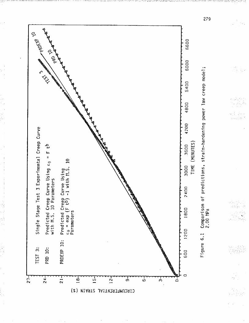
TE

ST

3:

PR

D 1

0:

PR

DE

XP

10:

ùeI

z. d F- v',

IJ F z. t!l É

.t¡

JtJ

- = =(J É.

(J

Sin

qle

Sta

qe T

est

3 E

xper

imen

tal

Pre

dict

ed C

reep

Cur

ve U

sing

eg

=w

i th

14. S

. 10

Par

amet

ers

Pre

dict

ed C

reep

Cur

ve U

sing

es =

êX

p (r

tu¡

-1 w

ith it

.5.

10P

aram

eter

s

Cre

ep C

urve

Ftb

600

r 20

0 I 80

0 24

00

Fig

ure

6.1

Çom

pa.q

!son

of

pred

ictio

ns,

stra

in-h

arde

ning

pow

er ì

aw c

reep

mod

eJ;

2.00

tlP

a

,\

^t1,

qs$t

\e r0

lss^

*

3000

36

00

4200

TItt

t (H

INU

TE

S)

4800

54

00

6000

6600

f\) \¡ (.o

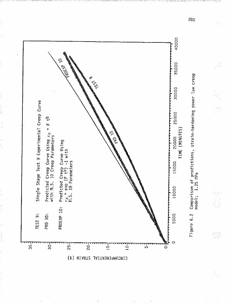
35 30

TE

ST

9:

PR

D 1

0:

PR

DE

XP

10:

te z. d. l-- v) J F- z. UJ É.

t¡J t! = =(J É.

(J

25

Sin

gle

Sta

ge T

est

9 E

xper

imen

ta'l

Pre

dict

ed C

reep

Cur

ve U

sing

ea

=w

ith l{

.S.

10 C

reep

par

amet

ãrs'

Pre

dict

ed.C

reep

Cur

ve U

sing

es =

êX

p (r

to)

-1 w

ithÞ

1.S

. 10

Par

amet

ers

20 l5 t0

Cre

ep C

urve

Ftb

5 00

0

Fìg

ure

6.2

Com

paris

on_o

f pr

edic

tions

, st

rain

-har

deni

ng p

ower

law

cre

epm

odel

; 1.2

5 ilp

a

#T r

oQ

RV

.J

I 00

00

ó:

r 50

00

2000

0 25

000

TIM

E (

MIN

UT

ES

)

r,g

1ç-5

'

3000

035

000

4 00

00

\) co o

28L

CHAPTER 7

COHCLUDING REþIARKS

7 "I PRESSUREHETER TESTING EQUIP¡{ENT

The 0Y0 Elastmeter-100, or a pressuremeter similar to this,

with an electronic radius measuring device is recornmended for testing

in frozen soils or ice. l.lith the radius beìng measured electronically,

the membrane can be inflated with a gas such as compressed nitrogen.

There is no need for mixing antifreeze solutions nor for saturating

the probe in sub-zero temperatures, as there would be for a Menard-type

pressuremeter, in which the volume change of the probe must be measured.

Moreover, the problems associated with testing in a dry hole deeper

than about 10 m with a hydrauìic pressuremeter are avoided.

The 0Y0 Elastmeter-100 has performed exceedìng'ly wel I for

the test program presented in this thesis. Even for the'longest test,

which lasted about 52 days, electronic drift of the radius measuring

system was almost negìigibìe, giving a maximum error in the calculated

cavity radjus on the order of t 0.10 nm. It is stressed, however,

that this degree of accuracy may be obtained on'ly if calibratjons

of the radius detecting system and membrane are carefully run both

before and after the test. Savigny (1980) also concluded that carefully

run cal ibratÍons are required during his use of a sìope indicator

sensor to measure very smal I creep rates in a natural , ice-rich

permafrost sìope.

The modifjed CRREL-type auger core barrel des'igned

speci fi ca'l ìy to dri I I a pressuremeter test cavi ty has worked very

well. The holes drilled in this study were well calÍbrated, smooth

282

and therma'lìy undi sturbed.

A pressuremeter testíng program i s now underway (at the

time of publication of this thesis) on an ice island off the northern

coast of Alaska. From all reports (Shields, persona'l cor¡nnunicatìon),

the pressuremeter testing system deve'loped in thÍs study has been

successful in testing the sprayed ice makÍng up the is'land.

7.2 ANALYSIS OF TEST RESULTS

From the analysi s of the test resul ts presented in thi s

thesis, it has been found that the creep of ice, as measured with

.the pressuremeter, conforms to the power law creep model after the

ice has undergone a requ'ired amount of strain. In other words, after

strain (tn fr) on the order of 0.03 to 0.05, a steady-state, oF

secondary creep condition, is established and the cavity expands

according to:

( s. 17 )

i.e. the cavity radius increases exponentialìy with time.

Creep parameters derived from multistage tests using both

the strain-hardening, power law creep model (when b average is greater

than 0.90 and essential ìy steady-state conditions prevail ing), and

the modified second-order fluid model may be used to generate fictit'ious

creep curves which represent the singìe stage creep curves reasonably,

at least in warm íce and in the pressure range from 1.0 to 2.5 MPa.

Differences in the strain rates, particularly near the end of the

comparíson period, could be due to the single stage tests passing

into tertiary creep at ìarge deformations. Tertiary creep may be

r(t) = r(o) exp I (+)n*1 Ë. (# )n t I ;

283

representedbyb>1.0.

It has been found that the mod'ified second-order fl uid

ana'lysi s , us'ing an i terati ve scheme to optìmi ze the creep parameters '

produces less scatter in the equivalent creep exponent n than the

Stra'in hardening power law creep model. The average creep exponent'

m, derived from anaìys'is of the single stage tests is -0.705, wh'iìe

the average creep exponent from the four multistage tests is -0.704

(in terms of equiva'lent n values for steady-state creep, these would

be n = 3.39 and 3.38 respect'ively). These results are found to compare

well with results of unconfìned compression tests on poìycrystalline

ice reported in the literature. It appears also that an m value of

-0.695 (equivalent to an n of 3.28) represents the small strajn region

wh'ile an m value of -0.7i0 (equivalent to an n of 3.45) represents

'large stra'ins in the stress range 1.5 to 2.0 I'lPa. From this it appears

that the average m of -0.705 is an average of both the small strain

and large strain reg'imes. It may be concluded that multistage tests'

when each pressure increment is left on long enough to develop a

steady-state creep condition, yield essential'ly the same creep

parameters as a series of sing'le stage tests.

A considerable body of ìaboratory test resul ts and fiel d

observations is now available to support the concept that ice and

i ce-ri ch f rozen so j I s eventual'ly creep under essentì al'ly steady-state

conditions under sustained load. Thus, the strain-hardening, power

law creep model with b less than about 0.9 should not be used to pred'ict

'long term creep behaviour. Anaìyses have shown that not only will

a b of less than 1 indicate creep curves whjch are attenuat'ing, but

the computed creep exponent n will also differ significantly from

the steady-state n val ues. It i s recommended, therefore, that al I

284

creep tests be pro'longed until at least a value of b = 0.9 js achieved

(in each increment, in the case of multistage tests).

Unlike the power law creep model, the modified second-order

fluid model can predìct both primary and secondary creep. lchereas

the power law approach requires separate relationshìps to model both

the strain-time and secondary creep-stress behaviour (e.g. Sego and

Morgenstern, l983) with the modified second-order fluid concept, the

strain-time and secondary creep-stress functions are contajned in

one motion equation. The capability to model both primary and secondary

creep is important in the ìow stress range, where extended periods

of primary creep may prevai'1. For example, Sego (1980), found that

unconfined compression tests conducted on samples of polycrystalline

ice at stresses below 0.10 MPa require loading times 'in excess of

2,000 hours to reach a condition of steady-state creep.

Until boundary-va1ue-problems (other than the pressuremeter

probìem) have been solved in terms of the modified second-order fluid

model, use of the power law creep model should be contÍnued. For

ice, however, the power law model should only be used in its

steady-state form. This rule may be difficult to adhere to at very

low stresses where the majority of the creep deformation would be

of a primary nature.

7 .3 REC0ffiENDED PRESSUREHETER CREEP TESTIl{G TECHT{IQUES AND ANALYSIS

Iil ICE AND ICE-RICH FROZEN SOILS

From the anaìysis of multistage Tests # 10 and 13, it was

postu'lated that a multistage pressuremeter creep test could be started

at any stress level. It h,as also evident that there were advantages

?85

to starting at a high stress in order that steady-state creep could

be reached in a reasonable ìength of time. The first Íncrement could

be set to a pressure of as h'igh ôs, Say 1.5 þ{Pa, and I eft unti I a

steady-state creep condi ti on has devel oped. The pressure for al I

subsequent increments need be app'lied only unt'il a condit jon of

steady-state creep is clearìy defined. It must be remembered, however,

that pressures of even i MPa are much higher than the bearing stress

generated by most structures founded on or in contact with ice and

permafrost. There is merit, then, in usìng as low a pressure for

the first increment as possible. A low starting stress may not be

too dj sadvantageous if steady-state conditions deveìop rapidly.

Furthermore, in order to determine the creep parameters accurately,

a multistage test should have at least four or five increments.

As has been illustrated, even log-ìog p'lotting techniques

often resul t in a 'large scatter of F versus pressure data, and

difficulty in making an estimate of n. An improved approach may be

to apply the power law creep theory in'its integrated, steady-state

form:

( 5. 17 )

and to optimize the initjal estimates of oç and n (from the ìog-log

plotting) with the experimental cavity radius versus time data.

For the time being, it will have to be assumed that the

creep information determined at relatìvely high pressures, from

pressuremeter tests, mây be extrapo'lated to the lower stress region,

where most geotechnicaì work is involved. This has a'lready been done

successfuì ìy with unconf ined compression test data on po'lycrystal'line

r(t) = r(o) exp I (+)n*1 ¿. (# )n t l

286

ice (e.g. Sego and Morgenstern, 1983).

V "& RECOþ&{EHDATIO${5 FOR FURTHER RESEARCH

It is of utmost importance to conduct low stress range (i.e.

less than 1 MPa cavity pressure) tests on ice with the pressuremeter.

This would either validate or disprove the claim that it is reasonable

to extrapolate information from pressuremeter tests conducted at stress

levels above 1l'îPa down to the low stress regìon. As low stress tests

would be of very ìong duratÍon, possibly up to 1 year or longer, a

method should be devised whereby drift of the electronic radius

.detecting system could be checked during a test. ThÍs could probably

be accomp'l ished with an electronic circuit, similar to the shunt

cal i I bration resi stor sometimes incorporated on pressure transducers

or by a system whereby the ca'liper arms could be withdrawn or rotated

'into a sleeve of known dÍameter. In addition, the resistance of the

membrane and its change in th'ickness with deformation would need further

clarjfication for these'long-term tests.

Besides pressuremeter tests in the low stress region, a

series of pressuremeter tests should be conducted at other temperatures

to determine the temperature dependence of the creep parameters.

Before the modified second-order fluid model can be used

in practice, a set of solutions to boundary-value problems such as

pi'les and footings wil I have to be deve'loped in terms of thÍs model .

Foììowing Ladanyi's lead, spherical and cyìindrical cavity expansion

theories could be used to realistically model the deformation of ice

or ice-rich frozen soils beneath piles or footings.

The stress redi stri buti on theory proposed by Ladanyi et

287

al. (1984), should be re-Ínvestigated in the ìight of the results

presented in thís thesis. Rather than bejng time-dependent, the stress

redistribution within the specimen appears to be strain dependent.

The nature of tertiary creep for the pressuremeter probìem

should be investigated. It appears from this work that a b time

exponent greater than 1.0 represents tertiary creep in the pressuremeter

case.

The volume change associated with the deformation of frozen

soils needs clarification. A theoretical approach to this prob'lem,

such as that adopted by Goodman and Cowin (1972) and Nunziato et al.

(1980), should be investigated. in this approach, a granu'lar material

is treated as a continuum and the basfc princÍples of continuum

mechanics are utilized. The balance equations incorporate the rate

of change of mass density and the volume distributÍon function,

interpreted as the volume fraction of the grains. The system of

nonlinear differential equations governing the fìow require a numerical

solution. Experimentaì work to separate shear induced creep distortion

from volume change is currentìy underway at the University of Manitoba.

288

REFERENCES

Andersland, 0.8., Sayles, F.H. and Ladanyi, 8., 1978. "Mechanjcalproperties of frozen ground'r. Geotechnical Engineering for Coìd Regions,edited by 0.8. Andersland and D.M. Anderson, McGraw-Hill, Chapter5, pp. 216-275.

Baguelin, F., Jezequel, J.F. and Shields, D.H., I978. "The pressuremeterand foundation engineering". Trans Tech Publ icat'ions, Clausthal ,Germany, 617 p.

Briaud, J.-1. and Gambin, M., 1983. "Suggested practice for dri'lf ingboreholes for pressuremeter testing", to appear.

Briaud, J.-1. and Shields, D.H., 1981. "Pressuremeter tests at veryshallow depth". ASCE Journal of the Geotechnical Division, Vol. !07,No. GT8, pp. 1023-1040.

Campaneìla, R.G. and Robertson, P.K., 1982. "State of the art in insitu testing of soils: developments since 1978". Engineering FoundationConference on Updating Subsurface Samp'l ing of Soi I s and Rocks andTheir In Situ Testing, Santa Barbara, CA, January, 23 pp.

Cole, D.M., 1979. "Preparation of polycrystalline ice specimens forlaboratory experiments". Cold Regions Science and Technoìogy, Vol.1, pp.153-159.

Cole, D.M., 1983. "The relationship between creep and strength behavìourof ice at failure". Cold Regions Science and Technology, Vol.8, pp.189- 197.

Cole,0.M., 1984. "Grain growth and the creep behaviour of ice". ColdRegions Science and Technoìogy, Vo'1. 10, pp. 187-189.

Eckardt, H., 1981. "Laboratory borehole creep and relaxation testsin thick-walled cylinder samples of frozen sand". Report 22?, NorthernEngi neeri ng Centre , Ecol e Pol ytechn i que , I'lontreal , 125 p .

Fensury, H., 1985. "Determination of creep parameters of frozen soilusing the pressuremeter test". M.sc. Thesis, university of Manitoba,l'linnipeg, Manitoba, 209 pp.

Glen, J.ld., 1975. "The mechanics of ice". U.S. Army Cold Reg'ionsResearch and Engineering Laboratory, Hanover, N.H., Monograph II-2cb,47 p.

Goodman, M.A. and Cowin, S.C., Lg72. "Arch. Ration. Mech. Anal.". Vol.44, p. 249.

Hughes, J.M.0., 1985. "Sprayed ice island pressuremeter testing datareport". Prepared for the Sohjo Petroleum Company, Daìlas, Texas.

?89

Hult, J.A.H., 1966. "Creep in engineering structures". BlaisdellPublishing Company, Haltham, Mass. 115 pp.

Jacka, T.H. and Lile, R.C., 1984. "Sample preparation techniques andcompression apparatus for ice flow studies". Cold Regions Scjenceand Techno'logy, Vol . 8, pp. 235-240 .

James, M.L. , Smith, G.M. and Wolford, J.C., 1985. "Appl ied numericalmethods for digitaì computation". Third Edition, Harper and Row,PublÍshers, New York,753 p.

Johnston, G.H. and Ladanyi, B., 1972. "Fíeld tests of grouted rodanchors in permafrost". canadian Geotechnical Journal, vol. 9, pp.77 6-194.

Ladanyi, B.,7972. "An engineering theory of creep of frozen soiIs".Canadian Geotechnical Journal, Vol. 9, pp. 63-80.

Ladanyi,8., r975. "Bearing capacity of stríp footings'in frozen soils".Canadian Geotechnical Journal, Vo1. 12, pp. 393-407.

Ladanyi,8., L976. "Use of the static penetration test in frozen soils".Canadian Geotechnical JournaJ, Vol. 13, pp. 95-110.

Ladanyi, B., 198i. "Mechanical behaviour of frozen soils". Proc. ofthe International Symposium on the Mechanical Behaviour of StructuredMedia, 0ttawa, Part B, pp. 205-245.

Ladanyi, 8., 1982a. "Determination of geotechnicaì parameters of frozensoils by means of the cone penetration test". Proc. Znd EuropeanSymposìum on Penetration Testing, Amsterdam, Vol. 1, pp. 671-678.

Ladanyi, 8., 1982b. "Borehole creep and relaxation tests in ice-rjchpermafrost". Proc. 4th Canadian Permafrost Conference, the R.J.E. BrownI'lemorial Vol ume, Nationa'l Research Counc j I of Canada, 0ttawa, pp.406,41 5.

Ladanyi , B. , 1983. "Sha'l low foundations on frozen soi I : creepsettlement". ASCE, Journal of geotechnical Engineering, Vol. 109,No. 11, November, pp. 1434-1448.

Ladanyi,8.,1985a. "Use of the cone penetration test for the designof p'i les in permafrost". Proc. of the 3rd International 0ffshoreMechanics and Arctic Engineeríng Symposium, Vol. 3, ASME, edited byV.J. Lunardini, CRREL, Hanover, NH, pp. 45-50.

Ladanyi, 8., 1985b. "Stress transfer mechanism in frozen soils". Proc.of the Tenth Canadian Congress of Applied Mechanics, The Universityof Western Ontario, London, 0ntario, Vol. 1, pp. 11-23.

Ladanyi, B., 1986. "Input parameters for soil/structure mode'l'lingfor design". Workshop on Geotechnical in Situ Testing for the Canad'ian0ffshore, Dartmouth, NS, 6pp.

290

Ladanyi, B, Barthelemy, E. and Saint-Pierre, R., I979. "In situdetermination of creep propert'ies of ice covers by means of boreholecreep and relaxation tests". Proc. " hlorkshop on Bearing capacity ofIce Covers, Winnipeg, NRCC-ACGR Technical Memo., No. 123" pp.44-64.

Ladanyi, B. and Eckardt, H., 1983. "Dilatometer testing in thickcylinders of frozen sand". Permafrost: Proceedings 4th InternationalConference, Fairbanks, Alaska, Nat. Acad. Press, Wash. D.C., pp.677 -682.

Ladanyi, B. and Gill, D.E., 1981. "DetermÍnation of creep parametersof rock salt by means of a borehole dilatometer". Proc. First Conferenceon the Mechanical Behaviour of Saìt, Penn State Univ., (in print).

Ladanyi, B. and Gill. D.E., 1983. "In situ determination of creepproperties of rock salt". International Congress on Rock Mechanics,I'lel bourne, Austral ia, pp . AZIï-A225.

Ladanyi, B. and Johnston, G.H., 1973. "Evaluation of in situ creepproperties of frozen soils with the pressuremeter". In: Permafrostthe North American Contribution to the Znd International PermafrostConference, Yakutsk., NAS, l.lashington, D.C., pp. 310-318.

Ladanyi, B. and Johnston, G.H., I974. "Behavior of circular footingsand plate anchors embedded in permafrost". Canadian GeotechnicalJournal , Vo'l . 11, pp. 531-553.

Ladanyi , B. and Johnston, G.H. , 1978. "Field investigations in frozenground". Geotechnical Engineering for Cold Regions, edited by 0.8.Andersland and D.M. Anderson, McGraw-Hill, Chapter 9, pp. 459-504.

Ladanyi, B., Murat, J.-R. and Huneault, P.,1984. "4 parametric studyof long-term borehole dilatometer tests in 'ice". Proc. 7thInternatíonal Symposium on Ice IAHR, Hamburg, Voì. 2, pp. 393-404.

Ladanyi , B. and Paquin, J. , 1978. "Creep behaviour of frozen sandunder a deep circular 1oad". Proc.3rd International Conference onPermafrost, Vol. 1, Edmonton, Canada, pp. 679-686.

Ladanyi, B. and Saint-Pierre, R., L978. "Evaluation of creep propertiesof sea ice by means of a borehole dilatometer". Proc. IAHR Symposiumon Ice Problems, Lulea, Sweden, Vol. 1, pp. 97-115.

Lai, l,J.M., Rubin, D. and Krempì, E., L973. "Introduction to continuummechanics". Pergamon Press, Toronto, Canada,310 p.

l4an, C.-S., 1983. "Solution to the pressuremeter problem for thecreeping flow of several incompressible nonl inear material s".Unpub'lished Internal Report, Dept. of Civil Engineering, The Universityof l4ani toba , Ì,li nni peg, Canada.

f'lan, C.-S., 1985. "Refinements to the modified second-order fluidmodel". Unpublished Internal Report, Dept. of civjl Engineering, TheUniversity of Manitoba, [.linnipeg, Canada.

29r

f,lan, C.-S., Shields, D.H., Kjartanson, B.H. and Sun, Q.-X., 1995."Creep of i ce as a f 'lui d of compl exi ty 2: the pressuremeter probl em', .Proc. of the Tenth canadian congress of Appl'ied r4echanics, TheUniversity of Hestern Ontario, pp. 4347-4348.

Itlcïigue, D.F., Passman, S.L. and Jones, s.J. "Normal stress effectsin the creep of ice". To appear.

Mellor, M. and Cole, D.M.,1981. "Deformation and faílure of ice underconstant stress or constant strain-rate". Cold Reg'ions Science andTechnology, Vo'l . 5, pp. 207-279.

Mellor, M. and cole, D.M., 1982. "stress/strain/time relations forice under uniaxial compression". Cold Regions Science and Technology,Vol. 6, pp. 207-230.

Morgenstern, N.R., Roggensack, t^l.D. and l,Jeaver, J.S., 1980. "Thebehaviour of friction píìes in ice and ice-rich soils". canadianGeotechnical Journal, Vo'1. 17, pp. 405,415.

'Nixon, J.F., 1978. "Foundation design approaches in permafrost".Canadian Geotechnical Journal, Vol. 15, pp. 96:-LIz

Nixon, J.F. ' 1984. "Lateral'ly loaded piìes in permafrost". canadianGeotechnical Journal Vol. 21, pp. 431-439.

Nixon, J.F. and McRoberts, E.c., r916. "A design approach for p'i1efoundations in permafrost". canadian Geotechnical Journal, vol. ' 13,pp. 40-57.

Norton, F.H., 1'929. "Creep of steel at high temperatures". McGraw-HillBook Co., New York.

Nunziato, J.hl., Passman, s.L. and rhomas, J.p., 1990. "GravitationalI]o*: of granuìar materials with incompressible grains". Journal ofRheology, Vol. 24, pp. 395-420.

Odqvist, F.K.G., 1966. "Mathematical theory of creep and creep rupture".0xford I'lathemati cal Monograph , Cl arendon press , Cl arendon , '

Texas ,168 pp.

Ohya' s., L9S2. "Modification of the Elastmeter-100 to appry in moresoft or loose soil ground". Report prepared for the 0y0 Coiporation,Japan, 20 p.

Passman, s. L. , 1982. "creep of a second-order fl uid". Journal ofRheology, Voì. 26, No. 4, pp. 373-385.

Roggensack, l¡J.D., I977. "Geotechnical properties of fine-grainedpermafrost soils". Unpublished Ph.D. Thesis, university of Alberta,Edmonton, 449 p.

Roggensack, hl.D., L979. "Techniques for core driììing in frozen sojls".

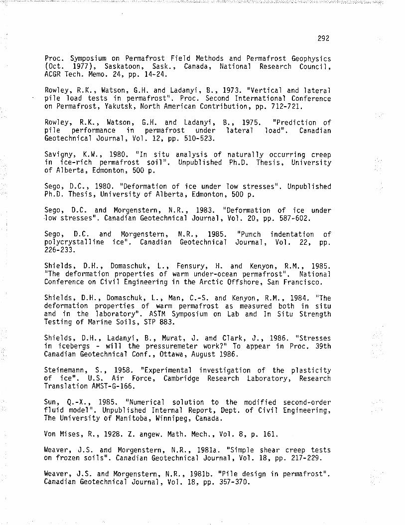
292

Proc. Symposium on Permafrost Field Methods and Permafrost Geophysics(0ct. L977), Saskatoon, Sask., Canada, National Research Council,ACGR Tech. Memo. 24, pp. 14-24.

Row'ley, R.K., Watson, G.H. and Ladanyi,8.,1973. "Vertical and lateralpi'le load tests in permafrost". Proc. Second International Conferenceon Permafrost, Yakutsk, North American Contribution, pp. 77?-72I.

Row'ley, R.K., hlatson, G.H. and Ladanyi, B., 1975. "Prediction ofpi'le performance in permafrost under lateral load". CanadianGeotechnical Journal, Vol . 12, pp. 510-523.

Savigny, K.lll., 1980. "In situ anaìysis of naturally occurring creepin ice-rich permafrost soil". Unpublished Ph.D. Thesis, Unìversityof Alberta, Edmonton, 500 p.

Sego, D.C., 1980. "Deformation of ice under low stresses". UnpubìishedPh.D. Thesis, University of Alberta, Edmonton, 500 p.

Sego, D.C. and Morgenstern, N.R., 1983. "Deformation of ice under.low stressesrr. Canadian Geotechnical Journal, Vol. 20, pp. 587-602.

Sego, D.C. and Morgenstern, N.R., 1985. "Punch indentation ofpo'lycrystal I ine ice". Canadian Geotechnical Journa'l , Vol . 22, pp.226-233.

Shields, D.H., Domaschuk, 1., Fensury, H. and Kenyon, R.M., 1985."The deformation properties of warm under-ocean permafrost". NationalConference on Civil tngineering in the Arctic 0ffshore, San Francisco.

Shields, D.H., Domaschuk,1., Man, C.-S. and Kenyon, R.M.,1984. "Thedeformation properties of warm permafrost as measured both in situand in the'laboratory". ASTM Symposium on Lab and In Situ StrengthTesting of Marine Soils, STP 883.

Shields, D.H., Ladanyi, 8., Murat, J. and Clark, J., 1986. "Stressesin icebergs - will the pressuremeter work?" To appear in Proc. 39thCanadian Geotechnical Conf., Ottawa, August 1986.

Steinemann, S., 1958. "Experimental investigation of the plasticityof ice". U.S. Air Force, Cambridge Research Laboratory, ResearchTransl ati on AMST-G-166.

Sun, Q.-X. , 1985. "Numerical solution to the modified second-orderfluid model". Unpubìished internal Report, Dept. of Civil Engineering,The Un i vers i ty of Man i toba , [,li nn i peg , Canada .

Von Mises, R. , L928. Z. angew. Math. l4ech., Voì. 8, p. 161

llleaver, J.S. and Morgenstern, N.R., 1981a. "Simp'le shear creep testson frozen soils". Canadian Geotechnical Journal, Vol. 18, pp. 2I7-229.

l{eaver, J.S. and Morgenstern, N.R., 1981b. "Pile design in permafrost".Canadian Geotechnical Journal, Voì. 18, pp. 357-370.

293

APPENDIX A

PRESSUREF{ETER CREEP TEST DATA PLOTS

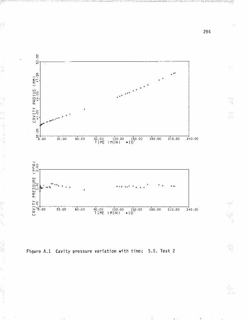
294

o?OØ

OoEr

='U)-O-aC)scsE.

FO-?cfq(J

++++ ++

++

f++l++ +++

+

.00

o?@_.D

;-o_95*LrJÉlo(J.)q* +

cDNt!E(L

!-s

> ^b'. ooCE(J

Fi qure A. I Cavi ty

+++ * + + +

90 .00 ¡ 20 .00 ¡ 50 .00TIHE f lllNì El0l

180.00 210.00 24 0 .00

t 80 .00 210 .00 240 .00

30 .00 60 .00 90 .00 I 20 .00TINE (IlIN} I 50 .00

ü10'

pressure variation with time; S.S. Test 2

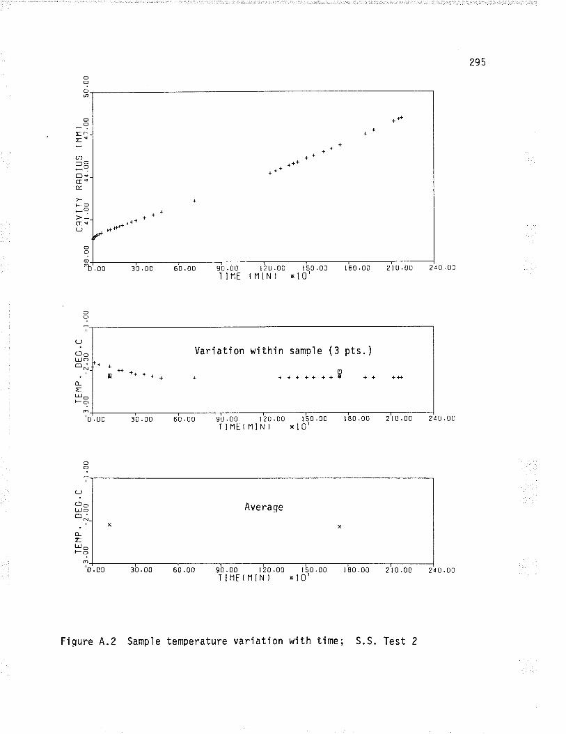
295ooOo

OO

Er

==a-O-Oo<cr<æ

l-o

-?Cfq()

+++

++++ ++

+_+

*+ +++* '

OO

@r-b'. oo 30 .00 60 .00 rzfj.00 r50.00 180.00 210.00 240.00(NtNÌ *10'

Variation within sample (g pts.)++E

* * ** * * * + + + + + + + + s + + +**

'0'.00 30 .00 60 .00 I 50 .00*10'

90 .00T INE

OO

oO

?CJOu-,oÉN

o_EL¡J o*g

?c)oLL, Oct ^:

(LELLJ otso

+l

9U .00 I 20 .00T IIlE ( N IN )

t80.00 210.00 24t).00

Average

0 .00 30 .00 60 .00 90.00 t20.00 I50.00 180.00 210.00 240.00T¡NEtNlN) ol0'

Fiqure 4.2 Sampìe temperature variation with time; S.S. Test 2

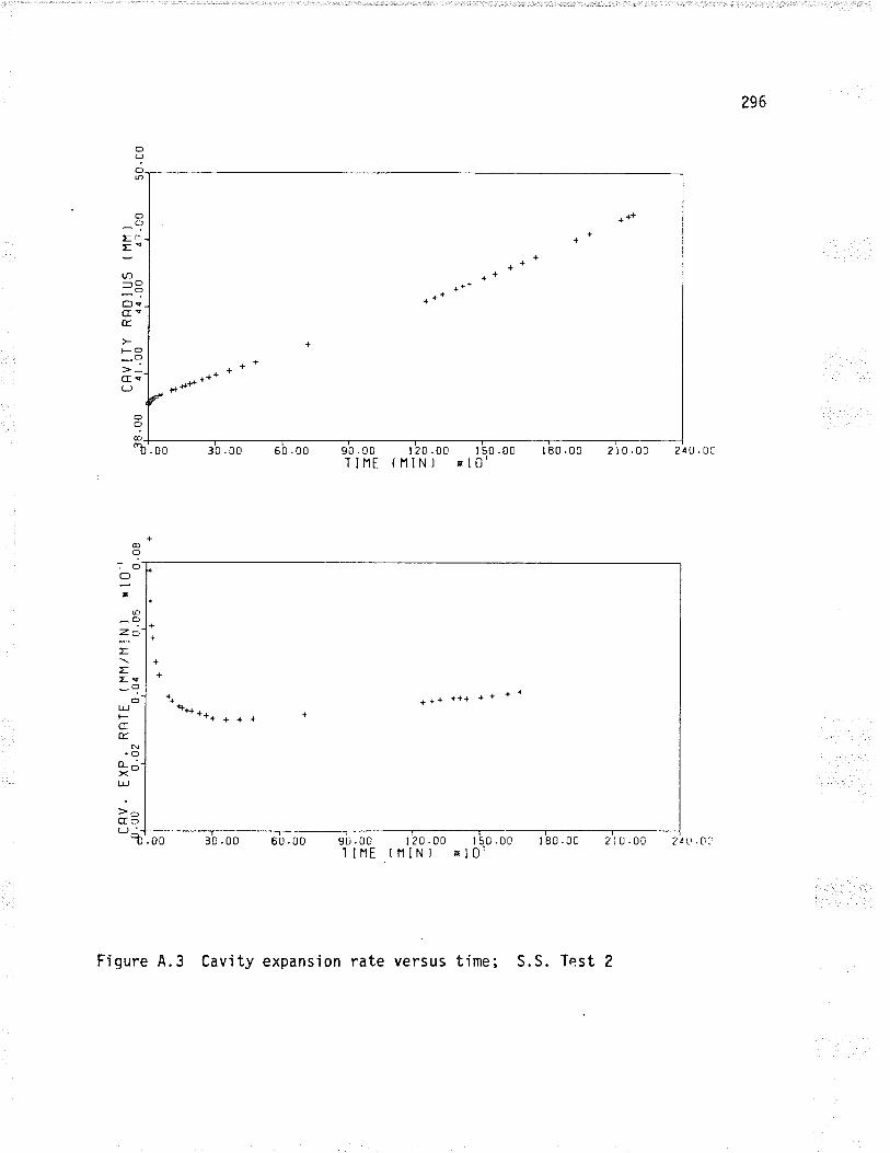
296

O?oØ

++

++++ ++

l+l}+++++

+

'b'. oo 30 .00 60 .00 I 20.00 I 50.00(11 INJ nl0'

180.00 210.00 240.0c

+

+

+

+

+++ +++ + + * *t**,

'+ + + +

30 .00 60 .00 ¡ 20 .00 t 50 .00(t1 lN) El0'

I 80 .00 z: u .00 24 Lr .0i

O(f

Eñ

:'U)-O-oC)?crÉ.

tso*?CJi(J

O?@

90 .00T INE

.00

@o,OOx

@

ZQ

;EEs-?.OLrJ

GÉ.

N

o- J-XLL,

>oCIo

I 90 .00T INE

Fiqure 4.3 Cavity expansion rate versus time; S.S. Test 2

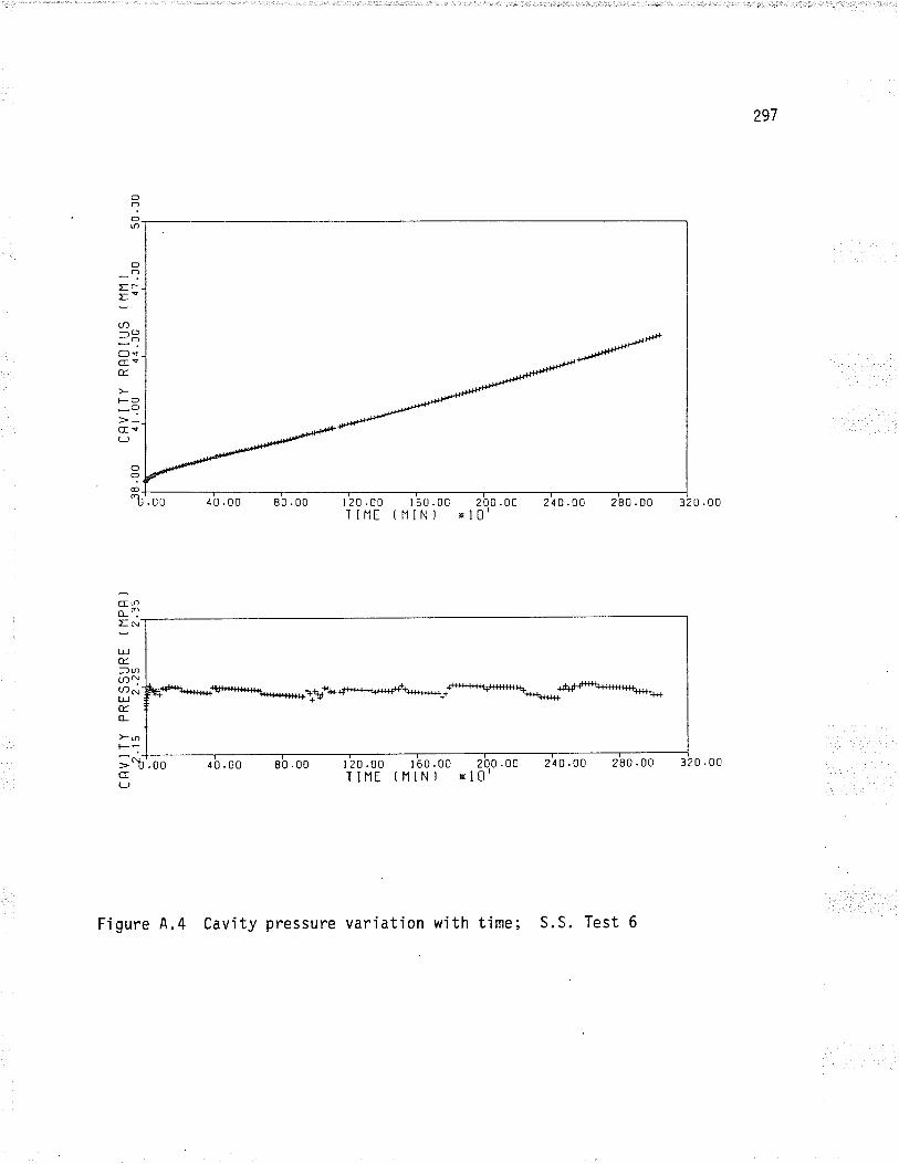
297

o?oô

ooEr

='Lt)--o-OOscsÉ.

+-o*9Ge(J

O?@-b'. oo ¿0.00 80 .00 I 20 .00 l 60.00 200.00 240.00

TIIlE (11lN) ol0'280.00 32U.00

240.00 280.00 0 .00

GÐo-13-l,¡JÉ=úØl(DNIJJÉ.o_

)-pF-

.00

ú

"b

Go_

=l,¡JÉ=U)(nIJJÉ.o_

:cr(J

¿0.00

F'igure 4.4 Cavity pressure variation with time; S.S. Test 6

I 20.00 I 60.00TINE (NIN}

200.00xl0'

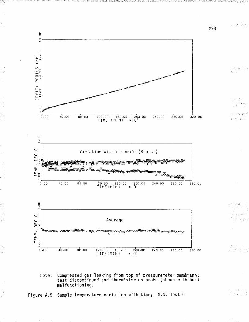
298O?OID

OO

fr

='U)-O_O

OTceÉ

tsO

-?ce(J

OO@_j_

'l'. on

O

sl

OI'0

cf?

?cJoLr,J c]o--

o-ELLl o*?

'0

.00

OI

?CJOti-i oON

o_Euo

40.00 80 .00 I 20 .00T IIlE (

I 60 .00 200 .00lllN) x10l

240.00 280.00 320.00

280 .00 320 .00

Variation within sampìe (a pts. )

ffiffiffir#s''#ryêffiæËffi.4æP@#Eç-- &@@o % qtr@6gqo* dryFdqffi**.wtrs* *

10.00 80.0u 1_29.u0 160.00 200.00 240.00IIIlE(NIN) !10'

¡çgu*ÞE@iu4*<x Ury,

Average

ry¡ðö¿r5ð#r. ¡¡+që*ì+t+ìèrèð8f¿Èfç vrx *$+rÉe{ðèrfðð+okÈ<

.00 ¡ 0 .00 80 .00 l20.rio t6u.00 200.00TINE(NIN) El0l

24 0 .00 280 .00 320 .00

llote: Compressed gas leaking from top of pressuremeter membrano;test discontinued and thermistor on probe (shown with box)ma I functi on i ng.

Figure 4.5 Sample temperature variation with tjme; S.S. Test 6

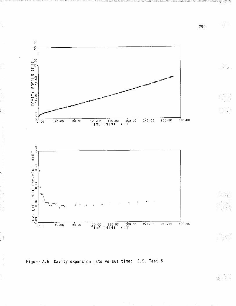
299

o?o\D

oO

EÈ

='tJ)-cl-aOqGeÉ.

.-.9G<(J

O

@-b'. oo

..1_-T¡b.oo 80.00 l-29:.0i...1.6.9:00 .200.00 zio.oo zeo.oo 32o.oo

TINE (11lN) xl0

10.00 80 .00 l 60 .00 200 .00(11lNl *10'

210.00 280 .0r) 320 .0c.00

@O

. olO

x

@_O

ZO

;EE!"=-

OLdFGÉ.

.Oo- --><"t!

>OCIo(J_-

I I 20 .00T I I1E

"-,"""".*--

+

++

++

Figure 4.6 Cavity expansion rate versus time; S.S. Test 6

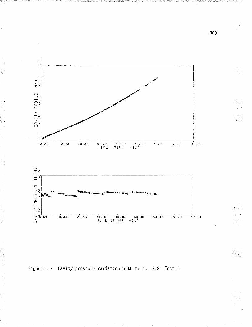
300

O?OØ

oO

=-E.

U)-O-oEsGeÉ.

l-o

-?c!!LJ

f

.00

öO

@-

"b 10.00 20 .00 60 .0030.00 40.00 50.0t)TIIlE tNIN] xl02

70 .00 80 .00

CTOo-:EN

l.¡JÉ.

=oØ?(f) st¡JE,o_

)-9FO

> 0,00CE(J

20.00 30.00 ¿0.00 50.00 60.00 70.00TINE tNIN) El0?

80 .00

Figure 4.7 Cavity pressure variation with time; S.S. Test 3

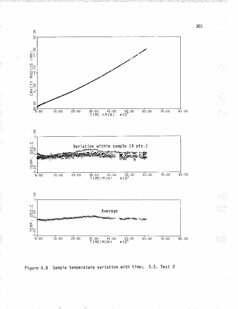
301o?OØ

ootr

==U)_O

OqGvÉ

l-o-?cEe(J

.00

o?O-

"b 70 .00 80 .00

?()oL¡J oo^'

o_

=L!oÌ-O

20 .00 30.00 ó0.00T INE ( H IN }

50 .00E l0?

60 .00

OO

Average

x }&çdå*kxryõr< X(>eår

20 .00 30 . OrJ 1 0 .00 50 .00 60 .00 70 . 00 80 . 00TlllE(11lNt xl02

t 0 .00 20 .00 30 . 00 { 0 .00 50 .00 60 .00TIIlE f lllN) El02

Tl-'0 .00

ol

:j

=ïo+'0'.

¿tl-Jcf

û_Et!F

.ë

oO

Vari at'ion wi thi n sampl e (4 pts . )

Figure 4.8 Sample temperature va¡iation wjth time; s.s. Test 3

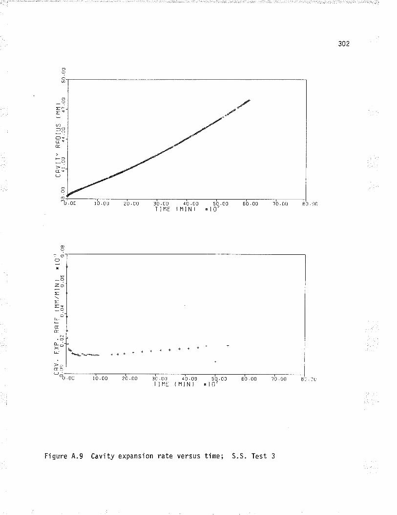
302

O?Oa

clO

Er

="(n-O-aclqc!É

tsc.-clc!LJ

.0c

OO

-ln 10.00 2A.OO 40.00 50.00 60.00t N IN ) n l0'

70 .0u 80 .0u

q+{r*au*al-r** ++ + + + + I + + a * +

I 0.00

30 .00T IIlE

@O

.O

:X

@_?Z.cEr*c

Ot!tscfÉ

.O

Xt-!

>cCfJLJ"

R .00 70 .00 8:r . i'u20 .00 30 .00 40 .00TIIlE (NIN}

s0 .00 60 .00x l0?

Ê


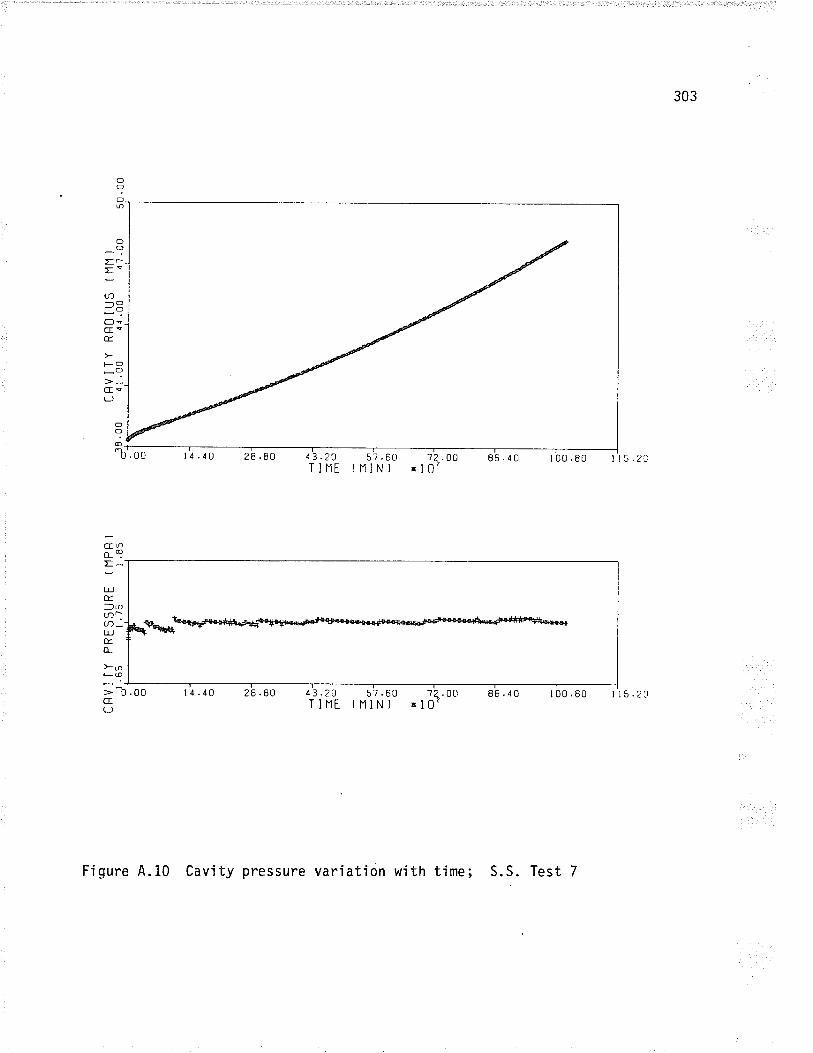
303

O?O6

O

TÈ

="U)-Õ-oO9GeÈ

FO

-?Ge(J

14.40

Gno_T

=-t!ÈlurrDlaf) _LUÉ.o_

)-6F@

(I(J

43.20 5?.60 ?2.OrJTIIlE tlllN) xl02

86.40 ¡00.80 ils.20

variation with time; S.S. Test 7

Á3.?0T IHE

5?.60 12.OOt N IN ) x I 02

86.40 100.80

> 0.00 l1 .40 28 .80

28 .80

Figure 4.10 Cavity pressure

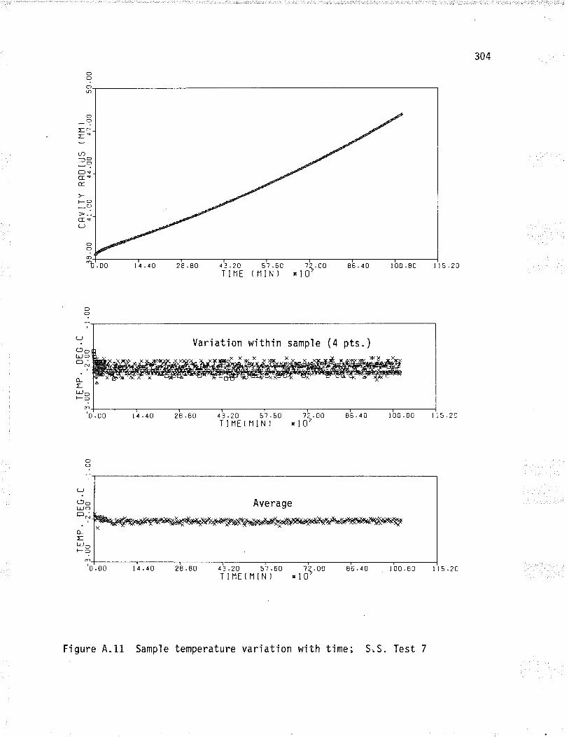
304

O?OØ

OO

Ir

='U)-O-oCleGqÉ.

l-o-.?CIT(J

oo

-ì¡'. oo I 4 .40 28 .80 86.40a3 .20T IIlE

57.60 11.00f N lN ) r l0'

100.80 il5.20

(JoL!oON

o_ELL, OF9

?()OL!, oON

o_Euo*?

Tr--0 .00 43.20 5? .6U 12 .OO

T INE ( ll lN ) x l0'100.80 lt5.2c86.40

Average

l¿t.10 28 .80

OO

0 .00 14.40 28.80 a3.20 57.60 ?4.00 86.10 t00.80 1t5.20TINE(NlN) xl0'

Vari ati on wi th i n samp'le (a pts . )

Figure 4.11 Samp'le temperature variation with time; S.S. Test 7

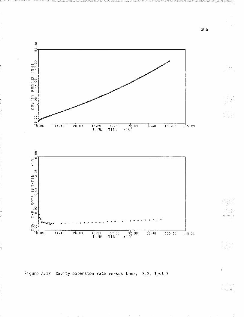
305

O?OØ

Oo

Er

='a-O-oOec!É.

tsO_(l

G!CJ

.0û

æO

;OOx

@

-OZO

;tEs_o

Ot¡-J

crÉ

.Oo-Õ-Xt!

>OCo

't

OO

@ _J_-b'. oo 85 .4tJ 115.2014.40 28 .80

ld./¡L) 2ts .8u

5r.60(11lN)

1? .OOo l0'

43,2OT IIlE

**++¡i++ +++++++t++++*+*¡l+*++++++++

A J.'¿U 57 .60 -ì? .t0TINE (11lN) xl0?

86.40 100 8Ll


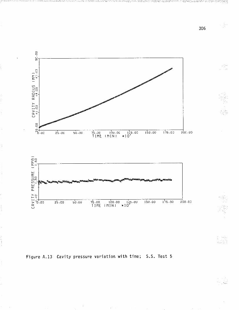
306

Oo

tr

='U)-O_O

OrGsÉ

tsO

-:cre(J

75 .00T IHE

I 75 .00 200 . u0

I ?5 .00 200 .00

;-o_9

=-LrJÉ=oØ2u)_tlJÈo_

)-9

-_ I> 0,00

G(J

lr25.00 50.00 ?.5.00 100.00 14s.00 150.00tlllt (NIN) xl0'

I U0 .0uININ)


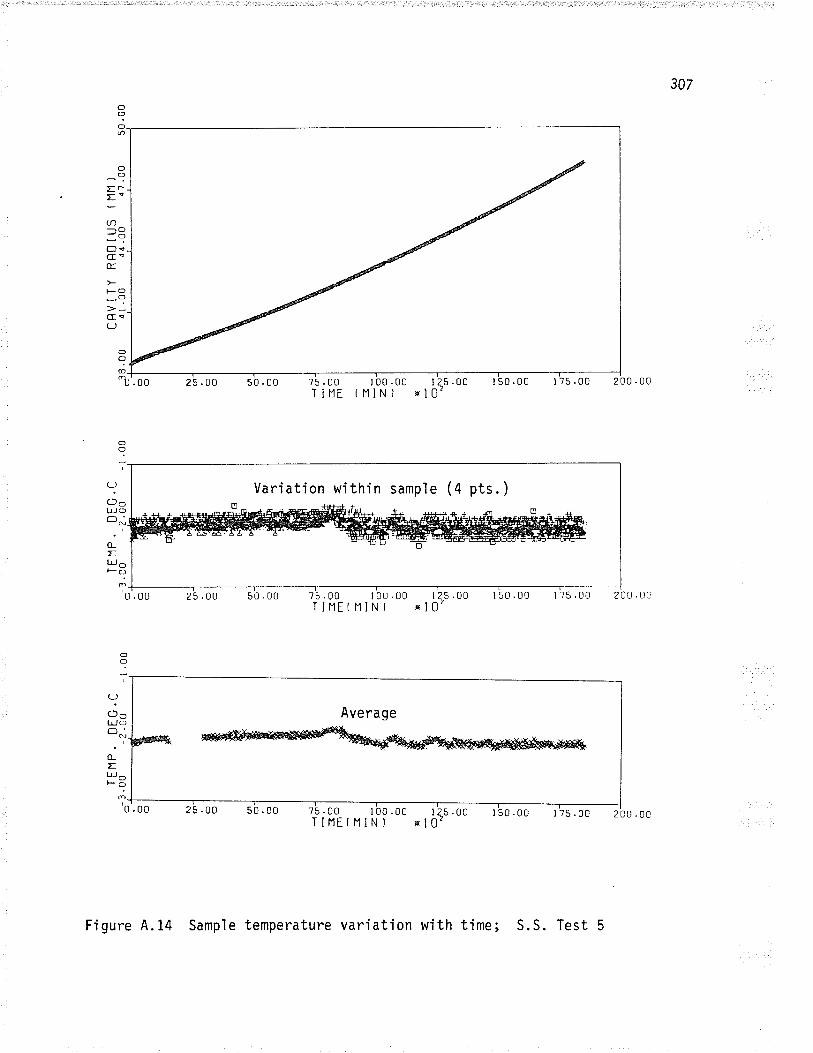
o?on

307

oO

Er

='ln_Ouo

OçG<É.

ÞO*?Ge(J

.00

o?,@_

n 25 .00 50 .00

0.00 25 .00 50 .00

75 .00T IIlE

s .00 0.00 I 75 .00 200 .00

I 50 .00 5 .00

?CJOt].J OoN

(LILLJ o*?

75 .00 l0u .00 r 45 . tiOIIIlE(11lN) xl0'

Average

00 25 .00 50 .00

2CU . Urj

O9

?lcJo IljJol-r{-lrluol*ql

T+0. 75 .00 1 00 .00

TIHEIIlIN)r as .00

x l0'1 50 . u0 l ?5 .00 2C0 .00


Figure 4.14 Sample temperature variation with time; S.S. Test 5

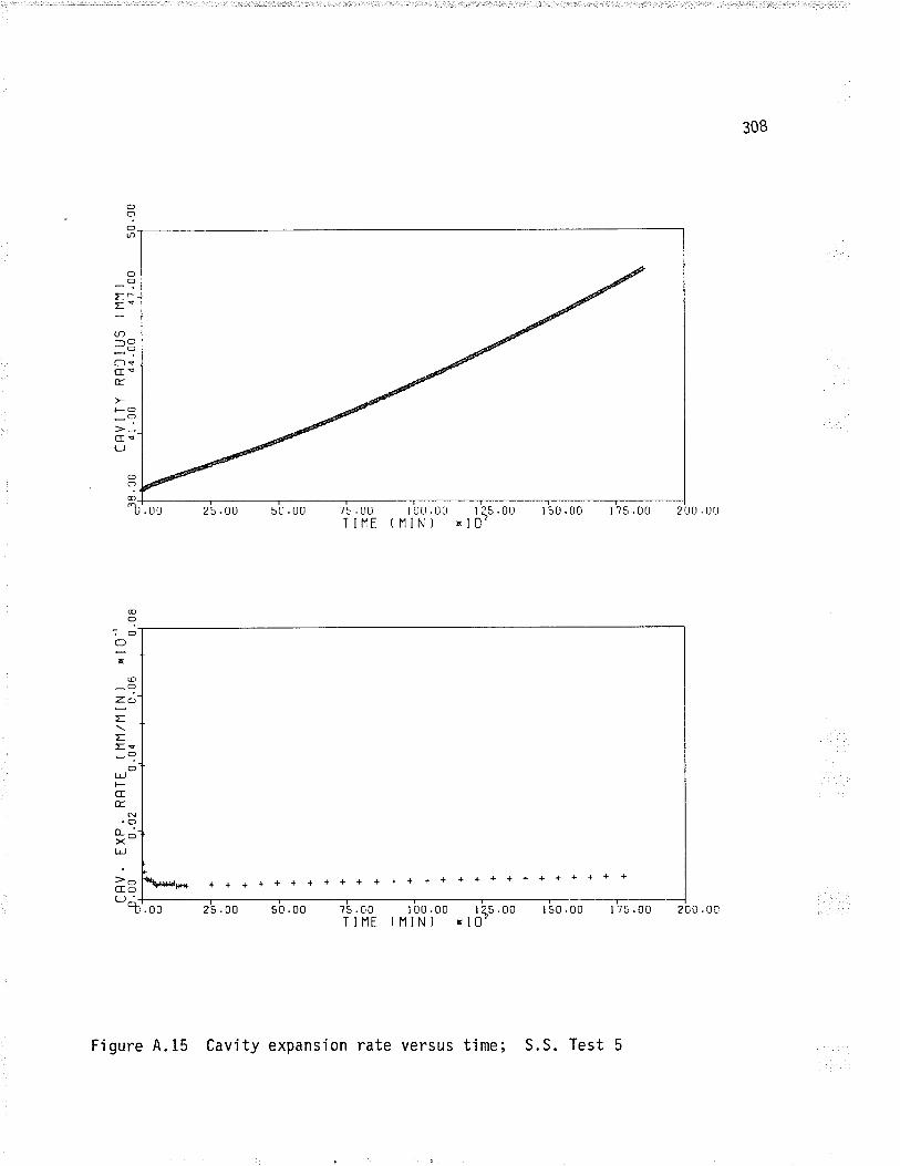
308

o?oÐ

(fO

Er

==U)-c)-oOscf<É

FO

-?G!(J

.00

OO

O-

U 25 .00

25 .00 50 .00

75 . LìU

T IIlEr 25 .00

x 102¡ 50 .00 t ?s .00 20tì .0rJ

.00

@()

Ox

o_O

-:-EEEç_o

O.LrJ

cÉ.

N

o- J=><llj

>OGcl

't+ + ++++ ++++ + ++ ++ ++++++++++ +

?5 .00T lrlt

r 00 .00 r 25 .00(11tNl !r102

I 50 .00 l 75 .00 200 .00


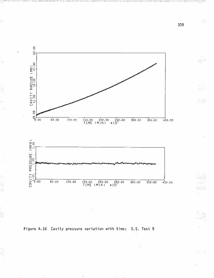
309

OO

OØ

oO

=r

==at)-O-oOeG<E

FO-.?cf!(J

r 00 .00

CIDo_T

=-t¡Jæ=nU)lln-UJÉo_

FoF_

>-b.ooG(J

I 50 .00 200 .00TINE (11IN}

.00 300.00 350.00 0 .00

variat'ion with time; S.S. Test 9

oo@-

"b .00 400.00l 50 .00T IHE

200 .00(NIN) 0xl

2t

0xl

Figure 4.16 Cavity pressure

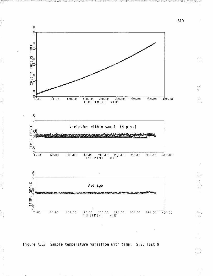
310

cf?on

(]o

EÈ

="U)-o-oClqG!É.

t-Õ

-9cEe(J

T IHE ( Il IN }

0 .00

400 .00

?()oLrJ o

o-EL!o*?

o

?(JoL¡J oo-'

o-'

o_

=uJo*?

'o', oo 50.00 I 00 .00 50 .00 200 .00 25-0 .00TINE(NIN) xl02

300.00 350.00

oo

Average

'0 .00 50 .00 t00.00 t50.00 200.00 250.00 300.00 350.00 400.00TIIIE(NINI '10'


Fi gure A. 17 Samp'le temperature variation wÍth tÍme; S.S. Test 9

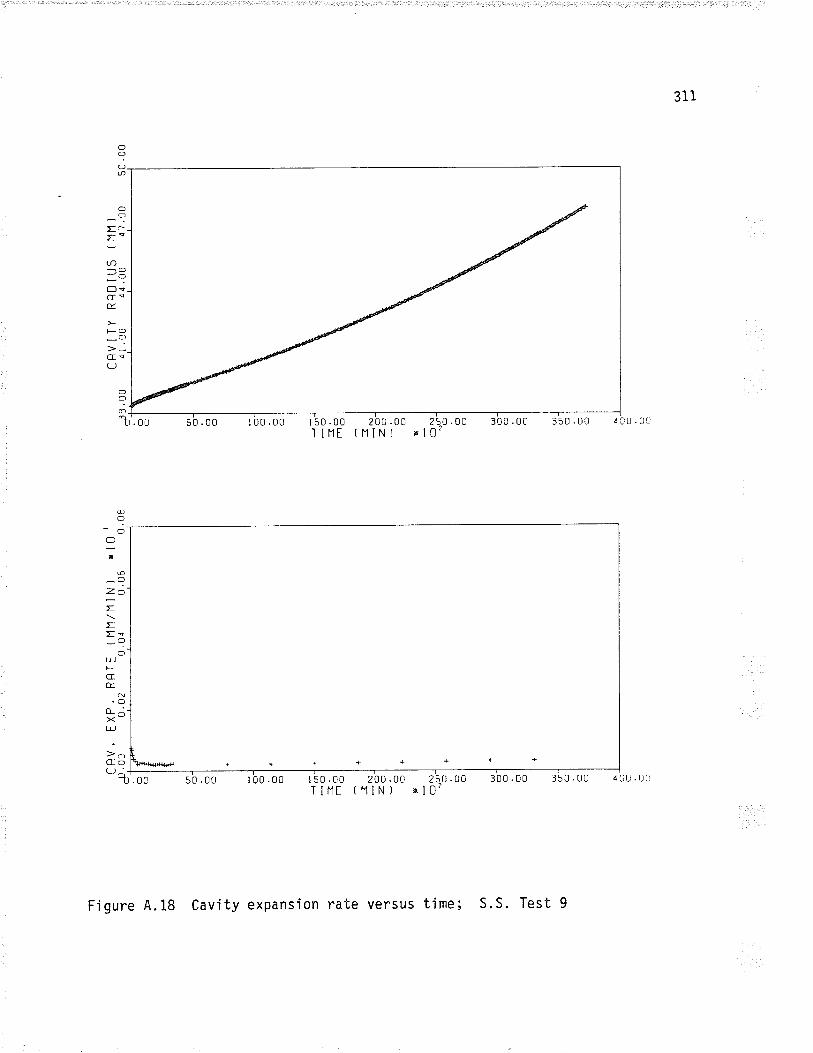
311

O?Oû

OO

-'U)-O_O

Oçcr<E

FO

-c)CIg(J

.00 5

OÕ@_

n .00 ¿ 0u . Lril s0 .00T INE

20u .00(tllNl

2

0.00 .00 350 .00

fl

.00

@C)

iO

?x

@

-OZO

;Its-?_

Ot¡-lFGæ.

.OrcXt¡J

)rrCOcJ;-

1 50 .00 t00.00 t50.00 200.00 25"tJ.u0 300.00 350.0c ¿0u'00TIIlE tlllN) xl0'

Figure 4.18 Cavity expansion rate versus time; s.s. Test 9

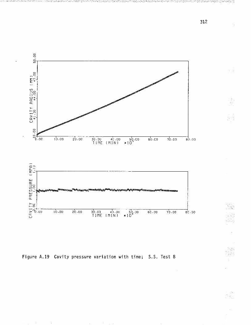
3r2

oO

Er

='Lr)

-O-oOçG!É,

tsO

-?G!LJ

10.00 30 .00T INE

40.00fNIN)

50 .00x l0'

60 .00 70 .00

t 0 .00 20 .00 30 .00 ¿0 .00 sb . ooTIHE tNIN) xl03

r¡t60 .00 70.00 80 .00


.00

COo-:L-

LlJÉ=oØ?(¡) _.LtjÉo_

)-9t--o

>Rcf(J

o?OØ

20 .00

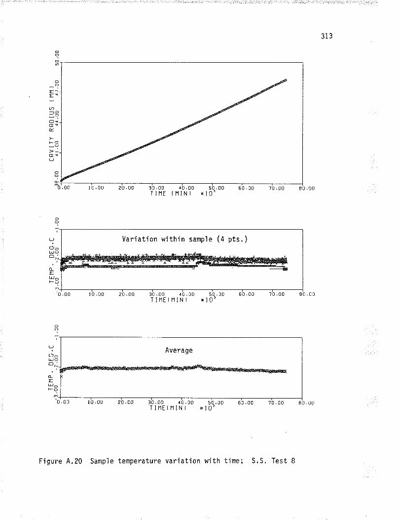
313

o?oØ

oE-

==U)

-oC)scEeÉ.

|-o-?cE!(J

Oo

?ôLrJo

o_EtrjF

TINE (NIN)

30.00 40.00TIIIEfIlIN)

50.00EIO3

oO

i(JoUJÕoN

o_Et¡J o-?

Average

'0 .00 10.00 2b.00 30.00 ¿o.oo s'0.00 s'o.oo zb.oo ab.ooTIHE(NIN) xl0l

VariatÍon within sample (4 pts.)

Figure 4.20 Sampìe temperature variation wjth time; S.S. Test I

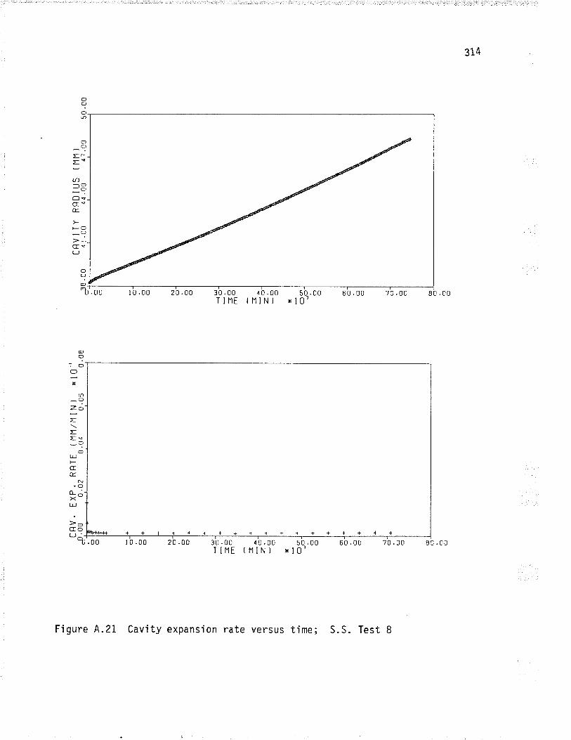
314

o?OØ

Oc)

Ir

==U)-(f_O

OscE<É.

C)

>-..cEs(J

.00

o-OZO

;EEç-O

Ot!FGÉ.

N.oo- o-Xt¡J

>OCfo(J_-

I

oo-:"b .00 20 .00 40.00

(NIN)50 .00

X I0360 .00 ?0 .00 8C.0u

4+++ +{++++++ ++t0.00 20 .00 10.00 50.00

tHIN) Rl0r60 .0u ?0 .00 83. C0

30 .00T IIII

@o,O(f

x

30 .00T INE

Figure 4.21 Cavity expansion rate versus tjme; S.S. Test 8

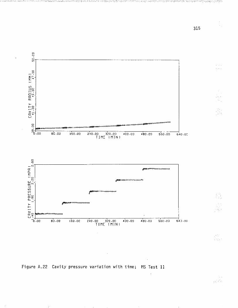
315

o?oØ

oO

=r:'U)-Õ-oOçG!É

+-o-?G<(J

240.00T INE

320 .00(lllN)

4 80 .00 560 .00 640.00

#@Þl++l+r{#l+H{-+++++

+@.{#+Ftsl+rHi"{+++

ff***{&'¡*{ri¡t-t-+t-}t

+t++fir++

80 .00 r 60 .00 240.00 320.00 400.00TINE f IlIN)

480.00 560.00 640.00

pressure variation with time; Ì4S Test i1

.00

O@

N

CEo_E-o(!l.¡-l '-EN

=1!)u')LJorBo_ ._

+-

-Oö:1;

I 60 .00 ó 00 .00

F'rgure A,.22 Cavity

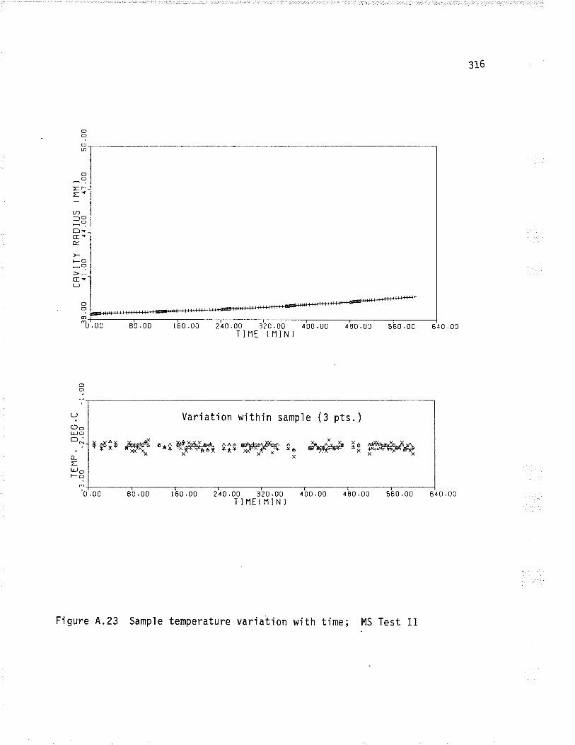
316

O?Oa

OO

E-

==U)-O-oOsG!É

|-o-?CEs(J

I 60 .00 21 0 .00 320 .00 ¿ 00 .00TINE(NIN)

640 .00

480.00 560.00 640.00

T INE

OO

Yc)oT¡J OON

o_z.uJo*g

o

Variation within sample (3 pts. )

ð#îu W FAçW¡S îieçryry îa en{l-Þ x9 @x4

0 .00 80 .00

Figure 4.23 Sample temperature variation with time; MS Test 11

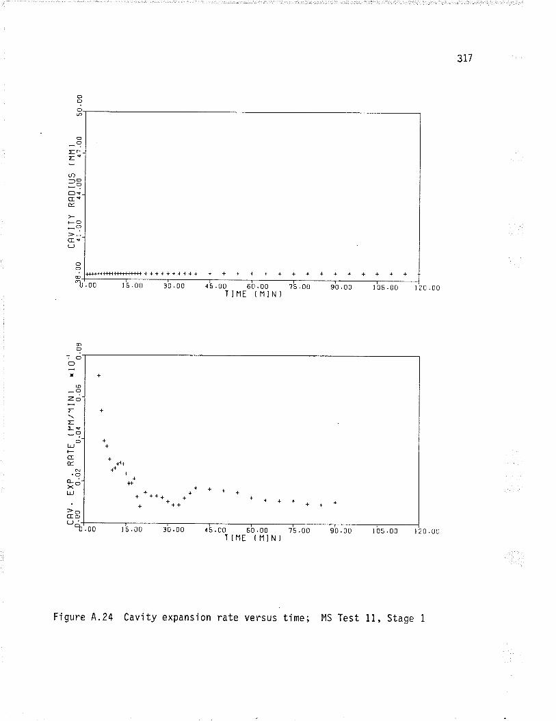
3r7

oOØ

OO

Er

==U)-o-oÕqc!É.

FO

-?ct!(-J

@o,oOÍ

@

-OZO

E

EEe-oclUJl-crÉ.

N.oL:-><LiJ

>oGO-%

++++++++++ + + + + + + + + + + + + + + +

t5.00 30 .00 45.00 60.00 r's.ooTINE (NIN)

.00

O?@_

"b I ì_90.00 I 05.00 120

.00 t 5.00 30 .00 45.OO O'O.OO r'S.OOTIHE f IlIN)

¡¡t90 ,00 1 05 .00 t 20 .00

++

I++ **+

++ **** * 1 + *++++++

Figure 4.24 Cavity expansion rate versus time; l1S Test 11, Stage

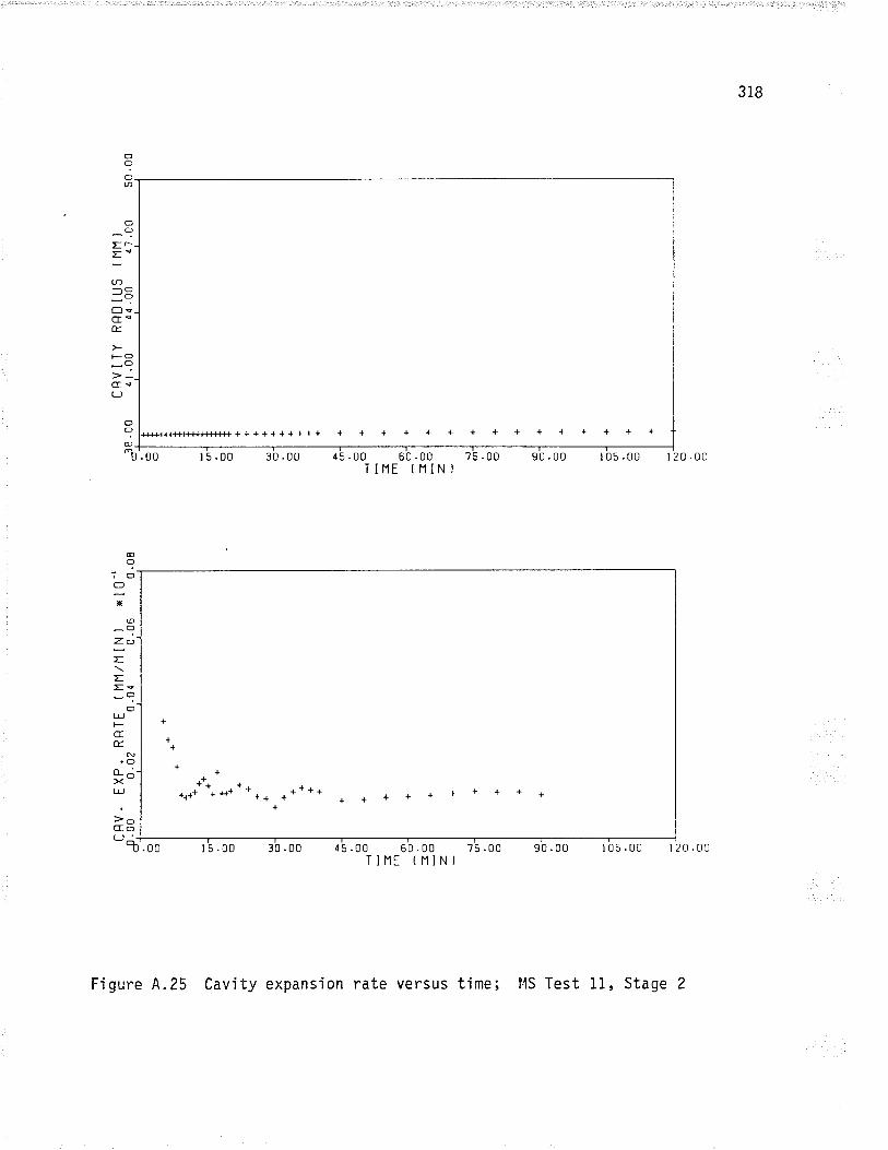
318

o?ov)

OoE-

='U)-O"ÕOs(r!æ.

F-O

-?cfec)

l#rr+H-H++Rl++++++++++ + + { + + + + + + + + + + + +

-b'. oo t5.00 30.0u

o?@

45.00 60.00 ?5.00TINE (HIN)

I 05 .00 I 20 .0090 .00

+.+

*.J******** *****+

00 15.00 30.00 ¿5.00 60.00 ?5.00 90.00 105.00 t20.0cTIIlE (NIN)

@O

,oCf

Ë

@

-ozà-E

==v_o

Ot!l-CIÉ.

N.C)o-;-><l,!,

>OCocJ^-I

Figure 4.25 Cavity expansion rate versus tjme; t4S Test 11, Stage

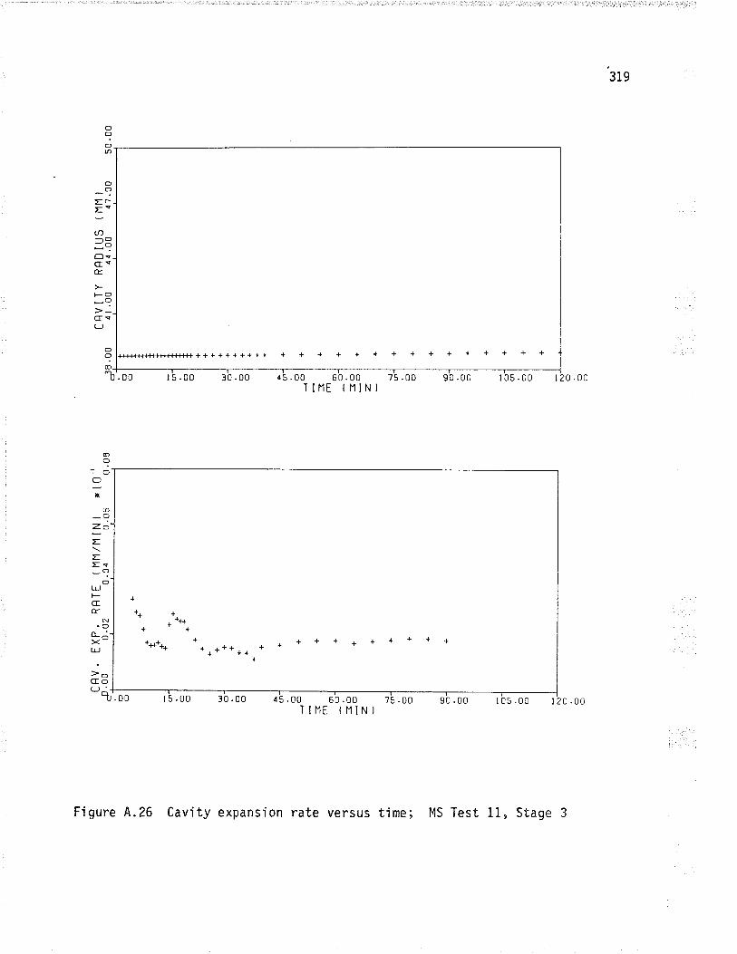
319

cf,

?Oú)

++++++++++ + + + + + + + + + + + + + + +

'b'. oo t5.00 30 .00

ooErE=

U)-O-ooq

æ

FO

-?G!(J

O?o

@o

,O

=xo

_OzÒ

;=Eç_o

Ol,!FcfÉ

N.oo--'fX]rrl.t=-lCol(J:-.1

U .00 t5.00

d5.00 60.00 75.00TINE f NIN)

90 .00 I 05 .00 l 20 .00

I

90 .00]-

l 05 .00 I 20 .0030.o0 4's.00 sb.oo rb.ooTINE IIlIN)

***+++'# ++ * . + + + 4*++*++++++

++

Fiqure 4.26 Cavity expansion rate versus time; MS Test 11, Stage

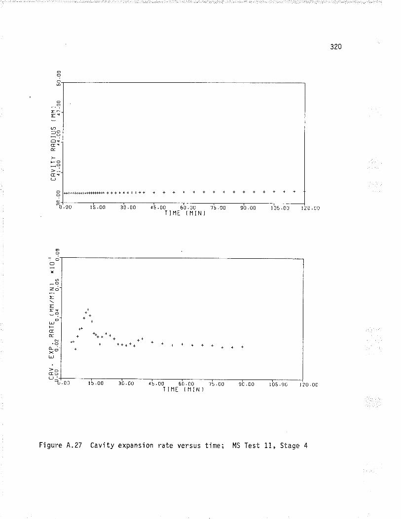
320

o?OØ

oO

E-

='a!)

-O-oOsG!É.

FO

-?G<L)

++++++++++

t5.00 30 .00

OI9lqr .00 45.00 60.00 75.00

TIHE IIlIN)90 .00

I _I 05 .00 r 20 .00

.00

@O

,OOT

@_(fz¿-

=EEç-?oL¡Jl-cÉ.

N.oo- --Xt!

>OCfoLJ ---1J

\****+ +++++

+{

l5 .00 3b.oo ¿b.oo s'o.oo r's.ooT IHE ( H IN }

I ]_90 .00 t 05 .00 1 20 .00

Figure 4.27 Cavity expansion rate versus time; MS Test 11, Stage

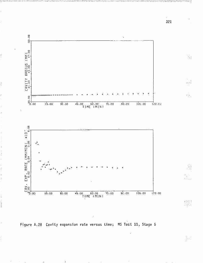
321

o?oø

c)o

=È

==(t)-O"oClqGqÉ

F_O

-?crs(J

o?o

{'{-{+++lÈH*l-+Fl-R++++++++++ + + + + + + + + + + + + + + +

.00

@o,OOø

@

^(]z.¿EEE<-?OLrJFCEÉ.

N

o-¿)<t!

>oCEo(Ji

oo

t

"b'. oo I 5 .00 30 .00

t5.00 30 .00

15 .00 60 .00 ?5 .00TINE (IlIN)

s0.00 105.00 120.u0

90.00 105.00 120.0045.00 60.00 ?5.00TIIlE f NIN)

+*+

++++++++ {+'+ *+* + + + + + + + + 4 *

*****

Figure 4.28 Cavity expansion rate versus time; l4S Test 11, Staqe 5

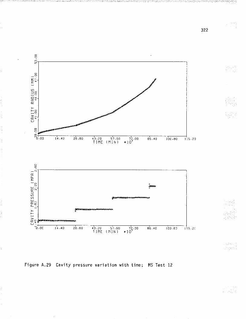
322

E

=U)

=ocfÉ.

F

CELJ

o?r

O?

c)?;

ooæ_

U

.00

O@

-Ncto-E

ON

t!'-olN=tJ)tJ-)tjJÈ3o_ '_

l-

col(J:-

-b

28 .80 43.20T INE

57 .60(t1lN)

74.00r l0'

I 00 .80 l l5 .20

11.40 28.80 a3.?O 5?.60 't1.OO 86.40TIIlE tlllN) rl0' 100.80 il5.21

+æ{É+

Figure 4.29 Cavity pressure variation with time; MS Test 12

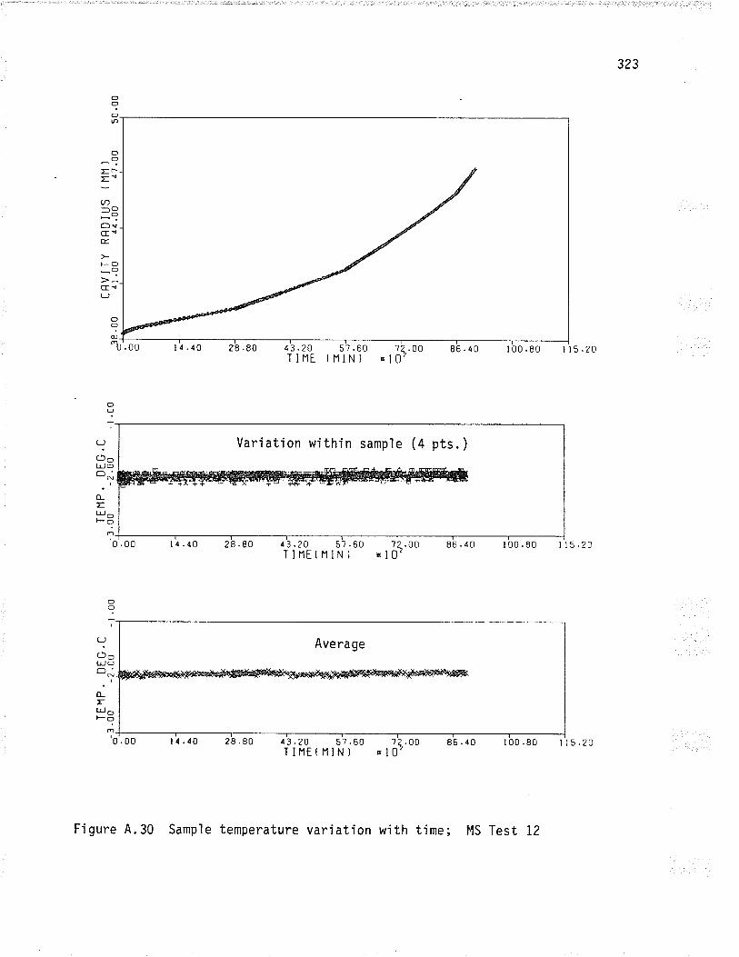
323

o?ou)

oO

E-

="U)'-o-oÉlqG!É.

FO

-9cEe(J

?C.fLr,Õ

o-=TLJF

.00

ooæ_

n

?

'I_lol*Ë's

I

-lol.lT+0.

oo

43.20T IIlE

57 .60( lllN l nl0

7 .00 86.40 100.80

?(JoLL, oo_'

(LEL¡J Õ*?

Variation within sample (a pts.)

l1 .40 28 .80 43.20 5?.60 ?2.00 86.10 t00.80 il5.20TIllEtlllNl ol0?

Average

'0 .0o td.10 zB.Bo Á'3.?o si.so 7a.00 86,10 l00.BO t't s.zoTINETNIN) *10'

Figure 4.30 Sampìe temperature variation with time; t4S Test 12

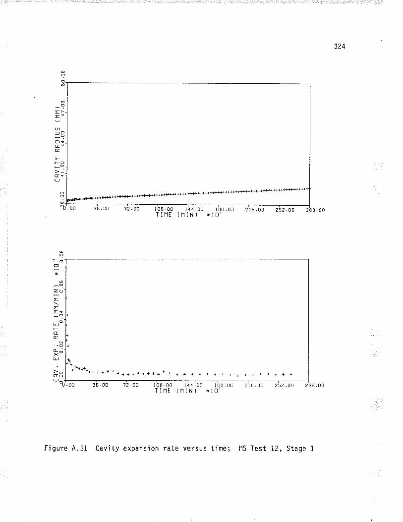
324

o?oLt)

oO

Er

='U)-O-oEçcE<É.

)-o-Oc<(-J

.00

@o

,OO

X

@

-o4O

E

==e*?

c)t¡Jl-CEÉ

N.oo-J-Xt!

>OGO(J^-

-t)

oO

@_

"b 2r6.00 25? .OO 288.00I .00INET

l4¿.00(NIN) I 80 .00

El0'

+

t*+******** + + * * + + + + + + + + + +++++++ ++

36 ,00 72 .00 I08.00 144.00 t80.00TIHt (11lN) El0'

2 ì 6 .00 252 .OO 288 .0C

Figure 4.31 Cavity expans'ion rate versus time; llS Test 12, Staqe

325

oooú)

OO

EÈ

==U)-cf-oOsG9É.

F-O

-?cEs(J

o?6

+++1+++14

-b'. oo 36 .00 '12 .oo t1¿.00 t80.00(HIN) xl0'

2 I 6 .00 252 .OD 288 .00

[þ******++++**++++++*+ + + + + + + + * + + + + * * * +

36 .00 72 .oo t 08 .00 t 44 .00 1 80.00TIIlE f NIN) xl0'

2 r 6 .00 252 .OO 288 .00

I 08 .00T IHE

.00

@O

,oOX

@

-OZ.oEEEç-9.OLrJi-cÉ.

N

X-t!

>OCEo(J '-'t

Fi gure A. 32 Cavi ty expansion rate versus time; MS Test 12, Stage

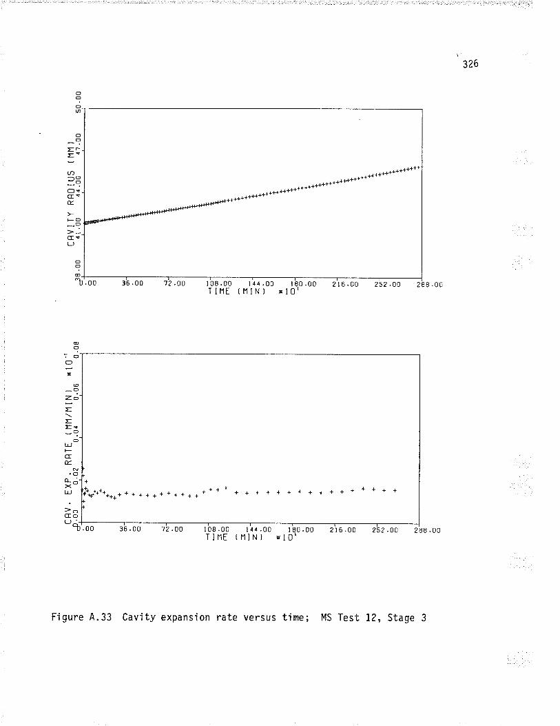
3?6

o?otn

++ #+ ++#++ + +#*{-}++ +++++++++{-}+{-}{4++++++++++++++++

+

36 .00 7?.OO 108.00 l{4.00 t80.00TIllt (NIN) El0l

I

2 I 6 .00 252 .OO 288 .00

?+*******++++**+*++**** * + + + + + + + + * + * * * + +

36 .00 7?.OO 108.00 I4a.66 180.00TIIlE (NIN) ã10'

rtt2 I 6 .00 252 .OO 288 .00

oO

Er

=*U)-O-oÉlqGeÉ.

ts()-?cEs(J

.00

otol;l"b'

.00

@o,ooI

@

z.¿-

=EEg-cfol¡Jf-CEÉ.

N

o-;-xt!

>OCEoI ì '--Ì

Figure 4.33 Cavity expansion rate versus time; MS Test 12, Stage

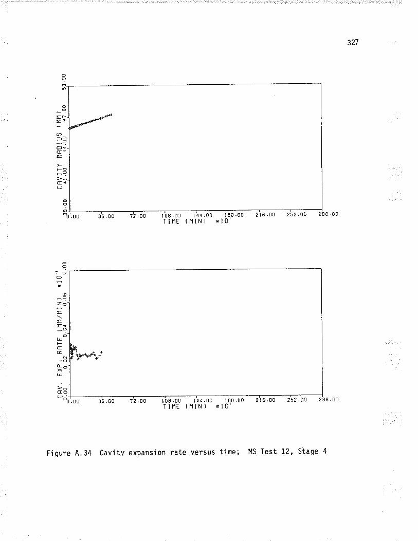
3?7

c)?oD

o(f

Er

='(t)-O-oOqcr!É

FO

-?c!(J

@(f

Ox

@_OZO

EEE?-?Ot¡Jf-CIÉ.

.00

o?@-

"b 216.00 252.O0 288 .0036 .00 72.DO

¡

72.OO

r 08 .00TIIlE

I 14 .00ttllN)

I 80 .00xl0l

i#¡\dd4 ++4t+

t__l^-l---T.oo 36.00

N.oo-¿Xt!

>oCEo

t08.00 144.00 1q0.00 216.00 252.00 288.00ilNE (11lN) xlo'

Figure 4.34 Cavity expansion rate versus time; MS Test 12, Staqe 4

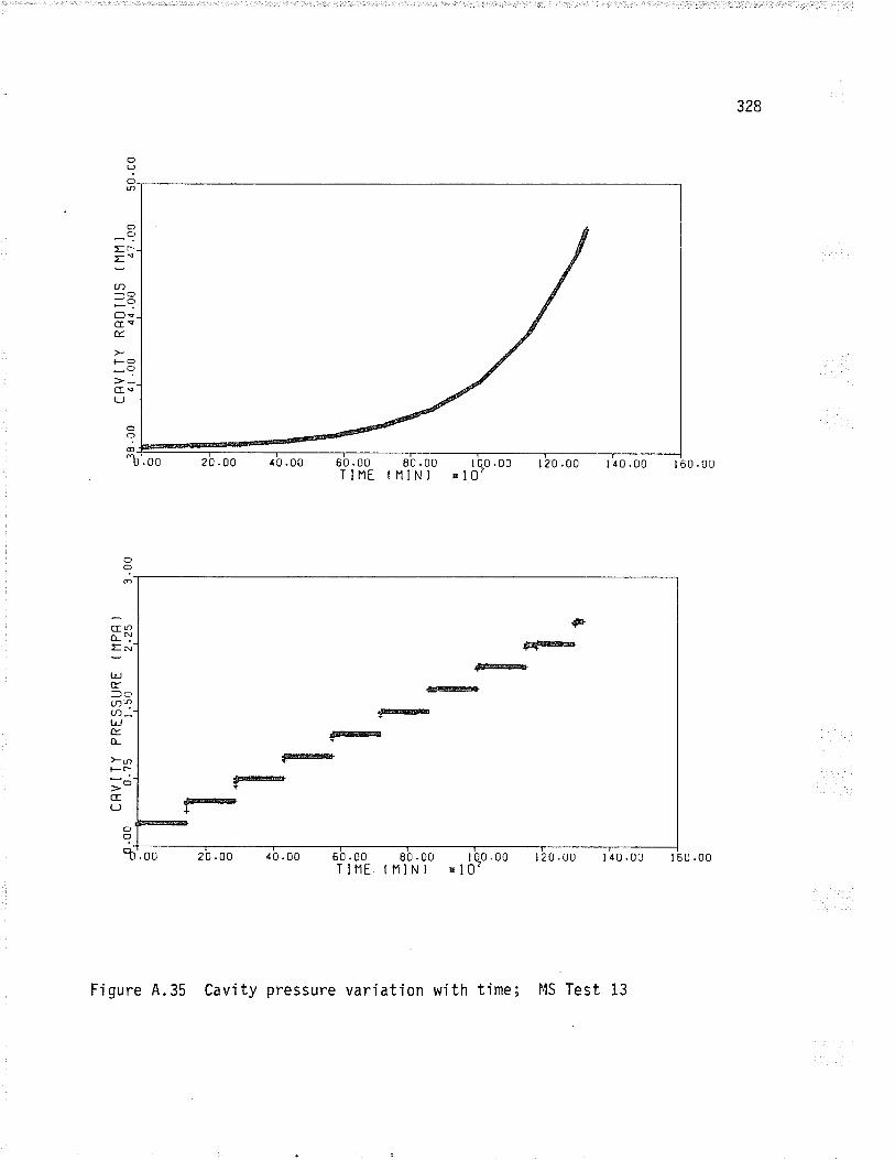
328

ooob

oO

E-

==U)-O-oOçc!çÉ.

FO

-?G!(J

(:t

?@_

"b

OI

.00 t40.00 I 60 .00Ï INE

@

fryry

l@@

ryffi

ryB@F+

.00I

0xl80 .00

(rllN)

GDo-l5*t!æ=ou)\n,u)-l,!,É.o_

F6|-r

CE(J

oo

20 .00 40.00 I 00 .00 I 20 .00x l0'

I 40.00 I 60.00R'.oo 60 .00 80 .00T Ir1E. f rl lN )

F'i gure A. 35 Cavi ty pressure varÍation with time; l4S Test 13

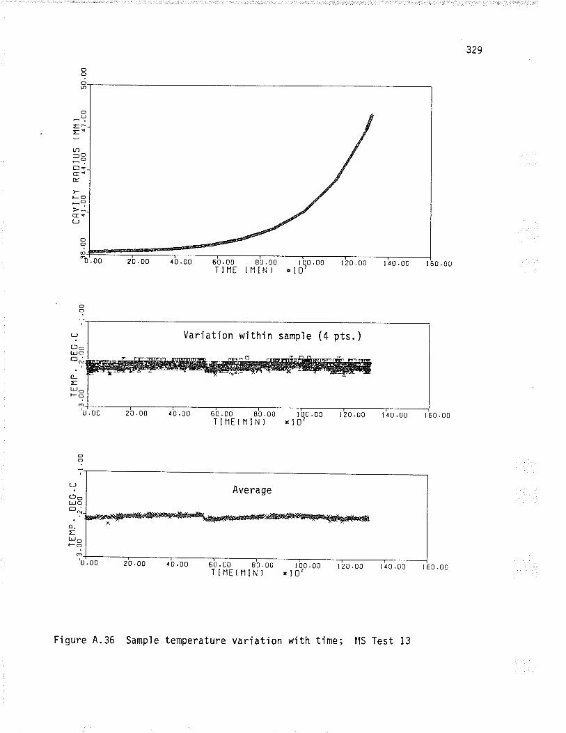
329

oooÚ>

ooEr

='(t)-'l o-oOçCJqÉ.

l-o*?ce(J

r 60 .00

?c)t¡L¡J oo^1

o_

=l,¡J ol-g

60 .00 80 .00TIIlE(11IN)

120.t)0 140.00 0.00

LJ

()oLTJ OoN

o_Et¡J ^Fõ

;'0'.00 20 .00 ;0 .00 80 .00 I 00 .00TIllttNIN) xl0' r20.00 ¡40.00 1 60 .00

I

0xl

I 00 .00E l0z

oO


Average

Figure 4.36 Sample temperature varÍation with time; llS Test 13

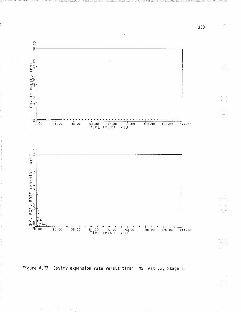
330

(f

?oø

clO

==U)-O-oOsG<É.

FO

-?C<(J

r{t{Èt-**lrtFt + + + + + + + + + + + + + + + + + + + + + + + + + + + + + + + + + + + + + + +

36 .0t),OU

OI@:

n ¡26.00 I4¿.0054.00T I HE

77 .OO(l1lN) 90.0rJ

x l0'I 08 .00

.00

@O

.OOx

@

-OZO

E

EEs-?Ol,¡J

-Gæ

N

o- ¿-><t!

>OGO-t 36 .00 54 .00 1? .O0 90 .00

TINE tlllN) 'l0l108.00 126.00 14d.00

++

+

r+è++,,_

Figure 4.37 Cavity expansion rate versus time; FIS Test 13, Stage

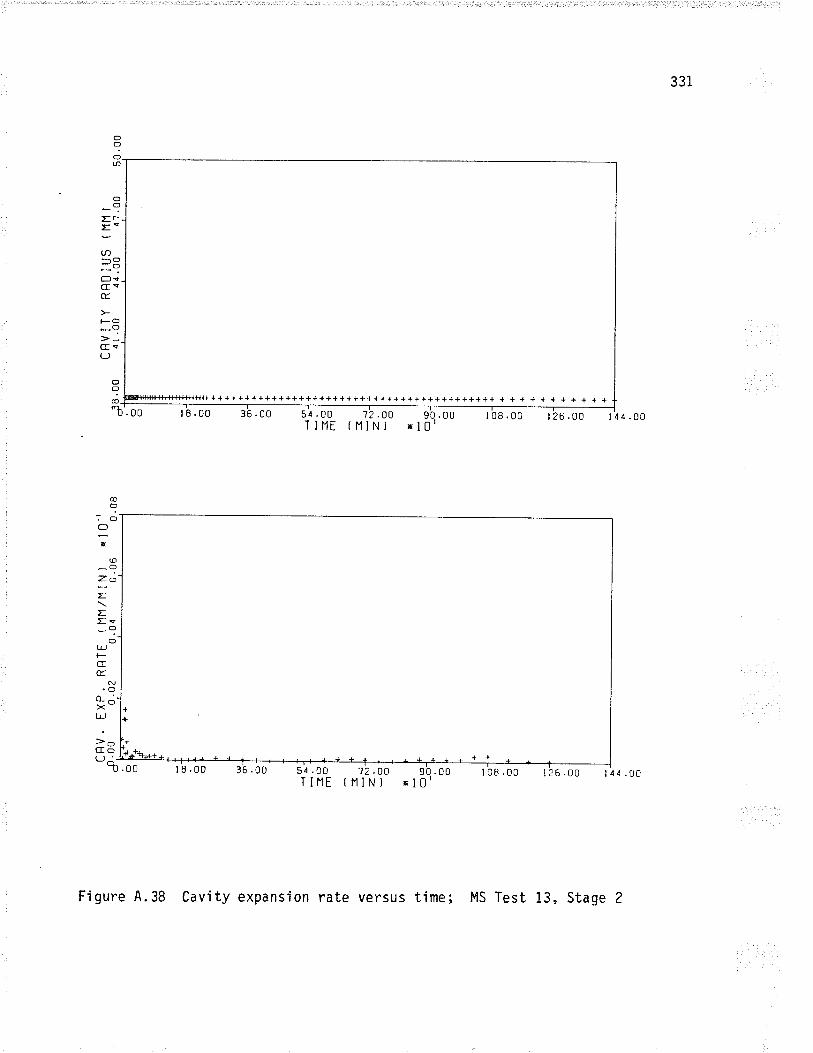
331

;:U)

=FGæ.

l-

(T(J

O

on

o?-

O?

o?

olol'J

Ft'

oO

,Ocfx

o_OZOEEEç-?cft¡JFGE

N.O

o-;-X_l"L,

>OCEo(J '-

'b

++++++++++++++++++++++++++++++++++++++++++ + + + + + + + + + + +

.00 18.00

18.00 36 .00

36.00 54.00 1?.OOÏINT (11IN)

I I

---1

90..00 108.00 t26.00 144.00xl0l

.00 51 .00T INE

72 .00 90 .00(HIN) Ã10'

I 08 .00 t26.00 I a a . g¡

2Figure A.38 Cavity expansion rate versus tíme; MS Test 13, Stage

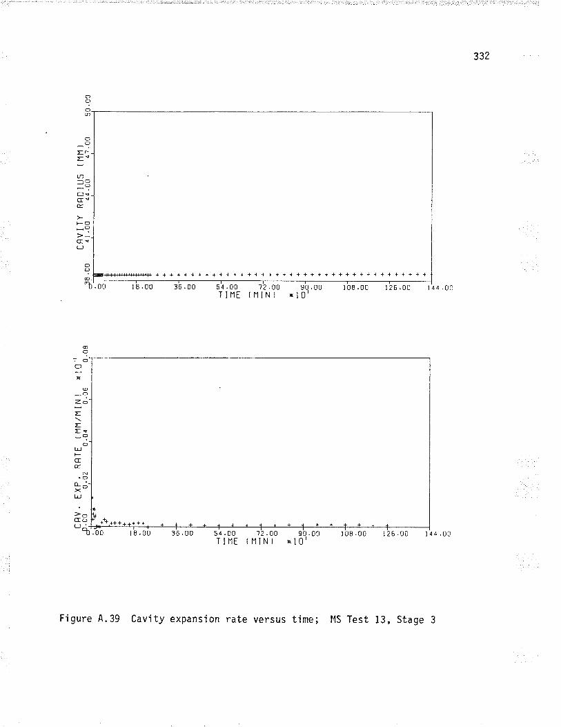
33?

ooØ

c)O

tr

='Lr)

-O-oo!csÉ.

FO

-?ccs(-)

+ ++++++++++ ++++++++ + +++++ +++++ +.1 + + + I + + +

o?ó'b'. oo 1 8 .00 36 .00 54.00 12.00 90.00

TINE (11lN) xl0' 108.00 126.00 l4a.g¡

+++.++++¡+++

18.0u 36.00 54.00 't?.oo 90.00 t08.00 ¡26.00 laa.g¡TIIlE (NINì kl0l

.00

@O

,OOx

C)

zaEEEs-?L!,|-cÉ

N.oo- --><l,¡J

>ÕCEO(J_-

I

Figure 4.39 Cavity expansion rate versus t'ime; t4S Test 13, Stage

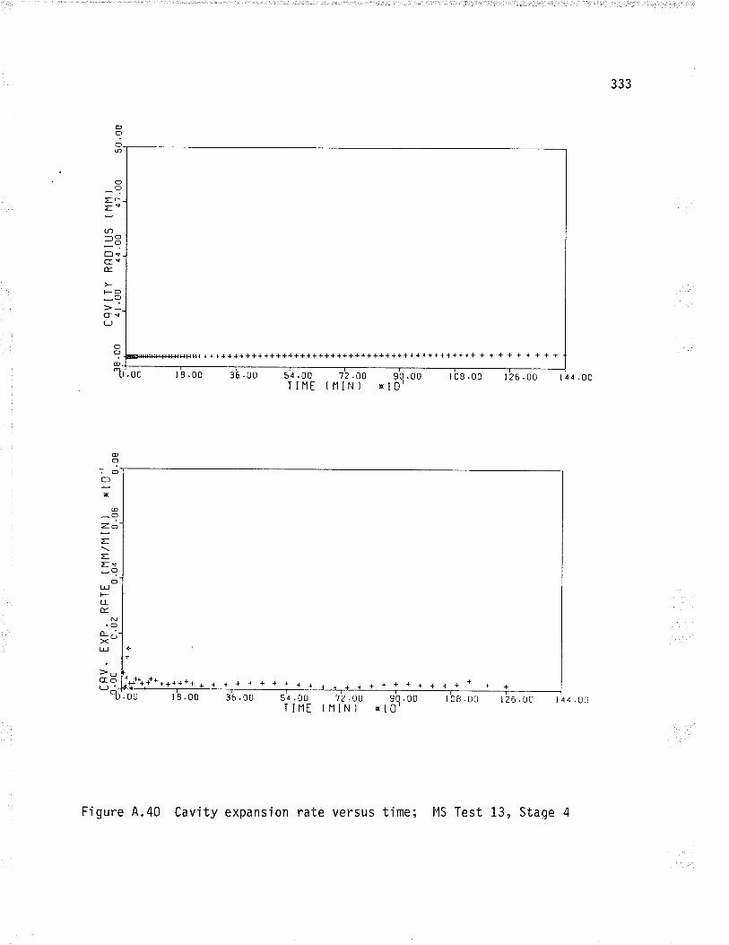
333

o?oØ

oO

=-='(n_O-oÐqG<É.

FO

-?c!(J

o? +++++++++++++++++++++++++++++++++++++++++++++ + + + + + + + + +

"b'. oo t8.00 36 .00 s¡ . oo 't'z .Do sb . ooTIHE tNIN) '10'

r _108.00 ¡26.00 l4a.¡g

.00

@o'oc)¡t

@_OZO

E

EEs_o

oL!Ì--crÉ.

N.ÕL--><"t!

>OCEo

-%

++

l1r**,********* a * * + + + + I + + ++++++++*++lB .00 36 .0rl 1? .OO

ttllN)54 .OrJ

T I NT90 .00

xl0l108.00 t26.00 l4a.¡3

Figure 4.40 Cavity expansion rate versus time; llS Test 13, Stage 4

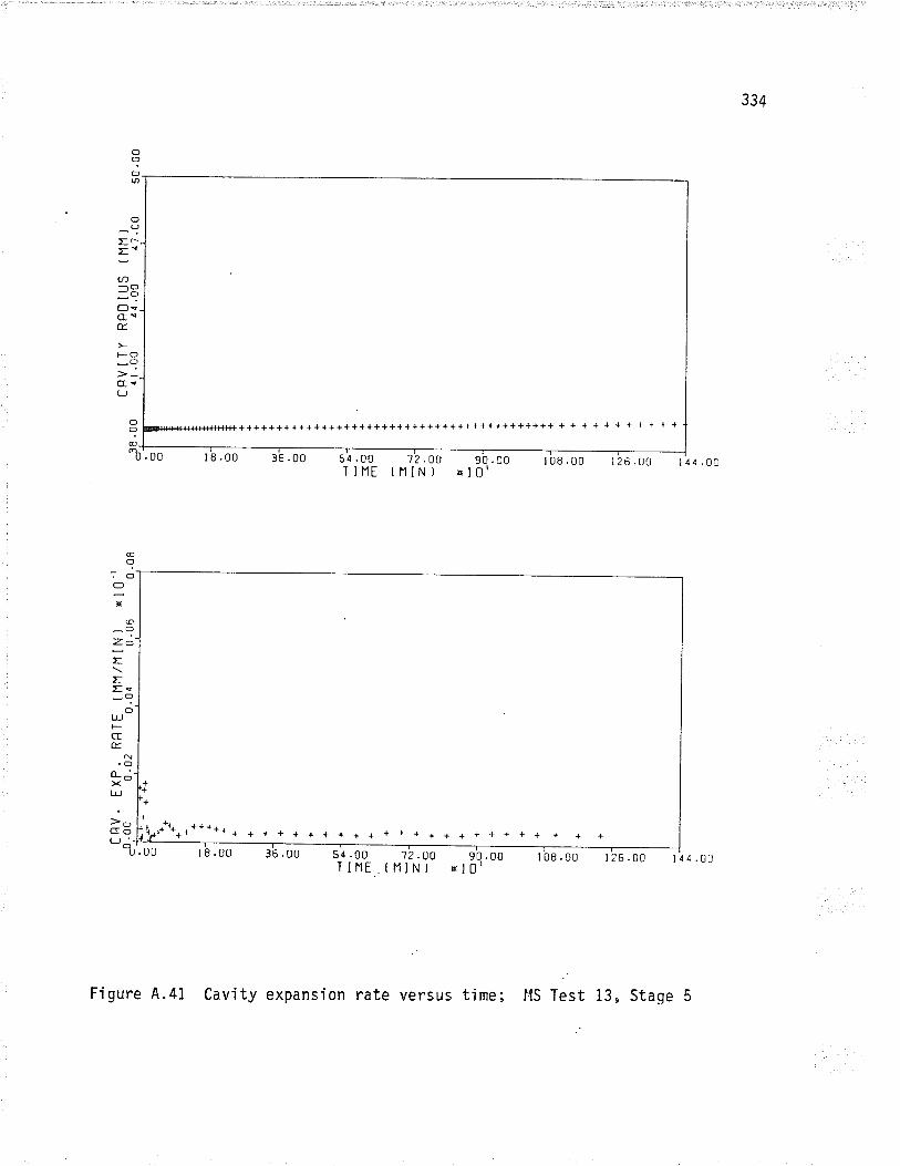
334

ooø

ooEÈ

==U)-O-oClçG!É.

FO*o

Ge(J

@cf

,O

=T@

_OZ.oELEs-9OLTJF-GÉ.

N.oo- ¿-Xl¡J

>OGoa I'-_R

++++++++++++++++++++++++++++++++++++++++++ + + + + + + + + + + +

t8.00.00

o

;-"b 36 .00 5 4 . 00 't? .oo

T IHE { N IN )

¡-90.00 ¡08.00 126.00 l4r.g¡El0l

+++

+ jt*******, + + + + + + + + + + + + + + + + + + + + + + + +

.0tJ 18.80 36 .00 72 .t)OtlllN)

90.00xl0'

54 .00T INE

1 08 .00 I 26 .00 l4d.0fì

Figure A.4i Cavity expansion rate versus time; l{S Test 13, Staqe 5

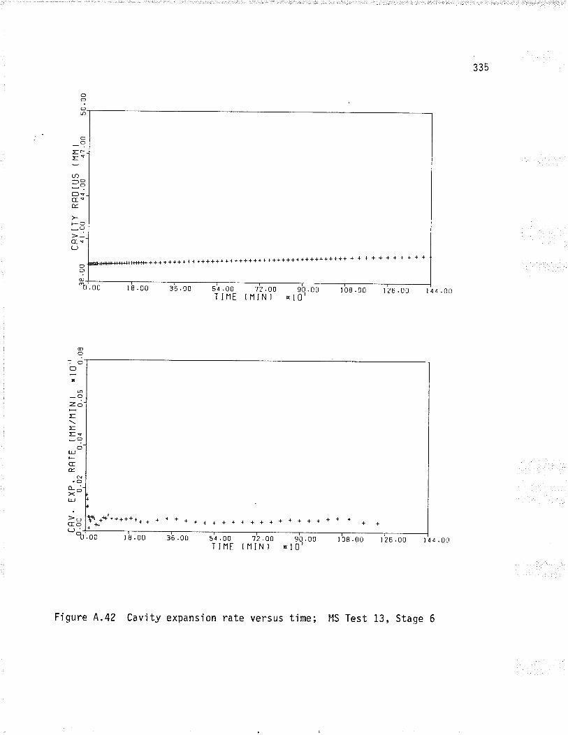
335

oIon

OO

EÈ

="(n_O-o(fsGeÉ

t-o-?cfe(J

++++++++++ ++++++++++++++++++++++++++++++++ + + + + + + + + + + +

1 8 .00 36 .00 54 .00 72 .00 90 .00TINE tHIN) xl0'

.00

o?@_-b ¡-

108.00 ¡26.00 l4¿.0n

@O

OX

T**"'-++++++ + + + + * + l + + + { + + + * * + + + + *

.00

@_OZO

E

EEs_o

Ot!l-CEÉ.

N.oo- --x-L!

>OCfoLJ '-ì t8.00 36 .0u 54 .00

T IIlEI'7?.OO 9q.00 t08.00 I26.00 rna.g¡

f lllN) xl0l

Figure 4.42 Cavity expansion rate versus time; FIS Test 13, Stage 6

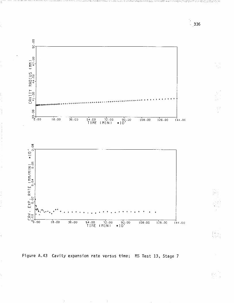
. 336

EE

U)

=oCEÉ

l-

G(J

o?oú

O?r

O?

OO

++++++++++++++++++++++{ +++++++i+++++++++++ + + + + { + + + + + +

o?@

"b'. oo t8.0u 36 .00 54 .00 12 .OOTIHI (NIN)

I 08 .00tt

126.00 l4a.6990 .00xl0'

+\*+**++* * + + + + + + r + + + * * + + * + + + + + +

18.ó0 36 .00 51 .00 't2 .oo 90 .00TIIlE (HlN) xl0'

108.00 I26.00 l4¿.00,00

@o'O

:x

V)

-ozå'

=EEe_o

Ot!FGÉ

N.oo-o-XL!

>OGO(J '-.t

Figure 4.43 Cavity expansion rate versus tÍme; llS Test 13, Stage 7

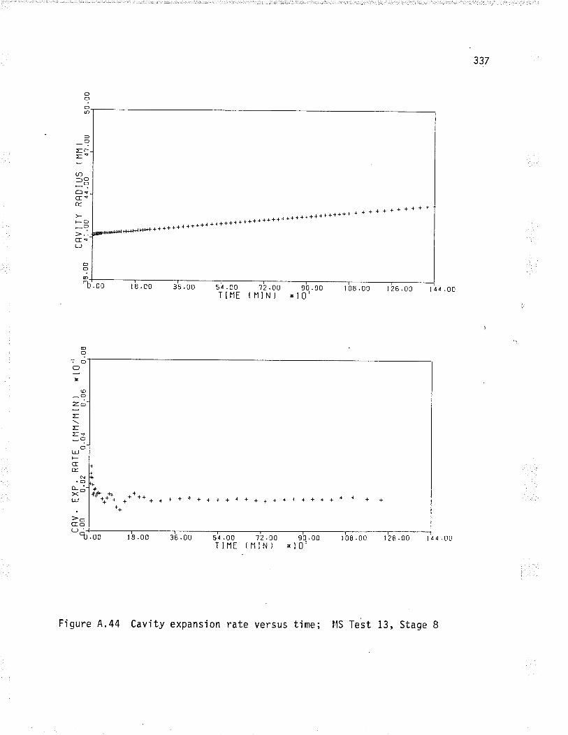
337

oO

\n

++++++++++++++ + + + + + + + + + + +

+++++++++++++++++

1 8 .00 35 .00

O?r

O?

(f

?

O?@_

"b

;

=U)ÐclCEÉ

)-

GCJ

.00 5¿.00T IHE

12 .00 90 .00(11lN) xl0'

t _-=---1108.00 t26.00 lla.g¡

++S .r++1 I **+** * + * * + + + + + + + + + + + r + + + + *

*+

18 .00 36 .0U 7?.00 90.00(NIN) xl0rt08.00 t26.00 l4¿.00

æO

'OOx

o_OZOtEEq-?.OTL,Ì-cE

N.oo- ¿-XtJJ

>OGO(J_-

I .00 54.00T INE

Figure 4.44 Cavity expansion rate versus time; l'1S Test 13, Stage 8

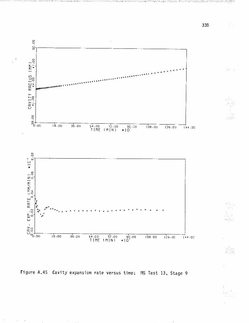
338

.00 I

o?oØ

O?r

o?

CfO

c)?@_

n

EE

(n

=OGÉ.

F

CE(-J

++++++++++++++++++++++++++++++++++++++++++

+ + + + + + + + + + +

.00 36 .00 12.OOfHIN)

s¿.ooT IHE

90 .00xl0'

I 08 .00 I 26 .00 I 4 a . ¡¡

.f*r+++

++'{+

i****** r + + + + + + + * + + + + + + + + + + + +

I I .00 36 .OrJ 12 .00 90 .00(11lN) xl0'

rtf108.00 lZti.00 td¿.u0.00

æo,OOx

o^Oz¿

EEr-?

Ot!F.CEÉ

N.(]o-;><_tL,

>OCIo(J '.

OO

n 54 .00T INE

Figure A.45 Cavity expansion rate versus t'ime; l1S Test 13, Stage

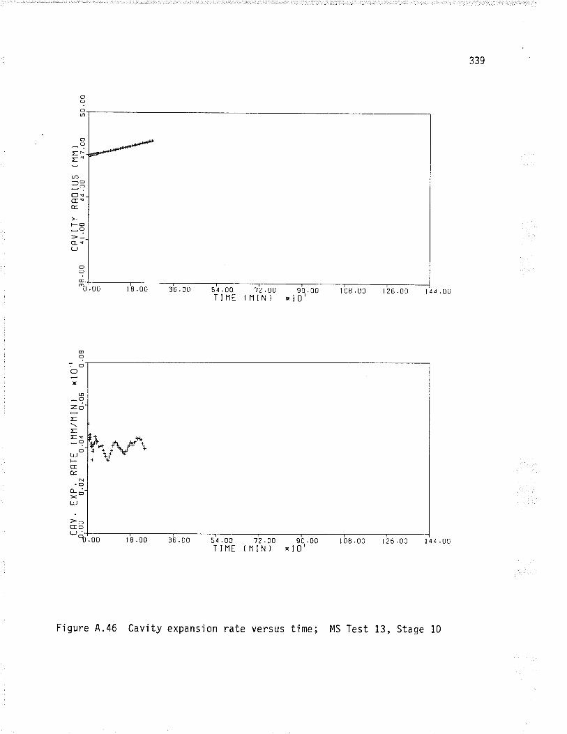
339

c)?otn

oO

Er

='tJ)

-O-oClncE<É.

l-o-..?cE!LJ

.00

o?o_"b 6 .00 l4a .gg18.00 54.00

T IIlE12.AO

{11lN) El0

.00

æO

,OoX

@

-Ozô

==Es_o

OLL,t-CEÉ

N.oo- Ò-xUJ

>OCfo(J^-'t t8.00 36 .00 51.00 12.OO 90.00

TINE f HIN) El0'108.00 126.00 I4¿.0c

itq.. 4 #it i-tu+* r++ rT+

+

Figure 4.46 Cavity expansion rate versus time; MS Test 13, Staqe 10

340

APPENDIX B

CAVITY EXPANSIOI{ RATE / RADIUS VERSUS TIHE PLOTS FOR

THE PRESSUREþIETER CREEP TESTS

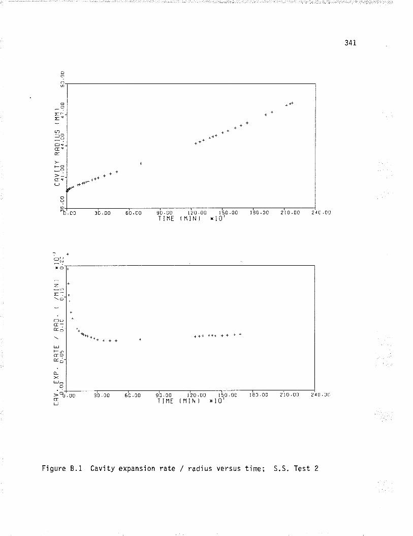
34i

O?ot¡)

OO

Ir

='U)-O-oOe

É

FOO

cs(J

, ++.+

. +++l++++

+++

O

ó'b'. oo 30.00 60 .00 210.00 240.otr 50 .00

ol0'90 .00T INE

I 20 .00{NIN}

l 80 .00

T

-N*O

zE:\O

1ULJG_È3

t!ÞgGOÉ¿

ùXL!o

o

+

+t

.q +{ r+++ 11* **+ + + + +

. _+->I.ooG(J

I 20 .00 I 50 .00(NIN) xl0'

t80.00 2r0.00 240.00¡t30.00 60.00

I

90 .00T IIlE

F'igure 8.1 Cavity expansion rate / radius versus time; S.S. Test 2

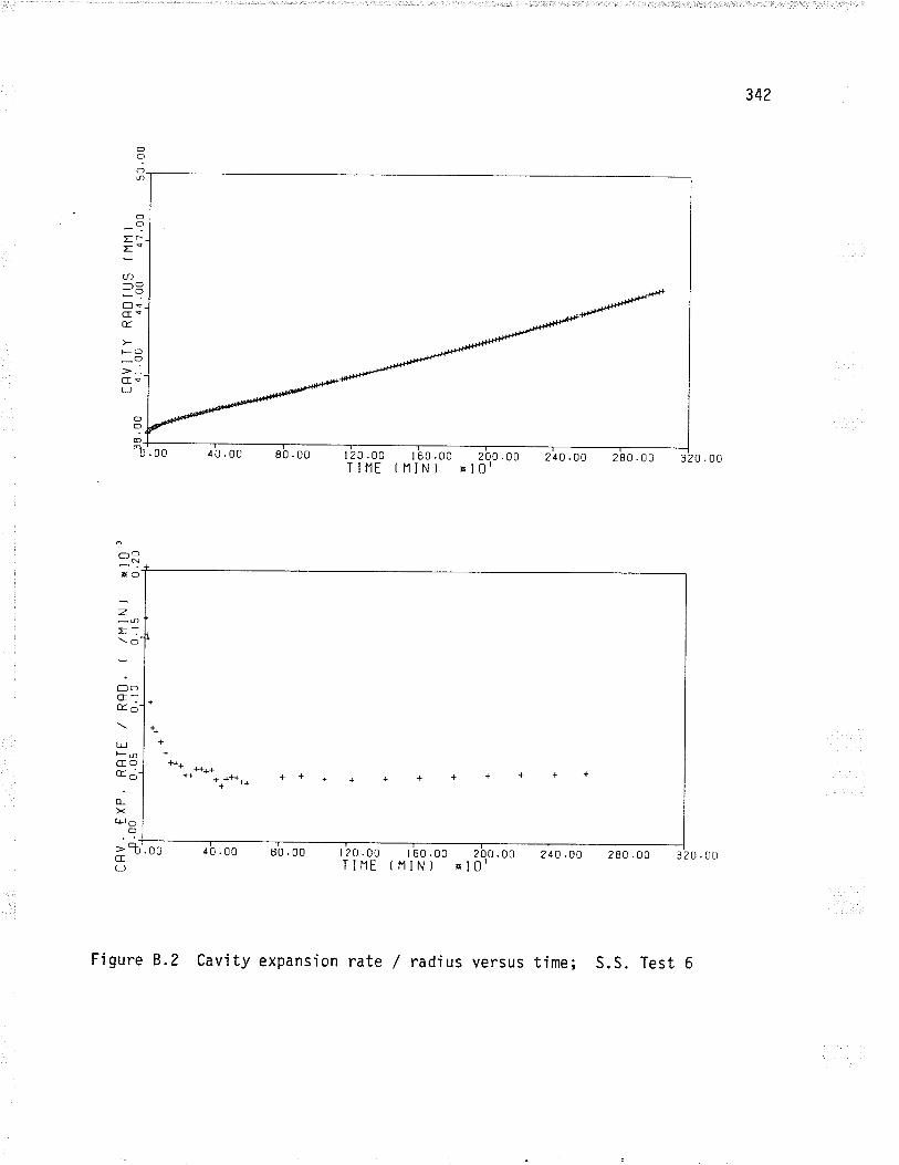
342

O?aØ

Oo

E-

='U)-o-oOvcE<E

tsO

>_G<(J

-"-"--t-t-

.00

O?æ_

"b

?

-C-N¡fo

z

\O,

;-cI:Éo'

t!FúGCÈ;-LXt!o

c)

=lG(J

+

++

** ***fr+*+++++++

40.00 80 .00 I 20 .00 I 60 .00 200 .00TIIlE tlllN) xl0'

10 .00 80 .00

¡ _----1210.00 280.00 320.00

I 20 .00T INE

I 60.00 200.00(HINÌ El0l240.OO 280 .00 320 .00.00

Figure 8.2 cavity expansion rate / radius versus time; s.s. Test 6

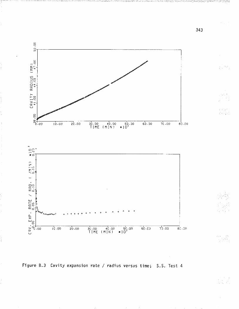
343

o?Oû

OO

Er

='-O-ÕOecsÉ

l-o

-?G!(J

.00

OO

@_

"b 10 .00 20 .00 30 .00T I NE

40.00 50.00t N I N ) x 102

60 .00 70 .00 80 .00

' -+_N

*O

zr:\O

;-C_oao

L¡Jl-nGOorc)

LXuJo

O

> tb'. oo

cr(J

++

'r ' + {+*{¿r+Ha+ 4+**++ ++ + + + + + + + +

I 0 .00 20 .00 30 .00 40 .00 50 .00 60 .00TINE (NIN) ã102

70 .00 8c .00

Figure 8.3 Cavity expansion rate / radius versus time; S.S. Test 4

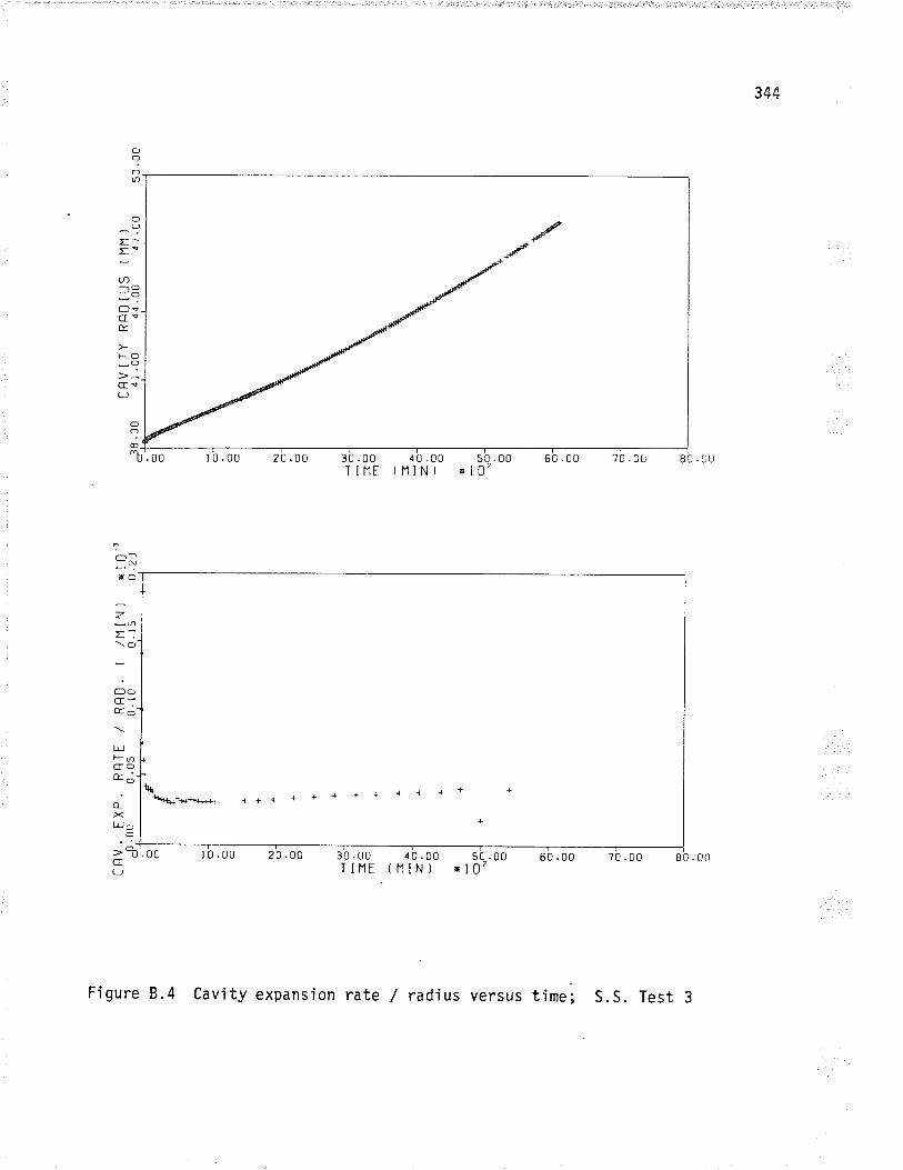
344

O?OØ

OO

Er

='U)

-oC)çcrsÉ.

F-O

-?cfrCJ

.00

OO

-:"b

0030 .00T IIlE

îU;.

XO

\O-

¿-G:Ès-

tLJFnCOo. ¿-

ù.XL!o

O

>lc(J

r0.00 20.DO 3u .00 4 0 .00 50 .00TINE f NIN) *lO'

60 .00 70 .0u 83 . rJU

t+\!++++r+++ ++ + + + + + i + + + +

.00 10.00 20 .00 ¡0.00(11lNl , I bo,'oo

60 ' oo 70 80 .00

time; S.S. Test

é

Figure 8.4 Cavity expansion rate / radi us versus

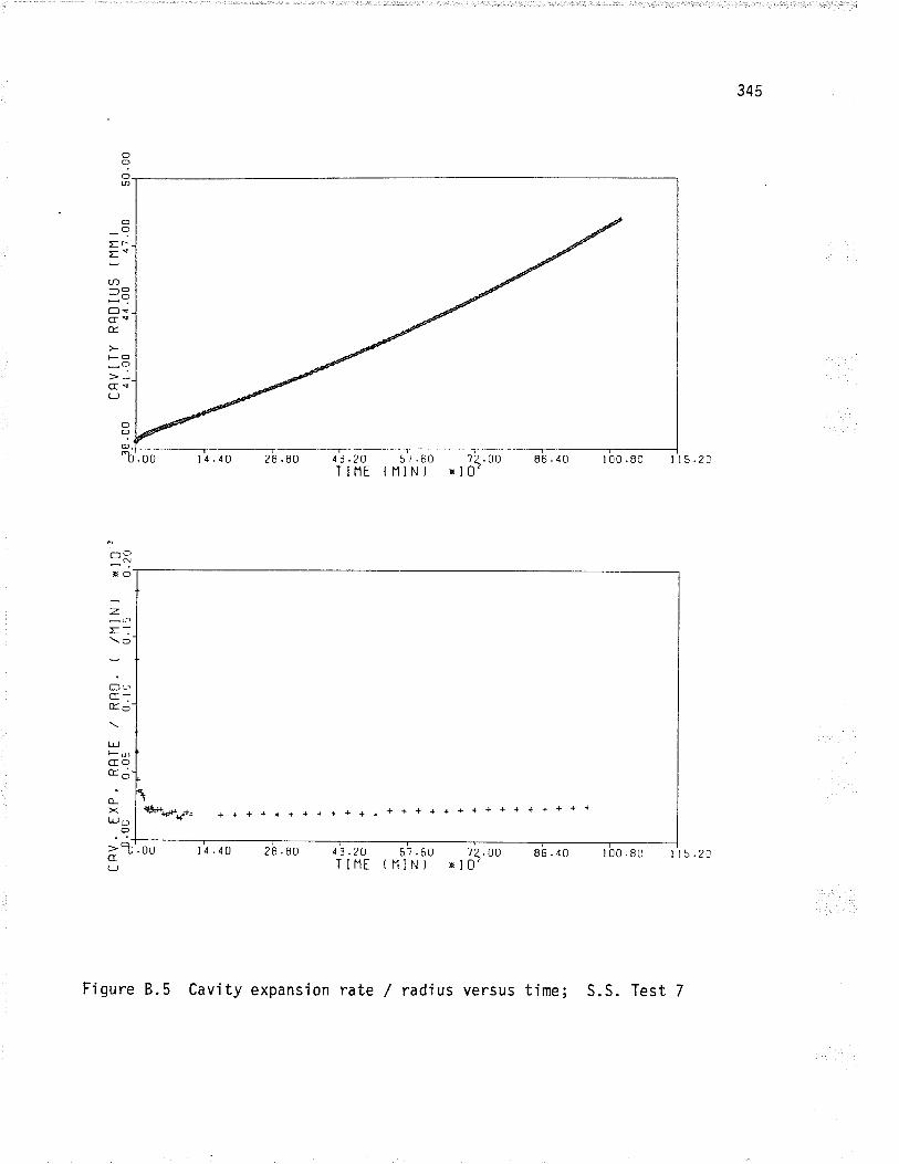
oqoÐ

34s

OO

Er

==U)-O-oOçG!É.

tso_?G!(J

l4 .10 28.80

14.40 28.80

13 .20Ï IHE

51 .60(NIN)

't2 .00x 102

86.40 r l5 .20

?c]RXO

zrl\O

å,_,C_È6

LLJtsurCOÉ.¿

ù><TLJ O

O

cr(J

n**.¡*+á + + ++++++++++++++++++++ +++++

-R'.oo 86.4043.2U 57.6u 't2.OO

TINE (NIN) xl0'100.80 il5.20

Figure 8.5 Cavity expansion rate / radius versus time; S.S. Test 7

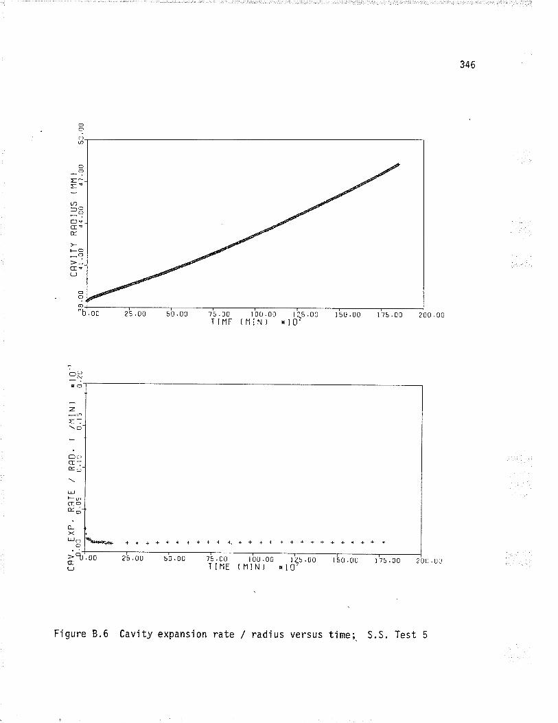
346

OIOØ

OO

Er

='U)-O-oCtçGeÉ

FCf

-?cEe(J

T

-Cl

"o.

zE:\6-

-c:)G_Èo-

t!l- rr¡colG;-l.to-l><lt¡J- IOI.t=alCELJ

o?@_

"b I 50 .00 5 .00 200.0075 .00 lOtJ .00(MIN)Ï IIlE

t 25 .00s l0?

++++++ + +{ { +.++ + { + +++++++++ +

7s.oo ¡oo.oo r¿s.ooffio.ouTINE (11lN) ã10'

25 .00 50 .0u

FÍgure 8.6 Cavity expansion rate / radius versus time; S.S. Test 5

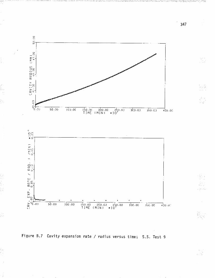
347

(fO

Er

="U)_O

OsÉ

'.--.1

cr!(J

--.-N

x3

z

\o

å,.c-

LLJtsúGO

-><LJJ o

O

> l'. ooc

I 50 .00T IIlE

3

@_

IJ 50 .00 r 00 .00

50 .00 I 0o .00

200 .00 250 .00( M IN ) x l0?

300 .00 350 .00 ¿0tJ.0c

I 50 .00T INT

200 .00 250 .00 300 .00( H IN I x 102

350 .00 { c0 .0:

FÍqure 8.7 cavity expansion rate / radius versus time; s.s. Test 9

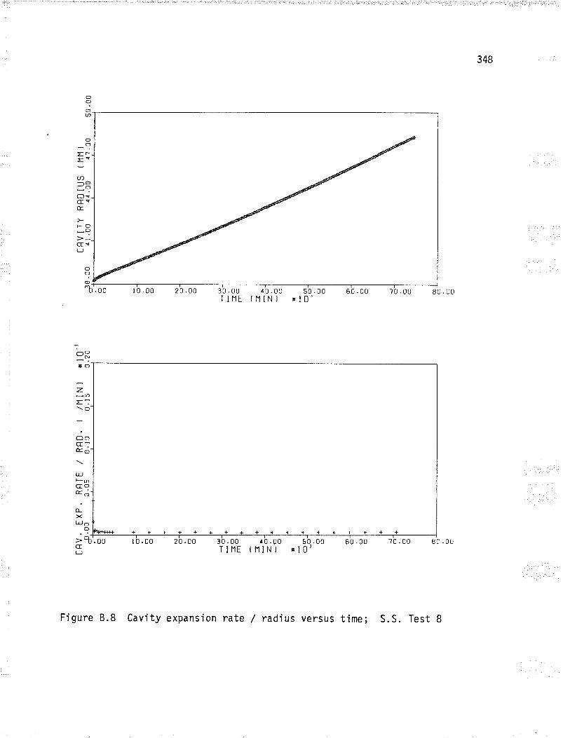
348

o?on

30.00T INE

¿u.00ININ)

50 .00xl0r

ORXO

z.

L.\O

;-c:olo

t!tsLnCTOÉ.¿

LXL¡J o

o

>R'.oo t0.00 20 .00 30.00 10.u0 50.00 60.0u ?0.00 8c.0uTINE (NINÌ al0lc

L-J

EÈ

='u-)

-O-OOqceÈ

FO

-Ocr<(J

Figure 8.8 Cavity expansion rate / radius versus time; S.S. Test I

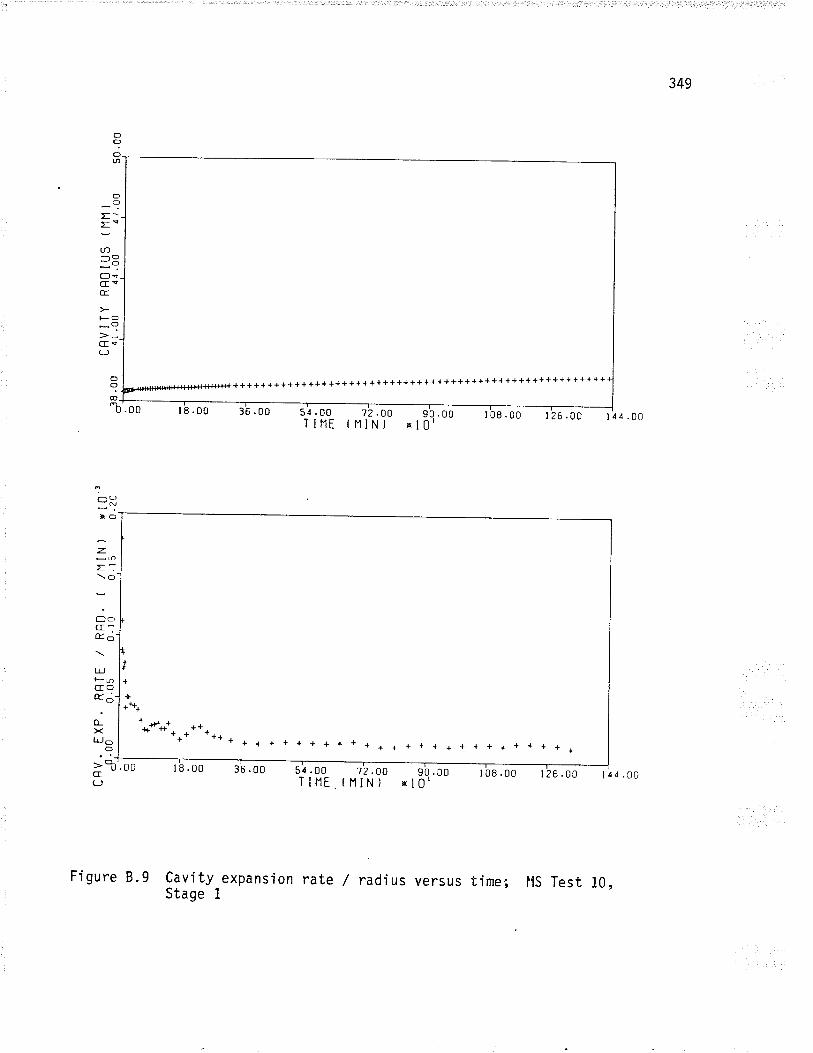
349

o?Otn

oO

EÈE!

u-)

-O-oOsGvÉ.

FO

-?CEe(J

+++++++++++++++++++ +++++++++++ ++++++++++++++++++++ +++++

.00

o?O-

"b 18.00 .00 54.00T IIlE

7? .OO(NIN) 90 .00

x l0'l 08 .00 r 26 .00 t4¿.00

-OTO

=\O

¿-C:olo

t!FncfoÈd

(L><uJo

o>R'.oocLJ

51 .00T I I1E

r+

++**+

'-l/*+*' *****-*** * * + + + + + + + + * + + * { + + + * * .r + * a * +

18.00 36 .00 12 .00 90 .00tHIN) El0'

1 08 .00 t 26 .00 l4a .3¡

Figure 8.9 cavity-expansion rate / radius versus time.; lls Test 10,Stage 1

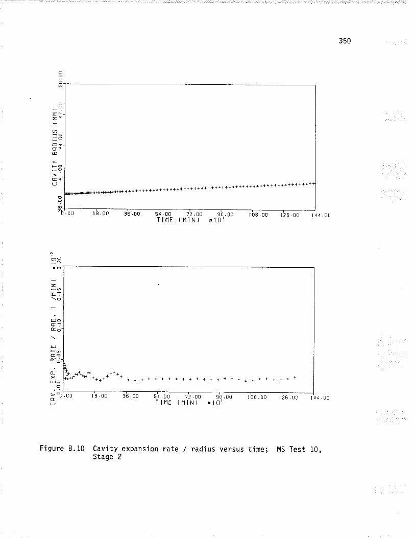
350

O9Oa

OO

Er

==U)-O-oOs

É

FO

-?G<(J

++++++++++++++++++++ ++++++++++++++++++++++ ++ ++++++ + +++

o?@

"b.oo r 8 .00 36 .00 s¡.oo 't2.oo s'olffio.ooTIllt (11lN) El0'

È *++. # .**++4** + +**++ *

* * * + + + + + + + + + + + * * * * * + { 1 .¡ + +

=R'.oo t8.00

ToRIO

z

\O

¿-c:olo

Ldl-oGOÉ.¿

o_XLL,o

O

cC-J

¡'o.oo s4.oo 1'z.oo s'0.ffi0TINE (NIN) xl0' UO

Figure 8.10 Cavity expans'ion rate / radius versus time;Stage 2

MS Test 10,

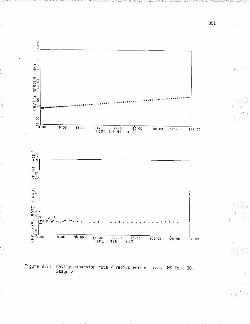
35i

oIo@

OO

Er

='U)-Ò-o(fvGrÉ.

FO

-?cE!LJ

++++++++++++++++++r ++++++++++++++++++'+

++++++++++++++++

oq@_

"b .00 I .00 36.00 72.O0 90.oollllNl xl0'

51 .00T I I1E

I 08 .00 1 26 .00 I44.00

-C_N

XO

z

=:\o

;-CI_Èo

LLJF-6CEOÉ.¿

o_Xl'!o

O

lr++'É+++l++l+ +++++++++ + + + + + + + + + + + + * + + + + + + + + t * .r *

>R'.oo r8.00 36 .00CE(J

54.00T INE

72 .OO 90 .00{11lN) El0'

I 08 .00 I 26 .00 I 4 a . g¡

Figure B.1i Cav'ity expansionStage 3

rate / radius versus time; l4S Test 10,

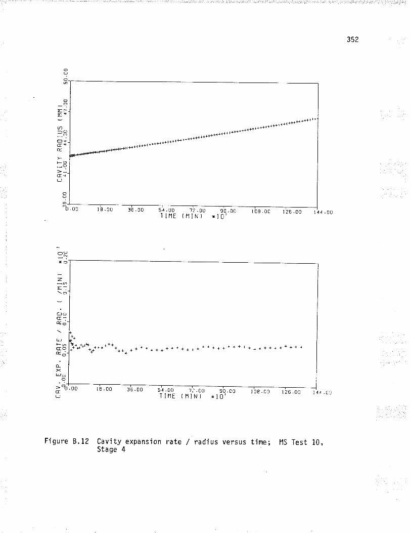
352

,00

a?oØ

oO

r

O?

OI

o?@_

1)

;

=(n=OqÉ.

cfLJ

18.00 36 .00

l8 .00 36 .00

't? .00(NINI

54 ,00T INE

90 .00xl0'

1 08 .00 r 26 .00 I 4 d .00

-O-ñXO

;\O

;-a;EO

UF-nGoE¿

o_xLL, O

Õ

i+Ì+ +.¡++ ¿*+++++r +J++ *++ ++++++++**++l +

=Ì'.ooC 108.00 126.0054 .0uT IIlE

7? .00(NIN) 90.00

El0'

Figure 8.12 Cavity expansion rateStage 4

time;/ radius versus llS Test 10,

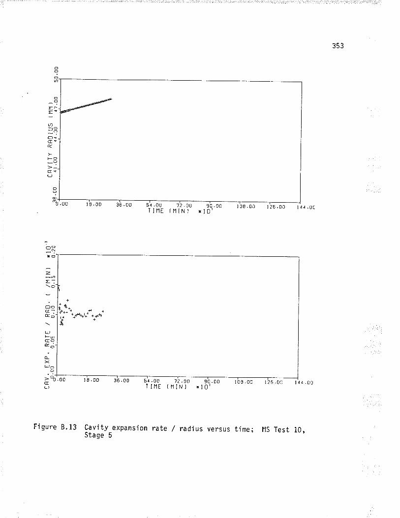
353

o?OØ

O?-

O?

o?

o?o_.U

E

=U)

=ocÉ.

F

c(J

36 .00

36 .00

54 .00T INE

't2 .00ftltN)

90 .00sl0' r 26 .00 I 4 ¿ . tJO

-o_N

XO

E:\o

;-G:olo

L¡JF6COÉ.¿

L><Lrj o

O

>ì'.ooCLJ

Figure 8.13 Cavity expansionStage 5

't?.oo 90.00f HIN) nl0' I 08 .00 I 26 .00 I { c . ¡¡51 .00

T IHE

Ii'o-."t

rate / radius versus time; ItS Test 10,

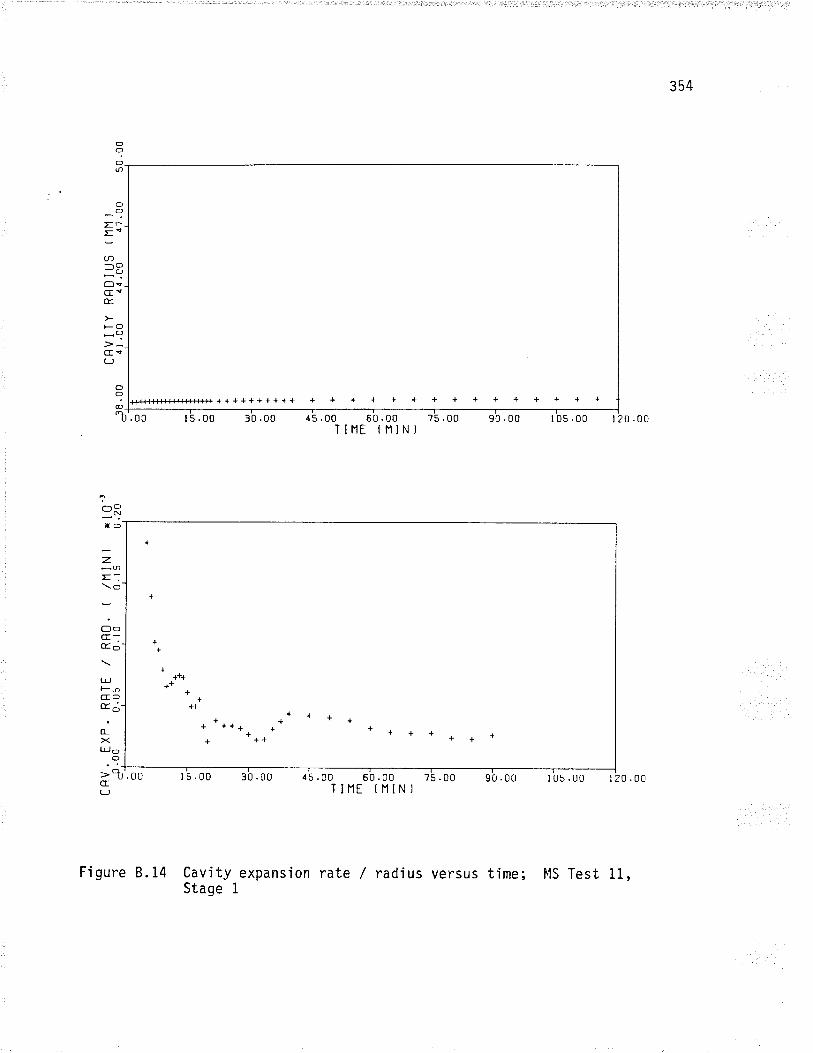
354

O?Oû

OO

EÈ

="aJ)

-oCleu-É

FÔ

-?G9(J

++++++++++ + + + + + + + + + + + + + + +

.00

o?@_

"b t5.00 30 .00

ToRXO

zE:\o

O-(I:olo

t!l-6GOÉ¿

o_XLJ-, o

O

>R'.oo 15.00 30 .00cr(-J


45 .00 60 .00 75 .00TIHT IHIN)

90.00 t05.00 I 20.00

¡tI 05 .00 l 20 .00I 5 . 00 60 .00 ?5 .00 90 .00

TIHE f IlIN)

++

+*+

++

++

++ *+++

** + + +

++*++++++

rate / radius versus time; FIS Test 11 ,

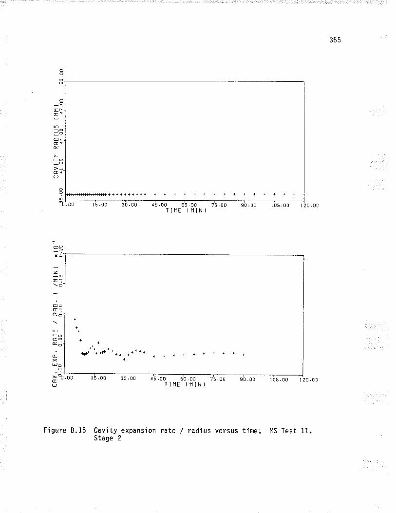
355

o?OØ

oO

r

OO

o

++++++++++

E

=U)

=cfCEÉ.

F

cr(J

O?@

îORTO

z

\o

O-a:Èo

t!f-6Goor¿

o_><uJo

O

-b'. oo t5.00 30 .00 1 5 .00 60 . 00 75 .00TINE (11IN)

90 .00r¡

I 05 .00 I 20 .00

+.+

****.**r****** *+{+++

.r*+++

>l'.ooCE

l5 .00 30 .00 t-45.00 60.00 ?5.00 90.00 105.00 120.00TIIlE (NIN}

Figure 8.15 Cavity expansion rate / radius versus time; MS Test 11,Stage 2

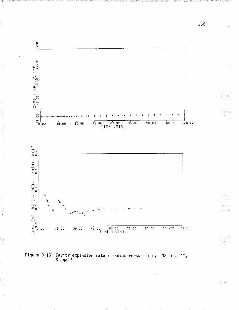
356

cl?OÐ

OO

E-

="tn-O-oC)q(reÉ.

FO

-=G<(J

CfO +tsts*t{-H+ts{-}*++È++++++++++ + + + + + + + + + + + + + + +

'l'b.00 15.00 30.00

15,00 30 .00


15.00 60.00 75.00TIIlE (NIN)

90.00 I 05 .00 I 20 .00

.00

îORXO

z

\o-

;-c:ol e-

trJF9coÈ¿-

L><LrJ o

O

=RCELJ

¿!.oo ob.oo r's.ooT.II1T ININ)

90 .00 t 05 .00 I 20 .orj

+

***+*+A+

l +*++ ++

rale / radius versus time; MS Test 11,

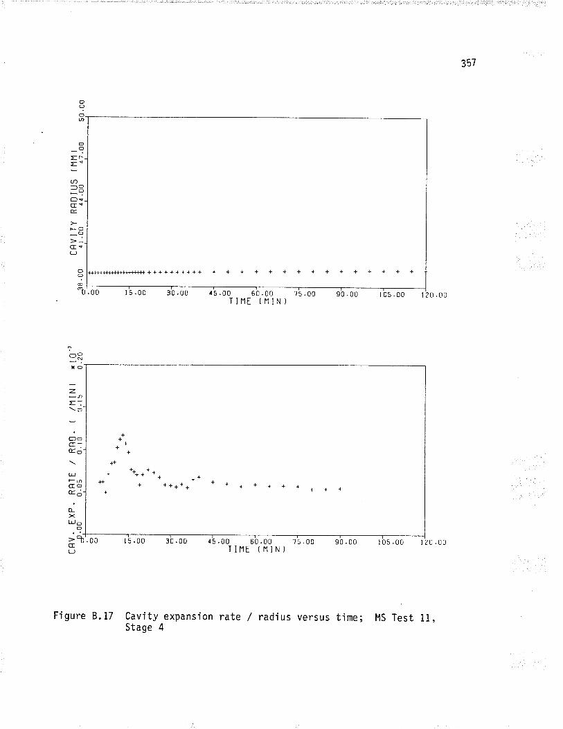
357

o?ID

OO

=r

=*(n-O-oOeGsE.

|-(]-?cIeL)

++{+}{-+ì++{{J-#++++++++++++ + + + + + + + + + + + + + + +

15.00 30 .00.00

()?@_r¡-

U 90 .00 I 05 .00 I 20 .0015 .00T INE

60 .00 ?5 .00fHIN)

ORHO

z

\O

;-G:olo

LÙFÐGoor;

L><L!, oo>l'.oo I5.00 30 .0t)CE(J


45 .00 60 .00 ?5 .00T IIlT ( N IN ì

I

90 .00 r 05 .00 t 20 .00

++

******** **+++

¡+'+*++++++{+

rate / radjus versus time; t4S Test 11,

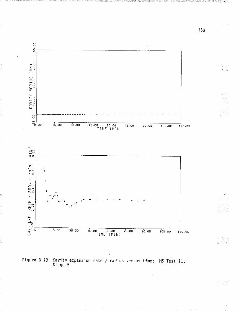
358

o?Oa

c)O

Er

='U)IO--Osolsæ

FO*?Gq(J

#+{-s{-{++l-{.j-Hl+++++++++++ + + + + + + + + + + + + + + +

.00

o?@_

"b 1's . oo e'o . oo z's . oo sb . o0 -tb; .00 --T2o . ooTINE (NIN)

+*+

++++++++

++¡++ *+*

+*

>R'.oo

-O

Xo

z.-ØE:\o

O-G_Èc)

LLIF6GOor;

o_><Lrj o

Õ

crLJ

I 5 .00 30 .00

t5.00 {5.00TINE

60 .00 75 .00ftllN)

90 .00 I 0s .00 I 20 .00

Fiqure 8.18 Cavity expansÍonStage 5

rate / radius versus time; llS Test 11,

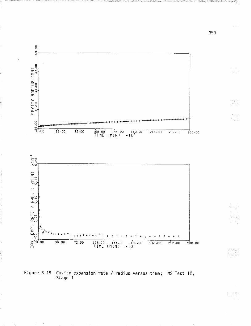
359

o?oÐ

oO

=r

=-U)-o-oOsG9É.

FO

-9cEe(J

288.00

cfRxo

z

\o

o-a:É.o

t¡Jl-mcfoÈ;LxuJo

o

CE(J

Figure 8.19 Cavity expansionStage I

rt-t11.00 t90.00 216.00 252.00 288.00(HlN) xl0r

f*o********++*+*+++++++++*

+ + + +++++ ++>l'.oo 36 .00 72 .00 I 08 .00

T I IlE

I 08 .00TIIlE

I 1¿ .00NIN)

?ate / radius versus time; l'1S Test 12,

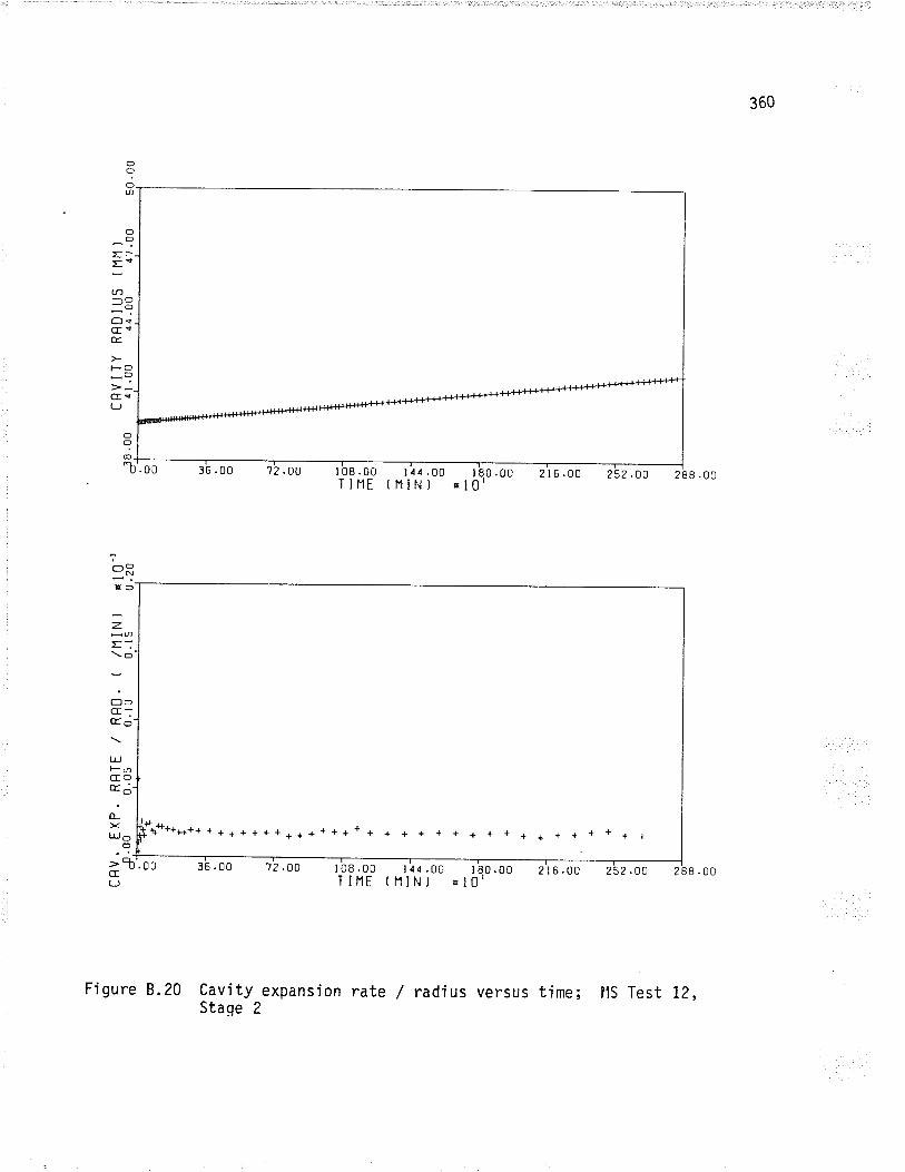
360

O?oú)

oO

Er

='u-)

-O-oOçGeæ

t-o*?cEq(J

oO

crR)fo

z.

E:\e

;-cr:Èo

L!FnGC)o<¿

o_><LrJ o

O

>l'.oocr

I 08 .00T INE

1 14 .00(HIN) I 80 .00

ql0l

{-t++++4-H+#++

tr'. oo 36 .00 216.00 252.OO 288 .00

i****** * + + + + + + + + + + + * n * * + + + + + + * + + + + * + + +

(J3b.oo j'z.oo lbe.oo lio.o e.ooTINE {HIN} "l0l

Figure 8.20 Cavity expansion rate / radius versus time; llS Test 12,Staqe 2

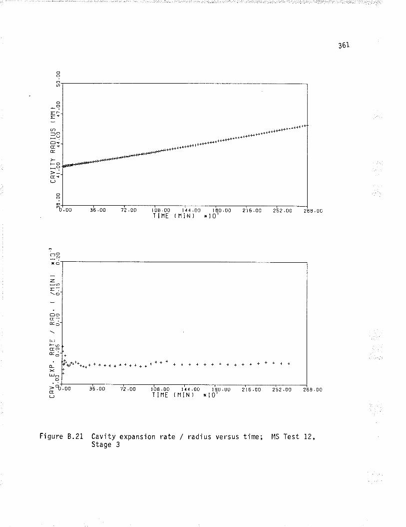
361

o?oa

o(f

Er

='u-)-O-oO!c{É.

f-o

-9cE!LJ

.00

OIO-

"b

TORXO

z

\o

ó-c:E6

t!F-OGOorJ

o_xL!o

o>l'.ooG

36 .00 72 .OO 108.00 l1ó.00 180.00 216.00TIIlE (t1lN) rl0' 252.00 288.00

+

Í**y'4****** + + + + + * * + * + + * * * * + + + + + + + + + + + + + + + +

(J36 .00 72.80 108.00 144.00 t80.00

TINE f NIN) xl0'2 I 6 .00 252 .OO 288 .00


yate / radius versus time; l.1S Test 12,

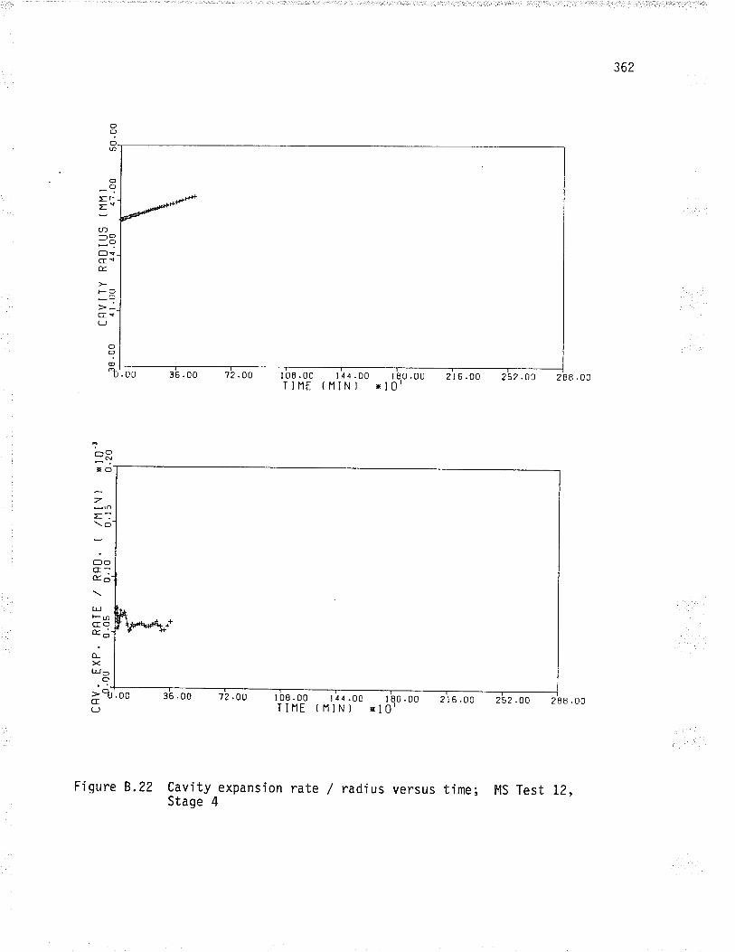
362

o?oU)

O

tr

='U)-O"oOvc!É.

tsO_?cv(J

o?O-

"b

^O-c

I 08 .00T INE

114.00 t80.00(11lNl xl0l

2 I 6 .00 ?52 .OA 288.0C

T I ilEt14.00

ttllN)I 80 .00

E l0'216.00 ?52 .OO 288 .00

XO

\e

¿-c:É.o

Lr,FmGOor¿

o_><l¡Jo

o>R'.oo 36 .00 72 .OO I 08 .00C(J

Fi gure 8.22 Cav'ity expansionStaqe 4

rate / radius versus time; l4S Test 12,

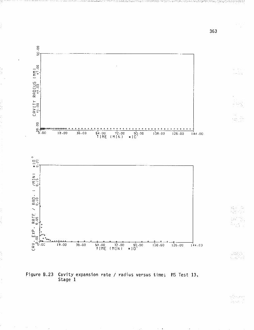
363

oO

Ð

oO

=r

==(/)-cf-oC'gGsÉ

tsc)-?Ce(-J

+l+{l#j# + + + + + + + + + + + + + + + + + + + + + + + + + + + + + + + + + + + + I + +"b'. oo t 8 .00 36 .0u s4 .00 iz .oo sb. oo r'oa . oo lfã. oõ-Jo o . ooTlllE (11lN) ol0'

++

+ {++*+

o?o

-Cr_N

XO

;E:\o

;-c:E6

L!*ØCOÉ.¿

L><l,¡J o

o

=R'.oo 36 .00 51.00Ï IIlE

't?..00 90.00(NINI "l0l

108.00 126.00 l4d.rioG(J

F'igure 8.23 Cavity expansion rate /Stage I

radius versus time; llS Test 13,

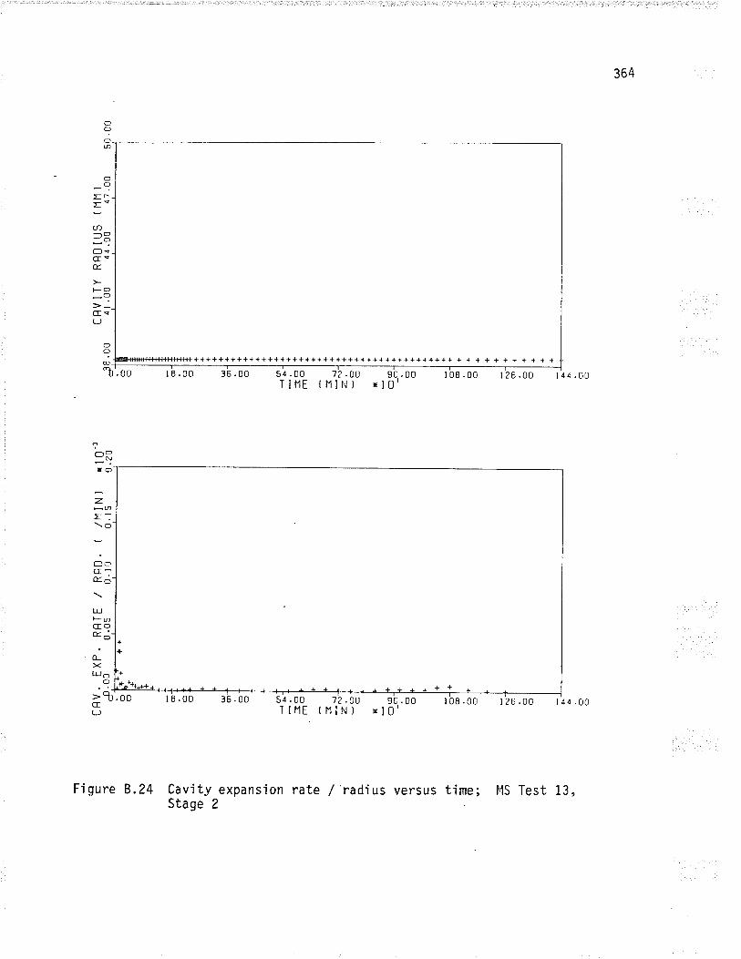
364

o?OtJ)

ooEr

==(n-O-oOscE<É.

FO

-?cf(J

@-tb'. o0

++++++++++++++++++++++++++++++++++++++++++ + + + + + + + + + + +

OO

l I .00 36 .00 51 .00T INE

1? .oo 90 . oo r ba . oo I'zsio l¿ o . oo(NIN) xl0r

ORXO

=E:\O

;-c:ol6

t!l- u:GOord

o_Xuo

o

Fiqure 8.24 Cavity expansionStage 2

I_9q.00 108.00 126.00 r44.00ol0'

. ' -l¡:L>R'.oocLJ

18.00 36 .00 54 .00T INE

't2.ootNIN)

rate / radius versus time; f1S Test 13,

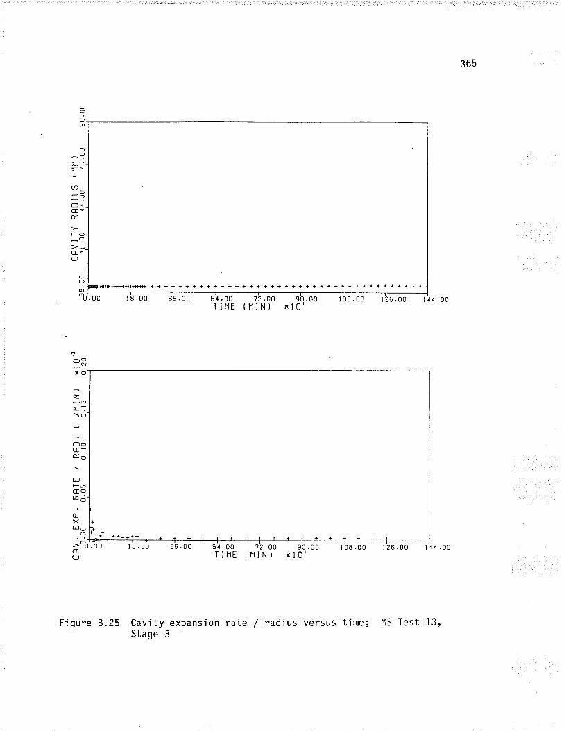
365

o?Oô

OO

Eñ

==-c)-ÕtlsG{æ.

l-o

-?G<(J

++++++++++++++++++++++++++++++++++ ++ +++

"b'. oo t8.00 36 .00 51 .00 72 .OO 90 .00llllE (HIN) xl0'

I 08 .00 126.00 I4a.g¡

It,+++++***36 .00

tttt54.00 'ì?.0o 90.00 t08.00 I26.00 t4a.¡9TINE tlllN) xl0'

O?@

.00 t 8 .00

ORfO

z.

\O-

O-CE:oa o-

LrJÈaGOÉ.¿-

ùXL!o

o

=RG(J

Figure 8.25 CavitySta ge

expansÍon rate / radius versus time; MS Test i3,3

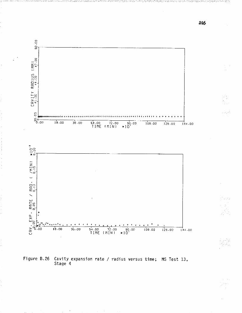
aw

c)?otn

oO

Er

='(t)-O-o

Ht*+++++++++++++++++++++++++++++++++++++++++++++ + + + + + + + + +

Ðrcf!É

FO

-?cf<(J

.00 I

O?@_

"b .00 36 .00 12 .OO(HINì

51 .00T IIlE

90 .00xl0'

.00 I 26.00 I 4 a . ¡¡

OHICI

z.

E:\o

Å-G:ol c)

t!F-oGoÈó

(L><L¡J O

O

=l'.ooG 54 .00T I NE

++

llr+*,*****+*+* 4 * * + + { + } + + + r ¿ ¿ + + + + + + + + * + +

t8.00 36 .0t) 't2 .oo 90 .00(HIN) xl0'

108.00 126.00 l4¡.(JCì

Figure 8.26 Cavity expansionStaqe 4

rate / radius versus time; F{S Test 13,

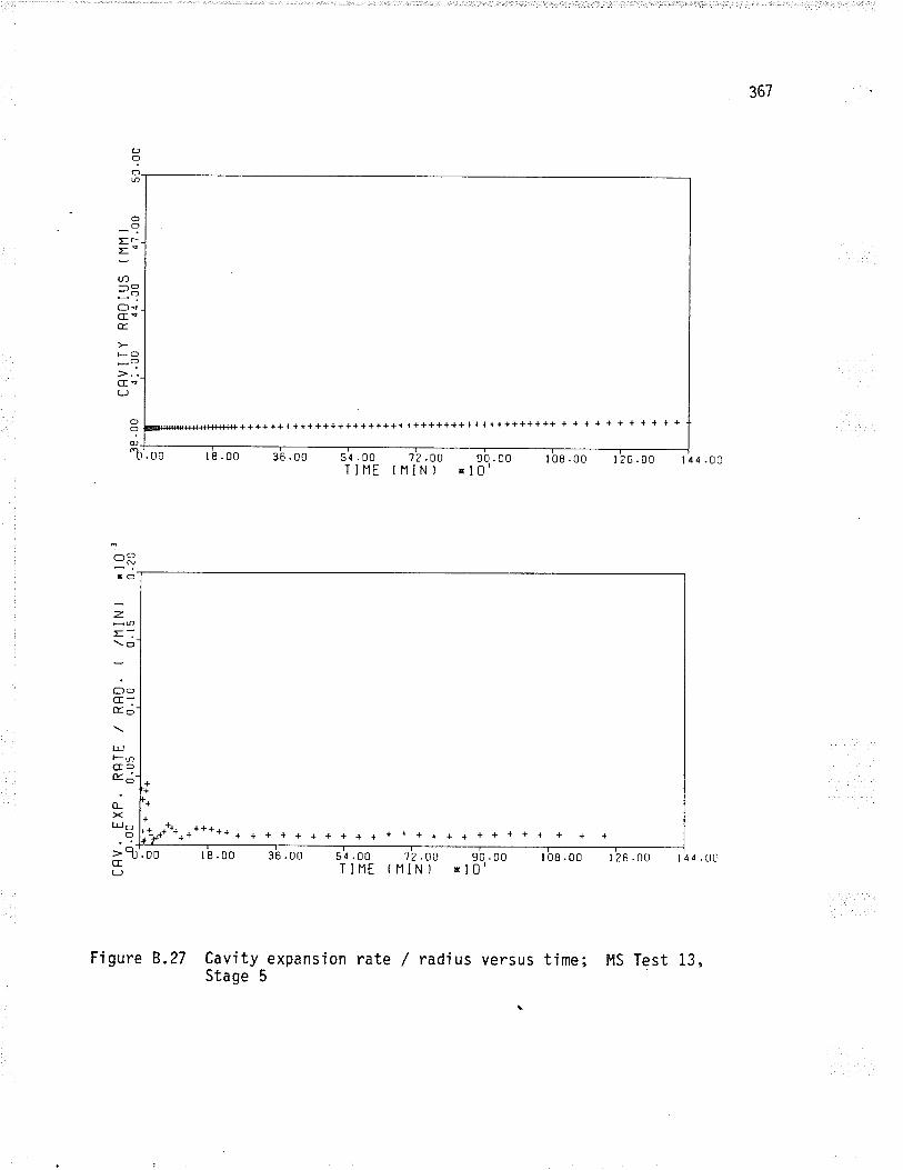
367

OIoa

OO

Er

='U)-o-oClv(I€É.

ts()-:G<LJ

oo ++++++++++++++++++++++++++++++-l+++++++++++ + + + + + + + + + + +

"b'. oo 18.00 36 .00 ¡26.00 144.00

+

+

+

t*************+ + + + + + + + + + * { + + + + + + + + + + + +

>'b . oocr l8 .00

54.00T IHE

't2 .oo 90 .00(NIN) xl0l

t 08 .00

-O-NxÕ

=L.\O

;-cfrÈo

t¿J)-ncroÉ.¿

Lxt!o

O

(J36 .00 54 .00 '1? .OO

TINE f IlIN)rtt

108.00 126.00 t4a.g¡90 .00xl0l

Figure 8.27 CavÍty expansion rate /Stage 5

radi us versus time; l4S Test 13,

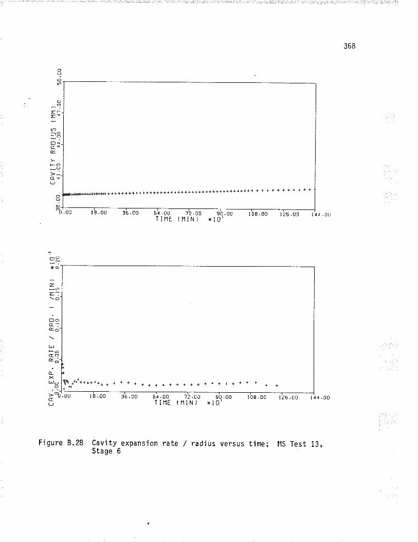
368

o?OtJ)

ooEr

='U)-O"o(]çÉ

tsO-?CEeLJ

++++++++++ Ì++++++++++++++{++++++++++++++++ + + + + + + + + + + +

o

'b'. oo 1 8 .00 36 .00 12 .00 90 .00f NIN) xl0'

r

---_--1

108.00 t26.00 l1a.¡¡

T{É ++{{++++++{ + ++

+++++++++++++*++++*

l8 .00 36.00 54.00 12.00 90.00TIIlE (NlN) El0'

trI08.00 t26.00 ¡1¿.00

51.00T INE

.00

TO9xÕ

z.

\o'

O-G:E6'

t¡-,Þ-6coÈ¿-

fLXLJo

o

>ncLJ

Figure 8.28 Cavity expansionStage 6 "ate / radius versus time; l.lS Test 13,

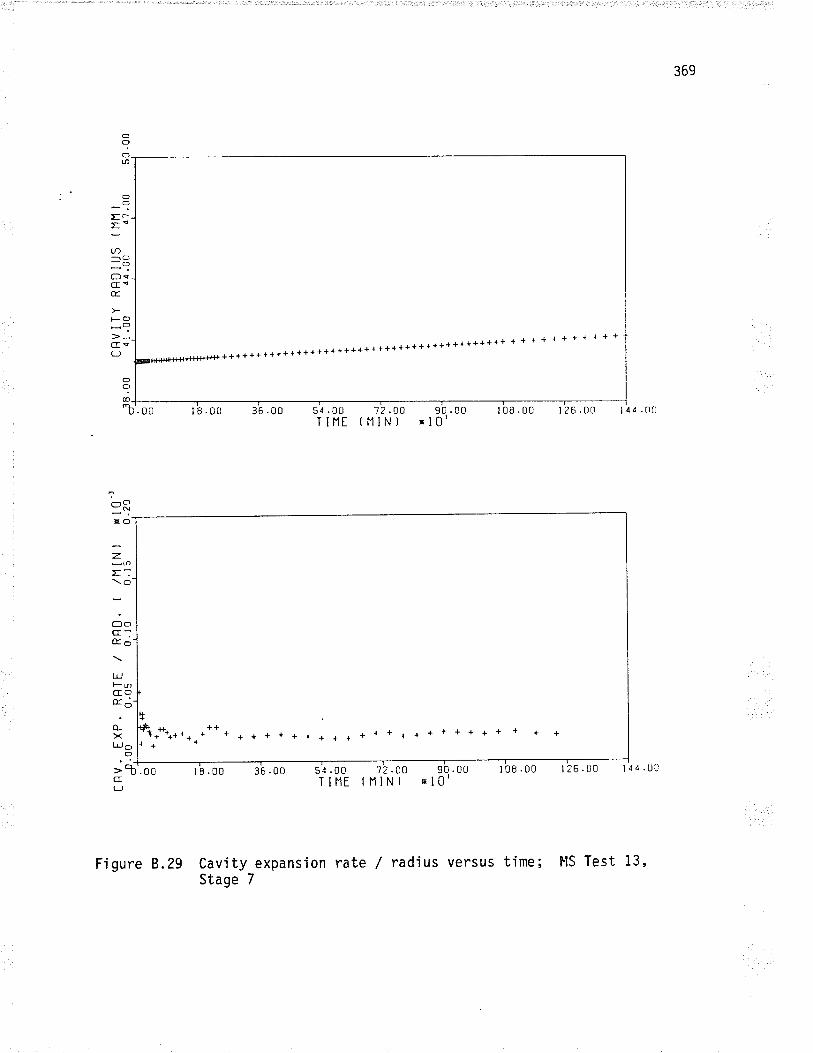
369

oIotn

oaEr

="U)-o-oOqcreÉ.

*?G<LJ ++++++++++++++++++++++l

+++++++ [+++++++++++ + + + + I + + + + + +

I 08 .00 126.00 l4¿.tì0.00

O?@_

"b 36 .00

îORXO

54.00 1?.oo 90.00TIllt (NIN) Ã10'

i***** ,. *, '+

++++++++++**l*+++{++++

+

=E:\o'

o-G:É¿

UJl-- Dcoæ¿

o_xL!o

o

G

..ì_ | |

l'8.00 36.00 5¿.00 '7?.oo 9q.00 108.00TINE tNlN) El0'

126.U0 l4¿.uLì

Cavity expansion rate / radius versus time;Stage 7

Figure 8.29 l'lS Test 13,

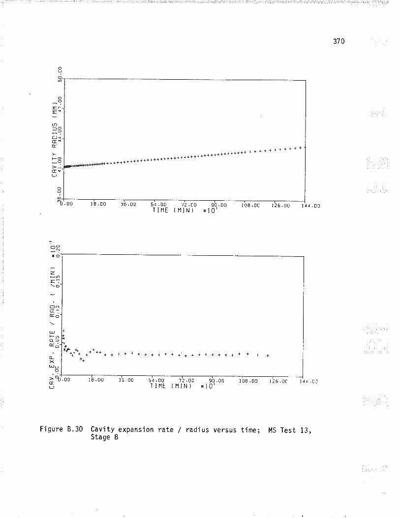
370

o?OØ

oO

EÈ

==U)-O-oÕscE<É.

tsO

-?Crq(J

++++++++++++++++++++++1++++{++++1+++l+++++

I + + + + { + + + + +

'b'. oo ¡8.00 36 .00 s¡ . oo i'z .oo sb . ooTIHE tNINì xl0'

ÕO

@

-

108.00 126.00 l4¿.00

TORxo

E:\C)

¿-GlÈo

t!F6cfooró

L><L!o

O

++l+ €. +'**** ** *** * + + + + + + + + * +'+ + + + + + + + * + + +**

>l'.ooG 54.00 '1?.OO 90.00

TlllE tHIN) xl0' 108.00 t26.00 t4¿.0a

8.30 Cavity expansion rate / radius versus time;Stage 8

t8 .00 36 .00

Fi qure MS Test 13,

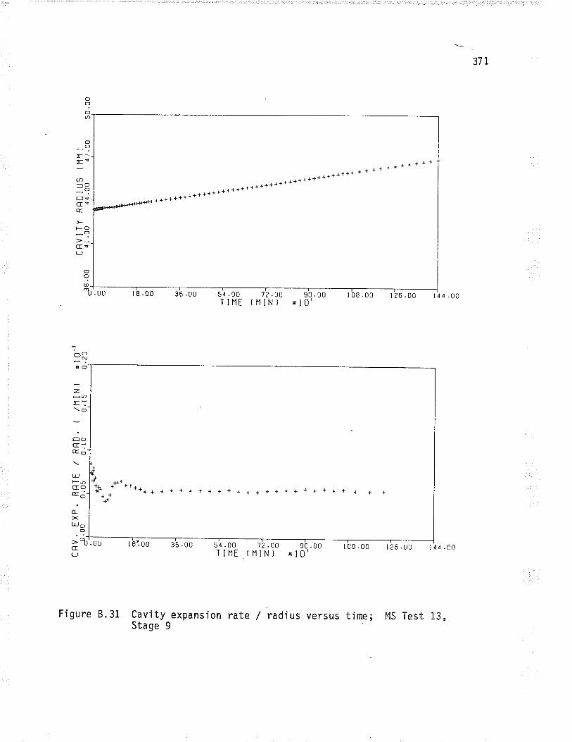
371

O?OØ

OO

r

OO

OO

;

=U)

=OcrÉ

F.

cr(J

o?

rtt-5{.00 1?.OO 9q.00 t08.00 126.00 ria.¡gTIIlE flllN) xl0'

+{+rl*.+

++4*

j*t * * .-*+ + + + + 4 + + + * + + + * * + + + + + + +

>R'.ooC tgioo

"b'. oo 1 8 .00 36 .00

-O-NIO

z.

\O

Ë-c:Èo

LTJl-4cc)oro

o-Xl'!o

O

(J54 .00Ï IHE

12.DO(rllN) 90 .00el0'

I 08 .00 I 26 .00 I 4 a . ¡¡

Figure 8.31 Cavíty expansionStage 9

rate / radius versus time; lrls Test i3,

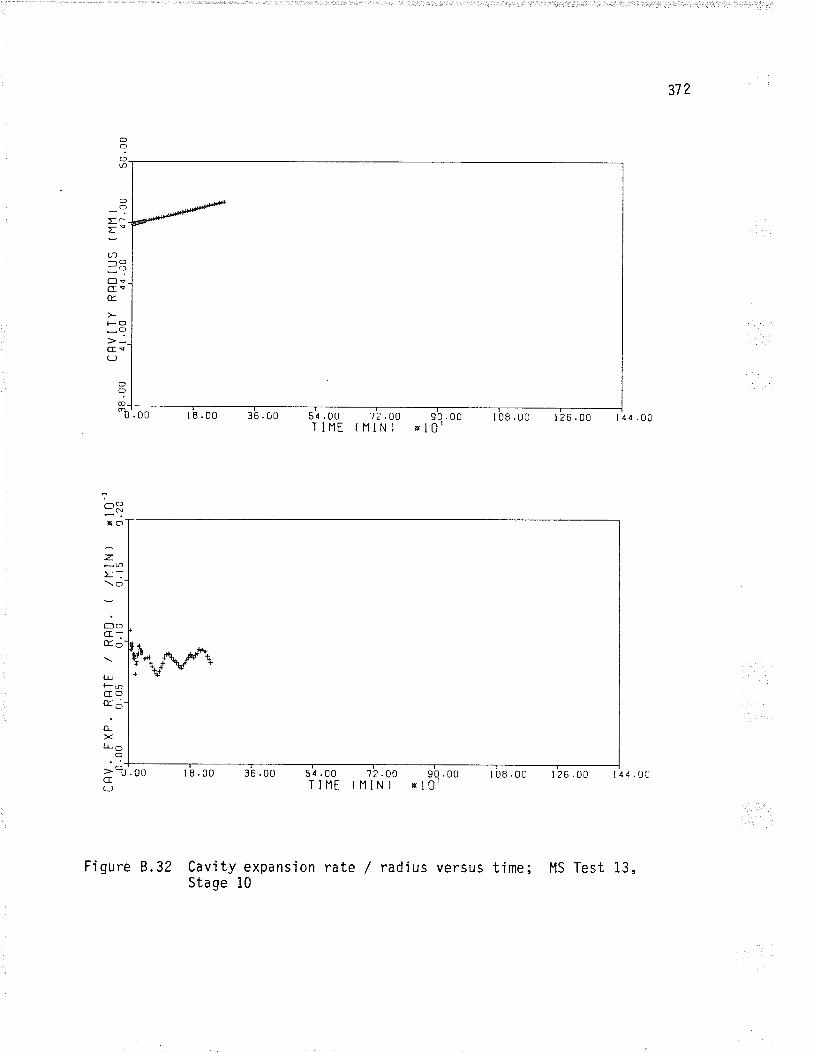
312

o?OØ

OO

Er

='U)-O-¡>OeGeÉ.

l-o

-?Ge(-J

O?o-b'. oo I I .00 36 .00 54 .00 ?2 .00 90 .00

TIIlE f HIN) lnl0'r l_108.00 t26.00 r4¿.00

TORXO

2

\O

Å.,G:olo

u_JtsnGCIEO

*><L!o

O

G(J

. ']->R'.oo 18.00 36.00 si.oo z'z.oo sb.oo lba.oc tþo.o¡ li¿.or-

TINE (HIN) xl0'

Fi gure 8.32 Cav'ity expansion rate / rad't us versus tíme; l4S Test 13,Stage 10

ç\t*\+

373

APPENDIX C

COI{PUTER PROGRAMS

}ÐYOPLI

OYORATE

LADFOSl

LADPL

PRDPLS

OSUÌ{

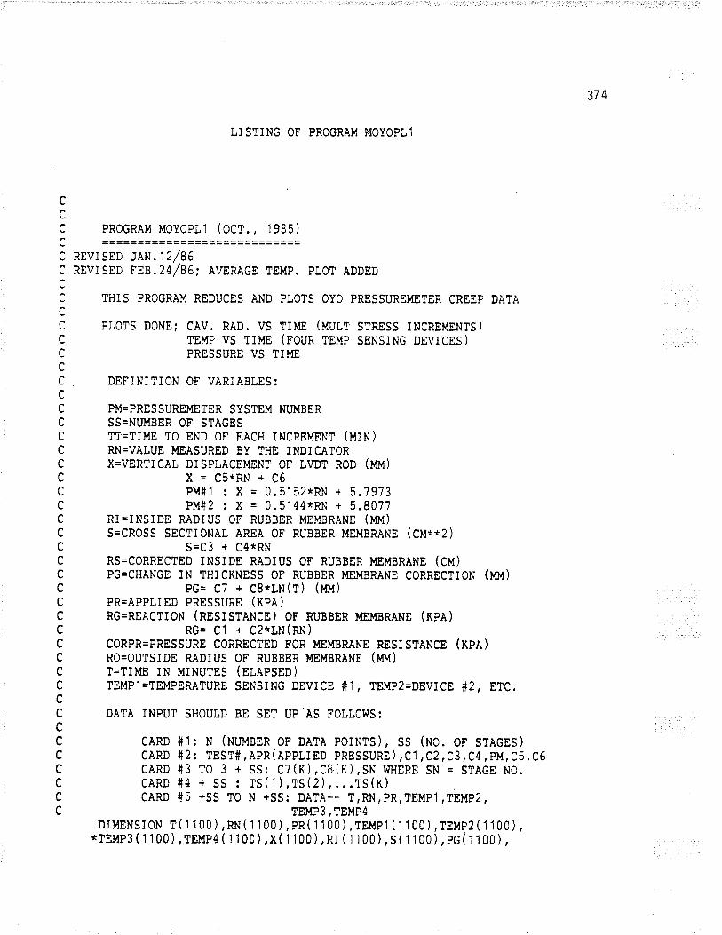
374

tISTiNG OF PROGRA}4 MOYOPLI

ccc PROGRAM MoYoPtl (ocr., 1985)a ---c REVTSED JÀN.tz/eøc REVTSED FEB.z+/ea; ÀvERÀcE TEMp. pLOT ADDEDcC THIS PROGRAM REDUCES AND PTOTS OYO PRESSUREMETER CREEP DÀTÀcc pLoTs DoNE; cÀv. RÀ0. VS TiME (UUr,r STRESS ¡HCnEMENTS)C TEMP VS TIME (r'oun TEMP sENsIHc o¡vlces)C PRESSURE VS TIMEcC DEFINITION OF VÀRIÀBLES:cC PM=PRESSUREMETER SYSTEM NTJMBER

C SS=NUMBER 0F STÀGESC TT=TIME TO END OF EÀCH INCREMENT (UTH)C RN=VÀLUE MEÀSURED BY THE INDICÀTORC X=VERTiCÀI DISPLÀCEMENT OF t\DT ROD (MM)

C X=95*p¡q+çgc PM#1:X=0.5152*RN+5.7973C PM#2:X=0.5144*RN+5.8077C RJ=INSIDE RÀDIUS OF RUBBER MEMBRÀNE (MM)

C S=CROSS SECTiONÀL ÀREÀ OF RUBBER MEI'IBRANE (CU**2)C S=C3 + C4*RNC RS=CORRECTED INSIDE RÀDIUS OF RUBBER MEMBRÀNE (CM)C PG=CHÀNGE IN THICKNESS OF RUBBER }.ÍEMBRÀNE CORRECTION (}T'{)C PG= C7 + C8*tN(T) (}.il)C PR=ÀPPLIED PRESSURE (XP¡)C RG=REÀCTION (NNSISTÀNCE) OT NUggER }.ÍEMBRANE (KPÀ)C RG= C'1 + C2*LN(RN)C CORPR=PRESSURE CORRECTED FOR MEMBRÀNE RESISTÀNCE (KPÀ)C RO=OUTSIDE RÀDIUS OF RUBBER MEMBRÀNE (¡n¡)C T=TIME IN MINUTES (NL¡PSEO)C TEMP1=TEMFERÀTURE SENSING DEVICE #1, TEMP2=DEVICE #2, ETC.cC DÀTÀ INPUT SHOUTD BE SET UP'ÀS FOLLOWS:cc cÀRD #1: N (¡lu'fgen 0F DÀTÀ poINTS), SS (HO. Or STÀGES)C CÀRD #2: TEST#,ÀPR(ÀPPLIED PRESSURE),C1 ,C2,C3,C4,PM,C5,C6C CARD #3 TO 3 + SS: C7(K),C6(K),SN WHERE SN = STÀGE NO.C CÀRD #4 + SS : TS(1),TS(2),...TS(K)C CÀRD f5 +SS TO N +SS: DÀTÀ-- T,RN,PR,TEMP1,TEMP2,c TEMP3,TEMP4

DTMENST0N T('1 1 00 ),RH ( 1 1 00 ), pR( 1 1 00 ), TEMPI ( 1 1 00 ),teUp2 ( 1 1 00 ),*TEMP3 ( 1 100 ) ,rsl'rp ( 1j 00 ) ,x( 1 '100 ) ,p,r ( 1 100 ) , s ( 1 100 ) , pG ( 1 100 ) ,

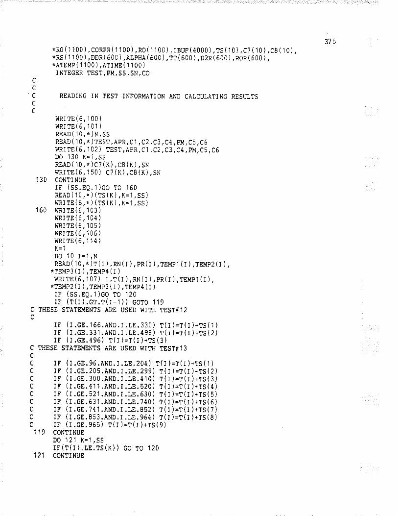
375*RG( 1 100 ) , coRpR(1 100 ) , no(1100 ) , rBUF (4000 ) ,rs (10 ) ,c7 ('10 ) ,cB ('10 ) ,*ns ('1 1 00 ), n¡n( 600 ),¡t pge ( 500 ), TT ( 600 ),n2n ( 600 ), noR ( 600 ),*ATEMP( 1 1 00 ) ,ÀTlun( r 1 00 )

I NTEGER TEST, P}.1, SS , SN , CO

cc.C

REÀDING iN TEST INFOR}.IÀTiON ÀND CÀLCUtÀTING RESULTScc

}¡RrrE(6,100)I.tRrTE(6,'101)Rn¡¡(10,*)¡,55ne¡p( 1 0, * )TEST,ÀpR,c|,c2,c3,C4,pM,c5,c6}tRITE (6,102 ) tnSr,ÀpR, C1 ,C2,c3,c4,pM,c5,C6D0 130 K=1,SSREÀD( 10, * )Ci (K),c8(K),SNI.¡RirE(6,150 ) c7 (K) ,c8 (lr) ,sN

1 3O CONTINUErF (ss.nQ.1)co ro 160nn¡¡( 1 0,* ) (fS(n),K=1,Ss)WRITE(6, * ¡ (rS (n),K='1,SS )

1 60 wRITE(6,1 03 )I.¡RrrE(6,104)I{RrTE(6,105)I,IRrrE(6,106)I{RITE(6,114)K='1

D0 10 I=1,NREAD( 10,*)T(r ),RN(I ),pR(I ),teUpl (t ),teMp2

*TEMP3(l),reUp¿(l)r{RtrE(6,107) I,t(l ),nH(l ),pR(i ),reup1(I ),

*TEMP2(t ),tnUp3(t ),rnup¿(l )

rF (ss.nQ.1)co ro 120rF (r(r ).Gr.r(r-1 ) ) coro ilg

C THESE STÀTEMENTS ÀRE USED WITH TEST#12c

rF (r.ce.166.ÀND.r.rE.330) r(¡ )=T(l )+rs(1iF (r.cn.33'1.ÀND.r.LE.495) r(i )=r(l )+rs(2rF (¡.cn.496) r(r )=T(r )+rs(3)

C THESE STÀTEMENTS ÀRE USED WITH TEST#13c

I),

c rr (l.ce.95.AND.r.LE.204\ r(r)=r(l)+rs(1)c rF (1.ce.205.ÀND.r.LE.299) r(l )=T(r )+rs(2c rr (¡.G8.300.ÀND.r.LE.4t0) T(r)=r(l)+rs(3)c rr (l.cn.411.AND.r.rE.520) r(l )=T(l )+TS(4)C iF (I.cE.521.ÀND.r.LE.630) T(i )=T(l )+rs(5)c IF (I.c8.631.ÀND.r.LE.i40) r(r )=r(l )+rs(6)c rr (1.G8.i41.ÀND.r.I,E.852) r(i )=r(r )+Ts(7)c rF (r.ce.853.ÀND.r.rE.964) r(l)=T(i)+rs(B)c iF (1.cn.955) T(r )=T(l )+rs(9)

1 19 CONTINUED0 12'1 K=1,SSrr(r(r ).rE.rs(K)) co ro 120

121 CONTINUE

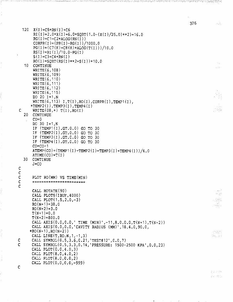
376

120 X(I )=C5*RH(l )+C6Rr ( r ) =2. 0*x ( r ) +6. 0*sgRr( 1 . 0_ ( xn ) /25. 0 ) **2 ) + 1 6. 0

RG( r )=C'1+C2*ALoG(RN( i ) )CoRPR(l )= (PR(r )-Rc 3)) h000.0pc( r )= (c; (K)+C8 (n) *¡i,oc(r( I ) ) ) /10 "0Rs (r )=Rr ( r ) h0 .o-pc (l )' S(l )=C3+C4*RI¡(l )

R0(I )=SQRT(nS(¡ )**2+S(t ) )nlO.O1 O CONTiNUE

I{RITE(6,108)I.tRrrE(6,109)}tRITE(6,110)I,ïRITE(6,11'1 )

}lRrrE (6,112)}tRirE(5,115)D0 20 I=1,NWRITE(5,1 13) I,T(r ),RO(I ),CORPR(l ),tgMpl (t ),

*TEMP2(t ),reUp3(l ),reup¿(t )

C WRTTE(08,*) T(I),RO(I)20 CONT]NUE

C0=0. D0 30 I=1,N

rF (rnupr (l ).cr.o.orF (rsup2(r ).cr.o.orF (reup3(r ).cr.o.orF (rsup¿(r ).cr.c.0gg=Çe+ 1

ATEMP(co)= (rsupl ( r )+TEMP2 ( r )+TEMp3 ( r )+TEl,{p4 fi) ) /t.OATrME(cc)=r(l)

3O CONTINUEl-^^

U -LVccc Pror Ro(MM) vs rl¡æ(ur¡l)t ---

cCALL ROTÀTE(90)cÀtl PtoTs(IBUF,4000)cÀtl PLoT(1.5,2"0,-3)R0(¡¡+1)=38.0R0(N+2)=3.0T(N+'t )=0.0T(H+Z)=800.0cÀLL ÀXI S (0.0,0.0,' TIME (UtH)

"-11 ,9.0,0.0,T1¡+'1 ) ,r(N+2 ) )

cÀLL AXIS(0.0,0.0,'CAVITy RÀDIUS (MM)

" 19,4.0,90.0,

*¡9(¡+1),no(¡t+2))cÀLL LINE(t,nO,N, 1,-1, 3)

c cÀLL syMBOL(0.5,3.6,0.21 ,' TEST#12"0.0,7)c cÀLL syMBoL(0.5,3.3,0.14,'.PRESSURE: 1500-2500 KpÀ"0.0,23)

cÀtl PtoT(0.0,4.0,3)cÀtt PtoT(8.0,4.0,2')cÀlt PLOT(8.0,0.0,2)cÀLL PtoT(0. 0, 0. 0,-ggg)

c

G0 T0 30G0 T0 30G0 T0 30G0 T0 30

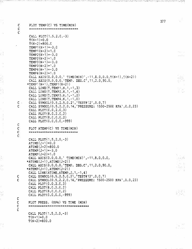
377C PLOT TEMP(C) VS TIME(MIN)^ ---L ---

ccÀLt PLOT(1.5,2.0,-3)t(H+1 )=0.0t(H+2)=800.0TEMPl (¡¡+1)=-3.0TEMPl (H+2 )=1 .0TEMP2(N+1 )=-3.0TEMP2 (¡¡+2 )= 1 . 0TEMP31¡¡+1)=-3.0TEMP3(H+2)=1.0TEMP4 1¡'¡+ 1 )=-3 . 0

TEMP4 (N+2 )=1 .0CÀLL ÀxIs(0.0,0.0,' TIME(ulH)',-11,8.0,0.0,T1¡+1 ),T(N+2) )

cÀtl ÀxIs(0.0,0.0,'TEMP. DEG.C" l 1,2.0,90.0,*TEMP1 (H+l ) ,TEMP'1 (N+2 ) )

cÀLL tINE(t,tnupl,N, 1,-1,3)CALL tiNE(T,TEMP2,N, 1,-1,4 )

cÀtl tINE(T,TEMP3,N, 1, -1,2\cÀtl LINE(T,TEMP4,N, 1,-',l,0)

c cÀLL syMBOL(0.5,2.5,0.21,'TEST#12"0.0,7)C CÀLL SYMBOL(0.5,2,2,0. 14,'PRESSURE: 1500-2500 KPÀ',0.0,23)

cÀLL PLor(0.0,2.0,3)cÀtl PLOT (8. 0, 2.0 ,2)cÀtl PLoT ( 8. 0 ,0. 0 ,2 )

cÀLL PtoT(0. 0, 0.0,-999)cC PLOT ÀTEMP(C) VS TIME(MIN)^ ---c

cÀLt PtoT(1.5,2.0,-3)ÀTIME(,1+1)=0.0ÀTIME1¡+2)=800.0ÀTEMp1¡+1 )=-3.0ÀTEMp(¡+2 )=1 .0cÀLL ÀXIS(0.0,0.0,' TIME(UlH)

"-11,8.0,0.0,*ÀTjuE(;*l ),ÀTIME(¡+2 ) )

cÀLt ÀxIs(0.0,0.0,'TEMP. DEG.C"1 1,2.0,90.0,*ÀTEMP 1¡+'1 ) , ÀÎEMP (¡+2 ) )cÀtL LINE(¡rIUe,ÀTEMP, J, 1,-1,4 )

c cÀLL syMBoL(0.5,2.5,0.21,'TEST#12"0.0,7)C CÀLt SYMBOt(0.5,2.2,0.14,'PRESSURE: 1500-2500 KPÀ',0.0,23)

cÀtt Ptor (0.0 , 2.0 ,3)CALL PLor (8. 0, 2.0 ,2)cÀI,L PLor(8.0,0.0,2)cÀLt PLoT(0. 0,0. 0,-999)

cc PLoT PRESS. (np¡) vS TIUE (ulN)a ---L ---

ccÀLL PLoT ( 1 . 5, 2.0 ,-3)T(N+1 )=0.0T(N+2)=800.0

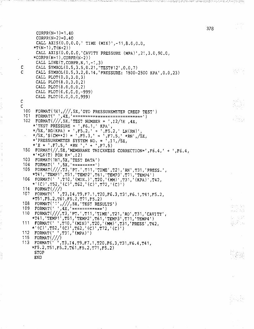
378

cc

cc

CORPR(N+1 )=1.40CoRPR ( H+z ) =0 .40cÀLL ÀXIS(0.0,0.0,, TIME (l¡ln) ' ,-11 ,9.0,0.0,*T(N+1),T(N+2))cÀtl ÀxIs(0.0,0.0,' CAVITy PRESSURE (MpÀ)

"21, 3.0, 90.0,

*coRPR 1¡,¡+ 1 ) , CORPR (H+2 ) )cÀtl LINE(r,CORpR,N, 1,-'1,3 )

cÀtl syMBot(0.5,3.5,0.21,'TEST# 12"0.0,7)CÀtL SYMBOt(0.5,3.2,0.14,'PRESSURE: 1S00-2500 KpÀ',0.0,23)CALL PtoT(0.0,3.0,3)cÀtL PLOT(8.0,3"0,2)CALL PtoT(8.0,0.0,2)cÀtl PLoT(0. 0,0. 0,-ggg)cÀLL PtoT(0.0, 0.0, ggg)

1 00 FoRMÀT (tlHt , /// ,5X, 'OyO PRESSUREMETER CREEP TEST' )

101 FORMÀT( t ' ,4X, | ============================t )

102 FoRMÀT(///,5x,'TEST NUMBER = , ,r2/1H ,4x,*'TEST pRESSURE = ',F6.1,' KpÀ',o/.5x,'RG(KpÀ) = ',F5.2,, + ',F5.2,' LN(RN)',- */5x,,'S(CM**2) = , ,F5.3,' * i ,F7.6,' *RN' ,/åx,*'PRESSUREMETER SYSTEM N0. = ',fj,/5X,*,x = , rF'l.5r' *RN trr + trF7.5)

150 FORMÀT(//,5X,'MEMBRÀNE THICKNESS CORRECTIO¡q="F5.4,' + "F6.4,

*'*LN(f) fOn ¡1=',I2)FoRltÀT( 1H1, 5X,' TEST DÀTÀ' )FORMÀT( t t ,5X, r=========r

)

FORI'{ÀT (///,T3,' pr.

"T1 1,'TIM8

"T21,'RN"T31,' PRESS.

"*T4 1 , ' TEMP 1 ' , T5 1 , ' TEMP2 ' , T6 1 , ' TEMP3 ' , T7 1 , ' TEMP4 ' )

FoRMÀT( ",T10,' (MIN. )

"T20,' (m,l)

"T31,' (Kp¡)

"142,'r' (c)

"T52,' (c)

",162,' (C)

"T72,' (C)' )

FoRMÀr (///)FoRUÀT( ",T3,I4,T9,F7 .1,120,F5.3,T31,F6. 1,T4 1,î5.2,

*T51,F5.2,T61,F5.2,T'7 1,F5.2 )

1 08 FORMÀT( ',1' ,///,5X, 'TEST RESULTS' )109 FORM.AT( ",4X,r============r )'1 10 FORMÀT(///,T3,'pT.

"T1 1,'TIl,{8"\21,'R0"T31,'CÀVITy"

*T4 1 , ' TEMP 1 ' , T5 1 , ' TEMP2 ' , T6 1 , ,TEMP3 ' , T7 1 , ' TEMP4 ' )

1'1 1 FORMÀT( ",T'10,, (MIN),,T20,' (!o,f)

"T31,'pREss"142,*' (c)

"T52,' (c)

"T62,' (C),,'172,' (C)' )

112 FoRMÀT(' ' ,T31,'(Mp¡)' )

11s FoRMÀr(///)113 FoRì,ÍÀT( ' ' ,T3,I4,Tg ,F7 .1 ,T20,F6.3,T3.1 ,F6 .4,T41 ,*F5.2,T51,F5.2,T61,F5 .2,T7 1,î5.2)

STOP

END

103104105

106

114107

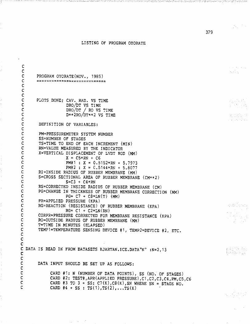
379

tISTING OF PROGRÀM OYORÀTE

ccc PROGRAM oYoRÀTE(NoV., 1gg5),^ ___L ============================cccC PLOTS DONE; CÀV. RÀ0. VS TIMEc DRO/DT vS TrMEc DRO/DT / nO vS rrunC D**2pg/97**2 VS TIMEcC DEFINITION OF VARIABLES:cC PM=PRESSUREMETER SYSTEM NUMBERC SS=NUMBER 0F STÀGESC TS=TIME TO END OF EÀCH iNCREMENT (UIH)C RN=VÀLUE MEÀSURED BY THE INDICÀTORC X=VERTICÀL DISPLÀCEMENT OF tVDT ROD (M¿)C X=CS*RN+C6C pM#1:x=0.5152*RN+5.7973C PM#2:X=0.5144*RN+5.8077C RI=INSIDE RADIUS OF RUBBER MEMBRÀNE (¡ru)C S=CROSS SECTIONÀI ÀREÀ OF RUBBER MEMBRÀNE (CU**2)C S=C3 + C4*RNC RS=CORRECTED INSIDE RÀDiUs OF RUBBER MEMBRÀNE (cu)C PG=CHÀNGE IN THICKNESS OF RUBBER MEMBRÀNE CORRECTION (MM)C pG= C7 + CB*LN(T) (lol)C PR=ÀPPLIED PRESSURE (xp¡)C RG=REÀCTION (NNSISTÀNCE) Or' NUggER MEMBRÀNE (KPÀ)C RG= C1 + C2*LN(RN)C CORPR=PRESSURE CORRECTED FOR MEMBRANE RESISTANCE (KPA)C RO=OUTSIDE RÀDIUS OF RUBBER },ÍEMBRÀNE (MM)C T=TIUE IN MINUTES (NtÀPSNP)C TEMP1=TEMpERATURE SENSING DEVICE #1, TEMP2=DEVICE #2, ETC.cccC DATÀ IS REÀD IN FROM DÀTÀSETS KJÀRTÀN.ICE.DATA',N" :N=2,13ccC DÀTÀ TNPUT SHOUTD BE SET UP ÀS FOLLOWS:cc cÀRD #1: ¡l (}{I¡UBER 0F DÀTÀ POTNTS), SS (t¡0. Or sTÀcES)c cÀRD #2: TEST#,ÀpR(ÀpptlED PRESSURE),cj,cz,c3,c4,pl,f ,c5,c6C CÀRD #3 T0 3 + SS: C7(K),C8(K),SN wunnE SN = STÀGE NO.c CÀRD #4 + SS : TS('1),TS Q) ,...TS(K)

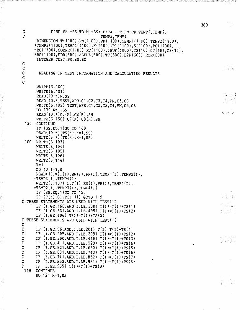
380

ccccc

CÀRD #5 +SS TO N +SS¡ DÀTÀ__ T,RN,PR,TEMP1,TEMP2,

DTMENSToN r( 1 100),R¡¡( 1 100),ifiiii¿äilÏårrr ( 1 i 00),reup2( 1 100),*TEMP3 ( 1 1 00 ),tsup4 ( 1 1 00 ),x( I 1 00 ),Rr ( 1 1 00 ), s ( 1 1 00 ), pc ( 1 1 00 ),*Rc( 1 I 00 ), CoRPR( 1 1 00 ), no( 1 1 00 ), IBUF ( 4000 ),ts ( 1 0 ), c7 ( 1 0 ),cB ( 1 0 ),*RS ( 1 1 00 ),DDR(500) ,elpH¡(600 ) ,TT(600 ) ,p2R(600 ) ,ROR(600 )

INTEGER TEST,PM,SS,SN

READING IN TEST INFORMÀTION ÀND CÀICUIÀTING RESULTS

r{RI TE (6, 1 00 )r.¡RITE(6,101)ng¡p('10,*)¡,5tnn¡u ( 1 0 , * )TEST, ÀPR, c1 ,c2 tc3 ,c4, PM, c5 , c6wRITE (6,102) tnst,ÀpR,C1,C2,c3,c4,pM,c5,c6D0 130 K=1,SSnn¡o( 1 0, * ) C7 (K),Cg (n), Sr,¡

I{RrrE(6, 150) cz(x),cB(n),s¡¡1 3O CONTINUE

rF (ss.nQ.1)co ro 160ng¡P( 1 0, * ) (fS (n),K='1,SS)i.¡Ri TE ( 6 , * ¡ ( rs (¡t ¡ , ¡= 1 , ss )

160 r{RrrE(6,103)I.¡RrrE(6,104)I{RrTE(6,105)I.rRrTE(6,106)I.¡RI TE ( 6, 1 14 )

K=1D0 10 I=1,NREÀD(10,*)1,(l ),Rw(l ),pR(l ),teup1 (l ),tn¡lp2(r ),

*TEMP3(i),rnUeA(l)t,lRITE(6,1 07 ) i ,T( I ) ,RN(l ) , pR( I ) ,reunt (l ) ,

*TEMP2(i ),reUp3(l ),rgì.rp¿(t )

rF (ss.eQ.1)co ro t20iF (T(r ).cr.T(i-1 ) ) coro rg

C THESE STÀTEMENTS ÀRE USED WITH TEST#12rF (r.cn.r66.ÀND.i.rE.330) r(r )=r(l )*rs(l )

rF (r.cn.331.ÀND.r.rE.495) T(r )=r(r )+rs(2)rF (r.cn.495) T(l )=r(i)+rs(3)

ccccccccccc

THESE STÀTEMENTS ÀRE USED WITH TEST#13

rF (1.cs.96.ÀND.r.rE.z04) T(l )=r(r )+rs(1 )

rF (1.cn.205.ÀND.r.rE.299) T(r¡r (l.cE.3oo.ÀND.I.LE.41o) T(rrn (t.cE.411.ÀND.i.tE.520) T(Iln (1.c8.521.ÀND.r.rE.530) T(rrF (r.cE.631.ÀND.r.tE.74o) T(rrF (1.cn.241.ÀND.r.rE.B52) T(rrF (1.cn.853.ÀND.r.LE.964) T(rrF (r.cn.965) r(l )=r(l )+rs(9)

119 CONTINUED0 121 K=1,SS

=t(t )+ts(2)=r(t )+TS(3)=T(l)+rs(¿)=r(l )+1S(5)=t(l )+rs(6)=r(l )+rS(7)=T(l )+rs(8)

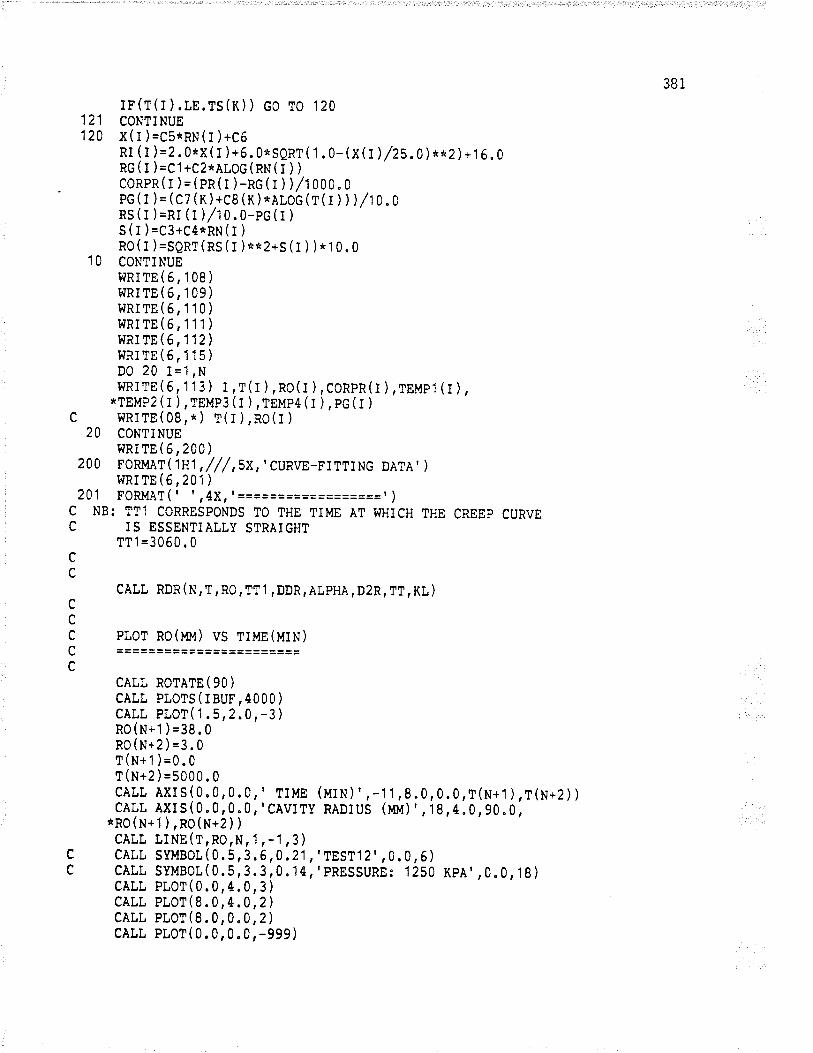
381

rF(r(r ).rE.Ts(K)) co ro 120121 CONTINUE120 X(I )=C5*Rw(l )+C6

nr ( I ) =2. 0*X ( I ) +6. 0*SQRT ( 1 . 0_ ß0 ) /ZS. 0 ) **2 ) +1 6. 0Rc(r )=C1+C2*ALoc(nH(l ) )coRPR(l )=(pn(l )-Rc(r )),/looo.opc ( r )= (c7 (n)+cB (lr ) *¡r,oc (r( I ) ) ) /10 .cns(r )=Rr (r ) /t0.0-pc(i )

S(I )=C3+C¿*nH(l )

no(i )=SQRT(ns(t )**2+s(l ) )olO.O1O CONTINUE

t{RITE(6,109)wRITE(6,109)t{RrrE(6,110)I{RrrE(5,1'11)I,¡Ri rE (6 ,112)I{RITE(6,'115)D0 20 I=1,N}lRirE(6,1 13) t,t(t ) ,Ro(i ),coneR(l ),rgMp1 (l ),

*TEMP2 (l ),rnup3 ( I ),tnup¿ ( I ),pc(t )c l.lRrrE(08,*) T(r),Ro(i).20 CONTINUE

I.¡Ri TE (5, 200 )200 FoRMÀT (ul , / / / ,5x, ' cuRVE-Fr rrl Nc DÀTÀ' )

}IRITE(6,20'l )

201 fOn¡¡¡f ( t t r4Xrt ==================r )cc

cc

ccccc

NB: TT1 CORRESPONDS TO THE TIME ÀT I.rHIcH THE CREEP CURVEIS ESSENTIÀLLY STRÀIGHT

TT1=3060.0

cAtL RDR(N,T,Ro,TT1,DDR,ÀtpHÀ,D2R,TT,KL)

:::l=::lil=::=l:i:iï )

cÀrl RorÀrn(90)cÀLL ProTS(rBUF,4000)cÀLt PtoT ( 1 . 5, 2.0 ,-3)R0(N+1 )=38.0R0(N+2)=3.0T(N+1)=0.0r(H+2)=5000.0cÀLt ÀxIS(0.0,0.0,' TIMEcÀtt ÀxIs(0.0,0.0,' cÀvlTY

*R0(N+1 ),no(N+z) )cÀLL LINE(t,RO,N, 1,-1,3)cÀtt SYMBoL(0.5,3.6,0.21,cÀLL SYMBoL(0.5, 3. 3,0.14,cÀtl PtoT(0.0,4.0,3)cÀLL PLoT(8.0,4.0,2)CALL PtoT(8.0,0.0,2)cÀtl PLoT(0. 0, 0. 0,-ggg)

(ulH)',-1 1,9"0, 0.0,T1¡+'1 ),T(N+2) )RÀDIUS (m¡)

" '18,4.0, 90 " 0,

'TEST12' ,0. 0,6 )

'PRESSUREz 1250 KPÀ',0.0, 18)

382

cc Pror DDR vs rrun(r¡l¡q)t- ___

ccÀtl PLor(1.s,2.0,-3)tt(nr+1 )=0.0TT(KL+2)=5000.0DDR(Kt+1 )=0.000DDR(KL+2)=0.002cÀLt ÀxIs(0.0,0.0,' TIME (Ut¡¡)

"-11,9.0,0.0,*11(6¡+1 ),rt(nr+2) )

cÀLt ÀxIs(0.0r0.0,'cÀv. Exp. RATE (¡n¡rlUlH)"23,4.0,90.0,*DDR(6¡+1 ),DDR(KL+2 ) )cÀLL LI NE (TT, DDR, KL, 1 , -'1 , 3 )c cÀtt syMBoL(0.5,3.5,0.21 ,' TEST12"0.0,6)

C CÀtt SYMBOL(0.5,3.2,0.14,'PRESSURE: 1250 KpÀ',0.0,18)cÀtl PLoT(0.0,4.0,3)cÀLL PLoT(8.0,4,0,2)cÀLt PtoT(8.0,0.0,2)cÀrt PLOT(0. 0, 0.0,-ggg)

cC PLOT ÀtPHÀ VS TIME(UT¡I)I ---

ccALt PtoT(1.5,2.0,-3)TT(KL+'1 )=0.0TT(KL+2)=5000.0ÀIPHA(nl+1 )=0.0000ÀLPHÀ (xl+2 ) =0.00005cAtL ÀxIS(0.0,0.0,' TIME (Ul¡¡)

"-11,9.0,0.0,*11(¡1¡+1),tt(nl+2))cÀLt ÀxIs(0.0,0.0r'cÀv. EXp. RÀTE / RAD. ( /UiH)"2g,4,0,90.0,

*ÀLPHÀ (Xl*1 ),¡lpH¡ ( n¡,+2 ) )cÀLL IINE(tt,¡t ptt¡,KL, 1,-1, 3 )

c cÀtt syMBot(0.5,3.5,0.21 ,, T8ST12"0.0,6)c cÀLt syMBoL(0.5,3.1,0.14,' PRESSURE: 1250 KpÀ"0.0,19)

cÀtt PtoT(0.0,4.0,3)cÀtt PtoT (8 . 0 , 4.0 ,2)cÀLL PtoT(8.0,0.0,2)cÀLt PtoT(0"0, 0.0,-ggg)

ccC PtOT D2R VS TIME(UIN)t\ ___

ccÀtt PLoT( 1 .5,2.0, -3 )

TT(Kr+1 )=0.0TT(Kr+2)=5000.0cÀtt scÀLE (D2R ,4 ,0 ,KL, 1 )cÀLL ÀXIS(0.0,0.0,' TIME (UlH)

"-11,9.0,0.0,*TT(KL+1 ),tr(Xl+Z) )

cAtt ÀxIS(0.0,0.0,'cÀv. ÀccEL. (oen),,15,4.0,90.0,*D2R(¡1¡+1 ),02n(Xl+2 ) )cÀtt tINE(tr,p2n,KL,1 ,-1 ,3)

383

c cÀLt syMBoL(0.5,3.5,0 ,21 ,' TEST12' ,0.0,6)c cÀLL syMBOL(0.5,3.1,0.14,', PRESSURE: 1250 KpÀ"0.0,19)cÀtL PLor(0.0,4"0,3)cÀrr PtoT(8.0, 4,0 ,2\cÀtL PtoT(8.0,0.0,2)cAtL Plor( 0. 0, 0. 0,-999)cÀtt PLor(0.0, 0. 0,999)

c100 FoRMÀT fiH1 ,///,5x, ,oyo pREssuREMETER cREEp resr' )1 01 FORMÀT( t t ,4X, I ============================l )102 îoilttL,t(///,5x, 'TEST NLTMBER = , ,I2/1H ,4X,

*'TEST pRESSURE = 'rF6.1r' KpA',*/5x, 'RG(Kp¡) = 'rF5.2r' + 'rF5.2r, LN(RN)',*/5X,t'5(gy**l) =',F5.3r' +'rF7.Sr' *RN'r/aX,*'PRESSUREMETER SySTEM NO. = ',I1,/5N,,*tx = rrF7.5rr *RN rrr + trF7.5)

150 FoRMÀT (//,5x, 'MEMBRÀNE THIcKNESs CoRRECTIo¡¡=' ,F6.4,' + ' ,F6.4,*'*tN(f ) ¡'On ¡=',I2)'103 FoRÌ'ÍÀT(1H1 ,5X, 'TEST DATÀ')104 FORMÀT(t t r5Xrt=========r )105 FORMÀT (///,T3,'pr.

"T11,'TIME"T21,'RN"T31,'PRESS. "*T41,' TEMP1

"T51,'TEMPz"T61,' TEMP3"'1'7 1,'TEMP4' )

106 FoRMÀT(' ' ,T10,'(MIN. )' ,T20,'(lOl)' ,T31,'(KpÀ)' ,!42,*' (c)

"r52,' (c)

",!62,' (c)

",!72,' (c)' )

114 FoRMÀr(///)107 FoRMÀT( ",T3,I4,T9,î7 .1,'!20 ìF6.3,T31,F6. 1,T41 tPs,2,

*T51,F5. 2,T51,F5 .2,T7'1,F5. 2 )108 FORMÀT(', 1"///,5X,'TEST RESUITS' )109 FORMÀT( t t

r4Xr r============r)

110 FORMÀT (///,T3,'pr.' ,T11,'TIME' ,T21,'RO' ,T31, 'CAVITy"*T41 I'TEMP1''T51 ''TEMP2' ,T61,'TEMP3' ,T71,'TEMP4' ,T81,'PG' )

111 FoRMÀT( '',T10,' (MIN)

"T20,' (Ì,î{)

"T31,'PRESS"142,*'(c)"T52,' (C)

"T62,' (C)

"T72,' (C)')

112 FoRMÀT(' ' ,T31,'(MPÀ)')11s FoRMÀr(///)113 FoRMÀT( " ,T3,I4,T9 ,F7 .1 ,T20 tF6.3,T31 ,F6 ,4 Ã41 ,

cccccccc

c

*F5.2,T51,î5,2,151,F5 .2,î'11,F5. 2,191,F7.5)STOPEND

FiTTING EXPERI}.IENTÀt DÀTÀ ÀND FINDING DERIVÀTIVESSUBRoUTINE RDR(L,T,R,TT1,DDR,ÀtpHÀ,D2R,TT,KL)DtMENST0N T(t),n(l),OOn(600),ÀLPHA(600 ),ROR(500),* D2R(600),TT(600),Ren(600)N--_NI]MBER OF POINTS FOR FITTING ONE SEGMENT OF CURVE

N MUST BE AN ODD INTERGERRRR---VÀIUES ON CI'RVEDDR---SIOP OF CURVEÀLPHA---Dn(r)/n(r)OTHER ÀRGM{ENTS EXPLÀINED IN SUBROUTINE DRIVCHÀNGE UKM'' TO CORRESPOND TO MÀX NO. OF SEGMENTSTT2=5680.0Kl'l=LN=9N1=31

384

ccc

N1=41N1=2'1

41 D0 22 KK=1,KMrF(KK.cr.1) co ro go

SET ''KU TO INiTIAI STÀRTING POINTK=1G0 T0 35

6O CONTINUEIF(T(K).LE.TT1) GO TO 38rF(T(K).Cn.rr2) co ro 38G0 T0 50

FOIIOWING ROUTiNE CÀtCULATES RÀTE FOR SHORT SEGMENTSNB: THE FOLTOWING EXPRESSION IS USED TO INCREMENT THE SEGS.

K=K+N T.IHERE N IS THE INCREMENT38 K=K+336 rF(K.cE. (r-N)) CO TO 22

CHANGE 'M' TO CORRESPOND TO POLYNOMIÀL DEGREE35 M=3

cÀtt DRIV( N,M, K, L, T, R, RRR, DI R, D2DR, ÀLpHÀ 1, TTT, RI R )G0 T0 51

FOtIOWING ROUTINE CÀLCULÀTES RÀTE FOR LONG SEGMENTS50 K=K+30

rF(K.cE. (r-N1) ) CO TO 22M=3cÀtt DRIVL ( N'1, M, K, L, T, R, RRR, DI R, D2DR, ÀLpHÀ 1, TTT, RI R )51 KL=KKTT(KK)=TTTROR(KK)=RRRRER(KK)=RIRDDR(KK)=DIRD2R(KK)=D2onÀLPHA ( KK ) =ÀLPHÀ 1

22 CONTiNUEr{RITE(5,104)

104 FoRMÀT(1H'1, ///,5X, 'VÀLUES ÀT MIDPOINTS OF SEGMENTS')27 Ì{RITE(6,102)102 FOW;¡T ( / / /, 5X, ' KK' , 6X, ' T' , 12X,'R' , 1 2X, ' RR' ,* 15x,'DR' ¡17Nt 'D2R' ,17N,, 'ÀLPHA')

DO 24 KK=1,KLI{RI TE ( 6, 1 00 ) nX, rr ( XK ), RER ( ttn ), ROR ( KK ), OOn ( nn ), o2R ( xn ),* ÀLPHÀ(KK)

100 FoRMÀT(3X,I3,3X,Fg .1,7X,F6.3,7X,F6.3,9X,F12.9,9X,î12.9,* 8x ,F12,9)24 CONTINUE

RETURNEND

FOtIOWING SUBROUTINE IS USED TO FIND VÀLUES ÀND DRIVÀTIVESOF ONE SEGI-IENT OF CURVEsuBRouTi NE DRI V ( N, M, K, L, T, R, RRR, DI R, D2DR, ÀLpHÀ 1, TTT, RI R )

CHÀNGE THE DIMENSION STÀTEMENT TO CORRESPOND TO ''N1''DIl.rENSr 0N X ( 7 ) , y ( 7 ) , À ( 3 ) , T ( t ) , R ( L ) , RR ( 7 ) , DR ( 7 ) ,* D2R(7),CC(3,4),F(7,3),enn(7)DTMENST0N X(11 ),y( 11 ),À(3),r(r,),R(t),RR(11 ),OR(.11 ),

ccc

cccc

385c * D2R(11),CC(3,4),F(1'1,3),ERR(11)

DiMENsi0N x(9),y(9) ,À(3) ,t(r) ,n(r,) ,nn(9) ,oR(9) ,* DzR(g),CC(3,4),F(9,3),ERR(g)C N-_--NT'MBER OF POINTS USED FOR FITTING ONE SEGMENT CURVEC X(¡¡)___EXpERIMENTÀL POINTS r r I I I r I I I I r r I I I I I I r I I I I I I I r I

C Y(H)---nxpERIMENTÀL vÀLUEs oH x(H)C M-1---POWER OF CURVE FITTEDc À(u)---usnD To sroRE coEFS oF poryNourÀLc cc(u,¡l)---woRKINc UNITC t--_TOTÀL NUMBER OF EXPERIUENTÀL POINTSc T(¡l)---wHoLE ExpERIMENTÀr poINTsC R(H)___rrrrrrrrrrrrrrrrtr VÀLUESC Rn(H)---v¡LUES FRoM cURVEC Dn(H)---nnIvÀTIVES FRoM cURvEc K---ORDERTH OF F¡RST POINT or x(H) TH r(r)

D0 104 I=1,NX(i)=0.0

104 Y(l)=0.0D0 10S I=1,3À(l )=0.0D0 106 J=1,4'105 cc(I,J)=0.0

105 CONTINUED0 100 I=1,NJ=K+I - 1

x(t)=t(,:)100 y(i)=n(,:)

¡4q=!,1+1

cÀLL PotY (N,X, YrM,A,MM, CC rF, K)D0 101 I=1,NRR(I )=0.0DR(t )=0.0DzR(I)=0.0D0 102 J=1,M

102 RR(r )=RR(I )+¡(,:)*(x(r )**(J-'1 ))D0 103 JJ--2 ,t4103 DR(r )=oR(¡ )+¡(,¡,:)*(x(l )**(JJ-2))*rloer(JJ-1 )D0 108 JJJ=3,M

1 08 DzR( I ) =D2R ( I ) +¡ (,:,:¡ ) * (x ( I ) n* (JJ¡-3 ) ) * (¡;J-l ) * (.:.1,:-z )1 O1 CONTINUE

t{RrrE(5,203)203 FORMÀT (//,11X,'pr ,' ,7x,'TIME' ,2X, 'EXPT. RAD.' ,1X,* 'cÀLc. RÀD.

"gx,'DR' ,14X, 'D2R' ,14X, 'ERR')

ÀBERR=0.0DO 202 I=1,NJ=K+I - 1

ERR( r )=(n(¡)-nn(l ) )/(n(;)-38.0 )ÀBERR=ÀBEnR+ (n(¡ )-nn( I ) ) **Z¡{RrrE(6,200) l,x(i ),y(r ),RR(r ),oR(l ),02n(¡ ),nRn(l )200 FoRMÀT(10X,i3,5x tl7 .1,5x,F6.3,5x,F6.3,5x,F12.9,.* 5x, F12.9,5x,F1 2.9)

202 CONTINUELL='l+ ß-1l'/zRRR=O.0

386

cc

cccc

ccccc

cccc

ccc

ÀLPHÀ1 =0.0DI R=0. 0

D2DR=0.0TTT=0.0RI R=0. 0

l{RITE (6,.2.01) lL,X(rl) ,y(Lt) ,RR(LL) ,pn(li,) ,D2R(LL)201 FORMÀT(//,10X,I3,5X,F7.1,5X,F6.3,5X,F6.3,åX,F12.9,* 5x ,F12.g',)

I,tRrrE (6,205) ¡snRn205 FORMÀT(//,10X,'SUM OF SQUÀRED RESIDUÀLS = ' ,F12.9)

TTT=X ( tL )

RRR=RR ( LL )DI R=DR ( tt )

D2DR=D2R ( tL )

ÀrPHA1 =On (ll)/nR (tt )

RIR=Y(LL)RETURNEND

LEÀST SQUÀRES CURVE-FITTING PROGRÀM

SUBRoUTINE poLy (N,X, y,M, C,MM, À, F, KK )DIMENSI0N X(N) ,y(N) ,F(N,M) ,À(M,Ifi) ,C(M)

GENERATE THE F MÀTRIX. MODIFY THE S?ÀTEMENTS ÀSREQUiRED FoR DIFFERENT NoS. 0F FUNCTIoNS

D0 2 I=1rNF(I,1)=1 .oFfi,2)=x(i )

F(I,3)=x(r )*x(l )2 CONTINUE

GENERÀTE THE tOT.JER TRIÀNGUtÀR ETEMENTS OF THECOEFFICIENT MÀTRIX ÀND ÀSSiGN VÀtUES TO THE SYMMETRICELEMENTS ÀBOVE THE MÀIN DIAGONAL.

D0 4 I=1rMD0 4 J=1,IÀ(I,J)=0.0D0 3 K=1,N

3 À(1,,:)=À(I,,:)+n(x,I)*F(¡t,,1)À(J,I)=¡(t,.1)

4 CONTINUE

GENERÀTE THE ELEMENTS OF THE COt[ffN MÀTRIX TOTHE RIGHT OF THE EQUÀL SIGN IN THE ÀLGORITHM

D0 5 I='1 ,MÀ(t,tt+1)=0.0D0 5 K=1,N

5 À(I,M+1)=¡(l,M+'1)+F(K,l)*y(¡t)

DETERMINE THE C VÀLUES OF Y(X) ¡Y SOi,VING THESIMUtTÀNEoUS EQUÀTIoNS WITH CHoIESKy'S !,ÍETHOD

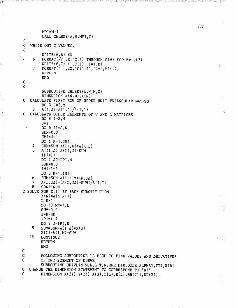
387

cc

ÌdP 1 =M+.1cÀtl CHLSKY(À,M,MP1,C )

cC WRITE OUT C VÀLUES.c

TIRITE(6,6) ttn ', 6 FoRMÀT(//,5x,'c(1) THRoucH c(M) FoR ¡1=',r3)ÞIRITE(6,7',) (l,C(t), I=1 ,Þt)7 FoRMÀT( " r3X,'C(

"I1 r')="814.7)

RETURNEND

SUBRoUTINE CHLSKY (À,N,M,X)DIMENSI0N À(N,M),X(N)

C CÀLCULÀTE FIRST ROW OF UPPER TJNIT TRIÀNGULÀR MATRIXD0 3 J=2rM

3 À(1,J)=À(1,¡)/x(t,1)C CÀICUIÀTE OTHER ELEMENTS OF U ÀND L MÀTRICES

D0 I I=2,Nr.,l - L

' D0 5 II=J,NSLIM=O.0JM'l=J-1D0 4 K=1,JM1

4 SIJM=SI.JM+À(II,K)*À(K,J)5 À(li,J)=À(II,J)-SLJÌ'J

¡p.l=l+1D0 7 JJ=IPI ,MSUM=0. 0

IM1=I-1D0 6 K='1,IM1

6 suM=stJM+À(i,K)*À(X,,:,:)7 A(l,JJ)=(¡(r,JJ)-suu)/À(l,r)8 CONTINUE

C SOLVE FOR X(I ) BY BÀCK SUBSTITUTIONx(N)=À(H,¡t+1)L=N-1D0 10 NN=1,LSLIM=0. 0I =N-NNJ p.l =l +.1

D0 9 J=IP1,N9 StJM=Suu+À(I,J)*x(J)

x(l )=¡(l,t't)-suu1 O CONTINUE

RETURNEND

cC FOTLOWING SUBROUTiNE IS USED TO FIND VÀtUES ÀND DRIVÀTIVESC OF ONE SEGI'IENT OF CURVE

suBR0uTI NE DRI Vt ( N, Þ1, K, L, T, R, RRR, DI R, D2DR, ÀLpHÀ1, TTT, RI R )C CHÀNGE THE DIMENSION STÀTEMENT TO CORRESPOND TO ''N1''c Dil-tENSI0N X(21') ,yQ1) ,A(3),T(t),R(t),RR(21),DR ,21) ,

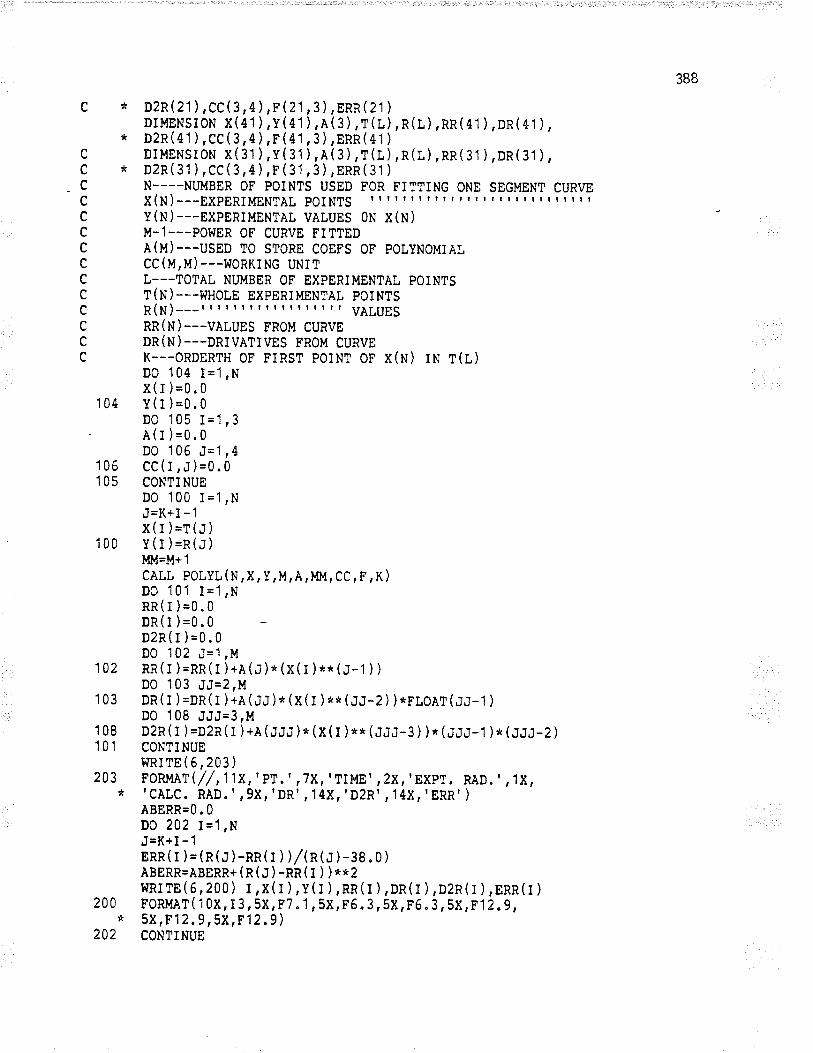
388

c * D2R(21 ),CC(3,4),F(21,3),ERR(21 )

DII'{ENSroN X(41 ),y(41 ),¡(3),r(r,),n(r),RR(41 ),DR (41),* o2R ( 4 1 ) , CC ( 3 , 4 ) , F ( 41 , 3 ) , ERR ( 4 1 )c DrMENsr0N x(31),y(31 ),A(3),r(r) ,n(l),RR(31 ) ,DR(31),c * DzR(31),CC(3,4),F(31,3),ERR(31)C N----NIJI'IBER OF POiNTS USED FOR FTTTING ONE SEGMENT CURVEc x(¡¡)___nxpERIMENTAt POINTS rr I r rr r r rr r rrr I I r rr I r r r I I I I r

c y(H)---sxpERrMENTÀr vÀruEs o¡¡ x(H)C M-1---POT.¡ER OF CURVE FITTEDC A(T'I)---USED TO STORE COEFS OF POLYNOMIÀLc cc(u,lr)---woRKrNG L¡NITC L---TOTAI NTTMBER OF EXPERIMENTAL POINTSc r(H)---r+uorn ExpERiMENTÀL porNTSc R(H)___rrrrrrrrrrrrrrrttr VÀLUESC Rn(H)---v¡tUES FRoM cURvEC Dn(H)---pnIVATIvES FRoM cURVEc K---oRDERTH 0F FrRsr porNT or x(¡¡) n¡ r(l)

D0 104 I=1,Nx(t )=0.0

104 y(l)=0.0D0 105 I=1,3. À(I)=0.0D0 105 J=1,4

106 cc(I,J)=0.0105 CONTINUE

D0 100 I=1,NJ=K+I -'lx(l )=r(¡)

100 y(l )=n(.:)MM-M+1cÀI,L PoLYL(N,x,Y,]t!,À,MM, cc,F, K )

D0 10'1 I=1,NRR(I )=0.0Dn(t )=0.0D2R(I )=0.0D0 102 J='1 ,M102 RR(r )=RR(i )+¡(J)o(x(l )**(J-1))D0 103 JJ=2,M

103 ¡n(t )=DR(I )+¡(,:¡)n(x(I )**(JJ-2) )*rlo¡t(,:,:-l )D0 108 JJJ=3,M

1 08 D2R ( i ) =D2R ( i ) +¡ (,:.1; ) * (x( I ) *o (.:,:,¡-3 ) ) * (,:¡,:-l ) * (,:.¡.:-z )101 CONTINUEI{Rr rE ( 6, 203 )

203 FoRMÀT (//,1 1x, ' pr ,, ,lx,'TIME, ,Zx, 'Expr" RAD.' ,1x,* 'cÀtc. RÀ0.

"9X,'DR' ,14X,, 'D2R' ,14N, 'ERR')

ÀBERR=0.0D0 202 I=1,NJ=K+I-1ERR( r )=(R(J)-RR( r ) )/(n(J)-38. 0 )ÀBERR=ÀBEnn+ ( R( J ) -RR( ¡ ) ) **2I{RITE(6,200) t,X(r ),y(I ),RR(l ),¡n(l ),02R(l ),eRn(l )200 FoRMÀT(10X,I3,5X,F7,1r5X,F6.3,5X,F5,3,5X,F12.9,* 5x,F12,9r5x,F12.9)

202 CONTINUE

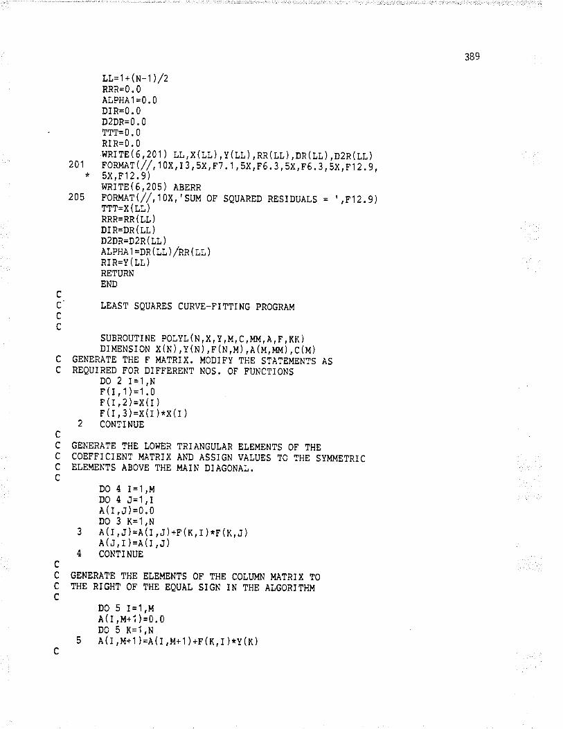
389

cc

cccc

ccccc

cccc

LL=1+ (N-1') /zRRR=0. 0ÀLPHÀ1 =0.0DIR=0.0D2DR=0. 0

TTT=0. 0

RIR=0.0_ lrRr rE ( 6 ,.2.01 ) rL, x ( LL ) , y ( ll ) , RR (LL ) , DR (Lr ) , DzR (LL )201 IoRMÀT(/1,10X,I3,5X,F7.1,5X,r0.¡,5i,16.3,åx,î12.g,* 5x ,F12.9')

r.rRrrE(6,205) ¡snRn205 FORMÀT(//,10X,'SuM OF SQUÀRED RESIDUÀLS = ' ,î12.g)

T?T=x ( tt )

RRR=RR (tt)DI R=DR ( LL )

D2PR=D2R ( LL )

ÀLPHÀ 1 =DR (LL ),/NN ( rI )

RIR=Y(tL)RETURNEND

tEÀsT SQUARES CURVE-FITTING pRocRAM

SUBROUTINE potyt(N,x,y,M, c,l"tM,À,F,KK)DIMENSI0N X(N) ,y(H) ,r(H,M) ,À(U,¡Ol) ,C(M)

GENERATE lHE F MÀTRIX. MODIFY THE SÎÀTEMENTS ÀSREQUIRED FOR DIFFERENT NOS. OF FUNCTIONS

D0 2 I='1,NF(i,1)=1.0F(I,2)=x(l)F(I,3)=x(t)*x(I)

2 CONTiNUE

GENERÀTE THE LOWER TRIÀNGULÀR ETEMENTS OF THECOEFFICIENT MÀTRIX ÀND ÀSSIGN VÀLUES TO THE SYMMETRiCETEMEN?S ÀBOVE THE MÀIN DIÀGONÀL.

D0 4 I=1,MD0 4 J=1,IÀ(I,J)=0.0D0 3 K=1,N

3 À(1,.1)=A(I,J)+r(x,I)*F(x,¡)À(J,I)=¡(l,J)

4 CONTINUE

GENERÀTE THE ETEMENTS OF THE COIU,TN MÀTRIX TOTHE RIGHT OF THE EQUÀL SIGN IN THE ÀLGORITHM

D0 5 I=1,MÀ(I,M+1)=0.0D0 5 K=1,N

5 A(I,M+1 )=À(I,M+'l )+r(x, t )*v(x)c

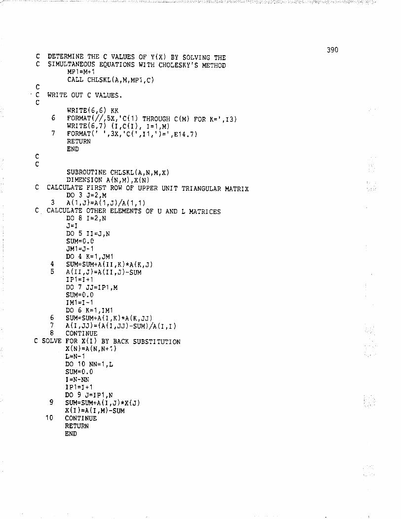
390

cc

c DETERMTNE THE c vÀLUEs 0F y(¡i) sy soLvINc rHEc SIMULTÀNEoUS EQUÀTIONS WITH CHOLESKY'S METHOD¡4P'l =!.1+ 1

cÀtL CHLSKL(À,M,MP1,C )c.C WRITE OUT C VÀLUES.c

I,rRrrE(6,6) KK6 FORMÀT(// tsx,'C(1) THROUGH C(M) FOR K="I3)

l{RITE(6,7) (i,C(t), I=1,M)7 FoRMAT( " r3x,'C(

"I 1 r')="E14.7)

RETURNEND

SUBRoUTINE CHLSKT(À,N,M,X)DIMENSI0N À(N,M) ,X(N)

C CÀLCULÀTE FIRST ROW OF UPPER UNIT TRIÀNGUtAR MÀTRIXD0 3 J=2,M

3 À(1,J)=À('1 , ¿)h(j,1)C CÀLCUIÀTE OTHER ETEMENTS OF U ÀND t MÀTRICES

D0 I I=2,NJ=ID0 5 II=J,NSUM=0.0JMl =J-1D0 4 K='l ,JM1

4 SI,]M=SUM+À(II,K)*À(K,J)5 À(ti,J)=¡(lI,J)-SIJM

¡p.l=l+1D0 7 JJ=Ip1,MSUM=0.0IM1=I-1D0 6 K=1,IM'l

6 SUM=SUu+A (I , K )*À (n,,:,: )

7 A(l,JJ)=(¡(r,JJ)-suM)/À(l,l)8 CONTINUE

C SOLVE FOR X(I) BY BÀCK SUBSTITUTIONX(N)=¡(H,N+.1)L=N-'1D0 10 NN='1 ,LSUM=0.0I =N-NN1p.l =l + 1

D0 9 J=Ip1,N9 sul't=sul.r+À(I,J)*x(J)x(l )=¡(t,u)-suq

1 O CONTINUERETURNEND

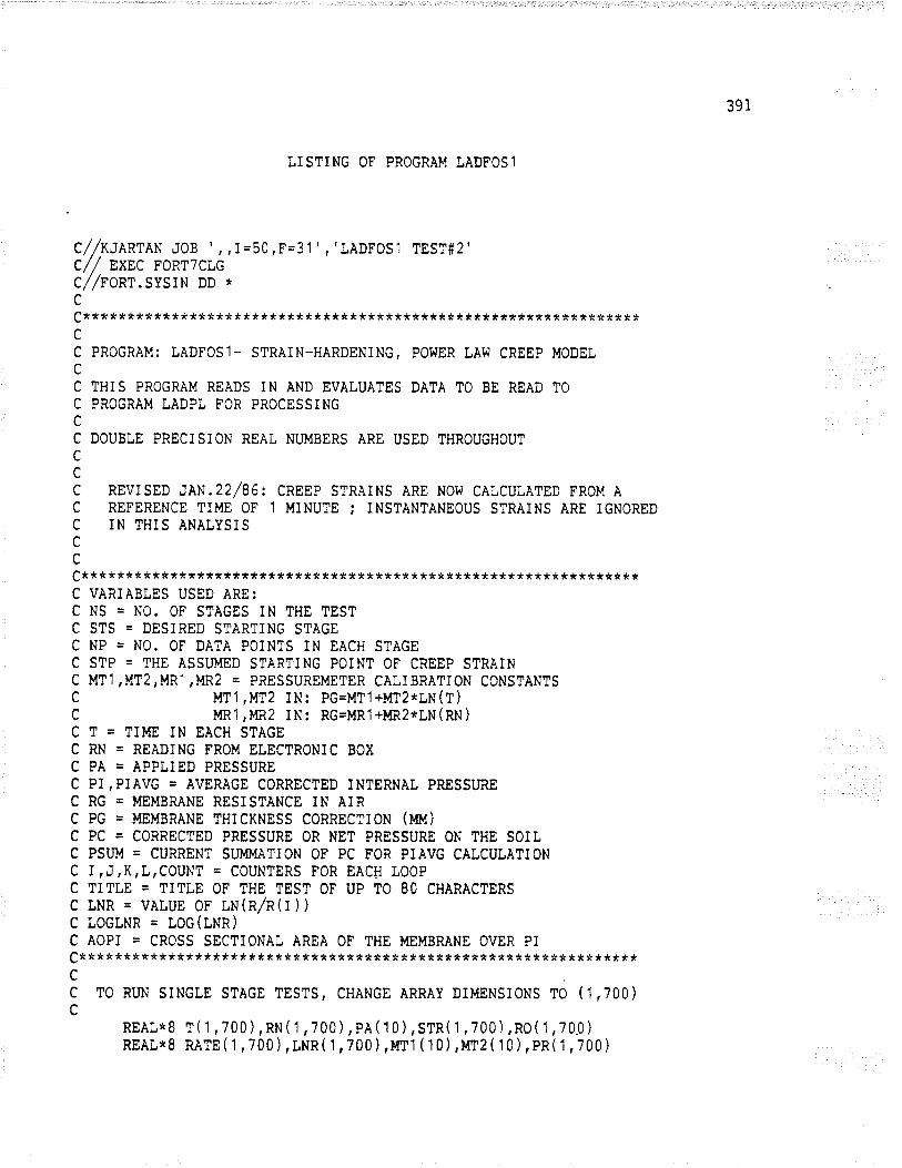
391

TISTING OF PROGRÀM tÀDFOS1

c//x¡xw¡N JoB',,I=50,F=31','LÀDFos1 TEST#2'c// exec FoRrTcLGc//tonr.sYsIN DD *cc****************************t**********************************cC PROGRÀM: LADFOS1- STRAIN-HÀRDENING, POI¡ER tÀW CREEP MODELcC THIS PROGRÀM REÀDS TN ÀND EVÀLUÀTES DÀTÀ TO BE REÀD TOC PROGRÀM LÀDPL FOR PROCESSINGcC DOUBLE PREC]SION REÀL NUMBERS ÀRE USED THROUGHOUTccc REVISED JAN.22/86: CREEF STRÀINS ÀRE NOr{ CÀLCULÀTED FROM À

C REFERENCE TIME OF 1 MINUTE ; INSTÀNTÀNEOUS STRÀINS ÀRE iGNOREDC IN THIS ÀNÀLYSISccc*** *** * * ** * * ***** * ****** *** ********** * *** ************* ** *******C VÀRIÀBLES USED ÀRE:C NS = N0. 0F STÀGES IN THE TESTC STS = DESIRED STÀRTING STÀGEC NP = N0. 0F DÀTÀ POINTS IN EÀCH STÀGEC STP = THE ÀSSUMED STÀRTING POINT 0F CREEP STRÀINC MT1,MT2,MR1,MR2 = PRESSUREMETER CÀLIBRÀTI0N CONSTÀNTSC MT1 ,l'ÍT2 IN: PG=MT1+MT2*LN(T)C MR1,MR2 IN: RG=MR1+MR2*LN(RN)C T = TIME IN EÀCH STAGEC RN = REÀDING FROM ETECTRONIC BOXC PÀ = ÀPPLIED PRESSUREC PI,PIÀVG = ÀVERAGE CORRECTED INTERNÀt PRESSIIREC RG = MEMBRÀNE RESISTÀNCE IN ÀIRC PG = MEMBRÀNE THICKNESS CORRECTION (}'fM)

C PC = CORRECTED PRESSURE OR NET PRESSURE ON THE SOILC PSU'r = CURRENT SUMMÀTION 0F PC FOR PIÀvc CÀLCUtÀTIONC i,J,K,L,COUNT = COUNTERS FOR EÀCH L00PC TITLE = TITLE 0F THE TEST 0F UP T0 80 CHARÀCTERSC tNR = VÀIUE OF tN(R/R(I))C TOGLNR = LOG (T,HN )

C ÀOPI = CROSS SECTIONAL ÀREA OF THE MEMBRÀNE OVER P]C***************************************************:t*********t(*cc T0 RIJN SINGLE STÀGE TESTS, CHÀNGE ÀRRAY DIMENSIoNS T0 (1,700)c

REÀL*8 T('1 ,700 ) ,RH('1 ,700) ,p¡(10) ,STR('t ,700) ,RO(1 ,70.0)REÀL*8 RÀTE( 1,700),lNn( 1,700),¡tt'l ( 10),tfr2( 10),pR( 1,700)

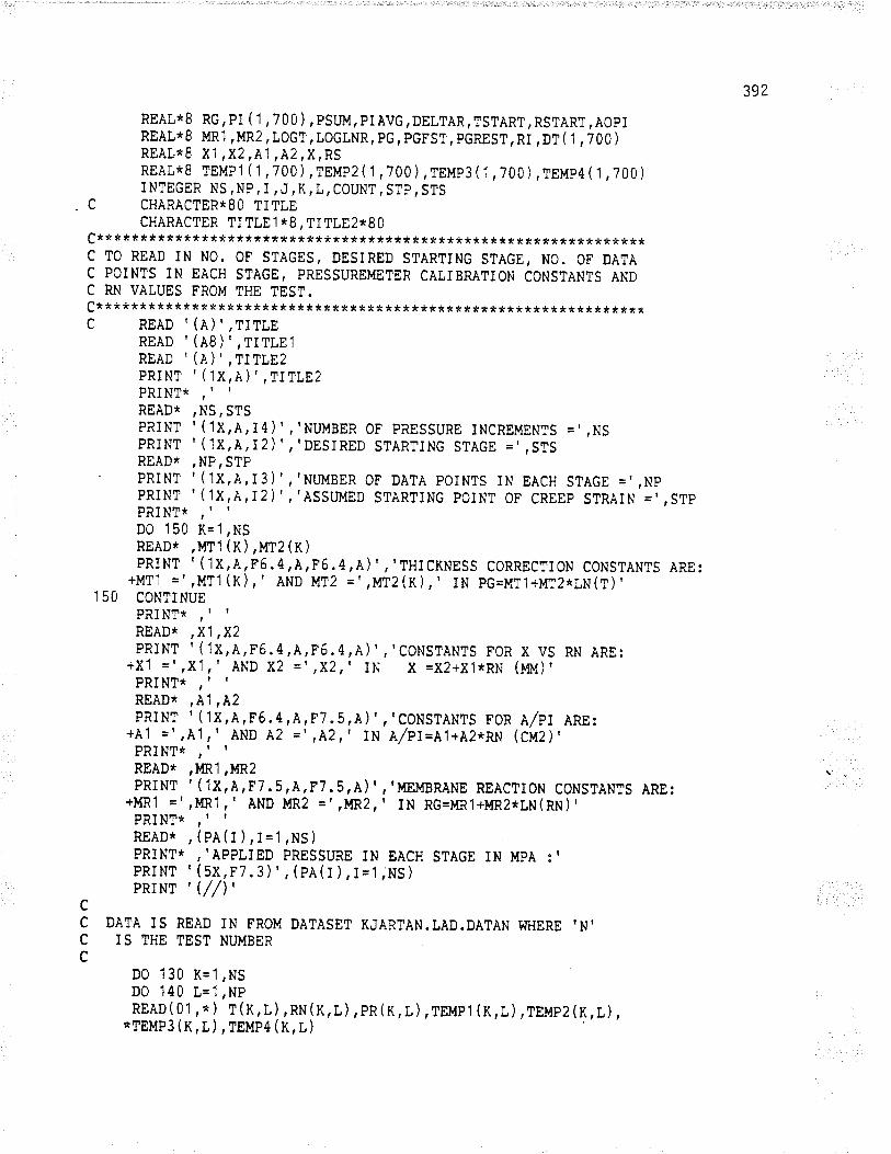
392

REÀL*8 RG, pI ( 1, 700 ),psuM,pIÀvG,DELTÀR,TSTÀRT,RSTÀRT,ÀOpIREÀL*8 MR1 ,UR2,LOGT,LOGLNR,PG, PGFST,PGREST,RI ,DT( 1 ,7OO)REÀL*8 Xl ,N2,A1 ,A2,X,RSREÀL*8 TEMPl ('1,700),tnup2( 1,700),lgup3( 1,700),rg¡tp4( 1,700)I NTEGER NS , NP ,7 , J , K , L , COUNT , STP , STS

. C CHÀRÀCTER*8O TITLECHÀRÀCTER TITLEl *8, TITLE2*80

C***************************************************f***********C TO REÀD IN NO. OF STÀGES, DESIRED STÀRTING STÀGE, NO. OF DÀTÀC POINTS IN EACH STÀGE, PRESSUREMETER CÀLIBRATION CONSTÀNTS ÀNDC RN VALUES FROM THE TEST.c***************************************************************C REÀD ' (À)' ,TITLE

REÀD '(À8) "TITLElREÀD ' (À)' ,TITLE2

PRINT'(1X,À)"TITLE2PRINT*,'IREÀD*,NS,STSPRINT' (1x,À,I4)','NUMBER oF PRESSURE INCREME¡¡1'5 =',NSPRTNT' ('IX,À,I2)

"'DESIRED STARTING STÀGE ="STS

REÀD* ,NP,STPPRINT '(.1X,À,I3)','NUMBER oF DÀTÀ PoINTs IN EÀcH STÀGE =',NPPRINT '(1x,A,rz) ','ÀssuMED STÀRTING poINT oF cREEp srRÀIN =',srpPRINT* ,' I

D0 150 K=1,NSREÀD* ,MT1 (K ) ,MT2 (K )

PRINT' ( 1x,À,F6. 4,À, F6. 4,À )',' THI cKNEss coRREcrIoN coNsrÀNTS ÀRE:+MT1 =' ,Ifl|1 (K),' ÀND MT2 =, ,vfl2(K),' IN pG=MT1+MT2*LN(T)'

1 5O CONTINUEPRINT* ,' I

REÀD* ,Nl ,N2PRINT '(1X,À,F6.4,A,î6.4,À)"'CONSTÀNTS FOR X VS RN ÀRE:

+X1 =',X'1,' ÀND X2 =' ,X2,, IN X =X2+X1*RN (MM)'PRINT* ,' I

REÀD* ,A1,AzpRINT '(1X,A,F6.4,À,F7.5,À)

"'CONSTÀNTS

FOR e/et ann:+À'1 =' ,À1¡' ÀND À2 =, ,A2,, IN À/pI=À1+À2*RN (CU2)'PRINT*,'IREAD* ,!m1 ,MR2PRINT' (1X,À,F7.5,A,F7.5,À)

"'}ßMBRÀNE REÀCTION CONSTÀNTS ÀRE:

+!lR'l =' ,MR1 ,' ÀND MR2 =' ,MR2,' IN RG=MR1+MR2*LN(RX)'PRINT*,'IREÀD* , (P¡(I ),I=1,NS)PRINT* ,'ÀppLIED PRESSURE IN EACH STÀGE IN MpÀ :rPRINT '(5X,F7.3)' , (PA(l ),t=1,NS)PRiNr '(//)'

cC DÀTA iS REÀD IN FROM DÀTÀSET KJARTÀN.IÀD.DÀTAN WHERE 'N'C I S THE TEST NIJMBERc

D0 130 K=1,NSD0 140 L=1,NpREÀD ( 0'1, * ) T ( K, L I, RN ( K, L), pR ( K, I, ), TEMP j (x,l ), TEMP2 ( K, L ),

*TEMP3 (X , t ) , TEMP4 (X, ¡, )

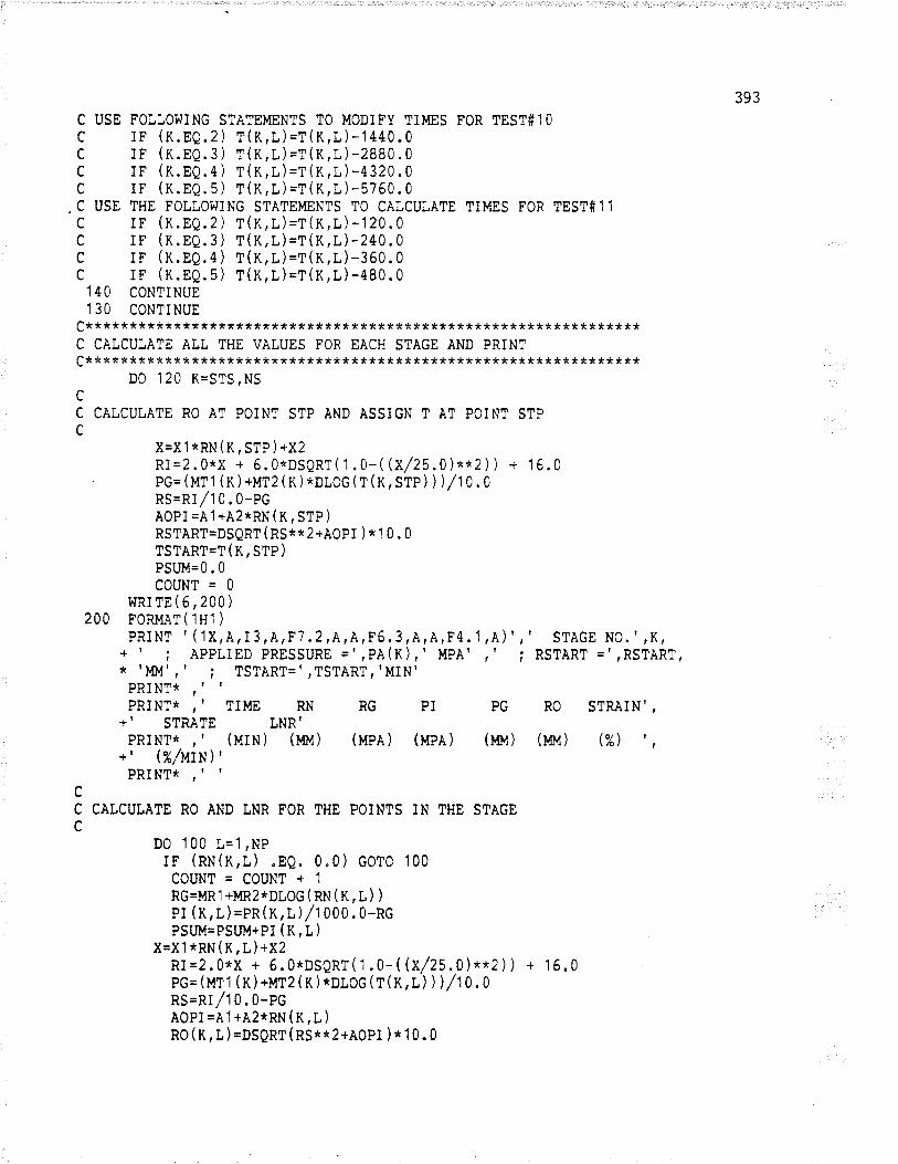
393

C USE FOLLOWING STÀTEMENTS TO MODIFY T]MES FOR TEST#10c rF (K.EQ.2c rF (K.EQ.3c rF (K.EQ.4c rF (K.EQ.5

T(K,L)=r(x,L)-1440.0T(K,L)=r(n,L)-2880.0T (K , L ) =t (x ,L) -4320 .0T(K,L)=t(n,L)-5760.0

C USE THE FOLLOWING STÀTEMENTS TO CÀLCUIATE TiMES FOR TEST#'11c IF (K.EQ.2) T(K,L)=r(n,L)-120.0c IF (K.EQ.3) T(K,L)=T(n,L)-240.0c iF (K.EQ.4) T(K,L)=r(n,t)-350.0c rr (n.EQ.5) T(K,L)=T(n,L)-480.0140 CONTINUE'130 CONTINUE

C****tr**********************************************************C CÀLCUIATE ÀLL THE VÀLUES FOR EÀCH STÀGE ÀND PRINTc***************************************************************

D0 120 K=STS,NScC CÀtCULÀTE RO ÀT POINT STP ÀND ÀSSIGN T AT POINT STPc

X=Xt*RN(n,Sfp)+X2Rr=2.0*X + 6.o*DSQRT(1.0-($/25.0)**2)) + 16.0. pc=(MT1(x)+urz(¡t)*nloc(r(n,srp)))/10.0RS=RI/1 O. O-PGÀoPI =À 1 +À2*RN (lt , Stp )

RSTÀRT=DSQRT ( RS**2+ÀOPI ) * I O. O

TSTÀRT=T ( N, STP )PSUM=0. 0

COUNT = 0

lrRrrE(6,200)2OO FORMÀT( 1H1 )

pRINT ' (1X,À,I3,A,F7.2,A,A,F6.3,À,À,F4.'1 ,À)' ,' STAGE NO.' ,K,+ ' ; ÀPPLiED PRESSURE ="PÀ(K),' MPÀ' ,', ; RSTÀRT ="flSTÀRT,* 'MM' ,' ; TSTÀRT=' ,TSTÀRT,'MIN'PRINT*,'IPRINT* ,, TIME RN RG PI PG RO STRÀIN"

+' STRÀTE LNR'pRrNT*,' (UlH) (mq) (up¡) (MpÀ) (mq) (m¡) (%)

"+' &/wn)'PRINT*,'I

cC CÀICUIÀTE RO ÀND LNR FOR THE POINTS IN THE STÀGEc

D0 '100 L=1,NPrF (nH(x,r) .EQ.0.0) coTc 100CgUNT=ggg¡¡1 +.1RG=MR'I +MR2*DLOG ( RH ( N, I ) )PI (K, L )=PR (X,1, ) /tOoO. 0-RGPSIJM=PSI,JM+PI (K, L )

X=X1*RN(n,l)+X2Rr=2.0*x + 6.g*DSQRT(1.0-(ß/25.0)**2)) + 15.0pc= (MT1 ( x ) +r,{T2 ( x ) *oloc ( r ( n, L\ ) I /1 0 . 0RS=Rr/1 0.0-PcÀoPi=À1+À2*RN(X,l)R0 ( K, t ) =DSQRT ( Rs**2+¡oPI ) * 1 0. 0

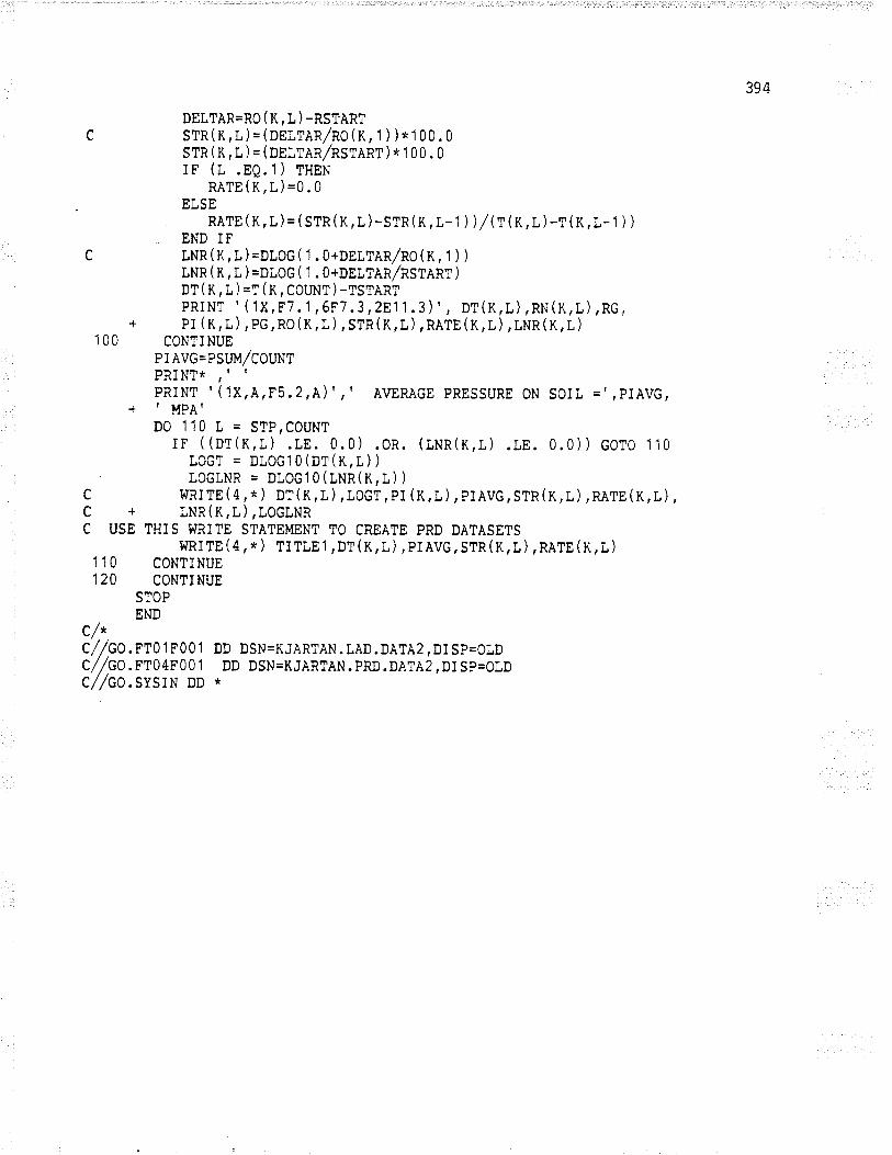
394

DELTÀR=RO (X ,I, ) -RSTARTc srR(K,l)=(onr,r¡n/no(K,1) )*100.0srR ( K, L ) = (Dnlren/nsrent ) * 1 00 . 0rF (r .EQ.1) THEN

RÀTE(K,L)=0.0ELSE

RÀTE ( ¡t, t ) = ( srR ( n, I ) -srR( K, L-1 ) ) / ß( n, i, ) -T ( K, L- 1 ) )

END IFc tt¡R(x,L)=DLOG(1.o+pei,rnn/no(x,l ) )

l¡¡n ( n, L ) =DLOG ( 1 . 0+oei,ran/nStenr )

Dt (x , ¡, ) =t (x , couNT ) -tsrenrpRINT' (1X,F7.1,6F7.3,2811.3)

" nt(K,L),Rt¡(K,L),RG,

+ pI(n,l),pG,Ro(x,l),srR(K,L),RÀTE(K,L),lNR(n,l)1 OO CONTINUE

PI AVG=PSUM/COUNTPRINT* ,, t

PRINT '(1X,A,F5.2,A)', ,', ÀVERÀGE PRESSURE ON SOIL ="pIÀVG,+ ' MPÀ'D0110L=STP,COUNT

rF ((pr(x,l) .rE. 0.0) .oR. (lNn(n,i,) .rE. 0.0)) coro 110LOGT = DLOG1 O (DT(K,L) )

LOGLNR = DLOG1O(LNR(K,L) )

c llRITE(4,*) DT(K,L),LoGT,pI (K,l),p¡¡vG,srR(K,L),n¡rg(K,L),C + LNR(K,L),LOGLNRC USE THIS WRITE STÀTEI'IENT TO CREÀTE PRD DATÀSETS

WRI TE ( 4 , * ) TI TLE 1 , DT (K, L ) , PI ÀVG , STR (K , L ) , RÀTE ( K , L )

1 1 O CONTINUE120 CONTINUE

STOPEND

c/*c//co.FTo1F001 DD DSN=KJÀRTÀN.LÀD.DÀTÀ2,Drsp=oLDc//co.FT04F00 1 DD DSN=KJÀRTÀN.pRD.DÀTÀ2,DISp=oLDc//co.sYsIN DD *

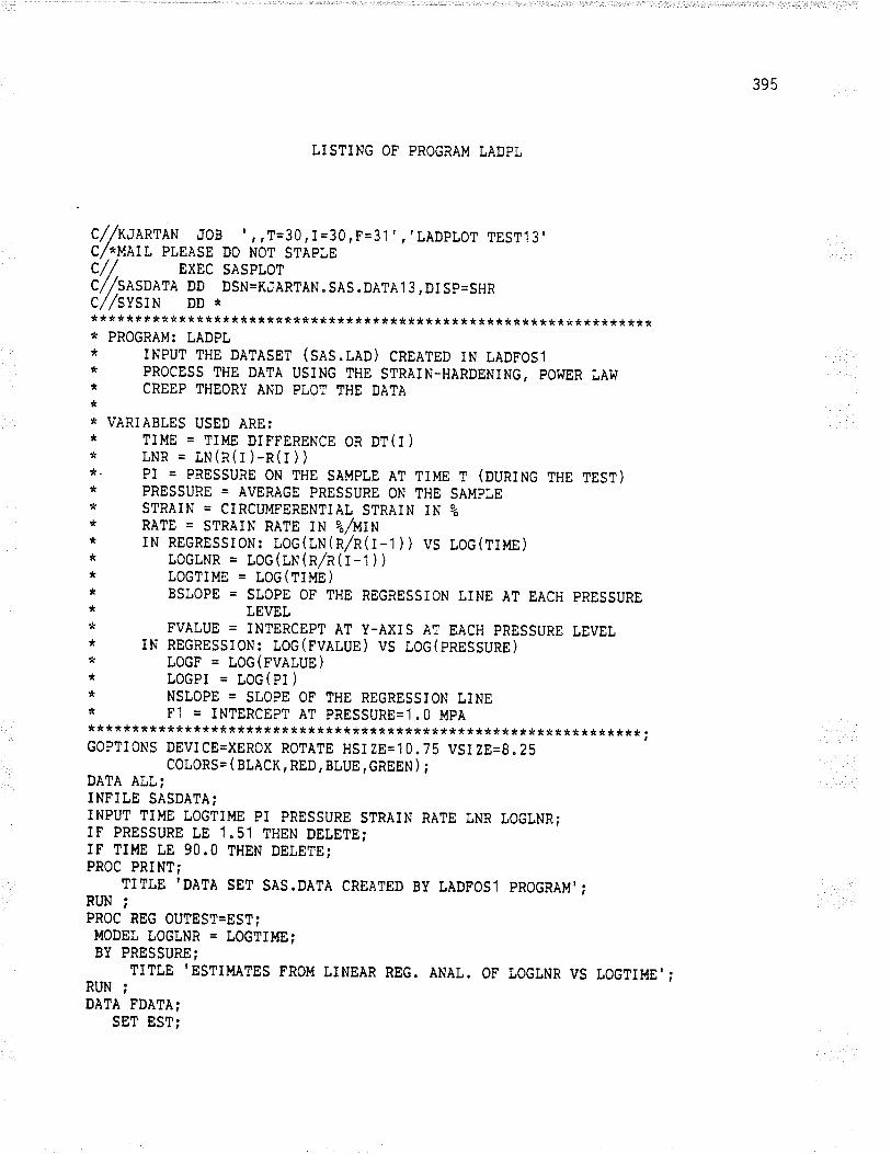
395

LiSTING OF PROGRÀM LÀDPL

c//rcnmm JoB',,T=30,I=30,F=31','LÀDpLor rEsr13'C/*U¡TL PLEÀSE DO NOT STÀPLEc// ExEc sÀsplorcr/sesoltl oo DSN=KJÀRTÀN.sls.DÀTÀ13,DISp=sHRc//sYsrv DD ** * ** * * :k * ** * * * *** * * * ** * ** * * * * * * ** * * ** rt * * * * * * * * * * * * * * * * * * * * * * * * * * ** PROGRÀM: LÀDPL* INPUT THE DÀTÀSET (S¡S.LÀD) CREÀTED IN LÀDFOS'I

'r PROCESS THE DÀTÀ USING THE STRÀIN-HÀRDENING, POWER LAFI* CREEP THEORY ÀND PIOT THE DÀTÀ** VÀRIÀBtES USED ÀRE:* TIME = TIME DIFFERENCE OR DT(I)* LNR = LN(R(I )-R(r ) )*- PI = PRESSURE ON THE SÀMPLE ÀT TIME T (DURING THE TEST)* PRESSURE = ÀVERÀGE PRESSURE 0N THE SÀMptE* STRÀIN = CIRCUMFERENTIÀt STRÀIN IN e"

* RÀTE = STRÀIN RÀTE IN 9",/MIN* rN REGRESSToN: roc(rN(n/n(r-1)) vs roc(uue)* LOGLNR = LOG(r,H(N,/N(I-1))* LOGTIME = LOG(TiUN)* BstOPE = sLOPE 0F THE REGRESSION LINE ÀT EACH pREssuRE* LEVEL* FVÀLUE = INTERCEPT ÀT Y-ÀXIS ÀT EÀCH PRESSURE LEVEL* IN REGRESSTON: LOG(FVÀtUE) VS IOG(PRESSURE)* LOGP = LOG(FVÀLUE)* LOGPi = tOG(PI )* NSLOPE = SLOPE 0F THE REGRESSION tINE* F1 = INTERCEPT AT PRESSURE='I .0 MpÀ**************************************************:t************ .

GOPTIONS DEVICE=XEROX ROTÀTE HSIZE=10.75 VSIZE=8.25COLORS= ( ¡r,¡CIt, RED, BLUE, GREEN ) ;

DÀTÀ ÀLL;INFILE SÀSDÀTÀ;INPUT TIME LOGTIME PI PRESSURE STRÀIN RÀTE LNR LOGLNR;IF PRESSURE tE 1.51 THEN DELETE;IF TIME LE 9O.O THEN DEIETE;PROC PRINT;

TITTE IDÀTÀ SET SÀS.DÀTÀ CREÀTED BY IADFOS1 PROGRÀM';RIJN ;PROC REG OUTEST=EST;MODEt tOGtNR = LOGTIME;BY PRESSURE;

TITTE 'ESTIMÀTES FRO}T IINEÀR REG. ÀNÀt. OF tOGtNR VS LOGTII,IE';RUN ìDÀTÀ FDÀTÀ;

SET EST;

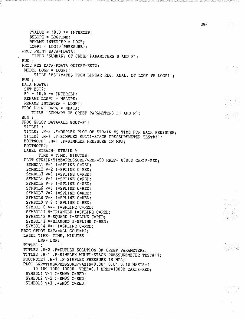
396

FVÀtUE = 1O.O T* INTERCEP;BSLOPE = LOGTIME;RENÀME INTERCEP = LOGF;tOGPi = LOGlO(PRESSURE) ;

PROC PRINT DATÀ=FDÀTÀ;TITLE 'SIJMMÀRY OF CREEP PÀRÀMETERS B AND F';

RUN ìPROC REG DÀTA=FDÀTÀ OUTEST=EST2;MODEL LOGF = tOGPI;

TiTtE IESTIMÀTES FROM LINEÀR REG. ÀNÀL. OF IOGF VS LOGPI';RUN tDÀTÀ NDATÀ;

SET EST2;F1 = 10.0 ** INTERCEp;RENÀME tOGPI = NSLOPE;RENÀME INTERCEP = LOGFI;

PROC PRiNT DÀTÀ = NDÀTÀ;TITTE 'SUMMÀRY OF CREEP PÀRÀMETERS F1 ÀND NI.

RUN ;PROC GPLOT DÀTÀ=ALL GOUT=P1;TITLEI iTITLE2 .H=2 .F=DUPLEX PLOT 0F STRAIN vs TIME FoR EÀcH pRESSURE;Ti?LE3 .H=1 .F=SIMPLEX MULTI-STÀGE PRESSUREMETER TEST#'11 ;F00TN0TE'l .H=1 .F=SIMPLEX PRESSURE IN MPÀ;FOOTNOTE2;LABEL STRÀIN= STRÀIN 9"

TIME = TIME, MINUTES;PLOT STRÀIN*TIME=PRESSURE/VREF=50 HREP=1 OOOOO CÀXIS=RED;

SYMBOLl V=1 I=SPLINE C=RED;SYMBOL2 Y=2 I=SPLINE C=RED;SYMBOL3 V=3 I=SPIINE C=REDiSYMBOL4 V=4 I=SPLINE C=RED;SYMBOLS V=5 I=SPLINE C=REDiSYMB0I6 V=6 I=SPLINE C=RED;SYMBOLT V=7 I=SPLINE C=RED;SYMBOLB V=8 I=SPLINE C=RED;SYMBOL9 V=9 I=SPLINE C=RED;SYMBOL10 V=- I=SPLINE C=RED;SYMBOL1 1 V=TRIÀNctE I=SPLINE C=RED;SYMBOI12 V=SQUARE I=SPLINE C=RED;SYMBOI13 V=DIÀl.tOND I=SPIINE C=RED;SYMBOL14 V=+ I=SPLINE C=RED;

PROC GPLOT DATÀ=ÀLL GOUT=P2;LÀBEL TIME= TIME, MINUTES

LNR= LNR;TITtEl ìTITLE2 .H=2 .F=DUPLEX SotUTIoN 0F CREEP PÀRÀMETERS;TITtE3 .H=1 .F=SII'IPLEX MULTI-STAGE PRESSUREMETER TEST#11 ;F00TN0TE1 .H=1 .F=SIMPLEX PRESSURE IN MPÀ;PLOT LNR*TI}.TE=PRESSURE/VÀXIS=O.OO1 O.O1 O. 1O HÀXIS='1

10 100 1000 10000 VREF=0.1 HREF=10000 CÀXrS=REDiSYMBOLI V=1 I=SM99 C=RED;SYMBOt2 V--2 l=SM99 C=RED;SYl.lBOt3 V=3 I=SM99 C=RED;

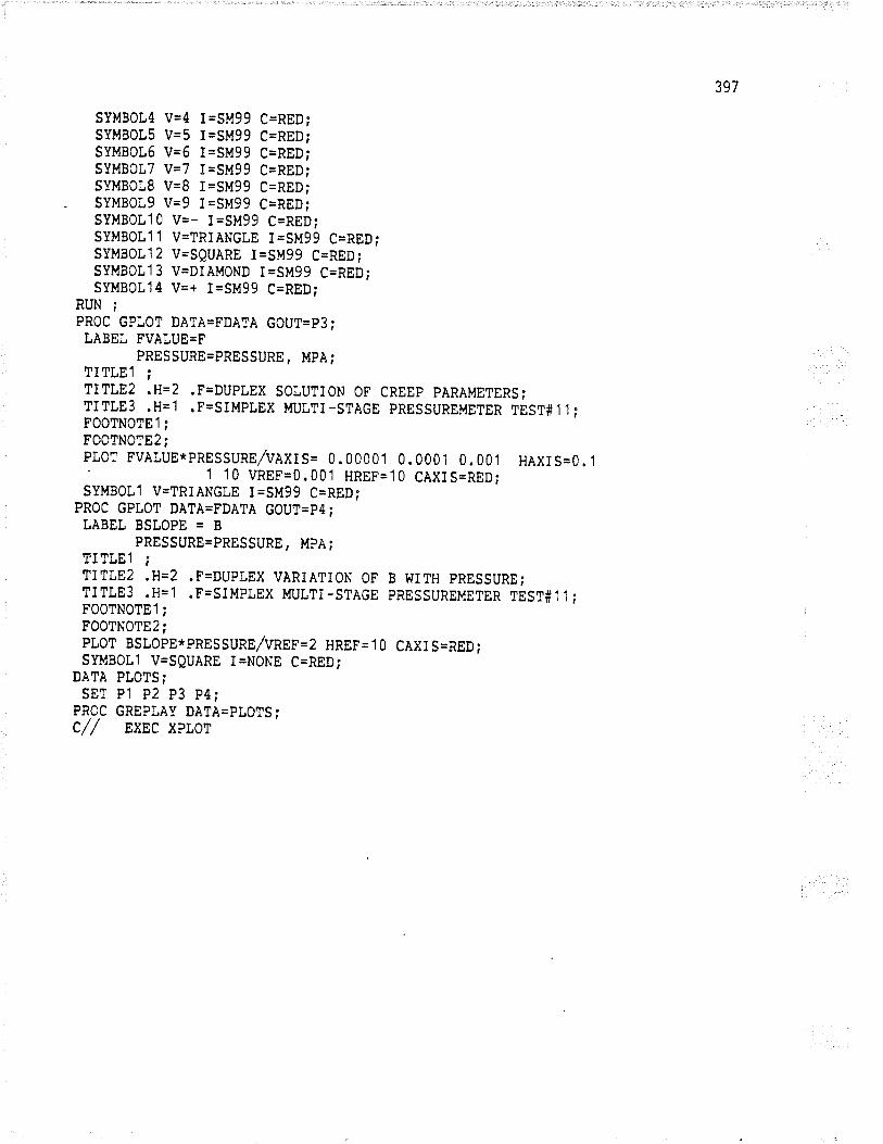
397

SYMBOL V=4 I=SM99 C=RED;SYMBOIS V=5 I=SM99 C=REÐ;SYMB0I6 V=6 I=SM99 C=REDiSYMBoLT V=7 I=SM99 C=RED;SYMBOIB V=8 I=SM99 C=RED;

. SYMBOI9 V=9 I=SM99 C=RED;SYMBOL10 V=- I=SM99 C=RED;SYMBOt11 V=TRIÀNGLE I=SM99 C=RED;SYMBOLl2 V=SQUÀRE I=SM99 C=RED;SYMBOL13 V=DIAM0ND I=SM99 C=RED;SYMBQL14 V=+ I=SM99 C=RED;

RUN ;PROC GPtOT DÀTÀ=FDÀTÀ GOUT=p3;LÀBEL FVÀLUE=F

PRESSURE=PRESSURE, MPÀ ;TiTtE'1 ìTITtE2 .H=2 .F=DUPLEX SOLUTION OF CREEP pÀRÀMETERS;TITtE3 .H=1 .F=SIMPLEX MULTI-srÀcE pREsSUREMETER TEsr#1'1 ;FOOTNOTEl;FOOTNOTE2;PtOT FVÀLUE*PRESSURE/VÀXiS= O.OOOOl O.OOOl O.OO1 HÀXIS=0.1

1 '10 VREF=O.001 HREF=10 CAXI S=RED;SYMBOL1 V=TRIÀNGLE I=SM99 C=RED;

PROC cPtOT DÀTA=FDÀTÀ GOUT=p4;LÀBEI BSLOPE = B

PRESSURE=PRESSURE, MPÀ ;TiTtEl iTITtE2 .H=2 .F=DUPLEX VÀRIÀTION OF B I.JITH pRESSURE;TITtE3 .H='1 .F=SIMPLEX MULTi-srÀcE PRESSUREMETER TEST#1 1 ;FOOTNOTE'I ;FOOTNOTE2;PtOT BSTOPE*PRESSUNE,/VNCr=2 HREF=1 O CÀXIS=RED;SYMBOII V=SOUÀRE I=NONE C=RED;

DÀTÀ PLOTS;SET P'l P2 P3 P4¡

PROC GREPLÀY DÀTÀ=PIOTS;c// ExEc xpror

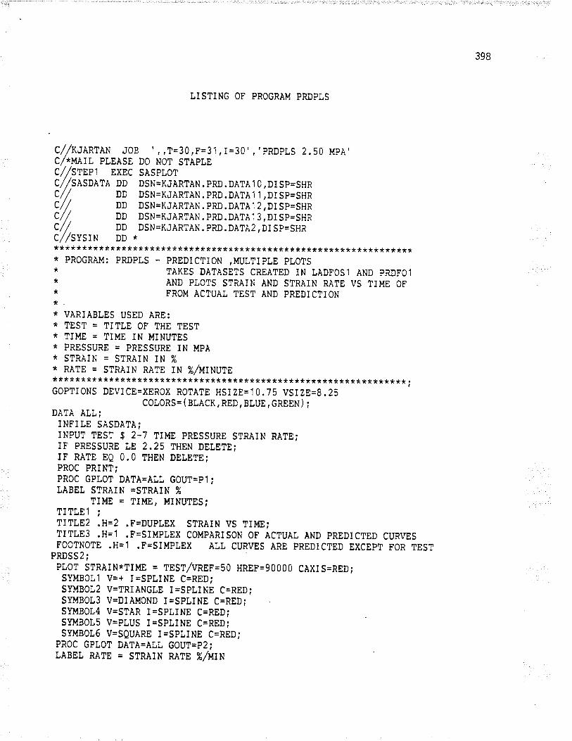
398

TISTING OP PROGRÀM PRDPLS

c//wnnteN JoB',,T=30,F=31,I=30','pRDpLs 2.50 MpÀ'C/*U¿It PtEÀSE DO NOT STÀPLEc//,srnet EXEc sÀsplorC//SÀSDÀTÀ DD DSN=KJÀRTAN.PRD.DÀTÀ1 0,DISp=SHRc// DD DSN=KJÀRTÀN.pRD.DÀTÀ1 1,DISp=sHRc/ /. DD DSN=KJÀRTÀ¡ì . pRD . DÀTÀ 1 2 , DI sp=sHRc//. DD DSN=KJÀRTÀN.pRD.DÀTÀ1 3,DISp=SHRC//, DD DSN=KJÀRTÀN. PRD.DÀTÀ2 ,DI SP=SHRC//SYSIN DD ******************:t*********************************************** PROGRAM: PRDPLS - PREDICTION ,MULTIPtE PLOTS***

TÀKES DATÀSETS CREÀTED IN LÀDFOSl ÀND PRDFO1ÀND PTOTS STRÀIN ÀND STRÀIN RÀTE VS TIME OFFROM ÀCTUÀL TEST ÀND PREDICTION

** VÀR]ÀBLES USED ÀRE:* TEST = TITLE OF THE TEST* TIME = TIME IN UINUTES* PRESSURE = PRESSURE iN Ì.tPÀ* STRÀIN = STRÀIN IN %* RÀTE = STRÀIN RATE IN %/UIHUTN***************************************************************

;GOPTIONS DEVICE=XEROX ROTÀTE HSIZE=10.75 VSIZE=8.25

COLORS= ( SL¡CX , RED , BIUE , GREEN ) ;DÀTÀ ÀLL;

INFILE SÀSDÀTÀ;INPUT TEST $ 2-7 TIME PRESSURE STRÀIN RÀTE;IF PRESSURE LE 2.25 THEN DEIETE;IF RÀTE EQ O.O THEN DETETE;PROC PRINT;PROC GPIOT DÀTÀ=ÀLL GOUT=P1;tÀBEL STRÀIN =STRÀIN %

TIME = TIME, MINUTES;TITLEl iTITLE2 .H=2 .F=DUPtEX STRAIN VS TIUE;TITLE3 .H=1 .F=SIMPLEX COMPÀRIsoN oF ÀcruÀL AND PREDICTED cuRVEsFOOTNOTE .H=1 .F=SIMPLEX ÀLL CURVES ÀRE PREDTCTED EXCEPT FoR TEsT

PRDSS2 ìPIOT STRÀIN*TIME = TEST/VREF=50 HREF=9OOOO CAXIS=RED;

SYMBOLl V=+ I=SPLINE C=RED;SYMBOL2 V=TRIANGLE I=SPLINE C=RED;SYMBOI3 V=DIÀMOND I=SPLINE C=RED;SYMBOL4 V=STÀR I=SPLINE C=RED;SYMBOL5 V=PLUS I=SPLINE C=RED;SYMB0t6 V=SQUÀRE I=SPLINE C=REDi

PROC GPIOT DÀTA=ÀLL GOUT=P2;LÀBEI RÀTE = STRÀIN RÀTE %ATIN

399TIME = TIME, MINUTES;

TITtEl ;TITtE2 "H=2 .F=DUPLEX STRÀIN RÀTE VS TIME;TITLE3 .H=1 .F=SIMPLEX COMPÀRISON 0F ÀCTUÀL ÀND PREDICTIONS ÀT P=2.50MPÀ;F00TN0TE .H=1 .F=SIMPLEX ALL CURVES ÀRE PREDICTED EXCEPT FOR TEST.

PRDSS2;PLOT RÀTE*TiME = ?EST/VREF=0.01 HREF=9OOOO CAXIS=REDi

SYMBOLl V=+ I=SPLINE C=RED;SYMBOL2 V=TRIANGLE I=SPLINE C=RED;SYMBOL3 V=DIÀMOND I=SPLINE C=RED;SYMBOL4 V=STÀR I=SPLINE C=RED;SYMBOLS V=PLUS I=SPLINE C=RED;SYMBOLS V=SQUÀRE I=NONE C=REDi

DÀTÀ PLOTS;SET P1 P2;

PROC GREPLÀY DÀTÀ=PLOTS;c//stnpz EXEc xPLOT

400

!_rsTrruG 0F PROGRAH QSUN

The listing of Program QSUN is unavairable as it forms a

part of Mr. Sun's Ph.D. Thesis which has not yet been pubìished.

in part'ial fulfillment of the - mspace

Documents