Wevnr-,ET AND Mul,lIFRACTAr, ANerysrsOn TnaNSIBNTS II{ Fownn SvsrEMS

by

LEILA S. SAFAVIAN

A ThesisSubmitted to the Faculty of Graduate Studies

in Partial Fulflrllment of the Requirementsfor the Degree of

MASTER OF SCIENCE

Department of Electrical and Computer EngineeringUniversity of Manitoba

Winnipeg, Manitob a, Canada

Thesis Advisor: Prof. W. Kinsner, Ph.D., P.Eng.

(xvii + 122+ A-2 + B-28) -- 169 pp.

@ Leila S. Safavian; January 2006

THB UNIVERSITY OF MANITOBA

F'ACULTY OF G,RA-DUATE STUDIES

COPYRIGHT PERMISSION

Wavelet and Multifractal Analysis of Transients in Power Systems

BY

Leila S. Safavian

A ThesisÆracticum submitted to the Faculty of Graduate Studies of The Universify of

Manitoba in partial fulfillment of the requirement of the degree

Master of Science

Leila S. Safavian O 2005

Permission has been granted to the Library of the University of Manitoba to lend or sell copies ofthis thesis/practicum, to the National Library of Canada to microfilm this thesis and to lend or sellcopies of the film, and to University Microfilms Inc. to publish an abstract of this thesis/practicum.

This reproduction or copy of this thesis has been made available by authority of the copyrightowner solely for the purpose of private study and research, and may only be reproduced and copied

as permitted by copyright laws or with express written authorization from the copyright owner.

of

To Shaahin

CLASSIFIcATIoN oF PowER Svsrprvrs TReNsreNrs Abstract

Ansrn¡,cr

This thesis is an investigation into the charactenzation and classification of power

system transients, using advanced signal processing and pattern classification techniques.

In the system developed in this thesis, which is intended to act as an artificial consultant

to power systems operators, wavelet and multifractal analyses have been used to

charactenze transients in power systems and to extract features from them. The

Daubechies wavelet family used in this thesis decomposes the signal into details and

approximations, which contain the high and low frequency content of the signal,

respectively. The variance fractal dimension trajectory method characterizes the

complexity of the signal using a sequence of fractal dimensions. The thesis considers the

usefulness of each of these methods in charactenzing the transients as well as their

combination. Various classification methods, namely the Bayes rule (based on the

method of maximum likelihood, ML), the nearest neighbor (fr-NN), and the probabilistic

neural networks (PI.IN) have been used to identify the corresponding class of a transient.

The performance of the system is evaluated both on simulated transients and recorded

data obtained from Manitoba Hydro. For the simulated data, the Ml-based Bayes rule

produced an average accuracy of 82.92% with the VFDT-based features, an average

accuracy of 96.250/o with the wavelet features and 100o/o with the combined features. The

PNN yielded an average accuracy of 95%o with the training set and 88.75% with the

testing set of data. Classification of the recorded data produced an average of 82o/o using

the Æ-NN classifier. The results show superior performance to previous work, both in the

accuracy of the classification and significant reduction of the number of features used.

-lv-

Classification of Power Systems Transients Acknowledgement

Acrctowr,EDGEMENT

I would like to express my most sincere thanks to my thesis advisor, Prof. Witold

Kinser, for his guidance, encouragement and support throughout this project. Completion

of this thesis could not be reached without useful discussions with him that produced

much insight into this work.

I would also like thank Manitoba Hydro for their financial support; special thanks go

to Dr. Hilmi Turanli and Mr. Ray Armstrong from Manitoba Hydro for their assistance

and making recorded data avallable to this research project.

I also acknowledge the members of the Delta research group, both past and present,

including Robert Barry, Dr. Hakim El-Boustani, Stephen Dueck, Aram Faghfouri, Neil

Gadhok, Dr. Bin Huang, Michael Potter, Sharjeel Seddiqui, and Lily Woo, for their

support and useful discussions throughout this work.

I would also like to thank my parents for their belief in me through all the stages of

my life, and for encouraging me endlessly to learn more.

Last but not least, I would like to thank my beloved husband, Shaahin, for his help

and encouragement, and for staying beside me in the most difficult times. Without his

unwavering support, the completion of this work was impossible.

CL,qssrprc¡,rror{ or Powsn SvsrEMS TRANSTENTS Table of Contents

T.rnr,n oF CoNTENTS

Abstract iv

Acknowledgment v

Table of Contents vi

List of Figures .... x

List of Tables ... xiii

List of Abbreviations xv

List of Symbols xvi

I. I}.ITRODUCTION

1.1 Problem Definition and Motivation . . .

1.2 Power System Transients

1.3 Feature Extraction Algorithms

1.4 Classification Unit .

1.5 Statement of Objectives of the Thesis

1.6 Oryantzation of the Thesis

il. POWER SYSTEM TRANSIENTS ....... 8

2.1 Electric Power Systems - An Overview .. 8

2.2Transient Phenomena in Power Systems 9

2.3 Signal Processing for Power System Protection. 12

2.4 Chapter Summary 14

III. WAVELET ANALYSIS ........

3.1 Introduction .

I

2

J

4

5

6

15

-vl-

15

Cu.ssrFlc¡,rroN on Powen SysrEMS TRANSIENTS Table of Contents

IV.

3.2 \Mavelet Analysis - Essentials .... . 11

3.3 Discrete Wavelet Analysis - Implementation and the Filter Bank theory 19

3.4 Chapter Summary 27

MULTIFRACTAL ANALYSIS ........... 28

4.1 Introduction. 28

4.ZFractals - An Overview .. 28

4.3FractalDimensions..... 32

4.4Yanance Fractal Dimension 34

4.5Yanance Fractal Dimension Trajectory 35

4.6 Chapter Summary 37

PATTERI\ RECOGNITION AND CLASSIFICATION OF

TRANSIENTS .......

5.1 lntroduction.

5.2 Statistical Foundations of Classification

5.3 The Method of Maximum-Likelihood (ML) .

5.4 The Nearest Neighbor Classifier (k-l.IN)

5.5 The Probabilistic Neural Network (PltIN)

Estimating a PDF Using the Parzen Method

The PNN Architecture .....

Training of a PNN

5.6 Chapter Summary

VI. SYSTEM DESIGN AND IMPLEMENTATION

6.1 Introduction.

V.

39

40

42

44

46

46

50

52

39

55

50

-vll -

56

Clessrprc.crroN or Pow¡n Svsrelrs Tn-exsrexts Table of Contents

6.2 Simulation of Transients in a Power System

PSCAD/EMTDC@ Transient Simulation Program

Simulated Transients

6.3 Segmentation of the Transient

PLL Application and Structure .....

Analysis of the PLL Circuit . ....

6.4 Feature Extraction

6.4.1 Implementation of the Wavelet Transform

Choice of a Suitable Mother Wavelet

Feature Extraction from'Wavelets

6.4.2ImpIementation of the VFDT Analysis

Determination of the V/indow Width and Window

Displacement ...

Feature Extraction from VFDT

6.5 Implementation of the Classifier

6.6 Overall System Layout

6.7 Chapter Summary

ExpnmunNTAL

7.1 Introduction

RnsuT,Ts AND DISCUSSIoN

7 .2 Expenmental Results Using Simulated Transients

ML-Based Classification Using the VFDT Features

ML-B ased Classification Using the'Wavelet Feature

ML-Based Classifi cation Using Combined Features

56

57

59

61

62

63

65

66

66

69

70

71

78

VII.

79

79

80

81

81

81

82

89

93

- vlll -

CU,SSI¡ICATIoN oF PowER SYSTEMS TRANSIENTS Table of Contents

Discussion on the ML-Based Bayes Rule for Simulated Data

Classification of Simulated Transients Using a PNN

Discussion on the PNN Classification of Simulated Data

7.3 Experimental Results Using Recorded Transients

Extraction of Features from Recorded Transients ...

Classification of Recorded Transients .

Discussion on the Feature Extraction and Classification of Recorded

Data. 108

7.4 Chapter Summary 109

vrrr. CoNcr.usroNs AND RrconmNDATroNS 111

8.1 Conclusions . 111

Feature Extraction 111

Classification .... ll2

8.2 Thesis Contributions .... II4

8.3 Recommendations for Future Work 115

tt7RnrBnnNcns

App¡NoIcns

A: Up.SaupLING AND Dow¡.I-SAT{PLING IN Z.DoMÄIN

B: CoIn SrRucruRn AND SoURcE CoDE

94

94

97

98

100

105

A-1

B-1

-lX-

ClessrHc¡,rrorq or Powen SvsrEMS TRANSIENTS List ofFigures

Fig.2.1

Fig.2.2

Fig.2.3

Fig.3.1

Fíg.3.2

Fig.3.3

Fig. 3.4

Fig.3.5

Fig.4.1

Fig.4.2

Fig. 4.3

Fig.4.4

Fig.4.5

Fig. 5.1

Fig.5.2

Fig. 5.3

Fig. 5.4

Fig.6.1

Fis.6.2

Fig.6.3

Fig.6.4

Fig. 6.5

Lrsr oF FrcuREs

Schematic diagram of a power system

Examples of transients in power systems

Samples of simulated transients

Reconstruction of a square wave signal using its Fourier Components .

Filter bank implementation of the wavelet transform

Down-sampling of a discrete signal

Scaling and wavelet function waveforms

Wavelet analysis of a signal with a transient

Koch curve fractal

Sierpinski carpet fractal

Mandelbrot set ..

Electric discharge in a lightning ...

VFDT analysis of atransient....

Decision-making in a two-class problem

The nearest neighbor classification method

Effect of window width on Parzen pdf estimation ....

Structure of a PNN

Snapshot of a simulation case in PSCAD/EMTDC

Schematic diagram of the power system under consideration ...

Samples of simulated transients

Schematic diagram of the PLL .

Samples of input and output waveforms of the PLL .

t6

9

11

T2

20

2T

25

26

29

31

30

3¿

37

4l

45

50

51

58

59

6l

63

65

CLASSIFIcATIoN oF Pov/ER SysrEMS TRANSTENTS List ofFigures

Fig.6.6

Fig.6.7

Fig. 6.8

Fig. 6.9

Fig. 6.10

Fig. 6.11

Fig.6.I2

Fig. 6.13

Fig.7.l

Transient caused by lightning strike 72

VFDT of the signal with l/,'' : 728 and l/," : 128 (no overalp) . ...... . 74

VFDT of the signal withl/'', :5I2 andN," :512 (no overalp) . ...... 74

VFDT of the signal with l/,, :2048 and N,, :2048 (no overalp) ...... 75

VFDT of the signal with i/,, : 512 and iy',, : 64 . 75

VFDT of the signal with N,, : 512 and N,, :256 76

VFDT of the signal with,^/,, : 512 and l/," : 511 76

Schematic diagram of the overall system 80

PDF estimation for feature moment 1 in the class of capacitor

switchings 83

PDF estimation for feature moment 2 inthe class of capacitor

switchings

PDF estimation for feature moment 1 in the class of faults . ...

PDF estimation for feature moment 2 ínthe class of faults ....

PDF estimation for feature moment 1 in the class of breaker

operations

Spread of features obtained using VFDT

PDF estimation for the wavelet feature in the class of capacitor

switching

PDF estimation for the wavelet feature in the class of faults . . ..

operations 85

Fig.7.6 PDF estimation for feature moment 2 inthe class of breaker

Fig.7.2

Fig.7 .3

Fig.7.4

Fig.7.5

Fig.7.7

Fig. 7.8

84

84

85

86

89

90

90Fis.7 .9

-xl-

ClessrprcerroN oF PowER Svsrevs Tur.¡slpNrs List of Figures

Fig. 7.10 PDF estimation for the wavelet feature in the class of breaker

operations 91

Fig.1.Il Samples ofrecordedtransients ..... 100

Fig.7.I2 Average power variations I02

Fig. 7.i3 Calculation of duration of and initial voltage drop caused by a

transient 103

Fig.7.I4 Distribution of the physical samples for the classes of bird and

lightning 104

-xll-

Cmssl¡rceroN oF Pov/ER Sysr¡us TRANSTENTS List of Tables

Lrsr oF TABLES

Table 6.1 Computational characteristics of the VFDT 77

Table7.l Parameters estimated using the maximum likelihood (VFDT

features) 87

Table 7 .2 Classification results for the VFDT features using the Bayes rule 88

Table7.3 Parameters estimated using the maximum likelihood (wavelet

feature) 9l

Table7.4 Classification results for the wavelet feature using the Bayes rule 92

Table 7.5 Classification results for the combined features using the Bayes

rule .. 93

Table 7 .6 Data for the training phase of a PNN 95

Table 7 .7 PNN classification results for the training set ... 96

Table 7.8 PNN classification results for the testing set ... 96

Table7.9 Recorded transients obtained from Manitoba Hydro 99

Table 7.10 Statistical properties of the duration and initial voltage drop ....... 103

Table 7.11 1-NN classification results for voltage drop and duration used as

features 106

Table7.I2 l-NN classification results for VFDT-mean, voltage drop and

duration used as features

Table 7.i3 l-NN classification results for VFDT-mean, VFDT-variance,

voltage drop and duration used as features

t07

t07

- xllt-

CLASSIFICATIoN OF POwER SYSTEMS TRANSIENTS List ofTables

Table7.l4 1-NN classification results for wavelet-rms, VFDT-mean, voltage

drop and durationused as features 107

- xlv-

Cr-¡ssr¡lc¡,rroN o¡ Pow¡,n SysrEMS TRANSIËNTS List of Abbreviations

Lrsr oF ABBREVTATToNS

PSCAD@ Power System Computer-Aided Design

EMTDC@ ElectromagneticTransientsincludingDC

VFD Variance ßractal Dimension

VFDT Variance Fractal Dimension Trajectory

ML Maximum Likelihood

CWT Continuous \üavelet Transform

DWT Discrete Wavelet Transform

FIR Finite Impulse Response

DB Daubechies wavelet family

Var Variance operator

Ë-NN k-Nearest Neighbor

PNN Probabilistic Neural Network

HVDC High Voltage Direct Current

FORTRAN Formula Translation (computer programming language)

PLL Phase-Locked Loop

SNR Signal to Noise Ratio

NOTE

The spelling used in this thesis follows the Canadian spelling, and not the American orBritish.

- xv-

CIASSITICATIoN oF PowER SYSTEMS TRANSIENTS List of Symbols

Lrsr oF SYMBoLS

W(a,b) 'Wavelet transform for scale a and shift å

/ Time

v'G) Wavelet function

h(") 'Wavelet decomposition low-pass filter

S@) Wavelet decomposition high-pass filter

U¿(z) Down-sampled approximation signal

V¿(z) Down-sampled detail signal

U,(z) Up-sampled approximation signal

V,,(z) Up-sampled detail signal

dØ Scaling function

nn n-dimensional real space

Lt Time incerement

& Variance

H Hurst exponent

E Euclidian dimension

Do Variance fractal dimension

S@) Probability density function of the random variable x

P(a,lx) Probability of class ar¡ given the pattern x

S$lú)) Class-conditionalpdf

P(at) Prior probability of class ø;

C Number of classes

0 Parameter set for a pdf

- xvl-

CLASSIFICATION oF PowER SYSTEMS TRANSIENTS List of S¡'rnbols

¿(e) Optimization objective function for the maximum likelihood method

G(x) A mixture model pdf

M The number of constituent models in a mixture model

m Mixing proportions for mixture models

W(r) Window function (in Parzen pdf estimation)

¡/, Total number of training samples

!¡ The ith ouþut of a PNN

Q¡ Normalized share of the tth PNN output

e(x) Partial objective function for the input x¡

OF The overall objective function of a PNN

cth Angular frequency of the power system (:367 .99 radlsec in North America)

V1 The estimated magnitude in a PLL

ó, The estimated phase angle in a PLL

K Number of wavelet vanishing moments

,¿(n) Detail waveform (in wavelet analysis)

v ¡ The squared RMS of the wavelet detail waveformrms-

N*, The window width parameter in the VFDT analysis

l/,, The window shift parameter in the VFDT analysis

f¿ Trajectory of the variance fractal dimensions

Nd Total number of fractal dimensions in a trajectory

mr First moment of a VFDT

t7t2 Second moment of a VFDT

- xvll-

CLASSIFICATION oF POWER SYSTEMS TRANSIENTS Ch. I: Inrroduction

CnaprER I

trnrnonucrxoN

1"1 Froblem Definition and Motivation

Electric energy systems are the backbones of modern industrial societies. Their

purpose is to meet the demand of energy in a safe, secure and reliable manner with the

highest quality. Energy transmission and distribution systems are constantly subjeðted to

disturbances that inevitably occur due to planned operations, as well as unforeseen events

such as faults and lightning strikes. Such disturbances, which commonly are referred to

as electromagnetic transients, affect adversely the quality of electric power delivery and

hence are considered as unfavorable events. Consumers of the electric power as well as

the equipment used in power systems are affected by the occurrence of transients. The

impact of transients can vary from hardly-noticeable flicker of incandescent lamps to

massive service intemrptions and blackouts affecting millions of consumers.

The recent awareness of the power quality concepts has driven the power systems

industry to devize intelligent methods for the operation of the existing and design of

emerging infrastructure so that the adverse impact of transients is minimized.

Signal processing techniques can be used to assist effectively power system operators

in making appropriate decisions when transients do occur. Such techniques can be used to

detect, charactenze and classiSr transients accurately and in the shortest time possible, so

that the system operators or other components of the protection system can initiate the

appropriate corrective measures. The ultimate goal of the research activities in this field

-l-

CLASSIFICATION oF PowER SYSTEMS TRANSIENTS Ch. I: Introduction

is to devize an artificial-intelligence agent that gives instant, accurate consultation to the

power system operators. A critical task in developing such a system is to use suitable

signal analysis techniques to extract and examine the underlying features of transients,

and then to carry out identification and classification.

The major steps that need to be taken in order to develop such a system are

(i) to obtain an abundant, rich collection of various waveforms of transients in power

systems either through simulation or by using recorded data;

(ii) to develop robust, accurate methods for the extraction of a suitable number of

features that precisely describe the underlying transient phenomena; and

(iii) to develop methods for rapid classification of the transients to provide the power

systems operator with a reliable means of identifring as to what has initiated such a

transient.

Although some details about each of these essential tasks are provided next,

comprehensive treatment of the subjects is presented in the subsequent chapters of the

thesis.

1.2 Power System Transients

In order to develop the classification algorithms, several instances of transients in

power systems are required. In this research, two sets of such waveforms have been used,

namely simulated transients and real, recorded transients. The simulated waveforms,

which are obtained using the PSCAD/EMTDC electromagnetic transient simulation

.,

Clnsslrrc¡,rroN or PowEn SysrsN.{s TRANSTENTS Ch. I: Inhoduction

program, include transients caused by three-phase faults, capacitor switchings and

breaker operations.

The recorded data that has been used for the final testing of the overall system

contains several instances of such transients as those caused bV (i) lighting, (ii) switching,

(iii) birds, (iv) storm, and (v) mis-operation, such as transients caused by operator's

efïor.

Use of recorded transients for the verification of the usefulness of the proposed

methods is a salient feature of this research that gives further credibility to its results.

1.3 Feature Extraction Algorithms

Features are underlying properties of signals that can be used to distinguish them

from one another. It is desirable to have as small number of features as possible, while

being able to uniquely identiff signals using their features. Feature extraction involves

use of methods that condense a given signal into a number of features while preserving

its fundamental properties. The choice of the feature extraction algorithm depends largely

on the nature of the signals to be analyzed.

Transients in power systems are short-tenn, non-stationary, and normally non-

periodic waveforms. While conventional signal analysis methods, such as the Fourier

transform, find numerous applications in the analysis of various signals, their capabilities

fali too short when applied to transient waveforms. This is mainly because transients are

non-periodic, whereas Fourier methods are based essentially on periodic waveforms.

Moreover, the analysis of power system transients usually involves the study of both time

-J-

Clessrrrc¡.rroN or Powpn Svsrpvs Tn¡tslrNrs Ch. I: Introduction

and frequency content of a signal and as such more advanced signal processing

techniques are to be employed.

In this research two signal analysis methods, namely the wavelet analysis and multi-

fractal analysis have been used. Both methods provide useful means for the investigation

of the non-stationary signals and preserve both time and frequency/dimension

information. They are also efficient in compressing the signals and thus can provide

condensed, yet very rich sets of features. The features obtained from either of these two

methods are assossed individually and then are combined and used as the input to the

classifier.

1.4 Classifïcation Unit

Classification refers to the task of assigning appropriate labels (classes) to the

transient waveforms based on their features. There are several options as to what

classification algorithm should be used. ln the majority of the research activities

conducted in this area, afüftcial neural networks have been used. While neural networks

do demonstrate acceptable perforlnance in the classification of transients in power

systems, there are other options, such as Bayes rule (with estimated probability density

functions) and the nearest neighbor classifier, which can be of comparable performance.

The study carried out in this research has incorporated two important tasks. Firstly, unlike

the majority of the previous studies, the classification has been made with the aim of

identifying what event has caused the transient, rather than identi$ring the type of the

transient. This provides an insight to the actual cause of the event and provides the

operator or the protection system with invaluable information as to what needs to be done

-4-

ClesslnlcerroN oF PowER Sysr¡n¿s TRANSIENTS Ch. I: Introduction

in reaction to the observed transient. Secondly, the study has considered other classifiers

in conjunction with the neural networks and has performed critical assessment of their

suitability for the classification of transients in power systems.

It is important to note that the existence of elements such as transformers with

nonlinear cores (due to saturation, hysterises and many interacting subsystems) makes

power systems nonlinear. Nonlinear systems give rise to the question about uniqueness of

solutions. The system studied in this thesis is stable and our solutions have shown

convergence; therefore, eliminating the concern over non-uniqueness of the solution.

1.5 Statement of Objectives of the Thesis

The main goal of this thesis is to establish a firm groundwork for the development of

an artificial intelligence consultant to assist the power system operator with a powerful,

reliable means for the detection, analysis and classification of the transients and to

provide them with appropriate input to enable them to decide what type of corrective

measure needs to be taken in response to the identified event.

ln order to achieve this goal, it is necessary to develop:

1. Suitable methods for the extraction of a minimal number of features that can

describe accurately the nature of the transients, and

2. Classification methods that are rapidly adaptable and produce accurate results.

As a major outcome of thesis, care has been devoted to the study of a fairly wide

range of possible options and to assess the suitability of various options in a critical

manner.

-5-

CLASSTFTCATToN oF Pov/ER Svsrsvs TRANsleNrs Ch. I: Introduction

Unlike prior works in this area, e.g.) lKiAg0Ol, [LiMo99], and [Yous03], which either

focused on extraction of features or development of classifiers, this work has a

comprehensive approach to the problem and places equal emphasis on both feature

extraction and classification. Reduction of the number of features without sacrificing the

accuracy of the classifier has been another major focus of this thesis.

L.6 Organization of the Thesis

Following the introduction presented in this chapter, the remaining chapters are

organized to present a logical transition from technical and mathematical background to

the system design and finally to the experiments carried out.

Chapter 2 presents a qualitative overview of the transient phenomena in power

systems, and the protection schemes deployed to react to such transients. It also discusses

the need for an intelligent transient processing and classification from the viewpoint of

power systems operation.

Chapter 3 is devoted to the theory of wavelet analysis. In particular, the chapter

discusses the suitability of the method for the analysis of transient signals.

Implementation of the method using f,rlter banks is also presented.

Chapter 4 presents the essentials of the fractal analysis, including fractals and fractal

dimensions, and their suitability for charactenzation of transients in power systems.

Particularly, the variance fractal dimension trajectory ryFDT) method is described and its

benefits for the intended application in this thesis are highlighted.

-6-

CLASSIFTcATIoN oF PowER Svsrerurs TRANSIENTS Ch. I: Introduction

Chapter 5 is dedicated to the theory and mathematical essentials of pattem

classifications. The chapter begins with an overview of the statistical foundations of

classification and the Bayes rule. The implications of practical limitations (such as lack of

probability density functions) on the Bayes rule are then discussed, which lays the

foundation for other classification methods discussed, including the Bayes rule'using

maximum likelihood (ML), the nearest neighbor (NN) and the probabilistic neural

network (PI.IN). The treatment presented in Ch. 5 is organized so that the underlying

coÍtmon foundations of the classification methods discussed are revealed.

The material presented in Chs. 3 to 5 form the mathematical basis of the thesis,

followed by a description of the system design in Ch. 6, which provides details on the

design and implementation of various components.

In Ch. 7, the experimental results obtained using the simulated transients as well as

recorded data obtained from Manitoba Hydro are presented. In particular, the

performance of individual feature extraction methods and their combination is presented.

Chapter 8 provides a summary of conclusions and specifies the contributions made

through this research. Recommendations for further research in the area conclude this

chapter.

n

ClesslprcerroN oF PowER SysrEMS TRANSTENTS Ch. II: Power System T¡ansients

CnaprER trt

Fowpn Svsrnvr TnaxsrENTS

2.1 Electric Power Systems - An Overview

Electric power systems are known to be the largest dynamical systems created by

man. They are used for the generation, transmission and distribution of electric energy.

Normally, generation of power is done in remote locations and then the energy is

transmitted to load centers, e.g. metropolitan areas, through high voltage, long

transmission lines. Distribution systems are often located within or very close to densely

populated areas, and are used primarily for stepping down the voltage to the levels used

by the consumers [GlSa87].

Power systems are often interconnected with each other resulting in even larger

systems. This is to increase the reliability and stability of power delivery. Such

interconnected power systems usually span vast geographical areas; they may include

several power generation plants producing power from different sources (such as hydro-

electric, thermal or nuclear plants), a large number of transmission lines of various

lengths, and thousands of transforTners, and they can provide power to millions of energy

consumers. Figure 2.1 shows a schematic diagram of a typical porver system. In an actual

power system the loads are complex combinations of thousands of consumer apparatus;

such complex combinations as well as the dynamic behaviour of other system

components make the operation and control of a power system a task that requires

advanced control and protection schemes.

-8-

CL¿,sslncRrroN o¡ Powpn SysrEMS TRANSTENTS Ch. II: Power System Transients

T7 IAT8

T9

L2

G: GenerationunitsT: Transmission linesL: Loads

Fig. 2.1 Schematic diagram of a power system.

In order to ensure safe and reliable delivery of electric energy, several layers of

control and protection are used to ensure proper operation of the network as well as

sufficient protection for the network equipment and energy consumers [Kund95]. The

role of interconnected power systems is to provide the users with a reliable, secure, and

clean source of energy.

2.2 Transient Phenomena in Power Systems

Under ideal circumstances, ac power systems should operate at the specified

frequency, e.g. 60 Hz in North America, with all the voltages and currents being within

their safe operating ranges. However, this is hardly the case, as there are a large number

of events that can cause deviations in the frequency as well as voltage and current

waveforms from their specified values. Some of these changes are so small that can be

tolerated without causing any significant impact of the quality of electric power delivery.

For example, switching on a mid-size electric motor in a factory in the suburbs of a city

will result in a momentary voltage drop; however, this voltage drop can be noticed hardly

by energy consumers inside the city, although these electric power systems are

interconnected. However, in many cases, the deviations are more significant so that they

impact the performance of the systems and deteriorate its performance below acceptable

CL,csslFlcerroN oF PowER SysrEMS TRANSIENTS Ch. II: Power System Transients

limits. A well-known example of these minor, yet irritating, transients is the voltage

flicker that is caused by loads such as arc fumaces and causes fluctuations in the

brightness of incandescent lamps. In severe cases, such unfavorable events can lead to

line outages, instability of the network and massive blackouts, which affect vast areas and

alarge number of consumers and cause significant economical losses.

In many cases, these deviations are short-term and impact the system in a relatively

short period of time, and hence are referred to rightfully as transients. Transients can be

initiated by an abundance of causes, including natural, unplanned events such as lighting

strikes, storms, birds, and a wide variety of faults, as well as planned operations such as

switching of large capacitor banks, opening and closing of transmission lines and changes

in the settings of power system controls.

Two examples of actual power system transients are shown in Fig. 2.2. These

recorded waveforms show how the pre-transient sine waves are disturbed by the presence

of transients. In Fig. 2.2 (a), the impact of the transient on the voltage waveform persists

for a relatively large number of cycles and finally causes intemrption in the voltage

waveform. The other waveform shows significant distortion of the waveform during the

transient followed by restoration of the voltage waveform caused by the removal of the

cause of the event.

Taking into account that power systems physically span large areas, it is easy to

imagine that transients, at least the ones initiated by natural causes, are quite likely to

occur. For example, even the most well-designed transmission systems will be still prone

to lightning strikes. Although it is possible to reduce the unfavorable impact of transients,

-10-

Cl¡.ssrprc¡,lo¡¡ op Powpn SvsrEMS TRANSTENTS Ch. II: Power System Transients

it is impractical to design systems 'with no risk of transients. Presence of transients

deteriorates the quality of electric power delivery by disturbing the frequency of

operation and also the voltages and currents supplied to the consumers. The undesirable

impact of transients tends to become even further pronounced as the number of sensitive

loads, such as computers and other digital devices, increases.

(a)

0 0.1 0.2 0.3 0.4 0.5 0.6 0.7 0.8 0.9 1

0 0.05 0.1 0.1s 0.2 0.25 0.3 0.35 0.4 0.45 0.5

ïme [sec]

ßig.2.2 Examples of transients in power systems.(a) Transient caused by a bird; (b) Transient caused by lightning.

It is possible to simulate transient waveforms of a power system using a computer

program. Electromagnetic transient simulation programs do exactly this. It is a very safe

approach to studying transient phenomena in a power system without disturbing the

actual power system, which can be expensive, unsafe andhazardous. Simulated transients

have been extensively used in this thesis for feature extraction and classification. Figure

I

8'06

-1

4

2

loooõ

-4

-6

(b)

-1 l-

CLesslncnrroN oF Pov/ER SysrEMS TRetqsmNrs Ch. II: Power System Transients

2.3 shows two samples of simulated transients cause by three-phase faults (Fig. 2.3 (a))

and capacitor switching (Fie. 2.3 (b).

0

-200

-400 L-0.95

100

50

0

-50

-100

0.95

400

200

Yoo)(g

=o

xc)o)(ú

=o

2.3 Signal Processing for Power System Protection

Power systems protection systems are designed to react to the cause of transients by

temporary or pennanent removal of the faulted section of the network. In general, a

number of relays are installed in appropriate locations in a power system and they

constantly monitor various quantities, such as voltage, current, impedance, phase angle,

rotor angle, real and reactive power, in their respective protection zone. As soon as a

transient causes the measured quantities to fall outside their specified safe limits, the

1 1.05 1.1 1.15

l.ìme [sec]

Fig. 2.3 Samples of simulated transients.(a) Three-phase fault; (b) Capacitor switching.

-12-

Clessrr¡cerroN oF PowER Svsrpus TneNsr¡¡¡rs Ch. II: Power System Transients

relays generate command signals to switches that would react by switching out the

faulted section. An essential task is to identifu correctly the true cause of a transient, so

that appropriate corrective measure can be taken. For example, a protection system may

tolerate the presence of a capacitor switching transient but its reaction to a line stricken

by lighting will be to disconnect it until it is repaired. Misjudgment about the true nafure

of a transient wili result in an incorrect protective reaction that can cause actually further

damage, e.g., by intemrpting service to critical loads.

Older generations of protective relays used electromechanical systems to detect the

occurrence of transients. Later generations have incorporated successfully digital systems

in the relays, thus improving the longevity of relays as well as their accuracy. Although

digital relays have shown superior performance over their electromechanical

predecessors, they still mainly rely on conventional methods for detection of transients. It

is evident that an intelligent signal processing unit that constantly monitors the voltage

and/or current waveforms, detects correctly the occurrence of transients, analyzes the

waveforms and identifies the cause of transients can be an invaluable asset to the power

system operators and an integral part of a comprehensive power system protection

scheme. The ouþut of such a system will assist greatly the protection system or the

operator to initiate correctly the necessary remedial action with minimal risk of further

deteriorating the operation of the system by making incorrect decisions.

High perforrnance fault recorders are becoming essential components of modem

power systems, where high quality power delivery is a prime concern. An artificial

intelligence consultant, as described above, in conjunction with modern transient

recorders and advanced protection algorithms can enhance significantly the reliability of

-13-

CLASSIFIcATIoN oF PowER SYSTEMS TRANSIENTS Ch. II: Power System Transients

power systems and contribute greatly to its quality. Development of such a system is the

subject of the following chapters.

2.4 Chapter Summary

This chapter presented a brief overview of some essential concepts related to power

systems operations and protection. It was mentioned that occuffence of transients, even in

the most well-designed systems, is inevitable due to the vast geographical span of power

systems that exposes them to a wide range of natural events such as lightning strikes,

birds, falling tree branches. Other planned operations such as line or capacitor switching

also cause transients.

Proper operation of a power system requires high quality, disturbance-free delivery of

power to consumers. Signal processing techniques can be used effectively to improve the

performance of protection system by enabling them to detect and identiff transients and

by enabling them to respond to such events appropriately. Such tools and techniques are

discussed in detail in the upcoming chapters.

-14-

CLASSIFICATToN oF Pov/ER Sysrptvls TRANSTENTS Ch. III: Wavelet Analysís

CuapTER IIT

\VavplET ANAr,YSrs

3.1 Introduction

Charactenzation of the transients and extraction of their features is an important task

in the identification and classification of power system transients. Several techniques for

the analysis of signals exist, including Fourier transform, windowed Fourier transforms,

and wavelets. These techniques are based on charactenzing signals using known

waveforms with either infinite or finite support. Other techniques such as the multi-

fractal analysis also exist; however, their consideration is postponed to the next chapter.

Fourier transform techniques are based on charactenzing a given signal using sine

waves with different frequencies, phase shifts and amplitudes. [n other words, a given

waveform is represented as a combination of various sine waves. This combination may

contain only a limited number of terms or on the other hand may require an infinite

number of sinusoidal components to represent the original waveform accurately. This

technique is best suited for the analysis of periodic waveforms, which repeatedly

represent the same pattern. The reason is that sine waves are not limited to a bounded

interval (in time) and extend over the entire time axis. Figure 3.1 shows the

reconstruction of a periodic square-wave signal using its Fourier components. It is worth

examining this figure as it reveals some of the important properties of the Fourier

transform. As shown the original waveform has sharp edges resulting from instantaneous

jumps between +1 and -1. These sharp edges translate in terms of high frequency

components in the Fourier domain. lncorporating more frequency components (with

-15-

CLessI¡IceTIoN oF PowER SYSTEMS TRANSIENTS Ch. III: V/avelet Analysis

increasing frequencies) results in a more accurate estimation of the original waveforms,

especially better approximation of the sharp edges. An infinite number of components are

required to obtain accurately the original waveform. Since such an approach is not

feasible, in practice the number of components used for reconstruction (approximation) is

limited, and therefore an approximation error will be associated with process.

I

0

-1

ox

@

N

0 0.2 0.4

0 o.2

2

0

-2

0.80.6

1.20.80.6o.4

2

0

-20

2

0

0,8 1 1.2 1.4 1.6 1.8 2

Ïìme [s]

Fig. 3.1 Reconstruction of a square-wave signal using its Fourier components.(a) Original square wave; (b) Signal reconstruction using first two components;

(c) Signal reconstruction using first three components; (d) Signal reconstruction usingfirst four components.

Transients in power systems, however, are not periodic waveforms. They are usually

short-term, abrupt changes that last for a short while. Originally the characterization of

transients was attempted also using conventional signal analysis tools, e.g. Fourier

1.81-6

0.4

(a)

(b)

(c)

(d)

-t6-

CLASSIFICATION OF POWER SYSTEMS TRANSIENTS Ch. III: Wavelet Analysis

transform and windowed Fourier transform; however, soon it was realized that enhanced

methods are required to best describe such short-term phenomena.

One of the techniques that have found numerous applications in the analysis of short-

term, non-stationary phenomena is the wavelet transform lKiAg00], [KiAgO1], [PaSa98],

lYous03l, lSPGH96l, [SaPG97]. Unlike the Fourier analysis, which transforms totally a

signal from time domain to frequency domain, the wavelet analysis extracts the

frequency contents of the signal while preserving its time-domain properties lMa1199]. In

other words, the wavelet analysis is a time-frequency transformation. The analysis of

transients in power systems often requires both time and frequency contents of the signal

to be charactenzed and as such the wavelet analysis is suited completely for studying

them.

3.2 Wavelet Analysis: Essentials

The underlying idea in the wavelet analysis is to decompose the original waveform

into the shifted and scaled versions of a short-term waveform called a wavelet. Since the

original wavelet is a short-term waveform, it provides a localized representation of the

signal. Depending on the local complexity of the original signal, this representation can

contain low or high frequency components. This variability is the reason why it is also

called the multi-resolution analysis.

Mathematically, the continuous wavelet transform W(a,b) of the signal .r(r) can be

represented using the following formula

W(a,b): +\ xçt¡,y1t -b¡at.laL a

-17-

(3.1)

Clessr¡rcarron op Powpn SvsrEMS TRANSTENTS Ch. III: Wavelet Analysis

where, ry(t) is the mother wavelet function and a and b are the scaling and shifting

parameters, respectively [SSAS98], [SaSu98]. Parameter a determines how much the

original wavelet function rp(t) is contracted (for a < 1) or stretched (for a > 1). Parameter

å determines how much the original wavelet function is shifted to the right (for å > 0) or

to the left (for ó < 0). Altogether, various combinations of these two parameters

correspond to the shifted and scaled versions of the wavelet function. For every such

combination, Eq. (3.1) is a measure of the closeness (or correlation) of the waveform x(r)

wittt y1L!). Apparently, a closely similar.r(r) with a given V(-b) results in aaa

corresponding W(a,b) of a large value. ln other words, Eq. (3.1) yields a localized

measure of the correlation between the two waveforms.

Unlike Fourier analysis, where infinite-duration, periodic sine waves are used,

wavelet analysis uses short-term wave(lets) as the analyzing function. A wavelet function

is a short-term, oscillatory function with afi average equal to zero and with both ends

vanishing to zero. Such a choice of the analyzing function makes wavelet transform an

ideal choice for the analysis of signals with hansients in them, e.g. power system

transients.

It was mentioned that the parameters a and ó in (3.1) represent the scaling and

shifting of the original wavelet. In continuous wavelet transform (CWT), these two

parameters can assume any value on a continuous basis. Such an approach results in a

tremendous amount of information, which will be very inconvenient for further

processing. To facilitate convenient and accurate analysis, a afld b are selected to be

powers of 2, the so-called dyadic or discrete wavelet transform (DWT) [SSAS98].

- l8-

ClessrnlcerloN or Pownn Svsrsvs TRANslpNrs Ch. III: Wavelet Analysis

Both versions of the wavelet analysis are based on determining the closeness

(correlation) of the original signal with shifted and scaled versions of the wavelet

function. In other words, the wavelet coefficients obtained by finding the closeness

between the two waveforms will attain larger magnitudes, as the two waveforms become

more similar.

3.3 Discrete Wavelet Analysis: Implementation and the Filter Bank

Theory

Close examination of the properties of the wavelet transform reveals that the analysis

can be thought of as filtering the original using a carefully selected set of filters. The

rationale behind this is that the scaled versions of the mother wavelet are in fact similar to

filters (in frequency domain) that select sub-bands of the original signal. A large value of

d coffesponds to an expanded wavelet, which has smoother changes and so extracts low

frequency content of the waveform, while lowering ø results in a compressed wavelet,

which has more abrupt changes and hence is suitable for extracting high frequency

contents.

Figure 3.2 shows the filter bank implementation of the discrete wavelet transform

(DWT). Before proceeding any further into the details, it should be noted that the filter

bank implementation is demonstrated in such a way to establish the underlying ideas of

wavelet decomposition and reconstruction. In other words, the input signal x(n) is

decomposed (for example at the sending end) and reconstructed (at the receiving end)

using filters that implement the wavelet transform. The idea is to design filters such that

the input signal could be retrieved at the receiving end without any artifacts.

-19-

CLASSIFICATIoN oF PowER SYSTEMS TRANSIENTS Ch. III: Wavelet Analysis

Input Signal Ouþut Signal

x(n) ,(")

v(z) vk)

Decomposition Reconstruction

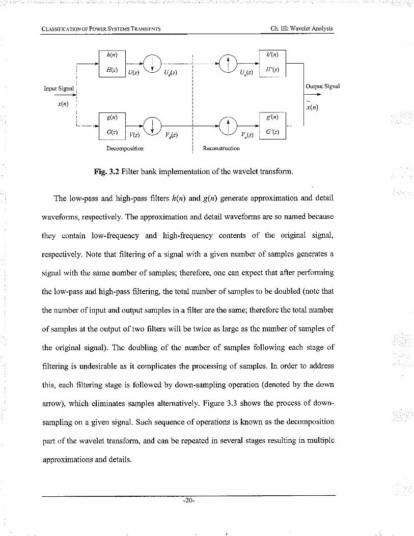
Fig.3.2 Filter bank implementation of the wavelet transform.

The low-pass and high-pass filters h(n) and g(n) generate approximation and detail

waveforms, respectively. The approximation and detail waveforms are so named because

they contain low-frequency and high-frequency contents of the original signal,

respectively. Note that filtering of a signal with a given number of samples generates a

signal with the same number of samples; therefore, one can expect that after performing

the low-pass and high-pass filtering, the total number of samples to be doubled (note that

the number of input and output samples in a filter are the same; therefore the total number

of samples at the ouþut of two filters will be twice as large as the number of samples of

the original signal). The doubling of the number of samples following each stage of

filtering is undesirable as it complicates the processing of samples. ln order to address

this, each filtering stage is followed by down-sampling operation (denoted by the down

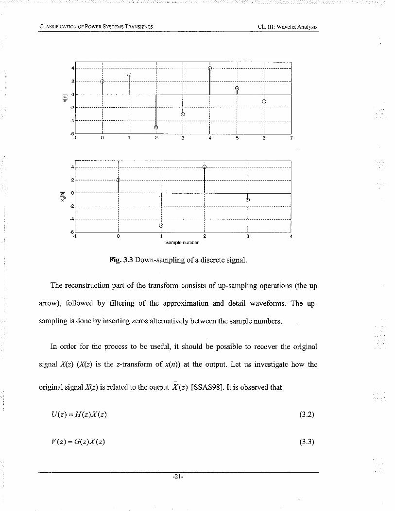
arrow), which eliminates samples alternatively. Figure 3.3 shows the process of down-

sampling on a given signal. Such sequence of operations is known as the decomposition

part of the wavelet transform, and can be repeated in several stages resulting in multiple

approximations and details.

-20-

CLnsslrtceloN on Powen Sysr¡us TRANSIENTS Ch. III: Wavelet Analysis

0

-2

-4

-b-1

Sample number

Fig. 3.3 Down-sampling of a discrete signal.

The reconstruction part of the transform consists of up-sampling operations (the up

affow), followed by filtering of the approximation and detail waveforms. The up-

sampling is done by inserting zeros alternatively between the sample numbers.

cÞ

In order for the process to be useful, it should be possible to recover the

signal X(z) (X(z) is the z-transform of x(n)) at the ouþut. Let us investigate

original signal X(z) isrelated to the output X1r¡ ¡SSnS98l. It is observed that

U(z) = H(z)X(z)

V(z): G(z)X(z)

original

how the

(3.2)

(3.3)

-21-

ClesslHcerloN oF PowER SysrEMS TRANSTENTS Ch. III: Wavelet Analysis

Appendix A contains a proof of the above formulae. For the reconstruction part, the

decimated signals U¿(z) and V¿(z) arc up-sampled, resulting ín U,(z) and V,(z), which

are expressed as follows (see Appendix A for prooÐ

The down-sampled signals can be obtained using the following formulae

1u¿(r): ,fu<Jl)+uGJh)

1-va@) =;frr<Ji)+rteJ|)

U,(") = U ¿ (22) = |V <, ) + U (-z))

vu(") : vo þ1 = Irr r, ) + v (-z))

Thus, the ouþut signal can be expressed as follows

H (z) = h(o) + h(l)z-, + "' + h(N)z-'

and with the three remaining filters described as

(3.4)

(3.s)

(3.6)

(3.7)

i 1,¡ = f,{o clo' tz) + H (z) H' qz¡\x 1z¡ +

r{G e òG' (z) + H (- z) n' þ)}x e) (3. s)

The ouþut signal is therefore a combination of the original signal X(z) and an aliased

part X(-z). Suitable choice of the filter coefficients can eliminate the aliased component

by setting its coefficient equal to zero. Usually FIR filters are used in the filter bank

implementation of the DV/T. It can be shown that with a low-pass ñlter H(z) of the form

a.l

(3.e)

CLASSIFICATION OF POwER SYSTEMS TR,A,NSIENTS Ch. III: Wavelet Analysis

H'(") = z-N H(z-1) i.e.,h'(n) : h(N - n)

G'(z): z-* H(-z-' ) i.e., g'(n): -(-l)" h(n)

G(z): -z-'Hç-z-t) i."., g(n): (-I)" h'(n)

(3.10)

(3.11)

(3.12)

the aliased component in the ouþut signal vanishes. By substituting the above four

equations into (3.8) it can be shown that if the filter coefficients for h(n) (and hence for

the rest of the filters) are chosen, through a simultaneous system of equations, in a way so

that

H (-z)H (-z-l) + H (z)H (z-t¡ = 2

then the reconstructed signal will be as follows

kçr¡ = z-'Xlz¡ i.e.,r1r¡: x(n- N)

(3.13)

(3.r4)

In other words, the output signal will be a delayed version of the input signal, and has no

other artifacts. Note that the delay is determined by the order of the filters used. Equation

(3.13) usually yields a system of simultaneous equations (in terms of the filter

coefficients) with more unknowns than the equations. Other conditions, such as the

smoothness of the filters, are usually imposed on the filters to produce an adequate

number of equations.

The filter bank implementation is linked to the original waveform representation of

the wavelets through a recursive equation, which yields the following scaling and wavelet

functions, respectively. These equations are given as follows

-23-

Classrprc¡.rtoN oF PowER SysrEMS TRANSIENTS Ch. III: Wavelet Analysis

N

þ(t)=JrZh(N-mþ(Zt-m)m=0

N

v (t) = Jr>-(-l)¡/¿'(¡/ - m)þ(2t - m)m=O

h(o) =#, he) = ff , rrr) = ï#, h(3) :4J'

1+"Æ

(3.15)

To solve for the scaling function in Eq. (3.15) one needs to start with an initial guess

and recursively substitute it until the difference between the two successive iterations

becomes negligibly small. For a third-order filter (i/: 3), four parameters need to be

determined. The system of equations obtained using (3.13), yields 2 simultaneous

equations, and therefore 2 extra equations need to be established. One equation is

obtained by observing that for a high-pass filter G(z), one can impose G(0) : 0; the fourth

equation can be obtained by imposing smoothness on the low pass filter H(z); i.e., zero

slope at cù: 0. Solution of the systems of simultaneous equations so obtained yields the

four coefficients as follows

(3.16)

(3.r7)

The wavelet corresponding to the four-coefficients found above is called the

Daubechies a (DBa) wavelet after Ingrid Daubechies [Daub92], who proposed the

method of smoothness for creation of the extra equations. ln case more than one equation

is required to complete the system of equations, higher order derivatives also can be set to

zero [SSAS98].

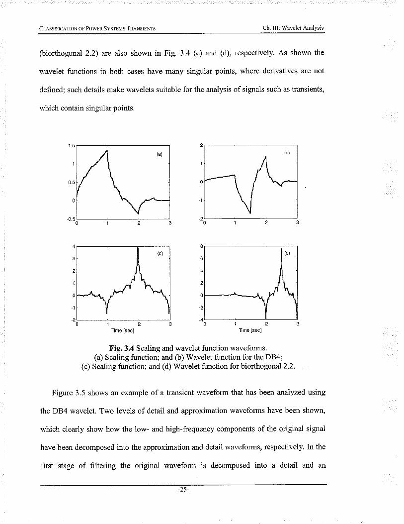
Figure 3.a @) and (b) show the scaling and the wavelet functions for the Daubechies

4 family, respectively. The scaling and wavelet functions for another wavelet family

-24-

CLASSIFICATIoN oF PowER SYSTEMS TRANSIENTS Ch. III: Wavelet Analysis

(biorthogonal 2.2) are also shown in Fig. 3.a @) and (d), respectively. As shown the

wavelet functions in both cases have many singular points, where derivatives are not

defined; such details make wavelets suitable for the analysis of signals such as transients,

which contain singular points.

1.5

'1

0.5

0

-0.5

4

õ

2

1

0

-1

-2

2

1

0

I

-2

o

t)

4

2

0

-2

4

ïme [sec] ïme [sec]

Fig. 3.4 Scaling and wavelet function waveforms.(a) Scaling function; and O) Wavelet function for the DB4;

(c) Scaling function; and (d)'Wavelet function for biorthogonal2.2.

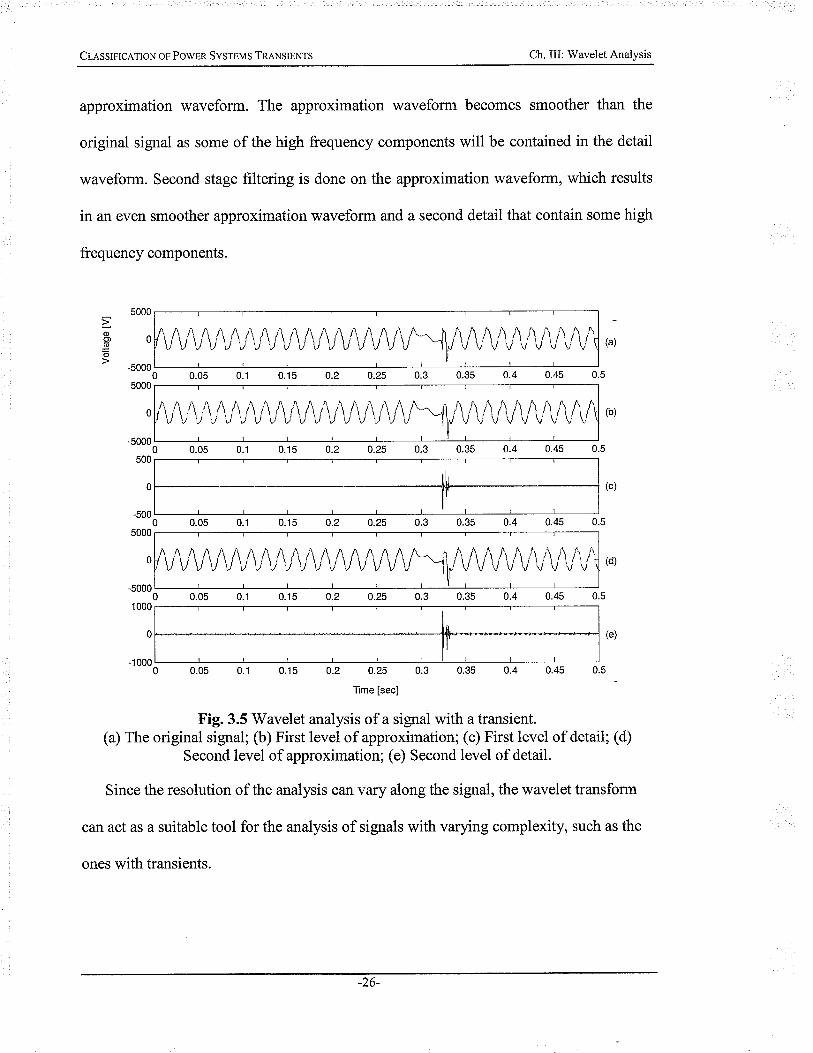
Figure 3.5 shows an example of a transient waveform that has been anaiyzed using

the DB4 wavelet. Two levels of detail and approximation waveforms have been shown,

which clearly show how the low- and high-frequency components of the original signal

have been decomposed into the approximation and detail waveforms, respectively. In the

first stage of filtering the original waveform is decomposed into a detail and an

(a) (b)

(c) (d)

-25-

ClessrFlcRÏoN oF PowER Svsr¡vs TReNs¡sNrs Ch. III: Wavelet Analysis

approximation waveform. The approximation waveform becomes smoother than the

original signal as some of the high frequency components will be contained in the detail

waveform. Second stage filtering is done on the approximation waveform, which results

in an even smoother approximation waveform and a second detail that contain some high

frequency components.

5000

0

-5000

5000

0

-5000

s00

0

-s00

5000

0

-s000

1 000

0

-1 0000 0.05 0.1 0.15 0.2 0.25 0.3 0.35 0-4 0.4s 0.5

ïme [sec]

Fig. 3.5 Wavelet analysis of a signal with a transient.(a) The original signal; (b) First level of approximation; (c) First level of detail; (d)

Second level of approximation; (e) Second level of detail.

Since the resolution of the analysis can vary along the signal, the wavelet transform

can act as a suitable tool for the analysis of signals with varying complexity, such as the

ones with transients.

oo(ú

=o

0.50.45

-26-

Cl¡.ssr¡lc¡,rroru or Powpn SvsrEMS TRANSTENTS Ch. III: Wavelet Analysis

Choice of a particular mother wavelet for a given application is an important task that

needs careful examination of the signals tobe analyzed as well as awareness of the

properties of the wavelet family [SaKTO5]. Study of transients in power systems is no

exception in this regard and this issue is dealt with in Ch. 6, where the design of the

overall system is discussed

3.4 Chapter Summary

This chapter presented a short mathematical background on the wavelet analysis of

signals containing transients. Implementation of the wavelet transform using an

equivalent filter bank was demonstrated. As an example, development of a wavelet

family, namely the Daubechies 4, was shown. The process, in general, usually starts with

the design of appropriate filters that have a number of specified properties, and then the

filter is translated into the corresponding scaling and wavelet functions.

The wavelets have several advantages over conventional signal analysis tools (such as

the Fourier-based methods), including multi-resolution representation of signalS with

varying local complexity, and preservation of time and frequency content of the signal.

These two important features prove to be very essential in the analysis of transients in

power systems and will be further discussed in later chapters.

aa

CLASSIFICATION oF PowER SYSTEMS TRANSIENTS Ch. IV: Multifractal Analysís

CrreprnR IV

Mur,rrFRrÀc rdtr, Auar.ysr s

4.1 Introduction

As mentioned in previous chapters, transients in power systems are short-term

phenomena that occur due to various events and disturb the original waveforms of

voltage and current in the network.

Charactenzation of transients could be tackled using various methods, including

wavelet analysis presented in the previous chapter. Another method, called the

multifractal analysis, could also be employed [Chen0l], [Shaw97]. Multifractal analysis

is based on charactenzing the signal using the notion of complexity. In particular, the

variance fractal dimension trajectory ryFDT) will be addressed. This method has several

favorable features, such as capability for real-time implementation, which make it very

suitable for real-time characterization of transients in power systems.

4.2 Fractals - An Overview

The term fractals and fractal analysis deal with the study of objects that demonstrate

immense complexity. As one may expect from the words, this study involves objects, e.g.

images, which look rough and contain intricate complexity. The word "fractal" was first

introduced by Mandelbrot and it originates from the Latin adjective fractus, which means

broken [Mand82].

In order to provide a better understanding of the concept, two well-known fractals,

the Koch curve (Fig. a.1) and Sierpinski carpet (Fíg. a.Ð are shown below. For each of

-28-

CLASSIFICATIoN oF Po\ilER SYSTEMS TRANSIENTS Ch. IV: MultiÍÌactal Analysrs

these two objects, the first few steps taken to generate the final object are also shown. It

is interesting to see that each of these fractals are generated by repeating a simple

procedure on an initially plain object (a line segment for the Koch curve and a square for

the Sierpinski carpet); however, the resulting image that starts to appear after a few

iterations demonstrates significant complexity as weil as visual appeal. It is also very

important to see that the images all share similar components that can be observed at

various scales.

(a) Initiator

(b) Step I

(c) Step 2

(d) Step 3

(e) Step co

Fig.4.1 Koch curve fractal. (After [PeJS92])

-29-

CLnssrplcntloN o¡ Powpn Svsrpr'¿s Tr¡.r.¡sreNrs Ch. IV: Multifractal Analysis

Visual inspection of these two objects reveals that the fractals are self affine; i.e., part

of the object is related to the whole through the property of scaling; this is fundamental to

the understanding of the fractals.

(a) Initiator (b) Step I (c) Step 2 (d) Step 3

Fig.4.2 Sierpinski carpet fractal. (After [Kins95])

It is noted that the final objects has details (singularity and transition) and as such the

Euclidian, Riemannian, ffid Lobachevskiy geometries fail to describe the objects

properly. One can define a fractal as a subset in Bn, which is self-similar and whose

fractal dimension exceeds its topological dimension [Kins95].

Further analysis of fractals leads to the notion of fractal dimensions, which are non-

integer values (contrary to the coÍrmon Euclidian dimensions). In broad terms, a fractal

dimension is a measure of roughness or inegularity of the object. Intuitively, the concept

of fractal dimension is derived from the self-similarity property þower law) [Kins94a].

It is interesting to note that fractals have a profound existence in the nature and are

not limited only to mathematical ones, such as the two examples given above.

Mathematical fractals usually can be generated using relatively simple mathematical

procedures. The overall procedure has two components, namely the initiator and the

generator. In case of the Koch curve, the initiator is the straight line segment shown in

-30-

CLasslprcnloN op PowsR Svsrsvs TRANSI¡NIs Ch. IV: Multifractal Analysis

Fig. 4.1(a). To move on to the next stage, the line segment is divided into three equal line

segments and the middle one is replaced with two line segments of equal length (and

equal to the length of the removed segment) that meet at a 60o angle. Note that each of

the line segments in the object in stage 2 has the same length (1/3 of the length of the

original line). The objects in the following stages are obtained by performing the same

procedure on each of the line segments. The resulting objects can become increasingly

complicated, but careful analysis reveals profound similarity, simplicity and beauty

within the object.

Another example of a mathematically generated fractal, the 2-dimensional (2D)

Mandelbrot set, is shown in Fig. 4.3. The object has intricate details, but it could be

generated using a simple mathematical procedure.

Fig.4.3 Mandelbrot set. (From Technical University of Athens)

Fractals also exist in nature, but are much more complicated in their design and

description. In other words, while mathematical fractals, such as the Mandelbrot set, can

be generated using an initiator and an iterative process, natural fractals are far more

-3 1-

CLASSIFICATIoN oF PowER Sysr¡us TReNsmiIrs Ch. IV: Multifractal Analysis

complex and can be described hardly ìlsing such mathematics. As an example of a natural

fractal, Fig. 4.4 shows a picture of an electric discharge in a lightning. As shown, the

object has a very complex form that possesses the fundamental properties observed in

mathematical fractal; i.e., parts of the object show similar pattern to those observed in

whole. For example, the tiny portions that branch out form the main branches, still show

similar patterns to those of the larger ones. Naturally, it is expected that the Euclidian

geometry should fail to provide an accurate description of such an object.

Fig.4.4 Electric discharge in a lightning. (From www.flatrock.org.nz)

4.3 Fractal Dimensions

Fractals have a ubiquitous presence and as such it is important to be able to study

them quantitatively, so that their description and comparison becomes possible. As stated

before, fractal dimension is an approach for measuring the roughness or irregularity of

such objects. The fractal dimension has its roots in the similarity that exists in a fractal at

-32-

CL¡,ssrrrc¿.rroN or Powsn Sysrpvs TReNsrpurs Ch. IV: Multifractal Analysis

different scales, and hence has strong connections with the power law relationship. For

some fractals, a single fractal dimension is adequate to describe them, while more

complex objects may require more than one fuactal dimension.

Generally, fractal dimensions may be classified into the following four categories

lKins94al:

" Morphological-based dimensions, which are based on geometrical properties of

the object under consideration and are used if the distribution of a measure (sùch as

probability) is uniform or the information about the dishibution is not available

lKins94al;

. Entropy-based dimensions, which take into account a measure of a fractal and

therefore deal with inhomogeneous fractals;

. Spectrum-based dimensions, which are based on the fact that the power spectrum

or power spectrum density of a signal reveals a power-law relation with frequency, in

which the exponent characterizes the persistence or antipersistence of the corresponding

fractal object; and

. Variance-based dimensions, (see below for details).

Our focus throughout the rest of this chapter will be on a particular variance-based

dimension, namely the variance fractal dimension, which will be shown to be an efficient

method for charactenzingwaveforms with transients such as power system transients.

-JJ-

CLASSIFICATIoN oF PowER SYSTEMS TRANSIENTS Ch. IV: Multifractal Analysis

4.4 Yariance Fractal Dimension

Analysis of a time series is possible directly in real time by analyzing the spread of

the increments in the signal amplitude (variance, l¡ ¡finse4bl. This approach has its

roots in the work done by Mandelbrot and Van Ness [MaVa68]; however, the approach

presented in this thesis is based on the work developed by Kinsner [Kins94a].

Let us assume that the signal x(r) is either continuous or discrete in time r. The

variance I of its amplitude increments over a small time increment is related to the time

increment according to the following power law

Y arlx(t r) - x(t )l - lr, - t rl' u

where Var is the variance operator, and H is the Hurst exponent. By

and (A.r)& : x(t2)-x(t), the exponent H can be calculated from

2 H lo g(Lt) - log[Var(&) o, ]

(4.1)

setting Lt: lt2+11,

(4.2)

the points

Euclidean

(4.3)

which H is Yz times the slope of the best fitted line that passes through

log[Var(Ax)o,] versus log(Ar) , for small values of Ar. Finally, for embedding

dimension E,the variance dimension can be computed from

Do=E+r-H

In practice, the limit of Eq. 4.2 shown above translates into the slope of a log-log plot

with a finite number of time increments. The sequence is usually chosen to be b-adic. For

this case, the following formula will hold

-34-

CIessIpIceTIoN oF PoV/ER SYSTEMS TRANSIENTS Ch. IV: Multifractal Analysis

where fr is in the range lh,kzl. Within the range where power-law relation holds, the slope

of the line polynomial whose curve passes through these points is given by

Xo =logr(Lto)fr = log¡(var(Axo))

The Hurst exponent,Flis obtained by

H:s12

(4.4)

(4.s)

(4.6)

(k, - k)Z!o,x,Y, -Z]o,x,Zoi=*,Y, ,

(k, - k)Zoi=o,x,' - (Zo1o,x,)'

A useful property of the variance fractal dimension approach is that the result is

bounded automatically between I (dimension of a straight line) and 2 (dimension of

white noise). This is a very appealing feature that can be of importance when such results

are used for the purpose of classification as it often requires input data to belong to

bounded intervals.

4.5 Variance Fractal Dimension Trajectory

Often times there are objects that contain more than a single fractal and are

charactenzed by having a spatial or temporal combination of a number of fractals. Such

objects are called multifractals. An extension of the previously discussed variance fractal

dimension is used for the characterization of signals with multifractality.

In this method, a window over which the fractal dimension is calculated is shifted

along the signals [Kins94b]. Usually the windows are selected to have some overl?p. By

-35-

CIaSSIpIc¡,rIoN oF POV/ER SYSTEMS TRANSIENTS Ch. IV: Multifractal Analysrs

calculating the fractal dimension of the portion of the signal within a window, the

resulting variance fractal dimension trajectorl (VFDT) will have smaller samples points,

resulting in a significant reduction in the number of charactenzing features [Kins94b].

Decision on the width of the sliding window and the overlap between successive

windows is very important and will be discussed in detail in Ch. 6, where the system

design is presented.

For signals with a single fractal nature, the VFDT approach results in a single value

for all the windows; however, for signals with transients, such as the ones considered in

this thesis, the variance fractal dimension approach will result in a sequence of

dimensions that assumes different values, thus providing an indication of the onset and

type of the transient. This is because the presence of transients, which are mostly much

more complicated than the signal itself, introduces short-term changes in the complexity

of the signal and as such the variance fractal dimension attains a different value during

the transient portion. Such sequence is rightfully called the variance fractal dimension

trajectory or VFDT.

As an example of how the VFDT actually characteizes a signal, Fig. 4.5 shows a

waveform with a transient along with its VFDT. The original sine wave is disturbed by

the presence of a short-term transient occurred between [0.29,0.33] sec (approximately).

The variance fractal dimension trajectory of the signal shows a relatively constant value

before and after the transient period, which corresponds to the fractal dimension of the

original undisturbed waveform. During the transient period however, the fractal

dimension calculated changes significantly, which is an indication of subtle variation in

-36-

Cr,¡,sslHc¡,ïoN o¡ PoweR SysrEMS TRANSIENTS Ch. IV: Multifractal Analysrs

the complexity of the signal. The resulting VFDT is automatically scaled between I and2

and has by far less samples than the original waveform.

t.b

Do 1.4

1.2

1

Fig.4.5 VFDT analysis of a transient.(a) Original waveform; (b) VFDT.

4.6 Chapter Summary

An efficient approach for the analysis and charactenzation of complex signals, e.g.

signals with non-stationarities, is based on using the notion of fractals and fractal

dimensions. It was shown that variance fractal dimensions are suitable measures for

describing signals with transients and they reveal important underlying properties of the

signals.

0)o)(ú

=o

1.8

-37-

CLesslHcrtoN on Powpn Sysrp\,rs TRaNslsNts Ch. IV: Multifractal Analysis

In particular, the VFDT approach was described and it was shown that the method

lends itself to a fairly straight forward implementation that proves to be useful for real-

time applications. The VFDT approach involves calculating the variance-based fractai

dimension of the signal in a number of overlapping windows along the signal and results

in a trajectory of fractal dimensions that track the changes that occur in the signal as the

time progresses. A trajectory so obtained (i) has significantly less number of samples

(high compression ratio) and (ii) contains important properties of the original signal that

can be used efficiently in a well-designed classifier.

Classification of transients becomes possible once their features are extracted using

the method presented in this and the previous chapter. In the next chapter, essentials of

the pattern classification are presented.

-38-

CLASSIFICATIoN oF PowER SYSTEMS TRANSIENTS

CnnprER V

F¿.rrnnx RpcocNITIoN ANÐ

Cr-assrFICATIoN oF Tn¿NsrENTs

5.1 Introduction

Analysis of transients using the techniques mentioned in the previous chapters

provides means for charactenzing them using a number of properties, also commonly

referred to as features, which could be used to distinguish between various transients.

The task of determining the class of an object based on its features is called

classification and the procedures that perform such tasks are called classifiers [DuHS01].

Depending on the objectives of the study, the 'class' of an object is defined. For example,

in classifuing transients in power systems, the classes may be iabeled as 'faults',

'breaking operation, 'capacitor switching', and so on. Classification of transients involves

their analysis, extraction of features and determination of their true cause (whether they

have been caused by faults, breakers operations, capacitor switchings, etc.).

Consider a classification problem with C classes. An input sample, whose class is to

be determined, is charactenzed by n number of features. Each feature can be considered

to represent part of the characteristics of an object; for example the length, color, or

weight can be the features used to describe a given object. In the study of transients in

power systems, features can be extracted from signals using the results of wavelets and

multifractal analyses. The task of the classifier is to assign the input sample, using its n

features, to one of the C existing classes. Therefore, the classifier is a system wíth n

-39-

CLessrnlcelrou or Powpn SvsrEMS TRANSIENTS Ch. V: Pattem Recognition & Classification of Transients

inputs aîd C outputs, which uses the statistical properties of the input samples to assign

them to one of the classes considered.

5.2 Statistical Foundations of Classification

Classification deals with the probability theory. The underlying idea in pattern

classification is expressed by the Byes rule given below [DuHS01]

P(a, l*,, _ g(x I ø¡)P(ø;)\ ¡' g(x)C

g(x): Ig(* lø,)P(at,)i=I

(s.1)

where o¡¡, g(x | ø,) and P(a¡,) are the class i, class-conditional probability density function

þdf) of x in class i, and the prior probability of class i, respectively, and C is the number

of classes. P(a,lx)is the posterior probability of class i, given the input vector (input

sample) x. It is worth discussing the Bayes rule a little further, as it forms the basis for

other classifi cation techniques.

The prior probabilities P(ø) simply, and roughly, determine the likelihood of

occuffence of their respective classes. For example in a 2-class problem, where either of

the two classes is equally likely to happen, the prior probabilities P(ø1) and P(an) are

both equal to %.Itbecomes apparent readily that prior probabilities are simply a digest of

the past history of the events in a given system, and do not depend on the observations

made on the current sample. The Bayes rule uses the extra information available in x to

come up with a better estimation of the actual class of a given input than the prior

probabilities. In fact the underlying idea is to improve the estimation provided by the

-40-

CLessrHcaÏoN or PowEn Sysr¡us TRANSTENTS Ch. V: Pattern Recognition & Classification of Transients

prior probabilities by incorporating the observations contained in the features. This is

carried out by evaluating the probability density function of each class for the input

sample presented. An input sample that has more resemblance to a specific class,

produces a larger S$la)for that class, and as such results in a larger numerator in

(5.1). It is instructive to demonstrate the procedure on a 2-class problem with a single

feature. Figure 5.1 shows the pdfs of the feature x in each of the two classes A and B. An

input sample, with a feature value equal to "*

has much more likelihood of belonging to

class A than class B. With equal prior probabilities for both classes, the input sample will

be assigned to class A.

0.5 I 1.5 2 2.5 3 3.5 4

x

Fig. 5.1 Decision-making in a two-class problem.

Since the denominator in (5.1) is the same for all classes, the decision-making process

using the Bayes rule could be simplified as follows

1iè 0.4Ò0

-41-

CLASSIFICATToN oF PowER Sysrplts TRANSTENTS Ch. V: Pattern Recognition & Classification of Transients

Decide ø, if

g(xlØ,)P(a¡) > g(xlat,)P(ø¡) Yi,i + j(s.2)

Under circumstances where the classes are equally likely, the prior probabilities P(at¡)

could also be dropped. The Bayes rule is the most accurate method of determining the

class of a given input (represented by the features contained in x); however, in many

cases, the class-conditional pdfs required in (5.2) are not available. Therefore, the Bayes

rule can be applied only when either the pdfs are known explicitly or they can be

estimated accurately.

In the following sections of this chapter, three classification methods will be

discussed, namely the Bayes rule using the maximum-likelihood (ML), the nearest

neighbor classifier (fr-l'IN) and the Probabilistic Neural Networks (PI.IN). It will be

shown that PNN and ML based methods, despite their visual differences, share roots in

estimating the pdfs and using the Bayes rule.

5.3 The Method of Maximum-Likelihood (Mt)

The method of maximumJikelihood (l|i4L) is based on finding the parameters of a pdf

with a given structure so that it best matches the true pdf (unknown) of the samples

available. The pdfs estimated using the method of ML could be used in the Bayes rule.

Note that

(Ð the procedure requires a sufficiently large number of samples with known

classes so that they can be used for determining the parameters of the pdf of

each class. These samples are referred to as the training set; and

-42-

ClessrplcerroN or Pow¡n SysrEMs TRANSTENTS Ch. V: Pattem Recognition & Classification of Transients

(iÐ the method of ML assumes a given form for the pdfs, e.g. Gaussian, Poisson,

and only determines the parameters of the given pdf.

If the training samples belonging to a specific class are {x1,x2,.'.,*"}, the parameter

set 0 of a pdf g(x, 0) are estimated such that the following product is maximized

The rationale behind maximizing the function above is that a correctly identified pdf

will generate higher values when samples of its respective class are presented to it.

Therefore, by maximizing the function in Eq. 5.3, a suitable set of parameters for that

class will be obtained. Since the form of the pdfs are assumed to be known, the problem

is reduced to an ordinary maximization problem and can be solved using an optimization

method. Further details about this method can be found in [DuHSO1].

In many cases, the pdfs to be estimated are found to be mixtures of some underlying

pdfs. For example, each of the pdfs shown in Fig. 5.1 are in fact combinations of two

Gaussian pdfs. A tlpical 'mixture model' can be expressed as follows

¡ú

¿(0) =f[s(x,,e)i=l

MG(x) = ltr,g(x,O,)

j=l

(5.3)

(s.4)

where g(x,0¡) are the constituent pdfs, n,are the mixing factors and M is the number of

constituent models . The estimation of the parameters of such a mixture model (again

with assumed forms for the underlying pdß) involves determination of individual pdf

-43-

Cl¡.sslplc¡,rroN op Powsn Sysrpus TRANSTENTS Ch. V: Pattern Recognition & Classification of Transients

parameters (0r) as well as the mixing factors. A similar optimization approach can be

adopted for such cases as well [FiJaO2].

5.4 The Nearest Neighbor ClassifTer (fr-NN)

The nearest neíghbor classífier (fr-l.IN) is a simple, yet effective, classification

method. Similar to the ML, this method is based on using a given number of training

samples; however, unlike the previous method, where the training samples belonging to a

certain class are treated as constituents of an overall pdf, the k-NN classifier treats them

as individuals. In other words, while the training samples in an Ml-based classifìer do

contribute to an overall pdf, which replaces the individual members, the Æ-NN relies on

the individual samples directly in the decision-making process [DuHSO1].

In simple terms, the Æ-NN classifier determines the class of a given sample by

calculating its distance (using an appropriate measure) from its Æ closest neighbors in the

training set. In a two-class problem, a 1-NN classifier will assign the input sample to the

same class as that of the nearest neighbor.

Figure 5.2 shows a schematic diagram of a two-class problem (classes are denoted by

circles and crosses). The input sample shown as X will be assigned to the class of crosses

as its nearest neighbor belongs to that class (the Euclidian distance is used). The line

segments shown on the graph represent the boundaries of an area around each sample,

where a given input sample finds the enclosed point as its nearest neighbor.

-44-

Cl¡,ssrprcnÏoN oF PowER SysreN4s TRANSI¡NTs Ch. V: Pattern Recognition & Classification of Transients

E

4.5

4

3.5

X2 2.5

2

1.5

'I

0.5

0

X1

Fig. 5.2 The nearest neighbor classification method.

It is evident that the l-NN classifier gives any of the training set samples the

possibility to determine the class of an unknown sample. The individual emphasis of the

i-NN classifier versus the cumulative approach of the Ml-based methods is an important

property that deserves careful attention.

To lower the significant impact of individual training samples on the outcome of the

classifier, it is possible to include more than one neighbor in the decision-making

process. For example in a two-class problem, it is possible to use a Æ-NN approach (with

an odd k, to prevent ties). Under such cases, the winning class is the one that contains the

majority of the k nearest neighbors of the unknown sample. The Æ-NN (k + l) classifier is

a movement towards incorporating more than one training sample in the process of

-45-

CLesstncerroN op Powpn SysrEMS TRANSIENTS Ch. V: Pattem Recognition & Classification of Transients

decision making. Although more computationally demanding, a fr-NN classifier does take

into consideration the clusters of data that can be observed normally in'many

classification problems and lowers the impact of out-of-cluster samples in the final result.

One major benefit of the Æ-NN classifiers is the simplicity of implementation. The

classifier requires no 'training' as the task of classification is done simply by calculating

the distance, for example by the Euclidian distance, between the input sample and the

training samples. This property makes the Ë-NN classifier a prime choice when the

number of training samples is not sufficient to train other classifiers.

5.5 The Frobabilistic Neural Networks (PNN)

The probabilistic neural networlu (PI.IN) are classifiers that implement the Bayes

rule; however, their training methodology is different from the Ml,-based apþroach

described earlier.

It was mentioned that classification using the Bayes rule requires the pdfs of

individual classes. The PNN is a mathematical representation of the Bayes rule and is

trained so that the pdfs are obtained optimally.

Before proceeding to the concept of a PNN and its training procedure, a useful

method of estimating a pdt namely the Parzen method is presented.

5.5.1 Estimating a PDF Using th,ePzrzen Method

A popular method for estimating a pdf was introduced by ParuenfParzí2l. According

to this method, which is demonstrated first for a single-variable case, for a given class k

-46-

CLASSIFICATION OF POwER SYSTEMS TRANSIENTS Ch. V: Pattern Recognition & Classification of Transients

wiÍh n¡, training samples given by

following expression

1frtgt@)= t iw(*-*')nroà o

1 .-x2,w(x)=rUrexv( * )

xr )r e [,2,...,n0], the pdf can be estimated using the

where gdx) is the estimated pdf, ois a scaling factor and

satisfies the following conditions

1. W(O)>W(x) Vx, and

2. W(+æ) approaches zero.

(5.s)

W(x) is a window function that

Note that for a given x, the pdf g¡dx) first calculates the distance between this point

and every one of the points of the training set. The distances are then normalized by o

and passes through the window function W. For an input x lying in close proximity to

other training sample alarge g¿(x) will be obtained (according to condition 1 above); an

input x lying far from other data points (which is less likely to belong to class Æ) will have

a small pdf evolution (see condition 2 above).

A good candidate for a window function is the Gaussian function given by

(s.6)

Note that the parameter o determines effectively the width of the window function used.

ln other words, larger values of øallow farther points to still contribute effectively to the

-47-

Cresslncerro¡¡ or Pow¡n SysrEMS TRANSTENTS Ch. V: Pattem Recognition & Classification of Transients

overall pdf. It is also worth noting that the use of a Gaussian window function is

completely arbihary and is not a necessary condition.

In multivariable cases, where the input sample has p features, the estimation is

expressed as follows

g¿(x)- 1 f,w1"-'"t,&,...,*'-*''')nkoroz"'opà ot oz ap(s.7)

the rthwhere x = ("1 ,x2,...,xo)is the input sample, and xr:(xr,t,xr,2,'..,xr,')ís

sample in the training set.

The multivariable function W canbe assumed to have the following form

p

W (x1, x2,. . ., * o) = lIW,(r,)i=t

nkoto2... o p

which is simplified to

(s.8)

and with the choice of W¡(x¡) to be as in (5.6), the expression forpdx) will be as follows

g¿(x) = 7"år"-ncfffi) (s.e)

(s.10)

The problem of estimating the pdf, therefore, reduces to an optimal estimation of the

o; in (5.10).

-48-

Clessr¡lceÏoN oF Pov/ER SysrEMS TRANSIENTS Ch. V: Pattern Recognition & Classification of Transients

In simple cases, the oi par¿rmeters aÍe sometimes assumed to equal;

i.e.,or-õr=...=op=a. The original PNN architecture used this simplified

assumption; however, this is a limiting condition and poses a single spread on all the

features. lmproved PNNs use multiple spread parameters for the feature vector resulting

in a better estimation of the underlying pdf [Mast95].

Choice of suitable values for the spread parameter(s) is an important task and has a

profound impact on the performance of the classifier obtained using the estimated pdfs.

To illustrate this, consider the haining set shown in the x-y plane in Fig. 5.2(a). Note that

the training set essentially consists of two clusters each with 4 points. The estimation of

the pdf is shown for three sets of lo,,orTvalues. The estimation in Fig. 5.2(b) is for

lo,,or7:10.2,0.2] and it is evident that the naffow width of the window function has

results in separation of the sample points and therefore the resulting pdf pertains to a k-

NN classifier. This is because with a small window width, only the points that lie very

close to a data point will be contributing to the total pdf evaluation, resulting in a loss of

clusters in the overall pdf. The estimation with very large values of 12.2, 2.21 in Fig.

5.2(c) shows excessive smoothness in the estimated pdf. In other words, the pdf estimated

using such large values suppresses the fact that the data effectively exists in two clusters

(see Fig. 5.3(a)) and allows very far points to contribute almost equally as the points in a

cluster. The estimation with well-selected values for [o,,orJ:10.7,0.7], as shown in

Fig. 5.3(d), results in a pdf with adequate smoothness around each of the two clusters.

Note that proper selection of the window widths, not only separates the clusters, but also

identifies the cumulative impact training set samples within each cluster.

-49-

Clesslrrc¡.rlo¡¡ or Powsn SysrEMS TRANSTENTS Ch. V: Pattem Recognition & Classification of Transients

.....i....:. :.....;.....:...''i : : ' rli: i I i içû::lii::ìi:ìi::, : : , I : i'{o'C ':""r"": ":''i'': . : : , ,{a),9ð.1':'1.:::::':

4

J

2

1

=0-1

-2

_!

-4-4

0.4

q 0.2-l ....Ð

Fig. 5.3 Effect of window width on Parzen pdf estimation.

5.5.2 The PNN Architecture

The PNN is essentially an implementation of the Bayes decision-making rule;

however, it is possible to represent the overall procedure in the form of a multi-layer

neural network as well [Spec88]. The PNN consists of 4 layer, namely the 'Input Laye{,

the 'Pattern layer', the 'Summation Layer', and the 'Output Layer'. These four layers are

shown in Fig. 5.4 and their function is described in the following [Spec99].

The input layer consists of p nodes corresponding to the number of features used.

Therefore, when an input sample x:(x1,x2,...,.rco) is presented to the network, each

one of its components are assigned to its corresponding node in the input layer.

-1 0Y

-50-

CLnsslncRtloN oF PowER Svsrnrr,ls TRANSTENTS Ch. V: Pattern Recognition & Classification of Transients

l?, Inputs

!c

Pattern Summation OuþutLayer Layer Layer

Fig. 5.4 Structure of a PNN.

The pattern layer contains as many neurons as the number of training samples. If the

number of training samples for class fr are denoted by n¡, àîdthe total number of classes

is denoted by C, the following expression holds

xl

x2

!t

V"

Input

Layer

(5.11)

where,^/¡ is the total number of training samples. Therefore the pattern layer of a PNN has

Àd neurons.

Each neuron in the pattern layer has two major functions. Firstly, it calculates the

squared Euclidian distance between the input sample and its respective training sample

and then passes the scaled result through the nonlinear window function according to

C

Z', = N,i=1

-51-

Clesslflcnrrol¡ oF PowER Sysrpvs TReNslEwrs Ch. V: Pattem Recognition & Classification of Transients

(5.9). The function of the pattern layer is therefore to calculate the expression

J-(x.-x ,\2exp(-),-;-iL) for each of the training set samples.i=l lA¡

The summation layer has as many neurons as the number of classes, C. Each neuron

receives its inputs from those neurons in the pattern layer that contain training samples

belonging to that specific class. For example, the neuron number 2 in the summation

layer receives n2 inpìrts stemming from those neurons in the pattern layer that contain the

n2 samples belonging to class 2.

The ouþut of the summation layer is the pdf evaluation of each class for the input

sample. According to the Bayes rule, the input sample should be assigned to the class

whose pdf evaluation (multiplied by the prior probability) is larger than the rest. The

output layer is simply a decision-making engine with C outputs. The output values !¡ are

determined according to the following rule (assuming equal prior probabilities)

,. _ it if g,(x) > 8;(x) Vj j + i!¡:1 ",,"''.' (5.12)

|.0 otherwise

It is worth noting again that the architecture used for a PNN is simply an

implementation of the Bayes rule with an embedded pdf estimation using the Parzen

method.

5.5.3 Training of a PNN

Training of a PNN involves determination of the window-width parameters oi

optimally. Once a PNN is trained (its window widths estimated), it can be used as a

classifier that essentially applies the Bayes rule. Essentially this is an optimization task

-52-

CL¿,sslnrc¡.rou or Pow¡R Sysrstrs Tn¡Nsrpxrs

and therefore requires an objective function, whose minimization results in the optimal

set of o,'parameters.

Suppose that an input sample x belonging to class k is presented to the PNN; the C

outputs of the summation are indications of the pdf evaluations for their respective

classes. In order to assess the relative significance of these evaluations, we use the

following formula

U;Q¡ =-c-

2",j=r

(s.13)

(s.14)

where u¡ is the ouþut of the ith neuron in the summation layer. Note the under ideal

circumstances, presentation of the sample described above (belonging to class Ë) should

result in

8r =Iandq,:0,j+k

With non-optimal o; parameters, the 4¡ values deviate from these ideal values. Such

deviations can be used to form a suitable objective function whose minimization reduces

the deviation of 4¡ values thus yielding optimal o;. For a set of poorly selected o¡ the

deviation becomes larger, as the node corresponding to the true class of the input sample

fails to produce a pdf evaluation significantly larger than the rest.

The objective function should include all of deviations for every sample in the

training set. Therefore, for each sample x belonging to class k, apartial objective function

is defined as follows

-53-

Clnsslnlc¡,rlo¡¡ or Pow¡n Systpl,ls TR¡ustpNrs Ch. V: Pattern Recognition & Classification of Transients

C

e(x,)=(T-qÐ' *Zq¡'j=rj+k

(s.15)

(s.16)

Note that for an o., optimal set of parameters, the partial objective function of (5.15) wiil

become very small (the absolutely lowest value for the expression in Eq. 5.15 is zero,

which is obtained when qo = land Qj:0,j+k), while non-optimal values for o¡

result in large deviations and hence large e(x¡) values. The overall objective function,

used for the minimizationproblem, is defined as follows

OF :I"(*,)i=1

Optimization of the above objective function can be done using a nonlinear

optimization algorithm, such as gradient-based optimization algorithms [Mast95].

There is a fundamental difference between the Ml-based approach and the PNN in

the way the pdfs are estimated. The Ml-based approach estimates a pdf using only the

samples belonging to that class. Also the parameters used in the pdf of a given class are

independent of the parameters used in other pdß. The PNN however, takes a unified

approach and uses the same set of q parameters in all of the classes; the optimization

setup is also comprehensive of all classes in that it aims atmaximizing the contribution of

the true class on each training sample and minimizing the contribution of other classes.

The training complexity of the PNN is therefore, usually higher than the Ml-based Bayes

rule. Further details about the computational intensity of the three algorithms will be

presented in the following chapters.

-54-

Clessl¡lcntloN oF PowER Sysrelr.ts TR¡Nslsb¡rs

5.6 Chapter Summary

This chapter dealt with the methods that can be used for classification of various

objects including transients in power systems. It was shown that the Bayes rule, which is

the foundation of classification methods, requires such information as the class-

conditional pdfs that are not available in most cases and as such methods are developed

to estimate such pdfs.

Three classification methods, namely the Bayes rule using maximum-likelihood, the

k-NN and the PNNs were discussed in detail. It was shown that these methods, despite

their differences, are essentially estimations of the Bayes rule in the absence of readily

available pdfs.

The Parzen method for estimating pdfs was introduced and it was shown that the

PNN is an implementation of the Bayes rule with Parzen pdf estimation expressed in the

frame of a neural network. An optimization objective function for the estimation of the

parameters of a PNN was also developed.

The following chapter uses the mathematical foundation laid in the preceding

chapters in the design of a comprehensive transient classification system. Design

specifications and implementation are also presented.

-55-

Clessr¡rc¡.rro¡¡ or Powen Sysrevs Tnaxsl¡Nrs Ch. VI: System Design & Implementation

CnaprER Vtr

Sysrnnn Dpsrclq AND Innpr-nnnENT'ATIoN

6.1 Introduction

The material presented in the previous chapters form the mathematical foundation of

a system used for extraction of features from transients in a power system and their

classification using the extracted features. In this chapter, detaiis of the design of such a

system will be presented. The chapter will also address the implementation procedures

including the tools and techniques used for doing so.

This chapter is divided into three major sections, namely generation of samples of

transients using simulation, feature extraction using VFDT and wavelet analyses, and

implementation of classification methods.

6.2 Simulation of Transients in a Power System

As mentioned in Ch. 2, transients in a power system occur due to a large number of

planned and unplanned causes, and they disturb the performance of a power system.

Once a transient occurs, it disturbs the originally sinusoidal voltage and current

waveforms by introducing various frequencies into the waveforms. Transients cover a

wide frequencyband ranging from a few Hertz (Hz) to several megahertz (MHz) and also

tend to persist from a few microseconds (ps), e.g., switching transients, to several

minutes, e.g., voltage instability, depending on their nature. The focus throughout this

thesis is mainly on hansients that can be categonzed as short-term and mid-term

-56-

CLASSIFICATIoN OF POV/ER SYSTEMS TRANSIENTS Ch. VI: System Design & Implementation

transients, which usually have frequency content in the order of kilohertz (kHt) and last

for a few cycles of the po\Mer frequency.

Simulation of such transients involves precise modeling of the underlying eiectric

network and solution of the resulting equations. In order to do so, it is possible to either

use dedicated circuit simulation tools or develop a simulation program from scratch.

Needless to say, the latter option requires not only much work, but also deep knowledge

of and expertise in power systems that are beyond the scope of this project. Therefore, in

this thesis simulation of transients in a power system has been tackled using a

commercially available electromagnetic transient simulation program, namely the

PSCAD/EMTDC@ [EMTDO3].

6.2.1 PSCA,D/EMTDC@ Transient Simutation Program

PSCAD/EMTDC is a time-domain electromagnetic transient simulation program

developed by the Manitoba HVDC Research Center with close collaboration with the

University of Manitoba. The program provides a fully interactive user interface and

access to a library of various components used in electrical power systems. The user can

select the desired components from the Master Library and place them on a draft. page

and make necessary connections between them. Upon completion of the circuit

construction, the user can simulate the circuit and visually examine the results through

graphs that can be generated as the simulation progresses.

The program also provides the user with the option of designing their specific custom

components that are not available through the Master Library. Such a task is made

possible through the Component Workshop, and is done by coding the function of the

-57-

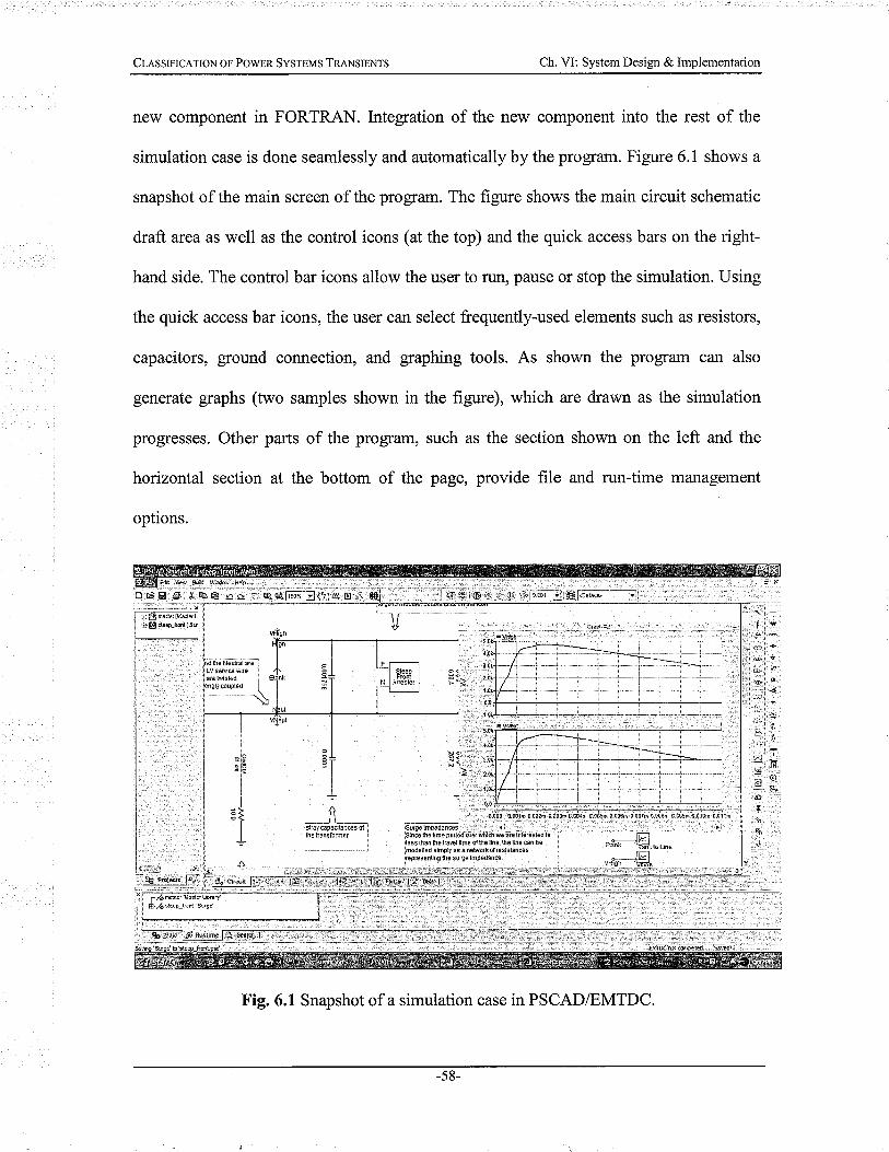
CLASSIFICATIoN oF PoV/ER SYSTEMS TRANSIENTS Ch. VI: System Design & Implementation

new component in FORTRAN. lntegration of the new component into the rest of the

simulation case is done seamlessly and automatically by the program. Figure 6.1 shows a

snapshot of the main screen of the program. The figure shows the main circuit schematic

draft area as well as the control icons (at the top) and the quick access bars on the right-

hand side. The control bar icons allow the user to run, pause or stop the simulation. Using

the quick access bar icons, the user can select frequently-used elements such as resistors,

capacitors, ground connection, and graphing tools. As shown the program can also

generate graphs (two samples shown in the figure), which are drawn as the simulation

progresses. Other parts of the program, such as the section shown on the left and the

horizontal section at the bottom of the page, provide file and run.time management

options.

:¿l !'Ê;r 'eld 9-&a È

D É Elgi å Þ ts; o o ì¿: qqþ*llq1:A O *";¡Otl f:in w,t';r ut.t 'ei¡.,'=¡lietffi

\

'J

__n_ _*âiÉpadbnøs oi I

iT:''"-:' ]

.:. i..T

:;::::: r: .

-:¡¡

".i 9'- l{-L:'' !+1¡!: :

,tt'- j

''tL

.¡d._-:õ.. @9..¿bi '

ri\:tli+;

ãlEI

I

-t1l)

Fig. 6.1 Snapshot of a simulation case in PSCAD/EMTDC.

-58-

CLRsslFrcnrloN oF PowER Sysr¡us Tn¡Nsl¡Nrs Ch. VI: System Design & Implementation

6.2.2 Simulated Transients

Three types of power system transients,

swithcings and breaker operations have been

program on a power system shown in Fig. 6.2.

Transmission Line I

il

namely three-phase

simulated using the

faults, capacitor

PSCAD/EMTDC

Transmission Line 2

Generator I Generator 2Transformer I Transformer 2

0.1 H

0.8 ¡rF

.: Capacitor Bank

Fig. 6.2 Schematic diagram of the power system under consideration. (After [GlSaST])

The diagram shown is a single-line representation of the three-phase system, with the

other two phases identical to the phase shown. The system represents a simple power

transmission network, in which two generating stations (generators 1 and 2) are

connected through transmission lines to a load (the vertical branch in the middle). The

transmission lines are represented by a simplified series RL model, which is used

commonly in power system studies [GlSa87], [Kund95]. These elements show the total

resistance and inductance of the line, and are influenced by factors such as line geometry,

material, and frequency. Transmission lines are complex elements in a power system and

their accurate modeling requires extensive studies, which are beyond the scope of this

thesis [Kund95].

0.67 0 0.024H 0.072a 2.01H

-s9-

ClessrnlcerroN oF PowER Sysrpus TneNsrcHrs Ch. VI: System Design & Implementation

The load is represented using a series RL combination, and represents an inductive

load, such as the majority of conventional residential and industrial loads. The numerical

values shown on the schematic diagram of the network belong to the parameters of the

transmission lines and generator equivalent impedances, and are in the typical ranges for

such an apparatus [Kund95]. The LC branch shown in parallel with the load represents a

switched capacitive branch (the inductance in series with the capacitor limits the current

flow through the capacitor and serves a protection purpose) that can be connected (using

the switch shown) to compensate partially the reactive power demand of the load. Such

topologies for local generation of reactive power are employed commonly to lower the

amount of reactive power flow through congested transmission lines and to release

transmission capacity. The circuit is constructed in the simulation program and is used for

simulation of samples of transients.

Selection of the number of samples to be simulated for each class is an important

task. Since the number of recorded transients (from the Manitoba Hydro) was found to be

fairly small, it was decided to keep the number of simulated transients low in order to

make the methods to be developed still applicable to recorded transients. On the other

hand, this number should be sufficiently large to allow estimation of pdfs (according to

the central limit theorem). As a result, a total number of 120 sample transient waveforms

have been simulated for each of the three classes of transients. Total simulation time is

equal to 2.0 seconds, and each transient sample has a randomly (and uniformly) selected

onset instant belonging to an interval of [0.6,1.0] seconds. This ensures that the transients

are initiated only after the initial startup transient is over or after steady state is reached.

Theses samples are used for the testing and training of the classifiers. For each class, a

-60-

Cr-¡,ssrnrc¡.roN oF Pov/ER Sysrpvs TR¡NsrsNrs Ch. VI: System Design & Implementation

total number of 40 samples are used for the training and the remaining 80 samples are

used for the testing of the classifier. In practice, the number of recorded transients with

identified causes (classes) was found to be very small (see Ch. 7); therefore, to assess the

performance of the designed system with a small training set, only 40 samples/class are

used for the training. Three sample waveforms from the transients simulated are shown in

Fig. 6.3.

-500 L0.95

400

200

0

-æ0

-400 L-0.95

400

200

0

-200

-400 L0.95 1.05

ïme [sec]

Fig. 6.3 Samples of simulated transients.(a) Breaker operation; (b) Capacitor switching; (c) Three-phase fault.

6.3 Segmentation of the Transient

The waveforms used in this thesis, either simulated or recorded, consist of two

components: (i) the underlying sinusoidal component, and (iÐ the superimpozed

l¿g'o(ú

=o

v0)o)6=o

Io(g

=o

-61-

ClessrrrcetloN oF PowER Svsrptrs TRANSTENTS Ch. VI: System Design & Implementation

transient. Extraction of features and the subsequent classification needs to be done only

on the transient component. This is because in a practical setting, the process of feature

extraction should be initiated only when a transient occurs. Therefore, it is necessary to

use a monitory system whose role is to monitor the voltage (or current waveform) and to

generate pulses at the start and end of the transient. Such a system would trigger the

feature extraction engines only when a transient occurs and simplifies greatly the

computational aspects of the overall system. A phase-locked loop (PLL) is such a system

and it is, therefore, used as a segmentation block in this thesis.

6.3.1 PLL ApplicatÍon and Structure

In power systems, it is often necessary to extract the phase of a voltage waveform and

use that as a reference. For example, in systems that involve power electronics,

generation of firing pulses to controlled switches requires a reference phase angle'that is

obtained normally by using the output of a PLL locked to a given voltage waveform

[Kund95]. A PLL is a system that generates a signal (e.g., a sine wave, or a sawtooth

waveform) that follows exactly the variations of an externally supplied (sinusoidal)

waveform. Any change in the external waveform characteristics, such as the frequency or

phase shift, that can happen due to the operator command or presence of a transient is

quickly traced by the PLL and the ouþut is adjusted respectively.

Various PLL structures have been proposed that perform the same task, but have

different characteristics [Rohd83]. In this thesis, aPLL structure shown in Fig. 6.4 is used

because (i) it provides instantaneous detection of the onset of a transient, (ii) provides

directly an elror signal that is an indication of the superimpozed transients section and

-62-

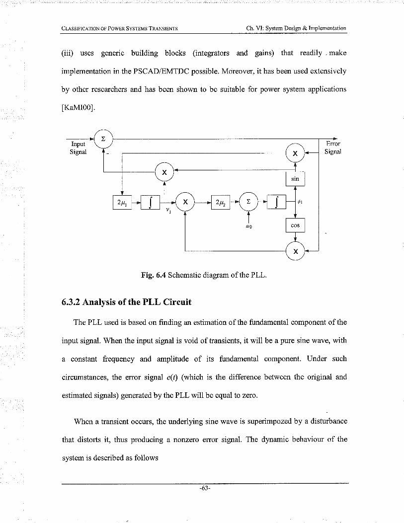
Clessr¡rc¡,r¡oN o¡ Pow¡n Sysr¡,tts TRANSIENTS Ch. VI: System Design & Implementation

(iiÐ uses generic building blocks (integrators and gains) that readily - make

implementation in the PSCAD/EMTDC possible. Moreover, it has been used extensively

by other researchers and has been shown to be suitable for power system applications

[KaMIO0].

Fig. 6.4 Schematic diagram of the PLL.

6.3.2 Analysis of the PLL Circuit

The PLL used is based on finding an estimation of the fundamental component of the

input signal. When the input signal is void of transients, it will be a pure sine wave, with

a constant frequency and amplitude of its fundamental component. Under such

circumstances, the error signal e(r) (which is the difference between the original and

estimated signals) generated by the PLL will be equal to zero.

When a transient occurs, the underlying sine wave is superimpozed by a disturbance

that distorts it, thus producing a nonzero error signal. The dynamic behaviour of the

system is described as follows

-63-

Clesslnrc¡,rroN oF PowER Sysr¡vs TneNsrpxrs Ch. VI: System Design & Implementation

#:2prsin(fi)e(t)

# : 2 prv, cos(þr)e(t) + ato

(6.1)

(6.2)

where the v1 ^d þ, are the estimated fundamental component amplitude and phase,

respectively. The parameters h and ltz a¡s adjustable gains that determine the speed of

the operation of the PLL, and a¡ is the angular frequency of the input signal

(fundamental component), which is equal to 2nx60=376.99radlsec in the North

American power system.

An important feature of the PLL described above is that following a transient, an

error signal is generated immediately, which makes it adequate for real-time applications

|KaMIOO], where fast computations are necessary. Any change in the ouþut of the PLL

is an indication of a deviation from the original sine wave and could be used to initiate

further analysis. In practice, deviations within a certain range are tolerated, and are not

considered as transients. This range normally is equal to a +5o/o interval around the

nominal operating voltage, and is accepted normally by the powor systems industry to be

a safe boundary around the nominal values. Any deviation beyond this range is

considered a transient that requires reaction. Using this concept, any PLL ouþut beyond

this limit is used in the subsequent feature extraction unit for identification of the true

cause of the disturbance.

Figure 6.5 shows an example of a transient overvoltage along with the ouþut of the

PLL system. As shown, the PLL ouþut is equal to zero prior to the occurrence of the

-64-

CLASSIFICATIoN oF PowER SYSTEMS TRANSIËNTS Ch. VI: System Design & Implementation

transient, which indicates that the PLL has been able to estimate coffectly the underlying

sine wave voltage. Following the onset of the transient, the ouþut of the PLL exhacts the

imposed disturbance and provides it to the feature extraction unit.

Fig. 6.5 Samples of input and ouþut waveforms of the PLL.Solid line: the input waveform; Dotted line: the PLL ouþut.

6.4 Feature Extraction

Transient waveforms, either simulated or recoded, contain alarge number of samples,

which makes them impractical to use as the input to a classifier. As noted in the

preceding chapters, the VFDT and the wavelet transform are used in this thesis as the

main methods for the extraction of a number of properties from the transients so that the

essence of each waveform is represented by a few, convenient-to-analyze features. The

CLessrncerlo¡¡ oE Pownn Svsrpus Tn-exsr¡Nrs Ch. VI: System Design & Implementation

following presents the techniques used for the implementation of these two features

extraction methods.

6.4.1 Implementation of the Wavelet Transform

The wavelet analysis was sho\Mn to be an effective method for charactenzing signals

with abrupt, short-term distortions, such as the transients in power systems. Doing so,

however, involves several steps such as selection of a suitable mother wavelet,

implementation of the transform and reduction of features. These steps are described in

detail in the following.

6.4.I.1 Choice of a Suitable Mother Wavelet

Selection of a suitable mother wavelet for a given application depends on a number of

factors, including the type of the signals involved, the computational requirements of the

algorithm, and the goals of the analysis to be carried out. Use of wavelets in the analysis

of power systems has been considered by several researchers, and the pertinent literature

shows a handful of mother wavelets used for this purpose [KiAg0O], [BuBa03],

lliMo99l, [HuHH99], [HuHs02]. The studies in this area have made important

contributions to the development of advanced intelligent systems for the detection,

charactenzation and classification of transients [ChenOl], IKaMIOO]; however, little

insight has been provided as to what fi¡ndamental properties should be considered for the

selection of a mother wavelet. tn the following four subsections, important properties of a

wavelet are presented that need to be considered before selecting a mother wavelet for the

analysis of power system transients.

-66-

CL¡,sslplc¡,rrow o¡ Powpn SysrEMS TRANSIENTS Ch. VI: System Design & Implementation

Visuql Similaríty

Wavelets are based on finding the correlation between the original waveform and

shifted and scaled version of a short-duration wave called a mother wavelet. [n this sense,

it is obvious that the visual similarity between the signal and the original mother wavelet

can be used as a simple, initial criterion for selecting a group of wavelets. It should be

noted that the visual similarity is a very crude property and should not be relied on

entirely, although in many publications it has been used solely for the selection of

wavelets.

Vanishing Wavelet Moments

A wavelet is said to have K vanishing moments if the following relation holds for all

k<K

tto ¡ç¡at =o (6.1)

The vanishing moments relate to the order of function that can be approximated by

the corresponding wavelet and also the level of compression that can be achieved through

wavelet decomposition. For example, in the popular family of Daubechies wavelets

(DBn), the number of vanishing moments for DB4 is equal to 2. For the analysis of

highly transient signals with high complexity, wavelets with more vanishing moments are

more suitable as they result in a more compact representation of the signals. However,

there is always a trade-off between the performance and complexity that has to be

resolved by the user. For example, more complex wavelets tend to be more

-67-

CIessIrIc¡.rIo¡¡ or PowEn SYsTEMS TRANSIENTS Ch. VI: System Design & Implementation

computationally intensive, which makes them less suitable for real-time applications

where fast computations are required.

Implementation and Computatíonal Intensity

It is very important to consider the implementation and computational complexity of

an approach when selecting a mother wavelet for a given application. For example,

wavelets with higher order filters (see Ch. 3) impose more intense computational

complexity, and tend to be less suitable for real-time applications. ln the analysis of

power system transients, fast response is a major consideration as it directly affects the

usefulness of the method in assisting the operator or the protection system to adopt the

appropriate counter-measure. It is also important to make the storage and processing

requirements as low as possible.

App li catio n- Re I ated As p ect s

Apart from visual similarity, the number of vanishing wavelet moments and

implementation and computational intensity, which can be used to limit the choices to a

few mother wavelets, it is important to consider the actual performance of individual

mother wavelets in the charactenzation of the transients. This is due to the variability of

the transients in different power networks, depending on a large number of factors,

including the physical properties of the underlying power network, proximity, and

environmental aspects.

Due to this wide range of influential factors, which partially may not be known

accurately, it is impractical to single out one specific wavelet that performs uniformly

-68-

Cl¡,sslilcer¡oN or Pow¡n SysrEMS TnnNslpNrs Ch. Vl: System Design & Implementation

well for all transients in all power networks and it is, therefore, important to consider the

perfbrmance of a number of candidate wavelets (selected according to the criteria

outlined above) to determine which one does perform better in practice.

Extensive literature survey, as well as personal experience with both simulated and

recorded data, has led to the selection of DB4 wavelet for the analysis of transients in this

thesis. This is because (i) power system transients, even the ones recorded in field, do not

show an excessive level of complexity and as such higher order wavelets do not seem to

be necessary, (ii) the performance of this wavelet has been considered versus other

mother wavelets and no meaningf,rl difference (neither in detection nor in

charactenzation) has been identified [SaKTO5] and (iii) the DB4 wavelet has been used

by other researchers studying power systems transients and numerous publications exist

that have used this wavelet lchKi0Ol, [MoKi97], [PiBh96], [MaAgOl]; by selecting this

mother wavelet, the results of the studies conducted in this research find more

comparability with those of the researchers' and, therefore, provides the outcomes with

further credibility in the community of peers.

6.4.1.2 Feature Extraction from Wavelets

Wavelet analysis has been performed on both simulated and recorded transients and

the first detail and approximation waveforms have been obtained. Although it is possible

to continue the decomposition to include more stages, the results (as shown in the next

chapter) have shown that the first level of detail and approximation is adequate. Careful

consideration of a detail waveform shows that it still contains a large number of samples,

although it contains almost half of the number of samples as in the original waveform. ln

other words, while the wavelet analysis is valuable in revealing important properties of

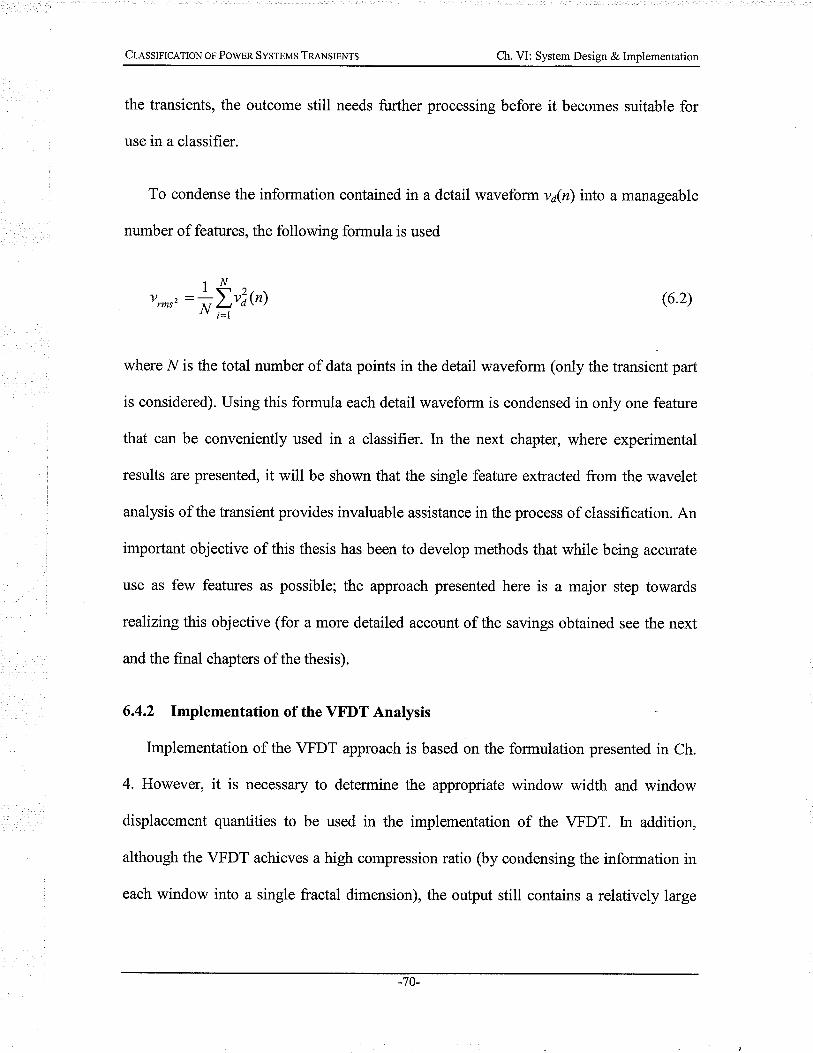
CL¡sslplc¡,rroN or Pow¡n SysrEMS TR-A,NSTENTS Ch. VI: System Design & Implementation

the transients, the outcome still needs fuither processing before it becomes suitable for

use in a classifier.

To condense the information contained in a detail waveform v¿(n) into a manageable

number of features, the following formula is used

vr^r':*¿t@ (6.2)

where Nis the total number of data points in the detail waveform (only the transient part

is considered). Using this formula each detail waveform is condensed in only one feature

that cær be conveniently used in a classifier. In the next chapter, where experimental

results are presented, it will be shown that the single feature extracted from the wavelet

analysis of the transient provides invaluable assistance in the process of classification. An

important objective of this thesis has been to develop methods that while being accurate

use as few features as possible; the approach presented here is a major step towards

rcalizingthis objective (for a more detailed account of the savings obtained see the next

and the final chapters of the thesis).

6.4.2 Implementation of the VT'DT Analysis

Implementation of the VFDT approach is based on the formulation presented in Ch.

4. However, it is necessary to determine the appropriate window width and window

displacement quantities to be used in the implementation of the VFDT. In addition,

although the VFDT achieves a high compression ratio (by condensing the information in

each window into a single fractal dimension), the ouþut still contains a relatively large

-70-

CLessrnrcerroN or Pow¡n SysrEMs TRANSTENTS Ch. VI: System Design & Implementation

number of data points, which are inconvenient to be used as features and as such feature

reduction is still necessary. The following subsections address these important issues.

6.4.2.I Determination of the Window Width and Window displacement

Careful examination of the VFDT analysis reveals important aspects of the approach

that will affect the quality of the features extracted using this method. The most important

parameters that need to be determined carefully, are the window width l/,, and the

window displacement -ð/''r.

We note that the VFDT is based on calculating the variance fractal dimension of a

signal in a number of windows along the signal. The data points contained in every

window will be condensed into a single number, thus providing data compression. If the

window width is too large, a large number of data points will be replaced with a single

number; this is analogous to filtering the signal with a low-pass filter with a small pass

band. The result of VFDT with an excessively large N** is that the important properties

of the signal will be surpassed by the presence of many other data points, and hence the

high frequency data will be lost. On the other hand, a very small window width will not

contain enough sample points to ensure proper estimation of the variance fractal

dimension and will also result in computational complexity due to the large number of

windows required to cover the signal.

The window displacement parameter controls the amount of overlap between adjacent

windows. It can vary between 1 (maximum overlap) and N,, (no overalp). Apparently

with maximum overlap, the computational intensity of the VFDT becomes overwhelming

and the resulting trajectory will show significant correlation as the data points used for

-7t-

CLASSIFICATIoN oF PowER SYSTEMS TRANSIENTS Ch. VI: System Design & Implementation

calculation of the fractal dimension in the crurent window will heavily contribute to the

dimension calculated in the next window. V/ith no overlap (for l/', : N*r) each point is

considered only once in the calculation of the fractal dimension and hence little

correlation will be preserved.

To illustrate the impact of these two parameters, several variance fractal trajectories

(corresponding to various combinations of N*, and ly',r) are presented below. The

original signal whose VIDT is calculated is a transient caused by a lightning strike, and

is shown in Fig. 6.6 (a). The signal is a sine wave that is intemrpted severely by the

lightning. A more detailed view of the intemrption is also shown in Fig. 6.6 (b).

2000

1 000

0

-1 000

-20000

2000

1 000

0

-1 000

-2000 L-0.26 0.34 0.36

Time [sec]

Fig. 6.6 Transient caused by lightning strike.

()bo(!

o

oÒ0

o

0.44

(b)

-72-

CLRssrprcerroN or Powsn SysrEMS TRANSTENTS Ch. VI: System Design & Implementation

In the following figures the VFDT of the signal is shown for various combinations of

the window size and displacement parameters. As seen from these figures, VFDT with a

relatively small window size (128 samples), as shown in Fig. 6.7, has a very fine

resolution, and as such results in a low compression (large number of fractal dimensions).

The excessively large window size of 2048 samples (Fig. 6.9) yields a very smooth

VFDT with very few samples of fractal dimension, and as such suppresses the details of

the transient. The suitably sized window width of 512 samples (Fig. 6.8) has enough

number of samples of the fractal dimension in the trajectory it produces and is void of

excessive details and is also capable of showing enough about the transient nature of the

waveform.

The impact of the window displacement parameter is illustrated through Figs. 6.10 to

6.12. Figure 6.10 shows the VFDT with a window width of 512 samples and a window

displacement of only 64 samples. As shown the trajectory possesses a great deal of detail

resulting from significant overlap of successive windows. The two other hajectories with

256 (50% overlap) and 511 samples (minimum overlap) of window displacement show

less detail. Figure 6.12 (with l/,, : 511) shows inadequate detail of the transient portion

and as such is not completely suitable for the charactenzation of complex transient nature

of the signal.

Besides the resolution issues discussed above, it is important to consider the

computational intensity of the method as well. Table 6.1 summarizes the results for such

combinations, including the total number of fractal dimensions calculated and the

processing time obtained on an lntel Centrino@ 1.6 G[zmachine with 512 Mb of RAM.

-tJ-

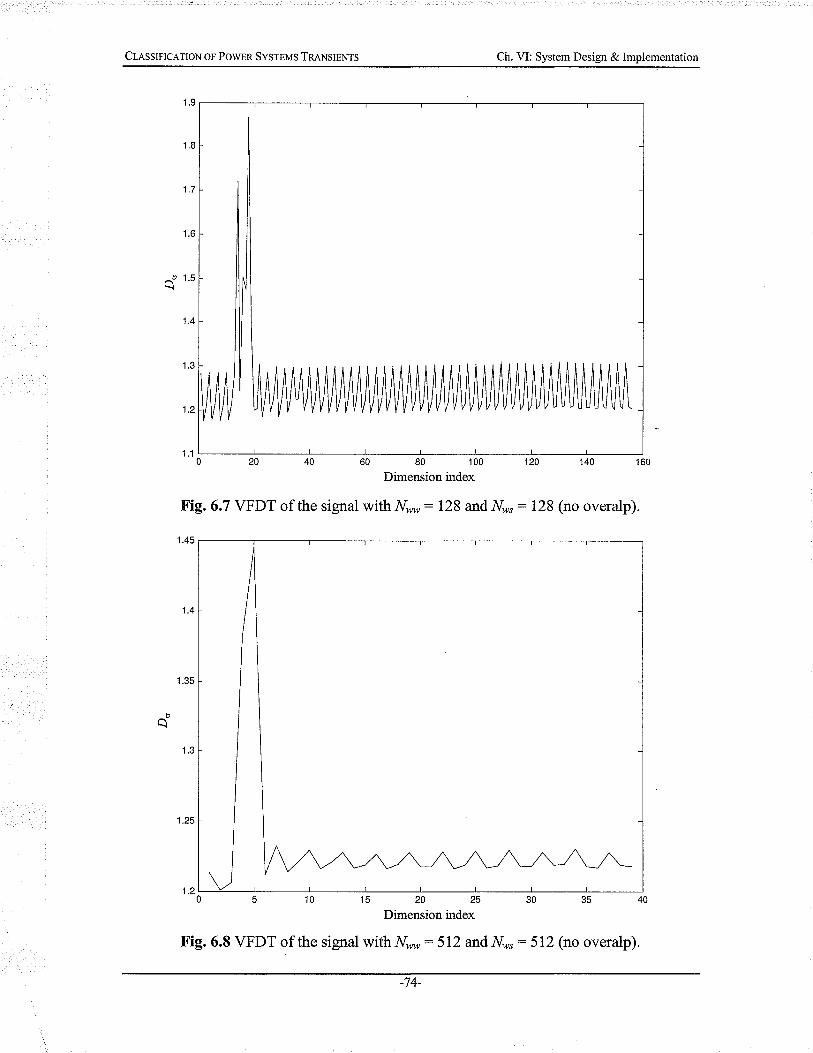
Clessrprc¡,rroN oF PowER Sysrelrs TReNslpnrs Ch. VI: System Design & Implementation

1.6

^þ 1.5!

1.4

1.3

1.2

1.1

Dimension index

VFDT of the signal with ¡/,, : 128 and ¡y',s : 128 (no overalp).Fig.6.7

1.45

Þ

a

1.215IU

Dimension index

Fig.6.8 VFDT of the signal withN,, :5I2 and¡tr4/s :5I2 (no overalp).

-74-

Cr¡.ss¡¡rcaloN op Pow¡n Svsr¡us Tn¡¡¡sl¡¡¡ts Ch. VI: System Design & Implementation

1.32

\

1.28

1.26

1.24

1.2256

Dimension index

Fig. 6.9 VFDT of the signal ',^/ith ¡'/'', : 2048 and ¡y'," :2048 (no overalp).

10

Dimension index

Fig. 6.10 VFDT of the signal with¡¡n- :512 andN,,:64.

oa

-7 5-

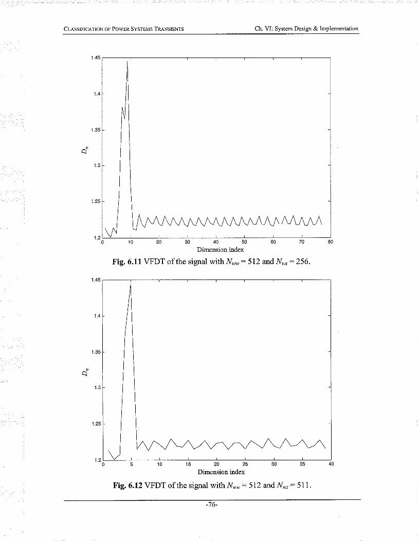
CLasslncelor.¡ or Powen SvsrEMS TR-A.NSIENTS Ch. VI: System Design & Implementation

Dimension index

Fig. 6.11 VFDT of the signal with¡/,, :512 and N,, = 256.

Dimension index

Fig. 6.L2 VFDT of the signal with ¡/,, : 572 and ¡y'," : 51 1.

-76-

Cless¡rrc¡.rox or Powen SysrEMS TRANSTENTS Ch. VI: System Design & Implementation

Table 6.1 Computational characteristics of the VFDT.

In the calculation of the VFDT of the transient signals (either simulated or recorded),

the length of the signal varies depending on the duration of the transient. This poses a

challenge as the number of samples within each waveform would vary. In order to

overcome this and with consideration of the post-processing of the VFDT for extraction

of feature (see below), a total number of 30 variance fractal dimensions were extracted

from each transient. Since the sampling of signal is done at arelatívely high rate (5760

for recorded data), the waveforms will have enough samples to allow for an accurate

representation within each window. A window displacement of 50o/o is also considered

for successive windows. This will eliminate excessive details and will reduce the

computational intensity of the procedure while ensuring enough resolution for the final

trajectory.

Window Width

(¡/,,)Window

Displacement (l/,")

Number of Dimensions

(N¿)

Total Processing

Time [sec]

r28 r28 155 < 0.02

5t2 5t2 38 < 0.02

2048 2048 I < 0.02

512 64 304 < 0.06

512 2s6 76 < 0.03

sr2 511 38 < 0.02

-77-

ClessrHc¡,ÏoN oF PowER Sysr¡us Tn¡,nsr¡Nrs Ch. VI: System Design & Implementation

6.4.2.2 Feature Extraction from VFDT

The VFDT analysis as described in Ch. 4 and the preceding section, compresses the

data points in a signal into a number of fractal dimensions. Although this compression

ratio is quite high, the fractal dimension trajectory so obtained still has alarge number of

components to make it inconvenient to be used as features.

In order to reduce the VFDT of each sample, a number of options have been

developed and used in this thesis. The studies have confirmed that the extracted features

(described in the following) do perform satisfactorily and can be good measures for

distinguishing between various power system transients.

Although the distributions are not Gaussian, it was found that first and second

moments could provide valuable information that can assist greatly in the classification

process lSaKTO4]. These moments are defined as follows

*,=fir,,r,<,>

*r:+7,u¿Ø-*,)2

(6.3)

(6.4)

where my and tn2 &ra the first and second moments of the VFDT/(Ð, and N¿ is the total

number of values on the VFDT, each computed according to the algorithm described in

Secs. 4.5 and 4.6.

Using these two features, it becomes possible to classify the transients in a power

system; however, the performance of the classifier can be improved by combining the

-78-

CL¡,ssrprc¡,rroN or Pow¡n Systovs TreNslrNts Ch. VI: System Design & Implementation

two features obtained above with the feature obtained the wavelet analysis. The next

chapter presents the numerical results obtained from individual feature extraction

methods used as well as their combined features.

6.5 Implementation of the ClassifÌer

The three types of classifiers described in the previous chapter are implemented and

their perfoÍnances are evaluated. The details about the implementation of the methods

have been provided in Ch. 5. Although design of the classifiers such as the Ml-based

Bayes rule and the PNN is part of the overall system design, it is intentionally left to Ch.

7, since it will blend in more logically with the rest of the material in that chapter.

6.6 Overall System Layout

The mathematical foundations of the components of the overall system for detection,

feature extraction and classification of transients in a power system have been described

in the previous chapters. Their actual implementation details were given in this chapter.

To be used as a suitable tool, these components need to be interconnected.

Figure 6.13 shows a schematic diagram of the overall system. It is seen that the PLL

performs the segmentation of the transient and provides the feature extraction engine with

its output. Feature extraction is done by two engines, namely the wavelet and the VFDT.

The ouþuts of these two units are then condensed into a small number of features,.which

are then combined and used in a classifier. The ouþut of the classifier is an indication of

the underlying cause of the disturbance observed in the voltage waveform given to the

system. Apart from the transient simulation done in the PSCAD, the remaining modules

-79-

CL¿.sslptcetloN oF Pov/ER Svstpvs Tn¡¡gsler.¡rs Ch. VI: System Design & Implementation

of the system are coded in MATLAB. The developed source code has several moduies

that are shown, along with the code structures, in App. B.

Fig. 6.13 Schematic diagram of the overall system.

6.7 Chapter Summary

This chapter presented the details of the design of the overall feature extaction and

classification system. The chapter discussed in detail the process of selection of a suitable

mother wavelet as well as extraction of features from wavelet analysis. One level of

wavelet decomposition is carried out on each transient signal using the DB4 wavelet. The

RMS of resulting detail waveform is used as one of the features.

The chapter also discussed the implementation of the VFDT. In particular the

selection of window width and window displacement parameters was discussed in detail.

The VFDT analysis is done on each signal to yield a total of 30 variance fractal

dimension (with a window displacement of 50%); the trajectory is then condensed into

two features being the first and second moments of the trajectory. The two sets of

features extracted from wavelet and VFDT analyses are combined and used in a

classifier. The next chapter presents the experimental results obtained using simulated

and recorded transients.

-80-

ClessrHcRt¡o¡¡ on Powpn Sysr¡\¡s Tn¡NsrpNrs Ch. VII: Experimental Results & Performance

Cn.rprER VII

ExpnnrMENTAL R.ustIr,IS ANÐ DrscussloN

7.1 Introduction

Following the mathematical description of the feature extraction and classification

methods, as well as a description of the design of the overall system presented in the

previous chapter, this chapter presents the experimental results obtained by applying the

tools and techniques to both simulated and recorded transients, and also provides

technical discussion on the results and their significance.

The chapter is organized into two major sections: (i) the simulated transients and (ii)

recorded transients. For each section, feature extraction details and classification results

are presented.

7.2 Experimental Results Using Simulated Transients

Simulated transient waveforms are obtained using the PSCAD/EMTDC program. The

simulated transients include samples from three types of disturbances, namely three-

phase faults, capacitor switchings and breaker operations. A total of 120 samples are

generated for each class, of which 40 samples are used for training and the remaining 80

are used for testing the classifier. Feature extraction from these transients is carried out

using both wavelets and the variance fractal dimension trajectory, VFDT.

In the following subsections, classification results using the Ml-based Bayes rule for

each of these two sets of features are presented. It is followed by the results obtained

using combined features and the classification results using the PNN.

-81-

Cu.sstplc¡rioH or Pow¡n Sysrpus TnensrpNrs Ch. VII: Experimental Results & Performance

7.2.lML-Based Classification Using the VFDT Features

The VFDT for each of the 40 training samples from each class is computed, and the

results are then condensed into two features being the first and second moments of the

trajectory of variance fractal dimensions, resulting in two features per sample.

The Ml-based Bayes rule, as described earlier, intends to fit a pdf to the features so

obtained. Since there are two features for each sample from the three classes, there are a

total of 6 pdfs to be fitted. Parts (a) of Figs. 7.1 to 7.6 show the histograms of the

features in each class. An important consideration in generation of such histograms is

number of bins used. While use of too few bins would result in an overly smooth Braph,

too many bins can introduce excessive detail. Both such cases will affect adversely the

estimation of underlying pdfs. The histograms shown have been obtained using 10 bins,

which in this case provides sufficient resolution.

The next step after generation of data histograms is the estimation of pdfs. The

histograms of Figs. 7.I to 7.6 show that the underlying distributions are often

multimodal, and are not single Gaussians. ln order to use the Ml-based Bayes rule, one

needs to assume known forms for the underlying pdfs; as such, we have attempted to

model these distributions using a combination of local Gaussian pdß. This is because a

Gaussian distribution is identified by only two parameters and its higher order moments

are equal to zero,thus making the estimation convenient. The estimated pdfs are shown

in parts (b) of Figs. l.l to 7.6.The classification results obtained using these pdfs confirm

the suitability of this assumption. Estimation of the parameters of the underlying pdß

involves an iterative optimization that maximizes the objective function given in Eq.

(5.4). Table 7.1 summarizes the starting and final parameters of the estimated pdfs. It is

-82-

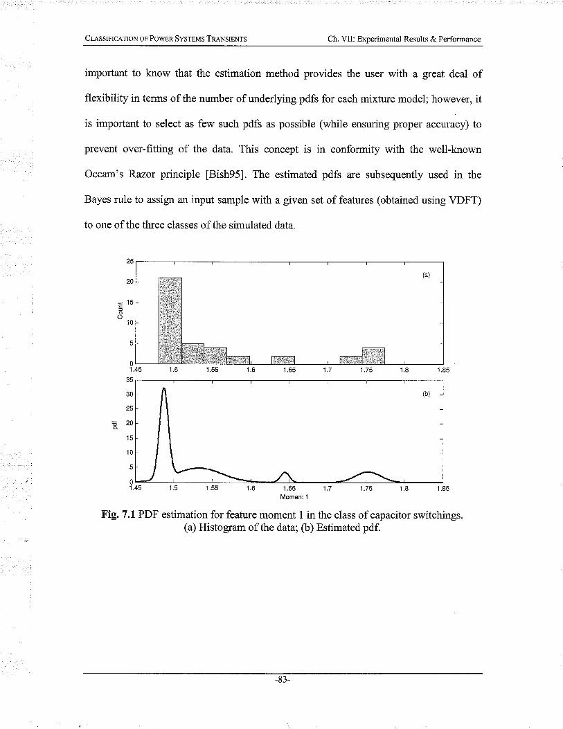
Cr¿ssrrrcRloN or Powen SysrEMS TRANSTENTS Ch. VII: Experimental Results & Performa¡ce

important to know that the estimation method provides the user with a great deal of

flexibility in terms of the number of underlying pdß for each mixture model; however, it

is important to select as few such pdfs as possible (while ensuring proper accuracy) to

prevent over-fitting of the data. This concept is in conformity with the well-known

Occam's Razor principle [Bish95]. The estimated pdfs are subsequently used in the

Bayes rule to assign an input sample with a given set of features (obtained using VDFT)

to one of the three classes of the simulated data.

25

20

* 15Elo

10

Ã

0L1.45

35

30

25

820o

15

10

5

0l-1.45 1.6 1.65 1 .7 1.75 1 .8 1.85

Moment 1

Fig. 7.L PDF estimation for feature moment 1 in the class of capacitor switchings.(a) Histogram of the data; (b) Estimated pdf.

-83-

CressrncerroN oF PowER Sysretrs TRANSIENTS Ch. VII: Experimental Results & Performa¡ce

0.010

80

60

40

20

0.014 0.016 0.018

1.285

0.024 0.026 0.028

350

300

250

200

150

100

50

0.01 0.015 0.02 0.025 0.03Moment 2

Fig.7.2 PDF estimation for feature moment 2 inthe class of capacitor switchings.(a) Histogram of the data; (b) Estimated pdf.

10

I

þ

4

2

0.005

0t_1.27 1.275 1.29 1.295

0f r r I I I

1 .27 1 .275 1.28 1 .285 1 .29 1 .295 1.3 1 .305 1.31 1 .315Moment 1

Fig. 7.3 PDF estimation for feature moment 1 in the class of faults.(a) Histogram of the data; (b) Estimated pdf.

(b)

(b)

-84-

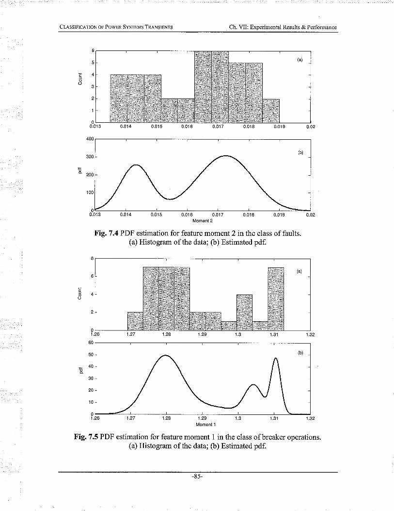
CLnssIrIc¿,TIoN or Pow¡R SySTEMS TRANSIENTS Ch. VII: Experimental Results & Performance

6

5

4

J

2

'I

0L-0.013 0.014 0.015 0.016

!o

400

300

200

0.013

Fis.7.4

6

4

2

0.014 0.015 0.016 0.017 0.018 0.019Moment 2

PDF estimation for feature moment 2 inthe class of faults.(a) Histogram of the data; (b) Estimated pdf.

1.27 1.28

cfoo

1.26

60

50

40

30

20

10

0-1.26 1.3 1.321.29

Moment 1

Fig. 7.5 PDF estimation for feature moment 1 in the class of breaker operations.(a) Histogram of the data; (b) Estimated pdf.

(b)

(b)

-85-

ClesslplcerloN or Powsn SysrEMS TRANSIENTS Ch. VII: Experimental Results & Performance

20

15

IU

5

0r0.014 0.016

500

400

ä óuuo

200

100

0.01 6 0.018 0.02 0.022 0.024 0.026 0.028Moment 2

Fig. 7 .6 PDF estimation for feature moment 2 in the class of breaker operations.(a) Histogram of the data; (b) Estimated pdf.

The parameters listed in Table 7.1 are obtained using the 40 training samples from

each class. For testing the performance of the Ml-based Bayes classifier the remaining

80 samples from each class are used. Upon presentation of each testing sample the

corresponding class-conditional pdß are calculated and the class with the highest

probability is chosen as the winner and the input sample is assigned its label. Note that

we have assumed equal prior probabilities for each of the three respective classes.

0.014

(b)

-86-

CLesslFIcerroN oF PO.üER Sysrgvs TnensnNrs Ch. VII: Experimental Results & Performance

Class/FeatureIdentifier Initial Parameters Final Parameters

Capacitor

Switching

I

o

o¿

m: [1.5 1.55 1.651.75]

o: 10.01 0.02 0.01 0.011

tt: [0.5 0.25 0.1 0.15]

m:11.49 1.53 1.64 L751

o: [0.0057 0.029 0.0058 0.0167]

ú:10.44 0.357 0.0499 0.151

N

c)

oå

m: [0.014 0.019 0.026]

o: 10.002 0.002 0.0031

n: [0.15 0.15 0.7]

m: [0.0141 0.0196 0.0264]

6 : 10.0022 0.0023 0.0009731

,r : [0.073 0.18 0.74]

Faults

€o

Å

m : 11.27 1.29 1.295 1.3051

o: [0.01 0.01 0.02 0.01]

æ:10.25 0.5 0.15 0.101

m : 11.27 4 1.29 1.294 1.2971

o: [0.0015 0.006 0.007 0.0072]

n:10.246 0.52 0.122 0.1081

c.l€oH

oà

m: [0.0145 0.0168 0.018]

o: [0.002 0.001 0.001]

îE:10.25 0.5 0.251

m: [0.014 0.01696 0.01771

o: 10.0005 0.00084 0.00071

n:10.311 0.445 0.241

Breaker

Operations

c)Êo¿

m: [1 .281.295 1.305 1.31]

o: [0.02 0.01 0.005 0.005]

?E: [0.65 0.15 0.1 0.1]

m: 11 .279 1.2921.30 1.311

o = [0.0049 0.008 0.0028 0.0014]

æ: f0.581 0.12 0.143 0.1571

c.lÐ()é

¿

m: [0.015 0.016 0.019 0.022]

o: [0.001 0.001 0.001 0.001]

ß:10.2 0.4 0.2 0.21

m: [0.017 0.0173 0.0184 0.023]

o: [0.36 0.3621.55 1.1]*10r

n:10.125 0.25 0.44 0.1821

Table 7.1 Parameters estimated using the maximum likelihood (VFDT features).

Table 7.2 shows the summary of the classification results obtained by using the

features obtained from the VFDT analysis and the Ml-based Bayes rule. For each entry

the total number of features along with their percentage share is given.

-87-

Cless¡r'rceÏoN oF PowER SysrEMS TReNsleNrs Ch. VII: Experimental Results & Performance

Test Sample Class

Assigned Class

Capacitor Switching Faults Breaker Operations

Capacitor Switching 80 (1.00%) 0 (o%) o (o%)

Faults 0 (0%) 7l (88.75o/o) e (lt.2s%)

Breaker Operations o (o%) 20 (2s%) 60 (7s%)

Table 7.2 classification results for the VFDT features using the Bayes rule.

The results presented in Table 7.2 show that the VFDT-based features have been able

to separate completely the class of capacitor switching transients from the remaining two

classes. However, the classes of faults and breaker operations show some error, indicated

by the misclassification of some of their samples into the other class. In order to visualize

the case, it is instructive to consider Fig. 7.7, which shows the training samples.in the

moment l-moment 2 plane. As shown the class of capacitor switching is separated

entirely from the other classes, which show overlap.

VFDT-based features are not the only features available to us for classification.

Wavelet analysis also provides us with means for classification. In the following

subsection we firstly consider the performance of wavelet analysis on its own and then

examine the performance of combined features.

-88-

Cl¡.ssr¡rcerro¡¡ or Powpn SysrpNrs TReNsr¡Nrs Ch. VII: Experimental Results & Performance

* Breaker operationsA Capacitor switching

O Faults

^

Aðê^f--A ^

AAA

A+

+*.*t4+gÈê9

ffi-"wU-

ssffo

AAA

A

A

C!EoEo

0.03

0.028

0.026

0.024

0.022

0.02

0.018

0.016

0.014

0.012

0.011.2 1.5 1.6

Moment 1

Fig.7.7 Spread of features obtained using VFDT.

7.2.2NIL-B.ased Classification Using the Wavelet Feature

Since there was only one feature extracted from the wavelet analysis of simulated

data, classification of the three types of simulated classes only requires three pdfs to be

estimated for implementation of the Bayes rule. Following the same procedure as in the

previous section for VFDT features, we start by examining the histograms of the training

samples and then use the Ml-based mixture model approach to fit pdfs.

Figures 7.8 to 7.10 show the histograms of the wavelet-based features along with the

estimated pdfs. The initial parameters as well as final parameters for the pdf estimation

are listed in Table 7.3.

-89-

CLRsslncerroN or Powpn SysrEMS TRANSIENTS Ch. VII: Experimental Results & Performance

0L0.14

20

15

10

50

40

30

20

10

0

5

4

J

2

1

0.16 0.18 0.2 0.22 0.24Feature (using wavelet analysis)

0.26 0.28

Fig. 7.8 PDF estimation for the wavelet feature in the class of capacitor switching.(a) Histogram of the data; (b) Estimated pdf.

12

10

o

4

2

clo()

0L0.1

Eo

0L0.1 0.3 0.4 0.5 0.6 0.7 0.8

Feature (using wavelet analysis)

Fig. 7.9 PDF estimation for the wavelet feature in the class of faults.(b) Histogram of the data; (b) Estimated pdf.

(b)

(b)

-90-

0.9

CLesslncerror'r oF Pov/ER SysrEMS TRANSIENTS Ch. VII: Experimental Results & Performance

25

20

t5

-çãroO

5

0

1

0.8

5 0.6o

0.4

0.2

09 10 11

Feature (using wavelet analysis)

Fig. 7.10 PDF estimation for the wavelet feature in the class of breaker operations.(a) Histogram of the data; (b) Estimated pdf.

Table T.3Paraneters estimated using the maximum likelihood (wavelet feature).

(b)

ClassIdentifier Initial Parameters Final Parameters

Capacitor

Switching

m: [0.17 0.21 0.25]

o: [0.02 0.02 0.001]

æ: [0.8 0.15 0.05]

m: [0.173 0.2120.26]

o: [0.009 0.026 10-8]

ß: [0.856 0.145 2x10-8]

Faults

m: [0.25 0.4 0.65 0.75]

o: [0.08 0.08 0.05 0.02]

n:10.4 0.2 0.1 0.31

m: [0.26 0.3910.646 0.79]

o: [0.048 0.079 0.0878 0.03]

n:10.443 0.186 0.067 0.301

Breaker

Operations

m:12.5 5.0 7.01

o: [0.1 1.0 0.5]

n:10.7 0.15 0.151

m:12.34 4.93 I .l7l

o:10.265 2.13 0.3251

?¡: 10.536 0.366 0.10371

-91-

CLRsslncerloN oF PowER Sysr¡ti¡s Tn¡Nslsxrs Ch. VII: Experimental Results & Performance

Bayes rule classification using the feature obtained from the wavelet analysis yields

the results contained in Table 7.4. Note that similar to the VFDT approach, 40 samples

are used for training and the remaining 80 samples are used for testing.

Table 7.4 Classification results for the wavelet feature using the Bayes rule.

Table 7.4 contains important information about the performance of the wavelet

analysis in classification of the three types of simulated transients. As shown the analysis

is capable of separating completely the class of breaker operations from the other two

classes. The classes of capacitor switchings and faults also show very good level of

separation but still have some small overlap. It is also important to note that the wavelet

analysis has been able to remove the overlap between the faults and breaker operations

observed in VFDT analysis (see Table 7.2).In other words, it seems that the wavelet and

VFDT analyses can be used cooperatively in a classifier, which takes advantage of both

methods to remove as much overlap among the classes as possible.

The following subsection presents the classification results of the combined features

using the Ml-based Bayes rule.

Test Sample Class

Assigned Class

Capacitor Switching Faults Breaker Operations

Capacitor switching 77 (96.250/0\ 3 (3.7s%) 0 (0%)

Faults 6 (7.s%) 74 (e2.s%) 0 (0%)

Breaker Operations o (o%) 0 (0%) 80 (100%)

-92-

Cresslnc¡,loN o¡ Powr,n SvsrEMS TR.ANSTENTS Ch. VII: Experimental Results & Performance

7 .2.3 NIL-Bas ed Clas sifïcation Using C ombined Features

Examination of the experimental results of the previous sections suggests that

combination of the features obtained using VFDT and wavelet analyses could improve

potentially the correct classification rate by removing the overlap areas observed in

individual sets.

The new input vector, which combines the two features form the VFDT with the

single feature from waveiet analysis, has the following form.

¡ = þrst moment from VFDT, second moment from VFDT, feature from wavelet] (7.1)

Upon presentation of this combined feature to the classifier, the overall pdf is

calculated and the one with the largest numerical evaluation is chosen as the winner.

Table 7.5 shows the classification results using the combined features in an Ml-based

Bayes classifier.

Table 7.5 Classification results for the combined features using the Bayes rule.

Test Sample Class

Assigned Class

Capacitor Switching Faults Breaker Operations

Capacitor Switching 80 (100%) 0 (0%) o (o%)

Faults o (o%) 80 (100%) 0 (0%)

Breaker Operations o (0%) 0 (0%) 80 (100%)

-93-

Cu.ssrnc¡,loN or Pow¡n Sysrnvrs TR¡usrpnrs Ch. VII: Experimental Results & Performance

7.2.4 Discussion on the ML-Based Bayes Rule for Simulated Data

The experimental results presented in the previous subsections addressed the

performance of the Ml-based Bayes rule in classification of simul ated data. The two

signal analysis methods used for feature extraction, namely the VFDT and the wavelets,

each charactenze the transient signal from a different standpoint, and that is the reason

why combination of the two sets of features obtained using these methods results in such

a high correct classification rate.

Besides the merit of the features used, it is very important to consider the

classification method itself too. The Ml-based Bayes rule provides a very convenient

method for training a good classifier. The training time, which is the time required for

optimizing the pdf parameters, is very short and the optimization completes in a fraction

of a second. The method also provides flexibility in terms of adjusting the complexity of

the pdfs and allows for derivation of low-order models conforming with the Occam's

razot rule.

The important point when using the Ml-based method is to ensure that enough

training samples are available so that the underlying pdf can be accurately estimated. This

is however, a limitation on a wide variety of classifiers.

7.2.5 Classifïcation of Simulated Transients Using a PNN

As mentioned earlier in our discussion of classification methods, a probabilistic

neural network is an implementation of the Bayes rule with the Parzen pdf estimation

embedded in it. The beauty of a PNN is in the fact that depending on the selection of the

window-width parameter(s) it can resemble anything ranging from a nearest neighbor

-94-

ClasslprceloN oF PowER Sysr¡prs TRANSTENTS Ch. VII: Experimental Results & Performance

classifier to overly smooth pdß. The challenge in using a PNN is to find suitably optimal

values for these window-width parameters. PNNs have been used by Chen [Chen01] for

the classification of power system transients. Although we have been able to obtain a

very high correct-classification rate using the previously presented Ml-based Bayes rule,

it is worthwhile to consider the PNN option as it provides us with opportunity to (i)

assess the performance of our approach to that of the previous work, and (ii) compare the

performance with that of the Ml-based Bayes rule, which can prove to be useful in

advising the user as to which method has superior performance in the task given.

We will follow the same approach as presented earlier for the combined features, and

will use 40 samples from each class for the training and 80 samples per class for the

testing of the classifier. Table 7.6 shows a surnmary of the training phase of the PNN,

including the starting and final values of the window-width parameters.

Table 7.6Data for the training phase of a PNN.

Initial Values of the Window-Widths (ør, o2, q\

0.05 0.1 0.2

Final Values of the Window-Widths (q, o2, q)

0.001378 0.089746 0.1 89898

Total Calculation Time [sec] Number of Iterations

316.4 95

-95-

CLessr¡rcerloN oF PowER Sysrsvs TRANslpNrs Ch. VII: Experimental Results & Performance

The training of the PNN is done in 316.4 seconds (see Table 7.6) on an Intel Centrino

1.6 GHz processor with 512 Mb of RAM. ln order to ease the burden of the optimization

of the window-widths, the input data (features) have been normalized by their mean

values. This causes the values to be numerically comparable, thus improving the

numerical stability of the optimization algorithm. Tables 7.7 and 7.8 show the PNN

classification results for both the training and testing sets.

Table 7.7 PNN classification results for the training set.

Table 7.8 PNN classification results for the testing set.

Test Sample Class

Assigned Class

Capacitor Switching Faults Breaker Operations

Capacitor Switching 3e (e7.s%) t (25%) 0 (0%)

Faults o (0%) 37 (92.s%\ 3 (7.s%)

Breaker Operations 0 (0%) 2 (s%) 38 (es%)

Test Sample Class

AssÍgned Class

Capacitor Switching Faults Breaker Operations

Capacitor Switching 73 (91.2s%\ 4 (s%) 3 (3.7s%)

Faults 0 (0%) 72 (e0%) 8 (i0%)

Breaker Operations 2 (2.s%) r0 (rz.s%) 68 (8s%)

-96-

ClesslplceloN oF PowER Sysrel.ts TR¡,NSTENTS Ch. VII: Experimental Results & Performance

7.2.6 Discussion on the PNN Classification of Simulated Data

The PNN, as discussed in Ch. 5, is a unified approach to classification. Using the

Parzen pdf estimation method, it estimates the underlying pdß in a classification problem

and implements it as a neural network.

The experimental results reported before do reveal important properties of PNN

classifiers. As shown a PNN needs a fairly burdensome training, which in our case took

more than five minutes. In comparison to the Ml-based Bayes rule, which as indicated

before takes only a fraction of a second to optimize, this longer training time is a serious

drawback. Another important observation is that despite significant computational

intensity during its training, the PNN still fails to produce as accurate results as the ML-

based Bayes rule. This could be explained by nothing that the PNN imposes the same

window-width for each of the features in all classes involved. ln the Ml-based Bayes

rule method, each feature in each class has a different distribution; however, the PNN

assumes that a given feature has the same o in all classes, which does not necessarily

hold in all cases. The optimization carried out during the training, aims at finding a

suitable value for each oso that the best tradeoff is achieved; however, this tradeoff can

sometimes result in a loss of accuracy. For example, the feature 'moment 1' obtained

from the VFDT analysis does not show the same scattering in the three classes of

transients (see Fig. 7.7).

In other research works in this area, PNNs have been used for the classification of

transients in power systems [Chen0l]. The experimental results presented in that work

show slightly higher classification rates; however, the training set in that work has had

-97-

CLASSIFICATION OF PowER SYSTEMS TRANSIENTS Ch. VII: Experimental Results & Performance

much more samples than the training set in this work and also it had a different set of

samples from different classes of transients; besides the classification in that work was

carried out using 60 features, which is by far larger than the number of features used here.

As mentioned earlier, the number of training samples are selected intentionally fairly low

to comply with the lack of an abundant training set in practice.

Despite its less accurate performance in this work, PNNs do provide a powerful

means for classification of pattems where a large number of features are used. In such

cases, the Ml-based Bayes rule requires an overly large number of pdfs to be estimated

that can potentially reduce the classification performance; however, the PNN is a

convenient, easy to implement method especially if the training set has an adequateiy

large number of samples.

7.3 Experimental Results Using Recorded Transients

The experimental results obtained using the simulated data provide a confidence level

as to how effective our methods will be when applied to data obtained using field

measurement. The overall design of the power system transient detection,

charactenzation and classification unit has been done on simulated data, which is safe,

fairiy accurate and inexpensive to obtain. However, the final stage of the design will

focus naturally on its performance on real data. Further adjustments and modifications

will be introduced as necessary.

The recorded data used in this research has been obtained from Manitoba Hydro. The

data belongs to the Manitoba Hydro system at various locations and different times of the

year. Hydro has several recording facilities that record the transients in the system;

-98-

Clessrntc¡.tloll or Pow¡n SysrEMS TRANSIENTS Ch. VII: Experimental Results & Performance

however, labeling of the data has been started recently and as such the volume of the

labeled recoded data available to the researchers is not very high. Besides, alarge number

of transients are caused by severe weather conditions and in the absence of such extreme

cases some specific types of transients may not have more than a few occurrences. This

also puts further limitations on the training samples in our experimentation with real data.

Table 7.9 shows a suÍrmary of the recorded data made available by the Manitoba

Hydro, including the type and number of samples of each transient. The sampling

frequency used for recording the transients is equal to 5760Hz

Table 7.9 Recorded transients obtained from Manitoba Hydro.

Figures 7.11 (a-e) shows samples of recorded transients. In the following, we

consider the feature extraction and classification of these recorded data. Of special

interest will be the selection of features and also selection of an appropriate feature

extraction method.

Type of Transient Number of Samples

Bird 24

Lightning 15

Storm 12

Switching 5

Mis-Operation (No Fault) 2

-99-

CLassl¡rcerloN oF Pov/ER Svsrpn¡s TRANSTENTS Ch. VII: Experimental Results & Performance

7.3.1Extraction of Features from Recorded Transients

The simulated data used in the previous sections was created for three classes of

transients that are different from the real data obtained. Careful consideration of the

recorded transients reveals that the number of samples available in the classes of mis-

operation and switching is inadequately small so that development of a pdf for these

classes becomes impossible. In other words, the insufficient number of samples in these

two classes does not permit the distribution of other samples in this class to be

discovered. Therefore, any attempt for establishment of a feature extraction method and

the subsequent classification using such data will be pointless. Our focus will therefore be

on the remaining three classes; i.e., bird, lightning and storm.

2000

0

-2000 L-0.5

2000

0

-2000Lo.2 0.3 0.32 0.34 0.36 0.38 0.4

2000

0

-2000 L-0-3 0.32 0.34 0.36

5000

0

-5000 L-o.2

s000

0

0.480.460.M0.420.40.38

(e)

0.24 0.26 0.28 0.3 o.32 0.34 0.36 0.38 o.4

Fig. 7.L1 Samples of recorded transients.(a) Bird; (b) Lightning; (c) Storm; (d) Mis-operation; (e) Switching.

-5000 Lo.2

-100-

CL¡,ssrnrcerroN o¡ Powpn Svsrprrls Tn¡.rqsrprqts Ch. VII: Experimental Results & Performance

The three classes mentioned above have marginally enough number of samples to

make an initial attempt for classification possible. Further examination of the transients in

this class also reveals that the class of storms represents a totally distinguishable pattern

from the other two classes. Transients in this class are chanctenzed by having small

variations in the voltage magnitude and the distortion is mainly affecting the harmonic

content of the waveform. Such distinguishable patterns make separation of the class of

storm very straightforward, and as such the challenge remains on how the transients

caused by bird or lightning strike can be separated.

Since the classes of recorded data are different from the classes of simulated data, it is

always intriguing to re-consider the feature extraction in order to ensure that features that

are most readily accessible have been considered as well. At first sight, it is observed that

the transients caused by lightning and bird strikes cause significant changes in the voltage

levels. It therefore seems reasonable to consider the variations of the power through the

line due to the changes in the voltage to see how viable it could be to be used as a feature.

Although the load characteristics are essential in the power delivered to them, initially,

we can assume that average power is proportional to the square of the voltage. Figure

7.12 shows the variations of the average power during the transient caused by a bird

striking the line. The average power signal (i) has by far fewer samples than the original

signal, as the samples in every period of the waveform are condensed in a single number,

and (ii) has much smoother variations due to the integration involved.

Despite these properties, the average power waveform fails to act as suitable feature,

because (i) calculation of the average power is done over a period and as such a

considerably large amount of delay is introduced, which makes the overall scheme unfit

-101-

Classrrrc¡,rron op Pow¡R Sysr¡Nls TneNslsNrs Ch. VII: Experimental Results & Performance

for real-time applications, (ii) the averaging involved does eliminate some of the

important details of the waveform that makes classification very difficult. For example

note that the average power for the classes of bird and lightning strikes will not be

different completely as both classes present a quick intemrption of the voltage following

the transient.

2

1

0

-1

-2

30Period number

Fig. 7 .12 Average power variations.(a) Transient waveform; (b) Average power waveform.

Although the average power does not seem to be a suitable feature, other physical

properties of transients could be considered. To extract as much information from the

physical properties of signal as possible, we considered two other factors: the initial

voltage and the duration of the transient. Figure 7.13 shows how these two indices are

vo)

(ú

=o

0.90.80.70.60.5

2

F r.s

=oìolo0)oE

åou

0

(a)

(b)

-102-

Cl¡,ssrplcnttoN op Powpn Sysrptus Tn¡Nslenrs Ch. VII: Experimental Results & Performance

calculated for a typical waveform in the two classes of interest. Table 7.10 shows

statistical properties of these two indices in the classes of bird and lighting strikes.

0.6ïme [sec]

Fig. 7.13 Calculation of duration of and initial voltage drop caused by a transient.

Table 7.10 Statistical properties of the duration and initial voltage drop.

lnitial \oltage drop

Class/Feature Identifier Min Max Mean

BirdInitial Voltage Drop [V] 10 300 97.08

Duration lsecl 0.38 0.82 0.63

LightningInitial Voltage Drop [V] 10 1700 499

Duration [sec] 0.r7 0.78 0.45

-103-

CL¡,ssrprc¡,rou op Powrn Sysr¡røs TRANSIENTs Ch. VII: Experimental Results & Performance

Distribution of these two features is shown in Fig. 7.I4. As shown these physical

features can partially separate the two classes despite the fact the overall trend of

transients in these two classes are very similar. Another important observation in Fig.

7.14 is that the transients in the class of bird tend to be slower (with longer durations) and

less severe (in terms of the initial voltage drop) than those caused by the lightning strike.

Such observations agree with intuitive impressions that suggest lightings should be

typically faster and more severe than bird strikes.

It should also be mentioned that the same features could also be extracted for the

class of storms. This class is charactenzedby having very small voltage drops and very

long durations (with a mean duration of 1.66 sec), which once again confirms that this

class is entirely separable from the two classes of bird and lightning strikes.

o_oþ0)o)(ú

=oE.=c

* Bird

O Lightning

o

o

o

oof

+o ++++åg

-200 L0.1 0.4 0.5 0.6 0.7 0.8 0.9

Duration of transient [sec]

Fig.7.l4 Distribution of the physical samples for the classes of bird and lightning.

1 800

r 600

1 400

1 200

1 000

800

600

400

200

0

-t04-

ClessrrrcerloN or PowEn Sysretts TneNsl¡nrs Ch. VII: Experimental Results & Performance

The two physical features extracted are successful partially in separating the two most

challenging classes of the recorded data; however, it is observed that the two classes still

have some overlap, which contributes to the classification enor. To improve the

performance of classification, it is necessary to add other features that can contribute

further to the separation of samples (see below for numerical results). Experimental

results using these combined approaches are reported in the following section.

7.3.2 Classification of Recorded Transients

The methods presented in Ch. 6 are suitable techniques for classification of pattems

based on features extracted from samples. Despite their similar function, which is

assignment of an input sample to a given class, they possess different properties that

make them suitable for only a limited number of classification problems. In other words,

selection of a classification method should only be done with careful consideration of

properties of the underlying problem as well as capabilities of the method itself.

In general, the Ml-based Bayes rule and the PNN are aimed at estimating the pdfs of

the underlying classes, and this is done through analysis of the distribution of samples

belonging to each class. The procedure therefore, requires a certain amount of input data

before an accurate estimation of the pdf could be obtained. The recorded data in this

research, as indicated in Table 7.9,has very limited number of samples per class, which

is insufficiently low for estimation of the pdfs, thus making the Ml-based Bayes rule and

the PNN impractical options.

A feasible method for pattern classification when the number of samples i, ,roì t*g"

enough to make estimation of parameters possible is the nearest neighbor classification

-105-

CL¡.ssrrrcnrloN or Powsn Sysrplrs TRANSTENTS Ch. VII: Experimental Results & Performance

method. Since individual samples have enough contribution in the final decision-making

process, the l-NN classifier can provide a more reliable means for classification in the

presence of a small training set. In the following, classification results of the recorded

data for various combinations of features are reported. It should be noted that since the

number of samples in the classes of mis-operation and switching transients are extremely

small, the performance of the classifier is not tested for them as such numerical values

could be misleading drastically.

The procedure for testing is similar to a PNN, where a given sample is expected to be

identified by its peers belonging to the same class. Therefore, testing happens for all24

samples of the class of birds and 12 samples of the class of lightning. As before, the

features are normalized by their mean to yield a more numerically well-posed condition.

Table 7.11 l-NN classification results for voltage drop and duration used as features.

As shown the physical features cannot provide desirable separation between the

classes. This is the main incentive why advanced signal analysis techniques, such as the

VFDT and wavelet analyses presented in previous chapters, should be used to enhance

the performance of our classifier.

Test Sample Class

Assigned Class

Bird Lightning Unclassified (tie)

Bird t6 (66.67%) 4 (16.67%) 4 (16.67%)

Lightning 6 (40%) e (60%) 0 (0%)

-i06-

CLASSIFICATION oF PowER SYSTEMS TRANSIENTS Ch. VII: Experimental Results & Performance

Table 7.12 l-NN classification results for VFDT-moment 1, voltage drop and duration

used as features.

Table 7.13 l-NN classification results for VFDT-moment 1, VFDT-moment 2, voltage

drop and duration used as features.

Since the VFDT-moment 2 does not improve the results, it is not used along with the

wavelet-based feature, whose results are in Table 7 .14.

Table 7.14 1-NN classification results for wavelet-rms, VFDT-moment 1, voltage drop

and duration used as features.

Test Sample Class

Assigned Class

Bird Lightning Unclassified (tie)

Bird 20 (83.33%) 4 (16.67%) 0 (0%)

Lightning 6 (40%) e (60%) 0 (0%)

Test Sample Class

Assigned Class

Bird Lightning Unclassified (tie)

Bird 20 (83.3s%) 4 (16.67%) 0 (0%)

Lightning 6 (40%) e (60%) 0 (0%)

Test Sample Class

Assigned Class

Bird Lightning Unclassified (tie)

Bird 2t (87.s%) 3 (tz.s%) o (o%)

Lightning 4 (26.67%) ll (73.33o/o) 0 (0%)

-107-

CLessrprc¡,rroN on Powsn SvsrEMS TRÂNSrENrs Ch. VII: Experimental Results & Performance

7.3.3 Discussion on the Feature Extraction and ClassifTcation of Recorded Dat4

The recorded data of transients in the Manitoba Hydro system proved to be an

interesting and important portion of this research project. 'We discussed how physical

properties of transients could assist us in the task of classification; however, improvement

of the performance does require advanced signal processing techniques, such as the ones

developed throughout the previous chapters. Examination of the experimental results

obtained reveals that the classification rate for recorded data is lower than the simulated

ones. The main reason for this is the fact that the number of samples of recorded data is

very low, thus making the estimation of the underlying distributions almost impossible.

The nearest neighbor classifier used performs appreciably higher for the class of bird-

caused transients, as this class has a larger number of samples, which increases the

chance of correct estimation.

Another issue that plays an important role in the classification is the quality of the

samples. Since the recorded data have a very high signal to noise ratio (SNR), they are

used directly for feature extraction. Analysis of the sensitivity to white and coloured

noise has been reported in previous work and confirms that the developed methods are

robust in noisy environment lChen00l. The recorded data obtained from Manitoba Hydro

is labeled according to the cause of transients observed in the network. In a power system

protection setting, such labeling does not yield much valuable information as it does not

provide the operator or the protection systems with an indication whether the transient is

due to a severe event that requires immediate attention or by a planned operation that will

affect transiently the system voltage and current waveforms. For example, in a practical

power system protection scheme, separation of the two classes of birds and lightings (as

-108-

CLASSIFICATIoN oF PowER SYSTEMS TRANSIENTS Ch. VII: Experimental Results & Performance

done here) has little practical significance, as both events have caused service

intemrption. In other words, a better scheme for labeling will be to determine whether a

transient is an indication of a low-risk or a high-risk event so that proper remedial action

could be initiated.

Despite the above-mentioned issues, the feature extraction and classification methods

used demonstrate reasonably high performance, which can be improved by using larger

training sets.

7.4 Chapter Summary

This chapter dealt with the experimental results obtained using the mathematical tools

developed for extraction of features and classification of transients in power systems. The

chapter included a comprehensive treatment of the simulated data as well as the results

obtained using the developed techniques on the real transient recordings obtained from

Manitoba Hydro.

The experimental results presented throughout this chapter do prove the suitability of

our methods for correct classification of transients. It was shown that the Ml-based

Bayes rule and the PNN are suitable options when the training data set has enough

number of samples to ensure proper estimation of the underlying pdfs. It was also shown

that the PNN had slightly lower performance in classification than the Bayes rule;

however it is a prime option is classification of pattern that have large number of

samples, as it has a fairly shaightforward training phase and typically has good

performance.

-109-

CLASSIFICATIoN oF PowER SysrsN4s TRANSTENTS Ch. VII: Experimental Results & Performance

Our experiments with the recorded data showed that physical properties of

\ /aveforms can sometimes be used in classification; however, improvement of the

performance necessitates their combination with the features obtained using advanced

si gnal analysis techniques

It was also observed that the nearest neighbor classifier is a feasible option in

classification cases where the size of the training set is inadequate for methods based on

pdf estimation. The impact of the size and quality of the training set was demonstrated by

the higher classification rate in the class of birds as this class had a larger number of

training samples.

-i 10-

CLRsslprc¡,rroN op Pow¡n Sysr¡rus TreNsnNts Ch. VIII: Conclusions & Recommendations

CrraprnR VIIT

C oTqcLUSIoNS AND RTcovTMENDATIoNS

8.1 Conclusions

The objective of the research undertaken through this project was to develop new

techniques and to improve existing methods for extraction of features and classification

of transients in power systems. Such a system can be an essential part of an intelligent

power system protection scheme, and can significantly contribute towards improvement

of the quality of electric power delivery, by increasing the accuracy of the protection

system in identifying the true cause of transients and reducing their adverse impact.

The approach adopted for the development of such a system, was to use firstly

simulated transient waveforms, ffid subsequently to use recorded transients obtained

from Manitoba Hydro. The overall system has two major components, namely the feature

extraction and the classification units.

8.1.L Feature Extraction

'Wavelet and multifractal analyses were used to extract features from simulated

transients. These two methods offer excellent capability for charactenzing complex non-

stationary signals, such as transients in power systems. Wavelet analysis can provide a

multi-resolution image of the signal that adapts itself to the varying complexity of signals

and provides invaluable information about the frequency and time content of transients.

The thesis discussed, in detail, the major aspects that need to be taken into consideration

for selection of a mother wavelet. ln particular, DB4 wavelet family was implemented

-111-

CI¡,ssITIc¡,TIoN oF PowER SYSTEMS TRANSIENTS Ch. VIII: Conclusions & Recommendations

using a filter bank structure and was used for charactenzation of transients. One level of

detail was derived from the transient waveforms and was then condensed into its RMS

value, which was used as one of the features in the classifier.

Another signal analysis tool, namely the variance fractal dimension trajectory

(VFDT) was used in conjunction with wavelets for improvement of the quality of the

features extracted. ln total, 30 overlapping windows (with 50% overlap) were selected

along the transient portion of the waveform. The trajectory of the variance fractal

dimensions calculated was condensed subsequently into two features, namely the first

and second moments of the dimensions.

Selection of these two techniques has enabled us to charactenze the transient signals

from two different, yet complementary, points of view, which gives this study conducted

a leading edge over other studies in this area.

For both wavelet and multifractal analyses, a preceding phase-locked loop (PLL) was

deployed to extract the transient section of the waveform. As a result of these two

techniques, a fotal of three features were extracted from each simulated transient. From

the total number of 360 simulated transients for the three classes of capacitor switchings,

faults and breaker operations, 120 (40 per class) samples were used for training of two

ciassifiers: an Ml-based Bayes rule and a PNN.

8.1..2 Classification

The Ml-based Bayes rule produced an average accuracy of 82.92% with the VFDT-

based features, an average accuracy of 96.25% with the wavelet features and 100% with

-t12-

CLessr¡rcnlor.¡ op PowER SysrEMS TRANsTENTS Ch. VIII: Conclusions & Recommendations

the combined features. The PNN yielded an average accuracy of 95Yo with the

set and 88.75% with the testing set of data.

The lower accuracy of the PNN could be athibuted to the single window-width

parameter that is imposed on each feature in various classes. Although different features

still have different window-widths, this still could restrict the accuracy of estimation.

Although the Ml-based Bayes rule could produce results of higher accuracy, users

should be cautioned about the growing computational burden of this method, when the

number of features or number of classes increases. Under such circumstances, the number

of pdfs to be estimated grows so large that makes the task of pdf estimation very

inconvenient. For such cases, a more viable approach will be to use the PNNs, which

provide more convenience in training.

Once the algorithms were tested and verified on the simulated data, their performance

was considered on the recorded data as well. Unfortunately the recoded data obtained

from Manitoba Hydro had very few samples in most of the 5 classes, such that any

extrapolation using classification techniques would be premature at this stage.

The three classes with the largest number of features were the transients caused by

bird and lightning strikes and storms. The class of storm had completely distinguishable

features that made it completely separable from the remaining two classes. The challenge

therefore was in classiffing the samples from the bird and lightning transients. The

treatment started with examination of physical features, namely the duration and'initial

voltage drop, and was then supplemented by features extracted from VFDT and wavelets.

The viable option for classification cases where inadequate samples exist to enable

haining

-l l3-

Clesslgcerro¡¡ op PowrR Sysr¡Nrs TRaNslsxrs Ch. VIII: Conclusions & Recommendations

estimation of pdfs is the k-NN. Classification resulted in an average accuracy of 64.10/o

with the physical features, 74.36% with the physical and VFDT features and 82Yo with

the physical features along with wavelet and VFDT features.

Careful examination of the results reveals that the results of classification are less

accurate for the class of lightning, which has by far fewer samples than the class of bird,

thus making estimation very difficult.

With consideration of the effectiveness of the methods developed and significance of

the results, it could be concluded that the objectives of the research project are fully met.

The following section summarizes the most notable contributions of the thesis.

8.2 Thesis Contributions

The thesis has made several important contributions to its respective area, including:

a) A rich library of simulated transient was created using the PSCAD/EMTDC

transient simulation program. The simulated transients are faithful replicas of

actual transients in a real power system; the set of simulated transients can

serve as a reliable resource for further studies involving power system

transients;

b) Segmentation of the transient section of a waveform has been done

successfully using a phase lock loop (PLL) module;

c) The VFDT method has been implemented successfully for extraction of

suitable features from transients;

-tt4-

CLASSTFTCATTON oF PowER SvsrsÀ,rs TRANsreNrs Ch. VIII: Conclusions & Recommendations

d) A comprehensive study of influential properties of various mother \ /avelets

has been done, which sheds light on the important issues of selection of a

suitable wavelet family for transients in power systems;

e) Wavelet transform of power system transients has been conducted

successfully;

Ð Feature reduction has been successfully done, with significant improvement

over previous works in this area (the work by Chen [ChenOl] used a tãtd of

60 features for classification);

g) Three different classifiers have been implemented and used for classification

of transients and comparative studies have been made;

h) Classification has been done using various combinations of features providing

a quantitative measure of the effectiveness of individual features in

char actenzing trans ients ;

Ð Recorded transients have been used for the verification of the effectiveness of

the algorithms for feature extraction along with the l-NN classifier;

8.3 Recommendations for Future Work

Although the research conducted and reported in this thesis has resulted in favorable

outcomes, the topic could greatly benefit from further research and development in the

areas recofllmended below:

-1 15-

CLASSIFICATION oF PowER SYSTEMS TRANSIENTS Ch. VIII: Conclusions & Recommendations

a) Recorded transients, feature extraction and their classification require fuither

consideration before practically applicable outcomes could be obtained;

therefore, further research is deemed to be necessary on real data;

b) Communication with Manitoba Hydro and other utilities could improve the

mariner in which transients are recorded and labeled;

c) The theoretical work in the area seems to have reached enough maturity to

allow focusing on the development of a practical hardware setup for using the

recorder information for the purpose of feature extraction and classification.

Such a system can be used ultimately as an integral part of an intelligent

protection system;

d) Development of a user-friendly interface between the computational engines

for feature extraction and classification can enhance the ease with which the

studies can be conducted.

-116-

Cmsslnlcnrro¡¡ op Powen SysrpN¿ TR¡¡rslsNrs References

RrcngnnNCEs

[Bish95] C. M. Bishop, Neural Networl<sþr Pattern Recognitioz. New York, NY:

Oxford University Press, 1995, 504 pp.

fBuBa03] K. L. Butler-Puurry and M. Bagriyanik, "Characterizationof transients in

transformers using discrete wavelet transforms," IEEE Trans. on Power

Systems, vol. 18, no.2,pp.648-656, May 2003.

[Chen0l] J. Chen, "Classification of transients in power system," M. Sc. Thesis.

Winnipeg, MB: Department of Electrical and Computer Engineering,

University of Manitob a, 200I, 201 pp.

[ChKiOO] J. Chen and W. Kinsner, "Multifractal analysis of transients in power

systems," Proc. IEEE 2000 Canadian Conference on Electrical and

Computer Engíneering, CCECE 00 (Halifax, NS, Canada; May 7-10,2000),

vol. 1, pp.307-311.

[Daub92] I. Daubechies, Ten Lectures on'\ï/avelets. Philadelphia, PA: Capital City,

1992,376 pp.

[DuHS01] R. O. Duda, P. E. Hart, and D. G. Stork, Pattern Classificatioz. New York,

NY: Wiley Interscience,200I (2nd ed.), 680 pp.

[EMTDO3] EMTDC Users' Guide. Winnipeg, MB: Manitoba HVDC Research Center,

2003,154 pp.

[FiJaO2] M. A. T. Figueiredo, and A. K. Jain, "{Jnsupervised leaming of finite

mixture models," IEEE Trans. on Pattern Analysís and Machíne

Intelligence, vol. 24,no.3, pp. 381-396, March 2002.

-117 -

CLasslncRtioN or Powgn SysrsN.f TRANSTENTS References

[GlSa87] J. D. Glover and M. Sarma, Power System Anølysís and Desígn Boston, MA,

PV/S Publishers, 1987, 450 pp.

[HuHH99] S. J. Huang, C.T.Hsieh, and C. L. Huang, "Application of Morlet wavelet

to supervise power system disturbances," IEEE Trans. on Power Systems,

vol. 14, no. 1, pp.235-241, January 1999.

[HuHs02] S. J. Huang and C. T. Hsieh, "Coiflet wavelet transform applied to inspect

power system disturbance-generated signals," IEEE Trans. on Aerospace

and Electronic Systems, vol. 38, no. 1, pp.204-210, January 2002.

[KaMIO0] M. Karimi, H. Mokhtari, and M. R. Iravani, "Wavelet based on-line

disturbance detection for power quality applications," IEEE Trans. on

Power Systems, vol. 15, no. 4,pp. 1212-1220, October 2000.

[KiAgOO] C. H. Kim and R. Aggarwal, "Wavelet transform in power systems, Part 1:

General introduction to the wavelet hansforms," Power Engineering

Journal, vol. 14, no.2,pp. 81-87, April2000.

[KiAgO1] C. H. Kim and R. Aggarwal, "Wavelet transform in power systems, Part2:

Examples of application to actual power system transients," Power

Engíneering Journal, vol. 15, no. 4, pp.193-202, August 2001.

[Kins94a] W. Kinsner, "Fractal dimensions:morphological, entropy, spectrum, and

variance classes," Technícal Report, DEL 9 4-4. Winnipeg, MB : Department

of Electrical and Computer Engineering, University of Manitoba, May 1994,

146 pp.

-118 -

Clessr¡rc¡,rro¡¡ oF PowER Syst¡trl Tnanslpxts References

[Kins94b] W. Kinsner, "Batch and real-time computation of a fractal dimensions based

on variance of a time series," Technícal Report,DEL94-6. Winnipeg, MB:

Department of Electrical and Computer Engineering, University of

Manitoba, }lf:ay 1994, 22 pp.

lKins95l W. Kinsner, "Self similarity: Fractals, chaos, scaling and their applications,"

Technícal Report,DEL95-2. Winnipeg, MB: Department of Electrical and

Computer Engineering, University of Manitoba, January 1995,113 pp.

[Kund95] P. S. Kundur, Power System Stabilíty and Control. New York, NY:

McGrawHill, 1995, ll7 6 pp.

[LiMo99] T. B. Littler and D. J. Morrow, "Wavelets for the analysis and compression

of power system disturbances," IEEE Trøns. on Power Delivery, vol. 14, no.

2, pp. 358-364, April 1 999.

fMaAg0l] P. L. Mao and R. K. Aggarwal,"ANovel approach to the classification of

transient phenomena in power transformers using combined wavelet

transform and neural network," IEEE Trans. on Power Delivery, vol. 16, no.

4, pp. 654-660, October 2001.

[Mall99] S. G. Mallat, A Tour of Signøl Processing. San Diego, CA: Academic Press,

1999,557 pp.

[Mand82] B.B. Mandelbrot, The Fractal Geometry of Nature. New York, NY: V/. H.

Freeman, 1982,465 pp.

[Mast95] T. Masters, Advanced Algorithms for Neural Networks: A C++ Sourcebook.

New York, NY: John Wiley & Sons, 1995,448 pp.

-119-

Clesslnc¡,tloN or Powsn Sysrsv TR¡,NSIENTS References

lMaVa6S] B. B. Mandelbrot and J. W. Van Ness, "Fractional Brownian motions,

fractional noises and applications," SIAM,Rev., vol. 10, no. 4,pp. 422-437,

1968.

[MoKi97] F. Mo and W. Kinsner, "Wavelet modeling of transients in power systems,"

Proc.IEEE 1997 Can. Conf, on Communications, Power and Computing

(Winnipeg, MB, Canada; Ill4ay 22-23, 1 997), pp. I 32-137 .

lParu62] E.Parzen, "On estimation of a probability density function and mode,"

Annual of Mathematícal Statistics, vol. 33, no. 3, pp. 1065-1076, September

1962.

[PaSa98] S. K. Pandey and L. Satish, "Multiresolution signal decomposition: a new

tool for fault detection in power transformers during impulse tests," IEEE

Trans. on Power Delivery, vol. 13, îo.4,pp.1194-1200, October 1998.

[PeJS92] H. O. Peitgen, H. Jürgens, and D. Saupe, Chaos and Fractals: New Frontiers

of Science. New York, NY: Springer-Verlag, 1992,984 pp.

lPiBh96l P. Pillay and A. Bhattacharjee, "Application of wavelets to model short-term

power system disturbances," IEEE Trans. on Power Systems, vol. 1 l, n3s. 4,

pp. 2031 -2037, November 1 996.

[Rohd83] U. L. Rohde, Digital PLL Frequency Synthesizers: Theory and Design.

Englewood Clifß, NJ: Prentice Hall, 1983,494 pp.

[SaKT04] L. Safavian, W. Kinsner, and H. Turanli, "Classification of transients in

power systems using multifractal analysis," Proc. IEEE 2004 Canadían

Conference on Electrical and Computer Engineeríng, CCECE 04 (Niagara

Falls, ON, Canada; May 2-5,2004), vo1.3, pp.1445-1448.

-120 -

CLASSIFICATION OF PowER SYSTEM TRANSIENTS References

[SaKT05] L. Safavian,'W. Kinsner, and H. Turanli, "A quantitative compression of

different mother wavelets for charactenzingtransients in power systems,"

Proc. IEEE 2005 Canadian Conference on Electrical and Computer

Engineering, CCECE 05 (Saskatoon, SK, Canada;May l-4,2005),pp. 1435-

1438.

[SaPG97] S. Santoso, E. J. Powers, and W. M. Grady, "Power quality disturbance data

compression using wavelet transform methods," IEEE Trans. on Power

Delívery,vol. 12,no.2, pp. 1250-1257, July 1997.

[SaSu98] T. K. Sarkar and C. Su, "A tutorial on wavelet from an electrical engineering

perspective,Part2: The continuous case," IEEE Antennas and Propagation

Magazine, vol. 40, no. 6, pp.36-49, December 1998.

[Shaw97] D. B. Shaw, "Classification of transmitter transients using fractal measures

and probabilistic neural networks," M. Sc. Thesis. Winnipeg, MB:

Deparfment of Electrical and Computer Engineering, University of Manitoba,

1997,375 pp.

[Spec88] D. F. Specht, "Probabilistic neural networks for classification, mapping or

associative memory," Proc. IEEE Intern. Conf. Neural Networks, vol. 1, pp.

525-532, July 1988.

[Spec99] D. F. Specht, " Probabilistic neural networks," Neural Networks,vol.3, pp.

109-118,1990.

[SPGH96] S. Santoso, E. J. Powers, Vy'. M. Grady, and P. Hofrnann, " Power quality

assessment via wavelet transform analysis," IEEE Trans. on Power Delivery,

vol. 1 l, no. 2, pp. 924-930, April 1996.

-121 -

CLASSIFICATI0N oF PowER SYSTEM TRANSISNTS References

[SSAS98] T. K. Sarkar, C. Su, R. Adve, M. Salazar-Palma, L. Garcia-Castillo, and R. R.

Boix, "A tutorial on wavelet from an electrical engineering perspective, Part

1: Discrete wavelet techniques," IEEE Antennas and Propagatíon Magøzíne,

vol. 40, no. 5, pp.49-70, October 1998.

[YousO3] O. A. S. Youssef, "Online applications of wavelet transforms to power

system relaying," IEEE Trans. on Power Delívery, vol. 18, no. 4,pp.1158-

1165, October 2003.

-r22 -

ClasslrlcRtloN oF PowER Svsrevs TRANSIENTS App. A: Up-Sampling & Down-Sampling in z-Domain

AppnNDIX A

Up.SenaPLING AND DowN-SavIpr,ING IN z.DoMAIN

In the filter bank implementation of wavelets, up-sampling and down-sampling

operators are used. It is necessary to know the inpulouþut relationships for these two

operations in the z-domain in order to determine the ouþut of the filter bank in terms of

the input and filters.

,4'.1 Down-Sampling of a Discrete Signal

When a discrete signal is down-sampled (by a factor of two in this case), the resulting

decimated signal includes alternative samples of the original one. In mathematical

expressions, we have

Y(n) = x(2n)

where x(n) and y(n) are the original and decimated signal, repetitively.

In z-domain the above expressions can be written as

Y(z) =4r-'rr",

= lz-^/2x(m)'å* _-r,: Lz ,*(*)

:ï"brt+(-t)^)z-^,2L¿)m

t_= ltx("li) + xt-J

">)2-

(A.1)

(A.2)

-A-1-

CLASSIFIcATIoN oF Po'ù/ER SysrEMS TRANSIENTS App. A: Up-Sampling & Down-Sampling in z-Domain

Down-sampling occurs at every level of wavelet decomposition following the

filtering of the original signal using appropriately designed low-pass and high-pass filters.

4.2 Up-Sampling of a Discrete Signal

Up-sampling of a discrete signal can be done by inserting zeros in between

alternatives samples of the original signal. Mathematically, this can be expressed as

,n.y(n): x(=),¿

In the z-domain the expression becomes

Y(z):4'-'rr",

:Y "--.(L\.L" '"r),n-

=lz-2,x{n)

: X(22)

The up-sampling operator is used in the reconstruction of wavelet transform.

(4.3)

(A.4)

-A-2-

CL¡.ssr¡rcerloru o¡ Pow¡n Svsrpvs Tn¡Nsrg¡¡rs App. B: Code Structure & Source Code

Apppruolx B

ConE SrRucrURE AND SOUNCN COOB

8.1 Code Structure for the Simulated Data

VFDTCalculates the VFDT

MAXLIKEMIXõphmEes ttrñ.tu.e-

NORMAL

Normal

PNNTRAIN

Reads simulated dataand calculates the

VFDT

DATAREAD2WAVE

Extracts features fromthe VFDT for each

signal

Reads simulated data

and calculates thewavelet transform

MIXMODEL_WAVE

Calculates the mixturemodel of the VFDT

feafuers

Calculates the mixturemodel of the wavelet

featuers

MIXTURETEST VFDTONLY

Calculates the mixture model ofthe wavelet featuers

the mixture model ofthe VFDT featuers

lmplements a PNN structure

I MrxrtrRE-----l-]*nl-+

-B-1-

CLRsslncerroN oF PowER Sysrsvs TRANslpNrs App. B: Code Structure & Source Code

The code developed for the simulated data is based on the algorithms for feature

extraction using the variance fractal dimension trajectory (Secs. 4.4 and 6.4.2) and DB4

wavelet (Secs. 3.3 and 6.4.2.2), and classification using the Ml-based Bayes rule (Secs.

5.3 and 7.2.I), and probabilistic neural networks (Secs. 5.5 and 7.2.5). Simulated data

(obtained using transient simulation of the sample network (see Sec. 6.2.2) in the

PSCAD/EMTDC) are read into the MATLAB environment for feature extraction (using

DATAREAD2VFDT and DATAREAD2V/AVE scripts) as described in Chs. 3 and 4.

Extraction of the first and second moments from the VFDT is done by the script

VFDT2MEANVAR, as described in Sec. 6.4.2.2.

Classification of the samples can be done using either the Ml-based Bayes rule or the

PNN. It could involve either or both of the VFDT-based and wavelet-based features.

Ml_based Bayes rule (see Ch. 5) for the VFDT-based features are done using

MIXMODEL_VFDT and MD(TURETEST_VFDTONLY (as described in Sec. 7.2.1).

The same is done using MD(MODEL_WAVE and MD(TURETEST_WAVEONLY for

the wavelet-based features (as described in 5ec.7.2.2). Bayes rule for the combined

features are used in the MIXTURETEST-COMBINATION. The PNN classifier (see Ch.

5) uses only the combined features and is implemented in the function PNN, which uses

PNNTRAIN for the training of the classifier.

-B-2-

CLASSIFICATIoN oF PowER SYSTEMS TRANSIENTS App. B: Code Structure & Source Code

RDATAREAD2WAVE

Reads recorded data and

calculates the VFDTPrepares the physical

features for the bird and

lightning classes

Reads real data andcalculates the wavelet

transform

VFDT2MEANVAR

Exhacts features fromthe VFDT for each

signal

WAVEVFDTCOMBNN

Performs the &-NNclassification ofthe

combined data

8.2 Code Structure for the Recorded Data

The source code for processing of the recorded transients uses physical features, as

described in Sec. 7.3.1 (declared in BIRDLIGHTFEAT), VFDT-based features (obtained

using RDATAREAD2VFDT and VFDT2MEANVAR), and wavelet-based features

(obtained using RDATARED2WAVE). The combined features are used in a fr-NN

classifier (see Secs. 5.4 and 7.3.2) implemented in WAVEVFDTCOMBNN, in which

selection of the type of combination is also permitted.

-B-3-

Cu.ssrrrcnrroN op Pow¡n SysrEMS TRÄNSIENTS App. B: Code Structure & Source Code

8.3 Script DATAREAD2VFDT

% Script frle DATAREAD2VFDT% Input: File extension corresponding to a given class of simulated data.

% Ouþut: The VFDT of the signal.o% Function: This script reads the simulated data and calculates its VFDT.forj:1 ,9

eval(['signal : load("e:\000' num2strfi )'.brk");']);brk_vfdt(i, ;) : vfdt(signal);clear signalj:j+l;

end

forj: 10 : 99

eval(f'signal : load("e:\O0' num2strO'.brk") ;']);brk_vfdtfi , :): vfdt(signal);clear signalj:j+t;

end

forj: 100 : i20eval(['signal : load("e:\O' num2strfi )'.brk");']);brk_vfdtfi , :): ddt(signal);clear signalj:j + l;

end

YoThe three matrices generated by this script (you need to run it threeo/o times each time with the proper na-es for matrices), should be saved in ao/o .mat file named VFDT 3class.

-B-4-

Cr¡.sslptcerroN oF PowER Sysr¡vs Tn¡NslENrs App. B: Code Structure & Source Code

8.4 Script VFDT2MEANVAR

% ScTiptVFDT2MEANVAR0/o Input: The .mat file containing the VFDT of all simulated signals.% Ouþut: The VFDT-based features for each sample (the .mat file vfdtfeatures).% Function: This script loads the .mat file VFDT_3class. The .mat file contains threeo% matrices: cap_vfdt, flt_vfdt and brk_vfdt, each with 120 rows and 30o% columns, being 30 fract¿l dimensions for 120 samples of each transient type.%% This script also calculates the mean and variance ofeach row and storeso/o the results in respective matrices.

load VFDT 3class

for i: 1:120,mean_vfdt_cap(Ð: mean(cap_vfdt(i, :)); Yomean of the VFDT for class capmean_vfdt flt(i) : mean(flt_vfdt(i, :)); %o mean of the VFDT for class fltmean_vfdt brk(Ð : mean(brk_vfdt(i, :)); %o mean of the VFDT for class brk

end

for i: 1:120var_vfdt_cap(i): mean(cap_vfdt(i, :).^2); %E{x^2} for class capvar_vfdt_fl(i) : mean(flt_vfdt(i, :).^2); %E{x^2} for class fltvar_vfdt brk(i): mean(brk_vfdt(i, :).^2); %E{x^2\ for class brk

end

for i: 1:120var_vfdt cap(i): var_r,fdt_cap(i) - mean_vfdt_cap(i)^2; %E{x^21-(E{*})"2 : var(x) for class capvar_vfdt_flt(i) : var_vfdt_flt(i) - mean_vfdt_flt(i) 2; % E{x^2}-(E{*})"2: var(x) for class flrvar_vfdt brk(i) : var_vfdt_brk(Ð - mean_vfdt brKi)^2; %E{x^2}-(E{x})"2: var(x) for class brk

end

plot(mean_vfdt_cap, var_vfdt cap,'o', mean_vfdt_fl1, var_vfdt_flt, '*', mean_vfdt_brk, var_vfdt_brh '+')legend('Capacitor switching','Faults','Breaker operation')xlabel('Mean'), ylabel('Variance')

save vfdtfeatures mean_vfdt cap var_vfdt¡ap mean_vfdt_flt var_vfdt_fit mean_vfdt brk var_vfdt_brk

o/oclear all

-B-5-

CLesslplcefloN oF PowER SysrEMS TRANSIENTS App. B: Code Structure & Source Code

8.5 Function VFDT

o/o Function VFDT% Input: signal whose VFDT is to be calculated.% Ouþut: The VFDT of the signal.0/o Function: The function reads in a given signal and calculates its VFDT.function feature : vfdt(signal);

kl: l;þ2:6;k_total: k2 - kl + 1;E: t.

signal=signal(:,2);le: length(signal);

if mod(le,31) :: 0

le: le - 1;

end

shift_window: floor(le / 31);window_width : floor(shift_window * 2);

last_location: le - window_width;dimension_number : last location / shift_window;

m: l;forl:l : shift_windov¿; l¿st location

for k: kl : k2suml :0;sum2 :0;nk:2nk;NK: window_width - nk;forn:1 : NK

dB : signal(L+n+nk) - signal(L+n);suml:suml+dB*dB;sum2: sum2 + dB;

endvarB(k) : suml - (sum2 *sum2) / NK;varB(k) : varB(k) / (NK -l);varB(k) : log2(varB(k));x(k) : k;Y(k): varB(k);

end

s1:0;s2:0;s3:0;s4:0;for i: kl : k2

s1:sl+X(i)*Y(i);s2: s2 + X(i);s3:s3+Y(i);s4: s4 + X(i) * X(i);

end

-B-6-

Cusslnc¡,lou on PowpR SysrEMS TRANSTENTS App. B: Code Structure & Source Code

s: (k_toøl *s1 - s2 *s3) / (k_total *s4 - s2 * s2);H:s/2;D(m):E+1-H;m:m+ 1;

end

feature: D;

-B-7-

CI¡,ssIpIc¡,rIoN oF PoV/ER SYSTEMS TRANSIENTS App. B: Code Structure & Source Code

8.6 Script MIXMODEL_VFDT

% S cript MDC\4ODEL_VFDT%o Input: The VFDT features of the simulated data.% Ouþut: The mixture model for the VFDT-based features.o/o Function: This script is used to develop the mixture model of the0/o simulated data for the VFDT-based featwes. The ouþuts are the mean,Yovanance and proportions of the mixture components.

%oclear all, close all, clc

%o load the data file and calculate the mean and var featuresvfdt2meanvar;

%o visualize the data (only the portion used for training, which is the%o first 40 samples is used)figure(l), subplot(211), hist(mean_vfdt_cap(1:40), 10), title('Mean for Cap'),subplot(2 I 2), hist(var_vfdt_cap ( 1 :40), 1 0), title('Var for Cap'),figwe(2), subplot(211), hist(mean_vfclt_flt(1:40), 10), title('Mean for flt'),subplot(2 I 2), hist(var_vfdt_fl t( 1 :40), 1 0), title('Var for fl t'),frgure(3), subplot(2l1), hist(mean_vfclt brk(l:40), 10), title('Mean forBrk'),subplot(2 1 2), hist(var_vfdt_brk( I : 40), I 0), title('Var for Brk'),

kmax: 12;o/o estimate the parameters of the mean in the class of Cap

IM_MC, S_MC, P_MC]: maxlikemix( mean_vfdt_cap(l:40),4, [1.5 1.55 1.651.751, [0.01 0.02 0.010.011.^2, [0.5 0.25 0.1 0.15], h*);%ó estimate the parameters of the var in the class of Cap

I M_VC, S_VC, P_VC] : maxlikemix( var_vfdt_cap(1:40), 3, [0.014 0.019 0.026], [0.002 0.002 0.003]."2,[0.15 0.15 0.7], krnax);

oó estimate the parameters of the mean in the class of FltI M_MF, S_MF, P_lvIF] : maxlikemix( mean_vfdt_fl(1:40), 4,11.273 1.287 7.295 1.3051, [0.0] 0.01 0.020.011.^2, [0.25 0.5 0.15 0.10], kmax);0/o estimate the parameters of the mean in the class of FltI M_VF, S_VF, P_VF] : maxlikemix( var_vfdt flt(l:40), 3, [0.0145 0.0168 0.018], [0.002 0.001 0.001].^2,[0.25 0.5 0.25], krnax);

o/o estimate the parameters of the mean in the class of BrkI M_MB, S_MB, P_MB] : maxlikemix( mean_vfdt_brk(1:40), 4,11.281.295 1.305 1.311, [0.02 0.01 0.0050.0051.^2, [0.65 0.15 0.1 0.1], kmax);%o estimafe the parameters of the var in the class of BrkI M_VB, S_VB, P_VBI : maxlikemix( var_vfdt_brk(1:40), 4, [0.015 0.015 0.019 0.022], [0.001 0.0010.00 1 0.0011.^2, f0.2 0.4 0.2 0.21, lcnax);

xl : 1.45:0.00001:1.85;mean_cap_est: mixture( xl, P_MC(kmax, :), M_MC(kmax, :), S_MC(kmax, :));

x2 : 0.005:0.000001 :0.03;var_cap_est: mixture( x2, P_VC( kmax, :), M_VC( lanax, :), S_VC( krnax, :));

x3 : L27 :0.00001 : 1.3 15;mean_flt_est: mixture( x3, P_MF( lcnax, :), M_MF( kmax, :), S_l\ß( krnax, :));

-B-8-

Clesslnc¡,troN o¡ Pow¡R Sysrevs Tnexslp¡¡rs App. B: Code Structure & Source Code

x4 : 0.013:0.00001 :0.02;var_flt_est: mixture( x4, P_VF( kmax, :), M_VF( kmax, :), S_VF( kmax, :));

x5 : 1.26:0.0001:1.32;mean_brk est: mixture( x5, P_MB( kmax, :), M_MB( kmax, :), S_MB( kmax, :));

x6 : 0.014:0.00001:0.028;var_brk_est: mixture( x6, P_VB( kmax, :), M_VB( krnax, ;), S_VB( knax, :));

figure(4), subplot(21l), hist( mean_vfdt cap(l:40), 10), subplot(212), plot( xl, mean_cap_est), axis( [min(xl) max( xl) 0 551)

figure(5), subplot(211), hist( var_vfdt cap(l:40), l0), subplot(212), plot( x2,var_cap_est), axis( [min( x2)max( x2) 0 3501)

figure(6), subplot(21 1), hist( mean_vfdt_flt(l:40), 10), subplot(212), plot( x3, mean_flt_est), axis( [min(x3) max( x3) 0 1801)

figure(7), subplot(211), hist( var_vfdt_flt(l:40), l0), subplot(212), plot( x4, var_flt est), axis( [min( x4)max( x4) 0 4001)

figure(8), subplot(2l1), hist( mean_vfdt brk(l:40), l0), subplot(212), plot( x5, mean_brk est), axis( [min(x5) max( x5) 0 601)figure(9), subplot(211), hist( var_vfdt_brk(l:40), l0), subplot(212), plot( x6, var_brk_est), axis( [min( x6)max( x6) 0 4501)

SAVC MiXMOdEIVfdt M_MC S-MC P-MC M-VC S-VC P-VC M_MF S_MF P_MF M_VF S-VF P-VFM-MB S-MB P-MB M-VB S-VB P-VB

%oclear all

-B-9-

Cr-¡,ssrgc¡,tlox oF PowER Svsrpus TRANSIENTs App. B: Code Structure & Source Code

8.7 Script MIXTURETEST_VFDTONLY

% Script MIXTURETEST_VFDTONLYo/o Input: The mixture model of the VFDT-based features.% Ouþut: The respective class of the input samples.o/o Function: This script is used to test the mixture model obtained for either the%o txaintng or the test set of data. The inputs to the script are the mixture% model parameters obtained using the script mixmodel.m%oThe ouþut is a vector whose elements show the classes assigned.

o/oThe Bayes Rule0/o we use the first 300 samples (200 samples already used for training) to test the ruleTowl: fault%ow2: cap sw.

clear all, close all, clc

load vfdtfeaturesload mixmodelvfdtYo The data to be testedxt : fmean_vfdt_brk(4 I : 1 20); var_vfdt_brk(a 1 : I 20)] ;

flcnax, m]: size(P_MC);

classofx: [];

for i : 1:80,P_X_wl : mixture(xt(l, i), P_MF(kmax, :), M_MF(lanax, :), S_MF(kmax, :)) * ...

mixture(xt( 2, i), P_VF(krnax, :), M_VF(kmax, :), S_VF(krnax, :));

P_X_w2: mixture(xt(I, i), P_MC(knax, :), M_MC(kmax, :), S_MC(kmax, :)) * ...mixfure(xt(2, Ð, P_VC(kmax, :), M_VC(kmax, :), S_VC(lcnax, :));

P_X_w3 : mixture(xt(1, Ð, P_MB(kmax, :), M_MB(kmax, :), S_MB(kmax, :)) * ...

mixture(xt(2, Ð, P_VB(kmax, :), M_VB(kmax, :), S_VB(kmax, :));

if ( P_X_wl > P_X_w2 & P_X_wl > P_X_w3)classofr(i) = 1;

end

if ( P_X_w2 > P_X_wl &P_X_w2 > P_X_w3)classoft(i) :2;

end

if ( P_X_w3 > P_X_wl & P_X_w3 > P_X_w2)classoft(i) :3;

end

end

classofx

-B-10-

CLASSIFICATION OF PowER SYSTEMS TRANSIENTS App. B: Code Structure & Source Code

8.8 Function MICTURE

o/o FunctionMIXTURE%o Input: The mean, variance, proportions and input values.% Ouþut: The mixture pdf evaluation.o/o Function: The function implements a mixture model pdf.function y: mixture( x, P, M, S)

% This function generates a mixture pdf of proportions P,o/o menas M and variance S.

%oIt evaluates the mixture model at xG : length( P); % number of mixture pdfs

v:0;fori: l:G,y: y + P( i) * normal( x, M( i), sqrt( S( i)));

end

8.9 Function NORMAL

o/o FunctionNORMAL%olnpuf: Input, mean and variance.% Ouþut: The pdf evaluation.o/o Function: The function implements a normal pdf.function y = normal( x, m, s)y : 1 /(sqrt(2*pi)*s)*exp((x-m).^21 (2* s^2));

8.L0 Function MAXLIKEMIX

o/o Function: MAXLIKEMiXo/o Input: The initial guess values for the mixture model.% Ouþut: The optimized values of the mixture model.

function I M, S, P] : maxlikemix( x, g, ü, s, p, kmax)% This m-file finds the parameters of a mixture model using the method ofo/o maximum likelihood.o//oYo[M, S, P] : maxlikemix( X, g, ffi, s, p, kmax)o/o x: the samples%o g: the number of Gaussians%o p: intial guess for mixing proportionso/o m: irutial guess for the means% s: initial guess for the variances (not standard deviations!)Yo lsnax: maximum number of iterationso//o% M: the final values of the mean values% S: the final values ofthe var values%oP: the final values of mixing proportions

n: length( x); o/o number of samples in x

k = 1; o/o iteralion numberM: m;P:P;S:S;

-B-11-

Cl¡.ssrprc¿,ÏoN on Powsn Sysr¡vs Tn¡Nsr¡Nrs App. B: Code Structure & Source Code

while k<kmaxfor i : 1:n,

den: 0;for I : 1:g,

den: den + normal( x(i), M( k, l), sqrt(S( k, l))) * P( h l);endforj:1:g,

W( i, j): normal( x(i), M( h j), sqrt(S(h j))) * P( k, j) / den;end

end%oupdate p, ffi, s

forj:1:g,P( k+1, j) : l/n * sum( W( :, j));den: 0;for i : 1:n,

den: den + W( i, j) * x(i);endM( k+1, j) = l/(n*P( k+1, j)) * den;den = 0;for i : l:n,

den: den + W( i, j) * ( x(i) - M( k+1, j))^2;endS( k+1, j) : l/(n*P( k+1, j)) * den;

endk: k+1;

end%oend

-B-t2-

ClesstncnloN or Pow¡n Systplvrs TReNslp¡¡rs App. B: Code Structure & Source Code

8.1 I Script DATAREAD2WAVE

% ScTiptDATAREAD2WAVEo/o Input: The simulated data.% Ouþut: The wavelet analysis.o/o Function: This script reads the transient data into MATLAB and submits them for%o wavelet analysis. The results are stored in th¡ee matrices, oneo/o corresponding to each class.o//o

YoThe wavelet analysis is carried out to yield the first detailo/o coefficients ofthe signal. They are then squared and averaged and used so/o features. So each waveforms is distilled into only one feature.%% the file extensions are (.cap) for capacitor switching, (.flt) for faults% and (.brþ for breaker operations.%oFor each class, a total number of 120 samples are used.

forj: 1 ,9eval(['signal : load("e:\000' num2strO'.cap");']);

signal:signal(:,2);[C, L] : wavedec(signal, 3,'db4');cDl : detcoef(C , L, 1);cap_Dl(, :) : mean(cDl.^2);

clearsignalCLcDIi

-: r 1-

J _J T I,end

forj: 10 : 99eval(['signal : load("e:\00' num2str(j)'.cap");']);

signal: signal( : ,2);[C, L] : wavedec(signal, 3,'db4');cDl : detcoef(C , L, 1);cap_Dl (j, :) : mean(cDl.^2);

clearsignalCLcDlj:j+1;

end

forj: 100: 120

eval(['signal : load("e:\0' num2stufi )'.cap");']) ;

signal:signal(:,2);[C, L] : wavedec(signal, 3,'db4');cDl = detcoef(C , L, 1);cap_Dlfi , :) : mean(cDl.^2);

clearsignalCLcDlj:j + 1;

end

o/oThe tlree matrices generated by this script (you need to run it threeo/o times each time with the proper names for matrices), should be saved in a%o .mat file named Vy'avelet 3class.

-B-13-

CLASSIFICATION oF PowER SYSTEMS TRANSIENTS App. B: Code Structure & Source Code

8.L2 Script MIXMODEL_WAVE,

% ScTiptMIXMODEL_WAVEYo Inputl. The wavelet-based features.% Ouþut: The mixture model based on the wavelet features.o/o Function: The script uses the features obtained using wavelet analysis to% establish an Ml-based mixture model for the data.

clear all, close all, clc%oload the data file that contains the wavelet dataload Wavelet 3class

%oThe loaded hle cntains three vectors: brk_Dl, cap_Dl, flt_Dl

%o visualize the data (only the portion used for training, which is theo/o ftrst 40 samples is used)figure( I ), hist(cap_D 1 ( I :40), I 0), title('Daø for Cap'),

frgwe(2), hist(flr_D1(1:40), 10), title('Data for flt'),

figure(3 ), hist(brk_D I ( I :40), I 0), title('Data for Brk'),

kmax: 3;0/o estimate the parameters of the class of Cap

I M_C, S_C, P_C] : maxlikemix(cap_Dl(l:40), 3, [0.17 0.210.25],10.02 0.02 0.00i1.^2, [0.8 0.15 0.05],kmax);

0/o estimate the parameters of the class of FltIM_F, S_F, P_F]: maxlikemix(flt_Dl(l:40),4,10.25 0.4 0.65 0.751, [0.08 0.08 0.05 0.021.^2, [0.4 0.2 0.1

0.3], kmax);

0/o estimate the parameters of the class of BrkI M_8, S_8, P_B] : maxlikemix(brk_D1(1:40),3,12.5 5.0 7.01, [0.1 1.0 0.5f.n2, [0.7 0.15 0.15], kmax);

%;oPlot the hostograms and the estimated PDFsx1 : 0.14:0.00000i:0.28;cap_est: mixture( xl, P_C(kmax, :), M_C(kmax, :), S_C(kmax, :));

x2 : 0.1:0.000001:0.9;flt_est: mixture( x2, P_F( kmax, :), M_F( kmax, :), S_F( kmax, :));

x3:1.0:0.00001:11.0;brk_est: mixture( x3, P_B( kmax, :), M_B( kmax, :), S_B( kmax, :));

figure(4), subplot(211), hist(cap_D1(1:40), 10), subplot(212), plot(xl, cap_est), axis( [min( xl) max( xl) 0

551)

figure(5), subplot(211), hist(flt_Dl(l:40), 10), subplot(2i2), plot(x2, flt_est), axis( [min( x2) max( x2) 0

sl)

frgure(6), subplot(2l1), hist(brk-Dl(1:40), 10), subplot(212), plot(x3, brk est), axis( [min( x3) max( x3) 0

1l)

save mixmodelwave M_C S_C P_C M_F S_F P_F M_B S B P BYoclear al7

-B-14-

CLessrncnrroN o¡ Powpn Sysr¡lts TRANSIENTS App. B: Code Structure & Source Code

8.13 Script MIXTURETEST_WAVEONLY

% Script MIXTLJRETEST_WAVEONLY% Input: The mixture model of the wavelet-based features.% Ouþut: The corresponding class of the input sample.

%oThe Bayes Ruleo/o we use the fnst 120 samples (40 samples already used for haining) to test the rule% wl: faultYow2: cap sw.o/o w3: breaker op.clear all, close all, clc

load mixmodelwaveload Wavelet 3class

%oThe datato be testedxt: [brk_Dl Ø1:120)];

fkmax, m] = size(P_C);

classofx: [];

for i : 1:80,P_X_wl : mixture(xt(i), P_F(knax, :), M_F(kmax, :), S_F(kmax, :));

P_X_w2: mixture(xt(i), P_C(kmax, :), M_C(kmax, :), S_C(krnax, :));

P_X_w3: mixture(xt(i), P_B(kmax, :), M_B(kmax, :), S_B(kmax, :));

if ( P_X_wl > P_X_w2 & P_X_wl > P_X_w3)classofr(i) : 1;

end

if ( P_X_w2 > P_X_wl & P_X_w2 > P_X_w3)classoft(i):2;

end

if (P_X_w3 >P_X_wl &P_X_w3 >P_X_w2)classofr.(i):3;

end

end

classofr

-B-15-

CLesslEIc¿.rloN or Pownn Svsrens TnanqslpNrs App. B: Code Structure & Source Code

8.14 Script MIXTURETEST_COMBINATION

% Script: MIXTURETEST_COMBINATIONo/o Input: The mixture models of VFDT and wavelet features.% Ouþut:% This script is used to test the mixture model obtained for either the%o trairung or the test set of data.o/oThe MIXTURE models obtained for the VFDT and wavelet data are used%otogether.%o/o Input:% mixmodelvfdt.mat and mixmodelwave.mat --> for the mixture models% vfdffeatures and Vy'avelet 3class for the dataclear all, close all, clc

load mixmodelvfdtload mixmodelwaveload vfdtfeaturesload Waveler 3class

o/oThe data to be tested is the combination of the featuresxt : [mean_vfdt_brk(4 1 : 1 20) ; var_vfdt_brk(4 1 : 1 20) ; brk_D 1 (4 1 : 1 20)'] ;

[kl, m]: size(P_MC);

[k2,m): size(M_C);

classofx: [];

for i : 1:80,P*X_wl : mixture(xt(1, Ð, P_MF(kl, :), M_MF(k1, :), S_MF(k1, :)) * ...

mixture(xt(2, Ð, P_VF(kl, :), M_VF(k1, :), S_VF(k1, :)) * ...

mixture(xt(3, i), P_F(k2, :), M_F(k2, :), S_F(k2, :));

P_X_w2 : mixture(xt(1, Ð, P_MC(kl, :), M_MC(k1, :), S_MC(kl, :)) * ...

mixture(xt(2, Ð, P_VC(ki, :), M_VC(k1, :), S_VC(kl, :)) * ...

mixture(xt(3, i), P_C(k2, :), M_C(k2, :), S_C(k2, :));

P_X_w3 : mixture(xt(I, i), P_MB(kl, :), M_MB(kl, :), S_MB(k1, :)) * ...

mixture(xt(2, i), P_VB(k1,:), M_VB(kl,:), S_VB(k1, :)) *...mixture(xt(3, i), P_B(k2, :), M_B(k2, :), S B(k2, :));

if ( P_X_wl > P_X_w2 & P_X_wl > P_X_w3)classoft(i): 1;

end

if ( P_X_w2 >P_X_wl &.P_X_w2 >P_X_w3)classofi<(i) :2;

end

if ( P_X_w3 > P_X_wl & P_X_w3 > P_X_w2)classoft(i): 3;

end

endclassofx

-B-16-

CLASSIFICATIoN oF PowER SYSTEMS TRANSIENTS App. B: Code Structure & Source Code

8.15 Function PNN

% FunctionPNN% Input: The input sample, sigma, trainings set and sample numbers.% Ouþut: The resulting ouþut of a PNN using the parameters given in the% input.function g : pnn(x, sig, trset, n)% firnction g: pnn(x, sig, trset, n)%% g: ouçut vector -- has C elements. The largest element indicates the%o class of the input vector.%io x: tnput vector -- has p elements.%o sig: vector of the sigms -- has p elements.%o trset: training set -- contains the training set samples. Trainingo/o samples are given as row vectors of length p each.%o n: vector of the number of training samples per class -- has C elements.

% Step I : calculate the distance of the input vector x to the individual members of the training set.

% Step 2: apply the kernel function to the distances.% Step 3: Do the summation for individual classes.

[N, p] :size(trset); % N: total number of training samples; p = number of feahues.C : length( n); %io total number of classes

for i : 1:N%o calctlJate the distance between the input vector and the trainingo/o samplesD(i) : euclidian(x, trset(i,:), sig);

end

% offset is the i¡dex number that shows the start of the samples in the%o trset vectoroffset: 0;

for k: 1:C

e(k): 0;for r: 1:n(k)

g(k): g(k) + exp(D(d-ofßet)/2.0);end

e(k): e(k)/n(k);offlset = offset + n(k);% increment offset to shift it to the next bacth

end

function d: euclidian(x, vec, sig)% d: distance between the vectors x and vec.%o x: vector one -- has p elementso/ovec: vector two -- has p elementsYo sig-- vector of sigmas -- has p elements

p: length(x);d: 0;

for i : l:pd: d + ((x(i)-vec(i))/sig(i))^2;

end

-B-t7-

CL¡ssl¡rcerrox or Pow¡n Sysrevs TRanslsNrs App. B: Code Structure & Source Code

8.L6 Function PNNTRAIN

o/o Function PNNTRAINo/obpuI: The initial guess values for the sigma, as well as the trainingo/o set and other optimization parameters.% Ouþut: The optimal sigma values.function optsigma: pnntrain(insig, trset, n, ds, alpha, epsil)o/o function optsigma: prurtrain(insig, trset, n, ds, alpha, epsil)o//o

% optsigma: vector for the optimized sigma values -- has p elements% insig: vector for the initial sigma values -- has p elements0/o trset: training set -- contains the training set samples. Trainingo/o samples are given as row vectors of length p each.

Yo n: vector of the number of training samples per class -- has C elements.%o ds: percent change in the sigmas for derivative calculation%o alpha: initial step length% epsil: termination criterion

o/o Note: gradient-based optimization (with numerically evaluatedo/o derivatives) is used.ticp: length(insiù;% number of featuresC : length(n); o/o number of classes

tempsig: insig;%tempsig: insig."2;

magder : l: % irutialize the magnitude of the gradient so that we enter the while loopLC:0; o/oloop counter

while (magder > epsil &.&.LC <: 95)% Step 1) find the derivativesfor i : 1:p

sigplus: tempsig;sigplus(i) : sigplus(i) * (1+ds/100);sigminus: tempsig;sigminus(i) = sigminus(i) * (1-ds/l00);%deriv(i): (objf(sigplus.^2, trset, n) - objf(sigminus.^2, trset, n)) / (2*tempsig(i)*ds/100);deriv(i): (objf(sigplus, trset, n) - objf(sigminus, trset, n)) / (2*tempsig(i)*ds/100);

endo/o calculate the magnitude of the gradient vectormagder: 0;for i : l:p

magder: magder + deriv(i)^2;endmagder: sqrt(magder);deriv : deriv / magder; o/o normalize the derivative vector

% Step 2: determine the step length in the opposite direction of the

%o gradientak: alpha; o/o irl.tlalrze the step lengthak: findsteplength(tempsig, ak, deriv, trset, n);

% Step 3: move along the di¡ection with the step length just foundtempsig: tempsig - akxderiv;

-B-18-

CLnssl¡rcarloN or Powpn Svsrpus TR¡Nsrrnrs App. B: Code Structure & Source Code

LC:LC+ 1;

info: lobjf(tempsig, trset, n) LC tempsig]end

optsigma: tempsig.^2;toc

YoThe functions used in the algorithm are defined below.

function ise: objf(sig, trset, n)

0/o Note: n is a vector with C elements. Each element shows how many smaples

%o tnthe training set trset belongs to each class. For example n: I l0 20

% 12] shows that classes 1,2 arñ 3 have 10, 20 and 12 samples,o/o respectively.

[N, p] : size(tset);nintopnn: n;offset: 0;ise : 0; %o :u¡,itlial value of the objective firnctionC: length(n);

for i : l:Cfor j : 1:n(i)

xintoprur : trset(offset+j , :); o/o the sample going into the pnn%o now form the training set, which is the given (input) trset withoutYo the very smaple that is used as the input.for k: 1:(offset+j-l)

trsetintopnn(k, :) : trset(k, :);endfork: (offset+j+l):N

trsetintopnn(k-1, :) : trset(k, :);endo/o the samples of class i are decreased by 1 as one of them is used as

% the input; so ,..nintopnn(i)=n(i)-1;%o now call the pnn to see the respective ouþut when the j-th% sample of the i-th class is presented to the network.G = pnn(xintopnn, sig, hsetintopnn, nintopnn);%otpdate the objective functionfor il : 1;C

s(il): G(i1)/sum(G);endfor il : 1:C

if il:i%oCççCCCCCCCCCCCCCCCCCCCCCCCCCCCCCCCCCCCCCCCCCCCçCCCCCCCCCCCCCCCCCCCCCCCCCCC

ise: ise + (1-q(i1))^2;o/oise: ise + abs(l-q(il));

elseise: ise + q(il)^2;%oise: ise + abs(q(il));%o}}}CCCCCCCCCccccccccCCCCCCCCCCCCCCCCCCCCcccccCCCCCCCCCCccCCCCCcccccccCCCCC

endend

endoffset: offset+n(i);

-B-19-

CLASSIFICATIoN oF PoV/ER SYSTEMS TRANSIENTS App. B: Code Structure & Source Code

nintoprur: n;end

o/

-

function anew: findsteplength(sig, aold, deriv, hset, n)

anew: aold;while anew >:0.0001

% if the step length is less than 0.0001, we stopsigtempl : sig - anew*deriv;%if objf(sigtempl.^2, ftset, n) < objf(sig.^2, trset, n)if objf(sigtempl, trset, n) < objf(sig, tset, n)

sigtemp2: sig - 1.5+anew*deriv;%if objf(sigtemp2.n2, trset, n) < objf(sigtempl.^2, trset, n)if objf(sigtemp2, trset, n) < objf(sigtempl, hset, n)

anew: l.5*anew;return

elsereturn

endelse

sigtemp2: sig - 0.5*anew*deriv;%if objf(sigtemp2.n2, trset, n) < objf(sig.^2, trset, n)if objf(sigtemp2, trset, n) < objf(sig, trset, n)

anew: O.5*anew;return

elseanew:0.25*anew;continue

endend

end

-B-20-

CL¿ssrntcerroN or Pow¡n SvsrEMS TRANSfENTS App. B: Code Structure & Source Code

8.L7 Script BIRDLIGHTFEAT

% ScTiptBIRDLIGHTFEATo% Input: None.% Ouþut: The features obtained using physical properties of bird and

% lightning classes.

% This m-file contains the visually extracted features from the classes of%bkd and lightning.

clear all, clc

o/o Duration of the transients in the class of bi¡dbdu: [6000-1500, 6000-1500,4000-1500, 6000-3800, 6000-1500, 6000-1500, 6000-1300, 5500-1500, ...

6000-1500,4000-1500,4000-1500,4000-1500,4000-1500,4000-1500,6000-1500,6000-1500, ...

5000-1500,5000-1500,6000-2000,6000-1500,6000-1500,6000-1500,5000-1500,4000-15001 /5760;

o/oInttíalvoltage drop in the class ofbirdbvd: [1800-1730, 1800-1720,1800-1620,1800-1770, 1800-1730, 1800-1680, 1800-1680, 1800-1600,

1800-1600, 1800-1900, ...

1800-1810, 1800-18i0, 1800-1500, 1800-1810, 1800-1630, 1800-1750, 1800-1760, 1800-1840, 1820-

1800,...I 800- 1720, I 800-1780, 1800-1680, 1800-1 560, I 800-18 101;

0/o Duration of the transients in the class of ligtlrningldu: [2500-1500, 2800-600, 4000-1200, 6000-1500, 6000-1500, 4000-1500, 4000-1500, 4000-1500, 4000-1500, ...

2500-1500, 4000-1500, 4000-15001 I 57 60;

%olntialvoltage drop in the class of lightning1y6: [2000-700, 1950-2000, 1900-1750, 1800-100, 1950-1530, 1900-1250, 1830-1500, 1850-800, 1930-

1900, ...

1830-1610, 1800-1810, 1800-18801;

save phyfeatures bdu bvd ldu lvd

figure (1),plot( bdu, bvd, '+', 'linewidth', 2), hold, plot( ldu, lvd,'ro','linewidth', 2),xlabel('Duration of transient [sec]'), ylabel('Initial voltage drop [V]')legend('B ird','Lightning')

%o combine features with vfdt and waveletload wave_featuresload rvfdtmv

frgure (2),plot3(bdu, wave bird, bvd,'+', ldu, wave_light, lvd,'o'), grid on,

xlabel('Mean'), ylabel('Duration'), zlabel('Voltage drop')legend('B ird','Lightning')

-B-21-

CLASSIFICATION OF POWER SYSTEMS TRANSIENTS App. B: Code Structure & Source Code

B.l8 Function RDATA2VFDT

o/o Function RDATA2VFDT% Input: The signal to be submined for VFDT calculation.% Ouþut: The VFDT.

function sig_vfdt: rdaø2vfdt(foame, a, b, krnax)% This function reads the data file çsnþining the recordedo/o transient (given in firame) and calculates its VFDT fromo/o sample number a to sample number b. The sampling time iso/o 115760 sec.%okmax is the number of points used for the linear approximation on the%olog-logplot (is an integer and is larger than l).

signal: load(ûrame);signal : signal(a:b, :);

sig_vfdt : rvfdt(signal, kmax) ;

%oTbts function should be applied on all the recorded daø and the results

% should be stored for later use.

-B-22-

CLnssrplcerroN oF Po\ryER Svsrpus TR¡,Nslsurs App. B: Code Structure & Source Code

8.19 Function VFDT MVAR

% ScriptVFDT_MVARo/olnput The VFDT of recorded signals.% Ouþuû The VFDT-based features.% This script loads the .mat file rvf<lt_data.%oThe.mat file cont¿ins six matrices:% vfdt_bird [24*30], vfdt_light F2*301, vfdt¡torm [12*30], vfdt_tran% [10x30], vfdt_swit [4*30], vfdt_nflr [2*30]%% This script also calculates the mean and variance (and more) of each row and storeso/o the results in respective matrices.o//o

% Ouþut: the mat-file rvfdtmv

clear all, clc, close all

load ri.f<lt_data

for i: I:24,mean_vfdt bird(Ð : mean(vfdt_bird(i, :)); %omean of the VFDT for class birdvar_vfdt_bird(i): mean(vfdt_bird(i, :).^2); %E{x^2} for class bird

end

for i: 1:12,mean_vfdtjiCh(Ð: mean(vfdtjight(i, :)); Yomeanof the VFDT for class lightningvar_vf<1ilight(i): mean(vfdt_ligh(i, :).^2); % E{x^2} for class light

end

for i: 1:12,mean_vfdt_storm(i) : mean(vfclt_storm(i, :)); o/omeanof the VFDT for class stormvar_vfdt_storm(i): mean(vfdt_storm(i, :).^2); % E{x^2} for class storm

end

for i = l:10,mean_vfdt_tran(i) : mean(vfdt_han(i, :)); Yo mean of the VFDT for class transientvar_vfdt_tran(i) : mean(vfdt_tran(i, :).^2); %E{x"2} for class tran

end

for i = l:4,mean_vfdt_swit(Ð : mean(vfdt_swit(i, :)); o/o mean of the VFDT for class switchingvar_vfdt¡wit(Ð = mean(vfdt_swit(i, :).^2); % E{x"2} for class switching

end

for i: l:2,mean_vfdt_nfl(Ð : mean(vfdt_nflt(i, :)); %o mean of the VFDT for class no faultvar_vfdt_nflt(i) : mean(vfdt_nfl t(i, :).^2); % E {x^2} for class no fault

end

for i: l:24var_vfdt_bird(i) : var_vfclt_btud(Ð - mean_vfdt_bird(i)^2; %E{x^2\-(E{x})^2 : var(x) for class bird

end

fori:1:12var_vfdt light(i): var_vfdtJight(i) - mean_vfdt light(i)^2; %E{x^2)-(E{x})"2 : var(x) for class light

-B-23-

CLassrrrcnrloN oF PowER Svsr¡vs Tn¡,Nsln¡rs App. B: Code Structure & Source Code

end

fori:1:12var_vfdt_storm(i): var_vfdt_storm(i) - mean_vfdt_storm(i)^2; %E{x^2}-(E{x})"2: var(x) for class

stormend

for i: 1:10

var_vfdt_tran(i) : var_vfdt_fan(i) - mean_vfdt_tran(1)^2; % E{x^2}-(E{x})"2 : var(x) for class tran

end

for i -- I:4var_vfdt_swit(i) : var_vfdr_swir(i) - mean_vfdt_swit(i)^2; %E{x"2}-(E{*})"2 : var(x) for class swit

end

for i: l:2var_vfdt_nflt(i): var_vfdr_nf(Ð - mean_vfdt_nflt(i) 2; % E{x^2}-(E{x})^2 : var(x) for class no fault

end

for i: l:24min_rdCt_bird(Ð : min(vfdt_bird(i, :));max_r{dt_bird(i) : max(vfdt_bird(i, :));

end

fori:1:12min_vfdtJight(i) : min(vfdtJight(i, :));max_vfdt light(i) : max(vfdilight(i, :));

end

for i: 1:12min_vfdt_storm(i) : min(vfdt¡torm(i, :));max_vfdt storm(i) : max(vfdt_storm(i, :));

end

for i: 1:10min_vfdt_tran(i) : min(vfdt_tran(i, :)) ;

max_vfdt_tran(i) : max(vfdt_tran(i, :)) ;

end

for i : 1:4

min_vfdt_swit(Ð : min(vfdt_swit(i, :));max_vfdt_swit(i) : max(vfdt¡wit(i, :));

end

for i : l:2min_vfdt_nflt(i) : min(vfdt_nflt(i, :)) ;

max vfdt_nflt(i) : max(vfdt_nflt(i, :));end

frgure(1)plot(mean_vfdt_bird, var_vfdt_bird, 'o', mean_vfdtJight, var-vfdt light,'*', mean-vfdt. storm,

var_vfdt_storm,'*', ...

mean_vfdt_tran, var_vfdt tran,'^', mean_vfdt swit, var_vfdt-swit, 'd', mean-vfdt-nflt, var-vfdt-nflt, 's')

legend('Bird', 'Lightning', 'Strom', 'Transient', 'Switching','No Fault')xlabel('Mean'), ylab el('Variance')

-B-24-

CLASSTFIcATIoN oF PowER Svsrprvls TnerqslpNrs App. B: Code Stn¡ch¡re & Source Code

frgure(2)plot(mean_vfdt_bird, min_vfdt_bird,'o', mean_vfdt light, min-r,{cltJight,'*', mean-vfdt-storm,min_vfdt_storm,'+', ...

mean_vfdt_tran, min_vfdt_tran,'^', mean_vfdt¡wit, min_vfdr. swit,'d', mean_vfdt_nflt, min_vfdt_nflt,'s')

legend('B ird','Lightning',' Shom','Transient','S witching','No fault')xlabel('Mean'), ylabel('Min')

figure(3)plot(mean_vfdt_bfud, max_vfdt_bird,'o', mean_vfdllight, max-vfdt-light, '*', mean-vfdt storm,

max_vfdt storm,'+', ...

mean_vfdt_tran, max_vfdt_tran, '^', mean_vfdt_swit, max_vfdt5wit, 'd', mean_vfdt_nflt, max_vfdt_nflt,

's')

legend('Bird', 'Lightning', 'Strom', 'Transient', 'Switching','No Fault')xlabel('Mean'), ylabel('Max')

figure(4)plot(min_vfdt_btd, max_vfdt_bird, 'o', min_vfdt light, max_vfdt light, '*', min-vfdt storm,

max_vfdt_storm,'+t, ...

min_vfdt_tran, max_vfdt_tran, '^', min_vfdt5wit, max_vfdt_swit, 'd', min_vfdt_nflt, max_vfdt_nflt, 's')

legend('Bird', 'Lightning', 'Strom', 'Transient', 'Switching','No Fault')xlabel('Min'), ylabel('Max')

save rvfdtmv mean_vfd1_bird var_vfdt_bird mean_vfdtJight var_vfdt light ¡¡¡s¿¡¡_vfdt stormvar_vfdt¡torm mean_vfdt¡ran var_vfdt_tran ...

mean_vfdt swit var_vfdt_swit min_vfdt bird max_vfdt_bird min_vfdilight max_vfdtJightmin_vfdt_storm max_ddt¡torm min_vfdt_tran max_vfdt_tran ...

min_vfdt swit max_vfdtSwit mean_vfdt_nflt var_vfdt_nflt min_rddt_nflt max-vfdt-nflt

clear all

-B-25-

Clessrrrc¡.tloN oF PowER Svsrovs TRANSTENTS App. B: Code Structure & Source Code

8.20 Function RDATA2WAVE

o% FunctionRDATA2WAVE% Input: The recorded signals.o/o ouþut The wavelet-based features.function sig_wave = rdata2wave(füame, a, b)% This script reads the transient data into MATLAB and submits them foro/o wavelet analysis.o//o

%oThe wavelet analysis is carried out to yield the fust detail%o coefFrcients ofthe signal. They are then squared and averaged and used aso/o features. So each waveform is distilled into only one feature.

signal: load(ûrame); o/oload the data file

signal : signal(a:b, 3);

[C, L] : wavedec(signal, 3,'db4');cD1 : detcoef(C , L, 1);o/ocD2 : detcoef(C, L, 2);%rmsD I : sqrt(2*mean(cD l.^2)/(b-a));o/orrnsD2 : s qrt(2 * mea n(cD 2.^2) I (b - a)) ;

fl : mean(cD1);f2: var(cD1);%omeanD2 : mean(cD2. ^2) ;

sig_wave: [fl f2];%plot(cD1);

clearsignalCLcDl

Yo All real data files need to be anal'¡zed using this function. Once this is%o done, the features should be save in the data file WAVE FEATURES.MAT

-B-26-

CL¡,sslplc¡.tlox or Powsn SvsrEMS TRANSTENTS App. B: Code Structure & Source Code

8.2 1 Script WAVEVFDTCOMBNN

o/o Function WAVEVFDTCOMNNo/o Input: The pointer to a sample input.% Ouþut: The corresponding class of the input, using the k-NN method.

function sampclass : wavevfdtcombnn(row_num)% This function does the following tasks:

% 1) combines the features from the vfclt with the features form the wavelet% analysis;% 2) for a sample in the training set (specified by rom_num), it discardso/o the sample from the training set and uses it as a test sample.% 3) The class of the test sample is retumed in the sampclass%oThe row_num has to be lass than 49

o/oload wave_featuresload wave_features2load rvfdtmvload phyfeatures

training: Ibvd' bdu' mean_vfdt_bird' wave_birdlvd' ldu' mean_vfdt light' wave light];

o/oFonna| of the data:o/o Rows I to 24 --> Bfudo% Rows 25 to 36 --> Lightning

o/o Onginal numbersbirdc:24;líghtc: 12;

%oUpdate numbersif (1 <: row_num & row_num <: birdc)

birdc: birdc-l;elseif (25 <: row_num & row_num <:birdc+lightc)

lightc: lightc-l;end

new_training: I training(l:row_num-l, :); training(row_num*1:length(taining), :)];

nn3 : f,rndclose(new_training, training(row_num, :));

btudind: find( nn3 <: birdc);

if (length(birdind) >: 3)sampclass: 'Bi¡d';

elsesampclass :'Lightning';

end

o/osampclass

function rur: fi¡dclose( Tmat, Samp)D: O;

-B-27-

CLASSIFICATION OF POWER SYSTEMS TRANSIENTS App. B: Code Structure & Source Code

[N,ûrum]: size(Tmat);

% Firstly normalize the training set and the input smaple

for i:l:ûrummm: mean(Tmat(:,i));Tmat(:, i): Tmat(:, i) / mm;Samp(i):Samp(i)/mm;

end

for i: 1:length(Tmat)D(i):0;forj: 1:frrum

o/oif fttum:4% G:1000;o/o elseYo G:l;o/oend

D(Ð : D(Ð+(Samp0-Tmat(ii))^2 ;

endD(i): sqrt(D(i));

endnl : frnd( D: min(D));% D(ni): Inf;%î2:frnd(D:min(D));%DAÐ)--I¡f;"/on3: find( D: min(D));% D(n3): Inf;%on4:frnd(D::min(D));%D@Ð:rnf;%on5: frnd( D: min(D));%o nn: lnl n2 n3 n4 n5];o/o wt= nn(1:5);

-B-28-