implications of low-pass filtering on power spectra and autocorrelation functions of turbulent...
TRANSCRIPT

Mathematical Geology, Vol. 29, No. 5, 1997
Implications of Low-Pass Filtering on Power Spectra and Autocorrelation Functions of Turbulent
Velocity Signals 1
Andr6 G. R o y , 2 Pasca le M . B iron , 2 and M i c h e l F. L a p o i n t e 3
Filtering either through the electronics o f an instrument or through digital procedure is performed routinely on geophysical data. When velocity fluctuations are measured in turbulent flows using electromagnetic current meters (ECMs), a built-in low-pass Butterworth filter o f order n usually attenuates fluctuations at high frequencies. However, the effects of this filter may not be acknowl- edged in turbulence studies, thus impeding comparisons between data collected with different ECMs. This paper explores the implications o f the filters on the characteristics o f velocity signals, mainly on variance, power spectra, and correlation analyses. Variance losses resulting from filtering can be important but will vary with the order n o f the Butterworth filter, decreasing as n increases. Knowing the filter response, it is possible to reconstruct the original signal spectrum to evaluate the effect o f filtering on variance and to allow comparisons between data collected with different instruments. The autocorrelation function also is affected by filtering which increases the value o f the coefficients in the first lags, resulting in an overestimation of the integral length scale o f coherent structures. These important effects add to those related to size and shape differences in ECM sensors and must be taken into account in comparative studies.
KEY WORDS: Butterworth filters, time-series analysis, turbulence statistics, defiltering, Electro- magnetic Current Meters (ECMs).
INTRODUCTION
Filtering data is a procedure in time-series analysis either for attenuating noise or to modulate various frequencies in a signal. Although filtering applications traditionally have been in electrical engineering, they are becoming more and more important in earth sciences with the development of new electronical meas- uring devices. Digital filtering also may be applied a pos ter ior i to these data, for example before decimating data to a lower frequency (Biron, Roy, and Best, 1995).
~Received 29 November 1995; revised 23 September 1996. 2Drpartement de grogmphie, Universit6 de Montrral, C.P. 6128, succ. Centre-ville, Montrral, Qudbec, H3C 3J7, Canada. e-mail: [email protected]
3Department of Geography, McGill University, 805 Sherbrooke Street West, Montreal, Quebec, H3A 2K6, Canada.
653
0882-8121/9710700-0653512.50/1 �9 1997 International Association for Mathematical Geology

654 Roy, Biron, and Lapointe
In fluvial geomorphology and sedimentology, velocity fluctuations are measured in order to quantify and understand flow turbulence and to establish relationships between sediment transport and flow characteristics (Heathershaw, 1979; Williams, Thome, and Heathershaw, 1989; Lapointe, 1992). The mea- surement of velocity fluctuations in the field may rely on electromagnetic current meters (ECMs). ECMs are built using Faraday's law of electromagnetic induc- tion: when an electrically conductive fluid moves through a magnetic field, an electromotive force proportional to flow velocity is induced normal to the mag- netic field and the motion of fluid. The magnetic field is generated by an elec- tromagnet within the head of the ECM sensor. Most ECMs measure flow ve- locity for two orthogonal components simultaneously. Measurements are possible at relatively high rates (= 10-20 Hz). Both the moderately high rate of mea- surements and the simultaneous measurement of two velocity components have resulted in an extensive use of ECMs in turbulence field studies over the last four decades in oceanography (Bowden and Fairbaim, 1956; Heathershaw, 1979; Williams, Thome, and Heathershaw, 1989) and for two decades in fluvial geo- morphology (Bathurst, Thome, and Hey, 1977; Ashmore and others, 1992; Lapointe, 1992; Biron and others, 1993; Robert, Roy, and De Serres, 1993). Important statistics for the quantification of flow turbulence such as variance and Reynolds shear stress can be obtained from ECM velocity data. Further- more, time-series analysis (power spectra, autocorrelation function) performed on these velocity signals give useful information on the scale of turbulent co- herent structures in river flows. These structures are critical in sediment entrain- ment and bedform development (Leeder, 1983; Drake and others, 1988; Best, 1992, 1993).
The quality and usefulness of the velocity records depend on selecting the sampling rate with regards to the temporal scale of the flow structures of interest (e.g., Roy, Buffin-B61anger, and Deland, 1996). However, the sampling rate is dictated by the physical characteristics of the sensor (Soulsby, 1980). The size, shape, and electronic design of the sensor control its frequency response. Soulsby (1980) considered the effects of the size of the sensor. A large sampling volume entails spatial averaging of the finer structures and, consequently, generates losses in the variance of the velocity fluctuations associated with these structures (Roy, Buffin-B61anger, and Deland,1996). Lane, Richards, and Warburton (1993) mainly examined the role of sensor shape, comparing a spherical sensor head with a discoidal head. They point out that a sensor with a spherical head will be less sensitive than the discoidal head. However, the effect of the elec- tronic design of ECMs seems to have been neglected up until now in evaluation tests of current meter responses (e.g., Aubrey and Trowbridge, 1985; Guza, Clifton, and Rezvani, 1988).
The electronic design controls the low-pass filtering of the velocity signal. Low-pass filtering attenuates undesirable noise as well as true variance contri-
Turbulent Velocity Signals 655
butions to the phenomena, resulting in a smoother signal. Filtering therefore will affect turbulence statistics which are dependent upon the amplitude of ve- locity fluctuations (e.g., instantaneous Reynolds shear stress = - p u v , where p is water density and u and v are streamwise and vertical velocity fluctuations, respectively) and will affect the characteristics of the structure of the signal (e.g., power spectra, autocorrelation function). It seems that the importance of the filter design on these statistics may be underestimated in turbulence studies. Any comparison between velocity fluctuation data obtained from different in- struments must take into account not only the differences in the shape and size of the sensor but also differences in filters. In a recent paper comparing the responses of two widely used ECM designs (Marsh McBimey and Colnbrook- Valeport), Lane, Richards, and Warburton (1993) contribute interesting results on the effects of the sensor shape but did not address directly the role of the filters. They concluded that one sensor (Marsh McBirney) is designed better for measuring average velocity whereas the other, being more responsive, assesses more accurately velocity fluctuations and therefore is more appropriate for tur- bulence studies. This conclusion, however, is necessarily a function of the filters used in the design of the sensors. Furthermore, the losses of variance in high frequencies with ECM data has so far been examined only with respect to the spatial averaging resulting from the sensor size. For instance, in his otherwise excellent analysis of variance losses resulting from the experimental design in turbulence studies, Soulsby (1980) did not consider the temporal filtering effect of the sensor electronics. It indeed is the combination of the effects from the size, shape and low-pass filtering which will impede comparisons between sen- sors.
The purpose of this paper is to explore the implications of the filters on the characteristics of the velocity signals. The role of filtering on turbulence staffs- tical analysis, mainly variance, power spectra, and correlation analyses will be emphasized. These effects will be illustrated using simulated signals as well as actual ECM velocity measurements in a fiver flow above a gravel bed. It is clear, however, that some results presented herein have more general applica- tions as any geophysical time series will be affected in a similar way by filtering.
FILTER RESPONSES IN ECMS
The output of an ECM is a difference in voltage which is modulated by an analog low-pass filter, that is a filter that removes fluctuations above a certain frequency threshold. The effects of the physical low-pass filter can be replicated by a digital filter where a set of weights is applied to a sequence of individual discrete data points within the series.
Similar to any physical filter, the low-pass filter used in ECMs is asym- metrical because the measuring device only responds to present or past stimuli.

656 Roy, Biron, and Lapointe
The type of low-pass filter used in ECMs is the Butterworth filter of order n, where n is the number of active components. As a rule in ECM design, the number of active components is odd. Marsh McBirney ECMs use a Butterworth filter of order 1, which corresponds to a Resistance/Capacitor (R/C) filter whereas Colnbrook-Valeport ECMs use a Butterworth filter of order n greater than 1, where the number of active components can differ depending on the year of manufacturing (usually the order is higher in more recent models). The digital equivalent of the physical R/C filter is a nonrecursive filter operating only on antecedent measured values which takes the form:
Y,. = ~ wjXi_j (1) j=O
where Y~ is the filtered value at time i, wj is the weight applied to Xi_:, the measured value at time i - j , and m is the number of lags (number of time units) upon which the filter is applied on sample values preceding Xv It is an exponential filter with an analog weight function equal to:
I e_t/~, wft) = ~ (2)
where X is the time constant of the filter (Holloway, 1958). By definition, X is given by the inverse of the RC product. The discrete weights for an exponential filter correspond to:
wj = e-J(At/X)(e at/x -- 1) (3)
where At is the sampling interval. A digital approximation of Butterworth filters of order n > 1 is given by a recursive digital filter (i.e., a filter where the output time series is generated using the previous output terms as well as the input terms) of the general type:
Y~ = cX~ + ~ wj Yi-j (4) j = l
which uses m previous outputs and only one input with a weight c (Bendat and Piersol, 1986).
The losses in the magnitude of the signal because of the low-pass filter can be determined by the frequency response of the filter. The general form of the frequency response function, I R(f)l , for a Butterworth filter of order n is:
I R ( f ) l = (1 + 22nTr2nf2n)x2n) -1/2 (5)
(Frederick and Carlson, 1971) where k is the time constant parameter for the filter. As a special situation where n = 1, the exponential filter has the frequency response given by
Turbulent Velocity Signals
0.8
0.6
0.4
= 0.2 �9
o 10 -3
= 1
- - E x p o n e n t i a l f i l t e r
- - - I d e a l f i l t e r
A . . . . . . . . i
10 -2 10 -I 10 ~
0.8
0.6
0.4
0.2 B
qO-3 10 "2 10 -I 10 ~
Nondimensional frequency
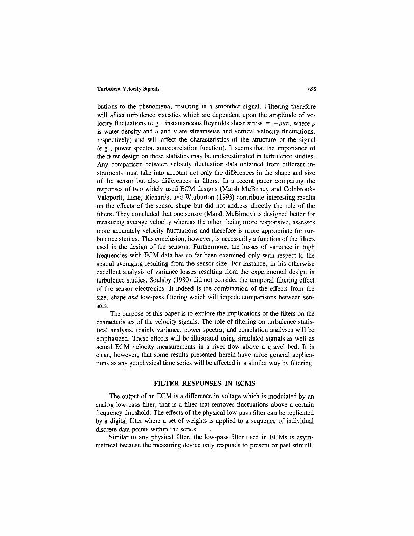
Figure 1. A, Frequency response function of exponential filter in comparison with ideal filter; B, frequency responses of But- terworth filters of different orders n. Nondimensionalized fre- quency is frequency divided by sampling frequency.
657
IR ( f ) [ = (1 + 47r2f2X2) - m (6)
wherefis the frequency in Hz. Figure 1A shows the frequency response function of the exponential filter in comparison with an ideal filter which leaves intact all fluctuations below the cutoff frequency, and removes all fluctuations above that frequency. Note the long roll-off in the frequency response which is char- acteristic of the exponential filter, indicating that fluctuations in the signal are lost at frequencies lower than the ideal filter cutoff frequency. Above this thresh- old, fluctuations are not completely lost. Figure 1B illustrates how the frequency response of the Butterworth filter approaches that of an idea filter as the order n increases.
Losses in signal variance are computed by squaring the frequency response function. The half-power frequency (fso) is the frequency where 50% of the variance of the signal is lost because of filtering. For the exponential filter, this value is given by:
{ 1 ~ '/2 fso = \ ~ / / = (2rX)- ' (7)

658 Roy, Biron, and Lapointe
The general equation for a Butterworth filter of order n is:
fso = 22 7r2n~k2n = (27r~.) - l (8)
Therefore, the half-power frequency is identical for any order of the Butterworth filter for a given time constant ~,. This also is illustrated on Figure 1B where all the frequency response functions cross at the same point, that is atfs0, which corresponds to the cutoff frequency of an ideal filter. Therefore, it is convenient to define the cutoff frequency as the half-power frequency for any type of filter.
LOSS OF VARIANCE AND POWER SPECTRA
Selection of a Sampling Frequency to Avoid Aliasing
As shown in Figure 1, not all the variance is removed at the cutoff fre- quency of Butterworth type filters and the rate at which variance is lost above that threshold varies with the order n of the filter. This rate has important practical implications for the selection of an appropriate experimental design. For instance, in order to avoid significant aliasing in the measured signal, the sampling frequency must be selected carefully with respect to the time constant and order of the Butterworth filter. Aliasing is the folding back into lower frequencies of the variance above the Nyquist frequency, fN, defined as:
fN = fo/2 (9)
wherefD is the sampling frequency (Bendat and Piersol, 1986). If an ideal filter were used, the appropriate choice of a sampling frequency would be twice the cutoff frequency because no variance would be left above fN. However, in the instance of Butterworth filters, half the variance remains at the cutoff frequency and, therefore, fo must be higher than twice the cutoff frequency. Because the frequency response of a Butterworth filter is asymptotic and never actually reaches zero, a role of thumb must be established to give a compromise between the minimization of aliasing effects and the data storage problems of sampling at a frequency that is too high with respect to the phenomenon. A threshold value of 9.2% of the variance left at the Nyquist frequency has been used for Marsh McBirney ECMs (Lapointe, 1992) because this threshold is obtained by a sam- piing rate equal to the time constant of the instrument for a Butterworth filter of order 1 (Table 1). If this threshold value is used for Butterworth filter of higher orders, the minimal sampling rate required approaches a value of 2fs0 (Table 1), the value for an ideal filter where the slope of the roll-off is .infinite (cf. dashed line in Fig. 1).

Turbulent Velocity Signals 659
Table 1. Sampling Frequency (.to) as a Function of Time Constant (k) or Half-Power Frequency (f5o) for Different Orders n of Butterworth Filters with 9.2% of Variance
Left Above Nyquist Frequency
n = l n = 3 n = 5 n = 7 n = 9
.,co in lerms of time constant )`- ~ 0.47)`-~ 0.40X- ~ 0.37)`- l 0.36),-
fo in terms off5o 27rf5o 2.93f5o 2.51f5o 2.32f5 o 2.26f5o
E s t i m a t i o n o f V a r i a n c e Losses
In order to illustrate the role of filtering on the variance of a signal, a simulated 10,000 point t ime series consisting of a stationary purely random
process (white noise) with a mean value of zero is used. By definition, the power
spectrum of a white noise is characterized by an evenly distributed variance across all frequencies or, in other words, the slope of the spectra is equal to zero up to the Nyquis t frequency (Fig. 2A). When the white noise is filtered using an exponential filter with a time constant equal to the sampling interval, it creates a roll-off in the higher frequencies of the spectrum (Fig. 2B). This
loss of variance in frequencies lower than the Nyquist frequency is the result of the long roll-off of the exponential filter frequency response (Fig. 1A). If an ideal filter with a frequency cutoff equal to half the sampling frequency had been used, the slope of the power spectra would have remained zero. It is
Figure 2. Power spectra of A, white noise; B, filtered white noise. Nondimensional val- ues result from division by sampling fre- quency for x-axis and by total variance for y-axis.
o
o
100.0
10~
10-1.0
101.~
10-2.0 A
10 3.0 10 -2-5 10-2.0 10-1.5 10-1.o 10-o.5 10o.o
10 o-o
10 .o.5 -0.90
lO-L~
10 -ls B
10-2.0 , , 10-3.0 10'-2.5 10'-2.0 10-1.5 10'-1.0 10-0.5 100.0
Nondimensional frequency (log)

660 Roy, Biron, and Lapointe
interesting to note that the mean slope of the roll-off after filtering is equal to -0 .90 (Fig. 2B). In a turbulent boundary layer, a slope of -5 /3 (i.e., - 1.67) is normally expected in the inertial subrange (i.e., in high frequencies) of the power spectra (Panofsky and Dutton, 1984). This indicates that although it is expected that the variance of a turbulent velocity signal decreases at high fre- quencies, the actual slope of this decrease can be greater as a result of filtering and will vary depending on the type of low-pass filter and also on the time constant of the instrument. The consequences of these differential effects of filtering on the variance of the signal are important as they clearly are a limiting factor in attempts to compare standard deviations, turbulence intensities, vari- ance, or Reynolds shear stress from different ECMs.
However, using the frequency response of the filter, it is possible to obtain a "defiltered power spectra" and, therefore, to estimate the "real" slope of the spectra for the unfiltered measurements and, hence, a true variance estimate. If Gy(f) is the spectral function of the filtered signal, then the unfiltered spectral function of the same signal, Gx(f), is (Bendat and Piersol, 1986):
Gy(f) Gx(f)- [R(f)12 (10)
For a Butterworth filter of order n [Eq. (5)], this becomes:
Gx(f) = Gy(f ) (1 + (27rkf) 2") (11)
Figure 3 illustrates how Equation (11) affects the slope of the power spectra in the higher frequencies for turbulent velocity signals collected with an ECM.
10 2~
10 .3.0
10 .4.0
10-5.o
10 .6.0
10-7.0 10q.5
10_2.o
~o 10 .3.0 o
10-4.o
10 -~'~
10 -6"~
10-7.0 10-1.5
10-1.o 10-o.5 10o.o 10 o.5 101.o
1 " ~ , ~ _ ..260 /
B, , _v, , ~ 10 q'~ 10 -~ 10 ~176 100.5 10 a.o
Log frequency (Hz)
Figure 3. Average spectral values A, f rom nine u-component velocity signals measured with Marsh McBirney ECM; B, f rom same signals after they have been defiltered using Equation (1 I).
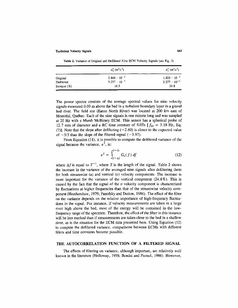
Turbulent Velocity Signals 661
Table 2. Variance of Original and Defiltered Nine ECM Velocity Signals (see Fig. 3)
o2 (m2/s 2) a 2 (m2/s 2)
Original 2.844. 10 -3 1.825" 10 -3
Defiltered 3.257 �9 10 -3 2.277- 10 -3
Increase (%) 14.5 24.8
The power spectra consists of the average spectral values for nine velocity signals measured 0.03 m above the bed in a turbulent boundary layer in a gravel bed river. The field site (Eaton North River) was located at 200 km east of Montrral, Qurbec. Each of the nine signals is one minute long and was sampled at 20 Hz with a Marsh McBirney ECM. This sensor has a spherical probe of 12.7 mm of diameter and a RC time constant of 0.05s [fso = 3.18 Hz, Eq. (7)]. Note that the slope after defiltering ( -2 .60 ) is closer to the expected value of -5 /3 than the slope of the filtered signal ( -3 .97) .
From Equation (11), it is possible to compute the defiltered variance of the signal because the variance, 02 , is:
I f= fN
O 2 : G x ( f ) df (12) Of= A f
where Af is equal to T- 5, where T is the length of the signal. Table 2 shows the increase in the variance of the averaged nine signals after defiltering them for both streamwise (u) and vertical (v) velocity components. The increase is more important for the variance of the vertical component (24.8%). This is caused by the fact that the signal of the v velocity component is characterized by fluctuations at higher frequencies than that of the streamwise velocity com- ponent (Heathershaw, 1979; Panofsky and Dutton, 1984). The effect of the filter on the variance depends on the relative importance of high-frequency fluctua- tions in the signal. For instance, if velocity measurements are taken in a large river high above the bed, most of the energy will be contained in the low- frequency range of the spectrum. Therefore, the effect of the filter in this instance will be less marked than if measurements are taken close to the bed in a shallow river, as is the situation for the ECM data presented here. Using Equation (12) to compute the defiltered variance, comparisons between ECMs with different filters and time constants become possible.
THE AUTOCORRELATION FUNCTION OF A FILTERED SIGNAL
The effects of filtering on variance, although important, are relatively well known in the literature (Holloway, 1958; Bendat and Piersol, 1986). However,

662 Roy, Biron, and Lapointe
some significant effects of filtering concem the structure of the velocity time series, which can be examined through autocorrelation analysis. For velocity fluctuation data, the autocorrelation function (acf) may be used to estimate the integral time and length scale of coherent structures (Townsend, 1976; West, Knight, and Shiono, 1986; Williams, Thorne, and Heathershaw, 1989). Low- pass filtering modifies the structure of the signal by attenuating fluctuations and noise in the high-frequency range. It has long been recognized that applying a series of weights to a random signal such as a white noise introduces an auto- correlation structure and apparent periodicities in the series (Slutzky, 1927; Yule, 1927). The effects of filtering can be derived theoretically by determining the acf of a filtered signal in terms of the weights of the filter. This is illustrated in this section for a nonrecursive filter (exponential). For the situation of recur- sive filters corresponding to higher orders of Butterworth filters, the autocorre- lation structure also is dependent upon the weight function but the analytical derivation of these effects is complicated.
Derivation of the Autocorrelation Function of a Filtered Signal
The autocorrelation coefficient (PD at lag k for a signal constituted of a sampled series X i is given by:
E [ ( X i - # ) ( X i + k - t~)] (13)
Ok = x / E [ X i _ # ] 2 E [ X i + k _ ~]2
where # is the mean value of the signal and can be taken as zero for simplicity. Hence the acf of a filtered signal is given by:
E[Y/" Yi+k] Pk = (14)
x, /E[Yi]2E[Yi +k] z
where - indicates a filtered value. For an asymmetrical filter such as the expo- nential filter [Eq. (1)], this becomes:
~ = m 2 (15)
Knowing that:
E [ X , �9 X,+J = o k E t X ~ ] (16)
it is possible to determine a general expression for the acf of the filtered signal in terms of the values of the weights of the filter:

Turbulent Velocity Signals 663
m m - - 1 m
W2tDk "1- ~ ~ WjWi(Pk+j-i "q- Pk-j+i) j = O j = O i = j + l
P k ~--" m - 1 (17)
~W2dr2 ~ ~ WjWiPi- j j = O j = 0 i = j + l
Examples of Autocorrelation Function
Using the exponential filter weight distribution [Eq. (3)] and Equation (17), it is possible to examine the effect of low-pass filtering on a white noise acf (Fig. 4). When no filter is applied, the acf drops to zero at the first lag, indicating the absence of structure in a purely random signal. However, the acf does not drop to values close to zero until lag 4 when the exponential filter is applied (Fig. 4). Therefore, even a nonstructured velocity signal can show some type of temporal correlation when low-pass filtered. In their comparison between Marsh McBimey and Colnbrook-Valeport ECMs, Lane, Richards, and War- burton (1993) have noticed a significant difference in the acf from the two instruments, the Marsh McBimey being characterized by an acf which decayed more slowly toward 0 than the Colnbrook-Valeport. They have acknowledged the differences in response time and in sensitivity of the two instruments but have not stressed specifically the importance of the differences in the response function between the different orders of Butterworth low-pass filters (see Fig. 1).
The presence of a filter-induced correlation in the data has important im- plications for the study of the structure of a signal. The null hypothesis for complete randomness is that the acf at any lag greater or equal to 1 is zero. However, this must be revised in the situation of a low-pass filtered signal such that the null hypothesis for randomness becomes equal to the filtered white noise acf which can be evaluated with Equation (17) when the weight function is
Figure 4. Autocorrelation functions for first 6 lags of white noise (continuous line) and white noise filtered with exponential filter using weight distribution of Equation (3) (dashed line).
tl)
L~
O
O L)
0.5
-
i i i i i -0.5 0 1 2 3 4 5
LAG

664 Roy, Biron, and Lapointe
Table 3. Increase in Value of Autocorrelation Coefficient for First Lag After Filtering Repeatedly Using Exponential Filter
Value of p~
Difference between two steps of filtering
White noise 0 White noise
filtered once 0.365 0.365 White noise
filtered twice 0.646 0.281 White noise
filtered three times 0.801 0.155
known. The effects of filtering shown in Figure 4 are the strongest because the filter is applied on a signal characterized by a total lack of correlation. I f the signal is correlated already, the relative effect of filtering will be less (Biron, Roy, and Best, 1995). This is illustrated in Table 3 where the increase in the value of the autocorrelation coefficient for the first lag is shown to decrease as the white noise signal becomes more and more structured by being filtered one, two, and three times. The corollary of this is that the autocorrelation function of streamwise u and vertical v velocity components will be affected differently because the v component is less structured than the u component (Biron, Roy, and Best, 1995).
The increase in the value of the autocorrelation function in the first lags has implications for the analysis of the flow structure as it translates into an increase in the integral time scale of the signal, It, defined as:
O(t) dt (18) It = t=0
(Lumley and Panofsky, 1964). The integral time scale is used to estimate the integral length scale of the signal, that is the characteristic length of coherent structures within the turbulent flow. This estimate of structure length scale relies on the use of Taylor 's hypothesis, which assumes that eddies do not change as they are convected by the mean flow past a sensor, and is obtained by multi- plying I t by the mean velocity (e.g., Williams, Thorne, and Heathershaw, 1989). Therefore, the low-pass filter of the measuring device tends to produce an over- estimation of the size of coherent structures. However, this overestimation will differ depending on the sampling design of each experiment and cannot be estimated in a general way.
With velocity fluctuation data, it may be useful to estimate the autoregres-

Turbulent Velocity Signals 665
Table 4. Identification of Autoregressive Model for White Noise and for White Noise Filtered with Exponential Filter
Model Parameters Equation
White noise AR(0) ~b I = -0.005* Zt = r Filtered white noise AR(1) q~ = 0.365 Zt = dPiZt-l + e,
~2 = 0.0044*
*Not significantly different from zero if n < 50000. The standard error for ~b estimates is 1/~n.
sive (AR) model corresponding to the velocity signal. The AR(2) model is the most widely used and has been applied in turbulent flows at riffle-pool sequences (Clifford, Robert, and Richards, 1992) or over gravel beds (Robert, Roy, and De Serres, 1993). It is described by:
Zt : (~lZt-1 @ ~92Zt-2 -~ 6t (19)
where Zt is a random variable at time t, ~b I and ~b 2 are the parameters of the AR(2) model, and el is the random error term (Box and Jenkins, 1976). The Yule-Walker estimates for the parameters of an AR(2) model are:
~ 1 - 0 1 ( 1 - 02) 1 - p 2 ( 2 0 )
- o 2 -
1 - , ~ (21)
where" denotes an estimation. For an AR(1) model, ~1 is simply estimated by Pl. The identification of the model for the two signals depicted in Figure 4 reveals that, as expected, an AR(0) describes the white noise, but that an AR(1) model applies to the filtered white noise signal (Table 4). This indicates that whatever the degree of structure, any turbulent velocity signal measured with an ECM with an exponential filter is always described at least by an AR(1) model solely because of the low-pass filter.
DISCUSSION AND CONCLUSION
The analysis presented here highlights the important effects low-pass fil- tering in ECMs or in other electronical flow sensors can have on velocity fluc- tuation data and on turbulence statistics. The main effects are a reduction in the variance of the signal at high frequencies, therefore increasing the slope of the power spectra, and an increase of the time scale of the autocorrelation structure within the data. Thus, it is problematic to compare velocity fluctuations inca-

666 Roy, Biron, and Lapointe
sured by different types of filter, e.g., Butterworth filters of different orders in the situation of ECMs. Standard turbulence statistics such as variance and Rey- nolds shear stress are likely to be different in Marsh McBimey and Colnbrook- Valeport ECMs. Furthermore, even for measuring devices with the same type of filter, the time constant may change and create difficulties when comparing variances. Using the filter frequency response, it is possible to defilter the signal and to obtain variance estimates for an unfiltered signal. Nonetheless, it also must be kept in mind that the low-pass filter differences add to the physical differences already described in the literature concerning the size and shape of the sensors (Soulsby, 1980; Lane, Richards, and Warburton, 1993). Therefore, attempts to limit the filtering effects by defiltering the signal are not guaranteed to result in the " t rue" velocity signal that describes the phenomenon. Ideally, velocity data should be collected with instruments having exactly the same physical and electronical characteristics in order to obtain comparable results at a given site. In any situation, researchers should give a complete description of their sensors, including the filter type and cutoff frequency (i.e., fso)-
The filtering effects must be acknowledged when carrying time-series anal- ysis in order to interpret correctly the results. For example, the null hypothesis for randomness can be equal to the acf of a filtered white noise [Eq. (17)] or to the filtered value of ~b~ for an autoregressive model estimation (Table 4).
The type of filter in a measuring device also will determine the sensitivity of the response. In the Lane, Richards, and Warburton (1993) analysis, the Colnbrook-Valeport ECM was determined to be more appropriate for high- frequency velocity fluctuation measurements because of its highest sensitivity. This is partly or mostly because of the higher order of the Butterworth filter in these ECMs compared to the Marsh McBirney instruments, and not solely to the shape of the sensor's head.
However, given the relatively high potential for noise contamination at high frequencies in ECMs (Lapointe and others, 1996), it perhaps is not so desirable to aim for an instrument with a Butterworth filter of high order which would behave almost as an ideal filter. The long roll-off in the frequency re- sponse of an exponential filter (n = 1) is less sensitive but it can prevent noise contamination by reducing high frequency spikes in the signal. It therefore is not necessarily less appropriate for turbulence studies.
Filtering will remain an essential concept in time-series analysis, either as an analog filter in the electronics of a measuring device such as in ECMs, or as a digital filter applied a posteriori in order to attenuate undesirable noise or to concentrate on a specific frequency band for a band-pass filter. These oper- ations may be performed routinely on data without a full assessment of their implications on the subsequent analysis. For instance, losses in variance in the streamwise and vertical velocity components (Table 2) will affect statistics such as turbulence intensity and Reynolds shear stress. Third- or fourth-order mo-

Turbulent Velocity Signals 667
ments statistics will amplify velocity fluctuation differences and will necessarily be more dramatically affected by filtering procedures. It is essential to state with as much detail as possible how data were processed and to take filtering into account in the interpretation of the results. This will facilitate future comparisons between data.
ACKNOWLEDGMENTS
We thank Bernard De Serres for his help during preliminary analyses of this work. This research was supported through NSERC funding of A. G. Roy and M. F. Lapointe. The comments of four anonymous reviewers helped to revise the paper.
REFERENCES
Ashmore, P. E., Ferguson, R. I., Prestegaard, K. L., Ashworth, P. J., and Paola, C., 1992, Secondary flow in coarse-grained braided river confluences: Earth Surf. Processes Landforms, v. 17, no. 3, p. 299-311.
Aubrey, D. G., and Trowbridge, J. H., 1985, Kinematic and dynamic estimates from electromag- netic current meter data: Jour. Geophys. Res., v. 90, no. C5, p. 9137-9146.
Bathurst, J. C., Thorne, C. R., and Hey, R. D., 1977, Direct measurements of secondary currents in river bends: Nature, v. 269, no. 5628, p. 504-506.
Bendat, J. S., and Piersol, A. G., 1986, Random data: analysis and measurement procedures: Wiley-Interscience, New York and Toronto, 407 p.
Best, J. L., 1992, On the entrainment of sediment and initiation of bed defects: insights from recent developments within turbulent boundary layer research: Sedimentology, v. 39, no. 5, p. 797-811.
Best, J. L., 1993, On the interactions between turbulent flow structure, sediment transport and bedform development: some considerations from recent experimental research, in Clifford, N. J., French, J. R., and Hardisty, J., eds., Turbulence: perspectives on flow and sediment transport: John Wiley & Sons, Chichester, p. 61-92.
Biron, P., De Serres, B., Roy, A. G., and Best, J. L., 1993, Shear layer turbulence at an unequal depth channel confluence, in Clifford, N. J., French, J. R., and Hardisty, J., eds., Turbulence: perspectives on flow and sediment transport: John Wiley & Sons, Chichester, p. 197-213.
Biron, P., Roy, A. G., and Best, J. L., 1995, A scheme for resampling, filtering and subsampling unevenly spaced laser Doppler anemometer data: Math. Geology, v. 27, no. 6, p. 731-748.
Bowden, K. F., and Fairbaim, L. A., 1956, Measurements of turbulent fluctuations and Reynolds stress in a tidal current: Proc. Roy. Soc. London, Ser. A, v. 237, no. 1210, p. 422-438.
Box, G. E. P., and Jenkins, G. M., 1976, Time series analysis: forecasting and control: Holden- Day, San Francisco, 575 p.
Clifford, N. J., Robert, A., and Richards, K. S., 1992, Estimation of flow resistance in gravel- bedded rivers: a physical explanation of the multiplier of roughness length: Earth Surf. Pro- cesses Landforms, v. 17, no. 2, p. 111-126.
Drake, T. G., Shreve, R. L., Dietrich, W. E., Whiting, P. J., and Leopold, L. B., 1988, Bedload transport of fine gravel observed by motion-picture photography: Jour. Fluid Mechanics, v. 192, p. 193-217.

668 Roy, Biron, and Lapointe
Frederick, D. K., and Carlson, A. B., 1971, Linear systems in communication and control: John Wiley & Sons, New York, 575 p.
Guza, R. T., Clifton, M. C., and Rezvani, F., 1988, Field intercomparison of electromagnetic current meters: Jour. Geophys. Res., v. 93, no. C8, p. 9302-9314.
Heathershaw, A. D., 1979, The turbulent structure of the bottom boundary layer in a tidal current: Geophys. Jour. Roy. Astron. Soc., v. 58, no. 2, p. 395--430.
Holloway, J. L., 1958, Smoothing and filtering of time series and space fields: Adv. Geophys., v. 4, p. 351-388.
Lane, S. N., Richards, K. S., and Warburton, J., 1993, Comparison between high frequency velocity records obtained with spherical and discoidal electromagnetic current meters, in Clif- ford, N. J., French, J. R., and Hardisty, J., eds., Turbulence: perspectives on flow and sediment transport: John Wiley & Sons, Chichester, p. 121-163.
Lapointe, M., 1992, Burst-like sediment suspension events in a sand bed river: Earth Surf. Processes Landforms, v. 17, no. 3, p. 253-270.
Lapointe, M. F., De Serres, B., Biron, P., and Roy, A. G., 1996, Using spectral analysis to detect sensor noise and correct turbulence intensity and shear stress estimates from EMCM flow records: Earth Surf. Processes Landforms, v. 21, no. 2, p. 195-203.
Leeder, M. R., 1983, On the interactions between turbulent flow, sediment transport and bedform mechanics in channelized flows: Intern. Assoc. Sedimentologists Spec. Publ., v. 6, p. 5-18.
Lumley, J. L., and Panofsky, H. A., 1964, The structure of atmospheric turbulence: Interscience Publishers, New York, 239 p.
Panofsky, H. A., and Dutton, J. A., 1984, Atmospheric turbulence: models and methods for engineering applications: John Wiley & Sons, New York, 397 p.
Robert, A., Roy, A. G., and De Serres, B., 1993, Space-time correlations of velocity measurements at a roughness transition in a gravel-bed river, in Clifford, N. J., French, J. R., and Hardisty, J., eds., Turbulence: perspectives on flow and sediment transport: John Wiley & Sons, Chich- ester, p. 165-183.
Roy, A. G., Buffin-Brlanger, T., and Deland, S., 1996, Scales of turbulent coherent flow structures in a gravel-bed river, in Ashworth, P. J., Bennett, S. J., Best, J. L., and McLelland, S. J., eds., Coherent flow structures in open channels: John Wiley & Sons, New York, p. 147-164.
Slutzky, E., 1927, The summation of random causes as the source of cyclic processes (English translation, 1937): Econometrica, v. 5, p. 105-146.
Soulsby, R. L., 1980, Selecting record length and digitization rate for near-bed turbulence mea- surements: Jour. Physical Oceanography, v. 10, p. 208-219.
Townsend, A. A., 1976. The structure of turbulent shear flow (2nd ed.): Cambridge Univ. Press, Cambridge, 429 p.
West, J. R., Knight, D. W., and Shiono, K., 1986, Turbulence measurements in the Great Ouse Estuary: Jour. Hydraulic Eng. ASCE, V. 112, no. 3, p. 167-180.
Williams, J. J., Thorne, P. D., and Heathershaw, A. D., 1989, Measurements of turbulence in the benthic boundary layer over a gravel bed: Sedimentology, v. 36, no. 6, p. 959-979.
Yule, G. U., 1927, On a method of investigating periodicities in disturbed series, with special reference to Wolfer's sunspot numbers: Philosophical Trans. Roy. Soc., v. A 642, p. 267-298.