implementation of the 1997 indonesian highway capacity manual (mkji) volume delay function

Proceedings of the Eastern Asia Society for Transportation Studies, Vol.7, 2009

Implementation of the 1997 Indonesian Highway Capacity Manual (MKJI) Volume Delay Function

Muhammad Zudhy IRAWAN Doctoral Student Graduate School of Engineering Kyushu University (ITO Campus) 744, Motooka, Nishi-ku, Fukuoka, 819-0395, Japan Fax: +81-92-802-3403 E-mail: [email protected]

Tomonori SUMIProfessor Graduate School of Engineering Kyushu University (ITO Campus) 744, Motooka, Nishi-ku, Fukuoka, 819-0395, Japan Fax: +81-92-802-3403 E-mail: [email protected]

Achmad MUNAWARProfessor Magister of Transportation System and Engineering Gadjah Mada University Jl. Grafika 2 Kampus UGM, Bulaksumur, Yogyakarta, 55281, Indonesia Fax: +62-274-524-713 E-mail: [email protected]

Abstract: The delay function is a central component of equilibrium trip assignment models that influences the traffic volume on a road section. The Volume Delay Function (VDF) developed by US Bureau of Public Roads (BPR) in 1964 is commonly used to iterate traffic volume in Indonesia despite the fact that the Indonesian Highway Capacity Manual (MKJI) also has a curve of the VDF describing delay in Indonesia. This paper attempts to obtain the delay equation and its parameters refer to the curve of MKJI VDF. This is followed by an implementation using field data is carried out to compare traffic volume produced using the BPR VDF and the MKJI VDF. The results show that the application of the MKJI VDF can obtain a more accurate representation of the actual traffic volume compared to the BPR VDF. Key Words: Volume delay function, Travel time, Traffic assignment 1. INTRODUCTION Travel time is an essential element in shaping transportation systems. How the driver chooses the path to reach their destination is determined by travel time. In the traffic assignment method, travel time depends on many factors. One is the Volume Delay Function (VDF). VDF is a central component of equilibrium trip assignment models, because it can influence the driver to change the trip route by considering and comparing the traffic volume on each road. VDFs may range from a simple linear function to a complicated formula. The VDF developed by US Bureau of Public Roads (BPR) in 1964 is commonly used to iterate traffic volume in Indonesia despite the fact that the Indonesian Highway Capacity Manual (MKJI) also possesses a VDF curve describing delay in Indonesia (Direktorat Jenderal Bina Marga, 1997). While the BPR VDF is popular, in regards to the Indonesian conditions in the case of Yogyakarta, it should be noted that from 77 road sections recorded, volume-capacity ratios in 33 road sections (42.86%) are less than 0.5 (Dinas Perhubungan Kota Yogyakarta, 2006). When the BPR equation is used for low volume-capacity ratio, it has been found that delay


function results in almost the same value, thus degenerating the equilibrium model to an all or nothing model. Spiess (1990) proposed a conical volume delay function to overcome these shortcomings of the BPR function. The conclusion interpret the parameters used to characterize the specific congestion behavior of a road link, i.e. capacity and steepness (α), is the same for both BPR and conical function, which makes the transition to conical functions particularly simple. Since the difference between a BPR function and a conical function with the same parameter α is very small within the feasible domain, i.e. v-c ratio less than 1.00, the parameters can be transferred directly in most cases. This paper attempts to obtain the delay equation and its parameters based on the MKJI VDF curves. An implementation using field data is subsequently carried out to compare traffic volume produced using the BPR VDF and the MKJI VDF. It is expected that the MKJI VDF can produce traffic flow which more similar to actual conditions compared to the BPR VDF. The EMME/2 (Equilibre Multimodal, Multimodal Equilibrium) transportation planning software was applied to assign the traffic volume as the VDF equation can be set manually by the user. Other transportation programs often use a default VDF. 2. THEORITICAL BACKGROUND 2.1 The BPR Volume Delay Function The traffic assignment method concerns the selection of routes (r route) between origins (Oi) and destinations (Dj) throughout transportation networks. This selection of routes will influence the distribution of flow on each route and thus influence road performance and ultimately network performance as a whole. Most trip assignment methods explain that VDF represents the impact of road capacity on travel time. The VDF developed by US Bureau of Public Road (BPR) is a very popular function to determine the travel time in each link as shown in Equation 1 (BPR, 1964).

⎟⎟⎠

⎞⎜⎜⎝

⎛⎟⎠⎞

⎜⎝⎛⋅+⋅=

β

αcvTT 10 (1)

Where

T = travel time (minute) T0 = free flow travel time (minute) v = traffic volume (passenger car unit/hour) c = practical capacity (passenger car unit/hour) α, β = parameter

2.2 The MKJI Volume Delay Function 2.2.1 Travel Time It should be noted that MKJI does not present the VDF in the form of equations. Therefore, the equations must be derived beforehand. By examining the curves presented in MKJI, the VDF equations can therefore be obtained.


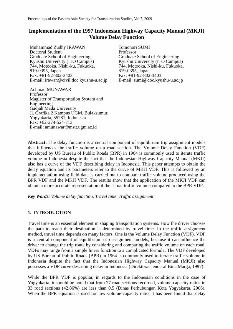
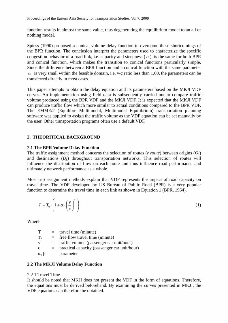
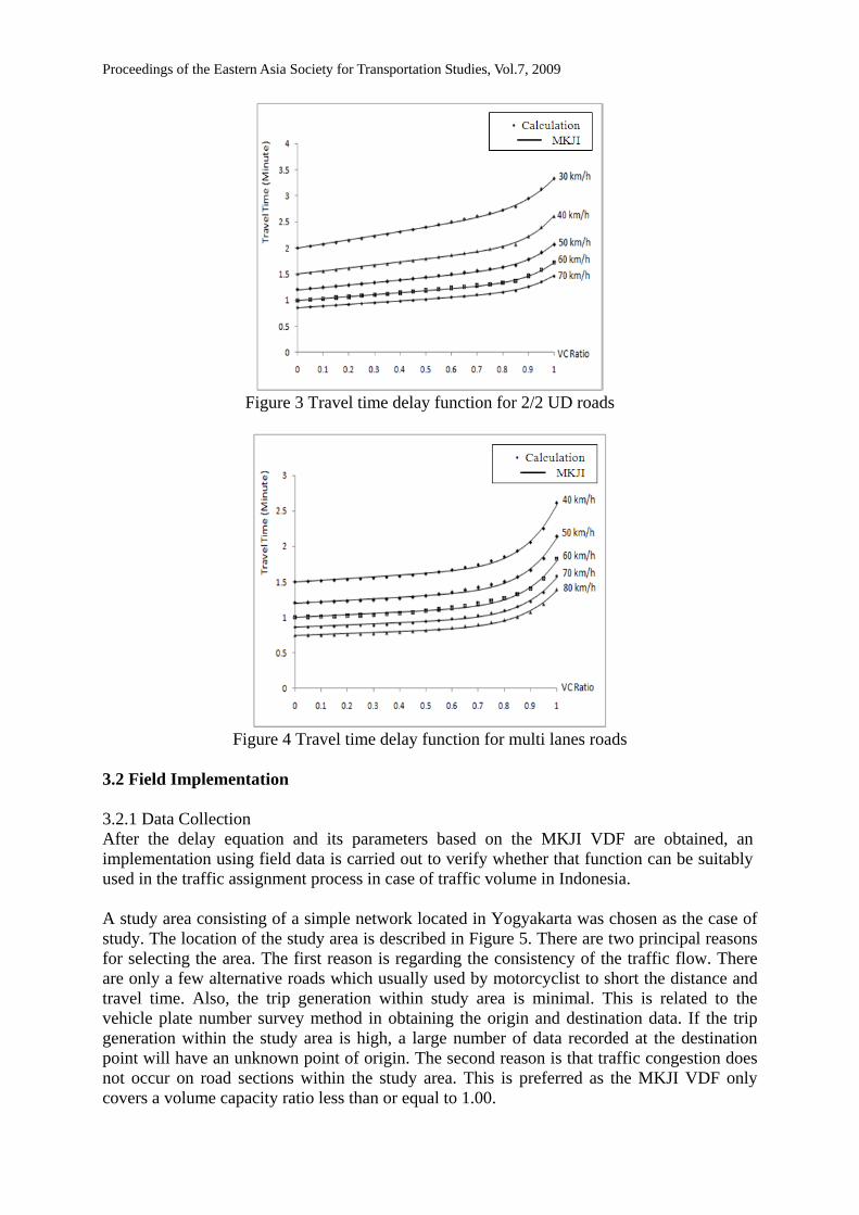
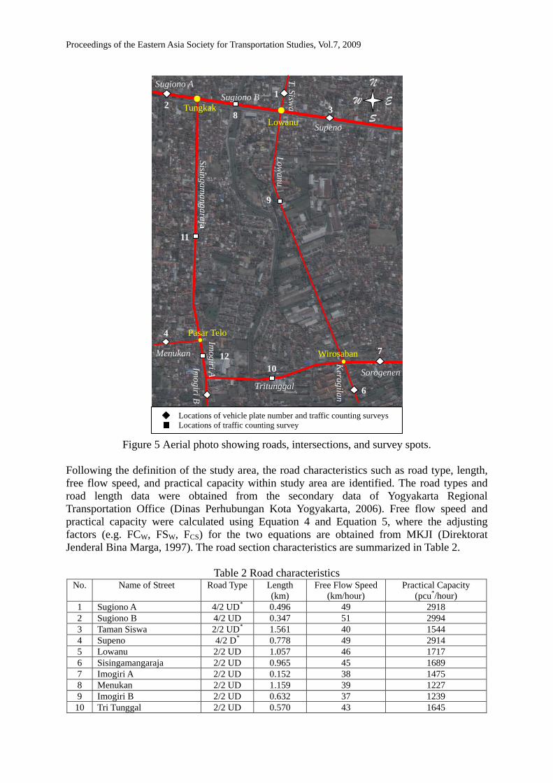
MKJI divides the VDF into two categories. The first is a VDF for 2/2 UD (two lanes, two ways, undivided) roads. The second is a VDF for multi lane roads, such as 4/2 D (four lanes, two ways, divided) or 3/1 UD (three lanes, one way, divided) roads. Figure 1 and Figure 2 respectively show the curves for these functions.

Figure 1 VDF for 2/2 UD roads

Figure 2 VDF for multi lanes roads

From the curves in Figure 1 and Figure 2, an equation to describe travel time can be obtained. Since the velocity represented in the figures is inversely proportional to travel time, the travel time (T) can be written in the form of Equation 2.

021 Tcv

cvT +⎟

⎠⎞

⎜⎝⎛+⎟

⎠⎞

⎜⎝⎛⋅= αα

β

(2)

Travel time (T) is a function of free flow travel time (T0) and volume-capacity ratio (v/c). The coefficients α1, α2, and β are parameters which will be found using the least squares method.


MKJI determined road capacity per lane except for 2/2 UD roads. However, the volume was still determined for the entire road width. Therefore, from Figure 1 and Figure 2, and based on Equation 2, the travel time (T) can be calculated as Equation 3 with the practical capacity value (c) multiplied by the number of lanes (n) in which n = 1 for Figure 1.

⎟⎠⎞

⎜⎝⎛ ⋅+⎟

⎠⎞

⎜⎝⎛ ⋅+⎟

⎠⎞

⎜⎝⎛ ⋅⋅= L

Scv

ncv

nT 6011

21 ααβ

(3)

Where

T = travel time (minute) v = traffic volume (passenger car unit/hour) c = practical capacity (passenger car unit/hour) S = free flow speed (km/hour) L = road length (km) α1, α2, β = parameter

2.2.2 Practical Capacity MKJI defines the practical capacity as the maximum vehicle volume which constantly passes through a defined road section within a set time interval (i.e. 1 hour). Practical capacity (c) is influenced by several factors depending on road conditions as shown in Equation 4 (Direktorat Jenderal Bina Marga, 1997).

( )CSSFSPW FFCFCFCcc ⋅⋅⋅⋅= 0 (4) Where

c0 = free flow capacity (passenger car unit/hour) FCW = link width capacity factor FCSP = link separated capacity factor FCSF = side friction capacity factor FCS = city size factor

2.2.3 Free Flow Speed Free flow speed (S) is defined as vehicle speed in km/hour in which the vehicle is unobstructed by the presence of other vehicles. MKJI calculates free flow speed based on a basic free flow speed value which is influenced by several factors. Equation 5 shows the MKJI free flow speed formula (Direktorat Jenderal Bina Marga, 1997).

( ) CSSFW FFSFSSS ⋅⋅+= 0 (5) Where

S0 = basic free flow speed (km/hour) FSW = effective width factor FSSF = side friction factor FCS = city size factor


3. APPLICATION OF PROPOSED METHOD 3.1 Determining MKJI VDF Parameters As mentioned previously, the equations of the MKJI VDF must be determined beforehand. From Equation 3 and referring to the least squares method, the parameter of α1, α2 and βcan be calculated. With given set of m data (x1,y1), (x2,y2),…, (xm,ym) and a model function of the form f(x,β), an equation which best represents the data can be obtained when its value of the residual sum of squares is minimum (Equation 6).

∑=

=m

iir

1

2min(SSE)Error Square of Sum (6)

Where ri = yi – f(xi,α)

The minimum value of SSE occurs when the gradient j

SSEα∂

∂ is zero. Since the models

consist of m parameters there are m gradient equations as follows (Equation 7).

021

=∂∂

=∂∂ ∑

=

m

i j

ii

j

rrSSEαα

(j=1, 2, 3 … n) (7)

To find the equations for the curves on Figure 1 and Figure 2, values of velocity (y axis) are tabulated for the entire range of volume-capacity ratio given (i.e. 0 to 1). It should be remembered that for figure 2, MKJI determined capacity for each lane while the volume was determined for the entire road width.

After assigning arbitrary initial values to β, the values of 1α∂

∂SSE and 2α∂

∂SSE are substituted.

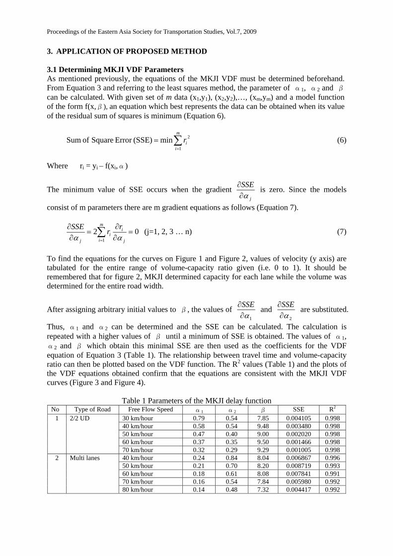
Thus, α1 and α2 can be determined and the SSE can be calculated. The calculation is repeated with a higher values of β until a minimum of SSE is obtained. The values of α1,α2 and β which obtain this minimal SSE are then used as the coefficients for the VDF equation of Equation 3 (Table 1). The relationship between travel time and volume-capacity ratio can then be plotted based on the VDF function. The R2 values (Table 1) and the plots of the VDF equations obtained confirm that the equations are consistent with the MKJI VDF curves (Figure 3 and Figure 4).

Table 1 Parameters of the MKJI delay function No Type of Road Free Flow Speed α1 α2 β SSE R2

1 2/2 UD 30 km/hour 0.79 0.54 7.85 0.004105 0.99840 km/hour 0.58 0.54 9.48 0.003480 0.99850 km/hour 0.47 0.40 9.00 0.002020 0.99860 km/hour 0.37 0.35 9.50 0.001466 0.99870 km/hour 0.32 0.29 9.29 0.001005 0.998

2 Multi lanes 40 km/hour 0.24 0.84 8.04 0.006867 0.99650 km/hour 0.21 0.70 8.20 0.008719 0.99360 km/hour 0.18 0.61 8.08 0.007841 0.99170 km/hour 0.16 0.54 7.84 0.005980 0.99280 km/hour 0.14 0.48 7.32 0.004417 0.992


Figure 3 Travel time delay function for 2/2 UD roads

Figure 4 Travel time delay function for multi lanes roads

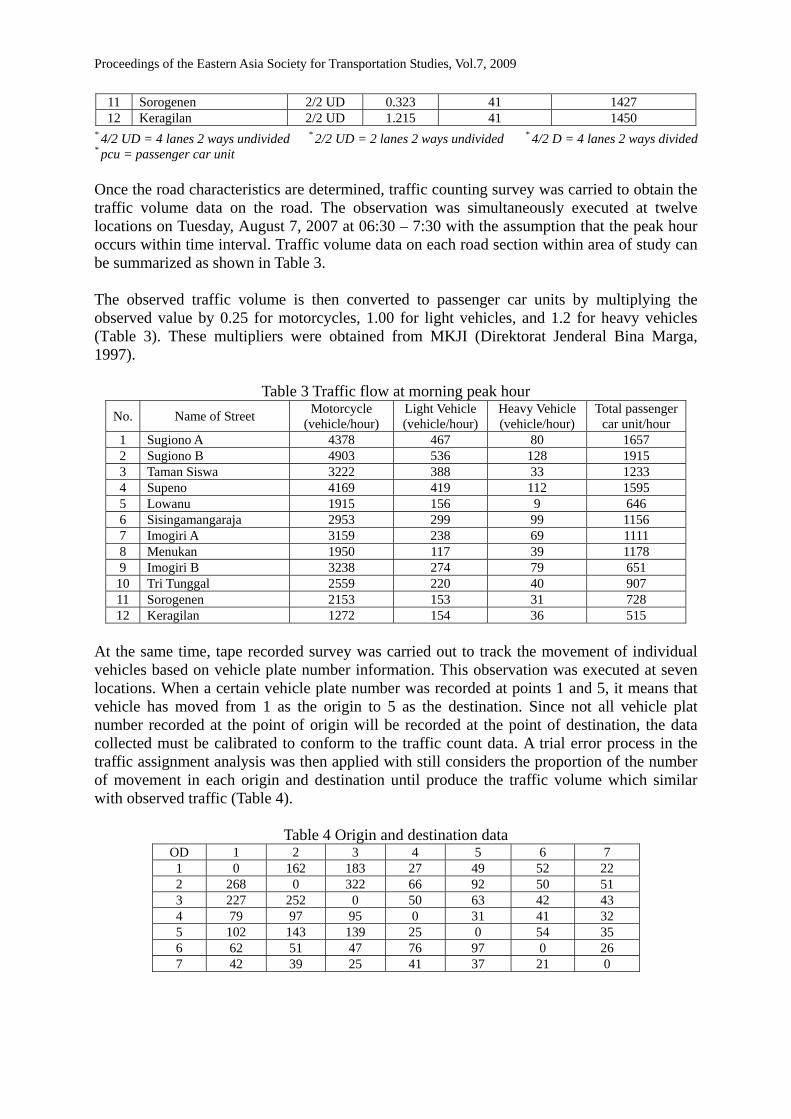
3.2 Field Implementation 3.2.1 Data Collection After the delay equation and its parameters based on the MKJI VDF are obtained, an implementation using field data is carried out to verify whether that function can be suitably used in the traffic assignment process in case of traffic volume in Indonesia. A study area consisting of a simple network located in Yogyakarta was chosen as the case of study. The location of the study area is described in Figure 5. There are two principal reasons for selecting the area. The first reason is regarding the consistency of the traffic flow. There are only a few alternative roads which usually used by motorcyclist to short the distance and travel time. Also, the trip generation within study area is minimal. This is related to the vehicle plate number survey method in obtaining the origin and destination data. If the trip generation within the study area is high, a large number of data recorded at the destination point will have an unknown point of origin. The second reason is that traffic congestion does not occur on road sections within the study area. This is preferred as the MKJI VDF only covers a volume capacity ratio less than or equal to 1.00.


Figure 5 Aerial photo showing roads, intersections, and survey spots. Following the definition of the study area, the road characteristics such as road type, length, free flow speed, and practical capacity within study area are identified. The road types and road length data were obtained from the secondary data of Yogyakarta Regional Transportation Office (Dinas Perhubungan Kota Yogyakarta, 2006). Free flow speed and practical capacity were calculated using Equation 4 and Equation 5, where the adjusting factors (e.g. FCW, FSW, FCS) for the two equations are obtained from MKJI (Direktorat Jenderal Bina Marga, 1997). The road section characteristics are summarized in Table 2.

Table 2 Road characteristics No. Name of Street Road Type Length

(km) Free Flow Speed

(km/hour) Practical Capacity

(pcu*/hour) 1 Sugiono A 4/2 UD* 0.496 49 2918 2 Sugiono B 4/2 UD 0.347 51 2994 3 Taman Siswa 2/2 UD* 1.561 40 1544 4 Supeno 4/2 D* 0.778 49 2914 5 Lowanu 2/2 UD 1.057 46 1717 6 Sisingamangaraja 2/2 UD 0.965 45 1689 7 Imogiri A 2/2 UD 0.152 38 1475 8 Menukan 2/2 UD 1.159 39 1227 9 Imogiri B 2/2 UD 0.632 37 1239

10 Tri Tunggal 2/2 UD 0.570 43 1645

5

N

S E W 1

Tungkak Lowanu

Wirosaban

Pasar Telo

Sisingamangaraja

Lowanu

Menukan

Tritunggal

Sugiono A Sugiono B

Sorogenen

Supeno

T. Siswa

Keragilan

Imogiri B

Imogiri A

3 2

4

6

7

8

11

10

9

12

Locations of vehicle plate number and traffic counting surveys Locations of traffic counting survey


11 Sorogenen 2/2 UD 0.323 41 1427 12 Keragilan 2/2 UD 1.215 41 1450

* 4/2 UD = 4 lanes 2 ways undivided * 2/2 UD = 2 lanes 2 ways undivided * 4/2 D = 4 lanes 2 ways divided * pcu = passenger car unit Once the road characteristics are determined, traffic counting survey was carried to obtain the traffic volume data on the road. The observation was simultaneously executed at twelve locations on Tuesday, August 7, 2007 at 06:30 – 7:30 with the assumption that the peak hour occurs within time interval. Traffic volume data on each road section within area of study can be summarized as shown in Table 3. The observed traffic volume is then converted to passenger car units by multiplying the observed value by 0.25 for motorcycles, 1.00 for light vehicles, and 1.2 for heavy vehicles (Table 3). These multipliers were obtained from MKJI (Direktorat Jenderal Bina Marga, 1997).

Table 3 Traffic flow at morning peak hour No. Name of Street Motorcycle

(vehicle/hour) Light Vehicle(vehicle/hour)

Heavy Vehicle (vehicle/hour)

Total passenger car unit/hour

1 Sugiono A 4378 467 80 1657 2 Sugiono B 4903 536 128 1915 3 Taman Siswa 3222 388 33 1233 4 Supeno 4169 419 112 1595 5 Lowanu 1915 156 9 646 6 Sisingamangaraja 2953 299 99 1156 7 Imogiri A 3159 238 69 1111 8 Menukan 1950 117 39 1178 9 Imogiri B 3238 274 79 651

10 Tri Tunggal 2559 220 40 907 11 Sorogenen 2153 153 31 728 12 Keragilan 1272 154 36 515

At the same time, tape recorded survey was carried out to track the movement of individual vehicles based on vehicle plate number information. This observation was executed at seven locations. When a certain vehicle plate number was recorded at points 1 and 5, it means that vehicle has moved from 1 as the origin to 5 as the destination. Since not all vehicle plat number recorded at the point of origin will be recorded at the point of destination, the data collected must be calibrated to conform to the traffic count data. A trial error process in the traffic assignment analysis was then applied with still considers the proportion of the number of movement in each origin and destination until produce the traffic volume which similar with observed traffic (Table 4).

Table 4 Origin and destination data OD 1 2 3 4 5 6 7 1 0 162 183 27 49 52 22 2 268 0 322 66 92 50 51 3 227 252 0 50 63 42 43 4 79 97 95 0 31 41 32 5 102 143 139 25 0 54 35 6 62 51 47 76 97 0 26 7 42 39 25 41 37 21 0


Finally, delay time in each signalized intersection due to the close proximity of the closest signalized intersection must be observed. This is important in regards to driver route choice as drivers tend to choose routes which have the least amount of signalized intersections. This survey was conducted the following day on Wednesday, August 8th 2007 at 06:30 – 7:30. The timing of survey was chosen with the assumption that the traffic pattern and volume between Tuesday and Wednesday are the same. Calculated delay time is the delay for light vehicles and heavy vehicles which are stopped at intersections due to traffic signals, while motorcycles are not considered in this survey. This is due to the transport behavior of motorcycles being highly unpredictable. The survey was conducted as follows. Two surveyors calculated delay time at each intersection approach. The first surveyor counts the number of vehicle that approaching and stopped at the intersection. The second surveyor counts the number of vehicle stopped at the intersection during a 15 second interval. It should be noted that this 15 second sampling interval cannot be a multiple of the intersection signal cycle time. The average delay for stopped vehicles as shown in Table 5 are then calculated by multiplying the total number of vehicles stopped during the interval by 15 and then dividing by the approaching traffic volume that stopped at intersection (Pignataro, 1973).

Table 5 Delay time at signalized intersection

No. Intersection Time of Delay (Second)

North South East West 1 Lowanu 50 61 56 47 2 Tungkak 28 26 29 3 Pasar Telo 23 28 28 4 Wirosaban 34 34 32 31

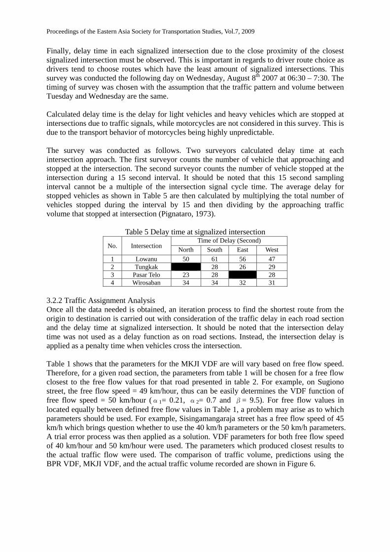
3.2.2 Traffic Assignment Analysis Once all the data needed is obtained, an iteration process to find the shortest route from the origin to destination is carried out with consideration of the traffic delay in each road section and the delay time at signalized intersection. It should be noted that the intersection delay time was not used as a delay function as on road sections. Instead, the intersection delay is applied as a penalty time when vehicles cross the intersection. Table 1 shows that the parameters for the MKJI VDF are will vary based on free flow speed. Therefore, for a given road section, the parameters from table 1 will be chosen for a free flow closest to the free flow values for that road presented in table 2. For example, on Sugiono street, the free flow speed = 49 km/hour, thus can be easily determines the VDF function of free flow speed = 50 km/hour (α1= 0.21, α2= 0.7 and β= 9.5). For free flow values in located equally between defined free flow values in Table 1, a problem may arise as to which parameters should be used. For example, Sisingamangaraja street has a free flow speed of 45 km/h which brings question whether to use the 40 km/h parameters or the 50 km/h parameters. A trial error process was then applied as a solution. VDF parameters for both free flow speed of 40 km/hour and 50 km/hour were used. The parameters which produced closest results to the actual traffic flow were used. The comparison of traffic volume, predictions using the BPR VDF, MKJI VDF, and the actual traffic volume recorded are shown in Figure 6.


Figure 6 Comparison of traffic volume

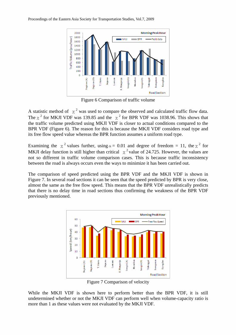
A statistic method of χ2 was used to compare the observed and calculated traffic flow data. Theχ2 for MKJI VDF was 139.85 and the χ2 for BPR VDF was 1038.96. This shows that the traffic volume predicted using MKJI VDF is closer to actual conditions compared to the BPR VDF (Figure 6). The reason for this is because the MKJI VDF considers road type and its free flow speed value whereas the BPR function assumes a uniform road type. Examining the χ2 values further, usingα= 0.01 and degree of freedom = 11, theχ2 for MKJI delay function is still higher than critical χ2 value of 24.725. However, the values are not so different in traffic volume comparison cases. This is because traffic inconsistency between the road is always occurs even the ways to minimize it has been carried out. The comparison of speed predicted using the BPR VDF and the MKJI VDF is shown in Figure 7. In several road sections it can be seen that the speed predicted by BPR is very close, almost the same as the free flow speed. This means that the BPR VDF unrealistically predicts that there is no delay time in road sections thus confirming the weakness of the BPR VDF previously mentioned.

Figure 7 Comparison of velocity

While the MKJI VDF is shown here to perform better than the BPR VDF, it is still undetermined whether or not the MKJI VDF can perform well when volume-capacity ratio is more than 1 as these values were not evaluated by the MKJI VDF.


4. CONCLUSION This research proposed to obtain the delay equation and its parameters based on the MKJI VDF curves. Field data was used to compare the traffic volume predicted using the BPR VDF and the MKJI VDF. The results show that traffic volume predicted using the MKJI VDF represents the actual traffic volume better than the BPR VDF. This is due to the MKJI VDF considering road type and free flow speed value whereas the BPR function may incorrectly assume a uniform road type. Also, at low volume-capacity ratio, MKJI VDF is still considers the delay time that occurs while the BPR VDF predicts a negligible delay time.

REFERENCES Bureau of Public Roads (1964) Traffic Assignment Manual, U.S. Dept. of Commerce,

Urban Planning Division, Washington D.C. Dinas Perhubungan Kota Yogyakarta (2006) Data Ruas Jalan dan Arus Lalulintas,

Yogyakarta, Indonesia. Direktorat Jenderal Bina Marga (1997) Manual Kapasitas Jalan Indonesia (MKJI), Jakarta,

Indonesia. Hansen, S., Byrd, A., Delcambre, A., Rodriguez, A., Matthews, S., Bertini, R.L. (2005) Using

Archived ITS Data to Improve Regional Performance Measurement and Travel Demand Forecasting, Canadian Institute of Transportation Engineers, Quad Conference, Vancouver, B.C.

INRO Consultants Inc. (1998) EMME/2 User’s Manual Software Release 9, Canada. Justrzebski, W. P. (2000) Volume Delay Function, 15th International EMME/2 Users`

Group Conference, Vancouver, B.C. Ortuzar, J. D., and Willumsen, L.G. (1994) Modeling Transport, Second Edition, John

Wiley & Sons, Great Britain. Pignataro, L. J. (1973) Traffic Engineering Theory and Practice, Prentice Hall, New

Jersey. Spiess, H. (1990) Conical Volume-Delay Functions, Transportation Science, Vol. 24, No. 2,

153-158. Walpole, R. E., and Myers, R. H. (1993) Probability and Statistics for Engineers and

Scientist, Macmillan Publishing Company, New York. Wang, J., and Lu, W. (2003) The Research On The Method of Traffic Impact Analysis,

Proceedings of The Eastern Asia Society For Transportation Studies, Vol. 4, 1-16. Wu, J., Gao Z., and Sun H. (2008) Statistical Properties of Individual Choice Behaviors on

Urban Traffic Networks, Journal of Transportation Systems Engineering and Information Technology, Volume 8, Issue 2, 69-74.

implementation of the 1997 indonesian highway capacity manual (mkji) volume delay function

Documents