INTERNATIONAL COMPUTER SCIENCE INSTITUTE I1947 Center St. � Suite 600 � Berkeley, California 94704-1198 � (510) 643-9153 � FAX (510) 643-7684Image segmentation throughcontextual clusteringA. Baraldi�, P. Blonday, F. Parmiggianiz and G. SatalinoxTR-98-009June 1998Abstract. Several interesting strategies are adopted by the well-known Pappas clusteringalgorithm to segment smooth images. These include exploitation of contextual informationto model both class conditional densities and a priori knowledge in a Bayesian framework.De�ciencies of this algorithm are that: i) it removes from the scene any genuine but smallregion; and ii) its feature-preserving capability largely depends on a user-de�ned smoothingparameter. This parameter is equivalent to a clique potential of a Markov Random Fieldmodel employed to capture known stochastic components of the labeled scene. In this pa-per a modi�ed version of the Pappas segmentation algorithm is proposed to process smoothand noiseless images requiring enhanced pattern-preserving capability. In the proposed al-gorithm: iii) no spatial continuity in pixel labeling is enforced to capture known stochasticcomponents of the labeled scene; iv) local intensity parameters, pixel labels, and global in-tensity parameters are estimated in sequence; and v) if no local intensity average is availableto model one category in the neighborhood of a given pixel, then global statistics are em-ployed to determine whether that category is the one closest to pixel data. Results show thatour contextual algorithm can be employed: vi) in cascade to any noncontextual (pixel-wise)hard c-means clustering algorithm to enhance detection of small image features; and vii)as the initialization stage of any crisp and iterative segmentation algorithm requiring pri-ors to be neglected on earlier iterations (such as the Iterative Conditional Modes algorithm).Keywords: Markov Random Field, Bayes' theorem, image segmentation.�ICSI, 1947 Center Street, Suite 600, Berkeley, CA 94704-1198, baraldi@icsi.berkeley.eduyIESI-CNR, Via Amendola 166/5, 70126 Bari (Italy), blonda@iesi.ba.cnr.itzIMGA-CNR, Via Gobetti 101, 40129 Bologna (Italy), parmi2@imga.bo.cnr.itxIESI-CNR, satalino@iesi.ba.cnr.it

1 IntroductionIn recent years, the scienti�c community has been involved in an important debate on thereasons why the many image processing techniques presented in the literature have hadsuch a slight impact on their potential �eld of application [1], [2], [3]. To take this debateinto account, we have attempted to make this paper as \focused on its very original core"[1] as possible. This original core is regarded as a set of useful items that a broad scienti�caudience would be willing to include in commercial image-processing all-purpose softwaretoolboxes [1].Picture segmentation is a subjective and context-dependent cognitive process. In math-ematical terms, this process is ill-posed, i.e., there is no single goal for picture partitionalgorithms [4], [5]. To make picture segmentation a well-posed problem, it is regarded asan optimization task featuring a �rm statistic foundation. Recently, there has been consid-erable interest in statistical clustering techniques for image segmentation inspired by themethods of statistical physics, which were developed to study the equilibrium properties oflarge, lattice-based systems consisting of identical, interacting components [6]. In a cluster-ing technique for image segmentation, each pixel is associated with one of a �nite numberof categories (also termed pure substances, or colors, or region types, or states) to formdisjointed regions.It is well known that, when applied to image segmentation, the traditional hard c-means clustering algorithm features one main limitation: it assumes that each region typeis characterized by uniform intensity throughout the image, i.e., it assesses global intensityparameters that do not account for local intensity variations. As a consequence, the c-meansclustering algorithm tends to generate noisy (salt-and-pepper) segmentation results [7]. Thesame problem a�ects any noncontextual (pixel-wise) classi�cation algorithm (independentmodel, [10]) by assuming the independence of observables y given pixel labels (states) x (see(2) below) as well as the independence of pixel labels, such as the Maximum Likelihood (ML)parameter estimation procedure [9], [10], [11]. It is obvious that adjacent pixels are likelyto have similar labels when the pixel's size is smaller than the smallest detail of interest.Therefore, to obtain smooth segmentations, a Markov Random Field (MRF) model (for ageneral overview of MRF models, refer to [12]) is often imposed on the spatial distribution ofdi�erent image categories to introduce spatial correlation in pixel labeling (interpixel classdependency) [6], [7], [8], [9], [10], [13], [14]. This underlying MRF model can be considereda \stabilizer" in the sense of the regularization theory [10], which helps in solving otherwiseill-posed problems [15], [16]. Parameters of the MRF model, i.e., the neighborhood sizeand the smoothing parameters (clique potentials), incorporate a priori knowledge into themodeling process, i.e., they are either user-de�ned or known on an a priori basis, e.g., bymeans of o�-line [6], [8], [9], [21], or on-line [9] parameter estimation techniques employingsupervised data. The MRF parameters a�ect the size of disjointed regions, i.e., the amountof spatial details preserved by the segmentation process [9]. In [21], a detail-preserving imagesegmentation method utilizing MRFs is proposed. In this algorithm, minimization of theenergy function also requires selection of the most appropriate neighborhood system for thepixel under analysis. In [22] and [23], coarse-to-�ne multiresolution segmentation approachesare proposed with no adaptive neighborhood being employed, although in [23] smoothingparameters are �xed as a function of scale. The multiresolution segmentation algorithmii

proposed in [23] is found to be less likely to be trapped in local minima than the IterativeConditional Mode (ICM) algorithm [9], since, at each resolution, regions are classi�ed andused to guide �ner resolutions. This conclusion is complementary to the observation thatconvergence of MRF-based segmentation algorithms can be improved by varying the localneighborhoods [24]. In conclusion, adaptive and multiresolution approaches to parameterestimation in segmentation algorithms exploiting MRF models appear to be highly desirable.Several clustering algorithms that exploit a MRF model to impose spatial continuity inpixel labeling assume that the intensity of each region type is uniform throughout the image[6], [8], [9], [13], and/or employ hard pixel labeling [6], [7], [8], [9]. When these two con-ditions hold true, these segmentation algorithms can be considered a generalization of thetraditional c-means clustering algorithm, such that pixels are hard-clustered on the basis ofboth their intensity and their context (neighboring labels). From an information-processingperspective, it is well known that a hard-decision approach to parameter estimation isless e�ective than the use of soft decisions which, in picture segmentation applications,would compare the probabilities of all possible pixel labels [10]. This consideration led tothe development of fuzzy clustering algorithms for image classi�cation [17], in which theExpectation-Maximization (EM) procedure [18] can be employed to determine the Maxi-mum Likelihood (ML) estimate of parameters of a Gaussian mixture decomposition [19],where a MRF model is often imposed on the spatial distribution of the pixel labels [10],[13].An interesting algorithm that includes multiresolution analysis and adaptive spatial con-straints in a traditional hard c-means clustering algorithm is the Pappas Adaptive Clustering(PAC) algorithm for image segmentation [7]. Unlike the c-means algorithm, this schemeassumes that each image category is characterized by a slowly varying intensity function,i.e., the same region type may feature di�erent intensity parameters in di�erent parts ofthe image. PAC is iterative, alternating between estimating category local intensities andhard pixel labels. Moreover, PAC adapts and progressively reduces the neighborhood size:local intensities of each category are estimated by averaging over a sliding window whosesize decreases monotonically as the algorithm approaches convergence. This means thatPAC starts with global parameter estimates and progressively adapts these estimates to theimage's local properties. Parameter estimates in each iteration employ current hard pixellabels, assuming they are correct. Exploitation of a decreasing window size should miti-gate de�ciencies in crisp label assignments [10]. Finally, PAC can employ a multiresolutionimplementation scheme. Since PAC preserves large image features while removing smalldetails, it is employed to provide sketches or caricatures of the original image.This paper proposes a Modi�ed version of PAC (MPAC) to be employed in cascadewith a hard noncontextual c-means clustering stage. MPAC aims to: i) enhance pattern-preserving capability of both c-means and PAC algorithms, such that genuine but smallregions are not removed; and ii) feature high usability, because no user-de�ned parameteris required. Experimental results con�rm that MPAC may be considered an easy-to-useand e�ective algorithm for use in cascade with a c-means clustering algorithm to segmentimages featuring smooth surfaces and no texture. Within the frame of the debate startedby Zamperoni [1], we recommend inclusion of the proposed algorithm in a commercialimage-processing all-purpose software toolbox.The organization of this paper is as follows: Section 2 presents a brief review of statisticaliii

clustering algorithms for image segmentation; Section 3 reviews the PAC algorithm; inSection 4 the MPAC scheme is proposed. Experimental results are discussed in Section 5;conclusions are presented in Section 6.2 Statistical approaches to image analysisLet us consider clustering algorithms for image segmentation de�ned as optimization prob-lems. We identify as yi the observed vector at pixel i, which belongs to a two-dimensionalregion (image) S, such that i 2 f1; ng, where n is the total number of pixels. Each pixeli can take one label (pure substance) xi 2 f1; cg. An arbitrary labeling (clustering) of Sis denoted by x = (x1; :::; xn). Some probabilistic methods provide estimate x of the true(although unknown) labeled scene x�, which is chosen to have maximum probability, givenobservables y. By Bayes' theorem, x maximizes the posterior probabilityP (x=y) / l(y=x)p(x); (1)where l(y=x) is the class conditional density and p(x) is the prior. Thus, x is the maximum aposteriori (MAP) estimate of x� that maximizes the posterior cost function (1). A commonassumption is that given any particular scene x, observables are conditionally independentand each pixel value has the same class conditional density function f(yi=xi), dependentonly on xi. Then, l(y=x) = nYi=1 f(yi=xi): (2)In the hypothesis that the 2-D random �eld (stochastic process) fp(x)g is any locally de-pendent Markov Random Field (MRF), thenP (xi=xS�i) � pi(xi=xNi); (3)where xS�i is the scene reconstruction anywhere, but pixel i, pi is speci�c to pixel i, andxNi is the scene reconstruction in the neighborhood of pixel i to be de�ned according to anm�th order MRF (typically, second-order; for more details refer to [6], [8], [20]). Supposethat our goal is to estimate xi at pixel i given all observables y and current reconstructionxS�i elsewhere, i.e., xi maximizes P (xi=y; xS�i). According to assumptions (2) and (3), wecan write [9] P (xi=y; xS�i) / f(yi=xi)pi(xi=xNi): (4)In an iterative optimization procedure the \hats" in Equation (4) imply the use of estimatedlabel assignments from the previous iteration in the current iteration. SinceP (x=y) = P (xi; xS�i=y) = P (xi=y; xS�i)P (xS�i=y);maximization of Equation (4) guarantees that P (x=y) never decreases at any maximizationstep, i.e., convergence to a local maximum of P (x=y) is assured. When addressing pixeli with Equation (4), only yi, xi and the labels of the neighbors are required. Implemen-tation of Equation (4) is trivial for any MRF fp(x)g, which is locally dependent. Whilemaximization of Equation (4) is performed at every point in the image, label updatingiv

can be implemented, for example, in a batch mode (at the end of each raster scan). Thisiterative suboptimal procedure, termed the Iterated Conditional Modes (ICM) algorithm,guarantees convergence to a local maximum of P (x=y) in few processing cycles (e.g., aboutsix [9]). Then, ICM must be started with a good initialization of the scene x, which is oftenprovided by a noncontextual ML classi�er [9]. ICM has been criticized for its heavy depen-dence on initial classi�cation [25], and because it ignores the fuzzy membership (degree ofcompatibility) with which a pixel is associated with a given class [9], [11], [26]. For example,when applied to satellite image applications, fuzzy classi�cation can be employed to identifymisclassi�ed cases and to direct ground surveys [11], [17], [27]. Simulated Annealing (SA)exploiting the \Gibbs sampler" is capable of reaching the global maximum ofPT (x=y) / fl(y=x)p(x)gT ; (5)where T > 0 is a user-de�ned parameter representing the \absolute temperature" of thesystem, when at each pixel i label xi is chosen to maximize the posterior probability [6], [9]PT (xi=y; xS�i) / ff(yi=xi)pi(xi=xNi)g1=T : (6)Observe that ICM, which provides simple suboptimal iterative scene estimates, is equivalentto SA when T is �xed to 1 [9].If pairwise interactions in a second-order MRF fp(x)g are considered exclusively (i.e.,three- and four-point cliques are ignored), and a single smoothing parameter (two-pointclique potential) � is employed (i.e., all neighbor pairs are treated equally), then [7], [9],[12], pi(xi=xNi) / exp[�(xi) + �ui(xi)]; (7)where �(xi), related to one-point clique potential, is the a priori knowledge of the relativelikelihood of category assignment xi [7], while ui(xi) is the current number of 8-adjacencyneighbors of i having label xi. Counter ui(xi) is termed \self-aura measure" [20]. Comple-mentary to the self-aura measure is the \cross-aura measure", vi(xi), de�ned as the currentnumber of 8-adjacency neighbors of i having a label di�erent from xi, such thatui(xi) + vi(xi) = 8:Parameter � in Equation (7) can be considered an intensive quantity, independent of thenumber of particles (pixels) present in the system; this term describes pairwise interac-tion potential between two categories that can be related to pure substances or uids. Tocontinue with the analogy to pure substances, the self-aura measure, which is an exten-sive quantity, increases when the spatial clumpiness of the clustered (segmented) imageincreases, that is, when the separability between cluster types increases, which is to saywhen the common boundary between di�erent clusters decreases. Vice versa, the cross-aura measure increases when the mixing between pairs of di�erent clusters increases, i.e.,when the common boundary between pairs of clusters increases.As underlined by several authors [7], [28], the MRF model by itself is not very useful,unless we provide a good model for class conditional density f(yi=xi). Modeling of jointclass conditional density l(y=x) a�ects MAP estimate x not only because the model is simplyinvolved in characterizing the posterior cost function (1), but also because it a�ects estimatev

x when used to provide starting scene x (e.g., determined by the use of a noncontextualML classi�er) for a contextual iterative classi�cation method such as ICM [28].Two major models can be used in formulating class conditional densities. The �rstmodel, termed continuous random �eld model [28], employs the causal autoregressive model,the simultaneous autoregressive model, or the conditional Markov model [28], to describestatistical dependency of a gray level at a lattice point on that of its neighbors, given the un-derlying classes (interpixel feature correlation, [14]), e.g., see [10], [23]. It is computationallyexpensive and may be preferred in modeling images featuring distinct texture information[10], [28]. It will not be further considered in this paper, since we address images featuringlittle useful texture information. The second model in formulating class conditional densi-ties is the conventional spectral model based on a multivariate-Normal assumption for thedistribution of independent spectral responses [28]: in the hypothesis that each categoryj 2 f1; cg has uniform intensity �(j) and that the image is corrupted by a white Gaussiannoise �eld independent of the scene and featuring standard deviation �, then the conditionaldensity term f(yi=xi) becomes [7], [9], [10]f(yi=xi) = exp�� 12�2 [yi � �(xi)]2� : (8)This spectral model is computationally simple and yields good classi�cation results whenapplied to images holding little useful texture information [28]. Substituting Equations (7)and (8) in Equation (4), and setting = 1=2�2, we obtain the �nal form of the suboptimaliterative solution to the maximization of (1), which isxi = arg minxi2f1;cgf [yi � �(xi)]2 � �(xi) + �vi(xi)g; 8i 2 S: (9)The �rst term on the right side of Equation (9), called the error term [15], constrains inten-sity of the region type �(xi) to be close to data yi, i.e., it represents �delity of the regiontype to the data [9]. The third term on the right side of Equation (9) imposes spatial con-tinuity in pixel labeling to reduce \mixing" between di�erent pure substances (categories).In the framework of regularization theory, the sum [��(xi)+�vi(xi)] is termed smoothnessfunctional or stabilizer. A stabilizer embodies our a priori knowledge of the labeled sceneand is used to impose constraints on the solution, since signi�cant probabilities are assignedonly to underlying scenes that satisfy these constraints [15]. According to regularizationtheory, parameter � in Equation (9) is a regularization parameter that determines the trade-o� between the strength of the a priori assumptions about the solution and the closenessof the solution to the data. For example, as noise (degree of uncertainty) increases, then �should increase, to �nd a solution diminishingly closed to the raw data.It is to be observed that and � are inversely correlated: reducing (increasing �)is equivalent to increasing � to obtain smoother segment contours while larger details arelost, and vice versa [7]. When � = 0, Equation (9) is equivalent to an ML classi�erignoring contextual information. In [9], it is remarked that the exact value of � is usuallyunimportant with ICM if smaller values are used on earlier iterations [9], so that at an earlystage the algorithm follows the data, while at later stages the algorithm follows the regionmodel [7]. However, in many practical applications, � is kept constant [7], [9], [23] becausethe schedule needed for changing this parameter would require additional free parametersvi

which are generally image dependent [23]. If the 2-D stochastic process fp(x)g is to supportspecial features such as thin lines, then pairwise interaction models do not su�ce, andsmoothing parameters �s, as well as the neighborhood size, must be adapted depending onthe type of scene and, possibly, on local image properties [8], [9], [21].3 Pappas clustering for image segmentationIn [7], Equation (9) is adapted to exploit both types of contextual information, namely,interpixel feature correlation given the underlying classes and interpixel class dependency[14] (see Sections 1 and 2). Equation (9) is modi�ed as followsxi = arg minxi2f1;cgf [yi � �Wi(xi)]2 � �(xi) + �vi(xi)g; 8i 2 S; (10)where the model for conditional density (error term) employs a slowly varying intensityfunction �Wi(xi) estimated as the average of the gray levels of all pixels that currentlybelong to region type xi and fall inside a window Wi which is centered on pixel i. Thewindow size decreases monotonically as the algorithm approaches convergence to guaranteerobust estimation of intensity functions as the segmentation, which is \crude" in the earlystages of the algorithm, becomes progressively more sensitive to local image properties [7].When the number of pixels of type xi within window Wi is less than or equal to windowwidth Wi;w, then estimate �Wi(xi) is not considered reliable and pixel i cannot be assignedto region type xi. Thus, isolated regions with area smaller than Wi;w are removed by theclustering algorithm. As shown in [7], the new spectral model of the error term proposedin Equation (10) makes PAC more robust than traditional c-means clustering algorithmsin the choice of the number of clusters [19], because regions of entirely di�erent intensitiescan belong to the same category, as long as they are separated in space.In Equation (10), Pappas also �xes �(xi) = 0;8xi 2 f1; cg, i.e., all pixel states areassumed to be equally likely, and employs a constant � = 0:5 for all iterations and forany image. Vice versa, coe�cient , which is inversely related to noise variance, is eitheruser-de�ned or assessed from the image of interest to control the amount of details detectedby the algorithm (which increases as increases). Then, Equation (10) becomesxi = arg minxi2f1;cgf [yi � �Wi(xi)]2 + 0:5 � vi(xi)g; 8i 2 S; (11)where is a free parameter.In [7], a PAC hierarchical multiresolution implementation is proposed to reduce theamount of computation. This implementation constructs a pyramid of images at di�erentresolutions by low pass �ltering and decimating by a factor of two. At each level in thepyramid, the algorithm uses the segmentation generated at the previous level, expandedby a factor of two, as a starting point. The parameter doubles when the resolution leveldecreases (i.e., noise standard deviation is reduced by half, then algorithm follows the dataat low resolution stages), while parameter � is kept unchanged (otherwise, can be �xedwhile � is reduced by half). This multiresolution approach, besides reducing computationtime, may improve feature-preserving capability (for details, refer to [7]). The Pappasadaptive clustering algorithm for image segmentation at a given resolution level is shownvii

in Fig. 1. For implementation details about how to reduce computation time in estimatingthe intensity parameters, refer to [7].4 Modi�cation of Pappas' algorithmOur main objective is to segment noiseless images featuring smooth surfaces and no texturewhile preserving genuine but small details. Real data sets satisfy these pictorial constraints.For example, high resolution satellite images acquired by SPOTHRV or Landsat TM sensorsmay be not severely degraded by noise. If this is the case, the model used to expressthe joint class-conditional distribution can be based on a multivariate-Normal assumptionof independent spectral responses [28], which is consistent with Equations (9) and (10).Therefore, to reach our goal, a feasible approach is to develop a Modi�ed PAC (MPAC)algorithm featuring enhanced pattern-preserving capability. Thus, in line with the debatestarted by Zamperoni [1], we do not claim to present yet another picture segmentationalgorithm. As an adaptation of Equation (10), we adopt the following cost functionxi = arg minxi2f1;cgf4(xi)g; 8i 2 S; (12)such that4(xi) = 8>>><>>>: minf[yi � �Wi(xi)]2; [yi � �W (xi)]2g;if �Wi(xi) exists and is considered reliable; (13)[yi � �W (xi)]2; if �Wi(xi) does not existor is considered unreliable; (14)where W identi�es the �xed window that covers the entire image.A scheme of the MPAC algorithm at a given resolution level is shown in Fig. 2. Themain di�erences between MPAC and PAC, emerging from the comparison of Figs. 1 and 2and Equations (10) to (12) respectively, can be summarized as follows:1. In MPAC, since � = 0 (see Equations (10) and (12)), no spatial continuity in pixel la-beling is enforced, i.e., contextual information is employed to model class conditionaldistributions exclusively. Since it ignores any regularization term in its objective func-tion, MPAC focuses on keeping the error term low, so that local intensity parameter�Wi(xi) of region type xi is kept as close as possible to observable data yi. This alsomeans that MPAC assumes to deal with noiseless raw images (see Section 2). Since itemploys no regularization coe�cient, MPAC is also easy to use: in cascade to a non-contextual c-means clustering algorithm, MPAC requires no user-de�ned parameter.2. Rather than alternating estimation of local intensity parameters and pixel labels,MPAC alternates between estimating local intensity parameters, pixel labels, andglobal intensity parameters.3. If no local intensity average is available to model one category in the neighborhood ofa given pixel, MPAC employs global statistics to determine whether that category isthe one closest to pixel data. Note that when an intensity estimate �Wi(xi), computedin neighborhoodWi < W centered on pixel i, does not exist or is considered unreliableviii

reduce windowsize W;n = 1;

given the intensityfunction, get new

estimates of x;n=n+1;

given x, get newestimates of the

intensity function;

window size Wequals image size;

n=1;

get segmentation xby c-means;

x has reached convergence?

n = n_max?

W = W_min?

STOP

NO

NO

NO

YES

YES

YES

Figure 1: The Pappas adaptive clustering algorithm for image segmentation at a givenresolution level. ix

reduce windowsize W;n = 1;

given the intensityfunction and the

c-means, get newestimates of x;

n=n+1;

given x, get newestimates of the

intensity function;

window size Wequals image size;

n=1;

get segmentation xby c-means;

x has reached convergence?

n = n_max?

NO

NOYES

YES

given x, get newestimates of the

c-means;

W = W_min?

STOP

NO

YES

Figure 2: The modi�ed Pappas adaptive clustering algorithm for image segmentation at agiven resolution level. x

by Equation (12), then global intensity �W (xi), which is the image-wide estimate ofthe average gray value of all pixels currently belonging to region type xi, is employedinstead for comparison with the pixel data according to Equation (14). In line withEquation (10), local estimate �Wi(xi) is not considered reliable by Equation (12) whenthe number of pixels of type xi within window Wi is less than or equal to adaptivewindow width Wi;w. This adaptation of the Pappas algorithm is su�cient to avoidremoval of isolated but genuine regions whose area is smaller than Wi;w.4. In MPAC, when local intensity estimate �Wi(xi) exists and is considered reliable byEquation (12), both local and global intensity estimates, �Wi(xi) and �W (xi) respec-tively, are employed for comparison with the pixel data according to Equation (13).It is worthy of mention that we have found images to which Equations (12) to (14)apply successfully while exclusive exploitation of local intensity estimates in Equation(13) is uncapable of providing satisfactory image partitions.Theoretical failure modes and limitations of the MPAC algorithm are listed below:1. MPAC can be applied only to images where sharp intensity transitions occur at re-gion boundaries, i.e., where each category is characterized by a slowly varying intensityfunction. In fact: i) MPAC employs no texture model; and ii) owing to its crisp label-ing strategy, MPAC is unable to ignore noisy pixels while segmentation parametersare estimated.2. MPAC is a suboptimal iterative algorithm detecting local minima. This is tantamountto stating that MPAC largely depends on its initialization. To initialize MPAC, anyhard c-means clustering algorithm can be chosen from those found in the literature,see for example [30], [31]. One main issue regards the number of clusters to bedetected [19], [23]. Nonetheless, in line with PAC, MPAC is more robust than c-means clustering algorithms in the choice of the number of clusters, because regionsof entirely di�erent intensities can belong to the same category, as long as they areseparated in space.3. MPAC exploits higher degree of heuristics than PAC, i.e., MPAC features a statisticalframework which is less rigorous than that featured by PAC.5 Quantitative evaluation of segmentationMost picture partitions are evaluated visually and qualitatively on a subjective, perceptualbasis. This is also due to the fact that traditional supervised measures employed in imageprocessing tasks, such as the mislabeling rate, are global statistics unable to account forlocal visual properties. For example, the segmentation of a crossboard picture may improvewhen the number of small holes decreases even though its mislabeling rate actually increases[22]. Therefore, these global statistics cannot be employed for quantitative evaluation ofpicture segmentation [29]. Since no single segmentation goal exists because of the subjectiveappraisal of continuous perceptual features, a system developed to compare segmentationresults must employ [4], [5]: i) an entire set of measures of success (termed battery test)to account for the fuzziness of perceptual segmentation; ii) a test set of images to allowxi

exploitation of supervised data, i.e., of a priori knowledge about the objects in a scene,so that the external environment (supervisor) provides the generic (vague) segmentationtask with an explicit goal; and iii) a set of exisiting techniques against which the proposedalgorithm must be compared.Let us start by de�ning the battery test. As we are dealing with image segmentationalgorithms that minimize a given cost function, i.e., algorithms that are well-posed andfeature one explicitly de�ned segmentation objective, this function is included in the batterytest of the system we have developed to compare segmentation results. Other statisticsthat are considered in the segmentation comparison are: average value of the error term,number of cycles required to reach convergence, number of label replacements, and numberof misclassi�ed pixels when ground truth data are available. Note that computation time isnot considered in the battery test since the proposed MPAC algorithm may employ a PAC-based hierarchical multiresolution implementation that signi�cantly reduces the amount ofcomputation (for details, refer to [7]).The test set of images must consist of a su�cient number of real and standard data setscapable of demonstrating the potential utility of MPAC, i.e., these images must feature ahigh signal-to-noise ratio and little texture. We selected a standard achromatic human face(Lenna), a three-band SPOT HRV image, and a Landsat TM image provided with super-vised data �elds. Because of di�culties in comparing alternative classi�cation procedures ina meaningful way, the �rst application uses a face as opposed to natural scenes because weknow what a face looks like and can therefore judge the results of the clustering algorithmintuitively [11].To demonstrate its potential utility, MPAC is compared against two existing segmen-tation algorithms based on probabilistic theory. The �rst of these clustering algorithms isthe PAC iterative procedure implemented to detect a local minimum of the following costfunction: xi = arg minxi2f1;cgf[yi � �Wi(xi)]2 + � � vi(xi)g; 8i 2 S; (15)where �, rather than , as in Equation (11), is the free parameter to be user-de�ned, whichmakes the error term in Equation (15) more similar to that employed in Equations (13) and(14). Experimentally, we discovered that in our test images several pixels may feature noreliable intensity estimate in their adaptive neighborhood at some resolution level. Thus,we had to remove the Pappas constraint that considers any estimate �Wi(xi) unreliablewhen the number of pixels of type xi in window Wi is less than or equal to window widthWi;w. In other words, in our implementation of the Pappas algorithm, any category xifeaturing pixel occurrence above zero within window Wi is considered in the minimizationof Equation (15).The second segmentation scheme employed for comparison is the SA algorithm, whichis a general purpose approach for detecting the absolute minimum of a cost function [32].We employ SA to minimize the cost function:xi = arg minxi2f1;cgf[yi � �(xi)]2 + � � vi(xi)g; 8i 2 S; (16)where � is the free parameter to be user-de�ned, and �(xi) is the non-adaptive (image-wise)vector parameter of region type xi to be provided by a noncontextual classi�er (e.g., the hardxii

c-means clustering algorithm). Note that Equation (16) is a special form of Equation (9)to be compared with Equation (15). According to the principles of simulated annealing [8],as temperature T decreases, the chance of random label assignments decreases accordingly.At each iteration, T is lowered by a constant cooling rate �, which is �xed at 0.95. Pixelsare visited according to a raster scan and updated in batch (synchronous) mode at the endof each cycle [9]. Unfortunately, SA requires long computation times to run successfully.5.1 Standard image applicationThe standard achromatic input image of Lenna is shown in Fig. 3. Six category templatesare �xed by a photointerpreter: �(1) = 68 (corresponding to surface classes: shadow wall,hair), �(2) = 100 (hair), �(3) = 143 (wall, hat), �(4) = 160 (skin), �(5) = 190 (hat),�(6) = 213 (wall, skin). This set of templates is larger than what is suggested in [7], where2 to 4 clusters were employed to obtain caricatures of the original images. These templatesare employed by the noncontextual hard c-means clustering algorithm to provide the threesegmentation algorithms under testing with an initial segmentation to start from. To high-light functional di�erences between the three algorithms, free parameter � in Equations(15) and (16) is kept low. This choice yields SA and PAC segmentation results where smallspatial details tend to be preserved, and can be compared to segmentation results of MPAC,which implicitly adopts parameter � = 0.Fig. 4 shows the output of the Simulated Annealing (SA) algorithm exploiting param-eters T = 800, � = 0:95, � = 0:5, tmax = 150, where tmax is the epoch at which thealgorithm is stopped [32]. Since weight � of the term enforcing spatial continuity in pixellabeling is small, then, as expected, minimization of Equation (16) provides a segmentationresult almost identical to that generated by the hard c-means clustering algorithm at theinitialization step. For this reason the initial segmentation provided by the hard c-meansclustering is not shown. Figs. 5 to 7 show the plots of the mean value of Equation (16), themean value of the error term in Equation (16), and the percentage number of replacementsper pixel (multiplied by factor 100) respectively. All plots are in terms of the epoch number.Of course, since � is small, the two plots in Figs. 5 and 6 respectively are quite similar.Fig. 8 shows the output of the PAC algorithm exploiting parameter � = 0:5, tmax = 150,where tmax is the epoch at which the algorithm is stopped. Figs. 9 to 11 provides meaningfulplots of this PAC application at full resolution. PAC reaches convergence after about 10iterations, although the cost function tends to oscillate once its asymptote has been reached.Since weight � of the term enforcing spatial continuity in pixel labeling is small, thenminimization of Equation (15) is mostly focused on minimization of the error term. This isshown in Figs. 9 and 10 where plots of the PAC mean cost and error term appear similar.Observe that although � is the same as the one in the SA application, small details arebetter preserved in Fig. 8 than in Fig. 4 (e.g., in the woman's hat). The conclusion is thatthe enhanced feature-preserving capability of PAC with respect to SA is totally dependenton their di�erent class conditional density models (error term). As expected, Figs. 9 to 11also show that PAC reaches convergence earlier than the time-consuming SA algorithm atfull resolution.Fig. 12 shows the output of the MPAC algorithm exploiting parameter tmax = 150,where tmax is the epoch at which the algorithm is stopped. Since MPAC does not enforcexiii

Figure 3: Standard achromatic input image of Lenna (521x512 pixels).xiv

Figure 4: Output of the SA algorithm applied to Fig. 3. SA parameters are: T = 800,� = 0:95, � = 0:5, tmax = 150.xv

20 40 60 80 100 120 14060

80

100

120

140

160

180

200

220

240Simulated Annealing

Iterations

Mea

n co

st

Figure 5: Plot of the SA algorithm applied to Fig. 3: mean value of Equation (16).

0 50 100 15060

80

100

120

140

160

180

200

220

240Simulated Annealing

Iterations

Mea

n Er

ror T

erm

Figure 6: Plot of the SA algorithm applied to Fig. 3: mean value of the error term inEquation (16).

20 40 60 80 100 120 1400

2

4

6

8

10

12

14

16

18

Iterations

Repl

acem

ents

per

pixe

l (x1

00)

Simulated Annealing

Figure 7: Plot of the SA algorithm applied to Fig. 3: the percentage number of replacementsper pixel. xvi

Figure 8: Output of the PAC algorithm applied to Fig. 3. PAC parameters are: � = 0:5,tmax = 150.xvii

20 40 60 80 100 120 14012

13

14

15

16

17

18Pappas

Iterations

Mea

n co

st

Figure 9: Plot of the PAC algorithm applied to Fig. 3: mean value of Equation (15).

20 40 60 80 100 120 14012

13

14

15

16

17

18Pappas

Iterations

Mea

n Er

ror T

erm

Figure 10: Plot of the PAC algorithm applied to Fig. 3: mean value of the error term inEquation (15).

20 40 60 80 100 120 1400

1

2

3

4

5

6Pappas

Iterations

Repl

acem

ents

per

pixe

l (x1

00)

Figure 11: Plot of the PAC algorithm applied to Fig. 3: percentage number of replacementsper pixel. xviii

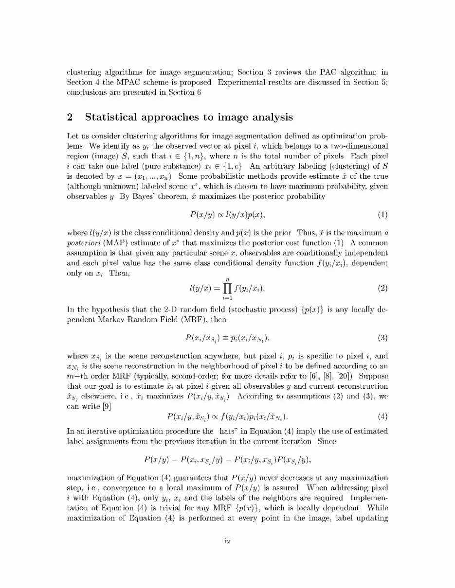
any spatial continuity in pixel labeling, small details are preserved better in Fig. 12 than inFig. 8 (e.g., in the woman's hat). MPAC tolerates isolated pixels, which are considered aproblem in [7] even though they feature high contrast to their neighbors. This creates a sortof dithering e�ect around the woman's shoulder, for example. Overall, subjective appraisalof Fig. 12 with respect to Fig. 8 may be either positive or negative, accounting for thesubjective nature of segmentation problems. However, this subjective assessment may notbe relevant, with Fig. 12 representing a limiting product (when � = 0) of MPAC, which isa (slightly modi�ed, see Section 4) PAC algorithm capable of generating, in its traditionalform, Fig. 8 when � is small, starting from Fig. 3. Figs. 13 and 14 provide meaningfulplots of this MPAC application at full resolution. MPAC reaches convergence after about20 iterations. To be compared with initial centroid values, �nal templates estimated by theMPAC algorithm are: �(1) = 69:1, �(2) = 107:1, �(3) = 138:8, �(4) = 161, �(5) = 185:4,�(6) = 206.5.2 Unsupervised satellite image applicationFigs. 15 to 17 show a multispectral SPOT HRV image of the city of Porto Alegre (RioGrande do Sul, Brazil) acquired on Nov. 7, 1987. Spectral bands are Green, Red and NearInfraRed, respectively. We underline the presence of three bay bridges linked to the largeisland in the upper left-hand corner of these images. A zoomed area around the city airportextracted from Fig. 17 is shown in Fig. 18.Eight category templates are �xed by a photointerpreter: �(1) = (49; 43; 18) (water),�(2) = (39; 30; 66) (vegetation), �(3) = (46; 30; 112) (vegetation), �(4) = (49; 42; 36) (air-port, asphalt), �(5) = (66; 66; 85) (street), �(6) = (207; 193; 152) (metal roofs), �(7) =(50; 46; 62) (houses), �(8) = (57; 51; 62) (houses). This set of templates is larger than thatsuggested in [7] to obtain caricatures of the original images. These templates are employedby the noncontextual hard c-means clustering algorithm to provide PAC and MPAC withan initial segmentation to start from. This initial segmentation is shown in Fig. 19. Thezoomed area taken from Fig. 19 and corresponding to Fig. 18 is shown in Fig. 20. This clus-tered image shows the presence of several isolated pixels which are typical of noncontextualclassi�cation.To highlight functional di�erences between the three algorithms, free parameter � inEquations (15) and (16) is kept rather low. This choice yields SA and PAC segmentationresults in which small spatial details tend to be preserved (i.e., the algorithm follows thedata, rather than following the prior region model [7]), and can be compared to MPACsegmentation performances. As in [7], the standard deviation of noise in each spectral bandof the satellite image was assumed to be � = 4 gray levels, then = 1=2�2 = 0:031. In thiscase, from Equation (11), ratio �= = 0:5=0:031 is approximately equal to 16. In Equations(15) and (16), this parameter condition is equivalent to �xing � = 16 given = 1.Fig. 21 shows the output of the SA algorithm exploiting parameters T = 800, � =0:95, � = 16, and tmax = 150. Fig. 22 shows the zoomed area extracted from Fig. 21and corresponding to Fig. 18. As expected, since weight � of the term enforcing spatialcontinuity in pixel labeling is small with respect to the error term, which tends to increasewith the number of image bands, minimization of Equation (16) provides segmentationresults that are not so di�erent from those depicted in Fig. 19, although spatial details arexix

Figure 12: Output of the MPAC algorithm applied to Fig. 3. MPAC parameter is: tmax =150.xx

20 40 60 80 100 120 14012

13

14

15

16

17

18Modified Pappas

Iterations

Mea

n co

st

Figure 13: Plot of the MPAC algorithm applied to Fig. 3: mean value of Equation (12)

20 40 60 80 100 120 1400

1

2

3

4

5

6Modified Pappas

Iterations

Repl

acem

ents

per

pixe

l (x1

00)

Figure 14: Plot of the MPAC algorithm applied to Fig. 3: percentage number of replace-ments per pixel.xxi

Figure 15: SPOT HRV image of the city of Porto Alegre (Rio Grande do Sul, Brazil): Band1 (Visible Green; 512x512 pixels).xxii

Figure 16: SPOT HRV image of the city of Porto Alegre: Band 2 (Visible Red).xxiii

Figure 17: SPOT HRV image of the city of Porto Alegre: Band 3 (Near IR).xxiv

Figure 18: A zoomed area around the city airport extracted from Fig. 17.lost (e.g., see the bay bridges in Fig. 21 and some linear patterns in Fig. 22).Fig. 23 shows the output of the PAC algorithm exploiting parameter � = 16, andtmax = 150. The asymptote of the cost function (16) is reached after about 20 iterations atfull resolution. Fig. 24 shows the zoomed area extracted from Fig. 23 and correspondingto Fig. 18. Note that although � is the same as the one in the SA application, small detailsare preserved better in Fig. 24 than in Fig. 22. In Fig. 24, the number of isolated pixelsis reduced with respect to Fig. 20 (some of them are still present due to oscillations in theestimation of the labeled scene). The conclusion is that the enhanced feature-preservingcapability of PAC with respect to SA is totally due to their di�erent class conditional densitymodels (error term).Fig. 25 shows the output of the MPAC algorithm exploiting parameter tmax = 150.The asymptote of the cost function (15) is reached after about 15 iterations at full reso-lution. Fig. 26 shows the zoomed area extracted from Fig. 25 and corresponding to Fig.18. In Fig. 26, the number of isolated pixels is reduced with respect to Fig. 20. Manyisolated pixels, rather than being �ltered out, as occurred in Fig. 24, have been linked toneighboring pixels featuring similar spectral signatures. Since MPAC does not enforce anyspatial continuity in pixel labeling, small details are better preserved in Figs. 25 and 26than in Figs. 19 to 24 (e.g., in Fig. 25 the three bay bridges have been reconstructed).To be compared with initial centroid values, �nal templates estimated by the MPAC algo-rithm are: �(1) = (49:2; 43:3; 20), �(2) = (41:4; 31:6; 73:1), �(3) = (45:1; 33:6; 96:4), �(4) =(49:2; 44:1; 45:3), �(5) = (70; 68:5; 78), �(6) = (148:6; 137:2; 105:1), �(7) = (50:8; 45:8; 65:4),�(8) = (59:6; 55:9; 63:8).xxv

Figure 19: Initial segmentation of Figs. 15-17, obtained by a noncontextual c-means clus-tering algorithm.xxvi

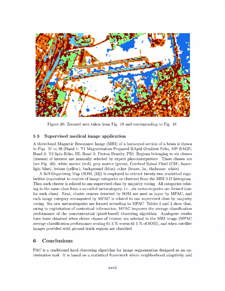
Figure 20: Zoomed area taken from Fig. 19 and corresponding to Fig. 18.5.3 Supervised medical image applicationA three-band Magnetic Resonance Image (MRI) of a horizontal section of a brain is shownin Figs. 27 to 29 (Band 1: T1 Magnetization-Prepared RApid Gradient Echo, MP-RAGE;Band 2: T2 Spin-Echo, SE; Band 3: Proton Density, PD). Regions belonging to six classes(tissues) of interest are manually selected by expert photointerpreters. These classes are(see Fig. 30): white matter (red), grey matter (green), Cerebral Spinal Fluid (CSF, liquor:light blue), lesions (yellow), background (blue), other (bones, fat, thalamus: white).A Self-Organizing Map (SOM, [33]) is employed to extract twenty-two statistical regu-larities (equivalent to centers of image categories or clusters) from the MRI 3-D histogram.Then each cluster is related to one supervised class by majority voting. All categories relat-ing to the same class form a so-called metacategory, i.e., six metacategories are formed (onefor each class). Next, cluster centers detected by SOM are used as input by MPAC, andeach image category recomputed by MPAC is related to one supervised class by majorityvoting. Six new metacategories are formed according to MPAC. Tables 1 and 2 show that,owing to exploitation of contextual information, MPAC improves the average classi�cationperformance of the non-contextual (pixel-based) clustering algorithm. Analogous resultshave been obtained when eleven classes of interest are selected in the MRI image (MPACaverage classi�cation performance scoring 64.3 % versus 61.5 % of SOM), and when satelliteimages provided with ground truth regions are classi�ed.6 ConclusionsPAC is a traditional hard clustering algorithm for image segmentation designed as an op-timization task. It is based on a statistical framework where neighborhood adaptivity andxxvii

Figure 21: Output of the SA algorithm applied to Figs. 15-17. SA parameters are: T = 800,� = 0:95, � = 16, and tmax = 150.xxviii

Figure 22: Zoomed area taken from Fig. 21 and corresponding to Fig. 18.multiresolution analysis are pursued. In this paper, the MPAC algorithm is proposed asa modi�ed version of PAC to feature enhanced pattern-preserving capability with noise-less and textureless images, i.e., when image categories feature slowly varying intensities.These basic assumptions, although severe, reasonably approximate characteristics of severalreal-world images. MPAC is an iterative suboptimal segmentation algorithm featuring: i)adaptive- and shrinking-neighborhood approach to the estimation of reliable category pa-rameters; ii) a multiresolution approach to improve computation time and segmentationaccuracy [7]; iii) hard (crisp) pixel labeling; iv) a spectral model of the error term thataccounts for the interpixel feature correlation given the underlying classes (i.e., it exploitscontextual information); and v) no interpixel class correlation model of the prior term, i.e.,no contextual information is exploited to detect known stochastic components of the labeledscene.To segment an image featuring no texture and noise, MPAC must be used in cascadewith a noncontextual hard c-means clustering algorithm (e.g., see [30], [31]), that provideshistogram analysis of pixel values. By alternating between estimating pixel labels and localand global intensity values, MPAC preserves small details better than noncontextual hardc-means clustering algorithms. Moreover, in line with PAC, MPAC is more robust thanc-means clustering algorithms in the choice of the number of clusters, because regions ofentirely di�erent intensities may belong to the same category as long as they are separatedin space [7]. Since MPAC is also easy to use, requiring no user-de�ned parameter, itsexploitation is recommended in a commercial image-processing all-purpose software toolbox[1]: a) to improve segmentation performances of a noncontextual hard c-means clusteringalgorithm; and/or b) to provide initial conditions to hard iterative contextual segmentationxxix

Figure 23: Output of the PAC algorithm applied to Figs. 15-17. PAC parameters are:� = 16, tmax = 150.xxx

Figure 24: Zoomed area extracted from Fig. 23 and corresponding to Fig. 18.algorithms where spatial continuity in pixel labeling should be enforced as a monotoneincreasing function of processing time (i.e., as the algorithm approaches convergence), suchas ICM or PAC (see Sections 2 and 3).Future developments in the �eld of image segmentation algorithms based on iterative(suboptimal) optimization approaches should employ in parallel:1) soft decision strategies in pixel labeling to identify pure pixels, mixed pixels and mis-classi�ed cases [11], [13], [27], this information being necessary in map accuracy assessmentand/or for directing ground surveys [11];2) adaptive neighborhood approaches, allowing reliable estimation of local pictorial param-eters when the iterative procedure alternates between estimates of pixel labels and categoryparameters [7];3) multiresolution approaches, to improve computation time and performances [7], [22],[23];4) locally adaptive combinations of the two types of contextual information, namely, in-terpixel feature correlation, given the underlying classes, and interpixel class dependency,where all the a priori knowledge, if any, is employed to capture (detect) known stochasticcomponents of the labeled scene [7], [9], [21], [28].xxxi

Figure 25: Output of the MPAC algorithm applied to Figs. 15-17. MPAC parameter is:tmax = 150.xxxii

Figure 26: Zoomed area extracted from Fig. 25 and corresponding to Fig. 18.References[1] P. Zamperoni, \Plus �ca va, moins �ca va," Pattern Recognition Letters, vol. 17, no. 7, pp.671-677, 1996.[2] R. C. Jain and T. O. Binford, \Ignorance, myopia and naivet�e in computer visionsystems," Comput., Vision, Graphics, Image Processing: Image Understanding, vol. 53,pp. 112-117, 1991.[3] M. Kunt, Comments on \Dialogue", a series of articles generated by the paper enti-tled \Ignorance, myopia and naivet�e in computer vision systems," Comput., Vision,Graphics, Image Processing: Image Understanding, vol. 54, pp. 428-429, 1991.[4] L. Delves, R. Wilkinson, C. Oliver and R. White, \Comparing the performance of SARimage segmentation algorithms," Int. J. Remote Sensing, vol. 13, no. 11, pp. 2121-2149,1992.[5] A. Hoover, G. Jean-Baptiste, X. Jiang, P. J. Flynn, H. Bunke, D. G. Goldgof, K. Bowyer,D. W. Eggert, A. Fitzgibbon, and R. B. Fisher, \An experimental comparison of rangeimage segmentation algorithms," IEEE Trans. Patt. Anal. Machine Intelligence, vol. 18,no. 7, pp. 673-688, 1996.[6] S. Geman and D. Geman, \Stochastic relaxation, Gibbs distributions, and the Bayesianrestoration of images," IEEE Trans. Patt. Anal. Machine Intelligence, vol. PAMI-6, no.6, pp. 721-741, 1984.[7] T. N. Pappas, \An adaptive clustering algorithm for image segmentation," IEEE Trans.on Signal Processing, vol. 40, no. 4, pp. 901-914, 1992.xxxiii

Figure 27: MRI, Band 1: T1 MP-RAGE.

Figure 28: MRI, Band 2: T2 SE.xxxiv

Figure 29: MRI, Band 3: PD.

Figure 30: MRI, Areas of interest.xxxv

Input Class Tot. Purity1 2 3 4 5 6 Pixels (%)Metacategory 1 1232 164 4 119 0 505 2024 60.9Metacategory 2 26 723 28 90 0 250 1117 64.7Metacategory 3 0 10 1168 89 0 74 1341 87.1Metacategory 4 5 2 32 157 0 1 197 79.7Metacategory 5 0 0 0 0 727 322 1049 69.3Metacategory 6 412 395 19 24 121 1928 2899 66.5Tot. Pixels 1675 1294 1251 479 848 3080 8627Efficiency (%) 73.6 55.9 93.4 32.8 85.7 62.6 68.8Table 1: Confusion matrix: SOM.Input Class Tot. Purity1 2 3 4 5 6 Pixels (%)Metacategory 1 1213 60 2 40 0 374 1689 71.8Metacategory 2 23 737 35 91 0 243 1129 65.3Metacategory 3 0 16 1168 85 0 77 1346 86.8Metacategory 4 5 1 24 160 0 1 191 83.8Metacategory 5 0 0 0 0 770 275 1045 73.7Metacategory 6 434 480 22 103 78 2110 3227 65.4Tot. Pixels 1675 1294 1251 479 848 3080 8627Efficiency (%) 72.4 57.0 93.4 33.4 90.8 68.5 71.4Table 2: Confusion matrix: MPAC.[8] H. Derin and H. Elliott, \Modeling and segmentation of noisy and textured images usingGibbs random �elds," IEEE Trans. Patt. Anal. Machine Intelligence, vol. PAMI-9, no.1, pp. 39-55, 1987.[9] J. Besag, \On the statistical analysis of dirty pictures," J. R. Statist. Soc. B, vol. 48,no. 3, pp. 259-302, 1986.[10] J. Zhang, J. W. Modestino and D. A. Langan, \Maximum likelihood parameter es-timation for unsupervised stochastic model-based image segmentation," IEEE Trans.Image Processing, vol. 3, no. 4, pp. 404-419, 1994.[11] P. C. Van Deusen, \Modi�ed highest con�dence �rst classi�cation," PE&RS, vol. 61,no. 4, pp. 419-425, 1995.[12] R. Chellappa and A. Jain, Eds., Markov Random Fields: Theory and Application. NewYork: Academic, 1993.[13] J. Dehemedhki, M. F. Deami and P. M. Mather, \An adaptive stochastic approach forsoft segmentation of remotely sensed images," in Series in Remote Sensing: vol. 1 (Proc.xxxvi

of the Int. Workshop on Soft Computing in Remote Sensing Data Analysis, Milan, Italy,Dec. 1995), E. Binaghi, P. A. Brivio and A. Rampini, Eds., World Scienti�c, Singapore,pp. 211-221, 1996.[14] A. H. Schistad Solberg, T. Taxt, and A. K. Jain, \A Markov Random Field Model forclassi�cation of multisource satellite imagery," IEEE Trans. Geosci. Remote Sensing,vol. 34, no. 1, pp. 100-113, 1996.[15] F. Girosi, M. Jones and T. Poggio, \Regularization theory and neural networks archi-tectures," Neural Computation, vol. 7, 1995, pp. 219-269.[16] T. Poggio, V. Torre, and C. Koch, \Computational vision and regularization theory,"Nature, vol. 317, pp. 314-319, 1985.[17] F. Wang, \Fuzzy supervised classi�cation of remote sensing images," IEEE Trans.Geosci. Remote Sensing, vol. 28, no. 2, pp. 194-210, 1990.[18] A. P. Dempster, N. M. Laird and D. B. Rubin, \Maximum likelihood from incompletedata via the EM algorithm," J. Royal Statist. Soc. Ser. B, vol. 39, pp. 1-38, 1977.[19] S. Medasani and R. Krishnapuram, "Determination of the number of components inGaussian mixtures using agglomerative clustering," Proc. Int. Conf. on Neural Networks'97, Houston, TX, June 1997, pp. 1412-1417.[20] I. Elfadel and R. Picard, \Gibbs random �elds, cooccurrences, and texture modeling,"IEEE Trans. Pattern Anal. Machine Intell., vol. 16, no. 1, pp. 24-37, 1994.[21] P. C. Smits, and S. G. Dellepiane, \Synthetic aperture radar image segmentation bya detail preserving Markov Random Field approach," IEEE Trans. Geosci. RemoteSensing, vol. 35, no. 4, pp. 844-857, 1997.[22] J. Liu, and Y. Yang, \Multiresolution color image segmentation," IEEE Trans. PatternAnal. Machine Intell., vol. 16, no. 7, pp. 689-700, 1994.[23] C. Bouman, and B. Liu, \Multiple resolution segmentation of textured images," IEEETrans. Pattern Anal. Machine Intell., vol. 13, no. 2, pp. 99-113, 1991.[24] H. Derin, and C. S. Won, \A parallel image segmentation algorithm using relaxationwith varying neighborhoods and its mapping to array processors," Comput. VisionGraphics Image Processing, vol. 40, pp. 54-78, Oct. 1987.[25] R. Klein and S. J. Press, \Adaptive Bayesian classi�cation of spatial data," Journal ofthe American Statistical Association, vol. 87, no. 419, pp. 844-851, 1992.[26] P. B. Chou and C. M. Brown, \The theory and practice of Bayesian image labeling,"Int. Journal of Computer Vision, vol. 4, pp. 185-210, 1990.[27] G. M. Foody, N. A. Campbell, N. M. Trodd and T. F. Wood, \Derivation and ap-plications of probabilistic measures of class membership from the maximum-likelihoodclassi�cation," PE&RS, vol. 58, no. 9, pp. 1335-1341, 1992.xxxvii

[28] Y. Jhung and P. H. Swain, \Bayesian contextual classi�cation based on modi�ed M -estimates and Markov Random Fields," IEEE Trans. Geosci. Remote Sensing, vol. 34,no. 1, pp. 67-75, 1996.[29] B. D. Ripley, \Statistics, images, and pattern recognition," Canadian Journal of Statis-tics, vol. 14, no. 2, pp. 83-111, 1986.[30] B. Fritzke, \The LBG-U method for vector quantization - an improvement over LBGinspired from neural networks," Neural Processing Letters, vol. 5, no. 1, pp. 83-111,1997.[31] J. C. Bezdek and N. R. Pal, \Two soft relatives of learning vector quantization," NeuralNetworks, vol. 8, no. 5, pp. 729-743, 1995.[32] M. Sonka, V. Hlavac, and R. Boyle, Image Processing, Analysis and Machine Vision,Chapman & Hall, London, 1993.[33] T. Kohonen, Self-Organizing Maps, Springer Verlag, Berlin, 1995.

xxxviii