contextual cuing by global features
TRANSCRIPT

1
Contextual cueing by global features
Melina A. Kunar 1,2, Stephen J. Flusberg2, & Jeremy M. Wolfe 1,2
(1) Harvard Medical School
(2) Brigham & Women’s Hospital
Visual Attention Laboratory64 Sidney Street, Suite 170CambridgeMA 02139, USA
E-mail: [email protected]
Tel: + 1 617 768 8817
Fax: + 1 617 768 8816
Running Head: Contextual cueing by global features (P357)
2
Abstract
In visual search tasks, attention can be guided to a target item, appearing amidst
distractors, on the basis of simple features (e.g. find the red letter among green). Chun
and Jiang's (1998) "contextual cueing" effect shows that RTs are also speeded if the
spatial configuration of items in a scene is repeated over time. In these studies we ask if
global properties of the scene can speed search (e.g. if the display is mostly red, then the
target is at location X). In Experiment 1a, the overall background color of the display
predicted the target location. Here the predictive color could appear 0, 400 or 800 msec in
advance of the search array. Mean RTs are faster in predictive than in non-predictive
conditions. However, there is little improvement in search slopes. The global color cue
did not improve search efficiency. Experiments 1b-1f replicate this effect using different
predictive properties (e.g. background orientation/texture, stimuli color etc.). The results
show a strong RT effect of predictive background but (at best) only a weak improvement
in search efficiency. A strong improvement in efficiency was found, however, when the
informative background was presented 1500 msec prior to the onset of the search stimuli
and when observers were given explicit instructions to use the cue (Experiment 2).

3
Introduction
To interact with the world we often have to parse visual information into relevant and
irrelevant stimuli. For example, when searching for a friend in a crowd we have to ignore
non goal-relevant information (such as other people’s faces, or inanimate objects) in
order to select the correct face. If we were to pay attention to every visual stimulus we
may be overwhelmed and thus could not perform many important tasks.
In the laboratory, we can study how we process visual information by asking observers to
search for a target item among a number of distracting items and record the reaction time
(RT) taken to respond. We can we use these measurements to understand how we process
the world. For example, if we measure RT as a function of set size (the number of items
in the display), then the slope of the RT x set size function gives an estimate of the cost of
adding items to the display, so that slope is a measure of search efficiency. If attention
can be deployed to a target independent of the number of distractor items, then the slope
will be 0 msec/item and the visual search task can be labeled "efficient". According to a
Guided Search model of attention (e.g., Wolfe, 1994; Wolfe et al., 1989) a limited set of
features are able to guide attention toward a target (see Wolfe & Horowitz, 2004 for a
review). For example, color - finding the red bar among green bars or orientation -
finding a vertical bar among horizontal bars both produce efficient search (Treisman &
Gelade, 1980). The efficiency of search is related to the strength of guidance (Wolfe,
1994; Wolfe et al., 1989). Thus, if participants search for a target defined by a
conjunction of properties (e.g. find the red horizontal bar, among green horizontals and
4
red verticals), search is less efficiently guided than in a simple feature search, typically
producing search slopes of around 5-15 msec/item on target present trials (e.g. Treisman
& Sato, 1990; Wolfe, 1998). In the absence of guiding feature information, search is still
less efficient, producing target present slopes of around 20-40 msec/item even when the
items are large enough to identify without fixation (e.g. Braun & Sagi, 1990; Egeth &
Dagenbach, 1991; Wolfe, 1998).
Beyond attributes of the target and distractor items, there are global visual properties that
can help us process the world. Participants find it more difficult to search for an object in
a jumbled incoherent scene than when it is in a coherent one (Biederman, 1972,
Biederman, Glass & Stacey, 1973). Scene information does not need to be meaningful or
explicitly recognized. Chun and Jiang (1998) have found that participants are faster to
respond to a target if it is always accompanied by the same spatial context than if it is not.
If participants need to determine the orientation of a T, they are faster to respond when a
specific target location is always accompanied by Ls in a unique layout. The benefit of
having the target appear in a predictive, repeated display is known as ‘contextual cueing’
(Chun & Jiang, 1998; see also Chun, 2000, for a review) and can be based on implicit
knowledge. At the end of the experiment, when asked to perform a two-alternative-
forced-choice recognition task, participants are at chance when asked if they have seen a
display before (Chun & Jiang, 1998; see also Chun & Jiang, 2003).
Given that the spatial context of a scene can produce an RT advantage (or a ‘cueing’
effect), we ask whether other aspects of a scene can produce similar results. In particular,
5
we investigate whether a non-spatial property like the overall color of a scene can
produce a similar effect in the absence of a consistent spatial layout. We know that
features like color are often used to guide our attention to the target item in the face of
competing stimuli when those features differentiate target and distractors. For example, if
you are searching for a RED item among GREEN distractors you can efficiently guide
attention towards red and away from green (Carter, 1982; Green & Anderson, 1956;
Wolfe, 1994; Wolfe et al., 1989). Can feature information also be useful if it indirectly
identifies the target location? If a red display means the target is in one location and a
green display means that it is in another unique location, can the searcher use that
information to speed response and, in turn, increase search efficiency?
Please note that although we have mentioned search performance in terms of Guided
Search above (Wolfe, 1994; Wolfe et al., 1989), any decrease in search efficiency could
also be accounted for by other models, such as limited capacity models (e.g. Posner,
1980) or unlimited capacity models of attention (e.g. Palmer et al., 1993, Palmer, 1994;
Palmer et al., 2000; Shaw & Shaw, 1977; Townsend & Ashby, 1983). Guided search and
other limited attention capacity models may assume an improvement in search efficiency
as one could orientate attention to items appearing around the cued location rather than
across all items in the visual field (in fact, Song & Jiang, 2005, suggest that participants
need only to encode the configuration of 3 to 4 distractor items to find a valid contextual
cueing effect). Alternatively, unlimited capacity models (especially those based on signal
detection theories, e.g. Palmer et al., 1993 and Palmer, 1994) might claim that contextual
cueing allows participants to better ignore distractor items. The experiments presented
6
here do not seek to suggest one attention model over another, but instead ask the overall
question: does contextual cueing by global features improve search efficiency? For the
sake of simplicity, we will refer to this as an improvement in guidance.
In Experiment 1, we investigate whether the average features of a background can speed
response and/or aid search efficiency, when the background appears 0, 400 or 800 msec
prior to the search stimuli. The results reveal a speeding of mean RT, but no decrease in
RT x set size slopes (thus no evidence of guidance). Experiments 1b - 1f show
replications of this effect using different predictive properties, such as the background
texture or the color of the search stimuli. In Experiment 2, we presented the background
1500 msec prior to the search stimuli and gave participants explicit knowledge that some
background features were predictive of the target location. In this case, we observed both
a speeding of mean RT and a decrease in slope. Global color information can guide
search if it is presented explicitly, well in advance of the search display. However, with
less lead-time and less explicit awareness, global predictive properties only produce an
RT cueing effect.
Experiment 1a
Experiment 1a investigated whether the average background color of a display could
speed response if that color predicted the target location.
7
Participants:
Twelve participants between the ages of 18 and 55 years served as participants. Each
participant passed the Ishihara test for color blindness and had normal or corrected to
normal vision. All participants gave informed consent and were paid for their time.
Apparatus and Stimuli:
The experiment was conducted on a Macintosh computer using Matlab Software with the
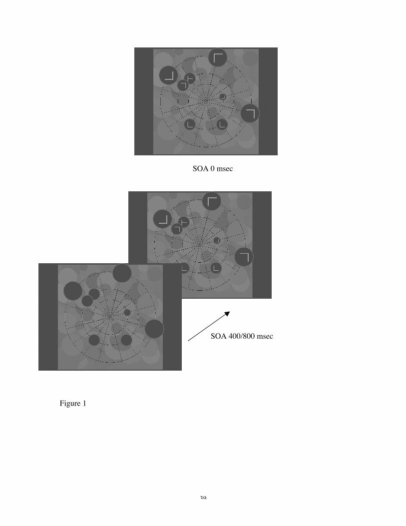
PsychToolbox (Brainard, 1997; Pelli, 1997). Search displays are shown in Figure 1. The
distractor items were L shapes presented randomly in one of four orientations (0, 90, 180
or 270 degrees). The target item was a T shape rotated 90 degrees either to the left or to
the right with equal probability. A blue dot at the center of the screen served as a fixation
point. Three black concentric circles surrounded the fixation point with diameters of 9.5
degrees, 15.5 degrees, and 25 degrees. Sixteen black lines radiated out from the fixation
point roughly equidistant from one another to form a spider web lattice. On every trial,
either eight or twelve (depending on the set size) circular “placeholders” appeared at
locations where a spoke crossed a concentric circle. Because visual acuity declines with
distance from the fixation point, the size of the place-holding circles and of the search
stimuli increased with eccentricity. Those on the closest concentric circle were 2 degrees
in diameter, those on the middle concentric circle were 3.3 degrees, and those on the
furthest concentric circle were 5.4 degrees. The background measured 29 degrees x 29
degrees and was composed of a texture of different sized, overlapping circles that were
8
filled with variations of a single color. There were eight background colors: yellow, red,
dark blue, orange, cyan, green, purple, or white/gray. Background color changed from
trial to trial. Each color was equally probable. Please note that within a background the
global texture remained unchanged (e.g. the background was overall ‘red’), however on
each successive ‘red’ displays the local properties varied (e.g. the color and size of the
individual circles making up the display changed across each ‘red’ display).
-------------------------------------
Figure 1 about here
--------------------------------------------
All stimuli were made up of 2 lines of equal length (forming either an L or a T). Ts and
Ls appeared within the circular placeholders. Stimuli enclosed in the smallest
placeholders subtended a visual angle of 1 degree x 1 degree, those enclosed in the
middle placeholders subtended 1.5 degrees x 1.5 degrees, and those enclosed in the
largest placeholders subtended 2.5 degrees x 2.5 degrees. The targets, distractors and
outline of the placeholders were the same color as the overall background color, whereas
the inside of the placeholders was dark gray.
Procedure:
A tone sounded at the start of each trial. There were 10 practice trials followed by 512
experimental trials that were divided, for analysis purposes, into 8 epochs of 64 trials.
9
Approximately half of the trials in each epoch had a set size of 8; the remaining trials had
a set size of 12.
Each participant was tested in three conditions (i) a search task where the background
appeared simultaneously with the search stimuli, (ii) a search task where the background
preceded the stimuli by 400 msec and (iii) a search task where the background preceded
the stimuli by 800 msec. In each condition, participants were asked to respond to whether
the bottom of target letter, T, was facing left (by pressing the letter ‘a’ on the keyboard)
or whether it was facing right (by pressing the letter ‘l’). For epochs 1 to 7, four of the
background colors were always associated with a specific target location (e.g. if the
display is purple, then the target is always at location X, regardless of set size or spatial
layout). The other four colors did not predict the target location (i.e. the target changed its
location on every presentation of the color). The four predictive colors were randomly
assigned within each condition. In epoch 8 the target locations for BOTH the predictive
and random trials changed with every presentation of the colored background (i.e., the
predictive colors no longer predicted the target location). If participants were using the
background information in epochs 1-7 then this would no longer be beneficial in epoch 8,
and so we would predict an increase in RTs. Each SOA condition was blocked and the
order of the blocks was randomized. Feedback was given after each trial.
Results and Discussion
10
Figure 2 shows the RTs and slopes for each set size in the predictive and non-predictive
(random) conditions. Different graphs show different SOA conditions. Table 1 shows the
low overall error rates. As they were not indicative of any speed-accuracy trade-off, we
do not discuss them further and instead concentrate on RT and slope analysis. RTs below
200 msec and above 4000 msec were eliminated. This led to the removal of less than 1%
of the data.
-------------------------------------
Figure 2 about here
--------------------------------------------
Examining SOA 0 msec first, the RT data shows an overall reduction in RTs when the
background color was predictive than when it was random (epochs 1-7). This effect is
reliable for set size 8 (F(1, 11) = 10.5, p < 0.01) and set size 12 (F(1, 11) = 5.9, p < 0.05).
To examine how learning influences performance, previous contextual cueing
experiments compared predictive and random RTs averaged across the latter part of the
experiment (here epochs 5-7, following the design of Chun & Jiang, 1998 and Jiang,
Leung & Burks, submitted, who also collapsed RTs across the last three predictive
epochs). Using this measurement, we see with set size 8, there is a 74 msec RT benefit of
having a predictive background, t(11) = -5.4, p < 0.01, and at set size 12 there is a 91
msec benefit, t(11) = -2.7, p < 0.05. The reliable difference between predictive and
random RTs disappears at epoch 8 where all trials are random. These data suggest that
RTs are becoming faster as participants are learning the association between background
and target location, rather than the actual target locations per se. In epoch 8, the target
11
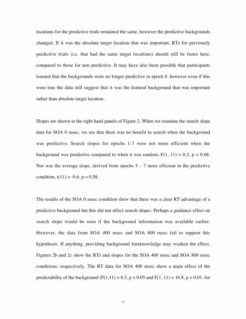
locations for the predictive trials remained the same, however the predictive backgrounds
changed. If it was the absolute target location that was important, RTs for previously
predictive trials (i.e. that had the same target locations) should still be faster here,
compared to those for non predictive. It may have also been possible that participants
learned that the backgrounds were no longer predictive in epoch 8, however even if this
were true the data still suggest that it was the featural background that was important
rather than absolute target location.
Slopes are shown in the right hand panels of Figure 2. When we examine the search slope
data for SOA 0 msec, we see that there was no benefit in search when the background
was predictive. Search slopes for epochs 1-7 were not more efficient when the
background was predictive compared to when it was random, F(1, 11) = 0.2, p = 0.68.
Nor was the average slope, derived from epochs 5 – 7 more efficient in the predictive
condition, t(11) = -0.6, p = 0.58.
The results of the SOA 0 msec condition show that there was a clear RT advantage of a
predictive background but this did not affect search slopes. Perhaps a guidance effect on
search slope would be seen if the background information was available earlier.
However, the data from SOA 400 msec and SOA 800 msec fail to support this
hypothesis. If anything, providing background foreknowledge may weaken the effect.
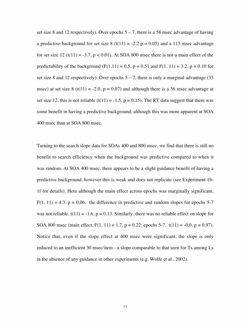
Figures 2b and 2c show the RTs and slopes for the SOA 400 msec and SOA 800 msec
conditions, respectively. The RT data for SOA 400 msec show a main effect of the
predictability of the background (F(1,11) = 8.3, p < 0.05 and F(1, 11) = 16.8, p < 0.01, for
12
set size 8 and 12 respectively). Over epochs 5 – 7, there is a 58 msec advantage of having
a predictive background for set size 8 (t(11) = -2.2 p = 0.05) and a 113 msec advantage
for set size 12 (t(11) = -3.7, p < 0.01). At SOA 800 msec there is not a main effect of the
predictability of the background (F(1,11) = 0.5, p = 0.51 and F(1, 11) = 3.2, p = 0.10 for
set size 8 and 12 respectively). Over epochs 5 – 7, there is only a marginal advantage (35
msec) at set size 8 (t(11) = -2.0, p = 0.07) and although there is a 36 msec advantage at
set size 12, this is not reliable (t(11) = -1.5, p = 0.15). The RT data suggest that there was
some benefit in having a predictive background, although this was more apparent at SOA
400 msec than at SOA 800 msec.
Turning to the search slope data for SOAs 400 and 800 msec, we find that there is still no
benefit to search efficiency when the background was predictive compared to when it
was random. At SOA 400 msec, there appears to be a slight guidance benefit of having a
predictive background, however this is weak and does not replicate (see Experiment 1b-
1f for details). Here although the main effect across epochs was marginally significant,
F(1, 11) = 4.3, p = 0.06, the difference in predictive and random slopes for epochs 5-7
was not reliable, t(11) = -1.6, p = 0.13. Similarly, there was no reliable effect on slope for
SOA 800 msec (main effect, F(1, 11) = 1.7, p = 0.22; epochs 5-7, t(11) = -0.0, p = 0.97).
Notice that, even if the slope effect at 400 msec were significant, the slope is only
reduced to an inefficient 30 msec/item - a slope comparable to that seen for Ts among Ls
in the absence of any guidance in other experiments (e.g. Wolfe et al., 2002).
13
The results of Experiment 1a suggest that the featural properties of the background can
speed response to the target. However, this facilitation does not appear to be the result of
the background information guiding attention toward likely target locations. Guidance
should produce a reduction in the effective set size and, thus, a reduction in the slope of
the RT x set size functions. This is not found. Increasing the time between the onset of
the predictive/non-predictive background, and hence the amount of ‘warning’ or
preparation time given to a participant did not produce more efficient guidance. If
anything, pre-cueing with the background seems to weaken the featural cueing effect.
Experiments 1b - 1f: Replication and extension
Because the failure to find guidance is an essentially negative finding, we have attempted
several replications. All are similar in design to Experiment 1a and are briefly described
here.
Experiment 1b: the global background texture predicted the target location. Here the
background was composed of differently orientated lines, rectangles or squares that could
either be densely or sparsely packed. All stimuli here were achromatic.
Experiments 1c: the exact color of the stimuli and their placeholders predicted target
location. Participants searched for a T (orientated to the left or the right) among rotated
Ls (similar to Experiment 1a).
14
Experiment 1d: the exact color of the stimuli and their placeholders predicted target
location. Participants searched for either a vertical or horizontal line among distractor
lines of orientation –60, -30, 30 or 60 degrees.
Experiment 1e: the global color of the background predicted target location (as in
Experiment 1a). In this experiment, however, the spatial layout of the display remained
constant across trials (i.e. it never changed).
Experiment 1f: the global color of the background predicted target location (as in
Experiment 1a). In this experiment, the target was a vertical or horizontal line among
oblique distractors (as in Experiment 1d). Moreover, larger set sizes were used (18 and
24).
In Experiments 1b, c and d, the backgrounds were presented at SOAs of 0, 400 and 800
msec prior to the onset to of the search stimuli. In Experiments 1e and 1f only SOA 0
msec was used. Figures 3 – 7 give example displays of each condition. In all experiments
at least ten participants between the ages of 18 and 55 years took part. Each participant
passed the Ishihara test for color blindness and had normal or corrected to normal vision.
All participants gave informed consent and were paid for their time.
-------------------------------------
Table 2 and Figures 3 to 7 about here
--------------------------------------------

15
Results and Discussion
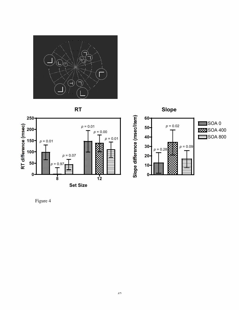
Figures 3 – 7 show the difference between predictive and non-predictive RTs and slopes
for each set size averaged across epochs 5 – 7, whereas Table 2 shows the average search
slopes for predictive and non-predictive displays, again averaged across epochs 5 - 7. As
we can see with SOA 0 msec, there is an RT benefit for each condition. In all cases
predictive RTs are faster than non-predictive. A similar effect occurs at SOA 400 and
SOA 800 msec, however unlike SOA 0 msec this result is often not reliable. This lack of
statistical reliability is most pronounced for SOA 800 msec. As in Experiment 1a, it
seems that presenting the background prior to the search stimuli may weaken the cueing
effect. We will discuss this further in the General Discussion.
Turning to the differences between predictive and non-predictive search slopes, we see
that there is, at best, a weak improvement in search efficiency with predictive global
features. The improvement in search efficiency is only statistically reliable when
observers search for a colored T among colored Ls in Experiment 1c at SOA 400 msec1.
To investigate whether a stronger effect of guidance would be found if we increased the
power, we performed a meta-analysis across experiments (using the data from epochs 5-
7). As the SOAs and set size varied we chose conditions that had been used in the
1 A similar pattern occurs if we collapse the data across epochs 3 – 7. Here, out of the fourteen conditionsfrom Experiments 1a – 1f, ten of the conditions showed that there was no benefit in search slope betweenpredictive and random trials, one showed that there was a marginal slope benefit of having a predictivecontext over a random context (Experiment 1b – SOA 800, p = 0.09), while the other 3 conditions showeda reliable slope benefit (Experiment 1a – SOA 400 msec, Experiment 1c - SOA 400 msec and Experiment1f). Again, the data confirm that any improvement in search efficiency is at best weak, and that the majorityof experiments showed no benefit at all.
16
majority of experiments (i.e., conditions that used set sizes 8 and 12 with an SOA of 0
msec). This allowed us to pool data from 66 participants who had taken part in
Experiments 1a-1e. Even with this increased power, there was still no search slope
benefit of predictive context over non-predictive, t(65) = -1.4, p = n.s.. We also
performed a similar meta-analysis on the first block of trials that each participant was
tested on. This ensured that previous global feature to target location mappings between
blocked conditions did not interfere with any potential slope effect. Here, we pooled data
across Experiments 1a – 1d, where nineteen participants were tested in the SOA 0 msec
condition first, eighteen participants in the SOA 400 msec conditions and seventeen
participants in the SOA 400 msec conditions. The data show that even when participants
had no previous exposure to the mapping of background to target location, there was no
difference in search efficiency between predictive and non predictive backgrounds (t(18)
= -0.5, p = n.s., t(17) = -1.7, p = n.s., and t(16) = -1.6, p = n.s., for SOAs 0 msec, 400
msec and 800 msec respectively).
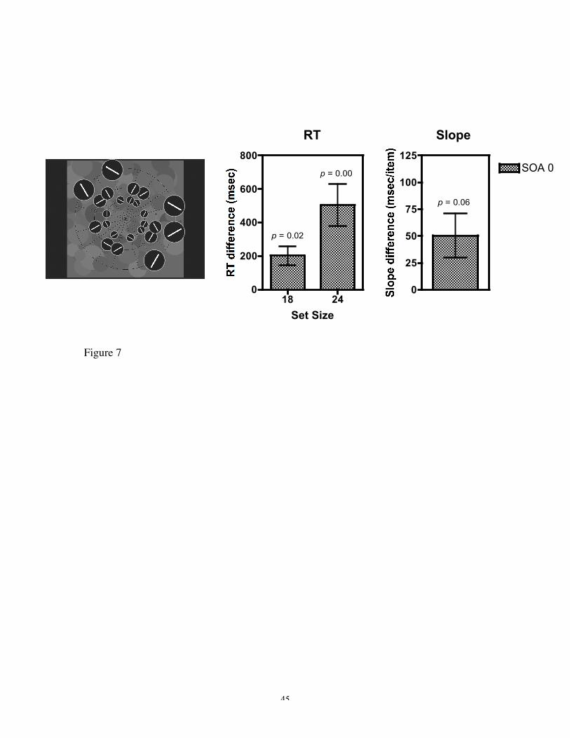
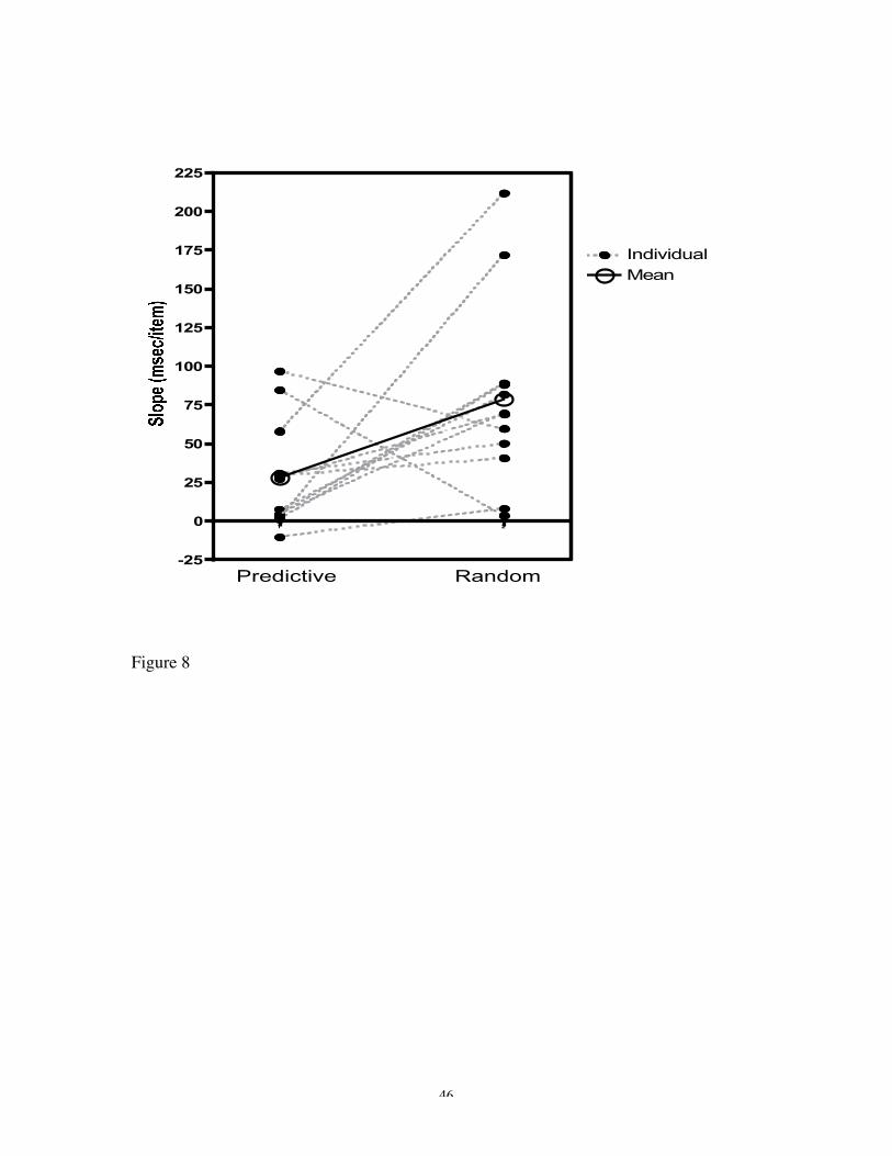
Despite this, nine of the eleven individual conditions (pooled over Exps 1b-1f) produced
(non-reliable) changes whose sign was in the direction of improvement. In the most
dramatic case, Experiment 1f, we see that there is an impressive 50 msec/item difference
in slope between predictive and non-predictive search slopes. Although it is only
marginally significant (p = 0.06), the bulk of participants do seem to show an effect. As
shown in Figure 8, the large size is driven by two participants, both showing a 150 – 170
msec/item difference, whereas the lack of significance is driven by two other participants
whose results go in the opposite direction. It may be noteworthy that Experiment 1f is the
17
hardest search task of the group - a consequence of the use of larger set sizes and of the
similarity between targets and distractors (Duncan & Humphreys, 1989). As a result, RTs
are quite slow (averaging 2230 msec across conditions). This may give participants
enough time to finally be able to use the global feature information for guidance, an idea
that is confirmed in Experiment 2 where guidance by global features is possible if
participants are given enough time as well as explicit instruction.
-------------------------------------
Figure 8 about here
--------------------------------------------
In summary, Experiment 1, in all of its forms, reveals that global feature information can
speed mean RT. Its ability to guide search and, thus, increase search efficiency, however,
appears to be more limited.
Experiment 2: Does explicit knowledge aid guidance?
Is there something fundamentally wrong with the idea that the attributes of the
background could inform the observer about the probable location of that target?
Experiment 2 investigates whether featural properties of the display as a whole can ever
guide the deployment of attention. In this experiment, we give participants explicit
knowledge that a background is predictive (e.g. telling them that, if the overall
background is ‘red’, a target will appear in location X). Moreover, we increase the SOA
18
between background and search display to 1500 msec in order to give participants
adequate preparation time to orientate to the expected target location. Given this
information, it seems unlikely that participants will still feel the need to search for the
target. Therefore we expect search slopes for predictive displays to be shallower than
those for random (i.e. a guidance effect). This experiment should show us what the
results of Experiment 1 would have looked like if overall image properties had guided
attention.
Participants:
Fourteen participants between the ages of 18 and 55 years served as participants. Each
participant passed the Ishihara test for color blindness and had normal or corrected to
normal vision. All participants gave informed consent and were paid for their time.
Stimuli and Procedure:
The stimuli and procedure were the same as those used in Experiment 1a. However,
participants were tested with only a single SOA of 1500 msec between the onset of the
background and the onset of the search stimuli. Furthermore, participants were given
explicit instructions informing them that four of the background colors were predictive of
the target location, whereas the other four colors were not. They were told exactly which
four colors would be predictive (e.g. red, purple, green and orange). As in Experiment 1a,
this was true of epochs 1-7. In epoch 8, the target locations in all conditions were
19
randomized so that the predictive background colors no longer predicted the target
location.
Results and Discussion
Overall error rates were low (2%) and presented in Table 1. As they were not indicative
of any speed-accuracy trade-off, we do not discuss them further and instead concentrate
on RT and slope analysis. RTs below 200 msec and above 4000 msec were eliminated.
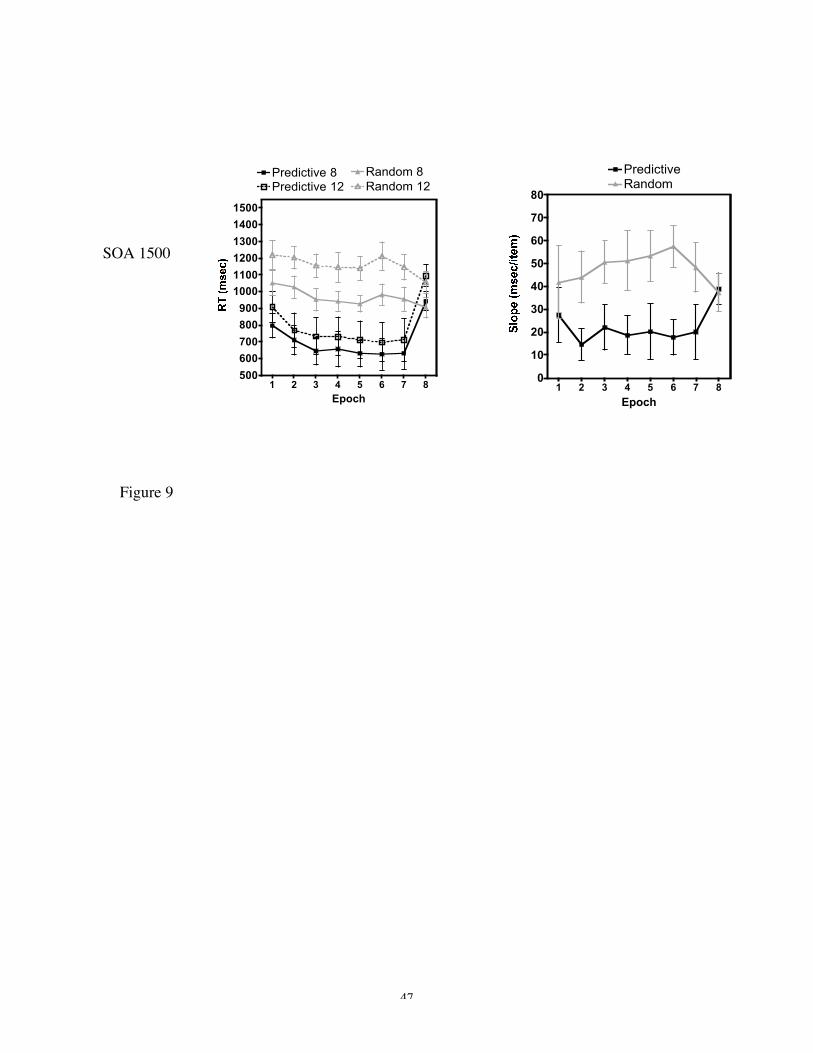
This led to the removal of less than 1% of the data. Figure 9 shows the RT and slope data,
respectively, for both predictive and random configurations. There was a main effect of
having a predictive background. This occurred for both set size 8, F(1, 13) = 37.6, p <
0.01, and set size 12, F(1, 13) = 26.4, p < 0.01. Comparing predictive and random trials
for RTs collapsed across epochs 5 – 7 we see a feature cueing effect of 324 msec for set
size 8, t(13) = - 5.8, p < 0.01, and 459 msec for set size 12, t(13) = -5.2, p < 0.01. There
was no difference between predictive and random RTs in epoch 8 (for both set size 8 and
12), where none of the backgrounds remained predictive. Clearly, as in Experiment 1a,
participants were faster when the background color predicted the target location opposed
to when it did not.
-------------------------------------
Figure 9 about here
--------------------------------------------
20
However, unlike Experiment 1a, there was also a positive guidance effect. There was a
strong main effect on search slope, F(1, 13) = 10.2, p < 0.01, and averaging slopes across
epochs 5 – 7 showed a 34 msec/item advantage in search efficiency with predictive
backgrounds compared to random, t(13) = -2.8, p < 0.05. In this situation prior
knowledge helped guidance. As mentioned briefly in the Introduction, an increase in
guidance is one attentional model that can account for the reduction in predictive slopes.
This is not to say that the data cannot be accounted for by other attention models (for
example, limited resource models of attention, e.g. Posner, 1980; Posner & Peterson,
1990, or unlimited capacity models, e.g. Palmer et al., 1993, Palmer, 1994; Palmer et al.,
2000; Shaw & Shaw, 1977; Townsend & Ashby, 1983). Nevertheless, regardless of
which attention model is accountable, the important point remains that search slopes can
be dramatically reduced when participants are given time and explicit knowledge about
predictive contexts.
It is also interesting to note that search slopes for predictive trials did not reach 0
msec/item – but instead asymptote at around 20 msec/item. Breaking down the data into
individual participants we see that 64% of participants do reach 0 msec/item in slope
efficiency by the latter epochs, whereas the other 36% do not. Similar effects have been
shown in the contextual cueing literature where it has been reported that approximately
30 % of participants do not show a standard contextual cueing effect (e.g. Jiang, Leung &
Burks, submitted, & Lleras & Von Muhlenen, 2004). In contrast, just 20% of participants
overall have slopes near zero in Experiments 1a - 1f here (0% in both Experiments 1a and
b; 13% in both Experiments 1c and d; 43% in Experiment 1e; and 50% in Experiment 1f;
21
presumably the relatively high number of participants producing efficient slopes in
Experiment 1f reflects the notion that guidance by global features is relatively slow and
may appear when participants are given lots of time, as well as, explicit knowledge).
General Discussion
During visual search, a predictive spatial layout can be used to speed target response (e.g.
Chun & Jiang, 1998; 2003). We conducted several experiments investigating whether
global featural properties of the display, in the absence of a consistent spatial layout, can
be used to (a) cue the target location and thus speed RT response and (b) guide attention
to the target item, resulting in shallower search slopes. Experiment 1a investigated
whether the average background color could cue and/or guide search. In this case, the
background was either presented concurrently or in advance (e.g. 400 msec or 800 msec
prior to) of the stimuli onset. The results showed that when the background was presented
simultaneously with the stimuli (SOA 0 msec), RTs to predictive background features
were faster than those of non-predictive background features. A similar effect occurred
when the background appeared prior to the stimuli: RTs were faster when the background
was predictive compared to when it was random. This effect remained reliable when the
background appeared 400 msec prior to the onset of the search items. When the SOA
increased to 800 msec, the effect was less reliable (only marginally significant at set size
8). Experiments 1b -1f showed a similar pattern of results. In these experiments, we
varied the nature of the predictive feature to include background texture/orientation and
stimulus color. We also varied the nature of the search task and varied the set size. The

22
basic pattern of the data, however, remained unchanged. Collectively the results of
Experiment 1 show that a predictive display speeds RT.
Compared to the evidence for a main effect of background on RT, the evidence for
guidance in Experiments 1a - 1f was much less convincing. If one looks at the whole set
of data, one may get the impression that there is some guidance of attention. The slopes
of RT x set size functions seem more likely to be shallower in the predictive cases than in
the non-predictive cases. However, this effect, if it is real, is statistically fragile. The
important point is that guidance by simple feature backgrounds is nothing like guidance
by simple target features. Imagine an experiment in which observers search for a T of
arbitrary color among L's of other arbitrary colors. With stimuli like those used in
Experiment 1a, the RT x set size slope will be about 30-40 msec/item. If, however, the
target, T, is always red, the slope will drop dramatically. With appropriate choice of
distractor colors, the slope will drop to near zero. That is perfect guidance by target color.
Suppose, instead, that the target, T, is always in a specific location when the display, as a
whole, is red. In both cases, red tells the observer where to look for the target but the
results of the present experiment show that the global redness provides little if any
guidance, unless the participant is given sufficient time and explicitly told to use the
information.
Perhaps the predictive global feature assignments in these experiments were too weak.
Here half of the global features were predictive of the target location, whereas the other
half, were not. If participants were learning that the global feature was only valid 50% of
23
the time, they might also learn that it was not a reliable cue and chose not to use it.
Although possible, we do not believe this to be the case. In a separate experiment, we
investigated what would happen to the search slope, if all the displays were predictive.
Even in this case, search slopes did not become more efficient over time, F(6, 72) = 0.9, p
= n.s.. Please note also that an RT benefit occurred in all the experiments reported above
showing that repeating the non-predictive feature does not disrupt RT contextual
learning. This replicates most of the findings in the contextual cueing literature, which
concentrate on RTs rather than search slopes (see Chun & Jiang, 1998 for the exception).
Interestingly, in other work we have also looked for the effect on search slopes of
standard contextual cueing by spatial layout. The results are similar to those presented
here. We replicate the standard reduction in mean RT but there is little effect of
predictive configurations on search slopes (Kunar, Flusberg, Horowitz & Wolfe, in
preparation).
Another suggestion explaining the lack of guidance may be that in the present studies
participants were not actively attending the predictive global features. Previous research
has found that unattended stimuli do not produce contextual cueing (Jiang & Chun, 2001;
Jiang & Leung, 2005). This may explain why a strong guidance effect only occurred in
Experiment 2, when participants were given explicit knowledge and encouraged to attend
the backgrounds. Although this hypothesis has some merits, it cannot account for all of
the data. In the experiments reported here, although there was little benefit to guidance
when the background features were not explicitly ‘attended’, there was an RT effect. This
suggests that the global features were being attended, at least to some degree: in the

24
previous studies where context was unattended no RT benefit was found (Jiang & Chun,
2001; Jiang & Leung, 2005). Of course, it could be the case that the feature mismatch in
these studies was the reason that there was little guidance benefit. In the standard
contextual cueing studies the spatial configuration of the display is said to ‘guide’
attention to the spatial target location. However, in the studies presented here the
‘guiding’ feature was non-spatial. This raises an interesting point: perhaps guidance to
spatial target locations can only be found with a predictive spatial cue? Although this is
possible, other studies in our lab suggest otherwise. As mentioned briefly above, even
when the predictive cue was spatial we found that there was little benefit to guidance
(Kunar, Flusberg, Horowitz & Wolfe, in preparation).
It is curious that increasing the timing between the predictive feature onset and the
stimuli onset seemed to weaken the RT cueing effect. A positive cueing effect was
always found in the SOA 0 msec conditions but not always in the SOA 400 or 800 msec
conditions2. At present, we are not sure why this should be. One possibility could be our
use of different layouts in the backgrounds. For example, in Experiment 1a the global
feature of a red background would predict the target appearing in location X. However,
no two ‘red’ backgrounds were identical (i.e. each background was composed of
randomly generated luminance values that produced the overall impression of red, but
were individually unique). With an SOA of 0 msec, perhaps participants only had time to
analyze the global properties of the background (i.e. an overall impression of red) leading 2 This data is puzzling and perhaps suggests that the explicit instruction in Experiment 2 was moreimportant than the increased SOA for producing a guidance benefit. Although this might be the case, we donot want to rule out the effect of SOA entirely. Please remember that a marginal guidance benefit was alsofound in Experiment 1f, where, due to increased response times, there was also more time to encode thebackground.
25
to a strong RT effect. With longer SOAs, participants may have had time to process the
local features within each display as well. As these local features changed from trial to
trial their inconsistency could have interfered with the global contextual cueing effect.
Although this may explain some of the data, it cannot account for the results of
Experiment 1c and 1d. A weakened contextual cueing effect occurred with longer SOAs
in these conditions, however here the specific local features around the target (i.e. the
color of the stimuli and their placeholders for each predictive feature) did not change. A
second possibility suggests that the association between predictive context and target
location is strongest when they temporally group. Therefore the strongest cueing effect
will occur at SOA 0 msec, whereas it may dissipate somewhat at SOA 400 msec and 800
msec. However, further research needs to be conducted before any firm conclusions can
be reached.
The data presented here show that global featural properties (in the absence of explicit
knowledge) speed RT but do not guide search effectively. If the RT-speeding advantage
is not due to guidance then what is facilitating RTs? Perhaps the RT benefit is due to a
reduction in target processing time. Given the predictive context, it may be that less
evidence needs to be accumulated before a correct response can be made. Studies in other
fields concur with this hypothesis. For example, when looking at eye movements in scene
recognition, Hidalgo-Sotelo, Oliva and Torralba (2005) found that when a scene
predicted the target location, the gaze duration (i.e. amount of time a participant gazed at
26
the target before responding) was reduced over time3. This suggests that participants
required less evidence about the target before they would commit to a correct response.
Likewise, pilot data in our lab has shown that when there is no target in a predictive
context (i.e. a target absent trial), there is no contextual cueing. In this case, as there is no
target, its recognition cannot be facilitated. Future work needs to investigate this further.
Our current results can also give us insight as to what we mean by ‘context’. In their
initial paper, Chun and Jiang (1998) found that a given distractor configuration could cue
the target location – the ‘classical’ contextual cueing effect. However, since then, other
research has suggested that different aspects of the scene context can also speed target
response. For example, Song and Jiang (2005) have found that only the invariant context
of approximately three of these distractors is needed to produce a contextual cueing
effect. Furthermore, the configuration of two individual displays can be re-combined to
produce a ‘novel’ context and still produce valid cueing (Jiang & Wagner, 2004). Work
from our lab has shown that the overall context, need not involve distractor items, but
instead can be marked out by placeholders (Kunar, Michod & Wolfe, 2005). Interactions
between spatial layout of the distractors and background type also accrue. DiMase &
Chun (2004) found that when the spatial layout of the display was invariant across all
trials, a predictive scene in the background could produce effective cueing of target
position, whereas Neider and Zelinsky (2005) found that targets were found faster if a
scene semantically constrained the target location. Similarly, Hyun and Kim (2002)
found that both the predictive spatial layout along with its background were implicitly 3 As this study investigated search within a scene, there was no direct measure of set size. Further researchwould need to be conducted before we could speculate on set size x RT interactions (i.e. an interactioncould occur if gaze durations for distractor items also decreased across repeated displays).
27
learned and useful in contextual cueing (see also Yokosawa & Takeda, 2004, who found
that combining a consistent background with a spatial layout produces stronger
contextual cueing). The present results take this one step further and say that, in the
absence of useful spatial information, predictive global featural aspects of the display (be
it the background or stimuli properties) can also produce a valid ‘contextual cueing’
effect. It seems that global features can serve as the ‘context’ in contextual cueing. They
only served as guiding features, however, when their association with target location was
made explicit and when enough time was provided.

28
Acknowledgements
This research was supported by a grant from the National Institute of Mental Health to
JMW. The authors would like to thank Diana Ye for her help with the initial data
collection, as well as Marvin Chun and two anonymous reviewers for their helpful
comments.
29
References
Biederman, I. (1972). Perceiving real-world scenes. Science, 177, 77-80.
Biederman, I., Glass, A. L., & Stacey, E.W. (1973). Searching for objects in real world
scenes. Journal of Experimental Psychology, 97, 22-27.
Brainard, D. H. (1997). The Psychophysics Toolbox. Spatial Vision, 10, 443-446
Braun, J., & Sagi, D. (1990). Vision outside the focus of attention. Perception &
Psychophysics, 48, 45–58.
Carter, R. C. (1982). Visual search with color. Journal of Experimental Psychology:
Human Perception and Performance, 8, 127-136.
Chun, M. M. (2000). Contextual cueing of visual attention. Trends in Cognitive Science,
4, 170-178.
Chun, M. M., & Jiang, Y. (1998). Contextual cueing: implicit learning and memory of
visual context guides spatial attention. Cognitive Psychology, 36, 28-71.
Chun, M. M., & Jiang, Y. (2003). Implicit, long-term spatial contextual memory. Journal
of Experimental Psychology: Learning, Memory, & Cognition, 29, 224-234.
30
DiMase, J. S., & Chun, M. M. (2004). Contextual cueing by real-world scenes [Abstract].
Journal of Vision, 4, 259a.
Duncan, J., & Humphreys, G.W. (1989). Visual search and stimulus similarity.
Psychological Review. 96, 433-458.
Egeth, H., & Dagenbach, D. (1991). Parallel versus serial processing in visual search:
Further evidence from subadditive effects of visual quality. Journal of Experimental
Psychology: Human Perception and Performance, 17, 551–560.
Green, B. F., & Anderson, L. K. (1956). Color coding in a visual search task. Journal of
Experimental Psychology, 51, 19-24.
Hidalgo-Sotelo B., Oliva A., & Torralba A. (2005). "Human Learning of Contextual
Priors for Object Search: Where does the time go?" Proceedings of 3rd Workshop on
Attention and Performance in Computer Vision, San Diego, CA.
Hyun, J. & Kim, M. (2002). Implicit learning of background context in visual search.
Technical Report on Attention and Cognition, 7, 1-4.
Jiang, Y., & Chun, M. M. (2001). Selective Attention Modulates Implicit Learning.
Quarterly Journal of Experimental Psychology (A), 54(4), 1105-1124.
31
Jiang, Y., & Leung A.W. (2005). Implicit learning of ignored visual context.
Psychonomic Bulletin & Review, 12(1), 100-106.
Jiang, Y., Leung, A. & Burks, S. (submitted). Source of individual differences in spatial
context learning. Memory & Cognition.
Jiang, Y., & Wagner, L.C. (2004). What is learned in spatial contextual cueing –
configuration or individual locations? Perception & Psychophysics, 66, 454 – 463.
Kunar, M.A Flusberg, S.J., Horowitz, T.S. & Wolfe, J.M. (in preparation). Does
contextual cueing guide the deployment of attention?
Kunar, M. A., Michod, K. O., & Wolfe, J. M. (2005). When we use the context in
contextual cueing: Evidence from multiple target locations [Abstract]. Journal of Vision,
5(8), 412a.
Lleras, A. & Von Muhlenen, A. (2004). Spatial context and top-down strategies in visual
search. Spatial Vision, 17, 465-482.
Neider, M. B., & Zelinsky, G. J. (2005). Effects of scene-based contextual guidance on
search [Abstract]. Journal of Vision, 5(8), 414a.
32
Palmer, J. (1994). Set-size effects in visual search: the effect of attention is independent
of the stimulus for simple tasks, Vision Research, 34, 1703-1721.
Palmer, J., Ames, C. T., & Lindsey, D. T. (1993). Measuring the effect of attention on
simple visual search. Journal of Experimental Psychology: Human Perception and
Performance, 19, 108–130.
Palmer, J., Verghese, P. and Pavel, M. (2000). The psychophysics of visual search,
Vision Research, 40, 1227-1268.
Pelli, D. G. (1997) The VideoToolbox software for visual psychophysics: Transforming
numbers into movies, Spatial Vision, 10, 437-442.
Posner, M. I. (1980). Orienting of attention. Quarterly Journal of Experimental
Psychology, 32, 3-25.
Posner, M., & Peterson, S. (1990). The attention system of the human brain. Annual
Review of Neuroscience, 13, 25-42.
Shaw, M. L., & Shaw, P. (1977). Optimal allocation of cognitive resources to spatial
locations. Journal of Experimental Psychology: Human Perception and Performance, 3,
201–211.
33
Song, J. H., & Jiang, Y. (2005). Connecting the past with the present: How do humans
match an incoming visual display with visual memory? Journal of Vision, 5, 322-330
Townsend, J. T., & Ashby, F. G. (1983). The stochastic modeling of elementary
psychological processes. New York: Cambridge University Press.
Treisman, A., & Gelade, G. (1980). A feature-integration theory of attention. Cognitive
Psychology, 12, 97-136.
Treisman, A., & Sato, S. (1990). Conjunction search revisited. Journal of Experimental
Psychology: Human Perception and Performance, 16, 459-478.
Wolfe, J.M. (1994). Guided Search 2.0.: A revised model of visual search. Psychonomic
Bulletin & Review, 1, 202-238.
Wolfe, J. M. (1998). What do 1,000,000 trials tell us about visual search? Psychological
Science, 9(1), 33-39.
Wolfe, J.M., Cave, K.R., & Franzel, S.L. (1989). Guided search: An alternative to the
feature integration model for visual search. Journal of Experimental Psychology: Human
Perception and Performance, 15, 419-433.
34
Wolfe, J. M., & Horowitz, T. S. (2004). What attributes guide the deployment of visual
attention and how do they do it? Nature Reviews Neuroscience, 5(6), 495-501.
Wolfe, J. M., Oliva, A., Horowitz, T. S., Butcher, S. J., Bompas A. (2002). Segmentation
of objects from backgrounds in visual search tasks. Vision Research, 42, 2985–3004
Yokosawa, K., & Takeda, Y. (2004). Combination of background and spatial layout
produces a stronger contextual cueing effect [Abstract]. Journal of Vision, 4, 686a.
35
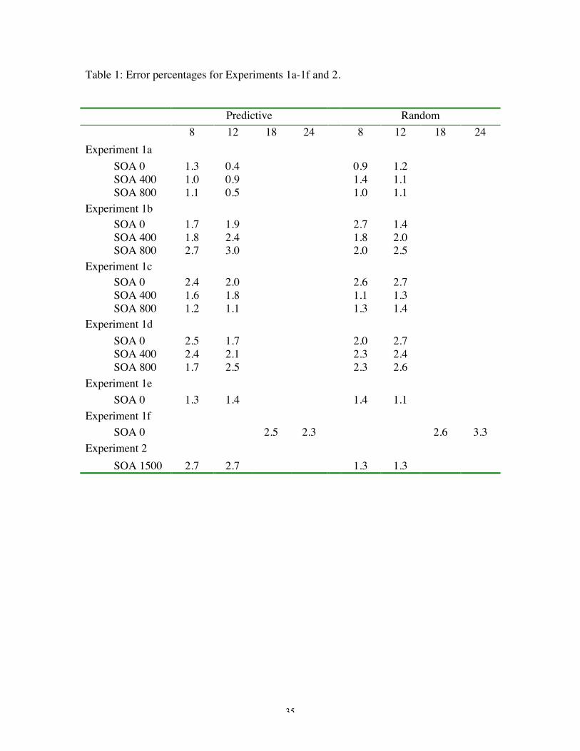
Table 1: Error percentages for Experiments 1a-1f and 2.
Predictive Random8 12 18 24 8 12 18 24
Experiment 1a SOA 0 1.3 0.4 0.9 1.2 SOA 400 1.0 0.9 1.4 1.1 SOA 800 1.1 0.5 1.0 1.1Experiment 1b SOA 0 1.7 1.9 2.7 1.4 SOA 400 1.8 2.4 1.8 2.0 SOA 800 2.7 3.0 2.0 2.5Experiment 1c SOA 0 2.4 2.0 2.6 2.7 SOA 400 1.6 1.8 1.1 1.3 SOA 800 1.2 1.1 1.3 1.4Experiment 1d SOA 0 2.5 1.7 2.0 2.7 SOA 400 2.4 2.1 2.3 2.4 SOA 800 1.7 2.5 2.3 2.6Experiment 1e SOA 0 1.3 1.4 1.4 1.1Experiment 1f SOA 0 2.5 2.3 2.6 3.3Experiment 2 SOA 1500 2.7 2.7 1.3 1.3

36
Table 2: Search slopes (msec/item) for Experiments 1b-1f (averaged across epochs 5-7).
Predictive Random
Experiment 1b SOA 0 39 36 SOA 400 48 55 SOA 800 43 55Experiment 1c SOA 0 38 50 SOA 400 36 70 SOA 800 34 50Experiment 1d SOA 0 57 65 SOA 400 45 70 SOA 800 64 61Experiment 1e SOA 0 14 17Experiment 1f SOA 0 28 78
37
Figure Legends
Figure 1. Example displays for Experiment 1a.
Figure 2. Mean correct RTs (msec) and search slopes (msec/item) for each SOA over
epoch in Experiment 1a.
Figure 3. Example displays, RT differences (msec) and slope differences (msec/item) for
Experiment 1b. The RT differences and slope differences both reflect the difference in
random (non-predictive) and predictive trials averaged across epochs 5 – 7. Here the
background texture/orientation was the predictive feature.
Figure 4. Example displays, RT differences (msec) and slope differences (msec/item) for
Experiment 1c. The RT differences and slope differences both reflect the difference in
random (non-predictive) and predictive trials averaged across epochs 5 – 7. Here the
stimuli and placeholder color was the predictive feature.
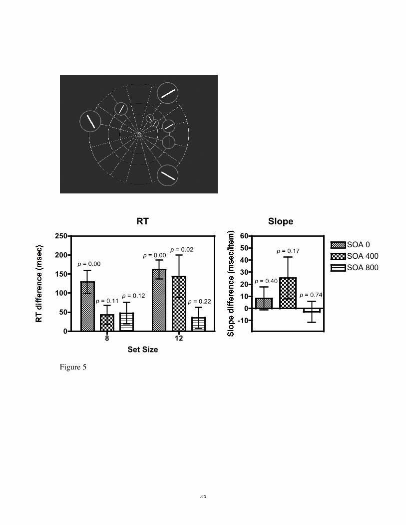
Figure 5. Example displays, RT differences (msec) and slope differences (msec/item) for
Experiment 1d. The RT differences and slope differences both reflect the difference in
random (non-predictive) and predictive trials averaged across epochs 5 – 7. Here the
stimuli and placeholder color was the predictive feature. The target in this condition was
either a horizontal or vertical line and the distractors were made up of oblique lines
orientated at –60, -30, 30 or 60 degrees.
38
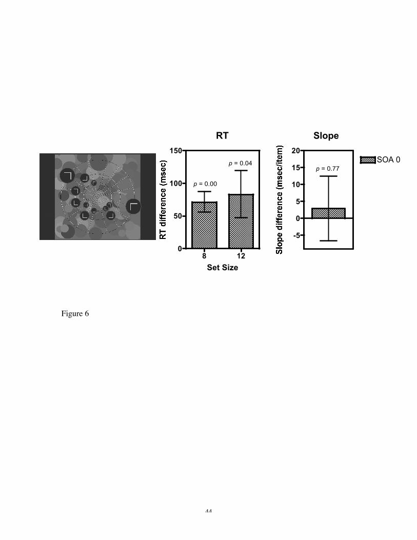
Figure 6. Example displays, RT differences (msec) and slope differences (msec/item) for
Experiment 1e. The RT differences and slope differences both reflect the difference in
random (non-predictive) and predictive trials averaged across epochs 5 – 7. Here the
background color was the predictive feature. The spatial configuration of the display
remained constant throughout the experiment.
Figure 7. Example displays, RT differences (msec) and slope differences (msec/item) for
Experiment 1f. The RT differences and slope differences both reflect the difference in
random (non-predictive) and predictive trials averaged across epochs 5 – 7. Here the
background color was the predictive feature. The target in this condition was either a
horizontal or vertical line and the distractors were made up of oblique lines orientated at
–60, -30, 30 or 60 degrees. The set size on a giving trial was either 18 or 24 items.
Figure 8. Individual search slopes (msec/item) for each participant in Experiment 1f for
both predictive and non-predictive (random) trials.
Figure 9. Mean correct RTs (msec) and search slopes (msec/item) over epoch for
Experiment 2. Participants were told in advance which background colors were
predictive.
39
Figure 1
SOA 400/800 msec
SOA 0 msec

40
Figure 2
(a)
(b)
(c)
SOA 0
SOA 400
SOA 800
1 2 3 4 5 6 7 8700
800
900
1000
1100
1200
1300
Predictive 8 Random 8Random 12Predictive 12
Epoch
1 2 3 4 5 6 7 80
10
20
30
40
50
60
70
80
PredictiveRandom
Epoch
1 2 3 4 5 6 7 8700
800
900
1000
1100
1200
1300
Epoch1 2 3 4 5 6 7 8
0
10
20
30
40
50
60
70
80
Epoch
1 2 3 4 5 6 7 8700
800
900
1000
1100
1200
1300
Epoch1 2 3 4 5 6 7 8
0
10
20
30
40
50
60
70
80
Epoch

41
Figure 3
RT
8 120
50
100
150
p = 0.00
p = 0.09 p = 0.20 p = 0.04
p = 0.12
p = 0.06
Set Size
Slope
-10
0
10
20
30
40
SOA 400
SOA 800
SOA 0
p = 0.73
p = 0.48
p = 0.37
42
Figure 4
RT
8 120
50
100
150
200
250
p = 0.01
p = 0.01
p = 0.00
p = 0.01
p = 0.97
p = 0.07
Set Size
Slope
0
10
20
30
40
50
60
SOA 400
SOA 800
SOA 0p = 0.02
p = 0.28p = 0.09
43
Figure 5
RT
8 120
50
100
150
200
250
p = 0.11p = 0.12
p = 0.00p = 0.02
p = 0.22
p = 0.00
Set Size
Slope
-10
0
10
20
30
40
50
60
SOA 400
SOA 800
SOA 0
p = 0.40
p = 0.17
p = 0.74
44
Figure 6
RT
8 120
50
100
150
p = 0.00
p = 0.04
Set Size
Slope
-5
0
5
10
15
20SOA 0
p = 0.77
45
Figure 7
RT
18 240
200
400
600
800
p = 0.02
p = 0.00
Set Size
Slope
0
25
50
75
100
125SOA 0
p = 0.06
46
Figure 8
1 2
-25
0
25
50
75
100
125
150
175
200
225
Individual
Mean
Predictive Random
47
Figure 9
SOA 1500
1 2 3 4 5 6 7 8500
600
700
800
900
1000
1100
1200
1300
1400
1500
Predictive 8 Random 8Random 12Predictive 12
Epoch1 2 3 4 5 6 7 8
0
10
20
30
40
50
60
70
80
PredictiveRandom
Epoch