high power laser matter interaction (springer, 2010) bbs
TRANSCRIPT

Springer Tracts in Modern PhysicsVolume 238
Managing Editor: G. Hohler, Karlsruhe
Editors: A. Fujimori, TokyoJ. Kuhn, KarlsruheTh. Muller, KarlsruheF. Steiner, UlmJ. Trumper, GarchingP. Wolfle, Karlsruhe
Starting with Volume 165, Springer Tracts in Modern Physics is part of the [SpringerLink] service.For all customers with standing orders for Springer Tracts in Modern Physics we offer the full textin electronic form via [SpringerLink] free of charge. Please contact your librarian who can receivea password for free access to the full articles by registration at:
springerlink.com
If you do not have a standing order you can nevertheless browse online through the table of contentsof the volumes and the abstracts of each article and perform a full text search.
There you will also find more information about the series.
Springer Tracts in Modern Physics
Springer Tracts in Modern Physics provides comprehensive and critical reviews of topics of current in-terest in physics. The following fields are emphasized: elementary particle physics, solid-state physics,complex systems, and fundamental astrophysics.Suitable reviews of other fields can also be accepted. The editors encourage prospective authors to cor-respond with them in advance of submitting an article. For reviews of topics belonging to the abovementioned fields, they should address the responsible editor, otherwise the managing editor.See also springer.com
Managing EditorGerhard HohlerInstitut fur Theoretische TeilchenphysikUniversitat KarlsruhePostfach 69 8076128 Karlsruhe, GermanyPhone: +49 (7 21) 6 08 33 75Fax: +49 (7 21) 37 07 26Email: gerhard.hoehler@physik.uni-karlsruhe.dewww-ttp.physik.uni-karlsruhe.de/
Elementary Particle Physics, EditorsJohann H. KuhnInstitut fur Theoretische TeilchenphysikUniversitat KarlsruhePostfach 69 8076128 Karlsruhe, GermanyPhone: +49 (7 21) 6 08 33 72Fax: +49 (7 21) 37 07 26Email: johann.kuehn@physik.uni-karlsruhe.dewww-ttp.physik.uni-karlsruhe.de/∼jk
Thomas MullerInstitut fur Experimentelle KernphysikFakultat fur PhysikUniversitat KarlsruhePostfach 69 8076128 Karlsruhe, GermanyPhone: +49 (7 21) 6 08 35 24Fax: +49 (7 21) 6 07 26 21Email: thomas.muller@physik.uni-karlsruhe.dewww-ekp.physik.uni-karlsruhe.de
Fundamental Astrophysics, EditorJoachim TrumperMax-Planck-Institut fur Extraterrestrische PhysikPostfach 13 1285741 Garching, GermanyPhone: +49 (89) 30 00 35 59Fax: +49 (89) 30 00 33 15Email: [email protected]/index.html
Solid-State Physics, EditorsAtsushi FujimoriEditor for The Pacific RimDepartment of PhysicsUniversity of Tokyo7-3-1 Hongo, Bunkyo-kuTokyo 113-0033, JapanEmail: [email protected]://wyvern.phys.s.u-tokyo.ac.jp/welcome en.html
Peter WolfleInstitut fur Theorie der Kondensierten MaterieUniversitat KarlsruhePostfach 69 8076128 Karlsruhe, GermanyPhone: +49 (7 21) 6 08 35 90Fax: +49 (7 21) 6 08 77 79Email: woelfle@tkm.physik.uni-karlsruhe.dewww-tkm.physik.uni-karlsruhe.de
Complex Systems, EditorFrank SteinerInstitut fur Theoretische PhysikUniversitat UlmAlbert-Einstein-Allee 1189069 Ulm, GermanyPhone: +49 (7 31) 5 02 29 10Fax: +49 (7 31) 5 02 29 24Email: [email protected]/theo/qc/group.html

Peter Mulser · Dieter Bauer
High Power Laser–MatterInteraction
ABC

Prof. Dr. Peter MulserTU DarmstadtInstitut fur Angewandte Physik (IAP)Hochschulstr. 664289 [email protected]
Prof. Dr. Dieter BauerUniversitat RostockInstitut fur PhysikAG Quantentheorie u.VielteilchensystemeUniversitatsplatz 318051 [email protected]
P. Mulser, D. Bauer, High Power Laser–Matter Interaction, STMP 238 (Springer, BerlinHeidelberg 2010), DOI 10.1007/978-3-540-46065-7
ISSN 0081-3869 e-ISSN 1615-0430ISBN 978-3-540-50669-0 e-ISBN 978-3-540-46065-7DOI 10.1007/978-3-540-46065-7Springer Heidelberg Dordrecht London New York
Library of Congress Control Number: 2010927139
c© Springer-Verlag Berlin Heidelberg 2010This work is subject to copyright. All rights are reserved, whether the whole or part of the material isconcerned, specifically the rights of translation, reprinting, reuse of illustrations, recitation, broadcasting,reproduction on microfilm or in any other way, and storage in data banks. Duplication of this publicationor parts thereof is permitted only under the provisions of the German Copyright Law of September 9,1965, in its current version, and permission for use must always be obtained from Springer. Violations areliable to prosecution under the German Copyright Law.The use of general descriptive names, registered names, trademarks, etc. in this publication does not imply,even in the absence of a specific statement, that such names are exempt from the relevant protective lawsand regulations and therefore free for general use.
Cover design: Integra Software Services Pvt. Ltd., Pondicherry
Printed on acid-free paper
Springer is part of Springer Science+Business Media (www.springer.com)

This book is dedicated to Professor GerhardHöhler. Without his continuousencouragement the work would not havebeen completed.


Preface
In the present volume the main aspects of high-power laser–matter interaction inthe intensity range 1010–1022 W/cm2 are described. We offer a guide to this topicfor scientists and students who have just discovered the field as a new and attractivearea of research, and for scientists who have worked in another field and want tojoin now the subject of laser plasmas. Being aware of the wide differences in thedegree of mathematical preparation the individual candidate has acquired we triedto present the subject in an almost self-contained manner. To be more specific, abachelor degree in physics enables the reader in any case to follow without diffi-culty. Generally fluid or gas dynamics and its relativistic version is not a part ofthis education; it is developed in the context where it is needed. Basic knowledge intheoretical mechanics, electrodynamics and quantum physics are the only prerequi-sites we expect from the reader. Throughout the book the main emphasis is on thevarious basic phenomena and their underlying physics. Not more mathematics thannecessary is introduced. The preference is given to ideas. A good model is the bestguide to the adequate mathematics.
There exist already some but not so many, however, good volumes and somemonographs on high-power laser interaction with matter. After research in this fieldhas grown over half a century and has ramified into many branches of fundamentalstudies and applications producing continuously new results, there is no indicationof saturation or loss of attraction, rather has excitement increased with the years:“There are no limits; horizons only” (G.A. Mourou). We take this as a motivationfor a new attempt of presenting our introduction to the achievements from the begin-ning up to present. An additional aim was to offer a more unified or more detailedview where this is possible now. Furthermore, the reader may find considerationsnot encountered in existing volumes on the field, e.g., on ideal fluid dynamics,dimensional analysis, questions of classical optics, instabilities and light pressure.In view of the rapidly growing field of atoms, molecules and clusters exposed tosuperstrong laser fields we considered it as compulsory to dedicate an entire chapterto laser–atom interaction and to the various modern theoretical approaches relatedto it. Finally, a consistent model of collisionless absorption is given.
Depending on personal preferences the reader may miss perhaps a section oninertial fusion, on high harmonic generation and on radiation from the plasma, oron traditional atomic and ionic spectroscopy. In view of the specialized literature
vii

viii Preface
already available on the subjects we think the self-imposed restriction is justified.Our referencing practice was guided by indicating material for supplementary stud-ies and establishing a continuity through the decades of research in the field ratherthan by the aim of completeness. The latter nowadays is easily achievable with theaid of the Internet.
We have tested the text with respect to comprehension and readability. Our firstthanks go to Prof. Edith Borie from the Forschungszentrum Karlsruhe. She proof-read great parts of the text very carefully and gave valuable comments. In secondplace we would like to thank Mrs. Christine Eidmann from Theoretical QuantumElectronics (TQE), TU Darmstadt, for typing in LATEX half of the book. We arefurther indebted to Prof. Rudolf Bock from GSI, Darmstadt, for helpful discussionsand precious hints. Further thanks for helpful discussions, critical comments, check-ing formulas go to Dr. Herbert Schnabl, Prof. Werner Scheid, Dr. Ralf Schneider,Dipl.-Phys. Tatjana Muth, Dr. Steffen Hain, and Dr. Francesco Ceccherini. We wantto acknowledge explicitly the continuous effort and support in preparing the finalmanuscript by Dr. Su-Ming Weng from the Insitute of Physics, CAS, China, atpresent fellow of the Humboldt Foundation at TQE. For his professional input tothe section on Brillouin scattering special thanks go to Dr. Stefan Hüller from EcolePolytechnique in Palaiseau.
Darmstadt, Germany Peter MulserRostock, Germany Dieter Bauer
Contents
1 Introductory Remarks and Overview . . . . . . . . . . . . . . . . . . . . . . . . . . . . . 1
2 The Laser Plasma: Basic Phenomena and Laws . . . . . . . . . . . . . . . . . . . . 52.1 Laser–Particle Interaction and Plasma Formation . . . . . . . . . . . . . . . . . 6
2.1.1 High-Power Laser Fields . . . . . . . . . . . . . . . . . . . . . . . . . . . . 62.1.2 Single Free Electron in the Laser Field (Nonrelativistic) . . 92.1.3 Collisional Ionization, Plasma Heating, and Quasineutrality 13
2.2 Fluid Description of a Plasma . . . . . . . . . . . . . . . . . . . . . . . . . . . . . . . . . 242.2.1 Two-Fluid and One-Fluid Models . . . . . . . . . . . . . . . . . . . . . 242.2.2 Linearized Motions . . . . . . . . . . . . . . . . . . . . . . . . . . . . . . . . . 372.2.3 Similarity Solutions . . . . . . . . . . . . . . . . . . . . . . . . . . . . . . . . 44
2.3 Laser Plasma Dynamics . . . . . . . . . . . . . . . . . . . . . . . . . . . . . . . . . . . . . . 582.3.1 Plasma Production with Intense Short Pulses . . . . . . . . . . . 602.3.2 Heating with Long Pulses of Constant Intensity . . . . . . . . . 632.3.3 Similarity Considerations . . . . . . . . . . . . . . . . . . . . . . . . . . . . 69
2.4 Steady State Ablation . . . . . . . . . . . . . . . . . . . . . . . . . . . . . . . . . . . . . . . . 742.4.1 The Critical Mach Number in a Stationary Planar Flow . . . 752.4.2 Ablative Laser Intensity . . . . . . . . . . . . . . . . . . . . . . . . . . . . . 782.4.3 Ablation Pressure in the Absence of Profile Steepening . . . 82
References . . . . . . . . . . . . . . . . . . . . . . . . . . . . . . . . . . . . . . . . . . . . . . . . . . . . . . 85
3 Laser Light Propagation and Collisional Absorption . . . . . . . . . . . . . . . 913.1 The Optical Approximation . . . . . . . . . . . . . . . . . . . . . . . . . . . . . . . . . . 92
3.1.1 Ray Equations . . . . . . . . . . . . . . . . . . . . . . . . . . . . . . . . . . . . . 933.1.2 WKB Approximation . . . . . . . . . . . . . . . . . . . . . . . . . . . . . . . 983.1.3 Energy Fluxes . . . . . . . . . . . . . . . . . . . . . . . . . . . . . . . . . . . . . 101
3.2 Stokes Equation and its Applications . . . . . . . . . . . . . . . . . . . . . . . . . . . 1073.2.1 Homogeneous Stokes Equation . . . . . . . . . . . . . . . . . . . . . . . 1073.2.2 Reflection-Free Density Profiles . . . . . . . . . . . . . . . . . . . . . . 1123.2.3 Collisional Absorption in Special Density Profiles . . . . . . . 1133.2.4 Inhomogeneous Stokes Equation . . . . . . . . . . . . . . . . . . . . . 115
3.3 Collisional Absorption . . . . . . . . . . . . . . . . . . . . . . . . . . . . . . . . . . . . . . . 118
ix

x Contents
3.3.1 Collision Frequency of Electrons Drifting at ConstantSpeed (Oscillator Model) . . . . . . . . . . . . . . . . . . . . . . . . . . . 120
3.3.2 Thermal Electrons in a Strong Laser Field . . . . . . . . . . . . . . 1293.3.3 The Ballistic Model . . . . . . . . . . . . . . . . . . . . . . . . . . . . . . . . 1343.3.4 Equivalence of Models . . . . . . . . . . . . . . . . . . . . . . . . . . . . . . 1423.3.5 Complementary Remarks . . . . . . . . . . . . . . . . . . . . . . . . . . . . 143
3.4 Inverse Bremsstrahlung Absorption . . . . . . . . . . . . . . . . . . . . . . . . . . . . 1463.5 Ion Beam Stopping . . . . . . . . . . . . . . . . . . . . . . . . . . . . . . . . . . . . . . . . . . 149References . . . . . . . . . . . . . . . . . . . . . . . . . . . . . . . . . . . . . . . . . . . . . . . . . . . . . . 150
4 Resonance Absorption . . . . . . . . . . . . . . . . . . . . . . . . . . . . . . . . . . . . . . . . . . 1534.1 Linear Resonance Absorption . . . . . . . . . . . . . . . . . . . . . . . . . . . . . . . . . 154
4.1.1 The Capacitor Model . . . . . . . . . . . . . . . . . . . . . . . . . . . . . . . 1594.1.2 Steep Density Gradients and Fresnel Formula . . . . . . . . . . . 1604.1.3 Comparison with Experiments . . . . . . . . . . . . . . . . . . . . . . . 163
4.2 Nonlinear Resonance Absorption . . . . . . . . . . . . . . . . . . . . . . . . . . . . . . 1644.2.1 High Amplitude Electron Plasma Waves at Moderate
Density Gradients . . . . . . . . . . . . . . . . . . . . . . . . . . . . . . . . . 1654.2.2 Resonance Absorption by Nonlinear Electron Plasma
Waves . . . . . . . . . . . . . . . . . . . . . . . . . . . . . . . . . . . . . . . . . . . 1684.3 Hot Electron Generation . . . . . . . . . . . . . . . . . . . . . . . . . . . . . . . . . . . . . 172
4.3.1 Acceleration of Electrons by an Intense SmoothLangmuir Wave . . . . . . . . . . . . . . . . . . . . . . . . . . . . . . . . . . . 173
4.3.2 Particle Acceleration by a Discontinuous Langmuir Wave . 1784.3.3 Vlasov Simulations and Experiments . . . . . . . . . . . . . . . . . . 179
4.4 Wavebreaking . . . . . . . . . . . . . . . . . . . . . . . . . . . . . . . . . . . . . . . . . . . . . . 1824.4.1 Hydrodynamic Wavebreaking . . . . . . . . . . . . . . . . . . . . . . . . 1844.4.2 Kinetic Theory of Wavebreaking . . . . . . . . . . . . . . . . . . . . . 186
References . . . . . . . . . . . . . . . . . . . . . . . . . . . . . . . . . . . . . . . . . . . . . . . . . . . . . . 191
5 The Ponderomotive Force and Nonresonant Effects . . . . . . . . . . . . . . . . 1935.1 Ponderomotive Force on a Single Particle . . . . . . . . . . . . . . . . . . . . . . . 194
5.1.1 Conservation of the Cycle-Averaged Energy . . . . . . . . . . . . 1955.1.2 The Standard Perturbative Derivation of the Force . . . . . . . 1995.1.3 Rigorous Relativistic Treatment . . . . . . . . . . . . . . . . . . . . . . 201
5.2 Collective Ponderomotive Force Density . . . . . . . . . . . . . . . . . . . . . . . . 2065.2.1 Bulk Force . . . . . . . . . . . . . . . . . . . . . . . . . . . . . . . . . . . . . . . . 2065.2.2 The Force Originating from Induced Fluctuations . . . . . . . 2065.2.3 Global Momentum Conservation . . . . . . . . . . . . . . . . . . . . . 209
5.3 Nonresonant Ponderomotive Effects . . . . . . . . . . . . . . . . . . . . . . . . . . . 2105.3.1 Ablation Pressure . . . . . . . . . . . . . . . . . . . . . . . . . . . . . . . . . . 2115.3.2 Filamentation and Self-Focusing . . . . . . . . . . . . . . . . . . . . . . 2195.3.3 Modulational Instability . . . . . . . . . . . . . . . . . . . . . . . . . . . . . 222
References . . . . . . . . . . . . . . . . . . . . . . . . . . . . . . . . . . . . . . . . . . . . . . . . . . . . . . 225
Contents xi
6 Resonant Ponderomotive Effects . . . . . . . . . . . . . . . . . . . . . . . . . . . . . . . . . 2296.1 Tools . . . . . . . . . . . . . . . . . . . . . . . . . . . . . . . . . . . . . . . . . . . . . . . . . . . . . 229
6.1.1 Waves, Energy Densities and Wave Pressure . . . . . . . . . . . . 2306.1.2 Doppler Shifts . . . . . . . . . . . . . . . . . . . . . . . . . . . . . . . . . . . . . 232
6.2 Instabilities Driven by Wave Pressure . . . . . . . . . . . . . . . . . . . . . . . . . . 2386.2.1 Resonant Ponderomotive Coupling . . . . . . . . . . . . . . . . . . . . 2386.2.2 Unstable Configurations . . . . . . . . . . . . . . . . . . . . . . . . . . . . . 2426.2.3 Growth Rates . . . . . . . . . . . . . . . . . . . . . . . . . . . . . . . . . . . . . . 245
6.3 Parametric Amplification of Pulses . . . . . . . . . . . . . . . . . . . . . . . . . . . . 2566.3.1 Slowly Varying Amplitudes . . . . . . . . . . . . . . . . . . . . . . . . . . 2576.3.2 Quasi-Particle Conservation and Manley–Rowe Relations 2586.3.3 Light Scattering at Relativistic Intensities . . . . . . . . . . . . . . 259
References . . . . . . . . . . . . . . . . . . . . . . . . . . . . . . . . . . . . . . . . . . . . . . . . . . . . . . 265
7 Intense Laser–Atom Interaction . . . . . . . . . . . . . . . . . . . . . . . . . . . . . . . . . . 2677.1 Atomic Units . . . . . . . . . . . . . . . . . . . . . . . . . . . . . . . . . . . . . . . . . . . . . . . 2677.2 Atoms in Strong Static Electric Fields . . . . . . . . . . . . . . . . . . . . . . . . . . 270
7.2.1 Separation of the Schrödinger Equation . . . . . . . . . . . . . . . . 2727.2.2 Tunneling Ionization . . . . . . . . . . . . . . . . . . . . . . . . . . . . . . . . 277
7.3 Atoms in Strong Laser Fields . . . . . . . . . . . . . . . . . . . . . . . . . . . . . . . . . 2817.3.1 Floquet Theory and Dressed States . . . . . . . . . . . . . . . . . . . . 2837.3.2 Non-Hermitian Floquet Theory . . . . . . . . . . . . . . . . . . . . . . . 2877.3.3 Stabilization . . . . . . . . . . . . . . . . . . . . . . . . . . . . . . . . . . . . . . . 2887.3.4 Strong Field Approximation . . . . . . . . . . . . . . . . . . . . . . . . . 2927.3.5 Few-Cycle Above-Threshold Ionization . . . . . . . . . . . . . . . . 3017.3.6 Simple Man’s Theory . . . . . . . . . . . . . . . . . . . . . . . . . . . . . . . 3047.3.7 Interference Effects . . . . . . . . . . . . . . . . . . . . . . . . . . . . . . . . . 3067.3.8 High-Order Harmonic Generation . . . . . . . . . . . . . . . . . . . . 3087.3.9 Strong Field Approximation for High-Order Harmonic
Generation: the Lewenstein Model . . . . . . . . . . . . . . . . . . . 3137.3.10 Harmonic Generation Selection Rules . . . . . . . . . . . . . . . . . 315
7.4 Strong Laser–Atom Interaction Beyond the Single Active Electron . . 3197.4.1 Nonsequential Ionization . . . . . . . . . . . . . . . . . . . . . . . . . . . . 320
References . . . . . . . . . . . . . . . . . . . . . . . . . . . . . . . . . . . . . . . . . . . . . . . . . . . . . . 326
8 Relativistic Laser–Plasma Interaction . . . . . . . . . . . . . . . . . . . . . . . . . . . . . 3318.1 Essential Relativity . . . . . . . . . . . . . . . . . . . . . . . . . . . . . . . . . . . . . . . . . . 331
8.1.1 Four Vectors . . . . . . . . . . . . . . . . . . . . . . . . . . . . . . . . . . . . . . 3318.1.2 Momentum and Kinetic Energy . . . . . . . . . . . . . . . . . . . . . . 3368.1.3 Scalars, Contravariant and Covariant Quantities . . . . . . . . . 3378.1.4 Ideal Fluid Dynamics . . . . . . . . . . . . . . . . . . . . . . . . . . . . . . . 3408.1.5 Kinetic Theory . . . . . . . . . . . . . . . . . . . . . . . . . . . . . . . . . . . . 3418.1.6 Center of Momentum and Mass Frame of Noninteracting
Particles . . . . . . . . . . . . . . . . . . . . . . . . . . . . . . . . . . . . . . . . . . 343

xii Contents
8.1.7 Moment Equations . . . . . . . . . . . . . . . . . . . . . . . . . . . . . . . . . 3448.1.8 Covariant Electrodynamics . . . . . . . . . . . . . . . . . . . . . . . . . . 348
8.2 Particle Acceleration in an Intense Laser Field . . . . . . . . . . . . . . . . . . . 3518.2.1 Particle Acceleration in Vacuum . . . . . . . . . . . . . . . . . . . . . . 3538.2.2 Wakefield and Bubble Acceleration . . . . . . . . . . . . . . . . . . . 359
8.3 Collisionless Absorption in Overdense Matter and Clusters . . . . . . . . 3638.3.1 Computer Simulations of Collisionless Laser–Target
Interaction . . . . . . . . . . . . . . . . . . . . . . . . . . . . . . . . . . . . . . . . 3648.3.2 Search for Collisionless Absorption . . . . . . . . . . . . . . . . . . . 3718.3.3 Collisionless Absorption by Anharmonic Resonance . . . . . 378
8.4 Some Relativity of Relevance in Practice . . . . . . . . . . . . . . . . . . . . . . . 3928.4.1 Overview . . . . . . . . . . . . . . . . . . . . . . . . . . . . . . . . . . . . . . . . . 3928.4.2 Critical Density Increase for Fast Ignition . . . . . . . . . . . . . . 3938.4.3 Relativistic Self-Focusing . . . . . . . . . . . . . . . . . . . . . . . . . . . 400
References . . . . . . . . . . . . . . . . . . . . . . . . . . . . . . . . . . . . . . . . . . . . . . . . . . . . . . 401
Index . . . . . . . . . . . . . . . . . . . . . . . . . . . . . . . . . . . . . . . . . . . . . . . . . . . . . . . . . . . . . 405

Chapter 1Introductory Remarks and Overview
Laser-produced plasmas represent a modern, physically rich topic of electromag-netic interaction with macroscopic matter. The laser intensities extend from thethreshold of plasma formation at approximately 1010 W/cm2 on the nanosecondtime scale up to the highest energy flux densities of several 1022 W/cm2 currentlyavailable in the femtosecond domain. The laser is capable of supplying enormousamounts of energy in very short times. The first salient aspect of the laser plasmais its fast dynamics, and in concomitance, its inhomogeneity in density, tempera-ture and flow velocity. As the laser acts preferentially on the light electrons theydetermine the fast time scale. The interaction itself is characterized by a limitingelectron density beyond which no electromagnetic propagation is possible (criticaldensity, cut-off). This property is the main reason for laser plasmas to be very hotand more or less close to ideality, and is responsible for steep density variationsin the transition zone from underdense to overdense plasma. The irreversible inter-action (absorption, heating of the electrons) is accomplished by friction betweenelectrons and ions due to electron–ion collisions, so-called collisional or inversebremsstrahlung absorption, and by resonances of the free electrons in the self-generated electrostatic fields. At super-high intensities when the mitigating effectof collisions (and absorption) is almost absent the laser acts more and more as anextremely efficient accelerator of energetic electrons by anharmonic resonance. Thiscollisionless absorption process gives the electron fluid properties far from thermalequilibrium, not to mention the formation of an electron temperature very muchexceeding that of the ion fluid. Overdense samples of matter are indirectly heatedonly by electron heat conduction, fast electron jets, electron plasma waves, plasmaradiation and plasma shock waves. On the slow time scale of the ions the electronsare bound to them by quasi-neutrality, one of the fundamental properties of anyplasma state.
The dynamics of the laser plasma on the ion time scale is governed by the ther-mal pressure of the electrons, and to a certain extent, by that of the ions. However,this is only half the truth. Any oscillating force, like that impressed by the laserfield, in presence of inhomogeneities gives origin to a secular force on the slowtime scale, here in the plasma on the ions. This so-called ponderomotive force, orpressure gradient of light, and more in general, of waves not only does inhibit thetendency towards uniformity in the process of plasma expansion; it does impress
P. Mulser, D. Bauer, High Power Laser–Matter Interaction, STMP 238, 1–4,DOI 10.1007/978-3-540-46065-7_1, C© Springer-Verlag Berlin Heidelberg 2010
1

2 1 Introductory Remarks and Overview
also a whole variety of structures onto the plasma, of resonant character like stimu-lated Raman and Brillouin scattering as well as various other parametric three-waveinteraction phenomena; or of non-resonant character as laser beam filamentationand self-focusing, self-trapping of light, beam self-modulation and ion density pro-file steepening. The ponderomotive force, although considerably weaker than thedirect high-frequency force of the laser beam, determines the plasma dynamics toa decisive degree due to its secular character. It makes the laser plasma inherentlyunstable.
Under several aspects the laser plasma represents an extreme state of matter farfrom thermodynamic equilibrium, both on large scale (e.g., spatial gradients of den-sity, temperature, pressure, ionization) and on local scale (e.g., electron and iontemperatures differing from each other, non-equilibrium velocity distribution). Inthe intense field collisional heating tends towards the generation of super-Gaussianelectron distributions in place of a Maxwellian. At resonance electron plasma wavesare driven into non-linearities to the extent of breaking, i.e. quenching of modes byself-interaction, and to the already mentioned generation of relativistic electron jets,directly by the action of the laser electric field itself near the critical density or, inthe underdense plasma, by the ponderomotive wake behind the laser propagatingthrough the plasma. The Lorentz force governing the electron motion is nonlinear,hence introducing anharmonicities in the high-frequency current densities whichas sources for the fields in the Maxwell equations generate high harmonics of thefundamental laser frequency up to some thousandth order. Of particular interest isthe interaction of the intense laser field on the atomic and molecular level where, incontrast to standard perturbative external interaction, the main actor is the laser fieldwhile the atomic potential represents the perturbation once ionization has occurred.In concomitance, above threshold ionization into the high continuum becomes sig-nificant. Effects based on electrons driven back to the ion core by the laser fieldemerge, such as nonsequential ionization and high-harmonic emission, the latterbeing particularly relevant for applications, e.g., the generation of attosecond pulsesand structural imaging. The dynamics of atoms in strong laser fields have become arich and fascinating field of modern atomic and plasma physics.
In view of the strong nonlinearities of the basic equations governing the observedphenomena numerical simulation codes have become an indispensable means ofaccompanying the experiments for analysis and interpretation. Sometimes the sim-ulations themselves need interpretation in the sense that they may not tell at all whatthe underlying physics producing the results is. An eminent example is collisionlessabsorption and generation of energetic electrons by anharmonic resonance. Suchsituations are the moment of truth for simple analytical models.
In the second chapter an introduction to the plasma formation process by intenselaser beams is given and the subsequent plasma dynamics is described phenomeno-logically by the use of a two fluid model. The salient features thereby are quasineu-trality and shielding of the plasma. Experience shows that having assimilated theseprinciples may serve as a criterion for the definition of who is a plasma physicistand who is not yet. Another basic concept is laser light absorption by collisionsand its equivalence to the inverse bremsstrahlung model. For this reason, in a crude

1 Introductory Remarks and Overview 3
way it is already introduced in Chap. 2 and then treated extensively in Chap. 3.Generally it is believed that the so-called dielectric approach gives the most satisfac-tory answer. However, by comparison with the ballistic model we show that undera strong electron drift in the intense laser field the standard dielectric models areinappropriate because of showing very bad convergence and leading to erroneousphysical conclusions, for instance on shielding. The root of the difficulties lies inthe inappropriate choice of harmonic waves as a basis of description. In other words,describing the hydrogen atom by choosing as a basis the Hermite polynomials of theharmonic oscillator would not lead to enlightenment. The search for an adequatebasis is still going on. Chapter 4 is dedicated mainly to the description of linearresonance absorption at the plasma frequency and its mild nonlinearities as well asthe self-quenching of the high amplitude electron plasma wave by wave breaking.
Until the first half of the past century light pressure was believed to be a subjectof academic interest in the laboratory, only for the equilibrium of stars it played adecisive role, as discovered by A. S. Eddington. In recent years the situation hasreversed. We are able to generate pressures by laser light in the laboratory whichexceed the gas pressure in the sun easily by a factor of 100. However, already atmoderate laser intensities the salient role of light and wave pressure (ponderomo-tive force) for the plasma dynamics and ablation pressure (profile steepening) aswell as for the origin of a whole class of parametric plasma instabilities has becomeevident. This is shown in detail and under various aspects in Chaps. 5 and 6. Atthe threshold of laser break down avalanche ionization is by electron impact once asufficient number of free electrons has been created (first free mysterious electronof Chap. 2). At high laser intensities above 1012 W/cm2 multiphoton and sequentialand non-sequential field ionization start dominating and, in concomitance, lead to avariety of other effects, described altogether in Chap. 7. Finally, Chap. 8 is dedicatedto physics induced by relativistic laser beam intensities beyond 1018 W/cm2, likeelectron acceleration, collisionless absorption in simulations and the analysis of theunderlying heating mechanism in overdense targets, self-focusing, and applications.Owing to the dominance of relativistic effects a short systematic introduction torelativity and to relativistic kinetic theory is also presented. In general we preferfluid models to the various kinetic approaches for their physical evidence and sim-plicity. The hydrodynamic description of plasmas may never be totally correct, onthe other hand however, it may be extremely difficult to find situations in which itfails completely. Hydrodynamics is never true and never wrong.
After all, the reader may find some considerations not encountered in existingvolumes in the field. Examples may be the topological aspect of ideal fluid dynamicsand an elementary introduction to dimensional analysis and similarity in Chap. 2,the oscillator model of dynamical shielding, the nonphysical origin of asymptoticformulas of collisional absorption under strong drift containing the product of twologarithms and a true argument on why the classical Landau length is to be replacedby the reduced de Broglie wavelength in Chap. 3, a thorough discussion of the Fres-nel limit of linear resonance absorption in steep density profiles and an attemptto classify the various routes into wave breaking (Chap. 4), alternative derivationsof the ponderomotive force density in plasmas and a purely physical proof of the
4 1 Introductory Remarks and Overview
unstable response of a plasma to this force in Chaps. 5 and 6, the treatment of theionization dynamics in strong laser fields by a whole variety of modern theoreticalapproaches (Chap. 7), and finally, the already mentioned solution of the problemof collisionless absorption in overdense matter. As with growing laser intensitiesthe researcher in the field is more and more faced with relativistic phenomena wepresent a short introduction to essential relativity also.
Chapter 2The Laser Plasma: Basic Phenomena and Laws
High power lasers when focused onto matter lead to extremely rapid ionization bydirect photoeffect or, depending on wavelength and material, by multiphoton pro-cesses. When a sufficient number of free electrons is created the formation of adense, highly ionized plasma is more efficiently continued by electron–neutrals andelectron–ion impact ionization. In view of many important applications the genera-tion of a homogeneous high density and, at the same time, very hot plasma wouldbe most desirable. Unfortunately, at present high power lasers operate in the nearinfrared domain. As a consequence, direct interaction of the laser beam with matteris possible only below a limiting density, the so-called critical density which, atnonrelativistic intensities, is typically a hundred times lower than solid density. Onlywhen the oscillatory velocity of the electrons becomes relativistic at laser intensitiesbeyond 1018 Wcm−2 direct interaction with higher densities takes place. It is due tothis cut-off that the plasma production process becomes a very dynamic interplaybetween laser beam stopping and plasma expansion and makes the plasmas createdby lasers from overdense matter very inhomogeneous and short-living. Within cer-tain limits efficient energy transfer from the laser to overdense plasma regions ismade possible by electron thermal conduction. As there are physical limits inherentin this process also energy transfer to more dense matter is accomplished by shockwave heating and UV and X radiation from the moderately dense plasma.
The dynamics of plasma formation and heating is best understood on the basisof elementary processes induced in atoms and on the electrons by the laser beam.Hence, first, elements of the motion of a single electron in the electromagnetic fieldand its collisions with atoms and ions are presented. The charged particles lead tocollective fields which in turn act back on the single particles. These processes aredescribed in the simplest way by the conservation equations of charge, momen-tum, and energy of the two-fluid plasma model. Owing to the high mobility of theelectrons and ions under intense laser irradiation such a hydrodynamic descriptionin terms of averaged quantities, density, flow velocity, temperature, averaged elec-tric and magnetic fields, can never be the full truth. On the other hand there is itsconceptual simplicity which makes of it a very powerful instrument for describingphenomena, even in regions where its validity is questionable. In the following sec-tions of this chapter the basic concepts of collisional heating and quasineutrality areintroduced and the basic building blocks of laser-plasma dynamics, linear plasma
P. Mulser, D. Bauer, High Power Laser–Matter Interaction, STMP 238, 5–89,DOI 10.1007/978-3-540-46065-7_2, C© Springer-Verlag Berlin Heidelberg 2010
5

6 2 The Laser Plasma
waves, thermal waves, shocks and the rarefaction wave are presented and applied togive a first picture of the laser plasma dynamics.
2.1 Laser–Particle Interaction and Plasma Formation
It is a common experience that a laser beam when focused in air, generates a spark assoon as the flux density exceeds a well defined, i.e., a reproducible threshold value[1–3]. Such a plasma formation process also occurs in liquids and solids at compa-rable flux densities. The typical average threshold in insulators is I0 = 109 Wcm−2;in conducting materials I0 is lower by orders of magnitude [4, 5]. Thresholds arematerial- and density-dependent and they are particularly sensitive to impurities andsurface quality. As a rule, the thresholds decrease with increasing laser wavelengthand pulse duration [6–8].
In this book the interaction of laser radiation with dense matter at flux densitiesabove the threshold for plasma formation is treated. By high power lasers we meansystems for which the intensity exceeds I0. Dense matter is characterized by theexistence of a critical surface in the plasma, to be defined later. As the plasma rar-efies during interaction with the laser beam, many important processes begin to takeplace in the underdense region in front of the critical surface. Such phenomena mayalso occur in completely underdense plasmas, in which no critical layer exists.
2.1.1 High-Power Laser Fields
Extremely powerful laser systems have been built for various applications, amongwhich inertial confinement fusion (ICF) plays a central role [9–14]. They can benaturally subdivided into two classes: energetic lasers in the ns–ps terawatt (TW)regime and superintense ultrashort lasers, sometimes also called U3 systems (“Ultra-short, Ultraintense, Ultrapowerful”) or T3 lasers (“Table-Top TW”) depending onwhether operating in the petawatt (PW) or TW sub-ps domain.
The peak of large laser system engineering is currently represented by NIF(“National Ignition Facility”) at Lawrence Livermore National Laboratory (LLNL)and LMJ (“Laser Mega Joule”) in Bordeaux.
At low energies of the order of 1–100 J advances in laser technology have madeit possible to generate subpicosecond pulses approaching intensity levels of up to1023 Wcm−2, and, nonetheless, containing energy at a level of not more than 1 J.This fact renders the U3 systems extremely flexible compared to the large ns laserfacilities. The use of novel pulse compression techniques leads to pulses as shortas 5 fs [15]. In itself the CO2 laser also represents an interesting and, in contrastto the glass and iodine lasers [16], a highly efficient system. However, owing toits low frequency (ωCO2 = ωNd/10) collisional coupling to the plasma is reduced,and anomalous interaction with matter intensifies via undesirable parametric andcollective processes [17]. For these reasons the high power Antares laser at LosAlamos National Laboratory (LANL) (40 kJ in τ � 2 ns) was shut down.

2.1 Laser–Particle Interaction and Plasma Formation 7
Studying high power laser-matter interaction at present means that the powerdensity to be covered ranges from I = 1010 to approximately 1023 Wcm−2 forwavelengths having λ <∼ λNd, i.e., from the near IR to the near UV with λ >∼ λKrF,over times τ from tens of nanoseconds down to a few femtoseconds. One shouldremember that a high power laser pulse with τ = 1 ns is an energy packet oflength l = 30 cm; at τ = 100 fs this length shrinks to l = 30 µm = 0.03 mm!For meaningful laser-matter interaction studies a well defined short rise time andthe absence of an undefined prepulse, even of relatively low intensity, is an absolutenecessity.
In most cases a clean pulse is composed of many modes characterized by awavevector k and polarization σ so that its total electric field E(x, t) is the sumof the single components Ekσ (x, t),
E(x, t) =∑
kσ
Ekσ (x, t), Ekσ (x, t) = Ekσ (x, t)ei(kx−ω(k)t), (2.1)
ω(k) obeying a proper dispersion relation. Ekσ (x, t) is, in contrast to Ekσ (x, t), aslowly varying function of space and time and is called the amplitude of the modekσ . By choosing Ekσ complex, phase differences between modes are automaticallytaken into account. Since, on the other hand, physical quantities are real, (2.1) readsas �E = ∑�Ekσ . When studying nonlinear relations among the Ekσ ’s we haveto take care of this explicitly. Throughout the book the scalar product of two threevectors a, b is written in the compact form ab, and the same convention is used inChap. 8 for the scalar product of two four vectors A and B: AB = AαBα . Possibleambiguities are avoided by the use of brackets, e.g., a × (b× c) = (ac)b− (ab)c;(v∇)v = (v ·∇)v.
One can simplify the radiation field when the interaction process under investiga-tion occurs on a time scale T of the order of an oscillation period 2π/ω or shorter asis the case for collisional interaction, light propagation, and incoherent scattering. Insuch and numerous other cases the focused laser beam can be approximated locallyby a linearly polarized plane wave of complex amplitude E (index σ suppressed forcompactness),
E(x, t) = Eeikx−iωt , B = kω× E, (2.2)
with the intensity I , in vacuum, defined by the cycle-averaged modulus of the Poynt-ing vector S,
I = |S| = c2ε0|E × B| = 1
2cε0 E E
∗. (2.3)
It is in this approximation that the laser energy flux density is identical with an“intensity” I . For practical purposes the numerical relation between amplitude andintensity is very useful,

8 2 The Laser Plasma
Table 2.1 Wavelength, circular frequency ω, photon energy hω, and critical density nc of a fewhigh power lasers
Laser Wavelength, nm ω, s−1 hω, eV nc, cm−3
CO2 10,600 1.78× 10¹⁴ 0.12 1019
I 1315 1.46× 10¹⁵ 0.96 6.5× 10²⁰
Nd 1060 1.78× 10¹⁵ 1.17 1021
Ti:Sa 800 2.36× 10¹⁵ 1.55 1.8× 10²¹
KrF 248 7.59× 10¹⁵ 4.99 1.8× 10²²
E [V/cm] = 27.5×{
I [W/cm2]}1/2
. (2.4)
We list wavelengths, frequencies, photon energies, and critical electron density nc =mε0ω
2/e2 [see also (2.94)] for the most common high power lasers in Table 2.1.For the interested reader it should be mentioned that the classical coherent wave(2.2) is an approximation which is only asymptotically reached by the best systemslasing well above threshold. A single mode having a well-defined wavevector kσand polarization σ can contain 0, 1, 2, 3, . . . , n photons. Accordingly, the radiationfield is in one of the following photon number states (Fock states) |0〉 (vacuum),|1〉, |2〉, |3〉, . . . .., |n〉, or a superposition of them. Since the amplitude of thesestates is sharp,
E =(
2hω
ε0V
)1/2 (n + 1
2
)1/2
, (2.5)
their phase ψ is completely uncertain (see, e.g., [18, 19]). Here, V is the volume ofan arbitrary cube containing the mode kσ . The quantum state coming closest to theclassical mode (2.2) is the so-called coherent or Glauber state |α〉 [18],
|α〉 = exp
(−|α|
2
2
)∑
n≥0
αn
(n!)1/2|n〉, (2.6)
where α is an arbitrary complex number. Each number state contributes with theprobability Pn of a Poisson distribution,
Pn = |〈n|α〉|2 = |α|2n
n! e−|α|2 .
It is easily seen that the average photon number n and its relative mean squaredeviation Δn = 〈n2 − 〈n〉2〉1/2 are, by definition,
〈n〉 =∑
n≥0
Pnn = |α|2, Δn
〈n〉 =1
|α| . (2.7)

2.1 Laser–Particle Interaction and Plasma Formation 9
In high power laser experiments with Ti:Sa wavelength 〈n〉 ranges typically from1010 to 1020 cm−3. The electric field E is the expectation value of the field operator
Eop = i(hω/2ε0V )1/2{ei kx−iωt a − e−ikx+iωt a†}, [a, a†] = 1,
E(x, t) = 〈α|Eop|α〉 = −(2hω/ε0V )1/2|α| sin(kx − ωt + ϕ). (2.8)
It differs from the coherent classical wave (2.2) merely by the uncertainty in E [18]:
ΔE =(〈α|E2
op|α〉 − E2(x, t))1/2 = (hω/2ε0V )1/2. (2.9)
This shows that all uncertainty originates from the vacuum state |0〉. It followsfrom (2.5) to (2.9) that at high intensities and acceptable coherence the classicalfield (2.2) is an excellent approximation and that quantum field effects do not playa significant role in high power laser matter interaction. However, one must bear inmind that “nonclassical” states of light exist, even at high intensities, for instancephoton number states |n〉, the preparation of which is certainly a very difficult task,but nevertheless possible [20, 21]. One of the most striking successes of field quanti-zation is the derivation of the Einstein coefficient A for spontaneous emission solelyfrom the commutation relations of the photon creation and annihilation operators a†
and a.
2.1.2 Single Free Electron in the Laser Field (Nonrelativistic)
Above the breakdown threshold, matter is transformed into a dense plasma. Theproperties of such a fluid are largely determined by the collective motion of freeelectrons. The electrons themselves move as single particles in the E- and B-fieldswhich are the superposition of fields Eex, Bex, imposed from outside, and internalfields Ein, Bin, produced by their collective motions. Classically, the dynamics of afree electron of mass m is governed by the Lorentz force
d
dt(mv) = −e(E + v × B), (2.10)
which in this form with variable mass is correct at any relativistic speed. Throughoutthe book however all symbols referring to masses m, mi , etc. indicate their restmasses. Accordingly, the left-hand side of (2.10) is written as d(γmv)/dt with γ
the Lorentz factor. See also the comment on the “relativistic mass increase” follow-ing (8.17) in Sect. 8.1.1. A solution x(t) is such that the equation is satisfied forgiven values E(x(t), t) and B(x(t), t) which shows that (2.10) is in general highlynonlinear. However, for a field of the form (2.2) the nonrelativistic solution is easilyobtained. To a first approximation, B can be disregarded because its magnitude isB = E/vϕ , with the phase velocity vϕ = ω/k, and d/dt can be replaced by ∂/∂t .One finds for the purely oscillating quantities

10 2 The Laser Plasma
v = −ie
mωE = veikx−iωt ; v = −i
e
mωE, (2.11)
δ = e
mω2E = δeikx−iωt ; δ = e
mω2E. (2.12)
δ is the periodic displacement of the electron; v and δ are the amplitudes of v andδ. For practical purposes it is convenient to normalize their numerical values to theTi:Sa laser field with intensity I in Wcm−2 and λTi:Sa = 800 nm,
β = v
c= 6.8× 10⁻¹⁰ λ
λTi:Sa
{I [W/cm2]
}1/2(2.13)
δ [nm] = 8.7× 10⁻⁸(
λ
λTi:Sa
)2 {I [W/cm2]
}1/2. (2.14)
Another expression of interest is the cycle-averaged oscillation energy W ,
W = 1
4mv
2 = e2
4mω2E E
∗ = 1
4eδ∗
E; (2.15)
W [eV] = 6.0× 10⁻¹⁴(
λ
λTi:Sa
)2
I [W/cm2]. (2.16)
When the electron oscillation becomes relativistic,
W = mc2
{[1+ 1
2
(e Amc
)2 ]1/2
− 1
}(2.17)
where A is the vector potential amplitude. For circular polarization the factors 1/4in (2.15) and 1/2 in (2.17) have to be multiplied by 2.
The various expressions for W are given in view of another interpretation lateron. In Table 2.2 representative values of E, β, δ and relativistic W are given forthe Nd and KrF laser in the intensity range from 1012 to 1020 Wcm−2 and fora monochromatic wave of sun light intensity, all assumed to be concentrated atλNd = 1060 nm or at λKrF = 248 nm, respectively. At I = 1018 Wcm−2 relativisticeffects become noticeable for Nd. The comparison reveals that in normal nonreso-nant optics the additional motion induced by the light field is completely negligiblerelative to the internal dynamics of matter and, as a consequence, optics is linear(e.g., the refractive index does not depend on E); however this may no longer betrue for intense laser fields. It is fortunate for our survival that sunlight is of highfrequency, and not coherent over appreciable length scales; otherwise, a voltagedifference of 1 kV over 1 m would be generated! Note that at 1011 Wcm−2 and Ndfrequency the oscillation amplitude is equal to the Bohr radius.
The nonrelativistic Hamiltonian of the free electron in the Coulomb (or trans-verse) gauge is

2.1 Laser–Particle Interaction and Plasma Formation 11
Table 2.2 Fields and oscillations (relativistic). I intensity, E, β = v/c, δ amplitudes of field, rel-ative velocity, and oscillation amplitude, respectively; W oscillation energy. The last row containsdata for sunlight
I E λNd = 1060 nm λKrF = 248 nm
[Wcm−2] [V cm−1] β δ [nm] W [eV] β δ [nm] W [eV]
1012 3× 10⁷ 9× 10⁻⁴ 0.15 0.1 2× 10⁻⁴ 8× 10⁻³ 6× 10⁻³
1013 9× 10⁷ 3× 10⁻³ 0.5 1.0 7× 10⁻⁴ 2.6× 10⁻² 0.061014 3× 10⁸ 9× 10⁻³ 1.5 10 2× 10⁻³ 8.2× 10⁻² 0.581016 3× 10⁹ 0.09 15.3 1050 0.02 0.82 581018 3× 10¹⁰ 0.68 128.0 96 keV 0.21 8.2 5.7 keV1020 3× 10¹¹ 0.995 235.5 2803 0.91 46.3 410
0.133 10 3× 10⁻¹⁰ 6× 10⁻⁸ 1.4× 10⁻¹⁴ 8× 10⁻¹¹ 3× 10⁻⁹ 8× 10⁻¹⁶
H = 1
2m( p+ e A)2. (2.18)
A(x, t) is the vector potential; it is related to the electric field by E = −∂t A.For a monochromatic plane wave A = E/iω. The quantity p + e A = mv is themechanical momentum. In the dipole approximation A does not depend on x, A =A(t), and the Schrödinger equation (with A nonquantized),
1
2m[ p+ e A(t)]2|ψ〉 = ih
∂
∂t|ψ〉, (2.19)
is solvable analytically. In fact, it is easily shown that the Volkov states ψ(x, t) =〈x|ψ〉, (see also Chap. 7),
ψ(x, t) = exp
[ikx − i
2mh
∫ t [hk + e A(t ′)
]2dt ′]
(2.20)
satisfy (2.19). In the absence of the radiation field (A = 0) they reduce to theelementary plane waves ψ = exp(ikx − iEt/h) of the free electron. The energyexpectation values E are
E = ih〈ψ |∂t |ψ〉 = 〈ψ |H |ψ〉 = 1
2m(hk + e A)2.
Cycle-averaging leads to
E = 1
2m(hk + e� Ae−iωt )2 = (hk)2
2m+ e2
4mA A
∗ = Ekin +W, (2.21)
in perfect agreement with the classical result for the oscillation energy. Silin andUryupin [22] used Volkov states to calculate inverse bremsstrahlung absorption inan elegant way in a strong radiation field (see the next chapter).

12 2 The Laser Plasma
Expression (2.15) for W or its quantum mechanical counterpart (2.21) are strictlyvalid for a plane wave with an amplitude which is constant in space and time. Nowimagine that E varies in space in such a way that |(δ∇)E| is much smaller than|E|. Such a condition is fulfilled at all nonrelativistic oscillatory speeds, since then|δ| � λ holds and, on the other hand the amplitude variation cannot be steeper than4|E|/λ in a standing wave. Consequently, W given above is also a good approxi-mation in any inhomogeneous monochromatic wave field, for example in a standingwave. W is a unique function of position only, W = W (x), as long as the electron isshifted slowly from one point to another. The question arises as to where the energychange ΔW goes. Since a free electron can neither emit nor absorb photons of fre-quency ω > 0 (it can only scatter them) the only possible answer to the questionof where the change ΔW goes to is that the radiation field has done work on thefree electron causing the motion of the oscillation center of the electron (velocityv0, Ekin = mv2
0/2), according to the energy conservation equation,
Ekin +W = 1
2mv2
0 +e2
4mω2E E
∗ = const.
Consequently, W is effectively a potential and its negative gradient is a force, theso-called ponderomotive force fp,
fp = −∇Φp, Φp = W = e2
4mω2E E
∗ = e2
4mA A
∗. (2.22)
Φp is called the ponderomotive potential. This interpretation becomes particularly
clear when W is written in the form W = 14 eδ
∗E which is nothing but the time-
averaged energy −� p · � E/2 of an oscillating dipole p = −eδ in an electricfield. It is intuitively clear that the arguments leading to Φp and fp are not limited tomonochromatic fields and nonrelativistic motions of free particles, as will be shownin Chap. 5. For laser plasma dynamics and laser-matter interaction fp will revealitself to be a quantity of central importance.
In the radiation field the energy states of an electron change from those of a freeelectron, E = Ekin, to Ed = Ekin + W ; the laser “dresses” the electron, Ed are the“dressed states” of a free electron. The same holds for a bound electron: the energystates of an atom subject to a radiation field change (known as the dynamic Starkshift); they become dressed states [19]. The energy shift is a function of field ampli-tude and, consequently, a function of position. Therefore the quantity ΔE = Starkshift minus field-induced internal energy [23] may be regarded as the ponderomotivepotential Φp of the bound electron or atom.

2.1 Laser–Particle Interaction and Plasma Formation 13
2.1.3 Collisional Ionization, Plasma Heating, and Quasineutrality
The photon energy of a high power laser is generally too low to ionize matter directly(see Table 2.1). Ionization occurs instead by collisions of fast electrons and by mul-tiphoton and field ionization. In this section a simple model is presented to evaluatethe energy absorbed from the laser field by collisions of electrons with atoms andions. The simplest way to take energy absorption into account is to introduce a fric-tional force in the nonrelativistic equation of motion of the single electron (Drudemodel)
mdv
dt+ mνv = −eE. (2.23)
v is the velocity of the single electron relative to the heavy particle and ν is thefriction coefficient or “collision frequency.”ν is a function of the heavy particledensity n (ions, neutrals) and of the electron kinetic energy. When the oscillatoryvelocity v becomes of the order of the thermal speed
vth =(
kBTe
m
)1/2
, (2.24)
kB Boltzmann constant, Te electron temperature, ν will also depend on the oscilla-tion energy W . In the opposite case of v � vth it is convenient to average (2.23) overall relative velocities. Then, under the assumption of an isotropic thermal velocitydistribution function f (v) = f0(v) the thermal contributions cancel in the averagingprocess of the momenta. Equation (2.23) remains valid but now v = v(x, t) is thevelocity of an electron fluid element, i.e., the sum of a drift and the oscillatory speedinduced by the field. The average electron collision frequency ν = 〈ν〉 becomesa function of particle density n and Te only (see Sect. 3.3). The frictional forcein (2.23) is a phenomenological ansatz. There are two aspects of it which requirejustification: (i) that it also makes sense when the electron undergoes several ornumerous oscillations between two collisions and (ii) how, physically, field energydissipation, i.e., absorption, comes about.
Consider the hard sphere model of Fig. 2.1. An electron having a relative speedv0 collides with an atom or ion at the time instant t0. After the collision its directedvelocity is v′0. When no field is applied the incident and reflected angles are equal,α′ = α, and the same holds for |v0| and |v′0|. However, in the presence of an oscil-
latory field E(x, t) = E cos(kx − ωt) the magnitude of the sum of velocities,v(t) = v0 + v sin(kx − ωt), is conserved in the collision. That is the origin ofirreversibility: v(t) now points in an arbitrary direction and α′ is different from α
(“symmetry breaking”). This can be expressed quantitatively as follows. Before thecollision the speed of the electron is
v(t) = v0 + v sin(kx − ωt), v = e
mωE; t < t0 ,

14 2 The Laser Plasma
ví0
v0
α’
e’
e
v
vE
α
atomor ion
electron
Fig. 2.1 Elastic collision of an electron with an ion or atom (hard sphere model). A strong E-fieldbreaks the symmetry of reflection (α′ = α)
with v0 pointing in the direction of the unit vector e. Due to the collision v(t0) isscattered into the direction of e′, so that the total velocity at t ′ ≥ t0 is
v(t ′) = |v0 + v sin(kx − ωt0)|e′ + v{sin(kx − ωt ′)− sin(kx − ωt0)}.
The energy gain of the electron is me{v2(t ′) − v2(t)}/2 and, with the help of ψ =kx − ωt , ψ ′ = kx − ωt ′, ψ0 = kx − ωt0 the difference Δv2 is
Δv2 = v2(t ′)− v2(t) = 2v0v(sinψ0 − sinψ)+ 2v2 sin2 ψ0
+2e′v|v0 + v sinψ0|(sinψ ′ − sinψ0)+ v2(sin2 ψ ′ − sin2 ψ)
−2v2 sinψ0 sinψ ′. (2.25)
The times t < t0 and t0 are completely arbitrary with equal probability for acollision to occur at any t0. Since the motion is reversible in the interval [t, t0], t canbe taken arbitrarily close to t0, t being just before collision, and it can be identifiedwith t0 in (2.25). Then averaging over one oscillation period T yields
1
T
∫ t0+T
t0Δv2dt0 = v
2 + 2e′v|v0 + v sinψ0| sinψ ′ + v2 sin2 ψ ′ −
2e′v|v0 + v sinψ0| sinψ0 − 1
2v
2 = Δv2(t ′).
This, finally, has to be averaged over t ′:
w2 = Δv2(t) = v2 − 2e′v|v0 + v sinψ0| sinψ0. (2.26)

2.1 Laser–Particle Interaction and Plasma Formation 15
For the two special cases e′ = −e (central collision) and e′ = e (no collision) theintuitive results w2 = 2v
2 and w2 = 0 are recovered. Equation (2.26) is easilyevaluated only for |v| � |v0| (weak electric field or high electron temperature Te):
|v0 + v sinψ0| = v0
{1+ 2
|v|v0
cos(v0, v) sinψ0
}1/2
= v0 + |v| cos(v0, v) sinψ0
with cos(v0, v) being the cosine of the angle between v0 and v. From this oneobtains
|v0 + v sinψ0| sinψ0 = 1
2|v|cos(v, v0). (2.27)
In the absence of strong electric currents this angular average is zero and the netmean energy gain in one collision is mv
2/2 = 2W , with W from (2.22).
For hard spheres the differential cross section σΩ is constant and the collisionfrequency for the single electron is given by ν = nσv0 = nπr2v0 (with n the iondensity, r = re + ri , the differential cross section σΩ = r2/4, σ = 4πσΩ , andre, ri are the collisional radii of the electron and atom or ion). Averaging over aMaxwellian electron distribution
f0 =(β
π
)3/2
e−βv20 , β = m/2kBTe = 1/2v2
th. (2.28)
yields 〈v0〉 = 4π∫v3
0 f0 dv0 = (8/π)1/2vth and the average collision frequency
ν = (8π)1/2nr2vth. (2.29)
Using this, the average energy an electron acquires per unit time is
d Ee
dt= d
dt
(3
2kBTe
)= 2Wν = nσ
(8
π
kBTe
m
)1/2 e2
mε0cω2I = αe I, (2.30)
with the absorption coefficient αe per single electron
αe =(
8kB
π
)1/2 ne2
m3/2ε0cω2σT 1/2
e . (2.31)
In passing from W to I in (2.30) it has been assumed that the phase and groupvelocities vϕ, vg are (approximately) related by vϕvg = c2, and that the refractiveindex is not far from unity.
As the mean electron energy increases, the excitation and ionization cross sec-tions σex, σI also grow. An avalanche process starts and plasma breakdown occurswhen the inequality

16 2 The Laser Plasma
d Ee
dt= αe I − νI EI − d
dtEloss ≥ 0
is fulfilled until a significant electron density ne has formed. Here, νI = n〈σI v0〉 isthe mean ionization frequency, EI is the ionization energy and Eloss comprises allenergy losses due to hot electron diffusion (thermal conduction), ion and atom exci-tation, radiation losses, recombination, and energy loss by expansion of the electrongas. For an approximate breakdown criterion the losses can be disregarded in not toosmall foci (diameter ≥ 50–100 λ) and νI may be determined from the Lotz formula[24, 25],
σI = 2.8πa20
(EH
EI
)2 ln(u + 1)
u + 1, u = Ee − EI
EI,
〈σI v0〉 [cm3 s−1] = 6× 10⁻⁸(
EH
EI
)3/2
β1/2I e−βI Ei(−βI ), βI = EI
kBTe(2.32)
EH = 13.6 eV (hydrogen), a0 is the Bohr radius, EI the ionization energy andEi = − ∫∞
βIe−x2
dx is the exponential integral. Breakdown occurs when I = I0,
I0 � n〈σI v0〉αe
EI (2.33)
is satisfied. Multiphoton or field ionization does not play a role in the breakdownprocess at low laser intensities I <∼ I0.
2.1.3.1 Quasineutrality
Well above threshold I0, violent ionization and production of ion-electron pairsoccurs. At low electron density ne the faster electrons may escape from the volumein which ionization takes place. Due to such a process the volume becomes elec-trically charged and a macroscopic static electric field builds up which prevents theremaining electrons from escaping. As ne increases, the charge imbalance Zni − ne
(Z is the average ionic charge, ni the ion density) is small, i.e., (Zni − ne)/ne � 1.We say that the ion–electron fluid is quasineutral and call it a plasma. A criterion forthis can be given with the help of the Debye length λD . For this purpose considerFig. 2.2. The surface charge density σ of an infinitely extended plate in vacuum gen-erates a constant electric field of strength E = σ/2ε0. When the plate is immersedin a fluid of constant electron and ion temperature T = Te = Ti and Zni = ne,
with ne, ni = const in the absence of E , the free charges rearrange themselves, dueto the influence of E in such a way that equilibrium exists between the pressurespe = nekBT and pi = ni kBT . In a fluid layer of thickness dx
dpe = kBT dne = −ene Edx, ⇒ 1
ne
∂ne
∂x= e
kBT
∂Φ
∂x, E = −∂Φ
∂x, (2.34)

2.1 Laser–Particle Interaction and Plasma Formation 17
dx
x
E
σ p p+dp
Fig. 2.2 Screening of an electric charge σ immersed in an isothermal plasma. Potential Φ and fieldE fall off as exp(−x/λD) with the Debye length λD . p is the thermal pressure
holds and hence,
ne(x) = ne exp
(eΦ
kBT
); ne = ne(x = ∞). (2.35)
Analogously, the ion density obeys ni (x) = ni exp(−ZeΦ/kBT ). With ne = Zni
Poisson’s law now states
∂2
∂x2Φ = ene
ε0
(exp
(eΦ
kBT
)− exp
(− ZeΦ
kBT
)). (2.36)
Under the condition ZeΦ/kBT � 1 this simplifies to
∂2
∂x2Φ = nee2(Z + 1)
ε0kBTΦ ⇒ Φ(x) = Φ0 exp
(− x
λD
),
which shows that σ and its field E are screened by 63% at the distance of a Debyelength λD ,
λD =(
ε0kBT
nee2(1+ Z)
)1/2
,
λD [cm] = 6.9
(T [K]
(1+ Z)ne [cm−3])1/2
= 743
(T [eV]
(1+ Z)ne [cm−3])1/2
.
(2.37)
A thermal fluid of minimum extension d � λD is quasineutral. Consequently, afluid of free charges becomes a plasma when its dimensions exceed λD severaltimes.

18 2 The Laser Plasma
For λD one frequently uses the expression
λD =(ε0kBTe
nee2
)1/2
, λD [cm] = 6.9
(Te[K]
ne[cm−3])1/2
. (2.38)
Equation (2.38) is the correct screening length when σ or E change so rapidlythat the ions do not have time to redistribute. For Z = 1 and ions in equilib-rium, (2.37) becomes λD [cm] = 5(T/ne)
1/2, if ne = ne is used for simplicity.In laser plasmas the following situation may occur: n1 electrons have temperatureT1 while n2 = ne − n1 have temperature T2. Then λD = 6.9 {T1T2/[(ξ1T2 +ξ2T1)ne]}1/2, ξ1,2 = n1,2/ne, is the correct screening length of the electrons. Ifξ1 and ξ2 are of the same order and T1 � T2 screening is dominated by the coldelectrons.
Every point charge in the plasma is subject to the same screening pro-cess described above. When in the Poisson equation ∂2
xx is substituted by∇2 = (1/r)∂2
rr r for spherical symmetry the screened Coulomb potential of afixed charge q (i.e., v2
q � kBTe/m) turns out to be the Debye potential
Φ(r) = q
4πε0rexp
(− r
λD
). (2.39)
However, in applying this formula the reader has to make sure in cases of highZ -values, q = Ze, that truncating the expansion of exp[−ZeΦ/(kBT )] after thefirst order still holds. In dense plasmas the Fermi energy of the free electrons ofdensity ne,
EF = (3π2)2/3 h2
2mn2/3
e = 3.6× 10⁻¹⁵(ne [cm−3])2/3 eV (2.40)
may exceed kBTe. In such a degenerate plasma screening is determined by the num-ber density of the quantized free electron states. For kBTe � EF , the Debye lengthis given by
λD = (3π2)1/3( ε0
3m
)1/2 h
en−1/6
e = 3.7× 10⁻⁵(ne [cm−3])−1/6 cm, (2.41)
with 3kBTe/2 replaced by EF and Ti = 0.A numerical example may illustrate why plasmas are quasineutral. Assume ne =
1020 cm−3 and Zni − ne = 10−6ne. This charge imbalance creates a voltage ΔVover the distance d = 0.1 cm of
ΔV = e
2ε0(Zni − ne)d
2 = 9× 10⁵ V.
In a thermal plasma an electron temperature of 1 MeV is needed to produce such apotential difference.

2.1 Laser–Particle Interaction and Plasma Formation 19
Four useful remarks may be added:
Remark 1 Relation (2.35) is not limited to thermal equilibrium. From the derivationpresented here it becomes clear that all that is needed is the knowledge of pressurepe (and possibly also pi ) and the kinetic temperature Te [possibly also Ti ; for akinetic definition see (2.83)]. The only change is that pe/ne is no longer connectedwith Te by the factor 2/3 but by another proportionality, generally not differing muchfrom unity.
Remark 2 In order to decide which particles do the screening in fast processes phys-ical insight into the screening process is useful. The electrons passing close to anion move along orbits bent towards the ion, in this way coming closer to it. Theconsequence is that on the average the electron density is increased above its aver-age value ne. The time needed to establish screening is given by the inverse of theplasma frequency ωp, τs � 2π/ωp [explicitly shown by (3.77) in Sect. 3.3.1]. Fromthe picture follows that in the “standard” case of nearly straight orbits screeningbegins to weaken when the number of particles in a Debye sphere ND = 4πλ3
Dne/3drops below Z .
Remark 3 Classical screening is due to free electrons. In dense, nonideal plasmasbound electrons in Rydberg states may contribute appreciably to screening. In prac-tice such an effect can adequately be taken into account by introducing an effectiveion charge number Zeff > Z .
Remark 4 In Poisson’s equation for a point charge (2.35) is used in its linearizedversion to obtain the Debye potential (2.39). One might argue that eφ/(kTe) � 1is violated for small radii r , and one might try to solve the spherical analogue of(2.36). However, close to the nucleus the Boltzmann factor is incorrect and the Fermiexpression has to be used. On the other hand shielding by free or Rydberg electronsis weak for r/λD � 1, and hence the expression obtained from linearization is anacceptable approximation.
Charge of a Spherical Cluster
In order to gain additional, more quantitative insight into quasineutrality the netcharge q ′ of conducting microspheres of radius R is calculated. The subject is ofmuch interest in the context of laser heated clusters, dust, impurities, aerosols, andsmall droplets [26]. When a conducting sphere of charge q = Ne is embedded inan isothermal background plasma it attracts or repels electrons and rearranges theions in its neighborhood until a new equilibrium charge q ′ is reached. If the micro-sphere is originally uncharged it looses electrons until a new equilibrium of electricand thermal forces is established and a net positive charge of the core results. Theequilibrium charge q ′ is determined by the Maxwell equation (Z = 1 is assumed)
1
r2
∂
∂r(r2 E) = − e
ε0
(ne(r)− ni
), ni = αn0 = const (2.42)

20 2 The Laser Plasma
and the electron pressure balance (2.34)
E(r) = −kBTe
ene
∂ne
∂r.
Inside the sphere α = 1 and outside α < 1 is set. Substitution of E in (2.42)and introducing the dimensionless variables n = ne/n0 and x = r/λD , λD =[ε0kBTe/(e2n0)]1/2, leads to
1
x
d2
dx2(x ln n) = n(x)− α. (2.43)
This nonlinear equation was solved numerically [26]. The net relative charge q ′/qis obtained from
q ′
q= 3
(R/λD)3
∫ ∞
R/λD
x2n(x) dx;
it is a unique function of the dimensionless parameter ξ = R/λD . In Fig. 2.3 resultsof (a) n(x) for various parameters ξ and (b) the relative charge q ′/q as a functionof the normalized cluster radius ξ , embedded in background plasmas of differentdensities, are presented.
Spheres with radii below 2λD , when embedded in a background plasma oflow density (α = 10−3) are fully ionized. At R = 10 λD the residual charge isq ′ = 0.3 q. Quasineutrality is guaranteed only from R � 30 λD on. As expected,with increasing background plasma density, quasineutrality sets in at smaller radii.Contrary to cold Thomas–Fermi theory applied to clusters in the isothermal case noequilibrium exists for a sphere in vacuum (α = 0), as may be seen from n → 0 with
0 10 20 30 40x
0,2
0,4
0,6
0,8
1
n
R/λD
=1, q’/q=1.00
R/λD
=3, q’/q=1.00
R/λD
=10, q’/q=0.40
R/λD
=20, q’/q=0.16
0 5 10 15 20R/λD
0
0,2
0,4
0,6
0,8
1
q’/q
0.00.1
0.2
0.4
0.6
0.9(a)
(b)
Fig. 2.3 (a) Equilibrium distribution of electrons of a conducting sphere embedded in an isother-mal plasma of relative density α = ni/n0 = 0.001. The spheres of radius smaller than a Debyelength λD are completely ionized. At R = 20 λD the residual charge q ′ is 16%. (b) Charge fractionq ′/q of a conducting sphere as a function of normalized cluster radius R/λD for different valuesof α, α = 0.001, 0.1, 0.2, 0.4, 0.6, and 0.9

2.1 Laser–Particle Interaction and Plasma Formation 21
r →∞. This is analogous to (i) the fact that no isothermal atmosphere can surviveon a planet, (ii) the existence of a solar wind from stars, or (iii) the fact that noperfect plasma confinement can be achieved in a ponderomotive trap (see Chap. 5).
2.1.3.2 Collision Frequency
The collision frequency ν = nσv0 for a single electron and its average ν = nσvthintroduced through (2.30) were obtained from an energy consideration under theassumption of v � v0, v0 drift velocity, or v � vth, respectively. Strictly speak-ing, ν obtained in this way is the collision frequency for energy transfer. Under theabove restriction on v it is the same as the cycle-averaged collision frequency ν formomentum transfer, introduced phenomenologically by (2.23). In fact, multiplyingthe momentum equation by v and averaging over one period yields
1
τ
∫
τ
d
dt
1
2mv2dt + 1
τν
∫
τ
mv2dt = −1
τe∫
τ
Ev dt.
When E(x, t) is slowly varying in time the first term is (nearly) zero; the second is2νW and the term on the right-hand side represents the irreversible work d Ee/dtdone by the laser field on the electron during one cycle; in that case (2.30) is recov-ered. The finite value of
∫Ev dt originates from a phase shift of v with respect to
(2.11) owing to the frictional force −mνv in (2.23).Generally, the collision cross section σ is velocity-dependent and the average
collision frequency ν is obtained from explicitly calculating the average 〈σv〉. Anexample of strong energy dependence and of particular relevance in plasmas is thedifferential Coulomb cross section for scattering of an electron with an electron oran ion,
σΩ = b2⊥4 sin4(ϑ/2)
, tanϑ
2= b⊥
b, b⊥ = Ze2
8πε0 Er= 0.7
Z
Er [eV] nm. (2.44)
ϑ is the deflection angle in the center of mass system and b⊥ is the impact param-eter for a 90◦ deflection; it is sometimes referred to as the Landau parameter [27].Er = m1m2(v1 − v2)
2/2(m1 + m2) is the reduced energy of the colliding parti-cles (Fig. 2.4). The detailed calculation of σ(v) from (2.44) and folding with theMaxwellian distribution (2.28) for a thermalized plasma leads to the electron–ioncollision frequency νei
νei = 4
3(2π)1/2
(Ze2
4πε0m
)2 (m
kBTe
)3/2
ni lnΛ, (2.45)
νei [s−1] = 3.6× Zne[cm−3](Te[K])3/2
lnΛ
where

22 2 The Laser Plasma
b
b q
e
e
v
χ
v’
Fig. 2.4 Deflection of a positive (- - - - -) or negative charge e (——) by a positive ion of chargeq = Ze. v = ve − vi relative velocity, b impact parameter
Λ = λD/bmin (2.46)
(see also Sect. 3.3). ni is the ion density of charge Z . In the Coulomb logarithm lnΛit is standard to identify bmin with the maximum of b⊥ and half the reduced thermalde Broglie wavelength -λB for electrons ([28], justified in Sect. 3.3.2),
-λB = h
mvth, -λB [nm] = 0.3
(Te[eV])1/2, vth =
(kBTe
m
)1/2
. (2.47)
Equality -λB = 2b⊥ is reached at Te = 25 Z2 eV. In the typical laser plasma lnΛ �2–5 are reasonable values. Since the knowledge of νei is of central importance forunderstanding collisional laser plasma interaction, the reader should know its valueby heart,
νei � (10–20)× Z2ni [cm−3](Te[K])3/2
s−1 � (1–2)× 10−5 Z2ni [cm−3](Te[eV])3/2
s−1. (2.48)
The majority of Coulomb collisions are small angle deflections; this will be seenin detail in Chap. 3. It follows from (2.23) that τei = 1/ν, ν = νei , is the averagetime for single electron collisions adding up to a 90◦ deflection. For Z = 1 theelectron–electron collision frequency νee is of the order of νei . τee = 1/νee can beregarded as a measure of the thermalization time of the electron fluid in the sensethat in a given time τ it is thermalized if τee � τ holds, and not thermalized bycollisions in the opposite case τee � τ . If τee � τ holds, only a more accuratecalculation can give the correct answer. The ions thermalize in a characteristic timeτi i � τee(mi/m)1/2/Z4 and Ti becomes equal to Te in about τeq � τeemi/(Z2m)owing to the average energy transfer ratio m/mi in a collision. The three timescompare with each other in the ratios
τee : τi i : τeq = 1 :(mi
m
)1/2 1
Z4: mi
m
1
Z2. (2.49)

2.1 Laser–Particle Interaction and Plasma Formation 23
Isotropization of the electron distribution function is increased by electron–ion col-lisions, especially when the ions are highly charged. An additional contribution toincrease νei may originate from inelastic collisions of not fully stripped ions.
2.1.3.3 The Mysterious First Free Electron
The electron heating mechanism described by (2.30) and subsequent thermal ion-ization can work only if a few free electrons in the region of high laser intensity arepresent. Typical ionization energies EI of atoms and molecules range from about 4to 25 eV (Cs 3.9, H 13.6, He 24.6 eV), and hence none of the high-power lasersof Table 2.1 are capable of directly photo-ionizing them, except Cs by the KrFlaser. The only possible mechanism is multiphoton ionization which consists ofthe “simultaneous” absorption of N ≥ (EI + W )/hω photons. As long as both,photon energy hω and ionization energy EI , are large compared to W , multiphotonionization can be treated in lowest order perturbation theory (LOPT, see, e.g., [29]).Ionization in stronger laser fields is discussed in Chap. 7.
The ionization cross sections depend sensitively on the individual matrix ele-ments between virtual states and may change by orders of magnitude when the laserfrequency or a multiple of it approaches a transition frequency ωi j = (Ei − E j )/hof two virtual energy levels [29, 30]. Fortunately, as the photon number N neededfor ionization increases, the ω-dependence greatly decreases and approaches a non-resonant behavior, and the ionization probability PN assumes the structure
PN � σN I N (2.50)
in a wide range of intensities. It can be shown by several independent argumentsthat the N th root of the generalized cross section σN for multiphoton ionization –with the contributions from higher order diagrams included – σ 1/N
N is almost a con-stant [31], and therefore ln PN plotted as a function of ln I is a straight line, as wasconfirmed by numerous experiments [32–35]. Deviations from this behavior onlyoccur at resonances, close to saturation (when PN → 1), or when nonsequentialionization is important (see Chap. 7).
The calculated and measured thresholds for appreciable multiphoton ionizationlie all above 1012 Wcm−2 or an order of magnitude higher and there is no doubtthat in very pure atomic gases (and probably very pure liquid or solid dielectricswith extremely clean surfaces) these are the thresholds for plasma formation byfocused laser beams [36]. On the other hand, it is known that normally breakdownoccurs at much lower intensities, sometimes as low as 109 Wcm−2 [37]. From thisdiscrepancy the question arises where the “first” electron comes from. Although ingeneral this is an unsolved question, many reasons for the presence of a few freeelectrons can be given: ionization by UV light from outside or from the flash lampsof the laser, aerosols or dust particles carrying very weakly bound electrons, negativesurface charges on solids. Densely spaced energy levels in molecules may facil-itate multiphoton ionization, or two-step ionization-dissociation processes which,for instance in Cs, require much lower laser intensity. Hence, no general answer to
24 2 The Laser Plasma
the question is to be expected, nor would one be of much interest. Rather the searchfor further individual well-defined effects which may lead to breakdown thresholdlowering in the actual case under consideration is needed [38–42].
2.2 Fluid Description of a Plasma
2.2.1 Two-Fluid and One-Fluid Models
The plasma produced by a high power laser is a mixture of ions of several chargestates, free electrons, and neutrals. At laser flux densities as high as 1012 Wcm−2
only a plasma produced from frozen hydrogen is fully ionized and consists of a sin-gle ionic fluid, the protons, and the electronic fluid. All other plasmas will be fullyionized two-component fluid mixtures only at considerably higher temperatures orlaser intensities. Nevertheless, even in the case of partial ionization the two-fluidmodel of a fully ionized plasma with an average charge number Z may be ade-quate to describe its dynamical behavior. With ns laser pulses usually the collisionfrequencies are also high enough that the existence of an electron temperature Te
and of an ion temperature Ti is guaranteed. Then an electron and an ion thermalenergy density εe and εi and pressure pe and pi are also defined. The latter are welldescribed by the equation of state of the classical ideal gas,
εe = 3
2pe, pe = nekBTe, εi = 3
2pi , pi = ni kBTi , ne = Zni , (2.51)
since kBTe � EF generally holds. At first glance this may be surprising, owingto the Coulomb force interactions among the particles. Deviations from the idealplasma state are characterized by the plasma parameter g = 1/(neλ
3D), or in physi-
cal terms,
g = e2
ε0λDkBTe= 6π
〈Epot〉〈Ekin〉 , ne = ne, (2.52)
or by the number of particles in the Debye sphere ND = 4π/(3g) � 4/g. With thefirst order corrections for interaction, εe and pe are given by [43]
εe = 3
2nekBTe
(1− g
12π
), pe = nekBTe
(1− g
24π
). (2.53)
For example, at ne = 1020 cm−3 and Te = 100 eV, Ti = 0, one obtains λD =7.4 nm, ND = 172, g = 0.024, EF = 0.08 eV. In this case the relative correctionsto εe and pe are less than 10−3.
The two fluids are characterized by their mass densities ρe = mne, ρi = mi ni ,flow velocities ve, vi and by Te, Ti , with Te > Ti in general, since the laser heatsthe electrons (see (2.30)). Let V be a fixed but arbitrary volume. Particle or mass
2.2 Fluid Description of a Plasma 25
conservation requires that the change of particles of species α, α = e, i in V equalsthe flux of matter through its surface Σ ,
d
dt
∫
VnαdV =
∫
V
∂
∂tnαdV = −
∫
Σ
nαvαdΣ = −∫
V∇(nαvα)dV,
(for the divergence ∇ is used instead of ∇· everywhere). Since V is arbitrary theintegrands must be equal; thus
∂
∂tne +∇(neve) = 0,
∂
∂tni + ∇(nivi ) = 0. (2.54)
This is the equation of mass conservation in the Eulerian picture where all dynamicvariables nα, vα, etc. are field quantities which depend on position x and timet : nα = nα(x, t), vα = vα(x, t), etc.
Often it is useful to choose the Lagrangian fluid picture, for instance to describethe expansion of a laser plasma into vacuum or into a surrounding gas. It consistsof looking at fluid flow as a continuous mapping (even as a homeomorphism) ofone region in space onto another one (Fig. 2.5): A volume element dV0, initially atposition x(t = 0) = a = (a1, a2, a3),is found at the point x(t) after time t , i.e.,x(t) is the image of a. The set of points x(a, t),with a held fixed and x(a, 0) = a,is the trajectory of the volume element starting from a. It carries all dynamicalvariables nα, vα, etc. which now, in this picture, are uniquely identified by thecoordinates (a, t). For instance, ρe(a, t)means ρe(x(a, t), t) = ρe(x, t). In contrastto the Eulerian picture, in the Lagrangian description each fluid element tells uswhere it has come from. The latter is perfectly analogous to Newton’s formulationof particle mechanics, the only difference being now that a is a continuous index,xi (t)→ xa(t) = x(a, t).
hole
holehole
x( ,t)a
holepoint
D
D
0
t
Fig. 2.5 Formally, fluid flow is a continuous mapping of one domain D0 onto another domainDt characterized by the parameter t (homeomorphism). In an ideal fluid a hole cannot be closedor opened (but can degenerate to a point) and a point on a boundary is always mapped onto theboundary. a initial position, x(a, t) trajectory of a fluid element. The degree of connectivity of adomain is conserved
26 2 The Laser Plasma
Mass conservation in the Lagrangian representation is formulated as follows. Thearbitrary domains D0, Dt = D(t) contain the same number of particles (however,not necessarily the same particles). To compare the integrands nα as before theyhave to be transformed to the same domain, say D0, with the help of the Jacobian J
∫
D0
nα(a, t = 0)dV0 =∫
Dt
nα(x, t)dV =∫
D0
nα(a, t)JdV0, (2.55)
J (a, t) =∣∣∣∣∂(x(a, t))
∂(a)
∣∣∣∣ . (2.56)
D0 is arbitrary and hence
ne(a, 0) = ne(a, t)
∣∣∣∣∂(x)∂(a)
∣∣∣∣ , ni (a, 0) = ni (a, t)
∣∣∣∣∂(x)∂(a)
∣∣∣∣ (2.57)
is the mass conservation (continuity equation) in Lagrangian coordinates. For theinfinitesimal time t = dt and x = a + vdt one obtains for ne (or ni ),
ne(a, 0) =
∣∣∣∣∣∣∣∣∣∣∣
∂
∂a1(a1 + v1dt)
∂
∂a1(a2 + v2dt)
∂
∂a1(a3 + v3dt)
∂
∂a2(a1 + v1dt)
∂
∂a2(a2 + v2dt)
∂
∂a2(a3 + v3dt)
∂
∂a3(a1 + v1dt)
∂
∂a3(a2 + v2dt)
∂
∂a3(a3 + v3dt)
∣∣∣∣∣∣∣∣∣∣∣
ne(a, dt).
The determinant is 1 + (∂a1v1 + ∂a2v2 + ∂a3v3)dt = 1 + ∇avdt , plus 15terms of higher order in dt . To leading order it follows that ne(a, dt) −ne(a, 0) = − ne(a, dt)∇av dt or, by continuity of ne with respect to t ,
∂
∂tne(a, 0) = −ne(a, 0)∇av. (2.58)
The temporal derivative is to be taken at constant a which means along the trajectoryx(a, t),
∂
∂tne(a, 0) = lim
Δt→0
ne(x(a,Δt),Δt)− ne(a, 0)
Δt
= d
dtne(x, t = 0) =
(∂
∂t+ v∇
)ne(x, 0). (2.59)
Hence, the partial time derivative ∂t in the Lagrangian representation is the total(“convective” or “substantial”) time derivative dt = ∂t + (v∇) of the Eulerian pic-ture. ∂Lag.
t becomes equal to ∂Eul.t when v is zero. In this sense the Lagrangian time
derivative is the derivative in the (tangent) inertial system co-moving with the fluid.With the help of (2.59), mass conservation in the Eulerian picture (2.54) follows

2.2 Fluid Description of a Plasma 27
immediately from (2.58). In one dimension (2.57) is particularly intuitive and sim-ple. The particles contained in the interval da at t = 0 will occupy the intervaldx at a later time, i.e., ne(a, 0)da = ne(a, t)dx , or ne(a, 0) = ne(a, t)|∂x/∂a| =ne(a, t)J . Correspondingly, in 3 dimensions J is the volume ∇x1(∇x2 × ∇x3) ofthe parallelepiped formed by the three oblique vectors ∇axi in a-space.
The momentum and energy equations are most easily derived in the Lagrangianpicture. For this purpose we assume (for the moment) that the fluid is sufficientlydense so that (i) the extension d of a volume element ΔV in which nα, vα etc. arereasonably constant is much larger than min{λ, λD}, (λ is the mean free path), andthat (ii) the pressure pα is isotropic. Then, as a consequence of (i) pα is transmittedto the surfaceΣ ofΔV which contains the massΔmα = ραΔV . With the additionalforce density f α (e.g., friction), Newton’s second law reads
Δmα
dvα
dt= nαqα(E + vα × B)ΔV −
∫
Σ
pαdΣ + f αΔV .
With the help of Gauß’ theorem the surface integral transforms into the approximateexpression
∫ ∇ pαdV � ∇ pαΔV ; dividing by ΔV yields
ρedve
dt= −nee(E + ve × B)−∇ pe + f e,
ρidvi
dt= ni Ze(E + vi × B)−∇ pi + f i . (2.60)
The reader preferring more mathematical rigor may start from a macroscopicvolume V (t) moving with the fluid,
d
dt
∫
V (t)ραvαdV = lim
1
Δt
(∫
V ′ρ′αv′αdV ′ −
∫
VραvαdV
)
= lim1
Δt
∫
V
(J ′ρ′αv′α − ραvα
)dV
= lim∫
Vρα(t)
vα(t ′)− vα(t)
ΔtdV =
∫
Vρα
dvα
dtdV,
with t ′ = t + Δt , and ρ′, v′, V ′, ρ, v, V taken at t ′ and t , respectively. In oneof the steps (2.57) has been used. The rest of the calculations leading to (2.60) arestandard. However, for omitting the integral signs assumption (i) has to be fulfilled.Alternatively, this result is directly obtained by the substitution dmα = ρα dV andby observing that d dmα/dt = 0 and M = ∫ ρα dV = const, thus
d
dt
∫
V (t)ραvα dV = d
dt
∫
Mvα dmα =
∫
M
dvαdt
dmα =∫
V (t)ρα
dvαdt
dV .
Energy conservation is expressed by the first law of thermodynamics dU = d Q+dW in the comoving inertial system. Thereby d Q is the heat supplied to the mass

28 2 The Laser Plasma
M in the volume V (t), and dW is the mechanical compression work done by thepressure pα . Recalling (i) and (ii) we have dU = d
∫εα dV = ∫ d(εα/ρα) dmα =∫
ραd(εα/ρα) dV , d Q = −dt∫
qα dΣ+dt∫
hα dV , with qα the heat flux densityand hα the heating power density (e.g., the absorbed laser light), and finally dW =−dt
∫pαvα dΣ = −dt
∫ ∇(pαvα) dV = −dt∫(pα∇vα) dV since v∇ p is zero
in the comoving system. As V (t) is arbitrary equating the integrands requires forthe two fluids
3
2nekB
dTe
dt= −pe∇ve + he −∇qe,
3
2ni kB
dTi
dt= −pi∇vi + hi −∇qi . (2.61)
As long as ve, vi and the internal energy densities εe, εi are continuous in space andtime, d Qα = Tαd Sα = TαΔmαdσα holds for the entropy Sα = σαΔmα , and (2.61)assumes the equivalent form for the specific entropy per unit mass
Teρedσe
dt= he − ∇qe, Tiρi
dσi
dt= hi − ∇qi . (2.62)
As a special case, when there is no energy deposition by hα or qα , all energy changeis adiabatic and (2.62) reduces to
dσe
dt= dσi
dt= 0. (2.63)
The main contributions to f e and f i in (2.60) come from collisions betweenelectrons and ions. According to (2.23) f e = −nemeνei (ve−vi ) = − f i . For νei tobe given by (2.45) |ve−vi | � vth,e has to be fulfilled. Further, there is a continuousexchange of particles of the same fluid between adjacent volume elements ΔV andthe momentum exchange associated with it gives rise to viscous effects. The viscos-ity is estimated as follows. Assume the flow component vy to have a gradient ∂xvy
in x-direction. By the exchange of two electrons between adjacent volume elementsΔV, ΔV ′ the momentum difference mλx∂xvy is transmitted to the slower volume.λx = λvth,x/vth is the mean free path in x-direction. The total momentum changeper unit area is obtained by multiplying with the particle flux nevth,x ; hence, thepressure pe is augmented by
Δpe = mnevth,xλx∂xvy = mnev2th,x∂xvy/ν = (pe/ν)∂xvy, ν = νee + νei .
μe = pe/ν is the approximate shear viscosity coefficient. The same considerationholds for a gradient in the y-direction leading to a volume viscosity with the samecoefficient μe. The coefficient for the ion fluid is μi = pi/νi i . Both μe and μi aredensity-independent. Their ratio is

2.2 Fluid Description of a Plasma 29
μi
μe� 1+ Z
Z4
(Ti
Te
)5/2 (mi
m
)1/2.
In low-Z laser plasmas the ion viscosity dominates due to the large mass ratio.Numerical estimates in typical low-Z laser plasmas showed only a minor influenceon the overall plasma dynamics [44] so that it will be omitted in the momentum andenergy equations in the following.
In the energy equations (2.61) electronic heat conduction is of great importance.An analogous consideration for the diffusive energy flux, as before for viscosity,leads to the heat flux density qe,
qe = −nevth,gradλgrad∇ 1
2mv2
th = −3pe
2(νee + νei )
kB
m∇Te = −κe∇Te.
The index “grad” thereby indicates the projection on the ∇Te-direction. It becomesclear from this formula that electron heat conduction is dominated by the fast elec-trons in the thermal distribution since κe ∼ T 5/2
e . On the other hand, fast electronsexhibit a much longer mean free path than slower ones; consequently, averaging ofsingle quantities as vth, λ,etc. instead of their products underestimates κe. Its truevalue for Z = 1 is larger by a factor of 3–4 [45],
qe = −κe∇Te; κe = ηepe
νei
kB
m= κ0T 5/2
e , (2.64)
κ0 [cgs K] = 1.8× 10⁻⁵, ηe = 3.16.
As Z increases ηe increases to ηe = 13. κ0 depends on the charge state as κ0 ∼ Z−1.It is essential for (2.64) to be valid that λ � L = Te/|∇Te| holds everywhere.Another limit on the heat flux qe is imposed by the condition that it can never exceedthe energy flux into the half space u+, qmax = neme
∫u2u fe(x, u, t) du+/2 ( fe
electron distribution function, obtained from the Vlasov equation (2.86). For aMaxwellian distribution f0 this yields
qmax =(
2
π
)1/2
kBTevth;(
2
π
)1/2
= 0.8.
The heating function he consists of local laser energy transfer owing to electron–ioncollisions (“collisional absorption”) according to neαe I = α I after (2.30), localdamping of resonantly excited electron plasma waves (“resonance absorption”) andlocal energy transfer from hot electrons accelerated by the laser field and by elec-tron plasma waves (“anomalous heating”). In addition, there is a negative termwhich is due to cooling of the electron fluid by the colder ions; its magnitude is(2m/mi )νei ne(3kBTe/2− 3kBTi/2). For the ions only the latter term contributes tohi . The two-fluid model is now given by the following system of equations:
30 2 The Laser Plasma
∂ne
∂t+ ∇neve = 0,
∂ni
∂t+ ∇nivi = 0; (2.65)
nem
(∂
∂t+ ve∇
)ve = −∇ pe − ene(E + ve × B) (2.66)
−nemνei (ve − vi ),
ni mi
(∂
∂t+ vi∇
)vi = −∇ pi + ene(E + vi × B) (2.67)
+nemνei (ve − vi );3
2nekB
(∂
∂t+ ve∇
)Te = −pe∇ve + 2
7κ0∇2T 7/2
e + α I (2.68)
−3m
miνei nekB(Te − Ti ),
3
2ni kB
(∂
∂t+ vi∇
)Ti = −pi∇vi + 3
m
miνei nekB(Te − Ti ). (2.69)
For reasons of simplicity at this point only collisional absorption α I is taken intoaccount in its simplest form with
α = neαe = e2ne
ε0mω2cνei , (2.70)
α [cm−1] = 6.9× 10⁻²⁴ Z(ne[cm−3])2(Te[K])3/2
(ωTi:Sa
ω
)2lnΛ.
In E and B all high and low-frequency fields are included. As a consequenceof the large mass ratio mi/m only the electrons are affected by the high frequencycomponent. This makes it possible to split off the fast motion of the electrons fromve. On the fast time scale the remaining equations are
∂ne
∂t+∇neve = 0; (2.71)
nem
(∂
∂t+ ve∇
)ve = −∇ pe − nee(E + ve × B)− nemνeive.
On the slow, hydrodynamic time scale (index s) the momentum equation for theelectrons becomes with their slow velocity component vs = ve − ve,fast
ne,sm
(∂
∂t+ vs∇
)vs = −∇ pe,s − ne,se (Es + vs × Bs)+ π . (2.72)
The quantity π = ne,s fp is the ponderomotive force density (see Sect. 2.1.2). If noself-generated dc and external static magnetic fields are considered Bs is zero and,as a consequence of quasineutrality, vs becomes equal to vi , vs = vi = v, so thatthe separate momentum equations (2.66), (2.67) and (2.72) for the two fluids can becombined into the single-fluid momentum equation

2.2 Fluid Description of a Plasma 31
ρ
(∂
∂t+ v∇
)v = −∇(pe,s + pi )+ π . (2.73)
This is a great simplification in numerical calculations. The electron pressure pe andthe ponderomotive force couple to the ions by a quasistatic electric field Es . Thelatter is easily determined from (2.72): ne,seEs is the same term in (2.72), as wellas in (2.67), but ne,smdvs/dt is a factor Zm/mi smaller than ni mi dvi/dt owingto quasineutrality. From this one has to conclude that the right-hand side terms in(2.72) have to be equal to zero, and hence
Es = 1
ne,se(π −∇ pe,s)− vs × Bs, (2.74)
i.e., the static field Es is of thermal, magnetic and ponderomotive origin. In theabsence of π and Bs in an isothermal plasma with Ti = 0,
Es = − 1
kBTe
∇ne
ne(2.75)
holds, and (2.35) follows by integration of (2.75). The model of two coupled fluids iskept solely in the energy equations (2.68), (2.69). For the rest a one-fluid descriptionsuffices. At the short time scale imposed by the laser frequency only the electronsreact and at the hydrodynamic level the electrons are tied to the ions by the staticfield Es from (2.74). Radiation effects are important in high-Z targets and can betaken into account in a simple way by introducing a radiation temperature Ts inaddition to Te and Ti . In low-Z underdense plasmas, however, the radiation energybalance plays a minor role and is omitted in this chapter.
In laser generated plasmas situations may occur in which strong dc electric fieldsEΩ are induced by fast electron jets penetrating across (see Sect. 8.3). As a reactionintense neutralizing return currents of density jr = −enevd are driven and lead toOhmic heating of the background plasma of amount jr EΩ . If Ec = mνeive,th/e isthe critical field at which the electrons start drifting away (“runaway field”), it hasbeen shown by Fokker–Planck simulations that for EΩ > 0.1Ec (2.68) has to bereplaced by two equations, one for Te‖ parallel to EΩ containing the heating termjr EΩ and a second one for Te⊥ perpendicular to EΩ , with coupling coefficientsgiven in [46].
2.2.1.1 Conservative Form of the Balance Equations
For theoretical considerations of general nature as well as for numerics it is some-times useful to formulate all dynamic equations in their canonical form (“conser-vative” formulation) which states that the temporal change of a conserved physi-cal quantity R in a fixed volume V is due to the flux S of the quantity across itssurface Σ ,

32 2 The Laser Plasma
d
dt
∫
VRdV +
∫
Σ(V )SdΣ = 0 ⇐⇒ ∂
∂tR + divS = 0. (2.76)
When R is a tensor of rank r, S is a tensor of rank r + 1. The mass conservation(2.54) is written in this canonical form. ρα and nα are scalars (r = 0) and ραvα arevectors (r = 1). Next consider (2.73) in the absence of the ponderomotive force π .It is brought into canonical form by multiplying the continuity equation for ρ by v
and adding,
∂
∂t(ρv)+∇{ρvv + (pe + pi )I} = 0.
ρv is the momentum density vector and Πi j = {ρvv + (pe + pi )I}i j = ρviv j +(pe + pi )δi j is the symmetric 2nd rank tensor of momentum density flux. Ifthe pressure is not isotropic the momentum flux density tensorΠ reads Πi j ={ρviv j + pe,i j + pi,i j
}(see (2.84)). Momentum is neither created nor destroyed;
the system is closed. When π does not vanish (2.73) becomes
∂
∂t(ρv)+∇Π = π . (2.77)
The ponderomotive force must appear as a source term because it generatesmomentum density with the help of the laser radiation field. The source termvanishes only when the latter is included and its momentum density S/c2 (S isthe cycle averaged Poynting vector) is added to ρv, since the total momentum∫(ρv+ S/c2)dV is conserved (the interested reader may look ahead to Sect. 5.2.3).
Similarly fe and fi and the Lorentz forces appear as source terms in the conser-vative form of (2.60). Equation (2.77) can also be used as the definition of a forcedensity instead of making recourse to the Eulerian equations (2.60) which are thecontinuum form of Newton’s second law. According to (2.76) or (2.77) a force (den-sity) is the amount of momentum (density) and momentum flux (density) changesthat do not sum to zero. There are situations, in particular with the ponderomotiveforce, in which such a criterion is helpful to find out which is the correct force(density).
To see how an energy balance is brought into canonical form let us first reducethe equations (2.68), (2.69) to obtain the single fluid relation by adding them toyield
3
2nkB
(∂
∂t+ v∇
)T = −p∇v + α I − ∇qe. (2.78)
Here n = ne + ni = ni (1 + Z) is the total particle density, T = (Z Te +Ti )/(1 + Z) the average temperature and p = pe + pi the total fluid pressure.Multiplying (2.77) by v and mass conservation by v2 and adding them to (2.78)leads to

2.2 Fluid Description of a Plasma 33
∂
∂tρ
(v2
2+ 3
2
Z + 1
mikBT
)+ ∇
{ρv
(v2
2+ 3
2
Z + 1
mikBT + p
ρ
)}
= α I −∇qe + πv. (2.79)
Equations (2.77) and (2.79) show that the total flux densities are Π = ρvv + p Ifor momentum (viscosity neglected) and S = ρv(v2/2+ ε+ p/ρ) = ρv(v2/2+ h)for energy, respectively. ε = 3(Z + 1)kBT/2mi is the internal energy per unit massand h = ε+ p/ρ the specific enthalpy (not to be confused with the heating functionshe, hi ). Under steady state conditions the time derivatives ∂t are zero and the fluxesof mass, momentum and energy are conserved through any section Σ of an arbitraryflux tube,
∫ρvdΣ = const,
∫(ρvv + p I)dΣ = const,
∫ρ(v2/2+ h)(v/v)dΣ = const, (2.80)
provided the right-hand side terms in (2.77) and (2.79) vanish. As a result, thermalpressure carries momentum and energy. In other words, the reason why p appears inthe energy flux density term in (2.79) whereas it does not in the term for the energydensity is that a fluid volume in motion has to do work against the adjacent elementsto remove them from where they are presently located.
2.2.1.2 Topological Aspects of Fluid Dynamics
When Euler’s field equation (2.73), ρdv/dt = −∇ p+ π , together with dx/dt = v
is solved for all initial positions x = a at t = t0, the flow field v(a, t) and thetrajectories x = x(a, t) of all material points a in the Lagrangian description aredetermined [47]. x(a, t) can be assumed to be piecewise continuously differen-tiable with respect to a and t . As long as the fluid density ρ remains finite, dif-ferent material points cannot merge into one since mass conservation states thatρ(a, t0) = ρ(x, t) J (x, a, t). Thus, the Jacobian J = |∂(x)/∂(a)| differs from zeroeverywhere. Mathematically, this fact is expressed by the property that x(a, t) hasto be a continuous one-to-one (biunique) correspondence or, in short, x(a, t) is atopological mapping or a homeomorphism.
A topological mapping and a diffeomorphism in particular, i.e., a continuouslydifferentiable mapping with respect to a, have some interesting consequences for anarbitrary fluid volume V0, namely:
(i) A trajectory starting from the interior of V0 ends in an interior point of V1, anda boundary point of V0 remains a boundary point of V1.
(ii) The degree of connectivity of V1 is an invariant of fluid motion.

34 2 The Laser Plasma
In fact, properties (i) and (ii) are easily shown to be consequences of the conti-nuity of mapping x(a, t), i.e., open neighborhoods are mapped onto open ones, andthe existence of the inverse mapping x−1 is also guaranteed. The situation of a fewcases is illustrated by Fig. 2.5. They have some surprising implications for appliedfluid dynamics.
Example 1. As a first example a hollow shell of matter is considered which is com-pressed to a very small diameter. According to property (ii) the hole may shrink toa point; however in ideal fluid dynamics it can never disappear which means that atleast at one point inside the shell the density must remain zero. Kidder’s analyticalsolutions [48] for homogeneous pellet compression behave in this way. Prior to theinstant of collapse t = tc the hole inside the pellet does not fill up with matterto yield ρ = 0 everywhere, no matter how small the outer radius R of the shellhas become. Only when R has reduced to zero at t = tc can pellet and void bothdegenerate to a singularity simultaneously.
Example 2. As a second example we consider the problem of foil acceleration andits impact on a solid wall [49]. A mathematically equivalent problem is the followingversion of the historical Gay-Lussac experiment (Fig. 2.6): A box is subdivided intotwo chambers one of which is filled with a compressible fluid and the other of whichis empty. When the fluid is released by instantaneously removing the separatingwall, a rarefaction wave develops, and matter is accelerated into the vacuum. Whenthe fluid arrives at the opposite wall it is stopped; a strong shock then originatesfrom the wall and propagates backward into the counter-streaming fluid [50]. Againa singular point exists; this time it is located at the solid wall. If the rarefactionwave is such that at its front both the density and the sound speed drop to zero, ρwill remain zero for all times at the wall, the reason being exactly the same as inthe former case of pellet compression. To recognize this it is sufficient to mirrorthe Gay-Lussac (or the foil impact) experiment in the plane of the solid wall. Thena hole of the shape of an infinite slit results which is topologically equivalent tothe spherical case. In numerical calculations such a behavior is reproduced onlyapproximately as a result of numerical diffusion. However, the hole is clearly seen.It is useful to know in this context that it is not a numerical artifact but a topologicalnecessity [51].
2.2.1.3 The Particle Aspect of the Plasma Fluid
Mass, momentum and energy conservation as derived above are valid for dense flu-ids in which the lifetime of a fluid element ΔV is approximately τ = (ΔV )2/3/4D,with the diffusion constant D = 〈vthλ〉/3, λ mean free path. For instance in airunder standard conditions τ = 1.5 ms for a volume element ΔV = (100 λ)3 =(10−3)3 cm3. As a fluid becomes more and more rarefied τ decreases and collisionsare so infrequent that the lifetime τ of a volume element (“mass point”) becomesequal to the mean volume-crossing time, τ = (ΔV )1/3/vth. On the other hand, thesmallest dimension of plasma structures is given by l = min{λ, λD}. l representsthe lower limit of the fluid picture for any meaningful subdivision of the plasma.
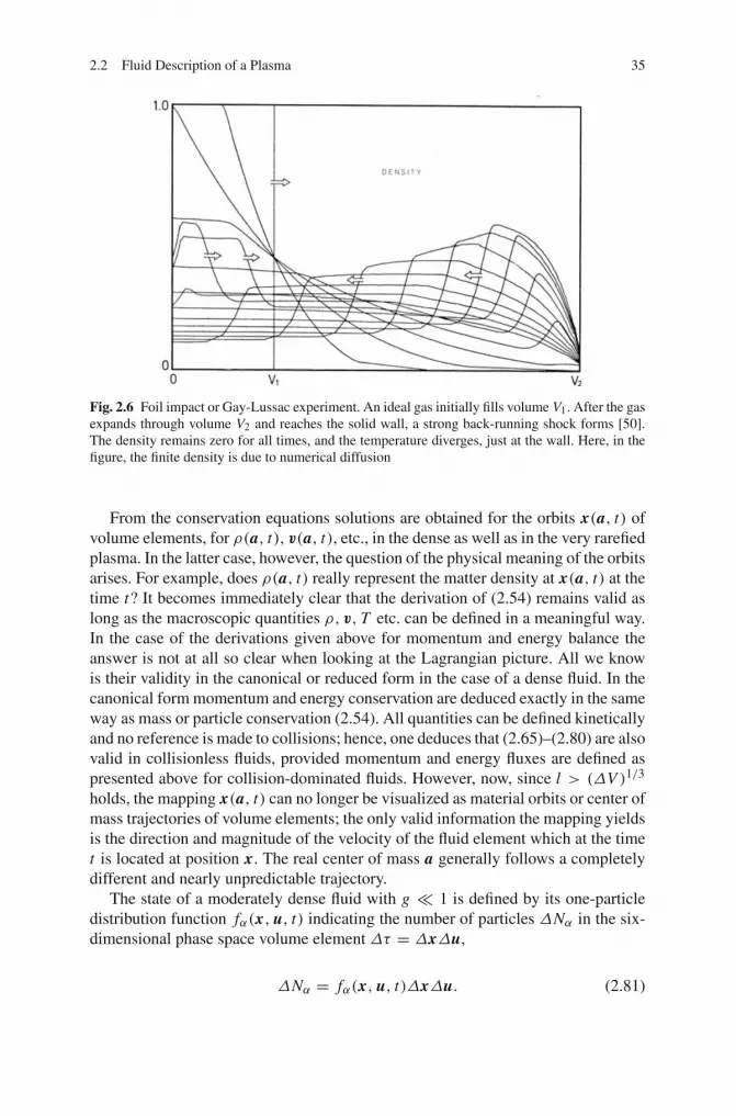
2.2 Fluid Description of a Plasma 35
Fig. 2.6 Foil impact or Gay-Lussac experiment. An ideal gas initially fills volume V1. After the gasexpands through volume V2 and reaches the solid wall, a strong back-running shock forms [50].The density remains zero for all times, and the temperature diverges, just at the wall. Here, in thefigure, the finite density is due to numerical diffusion
From the conservation equations solutions are obtained for the orbits x(a, t) ofvolume elements, for ρ(a, t), v(a, t), etc., in the dense as well as in the very rarefiedplasma. In the latter case, however, the question of the physical meaning of the orbitsarises. For example, does ρ(a, t) really represent the matter density at x(a, t) at thetime t? It becomes immediately clear that the derivation of (2.54) remains valid aslong as the macroscopic quantities ρ, v, T etc. can be defined in a meaningful way.In the case of the derivations given above for momentum and energy balance theanswer is not at all so clear when looking at the Lagrangian picture. All we knowis their validity in the canonical or reduced form in the case of a dense fluid. In thecanonical form momentum and energy conservation are deduced exactly in the sameway as mass or particle conservation (2.54). All quantities can be defined kineticallyand no reference is made to collisions; hence, one deduces that (2.65)–(2.80) are alsovalid in collisionless fluids, provided momentum and energy fluxes are defined aspresented above for collision-dominated fluids. However, now, since l > (ΔV )1/3
holds, the mapping x(a, t) can no longer be visualized as material orbits or center ofmass trajectories of volume elements; the only valid information the mapping yieldsis the direction and magnitude of the velocity of the fluid element which at the timet is located at position x. The real center of mass a generally follows a completelydifferent and nearly unpredictable trajectory.
The state of a moderately dense fluid with g � 1 is defined by its one-particledistribution function fα(x, u, t) indicating the number of particles ΔNα in the six-dimensional phase space volume element Δτ = ΔxΔu,
ΔNα = fα(x, u, t)ΔxΔu. (2.81)
36 2 The Laser Plasma
From elementary gas-kinetic theory it is known that the macroscopic quantities aredefined as follows,
nα(x, t) =∫
fα(x, u, t) du, vα = 1
nα
∫u fα(x, u, t) du, (2.82)
Tα = 1
3
1
nαkB
∫mα(u − vα)
2 fα(x, u, t) du, (2.83)
pα,i j =∫
mα(ui − vαi )(u j − vα j ) fα(x, u, t) du, (2.84)
qα =1
2mα
∫(u − vα)
2(u − vα) fα(x, u, t) du. (2.85)
The tensor pα = pα,i j is the scalar pressure pα plus the viscosity tensor and qαis the heat flux density. As long as the dynamical variables are defined in this waythe conservation equations deduced above are valid for arbitrarily diluted fluids.This can be directly verified by starting from the conservation equation of the one-particle distribution function f (x, u, t) (the index α is omitted for simplicity). Let usfirst consider a collisionless fluid. By observing that f is the particle density in the6-dimensional phase space and its flux density is given by f w with the 6-dimen-sional velocity w = (u, du/dt), particle conservation requires ∂t f + div( f w) = 0.Liouville’s theorem states for noninteracting particles
∇w = ∇x u +∇uq(E + u × B)/m = 0
(or Δτ = const ) owing to ∇x u = ∇x ( p/m), p = mu+q A; thus, the conservationequation reads ∂t f + w grad f = 0, or explicitly,
∂ f
∂t+ u∇x f + q
m(E + u × B)∇u f = 0. (2.86)
This is the celebrated Vlasov equation. It will be used in several contexts in thefollowing chapters. In an alternative manner it follows from the fact that the numberof particles ΔN in the volume Δτ is conserved,
d
dtΔN = d
dt( fΔτ) = f
d(Δτ)
dt+Δτ
d f
dt= Δτ
d f
dt= 0.
d f/dt = 0 is identical to (2.86). The effect of collisions can no longer be describedin terms of a single set of coordinates (x, u, t); it must contain at least pairs ofsets (x, u) (binary collisions). Physically this is clear from the fact that owing tocollisions particles are lost from Δτ or scattered into it from outside. Consequently,a source term (“collision term”) appears on the right-hand side of (2.86) whichcannot be just a function of f depending only on x, u, t . It is shown in volumeson statistical mechanics that the correct source term is expressed as an integral overthe two-particle distribution function f2(x1, u1, x2, u2, t) for which in turn a new

2.2 Fluid Description of a Plasma 37
conservation equation with a source term containing the three particle distributionfunction is needed. In this way one arrives at the famous BBGKY hierarchy, namedafter Bogoljubov, Born, Green, Kirkwood and Yvon. Only the latter is equivalentto the complete description of an ensemble of interacting particles by Liouville’sequation [43].
The direct derivation of the fluid equations from (2.86) with or without a collisionterm is accomplished by multiplying it successively with |u|0 = 1, u, u2 and inte-grating over all u-subspace and making use of the definitions (2.82), (2.83), (2.84),and (2.85), see Sect. 8.1.7. The use of the distribution function f is appropriate fordilute and moderately dense fluids. Nowadays laser plasmas can be created in whichthe plasma parameter g is of the order of unity or larger and the potential energyalso contributes significantly, e.g., to the pressure, so that the definitions (2.82),(2.83), (2.84), and (2.85) are no longer appropriate. The macroscopic conservationequations, however, still maintain their validity since, for a dense fluid, all dynamicvariables can be defined without making use of f .
2.2.2 Linearized Motions
Equations (2.65), (2.66), (2.67), (2.68), and (2.69) or their simplified versions arehighly nonlinear and, consequently very few analytical solutions exist. Owing totheir relevance for estimates and understanding and interpreting numerical results,those solutions relevant to laser plasma dynamics are treated in this and thefollowing two sections. At moderate laser intensities static magnetic fields are ofminor importance and are omitted here.
2.2.2.1 Electron Plasma Waves and Linear Landau Damping
The two-component plasma is capable of rapid charge density oscillations. Owing totheir large mass the ions can be considered as a uniform background at rest whereasfor the electrons (2.71) apply. For short time intervals qe and heat flow to the ionsneed not be considered and in the absence of radiation the energy equation simplifiesto
3
2
dTe
dt− Te
ne
dne
dt= 0. (2.87)
Here ∇ve has been replaced by −(dt ne)/ne from mass conservation. Equa-tion (2.87) can be integrated immediately to yield the familiar adiabatic behavior
Ten−(γe−1)e = const, pen−γe
e = const; γe = 5
3. (2.88)
However, it must be pointed out that the adiabatic coefficient γe = 5/3 is cor-rect only under the assumption that there are enough collisions during a change

38 2 The Laser Plasma
of ne to redistribute the compression work isotropically. In contrast, in a fast one-dimensional compression occurring during a time shorter than the collision timeτee the compression (or expansion) work acts only on one of r degrees of freedomso that r/2 = 3/2 in (2.87) has to be replaced by r/2 = 1/2 and the adiabaticcoefficient becomes γe = (r + 2)/r = 3 in (2.88), in agreement with the kineticresult from (2.86).
Under the above assumptions the electronic fluid decouples from the ions and itsdynamics is determined by the equations
∂ne
∂t+∇(neve) = 0, ne
(∂
∂t+ ve∇
)ve = − 1
m∇ pe − ne
e
mE − neνeive,
∇E = − e
ε0(ne − Zn0), pen−γe
e = const. (2.89)
In general this system is still “intractable” [52]. However, it becomes solvable inthe case of small disturbances n1 = ne − Zn0 from equilibrium ne0 = ne − n1 =Zn0 = const, ve0 = 0, Te0 = Te − T1 = const, |n1| � ne. In this case the systemcan be linearized by omitting all higher order terms,
∂n1
∂t+ ne0∇ve = 0, ne0
∂ve
∂t= −s2
e∇n1 − ne0e
mE − ne0νeive;
s2e = γe
kBTe0
m.
The quantities ve and E are removed by differentiating the first equation with respectto time and taking the divergence of the second one, and then using Poisson’s equa-tion. The straightforward result is
∂2
∂t2n1 + νei
∂
∂tn1 + (ω2
p − s2e∇2)n1 = 0 (2.90)
with
ω2p =
ne0e2
ε0m. (2.91)
The (electron) plasma frequency ωp is a fundamental quantity in plasma physics.Keeping ve, E or T1 instead of n1 leads to an equation in which n1 is merelyto be replaced by ve, E or T1, respectively. The plane electron plasma waves (orLangmuir, or electrostatic waves)
n1(x, t) = nei(ke x−ωt)
form a complete orthonormal set of solutions of (2.90) if ω satisfies the Bohm-Grossdispersion relation

2.2 Fluid Description of a Plasma 39
ω2 = ω2p + s2
e k2e − iνeiω. (2.92)
If we set νei = 0, this has the remarkable property of the phase and group velocitiesvϕ = ω/k and vg = ∂ω/∂k satisfying vϕvg = s2
e . The connection of n1 withT1, ve, E and the potential Φ in a harmonic wave is
T1 = (γe − 1)Te0n1
ne0, ve = vϕ
n1
ne0, E = i
e
ε0ken1,
Φ = iE
ke= − e
ε0k2e
n1. (2.93)
In the cold plasma (Te = 0) the restoring force is entirely of electrostatic nature andan arbitrary, small charge distribution oscillates at the plasma frequency ωp givenby the expression (2.91), and vg is zero. In the warm plasma (Te > 0) there is theadditional thermal contribution s2
e k2e to the eigenfrequency of the electrostatic wave
and vg is finite; ωp is the lower limit (“cut-off”) of ω for the wavelength λ tending toinfinity. Formally, for λ tending to zero ω approaches the other asymptote ω = seke
and vϕ = vg = se. For this reason se is called the electron sound velocity. However,such a wave does not exist since its wavelength λ would be much smaller thanλD = vth,e/ωp. This cannot occur because in the collisionless plasma there is noway to transmit the electron pressure to a neighboring volume element much closerthan λD via the space charge field alone. The electron density for which a givenfrequency ω equals ωp is called the “critical density nc”,
nc = ε0m
e2ω2 = 1.75× 10²¹
(ω
ω Ti:Sa
)2
cm−3. (2.94)
The critical density nc is one of the fundamental quantities characterizing the inter-action of the laser with dense matter. According to (2.92) a Langmuir wave of fre-quency ω cannot propagate into an “overdense region” with ne0 > nc. The sameholds for electromagnetic waves; they are cut off at nc (see Chap. 3).
Collisional damping, with �ω = −νei/2, is generally small; for exampleνei/ωNd = 3 × 10⁻⁵ Z at ne0 = 1020 cm−3 and Te = 1 keV. However, for ke
approaching the order of magnitude of kD = 1/λD the particle nature of the electronfluid manifests itself through the phenomenon of Landau damping. Assume a smallharmonic electron density disturbance in a field-free plasma at rest with equilibriumdistribution function f0(v). By setting
f (x, v, t) = f0(v)+ f1(v)ei(ke x−ωt)
and linearizing (2.86) in f1 with B = 0, a more general dispersion relation than(2.92) is obtained for the frequency which, although no collisions are considered, iscomplex: ω→ ω + iγ (see any volume of plasma physics). Under the assumptions(i) γ � ω and (ii) (keλD)
2 � 1 the dispersion relation reduces to the algebraicrelations

40 2 The Laser Plasma
ω2 = ω2p(1+ 3k2
eλ2D + · · · ) = ω2
p + s2e k2
e + · · · , s2e = 3v2
th,
γ = π
2
ωω2p
k2e
∂ f0
∂v
∣∣∣∣v=vϕ
; f0 =(β
π
)1/2
e−βv2. (2.95)
The first line is the Bohm–Gross dispersion relation with γe = 3, in accordance withthe number of degrees of freedom r = 1 activated by a plane wave in a collisionlessplasma. The expression for γ is negative for an equilibrium distribution function f0with negative slope and the wave is damped, as is the case for a Maxwellian plasma.For the latter, γ becomes under assumption (i)
γ = −(π
8
)1/2 ωp
(keλD)3exp
(− 1
2(keλD)2− 3
2
)
= −0.14ωp
(keλD)3exp
(− 1
2(keλD)2
). (2.96)
For instance, at (keλD)2 = 1/6, where (2.95) still holds, λ = 15λD, ω = 1.2ωp
and the damping is given by |γ /ω| = 0.08, i.e., the mean lifetime of the waveis N = Δt/τ = ω/2π |γ | = 2 periods. In contrast, at twice the wavelength,λ = 30λD , the wave undergoes nearly 1000 oscillations until its amplitude reducesto 1/e. If, for some reason, f0 is flat at vϕ = ω/k linear Landau damping does notoccur as long as (i) and (ii) hold. It is also seen from (2.95) that a weak electron beamwhen superposed on f0 with a suitable velocity such as to produce a positive slopeat vϕ , excites the Langmuir wave instead of reducing its amplitude (“electron beaminstability”). In a Maxwellian plasma, frequencies considerably higher than ωp donot occur, unless the waves are strongly driven. As λ approaches λD , Langmuirwaves are heavily damped.
Generally electron plasma waves are excited in a limited region from which theyare emitted as free-running waves. In laser plasmas such waves are most effectivelyexcited at the critical point in a very narrow region. The situation is very similar toLangmuir wave excitation by an antenna. In both cases one has to look for complexroots of ke as functions of real values of ω. For a Maxwellian electron fluid thedispersion relation is
k2e = k2
n =1
2√πλ2
D
d
dξ
∫ +∞
−∞e−z2
z − ξdz, ξ = 1√
2vth
ω
kn. (2.97)
The wave vector has now been assigned an index n because there is an infinitesequence of roots kn for a fixed ω. To give a feeling for the strength of damping, inTable 2.3 the first 3 roots of ke are calculated as functions of ω/ωp. For λ/λD � 1higher Landau modes are much more strongly damped than the fundamental mode.As ke increases, also the fundamental mode becomes heavily Landau-damped; e.g.,at λ1 = 5λD the amplitude has reduced by a factor of e = 2.718 after Δx1 =0.21λ1 � λD . From the table also results that for ω ≥ 1.1ωp, k1 no longer follows

2.2 Fluid Description of a Plasma 41
the Bohm-Gross dispersion relation. �k1 and �k1 from (2.97) and Table 2.3 werefound to be in excellent agreement with experiments [53].
Landau damping is not easy to explain in physical terms. The standard argumentstarts from a single particle in the periodic wave potential given in (2.93). An elec-tron traveling up the potential hill −eΦ at speed slightly faster than vϕ is sloweddown in transferring part of its kinetic energy to the wave; an electron travelingdown the hill at a slightly lower speed than vϕ gains energy from the wave. Ifthere are more such “resonant” particles with v < vϕ than with v > vϕ there isa net energy flow into the electrons and the wave is damped. The deficiency of thisexplanation is that the attempt to quantify it to obtain (2.96) becomes more involvedthan Landau’s derivation [54, 55]. Upon changing to a reference system comovingwith the wave, Φ becomes static. Then, one could make the objection that on theaverage an electron neither loses nor gains energy. Therefore we prefer a differentpoint of view. Imagine an initial sinusoidal density perturbation ne = neo+n1 with aMaxwellian velocity distribution everywhere. Such a perturbation exactly fulfills thefluid equations (2.89) and leads to an undamped wave in the absence of collisions,i.e., νei = 0. However, in the wave frame energy conservation requires
1
2mu′2 − eΦ = E ′, u′ = u − vϕ.
Those electrons with E ′ < −eΦmin are stopped and forced to oscillate, each inits potential well; they are “trapped” and travel with the wave. Those with E ′ >−eΦmin are free. However, owing to the periodic potential the time to move onewavelength further for all free electrons becomes longer than |u − vϕ |/λ which isthe crossing time in the absence of Φ. The closer an electron comes to the separatrixbetween trapped and untrapped particles the larger is the resulting deviation. Hence,groups of electrons traveling at a constant difference Δu′ in the field-free region,Δu′ = Δu, when entering the wave change their relative speed, and coherence isgradually lost. The trapped electrons oscillate at the so-called bounce frequency ωB
[52]. For E ′kin � −eΦmin it is easily determined from
d2x ′
dt2+ e
mE sin kex ′ � d2x ′
dt2+ e
mke Ex ′ = 0.
Table 2.3 Landau damping of the first 3 modes. Δxn/λn relative distance at which the waveamplitude reduces to 1/e
ω/ωp λ1/λD Δx1/λ1 λ2 = ∞, Δx2/λD λ3/λD Δx3/λ3
1.0 ∞ ∞ 0.64 30.1 0.401.1 25.8 23.1 0.62 29.5 0.351.5 12.8 0.80 0.55 22.4 0.272.0 9.2 0.43 0.48 17.1 0.252.5 7.5 0.32 0.43 13.7 0.233.0 6.5 0.27 0.40 11.6 0.224.0 5.2 0.22 0.33 8.9 0.21
42 2 The Laser Plasma
This is a harmonic oscillator with frequency
ωB =(
eke E
m
)1/2
. (2.98)
The quantity τB = 2π/ωB indicates the order of magnitude of time duration for aparticle to be trapped. In resonance absorption particle trapping plays a dominantrole for damping and eventual breaking of the highly nonlinear electron plasmawave. Collisionless damping due to trapping is denoted as nonlinear Landau damp-ing. Linear Landau damping does not lead to any entropy increase of the system; itsreversibility has been successfully demonstrated by the technique of plasma echoes[52]. The latter are completely analogous to spin echoes [56, 57] and to laser echoesin two-level systems and are best visualized by the vector model of the Bloch equa-tions [58].
2.2.2.2 Ion Acoustic Waves
In a formal treatment of the ionic fluid in complete analogy to Langmuir wavesthe frequencies ω and ωp would be reduced by the ratio (Zm/mi )
1/2. However, insuch a slow motion the electrons have time to follow adiabatically and to neutralizeany ion disturbance. In other words, the momentum equation for the electron fluidreduces to (2.72) with π = 0, Bs = 0. Neglecting viscosity, (2.73) applies for theions. For small density disturbances n1 = ni − n0, ne1 = ne − Zn0 it reads asfollows,
n0∂v
∂t= − 1
mi∇ pi − 1
mi∇ pe = −s2
i ∇n1 − m
mis2
e∇ne1; s2i = γi
kBTi
mi.
For the ions the adiabatic law pi n−γii = const applies in the absence of heating from
which si follows as specified. From (2.74) and the Poisson equation,
E = − m
ne0es2
e∇ne1, ∇E = e
ε0(Zn1 − ne1),
ne1 is determined as a function of n1 through elimination of E,
−s2e∇2ne1 = ω2
p(Zn1 − ne1) ⇒ (1− γeλ2D∇2)ne1 = Zn1;
λD from (2.38). Eliminating v from the linearized momentum equation above withthe help of ∂t n1 + n0∇v = 0 yields
∂2n1
∂t2= s2
i ∇2n1 + m
mis2
e∇2ne1 =[
s2i +
Z mmi
s2e
1− 1ne1γeλ
2D∇2ne1
]∇2n1. (2.99)
Fourier analysis shows that the plane ion acoustic waves
2.2 Fluid Description of a Plasma 43
n1 = nei(ka x−ωa t)
form a complete set of solutions to (2.99) if ωa satisfies the dispersion relation
ωa = ska, s2 = kB
mi
(γi Ti + γe
Z Te
1+ γe(kaλD)2
). (2.100)
Quasineutrality requires that ne1 is modulated with the same ka . The quantity sis the ion sound velocity. It remains finite when Ti approaches zero owing to theelectron pressure which in the ion sound wave is transmitted to the ions by theelectrostatic field of type (2.74) rather than by collisions. The condition howeverfor this to happen is kaλD � 1. The ion plasma frequency ωpi does not appear in(2.100) since the slow ionic charge disturbance is nearly completely screened by thefast electrons. Again, if y stands for any of the perturbations of particle densitiesne, ni , temperatures Te, Ti , velocities ve, vi , electric field E or potential Φ, each ofthem obeys the linear acoustic wave equation
∂2
∂t2y − s2∇2 y = 0.
They are related by
Tα1 = (γα − 1)Tα0nα1
nα0, vα = s
nα1
nα0, ne1 = Zn1
1+ γe(kaλD)2,
E = −ie
ε0γekaλ
2Dne1, Φ = i
E
ka. (2.101)
In the long-wavelength limit s is nearly a constant owing to nearly perfect screening;ve is very close to vi = v and frictional damping plays no role. Generally the elec-trons have time to transmit their compression energy to their neighborhood duringan oscillation whereas the ions do not. Hence, γe = 1, i.e., the electrons behaveisothermally and γi = 3 holds. If however, νi i > ω/2π is fulfilled, γi has to be setequal to 5/3.
According to the standard interpretation of Landau damping at Te � Ti , vϕ = sis much greater than vth,i = (kBTi/mi )
1/2 and the number of resonant particles isnegligibly small. Solving Vlasov’s equation for electrons and ions under this condi-tion leads to the Landau damping coefficient
γa
ω=(
m
mi
)1/2 (π8
)1/2exp
(− Z Te
Ti− 3
2
). (2.102)
For a hydrogen plasma we obtain γa/ωa = 1.5 × 10⁻² exp(−Te/Ti − 3/2). In therange 1 ≤ Z Te/Ti ≤ 10 a numerical fit of the kinetic dispersion relation leads to[55]
44 2 The Laser Plasma
γa
ω= 1.1
(Z Te
Ti
)7/4
e−(Z Te/Ti )2. (2.103)
When Ti approaches Z Te, vϕ becomes comparable to vth,i and strong Landau damp-ing sets in. It was due to the fact that Te � Ti in a gas discharge that ion acousticwaves were first detected there. In laser-generated plasmas Te � Ti may be easilyreached. If λD is much larger than the wavelength λi of a periodic perturbation in ni
the electrons form a uniform homogeneous negative background in which the ionsoscillate according to a dispersion relation of Bohm-Gross structure (2.92) or (2.95)with all electron quantities (index e) replaced by those for the ions (index i). For thepressure term to be efficient the ion mean free path must be smaller than λi .
2.2.3 Similarity Solutions
In laser dynamics the diffusion of the absorbed energy by electronic heat conductionand by thermal radiation as well as subsequent expansion of the hot plasma into thevacuum or a surrounding low-density gas and plasma cooling by expansion are ofparticular interest. The dynamics studied in the laboratory are nonstationary andat best exhibit rotational symmetry around the normal to the target onto which thelaser beam is focused. This is a typical case for numerical computation. Only muchsimpler idealized, so to say, few purely one-dimensional cases, are accessible to ananalytical treatment. Such solutions are of great relevance for the laser plasma inplane and spherical geometry.
2.2.3.1 The Buckingham π -Theorem and Similarity
Nonlinear similarity solutions play such an important role in fluid dynamics thata brief outline of dimensional analysis and its theoretical basis is justified here. Itwas pointed out by Lord Rayleigh that sometimes physical laws can be found bydimensional considerations alone. His research in hydrodynamics is a good demon-stration for this assertion [59, 60]. In 1914 the so called π -theorem was formulatedby Buckingham which yields the formal basis for all dimensional and similarity con-siderations [61]. Roughly spoken, it states that any physical law must be expressibleas an equation among dimensionless variables (so called π -variables). As a simpleconsequence it follows that a fundamental physical theory cannot be constructedwithout a minimum number of fundamental constants. However, this was explicitlyexpressed much later only by Sedov [62].
Any physical law may be put into the form
y = f (x1, x2, · · · , xn), n integer (2.104)
with quantities y, xi of certain dimensions. By dimension we mean the following:Given a system of k units M,L,T, . . . (e.g., mass, length, time, . . .) one has
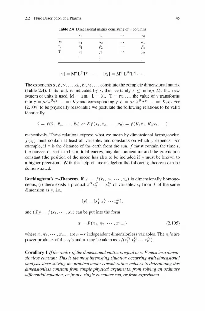
2.2 Fluid Description of a Plasma 45
Table 2.4 Dimensional matrix consisting of n columns
x1 x2 · · · xn
M α1 α2 · · · αnL β1 β2 · · · βnT γ1 γ2 · · · γn...
.
.
....
.
.
.
[y] = MαLβTγ · · · , [xi ] = Mαi Lβi Tγi · · · .
The exponents α, β, γ , . . ., αi , βi , γi , . . . constitute the complete dimensional matrix(Table 2.4). If its rank is indicated by r , then certainly r ≤ min(n, k). If a newsystem of units is used, M = µm, L = λl, T = τ t, . . ., the value of y transformsinto y = μαλβτγ · · · =: K y and correspondingly xi = μαiλβi τγi · · · =: Ki xi . For(2.104) to be physically reasonable we postulate the following relations to be valididentically
y = f (x1, x2, · · · , xn) or K f (x1, x2, · · · , xn) = f (K1x1, K2x2, · · · )
respectively. These relations express what we mean by dimensional homogeneity.f (xi ) must contain at least all variables and constants on which y depends. Forexample, if y is the distance of the earth from the sun, f must contain the time t ,the masses of earth and sun, total energy, angular momentum and the gravitationconstant (the position of the moon has also to be included if y must be known toa higher precision). With the help of linear algebra the following theorem can bedemonstrated:
Buckingham’s π -Theorem. If y = f (x1, x2, · · · , xn) is dimensionally homoge-neous, (i) there exists a product xs1
1 xs22 · · · xsn
n of variables xi from f of the samedimension as y, i.e.,
[y] = [xs11 xs2
2 · · · xsnn ],
and (ii)y = f (x1, · · · , xn) can be put into the form
π = F(π1, π2, · · · , πn−r ) (2.105)
where π, π1, · · · , πn−r are n− r independent dimensionless variables. The πi ’s arepower products of the xi ’s and π may be taken as y/(xs1
1 xs22 · · · xsn
n ).
Corollary 1 If the rank r of the dimensional matrix is equal to n, F must be a dimen-sionless constant. This is the most interesting situation occurring with dimensionalanalysis since solving the problem under consideration reduces to determining thisdimensionless constant from simple physical arguments, from solving an ordinarydifferential equation, or from a single computer run, or from experiment.

46 2 The Laser Plasma
Definition 1 If from πσ11 π
σ22 · · ·πσn−r
n−r = 1 follows σ1 = σ2 = · · · = σn−r = 0 theπi ’s are called independent. If in a solution y = f (x1, x2, · · · , xn) the number n ofindependent variables can be reduced at least by one we call it a similarity solution.f (x1, x2, · · · , xn) is a self-similar solution if the number of dimensionless variablesπi reduces to a single variable. (In the Soviet literature all similarity solutions areoften called self-similar. The authors do not follow this convention because there iseffectively no need for it). It may be helpful to illustrate the use of the π -theoremby a few simple examples.
Example 1 Stokes law Assume a heavy sphere falling in deep water. What is theasymptotic velocity v of the sphere? One recognizes that a maximum number ofvariables is viscosity μ, weight G and radius R. The dimensional matrix in the cgssystem of units is presented in Table 2.5. Since its rank is r = 3, F from (2.105) isa constant, F = C , and v is uniquely determined by
v = CG
μR= C ′ R
2g
η; η = μ
ρ.
This is Stokes’ formula with C = (6π)−1. It provides a counter example for thefrequently expressed contention that C is always near unity in a “physical problem”.If instead of this choice one takes μ, ρ, g and R as independent variables the rank ofthe matrix is still r = 3 so that 4 − 3 = 1 dimensionless quantity π1 = ρ2gR2/μ2
can be formed and v is no longer uniquely determined. The reason is that ρ, g, Rappear in the problem only in the combinations R and ρR3g = 3G/4π and not asthree independent quantities. The success of dimensional analysis depends cruciallyon the selection of the most restricted number of variables.
Example 2 Harmonic oscillator The motion of the harmonic oscillator mx + κx =0 is completely determined by the quantity κ/m and the oscillation amplitude x . Thedimensions of the two quantities are s−2 and cm, respectively. The oscillation periodtherefore is independent of x and is T = C(m/κ)1/2. The unknown dimensionlessconstant C can be determined as follows. From elementary geometry it is knownthat by introducing a second oscillator my + κy = 0 perpendicular to x with equalamplitude y = x but a difference in phase of π/2 the trajectory x = (x, y) is acircle of radius R = x . The only velocity that can be constructed from x and κ/mis v = x(κ/m)1/2. This velocity equals 2πR/T from which T = 2π(m/κ)1/2
follows.
Table 2.5 Dimensional matrix of the falling sphere (left-hand side) and charged sphere (right-handside) problem. In both cases r = 3
μ G R v
g 1 1 0 0cm −1 1 1 1s −1 −2 0 −1
q p ε0 R
C 1 1 1 0V 0 1 −1 0cm 0 −3 −1 1

2.2 Fluid Description of a Plasma 47
All Galileo would have had to do is to verify that the oscillation period of hispendulum becomes independent of amplitude when the excursion is small. ThenT = 2π(�/g)1/2 follows automatically.
Example 3 Blast wave How secret can the TNT equivalent of a bomb be kept?Consider a homogeneous atmosphere of mass density ρ0. In one very restrictedregion the energy W is supplied instantaneously (“point explosion”). As a conse-quence, a blast wave, i.e., a strong shock propagates out into the surrounding space.Its position xs(t) depends, under idealized conditions, on W/ρ0 and t only. From[W/ρ0] = cm5 s−2 and [xs] = cm follows
xs(t) = C
(W
ρ0
)1/5
t2/5. (2.106)
By taking pictures of the blast wave at different times W is recovered with goodaccuracy. Subsequently, corrections may have to be made for radiation losses andamplification of the shock front by absorption of radiation. For the constant C andvariants of the model, for example supply of the energy W to a vacuum-solid inter-face see [62, 63]. In the kbar pressure range the time-dependence ∼ t2/5 in (2.106)has been confirmed recently in air [64].
Example 4 Rayleigh–Taylor instability Consider a fluid of density ρ1 superposedto a fluid of density ρ2 in a gravity field of acceleration g. Assume that the origi-nal horizontal interface extending in x-direction is subject to a vertical sinusoidaldisplacement y = y0 sin kx , k = 2π/λ. It is known from ocean waves in deepwater that the vertical motion decays exponentially over the depth of a wave-length Δy � λ. Hence, the mass per unit length involved in the acceleration is(ρ1+ρ2)(λ/s). The gravity force acting on this mass per unit length is (ρ1−ρ2)gy0.This results in the equation of motion
y0 + (s/λ)Agy0 = 0, A = (ρ2 − ρ1)/(ρ1 + ρ2). (2.107)
A is the Atwood number. The complete analysis yields the dimensionless factors = 2π for small perturbations y0 � λ. For A > 0 the liquid is stable fulfillingharmonic oscillations around y = 0. For A < 0 the interface becomes Rayleigh-Taylor unstable, y0(t) = y0eγ t , with the linear growth rate
γ = √k Ag, k = 2π/λ (2.108)
[65, 66]. The exponential growth (and the harmonic oscillation) originates from theaccelerated mass ∼ λ.
Example 5 Net charge of a cluster As a last example the net charge q ′ of ahot plasma sphere (cluster) of positive charge q and radius R is considered. Evi-dently q ′ = q f (π1, · · · ). The dimensionless function f depends on combina-tions of the equilibrium pressure p, [p] = VCcm−3, the dielectric constant ε0,
48 2 The Laser Plasma
[ε0] = CV−1cm−1, and the radius R. The dimensional matrix, Table 2.5 (right-hand side), shows that q, p, ε0 must appear in the combination ε0 p/q2 and hencethe set of possible π variables is π1 = ε0 pRn+4/(q2 Rn) with n real and arbitrary.By choosing n = 2, π1 ∼ λ2
D/R2, i.e., q ′/q is a function of π−1/21 ∼ R/λD , in
agreement with what was found in Sect. 2.1.3.
2.2.3.2 Adiabatic and Isothermal Rarefaction Waves in Plane Geometry
In a first approach the expansion of a laser plasma into vacuum can be modeled asfollows: consider a half-space (x ≤ 0) filled with an ideal gas of uniform density ρ0,temperature T0, and pressure p0. Suppose the surface pressure at x = 0 is suddenlyreduced to zero at t = 0. The subsequent dynamics is then governed by
∂ρ
∂t+ ∂
∂x(ρv) = 0, ρ
(∂v
∂t+ v
∂v
∂x
)= −s2
0
(ρ
ρ0
)γ−1∂ρ
∂x. (2.109)
The adiabatic sound velocity is s = (γ p/ρ)1/2 = s0(ρ/ρ0)(γ−1)/2. The isother-
mal case T = const is characterized by infinite thermal conductivity or an infinitenumber of degrees of freedom with γ = 1. Equations (2.109) show that ρ andv depend on ρ0, s0, x, t . From the corresponding dimensional matrix we deduceone dimensionless variable π = x/(s0t). Therefore the system above reduces toordinary differential equations for ρ = ρ0 P(π), v = s0V (π):
P ′(V − π)+ PV ′ = 0, V ′(V − π)+ Pγ−2 P ′ = 0,
where the prime denotes d/dπ . By eliminating P ′ one obtains
V ′(V − π)2 − Pγ−1V ′ = 0, or(v − x
t
)2 = s2.
Using this relation in one of the dimensionless conservation equations it follows thatdv = −sdρ/ρ and hence, for γ = 1 (adiabatic case)
ρ(x, t) = ρ0
[1− γ − 1
2
v
s0
] 2γ−1
, v = 2
γ + 1
( x
t+ s0
). (2.110)
For γ approaching unity (isothermal case) ρ becomes
ρ(x, t) = ρ0 limγ→1
(1− γ − 1
2
v
s0
) 2γ−1 = ρ0e
− vs0 = ρ0e
−(
1+ xs0t
)
. (2.111)
These solutions hold in the interval −s0t ≤ x ≤ 2γ−1 s0t . The rarefaction wave
propagates with the phase velocity vϕ = s0 into the undisturbed gas. For anyinstant t > 0 the front of the rarefaction wave xF moves with constant speed
2.2 Fluid Description of a Plasma 49
vF = 2s0/(γ − 1). For γ = 5/3, vF = 3s0. For this case the rarefaction waveis shown in Fig. 2.6 before it collides with the wall at V2.
It is interesting to calculate the heat flow density q(x, t) which is needed formaintaining the temperature at the constant value T0. From the energy equation
3
2nkB
dT
dt= −p
∂v
∂x− ∂q
∂x= 0
we obtain
q(x, t) = −∫ ∞
xp∂v
∂xdx = −s3
0ρ0
∫ ∞
v(x)/s0
exp
(− v
s0
)d
(v
s0
)
= s30ρ = ps0. (2.112)
This is a useful formula for deducing a criterion for nearly isothermal plasmaexpansion in regions where the flow is planar. In fact, from (2.64) follows ps0 =κ0T 5/2
e |∂Te/∂x |. If the dimension of the plane region is L and Δp is the pressuredifference at its end points, then the fractional temperature difference
ΔTe
Te� L
s0Δp
κ0T 7/2e
(2.113)
must be much smaller than unity. In the adiabatic rarefaction wave q is zero and noentropy increase occurs by the expansion into vacuum.
With the discovery of fast ion jets from solid targets produced by intense fs laserpulses ion separation in the accelerating electrostatic field accompanying the plasmararefaction wave has gained new interest. Electron-ion charge separation, originallystudied under idealized conditions by Gurevich et al. [67], as well as maximum ionenergy and ion energy spectrum have been ivestigated in great detail in [68] forisothermal targets filling a halfspace and for isothermal thin targets of finite mass[69]. A self-similar solution of expansion of finite mass targets into vacuum in plane,cylindrical and spherical geometry is presented in [70]. Full account is taken ofcharge separation effects, and the position of the ion front and the asymptotic energyof accelerated ions are calculated analytically. Generalization to a two-temperatureelectron system reveals the conditions under which the high-energy tail of acceler-ated ions is determined solely by the hot-electron population. See also [71] on theacceleration of a test ion in a dynamic planar electron sheath, [72] on high energyproton acceleration by short laser pulses interacting with dense plasma targets, and[73] on efficient generation of quasimonoenergetic ions by Coulomb explosions ofoptimized nanostructured clusters.
The spherical rarefaction wave cannot be solved by dimensional analysis sincethe initial radius r0 of the gas cloud enters as an additional independent variable.Only for t = d/s0, corresponding to distances d � r0, is the expansion planar
50 2 The Laser Plasma
and it becomes clear that the front rF moves at constant velocity vF at all timeswhich is the same as in planar geometry. However, with the aid of an additionalassumption the authors of [74] were able to obtain a spherical self-similar solutionof nanocluster explosion. Of particular relevance for various applications is a demix-ing and energy selection process occurring in spherical geometry. Clusters in theCoulomb explosion mode, i.e., when all free electrons have escaped from the cluster(“outer ionization” degree equals unity), are capable of generating monoenergeticbeams of fast ions. A mixture of ions of different charge to mass ratio α is unstableagainst uniform mixing. Under appropriately chosen mixing ratios the componentwith higher α is accelerated to nearly monochromatic energies in the Coulomb fieldof the heavy ions [74].
2.2.3.3 The Nonlinear Heat Wave and Huntley’s Addition
Here we solve the following nonlinear heat conduction problem by dimensionalanalysis [75]. A quantity of energy per unit area Q0 is instantaneously released att = 0 in a plane of a solid, liquid or gas from which it diffuses according to thenonlinear equation into its interior
∂T
∂t= a
∂
∂x
(T α ∂T
∂x
); a = κ0
cV, (2.114)
cV specific heat. For heat conduction in a fully ionized plasma the exponent hasto be taken α = 5
2 ; with other appropriate values of α it describes radiation trans-port. It is easy to show that for α > 0 the heat front coordinate xT (t) is finite. Forα = 0 (constant thermal conductivity) xT = ∞ for all t > 0. The temperature Twill depend on q0 = Q0/cV , x and t . This leads to the conclusion that only onedimensionless variable
π = x
(aqα0 t)1/(α+2)
exists (see Table 2.6) and that xT (t) and the maximum temperature T0 (at x = 0)are uniquely determined by
xT (t) = A(aqα0 t)1/(α+2), T0(t) = B
(q2
0
at
)1/(α+2)
.
With BT (x, t) = T0 f (π). Equation (2.114) reduces to the ordinary differentialequation
(α + 2)d
dπ
(f α
d f
dπ
)+ π
d f
dπ+ f = 0. (2.115)

2.2 Fluid Description of a Plasma 51
Table 2.6 Dimensional matrix in cgsK units for solving (2.114). r = 3
q0 a x t
cm 1 2 1 0s 0 −1 0 1K 1 −α 0 0
The solution is
T (x, t) = T0
(1− x2
x2T
) 1α
, xT = A(aqα0 t)1/(α+2),
∫ xT
0T dx = q0.
A =⎡
⎢⎣2α + 2
α
⎛
⎝2�(
32 + 1
α
)
�(
12
)�(
1α+ 1
)
⎞
⎠α⎤
⎥⎦
1α+2
; α = 5/2 ⇒ A = 1.480.
B = A2/α(
α
2(α + 2)
)1/α
T0(t) = q0
xT (t)
2�(
32 + 1
α
)
�(
12
)�(
1α+ 1
) , 〈T 〉 = q0
xT (t). (2.116)
For electron heat conduction α = 5/2; for this case,
T = T0
(1− x2
x2T
)2/5
, xT = A q5/90
(κ0
cV Zt
)2/9
,T0
〈T 〉 = 1.223. (2.117)
As α increases the temperature assumes a rectangle-like distribution. At the begin-ning the heat diffusion speed tends to infinity and soon after it slows down drasti-cally (Fig. 2.7).
Another relevant situation is given when the heat applied to the surface is deliv-ered continuously with the power law
Φ = I
cV= Btγ .
If one looks for solutions of the form T (x, t) = A(vtβ − x)δ one finds β = 1, γ =δ = 1/α. At the boundary x = 0 Φ = −aT α∂T/∂x must hold. Inserting this in(2.114) yields
T (x, t) =[αv
a(vt − x)
]1/α, v = xT = Bα/(α+2)
(a
α
)1/(α+2). (2.118)
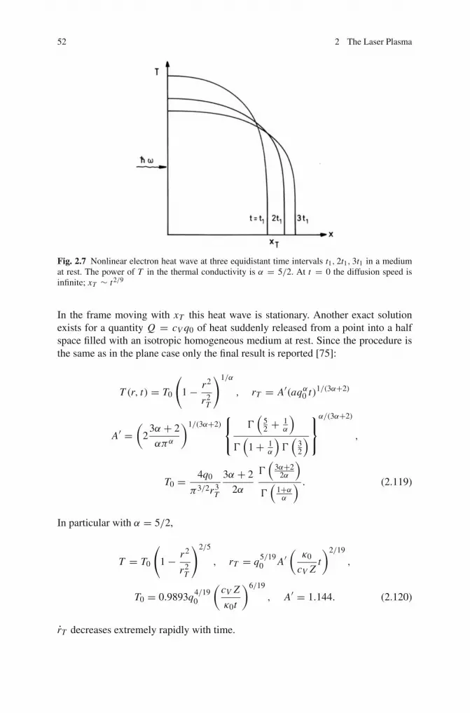
52 2 The Laser Plasma
Fig. 2.7 Nonlinear electron heat wave at three equidistant time intervals t1, 2t1, 3t1 in a mediumat rest. The power of T in the thermal conductivity is α = 5/2. At t = 0 the diffusion speed isinfinite; xT ∼ t2/9
In the frame moving with xT this heat wave is stationary. Another exact solutionexists for a quantity Q = cV q0 of heat suddenly released from a point into a halfspace filled with an isotropic homogeneous medium at rest. Since the procedure isthe same as in the plane case only the final result is reported [75]:
T (r, t) = T0
(1− r2
r2T
)1/α
, rT = A′(aqα0 t)1/(3α+2)
A′ =(
23α + 2
απα
)1/(3α+2)⎧⎨
⎩�(
52 + 1
α
)
�(
1+ 1α
)�(
32
)
⎫⎬
⎭
α/(3α+2)
,
T0 = 4q0
π3/2r3T
3α + 2
2α
�(
3α+22α
)
�(
1+αα
) . (2.119)
In particular with α = 5/2,
T = T0
(1− r2
r2T
)2/5
, rT = q5/190 A′
(κ0
cV Zt
)2/19
,
T0 = 0.9893q4/190
(cV Z
κ0t
)6/19
, A′ = 1.144. (2.120)
rT decreases extremely rapidly with time.

2.2 Fluid Description of a Plasma 53
The temperature T in our treatment has the dimension of Kelvin (K). By assign-ing such a dimension T is assumed as a separate physical entity. However, it isequally legitimate to define T as the ratio of two energies. In this latter case T isa pure number; the unit K disappears from the dimensional matrix and the rank ris reduced to r = 2: the transition from (2.114) to (2.115) is no longer possible inthe pure cgs-system of units. The important question arises which system of unitsshould be used in dimensional analysis. The answer was given by H. E. Huntley[76].
Huntley’s addition: In problems of dimensional analysis take the maximum possi-ble number of independent units. For example, in some cases it is possible to distin-guish between masses in the x and y directions or between “inertial” and “thermal”masses as separate physical entities. In this way problems were solved successfullyby dimensional analysis that were not reducible a priori by the π -theorem. A nec-essary implication for the success of Huntley’s method is that in the process underconsideration there is no interaction between the quantities that are given differentdimensions.
The interested reader may consult with profit several other volumes ondimensional analysis in addition to Sedov [77–82]. The successful application ofdimensional analysis and similarity considerations to continuum mechanics andhydrodynamics sometimes led to the conclusion that dimensional analysis would beappropriate mainly to these disciplines. Only rather recently has it become appar-ent that the application of Buckingham’s π -theorem is not limited to such fields;it should also be important for example in quantum field theory and the theory ofphase transitions [83]. Its successful application in biology was demonstrated forexample by Günther [84–86].
There are several solutions relevant for laser matter interaction which are not self-similar but become asymptotic solutions of this type. An example is the analyticaltreatment of homogeneous pellet compression for laser fusion with a behavior intime for ρ, v and T according to Kidder [48]
ρ, v, T ∼ 1
[1− (t/t0)2]3/2= f (t).
For instance, ρ(R, t) = ρ0(R/R0)2 f (t) is not self-similar. However, for t approach-
ing the instant of collapse t0 it comes arbitrarily close to
ρ = ρ0
23/2
(t1/20 R2/3
R2/30 τ 1/2
)3
, τ = t0 − t,
which is self-similar. Kidder’s solutions are interesting also from the topologi-cal point of view: The void in a spherical shell only closes at t = t0 when thewhole pellet shrinks to a point, as is required from the topological considerations ofSect. 2.2.1.

54 2 The Laser Plasma
In connection with converging shocks and compression waves Zeldovich [75]introduced a second “type of self-similar” solutions, a concept which was devel-oped further by Barenblatt [83] with his formulation of intermediate asymptotics.Such a distinction may sometimes be justified from a practical point of view, butfrom a fundamental point of view no second class of similarity exists. In order tomake sense for subdivision into similarities of the first and second kind all similarityproblems should belong to these two classes. However, in view of certain solutions[87] a third class of similarity solutions would have to be introduced, and, it is notdifficult to imagine that soon a fourth and fifth kind of similarity would have tobe invented for other problems. Eventually some further progress beyond Bucking-ham’s theorem may come from group theoretical methods and the determinationof symmetry groups of differential equations [88, 89]. For the diffusion equation(2.114) with α = −2 (e.g., magnetic field diffusion) see in this context Euler et al.[90]. For symmetry properties of Euler-type plasma equations including magneticfields see [91].
2.2.3.4 Plane Shock Wave
The momentum which can be transmitted to a medium by a linear sound wave ofintensity I is given by the wave pressure pw,
pw = I
s(1+ R) , (2.121)
where R is the reflection coefficient and s is the sound speed. A hot plasma expand-ing from the surface of dense matter, e.g., of a solid, acts like a piston of very highstrength. The effect is the generation of a compression wave the intensity of whichis far beyond the limit of a linear wave. A compression wave in quasineutral mattersteepens until a discontinuity or a steep, narrow transition region has formed. Forexample, when an ideal gas of density ρ0, temperature T0 and pressure p0 at restis compressed by a piston moving at constant speed v1 a compression wave withspatially constant values ρ1, T1, p1, v1 builds up which is separated from the undis-turbed gas by a transition layer a few mean free path lengths thick. Such a structureis called a shock wave (Fig. 2.8). It propagates with the shock velocity vs . For such adiscontinuity or transition layer to be stationary vs must be supersonic with respectto the undisturbed medium, vs > s0; otherwise a rarefaction wave would develop atits front.
In a system moving with vs the shock wave is stationary and matter flows withvelocity u0 = −vs into the discontinuity and streams out of it at the speed u1 =v1 − vs . The two regions are connected by the continuity of mass, momentum andenergy flows. The latter are obtained by integrating the equations of motion in theconservative form across the transition zone and by setting all partial derivativeswith respect to time to zero. Then, when π = 0, I = 0, qe = 0 the Rankine–Hugoniot relations follow from (2.54), (2.77) and (2.79),

2.2 Fluid Description of a Plasma 55
Piston
Fig. 2.8 Shock wave driven by a piston moving at speed v1 = const propagates with phase velocityvs into an undisturbed gas at rest of density ρ0 and temperature T0
ρ1u1 = ρ0u0,
p1 + ρ1u21 = p0 + ρ0u2
0,
ε1 + p1
ρ1+ 1
2u2
1 = ε0 + p0
ρ0+ 1
2u2
0. (2.122)
ε is the internal energy per unit mass. On eliminating u0, u1 from (2.122) one arrivesat the Hugoniot equation of state,
ε1 − ε0 = 1
2(p0 + p1)
(1
ρ0− 1
ρ1
), (2.123)
i.e., at the change a volume element undergoes from state ρ0, p0, ε0 to stateρ1, p1, ε1 when crossing the shock front.
For an ideal gas, or dilute fully ionized plasma, from (2.122) one calculates thefollowing changes as functions of the Mach number M = vs/s0 and γ = γe = γi
in a straightforward way:
κ = ρ1
ρ0= (γ + 1)M2
(γ − 1)M2 + 2; T1
T0= 2γ M2 + 1− γ
(γ + 1)κ. (2.124)
For M or the piston pressure p1 tending to infinity the compression ratio κ reachesthe asymptote κ = (γ + 1)/(γ − 1). For a hot plasma this has the value 4. Owingto the violent entropy production in the shock front, κ cannot exceed this limit, incontrast to an adiabatic compression following (2.88) where κ reaches arbitrarilyhigh values. A shock is given the name strong shock when κ can be approximatedby κ = (γ + 1)/(γ − 1). Formally one arrives at this ratio by disregarding p0 in theRankine-Hugoniot relations. As long as the width of the shock front is much smallerthan its curvature radius equations (2.122), (2.123), (2.124) are equally valid forspherical shocks. This is not true in the center of a converging shock, where muchhigher values of κ are reached [92, 93]. When a second plane shock is superimposedon the first one the overall compression is κ = κ1κ2. However, as soon as their twofronts merge a rarefaction wave starts from that point which causes κ to be instan-taneously reduced there to a value not exceeding the asymptote (γ + 1)/(γ − 1).

56 2 The Laser Plasma
Only in the presence of a cooling mechanism (e.g., ionization, radiation losses; see,e.g., [94]) can a higher κ be reached at the front.
It is useful and physically illuminating to deduce the balance equations (2.122)in the lab frame. The amount of matter compressed per unit time is ρ1(vs−v1). Theoverall force per unit area acting on an arbitrary volume which includes the shockfront is p1 − p0. This difference must be equal to the momentum change per unittime Δmv1 = ρ0vsv1. In a strong shock this quantity is equated to p1. Finally, thework done by two planes including the shock front per unit time and unit area isp1v1. This leads to a change of kinetic and internal energy ρ0vs(ε1 − ε0 + v2
1/2).Summarizing one obtains
ρ0vs = ρ1(vs − v1), p1 − p0 = ρ0vsv1,
p1v1 = ρ0vs
(ε1 − ε0 + v2
1
2
). (2.125)
By changing to the relative speeds u0, u1 system (2.122) follows. From the firstequation the relation between v1, vs and κ is deduced,
v1 = vs
(1− 1
κ
). (2.126)
By a properly programmed piston which avoids intermediate shock formationarbitrarily high density values are attainable. For plane geometry the situation issketched in Fig. 2.9. Infinite density is reached after t = τ at position x0 if thepiston (coordinate x p) of Fig. 2.8 moves according to
x p(t) = x0
γ − 1
{γ + 1− 2
t
τ− (γ + 1)
(1− t
τ
)2/(γ+1)}; t ≤ τ.
x p is obtained from the requirement that all characteristics v1 + s0 (straight lines,v1 = x p(t)) converge to the point (x0, τ ). Generally, when a piston is not properlytimed some characteristics intersect earlier; from such intersections shock frontsoriginate and concomitant entropy production opposing the compression sets in.
The plasma produced by laser breakdown at the surface of a solid acts like a semi-transparent, very energetic piston. In Fig. 2.10 the dynamics of crater formationand plasma outflow is simulated [95]. A laser beam of 1015 Wcm−2 peak intensityimpinges on a hydrogen target. At the very beginning the target is transparent tothe laser light. After breakdown has occurred, the electron density ne soon reachesvalues higher than the critical value nc, given by (2.94), at its surface and stopsthe beam there by metal-like reflection, as well as by collisional and resonanceabsorption. The electron temperature rises to several keV and the plasma expands,thereby enabling the beam to penetrate to deeper layers of matter which successivelyundergo the same process of collisional ionization, heating and expansion. The hotplasma acts like a semipermeable piston onto the target. As a consequence, a strong

2.2 Fluid Description of a Plasma 57
Fig. 2.9 Fast adiabatic compression in plane geometry. The piston starts from rest and its accel-eration is so controlled that all Mach lines v + s starting from the face of the piston intersectin the point (1,1). The numbers entered along the distance-time curve of the piston represent thecompression ratio κ immediately in front of the piston
shock propagates at a typical speed of several 107cm/s through the target (darksemicircle in the figure), leaving behind a crater as depicted in Fig. 2.11. Most ofthe matter removed has escaped by flowing out of the target more or less tangen-tially to the shock wave, very similar to the fluid flow which originates from thesupersonic impact of a projectile on dense matter. Only a small fraction of thematter removed is transformed into hot plasma. The tangential flow componentis also responsible for the reduced compression ratio of κ = 2.8 in the shock ofFig. 2.10, instead of κ = 4. Only when the diameter of the laser beam is increasedby a factor 3–5 is κ = 4 reproduced numerically. This is a general phenomenonand occurs also in far more sophisticated numerical codes [14]. The correct valueis κ = 4 because the one-dimensional Rankine–Hugoniot relations (2.122) apply.Numerics cannot resolve the shock; it averages over an extended domain, in thisway producing lower values of compression. By spherically illuminating pellets ofseveral hundreds of µm in diameter lateral flow is avoided and all ablated matteris transformed into hot plasma. The plasma outflow generates a strong sphericallyconverging compression wave. In this way compressions as high as κ = 600 timessolid hydrogen density have been achieved with the GEKKO XII laser, with thebest result of κ = 1000 [97–99]. Recently this value has been reconfirmed in directdrive experiments with the Omega laser system at LLE, Rochester University (oralannouncement on IFSA2007, Kobe, Sept. 9–14).
An interesting variant of compression wave is represented by the collisionlessshock. At high laser intensity I >∼ 1018 Wcm−2 the light pressure at the target

58 2 The Laser Plasma
I Laserbeam
r
0.0 0.5 1.2
2.01.71.4
Fig. 2.10 Laser-solid hydrogen target interaction at t = 0, 0.5, 1.2, 1.4, 1.7 and 2.0 ns. Laserintensity I = 1015 Wcm−2, beam radius = 4 cells, with intensity distribution as indicated, targetsize = 9×30 cells, critical density nc = n0/10, n0 = 5×1022 cm−3. Particle number per cell = 49.The shock width is due to numerical diffusion; in reality it is smaller by orders of magnitude
surface acts like an extremely energetic piston on the electrons into the direction ofthe laser beam. The electrons are pushed into the dense target until an electrostaticpotential Φ has built up in the ion layer remaining behind whose strength is capableof fulfilling the steady state momentum equation with p1 replaced by ρ1eΦ/mi
in (2.122). Under idealized conditions the internal energy ε and the undisturbedpressure p0 can be neglected so that the motion of the single particles is one-dimensional with r = 1 degree of freedom. Hence γ = 3 and the compressionbecomes κ = (γ + 1)/(γ − 1) = 2. It reveals once more that in order to reach highcompression in a plane shock γ must come as close as possible to unity. However,this is possible only in a system with a high effective number of degrees of freedomr , as represented by complex molecules and cooling mechanisms (sink of energylike ionization, diffusive and radiative heat conduction). Ponderomotive ion accel-eration by relativistic laser pulses is a prominent example of collisionless shockgeneration [100].
2.3 Laser Plasma Dynamics
In this section the dynamics of the hot laser plasma is treated. At moderate laserintensities, I <∼ 1014Wcm−2, collisional ionization prevails over multiphoton ion-ization as soon as a modest fraction of electrons has been set free. In the subse-
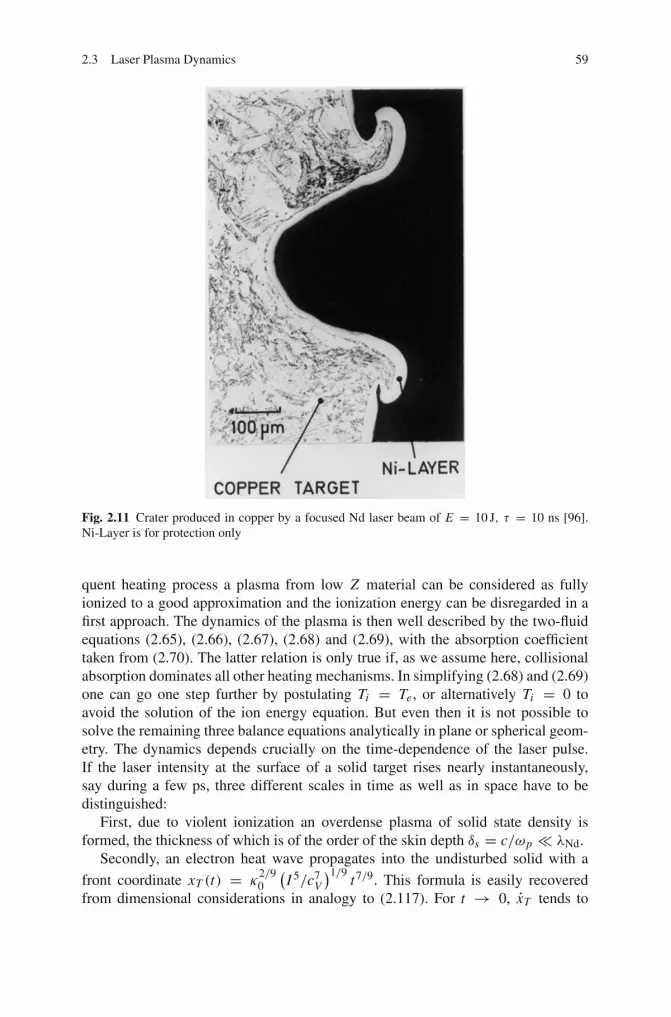
2.3 Laser Plasma Dynamics 59
Fig. 2.11 Crater produced in copper by a focused Nd laser beam of E = 10 J, τ = 10 ns [96].Ni-Layer is for protection only
quent heating process a plasma from low Z material can be considered as fullyionized to a good approximation and the ionization energy can be disregarded in afirst approach. The dynamics of the plasma is then well described by the two-fluidequations (2.65), (2.66), (2.67), (2.68) and (2.69), with the absorption coefficienttaken from (2.70). The latter relation is only true if, as we assume here, collisionalabsorption dominates all other heating mechanisms. In simplifying (2.68) and (2.69)one can go one step further by postulating Ti = Te, or alternatively Ti = 0 toavoid the solution of the ion energy equation. But even then it is not possible tosolve the remaining three balance equations analytically in plane or spherical geom-etry. The dynamics depends crucially on the time-dependence of the laser pulse.If the laser intensity at the surface of a solid target rises nearly instantaneously,say during a few ps, three different scales in time as well as in space have to bedistinguished:
First, due to violent ionization an overdense plasma of solid state density isformed, the thickness of which is of the order of the skin depth δs = c/ωp � λNd.
Secondly, an electron heat wave propagates into the undisturbed solid with a
front coordinate xT (t) = κ2/90
(I 5/c7
V
)1/9t7/9. This formula is easily recovered
from dimensional considerations in analogy to (2.117). For t → 0, xT tends to

60 2 The Laser Plasma
infinity which is characteristic of any continuum model of diffusion. From physicalconsiderations it is clear that the real maximum speed is xT
<∼ vth,e � se.In the third stage the plasma rarefies towards the vacuum with ion sound speed
s � se and, as the front of the heat wave slows down according to xT ∼ t−2/9 ashock wave propagating into the solid builds up as soon as xT < 2
γ−1 s is fulfilled(see vF after (2.111)). From now on a significant amount of the absorbed laserenergy originally stored in the electron fluid is transformed into kinetic energy ofthe plasma, i.e., of the ion fluid.
Owing to the complexity of laser induced plasma dynamics pure cases are ofparticular interest. Therefore in the following, instantaneous heating by powerfullasers in plane geometry, collisional heating and plasma expansion in plane andspherical geometry with long laser pulses of moderate intensity, similarity solutionsas well as steady state plasma production are treated.
2.3.1 Plasma Production with Intense Short Pulses
With respect to the achievement of dense, high temperature plasmas the most eco-nomic heating is realized when the energy input is so fast that the plasma is heatedbefore any appreciable motion sets in and hence all the absorbed energy is con-verted into thermal energy. Let us assume that a laser pulse of sub-ns duration τ
impinges onto the target. Let the absorbed energy per unit area, which is depositedat the surface of the target, be q0 =
∫τ
Iadt , Ia absorbed intensity. Then in planegeometry, with Te = Ti = T the system (2.65), (2.66), (2.67), (2.68), and (2.69)reduces to the heat diffusion equation (2.114) with α = 5/2. The specific heat perunit volume is cV = 3n0(Z + 1)kB/2. The temperature T (x, t) and its front xT (t)are given by (2.117). The value of T0/〈T 〉 = 1.223 shows that the temperatureprofile is roughly approximated by a rectangle. In order to apply these results toheating with ultrashort light pulses and to calculate the amount of heated matter wekeep in mind that the lifetime τp of the solid state density plasma is approximatelydetermined by the rarefaction wave which travels with the isothermal sound velocitys = √(pe + pi )/ρ0 into the heated material. The heat wave stops when the edge ofthe rarefaction wave reaches the front of the heat wave, i.e., when [101]
∫ τp
0sdt = xT (τp).
This relation yields the following expressions for the lifetime τp, thickness of theheated slab xT (τp), and maximum temperature T (τp) at the instant τp:
τp = 2
3
(8
9
)3/2
A9/4k−7/4B κ
1/20
m3/4i
n0 Z1/2(Z + 1)7/4q1/2
0 , (2.127)

2.3 Laser Plasma Dynamics 61
xT (τp) = 2
3
(8
9
)1/3
A3/2k−7/6B κ
1/30
m1/6i
n0 Z1/3(Z + 1)7/6q2/3
0 , (2.128)
T (τp) = q0
cV xT (τp)=(
8
9
)1/3
A−3/2k1/6B κ
−1/30
Z1/3(Z + 1)1/6
m1/6i
q1/30 . (2.129)
The constant A is given by (2.116). Note that T (τp) does not depend on the initialparticle density n0 and depends only weakly on the absorbed energy per unit areaq0. T (τp) represents an upper limit for the temperature since at the instant τp aconsiderable fraction of the energy is already converted into kinetic energy: if anisothermal rarefaction wave is assumed (worst case) the ratio of kinetic energy tothermal energy at the instant τp is 2/3.
The above relations are valid for Ti = Te. For the other limiting case of coldions, Ti = 0, one has merely to substitute Z + 1 by Z in (2.127), (2.128), and(2.129). In reality the ions are expected to be heated to a certain degree since theelectron-ion relaxation time τei = mi/2meνei can be shown to be of the same orderof magnitude as τp. In fact, with the relation sτp ≈ xF ≈ (κeτp/cV )
1/2 whichfollows from (2.127), (2.128) and κe/cV = 1
3λevth,e one obtains
τp ≈ 1
s2
κe
cV= 1
s2
λevth,e
3≈ mi
kTe
v2th,e
3νei= mi
2me
1
νei= τei .
Therefore, when effects are calculated for which the ion temperature enters verysensitively, e.g., neutron production, the ion temperature has to be evaluated accu-rately [102, 103]. The expansion of the plasma into vacuum for times t ≤ τp andover distances Δx less than the focal radius are approximately described by theplane rarefaction wave (2.110) or (2.111), respectively.
The foregoing model assumes τ � τp. With long pulses it depends on the risetime of the laser intensity whether or not a thermal or a shock wave develops ear-lier. If the intensity rises too slowly heat conduction only influences the expandingplasma and not the undisturbed or shocked solid. The problem was solved by Anisi-mov [104]. Let the absorbed intensity Ia(t) be such that 〈T 〉varies as tλ. Then
xT � d
dt
(aT 5/2t
)1/2 ∼ t (5λ−2)/4,
whereas the rarefaction wave travels at the speed of sound s ∼ 〈T 〉1/2 ∼ tλ/2.Comparing the two speeds leads to distinguishing the following situations:
(a) λ > 23 : For a certain time τp after the start of irradiation the sound velocity is
greater than the penetration velocity of the thermal wave. Thus the process ofplasma production at the beginning will be governed by the dynamics of plasmaexpansion.
(b) λ = 23 : Both velocities xT and s obey the same power law. The dominating
energy transport mechanism, either mass flow or heat conduction, is determined

62 2 The Laser Plasma
by the coefficients A and B of the relations vT = At1/3 and s = Bt1/3. If theheat conduction is the dominating process (xT > s), one can use the energyequation for a stationary medium without motion to calculate the time variationof the absorbed energy flux density Φ(t). From I (t) ∝ d[xT (t)〈T (t)〉]/dt , itfollows that the dependence is linear, Ia(t) ∼ t .
(c) λ < 23 : This is just the inverse case to (a). Up to a time τp, heat conduction
is the dominating energy transport mechanism. During this time the absorbedradiation intensity varies as tα with α < 1. The stationary heat wave (2.116)with Ia ∼ t2/9 belongs to this class.
The heat wave model was shown to be consistent with experiments performedwith 10 ps Nd laser pulses of intensities up to 3× 10¹⁵ Wcm−2 by Salzmann [105].The measured electron temperatures in deuterium and carbon targets at 1 J pulseenergy were 500 and 200 eV, respectively.
The model presented in this section is based on Spitzer–Braginskii’s thermalconductivity following a power law κe ∼ T α
e [see (2.64)]. Subsequent to exper-iments showing the failure of such a simple local law [106] an avalanche-likeenterprise started to investigate experimentally as well as theoretically phenom-ena of heat flux inhibition, nonlocal and anomalous transport. Despite the enor-mous effort concentrated on electron (and radiative) heat transport the problem isstill far from a satisfactory solution. To the reader who wishes a deeper insightin what the current state of the art is may start from the review article by Bell[107] and then consult more recent papers [108–113]. Perhaps only now withthe advent of greatly improved multidimensional particle-in-cell (PIC) and Vlasovcodes [114–118] is there a chance to come closer to a solution of this complexproblem.
2.3.1.1 Intense Sub-ps Pulses
At laser intensities of the order of 1017Wcm−2 and higher collisional absorption isno longer dominating. The interaction with solids and liquids becomes collision-less latest when Te exceeds 103 Z2 eV, Z average ion charge. The plasma formationprocess is very fast (a few laser cycles) and is a competition between field ion-ization (Chap. 7) and ionization by collisions. The final state is represented by ahighly overdense plasma of solid electron density. Only after 100 fs typical hydro-dynamic expansion sets in. According to classical linear optics the plasma shouldbehave like an ideal mirror of 100% reflectivity. General physical intuition tellsthat such ideal hypotheses have to be handled with care. In fact, early measure-ments showed that 70–80% “collisionless” absorption and even more is possible[119]. Soon after the experimental finding was qualitatively confirmed by computersimulations [120]. Thus, production of dense, extremely hot plasmas of relativisticelectron temperatures is possible with ultrashort superintense laser pulses. However,despite intense search for mechanisms leading to efficient collisionless absorptionover more than two decades, a satisfactory explanation of the underlying physical

2.3 Laser Plasma Dynamics 63
effects is available only since recently. The physics of these plasmas is the subjectof Chap. 8.
2.3.2 Heating with Long Pulses of Constant Intensity
In order to get a more detailed picture of the laser target interaction, the system(2.65), (2.66), (2.67), (2.68), and (2.69) has been solved numerically in plane andspherical geometry under the following conditions:
• The target material is solid hydrogen of particle density n0 = 4.5 × 10²² andinitial temperatures Te = Ti = 0;
• constant laser intensity I = I0 at Nd wavelength; the absorption is purely colli-sional;
• total reflection at the critical point;• heat conduction according to Spitzer–Braginskii, (2.64);• absence of ponderomotive force, π = 0.
2.3.2.1 Compression Wave
The dynamics of the high-density region in plane geometry is shown in Fig. 2.12for a 50 µm thick hydrogen foil irradiated by the laser intensity I0 = 1012 Wcm−2
[44]. For simplicity, in this special case Te = Ti = T is assumed. Starting froma low initial concentration of free electrons, in less than 0.1 ns a strong absorbinglayer forms at the front. Owing to the high plasma pressure a shock builds up whichtravels at 2.7 × 106 cm s−1 into the foil, reaching the rear surface in less than 2 ns.Since the shock wave has to balance the momentum of the expanding plasma, andthe densities in the two regions are very different, only a small fraction of the laserenergy is transferred to the shock wave (in the present case 8%). Transfer of a largeenergy fraction to the compressed phase is possible in gas targets, where the plasmadensity is comparable to the density in the shocked material. The results of Fig. 2.12were obtained by assuming the validity of the ideal gas law also for solid hydrogen.This may not be unreasonable because it is a very soft material; at only 40 kbars it iscompressed by κ = 2.7 [121]. For comparison, to reach a comparable compressionratio of 2.2 in lead, 4 Mbars are needed.
As the amount of energy going into the shock wave is small and we are inter-ested only in the properties of the hot plasma, the solid is treated as incompressiblein the following and the interest is concentrated entirely on the plasma properties.Equations (2.65), (2.66), (2.67), (2.68), and (2.69) are solved in plane and sphericalgeometry. In the spherical case the radius of the pellet is chosen as R0 = 100 µm. Inorder to make the two cases comparable and to show better the influence of purelygeometrical effects, R0 is kept constant by introducing a self-consistent mattersource on the pellet surface which balances the amount of ablated material. The lightflux F in spherical geometry is chosen to produce the intensity I0 on the originalpellet surface, i.e., F = 4πR2
0 I0.
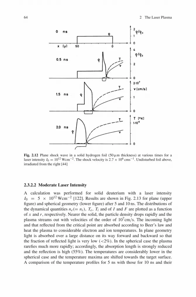
64 2 The Laser Plasma
Fig. 2.12 Plane shock wave in a solid hydrogen foil (50 µm thickness) at various times for alaser intensity I0 = 1012 Wcm−2. The shock velocity is 2.7× 10⁶ cms−1. Undisturbed foil above,irradiated from the right [44]
2.3.2.2 Moderate Laser Intensity
A calculation was performed for solid deuterium with a laser intensityI0 = 5 × 10¹² Wcm−2 [122]. Results are shown in Fig. 2.13 for plane (upperfigure) and spherical geometry (lower figure) after 5 and 10 ns. The distributions ofthe dynamical quantities ne(= ni ), Te, Ti and of I and F are plotted as a functionof x and r , respectively. Nearer the solid, the particle density drops rapidly and theplasma streams out with velocities of the order of 107cm/s. The incoming lightand that reflected from the critical point are absorbed according to Beer’s law andheat the plasma to considerable electron and ion temperatures. In plane geometrylight is absorbed over a large distance on its way forward and backward so thatthe fraction of reflected light is very low (<2%). In the spherical case the plasmararefies much more rapidly; accordingly, the absorption length is strongly reducedand the reflection is high (55%). The temperatures are considerably lower in thespherical case and the temperature maxima are shifted towards the target surface.A comparison of the temperature profiles for 5 ns with those for 10 ns and their

2.3 Laser Plasma Dynamics 65
Fig. 2.13 Plasma production from solid deuterium in plane (upper) and spherical (lower) geometrywith a Nd laser intensity I0 = 5× 10¹² Wcm−2 after 5 and 10 ns. ne electron density, Te electrontemperature, Ti ion temperature, I laser intensity, F = 4πr2 I laser flux. Laser pulse impingesfrom the right. The ratio between thermal ion and electron energies in plane (spherical) geometryis 0.62 (0.47) at 5 ns and 0.66 (0.51) at 10 ns
position as a function of r shows immediately that in spherical geometry the plasmaproduction process becomes stationary near the target.
The partition of the laser energy into internal and kinetic plasma energy stronglydepends on the geometry. In the plane case 43% of the absorbed energy is stored as

66 2 The Laser Plasma
thermal energy of the electrons and ions; this ratio remains approximately constantin time. For the pellet a much more unfavorable ratio is expected. In fact, at 5 and10 ns only 25 and 15%, respectively of the absorbed energy is stored as thermalenergy. At the intensity under consideration the influence of heat conduction turnedout to be very small. Therefore matter is heated only in regions where light pen-etrates, and the plasma density – with the exception of a very small region at thetarget surface – is less than its critical value nc.
2.3.2.3 Higher Laser Intensity
Corresponding calculations were performed with an intensity of I0 = 1015 Wcm−2.The results are shown in Fig. 2.14 at 2.5 and 5 ns after the start of irradiation.In both geometries the electron temperature is 10 times higher, the ion tempera-ture 4 times higher as compared with the previous case. At high temperatures theplasma production process is determined by light absorption and heat conduction.In contrast to light propagation, thermal diffusion is not limited by any cut-offdensity, and a large overdense region (ne > 1021cm−3) builds up in sphericaland especially in plane geometry. Whereas at low intensities its thickness is aboutone wavelength and its structure is determined by light tunneling at the reflectionpoint, for intensities greater than about I0 = 1013 Wcm−2 its extension is givenby heat conduction. From the figure in plane geometry one can see that the over-dense region is growing in time: at 5 ns two thirds of the plasma produced isheated by thermal diffusion alone. In spherical geometry the heat conduction zoneis much smaller and becomes stationary. In the plane case the ratio of thermal tototal plasma energy is 47% at 5 ns and increases very slowly with time. Althoughheat conduction also plays a dominant role in spherical geometry, the partition ofthermal and kinetic energy at I0 = 1015 Wcm−2 still favors the latter: at 2.5 ns only23% and at 5 ns not more than 16% of the absorbed radiation appears as thermalenergy.
With respect to laser light reflection we note that now, at the higher light inten-sity, the absorbing region has much larger dimensions; nevertheless the reflection isincreased in both geometries as a result of the rise in the electron temperature (16and 60 % reflection).
Beer’s law is a consequence of the WKB or optical approximation; it fails in thevicinity of the reflection point. By solving the wave equation for I0 = 1014 Wcm−2
in plane geometry one finds that about 15% of the total absorbed energy goes intothe slab where the optical approximation breaks down; in the overdense regiononly 5% is absorbed. At higher intensities the absorption behind the reflectionpoint is even lower because of the higher electron temperature. Thus the assump-tion of reflection at the critical density may be considered as approximately cor-rect for calculating the overall dynamic behavior. For considerations in detail seeSect. 3.2.1.

2.3 Laser Plasma Dynamics 67
Fig. 2.14 Plasma production from solid deuterium in plane (upper figure) and spherical (lowerfigure) geometry with a Nd laser intensity I0 = 5 × 10¹⁵ Wcm−2 after 2.5 and 5 ns. Symbols asin Fig. 2.13. The ratio between thermal ion and electron energies in plane (spherical) geometry is0.31 (0.10) at 2.5 ns and 0.32 (0.06) at 5 ns. The target is irradiated from the right
2.3.2.4 Multicomponent Plasma
As pointed out earlier, laser plasmas produced from high-Z elements represent mix-tures of different ion charge states [123–126]. Such plasmas are of interest as sourcesof highly stripped ions for accelerators [127]. Optical and mass-spectroscopic inves-tigations of the expanding plasma cloud show that the more highlycharged the ions

68 2 The Laser Plasma
are the higher is their kinetic energy [128–133]. A first explanation of the energyspectra was based on electrostatic acceleration [67, 129, 134]. In the hot plasmacloud a quasi-static thermoelectric field Es builds up according to (2.74) by whichthe various groups of ions should be accelerated corresponding to their individualcharge state Z . As early as 1971 it was shown that in a fluid model 1% of theactual friction force an ion feels in moving through the plasma cloud is alreadyable to inhibit ion separation [135]. Similar independent theoretical investigations adecade later came to the same conclusion [136]. Meanwhile further investigationsindicate that the observed ion separation is presumably a consequence of recom-bination [126, 137–139]. On such a background Kunz investigated the expansiondynamics of a multicomponent laser plasma numerically by solving coupled rateequations for a whole variety of ionization and recombination processes simultane-ously with the expansion process [140]. Independently, similar dynamic calculationswere performed in great detail by Granse et al. [141]. Very satisfactory agreementwas found with the ion energy spectra most carefully measured by Dinger et al.[131]. Subsequently Rupp and Rohr [142] performed detailed measurements of therecombination dynamics of a plasma as a function of distance from the target. Oneof the remarkable and basic aspects of these investigations is the important role thatreheating of the expanding plasma plays due to recombination: No charged particleswould reach the ion collectors if the plasma had cooled down adiabatically. Thesensitivity of the ion energies to reheating was shown also by an ingenious ana-lytical investigation [143]. Summarizing, it can be concluded that in the intensityrange I � 1011 − 1013 Wcm−2 the experimentally observed ion separation is verylikely to be based mainly on the phenomenon of recombination and that electrostaticacceleration has to be excluded as predicted in the early stage of investigations onthis subject. Meanwhile detailed measurements exist on the ion velocity distributionand anisotropy of kinetic ion temperature, angular emission distributions of neu-trals and ions, and on the effect of recombination processes and ionization states[144, 145]. Binary systems show no directional segregation. The neutrals dominateat low laser intensities (I < 1012 Wcm−2) and large distances from the target:their kinetic energy is generally low and is smaller than that of the singly chargedions. All measurements underline the importance of recombination (e.g. three bodyrecombination) up to distances of 1 m. The expansion dynamics shows also complexstructures, i.e., the formation of localized groups of ions propagating at differentvelocities and densities. In such an environment groups of highly charged ions mayalso survive [146, 147].
Ion separation is studied more recently with intense short laser pulses insmall liquid droplets and clusters. Here, the observed different energies of differ-ently charged ions are generally attributed to thermoelectric acceleration. How-ever, a quantitative proof has not been given yet. So, for instance in anal-ogy to [135], the question of friction between the different ion species wouldhave to be clarified for the new parameters associated with plasmas gener-ated by intense sub ps laser pulses. A kinetic Vlasov treatment of the parti-cle dynamics during the adiabatic expansion of a plasma bunch is presented in[148].

2.3 Laser Plasma Dynamics 69
2.3.3 Similarity Considerations
From a large number of computer runs with a systematic variation of the parame-ters the functional dependence of all variables on these parameters can be obtained.Such a procedure is generally time-consuming. Here dimensional analysis is muchsuperior. However, if this method is applied to system (2.65), (2.66), (2.67),(2.68), and (2.69) as it stands, more than one dimensionless variable π is foundand the method is not conclusive. If instead Ti is assumed to be proportional toTe, Ti = ξTe, heat conduction is neglected and the internal energy per unit massε = 3kB(Z Te + Ti )/2mi is introduced the system reduces in plane geometry to
∂ρ
∂t+ ∂
∂xρv = 0 (2.130)
∂v
∂t+ v
∂v
∂x= − 2
3ρ
∂
∂xρε (2.131)
∂ε
∂t+ v
∂ε
∂x= −2
3ε∂v
∂x+ α
ρI (x) (2.132)
α = Cρ2
ε3/2, I (x) = I0 exp
(−∫ ∞
xαdx
). (2.133)
The initial values are I0 = 0, v = 0, ε = 0, ρ = ρ0 for t ≤ 0 and I0 = const > 0for t > 0. A look at (2.130), (2.131), (2.132), and (2.133) and the boundary/initialconditions reveals that ρ, v, ε depend on I0,C, x, t and ρ0. However, as long asthe average plasma density is much lower than ρ0, almost all energy is fed into theplasma, only a small portion being coupled to the solid. The dependence on ρ0 isweak and hence ρ0 = ∞ can be set, so that ρ0 is no longer a free variable [149].The remaining dimensional matrix is given in Table 2.7. From this the existence ofone dimensionless variable π is deduced,
π = x
C1/8 I 1/40 t9/8
.
It is convenient to express all dimensional variables without using x ; then they areuniquely determined from the π -theorem as follows,
ρ = I 1/40 (Ct)−3/8 R(π), v = I 1/4
0 (Ct)1/8V (π),
ε = I 1/20 (Ct)1/4 E(π), I (x) = I0 J (π),
and (2.130), (2.131), (2.132), and (2.133) reduces to a system of ordinary differentialequations (the prime corresponds to d/dπ ),
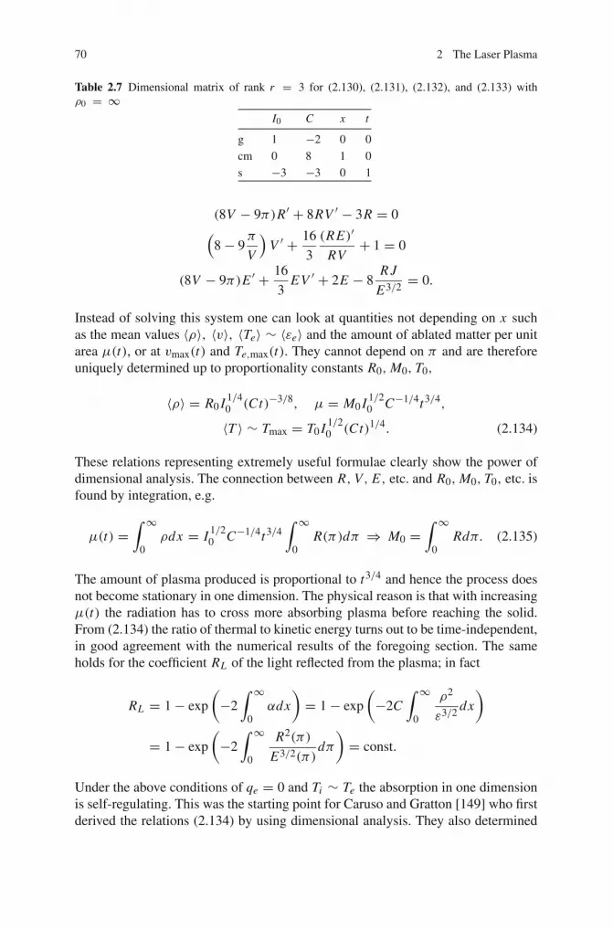
70 2 The Laser Plasma
Table 2.7 Dimensional matrix of rank r = 3 for (2.130), (2.131), (2.132), and (2.133) withρ0 = ∞
I0 C x t
g 1 −2 0 0
cm 0 8 1 0
s −3 −3 0 1
(8V − 9π)R′ + 8RV ′ − 3R = 0(
8− 9π
V
)V ′ + 16
3
(RE)′
RV+ 1 = 0
(8V − 9π)E ′ + 16
3EV ′ + 2E − 8
R J
E3/2= 0.
Instead of solving this system one can look at quantities not depending on x suchas the mean values 〈ρ〉, 〈v〉, 〈Te〉 ∼ 〈εe〉 and the amount of ablated matter per unitarea μ(t), or at vmax(t) and Te,max(t). They cannot depend on π and are thereforeuniquely determined up to proportionality constants R0, M0, T0,
〈ρ〉 = R0 I 1/40 (Ct)−3/8, μ = M0 I 1/2
0 C−1/4t3/4,
〈T 〉 ∼ Tmax = T0 I 1/20 (Ct)1/4. (2.134)
These relations representing extremely useful formulae clearly show the power ofdimensional analysis. The connection between R, V, E, etc. and R0, M0, T0, etc. isfound by integration, e.g.
μ(t) =∫ ∞
0ρdx = I 1/2
0 C−1/4t3/4∫ ∞
0R(π)dπ ⇒ M0 =
∫ ∞
0Rdπ. (2.135)
The amount of plasma produced is proportional to t3/4 and hence the process doesnot become stationary in one dimension. The physical reason is that with increasingμ(t) the radiation has to cross more absorbing plasma before reaching the solid.From (2.134) the ratio of thermal to kinetic energy turns out to be time-independent,in good agreement with the numerical results of the foregoing section. The sameholds for the coefficient RL of the light reflected from the plasma; in fact
RL = 1− exp
(−2∫ ∞
0αdx
)= 1− exp
(−2C
∫ ∞
0
ρ2
ε3/2dx
)
= 1− exp
(−2∫ ∞
0
R2(π)
E3/2(π)dπ
)= const.
Under the above conditions of qe = 0 and Ti ∼ Te the absorption in one dimensionis self-regulating. This was the starting point for Caruso and Gratton [149] who firstderived the relations (2.134) by using dimensional analysis. They also determined
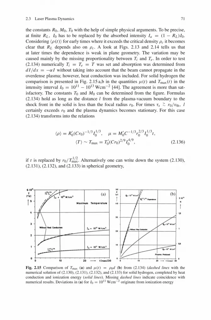
2.3 Laser Plasma Dynamics 71
the constants R0, M0, T0 with the help of simple physical arguments. To be precise,at finite RL , I0 has to be replaced by the absorbed intensity Ia = (1 − RL)I0.Considering 〈ρ(t)〉 for early times where it exceeds the critical density ρc it becomesclear that RL depends also on ρc. A look at Figs. 2.13 and 2.14 tells us thatat later times the dependence is weak in plane geometry. The variation may becaused mainly by the missing proportionality between Ti and Te. In order to test(2.134) numerically Ti = Te = T was set and absorption was determined fromd I/dx = −α I without taking into account that the beam cannot propagate in theoverdense plasma; however, heat conduction was included. For solid hydrogen thecomparison is presented in Fig. 2.15 a,b in the quantities μ(t) and Tmax(t) in theintensity interval I0 = 1011 − 1013 Wcm−2 [44]. The agreement is more than sat-isfactory. The constants T0 and M0 can be determined from the figure. Formulas(2.134) hold as long as the distance l from the plasma-vacuum boundary to theshock front in the solid is less than the focal radius r0. For times τs
>∼ r0/vth, lcertainly exceeds r0 and the plasma dynamics becomes stationary. For this case(2.134) transforms into the relations
〈ρ〉 = R′0(Cr0)−1/3 I 1/3
0 , μ = M ′0C−1/3r2/3
0 I 1/30 t,
〈T 〉 ∼ Tmax = T ′0(Cr0)2/9 I 4/9
0 , (2.136)
if t is replaced by r0/T 1/2max. Alternatively one can write down the system (2.130),
(2.131), (2.132), and (2.133) in spherical geometry,
Fig. 2.15 Comparison of Tmax (a) and μ(t) = ρ0d (b) from (2.134) (dashed lines with thenumerical solution of (2.130), (2.131), (2.132), and (2.133) for solid hydrogen, completed by heatconduction and ionization energy (solid lines). Missing dashed lines indicate coincidence withnumerical results. Deviations in (a) for I0 = 1011 Wcm−2 originate from ionization energy
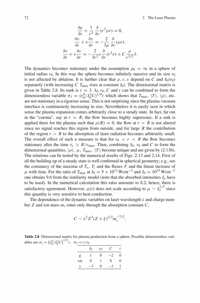
72 2 The Laser Plasma
∂ρ
∂t+ 1
r2
∂
∂r(r2ρv) = 0,
∂v
∂t+ v
∂v
∂r= − 2
3ρ
∂
∂r(ρε),
∂ε
∂t+ v
∂ε
∂r= − 2
3r2ε∂
∂r(r2v)+ C
ρ
ε3/2I.
The dynamics becomes stationary under the assumption ρ0 = ∞ in a sphere ofinitial radius r0. In this way the sphere becomes infinitely massive and its size r0is not affected by ablation. It is further clear that ρ, ε, v depend on C and I0(r0)
separately (with increasing C Tmax rises at constant I0). The dimensional matrix isgiven in Table 2.8. Its rank is r = 3. I0, r0,C and t can be combined to form thedimensionless variable π1 = (r8
0/I 20 C)1/9t which shows that Tmax, 〈T 〉, 〈ρ〉, etc.
are not stationary in a rigorous sense. This is not surprising since the plasma-vacuuminterface is continuously increasing in size. Nevertheless it is easily seen in whichsense the plasma expansion comes arbitrarily close to a steady state. In fact, far outin the “corona”, say at r = R, the flow becomes highly supersonic. If a sink isapplied there for the plasma such that ρ(R) = 0, the flow at r < R is not alteredsince no signal reaches this region from outside, and for large R the contributionof the region r > R to the absorption of laser radiation becomes arbitrarily small.The overall effect of such a measure is that for r0 < r < R the flow becomesstationary after the time τs � R/vmax. Then, combining I0, r0 and C to form thedimensional quantities, 〈ρ〉, μ, Tmax, 〈T 〉 become unique and are given by (2.136).The relations can be tested by the numerical results of Figs. 2.13 and 2.14. First ofall the building up of a steady state is well confirmed in spherical geometry; e.g., seethe constancy of the maxima of Te, Ti and the fluxes F and the linear increase ofμ with time. For the ratio of Tmax at I0 = 5× 10¹² Wcm−2 and I0 = 1015 Wcm−2
one obtains 9.6 from the similarity model (note that the absorbed intensities Ia haveto be used). In the numerical calculation this ratio amounts to 8.2; hence, there issatisfactory agreement. However, μ(t) does not scale according to μ ∼ I 1/3
a sincethis quantity is very sensitive to heat conduction.
The dependence of the dynamic variables on laser wavelength λ and charge num-ber Z and ion mass mi enter only through the absorption constant C ,
C ∼ λ2 Z3(Z + ξ)3/2m−7/2i ,
Table 2.8 Dimensional matrix for plasma production from a sphere. Possible dimensionless vari-
ables are π1 =(r8
0/I 20 C)1/9
t, π2 = r/r0
I0 r0 C t
g 1 0 −2 0
cm 0 1 8 0
s −3 0 −3 1
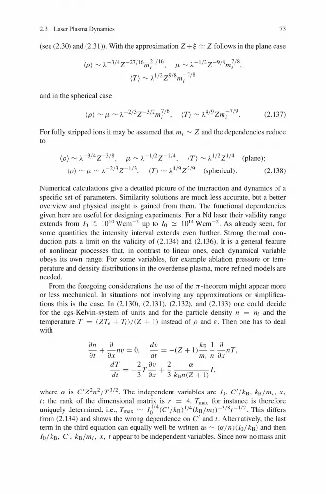
2.3 Laser Plasma Dynamics 73
(see (2.30) and (2.31)). With the approximation Z+ξ � Z follows in the plane case
〈ρ〉 ∼ λ−3/4 Z−27/16m21/16i , μ ∼ λ−1/2 Z−9/8m7/8
i ,
〈T 〉 ∼ λ1/2 Z9/8m−7/8i
and in the spherical case
〈ρ〉 ∼ μ ∼ λ−2/3 Z−3/2m7/6i , 〈T 〉 ∼ λ4/9 Zm−7/9
i . (2.137)
For fully stripped ions it may be assumed that mi ∼ Z and the dependencies reduceto
〈ρ〉 ∼ λ−3/4 Z−3/8, μ ∼ λ−1/2 Z−1/4, 〈T 〉 ∼ λ1/2 Z1/4 (plane);〈ρ〉 ∼ μ ∼ λ−2/3 Z−1/3, 〈T 〉 ∼ λ4/9 Z2/9 (spherical). (2.138)
Numerical calculations give a detailed picture of the interaction and dynamics of aspecific set of parameters. Similarity solutions are much less accurate, but a betteroverview and physical insight is gained from them. The functional dependenciesgiven here are useful for designing experiments. For a Nd laser their validity rangeextends from I0
>∼ 1010 Wcm−2 up to I0 � 1014 Wcm−2. As already seen, forsome quantities the intensity interval extends even further. Strong thermal con-duction puts a limit on the validity of (2.134) and (2.136). It is a general featureof nonlinear processes that, in contrast to linear ones, each dynamical variableobeys its own range. For some variables, for example ablation pressure or tem-perature and density distributions in the overdense plasma, more refined models areneeded.
From the foregoing considerations the use of the π -theorem might appear moreor less mechanical. In situations not involving any approximations or simplifica-tions this is the case. In (2.130), (2.131), (2.132), and (2.133) one could decidefor the cgs-Kelvin-system of units and for the particle density n = ni and thetemperature T = (Z Te + Ti )/(Z + 1) instead of ρ and ε. Then one has to dealwith
∂n
∂t+ ∂
∂xnv = 0,
dv
dt= −(Z + 1)
kB
mi
1
n
∂
∂xnT,
dT
dt= −2
3T∂v
∂x+ 2
3
α
kBn(Z + 1)I,
where α is C ′Z2n2/T 3/2. The independent variables are I0, C ′/kB, kB/mi , x,t ; the rank of the dimensional matrix is r = 4. Tmax for instance is thereforeuniquely determined, i.e., Tmax ∼ I 1/4
0 (C ′/kB)1/4(kB/mi )
−3/8t−1/2. This differsfrom (2.134) and shows the wrong dependence on C ′ and t . Alternatively, the lastterm in the third equation can equally well be written as ∼ (α/n)(I0/kB) and thenI0/kB, C ′, kB/mi , x, t appear to be independent variables. Since now no mass unit
74 2 The Laser Plasma
appears in I0/kB, C ′ and kB/mi the rank of the matrix is r = 3 and nothing can beconcluded on how Tmax depends on I0/kB, C ′, kB/mi and t ; only the contradictionhas disappeared. This digression illustrates that the use of the π -theorem generallyrequires physical intuition and it may stimulate the reader to find out the source ofthe wrong dependence of Tmax given above.
2.4 Steady State Ablation
The knowledge of ablation pressure is important for calculating shock strength indense matter and investigating equations of state [150], foil acceleration [151] andpellet compression for inertial confinement fusion (ICF) [11, 152, 153], and holeboring in fast ignition [13]. Fast ablation of matter by powerful lasers or particlebeams, e.g., light or heavy ions, is one of the methods to create pressures in theMegabar range [154]. Above a certain energy supply in solids and liquids a phasetransition occurs to the gaseous state; at even higher energies direct transforma-tion of matter into the plasma state is achieved. Currently the highest pressures inthe laboratory are obtained by laser ablation. Already at comparatively low laserpulse energies pressures up to 50 Mbars were measured in shock waves launchedin solid foils by direct irradiation [155, 151]. By using ultrashort laser pulses theirenergy content can be significantly reduced, e.g., a 120 fs pulse of only 30 mJ wasable to produce a 3 Mbar shock [156]. Higher pressures were reported in impactexperiments using laser-accelerated foils [157, 158]. In numerical simulations oflaser-accelerated colliding foils the calculated pressure maxima reached up to 2Gbar [159], and from experiments the authors concluded that shock pressures over400 Mbar are achievable [160]. More recently 750 Mbar planar shocks in gold tar-get foils impacted by X-ray driven gold flyer foils were measured by Cauble et al.[161]. Much higher pressures are achievable in converging shocks, as for example11 Gbar in a laser pellet compression experiment [162]. Intense shock generationrepresents an extremely significant tool to study equations of state of hot densematter in radiation physics and astrophysics. For such purposes the shock front hasto be planar. The best quality in this respect up to now was obtained by matterablation induced by thermal radiation from laser heated hohlraums [163, 164]. Asthe laser beam smoothing technique has gradually improved, shock generation bydirect laser drive has gained increasing attention and is now being used with growingsuccess [165–167]. In this way the unavoidable losses of pressure in indirect driveare bypassed. For such reasons and for inertial confinement fusion (ICF) research(pellet compression and spark ignition [168–171]) ablative pressure generationby laser has repeatedly attracted the interest of numerous theoreticians for manyyears.
The gas dynamic aspect of ablation pressure was studied in great detail in 1Dmodels and with two-dimensional corrections, taking also anomalous heat conduc-tion and fast electron production into account [168]. There are two situations acces-sible to an analytic treatment: sudden impact heating before hydrodynamic motion

2.4 Steady State Ablation 75
sets in, and the opposite case, i.e., after a steady state has developed. When the flowof the ablated material is quasi-stationary the ablation pressure is easily estimatedif the Mach number M is known at one fixed density value. In laser heating sucha natural fixed point is the critical density as soon as collisional absorption in thelower density plasma weakens and resonance absorption starts to dominate. For thisreason in a number of papers the problem of the critical Mach number, i.e., the Machnumber at this point, was investigated in plane and spherical flows [154, 172–178]Several arguments were used, in plane and spherical geometry, to show that theJouget point, that is M = 1, is located at the critical point or in the overdense region[175]. The analysis of spherical flow is rendered more difficult by the appearance ofa characteristic radius as a new parameter. Gitomer et al. [174] solved the problemfor high laser flux densities by the guidance of numerical calculations and obtainedsimple expressions for the ablation pressure. They also showed that in sphericalgeometry the mass flow at the critical point can be either subsonic or supersonicdepending on the limitation of heat flux qe.
At the moment there is no universally accepted ablation pressure model. Thereare contradictions in details between the various models themselves and betweenthe models and the experiments. In some experiments agreement was found moreor less with a whole class of simple theoretical pictures but not with those whichare believed to be particularly accurate [179]. In the following the basic aspectsof steady state laser-matter interaction also for laser intensities at which heat con-duction dominates, are elaborated, and a simple model for the ablation pressure ispresented. To the reader wishing to go more into detail at moderate laser intensi-ties [151, 168, 177, 180] are particularly recommended. There exists a consider-able amount of published material on ablation pressure; nevertheless the degreeof apparent contradictions and confusion is very high. In order to contribute toclarification, in the following sections steady state onedimensional models, planeand spherical, are developed. Thereby the effect of heat flow supplied to theexpanding corona, hitherto overlooked, is included and the basic gasdynamic rela-tions which hold with certainty once well-defined conditions are fulfilled, areelaborated.
2.4.1 The Critical Mach Number in a Stationary Planar Flow
First we study the plane 1D model. When a target with an initially flat surface isheated, the flow of evaporated matter is planar near the solid–gas or solid–plasmainterface. As the distance increases the flow pattern becomes more and more diver-gent creating in this way a zone of a stationary flow field in front of the interface.The temperature increases from a low value in the target, reaches a maximum some-where in the stationary zone and then decays because of cooling due to expansion(Fig. 2.16). Let us assume that the ablated gas or plasma follows a polytropic equa-tion of state of the form pρ−γ = const, γ = const, so that the sound velocity sis given by (2.100) with ka = 0. In the isothermal case (infinite heat conduction)

76 2 The Laser Plasma
γe = γi = γ = 1. Mass and momentum flow in the stationary zone are governedby ρv = const and, neglecting ponderomotive forces,
∂
∂x(ρv2 + p) = ρv
∂
∂x
(v + p
ρv
)= ρv
∂
∂xs
(M + 1
γ M
)= 0. (2.139)
The momentum equation tells that
Pa = p + ρv2 (2.140)
is invariant throughout the stationary flow region and represents the true ablationpressure. Differentiating the last expression of (2.139) leads to the relation
(M + 1
γ M
)1
s
∂s
∂x+(
M − 1
γ M
)1
M
∂M
∂x= 0. (2.141)
From this we conclude that at the position xm of the maximum of temperature orsound speed
M = 1√γ
(2.142)
holds. The proof is as follows. As one moves from the target to the vacuum Mincreases from M � 1 to M = ∞. Let xM be the smallest value at which (2.142)holds. xM < xm is not possible because the derivative of s is positive (for instance,there is no saddle point in s for x < xm). If xM ≥ xm holds, ∂s/∂x must againbe zero there. This implies either xM = xm , or ∂M/∂x = 0 at xm , respectively. In
Fig. 2.16 Steady state 1D model. Distributions of temperature T , sound speed s and Mach num-ber M = v/s in a typical ablation flow into vacuum. Ia absorbed laser flux, ql , qr heat fluxes;absorption region dashed

2.4 Steady State Ablation 77
Fig. 2.17 (a): Steady state plane ablation. Energy input at ρc/ρ0 = 0.2. Mc = √1/γ is exactlyconfirmed for γ = 5/3. Mc does not depend on the value of ρc; heat conduction according (2.64)is included. (b): Plane nonsteady ablation due to energy deposition at xc (50%) as well as in theablated plasma. Mc = 0.44. The inhomogeneity of the compressed matter is due to decrease ofPa(t) (see also Fig. 2.12)
the latter case differentiating (2.139) once more leads to the following relation atx = xm ,
(M + 1
γ M
)1
s
∂2s
∂x2+ s
M
(M − 1
γ M
)∂2 M
∂x2= 0, (2.143)
from which owing to ∂2s/∂x2 < 0 also ∂2 M/∂x2 < 0, i.e., v = max follows.But this is in contradiction to the physical assumption of the existence of only onemaximum in T . In addition, (2.143) shows that x = xm cannot be a saddle pointfor M .
Pa can now be calculated from (2.140) if s and ρ are known at xm . With res-onance absorption dominating over collisional absorption (see Chap.3), e.g., atIλ2 >∼ 1013 Wcm−2µm2, the energy deposition zone becomes centered around thecritical point x = xc in a narrow region. Furthermore, in numerous experiments qeseemed to be bounded by a limit considerably lower than the classical value (2.64)(“heat flux inhibition” [151, 177]). This situation implies that xm lies close to xc
and that the heat front xT is sufficiently close to xm to guarantee the flow to beapproximately planar in between. To prove numerically whether in this case (2.142)is fulfilled or not the fully time dependent initial value problem of target irradia-tion by a laser pulse of constant intensity was solved. The energy was depositedin a narrow zone around xc and, in order to simulate the divergent flow, ρ was setequal to zero far out in the supersonic region. As Fig. 2.17a shows, the relationMc = 1/
√γ = √
3/5 = 0.774 is extremely well fulfilled. This is even moresurprising if one takes into account that the maximum in T is very flat. A completelydifferent picture with Mc � 1/
√γ is obtained when half of the incoming laser flux
is deposited to the right of xc (Fig. 2.17b). However, M � 1/√γ is again reached
at the maximum of T which is now located far away from the critical point, outsidethe picture.
Several arguments have been given in the past to show that Mc = 1 should hold.It is evident from the analysis presented here that the validity of those arguments is
78 2 The Laser Plasma
questionable for γ = 1. It becomes further clear that a supersonic stationary flowat xc [175] can only be due to deviations from plane geometry (e.g., divergenceeffects) regardless of how strong the heat flux in the overdense region is. In anunsteady flow such a restriction does not hold owing to the presence of additional,i.e., inertial terms.
So far exact relations for M have been obtained in plane geometry if the flowis of hydrodynamic character. For a gas target this is always the case, even at arbi-trarily low energy flux densities, as soon as the mean free path is small comparedto the target dimensions, and the Mach number at T = Tmax is 1/
√γ . The situa-
tion changes drastically when the cohesive forces, i.e., the sublimation heat of thetarget material, become high. There is an energy regime in which the evaporatedmaterial is almost collision-free. Then the situation can be described by introducingthe potential barrier U representing the sublimation energy per particle. Inside thesolid the probability of the particle energies is given by the canonical distribution.When crossing the barrier U the molecules or atoms undergo a sufficient numberof collisions to become Maxwellian so that just above the surface their distributionfunction is
f (0+; v) = n0
2
(β
π
)3/2
exp
[−β
(2U
m+ v2
)], β = m/2kBT .
Therefrom the free streaming velocity v = vx results,
vx =∫vx f dv∫
f dv=(β
π
)1/2 ∫ ∞
0vx e−βv2
x dvx =(
kBT
2πm
)1/2
(2.144)
which is smaller by the factor (6π)1/2 = 4.3 than the thermal velocity vth =(3kBT/m)1/2. The density undergoes a discontinuous transition from n0 ton0e−U/kBT .
2.4.2 Ablative Laser Intensity
In general the energy supplied to the target may be deposited over a wide region inspace as, for instance, is the case of collisionally absorbed short wavelength radi-ation. However, the opposite situation of Fig. 2.16 in which the energy absorptionzone is centered in a narrow region of density as assumed here, is of particularrelevance for heating by strong laser pulses, in some deflagrations, and detonations[181]. In such cases the deposited energy flux density Ia may be thought of asdeposited locally and split into the two heat fluxes ql and qr to the left and to theright , as indicated in Fig. 2.16. In this model the slope of T is discontinuous atxm in order to satisfy ql = κ(∂T/∂x)xm and qr = −κ(∂T/∂x)xm . ql covers theconvection of enthalpy plus kinetic energy of the ablated material whereas qr goesentirely into expansion work of the outflowing matter [173] and does not contribute
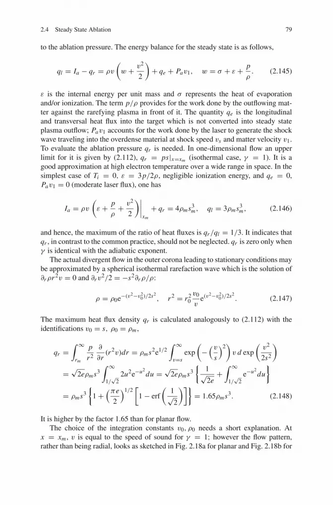
2.4 Steady State Ablation 79
to the ablation pressure. The energy balance for the steady state is as follows,
ql = Ia − qr = ρv
(w + v2
2
)+ qe + Pav1, w = σ + ε + p
ρ. (2.145)
ε is the internal energy per unit mass and σ represents the heat of evaporationand/or ionization. The term p/ρ provides for the work done by the outflowing mat-ter against the rarefying plasma in front of it. The quantity qe is the longitudinaland transversal heat flux into the target which is not converted into steady stateplasma outflow; Pav1 accounts for the work done by the laser to generate the shockwave traveling into the overdense material at shock speed vs and matter velocity v1.To evaluate the ablation pressure qr is needed. In one-dimensional flow an upperlimit for it is given by (2.112), qr = ps|x=xm (isothermal case, γ = 1). It is agood approximation at high electron temperature over a wide range in space. In thesimplest case of Ti = 0, ε = 3p/2ρ, negligible ionization energy, and qe = 0,Pav1 = 0 (moderate laser flux), one has
Ia = ρv
(ε + p
ρ+ v2
2
)∣∣∣∣xm
+ qr = 4ρms3m, ql = 3ρms3
m, (2.146)
and hence, the maximum of the ratio of heat fluxes is qr/ql = 1/3. It indicates thatqr , in contrast to the common practice, should not be neglected. qr is zero only whenγ is identical with the adiabatic exponent.
The actual divergent flow in the outer corona leading to stationary conditions maybe approximated by a spherical isothermal rarefaction wave which is the solution of∂rρr2v = 0 and ∂rv
2/2 = −s2∂rρ/ρ:
ρ = ρ0e−(v2−v20)/2s2
, r2 = r20v0
ve(v
2−v20)/2s2
. (2.147)
The maximum heat flux density qr is calculated analogously to (2.112) with theidentifications v0 = s, ρ0 = ρm ,
qr =∫ ∞
rm
p
r2
∂
∂r(r2v)dr = ρms2e1/2
∫ ∞
v=sexp
(−(v
s
)2)v d exp
(v2
2s2
)
= √2eρms3∫ ∞
1/√
22u2e−u2
du = √2eρms3{
1√2e+∫ ∞
1/√
2e−u2
du
}
= ρms3{
1+(πe
2
)1/2[
1− erf
(1√2
)]}= 1.65ρms3. (2.148)
It is higher by the factor 1.65 than for planar flow.The choice of the integration constants v0, ρ0 needs a short explanation. At
x = xm , v is equal to the speed of sound for γ = 1; however the flow pattern,rather than being radial, looks as sketched in Fig. 2.18a for planar and Fig. 2.18b for
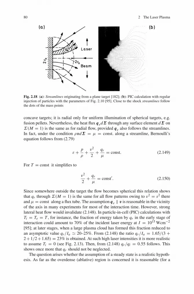
80 2 The Laser Plasma
Fig. 2.18 (a): Streamlines originating from a plane target [182]; (b): PIC calculation with regularinjection of particles with the parameters of Fig. 2.10 [95]. Close to the shock streamlines followthe dots of the mass points
concave targets; it is radial only for uniform illumination of spherical targets, e.g.fusion pellets. Nevertheless, the heat flux qedΣ through any surface element dΣ onΣ(M = 1) is the same as for radial flow, provided qe also follows the streamlines.In fact, under the condition ρvdΣ = μ = const. along a streamline, Bernoulli’sequation follows from (2.79)
ε + p
ρ+ v2
2+ qr
μ= const. (2.149)
For T = const it simplifies to
v2
2+ qr
μ= const′. (2.150)
Since somewhere outside the target the flow becomes spherical this relation showsthat qr through Σ(M = 1) is the same for all flow patterns owing to v2 = s2 thereandμ = const along a flux tube. The assumption qe ‖ v is reasonable in the vicinityof the axis in many experiments for most of the interaction time. However, stronglateral heat flow would invalidate (2.148). In particle-in-cell (PIC) calculations withTi = Te = T , for instance, the fraction of energy taken by qr in the early stage ofinteraction could amount to 70% of the incident laser energy at I = 1015 Wcm−2
[95]; at later stages, when a large plasma cloud has formed this fraction reduced toan asymptotic value qr/Ia � 20–25%. From (2.148) the ratio qr/Ia = 1.65/(3 +2+1/2+1.65) = 23% is obtained. At such high laser intensities it is more realisticto assume Ti = 0 (see Fig. 2.13). Then, from (2.148) qr/ql = 0.55 follows. Thisshows once more that qr should not be neglected.
The question arises whether the assumption of a steady state is a realistic hypoth-esis. As far as the overdense (ablative) region is concerned it is reasonable (for a
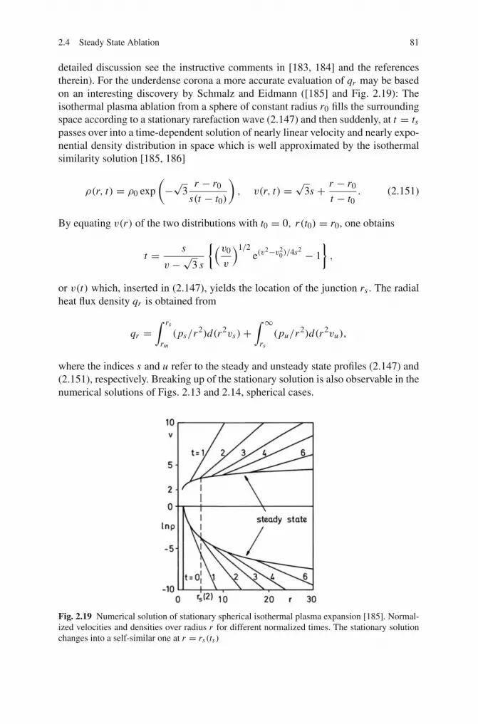
2.4 Steady State Ablation 81
detailed discussion see the instructive comments in [183, 184] and the referencestherein). For the underdense corona a more accurate evaluation of qr may be basedon an interesting discovery by Schmalz and Eidmann ([185] and Fig. 2.19): Theisothermal plasma ablation from a sphere of constant radius r0 fills the surroundingspace according to a stationary rarefaction wave (2.147) and then suddenly, at t = tspasses over into a time-dependent solution of nearly linear velocity and nearly expo-nential density distribution in space which is well approximated by the isothermalsimilarity solution [185, 186]
ρ(r, t) = ρ0 exp
(−√3
r − r0
s(t − t0)
), v(r, t) = √3s + r − r0
t − t0. (2.151)
By equating v(r) of the two distributions with t0 = 0, r(t0) = r0, one obtains
t = s
v −√3 s
{(v0
v
)1/2e(v
2−v20)/4s2 − 1
},
or v(t) which, inserted in (2.147), yields the location of the junction rs . The radialheat flux density qr is obtained from
qr =∫ rs
rm
(ps/r2)d(r2vs)+∫ ∞
rs
(pu/r2)d(r2vu),
where the indices s and u refer to the steady and unsteady state profiles (2.147) and(2.151), respectively. Breaking up of the stationary solution is also observable in thenumerical solutions of Figs. 2.13 and 2.14, spherical cases.
Fig. 2.19 Numerical solution of stationary spherical isothermal plasma expansion [185]. Normal-ized velocities and densities over radius r for different normalized times. The stationary solutionchanges into a self-similar one at r = rs(ts)

82 2 The Laser Plasma
2.4.3 Ablation Pressure in the Absence of Profile Steepening
The pressure arising from mass ablation Pa can be determined from (2.140) and(2.145) provided the flow velocity is measured in a reference system in which theablation region is stationary. In a strict sense this means an inertial frame in whichthe ablation front stays in a fixed position. For thick targets such a requirement isgenerally fulfilled to a good approximation. Thin targets undergo an acceleratedmotion like a rocket as soon as the first shock wave has moved through. Here thecorrect reference system has to be readjusted at each instant of time; it is a tangentinertial frame. For evaluating Pa , in principle, an arbitrary point can be chosen inthe steady state region. However, since v is known only at xm , this point plays aspecial role. Neglecting ionization and setting qe = 0, (2.145) becomes there
ql = 3γ − 1
2γ 3/2(γ − 1)ρms3
m for γ = 1; ql = 3ρms3m for γ = 1.
Elimination of sm from these expressions and from (2.145) leads to
Pa = 2
[2(γ − 1)
(3γ − 1)
]2/3
ρ1/3m (Ia − qr )
2/3 for γ = 1;
Pa = 2
32/3ρ
1/3m (Ia − qr )
2/3 for γ = 1. (2.152)
Specifying for planar isothermal heat flow, (2.112) leads to
Pa = 2
42/3ρ
1/3m I 2/3
a = 0.79ρ1/3m I 2/3
a ; γ = 1. (2.153)
For the spherical case, using (2.148) for qr , yields
Pa = 2
4.652/3ρ
1/3m I 2/3
a = 0.72ρ1/3m I 2/3
a ; γ = 1. (2.154)
If qr is set equal to zero the numerical factor for the isothermal ablation pressure is2/32/3 = 0.96, i.e., 33% higher.
So far formulas for the ablation pressure have been derived for laser pulsesof constant absorbed intensity Ia (i) under the assumptions of stationary plasmaoutflow (ii), plane flow in the overdense region (iii), no lateral heat flow in theunderdense corona (iv) and narrow absorption region around the critical point (v).If the latter condition is satisfied and ponderomotive effects are very small, i.e.,(|π |/|∇ p| � 1), ρm can be identified with the critical density ρc, and hence Pa
scales with the laser wavelength and absorbed intensity as Pa ∼ (Ia/λ)2/3.
To compare Pa deduced here with the experiment for irradiances Iλ2 >∼ 1013
Wcm−2, ponderomotive effects have to be included. They help to keep the plasmaflow one-dimensional in the absorption region owing to density profile steepening[condition (v)] but they also shift the point of critical Mach number M = 1/
√γ

2.4 Steady State Ablation 83
into the underdense region. Radiation pressure supported and dominated plasmaflow will be treated in Chap. 5. It will be shown that profile steepening takes alreadyplace at radiation pressures as low as a few percent of Pa .
At interaction times on the ns time scale crater formation takes place and thesteady state overall flow is two-dimensional (2D). Pa can be calculated in a narrowcylinder on the axis of radius r and length l. Due to profile steepening holds l <∼ λ.Taking radial flow vr into account mass conservation requires
∇(ρv) = ∂
∂x(ρv)+ 1
r
∂
∂r(rρvr ) = 0.
Regularity of flow on the axis implies vr = αr, α = const for r/r0 � 1, r0 radiusof the laser beam. Then α � v/r0 (confirmed by 2D simulations). Thus, the massflow through a narrow cylinder is one-dimensional, since with λ/r0 � 1 holds
πρ{
r2v + 2rλvr
}� πρv
{r2 + 2
λ
r0r2}� πr2ρv,
and the foregoing 1D formulas apply. Equation (2.141) is a special form of thegeneralized Bernoulli equation if ∂/∂x is interpreted as derivative along a streamline. In fact, the stationary momentum equation reads
ρ(v∇)v +∇ p = ρ∇(
v2
2+ ρs2
)− ρv ×∇ × v = 0.
On integrating along a streamline the term containing the curl of v vanishes andhence the generalized Bernoulli equation in its differential form results,
dv2
2+ 1
ρd(ρs2) = 0.
Taken along the axis this is identical with (2.139) and (2.141) under the conditionρv = const since dv2/2 = v dv = ρ−1 dρ v2.
In the absence of ponderomotive effects the time τs for Pa to become stationaryis given by the ratio of focal radius r0 to thermal velocity vth, τs � r0/vth. In thelong pulse regime with I0 � 1014 Wcm−2 a typical figure would then be τs =5×10⁻³cm/(5×107cm−1s−1) = 100 ps. However this is certainly too pessimistic.From I0λ
2 >∼ 1013 Wcm−2µm2 profile steepening and electronic or radiative heatconduction will be significant and r0 has to be replaced by the smaller of the twocharacteristic lengths associated with these phenomena. For profile steepening thisis the vacuum laser wavelength λ. The thickness d of the overdense conduction zoneis much harder to determine owing to nonlocal heat transport [107]; however d < r0and in most cases even d � r0, may hold.
The first difficulty with a quantitative comparison of experiments with Pa givenhere is that there is no measurement with constant intensity; instead, the laser pulse

84 2 The Laser Plasma
can be approximated by a Gaussian time dependence, Ia = I e−(t−t0)2/τ 2. Under the
assumption of a quasi-steady state the average ablation pressure Pa measured in theexperiments results as
Pa = aI 2/3a = I 2/3
τ
∫ +∞
−∞
(e−(t−t0)2/τ 2
)2/3dt =
(3
2
)1/2
a(I a)2/3
, (2.155)
thus showing that the power of Ia is preserved and only the numerical factor isincreased by (3/2)1/2. In experiments which are believed to be performed understeady state conditions, exponents lower than 2/3 are found, e.g., between 0.5 and2/3. In a few cases however, a slope of 2/3 was seen (see [187], Fig. 10). The rea-sons for the discrepancy may be manifold: lateral heat flow, change of irradiationgeometry during interaction at high intensities, quasi-steady state not well reached,anomalous transport and nonlocal laser energy deposition. When collisional absorp-tion dominates, the critical density no longer plays its predominant role and theablation pressure should follow the similarity laws (2.137) or (2.138), respectively,for spherical geometry (see also [188]),
Pa ∼ 〈ρkBT 〉 ∼ 〈ρ〉〈T 〉 ∼ λ−2/9 I 7/9a = λ−0.222 I 0.78
a . (2.156)
Gupta et al. [189] measured Pa produced by a 2 ns KrF laser pulse in the intensity
range 1011 − 1013 Wcm−2. Their result of Pa ∼ I(0.66−0.84)a confirms the trend
indicated by (2.156). A similar scaling, i.e., Pa ∼ I0.8a , was found by Grun et al.
[179] with 4 ns Nd laser pulse in the intensity range 1011−3×10¹³ Wcm−2. Pa,Iodine
agrees well with Pa,Nd, whereas Pa,KrF is 2.5 times as high [49, 151]. For a moredetailed discussion see Chap. 5.
An alternative way to generate high pressure which is accessible to an analyticaltreatment is by impulsive loading. Suppose the laser pulse energy E is given. In viewof the high pressure generation the question of the optimum pulse length is relevant.In general this is a complex problem. A partial answer can be given in the sensethat the pressure ratio is between impulsive loading Pi and the steady state case ofPa . For this purpose we observe that the shock wave cannot evolve before the heatdiffusion speed xT [see, e.g., (2.117)] has slowed down to the ion sound speed s.This means that the comparison of pressures has to be made at the time τp given by(2.127). Then the lowest value of Pi is determined at the edge of the rarefaction wavewhere v = 0 holds; hence Pi ≥ (Z + 1)n0kBT (τp), whereas Pa ≤ pm + ρms2
m .
On approximating ρm by ρc the inequality Pa ≤ nc
(1+ 1
Z
)kBT (τp)
(1+ 1√
γ
)
results and hence, the ratio Pi/Pa fulfills
Pi
Pa≥
√γ
1+√γ Zn0
nc. (2.157)
Generally this ratio is much larger than unity.
References 85
References
1. Raizer, Yu.P.: Laser-Induced Discharge Phenomena. Consultants Bureau, New York (1977) 62. Shen, Y.R.: The Principles of Nonlinear Optics, Chap. 27. John Wiley & Sons, New York
(1984)3. Turcu, I.C.E., Gower, M.C., Huntington, P.: Opt. Comm. 134, 66 (1997) 64. Evrastov, E.V., et al.: Sov. J. Quant. Electron. 18, 354 (1988) 65. Poprawe, R., Beyer, E., Herziger, G.: Proc. Conf. Gas Flow and Chem. Lasers, Oxford (1984) 66. Rosen, D.I., Weyl, G.: J. Phys. D: Appl. Phys. 20, 1264 (1987) 67. Ageev, V.P., Gorbunov, A.A., Danilov, V.P., Konov, V.I., Nikitin, P.I., Prokhorov, A.M.: Sov.
J. Quant. Electron. 13, 1595 (1983)8. Kovalev, A.S., et al.: Sov. J. Quant. Electron. 15, 468 (1985) 69. Storm, E.: J. Fusion Energy 7, 131 (1988) 6
10. Storm, E., Lindl, J.D., Campbell, E.M., Bernat, T.P., Coleman, L.W., Emmett, J.L., Hogan,W.J., Hunt, J.T., Krupke, W.F., Lowdermilk, W.H.: Progress in Laboratory High Gain ICF:Prospects for the Future LLNL Progress Report (1988), published in J. Fusion Energy (1990)
11. Lindl, J.: Phys. Plasmas 2, 3933 (1995) 7412. Atzeni, S., Meyer-ter-Vehn, J.: The Physics of Inertial Fusion. Oxford University Press,
Oxford (2004)13. Tabak, M., Hammer, J., Glinsky, M.E., Kruer, W.L., Wilks, S.C., Woodward, J., Camppbell,
E.M., Perry, M.D.: Phys. Plasmas 1, 1626 (1994) 7414. Hain, S., Mulser, P.: Phys. Rev. Lett. 86, 1015 (2001) 6, 5715. Brabec, T., Krausz, F.: Rev. Mod. Phys. 72, 545 (2000); Wittmann, T., et al.: Nature Physics
5, 357 (2009) 616. Brederlow, G., Fill, E., Witte, K.J.: The High-Power Iodine Laser. Springer, Berlin (1983) 617. Johnson, Th.H.: Proc. IEEE 72, 548 (1984) 618. Loudon, R.: The Quantum Theory of Light. Clarendon, Oxford (1986) 8, 919. Meystre, P., Sargent, M. III: Elements of Quantum Optics. Springer, Berlin (1990) 8, 1220. Varcoe, B.T.H., Brattke, S., Weidinger, M., Walther, H.: Nature 403, 743 (2000) 921. Lvovsky, A.I., Hansen, H., Aichele, T., Benson, O., Mlynek, J., Schiller, S.: Phys. Rev. Lett.
87, 050402 (2001) 922. Silin, V.P., Uryupin, S.A.: Zh. Exp. Theor. Fiz. 81, 910 (1981); Sov. Phys. JETP 54, 485
(1981) 1123. Mulser, P., Uryupin, S., Sauerbrey, R., Wellegehausen, B.: Phys. Rev. A 48, 4547 (1993) 1224. Lotz, W.: Z. Physik 216, 241 (1968); Z. Physik 220, 466 (1969) 1625. Janev, R.K., Presnyakov, L.P., Shevelko, V.P.: Physics of Highly Charged Ions. Springer,
Berlin (1985) 1626. Kanapathipillai, M., Mulser, P., et al.: Phys. Plasmas 11, 3911 (2004) 19, 2027. Pert, G.J.: J. Phys. B: At. Mol. Phys. 12, 2755 (1979) 2128. Shkarofsky, I.P., Johnston, T.W., Bachynski, M.P.: The Particle Kinetics of Plasmas.
Addison-Wesley, Reading, MA (1966) 2229. Faisal, F.H.M.: Theory of Multiphoton Processes. Plenum Press, New York (1987) 2330. Chin, S.L., Lambropoulos, P.: Multiphoton Ionisation of Atoms. Acad. Press, New York
(1984) 2331. Lambropoulos, P., Tang, X.: J. Opt. Soc. Am. B 4, 821 (1987) 2332. Voronov, G.S., Delone, N.B.: Sov. Phys. JETP 23, 54 (1966) 2333. Perry, M.D., Szoke, A., Landen, O.L., Campbell, E.M.: Phys. Rev. Lett. 60, 1270 (1988)34. Yergeau, F., Chin, S.L., Lavigne, P.: J. Phys. B: At. Mol. Phys. 20, 723 (1987)35. L’Huillier, A., Lompré, L.A., Mainfray, G., Manus, C.: J. Phys. B: At. Mol. Phys. 16, 1363
(1983) 2336. Poprawe, R., Herziger, G.: IEEE J. Quant. Electron. 22, 590 (1986) 2337. Bekefi, G.: Principles of Laser Plasmas. John Wiley & Sons, New York (1976) 2338. Clarke, P., et al.: Appl. Phys. A 69, 117 (1999) 24
86 2 The Laser Plasma
39. Izumida, S., Onishi, K., Saito, M.: Jap. J. Appl. Phys. 1 37, 2039 (1997)40. Koldunov, M.F., Manenkov, A.A., Pokotilo, I.L.: J. Opt. Technol. 63, 128 (1996)41. Hosada, M., et al.: Jap. J. Appl. Phys. 1 38, 3567 (1999)42. Fedonov, A.V., et al.: Appl. Surf. Sci. 197, 45 (2002) 2443. Balescu, R.: Equilibrium and Nonequilibrium Statistical Mechanics. Wiley-Interscience,
New York (1975) 24, 3744. Mulser, P.: Z. Naturforsch. 25a, 282 (1970) 29, 63, 64, 7145. Braginskii, S.I.: Transport Processes in Plasmas. In: Leontovich, M.A. (ed) Reviews of
Plasma Physics, Vol. 1. Consultants Bureau, New York (1966) 2946. Weng, S.M., et al.: Phys. Rev. Lett. 100, 185001 (2008) 3147. Chorin, A.J., Marsden, J.E.: A Mathematical Introduction to Fluid Mechanics. Springer,
Berlin (1979) 3348. Kidder, R.E.: Nucl. Fusion 16, 405 (1976) 34, 5349. Maaswinkel, A.G.M., Eidmann, K., Sigel, R., Witkowski, S.: Opt. Comm. 51, 255 (1984) 34, 8450. Mulser, P., Kärcher, B.: Phys. Lett. A 126, 383 (1988) 34, 3551. Mulser, P.: Z. Naturforsch. 42a, 1147 (1987) 3452. Davidson, R.C.: Methods in Nonlinear Plasma Theory. Acad. Press, New York (1972) 38, 41, 4253. Derfler, H., Simonen, T.: J. Appl. Phys. 38, 5018 (1967) 4154. Dawson, J.M.: Phys. Fluids 4, 869 (1961) 4155. Chen, F.F.: Plasma Physics and Controlled Fusion, Vol. 1. Plenum Press, New York (1984) 41, 4356. Hahn, E.L.: Phys. Rev. 80, 580 (1950) 4257. Carr, H.Y., Purcell, E.M.: Phys. Rev. 94, 630 (1954) 4258. Feynman, R.P., Vernon, F.L., Hellwarth, R.W.: J. Appl. Phys. 28, 49 (1957) 4259. Rayleigh, L.: Phil. Mag. 34, 59 (1892); Proc. Royal Soc. L XIV, 68 (1899) 4460. Rayleigh, L.: Nature 95, 66, 591, 644 (1915) 4461. Buckingham, E.: Phys. Rev. 4, 345 (1914) 4462. Sedov, L.I.: Similarity and Dimensional Methods. Acad. Press, New York (1959) 44, 4763. De Izarra, C., Caillard, J., Valle, O.: Mod. Phys. Lett. B 16, 69 (2002) 4764. Zhi-yuan, Z., et al.: Optoelectronics Lett. 3, 394 (2007) 4765. Eliezer, S.: The Interaction of High-Power Lasers with Plasmas, Chap. 11. IOP Publ., Bristol
(2002) 4766. Kull, H.-J.: Phys. Rep. 206, 197 (1991) 4767. Gurevich, V.A., Pariiskaya, L.V., Pitaevskii, L.P.: Sov. Phys. JETP 22, 449 (1966); Gurevich,
V.A., Pariiskaya, L.V., Pitaevskii, L.P.: Sov. Phys. JETP 36, 449 (1973) 49, 6868. Mora, P.: Phys. Rev. Lett. 90, 185002 (2003) 4969. Mora, P.: Phys. Rev. E 72, 056401 (2005) 4970. Murakami, M., Basko, M.M.: Phys. Plasmas 13, 012105 (2006) 4971. Basko, M.M.: Eur. Phys. J. D 41, 641 (2007) 4972. Sentoku, Y., Cowan, T.E., Kemp, A., Ruhl, H.: Phys. Plasmas 10, 2009 (2003) 4973. Murakami, M., Mima, K.: Phys. Plasmas 16, 103108 (2009) 4974. Murakami, M., Tanaka, M.: Phys. Plasmas 15, 082702 (2008) 5075. Zeldovich, Ya.B., Raizer, Yu.P.: Physics of Shock Waves and High-Temperature Hydrody-
namic Phenomena. Acad. Press, New York (1967) 50, 52, 5476. Huntley, H.E.: Dimensional Analysis. McDonald, London (1953) 5377. Bridgman, P.W.: Dimensional Analysis revised ed. (Yale Univ. Press, New Haven (1931) 5378. Duncan, W.J.: Physical Similarity and Dimensional Analysis. Arnold, London (1953)79. Birkhoff, G.: Hydrodynamics; A Study in Logic, Fact and Similitude. Princeton Univ. Press,
Princeton, NJ (1960)80. Langhaar, H.L.: Dimensional Analysis and Theory of Models. John Wiley, New York (1964)81. Görtler, H.: Dimensionsanalyse. Springer, New York (1975)82. Spurk, H.J.: Dimensionsanalyse in der Strömungslehre. Springer, Berlin (1992) 5383. Barenblatt, G.I.: Similarity, Self-Similarity, and Intermediate Asymptotics. Consultants
Bureau, New York (1979) 53, 54

References 87
84. Günther, B.: Dimensional Analysis and Theory of Biological Similarity, PhysiologicalReviews 55, 659 (1975) 53
85. Günther, B., Morgado, E.: Biol. Res. 36, 405 (2003)86. Yates, F.E.: Am. J. Physiol. 244, R589 (1983) 5387. Wilks, G.: Dyn. Problems Math. Phys. 26, 151 (1983) 5488. Bluman, G.W., Cole, V.D.: Similarity Methods for Differential Equations. Springer, New
York (1974) 5489. Glockner, P.G., Singh, M.C. (ed.): Symmetry, Similarity and Group Theoretical Methods in
Mechanics. The University of Calgary, Calgary (1974) 5490. Euler, N., Steeb, W.H., Mulser, P.: J. Phys. Soc. Japan 60, 1132 (1991) 5491. Ceccherini, F., Cicogna, G., Pegoraro, F.: J. Phys. A: Math. Gen. 38, 4597 (2005) 5492. Guderley, G.: Luftfahrtforschung 19, 302 (1942) 5593. Meyer-ter-Vehn, J., Schalk, C.: Z. Naturforsch. 37a, 955 (1982) 5594. Paul Drake, R.: High-Energy-Density Physics: Fundamentals, Inertial Fusion and Experi-
mental Astrophysics. Springer, Heidelberg (2008) 5695. Lackner-Russo, D., Mulser, P.: A Macroscopic PIC Code for Beam-Target Interaction Studies
Garching Report PLF 32 (1980) 56, 8096. Eidmann, K., Sigel, R.: Backscatter experiments. In: Schwarz, H.J., Hora, H. (eds.) Laser
Interaction and Related Plasma Phenomena, Vol. 3B. Plenum Press, New York (1974) 5997. Nakai, S. and the Super-Uniform Implosion Group: ILE Quarterly Progress Report 29, 9
(1989), ISSN 0289–1549 5798. Yamanaka, C.: Past, present and future of laser fusion research. In: Nakai, S., Miley, G.M.
(eds.) Laser Interaction, p. 3. American Institute of Physics, Woodbury (1996)99. Nakai, S.: Progress of laser fusion at ILE and ICF research in Japan. In: Nakai, S., Miley,
G.M. (eds.) Laser Interaction, p. 30. American Institute of Physics, Woodbury (1996) 57100. Badziak, J., et al.: J. Appl. Phys. 104, 063310 (2008) 58101. Caruso, A., Gratton, R.: Plasma Phys. 11, 839 (1969) 60102. Shearer, J.W., Barnes, W.S.: Phys. Rev. Lett. 24, 92 (1970) 61103. Zacharov, S.D., Krokhin, O.N., Kryokov, P.G., Tyurin, E.L.: JETP Lett. 12, 36 (1970) 61104. Anisimov, S.I.: JETP Lett. 12, 287 (1970) 61105. Salzmann, H.: J. Appl. Phys. 44, 113 (1973) 62106. Malone, R.C., McCrory, R.L., Morse, R.L.: Phys. Rev. Lett. 34, 721 (1975) 62107. Bell, A.R.: Transport in laser-produced plasmas. In: Hooper, M.B. (ed.) Laser Plasma Inter-
actions 5: Inertial Confinement Fusion, Proc. 45th Scottish Universities Summer School inPhysics, St. Andrews 1994, p. 139. Institute of Physics, Bristol and Philadelphia (1995) 62, 83
108. Tahraoui, A., Bendib, A.: Phys. Plasmas 9, 3089 (2002) 62109. Batishev, O.V., et al.: Phys. Plasmas 9, 2302 (2002)110. Santos, J.J., et al.: Phys. Rev. Lett. 89, 025001 (2002)111. Martinolli, E., et al.: Las. Part. Beams 20, 171 (2002)112. Jain, N., Das, A., Kaw, P., Sengupta, S.: Phys. Plasmas 10, 29 (2003)113. Sentoku, Y., Mima, K., Kaw, P., Nishikawa, K.: Phys. Rev. Lett. 90, 155001 (2003) 62114. Pukhov, A., Meyer-ter-Vehn, J.: Phys. Rev. Lett. 76, 3975 (1996) 62115. Adam, J.C., Guerin, S., Laval, G., Mora, P., Quesnel, B.: Phys. Rev. Lett. 78, 4765 (1997)116. Ruhl, H., Sentoku, Y., Mima, K., Tanaka, K.A., Kodama, R.: Phys. Rev. Lett. 82, 743 (1999)117. Gibbon, P., et al.: Phys. Plasmas 6, 947 (1999)118. Ruhl, H., Macchi, A., Mulser, P., Cornolti, F., Hain, S.: Phys. Rev. Lett. 82, 2095 (1999) 62119. Sauerbrey, R., et al.: Phys. Plasmas 2, 1635 (1994) 62120. Gibbon, P., Bell, A.R.: Phys. Rev. Lett. 73, 664 (1994) 62121. van Thiel, M., Alder, B.J.: Mol. Phys. 10, 427 (1966) 63122. Mulser, P., Sigel, R., Witkowski, S.: Phys. Lett. 6C, 196 (1973) 64123. Opower, H., Press, W.: Z. Naturforsch. 21a, 344 (1966) 67124. Gregg, D.W., Thomas, S.J.: J. Appl. Phys. 37, 4313 (1966)125. Basov, N.G. at al.: JETP Lett. 5, 141 (1967)

88 2 The Laser Plasma
126. Mattioli, M., Veron, D.: Plasma Phys. 11, 684 (1969); Mattioli, M., Veron, D.: Plasma Phys.13, 19 (1971) 67, 68
127. Irons, F.E., Peacock, N.J.: J. Phys. B 7, 2084 (1974) 67128. Fenner, N.C.: Phys. Lett. 22, 421 (1966) 68129. Paton, B.E., Isenor, N.R.: Can. J. Phys. 46, 1237 (1968) 68130. Demtröder, W., Jantz, W.: Plasma Phys. 12, 691 (1970)131. Dinger, R., Rohr, K., Weber, H.: J. Phys. D 13, 2301 (1980); Dinger, R., Rohr, K., Weber, H.:
J. Phys. D 17 1707 (1984); Las. Part. Beams 4, 239 (1986); Las. Part. Beams 5, 691 (1987) 68132. Pitsch, K., Rohr, K., Weber, H.: J. Phys. D 14, L51 (1980)133. Mann, K., Rohr, K.: Las. Part. Beams 10, 435 (1992) 68134. Boland, B.C., Irons, F.E., McWhirter, R.W.P.: J. Phys. B 1, 1180 (1968) 68135. Mulser, P.: Plasma Phys. 13, 1007 (1971) 68136. Begay, F., Forslund, D.W.: Phys. Fluids 25, 1675 (1982) 68137. Goforth, R.R., Hammerling, P.: J. Appl. Phys. 49, 3918 (1976) 68138. Matzen, M.K., Pearlman, J.S.: Phys. Fluids 22, 449 (1979)139. Latyshev, S.V., Rudskoi, I.V.: Sov. J. Plasma Phys. 11, 669 (1985) 68140. Kunz, I.: Interpretation of the Ion Energy Spectra in Laser-produced Plasmas Based on the
Recombination Model), PhD-Thesis (in German), TH Darmstadt (1990) 68141. Granse, G., Völlmer, S., Lenk, A., Rupp, A., Rohr, K.: Appl. Surf. Sci. 96–98, 97 (1996) 68142. Rupp, A., Rohr, K.: J. Phys. D: Appl. Phys. 28, 468 (1995) 68143. Caruso, A., Gatti, G., Strangio, C.: Nuovo Cim. 2, 1213 (1983) 68144. Sinha, B.K., Thum-Jäger, A., Rohr, K.P.: J. Plasma Fusion Res. 2, 406 (1999); Sinha, B.K.,
Thum-Jäger, A., Rohr, K.P.: J. Plasma Fusion Res. 410 (1999) 68145. Thum-Jäger, A., Rohr, K.P.: J. Phys. D: Appl. Phys. 32, 2827 (1999) 68146. Thum-Jäger, A., Sinha, B.K., Rohr, K.P.: Phys. Rev. E 61, 3063 (2000); Thum-Jäger, A.,
Sinha, B.K., Rohr, K.P.: Phys. Rev. E 61, 016405 (2001) 68147. Müller, T., Sinha, B.K., Rohr, K.P.: Phys. Rev. E 67, 026415 (2003) 68148. Kovalev, V.F., Bychenkov, V.Y., Tikhonchuk, V.T.: J. Exp. Theor. Phys. 95, 226 (2002) 68149. Caruso, A., Gratton, R.: Plasma Phys. 10, 867 (1968) 69, 70150. Anisimov, S.I., Prokhorov, A.M., Fortov, V.E.: Sov. Phys. Usp. 142, 395 (1984) 74151. Eidmann, K., et al.: Phys. Rev. A 30, 2568 (1984) 74, 75, 77, 84152. Meyer-ter-Vehn, J.: Nucl. Fusion 22, 561 (1982) 74153. Caruso, A.: Plasma Phys. Contr. Fusion 18, 241 (1976) 74154. Mulser, P., Hain, S., Cornolti, F.: Nucl. Instr. Meth. Phys. Res. A 415, 165 (1998) 74, 75155. van Kessel, C.G.M., Sigel, R.: Phys. Rev. Lett. 33, 1020 (1974) 74156. Evans, R., et al.: Phys. Rev. Lett. 77, 3359 (1996) 74157. Obenschain, S.P., Grun, J., Ripin, B.H., McLean, E.A.: Phys. Rev. Lett. 46, 1402 (1981) 74158. Fabbro, R., Faral, B., Virmont, J., Pepin, H., Cottet, F., Romain, J.P.: Las. Part. Beams 4, 413
(1986) 74159. Fabbro, R., Faral, B., Virmont, J., Cottet, F., Romain, J.P., Pepin, H.: Phys. Fluids B1, 644
(1989) 74160. Faral, B., Fabbro, R., Virmont, J., Cottet, F., Romain, J.P.: Phys. Fluids B2, 371 (1990) 74161. Cauble, R., Phillion, D.W., Hoover, T.J., Holmes, N.C., Kilkenny, J.D., Lee, R.W.: Phys. Rev.
Lett. 70, 2102 (1993) 74162. Regan, S.P., et al.: Phys. Rev. Lett. 89, 085003 (2002) 74163. Löwer, T., et al.: Phys. Rev. Lett. 72, 3186 (1994) 74164. Evans, A.M., et al.: Las. Part. Beams 14, 113 (1996) 74165. Koenig, M., Faral, F., Boudenne, J.M.: Phys. Rev. E 50, R3314 (1994) 74166. Benuzzi, A., et al.: Phys. Rev. E 54, 2162 (1996)167. Batani, D., et al.: Laser & Part. Beams 21, 481 (2003) 74168. Max, R., Claire, E., McKee, C.F., Mead, W.C.: Phys. Fluids 23, 1620 (1980) 74, 75169. Ahlborn, B., Key, M.H., Bell, A.R.: Phys. Fluids 25, 541 (1982)170. Yamanaka, C.: Laser plasma and inertial confinement fusion. In: Rosenbluth, M.N., Sagdeev,
R.Z. (eds.) Handbook of Plasma Physics, Vol. 3, p. 3. North-Holland, Amsterdam (1991)

References 89
171. Richardson, M.C.: Direct drive fusion studies. In: Rosenbluth, M.N., Sagdeev, R.Z. (eds.)Handbook of Plasma Physics, Vol. 3, p. 199. North-Holland, Amsterdam (1991) 74
172. Bobin, J.L.: Phys. Fluids 14, 2341 (1971) 75173. Cojocaru, E., Mulser, P.: Plasma Phys. 17, 393 (1974) 78174. Gitomer, S.J., Morse, R.L., Newberger, B.S.: Phys. Fluids 20, 234 (1977) 75175. Matzen, M.K., Morse, R.L.: Phys. Fluids 22, 654 (1979) 75, 78176. Sanz, J., A. Liñán, Rodriguez, M., Sanmartin, J.R.: Phys. Fluids 24, 2098 (1981)177. Fabbro, R., Claire, E., Max, R., Fabre, E.: Phys. Fluids 28, 1463 (1985) 75, 77178. Hain, S., Mulser, P.: Las. Part. Beams 15, 541 (1997) 75179. Grun, J., et al.: Phys. Fluids 26, 588 (1983) 75, 84180. Manheimer, W.M., Colombant, D.G.: Phys. Fluids 25, 1644 (1982) 75181. Pert, G.J.: J. Plasma Phys. 29, 415 (1983) 78182. Herbst, M.J., Grun, J.: Phys. Fluids 24, 1917 (1981) 80183. Sanmartin, J.R., Montanes, J.L., Barrero, A.: Phys. Fluids 26, 2754 (1983) 81184. Manheimer, W.M., Colombant, D.G., Gardner, J.H.: Phys. Fluids 26, 2755 (1983) 81185. Schmalz, R.F., Eidmann, K.: Phys. Fluids 29, 3483 (1986) 81186. Schmalz, R.F.: Phys. Fluids 29, 1389 (1986) 81187. Mulser, P.: Plasma Phys. Contr. Fusion 28, 203 (1986) 84188. Mora, P.: Phys. Fluids 25, 1051 (1982) 84189. Gupta, P.D., Tsui, Y.Y., Popil, R., Fedosejevs, R., Offenberger, A.A.: Phys. Fluids 30, 179
(1987) 84

Chapter 3Laser Light Propagation and CollisionalAbsorption
By absorption of electromagnetic radiation we understand the destruction of a cer-tain number of photons and the creation of other forms of energy of the sameamount, e.g., plasmons, phonons, accelerated and heated particles. In the languageof second quantization the absorption operator reads b+a (a annihilation operator,b+ creation operator); absorption occurs when its expectation value is nonzero. Wecall the absorption process collisional or inverse bremsstrahlung if the transforma-tion of photon energy is due to the Coulomb field of single particles, in contrastto collective or collisionless absorption which is due to the resonant interactionwith collective fields. There is a clear distinction between collisional and collective:collective interaction depends on one space variable only whereas collisional inter-action needs at least two space variables. An example of collisional absorption is theexcitation of plasmons by the plasma ions in a cold electron fluid oscillating in anintense laser field and their subsequent damping by breaking, particle acceleration,Landau mechanism and/or collisions.
In the second part of this chapter various models of collisional absorption arepresented. First the electron-ion collision frequency is derived from a harmonicoscillator model for a unidirectional particle beam; subsequently the dielectric the-ory of absorption at finite electron temperature is presented. Here the electronsare treated as a fluid collectively reacting to the electric field of a moving ion. Inthe ballistic model, introduced next, a friction coefficient is determined from themomentum loss in flow direction due to electron-ion scattering events. The dielec-tric model is able to describe small angle deflections along nearly straight orbits andscreening; the ballistic model adapts equally well to large angle scattering events andbent trajectories. However, screening must be introduced separately. To some extentthe two models are complementary to each other. In the weakly coupled plasma theywill be shown to lead to identical results.
At a first glance, collisional absorption seems to be the best understood dissipa-tion process. Closer inspection, however, shows that this is not always true for laserplasmas. For instance, there is much uncertainty about screening and the Coulomblogarithm at high electron densities and large laser intensities. The oscillator modelprovides some insight into the physics of self-consistent cutoffs for the variousplasma density domains. Also attention has to be paid to the effect of distortionsof a Maxwellian velocity distribution and the role of electron–electron collisions
P. Mulser, D. Bauer, High Power Laser–Matter Interaction, STMP 238, 91–152,DOI 10.1007/978-3-540-46065-7_3, C© Springer-Verlag Berlin Heidelberg 2010
91
92 3 Laser Light Propagation and Collisional Absorption
on ν. Finally the equivalence of inverse bremsstrahlung and collisional absorption isdemonstrated as this illustrates an interesting piece of radiation physics at moderatelaser intensities (Iλ2 ≤ 1016 Wcm−2µm2).
3.1 The Optical Approximation
All linear as well as nonlinear optics is governed by Maxwell’s equations,
ε0c2∇ × B = j + ε0∂
∂tE, ∇ × E = − ∂
∂tB. (3.1)
Classically, the electric current density j is given by j = −eneve + Zenivi ; inquantum plasmas ve and vi have to be substituted by the single-particle momentumoperators per unit mass pe/m, pi/mi . In both cases the relation between j and thepolarization P is given by [1]
j = ∂
∂tP +∇ ×
(P × p
ρ
), p = pe + pi . (3.2)
This relation can be regarded either as the definition of j or of P . Traditionally,for plasmas, one prefers to represent all free and dielectric currents by j , instead ofusing P ; but this of course is a pure convention. By eliminating B, (3.1) reduces tothe wave equation
∇ × ∇ × E + 1
c2
∂2
∂t2E = − 1
ε0c2
∂ j∂t. (3.3)
In the following all considerations are limited to the classical expression for j . Forhigh frequency oscillations it reduces to j = −eneve since in this case the ionmotion can be neglected. In an unmagnetized plasma of equilibrium density n0 thecurrent density may be obtained from the momentum equation of the electronic fluidof system (2.65), (2.66), (2.67), (2.68), and (2.69) in a straightforward manner:
∂ j∂t= ε0ω
2p E − ε0s2
e∇(∇E)− ν j −e
mj × B + e2
m(ne − n0)E − ( j∇)ve − ve(∇ j). (3.4)
ν is a linear collisional or noncollisional damping coefficient. Under the additionalconstraint of the oscillation amplitudes δe being small compared with the wave-length λ, as well as compared with the plasma density scale length L = n0/|∇n0|,i.e., |δe| � L , λ, a plasma frequency ωp = (n0e2/ε0m)1/2 is defined locally and nohigher harmonics of the laser frequency ω have to be considered in (3.4). Thus, ifthe flow velocity is v0(x) and j = jos = −en0(ve − v0) Ohm’s law can be writtenas follows:

3.1 The Optical Approximation 93
∂ j∂t= ε0ω
2p(E + v0 × B)− ε0s2
e∇(∇E)− ν j − ( j∇)v0 − v0(∇ j). (3.5)
With the help of the quantities k0 = ω/c, β = se/c, vϕvg = c2 for phase andgroup velocities of the electromagnetic and vϕvg = s2
e for the electrostatic waveone easily estimates
∣∣∣∣∣s2
e∇(∇E)ω2
p E
∣∣∣∣∣ = γe(λDke)2,
∣∣∣∣( j∇)v0
ε0s2e∇(∇E)
∣∣∣∣ ≤v0
c
β2
k0L(kλD)2,
∣∣∣∣v0(∇ j)
ε0s2e∇(∇E)
∣∣∣∣ ≤v0
vg. (3.6)
As a consequence, plasma flow is generally irrelevant in laser plasma optics and onemay set v0 = 0. Then, for a wave of frequency ω, (3.3) reduces to the wave equationof linear optics,
∇ × ∇ × E − k20η
2 E = β2∇(∇E), (3.7)
where the refractive index η is given by
η2 = 1− ω2p
ω2
1
1+ ν2/ω2+ i
ν
ω
ω2p
ω2
1
1+ ν2/ω2. (3.8)
E + v0 × B is the electric field seen by an observer comoving nonrelativisticallywith the plasma. The nonlinear terms of (3.4) which are dropped in (3.7) give riseto the ponderomotive force and most of nonlinear optics phenomena encountered inlaser plasmas (see Chaps. 5 and 6).
3.1.1 Ray Equations
For moderate density inhomogeneities the local wavelength λ(x) satisfies theinequality λ(x) � L(x) nearly everywhere and the electric field is expressed bythe eikonal approximation
E(x, t) = E(x, t)eiψ(x,t), (3.9)
in which E(x, t) and ∇ψ(x, t) are slowly varying functions of space and time (seefor instance Sect. 7.7 in [2]). E and ψ are called the amplitude and phase of thewave. The local wave vector and frequency are defined as
k = ∇ψ, ω = − ∂
∂tψ. (3.10)

94 3 Laser Light Propagation and Collisional Absorption
Starting from (3.3) and (3.5) with v0 = 0, and keeping only the leading terms in thederivatives of E(x, t) and j(x, t) one arrives again at (3.7) and from there at
(∇ψ)2 E − ∇ψ(E∇ψ)+ β2∇ψ(E∇ψ) = k20η
2 E
in a straightforward way. By splitting E into E⊥+ E‖ with respect to the wave vec-tor k = ∇ψ , the two eikonal and dispersion relations follow for the electromagneticand the electrostatic components,
E⊥ : (∇ψ)2 = k20η
2, ω2 = ω2p + c2k2, k0 = ω
c, k = k0η,
E‖ : (∇ψ)2 = k2β−2; ω2 = ω2p + s2
e k2e ; ke = kβ−1. (3.11)
Here and in the rest of this section we take ν = 0. Then, the refractive indexη = c/vϕ,em or η = se/vϕ,es, respectively, is the same for both waves and, in anisothermal plasma, both propagate along identical trajectories. These trajectories orrays are orthogonal to the surfaces of constant phase, ψ(x, t) = const (Fig. 3.1). Ina stationary plasma the phase difference between two points P1, P2 at a given timeis uniquely determined by
ψ(P2)− ψ(P1) =∫ P2
P1
|k|ds
along a ray segment C . Along an arbitrary path C ′ from P1 to P2 one has
ψ(P2)− ψ(P1) =∫
C ′kds ≤
∫
C ′kds.
This expresses Fermat’s principle [3].
Fig. 3.1 The rays form a manifold of curves which are perpendicular to the surfaces of constantphase at t fixed, ψ(x, t) = const
3.1 The Optical Approximation 95
From
d
ds(k0η) = 1
k0η(k0η∇)(k0η) = 1
2k0η∇(k0η)
2 − k0
k0×∇ × k0η,
∇ × k0η = ∇ × (∇ψ) = 0
the widely used ray equation
d
ds(k0η) = k0∇η (3.12)
follows immediately, if use is made of the vector identity a× (∇× a) = ∇(a2/2)−(a∇)a. Equation (3.12) is the basis for raytracing. From it η is again recognized asthe refractive index. In the fully ionized plasma it is the same for Langmuir waves asfor electromagnetic waves. For the electron plasma wave se plays the same role asthe speed of light c does for the laser wave. In general, (3.12) has to be solved numer-ically. Only in plane and spherical geometry (“stratified” or “layered” medium) is iteasily integrated. With the constant vector n = ∇η/|∇η| in plane geometry one has:
d
ds(n× k0η) = n× d
ds(k0η) = n× k0∇η = 0.
Similarly, in spherical geometry one finds for a vector r having its origin in thecenter of symmetry of η(r),
d
ds(r × k0η) = k0
k0× k0η + r × d
ds(k0η) = r × k0∇η = 0,
since ∇η is parallel to r . If α is the angle α between the local wave vector and ∇η,the two relations can be expressed in integrated form
η(x) sinα = const (plane), rη(r) sinα = const (spherical). (3.13)
Two examples of ray distributions for plane and spherical geometry are sketchedin Fig. 3.2. In the plane stratified medium the ray directions are such that they-component of k0η is conserved. In spherical geometry the momentum r × k0η
relative to the center of symmetry remains constant. It follows from (3.11) thatLangmuir and electromagnetic waves cannot propagate beyond the critical densitygiven by (2.94). At oblique or nonradial incidence from the vacuum at the angle α0or distance b from the radius, respectively, the turning point of a ray is located at
η(x) = sinα0 (plane), rη(r) = b (spherical). (3.14)
The phase ψ is a function of x and t . From the definition (3.10) of the wave vectorit is clear that k = k(x, t); hence, owing to the dispersion relations (3.11), thefunctional dependence of the frequency is ω = ω(k, x, t). The explicit dependence
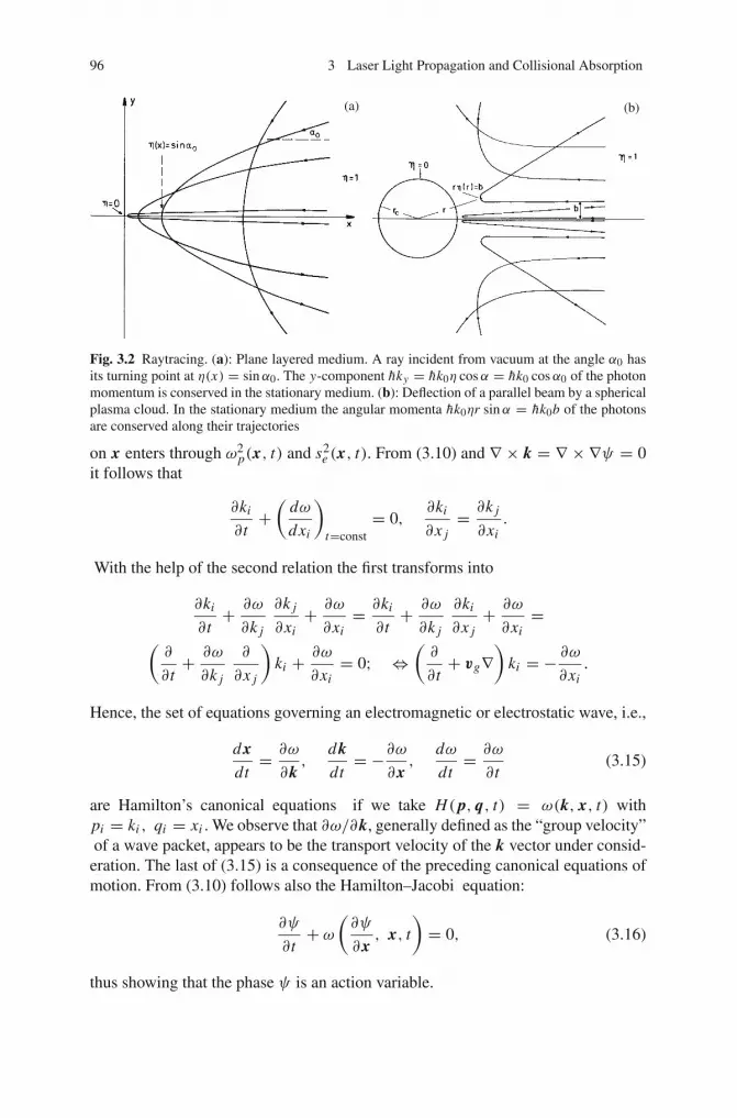
96 3 Laser Light Propagation and Collisional Absorption
(b)(a)
Fig. 3.2 Raytracing. (a): Plane layered medium. A ray incident from vacuum at the angle α0 hasits turning point at η(x) = sinα0. The y-component hky = hk0η cosα = hk0 cosα0 of the photonmomentum is conserved in the stationary medium. (b): Deflection of a parallel beam by a sphericalplasma cloud. In the stationary medium the angular momenta hk0ηr sinα = hk0b of the photonsare conserved along their trajectories
on x enters through ω2p(x, t) and s2
e (x, t). From (3.10) and ∇ × k = ∇ × ∇ψ = 0it follows that
∂ki
∂t+(
dω
dxi
)
t=const= 0,
∂ki
∂x j= ∂k j
∂xi.
With the help of the second relation the first transforms into
∂ki
∂t+ ∂ω
∂k j
∂k j
∂xi+ ∂ω
∂xi= ∂ki
∂t+ ∂ω
∂k j
∂ki
∂x j+ ∂ω
∂xi=
(∂
∂t+ ∂ω
∂k j
∂
∂x j
)ki + ∂ω
∂xi= 0; ⇔
(∂
∂t+ vg∇
)ki = − ∂ω
∂xi.
Hence, the set of equations governing an electromagnetic or electrostatic wave, i.e.,
dxdt= ∂ω
∂k,
dkdt= −∂ω
∂x,
dω
dt= ∂ω
∂t(3.15)
are Hamilton’s canonical equations if we take H( p, q, t) = ω(k, x, t) withpi = ki , qi = xi . We observe that ∂ω/∂k, generally defined as the “group velocity”of a wave packet, appears to be the transport velocity of the k vector under consid-
eration. The last of (3.15) is a consequence of the preceding canonical equations ofmotion. From (3.10) follows also the Hamilton–Jacobi equation:
∂ψ
∂t+ ω
(∂ψ
∂x, x, t
)= 0, (3.16)
thus showing that the phase ψ is an action variable.

3.1 The Optical Approximation 97
A wave vector k from (3.10) is given the name photon, plasmon, phonon by def-inition, in agreement with quantum theory where hk is its momentum. The domainof validity of the particle concept in both cases, classical and quantum mechanical,is exactly the same. From the Hamiltonian structure of (3.15) follows that the phasevolume Δx Δk is conserved (Liouville’s theorem). Introducing the phase spaceoccupation density f (x, k, t) for photons, plasmons or phonons, respectively, justin the same way as with the one-particle distribution function for material parti-cles in (2.81) along a characteristic the number ΔN = f (x, k, t)Δx Δk changesin accordance with the source terms for particle generation (emission) λ(x, k, t)and particle destruction (absorption) −α(x, k, t) f , i.e., d N/dt = Δx Δk d f/dt =Δx Δk (λ− α f ). In explicit form it reads with the help of (3.15)
∂ f
∂t+ ∂ω
∂k∂ f
∂x− ∂ω
∂x∂ f
∂k= λ(x, k, t)− α(x, k, t) f. (3.17)
For fixed (x, t) the term −α f expresses the fact that there is an equal probabilityto be absorbed for all photons k. Equation (3.17) is the basic equation for radiationtransport for photons, plasmons, and phonons. In the case of the refractive indexη = 1 for photons it reduces to the familiar relation
∂ f
∂t+ c
∂ f
∂x= λ(x, k, t)− α(x, k, t) f, (3.18)
which is valid for short wavelength radiation. From (3.17) it is easily seen how itmodifies for a homogeneous medium with η = const. With the help of the Poissonbrackets the left hand side of (3.17) can be written as ∂ f/∂t + {ω, f }.
Two remarks are in order. At first glance the ray equation (3.12) seems to contra-dict the momentum equation of motion for k from (3.15). This is not the case sincethe refractive index is a function of x and t only whereas ω depends on the triplek, x, t . If f is chosen to represent the photon density the quantity
f∂ω
∂k= 1
2
ε0
h
E E∗
ωvg (3.19)
is the photon flux density per unit angle and unit wavelength enclosed within anarrow bundle of rays with no lateral losses through its surface. Therefore the spatiallosses in the narrow tube are expressible by the gradient, i.e., the variation of fluxalong a single ray. In Poynting’s theorem the flux balance is taken in a volumeof arbitrary shape, with no restriction to an unit angle, and as a consequence alsolateral losses appear in general, expressible by the operator of divergence on the fluxdensity S (see Sect. 3.1.3).
From (3.19) and (3.18) follows that in the absence of sources the action den-sity (ε0/2)E E
∗/ω is conserved rather than the energy density (ε0/2)E E
∗. In the
neighborhood of a critical point the optical approximation λ(x) = 2π/k0η � L isnever fulfilled and the eikonal approach with its consequences (3.12), (3.13), (3.14),
98 3 Laser Light Propagation and Collisional Absorption
(3.15), (3.16), (3.17), and (3.18) becomes meaningless. In general, this is also true atthe turning points. To see this in the important case of a plane layered medium, theexact wave equation (3.7) may be split into its components. In the coordinate systemof Fig. 3.2a the fact that η is independent of y and z, a Fourier decomposition in theplanes x = const is convenient, with ky not depending on x . This is in agreementwith the ray equation (3.13), ky = k0η sinα = k0 sinα0 = const, and means thatthe momentum of a photon perpendicular to the density gradient is conserved alongits geometrical path. Hence,
E(x, t) = {Ex (x), Ey(x), Ez(x)}
eiky y−iωt . (3.20)
The individual components obey the three equations (′= d/dx)
E ′′x +k2
0
β2(η2 − sin2 α0)Ex = i
k0
β2(1− β2) sinα0 E ′y, (3.21)
E ′′y + k20(η
2 − β2 sin2 α0)Ey = ik0(1− β2) sinα0 E ′x , (3.22)
E ′′z + k20(η
2 − sin2 α0)Ez = 0. (3.23)
Hence, Ez (s-polarized light) decouples from Ex and Ey , and is of purely electro-magnetic nature. At its turning point kx = k0(η
2 − sin2 α0)1/2 vanishes and the
approximations leading to the dispersion relations (3.11) are no longer justified.For the LHS of (3.21) to be resonantly excited by its RHS “driver”, which in laserirradiation is an electromagnetic wave, in addition to ωes = ωem, both terms musthave the same spatial dependence. Outside the turning point region, (3.11) holdswith kx,em very different from kx,es = kx,em/β for nonrelativistic temperatures.As a consequence, there, the transverse and longitudinal components decouple andpropagate without affecting each other. At the turning points resonant coupling ispossible and generally very effective (see the next chapter).
A serious difficulty arises with the expressions (3.12) and (3.15) in an absorbingmedium, in particular when the absorption is strong, since then the imaginary partsof k and vg can no longer be ignored. Several solutions have been proposed toovercome this difficulty. We remark that an interesting reinterpretation of the groupvelocity in terms of a time-dependent combination of�(∂ω/∂k) and �(∂ω/∂k) waspresented and appropriate ray-tracing equations were derived in [4]. For more recentdevelopments on this subject the interested reader may consult [5] and [6].
3.1.2 WKB Approximation
From (3.10) and (3.11) the phase ψ is obtained by integrating dψ along a charac-teristic x = x(t) = ∫ vϕ dt or any other path in R
4,
ψ(x, t) = ±∫ x
k0η(x′, t ′)dx′ −∫ t
ω(k; x′, t ′)dt ′. (3.24)

3.1 The Optical Approximation 99
Since ∇ × E = i∇ψ × E and ∂t B = i B∂tψ = −iωB, (2.2) remains valid for Band, in a weakly absorbing medium, the Poynting vector S is parallel to k. Hence,the energy flows along the characteristics and propagates with the group velocity(Sect. 11.7 in [2]). Now, let the medium be stationary, i.e., ∂tη = 0, η = η(x). Thenthe characteristics x(t) coincide with the rays and (3.24) reduces to the familiarexpression ψ(x, t) = ±k0
∫ηds − ωt . By designating the local cross section of a
narrow ray bundle by Q(s), in the eikonal region x = x(s) the solutions of (3.7) forE = E⊥ are
E(s) =(
Q(s0)
η(s)Q(s)
)1/2 {E+eik0
∫ηds + E−e−ik0
∫ηds}
e−iωt . (3.25)
These are the WKB solutions with η(s0) = 1. They simply express the fact thatthe energy flows with the group velocity along the rays without being attenuatedby gradual reflection. The propagating wave E+ and counterpropagating wave E−are normal to the rays and do not interact with each other. Specializing for a planelayered medium results in
E = E+(η2 − sin2 α0)1/4
eik0∫ηdx−iωt + E−
(η2 − sin2 α0)1/4e−ik0
∫ηdx−iωt ,
|E+| = const, |E−| = const. (3.26)
At normal incidence the swelling factor of the amplitudes is η−1/2. In the caseof ν = 0 and η complex [and if one does not want to follow [4], for simplicity]the concept of rays still makes sense provided �η � �η. Then it does not mattermuch whether in the ray equation (3.12) and in (3.25) and (3.26) η is substituted byηr = �η or by |η| = (η2
r +η2i )
1/2 � ηr (1+η2i /2η2
r ) � ηr , (ηi = �η). If it is againpostulated that the energy flow is along the rays, i.e., S‖ds, then η is to be replacedby ηr in these equations. This is also in accordance with Ginzburg’s proposition (see[7], p. 249).
In regions of finite η steep density gradients are needed in order to cause appre-ciable reflection. To illustrate this point quantitatively an Epstein transition layer ofthe following form is considered [8]
η2(x) = 1+ Pexp(kx/s)
1+ exp(kx/s), (3.27)
where P and s are free parameters. In Fig. 3.3 η2(x), with P = −3/4, is sketched.The transition width Δ is determined through s in the following way:
Δ = 4s
k, k = 2π/λ.

100 3 Laser Light Propagation and Collisional Absorption
Fig. 3.3 Epstein transition layer of width Δ for the square of refractive index. The wave is incidentfrom the left. Parameter P = −3/4 is assumed
For a light beam normally incident from the left-hand side the reflection coefficientR is given by [8]
R = sinh2[πs(1−√1+ P)]sinh2[πs(1+√1+ P)] .
In Table 3.1 R normalized to the Fresnel value of the reflection coefficientR0 = (η − 1)2/(η + 1)2 for a refractive index step, r = R/R0, is shown forP = ±3/4 and different values of s. It may be surprising how fast reflection dropsfrom its Fresnel value r = 1 as soon as Δ becomes larger than λ/4; at P < −1 totalreflection occurs for all values of s [8]. As soon as a WKB condition is fulfilled, localreflection becomes extremely low, and the radiation field can be uniquely split intoincident and reflected waves. When the optical approximation fails, a local reflectioncoefficient R(x) is no longer uniquely determined.
In the overdense region well beyond the turning point,
κ = k0�(η2 − sin2 α0)1/2 � L−1
may be fulfilled so that the eikonal approximation applies again and the amplitudeof Ez from (3.23) decays exponentially (normal skin effect),
Ez(x) = Ez0 exp
(−∫κdx − ik0
∫�(η2 − sin2 α0)
1/2dx − iωt
). (3.28)
Table 3.1 Normalized reflection coefficient r for the layer of Fig. 3.3 (P = −3/4) and P = +3/4as a function of the transition width Δ
s 2 1 1/2 1/4 1/8 1/16Δ/λ 1.27 0.64 0.32 0.16 0.08 0.04P = +3/4 6.1× 10⁻¹⁰ 1.36× 10⁻⁴ 3.92× 10⁻² 0.37 0.77 0.93P = −3/4 3.1× 10⁻⁵ 1.5× 10⁻² 0.25 0.78 0.91 0.98

3.1 The Optical Approximation 101
When dissipation is absent (ν = 0), �(η2 − sin2 α0)1/2 is zero and the wave is
evanescent with no energy transport (S = 0) in the skin layer.All considerations in this section hold for longitudinal plasma waves as well. In
the formulas k0 has merely to be replaced by k0/β (β = se/c) and B has to be setequal to zero.
3.1.3 Energy Fluxes
Energy conservation is expressed by Poynting’s theorem,
1
2ε0
∂
∂t(E2 + c2 B2)+∇S = − j E. (3.29)
The term in parentheses contains the energy density of purely electromagneticnature. It can vary in time by irradiation, expressed by the divergence of the Poyntingvector S, and by doing mechanical work on matter through the j E term. To interpretthis source and sink term Ohm’s law (3.5) in a frame comoving with the plasma mayagain be used, with ( j∇)v0 set equal to zero,
E = 1
ε0ω2p
(∂ j∂t+ ν j + ε0s2
e∇(∇E)).
Now let E be purely transverse, E = E⊥. Multiplying by j and averaging overone period leads to �( j E) = ∂t (neW )+ 2νneW , where W is the mean oscillationenergy of the electron. Hence, the cycle-averaged relation (3.29) can be written as
∂
∂t
{ε0
4E E
∗ + ε0c2
4B B
∗ + 1
2neW
}+∇S = −2νneW. (3.30)
If there is no dissipation (ν = 0) the only energy “absorption” ∇S < 0 is accom-plished by increasing the electric, magnetic or kinetic energy densities; they arereversible. When the wave field as well as the plasma density are both stationary,∇S = 0 must hold. As the wave penetrates a fully ionized plasma with an electrondensity slowly varying in space the magnetic energy density decreases accordingto ε0c2 B B
∗/4 = η2ε0 E E
∗/4, whereas the kinetic energy density increases by the
same amount. In fact, the total density E is
E = ε0
4
(E E
∗ + c2 B B∗)+ 1
2neW
= ε0
4E E
∗(
1+ η2 + ω2p
ω2
)= ε0
2E E
∗, (3.31)
thus revealing that the magnetic energy gradually transforms into oscillation energy.At the critical point B = ηE/c ∼ η1/2 tends to zero and the oscillation energy is

102 3 Laser Light Propagation and Collisional Absorption
exactly equal to the electric energy. Equations (3.30) and (3.31) are in perfect agree-ment with the WKB solution (3.25). It is interesting to note that, without dissipation,(3.30) yields with the aid of (2.2) and (3.31)
∂
∂tE +∇S = ∂
∂tE + ∇
(ε0
2cη E E
∗) = ∂
∂tE + ∇(vgE) = 0
for the fully ionized plasma. In a general dispersive medium the last version ofenergy conservation also holds, but its derivation is more subtle. In the presence ofdissipation (ν > 0) the pure absorptive case with ∂E/∂t = 0 is of greatest relevance,
∇S = −2νneW, neW = 1
2
(1−�η2
)E . (3.32)
From this the attenuation of a light beam is immediately determined to be governedby
d I
ds= ∇S = − ν
cηr
ω2p
ω2 + ν2I = −α I ⇔ I (s) = I (s0)e
− ∫ ss0αds
. (3.33)
The integrated version is recognized as Beer’s law. Alternatively, I = |S| maybe calculated directly from (3.25) with the undamped local amplitude E(s) =E+(Q(s0)/η(s)Q(s))1/2,
I (s) = ε0c2|E × B| = 1
2ε0cηr E E
∗e−2k0
∫ s �ηds = I (s0)e− ∫ s
αds;α = 2k0�η. (3.34)
From A = �η2 and B = �η2 in (3.8) one deduces
ηr = �η ={
1
2
(√A2 + B2 + A
)}1/2
,
ηi = �η ={
1
2
(√A2 + B2 − A
)}1/2
. (3.35)
Expanding η for B2 � A2 leads to
ηr =(
1− ω2p
ω2 + ν2
)1/2
, ηi = B
2ηr, α = 2k0�η = ν
cηr
ω2p
ω2 + ν2, (3.36)
i.e., the absorption coefficients from (3.33) and (3.34) become identical, as expected.The refractive index ηr in the denominator is due to the increase of E and W with
3.1 The Optical Approximation 103
increasing plasma density. If the eikonal approximation is no longer valid, no simplerelation exists between E and S and the absorption has to be calculated from (3.30)and the wave equation (3.7) or a simplified version of it, e.g., ΔE + k2
0η2 E = 0.
For the longitudinal component E = E‖, S = 0 holds and the energy is carriedby the thermal motion of the electrons. On the other hand, one would argue thatdispersion relations of identical structures lead to energy conservation equations ofthe same structure. Hence, in the dissipation-free case, ∂tE + ∇(vgE) = 0 should
hold again with E = f ε0 E‖ E∗‖/2, where f is an eventual proportionality constant
and vg = s2e /vϕ .
To see whether such an argument holds in the general case one may start fromthe linearized momentum equations of Sect. 2.2.2 for electrons and ions withoutdissipation,
mne0∂tve = −ms2e∇ne1 − ne0eE,
mi n0∂tvi = −mi s2∇ni1 + n0 ZeE.
Multiplying the first equation by ve and the second one by vi and adding them yields
∂t
(1
2ne0mv2
e +1
2n0miv
2i
)− j E = −ms2
e ve∇ne1 − mi s2vi∇ni1
= −ms2e
(∇(ne1ve)− ne1∇ve)− mi s
2(∇(ni1vi )− ni1∇vi).
The linearized mass conservation equations imply
nα1∇vα = nα1
nα0∇nα0vα = −nα1
nα0∂t nα1 = −1
2nα0∂t
(nα1
nα0
)2
, α = e, i,
and, when substituted in the foregoing equation,
∂t
(1
2ne0mv2
e +1
2n0miv
2i
)+ ∂t
[1
2ne0ms2
e
(ne1
ne0
)2
+ 1
2n0mi s
2(
ni1
n0
)2]
+2∇(
1
2vg,ene0mv2
e +1
2vg,i n0miv
2i
)− j E = 0 (3.37)
is obtained, or
∂
∂t
(Ee,kin + Ei,kin + Ee,pot + Ei,pot
)+ 2∇ (vg,eEe,kin + vg,iEi,kin)− j E = 0,
vg,α group velocity. The divergence term was obtained with the help ofvα = vϕ,αnα1/nα0 from (2.93) and (2.101). When j E is substituted from (3.29)at every time instant the wave energy balance is given by

104 3 Laser Light Propagation and Collisional Absorption
∂
∂t
(Ee + Ee,kin + Ei,kin + Ee,pot + Ei,pot
)+ ∇ (S+ 2Se,kin + 2Si,kin) = 0;
Se,kin = 1
2
s2e
vϕne0mv2
e‖; Si,kin = 1
2sn0miv
2i‖. (3.38)
Specializing to a monochromatic electron-plasma wave we have, with the help of(2.93) and after cycle-averaging,
Ee,kin + Ee,pot = 1
2mne0
(1+ s2
e
v2ϕ
)v2
e =ε0
4
ω2 + s2e k2
e
ω2p
E E∗,
Se,kin = ε0
4vgω2
ω2p
E E∗.
Hence, the total cycle-averaged energy density Es and flux density I = 2Se,kin are
Es = Ee + Ee,kin + Ee,pot = ε0
2
ω2
ω2p
E E∗, I = vgEs. (3.39)
This shows that the idea based on the dispersion relations was correct withf = ω2/ω2
p. When an electron-plasma wave is resonantly excited by the laser,ω = ωp, f = 1 holds, since ke = 0 at resonance (see Chap. 4). Energy conservation(3.38) becomes simplest for the ion acoustic wave,
∂tEi +∇ I i = 0;Ei = E i,kin + E i,pot = 2E i,kin = 1
2n0mi v
2i , Ii = 2Si,kin = sEi . (3.40)
The derivation of a relation analogous to (3.38) for dielectric media is moreinvolved.
It is interesting to note that the group velocity enters in the energy flux densityonly when the total energy density E is considered. If, instead, one includes in Esolely the energy density Ec which is carried by the wave and transmitted frompoint to point vg has to be replaced by another speed. Thus, for instance, for an
electromagnetic wave in the plasma Ec = Ee − Ee,kin = ε0η2 E E
∗/4, as pointed
out in an enlightening article by Johnson [9], and the energy conservation ∂tE +∇(vgE) = 0 is replaced by the equivalent expression
∂tEc +∇S = ∂tEc + ∇(vϕEc) = 0;
Ec is always carried at the phase velocity vϕ = c/η.The energy balance presented above is strictly valid for waves of infinitesimal
amplitude in a homogeneous plasma. Its applicability to nonstationary inhomoge-neous plasmas is guaranteed as long as λ/L � 1 and 2π/ωT � 1, with L and T the
3.1 The Optical Approximation 105
characteristic length and time scales, respectively, are fulfilled. More precisely, thevalidity of the above analysis is intimately connected with the adiabatic behavior ofan action integral. Therefore, in the following subsection we make use of the prin-ciple of least action to derive energy conservation. The less theoretically orientedreader may skip it.
3.1.3.1 Variational Treatment
Lagrangian Mechanics is the most general and powerful formalism for solving prob-lems of point dynamics, once the Lagrangian L = L(qi , qi , t) of generalized pointcoordinates qi and their time derivatives qi is known. The familiar equations ofmotion dt Lqi − Lqi = 0 follow from the principle of least action,
δ
∫ t2
t1L(qi , qi , t)dt = 0.
When passing from discrete mass points (δ-functions) to the continuous distributionof fields the number of degrees of freedom becomes infinite and the coordinatesqi , qi become continuous variables q(x, t) of the field densities and their derivativesq = ∂t q+(v∇)q = f (qt , qx j ). Depending on the problem, q may represent a matterdensity ρ(x, t), a velocity field v(x, t) or, as in this section, an electric (or magnetic)field. With q = E(x, t) the principle of least action reads
δ
∫ t2
t1
∫
RL(Ei , ∂Ei/∂t, ∂Ei/∂x j , t)dtdx = 0; i = 1, 2, 3. (3.41)
By introducing the arbitrary variations hi (x, t) for
Ei (x, t) = Ei0(x, t)+ hi (x, t),
and after integrating by parts to eliminate ∂t hi and ∂ j hi = ∂hi/∂x j , the Lagrangeequations of motion
∂
∂tL Eit +
∂
∂x jL Eixj − L Ei = 0; L Eit =
∂L
∂Eit, Eit = ∂Ei
∂t, etc, (3.42)
are obtained in the standard way (see, e.g., [2], p. 391). It is seen by inspection thatall Lagrangians proportional to
L⊥ = 1
2
{ω2
p
c2E2
i +∑
j
(∂ j Ei )2 − 1
c2(∂t Ei )
2}
for E⊥, i = 1, 2, 3,
L‖ = 1
2
{ω2
p
c2E2
i + β2∑
j
(∂i E j )2 − 1
c2(∂t Ei )
2}
for E‖, i = 1, 2, 3, (3.43)

106 3 Laser Light Propagation and Collisional Absorption
reproduce the wave equation (3.3) with ∂t j = ε0ω2p E − ε0ω
2p∇(∇E). For E⊥ and
E‖ separately, these become
∇2 E⊥ − 1
c2
∂2
∂t2E⊥ −
ω2p
c2E⊥ = 0,
β2∇(∇E‖)− 1
c2
∂2
∂t2E‖ −
ω2p
c2E‖ = 0. (3.44)
Under the assumption that E, longitudinal or transverse, is described by the eikonalapproximation, i.e., E = E(x, t) exp(iψ(x, t)), with E and k = ∇ψ changingslowly in space and time, (3.41) transforms into equations containing only E,ψt = −ω, ψx j = k j , which are all slowly varying variables. Therefore, insteadof using L = L(E, ω, k, x, t) it is appropriate to introduce the phase-averagedLagrangian L = L(E, ω, k, x, t),
L(E, ω, k, x, t) = 1
2π
∫L(E, ω, k, x, t)dψ, (3.45)
which no longer exhibits any fast dependence on x and t . By observing that theaveraging procedure is interchangeable with the x and t-integration up to higherorders in the phase averaged hi (x, t),
δ
∫L(E, ω, k, x, t)dtdx = 1
2π
∫dψ
(δ
∫L(E, ω, k, x, t)dtdx
),
the “averaged” principle of least action ([2], Chap. 14),
δ
∫L(E, ω, k, x, t)dtdx = 0 (3.46)
results. Varying in E, ω, k as before leads to
LE = 0,∂
∂tLω − ∂
∂xLk = 0; (Lω = −Lψt ). (3.47)
In the WKB approximation the Lagrangians (3.43) transform into
L⊥ = 1
4
{ω2
p
c2+ k2 − ω2
c2
}E
2⊥; L‖ = 1
4
{ω2
p
c2+ β2k2 − ω2
c2
}E
2‖. (3.48)
LE = 0 is proportional to the dispersion relation D(ω, k) = 0; thus L =E
2D(ω, k), E = E⊥ or E‖. With this, the second of (3.43) can be written as
∂
∂t
(Dω E
2)− ∂
∂x
(E
2Dk
)= 0.

3.2 Stokes Equation and its Applications 107
From D = 0 follows with ω = ω(k, x, t) and
Dωvg + Dk = 0 ⇒ vg = − Dk
Dω
= − f (k, x, t)
g(k, x, t), Dk = −g(k, x, t)vg.
Assume now that there is no explicit time dependence. Then, replacing Dω and Dk
by g(k, x) and g(k, x)vg in the above equation leads to
∂
∂t
(g(k, x)E
2)+ ∂
∂x
(g(k, x)vg E
2) = g(k, x){∂
∂tE
2 +∇(vg E
2)}= 0.
In the last step ∇ × k = 0 has been used. This proves that dispersion relationsof the same structure lead to analogous energy conservation relations. In addition,it shows that the total energy density in linear dielectrics also propagates with thegroup velocity.
3.2 Stokes Equation and its Applications
No general solutions or asymptotic approximations exist for the steady state waveequation (3.7) once the WKB approximation begins to fail as is the case at theturning points of the rays or when the gradient length L of η2 becomes appreciablyless than λ. In practice, in such regions η2(x) may be approximated by a linearfunction if the curvature of η2 is not too large. In this way (3.21) and (3.23) can bereduced to the homogeneous and inhomogeneous Stokes or Stokes-Airy equations.In view of their relevance for determining field structures and mode conversion theyare treated here briefly.
3.2.1 Homogeneous Stokes Equation
In (3.21), (3.22), and (3.23) let η2 be a linear function of the spatial coordinate x ,
η2(x) = q(x − xc). (3.49)
With the new coordinate ξ ,
ξ = (k20q)1/3(x − x0), x0 = xc + sin2 α0
q, (3.50)
where x0 is the turning point, and y = Ez , (3.23) transforms into the homogeneousStokes equation,
y′′ + ξ y = 0. (3.51)

108 3 Laser Light Propagation and Collisional Absorption
A solution is found by Fourier-transforming y,
−k2ϕ(k)+ idϕ
dk= 0 ⇒ ϕ(k) = e−ik3/3
and inverting ϕ along a suitable contour C ,
y(ξ) = y0
∫
Cexp i
(kξ − k3
3
)dk. (3.52)
�y and �y represent two linearly independent solutions of (3.51). When a lightbeam is incident from the right the solution must become evanescent in the over-dense halfspace ξ < 0. This is accomplished by combining �y and �y in a suitableway; the resulting solution is the Airy function Ai(ξ), if y0 = 1/(2π):
Ai(ξ) = f (ξ)
32/3�(2/3)− g(ξ)
31/3�(1/3);
f (ξ) = 1− 1
3!ξ3 + 1 · 4
6! ξ6 − 1 · 4 · 7
9! ξ9 + 1 · 4 · 7 · 10
12! ξ12 ∓ . . . ,
g(ξ) = −ξ + 2
4!ξ4 − 2 · 5
7! ξ7 + 2 · 5 · 8
10! ξ10 ∓ . . . (3.53)
([10], §10.4 with ξ = −z). The second, linearly independent solution is chosen suchthat it diverges monotonically,
Bi(ξ) = f (ξ)
31/6�(2/3)+ g(ξ)
3−1/6�(1/3).
Ai and Bi are shown in Fig. 3.4a. The power series representation is suitable forsmall values of |ξ |. For large |ξ |, Ai(ξ) is expected to be well approximated byits asymptotic forms. With ζ = ∫
0 ηdξ ∼ ∫0 ξ
1/2dξ = 23ξ
3/2 and arg ξ3/2 =32 arg ξ, arg ξ1/4 = 1
4 arg ξ they are
Ai(ξ) = Ai1(ξ) = 1
2√πξ1/4
e−iζ , forπ
3≤ arg ξ ≤ 5
3π
Ai(ξ) = Ai2(ξ) = 1
2√πξ1/4
{exp i
(ζ − π
4
)+ exp
[−i(ζ − π
4
)]},
for − π
3≤ arg ξ ≤ π
3. (3.54)
The rays emanating from the origin under the angles δ = ±π/3, −π are the so-called anti-Stokes lines. They play an important role for the determination of thecorrect WKB solutions connecting different regions in the complex ξ -plane (see,e.g., [11], Sect. 1–4). In Fig. 3.4b a comparison is made between |Ai|2 and itsasymptotic expansion |Ai2|2 for real ξ . As soon as |ξ | ≥ 1.3 the relative error

3.2 Stokes Equation and its Applications 109
AiBi
ξ ξ
(a) (b)
Fig. 3.4 (a): Airy functions Ai (solid line) and Bi (dashed line) as functions of the dimensionlesscoordinate ξ from (3.50). (b): Comparison of the asymptotic expansion Ai2 · Ai∗2 (dashed line)with the Airy function Ai · Ai∗. ξ is taken real (no absorption). For |ξ | ≥ 1.5 the relative error|Ai|2 − |Ai2|2 is less than 1%; at |ξ | equal to unity it amounts to 4%. The standing wave pattern isgenerated by total reflection in the critical region around ξ = 0
|Ai − Ai2|/|Ai| becomes less than 1.5%. Even at the maximum of Ai which lies atξ = 1.045 the deviation is only 4%. The deviation starts to become exponentiallylarge when |ξ | is less than 0.5. It is typical for the WKB approximation in generalthat even the maximum E-field and its location are approximately reproduced. Theaccuracy of (3.54) can be estimated analytically by casting the exact solution intothe form
y(ξ) = C+W+ + C−W−; W± = ξ−1/4 exp(±iζ ), ξ > 0.
The deviations of C± from unity are a suitable measure of the accuracy of W±. Ingeneral (see, e.g., [11], Eq. (1-106))
|ΔC±| <∼ 5
48|ξ | . (3.55)
For large |ξ | the WKB form becomes extremely precise.Absorption and reflection coefficients can be calculated for arbitrary, smooth
density profiles by bridging the critical point with the help of Stokes’ equation.To this end let us assume a wave of unit amplitude incident from vacuum and letthe amplitude of the reflected wave be s. Then from the requirement that the electricfield must be continuous one obtains at x , with the associated |ξ | lying in the WKBregion,
η−1/2 exp
(−ik0
∫ ∞
xηdx
)+ sη−1/2 exp
(ik0
∫ ∞
xηdx
)
= Cξ−1/4(
ei(ζ−π/4) + e−i(ζ−π/4)). (3.56)

110 3 Laser Light Propagation and Collisional Absorption
In order to satisfy this relation the incident wave at the RHS must be equal to theincident wave at the LHS, and the same must be true for the reflected wave since,within the limit of the WKB approximation the two waves do not interact. By elim-inating the factor C one obtains for the amplitude ratio s
s = exp
[−2i
(k0
∫ ∞
xηdx − ζ + π/4
)].
The reflection coefficient R for the intensity is given by
R = ss∗ exp
[−4
(�ζ + k0
∫ ∞
x|�η|dx
)]. (3.57)
The position x is somewhat arbitrary. On the one hand Δx = x− xc must not be toosmall for the validity of the WKB approximation; on the other hand it should notbe too large in order to keep the difference between η2 and its linear approximationsmall. This difference can be evaluated by taking into account the quadratic termin the expansion of η2. The coefficient s would be independent of x if the WKBsolution were exact. In order to be a good approximation, |(1/s)(ds/dx)|Δx � 1has to be fulfilled. Straightforward algebra yields
∣∣∣∣1
s
ds
dx
∣∣∣∣Δx <
∣∣∣∣1
s
ds
dx
∣∣∣∣ (x − x0) = 1
2
∣∣∣∣q ′
(k0q2)2/3ξ5/2
∣∣∣∣� 1; q ′ = dq
dx
∣∣∣∣x0
. (3.58)
The inequality is certainly fulfilled if |q ′/(k0q2)2/3| � 1 holds.The formula (3.57) for determining R is rather general and can be cast into the
more convenient form
R = exp
(−4k0
∫ ∞
x0
|�η| dx
)= exp
(−2∫ ∞
x0
αdx
), (3.59)
provided that
(i) in the region around the turning point x0, η can be approximated by a linearfunction and
(ii) the position ξ connecting the linear function with the smooth but otherwisearbitrary function η2(x) lies in the Stokes region of Ai2.
In this form for R all direct evidence of use of Stokes’ equation has disappeared;it merely served to fix the correct lower limit of integration x0. Collisional absorp-tion occurring in the overdense (tunneling) region is already included when start-ing the integration in (3.59) from the turning point x0. The factor 4 comes fromα = 2k0|�η| in (3.36) and from the fact that the fraction of attenuation of the laserbeam is the same on its way into the plasma and out of it after reflection around x0.
3.2 Stokes Equation and its Applications 111
The homogeneous Stokes equation applies equally well to spherical geometryand normal incidence. Here ∇2 E = ∂r (r2∂r E)/r2 = ∂rr (r E)/r . Hence, by settingy = r E the stationary electromagnetic wave equation reads
∂2
∂r2y + k2
0η2 y = 0, (3.60)
of which (3.51) is the special case for linear η2. There is an important topologicaldifference between solutions of (3.60) for longitudinal and transverse waves. If yis polarized along r (e.g., acoustic or electron plasma wave) spherically symmetricsolutions of the form y = Ceiφ/r, C = const, exist with infinite amplitude atthe origin. No such solution exists for a transverse wave. In the latter case C isalways a function of the polar angles ϕ and ϑ as well; the wave shows diffractionat the origin and the amplitude remains finite [12]. It is not possible to uniformlyilluminate a sphere by a monochromatic light wave. However, as long as the typicalscale length L⊥ for the intensity variation across the beam is much smaller than λ,(3.60) is a good approximation for a focused laser beam. In the case of small scalebeam filamentation [13, 14] it may fail.
3.2.1.1 Maximum Electric Field Amplitude
Near the critical or turning point the electric field amplitude may increase consider-ably. The factor f by which this happens is the ratio between the maximum E-fieldin the plasma E P and the vacuum field amplitude EV at the same position,
f = |E P ||EV |
= |yP ||yV | .
Let the incident wave have an amplitude of unity. Then at a suitable position x or r ,(3.56) holds, from which the scaling factor C is determined,
|C | = ξ1/4r
η1/2r
exp
[−(�ξ + k0
∫ ∞
x|�η| dx
)]=(
k0
|q|)1/6
R1/4.
Keeping in mind that
f = |E P | = 2√π |C ||Ai|max,
one obtains for the field increase
f = 2× 0.54√π |k0q−1|1/6 R1/4 = 1.90(k0L)1/6 R1/4. (3.61)
This formula is valid for an arbitrary smooth electron density distribution. Itslimitation consists only in the approximation of (3.23) and (3.60) by the Stokes

112 3 Laser Light Propagation and Collisional Absorption
equation (3.51) around the turning point, the validity of which is guaranteed bycondition (3.58). In the case of considerable density profile distortions or when themaximum lies in front of the linear region the formula fails. The dependence of f onR is very weak. It reflects the experience that in numerical calculations, even withconsiderable absorption, the field still increases towards the reflection point. In fact,when, for example, 90% of light is absorbed (R = 0.1), f reduces by a factor ofonly about 2 with respect to the nonabsorbing case. The knowledge of the f factoris useful for calculating threshold intensities of parametric instabilities or local lightpressure effects.
3.2.2 Reflection-Free Density Profiles
Instead of starting from the energy flux conservation to derive the WKB solution(3.26) one can alternatively look for an approximate solution to the stationary waveequation (3.23) which, for simplicity, is used now for normal incidence only (theextension to α0 = 0 is straightforward),
E ′′ + k20η
2(x)E = 0. (3.62)
Differentiating twice the eikonal expression E = C1 exp(±ik0∫ηdx) yields
E ′′ = −k20 E + {±ik0(η
′C1 + 2ηC ′1)+ C ′′1}
exp
(±ik0
∫ηdx
).
Inserting this in (3.62) and dropping C ′′1 results in the constraint η′/η+2C ′1/C1 = 0,or when integrated, C1 = const/η1/2 in agreement with (3.26). Setting C1 =C2(x)/η1/2 and repeating the previous procedure generates the second correction,etc. However, it is a general experience that if the first order correction, gener-ally named the WKB expression, is not sufficiently accurate, inclusion of the nexthigher orders does not substantially alter the situation. The first approximation withC2 = const is an exact solution of (3.62) for a medium with the refractive index ngiven by
n2 = η2 + 1
4k20
{2η′′
η− 3
(η′
η
)2}= η2 + η2
1, (3.63)
as one may verify by differentiating it twice. The general solution of (3.60) withn2 for the refractive index squared and y = E (plane case) is the sum of twononinteracting terms,
E = C+η−1/2e+ik0∫ηdx + C−η−1/2e−ik0
∫ηdx = E+ + E−.
Consequently, E = E+ with C− = 0 is also an exact solution. This leads to aninteresting conclusion [15]: Any refractive index profile n constructed according to

3.2 Stokes Equation and its Applications 113
(3.63) on an arbitrary twice differentiable function η(x) is reflection-free. The η21
term acts in such a way that the reflected wave is canceled by interference with theincident wave. For the WKB approximation to hold η2
1 must be small in comparisonwith η2. When the collision frequency is high and η2 very smooth η2
1 � η2 may holdeven at xc. Consequently the overall reflection coefficient R is low, in agreementwith one would expect since in such a case the density scale length L is large andthe laser beam is nearly absorbed before reaching xc. In the opposite case of νei
small and/or high density gradient around xc, η21 is large and no longer monotonic;
hence, (3.59) no longer applies to such resonant (reflection-free) profiles and noconflict arises. For νei = 0 a reflection-free profile around xc does not exist.
3.2.3 Collisional Absorption in Special Density Profiles
For practical purposes it is very useful to present explicit formulas for the reflectivityR and absorption A = 1 − R for special isothermal density profiles in layeredplasmas.
3.2.3.1 Linear Density Profile
As long as ν2ei/ω
2 � 1 the refractive index can be approximated by
η2 = 1− ne
nc+ i
νei
ω
ne
nc= 1− ne
nc+ iμ
n2e
n2c; μ = νei,c
ω.
By νei,c the collision frequency at the critical point is meant. With ne/nc = 1 −x/L = 1− u, L profile length, and ηi approximated by (3.36),
ηi � μ
2u−1/2(1− u)2,
the integral in (3.59) becomes
∫ 1
u=0|�η|dx = μL
2
∫ 1
u=u0>0u−1/2(1− u)2du
= μL
2
(16
15− 2u1/2
0 + 4
3u3/2
0 − 2
5u5/2
0
). (3.64)
The Taylor expansion of ηi overestimates its true value (3.35) around the criticalpoint (it even diverges there); therefore the exact value is obtained when the lowerlimit of the integration is taken to be some positive u0 instead of zero. Since, onthe other hand the expansion is satisfactory from u = 2μ(1 − u)2 � 2μ upwards,the relative deviation from the leading term is of the order of 2.5μ1/2. Hence, withμ� 1, the reflection coefficient for a linear profile becomes
114 3 Laser Light Propagation and Collisional Absorption
R = RL � exp
(−32
15k0Lμ
); μ = νei,c
ω� 1. (3.65)
For high collision frequencies a more accurate value is obtained from (3.64) bydetermining u0 or integrating (3.59) numerically.
The Profile ne = nc(xc/x)
∫ ∞
0ηi dx = μxc
2
∫ 1
u=0
du
(1− u)1/2= μxc; u = xc/x .
R = R1 = e−4k0xcμ; μ� 1. (3.66)
The Profile ne = nc(xc/x)2
∫ ∞
0ηi dx = μxc
2
∫ 1
u=0
u2du
(1− u2)1/2= μxc
4arcsin 1 = μxc
4
π
2.
R = R2 = exp(−π
2k0xcμ
); μ� 1. (3.67)
This profile is a satisfactory approximation of a spherical isothermal rarefactionwave.
The Profile ne = nc(xc/x)3
The integral is evaluated with the help of the gamma function,
2
xcμ
∫ ∞
x>xc
ηi dx =∫ 1
0
u4du
(1− u3)1/2� 42/3 · 31/2
7π�2(2/3); μ� 1.
R = R3 = exp
(− 2
7π· 42/3 · 31/2�2(2/3)k0xcμ
)= exp(−0.73k0xcμ). (3.68)
This profile represents an asymptotically spherical rarefaction wave.Owing to (3.60) formulas (3.66), (3.67), and (3.68) are equally valid for spherical
targets with x and xc substituted by the radii r and rc. The scale length L of a profileof the form ne = nc(rc/r)α is connected with rc by L = Lα = rc/α and the abovereflection formulas read as follows,
RL = exp
(−32
15k0Lμ
), R1 = exp(−4k0L1μ), R2 = exp(−πk0L2μ),
R3 = exp(−2.2k0L3μ). (3.69)
If the absorption is low, i.e., k0rcμ is small, all four formulas give reasonablyaccurate results. In the case of strong absorption the formulas show that the form
3.2 Stokes Equation and its Applications 115
of the density profile very much influences the result. The parameter characterizingabsorption is the product k0rcμ. From this expression the wavelength dependencecan easily be studied under various conditions. If, for example, the critical radius iskept constant the absorption is independent of λ for a given density profile. In fact k0varies as 1/λ and μ = νei,c/ω is proportional to λ. On the other hand, from (3.69)a very strong dependence of R on the ion charge number Z should be expected.Since A ∼ Z holds for the atomic mass A, under otherwise identical conditions,the reflection coefficients for deuterium and a high-Z material are related by thepower law
RZ = RZD2.
If heat conduction plays a role this relation is drastically modified [16].
3.2.4 Inhomogeneous Stokes Equation
In contrast to Ez which propagates freely according to (3.23) the Ex component in(3.21) appears as a wave driven by the electromagnetic field component Ey . If thereis no incident Ez-wave from the vacuum, Ez remains zero everywhere in the layeredmedium. It decouples from the other field components. This is not the case for Ex .Under oblique incidence Ey is different from zero and produces an Ex -field through(3.21). To see more clearly the structure of this field it is convenient to transform thedriver with the help of Faraday’s law,
(∇ × ∇ × E)x = iky E ′y + k2y Ex = iω(∇ × B)x = −k0kycBz
to obtain Piliya’s equation [17], with B for Bz ,
E ′′x +k2
0
β2(η2 − β2 sin2 α0)Ex = −k0kyc
β2(1− β2)B(x).
At nonrelativistic temperatures β2 � 1 and k2/β2 � k20 holds and this equation
further simplifies to
E ′′x +k2
0
β2(η2 − β2 sin2 α0)Ex = −k0kyc
β2B(x). (3.70)
This shows that the magnetic field or, equivalently, the Ex -component forces theelectrons to oscillate along the density gradient and hence, produces a coher-ent charge separation or electron plasma wave. The mechanism of excitation issketched in Fig. 3.5. Its longitudinal character is revealed by the local wave num-ber k/β = k0η/β in (3.70) which is identical to that given in (3.11). Under theassumption of a linear density profile, with ηi = 0 and setting
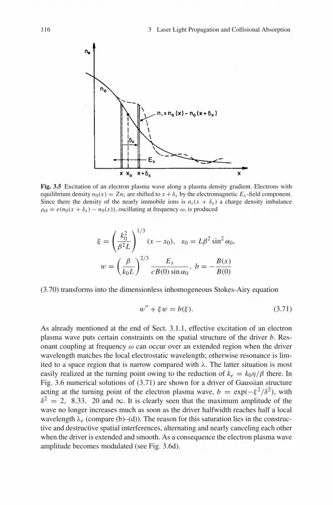
116 3 Laser Light Propagation and Collisional Absorption
Fig. 3.5 Excitation of an electron plasma wave along a plasma density gradient. Electrons withequilibrium density n0(x) = Zni are shifted to x+ δx by the electromagnetic Ex -field component.Since there the density of the nearly immobile ions is ni (x + δx ) a charge density imbalanceρel = e(n0(x + δx )− n0(x)), oscillating at frequency ω, is produced
ξ =(
k20
β2L
)1/3
(x − x0), x0 = Lβ2 sin2 α0,
w =(
β
k0L
)2/3 Ex
cB(0) sinα0, b = − B(x)
B(0)
(3.70) transforms into the dimensionless inhomogeneous Stokes-Airy equation
w′′ + ξw = b(ξ). (3.71)
As already mentioned at the end of Sect. 3.1.1, effective excitation of an electronplasma wave puts certain constraints on the spatial structure of the driver b. Res-onant coupling at frequency ω can occur over an extended region when the driverwavelength matches the local electrostatic wavelength; otherwise resonance is lim-ited to a space region that is narrow compared with λ. The latter situation is mosteasily realized at the turning point owing to the reduction of ke = k0η/β there. InFig. 3.6 numerical solutions of (3.71) are shown for a driver of Gaussian structureacting at the turning point of the electron plasma wave, b = exp(−ξ2/δ2), withδ2 = 2, 8.33, 20 and ∞. It is clearly seen that the maximum amplitude of thewave no longer increases much as soon as the driver halfwidth reaches half a localwavelength λe (compare (b)–(d)). The reason for this saturation lies in the construc-tive and destructive spatial interferences, alternating and nearly canceling each otherwhen the driver is extended and smooth. As a consequence the electron plasma waveamplitude becomes modulated (see Fig. 3.6d).
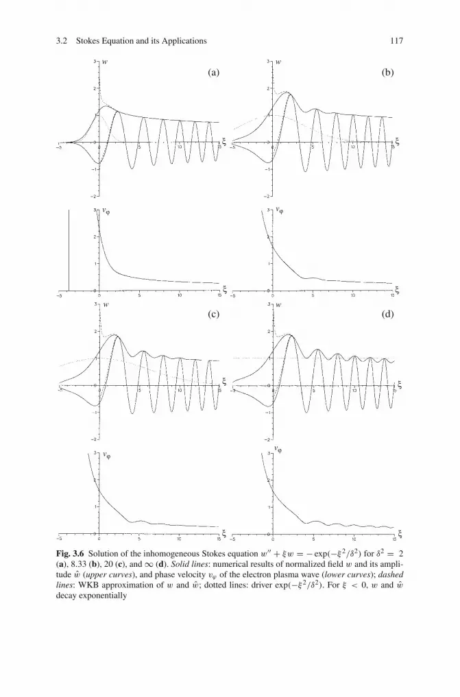
3.2 Stokes Equation and its Applications 117
Fig. 3.6 Solution of the inhomogeneous Stokes equation w′′ + ξw = − exp(−ξ2/δ2) for δ2 = 2(a), 8.33 (b), 20 (c), and∞ (d). Solid lines: numerical results of normalized field w and its ampli-tude w (upper curves), and phase velocity vϕ of the electron plasma wave (lower curves); dashedlines: WKB approximation of w and w; dotted lines: driver exp(−ξ2/δ2). For ξ < 0, w and w
decay exponentially

118 3 Laser Light Propagation and Collisional Absorption
Starting from Ai(ξ) and Bi(ξ) the general solution of (3.71) is constructed in thefamiliar way, i.e., using the Green’s function for (3.71)
w(ξ) = C1Ai(ξ)+ C2Bi(ξ)+∫ ξ
b(z)Ai(z)Bi(ξ)− Ai(ξ)Bi(z)
Wdz, (3.72)
with the Wronskian W = AiBi′ − Ai′Bi = 1/π . For a spatially constantdriver, b = −1, the inhomogeneous solution becomes the special functionHi(ξ) − 2Bi(ξ)/3. The correct, purely outgoing electron plasma wave isfound from the asymptotic representation of Ai,Bi and Hi and its evanescent behav-ior for ξ < 0,
w = π(Hi− Bi− iAi) = weiΘ. (3.73)
Here w is the amplitude of w, and Θ the phase. Around the saddle point ξ = 0 thesquare of the amplitude w2 has the power series expansion
w2(ξ) = 1.658+ 1.209ξ + 0.238ξ2 − 0.0839ξ3
−0.0523ξ4 − 7.40× 10⁻³ξ5 + . . . .
The maximum of w = 1.88 occurs at ξm = 1.8. Figure 3.6 also shows that the WKBsolution of (3.71) deviates very little from the exact solutions for ξ > ξm. The decayof w is slowest for b = 1 and behaves like 1/ξ1/4 for ξ >∼ ξm. On the other hand,since saturation of wmax occurs approximately for drivers of halfwidth ξm, ξm isthe correct measure of the width of the resonance xm − x0. It increases as L1/3. Thelower curves in Fig. 3.6 indicate the phase velocity vϕ at which a point ξ satisfyingw(ξ, t) = 0 propagates. In contrast to the Bohm-Gross expression the true vϕ doesnot diverge at the turning point.
3.3 Collisional Absorption
The physical mechanism of collisional absorption was analyzed in Sect. 2.1.3 underthe assumption that electrons and ions are elastic hard spheres. This model explainshow irreversibility, i.e., heating, and anisotropy of the electron distribution func-tion come about. It was also shown that all that is required of particle kineticsto determine absorption is the knowledge of the electron–ion (and, eventually, theelectron–electron) collision frequency, provided the model of a fully ionized plasmais valid. As long as the thermal electron speed is nonrelativistic all electrons havea mass close to their rest mass m and “see” nearly the same electric field E(x, t)with a frequency ω′ close to ω so that they all oscillate locally at nearly identicalvos. Hence, the momentum exchange in electron–electron collisions, occurring withfrequency νee, only leads to isotropization of the distribution function f (x, ve, t)and to thermalization, i.e., Maxwellization, at later times. In the reference system

3.3 Collisional Absorption 119
comoving at vos(t) an electron–electron collision looks the same as in the absenceof the laser field. Thus, they do not directly contribute to inverse bremsstrahlungabsorption.
In plasmas produced by high intensity lasers the electron temperatures are gen-erally such that the model of a two-component fully ionized plasma is valid. Thefrictional force, introduced phenomenologically by (2.23), originates, under mostconditions, from long-range, small-angle electron-ion collisions. As a consequence,the collision frequency νei becomes highly dependent on the energy of the collidingelectrons and, under standard conditions, it is the result of thousands of simultane-ous collisions rather than of single binary events (see Fig. 3.7). Expression (2.45)for νei was derived for a Maxwellian velocity distribution, vos � vth,e, and lnΛappreciably larger than unity. Since in laser plasmas each of these conditions maybe violated, a more general derivation of νei is needed. Large radiation field effectswere considered first by Silin [18] on the basis of a classical analysis. Early quan-tum mechanical treatments were given in [19] and [20]. A similar treatment fordense plasmas, in particular for -λB > λD , has only very recently been undertaken[21, 22]. In strong heating by lasers, the relaxation of slow electrons is faster thanthat of more energetic ones. As a consequence the electron velocity distribution maybecome non-Maxwellian [23] and nonisotropic [24].
In the following, the main physical effects determining collisional absorptionare described by introducing appropriate models in the test particle approxima-tion. First, νei is calculated for a monoenergetic unidirectional electron beam in theoscillator model approximation. This model turns out to be particularly useful forexplaining dynamical screening of the ion charges and for determining the variouscut-offs in a self-consistent way and the validity of the impact approximation usedby Pert [25–27]. The oscillator model is relevant for ion beam stopping and, to acertain degree, for absorption of superintense laser beams in dense targets.
Fig. 3.7 In the weak coupling case (standard plasma) an electron collides simultaneously withmany ions; small angle deflections dominate

120 3 Laser Light Propagation and Collisional Absorption
3.3.1 Collision Frequency of Electrons Drifting at Constant Speed(Oscillator Model)
Let us assume a homogeneous electron plasma streaming at constant velocity v0and a single ion of charge q = Ze at rest immersed in the electronic fluid (Fig. 3.8).The electrons are assumed to be held at equilibrium density n0 by a uniform nonin-teracting ion background (test particle model). During the passage, the electronsare attracted by the ion (and released after passage). Due to the passage of thecharge q an electron at equilibrium position x′ = −v0t in the comoving framewill be shifted by the amount δ(x, t) = δ‖ + δ⊥ parallel and perpendicular to v0.
As long as b⊥ � n−1/30 , the deflection angle χ is very small for almost all impact
parameters b and the electron trajectories can be approximated by straight linesx = v0t . It is this assumption which enables one to reduce multiple simultaneousCoulomb interactions to binary encounters. The disturbance in the electron densityne(x, t) induced by the passing ion is small for almost all impact parameters b sothat particle conservation is expressible in its linearized form,
0 = ∂
∂tn1 +∇
(ne
dδ
dt
)� ∂
∂tn1 +∇
(n0
∂
∂tδ
).
Integration in time leads to
n1(x, t) = −∇ (n0δ) . (3.74)
In the following n0 is assumed to be constant in space and hence n1 = −n0∇δ.Combining this with Poisson’s law one arrives at an expression for the electric field,
E = en0
ε0δ + q
4πε0r3r, (3.75)
Fig. 3.8 Oscillator model: A parallel monoenergetic beam of electrons is attracted by an ion at rest.As a consequence, the single orbits deviate by the vector δ(t) from straight lines and the electrondensity ne increases towards the symmetry axis. This nonuniformity of ne leads to a restoring forceacting back on the electrons

3.3 Collisional Absorption 121
since ∇(r/r3) = 4πδ(r). Magnetic fields can be neglected. From the approxima-tion of straight trajectories one obtains as a function of the collision parameter b
E‖ = en0
ε0δ‖ + κv0t
(b2 + v20 t2)3/2
, E⊥ = en0
ε0δ⊥ + κb
(b2 + v20 t2)3/2
;
κ = q
4πε0. (3.76)
By linearizing the momentum equation, ∂t tδ = −(e/μ)E (μ � m is the reducedmass) one ends up with two equations for forced harmonic oscillators with eigen-frequency ωp,
δ‖ + ω2pδ‖ = −
e
μκ
x
(b2 + x2)3/2, δ⊥ + ω2
pδ⊥ = −e
μκ
b
(b2 + x2)3/2, (3.77)
with x = v0t [28]. The restoring force has its origin in the induced space charge(see ne in Fig. 3.8) which screens the electrons from feeling the force of the barecharge q = Ze of the ion. Ignoring screening corresponds to setting ωp = 0 andleads to the well-known divergence in the total Coulomb cross section.
For its usefulness we remember in this place that a particular solution of theinhomogeneous linear differential equation y′′ + a(x)y = f (x) is given by [29]
y(x) = h(x)∫ x g(ζ ) f (ζ )
W (ζ )dζ − g(x)
∫ x h(ζ ) f (ζ )
W (ζ )dζ (3.78)
with W = gh′−g′h and where g and h are solutions of the homogeneous differentialequation.
Equations (3.77) have to be solved with appropriate initial conditions. Tofind them we observe that the solutions of the homogeneous equations are δ =δ exp(±iωpt), when switched on adiabatically at t = −∞. Hence, δ(−∞) =δ(−∞) = 0 and, after introducing the dynamic Debye length λ0,
λ0 = v0
ωp, (3.79)
and the dimensionless variables ξ = x/λ0, β = b/λ0 the solutions are
δ‖(ξ) = b⊥β
{sinβξ
∫ ξ
−∞u cos(βu)du
(1+ u2)3/2− cosβξ
∫ ξ
−∞u sin(βu)du
(1+ u2)3/2
},
δ⊥(ξ) = b⊥β
{sinβξ
∫ ξ
−∞cos(βu)du
(1+ u2)3/2− cosβξ
∫ ξ
−∞sin(βu)du
(1+ u2)3/2
}.
In this model the cold electron plasma oscillations at ω = ωp persist indefinitely. Inreality, owing to finite wave-wave and wave-particle interactions they slowly decay,thereby converting their kinetic and potential energies into thermal energy of the

122 3 Laser Light Propagation and Collisional Absorption
plasma. Their damping is mainly due to profile steepening and cold wavebreaking(see Sect. 4.4). The relevant amplitudes of δ⊥, δ‖ occur at ξ = ∞ and since inte-grals of the odd functions vanish, they are given by
δ‖ = b⊥β
∫ +∞
−∞u sin(βu)du
(1+ u2)3/2= b⊥
∫ +∞
−∞cos(βu)du
(1+ u2)1/2= 2b⊥K0(β), (3.80)
δ⊥ = b⊥β
∫ +∞
−∞cos(βu)du
(1+ u2)3/2= π1/2
�(3/2)b⊥K1(β) = 2b⊥K1(β). (3.81)
Expression (3.80) is obtained from a partial integration. K0 and K1 are modifiedBessel functions ([10], Sect. 9.6). For small values of β their expansions are, withγ = 0.57722,
K0(β) = −(
lnβ
2+ γ
)+(β
2
)2 (1− ln
β
2− γ
)+ · · ·
K1(β) = 1
β+(β
2
)(lnβ
2+ γ − 1
2
)+ · · · (3.82)
For β = 1 these expansions for K0 and K1 differ by 1 and 7% from the true values.For large values of β the corresponding asymptotic expansions are
K0(β) =(π
2β
)1/2
e−β{
1− 1
8β+ 9
128β2∓ . . .
},
K1(β) =(π
2β
)1/2
e−β{
1+ 3
8β+ 15
128β2± . . .
}.
Both amplitudes diverge for β → 0 (see Fig. 3.9.), since
K0(β → 0) ∼ − lnβ, K1(β → 0) ∼ 1
β.
The energy irradiated per unit time into plasma waves by a single ion through aplane orthogonal to v0 and at a fixed distance x →+∞ is given by
W = 1
2μω2
pn0v0λ20
∫ ∞
β0
2πβ(δ
2‖ + δ
2⊥)
dβ + v0 D(β0). (3.83)
This gives rise to a frictional force f on the ion, W = f v0. The lower cutoff isintroduced to avoid the divergence occurring at b → 0; it is a consequence of thestraight orbit approximation for the deflected electrons and is removed by takinginto account the finite deflection angles ϑ in close encounters. Their contribution toW is indicated by v0 D(β0). To calculate D it has to be mentioned first that stronglybent trajectories, e.g., with b <∼ b⊥, owing to widely varying curvatures intersect
3.3 Collisional Absorption 123
each other in such a way that almost no electron density disturbance n1 is produced,i.e., they do not contribute to screening as long as b⊥ � λ0 is fulfilled. As a con-sequence, (3.77) hold for impact parameters b ≥ b0 = αb⊥, with α not far fromunity and to be determined later. The frictional force D(β0) that the unscreened ionfeels from the electrons undergoing deflections from ϑ = π to a ϑ0 (correspondingto b = 0 and b = b0) is determined by the momentum change in the x-direction perunit time,
D(β0) = n0v0
∫ π
ϑ0
μv0(1− cosϑ)σΩdΩ
= 2πμn0v20b2⊥
∫ π
ϑ0
1− cosϑ
4 sin4(ϑ/2)sinϑdϑ
= 4πμn0v20b2⊥
∫ π
ϑ0
d sin(ϑ/2)
sin(ϑ/2)= Zμω2
pb⊥ ln1
sin(ϑ0/2). (3.84)
Equation (3.83) can be rewritten with the help of (3.84) and (2.44) as
W = Zμω2pv0b⊥
{β0 K0(β0)K1(β0)+ 1
2ln
(1+ b2
0
b2⊥
)}
since d(βK0 K1)/dβ = −β(K 20 + K 2
1 ) (see [10], Sect. 9.6.26). Hence,
W = Zμω2pv0b⊥
{− ln
β0
2− γ + β2
0
4− β2
0
2
(lnβ0
2+ γ
)2
+ 1
2ln
(1+ b2
0
b2⊥
)}
= Zμω2pv0b⊥
⎧⎨
⎩ln
⎡
⎣ λ0
b⊥
(1+ b2⊥
b20
)1/2⎤
⎦+ ln 2− γ
+β20
4
[1− 2
(lnβ0
2+ γ
)2]}
. (3.85)
The connection between the electron-ion collision frequency and W is obtainedfrom (2.23) by multiplying by v0,
W = Zμv20νei . (3.86)
Thus, the collision frequency becomes:
νei =ω2
pb⊥v0
⎧⎨
⎩ln
⎡
⎣ λ0
b⊥
(1+ b2⊥
b20
)1/2⎤
⎦+ 0.116
+β20
4
[1− 2
(lnβ0
2+ 0.58
)2]}
. (3.87)

124 3 Laser Light Propagation and Collisional Absorption
Fig. 3.9 Modified Bessel functions squared, K 20 and K 2
1 , their weighted integrals,∫ β
0.1 βK 20 dβ,∫ β
0.1 βK 21 dβ and their sum, as functions of the normalized collision parameter β = bωp/v0. The
dotted curve is the Coulomb logarithm ln(λ0/b⊥), with β = β⊥ = 0.1. Hence, when b = λ0,lnΛ = 2.3
The integrals∫βK 2
0 dβ and∫βK 2
1 dβ are shown in Fig. 3.9 for the lower limit ofintegration β = βl = 0.1. For βl approaching zero the first integral remains finitewhereas the second diverges logarithmically. When λ0 � max(b⊥, -λB) (weaklycoupled plasma) b0 can be chosen such that b⊥ � b0 � λ0 holds. The term in thecurly bracket then shrinks to the standard Coulomb logarithm lnΛ0 = ln(λ0/b⊥)and is insensitive to a particular choice of b0 which discriminates between “straight”and bent orbits. The parameter b⊥ enters in (3.87) in a natural way and is to be con-sidered merely as a convenient abbreviation for a combination of atomic and kine-matic quantities. There is no need to introduce additional concepts as, for example,a “parameter of closest approach,” frequently encountered in text books. The closestapproach is b = 0 and not b = b⊥ or b = -λB . In order to study the limits of validityof lnΛ0 for small ratios Λ0 = λ0/b⊥ it is convenient to choose b0 = (b⊥λ0)
1/2.Then νei becomes
νei =ω2
pb⊥v0
{lnΛ0 + B + C} , (3.88)
B = ln
(1+ 1
Λ0
)1/2
, C = 0.116+ 1
4Λ0
[1+ 1
2(0.23+ lnΛ0)
2].
In evaluating νei from (3.87), β0 as small as β0 = 2β⊥, or α = 2, is tolerable sincecos(ϑ0/2) = 0.89 is still sufficiently close to unity, and the factor (1 + b2⊥/b2
0)1/2
contributes only by ln√
1.25 = 0.11. In Table 3.2 typical values of lnΛ0 and thetwo corrections B and C are given. For lnΛ0 ≥ 3 the standard Coulomb logarithmis an acceptable approximation in the oscillator model. At Λ0 = 2, lnΛ0 deviatesfrom the more exact value lnΛ0 + B + C already by 40%. In high-density and/or

3.3 Collisional Absorption 125
Table 3.2 Behavior of lnΛ0 and its corrections B and C from (3.88) for small values of Λ0 =λ0/b⊥
Λ0 100 10 5 3 2 1.5 1lnΛ0 4.6 2.3 1.6 1.1 0.7 0.4 0.0B 0.005 0.05 0.09 0.14 0.2 0.25 0.35C 0.15 0.22 0.25 0.27 0.29 0.32 0.37
high-Z plasmas λ0 may become comparable to or even smaller than b⊥. In such acase (3.87) has to be modified for several reasons. One is immediately seen fromFig. 3.9, since then β0 is in the interval β > 1 where ln(β/0.1) starts deviatingconsiderably from
∫β(K 2
0+K 21 )dβ and hence νei depends sensitively on the choice
of α. Another criterion to be obeyed is 4πλ30n0/3 >∼ Z for effective Debye screen-
ing. We come back to these problems in connection with collisional absorption in athermal plasma.
From the oscillator model the cutoff of the Coulomb potential at the dynamicDebye length λ0 arises self-consistently. Performing all calculations with a bareCoulomb potential corresponds to ignoring the restoring force in (3.77) and leadsto the well-known divergent result. The origin of screening and the reason for con-vergence become clear from the oscillator model (see Fig. 3.8): An electron on thedistant orbit with b larger than a certain bmax feels a weak attractive Coulomb forceover a long time; the oscillators (3.77) are very slowly shifted from their equilibriumposition and then slowly released. The whole process occurs adiabatically and allenergy the oscillators had acquired is given back after the encounter. At an inter-mediate b, the oscillators associated with δ‖, δ⊥ are excited since the driving forcechanges rapidly enough to produce Fourier components not far from the eigenfre-quency ωp. As a result, energy is taken irreversibly from the translational motionand transformed into oscillatory energy. Finally, at very small b � b⊥ the excitingforce has frequencies much larger than ωp so that the oscillator behaves like anattracted particle with zero restoring force. It is well-known that the deflection angleϑ of a nearly straight orbit can be calculated exactly if the maximum Coulomb forceqe/4πε0b2 is assumed to act over the finite distance of 2b ([30], Sect. 13.1). Con-sequently, the effective interaction time in such a collision is τ = 2b/v0. A cutoffat bmax = λ0 means that interaction times during which the oscillator undergoesmore than
τ
2π/ωp= λ0ωp
πv0= 1
π(3.89)
oscillations have no irreversible, i.e., collisional effect on the system. It becomesclear from this picture that at zero temperature the parameter which separatescollective behavior from single particle events is b0 � 2b⊥, and not the Debyelength λ0.
The excitation of a plasma wave by an ion moving uniformly through a homoge-neous plasma was simulated numerically with a Vlasov code in full generality, i.e.,nonlinearities in ne and bent electron orbits are included [31, 32]. A typical example

126 3 Laser Light Propagation and Collisional Absorption
is shown in Fig. 3.10. For moderate ion charges the nonlinearity in ne and in theelectrostatic potential is small; at high Z-values, however, it is no longer negligible(see Fig. 3.10b) and leads, as a consequence of trapping of free electrons in theion potential, to a dependence of νei on ni which is smaller than Z2 of expressions(3.87) and (3.88).
So far the effect of a single ion on an electron has been calculated. When νei
produced by the ions of a plasma is considered, one electron feels simultaneouslythe influence of many ions and their collisions overlap since λ0 � n−1/3
0 (Fig. 3.7).Under the conditions that (i) the overlapping collisions occur along nearly straightorbits and that (ii) collisions with curved orbits do not overlap (b0 < n−1/3
0 ) thisproblem is easily solved. To this end imagine the ions at the locations xi . At thetime t each of them has produced the shift δi (t) = δi‖(t) + δi⊥(t) according to(3.77). They sum up to a total instantaneous shift δ(t) and hence the total oscillatoryenergy of an electron at position x = (a, b) is
1
2μ ˆδ2(a, b) = 1
2μ
(N∑
i=1
ˆδi (t)
)2
= 1
2μ
N∑
i, j=1
ˆδiˆδ j = 1
2μ
N∑
i=1
ˆδ2i , (3.90)
i.e., owing to randomly distributed phases all collisions add up as if they occurredone after another. As a consequence, N ions radiate N W power by electron plasmawaves and (3.86) remains valid for overlapping long-range Coulomb collisions.Expressed differently, in this way the collective part of νei is calculated in its firstBorn approximation (no multiple scattering), since v0 is kept constant over the dura-tion of the collision with one ion.
In most elementary derivations of νei based on the momentum change of a singleelectron in the forward direction, only δ⊥ is taken into consideration. From Fig. 3.9it is seen that δ‖ also contributes. Imagine two parallel layers of electrons at a suit-able distance from each other. When the first layer has reached the position of the
Fig. 3.10 (a): Excitation of an electron plasma wave by an ion at position z = 0, r = 0 of chargeZ (normalized by the number of electrons in the Debye sphere) in a plasma streaming from rightto left at speed v0/vth = 4 (from [31]). (b): Electrostatic potential/Z on the z axis as a function ofthe normalized charge Z (from [31]). In the linear theory the three curves coincide

3.3 Collisional Absorption 127
ion it has its maximum velocity v0 + ε by attraction whereas the layer behind hasnot yet. This difference in speed leads to a charge nonuniformity oscillating in thedirection of v0. Its relative importance increases with decreasing Coulomb logarithmln(λ0/b⊥). In fact, for v0 = const the ratio of the two contributions to the absorptioncoefficient α⊥ + α‖ for lnΛ0
>∼ 2 is given by
α‖α⊥
= 1
2 lnΛ0. (3.91)
In a harmonic laser field the electrons oscillate with the oscillation velocity vos(t)and the displacement p(t),
vos(t) = vos e−iωt , vos = −ie
mωE, p(t) = p e−iωt , p = e
mω2E.
As a consequence the collision frequency becomes time-dependent, νei = νei (t).The portion of energy irreversibly transferred to the electrons per unit time understeady state conditions is obtained from the cycle-averaged quantity j E. With thehelp of (2.23) a meaningful definition of the cycle-averaged collision frequency νei
is given by
j E = νei nemv2 = 2νei ne0Eos, ne0 = ne(t), Eos = 1
2mv2. (3.92)
With νei replaced by νei (t) in the foregoing sections all absorption formulas remainvalid.
The determination of the time-averaged collision frequency νei for vanishingelectron temperature represents a nearly exactly solvable problem. It may serve asa bench mark result for critically analyzing the various approximate results in theliterature. However, even under the limitation Te = 0 the analysis is of considerablecomplexity [33]. In (3.75) the former r = b + v0t is replaced by r = b + p(t).Under the assumption of steady state and no memory effect extending over morethan one oscillation, with the help of the Anger functions of index σ = ωp/ω [34],
Jσ (x) = 1
π
∫ π
0cos(σξ − x sin ξ) dξ,
one arrives (making use of trigonometric identities) at the collective part of the col-lision frequency νc,
νc = 2b⊥ω2
p
vos
∫ ∞
−∞b0
p|x | K0(b0|x |/ p) K1(b0|x |/ p) J 2
σ (x) dx; (3.93)
b⊥ = κe
mv2os, p = | p|. (3.94)
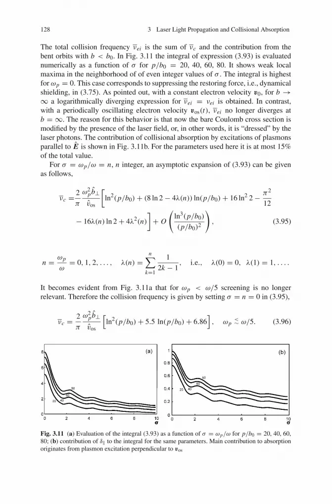
128 3 Laser Light Propagation and Collisional Absorption
The total collision frequency νei is the sum of νc and the contribution from thebent orbits with b < b0. In Fig. 3.11 the integral of expression (3.93) is evaluatednumerically as a function of σ for p/b0 = 20, 40, 60, 80. It shows weak localmaxima in the neighborhood of of even integer values of σ . The integral is highestfor ωp = 0. This case corresponds to suppressing the restoring force, i.e., dynamicalshielding, in (3.75). As pointed out, with a constant electron velocity v0, for b →∞ a logarithmically diverging expression for νei = νei is obtained. In contrast,with a periodically oscillating electron velocity vos(t), νei no longer diverges atb = ∞. The reason for this behavior is that now the bare Coulomb cross section ismodified by the presence of the laser field, or, in other words, it is “dressed” by thelaser photons. The contribution of collisional absorption by excitations of plasmonsparallel to E is shown in Fig. 3.11b. For the parameters used here it is at most 15%of the total value.
For σ = ωp/ω = n, n integer, an asymptotic expansion of (3.93) can be givenas follows,
νc = 2
π
ω2pb⊥vos
[ln2(p/b0)+ (8 ln 2− 4λ(n)) ln(p/b0)+ 16 ln2 2− π2
12
− 16λ(n) ln 2+ 4λ2(n)
]+ O
(ln3(p/b0)
(p/b0)2
), (3.95)
n = ωp
ω= 0, 1, 2, . . . , λ(n) =
n∑
k=1
1
2k − 1, i.e., λ(0) = 0, λ(1) = 1, . . . .
It becomes evident from Fig. 3.11a that for ωp < ω/5 screening is no longerrelevant. Therefore the collision frequency is given by setting σ = n = 0 in (3.95),
νc = 2
π
ω2pb⊥vos
[ln2(p/b0)+ 5.5 ln(p/b0)+ 6.86
], ωp
<∼ ω/5. (3.96)
Fig. 3.11 (a) Evaluation of the integral (3.93) as a function of σ = ωp/ω for p/b0 = 20, 40, 60,80; (b) contribution of δ‖ to the integral for the same parameters. Main contribution to absorptionoriginates from plasmon excitation perpendicular to vos

3.3 Collisional Absorption 129
A detailed analysis of (3.93) shows that for σ = 0 the integrand decays exponen-tially from x = p/b0 on. This means that screening acts as if the bare Coulombpotential is cut off at bmax = p = vos/ω. If σ > 0, J 2
σ (x < σ) � 0 holds and thecorresponding cut off is bmax = vos/ωp.
3.3.2 Thermal Electrons in a Strong Laser Field
The random motion of the plasma electrons in the mean field approximation maybe described by a classical one particle distribution function f (x, ve, t) when itskinetic temperature Te is much higher than the Fermi temperature TF = EF/kB . Inthe presence of the laser field a drift velocity is superposed and hence the distributionfunction g(x′, v′, t) in the lab frame is
g(x′, v′, t) = f (x, ve, t), x′ = x + p(t), v′ = ve + vos(t). (3.97)
As a consequence of the attraction by an ion an electric field Ein is induced bythermal and dynamical shielding. In the case that the screening length λ is muchlarger than b⊥ and -λB the majority of the particle orbits is nearly straight and again acollision parameter b0, max(b⊥, -λB)� b0 � λ, can be introduced which separatesclose encounters from remote ones. The electrons with b > b0 behave fluid-like andare adequately described by the linearized dielectric Vlasov model.
The Vlasov equation (2.86) with a test ion of charge q = Ze reads in the oscilla-tory frame x = x′ − p(t)
∂ f
∂t+ ve
∂ f
∂x+ e
m∇Φ ∂ f
∂ve= 0, (3.98)
Φ = ΦC +Φin, ΦC = κ
|x′| , ∇Φin = −Ein.
Φin is the induced screening potential. The Coulomb potential ΦC of the ion oscil-lates around its position in the lab frame x′ = 0 according to x = x′ − p(t). Bysetting f = f0(ve) + f1(x, ve, t), with f1 the disturbance introduced by the testcharge, and linearizing around f0 yields
∂ f1
∂t+ ve
∂ f1
∂x+ e
m∇(ΦC +Φin)
∂ f0
∂ve+ e
m∇ΦC
∂ f1
∂ve= 0. (3.99)
Poisson’s equation requires
∇2Φin = n0e
ε0
∫f1 dve, ∇2ΦC = − q
ε0δ(x + p(t)). (3.100)
It is standard to omit the last term in (3.99) although it is of first order. Byits neglect strong ion field effects (close encounters, bent orbits) are excluded.

130 3 Laser Light Propagation and Collisional Absorption
The ∇ operators are removed by a Fourier transform in space, Φ(k,Ω) =(2π)−2
∫Φ(x, t) exp(−i kx + iΩt) dxdt , etc., and (3.99), (3.100) reduce to alge-
braic relations. Equations (3.100) transform into
Φin(k,Ω) = − n0e
ε0k2
∫f1(k,Ω, ve) dve, (3.101)
ΦC(k,Ω) = q
(2π)2ε0k2
∫δ(x + p(t)) e−i kx+iΩt dxdt (3.102)
= q
(2π)2ε0k2
∫ei(Ωt+k p cosωt) dt
= q
2πε0k2
∞∑
n=−∞inδ(Ω + nω) Jn(k p)
where the identities
e±i z cos ζ =∞∑
n=−∞(±i)n Jn(z) e±inζ , δ(z) = (2π)−1
∫eikz dk
for the Bessel functions of integer order Jn and for the delta function have beenused. The Fourier transform of (3.99) yields
(Ω − kve) f1(k,Ω) = e
m(ΦC + Φin)k
∂ f0
∂ve. (3.103)
In a static linear homogeneous medium the dielectric constant ε connects the exter-nal, induced, and total electric fields Eex, Ein, E with the polarization P in thefollowing way,
εE = ε(Eex + Ein) = E + 1
ε0P .
By means of Poisson’s equation and ∇ P = −ρin this translates into
ερ = (ρ − ρin) = ρex, εΦ = (Φ −Φin) = Φex (3.104)
for the total, external, and induced charge densities ρ, ρex, ρin and potentials Φ,Φex, Φin. Thus, ρ = ρex/ε, E = Eex/ε, Φ = Φex/ε.
Introducing the dielectric function ε = ε(k,Ω), within the validity of linearresponse these relations hold for a single Fourier component in fields varying inspace and time. Substituting f1 from (3.103) in Φin in (3.101) yields
ΦC = "− "in = "
{1+ n0e2
ε0k2m
∫k∂ f0/∂ve
Ω − kvedve
}.

3.3 Collisional Absorption 131
Hence, owing to ΦC = Φex, ρC = ρex, and "C = "ex, ρC = ρex
ε(k,Ω) = "C
"= 1+ ω2
p
k2
∫k∂ f0/∂ve
Ω − kvedve. (3.105)
It is analytic in the entire half plane �Ω > 0. For a real quantity h(x, t) the relationh∗(k,Ω) = h(−k∗,−Ω∗) holds and, consequently, ε∗(k,Ω) = ε(−k∗,−Ω∗).The total potential Φ(x, t) = ΦC(x, t) + Φin(x, t) reads now in the frame movingwith vos(t)
Φ(x, t) = 1
(2π)3q
ε0
∞∑
n=−∞
∫in
k2ε(k,−nω)Jn(k p) eikx+inωt dk. (3.106)
The force f q acting on the ion at position x(t) = − p cosωt is
f q = −q∇Φ(− p cosωt, t)
= − 1
(2π)3q2
ε0
∞∑
n=−∞
∫in+1k Jn(k p)k2ε(k,−nω)
e−i k p cosωt+inωt dk
= − 1
(2π)3q2
ε0
∞∑
l,n=−∞
∫in+1−l k
k2ε(k,−nω)Jl(k p) Jn(k p) ei(n−l)ωt dk.
The cycle-averaged energy absorbed per unit volume and unit time is
j E = −n0
Zf qvos(t) = −i
n0
Z
1
2mωE f q(eiωt − e−iωt )
= n0e2q
2mωε0
E(2π)3
∞∑
n=−∞
∫i k dk
k2ε(k,−nω)
×{Jn−1(k p)Jn(k p)+ Jn(k p)Jn+1(k p)}
= 1
(2π)3ω2
p
ωq E
∞∑
n=−∞
∫i k dk
k2ε(k,−nω)J 2
n (k p)n
k p.
In the last step the property Jn−1(x)+ Jn+1(x) = 2n Jn(x)/x was used. E is the reallaser field amplitude. Owing to the cylindrical symmetry the integration over k ⊥ pcan be performed easily in polar coordinates,
j E = 1
(2π)3ω2
p
ωq E
∞∑
n=−∞
∫ ∞
0
i dk
ε(k,−nω)
2π
p
∫ 1
−1n J 2
n (k p cosϑ) d cosϑ
= mvos Zω2
p
π2 p2
∞∑
n=1
n∫ ∞
0
dk
k� 1
ε(k,−nω)
∫ k p
0J 2
n (ξ) dξ. (3.107)

132 3 Laser Light Propagation and Collisional Absorption
In the last passage the properties J−n(ξ) = (−1)n Jn(ξ), J 2n (−ξ) = J 2
n (ξ),ε(k,−Ω∗) = ε∗(k,Ω) for k real and Ω = −nω, and vos = eE/mω were used.The electron distribution function f0(ve) is to be used in a system of reference inwhich no net drift results, i.e.,
∫ve f0(ve) dve = 0; all drift is in the ions. The
time-averaged collision frequency νei follows from (3.92).For a Maxwellian distribution function fe (3.105) reads
ε(k, ω) = 1+ k2D
k2
(1− 2ηe−η2
∫ η
0ex2
dx + i√πηe−η2
), η = ω√
2kvth.
(3.108)
The electron thermal velocity is vth = (kBTe/m)1/2 and kD = 1/λD , withλD = vth/ωp the familiar electron Debye length. Simple expressions of j E areattainable for vos < vth and vos � vth; for intermediate ratios of vos/vth (3.107)must be evaluated numerically. A comparison of the classical expression for the dif-ferential Coulomb cross section σΩ in terms of the impact parameter b (2.44) withits identical quantum expression formulated in terms of plane waves of wave vectork (see [35], p. 387), b and |k| are related by k = |k| = 1/b and, correspondingly,k⊥ = 1/b⊥ and kB = 1/-λB . If b is a few times larger than -λB it is the center of anarrow wave packet around k = 1/b. Hence, for ω >∼ ωp the relevant k-interval in(3.108) is k > kD or, equivalently, ωp/kvth
<∼√
2η < 1. It yields
�(
1
ε
)� −
(π2
)1/2 k2D
k3
ω
vth
e− ω2
2k2v2th
(1+ k2D/k2)2
. (3.109)
Let us take for the moment vos � vth to arrive at k p � 1 and J1(ξ) = ξ/2 asthe leading term owing to Jn(ξ � 1) � (ξ/2)n/n!. Hence, in the weak laser fieldapproximation (3.107) simplifies to
j E = 4
3
(π2
)1/2Z
(nee2
4πε0m
)2mv2
os
v3th
∫ (∞)
0
k3
(k2 + k2D)
2dk. (3.110)
The indefinite integral is [ln(k2 + k2D)+ k2
D/(k2 + k2
D)]/2. It diverges for k →∞.This is a consequence of linearization and omission of the last term in (3.99) or,equivalently, of the straight orbit approximation. In perfect analogy to the treatmentof close encounters by D(β0) in (3.84)ff k0 = 1/b0 has to be introduced, withb0 dividing straight orbits from bent trajectories. After folding with a Maxwellianand averaging vos(t)〈D(β0)〉 over one laser cycle the resulting quantity has to beadded to (3.110). We do not continue further here because the subject is treatedmore adequately in the next subsection dedicated to the ballistic collision model.We conclude by observing that the classical dielectric model yields a lower self-consistent cut-off at k = kD , but it diverges for large k-values related to closeelectron-ion encounters. The divergence at large k-values is avoided in a quantum

3.3 Collisional Absorption 133
treatment, e.g., following a Kadanoff-Baym [36, 21] or a quantum Vlasov treatment[37]. A complementary derivation in some respect, based on a generalized linearresponse theory, is given in [38]. The authors arrive at the same expression (3.107) inwhich now the classical expression of ε(k, ω) is replaced by its quantum counterpartεq(k, ω) [39],
εq(k, ω) = 1+ k2D√2k2
kB
k
[D
(η + k√
2kB
)− D
(η − k√
2kB
)]
+i(π
2
)1/2 k2D√2k2
kB
ke−η2
e−12 (k/kB )
2sinh(
√2η), (3.111)
with η as before and D(y) = e−y2 ∫ y0 ex2
dx . The evaluation of (3.107) with ε = εq
is complicated. Following again [39] one arrives at
j E = Zmω4p
π2vos
∫ ∞
0
dk
kF
(k
kD,ω
ωp,vos
vth
), (3.112)
F =(ω
ωp
)2 ∞∑
l=1
l�εq(k, ilω)
|εq(k, ilω)|2∫ kvos/ω
0dξ J 2
l (ξ), νei = j E2ne Eos
for all ratios vos/vth. In many applications holds λD � b0 >-λB
>∼ 2b⊥. Then, forvos � vth with εq used in (3.107) follows the upper cut-off k = kmax =
√2kB .
The validity of (3.110) extends, strictly speaking, only up to k = 1/b0. However,when adding the cycle-averaged contribution of the close encounters vos(t)〈D(β0)〉the sum of both is obtained by extending the interval up to kmax and is insensitiveto the special choice of the cut b0 over an adequate range. Hence, the integral yieldsln(λD/
-λB) + 0.06 which is nearly identical with the familiar Coulomb logarithmlnΛ, Λ = λD/
-λB , and νei becomes identical to the Spitzer–Braginskii collision fre-quency (2.45) for a Maxwellian plasma. It should be stressed that although electrontrajectories with b = -λB are generally bent and invalidate any Born approxima-tion or linearization (3.99), under the limitations above the correct result for νei isobtained through the cut-off at bmin = -λB/2. The collision frequency for vos � vthis also obtained by making use of εq(k, ω) and the asymptotic forms of Jn(ξ) forlarge arguments. We list the results of [19, 20, 37], all derived for ω2 � ω2
p,
Shima–Yatom : νei = C ln2vos
vth
(lnvth/ω
-λB+ ln
2vos
vth
)
Silin : νei = 2C
(1+ ln
vos
2vth
)lnvth/ω
-λB(3.113)
Kull–Plagne : νei = 2C lnvos
vthln
[√2vth/ω
-λB
(vos
vth
)1/2]

134 3 Laser Light Propagation and Collisional Absorption
(“double Coulomb logarithm”) where C = meω4p/(nev
3os). The most careful asymp-
totic analysis is undertaken in [37]. In connection with the expressions (3.113) inparticular and with the dielectric model in general, several remarks are to be made.(i) Expressions (3.113) for the same physical quantity differ from each other. Evi-dently there is no unique asymptote. However, the validity of each expression maybe best for some interval of vos/vth. Do they hold for all ratios ωp/ω > (1 ∼ 3)? (ii)The evaluation of (3.107) in full generality is of considerable complexity and doesexclude close encounters. At ratios vos/vth � 1 up to 103 Bessel terms may haveto be added to achieve convergence. (iii) To remove the differential operators ∂/∂tand ∇ from (3.99) transformation to Fourier space is done which, as a consequencenecessitates the decomposition of the anharmonic time dependence exp(i cosωt) toa complete set of Bessel functions. Great loss of a physical picture is the conse-quence. For example, what is the physics behind a function like
ln
⎡
⎣(√
2vth/ω
-λB
(vos
vth
)1/2)ln vos/vth
⎤
⎦
from (3.113)? (iv) In its nature a collision is short in comparison to the laser plasmaperiod 2π/ω, it resembles a narrow Gaussian, if not even a δ-type interaction. Todecompose it into functions of kx of constant amplitude is counterintuitive (e.g., liketreating the hydrogen atom in the basis of the Hermite polynomials of the harmonicoscillator in R
3). In transport theory time-dependent quantities are of interest, e.g.,the heating function j(t)E(t) at low frequency ω. It is a hopeless enterprise toevaluate it in the framework of the standard dielectric theory (see the double sumof products Jl Jn). Searching for a more appropriate description, i.e., a more ade-quate basis, may represent a challenging problem of mathematical physics. Withthe introduction of the ballistic model for collisions a first step may be done in theright direction.
3.3.3 The Ballistic Model
Collisions of individual electrons with a fixed ion of charge number Z are consid-ered. The momentum loss along the original electron trajectory due to deflection iscalculated and the result is averaged over all impact parameters b and all velocitiesv(t) = vos(t) + ve, ve taken from f (x, ve, t) in the oscillating frame as beforein (3.97). As a result the time-dependent collision frequency νei (t) is obtained.Finally, cycle averaging yields νei . For simplicity the distribution function f isassumed to be homogeneous and locally isotropic; hence f (x, ve, t) = f (ve, t).The momentum loss Δ p in a Coulomb collision along v(t) follows from the differ-ential Coulomb cross section σΩ in (2.44) by integration over b, with σ = πb2
maxthe total cross section,

3.3 Collisional Absorption 135
Δ p = mvb2⊥σ
∫ π
ϑ=ε(1− cosϑ) sinϑ
4 sin4 ϑ2
dϑdϕ = 4πmvb2⊥σ
∫ π
ϑ=εd sin ϑ
2
sin ϑ2
= 4πmvb2⊥σ
ln(b2⊥ + b2
max)1/2
b⊥. (3.114)
The Coulomb logarithm lnΛ = ln[(b2⊥ + b2max)
1/2/b⊥] is discussed later. Themomentum loss per unit time is p = σni |v|Δ p,
p = −mνei (v)v = − K
v3v lnΛ, K = Z2e4ni
4πε20m
. (3.115)
By the first equality the collision frequency νei (v) for the momentum loss p = mv
is defined. Equation (3.115) implies that simultaneous collisions are reduced to asequence of successive encounters since small angle deflections obey the relations
〈Δv〉 = v〈[1 − cosϑ(t)]〉 = v〈ϑ2(t)〉/2 = v∑N
i=1 ϑ2i (t)/2 = v/v2∑ δ
2i (t)/2,
in perfect analogy to (3.90). To obtain the ensemble-averaged momentum loss 〈 p〉averaging has to be done on v/v3 over the thermal velocities ve. For an isotropicdistribution function f (ve) the velocity v consists of all vector sums as sketched inFig. 3.12. The quantity p is parallel to v, whereas 〈 p〉 is directed along vos. Withthe angle χ as indicated in the figure we find
〈 p〉 = mνei (t)vos = −K∫ ∞
0
∫ π
0
v
v32πv2
e sinχ f (ve) lnΛ dχdve. (3.116)
The combined velocity is v = |v| = (v2os+v2
e+2vosve)1/2. The collision frequencies
νei (t) and νei follow as
νei (t) = 2πK
mvos(t)
∫ ∞
0
∫ 1
−1
cosαv2e f (ve) lnΛ
v2os + v2
e + 2vosve cosχd cosχdve, (3.117)
νei = 4πK
mv2os
∫ ∞
0
∫ 1
−1
vosv
v3v2
e f (ve) lnΛ d cosχdve. (3.118)
Fig. 3.12 vi = ve,i + vos(t), vos(t) quiver motion

136 3 Laser Light Propagation and Collisional Absorption
These expressions are much simpler than (3.107), however they do not handlecollective resonances around ω = ωp. The integration over b in the Coulomb log-arithm runs from b = 0 to b = bmax. No lower cut-off appears, only bmax must bedetermined.
3.3.3.1 Cut-offs
Let us assume that b⊥ and -λB are well separated from bmax and λD . In additionbmax � b0, b0 separating straight from bent orbits, is assumed to be valid as is thecase in the weakly coupled plasma. First bmax is fixed. Under the current conditionsJackson’s model applies [see paragraph containing (3.89)]. For vos/vth
>∼ 3 the time-averaged speed is, owing to v2 ∼ sin2 ωt , v = v/
√2. From τint = 2b/v ≤ τlaser/3
follows
2bmax
v/√
2= 1
3
2π
ω ⇒ bmax = v√
2ω. (3.119)
The accuracy of this cut-off can be checked by comparing (3.118) with (3.112). Theoutcome will result very satisfactory, as shown in the following.
In the literature b = b⊥ or b = -λB is generally referred to as a “lower cut-off”bmin. This is unfortunate and totally misleading. Finally, to make the confusion com-plete, bmin = b⊥ is given the name of “closest approach” [Sect. 3.3.1, e.g. (3.84),(3.85)]. A standard argument for choosing -λB as a lower cut-off is that a higherdegree of localization of encounters b < -λB is meaningless because of the uncer-tainty principle. As seen in Sect. 3.3.1 in classical Coulomb scattering b⊥ resultsfrom an exact integration starting from b = 0. Perpendicular deflection plays no spe-cial role from the point of physics, it is merely a compact mathematical symbol. Wewant to stress further that the classical Rutherford cross section σΩ for the Coulombpotential is identical with the corresponding exact quantum mechanical expressionand with its first Born approximation [35]. In a quantum calculation integration isalso done over all scattering angles, corresponding classically to all values b > 0[see (2.44)]. However, owing to screening the cross section of a charged particlein the plasma falls off more rapidly than 1/b4. That is the reason why in transporttheory λD appears. Let us first consider the quasi-static screening at vos � vthgiven by the Debye potential (2.39) in the weak coupling limit. Its differential crosssection σD(ϑ) in first Born approximation is given by [35]
σD(ϑ) = b2⊥4[sin2(ϑ/2)+ (-λ/2λD)2]2
, -λB = h
mv. (3.120)
Replacing σD(ϑ) in Δ p from (3.114) leads to LC in place of lnΛ,
LC = 1
2ln
(1
ρ2+ 1
)− 1
1+ ρ2� 1
2
(ln
1
ρ2− 1
)= ln
λD-λB+ 0.2, ρ =
-λB
2λD.
(3.121)

3.3 Collisional Absorption 137
It shows that, taken the first Born approximation for granted, in (3.114) b⊥ shouldalways be replaced by -λB . This is in clear contradiction to the rule that bmin (whichis not a lower cut-off) in Λ = bmax/bmin = bmax/
-λB goes over into Λ = bmax/b⊥as soon as -λB
<∼ (1 ∼ 2)b⊥ ([40] p. 262). The contradiction arises for λD → ∞.Scattering of a plane wave is an acceptable concept for potentials falling off rapidly,e.g., a Debye potential, but not for V ∼ 1/r which is of infinite extension and givescontributions to scattering up to b = ∞. When scattering of finite wave packets isconsidered the contradiction disappears. However, the pertinent published literatureis not very clear and often merely formal (see for instance [41] and [42], to namejust two). Here we present a physically correct and more lucid explanation.
By setting k20 = 2m E/h2 = 1/-λ2
B and η2 = 1 − V (x)/E the stationary one-particle Schrödinger equation assumes the structure of (3.7) when ∇E = 0 is set.Under WKB conditions η obeys the ray equation (3.12). In the domain of validityof it the scattering angle ϑ is the deflection angle of the trajectory (“ray”) asso-ciated with the collision parameter b. According to (2.44) ϑ and b are related bysin2 ϑ/2 = b2⊥/(b2⊥ + b2). Let be -λB = rb⊥ and b0 = s-λB , where r and s areof order unity. By definition b0 subdivides the scattering potential into two regions,b > b0 and b ≤ b0. In the outer region WKB holds (“straight” orbits, b0 � b⊥).By setting for instance r = s = 2 follows ϑ(b0) = ϑ0 = 28◦, cosϑ0 = 0.88 � 1,and hence the first Born approximation (3.120) for σD(ϑ) is also valid there. Owingto b0 � bmax screening in the inner domain b ≤ b0 is irrelevant and scattering iscalculated to an excellent approximation from the unscreened Coulomb potential.With the help of (3.114) the total momentum loss Δ p is
Δ p = 4πmvb2⊥σ
[ln
b2⊥ + b20
b2⊥+ ln(x2 + ρ2)
∣∣∣x0
0− x2
x2 + ρ2
∣∣∣∣x0
0
](3.122)
where x = sinϑ/2, x0 = sinϑ0/2, ρ = -λB/2λD . If in the inner region σD(ϑ)
is used instead of σΩ , from the second and third terms in (3.122) taken within thelimits x = x0 and x = 1 follows
ln1+ ρ2
x20 + ρ2
− 1
1+ ρ2+ x2
0
x20 + ρ2
� ln1
x20 + ρ2
�
− ln
[b2⊥
b2⊥ + b20
+ b2⊥λ2
D
]� ln
b2⊥ + b20
b2⊥.
Thus, the Debye potential can be used in the entire region 0 ≤ b <∞ if (λD/b0)2 is
considerably larger than (b2⊥ + b20)/b2⊥, and the Coulomb logarithm reads as given
by LC in (3.121).The situation is more complicated for -λB < b⊥. In evaluating (3.122) the con-
dition b0 � b⊥ must hold to guarantee the validity of WKB and the first Bornapproximation in the outer region. At the same time the use of the unscreenedCoulomb potential in the inner region requires again b0 � λD . In general the

138 3 Laser Light Propagation and Collisional Absorption
frequently encountered simple rule of replacing -λB by b⊥ in the Coulomb logarithmrepresents an improvement. However, it is not exact; the correct cut-off results ina more complicated expression obtained from (3.122). In laser plasmas generally-λB � b⊥ holds and the opposite situation is not of great relevance.
In the following we limit ourselves to -λB > b⊥. Guided by the structure ofσD(ϑ) in (3.120) which contains (-λB/2)2/λ2
D we redefine bmin = -λB/2 = h/2mv.The formal justification for it may come from the kinetic formulation in terms ofWigner distribution functions and is therefore to be considered of universal charac-ter not bound to the special Debye potential of scattering [39]. In practice the modelof a coherent plane wave is not applicable to lateral extensions larger than � -λD .Under the condition vos � vth the quiver motion induces only small periodic oscil-lations of the screening Debye sphere. The much faster thermal motion compensatessmall deformations. This is expected to hold to an acceptable approximation up tovos
<∼ vth. In the Coulomb logarithm, however, λD = vth/ωp has to be replaced byvth/ω if ω > ωp holds, as outlined at the beginning of this subsection for arbitraryvelocity v. In case of ω < ωp the plasma frequency as the faster oscillation fre-quency takes the role of the limiting interaction time for a collision, in agreementwith the oscillator model of Sect. 3.3.1. In summary, the Coulomb logarithm to beused in the ballistic model for the individual velocity v is
lnΛ = lnbmax
bmin, bmax = v√
2 max(ω, ωp), bmin =
-λB
2= h
2mv. (3.123)
This expression for lnΛ is used now in evaluating (3.116) and (3.117), (3.118).
3.3.3.2 Collision Frequencies in the Ballistic Model
The evaluation is done for a Maxwellian f (ve) = fM(ve) as a representative casein many occasions. For a rough estimate of νei (t) in (3.117) lnΛ may be averagedover the angle χ and treated as a constant [43],
〈lnΛ〉 � ln〈Λ〉 = ln
√2m〈v2〉hωm
= ln
[√2m
hωm(v2
os + v2th)
], ωm = max(ω, ωp).
(3.124)When the further approximation cosα = 1 is introduced the integral reduces to asimple expression assuming the structure of the gravitational force of a sphericalmass distribution on a single mass point, and νei (t) reads
νei (t) = K ln〈Λ〉mv3
os(t)
∫ vos(t)
04πv2
e fM(ve) dve. (3.125)
For vos � vth it becomes time-independent and agrees with Spitzer-Silin [44] forω < ωp. By cycle-averaging νei (t) it turns out that ln〈Λ〉 is best approximated by

3.3 Collisional Absorption 139
ln〈Λ〉 = ln 〈Λ〉 = ln
[√2m
hωm(v2
os/4+ v2th)
]. (3.126)
The collision frequency νei becomes
νei = K ln 〈Λ〉mv2
os
1
vos(t)
∫ vos(t)
04πv2
e fM(ve) dve. (3.127)
Explicit expressions of (3.125) and (3.127) for various cases may be found in [43].The approximations introduced here,ln〈Λ〉 = ln 〈Λ〉 and cosα = 1, are not veryaccurate. Their main advantage is simplicity of evaluation which can be done analyt-ically with f (ve) = fM(ve). A thorough evaluation of (3.116), (3.117), and (3.118)has to be done numerically integrating over f (ve), (vosv)/v
3 and lnΛ from (3.123)at the same time [45]. Expression (3.118) has been determined in Fig. 3.13(a) forTe = 100 eV and a density ne = ni = 1021 cm−3 as a function of vos/vth andthe frequency ratios ω/ωp = 0.5 (black dots), 1.5 (gray rhombs), and 5.0 (graytriangles). Comparison is made with the dielectric expression (3.112), see blackand gray continuum lines. The Coulomb logarithm shown on the ordinate is thecycle-averaged multiple integral of (3.112). It may be regarded as the true effectiveCoulomb logarithm lnΛeff = 〈lnΛ〉. For Te = 1 keV the same quantities as beforeare shown in Fig. 3.13(b). The agreement between the two models is excellent. Thedashed lines result from the approximation (3.127). They show an increase above thecorrect quantities by 20–30%. On the other hand (3.127) is useful for its simplicity.
It has been stressed that evaluating (3.107) in the so-called “long wavelengthlimit” kp � 1 may lead to inexact values of absorption, for instance to lnΛ withbmax = 〈v〉/ωp instead of 〈v〉/max(ω, ωp) and concomitant incorrect evaluation of∑
J 2n (ξ). In other words, the long wavelength approximation seems to be appro-
priate for low laser intensities only (see (3.110)). However, this limitation has its
Fig. 3.13 Cycle- and velocity-averaged effective Coulomb logarithm lnΛeff = 〈lnΛ〉 as a functionof vos/vth for ω/ωp = 0.5 (dots), 1.5 (rhombs), and 5.0 (triangles). (a): Te = 100 eV; (b): Te =1 keV, and ne = ni = 1021 cm−3: ballistic model, continuous black and gray lines: dielectricmodel; dashed lines: (3.126) and (3.127)

140 3 Laser Light Propagation and Collisional Absorption
origin in the decomposition of exp(ik p cosωt) into Bessel functions, see (3.102).The ballistic model does not make use of the decomposition into Bessel functionsand the problem does not appear although it makes also use of the “long wavelengthapproximation” in another place [see vos(t) and p(t) in (3.97) not depending onx]. In terms of physics the long wavelength approximation is correct for all wave-lengths of interest, including the soft X-ray domain, and for intensities at least up toIλ2 = 1018 Wcm−2μm2.
Far from ω/ωp = 1 the dielectric values of νei are slightly lower than those fromthe ballistic model. Exception is made at ω/ωp = 1.5 where the situation is inverted(see rhombs and gray continuous line). The reason becomes clear from Fig. 3.14where lnΛeff is reported as a function of ω/ωp. It is clearly seen that there is aresonant increase around ω = ωp in the dielectric model which the ballistic modelis unable to reproduce (at least in the form given here). Such resonances have beenreported, in a simplified approximation, for the first time by Dawson and Oberman[46]; in the context see also [47]. In [48] the domain ω = ωp was investigatedwith more care which led to a qualitative agreement with Fig. 3.14 (maximum atω = 1.2ωp and a plateau for ω < ωp). Figure 3.14 shows in a convincing way thevalidity of the choice ωm = max(ω, ωp) in bmax of (3.123), (3.124) for ω = ωp. Atω � ωp the plasma is parametrically unstable (see Chap. 6), and resonant excitationof high-amplitude Langmuir waves may occur (Chap. 4), with the consequence thatthe dielectric model becomes invalid here also.
As a last point we have to discuss the asymptotic expressions (3.113) and tounderstand where the double logarithm comes from and why in the Coulomb loga-rithm appears vth and not an expression like (3.126). To this aim an exact averagedeffective Coulomb logarithm Lg(vos/vth) = 〈lnΛ〉 is determined in such a way asto make the two quantities (3.118) and (3.127) equal in magnitude [39],
Fig. 3.14 lnΛeff as a function of ω/ωp for ne = ni = 1021 cm−3 and Te = 100 eV and 1 keV.Black squares: ballistic model, continuous lines: dielectric model, dashed lines: approximation(3.126)
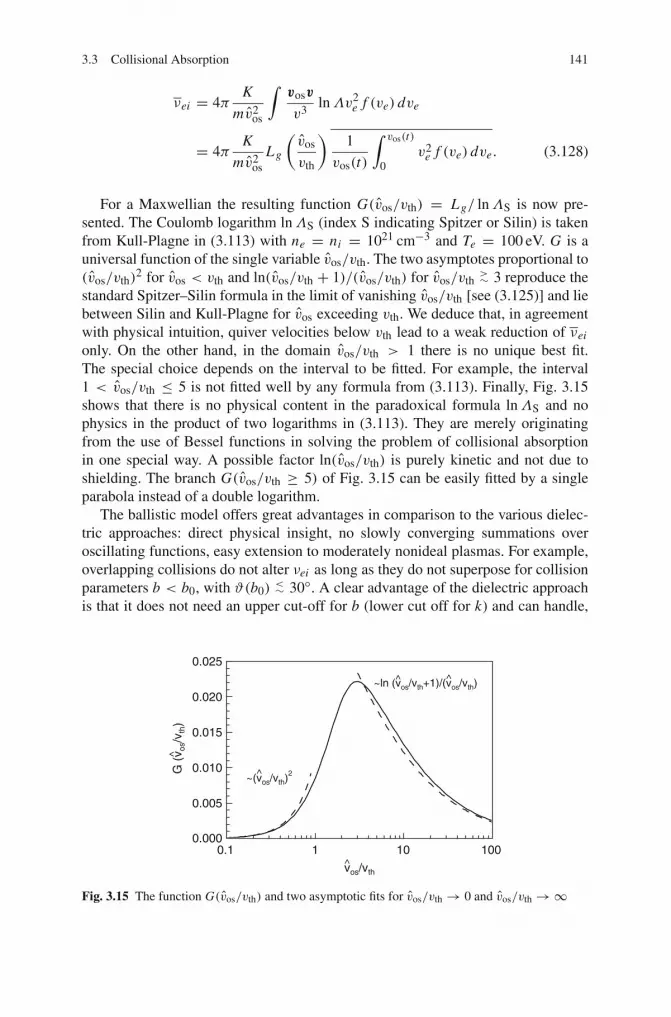
3.3 Collisional Absorption 141
νei = 4πK
mv2os
∫vosv
v3lnΛv2
e f (ve) dve
= 4πK
mv2os
Lg
(vos
vth
)1
vos(t)
∫ vos(t)
0v2
e f (ve) dve. (3.128)
For a Maxwellian the resulting function G(vos/vth) = Lg/ lnΛS is now pre-sented. The Coulomb logarithm lnΛS (index S indicating Spitzer or Silin) is takenfrom Kull-Plagne in (3.113) with ne = ni = 1021 cm−3 and Te = 100 eV. G is auniversal function of the single variable vos/vth. The two asymptotes proportional to(vos/vth)
2 for vos < vth and ln(vos/vth + 1)/(vos/vth) for vos/vth>∼ 3 reproduce the
standard Spitzer–Silin formula in the limit of vanishing vos/vth [see (3.125)] and liebetween Silin and Kull-Plagne for vos exceeding vth. We deduce that, in agreementwith physical intuition, quiver velocities below vth lead to a weak reduction of νei
only. On the other hand, in the domain vos/vth > 1 there is no unique best fit.The special choice depends on the interval to be fitted. For example, the interval1 < vos/vth ≤ 5 is not fitted well by any formula from (3.113). Finally, Fig. 3.15shows that there is no physical content in the paradoxical formula lnΛS and nophysics in the product of two logarithms in (3.113). They are merely originatingfrom the use of Bessel functions in solving the problem of collisional absorptionin one special way. A possible factor ln(vos/vth) is purely kinetic and not due toshielding. The branch G(vos/vth ≥ 5) of Fig. 3.15 can be easily fitted by a singleparabola instead of a double logarithm.
The ballistic model offers great advantages in comparison to the various dielec-tric approaches: direct physical insight, no slowly converging summations overoscillating functions, easy extension to moderately nonideal plasmas. For example,overlapping collisions do not alter νei as long as they do not superpose for collisionparameters b < b0, with ϑ(b0)
<∼ 30◦. A clear advantage of the dielectric approachis that it does not need an upper cut-off for b (lower cut off for k) and can handle,
0.1 1 10 1000.000
0.005
0.010
0.015
0.020
0.025
vos/vth^
G (
v os/
v th)
^
^ ^~ln (vos/vth+1)/(vos/vth)
~(vos/vth)2^
Fig. 3.15 The function G(vos/vth) and two asymptotic fits for vos/vth → 0 and vos/vth →∞

142 3 Laser Light Propagation and Collisional Absorption
to a limited extent, plasma resonances in a straightforward manner (in this contextsee [45]).
So far we have not specified vos(t). From the kinetic derivation of the firstmoment conservation equation it becomes clear that in (2.23) and in the Drudemodel v is the velocity of a fluid element and not that of a single electron. As longas νei � ω holds it makes very little difference whether vos(t) is identified with theoscillatory velocity of an individual electron or the drift velocity of an oscillatingfluid element. However, in the opposite case of νei � ω a consistency problemmay arise because the single particle drift from which νei is calculated and the fluiddrift may differ from each other. Some reasoning shows that at least for Coulomblogarithms somewhat larger than unity they still coincide since most of the orbitscontributing to νei are straight. Hence, vos(t) has to be calculated from (2.23) withνei included. At vos/vth > 1 the electron-ion collision frequency νei from (3.117)shows a strong time-dependence. As an immediate consequence higher harmonicsappear in vos and, in concomitance, in the current density j e, in E and B. Theanharmonicity is expected to be particularly strong in a dense plasma when Te islow and vos � vth.
3.3.4 Equivalence of Models
3.3.4.1 Boltzmann Model
Boltzmann’s kinetic equation,
∂ f
∂t+ v
∂ f
∂x− e
mE∂ f
∂v=∫( f ′ f ′i − f fi )σΩ |vei |dΩdvi (3.129)
is linearized, f = f0+ f1, fi ion distribution function, to obtain the current inducedby the laser field, j = −ene
∫v f1dv. Silin calculated this expression to obtain
the cycle-averaged absorption from j E [18]. To show the equivalence of the twomodels the ions may be assumed immobile owing to |vi | � |ve|. Then by tak-ing the first moment of (3.129) and observing the identity
∫v′ f (v)σ (ϑ)|v|dv′ =∫
v f (v′)σ (ϑ)|v|dv one obtains the momentum equation
dudt+ e
mE = −ni
∫(v − v′) f (v) · 2πσ(ϑ)|v|dvdϑ = −νei u. (3.130)
Remembering that j = −ene∫
v f (v)dv = −eneu, from Drude’s ansatz (2.23)results j E = 2νeiEos. This is identical with the Boltzmann result. The identity ismost easily seen if f is expressed in the frame moving with velocity u since there jstems entirely from f1 = f − f0. It is essential to use σ(ϑ) of the self-consistentlyscreened Coulomb potential.

3.3 Collisional Absorption 143
3.3.4.2 Drude vs Dielectric Model
In order to establish the equivalence of the models one has to show that Ein =mνei u/e. The correctness of this relation is recognized by intuition:
(i) The force on the test ion by all plasma electrons balances the Z -fold forceof all plasma ions on one electron (actio = reactio, owing to suppression ofretardation effects);
(ii) under the assumption that the collision time τ is the shortest time scale [whichis fulfilled, see (3.89)], the momentum change per unit time of an electron dueto collisions is just the instantaneous force of all ions on a single electron.
The formal proof is most conveniently done by calculating the first moment of(3.129) for the relative velocity ur ,
dur
dt− νei ur − e
m∇φ = 0; ur =
∫ve f1dve.
Summing this over all electrons in the same way as in Sect. 3.3.2 and making useof (i) above, the assertion follows since 〈dur/dt〉 = 0 holds by definition. All treat-ments of inverse Bremsstrahlung presented so far are equivalent to each other in theweak coupling limit and hω/kTe � 1.
3.3.5 Complementary Remarks
3.3.5.1 Non-Maxwellian Distribution Function
A serious impact of a large v on absorption is seen in the distribution function [23].By comparing the time τh of heating the electrons up to the temperature Te,
τh = 3
2nekTe/〈 j E〉 = 3τei
(vth
v
)2, τei = ν−1
ei ,
one finds that τh becomes shorter than the electron-electron collision time τee assoon as
Z v2 >∼ 3v2th
holds. After one electron-ion or electron–electron collision f (v) becomes nearlyisotropic for moderate vos/vth-ratios. However, when driven at constant E-fieldstrength, f (v) evolves into a self-similar distribution of the form (Fig. 3.16),
f (v) = κe−v5/5u5, u5 = 10πni Z2e4 lnΛ
6m2v2t. (3.131)

144 3 Laser Light Propagation and Collisional Absorption
Fig. 3.16 Effect of the laser field on the electron distribution function v2 f (v) for v2os/v
2th = 2.25
([24]: dotted, and [23]: solid)
The tendency towards the evolution of a super-Gaussian (broadened Maxwellian)has been confirmed in [49] for vos/vth = 2 and plasma parameter g = 0.1, inagreement with molecular dynamics simulations for vos/vth ≤ 1 [50]. In a morerecent treatment which includes electron-electron collisions self-consistently andallows for an anisotropic part of the distribution function it has been found that f (v)consists of a super-Gaussian of slow electrons and a Maxwellian tail of energeticelectrons [51]. The systematic study of the evolution of f (v) by Fokker–Planck sim-ulations in [52] reveals a departure from a Maxwellian when vos/vth � 1 and a finalreturning to a Maxwellian at vos/vth � 1 due to the inefficiency of absorption. Thisbehavior is easily understood if one bears in mind that with increasing drift motionthe electron-ion interaction time decreases whereas the electron–electron collisionsare not affected by a drift that is common to all electrons. Finally, significant andsurprising enough, at vos/vth = 10 and g = 0.1 the authors of [49] observed a sofar unexplained distribution function narrowing of the respective Maxwellian. Theyshowed that the effect originates from electron–ion collisions.
3.3.5.2 Coulomb Focusing
From the classical collision scheme Fig. 2.1 it follows that, depending on the scat-tering angle, under the influence of a strong laser field an electron can gain anappreciable amount of energy in a single collision. The gain is highest in the backscatter configuration from an attractive potential and less significant from a potentialthat is repulsive. The distinction between positive and negative charge scatteringfrom a Coulomb center clearly contrasts with pure Coulomb scattering for whichσΩ is indifferent with respect to charge conjugation. Additionally, in presence ofthe laser field an electron can be captured temporarily by the ion fulfilling severalcycles for a while before being ejected again. In the quantum scattering process

3.3 Collisional Absorption 145
Fig. 3.17 Spatial probability density of a Gaussian wavepacket with momentum hk0 = 0.005 mecscattered by an attractive (left graph) and a repulsive (right graph) Coulomb potential. The inter-ference maxima indicate Coulomb focusing in the attractive and defocusing in the repulsive case[53]
interference occurs between the plane incoming and the spherical outgoing waveand, as a consequence, charge accumulation (attractive potential) and rarefaction(repulsive) behind the ion can be observed in the direction of the laser field(Fig. 3.17). This so-called Coulomb focusing phenomenon can lead to stronglyenhanced scattering [53]. In a refined ballistic model it should be taken into account.
3.3.5.3 Giant Ions
Strong enhancement of collisional absorption can occur due to the coherent super-position of collisions in clusters. The absorption coefficient α due to collisions ina plasma is proportional to the ion density ni and the square of the ion charge,α ∼ Z2
i ni . When N ions cluster together the density of the scatterers nC decreasesby N but their charge increases by Zi N , resulting in an increase of α ∼ N . Inorder to obtain realistic amplification factors of collisional absorption due to clus-tering g = αC/α, αC absorption coefficient of the cluster medium, the fraction ξ
of ions forming clusters, their “outer ionization” degree ηC , i.e., the net charge ofthe cluster, and the collision frequency νeC of an electron with the cluster gas in thepresence of the intense laser field need to be known. It holds [54]
νeC = ξη2C
ZC
Zi
LC
lnΛeiνei , αC = νeC
c
ω2p
ω2. (3.132)
lnΛei is the Coulomb logarithm of the plasma ions and LC is the generalizedCoulomb logarithm of the cluster of radius R, both to be determined. The Coulombscattering angle χ is a function of the impact parameter b. For b > bc =R(1 + 2b⊥/R)1/2, χ(b = b⊥) = π/2, it coincides with the Rutherford scatteringangle. For orbits crossing the cluster it is determined numerically. For a uniformcharge distribution inside the cluster χ is shown in Fig. 3.18 for b⊥ = 2.5R andb⊥ = 0.5R. LC is

146 3 Laser Light Propagation and Collisional Absorption
Fig. 3.18 Scattering angle χ as a function of the impact parameter b for a uniform charged spheri-cal cluster. Bold dashed curve for b⊥ = 2.5R, and solid curve for b⊥ = 0.5R, R cluster radius. Thecorresponding deflections inside the cluster are indicated by the thin dashed and solid lines endingat their respective b = bc points. The dotted-dashed and the dotted lines starting from χ = 180◦refer to Coulomb scattering from a point charge q
LC = 1
2
∫ bc
0
(1− cosχ)b db
R2+ 1
2ln
[b2⊥ + b2
max
b2⊥ + b2c
]. (3.133)
Multiplication factors of order 103–104 are achievable for realistic cluster parame-ters. Coherent amplification of collisional absorption is relevant for dusty plasmas,aerosols, sprays, perhaps foams, and small droplets of liquids, all of them withR � λ.
3.4 Inverse Bremsstrahlung Absorption
To illustrate the physics of absorption of radiation by collisions from a differentpoint of view in this section the absorption coefficient α is deduced from the emis-sion of bremsstrahlung radiation of an optically thin plasma in the weak laser fieldlimit.
The total power P emitted by an accelerated nonrelativistic electron is given by([30], Sect. 14.2)
P = 2
3
e2
4πε0c3v2(t). (3.134)
In a nearly thermal plasma velocity changes v(t) are mainly produced by electron-ion and electron-electron collisions. An electron–ion pair constitutes a dipole sys-tem to a very good approximation as long as the maximum impact parameter bmaxis small compared to the wavelength emitted. For laser plasmas in the intensity

3.4 Inverse Bremsstrahlung Absorption 147
range vos < vth and frequencies of ω � ωNd this is always the case because ofλNd � λD � bmax. On the other hand, a colliding electron–electron system repre-sents a quadrupole which at nonrelativistic speeds and under the above conditionsgives negligible contribution to radiation emission. The colliding electron–electronpair can also be viewed as two electric dipoles of relative phase difference π . Asa consequence, their dipole emission cancels. Since the principle of detailed bal-ance applies, absorption of radiation does not occur in electron–electron encounterseither.
The total spectral intensity Iω emitted by ne electrons into the unit solid angle isobtained by Fourier-transforming Larmor’s formula (3.134), and averaging over allimpact parameters b and the corresponding velocity distribution f (v). In this way,for a Maxwellian velocity distribution
Iω = d2 P
dΩdω= �(η)ω2
p
4√
3π2c3νei kTe
σ(ω, Te)
lnΛe−hω/kTe (3.135)
is obtained with νei from (2.45) [55]. σ(ω, Te) is the Gaunt factor which providesfor the necessary quantum corrections in different (ω, Te) regions. For ωNd andmoderate harmonics hω � kTe holds and the ratio between the thermal de Brogliewavelength λB and b⊥,
λB/b⊥ = 4πε0
Ze2
(kTe
m
)1/2
h = 0.18(Te[eV])1/2/Z , (3.136)
in laser plasmas is such that the Born–Elwert expression for σ(ω, Te) applies since(λB/b⊥)2 � 1 holds ([40], Chap. 8):
σ(ω, Te) =√
3
πln
(4
G
kTe
hω
)= 0.55
[0.81+ ln
kTe
hω
]; G = 1.781. (3.137)
For instance, for kTe/hω = 103, σ = 4.2 results. The absorption coefficientαω can now be determined from Kirchhoff’s law. Bremsstrahlung radiation froman optically thin plasma generally represents such a small energy loss that (i) theplasma can be in thermal equilibrium kinetically even though thermal radiative equi-librium is not established and (ii) the spectral radiation intensity Iω(Te) is entirelydetermined – to a high degree of accuracy – by the kinetic electron distribution.Therefore, the relation
Iωαω= IPlanck = hω3
4π3c2
[�(η)]2exp
(hωkTe
)− 1
(3.138)
holds. Consequently, the absorption coefficient becomes

148 3 Laser Light Propagation and Collisional Absorption
αω =(
1− exp
(− hω
kTe
))kTe
hω
1
c
(ωp
ω
)2 νei
�(η)ln(
4G
kTehω
)
lnΛ. (3.139)
From hω/kT � 1 the factor(
1− exp(− hωkTe
))
kTe/hω becomes unity. Comparison
with (3.36) yields
αω
α= 1
lnΛln
(4
G
kTe
hω
).
To give a numerical example, for hω/kTe = 10−3 the ratio becomes αω/α =7.7/ lnΛ; for lnΛ = 7.7 the spectral absorption coefficient αω becomes equal to α.In any case these considerations show that
(a) αω is, within the uncertainty of lnΛ, practically the same as α, in this wayjustifying the identification of “inverse bremsstrahlung absorption” with “col-lisional absorption”;
(b) the bremsstrahlung intensity Iω(Te) represents the spontaneously emittedamount of radiation, whereas in the absorption coefficient α stimulated re-emission of radiation is also included;
(c) at very low temperatures or higher photon energies (e.g., hω/kTe � 1) a purelyclassical calculation of α begins to fail because then 1− e−hω/kT = hω/kT .
Observation (b) needs two further comments. There are several ways of formulatingthe principle of detailed balance and Kirchhoff’s law. It is convenient to use it in theform of (3.138) where the emitted power density per unit solid angle is indicatedby Iω. This is because experimentally Iω can be uniquely determined only when thesurrounding radiation field is zero; as a consequence Iω represents the spontaneouslyemitted radiation. On the other hand, in a measurement of αω the “true” or effectiveabsorption coefficient is determined which is the difference between absorption andstimulated re-emission of radiation between two energy levels E1 and E2 (E2 −E1 = hω). With their populations n1 and n2, the Einstein coefficients B12 = B21 forstimulated emission, and ρω the spectral radiant energy density, ρω = 4π Iω/c, αωis determined by
αω Iω = (n1 B21 − n2 B12)ρω = 4π
cB12(n1 − n2)Iω. (3.140)
The refractive index η and degeneracy are assumed to be unity. If κω refers to levelexcitation by absorption,
κω = 4π
cB12n1,

3.5 Ion Beam Stopping 149
and the levels are in thermodynamic equilibrium (for instance, because of collisions;Maxwellian distribution in the case of continuous energy spectrum), hence n2 =n1e(−hω/kTe), one obtains
αω = κω[1− exp(−hω/kTe)
]. (3.141)
κω is often used in theoretical work, however, it is not accessible to direct observa-tion. For correctness it has to be mentioned that the rate equation (3.140) holds assoon as the shortest time of interest is much longer than the transverse relaxation (orphase memory) time T2 [56]. In conclusion, when Kirchhoff’s law is written in theform Iω/αω = I Planck
ω , Iω is the spontaneously emitted radiation and αω is the netabsorption coefficient. Both Iω and αω are directly observable quantities.
3.5 Ion Beam Stopping
In a fully ionized plasma an ion projectile p of mass mp, charge Zpe and velocity v0is slowed down by collisions with the plasma electrons and its ions of charge Ze.For lnΛ >∼ 1 small angle deflections prevail and the energy transfer to an electronis by mi/Zm larger than to a plasma ion. At the same time the p-e and p-i collisionrates are related to each other by neσe � neσi/Z . This implies that the projectilemoves straight, except rare p-i events, and the energy loss of the projectile is nearlyall to the electrons. In the following p-i collisions are neglected. The energy loss ofthe projectile ion per unit length d E/dx , the so-called stopping power is given by[compare (3.117)]
d E
dx= −2πK Zp
∫ ∞
0
∫ 1
−1
v0v
v3lnΛv2
e f (ve) d cosχ dve (3.142)
with lnΛ from (3.124), K = Ze4ne/(4πε20m) from (3.115) and v = v0 + ve.
For a rough estimate the simplifications leading to (3.126) (see Fig. 3.13) may beintroduced to arrive at
d E
dx� −4πK Zp
ln〈Λ〉v0
∫ v0
0v2
e f (ve) dve. (3.143)
For a Maxwellian fe = fM(v) from (3.143) one obtains by multiple partial integra-tion in the domain v0/vth
<∼ 2
d E
dx� −1
3
√2
πK Zp ln〈Λ〉 v
20
v3th
e−v20/2v2
th (3.144)
×[
1+ 1
5
(v0
vth
)2
+ 1
5 · 7(v0
vth
)4
+ 1
5 · 7 · 9(v0
vth
)6
+ · · ·].

150 3 Laser Light Propagation and Collisional Absorption
At v0 = vth the bracket amounts to 1+ 0.23. By the same procedure for v0/vth>∼ 2
results
d E
dx� −K Zp ln〈Λ〉 1
v0
{1− 2
√2
π
v0
vthe−v2
0/2v2th
[1+
(vth
v0
)2
+(vth
v0
)4]}
.
(3.145)
For vth = 0 and Zp = Z this becomes identical with −W in (3.85).
Barkas effect. In 1953 F.M. Smith et al. [57] found a minute difference betweenstopping power in emulsion of positive and negative pions. Subsequently it was ver-ified in countless experiments that the range of a fast particle in matter differs fromthat of its antiparticle. Generally the difference in stopping of a negative particlefrom its positive counterpart is called Barkas effect. It clearly indicates that stop-ping is not just due to pure binary encounters because the Coulomb cross sectionσΩ respects charge conjugation. Hence, the difference must have its origin in thepresence of spectators involved in the collision. Theoretical investigations have con-firmed this interpretation for stopping in neutral matter [58]. In the plasma screeningassumes the role of a spectator and the Barkas effect is present there as well [59]. Atheoretical treatment of stopping in dense nonideal plasmas going well beyond thestandard analysis (Z3
b-term, see [57]) is presented in [60]. There is an asymmetrybetween the orbits of a positive and a negative point particle in a screened Coulombpotential as becomes clear from short inspection of Fig. 2.4.
References
1. Penfield, P., Haus, H.A.: Electrodynamics of Moving Media, Chap. 1. MIT Press, Cambridge,MA (1967) 92
2. Whitham, G.B.: Linear and Nonlinear Waves. John Wiley & Sons, New York (1974) 93, 99, 105, 1063. Born, M., Wolf, E.: Principles of Optics, Sec. 3.3. Pergamon Press, Oxford (1980) 944. Muschietti, L., Dum, C.T.: Phys. Fluids B 5, 1383 (1993) 98, 995. Sonnenschein, E., Rutkevich, I., Censor, D.: Phys. Rev. E 57, 1005 (1998) 986. Nordland, B.: Phys. Rev. E 55, 3647 (1997) 987. Ginzburg, V.L.: The Propagation of Electromagnetic Waves in Plasmas. Pergamon Press,
Oxford (1964) 998. Rawer, K.: Ann. Phys. 35, 385 (1939); 42, 294 (1942) 99, 1009. Johnson, F.S.: Am. J. Phys. 58, 1044 (1990) 104
10. Abramowitz, M., Stegun, I.A.: Pocketbook of Mathematical Functions. Harri Deutsch, Frank-furt/Main (1984) 108, 122, 123
11. Mathews, J., Walker, R.L.: Mathematical Methods of Physics. Benjamin/Cummings, MenloPark, CA (1964) 108, 109
12. Mulser, P., van Kessel, C.: J. Phys. D: Appl. Phys. 11, 1085 (1978) 11113. Willi, O., Rumsby, P.T.: Opt. Comm. 37, 45 (1981) 11114. Jones, R.D., Mead, W.C., Coggeshall, S.V., Aldrich, C.H., Norton, J.L., Pollak, G.D., Wallace,
J.M.: Phys. Fluids 31, 1249 (1988) 11115. Kofink, W.: Ann. Physik 1, 119 (1947) 11216. Cojocaru, E., Mulser, P.: Plasma Phys. 17, 393 (1974) 115

References 151
17. Piliya, A.D.: Sov. Phys. Tech. Phys. 11, 609 (1966) 11518. Silin, V.P.: Zh. Eksp. Teor. Fiz. 47, 2254 (1964); Sov. Phys. JETP 20, 1510 (1965) 119, 14219. Shima, Y., Yatom, H.: Phys. Rev. A 12, 2106 (1975) 119, 13320. Silin, V.P., Uryupin, S.A.: Sov. Phys. JETP 54, 485 (1981) 119, 13321. Bornath, Th., Schlanges, M., Hilse, P., Kremp, D., Bonitz, M.: Laser & Part. Beams 18, 535
(2000) 119, 13322. Reinholz, H., Redmer, R., Röpke, G., Wierling, A.: Phys. Rev. E 62, 5648 (2000) 11923. Langdon, A.B.: Phys. Rev. Lett. 44, 575 (1980) 119, 143, 14424. Jones, R.D., Lee, K.: Phys. Fluids 25, 2307 (1982) 119, 14425. Pert, G.J.: J. Phys. B: At. Mol. Phys. 8, 3069 (1975) 11926. Pert, G.J.: J. Phys. A: Gen. Phys. 9, 463 (1976)27. Pert, G.J.: J. Phys. B: At. Mol. Phys. 12, 2755 (1979) 11928. Mulser, P., Niu, K., Arnold, R.C.: Nucl. Inst. Meth. Phys. Res. A 278, 89 (1989) 12129. Korn, G.A., Korn, T.M.: Mathematical Handbook. McGraw-Hill, New York (1968) 9.3–3 12130. Jackson, J.D.: Classical Electrodynamics. John Wiley, New York (1975) 125, 14631. Boine-Frankenheim, O.: Energieverlust von schweren Ionen in Plasmen, Dissertation, TH
Darmstadt (1996) 125, 12632. Boine-Frankenheim, O.: Phys. Plasmas 3, 1585 (1996) 12533. Mulser, P., Saemann, A.: Contrib. Plasma Phys. 37, 211 (1997) 12734. Anger, C.T.: Neueste Schriften der Naturforschungs-Gesellschaft in Danzig, pp. 1–29 (1855) 12735. Sakurai, J.J.: Modern Quantum Mechanics, Sec. 7.13. Benjamin/Cummings, Menlo Park, CA
(1985) 132, 13636. Kremp, D., Bornath, Th., Bonitz, M.: Phys. Rev. E 60, 4725 (1999) 13337. Kull, H.-J., Plagne, L.: Phys. Plasmas 8, 5244 (2001) 133, 13438. Wierling, A., Th. Millat, Röpke, G., Redmer, R.: Phys. Plasmas 8, 3810 (2001) 13339. Schneider, R.: Equivalence and Unification of the Ballistic and the Kinetic Treatment of
Collisional Absorption, PhD thesis Tech. Univ. Darmstadt, Darmstadt (2002) 133, 138, 14040. Shkarofsky, I.P., Johnston, T.W., Bachynski, M.P.: The Particle Kinetics of Plasmas. Addison-
Wesley, Reading, MA (1966) 137, 14741. McDowell, M.R.C.: Phys. Fluids 4, 1332 (1961) 13742. de Ferrariis, L., Arista, N.R.: Phys. Rev. A 29, 2145 (1984) 13743. Mulser, P., Cornolti, F., Bésuelle, E., Schneider, R.: Phys. Rev. E 63, 016406 (2001) 138, 13944. Spitzer, L.: Physics of Fully Ionized Gases, p. 146. Interscience, New York (1967) 13845. Mulser, P., Schneider, R.: J. Phys. A: Math. Theor. 42, 214058 (2009) 139, 14246. Dawson, J.M., Oberman, C.: Phys. Fluids 5, 517 (1962) 14047. Decker, C.D., Mori, W.B., Dawson, J.M., Katsouleas, T.: Phys. Plasmas 1, 4043 (1994) 14048. Kaw, P.K., Salat, A.: Phys. Fluids 11, 2223 (1968); Salat, A., Kaw, P.K.: Phys. Fluids 12, 342
(1969) 14049. Bornath, Th., et al.: J. Phys.: Conf. Ser. 11, 180 (2005) 14450. Pfalzner, S., Gibbon, P.: Phys. Rev. E 57, 4698 (1998) 14451. Weng, S.M., Sheng, Z.M., He, M.Q., Wu, H.C., Dong, Q.L., Zhang, J.: Phys. Plasmas 13,
113302 (2006) 14452. Weng, S.M., Sheng, Z.M., Zhang, J.: Phys. Rev. E 80, 056406 (2009) 14453. Rascol, G., Bachau, H., Tikhonchuk, V.T., Kull, H.-J., Ristow, T.: Phys. Plasmas 13, 103108
(2006) 14554. Mulser, P., Kanapathipillai, M., Hoffmann, D.H.H.: Phys. Rev. Lett. 95, 103401 (2005); last
value in Table II must read 2.3×10⁵ 14555. Lang, K.R.: Astrophysical Formulae, p. 46. Springer-Verlag, New York (1974) 14756. Shoemaker, R.L.: Coherent transient infared spectroscopy. In: Steinfeld, J.I. (ed.) Laser and
Coherent Spectroscopy, Sec. 3.3. Plenum Press, New York (1978). 14957. Smith, F.M., Birnbaum, W., Barkas, W.H.: Phys. Rev. 91, 765 (1953) 15058. Sigmund, P., Schinner, A.: Nucl. Instr. and Meth. B 212, 110 (2003) 15059. Sayasov, Yu.S.: J. Plasma Phys. 57, 373 (1997) 15060. Gericke, D.O., Schlanges, M., Bornath, Th., Kraeft, W.D.: Contrib. Plasma Phys. 41, 147
(2001) 150

Chapter 4Resonance Absorption
The most familiar absorption process of laser radiation is inverse bremsstrahlung.As the electron temperature increases Coulomb collisions become less effective and,in the absence of other conversion processes, a plasma becomes highly transparentto the laser radiation when the electron density ne is below its critical value nc;alternatively, in case an overdense layer exists, i.e., ne > nc, the laser plasma ishighly reflecting. However, at oblique incidence of radiation there is an effectivecollisionless absorption process which consists of the resonant conversion of laserlight into an electron plasma wave of the same frequency ω. This phenomenon ofresonance absorption was first described by Denisov [1] for a cold and by Piliya[2] for a warm plasma. Only later was its relevance for collisionless laser plasmaheating recognized [3, 4]. Subsequently, accurate conversion rates as a function ofdensity scale length L and angle of incidence α0 were determined numerically [5].The most accurate and complete study of the phenomenon in the linear regime wasundertaken in [6, 7].
As already discussed in connection with the inhomogeneous Stokes equation inSect. 3.2.4. the excitation of a Langmuir wave occurring resonantly over a wideregion in space requires the simultaneous conservation of the photon (index em or noindex) and plasmon (index es) energies and momenta, hωes = hωem, hkes = hkem.Owing to the dispersion relations (3.11) for the two waves at nonrelativistic temper-atures (s2
e � c2)matching is fulfilled only at the critical points where kem � kes � 0holds, and hence the local plasma frequency equals the laser frequency. It followsfrom Fig. 3.6 that with a smooth driver, resonance does not extend over more thanhalf a local electrostatic wavelength λes. In the laser generated plasma the incidentelectromagnetic wave acts as a resonant driver for the electron plasma wave propa-gating down the density gradient and is dependent on the angle of incidence: At nor-mal incidence the laser field has no component along the density gradient; at grazingincidence the field has the right direction; however, the laser beam is reflected fromthe plasma too far away from the critical point. At an intermediate optimum angle aconversion factor of 0.5 is reached in flat density profiles. In steep plasma profiles aswell as at relativistic temperatures the conversion rate and the optimum angle bothincrease and conversion can rise up to 100% [7]. The excited electron plasma waveis not converted back into electromagnetic waves and is, consequently, absorbed bythe plasma. At low temperatures and flat density gradients significant damping can
P. Mulser, D. Bauer, High Power Laser–Matter Interaction, STMP 238, 153–192,DOI 10.1007/978-3-540-46065-7_4, C© Springer-Verlag Berlin Heidelberg 2010
153
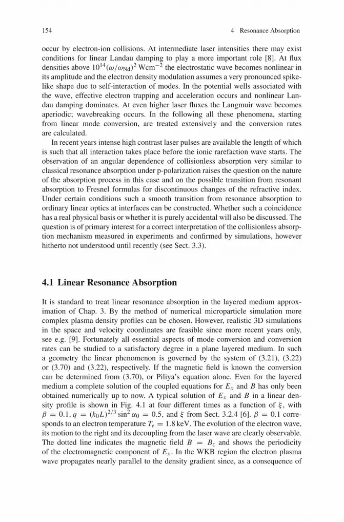
154 4 Resonance Absorption
occur by electron-ion collisions. At intermediate laser intensities there may existconditions for linear Landau damping to play a more important role [8]. At fluxdensities above 1014(ω/ωNd)
2 Wcm−2 the electrostatic wave becomes nonlinear inits amplitude and the electron density modulation assumes a very pronounced spike-like shape due to self-interaction of modes. In the potential wells associated withthe wave, effective electron trapping and acceleration occurs and nonlinear Lan-dau damping dominates. At even higher laser fluxes the Langmuir wave becomesaperiodic; wavebreaking occurs. In the following all these phenomena, startingfrom linear mode conversion, are treated extensively and the conversion ratesare calculated.
In recent years intense high contrast laser pulses are available the length of whichis such that all interaction takes place before the ionic rarefaction wave starts. Theobservation of an angular dependence of collisionless absorption very similar toclassical resonance absorption under p-polarization raises the question on the natureof the absorption process in this case and on the possible transition from resonantabsorption to Fresnel formulas for discontinuous changes of the refractive index.Under certain conditions such a smooth transition from resonance absorption toordinary linear optics at interfaces can be constructed. Whether such a coincidencehas a real physical basis or whether it is purely accidental will also be discussed. Thequestion is of primary interest for a correct interpretation of the collisionless absorp-tion mechanism measured in experiments and confirmed by simulations, howeverhitherto not understood until recently (see Sect. 3.3).
4.1 Linear Resonance Absorption
It is standard to treat linear resonance absorption in the layered medium approx-imation of Chap. 3. By the method of numerical microparticle simulation morecomplex plasma density profiles can be chosen. However, realistic 3D simulationsin the space and velocity coordinates are feasible since more recent years only,see e.g. [9]. Fortunately all essential aspects of mode conversion and conversionrates can be studied to a satisfactory degree in a plane layered medium. In sucha geometry the linear phenomenon is governed by the system of (3.21), (3.22)or (3.70) and (3.22), respectively. If the magnetic field is known the conversioncan be determined from (3.70), or Piliya’s equation alone. Even for the layeredmedium a complete solution of the coupled equations for Ex and B has only beenobtained numerically up to now. A typical solution of Ex and B in a linear den-sity profile is shown in Fig. 4.1 at four different times as a function of ξ , withβ = 0.1, q = (k0L)2/3 sin2 α0 = 0.5, and ξ from Sect. 3.2.4 [6]. β = 0.1 corre-sponds to an electron temperature Te = 1.8 keV. The evolution of the electron wave,its motion to the right and its decoupling from the laser wave are clearly observable.The dotted line indicates the magnetic field B = Bz and shows the periodicityof the electromagnetic component of Ex . In the WKB region the electron plasmawave propagates nearly parallel to the density gradient since, as a consequence of
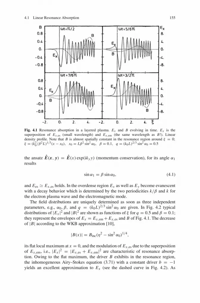
4.1 Linear Resonance Absorption 155
Fig. 4.1 Resonance absorption in a layered plasma. Ex and B evolving in time. Ex is thesuperposition of Ex,es (small wavelength) and Ex,em (the same wavelength as B!). Lineardensity profile. Note that B is almost spatially constant in the resonance region around ξ = 0;ξ = (k2
0/β2 L)1/3(x − x0), x0 = Lβ2 sin2 α0, β = 0.1, q = (k0 L)2/3 sin2 α0 = 0.5
the ansatz E(x, y) = E(x) exp(iky y) (momentum conservation), for its angle α1results
sinα1 = β sinα0, (4.1)
and Ees � Ex,es holds. In the overdense region Ex as well as Ey become evanescentwith a decay behavior which is determined by the two periodicities k/β and k forthe electron plasma wave and the electromagnetic mode.
The field distributions are uniquely determined as soon as three independentparameters, e.g., α0, β, and q = (k0L)2/3 sin2 α0 are given. In Fig. 4.2 typicaldistributions of |Ex |2 and |B|2 are shown as functions of ξ for q = 0.5 and β = 0.1;they represent the envelopes of Ex = Ex,em+ Ex,es and B of Fig. 4.1. The decreaseof |B| according to the WKB approximation [10],
|B(x)| = Binc(η2 − sin2 α0)
1/4,
its flat local maximum at x = 0, and the modulation of Ex,es due to the superpositionof Ex,em, i.e., |Ex |2 = |Ex,es + Ex,em|2 are characteristic of resonance absorp-tion. Owing to the flat maximum, the driver B exhibits in the resonance region,the inhomogeneous Airy–Stokes equation (3.71) with a constant driver b = −1yields an excellent approximation to Ex (see the dashed curve in Fig. 4.2). As

156 4 Resonance Absorption
outlined in Sect. 3.2.4 for a spatially constant driver B, resonance terminates atξm where |Ex |2 reaches its maximum; thus the resonance width in dimensionlessform is given by 2ξm. With xm indicating the position of the maximum |Ex |2 andwith x0 = Lβ2 sin2 α0 from Sect. 3.2.4 this becomes in real space
d = 2xm = 2
(β2L
k20
)1/3
ξm, ξm = 1.8, (4.2)
provided x0/(xm− x0) = (k0Lβ2)2/3 sin2 α0/ξm � 1 is fulfilled. With β = 0.1 andk0L ≤ 50 this latter inequality is well obeyed for all angles of incidence α0 and theresonance curve is nearly symmetric. Then d scales as (k1L)1/3/k1, k1 = k0/β.Although the density profile in Fig. 4.2 is flat, d is very small (dashed region). Asa consequence of the driver not being exactly constant, in the exact solution of thecoupled system of (3.21) and (3.22) ξm = 1.7 is obtained from Fig. 4.2. When L isfixed at small angles of incidence the electromagnetic turning point is close to thecritical point and much intensity reaches the coupling region, but the driver in (3.70),owing to the factor sinα0 in ky , is small. As α0 increases less intensity tunnels tothe critical surface; however, this may be overcompensated by the factor sinα0, andresonant excitation of Ees reaches a maximum. As α0 increases further the expo-nential decrease of intensity tunneling to the critical point prevails and resonanceabsorption becomes ineffective. This situation is illustrated in Fig. 4.3. Resonanceis strongest for q � 0.4 (3rd picture).
Let us now determine the conversion rate A = |Sx,es/Sx,em| for steady state reso-nance absorption. The electromagnetic and electrostatic flux densities in x-directionare (with I0 the vacuum flux density of amplitude E0)
Fig. 4.2 Resonance absorption: Distribution of |Ex |2 and |B|2 over the flat plasma density profilen0 as a function of ξ . Dashed region shows the resonance width 2ξm (ξm position of maximum|Ex |2). Stokes equation reproduces well resonance behavior (dashed curve close to resonance)

4.1 Linear Resonance Absorption 157
Fig. 4.3 Resonance absorption. The same distributions as in Fig. 4.2 for different angles ofincidence, q = (k0l)2/3 sin2 α0
Sx,em = 1
2vg,xε0|Eem(x)|2 = 1
2cη(1− sin2 α0)
1/2ε0|Eem(x)|2
= (1− sin2 α0)1/2 I0,
Sx,es = 1
2vg,xε0|Ees(x)|2 = 1
2seη(1− sin2 α1)
1/2ε0|Ees(x)|2 � Ies.
By making use of the asymptotic expansion of (3.71) with b = −1 (see [11],p. 162 ff),
w = −π1/2
ξ1/4exp i
(2
3ξ3/2 + π
4
); η
ξ1/2=(β
kL
)1/3
.
From the definition of w in Sect. 3.2.4 follows
Sx,es = π
2c3ε0kL|B(0)|2 sin2 α0. (4.3)
Hence, the conversion factor of resonance absorption is
A = πk0Lsin2 α0
(1− sin2 α0)1/2
∣∣∣∣B(0)
Binc
∣∣∣∣2
. (4.4)
As soon as A is known this relation may be used to determine the “driver” B(0).With I0 in W/cm2,

158 4 Resonance Absorption
|B(0)| sinα0 = Binc(1− sin2 α0)1/4(
A
π
)1/2
(k0L)−1/2
= 5.16× 10⁻⁶(
AI0
k0L
)1/2
(1− sin2 α0)1/4 [Tesla]. (4.5)
Expressions (4.4) and (4.5) are based on the assumption of |B| = const over thewhole resonance interval; for smooth density distributions with no significant cur-vature and k0L ≥ 2π this simplification is justified. In Fig. 4.4 the conversion factorA is shown as a function of q for different electron temperatures and k0L ≤ 2π . Asexpected from (3.71) there is almost no difference between cold and warm plasmaup to temperatures Te = 20 keV (i.e., β2 = 0.1; [6]). At Te = 0 the maximumconversion rate is A = 0.49. For ξ < 2 the local electric field amplitude is given by
∣∣∣∣∣Ex
E0
∣∣∣∣∣
2
= (1− sin2 α0)1/2(k0L)1/3 A
πβ4/3|w|2. (4.6)
Solving for its maximum value |Ex,max| yields
∣∣∣∣∣Ex,max
E0
∣∣∣∣∣
2
= 1.1(1− sin2 α0)1/2(k0L)1/3 Aβ−4/3. (4.7)
This may be compared with the maximum amplitude Ez,max of s-polarized light notexhibiting resonance, (3.61).
For Te = 0 analytical conversion rates A have been given by several authors[12–14], for finite Te but with B = const cf. [15]. Their result is
Fig. 4.4 Temperature dependence of resonance absorption. Conversion factor A as a function ofq = (k0 L)2/3 sin2 α0. Dashed line: Hinkel–Lipsker [15]

4.1 Linear Resonance Absorption 159
A = (k0L)2/3 sin2 α0
|1− iπ2(k0L)2/3Γ sin2 α0|2|2πAi′|2; Γ = Ai′(Bi′ + iAi′). (4.8)
Its numerical evaluation is the dashed line in Fig. 4.4. The deviations from the resultin [7] are due to the simplification B = const. For β ≤ 0.1 the power series solu-tion in [12] is much more accurate and practically coincides with the numericalresult in [7]. The conversion A peaks at sinα0 � (2kL)−1/3 [16]. As Te becomesrelativistic and se approaches c resonant phase matching occurs over a wide rangeand the conversion factor A approaches unity at q � 0.7 − 0.9 [7], whereas at lowtemperatures Amax = 0.49 at q = 0.5. The shift of the maximum of A towardshigher q-values is a consequence of x0 increasing with β in Sect. 3.2.4 and hencefavoring resonance in lower density regions.
4.1.1 The Capacitor Model
So far, all results were obtained by starting from a rather general wave equationand solving it in an inhomogeneous medium under some simplifying assumptionsamong which linearity of j is the most important one. Additional simplificationswere introduced by neglecting β2 in comparison to 1 in (3.21) and (3.70) and takinga spatially constant driver B = B(0). Owing to the exp(−iωt) time dependence ofEx and B (3.70) is equivalent to the equation of a resonantly driven electron plasmawave parallel to ∇n0,
∂2
∂t2Ex − s2
e∂2
∂x2Ex + ω2
p Ex = cω2 B sinα0. (4.9)
Let xc be the position of the critical point and let us integrate (3.22) over an intervalenclosing xc under the restriction λ ≤ L ,
ik0y
∫ x>xc
x<xc
E ′x dx = ik0y Ex (x) =∫ x>xc
x<xc
(E ′′y + k20η
2 Ey)dx � E ′y(x).
The inequality λ ≤ L enters in the last step; in steep density gradients η becomeslarge already in the vicinity of xc. From E ′y � ik0y Ex and |E ′y | � k0η|Ey |/β in theresonance interval, we have
|Ey | � |Ex |βη
sinα0 � |Ex |; β/η � 1. (4.10)
That is the main result of a more involved estimate [17]. It shows that ∇E =∂Ex/∂x is a good approximation in not too steep density gradients and the dis-placement δe of an electronic fluid element is nearly δe,x . The latter is the basicassumption of the so-called capacitor model [4, 10, 18, 19].

160 4 Resonance Absorption
When curvature of the ion density profile in the resonance zone does not playa decisive role (this is the case in expanding plasmas produced by smooth laserpulses) the wave number k∗e of the electron plasma wave at the edge of resonance isdeduced from ξm = 1.8 in (4.2),
k∗e =ω
se
{β2 sin2 α0 + ξm
(β
k0L
)2/3}1/2
� 1.81/2
(k2
0
β2L
)1/3
. (4.11)
The second expression holds when x0 can be ignored. As the electron plasma wavemoves out into the lower density corona, kes increases and Landau damping sets in;it can also be determined in the framework of the capacitor model [8]. This has tocompete with the WKB reduction of Ees ∼ η−1/2. The corresponding dependenceof the electron amplitude n1 = ne − n0, n0 = 〈ne〉, shows the opposite behavior;thus
E(x) =(η(x1)
η(x)
)1/2
E(x1), n1(x) =(η(x)
η(x1)
)1/2
n1(x1), (4.12)
if x1 is an arbitrary position out of resonance where the WKB approximation isvalid.
4.1.2 Steep Density Gradients and Fresnel Formula
The capacitor model developed here may fail either when the density profile cur-vatures become significant in the resonance interval or/and when L becomes of theorder of the electron displacement λe or less. The latter effect has been studied inthe literature by adopting Epstein type density transition layers of the form [7]
η2(x) = 1
2− 1
1+ exp(−x/Δ), L = 4Δ.
It was found, and it is shown in Fig. 4.5 that (i) the conversion A deviates from thecurves of Fig. 4.4 as soon as kΔ becomes smaller than 2, (ii) at a given tempera-ture the maximum of A increases with decreasing transition width Δ, and (iii) thelocal angle α at the resonant layer at which maximum conversion occurs is shiftedtowards larger values, in contrast to the vacuum angle α0 which is reduced. A partic-ularly interesting and clear result is obtained for an infinite plasma density step withΔ→ 0. In this case total mode conversion, i.e., A = 1, is found for all temperatureswhen the electron plasma wave is emitted into the direction of the incident radiationfield E0 [7]. It requires the existence of an underdense plasma shelf in front of thediscontinuity, generated for example by a laser prepulse.
Resonance absorption of intense electromagnetic fields at the surface of solid tar-gets plays an important role in the interaction of ultrashort laser pulses with matter
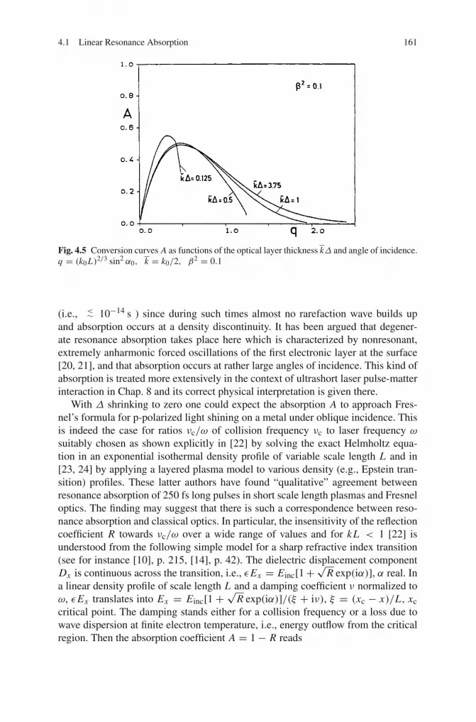
4.1 Linear Resonance Absorption 161
Fig. 4.5 Conversion curves A as functions of the optical layer thickness kΔ and angle of incidence.q = (k0 L)2/3 sin2 α0, k = k0/2, β2 = 0.1
(i.e., <∼ 10−14 s ) since during such times almost no rarefaction wave builds upand absorption occurs at a density discontinuity. It has been argued that degener-ate resonance absorption takes place here which is characterized by nonresonant,extremely anharmonic forced oscillations of the first electronic layer at the surface[20, 21], and that absorption occurs at rather large angles of incidence. This kind ofabsorption is treated more extensively in the context of ultrashort laser pulse-matterinteraction in Chap. 8 and its correct physical interpretation is given there.
With Δ shrinking to zero one could expect the absorption A to approach Fres-nel’s formula for p-polarized light shining on a metal under oblique incidence. Thisis indeed the case for ratios νc/ω of collision frequency νc to laser frequency ω
suitably chosen as shown explicitly in [22] by solving the exact Helmholtz equa-tion in an exponential isothermal density profile of variable scale length L and in[23, 24] by applying a layered plasma model to various density (e.g., Epstein tran-sition) profiles. These latter authors have found “qualitative” agreement betweenresonance absorption of 250 fs long pulses in short scale length plasmas and Fresneloptics. The finding may suggest that there is such a correspondence between reso-nance absorption and classical optics. In particular, the insensitivity of the reflectioncoefficient R towards νc/ω over a wide range of values and for kL < 1 [22] isunderstood from the following simple model for a sharp refractive index transition(see for instance [10], p. 215, [14], p. 42). The dielectric displacement componentDx is continuous across the transition, i.e., εEx = Einc[1+
√R exp(iα)], α real. In
a linear density profile of scale length L and a damping coefficient ν normalized toω, εEx translates into Ex = Einc[1 +
√R exp(iα)]/(ξ + iν), ξ = (xc − x)/L , xc
critical point. The damping stands either for a collision frequency or a loss due towave dispersion at finite electron temperature, i.e., energy outflow from the criticalregion. Then the absorption coefficient A = 1− R reads

162 4 Resonance Absorption
A =∫〈 jx Ex 〉 dx/Einc ∼ [1+
√Reiα]ν
∫|Ex |2 dx ∼ [1+√Reiα]
∫ν
ξ2 + ν2dξ
(4.13)For ν <∼ 0.3 the integral can be extended from −∞ to +∞ to yield the value 1/π .It shows that A becomes insensitive to damping ν and scale length L . On the otherhand one must keep in mind that the dependence of R on small damping values isalso weak and its value remains close to unity for electron densities of the order of100 times critical density. In fact, at 80◦ of incidence and L/λ < 0.1 the reflectionfor ν = 0.01, 0.1, and 1.0 is R = 0.99, 0.92, and 0.5, i.e., the penetrating fieldis very small and consequently A, despite the constant value of the integral closeto 1/π , vanishes for L → 0, except for unrealistically high collision frequencies.There is an additional restriction. In order for the above expression for A to holdwith ν reducing to zero the incident laser field must also reduce to zero to avoidwave breaking owing to Ex,max ∼ 1/ν. After all, Fresnel’s formulas are restrictedto linear optics. From such a requirement one deduces for the limiting intensity Imaxfor L → 0 [25] [see also (4.15) below]
Imax = 1
2
(4
3π
)2/3 (m
e
)2(c8ω7)1/3(εL1/3)2 (4.14)
→ Imax[W/cm2] = 2.9× 10¹⁸(ε × L[m]1/3)2.
The tolerable limit for linearity of the electron plasma wave n1 is indicated byε = n1/nc. With ε = 0.1 and L = 10 nm linear resonance absorption is for6 × 1013 Wcm−2 at its limit. The L2/3-dependence reflects the property of the res-onance width increasing with L1/3. Particular experimental effort was dedicatedto the collisionless absorption of sub-ps laser pulses in short scale length plasmasfrom solid targets in [22–24, 26]. In [22] it is shown how resonance absorption maybe used as an elegant and very reliable diagnostic tool for determining the laserscale length L . In [26] the reader may find an interesting comparison between fluidmodels and collisionfree PIC simulations. Both, although fundamentally differentfrom each other, fit well to the experimental results, at a price, however, of intro-ducing an artificial viscosity and, in concomitance, strong artificial damping in thefluid program to avoid wave breaking. In presence of artificial viscosity to checkthe absorption j E over the whole density transition profile is a necessity. Onlyif∫
j E dx is essentially localized around the critical point and in the evanescentregion the result perhaps may be reliable. In this context a short discussion of thecorrect boundary conditions at a vacuum-matter interface may shed additional lighton the question whether resonance absorption for Δ → 0 goes over into the lawsof linear optics. Thereby it must be kept in mind that such an analysis, owing to itslinear character, is valid only for very low intensities.
Fresnel’s reflection formula for R = 1 − A resembles one aspect of resonanceabsorption, namely the Brewster minimum of R which is a consequence of the factthat an oscillating electron does not radiate into its oscillation direction. This makesalso Kull’s result [7] of total conversion into an electron plasma wave emanating

4.1 Linear Resonance Absorption 163
into the lower density shelf understandable. Fresnel’s formula is derived from theconditions that the tangential component of the electric field Et and the normalcomponent of the electric displacement Dn are continuous. Now, to obtain Fresnel’ssituation the transition width Δ, together with the density of the lower shelf and theelectron temperature Te has to reduce to zero. From Maxwell’s equation (3.1), whenapplied to the infinitesimal area d F = eydxdz, follows for B = Bt :
ε0c2(∇ × B)d F = ( jy − iωε0 Ey)
dxdz = (Bz,vac − Bz,plasma)dz.
ForΔ→ 0, Ey and jy both diverge logarithmically at Te = 0, Ey, jy ∼ ln(1/Δ),and hence Bt = Bz ez is continuous across the vacuum-plasma interface. As a con-sequence the Poynting vector S = Sx ex is also continuous across the surface andresonance absorption reduces to zero. Continuity of S requires total reflection fromthe overdense plasma in perfect agreement with Fresnel’s result. In order to be inagreement with the foregoing absorption formula
√R exp(iα) = −1 must be set (in
this context the reader may consult [27] for a more detailed consideration).However, this is not the whole story. From Dn being continuous a discontinuity
of En , i.e., the induction of an oscillating surface charge follows. The oscillationleads to a delocalization of this charge and to a finite transition width, as consideredin [20, 21]. Such an argument led to the boundary condition of En being also con-tinuous at the interface and with it to a correction of Fresnel’s reflection formula forp-polarized light incident onto a metal surface with ωp > ω [28]. For a quantitativediscussion of this situation with a weak incident field the interested reader mayconsult the monograph of Forstmann and Gerhardts [29].
In conclusion, only within a restricted domain of parameters ν, L and laser inten-sity I the Fresnel formula for absorption of p-polarized waves may appear as thelimiting case of linear resonance absorption. On physical grounds, however, there isno basis for such an identification over the whole range of the densitiy scale lengthL → 0. For high laser intensities anharmonic resonance, not contained in Fresnel’sformula at all, will play a decisive role (see Sect. 8.3.3).
4.1.3 Comparison with Experiments
Resonance absorption with ns laser pulses was experimentally shown to occur byseveral groups [30–34] and to be in agreement with linear theory at Nd laser inten-sities up to I = 1014 W/cm2. A clear difference between s- and p-absorption wasfound at all angles of incidence α0 < 60o. The most accurate and complete measure-ments in the intensity range from 1013 to 1014 W/cm2 were performed in the past in[35] on plexiglass targets with a Nd-YAG laser of 35 ps pulse length. The absorptionwas detected simultaneously in five parallel channels of observation: reflection ofthe fundamental wave, second harmonic generation, charge and velocity distribu-tion of the expanding plasma cloud, and relative ablation pressure on the target. Allfive channels gave equivalent results and the absorption of p-polarization exceeded

164 4 Resonance Absorption
that for s-polarization by about a factor of 2 on the average. The excited Langmuirwave can interact nonlinearly with the incident laser light, thus creating the secondharmonic, 2ωNd with an intensity proportional to A. Some characteristic deviationsbetween experiments and theory of resonance absorption may have to be attributedto fluctuations of the plasma density profile. Theoretically the influence of stochasticdensity oscillations was studied by several authors [36–38] for long pulses. It wasfound that the excitation level of the Langmuir wave decreases monotonically withincreasing amplitude of the density fluctuations.
Resonance absorption by excitation of a plasma wave at twice the laser frequencyis possible at normal or nearly normal incidence when the Lorentz force −evos× Bprevails over the driving force −eE at the fundamental frequency.
4.2 Nonlinear Resonance Absorption
The theory of resonance absorption exposed in the preceding section is valid as longas the ratio n1/n0 is small compared to unity in the resonance interval. From (3.74)and from δ in (2.12), we have n1 � −in0keeE/mω2. At the maximum of E , onemust take ke = k∗e from (4.11), and (4.7) may be used to relate the amplitude n1 tothe incident laser intensity I0. After some transformations the following relation isobtained,
n1
n0= √2ξ1/2
me
m(cε0)1/2(k0L)5/6 A1/2 1
ωL
(I0
ω2
)1/2
. (4.15)
At the Nd laser intensity I0 = 1014 W/cm2 and L = λNd one obtains from there
n1
n0= 0.28 A1/2, (4.16)
which shows that for these parameters the linear description of the electron plasmawave in the resonance interval is close to its limit. At higher intensities a nonlineartheory of mode conversion must be developed. In general, a complete descriptionof this phenomenon can only be obtained by including Maxwell’s equations andemploying numerical methods. However, in order to describe essential features ofthe nonlinear behavior and to make analytical predictions, models of resonant elec-tron plasma wave excitation can be used. The simplest choice is again the capacitormodel. In the following it will be used to study some nonlinear resonance absorptioncharacteristics. Vlasov simulations of the capacitor model are then used to test thehydrodynamic approach and to study electron trapping and acceleration. An entirelydifferent model will be introduced in Chap. 8 to study collisionless absorption ofultrashort laser pulses on solid surfaces. The underlying idea is that with a strongdriver the resonance frequency becomes a function of the oscillation amplitude, i.e.,of driver strength. By this effect an originally nonresonant volume element may
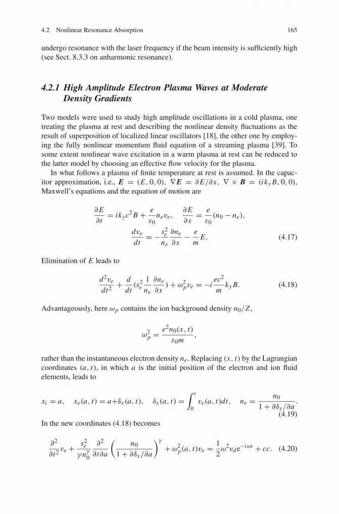
4.2 Nonlinear Resonance Absorption 165
undergo resonance with the laser frequency if the beam intensity is sufficiently high(see Sect. 8.3.3 on anharmonic resonance).
4.2.1 High Amplitude Electron Plasma Waves at ModerateDensity Gradients
Two models were used to study high amplitude oscillations in a cold plasma, onetreating the plasma at rest and describing the nonlinear density fluctuations as theresult of superposition of localized linear oscillators [18], the other one by employ-ing the fully nonlinear momentum fluid equation of a streaming plasma [39]. Tosome extent nonlinear wave excitation in a warm plasma at rest can be reduced tothe latter model by choosing an effective flow velocity for the plasma.
In what follows a plasma of finite temperature at rest is assumed. In the capac-itor approximation, i.e., E = (E, 0, 0), ∇E = ∂E/∂x, ∇ × B = (iky B, 0, 0),Maxwell’s equations and the equation of motion are
∂E
∂t= ikyc2 B + e
ε0neve,
∂E
∂x= e
ε0(n0 − ne),
dve
dt= − s2
e
ne
∂ne
∂x− e
mE . (4.17)
Elimination of E leads to
d2ve
dt2+ d
dt(s2
e1
ne
∂ne
∂x)+ ω2
pve = −iec2
mky B. (4.18)
Advantageously, here ωp contains the ion background density n0/Z ,
ω2p =
e2n0(x, t)
ε0m,
rather than the instantaneous electron density ne. Replacing (x, t) by the Lagrangiancoordinates (a, t), in which a is the initial position of the electron and ion fluidelements, leads to
xi = a, xe(a, t) = a+δx (a, t), δx (a, t) =∫ t
0ve(a, t)dt, ne = n0
1+ ∂δx/∂a.
(4.19)In the new coordinates (4.18) becomes
∂2
∂t2ve + s2
e
γ nγ0
∂2
∂t∂a
(n0
1+ ∂δx/∂a
)γ+ ω2
p(a, t)ve = 1
2ω2vde−iωt + cc. (4.20)

166 4 Resonance Absorption
The oscillation center approximation was assumed to obtain the term ω2p(a, t)ve.
This is justified for inhomogeneity lengths L and electrostatic wavelength λe ifL > 2λe. The electron fluid is assumed to obey an adiabatic law, pe = const× nγe ,the driver vd stands for vd = −iec2ky B(0)/mω2. For L > 2λe, one may furthertransform (4.20),
∂
∂t
{∂2
∂t2δx + s2
e
γ
∂
∂a(1+ ∂
∂aδx )
−γ + ω2pδx
}= 1
2ω2vde−iωt + cc.,
and integrate it once to obtain
∂2
∂t2δx + s2
e
γ
∂
∂a(1+ ∂
∂aδx )
−γ + ω2pδx = i
2ωvde−iωt + cc. (4.21)
For small amplitudes (1+∂δx/∂a)−γ � 1−γ ∂δx/∂a and, with the help of δe = δx
from (2.12), (4.21) reduces to (4.9), since then ∂/∂a � ∂/∂x . For a cold plasma(s2
e = 0) it leads to the Koch-Albritton model [18] of uncoupled harmonic oscilla-tors from which, through (4.19) the electron density is recovered. Although there isstrong coupling between the single fluid elements, ve and δx are sinusoidal in thecold plasma, but ne is not, in contrast to a linear wave which is sinusoidal in allvariables that can be used to describe it. By setting
δx = δ1 + 1
2
∑
σ≥2
{δσ e−iσωt + δ∗σ eiσωt
},
g = 1+ 1
4
(γ + 2
2
)k2
1 |δ1|2 + 1
8
(γ + 4
4
)k4
1 |δ1|4 + ....
in the warm plasma the amplitude-dependent dispersion relation for the fundamentalwave δ1,
ω2 = ω2p
{1+ g
(sek1
ωp
)2}, (4.22)
and the amplitude ratios for the higher harmonics are obtained [40],
δ2
δ1= γ + 1
2
η3/2g−1/2ω2
3ω2pg + 4(g − 1)η2ω2
v1
se, v1 = δ1,
δ3
δ1= γ + 1
4
η3ω2
g2
(v1
se
)23(γ+1)ω2
3ω2p g+4(g−1)η2ω2 + γ+2
2 η
8ω2p + 9(g − 1)η2ω2
. (4.23)
In the resonance region η2 � 1, (sek1/ωp)2 � 1, g = 1, ω2
p = ω2 holds andthese relations simplify to

4.2 Nonlinear Resonance Absorption 167
δ2
δ1� γ + 1
6η3/2 v1
se,
δ3
δ1� 1
2
(γ + 1
4
)2
η3(v1
se
)2
, (4.24)
showing the interaction of modes: As the excited wave moves away from the res-onance region towards lower densities the refractive index η increases from zeroto one, thus leading to an increase of higher order modes. The modified dispersion(4.22) is a consequence of self-interaction of the fundamental mode δ1. Due to theexcitation of higher harmonics at finite electron temperature ve and δx no longerremain sinusoidal. This behavior is clearly seen in the numerical solution of (4.20)in Fig. 4.6. The maxima of ve are more peaked than its minima. As a result, δx
has a tendency to assume a sawtooth shape. The spike-like character is especiallypronounced in the electron density ne. Such structures of “bubbles and spikes” arevery characteristic of large amplitude electrostatic waves and are encountered in thenonlinear evolution of the Rayleigh-Taylor istability (see Chap. 5 in [41]). The maincontribution to peaking of ne comes from mass conservation of (4.19) and is bestunderstood in the cold plasma case; there
δx = δ cosωpt, ne = n0
1+ (∂δ/∂a) cosωpt
holds and ne oscillates between n0/2 and∞. In the warm plasma ne remains aboven0/2 in all situations [42].
Fig. 4.6 Nonlinear electron plasma wave. Normalized electron density ne, electron quiver velocityve, excursion δx =
∫vedt and y = ∂δx/∂a as functions of x . Nearly the same picture results if
these quantities are plotted as functions of the Lagrange coordinate a

168 4 Resonance Absorption
4.2.2 Resonance Absorption by Nonlinear Electron Plasma Waves
With increasing laser intensity or at low electron temperature the electron plasmawave may exceed the linear limit and may even break. Furthermore, particle-in-cell(PIC) simulations have shown that the particle aspect appears more and more as theLangmuir wave potential increases and particle trapping and acceleration dominates[43]. As we shall see in the following these phenomena lead to strong collisionlessdamping of the Langmuir wave. It is therefore quite natural to extend the traditional,somewhat vague definition of nonlinear Landau damping (see for example [44]) toinclude such processes. This makes clear that at high intensities a kinetic descriptionof resonance absorption is needed. With particle trapping the following questionsarise: What structure does a strongly nonlinear Langmuir wave assume, and to whatextent does the much simpler fluid description still give a satisfactory answer? Howis the mode conversion efficiency, i.e., the absorption coefficient A, affected by thenonlinear evolution of the plasma wave? These questions can be answered properlyby numerically solving the Vlasov equation.
The evolution of the one-dimensional electron distribution function f (x, v, t)under the action of an external driver field Ed and the induced self-consistent fieldE(x, t) in such a fixed ion background of charge density en0(x) is governed by theVlasov and Poisson equations,
∂ f
∂t+ v
∂ f
∂x− e
m(E + Ed)
∂ f
∂v= 0,
∂E
∂x= e
ε0
(n0 − nc
∫ ∞
−∞f dv
). (4.25)
This procedure is much more involved than corresponding PIC simulations; how-ever, as a compensation, it generates almost no numerical noise and leads to finerresolution in regions of low density in phase space [45]. Starting with a Maxwelliandistribution function
f0(x, v) = 1
(2π)1/2vthexp
(− x
L
)exp
(− v2
2v2th
),
the result of the Vlasov calculation of the Langmuir wave is compared with hydro-dynamic solutions obtained from (4.20) [25]. In Fig. 4.7a the driving field amplitude,measured in units of the thermal electric field Eth = kB Te/eλD = (mekB Te)
1/2ω/e,is Ed = 0.02, and in (b)–(d) it is twice as strong, Ed = 0.04. All pictures are takenat the same time ωt = 120π . The first two, (a) and (b), are the hydrodynamic resultsand show the characteristic peaking as presented in Fig. 4.6. The analogous Vlasovresult is shown in (c). The agreement in the general wave structure is excellent. Forcomparison, in picture (d) the corresponding result of a PIC calculation with 6 · 104
particles, applied to a nonlinear density profile with the same gradient nc/L at theresonance point, is plotted. The advantage of the 1D Vlasov simulation is evident.
The amount of particles trapped and accelerated (detrapped) by the wave ofFig. 4.7 can be estimated from the distribution function in Fig. 4.8a: trapped particlesare recognized by closed loops in the potential wells, detrapped ones form the undu-

4.2 Nonlinear Resonance Absorption 169
Fig. 4.7 High-amplitude electron plasma wave in the capacitor model with driving field amplitude(a) Ed = 0.02 and (b)–(d) Ed = 0.04 and L = 600λD at time ωt = 120π . The critical densityis at x = 0. Normalized electron density ne/nc (a), (b) from the fluid model, (c) from the Vlasovsimulation, and (d) from a PIC calculation with 6·104 particles (large numerical noise). Jitter in thephase between (a)–(c) and (d) is due to small time step differences between the different numericalprocedures
lating contours leaning to the right. For comparison, in Fig. 4.8b the distributionfunction from the PIC calculation of the same wave is presented. Here, in contrast tothe Vlasov code, the evaluation of the distribution function is not possible in thoseregions where almost no simulation particles are present. How strongly nonlinearLandau damping exceeds linear Landau damping can be deduced from Fig. 4.9 forthe two driver strengths Ed = 0.04 and Ed = 0.08. It shows that, except at very lowEd -values, linear Landau damping (dotted curves) is totally dominated by dampingdue to particle trapping and acceleration (at low driver strength the comparison withlinear Landau damping was used to test the accuracy of the numerical procedureemployed here). More quantitatively, Vlasov simulations show that linear Landaudamping holds up to the following laser intensity limit,
I0 = 2× 10¹³(ωNd
ω
)2(
300λD
L
)1/3
Wcm−2. (4.26)
The first wave crest is the only resonantly driven maximum. All other maxima whichare outside the resonance region stop growing due to nonlinear Landau damping atEd ≈ 0.04; the additional absorbed energy is transferred to fast electrons. The firstfield maximum increases with growing driver strength as plotted in Fig. 4.10. For
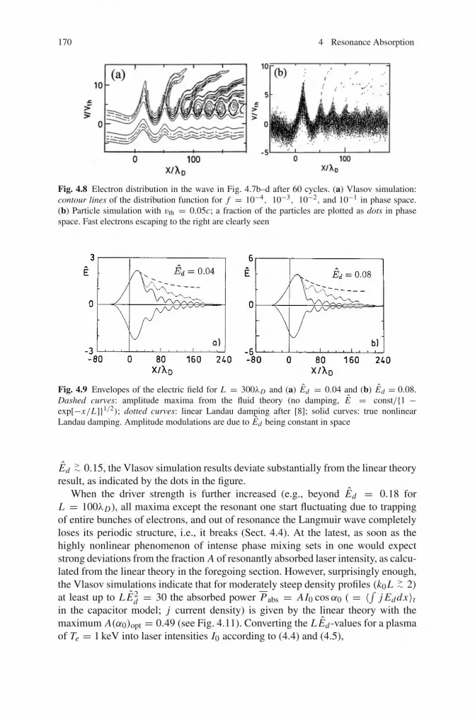
170 4 Resonance Absorption
Fig. 4.8 Electron distribution in the wave in Fig. 4.7b–d after 60 cycles. (a) Vlasov simulation:contour lines of the distribution function for f = 10−4, 10−3, 10−2, and 10−1 in phase space.(b) Particle simulation with vth = 0.05c; a fraction of the particles are plotted as dots in phasespace. Fast electrons escaping to the right are clearly seen
Fig. 4.9 Envelopes of the electric field for L = 300λD and (a) Ed = 0.04 and (b) Ed = 0.08.Dashed curves: amplitude maxima from the fluid theory (no damping, E = const/{1 −exp[−x/L]}1/2); dotted curves: linear Landau damping after [8]; solid curves: true nonlinearLandau damping. Amplitude modulations are due to Ed being constant in space
Ed>∼ 0.15, the Vlasov simulation results deviate substantially from the linear theory
result, as indicated by the dots in the figure.When the driver strength is further increased (e.g., beyond Ed = 0.18 for
L = 100λD), all maxima except the resonant one start fluctuating due to trappingof entire bunches of electrons, and out of resonance the Langmuir wave completelyloses its periodic structure, i.e., it breaks (Sect. 4.4). At the latest, as soon as thehighly nonlinear phenomenon of intense phase mixing sets in one would expectstrong deviations from the fraction A of resonantly absorbed laser intensity, as calcu-lated from the linear theory in the foregoing section. However, surprisingly enough,the Vlasov simulations indicate that for moderately steep density profiles (k0L >∼ 2)at least up to L E2
d = 30 the absorbed power Pabs = AI0 cosα0 ( = 〈∫ j Eddx〉tin the capacitor model; j current density) is given by the linear theory with themaximum A(α0)opt = 0.49 (see Fig. 4.11). Converting the L Ed -values for a plasmaof Te = 1 keV into laser intensities I0 according to (4.4) and (4.5),

4.2 Nonlinear Resonance Absorption 171
Fig. 4.10 Comparison of maximum electric-field amplitude from Vlasov simulations (dots) andfrom the linear theory (straight line). The latter scales as Emax = 1.28 · (L/λD)
2/3 Ed [8]
Fig. 4.11 Validity of linear resonance absorption: mean absorbed power Pabs as a function of thedriving field strength Ed (bottom scale) and laser intensity for λ = 1.06 µm and Te = 1 keV incase of maximum absorption (top scale). Dots: Vlasov simulations; straight line: linear theory
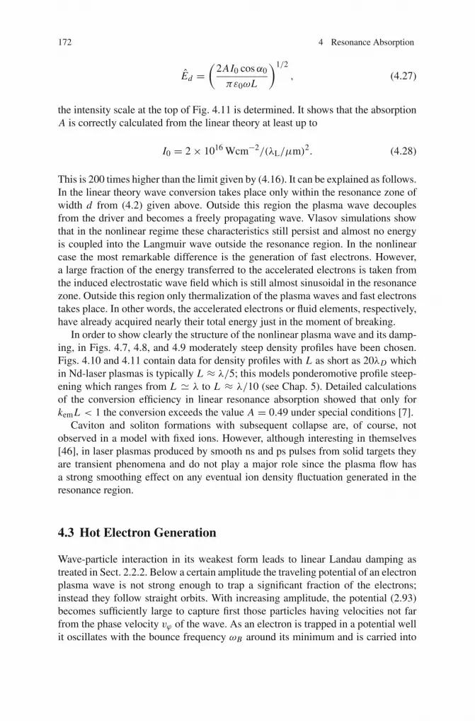
172 4 Resonance Absorption
Ed =(
2AI0 cosα0
πε0ωL
)1/2
, (4.27)
the intensity scale at the top of Fig. 4.11 is determined. It shows that the absorptionA is correctly calculated from the linear theory at least up to
I0 = 2× 10¹⁶ Wcm−2/(λL/μm)2. (4.28)
This is 200 times higher than the limit given by (4.16). It can be explained as follows.In the linear theory wave conversion takes place only within the resonance zone ofwidth d from (4.2) given above. Outside this region the plasma wave decouplesfrom the driver and becomes a freely propagating wave. Vlasov simulations showthat in the nonlinear regime these characteristics still persist and almost no energyis coupled into the Langmuir wave outside the resonance region. In the nonlinearcase the most remarkable difference is the generation of fast electrons. However,a large fraction of the energy transferred to the accelerated electrons is taken fromthe induced electrostatic wave field which is still almost sinusoidal in the resonancezone. Outside this region only thermalization of the plasma waves and fast electronstakes place. In other words, the accelerated electrons or fluid elements, respectively,have already acquired nearly their total energy just in the moment of breaking.
In order to show clearly the structure of the nonlinear plasma wave and its damp-ing, in Figs. 4.7, 4.8, and 4.9 moderately steep density profiles have been chosen.Figs. 4.10 and 4.11 contain data for density profiles with L as short as 20λD whichin Nd-laser plasmas is typically L ≈ λ/5; this models ponderomotive profile steep-ening which ranges from L � λ to L ≈ λ/10 (see Chap. 5). Detailed calculationsof the conversion efficiency in linear resonance absorption showed that only forkemL < 1 the conversion exceeds the value A = 0.49 under special conditions [7].
Caviton and soliton formations with subsequent collapse are, of course, notobserved in a model with fixed ions. However, although interesting in themselves[46], in laser plasmas produced by smooth ns and ps pulses from solid targets theyare transient phenomena and do not play a major role since the plasma flow hasa strong smoothing effect on any eventual ion density fluctuation generated in theresonance region.
4.3 Hot Electron Generation
Wave-particle interaction in its weakest form leads to linear Landau damping astreated in Sect. 2.2.2. Below a certain amplitude the traveling potential of an electronplasma wave is not strong enough to trap a significant fraction of the electrons;instead they follow straight orbits. With increasing amplitude, the potential (2.93)becomes sufficiently large to capture first those particles having velocities not farfrom the phase velocity vϕ of the wave. As an electron is trapped in a potential wellit oscillates with the bounce frequency ωB around its minimum and is carried into

4.3 Hot Electron Generation 173
regions where vϕ and n1 are increased or decreased. In the first case effective particleacceleration takes place. In the second case an electron may remain trapped and thedifference of its kinetic energy is given back to the wave, or it becomes free againand carries away the energy imparted to it by the wave. Such detrapped electrons areseen on the wave crests in Fig. 4.8b. The bounce frequency of an electron oscillatingclose to the minimum of a wave potential like (2.93) is easily determined. Expansionof Φ around its maximum yields
Φ = −e2n1
ε0
(x − x0)2
2.
Hence, the bounce frequency is
ωB =(
e2n1
ε0m
)1/2
, (4.29)
i.e., ωB is the plasma frequency of the electron density amplitude. With increasingoscillation amplitude ωB remains behind this formula in a sinusoidal potential, i.e.,in a linear electron plasma wave, and it does so owing to the flattening effect of theminima of ne according to Fig. 4.6 when the wave amplitude increases.
In laser produced plasmas fast, i.e., superthermal electrons were observed asearly as in 1971 [47]. Since their energy distribution was not far from a Maxwelliana hot temperature Th could be assigned to them, in contrast to the thermal electronswhose temperature Te was given the name cold electrons Tc although typical val-ues of Tc in laser produced plasmas on ns time scales range from 0.5 to 5 keV. Inplasmas produced by high-intensity CO2 lasers considerably higher values of Tc arereached. The hypothesis that the main sources for hot electron generation in the nsand ps regimes are resonance absorption at the critical density and stimulated Ramanscattering as well as two-plasmon decay at a quarter of the critical density (Chap. 6)was successively confirmed by particle simulations [48, 49]. Electron accelerationand, in concomitance, acceleration of ions up to several 10 MeV becomes an impor-tant phenomenon when superintense laser pulses interact with gas and solid targets(Chap. 8).
In view of the importance the wave-particle interaction in laser plasmas, an ana-lytical treatment of it and a classification of its main aspects are presented first.Thereby the authors mainly follows [50] (alternatively [40]).
4.3.1 Acceleration of Electrons by an Intense Smooth LangmuirWave
In the analytical treatment a one-dimensional model is used for the wave and theparticle motion in it. The electron plasma wave is assumed to propagate in thepositive x-direction, with amplitude E and wavelength λ = 2π/k being weakly

174 4 Resonance Absorption
space dependent. The electron equation of motion may be written as follows,
mx = −eE(x) sin
(∫ x
x0
k(x ′)dx ′ − ωt
). (4.30)
An asymptotic series solution of this equation can be obtained by a method dueto Kruskal [51]. In our context it is sufficient to determine only the first term. Toleading order the procedure is equivalent to the method of averaging [52], whichhas been employed in the computation of electron trajectories in a wave with slowlytime dependent amplitude [53].
In solving the equation of motion two different cases have to be treated sepa-rately: that of a trapped electron bouncing to and fro in a potential trough of thewave, moving on the average with the phase velocity, and that of an untrapped parti-cle going over hill and valley. The solutions are best given in terms of an amplitudevariable y which is taken to be the total particle energy in the wave frame dividedby 1
2 mv2ϕ .
As a result of Kruskal’s method one obtains the dependence of the normalizedparticle energy y on the wave amplitude E(x), wave number k(x) and an eventualstatic field E0(x). For untrapped particles it is given by [40, 50]
1
k2
[1+ y + σ
4
π(w + y)1/2E(κ)
]− 4Φ = const, (4.31)
while for trapped particles
1
k2
(w2
)1/2[
E
(1
κ
)+(
1
κ2− 1
)K
(1
κ
)]= const. (4.32)
w(x) is the wave potential amplitude eE(x)/k(x) normalized to 12 mv2
ϕ ,
w(x) = 2eE(x)k(x)
mω2. (4.33)
The modulus κ of the elliptic integrals of the first and second kind, K(κ) and E(κ),is defined as
κ2 = 2w
w + y. (4.34)
σ = ±1 is the sign of the particle velocity in the wave frame. Finally,
Φ(x) = − e
2mω2
∫ x
−∞E0(x
′)dx ′ (4.35)
is, apart from a factor, the potential of the static field.

4.3 Hot Electron Generation 175
The corresponding equations for the phase variable φ are skipped because theseare of no further importance. Relations (4.31) and (4.32) can be derived from anaction integral [50]. Thus, they are adiabatic invariants of the motion. The main pointof this derivation is that since the equation of motion is not autonomous (and cannotbe made so by simply transforming to the wave frame because time then reappearsin the amplitude), energy and time have to be considered as an additional pair ofcanonical variables. These additional variables contribute to the action integral foruntrapped particles, while their contribution vanishes in the case of trapped particles.
A difficulty arises from particles being trapped when the wave amplitudeincreases or being detrapped when it decreases. During such a transition the adi-abatic assumption is violated because of the logarithmic divergence of the particle’sbounce period T ,
T (κ) = 2
(2
w
)1/2
κK(κ), (4.36)
in the vicinity of the transition point where κ approaches unity. Thus, an appre-ciable change of the adiabatic invariant might occur in a transition; for example,in the limiting case of an electron sitting on a wave top all the time and travelingwith phase velocity the change of the adiabatic invariant is of order unity. However,for the vast majority of particle trajectories the adiabatic invariant changes by anamount of order ε = max |λ∂x E/E |, as has been explicitly shown [54]. Changes oforder unity can only occur if the trajectory crosses the separatrix within a narrowneighborhood of the potential energy maxima. Thus the effect of a nonadiabatictransition on the adiabatic invariant is negligible with respect to the whole ensembleof particle trajectories.
For the following considerations the acceleration of electrons in a wave field ofthe type shown in Fig. 4.12 is significant. For simplicity λ is taken to be constantand no static electric field is taken into account. Invariant (4.31) then becomes
1+ y + σ4
π(w + y)1/2E(κ) = v2
i , (4.37)
where vi is the initial particle velocity far outside of the wave field, normalized tothe phase velocity vϕ .Three different groups of particles have to be distinguished:
A. Particles entering from the right with initial velocity vi < 0. In the wave frame,these particles move initially to the left, i.e., σ = −1, with a normalized energyy0 = (vi − 1)2 > 1 in the wave frame.
B. Particles entering from the left with 0 < vi < 1. Initially, in the wave frame,they move to the left, σ = −1, with an energy in the range 0 < y0 < 1.
C. Particles entering from the left with vi > 1, which corresponds to a positivevelocity (σ = +1) in the wave and y0 > 0.

176 4 Resonance Absorption
Fig. 4.12 Electron plasma wave of constant wavelength moving at phase velocity vϕ to the right.Wave amplitude E(x) is fixed in the lab frame: for a comoving observer the wave grows untilreaching a maximum and then decays. Velocities of the incoming electrons, A: vi = v0/vϕ < 0,B: 0 < vi < 1, C: vi > 1
The motion of a particle entering with initial velocity vi is characterized in this caseby the dependence of the particle energy y on the wave amplitude w. This is shownin Fig. 4.13a for σ = −1 (particles of group A) and (b) for σ = +1 (particles ofgroup C). The upper parts above the straight lines y = w describe the motion ofuntrapped particles, whereas the lower parts describe trapped particles. The lowerparts of (a) and (b) are identical, since the direction of motion σ oscillates alongthe trajectory of a trapped particle. When a curve reaches the straight line y = w,the corresponding particle is trapped or detrapped. As discussed above, there is nodiscontinuity in the action integrals at the transition point, so that the trajectories oftrapped and untrapped particles can be connected there continuously.
If trapping occurs for a given vi , the transition point yt = wt can be calculatedfrom (4.37)
1+ wt + σ · 4
π
√2wt = v2
i . (4.38)
After trapping, the particle’s trajectory is given by
w1/2[
E
(1
κ
)+(
1
κ2− 1
)K
(1
κ
)]= w
1/2t . (4.39)
For a wave field with normalized maximum amplitude w0 (or w0) only those partsof Fig. 4.13a,b with w < w0 (w < w) apply. Particles moving on trajectorieswhich are inside the solid curve in (a) cannot be trapped by the wave, irrespectiveof the maximum wave amplitude. Within this region, particles are either reflectedwith final velocity outside the wave v f = −vi (curve c), or cross the wave packetwith v f = vi (curves b, d). In both cases no net change of particle energy results. Itfollows from (4.37) that all particles entering with 0 < vi < vc from the left or with
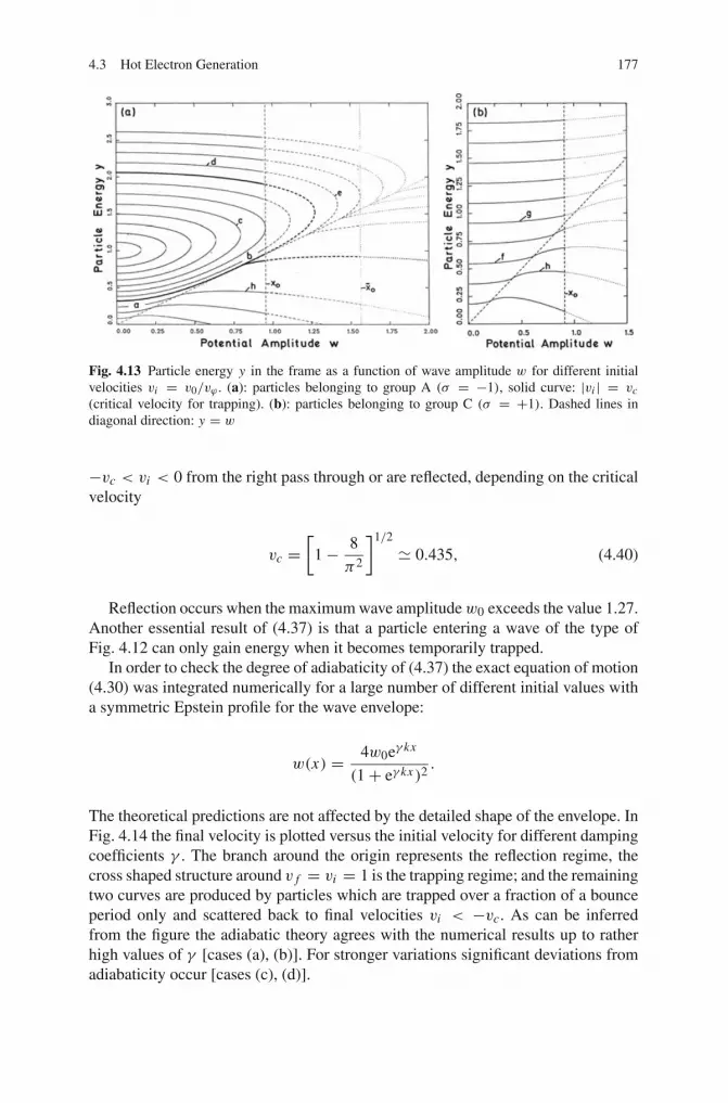
4.3 Hot Electron Generation 177
Fig. 4.13 Particle energy y in the frame as a function of wave amplitude w for different initialvelocities vi = v0/vϕ . (a): particles belonging to group A (σ = −1), solid curve: |vi | = vc(critical velocity for trapping). (b): particles belonging to group C (σ = +1). Dashed lines indiagonal direction: y = w
−vc < vi < 0 from the right pass through or are reflected, depending on the criticalvelocity
vc =[
1− 8
π2
]1/2
� 0.435, (4.40)
Reflection occurs when the maximum wave amplitudew0 exceeds the value 1.27.Another essential result of (4.37) is that a particle entering a wave of the type ofFig. 4.12 can only gain energy when it becomes temporarily trapped.
In order to check the degree of adiabaticity of (4.37) the exact equation of motion(4.30) was integrated numerically for a large number of different initial values witha symmetric Epstein profile for the wave envelope:
w(x) = 4w0eγ kx
(1+ eγ kx )2.
The theoretical predictions are not affected by the detailed shape of the envelope. InFig. 4.14 the final velocity is plotted versus the initial velocity for different dampingcoefficients γ . The branch around the origin represents the reflection regime, thecross shaped structure around v f = vi = 1 is the trapping regime; and the remainingtwo curves are produced by particles which are trapped over a fraction of a bounceperiod only and scattered back to final velocities vi < −vc. As can be inferredfrom the figure the adiabatic theory agrees with the numerical results up to ratherhigh values of γ [cases (a), (b)]. For stronger variations significant deviations fromadiabaticity occur [cases (c), (d)].

178 4 Resonance Absorption
Fig. 4.14 Spectra of final velocities v f as a function of initial velocity vi for differentcoefficients γ . Curves: theoretical spectra, dots: numerical points
4.3.2 Particle Acceleration by a Discontinuous Langmuir Wave
A resonantly excited electron plasma wave may be idealized by a suddenly risingwave structure as presented in Fig. 4.15 which results from cutting the wave struc-ture of Fig. 4.12 in the middle. The acceleration achievable in such a wave fieldcan be investigated by the same methods employed before. The main differencefrom the former case is that particles entering the wave field from the left across thediscontinuity start with an initial energy y0 which in the wave frame is given by
y0 = (vi − 1)2 − w0 cos τ0 . (4.41)
Now, y0 depends not only on the initial velocity vi , but also on the phase τ0(0 < τ0 < 2π). Thus, for particles entering with a given value of vi there existsa whole spectrum of initial energies y0, leading to a corresponding spectrum of finalvelocities v f .
The possible range of final velocities for given vi and w0 is obtained from (4.37)and Fig. 4.13a,b by taking into account all values of y0 which belong to an intervalof width 2w0 around the particle energies y = (vi − 1)2.
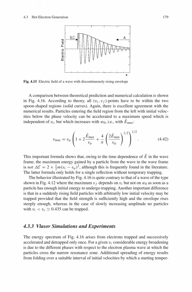
4.3 Hot Electron Generation 179
Fig. 4.15 Electric field of a wave with discontinuously rising envelope
A comparison between theoretical prediction and numerical calculation is shownin Fig. 4.16. According to theory, all (vi , v f )-points have to be within the twospoon-shaped regions (solid curves). Again, there is excellent agreement with thenumerical results. Particles entering the field region from the left with initial veloc-ities below the phase velocity can be accelerated to a maximum speed which isindependent of vi , but which increases with w0, i.e., with Emax:
vmax = vϕ
⎛
⎝1+ 2Emax
vϕ+ 4
π
(2Emax
vϕ
)1/2⎞
⎠1/2
. (4.42)
This important formula shows that, owing to the time dependence of E in the waveframe, the maximum energy gained by a particle from the wave in the wave frameis not ΔE = 2 × 1
2 m(vi − vϕ)2, although this is frequently found in the literature.
The latter formula only holds for a single reflection without temporary trapping.The behavior illustrated by Fig. 4.16 is quite contrary to that of a wave of the type
shown in Fig. 4.12 where the maximum v f depends on vi but not on w0 as soon as aparticle has enough initial energy to undergo trapping. Another important differenceis that in a suddenly rising field particles with arbitrarily low initial velocity may betrapped provided that the field strength is sufficiently high and the envelope risessteeply enough, whereas in the case of slowly increasing amplitude no particleswith vi < vc � 0.435 can be trapped.
4.3.3 Vlasov Simulations and Experiments
The energy spectrum of Fig. 4.16 arises from electrons trapped and successivelyaccelerated and detrapped only once. For a given vi considerable energy broadeningis due to the different phases with respect to the electron plasma wave at which theparticles cross the narrow resonance zone. Additional spreading of energy resultsfrom folding over a suitable interval of initial velocities by which a starting temper-

180 4 Resonance Absorption
Fig. 4.16 “Schneider’s spoons”. Spectrum of final velocities v f of particles accelerated in aLangmuir wave of suddenly rising amplitude
ature Tc, always present in a real plasma, is simulated. Finally, only a small fractionof electrons can escape from the plasma after having crossed the wave once, whereasthe majority of them are trapped by the electrostatic field and may cross the criticalregion several times. This mechanism leads to additional heating, if not increasedrelative energy spreading. To analyze these aspects a kinetic description or particlesimulations must be used.
Extensive particle simulations [19, 43, 48, 49, 55–57] have shown that the spec-trum of the hot electrons is close to Maxwellian and was sometimes attributed tomultiple acceleration by Langmuir waves [43]. More recent calculations based onthe Vlasov equation [45] clearly confirm the Maxwellian energy distribution of thetrapped electrons and thus the existence of a temperature Th . In Fig. 4.17 the spaceaveraged distribution functions f (v) = 〈 f (x, v)〉 for driver strengths of Ed = 0.04(a) and Ed = 0.08 (b) in a fixed ion density profile of Lc = 300λD are shownand the values of Th = 16 and 36 keV are calculated. In addition to the muchreduced noise in the Vlasov simulations the significant result which is found isthat the Maxwellian character of f (x, v) is already established at the right edgeof the resonance zone of Fig. 4.2. In a run with Ed = 0.05 and Lc = 300λD amodest variation of f (x, v) was only found when x was varied from x = xm (end ofresonance) to x = Lc. There is a maximum velocity vmax at which the Maxwelliandistribution suddenly breaks up. A comparison of these “experimental” values withformulas from the literature can be made, in particular with Schneider’s expression(4.42) and another simple expression, which in normalized quantities reads [58]
vmax =(
8Ed Lc
)1/2.

4.3 Hot Electron Generation 181
Fig. 4.17 Electron distribution function averaged over space, f (v) = 〈 f (x, v)〉 for a normalizeddriver Ed = 0.04 (a) and Ed = 0.08 (b). The ion density scale length is Lc = 300λD in bothcases. Th temperature of the fast electrons, Tc “cold” bulk temperature (steep straight lines)
The result of a comparison with seven Vlasov runs is summarized in Table 4.1.Thereby vϕ was taken at x = xm . The agreement with (4.42) is excellent whereasthe simpler formula above, though leading to too low values, may serve for a roughestimate. Its agreement with simulations is expected to improve with decreasingscale length Lc. According to both formulae vmax, and the corresponding Th increasewith phase velocity vϕ . This means that more energetic electrons are to be expectedfrom electron plasma waves excited in flat density profiles, e.g., from stimulatedRaman scattering and two-plasmon decay; its confirmation by particle simulationsand experiments is well established [48, 59–62] (see also Chap. 8). For practicalpurposes scaling laws for Th and the number density nh of hot electrons are impor-tant. For the construction of such functional dependences from simple models in thens laser pulse regime the reader may consult the excellent review by Haines [64]. Inthe long pulse regime all authors seem to agree on a combined (I0λ
2)δ-dependenceof Th , and most of them (Vlasov simulations included) find δ-values not far from1/3. According to [48],
Th � 14(I0λ2)1/3T 1/3
c , (4.43)
when Th, Tc are measured in keV, I0 in units of 1016 Wcm−2 and λ in µm. Theirbest fit to experiments at (I0λ
2) > 1015 Wµm2cm−2 was δ = 0.25. In this contextthe reader interested in a comparison with other simulations may consult [57].
Electron trapping and acceleration is one root of anomalous heat flux densityq = qe out of the critical layer [40, 45, 9]. In Fig. 4.18a the spatial distribution of
qe from a Vlasov simulation at τ = 60π (dashed line) and τ = 80π is presentedfor Ed = 0.04 and Lc = 300λD . The first isolated peak of qe reaches its maximumexactly at the border xm of the resonance zone. The divergence of qe manifestsitself in large deviations of single volume elements from adiabatic behavior. InFig. 4.18b the dependence of the kinetic pressure pe = m
∫(v − ue)
2 f dv [see(2.84), relativistic (8.53); here ue is the mean fluid velocity] on the electron density

182 4 Resonance Absorption
Table 4.1 Comparison of the maximum electron velocity from a Vlasov simulation of resonanceabsorption with analytical formulae
L = 100 λD L = 300 λD
Ed 0.06 0.1 0.2 0.04 0.08 0.12 0.16Vlasov simulation ≈ 10 ≈ 12 ≈ 15 ≈ 12 ≈ 17 19.5 ≈ 22Equation (4.42) 10.7 11.9 14.3 13 17.6 19.5 21.2vmax = (8Ed Lc)
1/2 6.9 8.9 12.6 9.8 13.9 17 19.6
(a) (b)
Fig. 4.18 (a): Anomalous heat current density q = (m/2)∫(v − ue)
3 f dv at τ = 60π (dashed)and 80π (solid) for a driver Ed = 0.04. (b): log ne- log pe- plot of an electron fluid element ofparticle density ne and pressure pe in the highly nonlinear electron plasma wave. The deviation ofthe trajectory from the straight line is a measure of the time-integrated divergence of the local heatflow q. Driver strength is Ed = 0.16
ne is shown in a log–log plot for a driver Ed = 0.16. In the absence of heat flow eachvolume element can move only along the diagonal corresponding to γ = 3. Owingto the heat flux of the fast electrons a single volume element, when compressed in adensity spike of the wave, at first remains in the neighborhood of the γ = 3 line (seelower arrow), but then, in the valley of the wave, a jet of fast electrons and with thema high value of qe have been built up. The latter is responsible for the trajectory inthe diagram far above the diagonal (follow upper arrow).
4.4 Wavebreaking
The excitation of large amplitude electron plasma waves has attracted great andcontinuous attention since 1959 when it was shown that cold plasma oscillationsbreak when the oscillatory velocity vos equals their phase velocity vϕ = ω/k[65]. Later this criterion was extended to warm electron plasma waves and it was

4.4 Wavebreaking 183
found from the fluid approach that the electron density ne of a free harmonicwave in a homogeneous plasma of density n0 must fulfill the inequality ne/n0 ≤(vϕ/se)
2/(γ+1) [66]. When approaching this limit, the electrostatic potential of thewave and its enthalpy are growing so rapidly that a single electron fluid elementbegins to be reflected from the periodic potential and wavebreaking sets in [42].
These criteria were derived for homogeneous plasmas. In not too steep densitygradients where the WKB approximation applies, the Coffey criterion may still beused (see below). In the resonance zone the wave becomes strongly inhomogeneous,the WKB approximation no longer holds and, therefore, breaking at resonance hasto be distinguished from breaking off resonance. For the cold plasma (Te = 0) at resta fluid dynamic breaking criterion was formulated in [18]. From these four papersit becomes clear what wavebreaking means within a fluid approach. On the otherhand, as seen in the foregoing section, kinetic phenomena greatly affect the structureof the Langmuir wave and its damping. Hence, two main questions arise: (i) whatis a meaningful definition of wavebreaking in the kinetic theory, and (ii) what isthe appropriate breaking criterion, if kinetic effects become significant or dominate.For example, one may ask whether such a phenomenon as kinetic wavebreakingoccurs at all when one keeps in mind how strongly the Langmuir wave is dampedby particle trapping and acceleration. It is amusing – and surprising – that the sci-entific community has been using the concept of “wavebreaking” in laser-matterinteraction for more than 20 years without having been aware of this situation,except [67]: “Thus we see that there is no one-to-one correspondence between hotelectron production and wavebreaking as is sometimes suggested”. Only tentative,more or less vague characterizations of wavebreaking have been presented which,at a closer inspection, may not appear very useful. A definition of wavebreakingwas given only later [68]. In connection with particle acceleration by superintenselasers the phenomenon of Langmuir-type wavebreaking has been enriched by newfundamental aspects [69–71].
For clarity, wavebreaking in the fluid approach is referred to as “hydrodynamicwavebreaking” here. Since resonance absorption of smooth laser pulses becomesquasi-stationary after very short times (several laser periods) it is appropriate todevelop a steady state model for cold wavebreaking in the resonance region [39].Such a model is interesting in itself and may serve to illustrate the difference of sta-tionary wavebreaking out of resonance. In the following subsection hydrodynamicbreaking criteria are derived. A possible solution to general wavebreaking is pre-sented in the subsequent paragraph. Currently we may distinguish five types of wavebreaking: geometrical breaking, cold plasma wave breaking, fluid-like breaking inthe warm plasma, kinetic wave breaking, and resonant (wave) breaking. The secondand third types are also referred to as hydrodynamic breaking.
Geometrical wavebreaking was discovered late although, intuitively, it mayappear as the most natural breaking scenario. It was found in 2D and 3D PICsimulations of the wake of an intense ultrahsort laser pulse traveling through anunderdense plasma. When the wave fronts off axis travel faster than the central partthey may collapse and interpenetrate leading to the destruction of the wave [70, 71].Resonant breaking of regular fluid dynamics, in particular of a wave, is induced bylocal anharmonic resonance (see Sect. 8.3.3).

184 4 Resonance Absorption
4.4.1 Hydrodynamic Wavebreaking
In a cold plasma (Te, se = 0) there is no energy transport out of the resonance regionunless the plasma is streaming at a finite velocity v0. Introducing this in (4.19) bysetting xi = a + ∫ v0(a, t)dt and xe = xi +
∫vedt one arrives at the harmonic
oscillator equation,
∂2
∂t2ve + ω2
p(a, t)ve = 1
2ω2vde−iωt + c.c., (4.44)
with resonance frequency ωp varying in time: A volume element starting in theoverdense region is off resonance owing to ωp � ω; it then approaches resonanceωp = ω and, rarefying further, in the underdense region (ωp < ω) it decouplesagain from the driver. Formally, (4.44) is obtained from (4.21) by setting se = 0.For v = ve−v0 a sufficiently accurate solution of (4.44) in our context here is foundfrom (3.78),
v = iω2vd
2ω1/2p
e−iϕ∫ t
0
ei(ωt ′−ϕ′)
ω1/2p
dt ′; ϕ(a, t) =∫ t
0ωp(a, t ′)dt ′, (4.45)
if the flow velocity obeys the inequality v0<∼ Lω/π . With L the density scale length
at resonance a self-consistent density profile is n0 = nc/(1 + a/2L)2. Inserting n0in (4.45) yields in the resonance region
v(a, t) = iL1/2ω1/2vdeiωa/v0+σ 2
v1/20
∫ σ
−∞e−iσ ′2 dσ ′, σ = 1
2t(ωv0
L
)1/2. (4.46)
The modulus of∫ σ−∞ e−iσ ′2 dσ ′ is the familiar Cornu spiral. It shows that secular
growth of |v(a, t)| occurs around resonance (Fig. 4.19). From it the resonance widthΔ, with σ running from −π/2 to +π/2, is deduced to be
Δ = 2π
(v0L
ω
)1/2
. (4.47)
Wavebreaking occurs when in (4.19) ∂δx/∂a = −1. For this to occur at the edge ofresonance (σ = π/2).
vd
v0=∣∣∣∣∣1
2+ i
π
2ei(π/2)2
∫ π/2
−∞e−iσ 2
dσ
∣∣∣∣∣
−1
= 0.36 (4.48)
must be fulfilled [39]. At resonance cold wavebreaking is due to the overlapping oftwo originally distinct volume elements as a result of their different phase shifts inthe neighborhood of the resonance point. Due to such shifts a Langmuir wave in acold streaming plasma may break as soon as vos > 0.75 vϕ is satisfied, i.e., at a
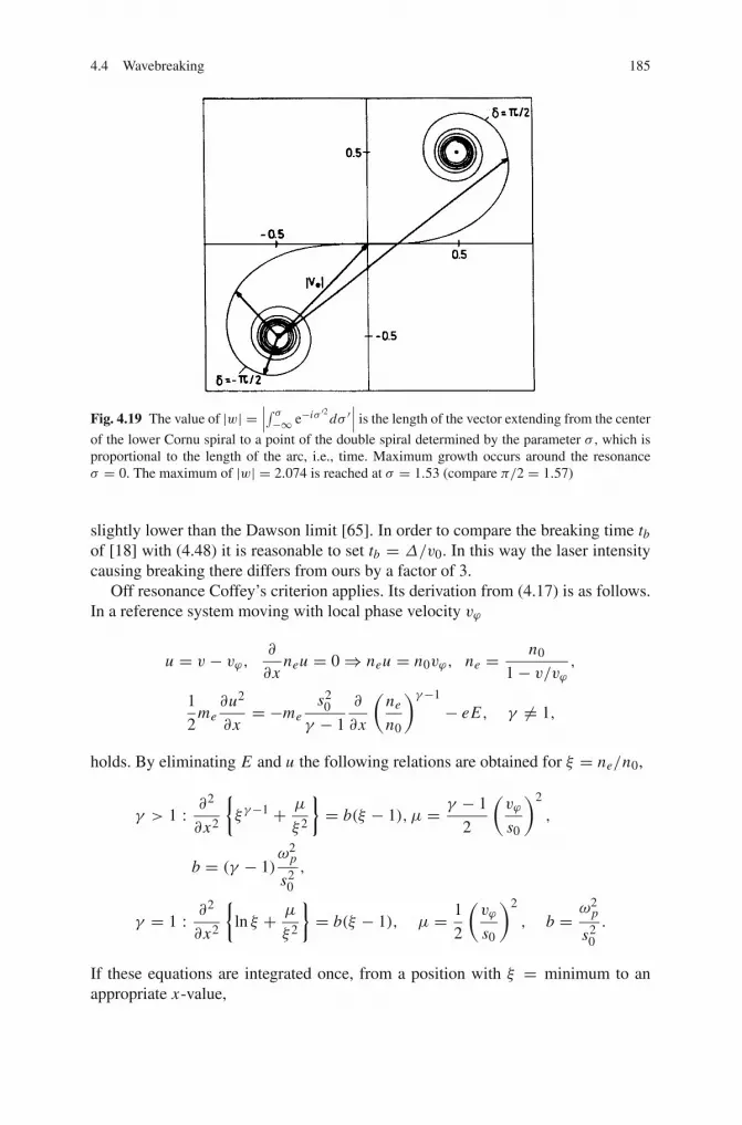
4.4 Wavebreaking 185
Fig. 4.19 The value of |w| =∣∣∣∫ σ−∞ e−iσ ′2 dσ ′
∣∣∣ is the length of the vector extending from the center
of the lower Cornu spiral to a point of the double spiral determined by the parameter σ , which isproportional to the length of the arc, i.e., time. Maximum growth occurs around the resonanceσ = 0. The maximum of |w| = 2.074 is reached at σ = 1.53 (compare π/2 = 1.57)
slightly lower than the Dawson limit [65]. In order to compare the breaking time tbof [18] with (4.48) it is reasonable to set tb = Δ/v0. In this way the laser intensitycausing breaking there differs from ours by a factor of 3.
Off resonance Coffey’s criterion applies. Its derivation from (4.17) is as follows.In a reference system moving with local phase velocity vϕ
u = v − vϕ,∂
∂xneu = 0 ⇒ neu = n0vϕ, ne = n0
1− v/vϕ,
1
2me
∂u2
∂x= −me
s20
γ − 1
∂
∂x
(ne
n0
)γ−1
− eE, γ = 1,
holds. By eliminating E and u the following relations are obtained for ξ = ne/n0,
γ > 1 : ∂2
∂x2
{ξγ−1 + μ
ξ2
}= b(ξ − 1), μ = γ − 1
2
(vϕ
s0
)2
,
b = (γ − 1)ω2
p
s20
,
γ = 1 : ∂2
∂x2
{ln ξ + μ
ξ2
}= b(ξ − 1), μ = 1
2
(vϕ
s0
)2
, b = ω2p
s20
.
If these equations are integrated once, from a position with ξ = minimum to anappropriate x-value,
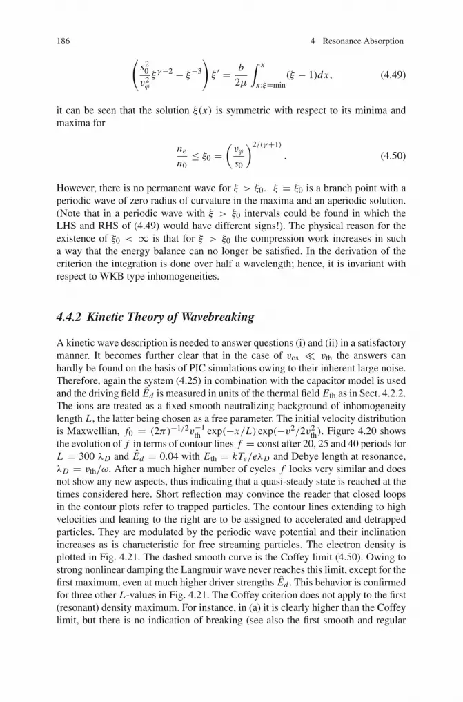
186 4 Resonance Absorption
(s2
0
v2ϕ
ξγ−2 − ξ−3
)ξ ′ = b
2μ
∫ x
x :ξ=min(ξ − 1)dx, (4.49)
it can be seen that the solution ξ(x) is symmetric with respect to its minima andmaxima for
ne
n0≤ ξ0 =
(vϕ
s0
)2/(γ+1)
. (4.50)
However, there is no permanent wave for ξ > ξ0. ξ = ξ0 is a branch point with aperiodic wave of zero radius of curvature in the maxima and an aperiodic solution.(Note that in a periodic wave with ξ > ξ0 intervals could be found in which theLHS and RHS of (4.49) would have different signs!). The physical reason for theexistence of ξ0 < ∞ is that for ξ > ξ0 the compression work increases in sucha way that the energy balance can no longer be satisfied. In the derivation of thecriterion the integration is done over half a wavelength; hence, it is invariant withrespect to WKB type inhomogeneities.
4.4.2 Kinetic Theory of Wavebreaking
A kinetic wave description is needed to answer questions (i) and (ii) in a satisfactorymanner. It becomes further clear that in the case of vos � vth the answers canhardly be found on the basis of PIC simulations owing to their inherent large noise.Therefore, again the system (4.25) in combination with the capacitor model is usedand the driving field Ed is measured in units of the thermal field Eth as in Sect. 4.2.2.The ions are treated as a fixed smooth neutralizing background of inhomogeneitylength L , the latter being chosen as a free parameter. The initial velocity distributionis Maxwellian, f0 = (2π)−1/2v−1
th exp(−x/L) exp(−v2/2v2th). Figure 4.20 shows
the evolution of f in terms of contour lines f = const after 20, 25 and 40 periods forL = 300 λD and Ed = 0.04 with Eth = kTe/eλD and Debye length at resonance,λD = vth/ω. After a much higher number of cycles f looks very similar and doesnot show any new aspects, thus indicating that a quasi-steady state is reached at thetimes considered here. Short reflection may convince the reader that closed loopsin the contour plots refer to trapped particles. The contour lines extending to highvelocities and leaning to the right are to be assigned to accelerated and detrappedparticles. They are modulated by the periodic wave potential and their inclinationincreases as is characteristic for free streaming particles. The electron density isplotted in Fig. 4.21. The dashed smooth curve is the Coffey limit (4.50). Owing tostrong nonlinear damping the Langmuir wave never reaches this limit, except for thefirst maximum, even at much higher driver strengths Ed . This behavior is confirmedfor three other L-values in Fig. 4.21. The Coffey criterion does not apply to the first(resonant) density maximum. For instance, in (a) it is clearly higher than the Coffeylimit, but there is no indication of breaking (see also the first smooth and regular

4.4 Wavebreaking 187
Fig. 4.20 Distribution function evolving from the initial distribution f0(x, v) = (2π)−1/2
exp(−x/L) exp(−v2/2v2th) with L = 300 λD and Ed = 0.04 after (a) 20, (b) 25, and (c) 40
periods; (d) enlarged plot of area indicated in (c) after 50 periods. The contour lines refer tof = 10−1, 10−2, 10−3, and 10−4, the critical density with ωp = ω is located at x = 0.Trapped electrons form closed loops (d); the velocity modulation of the detrapped electrons isdue to the periodic electric field of the Langmuir wave. Ed is normalized to Eth = kTe/eλD ,λD = vth/ω
maximum in Fig. 4.22a,b). For Ed ≥ 0.04 all maxima of ne except the first do notincrease further; but the wave remains periodic and smooth. As a first result, wecan clearly see that, although fast electrons are generated by trapping, the wave isstill regular and periodic in the sense mentioned above. In conclusion, fast electrongeneration alone does not indicate wavebreaking.
However, above a certain threshold E∗d the distribution function undergoes aqualitative change: the Langmuir wave becomes irregular, it breaks, as illustrated byFig. 4.22 for ne and E at Ed = 0.2 in a density profile of scale length L = 300λD .Inspection of the corresponding evolution of the distribution function (see Fig. 4.23)reveals the reason for such a behavior. The mean oscillatory velocity in the reso-nance region becomes so large that trapping of whole bunches of rather slow elec-trons occurs. These bunches of coherently moving electrons are partly coalescing(see black zones in Fig. 4.23) and remain trapped for at least several wavelengths,thus creating an additional aperiodic macroscopic electric field. From a fluid pointof view the phenomenon is similar to what is called intense mixing of volume ele-ments exhibiting different oscillation phases. (A Grassberger–Procaccia analysis ofthe electric field and the electron density at fixed x reveals the transition from aquasiperiodic to a chaotic attractor [45]). The electrons in these bunches contributeto the heat conduction, so that the heat flux q increases suddenly with wavebreaking.For example at x = 50 λD one obtains (η refractive index, q electron heat flowdensity)
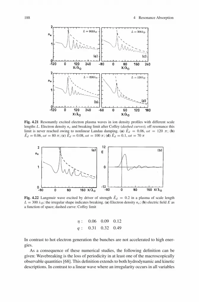
188 4 Resonance Absorption
Fig. 4.21 Resonantly excited electron plasma waves in ion density profiles with different scalelengths L . Electron density ne and breaking limit after Coffey (dashed curves); off resonance thislimit is never reached owing to nonlinear Landau damping. (a) Ed = 0.06, ωt = 120 π ; (b)Ed = 0.06, ωt = 80 π ; (c) Ed = 0.08, ωt = 100 π ; (d) Ed = 0.1, ωt = 70 π
Fig. 4.22 Langmuir wave excited by driver of strength Ed = 0.2 in a plasma of scale lengthL = 300 λD : the irregular shape indicates breaking. (a) Electron density ne; (b) electric field E asa function of space; dashed curve: Coffey limit
η : 0.06 0.09 0.12
q : 0.31 0.32 0.49
In contrast to hot electron generation the bunches are not accelerated to high ener-gies.
As a consequence of these numerical studies, the following definition can begiven: Wavebreaking is the loss of periodicity in at least one of the macroscopicallyobservable quantities [68]. This definition extends to both hydrodynamic and kineticdescriptions. In contrast to a linear wave where an irregularity occurs in all variables

4.4 Wavebreaking 189
Fig. 4.23 Route to wavebreaking. The distribution function for L = 300 λD and Ed = 0.2 after(a) 21, (b) 21.5, (c) 22.5, and (d) 23 periods. Contour lines for f = 10−1, 10−2, 10−3, and 10−4.Trapping and coalescence of entire electron bunches is evident (see black colored streaks)
simultaneously, breaking may appear to a different degree in the various quantities(e.g., ne and E in Fig. 4.22). The first, i.e., resonant density maximum may sat-isfy Coffey’s inequality or exceed this limit, even when the wave does not break(cf. Figs. 4.21 and 4.22).
Starting from the breaking condition for the streaming cold plasma, we replacethe streaming velocity by the group velocity of the plasma wave, because the latteris now the speed of energy transport (at least approximately in a nonlinear wave).From the fluid theory of resonance absorption we obtain for the group velocity atthe end of the resonance zone vg = s2
e /vϕ ≈ 2(L/λD)−1/3vth. Inserting this into
(4.48) at the place of v0 yields
Ed > E∗d = 0.72(L/λD)−1/3. (4.51)
This breaking threshold is in very good agreement with the results of the Vlasovsimulations, which are displayed in Fig. 4.24. The reason for the validity ofinequality (4.51) at finite electron temperature is that in the resonance region theelectronic oscillatory motion ve is mainly determined by the total electric fieldE = Ed + Ewave, and is only slightly affected by the much smaller force due tothe electron pressure gradient [72].
Next, the threshold intensity for wavebreaking is calculated. Making use of thescaling L/λD ∼ I−1/2
L from [49], where IL is the vacuum laser intensity, (4.51)translates to I ∗L = 2 · 1015 W/cm2 for the Nd-laser if a degree of absorption of 25%is assumed.

190 4 Resonance Absorption
Fig. 4.24 Driver strength threshold E∗d for wavebreaking as a function of scale length L . Straight
line: Eqs. (4.48) and (4.51). The circles in the (Ed , L)-plane represent Vlasov simulations withwavebreaking (solid) and without wavebreaking (blank)
Finally it is mentioned that the kinetic analysis of wavebreaking of freely propa-gating Langmuir waves in a homogeneous plasma shows that the same phenomenonalso occurs here and that one scenario of breaking (others may also exist) is againtrapping of entire bunches of electrons. However, the limit at which the wave breaksis much higher than the Coffey criterion would indicate. It must also be mentionedthat in the light of recent PIC and Vlasov simulations (for example [71]) it appearsdoubtful whether the hydrodynamic breaking limit becomes ever relevant becauseof the sudden increase of collective noise produced by kinetic effects. It is an openquestion how the two criteria correlate.
We conclude that wavebreaking is a phenomenon on its own, to be distinguishedfrom trapping of more or less uncorrelated electrons. The definition of wavebreakingpresented here has a clear meaning and is also applicable to a kinetic description.Further, it has been shown that a criterion for wavebreaking in smooth ion densityprofiles can be deduced from the model of a cold streaming plasma. In addition, theCoffey criterion is not applicable to resonance absorption.
In general, when adjacent electron fluid elements are driven by a spatially inho-mogeneous intense electromagnetic field they easily happen to cross and to mix uptogether, i.e., the regular motion becomes disordered. In particular this is believed tohappen in the so-called Brunel effect at the plasma-vacuum interface [20, 21] and in“ j × B heating” in the skin layer [73], and in collisionless absorption by collectiveinteraction [74, 75]. In the light of deeper insight into the nature of collisionlessabsorption at high laser intensities (wave) breaking is a consequence of anharmonicresonance (Chap. 8). Wavebreaking and breaking of flow will lead to an increasedplasma fluctuation level, spectral broadening of reflected laser light, temporal pulsa-tions, Maxwellian-like spectra of accelerated particles, and eventually to lower sat-uration levels of stimulated Raman and Brillouin scattering at high laser intensities.It seems to be a widely accepted belief that wave breaking is an efficient mechanismfor electron acceleration (“when the wave breaks electrons become fast”). Closerinspection, in particular analysis of resonant breaking, leads to the conclusion that

References 191
rather the opposite is true, i.e., first electrons are accelerated and then breaking setsin. Breaking is an extremely versatile phenomenon, like turbulence, and there mayexist as many scenarios for its onset as in the latter.
References
1. Denisov, N.G.: Sov. Phys. JETP 4, 544 (1957) 1532. Piliya, A.D.: Sov. Phys. Tech. Phys. 11, 609 (1966) 1533. Godwin, R.P.: Phys. Rev. Lett. 28, 85 (1972) 1534. Freidberg, J.P., Mitchell, R.W., Morse, R.L., Rudsinski, L.I.: Phys. Rev. Lett. 28, 795 (1972) 153, 1595. Forslund, D.W., Kindel, J.M., Lee, K., Lindman, E.L., Morse, R.L.: Phys. Rev. A 11, 679
(1975) 1536. Kull, H.-J.: Linear Mode Conversion in Laser Plasmas, Report MPQ 50, Max-Planck-Institute
for Quantum Optics, Garching (1981) 153, 154, 1587. Kull, H.-J.: Phys. Fluids 26, 1881 (1983) 153, 159, 160, 162, 1728. Colunga, M., Mora, P., Pellat, R.: Phys. Fluids 28, 854 (1985) 154, 160, 170, 1719. Ruhl, H.: Plasma Sources Sci. Technol. 11(3A), A154 (2002) 154, 181
10. Ginzburg, V.L.: The Propagation of Electromagnetic Waves in Plasmas. Pergamon Press,Oxford (1964) 155, 159, 161
11. Abramowitz, M., Stegun, I.A.: Pocketbook of Mathematical Functions. Harri Deutsch,Frankfurt/Main (1984) 157
12. Pert, G.J.: Plasma Phys. 20, 175 (1978) 158, 15913. Speziale, T., Catto, P.J.: Phys. Fluids 22, 681 (1979)14. Kruer, W.L.: The Physics of Laser Plasma Interactions, p. 39. Addison-Wesley, Redwood City,
CA (1988) 158, 16115. Hinkel-Lipsker, D.E., Fried, B.D., Morales, G.J.: Phys. Rev. Lett. 62, 2680 (1989) 15816. Gildenberg, V.B.: Sov. Phys. JETP 18, 1359 (1964) 15917. Speziale, T., Catto, P.J.: Phys. Fluids 20, 990 (1977) 15918. Koch, P., Albritton, J.: Phys. Rev. Lett. 32, 1420 (1974) 159, 165, 166, 183, 18519. DeGroot, J.S., Tull, J.E.: Phys. Fluids 18, 672 (1975) 159, 18020. Brunel, F.: Phys. Rev. Lett. 59, 52 (1987) 161, 163, 19021. Brunel, F.: Phys. Fluids 31, 2714 (1988) 161, 163, 19022. Landen, O.L., D.Stearns, G., Campbell, E.M.: Phys. Rev. Lett. 63, 1475 (1989) 161, 16223. Fedosejevs, R., et al.: Appl. Phys. B 50, 79 (1990) 16124. Fedosejevs, R., Ottmann, R., Sigel, R., et al.: Phys. Rev. Lett. 64, 1250 (1990) 161, 16225. Bergmann, A., Hüller, S., Mulser, P., Schnabl, H.: Europhys. Lett. 14, 661 (1991) 162, 16826. Eidmann, K., et al.: Europhys. Lett. 55, 334 (2001) 16227. Godwin, R.P.: Fresnel Absorption, Resonance Absorption, and Bremsstrahlung X-Rays in
Laser-Produced Plasmas, Los Alamos Report LA- UR 93–1679 (1993) 16328. Sauter, F.: Z. Phys. 203, 488 (1967) 16329. Forstmann, F., Gerhardts, R.R.: Metal Optics Near the Plasma Frequency, Chaps. 2, 3.
Springer, Berlin (1986) 16330. Manes, K.R., Ruppert, V.C., Auerbach, J.M., Lee, P., Swain, J.E.: Phys. Rev. Lett. 39, 281
(1977) 16331. Balmer, J.E., Donaldson, T.P.: Phys. Rev. Lett. 39, 1084 (1977)32. Godwin, R.P., Mueller, M.M.: Appl. Opt. 18, 3555 (1979)33. Maaswinkel, A.G.M., Eidmann, K., Sigel, R.: Phys. Rev. Lett. 42, 1625 (1979)34. Maaswinkel, A.G.M.: Opt. Commun. 33, 62 (1980) 16335. Dinger, R., Rohr, K., Weber, H.: Laser & Particle Beams 5, 691 (1987) 16336. Adam, J.C., Gourdin Serveniere, A., Laval, G.: Phys. Fluids 2, 376 (1982) 16437. Dragila, R.: Phys. Fluids 26, 1682 (1983)38. Adam, J.C., Heron, A.: Phys. Fluids 31, 2602 (1988) 164
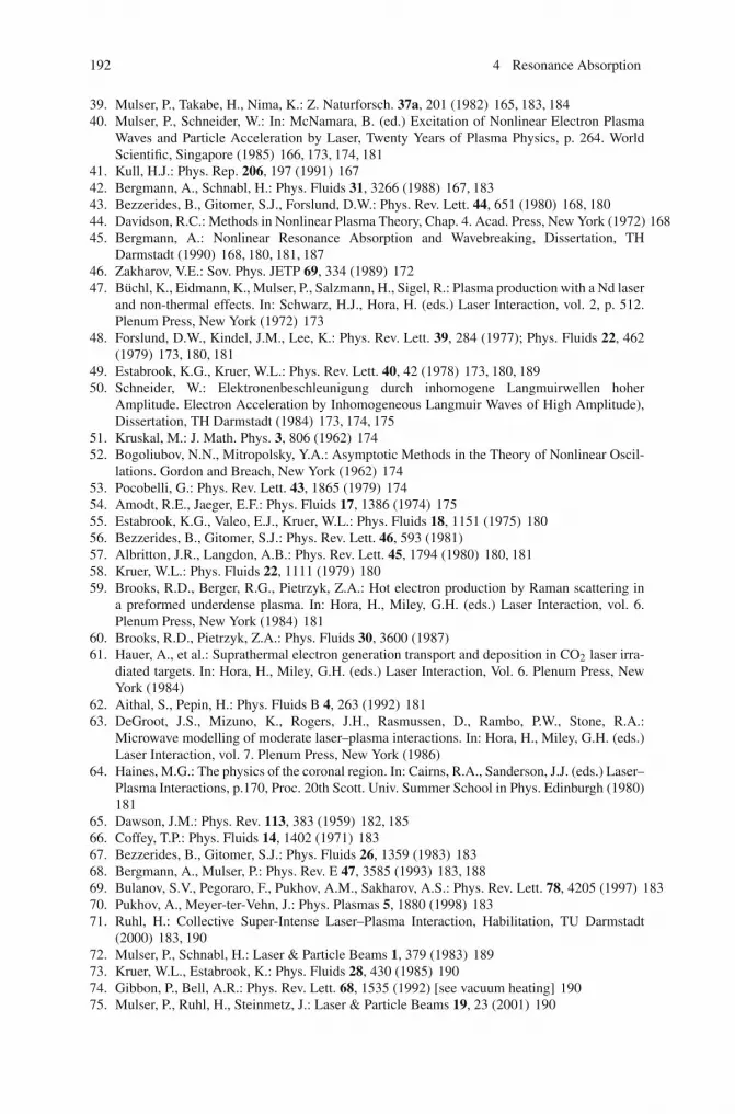
192 4 Resonance Absorption
39. Mulser, P., Takabe, H., Nima, K.: Z. Naturforsch. 37a, 201 (1982) 165, 183, 18440. Mulser, P., Schneider, W.: In: McNamara, B. (ed.) Excitation of Nonlinear Electron Plasma
Waves and Particle Acceleration by Laser, Twenty Years of Plasma Physics, p. 264. WorldScientific, Singapore (1985) 166, 173, 174, 181
41. Kull, H.J.: Phys. Rep. 206, 197 (1991) 16742. Bergmann, A., Schnabl, H.: Phys. Fluids 31, 3266 (1988) 167, 18343. Bezzerides, B., Gitomer, S.J., Forslund, D.W.: Phys. Rev. Lett. 44, 651 (1980) 168, 18044. Davidson, R.C.: Methods in Nonlinear Plasma Theory, Chap. 4. Acad. Press, New York (1972) 16845. Bergmann, A.: Nonlinear Resonance Absorption and Wavebreaking, Dissertation, TH
Darmstadt (1990) 168, 180, 181, 18746. Zakharov, V.E.: Sov. Phys. JETP 69, 334 (1989) 17247. Büchl, K., Eidmann, K., Mulser, P., Salzmann, H., Sigel, R.: Plasma production with a Nd laser
and non-thermal effects. In: Schwarz, H.J., Hora, H. (eds.) Laser Interaction, vol. 2, p. 512.Plenum Press, New York (1972) 173
48. Forslund, D.W., Kindel, J.M., Lee, K.: Phys. Rev. Lett. 39, 284 (1977); Phys. Fluids 22, 462(1979) 173, 180, 181
49. Estabrook, K.G., Kruer, W.L.: Phys. Rev. Lett. 40, 42 (1978) 173, 180, 18950. Schneider, W.: Elektronenbeschleunigung durch inhomogene Langmuirwellen hoher
Amplitude. Electron Acceleration by Inhomogeneous Langmuir Waves of High Amplitude),Dissertation, TH Darmstadt (1984) 173, 174, 175
51. Kruskal, M.: J. Math. Phys. 3, 806 (1962) 17452. Bogoliubov, N.N., Mitropolsky, Y.A.: Asymptotic Methods in the Theory of Nonlinear Oscil-
lations. Gordon and Breach, New York (1962) 17453. Pocobelli, G.: Phys. Rev. Lett. 43, 1865 (1979) 17454. Amodt, R.E., Jaeger, E.F.: Phys. Fluids 17, 1386 (1974) 17555. Estabrook, K.G., Valeo, E.J., Kruer, W.L.: Phys. Fluids 18, 1151 (1975) 18056. Bezzerides, B., Gitomer, S.J.: Phys. Rev. Lett. 46, 593 (1981)57. Albritton, J.R., Langdon, A.B.: Phys. Rev. Lett. 45, 1794 (1980) 180, 18158. Kruer, W.L.: Phys. Fluids 22, 1111 (1979) 18059. Brooks, R.D., Berger, R.G., Pietrzyk, Z.A.: Hot electron production by Raman scattering in
a preformed underdense plasma. In: Hora, H., Miley, G.H. (eds.) Laser Interaction, vol. 6.Plenum Press, New York (1984) 181
60. Brooks, R.D., Pietrzyk, Z.A.: Phys. Fluids 30, 3600 (1987)61. Hauer, A., et al.: Suprathermal electron generation transport and deposition in CO2 laser irra-
diated targets. In: Hora, H., Miley, G.H. (eds.) Laser Interaction, Vol. 6. Plenum Press, NewYork (1984)
62. Aithal, S., Pepin, H.: Phys. Fluids B 4, 263 (1992) 18163. DeGroot, J.S., Mizuno, K., Rogers, J.H., Rasmussen, D., Rambo, P.W., Stone, R.A.:
Microwave modelling of moderate laser–plasma interactions. In: Hora, H., Miley, G.H. (eds.)Laser Interaction, vol. 7. Plenum Press, New York (1986)
64. Haines, M.G.: The physics of the coronal region. In: Cairns, R.A., Sanderson, J.J. (eds.) Laser–Plasma Interactions, p.170, Proc. 20th Scott. Univ. Summer School in Phys. Edinburgh (1980)181
65. Dawson, J.M.: Phys. Rev. 113, 383 (1959) 182, 18566. Coffey, T.P.: Phys. Fluids 14, 1402 (1971) 18367. Bezzerides, B., Gitomer, S.J.: Phys. Fluids 26, 1359 (1983) 18368. Bergmann, A., Mulser, P.: Phys. Rev. E 47, 3585 (1993) 183, 18869. Bulanov, S.V., Pegoraro, F., Pukhov, A.M., Sakharov, A.S.: Phys. Rev. Lett. 78, 4205 (1997) 18370. Pukhov, A., Meyer-ter-Vehn, J.: Phys. Plasmas 5, 1880 (1998) 18371. Ruhl, H.: Collective Super-Intense Laser–Plasma Interaction, Habilitation, TU Darmstadt
(2000) 183, 19072. Mulser, P., Schnabl, H.: Laser & Particle Beams 1, 379 (1983) 18973. Kruer, W.L., Estabrook, K.: Phys. Fluids 28, 430 (1985) 19074. Gibbon, P., Bell, A.R.: Phys. Rev. Lett. 68, 1535 (1992) [see vacuum heating] 19075. Mulser, P., Ruhl, H., Steinmetz, J.: Laser & Particle Beams 19, 23 (2001) 190

Chapter 5The Ponderomotive Force and NonresonantEffects
A momentum flux is associated with all varieties of plasma waves: electrostatic,electromagnetic, acoustic. As a consequence, a force is transmitted from the waveto a plasma element whenever the momentum flow changes there either in space orin time. As early as 1861 James Clerk Maxwell found out that a light beam of fluxdensity I , when impinging normally upon a surface of reflectivity R in vacuo, exertsthe pressure
pL = (1+ R)I
c(5.1)
This is a global force. In physics in general, and in plasma physics in particular,expressions for the radiation force f p on a single charged particle or on a unitvolume, i.e. a force density π , are needed. They are secular forces, in contrast tothe rapidly changing oscillating force of an electric wave which causes the quivermotion of the electrons and, as far as they are of electric origin, they are given thename ponderomotive force (density). The expressions “light pressure”, “radiationpressure”, or “wave pressure” are also in use. In the following we treat them all asequivalent. f p and π originate from the nonlinearity of the momentum equation ofthe particles.
There are two kinds of ponderomotive forces, one which has its origin in the sin-gle particle motion and another one which is caused by collective motions inducedin the plasma. As a consequence the first kind leads to a force density π0 whichis proportional to the average particle density whereas the second type, indicatedby π t , is proportional to the fluctuation level changes of particle densities. In thetreatment given here the most general expression for the force on a single particlein a periodic electric field is deduced from the cycle-averaged relativistic singleparticle Lagrangian. The collective ponderomotive force density is derived fromgeneral momentum conservation in an unmagnetized plasma which enables us togive it a very immediate physical interpretation.
A ponderomotive force arises whenever the radiation or wave field in questionchanges in space. This force has been recognized as a quantity of central importancein physical phenomena such as the free electron laser [1, 2], particle acceleration[3–5], stabilization of magnetized plasmas [6–8], trapping and cooling of atoms
P. Mulser, D. Bauer, High Power Laser–Matter Interaction, STMP 238, 193–227,DOI 10.1007/978-3-540-46065-7_5, C© Springer-Verlag Berlin Heidelberg 2010
193

194 5 The Ponderomotive Force and Nonresonant Effects
[9–11], dressed atom model [12], multiphoton ionization [13], and chaotic plasmadynamics [14]. It is of particular relevance to the dynamics and nonlinear optics itinduces in laser plasmas. Whereas collisional absorption of laser light and electronicheat diffusion create plasma clouds of smooth density and temperature distributionsthe ponderomotive force has the tendency to modulate the plasma and to impressa whole variety of structures on it. At the critical points and caustics step- andplateau-like density profile modifications are induced which in turn tend to modifycollisional and resonance absorption [15–17]. Inside the plasma density structuresappear whenever the electric field amplitude of the laser beam or any strong plasmawave is nonuniform owing to inhomogeneities in the single beam or wave itself,or because the electric field amplitude is periodically modulated by the superposi-tion of different modes [18]. The density structures may be nonresonant; then theyappear as the following phenomena: static plasma density modifications, nonreso-nant self-focusing, filamentation, striation, modulational and oscillating two-streaminstabilities. Or they are resonant and are recognized as stimulated Brillouin andRaman scattering or two-plasmon and parametric decay instabilities. Most nonreso-nant phenomena are treated in this chapter, whereas Chap. 6 is mainly dedicated tothe class of resonantly induced ponderomotive effects.
5.1 Ponderomotive Force on a Single Particle
There are entire classes of relevant particle trajectories which can be decomposedinto two or more motions having distinct time scales. Often there is a fast, nearlyperiodic component superposed on a smooth orbit of secular character. Prominentexamples of this kind are the dynamics of a charged particle gyrating in a magneticmirror and the oscillatory motion of an electron subject to a nearly periodic hf force.Frequently, one is not interested in all details of the trajectories, but the knowledge ofthe averaged motion, i.e. its secular component (slow time scale) is of vital interest(e.g. particle acceleration, asymptotic dynamics, transport theory). In a magneticmirror the secular dynamics is represented by the gyrocenter motion, in the case ofa point charge oscillating in an electr(omagnet)ic field the secular component is theoscillation center motion. For an electromagnetic field E(x, t) of frequency ω andarbitrary space dependence E(x),
E(x, t) = �E(x)e−iωt , (5.2)
it was shown [19–23] that the oscillation center dynamics of a charge q is governedby the force f p,
f p = −∇Φp, Φp = q2
4mω2E E
∗. (5.3)
The ponderomotive potential Φp is obtained from a first order perturbation analysisof the Lorentz force (see next section) and is therefore subject to the usual smallness
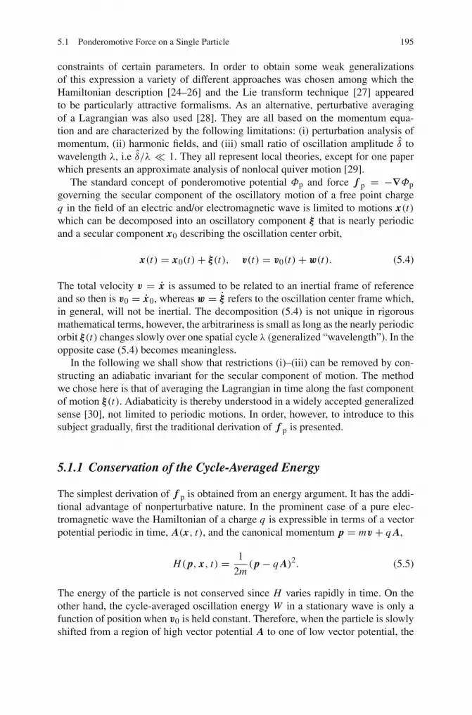
5.1 Ponderomotive Force on a Single Particle 195
constraints of certain parameters. In order to obtain some weak generalizationsof this expression a variety of different approaches was chosen among which theHamiltonian description [24–26] and the Lie transform technique [27] appearedto be particularly attractive formalisms. As an alternative, perturbative averagingof a Lagrangian was also used [28]. They are all based on the momentum equa-tion and are characterized by the following limitations: (i) perturbation analysis ofmomentum, (ii) harmonic fields, and (iii) small ratio of oscillation amplitude δ towavelength λ, i.e δ/λ � 1. They all represent local theories, except for one paperwhich presents an approximate analysis of nonlocal quiver motion [29].
The standard concept of ponderomotive potential Φp and force f p = −∇Φpgoverning the secular component of the oscillatory motion of a free point chargeq in the field of an electric and/or electromagnetic wave is limited to motions x(t)which can be decomposed into an oscillatory component ξ that is nearly periodicand a secular component x0 describing the oscillation center orbit,
x(t) = x0(t)+ ξ(t), v(t) = v0(t)+ w(t). (5.4)
The total velocity v = x is assumed to be related to an inertial frame of referenceand so then is v0 = x0, whereas w = ξ refers to the oscillation center frame which,in general, will not be inertial. The decomposition (5.4) is not unique in rigorousmathematical terms, however, the arbitrariness is small as long as the nearly periodicorbit ξ(t) changes slowly over one spatial cycle λ (generalized “wavelength”). In theopposite case (5.4) becomes meaningless.
In the following we shall show that restrictions (i)–(iii) can be removed by con-structing an adiabatic invariant for the secular component of motion. The methodwe chose here is that of averaging the Lagrangian in time along the fast componentof motion ξ(t). Adiabaticity is thereby understood in a widely accepted generalizedsense [30], not limited to periodic motions. In order, however, to introduce to thissubject gradually, first the traditional derivation of f p is presented.
5.1.1 Conservation of the Cycle-Averaged Energy
The simplest derivation of f p is obtained from an energy argument. It has the addi-tional advantage of nonperturbative nature. In the prominent case of a pure elec-tromagnetic wave the Hamiltonian of a charge q is expressible in terms of a vectorpotential periodic in time, A(x, t), and the canonical momentum p = mv + q A,
H( p, x, t) = 1
2m( p− q A)2. (5.5)
The energy of the particle is not conserved since H varies rapidly in time. On theother hand, the cycle-averaged oscillation energy W in a stationary wave is only afunction of position when v0 is held constant. Therefore, when the particle is slowlyshifted from a region of high vector potential A to one of low vector potential, the
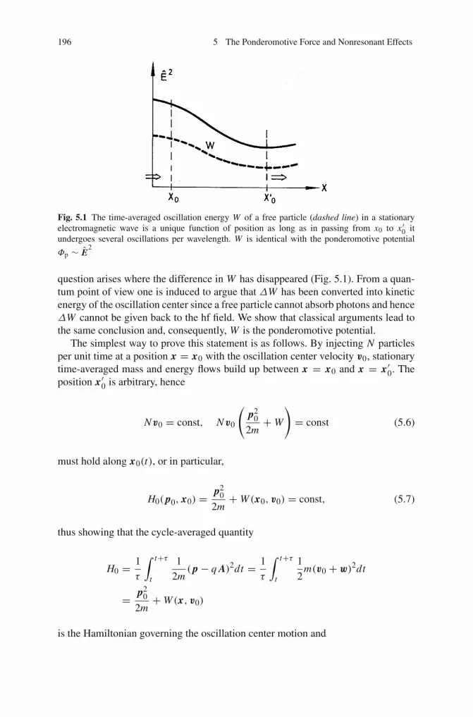
196 5 The Ponderomotive Force and Nonresonant Effects
Fig. 5.1 The time-averaged oscillation energy W of a free particle (dashed line) in a stationaryelectromagnetic wave is a unique function of position as long as in passing from x0 to x ′0 itundergoes several oscillations per wavelength. W is identical with the ponderomotive potential
Φp ∼ E2
question arises where the difference in W has disappeared (Fig. 5.1). From a quan-tum point of view one is induced to argue that ΔW has been converted into kineticenergy of the oscillation center since a free particle cannot absorb photons and henceΔW cannot be given back to the hf field. We show that classical arguments lead tothe same conclusion and, consequently, W is the ponderomotive potential.
The simplest way to prove this statement is as follows. By injecting N particlesper unit time at a position x = x0 with the oscillation center velocity v0, stationarytime-averaged mass and energy flows build up between x = x0 and x = x′0. Theposition x′0 is arbitrary, hence
Nv0 = const, Nv0
(p2
0
2m+W
)= const (5.6)
must hold along x0(t), or in particular,
H0( p0, x0) = p20
2m+W (x0, v0) = const, (5.7)
thus showing that the cycle-averaged quantity
H0 = 1
τ
∫ t+τ
t
1
2m( p− q A)2dt = 1
τ
∫ t+τ
t
1
2m(v0 + w)2dt
= p20
2m+W (x, v0)
is the Hamiltonian governing the oscillation center motion and

5.1 Ponderomotive Force on a Single Particle 197
Φp = W =⟨
1
2mw2
⟩(5.8)
is the ponderomotive potential of a transverse wave. The dependence of W on v0 in(5.7) takes care of the Doppler effect.
A formal, but physically less immediate proof of (5.7) is obtained from dimen-sional analysis. The quantity H0 merely depends on m, v0 and the scalar functionW (x, v0). From these three variables no quantity with the dimension of time can beconstructed. Hence, according to Buckingham’s π theorem, H0 is time-independentand H0 = E = const holds along each trajectory. As a consequence, H0( p0, x) isthe Hamiltonian governing the oscillation center motion, with the desired general-ized ponderomotive potential Φp = W .
The concept adopted here is directly subject to a generalization in different direc-tions:
I. For an arbitrarily strong monochromatic propagating electromagnetic wave
W = mc2
{(1+ q2
αm2c2ω2E E
∗)1/2
− 1
}, f p = −∇W, (5.9)
holds for the oscillation energies corresponding to plane (α = 2) and circular(α = 1) polarization [31, 32]. For moderate fields Taylor expansion of this expres-sion leads back to Φp of (5.3). For a detailed derivation see Sect. 8.2.1.
II. Next a point particle is considered, with an internal degree of freedom that is aharmonic oscillator in dipole approximation,
δ + ω20δ =
q
μE(x)e−iωt ; μ = m1m2/(m1 + m2). (5.10)
The averaged oscillation energy is
W =⟨
1
2μδ
2⟩+ Epot = q
4μ
ω2 + ω20
(ω2 − ω20)
2E E
∗.
In determining Φp one has to keep in mind that when the field is switched on theoscillator gains internal energy Ein also and that the forces producing this energyare internal forces and as such, by definition, cancel each other. Thus Φp is given by
Φp = W − 〈Ein〉 = W − Epot,max = W − q2
4μ
2ω20
(ω2 − ω20)
2E E
∗
= q2
4μ(ω2 − ω20)
E E∗. (5.11)

198 5 The Ponderomotive Force and Nonresonant Effects
ω0
ν>0
ν = 0
ω
fp
Fig. 5.2 A harmonic oscillator with eigenfrequency ω0 and a charged point particle in a constantperpendicular magnetic field B0 (cyclotron frequency ωc) are shifted towards decreasing electricfield amplitude when its frequency ω exceeds ω0 and ωc (special case: free particle with ω0 =ωc = 0); it moves into opposite direction if ω < ω0, ωc holds. At resonance (ω = ω0, ωc) fp iszero. Solid curve: damped oscillator, dashed curve: oscillator without damping
The same result is obtained by solving (5.10) up to the first order and determin-ing its secular component. However, the procedure used here is shorter and moregeneral, e.g. a force may result from constant E but changing frequencies ω, ω0.Φp = W − 〈Ein〉 also holds for anharmonic E fields or when the Lorentz force isincluded . For ω0 < ω the oscillator behaves like a free particle, i.e. f p tries to driveit into a region of decreasing field amplitude. For ω0 > ω it moves into the oppositedirection. By introducing a damping term it is shown that at exact resonance f preduces to zero (Fig. 5.2). Φp is identical with what in quantum mechanics is calledthe expectation value of the interaction energy Eint.
It can be shown that (5.11) is correct also for a quantum oscillator [33]. If ω0 isproperly chosen and an effective oscillator strength is inserted the expression alsoapplies to the radiation force on an atom with negligible degeneracy. Φp in this caseis identical to the level shift ΔE of the linear dynamical Stark shift by the electricwave. If degeneracy is present, (5.11) changes accordingly. At first glance one mightargue that (5.11) is not useful for a fully ionized plasma in which all electrons arefree. However, in the next chapter it will become clear that it is just this expressionwhich enables one to understand the difference between the oscillating two-streamand the parametric decay instability.
III. It is instructive to generalize f p to include the case of a charged point particlein a static magnetic field B0. In addition, there exist important applications of thistype of situation in magnetically confined plasmas. With E(x, t) in the x-directionand B0 parallel to z one has to set
W = 1
2m〈v2
x + v2y〉, 〈V 〉 = μB0.
5.1 Ponderomotive Force on a Single Particle 199
μB0 = AI B0 (μ magnetic moment, A cross section of the closed orbit, I current)is the “inner” energy of the orbiting particle configuration which has to be sub-tracted since, by definition, internal forces do not contribute to f p. Specializing toE = Ex ∼ e−iωt yields in analogy to (5.10) and (5.11)
vx + ω2cvx = −iω
q
mEx , vy = −i
ωc
ωvx , ωc = q
mB;
Φp = W − 〈V 〉 = q2
4m
ω2 + ω2c
(ω2 − ω2c )
2E E
∗ − q2
4m
2ω2c
(ω2 − ω2c )
2E E
∗
= q2
4m(ω2 − ω2c )
E E∗, (5.12)
in agreement with results obtained from the momentum equation with weak fields[34]. The cyclotron frequency ωc takes the place of ω0.
In the three cases of a free particle, a harmonic oscillator and a particle in a staticmagnetic field, considered here, the ponderomotive potential can be written with thehelp of the dipole moment p = qδ as
Φp = Eint =⟨−1
2pE⟩.
If ω0 > ω, p is parallel to E and the oscillator moves into the direction of increas-ing field; if ω0 < ω, p is anti-parallel to E; at resonance the phase shift is π/2(Fig. 5.2).
When two or more plane waves are coherently superposed, a variety of spatialstructures of f p can be produced which may lead to induced striation or vortices.Vortices have been experimentally observed with neutral atoms in two crossed, nearresonant standing waves [35].
5.1.2 The Standard Perturbative Derivation of the Force
Despite its inherent limitations this procedure may provide an alternative, detailed,physical insight in how the secular force f p originates. It starts from the Lorentzequation of a charged particle in a monochromatic electromagnetic field of the form(5.2),
mdv
dt= q(E + v × B),
and makes use of the decomposition (5.4). Under the restriction that the oscillationamplitude ξ is much smaller than the local wavelength λ(x0), i.e. ξ � λ(x0), theLorentz equation may be linearized in ξ and solved separately,

200 5 The Ponderomotive Force and Nonresonant Effects
mdv
dt� m
[∂w
∂t+ (v0∇)w
]= q [E(x0)+ v0 × B(x0)] .
In general E(x) is the superposition of a large set of modes,
E(x) =∑
{k}Ekeikx .
For a single mode holds
wk(t) = iq
mωk(Ek + v0 × Bk), ωk = ω − v0k.
The Doppler shift Δωk = v0k originates from the convective derivative (v0∇)w.For nonrelativistic temperatures all Δωk and v0 × Bk can be chosen small so that allFourier components wk superpose to yield
w(t) = iq
mωE(x0)e
−iωt = q
mA(x0)e
−iωt ,
E = −∂t A, A vector potential. In the next order from the Lorentz equation v0(t) iscalculated, the time variation of which determines f p,
f p = mdv0
dt= q
{E(x0 + ξ(t))+ w(t)× B(x0)
}0.
The bracket contains terms varying with 2ω and zero frequency. Therefore the sub-script “0” has been added to indicate that in determining the secular force f p the 2ω-term has to be suppressed. Taylor expansion of E in ξ = iw/ω, using B = ∇ × A,and observing that physical quantities have to be real leads directly to
q{E + w × B}0 = − q2
4m{( A
∗∇) A+ A∗ ×∇ × A+ c.c.}
= − q2
4m∇( A A
∗).
Hence, f p is the gradient of a quantity which can be interpreted as a potential Φp,the ponderomotive potential given by (5.3). In a transverse plane wave (w∇)E iszero; if E is longitudinal (e.g. an electron plasma wave) B is zero and f p arisesentirely from (w∇)E.
Expression (5.3) for Φp is valid when damping can be ignored. In the presenceof a linear damping ν according to (2.23) the following expression for f p is foundstraightforwardly in terms of E = Er + i Ei [36],

5.1 Ponderomotive Force on a Single Particle 201
Fig. 5.3 In an oscillating longitudinal electric field a charged particle experiences a drift in thedirection of decreasing wave amplitude. The drift is independent of the sign of charge. x0 startingpoint; x1, x2, x3 turning points. In a transverse wave the drift is caused by the Lorentz force
f p = −q2
4meω2(1+ ν2
ω2 )
{∇ E E
∗ + 2ν
ω
[Ei × (∇ × Er )− Er × (∇ × Ei )
]},
(5.13)ω,ν = const, and ∇ × f p differs from zero in this case.
In terms of the momentum equation the physical interpretation of the pondero-motive force f p is as follows. Let us first assume a pure electrostatic wave in the
x-direction of the form E(x)e−iωt with decreasing amplitude E(x) (Fig. 5.3). A freeelectron is shifted by the E-field from its original position x0 to x1. From there it isthen accelerated to the right until it has passed x0. From that moment on the electronis decelerated by the reversed E-field and is stopped at position x2. If x ′0 designatesthe position in which the field is reversed (x ′0 > x0), the deceleration interval x2−x ′0is larger than that of acceleration since on the right hand side of x0 the E-field isweaker and therefore a longer distance is needed to take away the energy gained inthe former quarter period of oscillation. On its way back the electron is stopped inthe region of higher amplitude; the turning point is shifted from x1 to x3 into thedirection of decreasing wave amplitude E(x). In an (inhomogeneous) medium thisdrift produces, by charge separation, a static E-field which transmits the force tothe ions. Since this consideration is based only on energy and work – there was noneed to specify the field direction with respect to the particle speed – it follows thatthe drift (or force) is independent of the sign of charge: positrons would drift in thesame direction. In the case of a plane electromagnetic wave the drift is caused bythe v × B force which also acts along the direction of propagation.
5.1.3 Rigorous Relativistic Treatment
In connection with the development of ultrashort super-intense laser beams a realneed for relativistic expressions for f p, not bound by the above-mentioned con-straints (i)–(iii) arises. As we show in this section the most general result for a freecharge q is obtained again from a cycle-averaging method. However, since such
202 5 The Ponderomotive Force and Nonresonant Effects
a procedure does not preserve the canonical character of the Hamiltonian [37] aLagrangian formulation will be used [14].
The relativistic Lagrangian L(x, v, t), v = dx/dt , of a charge q in an arbitraryelectromagnetic field E = −∇Φ − ∂A/∂t is given by
L(x, v, t) = −mc2
γ+ qv A− qΦ, γ = (1− v2/c2)−1/2. (5.14)
When an oscillation center exists, the transformation to action-angle variables S =S(x, t), η = η(x, t), is possible (e.g., ψ(x, t) = ∫
(k dx − ω dt) in the case ofa traveling monochromatic wave). The action S and the angle η are both Lorentzinvariant. The motion of the particle is governed by Hamilton’s principle,
δS = δ
∫ η2
η1
L(x(η), v(η), t (η))dt
dηdη = 0. (5.15)
From the Lorentz invariance of S and η it follows that the Lagrangian L(η) =L(dη/dt)−1 is invariant with respect to a change of the inertial reference system.Assuming that η is normalized to 2π for one full cycle or period of motion, thecycle-averaged Lagrangian L0,
L0(η) = 1
2π
∫ η+2π
η
L(η′)dη′, (5.16)
depending only on the secular (i.e., oscillation center) coordinates x0, v0 throughη, is defined. The oscillation center motion is governed by the Lagrange equationsof motion,
d
dt
∂L0
∂v0− ∂L0
∂x0= 0, (5.17)
with L0 = L0dη/dt . To demonstrate this assertion we prove the following theorem.
Theorem 1 The validity of (5.15) implies
δ
∫ η f
ηi
L0(η)dη = o(N−1), (5.18)
where N = (η f − ηi )/2π is the number of cycles over which L0 undergoes anessential change. The symbol o(N−1) means “vanishes at least with order 1/N”.
Proof Let the variation be an arbitrary piecewise continuous function Δ(η). Thenth cycle starts at η = ηn , where for brevity we use the symbols Δn = Δ(ηn),∂L0/∂ηn = (∂L0/∂η)η=ηn . If the same quantities refer to an intermediate pointη ≤ ηa ≤ ηn + 2π we write Δa and ∂L0/∂ηa and omit the index n for the interval.To leading order the following holds:

5.1 Ponderomotive Force on a Single Particle 203
∣∣∣∣δ∫ η f
ηi
L0dη
∣∣∣∣ =∣∣∣∣∫ η f
ηi
δ(L0 − L)dη∣∣∣∣
=∣∣∣∣∫ η f
ηi
[L0(η +Δ)− L(η +Δ)] dη −∫ η f
ηi
[L0(η)− L(η)] dη
∣∣∣∣
≤∑
n
∣∣∣∣∣
∫ ηn+2π
ηn
L0(η +Δ)dη − 2πL0(ηn +Δn)
−∫ ηn+2π
ηn
L0(η)dη − 2πL0(ηn)
∣∣∣∣∣
=∑
n
∣∣∣∣∣
∫ ηn+2π
ηn
∂L0
∂ηnΔ(η)dη − 2π
∂L0
∂ηnΔn
∣∣∣∣∣
= 2π∑
n
∣∣∣∣∂L0
∂ηaΔa − ∂L0
∂ηnΔn
∣∣∣∣ .
In the last step the mean value theorem is used. The function Δ(η) is arbitrary.Therefore at η = ηn, Δn = Δa can be chosen without affecting Δa. With thissubstitution the leading order gives the result
∣∣∣∣δ∫ η f
ηi
L0dη
∣∣∣∣ ≤ (2π)2∑
n
∣∣∣∣∂2L0
∂η2nΔa
∣∣∣∣ ≤ (2π)2 N max
∣∣∣∣∂2L0
∂η2n
∣∣∣∣×max |Δa|.
In this last step it is essential that ∂L0/∂η is a smooth function (in contrast to ∂L/∂η,which is generally not). Now, N = min(1/2π)|L0 max/(∂L0/∂ηn)| is chosen; i.e.,over N cycles L0 max changes at most by L0. It follows that
∣∣∣∣δ∫ η f
ηi
L0dη
∣∣∣∣ ≤|L0 max|
N×max |Δ|. (5.19)
Performing the variation of this inequality leads to (5.17) with the 0 replaced by afunction f not larger than |L0 max| ×max |Δ|/N 2.
In order to understand what inequality (5.19) means let us specialize to acase of the averaged Lagrangian L0 not depending explicitly on time. Then theHamiltonian H0 = p0v0 − L0(x0, v0), where L0 = −L0(ω − kv0), owing tod H0/dt = ∂H0/∂t = −∂L0/∂t = 0, expresses energy conservation
H0 = E = const.
A straightforward estimate shows that the uncertainty f in (5.17) leads to an energyuncertainty ΔH0/H0
<∼ 2π/N . This means that (5.17) is adiabatically zero and thetotal cycle-averaged energy is an adiabatic invariant in the rigorous mathematicalsense in agreement with Arnold’s definition [30]. For N → ∞ (5.17) becomesexact. This is the mathematical proof of assertion (5.7) which was established there
204 5 The Ponderomotive Force and Nonresonant Effects
by physical arguments. Furthermore, physical arguments were used for expressions(5.11) and (5.12). By making use of (5.15) both expressions follow without usingfurther arguments since nonrelativistically L(x, v) = 1/2mv2−V (x), V (x) poten-tial energy, and L(x, v) = 1/2mv2 − V (x) + qv A in the presence of a magneticfield.
The relativistic Hamiltonian of point charge in the electromagnetic field followsform (5.14),
H = pv − L ={
m2c4 + c2( p− q A)2}1/2 +Φ, (5.20)
with the canonical momentum p = ∂L/∂v = γmv + q A. Its numerical value isthe total energy E = γmc2 + Φ. Considering a monochromatic wave in vacuumwe can set Φ = 0. This motion is exactly solvable with the result for the oscillationenergy given by (5.9). If the effective mass meff = L0γ0(dη/dt)/c2 is introduced,L0 = L0dη/dt shows that, in an arbitrary inertial frame in which the oscillationcenter moves at speed v0, L0 and H0 are those of a free particle with space andtime dependent mass meff,
L0(x0, v0, t) = −meffc2
γ0, H0(x0, p0, t) = γ0meffc
2; (5.21)
γ0 =(
1− v20
c2
)−1/2
, p0 = γ0meffv0.
Expressions (5.21) hold in any electromagnetic field in vacuum in which an oscil-lation center can be defined. In the special case of (5.9) meff = (1 + q2 A ·A∗/αm2c2)1/2m.
In the oscillation center system, i.e., in the inertial frame in which at the instantt v0(t) = 0 holds, the ponderomotive force follows from (5.17) and (5.21):
f Np ≡
d p0
dτ= ∂L0
∂x0= −c2∇meff. (5.22)
For the meaning of f Np and its transformation to another reference system see
Sect. 8.1.To see the power of the Lagrangian formulation, (5.17), we calculate f p in a non-
relativistic Langmuir wave of the form E(x, t) = E(x, t) sin(kx − ωt) with slowlyvarying amplitude E . In lowest order the potential is Φ(x, t) = (E/k) cos(kx−ωt)and L = mv2/2 − qΦ. In the frame comoving with x0 the particle sees theDoppler-shifted frequency Ω = ω− kv0 (plus higher harmonics that are not essen-tial here). With the periodic excursion ξ(t) around x0 the potential is Φ(x, t) �Φ(x0, t)+ ξ(t)∂Φ/∂x0. From this L0 = mv2
0/2−α E2/Ω2, α = q2/4m, results in
lowest order. With this Lagrangian it follows from (5.17) for E = E(x) (no explicittime dependence) that

5.1 Ponderomotive Force on a Single Particle 205
fp = mdv0
dt= −α (1− V0)(1− 3V0)
ω2(1− V0)4 − 6α E2/mv2ϕ
∂
∂xE2. (5.23)
In the last expression V0 is the oscillation center velocity normalized to the phasevelocity vϕ = ω/k, V0 = v0/vϕ . Equation (5.23) shows that fp changes sign whenthe particle is injected into the Langmuir wave with a velocity v0 exceeding vϕ/3.In regions where the standard expression for fp, (5.3), always exhibits repulsion themore exact treatment can lead to attraction.
Equation (5.23) was also derived in a more formal but physically less transparentmanner in [26]. Uphill acceleration in an electron plasma wave of increasing ampli-tude E(x) is confirmed by the numerical solution of the exact equation of motion(Fig. 5.4). If E(x) grows indefinitely the exact ponderomotive force changes signagain, and the particle stops and is finally reflected; the corresponding path in phasespace exhibits a hysteresis. Uphill acceleration, occasionally observed in anothercontext of wave particle interaction [38], is a general ponderomotive phenomenon.It should also be mentioned that for the electrostatic wave considered here uphillacceleration identical with the result of Fig. 5.4 follows from the adiabatic invariant(4.31) for nontrapped particles (see [39] and Chap. 4).
The results can be summarized as follows: (i) When an oscillation center ofmotion exists, the invariant cycle-averaged Lagrangian describes the ponderomotivemotion in arbitrary strong fields. (ii) The ponderomotive force in a monochromatictraveling, locally plane wave of arbitrary strength in any reference system can beexpressed analytically. (iii) In a longitudinal wave, uphill acceleration and phase
Fig. 5.4 Normalized kinetic energy V 20 /2 is shown as a function of Φp/mev
2ϕ from (5.3) for the
linearly increasing field 2.5× 10⁻³ X sin(X − T ) and injection velocities V0 = 1/3 (lower curves)and V0 = 0.43 (upper curves). The motion shows a pronounced hysteresis in phase space owingto different acceleration in comotion and countermotion

206 5 The Ponderomotive Force and Nonresonant Effects
space hysteresis may occur. (iv) The ponderomotive force on particles with internaldegrees of freedom and the influence of dissipation (radiation losses, friction) onthe ponderomotive force are best understood from conservation of the field-particleinteraction energy. A detailed study of the validity of the ponderomotive conceptfor free electrons in finite laser pulses was presented in [40]. For an extension ofponderomotively induced motion for ω→ 0 see Sect. 8.2. Finally we want to pointout that at relativistic energies cycle-averaging in the time parameter t becomesincorrect; rather one has to switch to an angle variable η in order to guarantee aLorentz-invariant definition of the oscillation center. The problem is similar to thecorrect definition of the relativistic center of mass discussed in Sect. 8.1.6.
5.2 Collective Ponderomotive Force Density
5.2.1 Bulk Force
The force density exerted by an electric wave on the bulk of the plasma is propor-tional to the time averaged electron particle density n0. Thus π is given by π0,
π0 = n0 f p, or π0 = −n0∇Φp, (5.24)
respectively, with Φp taken from the preceding section. In the weak field approxi-mation of Sect. 5.1.2 π0 is given with Φp from (5.11),
π0 = −ε0
4
ω2p
μ∇ E E
∗
ω2 − ω20
. (5.25)
For free electrons ω0 is zero; for free electrons in a constant magnetic field in theabove configuration ω0 is replaced by ωc and μ = m.
5.2.2 The Force Originating from Induced Fluctuations
It would be most desirable now to obtain the collective ponderomotive force densityπ t also from an energy principle or an action integral. Since a sufficiently generalderivation of this kind does not seem to exist so far, the following considerations arebased on momentum conservation. By definition the ponderomotive force densityπ is a secular, i.e. low frequency force which originates from a high frequencytransverse or longitudinal electric field and applies to the one-fluid model. Thus,when ρ0 = 〈ρ(t)〉 and v0 = 〈v(t)〉 are the density and velocity of a volume ele-ment averaged over the high frequency oscillations, π0 is defined by the equation ofmotion

5.2 Collective Ponderomotive Force Density 207
ρ0dv0
dt= −∇(pe + pi )+ f 0 + π0 (5.26)
where pe, pi are the electronic and ionic thermal pressures and f 0 is any low fre-quency force (electric and magnetic, gravitational, viscous, frictional, etc.). For theconcept of ponderomotive force to apply it is important that the spectra of fast andslow motions in ρv = ρivi+ρeve are well separated from each other. When includ-ing all forces f , f = f 0+ f h, where f h originates from the high frequency fieldsthe general momentum conservation equation in the one-fluid model is
∂
∂tρv +∇(ρvv + p I) = f .
The momentum flow density T = ρvv + p I, p = pe + pi , is a second rank tensorwith the components Tkl = ρvkvl + pδkl . Hence, by comparison with (5.26) π t
results as follows,
π t =⟨∂
∂tρv +∇(ρvv + p I)− f h
⟩− ρ0
dv0
dt. (5.27)
In the absence of ionic resonances (i.e., no static magnetic fields)
ρivi = mi ni0vi0, ve0 = vi0,
ρeve = me(ne0 + ne1 + ne2 + . . . . .)(ve0 + ve1 + ve2 + . . . . .); (5.28)
holds. The indices 1, 2, etc. indicate the Fourier components of frequencies ω, 2ω,etc. induced by the high frequency electric or electromagnetic field
E(x, t) = E(x, t)e−iωt . (5.29)
E(x, t) is the amplitude slowly varying in space and time. Inserting the quantities(5.28) into (5.27) leads to
(mi ni0 + mene0)〈∇(ve1ve1 + ve2ve2 + . . . . . .)− f h〉 = π0,
where the brackets 〈〉 contain, in addition, all sums of products vejvek with an evennumber l = j + k and j < k. The first nonvanishing term contributing to thecollective force π t originates from ne1ve1 in 〈∂ρv/∂t〉. Since this is also the leadingterm, to lowest order follows
π t =⟨∂
∂t(mene1ve1)
⟩. (5.30)
There is no corresponding contribution from the flux term since 〈mene1ve1ve1〉 iszero. With the help of the electronic equation of motion,
208 5 The Ponderomotive Force and Nonresonant Effects
∂ve1
∂t= − e
meE(x, t)e−iωt ,
for ve1 and displacement δe1 one obtains
ve1 = ie
meωe−iωt
(1− i
ω
∂
∂t
)E(x, t),
δe1 = e
meω2e−iωt
(1− 2i
ω
∂
∂t
)E(x, t). (5.31)
The density variation ne1 follows from (3.74):
ne1 +∇ne0δe1 = 0.
With these relations for δe1 and ne1, π t can be expressed in terms of the electricfield amplitude of the high frequency wave as follows:
π t = iε0
4ω
∂
∂t
{E(∇ω2
p
ω2E∗)− E
∗(∇ω2
p
ω2E)
}. (5.32)
As shown in Chap. 6 π t plays a decisive role when an electrostatic fluctuation ismodulated by the laser field to resonantly drive another electrostatic mode, as forexample in the two-plasmon decay. There is a whole variety of expressions for π t inthe literature differing from each other [41–43] and, when π t is presented in termsof E as in (5.32), it is not easy to recognize which of them are correct and whichare not. However, the correctness of (5.32) is easily revealed through (5.30), sincethe latter is accessible to an immediate physical interpretation: Due to the variationof E(x, t) in time the secular component of the momentum density 〈mene1ve1〉induced by the wave changes also. Since, on the other hand the associated momen-tum flux density term 〈mene1ve1ve1〉 is zero, the momentum change of a volumeelement appears as an external force applied to it.
In principle the contributions of pi , pe to π0 as well as to π t have to be consid-ered also. However, by keeping in mind that kinetically pe and pi are defined eachrelative to their mean flow velocities ve(x, t) and vi (x, t) (and not relative to thecommon center of mass speed v = (ρi vi + ρe ve)/(ρi + ρe)) there is no changein pe and pi due to the presence of a hf E-field as long as the particle distributionfunctions fi (x, u, t), fe(x, u, t) look unchanged in the presence and absence of Ewhen both are observed from the systems co-moving with ve and vi . For electrons(and, a fortiori, for ions) this is the case as long as v3
e1 � 〈ue〉3 is fulfilled, sincethen the electron-ion collision frequency νei remains essentially unchanged. It mustfurther be pointed out that π t according to (5.30) or (5.32) is a good approximationonly as long as the higher harmonics are weak. For a resonantly excited electronplasma wave close to the breaking limit this may no longer be the case, because allhigher harmonics may then become important.

5.2 Collective Ponderomotive Force Density 209
5.2.3 Global Momentum Conservation
It may be instructive to cast π into a different form. Let κ be the force density causedby a hf field. With the help of the Poynting vector S and Maxwell’s stress tensor Tit is expressed in conservation form as
κ = − 1
c2
∂
∂tS−∇T .
κ is the sink of electromagnetic momentum and must, therefore, appear as a mechan-ical force density for the electronic and the ionic fluids according to
κ = ∂
∂t(ρe ve + ρi vi )+∇(ρe ve ve + ρi vi vi + pe I + pi I),
since the momentum of the three fluids, electrons, ions, and photons, must be con-served. κ is rapidly oscillating. Thus, in order to formulate a law of momentumconservation for observable quantities one has to pass to a one-fluid description forρ and v as used above which after some algebraic manipulations is convenientlyexpressed as follows,
∂
∂tρv +∇(ρvv + p I)+ 1
c2
∂
∂tS+∇(T + ρeρi
ρww) = 0, (5.33)
where w = vi −ve [44]. When E = Ee−iωt reduces to zero π vanishes and the lasttwo terms in (5.33) disappear. Hence, π = π0 + π t is to be identified by
π = −⟨
1
c2
∂
∂tS+∇T +∇ρeρi
ρww
⟩, (5.34)
which clearly shows that the ponderomotive force π is not the divergence of theMaxwellian stress tensor only; ∇ρeρiww/ρ is of the same order of magnitude.
The two terms π0 and π t are qualitatively different: In the absence of dissipationπ0 according to (5.24) is a real potential force, or for not too strong fields usuallyclose to it, whereas π t is not since ∇× π t = 0. For instance, the latter appears as apossible source term for magnetic field generation according to [41]
∂B0
∂t= −me
ε0c2
e2∇ ×
(1
ni0∇ × ∂B0
∂t
)− 1
e∇ × π t
ni0. (5.35)
It is further clear from the derivation presented in this section that π0 = −ne0∇Φp iscorrect and not −∇(ne0Φp). A derivation of π t in the presence of a static magneticfield is given by several authors [8, 45, 46].

210 5 The Ponderomotive Force and Nonresonant Effects
5.3 Nonresonant Ponderomotive Effects
The ponderomotive force is strongest in regions of high electric wave field gradients.Such large gradients are produced by strong local absorption or by the superposi-tion of waves of equal frequencies but different wave vectors. In the critical regiongenerally both effects contribute to produce large standing amplitude variations.
The radiation pressure pL on a plane surface is given by (5.1). In the case of aplasma layer, e.g., an overdense plane target, (5.1) must follow from (5.24). To showthis a plasma filling the half space x > 0 with an arbitrary density distribution ne(x)is assumed which at some depth becomes overcritical. A plane wave E(x, t) in ahomogeneous medium is the superposition of an incident and a reflected wave,
E(x, t) = Ê0eikx−iωt + Êre−i kx−iωt = E0(x, t)+ Er(x, t). (5.36)
In the vacuum k = k0 = ω/c. In the plasma such a decomposition does not holdin general. However, for k = kex in the whole space E(x, t) obeys the stationarywave equation
∂2 E∂x2
+ k20
(1− ω2
p
ω2
)E = 0 (5.37)
The total ponderomotive force per unit area is given by
pL = −∫ ∞
x<0
ε0
4
ω2p(x)
ω2
∂
∂xE E∗ dx = −ε0
4
∫ ∞
x<0
∂
∂x
(E E∗ + 1
k20
∂E∂x
∂E∂x
)dx
= ε0
4
[(E0 + Er)(E∗0 + E∗r )+ (E0 − Er)(E∗0 − E∗r )
]x<0
= ε0
2
(|E0|2 + |Er|2
)= (1+ R)
I
c, I = ε0
2c|E0|2.
The result is obtained by multiplying the wave equation (5.37) by E∗′ = ∂x E∗and its complex conjugate by E′. If in the case of an arbitrary ω2
p/ω2 is replaced
by (η2 − 1)/2 in the wave equation, η refractive index, again (5.1) is recovered, asexpected. However, the force density π in a dielectric medium is obtained by sucha replacement only in the limit of a dilute medium, as may be seen from (5.25). Indense matter the field polarizing the single molecule differs from the mean field E inthe medium. Well-known examples for this are the Clausius–Mosotti and Lorentz-Lorenz corrections.
In order to see how a static amplitude modulation acts on a streaming plasma letus consider a partially standing electric wave E(x, t) of the simplest form (5.36),acting on a stationary isothermal plasma flow parallel to the x-axis. The flow isdetermined by

5.3 Nonresonant Ponderomotive Effects 211
|E|2
n1
M>1
M<1
ni
n0
M = 1(SBS)
x
Fig. 5.5 A homogeneous plasma is periodically modulated by the pressure of a partially standingwave. |E | electric field amplitude, n0 average plasma density, ni = n0 + n1(x) local plasmadensity, M = v/s Mach number. M > 1: maxima of n1 in phase with maxima of |E |2; M < 1: n1dephased by π ; M = 1 : n1 dephased by π/2 (resonance: stimulated Brillouin scattering, SBS);lower arrows: direction of ponderomotive force
ρv = ρ0v0 = const, ρv∂v
∂x= −s2 ∂ρ
∂x− ε0
4ρcρ∂
∂x|E0 + Er |2.
With the help of the Mach number M = v/s, for ρ � ρc these relations lead to
(1− M2
) ∂ρ∂x= ε0
s2
ρ
ρck E0 Er sin 2kx ∼ − ∂
∂x|E |2. (5.38)
The solutions of this equation are characterized as follows. If M is less than unityeverywhere a wave field of periodically modulated amplitude produces a stationarydensity modulation the maxima of which coincide with the minima of |E |2 andthe modulation amplitude increases with increasing Mach number. If the flow issupersonic in the whole region the density modulation is in phase with |E |2. AtM = 1 the phase shift is π/2 (see Fig. 5.5). For a fixed modulation depth of |E |the density modulation increases monotonically with the flow velocity approachingthe sound speed from both sides; it is lowest for the plasma at rest (M = M0 = 0)and tends to zero with M → ∞. At M = 1 the force becomes resonant withthe flow: an infinitesimal modulation of |E |, e.g. infinitesimal reflected wave Er isalready capable of producing a density modulation, i.e. a sound wave in this case,for which in the linear regime no steady state exists. This situation is treated in detailin Sect. 6.2.
Major nonresonant ponderomotive effects leading to considerable ion densityvariations are profile steepening at critical density, laser beam self-focusing andfilamentation. They are treated in the following sections.
5.3.1 Ablation Pressure
Owing to the importance of ablation pressure for applications, it was already treatedin Sect. 2.4.3, however, without radiation pressure. The laser beam pressure influ-ences the ablation pressure Pa in a more complex way than one would assume at

212 5 The Ponderomotive Force and Nonresonant Effects
first glance. Already at very low ratios pπ/pc of ponderomotive pressure pπ at thefield maximum to the plasma pressure pc at the critical density the radiation pres-sure leads to plasma flow inhibition at the critical point and to subsequent plasmaacceleration around the maximum of E2 (see Fig. 5.6). The phenomenon is knownas ponderomotive profile steepening [47, 48]. At vanishing ratio pπ/pc the abla-tion pressure scales like I 2/3
a , provided that a steady state builds up in the plasmadynamics and the heat flux qe is negligible. As pπ dominates more and more atransition occurs to direct proportionality Pa ∼ I . With radiation pressure includedthe equations governing the steady state model developed in Sect. 2.4 are now
nv = const, ρv2 + p + pπ = const,
Ia − qr = nv
{ε + p + pπ
n+ mi
v2
2
}+ Pav1, (5.39)
pπ = −∫
Zn
4nc
∂
∂x
(ε0 E2
)dx, (5.40)
Pa = ρv2 + p + pπ , (5.41)(
M + 1
γ M
)1
s
∂s
∂x+(
M − 1
γ M
)1
M
∂M
∂x+ ε0
4ρcs2 M
∂
∂xE2 = 0. (5.42)
The term Pav1 stands for the work done by the laser to generate the shock wavetraveling into the dense material at speed vS and matter velocity v1. In what followsγ = 1 (isothermal situation) is set. We observe that E2 has the typical sharp maximaof a standing wave whereas that of s(x > xc) is flat. Therefore, in (5.42) the firstterm may be dropped since it cannot balance the two following expressions. Hence
(M − 1
M
)∂M
∂x+ ε0
4ρcs2
∂
∂xE2 = 0. (5.43)
Fig. 5.6 Ponderomotive density profile steepening in the critical region. xc critical point; ρ0 densitydistribution under condition π = 0. Transition from the subsonic to supersonic flow occurs at theposition xm of the first maximum of E2
m
5.3 Nonresonant Ponderomotive Effects 213
With profile steepening a steady state is reached during a time of the order ofτ = λ/4s, thus τ <∼ 25 ps. Under this assumption in the very overdense regionv is subsonic (M < 1). In the corona v is supersonic (M > 1). Equation (5.43)states then that the sonic point must coincide with the absolute maximum E2
m at xm .Generally E2
m coincides with the first local maximum of E2 when counting them inpositive x direction.
In principle Pa can be evaluated at any point in the coaxial cylinder owing toPa = const throughout the steady state flow region. However, owing to the densitydependence of pπ according to (5.40) it is convenient to evaluate Pa in a maximumor minimum of E2. We chose here the maximum at x = xm . At normal incidencethe laser pulse amplitude follows the stationary wave equation
∂2
∂x2E + k2
(1− Zn
nc
)E = 0; k = ω/c. (5.44)
Multiplying it by E ′ = ∂ E/∂x yields at an arbitrary position
pπ =∫
Zn
4nc
∂
∂x
(ε0 E2
)dx = ε0
4E2 + ε0
4k2E ′2. (5.45)
In the maxima and minima E ′ vanishes and pπ simplifies. At xm holds
Pa = 2ρms2 + ε0
4E2
m; ρm = ρc Mc. (5.46)
It is convenient to introduce the normalized quantity E2 = ε0 E2/4pc. The criticalMach number Mc is obtained from integrating (5.43) between xc and xm ,
E2c = E2
m −1
2
(M2
c − ln M2c − 1
). (5.47)
This equation together with (5.44) determines Ec uniquely if E2m is assumed to be
known. Although it is a simple system, it resisted to all attempts to solve it ana-lytically in explicit form so far. The numerical analysis yields the following bestfits
E2m < 1 : Mc � 1−
√0.4E2
m; E2m ≥ 1 : Mc � E2
m
exp(E2m + 0.5)− 2
. (5.48)
Owing to the action of the radiation pressure Mc reduces monotonically withincreasing Em . At E2
m = 1 the critical Mach number is reduced to Mc = 0.38.Now E2
m must be linked to the incident intensity I . In the following this is donefor four relevant cases: normal incidence on a flat target, oblique incidence on a flattarget under the angle α and s- and p-polarization, perpendicular incidence on acrater.

214 5 The Ponderomotive Force and Nonresonant Effects
5.3.1.1 Perpendicular Incidence
Generally at densities below ρm at x > xm almost no collisional and collectiveabsorption takes place; the reflection coefficient R(x = xm) is close to the overallreflection coefficient R and ρ is sufficiently smooth to apply the WKB approxima-tion on Em ,
E2m =
(1+√R)2
(1− ρm/ρc)1/2
pL
2pc, pL = I
c. (5.49)
In pL the vacuum laser intensity I enters, eventually corrected by the collisionalabsorption in the corona x > xm ; pc must be determined from the flux differenceql − qe − Pav1 defined in (2.145). For LC � λ and shorter (3.61) will yield moreprecise values of Em . The transition to Fresnel’s formula for strong profile steepen-ing may be estimated from (3.27) and Table 3.1. For E2
m < 1 this becomes with thehelp of (5.48)
E2m = 1.2
(1+√R
)8/5(
pL
2pc
)4/5
(5.50)
The radiation pressure-corrected ablation pressure from (5.41) is given by
Pa = 2pc
(Mc + E2
m
2
)= pc
(2Mc + (1+√R)2
2(1− Mc)1/2
pL
pc
). (5.51)
Contrary to what one may expect, for E2m < 1.4 radiation pressure leads to a reduc-
tion of Pa/pc since at low ratios pL/pc the stagnation effect of the plasma flowprevails.
In Fig. 5.7 Pa/pc is plotted as a function of E2m . The dashed lines are obtained by
making use of (5.48) for Mc. In the interval 0 ≤ E2m ≤ 1.41 there is a depression of
Pa due to the stagnation effect of pπ on Mc, with a maximum reduction of 22% at E2m
as low as E2m = 0.35. For E2
m = 0.15 the light pressure contributes to Pa by at mostby 10% and can be neglected for E2
m ≤ 0.15 and hence (5.46) yields Pa � 2pc Mc.In particular, at E2
m = 0.15 follows Pa = 1.7 pc. With ns laser pulses generallyone moves around such low values of E2
m and it was correct to neglect pπ as anadditional term in Pa of (5.41), as done by all authors so far. However, to neglect itsstagnation effect on Mc would be incorrect. Flow inhibition at xc becomes sensitivealready at values as low as E2
m = 0.02, with a 10% reduction of Pa at temperatureT held fixed. Only from E2
m = 0.84 on the radiation pressure starts dominating theablative plasma pressure 2pc Mc.
Stagnation and flow inhibition are synonymous with profile steepening [48, 49].With the help of (5.43) its scale length L is given by
L = n
|∇n| =M
|∇M | =|1− M2|
∇E2.

5.3 Nonresonant Ponderomotive Effects 215
Fig. 5.7 Normalized ablation pressure Pa/pc as a function of E2m
At the critical point it becomes in units of vacuum wavelength λ
L
λ= 1− M2
c
2λEc∂E/∂x |x=xc
. (5.52)
Multiplying (5.43) by ρ/ρc = Mc/M , then integrating it from xc to xm and substi-tuting pπm − pc from (5.45) yields
Mc
{2− Mc − 1
Mc
}+ E2
m − E2c −
1
k2E ′2c = 0.
Introducing E2m and E2
c from (5.47) leads to the desired expression for E ′c as a func-tion of Mc,
E ′2c =(
2Mc − ln Mc − 1
2M2
c −3
2
)k2. (5.53)
With this (5.52) becomes
L
λ= 1− M2
c
2λk{E2m + (1− M2
c + ln M2c )/2}1/2{2Mc − ln Mc − M2
c /2− 3/2}1/2.
(5.54)The evaluation of this equation proceeds as follows: Em is fixed first. Then the waveequation (5.44) is solved simultaneously with (5.43). In this way Mc is recovered tobe used in (5.54). The result is shown in Fig. 5.8, solid line. If, instead, Mc is takenfrom (5.48) and used in (5.54) to determine L/λ, coincidence with the exact resultis found (see Fig. 5.8, solid line, dots). For a quick estimate of L the derivative ofE2
c may be approximated by ∂E2c /∂x � 3kE2
m[1− 2Mc/(1+ Mc)]1/2/4, thus

216 5 The Ponderomotive Force and Nonresonant Effects
Fig. 5.8 Scale length at critical point Lc/λ as a function of E2m from wave equation (solid), from
(5.48) and (5.54) (dotted) and from (5.55) (crosses)
L
λ� 2
3π(1− Mc)
1/2(1+ Mc)3/2 = 0.17
(2
Em− 0.63
)3/2
; E2m < 1. (5.55)
As the crosses in Fig. 5.8 show this simple formula is an excellent fit to (5.54).
5.3.1.2 Oblique Incidence, s-Polarization
The electric field follows the wave equation
∂2
∂x2E + k2
(1− Zn
nc− sin2 α
)E = 0.
Proceeding in the same way as before one finds at the position xm
pπ = ε0
4
E2m
cos2 α.
The density, pressure and Mach number at the vertex, ρV , pV , MV ,
ρV = ρc cos2 α, pV = pc cos2 α, ρm = ρV MV ,
assume the role of the former critical parameters ρc, pc and Mc. With this step (5.50)transforms into
E2m =
(1+√R)2
(1− ρm/ρV )1/2
pL
2pc cos2 α= (1+√R)2
(1− MV )1/2
pL
2pV, (5.56)

5.3 Nonresonant Ponderomotive Effects 217
i.e., its structure remains invariant. Analogously, in (5.48) and (5.54) for the profilesteepening, Mc is substituted by MV and all calculations proceed in the same wayas in the case of perpendicular incidence.
5.3.1.3 Oblique Incidence, p-Polarization
This is the situation of resonance absorption in a layered medium [50]. At electrontemperatures Te
<∼ 10 keV the electron plasma wave is emitted under the smallangle α′ = β sinα0, β = se/c (see Sect. 3.2.4). In the region xc ≤ x ≤ xm holds|Ex | � |Ey | for all angles under which absorption is significant. Therefore pπand Em can be evaluated by using Piliya’s equation (3.70) in the capacitor modelapproximation, i.e., neglecting Ey , β2 sin2 α0, and setting 1− β2. The driving termcontaining B on the RHS of (3.2.4) is much smaller than Ex,m and (5.45) appliesagain with pπ,m = ε0/4E2
x,m . Then (4.7) yields for E2m = E2
x,m
E2m = 1.1(1− R)
(kL
β4
)1/3 pL
2pccosα0. (5.57)
Alternatively E2m can be calculated from the energy flux conservation (3.38) in com-
bination with (3.39),
Ses = se
(1− ρ
ρc
)1/2ε0
2
ω2
ω2p
E2m = (1− R)cpL cosα0 (5.58)
⇒ E2m =
1
β
1− R
(1− Mc)1/2
pL
2pccosα0. (5.59)
With (5.45), (5.46), (5.47), and (5.48) remaining valid the ablation pressure isgiven by
Pa = 2pc
(Mc + E2
m
2
)(5.60)
and Lλ follows from (5.54). For low intensities (5.58) may be correct. It has tobe made sure that the resonance width d from (4.2) does not exceed the densityscale length L of the Stokes equation. The second expression (5.59) is more robust;however, it has also its limitations because Ses is based on linearized equations. Onthe other hand (4.14) on the limiting intensity Imax, Fig. 4.10 and the considerationson wave breaking in Sect. 4.4.2 may be helpful in the specific case.
5.3.1.4 Perpendicular incidence, focused beam
First it has to made sure which of the absorption mechanisms dominates, collisionalor resonance absorption. Such an estimate requires suitable averaging over all anglesof incidence α0 of the beam into the target crater. If resonance prevails (5.60) and

218 5 The Ponderomotive Force and Nonresonant Effects
the angle-averaged (5.57) apply. If this is not the case no general recipe can begiven here. Rather has there a combination between Em electromagnetic and Em
electrostatic to be found. In the intensity regime Ia = 1012 ∼ 1016 Wcm−2 µm2
and pulse durations ranging from several ns to ten ps pπ � pc is fulfilled. A similarinequality holds for the compression work going into the shock wave Pav1. With
Pa = ρ0vSv1 = gρ0v2S, v1 =
(g
Pa
ρ0
)1/2
(5.61)
follows
Pav1
I≤ Pav1
Ia≤ 2
(Mc
ρc
ρ0
)1/2
. (5.62)
At short wavelengths in the UV range Pav1 must be taken into account. With E2m as
a free parameter Pa follows from (2.154) by replacing ρm by ρc Mc,
Pa = 2(1− R)2/3
4.652/3ρ
1/3c M1/3
c I 2/3
= 3.3× 10⁻⁸(1− R)2/3 M1/3c (ρc[g])1/3
(I [Wcm−2]
)2Mbar. (5.63)
The critical Mach number Mc may be taken from (5.48). For plane isothermal heatflow into the corona the corresponding numerical factor is 3.6× 10⁻⁸.
Formula (5.63) holds for idealized conditions described in the previous analy-sis. It may be helpful in evaluating the single effects contributing to the ablationpressure in the individual experiment, like heat conduction, different kinds of laserenergy absorption, radiation pressure and profile steepening, nonsteady state effects.Within the model presented here the most sensitive aspects are local and nonlo-cal energy deposition through direct laser light absorption, diffusive heat flow anddelocalized preheat by fast electrons. Radiation pressure effects are important forprofile steepening and its influence on energy absorption. For E2
m ≤ 1.4, Pa isreduced as a consequence of the stagnation effect on the flow at critical density.The dependence of Pa on the laser intensitiy to the power of 2/3 remains substan-tially unchanged as long as preheat and lateral heat losses can be ignored. In theexperiment a whole variety of power dependences ranging between 0.15 and 2.5are measured, e.g., 0.3 in [51]. Extensive experimental studies in the intensity range1013 ∼ 1015 Wcm−2 and comparison with previous results have been presentedby F. Dahmani [52]. The author finds a 2/3 power in Ia/λ, in agreement with(5.63), however, with a numerical factor slightly higher than 3.3 × 10⁻⁸. Fromthorough acceleration studies of thin low-Z foils at the Asterix III iodine laser(λ = 1.315μm) by K. Eidmann et al. [53] in the intensity range 1011 – 1016 Wcm−2
one extracts Pa [Mbar] = 5.5 × 10⁻⁹(I [Wcm−2])0.65
. In another series of exper-iments with the Asterix III laser at fundamental and third harmonic wavelength(λ = 0.44μm) the law Pa = 2.8× 10⁻⁸ I 0.6
a λ−0.4 was found [54]. In a last example

5.3 Nonresonant Ponderomotive Effects 219
[55] 12μm thick gold foils under Nd laser irradiation were analyzed with the resultPa = 5.1× 10⁻⁹ I 0.71
a . For additional comparisons with early experiments consider[56]. In a more recent experiment [57] the authors aimed at achieving 1D conditionswithout lateral energy losses for λ = 0.44 µm up to intensities Ia = 2×10¹⁴ Wcm−2
on aluminum targets. They found a dependence of Pa on the target thickness d−2/15
and an overall intensity dependence in “fair agreement with analytical models”, e.g.,[58]. In a numerical study by R.G. Evans et al. [59] at Nd wavelength with planetargets and no heat flux limit, and with spherical targets of radius 100 µm and heatflux limit f = 0.03 Pa = 2.5×10⁻⁹ I 0.67
a and Pa = 1.9×10⁻¹⁰ I 0.767a , respectively,
was obtained in the interval 1012 – 1016 Wcm−2. To the authors’ knowledge noinvestigation on the contribution of radiation pressure in this intensity regime isavailable except [60].
At laser intensities well beyond 1017 Wcm−2 and on fs ∼ ps time scale the lightpressure pL clearly prevails on plasma pressure. The reason is that qe of the fast andmedium fast electrons nearly compensates Ia. To see this we consider heat diffusionin a solid target of n0 = 1023 cm−3 for Ia = 1017 Wcm−2 irradiance at t = 1 ps.From (2.117) a penetration depth xT = 26( f/Z)2/9 μm, f heat flux inhibition fac-tor, and a plasma pressure p = nckBT = 2.5× 10¹²( f/Z)−2/9 [cgs] are calculated.This has to be compared with the radiation pressure pL = Ia/c = 3 × 10¹³ [cgs]which is an order of magnitude higher. In the transition region from Pa ∼ I 2/3
a toPa ∼ Ia around I = 1017 Wcm−2 accurate values of p/pL are accessible only tonumerical simulation.
5.3.2 Filamentation and Self-Focusing
Filamentary structures in ns beam plasma interactions were reported for the firsttime by O. Willi and P.T. Rumsby in 1981 [61] to the surprise of the scientificcommunity. At the fundamental, 2nd, and 3rd harmonic Nd laser frequency periodicplasma density perturbations parallel to the incident laser beams had been diagnosedat intensities I � 1012 – 1015 Wcm−2. In a representative number of shots the spatialperiodicity was ranging from 10 to 18μm. From an expression for the most unstablemode according to [62], the authors obtained 15 µm for I = 3 × 10¹³ Wcm−2 andTe = 500 eV. In burn-through experiments with flat solid targets the back actionof the density modulations onto the intensity profile of the laser could be demon-strated. The plasma flow velocity under different geometries, oblique incidence onflat targets, radial irradiation of spherical targets, had no noticeable influence on thephenomenon of filamentation [63].
Filamentary structures with periodicity orthogonal to the laser beam direction areknown to be driven by thermal, ponderomotive, and relativistic effects. The thermalinstability [64] arises in the resistive plasma from local collisional overheating by anintensity spike in the laser beam and subsequent plasma expansion. The concomitantincrease in the refractive index leads to bending of the rays in the single filamentaccording to (3.12), lateral motion (hosing instability [65]), and to filament self-

220 5 The Ponderomotive Force and Nonresonant Effects
focusing in the underdense plasma. In the overdense plasma the thermal instabilityis driven by jets of fast electrons generating a locally modulated cold return currentand a pinching magnetic field owing to spatially unstable current neutralization [66];see also [67, 68]. A kinetic description with the effect of e–e and e–i collisionsthoroughly examined is presented in [69, 70]. Although laser beam self-focusingcan be viewed as a special case of filamentation consisting of one single filament, ormerging of several filaments into one, whole beam self-focusing has bean observedonly ten years later [71]. In this case the driving force was attributed to the thermalinstability.
Ponderomotive filamentation is very simple in principle. Assume a periodicallymodulated laser beam propagating in x-direction with a periodic field modulationk⊥ perpendicular to it, say in z-direction. If the stationary motion of the isother-mal plasma is also in z-direction from (5.26) follows that equilibrium is gov-erned by (5.43). In the subsonic flow (M < 1) growth of the modulation occurswhen the first term is smaller than the second, ponderomotive term. Above a cer-tain threshold such an imbalance is induced by the lateral expulsion of plasmafrom regions of high laser intensity and the concomitant increase of the refrac-tive index η along the filament axis. For k > several k⊥ the ray equation (3.12)applies. It describes bending and compression of the rays towards increasing η
which, in turn, reinforces plasma expulsion by increased ponderomotive action.Alternatively, when the plasma density modulation n1[exp(ik⊥z) + exp(−ik⊥z)]is small compared with the unperturbed density n0 a linearized ansatz for the laserwave E = E0 + E1 = Ê0 exp(ikx) + Ê1 exp(ikx + ik⊥z) with E0 ⊥ kex andE1 ⊥ (kex + k⊥ez) is appropriate. Its spatial distribution must fulfill the waveequation (3.7), i.e., ∇2 E+ k2
0[1− (n0+n1)]E = 0. Ordering according to k = kex
and k′ = kx ex±k⊥ez , and by observing that E0 and E1 obey the dispersion relationk2 = k2
0(1− n0/nc) yields
− k2⊥ E1 exp(ik⊥z) = k20
n1
n0E∗0 exp(ik⊥z), k0 = ω
c. (5.64)
E1 is nearly parallel to E0 (the sum of both components kx ex ± k⊥ez is exactlyparallel). Maxima and minima of E1 and n1 are out of phase by π , in agree-ment with the prediction from the ray equation. There is an optimum wave-length to be expected for maximum growth of the filamentary instability becausethe ponderomotive force increases with increasing k⊥; when k⊥ becomes ofthe order of k or shorter, contrast saturation by diffraction between intensitymaxima and minima sets in. Ponderomotive filamentation may be viewed as aspecial case of Stokes/anti-Stokes stimulated Brillouin forward scattering (seeSect. 6.2.3). The modulations seen in [61, 63] can be interpreted as thermally aswell as ponderomotively driven structures. Final clarification is difficult and stillmissing.
A criterion for whole beam self-focusing is obtained most simply with the aid ofa Gaussian laser beam of a radial profile

5.3 Nonresonant Ponderomotive Effects 221
E(x, r) = E0e−r2/σ 2, σ 2 = σ 2
0 (1+ x2/x20), θ = σ0
R= 2
kσ0,
k = k0η, R = x0 = kσ 20
2, Rc = 1
∂xxσ|x=0 = R2
r; (5.65)
R Rayleigh length, θ diffraction angle in the homogeneous medium, σ 20 beam waist
(see any volume on optics or diffraction), Rc curvature radius at (x = 0, r ). Thecurvature κ = 1/Rc averaged over 2R results as
κ = 1
Rc= 1
2R{∂xσ(x = 0)+ ∂xσ(x = 2R)} = r√
5R2⇒ Rc � 2
R2
r.
Note, for r < σ0 at x = 0, σ0 has to be replaced by r . It is instructive to observethat the same average curvature Rc is alternatively obtained by elementary means,see Fig. 5.9.
In the ponderomotively driven inhomogeneity of η a ray through (x = 0, r )undergoes a curvature 1/Rc in the direction opposite to the diffraction that is deter-mined from the ray equation (3.12) with the help of the first Frenet formula andk0∇η = 0, ∂r = ∂z as follows,
d
ds
ηk0
k0= η
d
ds
k0
k0= n
∂η
∂r= − n
2ηnc
∂ne
∂r;
Frenet : nRc= d
ds
k0
k0⇒ Rc = 2η2 nc
∂ne/∂r; n ⊥ k0, n2 = 1. (5.66)
From the equilibrium condition ∇ pe + π = 0 the spatial variation of ne and Rc
result as
Fig. 5.9 Determination of the curvature radius Rc of a Gaussian ray passing through PP’.Infinitesimal deflection angle α = Δr/Δs = ϕ/2; Δs = Rcϕ = 2R, R Rayleigh length. Tofirst order holds 2Δr Rc = h2 = Δs2 ⇒ Rc = Δs2/2Δr;Δr = (
√5− 1)r � r ⇒ Rc � 2R2/r

222 5 The Ponderomotive Force and Nonresonant Effects
∂ne
∂r= 2r
σ 20
ne
pc
I (r)
c, Rc = η2 σ
20 pcc
r I (r)
nc
ne; (5.67)
pc electron pressure at critical density. The threshold for self-focusing of the limit-ing ray through (x = 0, r ) is reached when the two curvature radii Rc and Rc from(5.67) become equal, i.e., when the local intensity I (r) amounts to
I (r) = 2cpc
(σ0k0)2
nc
ne. (5.68)
The higher the intensity I (σ ) = const the higher the fraction of the total beampower P = (π/2)σ 2
0 I0 that is focused; I0 = I (r = 0). From P and (5.68) follows
I (r) = 2P
πσ 20
e−2 r2
σ20 , P(r) = π
c3 pc
ω2p
e2 r2
σ20 . (5.69)
Half power (r = 0.6σ0) and 86% power focusing (r = σ0) require
r = 0.6σ0 : P1/2 = 2πc3 pc
ω2p; r = σ0 : Pσ0 = π
c3 pc
ω2p
e2, e = 2.718 . . . .
For illustration, nc = 10ne = 1021 cm−3, Te = 1 keV, σ0 = 10λ (5.69) yieldsI0 = 4.3 × 10¹³ Wcm−2 on axis for P1/2 and I0 = 1.6 × 10¹⁴ Wcm−2 for Pσ0 .The intensity measured by the experimentalist is I = P/πσ 2
0 = I0/2. Relativisticself-focusing is postponed to Chap. 8.
Geometrical optics is based on the concept of light rays and is of limited applica-bility. Further limitation is imposed by the use of Gaussian beams. In particular, afterself-focusing has occurred once, the beam intensity behind will no longer resume adistribution of this type. Ray tracing is useful to show the effect of intensity on beampropagation and to get simple criteria for amplification of deviations from ideality.More recent studies in connection with stimulated Brillouin scattering have eluci-dated the significance of transient self-focusing for triggering various parametricinstabilities and its interplay with them (see Sect. 6.2.3 on SBS). The dynamics ofponderomotive self-focusing shows a whole variety of topological aspects alreadyunder the limitation to paraxial geometry in a static ion background [72]. Formationof intensity rings, oscillatory partial beam trapping and focusing on shorter thangeometrical distances with non-Gaussian beams have been observed.
5.3.3 Modulational Instability
In the oscillation center approximation the ponderomotive force depends on thegradient of the electric field squared and no distinction between transverse or lon-gitudinal polarization with respect to the wave propagation direction results. As

5.3 Nonresonant Ponderomotive Effects 223
a consequence, the steady state equation of motion (5.43) preserves its structureindependently of the angle of the irrotational flow relative to the field propaga-tion direction. Therefore unstable nonresonant pulse propagation is expected alsofor the case that the K vector of the pulse perturbation is parallel to the k vec-tor of the wave. This instability is named modulational instability and occurs inelectromagnetic as well as electron plasma and ion acoustic modes. Consider anelectromagnetic pulse with a narrow frequency spectrum centered around (k, ω)propagating in a homogeneous isothermal plasma of density n = n0 along x ,E(x, t) = E(x, t) exp(ikx − iωt). Evaluating the nonresonant ponderomotivelyinduced plasma density n from (5.43) one is led to n = n0 exp(−ε0 E2/4ρcs2) forM � 1 and to n = n0/[1 − ε0 E2/(2ρcv
20)]1/2 for M � 1. For small differences
n1 = n − n0 the two expressions become
M � 1 : n1 = n0ε0 E2
4ρcv20
; M � 1 : n1 = −n0ε0 E2
4ρcs2. (5.70)
With the current density j = j0 + j1 from n0 and n1 and by observing that (k, ω)obey the dispersion relation (3.11) for a smooth, slowly varying amplitude E thewave equation (3.3) reduces straightforwardly to
i∂
∂tE + i
c2k
ω
∂
∂xE + c2
2ω
∂2
∂x2E − e2n1
2ε0mE = 0. (5.71)
By observing that kc2/ω = cη0 is the group velocity vg = ∂ω/∂k the second termis recognized as the convective part of the total time derivative of E . Transformingto the reference system co-moving with the pulse and substituting n1 from (5.70),(5.71) assumes the structure of the nonlinear Schrödinger equation
i∂Ψ
∂t+ P
∂2Ψ
∂x2+ Q|Ψ |2Ψ = 0, (5.72)
with the coefficient P = c2ω′/2γ 2ω2p in the comoving frame; γ Lorentz factor.
It is a simple model equation used to study mild nonlinear phenomena in manybranches of physics. In our context Ψ = E , which without limitation can beassumed as real (for instance, by choosing t = t0 properly). The correctness of(5.72) after transforming to the relativistic co-moving frame follows from substitut-ing ∂t+vg∂x = ∂t ′/γ according to (8.29) and by observing that ∂xx ≈ γ 2∂x ′x ′ in thecontext here. From (8.11) follows ω = γω2
p/ω′. The plasma frequency is a Lorentz
scalar and E ′ = γ E for E ⊥ k and E ′ = E for the electron plasma wave [see(8.9)]. If the modulation n1 propagates with vg it transforms like n′1 = γ n1 and thecoefficient e2n1/2ε0m in (5.71) is also a Lorentz scalar. If, however, n1 and m moveat different speed owing to dispersion of n1, or the quiver motion in the E-fieldbecomes relativistic, the situation is more complex and must be treated properly.The complication arises from the nonlinear velocity addition theorem (8.19).

224 5 The Ponderomotive Force and Nonresonant Effects
The general solution of (5.72) is accomplished by the inverse scattering method[73]. Here we consider the steady state pump pulse E0 = E0 exp(iQE2
0 t) that is
a solution of (5.72), perturb it by E1 = E1 exp(+iQE20 t) and linearize (5.72) in
E = E0 + E1,
i∂
∂tE1 + P
∂2
∂x2E1 + QE2
0[E1 + E∗1 ] = 0. (5.73)
Splitting E1 into real and imaginary part, E1 = U + iV , yields the system of linearequations
∂U
∂t+ P
∂2V
∂x2= 0, −∂V
∂t+ P
∂2U
∂x2+ 2QE2
0U = 0 (5.74)
that is solved by the ansatz E1 = (U0 + iV0) exp[−i(K x −Ωt)], U0, V0 = const,provided the determinant is zero, Ω2 + P K 2(2QE2
0 − P K 2) = 0. It shows that
modulational growth occurs for Ω = i[P K 2(2QE20 − P K 2)]1/2 if P Q > 0 and
E20 > P K 2/2Q. The unstable K -interval, growth rate Γ , maximum growth Γmax
and related wave number Km are
0 ≤ K ≤(
2QE20
P
)1/2
, Γ = [P K 2(2QE20 − P K 2)]1/2,
Γmax = |Q|E20, Km =
(Q
P
)1/2
E0. (5.75)
P Q < 0 yields stability. The coefficient P = c2ω′/2γ 2ω2p is positive and hence n1
must be negative or M < 1 in (5.70).The electron plasma wave in one dimension exhibits the same structure as the
electromagnetic wave, see (3.3), (3.4), (3.7), and the same dispersion with the wavenumber substituted by k = ke = k0η0c/se, see (3.11). Hence, in lowest order (5.71)results again for E ‖ k and (5.75) follows for the modulationally unstable domainof the Langmuir wave. A relativistic treatment of the modulational instability forlongitudinal and transverse polarization with account of nonlinear Landau damp-ing is presented in [74]. There is a whole variety of theoretical papers on the pon-deromotively driven modulational instability under various conditions [75–80]. Byapplying a magnetic field in direction of the wave vector the modulational growthΓ is attenuated up to the degree of stabilization [81]. The first direct observation ofa modulationally unstable electron plasma wave was accomplished in an electronbeam-plasma experiment [82] (authors’ claim); the smooth Langmuir pulse evolvedinto two humps. The initially weak modulation may evolve into a highly nonlinearstructure of a finite number of solitons. The existence and stability of such structuresin three dimensions is investigated in [83]. The final stage of a pulse after breakingup into solitary humps may be self-contraction with a rate following theoretical

References 225
predictions and then a collapse after the onset of other nonlinearities, e.g., electrontrapping and acceleration. The collapse of the cavity density n proceeds under thefield trapped in it also after its decoupling from the outer driver [84].
The model equation (5.72) predicts instability only for M < 1. Modulationalinstability of E may occur also at M > 1. To see this one simply has to rememberthat the plasma density perturbation n1 is in phase with the humps of the electricwave at M > 1. For K � k0 (3.26) applies. In the maxima of E the group velocityis lower and hence, under steady state energy flux, wave amplitude, perturbation n1and wave pressure are altogether in phase there; n1 starts growing.
The ion acoustic wave is also modulationally unstable. The derivation of a non-linear Schrödinger equation of type (5.72) proceeds in a similar way. When Te ismuch higher than Ti an electric field builds up in the acoustic disturbance accordingto (2.75). It gives rise to a ponderomotive force acting on the plasma backgrounddensity and leading to a stabilization or destabilization of it. Detailed analysis showsthat at finite angle θ between the acoustic wave and the background modulation itsamplitude may become unstable. For θ exceeding π/3 instability extends to thewhole K -domain [85], whereas for θ = 0 stability is predicted [86].
In the plasma nearly all kinds of waves are subject to the modulational instability.It also occurs in many other branches of physics, e.g., nonlinear crystals and fibers.It is a very versatile phenomenon. An extreme example of electromagnetic pulsemodulation by intense laser field ionization may be found in [87].
References
1. Hopf, F.A., Meyestre, P., Scully, M.O., Louisell, W.H.: Opt. Commun. 18, 413 (1976) 1932. Hopf, F.A., Meyestre, P., Scully, M.O., Louisell, W.H.: Phys. Rev. Lett. 37, 1342 (1976) 1933. Kupersztych, J.: Phys. Rev. Lett. 54, 1385 (1985) 1934. Pukhov, A.: Rep. Prog. Phys. 66, 47 (2003)5. Malka, V.: Europhys. News. 35, No. 2 (2004) 1936. D’Ippolito, D.A., Myra, J.R.: Phys. Fluids 28, 1895 (1985) 1937. Cohen, B.I., Rognlien, Th.D.: Phys. Fluids 28, 2793 (1985)8. Similon, Ph.L., Kaufman, A.N., Holm, D.D. (1986): Phys. Fluids 29, 1900 (1986) 193, 2099. Phillips, W.D., Prodan, J.V., Metcalf, H.J.: J. Opt. Soc. Am. B 2, 1751 (1985) 194
10. Raab, E.L., Prentiss, M., Cable, A., Chu, S., Pritchard, D.E.: Phys. Rev. Lett. 59, 2631 (1977)11. Diedrich, F., Peik, E., Chen, J.M., Quint, W., Walther, H.: Phys. Rev. Lett. 59, 2931 (1987) 19412. Dalibard, J., Cohen-Tanoudji, C.: J. Opt. Soc. Am. B 2, 1707 (1985) 19413. Freeman, R.R., Bucksbaum, P.H., Milchberg, H., Darack, S., Schumacher, D., Geusic, M.E.:
Phys. Rev. Lett. 59, 1092 (1987) 19414. Bauer, D., Mulser, P., Steeb, W.-H.: Phys. Rev. Lett. 75, 4622 (1995) 194, 20215. Lee, K., Forslund, D.W., Kindel, J.M., Lindman, E.L.: Phys. Fluids 20, 51 (1977) 19416. Max, C.E., McKee, C.F.: Phys. Rev. Lett. 39, 1336 (1977)17. Fedosejevs, R., Burgess, M.D.J., Enright, G.D., Richardson, M.C.: Phys. Rev. Lett. 43, 1664
(1979) 19418. Hüller, S., Ahedo, E.: Phys. Plasmas 1, 4061 (1994) 19419. Landau, L.D., Lifshitz, E.M.: Mechanics, p. 93. Pergamon Press, Oxford (1976) 19420. Gapunov, A.V., Miller, M.A.: J. Exp. Theor. Phys. 7, 168 (1958)21. Boot, H.A.H., Self, S.A., Shersby-Harvie, R.B.R.: J. Electr. Contr. 4, 434 (1958)22. Kibble, T.W.B.: Phys. Rev. 150, 1060 (1966)

226 5 The Ponderomotive Force and Nonresonant Effects
23. Hora, H., Pfirsch, D., Schlüter, A.: Z. Naturforsch. 22, 278 (1967) 19424. Skoric, M.M., ter Haar, D.: Phys. Fluids 27, 2375 (1984) 19525. Grebogi, G.G., Littlejohn, R.G.: Phys. Fluids 27, 1996 (1984)26. Weyssow, B., Balescu, R.: J. Plasma Phys. 37, 467 (1987) 195, 20527. Cary, J.R., Kaufman, A.N.: Phys. Fluids 24, 1238 (1981) 19528. Kentwell, G.W.: J. Plasma Phys. 34, 289 (1985) 19529. Hatori, T.: Phys. Fluids 28, 219 (1985) 19530. Arnold, V.I.: Dynamical Systems III, ch. 5 § 2. Springer, Berlin (1988) 195, 20331. Sarachik, E.S., Schappert, G.T.: Phys. Rev. D 1, 2783 (1970) 19732. Landau, L.D., Lifshitz, E.M.: The Classical Theory of Fields, p. 118. Pergamon Press, Oxford
(1980) 19733. Mulser, P., Uryupin, S., Sauerbrey, R., Wellegehausen, B.: Phys. Rev. A 48, 4547 (1993) 19834. Sawley, M.L.: J. Plasma Phys. 32, 487 (1984) 19935. Hemmerich, A., Hänsch, T.W.: Phys. Rev. Lett. 68, 1492 (1992) 19936. Mulser, P.: In: Cairns, R.A., Sanderson, J.J. (eds.) Laser–Plasma Interactions, p. 117. Scottish
Universities Summer School in Physics, Edinburgh (1980) 20037. Balescu, R., R.: Transport Processes in Plasmas, vol. 1, Sec. 1.2. North-Holland, Amsterdam
(1988) 20238. Morawetz, K., Jauho, A.P.: Phys. Rev. E 50, 474 (1994) 20539. Schneider, W.: Elektronenbeschleunigung durch inhomogene Langmuirwellen hoher Ampli-
tude. Electron Acceleration by Inhomogeneous Langmuir Waves of High Amplitude) ThesisTH Darmstadt 1984 (in German) 205
40. Quesnel, B., Mora, P.: Phys. Rev. E 58, 3719 (1998) 20641. Zeidler, A., Schnabl, H., Mulser, P.: Phys. Fluids 28, 372 (1985) 208, 20942. Lee, N.C., Parks, G.K.: Phys. Fluids 26, 724 (1983)43. Kentwell, G.W., Jones, D.A.: Phys. Rep. 145, 319 (1987) 20844. Mulser, P.: J. Opt. Soc. Am. B 2, 1814 (1985) 20945. Stratham, G., ter Haar, D.: Plasma Phys. 25, 681 (1983) 20946. Skoric, M.M., Kono, M.: Phys. Fluids 31, 418 (1988) 20947. Fedosejevs, R., Tomov, L.V., Burnett, N.H., Enright, G.D., Richardson, M.C.: Phys. Rev. Lett.
39, 932 (1977) 21248. Attwood, D.T., Sweeney, D.W., Auerbach, J.M., Lee, P.H.Y.: Phys. Rev. Lett. 40, 184 (1978) 212, 21449. Raven, A., Willi, O.: Phys. Rev. Lett. 43, 278 (1979) 21450. Lindl, J.D., Kaw, P.K.: Phys. Fluids 14, 371 (1971) 21751. Key, M.H., et al.: Phys. Fluids 29, 2011 (1983); Phys. Rev. Lett. 45, 1801 (1979) 21852. Dahmani, F.: J. Appl. Phys. 74, 622 (1993); Phys. Fluids B 4, 1585 (1992) 21853. Eidmann, K., et al.: Phys. Rev. A 30, 2568 (1984) 21854. Maaswinkel, A.G.M., Eidmann, K., Sigel, R., Witkowski, S.: Optics Commun. 51, 255 (1984) 21855. Godwal, B.K., Shirsat, T.S., Pant, H.C.: J. Appl. Phys. 65, 4608 (1989) 21956. Ahlborn, B., Key, M.H., Bell, A.R.: Phys. Fluids 25, 541 (1982) 21957. Batani, D., et al.: Phys. Rev. E 68, 067403 (2003) 21958. Mora, P.: Phys. Fluids 25, 1051 (1982) 21959. Evans, R.G., Bell, A.R., MacGowan, B.J.: J. Phys. D: Appl. Phys. 15, 711 (1982) 21960. Mulser, P., Hain, S., Cornolti, F.: Nucl. Instr. Meth. Phys. Res. A 415, 165 (1998) 21961. Willi, O., Rumsby, P.T.: Opt. Comm. 37, 45 (1981) 219, 22062. Cohen, B.I., Max, C.E.: Phys. Fluids 22, 1115 (1979) 21963. Willi, O., Rumsby, P.T., Lin, Z.: In: Hora, H., Miley, G.W. (eds.) Laser Interactions and Related
Plasma Phenomena, vol. 6, p. 633. Plenum, New York (1986) 219, 22064. Haines, M.G.: Phys. Rev. Lett. 47, 917 (1981) 21965. Najmudin, Z., et al.: Phys. Plasmas 10, 438 (2003) 21966. Wei, M.S., et al.: Phys. Rev. E 70, 056412 (2004) 22067. Hill, J.M., Key, M.H., Hatchett, S.P., Freeman, R.R.: Phys. Plasmas 12, 082304 (2005) 22068. Deutsch, C., et al.: Laser and Particle Beams 26, 157 (2008) 22069. Hao, B., Sheng, Z.-M., Zhang, J.: Phys. Plasmas 15, 082112 (2008) 220

References 227
70. Hao, B., Sheng. Z.-M., Ren, C., Zhang, J.: Phys. Rev. E 79, 046409 (2009) 22071. Afshar-rad, T., et al.: Phys. Rev. Lett. 68, 942 (1992) 22072. Cohen, B.I., Lasinski, B.F., Langdon, A.B., Cummings, J.C.: Phys. Fluids B 3, 766 (1991) 22273. Zakharov, V.E., Shabat, A.B.: Zh. Eksp. Teor. Fiz. 61, 118 (1972) 22474. Pataraya, A., Melikidze, G.: Astrophys. and Space Sci. 68, 61 (1980) 22475. Mima, K., Nishikawa, K.: In: Rosenbluth, M.N., Sagdeev, R.Z. (eds.) Handbook of Plasma
Physics. North Holland, Amsterdam (1984) (vol. II, Sec. 6.5.4. and refs. therein) 22476. Vladimirov, S.V., Tsytovich, V.N., Popel, S.I., F.Kh. Kakimov: Modulational Interactions in
Plasmas. Kluwer Acad. Publ., Dordrecht (1995)77. Drake, J., Kaw, P.K., Lee, Y.C., Lin, C.S., Schmidt, G., Rosenbluth, M.: Phys. Fluids 17, 778
(1974)78. Shukla, P.K., Baruthram, R., Tsintsadze, L.N.: Phys. Rev. A 35, 4889 (1987)79. Tsytovich, V.N., Vladimirov, S.V.: Comm. Plasma Phys. Contr. Fusion 15, 39 (1992)80. Vladimirov, S.V., Popel, S.I., Tsytovich, V.N.: Phys. Fluids B 5 (1993) 22481. Shivamoggi, B.K.: Phys. Rev. A 31, 1728 (1985) 22482. Brodskii, Yu.Ya., Litvak, A.G., Nechner, S.I., Slatsker, Ya.Z.: Pis’ma Zh. Eksp. Teor. Fiz. 45,
176 (1987) 22483. Laedke, E.W., Spatschek, K.H.: Phys. Rev. A 30, 3279 (1984) 22484. Wong, A.Y., Cheung, P.Y.: Phys. Rev. Lett. 52, 1222 (1984) 22585. Mishra, M.K., Chhabra, R.S., Sharma, S.R.: Phys. Rev. A 41, 2176 (1990) 22586. Shukla, P.K.: Phys. Rev. A 34, 644 (1986) 22587. Mulser, P., Cornolti, F., Bauer, D.: Phys. Plasmas 5, 4466 (1998) 225

Chapter 6Resonant Ponderomotive Effects
Stimulated scattering of an electromagnetic wave from electron density fluctuationsinduced by acoustic and Langmuir waves plays an important role in laser gener-ated plasmas for understanding its dynamics in detail, fast electron generation andplasma heating, as well as in laser plasma applications. We show that these so-called parametric effects or instabilities, like stimulated Brillouin and Raman scat-tering, are all resonantly driven by light or wave pressure. In the system co-movingwith the electron density disturbance the incident pump wave is partially reflectedfrom the inhomogeneities of the refractive index and causes a standing amplitudemodulation by superposition of the reflected wave with the pump wave. We showthat the phase of the reflected wave with respect to the density modulation is suchthat the ponderomotive force resulting from the amplitude modulation amplifies thelatter which, in turn, leads to increased reflection and finally, by ponderomotivefeedback, to exponential growth of the electron density fluctuation and to stimu-lated scattering of the pump wave. Since in first approximation the longitudinalelectric wave obeys a wave equation of the same structure as the transverse elec-tromagnetic wave, and the same is true for the ponderomotive force, both types ofwaves are subject, damping rates permitting, to the same parametric instabilities.For the physical insight into the dynamics of unstable growth transformation to thereference system co-moving with the refractive index modulation is advantageousbecause there the modulation is static and the ponderomotive force is secular; forthe explicit calculation of growth rates however, the lab frame is generally moreappropriate.
6.1 Tools
To elaborate the governing equations it may be useful to summarize the nec-essary main laws and relations derived in the foregoing chapters. In a firstapproach let us assume a fully ionized ideal plasma of constant density n0,temperature T0 and flow velocity v0 on which a small static electron den-sity variation n1, possibly accompanied by a small temperature variation T1 issuperimposed.
P. Mulser, D. Bauer, High Power Laser–Matter Interaction, STMP 238, 229–266,DOI 10.1007/978-3-540-46065-7_6, C© Springer-Verlag Berlin Heidelberg 2010
229

230 6 Resonant Ponderomotive Effects
6.1.1 Waves, Energy Densities and Wave Pressure
6.1.1.1 Wave Equation
For the purpose of this chapter it is convenient to split the current density j =−ene(v − v0) of (3.3) into the two components
j = j0 + j1, j0 = −en0(v − v0) = −en0ve, j1 = −en1ve.
The wave equation for the transverse and parallel field components E⊥(x, ω) andE‖(x, ω) in the homogeneous medium (n1 = 0) is obtained from Ohm’s law (3.5)in its linearized version, j0(ω) = σ(ω)E(ω, x, t),
∇2 E⊥,‖ − 1
v2ϕ
∂2
∂t2E⊥,‖ = 0, ∇E⊥ = 0, ∇ × E‖ = 0. (6.1)
The individual Fourier components E⊥(k, ω) and E‖(k, ω) obey the same disper-sion relations, i.e., refraction law and ray equation, but propagate with differentphase velocities vϕ ,
E⊥(k, ω) : vϕ = c
η, η2 = 1− ω2
p
ω2= 1− n0
nc,
ω2 = ω2p + c2k2, k = k0η, k0 = ω
c, (6.2)
E‖(k, ω) : vϕ = se
η, η2 = 1− ω2
p
ω2= 1− n0
nc,
ω2 = ω2p + s2
e k2, k = k0η, k0 = ω
se, (6.3)
η refractive index, se electron sound speed. The density perturbation n(k, ω) of theion acoustic wave obeys
∇2n − 1
s2
∂2
∂t2n = 0; η = 1, ω = sk. (6.4)
In general plasmas are inhomogeneous and nonstationary. In the WKB limit in spaceand time all relations (6.1), (6.2), (6.3), and (6.4) remain valid locally, i.e., for given(x, t) dependence. In presence of n1 = 0 in leading order n0 is to be replaced byne = n0 + n1 in σ(ω), ωp and η; j0 = −enevos with vos from (2.11). Togetherwith these changes in (2.1), (2.2), and (2.3) the wave equation, complemented byj1, reads now
∇2 E⊥,‖ − 1
v2ϕ
∂2
∂t2E⊥,‖ = − 1
ε0c2β2
∂en1ve
∂t, E⊥ : β = 1, E‖ : β = se/c.
(6.5)
6.1 Tools 231
As we shall see resonant excitation of a density modulation n1 � n0 occurs whenn1 represents a plasma eigenmode, that is in our unmagnetized case an ion acousticor Langmuir mode propagating with its phase velocity vϕ . The current density j1 =−en1ve is parallel to E⊥,‖.
By changing to a co-moving reference system the perturbation n1 becomes static.Attention however must be paid to the fact that the wave vector k and the frequencyω of the pump wave are Doppler-shifted. In the co-moving frame the correctly trans-formed electric field E′(k′, ω′) obeys (6.1) with vϕ depending on (k, vflow). In theeigenmode system the steady state flow condition nev = n0vϕ holds.
6.1.1.2 Energy Transport
A summary of Sect. 3.1.3 on the total energy densities of an electromagnetic, elec-trostatic and ion acoustic wave Eem, Ees and Ea and their conservation equationsreads as follows,
Eem = Ee + Em + Eos = 1
2ε0 E E∗; ∂tEem +∇vgEem = 0, vg = c2
vϕ, (6.6)
Ees = Ee + Eos + Epot = 1
2ε0ω2
ω2p
E E∗; ∂tEes +∇vgEes = 0, vg = s2e
vϕ, (6.7)
Ea = Ei,kin + Ei,pot = n0miv2os; ∂tEa +∇vgEa = 0; vg = vϕ = s. (6.8)
The indices os, kin, pot indicate the oscillatory, kinetic and potential particle energydensities; Ee and Em are the electric and magnetic contributions. The group veloc-ity vg = ∂ω/∂k is the energy transport velocity of a narrow wave packet. Moreprecisely, as shown in Sect. 3.1.1, vg is the velocity at which a constant k-vectorpropagates. In a stationary plasma the energy flux of frequency ω along a ray bundleof cross section S(x) must be constant, vgEem,esS = const; hence, in one dimensionfollows the WKB result Eem,esη
1/2 = const in space. Along the way towards the crit-ical density the magnetic energy of E⊥(k, ω) and the potential energy of E‖(k, ω)transform gradually into oscillatory energy of the electrons. At the critical point themagnetic energy reduces to zero.
Imagine an electric wave with a fixed k-vector in a homogeneous plasma, forinstance a standing wave between two neighboring fixed boundaries, the density ofwhich changes slowly in time. Then
E2η = E2
ω(ω2 − ω2
p)1/2 = E2
ωck = const ⇒ E2
ω= const; (6.9)
thus the action E2/ω is an adiabatic invariant. This is in perfect analogy to thependulum of slowly varying length where the energy E ∼ ω. It shows that under anadiabatic change the photon (plasmon) number density N = Eem,es/hω ∼ E2/ω isconserved.

232 6 Resonant Ponderomotive Effects
6.1.1.3 Ponderomotive Force Density π = π0 + π t
Assume a pump wave E1(k, ω) incident onto a homogeneous plasma in which amuch weaker plane wave E2(k′, ω) is present. The total field E = E1 + E2 pro-duces the ponderomotive force density π0 capable of inprinting a regular structureof periodicity k − k′,
π0 = −ε0ω
2p
4ω2∇E E∗ = −i
ε0ω2p
4ω2(k − k′)(E1 E∗2)ei(k−k′)x + c.c.. (6.10)
Thereby weak or moderate damping has been tacitly assumed so that terms ∇|E1|2and ∇|E2|2 are negligible, the latter also owing to |E2| � |E1|. If one of the wavesor both are longitudinal the secular term π t = ∂t 〈mn1ve〉 has to be added to π0 [see(5.30)]. It plays a role, for instance, in the two plasmon decay. In case E is the sumof a transverse and a longitudinal component, E = E⊥ + E‖, in (6.10) only underthe condition E∇ne = 0 follows ∇E E∗ = ∇(E⊥E∗⊥ + E‖E∗‖). The general caseis more complex.
6.1.2 Doppler Shifts
6.1.2.1 Moving Objects and Structures
When transforming from one inertial system S to another inertial reference systemS′(v) in vacuum wave vectors k and frequencies ω change, however, the phase φ =kx − ωt is a Lorentz scalar, i.e.,
φ = kx − ωt = k′x′ − ω′t ′ = const. (6.11)
φ is not affected by S → S′(v). As outlined in Sect. 8.1.1 this property implies thatk and ω transform as follows,
k′ = k + γ − 1
v2(vk)v − γω
v
c2, ω′ = γ (ω − kv). (6.12)
If a (partially reflecting) mirror is moving at velocity v and it is oriented in such away that the wave vector of the reflected light is kr in the lab frame, its frequencyωr in the lab frame results shifted to
ωr = ω − (k − kr )v = ω
(1− k0 v/c
1− k0r v/c
); k0 = k
|k| , k0r =
kr
|kr | .(6.13)
This combined Doppler formula follows from (6.12) by observing that ω′ obeysthe equality ω′ = γ (ω − kv) = γ (ωr − krv). The orientation of the mirror invacuum follows from the condition of k′r to be the specularly reflected vector k′,i.e., k′r × n′ = k′ × n′, n′ normal vector. In forward direction kr = k the Dopplershift is zero, in backward direction it is
6.1 Tools 233
Δω = 2ωβ(1+ β), β = v
c.
Only for β � 1 the approximation kr = 2k sin(ϑ/2) is legitimate for the modulusof kr ; ϑ = (k, kr ). From the Doppler shift of a signal its velocity v can be inferredprovided the emitting region is of limited extension. In this case generally, howevernot necessarily, v is the material velocity of the emitting object, e.g., of a movingatom. In the case of a scattering or emitting object extending over several wave-lengths interference between the different emitters occurs. To analyze this situationlet us consider (3.3). The incident wave E(k, ω), transverse or longitudinal, pro-duces a current density j = −ene(x, t)vos, with vos = −i(e/mω)E exp(ikx−iωt).The scattered field Es obeys also (3.3). Expressing ne(x, t) in Fourier–Laplace com-ponents ne(K ,Ω), Es and j read
Es(x, t) = 1
(2π)2
∫E(ks, ωs)e
i(ks x−ωs t) dksdωs,
j(x, t) = − 1
(2π)2e2
mωE∫{ne(K ,Ω)ei[(k+K )x−(ω+Ω)t]
+ n∗e(K ,Ω)ei[(k−K )x−(ω−Ω)t]} d K dΩ.
{ks, ωs} represents an orthogonal basis and hence Es and j must fulfill the waveequation component-wise. Thus the
Stokes condition: ks = k − K , ωs = ω −Ω,
and (6.14)
anti-Stokes condition: ks = k + K , ωs = ω +Ω,
must be fulfilled. In spectroscopy the Stokes and anti-Stokes lines appear with fre-quencies ωs = ω − Ω and ωs = ω + Ω , respectively. The fluctuating densitymode (K ,Ω) propagates at phase velocity vϕ = K 0Ω/|K |, K 0 unit vector. Hencefrom Ω = vϕ K inserted in (6.14) relation (6.13) of the combined Doppler effect,ωs = ω − vϕ(k − ks), is recovered for both, Stokes and anti-Stokes frequencies.Here the relevant velocity responsible for the Doppler shift is the phase velocityvϕ of the refractive index modulation. Depending on the type of the modulationalmode it may represent a material velocity in some cases but in general does not. Forexample, in a sound wave the oscillatory velocity vos = vϕn1/n0 of the matter isvery different from the velocity of the propagation of the density disturbance vϕ . Incontrast, an entropy fluctuation in the absence of heat conduction is bound to thematerial flow because it does not propagate.
6.1.2.2 Doppler Effect in the Medium
One may ask how expressions (6.12) look like in matter because |v| may exceed c,for instance when transforming to an electron fluctuation near critical density. Toanswer this question first we make the formal extension to call ω′ by definition the

234 6 Resonant Ponderomotive Effects
co-moving frequency also in case of v > c. Formally this is accomplished by settingx′ = x − vt , t ′ = t . Now, consider a stationary layered plasma the density n(x) ofwhich increases smoothly from zero to the constant density n0 throughout the halfspace x > 0. An (infinitely) weak electron plasma wave (K ,Ω) is assumed topropagate along the density gradient with phase velocity vϕe. The laser wave (k, ω)with k ‖ K preserves its frequency ω throughout the plasma according to (3.15) andits direction. An “observer” moving at w ‖ k in the vacuum, fulfills the conditionω′ = γ (ω − kv) = const everywhere in the plasma if (and only if) v = w/η andγ = (1 − v2/c2
ϕ)−1/2 = (1 − w2/c2)−1/2 because of k = k0η and cϕ = c/η.
Including the transverse Doppler effect, v = v‖ + u, v‖ = w/η, u ⊥ k, one arrivesat (6.12) with γ = (1 − v2‖/c2
ϕ − u2/c2)−1/2. The considerations are valid for anyhomogeneous isotropic medium of refractive index η, hence
ω′ = γ (ω−kv), γ =(
1− v2‖/c2ϕ −
u2
c2
)−1/2
, v = u+v‖, v‖ = w
η, u ⊥ k.
Applied to the electron plasma mode (K ,Ω) in the frame moving at its phasevelocity vϕe = Ω/|K | the mode becomes static, (K ,Ω) → (K ′,Ω ′ = 0).If, for simplicity k ‖ K is assumed the Doppler shifted frequency results asω′ = γ (ω − kvϕe) = (ω − k0se)/(1 − s2
e /c2)1/2, irrespective of the value of vϕe.The electron sound velocity never exceeds c. The general case of oblique incidenceis reduced to ω′ in the vacuum by means of following the light path described by(3.12), or by applying first a Lorentz boost perpendicular to K (see Sect. 8.3.2).In the co-moving system of a given mode (K ,Ω) holds ω′r = ω′. This followsalready from the combined Doppler formula (6.13) since in deriving it use has beenmade of this equality. In the homogeneous isotropic medium at rest follows from thetranslational symmetry perpendicular to K ′ that k′r⊥ = k′⊥, i.e., angles of incidenceand reflection are equal. However, in presence of flow the fulfillment of the velocityaddition theorem (8.19) is incompatible with translational symmetry. It must be keptin mind that only in connection with phases and Doppler shifts c is substituted bycϕ = c/η. No conclusions on dynamics of massive particles should be drawn.
6.1.2.3 Transformation of π0 to the Lab Frame
In what follows the pump wave and the scattered wave are marked by the indexes1 and 2; the single Fourier-Laplace mode of the electron density perturbationn1(x, t) is given the index 3, and (K ,Ω) = (k3, ω3). In the frame co-moving withn1 according to Sect. 5.1.2 the linearized form of π0 from (6.10) is the secularcomponent of
π ′0 = −n0e{(ξ1∇)E2 + (ξ2∇)E1 + w1 × B2 + w2 × B1}0; (6.15)
see Sect. 5.1.2; dashes (′) on the transformed quantities on the RHS of (6.15) areomitted for simplicity. The quantities w1,2, ξ1,2 are the oscillation velocities andthe displacements. In the lab frame they oscillate at ω1 for the pump and at ω2

6.1 Tools 235
for the scattered wave. Substitution of w1,2 = −ie/2mω1,2(E1,2 − E∗1,2), ξ1,2 =e/2mω2
1,2(E1,2+ E∗1,2), B1,2 = −i/2ω1,2∇× (E1,2− E∗1,2) yields in the lab framefor ω3 = ω1 − ω2 the resonant ponderomotive component
π0 = −ε0ω
2p
2ω1ω2
{∇(E1 E∗c
2 )+ ∇(E∗2 Ec1)+
ω1 − ω2
2
[(E∗2∇)E1
ω2− (E1∇)E∗2
ω1
]}.
(6.16)
(c: field component kept constant). For E1∇n3 = 0 the term in the square bracketvanishes; hence
π0 = −iε0ω
2p
2ω1ω2(k1 − k2)(E1 E∗2)ei[(k1−k2)x−(ω1−ω2)]. (6.17)
The plasma frequency ωp is Lorentz-invariant [e.g. see (8.15)]. Compared to π0 =n0 fp from (6.10) in the co-moving frame, the new expression (6.17) differs only bythe product of the Doppler shifted frequencies ω1 and ω2 in the denominator andthe lab frame representation of the Lorentz-invariant phase φ(K ,Ω) = φ(K , 0).The reader interested in the explicit transformation of the fields E and B which wedo not need here may consult Chap. 8. The field components E1, E2 may stand fortwo transverse or two longitudinal waves or for a combination of a transverse witha longitudinal wave. In all cases π0 is the same formula (6.17).
6.1.2.4 Thomson Scattering
Spontaneous Thomson scattering is the scattering of light from the free plasma elec-trons. In the case of hard photons it is preferentially known as Compton scattering.In dense high-Z laser produced plasmas it has proven to represent a powerful toolof plasma diagnostics [1, 2]. Thomson and Compton scattering measurements inthe X ray domain have been applied to scan shock compressed solid Be [3]. Inorder to keep the theory of light scattering and its evaluation as simple as possiblethe plasma is assumed to be well underdense and locally, i.e., in the active vol-ume, homogeneous and the incident radiation does not alter the plasma properties(vos � vth). The far fields E(x, t) and B(x, t) and the power d P irradiated into thesolid angle dΩ by an electric dipole p = p exp (−iωt ′) at position x′ and retardedtime t ′ = t − |x − x′|/c = t − |r|/c are given by
E(x, t) = k2
4πε0|x − x′| [ p− k0( pk0)]eik(x−x′) − iωt ′, B = kω× E,
d P = ω4
8πω0c3p2 sin2 ϑdΩ. (6.18)
For a free electron at rest, exposed to the laser field E = E(x′) cosωt ′ and intensityI = ε0cE2/2, p is to be replaced by p = e2 E/(mω2) and thus the irradiated powerd P in direction dΩ is d P = σΩ I dΩ , with the nonrelativistic Thomson differential
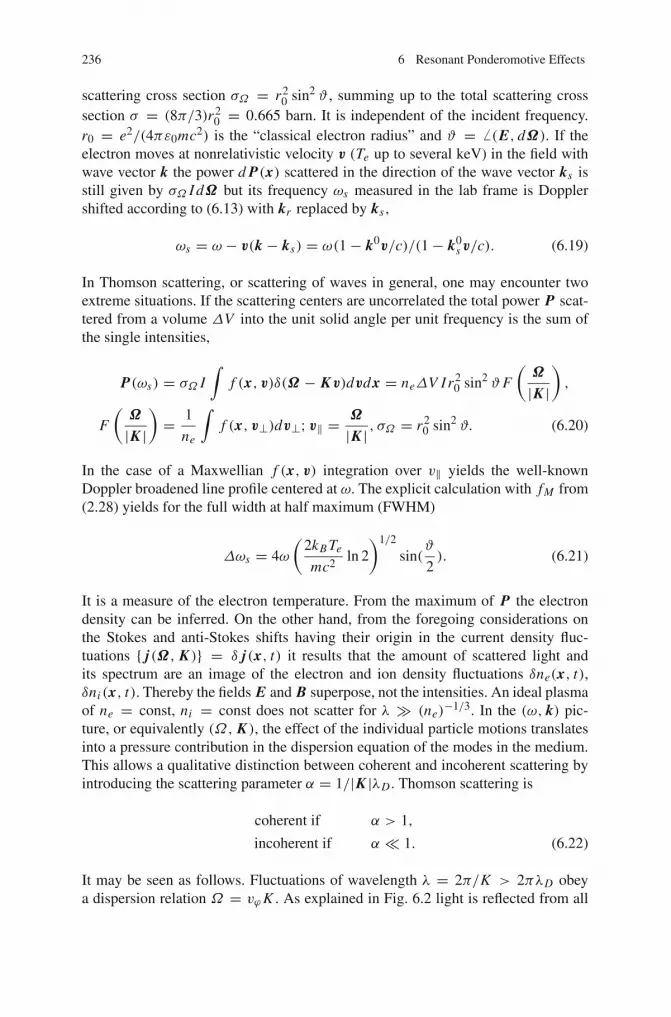
236 6 Resonant Ponderomotive Effects
scattering cross section σΩ = r20 sin2 ϑ , summing up to the total scattering cross
section σ = (8π/3)r20 = 0.665 barn. It is independent of the incident frequency.
r0 = e2/(4πε0mc2) is the “classical electron radius” and ϑ = (E, dΩ). If theelectron moves at nonrelativistic velocity v (Te up to several keV) in the field withwave vector k the power d P(x) scattered in the direction of the wave vector ks isstill given by σΩ I dΩ but its frequency ωs measured in the lab frame is Dopplershifted according to (6.13) with kr replaced by ks ,
ωs = ω − v(k − ks) = ω(1− k0v/c)/(1− k0s v/c). (6.19)
In Thomson scattering, or scattering of waves in general, one may encounter twoextreme situations. If the scattering centers are uncorrelated the total power P scat-tered from a volume ΔV into the unit solid angle per unit frequency is the sum ofthe single intensities,
P(ωs) = σΩ I∫
f (x, v)δ(Ω − Kv)dvdx = neΔV Ir20 sin2 ϑF
(Ω
|K |),
F
(Ω
|K |)= 1
ne
∫f (x, v⊥)dv⊥; v‖ = Ω
|K | , σΩ = r20 sin2 ϑ. (6.20)
In the case of a Maxwellian f (x, v) integration over v‖ yields the well-knownDoppler broadened line profile centered at ω. The explicit calculation with fM from(2.28) yields for the full width at half maximum (FWHM)
Δωs = 4ω
(2kB Te
mc2ln 2
)1/2
sin(ϑ
2). (6.21)
It is a measure of the electron temperature. From the maximum of P the electrondensity can be inferred. On the other hand, from the foregoing considerations onthe Stokes and anti-Stokes shifts having their origin in the current density fluc-tuations { j(Ω, K )} = δ j(x, t) it results that the amount of scattered light andits spectrum are an image of the electron and ion density fluctuations δne(x, t),δni (x, t). Thereby the fields E and B superpose, not the intensities. An ideal plasmaof ne = const, ni = const does not scatter for λ � (ne)
−1/3. In the (ω, k) pic-ture, or equivalently (Ω, K ), the effect of the individual particle motions translatesinto a pressure contribution in the dispersion equation of the modes in the medium.This allows a qualitative distinction between coherent and incoherent scattering byintroducing the scattering parameter α = 1/|K |λD . Thomson scattering is
coherent if α > 1,
incoherent if α � 1. (6.22)
It may be seen as follows. Fluctuations of wavelength λ = 2π/K > 2πλD obeya dispersion relation Ω = vϕK . As explained in Fig. 6.2 light is reflected from all

6.1 Tools 237
wave fronts and interferes constructively. In the opposite case, λ � 2πλD , K andΩ are more or less uncorrelated and to a spatially periodic disturbance of period-icity K corresponds a whole group of frequencies Ω = ±(ω − ωs) by which anyinterference is washed out. As a result the intensities scattered from the individualelectrons add up to the intensity observed in direction ks . Owing to K → 0 for ks
approaching k, scattering into forward direction becomes coherent. In fact, when kand ks are collinear, k and ks and ω and ωs become identical, and thus their phasesφ1 and φ2 are identical also,
φ1 = kx1 − ωt1 + ks(x − x1)− ωs(t − t1),
φ2 = kx2 − ωt2 + ks(x − x2)− ωs(t − t2) = kx − ωt = φ1.
In practice this means that in a coherent Thomson scattering experiment ω must bechosen sufficiently large to fulfill the first of relations (6.22) for scattering angles ϑlarger than the aperture cone of the probing light pulse.
Introducing the dynamic form factor or spectral density function S(K ,Ω),defined as
S(K ,Ω) = limΔT,ΔV→∞
1
ΔTΔV
|δne(K ,Ω)|2ne0
,
[δne(x, t)
ne0
]2
= 1
2πne0
∫S(K ,Ω)d KdΩ, (6.23)
and expressing it in terms of the dielectric susceptibilities χe,i (K ,Ω),
S(K ,Ω) = 2π
|K |[∣∣∣1− χe
ε
∣∣∣2
Fe
(Ω
|K |)+ Z
∣∣∣χi
ε
∣∣∣2
Fi
(Ω
|K |)]
, ε = 1+ χe + χi ,
(6.24)with ε given by (3.105) plus the analogous integral for the ions (ωp → ωpi ), followsfor the scattered power P(ωs) from the unit volume
d2 P/dΩdωs = I r20 sin2 ϑS(K ,Ω). (6.25)
The scattering time interval ΔT and the volume ΔV have to be chosen large enoughso that a Fourier analysis of δne,i(x, t) makes sense for min |K |, minω under con-sideration. In local thermal equilibrium and Te ≈ Ti the form factor simplifies toS = Se + Si [4]. With a view on (3.104) the corrections in (6.24) become clear: dueto the local polarization of the plasma by the surrounding electrons and ions eachbare electron charge is weakened by the susceptibilities χe,i . The asymmetry in thetwo correction terms expresses the fact that all scattering is due to the electronsonly. For details of derivations (6.23), (6.24), and (6.25) the reader may consultSheffield [5] or, for the essentials, Boyd and Sanderson [6], Chap. 9., and [7]. Inthe visible and UV spectral region no Compton shift has to be taken into accountfor the determination of ks , ωs . In nonideal dense plasmas (warm dense matter)
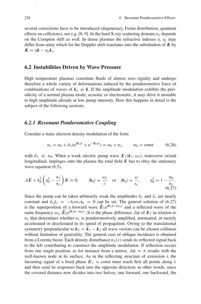
238 6 Resonant Ponderomotive Effects
several corrections have to be introduced (degeneracy, Fermi distribution, quantumeffects on collisions), see e.g. [8, 9]. In the hard X-ray scattering domain ωs dependson the Compton shift as well. In dense plasmas the refractive indexes η, ηs maydiffer from unity which for the Doppler shift translates into the substitution of K byK = ηk − ηs ks .
6.2 Instabilities Driven by Wave Pressure
High temperature plasmas constitute fluids of almost zero rigidity and undergotherefore a whole variety of deformations induced by the ponderomotive force ofcombinations of waves of ks = k. If the amplitude modulation exhibits the peri-odicity of a normal plasma mode, acoustic or electrostatic, it may drive it unstableto high amplitude already at low pump intensity. How this happens in detail is thesubject of the following sections.
6.2.1 Resonant Ponderomotive Coupling
Consider a static electron density modulation of the form
ne = n0 + n1(eik3 x + e−ik3 x) = n0 + n1, n0 = const (6.26)
with n1 � n0. When a weak electric pump wave E1(k1, ω1), transverse or/andlongitudinal, impinges onto the plasma the total field E has to obey the stationarywave equation (6.5),
ΔE + k20
(η2
0 −n1
nc
)E = 0; |k0| = ω1
cor |k0| = ω
se, η2
0 = 1− n0
nc.
(6.27)
Since the pump can be taken arbitrarily weak the amplitudes n1 and ve are nearlyconstant and ∂t j1 = −∂t en1ve = 0 can be set. The general solution of (6.27)is the superposition of a forward wave E1eik1x−iω1t and a reflected wave of thesame frequency ω1, E2eik2x−iω1t . It is the phase difference Δφ of E2 in relation ton1 that determines whether n1 is ponderomotively amplified, attenuated, or merelyaccelerated or decelerated in its speed of propagation. Owing to the translationalsymmetry perpendicular to k3 = k1 − k2 all wave vectors can be chosen collinearwithout limitation of generality. The general case of oblique incidence is obtainedfrom a Lorentz boost. Each density disturbance n1(x) sends its reflected signal backto the left contributing to construct the amplitude modulation. If reflection occursfrom one single position, as for instance from a mirror, Δφ = π results with thewell-known node at its surface. As in the reflecting structure of extension λ theincoming signal of a fixed phase E1 = const must reach first all points along λ
and then send its responses back into the opposite direction; in other words, sincethe covered distance now divides into two halves, one forward, one backward, the
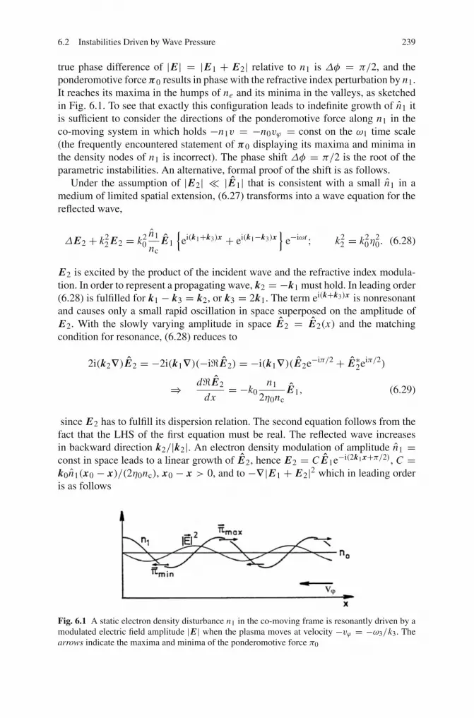
6.2 Instabilities Driven by Wave Pressure 239
true phase difference of |E| = |E1 + E2| relative to n1 is Δφ = π/2, and theponderomotive force π0 results in phase with the refractive index perturbation by n1.It reaches its maxima in the humps of ne and its minima in the valleys, as sketchedin Fig. 6.1. To see that exactly this configuration leads to indefinite growth of n1 itis sufficient to consider the directions of the ponderomotive force along n1 in theco-moving system in which holds −n1v = −n0vϕ = const on the ω1 time scale(the frequently encountered statement of π0 displaying its maxima and minima inthe density nodes of n1 is incorrect). The phase shift Δφ = π/2 is the root of theparametric instabilities. An alternative, formal proof of the shift is as follows.
Under the assumption of |E2| � |E1| that is consistent with a small n1 in amedium of limited spatial extension, (6.27) transforms into a wave equation for thereflected wave,
ΔE2 + k22 E2 = k2
0n1
ncE1
{ei(k1+k3)x + ei(k1−k3)x
}e−iωt ; k2
2 = k20η
20. (6.28)
E2 is excited by the product of the incident wave and the refractive index modula-tion. In order to represent a propagating wave, k2 = −k1 must hold. In leading order(6.28) is fulfilled for k1 − k3 = k2, or k3 = 2k1. The term ei(k+k3)x is nonresonantand causes only a small rapid oscillation in space superposed on the amplitude ofE2. With the slowly varying amplitude in space E2 = E2(x) and the matchingcondition for resonance, (6.28) reduces to
2i(k2∇)E2 = −2i(k1∇)(−i�E2) = −i(k1∇)(E2e−iπ/2 + E∗2eiπ/2)
⇒ d�E2
dx= −k0
n1
2η0ncE1, (6.29)
since E2 has to fulfill its dispersion relation. The second equation follows from thefact that the LHS of the first equation must be real. The reflected wave increasesin backward direction k2/|k2|. An electron density modulation of amplitude n1 =const in space leads to a linear growth of E2, hence E2 = C E1e−i(2k1x+π/2), C =k0n1(x0 − x)/(2η0nc), x0 − x > 0, and to −∇|E1 + E2|2 which in leading orderis as follows
Fig. 6.1 A static electron density disturbance n1 in the co-moving frame is resonantly driven by amodulated electric field amplitude |E| when the plasma moves at velocity −vϕ = −ω3/k3. Thearrows indicate the maxima and minima of the ponderomotive force π0

240 6 Resonant Ponderomotive Effects
−∇|E1 + E2|2 = −∇(E1 E∗2 + E∗1 E2)
= −C E21∇{
ei(2k1 x+π/2) + e−i(2k1x+π/2)}= 4k1 E2
1 cos 2k1x. (6.30)
Summarizing, we have shown that an electric wave incident on a static refractiveindex (= density) perturbation in a medium streaming at phase velocity is reflectedin such a way that the ponderomotive force of the total electric field leads to secularamplification of the initial modulation provided the spatial resonance condition
k1 = k2 + k3 ⇒ k3 = 2k1 (6.31)
is fulfilled. The comparison of the two arguments for π0 ∼ n1 is an example forthe superiority of physical (synthetic) reasoning over formal (analytic) proofs (oncea physical picture can be found). A remark is in order here. For simplicity a staticdensity modulation in a plasma at rest has been assumed. In reality n1 is movingat ion acoustic or Langmuir phase velocity as assumed in Fig. 6.1. Then, in thesystem of the density modulation n1 at rest the plasma exhibits a constant flowvelocity. A first consequence is that the second of relations (6.31) is only valid fortransverse waves E1, E2 in the vacuum. However, the first relation is fulfilled ateach position and, owing to the Lorentz invariance of the phase φ matching holds inall systems of reference. All relations in this section remain valid under oblique inci-dence of E1(k1, ω1) as a consequence of momentum conservation perpendicular tok3 which in turn is a consequence of translational symmetry along that direction.Under oblique incidence ponderomotive coupling from the superposition of an elec-tromagnetic and a Langmuir wave is also possible, for instance in the two plasmondecay. In conclusion, in any inertial system and in the lab frame in particular, forresonant coupling the matching conditions
k1 = k2 + k3, ω1 = ω2 + ω3 (6.32)
must be fulfilled. Among the natural plasma fluctuations those modes are selectedand driven unstable by a transverse or longitudinal electric wave that fulfill theseresonance conditions. The situation is sketched in Fig. 6.2 in the co-moving and inthe lab frame. The incident pump wave generates weak reflected signals from allinhomogeneities which interfere constructively to compose E2. This latter in turngenerates π0 in phase with the electron density disturbance.
For gaining additional insight it may be instructive to formalize also the proofof unstable growth based on Fig. 6.1. To this aim, given two electric waves withω1 = ω2 and k1 = k2, the density perturbation n1 they induce is shown to bein phase with π0. To see this consider (5.43) for nonrelativistic velocities v andvϕ . By setting M = v/vϕ and replacing mi by m in ρc its validity extends to theelectron plasma wave too (the extension to an arbitrary vϕ is guaranteed by thevalidity of the resonance conditions (6.32) in all systems of reference). At M < 1the density finds time enough to react to the ponderomotive potential Φp and toaccumulate in the valleys of |E|2; at M > 1 it is retarded by π , i.e., Φp is ahead

6.2 Instabilities Driven by Wave Pressure 241
Fig. 6.2 Induced scattering of an intense pump wave k1 from a refractive index modulation k3;k2 scattered wave. (a) Co-moving frame, sketched for slow mode k3, e.g., Brillouin scattering,α′ � β ′, (b) lab frame
by π with respect to the “subsonic” case (see Fig. 5.5). At M = 1 no steady stateexists. The ponderomotive potential Φp of the system, as it represents a harmonicoscillator, undergoes a phase shift by +π/2 for continuity reasons (−π/2 wouldmean stability and discontinuity in the phase shift), or seen explicitly by observingthat in the “sonic” region M = 1 total pressure and kinetic terms balance each otherin (5.43). Then, complemented by the partial derivative of v with respect to time(5.43) reduces to
ρ∂v
∂t= −v ∂ρ
∂t= −π0 ⇒ ∂ρ
∂t= π0
vϕ, (6.33)
i.e., growing ρ or n1 happen in phase with the ponderomotive force π0. This com-pletes our assertion.
For tutorial reasons we may ask ourselves at this point how an electric field doesaffect a plasma mode nl when |E|2, in contrast to π0, is modulated in phase withthe mode. Including π0 in the linearized (2.90) and (2.99), now all quantities takenconveniently in the lab frame, leads to
∂2
∂t2nl + k2
l v2l
(1+ ε0
2
n0
ncE1
E2
nl
)nl = 0. (6.34)
As the ratio of the amplitudes α = |E2|/nl is nearly constant, it follows fornl/n0 � 1 that the only effect of π0 on the wave is to increase its phase velocity,
v′l = vl
(1+ ε0
n0
2nc|E1|α
)1/2
> vl ,
but not its amplitude nl .

242 6 Resonant Ponderomotive Effects
6.2.2 Unstable Configurations
The excitation of a mode 2 and a mode 3 by the pump mode 1 can be interpreted asthe decay of quanta of type 1 into quanta of type 2 and 3, in symbols ω1 → ω2+ω3.By assigning the indexes em, es, and a to the different types of modes, electromag-netic, electrostatic, and acoustic, as the carriers of photons hωem, plasmons hωes,and phonons hωa, we conclude from the foregoing section that the following decayinstabilities are possible and underlie to the same physical principle:
1. Brillouin instability: ωem → ω′em + ωa2. Raman instability: ωem → ω′em + ωes3. Two plasmon decay: ωem → ω′es + ωes4. Parametric decay instability: ωem → ωes + ωa5. Oscillating two-stream instability: ωem → ωes + ωa, ωes > ωem6. Langmuir cascade: ωes → ω′es + ωa, ω′es → · · ·7. Two phonon decay of phonon: ωa → ω′a + ω′′a
Stimulated decay of a phonon into two phonons is possible. In high power-laserplasma interaction it plays at most a secondary role and will not be pursued here.The opposite is true for stimulated Brillouin [10] or Brillouin-Mandelstam [11] scat-tering (SBS). It consists in the stimulated amplification of an electromagnetic wavescattered off a low frequency ion acoustic mode satisfying the resonance conditions(6.32). In appositely prepared plasmas it can lead to 100% back reflection of theincident laser light [12, 13], in this way preventing the plasma from effective heat-ing. The acoustic mode is a low frequency wave, ωa � ωem, and hence ω′em � ωemand |ka| � 2|kem| sin(ϑ/2), ϑ = (kem, k′em). Owing to the virtual high reflectivitythe decay process has been intensively investigated experimentally and theoreticallyin connection with controlled inertial fusion over more than three decades [14–18].The repeated decay of a Langmuir wave into another Langmuir wave and an ionacoustic mode (cascading) is called Langmuir decay instability (LDI). It is the elec-trostatic equivalent to SBS since the underlying coupling physics is the same as forSBS [19, 20]. The process tends to degeneracy by multiple cascading into nearlyindistinguishable ion modes. In a limited parameter regime LDI appears to be asecondary instability that can saturate the Langmuir wave generated by the processof stimulated Raman scattering [21, 22].
The stimulated Raman scattering (SRS) in plasma has been investigated for atleast four decades [23]. It is the resonant decay of light into an electron plasmawave and a light wave of longer wavelength. The physical mechanism is the sameas for Brillouin scattering. Owing to the much higher frequency of the plasma wavethe scattered Stokes line undergoes a remarkable red shift, in perfect analogy tothe Raman effect in solids from optically active crystal vibrations (optical phonons)producing similar large red shifts. SRS exhibits fast growth rates and high saturationlevels in plasmas, at least under ideal conditions [24], and fast electron generationdue to particle trapping in the Langmuir wave [4]. The latter is of relevance to indi-rect drive of inertial fusion pellets [25]. From the inequality ω′em + ωes ≥ 2ωpfollows that the instability is limited to the density domain n ≤ nc/4. At compara-

6.2 Instabilities Driven by Wave Pressure 243
tively low density and high electron temperature there is another limit due to strongLandau damping of the electron plasma wave for kesλD
>∼ 0.35. On the other hand,kinetic effects induced by SRS show a fast onset which can lead to a strong modi-fication of the electron distribution function and thus to phenomena like nonlinearenhancement of the instability (“inflation regime” [26] and to the excitation of newmodes, so called (electron) beam acoustic modes (BAM) [27].
The two plasmon decay (TPD) is excited in the vicinity of nc/4 because of strongLandau damping outsideωes � ωp. Like SRS, it is a potential candidate for fast elec-tron generation [28] owing to the high phase velocity of the daughter waves limitedonly by the finite density scale length due to profile steepening at nc/4 (compareFig. 3.6). Langmuir cascading into two electron plasma waves, ωes → ω′ + ω′′ isnot possible because the resonance conditions (6.32) cannot be fulfilled in the entiredensity domain. For the same reason resonant transverse wave cascading into twoelectromagnetic waves does not occur either.
To give an intuitive physical picture of the TPD is more complex. It is true thatalso in this case the instability arises from the reflection of the pump wave k1 fromthe Langmuir wave k2 (k3) to result in a ponderomotive force in phase with k3(k2, respectively). However, the geometry for maximum growth is peculiar. Startingfrom the configuration in the lab frame with the pump k1 incident under the arbitraryangle α onto the plasma mode k2 we observe that in good approximation holds
ω2 = ω3 = ωp = ω1/2, η1 =√
3/2, cϕ = vϕ,1 = ω1/k1, (6.35)
k1 = k0η1, k2 = k3 � (c/2se)k0 � k1, k2,3 = ω/(2vϕ2,3).
It follows from k2,3 � k1 that the two plasma waves are nearly collinear (seeFig. 6.3). The growth of the two daughter waves k2,3 implies an increase of themomentum densities mn2,3v1 which, in turn, manifest themselves in a ponderomo-tive force like an inverse rocket effect. Thus, the ponderomotive force π2,3 driv-ing TPD unstable is given by (5.30). It is physically obvious and confirmed bythe quantitative analysis in the next section that it acts along k1 and exhibits theproportionality
π2,3 ∼ k1|E1 E∗2,3|. (6.36)
The growth rate γ is proportional to the projection of π2,3 in direction k2,3, i.e.,|k1k2,3| ∼ cosα. On the other hand, the modulus |π2,3| ∼ |E1 E∗2,3| ∼ sinα;hence γ ∼ sinα cosα, with maximum growth under α = π/4. In linear theoryone configuration and its mirror image with respect to k1 exhibit identical growthrates γ .
Excitation of TPD under perpendicular incidence, α = π/2 is not possible as aconsequence of γ ∼ sinα cosα. If however, one of the modes causing reflectionof the pump wave is a low frequency wave, π t is nearly zero and a symmetriccomposition of the k-diagram can be realized also in the lab frame. This differencein geometry originates from the fact that in presence of a slow (acoustic) mode, e.g.,n3, in the co-moving reference system two fast modes n2 are excited by the laser in

244 6 Resonant Ponderomotive Effects
Fig. 6.3 Stimulated two-plasmon decay; k1 = k2 − k3, k1 � k2,3. Its mirror image with respectto k1 shows equal growth
opposite directions almost symmetrically whereas in the co-moving system of oneof two fast modes, as in TPD, the left-right symmetry is destroyed. In the parametricdecay (PDI) and the oscillating two stream instability (OTSI) one plasma wave issubstituted by an acoustic mode (ka, ωa) = (k3, ω3) and thus (quasi)-symmetry isestablished with maximum growth occurring at α = π/2. Owing to se|kes|, ωa �ωp the instability is localized in the neighborhood of ωp � ω1 and k2 � (c/se)k1 �k1. Therefore according to (6.32) ka = k3 = k2 and k1 = 0 can be set. From π t � 0the force π = π0 that drives the instability now points into k1±k2 � ±k2 directionand causes maximum growth perpendicularly to k1. With respect to relative phasesof the decay products and the ponderomotive forces the considerations from aboveon SBS, SRS and TPD apply identically, with π0 being in phase with the acousticdensity modulation n3 that leads to an unstable situation again. The PDI has beendescribed first by Silin [29]. It is localized in the underdense plasma region close tonc. It was Nishikawa to recognize that it can also work above nc when ω1 < ω2 andω3 = ωa = 0 [30]. This is the case of the so-called oscillating two stream instabilityOTSI. We present the treatment of the two instabilities in terms of wave pressuregiven by [31].
Consider a spatially uniform laser field E1 = E1e−iω1t impinging orthogonallyon a static plasma density modulation n3 = n3eik3x , E1 ‖ k3. It forces the electronsto shift in ±x-direction by the amount
δ1 = � e
mω21
(1+ i
νei
ω1
)E1e−iω1t (6.37)
and, in the presence of an ion density modulation n3, it gives rise to an inducedelectric field Ed obtained from Poisson’s equation,
∂Ed
∂x= − e
ε0[n3(x − δ1)− n3(x)] = e
ε0δ1∂n3
∂x⇒ Ed = e
ε0δ1n3. (6.38)
The driver excites two symmetric plasmons E2 = E2ei(±k3x−ω1t) obeying the har-monic oscillator equation of the displacement δ2(x),
∂2δ2
∂t2+ν ∂δ2
∂t+ω2
2δ2 = − e
m(E1+Ed)e
−iω1t ; ω22 = ω2
p+s2e k2
2, k2 = k3. (6.39)
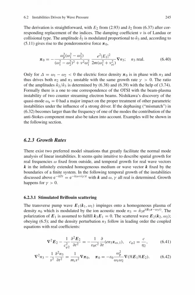
6.2 Instabilities Driven by Wave Pressure 245
The derivation is straightforward, with E2 from (2.93) and δ2 from (6.37) after cor-responding replacement of the indices. The damping coefficient ν is of Landau orcollisional type. The amplitude δ2 is modulated proportional to n3 and, according to(5.11) gives rise to the ponderomotive force π0,
π0 = −ω2
p(ω21 − ω2
2)
(ω21 − ω2
2)2 + ν2ω2
1
e2|E1|22m(ω2
1 + ν2ei )
∇n3; n3 real. (6.40)
Only for Δ = ω1 − ω2 < 0 the electric force density π0 is in phase with n3 andthus drives both n2 and n3 unstable with the same growth rate γ > 0. The ratioof the amplitudes n2/n3 is determined by (6.38) and (6.39) with the help of (3.74).Formally there is a one to one correspondence of the OTSI with the beam-plasmainstability of two counter streaming electron beams. Nishikawa’s discovery of thequasi-mode ωa = 0 had a major impact on the proper treatment of other parametricinstabilities under the influence of a strong driver. If the dephasing (“mismatch”) in(6.32) becomes larger than the frequency of one of the modes the contribution of theanti-Stokes component must also be taken into account. Examples will be shown inthe following section.
6.2.3 Growth Rates
There exist two preferred model situations that greatly facilitate the normal modeanalysis of linear instabilities. It seems quite intuitive to describe spatial growth forreal frequencies ω fixed from outside, and temporal growth for real wave vectorsk in the infinitely extended homogeneous medium or wave vector k fixed by theboundaries of a finite system. In the following temporal growth of the instabilitiesdiscussed above e−iΩt = e−i(ω+iγ )t with k and ω, γ all real is determined. Growthhappens for γ > 0.
6.2.3.1 Stimulated Brillouin scattering
The transverse pump wave E1(k1, ω1) impinges onto a homogeneous plasma ofdensity n0 which is modulated by the ion acoustic mode n3 = n3ei(k3x−ω3t). Thepolarization of E1 is assumed to fulfill k3 E1 = 0. The scattered wave E2(k2, ω2);obeying (6.5); and the density perturbation n3 follow in leading order the coupledequations with real coefficients:
∇2 E2 − 1
c2ϕ2
∂2 E2
∂t2= − 1
ε0c2
∂
∂t(en3vos,1), cϕ2 = c
η2, (6.41)
∇2n3 − 1
s2
∂2n3
∂t2= 1
mi s2∇π0, π0 = −ε0
ω2p
ω1ω2∇(�E1�E2). (6.42)

246 6 Resonant Ponderomotive Effects
We assume |E1| � |E2| and n3 � n0, and we consider growth in the small signalamplification domain and therefore do not need the coupled equation of E1. To takeadvantage of the complex Fourier analysis of these two equations in (k,Ω) one ofthe quantities must be taken real. We choose �E1 = (E1 + E∗1)/2 and obtain thenetted set of equations
(Ω2 − v2ϕ2k2
2)E(Ω)2 = ω1Ω
2nc1
(E1n(Ω−ω1)
3 + E∗1n(Ω+ω1)3
), (6.43)
(Ω2 − s2k2)n(Ω)3 = −ε0k2
2mi
ω2p
ω1ω2
(E1 E(Ω−ω1)
2 + E∗1 E(Ω+ω1)2
). (6.44)
On the RHS of (6.44) ω2 = ω1−ω3 is associated with the Stokes component of E2
and ω2 = ω1 + ω3 refers to the anti-Stokes component of E2. We express E(Ω−ω1)2
and E(Ω+ω1)2 from (6.44) with the help of (6.43),
[(Ω − ω1)2 − v2
ϕ2(k − k1)2]E(Ω−ω1)
2 = −ω1ω2
2nc1E∗1n(Ω)
3 , (6.45)
[(Ω + ω1)2 − v2
ϕ2(k + k1)2]E(Ω+ω1)
2 = ω1ω2
2nc1E1n(Ω)
3 , (6.46)
and eliminate them from (6.44) to obtain
[(Ω2 − s2k2)− ε0
4
k2ω2p
mi nc1E1 E∗1
(1
D(Ω−ω1)+ 1
D(Ω+ω1)
)]n(Ω)
3 = 0. (6.47)
The Stokes and anti-Stokes ω2 in (6.45) and (6.46) results from setting Ω = ω3 inthe RHS terms. The electromagnetic dispersion functions (Ω±ω1)
2−v2ϕ2(k± k1)
2
are abbreviated by the symbols D(Ω±ω1). The infinite chain of equations (6.43) hasbeen cut at n(Ω±ω1)
3 because owing to |Ω| � ω1 these and all following terms are
very small in comparison to the only resonant mode n(ω)3 . Furthermore, from (6.32)follows, even in the case of strong mismatch under a strong driver, ω2 � ω1, |k2| �|k1|, and hence k1 � k2 + k3 imposes k3 � 2k1 sin(ϑ/2), scattering angle ϑ = (k1, k2). For backscattering, i.e., ϑ = π , this implies k = k3 � k1 − k2 � 2k1.As the intensity of the pump wave tends to zero the mismatch in (6.30) decreasesalso to zero. For mild backscattering γ 2 � ω2
3 � ω2a holds, and from (6.30) follows
more precisely k3 = 2k1[1 − η1s/c]. Hence, in (6.47) only the Stokes componentE(Ω−ω1)
2 is resonant; the anti-Stokes term D(Ω+ω1) can be disregarded. This is theweak coupling limit [24]. The dispersion relation (6.47) shrinks to
(2iγω3 − γ 2)[(−2iγω1 − 2ω1ω3)− v2ϕ2(k
23 − 2k1k3)] = ε0
4
k23ω
2p
mi ncE1 E∗1. (6.48)
6.2 Instabilities Driven by Wave Pressure 247
With k3 from above for backscattering the sum of the real terms in the secondbracket yields ω2
3 and can be set to zero compared with 2γω1. Hence, one is leftwith the maximum growth rate for exact backscattering
γmax = 1
2
ωpi
c(mncs)1/2I 1/2 = 1
23/2ωpi
η1/21 vos
(cs)1/2; (6.49)
I = ε0cη1 E1 E∗1/2, ω2pi = (m/mi )ω
2pe, η2 � η1, vos is taken locally. In side scatter-
ing (ϑ < π/2) the term
−2ω1ω3 − v2ϕ2(k
23 − 2k1k3) = −4ω1k1 sin
ϑ
2
[s + c
η2
(sin
ϑ
2− cos
ϑ
2
)]
is positive and contributes to reduce γ . The reduction is, primarily, a consequence of|E1 E2| = |E1||E2| cosϑ . A short remark may be in order: In (6.41) the scatteredwave E2 depends linearly on the pump wave E1. As in side scattering the twovectors are not parallel to each other in general (ϑ = 0) additional terms appear ink3 E1 = 0 polarization. The dependence of γ on η1 is due to shrinking of the ionsound wave vector in the plasma, π0 ∼ k3 ∼ k0η1.
In the so called strong coupling regime [17, 24, 32], i e., when |Ω|2 � k23s2
holds under the strong driver, in back scattering the approximations
D(Ω−ω1) = Ω2 − 2Ωω1 + ω21 − ω2
p − c2k21(1− 2η1s/c)2
� −2Ωω1 + 4η21ω1sk1 � −2Ωω1, Ω2 − s2k2 � Ω2
are consistent and from (6.47), ignoring the anti-Stokes term, follows Ω as the com-plex cubic root
Ω = 1
24/3
[ω1ω
2piη
21
(vos
c
)2]1/3
(1+ i√
3). (6.50)
Unstable growth is particularly favored in presence of a strong counter propagat-ing electromagnetic wave, for example, when the incident wave reaches the criticaldensity before sufficient attenuation. In such a case γ may exceed ωa several times.In stationary plasmas with less than critical density a steady state solution of SBSusually establishes. In situations when light is reflected from the critical surfacewith frequency differing from the red-shifted E(Ω−ω1)
2 mode SBS becomes non-stationary for a sufficiently high pump wave and the scattered spectrum undergoesstrong broadening [33]. Latest in such a situation the scattered anti-Stokes fieldcomponent E(Ω+ω1)
2 can no longer be ignored a priori in the dispersion relationterm 1/D(Ω−ω1) + 1/D(Ω+ω1) in (6.47) [34].
The anti-Stokes wave is close to resonance for the matching condition
ω2 = ω1 + ω3, k2 = k1 + k3. (6.51)

248 6 Resonant Ponderomotive Effects
It travels into the forward direction as the driver E1(ω1, k1). This is most imme-diately seen in the co-moving frame. Under the influence of the driver E1 from
each position x an elementary electromagnetic disturbance E(ω′1)2 propagates into
opposite directions with strengths the difference of which reduces to zero with flowvelocity −s approaching zero. In the lab frame ω′1 becomes the anti-Stokes fre-quency ω1 = γ (ω′1 + k′2s) = ω1 + ω3 for k2k3 ≥ 0, see (6.12). When k1 and k2
are approximately collinear, |k3| � η1ω3/c � k0s/c is very small and D(Ω+ω1) isclose to resonant coupling,
D(Ω+ω1) = Ω2+2Ωω1+ω21−ω2
p−c2k21
(1+ 2η1s
c
)2
� Ω2+2Ωω1−4η21ω1sk1.
On the other hand, in nearly forward direction the Stokes |k3| can assume arbitrarilysmall values; anti-Stokes and Stokes frequencies ω2 = ω1 ± s|k3| are very close toω1 and with increasing pump wave intensity their bandwidths begin to overlap ina |k3| interval around the dispersion intersection points (see Fig. 6.4). This leadsto a redistribution of the energy fluxes and to back reaction onto the (ω3, k3) modethat rather to be a free mode will convert into a forced quasi-mode at downshiftedfrequency ωa. Nishikawas’s oscillating two-stream instability with ωa = 0 for finite|k2| = |k3| is perhaps the most instructive example for the Stokes-anti-Stokes inter-play and concomitant frequency shift. The instability results in a long wavelengthmodulation of the amplitudes n3 and |E| = |E1 + E2|. As a special case of SBSthe filamentary instability is obtained from (6.47) by setting k3k1 = 0 and Ω = iγ .Then, D(Ω±ω1) = ±2iγω1 − c2k2
3 leads to the equation of growth γ ,
(γ 2 + s2k2)1
4γ 2ω21 + c4k4
= ω2pi
8
(vos
c
)2
; k ⊥ k1. (6.52)
Here, as throughout the chapter, E1∇n3 = 0 is assumed. As long as the pump wavedoes not drive plasma resonances, for instance owing to ω1 > ωp, polarizationeffects can be disregarded [34, 35].
Stokes and anti-Stokes electromagnetic components both act to drive the ionacoustic and the electron plasma mode whenever the detuning due to growth exceedsthe Stokes shift Δω. It is advisable in general, also with other types of unsta-ble modes, to include both components in the analysis and to compare with theresult obtained from the resonant Stokes mode alone. After all it must be kept inmind that parametric systems of type (6.43), (6.44) represent a recurrence schemeof an infinite number of equations. For the PDI and OTSI sequences closureand impact of the anti-Stokes component are investigated quantitatively in [36].The arguments for closure may vary from case to case. So for example numeri-cal studies have shown that ion acoustic harmonics can couple to SBS and leadto reduction of reflectivity, spatial decorrelation and to temporal chaotic plasmadynamics [16].
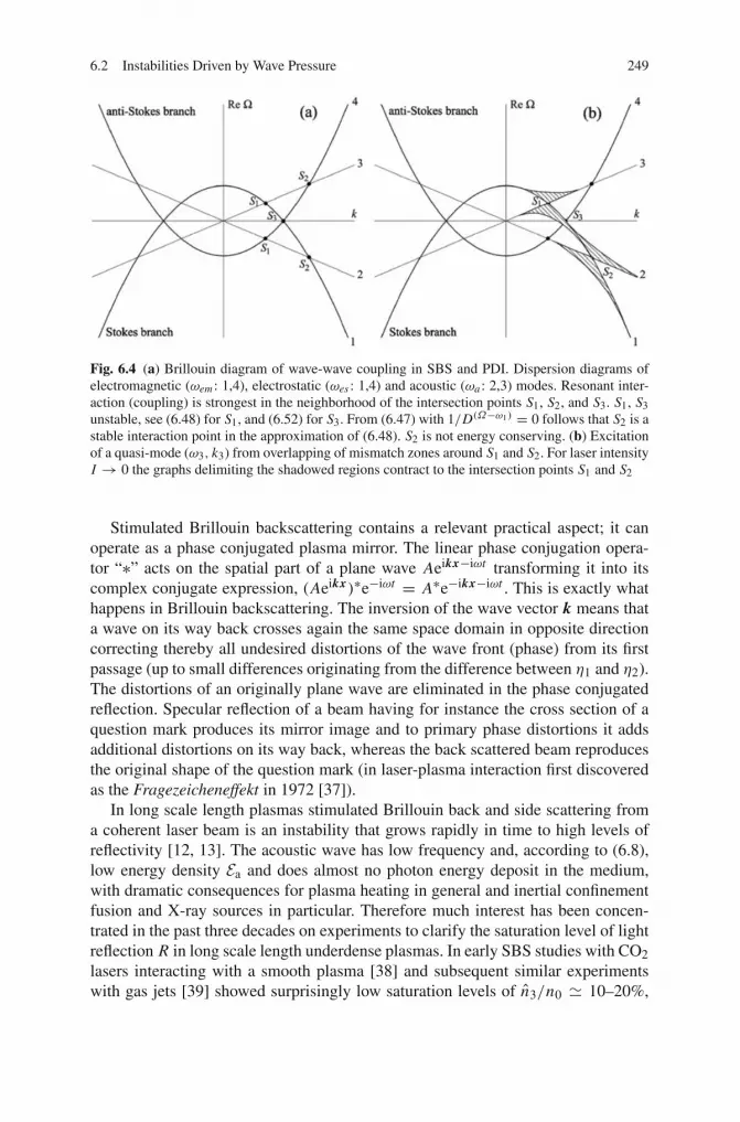
6.2 Instabilities Driven by Wave Pressure 249
Fig. 6.4 (a) Brillouin diagram of wave-wave coupling in SBS and PDI. Dispersion diagrams ofelectromagnetic (ωem : 1,4), electrostatic (ωes : 1,4) and acoustic (ωa : 2,3) modes. Resonant inter-action (coupling) is strongest in the neighborhood of the intersection points S1, S2, and S3. S1, S3unstable, see (6.48) for S1, and (6.52) for S3. From (6.47) with 1/D(Ω−ω1) = 0 follows that S2 is astable interaction point in the approximation of (6.48). S2 is not energy conserving. (b) Excitationof a quasi-mode (ω3, k3) from overlapping of mismatch zones around S1 and S2. For laser intensityI → 0 the graphs delimiting the shadowed regions contract to the intersection points S1 and S2
Stimulated Brillouin backscattering contains a relevant practical aspect; it canoperate as a phase conjugated plasma mirror. The linear phase conjugation opera-tor “∗” acts on the spatial part of a plane wave Aeikx−iωt transforming it into itscomplex conjugate expression, (Aeikx)∗e−iωt = A∗e−ikx−iωt . This is exactly whathappens in Brillouin backscattering. The inversion of the wave vector k means thata wave on its way back crosses again the same space domain in opposite directioncorrecting thereby all undesired distortions of the wave front (phase) from its firstpassage (up to small differences originating from the difference between η1 and η2).The distortions of an originally plane wave are eliminated in the phase conjugatedreflection. Specular reflection of a beam having for instance the cross section of aquestion mark produces its mirror image and to primary phase distortions it addsadditional distortions on its way back, whereas the back scattered beam reproducesthe original shape of the question mark (in laser-plasma interaction first discoveredas the Fragezeicheneffekt in 1972 [37]).
In long scale length plasmas stimulated Brillouin back and side scattering froma coherent laser beam is an instability that grows rapidly in time to high levels ofreflectivity [12, 13]. The acoustic wave has low frequency and, according to (6.8),low energy density Ea and does almost no photon energy deposit in the medium,with dramatic consequences for plasma heating in general and inertial confinementfusion and X-ray sources in particular. Therefore much interest has been concen-trated in the past three decades on experiments to clarify the saturation level of lightreflection R in long scale length underdense plasmas. In early SBS studies with CO2lasers interacting with a smooth plasma [38] and subsequent similar experimentswith gas jets [39] showed surprisingly low saturation levels of n3/n0 � 10–20%,

250 6 Resonant Ponderomotive Effects
corresponding to R < 10%. Further drastic reduction of this values of R fromSBS has been achieved by applying average laser beam smoothing through inducedspatial incoherence (ISI: broad band laser beam is first divided into many inde-pendent beamlets, with mutual time shifts exceeding the coherence time, and thenoverlapped on the target). With ISI applied to a 2-ns Nd laser beam of peak intensityI = 1014 Wcm−2 on CH disk targets R resulted below 1% [40]. These were goodnews but they resisted for nearly two decades to a satisfactory theoretical explana-tion. The studies focused on the discrepancy between theoretical expectations andexperimental results mostly concentrated on saturation effects of the ion acousticmodes due to steepening and wavebreaking, generation of harmonics, particle trap-ping and decay into subharmonics of n3.
In retrospect, however, the low backscatter levels measured in the past have notbeen analyzed with enough temporal resolution and therefore indicate merely theratio of back scattered to incident laser energy, generally ignoring transient highbackscatter levels that could potentially occur during a fraction of the laser pulse.The ability of combining fluid dynamic and kinetic SBS modeling with laser pulseshaping leads to a more realistic interpretation of the experiments. While often highbackscatter levels occur temporarily, in agreement with theory, the average levelover a longer time scale, e.g., tens of ps or entire laser pulses, may result moderateor low compared to the incident laser intensity. However, this should not lead to thehasty conclusion that SBS is not of concern under constraints imposed by specificgoals, as for example in laser fusion schemes. Independent of all nonlinear effectsexamined with the attempt to explain saturated SBS levels, laser beam smoothingin plasmas can itself lead to reduction of backscattering: self-focusing of individuallaser speckles of spatially smoothed beams (e.g. by random phase plate technique[RPP]) contribute in this way to an additional plasma-induced smoothing as thebeam propagates further into the plasma target.
Recently a breakthrough in understanding SBS suppression in long scale lengthplasmas has been achieved by Hüller et al. [41]. Sophisticated numerical simula-tions have shown a quite universal behavior applicable to laser beams containinghigh-intensity hot spots that are subject to self-focusing. Although the growth rateof SBS is higher than the one of self-focusing, SBS starts from a significantlylower noise level. Henceforth it grows primarily in intense self focused hot spots,giving rise to transient high backscatter flashes. Nevertheless, due to subsequentponderomotive density depletion disruption of the SBS signal takes place [42] and,eventually, backscattering remains on a moderate level averaged over the wholepulse length. It is important to mention that the region behind the self-focusinghot spots does not contribute significantly to SBS due to plasma induced smooth-ing, see [41]. In this paper the features of SBS were studied for a mono-specklelaser beam at Nd peak intensity I = 3 × 10¹⁴ Wcm−2 including self-focusingand nonlocal energy transport self consistently. In the linearly rising laser pulsewith its maximum at 200 ps SBS starts growing fast as predicted by (6.49) and(6.50) and reaches its maximum of R � 10% already at 50 ps and decays after100 ps so that averaged over the whole pulse of 1 ns 〈R〉 � 1–1.5% results withnonlocal transport included, and 〈R〉 � 4% without. The results are in excellent
6.2 Instabilities Driven by Wave Pressure 251
agreement with the concomitant experiment. On the other hand, when self-focusingwas suppressed in the simulation, maximum values of R = 50% were reachedin coincidence with the maximum of the laser pulse at 200 ps. The conclusion istwofold: (1) self-focusing, i.e., local intensity concentration, is responsible for thefast growth; (2) the sudden disruption of SBS after a short time is triggered by aneffect localized in spots of high laser intensity. The simulations allow the identifi-cation of (2) with the resonant filament instability [43, 44]. Due to the ponderomo-tive force a density well forms along a filament which is capable of supportingelectromagnetic eigenmodes like a waveguide. When the threshold intensity forself-focusing is reached they grow rapidly unstable and lead to lateral bending ofthe filament and eventually to its complete breakup. After some time it forms againand disrupts. The process leads to increased lateral scattering of the laser beam andto correlation length reduction to 10–15 µm in laser plasma interaction regions ofmm-scale. Very good agreement between experiment and the large scale simulationsand the identification of the resonant filament instability as the effect responsible forlow level SBS reflectivity may lead to the conclusion that herewith the two decadesold problem of Brillouin anomaly in high power laser interaction is solved, or veryclose to its solution. It should be stressed that the outlined scenario appears quiteuniversal with beams containing hot spots at power densities above the self-focusingthreshold [45].
6.2.3.2 Stimulated Raman Scattering
In (6.42) the low frequency plasma mode n3 from SBS is replaced by the highfrequency Langmuir wave. As for the rest the underlying physics is identical thegoverning equations are
∇2 E2 − 1
v2ϕ2
∂2 E2
∂t2= − 1
ε0c2
∂
∂t(en3vos,1), cϕ2 = c
η2, (6.53)
∇2n3 − 1
v2ϕ3
∂2n3
∂t2= 1
ms2e∇π0, π0 = −ε0
ω2p
ω1ω2∇(�E1�E2). (6.54)
Limiting ourselves again to the small signal amplification the Fourier analysis repro-duces equations (6.43), (6.44), (6.45), and (6.46), with s and mi replaced by vϕ3from (6.3) and m, and the corresponding dispersion equation
(Ω2 − v2ϕ3k2)− ε0
4
k2ω2p
mnc1E1 E∗1
(1
D(Ω−ω1)+ 1
D(Ω+ω1)
)= 0. (6.55)
For a moderately strong driver the matching conditions (6.32) are well satisfied. Thescattered frequency and wave number range from (ω2, k2) = (ω1, k1) to (ω1/2, 0).Since ω3 is close to ωp, for the Stokes component follows from ω2 � ω1 − ωpthat in back or side scattering the anti-Stokes frequency ω2a � ω1 + ωp is nonres-onant almost everywhere and 1/D(Ω+ω1) can be neglected. The dispersion relation

252 6 Resonant Ponderomotive Effects
reduces to
(ω23 + 2iω3γ − ω2
ps2e k2
3)[(ω3 − ω1)2 + 2iγ (ω3 − ω1)− ω2
p − c2(k3 − k1)2]
= ε0
4
k23ω
2p
mnc1E1 E∗1. (6.56)
Maximum growth occurs close to resonance of ω2 and ω3; hence
2iγmaxω3[2iγmax(ω3 − ω1)] = ε0
4
k23ω
2p
mnc1E1 E∗1. (6.57)
⇒ γmax = k3
4
[ω2
p(ω2ω3)e2
m2ω21
E1 E∗1
]1/2
= k3
4vos
[ω2
p
ω2ω3
]1/2
. (6.58)
For exact back scattering follows from (6.32) and (2.92) k2 = k0(1 − 2ωp/ω1)1/2,
k3 = |k3| = k1 + k2. The comparison of γmax for SRS and SBS for s � 10−3c andm/mi � 10−4 shows that they are of the same order of magnitude. SRS into exactforward direction is also possible. Its relevance lies in the possibility of exciting anelectron plasma wave of particularly high phase velocity in the low density plasmaof ωp � ω1, e.g., hohlraum plasma in indirect inertial fusion drive, and subsequentpreheat by trapped fast electrons [46–49]. In regions of low plasma densityω3 � ωp,η1 = η � 1, and in forward direction the matching condition implies for the anti-Stokes and Stokes lines k3 = |k1 − k2| = (ω1 ± ωp)/c � ω1/c. The dispersionfunctions D(Ω±ω1) = D(ω3+iγ±ω1) simplify to
D(Ω−ω1) = 2iγ (ωp − ω1) � −2iγω1, D(Ω+ω1) = 2iγ (ωp + ω1) � +2iγω1,
D(Ω−ω1) + D(Ω+ω1) = 4iγωp, D(Ω−ω1)D(Ω+ω1) = 4γ 2ω21.
Both terms are nearly resonant and must be used in (6.55) to yield the growth rate
γ = 1
23/2
ω2p
ω1
vos
c. (6.59)
6.2.3.3 Two Plasmon Decay
Short inspection of (6.53) and (6.54) shows that the equations governing the twoplasmon decay are obtained by replacing E⊥2 by E‖2 of a second plasma wave orassociated electron density perturbation n2,
∇2n2 − 1
v2ϕ2
∂2n2
∂t2= 1
mv2ϕ2
∇π2, ∇2n3 − 1
v2ϕ3
∂2n3
∂t2= 1
mv2ϕ3
∇π3. (6.60)
The wave pressure term now is given by the resonant terms of π = π0 + π t , i.e.,

6.2 Instabilities Driven by Wave Pressure 253
π2,3 = (π0 + π t )2,3 = −n0m∇(v1v2,3)+ m∂n2,3v1
∂t, (6.61)
with v1 = (vos + v∗os) induced by the laser. We substitute v2,3 by n2,3 with the helpof (2.92), Fourier-analyze (6.60) and keep only the resonant terms to obtain
(−Ω2 + ω22)n
(Ω)2 = −(k − k1)
vos
2
[k2(Ω − ω1)
(k − k1)2+Ω
]n(Ω−ω1)
3 ,
[−(Ω − ω1)2 + (ω2 − ω1)
2]n(Ω−ω1)3 = − kv∗os
2
[(k − k1)
2Ω
k2+ (Ω − ω1)
]n(Ω)
2 .
Elimination of n(Ω−ω1)3 and approximating ω2 = ω3 = ωp = ω1/2, yields the
dispersion equation
(Ω2 − ω22)[(Ω − ω1)
2 − (ω2 − ω1)2] − 1
4(k − k1)vos(kv
∗os)ω
2p[(k − k1)
2 − k2]2k2(k − k1)2
.
(6.62)Setting Ω = ωp + iγ and k − k1 � k determines the growth rate γ ,
γ = kvos
∣∣∣∣(k − k1)
2 − k2
k|k − k1|∣∣∣∣ . (6.63)
With the angle between the pump k1 and k = k2 of n2, α = (k1, k2), and(k − k1)
2 − k2 = −2k1k + k21 � −2k1k the growth γ results proportional
to |k2vos||k1k| ∼ sinα cosα, in agreement with the elementary reasoning. Forα = π/4 it assumes its maximum value,
γ = ω1
4√
2
vos
c. (6.64)
From experiments with multiple overlapping laser beams in spherical and planargeometry it is concluded that the TPD instability is the main source of superthermalelectron generation in the plasma corona with nonvanishing density scale length atnc. The experiments show that the total overlapped intensity governs their scalingrather than the number of overlapped beams [50]. Theoretical investigations andconcomitant numerical simulations confirm once more the production of hot elec-trons and show the transition of the SRS to the TPD when increasing the plasmadensity scale lengths [51]. An additional important feature is the emission of 3/2 ω1radiation as a consequence of the current density component j3ω/2 = −ene,ω/2vosin the wave equation of the driver E1.
6.2.3.4 Oscillating Two-Stream Instability
The growth rate γ of the OTSI is easily found with the help of π0 from (6.40).Combining it with the ion momentum equation and particle conservation afterlinearization leads to

254 6 Resonant Ponderomotive Effects
Fig. 6.5 Convective (a) and absolute instability (b). The convectively unstable quantity h(x) growsin time up to a maximum and then decays at an arbitrary position x1. The absolutely unstablequantity h(x) shows indefinite growth in time at any position x1
∂2
∂t2n3 = −
(π0
mn0+ s2
)k2
3n3. (6.65)
The interesting unstable domain for ω1 is close to ω2 � ωp. For νei � ω1 andω2
1 − ω22 = 2ωΔ follows
γ 2
k23
= − Δ
Δ2 + ν2/4
m
mi
v21
4− s2. (6.66)
Since n3 is quasi-static and not propagating the instability is absolute and, typicalfor it, even in the absence of any dissipation, exhibits a finite threshold for the pumpintensity. The reason is obvious: growth can start when the ponderomotive force(∼ |E1|2n3) prevails on the thermal plasma pressure gradient (∼ s2n3).
For practical purposes it may be convenient to distinguish between convectiveand absolute instabilities. The difference is illustrated by Fig. 6.5. A convectivelyunstable pulse grows and then decays at each arbitrary position of interest (a); anabsolutely unstable quantity grows indefinitely in time everywhere (b). The distinc-tion is dictated by experimental requirements. If the group velocity of the pulsemaximum in 6.5a is high enough the pulse may decay very quickly before grow-ing to a dangerous height. The distinction between convective and absolute is notcovariant; it depends on the relative motion of the system of reference.
6.2.3.5 Parametric Decay Instability
In contrast, the PDI is the resonant decay of a photon into a plasmon and a propagat-ing phonon. An observer co-moving with n3 at speed s > 0 sees a static modulationto which the former analysis applies, with the difference however that the plasmonsemanating from n3 are Doppler-shifted by Δω2 = ±ω3 whereas ω1, apart from aninsignificant transverse shift from time dilation, is not. Introducing ω± = ω2 ± ω3,dt = ∂t − s∂x momentum conservation and (6.40) combine to

6.2 Instabilities Driven by Wave Pressure 255
d2
dt2n3 = −
{[ω2
1−ω2+(ω2
1−ω2+)2+ν2ω21+ ω2
1−ω2−(ω2
1−ω2−)2+ν2ω21
]e−iπ/2
× e2ω2p |E1|2
4mmi (ω2+ν2)
}k2
3n3 (6.67)
This is in agreement with the somewhat lengthy treatments [29, 30, 52]. The phasechange by Δϕ = −π/2 comes from (5.43) at resonance, as extensively discussedin Sect. 6.2.1. In the denominator there appears the factor 4 now instead of 2 in(6.40) since, pictorially spoken, half the electrons have anti-Stokes eigenfrequencyω+ and the other half are resonant at the Stokes frequency ω− owing to the flowv = −s. The growth rate just above threshold follows from d2
t = (∂t − s∂x )2 �
−(2iγω3 + s2k23),
γ = −{
Δ+Δ2+ + ν2/4
+ Δ−Δ2− + ν2/4
}mω
miω3
v1
16; Δ± = ω+ − ω±. (6.68)
For vanishingly small damping it reduces to
γ = −{
1
Δ++ 1
Δ−
}mω
miω3
v21
16, (6.69)
thus indicating that at low driver intensity the PDI is convective. Both terms inthe bracket are negative for ω1 − ω− = Δ + ω3 < 0. Growth also occurs with0 > Δ > −ω3. At exact resonance Δ = 0 neither the OTSI nor the PDI can grow.
6.2.3.6 Impact of Dissipation and Inhomogeneities
At resonance an undamped harmonic oscillator δ(t) is excited to arbitrarily highamplitude by an arbitrarily weak driver Ed ; the onset of growth starts at threshold
zero. In presence of linear damping νδ growth can start when −eEd δ > mνδ2 isfulfilled. Applied to the parametric three wave process with dispersion equation oftype (6.47) this reads in the weak coupling limit at optimum matching, consistentwith weak damping ν2,3 � ω2,3,
ν2δ22 < C2 E∗1δ3δ2, ν3δ
23 < C3 E1δ2δ3 ⇒ ν2ν3 < C |E1|2, (6.70)
C = C2C3 = const. |Eth|2 = ν2ν3/C = γ 2th is the threshold pump intensity in
presence of dissipation. By intuition |Eth|2 follows from the undamped growth rate
γ = γth = √ν2ν3; C = ν2ν3
|Eth|2 . (6.71)
Alternatively, inserting the damping terms iν3ω3 and iν2(ω3−ω1) in (6.46), (6.47),at exact resonance (6.70) becomes

256 6 Resonant Ponderomotive Effects
(2γ + ν2)(2γ + ν3)− C |E1|2 = 0.
The solution for growth is
γ = −ν2 + ν3
4+ 1
2
{(ν2 + ν3)
2
4− (ν2ν3 − C |E1|2)
}1/2
,
with (6.71) for γ = 0 at the threshold. Hence, in presence of weak linear dissipationthe growth is given by
γ = −ν2 + ν3
4+ 1
2
{(ν2 − ν3)
2
4+ C |E1|2
}1/2
. (6.72)
If instead of ν the coefficient for kinetic energy damping νE is introduced νE = ν/2has to be kept in mind. Damping may be either of collisional nature or of linearLandau type. Perhaps less intuitive, if one of the ν2,3 vanishes |Eth| is again zero.
As a rule laser interaction creates inhomogeneous plasmas. In a region of validityof the optical WKB approximation the phase mismatch ψ(x) of the wave vectors isgiven by ψ = ∫ (k1 − k2 − k3) dx. It is independent of the path of integration fromx0 to x. Let us assume that at position x0 there is perfect matching. Spatial growthwill stop when ψ = π is reached. Owing to ∇ × k1,2,3 = 0 holds (dx∇)κ =∇(dxκ) = κ ′κ0dx, with κ = k1 − k2 − k3 and κ ′ = ∇|κ | pointing along κ .Under gentle electron density variation Taylor expansion in x0 along κ yields ψ =∫
x0(κ) dx = κ ′(x0)(x− x0)
2/2. Thus the amplification length is x− x0 =√
2π/κ ′.At threshold the energy fed into the unstable modes 2, 3 in the intervals Δ2,3 =(x − x0)/ cosα2,3, α2,3 = (κ, k2,3), is convectively carried out of the interactionregion, vg2,3 E2,3 = ν2,3Δ2,3 E2,3. The damping coefficients inserted in (6.71) yield
C |E1|2ν2ν3
= 2πC |Eth|2 cosα2 cosα3
|κ ′vg2vg3| = 1. (6.73)
This is the celebrated Piliya–Rosenbluth criterion for |Eth| in the inhomogeneousplasma [53, 54]. As the emphasis in this chapter is primarily on the basic physicaleffects driving the plasma unstable and on the basic wave dynamics the influence ofinhomogeneities on the individual growth rates is not pursued further. An extensiveintroduction to parametric instabilities in inhomogeneous plasmas may be found in[55] and a list of thresholds and linear growth rates may be found in [56].
6.3 Parametric Amplification of Pulses
The foregoing section was devoted to the basic mechanisms of resonant three waveinteractions in the homogeneous plasma in situations where the constant amplitudeapproximation is justified. It represents the purest, i.e. the most idealized, case of
6.3 Parametric Amplification of Pulses 257
wave-wave coupling by the wave pressure. To give this theory “a touch of reality”([6], Sect. 10.3) in the following the coupled three wave equations for slowly varyingamplitudes are formulated. At the same time such an extension will exhaust thelimits of the Hamiltonian description of wave dynamics in terms of action anglevariables and preserve the number of quasi-particles introduced in Sect. 3.1.1, andfinally, it will yield additional insight by revealing the perfect symmetry betweenthe three coupled waves.
6.3.1 Slowly Varying Amplitudes
The waves considered in this subsection exhibit the more general structureA(x, t) = A(x, t) exp[iΦ(x, t)] with amplitudes A(x, t) slowly varying in spaceaccording to the WKB approximation, and wave vectors k and frequenciesω definedby k = ∇Φ, ω = −∂tΦ. We begin with the laser pump wave E1 by expanding (6.5)up to first order,
(−c2ϕ1k2
1 + ω21)e
iΦ1 E1 + 2i[c2(k∇)E1 + ω∂t E1]eiΦ1 = e2ω1
2ε0mω2ei(Φ2+Φ3) E2n3
= −ieω1
2mω2ei(Φ2+Φ3) E2(k3 E3); E3 = i
e
ε0k3n3. (6.74)
Note that c in the second term is the light speed in vacuum. The first term vanishesby definition. Recalling cgcϕ = c2 one is led to
(cg1∇)E1 + ∂t E1 = −1
4
ek3ω1
mω1ω2E2 E3ei(Φ2+Φ3−Φ1). (6.75)
We chose the stimulated Raman effect as the most illustrative example in the contexthere. The scattered transverse wave E2 is subject to the same procedure as E1; itreads
(cg2∇)E2 + ∂t E2 = 1
4
ek3ω2
mω1ω2E1 E∗3 e−i(Φ2+Φ3−Φ1). (6.76)
Only the n3 and E∗3 components fulfill the resonance condition. Equation (6.54) is a
consequence of (6.5) because only the velocity component of ve parallel to E3 andk3 contributes. Analogously to (6.74) with vgvϕ = s2
e we obtain
(cg3∇)E3 + ∂t E3 = 1
4
ek3ω2p
mω1ω2ω3E1 E
∗2e−i(Φ2+Φ3−Φ1). (6.77)
Introducing the symbol di = ∂t + (vgi∇) for the total, i.e., convective, derivative,multiplying Ei by its cc E∗i in the last three equations above and settingΔΦ = Φ2+Φ3 − Φ1 for the dephasing (“mismatch”) of the modes and C = ε0ek3/8mω1ω2,
258 6 Resonant Ponderomotive Effects
(6.75), (6.76), and (6.77) read
1
ω1d1
(ε0
2E1 E
∗1
)= −C
(E∗1 E2 E3eiΔΦ + E1 E∗2 E∗3 e−iΔΦ
), (6.78)
1
ω2d2
(ε0
2E2 E
∗2
)= C
(E∗1 E2 E3eiΔΦ + E1 E∗2 E∗3 e−iΔΦ
), (6.79)
ω3
ω2p
d3
(ε0
2E3 E
∗3
)= C
(E∗1 E2 E3eiΔΦ + E1 E∗2 E∗3 e−iΔΦ
), (6.80)
The expressions on the LHS of (6.78), (6.79), and (6.80) represent the convectivederivatives of the energy densities εi divided by their frequencies ωi , i = 1, 2, 3.Throughout the chapter we have used the electric fields Ei with frequencies ωi =const for convenience. In the case of slight inhomogeneities in space and time the ωi
and ki both are subject to slow (secular) changes that have to be taken into accountin deriving the energy conservation relations. In Sect. 3.2.1 it has been shown thatin the absence of source terms the Hamiltonian concept leads to the conservationof ε0 Ei E∗i /2ωi for transverse waves [see (3.19)] rather than of the energy densitiesε0 Ei E∗i /2. That means that when identifying the quiver velocity with the vectorpotential, vos = −e A/m, instead of (2.11) and keeping the derivatives of the ampli-tudes one arrives at the correct expressions di (ε0 Ei E∗i /2ωi ). For the longitudinalmodes the same follows from the assertion that dispersion relations of identicalstructure lead to analogous conservation relations, proved in Sect. 3.1.3, (3.48)ff.
Introducing K = ek3ωp/(8m2ω1ω2ω3)1/2, a1,2 = (ε0/2ω1,2)
1/2 E1,2, and a3 =(ε0ω3/2ω2
p)1/2 E3, (6.78), (6.79), and (6.80) transform into
d1|a1|2 = −K (a∗1a2a3 + cc),
d1|a2|2 = +K (a∗1a2a3 + cc), (6.81)
d1|a3|2 = +K (a∗1a2a3 + cc),
These relations show the perfect equivalence of coupling of mode i by the twomodes j and k. It is straightforward to show it also for the acoustic mode. Sofar it has been evident from (6.54) and (6.60) that the longitudinal modes coupleponderomotively to transverse modes. The symmetry of (6.81) reveals the identi-cal nature of coupling due to wave pressure for all modes. However, the couplingcoefficients for E⊥ differ from those for E‖. When two modes drive a velocityfield v with divv = 0 the resulting unstable mode is an electromagnetic planewave.
6.3.2 Quasi-Particle Conservation and Manley–Rowe Relations
According to (3.19) the LHS of (6.78), (6.79), and (6.80) are the total derivatives ofthe quasi-particle densities f1,2,3. As the creation and annihilation rates on the RHSare identical the classical so-called Manley–Rowe relations hold [57–59],
6.3 Parametric Amplification of Pulses 259
− d f1
dt= d f2
dt= d f3
dt. (6.82)
These relations yield the justification for characterizing the parametric instabilitiesin Sect. 6.2.2 in terms of particle decay processes. The extension of the operatord/dt to linear damping and diffusion is very easy in the framework of classicaltheory. It may be surprising at first glance that for the expectation values a quantumconcept holds exactly with the same range of validity in a purely classical field. Onlyfor counting the real number of quasi-particles additional information not availablein classical physics is needed. This new element is Planck’s constant h. The surprisevanishes after some simple reflections on what classical and quantum theory havein common in the homogeneous and isotropic environment. Free particles can berepresented by plane waves and as such they are characterized by the parameters k(momentum) and ω (energy); furthermore, the complex exponentials eiΦ are eigen-states of the operators ∂k and ∂t of the wave operator ∇2 − ∂2
vet . Finally, the steady
state wave equation ∇2 E + k20η
2 E = 0 is identical with the Schrödinger equationif the identifications k2
0 = 2m E/h2 and η2 = 1 − V/E with potential and totalenergies V and E are made. When (6.82) is integrated over a finite volume V fixedin space the balance reads
d
dt
∫
V( f2 + f3 − f1)dV +
∫
Σ(V )( f2vg2 + f3vg3 − f1vg1)dΣ = 0. (6.83)
This is the conservation of quasi-particles in its standard form; the total loss throughthe surfaceΣ(V ) equals their production in the volume. As seen from (6.78), (6.79),and (6.80) the production rates depend on the dephasing angle ΔΦ. If in the inho-mogeneous plasma matching is perfect in one position in space it will, dependingon the dispersion relations, deteriorate in its neighborhood and may eventually stopunstable growth.
6.3.3 Light Scattering at Relativistic Intensities
Stimulated Raman and Brillouin scattering from a pump wave in the relativisticregime, typically I ≥ 1018 W/cm2, have been investigated analytically and semi-analytically by several authors, as for example [60–63]. By taking self-focusing,ponderomotive nonlinearities and pump depletion into account the latter author findsthat reflection of the backscattered Brillouin wave at normalized incident intensity incircular polarization a2 = (eE/mcω)2 = 4.0 does not exceed 15%. When consid-ering the effect of Landau damping on Raman forward and backward scattering in amoderately relativistic regime one should be aware that the Landau damping coeffi-cients for plasma parameters relevant to controlled thermonuclear fusion have to berevisited; they may be by several orders of magnitude lower than the nonrelativisticvalues [64]. A new and remarkable variant under several aspects of stimulated for-ward Raman scattering is reported in [65]: The Raman radiation is downshifted by
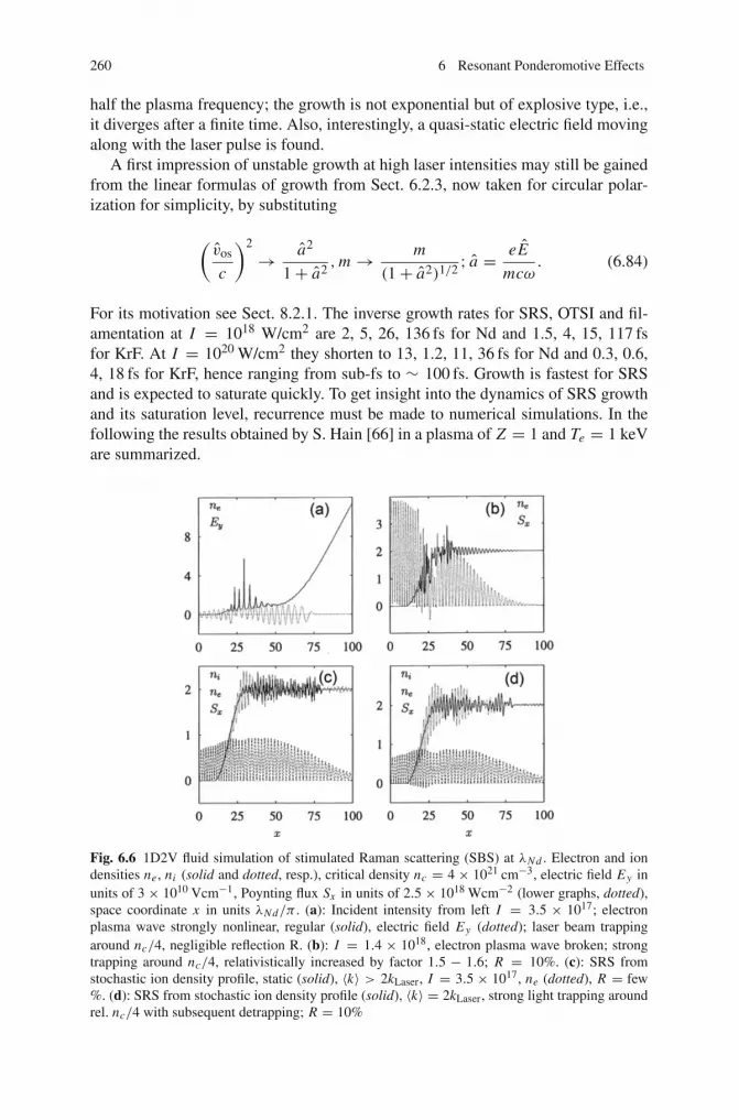
260 6 Resonant Ponderomotive Effects
half the plasma frequency; the growth is not exponential but of explosive type, i.e.,it diverges after a finite time. Also, interestingly, a quasi-static electric field movingalong with the laser pulse is found.
A first impression of unstable growth at high laser intensities may still be gainedfrom the linear formulas of growth from Sect. 6.2.3, now taken for circular polar-ization for simplicity, by substituting
(vos
c
)2
→ a2
1+ a2,m → m
(1+ a2)1/2; a = eE
mcω. (6.84)
For its motivation see Sect. 8.2.1. The inverse growth rates for SRS, OTSI and fil-amentation at I = 1018 W/cm2 are 2, 5, 26, 136 fs for Nd and 1.5, 4, 15, 117 fsfor KrF. At I = 1020 W/cm2 they shorten to 13, 1.2, 11, 36 fs for Nd and 0.3, 0.6,4, 18 fs for KrF, hence ranging from sub-fs to ∼ 100 fs. Growth is fastest for SRSand is expected to saturate quickly. To get insight into the dynamics of SRS growthand its saturation level, recurrence must be made to numerical simulations. In thefollowing the results obtained by S. Hain [66] in a plasma of Z = 1 and Te = 1 keVare summarized.
Fig. 6.6 1D2V fluid simulation of stimulated Raman scattering (SBS) at λNd . Electron and iondensities ne, ni (solid and dotted, resp.), critical density nc = 4 × 1021 cm−3, electric field Ey inunits of 3 × 10¹⁰ Vcm−1, Poynting flux Sx in units of 2.5 × 10¹⁸ Wcm−2 (lower graphs, dotted),space coordinate x in units λNd/π . (a): Incident intensity from left I = 3.5 × 10¹⁷; electronplasma wave strongly nonlinear, regular (solid), electric field Ey (dotted); laser beam trappingaround nc/4, negligible reflection R. (b): I = 1.4 × 10¹⁸, electron plasma wave broken; strongtrapping around nc/4, relativistically increased by factor 1.5 − 1.6; R = 10%. (c): SRS fromstochastic ion density profile, static (solid), 〈k〉 > 2kLaser, I = 3.5 × 10¹⁷, ne (dotted), R = few%. (d): SRS from stochastic ion density profile (solid), 〈k〉 = 2kLaser, strong light trapping aroundrel. nc/4 with subsequent detrapping; R = 10%
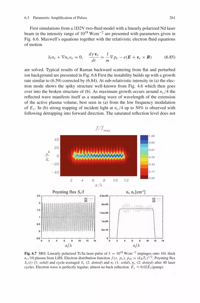
6.3 Parametric Amplification of Pulses 261
First simulations from a 1D2V two-fluid model with a linearly polarized Nd laserbeam in the intensity range of 1018 Wcm−2 are presented with parameters given inFig. 6.6. Maxwell’s equations together with the relativistic electron fluid equationsof motion
∂t ne + ∇neve = 0,dγ ve
dt= 1
m∇ pe − e(E + ve × B) (6.85)
are solved. Typical results of Raman backward scattering from flat and perturbedion background are presented in Fig. 6.6 First the instability builds up with a growthrate similar to (6.59) corrected by (6.84). At sub-relativistic intensity in (a) the elec-tron mode shows the spiky structure well-known from Fig. 4.6 which then goesover into the broken structure of (b). As maximum growth occurs around nc/4 thereflected wave manifests itself as a standing wave of wavelength of the extensionof the active plasma volume, best seen in (a) from the low frequency modulationof Ey . In (b) strong trapping of incident light at nc/4 up to 50% is observed withfollowing detrapping into forward direction. The saturated reflection level does not
Fig. 6.7 SRS: Linearly polarized Ti:Sa laser pulse of I = 1018 Wcm−2 impinges onto 10λ thicknc/10 plasma from LHS. Electron distribution function f (x, px ), pth = (kB Te)
1/2, Poynting fluxSx (t) (1: solid) and cycle-averaged Sx (2: dotted) and ni (1: solid), ne (2: dotted) after 40 lasercycles. Electron wave is perfectly regular; almost no back reflection. Ex ≈ 0.02E1(pump)

262 6 Resonant Ponderomotive Effects
Fig. 6.8 SRS: Linearly polarized standing pump pulse. Parameters and symbols as in Fig. 6.7.Electron density becomes chaotic when the two pump beams start overlapping. The ponderomo-tively driven ion density profile remains regular; amplitudes are reduced due to electron chaos,compare inset on ion density profile from hydrodynamic simulation. Back reflection level remainsvery low despite Ex ≈ 0.2E1
exceed 10%. Backscattering from a stochastic ion background becomes significant(∼10%) only from a Brillouin-matched spatial modulation of 2kLaser. In the fluiddynamic simulation local wavebreaking must be bridged somehow artificially eachtime over the instant of breaking.
Alternatively SRS is simulated kinetically by solving the Vlasov equation. Thisis a 3D problem. However, if only for the thermal vx velocity component Te = 0is assumed and the laser field is approximated by a plane wave Ey = −∂t Ay ,owing to the canonical momentum conservation mvy = eAy collinear scattering isreducible to a 1D1V problem for the electron distribution function f (x, px , py, t) =f (x, px , t)δ(py − eAy). Including the Lorentz force component (ponderomotiveterm) the relativistic Vlasov equation (8.39) reads
∂ f
∂t+ px
γm
∂ f
∂x− e(Ex + e
2γm∂x A2
y)∂ f
∂py= 0. (6.86)

6.3 Parametric Amplification of Pulses 263
Fig. 6.9 SRS after 40 cycles from a linearly polarized traveling pump pulse (L), I = 1018 Wcm−2,and two counter-propagating pulses (K) in nc/4 plasma, same intensity 1018 Wcm−2 both direc-tions. Symbols and rest of parameters as in Fig. 6.7. In both cases, L and K, the electron plasmawave breaks and stabilizes back scattering; the ion density remains regular. Ex ≈ 0.2E1 (L) andEx ≈ 0.3E1 (K). In the scattered low-frequency wave E2 trapping of E1 occurs up to 50% inintensity
In circular polarization Ay , Ey are to be substituted by A⊥ = (A2y + A2
z )1/2, E⊥ =
−∂t A⊥. The ion dynamics is calculated in the nonrelativistic fluid approach withan ion temperature Ti = 100 eV. For the electrons a “one-dimensional” temperatureTe = 1 keV is chosen. Simulations are made in linear and circular polarizationwith a Ti:Sa beam of constant 1018 Wcm−2 and rise time 30 fs that is impinging on∼ 10 wavelengths thick targets of constant densities ne = ni = nc/10 and nc/4.The results after different numbers of light periods are presented in Figs. 6.7, 6.8,and 6.9. We start with SRS from a beam in linear polarization propagating throughnc/10 density. In Fig. 6.7 f (x, px )/ fmax, normalized Poynting flux Sx and ni (1:solid) and ne are shown after 40 laser cycles. The electron distribution function andne, ni are perfectly regular and saturate at a very low level, Ex ≈ 0.02E1. Themodulation in Ex originates from the Raman anti-Stokes component. A completelydifferent picture of the electron dynamics is obtained from two counter-propagatingpump beams (standing wave, e.g. total reflection from critical point) after 40 cycles(Fig. 6.8). When the two beams overlap the electrons start moving chaotically andback reflection saturates, under a low level again as inferred from the cycle-averagedPoynting flux Sx (dotted line). The ions behave perfectly regular. Stronger Ramanback scattering and increased chaotic dynamics is to be expected from nc/4 density.

264 6 Resonant Ponderomotive Effects
Fig. 6.10 SRS after 40 cycles from a linearly polarized traveling pump pulse in nc/10 plasmadensity, I = 1018 Wcm−2. Symbols and parameters as in Fig. 6.7. Owing to breaking of ne, seef (x, px ) and Ex ≈ 0.02E1, reflection saturates at 2− 5%, see Poynting flux Sx/I in the inset
The latter is true as Fig. 6.9 shows, however, Sx/I (L) indicates that back reflectionremains low in this case again.
SRS of a circularly polarized traveling pump wave of I = 1018 Wcm−2 froman nc/10 plasma is presented in Fig. 6.10 after 40 cycles. The time for the instabil-ity to grow is 4 cycles only. At early times regular structures in ni and ne similarto those in Fig. 6.6 build up, however following onset of breaking destroys them(lower right picture) and stabilizes back reflection at 2–5%, see Sx/I in the insetof lower left picture of Ex . It has been a general observation through all simula-tions that circular polarization shows the tendency towards higher degree of chaoticdynamics and at the same time towards increased back reflection. With increasingbackground plasma density the difference tends to vanish. For the parameters ofFig. 6.9 there is almost no difference between linear and circular polarization. It canbe concluded that at relativistic intensities SRS saturates, mainly owing to breaking,at an insignificant low level, in qualitative agreement with hydro simulations wherethe latter overestimate scattering for obvious reasons. In the context here it may beinteresting to note that in a very early paper [67] it has been stated on pure physicalgrounds that at relativistic intensities parametric instabilities are not important, inagreement with the simulations presented here.

References 265
References
1. Glenzer, S.H., Rozmus, W., McGowan, B.J., et al.: Phys. Rev. Lett. 82, 97 (1999) 2352. Glenzer, S.H., Redmer, R.: Rev. Mod. Phys. 81, 1625 (2009) 2353. Lee, K.J., Neumayer, P., Castor, J., et al.: Phys. Rev. Lett. 102, 115001 (2009) 2354. Baldis, H.A., Campbell, E.M., Kruer, W.L.: In: Rosenbluth, M.N., Sagdeev, R.Z. (eds.)
Laser–Plasma Interactions, Handbook of Plasma Physics, vol. 3, pp. 383–396. North-Holland,Amsterdam (1991) 237, 242
5. John Sheffield: Plasma Scattering of Electromagnetic Radiation, Acad. Press. New York(1975) 237
6. Boyd, T.J.M., Sanderson, J.J.: The Physics of Plasmas, Cambridge Univ. Press. Cambridge(2003) 237, 257
7. Chihara, J.: J. Phys.: Metal Physics 17, 295 (1987); J. Phys.: Condensed Matter 12, 231 (2000) 2378. Fortmann, C., Redmer, R., Reinholtz, H., Röpke, G., Wierling, A., Rozmuws, W.: High Energy
Densitity Physics 2, 57 (2006) 2389. Fortmann, C., Thiele, R., Fäustlin, R.R., Bornath, Th., et al.: High Energy Density Physics 5,
208 (2009) 23810. Brillouin, L.: La theorie des solides er les quanta (1928), and Wave propagation in periodic
structures (1940). Experimental verification of the effect by Gross in 1930 (Léon Brillouinpredicted the effect in 1922) 242
11. Landsberg, G., Mandelstam, L.: Eine neue Erscheinung bei der Lichtstreuung in Metallen. Anew phenomenon in the light scattering from metals), Die Naturwissenschaften 16, 557 (1928) 242
12. Handke, J., Rizvi, S.A.H., Kronast, B.: Appl. Phys. 25, 109 (1981) 242, 24913. Gellert, B., Kronast, B.: Appl. Phys. B 32, 175 (1983) 242, 24914. Baldis, H., et al.: Phys. Fluids B 5, 3319 (1993) 24215. Kline, J.L., J. Phys.: Conf. Ser. 112, 022042 (2008)16. Hüller, S., Masson-Laborde, P.E., Pesme, D., Casanova, M., Detering, F., Maximov, A.: Phys.
Plasmas 13, 022703 (2006) 24817. Pesme, D. In: Dautray, R., Watteau, J.P. (eds.) La fusion thermonucléaire inertielle par laser
(1993) 24718. Johnston, T.W., et al.: Plasma Phys. Contr. Fusion 27, 473 (1985) 24219. Kadomtsev, B.B.: Plasma Turbulence. Acad. Press, New York (1965) 24220. Davidson, R.C., Goldman, R.: Phys. Rev. Lett. 21, 1671 (1968) 24221. Depierreux, S., et al.: Phys. Rev. Lett. 84, 2869 (2000) 24222. Fouquet, Th., Pesme, D.: Phys. Rev. Lett. 100, 055006 (2008) 24223. Goldman, M.V., DuBois, D.F.: Phys. Fluids 8, 1404 (1965) 24224. Forslund, D.W., Kindel, J.M., Lindman, E.L.: Phys. Fluids 18, 1002 (1975) 242, 246, 24725. Strozzi, D.J.: Vlasov simulations of kinetic enhancement of Raman backscatter in laser fusion
plasmas. Massachusetts Institute of Technology, Thesis (2006) 24226. Vu, H.X., DuBois, D.F., Bezzerides, B.: Phys. Plasmas 14, 012702 (2007) 24327. Yin, L., Daughton, W., Albright, B.J., et al.: Phys. Plasmas 13, 072701 (2006) 24328. Baldis, H.A., Campbell, E.M., Kruer, W.L.: In: Rosenbluth, M.N., Sagdeev, R.Z. (eds.)
Laser–Plasma Interactions, Handbook of Plasma Physics, vol. 3, pp. 397–408. North-Holland,Amsterdam (1991) 243
29. Silin, V.P.: Sov. Phys. JETP 21, 1127 (1965) 244, 25530. Nishikawa, K.: J. Phys. Soc. Japan 24, 1152 (1968) 244, 25531. Mulser, P., Giulietti, A.: Europhys. Lett. 12, 335 (1990) 24432. Kruer, W.L.: The Physics of Laser Plasma Interactions, p. 91. Addison-Wesley Publ., Red-
wood City, CA. (1988) 24733. Hüller, S., Mulser, P., Rubenchik, A.M.: Phys. Fluids B 3, 3339 (1991) 24734. Drake, J.F., Kaw, P.K., Lee, Y.C., Schmidt, G., Liu, C.S., Rosenbluth, M.N.: Phys. Fluids 17,
778 (1974) 247, 24835. Berger, R.L., et al.: Phys. Fluids B 5, 2243 (1993) 248

266 6 Resonant Ponderomotive Effects
36. Cassedy, E.S., Mulser, P.: Phys. Rev. A 10, 2349 (1974) 24837. Eidmann, K., Sigel, R.: In: Schwarz, H.J., Hora, H. (eds.) Laser Interaction and Related Plasma
Phenomena, vol. 3B, p. 667. Plenum, New York (1974) 24938. Clayton, C.E., Joshi, C., Chen, F.F.: Phys. Rev. Lett. 51, 1656 (1983) 24939. Bernard, J.E., Meyer, J.: Phys. Fluids 29, 2313 (1986) 24940. Mostovych, A.M., et al.: Phys. Rev. Lett. 59, 1193 (1987) 25041. Hüller, S., Masson, P.E.-Laborde, Pesme, D., Labaune, C., Bandulet, H.: J. Phys.: Conf. Series
112, 022031 (2008) 25042. Tikhonchuk, V.T., Hüller, S., Ph. Mounaix: Phys. Plasmas 4, 4369 (1997) 25043. Pesme, D., Rozmus, W., Tikhonchuk, V.T., Maximov, A., Ourdev, I., Still, C.H.: Phys. Rev.
Lett. 84, 278 (2000) 25144. Michel, P., Labaune, C.: Phys. Fluids 10, 3545 (2003) 25145. Masson-Laborde, P.E., Hüller, S., Pesme, D., Casanova, M., Loiseau, P.: J. Phys. IV France
133, 247 (2006) 25146. Drake, R.P., Turner, R.E., Lasinski, B.F., et al.: Phys. Rev. Lett. 40, 3219 (1989) 25247. Strozzi, D.J., Shoucri, M.M., Bers, A., Williams, E.A., Langdon, A.B.: J. Plasma Phys. 72,
1299 (2006)48. Ze, F., et al.: Comm. Plasma Phys. Contr. Fusion 10, 33 (1986)49. Mourenas, D., Divol, L., Casanova, M., Rousseaux, C.: Phys. Plasmas 8, 557 (2001) 25250. Stoeckl, C., Baldis, H., et al.: Phys. Rev. Lett. 90, 235002 (2003) 25351. Sheng, Z.-M., Li, Y.T., Zhang, J., Veisz, L.: IEEE Transactions on Plasma Sci. 33, 486 (2005) 25352. Sanmartin, J.R.: Phys. Fluids 13, 1533 (1970) 25553. Piliya, A.D.: Phenomena in Ionized Gases, p. 287. Proc. 11th Int. Conf., Oxford (1971) 25654. Rosenbluth, M.N.: Phys. Rev. Lett. 29, 565 (1972) 25655. Liu, C.S.: In: Simon, A., Thompson, W.B. (eds.) Advances in Plasma Physics, vol. 6,
pp.121–177. John Wiley & Sons, New York (1976) 25656. Babonneau, D.: Instabilites Parametriques en Plasma Inhomogene, Centre d’Etudes de Limeil
B.P.no 27, Note C.E.A. no 1749 (June 26 1974) 25657. Manley, J.M., Rowe, H.E.: Proc. Inst. Radio Engrs. 44, 904 (1956) 25858. Brown, J.: Electron. Lett. 1, 23 (1965)59. Brizard, A.J., Kaufman, A.N.: Phys. Rev. Lett. 74, 4567 (1995) 25860. Salimullah, M., Hassan, M.H.A.: Phys. Rev. A 41, 6963 (1990) 25961. Guerin, S., Laval, G., Mora, P., Adam, J.C., Heron, A.: Phys. Plasmas 2, 2807 (1995)62. Mahmoud, S.T., Sharma, R.P.: Phys. Plasmas 8, 3419 (2001)63. Mahmoud, S.T.: Phys. Scr. 76, 259 (2007) 25964. Bers, A., Shkarowski, I.P., Shoucri, M.: Phys. Plasmas 16, 022104 (2009) 25965. Shvets, G., Fish, N.J., Rax, J.M.: Phys. Plasmas 3, 1109 (1996) 25966. Steffen Hain: Ausbreitung intensiver Laserstrahlung in Materie. Propagation of intense laser
radiation in matter), PhD thesis, Tech. Univ. Darmstadt; GCAVerlag. Herdecke (1999),pp. 50–62, in German 260
67. Kaw, P., Dawson, J.: Phys. Fluids 13, 472 (1970) 264
Chapter 7Intense Laser–Atom Interaction
In this chapter we shall introduce the fundamental effects that occur when intenselaser light interacts with isolated atoms, that is, ionization by the laser field, laser-assisted recombination (i.e., harmonic generation), and laser-assisted collisionalionization (nonsequential ionization). The focus of this chapter is on a self-containedbut concise account of these most fundamental effects and the common theorybehind them. Readers interested in more details on particular subjects (or subjectsnot covered at all in this chapter) may find the following (incomplete) list of reviewsand monographs useful: [1–4] (general), [5] (tunneling ionization), [6] (intense-fieldS-matrix theory), [7] (few-cycle laser pulses), [8, 9] (above-threshold ionization),[10] (harmonic generation), [11] (stabilization), [12] (multiple ionization), [13–15](attosecond physics), [16] (“double-slit in time”), [17] (two-electron atoms in laserfields), [18] (Floquet method and beyond), [19, 20] (relativistic laser-atom interac-tion), [21, 22] (time-dependent density functional theory), [23–25] (molecules inintense laser fields), and [24–27] (laser–cluster interaction).
7.1 Atomic Units
We use atomic units (a.u.) in this chapter, not only because they greatly simplifyactual calculations but also give a feeling for whether an entity has to be consideredlarge or small on the atomic scale. For instance, the laser frequency of 800 nm laserlight is ω = 0.057 a.u., telling us immediately that the laser period is large comparedto the period of an electron on, e.g., the first Bohr orbit in a hydrogen atom.
We will introduce the atomic units in a somewhat formal way. For beginners,the use of atomic units is sometimes confusing because dimensional checks are notpossible in a straightforward way once h, me, e have been set “equal to unity”.Another practical problem for beginners is to convert the result of a calculationperformed using atomic units back to SI units. If one sticks to SI units and the resultof a calculation is, say, 42, one knows that the result is dimensionless. If in atomicunits the result is 42 it could be as well 42 h, 42 e, 42 me, 42 · 4πε0, 42 hme/e, . . ..A good example is the expression for the nonrelativistic eigenenergies of hydrogen-like ions, which in atomic units is simply given by
P. Mulser, D. Bauer, High Power Laser–Matter Interaction, STMP 238, 267–330,DOI 10.1007/978-3-540-46065-7_7, C© Springer-Verlag Berlin Heidelberg 2010
267

268 7 Intense Laser–Atom Interaction
En = − Z2
2n2, n = 0, 1, 2, . . . (atomic units) (7.1)
where Z is the nuclear charge, and n is the principal quantum number. The right-hand side appears to be dimensionless. Hence, without knowing that the left-handside is an energy, there would be no way back to SI units. If one performs the entirecalculation (i.e., the solution of the Schrödinger equation) in SI units, one obtains
En = − Z2
2n2
mee4
h2(4πε0)2, n = 0, 1, 2, . . . (SI units). (7.2)
Even without knowing the left-hand side we can recover from the right-hand sidealone that the result is an energy, provided we know the SI units of h, me, e, and ε0.This seeming asymmetry between the unit systems arise from the fact that “settingh, me, e, and 4πε0 equal to unity” is more than a change of units. It is like settingkg, m, s, and C to unity. However, if one knows what the dimension of the finalresult is, the conversion from atomic units back to SI units is unique.
As in Sect. 2.2.3, let us denote mass, length, time, and charge by M, L, T, and C,respectively. In atomic units we wish to use the action h, the electron mass me, themodulus of the electron charge e, and 4π times the permittivity of vacuum, 4πε0, asthe basic units. The relation between both system of units is established by (“[. . .]”meaning “units of . . .”, see also Sect. 2.2.3)
[h] = Ma11 La12 Ta13 Ca14, (7.3)
[me] = Ma21 La22 Ta23 Ca24, (7.4)
[e] = Ma31 La32 Ta33 Ca34, (7.5)
[4πε0] = Ma41 La42 Ta43 Ca44 . (7.6)
The exponents a41, . . . , a44, for instance, are determined by noticing that in SI unitsthe dimension of ε0 is Coulomb per Volt and meter. Volt is a derived unit, V =ML2/(CT2), and hence
[4πε0] = M−1L−3T2C2. (7.7)
Similarly, the remainder of the dimensional matrix is easily calculated and reads
A =
⎛
⎜⎜⎝
a11 a12 a13 a14a21 a22 a23 a24a31 a32 a33 a34a41 a42 a43 a44
⎞
⎟⎟⎠ =
⎛
⎜⎜⎝
1 2 −1 01 0 0 00 0 0 1
−1 −3 2 2
⎞
⎟⎟⎠ . (7.8)
The SI values of one atomic mass, length, time, and charge unit, denoted by M, L,T , and C, respectively, are needed for the transformation back to SI units. Mass andcharge are trivial: M = me, C = e. Let us calculate the value of the atomic lengthunit:
7.1 Atomic Units 269
L = hb21 mb22e eb23(4πε0)
b24 . (7.9)
Plugging in (7.3), (7.4), (7.5), and (7.6) and using the values for the ai j in (7.8) leadto
L = Mb21+b22−b24 L2b21−3b24T−b21+2b24Cb23+2b24, (7.10)
giving us four equations for the four b2 j . Since L is a length, 2b21 − 3b24 = 1, andthe exponents of mass, time, and charge must be zero. One finds b21 = 2, b22 = −1,b23 = −2, b24 = 1 so that
L = h24πε0
mee2= 0.5292 · 10−10m, (7.11)
which is the Bohr radius a0. The corresponding calculation for T is left as an exer-cise. The inverse dimensional matrix is
M = hb11 mb12e eb13(4πε0)
b14, (7.12)
L = hb21 mb22e eb23(4πε0)
b24, (7.13)
T = hb31 mb32e eb33(4πε0)
b34, (7.14)
C = hb41 mb42e eb43(4πε0)
b44 (7.15)
with
B =
⎛
⎜⎜⎝
b11 b12 b13 b14b21 b22 b23 b24b31 b32 b33 b34b41 b42 b43 b44
⎞
⎟⎟⎠ =
⎛
⎜⎜⎝
0 1 0 02 −1 −2 13 −1 −4 20 0 1 0
⎞
⎟⎟⎠ . (7.16)
It is readily checked that A · B = B · A = 1.We conclude this section by giving the explicit expressions and values for fre-
quently occurring entities in laser-atom interaction in Table 7.1. In the entry for thevelocity the fine structure constant
α = e2
h4πε0c= 1
137.04(7.17)
appears. The value of the light velocity in vacuum in atomic units equals the inversefine structure constant. Note that with h, e, me, and ε0 alone it is not possible toconstruct a dimensionless entity (as it is impossible with kg, m, s, and C). Oneneeds a fifth building brick, which is c in the case of the fine structure constant. Auseful and frequently used formula to convert the field strength E in atomic units toa laser intensity I in the commonly used Wcm−2 is
(I in Wcm−2) = 3.51 · 1016 × (E2 in a.u.). (7.18)

270 7 Intense Laser–Atom Interaction
Table 7.1 One atomic unit of frequently occurring entities expressed in SI units
One atomic unit of Value
Mass me 9.1094 · 10−31 kg
Length h24πε0e2me
= a0 0.5292 · 10−10 m
Time h3(4πε0)2
mee4 2.4189 · 10−17 s
Charge e 1.6022 · 10−19 CAction h 1.0546 · 10−34 JPermittivity 4πε0 4π · 8.8542 · 10−12 CV−1 m−1
Energy mee4
h2(4πε0)2 4.3598 · 10−19J = 27.21 eV
Velocity e2
h4πε02.1877 · 106 ms−1 = αc
El. field m2e e5
h4(4πε0)3 5.1422 · 1011 Vm−1
Magn. flux density m2e e3
h3(4πε0)2 2.3505 · 105 T
Laser intensity e12m4e
8παh9(4πε0)6 3.5095 · 1020 Wm−2
7.2 Atoms in Strong Static Electric Fields
Although we assume the external electric field to be static in this section, the fol-lowing analysis is useful for atoms in laser fields too, as will become clear below.The Hamiltonian governing an electron moving in a Coulomb potential −Z/r anda static electric field E = Eez reads
H = p2
2+ Veff, Veff = − Z
r+ Ez. (7.19)
The effective potential Veff describes a tilted Coulomb potential (see Fig. 7.1). Aperturbative treatment of the problem can be found in almost all quantum mechanicsor atomic physics text books (Stark effect, see, e.g., [28–30]). In first order (lin-ear Stark effect) the degeneracy with respect to the angular quantum number � isremoved while the degeneracy in the magnetic quantum number m is maintained.The non-degenerate ground state is only affected in second order (quadratic Starkeffect). It is down-shifted in energy since the potential widens in the presence ofthe field. In the case of the hydrogen atom (Z = 1) this down-shift is given byΔE = −9E2/4.
Let us first point out that, strictly speaking, there exist no discrete, bound statesanymore even for the tiniest electric field. This is because even a very small fieldgives rise to a potential barrier (see Fig. 7.1) through which the initially boundelectron may tunnel. The electric field couples all bound states to the continuumand thus all discrete states become resonances with a finite line width. Mathe-matically speaking, the Hamiltonian (7.19) has only a continuous spectrum, andthe eigenfunctions are no longer square-integrable. However, since the barrier forsmall fields is far out, the probability for tunneling is extremely low (note that the
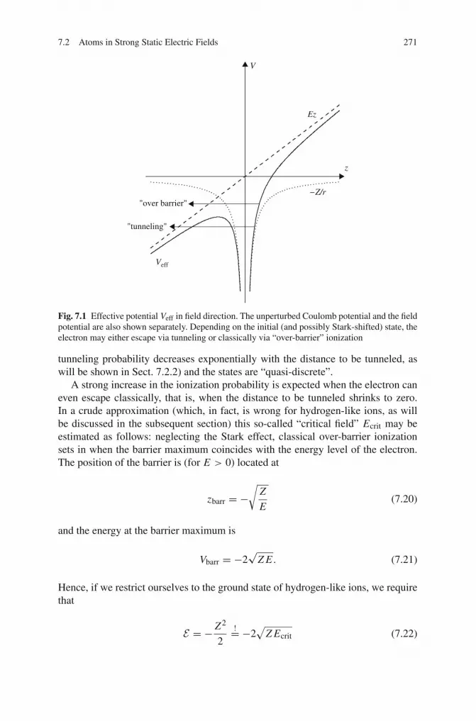
7.2 Atoms in Strong Static Electric Fields 271
Veff
V
z
Ez
−Z/r"over barrier"
"tunneling"
Fig. 7.1 Effective potential Veff in field direction. The unperturbed Coulomb potential and the fieldpotential are also shown separately. Depending on the initial (and possibly Stark-shifted) state, theelectron may either escape via tunneling or classically via “over-barrier” ionization
tunneling probability decreases exponentially with the distance to be tunneled, aswill be shown in Sect. 7.2.2) and the states are “quasi-discrete”.
A strong increase in the ionization probability is expected when the electron caneven escape classically, that is, when the distance to be tunneled shrinks to zero.In a crude approximation (which, in fact, is wrong for hydrogen-like ions, as willbe discussed in the subsequent section) this so-called “critical field” Ecrit may beestimated as follows: neglecting the Stark effect, classical over-barrier ionizationsets in when the barrier maximum coincides with the energy level of the electron.The position of the barrier is (for E > 0) located at
zbarr = −√
Z
E(7.20)
and the energy at the barrier maximum is
Vbarr = −2√
Z E . (7.21)
Hence, if we restrict ourselves to the ground state of hydrogen-like ions, we requirethat
E = − Z2
2!= −2
√Z Ecrit (7.22)
272 7 Intense Laser–Atom Interaction
so that
Ecrit = Z3
16. (7.23)
Because of the strong Z -dependence of the critical field even with the most intenselasers available today it is not possible to fully strip heavy elements. For hydrogen-like ions (7.23) even underestimates the critical field by more than a factor of two,as will be shown now.
7.2.1 Separation of the Schrödinger Equation
The Schrödinger equation with the Hamiltonian (7.19) separates in parabolic coor-dinates (ξ, η, ϕ) (see, e.g., [28–30]),
ξ = r+ z, η = r− z, r = 1
2(ξ+η), z = 1
2(ξ−η), 0 ≤ ξ, η. (7.24)
Here, r is the radial coordinate, and ϕ is the azimuthal angle (as in spherical, polaror cylindrical coordinates). Cuts of contours of constant ξ and η in the xz-plane areshown in Fig. 7.2. The Hamiltonian in parabolic coordinates reads
H = − 2
ξ + η
[∂ξ (ξ∂ξ )+ ∂η(η∂η)
]− 1
2ξη∂2ϕ −
2Z
ξ + η+ E
ξ − η
2. (7.25)
Plugging the ansatz
Ψ = f1(ξ) f2(η)eimϕ (7.26)
into the Schrödinger equation EΨ = HΨ and multiplying by (ξ + η)/2 leads to anequation that can be decoupled into
d
dξ
(ξ
d f1
dξ
)+(E
2ξ − m2
4ξ− E
4ξ2)
f1 + Z1 f1 = 0, (7.27)
d
dη
(η
d f2
dη
)+(E
2η − m2
4η+ E
4η2)
f2 + Z2 f2 = 0 (7.28)
where Z1, Z2 are separation constants fulfilling
Z1 + Z2 = Z . (7.29)
Division by 2ξ and 2η, respectively, yields the two Schrödinger equations

7.2 Atoms in Strong Static Electric Fields 273
0.11
2
3
4
5
6
7
8
9
0.11
2
3
4
5
67
89
Fig. 7.2 Illustration of parabolic coordinates. Cuts of contours ξ = const (dashed, values givennext to the lines) and η = const (solid) in the xz-plane (azimuthal symmetry with respect to thez-axis)
[−1
2
(d2
dξ2+ 1
ξ
d
dξ− m2
4ξ2
)− Z1
2ξ+ E
8ξ
]f1 = E
4f1, (7.30)
[−1
2
(d2
dη2+ 1
η
d
dη− m2
4η2
)− Z2
2η− E
8η
]f2 = E
4f2 (7.31)
which have the same shape as two Schrödinger equations in cylindrical coordinatesfor the potentials
Vξ = − Z1
2ξ+ E
8ξ, Vη = − Z2
2η− E
8η. (7.32)
Both potentials have a Coulombic part and a linear contribution, like Veff in(7.19). However, because ξ, η ≥ 0, the potential Vξ has only bound states (weassume without loss of generality E > 0). The potential Vη instead displays abarrier. Hence, in parabolic coordinates ionization happens with respect to the η
coordinate while the electron remains confined in ξ . The consequences of this inCartesian coordinates can be understood with the help of Fig. 7.2: confinement toa region ξ < ξmax implies preferred electron emission towards negative z with alateral spread that can be estimated by the confining contour ξmax. The potentials Vξand Vη are called “uphill” and “downhill potential,” respectively. They are illustratedin Fig. 7.3. Given an energy E one finds a sequence of Z1 for which the solutionof the Schrödinger equation in ξ , (7.30), leads to normalizable bound states. Thissequence can be labeled by the number of nodes in f1 for ξ > 0, n1 = 0, 1, 2, . . .(note that Z1 < 0 is also possible). The second equation (7.31) has to be solved for

274 7 Intense Laser–Atom Interaction
Z2 = Z − Z1 and the same energy E . This is possible because the correspondingHamiltonian Hη [i.e., the square bracket in (7.31)] has a continuous spectrum and isneither bound from below nor from above.
In the field-free case E = 0 the two Schrödinger equations (7.30) and (7.31) areidentical, and the relation between the “usual” principal quantum number n and theparabolic quantum numbers n1, n2 is given by
ni + |m| + 1
2= n
Zi
Z, n1 + n2 + |m| + 1 = n, i = 1, 2. (7.33)
Instead of working directly with the parabolic coordinates ξ and η, one can per-form an additional, simple coordinate transformation
u = √2ξ, v = √2η (7.34)
which, after multiplication of the new Schrödinger equation by (u2 + v2)/4, andwith the ansatz Ψ = Φu(u)Φv(v)eimϕ yields
V
ξ,η
V ξ
Vη
"downhill"(ionization)
(bound motion)
"uphill"
Fig. 7.3 Illustration of the potentials Vξ and Vη (7.32). The “uphill potential” Vξ (for E > 0)supports only bound states while the “downhill potential” Vη displays a barrier through which theelectron may tunnel
7.2 Atoms in Strong Static Electric Fields 275
[−1
2
(1
u∂u(u∂u)− m2
u2
)+ 1
2Ω2u2 − 1
4gu4
]Φu = Z1Φu, (7.35)
[−1
2
(1
v∂v(v∂v)− m2
v2
)+ 1
2Ω2v2 + 1
4gv4
]Φv = Z2Φv, (7.36)
where, again, Z = Z1 + Z2 is used, and Ω and g are defined as
1
2Ω2 = −E
4, E ≤ 0, g = − E
4. (7.37)
The Schrödinger equations (7.35) and (7.36) have the shape of two-dimensionaloscillators (with radial coordinates u and v, respectively) of frequency Ω and witha quartic perturbation that is proportional to the electric field. In the field-free case,the Coulomb problem is mapped to two two-dimensional oscillators where, how-ever, the energy assumes the role of the oscillator frequency, and the nuclear charge(splitted into Z1 and Z2) assumes the role of the energy. The transformation to thecoordinates (u, v, ϕ) corresponds to the Kustaanheimo–Stiefel transformation [31].
Let us now evaluate an improved critical field for the case of hydrogen-like ions[32]. As mentioned above, formula (7.23) underestimates the critical field by morethan a factor of two.
In the unperturbed case (g = 0) and for m = 0 (groundstate) the solutions to(7.35) and (7.36) are Gaussians. We therefore use
Φu(u) =√
au
πe−auu2/2 (7.38)
(and analogous for v) as trial functions with parameters au and av . Denoting thesquare bracket in (7.35) as Hu the “energy” reads
Z1(g) = 2π∫ ∞
0du uΦ∗u HuΦu = 1
au
(Ω2
2− a2
u
2
)+ au − g
2a2u. (7.39)
Minimizing this energy yields up to first order in g
au = Ω(
1− g
Ω3
), av = Ω
(1+ g
Ω3
). (7.40)
The oscillator “energies” are
Z1(g) = Ω(
1− g
2Ω3
), Z2(g) = Ω
(1+ g
2Ω3
). (7.41)
Note that this is consistent with the fact that the linear Stark effect vanishes for theground state since

276 7 Intense Laser–Atom Interaction
Z1(g)+ Z2(g) = 2Ω (7.42)
is independent of the field g. Since Z1 + Z2 = Z we have Z = 2Ω which is [see(7.37)] equivalent to E = −Z2/2, as it should for the ground states of hydrogen-likeions.
In physical coordinates the variationally determined wave function for, e.g.,hydrogen (Z = 1) reads
ΨH(r) = 1− 4E2
√π
e−r e−2E·r , (7.43)
i.e., the unperturbed wave function is multiplied by a “deformation factor”.If E > 0 we have g < 0 and vice versa. Let us assume g > 0 so that the
u-oscillator displays a barrier while the v-oscillator does not. The barrier is locatedat ubarr = Ω/
√g and the energy at the barrier maximum is Ω2u2
barr/2− gu4barr/4 =
Ω4/(4g). At the critical field strength the energy of the u-state coincides with thebarrier-energy, giving us
Z1(g) = Ω − g
2Ω2= Ω4
4g⇒ gcrit = Ω3(1− 2−1/2) � 0.3Ω3 (7.44)
which translates [using (7.37)] to [32]
EH−likecrit = (
√2− 1) E3/2. (7.45)
In the case of atomic hydrogen one obtains EH−likecrit = 0.147 instead of the 0.0625
predicted by (7.23). The new value is in agreement with [33]. The wrong predictionof (7.23) is due to the erroneous assumption that the electron motion in z-directionand in lateral direction are independent. Instead, the problem separates in paraboliccoordinates. However, since the “exceptional” symmetry of hydrogen-like ions isbroken in many-electron atoms, simple over-barrier estimates [such as those aboveleading to (7.23)] are useful and sufficiently accurate for many practical applica-tions. Of particular interest is the “appearance intensity” Iapp,Z for a charge state Zof an atom with ionization potential Eip,Z . Here, “appearance intensity” should beunderstood as the intensity where a certain charge state Z is becoming abundant.This is the case once the electron may escape classically from the binding potential.The derivation is thus analogous to (7.20), (7.21), (7.22), and (7.23), leading to
Iapp,Z =E4
ip,Z
16Z2. (7.46)
Comparison of the appearance intensities predicted by (7.46) for the experimentsreported in, e.g., [34, 35] yields good agreement, and the scaling is confirmed by aThomas–Fermi treatment [36].

7.2 Atoms in Strong Static Electric Fields 277
7.2.2 Tunneling Ionization
Going one step beyond a classical over-barrier analysis amounts to take tunnelinginto account. This can be done in a semi-classical way. Let us consider the tunnelingof the electron in atomic hydrogen through the barrier of the “downhill potential”in Fig. 7.3 [28]. We assume that the electron is initially in the 1s ground state. TheSchrödinger equation (7.31) for m = 0, Z2 = 1/2, E = −1/2 reads
[−1
2
(d2
dη2+ 1
η
d
dη
)− 1
4η− E
8η
]f2(η) = −1
8f2(η). (7.47)
Substituting χ(η) = √η f2(η) yields
d2χ
dη2+(−1
4+ 1
2η+ 1
4η2+ 1
4Eη
)χ = 0. (7.48)
Comparison with
− 1
2
d2χ
dη2+ V (η)χ = εχ (7.49)
shows that we effectively deal with one-dimensional motion of an electron in thepotential
V (η) = −1
2
(1
2η+ 1
4η2+ 1
4Eη
)(7.50)
with total energy ε = −1/8. The potential V (η) is of the form depicted in Fig. 7.4.We now match at a position η0 inside the barrier,
1 � η0 � 1/E (7.51)
the “left” quasi-classical wave function
χleft(η) = − iC√|p| exp
(∣∣∣∣∫ η
η0
p(η′) dη′∣∣∣∣
)(7.52)
with the “right” quasi-classical outgoing wave function
χright(η) = C√p
exp
(i∫ η
η0
p(η′) dη′ + iπ/4
)(7.53)
where
p(η) = √2[ε − V (η)] =√
−1
4+ 1
2η+ 1
4η2+ 1
4Eη. (7.54)

278 7 Intense Laser–Atom Interaction
1/E
η0
Fig. 7.4 Plot of the potential V (η) (7.50) for E = 0.0075. The tunnel “exit” η1 for sufficiently lowfields E is in good approximation given by η1 � 1/E . The matching point η0 is located inside thebarrier where 1 � η0 � 1/E holds
The semi-classical approximation breaks down at the classical turning point η1 �1/E since p(η1) = 0. In general, semi-classical wave functions are accurate as longas the de Broglie wave length 2π h/p is small compared to the length scale char-acterizing changes in the potential (i.e., the potential should be sufficiently “flat”).For vanishing momentum p the de Broglie wave length is infinite so that the semi-classical approximation necessarily breaks down. However, for the calculation ofthe probability flux out of the potential the disagreement between the semi-classicalwave function and the exact wave function in a narrow region around the classicalturning point η1 plays no role.
For the determination of the normalization constant C we set the left wave func-tion at position η0 equal to the unperturbed wave function so that
− iC√|p0| =√η0
1√π
e−(ξ+η0)/2 (7.55)
with p0 = p(η0). The “uphill” coordinate ξ appears as a parameter here which willbe integrated out later on; in other words: the wave function is assumed to retain itsground state shape with respect to ξ (i.e., the Stark effect is neglected). We obtainfor the right wave function
χright(η, ξ) = i
√η0|p0|πp(η)
e−(ξ+η0)/2 exp
(i∫ η
η0
p(η′) dη′ + iπ/4
)(7.56)
so that
|χright(η, ξ)|2 = η0|p0|πp(η)
exp
(−ξ − η0 + 2�
[i∫ η
η0
p(η′) dη′])
(7.57)

7.2 Atoms in Strong Static Electric Fields 279
where � denotes the real part. Because of (7.51) we can expand p(η) in ε = 1/η,
p(η) =
⎧⎪⎪⎨
⎪⎪⎩
1
2
(√Eη − 1+ 1
η√
Eη − 1+ · · ·
)outside barrier, η > η1
1
2
(i√
1− Eη + 1
iη√
1− Eη+ · · ·
)inside barrier, η < η1
. (7.58)
Since Eη0 � 1, it is sufficient to take |p0| = 1/2. In order to keep the leading termsdependent on E in the prefactor as well as in the exponent, we set in the denominatorof the prefactor in (7.57) p(η) = (
√Eη − 1)/2. In the exponent we integrate inside
the barrier and have to keep both terms in the expansion (7.58). We thus obtain
|χright(η, ξ)|2 = η0
π√
Eη − 1e−(ξ+η0) (7.59)
× exp
(−∫ η1
η0
[√Eη − 1− 1
η√
Eη − 1
]dη
).
The integral can be solved. Using η1 � 1/E and η0 E � 1 we obtain for theprobability density outside the barrier
|χright(η, ξ)|2 = 4 e−ξ
πE√
Eη − 1e−2/(3E). (7.60)
The total probability current through a plane perpendicular to the z-axis is
Γ =∫ ∞
0| f1(ξ) f2(η)|2vz2πρ dρ (7.61)
where f1(ξ), f2(η) are the wave functions introduced in (7.26), vz is the velocity inz-direction and ρ is the radial cylindrical coordinate. The ξ -dependent part | f1|2 isincluded in |χright(η, ξ)|2 so that
Γ =∫ ∞
0
|χright(η, ξ)|2η
vz2πρ dρ. (7.62)
With z = (ξ − η)/2 � −η/2 for small ξ and large η, we estimate for vz
− 1
2= 1
2v2
z + Ez � 1
2v2
z −1
2Eη ⇒ vz �
√Eη − 1 (7.63)
so that
Γ =∫ ∞
0
|χright(η, ξ)|2η
√Eη − 1 2πρ dρ. (7.64)

280 7 Intense Laser–Atom Interaction
Finally, with
ρ = √ξη ⇒ dρ = d√ξη = 1
2
η√ξη
dξ + 1
2
ξ√ξη
dη � 1
2
√η
ξdξ (7.65)
(where the last step again follows from η � ξ ) we arrive at
Γ =∫ ∞
0
|χright(η, ξ)|2η
√Eη − 1 2π
√ξη
1
2
√η
ξdξ =
∫ ∞
0
4
Ee−2/(3E) e−ξdξ
so that
Γ = 4
Ee−2/(3E). (7.66)
This is the Landau-rate for tunneling ionization of atomic hydrogen from the groundstate [28]. The Landau-rate is exact in the limit of low field strengths E while itoverestimates ionization as the over-barrier field strength is approached. Figure 7.5shows the rate Γ vs the field strength E .
It is desirable to extend the above calculation to laser fields, to more complexatoms, and to higher field strengths. All directions have been pursued, and thereexists a vast amount of literature on tunneling ionization (see [5] for a review).Undeservedly, the most commonly cited tunneling formula is the so-called “ADK-rate” [37] while full credit should go to the authors of [38–41] instead (see alsoSect. 13.13 in [5]). Introducing the characteristic momentum κ , the reduced fieldstrength F , the effective principal quantum number n∗, and the Keldysh parameterγ [42] (derived below in Sect. 7.3),
1/16 0.147
Fig. 7.5 The Landau-rate (7.66) vs field strength E . The vertical lines indicate the (here wrong)over-barrier field strength (7.23) (1/16, dashed) and the correct (7.45) 0.147 (solid), respectively

7.3 Atoms in Strong Laser Fields 281
κ =√
2Eip, F = E/κ3, n∗ = Z/κ, γ = κω
E, (7.67)
with ω the laser frequency, the so-called “PPT-rate” [39] for initial states of vanish-ing angular momentum � and for a linearly polarized laser field reads
Γ = κ2C2κ
√3F
π22n∗F1−2n∗ exp
[− 2
3F
(1− γ 2
10
)], (7.68)
where
C2κ =
22n∗−2
n∗(n∗)!(n∗ − 1)! . (7.69)
The factor√
3F/π arises from the averaging over one laser cycle. This factor isabsent for circular polarization, for which also the correction term γ 2/10 should bereplaced by γ 2/15. A rate formula for � > 0 has also been derived (see the review[5] or the original articles [38–41]). However, since � and m are no “good quantumnumbers” for many-electron atoms or ions, the question arises which values to takein actual calculations and whether in multiple ionization the electrons have time toconfigure in the “new” ionic ground state before the next ionization event occurs[35, 43].
7.3 Atoms in Strong Laser Fields
There are at least three different energy scales (and the related time scales) in thephysics of atoms in strong laser fields: (i) the ionization potential Eip = |E |, (ii)the photon energy ω, and (iii) the ponderomotive energy Up. The pulse durationmay introduce an additional laser-related time-scale while the energy spectrum ofthe atom, through typical transitions, could introduce an additional species-relatedtime-scale. If one ignores the two latter parameters, the atomic species enter throughEip only.
In case ω > Eip � Up or Eip > ω � Up perturbation theory in lowest non-vanishing order (LOPT) can be applied. In contrast, when with the increasing laserintensity the regime Eip > Up > ω is reached, non-perturbative effects such asabove-threshold ionization (ATI) and channel-closings take place. This regime iscommonly referred to as (nonperturbative) multiphoton ionization (MPI). Finally,increasing the intensity further (or decreasing the photon energy) one arrives atUp > Eip > ω. Translated into the time-domain this implies that both the inner-atomic time-scale and the ionization dynamics are fast with respect to a laser period.If this is the case, a quasi static field ionization picture may be applied where, at theinstant of ionization t ′, the electron moves in an effective potential which is the sumof the Coulomb (or effective core) potential and the instantaneous potential of thelaser, as depicted in Fig. 7.1. If the field reaches the critical field estimated above, the

282 7 Intense Laser–Atom Interaction
electron may escape classically over the barrier [over-barrier or barrier suppressionionization (OBI) and (BSI), respectively], as already discussed in Sect. 7.2.1. Belowthe critical field strength the electron can escape via tunneling through the barrier(tunneling ionization, cf. Sect. 7.2.2).
The Keldysh parameter γ [42] introduced in (7.67) above can be interpreted asthe ratio of the “tunneling time” and the laser period. In semi-classical WKB theorythe time to tunnel through a static Coulomb barrier is
Ttunnel �∫ zexit
0
dz
|p(z)| =∫ κ2/2E
0
dz√κ2 − 2Ez
= κ
E(7.70)
so that
γ = ωTtunnel = ωκ
E=√
Eip
2Up. (7.71)
Hence, the Keldysh parameter indicates whether the tunneling process is fast on theinneratomic time scale (γ < 1, tunneling ionization) or the laser field reverses signbefore the tunneling is completed (γ > 1, MPI). Besides γ < 1 also Eip/ω � 1must be satisfied (i.e., very many photons are involved in the tunneling process) torender the semi-classical tunneling approach applicable. Moreover, for higher andhigher field amplitude (and thus decreasing γ ) one sooner or later enters the BSIregime. Extrapolating tunneling rate formulas to the BSI usually overestimates theionization rate. By increasing the field strength or decreasing the laser frequencyone also approaches the relativistic regime where Up � mc2 or greater. However,just because the laser driven free electron dynamics is relativistic does not mean thatrelativistic corrections are already important for the tunneling dynamics. Relativisticand QED corrections to the binding energy E because of a high nuclear charge Zhave to be taken into account, of course.
Numerous strong laser-atom experiments operate around γ � 1 or at γ > 1and are thus not in the tunneling domain. Taking, for instance, the case of atomichydrogen in an 800 nm and 1014 W/cm2 laser pulse one finds γ � 1.1. This is atypical value for ATI measurements.
What are the differences between the ionization dynamics in the MPI and in thetunneling domain? Since in the tunneling regime the process is fast compared to alaser period, significant ionization occurs during a single half laser cycle, predom-inantly around the electric field maximum because the barrier is lowest then. Fur-thermore, in tunneling ionization the quiver amplitude E/ω2 of the freed electronin the laser field is large compared to the atomic dimension, unlike in MPI. This hasconsequences for the rescattering dynamics that is responsible for various effects,such as the ATI plateau, high-harmonic generation, and nonsequential ionization, aswill be discussed below.
7.3 Atoms in Strong Laser Fields 283
7.3.1 Floquet Theory and Dressed States
If the laser pulse duration is long, i.e., if the pulse contains many laser cycles, wemay in good approximation consider it infinitely long. As a consequence the Hamil-tonian is periodic,
H(t + T ) = H(t), T = 2π
ω, (7.72)
and the time-dependent Schrödinger equation (TDSE) is a partial differential equa-tion with periodic coefficients. This type of problem has been studied by Floquetmore than 120 years ago [44]. The Floquet theorem ensures that the TDSE
H(t)|Ψ (t)〉 = 0, H(t) = H(t)− id
dt(7.73)
has solutions of the form
|Ψ (t)〉 = e−iεt |Φ(t)〉, |Φ(t + T )〉 = |Φ(t)〉, (7.74)
i.e., the wave function |Φ(t)〉 is periodic (while |Ψ (t)〉 itself is not). The Blochtheorem used in solid state physics to treat particle motion in periodic potentialsis the Floquet theorem applied to spatially periodic systems. Inserting (7.74) into(7.73) leads to the eigenvalue equation
H(t)|Φ(t)〉 = ε|Φ(t)〉. (7.75)
ε is called quasi-energy or Floquet-energy. Note that if ε and |Φ(t)〉 solve (7.75),then also
ε′ = ε + mω, |Φ(t)〉′ = eimωt |Φ(t)〉, m ∈ Z (7.76)
do. Let |α〉 be the solution of the unperturbed problem, i.e., H(t) = H0+ W (t) and
H0|α〉 = E0α|α〉. (7.77)
Because of the periodicity of |Φ(t)〉 we can Fourier-expand
|Ψ (t)〉 = e−iεt |Φ(t)〉 = e−iεt∞∑
n=−∞
∑
α
Φ(n)α |α〉e−inωt (7.78)
where the expansion coefficients Φ(n)α are time-independent. Inserting (7.78) into
(7.73) gives

284 7 Intense Laser–Atom Interaction
∑
nα
[H(t)− ε − nω]Φ(n)α |α〉e−inωt = 0. (7.79)
Multiplying from the left with 〈β|, eimωt , and integrating T−1∫ T
0 dt yields
∑
nα
[〈β|H (m−n)|α〉 − (ε + mω)δnmδαβ ]Φ(n)α = 0 (7.80)
with the time-independent Hamiltonian
H (m−n) = 1
T
∫ T
0H(t) ei(m−n)ωt dt. (7.81)
Introducing the Floquet state
|αn〉 = |α〉 ⊗ |n〉, 〈t |n〉 = einωt (7.82)
we can recast (7.80) into
∑
nα
[〈βm|HF|αn〉 − ε〈βm|αn〉]Φ(n)α = 0 (7.83)
where HF is the Floquet-Hamiltonian whose matrix elements read
〈βm|HF|αn〉 = 〈β|H (m−n)|α〉 − mωδmnδαβ. (7.84)
Hence, we obtain the eigenvalue equation
∑
nα
〈βm|HF|αn〉Φ(n)α = εΦ
(m)β (7.85)
or, in matrix notation,
HF = ε. (7.86)
Here, HF and are an infinite matrix and an infinite vector, respectively. In practice,the size of the system has to be truncated, of course. Numerical solutions of the time-dependent Schrödinger equation following the Floquet approach have been pursuedby several groups (see, e.g., [3, 18] for reviews and [45] for a Floquet-solver). TheFloquet method is not applicable to atoms interacting with few-cycle laser pulsesbecause the assumption W (t + T ) � W (t) is not valid in this case.
We illustrate the Floquet approach by applying it to a laser-driven two-level sys-tem where the Hamiltonian in dipole approximation reads

7.3 Atoms in Strong Laser Fields 285
H(t) = ωa |a〉〈a| + ωb|b〉〈b|︸ ︷︷ ︸H0
− q Ez cosωt︸ ︷︷ ︸−W (t)
, ωa > ωb. (7.87)
We thus have
H (n) = 1
T
∫ T
0dt H(t) einωt = H0δn0 − q Ez
2(δn,−1 + δn1), (7.88)
i.e., a tridiagonal Hamiltonian in the “photon subspace”. For (7.84) we obtain
〈βm|HF|αn〉 =(〈β|H0|α〉 − mωδαβ
)δnm−1
2q E〈β|z|α〉(δm,n−1+δm,n+1) (7.89)
so that (using 〈β|H0|α〉 = ωαδαβ ) (7.85) reads
∑
n,α
[(ωα − mω)δαβδmn − q E
2〈β|z|α〉(δm,n−1 + δm,n+1)
]Φ(n)α = εΦ
(m)β .
Defining
A = −1
2q E〈a|z|b〉 = −1
2&Re−iϕ, E (m)α = ωα − mω, (7.90)
where&R is the Rabi-frequency, the corresponding matrix equation has the structure
⎛
⎜⎜⎜⎜⎜⎜⎜⎜⎝
E (−1)a A
E (−1)b A∗
A E (0)a A
A∗ E (0)b A∗
A E (1)a
A∗ E (1)b
⎞
⎟⎟⎟⎟⎟⎟⎟⎟⎠
⎛
⎜⎜⎜⎜⎜⎜⎜⎜⎝
Φ(−1)a
Φ(−1)b
Φ(0)a
Φ(0)b
Φ(1)a
Φ(1)b
⎞
⎟⎟⎟⎟⎟⎟⎟⎟⎠
= ε
⎛
⎜⎜⎜⎜⎜⎜⎜⎜⎝
Φ(−1)a
Φ(−1)b
Φ(0)a
Φ(0)b
Φ(1)a
Φ(1)b
⎞
⎟⎟⎟⎟⎟⎟⎟⎟⎠
(7.91)
around m = 0. We now restrict ourselves to “energy-conserving” transitionsbetween Floquet states |αn〉 and |βm〉 where E (n)α = E (m)β holds. This is equivalentto the application of the rotating wave approximation (RWA) (see any volume on
quantum optics, e.g., [46]). Hence, E (n)a = ωa − nω!= ωb − mω = E (m)b so that
E (n)a − E (m)b = Δ = ωa − ωb︸ ︷︷ ︸ωab
− (n − m)︸ ︷︷ ︸!=1
ω
where Δ is the detuning, and we are only interested in one-photon transitionsbetween |a〉 and |b〉 (so that n − m = 1). Equation (7.91) now reduces to the 2× 2equation
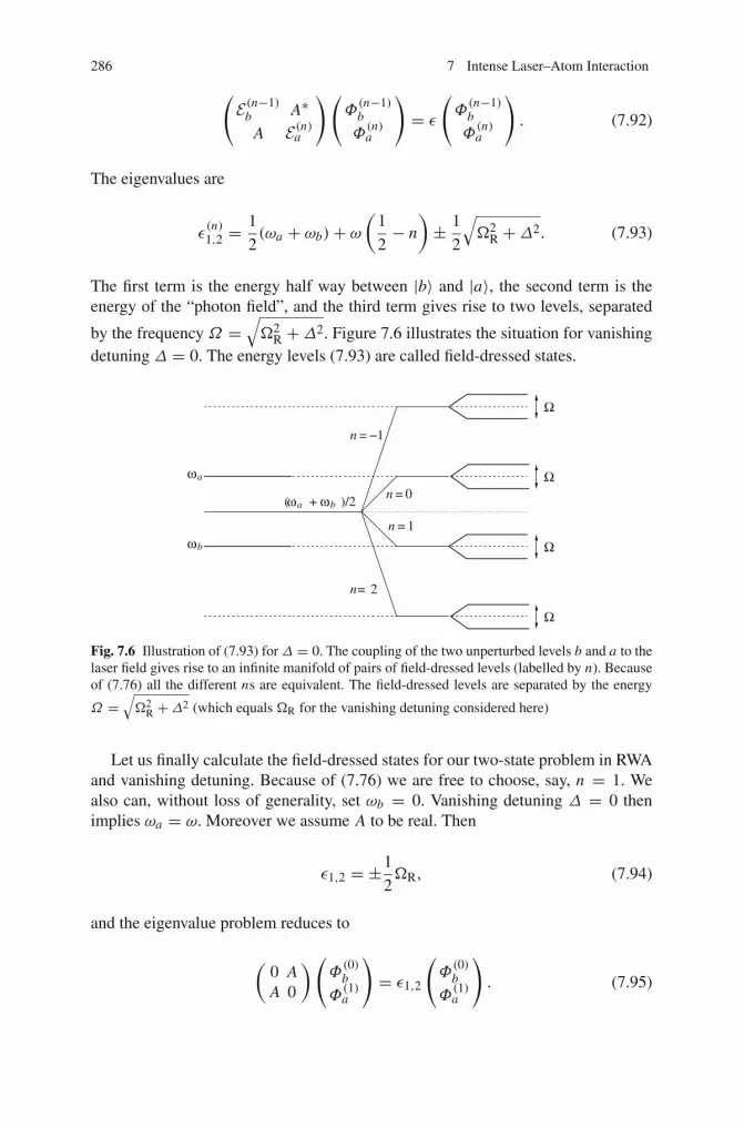
286 7 Intense Laser–Atom Interaction
(E (n−1)
b A∗A E (n)a
)(Φ(n−1)b
Φ(n)a
)= ε
(Φ(n−1)b
Φ(n)a
). (7.92)
The eigenvalues are
ε(n)1,2 =
1
2(ωa + ωb)+ ω
(1
2− n
)± 1
2
√&2
R +Δ2. (7.93)
The first term is the energy half way between |b〉 and |a〉, the second term is theenergy of the “photon field”, and the third term gives rise to two levels, separated
by the frequency Ω =√&2
R +Δ2. Figure 7.6 illustrates the situation for vanishingdetuning Δ = 0. The energy levels (7.93) are called field-dressed states.
ωa
ωb
ωa ωb( + )/2
n=
n = −1
n = 0
n = 1
2
Ω
Ω
Ω
Ω
Fig. 7.6 Illustration of (7.93) for Δ = 0. The coupling of the two unperturbed levels b and a to thelaser field gives rise to an infinite manifold of pairs of field-dressed levels (labelled by n). Becauseof (7.76) all the different ns are equivalent. The field-dressed levels are separated by the energy
Ω =√&2
R +Δ2 (which equals &R for the vanishing detuning considered here)
Let us finally calculate the field-dressed states for our two-state problem in RWAand vanishing detuning. Because of (7.76) we are free to choose, say, n = 1. Wealso can, without loss of generality, set ωb = 0. Vanishing detuning Δ = 0 thenimplies ωa = ω. Moreover we assume A to be real. Then
ε1,2 = ±1
2&R, (7.94)
and the eigenvalue problem reduces to
(0 AA 0
)(Φ(0)b
Φ(1)a
)= ε1,2
(Φ(0)b
Φ(1)a
). (7.95)

7.3 Atoms in Strong Laser Fields 287
The matrix
M = 1√2
(−1 11 1
)= M−1 (7.96)
diagonalizes (7.95). The two eigenvectors correspond to the field-dressed or Floquetstates
|Ψ+〉 = 1√2(|a〉 + |b〉) , |Ψ−〉 = 1√
2(|a〉 − |b〉) . (7.97)
If the system is, e.g., at time t = 0 in state |a〉, we have to choose a superposition offield-dressed states to fulfill the initial conditions:
|Ψ (t)〉 = 1√2(|Ψ+(t)〉 + |Ψ−(t)〉). (7.98)
Here, according (7.78)
|Ψ+(t)〉 = e−iε1t[e−iωt |a〉 + |b〉
], (7.99)
|Ψ−(t)〉 = e−iε2t[e−iωt |a〉 − |b〉
]. (7.100)
Calculating the populations |a(t)|2 = |〈a|Ψ (t)〉|2 or |b(t)|2 = |〈b|Ψ (t)〉|2, oneobtains the well-known Rabi-oscillations of frequency Ω .
7.3.2 Non-Hermitian Floquet Theory
As long as we are dealing only with discrete states the quasi-energies ε are real. If,on the other hand, we allow for transitions into the continuum, e.g., via (multipho-ton) ionization, the quasi-energies become complex,
ε = ε0 +Δε − iΓ
2. (7.101)
Here, ε0 is the unperturbed energy, Δε is the AC Stark shift, and Γ is the ion-ization rate. One may wonder why a Hermitian Floquet Hamiltonian should yieldcomplex eigenvalues. The reason for complex quasi-energies lies in the boundaryconditions. Decaying dressed bound states or dressed resonances must fulfill the so-called Siegert boundary conditions [47]. Instead of explicitly taking these boundaryconditions into account one may apply the complex dilation (also called complexscaling) method (see, e.g., [18, 48–50]).
Figure 7.7 shows the ionization rate of atomic hydrogen H(1s) for λ = 1064 nmlaser light as a function of the laser intensity, calculated by Potvliege and Shakeshaft[51] using the non-Hermitian Floquet method. At this wavelength at least 12 photons

288 7 Intense Laser–Atom Interaction
Fig. 7.7 Ionization rate vs laser intensity for H(1s) irradiated by linearly polarized light of wave-length λ = 1064 nm. Dashed curves are partial rates for (12+S)-photon ionization obtained withinLOPT. The arrows indicate the intensities at which the real part of the 1s Floquet eigenvalue crossesthe 13- and 14-photon ionization thresholds (from [51])
must be absorbed by the electron in order to escape. The LOPT results for S excessphoton-ionization (i.e., (12 + S)-photon ionization) are included in Fig. 7.7. Theyby far overestimate the ionization rate. The exact Floquet-result displays interestingstructures. As the AC Stark up-shift of the continuum (which is given by the pon-deromotive potential Up) increases, the minimum number of photons required forionization increases from 12 to 13 (first arrow) and to 14 (second arrow). After thesethresholds are passed because of the increasing laser intensity, structures appear,indicating a strong enhancement of the ionization rate at certain laser intensities.This is due to Rydberg states that are brought into (12+ S)-photon resonance withthe ground state via the AC Stark effect (Freeman resonances) [52].
7.3.3 Stabilization
The coupling W (t) to the laser field reads in dipole approximation and velocitygauge
W (t) = p · A(t)+ 1
2A2(t) (7.102)
with A(t) the vector potential. The transformation of the wave function
|Ψ (t)〉 = e−i2
∫ t−∞ A2(t ′) dt ′e−iα(t)· p|'PF(t)〉 (7.103)
removes the A2-term and transforms to the system of an electron oscillating with anexcursion
α(t) =∫ t
−∞A(t ′) dt ′ (7.104)
7.3 Atoms in Strong Laser Fields 289
in the laser field [Pauli–Fierz (PF) or Kramers–Henneberger transformation] [53–55]. In this system the nuclear potential appears to oscillate. The TDSE then reads
id
dt|'PF(t)〉 =
(p2
2+ V [r + α(t)]
)|'PF(t)〉. (7.105)
The PF Hamiltonian
HPF(t) = p2
2+ V [r + α(t)] (7.106)
is for an infinitely long laser pulse periodic as well so that we may apply the Floquettheorem. Introducing the time-averaged potential
VPF(α, r) = 1
T
∫ T
0V [r + α(t)] dt, α = max |α(t)|, (7.107)
which is the zero-frequency contribution in the Fourier-expansion of the potential[see (7.81)], (7.80) can be written as
− (ε + mω)Φ(m)β +
∑
α
〈β| p2
2+ VPF(α, r)|α〉Φ(m)
α +∑
αnn =m
〈β|V (m−n)|α〉Φ(n)α = 0.
(7.108)If the laser frequency is large compared to the relevant inner-atomic transitions, wemay neglect the third term so that we are left with an equation diagonal in the pho-ton index, which corresponds to the solution of the time-independent Schrödingerequation
ε|ΨPF〉 =(
p2
2+ VPF(α, r)
)|ΨPF〉. (7.109)
If it is possible to transfer the entire electron population to the bound states ofVPF(α, r) there will be no ionization whatsoever. For intense fields where α � 1the potential VPF(α, r) looks very different from the unperturbed nuclear potentialsince it has a double-well structure with the minima close to the classical turningpoints±α. If electronic probability density is trapped in this potential the ionizationrate decreases despite increasing laser field strength. This has indeed been observedin numerical simulations and is called adiabatic stabilization (see [11] for a review).The stabilization effect survives also for a “real” laser pulse with an up- and a down-ramp (dynamic stabilization).
Figure 7.8 illustrates stabilization of a one-dimensional model atom employinga soft-core binding potential V (x) = −(x2 + ε)−1/2 with ε = 1.9 (leading to abinding energy of −0.5). The full TDSE was solved. The laser pulse of frequency

290 7 Intense Laser–Atom Interaction
Ene
rgy
(a.u
.)(a)
Tim
e (c
ycle
s)
x (a.u.)
(b)
Fig. 7.8 Dynamic stabilization in a one-dimensional model atom. The cycle-averaged ionic poten-tial in a reference frame where a freely oscillating electron is at rest is depicted in (a) (solid line).The three lowest energy levels in this “dressed” potential and the corresponding probability densi-ties are also plotted. In (b) a shadowgraph of the probability density, obtained from the full solutionof the time-dependent Schrödinger equation, is shown. The probability density remains trapped inthe effective potential. Low-frequency Rabi-floppings are responsible for the oscillatory pattern.Note that the time scale of these oscillations is small compared to the laser period
ω = 2.5 was ramped over 10 cycles up to E = 62.5 and thereafter held constant.The excursion of a free electron in this field is α(t) = 10 sinωt . The cycle-averagedpotential, its three lowest levels and the corresponding probability densities are indi-cated in Fig. 7.8a. The potential has the above mentioned double-well shape withthe minima close to the classical turning points ±α. In Fig. 7.8b a shadowgraphof the probability density obtained from the TDSE solution in the PF frame isshown. The probability density remains confined between the two turning points.Only during the up-ramping of the pulse some density escapes. Obviously, not onlya single dressed state is occupied since the probability density distribution oscillatesin time. Note that the time-scale of this dynamics is slow compared to the laserperiod. The splitting of the probability density due to the double-well character ofthe PF potential is called “dichotomy” [56]. In circularly polarized multi-color laserfield configurations more complex structures were observed [57].
Figure 7.9 shows the lifetime (i.e., the inverse ionization rate) of atomic H incircularly laser pulses of various frequencies and intensities as predicted by thehigh-frequency Floquet theory [58]. With increasing laser intensity the lifetime firstdecreases (i.e., ionization increases). This is the expected behavior from LOPT.Then, however, the lifetime passes through a minimum (the “death valley” [11, 59])before it increases again (i.e., ionization is reduced).
So far, adiabatic stabilization with the electron starting from the ground state wasobserved in numerical simulations only. This is because there are no sufficientlystrong lasers available yet at short wavelengths. The photon energy ω has to exceedthe ionization potential, and the laser intensity must be strong enough in order tolead to the two minima in the time-averaged potential. Since the elongation α isinversely proportional to ω2, the laser intensity necessary for adiabatic stabilization

7.3 Atoms in Strong Laser Fields 291
Fig. 7.9 Lifetime of the H atom in the ground state according to the high-frequency Floquet theory,vs intensity, at various laser frequencies ω; circular polarization. Numbers adjacent to points onthe curves are the corresponding values of α. The descending branches of the curves correspondto LOPT, the ascending ones to adiabatic stabilization (the latter can be “trusted” as the laserfrequency increases beyond the ionization potential 0.5). From [59]
increases with ω. Because ω > Eip it is thus desirable to reduce Eip so that alreadyavailable laser sources can be used. In fact, the stabilization of Rydberg atoms wasalready demonstrated [60].
There are (at least) three effects which counteract against adiabatic stabilization.Firstly, there is the so-called “death-valley” effect [59]: an atom experiences duringthe rising edge of a strong laser pulse field intensities in which violent ionizationoccurs and hence no more electrons are left to be stabilized once the optimal sta-bilization condition is reached. Secondly, in more complex atoms or ions innerelectrons might be excited or removed by few photon processes induced by theincident high frequency radiation. Then the question arises whether an outer elec-tron can stabilize although there are electron holes in the lower lying shells [61].Thirdly, at high frequencies and high intensities the dipole approximation breaksdown, and the magnetic v× B-force pushes the electron into the propagation direc-tion, thus enhancing ionization [62, 63]. These three effects will probably make theexperimental verification of stabilization of atoms starting from the ground state aformidable task. Even the new short-wavelength free electron laser sources underconstruction worldwide are of too low intensity, let alone that they do not deliverlong flat-top pulses, which would be ideal to observe dynamic stabilization. How-ever, there is no doubt that sooner or later such light sources will be available so thata new and interesting kind of “meta-matter” will be produced: pseudo atoms withcharge clouds extending over tens or more atomic units and artificial molecules oftunable internuclear separations.

292 7 Intense Laser–Atom Interaction
7.3.4 Strong Field Approximation
The strong field approximation (SFA), also known as “Keldysh–Faisal–Reiss”(KFR)-theory [42, 64, 65], and its extensions are the theoretical workhorse in strongfield laser–atom and laser–molecule interaction and often gives insight into themechanisms behind strong field effects. As the laser field is far from being a smallperturbation, “conventional” perturbation theory in the number of photons involvedis not applicable [66]. The SFA does neither consider the laser field being smallcompared to the binding forces nor does it assume the contrary at all times duringthe interaction. Instead, in the SFA the binding potential is considered dominantuntil ionization whereas the laser field takes over after ionization. The SFA hasbeen applied to ionization, harmonic generation, and nonsequential ionization. Thebeauty of the SFA lies, besides in its predictive power, in the possibility to interpretits equations in intuitively accessible terms, as will be shown below in Sect. 7.3.5.However, there are limits as well, to be discussed in the last part of this section.
Let the initial state be an electronic eigenstate of the field-free Hamiltonian. Theelectron may at time ti be in the ground state |Ψ0〉 = |Ψ0(ti)〉 of energy E0 < 0,for instance, and the laser field is not yet switched on. Now let us consider thepicture-independent bound-free transition matrix element
M p(t) = 〈Ψ p|U (t, ti)|Ψ0〉 (7.110)
for a transition from the initial state |Ψ0〉 to the target state |Ψ p〉 = |Ψ p(ti)〉, which isa continuum state of asymptotic momentum p. U (t, ti) is the (picture-independent)time evolution operator. The probability to find the electron at time t in the scatteringstate |Ψ p〉 is w(t) = |M p(t)|2. The time-evolution operator U (t, t ′) = U †(t ′, t)fulfills
id
dtU (t, t ′) = H(t)U (t, t ′) (7.111)
in any picture [67]. The TDSE in the Schrödinger picture reads
id
dt|Ψ (t)〉 = H(t)|Ψ (t)〉, H(t) = 1
2
[p+ A(t)
]2 + V (r) (7.112)
where A(t) is the vector potential describing the laser field (in dipole approxima-tion). The minimum coupling Hamiltonian H(t) can be splitted in various ways:
id
dt|Ψ (t)〉 = [H0 + W (t)]|Ψ (t)〉 = [H (V)(t)+ V (r)]|Ψ (t)〉, (7.113)
with
H0 = p2
2+ V (r), H (V)(t) = p2
2+ W (t), (7.114)

7.3 Atoms in Strong Laser Fields 293
and W (t) the interaction with the laser field,
W (t) = p · A(t)+ 1
2A2(t) (velocity gauge). (7.115)
The gauge transformation of the potentials (both scalar potential φ and vectorpotential A) and the wave function |Ψ (t)〉,
A′ = A+∇χ(r, t), φ′ = φ − ∂χ(r, t)
∂t, |Ψ ′(t)〉 = e−iχ(r,t)|Ψ (t)〉
where χ(r, t) is an arbitrary differential scalar function, leaves the electric and themagnetic field unchanged:
E = −∂t A−∇φ = E′, B = ∇ × A = B′. (7.116)
This gauge invariance offers the possibility to choose a gauge that suits best, e.g., asfar as computational simplicity is concerned. Observables are not affected by gaugetransformations while the interpretation of the underlying physics may change (e.g.,there is no potential barrier in velocity gauge to tunnel through). Moreover, approx-imations may destroy the gauge invariance (see below).
The transformation to the so-called length gauge (also known as the Göppert–Mayer gauge [68]) is achieved by choosing
χ(r, t) = −A(t) · r. (7.117)
Because of ∇χ = −A the vector potential is “transformed away” while φ′ =−∂tχ = −E · r . The Hamiltonian in length gauge reads
H ′(t) = p2
2+ V (r)− φ′(r, t) = p2
2+ V (r)+ E(t) · r (7.118)
(one could also absorb V (r) in φ and φ′). Note that the transformation of the wavefunction
|Ψ ′(t)〉 = eir·A(t)|Ψ (t)〉 (7.119)
can be interpreted as a translation in momentum space. In fact, while in velocitygauge the quiver momentum is effectively subtracted from the kinetic momentum,leading to a canonical momentum different from the kinetic momentum, in lengthgauge kinetic and canonical momentum are equal.
From (7.118) we infer
W ′(t) = E(t) · r (length gauge) (7.120)
with E(t) = −∂t A(t).

294 7 Intense Laser–Atom Interaction
H0 describes the unperturbed atom and seemingly does not depend on the gaugechosen, i.e., H0 = H ′
0. However, one should bear in mind that the momentum p in
H0 is not the kinetic momentum (which, in atomic units, equals the velocity) whilein H ′
0 (length gauge) it is.
The Gordon–Volkov–Hamiltonian H (V)(t) governs the free motion of the elec-tron in the laser field [69, 70]. The Gordon–Volkov state |'(V)
p 〉 fulfills in theSchrödinger picture and velocity gauge
id
dt|'(V)
p (t)〉 = H (V)(t)|'(V)p (t)〉 = 1
2[ p+ A(t)]2|'(V)
p (t)〉. (7.121)
Thanks to the dipole approximation the Gordon–Volkov–Hamiltonian is diagonalin momentum space. The solution of (7.121), i.e., the Gordon–Volkov-state, is thusreadily written down:
|'(V)p (t, ti)〉 = e−iSp(t,ti)| p〉, Sp(t, ti) = 1
2
∫ t
tidt ′ [ p+ A(t ′)]2 (7.122)
where | p〉 are momentum eigenstates, 〈r| p〉 = ei p·r/(2π)3/2. Note that the lowerintegration limit ti affects the overall phase of the Gordon–Volkov solution only. Asmentioned above, the transition to the length gauge corresponds to a translation inmomentum space. It is thus easy to check that in length gauge one has
|'(V)p′(t, ti)〉 = e−iSp(t,ti)| p+ A(t)〉 (length gauge) (7.123)
with the same action Sp(t, ti) as in (7.122).Let us now continue to derive the SFA transition matrix element. As the time
evolution operator U (t, t ′) satisfies (7.111),
id
dtU (t, t ′) = [H0 + W (t)]U (t, t ′), (7.124)
the integral equations
U (t, t ′) = U0(t, t ′)− i∫ t
t ′dt ′′ U (t, t ′′)W (t ′′)U0(t
′′, t ′), (7.125)
= U0(t, t ′)− i∫ t
t ′dt ′′ U0(t, t ′′)W (t ′′)U (t ′′, t ′),
are fulfilled [71]. Here, U0(t, t ′) is the evolution operator corresponding to theTDSE with H0 only. Inserting (7.125) in the matrix element (7.110) leads to

7.3 Atoms in Strong Laser Fields 295
M p(t) = −i∫ t
tidt ′ 〈Ψ p|U (t, t ′)W (t ′)|Ψ0(t
′)〉 (7.126)
where use of 〈Ψ p|U0(t, ti)|Ψ0〉 = 〈Ψ p|Ψ0(t)〉 = 0 was made because |Ψ p〉 is a scat-tering state orthogonal to |Ψ0(t)〉 = e−iE0(t−ti)|Ψ0〉, and U0(t ′, ti)|Ψ0〉 = |Ψ0(t ′)〉.Since the propagator U (t, t ′) also satisfies the integral equations
U (t, t ′) = U (V)(t, t ′)− i∫ t
t ′dt ′′ U (V)(t, t ′′)V U (t ′′, t ′), (7.127)
= U (V)(t, t ′)− i∫ t
t ′dt ′′ U (t, t ′′)V U (V)(t ′′, t ′),
where U (V)(t, t ′) is the evolution operator corresponding to the TDSE (7.121), oneobtains, upon inserting (7.127) in (7.126),
M p(t) = −i
[∫ t
tidt ′ 〈Ψ p|U (V)(t, t ′)W (t ′)|Ψ0(t
′)〉 (7.128)
−i∫ t
tidt ′′
∫ t
t ′′dt ′ 〈Ψ p|U (V)(t, t ′)V U (t ′, t ′′)W (t ′′)|Ψ0(t
′′)〉].
Using∫ t
tidt ′′
∫ tt ′′ dt ′ = ∫ t
tidt ′∫ t
tidt ′′Θ(t ′ − t ′′) = ∫ t
tidt ′∫ t ′
tidt ′′ expression (7.128)
may be recast in the form
M p(t) = −i∫ t
tidt ′ 〈Ψ p|U (V)(t, t ′)
[W (t ′)|Ψ0(t
′)〉 (7.129)
−i∫ t ′
tidt ′′ V U (t ′, t ′′)W (t ′′)|Ψ0(t
′′)〉].
Equation (7.129) is still exact and gauge invariant. Whatever is missed in the firstterm of (7.129) is included in the second term where the full but unknown timeevolution operator U (t ′, t ′′) appears. Neglecting the second term, replacing the finalstate |Ψ p〉 by a plane wave | p〉, and making use of the expansion of the Gordon–Volkov-propagator into Gordon–Volkov waves
U (V)(t, t ′) =∫
d3k |'(V)k (t, ti)〉〈'(V)
k (t ′, ti)|, (7.130)
(ti is arbitrary since it cancels) we obtain the SFA or so-called Keldysh-amplitude
M (SFA)p (t) = −i
∫ t
tidt ′ 〈'(V)
p (t ′, t))|W (t ′)|Ψ0(t′)〉. (7.131)

296 7 Intense Laser–Atom Interaction
The SFA transition amplitude integrates over all ionization times t ′ where the tran-sition from the bound state |Ψ0(t ′)〉 to the Gordon-Volkov state |'(V)
p (t ′, t))〉, medi-ated by the interaction with the laser field W (t ′), may take place. Unfortunately, thereplacement of the final state by a plane wave destroys the gauge invariance, andunder certain circumstances SFA results can be very different in different gauges[72–74].
In velocity gauge, where W (t) = p · A(t) + A2(t)/2 is diagonal in momentumrepresentation, the Keldysh amplitude (7.131) becomes
M (SFA)p (t) = −i
∫ t
tidt ′ eiSp(t ′,t)
[p · A(t ′)+ 1
2A2(t ′)
]〈 p|Ψ0〉e−iE0(t ′−ti) (7.132)
with E0 the initial energy. Multiplying this matrix element by the overall phase factorexp[iSp(t, ti)] and splitting p · A(t ′)+ A2(t ′)/2 in the form [ p+ A(t ′)]2/2− E0 −p2/2+ E0 leads – upon integration by parts—to
M (SFA)p
′(t) = −Ψ0( p) eiSp,E0 (t
′,ti)∣∣∣t
ti
+iΨ0( p)(
p2
2− E0
) t∫
ti
eiSp,E0 (t′,ti) dt ′ (7.133)
with the classical action
Sp,E0(t, ti) =t∫
ti
[p2
2− E0 + W (t ′)
]dt ′ (7.134)
and Ψ0( p) = 〈 p|Ψ0〉 the Fourier-transformed initial state wave function
Ψ0( p) = 1
(2π)3/2
∫d3r e−i p·rΨ0(r). (7.135)
The first term in (7.133) vanishes when the asymptotic rate
Γ p = limT→∞
∣∣M p∣∣2
T, M p = lim
ti→−∞t→∞
M p(t) (7.136)
is calculated. In this way we recover Reiss’ result [65]
M (SFA)p
′ = iΨ0( p)(
p2
2− E0
)∫ ∞
−∞eiSp,E0 (t,−∞) dt. (7.137)

7.3 Atoms in Strong Laser Fields 297
7.3.4.1 Circular Polarization and Long Pulses
In this case one may write the vector potential in dipole approximation as
A(t) = 1
2A[ε exp(iωt)+ ε∗ exp(−iωt)] (7.138)
where the polarization vectors ε, ε∗ fulfill ε2 = ε∗2 = 0 and ε · ε∗ = 1, e.g.,ε = (ex + iey)/
√2. The factor 1/2 is introduced in order to obtain Up = A2/4, as
in the linearly polarized case. With
[ p+ A(t)]2 = p2 + 1
2A2 + 2 A| p · ε| cos(ωt − ϕ), (7.139)
where p · ε = | p · ε| exp(−iϕ), the action (7.134) reads
Sp,E0(t,−∞) =(
p2
2− E0 +Up
)t + A
ω| p · ε| sin(ωt − ϕ) (7.140)
where we neglected contributions from ti = −∞ since they just affect the irrelevant,overall phase of the SFA transition matrix element
M (SFA)p, circ.
′ = 2π iΨ0( p)∞∑
n=−∞(nω −Up) exp(inϕ) (7.141)
× Jn
(− A| p · ε|
ω
)δ(p2/2− E0 +Up − nω).
Jn(ζ ) are Bessel functions obeying
exp[−iζ sin(ωt − ϕ)] =∞∑
n=−∞Jn(ζ ) exp[−in(ωt − ϕ)]. (7.142)
The time integration in (7.137) leads to the energy-conserving δ-function. Employ-ing (7.136) and using
δ(Ω) = 1
2πlim
T→∞
∫ T/2
−T/2exp(iΩt) dt = lim
T→∞T
2πfor Ω = 0 (7.143)
(and zero otherwise) to evaluate the square of the δ-function one obtains the ioniza-tion rate
�(SFA)p, circ. = 2π |Ψ0( p)|2
∞∑
n=−∞(nω−Up)
2 J 2n
(− A| p · ε|
ω
)δ(p2/2−E0+Up−nω).
(7.144)
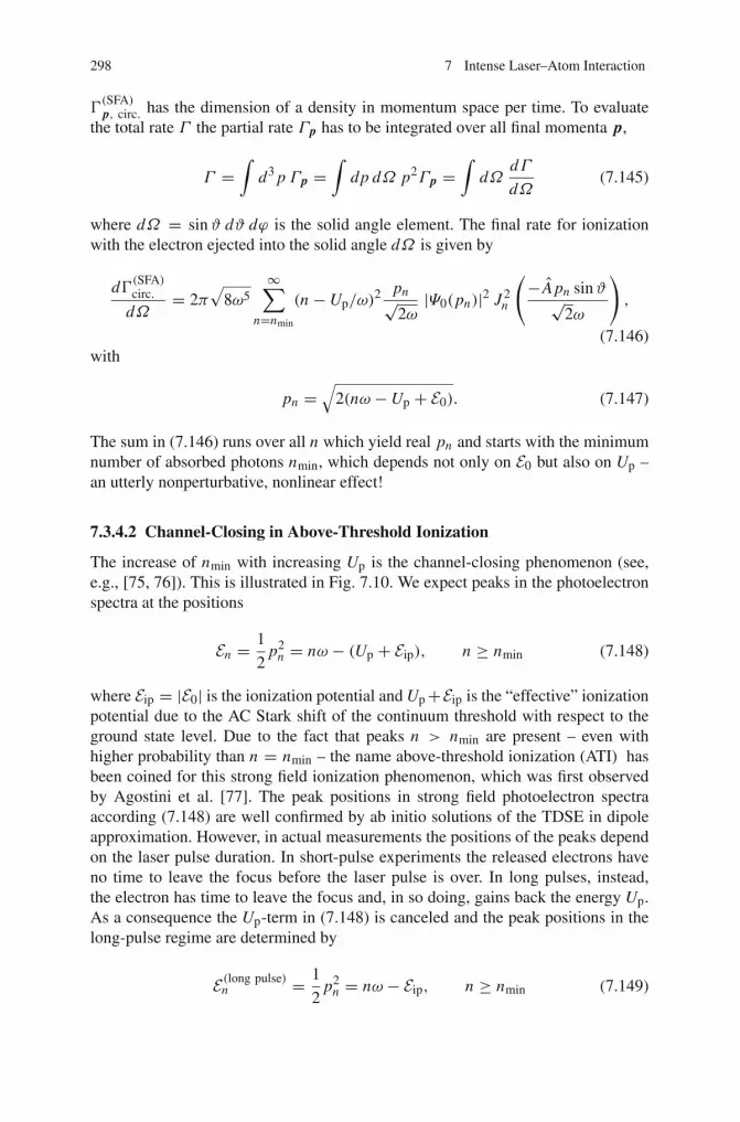
298 7 Intense Laser–Atom Interaction
�(SFA)p, circ. has the dimension of a density in momentum space per time. To evaluate
the total rate Γ the partial rate Γ p has to be integrated over all final momenta p,
Γ =∫
d3 p Γ p =∫
dp dΩ p2Γ p =∫
dΩdΓ
dΩ(7.145)
where dΩ = sinϑ dϑ dϕ is the solid angle element. The final rate for ionizationwith the electron ejected into the solid angle dΩ is given by
d�(SFA)circ.
dΩ= 2π
√8ω5
∞∑
n=nmin
(n −Up/ω)2 pn√
2ω|Ψ0(pn)|2 J 2
n
(− A pn sinϑ√
2ω
),
(7.146)with
pn =√
2(nω −Up + E0). (7.147)
The sum in (7.146) runs over all n which yield real pn and starts with the minimumnumber of absorbed photons nmin, which depends not only on E0 but also on Up –an utterly nonperturbative, nonlinear effect!
7.3.4.2 Channel-Closing in Above-Threshold Ionization
The increase of nmin with increasing Up is the channel-closing phenomenon (see,e.g., [75, 76]). This is illustrated in Fig. 7.10. We expect peaks in the photoelectronspectra at the positions
En = 1
2p2
n = nω − (Up + Eip), n ≥ nmin (7.148)
where Eip = |E0| is the ionization potential and Up+Eip is the “effective” ionizationpotential due to the AC Stark shift of the continuum threshold with respect to theground state level. Due to the fact that peaks n > nmin are present – even withhigher probability than n = nmin – the name above-threshold ionization (ATI) hasbeen coined for this strong field ionization phenomenon, which was first observedby Agostini et al. [77]. The peak positions in strong field photoelectron spectraaccording (7.148) are well confirmed by ab initio solutions of the TDSE in dipoleapproximation. However, in actual measurements the positions of the peaks dependon the laser pulse duration. In short-pulse experiments the released electrons haveno time to leave the focus before the laser pulse is over. In long pulses, instead,the electron has time to leave the focus and, in so doing, gains back the energy Up.As a consequence the Up-term in (7.148) is canceled and the peak positions in thelong-pulse regime are determined by
E (long pulse)n = 1
2p2
n = nω − Eip, n ≥ nmin (7.149)

7.3 Atoms in Strong Laser Fields 299
with nmin, however, still to be calculated with Up (since before leaving the laserfocus, ionization has to occur in the first place).
In Fig. 7.10a the Up-shift of the continuum threshold is small, and the channeln = 5 is responsible for the first peak in the photoelectron spectrum. At higherlaser intensity, in Fig. 7.10b, the channels n = 5 and n = 6 are closed since 6photons are not sufficient to overcome the effective ionization potential Eip + Up.In the long pulse regime peaks corresponding to a certain channel are always at thesame positions in the energy spectrum whereas in the short pulse regime the peaksmove with Up. As a consequence, focal averaging reduces the contrast in the shortpulse regime whereas it has less of an effect in the long pulse regime because of theautomatic cancellation of Up at the position of electron-emission.
In Fig. 7.11 we show the example of an experimental long-pulse spectrum wherelower order peaks are indeed suppressed due to channel-closings.
7.3.4.3 Linear Polarization and Long Pulses
We assume a laser field of the form
A(t) = Aε cos(ωt), ε2 = 1. (7.150)
The action (7.134) reads in this case
Sp,E0(t,−∞) =(
p2
2− E0 +Up
)t − A
ωp · ε sin(ωt)+ A2
8ωsin(2ωt).
Proceeding as in the circular field-case one arrives at [65]
M (SFA)p,lin.
′ =2π iΨ0( p)∞∑
n=−∞(nω −Up) Jn
(− A p · ε
ω,−Up
2ω
)δ(p2/2− E0 +Up − nω),
�(SFA)p,lin. = 2π |Ψ0( p)|2
∞∑
n=−∞(nω −Up)
2 J 2n
(− A p · ε
ω,−Up
2ω
)δ(p2/2−E0+Up−nω),
d�(SFA)lin.
dΩ= 2π
√8ω5
∞∑
n=−∞(n −Up/ω)
2 pn√2mω
|Ψ0(pn)|2 J 2n
(− A p · ε
ω,−Up
2ω
).
Jn is the generalized Bessel function of integer order n defined by
Jn(u, v) = 1
2π
∫ π
−πdθ exp[i(u sin θ + v sin(2θ)− nθ)].
The relation to the ordinary Bessel functions is

300 7 Intense Laser–Atom Interaction
ε0
(b)(a)
short pulse long pulse
short pulse
long pulse
Up
Fig. 7.10 Channel-closing in the short and long pulse regime. In (a) the laser intensity is small sothat the Up-shift of the continuum threshold is less than a photon energy. In (b) the channels n = 5and n = 6 are closed due to the pronounced AC Stark shift of the continuum. The photoelectronspectra look different in the short and long pulse regime since the released electrons gain Up in thelatter case upon leaving the laser focus
Fig. 7.11 Channel-closing in the long-pulse regime. The experimental spectrum was taken from[78]. The two channels in the shaded area are closed
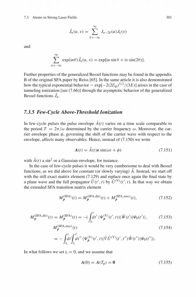
7.3 Atoms in Strong Laser Fields 301
Jn(u, v) =∞∑
k=−∞Jn−2k(u)Jk(v)
and
∞∑
n=−∞exp(inθ) Jn(u, v) = exp[iu sin θ + iv sin(2θ)].
Further properties of the generalized Bessel functions may be found in the appendixB of the original SFA paper by Reiss [65]. In the same article it is also demonstratedhow the typical exponential behavior∼ exp[−2(2Eip)
3/2/(3E)] arises in the case oftunneling ionization [see (7.66)] through the asymptotic behavior of the generalizedBessel functions Jn .
7.3.5 Few-Cycle Above-Threshold Ionization
In few-cycle pulses the pulse envelope A(t) varies on a time scale comparable tothe period T = 2π/ω determined by the carrier frequency ω. Moreover, the car-rier envelope phase φ, governing the shift of the carrier wave with respect to theenvelope, affects many observables. Hence, instead of (7.150) we write
A(t) = A(t)ε sin(ωt + φ) (7.151)
with A(t) a sin2 or a Gaussian envelope, for instance.In the case of few-cycle pulses it would be very cumbersome to deal with Bessel
functions, as we did above for constant (or slowly varying) A. Instead, we start offwith the still exact matrix element (7.129) and replace once again the final state bya plane wave and the full propagator U (t ′, t) by U (V)(t ′, t). In that way we obtainthe extended SFA transition matrix element
M (SFA)p (t) = M (SFA,dir)
p (t)+ M (SFA,resc)p (t), (7.152)
M (SFA,dir)p (t) = M (SFA)
p (t) = −i∫ t
tidt ′ 〈'(V)
p (t ′, t))|W (t ′)|Ψ0(t′)〉, (7.153)
M (SFA,resc)p (t) (7.154)
= −∫ t
tidt ′∫ t ′
tidt ′′ 〈'(V)
p (t ′, t)|V U (V)(t ′, t ′′)W (t ′′)|Ψ0(t′′)〉.
In what follows we set ti = 0, and we assume that
A(0) = A(Tp) = 0 (7.155)

302 7 Intense Laser–Atom Interaction
where Tp is the laser pulse duration. Note that the integral over the electric field of arealistic laser pulse must vanish (see, e.g., appendix A in [9]), so that A(0) = A(Tp),and (7.155) does not pose a loss of generality. It is left as an exercise to the readerthat relabeling the integration variables, multiplication by an overall phase factorand making use of the fact that ionization can only happen while the laser is on,(7.153) and (7.154) can be recast in length gauge in the form
M (SFA,dir)p
′ = −i∫ Tp
0dtion〈 p+ A(tion)|r · E(tion)|Ψ0〉 eiSp,E0 (tion), (7.156)
where
Sp,E0(t) =t∫
0
dt ′(
1
2[ p+ A(t ′)]2 − E0
), Sp(t) = 1
2
t∫
0
dt ′ [ p+ A(t ′)]2.
tion can be interpreted as the ionization time. Analogously, the rescattering matrixelement can be written for t →∞ in the form
M (SFA,resc)p
′ = −∫ Tp
0dtion
∫ ∞
tion
dtresc
∫d3k eiSp(tresc)〈 p+ A(tresc)|V |k + A(tresc)〉
×e−iSk(tresc)〈k + A(tion)|r · E(tion)|Ψ0〉eiSk,E0 (tion) (7.157)
with tresc the rescattering time or, introducing the new variables t = tresc, τ =tresc − tion,
M (SFA,resc)p
′ = −∫ ∞
0dt eiSp,E0 (t)
∫ t
0dτ
∫d3k Vp−ke−iSk,E0 (t,t−τ) (7.158)
×〈k + A(t − τ)|r · E(t − τ)|Ψ0〉
where
Sk,E0(t, t − τ) =∫ t
t−τdt ′
(1
2
[k + A(t ′)
]2 − E0
)(7.159)
and Vp−k = 〈 p|V |k〉. The time τ is the time the electron spends in the continuumbetween ionization and rescattering. The infinite upper limit in the integration overthe rescattering time in (7.157) can be restricted to Tp since rescattering after thelaser is off will not lead to energy absorption. As a consequence, the final energywill be within a region strongly dominated by the more probable direct ionizationprocess.
The integration over the intermediate momentum k can be approximated seekingthe momentum ks(t, τ ) contributing most to the k-integration:

7.3 Atoms in Strong Laser Fields 303
∇k Sk,E0(t, t − τ)!= 0 ⇒ ks(t, τ ) = −α(t)− α(t − τ)
τ(7.160)
with α(t) the excursion as in (7.104). Hence,
M (SFA,resc)p
′ = −∫ Tp
0dt eiSp,E0 (t)
∫ t
0dτ
(2π
iτ
)3/2
Vp−ks(t,τ )e−iSs,E0 (t,t−τ)
×〈ks(t, τ )+ A(t − τ)|r · E(t − τ)|Ψ0〉 (7.161)
where the stationary action Ss,E0(t, t − τ) is given by
Ss,E0(t, t − τ) = Sks(t,τ ),E0(t, t − τ) (7.162)
and the factor [2π/(iτ)]3/2 arises from the saddle-point integration (see, e.g., [79]).In actual numerical evaluations the denominator iτ is regularized by adding a real,positive ε. The results are independent of ε as long as it is not too small but muchsmaller than a laser period.
In the case of a hydrogen-like atom the matrix element needed in (7.161) reads
〈k|r · E(t)|Ψ0〉 = −i27/2(2Eip)5/4 k · E(t)
π(k2 + 2Eip)3. (7.163)
For rescattering at potentials of the form
V (r) = −(
b + a
r
)e−λr (7.164)
the matrix element Vp−k is given by
Vp−k = −2bλ+ aC
2π2C2, C = ( p− k)2 + λ2. (7.165)
In few-cycle laser pulses the concept of an ionization rate is not useful sincethe latter would be time-dependent and sensitive to all details of the pulse (duration,shape, carrier-envelope phase, peak field strength). In experiments one measures thedifferential ionization probability w p, which is the probability to find an electron offinal energy E p = p2/2 emitted in a certain direction corresponding to the solidangle element dΩ p. The probability w p is related to the transition matrix elementM p through
w p dE p︸︷︷︸p dp
dΩ p = |M p|2 d3 p = |M p|2 p2dp dΩ p (7.166)
so that
w p = p |M p|2. (7.167)

304 7 Intense Laser–Atom Interaction
7.3.6 Simple Man’s Theory
The remaining time integral(s) in (7.156) and (7.161) can be either solved numer-ically or approximately by using (modifications of) the saddle-point method withrespect to time (see [8] and Appendix B in [9]). We do not want to go into the detailsbut only emphasize here that the SFA transition matrix element can be approximatedby a sum over the stationary contributions,
M (SFA)p =
∑
s
as, peiSs, p . (7.168)
As it turns out the saddle-point equations define quantum orbits [80, 81] that areclose to the classical orbits of the so-called simple man’s theory, but complex. Inthe following we will use simple man’s theory to derive the cut-off laws for thephotoelectron spectra.
If an electron is set free at time tion and from thereon does not interact with theionic potential anymore, its momentum and position at times t > tion are given by
p(t) = −∫ t
tion
dt ′ E(t ′) = A(t)− A(tion), (7.169)
r(t) =∫ t
tion
dt ′ A(t ′)− A(tion)(t − tion)
= α(t)− α(tion)− A(tion)(t − tion) (7.170)
with the excursion α(t) as defined in (7.104). If the vector potential fulfills (7.155)the momentum at the end of the pulse is determined by the value of the vectorpotential at the time of ionization, p(Tp) = −A(tion), so that the final energy is
Edir, p(tion) = 1
2A2(tion) ≤ 2Up (7.171)
because the ponderomotive potential is Up = A2/4. The fact that the direct electronsare classically restricted to energies up to 2Up is one of the celebrated cut-off lawsin strong field physics.
Let us now allow for one rescattering event, i.e., at the time tresc the electronreturns to the origin (where the ion is located),
ε!> |r(tresc)| = |α(tresc)− α(tion)− A(tion)τ | (7.172)
where ε is a distance small compared to the Bohr radius. Let us assume the extremecase of 180◦ back-reflection where the electron changes the sign of its momentumso that immediately after the scattering event
p(tresc+) = −[A(tresc)− A(tion)]. (7.173)

7.3 Atoms in Strong Laser Fields 305
At later times we have
p(t > tresc) = −∫ t
tresc
dt ′ E(t ′)− [A(tresc)− A(tion)]= A(t)− 2A(tresc)+ A(tion) (7.174)
so that presc(Tp) = −2A(tresc)+ A(tion) and
Eresc, p(tresc, tion) = 1
2[A(tion)− 2A(tresc)]2 ≤ 10Up. (7.175)
Because of the condition (7.172) the 10Up cut-off law for the rescattered elec-trons is not so obvious. However, it can be readily checked numerically by plottingEresc, p(tresc, tion) vs all possible tresc, tion (where tresc > tion) and then indicatingthose pairs of tion, tresc that fulfill (7.172). The result is shown in Fig. 7.12.
"direct" electrons
electronsrescattered
final energy contours/Up
Fig. 7.12 Final photoelectron energy Eresc, p vs ionization time tion and rescattering time tresc >
tion (black: high value of Eresc, p, white: small value of Eresc, p, contours 2, 10 and 16Up labeledexplicitly). The branch labeled “rescattered electrons” indicates times tion and tresc where (7.172) isfulfilled (for an ε � 1). The highest energy those rescattered electrons can have is 10Up (see branchtouching the 10Up-contour). The inlet shows the final energy (7.171) of the “direct” electrons vsthe ionization time. The highest energy there is 2Up

306 7 Intense Laser–Atom Interaction
7.3.6.1 How Good Is the Strong Field Approximation?
In order to answer this question we compare the results of an ab initio TDSE solu-tion with the corresponding SFA predictions. Apart from the dipole approximation(which is well applicable here) the TDSE result is exact. Comparisons with TDSEresults serve as a much more demanding testing ground for approximate theoriessuch as the SFA than comparison with experiments, because of focal averagingeffects present in experiments, the uncertainties in laser intensity, pulse duration,and shape, the limited resolution in energy, and the limited dynamic range in theyields.
In Fig. 7.13 the results for an n = 4-cycle pulse of the form E(t) =Eez sin2[ωt/(2n)] cos(ωt + φ) for 0 < t < n2π/ω, ω = 0.056, E = 0.0834,φ = 0 are shown. The agreement between TDSE and SFA results improve withincreasing photoelectron energy. A possible explanation for that might be that slowelectrons spend more time in the vicinity of the atomic potential where Coulombcorrections are expected to be important. As can be seen in Fig. 7.13, the transitionregime between the cut-off for the direct electrons at E = 2Up = 1.1 up to energieswhere rescattered electrons start to take over at E ≈ 2.5 is quite smooth in the TDSEspectra whereas pronounced interference patterns are visible in the SFA results.Moreover, at very low energies the positions of the local maxima disagree. It hasbeen shown that the agreement at lower energies improves if the binding potentialis made short-range by cutting it at certain distances. This is expected since thecrucial assumption in SFA is that the electron is not affected by the ionic potentialanymore once ionization has occurred [9, 82]. This assumption is well justified forshort-range potentials but less so for long range Coulombic ones as, e.g., in theH(1s) case.
A lot of effort has been devoted to the development of Coulomb-corrections,taking into account the effect of the Coulomb-potential on the outgoing electron,e.g. in [83–86]. However, only a few of them are able to reproduce the strikingfeatures seen in experimental and numerical ab initio spectra, which are in strongdisagreement with the plain SFA, such as rotated angular distributions [87], fan-likestructures in momentum distributions at low energies [85], and the recently observed“low energy feature” at long wavelengths [88]. The pronounced interference patternshowing a spiky, downward-pointing structure in the rescattering plateau in Fig. 7.13between energies ≈ 3 and 6 a.u. instead is remarkably well reproduced using theextended SFA taking into account (7.158) without further Coulomb-correction.
7.3.7 Interference Effects
The spiky structure in Fig. 7.13 is due to quantum interference. For a fixed finalmomentum p the sum (7.168) is a sum over all quantum orbits that end up with thesame momentum at the detector. It turns out that, most of the time, there are twodominating contributions per cycle. Depending on their phase-difference those mayinterfere constructively (local maxima in Fig. 7.13) or destructively (downward-

7.3 Atoms in Strong Laser Fields 307
(a)θ = πφ = 0
Photoelectron energy (a.u.)
φ = 0(b)θ = 0
Yie
ld (
arb.
u.)
Up
Up
Up
Up
10
10
2 2
Fig. 7.13 Photoelectron spectra of the H(1s) electron after irradiation with a 4-cycle laser pulse(ω = 0.056, φ = 0, E = 0.0834). The TDSE and SFA results are drawn solid and dashed,respectively. Panel (a) shows the “left-going” electrons (i.e., opposite to the laser polarization ez),panel (b) the “right-going” electrons (in ez)-direction. The spectra were adjusted vertically bymultiplication with a single factor in such a way that agreement is best in the cut-off region for theright-going electrons. The spectra were not shifted in energy
pointing spikes in Fig. 7.13). The corresponding two trajectories of simple man’stheory can be readily calculated. As an example we show the final energy vs theionization time for a “flat-top” pulse in Fig. 7.14. In the lower panel of Fig. 7.14the course of the electric field is indicated. Let us focus on the time t = 0.5 cycleswhere the electric field has a maximum and ionization is therefore most likely. Theupper panel shows that a “direct” electron emitted at that time will have vanishingfinal energy. In order for a direct, classical electron to have the maximum energy2Up it has to be emitted at times where the electric field is zero (which is unlikely inthe tunneling and over-barrier regime). However, if an electron is emitted around themaximum of the electric field and rescatters once, its final energy may be close to10Up. It is clearly seen that two emission times very close to each other lead to thesame final energy (as indicated in the upper panel). These are the two trajectoriesthat interfere. Exactly at the cut-off 10Up those two solutions merge to a single one.The “travel times” tresc − tion between rescattering and ionization are color-codedfrom black (tresc − tion = 0) to yellow (tresc − tion = 2 cycles).
In very short pulses the situation is more complex than in the regular, flat-toppulse case. Since the ionization probability is strongly weighted with the modulusof the electric field, only a few “time-windows” may remain “open”, thus affectingthe number of interfering quantum orbits for a given p. The interference pattern is

308 7 Intense Laser–Atom Interaction
then very sensitive to the details of the few-cycle pulse, e.g., to the carrier-envelopephase. Because of the “time-windows” that are opened and closed depending onthe parameters of the few-cycle pulse, one may view the setup as a “double slitexperiment in time” [89], a detailed analysis of which is given in [16]. There aretwo dominating quantum trajectories contributing to a given final momentum inthe case of linear polarization. One of them goes directly to the detector while theother one starts in the “wrong” direction but turns around within a fraction of alaser half period. It thus sweeps over the nucleus on the way towards the detector.The two quantum orbits correspond to the reference wave and the object wave ina holography experiment. Hence, the interference pattern in the momentum spectramay be viewed as a hologram of the binding potential [90, 91].
7.3.8 High-Order Harmonic Generation
When an intense laser pulse of frequency ω1 impinges on any kind of target, in gen-eral harmonics of ω1 are emitted. A typical signature of the emission spectrum in thecase of strongly driven atoms, molecules or clusters is that the harmonic yield doesnot simply roll-off exponentially with increasing harmonic order. Instead, a plateauis observed. This is a prerequisite for high-order harmonic generation (HOHG)
(b)
(a)
"direct" electrons
rescattered electrons
same final energy
Fig. 7.14 (a) Final energy of direct electrons (black line) vs the ionization time. If rescatteredis allowed, higher energies may occur. The color coding for the rescattered electrons indicates thetime spent in the continuum between ionization and rescattering (the lighter the color the longer thetime). The cut-off energies for the direct and the rescattered electrons are 2 and 10Up, respectively.Panel (b) shows the course of the laser field. Ionization is improbable for small |E(t)|

7.3 Atoms in Strong Laser Fields 309
being of practical relevance as an efficient short wavelength source. As targets forHOHG one may think of single atoms, dilute gases of atoms, molecules, clusters,crystals, or the surface of a solid (which is rapidly transformed into a plasma bythe laser). In fact, for all those targets HOHG has been observed experimentally.Even a strongly driven two-level system displays nonperturbative HOHG [92, 93].The mechanism generating the harmonics and its efficiency, of course, vary withthe target-type. In the case of atoms the so-called “three-step model” explains thebasic mechanism in the spirit of simple man’s theory: an electron is freed by thelaser at a certain time t ′, subsequently it oscillates in the laser field, and eventuallyrecombines with its parent ion upon emitting a photon of frequency
ω = n ω1, n ≥ 1. (7.176)
This process is illustrated in Fig. 7.15. If the energy of the returning electron is E ,the energy of the emitted photon is ω = E + |Ef| where Ef is the energy of the levelwhich is finally occupied by the electron, for example, the groundstate.
From this simple considerations we conclude that the maximum photon energyone can expect is ωmax = Emax+|Ef|. Using (7.169) we obtain at the recombinationtime trec for the return energy Eret
Eret = 1
2p2(trec) = 1
2[A(trec)− A(tion)]2 (7.177)
where we have to impose [see (7.172)]
|r(trec)| = |α(trec)− α(tion)− A(tion)(trec − tion)| !< ε. (7.178)
Space
Energy
Fig. 7.15 Illustration of the three-step model for high harmonic generation. An electron is (i)released, (ii) accelerated in the laser field, and (iii) driven back to the ion. There it may recombineupon emitting a single photon which corresponds to a multiple of the photon energy of the incidentlaser light

310 7 Intense Laser–Atom Interaction
Fig. 7.16 Return energy as a function of the ionization time. The color coding indicates the timebetween ionization and recombination (the longer this time the lighter the color). The maximumreturn energy is � 3.17Up. The course of the laser field is shown in the lower panel
Figure 7.16 shows the possible return energies fulfilling (7.177) and (7.178). Weinfer that the maximum return energy is around � 3.2. Closer inspection shows thatthe number is 3.17 so that the cut-off law reads
ωmax = 3.17Up + |Ef|. (7.179)
This celebrated ≈ 3 Up cut-off rule was first established empirically [94] andexplained soon after within simple man’s theory [95, 96].
Lewenstein and co-workers [97] showed that, more precisely, it reads ωmax =3.17Up + 1.32|Ef|.
From simple man’s theory one expects that harmonic generation should bemuch less efficient in elliptically polarized laser fields since, classically, the freedelectron never comes back to its parent ion so that recombination can be consid-ered unlikely. This indeed was confirmed experimentally (see [10], and referencestherein).
Harmonic generation in atoms, molecules and clusters has huge practical rele-vance as an efficient source of intense XUV radiation. This is because (i) the pon-deromotive scaling of the cut-off allows to achieve high values of Emax and thushigh harmonic orders n, and (ii), fortunately, the strength of the harmonics does notdecay exponentially with the order n but displays, after a decrease over the first fewharmonics, an overall plateau (at least on the logarithmic scale) up to the cut-offenergy 3.17 Up + |Ef|, allowing relatively high intensities at short wavelengths. In

7.3 Atoms in Strong Laser Fields 311
fact, high-order harmonics below λ = 4.4 nm, the so-called water-window (betweenthe K-edges of carbon and oxygen) have been observed experimentally [98, 99].The intensity of the emitted radiation in the plateau region is about 10−6 of the inci-dent laser intensity which is typically 1015–1018 Wcm−2 in rare gas experiments.Therefore, the intensity of the high-order harmonics is sufficient for various kindsof applications, such as interferometry, for dense plasma diagnostics, holography,high-contrast microscopy of biological materials, and attosecond spectroscopy ormetrology. Attosecond pulses are generated via harmonic generation. If the incom-ing pulse is already short (i.e., consists only of a few cycles) the harmonic emissionis restricted to a narrow time window similar to the “double slit in time”-experimentmentioned above. As a consequence, the harmonic pulse has a duration that is shortcompared to the laser period of the incoming pulse (usually a few hundred attosec-onds). If the incoming laser pulse is longer, one can construct attosecond pulse trainsby selecting a few phase-locked harmonics. Attosecond pulses that are generated viaharmonic generation have been used to probe the ionizing laser field itself [100] aswell as fast atomic processes such as Auger decay [101].
For calculating the rate of harmonic emission one may follow the same route as inthe SFA treatment of ionization. Harmonic generation and ATI are complementaryto each other: while in harmonic generation the electron comes back to the ion andeventually recombines, upon emitting radiation, in high-order ATI it rescatters uponwhich it may gain additional energy. In harmonic generation one observes a plateaureaching up to photon energies 3.17 Up+|Ef|. In ATI a plateau is observed as well –this time with respect to the kinetic energy of the photo electrons – extending up to10 Up (for one rescattering event).
In classical electrodynamics, the total radiated power by a dipole of charge q isgiven by Larmor’s formula
P = 2q2
3c3|r|2. (7.180)
Thus, in a semiclassical approach, it appears reasonable to replace the accelerationby its quantum mechanical expectation value and making use of Ehrenfest’s theo-rem. One obtains (in length gauge)
P = 2q2
3c3
∣∣∣∣d2
dt2〈r〉∣∣∣∣2
= 2q2
3c3
∣∣∣∣∣1
m
⟨−∂ H
∂ r
⟩∣∣∣∣∣
2
. (7.181)
The last expression on the right-hand side is particularly suited for the numericalevaluation of the harmonic spectra. In order to simplify even further we write thedipole as a Fourier-transform,
d(t) = q 〈r〉 = 1√2π
∫ ∞
−∞dω exp(iωt)d(ω). (7.182)
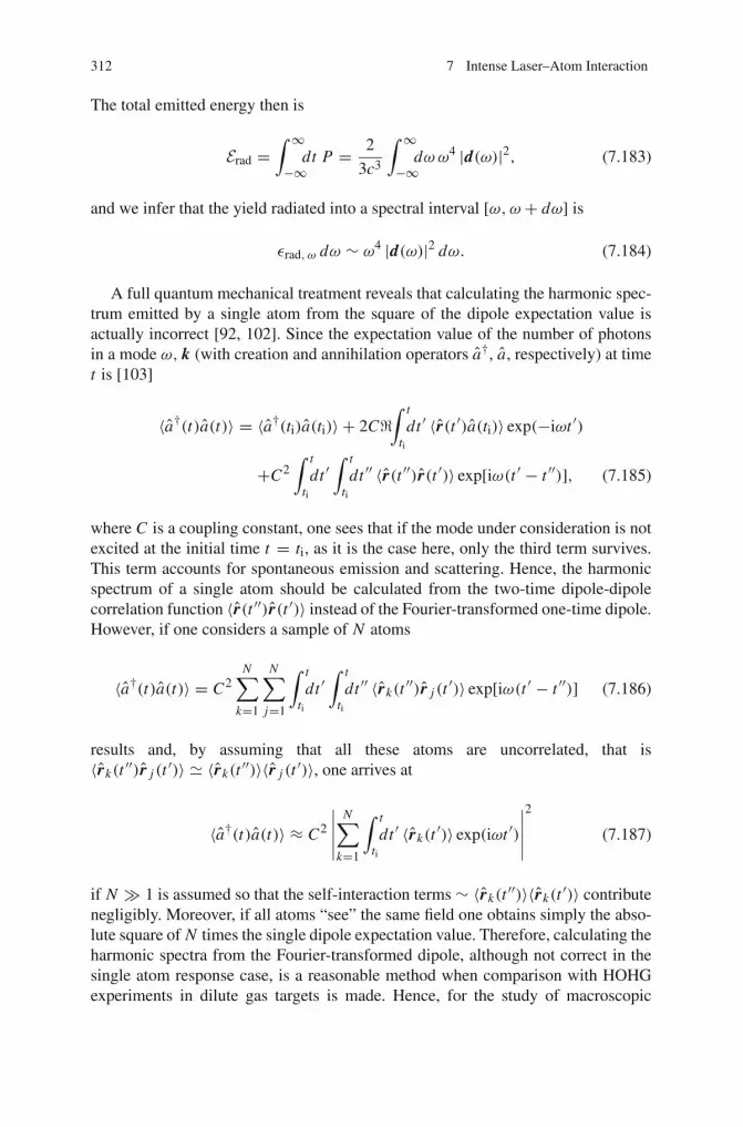
312 7 Intense Laser–Atom Interaction
The total emitted energy then is
Erad =∫ ∞
−∞dt P = 2
3c3
∫ ∞
−∞dωω4 |d(ω)|2, (7.183)
and we infer that the yield radiated into a spectral interval [ω,ω + dω] is
εrad, ω dω ∼ ω4 |d(ω)|2 dω. (7.184)
A full quantum mechanical treatment reveals that calculating the harmonic spec-trum emitted by a single atom from the square of the dipole expectation value isactually incorrect [92, 102]. Since the expectation value of the number of photonsin a mode ω, k (with creation and annihilation operators a†, a, respectively) at timet is [103]
〈a†(t)a(t)〉 = 〈a†(ti)a(ti)〉 + 2C�∫ t
tidt ′ 〈r(t ′)a(ti)〉 exp(−iωt ′)
+C2∫ t
tidt ′∫ t
tidt ′′ 〈r(t ′′)r(t ′)〉 exp[iω(t ′ − t ′′)], (7.185)
where C is a coupling constant, one sees that if the mode under consideration is notexcited at the initial time t = ti, as it is the case here, only the third term survives.This term accounts for spontaneous emission and scattering. Hence, the harmonicspectrum of a single atom should be calculated from the two-time dipole-dipolecorrelation function 〈r(t ′′)r(t ′)〉 instead of the Fourier-transformed one-time dipole.However, if one considers a sample of N atoms
〈a†(t)a(t)〉 = C2N∑
k=1
N∑
j=1
∫ t
tidt ′∫ t
tidt ′′ 〈rk(t
′′)r j (t′)〉 exp[iω(t ′ − t ′′)] (7.186)
results and, by assuming that all these atoms are uncorrelated, that is〈rk(t ′′)r j (t ′)〉 � 〈rk(t ′′)〉〈r j (t ′)〉, one arrives at
〈a†(t)a(t)〉 ≈ C2
∣∣∣∣∣
N∑
k=1
∫ t
tidt ′ 〈rk(t
′)〉 exp(iωt ′)∣∣∣∣∣
2
(7.187)
if N � 1 is assumed so that the self-interaction terms ∼ 〈rk(t ′′)〉〈rk(t ′)〉 contributenegligibly. Moreover, if all atoms “see” the same field one obtains simply the abso-lute square of N times the single dipole expectation value. Therefore, calculating theharmonic spectra from the Fourier-transformed dipole, although not correct in thesingle atom response case, is a reasonable method when comparison with HOHGexperiments in dilute gas targets is made. Hence, for the study of macroscopic

7.3 Atoms in Strong Laser Fields 313
propagation effects the dipole expectation value may be inserted as a source intoMaxwell’s equations.
7.3.9 Strong Field Approximation for High-Order HarmonicGeneration: the Lewenstein Model
The dipole expectation value of a single atom with one active electron (q = −1) is
d(t) = −〈Ψ (t)|r|Ψ (t)〉 (7.188)
= −〈Ψ0(ti)|U (ti, t) r U (t, ti)|Ψ0(ti)〉,
where we assumed again that at the initial time ti the electron starts in the state|Ψ0(ti)〉 =: |Ψ0〉. Using (7.125) we obtain
d(t) = −〈Ψ0(t)|r|Ψ0(t)〉 (7.189)
−i∫ t
tidt ′ 〈Ψ0(t
′)|W (t ′)U (t ′, t)r|Ψ0(t)〉
+i∫ t
tidt ′ 〈Ψ0(t)|rU (t, t ′)W (t ′)|Ψ0(t
′)〉
−∫ t
tidt ′∫ t
tidt ′′ 〈Ψ0(t
′)|W (t ′)U (t ′, t)rU (t, t ′′)W (t ′′)|Ψ0(t′′)〉.
The first term vanishes for a spherically symmetric binding potential. The secondand third term are complex conjugates of each other and describe ionization (W ),propagation (U ), and recombination (r) (i.e., the emission of harmonic radiation)in different time-ordering. The last term involves one additional interaction withthe laser field. We will neglect it here (see [104]). As in the SFA for ionization wereplace the full time evolution operator U by U (V),
d(L)(t) = −i∫ t
tidt ′ 〈Ψ0(t
′)|W (t ′)U (V)(t ′, t)r|Ψ0(t)〉 + c.c., (7.190)
recovering the Lewenstein-result [97]. In length gauge [W (t) = E(t) · r] we obtain(suppressing the “+c.c.”)
d(L)(t) = −i∫ t
tidt ′∫
d3 p 〈Ψ0(t′)|E(t ′) · r| p+ A(t ′)〉〈 p+ A(t)|r|Ψ0(t)〉e−iSp(t ′,t)
(7.191)where we used (7.123) and U (V)(t ′, t)| p+ A(t)〉 = e−iSp(t ′,t)| p+ A(t ′)〉. With
Sp,E0(t, t ′) =∫ t
t ′dt ′′
(1
2[ p+ A(t ′′)]2 − E0
)(7.192)
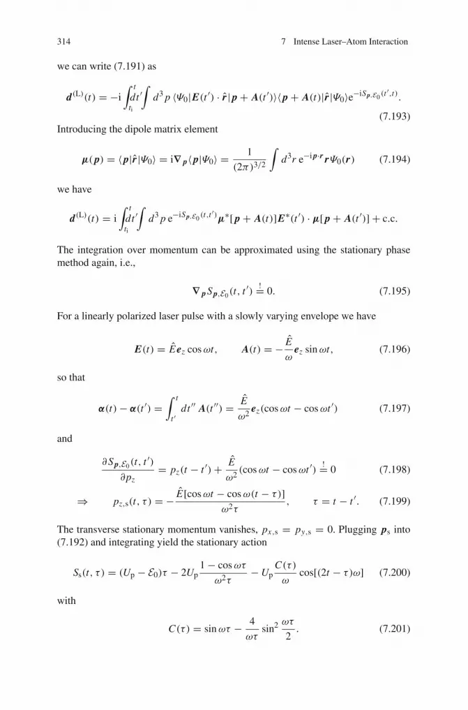
314 7 Intense Laser–Atom Interaction
we can write (7.191) as
d(L)(t) = −i∫ t
tidt ′∫
d3 p 〈Ψ0|E(t ′) · r| p+ A(t ′)〉〈 p+ A(t)|r|Ψ0〉e−iSp,E0 (t′,t).
(7.193)Introducing the dipole matrix element
μ( p) = 〈 p|r|Ψ0〉 = i∇ p〈 p|Ψ0〉 = 1
(2π)3/2
∫d3r e−i p·r rΨ0(r) (7.194)
we have
d(L)(t) = i∫ t
tidt ′∫
d3 p e−iSp,E0 (t,t′)μ∗[ p+ A(t)]E∗(t ′) · μ[ p+ A(t ′)] + c.c.
The integration over momentum can be approximated using the stationary phasemethod again, i.e.,
∇ pSp,E0(t, t ′) != 0. (7.195)
For a linearly polarized laser pulse with a slowly varying envelope we have
E(t) = Eez cosωt, A(t) = − E
ωez sinωt, (7.196)
so that
α(t)− α(t ′) =∫ t
t ′dt ′′ A(t ′′) = E
ω2ez(cosωt − cosωt ′) (7.197)
and
∂Sp,E0(t, t ′)∂pz
= pz(t − t ′)+ E
ω2(cosωt − cosωt ′) != 0 (7.198)
⇒ pz,s(t, τ ) = − E[cosωt − cosω(t − τ)]ω2τ
, τ = t − t ′. (7.199)
The transverse stationary momentum vanishes, px,s = py,s = 0. Plugging ps into(7.192) and integrating yield the stationary action
Ss(t, τ ) = (Up − E0)τ − 2Up1− cosωτ
ω2τ−Up
C(τ )
ωcos[(2t − τ)ω] (7.200)
with
C(τ ) = sinωτ − 4
ωτsin2 ωτ
2. (7.201)
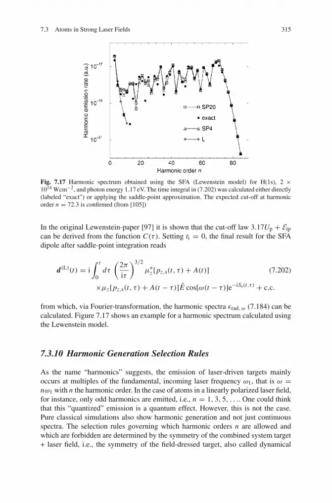
7.3 Atoms in Strong Laser Fields 315
Fig. 7.17 Harmonic spectrum obtained using the SFA (Lewenstein model) for H(1s), 2 ×10¹⁴ Wcm−2, and photon energy 1.17 eV. The time integral in (7.202) was calculated either directly(labeled “exact”) or applying the saddle-point approximation. The expected cut-off at harmonicorder n = 72.3 is confirmed (from [105])
In the original Lewenstein-paper [97] it is shown that the cut-off law 3.17Up + Eipcan be derived from the function C(τ ). Setting ti = 0, the final result for the SFAdipole after saddle-point integration reads
d(L)(t) = i∫ t
0dτ
(2π
iτ
)3/2
μ∗z [pz,s(t, τ )+ A(t)] (7.202)
×μz[pz,s(t, τ )+ A(t − τ)]E cos[ω(t − τ)]e−iSs(t,τ ) + c.c.
from which, via Fourier-transformation, the harmonic spectra εrad, ω (7.184) can becalculated. Figure 7.17 shows an example for a harmonic spectrum calculated usingthe Lewenstein model.
7.3.10 Harmonic Generation Selection Rules
As the name “harmonics” suggests, the emission of laser-driven targets mainlyoccurs at multiples of the fundamental, incoming laser frequency ω1, that is ω =nω1 with n the harmonic order. In the case of atoms in a linearly polarized laser field,for instance, only odd harmonics are emitted, i.e., n = 1, 3, 5, . . .. One could thinkthat this “quantized” emission is a quantum effect. However, this is not the case.Pure classical simulations also show harmonic generation and not just continuousspectra. The selection rules governing which harmonic orders n are allowed andwhich are forbidden are determined by the symmetry of the combined system target+ laser field, i.e., the symmetry of the field-dressed target, also called dynamical

316 7 Intense Laser–Atom Interaction
symmetry. We shall now employ the Floquet theory introduced in Sect. 7.3.1 toderive the selection rules for harmonic emission for a few exemplary systems.
Let H(t) be the Hamiltonian of an electron in a linearly polarized monochromaticlaser field E cos(ω1t)ez of amplitude E and an ionic potential V (r),
H(t) = p2
2+ V (r)+ Ez cosω1t. (7.203)
The Schrödinger equation reads i ddt |Ψ (t)〉 = H(t)|Ψ (t)〉, and since the Hamilto-
nian is periodic in time,
H(t + 2π/ω1) = H(t), (7.204)
from the Floquet theorem (cf. Sect. 7.3.1)
|Ψ (t)〉 = e−iεt |Φ(t)〉, |Φ(t + 2π/ω1)〉 = |Φ(t)〉 (7.205)
follows, and |Φ(t)〉 fulfills the Schrödinger equation
H(t)|Φ(t)〉 = ε|Φ(t)〉, H(t) = H(t)− id
dt(7.206)
which looks like a stationary Schrödinger equation in an extended Hilbert space[106] with the time as an additional dimension and ε a quasi-energy. The scalarproduct in this extended Hilbert space reads
〈〈Φ|Φ ′〉〉 := ω1
2π
2π/ω1∫
0
dt 〈Φ(t)|Φ ′(t)〉. (7.207)
For the derivation of the harmonic generation selection rules we consider aninfinitely long laser pulse and assume that the system is well described by a single,nondegenerate Floquet state. The only nonvanishing dipole expectation value is infield-direction and then reads
d(t) = −〈Ψ (t)|z|Ψ (t)〉 = −〈Φ(t)|z|Φ(t)〉. (7.208)
We define the dipole strength of the harmonic n as
|d(n)|2 =
∣∣∣∣∣∣∣
ω1
2π
2π/ω1∫
0
dt exp(−inω1t) d(t)
∣∣∣∣∣∣∣
2
=∣∣∣∣〈〈Φ| exp(−inω1t) z|Φ〉〉
∣∣∣∣2
,
(7.209)which is proportional to the absolute square of the Fourier-transformed dipole. Thesquared, extended Hilbert space matrix element on the right-hand side of (7.209)

7.3 Atoms in Strong Laser Fields 317
may be also interpreted as the probability for a transition from a Floquet state toitself, generated by the operator exp(−inω1t) z, accompanied by the emission ofradiation of frequency nω1.
The Floquet–Hamiltonian H(t) is invariant under space inversion plus a transla-tion in time by π/ω1,
Pinv = (r →−r, t → t + π/ω1) (7.210)
so that Pinv|Φ〉 = σ |Φ〉, and σ is a phase, i.e, |σ |2 = 1. Inserting the unity P−1inv Pinv
in the matrix element in (7.209) twice yields
〈〈Φ| exp(−inω1t) z|Φ〉〉 = 〈〈Φ|P−1inv︸ ︷︷ ︸
〈〈Φ|σ ∗Pinv exp(−inω1t) z P−1
inv Pinv|Φ〉〉︸ ︷︷ ︸σ |Φ〉〉
= 〈〈Φ|Pinv exp(−inω1t) z P−1inv |Φ〉〉 = − exp(−inπ) 〈〈Φ| exp(−inω1t) z|Φ〉〉.
It follows that n must be odd in order to fulfill
− exp(−inπ) = 1. (7.211)
Hence, only odd harmonics are emitted in the case of linearly polarized laser pulsesimpinging on spherically symmetric systems such as atoms.
In the case of monochromatic circularly polarized laser light (with the electricfield vector in the xy-plane) the Floquet–Hamiltonian may be written (using thecylindrical coordinates ρ and ϕ) as
H(t) = Hkin + V (r)+ E√2ρ cos(ϕ − ω1t)− i
d
dt. (7.212)
This expression is invariant under the continuous symmetry operation
Prot = (ϕ→ ϕ + θ, t → t − θ/ω1) (7.213)
with θ an arbitrary real number. We thus have
〈〈Φ| exp(−inω1t) ρ exp(∓iϕ)|Φ〉〉= exp(inθ ∓ iθ) 〈〈Φ| exp(−inω1t) ρ exp(∓iϕ)|Φ〉〉
where ρ exp(∓iϕ) is the dipole operator for circularly polarized light (with the samehelicity (−) and the opposite helicity (+) as the incident pulse, respectively). Hence,for all θ
exp[iθ(n ∓ 1)] = 1 (7.214)
318 7 Intense Laser–Atom Interaction
must hold, which cannot be fulfilled for any n > 1 so that no harmonics are emitted.However, circularly polarized harmonics may be emitted if bichromatic incidentlaser light is used [107–109]. With the two lasers polarized in opposite directionsand frequencies ω1 and mω1, respectively, the interaction Hamiltonian reads
W (t) = E1√2ρ cos(ϕ − ω1t)+ E2√
2ρ cos(ϕ + mω1t). (7.215)
E1 and E2 are the electric field amplitudes of the first and second laser, respec-tively. The symmetry operation under which the Floquet–Hamiltonian is invariantnow reads
P(m+1)rot =
(ϕ→ ϕ + 2π
m + 1, t → t − 2π
ω1(m + 1)
). (7.216)
In the same manner as in the two previous examples one arrives at the condition
1 = exp
(i2π
n ∓ 1
m + 1
). (7.217)
Hence, harmonics of order
n = k(m + 1)± 1, k = 1, 2, 3, . . . (7.218)
are expected. The harmonics with n = k(m + 1)+ 1 have the same polarization asthe incident laser, whereas those with n = k(m + 1) − 1 are oppositely polarized.With increasing m more and more low order harmonics are suppressed.
The same selection rule (7.218) is obtained for a target having an M-fold discreterotational symmetry axis parallel to the laser propagation direction [110]. An exam-ple for such a target is the benzene molecule with M = 6. The Floquet-Hamiltonianin this case may be written as
H(t) = Hkin + V (ρ, ϕ, z)+ E√2ρ cos(ϕ − ω1t)− i
d
dt. (7.219)
Owing to the discrete rotational symmetry CM of V (ρ, ϕ, z) the symmetry opera-tion of interest now is
P(M)rot =
(ϕ→ ϕ + 2π
M, t → t − 2π
ω1 M
), (7.220)
from which the selection rule
n = k M ± 1, k = 1, 2, 3, . . . (7.221)
7.4 Strong Laser–Atom Interaction Beyond the Single Active Electron 319
follows, which is indeed of the same form as in the bichromatic, atomic case (7.218).Note that (7.219) is only a single active electron-Hamiltonian but sufficient for thepurposes here because the electron-electron interaction term is invariant under theoperation (7.220) anyway.
For deducing these selection rules one assumes that the incident laser pulse isinfinitely long. This is required for (7.204) to be true. In finite laser pulses the simpleselection rules above may be violated and one has to consider not only a singleFloquet states but superpositions of them [111, 112].
7.4 Strong Laser–Atom Interaction Beyond the Single ActiveElectron
Since the early eighties sufficiently intense lasers were available to produce noncol-lisional multiple ionization of atoms [113]. A sequential viewpoint where at a certainintensity of the laser pulse envelope the currently outermost electron is released,leaving the remaining core essentially in the ground state, was successful in explain-ing most of the experimentally observed results [17]. Signatures of double-electronexcitation were observed but simultaneous two-electron ejection was not detected.The situation changed when in 1992 Fittinghoff et al. [114] observed nonsequen-tial double-ionization (NSDI) of helium at 614 nm in 120 fs laser pulses. This phe-nomenon will be discussed in more detail in Sect. 7.4.1.
The theoretical treatment of correlated multi-electron systems is a formidabletask already in the stationary case. The direct solution of the Schrödinger equationis prohibitive because of the so-called “exponential wall” [115]: the dimension of theconfiguration space scales with the number of particles N so that the computationalcost of the representation of the N -body wave function scales exponentially. Mattersget worse for nonperturbative, time-dependent problems where the wave functionmust be propagated in time. In full dimensionality, the simulation of helium in stronglaser fields is currently at the limit of feasibility [116].
A technique which allows to calculate nonperturbatively single (or, recently, alsodouble) ionization but taking into account excitation of the other electrons is the R-matrix Floquet theory [117–119]. This method is a combination of the powerful andin the electron-atom collisions-community well-known R-matrix method [120, 121]and Floquet theory. Alternative methods for the study of ionization in two activeelectron systems are the complex scaling technique used in [48–50], and the state-specific approach [122, 123]. However, none of these methods so far reproduced,e.g., nonsequential double ionization. On the other hand, low-dimensional modelsystems [124–133] where the degrees of freedom of the two or more electrons isrestricted, are rather inaccurate on a quantitative level but helped to identify, e.g., thenonsequential ionization mechanism and, moreover, serve as important test cases forapproximative approaches [61, 124, 127, 128, 134–136].
Methods such as time-dependent Hartree-Fock (TDHF) and simple versions oftime-dependent density functional theory (TDDFT) fail miserably in describing

320 7 Intense Laser–Atom Interaction
laser-driven correlated electron dynamics [129, 137, 138]. This triggered stronginterest in the multi-configurational TDHF (MCTDHF) approach [139–141] andin the improvement of TDDFT [134–136]. MCTDHF becomes exact if a sufficientnumber of configurations is taken into account but is very demanding computa-tionally. TDDFT, on the other hand, is also – in principle – exact and numericallyrather inexpensive as long as “standard” exchange-correlation functionals (such asthe local density approximation, for instance) are used as an approximation. How-ever, these standard functionals do not reproduce correlated strong-field phenomenasuch as NSDI or resonant interactions so that further improvements of the methodare required [134–136].
7.4.1 Nonsequential Ionization
As already mentioned in the introduction of this chapter Fittinghoff et al. [114]found a signature of nonsequential ionization (NSDI) in the He ion yields after theinteraction with a 614 nm, 120 fs laser pulses. A refined measurement at 780 nmwith 160 fs pulses was presented by Walker et al. [142]. The main result is shownin Fig. 7.18. One sees that below 1015 Wcm−2 the measured He2+ yield is manyorders of magnitude greater than expected from a sequential “single active electron”(SAE) ionization scenario. The latter is sketched by the solid curves in the plot. Ataround 1015 Wcm−2 the He2+ curve changes slope and tends to merge with thetheoretical SAE prediction, forming the so-called NSDI “knee”. This happens whenthe previous charge state saturates, indicating that the NSDI emission of the secondelectron is correlated with the dynamics of the first electron. The experimental ionyields continue to increase even after saturation because of the focal expansion ∼I 3/2 [143]. Obviously, the increased He2+ yield originates from the interaction ofthe two electrons in the laser field. NSDI was also observed in other rare gases andhigher charge states [34, 144, 145], and in In+ [146].
Two possible mechanisms responsible for NSDI were suggested. Corkumproposed a rescattering scenario [96] where the electron released first is drivenback to the ionic core by the laser and dislodges the second electron by a collision.Fittinghoff et al. [114] suggested a “shake-off” of the second electron due to thesudden loss of screening when the first electron is removed. Another mechanismone may think of is collective tunneling. However, the amplitude for such a processis too low for explaining NSDI [147, 148].
The measurement of strongly driven multi-particle dynamics received a newtwist with the invention of the so-called reaction microscope (see Ref. [149] for areview): cold target recoil ion momentum spectroscopy (COLTRIMS) and electronmomentum spectroscopy provide correlated momentum spectra containing muchmore information than just the total ion yields. For recent experiments using thenew technique see, e.g., [150–159].
In sequential ionization the momentum distribution of the ion is centered at zero.Note that the ion momentum equals the sum of the electron momenta because the

7.4 Strong Laser–Atom Interaction Beyond the Single Active Electron 321
Fig. 7.18 Experimental ion yields for He+ and He2+ after the interaction with a 160 fs 780 nmlaser pulse. The solid lines are the theoretically expected yields when a sequential, single activeelectron ionization scenario is assumed. It is seen that below 1015 Wcm−2 the measured He2+yield is many orders of magnitude greater before it merges with the theoretical prediction. Thedeviation from the sequential rate (solid curve) is the so-called nonsequential ionization (NSDI)“knee”. From [142]
photon momentum can be neglected for laser wavelengths � 800 nm. In NSDIinstead, the momentum distribution shows a clear double-peaked structure, as shownin Fig. 7.19. This is an indication that NSDI is not a pure “shake-off” effect becausean isotropic momentum distribution is expected for the second electron in this case.Experimentally obtained differential momentum spectra show that the two electronsescape finally in almost the same direction [152, 153]. This is in contrast to dou-ble ionization with energetic photons where the two electrons are emitted “back toback” in opposite directions due to their mutual Coulomb repulsion. At low frequen-cies the electric field of the laser prevails, thus forcing the electrons to move in thesame direction.
Theoretically, NSDI was successfully analyzed by solving the TDSE of low-dimensional two-electron model atoms [128–130, 133], by classical simulations[160–163], and simplified quantum models based on distinguishable electrons (i.e.,an “inner” and an “outer” one) [164–166]. As in the case of high-order ATI andHOHG, the SFA treatment gives the deepest physical insight into the NSDI process,especially when interpreted in terms of quantum trajectories. The standard, singleactive electron SFA needs to be extended in order to allow for (laser field-dressed)collisional ionization by the rescattered electron [6, 157, 167–179]. Starting point isthe still exact expression for the transition matrix element (7.129), but now formu-

322 7 Intense Laser–Atom Interaction
Fig. 7.19 Momentum distributions of Nen+ ions at 1.3 PWcm−2 (Ne+, Ne2+) and 1.5 PWcm−2
(Ne3+) after a 30 fs 795 nm laser pulse obtained with the COLTRIMS method. p‖ is the momentumparallel to the laser polarization, p⊥ perpendicular to it. The distribution for Ne2+ and Ne3+ showsa minimum at p‖, indicating that NSDI is not a (pure) shake-off effect but relies on Coulombinteraction of the electrons. From [150]
lated for two electrons. In terms of Feynman diagrams, this matrix element containsall graphs with arbitrary large numbers of vertices. Without having a physical pictureof the NSDI process in mind it is hard to extract the leading diagram describing theNSDI process. However, if rescattering of one of the electrons is crucial for NSDI, itis clear that the NSDI process is contained in the second term of (7.129). We assumethat initial and final state correlations are unimportant. Moreover, we approximatethe final states by plane waves, so that the matrix element of interest reads
M p1 p2 = −∫ t
tidt ′∫ t ′
tidt ′′ 〈 p1 + A(t ′)|〈 p2 + A(t ′)|V U (t ′, t ′′)W (t ′′)
×|Ψ01〉|Ψ02〉 exp
(−i(E01 + E02)t
′′ − i2∑
i=1
Spi (t, t ′))
with E0i the initial energies of the two electrons i = 1, 2. Here, we suppress anexplicit antisymmetrization of the initial and final two-electron states as the tran-

7.4 Strong Laser–Atom Interaction Beyond the Single Active Electron 323
sition matrix element with proper symmetry can easily be constructed a posteriori.The NSDI matrix element is obtained by selecting only a particular of the verymany processes implicitly contained in the sequence of operators V U (t ′, t ′′)W (t ′′),namely V12{[U (V)
1 (t ′, t ′′)W1(t ′′)] ⊗ U02(t ′, t ′′)}. Here, U02 is the field-free time
evolution operator U0 acting on electron 2, U (V)1 , W1(t ′′) act on electron 1, and
V12 governs the interaction between the two electrons (i.e., the collision). In lengthgauge we obtain
MNSDIp1 p2
= −∫ t
tidt ′∫ t ′
tidt ′′ 〈 p1 + A(t ′)|〈 p2 + A(t ′)|V12U (V)
1 (t ′, t ′′)W1(t′′)
×|Ψ01〉|Ψ02〉 exp
(−iE01t ′′ − iE02t ′ − i
2∑
i=1
Spi (t, t ′)).
The interpretation is that at time t ′′ electron 1 is ionized by the field (W1(t ′′)) andpropagates thereafter in the vacuum until time t ′ (U (V)
1 (t ′, t)). Electron 2 meanwhileremains in its bound state (U02(t ′, t ′′), which simply becomes exp[−iE02(t ′ − t ′′)]when applied to |Ψ02〉). At time t ′ the first electron returns to its parent ion andinteracts via V12 with the second electron. The latter may be dislodged due to thisinteraction. NSDI thus may be viewed as laser-driven collisional ionization. In real-ity, the second electron may be excited instead of immediately ejected. It then maybe freed later by the laser pulse, leading also to double ionization. This processwas coined RESI (recollision-induced excitation followed by subsequent field ion-ization) [156]. Whether NSDI or RESI are dominant in an actual experiment istarget-dependent and can be distinguished because both processes lead to differentmomentum spectra, as will become clear below. The SFA devised here does notinclude excited states so that RESI is not covered. Using (7.130) in length gauge forU (V)
1 (t ′, t ′′) yields
MNSDIp1 p2
= −∫ t
tidt ′∫ t ′
tidt ′′
∫d3k1 〈 p1 + A(t ′)|〈 p2 + A(t ′)|V12|k1 + A(t ′)〉
×〈k1 + A(t ′′)|r1 · E(t ′′)|Ψ01〉|Ψ02〉
× exp
(−iE01t ′′ − iE02t ′ − iSk1(t
′, t ′′)− i2∑
i=1
Spi (t, t ′)).
Introducing the form factor
Vpi k1(t′) = 〈 p1 + A(t ′)|〈 p2 + A(t ′)|V12|k1 + A(t ′)〉|Ψ02〉, (7.222)
the matrix element
Wk1(t′′) = 〈k1 + A(t ′′)|r1 · E(t ′′)|Ψ01〉, (7.223)

324 7 Intense Laser–Atom Interaction
and the total action
Spi k1(t, t ′, t ′′) = E01t ′′ + E02t ′ + Sk1(t′, t ′′)+
2∑
i=1
Spi (t, t ′) (7.224)
the NSDI matrix element reads
MNSDIp1 p2
= −∫ t
tidt ′∫ t ′
tidt ′′
∫d3k1 Vpi k1(t
′)Wk1(t′′) exp[−iSpi k1(t, t ′, t ′′)]. (7.225)
Upon integration by parts and neglecting boundary terms (cf. [71]) the matrixelement
MNSDIp1 p2
′ = −∫ t
tidt ′∫ t ′
tidt ′′
∫d3k1 Vpi k1(t
′)Vk1(t′′) exp[−iSpi k1(t, t ′, t ′′)] (7.226)
is obtained, where
Vk1(t′′) = 〈k1 + A(t ′′)|V1|Ψ01〉. (7.227)
The matrix element (7.226) is widely used in the literature (see, e.g., [178]).Assuming a monochromatic laser field and a contact-type interaction V12 ∼ δ(r1 −r2)δ(r2), all of the integrals in (7.226) apart from a single, remaining time inte-gral can be solved. For few-cycle pulses the two time integrals remain to be eval-uated numerically. This is nontrivial because of the highly oscillatory nature of theintegrand. Alternatively, the saddle-point method (or refined versions of it) maybe applied (see, e.g., [178]). Figure 7.20 shows results for correlated momentumspectra
P(p1‖, p2‖) =∫
d2 p1⊥∫
d2 p2⊥∣∣∣MNSDI
p1 p2
′∣∣∣2, (7.228)
calculated for neon in a 4-cycle, linearly polarized laser pulse of the form A(t) =A0ez exp[−4(ωt−πn)2/(πn)2] sin[ωt+φ]. The actual values of all the parametersare given in the figure caption. The momenta pi‖ and pi⊥ are parallel and perpen-dicular to the laser polarization direction, respectively. The typical diagonal “doubleblob” structure in the p1‖, p2‖-plane is observed, indicating that the electrons arepreferentially emitted in the same direction. In the case of phase-stabilized few-cycle laser pulses, the structure sensitively depends on the carrier-envelope phaseφ, as was also demonstrated experimentally [180]. Integrating P(p1‖, p2‖) for fixedsum momenta p‖ = p1‖ + p2‖) (i.e., perpendicular to the diagonal p1‖ = p2‖in the plots in Fig. 7.20) a double-hump structure is obtained in the NSDI regime.In the case of few-cycle pulses the weights of the two humps depend sensitively onthe carrier-envelope or absolute phase φ. Because of momentum conservation thedouble-hump in the electron sum momenta is reflected in the measured ion recoil

7.4 Strong Laser–Atom Interaction Beyond the Single Active Electron 325
Fig. 7.20 Differential electron momentum distributions computed for neon (E01 = −0.79 andE02 = −1.51 a.u.) subject to a four-cycle pulse of frequency ω = 0.057 (Ti:Sapphire, λ � 800 nm)and various intensities and absolute phases. The upper, middle and lower panels correspond to I =4 · 1014 Wcm−2(Up = 0.879), I = 5.5 · 1014 Wcm−2(Up = 1.2), and I = 8 · 1014 Wcm−2(Up =1.758), respectively. The absolute phases are given as follows: Panels (a), (e), and (i): φ = 0.8π ;panels (b), (f), and (j): φ = 0.9π ; panels (c), (g), and (k): φ = π ; and panels (d), (h), and (l):φ = 1.1π . Taken from [178]
momentum spectra (the momentum of the near infrared photons involved can beneglected).
As already demonstrated for ATI and HOHG, cut-offs in intense laser-atom inter-action can always be explained by means of classical electron trajectories. The sameholds true for the maximum electron sum momentum in NSDI. The link betweenclassical trajectories and the SFA is formally established by the stationary phaseapproach already used in (7.160) and (7.195). To that end we seek those values ofk = k1, t ′, and t ′′ such that S = Spi k(t, t ′, t ′′) is stationary. The conditions ∂t ′S = 0,∂t ′′ S = 0, and ∇k S = 0 give
2∑
i=1
[ pi + A(t ′)]2 = 2E02 + [k + A(t ′)]2, (7.229)
[k + A(t ′′)
]2 = 2E01, (7.230)∫ t ′
t ′′dt [k + A(t)] = 0, (7.231)
respectively. Equations (7.229) and (7.230) ensure energy conservation at the rescat-tering time t ′ and the emission time t ′′ of the first electron. Equation (7.231) restricts

326 7 Intense Laser–Atom Interaction
the first electron’s intermediate momentum such that rescattering occurs. SinceE01 < 0, (7.230) has only solutions for complex times t ′′ (k is kept real). Theclassical trajectories of simple man’s theory are obtained for vanishing E01. Equa-tion (7.230) then implies k = −A(t ′′). Together with (7.231) we have
−A(t ′′)(t ′ − t ′′)+ α(t ′)− α(t ′′) = 0.
Comparison with (7.170) shows that this expression is indeed equivalent to r1(t ′) =0 when electron 1 was emitted at time t ′′. If the second electron is dislodged withvanishing initial momentum at a time t ′ when the electric field of the laser vanishes,its kinetic energy will assume the maximum value 2Up so that |p2‖| = 2
√Up is
expected. This crude estimate is well confirmed by virtue of Fig. 7.20. If n elec-trons are involved in the multiple ionization process and all acquire this maximummomentum (in the same direction), the ultimate classical cut-off for the ion recoilmomentum is 2n
√Up. Recoil ion spectra of neon confirm this estimate [156]. How-
ever, if the returning electron is likely to excite but not to directly free the secondelectron (i.e., the above mentioned RESI occurs), the delayed ionization occurs athigh electric field values so that the drift momentum of the second electron willbe much lower than 2
√Up. Whether collisional ionization or collisional excitation
prevails strongly depends on the target.
References
1. Burnett, K., Reed, V.C., Knight, P.L.: J. Phys. B: At. Mol. Opt. Phys. 26, 561 (1993) 2672. Protopapas, M., Keitel, C.H., Knight, P.L.: Rep. Prog. Phys. 60, 389 (1997)3. Joachain, C.J., Dörr, M., Kylstra, N.J.: Adv. At. Mol. Opt. Phys. 42, 225 (2000) 2844. Brabec, Th. (ed.): Strong Field Laser Physics. Springer, New York (2008) 2675. Popov, V.S.: Physics Uspekhi 47, 855 (2004) 267, 280, 2816. Becker, A., Faisal, F.H.M.: J. Phys. B: At. Mol. Opt. Phys. 38, R1 (2005) 267, 3217. Brabec, T., Krausz, F.: Rev. Mod. Phys. 72, 545 (2000) 2678. Becker, W., et al.: Adv. At. Mol. Opt. Phys. 48, 35 (2002) 267, 3049. Milosevic, D.B., Paulus, G.G., Bauer, D., Becker, W.: J. Phys. B: At. Mol. Opt. Phys. 39,
R203 (2006) 267, 302, 304, 30610. Salières, P., L’Huillier, A., Antoine, P., Lewenstein, M.: Adv. At. Mol. Opt. Phys. 4, 83 (1999) 267, 31011. Mihai Gavrila: J. Phys. B: At. Mol. Opt. Phys. 35, R147 (2002) 267, 289, 29012. Becker, A., Dörner, R., Moshammer, R.: J. Phys. B: At. Mol. Opt. Phys. 38, S753 (2005) 26713. Agostini, P., DiMauro, L.F.: Rep. Prog. Phys. 67, 1563 (2004); corrigendum in 67, 1563
(2004) 26714. Scrinzi, A., Ivanov, M.Yu., Kienberger, R., Villeneuve, D.M.: J. Phys. B: At. Mol. Opt. Phys.
39, R1 (2006)15. Krausz, F., Ivanov, M.: Rev. Mod. Phys. 81, 163 (2009) 26716. Paulus, G.G., Bauer, D.: Time in Quantum Mechanics II, Lecture Notes in Physics, p. 303.
Springer, Berlin Heidelberg (2010) 267, 30817. Lambropoulos, P., Maragakis, P., Zhang, J.: Phys. Rep. 305, 203 (1998) 267, 31918. Chu, S.-I., Telnov, D.A.: Phys. Rep. 390, 1 (2004) 267, 284, 28719. Keitel, C.H.: Contemp. Phys. 42, 353 (2001) 26720. Salamin, Y.I., Hu, S.H., Hatsagortsyan, K.Z., Keitel, C.H.: Phys. Rep. 427, 41 (2006) 26721. Marques, M.A.L., Gross, E.K.U.: Annu. Rev. Phys. Chem. 55, 427 (2004) 267
References 327
22. Marques, M.A.L., Ullrich, C.A., Nogueira, F., Rubio, A., Burke, K., Gross, E.K.U. (eds.):Time-Dependent Density Functional Theory. Springer, Berlin (2006) 267
23. Bandrauk, A.D. (ed.): Molecules in Laser Fields. Marcel Dekker, New York (1993) 26724. Posthumus, J. (ed.): Molecules and Clusters in Intense Laser Fields. Cambridge University
Press, Cambridge (2001) 26725. Lein, M.: J. Phys. B: At. Mol. Opt. Phys. 40, R135 (2007) 26726. Saalmann, U., Siedschlag, Ch., Rost, J.M.: J. Phys. B: At. Mol. Opt. Phys. 39, R39 (2006)27. Fennel, Th., Meiwes-Broer, K.-H., Tiggesbäumker, J., Reinhard, P.-G., Dinh, P.M., Suraud,
E.: preprint arXiv:0904.2706 (to be published in Rev. Mod. Phys.) 26728. Landau, L.D., Lifshitz, E.M.: Volume 3 of Course of Theoretical Physics: Quantum Mechan-
ics. Pergamon, Oxford (1965) 270, 272, 277, 28029. Friedrich, H.: Theoretical Atomic Physics. Springer, Berlin (1998)30. Bransden, B.H., Joachain, C.J.: Physics of Atoms and Molecules. Prentice Hall, Harlow
(2003) 270, 27231. Kustaanheimo, P., Stiefel, E.: J. Reine Angew. Mathematik 218, 204 (1965) 27532. Bauer, D.: Phys. Rev. A 55, 2180 (1997) 275, 27633. Shakeshaft, R., Potvliege, R.M., Dörr, M., Cooke, W.E.: Phys. Rev. A 42, 1656 (1990) 27634. Larochelle, S., Talebpour, A., Chin, S.L.: J. Phys. B 31, 1201 (1998) 276, 32035. Gubbini, E., Eichmann, U., Kalashnikov, M., Sandner, W.: Phys. Rev. Lett. 94, 053602 (2005) 276, 28136. Pitrelli, D., Bauer, D., Macchi, A., Cornolti, F.: J. Phys. B: At. Mol. Opt. Phys. 33, 829 (2000) 27637. Ammosov, M.V., Delone, N.B., Krainov, V.P.: Sov. Phys. JETP 64, 1191 (1986) 28038. Nikishov, A.I., Ritus, V.I.: Zh. Eksp. Teor. Fiz. 50, 255 (1966) [Sov. Phys. JETP 23, 162
(1966)] 280, 28139. Perelomov, A.M., Popov, V.S., Terent, M.V.’ev: Zh. Eksp. Teor. Fiz. 50 1393; 51 309 (1966)
[Sov. Phys. JETP 23, 924 (1966); 24, 207 (1967)] 28140. Perelomov, A.M., Popov, V.S.: ZhE ksp. Teor. Fiz. 52, 514 (1967) [Sov. Phys. JETP 25, 482
(1967)]41. Nikishov, A.I., Ritus, V.I.: Zh. Eksp. Teor. Fiz. 52, 223 (1967) [Sov. Phys. JETP 25, 145
(1967) 280, 28142. Keldysh, L.V.: Eksp. Teor. Fiz. 47, 1945 (1964) [Sov. Phys. JETP 20, 1307 (1965)] 280, 282, 29243. Taïeb, R., Véniard, V., Maquet, A.: Phys. Rev. Lett. 87, 053002 (2001) 28144. Floquet, G.: Ann. Ecol. Norm. Sup. 12, 47 (1883) 28345. Potvliege, R.M.: Comput. Phys. Comm. 114, 42 (1998) 28446. Scully, M.O., Zubairy, M.S.: Quantum Optics. Cambridge University Press, Cambridge
(1997) 28547. Siegert, A.J.F.: Phys. Rev. 56, 750 (1939) 28748. Armin Scrinzi and Bernard Piraux: Phys. Rev. A 58, 1310 (1998) 287, 31949. Scrinzi, A., Geissler, M., Brabec, T.: Phys. Rev. Lett. 83, 706 (1999)50. Scrinzi, A.: Phys. Rev. A 61, 041402(R) (2000) 287, 31951. Potvliege, R.M., Robin Shakeshaft: Phys. Rev. A 40, 3061 (1989) 287, 28852. Freeman, R.R., Bucksbaum, P.H., Milchberg, H., Darack, S., Schumacher, D., Geusic, M.E.:
Phys. Rev. Lett. 59, 1092 (1987) 28853. Pauli, W., Fierz, M.: Nuovo Cimento 15, 167 (1938) 28954. Kramers, H.A.: Collected Scientific Papers. North-Holland, Amsterdam (1956)55. Henneberger, W.C.: Phys. Rev. Lett. 21, 538 (1968) 28956. Pont, M., Walet, N.R., Gavrila, M., McCurdy, C.W.: Phys. Rev. Lett. 61, 939 (1988) 29057. Bauer, D., Ceccherini, F.: Phys. Rev. A 66, 053411 (2002) 29058. Pont, M., Gavrila, M.: Phys. Rev. Lett. 65, 2362 (1990) 29059. Lambropoulos, P.: Phys. Rev. Lett. 55, 2141 (1985) 290, 29160. de Boer, M.P., Hoogenraad, J.H., Vrijen, R.B., Noordam, L.D., Muller, H.G.: Phys. Rev. Lett.
71, 3263 (1993) 29161. Bauer, D., Ceccherini, F.: Phys. Rev. A 60, 2301 (1999) 291, 31962. Gaier, L.N., Keitel, C.H.: Phys. Rev. A 65, 023406 (2002) 29163. Staudt, A., Keitel, C.H.: Phys. Rev. A 73, 043412 (2006) 291
328 7 Intense Laser–Atom Interaction
64. Faisal, F.H.M.: J. Phys. B: Atom. Molec. Phys. 6, L89 (1973) 29265. Reiss, H.R.: Phys. Rev. A 22, 1786 (1980) 292, 296, 299, 30166. Faisal, F.H.M.: Theory of Multiphoton Processes. Plenum Press, New York (1987) 29267. Fick, E.: Einführung in die Grundlagen der Quantentheorie. Aula-Verlag, Wiesbaden (1988) 29268. Göppert-Mayer, M.: Ann. Phys. 9, 273 (1931) 29369. Gordon, W.: Z. Phys. 40, 117 (1926) 29470. Volkov, D.V.: Z. Phys. 94, 250 (1935) 29471. Lohr, A., Kleber, M., Kopold, R., Becker, W.: Phys. Rev. A 55, R4003 (1997) 294, 32472. Bauer, D., Milosevic, D.B., Becker, W.: Phys. Rev. A 72, 023415 (2005) 29673. Becker, W., Chen, J., Chen, S.G., Milosevic, D.B.: Phys. Rev. A 76, 033403 (2007)74. Bergues, B., Ansari, Z., Hanstorp, D., Kiyan, I.Yu.: Phys. Rev. A 75, 063415 (2007); see also
Comment by Reiss, H.R.: Phys. Rev. A 77, 067401 (2008) 29675. Paulus, G.G., Grasbon, F., Walther, H. H, Kopold, R., Becker, W.: Phys. Rev. A 64, 021401
(2001) 29876. Kopold, R., Becker, W., Kleber, M., Paulus, G.G.: J. Phys. B: At. Mol. Opt. Phys. 35, 217
(2002) 29877. Agostini, P., Fabre, F., Mainfray, G., Petite, G., Rahman, N.: Phys. Rev. Lett. 42, 1127 (1979) 29878. Freeman, R.R., Bucksbaum, P.H.: J. Phys. B: At. Mol. Opt. Phys. 24, 325 (1991) 30079. Bleistein, N., Handelsmann, R.A.: Asymptotic Expansions of Integrals. Dover Publications,
New York (1986) 30380. Salières, P., et al.: Science 292, 902 (2001) 30481. Milosevic, D.B., Bauer, D., Becker, W.: J. Mod. Opt. 53, 125 (2006) 30482. Bauer, D., Milosevic, D.B., Becker, W.: J. Mod. Opt. 53, 135 (2006) 30683. Faisal, F.H.M., Schlegel, G.: J. Phys. B 38, L223 (2005); J. Mod. Opt. 53, 207 (2006) 30684. Smirnova, O., Spanner, M., Ivanov, M.: Phys. Rev. A 77, 033407 (2008)85. Arbó, D.G., et al.: Phys. Rev. A 77, 013401 (2008) 30686. Popruzhenko, S.V., Bauer, D.: J. Mod. Opt. 55, 2573 (2008) 30687. Popruzhenko, S.V., Paulus, G.G., Bauer, D.: Phys. Rev. A 77, 053409 (2008) 30688. Blaga, C.I., et al.: Nature Physics 5, 335 (2009) 30689. Lindner, F., et al.: Phys. Rev. Lett. 95, 040401 (2005) 30890. Arbó, D.G., Persson, E., Burgdörfer, J.: Phys. Rev. A 74, 063407 (2006) 30891. Gopal, R., et al.: Phys. Rev. Lett. 103, 053001 (2009) 30892. Sundaram, B., Milonni, P.W.: Phys. Rev. Lett. 41, 6571 (1990) 309, 31293. Di Piazza, A., Fiordilino, E., Mittleman, M.H.: J. Phys. B: At. Mol. Opt. Phys. 34, 3655
(2001) 30994. Krause, J.L., Schafer, K.J., Kulander, K.C.: Phys. Rev. Lett. 68, 3535 (1992) 31095. Kulander, K.C., Schafer, K.J., Krause, J.L.: In: Piraux, B., et al. (eds.) Super-Intense Laser–
Atom Physics, NATO ASI series B, vol. 316, p. 95. Plenum Press, New York (1993) 31096. Corkum, P.B.: Phys. Rev. Lett. 71, 1994 (1993) 310, 32097. Lewenstein, M., Balcou, Ph., Ivanov, M.Yu., L’Huillier, A., Corkum, P.B.: Phys. Rev. A 49,
2117 (1994) 310, 313, 31598. Spielmann, Ch., et al.: Science 278, 661 (1997) 31199. Chang, Z., Rundquist, A., Wang, H., Murnane, M., Kapteyn, H.: Phys. Rev. Lett. 79, 2967
(1997) 311100. Goulielmakis, E., et al.: Science 305, 1267 (2004) 311101. Drescher, M., et al.: Nature 419, 803 (2002) 311102. Eberly, J.H., Fedorov, M.V.: Phys. Rev. A 45, 4706 (1992) 312103. Knight, P.L., Milonni, P.W.: Phys. Rep. 66, 21 (1980) 312104. Becker, W., Lohr, A., Kleber, M., Lewenstein, M.: Phys. Rev. A. 56, 645 (1997) 313105. Milosevic, D.B., Becker, W.: Phys. Rev. A 66, 063417 (2002) 315106. Sambe, H.: Phys. Rev. A 7, 2203 (1973) 316107. Eichmann, H., Egbert, A., Nolte, S., Momma, C., Wellegehausen, B., Becker, W., Long, S.,
McIver, J.K.: Phys. Rev. A 51, R3414 (1995) 318
References 329
108. Becker, W., Chichkov, B.N., Wellegehausen, B.: Phys. Rev. A 60, 1721 (1999)109. Milosevic, D.B., Becker, W., Kopold, R.: Phys. Rev. A 61, 063403 (2000) 318110. Averbukh, V., Alon, O.E., Moiseyev, N.: Phys. Rev. A 60, 2585 (1999) 318111. Ceccherini, F., Bauer, D.: Phys. Rev. A 64, 033423 (2001) 319112. Ceccherini, F., Bauer, D., Cornolti, F.: J. Phys. B: At. Mol. Opt. Phys. 34, 5017 (2001) 319113. Luk, T.S., Pummer, H., Boyer, K., Shakidi, M., Egger, H., Rhodes, C.K.: Phys. Rev. Lett. 51,
110 (1983) 319114. Fittinghoff, D.N., Bolton, P.R., Chang, B., Kulander, K.C.: Phys. Rev. Lett. 69, 2642 (1992) 319, 320115. Kohn, W.: Rev. Mod. Phys. 71, 1253 (1999) 319116. Smyth, E.S., Parker, J.S., Taylor, K.T.: Comput. Phys. Comm. 114, 1 (1998) 319117. Burke, P.G., Francken, P., Joachain, C.J.: Europhys. Lett. 13, 617 (1990) 319118. Burke, P.G., Francken, P., Joachain, C.J.: J. Phys. B: At. Mol. Opt. Phys. 24, 761 (1991)119. Feng, L., van der Hart, H.W.: J. Phys. B: At. Mol. Opt. Phys. 36, L1 (2003) 319120. Wigner, E.P.: Phys. Rev. 70, 15 (1946) 319121. Burke, P.G., Robb, W.D.: Adv. At. Mol. Opt. Phys. 11, 143 (1975) 319122. Themelis, S.I., Mercouris, T., Nicolaides, C.A.: Phys. Rev. A 61, 024101 (2000) 319123. Mercouris, T., Themelis, S.I., Nicolaides, C.A.: Phys. Rev. A 61, 013407 (2000) 319124. Pindzola, M.S., Griffin, D.C., Bottcher, C.: Phys. Rev. Lett. 66, 2305 (1991) 319125. Grobe, R., Eberly, J.H.: Phys. Rev. Lett. 68(2), 905 (1992)126. Haan, S.L., Grobe, R., Eberly, J.H.: Phys. Rev. A 50, 378 (1994)127. Pindzola, M.S., Robicheaux, F., Gavras, P.: Phys. Rev. A 55, 1307 (1997) 319128. Bauer, D.: Phys. Rev. A 56, 3028 (1997) 319, 321129. Lappas, D.G., van Leeuwen, R.: J. Phys. B: At. Mol. Opt. Phys. 31, L249 (1998) 320130. Lein, M., Gross, E.K.U., Engel, V.: Phys. Rev. Lett. 85, 4707 (2000) 321131. Roso, L., et al.: Laser Phys. 15, 1393 (2005)132. Ruiz, C., Plaja, L., Roso, L.: Phys. Rev. Lett. 94, 063002 (2005)133. Ruiz, C., Plaja, L., Roso, L., Becker, A.: Phys. Rev. Lett. 96, 053001 (2006) 319, 321134. Lein, M., Kümmel, S.: Phys. Rev. Lett. 94, 143003 (2005) 319, 320135. Wilken, F., Bauer, D.: Phys. Rev. Lett. 97, 203001 (2006)136. Ruggenthaler, M., Bauer, D.: Phys. Rev. Lett. 102, 233001 (2009) 319, 320137. Petersilka, M., Gross, E.K.U.: Laser Physics 9, 105 (1999) 320138. Bauer, D., Ceccherini, F.: Optics Express 8, 377 (2001) 320139. Zanghellini, J., Kitzler, M., Brabec, T., Scrinzi, A.: J. Phys. B: At. Mol. Opt. Phys. 37, 763
(2004) 320140. Kitzler, M., et al.: Phys. Rev. A 70, 041401 (2004)141. Caillat, J., et al.: Phys. Rev. A 71, 012712 (2005) 320142. Walker, B., Sheehy, B., DiMauro, L.F., Agostini, P., Schafer, K.J., Kulander, K.C.: Phys. Rev.
Lett. 73, 1227 (1994) 320, 321143. Cervenan, M.R., Isenor, N.R.: Opt. Comm. 13, 175 (1975) 320144. Talebpour, A., Chien, C.-Y., Liang, Y., Larochelle, S., Chin, S.L.: J. Phys. B 30, 1721 (1997) 320145. Maeda, H., Dammasch, M., Eichmann, U.: Phys. Rev. A 62, 035402 (2000) 320146. Maeda, H., Dammasch, M., Eichmann, U.: Phys. Rev. A 63, 025401 (2001) 320147. Zon, B.: J. Exp. Theor. Phys. 89, 219 (1999) 320148. Eichmann, U., Dörr, M., Maeda, H., Becker, W., Sandner, W.: Phys. Rev. Lett. 84, 3550
(2000) 320149. Ullrich, J., et al.: Rep. Prog. Phys. 66, 1463 (2003) 320150. Moshammer, R., et al.: Phys. Rev. Lett. 84, 447 (2000) 320, 322151. Weber, Th., et al.: Phys. Rev. Lett. 84, 443 (2000)152. Weber, Th., et al.: Nature 404, 658 (2000) 321153. Dörner, R., Giessen, H., Moshammer, R., Rottke, H.: Phys. Bl. 57, 49 (2001) (in German) 321154. Moshammer, R., et al.: J. Phys. B: At. Mol. Opt. Phys. 36, L113 (2003)155. Weckenbrock, M., et al.: Phys. Rev. Lett. 92, 213002 (2004)156. Rudenko, A., et al.: Phys. Rev. Lett. 93, 253001 (2004) 323, 326157. Liu, X., et al.: Phys. Rev. Lett. 93, 263001 (2004) 321

330 7 Intense Laser–Atom Interaction
158. Böttcher, M., et al.: J. Phys. B: At. Mol. Opt. Phys. 38, L389 (2005)159. Zrost, K., et al.: J. Phys. B: At. Mol. Opt. Phys. 39, S371 (2006) 320160. Fu, L.-B., Liu, J., Chen, S.-G.: Phys. Rev. A 65, 021406(R) (2002) 321161. Haan, S.L., Wheeler, P.S., Panfili, R., Eberly, J.H.: Phys. Rev. A 66, 061402(R) (2002)162. Panfili, R., Haan, S.L., Eberly, J.H.: Phys. Rev. Lett. 89, 113001 (2002)163. Ho, P.J., Panfili, R., Haan, S.L., Eberly, J.H.: Phys. Rev. Lett. 94, 093002 (2005) 321164. Watson, J.B., Sanpera, A., Lappas, D.G., Knight, P.L., Burnett, K.: Phys. Rev. Lett. 78, 1884
(1997) 321165. Tolley, A.J.: J. Phys. B: At. Mol. Opt. Phys. 32, 3449 (1999)166. Prager, J., Keitel, C.H.: J. Phys. B: At. Mol. Opt. Phys. 35, L167 (2002) 321167. Becker, A., Faisal, F.H.M.: Phys. Rev. A 50, 3256 (1994) 321168. Becker, A., Faisal, F.H.M.: J. Phys. B: At. Mol. Opt. Phys. 29, L197 (1996)169. Becker, A., Faisal, F.H.M.: Phys. Rev. Lett. 84, 3546 (2000)170. Becker, A., Faisal, F.H.M.: Phys. Rev. Lett. 89, 193003 (2002)171. Kopold, R., Becker, W., Rottke, H., Sandner, W.: Phys. Rev. Lett. 85, 3781 (2000)172. Heinrich, A., Lewenstein, M., Sanpera, A.: J. Phys. B 37, 2087 (2004)173. Goreslavskii, S.P., Popruzhenko, S.V., Kopold, R., Becker, W.: Phys. Rev. A 64, 053402
(2002)174. Popruzhenko, S.V., Korneev, Ph.A., Goreslavskii, S.P., Becker, W.: Phys. Rev. Lett. 89,
023001 (2002)175. Figueira de Morisson Faria, C., Becker, W.: Laser Phys. 13, 1196 (2003)176. Figueira de Morisson Faria, C., Liu, X., Becker, W., Schomerus, H.: Phys. Rev. A 69,
021402(R) (2004)177. Figueira de Morisson Faria, C., Schomerus, H., Liu, X., Becker, W.: Phys. Rev. A 69, 043405
(2004)178. Figueira de Morisson Faria, C., Liu, X., Sanpera, A., Lewenstein, M.: Phys. Rev. A 70,
043406 (2004) 324, 325179. Figueira de Morisson Faria, C., Lewenstein, M.: J. Phys. B: At. Mol. Opt. Phys. 38, 3251
(2005) 321180. Liu, X., Figueira de Morisson Faria, C.: Phys. Rev. Lett. 92, 133006 (2004) 324

Chapter 8Relativistic Laser–Plasma Interaction
8.1 Essential Relativity
8.1.1 Four Vectors
Sporadically, relativistic energies have been considered already in the foregoingchapters. As the laser flux density in the near infrared and visible long wavelengthregime exceeds I � 1018 Wcm−2, the electron quiver energy assumes relativisticvalues. A brief presentation of basic relativity may be useful here.
Empty space is homogeneous and isotropic. As a consequence the transforma-tion from a system of reference S to one S′ moving at constant velocity v relativeto S must be linear. If the existence of states or characterizable configurations ispostulated, the linear transformations from S to S′ must form a group. If no limiting(maximum) speed exist the only possible transformation satisfying the requirementsabove is Galilean,
x′ = x − vt, t ′ = t. (8.1)
We recall that a reference system is called inertial if Newton’s law of motion holds,
dpdt= f (x, v). (8.2)
A force f explicitly depending on time would violate Galilean relativity [1]. From(8.1) follows that the class of inertial reference systems S′(v) comprises all systemsS′ moving at constant speed relative to each other. An example is the class of freefalling elevators, each starting at its individual velocity v0 at the instant t .
Einstein recognized that Maxwell’s equations put a finite limit c on every velocityv = |v| reachable in S. His argument is very simple. Imagine an observer followinga light front from behind at v slightly greater than c, slowing down to c when he hascaught up with the front and then accelerating slowly away. Along such a travel heobserves a finite, quasistatic electric field behind the light front and zero field ahead.In other words, he sees field lines ending in empty space. This is in contradictionwith Maxwell’s equation ∇E = ρel/ε0, which implies that static field lines must
P. Mulser, D. Bauer, High Power Laser–Matter Interaction, STMP 238, 331–403,DOI 10.1007/978-3-540-46065-7_8, C© Springer-Verlag Berlin Heidelberg 2010
331
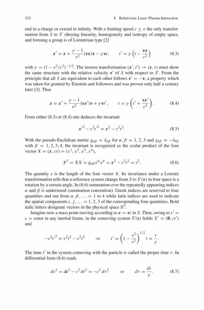
332 8 Relativistic Laser–Plasma Interaction
end in a charge or extend to infinity. With a limiting speed c ≥ v the only transfor-mation from S to S′ obeying linearity, homogeneity and isotropy of empty space,and forming a group is of Lorentzian type [2]
x′ = x + γ − 1
v2(vx)v − γ vt, t ′ = γ
(t − vx
c2
)(8.3)
with γ = (1− v2/c2)−1/2. The inverse transformation (x′, t ′)→ (x, t) must showthe same structure with the relative velocity v′ of S with respect to S′. From theprinciple that all S are equivalent to each other follows v′ = −v, a property whichwas taken for granted by Einstein and followers and was proven only half a centurylater [3]. Thus
x = x′ + γ − 1
v2(vx′)v + γ vt ′, t = γ
(t ′ + vx′
c2
). (8.4)
From either (8.3) or (8.4) one deduces the invariant
x′2 − c2t ′2 = x2 − c2t2. (8.5)
With the pseudo-Euclidean metric gαβ = δαβ for α, β = 1, 2, 3 and g4β = −δ4βwith β = 1, 2, 3, 4, the invariant is recognized as the scalar product of the fourvector X = (x, ct) = (x1, x2, x3, x4),
X2 = X X = gαβxαxβ = x2 − c2t2 = s2. (8.6)
The quantity s is the length of the four vector X . Its invariance under a Lorentztransformation tells that a reference system change from S to S′(v) in four space is arotation by a certain angle. In (8.6) summation over the repeatedly appearing indicesα and β is understood (summation convention). Greek indices are reserved to fourquantities and run from α, β, . . . = 1 to 4 while latin indices are used to indicatethe spatial components i, j, . . . = 1, 2, 3 of the corresponding four quantities. Bolditalic letters designate vectors in the physical space R
3.Imagine now a mass point moving according to x = vt in S. Then, owing to s′ =
s = const in any inertial frame, in the comoving system S′(v) holds X ′ = (0, ct ′)and
−c2t ′2 = v2t2 − c2t2 ⇒ t ′ =(
1− v2
c2
)1/2
t = t
γ.
The time t ′ in the system comoving with the particle is called the proper time τ . Indifferential form (8.6) reads
ds2 = dx2 − c2 dt2 = −c2 dτ 2 ⇒ dτ = dt
γ. (8.7)
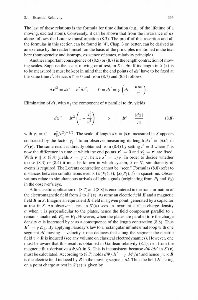
8.1 Essential Relativity 333
The last of these relations is the formula for time dilation (e.g., of the lifetime of amoving, excited atom). Conversely, it can be shown that from the invariance of dsalone follows the Lorentz transformation (8.3). The proof of this assertion and allthe formulas in this section can be found in [4], Chap. 3 or, better, can be derived asan exercise by the reader himself on the basis of the principles mentioned in the texthere (homogeneity and isotropy, existence of states, relativity principle).
Another important consequence of (8.5) or (8.7) is the length contraction of mov-ing scales. Suppose the scale, moving or at rest, in S is dx. If its length in S′(v) isto be measured it must be kept in mind that the end points of dx′ have to be fixed atthe same time t ′. Hence, dt ′ = 0 and from (8.7) and (8.3) follows
dx′2 = dx2 − c2 dt2, 0 = dt ′ = γ
(dt − v dx
c2
).
Elimination of dt , with v‖ the component of v parallel to dx, yields
dx′2 = dx2
(1− v2‖
c2
)⇒ |dx′| = |dx|
γ‖(8.8)
with γ‖ = (1 − v2‖/c2)−1/2. The scale of length dx = |dx| measured in S appears
contracted by the factor γ−1‖ to an observer measuring its length dx ′ = |dx′| in
S′(v). The same result is directly obtained from (8.4) by setting t ′ = 0 where t ′ isnow the difference in time at which the end points x′1 = 0 and x′2 = x′ are fixed.With v ‖ x (8.4) yields x = γ x ′, hence x ′ = x/γ . In order to decide whetherto use (8.3) or (8.4) it must be known in which system, S or S′, simultaneity ofevents is required. The Lorentz contraction cannot be “seen.” Formulas (8.8) refer todistances between simultaneous events
(x(P1), t
),(x(P2), t
)in spacetime. Obser-
vations relate to simultaneous arrivals of light signals (originating from P1 and P2)in the observer’s eye.
A first useful application of (8.7) and (8.8) is encountered in the transformation ofthe electromagnetic field from S to S′(v). Assume an electric field E and a magneticfield B in S. Imagine an equivalent E-field in a given point, generated by a capacitorat rest in S. An observer at rest in S′(v) sees an invariant surface charge densityσ when v is perpendicular to the plates, hence the field component parallel to v
remains unaltered, E′‖ = E‖. However, when the plates are parallel to v the chargedensity σ is increased by γ as a consequence of the length contraction (8.8). ThusE′⊥ = γ E⊥. By applying Faraday’s law to a rectangular infinitesimal loop with onesegment d l moving at velocity v one deduces that along the segment the electricfield v× B is induced (see any volume on classical electrodynamics). However, onemust be aware that this result is obtained in Galilean relativity (8.1), i.e., from themagnetic flux derivative dΦ/dt in S. This is inconsistent because dΦ/dt ′ in S′(v)must be calculated. According to (8.7) holds dΦ/dt ′ = γ dΦ/dt and hence γ v× Bis the electric field induced by B in the moving segment d l . Thus the field E′ actingon a point charge at rest in S′(v) is given by

334 8 Relativistic Laser–Plasma Interaction
E′‖ = E‖, E′⊥ = γ (E⊥ + v × B). (8.9)
The magnetic field generated by an infinitely long coil does not change when the coilmoves with velocity v ‖ B because cross section and magnetic field flux (numberof field lines) remain unchanged. To find the transformation law of B⊥ the inversetransformation E′⊥ → E⊥ = γ (E′⊥ − v × B′) can be used to calculate v × E⊥with the help of (8.9),
1
γ 2v × E⊥ = 1
γv × (E′⊥ − v × B′⊥) = v × (E⊥ + v × B⊥)− 1
γv × (v × B′⊥)
= v × E⊥ − v2 B⊥ + 1
γv2 B′⊥.
Thus B transforms according to
B′‖ = B‖, B′⊥ = γ
(B⊥ − 1
c2v × E
). (8.10)
The second equation in (8.10) is directly deduced from (8.9) by making use of theanalogy of ∇ × B = ∂t E/c2 with ∇ × E = −∂t B. From (8.9) and (8.10) onededuces E′2 − c2 B′2 = E2 − c2 B2, and E′B′ = E B, i.e., the two expressions areLorentz scalars. The second relation says that E ⊥ B is an invariant property withrespect to a Lorentz transformation; for example the k vector of a plane electromag-netic wave may change direction, however k, E, B remain mutually orthogonal.
Any quantity Y , which transforms like a position vector X = (x, y, z, ct) =(x1, x2, x3, x4) is called a four vector. The following easily provable criterion isvery useful. If the scalar product ZY = gαβ zα yβ of a four vector Z with a fourquantity Y remains unchanged under an arbitrary Lorentz transformation (8.3), Y isa four vector, and vice versa, i.e., the scalar product of two four vectors Z and Y isLorentz invariant. Using this criterion, the correct transformation laws of frequencyω and wave vector k of a light wave in vacuum is found. The phases φ = kx − ωtin S and φ′ = k′x′ − ω′t ′ in S′ must be equal because they count the number ofmaxima, for example, which reach the observers in S and S′. Hence, K = (k, ω/c)is a four vector and transforms as
k′ = k + γ − 1
v2(vk)v − γ
v
c2ω, ω′ = γ (ω − kv). (8.11)
It is evident that the following quantities with proper time τ and rest mass m arefour vectors:
four velocity V = d X/dτ = γ (v, c), V 2 = γ 2(v2 − c2) = −c2,
four momentum P = mV = ( p, γmc), p = γmv, P2 = −m2c2,
four acceleration A = dV/dτ, V A = 1
2dV 2/dτ = 0 ⇒ A ⊥ V,
A2 = a2, a = dv/dt.

8.1 Essential Relativity 335
A special criterion for a four quantity Y to be a four vector is that its square Y 2 =gαβ yα yβ is invariant against a Lorentz transformation. From the knowledge V 2 =−c2, P2 = −m2c2, A2 = a2 alone follows that V , P , A are four vectors. At firstglance it may surprise that V , P , A are constructed with the help of the positionvector X in S and the proper time τ related to the comoving frame S′(v). However,from (8.7) follows that dτ is proportional to ds, which, as an invariant, may beevaluated in S as well.
If a four quantity F = F(x, v) is related to the change of the four momentumP by
dP
dτ= F, (8.12)
F is called a four force or Minkowski force. If its spatial components are indicatedby f = ( f 1, f 2, f 3), it follows
dpdτ= f ⇔ dp
dt= f E, f E = f /γ. (8.13)
For obvious reasons f E is given the name Einstein force. It is the relativisticallycorrect three force describing the momentum change in an arbitrary inertial refer-ence frame. In a reference frame S′ comoving with the point particle, dp/dt reducesto m dv/dt , and f E becomes equal to f , which we give the index N, f = f N, andcall f N a Newton force,
mdv
dt= f N. (8.14)
In general it is correct only in the comoving inertial frame.As an application of (8.13) we show that the plasma frequency ωp is a Lorentz
invariant. For the infinitesimal displacement ξ (weak field!) in the electric fielddirection holds in an arbitrary reference system S(v0)
dpdt= d
dtγ (v)mv = γ (v0)m
dv
dt= γ (v0)m
d2ξ
dt2= −eE; E = e
ε0neξ
⇒ d2ξ
dt2= − e2ne
ε0γmξ = −e2n0
ε0mξ = −ω2
p(n0)ξ . (8.15)
The last step follows from ne(v0) = γ (v0)n0 as a consequence of the Lorentzcontraction of ξ = ξ ′/γ (v0). Note neξ = n0ξ
′.Owing to dp4/dt = dp4/dτ = 0 in the comoving frame S′, the Minkowski
force is F = ( f N, 0), and hence in an arbitrary reference system S(w) the fourforce F = ( f , f 4) is given through
f = f N + γ − 1
w2(w f N)w, f 4 = −γ w
cf N = −w
cf . (8.16)

336 8 Relativistic Laser–Plasma Interaction
Note that if the particle has a velocity v in S, owing to v = −w one has f 4 =γ v f N/c. This relation follows also from F ⊥ P . In fact, d P2/dτ = 2P F =2γm(v f − c f 4) = 0. With the help of (8.16) the Einstein force on a point chargeq is found. By definition of the electric field, in the rest frame S′ of the chargef N = q E′ = q[E‖ +γ (E⊥+v× B)] holds [see (8.9)]. In a frame S moving at−v
relative to S′ the transformation law (8.16) requires F=q[E‖ + γ (E⊥+v× B) +(γ −1)E‖, γ vE]. Hence, f E = q(E+ v× B), and the correct relativistic equationof motion in three-space reads
d
dt(γmv) = q(E + v × B). (8.17)
Sometimes the difference between the orbits from (8.13) and (8.17) and the corre-sponding nonrelativistic equation of motion is attributed to the “relativistic massincrease”. Except special cases this is not a good concept because the “massincrease” depends on the particular motion (e.g. “longitudinal” mass m‖ differingfrom “transverse” mass m⊥) and may obscure the real origin of (8.13) and (8.17)that is the Minkowski metric of space time.
8.1.2 Momentum and Kinetic Energy
Integrating (8.12) from τ = 0 to τ > 0 with the point particle initially at rest yieldswith the help of (8.13)
P(t)− P(0) =(∫ τ
0f dτ,
1
c
∫ τ
0f v dτ
)=(∫ t
0f E dt,
1
c
∫ t
0f E dx
)
= ( p, γmc − mc).
It shows that the kinetic energy of the particle is Ekin = γmc2 − mc2 = E − E0because
∫ t0 f E dx is the work done by the Einstein force. Hence
E = E0 + Ekin = γmc2 ⇔ E2 = m2c4 + p2c2. (8.18)
The second relation is nothing but P2 = −m2c2 = −E20/c2.
Sometimes formulas relating the velocity u and the four momentum P measuredin S to the corresponding quantities u′ and P ′ measured in S′(v) are useful. Accord-ing to (8.4) holds for dx = u dt and dx′ = u′ dt ′
u dt =(
u′ + γ − 1
v2(vu′)v + γ v
)dt ′, dt = γ
(1+ vu′
c2
)dt ′, γ = γ (v).
Elimination of dt ′ leads to the so-called relativistic velocity addition theorem v
and u′,

8.1 Essential Relativity 337
u = u′ + v[γ (1+ u′v/v2)− u′v/v2]γ (1+ u′v/c2)
. (8.19)
If u′ < c, v < c is fulfilled u < c follows because (8.19) implies (c2 − u2)/c2 =(c2 − u′2)(c2 − v2)/(c2 + u′v). The inverse transformation for u′ is obtained from(8.19) by interchanging u and u′ and substituting v by −v. The analogous formulafor P and P ′ is accordingly
P = ( p, γmc) =(
p′/γ ′ + v[γ (m + p′v/(γ ′v2))− p′v/(γ ′v2)]1+ p′v/(γ ′c2)
, γmc
)(8.20)
with γ ′ = γ (u′).The Lagrangian of a particle of rest mass m moving in a time-independent poten-
tial V = V (x) is
L(x, v) = T − V = −m
γc2 − V (8.21)
because it obeys the equation of motion
d
dt
∂L
∂v− ∂L
∂x= d
dt(γmv)+∇V = 0,
if the force is correctly given by−∇V . Keeping in mind that it should be an Einsteinforce f E, the weakness of a noncovariant Lagrangian (8.21), i.e., a Lagrangian notexpressed in four quantities, appears. For instance, when going from S to S′(v),the potential may assume the wrong time dependence. If (8.21) is acceptable theHamiltonian is given by
H( p, x) = ∂L
∂vv − L = (m2c4 + p2c2)1/2 + V (x), (8.22)
and the canonical equations of motion
d
dtp = −∂H
∂x,
dxdt= ∂H
∂p(8.23)
yield the equation of motion above and the connection between v and p for a pointparticle, respectively.
8.1.3 Scalars, Contravariant and Covariant Quantities
In the basis {ei } the vector x is the unique linear combination x = xi ei , with xi
the contravariant components (Fig. 8.1). The same vector can also be expresseduniquely by its covariant components xi , which are the projections of x onto the

338 8 Relativistic Laser–Plasma Interaction
e
e
1
2
x
x
x
x
x2
1
2
1
Fig. 8.1 Contravariant components x1, x2 and covariant components (projections) x1 and x2
vectors ei , xi = xei . With the help of the Euclidean metric gik = ei ek = gki andthe inverse matrix (gik) = (gik)
−1, the transformation from one set of componentsto the other is accomplished by
xi = gik xk, xi = gik xk . (8.24)
The use of the two types of coordinates allows a compact representation of the scalarproduct,
x y = (xi ei ) y = xi (ei y) = xi yi = gik xi xk,
ds2 = dx dx = gik dxi dxk .(8.25)
The metric of special relativity for a Cartesian coordinate system in R4 is given
by the gαβ of (8.6). It is identical with its inverse matrix, gαβ = gαβ .A scalar quantity, or Lorentz scalar, is by definition a quantity which is invariant
under a general Lorentz transformation. The rest mass m of a particle and its chargeq are Lorentz scalars, but the density of particles n, of charge ρel = nq and of massρ are not. In fact, from (8.8) and (8.18) follows in S′(v)
n = γ n0, ρel = γρel,0, ρ = γ 2ρ0, γ = (1− v2/c2)−1/2. (8.26)
The index “0” refers to the rest frame S.Any four quantity Y , which transforms like the position vector X , is a four vector,
e.g., V , P , A, K = (k, ω/c). For Y this is the case if XY = xα yα = f with anarbitrary X is a Lorentz scalar. Any four quantity T αβ , which transforms like theproduct xαxβ , is a four (or Lorentz) contravariant tensor of second rank, etc. Inparticular, any null four quantity is a four tensor. The four gradient ∂α ,
8.1 Essential Relativity 339
gradα = ∂α =(
∂
∂x1,∂
∂x2,∂
∂x3,∂
∂x4
)(8.27)
when applied to a scalar f generates a four vector since
d f = ∂ f
∂xαdxα = gradα f d X
is invariant under a Lorentz transformation, and d X is a four vector. According to thecriterion above gradα f = ∂α f is a covariant four vector. Analogously, gradα f =∂α f = ∂ f/∂xα is a contravariant four vector. Further, it is evident that gradαY =∂α yβ generates a mixed tensor of second rank T β
α . The four divergence of a fourvector V = vα , a four tensor T = T αβ , etc.,
div V = ∂αvα = ∂
∂xαvα, div T = ∂αT αβ = ∂
∂xαT αβ
generates a Lorentz scalar, a four vector, etc.. It is left as an exercise to the readerthat the converse is also true.
In practical applications one is frequently faced with the problem of how thepartial derivatives ∂t and ∂x of an entity F(x, t) transform to ∂t ′ and ∂x ′ operatingon F ′(x ′, t ′) in a system S′ moving with velocity v along x . To this aim let us assumex = g(x ′, t ′), t = h(x ′, t ′). Equating the total differentials d F and d F ′,
d F = ∂t ′F′ dt ′ + ∂x ′F
′ dx ′ = ∂t F dt + ∂x F dx
= ∂t F(ht ′dt ′ + hx ′dx ′)+ ∂x F(gt ′dt ′ + gx ′dx ′),
gt ′ = ∂t ′g, etc., leads to
∂t ′F′ = ∂t F ht ′ + ∂x Fgt ′, ∂x ′F
′ = ∂t F hx ′ + ∂x Fgx ′ . (8.28)
In the special case of g = γ (x ′ + vt ′), h = γ (t ′ + vx ′/c2) results
∂t ′F′ = γ (∂t F + v∂x F), ∂x ′F
′ = γ( v
c2∂t F + ∂x F
);
∂t F = γ (∂t ′F′ − v∂x ′F
′), ∂x F = γ(− v
c2∂t ′F
′ + ∂x ′F′) . (8.29)
They show the symmetry required by the relativity principle, i.e., the inverse trans-formation follows from interchanging F and F ′ and substituting v by −v. InGalileian relativity x = x ′ + vt ′, t = t ′ and ∂t ′F ′ = ∂t F + v∂x F , ∂x F = ∂x ′F ′.

340 8 Relativistic Laser–Plasma Interaction
8.1.4 Ideal Fluid Dynamics
In the reference system S in which an ideal fluid (isotropic pressure, no dissipation)is locally at rest, according to (2.54) and (2.77,π = 0) holds
∂t n0 + ∂i n0vi = 0, ∂tρ0v
i + ∂ j (ρ0viv j + pδi j ) = 0. (8.30)
The quantities Jn = n0V = n0γ (v, c) = jαn , n0 particle density, and T = ρ0vαvβ
are the four vectors of particle flow density and the momentum flow density ten-sor, respectively. Since their divergence div Jn and div T are a Lorentz scalar anda Lorentz vector, respectively, and since in the system locally at rest they reduceto (8.30) for a fluid in the absence of pressure (p = 0), relativistic particle andmomentum conservation for a pressure-free fluid read
∂α jαn = 0, ∂αT αβ = 0. (8.31)
Thus, divT α4 = ∂αρ0vαv4 = c∂i n0mγ 2vi + c∂t n0mγ 2 = 0 (note V = vα =
(γ vi , v4), v4 = γ ct in our convention). Hence, the familiar nonrelativistic equationsof particle and mass conservation,
∂
∂tn +∇nv = 0,
∂
∂tρ +∇ρv = 0, n = γ n0, ρ = γmn (8.32)
are also relativistically correct. However, at relativistic energies certain particlesmay transform into others.
In perfect analogy follows in the absence of pressure that
∂
∂tρvi + ∂
∂x jρviv j = 0,
∂
∂tρc2 + ∂
∂xiρc2vi = 0 (8.33)
hold for all energies. They are identical with their nonrelativistic expressions. Thequantity ρc2 is the internal energy density (see Sect. 8.1.6). If p = 0 the fourtensor ρ0v
αvβ must be completed by a four tensor Sαβ in such a way as to yield∂i Si j = ∂i pδi j , i, j = 1, 2, 3. This is accomplished by setting
T αβ = ρ0vαvβ + Sαβ =
(ρ0 + p
c2
)vαvβ + pgαβ. (8.34)
T αβ is clearly a tensor, and hence ∂αT αβ is a four vector F , which for vanishingvelocity v must reduce to zero (see (2.77), π = 0). Therefore F = 0 must holdin any inertial frame, i.e., ∂αT αβ = 0 are the relativistic conservation equations ofenergy (mass) and momentum. In (x, t) representation they read

8.1 Essential Relativity 341
∂t
(ρc2 + γ 2 p
v2
c2
)+∇(ρc2 + γ 2 p)v = 0, (8.35)
∂t
(ρ + γ 2 p
c2
)v +∇
{(ρ + γ 2 p
c2
)vv + p I
}= 0, I = (δi j ). (8.36)
In contrast to (2.77) and (2.79) in the relativistic formulation the pressure seemsto contribute to the internal energy density ρc2 and to the momentum density ρv.However, this would be an erroneous interpretation because the internal energy isdefined in the rest frame of the fluid where the pressure term in (8.35) reduces tozero. On the other hand, its presence in the time derivatives of the relativistic conser-vation equations is understandable from the spatial derivatives of the correspondingexpressions in (8.35) and (8.36). In fact, ∇(γ 2 pv) in (8.35) stands for the work avolume element spends to remove the neighboring fluid element undergoing a spa-tial change of the field quantities and inducing a corresponding temporal variationthrough the interconnecting space and time coordinates in a Lorentz transformation.With the help of (8.35) momentum conservation (8.36) can be cast into the Eulerianform just in the same way as in Chap. 2,
(ρ + γ 2 p
c2
)(∂v∂t+ (v∇)v
)= −
(∇ p + v
∂p
∂t
). (8.37)
8.1.5 Kinetic Theory
Multifluid equations may be derived from a relativistic kinetic equation amongwhich the simplest is the collisionless Boltzmann or Vlasov equation. It is obtainedas follows. If f (X, p) = f (xα, pi ) is the one-particle distribution function in the6-dimensional phase space (x, p) at time t , the number N (t) of noninteracting (i.e.,collisionless) particles of one species (electrons, ions of charge Z , etc.) contained inthe one-particle phase space volume element ΔΓ (t) = ΔxΔ p is given by
N (t) = f (x, p, t)ΔΓ (t),
with ΔΓ (t) centered around the trajectory(x(t), p(t)
). The motion of the individ-
ual particles is described by the relativistic Hamiltonian H(xi , pi , t) and its canon-ical equations
dxi
dt= ∂H
∂pi,
dpi
dt= −∂H
∂xi, i = 1, 2, 3. (8.38)
The trajectories contained in ΔΓ (t) differ only by their initial conditions xi0, pi
0 att = t0 and the Einstein force f E varying from point to point. First we show thatthe measure of the volume element ΔΓ is conserved in time (relativistic Liouvilletheorem). In fact, its i th projection in Cartesian coordinates is at time t + dt
342 8 Relativistic Laser–Plasma Interaction
ΔΓi (t + dt) = Δxi (t + dt)Δpi (t + dt)
=[Δxi (t)+ dΔxi
dtdt
] [Δpi (t)+ dΔpi
dtdt
]
={Δxi (t)+
[∂H(xi +Δxi )
∂pi− ∂H(xi )
∂pi
]dt
}
×{Δpi (t)−
[∂H(pi +Δpi )
∂xi− ∂H(pi )
∂xi
]dt
}
=[Δxi (t)+ ∂2 H
∂xi∂piΔxi dt
] [Δpi (t)− ∂2 H
∂pi∂xiΔpi dt
]
= Δxi (t)Δpi (t)
[1−
(∂2 H
∂xi∂pi
)2
(dt)2].
Thus d(ΔΓi )/dt = 0 and hence d(ΔΓ )/dt = 0. We have chosen this elementaryproof because it shows that the only condition for the validity of Liouville’s theoremin any finite-dimensional space is the existence of a correct relativistic Hamiltonian.Alternatively, if the validity of Liouville’s theorem is taken for granted in the nonrel-ativistic domain, by transforming to the system comoving with ΔΓ one is reducedagain to the nonrelativistic case of dΔΓ (v = 0)/dτ = d(Δx0Δ p0)/dτ = 0, andhence in S(v) holds ΔΓ (v) = (Δx0/γ )(γΔ p0) = ΔΓ (v = 0) and dΔΓ (v)/dt =(1/γ )dΔ(v = 0)/dτ = 0. From its definition it is clear that N (t) is a Lorentz scalarand as such it is conserved,
dNdt
= d f
dtΔΓ + f
d(ΔΓ )
dt= d f
dtΔΓ = 0 ⇒ d f
dt= 0,
or, written in explicit form, the Vlasov equation reads
∂ f
∂t+ ∂H
∂p∂ f
∂x− ∂H
∂x∂ f
∂ p= 0 ⇔ ∂ f
∂t+ {H, f } = 0. (8.39)
p is the canonical momentum which may differ from the mechanical momentumpm = γmv. It may be convenient to formulate the Vlasov equation in terms of xand pm instead of x and p. For this purpose we observe that Liouville’s theoremremains valid if a new momentum is defined by p′ = p + G(x, t) because theJacobian remains unaltered,
∂(x, p′)∂(x, p)
= ∂(x, p)∂(x, p)
= 1.
If G = −q A(x, t) is set, with A(x, t) the vector potential, (8.39) transforms into
∂ f
∂t+ pm
γm
∂ f
∂x+ f E
∂ f
∂pm= 0, (8.40)

8.1 Essential Relativity 343
where f = f (x, pm, t). In the case of charged particles one has f E = q(E+v×B).The one-particle distribution function f = N /(ΔΓ ) is a Lorentz scalar. The three-form (8.39) is clearly Lorentz invariant since no use of a special reference systemhas been made in any step of its derivation.
From (8.39) or (8.40) conservation equations, e.g., for momentum and energydensities and their fluxes, can be obtained in the form of moment equations bymultiplying it with tα1α2···αs = pα1 pα2 · · · pαs and integrating over the momentumspace R
3p, just in the same way as in the nonrelativistic case (see end of Sect. 2.2.1).
In order to preserve the four-character of tα1α2···αs one has to integrate over an invari-ant volume element in momentum subspace, i.e., dp/γ or dp/p4, p4 = γmc. Theintegrals
T α1α2···αs =∫
pα1 pα2 · · · pαs f (X, p)dp
γ ( p)mc(8.41)
clearly define a contravariant four tensor T of rank s because any finite sum overthe four tensor tα1α2···αs and hence also the limiting sum, i.e., the integral overthe invariant volumes dp/(γmc), are tensors of the same kind. The link with thefluid equations is established by introducing kinetic expressions for particle andcharge density, internal energy, pressure, etc. and their fluxes. To this aim the globaldynamics has to be split up into an inner component and a macroscopic outer flowcomponent. In other words, the relativistic concept of the center of momentum hasto be introduced.
8.1.6 Center of Momentum and Mass Frame of NoninteractingParticles
In analogy to the nonrelativistic limit we define for particles of nonvanishing restmass mi
P =N∑
i=1
mi Vi =N∑
i=1
miγi(vi , c
) = MV = Mγ (v)(v, c
)(8.42)
with γi = γ (vi ). This definition implies γ (v)M = ∑i miγi , which is compatible
with the definition of the center of mass position four vector
X = 1
γ (v)M
N∑
i=1
miγi Xi ⇔ x = 1
γ (v)M
N∑
i=1
miγi xi (8.43)
as long as no forces act on the particles. Then
d xdt= 1
γ (v)M
N∑
i=1
miγivi , (8.44)

344 8 Relativistic Laser–Plasma Interaction
in agreement with the center of momentum velocity v obtained from (8.42). Thepoint x(t) defined by (8.43) may vary from one reference system S to another S′. If,for instance, it coincides with the position x j (t) of a particle at time t , x(t) = x j (t),this may no longer be true when changing to another inertial frame S′, i.e., x′(t ′) =x′j (t ′) owing to the weighting factors γi having changed. In other words, due to the
presence of the γi , X is not a Lorentzian four vector, in contrast to P from (8.42).To illustrate this the reader may imagine two point masses m1 = m2 = m movingat speed close to c against each other. An observer comoving with mass m1 sees thecenter of mass close to m2, an observer comoving with m2 sees it close to m1.
It is evident that a reference system Sc exists in which V = (0, c) in (8.42). Then
Mc =N∑
i=1
miγic, P = McU = γ (u)Mc(u, c),
xc = 1
Mc
N∑
i=1
miγicxi , γic = γi (vic). (8.45)
By xc the center of mass in the rest frame is defined. Xc = (xc, ct) is a Lorentzvector, and with xc(t) = x j (t) also x′c(t ′) = x′j (t ′) holds. An additional advantage
of the special choice of the definition (8.45) is that Mcc2 can be given the simpleinterpretation of the total internal energy in the case of noninteracting particles.The kinetic energy of the system of N point masses in the rest frame then reads(Mc − ∑
i mi )c2. Owing to c4(∑
miγi )2 = M2
c c4 + c2 p2c , pc = Mcγcvc, the
internal energy Mcc2 is the minimum kinetic energy which the system can assumeunder a Lorentz transformation. If the center of mass is defined according to (8.43)no such interpretation exists for M . The only valid statement is that according to(8.44), besides xc, all centers of mass x are also at rest in the center of momentumsystem.
For the interested reader a proof of the existence of Sc with V = (0, c) is given.A four vector Y = ( y, y4) is time-like if Y 2 = y2 − (y4)2 < 0 and space-like ifY 2 > 0. By choosing a reference system S(vt) with γtvt = c y/y4 the time-likeY reduces to Y = (0, y4
0) in S(vt) whereas, when setting vs = cy4 y/ y2 a space-like Y becomes Y = ( y0, 0) in S(vs). Vi and Pi = mVi are time-like. Hence,P = P1 + P2 = (0, P4
1 )+ ( p2, P42 ) is also time-like owing to P2 = −P2
1 + p2 −(P4
2 )2 − 2P4
1 P42 < 0 and P4
1 , P42 > 0. Assertion V = (0, c) follows by induction
on P and from V = P/Mc, Mc from (8.45).
8.1.7 Moment Equations
In (8.41) the Lorentz invariant volume element in momentum space was introducedto preserve the four tensor character of tα1α2···αs under integration. It is shown nowthat such a choice is stringent on physical grounds and is helpful in interpreting thevarious moment terms. In Sect. 8.1.5 the distribution function f (x, p, t)was defined
8.1 Essential Relativity 345
with the help of the co-moving 6D phase space volume element dΓ0 = dx0 dp0,indicated here by the index “0”. dΓ = dxdp is also a Lorentz scalar and as suchinvariant in any inertial frame, e.g., in the lab frame S, and hence for the particlenumber dN holds
dN = f dx dp = f0 dx0 dp0. (8.46)
By definition the particle number density of momentum p in S in the co-movingframe is dn0 = dN /dx0 = f0 dp0. When calculating the particle density n(x, t) inS one has to bear in mind that for each momentum p the corresponding dx0 has tobe chosen such that owing to the Lorentz length contraction it assumes the size dxin S, i.e., dx0 = γ dx. Thus from (8.46) follows
dN = dx f dp = γ dx f0dpγ
⇒ n0(x, t) =∫
fdpγ, (8.47)
in agreement with dp0 = dp/γ , dΓ = dΓ0, and f = f0. From (8.41) with pα = p4
results n(x, t) = j4n /c which shows that n(x, t)c = γ (u)n0(x, t)c is the fourth
component of the particle current density. Furthermore, c∫
p f dp/p4 = ∫ v f dp =jn. With a view onto (8.42) it shows that the flow velocity u is defined by u = jn/n.In conclusion the following definitions are introduced:
Jn = c∫
P fdpp4= n(u, c) = n0U, U = γ (u)(u, c),
n =∫
f dp, u = 1
n
∫v f dp, n = γ (u)n0, (8.48)
ε = c∫(p4)2
dpp4= mc2
∫γ ( p) f dp = εin + εkin.
The internal energy density εin is the energy density in the center of momentumsystem (8.45) with u = 0. For clarity the average velocities of the ensemble hereand whenever it appears useful is given the symbol U and u to better distinguish itfrom the individual particle velocities V and v. Note that the averaging procedurefor particle density n(x, t) and mean flow velocity u(x, t) in the relativistic andnonrelativistic case are identical [compare (2.82)]. In this context formula (8.41) forthe moments was justified by the argument that in determining the total number ofparticles at the time instant t lying in the interval dxi around xi each group whenmoving at momentum pi contracts by γ in space. Since, on the other hand dxi dpi
is Lorentz invariant the shrinking dxi has to be compensated by choosing its sizein momentum space as dpi/γ . The averaging procedure (8.41) can be justified onpurely formal grounds: If a quantity under consideration coincides with its nonrela-tivistic expression in the rest frame (like n and jα) it is relativistically correct in anyframe S(v) because (8.41) generates four quantities out of four quantities.
Decomposition into intrinsic and dynamic components by means of the centerof momentum concept (8.45) (Eckart’s decomposition [5, 6]) is appropriate for
346 8 Relativistic Laser–Plasma Interaction
particles of finite rest mass. In contrast to the nonrelativistic case no simple additiontheorem exists for the individual velocity three vectors [see (8.19)]. Decomposi-tion is therefore done in four space. To this aim the individual particle momentumP = ( p, p4) is represented as the sum of a vector parallel to the mean flow fourvelocity U and a vector W = (w, w4) perpendicular to it,
pα = m(guα + wα), U W = uβwβ = 0 (8.49)
so that w4 = uiwi/u4. In the center of momentum system follows from (8.42)
wi = γicvic and w4i = 0. W is a space-like vector. From P2 = m2(gU + W )2,
U 2 = −c2, and P2 = −m2c2 the coefficient g = −U P/(mc2) is obtained asg = (1 + W 2/c2)1/2. The average 〈W 〉 is a measure of the internal energy perparticle in units of the rest energy mc2. In passing from p to w in (8.41)
dpp4= m2
g
dw
u4(8.50)
has to be used. The general validity of this relation can be verified by a lengthyexplicit calculation of the Jacobian |∂( p)/∂(w)|. Alternatively it follows directly inthe center of mass system (w4 = 0) and hence in any inertial frame because dp/p4
is an invariant measure. The decomposition (8.49) yields for the particle currentdensity J = jα and the energy-stress tensor T = T αβ
jα = n0uα, (8.51)
T αβ = (ρ0 + ε/c2)uαuβ + Pαβ + (uαqβ + uβqα), (8.52)
where, with h(X,w) = m3c f (X, p), the single terms are given by
ρ0 = m∫
hdw
u4, ε = mc2
∫(g − 1)h
dw
u4, Pαβ = m
∫wαwβh
dw
gu4,
qα = mc2∫(g − 1)wαh
dw
gu4. (8.53)
In the local rest frame (u4 = c, w4 = 0) the mass density ρ0, the internal energyε, and the corresponding three vectors and three tensors read with h′ = h/c
ρ0 = m∫
h′ dw, ε = mc2∫ [(
1+ w2
c2
)1/2
− 1
]h′ dw,
Pik = m∫
wiwk
(1+ w2/c2)1/2h′ dw, (8.54)
qi = mc2∫ [
1− 1
(1+ w2/c2)1/2
]wi h′ dw.

8.1 Essential Relativity 347
The quantity qi represents the local heat flow density. In the nonrelativistic limit qi
and the remaining quantities in (8.54) reduce to (2.82), (2.83), (2.84), and (2.85)after interchanging v for flow with u for the single particle there. The total energydensity in the rest frame is ρ0c2 + ε = T αβuαuβ . It is also possible to identify Uwith the energy transport velocity and J = Jm with ρ0u + R,
uα = (ρ0 + ε/c2)uαuβuβ = T αβuβ, Rα = mc2∫wαh
dw
gu4(8.55)
in which case qα = 0 and Rα = 0 holds (see Landau and Lifshitz [7]). With thisdecomposition the heat flux is hidden in J . Such a choice may be advantageous incase of massless particles, e.g., photons.
The conservation laws (equations of motion) are obtained from the zeroth orderand first order moments of P = pα ,
0th order:∫
f (X, p) dp =∫
p4 f (X, p)dpp4,
1st order:∫
pα f (X, p) dp =∫
pα p4 f (X, p)dpp4.
Folding the Vlasov equation (8.40) with p4 by the invariant measure dp/p4,
∫p4 [∂t f + v∂x f + q(E + v × B)∂ p f
] dpp4= 0, (8.56)
partial integration of the third term and comparison with (8.48) leads to the particlenumber or charge conservation ∂α jαn = 0 from (8.31):
0 =∫∂t f dp+
∫v∂x f dp+ q
∫(E + v × B)∂ p f dp
= ∂t
∫f dp+ ∂x
∫v f dp+ q
∑∫ [(E + v × B) j f
]p j=+∞p j=−∞ dpk dpl
= ∂t n(x, t)+∇[n(x, t)u(x, t)] = ∂α jαn .
The third term vanishes owing to f (pi = ±∞) = 0 and ∂pi v j =i = 0. Momentumand energy conservation are obtained in the same way by folding (8.40) with tα4 =pα p4 as the divergence of T αi and T α4,
∂αT αi = nq(E + u × B)i , ∂αT α4 = nquE, (8.57)
with T αi , T α4 given by (8.52). Thereby use has been made of

348 8 Relativistic Laser–Plasma Interaction
∫(E + v × B) j pi ∂ f
∂p jdp = δi j
{∫|ε jkl |(E + v × B) j pi f |p j=+∞
p j=−∞dpkdpl
−∫(E + v × B) j f dp
}, (k < l) (8.58)
and (8.17) for the fourth component of the Lorentz force.For a gas of weakly interacting particles in local thermal equilibrium all ther-
modynamic properties (specific heat, pressure, etc.) are obtained from Maxwell’svelocity distribution. From the canonical distribution for (distinguishable) particlesthe relativistic Maxwell distribution function is obtained by expressing the energyaccording (8.18) with p taken in the local center of mass system,
fM(x, p, t) = n0(x, t)N exp
[−(
E20 + p2c2
)1/2/(kBT )
]. (8.59)
N normalizes the exponential to unity, n0 is the local particle density in the localrest frame and t is a time variation which is slow on the microscopic time scale.With f strictly Maxwellian (8.54) yields qi = 0.
8.1.8 Covariant Electrodynamics
By introducing a vector potential A whose curl yields the magnetic field, ∇ × A =B, the induction law in differential form can be written as ∇× E+ B = ∇× (E+A) = 0. The general solution of this equation is E + A = −∇Φ where Φ is anarbitrary scalar function of x and t . Hence,
E = − A−∇Φ, B = ∇ × A. (8.60)
By defining the four quantity
A = (c A, Φ) = (A1, A2, A3, A4 = Φ) (8.61)
and supposing for the moment that A is a four vector, the quantity
Fαβc= ∂α Aβ − ∂β Aα (8.62)
is a covariant, antisymmetric four tensor (see Sect. 8.1.3). Equation (8.60) is linkedto Fαβ by
cBx = ∂2 A3 − ∂3 A2 = F23/c,cBy = ∂3 A1 − ∂1 A3 = F31/c,cBz = ∂1 A2 − ∂2 A1 = F12/c,
Ex = ∂1 A4 − ∂4 A1 = F14/c,Ey = ∂2 A4 − ∂4 A2 = F24/c,Ez = ∂3 A4 − ∂4 A3 = F34/c.
(8.63)

8.1 Essential Relativity 349
Hence
Fαβ = c
⎛
⎜⎜⎝
0 cBz −cBy Ex
−cBz 0 cBx Ey
cBy −cBx 0 Ez
−Ex −Ey −Ez 0
⎞
⎟⎟⎠ , Fαβ = c
⎛
⎜⎜⎝
0 cBz −cBy −Ex
−cBz 0 cBx −Ey
cBy −cBx 0 −Ez
Ex Ey Ez 0
⎞
⎟⎟⎠ .
In a general Euclidean metric g holds Fαβ = gαγ gβδFγ δ . According to (8.26) and(8.31) the four current density is given by
J = ρel,0V, ∂α jα = 0. (8.64)
The four current is divergence-free, i.e., the electric charge is conserved. It can beshown that with (8.64) the total charge Q is both conserved and a Lorentz-scalar(see [2], Sect. 6). The first pair of Maxwell equations
ε0c2∇ × B − ε0 E = j , ∇E = ρel
ε0(8.65)
reads in terms of Fαβ
∂αFαβ = − jβ
ε0⇔ div F = − J
ε0. (8.66)
Since J is a four vector Fαβ is a four tensor, and consequently A from (8.61) is afour vector potential.
By comparing the remaining pair of Maxwell equations
∇ × E + B = μ0c jmag, ∇B = μ0c3ρmag, Jmag = ( jmag, cρmag) = 0
with (8.65) the corresponding field tensor
F ′αβ = c
⎛
⎜⎜⎝
0 Ez −Ey cBx
−Ez 0 Ex cBy
Ey −Ex 0 cBz
−cBx −cBy −cBz 0
⎞
⎟⎟⎠ (8.67)
satisfying
div F ′ = 0 ⇔ ∂αF ′αβ = 0 (8.68)
is obtained.There are the two simple, nontrivial Lorentz scalars
FαβFαβ = 2c2(c2 B2 − E2),1
8c2εαβγ δFαβFγ δ = E B (8.69)

350 8 Relativistic Laser–Plasma Interaction
where εαβγ δ is the totally antisymmetric Levi–Civita tensor. The invariance of E Bagainst a Lorentz transformation also follows explicitly using (8.9) and (8.10),
E′B′ = E′‖B′‖ + E′⊥B′⊥ = E‖B‖ + γ2
[E⊥B⊥ − 1
c2(v × B)(v × E)
]
= E‖B‖ + E⊥B⊥ = E B,
or from the transformation law of the electromagnetic field tensors F and F ′. Infact, the Lorentz transformations (8.3) and (8.4) are linear and hence can be writtenin the form
x ′β = Λβαxα, xα = Λα
βx ′β, ΛγβΛ
βα = δγα ⇔ (Λβ
α) = (Λβα)−1 (8.70)
to obtain F ′αβ . It is more convenient to associate the dash ′ with the indices, i.e.,to write xβ
′for x ′β and Fα′β ′ for F ′αβ . Hence Fα′β ′ = Λα′
α Λβ ′β Fαβ . From this
equality formulas (8.9) and (8.10) are found again. The matrix Λ describes a so-called Lorentz boost.
The already familiar div-operator ∂α and the d’Alembertian �,
� = ∂αα = gαβ∂
∂xα∂
∂xβ= ∇2 − 1
c2
∂2
∂t2(8.71)
are Lorentz covariant and invariant operators, respectively. The invariance of thed’Alembertian is evident owing to the scalar product � = ∂α∂
α . To show thecovariance of the four divergence consider ∂αT αβ where T αβ is an arbitrary fourtensor. For xα
′ = Λα′α xα , T α′β = Λα′
κ T κβ
∂α′Tα′β = ∂xα
∂xα′∂αΛ
α′κ T κβ = Λα
α′Λα′κ ∂αT κβ = δακ ∂αT κβ = ∂αT αβ
holds, demonstrating the proper transformation behavior of ∂α as a four vector.Moreover, if ∂αT αβ = tβ with tβ a four vector, T αβ is a four tensor (and viceverse). Use of this criterion was made above after (8.66) for the electromagneticfield tensor.
The four vector potential leading to a given field configuration Fαβ is not unique.One may add the gradient ∇Ψ of an arbitrary scalar function Ψ (x, t) to A and −Ψto Φ without affecting the fields E and B (gauge transformation). Ψ can be chosensuch that
∂α Aα = ∇c A+ ∂
∂ctΦ = 0 (Lorentz gauge), (8.72)
leading to the two separate, inhomogeneous wave equations

8.2 Particle Acceleration in an Intense Laser Field 351
% A− 1
c2
∂2
∂t2A = − j
ε0c2, %Φ − 1
c2
∂2
∂t2Φ = −ρel
ε0(8.73)
or in covariant form
�A = − J
ε0c. (8.74)
The well-known particular solutions of these equations are given in terms of retardedintegrals of j and ρel. In the special case of a moving point charge the so-calledLiénard-Wiechert potentials read
A(x, t) = q
4πε0c2
v(t ′)R − Rv(t ′)/c
, Φ(x, t) = q
4πε0
1
R − Rv(t ′)/c, (8.75)
where t ′ = t − R/c. The vector R = x − x0(t ′) has its origin at the retardedposition x0(t ′) of the particle moving with velocity v(t ′) and points to the point ofobservation x.
8.2 Particle Acceleration in an Intense Laser Field
The principle of particle acceleration by a wave, either electromagnetic or elec-trostatic (or both) is simple and is illustrated by Fig. 8.2 where a point particle isinjected into potentials. In (a) the mass point acquires kinetic energy correspond-ing to its height, ΔEkin = mgh. It gains, however, more energy if the previouslyfixed structure is moving to the right, as indicated in (b). This is because now theforce perpendicular to the slope also does work upon accelerating the particle inx direction. In the intense electromagnetic wave an electron is first accelerated bythe ponderomotive force in the propagation direction (if the transverse gradient ofE2 is weak). In the relativistic regime, direct acceleration by E′ = v × B setsin preferentially into forward direction over arbitrarily long distances, in principle(c). This is a consequence of the strong frequency Doppler down shift at vx ≈ c.To avoid misinterpretations, in the lab frame all acceleration work is done by theE-field of the laser beam, the Lorentz force, perpendicular to v, merely providesfor bending the orbit into forward direction. From the engineering point of view themain problem consists in (i) trapping the particle, (ii) guiding the intense wave overa long distance and, perhaps most difficult, (iii) extracting the particle in the rightmoment before it starts to be decelerated and to lose energy again.
The covariant equation of motion reads
mdV
dτ= q
c2FV ⇔ m
dvαdτ
= q
c2Fαβv
β, (8.76)
which is identical with

352 8 Relativistic Laser–Plasma Interaction
(a) 1.
2.
3.
(b)
V
2.
3.
1.
mg mg
E’
1.
2.
3.
(c)
Fig. 8.2 The principle of particle acceleration in a finite potential structure. (a) Fixed slope,(b) moving slope, (c) electron trapped in a traveling wave
d
dtmγ v = q(E + v × B),
d
dtmγ c2 = qvE. (8.77)
The nonrelativistic Hamiltonian for a point charge in an electromagnetic field isaccomplished by the passage from the mechanical momentum pm = mγ v to itscanonical counterpart p = pm + q A. The Hamiltonian as the sum of kinetic andpotential energy E = p2
m/(2m)+V then is H = ( p−q A)2/(2m)+qΦ. Accordingto (8.18) the relativistic energy is E = [m2c4 + p2
mc2]1/2 + V = mγ c2 + V .Correspondingly, the relativistic Hamiltonian is set as
H = [m2c4 + ( p− q A)2c2]1/2 + qΦ (8.78)
= mc2[
1+( p
mc− a
)2]1/2
+ qΦ,
with
a = q Amc
.
The correctness of the relativistic Hamiltonian (8.78) follows from the canonicalequations

8.2 Particle Acceleration in an Intense Laser Field 353
x = ∂H
∂ p= p− q A
m[1+ ( p/(mc)− a
)2]1/2= mγ v
mγ= v,
p = −∂H
∂x= − 1
2mγ
∂
∂x( p− q A)2
= qv × B + q(v∇)A− q∇Φ =: C, (8.79)
and
p = d
dtmγ v + q
[∂A∂t+ (v∇)A
]!= C,
leading to the correct equation of motion (8.77). The identity ∇b2 = 2[b × (∇ ×b)+ (b∇)b] was used to arrive at expression (8.79).
8.2.1 Particle Acceleration in Vacuum
In order to explore the limits of particle acceleration by laser pulses the ideal-ized situation of a plane, linearly polarized electromagnetic wave propagating inx-direction and acting on a point charge of rest mass m and charge q is considered.Let the wave be described by the vector potential A and Φ = 0 (Coulomb gauge),
A = e⊥A(ξ), ξ = x − ct, e⊥ex = 0, e2⊥ = 1. (8.80)
The equations of motion with e⊥ = ey are
py = −∂H
∂y= 0, px = −∂H
∂x= q
mγ(py − q A)
d A
dξ. (8.81)
The first equation implies the conservation of the transverse canonical momentum
py = γmvy + q A = p0 = const. (8.82)
From (8.81) and (8.82) follows
vy(ξ) = p0
mγ− q
mγA(ξ),
d
dtγmvx = q
mγ(p0 − q A)
d A
dξ. (8.83)
By d/dt = (dξ/dt)d/dξ = (vx − c)d/dξ the first of the two equations transformsinto
dy
dξ= p0
mγ (vx − c)− q
mγ (vx − c)A(ξ). (8.84)
Energy and momentum conservation require
354 8 Relativistic Laser–Plasma Interaction
d
dtmγ c2 = q Eyvy,
d
dtmγ vx = qvy Bz
so that
d
dtmγ (vx − c) = qvy
(1
c
∂A
∂t+ ∂A
∂x
)= 0 ⇒ mγ (vx − c) = const. (8.85)
Starting with vx = 0, x = 0, and y = 0 at t = 0 yields
y(ξ) = q
mcγ0
∫ ξ
0A(ξ ′) dξ ′ − p0
mcγ0ξ, γ0 = γ (v0), v0 = vy(t = 0).
(8.86)By integration under the initial conditions vx (t = 0) = 0, v0 = vy(t = 0), γ0 =γ (v0) the second equation of (8.83) becomes
γmvx = q2
2γ0mc[A2(ξ)− A2(ξ = 0)] − q
γ0mcp0[A(ξ)− A(ξ = 0)]. (8.87)
Integrating once more vx = dx/dt of this expression in t under the initial conditionsabove one arrives at
x(ξ) =−(
q
mcγ0
)2 1
2
[∫ ξ
0A2(ξ ′) dξ ′ − A2(ξ = 0)ξ
]
+ q
(mcγ0)2p0
[∫ ξ
0A(ξ ′) dξ ′ − A(ξ = 0)ξ
]. (8.88)
The energy of the point charge follows from E2 = m2c4 + c2m2γ 2(v2x + v2
y). Bysubstituting the formulas above for vx , vy this results in a lengthy expression. Itshrinks to a compact size for the initial conditions vx (0) = vy(0) = A(0) = 0,
E = mc2
[1+ 1
2
(q A
mc
)2]. (8.89)
Finally, t (ξ) is recovered from ξ = x − ct ,
t = 1
c(x − ξ) = −ξ
c+ x(ξ)
c, (8.90)
with x(ξ) according to (8.88). The trajectory of the particle is completely deter-mined by the (8.86), (8.88) as a function of ξ . Owing to x < ct follows ξ < 0 forincreasing t and hence, a positive or negative charge initially at rest at x = ξ = 0 ispushed into the direction of the propagating wave, i.e., in positive x-direction here.

8.2 Particle Acceleration in an Intense Laser Field 355
For an arbitrary plane wave holds:
(i) After the pulse has left the particle behind, vx , vy , and the energy E of thepoint charge return to their initial values before the arrival of the pulse. Inparticular, no net energy gain (acceleration) is possible in an interaction overa whole number of cycles. This result for a plane wave in vacuum is a specialcase of the Lawson–Woodward theorem which states that the net energy gainof a relativistic electron interacting with a continuous electromagnetic field invacuum is zero [8]. In the photon picture this is a familiar statement: A freecharge cannot absorb or emit real photons. The only net effect is a shift inposition by Δx according to (8.88) or (8.94).
(ii) During the laser pulse, maximum acceleration of a charge initially at rest is
ΔE = 1
2a2mc2. (8.91)
Its lateral angular spread in a pulse of A(ξ = 0) = 0 is
tanα =∣∣∣∣vy
vx
∣∣∣∣ =2
a. (8.92)
The monochromatic plane wave with slowly varying amplitude A(ϕ)
A(x, t) = ey A(ϕ) sinϕ, ϕ = kx − ωt, ω = ck (8.93)
is of particular interest. With the charge initially (t = 0) at rest at x = 0 follows
γvx
c= 1
2a2 sin2 ϕ, γ
vy
c= −a sinϕ,
vz
c= 0, a = a A
mc,
x = − 1
4ka2(ϕ − 1
2sin(2ϕ)
), y = −1
ka cosϕ, z = 0 (8.94)
t = 1
ω(kx − ϕ), E = mc2
(1+ 1
2a2 sin2 ϕ
).
In an intense laser field (a � 1) a free charge is mainly accelerated in forwarddirection under the angle α = 2/a. It should be noted that the Lawson–Woodwardtheorem can be violated in the presence of additional E and B fields or in fields offinite extension.
The reference frame in which the oscillation center is at rest deserves specialattention. The vector potential in this frame may be assumed as
A(ϕ) = ey A(ϕ) cosϕ, ϕ = k(x − ct).
From (8.83) and (8.86), (8.87), and (8.88) follows

356 8 Relativistic Laser–Plasma Interaction
vy
c= − a
γ (ϕ)cosϕ, y = 1
k
a
γ0sinϕ,
vx
c= a2
4γ0γ (ϕ)cos(2ϕ), x = − a2
8γ 20
1
ksin(2ϕ).
(8.95)
Equation (8.95) describe a figure-8 trajectory. The constant γ0 is conveniently deter-mined with the help of (8.85) for ϕ = π/4 since vx (π/4) = 0 and v0 = vy(π/4) =−2−1/2ac/γ0. Hence,
γ0 =(
1− v20
c2
)−1/2
=(
1+ a2
2
)1/2
. (8.96)
The ratio of the excursion amplitudes is given by x/y = a/(8γ0). For I → 0 itbehaves proportional to I 1/2 while for I → ∞ it saturates at x/y = 2−1/2/4 =0.1768 (i.e., the figure-8 never becomes fat).
The mean oscillatory energy W in the reference frame of the oscillation centermay be regarded as an internal energy, W = mc2(γ − 1). From the considerationson how to define an invariant center of mass it becomes clear that averaging has tobe done over the invariant phase ϕ = k(x − ct) which differs from averaging overtime. By observing
γ dϕ = γdϕ
dtdt = γ k(vx − c) dt = −γ0 d(ωt) (8.97)
the invariant oscillation energy results as
W = mc2
[(1+ a2
2
)1/2
− 1
]. (8.98)
This is the elementary proof of (2.17) and the justification for identifying this aver-age with the ponderomotive potential Φp in (2.22). For an alternative derivationfrom the Hamilton–Jacobi theory the reader may consult [9].
For a circularly polarized laser field a2/2 has to be replaced by a2. If the lightpulse is not monochromatic but of the form (8.80) the averaging is meaningful ifthere exists a tangential reference frame in which the particle orbit is almost closed.If in this reference frame the averaged particle mass is γocm, its four momentum inthe lab frame L is P = γocmV . Owing to c2 P2 = γ 2
ocm2c4 the energy W averagedin ξ over one period in the lab frame is correctly given by
W = mc2[(
1+ a2(ξ))1/2 − 1
]= γLγocmc2 (8.99)
with γL = γ (voc) the Lorentz factor of the oscillation center velocity in L.

8.2 Particle Acceleration in an Intense Laser Field 357
With a monochromatic wave in the oscillation center frame the velocities vy maxand vx max are reached at, e.g., ϕ = 0 and ϕ = π/2, respectively. For a → ∞,vy max approaches c, as expected, whereas for vx max from (8.85) and (8.95)
vx max
c= a2
4(1+ 3a2/8), (8.100)
results with the high intensity limit vx max → 2c/3.To get a feeling for how efficient particle acceleration by laser in vacuum is, the
energy and other relevant parameters for free electrons and protons in a Ti:Sa laserbeam of intensities between I = 1018 and 1024 Wcm−2are shown in Table 8.1. Thefront of the laser pulse is assumed to pass x = 0 at t = 0 and then to increaseadiabatically to the steady state intensities given in the Table. Electron (index e)and proton (index p) are at rest at t = 0. Maximum energy Efree is gained during aquarter cycle (Δϕ = π/2). If instead a pulse of the form Ay cosϕ is used with anamplitude extremely rapidly rising from Ay(t = 0) = 0 to its constant full value,according to (8.89) follows the same maximum energy mc2a2/2 if now accelerationoccurs over half a period Δϕ = π , i.e., T ′ = π/ω′ in the co-moving frame. In thelab frame this “half period” T can be very long.
For comparison, the formulas relevant for Table 8.1 are listed below:
free particle acceleration
Ay = Ay(ϕ) sinϕ, ϕ = k(x − ct)
γvx
c= 1
2a2, γ
vy
c= −a
*x = 1
4ka2π
2
γfree = 1+ 1
2a2
Efree = 1
2mc2a2
quiver motion inoscillation center frame
Ay = Ay(ϕ) cosϕ, ϕ = k(x − ct)
x = − 1
8k
a2
γ0, y = 1
k
a
γ0
γ0 = γoc =(
1+ 1
2a2)1/2
W = mc2
[(1+ a2
2
)1/2
− 1
]
(8.101)
For electrons the amplitude ratio x/y of the quiver motion saturates already atI = 1020 Wcm−2. From I = 1022 Wcm−2on proton acceleration Efree and quiverenergy W are no longer negligible. It is further seen from Table 8.1 that in direct

358 8 Relativistic Laser–Plasma Interaction
Table 8.1 Maximum achievable acceleration Efree of electrons and protons in a fourth cycle ofa plane Ti:Sa laser pulse (row 5) and corresponding quiver energy W (row 8) in the oscillationcenter frame. I laser intensity, a normalized vector potential amplitude, vy/vx ratio of velocitiesin field and pulse direction, γfree, γos Lorentz factors, Δx/λ acceleration distance during a fourthcycle Δϕ = π/2 in units of Ti:Sa wavelength (λ = 800 nm) during a fourth cycle, x/y ratio ofoscillation amplitudes. First column for a given intensity gives the values for electrons, secondcolumn (where listed) the values for protons
I [Wcm−2] 1018 1020 1022 1024
ae, ap 0.69 6.87 68.67 3.7× 10⁻² 686.7 0.37vy/vx 2.91 0.3 0.03 53.5 2.9× 10⁻³ 5.35γfree − 1 0.24 23.6 2.36× 10³ 7× 10⁻⁴ 2.36× 10⁵ 0.07Efree 120.5 keV 12.0 MeV 1.2 GeV 656 keV 120 GeV 65.6 MeVΔx/λ 0.03 2.95 295 8.7× 10⁻⁵ 2.95× 10⁴ 8.7× 10⁻³
γoc − 1 0.16 3.96 47.6 3.5× 10⁻⁴ 484.6 0.034W 81.8 keV 2.02 MeV 24.3 MeV 292 keV 247.6 MeV 32.3 MeVx/y 0.0740 0.1730 0.1766 4.6× 10⁻³ 0.1767 0.045
acceleration by I = 1022 Wcm−2the electrons become “heavier” than the protons(1.2 GeV vs. 0.94 GeV). Comparing the two Lorentz factors, γfree vs. γoc, it becomesevident that, in order to get maximum energy gain from the laser field, free parti-cles gain higher energies than particles whose oscillation center is held fixed byreaction forces as is the case in overdense targets. For this reason highest electronenergies are observed in tenuous plasmas. Although formulas (8.87) and (8.89) arevalid for plane traveling waves only they represent a useful generalization of theponderomotive concept. When the laser pulse starts sweeping over a slow particle itis ponderomotively accelerated into the direction of the light pulse. With decreasingfrequency in the particle frame Φp increases faster than the intensity of the pulse.Finally, at sufficiently high laser field strength the particle is trapped in the waveand, from then on it gains energy by direct acceleration in the longitudinal fieldcomponent E
′ = γ vy × Bz thereby maintaining its velocity v perpendicular to thetotal Lorentz force. .
In order to set the accelerated particles free one could think of cutting a planepulse abruptly, latest at its maximum. However, a quick view to (8.87) shows thatthis does not help because a rapid change of Ay(x, t) produces an enormous mag-netic field Bz = ∂x Ay which reduces vx to zero. Nevertheless the plane waveconcept is very useful as it shows what the maximum possible acceleration is.With conventional accelerators not much higher energies per unit length than the“standard” s = 100 MeV/m can be reached. It is interesting to note that in the planemonochromatic laser pulse high multiples of s are achieved, to be precise, accordingto (8.91)
Efree,max
Δx= a2/2
π a2/8kmc2 = 8mc2
λ, (8.102)
or, for electrons and Ti:Sa, Efree,max/Δx = 5× 10⁴ s, independently of a. To makethe concept of laser acceleration feasible one could think of producing realistic

8.2 Particle Acceleration in an Intense Laser Field 359
intense 3D pulses of suitable length. In this case in B = ∇×A = ez(∂x Ay − ∂y Ax
)
the intense component ∂x Ay may be partially neutralized by ∂y Ax . Such studieswith realistic shock-like laser pulses can be found in the published literature [10].The pulses used were formed with a steep rise of the field strength inside a halfwavelength, with additional minor oscillations which did not disturb anymore themotion of the electron. With a = 10 for electrons Efree ∼= 30 mc2 was calculated.For comparison, an idealized box-like half a wavelength long 1D pulse would yieldEfree = 200 mc2 [11].
One complication is to inject the electrons into the intense laser field. In orderto study this problem the electromagnetic field of a realistic beam of finite widthwas considered. The Maxwell equations were solved numerically in the paraxialapproximation using the angular spectrum method. The idea is to let the electronenter sideways into the laser beam [12]. In most cases this processes leads to areflection of the electron by the laser beam. Under certain incident angles the elec-tron is captured, and a very moderate acceleration occurs in the periphery of thelaser beam. A first proof of principle of particle acceleration by lasers in vacuum wasgiven by focusing a 300 fs Nd laser pulse into the tenuous plasma cloud expandingfrom a plastic target [13]. At an intensity of about 1019 Wcm−2 typically 105 elec-trons could be accelerated into the MeV kinetic energy domain. Large spreads inangle and energy (ΔE is almost 100%) are characteristic features of this kind ofdirect acceleration. By replacing the extended tenuous plasma cloud by a very thinfoil of thickness much less than a wavelength it is possible to reduce considerablythe energy spread of the accelerated electron bunch in long pulses. To reduce alsothe angular spread clusters of diameters up to a few tens of nm have to be usedand placed into the beam focus in a reproducible way. Analytical studies of 3Dsolutions for electromagnetic waves, correct even for sub-cycle pulses, and relatedPIC simulations have shown the possibility of generating coherent ultracold electronbeams from very thin foils [14]. The first experimental observation of laser-drivenelectron acceleration by a single Gaussian laser beam in a semi-infinite vacuum isreported in [15]. The longitudinal field strengths measured are similar to those inconventional accelerators.
8.2.2 Wakefield and Bubble Acceleration
Instead of basing acceleration solely on the laser field the use of the high-intensitylongitudinal electric field of a plasma wave offers several advantages: (1) intensityincrease of the laser pulse by self-focusing and its guiding over longer distances thanthe geometric focal length, (2) tunability of the excited plasma wave length throughcareful choice of the plasma density, (3) electrostatic field increase by resonanceeffects, and (4) ponderomotive self-trapping of electron bunches by self-modulationand backward and forward Raman instability. As a result a much higher number ofparticles is accelerated, typically of the order of 109 electrons. On the other hand, theextraction of the particles after successful acceleration is in general a more complexenterprise.

360 8 Relativistic Laser–Plasma Interaction
In the laser wake field accelerator (LWFA, [16]) a highly intense laser pulseis focused into an underdense plasma of ne ranging typically from some 1018
to several 1019 electrons per cc. Resonant ponderomotive excitation of an elec-tron plasma wave occurs when the (cold) plasma wavelength λp = 2πcg/ωp,cg = ηc ∼= c group velocity of the laser pulse, is twice the laser pulse length.When the laser pulse power P is close to or above the relativistic self-focusingthreshold, P > 17 (ω/ωp)
2 GW, no such matching condition is necessary becausethe laser beam amplitude undergoes self-modulation at the plasma frequency by theRaman forward and side scattering instability [17]. This effect resonantly enhancesthe creation of wake fields by ponderomotively expelling locally the electrons andsubsequent overshooting in their return flow. LWFA in the self-modulated regimehas been demonstrated in several experiments [18]. Theoretical investigations onself-focusing dynamics and stability are presented in [19]. In the wake fields up toseveral 1011 Vm−1 could be generated. The spectra of electrons from such fieldsmay vary from purely Maxwellian to genuine spike structures depending in firstorder on the ratio of laser pulse length to the wavelength λp of the excited elec-tron plasma wave. However, next the laser intensity is most important because itdetermines the regime of operation (e.g., self-modulation).
From a good accelerator device monoenergetic, low divergence beams areexpected. A break-through in this respect has been achieved by A. Pukhov withthe discovery of the so-called bubble acceleration regime [20]. It consists in a short
laser pulse of length l = Nλ = 2πc/ω satisfying the inequality l<∼ λp/2 and an
intensity such as to generate an electron wake which breaks completely after thefirst oscillation. The laser pulse expels the electrons ponderomotively outward fromthe region of highest intensity a2, in forward and lateral direction in much the sameway as an electric charge does in the equilibrium plasma (see Fig. 8.3). In the subse-quent restoring motion, owing to weak damping, an electron plasma wave developswith wave fronts that move faster on the axis (higher electron density) than on the
Fig. 8.3 Solitary laser-plasma cavity produced by a 12 J, 33 fs laser pulse in a plasma of densityne = 1019 cm−3 [20]. (a) ct/λ = 500, (b) ct/λ = 700, (c) electron trajectories in the framemoving together with the laser pulse

8.2 Particle Acceleration in an Intense Laser Field 361
flanks of the laser pulse. As a consequence, transverse (geometrical) wave breakingmay set in downstream after a few oscillations. This has been simulated in 3D PICwith a 20 mJ, a = 1.7 laser pulse of 6.6 fs length propagating through a uniformplasma of ne = 3.5 × 1019 cm−3. Most significant, 109 electrons, preferentiallyalong the axis in front of the trailing electron wave crest, with acceleration up to 50MeV were observed. The conversion of laser energy into fast electrons amounted tosurprising 15%. Their energy spectrum had a plateau-like shape with an abundanceof population in the neighborhood of the cutoff. The angular divergence was ±1◦.
A second computer run was performed with a 12 J, a = 10, 33 fs long pulse in thesame background plasma as before. At such intensity the ponderomotive expulsionis so violent that a nearly evacuated region of the shape of a bubble is created withno following wave crest owing to destructive self-interaction of the electron wake(Fig. 8.3). From the rear side of this solitary bubble an axial high-density bunchof trapped electrons grows out and gains energy in running down the quasistaticpotential hill. As a consequence, successively a quasi-monochromatic (20% energyspread) unidirectional (±2◦ angular spread) electron beam of Efree � 350 MeVbuilds up after N = 750 cycles (Fig. 8.4). Starting from the relations N � λp/λ ∼n−1/2
e , Ewavebreaking/a ∼ (λp/λ)/a = const [21] the following scaling for laser irra-
diance Iλ2, laser power P , pulse energy EL and maximum electron energy Efree,maxon the number of laser cycles N is given in [20]:
Fig. 8.4 Time evolution of the spectra of accelerated electrons for the same parameters as inFig. 8.3. (1) ct/λ = 350, (2) ct/λ = 450, (3) ct/λ = 550, (4) ct/λ = 650, (5) ct/λ = 750,(6) ct/λ = 850

362 8 Relativistic Laser–Plasma Interaction
Iλ2 ∼ a2 ∼ N , P ∼ Iλ2,
λ2p
λ2∼ N 3, EL ∼ P N ∼ N 4, Efree,max = e Emax Ld ∼ N 5/2
(8.103)
Ld is the “dephasing length”, i.e., the distance an electron covers during its acceler-ation in the electrostatic field Emax. Ld plays an important role because, in order notto lose part of its energy gained along Ld, the electron must be extracted after thedephasing time τd = Ld/c. Finally, it has been found that most efficient accelerationis achieved when the parameters laser pulse length and gas (plasma) density are cho-sen such that acceleration is entirely by the plasma wave and not by the combinedaction of the laser and the wake field. For completeness it must be mentioned thatwake field acceleration driven by short duration intense electron beams in the bubbleregime should work in an analogous manner [22].
Recently successful generation of relativistic quasi-monochromatic, highly col-limated electron beams has been demonstrated in three experiments. Two of themwere run in the resonant mode acceleration [23, 24], the third was operated withpulses longer than 2λp in a plasma channel in the self-modulated LWFA mode[25]. The experiments yield surprising results and represent more than one stepforward in the development of table-top accelerators for significant applications, asfor example generation of fs X-rays and coherent TH and infrared radiation. Themain parameters and achievements are summarized in Table 8.2. The technique ofLWFA with self-guided laser beams in capillary tubes has made rapid progress sincethen and electron bunches of 1 GeV and beyond have been produced over lengths ofthe order of 3 cm [26].
8.2.2.1 Generation of Intense Ion Beams
The fast electrons produced at the front of a solid target by anharmonic resonance(see Sect. 8.3.3) lead, after crossing the target, to the formation of a hot electron
Table 8.2 Experiments by Mangles et al. [23], Faure et al. [24] and Geddes et al. [25]. Ti:Sa laserenergy EL, pulse duration τ , intensity I , background electron density ne, electron energy at peakmaximum Efree, energy spread ΔE , angular spread α, number of electrons in the bunch Ne, Nsmultiple of acceleration standards s = 100 MeV m−1, acceleration efficiency ηa = NeEfree/EL
Exp. [23] [24] [25]EL [J] 0.5 1.0 0.5τ [fs] 40 30 55I [W cm−2] 2.5× 10¹⁸ ∼= 1019∗ 1.1× 1019
ne [cm−3] 2× 10¹⁹ 6× 10¹⁸ 1.9× 10¹⁹
Efree ±ΔE [MeV] 70± 3 % 170± 11% 86± 2%α ± 2.5◦ ± 0.3◦ ± 1.7◦Ne 1.4× 10⁸ 3× 10⁹ 2× 10⁹
Ns 1.3× 10³ 570 430ηa [%] 0.3 8.1 5.5∗ Estimated

8.3 Collisionless Absorption in Overdense Matter and Clusters 363
cloud at the back side and to corresponding space charge fields of 1− 10 MeV/µm.Protons and ions are accelerated from the surface to high energies (“target normalsheath acceleration”, TNSA mechanism) [27–30]. At super-high laser intensities ofcircularly polarized light (∼ 1022 W/cm2) direct ponderomotive acceleration of ionsstarts competing with the TNSA mechanism [31–33].
8.3 Collisionless Absorption in Overdense Matter and Clusters
In this Section the interaction of ultrashort laser pulses of high irradianceIλ >∼ 1016 Wcm−2µm2 with overdense plasmas, i.e., with solid and liquid targets isstudied. The target surface is ionized in a few cycles of the light wave by field ion-ization and collisions. Under steady state conditions all phenomena of absorption ofintense laser light in extended media are described by the cycle-averaged Poyntingtheorem,
∇S = − j E, (8.104)
with I = |S|. In terms of this relation the absorption by the free electrons in theplasma is due to deviations of their phase from π/2 between j and E. By intro-ducing a phenomenological collision frequency ν in a generalized Drude model theright hand side term becomes for a harmonic field E = E(x) exp(−iωt)
j E = 1
2ε0ω
2p
ν
ω2 + ν2E E∗. (8.105)
The current density is the sum of three terms,
j = jb + j i + j e, (8.106)
where jb is the polarization current of the bound electrons, j i is the current densitygenerated by the electrons escaping from atoms undergoing ionization, and je is thecontribution by the free electrons. On the basis of kinetic considerations momentequations can be derived which result in nonstandard fluid equations [34]. With Withe ionization rate, nb the density of the bound electrons, and Ei + 〈Ej〉 the sum ofionization energy Ei and average ejection or above-threshold ionization energy 〈Ej〉,the ionization current density reads (neglecting the influence of B)
j i = nbWiEi + 〈Ej〉
E2E. (8.107)
As a rule, under the action of a strong laser field both classical as well as quantumcalculations lead to an average ejection energy [35]
〈Ej〉 ∼= 1
2Ei. (8.108)

364 8 Relativistic Laser–Plasma Interaction
Neglecting jb as a small quantity and keeping in mind that the power going intokinetic and heating energy is represented by je E − νinemu2
e with ue the electronfluid velocity, in the Drude model (see (2.23)) the ionization energy balance readsas νinemu2
e = nbWi(Ei + 〈Ej〉). Hence,
νi = nb
neWi
Ei + 〈Ej〉mu2
e, (8.109)
and ν from (8.105) is the sum ν = νi + νei + νen where νen is the collision fre-quency of the free electrons with the neutral atoms and molecules. The “ionizationfrequency” νi induces the necessary dephasing of j e with respect to its free motionto account for the amount of energy spent in field ionization. When ue is closeto changing sign, νi has a tendency to become singular. Therefore in numericalsimulations direct use of j i from (8.105) in j E is the better choice than νi incombination with the right hand side of (8.105) although the two expressions areequivalent.
From (8.105) an estimate of the efficiency of “collisional” absorption is obtainedby setting I = ε0c E E∗ and j E = −d I/dx . The absorption length Lα = 1/α, αabsorption coefficient in the sense of Beer’s law, becomes
L−1α = ne
nc
ν
c(1+ ν2/ω2). (8.110)
In using this expression one has to keep in mind that for large values of ne/ncgenerally almost all incident radiation is reflected unless ν2/ω2 >∼ ne/nc. Afterthe very initial phase of irradiation (I >∼ 1017 Wcm−2) νei prevails on νi. Then, atypical electron density may be of the order of ne = 1023 cm−3. With ne/nc ∼= 60,Te = 1 keV follows νei/ωTi:Sa ∼= 0.05 and Lα
∼= 0.07 λTi:Sa. This has to becompared with the skin length λs = c/ωp = 0.02λTi:Sa � Lα . Furthermore,the condition for strong reflection, R = (η − 1)2/(η + 1)2 ∼= 0.6, is fulfilledowing to ne � nc and η2 ∼= ne/nc. Thus, latest from Te = 1 keV×Z2 oncollisional absorption is ineffective. It has indeed been shown clearly in exper-iments that the laser plasma interaction assumes a universal behavior at highlaser irradiances which is predominantly determined by collective interactions[36].
8.3.1 Computer Simulations of Collisionless Laser–TargetInteraction
The interaction at relativistic intensities, i.e., when the oscillatory electron energy isdetermined by (8.98) and no longer by mc2 a2/4, is highly nonlinear even in the sim-plest geometry and is therefore a domain of computer simulations. The proceduresused so far are based on particle-in-cell (PIC) [37, 38], Vlasov [39], and moleculardynamics (MD) methods [40, 41]. PIC codes are, in principle, collisionless and

8.3 Collisionless Absorption in Overdense Matter and Clusters 365
suitable to describe collective interactions with reasonable computing effort in threespace dimensions and three dimensions in momentum/velocity space (3D3V). PICis flexible, bound to a mesh and relatively noisy. Entropy conservation is not so wellfulfilled. Relativistic Vlasov codes solve the Vlasov equation (8.40) in combinationwith Maxwell’s equations plus the momentum equation (8.17). At present, timeeconomy is possible only in 2D3V. As a compensation Vlasov codes are nearly freeof noise. MD codes can handle collective and collisional interactions, altogethermesh-free, with great precision. The effort in describing the collective interaction isgreatly reduced by making use of a tree hierarchy [42, 41].
The treatment of relativistic interaction of an obliquely incident plane wave ona half space filled with a fully ionized plasma is feasible in p-polarization by a1D2V Vlasov code [39]. Since it offers a detailed and very accurate picture of thecollisionless interaction a summary of the main aspects of interaction obtained fromVlasov runs is presented in what follows.
A fully ionized target is assumed with the ions forming an immobile over-dense background which is separated from the vacuum by a small plane transitionlayer of relative thickness L/λ � 1, λ being the vacuum wavelength. The laserpulse is represented by a plane p-polarized wave incident under the angle α. Thesize of the simulation box needed depends on the intensity and the scale length.Four vacuum wavelengths in the x-direction and 50 mvth (vth is the thermal veloc-ity) in momentum space proved to be sufficient to conserve energy and particlenumber.
First, collective absorption of a plane wave under normal incidence is stud-ied. The ion density ni , normalized to the critical density nc, is taken as large asni = 25. The electrons start from a Maxwellian distribution of initial temperatureTe = 10 keV and a local equilibrium particle density ne(x) corresponding to theambipolar field produced by Te. In order to simulate the pure case of a solid targetwith a step-like transition from the vacuum ne = 0 to ne = 25 the transition layerwas chosen as small as L/λ = 0.023. The laser beam is switched on over half anoscillation period. Four cycles later all physical quantities have turned into a steady
Fig. 8.5 Contour line plot of the cycle-averaged electron distribution function centered at T =8 cycles in a logarithmic scale [39] (a): fe(x, px , py, t) at critical density. (b): ge(x, py, t), xcposition of the critical density (“critical point”); the conservation of the canonical momentum isevident. The parameters are Iλ2 = 1018 Wcm−2µm2, n/nc = 25, Te = 10 keV, L/λ = 0.023,and θ = 0◦

366 8 Relativistic Laser–Plasma Interaction
state. Figure 8.5(a) shows the contour lines of the cycle-averaged electron distribu-tion function fe(x, px , py, t) at critical density x = xc. The perfect symmetry of fe
with respect to py = 0 suggests fast electron generation twice a cycle. Due to theconservation of the transverse canonical momentum the force on the electrons is ofsecond order in Ay and oscillates with twice the frequency of the laser field. Hence,it produces jets twice per cycle as was first described by Kruer and Estabrook [43].By simple reasoning their maximum energy Emax was obtained,
Emax = mc2
⎧⎨
⎩
[1+ v2
th
c2
(px
mvth
)2
max
]1/2
− 1
⎫⎬
⎭ � 310 keV; (8.111)
it equals four times the mean vacuum oscillation energy (vth = √kBTe/m). A sim-ilar expression was obtained by Wilks [44]. Since Ay vanishes in the overdenseplasma the electron distribution function ge(x, py, t) = ∫ dpx fe(x, px , py, t) mustretain its original shape there owing to canonical momentum conservation (8.82) iny-direction [see Fig. 8.5(b)]. For the parameters of Fig. 8.5 the formation of electronjets results in an absorption of 13.6%. The generation of fast particles is best seenfrom the time-resolved distribution function ge(x, px , t) = ∫
dpy fe(x, px , py, t).It is particularly pronounced for low ne/nc values (see Fig. 8.6 for ne/nc = 2).
The case of oblique incidence is studied in the boosted frame in which the trans-verse canonical momentum py − eAy(x, t) is again conserved (see next Section).Figure 8.7 shows that for an angle of incidence of θ = 45◦ particle jets of twodifferent peak velocities exist. The energy of the fastest particles now exceeds theenergy of those generated at normal incidence. The force on the electrons is now offirst order in Ay . Thus, it oscillates with the laser frequency and produces electron
Fig. 8.6 Contour line plot of the electron distribution function ge(x, px , t) in a logarithmic scaleat T = 9.54 cycles [39]. The parameters are Iλ2 = 1018 Wcm−2µm2, ne/nc = 2, Te = 10 keV,L/λ = 0.15, and θ = 0◦; xc is critical point

8.3 Collisionless Absorption in Overdense Matter and Clusters 367
Fig. 8.7 Contour line plot of the cycle-averaged electron distribution function fe(x, px , py, t),centered at T = 8 cycles, in the boosted frame at critical density in a logarithmic scale [39]. Theparameters are Iλ2 = 1018 Wcm−2µm2, ne/nc = 25, Te = 10 keV, L/λ = 0.023, and θ = 45◦
jets only once per cycle. This is the reason for the asymmetry of fe(x, px , py, t) inFig. 8.7. For the maximum energy (8.111) one obtains Emax � 485 keV which isnow six times the mean vacuum oscillation energy. The time-resolved distributionfunction ge(x, px , t) = ∫
dpy fe(x, px , py, t) for ne/nc = 2 is shown in Fig. 8.8.The isocontours in Figs. 8.5 – 8.8 are labeled according to ln[ fe(p)/ fe(p = 0)] =−p2/2mkB Te and ln[ge(px,y)/ge(px,y = 0)] = −p2
x,y/2mkB Te; Te initial temper-ature. Note, in the absence of collisions, as here, the electron orbits do not cross theisodensity contour lines.
Fig. 8.8 Contour line plot of the electron distribution function ge(x, px , t) in the boosted framein a logarithmic scale at T = 9.54 cycles [39]. The parameters are Iλ2 = 1018 Wcm−2µm2,n/nc = 2, Te = 10 keV, L/λ = 0.15, and θ = 45◦. The position of nc is indicated by xc. Thereturn current (px < 0 at x > 0) is only slightly disturbed (see lower contours for px < 0)

368 8 Relativistic Laser–Plasma Interaction
Fig. 8.9 Vlasov simulation of collective absorption A in a plane target as a function of the angleof incidence α. The parameters indicate the irradiance in Wcm−2µm2 and the ion density profilelength L in units of wavelength λ. The plasma is 25 times overcritical, except thin solid line for1018/0.15 where ne/nc = 2. With L fixed A decreases with increasing irradiance; A is verysensitive to L
Of particular interest is the cycle-averaged overall absorption coefficient A versusangle of incidence, given here for different parameters: irradiance, density, profilelength (Fig. 8.9). It shows important aspects not observed in earlier PIC simulations:(i) for short scale lengths the maximum absorption occurs around α = 70◦; (ii)for high irradiances substructures (secondary maximum and local minimum) arepresent; (iii) the degree of absorption correlates with the magnitude of a secular(dc) magnetic field generated on the target surface. For Iλ2 = 1017 Wcm−2µm2
and L/λ = 0.02 the magnetic field Bz is small (Bz ≤ 8 MG). The correspondingabsorption profile has a simple shape with only one maximum (Amax � 56%).For Iλ2 = 1018 Wcm−2µm2 and L/λ = 0.02 (bold solid curves) Bz reaches upto 33 MG. The associated peak absorption decreases by almost a factor of twocompared to the case where Bz max = 8 MG. In addition, the absorption pro-file shows a pronounced plateau. Furthermore, by increasing the scale length toL/λ = 0.05 the secular magnetic field more than doubles (Bz max � 85 MG), thuslowering the overall absorption below the former values and depressing the formerplateau to a pronounced minimum at α � 45◦. The origin of the dc B-field is tobe attributed to light pressure. The electron density is ponderomotively steepenedand hence in the largely overdense plasma (ne = 25 nc) a charge double layeris generated, positive (ne < ni ) at the vacuum boundary and negative (ne > ni )inside. In the system boosted at a speed c sinα the charge imbalance gives rise toa narrow current double layer which, according to Ampère’s law leads to a welllocalized dc magnetic field. In the slightly overdense plasma ne � 2 nc substruc-tures appear in the charge double layer, with the consequence of substructures inB. For Iλ2 = 1018 Wcm−2µm2, L/λ = 0.15, and n/nc = 2 one observes thefamiliar scaling of the peak of resonance absorption with a scale length according to

8.3 Collisionless Absorption in Overdense Matter and Clusters 369
Fig. 8.10 1D2V Vlasov results of jx Ex (solid) and jy Ey (dotted or dotted-dashed) at1018 Wcm−2µm2 as a function of position x for an angle of incidence α = 45◦ in the lab andin the boosted frame. Plasma (dotted line) is 25 times overcritical; critical density is located atxc = 0. jx Ex = 0 in the boosted frame is well fulfilled
(2πL/λ)2/3 sin2 α ≈ 0.5 (Sect. 4.1). The distribution of the absorbed power (8.104)at T = 8 laser periods in space is presented in Fig. 8.10 from the view of the labframe and the boosted frame. In the latter case jx Ex is nearly zero. Under whichconditions this holds is discussed in the next Section. The electrons (dotted line) arepushed into the target by the light pressure.
Plane geometry with translational symmetry as considered here is convenient forstudying basic aspects of the interaction. A more realistic picture is obtained bypassing to 2D3V simulations. In 2D corrugated targets can be described. Owingto the high light pressure the nonuniformity of the incident laser beam creates acrater-like structure resembling the interaction of long pulses with solid targets (seeChap. 2). As will be seen deviations from plane geometry will add additional topo-logical possibilities to the interaction dynamics. It would be desirable to performVlasov calculations also in 2D. However, at present they are too time-consuming ingeneral, and hence, in more complex cases, use of PIC simulations has to be madein the following analysis of 2D effects. Part of these simulations are performed withmobile ions. For them, surface corrugation is dynamically generated in the courseof the simulations. Other simulations are parametric, i.e., the corrugation is imposedin the first place [45].
In 2D simulations all fields depend on the spatial variables x and y. The Vlasovdistribution functions for the ions and electrons also depend on two momentumcoordinates px and py . A 350 × 128 × 51 × 51 grid for the electrons and a350 × 128 × 41 × 41 grid for the ions is used. In all Vlasov simulations presentednow the initial temperatures are 1 keV for ions and 10 keV for electrons. The laserwavelength is 1 µm. For the PIC simulations a 1500 × 1028 spatial grid for theelectrons and ions is used. The quasi-particle numbers for electrons and ions are1.5× 107 each. The initial electron and ion temperatures are zero. However, a reso-lution corresponding to the thermal Debye length at 10 keV is taken. The wavelengthis 1 µm. For both simulation methods the intensities are kept constant after a risetime of two optical cycles.

370 8 Relativistic Laser–Plasma Interaction
First a thin target is considered, i.e., a preformed plasma layer with animposed deformation characterized by the longitudinal position of the peak densityx(y) = δ exp[−(y − y0)
2/γ 2], where δ is the deformation depth as indicatedin Fig. 8.11 and γ is the deformation width. The beam diameter is 5 µm at full-width half maximum and γ = 3.8 µm. The laser beam is normally incident, andits axis coincides with y0. The thickness of the plasma layer is d = 0.2 µm, andthe ion mass is mi = 8.0 × 10⁻²⁷ kg. The absorption of the laser energy as afunction of time is presented in Fig. 8.11b for three different values of δ show-ing a monotonous increase with the deformation depth. For δ = 2 µm, absorptionsaturates close to 80%, much larger than what is obtained for planar targets (δ = 0).The plot of Fig. 8.11c shows that absorption weakly increases with intensity above≈ 1018 Wcm−2µm2. The plot of Fig. 8.11d shows that absorption decreases forhigher densities but is still high (∼45%) and has a similar temporal behavior as in1D. Hence, absorption tends to become a unique function of deformation.
The increase of absorption when a crater is formed suggests the following inter-pretation. At oblique incidence the laser beam drives a dc electric surface currenttowards the center of the crater in approximate radial direction. When arrived there,in order to form a closed loop, it is either turned around behind to form its own returncurrent, or continues flowing radially outwards underneath the direct surface currentcoming from the opposite direction. In other words, two closed loops are formedof the extensions of the beam radius, or one closed loop of an 8-like structure oftwice the extension before builds up. In both cases additional energy is stored in thetarget in contrast to the case of a laser beam interacting with a plane surface. High
Fig. 8.11 Vlasov simulation results for a deformed target [45]. (a) Electron density ne (normalizedto nc) for δ = 1 µm at t = 0 fs. The thick solid line shows the density along y = 5 µm. (b)–(d)Absorption A vs time (b) as a function of δ for Iλ2 = 4.0× 10¹⁸ Wcm−2µm2 and ne/nc = 15.0,(c) as a function of Iλ2 in units of 1018 Wcm−2µm2 for δ = 1 µm and ne/nc = 15.0, and (d) as afunction of ne/nc for Iλ2 = 4.0× 10¹⁸ Wcm−2µm2 and δ = 1 µm

8.3 Collisionless Absorption in Overdense Matter and Clusters 371
collisionless absorption up to 70% and beyond is well confirmed by experiments[46, 47].
8.3.2 Search for Collisionless Absorption
8.3.2.1 Lorentz Boost
In plane geometry with all physical quantities depending only on x it is sufficientto consider the case of normal incidence. In fact, by applying a Lorentz boost ofvelocity
v0 = cey
(key
)
|k| , v0 = c sinα, α = (k, ex ) (8.112)
along ey , in the reference system S′(v0) according to (8.11) the wavevector k trans-forms into [48]
k′ = k − v0
v20
(v0k), |k′| = k cosα = |k′x | . (8.113)
From (8.9), (8.10), and (8.11) and (8.32) and γ0 =(1− sin2 α
)−1/2 = cosα followsfor the incident wave
in p-polarization:
E ′y = Ey = |E|γ0
, E ′x = 0, B ′x = B ′y = 0, B ′z =|E|cγ0
(8.114)
in s-polarization:
E ′x = E ′y = 0, E ′z =Ez
γ0, B ′y = By = |B|
γ0, B ′x = 0. (8.115)
Owing to
ω′ = ω
γ0, A = −i
Eω, A′ = −i
E′
ω′, I = 1
2ε0c |E|2, I ′ = 1
2ε0c |E′|2
(8.116)it follows that
p-polarization: A′y = γ0 Ay,
s-polarization: A′z = Az,I ′ = I
γ 2= I cos2 α (8.117)
The transformation I → I ′ is most immediate in the photon picture, sinceI ′ = n′ch ω′ = (n/γ ) ch (ω/γ ) = I/γ 2 with the photon number density n′ = n/γ
372 8 Relativistic Laser–Plasma Interaction
owing to Lorentz contraction along y. The reduction of oblique incidence to normalincidence is of great advantage in analytic theory as well as for simulations. Inthe case of p-polarization it enables one to reduce an originally 2D2V problem to1D2V. In PIC such a Lorentz boost was used for the first time in [37] and in Vlasovsimulations in [39]. The term “Lorentz” in conjunction with “boost” may induceone to think that it is a relativistic transformation. The truth is that a boost in itself,i.e. k → k⊥ = k′, is of pure kinetic nature. Relativity comes into play only whenone claims that E′ ⊥ k⊥. It seems that exactly this fact, i.e. ∇E′ = 0 in the vacuum,induced Einstein to postulate the existence of a finite maximum velocity. For v > cfollows ∇E′ = 0 at X = (x, ct) appropriately chosen.
By a Lorentz boost of the foregoing kind an increase in symmetry is gainedwhich may enable one to try further conclusions as shown in the following. In fullgenerality, in plane geometry perpendicular incidence of the infinitely extended laserbeam may be considered. The interaction with the fully ionized plasma filling thehalf space x ≥ 0 is governed by the Maxwell and the Lorentz equation,
− ε0c2 ∂
∂xBz = ε0
∂
∂tEy + jy, (8.118)
0 = ε0∂
∂tEx + jx , (8.119)
∂Ex
∂x= e
ε0(n0 − ne) , Ex = − ∂
∂xΦ, (8.120)
γmvy = e Ay − mγ (v0) v0, v0 = c sinα, (8.121)d
dtγmvx = e
∂
∂xΦ − e vy
∂Ay
∂x. (8.122)
For simplicity, the ion charge number is assumed to be unity. Equation (8.122)implies vanishing electron temperature Te. From (8.118) and (8.119) follows
jx Ex = ε0
2
∂
∂tE2
x (8.123)
jy Ey = ε0
(c2 ∂Ay
∂t
∂2 Ay
∂x2− 1
2
∂
∂tE2
y
)(8.124)
Under the following reasonable assumptions, supported by PIC and Vlasov simula-tions,
1. a steady state is reached,2. Ex , Ey are periodic in time with finite but arbitrary period τ
holds
8.3 Collisionless Absorption in Overdense Matter and Clusters 373
jx Ex = ε0
2
1
τ
∫
τ
∂
∂tE2
x dt = 0, (8.125)
jy Ey = ε0c2 1
τ
∫
τ
∂Ay
∂t
∂2 Ay
∂x2dt. (8.126)
The first of these relations is of general validity and may serve as a test in numericalcalculations. In the boosted frame its validity can be deduced alternatively from thefollowing argument,
j E = jx Ex + jy Ey = jy ELaser, Ey = ELaser ⇒ jx Ex = 0, (8.127)
because in y-direction the only field is that of the laser and along x there is noexternal driver. Equation (8.127) also states that all absorption is accomplished bythe E-field in y-direction. In fact, in the absence of ELaser there is no net absorption.It is remarkable that under the assumptions (1) and (2) above a quite general fieldfor the overdense evanescent region of the structure
Ay = A(t) eikx , k = k(x), (8.128)
where k(x) is an arbitrary complex function of x , does not lead to any absorp-tion owing to − ∫ k2 ∂t A2(t) dt = 0 over an entire cycle τ . This is in contrast toFig. 8.10. Hence, absorption is made possible only by breaking the symmetry ofa nonpropagating evanescent wave Ay = f (t)g(x), which may be surprising atfirst glance.
On the basis of (8.125) one could be tempted to exclude the possibility of anyabsorption and heating or acceleration by claiming that no net work is done by theLorentz force j × B along x . However, this is not a stringent conclusion becauseit is model-dependent. It is true, of course, that all work is done by the laser fieldEy (or Ay) but it is difficult, if not impossible, to determine analytically the phaseshift between Ey and jy to obtain the correct absorption. An alternative proceduretherefore is to split Ex into the sum of a driving and an induced field, Ex = Ed+Ein,with Ed = vy Bz (p-polarization), and Ex = −∂xΦ, from (8.120). In this model theeffect of the laser is represented by Ed, the absorbed power results from jx Ed > 0and may be used to determine the actual phase shift between jy and Ey . The modelshows that the electrons are not free because of the presence of the space charge fieldEin. It will be shown in detail in the following that it is exactly Ein which makesthe absorption of a photon by a “free” electron possible. The Brunel effect [49] wasthe first attempt to explain collisionless absorption by means of Ein. We shall comeback to the underlying physics of Brunel’s model later.

374 8 Relativistic Laser–Plasma Interaction
8.3.2.2 Historical Routes to Irreversibility
At the latest when a solid target is heated up to an electron temperature Te �103 Z2 eV, Z ion charge, collisional absorption becomes negligibly small. Subse-quent heating and generation of fast electrons in the multi keV/several MeV rangeshows that the main absorption process occurs during this second phase, as provedby a variety of experiments with laser intensities I >∼ 1018 Wcm−2 during the lasttwo decades. Efficient collisionless absorption is also well confirmed by computersimulations [37–39]. However, neither the experiment, nor the numerical simu-lations tell which are the underlying physical mechanisms leading to irreversibleenergy gain by the electrons in the absence of collisions with the ions. Thus, theyneed interpretation. Good absorption, typically 50%, is measured and calculated forvery short sub-ps pulses during the irradiation by which almost no hydrodynamicmotion has set in. Here, linear resonance effects cannot be invoked because theplasma frequency ωp is by an order of magnitude higher at least than the laser fre-quency ω. Instead however, owing to the small penetration depth of the laser pulsewhich equals approximately the classical skin layer thickness λs = c/ωp, c vacuumlight speed, an electron can cross this layer in a fraction of the laser cycle time andpick up irreversibly energy from the laser field. For the first time a nonresonantcollisionless absorption mechanism based on such considerations was proposed in1977 for a sharp-edged slightly overdense plasma (ωp > ω) already before theinvention of the chirped pulse amplification (CPA) technique in 1985 (“sheath layerabsorption” [50]). For intense fs pulses and arbitrarily overdense plasma layers thisadiabaticity-breaking finite transit time mechanism was used in 1989 to calculateabsorption coefficients of the order of 3–10% at normal incidence [51]. As soon asthe interaction with the laser field is shorter than � τ/3, τ = 2π/ω, it is collision-like and, consequently the refractive index η can be cast into the Drude form
η2 = 1− ne
ncX + i
ne
ncY, (Drude) (8.129)
with X,Y > 0, X < 1, ne electron density, nc critical (= cut off) density. For a finitecollision frequency ν, X and Y assume the well-known form X = ω2/(ω2 + ν2),Y = νX/ω. In both papers [50, 51] the magnetic field B of the laser beam isneglected. This is incorrect because owing to the high gradients in the narrow skinlayer cB becomes much larger than the electric field E and, in general, must beincluded, also in a linearized treatment. Such a self-consistent calculation of theeffect in a highly overdense plasma slab (ω2
p � ω2) has been performed in linearapproximation [52]. For a Maxwellian electron distribution the authors find thatincluding the B-field leads to identical absorption coefficients as without mag-netic field, hence justifying a posteriori the assumptions made in the two foregoingreferences [50, 51]. In the analytical treatments it is standard to assume that the elec-trons are reflected instantaneously at the vacuum-target interface. In a more recentpaper arguments are presented for diffuse reflection of a fraction p of electrons as tobe closer to reality [53]. Increased absorption as well as enhanced heat diffusion are
8.3 Collisionless Absorption in Overdense Matter and Clusters 375
found as soon as p exceeds the value 0.15. Collisionless absorption under obliqueincidence is also treated analytically as well as numerically [54]. In all cases [50–54]the analysis is performed under the assumption that the thermal pressure exceeds theponderomotive pressure, or that the latter is absent.
Looking through the enormous amount of theoretical papers that have appearedsince the invention of the CPA technique in 1985 on ultrashort intense light pulseinteraction with dense matter including clusters three aspects emerge,
I. a quantitative analysis of the interaction (absorption, fast electron spectra) is notaccessible to an analytical treatment but has to rely on computer simulations;
II. (too) many collisionless absorption mechanisms have been proposed whichare not well separated from each other: j × B heating [43], Brunel effect[49], vacuum heating [55], sheath layer inverse bremsstrahlung [50], anoma-lous skin layer absorption [52, 54], stochastic heating [56, 57], relativistic pon-deromotive heating, both longitudinal [58] as well as transverse [59], absorp-tion and acceleration by wavebreaking, “laser dephasing heating” [60], linearand nonlinear Landau damping [61, 62], and excitation of surface plasmons[63];
III. the underlying physical principles of the collisionless absorption phenomenonhas not been elaborated with sufficient clarity and a clear ordering of the mech-anisms under II according to their strength is still missing.
The excitation of surface plasmons needs very peculiar conditions for efficient cou-pling [64]. Perhaps being very sensitive to distortions of the solid target surfaceunder the action of the laser and to the coupling conditions in general it has neverbeen observed so far in experiments with flat noncorrugated targets. Landau damp-ing is a very universal concept; probably all kinds of collisionless interaction maybe reducible to it. However, its success in a quantitative analysis depends on thespecific scenario on which the calculation is based. In the collisionless regime a“free” plasma electron only couples to an external field, e.g., that of a laser, andto the collective E and B fields generated by the hot plasma. In such an extendedenvironment the electrons undergo only adiabatic, i.e., reversible, changes as soonas the impinging light pulse contains more than two oscillations. In order to makeabsorption possible the adiabaticity must be broken. This is accomplished either bydisturbances, microscopic (“collisions”) or macroscopic (“field fluctuations”), thatare shorter than � τ/3 (with τ = 2π/ω oscillation period in the frame comovingwith the particle), or by resonances. In the absence of electron-ion collisions theonly marked collisional events are represented by the interactions with the steepgradients of the macroscopic fields. If the crossing time is short enough skin layerabsorption as discussed in [50–54] is expected to occur, however only as long as thediscontinuity of transition is not washed out.
There seems to be a kind of agreement that high degrees of collisionless absorp-tion are mainly due to j × B heating, Brunel effect, or vacuum heating, or a com-bination of them. It is therefore important to concentrate briefly on each of them.

376 8 Relativistic Laser–Plasma Interaction
8.3.2.3 j × B Heating
The majority of researchers in the field seem to favor the so-called “ j × B heat-ing” [43]. In PIC simulations “electrons are accelerated and then beamed intothe plasma by the oscillating ponderomotive force” resulting in up to 17% atIλ = 1018 Wcm−2µm2 under normal incidence. Since j×B is a reversible force forfree electrons, the question arises where does “beaming”, i.e., irreversibility comefrom. The value of their work consists in having recognized first the significanceof the motion perpendicular to the target surface for absorption and having done inthis way the first step towards understanding collisionless absorption. As we shallsee what has to be done is to associate a physical effect with “beaming” whichproduces it.
8.3.2.4 Brunel Effect
Two years later the “Brunel effect” was considered as to give rise to “beaming” withthe concomitant annihilation of photons [49]. Consider a harmonic electrostatic fieldE (or electromagnetic wave of infinite wavelength under angle of incidence α) withthe normal to an infinitely overdense plasma of collisionless electrons neutralizedby fixed ions of density n0 � nc. Under the assumption of a steady state thesurface layer of electrons is pulled out into the vacuum by the full field strengthand then, approximately half a cycle later pushed back into the target. If no mas-sive target were there, in the following half cycle the electrons would be sloweddown to rest. However, since the electric field is completely screened according toPoisson’s law after the thickness λes = ε0 |E| cosβ/n0 Ze, the evanescent fieldin the extremely thin skin layer can no longer hold them back from their freemotion through the solid. In each full cycle the number Ne = Zen0λes of “free”electrons is pushed into the target with an average energy 1.57 W per electron,W given by (8.99). The numerical factor is obtained from a simple transcendentalequation and is correct (the authors of the book found 1.61) under the assumption(i) that Ne is the correct number of electrons per bunch and unit area and that (ii)the electron layers do not overtake each other. The argument in favor of assump-tion (ii) is that the layer behind the forefront layer is already partially screenedby the latter, the third layer is screened by two layers in front of it, etc., up tothe last layer seeing no field at all at depth λes. The model leads to an absorbedenergy AI per cycle and unit area and fixed angle α = π/2 − β of laser beamincidence,
AI2π
ω= 1.6 Neω ∼ I 1/2 I
ω2⇒ A ∼
(Iλ2)1/2
. (8.130)
Such a dependence of A is neither observed in simulations nor in experiments.In addition somewhere beyond INd = 1018Wcm−2 A starts exceeding unity. Theoversimplified skin layer thickness λes originates from the omission of the mag-netic field of the wave through k = 0 (i.e., λ = ∞). However, despite the factthat hypothesis (ii) does not hold owing to resonance where the Jacobian (2.56)becomes singular and layers do overtake each other and mix up (wavebreaking;the author of [49] is aware of it; see also Fig. 8.8), the Brunel effect offers, on the

8.3 Collisionless Absorption in Overdense Matter and Clusters 377
qualitative level, a correct physical scenario into irreversibility: The “free” electronsare not free; rather they are subject to the additional space charge field which acts onthem, like a uniform gravitational field, providing for the necessary phase shift of jwith respect to the driving E-field. The main shortcoming of the model: resonancesare suppressed and are excluded mathematically by forbidden crossing of adjacentlayers.
8.3.2.5 Vacuum Heating
“Vacuum heating”, originally coined for a well-defined phenomenon in 1992 [37],has become subsequently one of the most mysterious and most popular expres-sions in the context of collisionless absorption. It has been invented to addressthe fact that at higher laser intensities a low-density, hot electron cloud formsin the vacuum which, as PIC simulations show, contains a certain amount ofparticles not entering the target with the periodicity of the laser frequency. Thecontribution to absorption of these electrons circulating in the vacuum has neverbeen investigated separately, presumably because of the lack of a clear defini-tion of the phenomenon. Some authors seem to attribute collisionless absorptionentirely to vacuum heating [65, 66], others consider a combination of j × Bheating [43] and vacuum heating responsible for absorption [67]. However, onemust be aware that none of these concepts explains any physics of absorption,i.e., they do not show any well defined route into irreversibility in physical terms.The situation does not change when vacuum heating is interpreted as a conse-quence of unspecified wavebreaking [68] because there are numerous differentscenarios (e.g., of fluid dynamics [69], kinetic [70], resonant (Sect. 8.3.3), geo-metric type [71]) leading to the vague and not well understood phenomenon ofwavebreaking.
To shed more light on the phenomenon test particle simulations under perpen-dicular and oblique incidence of intense laser beams have been performed [72].They reveal some important aspects of the electron dynamics in the vacuum. So,for instance, electrons entering the vacuum from the target acquire energies whichdepend strongly on the phase the laser wave exhibits at the instant of crossing theinterface. In addition, in contrast to a general belief, the moderately energetic elec-trons are not reflected in the narrow neighborhood of the interface but an appreciablefraction turns around before reaching the interface. This fact together with the skinlayer thickness oscillating with the periodicity of the laser frequency ω (2ω forperpendicular incidence) tells us that the standard static treatment of the anomalousskin effect and the absorption connected with it have to be handled with caution.The extension L of the plasma cloud into the vacuum is determined by the lightpressure competing with space charge effects. In [72] L � λ/3 is found (λ laserwavelength) whereas the Debye length was about three times longer. Finally, asthe collective electrostatic field within the plasma cloud is rather smooth, exceptperhaps around the critical point, the circulating electrons in the cloud experiencealmost no collisional or stochastic “vacuum heating”. Both terms j × B heatingand vacuum heating do not address well-defined physical effects, nor are theyselfexplaining.

378 8 Relativistic Laser–Plasma Interaction
8.3.3 Collisionless Absorption by Anharmonic Resonance
Any model of collisionless absorption in strongly overdense plasmas must be ableto explain the salient features of simulations, first of all,
(1) how adiabaticity of dynamics is broken or, equivalently, irreversibility, i.e., con-version and/or heating is accomplished. Under periodic excitations by a laserfield this is equivalent to indicate a physical effect causing a finite phase shift φin j . Under steady state conditions the absorbed power density averaged over afull laser cycle T = 2π/ω results from Poynting’s theorem as
j · E ∼ sin(ωt + φ) cosωt = 1
2sinφ. (8.131)
If, in the absence of collisions φ = 0, zero absorption follows unless a dynamicprocess guaranteeing φ = 0 is found. However, φ = 0 is not all. Furtherrequirements are
(2) capability of high conversion (≥ 70–80%);(3) instantaneous (i.e., on fs time scale) generation of fast electrons exceeding many
times their mean quiver energy W for the Maxwellian tail;(4) delay-less absorption at any ratio of target electron density to critical density
ne0/nc > 1;(5) polarization dependence of heating: strong heating in linear p-polarization,
almost no heating in circular polarization under normal incidence.
Property (3), although observed in all PIC simulations has never been commentedin the literature so far. Under the assumption that collisionless absorption is accom-plished by one single physical effect it follows from property (3) that it can only beresonance in the collective plasma potential, for no other physical effect is knowncapable of exciting to nearly arbitrary high energies during a few laser cycles andundergoing a phase shift at resonance. Property (4) requires that the resonance isanharmonic because only then the eigenfrequency ω0 can shift, through its ampli-tude dependence, from the harmonic plasma frequency down to the exciting laserfrequency ω and below. A final argument in favor of resonance is that anharmonicresonance may be viewed as an extension of the universally accepted principle thata single point charge cannot absorb a photon unless it resonates in an outer potentialor it undergoes a collision in a microscopic or macroscopic field.
Collisionless absorption of long ps and fs pulses is, in leading order, by linearresonance at ω = ωp. It is therefore quite natural to speculate whether such a res-onant conversion is the leading absorption mechanism also in ultrashort pulses onhighly overdense targets (solids, liquids, and clusters) before appreciable rarefactionhas set in. For more than two decades resonance absorption at ωp � ω has beencategorically excluded by the scientific community. The insight that this statementis incorrect, because limited to the harmonic oscillator only, is the key to the solutionof collisionless absorption [73]. This is shown in the following subsection.

8.3 Collisionless Absorption in Overdense Matter and Clusters 379
8.3.3.1 Irreversible Energy Gain by Linear and Nonlinear Oscillators
A nonlinear oscillator is governed by an equation of the type
ξ + f (ξ) = D(t), (8.132)
where f (ξ) is any sufficiently smooth restoring force, and D(t) is an external driver.The linear oscillator is described by f (ξ) = ω2
0ξ with constant eigenfrequency ω0 at
all excitation amplitudes. Under the action of a harmonic driver D(t) = D(t) cosωt ,ω = ω0, (8.132) behaves adiabatically as soon as D(t) is an envelope of severalcycles T = 2π/ω long, whereas it continues to oscillate indefinitely (net energyabsorption) if D(t) is δ-peak like [74].
To gain insight into the behavior of (8.132) it is advisable, following [74], toreconsider first collisional and adiabatic excitation of the linear oscillator with both,constant and with time-varying eigenfrequency ω0. The one-dimensional oscillator
ξ + ω20ξ = D(t) cosωt (8.133)
under the initial condition ξ(−∞) = ξ (−∞) = 0, D(−∞) = 0 evolves in timeaccording to
ξ(t) = sinω0t
ω0
∫ t
−∞D(t ′) cosω0t ′ cosωt ′ dt ′
−cosω0t
ω0
∫ t
−∞D(t ′) sinω0t ′ cosωt ′ dt ′. (8.134)
For D(t) = ω0ξ0δ(t) the ballistic solution ξ(t > 0) = ξ0 sinω0t results. Thegeneral solution can be cast into the form
ξ(t) = sinω0t
2ω0
∫ t
−∞D(t ′)[cosω1t ′ + cosω2t ′] dt ′
−cosω0t
2ω0
∫ t
−∞D(t ′)[sinω1t ′ + sinω2t ′] dt ′. (8.135)
where ω1 = ω0+ω and ω2 = ω0−ω. For laser interaction with solid density matterω � ω0 can be chosen. With a rectangular excitation amplitude D(t) = ω2
0x0,centered around t = 0 and Δt = 2t0 long,
ξ(t ≥ t0) = 2ξ0 sinω0t0 sinω0t (8.136)
results.Maximum irreversible energy gain is achieved with exciting pulses of length
Δt ≈ π/ω0 = 2T0 � T = 2π/ω. Alternatively, if D(t) is a smooth function ofhalfwidth Δt/2 = t0 >∼ T integration by parts of (8.135) with suitable test functions

380 8 Relativistic Laser–Plasma Interaction
Abs
orbe
d en
ergy
Number of cycles
Fig. 8.12 Ballistic vs adiabatic excitation of the linear oscillator (8.133). Absorbed energy in unitsof (D0/ω)
2 from a sin2-pulse, n cycles long; dashed: ω0 = 10ω, dotted: ω0 = 2ω. Maximumirreversible energy gain is achieved with pulses of length 0.1T = T0 for ω0 = 10ω and 0.7T =1.4T0 for ω0 = 2ω (ballistic excitation). The higher the detuning q, ω0 = qω, the faster dropsthe energy gain with increasing pulse duration (adiabatic behavior). For comparison the energyabsorption at resonance q = 1 is also shown (solid)
D(t) shows that the irreversible energy gain ea(t = ∞) compared to the maximumoscillatory energy emax during the pulse is much less than unity. In Fig. 8.12 thetransition of ea(t > t0) from ballistic to adiabatic excitation of (8.133) is shown atω0 = ω (solid), ω0 = 2ω (dotted), and ω0 = 10ω (dashed) as a function of thenumber of exciting ω-cycles n for D(t) = D0 sin2[ωt/(2n)] in the interval 0 <
ωt/(2n) < π and zero outside. It is seen that far from resonance ballistic excitationwith finite irreversible gain ea(t →∞) is achieved with very short pulses only. Tosave 1% of the maximum ea(t → ∞), reached with pulses of length 0.1T = T0for ω0 = 10ω and 0.7T = 1.4T0 for ω0 = 2ω, the exciting pulse length must notexceed 0.2T and 1.9T , respectively. For comparison the energy gain at resonanceω0 = ω is also plotted. It resembles the quadratic time dependence of the energygain at constant amplitude.
Next we consider the linear oscillator with time varying eigenfrequency ω0(t)from Sect. 4.4.1,
ξ + ω20(t)ξ = D cosωt, ω0(t) = ωe−αt , α > 0. (8.137)
It is a model for linear as well as nonlinear resonance absorption, and wave-breaking with nanosecond laser pulses. The driver is adiabatically switched on att = −∞ and held constant in the interval of interest. The eigenfrequency variesfrom ω0(−∞) = ∞ to ω0(+∞) = 0. Highest excitation is expected for α � ω,i.e., when the oscillator remains close to resonance ω0(t = 0) = ω for a time aslong as possible. Under α � ω the functions sinφ and cosφ, with

8.3 Collisionless Absorption in Overdense Matter and Clusters 381
φ =∫ t
0ω0(t
′) dt ′ = ω
α
(1− e−αt) , φ = −αω0 � −ω2
0, (8.138)
represent two independent solutions of the homogeneous oscillator equation (8.137)to a satisfactory approximation. Hence the desired solution of (8.137) withξ(−∞) = ξ (−∞) = 0 is
ξ(t) ≈ D
{sinφ(t)
∫ t
−∞cosφ(t ′)ω0(t ′)
cosωt ′ dt ′ − cosφ(t)∫ t
−∞sinφ(t ′)ω0(t ′)
cosωt ′ dt ′}.
(8.139)This expression becomes an exact solution if on the RHS of (8.137) the term
y(t) = φ D
{cosφ(t)
∫ t
−∞cosφ(t ′)ω0(t ′)
cosωt ′ dt ′ + sinφ(t)∫ t
−∞sinφ(t ′)ω0(t ′)
cosωt ′ dt ′}
(8.140)is added. The amplitude ξ (t) of ξ(t) is expected to grow appreciably only in a nar-row interval Δω0 around the resonant point t = 0. Therefore, under the integral(and only there) ω0(t) and φ(t) can be expanded to lowest order,
ω0(t) = ωe−αt ≈ ω(1− αt), φ(t) ≈ ω(t − αt2/2). (8.141)
By observing that cosφ cosωt = [cos(φ + ωt) + cos(φ − ωt)]/2, sinφ cosωt =[sin(φ + ωt) + sin(φ − ωt)]/2 the terms containing cos(φ + ωt) and sin(φ + ωt)can be omitted since they merely lead to fast low-amplitude modulations, whereasthe two terms containing φ − ωt exhibit a stationary phase around ω0 = ω. Thisis analogous to the rotating wave approximation in the magnetic and optical Blochmodels. Further, ω0(t) can be taken out of the integrals. Then ξ(t) from (8.139)reads in the resonance region
ξ(t) ≈ D
2ω
{sinφ(t)
∫ t
−∞cos
α
2ωt ′2 dt ′ + cosφ(t)
∫ t
−∞sin
α
2ωt ′2 dt ′
}. (8.142)
By the substitution t = [π/(αω)]1/2η it transforms into
ξ(η) ≈ π1/2 D
2α1/2ω3/2
{[1
2+ C(η)
]sinφ(η)+
[1
2+ S(η)
]cosφ(η)
}, (8.143)
with the Fresnel integrals [75]
C(η) =∫ η
0cos
π
2η′2 dη′, S(η) =
∫ η
0sin
π
2η′2 dη′. (8.144)
For η→∞ they behave as

382 8 Relativistic Laser–Plasma Interaction
C(η) = 1
2+ 1
πηsin
π
2η2 + O(η−2), S(η) = 1
2− 1
πηcos
π
2η2 + O(η−2).
Solution (8.143) can be expressed in terms of amplitude and phase,
ξ(η) ≈ ξ (η) sin[φ(η)+ ψ(η)], (8.145)
ξ (η) = π1/2 D
2α1/2ω3/2
{[1
2+ C(η)
]2
+[
1
2+ S(η)
]2}1/2
,
ψ(η) = arctan
(S(η)+ 1/2
C(η)+ 1/2
)+ ψ0.
The plot of I (η) = C(η) + iS(η) in the complex plane yields the familiar Cornuspiral, Fig. 4.19, well known from diffraction theory in classical optics. The path salong the spiral from the origin to a point P = C(η)+iS(η) is the parameter η itself,s(η) = η, the amplitude A(η) = {[1/2+C(η)]2+[1/2+S(η)]2}1/2, to be identifiedwith |w| in Fig. 4.19, is the length of the arrow pointing from O ′ = −(1/2 + i/2)to P = C(η) + iS(η). The resonance width and the factor of amplitude growth areconveniently defined by the change of phase ψ(η) (in Fig. 4.19 indicated by δ) fromψ0 − π/2 to ψ0 + π/2 and S(η) = C(η). This is the case for η = ηr = 1.27 andη = −ηr , respectively. According to (8.143) the resonance interval and frequencyhalfwidth are
ω +Δω0 ≥ ω0 ≥ ω −Δω0,Δω0
ω=(παω
)1/2η. (8.146)
The resonance interval 2Δω0 increases as α1/2 and covers the number of oscil-lations
N = 2tr2π/ω
=( ω
πα
)1/2ηr . (8.147)
For α = ω/100 and α = ω/10 results N = 7.2 and N = 2.3. The associatedresonance halfwidths are Δω0/ω = 0.23 and Δω0/ω = 0.7. In general the quanti-ties ξ(t) and y(t)/φ from (8.139) and (8.140) are of the same magnitude. Thereforeξ(t) is expected to be a good approximation if (α/ω)1/2 � 1 is fulfilled. The samerestriction follows also from (8.146) for the validity of expansion (8.141). Fromthe numerical examples above for Δω0/ω one sees that with α/ω = 10−2 the twoquantities exp(−αtr ) and (1 − αtr ) differ very little from each other at the borderof resonance (3%) whereas for α/ω = 10−1 the difference is 33%. Nevertheless theFresnel integrals yield very satisfactory results also in this case.
For determining the factor of resonant growth of ξ(t) and the amount of energyabsorbed by the oscillator we observe that outside the resonance width any adiabaticvariation of ω0(t) = ω under an adiabatically varying driver D(t) may influence theshape of the two spirals of Fig. 4.19 but has no effect on the resonance segment
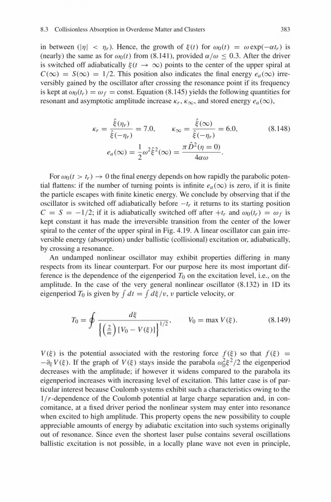
8.3 Collisionless Absorption in Overdense Matter and Clusters 383
in between (|η| < ηr ). Hence, the growth of ξ(t) for ω0(t) = ω exp(−αtr ) is(nearly) the same as for ω0(t) from (8.141), provided α/ω ≤ 0.3. After the driveris switched off adiabatically ξ(t → ∞) points to the center of the upper spiral atC(∞) = S(∞) = 1/2. This position also indicates the final energy ea(∞) irre-versibly gained by the oscillator after crossing the resonance point if its frequencyis kept at ω0(tr ) = ω f = const. Equation (8.145) yields the following quantities forresonant and asymptotic amplitude increase κr , κ∞, and stored energy ea(∞),
κr = ξ (ηr )
ξ (−ηr )= 7.0, κ∞ = ξ (∞)
ξ (−ηr )= 6.0, (8.148)
ea(∞) = 1
2ω2ξ2(∞) = π D2(η = 0)
4αω.
For ω0(t > tr )→ 0 the final energy depends on how rapidly the parabolic poten-tial flattens: if the number of turning points is infinite ea(∞) is zero, if it is finitethe particle escapes with finite kinetic energy. We conclude by observing that if theoscillator is switched off adiabatically before −tr it returns to its starting positionC = S = −1/2; if it is adiabatically switched off after +tr and ω0(tr ) = ω f iskept constant it has made the irreversible transition from the center of the lowerspiral to the center of the upper spiral in Fig. 4.19. A linear oscillator can gain irre-versible energy (absorption) under ballistic (collisional) excitation or, adiabatically,by crossing a resonance.
An undamped nonlinear oscillator may exhibit properties differing in manyrespects from its linear counterpart. For our purpose here its most important dif-ference is the dependence of the eigenperiod T0 on the excitation level, i.e., on theamplitude. In the case of the very general nonlinear oscillator (8.132) in 1D itseigenperiod T0 is given by
∫dt = ∫ dξ/v, v particle velocity, or
T0 =∮
dξ{(
2m
)[V0 − V (ξ)]
}1/2, V0 = max V (ξ). (8.149)
V (ξ) is the potential associated with the restoring force f (ξ) so that f (ξ) =−∂ξV (ξ). If the graph of V (ξ) stays inside the parabola ω2
0ξ2/2 the eigenperiod
decreases with the amplitude; if however it widens compared to the parabola itseigenperiod increases with increasing level of excitation. This latter case is of par-ticular interest because Coulomb systems exhibit such a characteristics owing to the1/r -dependence of the Coulomb potential at large charge separation and, in con-comitance, at a fixed driver period the nonlinear system may enter into resonancewhen excited to high amplitude. This property opens the new possibility to coupleappreciable amounts of energy by adiabatic excitation into such systems originallyout of resonance. Since even the shortest laser pulse contains several oscillationsballistic excitation is not possible, in a locally plane wave not even in principle,

384 8 Relativistic Laser–Plasma Interaction
Fig. 8.13 (a) Oblique incidence of parallel laser beam of wave vector k in the lab frame and k′ ‖ xin the system boosted by v0 = c sinα. The overdense target is cut into layers of thickness d. (b)Large electron displacement ξ in plasma layer (LHS) and harmonic (parabola) and anharmonicclosed (solid) and half-open potentials (solid, dashed). In wider potentials than harmonic the fre-quency decreases with increasing ξ
regardless of how short the electromagnetic pulse is. Energy coupling into a systemoriginally out of resonance is illustrated in the following for a cold plasma.
A plane, fully ionized target is assumed to fill the half space x > 0. A planewave E(x, t) = E0 exp[i(k · x − ωt)] in p-polarization in y-direction, wave vectork and frequency ω, is incident from −∞ under an angle α onto the plasma sur-face (Fig. 8.13a). After applying a Lorentz boost v0 = c sinα the wave impingesnormally. The target is thought to be cut into a sufficient number of thin parallel lay-ers, each of which is exposed to a driving force F acting along x of magnitude ev0 Band frequency ω, and an additional component originating from the Lorentz force ofthe oscillatory motion along y of frequency 2ω (e electron charge, B magnetic fieldof the laser). With the electron displacement ξ in x-direction and immobile ions ofdensity n0 (corresponding to ωp0) the motion of a single layer (Fig. 8.13b) in thenonrelativistic limit is determined by
d2ξ
dt2+ ω2
p0
(1− |ξ |
2d
)ξ = D, |ξ | ≤ d, (8.150)
d2ξ
dt2+ ω2
p0
(d
2|ξ |)ξ = D, |ξ | ≥ d. (8.151)
The free plasma oscillator (D = 0) oscillates at ωp0 if the displacement is small.For a fixed energy V0 = ε at high excitation and ωp0 � ω, T0 according to
(8.149) is given by T0 = 8(ω2p0d)−1/2ξ
1/20 . The eigenfrequency ω0 = 2π/T0 =
(π/4)(ω2p0d)1/2ξ
−1/20 decreases with increasing oscillation amplitude ξ0, in contrast
to the linear harmonic oscillator, and approaches zero for ξ → ∞. (An exactmechanical analogy is represented by an elastic sphere bouncing on an elastic hori-zontal glass plate under the influence of gravity, and its mirror image: ω0 →∞ forξ0 → 0 and ω0 → 0 for height ξ0 → ∞). Under a weak driver D and ωp0 > ω,

8.3 Collisionless Absorption in Overdense Matter and Clusters 385
ξ oscillates in phase with D; under a strong driver ξ becomes large and, owing toω0 → 0, it oscillates similarly to a free particle, i.e. dephased by π with respect toD. Principal resonance [76] occurs at ω0 = ω with ξ0 = ξr = (πωp0/4ω)2d.The transition from nonresonant to resonant state at ω0 = ω is irreversible,i.e., resonance breaks adiabaticity. In the neighborhood of resonance the product(dξ/dt)D ∼ j E changes from − sinωt × cosωt into cos2 ωt , with nonvanishingcycle average. This is illustrated by a numerical example now.
The two equations of motion above for |ξ | ≤ d and |ξ | ≥ d convert into a singledimensionless equation for the potential V = m(ωp0d/2)2(1+ ζ 2)1/2,
d2ζ
dτ 2+ ∂(1+ ζ 2)1/2
∂ζ= D(τ ), (8.152)
where ζ = 2ξ/d, m electron mass, τ = ωp0t and D → 2D/(ω2p0d). With
D = D0 sin2[ωt/(2K )] cosωt , sin2 for f (t), K number of periods, the resultsof Fig. 8.14 are obtained numerically. At D0 = 0.921 the layer remains belowresonance, the energy gain ε after the pulse is over is negligible (a). Increasing thedriver by only ΔD0 = 0.002, resonance takes place. Much energy, i.e., 43 timesmore than in (a), is stored now in the oscillator [see the horizontal orbits in (b)].Under the assumption that resonance lasts half a laser cycle, i.e., when the driveramplitude E0 = mω2
p0d/(4e), with d = 0.1 – 0.2 nm and ωp0 = 2 × 10¹⁶ s−1,
ζ
ε
Fig. 8.14 Excitation ε(ζ ) = ζ 2/2 + V (ζ ) of the oscillator from (8.152) by the driver D(τ ) =D sin2[ωτ/(2Nωp0)] cosωτ/ωp0, ω/ωp0 = 0.1, N = 20, (a) below resonance (D = 0.921),(b) above resonance (D = 0.923) with an 43 times higher final energy gain ε f than in (a) althoughthe driver strength is changed only by 0.2%. The potential and the resonant energy level are indi-cated dashed and dotted, respectively. Note the different scales in a, b

386 8 Relativistic Laser–Plasma Interaction
2
I II
1
ωτ/2πωp
εζ
D
Fig. 8.15 Driver D(τ ), excursion ζ(τ ) and absorbed energy ε(τ ) vs time (in driver cycles) for thecase in Fig. 8.14. Each time resonance is crossed ζ undergoes a phase shift by π . Bold lines I,II indicate instants of phase lag ζ±π/2 between D and ζ , i.e., maximum energy gain and loss(points of stationary phase); modulations in ε originate from the ω + ω0 spectral component
primary resonance of a single isolated layer happens at the laser intensity as low asI = 1015 Wcm−2.
Figure 8.15 is of particular relevance. It shows the driving field D(τ ), the dis-placement ζ(τ ), and the energy gained ε(τ ). At position 1 the oscillator is enteringresonance (ε starts increasing, ω0 > ω), D and ζ are in phase; at 2 it is leavingresonance (ε starts decreasing, ω0 < ω), D and ζ are dephased by π . Positions Iand II (points of stationary phase) indicate maximum energy gain and maximumenergy loss, D and ζ are dephased by ±π/2. Thus, the resonance signature is pre-served in a rapid transition. The phenomenon repeats in the second maximum ofε, etc. Resonance, i.e., ω0 becoming equal to ω, is intimately connected with thephase shift by π owing to the different reaction of the oscillator to the driver undera strong restoring force (ω0 � ω) and a weak one of a nearly free particle. Theabsorption term (8.131) j E ∼ ξD at resonance transits from ∼ sin τ × cos τ to∼ cos2 τ . This guarantees energy transfer from the driver to the oscillator. Furtherillustration of the phase shift at resonance for different parameters are found in [74],Fig. 5. The time-dependence of ω0 from (8.137) in (8.152) is accomplished throughthe amplitude ζ0, ω0 = ω0(ζ0[D(t)]).
8.3.3.2 Anharmonic Resonance Absorption in Cold and Warm Plasma
The extension of the dynamics from one layer of electrons and ions to N layers isaccomplished by considering all attractive forces of the fixed ion layers (index l)on all electron layers (index k) and all repulsive forces between the electron lay-ers (indices k, k′). This results into the nonseparable (nonintegrable, chaotic), yetelementary Hamiltonian
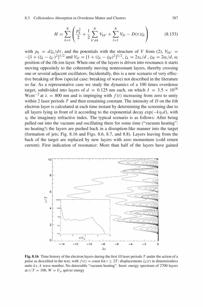
8.3 Collisionless Absorption in Overdense Matter and Clusters 387
H =N∑
k=1
⎛
⎝ p2k
2+ 1
2
N∑
k′ =k
Vkk′ +N∑
l=1
Vkl − D(τ )ζk
⎞
⎠ (8.153)
with pk = dζk/dτ , and the potentials with the structure of V from (2), Vkk′ =−[1+ (ζk − ζk′)2]1/2 and Vkl = [1+ (ζk − ζ0l)
2]1/2, ζk = 2xk/d , ζ0l = 2al/d, al
position of the lth ion layer. When one of the layers is driven into resonance it startsmoving oppositely to the coherently moving nonresonant layers, thereby crossingone or several adjacent oscillators. Incidentally, this is a new scenario of very effec-tive breaking of flow (special case: breaking of wave) not described in the literatureso far. As a representative case we study the dynamics of a 100 times overdensetarget, subdivided into layers of d = 0.125 nm each, on which I = 3.5 × 10¹⁸
Wcm−2 at λ = 800 nm and is impinging with f (t) increasing from zero to unitywithin 2 laser periods T and then remaining constant. The intensity of D on the kthelectron layer is calculated at each time instant by determining the screening due toall layers lying in front of it according to the exponential decay exp(−kηi d), withηi the imaginary refractive index. The typical scenario is as follows: After beingpulled out into the vacuum and oscillating there for some time (“vacuum heating”:no heating!) the layers are pushed back in a disruption-like manner into the target(formation of jets; Fig. 8.16 and Figs. 8.6, 8.7, and 8.8). Layers leaving from theback of the target are replaced by new layers with zero momentum (cold returncurrent). First indication of resonance: More than half of the layers have gained
kx
t / T
ε/Up
Fig. 8.16 Time history of the electron layers during the first 10 laser periods T under the action of apulse as described in the text, with f (t) = const for t ≥ 2T : displacements ζk(t) in dimensionlessunits kx , k wave number. No detectable “vacuum heating”. Inset: energy spectrum of 2700 layersat t/T = 100, W = Up quiver energy

388 8 Relativistic Laser–Plasma Interaction
energies exceeding their quiver energy W . The energy spectrum shows a plateaubetween 1W and the cut off at 6W (see inset in Fig. 8.16). In other runs withmore realistic driver field and the magnetic field included similar energy spectrawere obtained with plateaus extending up to 20W . To show the occurrence of res-onance explicitly the phase of each layer with respect to the driving laser field isinvestigated. A typical example with N = 120 is shown in Fig. 8.17 for layer #32,LHS trajectory and driver field (a), middle absorbed energy (b), RHS phase ϕ ofvelocity v∼ sin(ωt + ϕ) with respect to the driver E ∼ cosωt (c): over T/2 thereis a continuous and smooth transition of ϕ through −π/2 at t/T = 2.8 (I) with asimultaneous strong increase in the absorbed energy (b) and the excursion (a), withfollowing disruption of the layer at t/T = 3.6. The change of ϕ is clearly seen alsoin (a). Another resonance of the same kind is found at t/T = 8.8 (II). Other twopassages of ϕ through −π/2 at t/T = 5.7 (1) and 8.1 (2) show rapid fluctuationsand hence almost no energy gain [see (b)] and no disruption [see (a)]. Transitionsof this latter kind are morphologically clearly distinguishable from the former case,and for none of the 120 layers they are able to accelerate them across the target. Inthe cold plasma model we find that all layers (no exception) get their energy fromresonance and keep it in the underdense region. Only after undergoing resonance
ε/Up ϕ/π
I
II
1
2
(a) (b) (c)
k x
t / T
Fig. 8.17 Resonance dynamics of layer #32 as a function of laser periods. Position kx (a), k wavenumber, absorbed energy ε (b) and phase ϕ between velocity v and driving laser field from Fig. 8.16(mapped into the interval [−π , 0]) (c); ε in units of quiver energy Up . Passages through −π/2 areindicated by I, II, and 1 and 2 (see text). After resonance at 3.5 laser periods the layer is pushedback into the target with high velocity (“disruption”). After crossing the opposite target surface thelayer is substituted by a new layer. Note E ∼ −D

8.3 Collisionless Absorption in Overdense Matter and Clusters 389
each time the layers disrupt, in the present case in chaotic order 6, 5, 4, 3, 2, 15,17, 16, 9, 11, 10, 8, 12, 24, 31, 34, 28, 32, 14, 30, 1, 33, 45, 26, 36, 27, etc.; layer113 disrupts before front layer 0. This is one of the fundamental differences in thedynamics in comparison to [49]. It may be interesting in this context to comparewith an earlier PIC simulation of a cold plasma from [77]. They also show the res-onance character of absorption (although not properly understood when the articlewas written). The question at which intensity resonance sets in is difficult to answerand is reserved to further investigations. Simulations with 2, 10 and 20 layers showa decrease and a broadening of its threshold, in agreement with analytical estimates.The advantage of the model lies in its Hamiltonian structure. In combination withsimplified and oversimplified drivers it offers much flexibility and considerable helpin interpreting PIC simulations. So, for example, property (5) is easily explained: incircular polarization the electron motion is entirely transverse and no resonance isexcited in x-direction. The simplest driver considered here reproduces already allproperties (1)–(5) Figures 8.16 and 8.17 show no detectable “vacuum heating”. Asthis is of stochastic heating type by fluctuating fields it generates Brownian-likeorbits.
Resonance, i.e., energy gain during about half an oscillation implies a phase shiftϕl(t) for the individual electron or electron layer. All ϕl at a given position and time(x, t) sum up to a non vanishing φ(t) value once at least one electron (charge e,amplitude v0l ) is resonant,
j(x, t) = −e∑
l
δ(x − xl(t))v0l sin(ωt + ϕl)
= −enev0 sin(ωt + φ). (8.154)
With respect to resonance variations of D had no qualitative consequences. Forquantitative results recurrence must be made to PIC, Vlasov, or molecular dynam-ics. Anharmonic resonance constitutes a very efficient scenario leading to breakingof regular dynamics of a fluid (special case: wavebreaking). Once a fluid layerundergoes resonance it may move opposite to the adjacent fluid layer and thusdestroy the continuous mapping (2.57). We give it the name “resonant (wave)breaking”.
In order to reveal the dominant role in warm, i.e., realistic plasma, a 106 particlesPIC simulation with the PSC code [78] in its collisionless mode under 45◦ irradi-ation is performed. In the boosted frame a Gaussian Nd laser beam of I = 1017
Wcm−2 and halfwidth of 26 fs acts on a plane 80 times overcritical 7.3 µm thicktarget. In some sense 1D is the most severe case because it limits the number ofabsorption channels; for example storage of energy in induced ring currents andconcomitant magnetic fields decaying later [45] are excluded. On the other handthe absorption values of 70–80% have been achieved in PIC simulations in 1D andmeasured in 1D [37, 38, 79]. Requirement (3) is proven if we succeed in showingthat in 1D simulations almost all absorption is due to resonance. To reveal resonancesingle particle orbits must be followed. It is achieved by embedding a sufficient

390 8 Relativistic Laser–Plasma Interaction
Fig. 8.18 1D3V PIC simulation of a Nd laser beam interacting with a thick overdense targetwith mobile ions in the boosted frame (parameters see text). Regular shadow structure: laser field,LHS black trajectory: displacement x(t) of test electron #4, RHS black trajectory: correspondingmomentum px in units of mec, white line: total electric field at position x(t). Resonance (strongmomentum increase and phase shift ϕ(t)) and disruption are impressive. In all tests: no disrup-tion without preceding resonance. Resonances look all very similar to each other (see followingFigure)
number of test electrons, here 200, at equal distance from each other in the targetand following momentum px (t) and space coordinate x(t), during 15 laser periodsTNd = 5 fs.
The outcome of the statistics is overwhelming: all test electrons interacting withthe laser field are resonantly accelerated and either escape in a disruption-like man-ner into the target interior or move out into the vacuum from where they are drivenback by the space charge. In Fig. 8.18 the time history of a typical test electron isdepicted. The electron enters the laser field (shadowed interference pattern), inter-acts resonantly (see the evolution of momentum normalized to mc) and escapes intothe target an instant later with 15.3 times W . Resonance is ensured by the highenergy gain [property (2)], the total E-field deviating only slightly from sinusoidalbehavior (white line), and the phase shift in the last half electron oscillation: lastmaxima of the two lines exactly coincide, the former are dephased by π/2, as theyshould at ωp/ω > 1. The shadowed fine structure right of the laser field is dueto plasmons. All orbits entering the laser field undergo resonance and look verysimilar to each other, see Fig. 8.19 with other resonant layers. Properties (1)–(4) areherewith proven once more. One could object that only the contribution of j · E in xdirection has been considered. However, owing to the conservation of the canonicalmomentum in y direction in 1D at normal incidence, py + e�(E/ iω) = const,jy Ey leads only to the change of px described above. The simulation analysis tellsalso important details on the heating mechanism: The fast electrons are generatedfirst by resonance; they excite “solitary”, i.e., non-Bohm–Gross plasmons in the
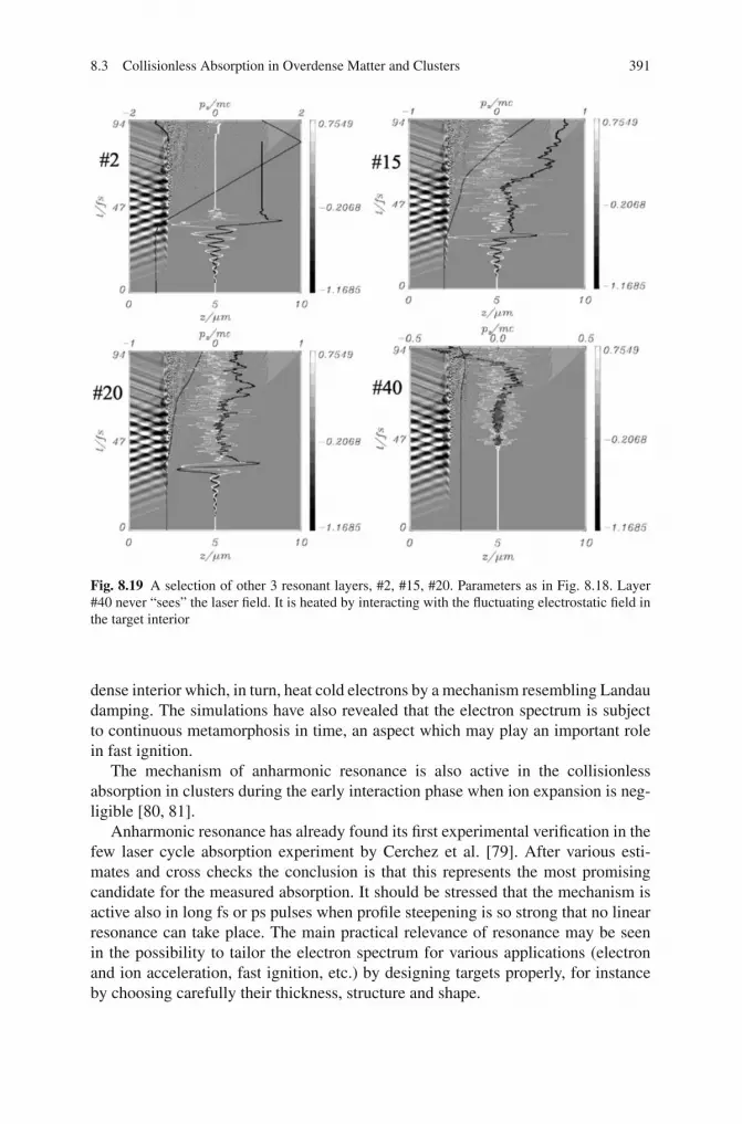
8.3 Collisionless Absorption in Overdense Matter and Clusters 391
Fig. 8.19 A selection of other 3 resonant layers, #2, #15, #20. Parameters as in Fig. 8.18. Layer#40 never “sees” the laser field. It is heated by interacting with the fluctuating electrostatic field inthe target interior
dense interior which, in turn, heat cold electrons by a mechanism resembling Landaudamping. The simulations have also revealed that the electron spectrum is subjectto continuous metamorphosis in time, an aspect which may play an important rolein fast ignition.
The mechanism of anharmonic resonance is also active in the collisionlessabsorption in clusters during the early interaction phase when ion expansion is neg-ligible [80, 81].
Anharmonic resonance has already found its first experimental verification in thefew laser cycle absorption experiment by Cerchez et al. [79]. After various esti-mates and cross checks the conclusion is that this represents the most promisingcandidate for the measured absorption. It should be stressed that the mechanism isactive also in long fs or ps pulses when profile steepening is so strong that no linearresonance can take place. The main practical relevance of resonance may be seenin the possibility to tailor the electron spectrum for various applications (electronand ion acceleration, fast ignition, etc.) by designing targets properly, for instanceby choosing carefully their thickness, structure and shape.
392 8 Relativistic Laser–Plasma Interaction
8.4 Some Relativity of Relevance in Practice
There are no limits; horizons onlyGerard A. Mourou
DPG Spring Meeting Düsseldorf 2007
8.4.1 Overview
At high intensities electromagnetic waves behave strongly nonlinear, at a degreewhich goes far beyond the familiar nonlinear optics. The origin of the drasticallyincreased nonlinearity lies in the self-generated sudden variation of the local elec-tron density due to field ionization (i), the ponderomotive (or wave pressure) effects(ii) and, at relativistic intensities, the coupling of transverse and longitudinal fieldsalready in the homogeneous plasma (iii). Whereas in standard nonlinear optics thenumber of wave crests of a pulse is invariant, as a consequence of (i) it can vary:after transition or reflection e.g. five crests become six or seven crests [34]. Pon-deromotive effects (ii) lead to a large number of instabilities, formation of irregularstructures, solitons, cavitons, wavebreaking, and chaos. In addition, due to (iii) alleffects may even become stronger. So far, transverse and longitudinal wave prop-agation at relativistic intensities has been studied extensively only with waves ofconstant phase velocity in plasmas of constant density [82–84], and recently sta-tionary quasiperiodic solutions have also been presented [85]. Under the influenceof (ii) the plasma medium is expected to become heavily deformed and even self-quenching of the electromagnetic mode may occur. As extreme intensities are tobe expected in the near future (I > 1023 Wcm−2) hot dense matter at solid andabove solid density may be produced by relativistic overcritical light penetration.The study of intense wave propagation in dense matter is of vital importance, initself as well as for applications (equation of state, fast ignition [86], astrophysics).The beauty in this context is that a great portion of related experiments can alreadybe performed, by analogy, at nonrelativistic and close to relativistic intensities insub- and super-critical foams and porous media with standard fs laser pulses. Withincreasing light intensity laser-based nuclear physics will become a reality [87].In analogy to atomic systems excitation, stimulated de-excitation and triggering ofsingle decay processes may be controlled by laser. Already with the next generationof photon flux densities (> 1023, perhaps � 1023 Wcm−2) the direct excitation ofnuclear levels and the triggered decay of isomeric nuclei can be studied, providedthe photon energy is high enough (order of keVs, free electron laser systems, [88]).Alternatively, the aim may be reached by the coherent superposition of extremelyhigh order harmonics generated from solid targets [89]. Such pulses will be usedalso to study the nuclear Stark effect and fine tuning of nuclear levels for variousapplications and diagnostics. All kinds of vacuum nonlinearities have their originin the separation (slang: “creation”) of electron-positron or more massive pairs bya corresponding energy supply. The critical field for the lightest pair production isE = 1.3 × 10¹⁸ V/m, corresponding to the laser intensity I = 2.3 × 1029 Wcm−2.
8.4 Some Relativity of Relevance in Practice 393
Their existence becomes noticeable already through their virtual appearance atmuch lower energies (and fortunately, after all “there are no limits” of I to makethem real). Nonperturbative vacuum nonlinearities manifest themselves in a varietyof processes and effects of the quantum vacuum exposed to superintense photonfields: generation of harmonics, photon splitting, light by light scattering, vacuumpolarization [90]. Two favored candidates, accessible to the most intense available fslaser installations, are the merging of two photons in the laser field interacting withTeV protons and the dramatic increase of electron bremsstrahlung from a nucleus inthe intense radiation field by many orders of magnitude.
8.4.2 Critical Density Increase for Fast Ignition
Currently high power lasers emit in the infrared (Nd YAG, Ti:Sa), or in the nearUV if for convenience a KrF system can be used. This means that the emitted laserbeams cannot penetrate matter of solid density with electron densities of typically1023–1024 cm−3. On the other hand it is of extreme interest to heat such dense, andeven denser, plasmas uniformly and isochorically for studies of equations of state,bright X ray sources, generation of high harmonics and for fast ignition of inertialfusion pellets [91, 92]. In the latter case, with a laser beam emitting in the soft Xray range several problems of radiation-pellet coupling of traditional lasers wouldbe eliminated. It is a fortune that at intensities at which the electrons gyrate rela-tivistically in a circularly polarized beam an increase of the critical electron densityis obtained owing to the electronic current decrease (“relativistic mass increase”) bythe relativistic Lorentz factor γ = (1−v2/c2)−1/2, v gyrovelocity, c speed of light invacuum [93]. In linear polarization “anomalous penetration” was found by means ofnumerical studies in [94], i.e., considerably weaker penetration than correspondingto their formula for nc. This and analogous results indicate that the general problemof relativistic penetration needs further investigations. At low, nonrelativistic laserintensities the fully ionized plasma can be treated as a monofluid for electromagneticwave propagation in the homogeneous medium with an invariant plasma frequency.At high laser intensities one is faced with a different situation: on the fast time scalethe ions can still be treated as immobile objects while the electrons move at relativis-tic velocity. Thus, in any reference system one has to deal with a two-fluid model andthe problem has to be faced what the implications of the transition from a monofluidto a two-fluid model are. In addition, the question arises whether the concept of acritical density remains still valid when at relativistic intensities highly nonlineardensity structures and cavitons may form [95, 96]. Both problems, the existence ofa critical density and its correct relativistic increase in a highly overdense plasma,are to be clarified “experimentally”, i.e., by particle-in-cell (PIC) simulations owingto the high nonlinearities involved, and fitted by analytical expressions.
8.4.2.1 Relativistic Critical Density Increase
Under the assumption of an invariant electron density an intense circularly polarizedelectromagnetic wave can penetrate considerably deeper into a fully ionized plasma

394 8 Relativistic Laser–Plasma Interaction
owing to the already mentioned relativistic electron current decrease by the Lorentzfactor γ ,
γ = (1+ a2)1/2, a = e A
mc, A = − i
ωE,
(A, E)(x, t) = ( A, E)(x, t) exp(−iωt); (8.155)
A, A, E, E vector potential and electric field with associated amplitudes [93]. Therefractive index is η = (1 − ne/γ nc)
1/2, thus showing that the relativistic criticaldensity for circular polarization is ncr = γ nc. By analogy, in linear polarizationthe true γ factor is expected to be γ = (1 + a2
/2)1/2 of a single electron in thevacuum. The departure from this value will depend on the electron density variationdne/dt = −ne∇v induced by the Lorentz force in propagation direction. The avail-able time for restoring quasineutrality, i.e., ∇v = 0, is only half a laser cycle π/ω.In a tenuous plasma (ωp � ω) perturbation theory yields ncr = (1 + 3a2
/8)1/2nc,with 3/8 < 1/2 for this reason [83, 82]. The dispersion of propagating plane wavesof arbitrary strength and linear polarization in a constant plasma density underLorentzian gauge is governed by the set of equations
�A = − J
ε0c2, ∂α Aα = 0, A = (A, φ/c), J = ( j , cρe),
ρe = e(ni0 − ne) = ε0
(v2ϕ
c2− 1
)∂2φ
∂x2,
∂φ
∂x= c2
vϕ
∂Ax
∂x, (8.156)
jy = −e2ne0
γmAy + ε0
[evϕ
(1− c2
v2ϕ
)∂2 Ax
∂x2
]Ay
γm.
φ is the scalar potential and vϕ the constant phase velocity. The second of theserelations is the Lorentz gauge. The current density jy follows from the canonicalmomentum conservation γmvy = eAy for a cold electron fluid initially at rest.In circular polarization the second term (square bracket) in jy vanishes owing toAx = φ/c = 0. The dispersion of waves described by (8.156) has been exten-sively studied and discussed recently also close to cut-offs and it has been foundthat the majority of electromagnetic modes exhibits the typical eight-like electronmotion as in the tenuous plasma [82]. Besides, a purely electrostatic mode withcircular electron motion in the plane of incidence is also possible, in accordancewith the fact that the B-field an electromagnetic wave near cut-off behaves likeBη → 0. Unfortunately, light coupling to high density matter, which is the typicalfast ignition-relevant situation, is accompanied by plasma density profile steepen-ing, partial reflection and extremely nonuniform electron fluid expansion [89] andrecession during one cycle, with a concomitant laser frequency Doppler shift inthe frame of co-moving critical layer. Owing to such complexity and, eventually,due to caviton formation [96, 97], a reliable determination of the critical densityincrease is accessible only to particle-in-cell (PIC) or similar simulation procedures

8.4 Some Relativity of Relevance in Practice 395
(e.g. Vlasov). Here the 3D PSC PIC code [78] is used to give the promised “exper-imental” answer.
8.4.2.2 Quasiperiodic and Chaotic Electron Orbits
In the critical region the phenomena addressed above lead to a strongly fluctuatingpotential φ which in combination with the laser field may transform the regular8-shape electron motion into quasiperiodic and chaotic orbits with unknown Lorentzfactor γp. To illustrate the situation a time-independent typical self generated poten-tial φ = mc2a[1+ κ2(x/λ)2]1/2 with the free parameter κ and the laser wavelengthλ is used. The beam propagates in x-direction. The laser field strength is held fixedat a = 1 and κ is varied (see Fig. 8.20). The first picture, obtained with κ = 6.2,shows a stable configuration of the electron orbiting around a vacuum-like 8-shapetrajectory. Only a slight asymmetry in diagonal direction is observable. At κ = 6.5the electron manages it to escape from the stable configuration after several turnsin the direction y of the laser field, and eventually it comes back again (picture atRHS). By a further increase of κ by only 8% to κ = 7.0 a very complex orbit results(3rd picture). By plotting the time history of the transverse motion ([y, t]-plot in4th picure) it becomes clear that during the registered 100 laser cycles the electron
Fig. 8.20 Evolution towards chaotic dynamics of the electron motion in presence of an electrostaticpotential φ = mc2a(1+κ2x2)1/2. The motion is very sensitive to variations of the free parameter κaround κ � 7.0. Note the close resemblance to chaotic ponderomotive motion in a standing wave,Fig. 2 in [98]

396 8 Relativistic Laser–Plasma Interaction
crosses 9 attractors. In a sense, the trajectory is a repeated composition of orbitsfrom the 2nd picture. The contribution of such orbits to the relativistic increase of thecritical density is not known. Additionally, due to inherent stochasticity anharmonicresonance is accompanied by a heating effect.
8.4.2.3 “Experimental” γ Factor
In the rest frame of an electron fluid element the bare electron mass m turns into the“dressed” thermal mass mth = γthm, with γth to be determined kinetically. The elec-tron becomes “heavier” by γth, thus acting in favor of a high γ value. γp originatingfrom orbit deformations as presented in Fig. 8.20 can act in both directions and hasnot been studied so far. As the γ values associated with these various effects interactin a complex nonlinear manner with the effect of the relativistic increase of the bareelectron mass, the correct value of the resulting γ actually is determined in the mostreliable manner by analyzing 1D PIC runs at a sequence of laser intensities. Further-more, only such an “experimental” procedure can reveal to what extent the existenceof a critical density and a well defined critical point are secure or whether they haveto be given up owing to irregular density fluctuations and aperiodic recessions atextreme laser intensities.
A fully ionized target of 100 times critical density with heavy ions (to suppresshole boring, of no interest in the context) is exposed to linearly polarized laserirradiance of Iλ2 = 10s Wcm−2µm2, s = 18–22, under perpendicular and p-45◦incidence and, when the interaction has become stationary, all field quantities areaveraged over two laser cycles [99]. A typical result for Iλ2 = 5×10²¹ Wcm−2µm2
under 45◦ on target is presented in Fig. 8.21 for t = 80 fs. In contrast tostrongly fluctuating pictures taken at single time instants, after sufficiently averag-ing quiescent shapes in all field quantities are obtained. Hence, a first result is that
Fig. 8.21 Cycle-averaged distributions in space (x coordinate) of the field amplitude squared |E|2with closest maximum M and minimum m, absorption j E and electron density ne after 80 fs ofirradiance Iλ2 = 5 × 10²¹ Wcm−2µm2. Critical density in the lab frame is nc = n0/100. Angleof incidence α = 45◦
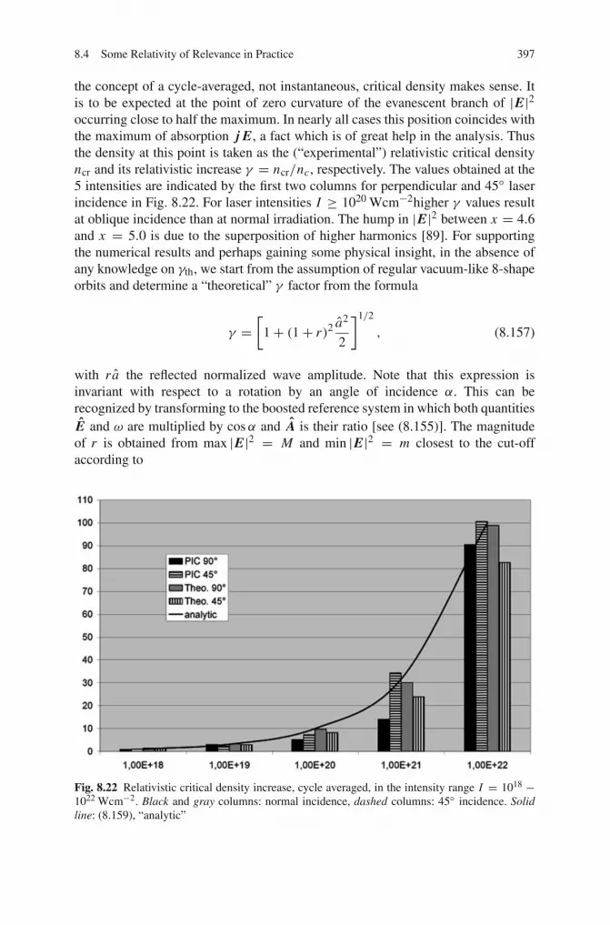
8.4 Some Relativity of Relevance in Practice 397
the concept of a cycle-averaged, not instantaneous, critical density makes sense. Itis to be expected at the point of zero curvature of the evanescent branch of |E|2occurring close to half the maximum. In nearly all cases this position coincides withthe maximum of absorption j E, a fact which is of great help in the analysis. Thusthe density at this point is taken as the (“experimental”) relativistic critical densityncr and its relativistic increase γ = ncr/nc, respectively. The values obtained at the5 intensities are indicated by the first two columns for perpendicular and 45◦ laserincidence in Fig. 8.22. For laser intensities I ≥ 1020 Wcm−2higher γ values resultat oblique incidence than at normal irradiation. The hump in |E|2 between x = 4.6and x = 5.0 is due to the superposition of higher harmonics [89]. For supportingthe numerical results and perhaps gaining some physical insight, in the absence ofany knowledge on γth, we start from the assumption of regular vacuum-like 8-shapeorbits and determine a “theoretical” γ factor from the formula
γ =[
1+ (1+ r)2a2
2
]1/2
, (8.157)
with r a the reflected normalized wave amplitude. Note that this expression isinvariant with respect to a rotation by an angle of incidence α. This can berecognized by transforming to the boosted reference system in which both quantitiesE and ω are multiplied by cosα and A is their ratio [see (8.155)]. The magnitudeof r is obtained from max |E|2 = M and min |E|2 = m closest to the cut-offaccording to
Fig. 8.22 Relativistic critical density increase, cycle averaged, in the intensity range I = 1018 −1022 Wcm−2. Black and gray columns: normal incidence, dashed columns: 45◦ incidence. Solidline: (8.159), “analytic”

398 8 Relativistic Laser–Plasma Interaction
r = (√
M −√m)2
M − m. (8.158)
The γ factors resulting from (8.158) are visualized in Fig. 8.22 by columns 3 and4 for normal and 45◦ incidence, respectively (“theoretical”). All values, theoreticaland experimental, are taken at t = 80 fs. Although at some intensities, in particularat Iλ2 = 1021 Wcm−2µm2, the γ values for 90◦ and 45◦ from PIC differ consider-ably from each other, and so does γ obtained by means of (8.157) for 90◦ and 45◦ atall intensities Iλ2 ≥ 1020 Wcm−2µm2, in first approximation the results look like asif produced by the relativistic mass increase only and almost no relativistic influencestemming from changes of ne and from chaotic orbits. The latter are revealed by testparticle injection in the PSC simulations and following their motion. The impressionof dominating mass increase is reinforced if a fit to the averages of each of the fivequadruplets is done. For this it was found
γ =(
1+ Iλ2[Wcm−2μm2]/1018)1/2
, (8.159)
see black solid line. The weak relativistic contribution from ne to γ has a qualitativeexplanation, a posteriori. By the radiation pressure strong electron density profilesteepening sets in over a scale length which is a small fraction of the laser wave-length λ only. As a consequence the laser wave acts mostly on a low density shelfwith ne � ncr and, in the evanescent region, on ne � ncr (see Fig. 8.21). Forne � ncr, γ is close to the vacuum value (3/8 instead of 1/2). At ne � n0 chargeneutralization is up to 20 times faster than 2π/ω. It can be concluded that up tothe intensities considered an average critical density makes sense and its approxi-mate relativistic increase is given by a simple formula which reflects essentially thevacuum-like 8-shape motion of the electrons.
8.4.2.4 Implications for Fast Ignition by Laser
The advantages of fast pellet ignition with powerful lasers for inertial confine-ment fusion are well known: Decoupling of compression from ignition phase, lessrequirements on pulse shaping of the main compression pulse, lowering of symme-try constraints on peak compression, explicitly shown in [100]. Extensive computerstudies with flux limited Spitzer heat transport have shown that a typical ignitionenergy is 70 kJ and, by optimizing the process, 50 kJ at a laser intensity not lowerthan I = 1020 Wcm−2 may represent the minimum energy and intensity require-ments [101]. Under the condition that such an amount of energy is deposited infast electrons the density of the deposition zone has not to be less than 4–5 gcm−3
DT; below 1 gcm−3 in no run a burn wave evolved. As the laser energy cannot bedeposited beyond the critical density in standard coronal ignition the flux of the ener-getic electrons has to travel a long distance up to the compressed core thereby under-going sensitive diffusive attenuation. For comparison, simulations in [100] with theheat flux limiter turned off show that the energy needed for the pure ignition process
8.4 Some Relativity of Relevance in Practice 399
(the “free ignition energy”) is typically 15 kJ, in agreement with simpler modelsof direct energy deposition in the most favorable region [102, 103]. Originally holeboring was intended as to reducing noticeably the distance between the laser deposi-tion region and the compressed core. Unfortunately hole boring has proven to be notefficient enough for this purpose [104]. Cone guided fast ignition is more advanta-geous to bring the two regions closer together and, in addition, to provide for bettercoupling of the laser beam [91]. However, also in this scheme there is the constrainton laser energy conversion into kinetic energy of the electrons not beyond the criticaldensity. Inspired by [91] and [105] we consider a model in which the hot electronsbasically propagate ballistically through the critical and intermediate densities andinteract collisionally in the compressed pellet core. The minimum flux density ofhot electrons q0 = 1021 Wcm−2 is estimated to be sufficient when generated by the3rd harmonic of Nd laser frequency ω = 1.78 × 10¹⁵ s−1. Assuming R = 0.5 forthe laser follow γ = 6.7 and ncr = 6.7× 1022 cm−3, the latter exceeding solid DTdensity nDT = 5 × 1022 cm−3. In order to transport the absorbed flux density q0with electron velocity u for the mean energy 〈E〉 of the hot electrons must hold
ncr〈E〉u = q0, u = c
(1− 1
γ
)1/2
, γ = 1+ 〈E〉mc2
. (8.160)
From (8.160) the mean energy results as low as 〈E〉 = 0.37 MeV. An upper limitfor 〈E〉 is obtained by making the very reasonable assumption that it may not bemuch higher than the mean oscillatory electron energy which in the specific casewith a = 4.3 is Eos = 1.1 MeV, i.e., consistency is guaranteed. If already in thecritical and medium density domain strong thermalization occurs a diffusive modelapplies. In [101] it was found on the basis of [100] that the minimum required fluxdensity has to be close to q0 = 1021 Wcm−2 because most of the energy suppliedis diffusively spread all over the compressed pellet and there in particular all overits low density corona. In addition the deposition density should not be inferiorto ρdep = (4–5) gcm−3 DT; below ρdep =1 gcm−3 no ignition was possible [100].With this value for ndep = 5×1022 cm−3 and a safety factor s = (4–5) the conditionncr = ndeps = γ (λ)nc(λ) together with I (λ) = 2q0 for R = 0.5 must be fulfilled.For Nd holds nc(λ) = ncNdλ
2Nd/λ
2. Hence, from (8.159) is recovered
λ
λNd= ncNd
ndeps
(2q0
1018
)1/2
= 0.9
s⇒ ω = 1.1sωNd;
γ (λ) =(
2q0
1018
)1/2λ
λNd= 40
s. (8.161)
At I = 2×10²¹ Wcm−2 the maximum wavelength for achieving ignition is close toλNd if s = 1 is set. For the fundamental of the Ti:Sa laser the condition is fulfilled.It is obvious that the consistency condition (8.160) is fulfilled with a large safetyfactor. As 〈E〉 = 0.95 MeV and u = 0.87c consistency is secured easily also fors = 5, i.e., the fifth harmonic of ωNd because of Eos = 3.5 MeV> 〈E〉. It can be

400 8 Relativistic Laser–Plasma Interaction
concluded that at high laser intensities the relativistic increase of the critical densityis favorable to achieve uniform heating of condensed matter and to facilitate energycoupling in fast ignition provided the production of fast electrons can be containedwithin reasonable limits.
8.4.3 Relativistic Self-Focusing
Whole laser beam self-focusing is considered in a tenuous underdense plasma underthe idealized condition of uniform electron density ne = n0. Provided it can beassumed that the change of the refractive index is essentially by the relativistic elec-tron mass increase only the refractive index η = (1−n0/γ nc)
1/2, γ = (1+a2/2)1/2,is higher in regions of high beam intensity, for example along the beam axis or atthe center of a filament, and the phase velocity is lower. As a consequence, local selffocusing and eventual beam or filament collapse occur. A threshold of self focusingas given by [106] is most easily derived for the Gaussian beam of Sect. 5.3.2. Underthe condition of n0 � nc, a2 � 1, from (5.66) and a2 = 2e2 I (r)/ε0c3m2ω2
∂
∂r
ne
γ nc= ne
nc
r
σ 20
a2, Rc = η2 nc
ne
ε0c3m2ω2
e2r I (r)σ 2
0 ;
Self-focusing will occur when equality of Rc with Rc = 2R2/r for a Gaussian rayis reached, i.e., at local intensity I (r) and power P(r)
I (r) = 2ε0m2c5
e2σ 20
nc
ne,
P(r) =∫ ∞
0I (r)e
2σ2
0(r2−r ′2)
2πr ′dr ′ = πε0m2c5
e2
nc
nee
2 r2
σ20 . (8.162)
The total beam power is P = πσ 20 I (r = 0)/2, hence the intensity measured by the
experimentalist is I = P/πσ 20 = I (r = 0)/2. The power required for half beam
self-focusing P1/2 and for 86% beam focusing Pσ0 result from (8.162) as
P1/2 = 2πε0m2c5
e2
nc
ne= 4.2
nc
neGW;
Pσ0 = e2πε0m2c5
e2
nc
ne= 15.5
nc
neGW. (8.163)
Frequently Pσ0 = 17nc/ne GW for “whole beam” focusing is given in the literatureas a result of averaged quantities used for this estimate. This and (8.163) are grosscriteria, see comments made on ponderomotive self-focusing, (5.69); they applyhere also. A far more detailed picture is gained by a linearized wave dynamic treat-ment of an initially Gaussian beam. Light and density nonuniformities along the

References 401
axis lead to variations in the focusing strength 1/Rc that may give rise to unsta-ble growth of hot spots, transverse and longitudinal coupling of modes and beamself-compression already in the weakly relativistic regime [107].
References
1. Arnold, V.I.: Mathematical Methods of Classical Mechanics, p. 8. Springer, New York (1978) 3312. Weinberg, S.: Gravitation and Cosmology, Chap. 2. John Wiley & Sons, New York (1972) 332, 3493. Berzi, V., Gorini, V.: Math. Phys. 10, 1518 (1969) 3324. Rindler, W.: Essential Relativity, Chaps. 2–6. Springer, New York (1979) 3335. Eckart, C.: Phys. Rev. 58, 919 (1940) 3456. Hain, S., Mulser, P., Cornolti, F., Opower, H.: Las. Part. Beams 17, 245 (1999); Hain, S.:
Propagation of Intense Laser Radiation in Matter PhD-thesis, TU Darmstadt (in German),Chap. 1.2. GCA-Verlag, Herdecke (1999) 345
7. Landau, L.D., Lifshitz, E.M.: Fluid Mechanics, Chap. XV. Pergamon, Oxford (1959) 3478. Lawson, J.D.: IEEE Trans. Nucl. Sci. NS-26, 4217 (1979) 3559. Landau, L.D., Lifshitz, E.M.: The Classical Theory of Fields. Pergamon, Oxford (1975), §
47, Problem 2 35610. Wang, J.X., Scheid, W., Hoelss, M., Ho, Y.K.: Phys. Lett. A 275, 323 (2000) 35911. Häuser, Th., Scheid, W., Hora, H.: Phys. Lett. A 186, 189 (1994) 35912. Wang, P.X., Ho, Y.K., et al.: J. Appl. Phys. 91, 856 (2002) 35913. Malka, G., Lefebre, E., Michel, J.L.: Phys. Rev. Lett. 78, 3314 (1997); Phys. Rev. Lett. 80,
1352 (1998) 35914. Rau, B., Tajima, T., Hojo, H.: Phys. Rev. Lett. 78, 3310 (1997); Kim, K.-J., et al.: Phys. Rev.
Lett. 84, 3210 (2000); Rau, B., Tajima, T., Hojo, H.: Phys. Rev. Lett. 84, 3211 (2000) 35915. Plettner, T., Byer, R.L., Colby, E., et al.: Phys. Rev. Lett. 95, 134801 (2005); Phys. Rev. ST
Accel. Beams 8, 121301 (2005) 35916. Tajima, T., Dawson, J.: Phys. Rev. Lett. 43, 267 (1979) 36017. Sprangle, P., et al.: Phys. Rev. Lett. 69, 2200 (1992); Antonsen, M., Mora, P.: Phys. Rev. Lett.
69, 2204 (1992) 36018. Modena, A., et al.: Nature 377, 606 (1995); Ting, A., et al.: Phys. Plasmas 4, 1889 (1997);
Santala, M.I.K., et al.: Phys. Rev. Lett. 86, 1227 (2001); Malka, V., et al.: Phys. Plasmas 8,2605 (2001); Giulietti, D., et al.: Phys. Plasmas 9, 3655 (2002) 360
19. Reitsma, A.J.W., et al.: Phys. Rev. Lett. 88, 014802 (2002); Schröder, C.B., et al.: Phys. Rev.Lett. 82, 1177 (1999) 360
20. Pukhov, A., Meyer-ter-Vehn, J.: Appl. Phys. B 74, 355 (2002) 360, 36121. Bulanov, S.V., Pegoraro, F., Pukhov, A., Sakharov, A.S.: Phys. Rev. Lett. 78, 4205 (1997) 36122. Rosenzweig, J.B., et al.: Phys. Rev. A 44, R6189 (1991) 36223. Mangles, S.P.D., et al.: Nature 431, 535 (2004) 36224. Faure, J., et al.: Nature 431, 541 (2004) 36225. Geddes, C.G.R., et al.: Nature 431, 538 (2004) 36226. Leemans, W.P., et al.: Nature Phys. 2, 696 (2006) 36227. Clarc, E.L., et al.: Phys. Rev. Lett. 84, 670 (2000) 36328. Snavely, R.A., et al.: Phys. Rev. Lett. 85, 2945 (2000)29. Roth, M., et al.: Phys. Rev. Lett. 86, 436 (2001)30. Wilks, S.C., et al.: Phys. Plasmas 8, 542 (2001) 36331. Yan, X.Q., et al.: Phys. Rev. Lett. 100, 135003 (2008) 36332. Yan, X.Q., Chen, M., Sheng, Z.M., Chen, J.E.: Phys. Plasmas 16, 044501 (2009)33. Schlegel, T., Naumova, N., Tikhonchuk, V., et al.: Phys. Plasmas 16, 083103 (2009) 36334. Mulser, P., Cornolti, F., Bauer, D.: Phys. Plasmas 5, 4466 (1998) 363, 39235. Bauer, D.: Phys. Rev. A 55, 2180 (1997) 363

402 8 Relativistic Laser–Plasma Interaction
36. Price, D.F., More, R.M., et al.: Phys. Rev. Lett. 75, 252 (1995) 36437. Gibbon, P., Bell, A.R.: Phys. Rev. Lett. 68, 1535 (1992); Gibbon, P.: Phys. Rev. Lett. 73, 664
(1994) 364, 372, 374, 377, 38938. Wilks, S.C., Kruer, W.L., Tabak, M., Langdon, A.B.: Phys. Rev. Lett. 69, 1383 (1992);
Denavit, J.: Phys. Rev. Lett. 69, 3052 (1992) 364, 38939. Ruhl, H., Mulser, P.: Phys. Lett. A 205, 388 (1995) 364, 365, 366, 367, 372, 37440. Hockney, R.W., Hockney, R.W., Eastwood, J.W.: Computer Simulation Using Particles. IOP,
Bristol (1988) 36441. Gibbon, P., Pfalzner, S.: Many-body Tree Methods in Physics. Cambridge University Press,
Cambridge (2005) 364, 36542. Pfalzner, S., Gibbon, P.: Comp. Phys. Comm. 79, 24 (1994) 36543. Kruer, W.L., Estabrook, K.: Phys. Fluids 28, 431 (1985) 366, 375, 376, 37744. Wilks, S.C.: Phys. Fluids B 5, 2603 (1993) 36645. Ruhl, H., Macchi, A., Mulser, P., Cornolti, F., Hain, S.: Phys. Rev. Lett. 82, 2095 (1999) 369, 370, 38946. Sauerbrey, R., et al.: Phys. Plasmas 1, 1635 (1994) 37147. Feurer, T., et al.: Phys. Rev. E 56, 4608 (1997) 37148. Boudier, A.: Phys. Fluids 26, 1804 (1983) 37149. Brunel, F.: Phys. Rev. Lett. 59, 52 (1987) 373, 375, 376, 38950. Catto, P.J., More, R.M.: Phys. Fluids 20, 704 (1977) 374, 37551. Mulser, P., Pfalzner, S., Cornolti, F.: In: Velarde, G., et al. (eds.) Laser Interaction with Matter,
p. 142. World Scientific, Singapore (1989) 37452. Brian Yang, T.-Y., Kruer, W.L., More, R.M., Bruce Langdon, A.: Phys. Plasmas 2, 3146
(1995) 374, 37553. Ferrante, G., Zarcone, M., Uryupin, S.A.: Phys. Plasmas 9, 4560 (2002) 37454. Brian Yang, T.-Y., Kruer, W.L., Bruce Langdon, A., Johnston, T.W.: Phys. Plasmas 3, 2702
(1996) 37555. Umstadter, D., J. Phys. D: Appl. Phys. 36, R151 (2003) 37556. Rastunkov, V.S., Krainov, V.P., Laser Physics 15, 262 (2005) 37557. Sentoku, Y., Bychenkov, V.Y., Flippo, K., Maksimchuk, A., Mima, K., Mourou, G., Sheng,
Z.M., Umstadter, D.: Appl. Phys. B 74, 207 (2002) 37558. Sofronov, A.V., Krainov, V.P.: J. Phys. B: At. Mol. Opt. Phys. 37, L329 (2004) 37559. Pukhov, A.: Rep. Progr. Phys. 66, 47 (2003) 37560. Jungreuthmayer, C., Geissler, M., Zanghellini, J., Brabec, T.: Phys. Rev. Lett. 92, 133401
(2004) 37561. Zaretsky, D.F., Korneev, Ph.A., Popruzhenko, S.V., Becker, W., J. Phys. B: At. Mol. Opt.
Phys. 37, 4817 (2004) 37562. Korneev, Ph.A., Popruzhenko, S.V., Zaretsky, D.F., Becker, W.: Laser Physics Lett. 2, 452
(2005) 37563. Macchi, A., Cornolti, F., Pegoraro, F., Liseikina, T.V., Ruhl, H., Vshivkov, V.A.: Phys. Rev.
Lett. 87, 205004 (2001); Macchi, A., Cornolti, F., Pegoraro, F.: Phys. Plasmas 9, 1704 (2002) 37564. Kahaly, S., Yadav, S.K., Wang, W.M., Sengupta, S., Sheng, Z.M., Das, A., Kaw, P.K., Ravin-
dra Kumar, G.: Phys. Rev. Lett. 101, 145001 (2008) 37565. Chen, L.M., Zhang, J., Dong, Q.L., Teng, H., Liang, T.J., Zhao, L.Z.: Wei, Z.Y., Phys. Plas-
mas 8, 2925 (2001) 37766. Dong, Q.L., Zhang, J., Teng, H.: Phys. Rev. E 64, 026411 (2001) 37767. Kato, S.: J. Plasma Fusion Res. Series 6, 658 (2004) 37768. Hong-bo Cai: Phys. Plasmas 13, 063108 (2006) 37769. Mulser, P., Schnabl, H.: Laser and Particle Beams 1, 379 (1983) 37770. Bergmann, A., Mulser, P.: Phys. Rev. E 47, 3585 (1993) 37771. Pukhov, A., Meyer-ter-Vehn, J.: Phys. Plasmas 5, 1880 (1998) 37772. Bauer, D., Mulser, P.: Phys. Plasmas 14, 023301 (2007) 37773. Mulser, P., Bauer, D., Ruhl, H.: Phys. Rev. Lett. 101, 225002 (2008) 37874. Bauer, D., Mulser, P.: J. Phys. Conf. Series 11, 169 (2005) 379, 38675. Born, M., Wolf, E.: Principles of Optics, p. 480. Cambridge University Press, Cambridge
(1988) 381

References 403
76. Nayfeh, A.H., Mook, D.T.: Nonlinear Oscillations, Chap. 4. John Wiley & Sons, New York(1979) 385
77. Mulser, P., Ruhl, H., Steinmetz, J.: Laser and Particle Beams 19, 23 (2001), Figs. 1 and 3 38978. Ruhl, H.: In Bonitz, M., Semkat, D. (eds.) Introduction to Computational Methods in Many
Particle Body Physics. Rinton Press, Paramus, New Jersey (2006) 389, 39579. Cerchez, M., et al.: Phys. Rev. Lett. 100, 245001 (2008) 389, 39180. Mulser, P., Kanapathipillai, M., Hoffmann, D.H.H.: Phys. Rev. Lett. 95, 103401 (2005) 39181. Kundu, M., Bauer, D.: Phys. Rev. Lett. 96, 123401 (2006) 39182. Pesch, T.C., Kull, H.-J.: Phys. Plasmas 14, 083103 (2007) 392, 39483. Kaw, P., Dawson, J.: Phys. Fluids 13, 472 (1970) 39484. McKinstrie, C.J., Forslund, D.W.: Phys. Fluids 30, 904 (1987) 39285. Pesch, T.C., Kull, H.-J.: In: Mulser, P. (ed.) Quasiperiodic Waves in Relativistic Plasmas,
ILIAS Prog. Rep. 3, GSI Darmstadt (2008) 39286. Tabak, M., et al.: Phys. Plasmas 1, 1626 (1994) 39287. Schwörer, H., Magill, L., Beleites, B. (eds.): Lasers and Nuclei. Springer, Heidelberg (2006) 39288. Pálffy, A., Evers, J., Keitel, C.H.: Phys. Rev. Lett. 99, 172502 (2008) 39289. Baeva, T.: High Harmonic Generation from Relativistic Plasmas. VDM Verlag Dr. Müller,
Saarbrücken (2008) 392, 394, 39790. Müller, C., Di Piazza, A., Shahbaz, A., Bürvenich, T., Evers, J., Hatsagortsyan, K., Keitel,
C.H.: Laser Physics 18, 175 (2008) 39391. Kodama, R., et al.: Nature 412, 798 (2001); Kodama, R., et al., Nature 418, 933 (2002) 393, 39992. Atzeni, S., et al.: J. Phys.: Conference Series 112, 022062 (2008) 39393. Akhiezer, A.I., Polovin, R.V.: Sov. Phys. JETP 3, 696 (1956) 393, 39494. Sakagami, H., Mima, K.: Phys. Rev. E 54, 1870 (1996) 39395. Lontano, M., Passsoni, M., Bulanov, S.V.: Phys. Plasmas 10, 639 (2003) 39396. Sircombe, N.J., Arber, T.D., Dendy, R.O.: Phys. Plasmas 12, 012303 (2005) 393, 39497. Weber, S., Lontano, M., Passoni, M., et al.: Phys. Plasmas 12, 112107 (2005) 39498. Bauer, D., et al.: Phys. Rev. Lett. 75, 4622 (1995) 39599. Mulser, P., Ruhl, H., Schneider, R., Batani, D.: J. Phys. Conf. Ser. 112, 022074 (2008) 396
100. Hain, S., Mulser, P.: Phys. Rev. Lett. 86, 015 (2001) (The calculated 10 kJ apply to the freeignition energy; total energy supplied to the corona amounts to 50–70 kJ) 398, 399
101. Mulser, P., Bauer, D.: Laser & Particle Beams 22, 5 (2004) 398, 399102. Atzeni, S.: Phys. Plasmas 6, 3316 (1999) 399103. Atzeni, S., Temporal, M., Honrubia, J.J.: Nucl. Fusion 42, L1 (2002) 399104. Mulser, P., Schneider, R.: Laser & Particle Beams 22, 157 (2004) 399105. Sentoku, Y., Chrisman, B., Kemp, A., Cowan, T.E.: Hot electron energy coupling in cone-
guided fast ignition, Paper Tu07.6 at IFSA 2007, Kobe, Sept. 9–14, 2007 399106. Sprangle, P., Tang, C.M., Esarey, E.: IEEE Transactions on Plasma Science 15, 145 (1987) 400107. Karle, Ch., Spatschek, K.H.: Phys. Plasmas 15, 123103 (2008) 401

Index
AAblation, 70, 74, 76, 77, 81
pressure, 74, 82, 211, 214Ablative
laser intensity, 78Above-threshold ionization, 281, 298
few-cycle, 301Absolute
instability, 254Absorption
anharmonic resonance, 386anomalous skin layer, 375coefficient, 15, 102coherent collisional, 146collisional, 91, 118, 148
in special density profiles, 113collisionless, 91, 363
by anharmonic resonance, 378inverse bremsstrahlung, 146linear resonance, 154nonlinear resonance, 164resonance, 42, 152
Accelerationbubble, 359electron, 173, 181of particles, 351, 353
in a Langmuir wave, 178wakefield, 359
Action, 294, 296stationary, 303
Adiabaticcompression, 55, 57stabilization, 289
ADKionization rate, 280
Airy function, 108, 109Amplification
parametricof pulses, 256
AmplitudeKeldysh, 295
Anharmonic resonanceabsorption, 378
in cold plasma, 386in warm plasma, 386
Anomalous heating, 29Anomalous skin layer
absorption, 375Anti-Stokes
component, 263line, 233, 246, 247
Appearance intensity, 276Approximation
eikonal, 93optical, 92strong field, 292, 306WKB, 92, 98
ATI, 281, 298few-cycle, 301
Atomic units, 267, 270Attosecond pulses, 311
BBackscattering
stimulated Brillouin, 249Ballistic model, 91, 134Barkas effect, 150Barrier suppression ionization, 282Beer’s law, 102Bernoulli
equation, 80, 83Bessel functions, 130, 140, 297
generalized, 299modified, 122
Bichromaticlaser light, 318
Blast wave, 47
P. Mulser, D. Bauer, High Power Laser–Matter Interaction, STMP 238, 405–416, 405DOI 10.1007/978-3-540-46065-7, c© Springer-Verlag Berlin Heidelberg 2010

406 Index
Bohm-Grossdispersion relation, 38
Bohr radius, 10Boltzmann equation, 142Bounce frequency, 41, 172Boundary conditions
Siegert, 287Breaking
resonant, 190threshold, 189
Bremsstrahlunginverse, 146
Brillouindiagram, 249instability, 242-Mandelstam scattering, 242scattering, 242, 245, 259
Brunel effect, 376BSI, 282Bubble
acceleration, 359Buckingham
π -theorem, 44, 45
CCanonical
equations, 337Hamilton’s equations, 96momentum, 342
conservation, 365Canonical momentum
conservation, 262Carrier envelope phase, 301Center
of mass, 343of momentum, 343
Channel-closing, 281, 298Chaos, 262Chaotic
attractor, 187electron orbits, 395
Circular polarization, 10, 263ionization in, 297
Cluster, 19, 145, 363Coherent, 236Cold
wavebreaking, 183Collective
fields, 5interaction, 91ponderomotive force, 206tunneling, 320
Collisionfrequency, 13, 21, 120, 127, 138
electron-electron, 22electron-ion, 135, 139
Collisionalabsorption, 90, 91, 118ionization
laser-driven, 323Collisional absorption
in special density profiles, 113Collisionless
absorption, 363by anharmonic resonance, 378
shock, 57Collisions
overlapping, 126simultaneous, 119
COLTRIMS, 320Complex
dilation, 287scaling, 287, 319
Compression, 63adiabatic, 55, 57ratio, 55wave, 57
Conservationcanonical momentum, 353, 365equation, 36quasi-particle, 258relativistic
of momentum, 340of particles, 340
Continuity equation, 26Continuous symmetry, 317Contraction
Lorentz, 333Contravariant, 337
components, 337coordinates, 337
Convectiveinstability, 254
CoordinatesEulerian, 25Lagrangian, 26parabolic, 272
Cornu spiral, 184, 185, 382Coulomb
correction, 306cross section, 21focusing, 144logarithm, 124, 127, 135–137, 139
double, 133generalized, 145

Index 407
potentialtilted, 270
Covariant, 337components, 337coordinates, 337electrodynamics, 348
CriterionPiliya-Rosenbluth, 256
Criticalfield, 271, 275, 276
runaway field, 31Mach number, 213, 215
Critical density, 5, 39, 95, 396increase, 393
relativistic, 393Cross section
Coulomb, 21Current
density, 92Curvature radius, 221Cut-off, 39
10Up, 3052Up, 304in electron-ion collisions, 136for HOHG, 310
Cut-off lawfor photoelectron spectra, 304
DDeath valley, 290De Broglie
wavelength, 22Debye
length, 17, 18, 121, 125potential, 18, 136
Decayinstabilities, 242processes, 259
DecompositionEckart’s, 345Landau’s, 347
Dense matter, 6Density
critical, 39energy, 231photon, 97
flux, 97ponderomotive, 232profile
reflection-free, 112Density functional theory
time-dependent, 319
Density profilemodifications, 194
Dephasing, 257Detrapping, 261Detuning, 285Diagram
Brillouin, 249Dichotomy, 290Dielectric
function, 130model, 91, 132, 143
Dimensionalanalysis, 45matrix, 45, 268
Dimensionlessvariables, 45
DipoleFourier-transformed, 311
Dipole-dipole correlation function, 312Direct electron, 307Dispersion
relation, 94Bohm-Gross, 38
DistributionMaxwellian, 348, 365
Distribution functionnon-Maxwellian, 143one-particle, 35, 341two-particle, 36
Doppler-broadenedline profile, 236
Doppler broadening, 236Doppler effect, 232
in the medium, 233Double slit
in time, 308Downhill potential, 273Dressed states, 283Drude form
of refractive index, 374Drude model, 142, 143Dusty plasma, 146Dynamic
stabilization, 289Dynamic form factor, 237
EEckart’s decomposition, 345Effective
potential, 271Ehrenfest theorem, 311Eigenvalue
equation, 284

408 Index
Eikonalapproximation, 93, 96, 97, 100, 106
Einsteincoefficients, 148force, 335
Electric fieldamplitude
maximum, 111, 158static
atoms in, 270Electrodynamics
covariant, 348Electromagnetic
field tensor, 350Electron
acceleration, 181beam instability, 40direct, 307plasma wave, 37, 38
high amplitude, 165nonlinear, 167
sound velocity, 39temperature, 24
Electron beamquasi-monochromatic, 361
Electron distribution function, 263Electron orbits
chaotic, 395Electron trapping, 181Electrostatic wave, 38Energy
balance, 32conservation, 101density, 231
thermal, 24electric, 101
kinetic, 101magnetic, 101
emitted in HOHG, 312equations, 27Floquet, 283flux, 101, 231internal, 345loss, 16oscillation, 358quasi, 283, 287quiver, 358transport, 231
Epstein profile, 177Epstein transition layer, 99Equation
Bernoulli, 80, 83Boltzmann, 142
canonical, 337conservation, 36eigenvalue, 284Hamilton-Jacobi, 96harmonic oscillator, 184relativistic Vlasov, 262Schrödinger
nonlinear, 223time-dependent, 283
Stokes, 107Vlasov, 36, 262
Euleriancoordinates, 25picture, 25
Exceptional symmetryof H-like ions, 276
ExpansionFourier, 289
Explosive instability, 260Exponential wall, 319
FFast ignition, 393Fermat’s principle, 94Fermi energy, 18Few-cycle
ATI, 301Field
critical, 271, 275, 276Field ionization, 13Field operator, 9Field-dressed
state, 286, 287Filamentation, 219Fine structure constant, 269Floquet
energy, 283Hamiltonian, 284, 317state, 287, 316theorem, 283, 316theory, 283, 316
high-frequency, 290non-Hermitian, 287R-matrix, 319
Fluid dynamicsideal, 340
Fluid models, 24Flux
energy, 231Focal
averaging, 299, 306expansion, 320
Fock state, 8

Index 409
Focusingself-, 251
Forcedensity, 27Lorentz, 199, 262, 348ponderomotive, 12, 204radiation, 193
Form factordynamic, 237
Four vector, 331Fourier
expansion, 283, 289Fragezeicheneffekt, 249Freeman resonance, 288Frequency
bounce, 172collision, 120, 127, 138
electron-ion, 135, 139Rabi, 285
Fresnel formula, 160
GGalilean relativity, 333Gauge
Göppert-Mayer, 293invariance, 293length, 293transformation, 293velocity, 293
Gaussianlaser beam, 220super, 144
Gay-Lussacexperiment, 34
Generationhot electron, 172magnetic field, 209
Geometricalwavebreaking, 183
Giant ions, 145Glauber state, 8Göppert-Mayer gauge, 293Gordon-Volkov-Hamiltonian, 294Gordon-Volkov state, 294Group velocity, 39, 96Growth rate, 47, 245, 260
HHamiltonian, 337
Gordon, 294of a free electron, 10relativistic, 352Volkov, 294
Hamilton-Jacobi equation, 96
Hamilton’s canonical equations, 96Harmonic generation, 267Harmonic oscillator, 184Harmonic oscillator model, 91Hartree-Fock
time-dependent, 319multi-configurational, 320
Heatconduction
electronic, 29current density
anomalous, 182flow, 49flux
inhibition, 62, 77flux density
anomalous, 181wave, 50, 52, 59, 62
Heatinganomalous, 29Brunel, 376j × B, 376stochastic, 375vacuum, 377
High harmonicselection rules, 315
High-frequencyFloquet theory, 290
High-orderATI, 311harmonic generation, 308
Hilbert spaceextended, 316
HOHG, 308Hologram
of binding potential, 308Hot electron
generation, 172Hugoniot
equation of state, 55Huntley’s addition, 50Hydrodynamic
wavebreaking, 183, 184Hysteresis
ponderomotive, 205
IIdeal fluid dynamics, 340Incoherent, 236Index
refractive, 93Induced scattering, 241

410 Index
Instabilityabsolute, 254Brillouin, 242convective, 254electron beam, 40explosive, 260Langmuir cascade, 242modulational, 222oscillating two-stream, 242, 253parametric decay, 242, 254Raman, 242Rayleigh-Taylor, 47resonant filament, 251two phonon decay, 242two plasmon decay, 240, 242, 252
Intensityappearance, 276
Interactioncollective, 91
Interferencein photoelectron spectra, 306quantum, 306
Internal energy, 345Inversion
spatial, 317Ion
acoustic wave, 42beam, 362
stopping, 149giant, 145plasma frequency, 43separation, 68sound velocity, 43temperature, 24
Ion momentumdistribution, 322
Ionization, 267above-threshold, 281, 298barrier suppression, 282collisional, 13energy, 16field, 13frequency, 16multiphoton, 23, 281multiple, 319nonsequential, 23, 267, 319, 320over barrier, 282probability
differential, 303rate, 287, 297
ADK, 280Landau, 280PPT, 281
time, 296, 302tunneling, 277, 282
Irreversibility, 374
JJacobian, 26, 342, 346
KKeldysh
parameter, 280, 282Keldysh amplitude, 295Keldysh-Faisal-Reiss theory (KFR), 292Kinetic theory, 341
wavebreaking, 186Kirchhoff’s law, 147Knee
NSDI, 320Kramers-Henneberger transformation, 289Kustaanheimo-Stiefel transformation, 275
LLagrange
equation, 105, 337Lagrangian, 105, 106, 337
coordinates, 26phase-averaged, 106picture, 25WKB approximation, 106
Landaudamping, 37, 39, 259ionization rate, 280parameter, 21
Landau’s decomposition, 347Langmuir
cascade, 242wave, 38, 95, 178
Larmor formula, 146, 311Laser
beamGaussian, 220
fieldsatoms in, 281
high power, 6intensity
ablative, 78light
bichromatic, 318Laser-atom
interaction, 267Laser-driven
collisional ionization, 323Laser-plasma
dynamics, 58relativistic, 331

Index 411
LawBeer’s, 102Kirchhoff’s, 147Ohm’s, 92
Least action principle, 105Length gauge, 293Lewenstein model, 313Liénard-Wiechert
potentials, 351Light scattering
at relativistic intensities, 259Light trapping, 261Line
anti-Stokes, 233, 246, 247Stokes, 233, 246
Linearresonance
absorption, 154Linear polarization
ionization in, 299Liouville
theorem, 36, 97relativistic, 341
Local densityapproximation, 320
LogarithmCoulomb, 124, 127, 135–137, 139
generalized, 145double, 141
Long-pulsephotoelectron spectrum, 299
LOPT, 281Lorentz
boost, 350, 371contraction, 333force, 9, 199, 262, 348gauge, 350scalar, 349transformation, 333
Lotz formula, 16
MMach number, 55, 211
critical, 75, 213, 215Magnetic field
generation, 209Manley-Rowe relations, 258Matching condition, 247Matrix
dimensional, 268Maxwellian
distribution, 348, 365electron distribution, 15
Mechanical momentum, 342Medium
layered, 95stratified, 95
Minkowski force, 335Mode
quasi, 248Model
ballistic, 91, 134dielectric, 91Drude, 142, 143harmonic oscillator, 91Lewenstein, 313
Modulational instability, 222Moment equations, 343, 344Moments
first-order, 347zeroth order, 347
Momentumcanonical, 342density, 32density flux, 32distribution
of ions, 322equations, 27flux density tensor, 32loss, 134mechanical, 342
MPI, 281Multicomponent plasma, 67Multi-configurational
Hartree-Focktime-dependent, 320
Multiphoton ionization, 281Multiphoton processes, 5Multiple ionization, 319
NNewton
force, 335Non-Hermitian
Floquet theory, 287Nonlinear
Schrödinger equation, 223Non-Maxwellian
distribution function, 143Nonresonant
ponderomotive effects, 210Nonsequential
ionization, 267, 319, 320NSDI, 320
knee, 320

412 Index
OOBI, 282Ohm’s
law, 92, 101One-fluid
description, 31model, 24
One-particledistribution function, 35, 341
Operatorphase conjugation, 249time evolution, 292
Opticalapproximation, 92
Orbits, 35Oscillating two-stream instability,
242, 253Oscillation
center, 194, 202, 355, 356frame, 195orbit, 195
energy, 10, 197, 356, 358Oscillator
model, 120, 125Over barrier ionization, 282Overdense matter, 363
PParabolic coordinates, 272Parabolic quantum numbers, 274Parameter
Keldysh, 280, 282Parametric amplification
of pulses, 256Parametric decay, 242, 254Particle
accelerationby Langmuir wave, 178in laser field, 351in vacuum, 353
trapping, 42, 187, 189Particle-in-cell
method, 62, 80, 376, 389Pauli-Fierz transformation,
289Perturbation
quartic, 275Perturbation theory
lowest order, 281Phase
velocity, 39, 117Phase conjugated
plasma mirror, 249
Phase conjugationoperator, 249
Photondensity, 97
flux, 97subspace, 285
Photon number, 8Photon number state, 8PIC
simulation, 62, 80, 376, 389Piliya-Rosenbluth criterion, 256Piliya’s equation, 115Plane wave, 7Plasma
breakdown, 15degenerate, 18echoe, 42formation, 5frequency, 38, 92
ion, 43fully ionized, 24heating, 13mirror
phase conjugated, 249multicomponent, 67production, 60rarefied, 35wave
electron, 37, 38Point explosion, 47Poisson distribution, 8Polarization
circular, 10ionization in, 297
linearionization in, 299
Ponderomotivecoupling
resonant, 238effects
nonresonant, 210resonant, 228
force, 12, 193collective, 193, 206density, 232harmonic oscillator, 198magnetized plasma, 193relativistic, 201on single particle, 194
hysteresis, 205potential, 12, 199resonant component, 235scaling, 310

Index 413
PotentialCoulomb
tilted, 270Debye, 18, 136downhill, 273effective, 271Liénard-Wiechert, 351ponderomotive, 12scalar, 293uphill, 273vector, 293
Poyntingtheorem, 101vector, 7
PPTionization rate, 281
Pressureablation, 74, 211, 214electron, 20radiation, 214
Principleleast action, 105
Probabilitycurrent, 279flux, 278
Profile steepening, 214Propagation
laser light, 91, 95Propagator
Gordon-Volkov, 295Proper time, 334Pseudo-Euclidean metric, 332
QQuantum holography, 308Quantum numbers
good, 281parabolic, 274
Quartic perturbation, 275Quasi
classicalwave function, 277
energy, 283, 287mode, 248monochromatic
electron beam, 361neutrality, 16particle
conservation, 258Quiver
energy, 358
RRabi
frequency, 285oscillations, 287
Radiationfield, 8force, 193pressure, 214temperature, 31transport, 97
Raman instability, 242Raman scattering, 242, 251,
259backward, 261
Rankine-Hugoniot relations, 54Rarefaction
isothermal, 81Rate
ADK, 280growth, 47, 245, 260ionization, 287, 297Landau, 280partial, 298PPT, 281
Rayequation, 93, 95tracing, 96
Rayleigh length, 221Rayleigh-Taylor instability, 47Raytracing, 95Reaction microscope, 320Recollision-induced
excitation, 323ionization, 323
Recombination, 267Reflection
coefficient, 100, 110, 113Reflection-free
density profiles, 112Refractive
index, 93, 102Drude form, 374
RelationsRankine-Hugoniot, 54
Relativisticconservation
of momentum, 340of particles, 340
critical densityincrease, 393
Hamiltonian, 352laser-plasma, 331self-focusing, 400

414 Index
velocity addition, 336Vlasov equation, 262
Rescattering, 304scenario, 320time, 302
Resonanceabsorption, 42, 152
linear, 154nonlinear, 164
Freeman, 288Resonant
breaking, 190coupling, 98, 156filament instability, 251interaction, 320ponderomotive
component, 235ponderomotive coupling, 238ponderomotive effects, 228wavebreaking, 183
Rotating wave approximation, 285Rotational
symmetry, 318Runaway field, 31
SSaddle-point
integration, 303method, 304
Scalar, 337potential, 293
ScatteringBrillouin, 242, 245Brillouin-Mandelstam, 242induced, 241Raman, 242, 251Thomson, 235
Schneider’s spoons, 180Schrödinger
equationnonlinear, 223separation, 272
Screening, 17, 18, 121, 125Screening length, 18Selection rules
high harmonic, 315Self-focusing, 219, 251
relativistic, 400Self-similar
solution, 46Separation
Schrödinger equation, 272Separatrix, 41, 175
SFA, 292, 306transition amplitude, 296transition matrix element, 294
Shake-off, 320Shock
collisionless, 57strong, 55velocity, 54wave, 54, 64
Short-rangepotential, 306
Siegert boundary conditions, 287Similarity, 44, 69
solutions, 44, 46Simple man’s theory, 304, 309,
310Simulation
PIC, 62, 80, 376, 389Vlasov, 179, 262, 368, 370
Small angle deflection, 22Solutions
self-similar, 46similarity, 44, 46
Sound velocityadiabatic, 48electron, 39ion, 43
Spaceinversion, 317
Spectral density function, 237Stabilization, 288
adiabatic, 289dynamic, 289
Starkeffect, 270
linear, 275shift, 12
AC, 287, 298State
field-dressedsuperposition, 287
Floquet, 287Gordon-Volkov, 294Volkov, 294
Stationaryaction, 303momentum, 302
Steady state wave equation, 259Stimulated Brillouin backscattering,
249Stimulated Raman
effect, 257, 259Stochastic heating, 375
Index 415
Stokesequation, 107
homogeneous, 107, 111, 117inhomogeneous, 115
line, 233, 246Stopping
ion beam, 149Strong field approximation, 292,
306Strong shock, 55Strong trapping, 261Super-Gaussian, 144Superposition
of field-dressed states, 287of Floquet states, 287, 319
Surface plasmonsexcitation of, 375
Symmetrycontinuous, 317rotational, 318
TTDSE, 283Temperature
electron, 24ion, 24radiation, 31
TheoremBuckingham π , 44
Theorykinetic, 341
Thermalenergy density, 24speed, 13
Thermalizationtime, 22
Thomas-Fermi, 276Thomson differential
scattering cross section, 236Thomson scattering, 235, 236
coherent, 236incoherent, 236
Three-step model, 309Threshold
breaking, 189Tilted
Coulomb potential, 270Time-dependent
density functional theory, 319Hartree-Fock, 319
multi-configurational, 320Schrödinger equation, 283
Time dilation, 333
Time evolutionoperator, 292
Time window, 307Topological aspects, 33Transformation
gauge, 293Kramers-Henneberger, 289Kustaanheimo-Stiefel, 275Lorentz, 333Pauli-Fierz, 289
Transitionmatrix element
SFA, 294Transition layer
Epstein, 99Translation
in momentum space, 293in time, 317
Transportof energy, 231
Trappingin laser beam, 260of electrons, 181, 187, 189of electrons in a wave, 177, 179
Tunneling, 282collective, 320ionization, 277, 282
Two phonon decay, 242Two plasmon decay, 240, 242, 243, 252Two-fluid model, 24Two-level system, 284Two-particle distribution function, 36
UUnits
atomic, 267, 270Uphill potential, 273
VVacuum heating, 377Variables
dimensionless, 45Vector
four, 331Vector potential, 10, 293Velocity
addition theorem, 336electron sound, 39gauge, 293group, 39, 96phase, 39, 117
Viscosityion, 29
Viscous effects, 28

416 Index
Vlasovequation, 36, 262, 342simulation, 179, 262, 368, 370
Volkov-state, 294
WWakefield
acceleration, 359Warm
wavebreaking, 182Wave
blast, 47breaking, 42compression, 57electron plasma
high amplitude, 165nonlinear, 167
electrostatic, 38equation, 92, 93ion acoustic, 42Langmuir, 38, 178
nonlinear heat, 50rarefaction
adiabatic, 48isothermal, 48
shock, 54, 64Wave function
quasi-classical, 277Wavebreaking, 182, 184, 262
cold, 183geometrical, 183hydrodynamic, 183, 184kinetic theory, 186resonant, 183, 389warm, 182
WKBapproximation, 92, 98, 106, 109theory, 282
XXUV radiation
from HOHG, 310