1 23

Environmental and EcologicalStatistics ISSN 1352-8505Volume 20Number 2 Environ Ecol Stat (2013) 20:237-252DOI 10.1007/s10651-012-0217-0

Hierarchical linear mixed models in multi-stage sampling soil studies

Adriana A. Gili, Elke J. Noellemeyer &Mónica Balzarini

1 23

Your article is protected by copyright and

all rights are held exclusively by Springer

Science+Business Media, LLC. This e-offprint

is for personal use only and shall not be self-

archived in electronic repositories. If you wish

to self-archive your article, please use the

accepted manuscript version for posting on

your own website. You may further deposit

the accepted manuscript version in any

repository, provided it is only made publicly

available 12 months after official publication

or later and provided acknowledgement is

given to the original source of publication

and a link is inserted to the published article

on Springer's website. The link must be

accompanied by the following text: "The final

publication is available at link.springer.com”.

Environ Ecol Stat (2013) 20:237–252DOI 10.1007/s10651-012-0217-0

Hierarchical linear mixed models in multi-stagesampling soil studies

Adriana A. Gili · Elke J. Noellemeyer ·Mónica Balzarini

Received: 9 May 2011 / Revised: 23 July 2012 / Published online: 15 August 2012© Springer Science+Business Media, LLC 2012

Abstract The issue of variances of different soil variables prevailing at differentsampling scales is addressed. This topic is relevant for soil science, agronomy andlandscape ecology. In multi-stage sampling there are randomness components in eachstage of sampling which can be taken into account by introducing random effectsin analysis through the use of hierarchical linear mixed models (HLMM). Due to thenested sampling scheme, there are several hierarchical sub-models. The selection of thebest model can be carried out through likelihood ratio tests (LRTs) or Wald tests, whichare asymptotically equivalent under standard conditions. However, when the compar-ison leads to a restricted hypothesis of variance components, standard conditions arenot maintained, which leads to more elaborated versions of LRTs. These versionsare not disseminated among environmental scientists. The present study shows themodeling of soil data from a sampling where sites, fields within sites, transects withinfields, and sampling points within transects were selected in order to take samples fromdifferent vegetation types (open and shade). For soil data, several sub-models werecompared using Wald tests, classic LRTs and adjusted LRTs where the distributionof the test statistic under the null hypothesis is the Chi-square mixture of Chi-square

A. A. Gili (B)CONICET—Department of Statistics and Experimental Design, Faculty of Agronomy,National University of La Pampa,La Pampa, Argentinae-mail: agili@agro.unlpam.edu.ar

E. J. NoellemeyerDepartment of Soil Studies, Faculty of Agronomy, National University of La Pampa,La Pampa, Argentina

M. BalzariniCONICET—Department of Statistics and Biometry, Faculty of Agronomy,National University of Cordoba, Cordoba, Argentina

123

Author's personal copy

238 Environ Ecol Stat (2013) 20:237–252

distributions. The inclusion of random effects via HLMM and suggested by the latestversion of LRT allowed us to detect effects of vegetation type on soil properties thatwere not detected under a classical ANOVA.

Keywords Bulk density · Likelihood ratio test (LRT) · Texture ·Total organic carbon · Variance components

1 Introduction

In environmental studies of soil and vegetation the fact that usually no fixed experi-mental design can be set up and the high spatial variability of soil variables make itchallenging to meet requirements of traditional statistical methods oriented to com-parisons of means. Lardy et al. (2002), despite the high number of samples, found fewdifferences in C and P stocks of soils by applying classic ANOVA models. Similarly,Feral et al. (2003) could only detect statistically significant differences in C contentsof soils in the extreme sites of a climatic gradient using traditional lineal models.Ringrose et al. (1998) already showed that vegetation and soil C data had very highvariation coefficients (59–67 %), and despite the high intensity of sampling, few differ-ences could be detected. Wang et al. (2007) used one-way ANOVA in paired samplesunder and outside tree canopy to evaluate the effect of canopy at different soil sites ina rainfall gradient, but the results referred to one site at a time. It is generally acknowl-edged that relationships between variables may change in sign or magnitude from onescale to another [i.e., scale dependence; (Wiens 1989; Levin 1992)]. Therefore soilscientists have to deal with a set of uncertainties from the design and sampling stage tothe analysis of mean differences among conditions of interest. A number of methodsof multi-scale analysis have been used to characterize and quantify variability in soildata (Pelletier et al. 2009a).

The stratification of sampling according to expected variation has shown to improvethe ability to detect changes in C stocks (Post et al. 2001) and other key environmen-tal variables, and Heim et al. (2009) suggest a paired sample approach with a veryintensive sample pattern (n ≥ 25) at each site. Other methods include the classicalgeostatistical analysis (Wang et al. 2009) and the use of multivariate methods to assessthe multi-scale variability of relationships between variables (Pelletier et al. 2009b).A disadvantage of conventional geostatistical analysis is that it might fail to identifythe spatial dependence correctly when sampling locations are very irregularly dis-tributed within a region (Lark 2005). Therefore the residual variability between andwithin sampling sites needed to contrast treatment means may be poorly modeled withclassical geostatistical approaches.

A convenient way to compare two treatment conditions taking into account the highvariability and correlation in the data is through a linear model taking into accountthe multi-stage nature of the sampling. In multi-stage sampling there are randomnesscomponents in each stage of sampling which can be considered at the modeling stageby introducing random effects through the use of hierarchical linear mixed models(HLMM) which allow modeling the underlying variability for a more precise inferenceabout the treatment effects than those obtained from classical geostatistical techniques

123

Author's personal copy

Environ Ecol Stat (2013) 20:237–252 239

in soil analyses. Even though HLMM constitute an efficient form of statistical analysisfor inferring the effects of conditions of interest in multi-stage sampling (Raudenbushand Bryk 2002; Snijders and Bosker 2000),they are rarely used in environmental andecological studies. In multi-scale studies, the units of analysis are nested within levelsof single-factor random samples, and the levels of that factor are nested within thelevels of another factor of greater hierarchy, and so on and so forth until the high-est level. Level 1 is the level with the lowest hierarchy and it represents the lowestpartition of the hierarchy; level k is the level with the highest hierarchy when thereare k factors that define the sampling stages. For example, in a soil study for whichvarious sample sites are randomly selected, within which even more sample sites arerandomly selected, and from which several samples are extracted at a specific depth,each soil sample (unit of analysis) is nested within (or belongs exclusively to) a sam-ple point, and consequently is also nested within the sample site to which that pointbelongs. In this two-stage sample, the Level 2 model will consider the effect of thesite and sample-point factors, while the Level 1 model will only consider the effect ofthe site factor (the factor with the highest hierarchy); in other words, it will classifythe samples only by site, and as a result, samples taken from different points withinthe same sample site will belong to the same partition.

This type of sampling strategy generates correlated data, since it is assumed thatdata from a single class are more similar to each other than to data from differentclasses. This phenomenon of data aggregation due to such partitions is not compatiblewith the assumption of data independence, and thus it should be taken into account(via the modeling of the corresponding variance and covariance structure) in order toeffectively compare the means of the conditions of interest, which are usually repre-sented in a model by fixed effects. This way, models of analysis have both fixed effects(due to the conditions that one is interested in comparing) and random effects whichare different from the classic error term (due to the type of sampling). The way inwhich sampling is done turns out to be a conditioning factor for the analysis of theeffects of interest, since the variability of observations among and between the groups,or classes, defined by the sampling strategy can be very different.

When using classical inference based on the sampling strategy, variance structureis examined through the calculation of error estimators obtained according to thesampling strategy used and which are independent of the data (Cochran 1980). Incontrast, in the context of HLMM, inference is done through the modeling of thesevariance components and their covariates based on the identification of the model thatbest adjusts to the group of data under study (Balzarini 2002). The modeling of thevariance structure of the data does not only provide interpretations regarding randomvariation due to sampling, but also allows for the identification of over-parameter-izations or under-parameterizations that could lead to inefficiencies in the inferenceabout fixed effects.

In analyzing data generated by multi-stage sampling, HLMMs allow us to deter-mine whether the variations within each level of the hierarchical structure (differentsample stages) have an impact on the dependent variable measured in level 1 of thedata. Several models, each one associated with the hierarchical structure up to a spe-cific level, are potential candidates for the analysis of a single group of data. Eachmodel is nested within another, and the model found in the level below a given model

123

Author's personal copy

240 Environ Ecol Stat (2013) 20:237–252

in the hierarchy is said to be the reduced model of the one above it. The group of fixedeffects and/or covariance parameters of the reduced model can be obtained throughthe imposition of restrictions on the model of greatest hierarchy, also known as thereference model. If we assume that the parameters of the fixed effects do not change,models can be compared to each other by assuming that certain variance and/or covari-ance parameters are equal to zero. In order to select the “best” model, that is, a modelthat is parsimonious in the number of variance parameters used and also best explainsthe variability in the dependent variable, tools based on hypothesis proofs of variancecomponents are used (Searle et al. 1992). Among the formal tools used are proceduresbased on the normal asymptotic theory, such as the Wald test, and procedures basedon the Likelihood ratio test (LRT) (Cox and Hinkley 1990).

This paper illustrates the performance of the three statistical tests used to evaluatevariance components in the context of an HLMM used to deal with uncertainties dueto hierarchical sampling. The motivation for using these models arose from a studybased on multi-stage sampling designed to evaluate the effect that vegetation patches,determined by the presence or absence of tree canopy, have on different soil propertiesin the Caldenal savanna of Central Argentina. The objective is to identify the variancestructure of the linear model that best describes the variation among the data, in orderto produce precise estimates regarding the effect of vegetation patch on soil texture,bulk density and C contents.

2 Materials and methods

2.1 Data

The group of data used in the illustration comes from a multi-stage sampling soilstudy carried out in the Caldenal, in the province of La Pampa, Argentina (between63◦ and 66◦ W longitude and between 35◦ and 39◦ S latitude). The vegetation in thearea of study is an open forest of Prosopis caldenia with gramineous arboreal strata.At present, it is possible to differentiate two well-defined vegetation patches: thosewithout tree canopy and those shaded by tree canopy. In the patches without canopy,forage species predominate and bovine foraging is concentrated here; thus a permanentextraction of plant biomass predominates, which accounts for the scarce deposit oflitter and the heterogeneous distribution of material that returns to the ground, whichcould modify the soil’s properties. In contrast, the patches with shaded by canopy,where non-forage species predominate, foraging is scarce, and thus soil exhibits agreater level of homogeneity.

2.2 Multi stage sampling scheme

Data come from a multi-stage sampling soil study carried out in the study area. Withinthe area, six sites were selected according to differences in soil texture, topographyand vegetation structure. Within each site, lots were set up, and transects of 100 meach were randomly established in the lots. In each transect, three sampling pointswere established, with approximately 30 m distance between points. The hierarchy

123

Author's personal copy

Environ Ecol Stat (2013) 20:237–252 241

of multi-stage sampling is defined as follows: site (level 4), lots within sites (level 3),transects within lots (level 2), and sampling points within transects (level 1). In eachpoint, vegetation patches were identified (open and canopy-shade vegetation) and soilsamples were taken at two depth levels (1: 0–06 m and 2: 0.06–0.12 m). The followingsoil variables were evaluated: Texture, Bulk Density (BD) and Total Organic Carbon(TOC).

2.3 Soil analyses

Soils core samples were taken at 0–6 and 6–12 cm depth and after drying, BD (g cm−3)

was determined on all soil samples by determining dry weight of the soil cores, beforegrinding them to pass a 2 mm sieve. The soil clay and silt content (Texture, %) of eachsample was determined by the hygrometer method of Bouyoucos (Gee and Bauder1986). Carbon contents of bulk soil (TOC, %) were determined by oxidation withpotassium dichromate in acid medium at 120 ◦C, and colorimetric valuation (Soonand Abboud 1991).

2.4 HLMM and significance tests

The following HLMMs were adjusted for each independent depth level:

A. Level 4 model

Yi jklmn = μ + τi + S j + L(S)k( j) + T (L)l(k) + P(T )m(l) + εi jklmn

B. Level 3 model

Yi jklmn = μ + τi + S j + L(S)k( j) + T (L)l(k) + εi jklmn

C. Level 2 model

Yi jklmn = μ + τi + S j + L(S)k( j) + εi jklmn

D. Level 1 model

Yi jklmn = μ + τi + S j + εi jklmn

E. Model without random effects

Yi jklmn = μ + τi + εi jklmn

where,Yi jklmn is the value of the soil variable in patch i, site j, lot k, and transect l, and atsample point m, it is the nth observationμ is the general mean

123

Author's personal copy

242 Environ Ecol Stat (2013) 20:237–252

τi is the effect (considered to be fixed) of the ith vegetation patch of interestS j is the random effect associated with site j (Level 4)

S j ∼ N(

0, σ 2si te

)

L(S)k( j)is the random effect associated with the lot k within site j (Level 3)

L(S)k( j) ∼ N(

0, σ 2lot

)

T (L)l(k) is the random effect associated with transect l within lot k (Level 2)

T (L)l(k) ∼ N(

0, σ 2tran sec t

)

P(T )m(l) is the random effect associated with sample point m within transect l (Level 1)

P(T )m(l) ∼ N(

0, σ 2point

)

εi jklmn is a random error term with normal distribution and mean and variance equalto zero

εi jklmn ∼ i id(0, σ 2)

The significance of the variance components at level k was evaluated by compar-ing the level k model to the level k + 1 model, and by comparing the model withoutrandom effects to the model with only one variance component. Different hypothesistest approximations for variance components were used: Wald test, likelihood ratio test(LRT) with a Chi-square distribution and degrees of freedom equal to the differencein the number of parameters of the models that are compared (Littell et al. 2005), anda LRT but with an asymptotic Chi-square mixture of Chi-square distributions, underthe null hypothesis (Molenberghs and Verbeke 2007).

The LRT statistic was calculated by extracting the log-likelihood of the referencemodel to the log-likelihood of the nested model:

−2 log

(Lnested

Lre f erence

)= −2 log(Lnested) − (−2 log(Lre f erence)) (1)

In Eq. (1), Lnested refers to the value of the likelihood function evaluated at theestimates for restricted maximum likelihood (REML) (Searle et al. 1992) of the param-eters in the reduced model (that is to say, that which has a variance component equalto zero), and Lre f erence is the value of the likelihood function in the reference model(that is to say, the model with the highest hierarchy level). In the classic hypothesiscontrast and under the assumption of a normal distribution, the LRT statistic asymptot-ically follows a Chi-square distribution with degrees of freedom equal to the differencebetween the number of parameters of the reference model and the nested model to

123

Author's personal copy

Environ Ecol Stat (2013) 20:237–252 243

which it is compared. In the context of the hypothesis regarding variance components(greater than or equal to zero), the Chi-square mixture of Chi-square distributions wasused to compare consecutive models from levels 1 to k with two or more degrees offreedom, taking into account that the models differ in one variance component andin the covariance(s) of that variance component with the other variance componentsassociated with the random effects of the reference model. In comparing models A andB, the significance of the variance associated with Level 4 and the covariances of thatlevel with levels 1, 2 and 3 are evaluated. When a hypothesis is rejected, one concludesthat the random effect associated with the sampling done in that stage should be keptin the model.

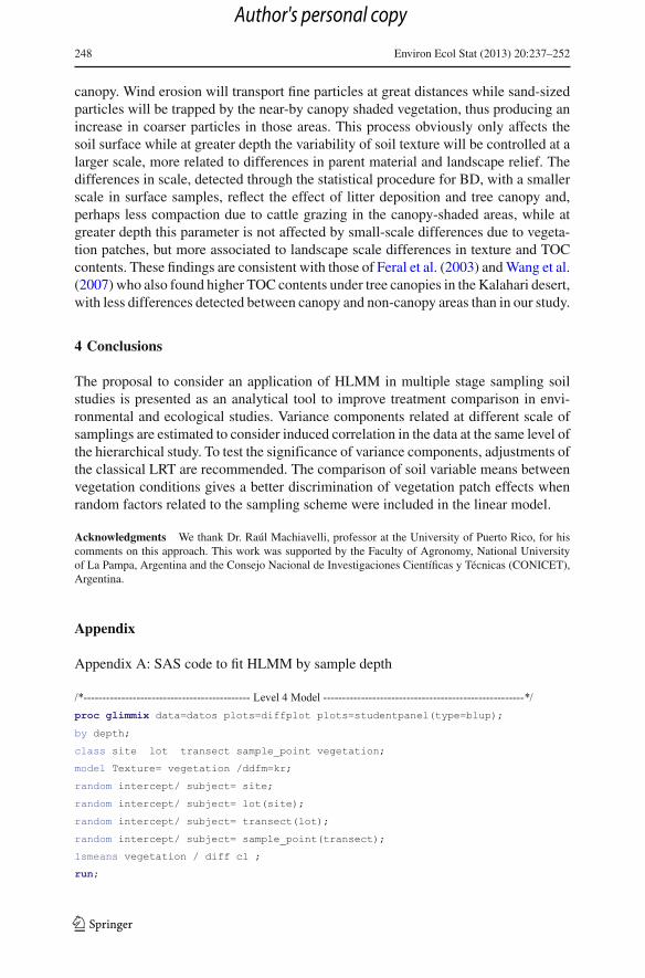
When comparing models E and D, we used a Chi-square distribution with 0.5degrees of freedom, because when the comparison involves the model with a randomcomponent vs. the model without random effects, it is assumed that the null hypothesisof the LRT is a Chi-square mixture of Chi-square distributions with 0 and 1 degreesof freedom, each with equal weight. In this case, the Chi-square distribution with 0degrees of freedom is not really a distribution, but a probability mass of 1 for value 0,and therefore the statistic is evaluated with respect to a Chi-square distribution with0.5 degrees of freedom (Verbeke and Molenberghs 2000). All the tests were done withProc GLIMMIX, SAS version 9.1 (SAS Institute 2008), with the codes found in theAppendix.

In all the cases in which the LRT statistic was used, and in which its value is suffi-ciently large (larger than the reference value of the distribution of the statistic), thereis evidence against the reduced model and in favor of the reference model. But ifthe likelihood values are very similar in both models, the LRT statistic turns out tobe very small, and therefore there is no evidence that favors the reduced model (nullhypothesis), because when faced with the lack of statistically significant differences,it is traditionally recommended to select the model with the fewest parameters.

In hierarchical models, it can be observed that the mean and the variance structureare simplified; the −2 log-likelihood REML increases. Nevertheless, in order to selectthe best model, the model with the smallest −2 log-likelihood REML is preferredsince this does not imply an excessive number of unnecessary parameters associatedto each stage of sampling.

In this paper, we analyze the significance of the estimated variance components foreach depth level, beginning with the Level 1 model and up until the Level 4 model.The model that includes the lowest significant level was selected. Once the best modelwas identified, we proceeded to study the differences between the means for the fixedeffects factor, for each one of the three soil variables in the study.

3 Results and discussion

3.1 Model selection

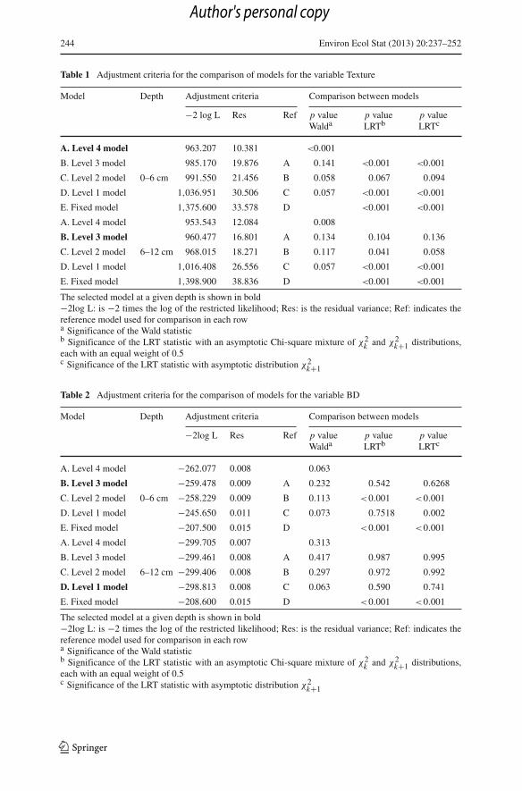
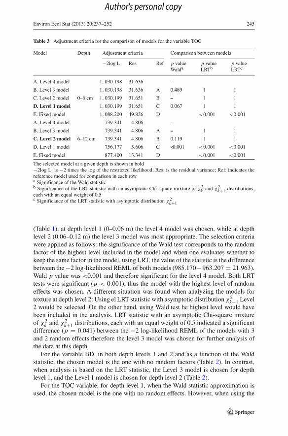
In Tables 1, 2, 3 goodness-of-fit criteria for the each depth level are shown, as are theresults of the three statistical tests used to determine the significance of the variancecomponents associated with the different sampling stages. For the case of Texture

123

Author's personal copy

244 Environ Ecol Stat (2013) 20:237–252

Table 1 Adjustment criteria for the comparison of models for the variable Texture

Model Depth Adjustment criteria Comparison between models

−2 log L Res Ref p valueWalda

p valueLRTb

p valueLRTc

A. Level 4 model 963.207 10.381 <0.001

B. Level 3 model 985.170 19.876 A 0.141 <0.001 <0.001

C. Level 2 model 0–6 cm 991.550 21.456 B 0.058 0.067 0.094

D. Level 1 model 1,036.951 30.506 C 0.057 <0.001 <0.001

E. Fixed model 1,375.600 33.578 D <0.001 <0.001

A. Level 4 model 953.543 12.084 0.008

B. Level 3 model 960.477 16.801 A 0.134 0.104 0.136

C. Level 2 model 6–12 cm 968.015 18.271 B 0.117 0.041 0.058

D. Level 1 model 1,016.408 26.556 C 0.057 <0.001 <0.001

E. Fixed model 1,398.900 38.836 D <0.001 <0.001

The selected model at a given depth is shown in bold−2log L: is −2 times the log of the restricted likelihood; Res: is the residual variance; Ref: indicates thereference model used for comparison in each rowa Significance of the Wald statisticb Significance of the LRT statistic with an asymptotic Chi-square mixture of χ2

k and χ2k+1 distributions,

each with an equal weight of 0.5c Significance of the LRT statistic with asymptotic distribution χ2

k+1

Table 2 Adjustment criteria for the comparison of models for the variable BD

Model Depth Adjustment criteria Comparison between models

−2log L Res Ref p valueWalda

p valueLRTb

p valueLRTc

A. Level 4 model −262.077 0.008 0.063

B. Level 3 model −259.478 0.009 A 0.232 0.542 0.6268

C. Level 2 model 0–6 cm −258.229 0.009 B 0.113 <0.001 <0.001

D. Level 1 model −245.650 0.011 C 0.073 0.7518 0.002

E. Fixed model −207.500 0.015 D <0.001 <0.001

A. Level 4 model −299.705 0.007 0.313

B. Level 3 model −299.461 0.008 A 0.417 0.987 0.995

C. Level 2 model 6–12 cm −299.406 0.008 B 0.297 0.972 0.992

D. Level 1 model −298.813 0.008 C 0.063 0.590 0.741

E. Fixed model −208.600 0.015 D <0.001 <0.001

The selected model at a given depth is shown in bold−2log L: is −2 times the log of the restricted likelihood; Res: is the residual variance; Ref: indicates thereference model used for comparison in each rowa Significance of the Wald statisticb Significance of the LRT statistic with an asymptotic Chi-square mixture of χ2

k and χ2k+1 distributions,

each with an equal weight of 0.5c Significance of the LRT statistic with asymptotic distribution χ2

k+1

123

Author's personal copy

Environ Ecol Stat (2013) 20:237–252 245

Table 3 Adjustment criteria for the comparison of models for the variable TOC

Model Depth Adjustment criteria Comparison between models

−2log L Res Ref p valueWalda

p valueLRTb

p valueLRTc

A. Level 4 model 1, 030.198 31.636 –

B. Level 3 model 1, 030.198 31.636 A 0.489 1 1

C. Level 2 model 0–6 cm 1, 030.199 31.651 B – 1 1

D. Level 1 model 1, 030.199 31.651 C 0.067 1 1

E. Fixed model 1, 088.200 49.826 D <0.001 <0.001

A. Level 4 model 739.341 4.806 –

B. Level 3 model 739.341 4.806 A – 1 1

C. Level 2 model 6–12 cm 739.341 4.806 B 0.119 1 1

D. Level 1 model 756.177 5.606 C <0.001 <0.001 <0.001

E. Fixed model 877.400 13.341 D <0.001 <0.001

The selected model at a given depth is shown in bold−2log L: is −2 times the log of the restricted likelihood; Res: is the residual variance; Ref: indicates thereference model used for comparison in each rowa Significance of the Wald statisticb Significance of the LRT statistic with an asymptotic Chi-square mixture of χ2

k and χ2k+1 distributions,

each with an equal weight of 0.5c Significance of the LRT statistic with asymptotic distribution χ2

k+1

(Table 1), at depth level 1 (0–0.06 m) the level 4 model was chosen, while at depthlevel 2 (0.06–0.12 m) the level 3 model was most appropriate. The selection criteriawere applied as follows: the significance of the Wald test corresponds to the randomfactor of the highest level included in the model and when one evaluates whether tokeep the same factor in the model, using LRT, the value of the statistic is the differencebetween the −2 log-likelihood REML of both models (985.170−963.207 = 21.963).Wald p value was <0.001 and therefore significant for the level 4 model. Both LRTtests were significant (p < 0.001), thus the model with the highest level of randomeffects was chosen. A different situation was found when analyzing the models fortexture at depth level 2: Using el LRT statistic with asymptotic distribution χ2

k+1 Level2 would be selected. On the other hand, using Wald test he highest level would havebeen included in the analysis. LRT statistic with an asymptotic Chi-square mixtureof χ2

k and χ2k+1 distributions, each with an equal weight of 0.5 indicated a significant

difference (p = 0.041) between the −2 log-likelihood REML of the models with 3and 2 random effects therefore the level 3 model was chosen for further analysis ofthe data at this depth.

For the variable BD, in both depth levels 1 and 2 and as a function of the Waldstatistic, the chosen model is the one with no random factors (Table 2). In contrast,when analysis is based on the LRT statistic, the Level 3 model is chosen for depthlevel 1, and the Level 1 model is chosen for depth level 2 (Table 2).

For the TOC variable, for depth level 1, when the Wald statistic approximation isused, the chosen model is the one with no random effects. However, when using the

123

Author's personal copy

246 Environ Ecol Stat (2013) 20:237–252

tests based on LRT, one chooses the Level 1 model with depth level 1. For depth level2, when using the Wald test, the selected model is the Level 1 model, and when usingthe LRT test, the selected model is the Level 2 model (Table 3).

For all the variables, except for Texture in depth level 2, models with very simplifiedvariance structures were selected when the Wald test was used. The results coincidewith the critiques of other authors (Pinheiro and Bates 1998; West et al. 2006) regard-ing the low sensibility of the Wald statistic, especially in cases such as this one, inwhich the number of levels for each random factor is low and the true parameter valueis within the limit of the parametric space, under the null hypothesis. The identifica-tion of the best model to chose for adjusting the experimental data is crucial, since theover-parameterization of the covariance structure can lead to the inefficient estimationand poor evaluation of the standard error for the estimation of differences betweenmeans for an effects factor, the under-specification that ignores variance componentsdue to the sampling strategy can lead to incorrect conclusions.

The LRT statistic with an asymptotic Chi-square mixture of Chi-square distribu-tions with k and k + 1 degrees of freedom, or with 0.5 degrees of freedom when afixed and mixed model are compared, turned out to be the most potent strategy foridentifying the variability due to the sampling strategy. Despite the fact that the p val-ues associated with the LRT, when dealing with the Chi-square mixture of Chi-squaredistributions, were always less than the uncorrected LRT p values, both tests led tothe selection of the same model. The fact that there was a reduction in the p valuessuggests that in other applications, disregarding this aspect of distributional correctioncould lead to an oversimplification of the covariance structure.

In the application illustrated in this paper, the models were selected in functionof the LRT statistic with asymptotic Chi-square mixture of Chi-square distributionsand are in bold in Tables 1, 2, 3. As can be observed, these models include a randomfactor of the lowest significant level and all the factors of a level higher than that one,regardless of their significance. These factors should remain in the model in order tomaintain the correlated structure of the data introduced by the sampling strategy.

It is noteworthy that the selected model for the variance and co-variance structurewas not the same at different soil depths. This shows that the variability occurs at dif-ferent scales at the two depths even for one variable. For Texture and BD we found thatat more depth the variation was detected at a higher hierarchical scale, while in surfacesamples variability was detected even in the finer scale. For TOC, on the contrary, weonly detected variability at the highest scale. These findings elucidate the processesthat cause variability of the observed soil properties: thus, TOC would be influencedby large scale processes that relate to changes in soil texture, geomorphology and veg-etation patches, while BD and Texture at the soil surface would be subject to smallerscale phenomena such as in this particular case, redistribution of soil particles due towind erosion and the trapping of specific size fractions in vegetation patches in themicro-relief (Pelletier et al. 2009a).

Once the variance structure was modeled for each variable, we studied the effectof the vegetation patches (fixed factor) contained in the mean structure of the samemodel. This unified approximation for the analyses is a substantial practical differ-ence between the use of HLMM compared to classical geostatistical techniques whichattend the multi-scale variability in a different analytical stage than that used for

123

Author's personal copy

Environ Ecol Stat (2013) 20:237–252 247

studying average trends, and in this sense they are more efficient in the use of theavailable information.

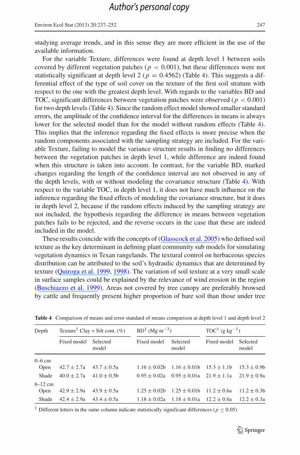
For the variable Texture, differences were found at depth level 1 between soilscovered by different vegetation patches (p < 0.001), but these differences were notstatistically significant at depth level 2 (p = 0.4562) (Table 4). This suggests a dif-ferential effect of the type of soil cover on the texture of the first soil stratum withrespect to the one with the greatest depth level. With regards to the variables BD andTOC, significant differences between vegetation patches were observed (p < 0.001)for two depth levels (Table 4). Since the random effect model showed smaller standarderrors, the amplitude of the confidence interval for the differences in means is alwayslower for the selected model than for the model without random effects (Table 4).This implies that the inference regarding the fixed effects is more precise when therandom components associated with the sampling strategy are included. For the vari-able Texture, failing to model the variance structure results in finding no differencesbetween the vegetation patches in depth level 1, while difference are indeed foundwhen this structure is taken into account. In contrast, for the variable BD, markedchanges regarding the length of the confidence interval are not observed in any ofthe depth levels, with or without modeling the covariance structure (Table 4). Withrespect to the variable TOC, in depth level 1, it does not have much influence on theinference regarding the fixed effects of modeling the covariance structure, but it doesin depth level 2, because if the random effects induced by the sampling strategy arenot included, the hypothesis regarding the difference in means between vegetationpatches fails to be rejected, and the reverse occurs in the case that these are indeedincluded in the model.

These results coincide with the concepts of (Glasscock et al. 2005) who defined soiltexture as the key determinant in defining plant community sub models for simulatingvegetation dynamics in Texan rangelands. The textural control on herbaceous speciesdistribution can be attributed to the soil’s hydraulic dynamics that are determined bytexture (Quiroga et al. 1999, 1998). The variation of soil texture at a very small scalein surface samples could be explained by the relevance of wind erosion in the region(Buschiazzo et al. 1999). Areas not covered by tree canopy are preferably browsedby cattle and frequently present higher proportion of bare soil than those under tree

Table 4 Comparison of means and error standard of means comparison at depth level 1 and depth level 2

Depth Texture1 Clay + Silt cont. (%) BD1 (Mg m−3) TOC1 (g kg−1)

Fixed model Selectedmodel

Fixed model Selectedmodel

Fixed model Selectedmodel

0–6 cmOpen 42.7 ± 2.7a 43.7 ± 0.5a 1.16 ± 0.02b 1.16 ± 0.01b 15.3 ± 1.1b 15.3 ± 0.9b

Shade 40.0 ± 2.7a 41.0 ± 0.5b 0.95 ± 0.02a 0.95 ± 0.01a 21.9 ± 1.1a 21.9 ± 0.9a

6–12 cmOpen 42.9 ± 2.9a 43.9 ± 0.5a 1.25 ± 0.02b 1.25 ± 0.01b 11.2 ± 0.6a 11.2 ± 0.3b

Shade 42.4 ± 2.9a 43.4 ± 0.5a 1.18 ± 0.02a 1.18 ± 0.01a 12.2 ± 0.6a 12.2 ± 0.3a

1 Different letters in the same column indicate statistically significant differences (p ≤ 0.05)

123

Author's personal copy

248 Environ Ecol Stat (2013) 20:237–252

canopy. Wind erosion will transport fine particles at great distances while sand-sizedparticles will be trapped by the near-by canopy shaded vegetation, thus producing anincrease in coarser particles in those areas. This process obviously only affects thesoil surface while at greater depth the variability of soil texture will be controlled at alarger scale, more related to differences in parent material and landscape relief. Thedifferences in scale, detected through the statistical procedure for BD, with a smallerscale in surface samples, reflect the effect of litter deposition and tree canopy and,perhaps less compaction due to cattle grazing in the canopy-shaded areas, while atgreater depth this parameter is not affected by small-scale differences due to vegeta-tion patches, but more associated to landscape scale differences in texture and TOCcontents. These findings are consistent with those of Feral et al. (2003) and Wang et al.(2007) who also found higher TOC contents under tree canopies in the Kalahari desert,with less differences detected between canopy and non-canopy areas than in our study.

4 Conclusions

The proposal to consider an application of HLMM in multiple stage sampling soilstudies is presented as an analytical tool to improve treatment comparison in envi-ronmental and ecological studies. Variance components related at different scale ofsamplings are estimated to consider induced correlation in the data at the same level ofthe hierarchical study. To test the significance of variance components, adjustments ofthe classical LRT are recommended. The comparison of soil variable means betweenvegetation conditions gives a better discrimination of vegetation patch effects whenrandom factors related to the sampling scheme were included in the linear model.

Acknowledgments We thank Dr. Raúl Machiavelli, professor at the University of Puerto Rico, for hiscomments on this approach. This work was supported by the Faculty of Agronomy, National Universityof La Pampa, Argentina and the Consejo Nacional de Investigaciones Científicas y Técnicas (CONICET),Argentina.

Appendix

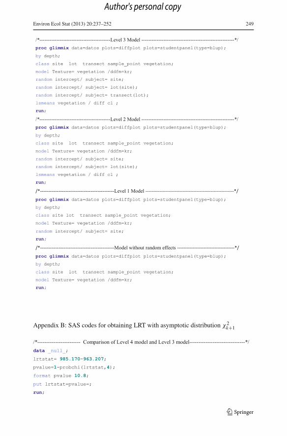
Appendix A: SAS code to fit HLMM by sample depth

123

Author's personal copy

Environ Ecol Stat (2013) 20:237–252 249

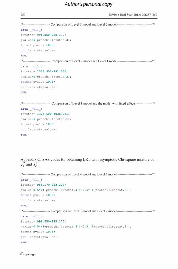
Appendix B: SAS codes for obtaining LRT with asymptotic distribution χ2k+1

123

Author's personal copy

250 Environ Ecol Stat (2013) 20:237–252

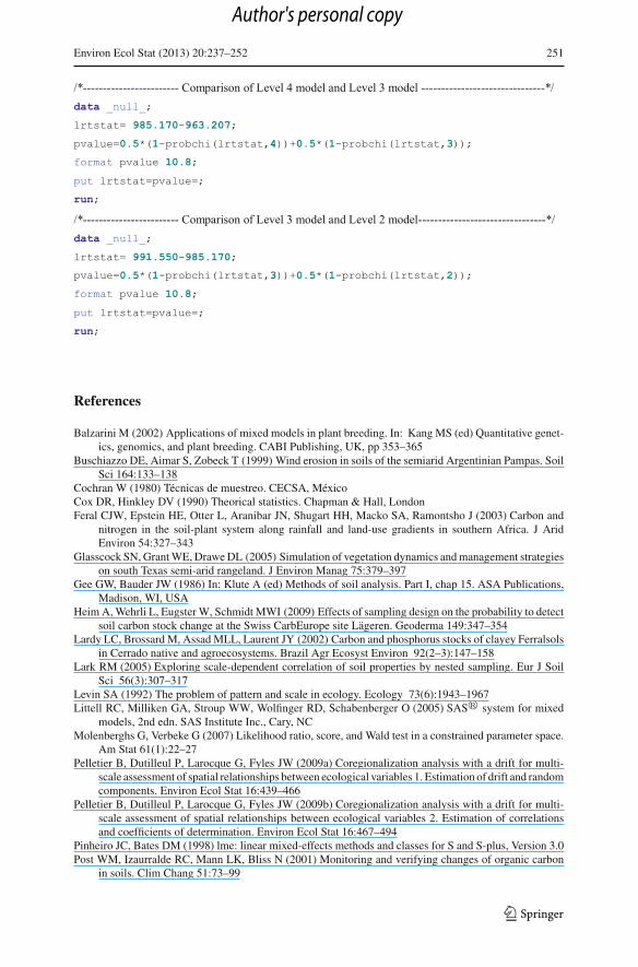
Appendix C: SAS codes for obtaining LRT with asymptotic Chi-square mixture ofχ2

k and χ2k+1

123

Author's personal copy

Environ Ecol Stat (2013) 20:237–252 251

References

Balzarini M (2002) Applications of mixed models in plant breeding. In: Kang MS (ed) Quantitative genet-ics, genomics, and plant breeding. CABI Publishing, UK, pp 353–365

Buschiazzo DE, Aimar S, Zobeck T (1999) Wind erosion in soils of the semiarid Argentinian Pampas. SoilSci 164:133–138

Cochran W (1980) Técnicas de muestreo. CECSA, MéxicoCox DR, Hinkley DV (1990) Theorical statistics. Chapman & Hall, LondonFeral CJW, Epstein HE, Otter L, Aranibar JN, Shugart HH, Macko SA, Ramontsho J (2003) Carbon and

nitrogen in the soil-plant system along rainfall and land-use gradients in southern Africa. J AridEnviron 54:327–343

Glasscock SN, Grant WE, Drawe DL (2005) Simulation of vegetation dynamics and management strategieson south Texas semi-arid rangeland. J Environ Manag 75:379–397

Gee GW, Bauder JW (1986) In: Klute A (ed) Methods of soil analysis. Part I, chap 15. ASA Publications,Madison, WI, USA

Heim A, Wehrli L, Eugster W, Schmidt MWI (2009) Effects of sampling design on the probability to detectsoil carbon stock change at the Swiss CarbEurope site Lägeren. Geoderma 149:347–354

Lardy LC, Brossard M, Assad MLL, Laurent JY (2002) Carbon and phosphorus stocks of clayey Ferralsolsin Cerrado native and agroecosystems. Brazil Agr Ecosyst Environ 92(2–3):147–158

Lark RM (2005) Exploring scale-dependent correlation of soil properties by nested sampling. Eur J SoilSci 56(3):307–317

Levin SA (1992) The problem of pattern and scale in ecology. Ecology 73(6):1943–1967Littell RC, Milliken GA, Stroup WW, Wolfinger RD, Schabenberger O (2005) SAS� system for mixed

models, 2nd edn. SAS Institute Inc., Cary, NCMolenberghs G, Verbeke G (2007) Likelihood ratio, score, and Wald test in a constrained parameter space.

Am Stat 61(1):22–27Pelletier B, Dutilleul P, Larocque G, Fyles JW (2009a) Coregionalization analysis with a drift for multi-

scale assessment of spatial relationships between ecological variables 1. Estimation of drift and randomcomponents. Environ Ecol Stat 16:439–466

Pelletier B, Dutilleul P, Larocque G, Fyles JW (2009b) Coregionalization analysis with a drift for multi-scale assessment of spatial relationships between ecological variables 2. Estimation of correlationsand coefficients of determination. Environ Ecol Stat 16:467–494

Pinheiro JC, Bates DM (1998) lme: linear mixed-effects methods and classes for S and S-plus, Version 3.0Post WM, Izaurralde RC, Mann LK, Bliss N (2001) Monitoring and verifying changes of organic carbon

in soils. Clim Chang 51:73–99

123

Author's personal copy

252 Environ Ecol Stat (2013) 20:237–252

Quiroga A, Buschiazzo D, Peinemann N (1999) Soil compaction is related to management practices insemiarid Argentine pampas. Soil Tillage Res 52:21–28

Quiroga A, Buschiazzo D, Peinemann N (1998) Management discriminant properties in semiarid soils. SoilSci 163:591–597

Raudenbush SW, Bryk AS (2002) Hierarchical linear models: applications and data analysis methods, 2ndedn. Sage Publications, Thousand Oaks, CA (Advanced quantative techniques in the social sciencesseries no. 1)

Ringrose S, Matheson W, Vanderpost C (1998) Analysis of soil organic carbon and vegetation cover trendsalong the Botswana Kalahari Transect. J Arid Environ 38(3):379–396

Searle SR, Casella G, McCulloch CE (1992) Variance components. Wiley, New YorkSAS Institute Inc (2008) SAS/STAT software: version 9.1. SAS Institute Inc, Cary, NCSnijders T, Bosker R (2000) Multilevel analysis: an introduction to basic and advanced multilevel modeling.

Sage, LondonSoon Y, Abboud S (1991) Comparison of some methods for soil organic carbon determination. Commun

Soil Sci Plant Anal 22:943–954Verbeke G, Molenberghs G (2000) Linear mixed models for longitudinal data. Springer, New YorkWang L, Okin GS, Caylor KK, Macko SA (2009) Spatial heterogeneity and sources of soil carbon in

southern African savannas. Geoderma 149:402–408Wang L, D’Odorico P, Ringrose S, Coetzee SH, Macko SA (2007) Biogeochemistry of Kalahari sands.

J Arid Environ 71(3):259–279West B, Welch KB, Galecki AT (2006) Linear mixed models: a practical guide using statistical software.

Chapman & Hall/CRC, Boca Raton, FLWiens JA (1989) Spatial scaling in ecology. Funct Ecol 3:385–397

Author Biographies

Adriana A. Gili is a Ph.D. candidate in biostatistics at the graduate school of the Facultad deCiencias Agrarias of the Universidad Nacional de Córdoba, and her basic formation was as an agrono-mist at the Universidad Nacional de La Pampa. Currently, she is Professor in the Department of Statisticsat the Facultad de Agronomía, Universidad Nacional de La Pampa and her main interests are statistics,ecology, landscape ecology, precision agriculture and geostatistics.

Elke J. Noellemeyer is Professor of Soil Science at the Facultad de Agronomía, Universidad Nacionalde La Pampa. She was trained as a soil scientist at the College of Agriculture of the University of Sas-katchewan, Canada, and has been working on soil management, with a special interest in organic matterand soil physical properties. She has been involved in several international research networks and activelyparticipates in the science-policy interface regarding environmental and agronomic topics.

Mónica Balzarini main background is in Statistics, and her research interests are in applications of statisticsin agricultural and environmental sciences. She is an agronomist from the Universidad Nacional de Córdo-ba and a Ph.D. from Louisiana State University-USA. She is Professor in the Department of Biometrics,Facultad de Ciencias Agrarias, Universidad Nacional de Córdoba and an independent researcher in theInstituto Nacional de Ciencias y Tecnología of Argentina.

123

Author's personal copy