Open Archive TOULOUSE Archive Ouverte (OATAO) OATAO is an open access repository that collects the work of Toulouse researchers and makes it freely available over the web where possible.

This is an author-deposited version published in : http://oatao.univ-toulouse.fr/2053 Eprints ID : 2053

To link to this article : DOI :10.1016/j.ijhydene.2008.12.035 URL : http://dx.doi.org/10.1016/j.ijhydene.2008.12.035

To cite this version : Hadj-Kali, Mohamed and Gerbaud, Vincent and Borgard, Jean-Marc and Baudouin, Olivier and Floquet, Pascal and Joulia, Xavier and Carles, Philippe ( 2009). HIx system thermodynamic model for hydrogen production by the sulfur-iodine cycle. International Journal of Hydrogen Energy, vol. 34 (n° 4). pp. 1696-1709.

1

HIX SYSTEM THERMODYNAMIC MODEL FOR HYDROGEN

PRODUCTION BY THE SULFUR - IODINE CYCLE

Mohamed Kamel Hadj-Kali1,2, Vincent Gerbaud1,2,*, Jean-Marc Borgard3, Olivier Baudouin4,

Pascal Floquet1,2, Xavier Joulia1,2, Philippe Carles3

1Université de Toulouse, INP, UPS, LGC (Laboratoire de Génie Chimique), 5 rue Paulin Talabot,

F-31106 Toulouse Cedex 01 – France

2CNRS, LGC (Laboratoire de Génie Chimique), F-31106 Toulouse Cedex 01 – France

3CEA, DEN, Physical Chemistry Department, F-91191 Gif-sur-Yvette, France.

4 ProSim, Stratège Bâtiment A, BP 27210, F-31672 Labège Cedex, France.

* corresponding author

2

Abstract

The HIx ternary system (H2O – HI – I2) is the latent source of hydrogen for the Sulfur – Iodine thermo-

chemical cycle. After analysis of the literature data and models, a homogeneous approach with the Peng-

Robinson equation of state used for both the vapor and liquid phase fugacity calculations is proposed for the

first time to describe the phase equilibrium of this system. The MHV2 mixing rule is used, with UNIQUAC

activity coefficient model combined with of hydrogen iodide solvation by water. This approach is theoretically

consistent for HIx separation processes operating above HI critical temperature. Model estimation is done on

selected literature vapor – liquid, liquid – liquid, vapor – liquid – liquid and solid – liquid equilibrium data for

the ternary system and the three binaries subsystems. Validation is done on the remaining literature data.

Results agree well with the published data, but more experimental effort is needed to improve modeling of

the HIx system.

Keywords: Sulfur – Iodine cycle, HIx system, phase equilibrium modeling, complex mixing rule

3

1. Introduction

Hydrogen is undeniably a very attractive energy carrier, superior to others for power generation,

transportation and storage. Nowadays, fossil resources account for 95% of hydrogen production. However,

given the prospect of an increasing energy demand, of a shortage of fossil resources and of greenhouse

gases release limitation, water could be the only viable and long term candidate raw material for hydrogen

production. Electrolysis and thermo-chemical cycles are the two leading processes for massive hydrogen

production from water. In thermo-chemical cycles, water is decomposed into hydrogen and oxygen via

chemical reactions using intermediate elements which are recycled. As the heat can be directly used, these

cycles have the potential of a better efficiency than alkaline electrolysis. For massive hydrogen production,

the required energy can be provided either by nuclear energy, by solar energy or by hybrid solutions

including both.

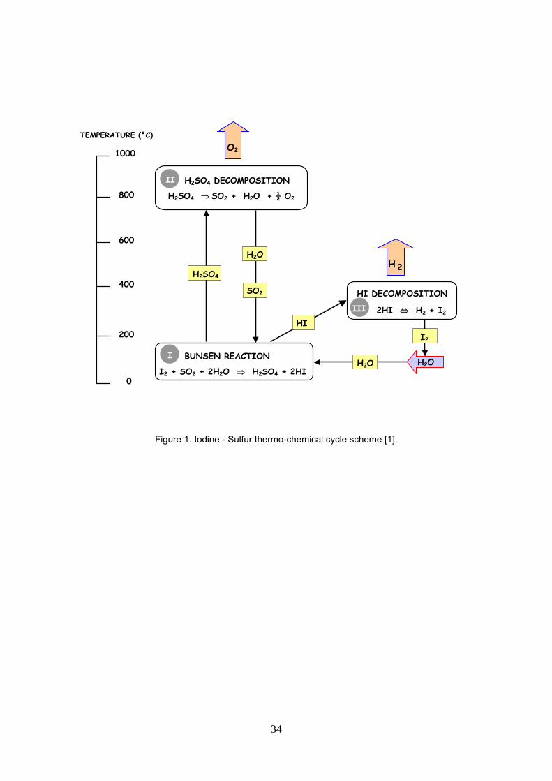
Among hundreds of possible cycles, the Sulfur – Iodine (S-I) cycle is a promising one [1] in combination with

high temperature heat coming from a nuclear reactor. The S-I thermo-chemical cycle is divided into three

sections (figure 1): (I) the Bunsen section, where water H2O reacts with iodine I2 and sulfur dioxide SO2 to

produce with excess water and iodine, two immiscible liquid aqueous sulfuric-rich and iodhydric acid/iodine-

rich phases. The latter is the so-called HIx phase; (II) the sulphuric acid section where oxygen is produced

and (III) the HIx section where hydrogen iodide concentrates and decomposes to produce hydrogen. Water,

iodine and sulfur dioxide are recycled in the system [2].

In 2005, Mathias quoted the ternary system HI – I2 – H2O, occurring in Section III among challenges for

applied thermodynamics [3]. He wrote: “ …The sulfuric acid decomposition section of …[the S-I]… process

can be simulated accurately, but other sections (acid generation and hydrogen iodide decomposition)

illustrate the difficulty of modeling phase behavior, particularly liquid-phase immiscibility, in complex

electrolyte systems.”

HI – I2 – H2O complexity is well illustrated by literature knowledge:

– Complex phase behavior of the ternary system and the derived binary subsystems:

o H2O – I2 binary is a highly immiscible liquid – liquid system, with solid – liquid equilibrium at low

temperatures because of the high melting temperature of iodine (113,6°C) [4],

4

o H2O – HI binary is a maximum boiling azeotropic, strong electrolyte system [5] with liquid – liquid

equilibrium above approx. xHI=0.34 at 25°C [6],

o HI – I2 binary exhibits solid – liquid equilibrium [7],

o HI – I2 – H2O ternary mixture has two type I liquid – liquid regions [8],

– Many reactions occur, within the liquid solution such as electrolyte decomposition, solvation reactions [9]

and poly-iodides formation [10-12] and within the vapor phase with the decomposition of HI in hydrogen

and iodine.

– The operating conditions presumed by many authors [13-15] for the unit operations of this section of the

cycle are severe (up to 50 bar and above 300°C), making H2 and possibly HI in supercritical state as seen

from table 1.

Where MW denotes the molecular weight, Pc the critical pressure, Tc, Tb and Tm respectively the critical, the

boiling and the melting temperature and ω the acentric factor. Under 1.013 bar and 25°C, HI is vapor, H2O is

liquid, I2 is solid and H2 is supercritical. Furthermore, the low critical temperature of hydrogen iodide

(150.70°C) and the high melting temperature of iodine (113.60°C) hint that HI could be supercritical under

process operating conditions and that iodine could easily crystallize in the process side streams.

The reactive distillation process initially suggested by Roth and Knoche in 1989 [13] is the reference process

chosen by CEA [14] for the HIx section. Until now, no pilot unit has operated under in the expected process

conditions (50 bars, 300°C). Such processes are not trivial to design and build, involving choices of suitable

holdup and catalyst [16]. So, simulation and modeling remain the sole alternative to evaluate the process

performance. The amount of hydrogen produced by hydrogen iodide decomposition (2HI ↔ H2 + I2) during

the process is closely related to the iodine and hydrogen iodide concentrations in the vapor. Thus the need

of an accurate and efficient thermodynamic model of vapor – liquid equilibrium for the HIx mixture.

The HIx system thermodynamic model used by Roth and Knoche was proposed by Neumann in 1987 [17]

based mostly on total pressure measurements performed at RWTH Aachen [18] and on liquid – liquid

equilibrium data tracked through various sources to ref. [8]. These measurements represent a significant

achievement, as the HIx system complexity mentioned above does not facilitate experimental work.

The present paper focuses on the thermodynamic modeling of the HIx system using VLE, LLE VLLE and

SLE experimental data available in the literature with the aim that, in addition to capture the system complex

features evoked before, the model can be used in the high pressure (20-50 bar) and high temperature (320-

5

380°C) conditions of the reactive distillation process. The paper is structured as follows: first, a synthesis of

available literature experimental data is presented. Then, an overview of thermodynamic phase equilibrium

calculations is given in perspective with the existing literature models and the new modeling approach we

propose. The parameter estimation procedure is detailed as well. Finally, results are discussed and

compared to literature experimental data.

2. Available experimental data

Available experimental data for the ternary system (HI – I2 – H2O) and each binary subsystem (H2O – HI),

(H2O – I2) and (HI – I2) are collected in table 2.

Total pressures of H2O – HI binary mixtures have been measured by Wüster in vapor – liquid equilibrium

conditions [19] and mixing enthalpies by Vanderzee and Gier [20]. Like other water – strong acid mixtures,

H2O – HI mixture exhibits a maximum temperature azeotrope (HI mass fraction equal to 57% (0.1573 molar

fraction) at 127°C and atmospheric pressure) [5, 21]. For HI concentrations higher than the azeotrope, the

vapor phase is very rich in HI. Furthermore, for high temperatures (> 200°C), HI dissociation in the vapor

phase into H2 and I2 becomes significant [22, 23]. Wüster [19] quoted that experimental data on the right side

of the azeotrope at temperatures above 170°C were discarded because the HI vapor decomposition led to

inaccurate measurements. Wüster originally published 119 experimental points (P,T,x) and iso-composition

correlations giving the saturation pressure dependence versus temperature for different HI mass fractions.

Engels published in DECHEMA series [9] a monograph about solvation modeling including the H2O – HI

system but with only 80 points of Wüster’s work.

Atmospheric vapor – liquid bubble and dew equilibrium curves of H2O – HI were measured by Sako and

coworkers in 1985 [24] and earlier by Carrière and Ducasse in 1926 [25]. Isothermal vapor – liquid – liquid

equilibrium curve at 25°C was published by Haase et al. [6]. However, Haase [6] data report the H2O – HI

azeotrope at xHI=0.146 (HI mass fraction of 54.8 %) at 25°C and 0.0166 bar. This is not consistent with other

measures. The Pascal monograph [5] reports a xHI=0.1768 (60.4% in mass) around 15–19°C (no pressure

reported) and xHI=0.1651 (58.4% in mass) at 100°C. Data of CRC handbook [21] (xHI=0.1573; 57.0% mass at

127.0°C and 1 atm), Sako [24], Carrière and Ducasse [25] (xHI=0.1557; 56.7% mass at 126.5°C and 1 atm),

and Wüster [19] agree also that the azeotrope molar and mass fraction increases as pressure is reduced.

Therefore, Haase’s azeotropic composition is seemingly too low.

6

However, Haase and coworkers [6] isothermal vapor – liquid equilibrium curves, (P, x, y) give clear evidence

of a H2O – HI vapor – liquid – liquid equilibrium at 25°C and 7.47bar between xHI=0.346 and xHI=0.995.

Unpublished liquid – liquid equilibrium data confirm the H2O – HI miscibility gap at 24°C/7.3bar and 70°C

/17bar in pages 3-55 to 3-63 of reference [8]. Neumann [17] extracted imprecise composition values at five

temperatures 70°C, 100°C, 120°C, 136°C and 149°C, likely from a rough sketch of the assumed liquid –

liquid equilibrium profiles of the ternary mixture H2O – HI – I2 reported in page 3-64 in reference [8].

Pascal [5] reported solid – liquid equilibrium of H2O – HI mixtures originally published by Pickering [26] (see

figure 2). The three eutectic points location tells us that at the azeotropic composition (xHI=0.157,

57.0%mass), solidification leads to hydrated hydrogen iodide crystals (HI, 4H2O). Evidently, the hydration

number decreases as the H2O molar fraction decreases because there are not enough water molecules to

hydrate HI: the (HI, 4H2O) hydrate (xHI=0.20, 64%mass) melts at -36.5°C; the (HI, 3H2O) hydrate (xHI=0.25,

70.3%mass) melts at -48.0°C and the (HI, 2H2O) hydrate (xHI=0.333, ≅78%mass) melts at -43.0°C. That

information will be considered with the hydration of HI in liquid H2O – HI mixtures discussed later.

For the binary H2O – I2, Kracek [4] measured the solubility of solid iodine in water and put in evidence a

miscibility gap at 112.3°C up to at least 210°C. At 112.3°C, the light aqueous liquid phase contains

xI2=0.0005 and the heavy iodine liquid phase xI2=0.98.

For HI – I2 O’Keefe and Norman [7] measured the solubility of iodine in HI at five different temperatures

(between 25°C and 90°C). These authors highlight that HI – I2 solutions follow an ideal behavior quite

closely, a claim that we reexamine later.

280 equilibrium total pressure measurements of the H2O – HI – I2 ternary mixture for a [HI]/[H20] ratio up to

19.4% and various iodine concentrations are found in the manuscript of Neumann [17]. A synthesis of these

results has been published by Engels and Knoche as correlations of the total pressure at equilibrium versus

the temperature for several couples of HI and iodine molar fractions [18].

General Atomics report [8] of liquid – liquid equilibrium isopiestic measurements of the ternary mixture H2O –

HI – I2 confirms a first ternary miscibility gap between water and hydrogen iodide in the presence of iodine

through 19 measurements between ≈24°C/7.0bar and 152.1°C/62.2bar from pages 3-55 to 3-63 in ref. [8].

They also hint at a second miscibility gap between water and iodine in the presence of hydrogen iodide

above the iodine melting point without providing the relevant ternary data. The second partial miscibility

7

region reduces as HI concentration increases, probably because of the formation of polyiodides ions like I3-

[10,11].

All literature data are summarized in table 2 where it is shown which data are used for the model parameter

estimation and which are used for its validation.

In addition, several authors have reported the occurrence of endothermic HI decomposition in the vapor

phase (2HI ↔ H2 + I2), clearly evidenced by a violet coloration characteristic of vapor iodine, both in the

binary H2O – HI [19] and the ternary H2O – HI – I2 [18]. High hydrogen iodide molar fraction in the vapor

phase occurs for HI liquid molar fraction above the H2O – HI azeotrope and favors the dissociation. High

iodine molar fraction in the vapor phase reduces this dissociation according to the Le Chatelier’s principle.

Furthermore, HI dissociation reaches equilibrium very slowly [22,23] making difficult to assess the exact

quantity of each species.

Palmer and Lietzke [10,11] evaluated poly-iodide formation in the low iodine content in water. Although no

precise measurement is available for the ternary H2O – HI – I2 mixture, this phenomenon may cause

significant dissolution of iodine in H2O – HI solutions. That would result in a lower iodine molar fraction in the

vapor phase, enhancing the suspected HI decomposition in favor of hydrogen production.

3. Model description

3.1. Thermodynamic models background

At constant temperature and pressure, mixture vapor – liquid equilibrium is expressed by equality between

liquid and vapor chemical potentials (alternatively fugacities) of each component within the two phases:

( ) ( xy ,P,Tf,P,Tf Li

Vi = ) (1)

Where x and y refer to the liquid phase L and the vapor phase V composition respectively.

Two approaches are commonly used to express the fugacity of each phase [27,28]:

1. In a homogeneous (φ−φ) approach, the reference state is the perfect gas and is the same for both vapor

and liquid phases. Each phase fugacity is calculated by means of components fugacity coefficients φi

from an unique equation of state (EoS):

( ) ( ) iLii

Vi x,P,Ty,P,T ⋅=⋅ xy φφ (2)

Our model is based on this approach.

8

2. In a heterogeneous (γ−φ) approach, vapor and liquid phases are handled differently. For the vapor phase,

the reference state is the perfect gas and vapor fugacities are obtained from an EoS. For the liquid

phase, the reference state is an ideal mixture and liquid fugacities are calculated by introducing

activity coefficients γi, derived from a Gex molar excess Gibbs energy model, to take into account the

possible non-ideality of the liquid phase. That gives:

Vif

Lif

( ) ( ) ( P,Tfx,TPy,P,T Liiii

Vi

0⋅⋅=⋅⋅ xy γφ )

)

(3)

Where expresses the fugacity of component i in one chosen reference state, calculated from the

vapor pressure law:

( P,Tf Liο

( ) ( ) (TP,P,TP,Tf iV

iL

i000 ⋅= yφ )

)

(4)

Literature models of the HIx section [17,29,30,31] are based on this approach.

The heterogeneous approach is well suited for strongly non ideal mixtures, but recommendation is to use it

far from the critical region. At high pressure, pressure correction like Poynting’s factor can be used in

. Above the critical point of a component, its vapor pressure law has to be extrapolated. Besides,

the heterogeneous approach does not handle correctly mixture critical points above one component’s critical

point, which in the S-I cycle holds for H2 and happens for HI at T > 150°C.

( P,Tf Li0

On the other hand, the homogeneous approach guarantees the continuity between the two phases at the

critical point and requires no extrapolation above and predicts mixture critical points. However, when using

simple Lorenz-Berthelot mixing rules, this approach is only appropriate for weakly polar mixtures.

To combine the advantages of both approaches, Huron and Vidal [32] proposed a EoS/Gex homogeneous

formalism in which both the liquid and the vapor are modeled by an equation of state but with mixing rules

based on the use of activity coefficient models calculation. Unfortunately, published binaries interaction

parameters at low pressure with the heterogeneous approach cannot be reused because the HV rule is set

on an infinite pressure reference state basis. Then, Michelsen [33,34] proposed the Modified Huron-Vidal

(MHV) formalism. He chose a zero pressure reference (ZRP), that could allow to reuse as such all the binary

interaction parameters previously published in the literature for the calculation of activity coefficients, or to

use a predictive model like UNIFAC [35] and thus make the EoS/Gex model predictive.

9

There are two MHV1 and MHV2 models as well as other ZRP EoS/Gex models [27,36], which differ mostly in

their expression of the function of the reduced attractive-term parameter, α. The MHV2 model complex

mixing rule [34] has a quadratic form of α that was estimated within the range α ∈ {8 – 18}:

( ) ( ) ( ) ∑∑∑ +=

=−+−i

ii

ex

iiii bbLnx

RTx,P,TGxqxq 022

21 αααα (5)

With:bRT

a=α ,

RTba

i

ii =α and Gex the excess Gibbs energy model. q1; q2 are numerical coefficients of the

mixing rule, depending on the equation of state that is used; a, b, ai and bi are the attractive and covolume

parameter of the equation of state chosen.

However, Kalospiros et al. [36] quoted that ZRP EoS/Gex models perform poorly when applied to systems

with components that differ appreciably in size, more specifically that differ in αi values. Indeed, for such

mixtures, significant differences arise between the EoS/Gex model and the Gex at zero pressure, that can only

be reduced by both a better fit of the real α variation by an α approximate equation and a better fit of the

approximate equation differential versus α. They demonstrated that the MHV2 rule could not really be

improved for asymmetric mixtures by fitting the quadratic function over a wider α range because a quadratic

form cannot match the α derivative, a reason for which it fails dramatically to predict accurate infinite activity

coefficients values. The two new fits proposed as solutions are however not conclusive according to their

own comments.

We now review the most popular existing HIx models (Neumann’s NRTL modified model and NRTL

electrolyte models) before developing the new model.

3.2. HIx Neumann’s model

3.2.1. Engels solvation model basis

Engels solvation model is based on the concept that ions exist in solution only within a stable solvent cloud.

The new molecule clusters called “complexes” C are made by the reaction of m solvent molecules S with one

electrolyte E molecule according to the expression:

mS + E ↔ υ C mSE

CmSE

CmSE

C

xxx

aaaK

××

×=

×=

υυυ

γγγ (6)

10

Where υ is the number of dissociation products of one electrolyte molecule; xi is the molar fraction of the

species i and ai, γi their activity and activity coefficient respectively.

Such a model rely upon a symmetric convention for the electrolyte and for the solvent, applicable over the

entire composition range. Under dilute electrolyte conditions, the excess of solvent favors the complete

dissociation and solvation of the electrolyte. Near pure electrolyte, lack of solvent leaves the electrolyte

undissociated. This is consistent with the discussion on the solid – liquid equilibrium of the binary H2O – HI,

given in figure 2 [26].

The Engels solvation concept significantly simplifies the model development, since no charged species are

considered in the liquid phase and the activity coefficient model adopted is only based upon the short range

interactions between molecules. The parameters are principally the molecule-molecule interaction terms,

including Engels’ complex molecule, both with the solvation number m.

For the binary mixture H2O – HI, Engels took the solvation number m equal to 5 and wrote the solvation

reaction under the form :

5 H2O + HI ↔ 2 C 52

2

OHHI

C

aaaK×

= (7)

Engels’s model dimensional analysis is similar to the strict thermodynamic description of an electrolyte

dissociation followed by solvation of the cation. For example, for H2O – HI, we write:

HI ↔ H+ + I- HI

IHondissociati a

aaK

−+ ⋅= (8)

mH2O + H+ ↔ (m-1)H2O), H3O+ ( )( )m

OHH

OH,OHmsolvationH aa

aK

2

321

⋅=

+

+

+− (9)

mH2O + HI ↔ [(m-1)H2O), H3O+; I-] ( )( )m

OHHI

OH,OHmI

aa

aaK

2

321

⋅

⋅=

+− − (10)

The equilibrium constants of equations 7 and 10 are equivalent with m = 5 and a complex 2C that would be

like [(m-1)H2O), H3O+; I-].

The hydronium ion H3O+ exists in aqueous solutions, with a hydration number that may vary upon conditions

[37]. Furthermore, molecular dynamic simulations have shown that cation hydrates in solution are dynamic

clusters where H2O molecule on the cluster surrounding can be replaced by bulk solvent molecules [38].

11

This model was first used successfully by Engels with the Wilson activity coefficient model [9] to describe the

vapor – liquid phase equilibrium of the binary mixture H2O – HI.

3.2.2. Neumann’s NRTL modified model description

In conjunction with the solvation reaction, Wilson’s model proposed by Engels is intrinsically unable to

describe liquid phase demixtion [28] that occurs in the HIx system, though. To study the ternary mixture H2O

– HI – I2, Neumann [17] used a heterogeneous approach with a perfect gas vapor phase and, for the non

ideal liquid phase, Engels’ solvation combined with a modified NRTL model that is suitable to model liquid –

liquid phase equilibrium. Above HI critical temperature, its vapor pressure law is extrapolated.

The original NRTL model activity coefficient expression of component i [39] is:

⎥⎥⎥⎥⎥

⎦

⎤

⎢⎢⎢⎢⎢

⎣

⎡

−+==

∑

∑∑

∑∑

∑

=

=

=

==

=N

kkkj

N

kkkjkj

ij

N

jN

kkkj

jijN

jjji

N

jjjiji

i

Ex

xG

xG

xG

xG

xG

xG

lnRTg

1

1

1

11

1τ

τ

τ

γ (11)

Where )exp(G jijiji τα−=

Components i and j binary interaction is defined by three parameters: τij, τji and the non-randomness

parameter αij, with αij set equal to αji. Neumann modified the NRTL model [17], considering αji = -αij, and a

specific temperature dependence for τij and τji. Furthermore he identified one set of binary interaction

parameters to be used for temperatures below 150°C and one set above 150°C. Notice that the 150°C is

close to the HI critical temperature (150.70°C)). He also identified a solvation equilibrium constant Ka(T)

(equation 8) applicable to any temperature.

Neumann’s model was recently revisited by Yoon et al., [40] who introduced a new NRTL model modification

with independent and positive αji and αij and evaluated the HI dissociation impact on the calculations. They

estimated on Neumann’s monograph data [17], three different sets of NRTL binary interaction parameters

and of solvation constant values, respectively for the binary H2O – HI and for the ternary H2O – HI – I2 below

and above 150°C.

Neumann’s model was formerly used by several authors [14,15] to simulate a reactive distillation process for

the recovery of hydrogen, designed with a column composition profile located on the H2O – HI – I2 mixture

temperature crest where the mixture has a single liquid phase in equilibrium with the vapor phase. The

phase diagrams can be calculated with confidence on the left-hand side of the binary H2O – HI azeotrope

12

and when the iodine content is low. Uncertainties remain for high iodine contents and high temperatures [15].

The nominal pressure proposed in these works was 22 bars, following Roth and Knoche suggestion that this

would favor hydrogen production [13]. This pressure is below any of the three components critical pressure,

but the mixture equilibrium temperature is above the HI critical temperature (150.70°C).

3.2.3. HIx Neumann’s model limitations

3.2.3.1. Vapor pressure law extrapolation:

In the heterogeneous approach vapor – liquid equilibrium equation (3) ( )P,Tf Li0 , the fugacity of the pure

liquid of each constituent at the temperature and pressure of the system, is expressed in terms of the vapor

pressure laws Pi°(T) usually estimated on vapor – liquid equilibrium data of pure components. However, for

HIx mixtures temperature above HI supercritical temperature (Tc,HI=150.70°C), HI vapor pressure law must

be extrapolated in order to compute any equilibrium above this temperature for a mixture containing HI. The

literature propose several laws consistent together:

o Engels proposed:

( )⎥⎥

⎦

⎤

⎢⎢

⎣

⎡

⎟⎟⎠

⎞⎜⎜⎝

⎛ −⋅+⎟⎟

⎠

⎞⎜⎜⎝

⎛ −⋅−⎟

⎠

⎞⎜⎝

⎛ −

⋅=°

2

50480434

10013251 b

b

b

bb

TTT

.T

TT..

TTT

HI .barP (T and Tb in K) (12)

Tb denotes the boiling temperature of HI equal to -35.55°C.

o Neumann added an extrapolated expression above HI critical temperature:

( )⎟⎠⎞

⎜⎝⎛ −

=° T..

barP31104037644

10 (13)

o DIPPR saturation pressure law for HI was used in other works [15] and is given by [40]:

( ) ( ) ⎟⎠⎞

⎜⎝⎛ ×+×−−=° T.Tln.

T..expPaP 00780575651334223354 (with T in K) (14)

The vapor – liquid equilibrium homogeneous approach doesn’t use nor requires any extrapolation of the

vapor pressure law.

3.2.3.2. vapor – liquid equilibrium calculation above HI critical point

With or without any vapor pressure extrapolation, a heterogeneous approach model is intrinsically unable to

compute correctly any mixture critical line. Phase equilibrium for any mixture containing HI, above HI critical

13

temperature cannot reach 100% HI because under such conditions, pure HI is supercritical and not involved

in any phase equilibrium. A homogeneous approach can predict so but a heterogeneous one cannot from

theory [28]. Within a reactive distillation column operating above HI critical temperature, the heterogeneous

approach could over predict the HI content in the vapour phase, with consequences on the estimated

hydrogen content obtained from the dissociation of HI.

3.2.3.3. Perfect gas hypothesis

Assuming a perfect gas vapor phase, as did Neumann or Engels, is dubious regarding the high total

pressures achieved. Preliminary calculation of the compressibility factor for the ternary system H2O – HI – I2

by a cubic equation of state like SRK or PR at pressures higher than 10 bars hints at values close to 0.90

rather than perfect gas unity value.

3.3. HIx NRTL electrolytic models

By using a solvation model with no explicit ionic species together with an activity coefficient model for the

non ideal liquid phase, Engels and Neumann’s HIx models rely upon a symmetric convention for all

components in the liquid phase, namely that the activity coefficient γi goes to 1 as the component fraction xi

goes to 1. That convention enables to explore the whole composition range without limitations.

But strong acidic mixture like the HIx one are often described with explicit ions. The electrolyte-NRTL model

developed by Chen [42,43] does it and combines the Pitzer-Debye-Hückel model [44] for long-range ion-ion

electrostatic interactions with the NRTL theory [39] for short-range energetic interactions among the species

in electrolyte solutions. Such an electrolyte model uses an asymmetric convention distinguishing solute and

solvent:

0111

→→→→

solutesolute

solventsolvent

xasxas

γγ

(15)

As the NRTL equation was developed using a symmetric convention, it is associated to the electrolyte Pitzer-

Debye-Hückel model by asymetrizing it using the usual formula:

∞⋅= iasymi

symi γγγ (16)

Where is the infinite dilution activity coefficient. ∞iγ

14

3.3.1. Brown’s electrolyte model (2001)

Brown and co-workers [29,30] used Chen’s electrolyte-NRTL model to describe the liquid phase by

considering the presence of H3O +, OH - and I - ions in the mixture:

H2O ↔ H3O + + OH - (17)

HI + H2O ↔ H3O + + I - (18)

Electrolyte parameters and NRTL binary interaction parameters were estimated from experimental data of

Kracek [4], Wüster [19], Engels [18] and O’Keefe and Norman [7]. Good representation of all binary

subsystems is achieved, including liquid – liquid demixtion and a maximum deviation error for the total

pressure of the ternary system about 30% is obtained. The perfect gas model is used for the vapor phase.

3.3.2. Annesini’s electroyte model (2007)

Annesini et al. [32] combined the Redlich-Kwong equation of state for the vapor phase and Chen’s

electrolyte-NRTL activity coefficient model for the liquid phase. In order to describe the vapor – liquid

equilibrium in a wide range of composition, HI has been chosen as the Raoult reference state.

3.3.3. NRTL electrolytic models limitation

Former limitations of heterogeneous vapor – liquid equilibrium approach still hold for NRTL electrolytic

models, namely the extrapolation of vapor pressure law and an incorrect behavior of mixture critical lines.

The asymmetric convention brings an additional limitation to use the model over the entire composition

range. Chen’s electrolyte-NRTL model claims accurate prediction of activity coefficient up to 16 mol/kg of

solvent for strong acid electrolytes like HCl or H2SO4 [45], which is still far from pure electrolyte. It remains

still questionable to choose an infinite dilution convention for the solute activity coefficient (γsolute → 1 when

xsolute → 0) when one expects to predict fluids behavior with almost pure electrolyte.

3.4. New homogeneous approach EoS/Gex model

Based on the literature survey, a homogeneous approach with the MHV2 complex mixing rule incorporating

UNIQUAC model [46,47] and Engels solvation is proposed to model the HIx system.

First, two cubic EoS are tested, Soave-Redlich-Kwong (SRK) and Peng-Robinson (PR) equation of state,

with Boston-Mathias modification of the α(T) function [48], reputed to perform better at high pressure than

15

the original cubic EoS α(T) function. PR predicts experimental vapor pressures of pure components with the

least deviation as shown in the table 3 below and is finally selected.

The MHV2 complex mixing rule [34] (equation 5) is chosen with no modification of the alpha estimated

function. The new excess Gibbs energy model (Gex), called UQSolv, is a combination of the UNIQUAC

activity coefficient model (equation 19) with Engels’ model solvation (equation 6) of HI by H2O.

)A,A,'q,x(f)q,r,x(fRTg

jiijresidualialcombinator

Ex+= (19)

The UNIQUAC model sums two contributions (equation 19). The combinatorial term handles molecule size

difference effects whereas the residual term accounts for fluid interactions [46]. Steric effects are expected

as iodine and water molecular weights and sizes are quite different (254 g.mol-1 vs 18 g.mol-1 respectively).

Defined as the Van der Waals volume and the area of the molecule, UNIQUAC structural parameters r and q

(q’=q) are taken from the literature [49] (see table 4). Following UNIQUAC’s authors suggestion [46], the

solvation complex parameters are calculated from an arithmetic mixing rule of the contribution of each

molecule involved in the complex [49].

The ZRP EoS/GEx model presumes that estimated binary interaction parameters Aij and Aji arising in

UNIQUAC’s residual term can be used either with a heterogeneous approach (involving standard mixing

rule) at low pressure or a homogeneous one (complex mixing rule) at any pressure.

Engels’ solvation model is suitable for multiple solvations [9] but we only consider the solvation of HI by H2O.

Polyiodide formation in the HIx system is strongly suspected when water is present [10,11] but is discarded

because experimental data on polyiodide in HIx mixtures is missing to allow calibration of the relevant

solvation constant. Brown and Annesini’s electrolyte model have also set it aside.

4. Parameter estimation procedure

The parameter estimation procedure deals separately with each binary subsystem before refining the

parameters of the ternary system. Furthermore, the estimation is done using a heterogeneous approach,

namely the UQsolv model for the liquid phase and the PR-Boston Mathias for the vapor phase. The use of

the UQSolv model within the MHV2 complex mixing rule and with the PR-Boston Mathias homogeneous

approach is recommanded and used for the H2O – HI – I2 ternary system and for the binary system H2O –

HI, especially for temperatures higher than the critical HI temperature and high pressure. High pressure

16

calculations are not reported here because experimental data is not available to validate predictions. The

UQsolv model alone is used for SLE, and LLE calculations.

For all binary mixtures, H2O – I2 and HI – I2 and H2O – HI UNIQUAC binary interaction parameters are

estimated. For H2O – HI, the hydrogen iodide solvation by water parameters are estimated in parallel as well.

Finally, ternary H2O – HI – I2 experimental data are used to refine the estimated parameters. Table 2 recall

the data used for the estimation procedure and for the model validation.

The model development is achieved within Simulis® Thermodynamics environment, a thermo physical

properties calculation server provided by ProSim [50] and available as an MS-Excel add-in. As Simulis® is a

CAPE-OPEN compliant object, the model could be used in any process simulator matching the CAPE-OPEN

thermodynamic standard 1.0 or 1.1.

Binary interaction parameters are estimated from Np experimental data points by minimizing the quadratic

relative criterion between calculated and experimental thermodynamic properties Y:

21 ∑ ⎟

⎟⎠

⎞⎜⎜⎝

⎛ −=

pN exp

calexp

p YYY

NCriterion (20)

Comparison of the model with experimental data is presented below and is done with the final set of

parameter values. Those are not provided due to confidentiality clause.

5. Results and discussion

5.1. H2O – I2 mixture

For water – iodine, interaction parameters are estimated using experimental liquid – liquid equilibrium data of

Kracek [4]. Figure 3 displays the experimental equilibrium temperature versus iodine molar fraction in each

liquid phase, comparing our UQSolv model and the Neumann’s modified NRTL model. The SLE is predicted

using the fusion enthalpy correlation and melting temperature data available in the DIPPR data bank [41].

The iodine rich phase is well estimated by both the UQSolv and Neumann’s models. The aqueous liquid

phase composition is better modeled by the new UQSolv model than by Neumann’s model. Furthermore,

UQsolv achieves without any further adjustment a remarkable prediction of the experimental solid iodine

solubility in water.

17

Better aqueous liquid phase description than what is displayed in figure 3 was obtained but that degraded

the iodine liquid phase description and the corresponding parameter set was not retained.

5.2. HI – I2 mixture

Hydrogen iodide – iodine interaction parameters are estimated using the experimental solid – liquid –

equilibrium data of O’Keefe and Norman [7] up to the iodine melting temperature. Figure 4 displays the

mass composition of iodine versus temperature at equilibrium. The UQSolv model fits nicely the

experimental data, as the NRTL electrolytic model did [29]. The ideal liquid model (unity activity coefficient in

equation 3) and the “standard UNIQUAC” models (null binary interaction parameters) are also displayed for

comparison on the figure. That shows how the size effects account for a significant deviation from the ideal

case and how non ideal is this mixture.

5.3. H2O – HI mixture

Water - hydrogen iodide UQSolv parameters are estimated using the experimental vapor – liquid equilibrium

data of Wüster [19] reported by Engels in the DECHEMA monograph [9].

5.3.1. solvation parameters estimation

At first, solvation parameters are estimated only on the basis of experimental data on the left side of the

azeotrope (xHI < 0.15) which are more accurately known than the right side. Engels’ solvation equation (6)

requires a solvation number (m) and A and B parameters for the solvation equilibrium constant Ksolv:

⎟⎠⎞

⎜⎝⎛ +=

TBAexpKsolv (T in K) (21)

Both Engels and Neumann set the solvation number equal to 5. Estimation of m=3.8 was done together with

the binary interaction parameters. We obtained a value of 3.8, consistent with the HI,4H2O solid hydrate

found at the azeotrope composition reported in figure 2 [26] and discussed in a previous section. Figure 2

hints that H2O – HI liquid solution has some tangible but variable degrees of solvation. Engels’ solvation

equation requires a single value though.

Comparison between Engels’, Neumann’s and our solvation curves shows that our solvation constant

approaches Engels’ one at high temperatures and Neumann’s one at low ones (see figure 5). We have

noted in preliminary calculations (not shown) that using the solvation constant alone, without any binary

18

interaction parameters, allows to estimate correctly the H2O – HI azeotropic point. Vidal [28] indicated that

maximum temperature azeotrope in binary mixtures like water – strong acids are due either to solvation

phenomenon or hydrogen bond formation in the solution. However, it is a combination of solvation with

binary interaction that fits the best the data.

5.3.2. Binary interaction parameters estimation

H2O - HI binary interaction parameters are estimated on Wüster’s experimental data on the left side of the

azeotrope (xHI<0.15). Data on the right side of azeotrope are assigned a high experimental uncertainty based

on Wüster’s comments and on the author’s own experience (see figure 6). Indeed, if measurements are

done in a constant volume cell, as is usual, introduction of a mixture of defined composition z in the cell

implies vaporization once the experiment temperature is achieved. Thus the exact liquid and vapor

composition in equilibrium can only be known through an evaluation of the vaporization. That could be done

by a flash calculation but it would requires a thermodynamic model, that we are precisely looking for. That

effect is even more pronounced on the right side of the maximum boiling azeotrope where the vapor is very

rich in the least volatile compound HI as vapor – liquid equilibrium data indicate. Furthermore, HI

decomposition in the vapor phase likely occurs and as a kinetically driven reaction, is difficult to consider

during the calculation unless hydrogen production experimental information is known.

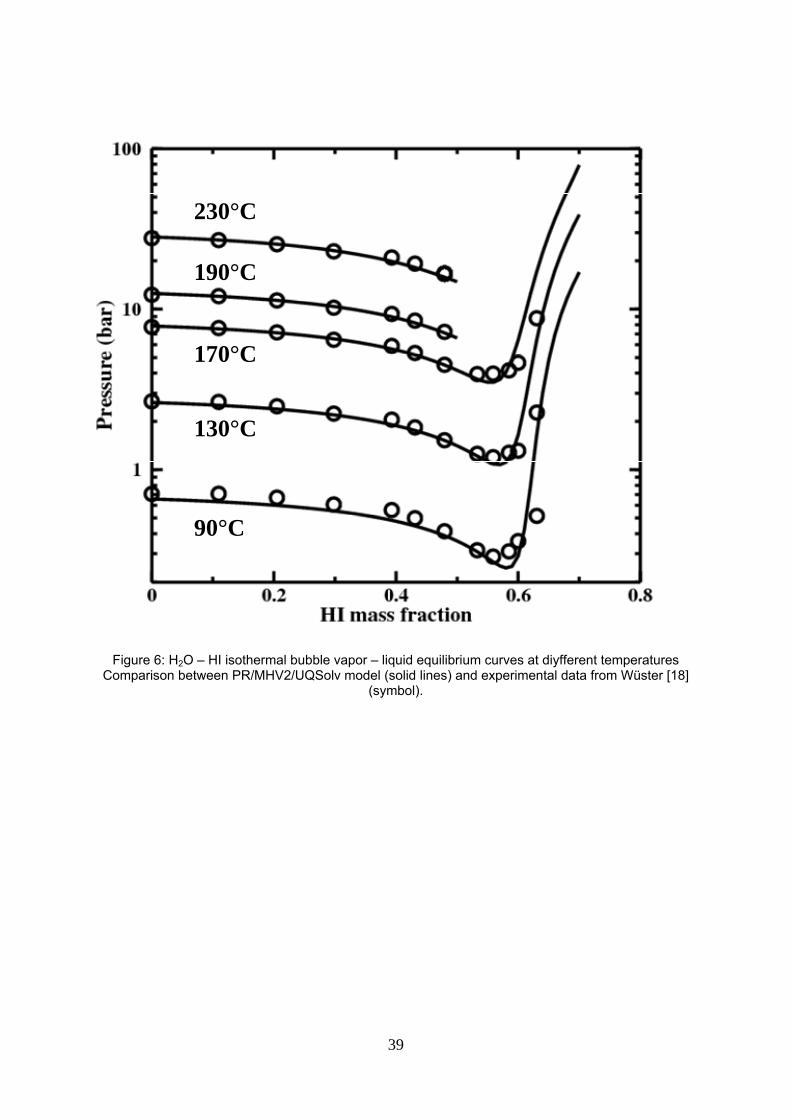
Figure 6 displays the reasonable fitting of the HI mass fraction data of Wüster with the PR/MHV2/UQSolv

model. On the right handside of the azeotrope, the vapor pressure is overestimated though but from the

discussion above, we may expect that if Wüster’s reported composition is the overall composition fed to the

measurement cell, the precise bubble composition would then be on the left of the reported point.

Figure 7 compares the predicted bubble and dew curves with experimental HI molar fraction data at

atmospheric pressure [25]. As expected from our estimation procedure, prediction of the bubble pressure

agrees well up to the azeotropic point but deviates significantly on the right of the azeotrope where the

experimental data are still uncertain. Neumann’s model does not predict the H2O – HI immiscibility at 1 atm.

Neumann sketched in his report the isothermal vapor – liquid – liquid equilibrium at 70°C with an immiscibility

region at approx. 20-21 bar [17].

Vapor – liquid – liquid and liquid – liquid equilibrium predictions of the new model are also displayed in figure

7, using UQSolv model or PR/MHV2/UQSolv model. Differences occur, especially in the calculation of the

19

liquid – liquid equilibrium span near the vapor – liquid – liquid temperature -35°C and are discussed below in

the paragraph about liquid – liquid equilibrium calculation.

Figure 8 compares the predicted and experimental [6] bubble pressure at 25°C. In this figure, a noteworthy

deviation is observed at the right side of azeotrope probably accentuated by the inaccurate azeotrope

measurement in this work, as mentioned earlier.

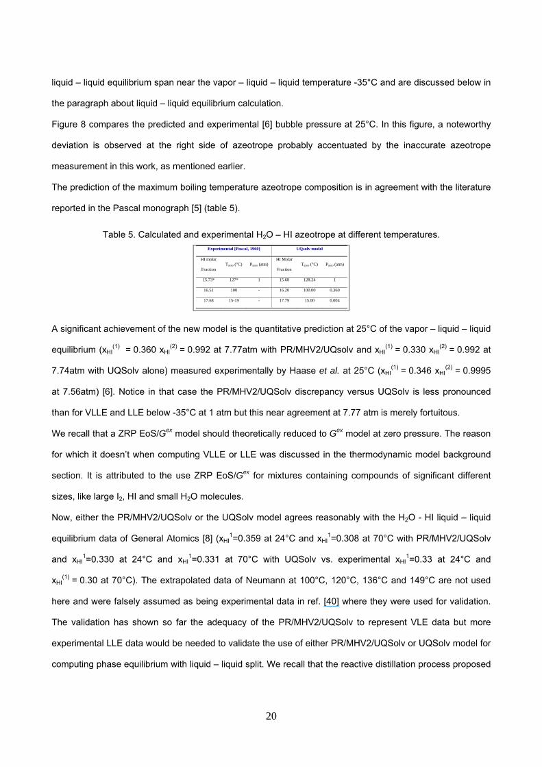
The prediction of the maximum boiling temperature azeotrope composition is in agreement with the literature

reported in the Pascal monograph [5] (table 5).

Table 5. Calculated and experimental H2O – HI azeotrope at different temperatures. Experimental [Pascal, 1960] UQsolv model

HI molar

Fraction Tazeo (°C) Pazeo (atm)

HI Molar

Fraction Tazeo (°C) Pazeo (atm)

15.73* 127* 1 15.68 128.24 1

16.51 100 - 16.20 100.00 0.360

17.68 15-19 - 17.79 15.00 0.004

A significant achievement of the new model is the quantitative prediction at 25°C of the vapor – liquid – liquid

equilibrium (xHI(1) = 0.360 xHI

(2) = 0.992 at 7.77atm with PR/MHV2/UQsolv and xHI(1) = 0.330 xHI

(2) = 0.992 at

7.74atm with UQSolv alone) measured experimentally by Haase et al. at 25°C (xHI(1) = 0.346 xHI

(2) = 0.9995

at 7.56atm) [6]. Notice in that case the PR/MHV2/UQSolv discrepancy versus UQSolv is less pronounced

than for VLLE and LLE below -35°C at 1 atm but this near agreement at 7.77 atm is merely fortuitous.

We recall that a ZRP EoS/Gex model should theoretically reduced to Gex model at zero pressure. The reason

for which it doesn’t when computing VLLE or LLE was discussed in the thermodynamic model background

section. It is attributed to the use ZRP EoS/Gex for mixtures containing compounds of significant different

sizes, like large I2, HI and small H2O molecules.

Now, either the PR/MHV2/UQSolv or the UQSolv model agrees reasonably with the H2O - HI liquid – liquid

equilibrium data of General Atomics [8] (xHI1=0.359 at 24°C and xHI

1=0.308 at 70°C with PR/MHV2/UQSolv

and xHI1=0.330 at 24°C and xHI

1=0.331 at 70°C with UQSolv vs. experimental xHI1=0.33 at 24°C and

xHI(1) = 0.30 at 70°C). The extrapolated data of Neumann at 100°C, 120°C, 136°C and 149°C are not used

here and were falsely assumed as being experimental data in ref. [40] where they were used for validation.

The validation has shown so far the adequacy of the PR/MHV2/UQSolv to represent VLE data but more

experimental LLE data would be needed to validate the use of either PR/MHV2/UQSolv or UQSolv model for

computing phase equilibrium with liquid – liquid split. We recall that the reactive distillation process proposed

20

by Roth and Knoche [13] showed column profile compositions in the vapor – liquid equilibrium region, with

no need for VLLE calculations.

5.4. H2O – HI – I2 mixture

5.4.1. Parameter estimation

For the ternary system H2O – HI – I2, the binary interaction parameters estimated for each binary system and

the solvation parameters of hydrogen iodide by water are kept constant. The interaction between iodine and

the solvation complex are then estimated using the ternary vapor – liquid equilibrium data.

The final parameter values are not shown due to the confidentiality clause of the funding partner.

5.4.2. Vapor – liquid equilibrium data comparison

The ternary vapor – liquid equilibrium data published by Neumann [17] are well described: the average

relative error, the maximum error and the criterion values are respectively 8.2%; 44% and 3.7 for the

PR/MHV2/UQSolv model. Those numbers are better than the values obtained with the parameter set

proposed by Neumann below 150°C but worse than the one above 150°C. We thus infer that the

extrapolated law for the vapour pressure used with the “above 150°C” parameter set of Neumann is

reasonable, although it has no theoretical support at all, on the basis of the existing experimental data.

In addition, as the full line shows on figure 9 for the PR/MHV2/UQSolv, we notice a trend to overestimate the

data at high pressures. However, one should keep in mind that the same set of parameters is used to

describe not only the ternary system but also all binary subsystems as described throughout this paper and

their respective SLE, LLE and VLE equilibrium.

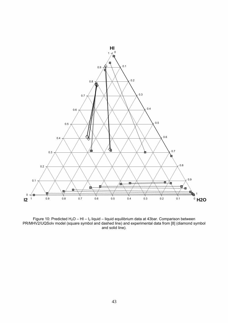
5.4.3. Liquid – liquid equilibrium data comparison

Figure 10 compares the new model predictions at 121.5°C and 43 bar with the experimental data at 120.9;

121,5 and 121.7°C under approx. 43 bar in ref. [8].

The MHV2/UQSolv model underpredicts the HI composition and overpredicts the H2O composition in the HI-

lean phase for two of the three tie lines but the slope of the tie line is reasonably predicted. The model also

predicts at 43bar the second partial miscibility region between H2O – I2 in presence of HI, which is postulated

21

in reference [8]. Neumann’s model could not predict such data but NRTL electrolytic model of Brown et al.

[29,30] did.

6. Conclusions

The so-called HIx (H2O – HI – I2) system has been modeled by using a ZRP EoS/Gex homogeneous

approach. The Peng-Robinson equation of state with Boston Mathias α function holds for both the vapor and

liquid phase. To capture the strong non ideal behavior of the mixture, the MHV2 complex mixing rule is used,

embedding the UNIQUAC Gibbs excess energy model together with a Engels’ solvation equilibrium of HI by

H2O. Literature data are criticized and selected ones are used to estimate the UNIQUAC binary interaction

parameters and the solvation constant parameter values. Other are used for validation of the model.

Former models proposed by Neumann, Yoon, Mathias or Annesini based on a heterogeneous liquid/Gibbs

excess energy model – vapor/equation of state approach are reviewed. Unlike the new homogeneous

approach, they are intrinsically unable to capture the supercritical behavior of HI likely occurring above HI

critical temperature of 150.7°C.

Based on the theoretical arguments discussed, the use of a ZRP EoS/Gex homogeneous approach is

recommended in place of a heterogeneous Gex model for any VLE calculation above HI critical temperature,

150.7°C. LLE and VLLE calculations could be done with either one approach as ZRP EoS/Gex calculation

usually match with Gex calculations at the low pressures under which liquid – liquid phase split may occur.

For the HIx system, this is not true due to large atomic size differences between the HIx system compounds.

The few liquid – liquid equilibrium data do not allow to discriminate between the PR/MHV2/UQsolv and the

UQsolv alone models for LLE and VLLE calculations.

The new model successfully represents most of the vapor – liquid, liquid – liquid, solid – liquid, vapor – liquid

– liquid experimental data available from the literature, with a unique set of temperature dependent binary

interation and solvation parameters, unlike the recent work of Yoon et al. who proposed three sets [40]. The

largest discrepancy is found for high HI concentration mixtures where experimental data are sparse and

uncertain due to the likely dissociation of HI into H2 and I2.

In fact, more and accurate detailed composition data are needed to consider system features like the

dissociation of HI in the vapor phase but also the probable poly-iodide formation in the liquid phase that

could be described by a solvation of HI by I2. The CEA has recently launched a program to measure the

22

relevant partial pressures [51], which are necessary to effectively estimate the hydrogen production potential

under the reactive distillation process expected conditions (up to 300°C and 50 bars).

7. Acknowledgment

The authors thank Pr. J.P. O’Connell for invaluable discussions on experimental data and theoretical models

on the HIx system.

8. References

[1] Funk J.E., Thermochemical hydrogen production: past and present, Int. J. Hydrogen

Energy, 2001;26(3):185-190.

[2] O’Keefe D., Allen C., Besenbruch G., Brown L., Norman J., Sharp R. and McCorkle K., Preliminary

results from bench-scale testing of a sulfur-iodine thermochemical water-splitting cycle, Int. J.

Hydrogen Energy, 1982;7(5):381-392.

[3] Mathias P.M., Applied thermodynamics in chemical technology: current practice and future challenges,

Fluid Phase Equilibria, 2005;228-229:49-57.

[4] Kracek F.C., Solubilities in the system water-iodine to 200°C, J. Phys. Chem., 1931;35 :417.

[5] Pascal P., Nouveau traité de chimie minérale. tome 16. chlore, brome, iode, astate, manganese,

technetium, rhenium (1960) Edition Masson. 1195 pages

[6] Haase R., Naas H., Thumm H., Experimental investigation on the thermodynamic behavior of

concentrated halogen hydrogen acids, Z. Phys. Chem. NF, 1963;37:210-229.

[7] O’Keefe D.R., Norman J.H., The vapour pressure , iodine solubility, and hydrogen solubility of

hydrogen iodide – iodine solutions, J. Chem. Eng. Data, 1982;27:77-80.

[8] O’Keefe D.R., Norman J.H., Brown L. and Besenbruch G. GA technologies thermochemical water –

splitting process improvements. Final Report 1984, (1984) Report GA A17752.

[9] Engels H., Phase equilibria and phase diagrams of electrolytes, Chemistry data Series, Volume XI,

Part I. (1990) Published by DECHEMA. ISBN 3-926959-17-7, 160 pages.

[10] Palmer A.D., Lietzke M.H., The equilibria and kinetics of iodine hydrolysis, Radiochimica Acta,

1982;31:37-44.

[11] Palmer A.D., Ramette R.W., Mesmer R.E., Triiodide ion formation equilibrium and activity coefficients

in aqueous solution, Journal of Solution Chemistry, 1984;13(9):673-683.

23

[12] Calabrese V.T., Khan A., Polyiodine and polyiodide species in an aqueous solution of iodine + KI:

Theoretical and experimental studies, J. Phys. Chem. A, 2000;104:1287-1292.

[13] Roth M. and Knoche K.F., Thermo-chemical water-splitting through direct HI decomposition from

HI/I2/H2O solutions, Int. J. Hydrogen Energy, 1989;14(8):545-549.

[14] Goldstein S., Borgard J.M., Vitart X., Upper bound and best estimate of the efficiency of the iodine

sulfur cycle, Int. J. Hydrogen Energy, 2005;30:619.

[15] Belaissaoui B., Thery R., Meyer X.M., Meyer M., Gerbaud V., Joulia X., Vapour reactive distillation

process for hydrogen production by HI decomposition from HI–I2–H2O solutions, Chem. Eng. Proc.,

2008;47(3):396-407.

[16] Sundmacher K., Kienle A., 2003, Reactive distillation status and future directions, WILEY-VCH, 308

pages ISBN: 978-3-527-30579-7.

[17] Neumann D., Phasengleichgewichte von HJ/H2O/J2 – Lösungen. Lehrstuhl für Thermodynamik,

RWTH Aachen, 5100 Aachen (Germany). Master’s thesis; January 1987,.

[18] Engels H., Knoche K., Vapor pressures of the systems HI/I2/H2O and H2, Int. J. Hydrogen Energy,

1986;11(11):703-707.

[19] Wüster G., p,v,T – und Dampfdrückmessengen zur Bestimmung Thermodynamischer Eigenschaften

Starker Elektrolyte bei Erhöhten Druck, june 1979, Thesis (1979) RWTH Aachen. (in German).

[20] Vanderzee C.E., Gier L.J., The enthalpy of solution of gazeous hydrogen iodide in water, and the

relative apparent molar enthalpies of hydriodic acid, J. Chem. Thermodynamics, 1974;6:441-452.

[21] CRC Handbook of chemistry and physics (1988) 69th Edition by CRC Press.

[22] Shindo Y., Ito N., Haraya K., Hakuta T., Yoshitome H., Kinetics of the catalytic decomposition of

hydrogen iodide in the thermochemical hydrogen production, Int. J. Hydrogen Energy, 1984;9(8):695-

700.

[23] Berndahauser C., Knoche K.F., Experimental investigations of thermal HI decomposition from H2O---

HI---I2 solutions. Int. J. Hydrogen Energy, 1994;19(3):239-244.

[24] Sako T., Hakuta T., Yoshitome H., Vapor liquid equilibria for hydrogen iodide – water, nitric acid –

water, hydrogen iodide – water – salt and nitric acid – water – salt systems. Kagaku Gijutsu

Kenkyusho Hokoku, 1985;80(5):199-203.

[25] Carrière E., Ducasse, Détermination des courbes de bulle et de rosée des mélanges d’acide

iodhydrique et d’eau sous une pression de 746 mm de mercure. CR de chimie, 1926;1281-1282.

[26] Pickering S.E., Die Hydrate der Jodwasserstoffsäure 1893;2307-2310.

[27] Sandler S.I., Models for thermodynamic and Phase Equilibria Calculations (1994) Marcel Dekker Inc.,

New York, ISBN 0-8247-9130-4.

24

[28] Vidal J., Applied thermodynamic for chemical engineering and oil industry, (2003) Technip Editions.

[29] Brown L.C., Mathias P.M., Chen C.C., Ramrus D. Thermodynamic Model for the HI-I2-H2O System,

AIChE Annual Meeting, 4-9 November, 2001.

[30] Mathias P.M., Brown L.C. Thermodynamics of the sulphur-iodine cycle for thermochemical hydrogen

production’, Presented at 68th Annual Meeting of the Society of Chemical Engineers, Japan, 2003.

[31] Annesini M.C., Gironi F., Lanchi M., Marrelli L., Maschietti M., S-I thermochemical cycle for H2

production: a thermodynamic analysis of the phase equilibria of the system HI-I2-H2O, Proceedings of

ICheaP-8, The eigth Italian Conference on Chemical and Process Engineering, 2007.

[32] Huron M.J., Vidal J., New mixing rules in simple equations of state for representing vapour-liquid

equilibria of strongly non-ideal mixtures, Fluid Phase Equilibria, 1979;3:255-271.

[33] Michelsen M.L., A method for incorporating excess Gibbs energy models in equations of state, Fluid

Phase Equilibria, 1990;60:47-58.

[34] Michelsen M.L., A modified Huron-Vidal mixing rule for cubic equations of state, Fluid Phase

Equilibria, 1990;60:213-219.

[35] Fredenslund A., Jones R.L., Prausnitz J.M., Group-contribution estimation of activity coefficients in

nonideal liquid mixtures, AIChE Journal, 1975;21(5):1086-1099.

[36] Kalospiros N.S., Tzouvaras N., Coutsikos P., Tassios D.P., Analysis of zero-reference-pressure

EoS/GE models, AIChE Journal, 1995;41(4):928-937.

[37] Zavitsas A.A., Properties of Water Solutions of Electrolytes and Nonelectrolytes, J. Phys. Chem. B,

2001;105:7805-7815.

[38] Iyengar S.S. , Petersen M.K., Burnham C.J., Day T.J.F., Voth G.A., The properties of ion-water

clusters. I. The protonated 21-water cluster, J. Chem. Phys., 2005;123:084309.

[39] Renon H., Prausnitz J.M., Local compositions in thermodynamic excess functions for liquid mixtures,

AIChE Journal, 1968;14(3):135-144.

[40] Yoon H.J., Kim S.J., No H.C., Lee B.J., Kim E.S., A thermo-physical model for hydrogen–iodide

vapor–liquid equilibrium and decomposition behavior in the iodine–sulfur thermo-chemical water

splitting cycle, Int. J. Hydrogen Energy, 2008;33(20):5469-5476.

[41] Danner R.P., Daubert T.E., DIPPR Project 801, Design Institute for Physical Property research.

Pennsylvania State University (1983), http://dippr.byu.edu/

[42] Chen C.C., Britt H.I., Boston J. F., Evans L.B., Local composition model for excess Gibbs energy of

electrolyte systems. Part I: Single solvent, single completely dissociated electrolyte systems, AIChE

Journal, 1982;28:588-596.

25

[43] Chen C.C., Evans L.B., A local composition model for the excess Gibbs energy of aqueous electrolyte

systems, AIChE Journal, 1986,32:444-454.

[44] Pitzer K., Electrolytes. From dilute solutions to fused salts, J. Am. Chem. Soc., 1980;102:2902-2906.

[45] Chen C.C., Mathias P.M., Orbey H., Use of hydration and dissociation chemistries with the electrolyte-

NRTL model, AIChE Journal, 1999;45(7):1576-1586.

[46] Abrams D.S., Prausnitz J.M., Statistical thermodynamics of liquid mixtures: A new expression for the

excess Gibbs energy of partly or completely miscible systems, AIChE Journal, 1975;21(3):116-128.

[47] Anderson T.F., Prausnitz J.M., Application of the UNIQUAC Equation to Calculation of Multicomponent

Phase Equilibria. 1. Vapor-Liquid Equilibria, I.E.C. Process Des. Dev., 1978;17(4):552-560.

[48] Boston J.F., Mathias P.M., Phase Equilibria in a Third-Generation Process Simulator (1980)

Proceedings of the 2nd International Conference on Phase Equilibria and Fluid Properties in the

Chemical Process Industries, West Berlin, pp. 823-849.

[49] Bondi A., van der Waals Volumes and Radii, J. Phys. Chem. 1964;68:441-451.

[50] http://www.prosim.net/

[51] Doizi D., Dauvois V., Roujou J.L., Delanne V., Fauvet P., Larousse B., Hercher O., Carles P., Moulin

C., Hartmann J.M., Total and Partial Pressure measurements for the sulphur-iodine thermo-chemical

cycle. Int. J. Hydrogen Energy. 2007;32(9):1183-1191.

26

List of table captions

Table 1 : intrinsic properties of pure compounds.

Table 2. Experimental available data in literature for HIx system and its binary sub-systems.

Table 3. Saturated vapor pressure prediction error using SRK and PR equation of state versus DIPPR

correlation.

Table 4. UNIQUAC parameters for the combinatorial term.

Table 5. Calculated and experimental H2O – HI azeotrope at different temperatures.

27

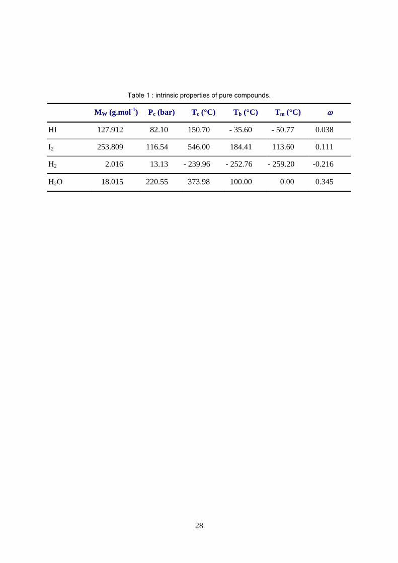
Table 1 : intrinsic properties of pure compounds.

MW (g.mol-1) Pc (bar) Tc (°C) Tb (°C) Tm (°C) ω

HI 127.912 82.10 150.70 - 35.60 - 50.77 0.038

I2 253.809 116.54 546.00 184.41 113.60 0.111

H2 2.016 13.13 - 239.96 - 252.76 - 259.20 -0.216

H2O 18.015 220.55 373.98 100.00 0.00 0.345

28

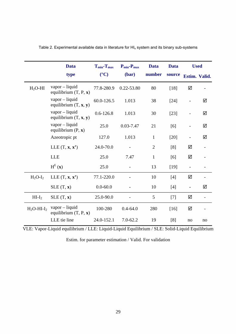
Table 2. Experimental available data in literature for HIx system and its binary sub-systems

VLE: Vapor-Liquid equilibrium / LLE: Liquid-Liquid Equilibrium / SLE: Solid-Liquid Equilibrium

Estim. for parameter estimation / Valid. For validation

Used

Data

type

Tmin-Tmax

(°C)

Pmin-Pmax

(bar)

Data

number

Data

source Estim. Valid.

H2O-HI vapor – liquid equilibrium (T, P, x)

77.8-280.9 0.22-53.80 80 [18] -

vapor – liquid equilibrium (T, x, y)

60.0-126.5 1.013 38 [24] -

vapor – liquid equilibrium (T, x, y)

0.6-126.8 1.013 30 [23] -

vapor – liquid equilibrium (P, x)

25.0 0.03-7.47 21 [6] -

Azeotropic pt 127.0 1.013 1 [20] -

LLE (T, x, x’) 24.0-70.0 - 2 [8] -

LLE 25.0 7.47 1 [6] -

HE (x) 25.0 - 13 [19] - -

H2O-I2 LLE (T, x, x’) 77.1-220.0 - 10 [4] -

SLE (T, x) 0.0-60.0 - 10 [4] -

HI-I2 SLE (T, x) 25.0-90.0 - 5 [7] -

H2O-HI-I2 vapor – liquid equilibrium (T, P, x)

100-280 0.4-64.0 280 [16] -

LLE tie line 24.0-152.1 7.0-62.2 19 [8] no no

29

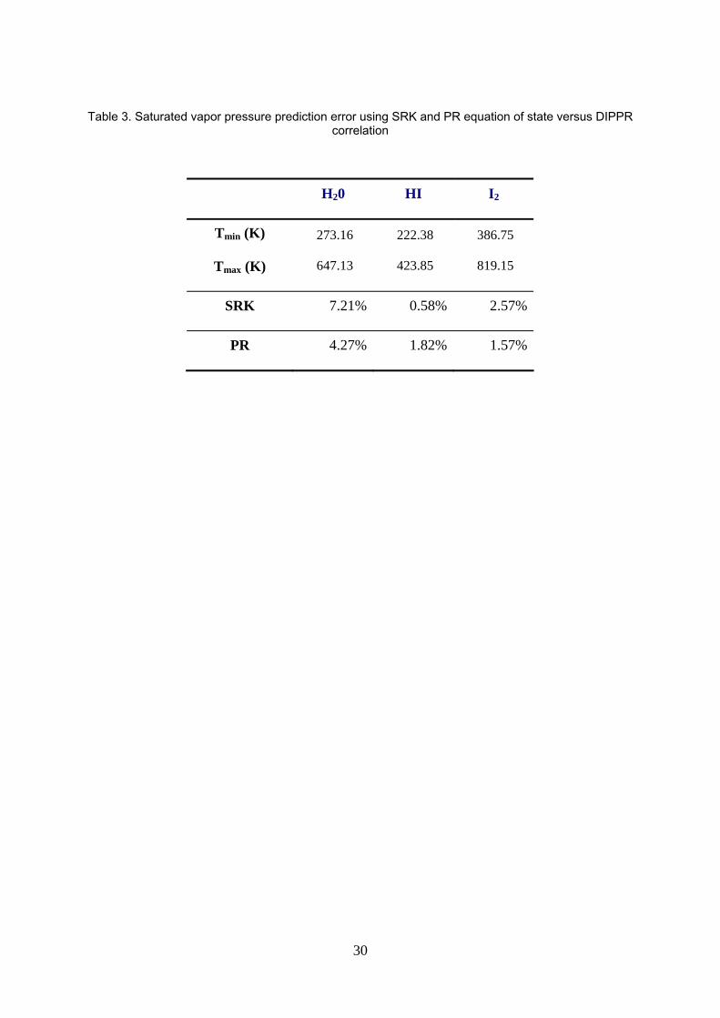
Table 3. Saturated vapor pressure prediction error using SRK and PR equation of state versus DIPPR correlation

H20 HI I2

Tmin (K)

Tmax (K)

273.16

647.13

222.38

423.85

386.75

819.15

SRK 7.21% 0.58% 2.57%

PR 4.27% 1.82% 1.57%

30

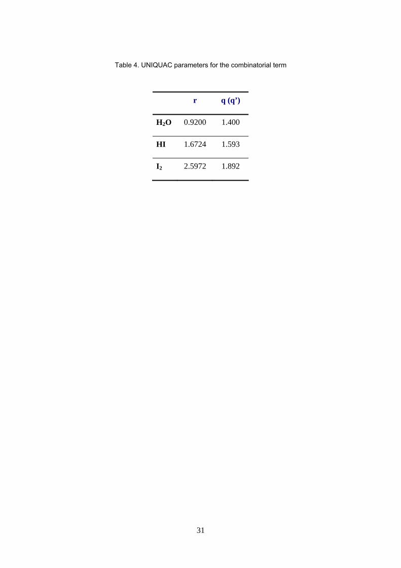
Table 4. UNIQUAC parameters for the combinatorial term

r q (q’)

H2O 0.9200 1.400

HI 1.6724 1.593

I2 2.5972 1.892

31

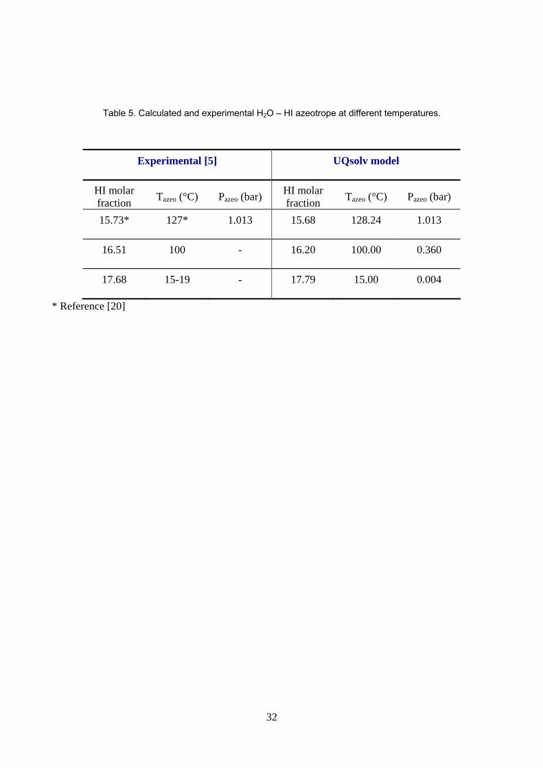
Table 5. Calculated and experimental H2O – HI azeotrope at different temperatures.

Experimental [5] UQsolv model

HI molar fraction Tazeo (°C) Pazeo (bar)

HI molar fraction Tazeo (°C) Pazeo (bar)

15.73* 127* 1.013 15.68 128.24 1.013

16.51 100 - 16.20 100.00 0.360

17.68 15-19 - 17.79 15.00 0.004

* Reference [20]

32

List of figure captions

Figure 1. Sulfur – Iodine thermo-chemical cycle scheme [1].

Figure 2. Solidification curve in mass fraction of H2O – HI mixtures from Pickering [26] reported in Pascal’s monograph [5].

Figure 3. H2O – I2 liquid-liquid and solid-liquid equilibrium curves. Comparison between the UQSolv (solid line) and Neumann (dashed line) models and experimental data from Kracek [4] (diamond for solid – liquid equilibrium, triangle for liquid – liquid equilibrium).

Figure 4: Solubility of iodine in hydrogen iodide. Comparison between the ideal liquid (dotted line), standard UNIQUAC (dashed line), UQSolv models (solid line) and experimental data from O’Keefe and Norman [8] (symbol).

Figure 5: Solvation constant versus temperature. Comparison between UQSolv (solid line), Engels’ [9] (dotted line) and Neumann’s models [17] (dashed line).

Figure 6: H2O – HI isothermal bubble vapor – liquid equilibrium curves at different temperatures Comparison between PR/MHV2/UQSolv model (solid lines) and experimental data from Wüster [19] (symbol).

Figure 7: Predicted H2O – HI isobaric liquid – liquid – vapor equilibrium curve at atmospheric pressure. Comparison between UQSolv calculations (solid line), PR/MHV2/UQSolv (dotted line) and experimental points from Carrière and Ducasse [25] (symbols).

Figure 8: Predicted H2O – HI isotherm liquid – vapor equilibrium curve at 25°C. Comparison between UQSolv model (solid line) and experimental data from Haase [6] (symbol).

Figure 9: PR/MHV2/UQSolv model relative deviation for the total pressure for the experimental H2O – HI – I2 ternary data of Engels and Knoche [18] available in the Neumann’s manuscript [17]. The line is merely a trend of the model’s calculations.

Figure 10: Predicted H2O – HI – I2 liquid – liquid equilibrium data at 43bar. Comparison between PR/MHV2/UQSolv model (square symbol and dashed line) and experimental data circa 121°C from [8] (diamond symbol and solid line).

33

BUNSEN REACTION

I2 + SO2 + 2H2O ⇒ H2SO4 + 2HI

H2SO4 DECOMPOSITION

HI DECOMPOSITION

2HI ⇔ H2 + I2

H2SO4

H2O

SO2

H2O

HI200

600

800

400

1000

0

H 2

O2

I

H2SO4 ⇒ SO2 + H2O + ½ O2

I2

II

III

H2O

TEMPERATURE (°C)

Figure 1. Iodine - Sulfur thermo-chemical cycle scheme [1].

34

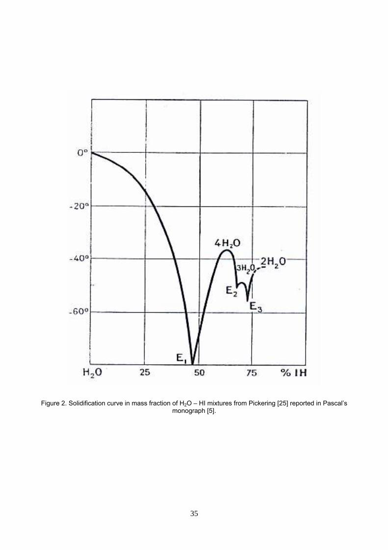
Figure 2. Solidification curve in mass fraction of H2O – HI mixtures from Pickering [25] reported in Pascal’s monograph [5].

35

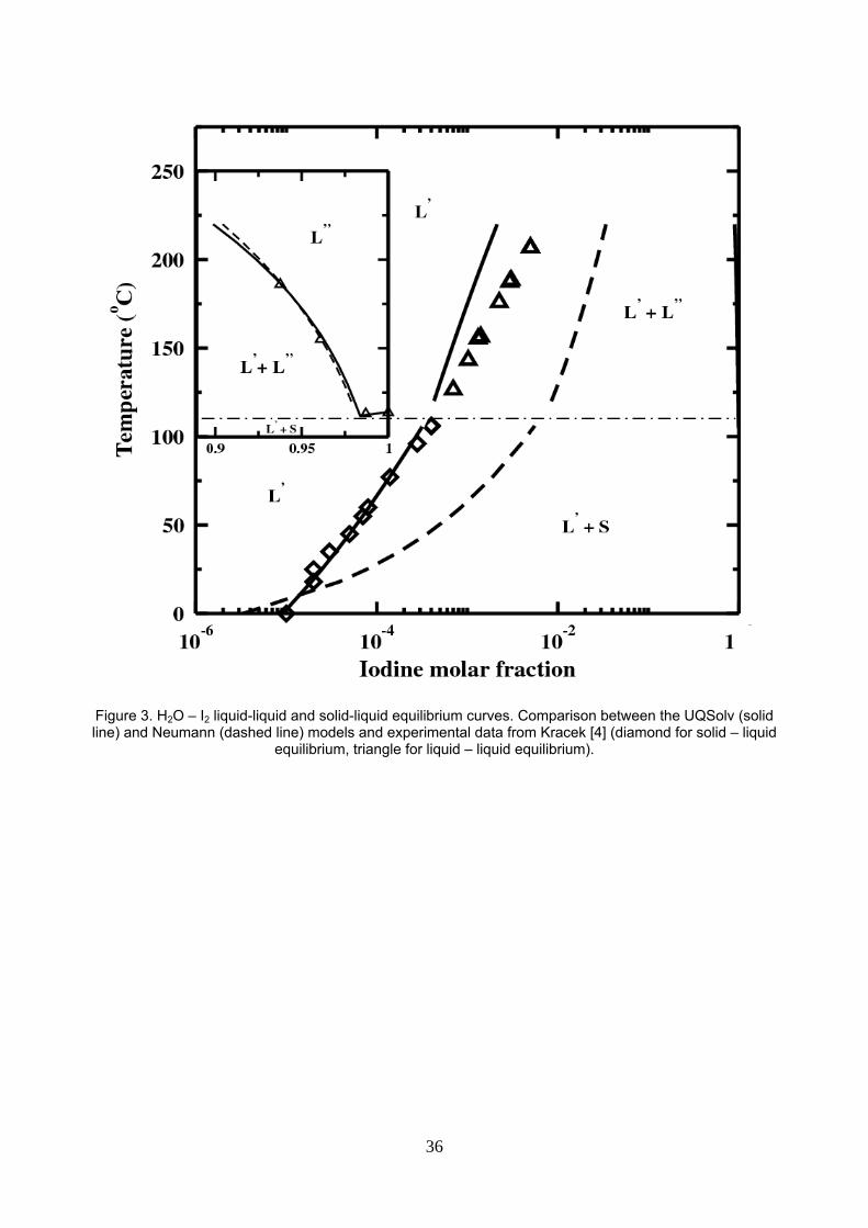
Figure 3. H2O – I2 liquid-liquid and solid-liquid equilibrium curves. Comparison between the UQSolv (solid line) and Neumann (dashed line) models and experimental data from Kracek [4] (diamond for solid – liquid

equilibrium, triangle for liquid – liquid equilibrium).

36

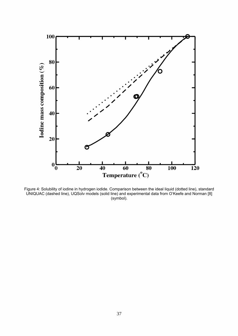
Figure 4: Solubility of iodine in hydrogen iodide. Comparison between the ideal liquid (dotted line), standard UNIQUAC (dashed line), UQSolv models (solid line) and experimental data from O’Keefe and Norman [8]

(symbol).

37

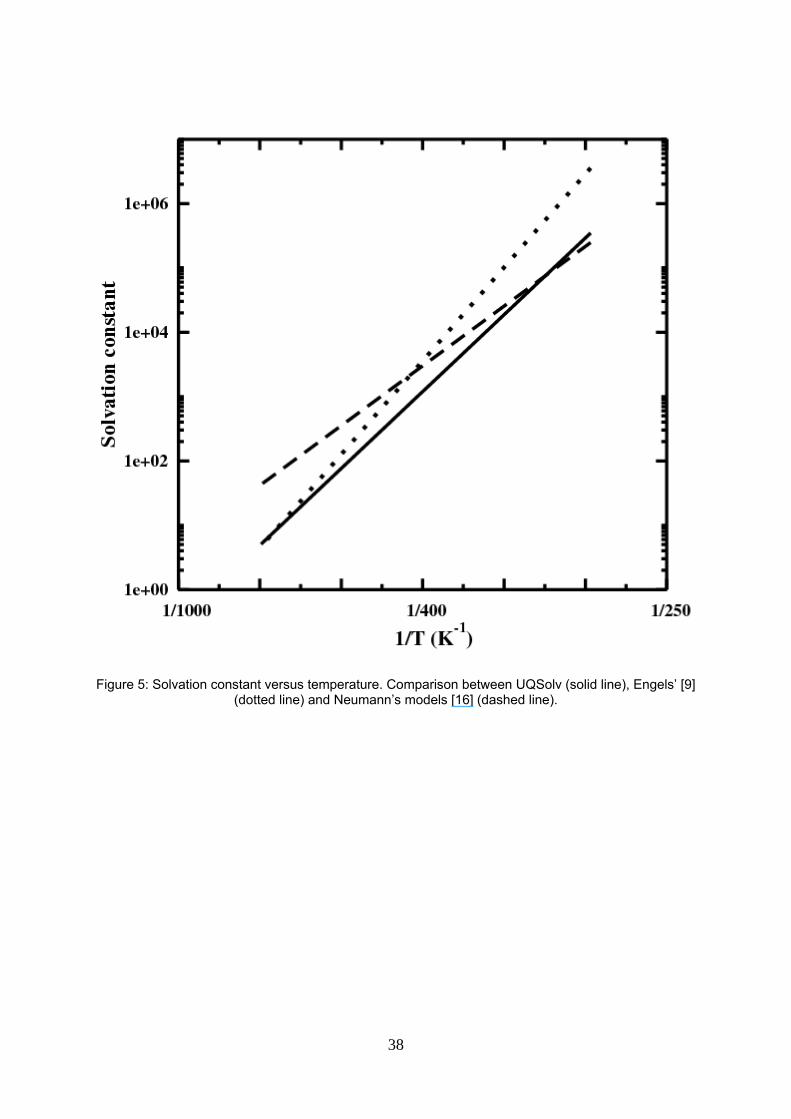
Figure 5: Solvation constant versus temperature. Comparison between UQSolv (solid line), Engels’ [9] (dotted line) and Neumann’s models [16] (dashed line).

38

90°C

130°C

170°C

190°C

230°C

Figure 6: H2O – HI isothermal bubble vapor – liquid equilibrium curves at diyfferent temperatures Comparison between PR/MHV2/UQSolv model (solid lines) and experimental data from Wüster [18]

(symbol).

39

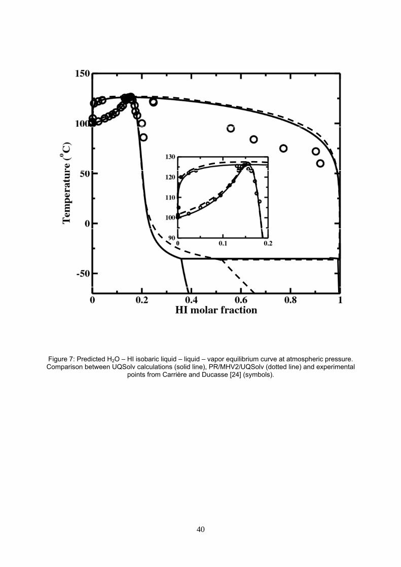
Figure 7: Predicted H2O – HI isobaric liquid – liquid – vapor equilibrium curve at atmospheric pressure. Comparison between UQSolv calculations (solid line), PR/MHV2/UQSolv (dotted line) and experimental

points from Carrière and Ducasse [24] (symbols).

40

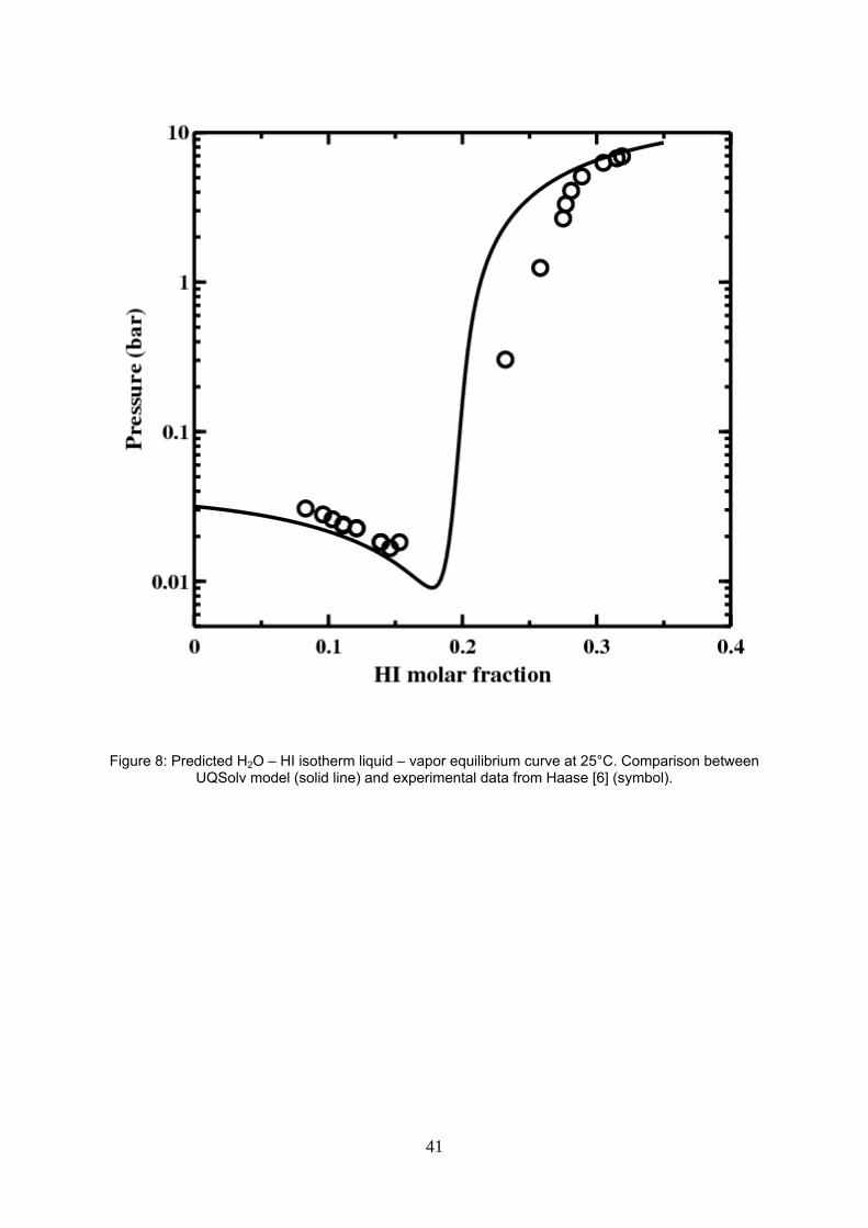
Figure 8: Predicted H2O – HI isotherm liquid – vapor equilibrium curve at 25°C. Comparison between UQSolv model (solid line) and experimental data from Haase [6] (symbol).

41

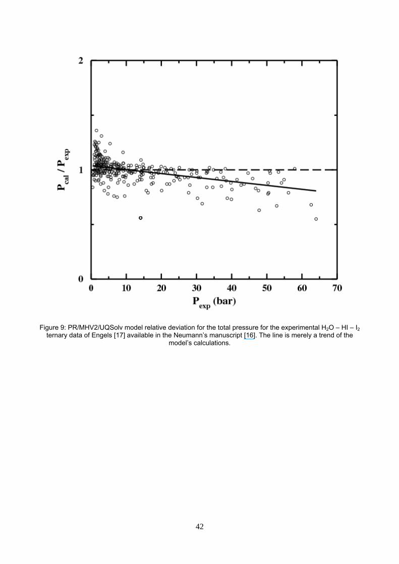
Figure 9: PR/MHV2/UQSolv model relative deviation for the total pressure for the experimental H2O – HI – I2 ternary data of Engels [17] available in the Neumann’s manuscript [16]. The line is merely a trend of the

model’s calculations.

42

HI1

0.9

0.8

0.7

0.6

0.5

0.4

0.3

0.2

0.1

0

H2O1

0.9

0.8

0.7

0.6

0.5

0.4

0.3

0.2

0.1

0

I2 1 0.9 0.8 0.7 0.6 0.5 0.4 0.3 0.2 0.1 0

Figure 10: Predicted H2O – HI – I2 liquid – liquid equilibrium data at 43bar. Comparison between PR/MHV2/UQSolv model (square symbol and dashed line) and experimental data from [8] (diamond symbol

and solid line).

43